Download LOGGER ver.4.1. - USER MANUAL

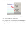
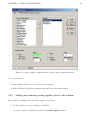
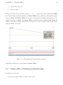
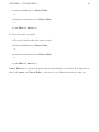
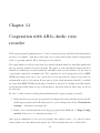
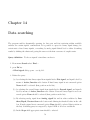
LOGGER ver.4.1. - USER MANUAL
mgr inż. Anna Jerzykowska
mgr inż. Krzysztof Błasiok
Katowice, March 2006/revision may 2010
Contents
1 Introduction
6
2 Program’s requirements
7
3 Program operation
8
3.1
Program’s user interface . . . . . . . . . . . . . . . . . . . . . . . . . . . . . . . . .
3.2
Getting started . . . . . . . . . . . . . . . . . . . . . . . . . . . . . . . . . . . . . . 11
3.3
Opening the data window – shaft choosing . . . . . . . . . . . . . . . . . . . . . . . 12
4 Page configuration
4.1
4.2
8
14
General window appearance configuration . . . . . . . . . . . . . . . . . . . . . . . 15
4.1.1
Background color defining . . . . . . . . . . . . . . . . . . . . . . . . . . . . 16
4.1.2
Page division definition . . . . . . . . . . . . . . . . . . . . . . . . . . . . . . 16
4.1.3
Grid displaying definition . . . . . . . . . . . . . . . . . . . . . . . . . . . . 16
4.1.4
Grid color setting . . . . . . . . . . . . . . . . . . . . . . . . . . . . . . . . . 17
4.1.5
Binary signals displaying mode setting . . . . . . . . . . . . . . . . . . . . . 17
4.1.6
Other plots’ configurations
. . . . . . . . . . . . . . . . . . . . . . . . . . . 18
Analog signals layout configuration . . . . . . . . . . . . . . . . . . . . . . . . . . . 19
4.2.1
Adding and removing analog signals’ plots to the window . . . . . . . . . . . 20
4.2.2
Additional displaying parameters . . . . . . . . . . . . . . . . . . . . . . . . 21
4.2.3
Defining plot’s color . . . . . . . . . . . . . . . . . . . . . . . . . . . . . . . 22
4.2.4
Defining of analog plots’ Y-axis position . . . . . . . . . . . . . . . . . . . . 22
4.2.5
Scaling of the plots . . . . . . . . . . . . . . . . . . . . . . . . . . . . . . . . 22
1
CONTENTS
2
4.2.6
Configuration of the Cursor and Cursor delta windows contents. . . . . . . . 23
4.3
Binary signals layout configuration . . . . . . . . . . . . . . . . . . . . . . . . . . . 23
4.3.1
Arranging signals’ order . . . . . . . . . . . . . . . . . . . . . . . . . . . . . 24
4.3.2
Adding and removing binary signals’ plots to the window . . . . . . . . . . . 25
4.3.3
Additional displaying parameters . . . . . . . . . . . . . . . . . . . . . . . . 25
4.3.4
Signals plot’s polarization . . . . . . . . . . . . . . . . . . . . . . . . . . . . 25
4.3.5
Configuration saving . . . . . . . . . . . . . . . . . . . . . . . . . . . . . . . 26
5 Data source
27
6 Graphs viewing
29
6.1
Direct jump to known time period . . . . . . . . . . . . . . . . . . . . . . . . . . . . 29
6.2
Graphs viewing . . . . . . . . . . . . . . . . . . . . . . . . . . . . . . . . . . . . . . 30
6.3
6.2.1
Next and previous page
. . . . . . . . . . . . . . . . . . . . . . . . . . . . . 30
6.2.2
Half page shifting . . . . . . . . . . . . . . . . . . . . . . . . . . . . . . . . . 30
Data range selection . . . . . . . . . . . . . . . . . . . . . . . . . . . . . . . . . . . 31
6.3.1
Data range choice . . . . . . . . . . . . . . . . . . . . . . . . . . . . . . . . . 32
7 Cursor
34
7.1
Cursor properietes . . . . . . . . . . . . . . . . . . . . . . . . . . . . . . . . . . . . 34
7.2
Cursor activating and inactivating . . . . . . . . . . . . . . . . . . . . . . . . . . . . 35
8 Cursor delta
37
8.1
Cursor Delta . . . . . . . . . . . . . . . . . . . . . . . . . . . . . . . . . . . . . . . . 37
8.2
Moving of cursor delta . . . . . . . . . . . . . . . . . . . . . . . . . . . . . . . . . . 38
8.3
Cursor delta activating and inactivating
. . . . . . . . . . . . . . . . . . . . . . . . 39
9 Single stroke signals
41
10 Emergency signals
42
11 “WUG” Displaying mode
44
CONTENTS
3
12 Data layers
46
13 Cooperation with AR3c-Audio voice recorder
48
14 Data searching
50
15 Reports
53
15.1 Reports configuration . . . . . . . . . . . . . . . . . . . . . . . . . . . . . . . . . . . 53
15.2 Reports performing . . . . . . . . . . . . . . . . . . . . . . . . . . . . . . . . . . . . 56
16 Shifts beginning configuration
59
17 Printing
60
18 Copying to clipboard
62
19 Data archiving
63
20 Datalogger’s contents
65
21 Datalogger time setting (available only for AR-2c dataloggers)
66
22 Communication
68
22.1 Communication with voice recorder (Logger ver. 4.1-0.11 and later) . . . . . . . . . 69
23 Exiting from the LOGGER program.
70
List of Figures
3.1
General program’s view with opened dat windows is shown on fig. . . . . . . . . . .
9
3.2
Data window showing graphs obtained from AR datalogger . . . . . . . . . . . . . . 10
3.3
An example of Choose shaft dialog . . . . . . . . . . . . . . . . . . . . . . . . . . . 13
4.1
A general window’s configuration tab view . . . . . . . . . . . . . . . . . . . . . . . 15
4.2
Activation of transmitting and playing audio files in Logger program. . . . . . . . . 19
4.3
Analog signals configuration tab in the Pages configuration dialog . . . . . . . . . . 20
4.4
Binary signals configuration tab in the Pages configuration dialog . . . . . . . . . . 24
5.1
Data source selection . . . . . . . . . . . . . . . . . . . . . . . . . . . . . . . . . . . 28
6.1
Half page shifting - graphs comparison . . . . . . . . . . . . . . . . . . . . . . . . . 31
6.2
Data range choice . . . . . . . . . . . . . . . . . . . . . . . . . . . . . . . . . . . . . 32
7.1
Illustration of two methods of viewing the binary signals in cursor window. . . . . . 35
8.1
A sample LOGGER program window with Cursor Delta . . . . . . . . . . . . . . . 38
8.2
: The graphs from previous figure zoomed in . . . . . . . . . . . . . . . . . . . . . . 39
9.1
A sample window showing single stroke signals series . . . . . . . . . . . . . . . . . 41
10.1 Two methods of displaying emergency signals information . . . . . . . . . . . . . . . 43
11.1 Comparison of two displaying modes of single stroke signals
. . . . . . . . . . . . . 45
12.1 Displaying of the first data layer . . . . . . . . . . . . . . . . . . . . . . . . . . . . . 47
4
LIST OF FIGURES
5
12.2 Displaying of the second data layer . . . . . . . . . . . . . . . . . . . . . . . . . . . 47
14.1 The “Find signal” dialog window for searching criteria definition . . . . . . . . . . . 51
15.1 Reports’ definition window . . . . . . . . . . . . . . . . . . . . . . . . . . . . . . . . 54
15.2 Report’s criteria definition dialog . . . . . . . . . . . . . . . . . . . . . . . . . . . . 55
15.3 Sample report’s view . . . . . . . . . . . . . . . . . . . . . . . . . . . . . . . . . . . 58
17.1 A sample printout performed by means of LOGGER program . . . . . . . . . . . . 61
19.1 data transmission progress window . . . . . . . . . . . . . . . . . . . . . . . . . . . 63
20.1 Datalogger memory contents dialog . . . . . . . . . . . . . . . . . . . . . . . . . . . 65
21.1 AR-2c datalogger time setting . . . . . . . . . . . . . . . . . . . . . . . . . . . . . . 67
22.1 Communication settings dialog box . . . . . . . . . . . . . . . . . . . . . . . . . . . 68
22.2 IP address and port number setting for voice recording . . . . . . . . . . . . . . . . 69
Chapter 1
Introduction
Logger ver. 4.1 is a utility program serving for visualization and archivisation of analog, binary and
single stroke signals of mining hoists’ systems obtained from AR-2c and AR-3c Digital Registers.
LOGGER cooperates with the registers through RS-232 or RS-485 serial links,or through network
interface. Using LOGGER program it is possible to directly browsing through the registers’ memory
contents or copying data to data storage (hard disc, floppy, external mass storage) for archivisation
purposes. Data fragments can be printed. Also an extended report functionality has been added.
The program can cooperate with several AR registers simultaneously.
6
Chapter 2
Program’s requirements
• PC - compatible computer with Windows (98,2000,NT,XP) OS
• 24 MB RAM (or more)
• 50 MB free hard disc space
• coloured screen,
• mouse
• printer
• audio board - in case of playing sound from voice recorder
• free serial port or network interface
• modem - in case of modem link
• network interface - adviced for AR-3c dataloggers
• MS Windows XP or later
7
Chapter 3
Program operation
3.1
Program’s user interface
During program operation two kinds of windows appear on the desktop:application window (main
program’s window)data windows appearing in the main window - see fig.3.1.
• Application window contains:
• control menu field – in the upper left corner
• tittle bar – with program’s name (LOGGER 4.1-0.4)
• menu bar containing main menu
• maximize, iconic buttons in upper right corner of the window
• scrolling bars
8
CHAPTER 3. PROGRAM OPERATION
9
Figure 3.1: General program’s view with opened dat windows is shown on fig.
Inside the main window there are data windows known also called “document windows”). One
can open simultanuously many data windows. Data windows serve for displaying the graphs of
machine’s work. Sample view of data window is shown on fig.3.2. Data windows use common
application menu.Data windows can be minimized or shown as icons
CHAPTER 3. PROGRAM OPERATION
10
Figure 3.2: Data window showing graphs obtained from AR datalogger
Data window contains:
• control menu field – in the upper left corner
• Title bar - with shaft name, and datalogger’ serial number
• maximize, iconic buttons in upper right corner of the window
• graph’s date in format: year – month – day, in the upper left corner
• analog graphs’ field – it occupies defined in the configuration option window’s part and
contains declared plots.
• Graphs’ timing information: data range begining, middle and ending is labeled in the format:
hour:minute
• position markers in the form of vertical red dashes (when applied)
• single stroke signals’ markers in form of red and green dots (if single stroke signals are present
on given graph)
CHAPTER 3. PROGRAM OPERATION
11
• Emergency signals (if applied) - displayed in the right part of the window in two columns:
short signal’s name and its time offset
• binary signals’ field in the bottom part of the window. Active binary signals are shown in
the form of coloured lines or diagrams,
• data source information displayed in the lower right corner
• range information displayed in the lower right corner
• tabs’ field enabling of choice of one configured pages. Current page’s tab is marked.
Additionally data windows can contain:
• moving cursor in the form of vertical blue line
• moving cursor window
• moving so called “delta cursor” in the form of vertical green line
• moving “delta cursor” window
• transmission progress window
• single stroke signals window
• “Particuliars” window serving for displaying additional information about emergency signals
After right mouse clicking a context menu appears on the screen. It serves for accessing of frequently
used items of application menu. For a given datalogger it is possible to define multiple sets of signals
to present on a single window page. The Pages’ configuration section covers this subject. The
LOGGEER program can simultaneously cooperate with multiple AR-2c and AR-3c dataloggers
what gives possibility of viewing several data graphs deriving from different hoists.
3.2
Getting started
In order to run LOGGER program one should choose Start -> Programs menu
1. Choose Register group
2. Double click LOGGER icon
The main application window opens
CHAPTER 3. PROGRAM OPERATION
3.3
12
Opening the data window – shaft choosing
In order to open the data window, where the graphs concerning given hoist will be viewed: (see
fig. 3.3):
• From menu File choose Open or
• From menu Window choose New window
or
• choose New window from context menu
or
• apply F3 key
A choose shaft dialog window opens with a shafts’ list control where: Choose shaft’s name from
where the diagrams are to be viewed:
• double-click the chosen shaft’s namedouble-click the chosen shaft’s name
or
• choose the shaft name by clicking on its name and then accept by "OK" button
or
• choose the shaft name by moving selection mark by means of arrow keys and then push
ENTER key
The data window opens – here the diagrams can be viewed.The window will be empty for the
first time it is used, next, every time, when opened, it will contain last viewed data. (concerns
only data archivized on the disc).It is possible to work simultaneously with many data windows
showing data from different or the same datalogger.
CHAPTER 3. PROGRAM OPERATION
13
Figure 3.3: An example of Choose shaft dialog
It is possible to simultanuously open many data windows with the plots taken from the same
datalogger - in case we want to compare plots from different time or apply different time scale.It
is also possible to open many windows with the plots from different dataloggers
Chapter 4
Page configuration
n order to adapt the LOGGER program screens appearance to personal demands or preferences a
special Page configuration function has been introduced. To run this function one has to:
• Choose Page configuration from Options menu
or
• choose Configuration . . . from the context menu
A Pages configuration dialog opens and current data window becomes a configuration preview
window.
• To choose other existing page for configuration or add or delete a page one has to:
– Enter the View tab of Page configuration dialog and choose correspondent page tab
(in the lower window’s part)
• to add new page
– apply Add button
We can configure up to 200 pages
• to delete a page
– choose corresponding page tab and apply Delete button
It is possible to define separately each page and data appearance on it.
14
CHAPTER 4. PAGE CONFIGURATION
4.1
General window appearance configuration
Figure 4.1: A general window’s configuration tab view
For defining general window’s view the View tab should be chosen - see fig.4.1.
Now it is possible to:
• define page name in the Page Name edit box
• set the background window’s color
• set the percentage division between analog and binary sections.
• Define grid displaying
• Set the grid color
15
CHAPTER 4. PAGE CONFIGURATION
16
• Set the grid step by entering in the Grid step edit box a value which means the quantity
of grid cells
• Define the mode of binary signals displaying.
• Set other elements in data windows
4.1.1
Background color defining
1. click Page color field - A Color window opens where:
(a) one of the standard background colors or
(b) one of pre-defined non-standard colors can be chosen
(c) or define our own non-standard color
2. confirm the choice by clicking OK button of Color window.
4.1.2
Page division definition
to do it enter the Page division field
• move the slider to a position according to desired page division or
• enter the value (0..100) in any of fields (Analog, Binary).Second field automatically fills
in with supplementary value after changing focus to other dialog’s field
4.1.3
Grid displaying definition
To define displaying of the grid in analog section layout one has to:
• Check the Grid checkbox to display the grid or
• Uncheck the Grid checkbox to remove the grid
CHAPTER 4. PAGE CONFIGURATION
4.1.4
17
Grid color setting
1. In order to set grid color enter the Grid color fieldA standard Color window opens to define
grid’s color. Grey is default. Here we can define:
(a) one of the stardard colors
(b) one of the non-standard predefined colors
(c) define our own non-standard color
2. confirm the choice by clicking OK button of Color window.
4.1.5
Binary signals displaying mode setting
If in the Binary signals field:
• the Coloured checkbox is checked – both the binary signals’ plots and their leading lines
are drawn in defined colors.
or
• the Coloured checkbox is unchecked – both the binary signals’ plots and their leading lines
are drawn in black.
• the As lines checkbox is checked – high states of binary signals are drawn as horizontal wide
lines and low states as a thin dashed leading lines (if Leading lines checkbox is checked)
or are not drawn (if Leading lines checkbox is unchecked)
or
• the As lines checkbox is unchecked – the binary signals’ plots are drawn as common twostate diagrams.
• the Leading line checkbox is checked – the binary signals’ plots are drawn with leading
lines
or
• the Leading line checkbox is checked – the binary signals’ plots are drawn without leading
lines
CHAPTER 4. PAGE CONFIGURATION
4.1.6
18
Other plots’ configurations
if in the Other field:
1. Text
(a) the Text checkbox is checked – the time information beneath the X-axis at the beginning, in the middle and at the end of the screen is displayed
(b) the Text checkbox is unchecked – the time information is disabled
2. Single stroke signals
(a) the Single stroke signals checkbox is checked – the single stroke signals marks in the
form of small red and green dots are displayed
(b) the Single stroke signals checkbox is unchecked – the single stroke signals marks
drawing is disabled
3. H.B. – Emergency signals
(a) the H.B. checkbox is checked – the emergency signals displaying is enabled
(b) the H.B. checkbox is unchecked – the emergency signals displaying is disabled
4. Location marks
(a) the Location marks checkbox is checked – the position marks’ drawing is enabled and
the position marks are drawn in form of vertical red dashes along with coresponding
position value
the Location marks checkbox is uchecked – the position marks’ drawing is disabled
WARNING!!! - the position marks are displayed only for time ranges less
than 20 minutes
(b) the Single stroke signals checkbox is unchecked – the single stroke signals marks
drawing is disabled
5. Sound recording
(a) if the Voice recording checkbox is checked - there is a possibility of transmitting audio
files from the “AR3c-Audio” recorder
(b) if this checkbox is unchecked – audio files can’t be transmitted
CHAPTER 4. PAGE CONFIGURATION
19
Figure 4.2: Activation of transmitting and playing audio files in Logger program.
4.2
Analog signals layout configuration
In order to set the analog signals’ layout appearance one should click the Analog signals tab of
the Pages configuration dialog – see fig.4.3. A configuration panel for analog signals opens. In
the left Accesible signals window a list of all analog signals registered by given AR datalogger
is displayed and in the right Signals window a list of displayed on current page analog signals is
shown. Here it is possible:
CHAPTER 4. PAGE CONFIGURATION
Figure 4.3: Analog signals configuration tab in the Pages configuration dialog
Now it is possible to:
• Define which signals are to be present on current page.
• Define additional displaying parameters separately for each analog signal.
4.2.1
Adding and removing analog signals’ plots to the window
It is possible to configure max. 16 analog signals on one page.
1. To add a signal (or group of signals) one should:
(a) select a signal or signals’ group in the Accesible signals window
20
CHAPTER 4. PAGE CONFIGURATION
21
i. single signal can be selected by the left mouse click,
ii. a group of signals can be selected by left mouse click while pushingShift or Ctrl
key
(b) click the “>” pushbutton
2. To remove a signal select a signal or signals’ group in the Signals window single signal can
be selected by the left mouse click,a group of signals can be selected by left mouse click while
pushingShift or Ctrl keyclick the “<” pushbutton
4.2.2
Additional displaying parameters
to define additional displaying parameters separately for each analog signal one should select chosen
signal’s name in the Signals window and do the following:
Now we can define following graphical elements:
• Axis,
• Inversion,
• Absolute value
if:
• the Axis checkbox is checked – the analog signal plot’s axis is drawn. This axis is always
drawn in black color separately for each analog plot.
• the Axis checkbox is unchecked - the analog signal plot’s axis isn’t drawn.
• the Inversion checkbox is checked – the corresponding analog signal’s plot is inverted
or
• the Inversion checkbox is unchecked – the corresponding analog signal’s plot is drawn
normally
• the Abs. Value checkbox is checked – the corresponding analog signal’s plot is drawn as an
absolute value
or
• the Abs. Value checkbox is unchecked – the corresponding analog signal’s plot is drawn
normally
CHAPTER 4. PAGE CONFIGURATION
4.2.3
22
Defining plot’s color
To do it one should:
1. click in the Color box
2. standard Color dialog opens
(a) one of the stardard colors
(b) one of the non-standard predefined colors
(c) define our own non-standard color
3. choose the color and confirm by OK button
4.2.4
Defining of analog plots’ Y-axis position
The value set in Location (0..100) field defines the percentage position of the signal’s „0” value
on the analog signals’ layout. The default setting is „0” (i.e. At the very bottom)
To change the signal plot’s position:
• set other value 0..100 in the Location (0..100) field
or
• clicking on the small arrows in the Location (0..100) field move the plot
4.2.5
Scaling of the plots
The value set in the Max field means the maximum value, which can be displayed on the signal’s
plot. The value set in “[]” brackets is the signal’s range for positive values. To change the scaling
factor one should enter the new value in Max field.
For instance: in order to decrease the graph’s amplitude a value less than shown in “[]” brackets
should be entered
WARNING!!! - only integers should be entered, the best way is to enter values divisible by 5
CHAPTER 4. PAGE CONFIGURATION
4.2.6
23
Configuration of the Cursor and Cursor delta windows contents.
• If we:
check the Value checkbox – the signal’s value under the cursor will be displayed in the
Cursor window
or
• uncheck the Value checkbox – the signal’s value won’t be displayed in the Cursor window
• check the Values checkbox – the signal’s values under both cursors will be displayed in the
Cursor delta window
or
• uncheck the Values checkbox – the signal’s values won’t be displayed in the Cursor delta
window
• check the Differential checkbox – the signal’s differential between both cursors will be
displayed in the Cursor delta window. This value is counted out as signal’s values difference
divided by the time bounded by two cursors.
or
• uncheck the Differential checkbox – the differential value won’t be displayed in the Cursor
delta window.
4.3
Binary signals layout configuration
After choosing Binary signals tab in the Pages configuration dialog – see fig. 4.4 – the Binary
signals configuration panel opens. In the left Accesible signals window a list of all binary signals
registered by given AR register is displayed and in the right Signals window a list of displayed on
current page binary signals is shown. Between both windows three radio buttons are placed:
CHAPTER 4. PAGE CONFIGURATION
Figure 4.4: Binary signals configuration tab in the Pages configuration dialog
4.3.1
Arranging signals’ order
If we choose:
• N - the signals will be arranged in an increasing order (by signals numbers)
• I - the signals will be arranged in a decreasing order (by signals numbers)
• A - the signals will be arranged in an alphabetical order (by signals names)
Now it is possible to:
• Define which binary signals to display on current page
• Define additional displaying parameters separately for each binary signal:
24
CHAPTER 4. PAGE CONFIGURATION
4.3.2
25
Adding and removing binary signals’ plots to the window
• To add a signal (signals) to a page one should:
select a signal or signals’ group in the Accesible signals window single signal can be selected by the left mouse click,a group of signals can be selected by left mouse click while
pushingShift or Ctrl key, click the “>” pushbutton
It is possible to configure max. 64 binary signals per page
• To remove a signal (signals) from the page one should:
select a signal or signals’ group in Signals window single signal can be selected by the left
mouse click,a group of signals can be selected by left mouse click while pushingShift or Ctrl
key
click the “<” pushbutton
4.3.3
Additional displaying parameters
in order to define additional displaying parameters separately for each binary signal one should:
1. select the signal’s name in the Signals window and after one can define following
2. Now it is possible to define:
(a) signal’s color: click in the Color field
(b) standard Color dialog opens
i. one of the stardard colors
ii. one of pre-defined non-standard colors can be chosen
iii. define our own non-standard color
3. choose the color and confirm by OK button
4.3.4
Signals plot’s polarization
1. if the Negation checkbox is checked the signal’s plot will inverted
(a) – it means that if As lines drawing mode had been chosen inactive state of a signal
will be represented as a line, active state will be drawn as leading line (if chosen),
CHAPTER 4. PAGE CONFIGURATION
26
(b) if As lines drawing mode is unselected active state of a signal will be drawn as low
level of the plot and inactive state of this signal as high level of the plot.
Additionally in the Cursor window the signal’s name will be accompanied by “N_” note.
2. if the Negation checkbox is unchecked the signal plot will be drawn normally
(a) active state of binar signal will be shown as a solid line, and inactive state will be
presented as lack of such line,
(b) or on charts that are lines, inactive part of the signal will be drawn as low level of the
plot and the active part as high level of the plot
4.3.5
Configuration saving
The configuration, when finished, can be stored by applying Save button. It is also possible to
abandon changes by selecting Cancel button or finish the configuration by clicking OK button
– in this case new configuration will be active unless one changes the window focus. Any new
window for the configured datalogger will be opened with old configuration. This option is useful
for temporary viewing the plots in configuration which won’t be used any longer.
Usually, after setting all configurations it is advisable to use Save button unless new
settings will be lost.
Chapter 5
Data source
The charts, which can be seen on the screen can be created basing on data directly transmitted
from the registers (also currently - in „on-line” mode). In this case, in order to view data from the
registers’ memory a connection to the register must be set. As data source Recorder should be
selected.If data are viewed directly from the register an On-line mode can be chosen. In this case
the charts on the screen are currently (minute by minute) updated as the data are registered in the
register and transmitted to the computer. As data source On line should be chosen. The charts also
can be created from data stored on the disc or other data archives. In this case the connection is not
necessary, but the data must have been stored and exist on the disc. (More about data archiving in
chapt. ??)If Disk is selected as data source a disk location from where the data will be read should
additionally be selected. The Default directory is the LOGGER program subdirectory proceeded
by "/Data" (usually c:/ Program Files/LOGGER/Data or c:/LOGGER/Data).Floppy disk A
means main directory of a floppy disk placed in A drive.Any directory selection enables randomly
choosing any location where data is stored (including flash disks – pen drives or CF cards).Data
source can be chosen separately for each opened data window. Hence it is possible to view and
compare the data diagrams made directly “from datalogger’s memory” and archivised on the disc
at a time. (see fig. 5.1)Data source is signalled at the right hand of the status bar:
• HD - data from disk archives
• FD - data from floppy
• REJ - data directly from AR datalogger
Data source selection
In order to select data source one has to:
27
CHAPTER 5. DATA SOURCE
28
1. Set the program focus on the window
2. from menu Data source select:
(a) disk -– if you want to work with data archives, or
(b) recorder – if you want to browse data directly from datalogger’s memory or
(c) On Line – if you want to view data in the “on-line” mode i.e. the screen will be updated
as the data are transmitted from the register (every minute)
3. In case we have chosen disk it is possible to view data:
(a) from default directory – menu Data source->Default directory or
(b) from floppy - menu Data source->Floppy disk A or
(c) from any chosen directory - menu Data source->any directory
NOTE:
For avoiding ambiguity select data source->recorder mode only for the data window opened
with the datalogger which is actually connected to the computer. If not you will get “wrong
recorder connected” error message and data reading attempt fails.
Figure 5.1: Data source selection
Chapter 6
Graphs viewing
Data viewing is possible in two modes – if a time of the interesting event is known one can choose
option Jump to... from menu View, if not, or longer periods of hoist’s activity are concerned it
is advisible to select paging option which makes it possible to view graphs in successive segments.
Their length can be changed by using View -> Range selection menu. For looking for the data
longer data ranges are useful, for data analyzing short (even very short) are better. After having
found an interesting event, one can, by means of Cursor delta and View->Zoom in function
enlarge the charts to simplify analyzing tasks. Sometimes, in case of a very particuliar event’s
conditions, the Search -> Find (F6) function is convenient which enables for efficient browsing
through the data (from disk or directly from the datalogger) in order to localize certain coincidences
of signals’ values.
6.1
Direct jump to known time period
In order to view graphs from known time period one has to:
1. From menu View select Jump to or
2. from context menu select Jump to or
3. apply F2 key
4. An Enter date and time dialog opens where one should:
enter the date in YY-MM-DD format and the time in HH:MM:SS format
new date can be entered in edit box or selected from the list after clicking small arrow button
which is next to the edit box. The list contains the full record of all data available from chosen
data source.
29
CHAPTER 6. GRAPHS VIEWING
30
choose “OK”
5. A new data graph beginning at the time chosen will appear on the screen.
6.2
Graphs viewing
The graphs can be shifted forwards and backwards, by one or half a page (screen). Half page
scrolling enables easier viewing of data fragments localized thereabouts the beginning or ending of
the screen. The same graph shifted by half a page is shown on fig.6.1
6.2.1
Next and previous page
To view next page:
• From menu View choose Next page
or
• push Page Down key
To view previous page:
• From menu View choose Previous page
or
• push Page Up key
6.2.2
Half page shifting
To shift the charts half a page forwards:
• from menu View choose Half next
or
• push the Page Down key holding Shift
To shift the charts half a page backwards:
CHAPTER 6. GRAPHS VIEWING
31
• from menu View choose Half previous
or
• push the Page Up key holding extbf Shift
Note: For one-seconds ranges half page shifting is not available.
Figure 6.1: Half page shifting - graphs comparison
6.3
Data range selection
Different time ranges for charts viewing are available. Long data periods (several hours) are handy
for quickly localize different abnormalities in hoist’s operation. The short ones enable an easy
way for given occurrence analyzis, precise values, times and sequence of events description. The
program enables following time ranges (for one page/screen): 2 seconds, 5 seconds, 10 seconds, 20
seconds, 1 minute, 2 minutes, 5 minutes, 10 minutes, 20 minutes, 1 hour, 2 hours and 8 hours (see
CHAPTER 6. GRAPHS VIEWING
32
fig. 6.2). If the cursor is active within the window changing of the time scale is made around it –
it means that the time of cursor is always in the middle of the screen. It is useful for easy changing
of the scale without losing sight of interesting data fragment. If the Cursor delta is active within
the window changing of the time scale by the View -> Zoom in function enlarges the date
range between the cursors to the full width of the window. It is a convenient way for zooming
interesting data fragment. Changing of the time scale by the View -> Zoom out function causes
the fragment between the cursors stay in the middle of the window.
Figure 6.2: Data range choice
6.3.1
Data range choice
To choose the data range:
• from menu View choose Range
or
• from context menu choose Range
ranges submenu spreads from where one of the time ranges can be selected
CHAPTER 6. GRAPHS VIEWING
To directly zoom in the graphs:
• From menu View choose Zoom in
or
• push the grey Up (up arrow) key
To directly zoom out the graphs:
• From menu View choose Zoom out
or
• push the grey Down (down arrow) key
33
Chapter 7
Cursor
7.1
Cursor properietes
For precisely reading a time or a value a cursor has been provided. The cursor has the form of thin
blue vertical line and is associated with the cursor window where following information is set:
1. Cursor’s time in format:
(a) hour : minute : second : thousands of sec - for data ranges equal or less than one
minute,
(b) hour : minute : second : hundreds of sec - for data ranges grater than one minute.
2. analog signals’ values
3. the names of binary signals that were active in given moment
If the color mode of binary signals presentation has been chosen each binary signal name is written
on a background which color corresponds with signal graph’s color. If the black and white mode has
been chosen the cursor window contains all configured binary signals names, but those which were
active at the time of cursor are marked as bold.The comparison of two methods of presentation
active binary signals is shown on fig.7.1.The cursor can be moved by using the mouse – to do it
just set the mouse pointer in new place and left-click the mouse,
34
CHAPTER 7. CURSOR
35
Figure 7.1: Illustration of two methods of viewing the binary signals in cursor window.
or by means of left (<–) and right (–>) arrow keys for precisely moving step by step.
• the <– key moves the cursor left
• the –> key – right
To move the cursor window one should drag by the time area of the window by left-clicking on
the mouse, holding down the left mouse button and drop it at new position. In case the cursor is
active in the data window and the data range (time scale) is changed the cursor always is placed
in the middle of the window.
By default the data windows open without the cursor.
7.2
Cursor activating and inactivating
To activate it one should:
CHAPTER 7. CURSOR
• Choose the window where we want to have cursor
• From menu View choose Cursor
or
• From the context menu choose Cursor
or
• use the Insert key
To delete the cursor one should:
• Choose the window where the cursor is active
• From menu View choose Cursor
or
• From the context menu choose Cursor
or
• use the Insert key
Cursors can be activated in many windows independently of each other.
36
Chapter 8
Cursor delta
8.1
Cursor Delta
For precise analyzis of differences between signals’ values or to estimate the time span to differentiate those values one can use Delta cursor. It has a form of two vertical lines : green and blue and
a window where following informations are shown:
1. Time span between cursor and Cursor Delta set in format:
(a) hour : minute : second : thousands of sec - for data ranges equal or less than one
minute,
(b) hour : minute : second : hundreds of sec - for data ranges grater than one minute.
2. Analog signals values at the beginning and the ending of the selected time period
3. Differentials of analog signals (if configured for displaying)
A sample window with Cursor Delta is shown on fig. 8.1.
37
CHAPTER 8. CURSOR DELTA
Figure 8.1: A sample LOGGER program window with Cursor Delta
8.2
Moving of cursor delta
To move the blue cursor to a new position one should:
• move mouse pointer to needed place
• left-click the mouse
To move the green cursor to a new position one should:
• move mouse pointer to needed place
• click the middle mouse button
or
• left-click the mouse holding down Shift key
Cursor keys precisely move the Cursor Delta
38
CHAPTER 8. CURSOR DELTA
39
• <– moves blue cursor left
• –> moves it right.
For precisely move the green cursor:use the “<–” or“–>” (arrow keys) while holding down Shift
key. An interesting and useful advantage of Cursor Delta is the possibility of widening the graphs
between cursor and Cursor Delta. If some part of diagrams is particularly interesting one can
mark it by means of cursor and Cursor Delta, and then from menu View select Zoom In
function. The chart between cursors will be zoomed in so that it would occupy nearly whole
window’s width – see fig.8.2)
Figure 8.2: : The graphs from previous figure zoomed in
Default data windows are opened without Cursor Delta.
8.3
Cursor delta activating and inactivating
To activate it one has to:
• Choose the window where we want to have cursor
CHAPTER 8. CURSOR DELTA
40
• from menu View choose Cursor Delta
or
• from the context menu chooseCursor Delta
or
• push Shift and Insert keys
To delete the cursor one should:
• Choose the window where the cursor is active
• from menu View choose Cursor Delta
or
• from the context menu chooseCursor Delta
or
• push Shift and Insert keys
Cursor Delta can be activated in many windows independently of each other. It is impossible to
show both: cursor and Cursor Delta – activation of one of them inactivates the other one.
Chapter 9
Single stroke signals
Single stroke signals are featured beneath the analog signals’ diagrams in form of small red and
green points – see fig. 9.1:
Each signal is associated with special color. The colors of the signals are:
pink – relay executive
red – acoustic executive
fair green – relay communicating
dark green – acoustic communicating
In order to see whole single stroke signals sequence (series) one has to:
• Left-click on the red point representing single stroke signals
• left-click the mouse
Figure 9.1: A sample window showing single stroke signals series
A grey small window showing single stroke signals will appear on the screenSignals are presented
in form of small pink, red and green squares. Colors are assigned as described above. Time scale
is divided to sections of 10 ms. If the computer, where LOGGER program works, is equipped
with sound card it is possible to replay the sound of bell by clicking a small button with louder
symbol. Only acoustic signals can be replayed. In order to close single stroke signals’ window the
pushbutton with small red cross (x) should be pushed.
41
Chapter 10
Emergency signals
LOGGER program, apart from drawing analog, binary and single stroke signals charts, can also
display and print so called emergency signals. Those signals usually come from emergency circuit
in series short before this circuit breaks and are registered in groups in a form of signal’s number
and precise time (in ms) of occurence respectively to first of them. Both sequence and time of
those signals are very important because it usually determines the cause of emergency break. In
LOGGER program those signals, if occured, are listed in form of symbols and time in right side
of analog plots layout. Page Configuration option enables to determine if those signals are to
be displayed or not. After activating Particulars panel it is possible to read full signals’ names –
see fig.10.1.
42
CHAPTER 10. EMERGENCY SIGNALS
43
Figure 10.1: Two methods of displaying emergency signals information
Activation and inactivation of Particulars window
should:
• From menu View choose Particulars —
• a submenu opens
• choose HB
To close Particulars window:
• From menu View choose Particulars —
• a submenu opens
• choose HB
To activate Particulars window one
Chapter 11
“WUG” Displaying mode
This displaying mode is destined to viewing the graphs in two-minutes periods. The single stroke
signals are drawn directly on the chart. Horizontal time axis (x-axis) is destined for analog and
binary signals’ charts, while the vertical (y-axis), apart from being analog signals’ amplitude scale,
is a five-seconds time axis for single stroke signals. Two methods of displaying single stroke signals
series are shown on fig. 11.1.
44
CHAPTER 11. “WUG” DISPLAYING MODE
45
Figure 11.1: Comparison of two displaying modes of single stroke signals
Activation and inactivation of “WUG” mode
• From menu View chooseWUG
To close “WUG” mode:
• From menu View chooseWUG
or
• select time range other than 2 minutes
To enter “WUG” mode one should:
Chapter 12
Data layers
As a result of changing datalogger’s internal time, when moving it back, in its memory are created records labelled with the same timestamp. In order to distingush data recorded before time
regulation and after it, apart from the timestamp, they are also associated with so called „layer”
number. Greater layer numbers are assigned to „later” data while less to earlier data.Those layers
are marked on LOGGER program windows as message “Layer 1 of 2” or “Layer 2 of 2” when
appropriate data fragment including doubled data is displayed.
Charts’ layers In order to display both (multiple) data layers one should:
• From menu View choose Layers
• A layers’ submenu opens:
– 1 Layer,
– 2 Layer
In case of multiple datalogger’s time regulations more than two data layers are created. LOGGER
program enables viewing up to 4 layers. In this case, in order to avoid ambiguity, data displaying is
cut down on the closiest change of layers’ number. The method of displaying data layers is shown
on fig. 12.1 and 12.2
46
CHAPTER 12. DATA LAYERS
Figure 12.1: Displaying of the first data layer
Figure 12.2: Displaying of the second data layer
47
Chapter 13
Cooperation with AR3c-Audio voice
recorder
The Logger program (beginning from ver. 4.1-0.11) can play and save audio files.Sound information
in form of one-minute *.gsm files comes from voice recorder AR3c-Audio which is independent
device cooperating with the AR-3c datalogger by the network.
The sound which is recorded comes from four external channels which are internally multiplexed
into two separate channels recorded on media. The whole of audio information input from those
channels is continuously recorded within the extbfAR3c-audio recorder memory /in the form of
*.gsm format compressed one-minute files. The *.gsm files are stored during the period of KEEP
TIME hours (this period can be set), and if they are not appointed for longer storage they are
automatically erased by the system. If some part of stored sound information should be available
for longer than KEEP TIME hours it must be marked as “wanted” by sending to the AR3c-Audio
special messages which make it copy of chosen files to other disc directory where they are stored
for next days
In order to enable sound recording/playing functioning the Logger program one should:
1. Make sure that voice recorder is connected (is working in the same network section as the PC
with Logger program) and its IP address is set - see the settings in the dialog “Transmission
settings” - description is in chapter 22.
2. Enable voice recording function in the Logger program in the View tab of “Pages Configuration” dialog box - see description in chapt. 4.1.
After proper configuration a new area in program’s data window opens – it is placed between
binary signals’ area and single stroke signals’ area. Two horizontal lines can be drawn there:
48
CHAPTER 13. COOPERATION WITH AR3C-AUDIO VOICE RECORDER
49
• blue for 1-st channel
• dark-blue for 2-nd channel
Presence of those lines means that the signals responsible for voice recording are active and there
are sound files kept for longer in the voice recorder – so they can be transmitted and played in
the Logger programIn order to transmit audio files one has to click in those lines’ area.A small
dialog box informing that audio files are available opens After clicking on a small pushbutton with
a louder symbol on it transmission of *.gsm files begins and after – upon completion – those files
are decompressed to the*.wav format and played on the computer’s louders. The *.wav files are
later stored in the \TMP Logger’s local folder and can be re-played again without re-transmitting
them whenever they are neccessary
The AR3c-Audio keeps all recorded voice information for some hours according to the setting in
KEEP_TIME parameter. Therefore it is possible to play this information (for as long time as it
is available) in the Logger program - to do it one has to click on the area just below the single
stroke signals’
Chapter 14
Data searching
The program enables dynamically querying for data sets and fast retrieving within available
archives for certain signals’ combinations. It is possible to query for binary signal change, for
certain state of two binary signals, or reaching by analog signal defined level or either. Searching
results by shifting the charts and posing the cursor at the first occurence of sought events.
Query definition To choose signals’ coincidence one has to
1. From menu Search select Find ...
2. press F6 key
A Find signal dialog opens – see fig.14.1.
3. Define the query:
(a) by selecting the first binary signal from signals list for Fist signal, and signal’s level by
means of Active/Inactive radio button. If first binary signal is not concerned option
None should be selected (first position on the list).
(b) by selecting the second binary signal from signals list for Second signal, and signal’s
level by means of Active/Inactive radio button. If second binary signal is not concerned option None should be selected (first position on the list).
(c) By selecting analog signal from Analog signal list and its value condition by Less
than/Equal/Greater than radio button and defining its threshold value in the edit
box. If analog signal is not concerned option None should be selected (first position on
the list). Searching query is composed by logical AND of all above conditions.
(d) In the Scope field appropriate term should be selected:
50
CHAPTER 14. DATA SEARCHING
51
• twenty-four hours,
or
• I shift,
• II shift,
• III shift
(e) The search beginning shoud be chosen:
i. from the beginning of the Scope time range
ii. from the current position (only if the cursor is active)
iii. from the currently displayed page
(f) Confirm by the “OK” button
Directly after the searching begins. If defined coincidence takes place within the scope of data the
screen will be shifted to the page where it was found. The cursor (if inactive) will appear at the
very beginning of interesting event. In case of negative search result a message will be displayed
and the operator will be asked for a decision whether to seek further on, change the criteria or
resign.
Figure 14.1: The “Find signal” dialog window for searching criteria definition
CHAPTER 14. DATA SEARCHING
52
Warning:
Searching process, depending on the data amount, the scope and searching criteria
complexity can take much time.
To seek further on
• From menu Search choose Find next
• use the F5 key
Searching can be performed only forwards. If the Scope period expires the operator will be
prompted for carrying on in the next time period.
Chapter 15
Reports
LOGGER program enables creating hoist operation reports according to given criteria. Both two
binary signals’ states and two analog signals values occurences can be reported. The reports comprise:
• report name
• report title
• reports’ criteria (concerned signals’ names)
• occurences’ beginning, ending and duration times
• occurences’ total time
• occurences’ amount and summary time for the report period
The reports can be performed in twenty hours or one shift scope. It is possible to print the reports
or to export them to text (*.txt) files. Those files can be subject of further processing and archiving
in the systematic manner.
15.1
Reports configuration
To define reports’ configuration one should:
• From menu Tools choose Report ...
• use the F10 key
53
CHAPTER 15. REPORTS
54
The Reports dialog opens – see fig.15.1.
Figure 15.1: Reports’ definition window
The Title field serves for defining the name of whole set of reports.
It is possible to configure of 10 independent reports or to change recent definitions. To enter
particular report’s definitions one has to double-click on the report’s number. Next dialog window
opens (see fig. 15.2) where reports’ details are declared.
CHAPTER 15. REPORTS
55
Figure 15.2: Report’s criteria definition dialog
Now it is possible to define:
1. Report’s name in Name edit box
2. Reports criteria:
(a) by selecting the first binary signal from signals list for Fist signal, and signal’s level by
means of Active/Inactive radio button. If first binary signal is not concerned option
None should be selected (first position on the list).
(b) by selecting the second binary signal from signals list for Second signal, and signal’s
level by means of Active/Inactive radio button. If second binary signal is not concerned option None should be selected (first position on the list).
(c) By selecting first analog signal from upper Analog signal list and its value condition
by Less than/Equal/Greater than radio button and defining its threshold value in
the edit box.
CHAPTER 15. REPORTS
56
(d) Next define the signal’s value to compare with. If the condition applies to the signal’s
absolute value theAbs. Val field should be checked.
(e) If analog signal is not concerned option None should be selected (first position on the
list).
(f) By selecting second analog signal from lower Analog signal list and its value condition
by Less than/Equal/Greater than radio button and defining its threshold value in
the edit box. If second analog signal is not concerned option None should be selected
(first position on the list).
(g) Next define the signal’s value to compare with.
i. If the condition applies to the signal’s absolute value theAbs. Val field should be
checked.
ii. If analog signal is not concerned option None should be selected (first position on
the list).
(h) In the Duration time edit box it is possible to define the minimal duration time of
above condition coincidence.
The reporting criteria is fullfiling of four first above conditions (logical AND of a,b,c,d) in a time
not shorted than defined in point e). TheOK button serves for confirming the report’s criteria
and for returning to the Reports dialog. After returning one can define successive reports (up to
10) or start reporting. In order to save reports’ definitions one should push Save pushbutton in
Reports dialog.
For each report it is possible to declare if following information will be enclosed within the report:
[B-E] – the beginning and ending time
[Time] – event’s duration time
[Quant.] – events’ quantity
[Total] – total time
In order to save above settings Save pushbutton should be used.
15.2
Reports performing
To perform the reports one should:
CHAPTER 15. REPORTS
57
• From menu Tools choose Report ...
• press F10 key
• the Reports dialog opens
– Now it is possible to define reports or to change previous definitions (following the
description in the the previous chapter).
– If, after entering the changes, Save button is not used, all changes will be valid only
for current reporting.
– By checking respective check boxes (B-E, Time, Quant., Total) it is possible to
modify reports’ merits. If none of them is checked no report will be performed. If, after
entering the changes, Save button is not used, all changes will be valid only for current
reporting.
– One should define the report’s date. By default the date of opened charts is assumed.
Next one should select the time period for reporting (Whole day, all shifts, I-st shift,
II-nd shift, III-rd shift)
– Choose report’s format One column or two columns)
– Apply OK button
• A new window filled with report’s text opens. (See fig.15.3). One set of all 10 (if configured
and chosen for reporting) reports will be createdThe data source for reports’ generating is
current data source for opened window (Disk or Register). The process can take much time
depending of criteria complexity and data capacity. One can break the process by using the
Stop button.
After viewing the report’s contents one can:
• print the report by pushing Print button
• save the report by pushing the To File button
In order to close reports End pushbutton should be used.
CHAPTER 15. REPORTS
58
Figure 15.3: Sample report’s view
Chapter 16
Shifts beginning configuration
The LOGGER program enables to define the hours which are assumed as day’s and shifts’ begginings accustomed in the mine. This data is then used for reports’ performing or for data searching.
In order to configure day’s/shifts’ beginnings:
• From menu Options choose Other config
• - the OthConfig dialog box opens
• Choose Shift tab and set the beginnings hours of each shift.
The format for time is: hh:mm:ss (hours:minutes:seconds). Default values are:
– 00:00:00 - for 24 hours
– 06:00:00 - for I shift
– 14:00:00 - for II shift
– 22:00:00 - for III shift
• PressOK button to confirm.
Entered values are global for whole mine - i.e. for every datalogger.
59
Chapter 17
Printing
Each charts from any window can be printed on the system printer. The print-outs’ quality depends
on the printer and its driver.
Warning: The printer should be connected to the computer and appropriate driver
should be installed in Windows system.
The printing can be accomplished in two following ways:
1. by means of Print... option - The screen contents completed with additional information
will be printed. This information comprises: signal’s names, analog signals’ scales, mine’s
and shaft’s names, datalogger serial number, date and time. Although the cursor’s window
or single stroke window, even if displayed, won’t be prinded.The print out will be performed
with printer’s resolution – so that usually with a good quality.
2. By means of Print copy. . . option The chosen window’s copy (with all its elements) will be
printed. The printout will be performed with screen resolution – so that usually with poor
quality..
To print the window’s contents one should:
• Set the program focus on the window
• from menu File choose Print. . . or
• from menu File wybrać Print copy. . .
• The standard Print dialog opens
60
CHAPTER 17. PRINTING
61
• Now it is possible to choose the printer (if more than one are available), and amount of
copies.
• set
– the printing properties and
– amount of copies.
• By default the printout orientation will be set for landscape, if needed it can be set for
portrait using Properietes option in the dialog window
• Confirm by using “OK” button
The active window’s contents will be printed – see fig.17.1.
Figure 17.1: A sample printout performed by means of LOGGER program
Chapter 18
Copying to clipboard
Any charts’ window contents can be copied to standard Windows clipboard. Then the clipboard
can be pasted to any text or graphical editor. This option is particularly useful when creating the
documentation. In order to copy window’s contents to the clipboard one has to:
• Set the program focus on the window
• From menu File choose Copy or
• apply Ctrl + C keys
62
Chapter 19
Data archiving
The data obtained from the AR dataloggers can be stored in disk, floppy or external mass storage
archives. This data are organized in files – blocks of one day length – those blocks are indivisible and
basic units of data for LOGGER program. Having been written once, in case they are complete,
it won’t be overwritten anymore, even if specified once again for transmission. A special data
protection system detecting every trial of unauthorized data modification and a complex procedure
of identification the register from where data had been transmitted have been implemented – so
that neither data replacement nor its fabrication or falsification is possible. Data transmission,
depending on the data amount to be sent and the type of transmission line (serial link or network
interface), can take quite much time (from couple of minutes up to several hours). Nevertheless
the transmission is performed in the background, so other tasks can be done in the same time.
The LOGGER application can be minimized, only a small transmission progress window is then
displayed (see fig. 19.1) to let the operator know what data are currently transmitted. This window
can be moved to any place on the screen.
Figure 19.1: data transmission progress window
In order to transmit data one should define the transmission range. A special dialog window (see
fig. 23) enables to enter the beginning and the end of data to transmit. This window shows the user
the data range which is available in the register – this is the default setting for the transmission,
but one can freely select less data. Usually data is transmitted in one-day blocks but it is also
63
CHAPTER 19. DATA ARCHIVING
64
possible to transmit current (not finished) day. In this case one should remember to retransmit
this data next day in order to have complete file comprising of all 24 hours.
To perform data archiving one should set the physical connection between the computer and the register and after do the following:
• From menu File select Transmission.
• The Choose shaft dialog opens
• Choose the datalogger (shaft) from where we want to transmit data.
• The Enter transmission time range dialog opens, the date and time fields are by default
filled in with values taken from the datalogger
• Enter From and To dates and times in the format: yy-mm-dd hh:mm or leave default
settings in order to transmit whole datalogger memory contents
• Apply OK button to confirm
Chapter 20
Datalogger’s contents
This option enables the user to get information how much data is collected within the datalogger’s
memory:
To view the datalogger’s memory contents one should:
• From menu File choose Contents. The Choose shaft dialog opens
• The Choose shaft dialog opens
• Choose the datalogger which contents is interesting,
• the Recorder contains data dialog opens – see fig. 20.1.
Figure 20.1: Datalogger memory contents dialog
65
Chapter 21
Datalogger time setting (available only for
AR-2c dataloggers)
By means of LOGGER program it is possible to read current register’s date and time, and , for
AR-2c registers, it is also possible to change this date and time.
Warning: Date and time settings can be done only in the AR-2c dataloggers, but
one should be very careful about using this function, because frequent date and time
changes can cause difficulties in reading data from the datalogger or even can cause
data damage.
In order to read/change the date or/and time one should have set the physical connection between
the computer and the datalogger and after do the following:
The AR-2c datalogger time setting:
• From menu Options choose Recorder time. The Choose shaft dialog opens.
• The Choose shaft dialog opens
• Choose the datalogger to change the time
• a Recorder time setting dialog opens (see fig. 21.1) where there is register’s date and time
displayed in upper edit box, and computer’s date and time in the lower edit box.
In case the time correction is necessary one should:
• Enter new date and time in the recorder time edit box by means of the keyboard or by
double-clicking in the computer time field – which makes the computer time be copied
into recorder time field
66
CHAPTER 21. DATALOGGER TIME SETTING (AVAILABLE ONLY FOR AR-2C DATALOGGERS)67
• Press the “Set” button – a warning message will appear on the screen
– To change the datalogger time press “Yes” or
– Choose “No” to abandon setting
Figure 21.1: AR-2c datalogger time setting
Chapter 22
Communication
It is possible to set communication parameters for each datalogger connected from within LOGGER
program. In case of serial link both the serial port number and transmission baudrate can be
programmed – fig. 22.1 - A, for the network interface one can set the IP adress and the port of the
register – fig. 22.1 - B. To enter communication settings one should use option Communication
from menu Options.
Figure 22.1: Communication settings dialog box
WARNING: Don’t change the settings made by the service, any casual and unconsidered changing
may cause transmission breaks.
68
CHAPTER 22. COMMUNICATION
22.1
69
Communication with voice recorder (Logger ver. 4.10.11 and later)
In order to configure Logger program to cooperate with AR3c-Audio voice recorder its IP address should be set. This address can be set in the Communication settings dialog box in the
Communication settings with voice recorder field.(menu Settings–>Communication)
Figure 22.2: IP address and port number setting for voice recording
Chapter 23
Exiting from the LOGGER program.
To exit LOGGER program one should:
• From menu File choose Exit
or
• close the main program window by using the mouse
or
• Apply Alt + F4 keys
70