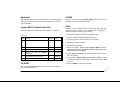
1
MR
Service Manual
Service Manual
© ESAOTE S.p.A.
AG2004
The reproduction, transmission or
use of this document or its
contents is not permitted without
written
authority.
express
Offenders will be liable for
damages. All rights, including
rights created by patent grant or
registration of a utility model or_
design,_are_ reserved.
Replaces: 8300096009
VER.C
8300096009 VER.D
English
Doc. Gen. Apr/2004
Document revision level
The document corresponds to the version/revision level effective at the time of
system delivery. Revisions to hardcopy documentation are not automatically
distributed.
Please contact your local ESAOTE office to order current revision levels.
Disclaimer
The installation and service of equipment described herein is to be performed
by qualified personnel who are employed by ESAOTE or one of its affiliates or
who are otherwise authorized by ESAOTE or one of its affiliates to provide
such services.
Assemblers and other persons who are not employed by or otherwise directly
affiliated with or authorized by ESAOTE or one of its affiliates are directed to
contact one of the local offices of ESAOTE or one of its affiliates before
attempting installation or service procedures.
Part 0 Table of Contents
Part 1
Introduction
73.3
3.3.1
3.3.2
3.3.3
1
Overview __________________________________ 7
2
General ___________________________________ 7
4
2.1
2.2
Distribution ............................................................................... 8
Service Manual structure.......................................................... 84.1
Part 2
Service Policy
114.2
3.1
4.2.1
4.2.2
4.2.3
Product Line Support Center ________________ 114.2.4
4.3
Sales and Service administration ........................................... 11
3.2
Orders .................................................................................... 125
3
Repairs ................................................................................... 12
General conditions for repair ............................................ 12
Procedure for returning goods to ESAOTE ...................... 12
Warranty after repair ........................................................ 14
Part 3
System
15
Strategy __________________________________15
System functionality ................................................................ 15
System error list ...................................................................... 22
Window messages text syntax ......................................... 22
Abbreviation codes........................................................... 22
Symbols used................................................................... 22
Error messages list .......................................................... 23
Broken Modules Identify ......................................................... 30
Procedures ________________________________31
3
8300096009 VER.D
Table of Contents
14
5.1
5.1.1
5.1.2
5.1.3
5.2
5.2.1
5.2.2
5.2.3
5.3
5.3.1
5.3.2
5.3.3
5.3.4
5.3.5
5.3.6
13
12
11
10
9
8
7
Recording files introduction .................................................... 319
Rec file list ....................................................................... 32
Service RecFilePlot introduction ...................................... 369.1
Monitored quantities ........................................................ 379.1.1
System Check ........................................................................ 399.1.2
Description....................................................................... 399.1.3
Operation......................................................................... 399.2
Functions ......................................................................... 399.3
Image quality .......................................................................... 44
Common interference problem analysis .......................... 44
General problems regarding noise................................... 47
Detecting artifacts on images .......................................... 49
Shielding efficiency .......................................................... 52
10
Necessary tools ............................................................... 52
Operations ....................................................................... 52
10.1
6
Repair ___________________________________ 55
11
6.1
6.1.1
6.1.2
6.1.3
Procedure............................................................................... 55
Magnetic Compensation .................................................. 55
12
DC Compensation ........................................................... 57
AC Compensation............................................................ 59
12.1
12.1.1
12.1.2
12.1.3
12.1.4
Trouble shooting strategy ___________________ 6312.1.5
12.2
Part 4
7
Software
63
6
5
4
3
2
1
0
4
Repair ____________________________________66
Complete Software installation ............................................... 66
Operating System SW Installation.................................... 66
Operating System Service Pack 3 Installation.................. 69
OPI SW Installation .......................................................... 71
Configuration restore .............................................................. 76
Images Restore....................................................................... 77
Part 5
Host
79
Trouble shooting strategy ___________________79
Images visualization and storing ............................................. 79
Procedure _________________________________79
Repair instructions _________________________80
Mother Board Bios .................................................................. 80
Standard CMOS set-up.................................................... 80
Bios features set-up ......................................................... 81
Chipset features set-up .................................................... 82
Power management set-up .............................................. 83
PNP and PCI set-up......................................................... 84
Hard disk................................................................................. 85
Procedure ________________________________ 6312.3
Fujitsu M2513 Optical disk drive ............................................. 85
CD ROM ................................................................................. 85
8.1
12.4
Configuration Backup ............................................................. 6312.5
8.2
Images Back up...................................................................... 6512.6
SCSI
8
CD RW ................................................................................. 85
................................................................................. 85
12.7
Computer board set-up........................................................... 8617.3
17.3.1
17.4
17.4.1
17.5
Trouble Shooting Strategy __________________ 8717.5.1
17.6
17.6.1
Part 6
13
14
Control
87
Procedure ________________________________ 87
14.1
DSP test ................................................................................. 8718
14.2
14.2.1
14.2.2
CNTR test............................................................................... 8718.1
Necessary tools ............................................................... 8718.1.1
Operation......................................................................... 8718.1.2
15
15.1
15.2
18.2
18.2.1
18.2.2
Change DSP .......................................................................... 88
18.2.3
Change CNTR or TRDIFF boards .......................................... 8818.2.4
Repair instructions_________________________ 88
Part 7
16
16.1
17
17.1
17.1.1
17.2
RF Subsystem
89
Trouble Shooting Strategy __________________ 8919
RFR check .............................................................................. 95
Procedure ........................................................................ 95
SINT check ............................................................................. 95
Procedure ........................................................................ 95
RFA check .............................................................................. 97
Procedure ........................................................................ 97
Transmission Coil Check ........................................................ 97
Receiving Coils Check ..................................................... 98
Repair ____________________________________99
Transmission Coil ................................................................... 99
Necessary Tools .............................................................. 99
Operations ....................................................................... 99
Receiving coil........................................................................ 101
Introduction .................................................................... 101
Necessary Tools ............................................................ 101
Hardware Connections................................................... 101
Check Procedure ........................................................... 102
Part 8
Patient Handling
105
Trouble shooting strategy __________________105
General ................................................................................. 89
20
Procedure ________________________________ 90
Transmitting Coil Driving ........................................................ 90
Use of System Check ...................................................... 91
Receiving chain driving........................................................... 92
Procedure ________________________________105
Part 9
Gradient
107
5
8300096009 VER.D
Table of Contents
14
13
12
11
10
9
8
7
21
Trouble shooting strategy __________________ 10725.3.3
22
Procedure _______________________________
22.1
22.1.1
23
25.3.4
25.3.5
10725.4
Gradient driving transmitting chain ....................................... 107
Use of the System Check .............................................. 108
Repair __________________________________ 10926
6
5
4
3
2
1
0
6
Shimming Parameter Calculations ................................. 132
Access to the shimming plates....................................... 137
Shimming parameters correction ................................... 137
Test and adjustment table..................................................... 142
Part 11 Power Distribution
143
Introduction ______________________________143
23.1
GRA replacement ................................................................. 109
23.2
23.2.1
23.2.2
23.2.3
23.2.4
23.2.5
23.2.6
23.2.7
23.3
GRA gradient check ............................................................. 10927
Necessary tools ............................................................. 109
Cables connection ......................................................... 109
Check the Gradients ...................................................... 11228
Gain gradient calibration (Geometrical distortion test) ... 117
Introduction.................................................................... 11728.1
Strategy _________________________________143
Necessary Tools ............................................................ 11728.2
Operations ..................................................................... 117
Test and adjustment table .................................................... 120
Adapting transformer to the line voltage ............................... 145
Part 10 Magnet
Repair ___________________________________145
Checking the line voltage...................................................... 145
Part 12 Maintenance Instructions 149
121
29
24
Trouble Shooting Strategy _________________ 121
25
Procedure _______________________________ 122
25.1
Thermal Control Check......................................................... 122
25.2
Sensors and Heaters Check................................................. 123
25.3
25.3.1
25.3.2
Shimming Check .................................................................. 128
Necessary tools ............................................................. 128
Shimming Parameter Acquisitions ................................. 130
Maintenance Plan _________________________149
Part 13 Index
153
Part 1 Introduction
1Overview
Parallel to the advent of a whole new generation of MR systems, a
totally new service support philosophy is dawning, matching and
tailored to the modularity and efficiency of the latest hardware technologies incorporated into this advanced line of machines. In keeping with this progress of newer and enhanced designs, it has become not only feasible but necessary to adapt to a service strategy
making failure isolation and repair as economical as possible. In
line with these trends, we have attained a level of service friendliness never before achieved. This introduction to the TSG documentation is designed to give you an overview of this new troubleshooting concept for the system.
NOTICE
Any installation, assembly, maintenance, extensions, regulation, modifications, or repairs must
be carried out by authorized personnel only.
2General
This register contains an introduction to the service manual: what
the service manual contains and how it can be best used. It will also
attempt to present how the service manual and FUN are coupled
together and complement one another. Here you will find a general
explanation of the concept structure, the various sections comprising the service manual and how they can be used most effectively
for trouble-shooting and repair.
Information on the new page format and on-line documentation are
covered in the manual FUN, part Prefix, section "Documentation
Intro“.
The contents of the service manual will support service technicians
during on-site trouble-shooting and faulty component isolation.
While the instructions are not a substitute for an in-depth knowledge
of the system, its components or the underlying physics, they will
facilitate, on the one hand, trouble-shooting procedures for the less
experienced technician and, on the other, support the more experi7
8300096009 VER.D
Introduction – Overview
14
13
12
11
10
9
8
7
enced technician in performing essential measurements and tests.
The instructions will also explain standard procedures such as
measurements of power supplies, etc.
6
5
4
Table of Contents
•
Introduction/Safety
It is not within the scope of the service manual to list all possible
tests. Its purpose is to support the search for frequently occurring
errors, to allow the technician to limit the error search to certain
functional groups, and to propose measurements for localizing a
faulty component.
•
System
•
Software
•
Host
•
Control
•
RF system
•
Patient handling
•
Gradient system
•
Magnet
•
Power distribution power
•
Maintenance instructions
•
Changes
•
Index
The goal is to distribute the Online-documentation as well as the
paper version to the MR CSE‘s via a distribution list. This means
that in the future this documentation will no longer be delivered with
the system.
1
The troubleshooting guide is structured as shown below:
•
2.1Distribution
2
2.2Service Manual structure
The service manual should not and does not take the place of an
error catalogue. In most cases hardware faults are easily and
quickly located. Intermittent errors require more time and patience.
We are aware that the first versions of this manual do not provide
the reader with an entire spectrum of information. The manual will
be updated accordingly in the future. Any feedback is strongly encouraged and will be warmly welcomed to provide you with the tools
you need. We need your help!
3
0
8
Suggestions for use
Repair
The information for the different system components has been subdivided into:
If a module needs to be replaced, procedures for its replacement
and subsequent necessary adjustments are described in this section.
– Test Strategy
– Test Procedures
– Diagrams
– Repair and Adjustment Procedures
Strategy
The flowchart is designed as a general guideline for selecting the
appropriate trouble-shooting procedures.
The objective of the accompanying descriptions is not to give detailed step-by-step instructions into the finer art of trouble-shooting,
but to offer a means of guiding you, given a particular problem, to
the right test procedure, briefly and simply. If more detailed instructions are necessary, then the CSE will be referred to the appropriate procedures in the section "Test Procedures“.
Index
An index at the end of the book provides you, in addition to the table of contents, with cross-references, to inform you about topics
that you may wish to look into for further information. It is a helpful
source of information when looking for related topics when you want
to concentrate on items of interest. For example, if you would like to
know more about the "adjust frequency“ you could either look under
"A“ for "adjust“ or "F“ for "frequency“. Many topic listings are redundant to help make your search more successful.
Procedures
Here the CSE will find detailed test instructions. You will also find
descriptions for "standard procedures“ - for example, starting the
SeSo, connecting the laptop to the Host, reading log files, etc. This
section also contains descriptions for interpreting the test results.
Furthermore you will find general information pertaining to parts
location, fuse ratings, power supply information, measuring points,
descriptions of LEDs and potentiometers in this section.
9
8300096009 VER.D
– General
14
13
12
Page intentionally left blank.
11
10
9
8
7
6
5
4
3
2
1
0
10
Part 2 Service Policy
3Product Line Support Center
All communications with the center must be in English at these addresses:
The Support Center provides all general activities targeted to customer support (manuals, training, Service Information, etc.)
Esaote S.p.A
Specific Service activities and responsibilities include:
16153 Genoa Italy
•
Service Manuals
Fax +39106547275
•
Service Information
•
Service Training
•
Product Part Lists
•
Part repairing process
The entire Service Administration is managed through your Sales
Area Manager. Responsibilities include:
•
On-line support (mail, phone, fax, etc.)
•
Spare Parts Price List
•
Order Processing
•
Repair Administration (invoices and shipments)
The support center are currently open from 8:00 a.m. to 5:00 p.m.
(local time) between Monday to Friday, excluding Public Holidays
and ESAOTE summer closing period.
Via Siffredi 58
E-mail: [email protected]
3.1Sales and Service administration
11
8300096009 VER.D
Service Policy – Product Line Support Center
14
13
12
11
10
9
8
7
3.2Orders
6
5
NOTICE
Part Numbers are required for prompt order process; items not included in Spare Part Price List cannot be ordered to ESAOTE.
Delivery terms on spare parts range between 60-90 days.
3
2
1
0
12
3.3.2Procedure for returning goods to ESAOTE
Orders shall be issued to the Export Sales Department according to
ESAOTE general rules and your Spare Parts Price List.
All orders are subject to ESAOTE approval and orders below half
million of Italian Lire are not accepted.
4
The modules shipped without following the correct procedure won’t be accepted
Follow this procedure to send back any item for reparation:
•
Fill the Trouble Report (one for every broken module)
– Make a copy of the T/R contained in this manual
– Fill the T/R number field following this criteria: XX – 001 – 01
3.3Repairs
XX = Distributor initials (ask Service Dep.)
001 = Progressive trouble number
3.3.1General conditions for repair
•
•
•
•
•
01 = Current year
– Leave empty the ESAOTE T/R number field
Any Defective item under warranty shall be returned to ESAOTE
for repair/substitution
Parts declared ”non repairable” in the Spare Part Price List are
not accepted once warranty expires
Parts or products cannot be returned for upgrades unless the
upgrade has been previously agreed in writing with ESAOTE
Parts damaged because of traumatic events or improper handling (example: non-authorized modification or improperly performed modification) will be automatically considered out of warranty and can be declared non-repairable by ESAOTE
Complete products cannot be returned for repair unless requested by ESAOTE or previously agreed in writing
NOTICE
•
•
If you don’t have the T/R form, download it from
the ESAOTE web site
Send the filled T/R by fax to the attention of or by e-mail to:
[email protected] or [email protected].
If you want to send the broken module to ESAOTE, fill the RMA
form in every field indicating:
– ITEM name of the broken module
– P/N part number of the broken module
– Item Ser/N serial number of the broken module
– System Ser/N serial number of the system
– T/R trouble report serial number
Code
Components
– Warranty if the module is under warranty or out of warranty
9500166010
ACQ
– Comments for example, write if you need an urgent replace-
9500176000
CNTR
9101533000
GRA
9101598000
RFA 250W
9100712001
RFR
9101148001
CTERM
9100805001
SINT02
9700020000
Electronic Units Left and Right
9500792010
DSP
9500722000
PRINT
9102274000
PC
9101721004
MONITOR CRT 19"
9101721005
MONITOR TFT 17"
9100711002
Magnetic Compensation Kit
– IC index configuration number (only for E-SCAN)
ment of one of the broken modules
The Medical
manufacturer,
traceability of
Every Trouble
components.
Device Directive (MDD 93/42) mandatory forces
distributor and technician to guarantee the Ser/N
some system components. See the below table.
Report must have the Ser/N of the broken and new
Tab. 1: The Ser/N of these modules must be written in the Trouble Report
Code
Components
9102398000
Insulating Transformer
9100773003
Magnet
9101294000
GANTRY
9100934002
LNA
9101310001
RIB
9500649100
REGNTC
9700004003
Magnet and Covers
9101585000
Knee Coil N.1
9101034001
Large Knee Coil N.2
9101584000
Hand Coil N.3
9500877010
TRDIFF
NOTICE
•
If you don’t have the RMA form, download it from
the ESAOTE web site
Send it by fax or e-mail to ESAOTE and wait for the RMA
authorization form. It is a word file that you will receive by e-mail
13
8300096009 VER.D
– Product Line Support Center
14
13
NOTICE
•
12
11
10
9
8
7
ESAOTE S.p.A.
Via Montecchi, 5
16153 Genova, ITALY
Att. Antonio Toso
•
The shipment without RMA authorization form
attached will be rejects. In case parts have not
been accepted for repair, a Notice of Rejection
detailing the reasons will accompany goods.
Make two orders and send them to [email protected] or
by fax (+39 010 6547275):
– under warranty modules at price zero
– out of warranty modules insert the price contained into the Re-
pairable Item list (50% off) of the Spare Part list
NOTICE
5
4
3
2
1
0
14
Not all the out of warranty modules will be 3.3.3Warranty after repair
authorized (refer to the Repairable Item list)
If originally out of warranty, those parts are warranted after repair
for a period of ninety days from ESAOTE shipment.
Print out the received RMA authorization form and place one
copy on the shipment crate. Send the goods to the following address:
NOTICE
6
Indicate on the order the RMA number
If in warranty, parts will be covered by saleable warranty or by the
extended ninety days, whichever is greater. As an example, should
the saleable warranty by expiring in 60 days, after repair warranty
will be applied.
Part 3 System
4Strategy
In this chapter you will find test strategies encompassing the complete system.
4.1System functionality
All modules present in the system are necessary for different processes.
You must know how the system is composed and how it works in
order to identify any kind of trouble.
•
Thermal control
•
Images visualization and storing
You can perform different tests for every chain to identify the defective modules.
A detailed description of the different chains and the different tests
is given below.
The most useful and powerful test is the System Check test.
In the next figures, the modules positions and connections are
shown.
You can identify some different chains:
•
Transmitting gradient driving
•
Transmitting coil driving
•
Receiving driving
15
8300096009 VER.D
System – Strategy
14
13
12
Fig. 1: System Layout
11
10
9
8
7
6
5
4
3
2
1
0
16
Fig. 2: Left Electronic Unit rear side
17
8300096009 VER.D
System – Strategy
14
13
12
11
Fig. 3: Left Electronic Unit front side
10
9
8
7
6
5
4
3
2
1
0
18
Fig. 4: Magnet top view
19
8300096009 VER.D
System – Strategy
14
13
12
11
Fig. 5: Right Electronic Unit front side
10
9
8
7
6
5
4
3
2
1
0
20
Fig. 6: Right Electronic Unit rear side
21
8300096009 VER.D
System – Strategy
14
13
12
11
10
9
8
7
6
5
4
3
2
1
0
22
4.2System error list
Configuration file error
4.2.1Window messages text syntax
Error: (error code) "message":
Scan disabled
This string means that the data of the configuration file,
which we are trying to read, are not in the expected format. This kind of error causes a NON RECOVERABLE
situation that usually need service intervention.
The control is turned off and an unrecoverable error is
4.2.2Abbreviation codes
indicated; the operator must click the "cancel" button to
exit the message window.
E: error
N: note
Warning: (error code) "message":
W: warning
Do you want to proceed?
There is a recoverable error and the user can continue to
work; the operator must decide whether he wants to
continue (button "Yes") or not (button "No"). After this he
exits the message window.
4.2.3Symbols used
COI: CPU control interface
LIF: lower control interface
OPI: operator interface
Note: (error code) "message"
There may be a failure, but the user can continue to
work; the operator must click the "cancel" button to exit
the message window.
System call error
With this string we refer to a generic system error related
to an operation (as opening/reading/writing file) which
fails.
This kind of error causes a NON RECOVERABLE situation that might need service intervention.
DSP: digital signal processing
Predef: files with all predefined scan data information
4.2.4Error messages list
For every error code there is the type (E/W/N) and the description.
The error codes are subdivided in paragraphs according to the
situation that can give rise to them.
Generic codes
1E: input error from LIF command.
9E: general COI fatal error.
10 E: fatal timeout error from OPI after abort signal.
COI sequence compilation time
401 E: bad input to compile MIF command.
402 E: system call error.
403 E: check error during compile time.
406 E: syntax error on sequence source file.
COI scan data load time
501 E: bad input to scan data load MIF command.
502 E: system call error.
COI MIF command parsing time
503 E: check error verifying scan data coherence.
101 E: invalid MIF command
506 E: format error on scan data file.
102 E: system call error from MIF interpreter
507 E: format error on predef file.
COI and DSP scan execution time
COI and DSP quit time
201 E: bad input to scan execution MIF command.
601 E: bad input to quit MIF command
202 E: system call error.
602 E: system call error
203 E: check error during preliminary phase of scan execution.
604 E: error from DSP performing the quit command
204 E: an error code has been returned by DSP during scan execution.
COI load scan vocabulary time
205 E: error during reconstruction on DSP board.
701 E: bad input to load scan MIF command
702 E: system call error
COI and DSP acquisition time
703 E: check error during load time
302 E: system call error.
706 E: syntax error on vocabulary file
303 E: data loaded from DSP have size greater than expected.
23
8300096009 VER.D
System – Strategy
14
13
12
11
10
9
8
7
6
5
4
3
COI and DSP initialization time
Step frequency calibration
802 E: system call error
1402 E: system call error
803 E: check error verifying execution environment and data structures loaded from DSP
1408 E: configuration file error
804 E: an error has been returned from DSP initialization code
Noise level calibration
808 E: COI configuration error
1502 E: system call error
810 E: timeout error waiting for DSP initialization code completion
1508 E: configuration file error
Frequency calibration time
Temperature measurement
902 E: system call error
1602 E: system call error
908 E: configuration file error
1608 E: configuration file error
Gain calibration time
180 calibration
1002 E: system call error
1702 E: system call error
1008 E: configuration file error
1708 E: configuration file error
Calibration of the codification
Noise measurements
1102 E: system call error
1802 E: system call error
1108 E: configuration file error
1808 E: configuration file error
90 calibration
Alarm codes
1202 E: system call error
1901 E: gradient amplifier not powered
1208 E: configuration file error
1902 E: gradient failure
2
1
1903 E: gradient failure, gradient amplifier not powered
Varicap calibration
1302 E: system call error
1308 E: configuration file error
1904 E: cterm failure
1905 E: cterm failure, gradient amplifier not powered
1906 E: cterm failure, gradient failure
0
24
1907 E: cterm failure, gradient amplifier not powered, and gradient
failure
1925 E: RF amplifier failure, RF amplifier not powered, gradient
amplifier not powered
1908 E: RF amplifier failure
1926 E: RF amplifier failure, RF amplifier not powered, gradient
failure
1909 E: RF amplifier failure, gradient amplifier not powered
1910 E: RF amplifier failure, gradient failure
1911 E: RF amplifier failure, gradient amplifier not powered, and
gradient fail
1912 E: RF amplifier failure, cterm failure
1913 E: RF amplifier failure, cterm failure, and gradient amplifier not
powered
1927 E: RF amplifier failure, RF amplifier not powered, gradient
failure, and gradient amplifier not powered
1928 E: RF amplifier failure, RF amplifier not powered, and cterm
failure
1929 E: RF amplifier failure, RF amplifier not powered, cterm failure, and gradient amplifier not powered
1914 E: RF amplifier failure, cterm failure, and gradient failure
1930 E: RF amplifier failure, RF amplifier not powered, cterm failure, and gradient failure
1915 E: RF amplifier failure, cterm failure, gradient amplifier not
powered, and gradient failure
1931 E: RF amplifier failure, gradient amplifier not powered, cterm
failure, gradient failure, and RF amplifier not powered
1916 E: RF amplifier not powered
1917 E: RF amplifier not powered, gradient amplifier not powered
1918 E: RF amplifier not powered, gradient failure
1919 E: RF amplifier not powered, gradient failure, and gradient
amplifier not powered
Timeout between OPI and COI
2065 E: error during initialization
2066 E: error during scan
Autofov
1920 E: RF amplifier not powered, cterm failure
2166 E: system call error
1921 E: RF amplifier not powered, cterm failure, and gradient amplifier not powered
2172 E: configuration file error
1922 E: RF amplifier not powered, cterm failure, and gradient failure
Automatic selection codes of calibrations
1923 E: RF amplifier not powered, cterm failure, and gradient failure gradient amplifier not powered
2266 E: system call error
2272 E: configuration file error
1924 E: RF amplifier failure, RF amplifier not powered
25
8300096009 VER.D
System – Strategy
14
13
12
11
10
9
8
7
6
5
4
3
2
1
Calibration of magnetic compensation
Frequency calibration
2466 E: system call error
3566:E: system call error
2472 E: configuration file error
3572:E: configuration file error
Frequency calibration during scout
Frequency (phase measurement) calibration
2666 E: system call error
3966:E: system call error
2672 E: configuration file error
3972:E: configuration file error
90 180 calibration
Gradient Offset calibration codes
2766 E: system call error
4066:E: system call error
2772 E: configuration file error
4072:E: configuration file error
Alarm codes
RX Offset calibration
2866 E: system call error
4166:E: system call error
2872 E: configuration file error
4172:E: configuration file error
Gain RF sweep codes
Signal missing in calibration
2966 E: system call error
18000W: frequency calibration, there is no signal
2972 E: configuration file error
18001W: gain calibration, there is no signal
Temperature measurement codes during scout
3066 E: system call error
3072 E: configuration file error
0
18002W: encoding calibration, there is no signal
18003W: 90 calibration, there is no signal
18004W: varicap calibration, there is no signal
18005W: frequency step calibration, there is no signal
Noise and temperature calibration
18007W: 90-180 calibration, there is no signal
3466:E: system call error
18008W: frequency calibration during scout, there is no signal
3472:E: configuration file error
18009W: gain sweep calibration, there is no signal
26
Noise level codes
19000W: media noise calculated from FFT signal is over threshold
19001W: there are spikes in the signal
19002W: media noise over threshold and spikes in the signal
Bad signal codes
20008W: frequency calibration during scout, we cannot obtain the
number of intersections wished with zero, check the .rec files
20009W: gains sweep calibration, the max value of the signal after
calibration is not in the wished range, there is something not OK.
20010W: 90 pulse calibration anomaly: insulating belt is recommended. Do you want to proceed?
20000W: frequency calibration, the shape of the signal during calibration isn’t in a wished form, there is something not OK, check the
.rec files.
Anomalous signal
20001W: gain calibration, the amplitude of the signal during calibration isn’t in a wished form, there is something not OK, and check
the .rec files.
Signal out of range
20002W: encoding calibration, the amplitude of the signal during
calibration isn’t in a wished form, there is something not OK, and
check the .rec files.
Off-line calibration codes
20003W: 90 calibration, the amplitude of the signal during calibration aren’t in a wished form, there is something not OK, check the
.rec files.
20004W: varicap calibration, the amplitude of the signal during
calibration isn’t in a wished form, there is something not OK, and
check the .rec files.
20005W: frequency step calibration, we can’t obtain the number of
intersections wished with zero, check the .rec files
20006W: 180 calibration, the amplitude of the signal during calibration isn’t in a wished form, there is something not OK, and check
the .rec files.
20007W: 90-180 calibration, the amplitude of the signal during calibration isn’t in a wished form, there is something not OK, and check
the .rec files.
20500W: temperature not in range
22000N: signal not in range
23000N: Correct temperature, the temperatures are in the wished
range
23001N: Incorrect temperature, one or more temperatures aren’t in
the wished range
23050N: Correct field, the frequency is in the expected range
23051N: Incorrect field, the frequency isn’t in the expected range
23052N: There isn’t signal during testing field
23100N: After calibration the value of 90 pulse is correct
23101N: After calibration the 90 pulse isn’t in the wished range
23102N: There isn’t signal during testing 90 pulse
23150N: After calibration the value of 180 pulse is correct
23151N: After calibration the 180 pulse isn’t in the wished range
23152N: There isn’t signal during testing 180 pulse
27
8300096009 VER.D
System – Strategy
14
13
12
11
10
9
8
7
6
5
4
3
2
1
0
28
23200N: After calibration the varicap values are in the right range
Alarm test codes
23201N: After calibration the varicap values aren’t in the right range
26500N: No alarms found
23202N: No signal testing varicap tuning
26501N: gradient amplifier not powered
23250N: Correct gain value after calibration
26502N: gradient failure
23251N: The signal after calibration isn’t in the correct range
26503N: gradient amplifier not powered, gradient failure
23252N: There isn’t signal during calibration gain
26504N: cterm failure
23300N: Correct encoding gradient
26505N: cterm failure, gradient amplifier not powered
23301N: Incorrect encoding gradient
26506N: cterm failure, gradient failure
23302N: There isn’t signal during encoding gradient calibration
26507N: cterm failure, gradient amplifier not powered, and gradient
failure
24000N: After frequency step calibration the found values are in the
wished range
24001N: After frequency step calibration the found values aren’t in
the wished range
25000N: The average of the FFT noise signal is over threshold
26508N: RF amplifier failure
26509N: RF amplifier failure, gradient amplifier not powered
26510N: RF amplifier failure, gradient failure
25001N: The average of the FFT noise signal isn’t over threshold
26511N: RF amplifier failure, gradient amplifier not powered, and
gradient fail
25002N: the are spikes in the signal
26512N: RF amplifier failure, cterm failure
25003N: media noise over threshold, spike in the signal
26513N: RF amplifier failure, cterm failure, and gradient amplifier
not powered
25100N: correct magnetic compensation
25101N: incorrect magnetic compensation
26514N: RF amplifier failure, cterm failure, and gradient failure
Timeout between OPI and COI
26515N: RF amplifier failure, cterm warning, gradient amplifier not
powered, and gradient failure
26000N: timeout on COI, incorrect scan duration
26516N: RF amplifier not powered
26517N: RF amplifier not powered, gradient amplifier not powered
26518N: RF amplifier not powered, gradient failure
26519N: RF amplifier not powered, gradient failure, and gradient
amplifier not powered
26520N: RF amplifier not powered, cterm failure
26521N: RF amplifier not powered, cterm failure, and gradient amplifier not powered
26522N: RF amplifier not powered, cterm failure, and gradient failure
26523N: RF amplifier not powered, cterm failure, gradient failure,
gradient amplifier not powered
26524N: RF amplifier failure, RF amplifier not powered
26525N: RF amplifier failure, RF amplifier not powered, and gradient amplifier not powered
26526N: RF amplifier failure, RF amplifier not powered, and gradient failure
26527N: RF amplifier failure, RF amplifier not powered, gradient
failure, and gradient amplifier not powered
26528N: RF amplifier failure, RF amplifier not powered, and cterm
failure
26529N: RF amplifier failure, RF amplifier not powered, cterm failure, and gradient amplifier not powered
26530N: RF amplifier failure, RF amplifier not powered, cterm failure, and gradient failure
26531N: RF amplifier failure, gradient amplifier not powered, cterm
failure, gradient failure, and RF amplifier not powered
26600W: the signal after sweep calibration is in the wished range
26601W: the signal after sweep calibration is not in the wished
range
26602W: during gain sweep calibration there is no signal
29
8300096009 VER.D
System – Strategy
14
13
12
11
10
9
8
7
4.3Broken Modules Identify
A malfunction involving the CPU, HD, SVGA, monitor, keyboard,
mouse and optical disc (and/or relative SCSI card) should be immediately obvious since their operation (or failure) is plainly ”visible”. If the message ”Non recoverable error. Scan disabled” appears this means that the software has found problems with one or
more modules, which compound the system.
Try to repeat the bootstrap and if it’s completed successfully, you
are advised to run the alarm diagnostics. With this procedure, you
can check whether amplifiers (GRA and RFA) and CTERM are operating correctly. In the event of a malfunction, a message appears
identifying the failed module. The acronyms used have the following
meanings:
– GRA-OFF: direct power supply failure to the gradient amplifier.
–
–
–
–
This event may also be due (besides to the fuse being blown,
or a disconnected 220VAC cable etc.) to failure to receive acknowledgement from the CTERM module.
GRA: gradient amplifier malfunction (failed PLL connection of
its internal switching amplifier and/or output voltage clamp).
Not significant when GRA-OFF is present.
RFA-OFF: direct power supply failure to the RF amplifier. This
event may also be due (as well as to the fuse being blown, or
disconnected 220VAC cable etc.) to overheating of the amplifier (T > 50°C).
RFA: RF amplifier malfunctioning (duty cycle over 25% and/or
reflected power greater than 40 watt). Not significant when
RFA-OFF is present.
CTERM: direct power supply failure to the CTERM module.
This event may also be due (as well as to the fuse being blown
or to a disconnected 220VAC-cable etc.) to overheating of at
least one side of the magnet. This failure is detected by the
temperature sensors (2 NTC in series) located on the side, or
by a short circuit or an open circuit on at least one of the four
groups of the NTC sensors.
6
5
4
3
2
1
0
30
After verifying that the standard part of the PC (successful completion of the bootstrap routine without any error messages) and the
power modules (GRA, RFA and CTERM are operating correctly,
with the diagnostic alarms), you can proceed to run the <System
Check> diagnostic. If the plot operates correctly, it is safe to assume that, generally speaking, the control subsystems (DSP and
CNTR) and the acquisition subsystems (DSP and ACQ) are operating correctly too. In particular, it is best to first display the values
relative to the driving of the receiving subsystem (modules RFR,
and BRX) which are generated and monitored from within the module ACQ. Their correct behavior confirms substantially that acquisition is operating correctly. From <System Check> you can also
verify the correct operation of ”Gradients” and ”RF Pulse”. Regarding the RF pulse, you must know the correct amplitude ratio between transmitted and reflected RF pulse (Pd/Pr>4) which shows
that the connection is correct and that the transmitting coil (BTX)
tuning is correct. Conversely, the absence of the RF pulse may be
due to:
– A malfunction of the SINT module: if, for instance, the module
is not receiving power (fuse, cable, etc.). You can also make
sure that the SINT is working at the correct frequency. To test
this, connect SINT5 (the local oscillator output, normally connected with RFR4) to a scope and check that the frequency
(f0) and the signal amplitude (1.2 Volt p-p) are correct. Another
way is to use the AINT service module.
– Bad tuning of the transmitting coil. If the ratio is about 1 (i.e. all
the power is reflected), the problem could be due to a bad
connection between RF amplifier and transmitting coil or a
broken component inside the transmitting coil. For example the
central capacitor on the tuning circuit inside the ”gantry”.
– A wrong value of the frequency set in the ”Homogeneity” calibration.
As for the receiving chain, you are advised to use the standard machine settings (central frequency search, noise level, S/N for the
various receiving coils and sequence calibration, etc.).
5Procedures
Fig. 7: REC File folder
5.1Recording files introduction
This section explains the possibility of evaluating information regarding the system operations. In fact this information is written in
some recording files which can be seen by the operator.
The following paragraph gives the recording files list, in which the
name of every file is followed by an extension name ”.rec”.
The Rec Files contain all the operations performed by the system.
Some of them are generic other are more specific. The system creates a new folder every day and every folder contain only the rec
files filled in that day.
All the rec files are self-explaining and not always are created by
the system every day.
To have access to the rec files, open the Internet Explorer and,
from the homepage, open the Rec File Management folder then
View Rec Folder: from this page you have to select the interested
day, opening it the system will show the compiled rec files.
31
8300096009 VER.D
System – Procedures
14
13
12
11
10
9
8
5.1.1Rec file list
4
3
2
1
0
32
freq.rec
The file contains the fine step frequency
values
freqstep.rec
The file contains the course step frequency values
noise.rec
The file contains the shielding test values
temp.rec
The file contains the temperature and
power values of the magnet
fov.rec
The file contains the <S/N Check> obtained by pressing a button from the Operator Interface
The dimensions along the Y and X-axes
of the object are stored in this file
alarms.rec
Alarm messages are stored in this file
diascope.rec
The file contains the image information
obtained and viewed by pressing the
<Service>/<Image info> button from the
Operator Interface
The file is the file to which “Diascope”
writes every time it runs
ortho.rec
The file is the trace (recording) of the activity of the executable ortho
resl_s_shm.rec
The file is the trace (recording) of the activity of the executable resl
work.rec
The file is the trace of the general activity
of the machine
ping.rec
The file contains the results of the inquiry
to the other system
Meaning
opierr.rec
The file contains the sentences written
every time an Error Message Window is
displayed
header.rec
5
Meaning
Rec file name
sn.rec
6
Rec file name
Tab. 2: Rec file list
opi.rec
7
The file contains all the sentences written by the Operator Interface (OPI) during the examination
coi.rec
The file keeps a record of the activity of
every work session of the Control Interface (COI)
opicoi.rec
The file contains information about the
UNIX core file
90.rec
The file contains the 90 pulse values
180.rec
The file contains the 180 pulse values
stab.rec
The file contains the data for the stability
test
varicap.rec
The file contains the varicap The file
contains the 180 pulse values
results.rec
The file contains the data of the shimming calculation
autotar.rec
This file contains information about two
different gain processes
Fig. 8: 180.rec
The 180° Pulse calibration is automatically done
by the system every scout acquisition to calibrate
the necessary energy to rotate the spin during the
sequence acquisition.
The 90° Pulse is automatically calculated by the
system starting from the 180° Pulse value.
The 180.rec file is also filled in during the Service
automatic calibrations.
Looking at this file is possible to understand when
the system wasn’t able to calibrate the pulse and
why the images went black, for example.
33
8300096009 VER.D
System – Procedures
14
13
12
11
10
9
8
7
6
5
4
3
2
1
0
34
Fig. 9: Freq.rec
Like for the 180.rec, the frequency calibration is
automatically done by the system every scout acquisition to find the magnet frequency in that moment.
A small frequency shift is normal and compensated by the system.
A frequency shift is related to a thermal shift,
usually, due to the environmental thermal shift.
During the day the temperature of the room increase and the CTERM has to follow this shift decreasing the power sent to the Magnet to warm
up it.
In case of big Magnet thermal shift, perform the
System Monitor to follow in real time the temperature and provided power to every channel.
Remember that the system is calibrated to the
Magnet central frequency and it must be stable,
all the specification written in the Planning Guide
and related to the installation room must be met.
Stable frequency means good image quality.
Fig. 10: Varicap.rec
The Varicap is a voltage value (0 – 9V) sent by
the RFR to the Coil in order to set it to the Magnet
frequency taking care of the inserted load.
Every Coil has its own Varicap value: when you
save it manually don’t overwrite the other values.
Also the Varicap is automatically calculated by
the system during every Scout acquisition.
The rec file is filled in by the system every time
the varicap is calculated either when is done
automatically or manually by the Service technicians.
If the Varicap is not correct or cannot be calculated by the system means that an error in the receiving channel occurred.
35
8300096009 VER.D
System – Procedures
14
13
12
11
10
9
8
7
5.1.2Service RecFilePlot introduction
This section deals with the monitoring and subsequent analysis of
various quantities whose time evolution is interesting while evaluating:
•
•
•
The characteristics of the environment in which the system must
operate (with particular reference to temperature and Magnetic
DC field strength)
System adjustments while responding to changing environmental
conditions (with particular reference to thermal and magnetic
compensation activities)
System parameters (with particular reference to central precession (Larmor) frequency and operating noise level).
This environment is organized in this way: analysis of the time evolution of the above mentioned quantities plays a critical role in identifying troubles relating to the presence of incorrect environmental
conditions and/or damage or malfunctioning of thermal and magnetic compensation units. Moreover, the analysis performed over a
long period of time can provide meaningful information (from a statistical point of view) about the relationships between failures and
certain environmental conditions.
In order to provide a complete tool, the monitoring procedure can
be performed in three different ways, characterized by different time
ranges:
•
•
For a maximum period of a day (<System Monitor>: short period analysis)
For a maximum period of one year (<System History>: analysis
performed over a part of the lifecycle of the system)
6
•
5
4
3
2
1
0
36
During a cycle of thermal stress (<Stress>: analysis performed
over a maximum period of three days, the appropriate sequences inspect the system’s thermal stress by observing the
relationships among the measured quantities listed below).
The practical tool used to inspect the quantities versus time functions resulting from the monitoring procedure is again the “Diascope” whose characteristics and functions are tailored for this specific application as described below.
5.1.3Monitored quantities
Three folders are available under the <Hist> icon of the ARAS toolbar: <RecFilePlot/System History>, <RecFilePlot/System Monitor> and <RecFilePlot/Stress>. They make it possible to display
the data items previously collected with one of the time ranges defined above. Here is a detailed list of the monitored quantities.
NOTICE
System history
– Environment temperature
– Central precession (Larmor) frequency of static magnetic field
– Noise (average FFT)
Fig. 12: <RecFilePlot/System History> folder
These files are created by the system only when
the corresponding test are performed (e.g.: the
<System Monitor> test compiles the <RecFilePlot/System Monitor> history file)
Fig. 11: History File Selection
37
8300096009 VER.D
System – Procedures
14
13
12
11
10
9
8
7
System monitor
6
5
4
3
2
1
0
38
Stress
– Temp/Power UP INNER; DOWN OUTER; DOWN INNER and
– Temp/Power UP INNER; DOWN OUTER; DOWN INNER and
UP OUTER (Temperature/power associated with each of the
four heaters)
– Environment temperature
– Magnetic field strength
– Magnetic field strength/Magnetic field strength in the gantry
UP OUTER (Temperature/power associated with each of the
four heaters)
– Environment temperature
– Central precession (Larmor) frequency of static magnetic field
(The last logical channel is fundamental also as a tool while performing magnetic compensation)
Like in all the other system features the scales can be set by the
user to better visualize the history data.
Fig. 14: History file Diascope visualization
Fig. 13: <RecFilePlot/System Monitor> folder
5.2System Check
5.2.1Description
The <System Check> menu contains several functions allowing
the operator to perform various checks of the system operation.
After entering this environment, the system will display ”Diascope”
instrument.
Please note that data is acquired with a 16-bit resolution in a two’s
complement mode and the display range of our oscilloscope (with
<Res. Div.> =1.0 and <Displacement> =0) is between -32768 and
+32767. Values exceeding the display range are shown with a tangent line to the upper or lower edge of the window. Displacement is
relative to the visualization and not to the signal.
The message “Note (26000) Incorrect scan duration”, that is displayed when quitting, is not a warning of a malfunction, but rather
indicates the time (longer than in a normal scan) that the <System
Check> environment has been active.
5.2.2Operation
Perform the following operations to access the <System Check>
environment:
•
•
Turn on the system and wait for the operator interface to appear
on the screen. If after 20 seconds no error messages are displayed (”Non recoverable error. Scan disabled.”), this means
that the computer has successfully completed its selfconfiguration (all modules are present) and is receiving the basic
clock (for control and acquisition) from the SINT module.
Open the ARAS program then select <Tests> <Hardware>
<System check> and press <Run>
You have now entered the <System check> environment, from
which you can test the apparatus electronics.
After approx. 10 seconds, you will hear the noise of pulsating gradients. After another 10 seconds, the screen will turn into a 2-channel
oscilloscope, displaying on the left a large window displaying a pair
of signals at the rate of about one pass per second, and on the right
a column containing a menu of commands. A detailed explanation
is given in the following paragraph.
5.2.3Functions
You can run the following tests from the System Check environment:
•
X, Y and Z Gradients Coil Driving
•
Receiving Chain Driving
•
Transmission Chain Driving
The control software operating on the DSP sends, on cable
HSSLO, the digital data, which are necessary to CNTR PCB. Both
CNTR and DSP are in the PC unit.
Within the CNTR command, data are processed and transformed
into analogue signals driving the gradient amplifier (GRA) and sent
to the same amplifier by the GRA cable and reaches the GRA ”INPUT” connector.
Gradients are sent to the magnet side through the filter panel to the
magnet connection panel (rear side). Gradient X, Y and Z coils are
fixed into the ”GANTRY” to the magnet and are made of multi layer
rigid circuit matter.
39
8300096009 VER.D
System – Procedures
14
13
12
11
10
9
8
7
6
5
4
3
2
1
0
40
Fig. 15: System Check X,Y and Z channels
The first three channels of
the System Check test are
the gradient waveforms. The
blue traces are the output of
the CNTR board and the input of the GRA module. The
red traces are the output of
the GRA module.
If the input traces are not
present means that or the
CNTR is broken or the cable
between the CNTR and the
GRA is broken.
If all the output traces are
flat probably the GRA is
broken or not powered or
disabled by the CTERM
module.
If only one of the output
trace is flat, swap the gradient cables (e.g.: X is flat, invert X with Y).
If the problem moves to another channel means that
the problem is from the GRA
on (cables or Gantry); if the
problem is still on the same
channel means that the gradient board is broken.
Fig. 16: System Check Varicap 1 and 2
The Varicap is a voltage
value (o – 9V) that the RFR
sends to the Coil in order to
set it at the magnet central
frequency taking care of the
inserted load: different load,
different varicap value.
Change the varicap value (0
– 255) and see if the voltage
value changes, if not means
that the RFR is broken or
that the cables from the
RFR to the Coil are broken
(short circuit).
41
8300096009 VER.D
System – Procedures
14
13
12
11
10
9
8
7
6
5
4
3
2
1
0
42
Fig. 17: System Check Gain 1 and 2
The Gain signals are operational amplifier gains present into the RFR module.
Performing a Scout acquisition using the Knee Coil 1
and the Geometrical phantom in axial position Gain 1
must be lower than 255 and
Gain 2 must be zero.
Change the Gain values (o
– 255) and check if it’s possible to move the trace on
monitor: 255 = 10V.
If the traces don’t change
their values means that the
RFR is broken.
Fig. 18: System Check RF pulse
To change the spin orientation we have to send power
to the phantom or patient.
The RFA takes care to amplifier the signal received
from the SINT module and
sent it to the Gantry (transmission circuit).
The blue trace is the direct
pulse: the energy that the
RFA is transmitting to the
Gantry.
The red trace is the energy
that we are losing because
the Gantry is not equal to
the ideal load (50Ω). It must
be lower than 20% of the direct pulse.
If the red trace is flat means
that the SINT module is broken or the cable between
SINT and RFA.
If the blue trace is flat disconnect the output cable
and connect a dummy plug
(50Ω) to the RFA output: if
the trace is still flat means
that the RFA is broken otherwise the Gantry or the cable are broken.
43
8300096009 VER.D
System – Procedures
14
13
12
11
10
9
8
7
5.3Image quality
1.1.1Common interference problem analysis
The most frequent cases are the presence of artifacts on the image
generated by external radio frequencies, interference created by
some electronic modules inside the electronic unit or ”spikes”.
A typical case of the radio-frequency problem generates a strip on
the image; this can be more or less thick. In both cases, the noise is
selective, but when the strip is thin, this means that the noise has
only a single frequency. On the other hand, if the strip is thick, it is
typically a frequency modulation. Instead, the ”spikes” could be
classified as a large bandwidth problem that is usually generated by
poor power supply or by certain motors (e.g. from elevators, air
conditioning, etc.).
In the same way you can study RF interference using the <Rx
Chain> service menu. Also in this case you can have different
kinds of disturbance:
1. A well determined RF interference (one thin strip on the image)
2. A frequency modulation (example: band of strips on the image)
In the first case, set <FFT> mode in the <RX Chain> (ARAS program, <Test> and <Manual>) environment to see a thin peak,
whereas, in <Echo> modality a sinusoidal signal will appear. While
if a frequency modulation (case 2) is present on the images, always
in <FFT> something like a narrow rectangle, formed by a given
number of peaks, will be displayed.
6
5
4
3
2
1
Fig. 19: Example of selective noise with a given frequency
0
44
Fig. 20: RX Chain test, FFT visualization
When this window appears,
select the FFT mode then the
A visualization and apply
these settings to all the channels (right button mouse,
check the <Apply to all channel> box then click on <OK>).
Set the Frequency to 5K to
visualize a larger bandwidth
(at least ±20 kHz from the
central magnet frequency).
Set the Y-axis to 1K.
If a central peak appears is
the SINT oscillator and means
that the Phase and Quadrature offsets are not properly
calibrated to the zero level.
The meaning of this test is
check if any radio frequency
peaks appear close to the
magnet central frequency (indicated by 0 kHz): if they appear they can generated
noises on the images.
45
8300096009 VER.D
System – Procedures
14
13
12
11
Fig. 21: Example of frequency modulation
10
9
8
7
6
5
4
3
2
1
Fig. 22: Example of artifact due to the present of “spikes”
0
46
5.3.2General problems regarding noise
This section covers some problems regarding high noise levels in
the system room and their possible solutions.
These kinds of problems could be generated by several things,
such as: the power line cable lacking a good filtering system, network lines to transmit data between different computers, the laser
camera installed close to the system or any other source not perfectly shielded. In all these cases, the normal noise level increases
until it exceeds the warning noise threshold, to the detriment of the
quality and resolution of the images so obtained.
ages). However, in any case, the image quality decreases significantly.
Both the machine ground and the central ground must also be
checked, because they sometimes generate problems. As a matter
of fact, it has often been noted that, if the grounding problem is
solved, the average-fft level decreases to a normal value (around
500).
A short list including things to be avoided during installation is given
below:
– Power lines without an UPS system
– Power lines must not pass close to the system
This is to say that everything (line cables, personal computer, network cable, central phone line, etc.) in the room must be checked
very carefully before installing the system to avoid any problems
after installation.
Therefore to reduce the noise level in the room, you must ascertain
in advance which are the possible causes of the problems by acquiring images in different conditions. For example, this can be
done by turning off all possible sources of problems, step by step,
then checking the average-fft value by clicking on the <Shielding>
in the <Automatic> service menu. If the problem has not been
identified yet, proceed by making sure that all power lines use a line
filter, that there are no other critical instruments in the system room
and that every ground cable of the machine is properly connected.
– A layout of cables that creates a coupling between them
– Avoid putting other kinds of instruments in the same room,
such as a personal computer, laser printer, mediator, etc.
– Ground cables wrongly connected
– Bad central ground
A method to understand how the noise level changes during the
day is described, so it will be possible to look at noise variations in
real time. Here are the operations useful for this check:
•
•
With regard to these problems, we recommend putting the power
line through an UPS system, so that the power line that arrives at
the system or at other instruments is without noise, without selective interference or noise with a large bandwidth.
•
Another critical factor for the noise level is the presence of personal
computers or other instruments that could create some interference
by increasing the noise level. This noise could be selective interference (lines on the images) or, more likely, white noise (noisy im-
•
•
Put the homogeneous phantom inside the knee coil
Inside the ARAS program select <Test>
Chain> menu then <Run>
<Manual>
<RX
set the <FFT> modality
Set the Y-axis to 1K. It is thus possible to visualize the noise
peak better. In this modality two kinds of noise may occur
Selective noise with a given frequency: a single peak will be displayed at that frequency; the higher the dB of the noise the
higher the peak
47
8300096009 VER.D
System – Procedures
14
•
•
13
12
11
10
9
8
7
A large bandwidth noise (white noise): the whole level of the
signal increases; this means that the noise in the room is too
high
To improve the signal display, click on the <Average> button
and set a number around 20
When the previous operations are completed verify if the level of
the signal is close to 1K (first step) of the vertical grid, or if the
”May” variable in the information window has a value of around
1350, that means that the noise level is good (average-fft less then
500).
On the contrary, if the level is higher, then you can carry out two
different trials:
•
•
Verify the noise level putting a Dummy cup in the suitable support supplied in the Gradient Tuning Kit
Verify the noise level when a patient puts a limb inside the coil
Regarding the first case you can reach this conclusion: if the noise
level is again in the specifications with the Dummy cup, this means
the problem could be external, otherwise some parts of the electronic unit would create a rise in the noise level. Check each module and cable, one at a time.
If the problem is external you must check as described in the previous points. In fact when a patient's limb is inside the coil every external disturbance is increased, because the patient acts as an antenna.
Therefore, at first you must check to see if the shielding parts are
correctly applied to the patient and if each ground cable is fixed,
then check what source could create the rise in noise.
6
5
4
3
2
1
0
48
If you find something such as a personal computer, telephone or
laser printer, that could be a source of noise, you will probably have
to apply the solutions described previously, decreasing the noise
level in the room (average-fft value around 400) until good quality
images are obtained.
5.3.3Detecting artifacts on images
Fig. 23: Radio frequency probably due to external factors
Simulation of examinations
After performing all the system’s calibrations and the relative quality
tests, check that the system is operating smoothly by performing
scans on patients using different sequence types (GE, Spin-Echo,
Turbo-Multi-Echo, etc.). For this type of testing, perform several
acquisitions on all the four coils and assess the quality for each type
of sequence.
More specifically, the images obtained must be observed in order to
exclude the presence of artifacts (such as lines, light spots, bands,
etc.) and magnetic fluctuations in DC mode (e.g. blurring) and in AC
mode (e.g. ghosts). In order to check that the signal/noise ratio is
good and that the contrast is appropriate.
Consider that some related problems (for instance lines, spots, etc.)
may be caused by:
– RF external frequencies
– RF frequencies within the system due to the failure of any
hardware modules
49
8300096009 VER.D
System – Procedures
14
13
12
11
10
9
8
7
Consider that some related problems, for instance ghost images,
may be caused by:
6
5
4
3
2
1
0
Consider that some related problems, for instance, out of focus
images called ”blurring” effect, may be caused by:
– Phase and quadrature offsets a long way out of the zero level
– Thermal instability of the system;
– Fluctuation of the signal due to external fields at about 50/60
– Fluctuation of the signal due to DC magnetic interference;
Hz and 16.6Hz
Fig. 24: Ghosts generated by external 50Hz
50
– Fluctuation of the signal due to miscellaneous HW problems.
Fig. 25: ”Blurring” artifact probably due to external DC
Consider that strong spikes in the power line may cause some
problems, such as the “moire” artifact.
Fig. 26: ”Moire” artifact probably due to strong spikes on the power line
If the operator detects the above-mentioned artifacts in the images,
he/she must first analyze them carefully.
A list of scans can be found in the OPI program (<Protocol List>
folder). The Service operator may use them to check the image
quality, hence to identify any of the above-mentioned problems.
All the current scans are to be taken in multi slice mode with the
slices oriented as desired. Have at least one standard direction and
one double oblique slice for each scan and change the directions
between scans.
Please note that, since before each scan an automatic fine calibration of resonance frequency and of the receiving chain gain is performed, any problems should be detected through the calibration
procedures and suitably signaled. It may be advisable, however, to
check the results produced by calibration in the store files (freq.rec
and autotar.rec).
51
8300096009 VER.D
System – Procedures
14
13
12
11
10
9
8
7
5.3.4Shielding efficiency
The purpose of this calibration is to check that no external noises
are present in the signal picked up by he coil, such as radiofrequencies which would generate lines or light spots on the image.
Moreover, the procedure checks that the noise level does not exceed a pre-set threshold value.
6
5
4
3
2
1
0
52
The program is based on running a sequence that carries out a
simple acquisition of the noise picked up by the receiving coil. By
submitting it to Fourier’s transform, you can detect the spikes resulting from external radio frequencies and to calculate the average
noise level.
5.3.5Necessary tools
– Geometrical phantom and its support
Fig. 27: Line generated by radio frequencies
5.3.6Operations
•
•
•
•
Position the knee coil 2 with the geometrical phantom placed in
axial position
From the ARAS program
<Shielding> then <Run>
select
<Tests>
<Automatic>
Look at the message sent by the calibration procedure. If this
was not successful, do not continue, but rather check the store
file ”noise.rec”
Exit by clicking on <OK> button
Fig. 28: Shielding Test
In the bottom part of the
window, look for the Average_fft value: if it’s to
lower than 400 means that
the system has a good
signal to noise ratio and is
good shielded.
53
8300096009 VER.D
System – Procedures
14
13
12
11
10
9
8
7
In the event of noise or of signal spikes exceeding the threshold
(threshold_f), the program indicates their position (co-ordinate,
range 1 to 256), amplitude and frequency.
Please note that a continuous signal corresponds to co-ordinate 1.
This is the so-called offset that is always present. Therefore, this
spike must not be considered for the purpose of evaluating the
situation.
In the event of persistent interference, on-site measurements must
be taken exactly like those taken before installation. In addition, you
must check that noise is not generated by the electronics. You must
also make sure that any type of lines or spots does not damage the
images. For this reason, some test scans must be taken.
Conversely, if the noise level exceeds the threshold, it is likely that
the receiving chain is malfunctioning or not properly calibrated.
Please note that the cause of this might be white noise picked up
directly by the coil. Therefore, you are advised to check that there
are no possible sources near the machine and that the shielding is
properly sealed.
The noise level is represented by average_fft, whose threshold
value is written in the software and has been set taking into account
the situation of the first machines.
Please note that this calibration may also be performed from the
operator’s interface as a diagnostics scan.
6
5
4
3
2
1
0
54
6Repair
In case of not perfectly shielding efficiency check all the system
grounds or provide a dedicated ground.
If you noticed that a RF spike causes noise of images, shift the
magnet central frequency changing the NTC board (send an order
to ESAOTE specifying system ser/n, magnet ser/n, magnet frequency, frequency of the RF noise and desiderated new magnet
frequency).
If the image problems are generated by magnetic interference follow this chapter to compensate them.
Sources of DC Interference
Trucks, subways, elevators, escalators and fans or other kinds of
iron masses running close to the magnet can generate DC noise.
NOTICE
It is possible to compensate only one DC source
Sources of AC interference
Power cable or railways close to the site.
Perform compensation during working hours when all the Systems
are on and the noises are usually stronger.
6.1Procedure
6.1.1Magnetic Compensation
This chapter describes the Magnetic Compensation Procedures for
external DC and AC (50, 60 and 16.6 Hz) noise.
Necessary tools
•
Gradient Tuning Service Kit
•
Magnetic Compensation Kit
•
Small and flat screwdriver
•
Allen wrenches 4mm
55
8300096009 VER.D
System – Repair
14
13
12
11
10
9
8
7
6
5
4
3
2
1
0
Fig. 29:CTERM module front and rear side
On the CTERM module front
side all the Magnetic connections are present.
Also the trimmers (dedicated
to the Magnetic compensation
gains) and the trimmers
(dedicated to the Ac magnetic
compensation phase) are
placed on the CTERM front
side.
On the rear side there are the
CTERM fans and plugs.
The upper plug is the power
supply for the unit. The magnet fast heaters are connected to the lower plug and
the CTERM module provides
or not powers to them automatically.
56
6.1.2DC Compensation
•
•
NOTICE
The probe must be fixed on the wall at the end of
the magnetic compensation procedure; use tape
to fix it during compensation
•
Remove the console front covers (plastic and metallic)
•
Connect the DC probe to its connector on the CTERM front side
•
Select <Test> <Hardware> <CMAG DC> then <Run>
Set the Diascope visualization settings in order to visualize both
traces inside the test window
Rotate the DC trimmer counter clockwise (remove the factory
compensation effect) until you hear the click
Fig. 31: Internal field not compensated
Fig. 30: DC probe
•
Put the Knee Coil 1 with the homogeneous phantom (115 mm)
inside
•
Check that the internal field has the same shape as the external
one (since in the previous step any kind of compensation is re57
8300096009 VER.D
System – Repair
14
13
12
11
10
9
8
7
moved) as shown in the next figure. The internal field is the difference between the internal noise (due to the external magnetic
variations) and the signal we sent to the magnet to compensate
the external noises
•
•
6
5
4
3
2
1
0
58
Fig. 32: Internal field with compensation
Keeping the DC probe horizontally, at the same magnet center
height and with the out wire in the magnet direction, move it
along the wall to identify the direction of the noise. Leave the
probe where the external noise is strongest
Rotate the DC trimmer clockwise flattening the white trace (internal field) till to meet the specification (maximum 1mG)
NOTICE
Un-checking the Automatic Scroll option inside
the Scope menu, it’s possible to modify the Time
division
•
•
•
Change the level division scale of the internal DC field to display
it better (as shown in the next figure)
If the internal field is displayed larger or in the opposite phase
with respect to the external field trace, you are overcompensating: rotate the trimmer in the opposite direction and try again
When the specification is met, fix the probe to the wall using the
suitable screws
CTERM02 of the CTERM module trough the cable already present and put the AINT box switch to AC and set the AINT box
counter to 0-0-0
6.1.3AC Compensation
It is possible to compensate only one AC source (50 or 60 Hz).
NOTICE
NOTICE
Perform the DC Compensation (if necessary)
before the AC Compensation. If it is not necessary to compensate for the DC noise, connect the
DC dummy plug (contained in the Magnetic
Compensation Kit) to the PROBE DC connector
of the CTERM module
•
Connect the pick up coil to the COIL IN bnc of the AINT box and
place it into the magnet at the X position of the gradient tuning
support
Fig. 33: Connection for AC Compensation
The probe must be fixed on the wall at the end of
the magnetic compensation procedure; use tape
to fix it during compensation
Hardware Connection
•
•
•
•
Remove the electronic left side cover (patient side)
Disconnect the cable connected to the Control6 connector of the
Control Unit module, then disconnect the cable connected to the
RFR3 connector of the RFR module and connect it to the P1
connector of the AINT box (use the extension cable provided
with the kit if necessary)
Disconnect the cable connected to the Control5 connector of the
Control Unit module
Connect the reset cable (code 8830505000) to the connector J1
of the AINT box, to Control6 of the Control Unit box and to
59
8300096009 VER.D
System – Repair
14
•
13
12
11
10
9
8
7
Connect the AC probe to the AC bnc of the CTERM module
NOTICE
If the DC probe is not installed, you must connect
to the DC probe connection of the CTERM module the enable connector contained into the ACDC compensation kit
6
5
4
3
2
1
0
60
Compensation
•
From the ARAS program, select <Test> <Hardware> <CMAG
AC> (blue internal field, red external)
Fig. 35: Internal field not compensated
Fig. 34: AC Probe and its support
•
•
Rotate the AC trimmer counter clockwise (remove the factory
compensation effect) until you hear the click
Keeping the probe horizontally and with the output cable in the
magnet direction, move the 50Hz probe to find where the AC
noise is strongest. This is where the noise is coming from: fix the
probe on the wall using tape. Place the AC probe between the
magnet and the noise source. The best probe position is between the noise source and the magnet but not too close to the
noise source (e.g.: cables and ferromagnetic material), at the
level of the magnet center (if possible). There should be a minimum distance of 1 meters between probes (AC and DC)
•
•
•
•
Tab. 3: Dip switches configuration for 50 Hz
Φ(phase) °
DIP SWITCH (LSB-MSB) DECIMAL
2.6
10000000
1
Turn the AC trimmer clockwise until you reduce the internal field
as much as possible. If you cannot meet the specification turn
the AC trimmer slightly clockwise then change the dip switches
configuration as in the following steps
23.1
10010000
9
41.1
00001000
16
82.2
00000100
32
Change the dip switches configuration to shift the compensation
signal phase to minimize the internal field. There are 8 dipswitches: number 1 is the LSB; number 8 is the MSB. The possible combinations are from 00000000 to 11111111 following the
mathematical binary code rule. It means that the LSB value is
more or less 3° for 50 Hz. See the next table for dip switches
configuration conversions
102.8
00010100
40
123.4
00001100
48
162
00000010
64
185
00010010
72
205.6
00001010
80
Start with 20° step (dipswitch 4) and increase the dip switches
configuration to reduce as much as possible the internal field.
When the noise is over compensated come back 20° and start
with smaller adjustments (dipswitches 1 to 3)
267.3
00010110
104
360
00110001
128
Now try again with the AC trimmer to reduce the internal field till
to meet the specification (maximum 1.5mG)
NOTICE
Also changing the dip-switches configuration the
internal and external noise don’t shift on monitor.
It’s possible to understand when the system generates a signal in phase with the external noise
because it’s possible to reduce the internal field
61
8300096009 VER.D
System – Repair
14
13
12
11
10
9
8
7
6
5
4
3
2
1
0
62
Fig. 36:Internal field compensated
Tab. 4: Dip switches configuration for 60 Hz
Φ(phase) °
DIP SWITCH (LSB-MSB) DECIMAL
6.1
10000000
1
21.7
11100000
7
41.1
10110000
13
82.2
01011000
26
99.2
00000100
32
123.4
00010100
40
162
00101100
52
185
00111100
60
198.4
00000010
64
267.3
00101010
84
360
00101110
116
•
•
•
When the correct dipswitch configuration is found, turn the trimmer AC (try both directions) to decrease the internal field. The
specification is less than 250µG.
If the internal field doesn’t reach the specification repeat the procedure
If the white trace is displayed larger with respect to the gray
trace, you are overcompensating: rotate the trimmer in the opposite direction and try again
•
At the end of the compensation procedure fix the AC probe to
the wall using the suitable screws
Part 4 Software
7Trouble shooting strategy
Software repair is a difficult task due to the complexity of today’s
software.
In most cases the first question that comes to mind is: “Is the problem caused by hardware or software?”
Reinstalling the software will answer this question quite reliably, but
will possibly cause other problems such as loss of data (e. g. images of patients, customer protocols or system specific dynamic
data that has not been saved).
To make software trouble-shooting as effective as possible some
procedures to assist you in dealing with software problems are
given below.
8Procedure
8.1Configuration Backup
This function allows the creation of a copy of the system calibration
data and user’s protocols and configurations, but does not save the
customer’s images.
To create a system back up:
•
•
•
•
Log on the system like SERV (typing the correct password) and
click on the Internet Explorer icon
Insert a optical cartridge into the ODD 3 ½
From the homepage, select Configuration Management and
Backup & Restore (like shown in the next figure)
Follow the SW indications
63
8300096009 VER.D
Software – Trouble shooting strategy
14
13
12
11
10
9
8
7
6
5
4
3
2
1
0
64
Fig. 37: Configuration backup
This page allows to create
the system software backup.
Don’t create the system
back up immediately after
the installation but do it
during the first maintenance
when the system parameters are stabilized and the
customer created his own
protocols.
8.2Images Back up
To create a User’s images backup, act as described:
•
Log the system as SERV and type the correct password
•
Launch the ARAS program
•
Select TOOLS and Images Backup
Fig. 38: Images Backup window
•
Insert an empty optical cartridge and store the images
65
8300096009 VER.D
Software – Procedure
14
13
12
11
10
9
8
7
•
9Repair
9.1Complete Software installation
WARNING
WARNING
Use this procedure only if the procedure contained into the Installation
Guide, Software chapter doesn’t work
properly or in case of HD failure or in
case of OPI incorrect starting!
Using this procedure all the data contained into the HD will be lost during
the formatting procedure of the Operating System installation!
9.1.1Operating System SW Installation
•
•
6
•
•
•
•
•
•
NOTICE
Ask the correct Password to your headquarter!
4
3
2
1
0
Take the WIN2000PRO CD provided with the System and insert
it into the CDROM (the CD must be inserted into the CD-RW if
installed)
Quit from the BIOS SETUP saving the new configuration and the
system will perform a re-boot automatically
For some BIOS releases is necessary to press a
button in order to perform the boot from CD-ROM
Now the System performs the boot from CD (if the written “Press
any key to boot from CD” appears press ENTER)
When the window “Welcome to setup” appears, press ENTER
to continue
Press F8 to agree with the End User License
Press ESC to continue with the installation without repairing the
present software (if you are installing on a brand new HD this
message doesn’t appear)
•
Press D to delete the current partition
•
Press ENTER and then L to confirm the previous selection
•
Press ENTER to start the SW installation
•
Choose the NTSF partition and press ENTER
•
66
Select the BIOS FEATURES SETUP menu and set the following
Boot Sequence using the PAG UP, PAG DOWN keys: CDROM,
A, C
NOTICE
Switch on the system
Type the DEL key during the BIOS boot and enter in the BIOS
SETUP menu typing the correct password (that same as the
user SERV)
5
At the end of the formatting procedure, the system copies the
data on the HD and then performs some re-boots
•
•
•
•
•
•
•
•
•
•
•
In the “Regional Setting” window, check if the English language and US Keyboard are set then press NEXT
In the “Personalize your software” window, insert the System
data then press NEXT
In the first “WIN2000PRO setup” window (Your Product Key),
insert the Product Key code copying it from the label placed on
the Computer case then press NEXT
•
•
•
•
In the second “WIN2000PRO setup” window (Computer Name
And Administrator Password), insert the Computer Name but
leave empty the Administrator Password field then press
NEXT
In the third “WIN2000PRO setup” window (Date And Time Settings), check if the present DATE and TIME settings are correct
then press NEXT
•
In the fourth “WIN2000PRO setup” window (Network Settings),
select Typical Settings then press NEXT
In the fifth “WIN2000PRO setup” window (Workgroup Or Computer Domain), select “No this computer is not on a network…” then press NEXT
In the sixth “WIN2000PRO setup” window (Completing the
WIN2000 Setup Wizard), press FINISH
•
•
Remove the SW CD during the automatic re-boot
In the first “Network Identification Wizard” window, press
NEXT
In the second “Network Identification Wizard” window, select
“User must enter a user name…” then press NEXT
•
In the third “Network Identification Wizard” window, press
FINISH
Perform the log-on like Administrator user (NO PASSWORD
NEEDED)
Uncheck the box “Show this screen at startup” and press EXIT
to close the window
From the desktop, select <START> <SETTINGS> <CONTROL
PANEL> and the <DISPLAY> icon. In the Display window select <SETTINGS>. Inside the SETTING window, MONITOR tab,
set “True Color” and “1280x1024” screen resolution then press
the “Advanced” button and set the refresh frequency to “75Hz”,
save and quit pressing OK in all the opened windows
From the <CONTROL PANEL> window, select the <ADMINISTRATIVE TOOLS> icon then in the opened window select <Local Security Policy> <Local Policies> <User Right Assignments> <Change The System time> <Add> <Users> <Add>
<Ok> then close it
Insert the WIN2000PRO CD and close the automatically opened
window
From the <CONTROL PANEL> window, select the
<Add/Remove Programs> icon then Add/Remove window
components and wait for the System refresh, then check the
Internet Information Services box and press NEXT, wait for the
end of the installation procedure then press FINISH and CLOSE
From the <CONTROL PANEL> window, select the <SYSTEM>
icon then <Hardware> <Device Manager> and verify that all the
System Peripherals are correctly installed (No “!” or “?” signs
close the components), otherwise select the Device the press
the right mouse button and then press “Up-date driver” choos67
8300096009 VER.D
Software – Repair
14
13
12
11
10
9
8
7
ing the correct drivers form the DRIVER CD provided with the
System
•
•
•
Remove the inserted CD and re-boot the System
Type the DEL key during the BIOS boot and enter in the BIOS
SETUP menu typing the correct password
Select the BIOS FEATURES SETUP menu and set the following
Boot Sequence using the PAG UP, PAG DOWN keys: C only
•
Quit from the BIOS SETUP saving the new configuration
•
Go ahead with the following procedure
6
5
4
3
2
1
0
68
9.1.2Operating System Service Pack 3 Installation
CAUTION
Perform this procedure before the OPI installation!!!
•
Select the Operating System Service Pack3 Installation and
the system will ask you to insert the activation code
Fig. 40: Selection page: code request
The patch is contained into the ESAOTE SW
Release CD-ROM!!!
•
Insert the ESAOTE CD-ROM into the CD-ROM driver
•
The following HTML page will be automatically displayed
Fig. 39: Selection page
•
Write 1209 and confirm it pressing the OK button to start the
patch installation
69
8300096009 VER.D
Software – Repair
14
13
12
11
10
9
8
7
Fig. 41: WIN2000 SP3 installation
6
•
•
The procedure goes ahead automatically and will take more or
less 30”. Don’t interact with the system and wait for the window
shown in the next figure
When the next window appears click on the FINISH button to reboot the system
4
3
2
1
0
70
Fig. 42: WIN2000 SP3 installed
•
•
5
Perform a log on as ADMINISTRATOR (no password required)
to complete the patch installation then re-boot the system
Proceed with the OPI SW Release installation
9.1.3OPI SW Installation
•
•
•
•
Select the E-MRI Scan 8.1A Installation and the system will ask
you to insert the activation code
Switch on the System and perform the log on like user ADMINISTRATOR (no password required)
Insert the ESAOTE CD, if already present open the CD-ROM
drive and close it back to start the autoplay function
Fig. 44: Selection page: code request
The following HTML page will be automatically displayed
Fig. 43: Selection page
•
•
Write 1611 and confirm it pressing the OK button to start the OPI
installation
When the next window appears click on the NEXT button
71
8300096009 VER.D
Software – Repair
14
13
12
11
10
9
8
7
Fig. 45: 8.1A installation step1
6
When the next window appears click on the sentence ”I accept
the terms in…” then click on the NEXT button
4
3
2
1
0
72
Fig. 46: 8.1A installation step2
•
•
5
When the next window appears insert the system own data or
the generic data as shown in the next figure, remember that the
system serial number must not start with 0 (zero), select the correct system you are installing then click on the CONTINUE button
Fig. 47: 8.1A installation step3
Fig. 48: 8.1A installation step4
•
•
The procedure goes ahead automatically and will take more or
less 30”. Don’t interact with the system till that the log on mask is
shown!!!
Check if the inserted data are correct and click on the INSTALL
button to proceed with the OPI installation otherwise go back
clicking on the BACK button to change the inserted data
73
8300096009 VER.D
Software – Repair
14
13
12
11
10
9
Fig. 49: 8.1A installation step5 (installation)
8
7
6
•
If the following message appear click on the OK button
4
3
2
1
0
74
Fig. 50: 8.1A installation step4
•
•
5
After the last re-boot remove the ESAOTE CD-ROM and perform
a log on with every user (Serv, Servdriver, ESAMRI and ADMIN)
Perform a log-on as SERV and check in the IE homepage if the
Operating System SP3 has been correctly installed (compare the
shown data against the date shown in the following figure)
Fig. 51: IE homepage
Fig. 52: IE Options page
•
•
Activate the system options opening the IE Options page
•
Set the Hardware Configuration page in according with your
system component status
The procedure is finished, proceed with the System restore or
data inserting and/or calibrations
75
8300096009 VER.D
Software – Repair
14
13
12
11
10
9
8
7
9.2Configuration restore
•
•
•
•
Log on the system like SERV (typing the correct password) and
launch Internet Explorer
Insert the back up optical cartridge (created during the Back up
procedure) into the ODD 3 ½
From the homepage, select Configuration Management and
Backup & Restore (like shown in the next figure)
Follow the SW indications
Fig. 53: Configuration Restore
6
5
4
3
2
1
0
76
9.3Images Restore
Fig. 54: Images Backup window
To restore the User’s images from the created backup, act as described:
NOTICE
The restore procedure erase the images contained on the system Hard Disk
NOTICE
The restore procedure works only if on the system Hard Disk and on the Backup Cartridge is
present the same SW Release and on the same
System that created the Backup Cartridge
•
Log the system as SERV and type the correct password
•
Launch the ARAS program
•
Select TOOLS and Images Restore
•
Load the images from the backup cartridge
77
8300096009 VER.D
Software – Repair
14
13
12
Page intentionally left blank.
11
10
9
8
7
6
5
4
3
2
1
0
78
Part 5 Host
10Trouble shooting strategy
In this chapter you will find test strategies encompassing the complete host system.
10.1Images visualization and storing
11Procedure
This section is designed to give the CSE an in-depth description of
trouble-shooting procedures for the complete host system.
Use the data present in the following section to check the host part
of the system.
Image visualization and storing is an important system chain. It
contains all the modules responsible for the last part of the image
process.
The modules contained in this chain are: CPU, SVGA, HD, PRINT,
ODD 3 ½, SCSI, CD-ROM and CD-RW.
79
8300096009 VER.D
Host – Trouble shooting strategy
14
13
12
11
10
9
8
7
6
5
4
3
12Repair instructions
In this chapter you will find repair instructions encompassing the
complete host system.
12.1Mother Board Bios
Switch on the system and press the “delete” key during the boot to enter in the CPU board bios set-up.
12.1.1Standard CMOS set-up
Date (mn/date/year)
: xxx,xxxx xx xxxx
Time (hour/min/sec) : xx:xx:xx
HARD DISKS
TYPE
SIZE
CYLS
HEAD
PRECOMP
LANDZ
SECTOR
MODE
Primary Master
Auto
0
0
0
0
0
0
LBA
Primary Slave
None
0
0
0
0
0
0
-------
Secondary Master
Auto
0
0
0
0
0
0
LBA
Secondary Slave
None
0
0
0
0
0
0
-------
Drive A:
1.44M 3.5 inch
Drive B:
None
Floppy 3Mode Support:
Disabled
Video
EGA/VGA
Halt On
All, but keyboard
2
1
0
80
12.1.2Bios features set-up
CPU Internal Core Speed
750MHz
PCI/VGA Palette Snoop
Disabled
Video ROM BIOS Shadow
Enabled
Boot Virus Detection
Disabled
C8000-CBFFF Shadow
Disabled
Processor Serial Number
Enabled
CC000-CFFFF Shadow
Disabled
CPU Level 1 Cache
Enabled
D0000-D3FFF Shadow
Disabled
CPU Level 2 Cache
Enabled
D4000-D7FFF Shadow
Disabled
CPU Level 2 Cache ECC Check
Disabled
D8000-DBFFF Shadow
Disabled
BIOS Update
Enabled
DC000-DFFFF Shadow
Disabled
Quick Power On Self Test
Disabled
Boot Up NumLock Status
On
HDD Seuqence SCSI/IDE First
IDE
Typematic Rate Setting
Enabled
Boot Sequence
C Only
Typematic Rate (Char/sec)
6
Boot Up Floppy Seek
Enabled
Typematic Delay (Msec)
250
Floppy Disk Access Control
R/W
Security Option
Setup
IDE HDD Block Mode Sectors
Disabled
HDD S.M.A.R.T. Capability
Enabled
PS/2 Mouse Function Control
Auto
OS/2 Onboard Memory > 64M
Disabled
81
8300096009 VER.D
Host – Repair instructions
14
13
12
11
10
9
8
7
6
5
4
3
12.1.3Chipset features set-up
SDRAM Configuration
By SPD
Onboard FDC Controller
Enabled
SDRAM CAS Latency
3T
Onboard FDC Swap A & B
No Swap
SDRAM RAS to CAS Delay
3T
Onboard Serial Port 1
3F8H/IRQ4
SDRAM RAS Precharge Time
3T
Onboard Serial Port 2
2F8H/IRQ3
DRAM Idle Timer
10T
Onboard Parallel Port
378H/IRQ7
SDRAM MA Wait State
Normal
Parallel Port Mode
EPP
Snoop Ahead
Enabled
ECP DMA Select
Disabled
Host Bus Fast Data Ready
Disabled
UART2 Use Infrared
Disabled
16-bit I/O Recovery Time
4 BUSCLK
Onboard PCI IDE Enable
Both
8-bit I/O Recovery Time
8 BUSCLK
IDE Ultra DMA Mode
Disabled
Graphics Aperture Size
64MB
IDE0 Master PIO/DMA Mode
Auto
Video Memory Cache Mode
UC
IDE0 Slave PIO/DMA Mode
Auto
PCI 2.1 Support
Enabled
IDE1 Master PIO/DMA Mode
Auto
Memory Hole At 15M-16M
Disabled
IDE1 Slave PIO/DMA Mode
Auto
DRAM are 64 (not 72) bits wide
Data Integrity Mode
Non-ECC
2
1
0
82
12.1.4Power management set-up
Power Management
User Define
** Fan Monitor **
Video Off Option
Suspend → Off
Video Off Method
V/H Sync Blank CPU Fan Speed
Chassis Fan Speed
Power Fan Speed
Ignore
4891RPM
Ignore
** PM Timers **
HDD Power Down
Disabled
Suspend Mode
Disabled
** Thermal Monitor **
CPU Temperature
N/A
MB Temperature
Ignore
** Power Up Control **
PWR Button < 4 sec
Soft On
** Voltage Monitor **
PWR Up On Modem Act
Disabled
VCORE Voltage
XxxV
AC PWR Loss Restart
Enable
+3.3V Voltage
XxxV
Power Up By Keyboard
Disabled
+5V Voltage
XxxV
Wake On LAN
Enabled
+12V Voltage
XxxV
Automatic Power Up
Disabled
-12V Voltage
XxxV
-5V Voltage
XxxV
83
8300096009 VER.D
Host – Repair instructions
14
13
12
11
10
9
8
7
6
5
4
3
12.1.5PNP and PCI set-up
PNP OS Installed
Yes
Slot 1 IRQ
Auto
DMA 1 Used By ISA
NO/ICU
Slot 2 IRQ
Auto
DMA 3 Used By ISA
NO/ICU
Slot 3 IRQ
Auto
DMA 5 Used By ISA
NO/ICU
Slot 4/5 IRQ
Auto
PCI Latency Timer
32 PCI Clock
IRQ 3 Used By ISA
Yes
SYMBIOS SCSI BIOS
Auto
IRQ 4 Used By ISA
Yes
USB IRQ
Enabled
IRQ 5 Used By ISA
NO/ICU
VGA BIOS Sequence
AGP/PCI
IRQ 7 Used By ISA
Yes
IRQ 9 Used By ISA
NO/ICU
IRQ 10 Used By ISA
NO/ICU
IRQ 11 Used By ISA
NO/ICU
IRQ 12 Used By ISA
NO/ICU
IRQ 14 Used By ISA
NO/ICU
IRQ 15 Used By ISA
NO/ICU
NO/ICU
2
1
0
84
12.2Hard disk
12.5CD RW
The hard disk must be set at “Primary Master”. Look for the jumpers
at the back of the HD and look at the labels at the top for their correct configuration.
12.6SCSI
12.3Fujitsu M2513 Optical disk drive
Set the DIP-switch in the upper part of the ODD 3 ½” as follows:
Tab. 5: SW1
Key
function
position
mode
01
SCSI ID
off
ID = 4
02
off
03
on
If present, must be set like “Secondary Master” and connect to the
Secondary IDE port of the Mother board.
04
SCSI data bus parity check
on
Enabled
05
SCAM mode
off
Disabled
06
Device type mode for INQUIRY on
command
Fixed disk
07
Spindle automatic stop mode
off
Disabled
08
LED mode
off
Normal
12.4CD ROM
Changing from the Adaptek 2910 to the Tekram Ultra SCSI DC315U follow this procedure if the Tekram board was already installed it’s enough to change it mechanically
•
Switch off the System and open the Computer case
•
Remove the SCSI board and install the new one
•
Close the Computer case and switch on the System
•
Perform the log-on like SERV
•
Minimize the OPI window
•
•
•
•
When the window “Found new hardware Wizard” appears,
select the “Search for a suitable driver for my device (recommended” and press NEXT
Select “Specify Location” and insert the DRIVER CD and select
the correct drivers
If the window “Digital signature not found” appears, means
only that the driver are not certified by Microsoft and press YES
to close it
Click on FINISH and re-boot the System
Must be set “Secondary Slave” and connect to the Secondary IDE
port of the Mother board.
85
8300096009 VER.D
Host – Repair instructions
14
13
12
11
10
9
8
7
6
5
4
3
2
1
0
12.7Computer board set-up
The table lists the adjustments required after replacing individual boards or assemblies.
Tab. 6: Test and adjustment
MODULE
TEST
ADJUSTMENT
PC : MODEM
Try to connect the system or vice-versa try to connect a PC
to the system
No adjustment required
PC : LAN
Try to connect the system to another system
Insert the new Filter Codes (Explorer, Options)
PC : CPU
Check the BIOS (refer to this chapter) when the system is
booting the Solaris software
Load into the software system the correct driver
for the CPU SVGA (Service Utilities)
PC : PRINT BOARD
Try to print some images
No adjustment required
PC : SCSI
Check if the operator system recognizes the SCSI
No adjustment required
Try to read some images from the ODD
PC : HD
Switch on the system, go inside the bios set-up and recognize the new HD
Insert the system data and the customer’s protocols, repeat all the system calibrations
DEVICES (ODD, CDR,
CDWR)
Check if the operator system recognizes the drive
Check the jumper on rear side
Try to read some images from the drive
86
Part 6 Control
13Trouble Shooting Strategy
14.1DSP test
This chapter contains the test strategies encompassing the complete control system.
To perform the standard peripheral controls the procedure is:
14.2CNTR test
Follow this procedure to perform the CNTR test:
14Procedure
14.2.1Necessary tools
This part contains the exchange procedures and the necessary
– Not necessary
adjustment procedures. Please observe normal safety precautions
in connection with the particular area in which you are working and
14.2.2Operation
overall safety precautions in general.
This part is designed to give the CSE an in-depth description of
trouble-shooting procedures for the complete control system.
•
Refer to the System Check description
87
8300096009 VER.D
Control – Trouble Shooting Strategy
14
13
12
11
10
9
8
7
15Repair instructions
This chapter contains repair instructions encompassing the complete control system.
15.1Change DSP
•
Switch off the system and disconnect the rear power cable from
the PC unit
6
5
4
3
2
1
0
88
15.2Change CNTR or TRDIFF boards
•
Switch off the system
•
Open the Electronic unit left (patient side) covers front and rear
•
Disconnect all the cables from the Control box
•
Remove and open it
•
Take out the broken board and change it
•
•
Close the Control box and insert it
Open the PC unit
•
•
Re connect all the cables and close the Electronic unit
Take out the broken DSP and change it
•
•
Switch on the system
Close the PC unit
•
•
Refer to the following table for necessary tests and adjustment
Re connect the power cable and switch on the system
•
Refer to the following table for necessary tests and adjustment
Tab. 7: Test and adjustment
MODULE
TEST
ADJUSTMENT
PC : DSP
Try to acquire one image
No adjustment required
PC : CNTR
From ARAS select <Test> <Hardware> <System check>
and look for the gradient the X, Y and Z input to the SGRA
module
No adjustment required
Part 7 RF Subsystem
16Trouble Shooting Strategy
For more explanations about the module described in this chapter
refer to the Functional Description manual RF chapter.
16.1General
One of the essential prerequisites for the excellent image quality of
an MR- system is a correct and stable RF system.
However, due to the complexity of a MR- system, image quality is
influenced by a great variety of components and functions, such as
•
Communication systems (e. g.: general data transfer, etc.)
•
Control systems (e. g. Host, etc.)
•
Image generating systems (e. g. RF system, gradient system,
etc.)
•
Image acquisition, processing and archiving systems
•
Software performance
89
8300096009 VER.C
RF Subsystem – Trouble Shooting Strategy
14
13
12
11
10
9
8
7
17Procedure
17.1Transmitting Coil Driving
A description of the process and identification of the modules responsible for the transmission process is shown in the following
figure.
Fig. 55: Transmission chain description (coil driving)
6
5
4
3
2
1
0
90
The control software operating on DSP sends the digital commands
necessary for driving the transmission coil to the CNTR. The CNTR
is in the Control Box while the DSP is in the PC box.
These commands are processed (multiplexed and synchronized)
inside the CNTR and sent, to SINT, inside SINT3 connector.
SINT processes the commands received by CNTR digitally and
sends, on SINT1, the driving RF signal to RFA (in connector RF).
Inside SINT, PCB, SINT2 connector, the GATE signal is also available to enable the GRFA. This signal is a TTL type-high active signal (RFA enable).
RFA amplifies the RF signal (impulse) and sends it through RFOUT
connector to the RFAOUT of the filter panel connected to the MBTX
connector of the magnet panel (BTX, flexible pressed matter circuit,
fixed inside GANTRY). On RFA there is another connector called
CONTROL connected (RFD cable) to the ACQ module. Inside the
CONTROL connector, there are the reference signals from reflected
and direct RF power, GATE signal and ALARM RFA signal.
17.1.1Use of System Check
You can display reflected and direct RF power using <System
Check> and examine the envelope of the RF pulse, as measured
at the RF amplifier output (RFA module) by a reflectometer. It gives
a voltage proportional to the square root of the transmitted power
(blue track or channel A), another voltage proportional to the square
root of the reflected power (red track or channel B).
If their ratio (Pd/Pr) is close to 1, you can locate the error by connecting a 50-Ohm load to RFOUT:
•
•
time base of a regular oscilloscope and allows enlarging or reducing
the RF pulse envelope.
In this case too, before displaying the two signals, click on <Scale>,
then select the <Dec> mode on the y axis, so that the values on the
y grid will be expressed in Volts.
The following figure shows the RF pulse using <Dec. Div.> = 1V
and <Res. Div.> = 2.0. The window information shows the values in
Volts of the transmitted (channel A) and of the reflected power
(channel B).
If you cannot see the direct pulse, the RFA is out of order
If you see the direct pulse this means that the trouble is on the
cables or on the Gantry
Check if the transmission circuits in the gantry are tuned to the correct frequency, which may be out of tune or not adjusted: the signal
going out from SINT5 allows checking of the frequency. If the frequency is correct, check the tuning capacitor inside the gantry with
a tester to identify any open or short circuit.
It is thus possible to check both the correct envelope form (generated with the contribution of the DSP, CNTR and SINT modules
and, of course, of the RFA module) and the quality of the coupling
with the transmission coil (BTX). If the ratio between the two direct
and reflected voltages (measurable in <Pause>) is less than 4 there
may be a tuning problem on the transmission coil or a malfunction
in the RFA output.
If the ratio is close to 1 (e.g. the tracks are virtually overlapping), the
RFA-BTX connection may be broken.
<Channel> = ”7” is used to modify the sampling frequency of the
acquisition subsystem (<Sampling rate>). It corresponds to the
91
8300096009 VER.C
RF Subsystem – Procedure
14
13
12
11
10
9
8
7
17.2Receiving chain driving
A description of the process and which modules are responsible for
the receiving process is shown in the following figure.
Fig. 56: Receiving channel description
6
5
4
3
2
1
0
92
Within RFR, the RF signal is amplified and demodulated in
quadrature (removing the local oscillator signal, central frequency of
magnet). Two 90 out of phase LF signals (with a 50 kHz band) are
generated.
The frequency digital synthesizer (SINT module), ”SINT5” connector, sends the local oscillator (FRX) to RFR, inside the ”RFR4” connector. You can check the “SINT5”’s amplitude (1.2 Vpp), frequency
(f0 of the magnet) and shape (sinusoidal) by connecting it to an
oscilloscope.
The two LF signals going out of RFR, through the ”RFR2” connector, reach ACQ (inside the PC unit)
ACQ converts the signals into digital signals and sends them,
through the HSSL1 cable, to DSP (inside the PC unit). You can test
the RF signal on RFR5 of the RFR module.
The RIB module is installed under the magnet; this box is the card
devoted to automatic coil acknowledgement. The signal is sent to
the RIB box through the cable in the “RIB4” connector, from the
”GANTRY. The signal goes out of the ”RIB1” connector to the Magnet panel connector R and reaches the DSP, inside the PC unit.
The Varicap driving signal in BRX (necessary for the fine-tuning of
the coil) is sent from RFR to the RX coil inserted into the Magnet.
The voltage can vary between 0 to 9V (center 2.1V) depending on
the digital value, between 0 and 255.
The RF signal picked up by the reception linear coil (BRX) is sent
through the cables from the RFR connectors (RFR5 and RFR7) to
the magnet panel connectors (respectively MRF and MRF1).
Fig. 57: Magnet basement connections
This picture shows
all the cable connections present
between the modules contained into
the magnet basement and from/to
the Gantry.
93
8300096009 VER.C
RF Subsystem – Procedure
14
13
12
11
10
9
8
7
6
5
4
3
2
1
0
94
Fig. 58: Magnet Panel Connectors
This picture shows
the Magnet Panel
Connector connections to the others
system modules.
17.3RFR check
17.3.1Procedure
17.4SINT check
17.4.1Procedure
– From the ARAS program, select <Test> <Hardware> <Sys-
– From the ARAS program, select <Test> <Hardware> <Sys-
tem Check> <Run>
– Click on channel and from the drop down menu, select the
Varicap channels and try to move the Varicap 1 changing its
value
– If the Varicap are not present or is not possible to move the
Varicap 1 the RFR module is broken
tem Check> <Run>
– Click on channel and select the 7 channel, as shown in the
next figure
– If the direct and reflected pulses are not present the SINT
module does not enable the RFA module and is probably broken
Or
Fig. 59: Gains 1 and 2
– Open the front console covers
– Disconnect the SINT5 BNC and connect the oscilloscope
probe to the SINT5 plug
– Check if the output is a sinusoidal wave of the same frequency
as the magnet (1.2Vpp). If it is not this means that the SINT
module is broken
95
8300096009 VER.D
RF Subsystem – Procedure
14
13
12
11
10
9
8
7
6
5
4
3
2
1
0
96
Fig. 60: System Check window
The blue trace is the
direct pulse: the energy that the RFA is
transmitting to the
Gantry.
The red trace is the
energy that we are
losing because the
Gantry is not equal to
the ideal load (50Ω). It
must be lower than
20% of the direct
pulse.
If the red trace is flat
means that the SINT
module is broken or
the cable between
SINT and RFA.
If the blue trace is flat
disconnect the output
cable and connect a
dummy plug (50Ω) to
the RFA output: if the
trace is still flat means
that the RFA is broken
otherwise the Gantry
or the cable are broken.
17.5RFA check
The RFA module is the system’s power amplifier. It is located inside
the system console.
17.5.1Procedure
•
•
•
•
•
•
•
From the ARAS program, select <Test> <Hardware> <System
Check> <Run>
Click on channel and select the seventh channel, as shown in
the previous figure
17.6Transmission Coil Check
The purpose of transmission coil calibration is to check the impedance matching to 50Ω ± 5Ω and the tuning to the central frequency
of the magnet.
The ”Diascope” allows the display of the ”return loss” between the
transmitted and the reflected power in dB. This waveform has a
peak that must be moved to the center of the X-axis, which means
that the coil is tuned to the correct frequency. Besides, it is very
important to check the impedance matching to 50Ω.
Operations:
The pulse values are different for every system (the displayed
90° Pulse value is obtained dividing by 2 the 180° pulse value of
the system Knee Coil 2)
The purpose of transmission coil calibration is to check the impedance matching to 50Ω ± 5Ω and the tuning to the central frequency
of the magnet.
Check the direct and reflected pulses: the reflected pulse (gray
trace) must be lower then the fifth part of the direct pulse (white
trace)
The ”Diascope” displays the ”return loss” between the transmitted
and the reflected power in dB. This waveform has a peak that must
be moved to the center of the X-axis, which means that the coil is
tuned to the correct frequency. Besides, it is very important to check
the impedance matching to 50Ω.
If the reflected pulse is equal to the direct pulse something is
broken in the transmission chain
Open the Console front covers and connect a dummy load to the
RFA output disconnecting the present cable
Using the TX Coil test, check the position and the matching of the
transmission pulse:
•
If the reflected pulse remains equal to the direct the RFA module
is broken
•
Insert the Coil 2 (Knee) with the homogeneous phantom into the
magnet in axial position then, from ARAS, select <Test> <Hardware> <TX Coil> <Run>. The pulse is shown in the following
figure
Changing the channel, select the SPAN STEP field and set it to
100 Hz
97
8300096009 VER.D
RF Subsystem – Procedure
14
•
13
12
11
10
9
Select the GAIN RF channel and set it the to 180
8
7
•
5
4
3
2
1
0
98
17.6.1Receiving Coils Check
Fig. 61: TX Coil test
•
6
Check if the pulse is in the central position of the screen because
the magnet frequency is shown at the screen center. The maximum acceptable range is ±2.5KHz from the central frequency.
Otherwise you must adjust the tuning circuit
Check if the highest point of the peak is at least 12dB, otherwise
you must adjust the matching circuit
Following the RX chain you can perform some checks directly on
the coil connectors of the Gantry in order to test if the Varicap voltage reaches the coil and from the Coil check the cable continuities
to the LNA modules and then to the RFR module.
•
18Repair
18.1Transmission Coil
Turn the variable capacitors by the same value (Example: two
turns for each capacitor) and see directly on the monitor if you
are moving the pulse in the right direction
Fig. 62: TX Coil Circuit
18.1.1Necessary Tools
– Non ferromagnetic screwdriver
– Kit capacitors for Transmission Coil tuning
– Solder
18.1.2Operations
If the transmission peak is not correct, first of all remove the transmission circuits cover (removing the four screws in the cover corners) in order to access the transmission circuits.
WARNING
Don’t touch the TX Coil circuit when
the Gain RF is set to 180 to avoid electric shock (the provided power is very
high)
•
Tuning
•
Using the variable capacitors present on the tuning circuit you
can move the pulse at maximum 100KHz (f0 ± 50KHz). The variable capacitor position is shown in the following figure
If the variable capacitors are not sufficient to reach the correct
frequency you can solder another capacitor (if it’s necessary to
increase the capacitance) in the close to the already soldered
capacitors or over them or change the their values
99
8300096009 VER.D
RF Subsystem – Repair
14
13
12
11
Fig. 63: Example of transmission peaks
10
9
8
7
6
5
4
3
2
1
0
100
Matching
•
•
•
If the pulse is lower than 12dB you must increase the matching
of the transmission coil.
In this case change the value of the fixed matching capacitors.
Remember that the sum of the left side matching capacitors
must be equal to the sum of the right side matching capacitors
Touch the TX Coil with your hand close to the circuit to find out if
you have to increase or decrease the capacitance value to obtain the correct matching value
– If the value of the matching increases you must decrease the
capacitance
– If it decreases you must increase the capacitance
Fig. 64: TX Coil Circuit Layout
•
Decrease or increase the capacitors by a small amount, then
repeat the test checking if the deepness of the peak is at least
12dB. You must change at least two capacitors at a time
18.2Receiving coil
Fig. 65: RX Coil hardware connections
18.2.1Introduction
This chapter describes the Service coils tuning procedure. This
procedure allows the Service technician to tune the RX coil in the
field, using the special capacitors kit and RX coils prepared for this
purpose.
18.2.2Necessary Tools
– RX Coil tuning kit
– Soldering
– Flat screwdriver medium tip
– Pincers and nippers
18.2.3Hardware Connections
•
Open the rear and front covers of the Electronic Unit left side
(patient view)
•
Open the Magnet cover not patient side
•
Disconnect the cable between SINT5 and RFR4
•
•
Connect the RIFL1 to SINT5, RIFL3 to RFR4, RIFL5 to RFR5
and RIFL4 to RFR6 (like shown in the next figure)
Disconnect the BNC connects to LNA2 inf and connect it to an
extension cable but don’t connect the extension to the RIFL2 till
now
101
8300096009 VER.D
RF Subsystem – Repair
14
13
12
11
10
9
8
7
18.2.4Check Procedure
•
•
6
5
4
3
2
1
0
102
Fig. 67: RX Coil peak
From the ARAS program, select <Test> <Hardware> <RX Coil>
<Run>
Wait for the system diascope (like shown in the next figure). Only
when the diascope appears the system has set the RFR gains (1
and 2) to 255 (maximum value)
Fig. 66: RX Coil diascope
•
In the center of the screen the Magnet central frequency is
automatically set:
– move the Varicap value and check if it’s possible to set the coil
peak to the magnet central frequency, if no refer to the Tuning
part
– check the deep peak, it has to be at least 20dB when the peak
is set to the Magnet central frequency, if no refer to the
Matching part
•
Now connect the extension cable to RIFL2 and check the peak
position and deep
Tuning & Matching
•
•
Remove the Coil and open the Coil base to have access to the
circuit
Change the central capacitors to tune the coil, change the lateral
capacitors (at least two per time) to reach the correct peak
match. Refer to the following figure for the capacitor positions
Fig. 68: Coil 1, 2 and 3 Circuits
•
•
To adjust the coil tuning, change the capacitors C15 and/or C17
(in black in the figure): increase them means decrease the coil
frequency tuning
To adjust the matching, act on the variable capacitors CV2 and
CV3 of the same amount. They reach the maximum and the
minimum values in one turn. If the variable capacitors are not
enough, set them to the middle values and then change the capacitors C14, C16, C18 and C19 (in gray in the figure) but remember: the total value C14 + C16 must be equal to the total
value C18 + C19
103
8300096009 VER.D
RF Subsystem – Repair
14
13
12
11
10
9
8
7
6
5
4
3
2
1
0
104
Tab. 8: Test and adjustment
MODULE
TEST
ADJUSTMENT
RFR
Try to acquire some images
Phase and Quadrature Channels inside <Test>
<Manual> <RX chain> and the Gain Channel
inside <Test> <Manual> <Gain Channel>
SINT
Carry out automatically 180° pulse inside <Test> <Automatic> <180 pulse>. Check TX coils
Save for every coil <Test> <Automatic> <180
pulse> manually
RFA
Go to <Test> <Hardware> <System check> and check if Save 180° pulse for every coil manually and
direct and reflect pulses are present.
calibrate the Transmission coil <Test> <Hardware> <TX coil>
COIL
Carry out automatically varicap and 180° pulse inside
<Test> <Automatic> <Varicap> <180° pulse>
GANTRY
Go to <Test> <Hardware> <System check> and check if Go to <Test> <Hardware> <TX coil> and set
direct and reflect pulses are present
the gantry tuning and matching to the system
frequency
Tune the Coil to Magnet frequency, save the
new varicap and 180° pulse value manually
Part 8 Patient Handling
19Trouble shooting strategy
In this chapter you will find test strategies encompassing Patient
Handling.
Refer to the Functional Description manual Patient Handling chapter for more information.
20Procedure
•
Check all the possible positions of the patient seat
•
Check the patient seat stability
Use the following scheme in case of adjustment or repair.
105
8300096009 VER.D
Patient Handling – Trouble shooting strategy
14
13
12
11
Fig. 69: Seat Composition Draw
10
9
8
7
6
5
4
3
2
1
0
106
Part 9 Gradient
21Trouble shooting strategy
Fig. 70: Transmission chain description (gradient driving)
In this section you will find test strategies, procedures and repair
instructions encompassing the complete gradient system.
For more information refer to the Functional Description manual
Gradient chapter.
22Procedure
22.1Gradient driving transmitting chain
A description of the process and which modules are responsible for
the transmission process is shown in the following figure.
107
8300096009 VER.D
Gradient – Trouble shooting strategy
14
13
12
11
10
9
8
7
22.1.1Use of the System Check
6
5
4
3
2
1
0
108
Fig. 71: Gradient waveforms
Select <Test> <Hardware> <System check> and wait for the diascope, then click on the <Channel> button and from the drop down
list you can select the three channel Gradient output (X, Y and Z).
When you select channel 0, the first line at the top right corner of
the monitor shows the label “X Grad”; channels 1 represents the “Y
GRAD” and channel 2 the ”Z GRAD”.
The blue trace (real component) is the driving voltage of the gradient amplifier’s X channel (GRA module), measured at the output of
the CNTR module, located in the control box unit.
The red trace (imaginary component) is the output current of the
GRA X channel, measured by shunting a part of it from the corresponding final stage.
The sequence used by <System Check> is designed specifically to
examine the variables concerned (X gradient, Y gradient or Z gradient).
If the coil relative to the Y gradient is driven correctly, the monitor
will display this waveform (use the <Res. Div.> and <Dec Div>
commands to display the optimal dimensions) for both channels (A
and B).
Please note that the GRA drive voltage (blue trace) must have a
rather square shape since it is driven directly by the D/A (except for
gains and offset). Whilst the output current (red trace), besides the
different gain value, shows overshoots and undershoots generated
by the eddy current compensation circuit located at GRA input.
If the blue track (GRA input) is correct, but the red (GRA output) is
not, there is probably a problem is related to the gradient amplifier.
If the blue track is not correct as well, probably the problem is related to the CNTR module (or DSP, which programs CNTR).
Obviously, using the apparatus as an oscilloscope assumes that the
acquisition subsystem (consisting of the DSP and ACQ modules) is
operating correctly. Any problems with this subsystem must be
identified if, for instance, the oscilloscope behaves incorrectly regardless of the selected channel. In this respect, note that channels
3, 4, 5 and 6 have special significance since the values being displayed are generated internally by the acquisition subsystem.
23Repair
23.2.2Cables connection
23.1GRA replacement
The GRA module (gradient amplifier) is placed into the electronic
unit at the right magnet side (patient view). Follow this procedure to
replace it.
•
Open the front and rear electronic unit covers (left side)
•
Disconnect the GRA power plug (rear side)
•
Disconnect all the cables (front side)
•
Take out the broken module and insert the new one replacing all
the cables
•
Switch off the system
•
Open the left electronic unit cover patient side
•
•
•
•
•
Disconnect RFR3 cable from the RFR module; use the nine pin
flat cable to connect RFR3 connector to RF3 cable and P1 connector on the AINT box (next figure)
Put the BNC cable between SINT2 (on SINT02 module) and
GATE IN (AINT box)
Insert the Pick-up coil support into the Gantry and lock it like a
normal coil
Connect the Pick-up coil to the to the COIL IN connector (AINT
box)
Put the AINT box switch on DC mode and set its counter to 000
23.2GRA gradient check
NOTICE
No other counter settings are allowed
23.2.1Necessary tools
•
Gradient Tuning Kit
•
Allen key 4 mm
•
Screwdriver, small and big standard tip
•
•
Disconnect the RFR2 cable from the RFR2 connector on the
RFR module and connect it to the J1 connector on the AINT box
using the 9 pin flat cable
Switch on the system
109
8300096009 VER.D
Gradient – Repair
14
13
12
11
10
9
Fig. 72: Cable connection (the thinner cables are the kit cables)
8
7
6
5
4
Fig. 73: Pick-up coil support
3
2
1
0
110
Fig. 74: GRA module
As you can see, every
channel (X, Y and Z)
have the same trimmers
in the same positions.
From the top the first six
trimmers are dedicated
to the gradient output
waveform adjustment,
the trimmer number
seven is the geometrical
distortion trimmer, the
number eight is the
hardware offset and the
jumper is the output enable (if you remove it the
GRA output is disabled).
111
8300096009 VER.D
Gradient – Repair
14
13
12
11
10
9
8
7
23.2.3Check the Gradients
•
•
•
•
Place the pick-up coil in the ”X” position of the support
Select <Test> <Hardware> <X gradient> then <Exec> and wait
for the system diascope
Click on the <Channel> and select <Coarse offset> channel
Click on the <Coarse offset> vertical arrows to transfer the gray
trace to the center of the screen. This operation allows eliminating the offset created by the AINT box. Then change the channel and select <Fine offset> to set the AINT box offset to zero
using smaller step than <Coarse offset>
NOTICE
During the whole calibration procedure, the offset
must be zero
NOTICE
To better visualize both traces they have two
different zero levels: the AINT box offset zero
level is in the middle of the screen
6
5
4
Fig. 75: Not correct AINT offset
3
2
1
0
112
Fig. 76: Correct AINT offset
The AINT offset must be set
to zero along the entire calibration.
If the offset is not to zero, the
gradient waveform is not correctly visualized and seems
that its linearity is not perfectly
flat.
In this example, the rise time
is a bit too fast and it generates an overshoot on the gradient waveform: it will be
compensated, before the
measurements, decreasing
the trimmer 1 and increasing
the trimmers 2 and 3.
113
8300096009 VER.D
Gradient – Repair
14
•
13
12
11
10
9
8
7
To check the gradient linearity, change the TIME visualization
scale till to visualize the entire waveform. In the previous figure
the TIME scale is set to 1 msec, in the next figures is set to 2
msec and 10 msec
6
5
4
3
2
1
0
114
Fig. 78: TIME scale set to 10 msec
Fig. 77: TIME scale set to 2 msec
•
•
•
Put the Diascope on pause
Check the gradient waveform measuring the rise time and the
gradient linearity. For the rise time, you must use the mouse arrow and measure when the signal moves up and when the gradient is in the final condition. Calculate 99% of the value obtained and put the second marker on the result value. It corresponds to the raise time and must be < 500 µs
The next figure is an real example of gradient waveform
Fig. 79: Rise time measurement
The most important parameter
of the gradient waveforms is the
rise time. It is the time that the
gradient takes to reach the 99%
of its maximum amplitude
value.
To measure it, put the test on
pause, move the cursor on the
waveform and read the measured values in the small panel
on the right bottom corner.
Use the WINWOS calculator to
compute the values (START,
Programs, Accessories and
Calculator).
In this example the TIME scale
is set to 1 msec.
115
8300096009 VER.D
Gradient – Repair
14
•
13
12
11
10
9
8
7
If this condition is not satisfied adjust it using the T1, T2 and T3
trimmers looking for the better compromise between the rise time
and the gradient linearity. To have an idea how the trimmers
work see the next figure
6
•
5
4
3
2
1
0
116
In the next figure it’s possible to see the most common cases of
incorrect gradient wave form:
– Low rise time: rotate the T1 clock wise
– Overshoot: rise time too fast, decrease the T2 (counter clock
wise)
NOTICE
If any gradient adjustment is necessary remove
the pause function
NOTICE
The higher trimmer acts also on the previous
portion of the gradient waveform
– Correct rise time: good compromise between overshoot and
rise time
NOTICE
Fig. 80: Trimmers working area
Gradient rise time: 99% < 500 µs. Don’t set the
rise time under 400 µs: very fast rise time don’t
increase the image quality
Fig. 81: Example of rise time correction
•
Repeat the same procedure for the Y and Z gradient moving the
pick up coil to the correct position and selecting <Y gradient>
and <Z gradient> from the <Hardware> menu
23.2.4Gain gradient calibration (Geometrical distortion
test)
23.2.7Operations
23.2.5Introduction
In order to check the image quality from the point of view of dimensional accuracy; use the pins fitted for this purpose in the geometrical phantom.
•
•
•
The distance between the pins of the various squares, as recorded
in the calibration protocol, may be measured with the <Distance>
tool in the OPI toolbar (Slash icon), zooming in the images if necessary, in order to reduce any measurement errors.
•
When moving the phantom, it is recommended that the scout be
repeated so as to ensure its exact position.
•
If errors exceeding the maximum permitted value occur, it is also
necessary to check that there are no shimming problems, perhaps
due to any ferrous objects placed inadvertently in the gantry.
•
Position the Knee Coil 2 with the geometrical phantom placed in
an axial position, using the suitable support
Perform one scout to check the phantom position and calibrate
the system to the phantom load
Click on the OPI <Protocol list>, on <Geometrical Distortion
Measurements> and then select the sequence <GRY Gain
transverse>
Display the reconstructed image in format 1. Zoom in the image
if necessary
Select <Distance> icon and measure from the left pin to the right
pin (horizontally from edge to edge) between the pins at 60 mm
If the measurement has an error exceeding 1% of the ideal
value, calibrate the gain of the Y gradient rotating the Y trimmer
7 (one turn = 0.4 mm)
23.2.6Necessary Tools
•
Geometrical Phantom and its supports
•
L-key 4 mm
•
Screwdriver, small and big standard tip
•
Screwdriver, medium Philips tip
NOTICE
The reference values for the pins at 60mm are:
59.4 mm ÷ 60.6 mm
117
8300096009 VER.D
Gradient – Repair
14
13
12
11
10
Fig. 82: Acquired image displayed in 1 format
9
8
7
6
5
4
3
2
1
0
118
Fig. 83: Zoom the image to reduce the measurement errors
•
If the measurement has an error exceeding 1% of the ideal
value, calibrate the gain of the X gradient rotating the X trimmer
7 (one turn = 0.4 mm)
NOTICE
•
•
•
•
•
•
•
•
Position the Knee Coil 2 with the geometrical phantom placed in
an sagittal position, using the suitable support and perform a
Scout
Click on the OPI <Protocol list>, on <Geometrical Distortion
Measurements> and then select the sequence <GRX Gain
transverse>
•
Position the Knee Coil 2 with the geometrical phantom placed in
an coronal position, using the suitable support and perform a
Scout
Click on the OPI <Protocol list>, on <Geometrical Distortion
Measurements> and then select the sequence <GRZ Gain
transverse>
Display the reconstructed image in format 1. Zoom in the image
if necessary
Select <Distance> icon and measure from the upper pin to the
lower pin (vertically from edge to edge) between the pins 60 mm
If the measurement has an error exceeding 1% of the ideal
value, calibrate the gain of the Z gradient rotating the Z trimmer 7
(one turn = 0.4 mm)
NOTICE
The reference values for the pins at 60mm are:
59.4 mm ÷ 60.6 mm
NOTICE
In the event of gain adjustment repeat the
Homogeneity and gradient offsets check
Display the reconstructed image in format 1. Zoom in the image
if necessary
Select <Distance> icon and measure from the left pin to the right
pin (horizontally from edge to edge) between the pins at 60 mm
The reference values for the pins at 60mm are:
59.4 mm ÷ 60.6 mm
119
8300096009 VER.D
Gradient – Repair
14
13
12
11
10
9
8
7
6
5
4
3
2
1
0
23.3Test and adjustment table
MODULE
TEST
ADJUSTMENT
Gantry
Select <Test> <Hardware> <System check> and see if the Check the gradient rise time and the geometrioutput signals from the GRA (gradients) are present.
cal distortion test for every channel, then calibrate the system (homogeneity, sequences,
etc)
GRA
Select <Test> <Hardware> <System check> and see if the Check the gradient rise time and the geometrioutput signals from the GRA (gradients) are present.
cal distortion test for every channel , then calibrate the system (homogeneity, sequences,
etc)
120
Part 10 Magnet
24Trouble Shooting Strategy
You will find test strategies, procedures and repair instructions encompassing the complete Magnet System in this section.
For more information refer to the Functional Description manual
Magnet chapter.
WARNING
Make sure you use only nonferromagnetic tools near the magnet.
Do not place any other ferromagnetic
objects near the magnet (e.g. the metal
support for the transportation of the
magnet).
Be careful that screws, etc. or other
foreign metallic bodies do not fall into
the equipment, because they could
cause a short circuit.
Be careful with the cables coming from
the unit: they should be positioned so
that they do not represent an obstacle
otherwise they could break, causing
damage to the unit and could be hazardous for both the patient and operator.
121
8300096009 VER.D
Magnet – Trouble Shooting Strategy
14
13
12
11
10
9
8
7
25Procedure
6
5
4
3
2
1
0
122
Fig. 84: Automatic temperature test
25.1Thermal Control Check
The magnet must always be at the correct temperature, to achieve
this result two dedicated modules have been fitted to the system.
The first one is the CTERM module that provides for the magnet to
keep the desired temperature. It is installed on the electronic unit,
between the RFR and the SINT modules and connected to the
magnet through the NTC board.
The CTERM, through CTERM2 connector is connected to ACQ
module, it sends the reference signal, concerns the power output
and temperature errors on the four sides of the magnet.
CTERM can disable SGRA by sending on the GROFF cable, connected between the CTERM1 connector and the ENABLE of GRA.
Its function is to protect the gantry: if the temperature on at least
one side of the magnet is higher than 0.5° C compared with the
normal magnet operating temperature or if the magnet temperature
is too low, it switches the heaters and SGRA off.
The second is NTC board that is installed on the magnet basement,
right beyond the magnet connection panel, F connector. Resistors
are fitted to the board and their values are calculated by taking note
of the value of the thermal sensors in the magnet. This means that
every magnet has its own NTC board.
To check if the magnet is at the correct temperature, perform the
automatic temperature test present in the ARAS program under
<Test> <Automatic> <Temperature>.
This test will give some information shown in the following figure.
If you want to visualize the temperature in real time, to evaluate any
kind of temperature instability, another test is available. This test is
called System monitor and is under <Test> <Hardware>. This test
allows you to follow the magnet temperature and power in real time
for every channel.
Each channel displays the power output to the heaters (gray track)
and the temperature error detected by the two sensors (white track)
located on the side being monitored.
No value may be changed since the thermal subsystem is inde-25.2Sensors and Heaters Check
pendent from the personal computer (it also works when the computer is off).
It is possible to measure the resistance values of the Sensors and
Heaters present into the magnet, doing that you can understand if
If the behavior is correct, we should be able to see straight lines
one channel is correct or if is a open or shirt circuit.
that either do not change in time or change very slowly. The System
monitor test visualizes a flat line if the temperature error is higher
then 0.7°C (depending of the CTERM offset) with respect to the
ideal value. As for the numerical values, the temperature error must
have an absolute value smaller than a few m °C and the power output to the heaters, always positive, must be lower than 20 Watts for
every channel.
Fig. 85 System Monitor Test:
Disconnect the CTEMA cable from the CTERM module connector,
and measure the resistance between pins of the cable connector
against the specification written in the following table.
Tab. 9: Heaters and sensors values
TYPE
MINIMUM
VALUE
MAXIMUM
VALUE
5
Heater up
90Ω
110Ω
2
5
Heater right
90Ω
110Ω
3
5
Heater down
90Ω
110Ω
4
5
Heater left
90Ω
110Ω
10
22
Sensor up
19KΩ
27KΩ
11
22
Sensor right
18KΩ
24KΩ
12
22
Sensor down
19KΩ
27KΩ
13
22
Sensor left
18KΩ
24KΩ
PIN
PIN
1
Consider the reference values for the sensors above reported are
indicative when the magnet is cold. To do a data evaluation when
the magnet is warm, it is necessary to know that the value of sensors at 36° C is 13.8 KΩ and that a variation of about 500Ohms
corresponds to 1° C, opposite in sign with respect to temperature.
123
8300096009 VER.D
Magnet – Procedure
14
13
12
11
Fig. 86: Magnet Heater positions
10
9
8
7
6
5
4
3
2
1
0
124
Fig. 87: Magnet Sensor positions
125
8300096009 VER.D
Magnet – Procedure
14
13
12
11
10
9
To check the CTEMA cable, use the following figure.
8
7
6
4
3
2
1
0
126
Operations
•
Fig. 88: CTEMA Cable pin out
5
•
•
•
•
From the ARAS program, select <Test> <Hardware> and <System Monitor> then <Run>
Use the arrow to set the logical channels 0, 1, 2, 3 to display the
parameters on the four sides of the magnet,
Click on the <Channel A> icon to display only the temperature
error or on the <Channel B> icon to display the power output to
the heaters, or on the <Dual> button to display them together
Press <Scale Div.> to set the correct value of the scale on the Y
axis (for example: 1m°C for the temperature error and 15 Watt
for the power output to the heaters)
Then, with the mouse cursor, click on the signal trace to obtain
some information about it in the information window
Environment temperature control
The <System Monitor> environment makes it possible to also display external temperature.
As a matter of fact, a particular probe is placed outside the system
to check the external temperature, so that you can understand if
something has changed in the external conditions. To check this
parameter, you must enter <System monitor> and set the logical
channel 4.
WARNING
Before performing this test check if the
correct CTERM offset values are inserted under <SERVICE> <TOOLS>
<SYS PARAMETERS>
The correct temperature value can be monitored, but you must
probably change the scale on the Y-axis with the <Scale Div.>
Button in °C and the <Displacement> button to improve the signal
display.
At this point, you can find out the exact external temperature value
by clicking with the mouse on the signal trace.
Operations:
•
•
•
Enter the service software ARAS and select <Test> <Hardware> and <System Monitor> button
Use the arrow to set the logical channel 4 to display the external
temperature. Press <Scale Div.> to set the correct value for the
scale on the Y-axis (usually 1°C or 5°C)
Then, with the mouse cursor, click on the signal trace to obtain
some information about it in the information window
127
8300096009 VER.D
Magnet – Procedure
14
13
12
11
10
9
8
7
6
5
4
3
2
25.3.1Necessary tools
25.3Shimming Check
Good homogeneity of the static field of the magnet is a necessary
condition if you want to obtain good quality images. The shimming
procedure carried out in the factory guarantees that magnetic field
homogeneity is within specification when the magnet comes out
from the factory.
However, due to several factors (transportation, storage etc.), the
magnetic field may change, and the service operator might find that,
on site, the homogeneity is not within specification anymore: this is
due to the fact that some field coefficients (notably the second order
coefficients) have increased.
The aim of this procedure is to detect and (if necessary) correct on
site the second order coefficients of the magnetic field.
The flow chart (shown below) illustrates the logical sequence of the
steps to be performed to check and, whenever necessary, to correct the static magnetic field and, in particular, the above-mentioned
parameters.
The chronological order of these steps is very important, because
the various parameters affect each other, so that correcting one of
them might cause the undesired change of the other magnetic field
parameters. Therefore, it is recommended to perform all the required steps and, in particular, the correction procedure, with the
utmost care.
NOTICE
Open the magnet, remove the shimming plates,
leave them outside for 5 minutes then insert them
back before to perform this procedure
•
Shimming Kit
•
Allen key 4 mm
•
Screwdrivers flat and Philips
•
Geometrical Phantom and its support
•
Coils 1, 2 and 3
1
0
128
Fig. 89: Shimming Flowchart
129
8300096009 VER.D
Magnet – Procedure
14
13
12
11
10
9
8
7
25.3.2Shimming Parameter Acquisitions
2.0 Cos
•
Place the vial in coil 3 (upper limbs) along the magnet’s axis using its suitable support and make sure the partition is in vertical
position
Fig. 90: Correct vial position
6
•
•
5
4
3
2
1
0
130
From OPI, perform a Scout scan and set the anatomical area as
“other“, then check its position
Click on <Protocol list> then select the <Shimming Test 2.0
Cos> sequence
2.1 Cos
•
•
•
Place the geometrical phantom on the suitable support in the
Knee coil 1 in Coronal position
From OPI, perform a Scout scan and set the anatomical area as
“other“, then check its position
Click on <Protocol list> then select the <Shimming Test 2.1
Cos> sequence
2.2 Sin
•
•
•
Place the geometrical phantom in the Knee coil 1 in Axial position, using its suitable support
From OPI, perform a Scout scan and set the anatomical area as
“other“, then check its position
Click on <Protocol list> then select the <Shimming Test 2.2
Sin> sequence
2.2 Cos
•
Place the vial in Large Knee coil 2, by using its special support,
in vertical position and make sure the partition is in horizontal direction
Fig. 91: Correct vial position
•
•
•
Perform a <Scout> and set the anatomical area as “knee”, then
check its position
From OPI, perform a Scout scan and set the anatomical area as
“other“, then check its position
Click on <Protocol list> then select the <Shimming Test 2.2
Cos> sequence
131
8300096009 VER.D
Magnet – Procedure
14
13
12
11
10
9
8
7
25.3.3Shimming Parameter Calculations
Image Selection
•
To load the correct image from ARAS, select the <Open Service
Img File> icon (as shown)
Fig. 92: Open the service image files
•
•
Select the Remote option then Shimming from the shown list
and the system will show you only the shimming images
Select the image corresponding to the shimming parameter has
to be calculated
6
5
4
3
Fig. 93: Select the shimming images
2
1
0
132
2.0 Cos
•
Fig. 94: 2.0 Cos calculation
Identify the co-ordinates of three points on the vial’s partition,
one at the center and two at a distance of 70 pixels vertically (A,
B and C). To do that, move the mouse prompt on the image and
on system will show the coordinates on the left bottom corner or
type the right mouse button when the mouse prompt is on the
selected images and the drop down menu will appear then select
the Distance option:
– A is at the center of the partition and its co-ordinates are
(A,128)
– B is above, at a distance of 70 pixels vertically and a few pix-
els offset horizontally, depending on the in-homogeneity. Its
co-ordinates are (B,58)
– C, opposite to B, is below. Its co-ordinates are (C ,198)
•
Calculate: E=[(B –A )+(C – A )] / 2
•
Calculate: ppm (20cos)= 113.63 x E / F0 / 4
NOTICE
F0 is the central frequency of the magnet in MHz
133
8300096009 VER.D
Magnet – Procedure
14
13
12
11
10
9
8
7
6
4
3
2
1
0
134
els from the center, (C, B, A and D in figure). To do that, move
the mouse prompt on the image and on system will show the coordinates on the left bottom corner:
2.1 Cos
•
5
Load the correct image from ARAS
– C is the top right pin. Its co-ordinates are (176, C) where C
must be measured by putting the mouse cursor exactly at the
center of the black pin
– B is the top left pin. Its co-ordinates are (80, B) where B must
be measured by putting the mouse cursor exactly at the center
of the black pin
– A, opposite to B, is below. Its co-ordinates are (80, A) and A
must be measured by putting the mouse cursor exactly at the
center of the black pin
– D, opposite to C, is below. It co-ordinates (176, D) and D must
be measured by putting the mouse cursor exactly at the center
of the black pin
Fig. 95: 2.1 Cos Calculation
•
Calculate: E=[(A – B ) + (C – D )] / 8
•
Calculate: ppm (21cos)= 212.68 x E / F0
NOTICE
•
Identify the co-ordinates of the four points corresponding to the
pins of the geometrical phantom located at a distance of 48 pix-
F0 is the central frequency of the magnet in MHz
2.2 Sin
•
Load the correct image from ARAS
•
Fig. 96: 2.2 Sin Calculation
Identify the co-ordinates of four points corresponding to the pins
of the geometrical phantom located at a distance of 48 pixels
from the center (A, B, C and D in figure). To do that, move the
mouse prompt on the image and on system will show the coordinates on the left bottom corner:
– A is in the bottom left part. Its co-ordinates are (80, A) and A
must be measured by putting the mouse cursor exactly at the
center of the black pin
– B is the top left pin. Its co-ordinates are (80, B) where B must
be measured by putting the mouse cursor exactly at the center
of the black pin
– C is the top right pin. Its co-ordinates are (176, C) where C
must be measured by putting the mouse cursor exactly at the
center of the black pin
– D is in the bottom right part. Its co-ordinates (176, D) and D
must be measured by putting the mouse cursor exactly at the
center of the black pin
•
Calculate: E=[(C – B ) – (D – A )] / 8
•
Calculate: ppm (21sin)= 159.51 x E / F0
NOTICE
F0 is the central frequency of the magnet in MHz
135
8300096009 VER.D
Magnet – Procedure
14
13
12
11
10
9
8
7
6
2.2 Cos
•
5
4
3
2
1
0
136
To do that, move the mouse prompt on the image and on system
will show the coordinates on the left bottom corner:
Load the correct image from ARAS
– B is at the center of the partition. Its co-ordinates are (128, B)
– A is at the left side of the screen, at a distance of 70 pixels
horizontally and a few pixels offset vertically, depending on the
in-homogeneity. Its co-ordinates are (58, A)
– C, opposite to B, is at the right side. Its co-ordinates are (198,
C)
Fig. 97: 2.2 Cos calculation
•
Calculate: D = [(A – B ) + (C – B )] / 2
•
Calculate: ppm (22cos)= 75.01 x D / F0 – ppm (20cos)
NOTICE
•
Identify the co-ordinates of three points on the vial’s partition,
one at the center and two at a distance of 70 pixels horizontally.
F0 is the central frequency of the magnet in MHz
25.3.4Access to the shimming plates
25.3.5Shimming parameters correction
•
WARNING
The GRA must be disabled while disconnecting the gradient cables
From ARAS, select the <Tools> menu and the <Shimming>
button
Fig. 98: Shimming Menu
•
•
•
•
•
Disable the GRA disconnecting the power cable (rear side)
Remove the magnet covers Leg Lock Motion Device (LLMD)
side
Remove the LLMD taking out the for bolts placed under it
Take out all the screws from the Gantry edges (operator and
patient side)
•
Disconnect all the gantry cables
•
Place one hand inside the Gantry and slide it out
•
•
Remove the metallic cover operator side taking out all the
screws
Remove the shimming plates (left and right):
– Slide one hand between the shimming plate and the iron pole
•
Insert zero for the correct parameters (also if their value is not
zero) and the real value of the parameter/s must be corrected
(like shown in the next figure)
Check if the inserted parameters are correct, then click on the
<Compute> button and the system will show a possible solution
NOTICE
The specification range is ppm = ± 10. Only one
parameter can be ppm = ± 15
NOTICE
In the position for 2.1 sin coefficient you must
insert value zero because we don’t measure it
till to reach the other side shimming plate edge
– Move the shimming plate to the magnet center then slide it out
– Repeat this procedure to the other shimming plate
•
Insert again the Gantry and place the metallic cover to avoid
thermal instability
137
8300096009 VER.D
Magnet – Procedure
14
13
12
11
10
9
8
Fig. 99: Parameter insertions
7
6
5
4
3
2
1
0
138
2.2 cosine = 23 (out of specification)
2.2 cosine = 23 (out of specification)
2.2 sine = -5 (in specification)
2.2 sine =0
•
Check if the suggested positions are empty and only in this case
accept the solution clicking on the <Yes> button. If there are not
empty click on the <No> button and the system will provide you
another solution. The solution is compound by:
– First line: parameter/s need to be adjusted
– Second line (on if the blocks are more than one): block di-
mension of neodymium necessary to compensate the above
in-homogeneity parameter/s
– Third line: polarity of the blocks (positive or negative)
– Fourth line: the co-ordinates (radius and phi) of the blocks on
the shimming plates
•
Example:
Real values are
Every position has other three symmetrical positions. Only the
positions on the horizontal or vertical shimming plate axis have
just one symmetrical position. Remember that all the pieces are
glued symmetrically: it’s enough to check one position to be sure
that also the others are empty. The silver coins glued laterally
always have a positive polarity: use them to check the polarity of
the neodymium pieces that you have to place and don’t forget
that positive polarity on the left plate means negative polarity on
the right plate
Inserted values will be
2.0 cosine = 8 (in specification)
2.0 cosine=0
2.1 cosine = -7 (in
tion)
2.1 cosine = 0
specifica-
2.1 sine = 0 (as default)
2.1 sine = 0 (as default)
NOTICE
You only need to check one position because the
neodymium pieces are glued on symmetrical
positions
Fig. 100: Shimming plate (the shown positions refer to the written example)
NOTICE
Positive for the right shimming plate means
negative for the left shimming plate and vice
versa
Fig. 101: Complete Shimming Solution
•
•
If you type <Yes> the system will show the entire solution: follow
it step by step to avoid errors
Place the neodymium pieces on the shimming plates making
sure about their positions, dimensions and polarities comply with
the software indications. Regarding polarity, use the lateral neodymium coins as a reference: their polarity is always positive in
every magnet. Use double-sided tape and paper tape to fix the
pieces, do not use glue for the moment
139
8300096009 VER.D
Magnet – Procedure
14
13
12
11
10
9
8
7
6
5
4
3
2
1
0
140
Fig. 102: Shimming Plate Reference Polarity
The silver coins placed
laterally on the shimming
plate are always positive,
but positive is a relative
concept related to that
shimming plate.
Remember that positive is
a relative concept: what is
positive on the right shimming plate is negative on
the left shimming plate
and vice-versa.
Test on the right coins
what has to be placed on
the right shimming plate
and do the same on the
left shimming plate.
Stack the neodymium
pieces only if the software
solution told you that.
•
•
Remove the Gantry and insert the shimming plates: the four pivots present on both the iron poles must fit the four holes present
on both the shimming plates. Insert the plates carefully because
the attraction between them and the magnet is very strong
Insert the Gantry and reconnect all the cables then place the
metallic cover
•
Enable the GRA module re-connecting the ENABLE cable
•
Calibrate the Homogeneity test and the SE and GE sequences
•
Repeat the shimming parameters procedure from the beginning
– If the parameters are now correct fix the neodymium pieces
with glue using this procedure to have access to the shimming
plates
– If the parameters are not correct remove the shimming plates
and check the polarities, dimensions and positions of the
shimming pieces placed to correct the wrong parameters. If
everything is correct proceed with another correction using this
procedure
141
8300096009 VER.D
Magnet – Procedure
14
13
12
11
10
9
8
7
6
5
4
3
2
1
0
142
25.4Test and adjustment table
MODULE
TEST
ADJUSTMENT
CTERM
Check if the new module is working automatically, monitoring the power inside <Test> <Automatic> <Temperature>.
After several hours check the temperature in the same way.
Read on the CTERM label the new offsets and
insert them into the Internet Explorer.
Repeat all the tests as during the installation.
Or check the power and the temperature inside <Test>
<Hardware> <System Monitor>
MAGNET SHIMMING
Perform the Homogeneity and gradient offset check
Calibrate the system and fill in the Quality Form
Part 11 Power Distribution
26Introduction
In this section you will find the strategies for trouble shooting on the
power distribution
27
Strategy
This chapter describes the test strategy for the Power Distribution
CAUTION
Voltage continues to be present at the line
voltage transformer even after the MR system
has been switched off. The line power Distributor must be switched off for service work
and the on-site circuit breakers must be set to
OFF
The green Power Light is located on the left side of the console.
If it goes off there is a problem in the main line or the light bulb.
143
8300096009 VER.D
Power Distribution – Introduction
14
13
12
11
10
9
Fig. 103: System Power Led and Power Cable connection
8
7
6
5
4
3
2
1
•
Check if the feeder circuit breaker is switched off
•
Check if the main system fuse is interrupted
•
Check if the secondary system fuse is interrupted
•
0
144
Check if the insulation transformer input and output are correctly
set
28.2Adapting transformer to the line voltage
28Repair
Check if the primary stage of the insulation transformer is correctly
set for the main supply voltage of the country where the system is
installed. Refer to the figure for transformer settings.
Use the cables supplied for the additional bridge if necessary.
Checking the line voltage
28.1
•
Lock all emergency shutdown buttons
– Prior to switch-on, several adaptations to the line voltage must
The insulation transformer is inside the Magnet basement, beyond
the Magnet Connection Panel as shown in the next figure.
be made
•
Ask your project manager about the on-site line voltage and
perform your own measurement
The on-site line voltage is:
NOTICE
Fig. 104: Insulating system transformer
V AC
Switch off the on-site power supply and secure it
with a lock to prevent anyone from inadvertently
switching it on
145
8300096009 VER.D
Power Distribution – Repair
14
13
12
11
10
9
8
7
Fig. 105: Possible transformer input voltages
6
5
4
3
2
1
0
146
– Fuse 6.3A for 220 out put voltage, Ch T
Other kinds of fuses are used in the system: the position of some of
them is shown in the following figure.
They are accessible without removing or opening the modules.
Remove the small cover on the main power plug of these system
modules to change their fuse or check that they work. Their values
are indicated in the next table.
Other fuses are present in the system modules and their values are
indicated in the following table.
Tab. 10: Fuses values and position
Module
NOTICE
The secondary voltage from the console transformer is 220V
Check if the main fuse has the correct value (depending on the
country main power supply) and check if it’s interrupted:
– Fuse 15A for 100÷110VAC supply voltage, Ch T
– Fuse 6.3A for 220÷240VAC supply voltage, Ch T
The secondary fuse already inserted in the secondary stage of the
transformer is:
Fuse value
GRA
6.3 A
SRFA
3.15 A
SINT
0.16 A
SRIB
1A
CTERM
1.6 A
10 A
4A
Ch
T
T
2A
0.8 A
T
T
4A
T
These fuses are present in the spare part installation kit.
The equipment must be permanently connected to the mains Power
supply: 100/110/220/230/240 VAC ±10%, 50/60 ±10%Hz, 1.3kW
(refer to the Site Planning Guide).
NOTICE
A TWO POLE SEPARATING SWITCH MUST
ALWAYS BE INSTALLED BETWEEN THE
MAINS AND THE SYSTEM
Grounding is required. An electric wire with a minimum nominal
cross-section of 1.5 mm² must be used to ground the equipment
(according to EN 60601-1).
WARNING
If the mains is equipped with a feeder circuit breaker, the system
must be connected to a standard two-pole separating switch.
If the mains is not equipped with a feeder circuit breaker, the system must be connected to a 16 A feeder circuit breaker.
These switches must have been approved according to the international and/or national and/or federal and/or local regulations in force
and they must be installed in a wall-mounted sheltered box near the
unit.
Wiring between the system and the switches must be via the threewire cable supplied with the system itself. It must be cut to the appropriate length and cable end sleeves must be inserted before
inserting them into the terminal connection.
This cable is 10 m long and the nominal cross-section of each of its
wires is 1.5 mm². This wiring will be permanent; therefore the cable
can be removed only by means of a special tool (e.g. a screwdriver).
The yellow-green wire is the grounding wire: it must be connected
to the ground terminal on the main line.
Be sure to correctly identify the phase
and neutral wires when connecting the
equipment or when wiring the separating switch
If additional optional lights are installed in the pavilion, you must
install a dedicated separating switch and insert the power cables
into a dedicated duct to avoid electric shocks.
The dedicated plug for the optional lights is located on the filter
panel and has the following characteristics: 250V MAX and 5A
MAX.
No dimmer or fluorescent lights may be used.
WARNING
All the main power cables and the cables from the console to the filter panel
and from the filter panel to the magnet
must be inserted under the floor or into
the delivered duct that must be fixed to
the floor
The brown wire is the phase wire: it must be connected to the
phase terminal on the separating switch.
The blue wire is the neutral wire: it must be connected to the neutral
terminal on the separating switch.
147
8300096009 VER.D
Power Distribution – Repair
14
13
12
11
Fig. 106: Power distribution Scheme
10
9
8
7
6
5
4
3
2
1
0
148
Part 12 Maintenance Instructions
29Maintenance Plan
The system maintenance does not require any critical or difficult
operations, but some periodic controls are summarized in the following table.
NOTICE
At the end of maintenance procedure, take a copy
of the table that has been filled in and file it in the
Logbook
149
8300096009 VER.D
Maintenance Instructions – Maintenance Plan
14
13
12
11
10
9
8
7
6
5
4
3
2
1
0
150
Page 1 of 4
Tab. 11: Maintenance instructions period six months and year
Performed by
System Ser/N
Customer
Date
DESCRIPTION
TOOLS & FORMS
PROCEDURE
FREQUENCY DONE
System calibration
control
Quality Form
See the Installation Guide calibration chapter
every six
months
TX signal control for
transmission coil
See the Installation Guide calibration chapter
every six
months
Power cord check
Visual inspection of the integrity of the external
sheath
Power light check
Visual inspection of the green light, and of the
switch placed in the left cover of the Electronic
box
every six
months
Extract the coil possibly present in the gantry and
clean the TX coil using the brush to remove any
dust
every six
months
Cleaning the gantry
brush (or compressed air spray)
N/A
OK
NOK
DESCRIPTION
TOOLS & FORMS
PROCEDURE
FREQUENCY DONE
Electronic Unit and
PC internal dust
cleaning
Screwdrivers Philips tip medium
size, standard tip,
Allen key 4mm,
brush
Following the standard procedure shut down the
system. Open the Electronic Unit covers and
open the PC unit. Using the brush remove any
dust from the boards (removing them from their
places if needed). At the end of the cleaning procedure connect everything again and check for
proper functioning.
every six
months
Cleaning and functional check of the
cooling fan (with the
exception of the
CTERM ones )
Screwdriver standard tip , Allen key
n. 4, brush (or
compressed air
spray)
Following the standard procedure shut down the
every six
months
system. Open the electronic unit covers not patient side to get access to the fan and remove any
dust. Be careful of the two smaller fans (for
CTERM module) which are still in function. At the
end restart the system and check fan functionality, then close the metallic cover and check for
functionality of the cover fan. Close the plastic
cover.
Cleaning of the RX
soft cloth, water,
coils and functionality neutral detergent
test of insertion in the
gantry
Extract the RX coils and remove any dust using
the soft cloth and the neutral detergent. Allow the
detergent residuals to evaporate, then mount the
coil in place and check functionality.
every six
months
Patient seat control
Check the wheel and brake functionality, if necessary lubricate the wheel bearings
every six
months
N/A
OK
NOK
151
8300096009 VER.D
Maintenance Instructions – Maintenance Plan
14
13
12
DESCRIPTION
11
10
TOOLS & FORMS
Check for integrity
and number of
cushions
9
8
7
6
5
4
3
PROCEDURE
FREQUENCY DONE
For the number of cushions required, refer to the
relevant chapter in the User Manual
every six
months
every six
months
RX coils tuning
check
Quality Form
Check varicap and 180° pulse for every coils
Check of the following: ground screws,
cables, connector
caps both of the
Magnet and of the
Electronic units
Screwdrivers Philips tips , standard
tips, Allen keys or
adjustable spanners
Remove the Electronic Unit and Magnet Unit cov- every six
ers to gain access to the cables and connectors: months
after checking and screwing all the covers until
they are closed
Check of the safety
labels
Shimming parameters check
Protective Conductor
Measurements
Shimming kit
2
Inspect the labels on the Magnet and on the Site
door to make sure they are legible
every six
months
Check and eventually correct the Magnet shimming parameters
every year
Check the System insulation
every year
1
N/A
0
OK
152
NOK
Page 3 of 3
Part 13 Index
A
Abbreviation codes...................................................................... 22
AC Compensation ....................................................................... 59
artifacts ....................................................................................... 49
B
Bios features set-up .................................................................... 81
Broken modules identify .............................................................. 30
C
Cables connection..................................................................... 109
CD ROM...................................................................................... 85
CD RW ........................................................................................ 85
Check X Gradient...................................................................... 112
Chipset features set-up ............................................................... 82
CMOS set-up............................................................................... 80
CNTR test.................................................................................... 87
Coils check .................................................................................. 98
Compensation kit connection....................................................... 59
Computer board set-up................................................................ 86
Configuration restore ................................................................... 76
D
DC Compensation ....................................................................... 57
DSP test ...................................................................................... 87
E
Error list explanation.................................................................... 23
F
Fujitsu M2513 Optical disk drive.................................................. 85
153
8300096009 VER.D
Index
14
13
12
11
10
9
8
G
Gain gradient calibration ........................................................... 117
Gradient .................................................................................... 107
Gradient driving transmitting chain............................................ 107
H
Hard disk ..................................................................................... 85
Heaters...................................................................................... 123
I
Image quality............................................................................... 44
Image quality check .................................................................... 49
Images Back up .......................................................................... 65
Images Restore........................................................................... 77
Images visualization and storing ................................................. 79
Interference problem analysis ..................................................... 44
L
line voltage ................................................................................ 145
M
Magnet ...................................................................................... 121
Magnetic Compensation.............................................................. 55
Maintenance.............................................................................. 149
Monitored quantities.................................................................... 37
N
Necessary tools......................................................................... 109
7
6
5
4
3
2
1
0
154
O
Operating System SW Installation ............................................... 66
OPI SW Installation ..................................................................... 71
P
Patient Handling ........................................................................ 105
Policy........................................................................................... 11
Power ........................................................................................ 143
Power management set-up ................................................... 83, 84
Problems regarding noise............................................................ 47
R
Receiving coil ............................................................................ 101
RecFilePlot .................................................................................. 36
Recording files............................................................................. 31
Repair instructions....................................................................... 80
Repair TX .................................................................................... 99
RFA ............................................................................................. 97
RFR ............................................................................................. 95
RX chain driving .......................................................................... 92
S
SCSI ............................................................................................ 85
Sensors ..................................................................................... 123
Shielding efficiency...................................................................... 52
Shimming .................................................................................. 128
Shimming Parameters ............................................................... 130
shimming plates......................................................................... 137
Simulation of examinations.......................................................... 49
SINT ............................................................................................ 95
Software ...................................................................................... 63
Software installation .................................................................... 66
Source of interference................................................................. 55
Sources of Interference ............................................................... 55
Stress .......................................................................................... 38
System back-up .......................................................................... 63
System Check ............................................................................. 39
System functionality .................................................................... 15
System history............................................................................. 37
System monitor ........................................................................... 38
T
transformer ................................................................................ 145
TX Check..................................................................................... 97
TX Coil Driving............................................................................. 90
TX System Check........................................................................ 91
U
Used symbols .............................................................................. 22
W
Window messages text syntax .................................................... 22
Table of Contents.......................................................................... 3
Thermal control ......................................................................... 122
155
8300096009 VER.D
Index
14
13
12
Page intentionally left blank.
11
10
9
8
7
6
5
4
3
2
1
0
156
xxxx
0
Table of Contents
1
Introduction
2
Service Policy
3
System
4
Software
5
Host
6
Control
7
RF Subsystem
8
Patient Handling
9
Gradient
10
Magnet
11
Power Distribution
12
Maintenance Instructions
13
Index
14
Tbd