Download VisualDSP++ 2.0 User's Guide for ADSP

4 DEBUGGING
Figure 2-0.
Table 2-0.
Listing 2-0.
In This Chapter
This chapter contains the following topics:
• “Debug Sessions” on page 4-2
• “Code Behavior Analysis Tools” on page 4-8
• “DSP Program Execution Operations” on page 4-10
• “Simulation Tools” on page 4-16
• “Plots” on page 4-17
• “Simulator Options” on page 4-27
• “Boot Options” on page 4-34
VisualDSP++ 2.0 User’s Guide for ADSP-21xxx DSPs
4-1
Debug Sessions
Debug Sessions
You run the DSP projects that you develop as sessions (debug sessions).
A session is defined by the elements described in the following table.
Element
Description
Debug target
The debug target is the software module that controls a
type of debug target (a simulator or emulator).
The simulator is software that mimics the behavior of a
DSP chip. Simulators are used to test and debug DSP
code before a DSP chip is manufactured.
An emulator is software that “talks” to a hardware
board that contains one or more actual DSP chips.
Platform
For a given debug target, several platforms may exist.
For a simulator, the platform defaults to the identically
named DSP simulator. When the debug target is an
EZ-ICE board, the platform is the board in the system
on which you want to focus. When the debug target is a
JTAG emulator, the platforms are the individual JTAG
chains.
Processor
Multiple processors can exist for a given debug target
and platform. When you create an executable file, the
processor is specified by the Linker Description File
(.LDF) and other source files.
When you set up a session, you set the focus on a series of increasingly
more specific elements.
4-2
VisualDSP++ 2.0 User’s Guide for ADSP-21xxx DSPs
Debugging
The target platform and processor settings specify the debug session. A
default session name is automatically generated. You can further identify
the session by modifying the default name, choosing a more meaningful
name.
Note: A well-chosen name can prevent confusion later.
Debug Session Management
You can run several debug sessions at once and can dynamically switch
between sessions.
You typically run multiple debug sessions to write different versions of
your program to compare their operating efficiencies. Another reason for
running multiple sessions is to debug completely different programs
without having to run multiple instances of VisualDSP++.
Simulation vs. Emulation
When connected to a simulator session, you may open as many sessions as
your system’s memory can handle.
When connected to actual hardware through an emulator, you can have
only one debug session connected to one emulator at any time. If multiple
emulators are installed and are connected to multiple target boards, one
debug session may be connected to each individual emulator.
Note: When connected to a JTAG emulator, one debug session only may
be connected to each physical target/emulator combination. Otherwise,
contention issues may arise. Upon switching to a different session,
VisualDSP++ detaches from the old session before attaching to the new
session.
VisualDSP++ 2.0 User’s Guide for ADSP-21xxx DSPs
4-3
Debug Sessions
MP Debug Sessions vs. Single-Processor Debug
Sessions
Often, performance-based products require two or more DSPs. A system
built with multiple DSPs is called a multiprocessor system, and a system
built with a single DSP is called a single-processor system.
Multiprocessor (MP) commands work like single-processor commands,
except that they work synchronously on all active processors in the
currently selected MP group. To debug individual processors in an MP
session, use pinning and the processor status items in the Multiprocessor
window with single-processor debug commands. See “Focus and Pinning
Features” on page 4-6.
Multiprocessor (MP) Debug Session
A multiprocessor system consists of multiple DSPs. In a multiprocessor
debug session, you synchronously run, step, halt, and observe program
execution operations in all the processors at once.
The following capabilities help to speed a multiprocessor debug session:
• Multiprocessor debug commands that operate like the
single-processor debug commands
• Multiprocessor window
• The Status tab enables you to view the status of each processor
and switch processor focus (see “Focus and Pinning Features” on
page 4-6)
• The Group tab enables you to group processors into multiple,
logical units to which all MP commands are applied
4-4
VisualDSP++ 2.0 User’s Guide for ADSP-21xxx DSPs
Debugging
• Window pinning (see “Focus and Pinning Features” on page 4-6)
• Window color specification (see “Additional Focus Indication” on
page 4-7)
Setup
The first step in setting up a multiprocessor debug session is to develop a
multiprocessing project by using the multiprocessing capabilities of the
linker and a .LDF file to describe the multiprocessing system.
Refer to your DSP’s Linker and Utilities Manual, especially the sections
about SHARED_MEMORY{} and MPMEMORY{} commands.
The second step depends on whether you are running a multiprocessor
simulator or emulator debug session.
• If you are running a simulator session, select the desired
configuration from the Platforms list in the New Session dialog
box.
• If you are running a JTAG emulator session, use the JTAG-ICE
Configurator utility to describe the JTAG emulator hardware to the
VisualDSP++ software. VisualDSP++ uses this description when
you set up your debug session. Refer to your DSP’s Hardware
Specification for information about the JTAG-ICE Configurator.
After specifying your hardware system, build your project.
The first time that you launch VisualDSP++ for a new project, the New
Session dialog box opens to enable you to configure the MP session. The
next time that you launch VisualDSP++, the debug session is
automatically configured for you.
VisualDSP++ 2.0 User’s Guide for ADSP-21xxx DSPs
4-5
Debug Sessions
Focus and Pinning Features
In a multiprocessor debug session, you often have to examine the behavior
of a single processor to better understand its interaction with the other
processors on the target.
When you debug a single processor in an MP session, the processor being
debugged has the focus.
By pinning a window to a processor, you dedicate the window, such as a
Memory window, to a particular processor in a multiprocessor group.
Pinning statically associates a window to a specific processor.
Tip: Before debugging, open and pin the register windows and Memory
windows you plan to use. If you do not pin them, these windows display
information for any processor that has focus.
When a window is pinned to a processor, a pin icon
window’s upper-left corner.
appears in the
For example:
4-6
VisualDSP++ 2.0 User’s Guide for ADSP-21xxx DSPs
Debugging
Window Title Bar Information
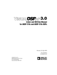
Figure 4-1 shows a pinned window in a multiprocessor debug session.
Figure 4-1. Pinned Window in a Multiprocessor Debug Session
The title bar of a pinned window shows:
• Processor name
• Pushpin icon
to indicate that the window is pinned
• Window title
• Number format, such as Hexadecimal (for windows that support
multiple formats)
Additional Focus Indication
If configured, VisualDSP++ shades unfocused windows with a specified
color. You can specify the background color of focused and unfocused
windows.
VisualDSP++ 2.0 User’s Guide for ADSP-21xxx DSPs
4-7
Code Behavior Analysis Tools
Code Behavior Analysis Tools
VisualDSP++ provides these code analysis tools:
• Traces
• Profiles
Use code behavior analysis tools to examine your code and analyze how
your code executes. These tools locate areas that may be optimized for
better performance.
Traces
You run a trace (also called an execution trace or a program trace) to
analyze the run-time behavior of your DSP program, enable I/O
capabilities, and simulate source to target data streaming.
A trace displays a history of processor activity during program execution.
A trace includes the following information:
• Buffer depth (instruction lines)
• Cycle count
• Instructions executed such as memory fetches, program memory
writes, and data/memory transfers
Viewing the disassembled instructions that were performed can also help
you to analyze code behavior.
4-8
VisualDSP++ 2.0 User’s Guide for ADSP-21xxx DSPs
Debugging
Profiles
Profiles examine program execution within selected ranges of code.
Statistical profiles and linear profiles measure program performance by
sampling the target’s PC register to collect data.
• Use linear profiling for simulator targets.
• Use statistical profiling for emulator targets.
The Linear Profiling Results window and Statistical Profiling Results
window display the data collected by these two profiling methods and
indicate where the application is spending its time. The window’s title
(Linear Profiling Results or Statistical Profiling Results) depends on
whether this tool is used during simulation or emulation.
Linear Profiling
Linear profiling with the simulator is not statistical because the simulator
samples every PC executed. This feature provides an accurate and
complete picture of what was executed in your program. Linear profiling
is much slower than statistical profiling. Simulator targets support linear
profiling but do not support statistical profiling.
Statistical Profiling
A statistical profile measures the performance of a DSP program by
sampling the target’s Program Counter (PC) register at random intervals
while the target is running the DSP program. The areas of the program
where most of the PCs are concentrated are where most of the time is
spent in executing the program. Statistical profiling provides a more
generalized form of profiling that is well suited to JTAG emulator debug
targets. Emulator targets do not support linear profiling. JTAG sampling
is completely non-intrusive, so the process does not incur additional
run-time overhead.
VisualDSP++ 2.0 User’s Guide for ADSP-21xxx DSPs
4-9
DSP Program Execution Operations
DSP Program Execution Operations
Program Loading
After completely specifying the debug session, the last step before you can
begin the debug session is to load the DSP executable program.
If you launch VisualDSP++ in stand-alone mode, ensure that the session is
configured correctly before you load your program.
After a successful build of the target executable, VisualDSP++, if
configured, loads the executable automatically to the current session when
the session processor type matches project’s processor. When the current
session processor does not match the project’s processor type, you are
prompted to choose another session.
If automatic load is not configured, VisualDSP++ does not try to load the
executable automatically after a successful build.
Note: The target must be an executable (.DXE) file.
This debugging feature saves time, as you do not have to load the
executable target manually, and you can start to debug right after a
successful build of the project.
Program Execution Operations
You can run program execution commands from the Debug menu or by
clicking toolbar buttons.
Executable files run until an event such as a breakpoint, watchpoint, or
user-issued Halt command stops execution. When program execution
halts, all windows are updated to current addresses and values.
4-10
VisualDSP++ 2.0 User’s Guide for ADSP-21xxx DSPs
Debugging
Use the following commands to control program execution.
Command
Description
Run
Runs an executable. The program runs until an event stops it,
such as a breakpoint or user intervention. When program
execution halts, all windows update to current addresses and
values.
Halt
Stops program execution. All windows are updated after the DSP
halts. Register values that have changed are highlighted, and the
status bar displays the address where the program halted.
Run to Cursor
Runs the program to the line where you left your cursor. You can
place the cursor in Editor windows and Disassembly windows.
Step Over
(C/C++ code only in an Editor window) Single-steps forward
through program instructions. If the source line calls a function,
the function executes completely, without stepping through the
function instructions.
Step Into
(Editor window or Disassembly window) Single-steps through
the program one C/C++ or assembly instruction at a time.
Encountered functions are entered.
Step Out Of
(C/C++ code only in an Editor window) Performs multiple steps
until the current function returns to its caller, and stops at the
instruction immediately following the call to the function.
VisualDSP++ 2.0 User’s Guide for ADSP-21xxx DSPs
4-11
DSP Program Execution Operations
Program Restart
You can set the program counter (PC) to the first address of the interrupt
vector table.
Performing a Restart during Simulation
In the simulator, restart works like a reset. The target's memory, however,
does not change. All registers are reset to their initial values.
Note: Memory is not reset. Thus, C and assembly global variables are not
reset to their original values. Your program may behave differently after a
restart. To re-initialize these values, reload your .DXE file.
Performing a Restart during Emulation
In the emulator, restart works exactly like a reset. Only registers with
default reset values are affected. All other registers remain unchanged.
4-12
VisualDSP++ 2.0 User’s Guide for ADSP-21xxx DSPs
Debugging
Debugging Tools
VisualDSP++ enables you to set breakpoints and watchpoints in your
executable program.
Breakpoints
You can set breakpoints at any address in program memory. Program
execution halts at the address or instruction at which the enabled
breakpoint is located.
Note: In addition to software breakpoints, you can also use hardware
breakpoints in an emulator debug session.
You can enable and disable breakpoints as well as add and delete
breakpoints.
A disabled breakpoint is set up, but not turned on. A disabled breakpoint
does not stop program execution. It is dormant and may be used later.
A break occurs when the conditions that you specify are met.
VisualDSP++ 2.0 User’s Guide for ADSP-21xxx DSPs
4-13
Debugging Tools
Symbols in the left margin of a Disassembly window or Editor window
indicate breakpoint status.
Symbol
Indicates
An enabled (set) breakpoint
A disabled breakpoint (recognized, but cleared)
Unconditional vs. Conditional Breakpoints
You can configure a breakpoint to occur when the program counter (PC)
reaches a specific address. This type of breakpoint is an unconditional
breakpoint, because it occurs when it is reached.
Note: You can quickly place an unconditional breakpoint at an address in
a Disassembly window or Editor window by using one of these options:
• Select the address and click the Toggle Breakpoint button
.
• Double-click on the line in the Disassembly or Editor window.
You can configure a breakpoint to occur when various conditions
(criteria) are met. This type is called a conditional breakpoint. The
conditions may include:
• A user-defined expression that must evaluate to TRUE
• A skip (count) that specifies the number of times to skip over the
breakpoint before finally halting
4-14
VisualDSP++ 2.0 User’s Guide for ADSP-21xxx DSPs
Debugging
If both an expression and skip are set, execution stops when the
breakpoint is reached “n” times when the expression is TRUE, where n
represents the skip count. When the expression is empty, execution stops
when the breakpoint is reached “n” times.
Watchpoints
Watchpoints are like breakpoints. Watchpoints, however, enable you to
set a condition such as a memory read or stack pop. You can then trap on
the specified condition to stop program execution and halt events.
Note: You can use watchpoints only during simulation.
You can set watchpoints on registers, stacks, and memory ranges. When
the condition is reached, program execution is halted and all windows are
updated.
Watchpoints are not attached to a specific address in the way that
breakpoints are. A watchpoint halts anywhere in your program once the
watchpoint conditions are satisfied.
VisualDSP++ 2.0 User’s Guide for ADSP-21xxx DSPs
4-15
Simulation Tools
Simulation Tools
You use simulation tools for simulating external devices and signals.
Interrupts
Use interrupts to simulate external interrupts in your program. You can
set up a serial port (SPORT) transmit and test SPORT activity with an
external interrupt. When you use interrupts with watchpoints and
streams, your program simulates real-world operation of your DSP system.
Data Input/Output Simulation (Streams)
In many products, DSPs exist as part of a larger system, where they can act
as a host or a slave. With their extensive I/O capabilities, Analog Devices’
DSPs can drive other devices or take part in processing a subset of data.
You can configure input and output streams, run a streams program to
simulate data movement through serial ports, and view the registers
associated with this functionality.
4-16
VisualDSP++ 2.0 User’s Guide for ADSP-21xxx DSPs
Debugging
Plots
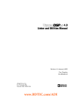
You can display DSP memory as a plot in a Plot window, as shown in
Figure 4-2.
Figure 4-2. Plot Window – Display of DSP Memory
You can visualize the DSP memory data and process it by using a data
processing algorithm. You can choose from multiple plot types and can
specify the plot’s data and presentation.
You can modify a plot’s configuration and immediately view the revised
plot. From a Plot window, you can zoom in on a portion of a plot or view
the values of a data point. You can print a plot, save the plot image to a
file, or save the plot’s data to a file.
VisualDSP++ 2.0 User’s Guide for ADSP-21xxx DSPs
4-17
Plots
Plot Types
You specify a plot as one of these plot types:
Plot Type
Description
Requires
Line plot
Displays points
connected by a line
Y value for each point
X-Y plot
Similar to a line plot,
but also uses X-axis
data
X value and Y value for
each data point
Constellation plot
Displays a symbol at
each data point
X value and Y value for
each data point
Eye diagram
Typically used to show
the stability of a
time-based signal
Y value for each data
point
Waterfall
3-D plot typically used
to show the change in
frequency content of
signal over time
Z value for each data
point
Spectrogram plot
2-D plot displays
amplitude data as a
color intensity
Z value for each data
point
The X, Y, and Z values are read from DSP memory.
4-18
VisualDSP++ 2.0 User’s Guide for ADSP-21xxx DSPs
Debugging
Line Plots
A line plot (shown in Figure 4-3) displays a range of DSP memory values
connected by a line. The values read from DSP memory are assigned to
the Y-axis. The corresponding X-axis values are automatically generated.
Figure 4-3. Line Plot Example
You can plot multiple data sets on a single graph.
VisualDSP++ 2.0 User’s Guide for ADSP-21xxx DSPs
4-19
Plots
X-Y Plots
An X-Y plot (shown in Figure 4-4) requires an X value and a Y value for
each data point. Unlike a line plot, an X-Y plot requires that you specify
the X-axis data.
Figure 4-4. X-Y Plot Example
The X data and Y data are specified separately in a user-defined memory
location. The number of X and Y points must be equal.
4-20
VisualDSP++ 2.0 User’s Guide for ADSP-21xxx DSPs
Debugging
Constellation Plots
A constellation plot (shown in Figure 4-5) displays a symbol at each (X,Y)
data point.
Figure 4-5. Constellation Plot Example
The X and Y data are specified separately in a user-defined DSP memory
location. The number of X and Y points must be equal.
VisualDSP++ 2.0 User’s Guide for ADSP-21xxx DSPs
4-21
Plots
Eye Diagrams
An eye diagram plot (shown in Figure 4-6) is typically used to show the
stability of a time-based signal. The more defined the eye shape, the more
stable the signal.
Figure 4-6. Eye Diagram Plot Example
This plot works like a storage oscilloscope, displaying an overlapped
history of a time signal. The eye diagram plot processes the input data and
optionally looks for a threshold crossing point (default 0.0). The trace is
plotted when the threshold crossing is reached, and it continues plotting
for the remainder of the trace data.
4-22
VisualDSP++ 2.0 User’s Guide for ADSP-21xxx DSPs
Debugging
When a breakpoint occurs (or a step is performed), the plot data is
updated and a new trace is plotted. The eye diagram uses a data shifting
technique that stores the desired number of traces in a plot buffer (default
is ten traces). Upon exceeding the number of traces, the first trace shifts
out of the buffer and the new trace shifts into the last buffer location. This
technique is referred to as first-in, first-out (FIFO).
You can modify options for threshold value, rising trigger, falling trigger,
and the number of overlapping traces.
VisualDSP++ 2.0 User’s Guide for ADSP-21xxx DSPs
4-23
Plots
Waterfall Plots
A waterfall plot (shown in Figure 4-7) is typically used to show the change
in frequency content of signal over time.
Figure 4-7. Waterfall Plot Example
The plot comprises multiple line plot traces in a three-dimensional view.
Each line plot trace represents a slice of the waterfall plot.
The easiest way to create a waterfall plot is to define a two-dimensional
array in C code (a grid). The first array dimension is the number of rows
in the grid, and the second dimension is the number of columns in the
grid. The number of columns is equal to the number of data points in
each line trace.
4-24
VisualDSP++ 2.0 User’s Guide for ADSP-21xxx DSPs
Debugging
A time-based signal is sampled at a predefined sampling rate and stored as
a slice in the grid (row 0, columns 0 through N).
The next time signal is sampled and stored (in row 1, columns 0 through
N). This process continues until all the rows are filled.
By default, an FFT is performed on each slice, resulting in a frequency
output display. Optionally, you can use a color map (3-D Axis tab of
Color Settings dialog box) to enhance the display. Each color corresponds
to a range of amplitude values.
The plot output displays a legend, showing each color and associated
range of values.
You can rotate the waterfall plot to any desired azimuth and elevation by
using the keyboard’s arrow keys.
VisualDSP++ 2.0 User’s Guide for ADSP-21xxx DSPs
4-25
Plots
Spectrogram Plots
A spectrogram plot (shown in Figure 4-8) displays the same data as a 3-D
waterfall plot, except in a 2-dimensional format.
Figure 4-8. Spectrogram Plot Example
Each (X,Y) location displays as color, representing the amplitude of the
data. By default, an FFT is performed on each slice, which results in a
frequency output display. A legend displays the colors and associated
range of values.
4-26
VisualDSP++ 2.0 User’s Guide for ADSP-21xxx DSPs
Debugging
Simulator Options
Depending on your selected DSP, several simulator options are available
on submenus under the Settings menu.
The Anomalies submenu provides these options:
• Shadow Write (ADSP-2116x DSPs only)
This command opens the Configure Simulator Event dialog box,
from which you can configure reporting for Shadow Write
anomalies.
• SIMD FIFO (ADSP-2116x DSPs only)
This command opens the Configure Simulator Event dialog box,
from which you can configure reporting for SIMD FIFO anomalies.
The Simulator submenu provides this option:
CLKDBL (ADSP-21161 DSPs only)
This command enables the 2x clock double circuitry. You can use this
command to configure CLKOUT as either 1x or 2x the rate of CLKIN.
The Load Sim Loader submenu provides these options:
• Boot from Host
• Boot from PROM
• Boot from Link
• Boot from SPI
• None of Above
VisualDSP++ 2.0 User’s Guide for ADSP-21xxx DSPs
4-27
Simulator Options
ADSP-2116x Anomalies
The simulator enables you to record the following anomaly events:
• Shadow Write FIFO anomaly
• SIMD read from internal memory with Shadow Write FIFO hit
anomaly
Shadow Write FIFO Anomaly
Refer to anomaly #39 at the following website for examples and
workarounds.
www.analog.com/support/dsp/anomalies/html/ANOM21160.html
This anomaly has been identified in the shadow write FIFOs that exist
between the internal memory array of the ADSP-21160M and core /IOP
buses that access the memory. (Refer to the Hardware Reference for more
details on shadow register operation.) A particular sequence of a core write
followed by a read of the same internal memory address, in conjunction
with a certain type of IOP activity can cause the core read to return
incorrect data.
Under the circumstances described below, the Read from Addr 1
incorrectly returns the data for Addr 2.
This problem is caused by the shadow write FIFO erroneously returning
data for a core read when data should have been returned from internal
memory. During write operations, data is placed in the 1st stage of a
two-stage shadow write FIFO. Data is moved from first to second stage
when a second write is performed (by either DSP core or IOP). Similarly
data is moved from the second stage of the FIFO to internal memory
when neither the core nor the IOP accesses memory in a core cycle.
4-28
VisualDSP++ 2.0 User’s Guide for ADSP-21xxx DSPs
Debugging
On read operations, address compare logic allows data to be fetched either
from internal memory or from the FIFOs. Note that each memory block
has one Shadow Register FIFO, and all core and IOP accesses to internal
memory use this FIFO. The internal memory clock (not visible to the
user) runs at twice the core clock frequency. So, each core cycle consists of
two memory cycles with one of the two memory cycles dedicated to the
core and the other dedicated to the IOP.
SIMD Read from Internal Memory with Shadow Write FIFO Hit
Anomaly
Refer to anomaly #40 at the following website for examples and
workarounds.
www.analog.com/support/dsp/anomalies/html/ANOM21160.html
This anomaly has been identified in the Shadow Write FIFOs that exist
between the internal memory array of the ADSP-21160M and core /IOP
busses that access the memory. (Refer to the Hardware Reference for more
details on shadow register operation.)
When performing SIMD reads that cross Long Word Address boundaries
(that is, odd Normal Word addresses or non-Long Word boundary
aligned Short Word addresses) and the data for the read is in the Shadow
Write FIFO, the read results in Revision 0.0 behavior for the read.
How to Record a Simulator Anomaly Event
You can record various simulator anomaly events for ADSP-2116x DSPs.
To record a simulator anomaly event:
1. From the Settings menu, choose Anomalies.
2. Choose the anomaly that you want to record.
VisualDSP++ 2.0 User’s Guide for ADSP-21xxx DSPs
4-29
Simulator Options
Currently, two choices are available:
• Shadow Write
• SIMD FIFO
The Configure Simulator Event dialog box (Figure 4-9) appears.
Use this dialog box to configure the simulator to handle silicon
anomalies.
Figure 4-9. Configure Simulator Event Dialog Box
3. Specify options, described in the following table.
4-30
VisualDSP++ 2.0 User’s Guide for ADSP-21xxx DSPs
Debugging
Item
Purpose
Event Fire Options
Specifies the frequency of reporting an event
Fire Once
Logs the event only the first time it occurs
Fire Unique
Logs the event once for each unique event. For each event
type (anomaly), a unique event comprises the PC at the
time of the memory write and the PC at the time of the
memory read taken as a pair. Select this option to prevent
reporting multiple messages for the same event.
Fire All
Logs every occurrence of the event
Severity
Specifies the degree of the event
INFO
Writes a message in black typeface to the Output window
WARN
Writes a message in black typeface to the Output window
ERROR
Writes a message appears in the Output window in red
typeface and rings a bell
FATAL
Writes a message appears to the Output window in red
typeface and rings a bell
Enabled
Enables this event check.
Verbose
Specifies that four-line messages are written to the Output
window
When this option is not selected, messages are one line
long.
VisualDSP++ 2.0 User’s Guide for ADSP-21xxx DSPs
4-31
Simulator Options
Event Actions
Print
Writes messages to the Output window
Halt
Halts after the event has occurred. Using this option is
similar to using a watchpoint.
4.Click OK.
Clock Doubling (ADSP-21161 DSPs Only)
Crystal Double Mode Enable Pin
The /CLKDBL pin enables the 2x clock double circuitry. You can use the
CLKDBL command to configure CLKOUT as either 1x or 2x the rate of
CLKIN.
The CLKIN double circuit is primarily intended for an external crystal
used with the internal clock generator and the XTAL pin. The internal
clock generator, when used with the XTAL pin and an external crystal,
supports an external crystal frequency up to 25 MHz.
You can use CLKDBL in XTAL mode to generate a 50-MHz input into
the PLL. Enable the 2x clock mode (during RESET low) by tying
CLKDBL to GND. Otherwise, CLKDBL is connected to VDDEXT for
1x clock mode.
For example, you can use a 25-MHz crystal to enable 100-MHz core clock
rates and a 50-MHz CLKOUT operation when CLK_CFG1='0',
CLK_CFG1='0', and CLKDBL='0'. You can also use this pin to generate
different clock rate ratios for external clock oscillators as well.
4-32
VisualDSP++ 2.0 User’s Guide for ADSP-21xxx DSPs
Debugging
Clock Rate Ratios
The possible clock rate ratio options (up to 100 MHz) for either CLKIN
(external clock oscillator) or XTAL (crystal input) are as follows:
CLKDBL
CLK_CFG1
CLK_CFG0
Core Clock
Ratio
EP Clock
Ratio
1
0
0
2:1
1x
1
0
1
3:1
1x
0
0
0
4:1
2x
0
0
1
6:1
2x
0
1
0
8:1
2x
An 8:1 ratio enables you to use a 12.5-MHz crystal to generate a
100-MHz core (instruction clock) rate and a 25-MHz CLKIN (external
port) clock rate.
Note: When you use an external crystal, the maximum crystal frequency
cannot exceed 25 MHz. For all other external clock sources, the maximum
CLKIN frequency is 50 MHz.
How to Configure the CLKOUT Pin
You can configure the DSP’s CLKOUT pin to be either 1x or 2x the rate
of CLKIN.
A black check mark () beside the CLKDBL command in the Settings
menu indicates that this option is selected.
To double the clock speed, choose CLKDBL from the Settings menu.
VisualDSP++ 2.0 User’s Guide for ADSP-21xxx DSPs
4-33
Simulator Options
Boot Options
Depending on your selected DSP, the following boot options are
available:
• Boot from Host
• Boot from PROM
• Boot from Link
• Boot from SPI
• None of Above
Boot from Host
Refer to your DSP’s Hardware Reference for more information about
bootloading through the external port.
Refer to your DSP’s Hardware Reference for information about host
booting.
Boot from PROM
Refer to your DSP’s Hardware Reference for more information about
bootloading through the external port.
Refer to your DSP’s Hardware Reference for information about PROM
booting.
4-34
VisualDSP++ 2.0 User’s Guide for ADSP-21xxx DSPs
Debugging
Boot from Link
Link port booting uses DMA channel 8 of the I/O processor to transfer
the instructions to internal memory. In this boot mode, the DSP receives
4-bit wide data in link buffer 0.
Refer to your DSP’s Hardware Reference for information about link port
booting.
Boot from SPI (32-bit Host)
This option specifies a 32-bit width for the SPI data.
Refer to your DSP’s Hardware Reference for information about SPI
booting.
Boot from SPI (16-bit Host)
This option specifies a 16-bit width for the SPI data.
Refer to your DSP’s Hardware Reference for information about SPI
booting.
Boot from SPI (8-bit Host)
This option specifies an 8-bit width for the SPI data.
Refer to your DSP’s Hardware Reference for information about SPI
booting.
VisualDSP++ 2.0 User’s Guide for ADSP-21xxx DSPs
4-35
Simulator Options
None of Above
When the simulator is reset or restarted, no booting occurs. When the
simulator is reset, all simulated processors boot.
Refer to your DSP’s Hardware Reference and Linker and Utilities Manual
for more information about bootloading.
4-36
VisualDSP++ 2.0 User’s Guide for ADSP-21xxx DSPs