Download Gfan version 0.5: A User's Manual

Gfan version 0.5: A User’s Manual
Anders Nedergaard Jensen
∗
January 25, 2011
Abstract
Gfan is a software package for computing Gr¨
obner fans and tropical
varieties. These are polyhedral fans associated to polynomial ideals. The
maximal cones of a Gr¨
obner fan are in bijection with the marked reduced
Gr¨
obner bases of its defining ideal. The software computes all marked
reduced Gr¨
obner bases of an ideal. Their union is a universal Gr¨
obner
basis. The tropical variety of a polynomial ideal is a certain subcomplex
of the Gr¨
obner fan. Gfan contains algorithms for computing this complex
for general ideals and specialized algorithms for tropical curves, tropical
hypersurfaces and tropical varieties of prime ideals. In addition to the
above core functions the package contains many tools which are useful in
the study of Gr¨
obner bases, initial ideals and tropical geometry. The full
list of commands can be found in Appendix B. For ordinary Gr¨
obner basis
computations Gfan is not competitive in speed compared to programs such
as CoCoA, Singular and Macaulay2.
Contents
1 Introduction
1.1 The Gr¨obner fan of an ideal
1.2 Gr¨obner bases . . . . . . . .
1.3 Algorithmic background . .
1.3.1 Local computations .
1.3.2 Global computations
.
.
.
.
.
.
.
.
.
.
.
.
.
.
.
.
.
.
.
.
.
.
.
.
.
.
.
.
.
.
.
.
.
.
.
.
.
.
.
.
.
.
.
.
.
.
.
.
.
.
.
.
.
.
.
.
.
.
.
.
.
.
.
.
.
.
.
.
.
.
.
.
.
.
.
.
.
.
.
.
.
.
.
.
.
.
.
.
.
.
.
.
.
.
.
.
.
.
.
.
.
.
.
.
.
5
6
7
8
8
9
Research partially supported by the Faculty of Science, University of Aarhus, Danish Research Training Council (Forskeruddannelsesr˚
adet, FUR) , Institute for Operations Research
ETH, grants DMS 0222452 and DMS 0100141 of the U.S. National Science Foundation and the
American Institute of Mathematics.
∗
1
2 Installation
2.1 Installation of the gmp library . . . . . .
2.1.1 Installing the gmp library on Mac
2.2 Installation of the cddlib library . . . . .
2.3 Gfan installation . . . . . . . . . . . . .
2.4 SoPlex (for the advanced user only) . . .
. .
OS
. .
. .
. .
. . . . . . . .
X using fink
. . . . . . . .
. . . . . . . .
. . . . . . . .
.
.
.
.
.
.
.
.
.
.
.
.
.
.
.
.
.
.
.
.
10
10
11
12
13
14
3 Using the software
3.1 Computing the Gr¨obner fan . .
3.1.1 Exploiting symmetry . .
3.2 Combining the programs . . . .
3.3 Interactive mode . . . . . . . .
3.4 Integers and p-adics . . . . . . .
3.5 Toric ideals and secondary fans
.
.
.
.
.
.
.
.
.
.
.
.
.
.
.
.
.
.
.
.
.
.
.
.
.
.
.
.
.
.
.
.
.
.
.
.
15
15
16
16
17
18
20
.
.
.
.
.
.
.
.
.
.
.
.
.
.
.
.
.
.
.
.
.
.
.
.
.
.
.
.
.
.
.
.
.
.
.
.
.
.
.
.
.
.
.
.
.
.
.
.
.
.
.
.
.
.
.
.
.
.
.
.
.
.
.
.
.
.
.
.
.
.
.
.
.
.
.
.
.
.
4 Doing tropical computations
4.1 Tropical variety by brute force . . . . . . .
4.2 Traversing tropical varieties of prime ideals
4.3 Intersecting tropical hypersurfaces . . . . .
4.4 Computing tropical bases of curves . . . .
4.5 Tropical intersection theory . . . . . . . .
4.6 Non-constant coefficients . . . . . . . . . .
4.6.1 Algebraic field extensions of Q . . .
.
.
.
.
.
.
.
.
.
.
.
.
.
.
.
.
.
.
.
.
.
.
.
.
.
.
.
.
.
.
.
.
.
.
.
.
.
.
.
.
.
.
.
.
.
.
.
.
.
.
.
.
.
.
.
.
.
.
.
.
.
.
.
.
.
.
.
.
.
.
.
.
.
.
.
.
.
.
.
.
.
.
.
.
.
.
.
.
.
.
.
22
22
23
27
27
28
30
33
A Data formats
A.1 Fields . . . . . . .
A.2 Variables . . . . . .
A.3 Polynomial rings .
A.4 Polynomials . . . .
A.5 Lists . . . . . . . .
A.6 Permutations . . .
A.7 Polyhedral fans . .
A.7.1 Data types .
A.7.2 Properties .
A.8 Polyhedral cones .
.
.
.
.
.
.
.
.
.
.
.
.
.
.
.
.
.
.
.
.
.
.
.
.
.
.
.
.
.
.
.
.
.
.
.
.
.
.
.
.
.
.
.
.
.
.
.
.
.
.
.
.
.
.
.
.
.
.
.
.
.
.
.
.
.
.
.
.
.
.
.
.
.
.
.
.
.
.
.
.
.
.
.
.
.
.
.
.
.
.
.
.
.
.
.
.
.
.
.
.
.
.
.
.
.
.
.
.
.
.
.
.
.
.
.
.
.
.
.
.
.
.
.
.
.
.
.
.
.
.
34
34
34
34
35
35
36
36
40
40
42
.
.
.
.
.
.
43
43
44
44
45
45
45
.
.
.
.
.
.
.
.
.
.
.
.
.
.
.
.
.
.
.
.
.
.
.
.
.
.
.
.
.
.
.
.
.
.
.
.
.
.
.
.
B Application list
B.1 gfan bases . . . . . . . . .
B.2 gfan buchberger . . . . . .
B.3 gfan combinerays . . . . .
B.4 gfan doesidealcontain . . .
B.5 gfan fancommonrefinement
B.6 gfan fanhomology . . . . .
.
.
.
.
.
.
.
.
.
.
.
.
.
.
.
.
.
.
.
.
.
.
.
.
.
.
.
.
.
.
.
.
.
.
.
.
.
.
.
.
.
.
.
.
.
.
.
.
2
.
.
.
.
.
.
.
.
.
.
.
.
.
.
.
.
.
.
.
.
.
.
.
.
.
.
.
.
.
.
.
.
.
.
.
.
.
.
.
.
.
.
.
.
.
.
.
.
.
.
.
.
.
.
.
.
.
.
.
.
.
.
.
.
.
.
.
.
.
.
.
.
.
.
.
.
.
.
.
.
.
.
.
.
.
.
.
.
.
.
.
.
.
.
.
.
.
.
.
.
.
.
.
.
.
.
.
.
.
.
.
.
.
.
.
.
.
.
.
.
.
.
.
.
.
.
.
.
.
.
.
.
.
.
.
.
.
.
.
.
.
.
.
.
.
.
.
.
.
.
.
.
.
.
.
.
.
.
.
.
.
.
.
.
.
.
.
.
B.7
B.8
B.9
B.10
B.11
B.12
B.13
B.14
B.15
B.16
B.17
B.18
B.19
B.20
B.21
B.22
B.23
B.24
B.25
B.26
B.27
B.28
B.29
B.30
B.31
B.32
B.33
B.34
B.35
B.36
B.37
B.38
B.39
B.40
B.41
B.42
B.43
B.44
B.45
B.46
B.47
B.48
B.49
gfan
gfan
gfan
gfan
gfan
gfan
gfan
gfan
gfan
gfan
gfan
gfan
gfan
gfan
gfan
gfan
gfan
gfan
gfan
gfan
gfan
gfan
gfan
gfan
gfan
gfan
gfan
gfan
gfan
gfan
gfan
gfan
gfan
gfan
gfan
gfan
gfan
gfan
gfan
gfan
gfan
gfan
gfan
fanlink . . . . . . . . .
fanproduct . . . . . . .
fansubfan . . . . . . . .
genericlinearchange . .
groebnercone . . . . . .
groebnerfan . . . . . .
homogeneityspace . . .
homogenize . . . . . .
initialforms . . . . . . .
interactive . . . . . . .
ismarkedgroebnerbasis
krulldimension . . . . .
latticeideal . . . . . . .
leadingterms . . . . . .
list . . . . . . . . . . .
markpolynomialset . .
minkowskisum . . . . .
minors . . . . . . . . .
mixedvolume . . . . . .
overintegers . . . . . .
padic . . . . . . . . . .
polynomialsetunion . .
render . . . . . . . . .
renderstaircase . . . . .
saturation . . . . . . .
secondaryfan . . . . . .
stats . . . . . . . . . .
substitute . . . . . . .
symmetries . . . . . . .
tolatex . . . . . . . . .
topolyhedralfan . . . .
tropicalbasis . . . . . .
tropicalbruteforce . . .
tropicalevaluation . . .
tropicalfunction . . . .
tropicalhypersurface . .
tropicalintersection . .
tropicallifting . . . . .
tropicallinearspace . . .
tropicalmultiplicity . .
tropicalrank . . . . . .
tropicalstartingcone . .
tropicaltraverse . . . .
.
.
.
.
.
.
.
.
.
.
.
.
.
.
.
.
.
.
.
.
.
.
.
.
.
.
.
.
.
.
.
.
.
.
.
.
.
.
.
.
.
.
.
.
.
.
.
.
.
.
.
.
.
.
.
.
.
.
.
.
.
.
.
.
.
.
.
.
.
.
.
.
.
.
.
.
.
.
.
.
.
.
.
.
.
.
3
.
.
.
.
.
.
.
.
.
.
.
.
.
.
.
.
.
.
.
.
.
.
.
.
.
.
.
.
.
.
.
.
.
.
.
.
.
.
.
.
.
.
.
.
.
.
.
.
.
.
.
.
.
.
.
.
.
.
.
.
.
.
.
.
.
.
.
.
.
.
.
.
.
.
.
.
.
.
.
.
.
.
.
.
.
.
.
.
.
.
.
.
.
.
.
.
.
.
.
.
.
.
.
.
.
.
.
.
.
.
.
.
.
.
.
.
.
.
.
.
.
.
.
.
.
.
.
.
.
.
.
.
.
.
.
.
.
.
.
.
.
.
.
.
.
.
.
.
.
.
.
.
.
.
.
.
.
.
.
.
.
.
.
.
.
.
.
.
.
.
.
.
.
.
.
.
.
.
.
.
.
.
.
.
.
.
.
.
.
.
.
.
.
.
.
.
.
.
.
.
.
.
.
.
.
.
.
.
.
.
.
.
.
.
.
.
.
.
.
.
.
.
.
.
.
.
.
.
.
.
.
.
.
.
.
.
.
.
.
.
.
.
.
.
.
.
.
.
.
.
.
.
.
.
.
.
.
.
.
.
.
.
.
.
.
.
.
.
.
.
.
.
.
.
.
.
.
.
.
.
.
.
.
.
.
.
.
.
.
.
.
.
.
.
.
.
.
.
.
.
.
.
.
.
.
.
.
.
.
.
.
.
.
.
.
.
.
.
.
.
.
.
.
.
.
.
.
.
.
.
.
.
.
.
.
.
.
.
.
.
.
.
.
.
.
.
.
.
.
.
.
.
.
.
.
.
.
.
.
.
.
.
.
.
.
.
.
.
.
.
.
.
.
.
.
.
.
.
.
.
.
.
.
.
.
.
.
.
.
.
.
.
.
.
.
.
.
.
.
.
.
.
.
.
.
.
.
.
.
.
.
.
.
.
.
.
.
.
.
.
.
.
.
.
.
.
.
.
.
.
.
.
.
.
.
.
.
.
.
.
.
.
.
.
.
.
.
.
.
.
.
.
.
.
.
.
.
.
.
.
.
.
.
.
.
.
.
.
.
.
.
.
.
.
.
.
.
.
.
.
.
.
.
.
.
.
.
.
.
.
.
.
.
.
.
.
.
.
.
.
.
.
.
.
.
.
.
.
.
.
.
.
.
.
.
.
.
.
.
.
.
.
.
.
.
.
.
.
.
.
.
.
.
.
.
.
.
.
.
.
.
.
.
.
.
.
.
.
.
.
.
.
.
.
.
.
.
.
.
.
.
.
.
.
.
.
.
.
.
.
.
.
.
.
.
.
.
.
.
.
.
.
.
.
.
.
.
.
.
.
.
.
.
.
.
.
.
.
.
.
.
.
.
.
.
.
.
.
.
.
.
.
.
.
.
.
.
.
.
.
.
.
.
.
.
.
.
.
.
.
.
.
.
.
.
.
.
.
.
.
.
.
.
.
.
.
.
.
.
.
.
.
.
.
.
.
.
.
.
.
.
.
.
.
.
.
.
.
.
.
.
.
.
.
.
.
.
.
.
.
.
.
.
.
.
.
.
.
.
.
.
.
.
.
.
.
.
.
.
.
.
.
.
.
.
.
.
.
.
.
.
.
.
.
.
.
.
.
.
.
.
.
.
.
.
.
.
.
.
.
.
.
.
.
.
.
.
.
.
.
.
.
.
.
.
.
.
.
.
.
.
.
.
.
.
.
.
.
.
.
.
.
.
.
.
.
.
.
.
.
.
.
.
.
.
.
.
.
.
.
.
.
.
.
.
.
.
.
.
.
.
.
.
.
.
.
.
.
.
.
.
.
.
.
.
.
.
.
.
.
.
.
.
.
.
.
.
45
46
46
46
46
47
48
48
48
49
50
50
50
50
50
51
51
51
52
52
53
54
54
54
55
55
56
56
56
56
57
57
57
57
58
58
58
59
59
60
60
60
60
B.50 gfan tropicalweildivisor . . . . . . . . . . . . . . . . . . . . . . . .
B.51 gfan version . . . . . . . . . . . . . . . . . . . . . . . . . . . . . .
4
61
61
1
Introduction
Gfan is a software package for computing Gr¨obner fans [18] and tropical varieties [20] of polynomial ideals. It is an implementation of the algorithms appearing in [9] and [5]. These two papers are joint work with Tristram Bogart,
Komei Fukuda, David Speyer, Bernd Sturmfels and Rekha Thomas. A combined
presentation can be found in [15]. For toric and lattice ideals, Gr¨obner fan programs already existed: TiGERS [12] and CaTS [13]. Gfan works on any ideal in
Q[x1 , . . . , xn ].
Gfan is based on Buchberger’s algorithm [6] and the local basis change procedure [7]. For traversal of Gr¨obner fans the simplex method, the reverse search
technique [3] and symmetry exploiting algorithms are used. This allows enumeration of fans with millions of cones. For tropical computations these methods
have been developed further.
Gfan has been used for studying the structure of the Gr¨obner fan. Among
the new results is an example of a Gr¨obner fan which is not the normal fan of a
polyhedron [16].
The software is intended to be run in a UNIX style environment. In particular,
the software works on GNU/Linux and on Mac OS X (with some effort). Gfan
uses the GNU multi-precision arithmetic library [11] and cddlib [8] for doing
exact arithmetics and solving linear programming problems, respectively. A new
feature of version 0.4 is the possibility to use the SoPlex [23] linear programming
solver which does its computations in floating point arithmetics. Gfan verifies
LP certificates in exact arithmetics and falls back on cddlib in case of a rounding
error.
The first section of this manual is a very short introduction to Gr¨obner fans
and algorithms for computing them. The second section describes the installation procedure of the software and the third gives some examples of how to use
it. Section 4 explains how Gfan can be used for computing tropical varieties,
prevarieties and tropical bases. More details on the data formats and programs
are given in Appendix A and B.
Note for the reader: As opposed to scientific journals the World Wide
Web has the advantage that its contents can be changed after publication. If you
have suggestions for improvements of this manual do not hesitate to let me know.
Suggestions for the installation instructions are of particular interest since I only
have access to / experience with a limited number of computer systems.
Acknowledgments: The first version of this software was written in the fall 2003
during the authors visit to the Institute for Operations Research, ETH Z¨
urich.
Many features have been added since then. Rekha Thomas and Komei Fukuda
have been involved in the development of the Gr¨obner fan algorithms, see the
joint paper [9]. The tropical algorithms were developed in the joint paper [5] with
5
Tristram Bogart, David Speyer, Bernd Sturmfels and Rekha Thomas. The author
is thankful to the following people and institutions for supporting the research:
Komei Fukuda and Hans-Jakob L¨
uthi (Institute for Operations Research, ETH
Z¨
urich), Douglas Lind and Rekha Thomas (University of Washington, Seattle)
and the American Institute of Mathematics. In recent years the research has also
been supported by University of Aarhus, University of Minnesota, TU-Berlin
and the German Research Foundation (DFG) through the institutional strategy
of Georg-August-Universit¨at G¨ottingen. The author would also like to thank his
advisor Niels Lauritzen and the many people who have been testing, been using
and helped improving the software.
1.1
The Gr¨
obner fan of an ideal
The Gr¨obner fan of an ideal I ⊆ k[x1 , . . . , xn ] in a polynomial ring over a field k
is a polyhedral complex consisting of cones in Rn . We provide a short definition
and refer the reader to the papers mentioned above for details.
Definition 1.1 Let ω ∈ Rn and a ∈ Nn . We define xa := xa11 · · · xann . The ωweight of αxa with α ∈ k \ {0} is ω · a. For f ∈ k[x1 , . . . , xn ] we define its initial
form inω (f ) to be the sum of all terms in f with maximal ω-weight. For an ideal
I ⊆ k[x1 , . . . , xn ] we define the initial ideal to be inω (I) := hinω (f ) : f ∈ Ii.
Notice that initial ideals might not be monomial ideals. If for some ω ∈ Rn>0 we
have inω (I) = I then we say that I is homogeneous in the ω-grading. We now fix
the ideal I ⊆ k[x1 , . . . , xn ] and consider the equivalence relation:
u ∼ v ⇔ inu (I) = inv (I)
on vectors u, v ∈ Rn . If I is homogeneous then any equivalence class contains
a positive vector. Any equivalence class containing a positive vector is convex.
Moreover, its closure is a polyhedral cone. We use the notation
Cω (I) := {u ∈ Rn : inu (I) = inω (I)}
to denote the closure of the equivalence class containing ω.
Definition 1.2 [9, Definition 2.8] Let I ⊆ k[x1 , . . . , xn ] be an ideal. The Gr¨obner
fan of I is the collection of cones Cω (I) where ω ∈ Rn>0 together with all their
non-empty faces.
Any cone in the Gr¨obner fan is called a Gr¨obner cone. The relative interior
of any Gr¨obner cone is an equivalence class. The equivalence class containing
0 is a subspace of Rn called the homogeneity space of I. The Gr¨obner fan is a
polyhedral fan; see [21] or [9]. The support of the Gr¨obner fan i.e. the union
of its cones is called the Gr¨obner region of I. If I is homogeneous then the
6
Gr¨obner region is Rn and, moreover, the Gr¨obner fan is the normal fan of the
state polytope of I; see [21] for a construction of this polytope. The lineality space
of a polyhedral cone is defined as the largest subspace contained in the cone. The
common lineality space of all cones in the Gr¨obner fan equals the homogeneity
space of I.
Remark 1.3 Definition 1.2 was chosen since it gives the nicest Gr¨obner cones.
In general our Gr¨obner fan does not coincide with the “restricted” Gr¨obner fan
nor the “extended” Gr¨obner fan defined in [18]. The common refinement (i.e.
“intersection”) of Rn≥0 and our Gr¨obner fan is the restricted Gr¨obner fan. For homogeneous ideals our definition coincides with [21, page 13] (which only contains
a definition for homogeneous ideals).
1.2
Gr¨
obner bases
Given a term order ≺ the initial term in≺ (f ) of a polynomial f is defined and,
analogously to the ω-initial ideal above, so is the initial ideal in≺ (I) of an ideal I.
We remind the reader that given generators for and ideal I ⊆ k[x1 , . . . , xn ] and a
term order ≺ Buchberger’s Algorithm produces a reduced Gr¨obner basis G≺ (I).
This basis is unique. It is useful to introduce the notion of a marked polynomial
and a marked reduced Gr¨obner basis. A polynomial is marked if one of its terms
has been distinguished. When writing such a polynomial we may either underline
the distinguished term or we may by convention write the distinguished term as
the first one listed. Gfan uses this second convention. A Gr¨obner basis G≺ (I) is
marked if the initial term in≺ (f ) of every polynomial f ∈ G≺ (I) has been marked
i.e. distinguished.
Example 1.4 The polynomial ideal I = hx + yi ⊆ Q[x, y] has two marked
reduced Gr¨obner bases: {x + y} and {x + y}. Gfan would write these Gr¨obner
bases as {x + y} and {y + x}.
By definition of Gr¨obner bases the initial ideal in≺ (I) is easily read off from the
marked (reduced) Gr¨obner basis G≺ (I), namely, it is generated by the marked
terms. In fact, for I ⊆ k[x1 , . . . , xn ] fixed the follow three finite sets are in
bijection:
• The set of marked reduced Gr¨obner bases for I.
• The set of monomial initial ideals in≺ (I) with respect to term orders.
• The set of n-dimensional Gr¨obner cones in the Gr¨obner fan of I.
The map from the first set to the second set has already been described. A monomial ideal in≺ (I) in the second set is mapped to {v ∈ Rn : inv (I) = in≺ (I)} in the
third set. Going from the first set to the third is easy, namely the inequalities
7
can be read off from the exponents of the marked reduced Gr¨obner basis. Thus
a useful way to represent the Gr¨obner fan of an ideal is by the set of its marked
reduced Gr¨obner bases.
1.3
Algorithmic background
We briefly describe the algorithms implemented in Gfan for computing Gr¨obner
fans. The algorithms are divided into two parts, the local algorithms and the
global algorithms. For more details we refer to [9] and [14].
1.3.1
Local computations
There are two local computations that need to be done:
• Given a full-dimensional Gr¨obner cone by its reduced Gr¨obner basis, we
need to find its facets. To be precise we need to find a normal for each
facet.
• Given a full-dimensional Gr¨obner cone represented by its reduced Gr¨obner
basis and a normal for one of its facets we need to compute the other fulldimensional cone having this facet as a facet (if one exists). Again, the
computed cone should be represented by a reduced Gr¨obner basis.
To do the first computation we need the following theorem telling us how to read
of the cone inequalities from the reduced Gr¨obner basis:
Theorem 1.5 Let G≺ (I) be a reduced Gr¨obner basis. For any vector u ∈ Rn
inu (I) = in≺ (I) ⇔ ∀g ∈ G≺ (I) : inu (g) = in≺ (g)
Each g introduces a set of strict linear inequalities on u. By making these inequalities non-strict we get a description of the closed Gr¨obner cone of G≺ (I).
This gives us a list of possible facet normals of the cone. Linear programming
techniques are now applied to find the true set of normals among these.
Suppose we know a reduced Gr¨obner basis G≺ (I) and a normal of one of its
facets. If ω is a vector in the relative interior of the facet we can compute a
Gr¨obner basis of inω (I) with respect to ≺ by picking out a certain subset of the
terms in G≺ (I), see [21, Corollary 1.9]. The initial ideal inω (I) has at most two
reduced Gr¨obner bases since it is homogeneous with respect to any grading given
by vectors in the n − 1 dimensional subspace spanned by the facet. The other
Gr¨obner basis of inω (I) can be computed using a term order represented by the
outer normal of the facet. A lifting step will take the Gr¨obner basis for inω (I)
to a Gr¨obner basis for I representing the neighbouring cone. See [21, Subroutine
3.7]. The method described above is the local change procedure due to [7]. The
procedure simplifies in our case since:
8
• We only walk through facets. Thus, the ideal inω (I) has at most two reduced
Gr¨obner bases.
• We know the facet normal. Thus, there is no reason for computing ω.
1.3.2
Global computations
We define the graph G whose set of vertices consists of all reduced Gr¨obner
bases of I with two bases being connected if their cones share a common facet
containing a strictly positive vector. With the two subroutines in the previous
section it is easy to do a traditional vertex enumeration of G starting from some
reduced Gr¨obner basis. However, for such algorithm to work it would need to
store the boundary of the already enumerated vertices to guarantee that we do
not enumerate the same vertex more than ones. For a planar graph this might
not seem too bad but as the dimension grows the boundary can contain a huge
number of elements. Storing these elements would require a lot of memory and
sometimes more memory than the size of the computers RAM which would cause
the computation to slow down.
A better way to do the enumeration is by the reverse search strategy [3]. If
there is an easy rule for orienting the edges of a graph so that it has a unique sink
and no cycles it is also easy to find a spanning tree for the graph. The reverse
search will traverse this spanning tree. The method works well for enumerating
vertices of polytopes since an orientation of the edges with respect to a generic
vector will have a unique sink and no cycles. A proof in [9] shows that a similar
orientation orienting G with respect to a term order will also give an acyclic
orientation with a unique sink and thus allow enumeration by reverse search.
Reverse search is the default enumeration method in Gfan .
If the ideal is symmetric we may want to do the Gr¨obner basis enumeration
up to symmetry. For example the ideal I = ha−bi ⊆ k[a, b] is invariant under the
exchange of a and b. The ideal has two marked Gr¨obner bases {a−b} and {b−a},
each defining a full dimensional Gr¨obner cone in R2 . Up to symmetry they are
equal. We only want to compute one of them. In general I ⊆ k[x1 , . . . , xn ] is
invariant under all permutations of some subgroup G ⊆ Sn . Applying a permutation in G to a marked reduced Gr¨obner basis of I we get another marked
reduced Gr¨obner basis of I. Hence, G acts on the set of marked reduced Gr¨obner
bases of I. We wish to compute only one representative for each orbit. We apply
techniques similar to the ones used in [19] for computing regular triangulations
of point configurations up to symmetry. Often the number of orbits is much
smaller than the number of reduced Gr¨obner bases and we save a lot of time by
not computing them all.
9
2
Installation
If you are using MacOS the easiest way to install Gfan is to use precompiled
executables: go to the Gfan webpage, go to the binaries.html subpage, and follow
the instructions there.
If you are using Linux the following might work
sudo apt-get install gfan
or
sudo emerge gfan
depending on your distribution and package manager. If you succeed, it is good
to know which version was installed. Run
gfan _version
Should this command fail, then you are using an old version of gfan.
The rest of this section eplains how to install Gfan by compiling it from source
on a Linux/Unix-like system with a modern version of gcc. Gfan has been compiled successfully with gcc version 4.1.1. Two libraries are needed in order
to compile Gfan : cddlib and gmp. Users of Microsoft Windows may be
able to use these installation instructions if they first install Cygwin. A new
feature in Gfan version 0.4 is the possibility to link to the SoPlex [23] library.
This does not add to the functionality of Gfan but improves speed of the polyhedral computations. In an attempt to keep the installation instructions simple,
instructions for how to use SoPlex are given in a separate section, Subsection
2.4. If you are a lucky Linux user it will suffice to follow the red part of these
instructions.
2.1
Installation of the gmp library
GMP stands for GNU Multi Precision arithmetic library. This library must be
installed on your system before you can install cddlib and gfan. On most some
GNU/Linux systems the library is already installed. If your system does
not already have gmp installed (which is the case if you have a usual Mac OS X
installation) follow the directions in this section.
IF YOU ARE USING Mac OS X AND YOU ARE NOT AN EXPERT FOLLOW THE INSTRUCTIONS IN SECTION 2.1.1 INSTEAD.
Make a new directory and download gmp-4.2.2.tar.gz from
http://gmplib.org/
for example by typing
10
cd ~
mkdir tempdir
cd tempdir
wget http://ftp.sunet.se/pub/gnu/gmp/gmp-4.2.2.tar.gz
Extract the file and go to the thereby created directory:
tar -xzvf gmp-4.2.2.tar.gz
cd gmp-4.2.2
Run the configure script and specify the installation directory:
./configure --prefix=$HOME/gfan/gmp
The above line specifies the installation directory which in this case will be the
folder gfan/gmp in your home directory. If you already have a directory by that
name its content may be destroyed by the subsequent commands.
Compile the gmp library and install it:
make
make install
Finally, a very important step when working with gmp: Let the program perform
a self-test:
make check
The gmp installation is now complete. The gmp files can be found in your home
directory under gfan/gmp.
2.1.1
Installing the gmp library on Mac OS X using fink
Current versions of Mac OS X and the gmp library have a compatibility problem
causing gmp to be compiled with errors if compiled without modifications. There
exist packages of gmp for Mac OS X on the internet which have been compiled
incorrectly. We recommend that Mac OS users use the packages provided by fink.
Install fink by following the instructions given on the page
http://www.finkproject.org/download/index.php?phpLang=en
Having installed fink now simply type
fink install gmp
The gmp library is now installed in the directory /sw.
11
2.2
Installation of the cddlib library
Cddlib [8] is a library for doing exact polyhedral computations, including solving
linear programming problems. Gfan can be compiled with cddlib version 094.
Older versions of cddlib will not work with Gfan version 0.2 or later. Notice that
cddlib itself needs gmp to compile. We give instructions on how to install cddlib.
Make a directory for the compilation process if you did not do that already:
cd ~
mkdir tempdir
cd tempdir
Download the file cddlib-094f.tar.gz from
http://www.ifor.math.ethz.ch/~fukuda/cdd_home/cdd.html
into that directory. Decompress the file and change directory to the directory
being created:
tar -xzvf cddlib-094f.tar.gz
cd cddlib-094f
Run the configure script. Here you have the chance of telling cddlib where to
find gmp and where to install itself.
./configure --prefix="$HOME/gfan/cddlib"
CFLAGS="-I$HOME/gfan/gmp/include -L$HOME/gfan/gmp/lib"
(On a single line). The above options say that cddlib should be installed in
your home directory under gfan/cddlib and where to look for gmp. If gmp was
installed by fink (see Section 2.1.1) you should run
./configure --prefix="$HOME/gfan/cddlib"
CFLAGS="-I/sw/include -L/sw/lib"
instead. If gmp was already installed on your system in its default
location run
./configure --prefix="$HOME/gfan/cddlib"
The content of gfan/cddlib might be destroyed by the subsequent commands.
Compile and install cddlib:
make
make install
You can now find the installed cddlib library files in your home directory under
gfan/cddlib.
If you had super user access you could also just have run
./configure
when you configured cddlib. This would cause cddlib to be installed in its default
place.
12
2.3
Gfan installation
Download the file gfan0.5.tar.gz from the Gfan homepage located at:
http://www.math.tu-berlin.de/~jensen/software/gfan/gfan.html
to your folder tempdir. Extract the file and enter the new directory by typing
cd ~
cd tempdir
tar -xzvf gfan0.5.tar.gz
cd gfan0.5
Gfan does not have a configure script, so you tell Gfan where to find gmp and
cdd when you compile the program. For example you should type
make
or
make cddpath=$HOME/gfan/cddlib
or
make cddpath=$HOME/gfan/cddlib gmppath=$HOME/gfan/gmp
or
make cddpath=$HOME/gfan/cddlib gmppath=/sw
depending on where you installed the libraries to compile the program.
The final step is to install the compiled program. Type
make PREFIX=$HOME/gfan install
or
make install
depending on where you want Gfan installed. (The second line attempts to install
it in /usr/local by default). If you chose to install in the directory gfan in your
home folder you will now find the file gfan in the subdirectory gfan/bin of your
home folder together with a set of symbolic links, for example gfan buchberger.
You can go to the subdirectory and type ./gfan --help and ./gfan buchberger
--help in the shell to test them. Or you can ask Gfan to compute the reduced
Gr¨obner bases of an ideal by typing
./gfan bases
followed by, for example,
Q[a,b,c]
{a^3+b^2c-a,c^2-2/3b}
Remark 2.1 If for some reason you did get gfan compiled but did not get the
symbolic links made like gfan buchberger you can still run that program by
typing gfan buchberger instead of gfan buchberger.
13
2.4
SoPlex (for the advanced user only)
Linking Gfan to SoPlex can lead to huge performance improvements. Notice
however, that the strict license of SoPlex propagates through the software to
your paper, requiring that you cite SoPlex appropriately if you choose to publish
results based on SoPlex. Furthermore, with the standard SoPlex license you are
only allowed to use SoPlex for non-commercial, academic work.
Download SoPlex here (version 1.3.2 has been used successfully):
http://soplex.zib.de/download.shtml
After download, follow the installation instructions
http://www.zib.de/Optimization/Software/Soplex/html/INST.html
After having installed SoPlex, you must tell Gfan where SoPlex is located. Do
this by editing the lines
SOPLEX_PATH = $(HOME)/math/software/soplex-1.3.2
SOPLEX_LINKOPTIONS = -lz $(SOPLEX_PATH)/lib/libsoplex.darwin.x86.gnu.opt.a
of the file Makefile in your Gfan directory. Most likely you need to change
darwin to linux in the last line. Finally you need to recompile Gfan . First run
make clean and then make with the options from Subsection 2.3 together with the
option soplex=true. Then do a make install as described in Subsection 2.3.
14
3
Using the software
In this section we will explain by examples how to use the software for the most
common computations. Gfan consist of a set of subprograms with names like
gfan bases and gfan buchberger each with a different purpose. See Appendix
A for an explanation of the data formats and Appendix B for a full list of the
various functions and their help files.
3.1
Computing the Gr¨
obner fan
The program gfan bases computes the set of reduced Gr¨obner bases of an ideal.
To use it type in the name in the UNIX shell 1
gfan_bases
and type in a polynomial ring followed by a set of generators for the ideal
Q[a,b,c]
{aab-c,bbc-a,cca-b}
For compatibility reasons the polynomial ring can be left out in which case the
ring is assumed to be the polynomial ring over the rationals with variable names
a, b, c, . . .. The program will output the polynomial ring and the list of reduced
Gr¨obner bases of the input ideal. In this example there are 33 such bases.
Often it is convenient to store your generators in a text file instead of typing
them in every time you use the program. You can redirect the standard input
for the program to read from a file instead of the keyboard. For example, if your
ring and generators are stored in the file myinputfile.txt you would type:
gfan_bases <myinputfile.txt
If you want to store the output in the file myoutputfile.txt you can redirect
the standard output as well:
gfan_bases <myinputfile.txt >myoutputfile.txt
The list of reduced Gr¨obner bases can be transformed into a polyhedral representation of the Gr¨obner fan by using the program gfan topolyhedralfan as
explained in Section 3.2.
Here is another example of a polynomial ring and an ideal:
Z/3Z[x_1,x_2,x_3]
{x_1^2x_2-x_3,x_2^2x_3-x_1,x_3^2x_1-x_2}
1
It is actually much more convenient to use the Emacs shell. In Emacs press Meta-x and type
shell. When you are in the Emacs shell Ctrl-up will allow you to easily reinput old polynomial
data to Gfan .
15
3.1.1
Exploiting symmetry
As explained in Subsection 1.3.2 the program can do its computations up to symmetry. In the example above we may cycle the three variables without changing
the ideal. Hence the subgroup G ⊆ Sn in Subsection 1.3.2 is the group generated by a three cycle. A way to write down the subgroup is by writing a list of
permutations that generate the subgroup:
{(0,1,2),(1,2,0)}
The first permutation is the identity (which can be left out). The second permutation is three-cycle. Together they generate G. See Appendix A for more
information on how to specify the permutations.
The option --symmetry tells gfan to do its computations up to symmetry.
For example,
gfan_bases --symmetry <anotherinputfile.txt
will read the generators for the ideal and the generators for the group and perform
the computation up to symmetry. The input file would have to look like this:
Q[a,b,c]
{aab-c,bbc-a,cca-b}
{(0,1,2),(1,2,0)}
The output will be a list of reduced Gr¨obner basis - one for each orbit.
3.2
Combining the programs
The various Gfan programs can be combined. For example, if we are interested
in the combinatorics of the Gr¨obner fan rather than the Gr¨obner bases, we can
run the command:
gfan_bases <myinputfile.txt | gfan_topolyhedralfan
The output is a polyhedral fan in the format explained in Appendix A.7.
Similarly, the command line
gfan_buchberger <myinputfile.txt | gfan_groebnercone
produces the polyhedral cone (Appendix A.8) of the computed reduced Gr¨obner
basis, and
gfan_buchberger <myinputfile.txt | gfan_groebnercone --asfan
computes the cone as a polyhedral fan (Appendix A.7) with all faces of the cone
listed.
As another example, if we are interested in the list of monomial initial ideals
rather than the complete list of reduced Gr¨obner bases of an ideal we will pipe
the output of gfan bases through the program gfan leadingterms:
16
Figure 1: Staircase diagrams of the monomial initial ideals in the example - up
to symmetry.
gfan_bases <myinputfile.txt | gfan_leadingterms -m
We need to use the option -m to tell gfan leadingterms that it should expect a
list of Gr¨obner bases rather than a single Gr¨obner basis on its input.
If we want the union of the Gr¨obner bases instead we should type:
gfan_bases <myinputfile.txt | gfan_polynomialsetunion >myoutputfile.txt
This will compute a universal Gr¨obner basis.
In three variables, if we want to draw staircase diagrams of the initial ideals
we may use the program gfan renderstaircase:
gfan_bases --symmetry <anotherinputfile.txt |
gfan_renderstaircase -m -w6 -d16 >out.fig
The output file is the xfig file in Figure 1. To save paper we used the --symmetry
option and gave the program the file also containing the group generators as
input.
In three variables, if we want to draw the Gr¨obner fan - or rather draw the
intersection of the 2-dimensional standard simplex with the Gr¨obner fan we may
use the program gfan render:
gfan_bases <myinputfile.txt | gfan_render >myoutputfile.fig
The output is shown in Figure 2. If there are more than three variables in
the polynomial ring this program can still be used but it is more difficult. See
Appendix B.29.
3.3
Interactive mode
To study the local structure of the Gr¨obner fan the program gfan interactive
is useful. It allows the user to walk along an arbitrary path of full dimensional
17
Figure 2: The Gr¨obner fan of the ideal intersected with the standard simplex.
Gr¨obner cones in the Gr¨obner fan of the ideal. At each step the user will specify
which facet to walk through. The input must be a marked Gr¨obner basis. The
program will minimise and autoreduce if necessary to get the reduced Gr¨obner
basis. For example running the program
gfan_interactive
with input
Q[a,b,c]
{
c^15-c,
b-c^11,
a-c^9}
will give us a list of facets to walk through. (One way to get a starting Gr¨obner
basis is by using the program gfan buchberger.) In this case only two flips are
possible, since the third wall does not lead to a new Gr¨obner cone. – The wall is
on the boundary of the Gr¨obner region. We may choose any of the two remaining
facets by typing in an index (a number) followed by < enter >. See Appendix
B.16 for more options.
3.4
Integers and p-adics
Gfan handles two settings in which the usual division and Buchberger algorithms
do not suffice. These are ideals in Z[x1 , . . . , xn ] and Q[x1 , . . . , xn ], where, in the
latter setting, the p-adic valuation is taken into account when defining initial
ideals.
18
At the moment these two settings are handled by the commands gfan overintegers
and gfan padic. They allow the computation of Gr¨obner bases, initial ideals,
Gr¨obner cones (or polyhedra) and Gr¨obner fans (or complexes). In this section
we give two examples. Use the --help option to get the full documentation.
Example 3.1 To compute the Gr¨obner fan of [21, Example 3.9], with the ideal
considered in the ring Z[a, b, c] we run the command
gfan_overintegers --groebnerFan -g --log1
on
Q[a,b,c]
{a^5+b^3+c^2-1, b^2+a^2+c-1, c^3+a^6+b^5-1}
Since the type-system of Gfan does not understand Z[a,b,c] we need to trick Gfan
by specifying the ring Q[a, b, c] when running gfan overintegers. From the output
we conclude that the ideal has 1659 reduced Gr¨obner bases over the integers (as
opposed to 360 over a field of characteristic 0).
Example 3.2 To compute the reduced Gr¨obner basis of I = hx1 +2x2 −3x3 , 3x2 −
4x3 + 5x4 i ⊆ Q[x1 , . . . , x4 ] with respect to the vector (1, 0, 0, 1) (tie-broken lexicographically) and with Q having the 2-adic valuation, we run
gfan_padic --groebnerBasis -p2
on the input
Q[x1,x2,x3,x4]
{
x1+2x2-3x3,
3x2-4x3+5x4
}
(1,1,0,0,1)
The first coordinate of the input vector is a 1, since padic requires “homogenized”
weight vectors. This is Example 2.4.3 in the upcoming book by Maclagan and
Sturmfels on tropical geometry. The division algorithm implemented in Gfan
used for this computation was proposed by Maclagan. To find all initial ideals,
we can use a combination of gfan padic --groebnerBasis, gfan combinerays
--section CONES -i filename and gfan padic --initialIdeals -m.
Notice that the Gr¨obner complex of I, where valuation is taken into account
(see Maclagan-Sturmfels), is not a fan. The output of gfan groebnerComlex,
however, will be a fan. To get the Gr¨obner complex we need to intersect the fan
with the hyperplane ω0 = 1.
NOTICE THAT padic USES THE MINIMUM CONVENTION AT THE
MOMENT - in order to be consistent with Maclagan and Sturmfels.
19
3.5
Toric ideals and secondary fans
Gfan is a replacement of the software CaTS [13] which computes Gr¨obner fans of
toric and lattice ideals. For convenience a program for computing lattice ideals
has been added to Gfan. To compute the lattice ideal of the lattice generated by
(2, −1, 0) and (3, 0, −1) we run:
gfan_latticeideal
{(2,-1,0),(3,0,-1)}
Gfan will transform the generators into binomials and compute the saturation
of the ideal they generate by the product of all variables. The computation is
independent of the characteristic of the field.
If on the other hand we wish to compute the toric ideal of a vector configuration given by the columns of the 1 × 3-matrix (1, 2, 3) we run
gfan_latticeideal -t
{(1,2,3)}
More rows can be added to the matrix if we want.
The choice of the term “vector configuration” is intentional and nonstandard.
The reason for this will become clear later in this section. In Gfan terminology a
point configuration is reserved for the collection of points we have before we add
a row of ones to construct a projective toric variety. By adding the row of ones
the point configuration is turned into a vector configuration. Notice that scaling
a vector of a vector configuration may change its toric ideal.
Computing toric ideals Gfan is not optimal. If one needs to do big examples
the software 4ti2 [1] is recommended.
For a toric ideal the radical of a monomial initial ideal is the Stanley-Reisner
ideal of a regular triangulation of the point configuration, see [21]. Hence the
toric Groebner fan is a refinement of the secondary fan, indexing all regular
triangulation of the point configuration.
The secondary fan of the vector configuration {(1, 0), (1, 1), (1, 2), (1, 3)} can
be computed by typing
gfan_secondaryfan
{(1,0),(1,1),(1,2),(1,3)}
Comparing this to the finer Gr¨obner fan of the corresponding toric ideal which
you get by doing
gfan_transposematrix | gfan_latticeideal -t | gfan_bases | gfan_topolyhedralfan
{(1,0),(1,1),(1,2),(1,3)}
you realise that three monomial initial ideals of the toric ideal have the same
radical, while four monomial initial ideals pairwise have the same radical.
20
The secondary fan computation was added for convenience. An alternative
is to use TOPCOM [19]. Notice however, that the vector configurations for
gfan secondaryfan do not have to be pointed. This means that all combinatorial
types of polytopes with a fixed set of normals can be easily enumerated. This is
not possible with TOPCOM.
21
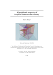
4
Doing tropical computations
This section follows the max convention for tropical arithmetic. For the nonconstant coefficient case tropical varieties are defined as in [17] and [15].
In this section we explain how to use Gfan to do tropical computations. For
a fixed ideal I ⊆ k[x1 , . . . , xn ] the set of all faces of all full-dimensional Gr¨obner
cones is a polyhedral complex which we call the Gr¨obner fan of I. For tropical
computations the lower dimensional cones of the complex will be of our interest.
In general every Gr¨obner cone is of the form:
Cω (I) := {ω ′ ∈ Rn : inω′ (I) = inω (I)}.
We define the tropical variety T (I) of an ideal I to be the the set of all ω
such that inω (I) does not contain a monomial. If the ideal I is homogeneous with
respect to a positive grading, then the Gr¨obner cones cover all of Rn and T (I)
is a union of Gr¨obner cones. Thus for a homogeneous ideal the tropical variety
gets the structure of a polyhedral fan which it inherits from the Gr¨obner fan. We
therefore also define the tropical variety T (I) to be the collection of all Gr¨obner
cones Cω (I) such that inω (I) is monomial-free.
We start by noticing that for computational purposes it is no restriction to
only consider the case of a homogeneous ideal:
Lemma 4.1 [15, Lemma 6.2.5] Let I ⊆ k[x1 , . . . , xn ] be an ideal generated by
h
f1 , . . . , fm ∈ k[x1 , . . . , xn ]. Let J = hf1h , . . . , fm
i ⊆ k[x0 , . . . , xn ]. Then inω (I)
is monomial-free if and only if in(0,ω) (J) is monomial-free where ω ∈ Rn . In
particular we have the following identity of sets in Rn+1 :
{0} × T (I) = T (J) ∩ ({0} × Rn ).
Here f h denotes the homogenization of the polynomial f . The homogenization
of a list of polynomials can be computed by the program gfan homogenize.
Notice that the lemma only requires the generators to be homogenized as a set
of polynomials and not in the sense of a polynomial ideal.
The tropical algorithms implemented in Gfan are explained in [5]. Notice
that Gfan follows the usual conventions for signs of weight vectors defining initial
forms while [5] uses opposite signs. This means that Gfan is compatible with the
max-plus convention whereas [5] is compatible with the min-plus convention.
4.1
Tropical variety by brute force
The command gfan tropicalbruteforce will compute all Gr¨obner cones of a
homogeneous ideal and for each check if its initial ideal contains a monomial. The
output is the tropical variety of the ideal. Since the tropical variety is usually
22
much smaller than the Gr¨obner fan this is a rather slow method for computing
the tropical variety. The line
gfan_buchberger | gfan_tropicalbruteforce
run on the input
Q[a,b,c,d,e,f,g,h,i,j]
{
bf-ah-ce,
bg-ai-de,
cg-aj-df,
ci-bj-dh,
fi-ej-gh
}
produces a tropical variety of the input ideal in a few minutes as a polyhedral
fan, see Section A.7. We use gfan buchberger since gfan tropicalbruteforce
requires its input to be a marked reduced Gr¨obner basis.
Remark 4.2 Notice that if k ′ ⊇ k is a field extension and I ⊆ k[x1 , . . . , xn ] an
ideal then T (I) = T (hIik′[x1 ,...,xn ] ) as a polyhedral fan. This identity follows since
both objects can be computed by Gr¨obner basis methods and Gr¨obner bases are
independent of such field extensions. The same argument of course also applies
to the Gr¨obner fans of the two ideals.
4.2
Traversing tropical varieties of prime ideals
Let I ⊆ C[x1 , . . . , xn ] be a homogeneous monomial-free prime ideal of dimension d. By the Bieri Groves Theorem [4] the tropical variety of I is a pure ddimensional polyhedral fan. It is connected in codimension one ([5, Theorem 14])
and can be traversed by Gfan. Let ω be a relative interior point of a d-dimensional
Gr¨obner cone in the tropical variety of I. Fix some term order ≺. Gfan represents Cω (I) by the pair of marked reduced Gr¨obner bases (G≺ω (inω (I)), G≺ω (I)).
To compute the tropical variety of an ideal we must begin by finding a starting d-dimensional Gr¨obner cone. For this gfan tropicalstartingcone is used.
This programs guesses a starting cone by heuristic methods. The guessing might
fail. In that case the program will terminate with an error message. After having computed a starting cone we use the program gfan tropicaltraverse to
traverse the tropical variety. We illustrate the procedure with an example.
Remark 4.3 Gfan does its computations over Q and thus the input should be
an ideal generated by polynomials in Q[x1 , . . . , xn ]. The assumption that I is
an ideal in C[x1 , . . . , xn ] is needed since by “prime ideal” in the above we mean
“prime ideal in the polynomial ring over the algebraically closed field C”. If I is a
23
prime ideal in Q[x1 , . . . , xn ] we do not know that its tropical variety is connected.
In Section 4.6 we address the problem of specifying non-rational coefficients.
Example 4.4 Let I ⊆ Q[a, . . . , o] be the ideal generated by the relations on the
2 by 2 minors of a 2 by 6 generic matrix. In C[x1 , . . . , xn ] the ideal I generates a
prime ideal. To get a starting cone for the traversal of T (I) we run the command
gfan_tropicalstartingcone
on the input
Q[a,b,c,d,e,f,g,h,i,j,k,l,m,n,o]
{
bg-aj-cf, bh-ak-df, bi-al-ef, ck-bm-dj,
cl-ej-bn, ci-eg-an, dn-co-em, dl-bo-ek,
gk-fm-jh, gl-fn-ij, hl-fo-ik, kn-jo-lm,
}
ch-am-dg,
di-ao-eh,
hn-im-go
and get a pair of marked reduced Gr¨obner bases
Q[a,b,c,d,e,f,g,h,i,j,k,l,m,n,o]
{
l*m+j*o, i*m+g*o, i*k-h*l, i*j-g*l, h*j-g*k,
e*m+c*o, e*k+b*o, e*j-c*l, e*h+a*o, e*g-c*i,
c*k-b*m, c*h-a*m, b*i-a*l, b*h-a*k, b*g-a*j}
{
l*m-k*n+j*o, i*m-h*n+g*o, i*k-h*l+f*o, i*j-g*l+f*n, h*j-g*k+f*m,
e*m-d*n+c*o, e*k-d*l+b*o, e*j-c*l+b*n, e*h-d*i+a*o, e*g-c*i+a*n,
c*k-d*j-b*m, c*h-d*g-a*m, b*i-e*f-a*l, b*h-d*f-a*k, b*g-c*f-a*j}
This takes a minute or so. We store the output in the file grassmann2 6.cone
for later use. Since I has many symmetries we add the following lines describing
the symmetry group to the end of the file:
{
(0,8,7,6,5,4,3,2,1,14,13,11,12,10,9),
(5,6,7,8,0,9,10,11,1,12,13,2,14,3,4)
}
We are ready to traverse T (I). We run the following command
gfan_tropicaltraverse --symmetry <grassmann2_6.cone
The computation takes a few (two - three) minutes. The output looks like this:
24
_application PolyhedralFan
_version 2.2
_type PolyhedralFan
AMBIENT_DIM
15
DIM
9
LINEALITY_DIM
6
RAYS
0 0 -1 0 0 0 0 0 0 0 0 0 0 0 0 # 0
0 0 0 0 0 0 0 -1 0 0 0 0 0 0 0 # 1
0 0 0 0 0 0 0 0 0 0 0 -1 0 0 0 # 2
0 0 0 -1 0 0 0 0 0 0 0 0 0 0 0 # 3
0 0 0 0 0 0 -1 0 0 0 0 0 0 0 0 # 4
0 -1 0 0 0 0 0 0 0 0 0 0 0 0 0 # 5
0 0 0 0 0 0 0 0 -1 0 0 0 0 0 0 # 6
0 0 0 0 0 0 0 0 0 0 -1 0 0 0 0 # 7
0 0 0 0 0 0 0 0 0 0 0 0 0 -1 0 # 8
0 0 0 0 0 -1 0 0 0 0 0 0 0 0 0 # 9
0 0 0 0 -1 0 0 0 0 0 0 0 0 0 0 # 10
0 0 0 0 0 0 0 0 0 0 0 0 0 0 -1 # 11
0 0 0 0 0 0 0 0 0 -1 0 0 0 0 0 # 12
-1 0 0 0 0 0 0 0 0 0 0 0 0 0 0 # 13
0 0 0 0 0 0 0 0 0 0 0 0 -1 0 0 # 14
0 0 0 -1 -1 -1 -1 0 0 -1 0 0 0 0 -1
-1 -1 0 0 0 -1 0 0 0 0 0 0 -1 -1 -1
-1 0 0 0 -1 0 0 0 -1 -1 -1 0 -1 0 0
1 1 0 0 0 1 2 2 0 2 2 0 1 1 1 # 18
1 0 2 2 1 0 0 0 1 1 1 0 1 2 2 # 19
0 0 0 1 1 1 1 0 0 1 2 2 2 2 1 # 20
1 1 0 2 2 1 0 2 2 0 0 0 1 1 1 # 21
1 2 2 0 1 2 2 0 1 1 1 0 1 0 0 # 22
2 2 0 1 1 1 1 0 2 1 0 2 0 0 1 # 23
0 -1 0 -1 0 0 -1 0 -1 0 -1 0 0 -1 0
N_RAYS
25
25
# 15
# 16
# 17
# 24
LINEALITY_SPACE
0 0 0 0 0 1 1 1 1
0 0 0 0 1 0 0 0 1
0 0 0 1 0 0 0 1 0
0 0 1 0 0 0 1 0 0
0 1 0 0 0 0 -1 -1
1 0 0 0 0 0 0 0 0
1 1 1 1 1 1
0 0 1 0 1 1
0 1 0 1 0 1
1 0 0 1 1 0
-1 0 0 0 -1 -1 -1
-1 -1 -1 -1 -1 -1
ORTH_LINEALITY_SPACE
0 0 0 0 0 0 0 0 0 0 1 -1 -1 1 0
0 0 0 0 0 0 0 0 0 1 0 -1 -1 0 1
0 0 0 0 0 0 0 1 -1 0 0 0 -1 1 0
0 0 0 0 0 0 1 0 -1 0 0 0 -1 0 1
0 0 0 0 0 1 0 0 -1 0 0 -1 -1 1 1
0 0 0 1 -1 0 0 0 0 0 0 0 -1 1 0
0 0 1 0 -1 0 0 0 0 0 0 0 -1 0 1
0 1 0 0 -1 0 0 0 0 0 0 -1 -1 1 1
1 0 0 0 -1 0 0 0 -1 0 0 0 -1 1 1
F_VECTOR
1 25 105 105
After this follows a list of cones and maximal cones. Every maximal cone has an
associated multiplicity which is also listed.
The output says that the tropical variety has dimension 9. Modulo the 6dimensional homogeneity space this is reduced to a 3-dimensional complex in
R9 and thus we may think of the tropical variety as a 2-dimensional polyhedral
complex on the 8-sphere in R9 . This complex is simplicial and has 105 maximal
cones.
The extreme rays (modulo the homogeneity space) are labeled 0, . . . , 24. In
the cone lists the cones are grouped together according to dimension and orbit
with respect to the specified symmetries. See Section A.7 for more information
on how to read the polyhedral fan format.
While traversing the variety the program gfan tropicaltraverse only computes d and (d − 1)-dimensional cones. The other cones are extracted after
traversing. Also the symmetries are expanded. Sometimes extracting all cones
is time consuming and one is only interested in the high dimensional cones up
to symmetry. These can be output using the option --noincidence. In that
case the output would be a list of orbits for maximal cones and a list of orbits
for codimension one cones. It is also listed how these cones are connected taking
symmetry into account. In general that format is rather difficult to read.
A final remark about gfan tropicaltraverse is that the polyhedral structure of the complex comes from the Gr¨obner fan. For some ideals it is possible
26
to find polyhedral fans covering the tropical variety with fewer cones.
4.3
Intersecting tropical hypersurfaces
The tropical variety of a principal ideal is called a tropical hypersurface. A tropical
prevariety is a finite intersection of tropical hypersurfaces or, to be precise, the
intersection of the support set of these hypersurfaces. In Gfan the intersection
is represented by the common refinement of the tropical hypersurfaces. The
program gfan tropicalintersection can compute such intersections.
Example 4.5 To compute the intersection of the tropical hypersurfaces T (ha +
b + c + 1i) and T (ha + b + 2ci) we run
gfan_tropicalintersection
on
Q[a,b,c]
{a+b+c+1,a+b+2c}
The output is a polyhedral fan whose support is the intersection. The balancing
condition for this fan is not satisfied which implies that it is not a tropical variety.
4.4
Computing tropical bases of curves
In Gfan an ideal I is said to define a tropical curve if k[x1 , . . . , xn ]/I has Krull
dimension equal to or one larger than the dimension of the homogeneity space of
I. A tropical basis of I is a finite generating set for the ideal such that the tropical
variety defined by I (as a set) is the intersection of the tropical hypersurfaces of
the generators. A tropical basis always exists [5]. The program gfan tropicalbasis
computes a tropical basis for an ideal defining a tropical curve.
Example 4.6 Again we consider the ideal ha + b + c + 1, a + b + 2ci. We notice
that this ideal defines a curve since the Krull dimension is 1 and the dimension
of the homogeneity space is 0. In the example above we saw that the listed set
is not a tropical basis. We run
gfan_tropicalbasis -h
on
Q[a,b,c]
{a+b+c+1,a+b+2c}
to get some tropical basis
27
Q[a,b,c]
{
-1+c,
2+b+a}
We needed the option -h here since the ideal was not homogeneous. If we run
gfan tropicalintersection on the output we see that the tropical variety consists of three rays and the origin.
4.5
Tropical intersection theory
Gfan contains a few experimental programs for doing computations in tropical
intersection theory. In [2, Definition 3.4] the tropical Weil divisor of a tropical
rational function on a (tropical) k-cycle in Rn is defined. This divisor can be
computed in Gfan. However, Gfan and [2] do not agree on the basic definitions
in tropical geometry. For example the definition of a fan is different. Here we
will adjust the necessary definitions to the Gfan conventions. A tropical k-cycle
will be a pure (rational) polyhedral fan F of dimension k in Rn with weights
which is balanced in the following sense: To every k-dimensional facet C we
assign a weight (or multiplicity) mC ∈ Z. The vector space Rn comes with
its standard lattice Zn . For a k − 1-dimensional ridge R ∈ F and a facet C
in its star2 in F corresponding to a cone L in the link3 of R in F , the semigroup L ∩ Zn /spanR (R) ∩ Zn ⊆ Zn /spanR (R) ∩ Zn is isomorphic to N. Define
uC/R ∈ Zn /span(R) ∩ Zn as the element identified with 1 ∈ N. The balancing
condition at R is that
X
mC uC/R = 0.
C∈F :R⊂C
For a (weighted) fan to be a tropical cycle this must hold at every ridge R.
It remains to define what a tropical rational function is. Take a polyhedral
fan F ′ and associate to each of its maximal cones a linear form. When evaluating
a point x in the support of F ′ simply evaluate the linear form of cone containing
x. If this gives a well-defined function we call this function a tropical rational
function. When computing Weil divisors we will require that the supports satisfy
supp(F ) ⊆ supp(F ′ ). There will be no further restriction on the polyhedral
structure.
For a definition of the Weil divisor itself we refer to [2, Definition 3.4]. Here
we just mention that it again is a cycle of dimension one lower.
To demonstrate the Gfan features we recompute [2, Example 3.10]. An easy
way to generate the k-cycle of that example is to compute it as a hypersurface.
2
the smallest polyhedral subcomplex of F containing all faces of F containing R.
take an ǫ-ball around a relative interior ω ∈ R and intersect it with F . Translating the ball
to the origin and scaling the intersection to infinity we get the link of R in F .
3
28
Since the paper is using min and Gfan is using max we need to change the
polynomial from the paper such that the Newton polytope is flipped:
gfan_tropicalhypersurface > tmpfile1.poly
Q[x_1,x_2,x_3]
{x_2x_3+x_1x_3+x_1x_2+x_1x_2x_3}
The weights/multiplicities are stored in the MULTIPLICITIES section of the
Polymake file.
It is harder specifying the rational function. We make the following file and
call in func.poly.
_application PolyhedralFan
_version 2.2
_type PolyhedralFan
AMBIENT_DIM
3
DIM
2
LINEALITY_DIM
0
RAYS
1 0 0
0 1 0
0 0 1
-1 -1
1 1 0
-1 -1
# 0
# 1
# 2
-1 # 3
# 4
0 # 5
N_RAYS
6
LINEALITY_SPACE
ORTH_LINEALITY_SPACE
1 0 0
0 1 0
0 0 1
MAXIMAL_CONES
{3 5} # Dimension 2
{5 2}
{0 2}
{1 2}
{1 3}
{0 3}
{1 4}
29
{0 4}
MULTIPLICITIES
1
1
1
1
1
1
1
1
RAY_VALUES
0
0
0
1
-1
0
LINEALITY_VALUES
Instead of specifying the linear function on each maximal cone we have to specify
its values on each of the rays in the fan and each of the generators of the lineality
space. Then Gfan will automatically interpolate the function. Since the lineality
space of the fan is empty we leave the LINEALITY VALUES section empty.
We now compute the Weil divisor:
gfan_tropicalweildivisor -i1 tmpfile1.poly -i2 func.poly >tmpfile2.poly
...and compute the Weil divisor again as in [2]...
gfan_tropicalweildivisor -i1 tmpfile2.poly -i2 func.poly >tmpfile3.poly
We get a fan with the origin being the only cone. It has multiplicity −1:
MULTIPLICITIES
-1
# Dimension 0
There is another useful command for computing polyhedral fans for rational
functions. The command gfan tropicalfunction takes a polynomial and turns
it into a fan representing its tropicalization which is a tropical rational function.
4.6
Non-constant coefficients
In tropical geometry it is common to take the valuation of C{{t}} into account
when defining the tropical variety of an ideal in C{{t}}[x1 , . . . , xn ]. Here C{{t}}
denotes the field of Puiseux series. The valuation val(p) of a non-zero Puiseux
series p is the degree of its lowest order term.
30
Definition 4.7 For ω ∈ Rn the t-ω-degree of a term cta xv with c ∈ C∗ , a ∈ Q
and v ∈ Zn is defined as −val(cta ) + ω · v = −a + ω · v. The t-initial form
t-inω (f ) ∈ C[x1 , . . . , xn ] of a polynomial f ∈ C{{t}}[x1 , . . . , xn ] is the sum of all
terms in f of maximal t-ω-weight but with 1 substituted for t.
Remark 4.8 Notice that since t has t-ω-degree −1, the maximal t-ω-weight is
attained by a term if the polynomial is non-zero. Furthermore, only a finite
number of terms attain the maximum. Therefore, it makes sense to substitute
t = 1 and consider the finite sum of terms as a polynomial in C[x1 , . . . , xn ].
Example 4.9 Consider f = (1 + t) + t2 x + tx2 ∈ C{{t}}[x1 , . . . , xn ]. Let ω =
( 21 ) ∈ R1 . Then t-inω (f ) = 1 + x2 . For any other choice of ω the t-initial form is
a monomial.
Definition 4.10 Let I ⊆ C{{t}}[x1 , . . . , xn ] and ω ∈ Rn . The t-initial ideal of
I with respect to ω is defined as:
t-inω (I) := ht-inω (f ) : f ∈ Ii ⊆ C[x1 , . . . , xn ].
Definition 4.11 Let I ⊆ C{{t}}[x1 , . . . , xn ] be an ideal. The tropical variety of
I is the set
T ′ (I) := {ω ∈ Rn : t-inω (I) is monomial-free}.
We use the notation T ′ (I) to avoid contradicting our original definition of the
tropical variety of an ideal in the polynomial ring over a field.
Proposition 4.12 [17, Proposition 7.3] Let I ⊆ C[t, x1 , . . . , xn ] be an ideal, J =
hIiC{{t}}[x1 ,...,xn ] and ω ∈ Rn . Then t-inω (I) = t-inω (J).
Remark 4.13 For f ∈ C[t, x1 , . . . , xn ] we have t-inω (f ) = (in(−1,ω) (f ))|t=1 . Consequently, for I ⊆ C[t, x1 , . . . , xn ] we have t-inω (I) = (in(−1,ω) (I))|t=1 . In order to
decide if t-inω (I) contains a monomial we may simply decide if the initial ideal
in(−1,ω) (I) contains a monomial. As a corollary we get
T (I) ∩ ({−1} × Rn ) = {−1} × T ′ (J).
In fact this gives a method for computing the tropical variety as a set of any
ideal J ⊆ C{{t}}[x1 , . . . , xn ] generated by elements in the polynomial ring over
the field of rational functions Q(t)[x1 , . . . , xn ] in Gfan by clearing denominators
and intersecting the result with the t = −1 plane. (We remind the reader that
Lemma 4.1 shows that for computational purposes it is no restriction if I is not
homogeneous.)
Intersecting the tropical variety with the t = −1 plane can with some difficulty be done by hand. If the tropical (pre)-variety has been computed with
31
gfan tropicalintersection then it is also possible to let Gfan do the intersection. What Gfan does is to compute the common refinement of the fan with the
fan consisting of the halfspace t ≤ 0 and its proper face. Of course this does not
remove the cones in the t = 0 plane, but they are easily removed by hand. We
illustrate the procedure by an example.
Example 4.14 Exercise 2 in Chapter 9 of [22] asks us to draw the variety defined
by the tropical polynomial f = 1x2 + 2xy + 1y 2 + 3x + 3y + 1. If we tropically
divide this polynomial by 3 we get f ′ := f /3 = −2x2 − 1xy − 2y 2 + 0x + 0y + −2
which defines the same tropical variety. This variety equals the variety defined
by the polynomial g = t2 x2 + txy + t2 y 2 + x + y + t2 ∈ C{{t}}[x, y]. Notice that
f ′ is the tropicalisation of g.
According to Remark 4.13 above the we may compute T ′ (hgi) by computing
the variety of ht2 x2 + txy + t2 y 2 + x + y + t2 i ⊆ C[t, x, y] and intersecting it with
the hyperplane t = −1. Running
gfan_tropicalintersection --tplane
on
Q[t,x,y]
{t^2x^2+txy+t^2y^2+x+y+t^2}
we get
RAYS
0 -1 0 # 0
-1 2 1 # 1
0 1 1 # 2
-1 1 1 # 3
-1 -2 -2 # 4
0 0 -1 # 5
-1 1 2 # 6
MAXIMAL_CONES
{3 4} # Dimension 2
{2 6}
{1 3}
{1 2}
{3 6}
{4 5}
{0 4}
{0 6}
{1 5}
32
2
6
3
1
0
4
5
Figure 3: The tropical variety defined by the tropical polynomial in Example 4.14.
among other information. We can now draw the two-dimensional picture asked
for in the exercise. The rays with non-zero first coordinate become points in the
picture. (If the first coordinate is not −1 scaling is required to get the rational
x, y-coordinates.) The rays with zero first coordinate become directions. The
maximal cones show how to connect the rays; see Figure 3. Notice that some of
the connections could have been “at infinity”.
4.6.1
Algebraic field extensions of Q
Ignoring time, memory usage and overflows Gfan can compute the tropical variety
T ′ (I) of any ideal I ⊆ C{{t}}[x1 , . . . , xn ] generated by elements of Q(t)[x1 , . . . , xn ].
This is a consequence of the following lemma:
Lemma 4.15 [17, Lemma 3.12] Let k be a field and M = hmi ⊆ k[a] a maximal
ideal where m is not a monomial. Let I ⊆ (k[a]/M)[x1 , . . . , xn ] be an ideal. For
ω ∈ Rn we have
inω (I) contains a monomial ⇐⇒ in(0,ω) (ϕ−1 (I)) contains a monomial
where ϕ : k[a, x1 , . . . , xn ] → (k[a]/M)[x1 , . . . , xn ] is the homomorphism taking
elements to their cosets.
33
A
Data formats
In this section we describe how polynomials, lists, marked Gr¨obner bases etc.
are represented as ASCII character strings. These strings will be input to the
programs by typing or by redirecting the standard input and be output by the
program on the standard output which may be the screen, a pipe or a file. Usually
files are used for input. For example,
gfan_bases < inputfile.txt > outputfile.txt
will read its input from inputfile.txt and write its output to outputfile.txt.
The following is an example of how to use pipes for computing a universal Gr¨obner
basis of the input:
gfan_bases < inputfile.txt | gfan_polynomialsetunion > outputfile.txt
In general spaces and newlines in the input are ignored, but for the polyhedral
formats described in Section A.7 and Section A.8 the rules are different.
A.1
Fields
Two kinds of fields are supported:
• The field Q of rationals which is represented by the string “Q”.
• Fields of the form Z/pZ where p is a prime number. These fields are represented by text strings “Z/pZ” where p is the prime number. For example
“Z/3Z” or “Z/17Z”. In Gfan the prime number p must be less than 32749.
A.2
Variables
A variable is denoted by its name which is an string of characters. The exact
rules for which names are allowed have not been decided on in this version of
Gfan and therefore Gfan accepts most names. However, white spaces, commas
and “]” are not allowed as characters in the name. Furthermore one should not
choose variable names such that one name is a starting substring of an other –
don’t choose names such as “x1” and “x” in the same polynomial ring.
A.3
Polynomial rings
A polynomial ring is represented first by a field and then by a list of variable
names. The list begins with “[” and ends with “]”. Names are separated
by commas. The ordering of the variables matters as this is also the ordering used for the entries of for example weight vectors. Examples: “Z/2Z[a,b]”
and “Q[x 1,x 2,y1,y2]”.
34
A.4
Polynomials
Coefficients in the field are given as fractions. A coefficient equals its numerator
multiplied by the inverse of the denominator. The numerator and denominator
themselves are given by an integer in Z which is mapped to the field by the homomorphism sending 1 ∈ Z to 1 in the field. The ’/’ character and the denominator
can be left out if the denominator is 1. If a field with non-zero characteristic was
chosen one should be careful that the denominator is not 0.
Monomials are written in the following formats:
• a^4dc
• a4dc
• aaadac
The monomial 1 cannot be written without writing it as a term in the usual
way “1”. Any other term is either a monomial or a coefficient and a monomial.
A polynomial is a list of terms separated by +. The + may be left out if the
numerator of the next monomial is negative.
That description did not cover every detail. Here is an example:
hello world - 3/8 a2+23abcge^4 +1
In our usual notation we would write it like this: dehl3 o2 rw + 1 + 23abce4 g − 83 a2 .
It is important to note that the first term written in a polynomial is
distinguished from the other terms in the polynomial. This is useful
when specifying marked Gr¨
obner bases.
A.5
Lists
A list begins with a ’{’ or a ’(’, contains elements separated by ’,’ and is ended
by a ’}’ or a ’)’. Different types of lists may be needed when specifying input for
the various programs:
An integer vector is a list of integers.
A list of integer vectors is a list of integer vectors. Such lists are used for
example when specifying generators for subgroups of Sn .
A polynomial list (or a polynomial set) is a list of polynomials.
A Gr¨
obner basis is the list of polynomials in a Gr¨obner basis with the leading
term of each listed polynomial being the initial term with respect to a term
order for which this a Gr¨obner basis.
A list of polynomial sets is a list of polynomial sets. Often the polynomial
sets are required to be Gr¨obner bases.
35
An ideal is written as a list of polynomials generating it.
For all other lists than integer vectors the characters ’{’ and ’}’ are used to start
and end the list.
A.6
Permutations
When exploiting the symmetry of an ideal one needs to input permutations to
the program. Each permutation is specified by a vector. The length of the vector
should equal the number of elements being permuted - for example the number
of variables in the polynomial ring. The first element in the vector describes
where the first element goes and so on. Of course we start indexing from 0. The
following vectors specify the identity, a transposition and a 3-cycle, respectively,
on an ordered set of four elements:
• (0,1,2,3)
• (1,0,2,3)
• (0,3,1,2)
A.7
Polyhedral fans
The output format for polyhedral fans is intended to be Polymake [10] compatible. Polymake recently switched to an XML based format. Gfan will keep
outputting data in the old text style by default as it is more convienient for the
command line Gfan user. The option --xml switches output to being XML. In
the Polymake world, the output objects will have type SymmetricFan. The new
XML files cannot be read by Gfan at the moment. In the following we describe
only the text (non-XML) format. For the XML format we refer to the Polymake
documentation.
The text representation of a fan begins with the lines
_application fan
_version 2.2
_type SymmetricFan
After this follows a list of properties. For example
LINEALITY_SPACE
0 0 0 0 0 1 1 1 1
0 0 0 0 1 0 0 0 1
0 0 0 1 0 0 0 1 0
0 0 1 0 0 0 1 0 0
0 1 0 0 0 0 -1 -1
1 0 0 0 0 0 0 0 0
1 1 1 1 1 1
0 0 1 0 1 1
0 1 0 1 0 1
1 0 0 1 1 0
-1 0 0 0 -1 -1 -1
-1 -1 -1 -1 -1 -1
36
Each property has a name and must be assigned a value of a certain type. You can
read more about the philosophy of the format in the Polymake documentation.
Example A.1 The ideal I = hab − c, bc − a, ca − bi has a cyclic symmetry. If we
run the commands
gfan --symmetry -e | gfan_topolyhedralfan --symmetry
on the input
Q[a,b,c]
{ab-c,bc-a,ca-b}
{(1,2,0)}
we get a polyhedral representation of the Gr¨obner fan of I:
_application PolyhedralFan
_version 2.2
_type PolyhedralFan
AMBIENT_DIM
3
DIM
3
LINEALITY_DIM
0
RAYS
1 1 0
1 0 1
0 1 1
0 1 0
1 0 0
0 0 1
2 1 1
1 1 2
1 2 1
1 1 1
#
#
#
#
#
#
#
#
#
#
0
1
2
3
4
5
6
7
8
9
N_RAYS
10
LINEALITY_SPACE
37
ORTH_LINEALITY_SPACE
0 0 1
0 1 0
1 0 0
F_VECTOR
1 10 18 9
CONES
{} # New orbit # Dimension 0
{0} # New orbit # Dimension 1
{1}
{2}
{3} # New orbit
{4}
{5}
{6} # New orbit
{7}
{8}
{9} # New orbit
{0 3} # New orbit # Dimension 2
{1 4}
{2 5}
{0 4} # New orbit
{1 5}
{2 3}
{6 9} # New orbit
{7 9}
{8 9}
{0 6} # New orbit
{1 7}
{2 8}
{0 8} # New orbit
{1 6}
{2 7}
{3 8} # New orbit
{4 6}
{5 7}
{0 3 8} # New orbit # Dimension 3
{1 4 6}
{2 5 7}
{0 4 6} # New orbit
38
Figure 4: The Gr¨obner fan in Example A.1 intersected with the standard simplex
in R3 .
{1
{2
{0
{1
{2
5
3
6
6
7
7}
8}
8 9} # New orbit
7 9}
8 9}
MAXIMAL_CONES
{0 3 8} # New orbit # Dimension 3
{1 4 6}
{2 5 7}
{0 4 6} # New orbit
{1 5 7}
{2 3 8}
{0 6 8 9} # New orbit
{1 6 7 9}
{2 7 8 9}
PURE
1
The most important properties are “RAYS” and “CONES”. A ray is given by
a relative interior point and a cone is given by a list of indices of rays that will
generate the cone. We may compare this combinatorial data to the drawing of
the Gr¨obner fan given in Figure 4. Notice that this example is particularly simple
as the dimension of the homogeneity space of I is 0.
The symbol “#” is used for writing comments in the file. The comments
39
should not be considered a part of the file. The comments are used by Gfan to
let the user know about dimensions, orbits and indices.
A detailed description of the properties follows in the following.
A.7.1
Data types
In Gfan’s Polymake format the following data types are supported:
Cardinal: One non-negative integer.
Boolean: 0 or 1.
Matrix: An array of integer vectors.
IncidenceMatrix: An array of sets of integers.
Vector: An integer vector.
A.7.2
Properties
Before we describe the properties we need to make a few definitions.
We do not consider the empty set to be a cone nor a face of a cone.
Definition A.2 The lineality space of a polyhedral cone is the largest subspace
contained in the cone.
The lineality space is the smallest face of the cone and if two cones are in the
same polyhedral fan then they must have the same lineality space. We define
the lineality space of a fan to be the common lineality space of its cones. In the
special case of a (non-restricted) Gr¨obner fan or a tropical variety the lineality
space of the fan coincides with the homogeneity space of the defining ideal.
Definition A.3 A cone (in a fan) is called a ray if its dimension is one larger
than the dimension of its lineality space.
A ray can be represented by a vector in its relative interior. This vector is contained in the cone but not contained in any of its proper faces. The representation
is not unique since the cone is invariant under translation by vectors in its lineality
space.
A Polyhedral fan in Gfan can have a subset of the following properties:
AMBIENT DIM is a Cardinal whose value is the dimension of the vector space
in which the fan lives. If the fan is a Gr¨obner fan or a tropical variety then
this number equals the number of variables in the polynomial ring of the
defining ideal.
40
DIM is a Cardinal whose value is the dimension of the highest dimensional cone
in the fan.
LINEALITY DIM is a Cardinal whose value is the dimension of the lineality
space of the fan.
RAYS is a Matrix. The rows of the matrix are vectors representing the rays of
the fan — one for each ray. The rows are ordered and Gfan writes an index
as a comment to make the file human readable.
N RAYS is a Cardinal which equals the number of rays in the fan.
LINEALITY SPACE is a Matrix whose rows form a basis for the lineality space
of the fan.
ORTH LINEALITY SPACE is a Matrix whose rows form a basis for the orthogonal complement of the lineality space of the fan.
F VECTOR is a Vector. The number of entries is DIM−LINEALITY DIM+1.
The ith entry is the number of cones in the fan of dimension
i+LINEALITY DIM−1.
CONES is an IncidenceMatrix. The section contains a line for each cone in the
fan. Each line is the set of indices of the rays contained in the corresponding
cone.
MAXIMAL CONES is an IncidenceMatrix and similar to CONES except that
only cones which are maximal with respect to inclusion are listed.
PURE is a Boolean. The value is 1 if the polyhedral fan is pure and 0 otherwise.
MULTIPLICITIES is a Matrix with one column. An entry is the multiplicity of
a maximal cone. Usually cones in polyhedral fans do not have multiplicities.
Thus this property only makes sense for weighted polyhedral fans of which
tropical varieties is a special case. The ordering of the rows in this property
is consistent with the ordering in MAXIMAL CONES.
RAY VALUES is a Matrix with just one column. It is used when the fan is
meant to specify a piece-wise linear (or tropical rational) function. The
function value on the ith ray of the fan is listed in the ith row of the
matrix.
LINEALITY VALUES is a Matrix with just one column. It is used when the
fan is meant to specify a piece-wise linear (or tropical rational) function.
The function value on the ith generator of the lineality space (stored in
LINEALITY SPACE) is listed in the ith row of the matrix.
41
Besides sections listed above, the sections MAXIMAL CONES ORBITS, CONES ORBITS
and MULTIPLICITIES ORBITS are introduced when doing symmetric computations with the --symmetry option. These sections are analogous to MAXIMAL CONES, CONES and MULTIPLICITIES except that they operate on the
level of orbits of cones with respect to the symmetry rather than cones.
A.8
Polyhedral cones
The string representation of a polyhedral cone starts with
_application PolyhedralCone
_version 2.2
_type PolyhedralCone
After this follows the properties. For polyhedral cones they are as follows.
AMBIENT DIM — see previous section.
DIM is a Cardinal whose value is the dimension of the cone.
IMPLIED EQUATIONS is a Matrix whose rows form a basis of the space of
linear forms vanishing on the cone.
LINEALITY DIM — see previous section.
LINEALITY SPACE — see previous section.
FACETS is a Matrix which contains an outer normal vector for each facet of
the cone.
RELATIVE INTERIOR POINT is a Vector in the relative interior of the cone.
42
B
Application list
This section contains the full list of programs in Gfan. For each program its
help file is listed. The help file of a program can also be displayed by specifying
the --help option when running the program. Besides the options listed in this
section all programs have options --log1, --log2,... which tell Gfan how much
information to write to “standard error” while a computation is running. These
options are VERY USEFUL when you wish to know if Gfan is making
any progress in its computation.
Additional options which can be used for all programs, but which are not
listed in the following subsections are:
--stdin value Specify a file to use as input instead of reading from the standard
input.
--stdout value Specify a file to write output to instead of writing to the standard output.
--xml To let polyhedral fans be output in an XML format instead of in the text
format. (The XML files are not readable by Gfan.)
B.1
gfan bases
This is a program for computing all reduced Gr¨obner bases of a polynomial ideal.
It takes the ring and a generating set for the ideal as input. By default the
enumeration is done by an almost memoryless reverse search. If the ideal is
symmetric the symmetry option is useful and enumeration will be done up to
symmetry using a breadth first search. The program needs a starting Gr¨obner
basis to do its computations. If the -g option is not specified it will compute one
using Buchberger’s algorithm.
Options:
-g Tells the program that the input is already a Gr¨obner basis (with the initial term of each polynomial being the first ones listed). Use this option
if it takes too much time to compute the starting (standard degree lexicographic) Gr¨obner basis and the input is already a Gr¨obner basis.
--symmetry Tells the program to read in generators for a group of symmetries
(subgroup of S n) after having read in the ideal. The program checks that
the ideal stays fixed when permuting the variables with respect to elements
in the group. The program uses breadth first search to compute the set
of reduced Gr¨obner bases up to symmetry with respect to the specified
subgroup.
-e Echo. Output the generators for the symmetry group.
43
--disableSymmetryTest When using --symmetry this option will disable the
check that the group read off from the input actually is a symmetry group
with respect to the input ideal.
--parameters value With this option you can specify how many variables to
treat as parameters instead of variables. This makes it possible to do computations where the coefficient field is the field of rational functions in the
parameters. This does not work well at the moment.
B.2
gfan buchberger
This program computes a reduced lexicographic Gr¨obner basis of the polynomial
ideal given as input. The default behavior is to use Buchberger’s algorithm. The
ordering of the variables is a > b > c... (assuming that the ring is Q[a,b,c,...]).
Options:
-w Compute a Gr¨obner basis with respect to a degree lexicographic order with
a > b > c... instead. The degrees are given by a weight vector which is read
from the input after the generating set has been read.
-r Use the reverse lexicographic order (or the reverse lexicographic order as a tie
breaker if -w is used). The input must be homogeneous if the pure reverse
lexicographic order is chosen. Ignored if -W is used.
-W Do a Gr¨obner walk. The input must be a minimal Gr¨obner basis. If -W is
used -w is ignored.
-g Do a generic Gr¨obner walk. The input must be homogeneous and must be
a minimal Gr¨obner basis with respect to the reverse lexicographic term
order. The target term order is always lexicographic. The -W option must
be used.
--parameters value With this option you can specify how many variables to
treat as parameters instead of variables. This makes it possible to do computations where the coefficient field is the field of rational functions in the
parameters. This does not work well at the moment.
B.3
gfan combinerays
This program combines rays from the specified polymake file by adding according
to a list of vectors of indices given on the standard input.
Options:
-i value Specify the name of the input file.
--section value Specify a section of the polymake file to use as input, rather
than standard input.
44
B.4
gfan doesidealcontain
This program takes a marked Gr¨obner basis of an ideal I and a set of polynomials
on its input and tests if the polynomial set is contained in I by applying the
division algorithm for each element. The output is 1 for true and 0 for false.
Options:
--remainder Tell the program to output the remainders of the divisions rather
than outputting 0 or 1.
--multiplier Reads in a polynomial that will be multiplied to the polynomial to
be divided before doing the division.
B.5
gfan fancommonrefinement
This program takes two polyhedral fans and computes their common refinement.
Options:
-i1 value Specify the name of the first input file.
-i2 value Specify the name of the second input file.
B.6
gfan fanhomology
This program takes a polyhedral fan and computes its reduced homology groups.
Of course the support of a fan is contractible, so what is really computed is the
reduced homology groups of the support of the fan after quotienting out with the
lineality space and intersecting with a sphere. Notice that taking the quotient
with the lineality space results in an inverted suspension which just results in a
shift of the reduced homology groups.
Options:
-i value Specify the name of the input file.
--no-optimize Disable preprocessing of boundary maps before doing lattice
computations.
B.7
gfan fanlink
This program takes a polyhedral fan and a vector and computes the link of the
polyhedral fan around that vertex. The link will have lineality space dimension
equal to the dimension of the relative open polyhedral cone of the original fan
containing the vector.
Options:
-i value Specify the name of the input file.
45
--symmetry Reads in a fan stored with symmetry. The generators of the symmetry group must be given on the standard input.
--star Computes the star instead. The star is defined as the smallest polyhedral
fan containing all cones of the original fan containing the vector.
B.8
gfan fanproduct
This program takes two polyhedral fans and computes their product.
Options:
-i1 value Specify the name of the first input file.
-i2 value Specify the name of the second input file.
B.9
gfan fansubfan
This program takes a polyhedral fan and a list of vectors and computes the
smallest subfan of the fan having the list of vectors in its support.
Options:
-i value Specify the name of the input file.
--symmetry Reads in the cone stored with symmetry. The generators of the
symmetry group must be given on the standard input.
B.10
gfan genericlinearchange
This program takes a list of polynomials and performs a generic linear change of
coordinates by introducing nxn new variables.
B.11
gfan groebnercone
This program computes a Gr¨obner cone. Three different cases are handled. The
input may be a marked reduced Gr¨obner basis in which case its Gr¨obner cone is
computed. The input may be just a marked minimal basis in which case the cone
computed is not a Gr¨obner cone in the usual sense but smaller. (These cones
are described in [Fukuda, Jensen, Lauritzen, Thomas]). The third possible case
is that the Gr¨obner cone is possibly lower dimensional and given by a pair of
Gr¨obner bases as it is useful to do for tropical varieties, see option --pair. The
facets of the cone can be read off in section FACETS and the equations in section
IMPLIED EQUATIONS.
Options:
--restrict Add an inequality for each coordinate, so that the the cone is restricted
to the non-negative orthant.
46
--pair The Gr¨obner cone is given by a pair of compatible Gr¨obner bases. The
first basis is for the initial ideal and the second for the ideal itself. See the
tropical section of the manual.
--asfan Writes the cone as a polyhedral fan with all its faces instead. In this
way the extreme rays of the cone are also computed.
--vectorinput Compute a cone given list of inequalities rather than a Gr¨obner
cone. The input is an integer which specifies the dimension of the ambient
space, a list of inequalities given as vectors and a list of equations.
B.12
gfan groebnerfan
This is a program for computing the Gr¨obner fan of a polynomial ideal as a
polyhedral complex. It takes a generating set for the ideal as input. If the ideal
is symmetric the symmetry option is useful and enumeration will be done up to
symmetry. The program needs a starting Gr¨obner basis to do its computations.
If the -g option is not specified it will compute one using Buchberger’s algorithm.
Options:
-g Tells the program that the input is already a Gr¨obner basis (with the initial term of each polynomial being the first ones listed). Use this option
if it takes too much time to compute the starting (standard degree lexicographic) Gr¨obner basis and the input is already a Gr¨obner basis.
--symmetry Tells the program to read in generators for a group of symmetries
(subgroup of S n) after having read in the ideal. The program checks that
the ideal stays fixed when permuting the variables with respect to elements
in the group. The program uses breadth first search to compute the set
of reduced Gr¨obner bases up to symmetry with respect to the specified
subgroup.
--disableSymmetryTest When using --symmetry this option will disable the
check that the group read off from the input actually is a symmetry group
with respect to the input ideal.
--restrictingfan value Specify the name of a file containing a polyhedral fan in
Polymake format. The computation of the Gr¨obner fan will be restricted
to this fan. If the --symmetry option is used then this restricting fan must
be invariant under the symmetry and the orbits in the file must be with
respect to the specified group of symmetries. The orbits of maximal cones
of the file are then read in rather than the maximal cones.
47
--parameters value With this option you can specify how many variables to
treat as parameters instead of variables. This makes it possible to do computations where the coefficient field is the field of rational functions in the
parameters. This does not work well at the moment.
--nocones Tells the program not to output the CONES and MAXIMAL CONES
sections, but still output CONES COMPRESSED and MAXIMAL CONES COMPRESSED
if --symmetry is used.
B.13
gfan homogeneityspace
This program computes the homogeneity space of a list of polynomials - as a
cone. Thus generators for the homogeneity space are found in the section LINEALITY SPACE. If you wish the homogeneity space of an ideal you should first
compute a set of homogeneous generators and call the program on these. A
reduced Gr¨obner basis will always suffice for this purpose.
B.14
gfan homogenize
This program homogenises a list of polynomials by introducing an extra variable.
The name of the variable to be introduced is read from the input after the list of
polynomials. Without the -w option the homogenisation is done with respect to
total degree. Example: Input: Q[x,y]{y-1} z Output: Q[x,y,z]{y-z}
Options:
-i Treat input as an ideal. This will make the program compute the homogenisation of the input ideal. This is done by computing a degree Gr¨obner basis
and homogenising it.
-w Specify a homogenisation vector. The length of the vector must be the same
as the number of variables in the ring. The vector is read from the input
after the list of polynomials.
-H Let the name of the new variable be H rather than reading in a name from
the input.
B.15
gfan initialforms
This program converts a list of polynomials to a list of their initial forms with
respect to the vector given after the list.
Options:
--ideal Treat input as an ideal. This will make the program compute the initial
ideal of the ideal generated by the input polynomials. The computation is
done by computing a Gr¨obner basis with respect to the given vector. The
48
vector must be positive or the input polynomials must be homogeneous in
a positive grading. None of these conditions are checked by the program.
--pair Produce a pair of polynomial lists. Used together with --ideal this option
will also write a compatible reduced Gr¨obner basis for the input ideal to
the output. This is useful for finding the Gr¨obner cone of a non-monomial
initial ideal.
--mark If the --pair option is and the --ideal option is not used this option will
still make sure that the second output basis is marked consistently with the
vector.
--list Read in a list of vectors instead of a single vector and produce a list of
polynomial sets as output.
B.16
gfan interactive
This is a program for doing interactive walks in the Gr¨obner fan of an ideal. The
input is a Gr¨obner basis defining the starting Gr¨obner cone of the walk. The
program will list all flippable facets of the Gr¨obner cone and ask the user to
choose one. The user types in the index (number) of the facet in the list. The
program will walk through the selected facet and display the new Gr¨obner basis
and a list of new facet normals for the user to choose from. Since the program
reads the user’s choices through the the standard input it is recommended not to
redirect the standard input for this program.
Options:
-L Latex mode. The program will try to show the current Gr¨obner basis in a
readable form by invoking LaTeX and xdvi.
-x Exit immediately.
-f Tell the program to list the flipped reduced Gr¨obner basis of the initial ideal
for each flippable wall in the current Gr¨obner cone.
-w Tell the program to list (a Gr¨obner basis with respect to the current term
order for) the initial ideal for each flippable wall in the current Gr¨obner
cone.
-i Tell the program to list the defining set of inequalities of the non-restricted
Gr¨obner cone as a set of vectors after having listed the current Gr¨obner
basis.
-W Print weight vector. This will make the program print an interior vector
of the current Gr¨obner cone and a relative interior point for each flippable
facet of the current Gr¨obner cone.
49
--tropical Traverse a tropical variety interactively.
B.17
gfan ismarkedgroebnerbasis
This program checks if a set of marked polynomials is a Gr¨obner basis with respect
to its marking. First it is checked if the markings are consistent with respect to a
positive vector. Then Buchberger’s S-criterion is checked. The output is boolean
value.
B.18
gfan krulldimension
Takes an ideal I and computes the Krull dimension of R/I where R is the polynomial ring. This is done by first computing a Gr¨obner basis.
Options:
-g Tell the program that the input is already a reduced Gr¨obner basis.
B.19
gfan latticeideal
This program computes the lattice ideal of a lattice. The input is a list of generators for the lattice.
Options:
-t Compute the toric ideal of the matrix whose rows are given on the input
instead.
--convert Does not do any computation, but just converts the vectors to binomials.
B.20
gfan leadingterms
This program converts a list of polynomials to a list of their leading terms.
Options:
-m Do the same thing for a list of polynomial sets. That is, output the set of
sets of leading terms.
B.21
gfan list
This program lists all subcommands of the Gfan installation.
Options:
--hidden Show hidden commands which are not officially supported.
50
B.22
gfan markpolynomialset
This program marks a set of polynomials with respect to the vector given at the
end of the input, meaning that the largest terms are moved to the front. In case
of a tie the lexicographic term order with a > b > c... is used to break it.
B.23
gfan minkowskisum
This is a program for computing the normal fan of the Minkowski sum of the
Newton polytopes of a list of polynomials.
Options:
--symmetry Tells the program to read in generators for a group of symmetries
(subgroup of S n) after having read in the ideal. The program checks that
the ideal stays fixed when permuting the variables with respect to elements
in the group. The program uses breadth first search to compute the set
of reduced Gr¨obner bases up to symmetry with respect to the specified
subgroup.
--disableSymmetryTest When using --symmetry this option will disable the
check that the group read off from the input actually is a symmetry group
with respect to the input ideal.
--nocones Tell the program to not list cones in the output.
B.24
gfan minors
This program will generate the r*r minors of a d*n matrix of indeterminates.
Options:
-r value Specify r.
-d value Specify d.
-n value Specify n.
-M2 Use Macaulay2 conventions for order of variables.
--names Assign names to the minors.
--dressian Produce tropical defining the Dressian(3,n) instead. (The signs may
not be correct, that is the equations may not be Pluecker relations.)
--pluckersymmetries Do nothing but produce symmetry generators for the
Pluecker ideal.
51
--symmetry Produces a list of generators for the group of symmetries keeping
the set of minors fixed. (Only without --names).
--parametrize Parametrize the set of d times n matrices of Barvinok rank less
than or equal to r-1 by a list of tropical polynomials.
B.25
gfan mixedvolume
This program computes the mixed volume of the Newton polytopes of a list of
polynomials. The ring is specified on the input. After this follows the list of
polynomials.
B.26
gfan overintegers
This program is an experimental implementation of Gr¨obner bases for ideals in
Z[x 1,...,x n]. Several operations are supported by specifying the appropriate option: (1) computation of the reduced Gr¨obner basis with respect to a given vector
(tiebroken lexicographically), (2) computation of an initial ideal, (3) computation of the Gr¨obner fan, (4) computation of a single Gr¨obner cone. Since Gfan
only knows polynomial rings with coefficients being elements of a field, the ideal
is specified by giving a set of polynomials in the polynomial ring Q[x 1,...,x n].
That is, by using Q instead of Z when specifying the ring. The ideal MUST BE
HOMOGENEOUS (in a positive grading) for computation of the Gr¨obner fan.
Non-homogeneous ideals are allowed for the other computations if the specified
weight vectors are positive. NOTE: This program is experimental and expected
to change behaviour in future releases, so don’t write your SAGE and M2 interfaces just yet.
Options:
--groebnerBasis Asks the program to compute a marked Gr¨obner basis with
respect to a weight vector tie-broken lexicographically. The input order is:
Ring ideal vector.
--initialIdeal Asks the program to compute an initial ideal with respect to a
vector. The input order is: Ring ideal vector.
--groebnerFan Asks the program to compute the Gr¨obner fan. The input order
is: Ring ideal.
--groebnerCone Asks the program to compute a single Gr¨obner cone containing the specified vector in its relative interior. The output is stored as a
fan. The input order is: Ring ideal vector.
-m For the operations taking a vector as input, read in a list of vectors instead,
and perform the operation for each vector in the list.
52
-g Tells the program that the input is already a Gr¨obner basis (with the initial
term of each polynomial being the first ones listed). Use this option if the
usual --groebnerFan is too slow.
B.27
gfan padic
This program is an experimental implementation of p-adic Gr¨obner bases as proposed by Diane Maclagan. Several operations are supported by specifying the
appropriate option: (1) computation of Gr¨obner basis with respect to a given vector (tiebroken lexicographically), (2) computation of the p-adic initial ideal, (3)
computation of the p-adic Gr¨obner complex as defined by Maclagan and Sturmfels, (4) computation of a single polyhedron of the p-adic Gr¨obner complex. The
input ideal should be an ideal of the polynomial ring with coefficient field Q. The
valuation is specified with the option -p. The ideal MUST BE HOMOGENEOUS
(in a positive grading). Since gfan can only handle fans and not polyhedral complexes in general, what is computed as the Gr¨obner complex is actually the ”fan
over” the complex - in other words, the first coordinate is supposed to be 1 in the
output fan. Similarly, the weight vectors must be specified in an homogeneous
way, for example by adding an additional 1 entry as first coordinate. (If fractions
are needed, use the entry as a common denominator.) NOTE: This program is
experimental and expected to change behaviour in future releases, so don’t write
your SAGE and M2 interfaces just yet. In particular this program uses the tropical minimum-convention!!
Options:
-p value Defines the prime used for the valuation.
--groebnerBasis Asks the program to compute a marked Gr¨obner basis with
respect to a weight vector (tie-broken lexicographically). The input order
is: Ring ideal vector.
--initialIdeal Asks the program to compute an initial ideal with respect to a
vector. The input order is: Ring ideal vector.
--groebnerComplex Asks the program to compute the p-adic Gr¨obner complex. The input order is: Ring ideal.
--groebnerPolyhedron Asks the program to compute a single polyhedron of
the Gr¨obner complex containing the specified vector in its relative interior.
The output is stored as a fan. The input order is: Ring ideal vector.
-m For the operations taking a vector as input, read in a list of vectors instead,
and perform the operation for each vector in the list.
53
B.28
gfan polynomialsetunion
This program computes the union of a list of polynomial sets given as input. The
polynomials must all belong to the same ring. The ring is specified on the input.
After this follows the list of polynomial sets.
Options:
-s Sort output by degree.
B.29
gfan render
This program renders a Gr¨obner fan as an xfig file. To be more precise, the input
is the list of all reduced Gr¨obner bases of an ideal. The output is a drawing of the
Gr¨obner fan intersected with a triangle. The corners of the triangle are (1,0,0) to
the right, (0,1,0) to the left and (0,0,1) at the top. If there are more than three
variables in the ring these coordinates are extended with zeros. It is possible to
shift the 1 entry cyclic with the option --shiftVariables.
Options:
-L Make the triangle larger so that the shape of the Gr¨obner region appears.
--shiftVariables value Shift the positions of the variables in the drawing. For
example with the value equal to 1 the corners will be right: (0,1,0,0,...), left:
(0,0,1,0,...) and top: (0,0,0,1,...). The shifting is done modulo the number
of variables in the polynomial ring. The default value is 0.
B.30
gfan renderstaircase
This program renders a staircase diagram of a monomial initial ideal to an xfig
file. The input is a Gr¨obner basis of a (not necessarily monomial) polynomial
ideal. The initial ideal is given by the leading terms in the Gr¨obner basis. Using
the -m option it is possible to render more than one staircase diagram. The
program only works for ideals in a polynomial ring with three variables.
Options:
-m Read multiple ideals from the input. The ideals are given as a list of lists
of polynomials. For each polynomial list in the list a staircase diagram is
drawn.
-d value Specifies the number of boxes being shown along each axis. Be sure
that this number is large enough to give a correct picture of the standard
monomials. The default value is 8.
-w value Width. Specifies the number of staircase diagrams per row in the xfig
file. The default value is 5.
54
B.31
gfan saturation
This program computes the saturation of the input ideal with the product of the
variables x 1,...,x n. The ideal does not have to be homogeneous.
Options:
-h Tell the program that the input is a homogeneous ideal (with homogeneous
generators).
--noideal Do not treat input as an ideal but just factor out common monomial
factors of the input polynomials.
B.32
gfan secondaryfan
This program computes the secondary fan of a vector configuration. The configuration is given as an ordered list of vectors. In order to compute the secondary
fan of a point configuration an additional coordinate of ones must be added. For
example {(1,0),(1,1),(1,2),(1,3)}.
Options:
--unimodular Use heuristics to search for unimodular triangulation rather than
computing the complete secondary fan
--scale value Assuming that the first coordinate of each vector is 1, this option
will take the polytope in the 1 plane and scale it. The point configuration
will be all lattice points in that scaled polytope. The polytope must have
maximal dimension. When this option is used the vector configuration must
have full rank. This option may be removed in the future.
--restrictingfan value Specify the name of a file containing a polyhedral fan in
Polymake format. The computation of the Secondary fan will be restricted
to this fan. If the --symmetry option is used then this restricting fan must
be invariant under the symmetry and the orbits in the file must be with
respect to the specified group of symmetries. The orbits of maximal cones
of the file are then read in rather than the maximal cones.
--symmetry Tells the program to read in generators for a group of symmetries
(subgroup of S n) after having read in the vector configuration. The program checks that the configuration stays fixed when permuting the variables
with respect to elements in the group. The output is grouped according to
the symmetry.
--nocones Tells the program not to output the CONES and MAXIMAL CONES
sections, but still output CONES COMPRESSED and MAXIMAL CONES COMPRESSED
if --symmetry is used.
55
B.33
gfan stats
This program takes a list of reduced Gr¨obner bases for the same ideal and computes various statistics. The following information is listed: the number of bases
in the input, the number of variables, the dimension of the homogeneity space,
the maximal total degree of any polynomial in the input and the minimal total
degree of any basis in the input, the maximal number of polynomials and terms
in a basis in the input.
B.34
gfan substitute
This program changes the variable names of a polynomial ring. The input is a
polynomial ring, a polynomial set in the ring and a new polynomial ring with the
same coefficient field but different variable names. The output is the polynomial
set written with the variable names of the second polynomial ring. Example:
Input: Q[a,b,c,d]{2a-3b,c+d}Q[b,a,c,x] Output: Q[b,a,c,x]{2*b-3*a,c+x}
B.35
gfan symmetries
This program computes the symmetries of a polynomial ideal. The program is
slow, so think before using it. Use --symmetry to give hints about which subgroup
of the symmetry group could be useful. The program checks each element of the
specified subgroup to see if it preserves the ideal.
Options:
--symmetry Specify subgroup to be searched for permutations keeping the ideal
fixed.
--symsigns Specify for each generator of the group specified wiht --symmetry an
element of {−1, +1}n which by its multiplication on the variables together
with the permutation is expected to keep the ideal fixed.
B.36
gfan tolatex
This program converts ASCII math to TeX math. The data-type is specified by
the options.
Options:
-h Add a header to the output. Using this option the output will be LaTeXable
right away.
--polynomialset The data to be converted is a list of polynomials.
--polynomialsetlist The data to be converted is a list of lists of polynomials.
56
B.37
gfan topolyhedralfan
This program takes a list of reduced Gr¨obner bases and produces the fan of all
faces of these. In this way by giving the complete list of reduced Gr¨obner bases,
the Gr¨obner fan can be computed as a polyhedral complex. The option --restrict
lets the user choose between computing the Gr¨obner fan or the restricted Gr¨obner
fan.
Options:
--restrict Add an inequality for each coordinate, so that the the cones are restricted to the non-negative orthant.
--symmetry Tell the program to read in generators for a group of symmetries
(subgroup of S n) after having read in the ring. The output is grouped
according to these symmetries. Only one representative for each orbit is
needed on the input.
B.38
gfan tropicalbasis
This program computes a tropical basis for an ideal defining a tropical curve.
Defining a tropical curve means that the Krull dimension of R/I is at most 1 +
the dimension of the homogeneity space of I where R is the polynomial ring. The
input is a generating set for the ideal. If the input is not homogeneous option -h
must be used.
Options:
-h Homogenise the input before computing a tropical basis and dehomogenise the
output. This is needed if the input generators are not already homogeneous.
B.39
gfan tropicalbruteforce
This program takes a marked reduced Gr¨obner basis for a homogeneous ideal and
computes the tropical variety of the ideal as a subfan of the Gr¨obner fan. The
program is slow but works for any homogeneous ideal. If you know that your ideal
is prime over the complex numbers or you simply know that its tropical variety
is pure and connected in codimension one then use gfan tropicalstartingcone and
gfan tropicaltraverse instead.
B.40
gfan tropicalevaluation
This program evaluates a tropical polynomial function in a given set of points.
57
B.41
gfan tropicalfunction
This program takes a polynomial and tropicalizes it. The output is piecewise
linear function represented by a fan whose cones are the linear regions. Each
ray of the fan gets the value of the tropical function assigned to it. In other
words this program computes the normal fan of the Newton polytope of the
input polynomial with additional information.
B.42
gfan tropicalhypersurface
This program computes the tropical hypersurface defined by a principal ideal.
The input is the polynomial ring followed by a set containing just a generator of
the ideal.
B.43
gfan tropicalintersection
This program computes the set theoretical intersection of a set of tropical hypersurfaces (or to be precise, their common refinement as a fan). The input is
a list of polynomials with each polynomial defining a hypersurface. Considering
tropical hypersurfaces as fans, the intersection can be computed as the common
refinement of these. Thus the output is a fan whose support is the intersection
of the tropical hypersurfaces.
Options:
-t Note that the input polynomials generate an ideal. This option will make the
program choose a relative interior point for each listed output cone and
check if its initial ideal contains a monomial. The actual check is done on
a homogenization of the input ideal, but this does not affect the result.
--tplane This option intersects the resulting fan with the plane x 0=-1, where
x 0 is the first variable. To simplify the implementation the output is
actually the common refinement with the non-negative half space. This
means that ”stuff at infinity” (where x 0=0) is not removed.
--symmetryPrinting Parse a group of symmetries after the input has been
read. Used when printing with --incidence.
--symmetryExploit Restrict computation to the closed lexicographic fundamental domain of the specified symmetry group. This overwrites --restrict.
--nocones Tells the program not to output the CONES and MAXIMAL CONES
sections, but still output CONES COMPRESSED and MAXIMAL CONES COMPRESSED
if --symmetry is used.
58
--restrict Restrict the computation to a full-dimensional cone given by a list of
marked polynomials. The cone is the closure of all weight vectors choosing
these marked terms.
--stable Find the stable intersection of the input polynomials using tropical
intersection theory. This can be slow. Most other options are ignored.
B.44
gfan tropicallifting
This program is part of the Puiseux lifting algorithm implemented in Gfan and
Singular. The Singular part of the implementation can be found in:
Anders Nedergaard Jensen, Hannah Markwig, Thomas Markwig: tropical.lib.
A SINGULAR 3.0 library for computations in tropical geometry, 2007
See also
http://www.mathematik.uni-kl.de/˜keilen/de/tropical.html
and the paper
Jensen, Markwig, Markwig: ”An algorithm for lifting points in a tropical
variety”.
Example:
Run Singular from the directory where tropical.lib is located. Give the following sequence of commands to Singular:
LIB ”tropical.lib”; ring R=0,(t,x,y,z),dp; ideal i=-y2t4+x2,yt3+xz+y; intvec
w=1,-2,0,2; list L=tropicallifting(i,w,3); displaytropicallifting(L,”subst”); This
produces a Puiseux series solution to i with valuation (2,0,-2)
Options:
--noMult Disable the multiplicity computation.
-n value Number of variables that should have negative weight.
-c Only output a list of vectors being the possible choices.
B.45
gfan tropicallinearspace
This program generates tropical equations for a tropical linear space in the Speyer
sense given the tropical Pluecker coordinates as input.
Options:
-d value Specify d.
-n value Specify n.
--trees list the boundary trees (assumes d=3)
59
B.46
gfan tropicalmultiplicity
This program computes the multiplicity of a tropical cone given a marked reduced
Gr¨obner basis for its initial ideal.
B.47
gfan tropicalrank
This program will compute the tropical rank of matrix given as input. Tropical
addition is MAXIMUM.
Options:
--kapranov Compute Kapranov rank instead of tropical rank.
--determinant Compute the tropical determinant instead.
B.48
gfan tropicalstartingcone
This program attempts to compute a starting pair of marked reduced Gr¨obner
bases to be used as input for gfan tropicaltraverse. If unsuccessful the program
will say so. The input is a homogeneous ideal whose tropical variety is a pure
d-dimensional polyhedral complex.
Options:
-g Tell the program that the input is already a reduced Gr¨obner basis.
-d Output dimension information to standard error.
--stable Find starting cone in the stable intersection or, equivalently, pretend
that the coefficients are genereric.
B.49
gfan tropicaltraverse
This program computes a polyhedral fan representation of the tropical variety of
a homogeneous prime ideal I. Let d be the Krull dimension of I and let ω be
a relative interior point of d-dimensional Gr¨obner cone contained in the tropical
variety. The input for this program is a pair of marked reduced Gr¨obner bases
with respect to the term order represented by ω, tie-broken in some way. The
first one is for the initial ideal in ω(I) the second one for I itself. The pair is the
starting point for a traversal of the d-dimensional Gr¨obner cones contained in the
tropical variety. If the ideal is not prime but with the tropical variety still being
pure d-dimensional the program will only compute a codimension 1 connected
component of the tropical variety.
Options:
60
--symmetry Do computations up to symmetry and group the output accordingly. If this option is used the program will read in a list of generators
for a symmetry group after the pair of Gr¨obner bases have been read. Two
advantages of using this option is that the output is nicely grouped and
that the computation can be done faster.
--symsigns Specify for each generator of the symmetry group an element of
{−1, +1}n which by its multiplication on the variables together with the
permutation will keep the ideal fixed. The vectors are given as the rows of
a matrix.
--nocones Tells the program not to output the CONES and MAXIMAL CONES
sections, but still output CONES ORBITS and MAXIMAL CONES ORBITS
if --symmetry is used.
--disableSymmetryTest When using --symmetry this option will disable the
check that the group read off from the input actually is a symmetry group
with respect to the input ideal.
--stable Traverse the stable intersection or, equivalently, pretend that the coefficients are genereric.
B.50
gfan tropicalweildivisor
This program computes the tropical Weil divisor of piecewise linear (or tropical
rational) function on a tropical k-cycle. See the Gfan manual for more information.
Options:
-i1 value Specify the name of the Polymake input file containing the k-cycle.
-i2 value Specify the name of the Polymake input file containing the piecewise
linear function.
B.51
gfan version
This program writes out version information of the Gfan installation.
61
References
[1] 4ti2 team. 4ti2—a software package for algebraic, geometric and combinatorial problems on linear spaces. Available at www.4ti2.de.
[2] Lars Allermann and Johannes Rau. First steps in tropical intersection theory.
Mathematische Zeitschrift, 2009.
[3] David Avis and Komei Fukuda. A basis enumeration algorithm for convex hulls and vertex enumeration of arrangements and polyhedra. Discrete
Computational Geometry, 8:295–313, 1992.
[4] Robert Bieri and J. R. J. Groves. The geometry of the set of characters
induced by valuations. J. Reine Angew. Math., 347:168–195, 1984.
[5] T. Bogart, A. N. Jensen, D. Speyer, B. Sturmfels, and R. R. Thomas.
Computing tropical varieties. J. Symbolic Comput., 42(1-2):54–73, 2007,
math.AG/0507563.
[6] Bruno Buchberger. An algorithm for finding a basis for the residue class ring
of a zero-dimensional polynomial ideal, 1965. PhD-thesis (German).
[7] S. Collart, M. Kalkbrener, and D. Mall. Converting bases with the Gr¨obner
walk. J. Symbolic Comput., 24(3-4):465–469, 1997. Computational algebra
and number theory (London, 1993).
[8] Komei Fukuda. cddlib reference manual, cddlib Version 094b. Swiss Federal
Institute of Technology, Lausanne and Z¨
urich, Switzerland, 2005. http:
//www.ifor.math.ethz.ch/∼ fukuda/cdd home/cdd.html.
[9] Komei Fukuda, Anders Jensen, and Rekha Thomas. Computing Gr¨obner
fans. Mathematics of Computation, to appear, 2007, math.AC/0509544.
[10] Ewgenij Gawrilow and Michael Joswig. polymake: a framework for analyzing
convex polytopes. In Gil Kalai and G¨
unter M. Ziegler, editors, Polytopes —
Combinatorics and Computation, pages 43–74. Birkh¨auser, 2000.
[11] Torbj¨orn Granlund et al. GNU multiple precision arithmetic library 4.1.2,
December 2002. http://swox.com/gmp/.
[12] Birkett Huber and Rekha R. Thomas. Computing Gr¨obner fans of toric
ideals. Experimental Mathematics, 9(3/4):321–331, 2000.
[13] Anders Jensen. CaTS, a software system for toric state polytopes. Available
at http://www.soopadoopa.dk/anders/cats/cats.html.
[14] Anders N. Jensen. Traversing symmetric polyhedral fans. to appear in
“Mathematical Software - ICMS 2010”, 2010.
62
[15] Anders Nedergaard Jensen. Algorithmic aspects of Gr¨obner fans and tropical
varieties. PhD thesis, University of Aarhus, 2007. http://www.imf.au.dk/
publs?id=655.
[16] Anders Nedergaard Jensen. A non-regular Gr¨obner fan. Discrete Comput.
Geom., 37(3):443–453, 2007, math.CO/0501352.
[17] Hannah Markwig, Thomas Markwig, and Anders Jensen. An algorithm for
lifting points in a tropical variety. 2007, math.AG/0705.2441.
[18] Teo Mora and Lorenzo Robbiano. The Gr¨obner fan of an ideal. J. Symbolic
Comput., 6(2-3):183–208, 1988. Computational aspects of commutative algebra.
[19] J¨org Rambau. TOPCOM: Triangulations of point configurations and oriented matroids. ZIB report, 02-17, 2002.
[20] David Speyer and Bernd Sturmfels. The tropical Grassmannian. Adv. Geom.,
4(3):389–411, 2004, math.AG/0304218.
[21] Bernd Sturmfels. Gr¨obner bases and convex polytopes, volume 8 of University
Lecture Series. American Mathematical Society, Providence, RI, 1996.
[22] Bernd Sturmfels. Solving systems of polynomial equations, volume 97 of
CBMS Regional Conference Series in Mathematics. Published for the Conference Board of the Mathematical Sciences, Washington, DC, 2002.
[23] Roland Wunderling. Paralleler und objektorientierter Simplex-Algorithmus.
PhD thesis, Technische Universit¨at Berlin, 1996. http://www.zib.de/
Publications/abstracts/TR-96-09/.
63