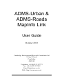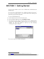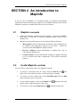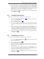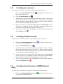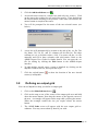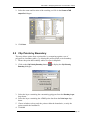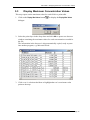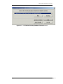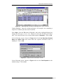
1
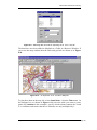
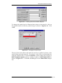
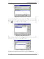
ADMS-Urban & ADMS-Roads MapInfo Link User Guide CERC ADMS-Urban & ADMS-Roads MapInfo Link User Guide October 2013 Cambridge Environmental Research Consultants Ltd 3 King’s Parade Cambridge CB2 1SJ Telephone: +44 (0)1223 357773 Fax: +44 (0)1223 357492 Email: [email protected] Web: http://www.cerc.co.uk Page i CONTENTS SECTION 1 GETTING STARTED................................................................................................................ 1 SECTION 2 AN INTRODUCTION TO MAPINFO ........................................................................................ 2 2.1 2.2 2.3 MAPINFO CONCEPTS................................................................................................................................. 2 USEFUL MAPINFO CONTROLS ..................................................................................................................... 2 DISPLAYING A MAP IMAGE IN MAPINFO ........................................................................................................ 3 SECTION 3 3.1 3.2 3.3 3.4 3.5 3.6 3.7 3.8 3.9 OVERVIEW .............................................................................................................................................. 6 CREATING POINT SOURCES ......................................................................................................................... 7 CREATING ROAD SOURCES .......................................................................................................................... 8 CREATING LINE SOURCES............................................................................................................................ 8 CREATING AREA SOURCES .......................................................................................................................... 9 CREATING VOLUME SOURCES ...................................................................................................................... 9 CREATING AIRCRAFT SOURCES (ADMS-AIRPORT ONLY)................................................................................... 9 DEFINING AN OUTPUT GRID ...................................................................................................................... 10 ADDING SPECIFIED POINTS ....................................................................................................................... 11 SECTION 4 4.1 4.2 4.3 DISPLAYING MAXIMUM CONCENTRATION VALUES ........................................................... 18 IMPORTING ADMS OUTPUT FILES ............................................................................................................ 18 CLIP POINTS BY BOUNDARY ...................................................................................................................... 19 DISPLAY MAXIMUM CONCENTRATION VALUES ............................................................................................ 20 SECTION 6 6.1 6.2 6.3 6.4 DISPLAYING ADMS RESULTS IN MAPINFO .......................................................................... 12 PRODUCING CONTOUR PLOTS FROM ADMS RESULTS .................................................................................... 12 CREATING A LEGEND FOR YOUR CONTOUR PLOT............................................................................................ 14 FURTHER HINTS ON CONTOUR PLOTS .......................................................................................................... 16 SECTION 5 5.1 5.2 5.3 SETTING UP AN ADMS RUN USING MAPINFO ...................................................................... 6 EMISSIONS INVENTORY ..................................................................................................... 21 STEP F – TRANSFERRING DATA FROM THE ADMS EMISSIONS INVENTORY TO MAPINFO ...................................... 24 STEP G – IMPORTING RAW SOURCE AND EMISSIONS DATA INTO MAPINFO....................................................... 26 STEP H – CREATING A GRID SOURCE IN MAPINFO AND EXPORTING IT TO AN ADMS EMISSIONS INVENTORY ............ 31 STEP I – EXPORTING SELECTED POINT, ROAD, AREA, VOLUME, LINE AND GRID SOURCE CELLS ................................. 37 Page ii SECTION 1 – Getting Started SECTION 1 Getting Started In this document ADMS is used to refer to ADMS-Urban, ADMS-Roads and ADMS-Airport. You will need the ADMS MapInfo Link, ADMS and MapInfo Professional1. If you have not already done so, you should install them following the instructions provided with each product. To use the ADMS MapInfo link: (a) Launch MapInfo Professional from the Start menu. (b) From the MapInfo Tools menu choose Run MapBasic Program. (c) The dialogue box shown below will appear. Browse for the ADMS MapInfo extension file ADMS_MI.MBX, which will have been created when you installed the link. By default it will be in the directory <install_path>\Support\MapInfo. You are now ready to use ADMS with MapInfo. 1 Check cerc.co.uk for the full list of supported MapInfo Professional versions. MapInfo Link User Guide Page 1 SECTION 2 An introduction to MapInfo SECTION 2 An introduction to MapInfo If you are new to MapInfo, we recommend that you complete the MapInfo tutorial and read the introductory chapters in the MapInfo manual. Some useful MapInfo concepts are summarised below to get you started. 2.1 MapInfo concepts All data in MapInfo, whether textual or graphic, is organized in tables. Each table is a collection of files that constitute either a map file or a database file. MapInfo presents table data on screen in three different formats 2.2 Map windows present information arranged as maps, allowing you to visualize the geographic patterns of your data. Tables are viewed in individual layers in a Map window. Browser windows present information as tabular lists, just as conventional databases do. Graph windows present information arranged as graphs, allowing you to visualize and make comparisons of the purely numerical patterns. Useful MapInfo controls You may like to experiment with a few MapInfo controls. To zoom to a particular area of a map, click the Zoom In tool either click on a particular point, or click and drag a rectangle. To return to see the whole map, select View Entire Layer from the Map menu, and then choose All Layers. To pan a Map window, click on the Grabber tool drag to show a different portion of the map. To zoom out, click on the Zoom Out button MapInfo Link User Guide and and then click and and click on the map. Page 2 SECTION 2 An introduction to MapInfo 2.3 Displaying a map image in MapInfo It is often useful to check the positions of your ADMS sources against a map image, such as an Ordnance Survey map tile. Before you can do this, you must register the image so that it can be shown in a Map window. The advice below has been adapted from the MapInfo manual. Please refer to your MapInfo manual for more details. 1. Select Open... from the File menu. 2. Change the file type to Raster Image. Select your map file and press Open. 3. Press the Register button in the resulting dialogue. The Image Registration screen will appear: 4. Press the Projection... button, and choose an appropriate projection. For instance, in the UK you will probably select ‘British National Grid’ from the ‘British Coordinate Systems’ as shown below. Press OK when you have made a selection. MapInfo Link User Guide Page 3 SECTION 2 An introduction to MapInfo 5. Now you must provide co-ordinates for at least four control points on the map so that MapInfo can determine the position, scale and rotation of the image. A control point is added as follows. Find a point on the image whose coordinates you know, such as a prominent landmark or perhaps a corner of the image. Click on the point and the dialogue box shown below will appear. Enter the co-ordinates of the point in the Map X and Map Y boxes then click OK. MapInfo Link User Guide Page 4 SECTION 2 An introduction to MapInfo The control point co-ordinates are listed in the Image Registration dialogue and can be edited if they are incorrect. Click OK when you have finished. The map is then displayed in a map window: 6. Save the registered map image by selecting Save Workspace... from the File menu, and selecting the map layer. This will save your map with the extension .wor. You only have to register a raster image once. Each subsequent time you open the file, it can be opened like any other MapInfo workspace. Choose Open... from the File menu and select the .wor file created in step 6 above. MapInfo Link User Guide Page 5 SECTION 3 Setting up an ADMS run using MapInfo SECTION 3 Setting up an ADMS run using MapInfo 3.1 Overview Once your map image is registered, you are ready to position sources on the map and set up an ADMS run. You use the ADMS MapInfo extension by choosing options from the ADMS menu or by clicking buttons on the toolbar. The toolbar is shown in Figure 3.1, and the buttons are described in Table 3.1. Figure 3.1 – The ADMS toolbar Table 3.1 – Brief description of toolbar buttons in the MapInfo extension for ADMS. Butto n Button Name Action Show ADMS Makes the ADMS model interface active Show Aircraft Sources Toggles the display of aircraft sources in the current ADMS .upl file in a Map window (only available with ADMS-Airport) Show Point Sources Toggles the display of point sources in the current ADMS .upl file in a Map window Show Road Sources Toggles the display of road sources in the current ADMS .upl file in a Map window Show Line Sources Toggles the display of line sources in the current ADMS .upl file in a Map window Show Area Sources Toggles the display of area sources in the current ADMS .upl file in a Map window Show Volume Sources Toggles the display of volume sources in the current ADMS .upl file in a Map window Show Grid Sources Displays the grid sources in the current ADMS .upl file in a Map window (not available with ADMS-Roads) MapInfo Link User Guide Page 6 SECTION 3 Setting up an ADMS run using MapInfo Butto n 3.2 Button Name Action Show Receptor Points Toggles the display of receptors in the current ADMS .upl file in a Map window Plot Pollution Contours Creates a contour plot of concentrations based on ADMS output in the Map window Refresh Updates the display Add Aircraft Source Adds a new ADMS-Airport aircraft source where you click (only available with ADMS-Airport). Release the mouse button to end the aircraft source. Add Point Source Adds a new ADMS point source where you click Add Road Source Adds a new road source where you click (double-click to end the road source) Add Line Source Adds a new line source where you click (double-click to end the line source) Add Area Source Adds a new ADMS area source where you click (doubleclick to end the area source) Add Volume Source Adds a new ADMS volume source where you click (double-click to end the volume source) Add Receptor Point Locates a new receptor point for generating output concentrations Define Grid Area Defines an output grid over the rectangle drawn Import ADMS File Imports an ADMS output file into MapInfo Clip Points By Boundary Clips a point layer according to the boundaries in a polygon layer Display Max Values Displays the maximum concentration values in a layer Creating point sources Follow the steps below to create a point source from within MapInfo. 1. Click on the Show Point Sources button you have not already done so. 2. Click the Add Point Source tool. 3. Click on the map window at the position you want to put your point source. MapInfo Link User Guide to display point sources, if Page 7 SECTION 3 Setting up an ADMS run using MapInfo 4. A new point source is created and displayed in the ADMS Source screen. The source co-ordinates will have been filled in automatically, but you will need to enter the other parameters for the source. To add another point source, return to MapInfo by clicking on the MapInfo window title bar, and click on a second position on the map. 5. To see the new point source in MapInfo, save the .upl file and then click on the Refresh button . 3.3 Creating road sources Road sources can be created in a similar way to point sources. 1. Click on the Show Road Sources button you have not already done so. 2. Click the Add Road Source tool. 3. Click on the map at the starting point of your road. Then, draw the road on the map, clicking once for each vertex. Double-click at the final vertex. 4. A new road source is created and displayed in the ADMS Source screen. The source co-ordinates will have been filled in automatically, but you will need to enter the other parameters for the source. For instance, refer to the ADMS manual for advice about road widths and canyon heights 5. To see the new source in MapInfo, save the .upl file and then click on the Refresh button . 3.4 to display road sources, if Creating line sources Line sources can be created in a very similar way to road sources. 1. Click on the Show Line Sources button have not already done so. 2. Click the Add Line Source tool. 3. Click on the map at the starting point of your line source. Then, draw the source on the map, clicking once for each vertex. Double-click at the final vertex. 4. A new line source is created and displayed in the ADMS Source screen. The source co-ordinates will have been filled in automatically, but you will need to enter the other parameters for the source. 5. To see the new source in MapInfo, save the .upl file and then click on the Refresh button MapInfo Link User Guide to display line sources, if you Page 8 SECTION 3 Setting up an ADMS run using MapInfo 3.5 Creating area sources Area sources can also be created in a similar way to point sources. 1. Click on the Show Area Sources button have not already done so. 2. Click the Add Area Source tool 3. An area source can have between three and fifty vertices. Click on the map at the position of one of the vertices. Then, moving around the source clockwise or anticlockwise, click at the position of the remaining vertices, double-clicking at the final vertex. 4. A new area source is created and displayed in the ADMS Source screen. The source co-ordinates will have been filled in automatically, but you will need to enter the other parameters for the source. 5. To see the new area source in MapInfo, save the .upl file and then click on the Refresh button . 3.6 to display area sources, if you . Creating volume sources Volume sources can be created in a very similar way to area sources. 1. Click on the Show Volume Sources button if you have not already done so. 2. Click the Add Volume Source tool 3. A volume source can have between three and fifty vertices. Click on the map at the position of one of the vertices. Then, moving around the source clockwise or anticlockwise, click at the position of the remaining vertices, double-clicking at the final vertex. 4. A new volume source is created and displayed in the ADMS Source screen. The source co-ordinates will have been filled in automatically, but you will need to enter the other parameters for the source. 5. To see the new volume source in MapInfo, save the .upl file and then click on the Refresh button . to display volume sources, . 3.7 Creating aircraft sources (ADMS-Airport only) Aircraft sources can also be created in a similar way to point sources. 1. Click on the Show Aircraft Sources button if you have not already done so. MapInfo Link User Guide to display aircraft sources, Page 9 SECTION 3 Setting up an ADMS run using MapInfo 2. Click the Add Aircraft Source tool 3. An aircraft source must be a simple line with only two vertices. Click on the map at the position for one end of the source. Then, hold down the mouse button and drag to the position of the other end. Release the mouse button to complete the source. 4. You will be prompted for the name of the new aircraft source (see below). 5. A new line will automatically be written to the end of the .air file. The Src_Name, X0, Y0, X1, and Y1 columns will be filled in. The other columns are set to default values (-999). You must edit the .air file manually and fill in these columns with valid entries. Refer to the ADMS-Airport User Guide for further details. You can open the .air file for editing by clicking the Edit button in the ADMS-Airport interface. 6. To add another aircraft source, return to MapInfo by clicking on the MapInfo window title bar, and repeat the steps. 7. Click the refresh button source(s) in MapInfo. 3.8 . to show the location of the new aircraft Defining an output grid You can use MapInfo to help you define an output grid. 1. Click on the Define Grid Area button 2. Click on the map at one of the corner of the output grid area and hold down the mouse button. Now drag the mouse to the opposite corner of the area. A rectangle will appear on the map while you drag the mouse. When the rectangle reaches the size you require release the mouse button. 3. The ADMS Grids screen will appear with the new output grid coordinates. You may correct them by hand if you wish. MapInfo Link User Guide . Page 10 SECTION 3 Setting up an ADMS run using MapInfo 3.9 Adding specified points Follow the steps below to define receptors (also known as “specified points”) using MapInfo. 1. to view the location of existing Click the Show Receptor Points button receptors, if you have not already done so. 2. Click the Add Receptor Point button 3. Click on the map at the position for the new receptor point. 4. The ADMS Grids screen appears, showing your new specified point with the coordinates of the point at which you clicked. You should provide a name for the point. 5. Save the .upl file and then click on the Refresh button new receptor in MapInfo. MapInfo Link User Guide to view the Page 11 SECTION 4 Displaying ADMS results in MapInfo SECTION 4 Displaying ADMS results in MapInfo 4.1 Producing contour plots from ADMS results Once you have completed the definition of a problem in an .upl file and run the model, you can create contour plots. Please note that you must have used gridded output to create a contour plot. On the Grids screen the Select output option must be either Gridded or Both. Follow the steps below to produce a contour plot. 1. Press the Plot Pollution Contours button 2. The ADMS Contour Plotter screen will appear. Select the data file and dataset you wish to plot, and press Plot. MapInfo Link User Guide . Page 12 SECTION 4 Displaying ADMS results in MapInfo 3. 4. The screen below will appear, allowing you to specify a file name and the cell size for the calculation. Click OK when you have done this. MapInfo stores contour plots in .tab files, like all tables. It is good practice to store your .tab files in a directory with your input files and other data. Click Browse... and choose a suitable location. You can use the cell size to control how much detail is shown in your contour plot. MapInfo calculates a value for each cell in the grid and plots the contours accordingly. After spending a few moments interpolating the data, MapInfo will display a contour plot of your results. An example contour plot is shown below. MapInfo Link User Guide Page 13 SECTION 4 Displaying ADMS results in MapInfo 4.2 Creating a legend for your contour plot You may want to create legends for your contour plots. The advice below has been adapted from the MapInfo manual. Please consult the online help or your MapInfo manual for further details. 1. Select Create Legend from the MapInfo Map menu. The Create Legend wizard will appear as shown below. 2. If necessary, use the Add and Remove buttons to make sure that the Legend Frames group contains only the layers for which you want to create a legend. 3. Click Next. Step 2 of the wizard appears as shown below. 4. Provide a title for the legend and click Next. Step 3 of the wizard appears as shown below. MapInfo Link User Guide Page 14 SECTION 4 Displaying ADMS results in MapInfo 5. Click Finish. The legend will be displayed in MapInfo. You may wish to choose Tile Windows from the Window menu to view the legend and the contour plot together, as shown below MapInfo Link User Guide Page 15 SECTION 4 Displaying ADMS results in MapInfo 4.3 Further hints on contour plots As you become more experienced with MapInfo contour plots you may find the following hints useful. You may also like to consult the MapInfo user manuals and online documentation for more information on the commands involved. To temporarily hide a contour plot layer 1. Click on the MapInfo Layer Control button 2. Find the layer you wish to hide in the resulting dialogue. Click to remove the tick for the mouse under the Visible column that layer. To remove a contour plot from a map window 1. Click on the MapInfo Layer Control button 2. Find the layer you wish to hide in the resulting dialogue. Click Remove at the bottom of the dialogue box. To generate a translucent plot or change the colours used MapInfo gives you great control over the display of your contour plots. The steps below are provided simply as an example. Consult the MapInfo documentation for more ideas about the display of your plots. 1. Select Modify Thematic Map from the Map menu. The Modify Thematic Map dialogue will appear. MapInfo Link User Guide Page 16 SECTION 4 Displaying ADMS results in MapInfo 2. Click the Styles button. The screen shown below will appear. You may like to use the Translucency slider so that your background map shows through the contours. The colours used in the plot are controlled by the inflection method and the number of inflection points. You can change the number of colours by changing the Number of inflections in the dialogue. You can change the colour for a particular value by double-clicking the colour sample in the list under the Percentage caption, and selecting a new colour in the resulting dialogue. The example below uses translucency and custom colours. MapInfo Link User Guide Page 17 SECTION 5 Displaying Maximum Concentration Values SECTION 5 Displaying Maximum Concentration Values The ADMS Link provides the facility to calculate the maximum concentration values in an ADMS output file outside, or inside, a site boundary. Typically you would run the following three options in order: import an ADMS output file, following the instructions in Section 5.1; delete unwanted points by following the instructions in Section 5.2; and finally display the maximum concentration values of the remaining points, following the instructions in Section 5.3. 5.1 Importing ADMS Output Files Converts an ADMS output file (.glt, .gst, .plt, .pst) into a point table, which can be viewed in MapInfo. The field values of the points provide the ADMS output values and coordinates for that point. 1. Click on the Import ADMS Output button and locate the file to import from the Select the ADMS output file to import dialogue. MapInfo Link User Guide Page 18 SECTION 5 Displaying Maximum Concentration Values 2. Select the name and location of the resulting .tab file in the Choose a TAB output file dialogue. 3. Click Save. 5.2 Clip Points by Boundary This step deletes points from a point table, by comparing against a set of polygons in a boundary table, e.g. deleting the points outside a site boundary. 1. Ensure the point and boundary tables are open in MapInfo. 2. Click on the Clip Point by Boundary button Boundary dialogue. to display the Clip Points by 3. Select the layer containing the constraining polygons from the Boundary Layer drop-down. 4. Select the layer containing the ADMS point data from the Point Layer dropdown. 5. Choose whether to keep only the points within the boundaries, or only the points outside the boundaries. 4. Click OK MapInfo Link User Guide Page 19 SECTION 5 Displaying Maximum Concentration Values 5.3 Display Maximum Concentration Values This step reports on the maximum value for each field in a point table. 1. Click on the Display Max Values button dialogue. to display the Display Max Values 2. Select the point layer in the drop-down and click OK to open a new browser window containing the maximum values for each concentration recorded in the file. The information in the browser is also automatically copied, ready to paste into another program, e.g. Microsoft Word. 3. Click a row’s selection checkbox to highlight that row’s maximum value point on the map. MapInfo Link User Guide Page 20 SECTION 6 Emissions Inventory SECTION 6 Emissions Inventory Sections 3 and 4 of the ADMS User Guide describe how to set up ADMS model runs when there is a small amount of source data involved by typing the data into boxes in the interface. However, ADMS users will typically have a large volume of data, for instance, if they have compiled their own emissions inventory. In that case, rather than typing data into the interface, the tools described in this section can be used to set up model runs and manipulate the data. These tools use the ADMS Emissions Inventory, which is a Microsoft Access database with a format such that the data can be directly imported into ADMS. The available routes for getting from the raw emissions data to an ADMS .upl file are illustrated in Figure 6.2. The route from raw data to a .upl file followed by most users is via Steps A, B, C and E. The route shown by Step I is for grid (aggregated) sources only, although in Step G point, road or grid sources may be imported and then aggregated. These steps are described in the sections below. The route shown by step J makes use of the Extract Sources From CSV File... utility which provides an alternative method for importing sources, this is described in Section 6.6 of the ADMS User Guide. Another piece of CERC software, EMIT, an EMissions Inventory Toolkit, is a convenient, alternative way to prepare data corresponding to Steps A to B. Further information about EMIT can be found at www.cerc.co.uk/environmental-software/EMIT-tool.html. Selecting an ADMS Emissions Inventory file When ADMS is installed on your PC, the default ADMS Emissions Inventory file is the file inventry.mdb located in the ADMS installation directory, for example, C:\CERC\ADMS-Urb. You will probably want to work with several different inventories (i.e. several different .mdb files), for instance, because each inventory contains a different year’s data or a different management scenario. You can create new inventory files, and change from one to another, via the ADMS interface. In ADMS, select the File, Preferences, Inventory Database… menu. This will open the screen shown in Figure 6.1. MapInfo Link User Guide Page 21 SECTION 6 Emissions Inventory Figure 6.1 – The Emissions Inventory Database Preference screen. MapInfo Link User Guide Page 22 SECTION 6 Emissions Inventory START RAW SOURCE & EMISSIONS DATA G A EXCEL TEMPLATES EXCEL TEMPLATES J B CSV import utility ACCESS EMISSIONS INVENTORY Partial ADMSUrban .UPL file F MapInfo C D ADMS-Urban INTERFACE I E END ADMS-Urban .UPL FILE Figure 6.2 – The steps involved in manipulating raw source and emissions data into an ADMS .upl file. Note that Step H applies to grid sources only. (Grid sources are not available with ADMS-Roads.) MapInfo Link User Guide Page 23 SECTION 6 Emissions Inventory In the remainder of this section, details of steps F, G, H and I for manipulating source and emissions data depicted in Figure 6.2 are given. 6.1 Step F – Transferring data from the ADMS Emissions Inventory to MapInfo Once you have loaded your data into the Access Emissions Inventory, it can be transferred into MapInfo. This can be useful, for example, to check whether sources have been correctly located. To use MapInfo and ADMS in conjunction with the Inventory, start up MapInfo. Select Run MapBasic Program… from the Tools menu of MapInfo and load both the ADMS Urban and Roads extension (adms_mi.mbx) and the ADMS Emissions Inventory extension (ei_mi.mbx) (see Figure 6.3). Figure 6.3 – The Run MapBasic Program dialogue box. MapInfo will then ask you to select an emissions inventory database, as shown in Figure 6.4. Figure 6.4 – The Select emissions inventory database screen. Use the Browse… button to choose a database and click OK. To display the emissions inventory sources in MapInfo, first ensure there is a Map window already open and active (see the earlier sections for information on how to do this), then select the appropriate option for the source type you MapInfo Link User Guide Page 24 SECTION 6 Emissions Inventory wish to display from the Emissions menu. For example, to display the road source data, select Add Emissions Inventory Road Source Layer from the Emissions menu and after a few seconds the data will be added to the Map Window. The title bar of the Map window lists the layers that are displayed in the Map window. If the Map window then appears blank, but the name of a layer is written in the title bar of the Map window, select View Entire Layer… from the Map menu, then select the layer shown in the map window title bar from the drop down menu in the resulting dialogue box, and click on OK. To remove a map layer from the , select the layer to be Map window, press the Layer Control button removed, and then click on OK. An example of a displayed emissions inventory road source layer is shown in Figure 6.5. Figure 6.5 – Emissions inventory road source displayed in a Map Window. To view the data in the emissions inventory in the form of a table, select New Browser Window from the Window menu, or press the New Browser button , then choose the layer you want to be displayed as a table in the browser window. If there is only one layer displayed in the map window, then the table for this layer is automatically displayed in the browser window when the above steps are followed. To change to a different emissions inventory database, choose Change Database from the Emissions menu. You will be notified that MapInfo will automatically refresh the data from a database selected by this method (see Figure 6.6), and you are given the option to Proceed or Cancel. MapInfo Link User Guide Page 25 SECTION 6 Emissions Inventory Figure 6.6 – Query box shown when changing Emissions database. As well as displaying the data from the emissions inventory the MapInfo Emissions Inventory link can be used to create a grid source by aggregating other sources, and then to export the grid source to the ADMS interface for modelling. These options are described in Sections 6.3 and 6.4. The ADMS MapInfo Emissions Inventory link can also be used to select sources, for instance those emitting above a certain threshold or those belonging to a certain plant operator, and export the sources to ADMS. This is described in Section 6.4. 6.2 Step G – Importing Raw Source and Emissions Data into MapInfo It is possible to transfer raw source and emissions data for industrial sources directly into MapInfo (Step G). These data cannot be exported as individual sources to the ADMS Emissions Inventory or the ADMS interface. However, the sources can be aggregated into a grid source in MapInfo, as described in Section 6.3. This grid source can then be exported to the emissions inventory and hence to the ADMS interface. This example shows how data for four industrial stacks can be imported to MapInfo. If the point source data are held in an Excel file, you should save these data as a .txt, .xls or .xlsx file in order to import it into MapInfo. To save the data as an .xlsx file, select all cells containing data as shown in Figure 6.7. In Excel select File, Save As and save the data as an Excel workbook. This .xls or .xlsx file can now be read into MapInfo as a table. Road or grid source data are likely to be available as an ArcView .shp or MapInfo .mif file in which case the data can be loaded directly into MapInfo. MapInfo Link User Guide Page 26 SECTION 6 Emissions Inventory Figure 6.7 – Selecting data in Excel for exporting as an .xls or .xlsx file. Launch MapInfo. Open an existing workspace, for example, one containing a map tile on which to plot the source locations. Select Open... from the File menu of MapInfo, and in the resulting dialogue box change the file type to .xls or .xlsx. Browse to select the file that you wish to add. Leave the preferred view on the default option of Automatic. Click on OK. In the following screen, shown in Figure 6.8, check Use Row Above Selected Range for Column Titles and ensure that the required worksheet name is displayed. Click on OK. Figure 6.8 – MapInfo Excel Information screen In the following screen, shown in Figure 6.9, leave the Field Properties on the default setting. Click on OK. MapInfo Link User Guide Page 27 SECTION 6 Emissions Inventory Figure 6.9 – Selecting data in Excel for exporting as an .xls or .xlsx file. The data have now been added to MapInfo as a Table in a Browser Window. If you resize the map window then the table and grid tile are shown as in Figure 6.10. Figure 6.10 – An imported .xls or .xlsx file in MapInfo. To plot these data on the map tile, select Create Points… from the Table menu. In the dialogue box, as shown in Figure 6.11, select the table you want to create points for (Locations in this example), specify which column contains the X and Y co-ordinates and ensure that the co-ordinates are only multiplied by 1. MapInfo Link User Guide Page 28 SECTION 6 Emissions Inventory Figure 6.11 – Creating points from a table in MapInfo. To change the symbol used to illustrate these points on the map tile, click on the symbol button and edit the symbol design, as shown in Figure 6.12. Click on OK. Figure 6.12 – Changing the symbol style. The projection of the data in this table also needs to be defined so that it is the same as that used in the map tile. For instance, in the UK you will probably be using the National Grid, so click the Projection… button, change the category to British Coordinate Systems, and the category member to British National Grid, as shown in Figure 6.13. Click OK, then OK again in the Create Points dialogue box. MapInfo Link User Guide Page 29 SECTION 6 Emissions Inventory Figure 6.13 – Projection selection in MapInfo. Make the Map Window active by clicking on the title bar of the map window (the title bar should now show blue rather than grey). Bring up the Layer Control dialogue box as shown in Figure 6.14 either by using the button on the toolbar , or from the Map menu, and click Add. Figure 6.14 – Layer Control dialogue box. In the resulting dialogue box shown in Figure 6.15 select the layer to be added (Locations in this example), then click Add, then OK. Figure 6.15 – Adding a layer in MapInfo. The data are now added to the chosen view as a layer as in Figure 6.16. MapInfo Link User Guide Page 30 SECTION 6 Emissions Inventory Figure 6.16 – An imported .xls or .xlsx file added to a Map window as a Layer. 6.3 Step H – Creating a grid source in MapInfo and exporting it to an ADMS Emissions Inventory Grid sources are not available in ADMS-Roads. ADMS-Roads users should skip this section. How to create a grid source in MapInfo and export it to an Emissions Inventory The MapInfo Emissions Inventory extension contains a useful tool for creating a grid source of total emissions from explicit sources that you have in an existing emissions inventory. This grid source can then be exported to an emissions inventory database. Step 1 In MapInfo, ensure that the ADMS Emissions Inventory link is open, and select the emissions inventory database containing the source emissions data that you want to aggregate into a grid source. Step 2 Display the sources you wish to aggregate into a grid source by selecting the appropriate layers from the Emissions menu. An example is shown in Figure 6.17, where a point source, a road source and an area source are displayed. MapInfo Link User Guide Page 31 SECTION 6 Emissions Inventory Figure 6.17 – A point, area and road source in MapInfo. Step 3 Move the cursor over your data and make a note of the coordinates and extent of the grid source required to cover all your source data. In the case shown above, it turns out that the southwest corner of the grid source should be (272000,196000) and the grid should extend 3km east-west and 3km north-south. In ADMS the extent of the grid source must be less than 60km from east to west and 60km from north to south. Step 4 Select Aggregate As Grid Source... from the Emissions menu. Step 5 Select the source layer that you wish to aggregate from the Aggregate emissions dialogue box, shown in Figure 6.18, and press Next >>. Only one layer may be aggregated at a time. Figure 6.18 – Aggregate emissions dialogue box. Step 6 You will now be prompted to select an existing grid table into which the source emissions will be aggregated (proceed to Step 8). At this stage, you can also use New... to create a new grid table (proceed to Step 7). MapInfo Link User Guide Page 32 SECTION 6 Emissions Inventory Figure 6.19 – Creating a new table. Step 7 The Create grid dialogue box is shown in Figure 6.19. Give the new grid table a sensible name, and choose a filename and directory for the resulting .tab file using the Browse... button. Make sure the correct values are present for the coordinates of the southwest corner of the grid, the grid spacing and the number of cells required in the north and west directions. Press OK. Figure 6.20 – Aggregate Emissions dialogue box. Step 8 The Aggregate Emissions dialogue box is shown in Figure 6.20. Select the units for the emissions you wish to aggregate, and the pollutant column(s). If the pollutant names contain a unit suffix (this will be shown in the pollutant column box) then enter it in the appropriate box. Otherwise leave it blank. Ensure that a unique identification field has been identified for both the grid table and the source table. If you have sources which have the same name, for MapInfo Link User Guide Page 33 SECTION 6 Emissions Inventory example multiple sections of the same road, then you may have to add a column in the source table which contains a unique ID – this is required for aggregation Step 9 Clicking on Next >> results in a new message. If the source contains zero or blank values for NOX emissions but nonzero NO2 values then the aggregation will assume that all NOx is emitted as NO2 and the dialogue box shown in Figure 6.21 will appear; click OK. Figure 6.21 – Message about treatment of NOx emissions. If the source contains NOX emissions but no NO2 emissions you will be asked to specify the percentage of NOX that is emitted as NO2. The format of the dialogue box that appears depends on the type of source that is being aggregated to the grid. Figure 6.22 shows the format of the dialogue box for road sources. The format is the same for industrial sources except that the initial value shown for the percentage of NO2 is 5%. Specify the percentage of the NOX that is NO2, or alternatively use the default value provided. Then click OK. Figure 6.22 – Specifying percentage NO x as NO2. See ADMS manual Appendix B for further information on the assumptions ADMS uses when modelling NOX and NO2. Step 10 Select Depth Column dialogue box is shown in Figure 6.23. This will appear if you selected g/m³/s emissions units on the Aggregate Emissions dialogue box. The grid aggregation requires the vertical depths of the sources in metres. Choose the column that contains this data, and click Next >>. MapInfo Link User Guide Page 34 SECTION 6 Emissions Inventory Figure 6.23 – Select Depth Column dialogue box. Step 11 MapInfo will then create the grid source, if necessary, and add the aggregated emissions from the source table you have selected. You will then be asked if you wish to display the new grid source in the current map window. Answer Yes to display the new grid source. Step 12 Repeat the steps from Step 4 to Step 10 for each source layer that you wish to aggregate into the grid source. Step 13 The grid source you have created is now ready to export to the emissions inventory, as described below. Exporting a grid source If you have created a grid source as described in Step H, Section 6.3, or displayed a grid source from an existing emissions inventory as described in Step F, Section 6.1, click Emissions, Export Grid Source to Emissions Inventory to export all the cells of the grid source to an Emissions Inventory. You will be reminded that you should have no grid sources in the inventory database to which you are about to export. Step 14 Select Export Grid Source To Emissions Inventory. The dialogue in Figure 6.24 will appear. Figure 6.24 – Selection of destination database for exported grid Step 15 Select the destination database to which you wish to export the grid source. The default option is the database you are already connected to. Press Next >>. MapInfo Link User Guide Page 35 SECTION 6 Emissions Inventory Figure 6.25 – Selection of grid table to be exported Step 16 In the dialogue shown in Figure 6.25, select the grid source table that you wish to export and press Next >>. Figure 6.26 – Selection of emissions fields to be exported Step 17 In the dialogue shown in Figure 6.26, select the emissions fields for the grid source and press Next >>. If NOx and NO2 emissions are present, it is important that both are selected for export. Note that in the example shown, NO2 emissions have been created during aggregation, with emission levels calculated from the NOx emissions. MapInfo Link User Guide Page 36 SECTION 6 Emissions Inventory Figure 6.27 – Matching emissions fields to be exported with pollutants Step 18 The next screen, as shown in Figure 6.27, prompts the user to ensure that the pollutant names have been correctly deduced from the table headings in MapInfo. The available list of pollutants is based on the list of pollutants defined in the Pollutants Palette in the ADMS interface. If you wish to use a non-standard pollutant, you must explicitly define it in the ADMS interface Pollutant Palette before attempting to export the emissions from MapInfo. When you are satisfied that the correct ADMS pollutant is chosen from the dropdown list for each emission heading, press Next >>. Step 19 Finally, choose the grid source depth that you require, and press Finish to complete the export process. Your grid source will be exported to the emissions inventory. Data for any grid source cells that already exist in the emissions inventory will not be overwritten. A message warns the user if grid source cells already exist in the emissions inventory. 6.4 Step I – Exporting selected point, road, area, volume, line and grid source cells MapInfo can be used to export selected emissions inventory sources, for instance those emitting above a certain threshold or those from a certain plant operator or lying within a certain area, to ADMS for modelling. Before exporting data from MapInfo to ADMS users must make sure that both programs are using the same emissions inventory. In the ADMS interface select File, Preferences, Inventory Database…, and browse to locate the correct database. In MapInfo clicking Emissions, Change database will show the emissions inventory being used currently. Display the emissions inventory source data as explained in Section 6.1. Use the Select Feature Tool in MapInfo to select the sources to be transferred from the emissions inventory to the ADMS Interface. MapInfo Link User Guide Page 37 SECTION 6 Emissions Inventory Only sources in the top layer will be selected. To select and export sources from other layers, first you must use the layer control button to move the required layer to the top position. In MapInfo click Emissions and Export Selected Sources to ADMS. The screen shown in Figure 6.28 will be displayed. Follow the instructions outlined under Step C to select the pollutants to import. Click Next> when you have made your selection. Figure 6.28 – The Import from Emissions Inventory (1: Pollutants) window. The screen shown in Figure 6.29 is then displayed. The sources that you have selected in MapInfo are shown in the Sources to import box on the left of the screen. Sources listed in this box will be imported into the ADMS interface; those shown in the box on the right hand side will not. If you decide not to import some of your sources that you have selected in MapInfo, click on Remove> to remove them from the Sources to import box. Alternatively, if you want to import sources from the emissions inventory that you have not already selected in MapInfo, these can be added to the Sources to import box by clicking on the <Add button. Click on Finish when you have made your selection. MapInfo Link User Guide Page 38 SECTION 6 Emissions Inventory Figure 6.29 – The Import from Emissions Inventory (2:Sources) window. MapInfo Link User Guide Page 39