Download User guide - Standalone version 2-11

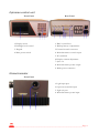
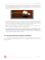
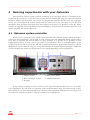
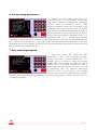
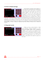
The Cairn Research
Optoscan Monochromator
User Guide 2.01
Standalone Optoscan
June 2001
______________________________________________________________Important information
I. Important - Please read before installation
As with all our equipment, we have tried to impose as few constraints as practicable on the
flexibility and performance of the Optoscan Monochromator. For maximum reliability we would
recommend using the equipment within certain guidelines, but with care the Optoscan can be driven
somewhat harder than this. If in any doubt, then please feel free to contact our technical support
department (e-mail [email protected]).
The following points should be considered when using the Optoscan:
1. Xenon arc lamps are pressurised and a potential hazard. If using the Optoscan with our light
source than please refer to the relevant section of the manual when changing lamps. If using a third
party product then please refer to the manufacturer's documentation.
2. Use suitable protective eyewear when focussing the light. The short wavelengths generated by
the monochromator are potentially hazardous, so care should be taken to avoid direct exposure to
the beam.
3.
The diffraction grating is galvanometer driven and can change between wavelengths very rapidly
(less than a millisecond for most practical purposes). This level of performance is attainable in
prolonged repeat sequences provided that either the steps are very small, such as in scan mode, or
if there are sufficient periods of inactivity within a cycle. If the grating is overdriven then both the
galvanometer and the drive electronics will cut out transiently. These measures should not be
regarded as a full protection against damage, and if the instrument does start to behave erratically it
should be switched off and allowed to cool down before re-use. Please refer to the control
interface section of this manual (section 4.3) for suggested protocols.
4. The slit changers are the most vulnerable part of the instrument to mechanical damage. When
operating the galvanometer-controlled slits, it is important to consider not only the points in note 3
above, but also the physical implications of rapidly opening and shutting a pair of sprung blades. If
operating fast or for long periods it is advisable to keep the degree of movement relatively low.
Particular care should be taken if driving the galvanometer slits from an external source because an
inappropriate applied voltage could destroy the blades by over opening or closing the slits. We
recommend a maximum opening of 3mm.
5. If either or both slits are micrometer controlled then care should be taken not to over open the
blades. It is however acceptable to unwind the micrometer head to below zero in order to provide
an overlap in the blades for shuttering.
6. The output light guide connector should be fitted very carefully so as not to push the guide into the
exit slit mechanism.
7. The lamps we supply for use with our light source have a built in filter to cut off the short
wavelengths which generate ozone, so there is little or no ozone emitted from the light source.
_________________________________________________________________________Page
i
II. Package Contents
Light Source (includes lamphouse and power supply)
q
Opto- 75W
q
Classic 75W
q
Opto- 150W
Monochromator style
Input slit:
q
Automated
q
Manual
q
Fixed
Exit slit:
q
Automated
q
Manual
Control box style
q
Standalone imaging box
q
Single height system rack
q
Double height system rack
q
DAC card with Optoscan power supply
q
Optoscan power supply
Additional Control Modules
q
Input signal amplifier module
q
Photomultiplier signal amplifier module
q
Photomultiplier power supply module
q
Signal ratio module
q
Signal output module
q
Signal gain / offset module
q
Metering module
q
Signal combiner module
_________________________________________________________________________Page ii
________________________________________________________________Package Contents
Coupling Hardware
q
Diaphragm coupling with focussing assembly
q
Liquid light guide
q
Direct epifluorescence coupling [for .............................. Microscope]
q
Collimated epifluorescence coupling [for .............................. Microscope]
Emission Hardware
q
Adjustable square diaphragm and holder
q
Single emission coupling box (with appropriate dichroic mirror fitted)
q
Dual emission coupling box (with appropriate dichroic mirrors fitted)
q
Two position filter holder (with appropriate filter fitted)
q
Photomultiplier
q
CCD camera & power supply
q
Monitor
Cabling
q
Mains leads
q
Light source power lead
q
Monochromator controller power and signal leads
q
Serial and parallel PC control leads for monochromator.
q
68-way DAC card connector
_________________________________________________________________________Page iii
III. Table of Contents
I.
Important - Please read before installation......................................................................................i
II. Package Contents ..........................................................................................................................ii
III. Table of Contents.........................................................................................................................iii
1
Introduction...................................................................................................................................1
2
System Components ......................................................................................................................3
2.1 Illumination system components .......................................................................................3
Lamphouse power supply .............................................................................................3
Lamphouse ...................................................................................................................3
Optoscan control unit...................................................................................................4
Monochromator............................................................................................................4
2.2 Illumination system couplings and mounts ........................................................................5
2.3 Emission detection components ........................................................................................5
3
System Installation.........................................................................................................................6
3.1 Lamp Installation...............................................................................................................6
3.2 Lamp Removal ..................................................................................................................7
3.3 Illumination Set up sequence .............................................................................................8
3.4 Emission detection hardware installation ...........................................................................9
4
Running experiments with your Optoscan...................................................................................11
4.1 Optoscan system controller .............................................................................................11
Software Menu System................................................................................................12
1. Set wavelengths and times.....................................................................................12
2. Show wavelengths and times.................................................................................13
3. Run wavelength program ......................................................................................14
4. Manual wavelength control ...................................................................................15
5. External wavelength control..................................................................................15
6. Set scanning parameters ........................................................................................16
7. Run scanning program ..........................................................................................16
8. Restore default settings .........................................................................................17
9. Diagnostic mode...................................................................................................17
_________________________________________________________________________Page iv
________________________________________________________________________Contents
4.2 External control of the Optoscan ....................................................................................18
4.3 Suggested starting protocols.............................................................................................18
Calcium monitoring with Fura-2 .................................................................................18
Finding the optimum wavelengths for Fura-2 .............................................................18
5
Upgrading your monochromator..................................................................................................21
6
Technical Support........................................................................................................................23
_________________________________________________________________________Page
v
_________________________________________________________________________Page vi
______________________________________________________________________Introduction
1
Introduction
The Cairn monochromator system comprises of four main components; namely a light source, a
power supply for the light source, the monochromator box itself, and a programmable system control
box. If you have the rack-mounting version of the control system it will also contain support for our
photometry modules. In addition, components for connecting the monochromator output to a
fluorescence microscope via an epifluorescence port will usually be supplied.
A key design requirement for our monochromator was to ensure compatibility with other Cairn
products. It has been possible to achieve this without any performance compromises as the design of
our other equipment - in particular our fluorescence photometry modules - anticipated the
introduction of such an instrument. As with all our equipment there is considerable versatility in its
configuration and mode of use, allowing it to be optimised for a specific application. We concentrate in
this guide on getting started with the system. This includes initial set-up of the Optoscan, and basic
operation and control of the monochromator using the terminal provided on the system control box.
For information on advanced control options please refer to the Optoscan technical manual.
If you are using third-party software to control the monochromator then please refer to their
software manual for wavelength selection and control. Details on how to connect the Optoscan to
your PC can be found in the installation guide (Sections 2 & 3).
_________________________________________________________________________Page
1
_________________________________________________________________________Page 2
__________________________________________________________________Installation Guide
2
System Components
Before beginning to install a Cairn system it is advisable to have to hand an oscilloscope (any age
or condition is fine provided that it’s not completely dead!), screwdrivers, Allen keys, and safety glasses.
We would also urge our customers to take some time to carefully check the delivery note to make sure
that they can identify all the components. Having checked that all components are present and correct
the next step is to assemble and test the different sections of the system.
2.1 Illumination system components
Lamphouse power supply
Front Panel
Rear Panel
1. Power Switch
3. Timer reset
1. Power connector to lamphouse
2. Lamp on indicator
4. Hours of use display
2. Mains power socket
Lamphouse
Front Panel
1. Output window
Rear Panel
1. Arc lamp power supply connector
2 & 3. Arc horizontal and vertical adjustments
4. Arc focussing adjustment
_________________________________________________________________________Page
3
Optoscan control unit
Front Panel
Rear Panel
1. Display screen
1. BNC control lines
2. Backlight level control
2. Backup battery compartment
3. Keypad
3. External control connector
4. Main power switch
4. Monochromator control output
5. PC serial link
6. Display contrast adjustment
7. Sync out
8. Monochromator power output
9. Mains power connector
Monochromator
Front Panel
1. Light input port
2. Optoscan controller input
3. Light exit port
4. Monochromator power input
_________________________________________________________________________Page 4
__________________________________________________________________Installation Guide
2.2 Illumination system couplings and mounts
Lamphouse to monochromator coupling tube with diaphragm
Monochromator light guide mount
Liquid light guide
Microscope light guide mount
Microscope coupling
(Nikon coupling shown)
2.3 Emission detection components
For imaging applications this will consist of a third party CCD camera that will fit onto the
microscope C-mount. See suppliers' documentation for installation and configuration.
_________________________________________________________________________Page
5
3
System Installation
3.1 Lamp Installation
As delivery companies are inclined to treat packaged equipment with less respect than perhaps
they should, we have found it prudent to remove lamps from the lamphouses after testing. This
ensures you receive both a lamp and lamphouse that are functional on arrival.
After removing from the packaging, first check the components for any obvious signs of
damage. The first stage in the installation is to fit the supplied lamp into the lamphouse.
Ensure the power supply is disconnected before continuing.
1. There are four hexagonal retaining screws on the top cover of the lamphouse. These need to be
removed, followed by the cover to gain access to the lamp fittings.
2.
The upper lamp fitting will be clipped to one side for shipping; this should be released, and fixed
to the upper end of the lamp, taking care not to touch the silica envelope surrounding the
electrodes. The lamp should be orientated so the nodule is facing forward and perpendicular to the
side arm.
Safety glasses should be worn when handling the arc lamps.
If you inadvertently touch the envelope it is important to clean the lamp with the alcohol wipe
provided as grease residues from your skin will burn on to the lamp when in use and reduce its
operating efficiency.
1. Arc lamp
2. Lower fitting thumbscrew
3. Upper fitting arm
3. Holding the lamp by the upper fitting, drop into place in the lamphouse with the lamp nodule
facing forwards. Fix the lamp in place by tightening the lower thumbscrew.
_________________________________________________________________________Page 6
__________________________________________________________________Installation Guide
4. Replace the top cover.
N.B. It is not possible to connect the lamp in the incorrect orientation, or fit the incorrect lamp, as
the anode and cathode fittings are different.
3.2 Lamp Removal
Ensure the lamp is fully cooled before removing.
To change the lamp after it has reached the end of its useful life, remove the top cover then
release the thumbscrew at the lower lamp fitting. The lamp can then be lifted out of the housing using
the upper mount. Free the lamp from the upper fitting, then fit a new lamp as described above in
section 3.1. The lamphouse enclosure reaches extremely high temperatures when in use and could
cause severe burns, please exercise caution when exchanging lamps.
_________________________________________________________________________Page
7
3.3 Illumination Set up sequence
After removing from the packaging, the monochromator and light source should be located on a
firm level surface, and then set up following the steps below.
1. Install the lamp into lamphouse and connect one end of the four-pin lamphouse power lead to the
lamphouse and the other to the power supply unit.
2. Attach the monochromator coupling to the light source, with the focussing assembly in place and
the diaphragm fully open.
3. Connect the lamp power supply to the mains and turn on the lamp. Leave the unit to warm up for
about ten minutes and then adjust the lamp focus and position to give a sharp image of the lamp
arc at the centre of the focussing assembly. This ensures the maximum amount of light is focussed
onto the input slits of the monochromator.
û Unfocussed, uncentred
û Unfocussed, centred
ü Focussed, centred
4. Turn off the lamp and remove the focussing assembly from the light source coupling before
attaching the monochromator unit in its place.
5. Site the Optoscan control box near the monochromator unit and connect the four-pin power
connector and 25-way D'connector between them.
6. Connect the light guide to the monochromator output coupling, positioning the end of the light
guide flush with the end of the coupling, as shown below. Then slide the combination into the exit
port of the monochromator, fixing in place when the coupling is fully inserted.
7. Power up both the light source and the optoscan and select a visible wavelength using the 'set
wavelengths and times' function with real time adjustment on (see section 4.1).
_________________________________________________________________________Page 8
__________________________________________________________________Installation Guide
8. With the light guide mount detached from the microscope epifluorescence coupling, feed the free
end of the light guide into the light guide mount and tighten in place at the end stop. Replace the
mount, with the light guide fitted, into the microscope coupling tube and fit the assembly into the
epifluorescence port of the microscope.
9. To focus the light beam, remove one of the microscope objectives and position the appropriate
filter cube in the light path. Using a piece of paper at the microscope stage as a target, adjust the
position of the light guide mount until a sharp image of the end of the light guide is seen at the
stage. Centre the image using the offset adjustments on the light guide mount.
10. Replace the microscope objective and check for uniform illumination at the image plane. The
illumination path is now fully aligned and the system ready for use.
11. To ensure optimum performance from your lamp housing it is recommended that after
approximately 1 hour from turn on fine focussing is carried using the detector attached to your
system. Small adjustments of the horizontal, vertical and focussing controls on the lamp should be
made to maximise the signal from the detector. We recommend that this fine calibration be
repeated periodically during the lifetime of the lamp.
3.4 Emission detection hardware installation
The emission detection hardware will most likely have been designed to fit onto the C-mount
port on the side of the microscope. Please refer to the suppliers' documentation for details on
installation and use.
_________________________________________________________________________Page
9
_________________________________________________________________________Page 10
_______________________________________________________________Use of the Optoscan
4
Running experiments with your Optoscan
The Optoscan control system is actually a small PC in its own right, which is controlled via the
keypad on the system box. It can also take its input from a standard PC using the Optoscan terminal
emulator, which is provided with your system. To program the controller via this route, the serial port
on the rear of the Optoscan control system must be connected to any serial port on your PC. The
description here describes data input from the keypad, but the process is identical via the PC. Some
systems are supplied without the built in keypad and display, in which case the emulator will have to be
used to program and run the Optoscan.
4.1 Optoscan system controller
When power is switched on, the display screen presents a list of menu options, which are used to
control the monochromator. The keypad is used to both select the numbered menu options and to
enter data as required. All entered values are range checked, so it should not be possible to enter
inappropriate settings. In some cases it is possible to enter fractions. There is no decimal place on the
keypad, but the up and down arrows will add or subtract fractions in permissible increments. Screen
illumination can be adjusted using the rotary dial beneath the keypad labelled backlight. Additional
control modules may or may not be present in your system depending on the configuration.
1. Display Screen
4. Main power switch
2. Rotary backlight control
5. Additional modules
3. Keypad
In this section we will give you an overview of the Optoscan and describe how to use it to drive
your experiments. We will focus on operation of the monochromator using the built in menu system,
then outline how to drive the monochromator from external equipment. Sample protocols are given at
the end of the section as a guide to using the system for real experiments.
_________________________________________________________________________Page 11
Software Menu System
The monochromator functions in two principal modes namely step and scan. These are referred
to as wavelength programs and scan programs respectively. On power on you are presented with the
main system menu, shown above in the above figure. The first four menu functions control the
wavelength position programs, where the monochromator switches between discrete wavelengths of
defined bandwidth. Function five configures how the Optoscan responds to external control signals,
and the remaining functions control the scan programs, where the system operates as a
spectrophotometer with user selected wavelength ranges. The use of each of these functions is outlined
in this section. More detailed information on the functions is available in the technical manual.
1. Set wavelengths and times
Selecting function 1 from the main menu leads
to this sub-menu, from which up to four
independent sets of eight wavelength positions can
be programmed. Each set of positions is referred to
as a program, and the user can switch between these
programs at any time. Associated with each
wavelength position is a user programmable time,
input slit bandwidth and exit slit bandwidth.
Choosing the appropriate option from this submenu sets each parameter. The programs can be thought of as an eight-position filter wheel where you
can define the centre wavelength and bandwidth of each filter
To set a wavelength position, first select the program and position number. In the display shown
above changes currently apply to program 1, position 1. Selecting options 3 to 6 using the keypad will
now take you into data entry modes, where you can set the wavelength required, the size of the input
slit, the size of the exit slit and the time the grating should stay at that position. Theoretical
considerations for the optimum slit widths are given in the technical manual, but a good starting point
would be to set the bandwidths to around 15nm, which is comparable to a typical interference filter.
The time for the grating to wait at the position will depend on the time signals need to be acquired at
that wavelength (e.g. If sampling two output signals, each at 100Hz, a time of 5ms per position would
be just adequate).
_________________________________________________________________________Page 12
_______________________________________________________________Use of the Optoscan
To assist setting up the wavelength positions there is a real time adjustment option. If this is set
to ON, the grating and slits are set to the positions
shown on the display and the selected wavelength
will be output from the monochromator. This setting
also generates the timing signals required for our
photometry modules, allowing the effect of changing
the individual parameters on system output signals to
be monitored. If this setting is OFF, the slits are fully
closed to prevent any unnecessary illumination of the
sample, and timing signals are not generated.
Each wavelength position to be utilised during
a particular experiment needs to be set for inclusion in the wavelength program. This is done via
option 7, and allows easy inclusion or exclusion of individual positions depending on the nature of the
experiment being carried out. To review the current program settings and see which positions are
included in the program use option 9, which will give you a display similar to that shown above.
2. Show wavelengths and times
Function 2 on the main menu leads to this
sub-menu, where more detailed information about
the program position settings can be obtained. The
facility for the display of the actual slit widths used
for a given position (Option 3) allows users with
manual slit adjustment to set the most appropriate
setting for a given experiment. The same mechanical
slit width will not apply for all positions, as the
relationship between mechanical slit width and
optical bandwidth is somewhat wavelength
dependent. The information here will allow the micrometer to be set to the best compromise.
A facility that is potentially very useful under ALL circumstances is option 4, "Show optical
bandpass profiles", as it allows the actual bandpass characteristics for each position to be displayed.
This is particularly valuable when experimenting with different input and exit slit widths. A very
important guide is that the optical throughput at each position is proportional to the area enclosed by
the bandpass characteristic. In general, for maximum throughput the input and exit slit widths
(defined optically, as we do, rather than mechanically) should be the same. The bandpass characteristic
is then triangular, with the bandwidth, as defined between the 50% points (full width half maximum,
FWHM), being half the total width of the spectrum along its baseline. This topic is well described in
the theoretical part of the technical manual, so for more information, please read that section.
_________________________________________________________________________Page 13
3. Run wavelength program
Selecting function 3 from the main menu
enables you to run any of the four wavelength
programs. The first option selects the wavelength
program, or it allows the program number to be
controlled externally. Before running a program we
need to specify whether the program is to be
repeated for a specified number of cycles or
indefinitely. Each position (if included in the
program) is visited in numerical order, but since each
position can correspond to any wavelength, the
actual wavelengths can be visited in any desired sequence.
To start a wavelength program select option 6. If the system is not set to wait for a trigger pulse
the program will run immediately. Position changes can be set to start on receipt of a trigger-input
pulse (via the run/stop-input pin on the computer connector) and using option 3 from the menu.
The major control feature to be considered in relation to wavelength changing is the control and
display of transition times between wavelength positions. It is important to switch off signal detection
during wavelength transitions, since the grating will be scanning across intermediate wavelengths
during this time. The transition time between positions clearly depends on the angle through which
each galvo needs to move, so it will be different for each transition in the program cycle. However, the
time for any given transition will be essentially constant from one cycle to the next. This has the
advantage that the overall cycle times are entirely regular and predictable, but a key question now arises
as to whether or not the transition time should count as part of the total time spent at each position.
What does this mean in practice? Imagine that the monochromator is programmed to spend
10.0msec at each of three positions, and that the transition times to reach each position are 0.3, 0.5 and
0.6msec respectively. If we include the transition times within the time at each position, then the actual
sampling times are 9.7, 9.5 and 9.4msec respectively, and the total cycle time is 30.0msec. On the other
hand, if the transition times are not included, then the sampling times at each wavelength are all exactly
10.0msec, but the total cycle time is extended by the sum of the transition times, to 31.4msec.
The decision on which is the most appropriate is up to the user, as the software allows either
mode of operation, although our preference is to count the transition time as part of the total time. Be
aware that if the transition time (however specified) exceeds the total time at any position, it will be
impossible for the system to operate correctly. It is the responsibility of the user to avoid such a
situation!
Further control is added with the facility for transition time extension. This allows a minimum
transition time value to be specified, which is the same for all positions. In the above case, we could
specify a minimum transition time of 1.0 msec. Depending on whether or not transition times are
included within the times at each position, this would give either 9.0msec sampling time at each
wavelength and a 30.0msec cycle time, or 10.0msec sampling time at each wavelength and a 33.0msec
cycle time. However, in both cases both the sampling times and the cycle time are now explicitly
specified. Although this would appear to give the best of both worlds, it does have the disadvantage
that one has thrown away a total of 1.6msec of usable data during the cycle. No method is perfect!
The above discussion has presumed that there is some way of determining the actual transition
times, so that an appropriate value for the minimum transition time can be specified, and indeed there
is. After a wavelength program has run, there is a menu option to show the actual transition times for
each position change, to microsecond precision. These times will of course include the specified
transition time.
_________________________________________________________________________Page 14
_______________________________________________________________Use of the Optoscan
4. Manual wavelength control
Operation of this sub-menu should be largely
self-explanatory. The choice of positions is the same
as that specified for menu function 1, i.e. four sets of
eight. All eight positions in each set are always
available, so a position does not have to be included
in a wavelength program in order to select it from
this menu. Within a given program, positions 1-8 are
selectable directly using keys 1-8 respectively, and the
currently selected position is also indicated by a
marker at the appropriate position on the display.
Please note, however, that when this function is selected, the slits will initially be closed. They
can be opened and re-closed from this menu, regardless of which wavelength is selected, by using the
keypad (or PC keyboard) arrow keys. Their condition is indicated on the display.
During manual wavelength control, the microprocessor system generates the necessary switching
waveforms for controlling the photometry modules and/or external equipment. The integration
period is set by the time entered for that position, so the signal values will correspond with those that
would be obtained while running a wavelength program.
5. External wavelength control
Using this function the user can define how
the Optoscan responds to external control signals. In
this mode the system is controlled by external
equipment, rather than from the keypad or from the
internally programmable facilities. It is however
possible to override the external controls, which can
be useful during set-up and testing. The first three
menu options determine whether the program
number, position number and slits respectively can
be controlled externally, the default condition being
yes for all three. The display shows the status of the
external command lines as well as the current program number, position number and slit status.
Even if the program and position numbers are under external control, they can still be changed
by the keypad, since the external inputs are read by the controller only on receipt of the go signal. Any
changes made via the keypad will therefore remain in effect until the next go command is received.
However, the slits control input is active all the time, so it is not possible to open or close them from
the keypad when they are under external control. Further information on driving the monochromator
using external controls can be found in the technical manual.
_________________________________________________________________________Page 15
6. Set scanning parameters
Function 6 on the main menu allows four
wavelength scans to be programmed, in much the
same way as function 1 programs the wavelength
positions. Scans are allowed to run in either
direction, anywhere within the wavelength range
300-800nm. The scans occur as a series of discrete
steps, with the wavelength incrementing through the
range in intervals as low as 1nm. With the shortest
intervals this approximates arbitrarily closely to a
continuous scan, but if desired much broader
wavelength intervals can also be selected, as can a much narrower scan range. An individual scan may
thus contain anywhere between a few and several hundred individual measurements. The scan
adjustment menus allow refining of the way the scans are performed. Information on these functions
can be found in the technical manual.
7. Run scanning program
This menu option has exactly the same
functionality as the "run wavelength program"
function, but there are some differences. For
example, there is no facility to change the program
number while a scan program is running, since that is
unlikely to be of so much practical use. This is
because different scan programs are likely to be used
in conjunction with, say, different microscope
objectives, which are only going to be changed
between, rather than during, data acquisition periods.
However, the control of scanning programs by an external trigger pulse is exactly the same as for the
wavelength programs.
_________________________________________________________________________Page 16
_______________________________________________________________Use of the Optoscan
8. Restore default settings
The parameters entered for menu functions 17 are stored in non-volatile memory for indefinite reuse, but menu function 8 allows these to be replaced
by the default values with which the system was
originally supplied. This function may not be of
much practical use, but the main reason for
providing it is so that it can be run automatically if
system memory is lost for any reason. Memory is
normally preserved by a backup battery, which is
recharged whenever the microprocessor control unit
is powered. A full charge should be sufficient to last for many months, but if the battery does become
discharged, or if the memory is corrupted for some other reason (such as severe electrical interference),
the microprocessor will detect this when the unit is next switched on and it will automatically load the
default settings. However, there is a possibility that a partial memory corruption will not be detected
automatically, so if such a condition is suspected, then menu function 8 can be run to correct the
situation.
9. Diagnostic mode
Finally we come to menu function 9. This
allows third-party software developers to access
some of the program facilities without having to go
through the menu system. A list of functions
provided so far is given in the appendix of the
technical manual. The diagnostic mode also allows
full access to the microprocessor program, although
that is primarily of use only to us. However, for
diagnosis of possible faults, we may ask users to
perform some specific tests while the system is in
this mode.
_________________________________________________________________________Page 17
4.2 External control of the Optoscan
The Optoscan is supplied with terminal emulator software. This has been designed and tested for
PCs running under Windows-98 and Windows-2000. The PC is linked to the Optoscan using a nullmodem (standard serial) cable. When the emulator is first run it must be configured to the port the
Optoscan is connected to. Control is identical to the functions and options on the controller box.
Control of the Optoscan by external equipment is implemented via the 37-way D-connector or
the adjacent BNC connectors on the controller rear panel. Details of the Pin connections and
Optoscan timing sequences are given in the technical manual.
4.3 Suggested starting protocols
The monochromator can be used for a wide range of applications, so it is impossible to give a
comprehensive list of protocols here, so we have given sample protocols from commonly used probes.
We have used the book values for peak excitation wavelengths, but in our experience the peak values
found experimentally by running a wavelength scan on the sample do vary from this.
Calcium monitoring with Fura-2
This is a dual wavelength excitation probe, and we must first set wavelengths and times using
function 1 from the main menu. Fura-2 has listed excitation peaks at 340 and 380nm, and an emission
peak at 510nm. We first need to set the wavelength positions, so select a program number then enter
the details for the two wavelength positions:
Position 1: Centre wavelength = 340nm, Input slit = 15nm, Exit slit = 15nm, Duration = 200ms
Position 2: Centre wavelength = 380nm, Input slit = 15nm, Exit slit = 15nm, Duration = 100ms
Check the two positions are included in the wavelength program and that the remaining six
positions are not (The 'review program settings' option will let you quickly check this). We are now
ready to run the protocol, so return to the main menu and select function 3, 'run a wavelength
program'.
We are going to run the experiment from the Optoscan without external input signals, so set the
program number to that just used to program the wavelength positions. Review the function settings,
checking that the controller is not expecting an external trigger pulse, and is set to repeat the program
continuously. Selecting option 6 from the keypad will run the protocol and you should here the shutter
click open, then soft clicking sounds as the grating position changes.
Finding the optimum wavelengths for Fura-2
This is a potentially valuable use of the monochromator, allowing the wavelengths where the
maximum change of signal occurs to be found. Using the experimentally determined peak wavelengths
will at the very least give larger output signals for a given light input, and could even allow lower dye
concentrations to be loaded (with consequent smaller perturbations in the intracellular environment).
In addition, in ratiometric imaging and photometry, the isosbestic wavelength (the point in the
spectrum where no change in signal occurs as the ion of interest changes) is often used to track
changes in dye concentration. This point can also be identified at the same time as the excitation peaks.
_________________________________________________________________________Page 18
_______________________________________________________________Use of the Optoscan
This protocol demands a wavelength scan, so we will use function 6 from the main menu, 'set
scanning parameters'. Using the keypad set the scan to run from 300 to 420nm with a 2nm bandwidth
at both slits and a 2nm step size. The time at each step should be set according to your sampling rate
or the amplitude of the signals you expect (Longer integration times will obviously give you larger
signals). Once the parameters are set, return to the main menu and select function 7 to run the scan.
Check the controller is set to the program you have just set and also confirm that the number of cycles
is continuous and no trigger signal is expected. Option 6 will run the scan, which will continue until
indefinitely.
To identify the emission peaks for Fura-2 in isolated cells we would first permeabilise the
membrane then run the scan in high calcium conditions to obtain the spectra at maximum ion
concentration. We then change the perfusing solution to low or nominally zero calcium conditions (e.g.
using 10mM EGTA or BAPTA ) and repeat the scan to obtain the spectra at minimum ion concentration.
Comparison of the spectra obtained in each situation will allow identification of the two regions of
maximum signal change and the isosbestic point. For more accurate determination of the emission
peaks, the residual spectrum after quenching the dye should be recorded and subtracted from the
traces obtained.
_________________________________________________________________________Page 19
_________________________________________________________________________Page 20
_______________________________________________________________________Upgrading
5
Upgrading your monochromator
The hardware control software is resident in a pair of read-only memory (ROM) chips within the
system control box. Installation of a software update consists of replacing the existing chips with
updated ones. Although this is a straightforward task, we normally recommend that the microprocessor
control unit be returned either to ourselves or to your local distributor for this to be done. However,
we can provide instructions on how to do this yourself if preferred. Please contact our technical
support department for further information (e-mail [email protected]).
_________________________________________________________________________Page 21
_________________________________________________________________________Page 22
_________________________________________________________________Technical Support
6
Technical Support
e-mail : [email protected]
Web : http://www.cairnweb.com/
Address : Cairn Research Ltd
Unit 3G
Brents Shipyard Industrial Estate
Faversham
Kent
ME13 7DZ
Telephone : +44 (0) 1795 590 140
Fax : +44 (0) 1795 590 150
_________________________________________________________________________Page 23
_________________________________________________________________________Page 24