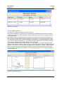
1
SpectraProc User Guide Version: Date: 1.2b 13.10.2008 Status: Author: File: Pages: Valid A. Hueni \UserGuide_V1.2b.doc 53 Classification: Distribution: SpectraProc User Guide Page 2 of 53 History Version Date Author Remark 0.1 03.04.2006 A. Hueni First draft 0.11 06.04.2006 A. Hueni Modified MySQL installation 0.2 16.06.2006 A. Hueni Modified Tutorial for new example set 1.1 20.10.2006 A. Hueni Added description of new SpectraProc Features. Added description of new SpectraProc Query interface. Added new section in the Tutorial about disabling of outliers. Added change history of added features, fixed bugs and known bugs. 16.11.2006 A. Hueni Added another table change statement for the spectrum table (see Upgrading to SpectralDB V1.1) 1.2 17.12.2006 A. Hueni Added description how to change the database connection string for SpectraProc Query 1.2a 15.02.2008 A. Hueni Upgraded the supplied spectral_db schema to V1.1 and therefore adapted the installation instructions in this user guide. Removed the ‘upgrade database’ section. 1.2b A. Hueni 13.10.2008 A. Hueni Updated the application bundle (TCL relevant) \UserGuide_V1.2b.doc Version 1.2b / 13.10.2008 SpectraProc User Guide Page 3 of 53 Table of Contents 1 Introduction ...................................................................................................... 5 2 Installation and Configuration ........................................................................ 6 2.1 Database...................................................................................................................................6 2.1.1 Installing MySQL ................................................................................................................6 2.1.2 Installing MySQL-Administrator and Query Browser ......................................................... 6 2.1.3 Setting up the Spectral Database Schema, Tables and Users ..........................................6 2.1.4 Network Access .................................................................................................................6 2.2 SpectraProc Application............................................................................................................7 2.3 SpectraProc Query Interface ....................................................................................................8 2.3.1 Installing TCL/TK ...............................................................................................................8 2.3.2 Installing Mysqltcl Package ................................................................................................ 8 2.3.3 Plotchart Package ..............................................................................................................8 2.3.4 Installing SpectraProc Query Interface ..............................................................................8 2.3.5 Changing the Database Connection ..................................................................................8 2.3.6 Running SpectraProc Query Interface ...............................................................................8 3 Design of Sampling Experiments ................................................................. 10 3.1 Overview .................................................................................................................................10 3.2 Hierarchical Structure .............................................................................................................10 3.3 Directory Structure and Spectral Files ....................................................................................10 4 Operation ........................................................................................................ 12 4.1 Overview .................................................................................................................................12 4.1.1 Dataflow ........................................................................................................................... 12 4.1.2 File System Interfaces .....................................................................................................12 4.1.3 SpectraProc Operation ....................................................................................................13 4.1.4 Spectral Processing Concept........................................................................................... 13 4.2 SpectraProc ............................................................................................................................ 14 4.2.1 User Interface ..................................................................................................................14 4.2.2 Creating a new Study.......................................................................................................15 4.2.3 Deleting an existing Study ............................................................................................... 16 4.2.4 Study Report ....................................................................................................................16 4.2.5 Selecting Studies .............................................................................................................16 4.2.6 Loading Spectra ...............................................................................................................17 4.2.7 Processing Chain Settings ............................................................................................... 17 4.2.7.1 Waveband Filtering...................................................................................................................17 4.2.7.2 Smoothing.................................................................................................................................18 4.2.7.3 Sensor Synthesizing / Downsampling ......................................................................................20 4.2.7.3.1 4.5.3.1 Ratio Sensors .........................................................................................................20 4.2.7.3.2 Gaussian Sensors ...............................................................................................................20 4.2.7.3.3 Supplied Sensors ...............................................................................................................22 4.2.7.4 Derivative Calculation ..............................................................................................................22 4.2.7.5 Feature Space Transformation ..................................................................................................23 4.2.7.5.1 DI (DGVI) .........................................................................................................................23 4.2.7.5.2 NTBI..................................................................................................................................23 4.2.7.5.3 PCT....................................................................................................................................24 4.2.7.5.4 Creation, Modification and Deletion of Feature Space Definitions ..................................24 4.2.7.5.5 Feature Space Selection.....................................................................................................25 A. Hueni \UserGuide_V1.2b.doc Version 1.2b / 13.10.2008 SpectraProc User Guide Page 4 of 53 4.2.8 File Export ........................................................................................................................ 26 4.2.9 Saving the Contents of the Report Window .....................................................................28 4.2.10 Spectral Mixtures ...........................................................................................................28 4.2.10.1 Endmember Designation.........................................................................................................28 4.2.10.2 Abundance Settings ................................................................................................................29 4.2.11 Library Building ..............................................................................................................29 4.2.12 Analysis.......................................................................................................................... 29 4.2.12.1 Separability .............................................................................................................................29 4.2.12.2 Discriminant Analysis ............................................................................................................30 4.2.12.3 Principal Component Analysis ...............................................................................................32 4.2.12.4 Unmixing ................................................................................................................................32 4.2.13 Adding new Sensors ......................................................................................................33 4.2.14 Linking to a GIS System ................................................................................................ 35 4.2.14.1 Setting up the Spectral DB as a Data Source..........................................................................35 4.2.14.2 Establishing a Database Connection in ArcCatalog ...............................................................35 4.2.14.3 Adding Table Data to a Map...................................................................................................37 4.3 SpectraProc Query Interface ..................................................................................................39 4.3.1 Introduction ...................................................................................................................... 39 4.3.2 Database Connection ......................................................................................................39 4.3.3 User Interface ..................................................................................................................39 4.3.4 Report Windows...............................................................................................................40 4.3.4.1 Campaign Report ......................................................................................................................40 4.3.4.2 Species Report ..........................................................................................................................41 4.3.4.3 Site Report ................................................................................................................................41 4.3.4.4 Spectrum Report .......................................................................................................................42 5 Tutorial ............................................................................................................ 43 5.1 Overview .................................................................................................................................43 5.2 Examine the Folder and File Structure ...................................................................................43 5.3 Creating a new Study and Loading the Spectra .....................................................................43 5.4 Get to Know Your Data ...........................................................................................................43 5.5 Discriminant Analysis in PCT Feature Space .........................................................................47 5.6 Disabling Outliers....................................................................................................................48 6 Change History............................................................................................... 51 6.1 SpectraProc ............................................................................................................................ 51 6.1.1 Added Features ...............................................................................................................51 6.1.2 Fixed Bugs ....................................................................................................................... 51 6.1.3 Known Bugs .....................................................................................................................52 6.2 SpectraProc Database............................................................................................................52 6.2.1 Added Features ...............................................................................................................52 7 References ...................................................................................................... 53 A. Hueni \UserGuide_V1.2b.doc Version 1.2b / 13.10.2008 SpectraProc User Guide Page 5 of 53 1 Introduction Field spectroradiometry has become increasingly popular in the last few years. The technology has advantages over conventional techniques, allowing the non-destructive sampling of objects and possibly enabling the user to gain critical information more quickly and cheaply. As a result, many scientists are now actively researching applications of hyperspectral sensing. The operation of the instruments tends to be relatively easy and data are collected quickly. However, the interpretation of these data is not so simple. The main issue when dealing with hyperspectral data is their dimensionality which is the result of sampling a wide spectral range in very narrow bands. This is in itself a problem because the influence of noise on narrow channels is much higher than on traditional broadband channels. Hyperspectral data are more complex than previous multispectral data and different approaches for data handling and information extraction are needed (Landgrebe, 1997, Vane and Goetz, 1988). Hyperspectral data are essentially multivariate data, consisting of hundreds or even thousands of variables. It has been shown that more bands do not automatically imply better results. Although the separability of classes does increase with growing dimensionality, the classification accuracy does not follow this trend endlessly but will decrease at a certain point. This is called the Hughes Phenomenon and is caused by the ever increasing number of samples needed to build sound statistics if the dimensionality grows (Landgrebe, 1997). In practice this means that more samples must be collected to ensure successful statistical analyses. It is necessary, therefore, to collect a large number of spectral data files, each containing a hyperspectral spectrum. The sheer number of files and variables can become overwhelming. Interestingly, very few studies concerned with hyperspectral data have ever mentioned how the data had been organised and stored. A further issue that is rarely addressed is the reusability of the data. Reference data is usually compiled in so called spectral libraries. The majority of the publicly available spectral libraries are distributed as physical files. This has drawbacks such as low flexibility and low query performance (Bojinski et al., 2003). Another drawback of most libraries is their restriction in the number of spectra per class. In many cases, only one reference spectrum is supplied. This reduces any statistical analysis to first order statistics. The use of average values may be useful in some circumstances, however, Landgrebe (1997) noted that the reduction of data to mean values results in a loss of information. Second order statistics contain vital information about the distribution of data in spectral or feature space and should therefore be included in spectral data collections. The time and effort that is spent in collecting spectral data, combined with the characteristically large number of files, makes it clear that spectral data should be well organised. Otherwise valuable data can be lost or loses its value because of missing metadata. Considering the above, it seems logical to employ a database to store spectral data in a suitable form. A further characteristic of hyperspectral data is the data redundancy. It has been shown that neighbouring wavebands have a high degree of correlation (Thenkabail et al., 2004). This redundancy is created by oversampling, i.e. the spectral signal is sampled at small enough steps to describe very narrow features that could be discriminating (Shaw and Manolakis, 2002). The redundancy and general noisiness of the data usually mean that certain pre-processing must be carried out before any useful analysis can be performed. SpectraProc and ‘SpectraProc Query’ bundled with the associated spectral database is a solution for the efficient storage and pre-processing of field spectroradiometer data. The system has been successfully used in studies concerned with New Zealand native vegetation, soil properties and pastures (Kusumo et al., 2008). SpectraProc has also lately been used in a study of rapid avalanche mapping at the Remote Sensing Laboratories, Zurich, Switzerland. For the storage of spectral data and associated metadata, you may wish to consider using the SPECCHIO spectral database. However, SPECCHIO is still lacking the processing features as offered by SpectraProc at this point of time. For more information see www.specchio.ch. A. Hueni \UserGuide_V1.2b.doc Version 1.2b / 13.10.2008 SpectraProc User Guide Page 6 of 53 2 Installation and Configuration 2.1 Database 2.1.1 Installing MySQL SpectraProc runs on versions 4 and 5 of MySQL database. SpectraProc Query only runs on version 5. □ Download the installation wizard ZIP file for Windows from www.mysql.com: mysql5.0.26-win32.zip □ Install the above ZIP file by running it □ Use standard configuration □ In the configuration section select: o Install as windows service o Root password: ‘root’ (or any other password, but make sure you can remember it) 2.1.2 Installing MySQL-Administrator and Query Browser □ □ Download the windows install MSI file from www.mysql.com mysql-gui-tools-5.0-r4win32.msi Install both applications by running the above MSI file 2.1.3 Setting up the Spectral Database Schema, Tables and Users □ □ □ □ Run MySQL Administrator Go to Restore and load the supplied Spectral_DB_XXXXXXX.SQL file. This will create all tables and populate them. Go to the User Administration tab and create a new user. User name and password are both ‘SpectraProc’. Edit the spectral_db schema privileges by adding SELECT, INSERT, UPDATE AND DELETE to the assigned privileges. Assign Resources: max_questions: 0, max_updates: 0, max_connections: 0 (This allows unlimited access. If you want to limit the access select positive values) The new user should have access rights for localhost by default. If not so: add ‘localhost’ to the list of hosts from which the user SpectraProc can connect (click on the icon under User Accounts to do this). 2.1.4 Network Access The SpectraProc application can access the database over the network if the following configurations are performed: □ The IP addresses of all machines from which the user ‘SpectraProc’ can connect are added to the ‘SpectraProc’ privileges. Alternatively a range of IP addresses can be configured using a netmask (see MySQL online documentation for details) or a value of ‘%’ will allow access from any possible machine. □ The port of the MySQL server (3306 by default) is not blocked by Microsoft Windows A. Hueni \UserGuide_V1.2b.doc Version 1.2b / 13.10.2008 SpectraProc User Guide Page 7 of 53 2.2 SpectraProc Application Copy the SpectraProc directory supplied on the installation CD to C:\Program Files\. Open the directory after copying it and open spectra_config.txt. Edit the configuration file as described below. □ Server: if the database is running on a machine different to the machine this copy of SpectraProc is installed on change ‘localhost’ to the IP address of the database server. If the database is access over the network also see 2.1.4. □ Database: if the database has been given a different name during the restore operation change the name of the database. □ Default filter settings: these are the waveband filter ranges that are used as default values in the waveband filter setup (see 4.2.7.1). More filter ranges can be added to the configuration file by adding a new line starting with ‘filter_br’ for each range. □ Output drive and directory: specify the output drive and the output directory. All file output is written to this directory. This must be a valid (i.e. existing) pathname. # Configuration settings for spectraProc # database settings server localhost user SpectraProc password SpectraProc database spectral_db # default filter_br filter_br filter_br filter settings 1350-1440 1790-1980 2360-2500 # specification of file output drive and directory output_drive C: output_dir \Data\MPhil Remote Sensing\SpectraProc_output Hint: access to SpectraProc is made easier by placing a shortcut to the executable on the desktop. A. Hueni \UserGuide_V1.2b.doc Version 1.2b / 13.10.2008 SpectraProc User Guide Page 8 of 53 2.3 SpectraProc Query Interface The SpectraProc Query Interface is written in TCL/TK. Access to the database is provided by a package called mysqltcl. TCL/TK and the package must be installed on the same machine as the SpectraProc Query Interface. SpectraProc Query only runs on MySQL version 5 and SpectraProc DB V1.1. 2.3.1 Installing TCL/TK TCL/TK is open source software and can be downloaded for free on the web on http://www.activestate.com/Products/ActiveTcl/. Choose C:\TCL as installation directory. 2.3.2 Installing Mysqltcl Package Mysqltcl is a package that handles the communication between a TCL client and a MySQL database. The package can be downloaded on http://www.xdobry.de/mysqltcl/#downloads (select the Windows binary version (ZIP). The ZIP file contains a folder called mysqltcl-3.02, which has been included This folder needs to be copied into the TCL library. If TCL was installed on the C: drive (C:\TCL) then the library folder is: C:\Tcl\lib. 2.3.3 Plotchart Package The Plotchart package is usually part of the general TCL/TK distribution: the package is contained in /tcl/lib/tcl8.5/tklib0.4/ or similar. In some distributions, it might be missing. In the later case, copy the plotchart directory contained in the SpectraProc distribution into /tcl/lib/. 2.3.4 Installing SpectraProc Query Interface The source files of SpectraProc Query are supplied in a folder. The folder can be copied wherever seems convenient, e.g. in C:\Program Files. 2.3.5 Changing the Database Connection By default the SpectraProc Query connects to the local host. If the SpectraProc database is installed on a different machine the connection string must be edited manually. Open the file spectra_proc_query.tcl in some editor. Then replace the string localhost with the name or IP address of the database server. #-------------------------------------------------# Database Connection #-------------------------------------------------set db_handle [mysqlconnect -host localhost -db spectral_db -user SpectraProc -password SpectraProc] 2.3.6 Running SpectraProc Query Interface The main source file is called spectra_proc_query.tcl. Double clicking this file will invoke the TCL interpreter and start the application. Tip: create a shortcut to spectra_proc_query.tcl on your desktop for easy access. A. Hueni \UserGuide_V1.2b.doc Version 1.2b / 13.10.2008 SpectraProc User Guide A. Hueni Page 9 of 53 \UserGuide_V1.2b.doc Version 1.2b / 13.10.2008 SpectraProc User Guide Page 10 of 53 3 Design of Sampling Experiments 3.1 Overview The data collected during sampling campaigns must be organised in a structured way in order to allow the automated import into the spectral database. Section 3.2 explains the background of the structure used and section 3.3 gives a practical example of a directory and file structure that should be adopted for data collection. Preferably sampling experiments should be designed to reflect the structure used by SpectraProc. Alternatively, existing data can be arranged to meet the requirements. 3.2 Hierarchical Structure A hierarchical data structure that reflects the real world and the setup of sampling campaigns for vegetation is used. This structure is derived from the following conditions: 1. Reflectances of several different species are captured 2. In order to describe the in-species variation, several specimens of a species are sampled 3. The variability of the specimens is described by several measurements per specimen The spatial extent where a specimen is sampled is termed a sample site, thus a species contains a number of sample sites. The sites are numbered in the order of sampling. At each site, several readings are taken to capture the variation exhibited by the specimen in question. A site therefore contains a number of spectra. This leads to a hierarchical directory structure (Figure 1). Figure 1: Hierarchical directory structure Although the term species is used it essentially represents the different classes found in a study. These classes can either be assigned due to already existing classification systems for e.g. plants or minerals. In other cases a hypothesis might exist that a group of objects can be separated into classes. If so the setup of the experiment should mirror this hypothesis. If no such assumption exists all objects can be put into the same class (i.e. species) and the identification of classes could then be carried out by e.g. cluster analysis. 3.3 Directory Structure and Spectral Files The hierarchical structure is used for the directory structure that holds the spectral files. Ideally, this directory structure is setup when designing the experiment. Figure 2 shows an example of a directory structure. The main directory ‘Vegetation_example’ holds all species directories of the study. This main directory is the folder that needs to be specified when creating a study in the database (see 4.2.2). The names given to the species directories are stored in the database and are included in file output if ‘Folder name’ is specified as desired name type (see 4.2.8 for more information on file export). A. Hueni \UserGuide_V1.2b.doc Version 1.2b / 13.10.2008 SpectraProc User Guide Page 11 of 53 The species directories contain the site directories. These can be named freely and the sites will be automatically numbered when read into the database. Thus, naming a site ‘1’ or ‘s1’ is perfectly acceptable. The site directories contain all spectral files collected at this site. They are auto-numbered by the ASD capturing software. Figure 2: Example of a directory structures holding spectral files A. Hueni \UserGuide_V1.2b.doc Version 1.2b / 13.10.2008 SpectraProc User Guide Page 12 of 53 4 Operation 4.1 Overview 4.1.1 Dataflow A typical dataflow is illustrated in Figure 3. An ASD FieldspecPro spectroradiometer is used to capture the radiance of field objects. A GPS connected to the field laptop records the spatial position of the field object. Reflectance and metadata are automatically saved on the field laptop in a binary file for every reading taken. These binary files are transferred to a laboratory computer where they are read by SpectraProc and stored in the relevant tables in the spectral database. GPS Spatial data Radiance Field object Reflectance ASD Spectroradiometer Reflectance & metadata Binary file Field laptop Lab computer Spectral database Figure 3: Dataflow and involved hardware 4.1.2 File System Interfaces SpectraProc provides input and output interfaces to the file system (see Figure 4). Input file formats are: ASD binary file as produced by the ASD FieldSpecPro Spectroradiometer, ENVI Z-Profiles that are signatures extracted from hyperspectral imagery in ENVI and sensor specifications in a proprietary, tabulator separated format. ASD files can be imported into the database as part of a study or loaded into memory for classification against a study dataset. ENVI Z-Profiles can be loaded for classification only. Sensor specification files are a way of defining new sensors in the database. Output can be written in three data formats: (1) CSV (Comma Separated Values) for import into rd various 3 party applications like spreadsheets or statistic packages, (2) ENVI Spectral Library for import into ENVI and subsequent use for e.g. signature matching and (3) ARFF which is a special format used by WEKA. WEKA is a collection of machine learning algorithms for data mining tasks (University of Waikato, 2005). ASD Binary File SpectraProc Output Interface Input Interface ENVI ZProfile File CSV File Sensor Specifications ENVI Spectral Library File ARFF File Spectral DB Figure 4: File System Interfaces A. Hueni \UserGuide_V1.2b.doc Version 1.2b / 13.10.2008 SpectraProc User Guide Page 13 of 53 4.1.3 SpectraProc Operation SpectraProc is study based, i.e. spectral data is grouped into studies. Advisably, a new study is created to hold data for every new sampling experiment. The spectral data files of studies must be structured according to the hierarchical structure introduced in 3. This structuring allows the automated loading of spectra into the database. Typically, the operations carried out on a study are: 1. Creation of a new study 2. Loading of spectra 3. Repeated pre-processing and analysis In ongoing studies, new data can be added to the database by simply selecting the loading operation again. Only new spectra will be added to the database in this case. 4.1.4 Spectral Processing Concept The spectral database only stores the raw spectral data. Further processing of the spectra is performed at runtime and the results are held in memory. Once a spectrum is loaded from the database it is put through a cascade of operations as shown in Figure 5. The result of every stage is saved in a separate data structure in memory. This allows easy file export of spectral data at any processing step. Consequently, the structure of this processing chain implicates that a change of processing parameters of any stage will influence the results of the subsequent stages. A complete set of pre-processing parameters thus describes the processing from raw to feature space transformed data. All processing settings are stored in the database when a library is built. Repeated processing of the data with the same settings will always result in the same final data set. Spectral DB Load spectrum Waveband filtering Raw data Smoothing Waveband filtered data Synthesizing Derivative calculation Smoothed data Synthesized data Derived data Feature Space Transformation Data in Feature Space Figure 5: Spectral data processing cascade A. Hueni \UserGuide_V1.2b.doc Version 1.2b / 13.10.2008 SpectraProc User Guide Page 14 of 53 4.2 SpectraProc 4.2.1 User Interface The graphical user interface (GUI) is based on the structure of the processing cascade (see Figure 6). The left side of the main window consists of controls for the selection of the study and the main settings for smoothing filter, synthesizing, derivative calculation, feature space transformation and classifier discriminant function. Processing details are entered in pop up windows which are explained in the relevant sections. The text output panel (report window) in the middle of the main window is used to display processing and error information. The listbox on top of the text output panel is used to display spectra files that are loaded directly into memory. The ‘Indiv. Classify’ button under it classifies the selected, individually loaded spectra against the current library. The library status box on the top right of the screen indicates whether statistical information has been compiled for the current pre-processing settings. Study selection List of directly loaded spectra Classification button for directly loaded spectra Library status field Smoothing filter Smoothing filter detail settings button Sensor Derivative order Derivative calculation method Report window Derivative calculation detail settings button Feature space type Feature space Classifier discriminant function Figure 6: Main window elements A. Hueni \UserGuide_V1.2b.doc Version 1.2b / 13.10.2008 SpectraProc User Guide Page 15 of 53 4.2.2 Creating a new Study To create a new study, select ‘Database‘->‘Create New Study’ (Figure 7). This brings up the new study dialog (Figure 8). Figure 7: Create New Study menu entry Enter a study name of 45 character maximum and not containing special characters that can not be part of any Windows file name like: \ / : * ? < > “ |. The study description is optional and can contain any string up to 200 characters long. The species directory path is a Windows pathname pointing to the directory that contains all species folders of this study. To set the path either type it in manually or select the ‘Browse’ button that brings up a directory tree (Figure 9) and select the appropriate directory. The number of samples per species for library inclusion can be set to any positive number. If a species has less than the specified number of samples it will not be included in the statistics calculations when building libraries. Once a new study is created it will automatically be selected as the current study. Figure 8: New study dialog A. Hueni \UserGuide_V1.2b.doc Version 1.2b / 13.10.2008 SpectraProc User Guide Page 16 of 53 Figure 9: Directory tree dialog 4.2.3 Deleting an existing Study To remove a study and all associated data from the database select this study as the current study, then select ‘Database’->’Delete Current Study’ (Figure 10). Before any data is deleted a warning will be displayed (Figure 11). To delete all data of the current study click OK, to abort the operation click ‘Cancel’. The message window will list the involved operations of the deletion. Figure 10: Delete Current Study menu entry Figure 11: Deletion warning box 4.2.4 Study Report To display name, description, datapath, number of minimum spectra per endmember, number of species, number of spectra and the capturing timeframe of a study select ‘Database’->’Study Report’ (Figure 13). Figure 12: Starting a study report 4.2.5 Selecting Studies To select a study to work with, select the appropriate study from the drop down list in main window (Figure 13). A. Hueni \UserGuide_V1.2b.doc Version 1.2b / 13.10.2008 SpectraProc User Guide Page 17 of 53 Figure 13: Selection of current study 4.2.6 Loading Spectra To load the spectra of a study into the database make sure the correct study is selected. Please refer to 4.2.3 on the process of selecting the current study. Then select ‘Database‘->‘Import Spectra into current Study’ (Figure 14). A popup window will appear indicating the loading progress. Additionally, the loaded species are listed in the message window. Figure 14: Import Spectra menu entry 4.2.7 Processing Chain Settings 4.2.7.1 Waveband Filtering Waveband filtering is the process of removing unwanted regions of the spectrum. All subsequent processing operations will then ignore these regions. A typical example is the removal of water bands. These water band regions are usually found around 1350-1440 nm, 1790-1980 nm and 2360-2500 nm (Figure 15). If contact probes are used the noise can be minimal because the atmosphere is effectively non existent. Filtered Reflectance Curve of Pittosporum eugenioides 1.00E+00 1.00E+00 9.00E-01 9.00E-01 8.00E-01 8.00E-01 7.00E-01 7.00E-01 Reflectance Reflectance Raw Reflectance Curve of Pittosporum eugenioides 6.00E-01 5.00E-01 4.00E-01 3.00E-01 2.00E-01 6.00E-01 5.00E-01 4.00E-01 3.00E-01 2.00E-01 1.00E-01 1.00E-01 0.00E+00 300 0.00E+00 300 500 700 900 1100 1300 1500 1700 1900 2100 2300 2500 500 700 Wavelength [nm] 900 1100 1300 1500 1700 1900 2100 2300 2500 Wavelength [nm] Figure 15: An example of pre and post filtering of water noise bands The waveband filter regions are freely configurable for each study. To modify the current filter settings select ‘Chain Settings‘->‘Waveband Filter Setup’ (Figure 16). A. Hueni \UserGuide_V1.2b.doc Version 1.2b / 13.10.2008 SpectraProc User Guide Page 18 of 53 Figure 16: Waveband Filter Setup menu entry Figure 17: Waveband Filter Setup dialog (no regions defined) The Waveband Filter Setup dialog lists the waveband filter ranges in the listbox on the left side Figure 17). To add a new filter region click ‘New’. In the pop-up window enter the lower and upper wavelengths in nanometres of the region (Figure 18). After clicking on OK in this dialog, the newly created filter range is shown in the Waveband Filter Setup dialog (Figure 19). Figure 18: Filter band definition dialog Figure 19: A new waveband filter range added to the list of filter ranges To modify an existing range, select the range to be modified in the listbox and click ‘Modify’. To delete an existing range, select the range and click ‘Delete’. To add the default ranges as defined in the configuration file click on ‘Add default ranges’ (see 2.2 on how to configure the default filter ranges). 4.2.7.2 Smoothing Smoothing applies a smoothing function to the spectra. The default smoothing filter type is ‘None’ meaning no smoothing is carried out. The smoothing type is selected using the drop down list box in the main window (Figure 20). Two different Savitzky-Golay implementations are offered in this A. Hueni \UserGuide_V1.2b.doc Version 1.2b / 13.10.2008 SpectraProc User Guide Page 19 of 53 list: Moving Window (MW) and Fast-Fourier-Transformation (FFT). The output is exactly the same, however, due to internal overhead the MW method is currently the faster of the two. Figure 20: Smoothing filter type drop down list box The processing details of the smoothing filter are set by clicking on the ‘Edit’ button below the list box. This brings up a dialog where the polynomial order and the filter window size can be changed (Figure 21). The filter size is automatically incremented resp. decremented in steps of two to keep the filter size and uneven number, i.e. the number of points on the left and right of the point to be smoothed are equal. The polynomial order sets the order of the curve that is used in the least squares approximation. Note that the Savitzky-Golay coefficients for quadratic and cubic functions are the same and the same applies to orders 4 and 5 (Savitzky and Golay, 1964). Figure 21: Smoothing Filter Details dialog The result is automatically filtered to remove artefacts that appear at the start and end of every valid waveband segment (Figure 22). The new valid segment sizes are calculated by: λu smoothed = λu − pos _ filter _ size λl smoothed = λl − neg _ filter _ size where λl , λu = lower and upper segment wavelengths Thus every segment looses information of filter_size – 1. Smoothed Reflectance Curve of Pittosporum eugenioides showing smoothing artefacts Smoothed Reflectance Curve of Pittosporum eugenioides after the removal of smoothing artefacts 1 1 0.9 0.9 0.8 0.8 0.7 0.7 0.6 Reflectance Reflectance 0.6 0.5 0.4 0.5 0.4 0.3 0.3 0.2 0.2 0.1 0.1 0 0 500 1000 1500 2000 2500 3000 0 0 Wav elength [nm] 500 1000 1500 2000 2500 Wav elength [nm] Figure 22: A smoothed signature of Pittosporum eugenoides before and after the removal of smoothing artefacts A. Hueni \UserGuide_V1.2b.doc Version 1.2b / 13.10.2008 3000 SpectraProc User Guide Page 20 of 53 Generally, bigger filter sizes remove more noise while higher polynomial orders fit the original data values better. 4.2.7.3 Sensor Synthesizing / Downsampling The sensor synthesizing/downsampling is effectively a data reduction operation. The response of the sensor selected as the current sensor is calculated from ASD data. The synthesizing of other sensor responses using ASD data is useful due to several reasons: 1. Reduction of dimensionality 2. Direct comparison of airborne/spaceborne sensor and ground data 3. Implicit smoothing of the data 4. Prediction and assessment of the usefulness of a certain sensor Two classes of sensors are supported: Ratio and Gaussian. 4.2.7.3.1 4.5.3.1 Ratio Sensors The sensor element function of these sensors is modelled by a number of known coefficients, thus the synthesizing operation is simply a convolution of a defined wavelength region using these coefficients. An example of such ratios is shown for Landsat7 TM band 1 (Figure 23). Ratios for Landsat Band 1 1.2 1 Ratio 0.8 0.6 0.4 0.2 520 510 515 505 495 500 490 480 485 475 465 470 460 450 455 445 435 440 0 Wavelength (nm) Figure 23: Ratios for Landsat7 TM band 1 The convolution is calculated by: uw _ j rj = ∑c i ⋅ ri i =lw _ j uw _ j ∑c i i =lw _ j where r j = the synthesized reflectance value of the j-th synthesized band ci = the coefficient for wavelength i ri = reflectance value of i-th ASD band lw _ j = lower wavelength of the j-th band uw _ j = upper wavelength of the j-th band 4.2.7.3.2 Gaussian Sensors A. Hueni \UserGuide_V1.2b.doc Version 1.2b / 13.10.2008 SpectraProc User Guide Page 21 of 53 The sensor element response function of these sensors is best approximated by a Gaussian function. The sensor elements are technically defined by the middle wavelength and the full width at half the maximum (FWHM) (see Figure 24). Gaussian function for mu=0 and sigma=2 0.2 0.18 0.16 0.14 FWHM 0.12 0.1 0.08 0.06 0.04 0.02 0 -10 -8 -6 -4 -2 0 2 4 6 8 10 Figure 24: Gaussian curve illustrating the FWHM measure The coefficients used for the convolution operation are given by the Gaussian function: ci = f ( wavelength _ band _ i ) = 1 2 ⋅π ⋅σ ⋅e 1 wavelength _ band _ i − wavelenth _ band _ j − 2 σ 2 where wavelength _ band _ i = wavelength of the i-th ASD band wavelength _ band _ j = wavelength of the j-th band of the sensor to be synthesized ci = the i-th coefficient for the convolution operation The band convolution is calculated by µ + range rj = ∑c i i = µ − range ⋅ ri µ + range ∑c i i = µ − range where r j = the synthesized reflectance value of the j-th synthesized band ci = the coefficient determined by the Gaussian function for the wavelength of the i-th ASD band ri = reflectance value of i-th ASD band range = defines the range of values to be used for the band convolution symmetrically to the middle ASD waveband. The middle ASD waveband is the one closest to the average wavelength of the jth synthesized band. The nature of the Gaussian function effectively carries out a smoothing of the data. The range of values used for the convolution is set to 3 times the standard deviation: range = 3 ⋅ σ , i.e. 99.74% of all contributing values are used (Papula, 1994). This range is practically not usable for all bands because some wavelengths may have been filtered previously, segmenting the spectrum. In these situations, the range is symmetrically reduced to avoid filtered regions. A. Hueni \UserGuide_V1.2b.doc Version 1.2b / 13.10.2008 SpectraProc User Guide Page 22 of 53 4.2.7.3.3 Supplied Sensors The sensors currently supplied with the software are: Name Hyperion ASD Opt_Hyperion Type Gaussian Ratio Gaussian Downsampling_by_10 Landsat7 ACS_210 Red_NIR ACS_210 Yellow_NIR Downsampling_by_5 Ratio Ratio Gaussian Gaussian Ratio Description Sensor as flown on EO-1 Effects a 1:1 copy of ASD data, i.e. no data reduction The Hyperion sensor according to the blueprint, i.e. all sensor elements are operating Effects a downsampling by selecting every tenth waveband Sensor as flown on Landsat7 ETM satellite Crop circle sensor simulation with red – NIR illumination Crop circle sensor simulation with yellow – NIR illumination Effects a downsampling by selecting every fifth waveband To change the current sensor select a sensor from the sensor drop down list box (Figure 25). Figure 25: Selection of current sensor It may be advisable to apply the downsampling only to smoothed data in order to avoid aliasing. The combination of smoothing and downsampling is called decimation (Fliege, 1994). 4.2.7.4 Derivative Calculation The derivative order is set to zero by default, i.e. no derivative is calculated. To change the order use the up and down arrows next to the box showing the derivative order (Figure 26). If the order is changed to a non-zero value, the calculation method can be selected. Iterative calculation is based on the gradient of the linear curve segment between two wavebands: ρ ' (bi bi +1 ) = ρ (bi +1 ) − ρ (bi ) λ (bi +1 ) − λ (bi ) where ρ (bi ) = reflectance of band i λ (bi ) = wavelength of band i ρ ' (bi bi +1 ) = first derivative of linear curve segment between reflectances of band i and band i+1 The n-th derivative is thus calculated by applying the above formula n times. The SavGol method uses Savitzky-Golay coefficients to calculate the derivatives. In this case the derivative is actually the derivative of the approximating function at the wavelength of interest. Thus the SavGol method automatically performs a smoothing of the data. This can be useful when dealing with noisy data where a single smoothing operation is not removing enough noise. Both methods loose N data points per valid segment where N is the derivative order. A. Hueni \UserGuide_V1.2b.doc Version 1.2b / 13.10.2008 SpectraProc User Guide Page 23 of 53 Figure 26: Derivative calculation settings: zero derivative (left), first derivative iterative (middle) and first derivative SavGol method (right) For the SavGol method the filter size and polynomial order can be modified by clicking on the ‘Edit’ button. This brings up the Derivative Filter Details dialog (Figure 27). The filter size and order are automatically restricted to meet the following minimal conditions for the calculation of the derivative: polynomial _ order ≥ derivative _ order filter _ size ≥ max( polynomial _ order + 1, derivative _ order + 1) Thus the minimal filter size depends on both the polynomial and the derivative order. A minimal filter size of (derivative_order+1) will result in the removal of n = derivative_order number of points. Figure 27: Savitzky-Golay settings for derivative calculation Note that too big filter sizes remove relatively lot of data because the derivative calculation takes place after the data reduction step (sensor synthesizing/downsampling). E.g. a filter size of 5 applied to data downsampled by factor ten will remove 4 data points, i.e. 40nm, per segment. 4.2.7.5 Feature Space Transformation Three types of feature spaces are implemented: □ Derivative Indices (DI) □ Normalized Two Band Indices (NTBI) □ Principal Component Transformation (PCT) 4.2.7.5.1 DI (DGVI) DGVIs (Derivative Greenness Vegetation Indices) are an example of a DI. These indices are trying to describe the shape of the reflectance curve. The DGVI calculation is based on the equations used by Thenkabail et al. (Thenkabail et al., 2004) and Elvidge and Chen (Elvidge and Chen, 1995): ρ ' (bi −1bi )− ρ ' (bi bi +1 ) Δbi i =m n DGVI = ∑ where ρ’(bi-1bi) = first derivative of reflectance curve between bi-1 and bi m..n = start and end band number of DGVI area bi = centre wavelength of band i i = band number Δbi = step width: bi+1 – bi-1 4.2.7.5.2 NTBI Normalized two band indices are calculated by: A. Hueni \UserGuide_V1.2b.doc Version 1.2b / 13.10.2008 SpectraProc User Guide NTBI = Page 24 of 53 ρ (bx ) − ρ (b y ) ρ (bx ) + ρ (b y ) 4.2.7.5.3 PCT Principal components transformation requires as input the eigenvectors of a given dataset. A principal component analysis (PCA) must be carried out before PCT can be applied to the data. PCA results in eigenvalues and eigenvectors. The eigenvectors are used in the transformation matrix G. If only the first n components are to be used, the transformation matrix is a sub-matrix of G, consisting of the first n column vectors. The dimension of the resulting feature space is therefore n: y = G⋅ x n×1 n×m m×1 where m = original size of data space n = new size of data space, equal to the number of selected components 4.2.7.5.4 Creation, Modification and Deletion of Feature Space Definitions Based on the three basic feature space types new feature spaces can be created. Existing feature spaces can be edited or deleted. For any of these functions navigate to the ‘Chain Settings’>‘Feature Space’ submenu (Figure 28). Figure 28: Feature Space Submenu To create a new feature space select ‘Copy and Edit’ or ‘New’ in the ‘Feature Space’ submenu. ‘New’ opens up an empty dialog for the definition of a new feature space. ‘Copy and Edit’ copies the settings of the currently selected feature space into the dialog. The settings can subsequently be changed before creating the new feature space in the database. To modify an existing feature space select ‘Edit’. All the above three commands invoke the same dialog, shown here on the example of a NTBI feature space consisting of three individual NTBIs (Figure 29). The name of the feature space can be any alphanumeric string of maximal 45 characters, the description can be any alphanumeric string of maximal 250 characters. The bands listbox lists the band combinations used to calculate the indices. E.g. index 1 uses bands 550nm and 468nm. New band combinations are entered by clicking on ‘New’, existing band combinations are modified by clicking modify. Both commands bring up a dialog box to define the two bands (Figure 30). To delete an existing band combination select the combination in the list and click ‘Delete’. The dimension field in the Feature Space dialog is non editable for DIs and NTBIs where it reflects the number of band combinations. For PCT feature spaces, the dimension field specifies how many components are to be used for the transformation. In the given example, the first 10 components will be used (Figure 31). A. Hueni \UserGuide_V1.2b.doc Version 1.2b / 13.10.2008 SpectraProc User Guide Page 25 of 53 Figure 29: Feature Space edit dialog on the example of a NTBI feature space Figure 30: Waveband Definition Dialog Figure 31: PCT Feature Space dialog To delete an existing feature space make sure the currently selected feature space is the one to be deleted. Then select ‘Delete’ from the ‘Feature Space’ submenu. The current feature space is removed from the database. 4.2.7.5.5 Feature Space Selection A. Hueni \UserGuide_V1.2b.doc Version 1.2b / 13.10.2008 SpectraProc User Guide Page 26 of 53 The feature space selection is comprised of two panels: (a) a selection of the feature space type offering DI, NTBI and PCT and (b) a drop down list box that contains all feature spaces of the current type (see Figure 32). Figure 32: Feature space settings 4.2.8 File Export SpectraProc features a powerful file export that facilitates the analysis and visualisation of the data in third party products. All output files are written to the directory The output is controlled by a single dialog (see Figure 33). The file export dialog is displayed by selecting ‘File’->’Export’. Data can be exported at any processing stage: □ Raw □ Filtered (removal of noisy band regions) □ Smoothed □ Synthesized □ Derived □ Feature Space transformed The processing for these stages depends upon the parameters that are defined at that point in time for the processing cascade. If e.g. ‘Synthesized’ is selected, every spectrum is put through the cascade of filtering, smoothing and synthesizing and is then written to the file. I.e. if a certain stage is selected all the preceding stages are automatically performed. The data can be averaged either on site level or on species level. If the site mean is chosen a column containing the site number will be added to the output file. Selecting the ‘All spectra’ option performs no averaging but writes every spectrum to the file. The averaging is the last step of the processing, e.g. if the ‘Synthesized’ and ‘Mean per species’ is selected, then all spectra of each species are processed till the synthesizing stage and then averaged and written to the file. Three file formats are currently supported: □ CSV (Comma Separated Values) □ ENVI spectral library file □ ARFF (WEKA file format) The species that are written to the file can be controlled by selecting on of four options: □ Include all species: all species are written □ Include only library relevant species: only species that have equal or more than the minimum number of spectra are written. The minimum number of spectra is set when defining a new study (see 4.2.2) □ Only endmembers: only species that have been designated as endmembers are written □ Only mixtures: only species that are not designated endmembers are written The name that is used as species name can be one out of five choices: □ Common: common name is defined in database □ Maori: Maori name as defined in database □ Latin: Latin name as defined in database A. Hueni \UserGuide_V1.2b.doc Version 1.2b / 13.10.2008 SpectraProc User Guide □ □ Page 27 of 53 Folder: name of the folder that contains the site directories of the species Auto number: incrementing numbers are assigned to the species according to their order in the database The current version of the software supports only one file level setting: study. I.e. all species of the current study are written to one single file. Four checkboxes allow for the following operations: □ Transpose: the observations are written as columns instead of rows. This option can make the import of data into other programs easier. □ Include filtered bands: this is for visualisation purposes only. The regions that were removed in the waveband filtering stage are written as empty cells, i.e. when plotted the filtered regions will appear as gaps. □ Offset: each species will be set off by a freely choose able percentage of 100% reflectance. This is to be used for visualisation purposes only. □ Interpolate: this option is only available when the ‘Synthesized’ stage is selected as output step. The synthesized data is interpolated to ASD data using straight line segments. This is useful for the assessment of the smoothing effect of the synthesizing operation e.g. by plotting a noise spectrum (smoothed minus interpolated synthesized data). □ Sort species numerically: Sorts the species by interpreting the species names as numbers Species restriction selection Name type selection File level selection Processing stage for file export Data averaging options Transpose observations Include the filtered band regions Offset each species by a given percentage File format selection Sort the species names numerically Interpolate output by linear segments Figure 33: File Export dialog A. Hueni \UserGuide_V1.2b.doc Version 1.2b / 13.10.2008 SpectraProc User Guide Page 28 of 53 4.2.9 Saving the Contents of the Report Window The contents of the report window can be saved to a file by selecting: File -> Save Report Window Content. The file is written to the default output directory and named report_window_output.txt (see Figure 34). Figure 34: Saving the report window content 4.2.10 Spectral Mixtures Spectral mixtures occur when more than one endmember is present in the field of view. If the endmembers are known the mixtures can be unmixed to give estimates of the abundance of each endmember in the mixture. For the process of unmixing refer to 4.2.12.4. The unmixing process needs to have a set of endmembers and a set of mixtures to be unmixed using the endmember information. For this purpose species can be designated as endmembers. If the spectral mixtures are the result of a controlled mixing experiment the abundances of the endmembers are usually know. These known endmember fractions can be entered into the database for each mixture, thus allowing the automatic calculation of the error involved in the estimation by the unmixing procedure. 4.2.10.1 Endmember Designation To display the endmember designation dialog choose ‘Spectral Mixing’->‘Endmember Selection’ (Figure 35). Figure 35: Endmember Selection menu entry Initially, all species will be listed in the ‘Classes’ list while the ‘Endmembers’ list is empty. To designate a species as an endmember select the class by clicking on it, then click on the arrow pointing towards the right to shift this class into the Endmember list. Similarly, to move an endmember back to the Classes list, select the endmember and click the arrow pointing towards the left. A. Hueni \UserGuide_V1.2b.doc Version 1.2b / 13.10.2008 SpectraProc User Guide Page 29 of 53 Figure 36: Endmember Selection dialog 4.2.10.2 Abundance Settings Before invoking the abundance settings the endmembers should be selected as described in 4.2.10.1. To display the abundance settings dialog select Spectral Mixing’->‘Abundance Settings’. All mixtures are listed in the ‘Classes (excl endmembers)’ list box. The abundances of the endmembers are set for each of these mixtures by: 1. Selecting the mixture 2. Select the endmembers that are contained in the mixture one after another from the ‘Available endmembers’ list box and shift them down into the ‘Selected endmembers’ list box. 3. For every selected endmember do: select the endmember by clicking on it, then enter the abundance in the provided box. Click ‘Save’. The total abundance is updated. When defining the abundance of the last endmember, click on ‘Complement’. This automatically assigns the abundance to the last endmember by summing the total abundance to 1. Figure 37: Abundance Settings dialog 4.2.11 Library Building A library is a collection of statistics data built for a certain configuration of the processing chain. The ‘Library status’ field in the main window indicates if a library has been built for the current processing settings. To build a library select ‘Library’->’Build’. 4.2.12 Analysis 4.2.12.1 Separability Before running the separability analysis the library for the current pre-processing settings must be built. See 4.2.11 on how to build libraries. The JM and B distance analyses are carried out in the A. Hueni \UserGuide_V1.2b.doc Version 1.2b / 13.10.2008 SpectraProc User Guide Page 30 of 53 currently selected feature space. I.e. the discriminating power of feature spaces can be assessed by the separability analysis. To run the separability analysis select ‘Statistics’->’Separability Report’. In the displayed JM/B Distance dialog select the name and distance type and press OK (Figure 38). A short message will be displayed in the message window, looking similar to: Separability Analysis Using JM and B distance JM and B output written to file: C:\Data\MPhil Remote Sensing\SpectraProc_output\JM and B output.csv The output filename is shown in this message. Note that only library relevant species are included in this report. Figure 38: JM/B Distance dialog The JM distance is listed in the upper triangular matrix, the B distance in the lower triangular matrix (see Table 1). The JM distance is asymptotic to 2.0. A JM distance of 2.0 indicates a complete separability and a distance of 1.9 a good separability (Richards, 1993). The B distance is not asymptotic and can get infinite (Inf.) due to limits in numerical precision. Table 1: Example of a JM and B output using a 10 dimensional DI feature space Blackfern Blackfern Cabbage_tree - Lemonwood 1.93 Cabbage_tree 3.41 Lemonwood 2.99 1.90 - 1.76 2.11 - 4.2.12.2 Discriminant Analysis Discriminant analysis (DA) uses a discriminant function to assign a class to samples. In the case of the calibration set being subjected to DA the result is an assessment of the separability of the classes. The DA is carried out in the currently selected feature space. The DA result is thus also an assessment of the discriminating power of the feature space. Note that the discriminant function used is the one currently selected in the main window. Before running DA the library for the current pre-processing settings must exist. See 4.2.11 on how to build libraries. To run the DA select ‘Statistics’->’Discriminant Analysis’. A dialog will be displayed to select the names to be used in the output (Figure 39). A. Hueni \UserGuide_V1.2b.doc Version 1.2b / 13.10.2008 SpectraProc User Guide Page 31 of 53 Figure 39: Discriminant Analysis dialog A message stating the file name of the error matrix and the overall accuracy is reported in the message window, similar to the example shown below. Discriminant Analysis --------------------------------------------------Error matrix written to file: C:\Data\MPhil Remote Sensing\SpectraProc_output\Error Matrix.csv --------------------------------------------------Overall Accuracy: 78.46154 --------------------------------------------------- The error matrix written to a file contains the errors of omission and commission, the total accuracy, the producer and user accuracy and the minimum, maximum and mean for both producer and user accuracy. Table 2: Error matrix of DA using a 3 dimensional NTBI feature space Blackfern Blackfern Cabbage_tree Lemonwood Row Total User Accuracy 11.00 0.00 0.00 11.00 100.00 Cabbage_tree 7.00 19.00 6.00 32.00 59.38 Lemonwood 0.00 1.00 21.00 22.00 95.45 Column Total 18.00 20.00 27.00 65.00 Producer Accuracy 61.11 95.00 77.78 Prod. Acc. Min 61.11 Prod. Acc. Max 95.00 Prod. Acc. Mean 77.96 User Acc. Min 59.38 User Acc. Max 100.00 User Acc. Mean 78.46 84.94 To run the DA with an independent data set choose ‘Statistics’->’Discr. Analysis using indep. set’. A dialog is displayed to select the study that contains the independent set (Figure 40). Note that in order to work correctly the folder names of corresponding species in the training and in the independent study must be identical. A. Hueni \UserGuide_V1.2b.doc Version 1.2b / 13.10.2008 SpectraProc User Guide Page 32 of 53 Figure 40: Selection dialog for independent data sets 4.2.12.3 Principal Component Analysis Principal components analysis (PCA) is applied after the derivative calculation step. I.e. the PCA is carried out for the current settings of waveband filtering, sensor synthesizing and derivative calculation. To run PCA select ‘Statistics’->’PCA’. A message stating the output file similar to the one below is displayed in the message window: Principal Component Analysis --------------------------------------------------PCA output written to file: C:\Data\MPhil Remote Sensing\SpectraProc_output\pca_output.csv --------------------------------------------------- The two first components will be plotted as a scatterplot in a graphics window, this plot is also known as scoreplot. The pca_output file contains the eigenvalues, proportions, cumulative proportions (see Table 3 for an example) and the eigenvectors (also know as factor loadings). The eigenvectors can possibly be used to assess the significance of the wavelengths in respect to the each component. The eigenvalues and eigenvectors are stored in the database. Table 3: First ten eigenvalues and proportions of a PCA PC# Eigenvalue Proportion Cumulative 1 2.211 0.944 0.944 2 0.097 0.042 0.986 3 0.019 0.008 0.994 4 0.007 0.003 0.997 5 0.005 0.002 0.999 6 0.001 0.001 0.999 7 0.000 0.000 0.999 8 0.000 0.000 1.000 9 0.000 0.000 1.000 10 0.000 0.000 1.000 4.2.12.4 Unmixing The unmixing procedure implemented is experimental at this stage and works on Landsat7 data only. Before starting the unmixing, make sure that the current sensor is Landsat7, the study has the mixtures and endmembers defined and the abundances are entered for each mixture. The model used is unconstrained (Keshava and Mustard, 2002): −1 ( ) aˆU = S T S A. Hueni ST x \UserGuide_V1.2b.doc Version 1.2b / 13.10.2008 SpectraProc User Guide Page 33 of 53 where: x = spectrum vector to be unmixed (L x 1) S = endmember matrix (L x M) consisting of M endmembers with the columns being the endmember spectra vectors aˆU = the unconstrained least squares solution for the abundances of the endmembers in the spectrum vector x To start the unmixing select ‘Spectral Mixing’->’Unmix’. For each mixture the unmixing results are displayed in the message window; first stating the calculated abundances for each endmember, then the abundances stored in the database and finally the absolute errors for each endmember abundance (see example of such an output below). Spectral Unmixing --------------------------------------------------120V_240P --------------------------------------------------0.69 0V_360P 0.35 360V_0P simulated mixture abundances from database: 0.67 0V_360P 0.33 360V_0P absolute errors: 0.03 0V_360P 0.02 360V_0P 4.2.13 Adding new Sensors New sensors can be added to the database if their properties are known. The sensors details must be entered in a tabulator formatted file as described below. Two classes of sensors are supported: Gaussian and Ratio (see also 4.2.7.3). The header structure is identical for both sensor classes: <Sensor name> <Sensor description> <Column headers> The sensor name should not include any of the following characters: \ / : * ? < > “ |. The column header line is not interpreted by the program and exists only for the convenience of the user preparing the sensor description file. For Gaussian sensors the file body contains one line per sensor band: <Band> TAB <Average Wavelength (nm)> TAB <FWHM (nm)> TAB <Calibrated (Y/X)> For Ratio sensors the file body contains 1 to many lines per band to model the response (see also Figure 23): <Band> TAB <Wavelength(nm)> TAB <Ratio> Examples of Gaussian and Ratio sensor description files are given in tables 4 and 5: A. Hueni \UserGuide_V1.2b.doc Version 1.2b / 13.10.2008 SpectraProc User Guide Page 34 of 53 Table 4: Example of a Gaussian sensor (Hyperion) Hyperion Hyperion Sensor as flown on EO1 Hyperion Band Average Wavelength (nm) 1 355.59 FWHM (nm) 11.3871 Calibrated X 2 3 4 5 6 365.76 375.94 386.11 396.29 406.46 11.3871 11.3871 11.3871 11.3871 11.3871 X X X X X 7 8 9 10 416.64 426.82 436.99 447.17 11.3871 11.3871 11.3871 11.3871 X Y Y Y 11 12 13 14 457.34 467.52 477.69 487.87 11.3871 11.3871 11.3871 11.3784 Y Y Y Y Table 5: Example of a Ratio sensor (Landsat7) Landsat7 Landsat 7 Thematic Mapper Sensor Band Wavelength(nm) 1 435 1 436 1 437 1 438 1 439 1 440 1 441 1 442 1 443 1 444 Ratio 0.016 0.027 0.048 0.094 0.167 0.287 0.459 0.605 0.728 0.769 To import a new sensor select ‘Database’->’Import Sensor’. In the Import Sensor dialog select the sensor response type and the input file by clicking on ‘Browse’. Then click OK and the sensor data will be imported. An according message will be displayed in the message window when the sensor is loaded. Figure 41: Import Sensor dialog A. Hueni \UserGuide_V1.2b.doc Version 1.2b / 13.10.2008 SpectraProc User Guide Page 35 of 53 4.2.14 Linking to a GIS System If a GPS unit is used to record the spatial position of the sampling sites during the sampling process every site in the database contains the latitude, longitude and altitude in WGS84 format. The database tables can be accessed by a GIS system if ODBC connections are supported. The connection is shown here on the example of ArcGIS. 4.2.14.1 Setting up the Spectral DB as a Data Source Note that before the Spectral DB can be configured as a data source the MySQL ODBC driver (available from the MySQL website) must be installed on the system. Start ‘Data Sources (ODBC)’ from the Windows administrative tools. In the New Data Source dialog (Figure 42) select the MySQL ODBC Driver and click on ‘Finish’. Figure 42: New Data Source dialog This brings up the ODBC configuration dialog (Figure 43). Type in a name for the Data Source Name. Set the Server to the address of the database server. Enter the User name and Password (SpectraProc). Select the database schema containing the spectral data from the Database dropdown list. Figure 43: MySQL ODBC Configuration dialog 4.2.14.2 Establishing a Database Connection in ArcCatalog Start ArcCatalog and select ‘Add OLE DB Connection’ (Figure 44). A. Hueni \UserGuide_V1.2b.doc Version 1.2b / 13.10.2008 SpectraProc User Guide Page 36 of 53 Figure 44: Adding an OLE DB Connection in ArcCatalog In the Data Link Properties select ‘Microsoft OLE DB Provider for ODBC Drivers’ (Figure 45) and click ‘Next>>’. Figure 45: Data Link Properties; Provider tab In the Connection tab select the data source from the dropdown list and enter again the username and password (SpectraProc) (Figure 46). Click ‘OK’. Figure 46: Data Link Properties; Connection tab A. Hueni \UserGuide_V1.2b.doc Version 1.2b / 13.10.2008 SpectraProc User Guide Page 37 of 53 The database is now listed in ArcCatalog and the tables are displayed when selecting the database (Figure 47). Figure 47: SpectralDB and tables in ArcCatalog 4.2.14.3 Adding Table Data to a Map To add table data to a map select ‘Add Data’ in ArcMap and choose the SpectralDB under Database Connections (Figure 48). Then select the site table as the data source (Figure 49). The sampling sites can then be displayed on the map by selecting ‘Display XY Data’ and using the longitude and latitude fields of the site table as X and Y coordinates. Figure 48: Selecting the SpectralDB as data source A. Hueni \UserGuide_V1.2b.doc Version 1.2b / 13.10.2008 SpectraProc User Guide Page 38 of 53 Figure 49: Selecting the site table as data source A. Hueni \UserGuide_V1.2b.doc Version 1.2b / 13.10.2008 SpectraProc User Guide Page 39 of 53 4.3 SpectraProc Query Interface 4.3.1 Introduction SpectraProc Query was written as an example of an intuitive, interactive query building interface. It was written in TCL/TK with the goal to get to know the characteristics of that language. It has proven to be extremely powerful for rapid development of graphical user interfaces. A further advantage are the string handling capabilities that are useful for the building of SQL queries. One of the shortcomings of SpectraProc is the limitation in graphic output. Certainly most users would like to see their spectral data visualized. Furthermore, an overview over the different studies (campaigns), species and sites was not available via the SpectraProc application. SpectraProc Query can build reports on four different levels: campaign (study), species, site and spectrum. The report output can be restricted by specifying conditions. 4.3.2 Database Connection The database connection is currently hard coded and SpectraProc Query will consequently only run on the localhost, i.e. the same machine as the database is installed on. This can be changed by editing the file spectra_proc_query.tcl. The localhost string must be replaced with the network name of the database server (this is similar to running SpectraProc over a network). #-------------------------------------------------# Database Connection #-------------------------------------------------set db_handle [mysqlconnect -host localhost -db spectral_db -user SpectraProc -password SpectraProc] 4.3.3 User Interface This section describes the user interface of SpectraProc Query. Please refer to Figure 50 for an example of the GUI. As indicated above, the resulting rows in reports can be restricted by setting conditions. These conditions are situated at the left side of the GUI. The campaign conditions refer to conditions that restrict the campaigns (studies). The campaigns can be restricted by either choosing a specific campaign name in the Campaign Name Selection box or by entering a string in the Campaign Name Wildcard String box. The latter also accepts wildcards: % stands for any string and _ stands for a single character. The species conditions restrict the species by their folder names. A name can be selected in the Species Name Selection box or be entered as a string with wildcards in the Species Name Wildcard String box. A restriction of the campaigns has a direct impact on the names available in the list of species names: only species contained in the resulting campaigns are available in the list. The result set can be temporally restricted by entering dates in the Collection Date From and To Fields. The dates have the format DD MM YYYY. They greyed out fields to the right of the date fields automatically show the resulting dates when one of the date fields is filled. The years are automatically restricted to the maximal or minimal year of all records in the database. Spatial restrictions can be added by specifying a threshold for the altitude in the Minimal/Maximal Altitude Fields. The report level is chosen by clicking on the option buttons in the Report Level Selection. The resulting SQL query is displayed in the Auto-Built SQL Query Text Field. The number of records (rows) that will be selected by the current query is displayed in the Result Set Counter field. Any change in conditions or report level will automatically update the auto-built query and the number of resulting rows. A. Hueni \UserGuide_V1.2b.doc Version 1.2b / 13.10.2008 SpectraProc User Guide Page 40 of 53 Finally, there are two buttons at the bottom right side of the GUI. ‘Exec Query’ will run the current query and display a report in a new window. ‘Reset’ will return all conditions to their starting values and reset the level to ‘Campaign’. Campaign Name Selection Campaign Name Wildcard String Species Name Wildcard String Report Level Selection Auto -built SQL Query Text Field Species Name Selection Campaign Conditions Species Conditions Collection Dates Conditions Spatial Attributes Conditions Collection Date From and To Fields Minimal Altitude Field Maximal Altitude Field Exec Query Button Reset Button Result Set Counter Figure 50: SpectraProc Query GUI 4.3.4 Report Windows The number of report windows is not restricted by the software, although a limit might exist due to memory or operating system restrictions. All reports start with a title that contains the level of the report plus a subtitle indicating the time taken for the report building. This is followed by the main table containing the data. 4.3.4.1 Campaign Report An example of a campaign report is shown in Figure 51. The reported attributes are: campaign name, description and file system path. A. Hueni \UserGuide_V1.2b.doc Version 1.2b / 13.10.2008 SpectraProc User Guide Page 41 of 53 Figure 51: Campaign Report 4.3.4.2 Species Report An example of a species report is shown in Figure 52. The reported attributes are: folder_name, common_name, latin_name. Figure 52: Species Report 4.3.4.3 Site Report An example of a site report is shown in Figure 53. The reported attributes are: capture_date, longitude, latitude and altitude. A. Hueni \UserGuide_V1.2b.doc Version 1.2b / 13.10.2008 SpectraProc User Guide Page 42 of 53 Figure 53: Site Report 4.3.4.4 Spectrum Report An example of a spectrum report is shown in Figure 54. The reported attributes are: reflectances as a spectral plot, disabled flag as checkbox, spectrum number (auto-number by ASD), pathname, ASD comments (as entered in the capturing software on the field laptop). The graphics output is relatively computing intensive. One should be careful not to start a report with too many (several hundred) resulting rows as the report can run for a while (e.g. 45 seconds for 1100 spectra). Note that the spectral resolution of the graphic is reduced (decimated by factor 10) in order to speed up plotting time. I.e. the data points are spaced at 10 nm intervals. This may result in some noise being less accentuated than in the raw data. The ‘disabled’ checkbox offers some interaction with the database. If checked it will set the field ‘disabled’ in the spectrum table to TRUE. Likewise, unchecking sets the field to FALSE. Setting this field has a direct impact on the processing by SpectraProc. Disabled (i.e. disable = TRUE) spectra will not be included in any processing. It is therefore a chance to remove outliers from the data while still retaining all data in the database. An example illustrating this functionality is included in the tutorial (see 5.6). Figure 54: Spectrum Report A. Hueni \UserGuide_V1.2b.doc Version 1.2b / 13.10.2008 SpectraProc User Guide Page 43 of 53 5 Tutorial 5.1 Overview The tutorial is based on an example dataset comprised of three plant species. The folder containing the species folders is called ‘Vegetation_example’. 5.2 Examine the Folder and File Structure Open the folder ‘Vegetation_example’. It contains three species folders: Blackfern, Cabbage tree and Lemonwood. Open each of these species folders and examine the contents of the site directories contained in them. Blackfern has only one sample site while Lemonwood and Cabbage tree have two. Also browse inside the site directories to find the ASD binary files. 5.3 Creating a new Study and Loading the Spectra Create a new study as detailed in 4.2.2. As study name type ‘your-name_example’, e.g. ‘Mikes_example’. The ‘Species directory path’ is in this case the path pointing to the folder named ‘Vegetation_example’. Set the number of samples per species for library inclusion to 10. Once the new study is created it will be automatically selected as the current study (otherwise select it (see 4.2.5)) and import the spectra (see 4.2.6). 5.4 Get to Know Your Data Check the settings of the processing chain: □ Smoothing filter: none □ Current Sensor: Hyperion □ Derivative: 0 Use the ‘Export’ function (see 4.2.8) to export the Hyperion synthesized spectra to a CSV file: □ Processing Stage: Synthesized □ Data Details: All Spectra □ Species Restriction: Include all species □ Names: Folder □ Transpose: Ticked □ Format: csv This will create a file in the SpectraProc output directory. The output file name is shown in the message window. Open this file by double-clicking which should load it directly into Excel. The columns displayed should be similar to the example shown in Figure 55. Column A contains the average wavelengths of the Hyperion bands. The following columns contain the spectral data for each spectrum. The column headers are the species folder names. A. Hueni \UserGuide_V1.2b.doc Version 1.2b / 13.10.2008 SpectraProc User Guide Page 44 of 53 Figure 55: Example of a SpectraProc CSV output Create an X-Y plot. The result should be similar to the one shown in Figure 56. Maybe surprisingly the plot shows not the expected spectra but some noise that reaches values of up to 140. To see the vegetation spectra rescale the Y axis to a maximum of 1.0 (see Figure 57). The noise is caused by atmospheric absorption (Thenkabail et al., 2004). As first step this waterband noise should be removed from the data before any further processing or analysis is carried out. To remove the noise affected regions from the spectra open the waveband filter dialog (see 4.2.7.1) and click on ‘Add default ranges’. This adds three wavelength regions that are known to contain waterband noise. Blackfern 1.60E+02 Blackfern Blackfern 1.40E+02 Blackfern Blackfern 1.20E+02 Blackfern Blackfern Blackfern 1.00E+02 Blackfern Blackfern 8.00E+01 Blackfern Blackfern 6.00E+01 Blackfern Blackfern 4.00E+01 Blackfern Blackfern 2.00E+01 Blackfern Blackfern Cabbage_tree 0.00E+00 0.00E+00 5.00E+02 1.00E+03 1.50E+03 2.00E+03 2.50E+03 3.00E+03 Cabbage_tree Cabbage_tree Figure 56: A plot showing mainly noise A. Hueni \UserGuide_V1.2b.doc Cabbage_tree Version 1.2b / 13.10.2008 SpectraProc User Guide Page 45 of 53 Blackfern 1.00E+00 Blackfern Blackfern 9.00E-01 Blackfern 8.00E-01 Blackfern Blackfern 7.00E-01 Blackfern Blackfern 6.00E-01 Blackfern Blackfern 5.00E-01 Blackfern Blackfern 4.00E-01 Blackfern 3.00E-01 Blackfern Blackfern 2.00E-01 Blackfern Blackfern 1.00E-01 0.00E+00 0.00E+00 Blackfern Cabbage_tree 5.00E+02 1.00E+03 1.50E+03 2.00E+03 2.50E+03 3.00E+03 Cabbage_tree Cabbage_tree Cabbage_tree Figure 57: The same plot as above but rescaled to a reflectance of 1.0 Once the waveband filter is setup, repeat the export function (close the previously written file first in Excel) and load it again into Excel and plot it. The plot will look similar to the one shown in Figure 58. Note that now the noise regions are plotted as straight line segments. For visualization purposes this should be avoided as it suggests that data exists in the filtered regions. Blackfern 1.20E+00 Blackfern Blackfern Blackfern 1.00E+00 Blackfern Blackfern Blackfern 8.00E-01 Blackfern Blackfern Blackfern 6.00E-01 Blackfern Blackfern Blackfern 4.00E-01 Blackfern Blackfern Blackfern 2.00E-01 Blackfern Blackfern Cabbage_tree 0.00E+00 0.00E+00 5.00E+02 1.00E+03 1.50E+03 2.00E+03 2.50E+03 Cabbage_tree Cabbage_tree Cabbage_tree Figure 58: Spectra after setting up the waveband filter regions Cabbage_tree To plot the filtered regions as gaps, select the option ‘Include filtered bands’ in the file export dialog. If the data is plotted again the result will be similar to the one shown in Figure 59. Two other points are noteworthy: (a) some reflectance values are higher than one and (b) one Cabbage tree spectrum seems to be an outlier. The reflectances higher than one could be the effect of changing illumination conditions during the sampling or a result of the BRDF. The outlier problem can currently not be solved automatically. Two options exist: (a) remove the concerned spectrum from the file system and then delete, recreate and reload the study or (b) reA. Hueni \UserGuide_V1.2b.doc Version 1.2b / 13.10.2008 SpectraProc User Guide Page 46 of 53 move the concerned spectrum from the database using SQL commands. Future versions of the software may feature automatic outlier detection and elimination. Blackfern 1.20E+00 Blackfern Blackfern Blackfern 1.00E+00 Blackfern Blackfern Blackfern 8.00E-01 Blackfern Blackfern Blackfern 6.00E-01 Blackfern Blackfern Blackfern 4.00E-01 Blackfern Blackfern Blackfern 2.00E-01 Blackfern Blackfern Cabbage_tree 0.00E+00 0.00E+00 5.00E+02 1.00E+03 1.50E+03 2.00E+03 2.50E+03 3.00E+03 Cabbage_tree Cabbage_tree Cabbage_tree Figure 59: Waveband filtered data export with the 'include filtered bands' option Reflectance (offset for clarity) To generate stacked plots select the option ‘Offset by [%]’ in the file export dialog and set the percentage to 100. Then plot the data again. The spectra of each species are offset by the same amount (see Figure 60). If only the species mean is selected, the resulting plot is similar to the ones shown in diverse journal articles (see Figure 61). Note that when creating graphs in these cases the Y axis scale should not displayed as it makes physically not much sense (reflectances bigger than 1). 350 550 750 950 1150 1350 1550 1750 1950 2150 2350 Wavelength[nm] Figure 60: Stacked plots offset by 100% showing all spectra per species A. Hueni \UserGuide_V1.2b.doc Version 1.2b / 13.10.2008 Page 47 of 53 Reflectance (offset for clarity) SpectraProc User Guide Blackfern Cabbage_tree Lemonwood 250 450 650 850 1050 1250 1450 1650 1850 2050 2250 2450 Wavelength[nm] Figure 61: Stacked plot showing the mean per species 5.5 Discriminant Analysis in PCT Feature Space Discriminant Analysis (DA) is carried out in feature spaces. As an example the data will be transformed by a principal component transformation (PCT). The number of components used in the transformation has a direct impact on the classification accuracy achieved by DA as will be demonstrated hereafter. Select ‘PCT’ as the current feature space type. Note that the ‘Feature Spaces’ dropdown listbox states that there exist no feature spaces of this type (see Figure 62). A PCT is only possible if a Principal Components Analysis has been carried out. Perform PCA (see 4.2.12.3 for details). Figure 62: PCT feature spaces Open the PCA output file in Excel and plot the first 10 eigenvalues against the component number. The result should be similar than the one showed in Figure 63. This graph is called ‘screeplot’. The sharper the drop off in eigenvalues the better are the results that can be expected from the following PCT. Note that once the PCA has been performed the ‘Feature Spaces’ dropdown listbox contains a selection of feature spaces. The numbers at the end of the names are equal to the number of components used in the feature space. E.g. PCT_10 will effect a PCT using the first 10 components of the transformation matrix, i.e. the data will be reduced to 10 variables (dimensions). Select ‘PCT_5’ as feature space. The discriminating power of feature spaces can be assessed by carrying out a discriminant analysis. Before the DA can be executed the library for the current processing chain settings must be built (see 4.2.11 how to build libraries). Then subject the data to DA (see 4.2.12.2 for details). The resulting overall accuracy should be around 90.7%. The DA results are detailed in the DA output file ‘Error_Matrix.csv’ (see Table 6). The columns are the species that were classified. The number of correctly classified spectra is contained in the diagonal elements. The errors of omission are written in the off-diagonal elements. E.g. 6 Blackfern spectra were wrongly classified as Cabbage tree. Close the DA output file, select PCT_10 as feature space and repeat the process of library building and DA and inspect the DA output file once more. The classification accuracy should have risen to 100%. A. Hueni \UserGuide_V1.2b.doc Version 1.2b / 13.10.2008 SpectraProc User Guide Page 48 of 53 Scree Plot 2.5 2 1.5 Eigenvalue 1 0.5 0 0 2 4 6 8 10 Figure 63: Scree plot of the eigenvalues of the first 10 components Table 6: Error Matrix for DA on PCT_5 feature space Blackfern Blackfern Cabbage_tree Lemonwood Row Total User Accuracy 12 0 0 12 1.00E+02 Cabbage_tree 6 20 0 26 7.69E+01 Lemonwood 0 0 27 27 1.00E+02 Column Total 18 20 27 65 6.67E+01 1.00E+02 1.00E+02 Producer Accuracy 9.08E+01 5.6 Disabling Outliers By combining SpectraProc and SpectraProc Query, outliers can be identified and disabled. In the example dataset you might have spotted one cabbage tree spectrum that looks different (low reflection in the NIR) than all others. If PCA is run on this data set, the outlier can also be spotted (see Figure 64). Figure 64: Score Plot showing an outlier A. Hueni \UserGuide_V1.2b.doc Version 1.2b / 13.10.2008 SpectraProc User Guide Page 49 of 53 Now start SpectraProc Query, select the ‘example’ campaign in the Campaign Conditions, select ‘Cabbage Tree’ as Species Condition, select ‘Spectrum’ as report level and click ‘Exec Query’ (see Figure 65). Figure 65: Conditions set to select Cabbage Tree spectra from the 'example' campaign In the spectrum report (see Figure 66) scroll down till you see the wrong looking cabbage tree spectrum (spectrum number 9 of site 1, you can deduce the site number from the pathname).Tick the checkbox in order to disable the spectrum. Now rerun the PCA calculation in SpectraProc and the outlier will vanish from the Score plot (see Figure 67). Figure 66: Spectrum Report showing a wrong looking Cabbage Tree spectrum A. Hueni \UserGuide_V1.2b.doc Version 1.2b / 13.10.2008 SpectraProc User Guide Page 50 of 53 Figure 67: Score Plot after disabling an outlier To assess the impact of an outlier on the building of covariances and thus on the classification result build a library using a PCT feature space of low dimensionality, e.g. 2, and run ‘Discriminant Analysis’. Repeat library building and discriminant analysis after re-enabling the outlier in SpectraProc Query. You should see a significant change in classification accuracy: --------------------------------------------------Principal Component Analysis --------------------------------------------------PCA output written to file: C:\Data\MPhil Remote Sensing\SpectraProc_output\pca_output.csv --------------------------------------------------New library built and reloaded --------------------------------------------------Discriminant Analysis --------------------------------------------------Error matrix written to file: C:\Data\MPhil Remote Sensing\SpectraProc_output\Error Matrix.csv --------------------------------------------------Overall Accuracy: 70.31250 --------------------------------------------------Principal Component Analysis --------------------------------------------------PCA output written to file: C:\Data\MPhil Remote Sensing\SpectraProc_output\pca_output.csv --------------------------------------------------New library built and reloaded --------------------------------------------------Discriminant Analysis --------------------------------------------------Error matrix written to file: C:\Data\MPhil Remote Sensing\SpectraProc_output\Error Matrix.csv --------------------------------------------------Overall Accuracy: 47.69231 --------------------------------------------------- A. Hueni \UserGuide_V1.2b.doc Version 1.2b / 13.10.2008 SpectraProc User Guide Page 51 of 53 6 Change History 6.1 SpectraProc 6.1.1 Added Features SpectraProc Version V1.1 Feature Date Eigenvectors are written into the PCA output file When creating a new study the new study is automatically selected as the active study Study information report PCA Score Plot shown when performing PCA The contents of the report window can be saved to a file by selecting: File -> Save Report Window Content. The file is written to the default output directory and named report_window_output.txt Disabled spectra are not utilized in the calculations (disabling spectra with the SpectraProc Query tool) Depending on the sensor dimensionality, only feature spaces with less or equal number of dimensions are selectable in the GUI. E.g. DGVI’s (dimension 10) cannot be built if Landsat data is synthesized. PCA can now be carried out on multispectral sensors like Landsat and Cropcircle (ACS210) 13.4.2006 24.4.2006 26.4.2006 10.5.2006 20.10.2006 20.10.2006 20.10.2006 20.10.2006 6.1.2 Fixed Bugs SpectraProc Version V1.1 A. Hueni Problem Fix Date Mixtures not deleted when deleting studies. Crash when trying to write PCA output and file is open Feature space list not updated when derivative settings change ARFF file output produces corrupt files PCA crashes when no data is available PCA on Landsat7: crashes st because 1 feature space is PCT_10 (cant build matrix) Include mixtures in the delete study function Check for open files when writing PCA output file Update feature space list when changing derivative calculation 12.4.06 Attributes list fixed 18.4.2006 Check if data exists before starting the eigenanalysis Limit the dimensionality of the feature spaces to smaller or equal the number of bands of the sensor. 24.4.2006 \UserGuide_V1.2b.doc 13.4.2006 18.4.2006 20.10.2006 Version 1.2b / 13.10.2008 SpectraProc User Guide Page 52 of 53 6.1.3 Known Bugs SpectraProc Version V1.1 Problem Work around The application will crash when building a library using a feature space that requires certain wavelengths on sensors with not enough band information. Can occur when e.g. redefining the DGVI’s to have only 5 dimensions and then try to calculate DGVI’s from Landsat data. Just avoid doing this. There is a logic explanation why this cannot be done. Implementing a check to disable such user actions is too time consuming at this point. The application can sometimes just refuse to load. This is some effect of the Symantec Internet security (SpectraProc not being in the list of programs that are allowed to access the database port), probably coupled with hibernating the machine. A reboot of the system helps here. 6.2 SpectraProc Database 6.2.1 Added Features SpectraProc Database Version V1.1 A. Hueni Feature Date Added ‘disabled’ field to spectrum table Removed the ‘not null’ constraint and added a default value of null for the BLOBS in: pca_data, spectrum and statistic 20.10.2006 \UserGuide_V1.2b.doc Version 1.2b / 13.10.2008 SpectraProc User Guide Page 53 of 53 7 References Bojinski, S., Schaepman, M., Schlaepfer, D., Itten, K., 2003. SPECCHIO: a spectrum database for remote sensing applications. Computers & Geosciences 29, 27-38 Elvidge, C. D., Chen, Z., 1995. Comparison of broadband and narrowband red and near-infrared vegetation indices. Remote Sensing of Environment 54, 38-48 Fliege, N. J., 1994. Multirate Digital Signal Processing, John Wiley & Sons, Chichester. Keshava, N., Mustard, J. F., 2002. Spectral Unmixing. IEEE Signal Processing Magazine 19(1), 4457 Kusumo, B., Hedley, C. B., Hedley, M. J., Hueni, A., Tuohy, M., Arnold, G. C., 2008. The use of diffuse reflectance spectroscopy for in situ carbon and nitrogen analysis of pastoral soils. Australian Journal of Soil Research 46, 623-635 Landgrebe, D., 1997. On Information Extraction Principles for Hyperspectral Data, Purdue University, West Lafayette, IN, 34 pp. Papula, L., 1994. Mathematik fuer Ingenieure und Naturwissenschaftler Vol. Band 3, Viewegs. Richards, J. A., 1993. Remote Sensing Digital Image Analysis, 2nd edn., Springer Verlag, Berlin. Savitzky, A., Golay, M. J. E., 1964. Smoothing and Differentiation of Data by Simplified Least Squares Procedures. Analytical Chemistry 36(8), 1627-1639 Shaw, G., Manolakis, D., 2002. Signal Processing for Hyperspectral Image Exploitation. IEEE Signal Processing Magazine 19(1), 12-16 Thenkabail, P. S., Enclona, E. A., Ashton, M. S., 2004. Accuracy assessment of hyperspectral waveband performance for vegetation analysis applications. Remote Sensing of Environment 91, 354-376 WEKA. 2005. Version 3-4-5, University of Waikato. Vane, G., Goetz, A. F. H., 1988. Terrestrial Imaging Spectroscopy. Remote Sensing of Environment 24, 1-29 A. Hueni \UserGuide_V1.2b.doc Version 1.2b / 13.10.2008