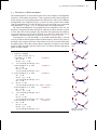
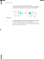
1
PTC
Library User Guide
Dan T. Abell
It doesn’t matter how beautiful your theory is,
it doesn’t matter how smart you are.
If it doesn’t agree with experiment, it’s wrong.
Richard P. Feynman
The purpose of science is not to lead us to everlasting wisdom,
but to place a limit on everlasting error.
Bertolt Brecht
Ignorance is no excuse, it’s the real thing.
Irene Peter
PTC
Polymorphic Tracking Code
PTC
Library User Guide
Dan T. Abell
Tech-X Corporation · Boulder CO · 2011
The writing of this manual was supported in part by the U.S. Department of Energy, Office
of Science, Office of Nuclear Physics under SBIR Grant No. DE-FG02-06ER84508.
Copyright © 2011 Tech-X Corporation. All rights reserved.
The Polymorphic Tracking Code, PTC, is copyright © 2008 Étienne Forest and CERN. All rights reserved.
The fibre and the integration node, with their resulting linked list types, the layout and the node layout,
are based on concepts first elaborated with J. Bengtsson. The node layout is similar to the Lagrangian
class that Bengtsson and Forest contemplated around 1990 for the C ++ collaboration later known as
Classic.
LEGO® is a registered trademark of the LEGO Group.
Windodw® is a registered trademark of Microsoft Corporation in the United States and other countries.
All other trademarks are the property of their respective owners.
Tech-X Corporation
5621 Arapahoe Avenue, Suite A
Boulder, CO 80303
http://www.txcorp.com
[email protected]
Typeset 15.05 on 29 July 2011 using the memoir class in LATEX 2ε .
Short contents
Short contents · vii
Contents · ix
List of Figures · xii
List of Tables · xiv
Note to the Reader · xv
Acknowledgements · xvii
1 Introduction · 3
2 Overview of PTC · 5
3 Modeling an Accelerator with PTC · 23
4 Linking Magnets Together and Moving Them as a Group · 43
5 Taylor Polymorphism and Knobs · 49
6 Computing Accelerator Properties · 57
7 Tracking Routines · 61
8 Geometric Routines · 67
9 Symplectic Integration and Splitting · 85
Appendices · 99
A Internal States · 101
B Data Types · 103
C PTC Geometry Tutorial Source File: ptc_geometry.f90 · 115
D PTC Splitting Tutorial Source File: ptc_splitting.f90 · 129
viii
short contents
Bibliography · 135
Index · 137
Contents
Short contents vii
Contents ix
List of Figures xii
List of Tables xiv
Note to the Reader xv
Acknowledgements xvii
1 Introduction 3
1.1 PTC and FPP 3
History of PTC 3, Where to Obtain PTC 4
1.2 PTC Library User Guide 4
Where to Start Reading 4
2 Overview of PTC 5
PTC and Reference Trajectories 6
2.1 Tracking Particles through an Accelerator 6
Blocks 6, Geometric Transformations 8, Particle Tracking 9, Data
Structures for Modeling Accelerator Topologies 11
2.2 Modeling Accelerator Topologies 13
Element 13, Fibre 13, Layout 13, Chart and Patch 15, Misalignments 16
2.3 Analyzing an Accelerator to Understand its Properties 16
Local versus Global Information 17, Polymorphs and Normal Form 18
2.4 Modeling Particle Interactions 19
Integration Node 19, Node Layout 20, Probe and Temporal Probe 20,
Time-based Tracking 21
3 Modeling an Accelerator with PTC 23
3.1 Accelerator Models 23
3.2 Geometry Tutorial Source File 24
Initial Code 25
3.3 Subroutines 26
build_PSR 26, build_PSR_minus 28, build_Quad_for_Bend 29
x
contents
3.4 Populating the DNA Database 30
3.5 Modeling Complex Accelerator Topologies 32
Ring with Forward and Reverse Propagation 32, Figure-Eight 35,
Collider 38
3.6 DNA Arrays 40
4 Linking Magnets Together and Moving Them as a Group 43
4.1 Siamese and Girders 43
4.2 Building Siamese, Girders, and their Reference Frames 44
4.3 Examples of Misalignments 47
5 Taylor Polymorphism and Knobs 49
5.1 Polymorphs 49
States of a Polymorph 49, Computing a Taylor Map 49
5.2 Knobs 50
Using Knobs 50, Creating Knobs 51, Polymorphic Blocks 51
5.3 Tutorial Example 53
6 Computing Accelerator Properties 57
6.1 Global Scalars 57
Tunes 57, Chromaticity 57, Anharmonicity 57
6.2 s-Dependent Global Quantities 57
Betatron Amplitude 57, Dispersion 58, Phase Advance 59, Beam
Envelope 60
6.3 Local Quantities 60
7 Tracking Routines 61
7.1 Standard Tracking Routines on Fibres 61
Track 61, Find_orbit 62
7.2 Tracking Routines on Integration Nodes 62
Routines for Tracking either Probe or Probe_8 62, Routines for Tracking
either Real or Real_8 63
7.3 Tracking Routines on 3-D Information through an Integration Node 63
Track_node_v 63
7.4 Time-based Tracking Routines 64
Track_time 64, Track_temporal_beam 64
7.5 Closed-Orbit Routine 64
Find_orbit_x 64
8 Geometric Routines 67
8.1 Affine Routines on Pure Geometry 67
Theory 67, Descriptions of the Routines 69
8.2 Affine Routines on Computer Objects 71
Affine Routines on Fibrous Structures 72, Misalignment Routines 77
8.3 Dynamical Routines 82
Exact Patching and Exact Misalignments: Dynamical Group 82, Inexact
Patching and Exact Misalignments 83
9 Symplectic Integration and Splitting 85
9.1 Philosophy 85
Integration Methods 85
9.2 Splitting Tutorial Source File 86
contents
9.3 Splitting the Lattice 86
Global Parameters 86, Splitting Routines 86, Arguments 87
9.4 Other Splitting Routines 95
Splitting a Single Fibre 95, Splitting an Entire Lattice 97
Appendices 99
A Internal States 101
B Data Types 103
B.1 S-based Tracking 103
Layout 103, Fibre 105, Chart 106, Patch 107
B.2 Time-based Tracking 108
Integration Node 109, Node Layout 113
C PTC Geometry Tutorial Source File: ptc_geometry.f90 115
D PTC Splitting Tutorial Source File: ptc_splitting.f90 129
Bibliography 135
Index 137
xi
List of Figures
2.1
2.2
2.3
2.4
2.5
2.6
2.7
2.8
2.9
2.10
2.11
2.12
2.13
2.14
2.15
2.16
2.17
3.1
3.2
LEGO-block element, with reference frames for the entrance, element
body, and exit. 7
Two LEGO blocks: drift (D) and bend (B). 7
Particle trajectories through “drift” and “bend” LEGO blocks. 8
Two LEGO blocks (elements) on a base (global frame). 9
Connecting two horizontal LEGO blocks and a vertical LEGO block. 9
Geometry and local coördinates, ( x, y, s), for a generic block in PTC. 10
Forward propagation of particles in a circular accelerator. 11
A recirculator illustrates particles traveling through a varying sequence
of magnets. 12
Particles circulating in different directions through an accelerator. 12
A layout with a linked list of fibres pointing to magnets. 14
DNA database with eight DNA sequences (L1 through L8). The arrows
represent the links in the doubly-linked list of fibres that constitutes
a layout. Each fibre points to (contains) the indicated magnet (M1–
M18). 14
Eight layouts or DNA sequences. 14
Patching elements in a single beamline. 15
Patching elements in multiple beamlines. 16
Misaligning an element. 16
N + 4 integration nodes cover an element. 20
Applying a space-charge kick at time τ. 21
3.3
3.4
3.5
3.6
3.7
3.8
Basic cells for the three accelerator models. 24
Accelerator models. Arrows indicate the direction of motion of particle
beams in the constituent layouts. 24
Subroutines for creating DNA sequences. 26
Geometry of the rectangular bend. 27
Ring with forward and reverse propagation. 32
Fig8 fibres pointing to elements in L3 and L4. 35
Matching L3 to L4. 36
Collider. 38
4.1
4.2
A pair of elements linked together as a siamese. 43
Incorrect and correct rotations of a siamese. 43
list of figures
4.3
4.4
4.5
4.6
4.7
4.8
A trio of elements linked together as a girder that has its own reference
frame. 44
Collider interaction region. The numbers show the indices of a few of
the fibres within the corresponding layout. 44
Collider interaction region. The small cross-hairs indicate the frame
location for each siamese. 46
No misalignment. 47
Examples 1 (top) through 5 (bottom). 47
Examples 6 (top) through 11 (bottom). 48
6.1
6.2
One-turn and partial-turn transfer maps. 59
This graphic illustrates the essential relationships between the oneturn map and the normal form at two different locations in a ring
lattice. 59
8.1
8.2
8.3
8.4
8.5
8.6
8.7
8.8
8.9
Rotating point a and vector basis (v1 , v2 , v3 ) by R. 67
Rotating and translating the frames of a magnet. 70
Example 0: girder. 78
Example 1: girder after 22.5 degree rotation. 78
Example 1: girder after an additive misalignment. 79
Example 2: misalign siamese followed by misalign girder. 80
Example 3: misalign girder followed by misalign siamese. 80
Example 4: misalign siamese with preserve_girder=.true. 81
Pseudo-Euclidean maps. 84
9.1
9.2
Drift-kick-drift for integration methods 1 and 2. 95
Matrix-kick-matrix for integration methods 2, 4, and 6. 96
B.1
B.2
B.3
B.4
B.5
A layout is a linked list of fibres. 105
Three charts attached to an element. 107
Misalignments for a element. 108
Misaligned planar fibre in three dimensions. 109
Type integration_node and type fibre. 111
xiii
List of Tables
3.1
DNA database for the PTC geometry tutorial 31
9.1
9.2
9.3
9.4
9.5
9.6
9.7
9.8
9.9
9.10
Results of Example 1. 87
Results of Example 2. 88
Results of Example 3 for Part 1A. 89
Results of Example 6 when even is not specified. 92
Results of Example 6 when even=.true. 92
Results of Example 7 for resplit_cutting=1. 93
Results of Example 7 for resplit_cutting=2. 93
Results of Example 8. 93
Results of Example 9 when useknob=.true. 94
Results of Example 9 when useknob=.false. 94
Note to the Reader
This manual describes Étienne Forest’s PTC, a software library of data structures
and tools for both integrating and analysing the orbital and spin motion of particles
in modern accelerators and storage rings. I believe that PTC is an important
contribution that should be more widely known, understood, and used by the
accelerator physics community, hence my efforts here. I will therefore greatly
appreciate your reporting any difficulties you have with this document—errors,
inconsistencies, infelicities of language, etc.—to [email protected].
Acknowledgements
First and foremost, I must thank Étienne Forest. Not only is he the author of PTC—
hence sine qua non—he has also answered innumerable questions over the years
and helped me to understand both the structure of PTC and the motivation behind
many of the decisions that went into its design. Many of the examples in this manual
are based on code he provided.
Al Kemp, of Impact Technical Publications, helped with the overall organisation
and the initial draft. In addition, several of my colleagues at Tech-X commented on
various parts of this document: George Bell, Andrey Sobol, and David Bruhwiler.
Very special thanks go to Desmond Barber, for his support, encouragement, and
detailed reviews of the manuscript. His keen ear for the English language, broad
knowledge of accelerator physics, and consistent willingness to help have improved
this document in more ways than I can possibly note. I am deeply in debt to him.
Financial support for the writing of this document was provided in part by the
U.S. Department of Energy, Office of Science, Office of Nuclear Physics under SBIR
Grant No. DE-FG02-06ER84508.
PTC
one
Introduction
1.1
PTC and FPP
The Polymorphic Tracking Code (PTC) is a library of Fortran90 data structures
and subroutines for integrating the equations of orbital and spin motion for particles
in modern accelerators and storage rings. The data structures hold the material
that we will mould into physically correct and consistent three-dimensional computer models of the complex topologies found in machines such as colliders and
recirculating linacs, including the effects of errors in both location and strength
of the various machine elements. We use the subroutines to actually construct the
computer model of a machine and then integrate through it—including the geometric transformations (translations and rotations) of machine elements, connecting
elements to form trackable beamlines, and tracking the orbital and spin degrees of
freedom. In a word, PTC is an integrator.
The Fully Polymorphic Package (FPP) is a package of polymorphic types and
tools that provide PTC with facilities for analysis. In particular, FPP implements a
polymorphic Taylor type (hence the P in PTC) that can change shape at execution
time. This Taylor type makes it possible for FPP to extract a Poincaré map from PTC
(or some other integrator). Moreover, FPP provides the tools to analyse the resulting
map. The most common—and most important—tool is the normal form: with this
at hand, one can compute tunes, lattice functions, and nonlinear extensions of these
and all other standard quantities of accelerator theory. Indeed, the combination of
PTC and FPP gives access to all of standard perturbation theory on complicated
accelerator lattice designs.
In a nutshell, then, the three central features of PTC1 are
• the Fortran90 types and code that facilitate fully three-dimensional placement
of beamline elements and construction of non-simple accelerator topologies:
colliders, recirculators, dog-bones, and combinations of these topologies;
• the polymorphic integration routines for orbit and spin;
• the use of maps derived from the integrator—via operator overloading and
polymorphism—for computing the full range of accelerator properties, including the parameter dependence of these properties.
History of PTC
Latter half of 1980s, at SSC-CDG: Berz introduces automatic differentiation and
develops DA package in Fortran77. Forest builds LieLib on top of DA, thus
bringing the power of map methods to the analysis of maps produced by integrators.
1
When we say “PTC”, we
shall (almost always) mean
PTC and FPP combined;
but you keep in mind the
distinction.
4
introduction
Early 1990s: J. Bengtsson pioneers the use of run-time polymorphism to greatly
simplify and improve the process of making run-time changes to, for example,
computing parameter dependence. Forest and Bengtsson together develop the ideas
from which derive the fundamental building blocks of PTC. Forest develops the
dynamical Euclidean group. Middle to late 1990s: Forest develops LieLib into
FPP (using LBNL versions of DA and LieLib). FPP replaces the real variable
type real(8) with a new type called real_8 to produce Taylor series for analysis.
Forest also develops PTC-proper (the integrator). Together these tools compose
PTC. Middle to late 2000s: Forest adds spin dynamics to PTC. L. Yang develops a
C ++ replacement for Berz’s DA package.
Where to Obtain PTC
http://www.takafumi.org/etienne/ptc/
1.2
PTC Library User Guide
Where to Start Reading
The Overview of PTC, chapter 2, presents concepts important for understanding
PTC. In-depth discussions of all these concepts can be found in several publications
by Étienne Forest:
• Étienne Forest, “A Hamiltonian-free description of single particle dynamics
for hopelessly complex periodic systems”, J. Math. Phys., 31(5):1133–1144, May
1990, doi: 10.1063/1.528795;
• Étienne Forest and Kohji Hirata, “A contemporary guide to beam dynamics”,
Technical Report KEK-92-12, KEK, Tsukuba, Japan, August 1992;
• Étienne Forest, “Locally accurate dynamical Euclidean group”, Phys. Rev. E,
55(4):4665–4674, April 1997, doi: 10.1103/PhysRevE.55.4665;
• Étienne Forest, Beam Dynamics: A New Attitude and Framework, volume 8 of
The Physics and Technology of Particle and Photon Beams, Harwood Academic
Publishers, Amsterdam, 1998;
• Étienne Forest, “Geometric integration for particle accelerators”, J. Phys. A:
Math. Gen., 39(19):5321–5377, May 2006, doi: 10.1088/0305-4470/39/19/S03.
If you want to get started right away, begin with chapter 3, Modeling an Accelerator
with PTC, and refer back to the overview as needed while working with the tutorial
examples.
two
Overview of PTC
This overview describes the PTC approach to simulating and analyzing particle
accelerators.
At the heart of PTC’s accelerator simulation code is an integrator capable of
tracking particles through various kinds of beamline elements. A particle going
through a beamline element sees only the local magnetic field, and PTC uses a local
reference frame for describing that magnetic field—the frame most appropriate
for the geometry of that type of element. To track through a series of beamline
elements, PTC locates the elements with respect to each other using geometric
transformations that connect the reference frame of one element to the reference
frame of neighboring elements. Those two pieces—the integrator and the geometric
transformations—give PTC the capability to model an accelerator with arbitrarily
placed beamline elements.
In tracking orbits through particle accelerators, we want the capability of modeling not only simple linear and ring accelerators, but also complex topologies,
for example, the Continuous Electron Beam Accelerator Facility (CEBAF) at the
Jefferson National Laboratory (JLab). To model a complex topology correctly1 , PTC
uses a data structure that captures the location of the physical elements as well as
the topology of the beam trajectory. It is that data structure that makes it possible
for us to modify a single PTC beamline element in our simulation code—even when
more than one distinct beam trajectory traverses that element. See the discussion of
Modeling Accelerator Topologies, § 2.2.
PTC itself handles the integrator, the geometric transformations, and the associated data structures, which provide the capability to track particle orbits through
complex topologies. Inside of PTC is a set of modules referred to collectively as the
Full Polymorphic Package (FPP).2 These routines extend the capabilities of PTC,
making it possible not only to track particles, but also to propagate maps. PTC uses
FPP to compute the maps one may analyze for accelerator properties of interest to
us: lattice functions and the like. Analyzing an Accelerator to Understand its Properties,
§ 2.3, discusses this topic.
Finally, when we track particles in accelerators, we must sometimes account for
particle interactions. Modeling Particle Interactions, § 2.4, discusses this topic.
For in-depth discussions of the topics introduced in this overview, see the Bibliography, page 135.
1
Here correctly means “in
a manner that respects the
physical reality”.
2
É. Forest, Y. Nogiwa, and
F. Schmidt. The FPP and
PTC libraries. In Int. Conf.
Accel. Phys. 2006, pages 17–
21; and É. Forest, Y. Nogiwa,
and F. Schmidt. The FPP
documentation. In Int. Conf.
Accel. Phys. 2006, pages
191–193
6
overview of ptc
PTC and Reference Trajectories
A reference trajectory or reference orbit describes the ideal path of a particle through an
ideal accelerator. Accelerator modeling codes that use a reference trajectory simulate
particle orbits as deviations from that ideal. However, a particle traveling through a
real accelerator “sees” only local magnetic and electric fields, and PTC respects this
physical reality. When pushing a particle through, say, a quadrupole, PTC makes
no distinction between that magnet sitting on a lab bench and that magnet in a
beamline: it simply integrates the particle motion in a frame local to that quadrupole.
As we shall see, an essential component—perhaps the essential component—of
PTC is the collection of geometry routines that handle transformations between
different frames of reference. This approach has the added benefit that even large
displacements—e.g., a quadrupole shifted to act as a combined-function bend—can
be handled in the same consistent and physically correct manner.
2.1 Tracking Particles through an Accelerator
This section discusses four important concepts that enable PTC to perform accurate
simulations of particles through an arbitrarily complex accelerator:
• blocks,
• geometric transformations,
• particle tracking,
• data structures for modeling accelerator topologies.
Blocks
3
PTC also has the capability
to perform first-order timebased tracking. See Modeling
Particle Interactions, § 2.4.
PTC uses the longitudinal coördinate, generically denoted s, as the independent
variable for integrating particle trajectories.3 The particulars of PTC’s s-based, or
element-based, tracking serve to maintain the physical and mathematical integrity
of each element in a beamline and, moreover, make it possible for PTC to provide
information about particles inside an element, again without violating the element’s
physical and mathematical integrity. To explain how PTC does this, we use an
analogy with LEGO® blocks.
Each different type of beamline element in an accelerator is analogous to a
different type of LEGO block in the sense that LEGO blocks are self-contained
objects. A magnet, for example, is a self-contained object that produces a local
field that affects local particle trajectories. Local geometric considerations (e.g., the
shape and symmetry of the magnetic field) determine the coördinate system and
frame of reference for a local Hamiltonian that describes the magnet. (We choose
the coördinate system and frame of reference so as to push particles through the
element as simply as possible.) If individual magnets have conflicting geometries,
we patch them together. In other words, we use local coördinate transformations
to connect particle trajectories between the differing geometries. The rest of the
accelerator does not—and should not—affect our choice of reference frame for any
given beamline element.
A local coördinate system attached to each beamline element permits us to
propagate physical quantities across the elements. That internal structure is the
province of the integrator. In addition, each element includes three reference frames:
a reference frame at the entrance, a reference frame at the midpoint (the element
reference frame), and a reference frame at the exit. See figure 2.1. These extra frames,
used by PTC when it hands a particle from one element to the next, allow PTC to
2.1 tracking particles through an accelerator
handle arbitrary changes in the placement of beamline elements. On entering an
element, a particle has a certain phase-space location with respect to the entrance
frame. PTC tracks the particle as it traverses the element, computing the particle’s
phase-space coördinates with respect to the element’s exit frame. Knowing the
relation between the exit frame of the current element and the entrance frame of
the subsequent element, PTC uses the transformations of the dynamical Euclidean
group4 to hand the particle to the next element.
7
4 É. Forest. Locally accurate
dynamical Euclidean
group. Phys. Rev. E, 55
(4):4665–4674, Apr. 1997.
doi: 10.1103/PhysRevE.55.4665
Figure 2.1: LEGO-block
element, with reference
frames for the entrance,
element body, and exit.
The beamline element represented in figure 2.1 is a drift: a block with parallel
entrance and exit faces to which local Cartesian reference frames are attached. The
entrance and exit reference frames have the same unit vectors. The line that links the
two frames has a length L, and it is perpendicular to both those frames. Note that
for the purposes of this discussion, any beamline element (quadrupole, sextupole,
solenoid, etc.) that does not bend the design orbit is a drift.
A LEGO-block element might also be a bend: a block with two faces that have
parallel y-axes (vertical), and x-axes (horizontal) that meet at an angle θ. The two
x-axes and the line joining the two origins form a plane perpendicular to the two
faces. An arc of circle of length L passes perpendicularly through the origin of both
faces. The purpose of this element is to bend an incoming particle trajectory by
approximately angle θ. The internal details of the element—whether it is a sector
bend, a bend with an irregular field, etc.—is, for this discussion, immaterial.
Figure 2.2 illustrates these two fundamental types of LEGO blocks with the
entrance and exit reference frames for their local coördinate systems. The solid
arrows show the direction of the local y-axes and the dashed arrows show the
direction of the local x-axes. In summary, the bend is characterized by a bending
radius ρ, a length L, and two faces, each with a reference frame. The drift is
characterized by a length L and also two faces, each with a reference frame. The
bend is the fundamental block used in the composition of complex blocks; the drift,
of course, is just a special case of the bend.
We are interested in the deterministic motion through each LEGO block, represented by the transformation
zin 7→ zout = f (zin ),
Note that calling the x and
y axes “horizontal” and
“vertical” reflects the bias
of accelerator physicists
towards flat rings with
vertical dipole fields. What
we locally (i.e., within the
element) call the x axis need
not be horizontal. See, for
example, the discussion of
the vertical bend indicated
in figure 2.5.
D
B
(2.1)
where f denotes a vector of generally nonlinear functions connecting the local
phase-space coördinate zin defined in the entrance frame, to the local phase-space
coördinate zout in the exit frame. The construction of such a transformation depends
on internal considerations that are not needed for an understanding of the LEGOblock approach. The LEGO block for a single element might, in fact, comprise a
Figure 2.2: Two LEGO
blocks: drift (D) and bend
(B).
8
overview of ptc
Figure 2.3: Particle trajectories through “drift” and
“bend” LEGO blocks.
sequence of simpler blocks. This structure, dictated by the internal geometry of the
element, may be hidden.
In figure 2.3 we show a pair of particle trajectories, in drift and bend LEGO
blocks, passing from the entrance face through to the exit face. As suggested by the
trajectories illustrated, the internal structure may be very complicated (think of a
wiggler); but seen from the outside, our LEGO blocks are, quite simply, blocks with
two faces that define local coördinates with respect to which one may define zin and
zout —nothing more.
A beamline element is defined by a block with three reference frames, together
with a model, or integrator, which describes how to propagate a particle from the
face with the entrance reference frame to the face with the exit reference frame:
element = block + model.
5 Appendix A discusses
PTC’s internal state variables, which describe
the characteristic dynamics you can choose for
your accelerator model.
The model transforms the phase-space variables from entrance to exit of the block
according to (2.1). In other words, it represents the physics of the device. Note that
the model also incorporates any approximations we make.
As an example, a block with a bend geometry might actually be a simple drift,
keeping the transverse momenta invariant and changing only the positions. Or it
might be a composition of blocks describing the body of a magnet and its fringe field
regions. An element might also have non-Hamiltonian effects such as radiation.5
The list of possible models is endless. In general, a model is defined by
• one or more blocks internal to the model;
• a model for each internal block;
• the equation of motion in each internal block together with its integration
method and associated number of integration steps.
In summary, we define a beamline element locally: the definition, whether the
element is on a work bench or in an accelerator, is determined solely by the
characteristics of that element. And once we have defined a model for our element,
we stick with it: the LEGO block is inviolate. Like a physical magnet, it exhibits
identical properties under identical conditions. A significant virtue of our computerbased element, however, is that it is free to report about what is happening inside.
Geometric Transformations
Now that we have defined our two basic types of beamline elements (drift and
bend), the next step is to fit them together. We need geometric transformations that
connect the exit reference frame of one beamline element to the entrance reference
frame of a subsequent element.
Continuing the LEGO-block analogy, we put the individual LEGO blocks on
a base, which represents the accelerator model’s global frame. Once we know the
location of each LEGO block with respect to the global frame, we know their
locations with respect to to one another. Figure 2.4 shows two such LEGO blocks
and their reference frames on a base, which represents the layout of beamline
elements in the global frame of an accelerator. With the LEGO blocks now on the
global frame, we require transformations that translate the phase-space coördinates
in the exit reference frame of one LEGO block to the phase-space coördinates in the
entrance reference frame of the next LEGO block.
To construct, for example, a recirculating accelerator out of LEGO blocks, we
connect bends and drifts one after another to model the desired machine. On
reaching the last LEGO block, we require that the last block’s exit face coincide
with the first entrance face. This means that
2.1 tracking particles through an accelerator
9
Figure 2.4: Two LEGO
blocks (elements) on a base
(global frame).
the blocks’ faces must be parallel;
and the frames on the two faces must line up.
Connecting a horizontal bend with a horizontal drift, as for elements BH and D in
figure 2.5, is easy because the x- and y-axes of the two elements match. Connecting a
horizontal drift with a vertical bend, as for elements D and BV in figure 2.5, is not as
straight-forward: their local x- and y-axes do not match. We need, in essence, a new
type of LEGO block—one with an x-y rotation of angle φ. (In figure 2.5, of course,
φ = 90°.) To build an arbitrary accelerator, we shall require a full complement of
such additional LEGO blocks.6 This is the subject of patching, which uses geometric
transformations to connect the exit frame of one beamline element to the entrance
frame of a subsequent element. Most significantly, patching enables us to position
beamline elements wherever we want them. We discuss this in more detail later in
Chart and Patch, page 15.
•
BV
•
BH
?
D
Figure 2.5: Connecting two
horizontal LEGO blocks and
a vertical LEGO block.
6
É. Forest. Locally accurate
dynamical Euclidean
group. Phys. Rev. E, 55
(4):4665–4674, Apr. 1997.
doi: 10.1103/PhysRevE.55.4665
Particle Tracking
Now that we have the basic building blocks and the geometric transformations to fit
them together, we can begin to think about how to track particles. Here we present
some essential information about particle tracking in PTC.
In keeping with its LEGO-block philosophy, PTC tracks particles with respect
to local frames of reference. The local phase-space coördinates together with PTC’s
knowledge of the local frames allow the interested user to reconstruct full 3D
particle trajectories with respect to the global frame. In fact, doing exactly that is
useful for checking that one has the constructed the correct lattice topology in PTC.
Units: PTC measures all lengths in meters, and all angles in radians. (It provides
the constant twopi to simplify the conversion from degrees.7 ) Particle momenta are
scaled by a value po . This scale momentum is usually set when defining the lattice
(see, for example, the discussion of set_mad on page 27). A subtle point involves the
7
Many other constants
are defined in the module
precision_constants.
10
overview of ptc
fact that the scale set for one element may differ from that in the preceding element,
e.g. in the case of acceleration. In such cases, the patching mentioned above must
include not only geometric transformations, but also energy transformations.
Tracking State: PTC defines a variable type called internal_state. Objects of this
type may be used to modify certain assumptions PTC makes when it performs
tracking. One may, for example, ask PTC to track only the 4D transverse phase-space
variables; or one may turn on or off radiation. A variable of type internal_state is
essentially a list of flags that one may pass to PTC tracking routines to modify the
algorithms used. For more information, see Internal States, appendix A.
8
PTC can turn all six of
the variables into Taylor
series, or it can omit two
of them. Setting an internal_state flag to “only
four dimensions” implements the latter behavior.
Phase-Space Coördinates: With the default tracking state, PTC uses the six
phase-space variables8
( x, p x , y, py , δ, `).
(2.2a)
Here x and y denote the local transverse coördinates, and p x and py denote the
corresponding canonical momenta (divided by a scale momentum po ). The fifth
variable, δ, denotes the relative momentum deviation
δ=
9
These last two variables
are kept in this order for
a technical reason. This
ordering allows us to retain the natural meanings:
positive δ implies higher energy, and positive ` implies
longer path length. Because
of the Hamiltonian structure, reversing their order
would require us to reverse
the sign on one of them.
p − po
;
po
and the sixth variable, `, denotes the path-length deviation.9
One may modify the tracking state so as to change the phase-space variables. If
desired, one may set a flag that causes PTC to compute flight time rather than path
length. In this case, the phase-space coördinates are
( x, p x , y, py , ε, ct).
(2.2b)
Here the fifth variable, ε, denotes the scaled energy deviation
ε=
E − Eo
,
po c
where Eo is the energy associated with po . (In other words, if po = mc2 β o γo , then
Eo = mc2 γo .) And the sixth variable, ct, is the time-of-flight deviation multiplied by
the speed of light.
One may set a separate flag that causes PTC to compute the total path length (or
flight time) rather than the deviation. In this case the phase-space variables will be
either
( x, p x , y, py , δ, L),
(2.3a)
or
y
( x, p x , y, py , ε, cT ),
s
x
ρ0
Figure 2.6: Geometry and
local coördinates, ( x, y, s),
for a generic block in PTC.
(2.3b)
where L and T denote respectively the total path length and total flight time.
Hamiltonians: In accord with its LEGO-block philosophy, PTC tracks a particle
across an element using a Hamiltonian that is local to that element. The Hamiltonian
used by PTC in the body of an element (no fringe field) then has the simple form
q
q
− (1 + κo x ) (1 + δ)2 − p2x − p2y + (1 + κo x ) As ( x, y)
(2.4a)
po
if one uses the variables (2.3a), or
r
2
q
− (1 + κ o x ) 1 +
ε + ε2 − p2x − p2y + (1 + κo x ) As ( x, y)
βo
po
(2.4b)
2.1 tracking particles through an accelerator
if one uses the variables (2.3b). Here κo = 1/ρo denotes the curvature defined by the
geometry of the element, and As denotes the longitudinal component of the vector
potential. Figure 2.6 indicates the variables, including the longitudinal coördinate s.
For straight elements, of course, κo = 0. If one uses the variables (2.2), then there is,
effectively, an additional term that subtracts the default path length or flight time
across that element.10
One may, if desired, have PTC track using an approximation of one of the
Hamiltonians (2.4) (i.e., using truncated expansions for the square-root and the
vector potential). One might, for example, do this to speed the computation, but of
course the validity of the expansion for your particular problem should be verified
with careful testing.
When integrating across an element described by one of the Hamiltonians (2.4),
one typically splits the Hamiltonian into two integrable pieces.11 If those pieces
are, for example, the two terms of (2.4a), then this is referred to as a drift-kick split.
Since the motion of a particle in a uniform dipole is integrable, an alternative split
involves writing As ( x, y) as a sum of two pieces: the part that produces a uniform
dipole field, and everything else. Then the dipole field part is added to the drift
term of the Hamiltonian, and we obtain a bend-kick split.12 One may ask PTC to use
one or the other of these splitting methods.
Structures for Particles and Beams: Because PTC tracks particles with
respect to local frames of reference, a set of values for (as an example) the six phasespace variables (2.2a) will not mean too much unless one knows the context—in
particular, where in the lattice the particle is located. When you need PTC to keep
track of such information for you, it provides some additional structures. The type
beam holds an N × 6 array for the phase-space variables, as well as a pointer that
tells you where in the lattice that beam is located. There is also a type probe that
holds not only phase-space data, but also data about a particle’s spin state.
10
D.P. Barber, K.A. Heinemann, and G. Ripken. A
canonical 8-dimensional
formalism for classical
spin-orbit motion in storage rings: I. A new pair
of canonical spin variables. Z. Phys. C, 64
(1):117–142, Mar. 1994.
doi: 10.1007/BF01557243
11
R.I. McLachlan and
G.R.W. Quispel. Splitting
methods. Acta Numer.,
11:341–434, Jan. 2002.
doi: 10.1017/S0962492902000053
12
É. Forest. Beam Dynamics: A New Attitude and
Framework, volume 8 of The
Physics and Technology of
Particle and Photon Beams.
Harwood Academic Publishers, Amsterdam, 1998;
and É. Forest. Geometric
integration for particle
accelerators. J. Phys. A: Math.
Gen., 39(19):5321–5377, May
2006. doi: 10.1088/03054470/39/19/S03
Data Structures for Modeling Accelerator Topologies
PTC data structures fully account for the three-dimensional structure of a lattice and
potential topological complexities such as those found in colliders and recirculators.
In this section, we discuss a simple lattice and then two complex lattices.
A very simple lattice is shown in Figure 2.7, which illustrates basic forward
propagation of particles through a sequence of magnets that never varies. Each
magnet appears once in the sequence, and particles go magnet-to-magnet from M1
through M8. At that point, they reënter the magnet M1. A simple linked list of
magnets suffices to model this basic topology:
ring = linked-list(M1, M2, M3, M4, M5, M6, M7, M8).
One might instead use an array of magnets, but that approach would require us to
recreate and reallocate the array whenever we wish to add or insert a new element.
A virtue of the linked list is that one may easily add or rearrange elements in
the lattice. However, such a simple approach does not suffice when an accelerator
topology reuses the magnets in different sequences, different directions, or both.
To see the difficulties associated with a recirculating beam, consider Figure 2.8,
which shows a machine similar to the Continuous Electron Beam Accelerator Facility
(CEBAF) at Thomas Jefferson National Laboratory (JLab). It illustrates the concept
of particles circulating through a varying sequence of magnets. The particles start
out traveling through an injector from magnet M1 through magnet M4. During the
11
M1
M8
M7
M2
M3
M6
M4
M5
Figure 2.7: Forward propagation of particles in a
circular accelerator.
In this discussion, we
use the word “magnet”
whether or not it is actually
a magnet, a drift, or any
other beamline element.
12
overview of ptc
first trip circulating around the accelerator, the particles go through the sequence of
magnets M5, M6, M7, M8, M9, M10, M11, and M12. During their second trip around
the accelerator, the particles go through the sequence of magnets M5, M6, M13,
M14, M9, M10, M15, and M16. And during their last trip, the particles go through
the sequence of magnets M5, M6, M17, M18, M9, and M10. The particles are then
dumped. Note that magnets M5, M6, M9, and M10 appear in all three circuits.
M1
Figure 2.8: A recirculator illustrates particles
traveling through a varying sequence of magnets.
M2
M3
M5
M4
M6
M16
M12
M7
M13
M17
M15
M11
M8
M14
M18
M10
M9
A linked list of magnets cannot properly represent the physics of this situation.
In a linked list, magnet M6, for example, must point to only one magnet. It cannot
point to M7, M13, and M17 unless we create two clones of M6. Creating clones,
however, is a bad idea: If we wish to adjust the position or strength of magnet M6,
such adjustments would have be made three times: once in the magnet itself, and
once in each of its two clones.
A better solution separates the magnets from the linked list that tracks the path of
particles through the magnets. PTC does this with a linked list of containers called
fibres, each with a pointer to the appropriate magnet. Adjustments to the position or
strength of a magnet are made once and are automatically taken into account each
time a container in the linked list points to that magnet. We discuss the linked list
of containers with pointers to magnets in Modeling Accelerator Topologies, § 2.2.
M1
M2
M3
M4
Figure 2.9: Particles circulating in different directions through an accelerator.
What about a collider? Figure 2.9, based on the intersecting rings of the Relativistic
Heavy Ion Collider (RHIC) at Brookhaven National Laboratory (BNL), shows
particles circulating in both directions (forward and backward propagation) through
some of the same magnets. For example, the particles following the blue path
go though one set of magnets in the sequence M1, M2, M3, M4. Meanwhile, the
2.2 modeling accelerator topologies
particles following the yellow path traverse the same set of magnets in the reverse
order: M4, M3, M2, M1.
Using an array or a linked list with clones of magnets creates the same problems as
before, and PTC alleviates the difficulties by using doubly-linked lists of containers
that follow the particle paths—containers which have inside them pointers to the
appropriate magnets. Changes to the strength or position of, say, magnet M3 are
made once in the object for magnet M3 and are immediately reflected in the two
linked lists—one linked list for each of the two particle beams.
2.2
Modeling Accelerator Topologies
To set up a linked list of containers with pointers to the elements in a beamline, PTC
employs three different data types: element, fibre, and layout. PTC also provides
what it refers to as a DNA database, which one may populate with layouts that
one may use to construct complex accelerator topologies. Finally, for the proper
positioning of elements in the accelerator, PTC uses two additional data types: chart
and patch. We discuss all these concepts in this section.
Element
The data type element represents a beamline element in a machine. It contains
information about the element type (dipole, quadrupole, rf cavity, etc.), its physical
properties (length, strength, etc.), and its location and orientation in space. In PTC, it
is the fundamental object. PTC preserves each element’s physical and mathematical
integrity to ensure that it can be positioned, repositioned, or misaligned as a whole.
At the same time, PTC provides the capability for one to look inside the element
to see, for example, details of a particle trajectory. One should therefore never feel
compelled to split an element in half.
In addition to information about the element itself, the data type element includes
information about which fibres point to it. This information is used by PTC to
ensure that if an element is moved, then all beamlines containing it know about the
move.
Fibre
The data type fibre contains a pointer to a beamline element as well as pointers to
the fibres that precede and follow it along a particle path. When strung together in
a linked list, a sequence of fibres defines a beamline. The fact that different fibres
can point to the same element means that separate beamlines can share common
elements; and this gives PTC the capability to model complex accelerator topologies.
A fibre contains, among other items,
• a pointer to an element;
• pointers to the previous and next fibres along a beamline;
• a pointer to a chart that locates the element within the global reference frame;
• a pointer to a patch that connects the elements of successive fibres geometrically,
energetically, and temporally;
• the direction of propagation through the element.
Layout
The data type layout represents a beamline as a doubly-linked list of fibres. It follows
the particle path by specifying the order of the fibres, which each point to an actual
13
The use of a doubly-linked
list enables both forward
and reverse propagation
through a given sequence of
beamline elements.
14
overview of ptc
13 Note that a layout need
not represent an entire machine: it may represent just
a piece of an machine. The
full accelerator would then
be built from several layouts.
element in the beamline.13 In addition, a layout defines the direction of propagation
through the sequence of fibres and whether the particles recirculate.
F5, F13, F21 M5
F1 M1 F2 M2 F3 M3 F4 M4
M13
M17
F20
F15
F23
F19
F16
F24
M14
M18
M16
Figure 2.10: A layout
with a linked list of fibres pointing to magnets.
As before, we say “magnet”, but it may mean any
type of beamline element.
L1: M1
M2
L2: M5
M6
L3: M7
M8
L4: M9
M10
M3
M4
L5: M11 M12
L6: M13 M14
L7: M15 M16
L8: M17 M18
Figure 2.11: DNA database
with eight DNA sequences
(L1 through L8). The arrows represent the links
in the doubly-linked list
of fibres that constitutes a
layout. Each fibre points
to (contains) the indicated magnet (M1–M18).
M15
F8 M8
F9, F17, F25 M9
Most accelerator modeling codes do not, as PTC does, enforce a dichotomy
between fibres and elements. As a consequence, it can be difficult to import lattice
descriptions from other codes into PTC in a manner consistent with PTC’s approach
to modeling accelerators. To overcome this difficulty, PTC provides what it refers
to as a DNA database. This database is first populated with a set of layouts whose
fibres point to unique elements. In other words, no element appears more than
once—via the fibres—in the set of DNA layouts. (This much may, if desired, be done
by importing from an external lattice description.) These simple layouts—we shall
refer to them as DNA sequences—may then be used to construct complex layouts of
the form shown in figure 2.10.
As a concrete example, consider how we might do this for the accelerator shown
in figure 2.8 or 2.10: We first create a set of layouts in which no magnet appears
twice, and which have no magnets in common. The logical course in this case is
to create the eight layouts L1 through L8 shown in figure 2.11. Note that each of
the eighteen magnets appears just once in this database. Here we show each of the
DNA sequences in a different color; and these colors match those used in figure 2.12,
which shows the accelerator with the different DNA sequences indicated by the
corresponding colors.
F5, F13, F21 M5
F6, F14, F22 M6
M13
M17
F20
F15
F23
F19
F16
F24
M14
M18
M15
By contrast, we may
sometimes refer to the
DNA sequences—highlevel building blocks of
our accelerator model—
as non-trackable layouts.
M11 F11
F7 M7
As an example, consider the accelerator illustrated in figure 2.8. We could construct it as indicated in figure 2.10, which shows a PTC layout with a linked list of
26 fibres (F#) pointing to the 18 magnets (M#).
M16
14
M12 F12
F10, F18, F26 M10
F1 M1 F2 M2 F3 M3 F4 M4
Figure 2.12: Eight layouts or DNA sequences.
F6, F14, F22 M6
M12 F12
M11 F11
F10, F18, F26 M10
F7 M7
F8 M8
F9, F17, F25 M9
Having created the eight DNA sequences in our DNA database, we can now
use PTC to string these basic layouts together to create the trackable layout that
represents the full machine illustrated in figure 2.8, or 2.10 or 2.12. Evidently, a
trackable layout may be constructed from one or more DNA sequences.14
In general, once we have populated the DNA database (either from within PTC
or by importing external lattice descriptions) we can use PTC to string together these
basic layouts to create the additional layouts we need for tracking. These latter—T1
2.2 modeling accelerator topologies
15
through TN, say—contain fibres that point to elements in the DNA database. For
the recirculator shown in figure 2.8, we would create one beamline layout T1 with
26 fibres, each pointing to an element in the DNA database. For the collider shown
in figure 2.9, we would create two beamline layouts, T1 and T2, one layout for each
ring.
Chart and Patch
PTC uses the new data types chart and patch to locate, connect, and move the
elements of a beamline. The generic capability, which we term patching, connects
the exit frame of one element to the entrance frame of the subsequent element.
The data type chart contains a pointer to a frame of reference (actually the
collection of three frames illustrated in figure 2.1) that locates a fibre (really the
element the fibre points to) within PTC’s global three-dimensional reference frame.
The chart also contains information that describes, if present, any misalignment of
the fibre.
The data type patch contains information about the about the relation between
the exit reference frame of one element and the entrance reference frame of the
subsequent element. As a consequence, a patch is a property not of an element
but of a fibre, and it must be computed after placing both elements in their final
locations.
As a concrete example, consider the set of elements illustrated in figure 2.13.
There we see three elements separated by a pair of drifts. We know the locations
of these elements (in particular the reference frames attached to these elements)
because of the information stored in the corresponding charts. The second drift
is explicitly defined as the third beamline element. The first drift, however, is not
explicitly defined. The exit frame of element 1 and the entrance frame of element 2
do not coincide, and this indicates the need for a patch. The remaining elements all
have exit-entrance frame pairs that coincide, and hence no additional patches are
required.
element 1
particle
path
eleme
nt 2
patch
required
eleme
nt 3
(drift
)
eleme
nt 4
no pa
tc
requi h
red
As another example of patching, figure 2.14 shows three magnets in a recirculator.
A high-energy particle passing through magnet 1 follows the red trajectory to
magnet 2. After exiting magnet 2, the particle continues around the machine and
returns with a lower energy (after deceleration by appropriately phased rf fields) to
magnet 1. Because the particle has less energy, magnet 1, the separator, now bends
it along the blue trajectory towards magnet 3, the first magnet in a new beamline.
Magnet 1 of figure 2.14 must, of course, appear in two fibres: the first points to
magnet 2 as the subsequent element, while the second points to magnet 3. What
about the patches? Assuming the exit frame of magnet 1 and the entrance frame of
Figure 2.13: Patching elements in a single beamline.
16
overview of ptc
magnet 2 have the same unit vectors but different origins. then the patch between
the fibres pointing to magnets 1 and 2 must correspond to a simple drift of the
appropriate length—and that is exactly what PTC will compute. The patch between
the fibres pointing to magnets 1 and 3 corresponds to three actions: a drift of length
d, a coördinate frame rotation by angle α, and a translation of length h.
d
net
mag
α
1
magnet 2
h
mag
net 3
Figure 2.14: Patching elements in multiple beamlines.
Misalignments
The accelerator we design is never the one we build. This fact makes it essential to
investigate the margin for error in any design. To simulate misalignment errors, PTC
uses the approach illustrated in figure 2.15. There we show the original element 2
with a light gray outline, and the misaligned element 2 with a red outline. To
push a particle from the exit of element 1 to the entrance of element 3, PTC first
applies the patch from element 1 to the original element 2. Then PTC traverses
element 2 in three steps: an entrance misalignment, the standard element 2, and
an exit misalignment. PTC then applies the patch from element 2 to element 3. If
we remove the misalignment (which translates and rotates element 2), the element
returns to its design position in the fibre.
element 1
particle
path
elem
ent
2
eleme
nt 3
Figure 2.15: Misaligning an element.
2.3 Analyzing an Accelerator to Understand its Properties
In this overview chapter, the first two sections, Tracking Particles through an Accelerator
and Modeling Accelerator Topologies, discuss the essential concepts and data structures
used by PTC to construct a computer model of an accelerator and simulate particle
trajectories through that model. Your next activity is likely to be that of asking
questions of your simulated accelerator: Where is the particle in that magnet? What
are the Twiss parameters at this location in the ring? What are the horizontal and
vertical tunes of this machine? How much synchrotron radiation does my particle
emit while traversing this magnet? Such questions are the domain of analysis.
2.3 analyzing an accelerator to understand its properties
At the heart of the software design decisions made for PTC lies the desire to
analyze real accelerators. The fact that real accelerators are complicated beasts—with
many individual magnets performing many individual functions—leads directly to
PTC’s simulating accelerators using the LEGO-block approach, which emphasizes a
local view of beamline elements and particle tracking. Similarly, the desire to analyze
leads directly to PTC’s use of map-based methods, which emphasize a global view
of the accelerator.
Map-based methods are fundamental to the analysis of real accelerators. Think
of a one-turn map as a piece of sophisticated diagnostic hardware that you install at
some point in the ring. It enables you to observe the beam turn after turn. It follows
that any sensible question you might ask about the beam at that point in the ring
must be contained within that one-turn map. Indeed, all of standard perturbation
theory may be expressed entirely in terms of the one-turn map.15
If you desire information at some other point in the ring, then you must, of
course, install another sophisticated beam monitor at that new location. Using
map-based methods, this will be equivalent to a proper combination of the one-turn
map at your original location and the transfer map that connects the two locations of
interest. As a consequence, a one-turn map plus partial-turn transfer maps contain
the answers to all sensible questions you might ask of an accelerator model.
The analogy of a one-turn map as a sophisticated beam monitor also implies—
quite correctly—that no connection exists between the construction of a one-turn
map and its analysis. The construction is done using a strictly local approach, which
is our only hope of getting the physics right in this complicated and messy world.
Once we’ve obtained the one-turn map, we may forget where it came from and
what various frames of reference were used to compute it. We now concentrate on
asking sensible questions of our “beam monitor”.
Local versus Global Information
PTC provides you with two kinds of information: local and global.
Information about an element, or a particle in an element, is called local if it
can be obtained independently of any knowledge of the element’s position in an
accelerator. It could be obtained even if the element were a prototype sitting on a
test bench in your lab. The field strength at a particular location in the element is
an obvious example of local information. Another example is a particle’s trajectory
through a magnet: When, for example, an electron appears at the entrance of a
quadrupole, we can predict its (local) trajectory without any knowledge of where the
electron came from, or where it is going. Yet another example of local information is
the amount of synchrotron radiation emitted by a particle as it traverses a magnet.
Information is called global if it can be obtained only after constructing an
accelerator. The dynamic aperture is an example of global information, because it
makes sense only in the context of circulating particles around an accelerator ring.
Other examples include
tune
closed orbit
normal mode decomposition
tune shift
resonance
damping partition number
chromaticity
linear lattice function
nonlinear distortion function
anharmonicity equilibrium emittance short-, mid-, and long-term stability
and much more.
Note that all local quantities are governed solely by the particulars of an element
and the underlying equations of motion. Particle information, local field strengths,
and the Lorentz equation are all you need to know for the computation of local
15
17
É. Forest. A Hamiltonianfree description of single
particle dynamics for
hopelessly complex periodic
systems. J. Math. Phys., 31
(5):1133–1144, May 1990.
doi: 10.1063/1.528795
18
overview of ptc
quantities. Global quantities, on the other hand, are governed by the fact that an
accelerator ring is designed to circulate particles in stable orbits for many turns.
They result from our efforts to interpret the one-turn map.
Polymorphs and Normal Form
The simplest simulation of particle trajectories in an accelerator represents a particle
as an array z of real numbers, which constitutes the phase-space coördinates and
any other quantities (spin, for example) that need to be tracked. One then tracks
the particle through the accelerator by integrating the appropriate equations of
motion with initial conditions given by zi . If we wish to know the behavior of nearby
particles, then we could, of course, launch other particles with initial conditions
zi + ε and study how the results vary with ε. However, the polymorphic aspect of
PTC enables us to do this in a way that gives us access to all of standard perturbation
theory, including the kinds of global information mentioned above.
Given a software library that implements a truncated power series algebra (TPSA),
one can use polymorphism and operator overloading to turn any particle tracking
code into a map generation code. Rather than propagating a particle through the
accelerator, one may instead propagate an array of truncated power series (TPS)
that represents the particle and its phase-space neighborhood. The result of such
tracking is a one turn map for that region of phase space. The polymorphism of
PTC makes it possible to do this in a transparent manner.
The concept of a normal form is absolutely central to the modern view of
accelerator analysis. In the very simplest case, a one-turn map reduces to a matrix
M, and we factor it in the form of a similarity transformation:
M = A · N · A −1 .
Here N denotes a normal form, and A denotes the matrix that transforms between
N and M. Continuing our simplest example, N generates rotations in each of the
separate phase planes, and A converts the circles of normal form coördinates to
generic phase-space ellipses. If we go to another location in the accelerator, the
one-turn map will differ, but it will have the same normal form:
M0 = A0 · N · A0−1 .
In other words, N is an invariant of the ring. Global scalars, by which we mean
global quantities that do not depend on location around the accelerator, may be
derived from N. The s-dependent global quantities (SDGQs) may be derived from
the transformations A, A0 , . . . . Thus, for example, one extracts tunes from N and
linear lattice functions from the As.
Two very important benefits derive from a normal form factorization of the oneturn map: The first benefit is that this factorization generalizes in a straightforward
manner to nonlinear maps. We may thus write the map M(z) as the composition
M ( z ) = A ◦ N ◦ A −1 ( z ),
(2.5)
where now M, A, and N all denote nonlinear functions on phase space. As in the
matrix case, the normal form N (z) yields the global scalars, and the transformation
A(z) yields the SDGQs. N, for example, contains not only the tunes, but also the
nonlinear information of how the tunes vary with amplitude. The second benefit is
2.4 modeling particle interactions
that we may use the same code that produced the one-turn map M (z) to propagate
the normalizing transformation A(z). Doing exactly this—using the polymorphic
capabilities of PTC, of course—we can compute SDGQs at many locations around
the ring.
As with all things wonderful, some caveats attach to the normal form decomposition (2.5). The first caveat is associated with the approximate nature of the work
we do. Unless our system is extremely special, we can know M (z) only up through
some finite order. Moreover, because of the complicated nature of particle orbits in
accelerators, the expansion is generally asymptotic. As a consequence, we should
examine all analyses in the light of common sense and actual particle tracking.16
The second caveat is associated with the fact that the transformation A(z) is not
unique: If B denotes any transformation that commutes with N, then replacing
A(z) in (2.5) with A ◦ B(z) yields the same result. In other words, the particular A
we choose to work with depends on certain conventions. For physical quantities
associated with A(z), this freedom in the definition of A necessarily has no effect.
But some quantities17 that people discuss do, in fact, depend on the particular choice
for the normalizing transformation A. Such quantities, needless to say, cannot be
physical and should be used with great care, or not at all.18
2.4
Modeling Particle Interactions
This overview chapter has, until now, discussed concepts related to single-particle
dynamics. In this section we introduce some concepts related to the inclusion of
particle interactions in PTC simulations. Some of these concepts, however, apply
also to single-particle dynamics, and hence we urge even readers not interested in
space-charge to at least skim this section.
We begin with a caveat: The inclusion of particle interactions violates the philosophy of
PTC. To see this, consider a beam of self-interacting particles at a moment when
the head has entered a magnet and the tail has not. Particles in the head and tail
communicate via the self interactions, and hence the dynamics of particles in the
head and tail affect one another. If we place the magnet in a different location,
particles in the head will follow different trajectories. The particle interactions
communicate this information to the tail, and now particles in the tail also follow
different trajectories—their behavior differs because of a change in a magnet they
have yet to see. This scenario tells us that if our beam is spatially extended and selfinteracting, we cannot define an isolated propagator for each element. In other words,
particle interactions violate the LEGO-block approach to modeling accelerators.
To fit within the philosophy of PTC, beamline elements must be independent of
one another. This idealization—upon which most tracking codes rely—should be
borne in mind when using PTC—or any of those other codes—to simulate beams
with self-interacting particles.19
In the rest of this section, we discuss some of the data types useful for including
particle interactions: integration_node, node_layout, probe, and temporal_probe. We
also describe the basic idea behind the time-based tracking capability of PTC.
Integration Node
The data type integration_node represents a step of integration in PTC. In particular,
this data type includes entrance and exit reference frames, pointers to the previous
and next integration nodes along a particle path (see Node Layout), and a pointer
19
16
This should already be
part of your routine.
17
One example is the socalled phase advance. At
matched locations in a ring,
the normalizing transformations (chosen with common
conventions!) are identical;
as a consequence, the phase
advance between such
locations is well-defined. Between unmatched locations,
however, the definition of
phase advance can depend
on the conventions used in
extracting the As.
18 A.W. Chao. SLIM—
An early work revisited.
In Proceedings of the 11th
European Particle Acelerator
Conference, Genoa, Italy,
23–27 June 2008, pages
2963–2967, Geneva, 2008.
European Physical Society
19
Overlapping fringe fields
also violate the principle of
magnet independence; and
in that case, too, one must
exercise care.
20
overview of ptc
20
The choice of N, which
you are free to modify,
obviously affects the accuracy of your simulation. Chapter 9 discusses
how to split elements
into integration nodes.
to the parent fibre that contains it. Integration nodes allow us to examine data
inside a beamline element without violating the element as a fundamental unit—a
self-contained LEGO block. They allow us to resist the temptation to “slice” an
element by hand: they are the slices. The data type integration_node also contains
an integer that determines the type of integration node, of which there are five.
See figure 2.16. On traversing the integration nodes that represent an element, one
encounters, in order,
• an entrance patch (and misalignment, if any), which connects the geometry
described by the fibre to that of the preceding fibre in the linked list;
• an entrance fringe field, which contains approximate fringe effects (if any);
20
• N body integration nodes representing the body of element;
• an exit fringe field, which contains approximate fringe effects (if any);
• an exit patch, which connects the geometry described by the fibre to that of the
following fibre in the linked list.
entrance fringe
integration node
entrance patch
integration node
Figure 2.16: N + 4 integration nodes cover an element.
any number (N) of body
integration nodes (here 6)
exit fringe
integration node
exit patch
integration node
cle
rti
pa th
pa
Using s-based tracking, we can obtain particle data at the entrance and exit of
each integration node in the body of a magnet, that is, at the seven black lines in
figure 2.16. In addition, we can obtain first-order information about the location
within a node of a particle at some fixed time (see Time-based Tracking).
The integration nodes contain no duplicate data about the elements; they have no
existence apart from the beamline elements they represent. Because the data in the
integration nodes reside on the fibres (which point to the elements), PTC is able
to carry over changes affecting elements (e.g., a change in the magnetic field) and
changes affecting the fibres (e.g., misalignments) to the integration nodes.
Node Layout
The data type node_layout represents a beamline as a linked list of integration_nodes.
It includes pointers to the first and last integration nodes in the beamline, as well as a
pointer to the parent layout. To access the integration nodes of a particular fibre, one
may step through them, making use the fact that the data type fibre includes pointers
to the first, last, and middle integration nodes for the corresponding element.
A node_layout is not created automatically when you create a layout: You must
ask PTC to create it and populate the associated reference frames.
Probe and Temporal Probe
The data type probe represents a particle. In particular, it contains, for a given
particle, both the orbital phase-space data and a spinor for the spin data. Should the
2.4 modeling particle interactions
21
particle become lost, the probe contains a logical in which to record this fact, as well
a pointer to the integration_node in which the particle loss occured.
The data type temporal_probe contains a probe together with information relevant to the time-based tracking capability of PTC. This includes a pointer to the
integration_node that currently contains the particle.
Time-based Tracking
Any high-order s-based integrator may be converted to a first-order time-based
integrator provided information is available about the three-dimensional environment.
When we ask PTC to perform time-based tracking, PTC augments its s-based
information with temporal information. PTC’s tracking remains fundamentally
s-based, but with the additional information, it can determine which integration
node a particle is in at a given time. PTC can then compute a first-order accurate
location inside that node for the particle at that time.
t3
t4
τ
after SC kick
t2
no SC kick
t2′
t1
s2
sτ
s3
s4
s1
PTC’s time-based tracking capability allows us to obtain a snapshot of the beam
at a fixed time. Figure 2.17 illustrates this approach to applying a space-charge kick
at time τ:
1. PTC checks node by node the entrance and exit times of a particle to determine
the integration node for which τ ∈ [tentrance , texit ). After locating the appropriate
node, PTC returns the particle to the node entrance. At this point in figure 2.17,
because τ falls between times t2 and t3 , the particle is on the blue curve at the
point labeled with time t2 .
2. PTC determines the time difference δt = τ − tentrance . Then, using the particle’s position and momentum at the node entrance as an initial condition,
and assuming the current integration node to be a drift, PTC computes a
position and momentum for the particle at time τ. It records the shift δs in the
temporal_probe. If the element is a drift, the position of the particle at time τ is
exact. If the element is not a drift, the position of the particle at time τ is a close
approximation. At this point in figure 2.17, the particle is at the point labeled
with time τ.
3. After completing the above two steps for all particles in the beam, you can
apply space-charge kicks to your particles. At this point in figure 2.17, the
particle remains at the point labeled with time τ, but it has a new momentum,
as indicated by the angle between the light blue arrow and the red arrow.
Figure 2.17: Applying a
space-charge kick at time τ.
22
overview of ptc
4. PTC now drifts the particle—with its new momentum—back to the entrance of
the integration node. At this point in figure 2.17, the particle is back in the s2
plane, but now on the red curve at the point labeled with time t20 .
5. PTC now continues tracking the particle—with its new momentum—seeking
the integration node for which tentrance and texit bracket the time for the next
space-charge kick.
three
Modeling an Accelerator with PTC
This chapter explains how to use PTC to model the geometry for a range of
accelerators. To that end, we introduce three accelerator topologies and show how to
define their geometries using PTC. After going through these models in detail, you
should have a good understanding of how to use PTC to model your own accelerator
designs. If some of your elements move together as units—because they’re tied to a
girder, for example—then you will also want to absorb the information presented in
chapter 4, Linking Magnets Together and Moving Them as a Group.
In § 3.1 we describe briefly the accelerator topologies we shall model. In § 3.2 we
introduce the PTC source code for our examples. The three accelerator topologies
use some common structures, and we describe the subroutines for these in § 3.3.
Then, in §§ 3.4 and 3.5, we construct our DNA sequences and show in detail
how to construct our three accelerator designs. We conclude, in § 3.6, with some
housekeeping for our DNA database.
3.1
Accelerator Models
Figure 3.2 illustrates the three accelerator topologies we shall model:
• figure-eight,
• ring with both forward and reverse propagation,
• collider.
All three machines are based on a ten-cell ring, with each cell composed of seven
elements: a drift, a focusing quadrupole, a short drift, a dipole, a short drift, a
defocusing quadrupole, and another drift.1 In the figure-eight and collider examples,
the dipole is a rectangular bend. In the ring with forward and reverse propagation,
however, the dipole is what we shall call, for want of a better term, a “straight” bend
(with the quotation marks!). By this we shall mean a rectangular bending magnet
whose entrance and exit reference frames are parallel to one another and orthogonal
to the main axis of the magnet. This implies—see Chart and Patch, page 15—that any
cell containing a “straight” bend will require patching.
Figure 3.1 illustrates the two basic cells. We outline the quadrupoles in blue, the
rectangular bend in red, and the “straight” bend in green. The black lines indicate
the drifts. The cell with the rectangular bend does not require patching (unless the
direction or charge change), because the reference frames of adjacent elements lie
on top of one another. The cell with the “straight” bend, however, requires patching
(regardless of direction or charge), because the adjacent drifts have frames that are
rotated with repect to those of the “straight” bend.
1
When you see the particular numbers, in a few pages,
you may recognize this cell
as that of the Los Alamos
Proton Storage Ring.
24
modeling an accelerator with ptc
Figure 3.1: Basic cells for
the three accelerator models.
cell for figure eight and collider
cell for ring with forward and reverse propagation
The basic ring (see the build_PSR example in figure 3.3 on page 26) has ten
cells. It has 70 fibres pointing to 70 elements. The ring with forward and reverse
propagation has 140 fibres pointing to 140 elements.
The figure-eight and the collider each have 140 fibres pointing to 134 elements.
In each of those models the upper and lower rings share the elements at the start of
one cell (long drift, quadrupole, short drift) and the elements at the end of another
cell (short drift, quadrupole, long drift).
Col2
x
global ref.
frame
y
z
PSR1
Fig8
Col1
PSR2
Figure 3.2: Accelerator
models. Arrows indicate the direction of motion of particle beams in
the constituent layouts.
figure eight (Fig8)
forward and reverse rings (PSR1 and PSR2) collider (Col1 and Col2)
Our three tutorial examples are not real accelerators: They do not have particle
injectors or dumps; and two of the examples are not physically possible, because
some of their elements overlap. The goal of these examples is to introduce the
principal PTC concepts involved in modeling the geometry of an accelerator. After
learning these concepts, we can use PTC to model complex real-world accelerators.
3.2 Geometry Tutorial Source File
The example code in this chapter is from the PTC geometry tutorial source file,
ptc_geometry.f90, which is given in appendix C. The line numbers of the code in
the examples refer to the line numbers of the code in that appendix.
3.2 geometry tutorial source file
25
Initial Code
The initial code in the ptc_geometry.f90 source file includes type declarations and
performs some initialization.
ptc_geometry.f90
This program describes the geometry of several PTC lattices.
program ptc_geometry
use run_madx
use pointer_lattice
implicit none
5
character*48 :: command_gino
logical(lp) :: doit
integer :: i, j, mf, pos, example
real(dp) :: b0
10 real(dp), dimension(3) :: a, d
real(dp), dimension(6) :: fix1, fix2, mis, x
type(real_8), dimension(6) :: y1, y2
type(layout), pointer :: L1, L2, L3, L4, L5, L6
type(layout), pointer :: PSR1, PSR2, Fig8, Col1, Col2
15 type(fibre), pointer :: p1, p2, b, f
type(internal_state) :: state
type(pol_block) :: qf(2), qd(2)
type(normalform) :: n1, n2
20 type(damap) :: id
type(taylor) :: eq(4)
type(gmap) :: g
!----------------------------------25
Lmax = 100.d0
use_info = .true.
!== user stuff : one layout necessary before starting GUI
call ptc_ini_no_append
The module run_madx tells PTC to use the madx_ptc_module, which defines the
global variable m_u.2 This variable, which we shall use frequently, denotes a linked
list of layouts3 that will constitute our DNA database. The gino mentioned on line 6
refers to a Windows® -based graphical user interface developed for PTC by Étienne
Forest. Its use is not required.
PTC uses the following type declarations for modeling accelerator topologies:
• real(dp) for double precision real numbers,
• type(layout) for layouts,
• type(fibre) for fibres,
• type(internal_state) for setting the characteristic dynamics desired of your
accelerator (see Internal States, appendix A).
These data types will be discussed in this chapter.
PTC uses the following type declarations for analyzing accelerator properties:
• type(real_8) for polymorphs,
• type(pol_block) for polymorphic blocks,
2
3
Think "Mad Universe".
We use the linked-list
aspect of m_u only briefly in
§ 3.6, DNA Arrays,.
26
modeling an accelerator with ptc
type(normalform) for normal forms,
type(damap) for differential algebra maps,
• type(taylor) for Taylor maps,
• type(gmap) for a vector of Taylor maps.
•
•
These latter data types will be described in chapter 5, Taylor Polymorphism and Knobs.
The global variable Lmax defines the maximum length (here 100 meters!) of an
integration node. For more information about splitting elements into integration
nodes, see Symplectic Integration and Splitting, chapter 9.
This initial code also, on line 29, initializes a layout; this must be done before
starting PTC’s Gino-based graphical user interface for Windows.
3.3 Subroutines
The end of the ptc_geometry.f90 source file contains three subroutines we use to
create the DNA sequences—non-trackable layouts for our DNA database. Figure 3.3
shows the layouts that the three subroutines create. In subsequent sections of this
chapter, we describe how to use the layouts from this database, or pieces of these
layouts, to form the accelerator models of figure 3.2.
build_PSR
Figure 3.3: Subroutines for
creating DNA sequences.
build_PSR_minus
build_Quad_for_Bend
build_PSR
The subroutine build_PSR creates the basic ten-cell ring lattice shown on the left in
figure 3.3.
490
495
subroutine build_PSR(PSR)
use run_madx
use pointer_lattice
implicit none
type(layout), target :: PSR
real(dp) :: ang, brho, kd, kf, Larc
type(fibre) :: b, d1, d2, qd, qf
type(layout) :: cell
500 !-----------------------------------
3.3 subroutines
27
call make_states(.false.)
exact_model = .true.
default = default + nocavity + exactmis
505 call update_states
madlength = .false.
ang = (twopi * 36.d0 / 360.d0)
Larc = 2.54948d0
510 brho = 1.2d0 * (Larc / ang)
call set_mad(brho = brho, method = 2, step = 10)
madkind2 = drift_kick_drift
515
kf = 2.72d0 / brho
kd = -1.92d0 / brho
d1 =
d2 =
qf =
520 qd =
b =
cell
525
drift("D1", 2.28646d0)
drift("D2", 0.45d0)
quadrupole("QF", 0.5d0, kf)
quadrupole("QD", 0.5d0, kd)
rbend("B", Larc, ang)
= d1 + qd + d2 + b + d2 + qf + d1
PSR = 10 * cell
PSR = .ring.PSR
call survey(PSR)
end subroutine build_PSR
The lines 502–506 set important internal state variables for tracking. In the call
to make_states, the boolean argument .false. means we are modeling a proton
lattice. Use .true. for electrons.4 To use the full “square-root” Hamiltonian, we set
the global parameter exact_model to .true. The global variable default, of type
internal_state, is here modified from its default value by adding the following two
flags:
• nocavity, which tells PTC to ignore RF cavities;
• exactmis, which tells PTC to treat misalignments exactly.
(For more on internal-state variables, see appendix A.) Finally, we set the flag
madlength to .false. This means that PTC will use the arc length, rather than the
chord length, to define the geometry of a rectangular bending magnet. Use .true.
to make PTC use the chord length.
The call, in line 511, to set_mad defines (via brho) the scale momentum po for the
fibres in the layout returned by this subroutine. It also specifies the type (method
= 2) and number (STEP = 10) of integration steps in the body of each element. We
then define the five fibres needed for our basic cell:
• Fibres d1 and d2 denote the long and short drifts.
• Fibres qf and qd denote the focusing and defocusing quadrupoles.
• And fibre b denotes the rectangular bending magnet. Note that it is defined by
its arc length and bend angle—here Larc and ang, respectively. See figure 3.4.
The symbols in quotes (e.g., "QF") are the names given to these elements.5 We may
now define the variable cell, of type layout, as the appropriate sequence of fibres.
4
For other particles, use
the ratio of particle mass
to electron mass as the
argument of make_states.
Larc = 2.54948
ang
Figure 3.4: Geometry of the
rectangular bend.
5
Because a layout may have
any number of these elements, the names actually
define classes of elements.
28
modeling an accelerator with ptc
6
How to ask this of PTC
will become clear later in
this chapter. See, for example, page 33—especially
the discussion of moving
and rotating elements.
Finally, the layout PSR returned by this subroutine is defined as 10 cells, and line 525
modifies PSR to make it a ring, i.e., closed.
At this point, line 525, the elements of the PSR lattice are present, and in the
correct sequence of fibres, in layout PSR. But should we ask for the location of those
elements,6 we would discover that all of them have their entrance frames at the
global origin. In other words, they are all stacked on top of one another at the global
origin. The call to survey causes PTC to loop through the fibres in PSR, moving
each element so that its entrance frame coincides with the exit frame of the previous
element. For the PSR lattice, the reference frames for the bends and quadrupoles
line up exactly with those of their adjacent drifts. As a consequence, this lattice
requires no patching. We have therefore finished building the PSR lattice in PTC.
A few readers will complain that the set of lines 517 through 522 violates
the philosophy of PTC—and they have a point. This may seem subtle, but we urge
all other readers to invest the time required to comprehend this point. Look, for
example, at the definition of the bend given in line 521. After careful consideration
of this definition and what happens on the succeeding lines, the reader should
recognize that this definition actually serves a dual purpose. On the one hand, the
setting of arc length and bend angle define the geometry of the element. On the other
hand, this line also serves to define the physics of this element. To verify this claim,
query PTC for the magnetic field of this element:
write(6,’(a,f7.4)’) "PSR B-field = ", b%mag%bn(1) * brho
will do the trick. You will learn that PTC already knows the magnetic field has a
value of 1.2 T! This information, of course, requires a knowledge of not only the
geometry, but also the particle mass and energy. Here is the apparent violation of
the PTC philospophy, which aims to separate the geometric description of beamline
elements (location, reference frames, etc.) from their physical content (magnetic field
strength, etc.). The resolution of this conflict lies in the fact that once we have nailed
down the geometry, we are then free to modify the lattice with misalignments,
changes to the magnetic field, and the like.
build_PSR_minus
The subroutine build_PSR_minus defines the partial ring shown in the center of
figure 3.3. It begins with a bend, a short drift, a quadrupole, and a long drift; it
continues with eight PSR cells; and it concludes with a long drift, a quadrupole,
a short drift, and a bend. Relative to the PSR lattice, this partial ring is missing
a short drift, a quadrupole, two long drifts, a quadrupole, and a short drift. The
subroutine is a straightforward modification of that for build_PSR.
subroutine build_PSR_minus(PSR)
use run_madx
use pointer_lattice
535 implicit none
type(layout), target :: PSR
540
real(dp) :: ang, brho, kd, kf, Larc
type(fibre) :: b, d1, d2, qd, qf
type(layout) :: cell
!-----------------------------------
3.3 subroutines
call make_states(.false.)
545 exact_model = .true.
default = default + nocavity + exactmis
call update_states
madlength = .false.
550
ang = (twopi * 36.d0 / 360.d0)
Larc = 2.54948d0
brho = 1.2d0 * (Larc / ang)
call set_mad(brho = brho, method = 6, step = 10)
madkind2 = drift_kick_drift
555
kf = 2.72d0 / brho
kd = -1.92d0 / brho
560
d1 =
d2 =
qf =
qd =
b =
cell
drift("D1", 2.28646d0)
drift("D2", 0.45d0)
quadrupole("QF", 0.5d0, kf)
quadrupole("QD", 0.5d0, kd)
rbend("B", Larc, ang)
= d1 + qd + d2 + b + d2 + qf + d1
565
PSR = b + d2 + qf + d1 + 8 * cell + d1 + qd + d2 + b
PSR = .ring.PSR
570
call survey(PSR)
end subroutine build_PSR_minus
build_Quad_for_Bend
The subroutine build_Quad_for_Bend defines the layout shown on the right in
figure 3.3. It has ten “straight” bends, which have the same length as the rectangular
bends in the PSR lattice. Because this lattice contains no drifts, it will require
patching. In addition, because it contains no focusing elements, the elements of this
layout will actually be used only as entries in other layouts.
575
subroutine build_Quad_for_Bend(PSR)
use run_madx
use pointer_lattice
implicit none
type(layout),target :: PSR
580
real(dp) :: ang, ang2, brho, b1, Larc, Lq
type(fibre) :: b
!----------------------------------585
call make_states(.false.)
exact_model = .true.
29
30
modeling an accelerator with ptc
default = default + nocavity + exactmis
call update_states
madlength = .false.
590
ang = (twopi * 36.d0 / 360.d0)
Larc = 2.54948d0
brho = 1.2d0 * (Larc / ang)
call set_mad(brho = brho, method = 6, step = 10)
595 madkind2 = drift_kick_drift
ang2 = ang / two
b1 = ang / Larc
Lq = Larc * sin(ang2) / ang2
600
b = quadrupole("B_QUAD", Lq, 0.d0);
call add(b, 1, 0, b1)
b%mag%permfringe = .true.
b%magp%permfringe = .true.
605 b%mag%p%bend_fringe = .true.
b%magp%p%bend_fringe = .true.
PSR = 10 * b
PSR = .ring.PSR
610
call survey(PSR)
end subroutine build_Quad_for_Bend
7
They lie all in a straight
line, one after the other,
starting at the global origin and extending to a
point 10 Lq out along the
z axis. Making this layout look like the righthand layout of figure 3.3
will require more work.
Except for some changes in the type declarations, the code through line 595 in
this subroutine is identical to that in the previous two subroutines. The “straight”
bend is created in lines 597 through 606. We first compute the length Lq as the chord
length of the PSR’s rectangular bend. To achieve the desired “straight” reference
frames, we define the “straight” bend as a zero-strength quadrupole. Then, to make
this a dipole, we set, in line 602, the normalized dipole strength of b to the computed
value b1. Finally, we set some flags to give this magnet the fringe fields appropriate
to a rectangular bend.
Query: After the call to survey in line 611, where in the global frame are the
magnets that this subroutine defines?7
3.4 Populating the DNA Database
Using the subroutines described in the previous section, we shall populate our
DNA database with six DNA sequences (non-trackable layouts): L1, L2, L3, L4, L5,
and L6. Note that we shall want each element in our three accelerator models to
appear once and only once in the DNA sequence portion of the DNA database.
This uniqueness will reflect the uniqueness of the individual beamline elements in
our accelerators.
Layouts L1 and L2 will provide the elements for the concentric rings accelerator:
trackable layouts PSR1 and PSR2. (See figure 3.2.) Layouts L3 and L4 will provide
the elements for the figure-eight accelerator: trackable layout Fig8. And layouts
L5 and L6 will provide the elements for the collider: trackable layouts COL1 and
3.4 populating the dna database
Non-trackable layouts
L1:
L2:
L3:
L4:
L5:
L6:
70 elements (build_PSR)
10 elements (build_Quad_for_Bend)
64 elements (build_PSR_minus)
70 elements (build_PSR)
64 elements (build_PSR_minus)
70 elements (build_PSR)
31
Trackable layouts
PSR1:
PSR2:
Fig8:
Col1:
Col2:
created from L1 and L2
created from L1 and L2
created from L3 and L4
created from L6
created from L5 and L6
COL2. Table 3.1 summarizes the layouts we plan to create: six DNA sequences, or
non-trackable layouts, and five trackable layouts.
Query: As initially constructed (by build_PSR), layouts L1, L4, and L6 are identical.
So also are layouts L3 and L5. Why don’t we avoid this duplication?8
The following four lines create the first DNA sequence:
call append_empty_layout(m_u) ! DNA sequence 1
call set_up(m_u%end)
L1 => m_u%end
40 call build_PSR(L1)
The call to append_empty_layout appends an empty layout to the global linked list
of layouts m_u. The layout pointer m_u%end points to this empty layout. The second
line initializes this new layout; and the third line makes L1 point to it. Finally, the
call to build_PSR populates layout L1 with the 70 elements shown for the PSR in
figure 3.3.
We repeat this process five times for layouts L2, L3, L4, L5, and L6. For L2,
we call build_Quad_for_Bend, which populates that layout with 10 elements (the
“straight” bends). For L3, we call build_PSR_minus, which populates that layout
with 64 elements. And for L4, L5, and L6, we repeat the calls to build_PSR and
build_PSR_minus.
call append_empty_layout(m_u) ! DNA sequence 2
call set_up(m_u%end)
L2 => m_u%end
45 call build_Quad_for_Bend(L2)
call append_empty_layout(m_u) ! DNA sequence 3
call set_up(m_u%end)
L3 => m_u%end
50 call build_PSR_minus(L3)
call append_empty_layout(m_u) ! DNA sequence 4
call set_up(m_u%end)
L4 => m_u%end
55 call build_PSR(L4)
call append_empty_layout(m_u) ! DNA sequence 5
call set_up(m_u%end)
L5 => m_u%end
Table 3.1: DNA database for
the PTC geometry tutorial
8
Because we want to be
able to modify—move, mispower, etc.— the individual
elements. We do not want
changes made to COL1, for
example, to appear in Fig8.
32
modeling an accelerator with ptc
60
call build_PSR_minus(L5)
call append_empty_layout(m_u) ! DNA sequence 6
call set_up(m_u%end)
L6 => m_u%end
65 call build_PSR(L6)
We now have six DNA sequences, or non-trackable layouts, in our DNA database.
Moreover, each beamline element appears just once in that database.
The PTC type element contains an object, doko (from the Japanese word for
“where”), that enables PTC to keep track of which fibres point to a given beamline
element. This object doko allows PTC to use a given element multiple times in
the database of trackable layouts. We shall see several examples of this in the next
section.
3.5 Modeling Complex Accelerator Topologies
In the previous section, we created the layouts in the left-hand column of table 3.1.
We now set about creating the layouts (right-hand column of table 3.1) for the
three accelerator models shown in figure 3.2: the ring with forward and reverse
propagation, the figure-eight lattice, and the collider. Complex accelerator topologies typically have a one-to-many correspondence between some of the beamline
elements (stored in the DNA sequences of the DNA database) and the fibres in the
trackable layouts. By the end of this section, you should understand how to set up
such correspondences.
PSR1
Ring with Forward and Reverse Propagation
PSR2
Figure 3.5: Ring
with forward and reverse propagation.
9
The point of this complication is to illustrate some
of PTC’s geometry operations and the process of
patching. It should also,
we hope, emphasize the
LEGO-block concepts of
PTC (cf. figure 2.3 and
the associated discussion).
Here we model an accelerator that carries a pair of counter-propagating beams (figure 3.5, also middle lattice in figure 3.2). The two beams will propagate through different layouts—PRS1 for the forward-propagating beam, and PRS2 for the backwardpropagating beam—but the two trackable layouts must, of course, share the same
ring with the same beamline elements. They will just have different directions of
propagation and oppositely charged particles.
There is a further complication: this ring uses “straight” bends instead of rectangular bends (see figure 3.1). In order to place these elements in their proper
locations, we will use the lattice of layout L1 as a guide, taking the “straight” bends
from layout L2.9 The final result will be a pair of layouts, PSR1 and PSR2, each of
which refer to fibres in two different DNA sequences, L1 and L2.
We begin by calling append_empty_layout on m_u and then setting the layout
pointer PSR1 to point to this new layout:
72
!== PSR1 : forward ring (layout 7)
call append_empty_layout(m_u)
PSR1 => m_u%end
We shall populate this layout with a linked list of fibres taken appropriately from
layouts L1 and L2. Two fibre pointers p1 and p2 will step through these two layouts,
and a third fibre pointer, f, will keep track of our location in PSR1. Elements taken
from L1 have the correct geometric relations, but the “straight” bends taken from L2
will have to be moved to their correct locations.
3.5 modeling complex accelerator topologies
33
p1 => L1%start
p2 => L2%start
do i = 1, L1%n
if(p1%mag%name == "B") then
80
! read bends from L2
call append_point(PSR1, p2)
f => PSR1%end
d = p1%chart%f%o - f%chart%f%o
call translate(f, d)
85
call compute_entrance_angle(f%chart%f%mid, p1%chart%f%mid, a)
call rotate(f, f%chart%f%o, a, basis = f%chart%f%mid)
p2 => p2%next
else
call append_point(PSR1, p1)
90
end if
p1 => p1%next
end do ! elements in PSR1 now in correct locations
In the above block of code, we point p1 and p2 respectively to the starts of DNA
sequences L1 and L2. The do loop over the L1%n fibres in L1 appends to PSR1 the
desired fibres from L1 or L2—bends from L2, everything else from L1:
• If p1 points to a bend, then in line 81 we append the current fibre of L2 to PSR1.
This, of course, will always be a “straight” bend—a B_QUAD. Later, in line 87,
we advance p2 to the next fibre in L2.
• If p1 does not point to a bend, then in line 89 we append the current fibre of L1
to PSR1.
• In either case, we advance, in line 91, p1 to the next fibre in L1.
After we append a “straight” bend to PSR1, we must do some extra work to
place it in the correct location. Since we want a given “straight” bend to have the
same location and orientation as the corresponding rectangular bend, we simply
compute and perform the required translations and rotations. This happens in
lines 82 through 86:
1. Point f to the fibre most recently appended to PSR1.
2. Compute, in line 83, the vector d from the center of the newly appended
“straight” bend (f%chart%f%o)10 to the center of the corresponding rectangular
bend in L1 (p1%chart%f%o).
3. Translate the newly appended fibre (line 84).
4. Compute, in line 85, the rotation a from the frame attached to the middle of
the newly appended “straight” bend (f%chart%f%mid) to the frame attached to
the middle of the corresponding rectangular bend in L1 (p1%chart%f%mid).11
5. Rotate the newly appended fibre about its center (f%chart%f%o) by angles a,
which are given with respect to the frame attached to the middle of that element
(f%chart%f%mid).
When the above do loop terminates, the beamline elements of PSR1 are all in their
correct locations. However (recall the discussion concerning figure 3.1) the “straight”
bends of PSR1 all require patching. This happens in the following block of code:
95
f => PSR1%start
do i = 1, PSR1%n
if(f%mag%name == "B_QUAD") then
10 Read f%chart%f%o as
“f-chart-frame-origin”.
11
Because rotations do not
commute, their order is
important. PTC performs
coördinate rotations in the
order x-axis, −y-axis, z-axis.
34
modeling an accelerator with ptc
call find_patch(f%previous, f, next = .true.)
call find_patch(f, f%next, next = .false.)
end if
100
f => f%next
end do ! PSR1 now patched
Within the do loop over all elements in PSR1, we apply the patches required between
each B_QUAD (or “straight” bend) and its preceding and trailing elements. No other
elements require patching.
Finally, in the following three lines of code, we give layout PSR1 a formal name,
and we ensure that it forms a closed topological ring, so that particles can circulate.
Note that the second two lines must both be executed to make the layout PSR1 form
a closed ring. The call to ring_L in line 105 sets some pointers inside the layout
PSR1 that connect the end of PSR1 to the start, and vice versa.
PSR1%name = "PSR 1"
PSR1%closed = .true.
105 call ring_L(PSR1, .true.) ! make it a ring topologically
12
13
The geometry operations
performed on the bend
fibres of PSR1 applied, ultimately, to the elements
in L2. Hence those elements are now oriented
as in the right-hand layout of figure 3.3, with the
global origin centered between the adjacent ends
of the top two magnets.
Both direction and charge
are properties of fibres,
and both default to +1.
Query: At this point, where in the global frame are the magnets, the “straight”
bends, of layout L2?12
To construct layout PSR2 for the backward-propagating beam, we follow essentially the same steps as for PSR1. (See the next block of code.) There are three
significant differences: (i) In this case, all the elements are already in their proper
physical locations,12 so here we may omit the geometric computations and operations performed during the construction of PSR1. (ii) Because of the backwards
propagation, we initialize the pointers p1 and p2 respectively to the ends of layouts
L1 and L2; and we advance those pointers not to the next but to the previous fibres in
their respective layouts. (See lines 117 and 124.) (iii) We must add the information
that the beam described by this layout traverses its elements in the reverse direction
(line 122) and has particles with negative charge (line 123).13
!== PSR2 : backward ring (layout 8)
call append_empty_layout(m_u)
110 PSR2 => m_u%end
p1 => L1%end
p2 => L2%end
do i = 1, L1%n
115
if(p1%mag%name == "B") then
call append_point(PSR2, p2)
p2 => p2%previous
else
call append_point(PSR2, p1)
120
end if
f => PSR2%end
f%dir = -1
f%charge = -1
p1 => p1%previous
125 end do
3.5 modeling complex accelerator topologies
35
f => PSR2%start
do i = 1, PSR2%n
if(f%mag%name == "B_QUAD") then
130
call find_patch(f%previous, f, next = .true.)
call find_patch(f, f%next, next = .false.)
end if
f => f%next
end do
135
PSR2%name = "PSR 2"
PSR2%%closed = .true.
call ring_L(PSR2, .true.) ! make it a ring topologically
Trackable layouts PSR1 and PSR2 are now complete. Both contain 70 fibres pointing
to the same set of 70 elements in DNA sequences L1 and L2.
Figure-Eight
Here we model a figure-eight lattice—the left-hand lattice in figure 3.2. It carries
a single beam clockwise (forward) around the lower ring, then counter-clockwise
(backward) around the upper ring. The two rings share several elements in one
straight section. See figure 3.6. The single trackable layout Fig8 we shall construct
from DNA sequences L3 and L4 (see table 3.1). For the lower ring, we use the
full ten-cell PSR lattice in layout L4. For the upper ring, we use all of layout L3
(PRS_minus), and we re-use six of the fibres in layout L4. In addition, so that this
layout does not overlap our previous layouts, PSR1 and PSR2, we shall place it 40 m
distant in the negative z direction.
64 fibres in layout fig8 point to
64 fibres in DNA layout L3
12 fibres in layout fig8 point to
6 fibres in DNA layout L4
Fig8
64 fibres in layout fig8 point to
64 fibres in DNA layout L4
Figure 3.6: Fig8 fibres
pointing to elements in L3
and L4.
The construction of layout Fig8 takes place in the following six blocks of code.
We describe each in detail.
36
modeling an accelerator with ptc
L3
L4
Figure 3.7: Matching L3 to L4.
In this first block of code, we translate layout L4 a distance 40 m in the negative z
direction (lines 142–144). We then (lines 145–147) rotate layout L3 180° about the
entrance of its first element (L3%start%chart%f%a). This rotates the gap in L3 down
to the bottom. Now note that the bend to the right of this gap (after the rotation)
belongs to the last fibre in L3. To finish placing L3 in the correct location, we want
the end of its last bend to coincide with the entrance of the first bend in the lower
ring, L4. See figure 3.7. We therefore point, in line 148, the fibre pointer p1 to the first
bend ("B") in L4; compute, in line 149, the vector d from the exit of the last bend in
L3 (L3%end%chart%f%b) to the entrance of the first bend in L4 (p1%chart%f%a); and
then translate, in line 150, layout L3 by vector d.
!== Fig8 : figure-eight lattice (layout 9)
d = zero
d(3) = -40.d0
call translate(L4, d)
145 a = zero
a(2) = pi
call rotate(L3, L3%start%chart%f%a, a)
call move_to(L4, p1, "B", pos)
d = p1%chart%f%a - L3%end%chart%f%b
150 call translate(L3, d)
At this point, the beamline elements for the figure-eight lattice are all correctly
located and oriented.
In the next block of code, we first call append_empty_layout on m_u and set the
layout pointer Fig8 to point to this new layout. Then, in lines 154–158, we append
in order all the fibres of L4 to Fig8.
call append_empty_layout(m_u)
Fig8 => m_u%end
p1 => L4%start
155 do i = 1, L4%n
call append_point(Fig8, p1)
p1 => p1%next
end do
14 Each of those elements
already knows it belongs
to a fibre in layout L4.
We now have the complete lower ring.
In the next block of code, we start the upper ring by appending to Fig8 the first
three fibres of the lower ring. These three new fibres in Fig8 will, of course, point
to the same physical elements as do the first three fibres in Fig8: a long drift, a
defocusing quadrupole, and a short drift. During the calls to append_point, PTC
will add this information to the dokos of the corresponding elements in L4. As a
consequence, each of those three elements in DNA sequence L4 knows that it is
pointed to by two different fibres in trackable layout Fig8.14
Note that we need not initialize the pointer p1 to L4%start: the last execution, in
line 157, of p1 => p1%next returns p1 to the beginning of the layout.
160
write(6,*) p1%mag%name
call append_point(Fig8, p1)
p1 => p1%next
write(6,*) p1%mag%name
3.5 modeling complex accelerator topologies
call append_point(Fig8, p1)
165 p1 => p1%next
write(6,*) p1%mag%name
call append_point(Fig8, p1)
In the next block of code, we append the fibres of layout L3 to Fig8. Since our
beam traverses L3 in the reverse direction, we initialize the fibre pointer p1 to
L3%end (line 169), and we advance that pointer to the previous fibre (line 174). During
this process, we take care of two other tasks: We tell PTC that these elements are
traversed in the reverse direction (line 172); and, if the element is a bend, we reverse
the sign of the magnetic field (line 173). The particle charge remains the same
(default value +1).
p1 => L3%end
do i = 1, L3%n
call append_point(Fig8, p1)
Fig8%end%dir = -1
if(p1%mag%name == "B") p1%mag%bn(1) = -p1%mag%bn(1)
p1 => p1%previous
175 end do
170
To complete the upper ring, and hence our trackable layout Fig8, three fibres remain to be appended: the last three fibres of the lower ring, L4. This is accomplished
in the next block of code. First, in line 177, we point p1 to the fibre containing the
short drift near the end of layout L4. We then append to Fig8 that fibre and the next
two. During the calls to append_point, PTC will add the appropriate information
to the dokos of the corresponding elements.
p1 => L4%end%previous%previous
write(6,*) p1%mag%name
call append_point(Fig8, p1)
180 p1 => p1%next
write(6,*) p1%mag%name
call append_point(Fig8, p1)
p1 => p1%next
write(6,*) p1%mag%name
185 call append_point(Fig8, p1)
Finally, in the last block of code for Fig8, we give our new layout a formal name
("Figure-Eight"), ensure that it is topologically closed, and apply any necessary
patches. The call to check_need_patch, line 194, returns the integer pos equal to zero
if no patch is needed. A non-zero value indicates the type of patch required. By using
check_need_patch, we can apply patches only where necessary. Our figure-eight
lattice requires patching because some of the constituent elements are traversed in
the reverse direction. In particular, there are adjacent fibres f which have opposite
values of f%dir. This happens between the short drift at end of the common straight
section and the first bend of the upper ring; and also between the last bend of the
upper ring and the subsequent short drift.
write(6,*) "Fig8 has ", Fig8%n, " fibres"
Fig8%name = "Figure-Eight"
Fig8%closed = .true.
37
38
modeling an accelerator with ptc
190
call ring_L(Fig8, .true.) ! make it topologically closed
p1 => Fig8%start
do i = 1, Fig8%n
call check_need_patch(p1, p1%next, 1.d-10, pos)
195
if(pos /= 0) call find_patch(p1, p1%next, next = .false.)
p1 => p1%next
end do
Col2
Trackable layout Fig8 is now complete. It has 140 fibres pointing to 134 elements
in DNA sequences L4 and L3. Twelve of the fibres in Fig8 point to the six elements
(four drifts and two quadrupoles at the top of L4) which are common to the upper
and lower rings. See figure 3.6.
Collider
Col1
Figure 3.8: Collider.
15
Yes, this sounds much
like the description for
layout Fig8. Be sure
to note the differences.
Here we model a collider—figure 3.8, also the right-hand lattice in figure 3.2—which
has clockwise propagating beams in each of its two rings. This model comprises two
layouts, Col1 and Col2, which we shall construct from DNA sequences L5 and L6
(see table 3.1). For the lower ring, we use the full ten-cell PSR lattice in layout L6. For
the upper ring, we use all of layout L5 (PRS_minus), and we re-use six of the fibres
in layout L6.15 In addition, so that this layout does not overlap our previous layouts,
PSR1, PSR2, and Fig8, we shall place it 40 m distant in the positive z direction.
The construction of layouts Col1 and Col2 takes place in the following four blocks
of code. We describe each in detail.
In this first block of code, we place all the beamline elements of layouts Col1
and Col2 in their correct locations: We translate layout L6 a distance 40 m in the
positive z direction. We then rotate layout L5 180° about the entrance of its first
element (L5%start%chart%f%a). This rotates the gap in L5 down to the bottom.
To finish placing L5 in the correct location, we want the end of its last bend to
coincide with the entrance of the first bend in the lower ring, L6. We therefore point
layout pointer p1 to the first bend ("B") in L6; compute the vector d from the exit
of the last bend in L5 (L5%end%chart%f%b) to the entrance of the first bend in L6
(p1%chart%f%a); and then translate layout L5 by that vector d.
!== Col1 : lower collider ring (layout 10)
!== Col2 : upper collider ring (layout 11)
d = zero
d(3) = 40.d0
call translate(L6, d)
205 a = zero
a(2) = pi
call rotate(L5, L5%start%chart%f%a, a)
call move_to(L6, p1, "B", pos)
d = p1%chart%f%a - L5%end%chart%f%b
210 call translate(L5, d)
200
In the next block of code, we construct layout Col1: We call append_empty_layout
on m_u and set the layout pointer Col1 to point to this new layout. Then we append
in order all the fibres of L6 to Col1. Finally, we give our new layout a formal name
("Collider 1") and ensure that it is topologically closed. This layout does not
require patching.
3.5 modeling complex accelerator topologies
call append_empty_layout(m_u)
Col1 => m_u%end
p1 => L6%start
215 do i = 1, L6%n
call append_point(Col1, p1)
p1 => p1%next
end do
220
write(6,*) "Collider 1 has ", Col1%n, " fibres"
Col1%name = "Collider 1"
Col1%closed = .true.
call ring_L(Col1, .true.) ! make it a ring topologically
In the next block of code, we construct layout Col2: We call append_empty_layout
again on m_u, set the layout pointer Col2 to point to this new layout, and then locate,
in line 227, the first short drift in layout L6. To populate Col2, we now, in lines 228–
233, march backwards appending the six elements in the straight section at the top of
layout L6 (short drift, defocusing quadrupole, two long drifts, focusing quadrupole,
and short drift). While doing this, we inform PTC, in line 231, that this layout
traverses those elements in the opposite direction. Finally, in lines 234–238, we
append in order all the fibres of L5 to Col2.
call append_empty_layout(m_u)
Col2 => m_u%end
p1 => L6%start%next%next
do i = 1, 6
write(6,*) p1%mag%name
230
call append_point(Col2, p1)
Col2%end%dir = -1
p1 => p1%previous
end do
p1 => L5%start
235 do i = 1, L5%n
call append_point(Col2, p1)
p1 => p1%next
end do
225
In this last block of code for Col2, we give our new layout a formal name
("Collider 2"), ensure that it is topologically closed, and apply any necessary
patches. This layout requires patches only where fibre%dir switches sign. As in our
earlier layout Fig8, this happens at the two ends of the common straight section,
where they join the bends of the upper ring.
240
write(6,*) "Collider 2 has ", Col2%n, " fibres"
Col2%name = "Collider 2"
Col2%closed = .true.
call ring_L(Col2, .true.) ! make it a ring topologically
245
p1 => Col2%start
do i = 1, Col2%n
39
40
modeling an accelerator with ptc
call check_need_patch(p1, p1%next, 1.d-10, pos)
if(pos /= 0) call find_patch(p1, p1%next, next = .false.)
p1 => p1%next
250 end do
The trackable layouts Col1 and Col2 are now complete. They have 140 fibres
pointing to 134 elements in DNA sequences L6 and L5. Twelve of the fibres in Col1
and Col2 point to the six elements which are common to the upper and lower rings.
3.6 DNA Arrays
The following code constitutes a bit of housekeeping. We have created a set of
six layouts—L1–L6—that form the core of our DNA database. What we do here
is tell each of the trackable layouts we have created—PSR1, PSR2, Fig8, Col1, and
Col2—which DNA sequences they use. This information is stored in the array DNA
that is part of the data held in each PTC layout.
In line 258 we record in PSR1 the fact that DNA sequence L1 is used by PSR1.
Then line 260 records the fact that PSR1 also uses DNA sequence L2. Note that
this latter line makes use of the linked-list character of our DNA database. (Recall,
see page 25, that m_u is a linked list of layouts.) Since PSR1%DNA(1)%L already
points to L1 (see line 258), and since L2 is the next layout in the DNA database,
then PSR1%DNA(1)%L%next points to L2. (In this very simple case you could, of
course, replace lines 259–261 with the single statement PSR1%DNA(2)%L => L2.) The
remaining lines in this block of code populate the DNA arrays for the other trackable
layouts.
allocate(PSR1%DNA(2))
PSR1%DNA(1)%L => L1
do i = 2, 2
260
PSR1%DNA(i)%L => PSR1%DNA(i-1)%L%next ! L2
end do
allocate(PSR2%DNA(2))
PSR2%DNA(1)%L => L1
265 do i = 2, 2
PSR2%DNA(i)%L => PSR2%DNA(i-1)%L%next ! L2
end do
270
275
allocate(Fig8%DNA(2))
Fig8%DNA(1)%L => L3
do i = 2, 2
Fig8%DNA(i)%L => Fig8%DNA(i-1)%L%next ! L4
end do
allocate(Col1%DNA(2))
Col1%DNA(1)%L => L5
do i = 2, 2
Col1%DNA(i)%L => Col1%DNA(i-1)%L%next ! L6
end do
280
allocate(Col2%DNA(2))
3.6 dna arrays
Col2%DNA(1)%L => L5
do i = 2, 2
Col2%DNA(i)%L => Col2%DNA(i-1)%L%next ! L6
285 end do
41
four
Linking Magnets Together and Moving
Them as a Group
In many accelerator designs, there are groups of elements that move together as a
unit. The Large Hadron Collider, for example, has dual-bore magnets that carry the
two counter-propagating beams through the cryostats. A more common example is
a group of elements assembled onto a single substrate. When misalignments are
applied to such units, our accelerator modeling code should respect the internal
geometric constraints.
PTC allows us to link elements together to model groups of elements that move
as units. In this chapter, we describe the tools PTC provides, and we illustrate their
use by applying them to the collider (layouts Col1 and Col2) of the previous chapter.
4.1
Siamese and Girders
A siamese consists of elements that are linked together so that one can move them as
a group. Those elements may be in the same or different layouts. The elements in
a siamese are often parallel, as in a collider; but they may be in different arcs of a
recirculator—arcs, for example, that share common cryogenics.
To create a siamese, we build a circular linked list containing the several elements
we wish to tie together. See figure 4.1. When moving a siamese, PTC traverses
the linked list, moving all the siamese elements in concert. Note that doing this
properly—i.e. preserving the geometric relations between the siamese elements—
requires the use of a common reference frame. Figure 4.2, for example, illustrates
incorrect and correct rotations of a pair of elements linked together as a siamese.
In the left-hand graphic of that figure, the same rotation applied to the separate
elements breaks the geometry of the siamese. In the right-hand graphic, the use
of a common reference frame when rotating the elements preserves the geometry.
When we link the elements together as a siamese and then ask PTC to rotate the
siamese—as opposed to the individual elements—PTC takes care of the details
and preserves the internal geometric constraints. We discuss geometric operations
applied to siamese later in this chapter. See also Operations on Siamese, page 75.
A siamese does not have an independent reference frame; instead, a siamese
frame is defined in terms of translations and rotations with respect to the frame of
one of its constituent elements. Misalignments of a siamese are then specified in a
similar way with respect to the siamese frame. If we zero the misalignments, the
siamese returns to its original location.
s
s
Figure 4.1: A pair of elements linked together as a
siamese.
s
s
s
s
Figure 4.2: Incorrect and
correct rotations of a
siamese.
44
linking magnets together and moving them as a group
g
g
g
Figure 4.3: A trio of elements linked together
as a girder that has its
own reference frame.
14
Col2
7
4 3 70
67
70 1
A girder is a collection of siamese and regular elements tied to a substrate so that
one can move them as a unit. Like a siamese, we construct a girder as a circular
linked list containing the elements belonging to the common substrate. See figure 4.3.
Unlike a siamese, a girder typically has its own reference frame, independent of
any element on the girder. This is actually a pair of reference frames—stored in the
PTC data type affine_frame. The two frames specify location and orientation for the
original and misaligned girder. This structure simplifies the process of misaligning a
girder: If applying a different misalignment to the girder, PTC starts with the original
frame. If adding to an existing misalignment, PTC uses the misaligned frame as its
starting point. If we remove the misalignment, PTC easily returns the girder to its
original position in the lattice. We discuss geometric operations applied to girders
later in this chapter. See also Operations on Girders, page 76.
Do note that linking together a group of elements on a girder does not mean those
elements may no longer move with respect to one another. It is only the geometric
operations that apply specifically to girders that will preserve the geometric relations
between the girder elements. A similar comment applies for the siamese.
In this chapter we show how to create a pair of siamese and a girder in the
collider—trackable layouts Col1 and Col2 from chapter 3—as well as how to misalign
them. The code in this chapter is from the PTC geometry tutorial source file,
ptc_geometry.f90, which is given in appendix C. The line numbers of the code
shown here refer to the line numbers of the code in that appendix.
4.2 Building Siamese, Girders, and their Reference Frames
4
Col1
Figure 4.4: Collider interaction region. The numbers show the indices of
a few of the fibres within
the corresponding layout.
At each end of the straight section shared by layouts Col1 and Col2, see figure 4.4,
is a pair of overlapping bend magnets. In the first block of code below, we group
each pair of bends as a siamese. For the pair at the left-hand end of the straight, we
set, in the first two lines, pointers p1 and p2 respectively to the 67th and 7th fibres
of layouts Col1 and Col2. Those two fibres contain the pair of elements we wish to
group together as a siamese. Each of those elements—p1%mag and p2%mag—contains
an element pointer called siamese. In lines 388 and 389 we now set each element’s
siamese pointing to the other element, thus creating a circular linked list that ties
these two elements together.
In a similar fashion, the next four lines link together as a siamese the two bends
at the right-hand end of the common straight. Those elements belong to the 4th and
70th fibres respectively of layouts Col1 and Col2.
call move_to(Col1, p1, 67)
call move_to(Col2, p2, 7)
p1%mag%siamese => p2%mag
p2%mag%siamese => p1%mag
390 call move_to(Col1, p1, 4)
call move_to(Col2, p2, 70)
p1%mag%siamese => p2%mag
p2%mag%siamese => p1%mag
Our next goal is to group together onto a girder the above two siamese and all the
intervening elements shared by layouts Col1 and Col2. In addition, we will add one
more element to our girder: the bend in the 14th fibre of layout Col2 (see upper left
of figure 4.4). We do this not because this example seems likely from an engineer’s
perspective, but because we want to illustrate the flexibility of PTC’s approach. In
4.2 building siamese, girders, and their reference frames
45
particular, we wish to emphasize the fact that elements tied to a common girder
need not be adjacent. Nevertheless, tied to a common substrate, they will move as a
unit.
The next block of code links together the elements we want on our girder. As for
the case of siamese, every PTC element contains an element pointer called girders,
and we use this to construct the linked list that ties our girder elements together.
Pointing p1 to the short drift at the left-hand end of the common straight section (in
fibre 68 of layout Col1), we deal first with the girder elements common to layouts
Col1 and Col2. In lines 396–400, we march along the straight section, pointing p2
to the next fibre, linking the elements in p1 and p2 (line 398), and then advancing
p1. After that loop terminates, both p1 and p2 point to fibre 4 in layout Col1, and
we have linked together the elements of the common straight section plus that last
bend.
call move_to(Col1, p1, 68)
395 f => p1 ! remember start of girder linked-list
do i = 2, 7
p2 => p1%next
p1%mag%girders => p2%mag
p1 => p1%next
400 end do
call move_to(Col2, p2, 7)
p1%mag%girders => p1%mag%siamese
p1%mag%siamese%girders => p2%mag
p2%mag%girders => p2%mag%siamese
405 call move_to(Col1, p1, 67)
call move_to(Col2, p2, 14)
p1%mag%girders => p2%mag
p2%mag%girders => f%mag
In the rest of this block of code, we link in the remaining four bends we want on our
girder: 7, 14, and 70 from Col2, and 67 from Col1. (Because these four indices are
distinct, we simplify the following description: instead of saying, for example, “the
bend in fibre 4 of Col1”, we shall say simply “bend 4”.) First, we move p2 to bend 7.
Line 402 then links bend 4 to bend 70, because p1%mag%siamese already points to
the latter. Line 403 links bend 70 to bend 7; and line 404 links bend 7 to bend 67,
because p2%mag%siamese already points to the latter. It now remains for us to link in
bend 14 and then close our linked list of girder elements. To do this, we first point
p1 to bend 67 and p2 to bend 14. Then line 407 adds the girder link from one to the
other of those two elements. Finally, line 408 closes the linked list.
We now have a pair of siamese and a girder defined in our collider. Our next
task is to define appropriate siamese and girder frames. Though we may locate
those frames wherever we wish, a sensible choice for the girder might be to make it
coincide with the entrance frame of the first fibre in layout Col1, at the center of our
collider’s common straight section. We accomplish this in the next block of code.
After moving p1 to the first fibre in layout Col1, we then, in line 410, allocate memory for the special dual reference frame needed by our girder, p1%mag%girder_frame.1
This has four pieces we need to define: a and b for the origins of the original and
current (or misaligned) frames, and ent and exi for the bases of those two frames.2
In the remaining four lines of this block of code, we set these components equal to
the corresponding parts (origin or basis) of the entrance reference frame of the ele-
Read alloc_af as “allocate
affine frame”.
1
2 Here the origin of a reference frame refers to a
three-dimensional vector
that stores the coördinates
of the local frame’s origin
with respect to the global
frame. The basis refers to a
3 × 3 matrix whose rows
contain the orthogonal unit
vectors of the local frame,
written with respect to the
global frame. See chapter 8
for more details.
46
linking magnets together and moving them as a group
ment in fibre p1. This information is held in p1%mag%parent_fibre%chart%f, which
you might read as “the magnet frame attached to the chart associated with this
element’s parent fibre.”.
call move_to(Col1, p1, 1)
410 call alloc_af(p1%mag%girder_frame, girder = .true.)
p1%mag%girder_frame%a
= p1%mag%parent_fibre%chart%f%a
_
p1%mag%girder frame%ent = p1%mag%parent_fibre%chart%f%ent
p1%mag%girder_frame%b
= p1%mag%parent_fibre%chart%f%a
_
p1%mag%girder frame%exi = p1%mag%parent_fibre%chart%f%ent
Col2
Col1
Figure 4.5: Collider interaction region. The small crosshairs indicate the frame
location for each siamese.
3 This means the siamese
frame will be attached to
bend 67, but one could
equally well attach it
to bend 7, the other
magnet in this siamese.
As set here, the original and current frames are identical, so this girder is in its design
location. Later, if we ask PTC to misalign this girder, it will modify girder_frame%b
and girder_frame%exi, leaving girder_frame%a and girder_frame%ent to record
the design location and orientation of our girder.
In the following block of code, we also define reference frames for the two siamese.
In this case, we choose to locate the siamese frames along the axis of the common
straight section, five meters from the center of that straight, and oriented parallel to
the girder’s frame of reference. (See the cross-hairs in figure 4.5.) Consider first the
left-hand siamese: We compute, in lines 415–416, the desired origin of our siamese
frame. Then, in the following two lines, we move fibre pointer b to bend 67 and
allocate the necessary memory.3 Here is where a siamese and girder differ. When
PTC allocates a girder frame (by setting girder = .true., as in line 410 above), it
allocates memory for the data a, ent, b, and exi. For the siamese frame (the default,
as in line 418 below, is girder = .false.) PTC allocates memory for the data d and
angle, which specify not the frame itself, but rather how to get there (translation
and angle) from the entrance frame of the local element. Our next step is therefore to
compute d and angle. This we do in line 419 with a call to find_patch. The first two
arguments are respectively the origin and basis of bend 67’s entrance frame. The
second two arguments are the desired origin (a) and basis (same as for the girder).
And the last two arguments are the computed translation and angle, which we store
in our siamese frame: b%mag%siamese_frame%d and b%mag%siamese_frame%angle.
In a similar fashion, the remaining lines in this block of code define the reference
frame for the other siamese.
a = p1%mag%girder_frame%a
a(3) = a(3) - 5.d0
call move_to(Col1, b, 67)
call alloc_af(b%mag%siamese_frame)
call find_patch(b%mag%p%f%a, b%mag%p%f%ent, &
420
a, p1%mag%girder_frame%ent, &
b%mag%siamese_frame%d, b%mag%siamese_frame%angle)
a = p1%mag%girder_frame%a
a(3) = a(3) + 5.d0
call move_to(Col1, b, 4)
425 call alloc_af(b%mag%siamese_frame)
call find_patch(b%mag%p%f%a, b%mag%p%f%ent, &
a, p1%mag%girder_frame%ent, &
b%mag%siamese_frame%d, b%mag%siamese_frame%angle)
415
4.3 examples of misalignments
4.3
Examples of Misalignments
The remaining blocks of code in this chapter show some examples of misalignment
operations on the girder and siamese—with variations in their order and options.
In the margin are corresponding figures that illustrate the effect of the different
misalignments. (For comparison, figure 4.6 shows the same portion of the collider
with no misalignments.) To make the effects clear, we have made very exaggerated
“misalignments”: π/8 rad = 22.5° for rotations, and 2 m for displacements.
The various misalignments are specified by the six-component vector mis: the
first three components describe translation, while the last three describe rotation
in PTC order. This code is probably only somewhat self-explanatory. Nevertheless,
we present it here for you to look at and mull over, with only a little in the way of
comments. A detailed explanation is given in chapter 8, Geometric Routines.
Concerning line 431, note that bend 7 (i.e. the bend contained in fibre 7 of layout
Col2) is present in both the girder and the left-hand siamese, which are the parts we
misalign in the examples given here. That bend is not directly associated with either
the girder frame or the siamese frame. But it is indirectly associated: via the linked
lists that define the girder and the siamese, PTC can always find the appropriate
girder or siamese frame.
430
435
440
445
450
455
47
write(6,*) "Example # (from the manual) 1--11 ?"
read(5,*) example
call move_to(Col2, p2, 7)
if(example == 1) then
! Example 1
mis = 0.d0
mis(5) = pi / 8.d0
call misalign_girder(p2, mis)
elseif(example == 2) then
! Example 2
mis = 0.d0
mis(1) = 2.0d0
call misalign_girder(p2, mis)
elseif(example == 3) then
! Example 3
mis = 0.d0
mis(5) = pi / 8.d0
call misalign_girder(p2, mis)
mis = 0.d0
mis(1) = 2.d0
call misalign_girder(p2, mis, add = .false.)
elseif(example == 4) then
! Example 4
mis = 0.d0
mis(5) = pi / 8.d0
call misalign_girder(p2, mis)
mis = 0.d0
mis(1) = 2.d0
call misalign_girder(p2, mis, add = .true.)
elseif(example == 5) then
! Example 5
mis = 0.d0
mis(1) = 2.d0
mis(5) = pi / 8.d0
call misalign_girder(p2, mis)
Figure 4.6: No misalignment.
1
2
3
4
5
Figure 4.7: Examples 1 (top)
through 5 (bottom).
48
linking magnets together and moving them as a group
The examples above all misalign only the girder. In the following examples, we
apply a misalignment also to one of the siamese. Note that the difference between
examples 7 and 8 is solely to the optional argument add in lines 470 and 478.
460
465
6
470
7
475
480
8
485
9
490
495
10
500
11
Figure 4.8: Examples 6
(top) through 11 (bottom).
elseif(example == 6) then
! Example 6
mis = 0.d0
mis(1) = 2.d0
call misalign_siamese(p2, mis)
elseif(example == 7) then
! Example 7
mis = 0.d0
mis(1) = 2.d0
call misalign_siamese(p2, mis)
mis = 0.d0
mis(1) = 2.d0
mis(5) = pi / 8.d0
call misalign_girder(p2, mis, add = .false.)
elseif(example == 8) then
! Example 8
mis = 0.d0
mis(1) = 2.d0
call misalign_siamese(p2, mis)
mis = 0.d0
mis(1) = 2.d0
mis(5) = pi / 8.d0
call misalign_girder(p2, mis, add = .true.)
elseif(example == 9) then
! Example 9
mis = 0.d0
mis(1) = 2.d0
mis(5) = pi / 8.d0
call misalign_girder(p2, mis)
mis = 0.d0
mis(1) = 2.d0
call misalign_siamese(p2, mis, add = .false.)
elseif(example == 10) then
! Example 10
mis = 0.d0
mis(1) = 2.d0
mis(5) = pi / 8.d0
call misalign_girder(p2, mis)
mis = 0.d0
mis(1) = 2.d0
call misalign_siamese(p2, mis, add = .true.)
elseif(example == 11) then
! Example 11
mis = 0.d0
mis(1) = 2.d0
mis(5) = pi / 8.d0
call misalign_girder(p2, mis)
mis = 0.d0
mis(1) = 2.d0
call misalign_siamese(p2, mis, add = .false., &
preserve_girder = .true.)
end if
five
Taylor Polymorphism and Knobs
PTC supports the full usage of Taylor maps derived from the integrator for the
computation of lattice functions. PTC uses FPP, a package of polymorphic types
and tools to extract and analyze the Taylor maps. Information explaining FPP1 is at
http://mad.web.cern.ch/mad/PTC_proper/
5.1
Polymorphs
A polymorph is the Fortran90 type real_8:
type real_8
type (taylor) :: T
real(dp) :: r
integer :: kind
integer :: i
real(dp) :: s
logical(lp) :: alloc
end type real_8
!
!
!
!
!
!
active if Taylor
active if real or knob
1=real,2=Taylor,3=Taylor knob,0=special
used for knobs
scaling for knobs
is Taylor is allocated in DA-package?
Polymorphs allow the computation of parameter-dependent maps.
States of a Polymorph
A polymorph Y can be real (Y%kind = 1), Taylor (Y%kind = 2), or a special Taylor
called a knob (Y%kind = 3).
Computing a Taylor Map
Suppose we have a closed orbit at position 1 given by six real numbers fix(1:6).
We can construct the following array of six polymorphs:
type(real_8) :: Y(6)
type(damap) :: id
call init(state, NO, 0)
call alloc(Y)
1
The CERN folder is called
PTC_proper to distinguish
it from the information on
Mad-X. Most of the information in the PTC_proper
folder is about FPP.
50
taylor polymorphism and knobs
call alloc(id)
id = 1
Y = fix + id
The variable state describes internal states of PTC.
The variable id is a differential algebra map (damap), and id = 1 constructs the
identity map.
Then Y = fix + id creates the polymorphic component Y(i) given by Y(i) =
fix(i) + xi , where xi denotes the i-th component of the identity map id.
To compute a one-turn map, for example, we track Y around the machine (here R)
as if it were six real numbers:
call track(R, Y, 1, state)
At the end, Y contains the Taylor map, to order NO, about the closed orbit fix.
The internal state variable state determines the exact nature of the map:
1. state = default0 specifies a 6-D map with cavities;
2. state = default0 + nocavity0 specifies a 6-D map with cavities skipped;
3. state = default0 + only_4d0 specifies a 4-D phase space ( X, PX , Y, PY );
4. state = default0 + delta0 specifies a 4-D phase space ( X, PX , Y, PY ), plus
energy as the fifth variable; cavities are skipped.
For more information about states, see appendix A.
5.2 Knobs
A knob is a polymorph that turns itself into a simple Taylor series when used. A
knob cannot be on the left side of an equal sign.
Knobs let users set up parameters that can be changed without having to recompile.
Using Knobs
Example: The bn(2) (quadrupole component) of a magnet is made into the first
knob:
bn(2)%kind = 3
bn(2)%i = 1
bn(2)%s = 1
At execution time, during an operation involving bn(2), the knob becomes the
following Taylor map:
bn(2)= bn(2)%r + bn(2)%s * X_j
In the map above, j= npara_fpp + bn(2)%i.
The integer npara_fpp depends on the state: It equals the minimal number of
variables compatible with the state selected. In the four state examples above:
5.2 knobs
1.
2.
3.
4.
npara_fpp
npara_fpp
npara_fpp
npara_fpp
=
=
=
=
6
6
4
5
⇒j
⇒j
⇒j
⇒j
=
=
=
=
7
7
5
6
Creating Knobs
While FPP has a routine to help users make a knob, PTC has tailored routines to
put knobs into a layout and remove knobs from a layout. The types, subroutines,
and routines are
• type pol_block;
• subroutine scan_for_polymorphs(R,B) or R = B;
• unary +, as in +state, to activate knobs in a track routine;
• TPSAfit(1:lnv) array;
• set_TPSAfit and set_element logicals;
• subroutine kill_para_L(R).
For more information about the unary + used to activate knobs in a track routine,
see Internal States, appendix A.
Polymorphic Blocks
This section discusses type pol_block, setting values for polymorphic blocks, and
removing polymorphic blocks from layouts.
Type pol_block
This data type creates an object to be compared with an actual layout. It identities
families or single elements using the name, part of the name, or the vorname (first
name) of an element to make certain variables knobs. (The last name is the family,
for example: QF.)
type pol_block
character(nlp) name
integer :: n_name
character(vp) vorname
! types for setting magnet using global array TPSAfit
real(dp), dimension(:), pointer :: TPSAfit
logical(lp), pointer :: set_TPSAfit
logical(lp), pointer :: set_element
! types for parameter dependence
integer :: npara ! should not be used anymore
! knob index
integer :: ian(nmax), ibn(nmax)
real(dp) :: san(nmax), sbn(nmax)
integer :: ivolt, ifreq, iphas
integer :: ib_sol
! scales for knobs
51
52
taylor polymorphism and knobs
real(dp) :: svolt, sfreq, sphas
real(dp) :: sb_sol
! user defined functions
type(pol_block_sagan) :: SAGAN
end type pol_block
Consider the following pol_block qf:
qf = 0
! initialize the pol_block qf
qf%name = ’QF’ ! specify a family name
qf%ibn(2) = 1 ! set normal quad strength as first parameter
If we call the routine scan_for_polymorphs(R, qf) or R = qf, then the DNA layout
R is scanned. If a polymorphic magnet on any fibre of the layout R is named ’QF’,
then bn(2) becomes a knob. In our example:
bn(2) = bn(2%r + qf%sbn(2) * X(fpp_npara) + qf%ibn(2)
bn(2) = bn(2)%r + X(fpp_npara) + 1
The index fpp_npara depends on the state as explained above.
One may also specify an integer qf%n_name. If, for example, qf%n_name = 2, then
a polymorph is set if the magnet name matches ’QFxxxxxxxxxxxxxxx’, where x
denotes any character.
Once the knobs are set on the lattice using the routine scan_for_polymorphs,
tracking routines can be invoked after the DA-package has been initialized.
Setting Values using Polymorphic Blocks
Polymorphs allow for the computation of parameter-dependent maps. These maps
can be analyzed by various methods including normal forms. From these maps one
may attempt to fit certain computed quantities by modifying the parameters of the
polymorphs on the ring.
This is done as follows with scan_for_polymorphs or the = sign assignment. The
global parameter set_TPSAfit turns the scan_for_polymorphs routine into a routine
that inputs the array TPSAfit(1:C_%np_pol) into variables that the pol_blocks make
into knobs. Note that the knobs exist only in the polymorphic version of the magnet
located at fibre%magp. The polymorphic version is copied into the real magnet
fibre%mag if set_element is true.
set_TPSAfit = .true.
set_element = .true.
Col1%DNA(1)%L = qf(1)
Col1%DNA(1)%L = qd(1)
Col1%DNA(2)%L = qf(2)
Col1%DNA(2)%L = qd(2)
set_element = .false.
set_TPSAfit = .false.
Removing Polymorphic Blocks from Layouts
To remove a polymorphic block from a layout use the subroutines
5.3 tutorial example
call kill_para(Col1%DNA(1)%L)
call kill_para(Col1%DNA(2)%L)
5.3
Tutorial Example
The example code in this chapter is from the PTC geometry tutorial source file,
ptc_geometry.f90, which is given in appendix C. The line numbers of the code in
the examples refer to the line numbers of the code in the appendix.
This tutorial example shows how to create a map for the collider with polymorphs
and knobs.
The first six lines of code initialize the polymorphic block for the focusing
quadrupoles (qf) in Col1 and Col2, give the quadrupoles the family name ’QF’, and
set their normal strength as the first parameter in the Taylor series. The following
six lines do the same for the defocusing quadrupoles (’QD’).
qf(1) = 0
qf(1)%name =
315 qf(1)%ibn(2)
qf(2) = 0
qf(2)%name =
qf(2)%ibn(2)
qd(1) = 0
320 qd(1)%name =
qd(1)%ibn(2)
qd(2) = 0
qd(2)%name =
qd(2)%ibn(2)
’qf’
= 1
’qf’
= 3
’qd’
= 2
’qd’
= 4
The next four lines of code declare qf and qd as independent in DNA layouts L5
and L6. They perform the same function as calls to the subroutine scan_for_polymorphs.
If a polymorphic magnet on any fibre of the DNA layouts L5 and L6 is named ’QF’
or ’QD’, then ibn(2) becomes a knob.
325
Col1%dna(1)%L
Col1%dna(1)%L
CoL1%dna(2)%L
CoL1%dna(2)%L
=
=
=
=
qf(1)
qd(1)
qf(2)
qd(2)
Once the knobs are set on the lattice using the scan_for_polymorphs routine
(or equivalent), we can invoke tracking routines after the DA-package has been
initialized.
The following lines of code define the closed orbit if not 0.
330
101 continue
state = default0 + only_4d0
fix1 = 0.d0
53
54
taylor polymorphism and knobs
335
fix2 = 0.d0;
call init(state, 2, c_%np_pol) ! c_%np_pol is automatically computed
The 2 is automatically computed above—counting the number of DNA variables
(1-4). This means the Taylor series now has eight variables.
call
call
call
call
340 call
call
call
call
id=1
345 y1 =
y2 =
find_orbit(CoL1, fix1, 1, state, 1.d-6)
find_orbit(Col2, fix2, 1, state, 1.d-6)
alloc(y1)
alloc(y2)
alloc(id)
alloc(n1)
alloc(n2)
alloc(eq);
! identity damap
id + fix1 ! this is permitted in ptc only (not fpp)
id + fix2 ! closed orbit added to map
The plus sign in the next two lines of code activates the knobs. If we remove the
plus sign, PTC will ignore the knobs.
call track(Col1, y1, 1, +state) ! unary + activates knobs
call track(Col2, y2, 1, +state)
After accounting for knobs, the code computes the tunes (with and without
knobs). Equations 1 and 2 compute the tunes for col1; equations 3 and 4 compute
the tunes for col2.
The first number is the difference between the goal and what we have obtained,
which should be as close to 0 as possible.
n1 = y1 ! normal forms: abused of language permitted by ptc
n2 = y2 ! normally one should do => damap=y; normalform=damap
write(6,*) " tunes 1 "
write(6,*) n1%tune(1:2)
write(6,*) " tunes 2 "
write(6,*) n2%tune(1:2)
355 eq(1) = n1%dhdj%v(1) - 0.254d0
eq(2) = n1%dhdj%v(2) - 0.255d0
eq(3) = n2%dhdj%v(1) - 0.130d0
eq(4) = n2%dhdj%v(2) - 0.360d0
do i = 1, 4
360
eq(i) = eq(i) <= c_%npara
end do
350
call kanalnummer(mf,"eq.txt")
do i=1,4
365
call daprint(eq(i), mf)
end do
close(mf)
5.3 tutorial example
call kill(y1)
call kill(y2)
call kill(id)
call kill(n1)
call kill(n2)
call kill(eq)
375 call init(1,4)
call alloc(g,4)
call kanalnummer(mf,"eq.txt")
do i = 1, 4
call read(g%v(i), mf)
380 end do
close(mf)
370
g = g.oo.(-1)
tpsafit(1:4) = g
385 set_tpsafit = .true.
set_element = .true.
Col1%dna(1)%L = qf(1)
Col1%dna(1)%L = qd(1)
Col1%dna(2)%L = qf(2)
390 Col1%dna(2)%L = qd(2)
set_tpsafit = .false.
set_element = .false.
call kill(g)
We need to kill the knobs after we compute them: the two calls to kill_para kill
the knobs in DNA layouts L5 and L6.
395
write(6,*) " more "
read(5,*) i
if(i == 1) goto 101
call kill_para(Col1%dna(1)%l)
call kill_para(Col1%dna(2)%l)
55
six
Computing Accelerator Properties
This chapter explains how to compute global and local accelerator properties and
provides examples of the code required for the computations.
Global Scalars
6.1
Global scalars apply to the accelerator as a whole. They can be derived only after
the complete accelerator has been modeled, and they are the same at any point on
the closed orbit.
Tunes
x = zero
x(5) = delta
call find_orbit(lattice, x, 1, istate, 1.d-7)
call init(istate, 1, 0)
call alloc(y)
call alloc(normal)
call alloc(id)
id = 1
y = x + id
call track(lattice, y, 1, istate)
normal = y
write(6,’(a,3(2x,f9.6))’) ’tunes:’, normal%tune
Chromaticity
Anharmonicity
6.2
s-Dependent Global Quantities
Betatron Amplitude
x = zero
x(5) = delta
58
computing accelerator properties
call find_orbit(lattice, x, 1, istate, 1.d-7)
call init(istate, 1, 0)
call alloc(y)
call alloc(normal)
call alloc(id)
id = 1
y = x + id
call track(lattice, y, 1, istate)
normal = y
y = x + normal%a_t ! track this---normalizing transformation
p => lattice%start
beta_x = (y(1).sub.’10’) ** 2
+ (y(1).sub.’01’) ** 2
beta_y = (y(3).sub.’0010’) ** 2 + (y(3).sub.’0001’) ** 2
write(6,’(a,2(2x,f9.6))’) ’beta_x, beta_y: ’, beta_x, beta_y
do j = 1, lattice%n
call track(lattice, y ,j, j+1, istate)
beta_x = (y(1).sub.’10’) ** 2
+ (y(1).sub.’01’) ** 2
beta_y = (y(3).sub.’0010’) ** 2 + (y(3).sub.’0001’) ** 2
write(6,’(a,2(2x,f9.6))’) ’beta_x, beta_y: ’, beta_x, beta_y
p => p%next
end do
Dispersion
x = zero
x(5) = delta
call find_orbit(lattice, x, 1, istate, 1.d-7)
call alloc(id)
! type(damap)
call alloc(disp)
! type(damap)
call alloc(xt)
! type(damap)
call alloc(eta)
! type(real_8), dimension(6)
call alloc(y)
! type(real_8), dimension(6)
call alloc(normal) ! type(normalform)
id = 1
y = x + id
call track(lattice, y, 1, default)
normal = y
y = x + normal%A_t
p => lattice%start
do j = 1, lattice%n
call track(lattice, y ,j, j+1, default)
id = 0
xt = y
disp = xt * id
x = xt
id = 1
disp = id - disp
xt = disp * xt
eta = x + xt
6.2 s-dependent global quantities
dispx = (eta(1).sub.’00001’)
dispy = (eta(3).sub.’00001’)
write(6,’(a,2(2x,f9.6))’) ’disp_x, disp_y: ’, dispx, dispy
end do
59
M1
M12
M2
Phase Advance
Mn
M12 = A2 ◦ R(∆φ12 ) ◦ A1−1
Figure 6.1: One-turn and
partial-turn transfer maps.
A1−1
M12
R(∆φ12 )
A2
∆φ12
See caveat at end of § 2.3!
x = zero
x(5) = delta
call find_orbit(lattice, x, 1, istate, 1.d-7)
call init(istate, 1, 0)
call alloc(y)
call alloc(normal)
call alloc(id)
id = 1
y = x + id
call track(lattice, y, 1, istate)
normal = y
y = x + normal%a_t
theta_prev = zero
phi = zero
write(6,’(a,2(2x,f9.6))’) ’ CS phase adv:’, phi(1:2)
p => lattice%start
do j = 1, lattice%n
call track(lattice, y ,j, j+1, istate)
theta(1) = atan2((y(1).sub.’01’), (y(1).sub.’10’)) / twopi
theta(2) = atan2((y(3).sub.’0001’), (y(3).sub.’0010’)) / twopi
do k = 1, 2
if(theta(k) < zero .and. abs(theta(k)) > tiny) then
theta(k) = theta(k) + one
end if
dphi(k) = theta(k) - theta_prev(k)
Figure 6.2: This graphic
illustrates the essential
relationships between
the one-turn map and
the normal form at two
different locations in a ring
lattice.
60
computing accelerator properties
if(dphi(k) < zero .and. abs(dphi(k)) > tiny) then
dphi(k) = dphi(k) + one
end if
phi(k) = phi(k) + dphi(k)
end do
theta_prev = theta
write(6,’(a,2(2x,f9.6))’) ’ CS phase adv:’, phi(1:2)
p => p%next
end do
Beam Envelope
Text and example code here.
6.3 Local Quantities
Local properties do not apply to the accelerator as a whole. They are derived from
individual magnets, and they differ at different points on the closed orbit. The
trajectory of a particle through a magnet is local; it is derivable from the individual
magnet irrespective of the magnet’s position in the accelerator.
seven
Tracking Routines
PTC’s tracking routines are divided into four categories:
•
•
•
•
standard tracking routines on fibres,
tracking routines on integration nodes,
tracking routines on 3-D information through an integration node,
time-based tracking routines.
A fifth section documents the closed-orbit routine.
Mandatory arguments for the tracking routines are in regular black type. Optional arguments are in red italic type.
Positions are normally specified by I1, I2, fibre1, fibre2, node1, or node2.
Generally, if only x1 is present (x=I, fibre, or node), this produces a one-turn map
from position x1 back to position x1 if the layout is closed. If the layout is opened,
then it goes to the end of the line.
If x1 and x2 are present, the routine tracks through x1 all the way to the front of
x2 (x2 not included).
The only exception to all of this is the time-based tracking routine.
Standard Tracking Routines on Fibres
7.1
These routines do not support spin and radiation.
Track
track (R, X, I1, I2, K)
X is an array of six real(dp) or REAL_8.
I1 and I2 are the position of the fibres.
Result=TRACK_FLAG (R,X,I1,I2,k)
Result=logical; true indicates stable; false indicates unstable.
track (C, X, K, CHARGE)
This routine tracks through the fibre C.
62
tracking routines
Find_orbit
find_orbit(R, FIX, LOC, STATE, eps, TURNS)
The find_orbit routine works in the same way as the subroutine find_orbit_x
but on the fibre structure without radiation. For more information about the subroutine find_orbit_x, see Find_orbit_x.
LOC is the integer location in the layout R.
7.2
Tracking Routines on Integration Nodes
These routines support spin and radiation.
Routines for Tracking either Probe or Probe_8
For the type definitions of probe and probe_8, see Probe.
TRACK_PROBE2
TRACK_PROBE2(R,XS,K,I1,I2)
I1,I2 = NODE POSITION
I1 only implies a one-turn map.
K=INTERNAL STATE
TRACK_PROBE
TRACK_PROBE (R,XS,K,FIBRE1,FIBRE2,NODE1,NODE2)
FIBRE1,FIBRE2,NODE1,NODE2 are all integer positions of either the fibre or the
integration node.
TRACK_NODE_PROBE
TRACK_NODE_PROBE(T,XS,K)
T is an integration node.
Object-Oriented Routines
TRACK_PROBE2 (XS,K,FIBRE1,FIBRE2,NODE1,NODE2)
TRACK_PROBE (XS,K,FIBRE1,FIBRE2,NODE1,NODE2)
TRACK_NODE_PROBE (XS,K,FIBRE1,FIBRE2,NODE1,NODE2)
These are all calls to the same routine. The fibres and the nodes are actual pointers
to the objects.
One turn can be done as follows:
7.3 tracking routines on 3-d information through an integration node
TRACK_PROBE (XS,K,NODE1=T,NODE2=T%PREVIOUS)
In the TRACK_PROBE_X routine, the fibres and the nodes are pointers to the objects.
The routine wraps the TRACK_PROBE routine shown above.
TRACK_PROBE_X (R,X,K,U,T,FIBRE1,FIBRE2,NODE1,NODE2)
Routines for Tracking either Real or Real_8
All these routines wrap the above routines and therefore support radiation, beambeam and s-dependent apertures.
TRACK_NODE_X
TRACK_NODE_X(T,X,K)
TRACK_PROBE_X
TRACK_PROBE_X(R,X,K,U,T,FIBRE1,FIBRE2,NODE1,NODE2)
U=LOGICAL where TRUE indicates UNSTABLE (optional).
T is a pointer to the fibre where the particle is lost (optional).
TRACK_BEAM
This routine tracks a beam of particles.
TRACK_BEAM(R,B,K,T,FIBRE1,FIBRE2,NODE1,NODE2)
For the type definition of BEAM, see Section B.2.
7.3
Tracking Routines on 3-D Information through an
Integration Node
These routines track three-dimensional information through an integration node.
Track_node_v
The TRACK_NODE_V routine tracks a trajectory and records its three-dimensional
position for plotting at the beginning and the end of a node.
TRACK_NODE_V (T,V,K,REF)
63
64
tracking routines
T is an integration node.
V is of type THREE_D_INFO. The type definition is given below.
REF=TRUE or FALSE. If REF=TRUE, then the results of the TRACK_FILL_REF routine
are used. The ray is magnified by V%SCALE (see type THREE_D_INFO below) with
respect to a trajectory computed and stored by the TRACK_FILL_REF routine, which
tracks the ray FIX from fibre I1 back to fibre I1.
TRACK_FILL_REF(R,FIX,I1,K))
Here is the data type definition for three-dimensional information.
TYPE THREE_D_INFO
REAL(DP) A(3),B(3)
REAL(DP) ENT(3,3),EXI(3,3)
REAL(DP) WX,WY
REAL(DP) O(3),MID(3,3)
REAL(DP) REFERENCE_RAY(6)
REAL(DP) X(6)
REAL(DP) R0(3),R(3)
REAL(DP) SCALE
LOGICAL(LP) U(2)
END TYPE THREE_D_INFO
!
!
!
!
!
!
!
!
!
CENTRE OF ENTRANCE AND EXIT FACES
ENTRANCE AND EXIT FRAMES FOR DRAWING MAGNET FACES
WIDTH OF BOX FOR PLOTTING PURPOSES
FRAMES AT THE POINT OF TRACKING
RAY TRACKED WITH REFERENCE_RAY USING A TYPE(BEAM)
RAY POSITION GLOBAL RETURNED
MAGNIFICATION USING REFERENCE_RAY
UNSTABLE FLAG FOR BOTH RAY AND REFERENCE_RAY
7.4 Time-based Tracking Routines
These routines provide time-based tracking of temporal probes and temporal beams.
Track_time
TRACK_TIME(XT,DT,K)
XT is a temporal probe. For the type definition of TEMPORAL_PROBE, see Section B.2.
Track_temporal_beam
TRACK_TEMPORAL_BEAM(B,DT,STATE)
B is a temporal beam. For the type definition of TEMPORAL_BEAM, see Section B.2.
7.5 Closed-Orbit Routine
This routine finds the closed orbit.
Find_orbit_x
7.5 closed-orbit routine
FIND_ORBIT_X(R,FIX,STATE,eps,TURNS,fibre1,node1)
Here fibre1 and node1 are integer positions. The routine finds the fixed point
for TURNS turns; one turn if not specified.
The argument eps= real(dp) number is used to do numerical differentiation—
typically 1.d-6 works.
For a no-cavity fixed point, fix(5) must contain the energy variable.
65
eight
Geometric Routines
PTC’s geometric routines are divided into three categories:
• affine routines on pure geometry,
• affine routines on computer objects,
• dynamical routines.
Mandatory arguments for the geometric routines are in regular black type.
Optional arguments are in red italic type.
8.1
Affine Routines on Pure Geometry
Affine routines on pure geometry act on a pure geometrical affine basis: A(3) and
V(3,3) where A represents the coordinates of a point in the global frame, and V(3,3)
the coordinates of a triad of vectors.
Theory
Consider a point a and vector basis (v1 , v2 , v3 ) attached to a solid (a magnet, for
example). See figure 8.1.
Figure 8.1: Rotating point a
and vector basis (v1 , v2 , v3 )
by R.
The vector a can be expressed as follows:
a=
∑ ai vi .
i
68
geometric routines
The basis vectors vi can be expressed in terms of a global basis, that is, PTC’s
global frame:
vi = ∑ Vij e j .
j
Suppose we rotate the solid by a rotation R defined by its action on the basis
( v1 , v2 , v3 ):
wi = Rvi = ∑ Rij v j .
j
Then we ask the following question: what are the components of wi in the global
basis (e1 , e2 , e3 ) in terms of the component array Vij ?
Note: The components of b in the frame (w1 , w2 , w3 ), which is the image of a
upon rotation of the magnet, are also given ai because this point is fixed in the
magnet.
Solution:
wi = Rvi = ∑ Rij v j = ∑ Rij Vjk ek = ∑ Wik ek .
j
jk
k
Thus we have
W = RV.
The components of the vector b in the global frame are then
bk =
∑ ai Rij Vjk ek → b = ( RV )t a.
ij
We now address a slightly harder problem, which is essential in PTC. The rotation
R, instead of being defined in the frame (v1 , v2 , v3 ), might be defined on a totally
different frame (u1 , u2 , u3 ):
ui = ∑ Uik ek .
k
Therefore, prior to rotating the basis (v1 , v2 , v3 ), we must express it in the frame
( u1 , u2 , u3 ):
−1
a = ∑ ai Vik ek = ∑ ai Vik Ukn
un = ∑ ai Vik Unk un .
ikn
ik
ikn
We can now apply the rotation R defined on the basis (u1 , u2 , u3 ):
b=
∑
ai Vik Unk Rnm um =
iknm
∑
ai Vik Unk Rnm Umk ek .
iknm
Thus the final result of W is:
W = VU t RU
The point b in global coordinates is:
bi =
∑ ai Wik → b = (VU t RU )t a.
k
Notice that if V = U, we regain the previous result.
PTC factors the rotation R in the form
R = Rz Ry R x
Using local variables results in the need to go back and forth between frames.
The magnets must be placed within the global frame. However, the tracking is in
local variables. We need routines that are able to connect geometrically both points
of view.
8.1 affine routines on pure geometry
Descriptions of the Routines
This section describes the affine routines on pure geometry.
GEO_ROT
GEO_ROT(V(3, 3),W(3, 3),A(3),B(3),ANG(3),BASIS(3,3))
This routine exactly reproduces the theory in the previous section.
BASIS is an optional variable, which is set equal to the U described in Section 8.1.
The real array ANG(3) is used to define R:
R = Rz ( ang(3)) Ry ( ang(2)) R x ( ang(1))
GEO_ROT(V(3, 3),W(3, 3),ANG(3),BASIS(3,3))
This routine is the same as the previous routine except that A and B are not
needed.
GEO_ROT(V(3, 3),A(3),ANG(3),I,BASIS(3,3))
Here the final W and B are copied back into V and A. The integer I can be ±1 to
produce the inverse rotation: R±1 .
GEO_ROT(V(3, 3),ANG(3),I,BASIS(3,3))
This routine is the same as the previous routine without the A vector.
GEO_TRA
GEO_TRA(A(3),V(3, 3) (3),D,I)
A is translated by
± D expressed in the basis V; I = ±1.
result =
∑(a j e j ± di Vij e j )
ij
The result is put back in A, that is:
A ← A ± Vt D
Rotating and Translating the Frames of a Magnet
ROTATE_FRAME(F,OMEGA,ANG,ORDER,BASIS(3,3))
F is of type magnet_frame and contains three affine frames tied to the magnet.
F = {( F%A(3), F%ENT (3)), ( F%O(3), F%MID (3)), ( F%B(3), F%EXI (3))}
The entire content of F is rotated as shown in figure 8.2.
69
70
geometric routines
Figure 8.2: Rotating
and translating the
frames of a magnet.
TRANSLATE_FRAME(F,D,ORDER,BASIS(3,3))
CALL CHANGE_BASIS(D,BASIS,DD,GLOBAL_FRAME)
P%A = P%A + ORDER * DD
P%B = P%B + ORDER * DD
P%O = P%O + ORDER * DD
The frame is simply translated by D. The translation D is expressed in BASIS if
present.
CHANGE_BASIS
CHANGE_BASIS(A(3),V(3,3),B(3),W(3,3))
The component vector A, expressed in the basis V, is re-expressed as B using basis
W. B is the output of this subroutine.
∑ ai Vik ek = ∑ bi Wik ek → b = WV t a.
ik
ik
COMPUTE_ENTRANCE_ANGLE
COMPUTE_ENTRANCE_ANGLE(V(3,3),W(3,3),ANG(3))
This is a crucial routine. Given two frames V and W, which most likely represent
a magnet or a beam line, the routine computes a rotation R in the standard PTC
order, that is,
R = Rz (ang(3)) Ry (ang(2)) R x (ang(1))
such that V is transformed into W. It is the reverse routine from GEO_ROT.
8.2 affine routines on computer objects
FIND_PATCH_B
This routine connects the affine frame A,V to the affine frame B,W.
FIND_PATCH_B(A(3),V(3,3),B(3),W(3,3),D(3),ANG(3))
SUBROUTINE FIND_PATCH_B(A,V,B,W,D,ANG)
! FINDS PATCH BETWEEN V AND W : INTERFACED LATER FOR FIBRES
IMPLICIT NONE
REAL(DP), INTENT(INOUT) :: V(3,3),W(3,3)
REAL(DP), INTENT(INOUT) :: A(3),B(3),D(3),ANG(3)
CALL COMPUTE_ENTRANCE_ANGLE(V,W,ANG)
D=B-A; CALL CHANGE_BASIS(D,GLOBAL_FRAME,D,W);
END SUBROUTINE FIND_PATCH_B
The above code is a simple example of the usage of the geometric routines. This
geometric routine is very close to the dynamical set up of PTC. Patches are written
as an “x” rotation, a “y” rotation, a “z” rotation, followed by a translation (transverse
+ drift). Note that the translation D = B − A between is expressed in the final frame
W. This is normal if dynamical rotations precede the translations.
FIND_INVERSE_PATCH
This routine is the precise inverse of the FIND_PATCH_B routine. The affine frame B,W
is the output.
INVERSE_FIND_PATCH(A(3),V(3,3),D(3),ANG(3),B(3),W(3,3))
SUBROUTINE INVERSE_FIND_PATCH(A,V,D,ANG,B,W)
! USED IN MISALIGNMENTS OF SIAMESE
IMPLICIT NONE
REAL(DP), INTENT(INOUT):: V(3,3),W(3,3)
REAL(DP), INTENT(INOUT):: A(3),B(3),D(3),ANG(3)
REAL(DP) :: DD(3)
W=V
CALL GEO_ROT(W,ANG,1,BASIS=V)
CALL CHANGE_BASIS(D,W,DD,GLOBAL_FRAME)
B=A+DD
END SUBROUTINE INVERSE_FIND_PATCH
8.2
Affine Routines on Computer Objects
Affine routines on PTC’s computer objects act on the affine bases of magnets,
siamese, girders, integration nodes, and fibres. These objects contain a myriad of
affine bases to help us locate the trajectories in 3-D.
Within this category are two subcategories:
71
72
geometric routines
•
•
Affine Routines on Fibrous Structures: Displacements that correspond to the
design positioning and thus requiring patching.
Misalignment Routines: Misalignments representing errors that do not require
patching. The misalignments displace the magnet away from a fibre that contains it. The misalignments also displace girders away from their original
position.
Affine Routines on Fibrous Structures
1
The quotation marks indicate that there is really
nothing standard about the
so-called standard implicit
geometry of MAD8. It is
worth pointing out that the
code MAD of CERN and
the code SAD of KEK have
different implicit geometry
once vertical magnets are invoked: nothing is standard.
We discussed in the previous section PTC’s geometric tools on the affine frame.
This is useful in giving a pictorial representation of a ring in 3-D. One can imagine
linking PTC with a CAD program equipped with a magnet widget containing at
least one affine frame, say the cord frame O(3), MID(3,3) of a PTC magnet.
Of course, PTC is dynamically a more complex structure than just magnets:
fibres, integration nodes, layouts, etc. All these objects have affine frames attached
to them, and we must be able to move them.
We describe first the routines that displace PTC structures away from a standard
“MAD8” configuration.1 These are used in the generation of “non-standard” systems.
Patching Routines
The central power of PTC is its ability to place magnets in arbitrary positions. To
do so, the concept of a fibre with a patch is necessary.
FIND_PATCH
FIND_PATCH(EL1,EL2_NEXT,NEXT,ENERGY_PATCH,PRECi)
EL1 and EL2_NEXT
PREC is a small real(dp) number. If the norm of the geometric patch is smaller
than PREC, then the patch is ignored. If energy_patch is true, then it compares the
design momenta of the magnets in both fibres. If the magnitude of difference is
greater than PREC, then an energy patch is put on.
CHECK_NEED_PATCH
This routine checks whether a patch is needed without actually applying it to the
layout. The routine returns the integer PATCH_NEEDED. If zero, it is not needed.
CHECK_NEED_PATCH(EL1,EL2_NEXT,PREC,PATCH_NEEDED)
Fibre Content
Before going any further, we remind the reader of the frames contained within a
fibre:
• the frames of the fibre itself located in type chart, that is, fibre%chart%f,
• the frames of the magnet fibre%mag%p%f and its polymorphic twin,
• the frames of the integration nodes associated with this fibre/magnet, if they
are present,
• the frame of a girder that might be tagged on this magnet.
8.2 affine routines on computer objects
Subroutines Invoking the Magnet and Relying on the DNA
When complex structures are constructed in PTC, it is preferable to follow a strict
discipline. First various layouts with no “cloning” of magnets are created in a “mad
universe” of data type MAD_UNIVERSE. The code MAD-X calls this universe M_U.
These no-clone layouts contain the actual magnet database of the accelerator
complex. Therefore we refer to these layouts as the DNA of the complex.
Then trackable structures are appended after the DNA. Since the magnets of
these structures must be in the DNA, they are created with the APPEND_POINT
routine rather than the standard APPEND_EMPTY or APPEND_FIBRE used for the DNA
production.
When the APPEND_POINT routine is used, a magnet will automatically retain memory of its various fibre appearances though a data type called FIBRE_APPEARANCE.
TYPE FIBRE_APPEARANCE
TYPE(FIBRE), POINTER :: PARENT_FIBRE
TYPE(FIBRE_APPEARANCE), POINTER :: NEXT
END TYPE FIBRE_APPEARANCE
Each magnet of the DNA contains a pointer called:
TYPE(FIBRE_APPEARANCE), POINTER :: DOKO
which constitutes a linked list storing all the appearances of this magnet in the
pointer parent_fibre. The linked list is terminated, or grounded, at the last fibre
appearance. If more trackable structures are created, this linked list is extended for
each magnet.
There are all sorts of reasons why we may have multiple appearances of a
DNA magnet: recirculation, common section of colliders or even multiple trackable
structures of the same physical object.
It is through the DOKO construct that the following routines know where all the
magnets are located.
Translation Routines with No Automatic Patching
This section describes translation routines that do not automatically patch fibres
together.
TRANSLATE_FIBRE
This routine uses the DOKO construct, if associated, to locate all the appearances of a
magnet and rotate the frames on all integration nodes if present.
TRANSLATE_FIBRE(R,D(3),ORDER,BASIS(3,3),DOGIRDER)
Here R is a fibre to be translated by D. Dogirder=true forces the translation of the
girder frame if present.
TRANSLATE_LAYOUT
This routine
73
74
geometric routines
•
•
•
scans the layout R from position I1 to I2 inclusive if present. I1 and I2 are
defaulted to 1 and R%N respectively.
calls TRANSLATE_FIBRE with dogirder=true on each fibre.
uses the DOKO construct, if associated, to locate all the appearances of a magnet
and rotate the frames on all integration nodes if present.
TRANSLATE_LAYOUT(R,D,I1,I2,ORDER,BASIS)
Rotation Routines with No Automatic Patching
This section describes rotation routines that do not automatically patch fibres
together.
ROTATE_FIBRE
The comments that apply to TRANSLATE_FIBRE also apply to ROTATE_FIBRE.
ROTATE_FIBRE(R,OMEGA,ANG,ORDER,BASIS,DOGIRDER)
ROTATE_LAYOUT
The comments that apply to TRANSLATE_LAYOUT also apply to ROTATE_LAYOUT.
ROTATE_LAYOUT(R,OMEGA,ANG,I1,I2,ORDER,BASIS)
DNA-Designed Rotation Routines with Automatic Patching
This section describes rotation routines that automatically patch fibres together. The
routines have been designed to rotate magnets stored in the DNA database.
ROTATE_MAGNET
ROTATE_MAGNET(R,ANG,OMEGA,ORDER,BASIS,PATCH,PREC)
R is a magnet. The routine rotates parent_fibre, which rotates all the frames of
the magnet.
If patch=true, then all the appearances of this magnet stored in DOKO are patched—
provided the norm of the patches is greater than PREC. It is advisable to set PREC to
a not too small number (for example, 10−10 ) to avoid useless patches.
If there is no DNA, that is, if PTC runs in pure compatibility mode with standard
codes, then patches are on the parent fibre of the magnet.
TRANSLATE_MAGNET
This routine operates like ROTATE_MAGNET described above.
TRANSLATE_MAGNET(R,D,ORDER,BASIS,PATCH,PREC)
8.2 affine routines on computer objects
Operations on Siamese
For a discussion of siamese, see § 4.1.
Siamese are tied together by the pointer SIAMESE, which sits on fibre%mag%siamese.
To create a siamese structure, we make a circular linked list of magnets. For
example, suppose three DNA fibres f1, f2, and f3 must be tied together. This can
be done as follows:
f1%mag%siamese=>f2%mag
f2%mag%siamese=>f3%mag
f3%mag%siamese=>f1%mag
Siamese Frame of Reference
Because a siamese does not have its own frame of reference, it is advisable to set up
a so-called affine_frame on the siamese. In the above example, one picks up any
magnet of the siamese, for example f1%mag, and calls the routine:
CALL ALLOC_AF(F1%MAG%SIAMESE_FRAME)
CALL FIND_PATCH(F1%CHART%F%A,F1%CHART%F%ENT,A,ENT,&
F1%MAG%SIAMESE_FRAME%D,F1%MAG%SIAMESE_FRAME%ANGLE)
The siamese frame is located in relative coordinates from the entrance of the fibre
that contains the magnet on which siamese_frame is attached (green objects above).
Generally we may know the desired frame of reference in absolute coordinates
given by the red A(3) and ENT(3,3) above. The relative translation and rotation can
be computed, and the result is stored in the blue variables.
ROTATE_SIAMESE
This routine rotates the siamese by a set of angles ang(1:3) in the usual PTC order.
ROTATE_SIAMESE(S2,ANG,OMEGA,ORDER,BASIS,PATCH,PREC)
S2 is any fibre that contains an element of the siamese string. The intricate usage
of the optional variables OMEGA,ORDER,BASIS is best explained by displaying the
actual code:
CALL FIND_AFFINE_SIAMESE(S2,CN,FOUND)
IF(FOUND) CALL FIND_FRAME_SIAMESE(CN,B,EXI,ADD=MY_FALSE)
IF(PRESENT(BASIS)) THEN
BASIST=BASIS
ELSE
IF(FOUND) THEN
BASIST=EXI
ELSE
BASIST=GLOBAL_FRAME
ENDIF
75
76
geometric routines
ENDIF
IF(PRESENT(OMEGA)) THEN
OMEGAT=OMEGA
ELSE
IF(FOUND) THEN
OMEGAT=B
ELSE
OMEGAT=GLOBAL_ORIGIN
ENDIF
ENDIF
If OMEGA is present, then it is used. If BASIS is present, it is also used. Normally
one would expect both to be present or both to be absent. PTC does not check for
this.
If they are not present, PTC looks for a siamese frame which is then used if it
exists. Otherwise the global frame is used.
This routine calls the equivalent “magnet” routines over the entire string of
siamese, and this permits automatic patching.
TRANSLATE_SIAMESE
This routine functions like the above rotate_siamese with the same priorities
concerning the optional variable BASIS.
TRANSLATE_SIAMESE(S2,D,ORDER,BASIS,PATCH,PREC)
Operations on Girders
For a discussion of girders, see § 4.1.
To create a girder structure, we make a circular linked list of magnets. Let us
create a girder structure with the three siamese f1, f2, and f3 above. In addition, let
us put a single magnet f0 on the girder.
f0%mag%girder
f1%mag%girder
f2%mag%girder
f3%mag%girder
=>
=>
=>
=>
f1%mag
f2%mag
f3%mag
f0%mag
Four magnets are on the girder; three are in a siamese as well as on the girder.
Girder Frame of Reference
Unlike a siamese, a girder has a frame of reference. For example, we may elect to
put the frame of reference on f0:
CALL ALLOC_AF(F0%MAG%GIRDER_FRAME,GIRDER=.TRUE.)
Then we set the following two affine frames of the girder to the same value:
8.2 affine routines on computer objects
F0%MAG%GIRDER_FRAME%ENT
F0%MAG%GIRDER_FRAME%A =
F0%MAG%GIRDER_FRAME%EXI
F0%MAG%GIRDER_FRAME%B =
= ENT
A
= ENT
A
The affine frame A,ENT can be any convenient frame chosen by the people who
align the girder on the floor of the machine.
If a girder is misaligned, the affine frame B,EXI contains the new position of the
girder. If the misalignments are removed, then B,EXI coincides with A,ENT. This
allows the girder to have an existence independent of the fibres themselves. One
can move fibres within a girder during its creation while keeping this frame fixed.
ROTATE_GIRDER and TRANSLATE_GIRDER
The routines operate exactly as the siamese routines do and therefore do not require
any special description. The routines describe “design” displacements of the girder
and therefore the affine frames A,ENT and B,EXI are moved together.
ROTATE_GIRDER(S2,ANG,OMEGA,ORDER,BASIS,PATCH,PREC)
TRANSLATE_GIRDER(S2,D,ORDER,BASIS,PATCH,PREC)
Misalignment Routines
PTC has three fundamental misalignment routines related to a single magnet, a
siamese, and a girder.
The single magnet and the siamese are defined with respect to their fibre position and are thus inherently similar. The girder has a special frame of reference
independent of the fibre.
If one is not careful, a single magnet or a siamese misalignment may break the
girder. To avoid this problem, we start with the girder misalignment.
MISALIGN_GIRDER
MISALIGN_GIRDER(S2,S1,OMEGA,BASIS,ADD)
To understand how the misalignments affect single magnets, siamese, and girders,
we examine the following:
• example 0—girder,
•
example 1—girder after rotation and additive misalignment,
•
example 2—misalign siamese followed by misalign girder,
•
example 3—misalign girder followed by misalign siamese,
example 4—misalign siamese with PRESERVE_GIRDER=.true..
In these examples, we assume that a girder frame of reference has been defined;
otherwise the girder becomes simply a giant siamese.
•
77
78
geometric routines
Figure 8.3: Example 0: girder.
Example 0
On the image in figure 8.3, the red and the cyan magnets are part of a single girder.
The origin of the girder frame of reference is located in the middle of the red drift
and displayed with an orange cross.
The cyan magnets form two siamese: one on the left and one on the right. The
array MIS(1:6) contains the actual misalignments: the translations in MIS(1:3) and
the rotations in MIS(4:6). They are applied in the standard PTC order: rotation
around the x, then the y, and finally the z-axis, followed by the translation.
Example 1
Now we rotate the girder by 22.5 degrees, as shown in figure 8.4.
Figure 8.4: Example 1: girder after
22.5 degree rotation.
This was done with the command:
MIS=0.d0
MIS(5)=PI/8.d0
CALL MISALIGN_GIRDER(B,MIS,ADD=.FALSE.)
If we follow this command by:
8.2 affine routines on computer objects
MIS=0.d0
MIS(1)=2.d0
CALL MISALIGN_GIRDER(B,MIS,ADD=.TRUE.)
The ADD=.TRUE. indicates that the second misalignment of the girder is additive.
The misalignment is in the direction of the rotated girder, as shown in figure 8.5.
Figure 8.5: Example 1:
girder after an additive
misalignment.
MISALIGN_SIAMESE
MISALIGN_SIAMESE(S2,S1,OMEGA,BASIS,ADD,PRESERVE_GIRDER)
Example 2
Let us consider the following sequence of calls where the fibre pointer B is pointing
to a member of the left siamese:
MIS=0.d0
MIS(1)=2.d0
CALL MISALIGN_SIAMESE(B,MIS,ADD=.FALSE.)
MIS=0.d0
MIS(1)=2.d0
MIS(5)=PI/8.d0
CALL MISALIGN_GIRDER(B,MIS,ADD=.TRUE.)
Figure 8.6 shows the result.
Example 3
Now let us switch the order.
79
80
geometric routines
Figure 8.6: Example 2:
misalign siamese followed by misalign girder.
MIS=0.d0
MIS(1)=2.d0
MIS(5)=PI/8.d0
CALL MISALIGN_GIRDER(B,MIS,ADD=.FALSE.)
MIS=0.d0
MIS(1)=2.d0
CALL MISALIGN_SIAMESE(B,MIS,ADD=.FALSE.)
Here we purposely made ADD=.FALSE. on the siamese call since naively one
expects the position to be relative to the girder on which it is attached. The results
should be the same, but they are not—as we see in figure 8.7.
Figure 8.7: Example 3:
misalign girder followed
by misalign siamese.
All the magnets store their effective misalignments in one array. Therefore the
siamese has no knowledge of being on a girder. ADD=.FALSE. sends the siamese
back to its original fibre.
8.2 affine routines on computer objects
Example 4
This command avoids sending the siamese back to its original fibre prior to the
misalignment:
MIS=0.d0
MIS(1)=2.d0
CALL MISALIGN_SIAMESE(B,MIS,ADD=.FALSE.,PRESERVE_GIRDER=.TRUE.)
Figure 8.8 shows the result.
Figure 8.8: Example 4:
misalign siamese with
preserve_girder=.true.
The same command with MIS=0.d0 in the siamese always returns the siamese to
its girder position, not to fibre position.
MISALIGN_FIBRE
This routine behaves like the siamese routine but acts on a single fibre.
MISALIGN_FIBRE(S2,S1,OMEGA,BASIS,ADD,PRESERVE_GIRDER)
Note: If the MISALIGN_FIBRE routine is used on a siamese, it mildly breaks the
siamese. One can imagine very tiny errors internal to a siamese and bigger errors
on the siamese and yet bigger errors on a girder containing siamese and individual
elements.
Therefore the following sequence of commands is acceptable if B is an element
part that is of a siamese and part of a girder:
CALL MISALIGN_FIBRE(B,MIS1)
CALL MISALIGN_SIAMESE(B,MIS2,ADD=.TRUE.)
CALL MISALIGN_GIRDER(B,MIS3,ADD=.TRUE.)
Here we would imagine MIS1 < MIS2 < MIS3. Notice that ADD=.TRUE. on a siamese
does not break a girder.
81
82
geometric routines
CALL MISALIGN_GIRDER(B,MIS3)
CALL MISALIGN_SIAMESE(B,MIS2,ADD=.FALSE. ,PRESERVE_GIRDER=.TRUE.)
CALL MISALIGN_FIBRE(B,MIS1,ADD=.TRUE.)
8.3 Dynamical Routines
Dynamical routines perform geometric rotations and translations, which act on the
tracked object itself. PTC has an “exact” dynamical group and an “approximate”
dynamical group. It is remarkable that the approximate dynamical rotations and
translations also form a group—but it is not isomorphic to the affine Euclidean
group.
The ultimate goal of PTC is to propagate particles and maps thanks to Taylor
polymorphism. Placing geometric objects in three dimensions is worthless unless
our rotations and translations can be translated into dynamical equivalents acting
on rays (and on spin).
It is useful first to look at the Lie algebra acting on the t-based dynamics because
it contains within it as a subgroup the affine part discussed above.
Exact Patching and Exact Misalignments: Dynamical Group
PTC first computes patching and misalignments geometrically. The connection
between two affine frames is always expressed as follows through pure geometric
computations:
Connection = T (d x , dy , dz ) ◦ Rz ◦ Ry ◦ R x
This product of operators is in the usual matrix ordering. Therefore the rotation
in the x-axis acts first, followed by the y-axis, etc. The rotations are computed using
COMPUTE_ENTRANCE_ANGLE.
We factor the rotation in that manner because the operators Rx and Ry are drifts
in polar coordinates and are therefore nonlinear. For example, the rotation Ry is a
pole face rotation, dubbed “prot” by Dragt in the code MARYLIE. The formula is
given by:
x=
s
x
cos α 1 −
px
pz
tan α
, where pz =
2
1−
pt + p2t
β0
− p2x − p2y
p x = p x cos α + pz sin α
xpy tan α
y = y+ p
pz 1 − pxz tan α
py = py
− pt tan α
t = t+ p
pz 1 − pxz tan α
x
1
β0
pt = pt
Here (t, pt ) form a canonical pair. In PTC (− pt , t) form a canonical pair.
8.3 dynamical routines
We get the rotation R x from Ry by interchanging x and y. Both rotations rotate
the magnet towards the direction of propagation, that is, towards the z-direction.
The rotation Rz is the usual affine rotation along the z-axis. It is linear and
transforms ( x, y) and ( p x , py ) identically, leaving (t, pt ) untouched. It rotates the
x-axis of the magnet towards its y-axis.
The Lie operators for the three translations and rotations are given by:
:Tx : = : p x :,
:Tx : = : p x :,
:Ty : = : py :,
q
:Tz : = : (1 + δ)2 − p2x − p2y :,
q
:L x : = : y (1 + δ)2 − p2x − p2y :,
q
:Ly : = − : x (1 + δ)2 − p2x − p2y :,
:Lz : = :xpy − yp x : .
It is remarkable that these Lie operators have the same Lie algebra as the ordinary
affine (or time) Lie operators:
[ L x , Ly ] = Lz ,
[ L x , py ] = pz ,
[ L x , pz ] = − py ,
[ Ly , Lz ] = L x ,
[ Ly , pz ] = p x ,
[ Ly , p x ] = − pz ,
[ Lz , L x ] = Ly ,
[ Lz , p x ] = py ,
[ Lz , py ] = − p x .
The Lie groups are therefore locally isomorphic. Of course one notices that “prot”
(R x and Ry ) has a divergence at α = 90◦ . It is not possible in the “lens” or “s”
paradigm to rotate a magnet map by 90◦ and get meaningful propagators. Therefore
the dynamical group is locally isomorphic.
Inexact Patching and Exact Misalignments
PTC provides for an emasculated pseudo-Euclidean group. The Lie operators are
obtained by expanding the dynamical maps keeping the energy dependence exact.
This is in tune with the exact_model=false option.
:Tx : = : p x :,
:Ty : = : py :,
p2 + p2 x
y
:Tz (r1 , r2 ) : = : r1 −
+r2 δ :,
1(1 + δ )
|
{z
}
Dz
:L x : = :y(1 + δ) :,
:Ly : = − :x (1 + δ) :,
:Lz : = :xpy − yp x : .
This group has seven generators for convenience. The Lie algebra differs from the
original algebra of the Euclidean group as follows:
[ L x , Ly ] = 0,
[ L x , py ] = Tz (0, 1) = emasculatedpz ,
[ Ly , p x ] = − Tz (0, 1).
83
84
geometric routines
Why do we care about the approximate Euclidean group?
The reason is speed: if a fast post-processor to PTC is written. Let us assume that
we have represented a (large) machine with exact_model=false and the drift-kickdrift option. Figure 8.9 schematically shows two magnets separated by a drift.
Figure 8.9: PseudoEuclidean maps.
The drifts (1,3,6) are in red. Some of the drifts (1,6) are part of the integration
scheme. The misalignments are made of our six pseudo-Euclidean operators; they
are in cyan (2,4). Finally a patch (4) is needed; it is in magenta.
The blue and cyan operators contain our six pseudo-Euclidean maps. Therefore
to go from 1 to 6 in the figure may involve over 20 maps. By using the group
properties, this can be reduced to six maps!
nine
Symplectic Integration and Splitting
PTC generally attempts to integrate the maps of each magnet using a symplectic
integrator. The current release of PTC supports two exceptions to explicit symplectic
integration: the traveling wave cavity used in linear accelerators and the pancake
type for fitted B-fields. Support for other exceptions could be added to be PTC:
exact wigglers and exact helical dipoles, exact solenoids, etc.
This chapter discusses the elements of PTC amenable to explicit symplectic
integration.
9.1
Philosophy
PTC’s philosophy for symplectic integration, which is based on the work of Richard
Talman,1 involves six steps:
1. Split the elements in the lattice into integration nodes2 using one of PTC’s
integration methods. For a list of PTC’s integration methods, see Section 9.1.
2. Fit all the stuff you would normally fit using your matching routines.
3. Examine the resulting lattice functions and perhaps some short-term dynamic
aperture.
4. If your results are satisfactory, reduce the number of integration nodes, the
sophistication of the integration method, or both. Then go back to step 1.
5. If your results are not satisfactory, increase the number of integration nodes,
the sophistication of the integration method, or both. Then go back to step 1.
6. After oscillating between steps 4 and 5, make up your mind and call that the
lattice.
For your particular lattice, store all the information at step 6 so that you do not
have to repeat the process!
In this chapter, we describe step 1 in detail. The other steps depend on the results
you want for your simulation.
Example 3 in Section ?? gives an example—the “Talman algorithm”—of PTC
code that performs these steps.
Integration Methods
PTC has six integration methods.
In the drift-kick-drift (D-K-D) case, PTC has three methods of integration:
• method 2, the naïve second-order method, which has one kick per integration
step,
1
In the early days of “kick”
codes, physicists believed
that the drift-kick-drift
(D-K-D) kick model was
massively inadequate
because it requires a large
number of steps to achieve
decent convergence and
thus the correct tunes.
Such codes were restricted
to special applications
such as radiation and spin
calculations—Chao’s code
SLIM.
The reason for this state of
affairs was two-fold. First, a
technical reason. We did not
have high-order symplectic
integrators. Second, a
philosophical reason. People
did not understand their
own approaches, which
contradicted the inadequacy
of kick codes.
The technical issue was
resolved by Ruth and
later by a cabal of authors
including Neri, Forest, and
finally Yoshida. We can
use high-order symplectic
integrators on our usual
“MAD8” Hamiltonian for
the body of the magnet.
Almost simultaneously,
the code TEAPOT emerged
from the suffocating entrails
of the SSC-CDG. TEAPOT
integrated exactly using
a D-K-D method—or
more accurately, a PROTKICK-PROT method—the
combined function S-bend.
TEAPOT was a second-
86
symplectic integration and splitting
method 4, the Ruth-Neri-Yoshida fourth-order method, which has three kicks
per integration step,
• method 6, the Yoshida sixth-order method, which has seven kicks per integration step.
In the matrix-kick-matrix (M-K-M) case, PTC also has three methods of integration:
• method 1,
• method 3,
• method 5.
For more information about integration methods, see Section 9.4.
•
9.2 Splitting Tutorial Source File
The example code in this chapter is from the tutorial source file ptc_splitting.f90
in PTC Splitting Tutorial Source File: ptc_splitting.f90, appendix D. The line
numbers of the code in the examples refer to the line numbers of the code in the
appendix.
9.3 Splitting the Lattice
This section describes the routines, global parameters, and arguments involved in
splitting elements in the lattice.
Global Parameters
The default values for the global parameters are in red italic type.
Four global parameters are involved in splitting the lattice:
• resplit_cutting (0, 1, or 2) For more information, see Section 9.3.
• sixtrack_compatible (true or false) This global parameter enforces a secondorder integrator for all magnets.
• radiation_bend_split (true or false) This global parameter splits bends with
integration method 2 to improve radiation or spin results. For more information
about PTC’s methods of integration, see Section 9.1.
• fuzzy_split (default to 1.0) If this global parameter is greater than 1.0, PTC
lets some magnets with slightly too-long integration steps go through, i.e., if
ds<lmax0*fuzzy_split.
Splitting Routines
Mandatory arguments for the routines are in regular black type. Optional arguments are in red italic type.
THIN_LENS_RESTART(R1,FIB,USEKNOB)
This routine resets all magnets to second-order integration with one step.
THIN_LENS_RESPLIT(R,THIN,EVEN,LIM(1:2),LMAX0,XBEND,FIB,USEKNOB)
This routine splits all the magnets in the lattice into integration nodes, or thin
lenses.
To restrict the action of THIN_LENS_RESTART and THIN_LENS_RESPLIT to specific
fibres or groups of magnets, use the optional arguments FIB and USEKNOB. For more
information, see Section 9.3.
9.3 splitting the lattice
87
Arguments
This section describes the arguments for the THIN_LENS_RESTART and THIN_LENS_RESPLIT
routines.
R1 or R Argument
The name of the layout to be split.
Optional Argument THIN
The optional argument THIN describes an approximate integrated quadrupole
strength for which a single integration node, or thin lens, in the body of an element should be used. For example, the quadrupoles QF and QD in Example 1
below have an integrated strength of
KF L = 0.279309637578521
KD L=-0.197159744173073
Example 1
For our build-psr layout (see build_PSR, page 26), we make following calls:
CALL MOVE_TO(R1,QF,"QF",POS)
CALL MOVE_TO(R1,QD,"QD",POS)
THIN=0.01D0
LIMITS(1:2)=100000
CALL THIN_LENS_RESPLIT(R1,THIN,LIM=LIMITS)
WRITE(6,*) QF%MAG%NAME,QF%MAG%P%METHOD,QF%MAG%P%NST
WRITE(6,*) QD%MAG%NAME,QD%MAG%P%METHOD,QD%MAG%P%NST
NST is the number of integration steps.
Table 9.1 shows the results.
Element
Method
Steps
Kicks/Step
Total Kicks
QF
QD
B
2
2
2
27
19
15
1
1
1
27
19
15
KF/THIN is about 27.9, which is close to the 27 integration steps that result from
Example 1, and KD/THIN is about 19.7, which is close to the 19 integration steps
that result from Example 1. Example 1 behaves as expected: it splits according to
quadrupole strength. The method stayed 2, i.e., second-order integrator. This is not
efficient if the number of steps must be large. Therefore we must teach the splitting
algorithm to switch to the fourth-order or sixth-order integrator. We discuss how to
do this in Section 9.3.
In the bend, we also look at the amount of natural horizontal focusing, vertical
focusing, or both. In this example, a small ring with bends of 36 degrees, the bends
are unusually strong. The global parameter radiation_bend_split and the optional
argument xbend can be used to affect the bends.
Table 9.1: Results of Example 1.
88
symplectic integration and splitting
LIM Optional Argument
The optional array lim(2) determines when PTC should choose the second-order,
fourth-order, or sixth-order integration method.
lim(1) > KL/THIN: second-order method,
lim(2) > KL/THIN > lim(1): fourth-order method,
• KL/THIN > lim(2): sixth-order method.
•
•
Example 2
Let us rerun the previous case with a different limit array:
THIN = 0.01D0
LIMITS(1) = 8
LIMITS(2) = 24
CALL THIN_LENS_RESPLIT(R1,THIN,LIM=LIMITS)
WRITE(6,*) QF%MAG%NAME, QF%MAG%P%METHOD, QF%MAG%P%NST
WRITE(6,*) QD%MAG%NAME, QD%MAG%P%METHOD, QD%MAG%P%NST
Note that KF/THIN, which is about 27.9, is greater than lim(2), which is 24.
KD/THIN, which is about 19.7, is less than lim(2). Both are greater than lim(1).
Table 9.2 shows the results.
Element
Method
Steps
Kicks/Step
Total Kicks
QF
QD
B
6
4
4
3
6
5
7
3
3
21
18
15
Table 9.2: Results
of Example 2.
PTC uses integration method 6 for element QF, which results in three integration
steps with seven kicks per step: a total of 21 kicks. PTC uses integration method 4
for element QD, which results in six integration steps with three kicks per step: a
total of 18 kicks. As we can see, the number of kicks has remained more or less
constant while the integration method has increased in order.
Example 3
This PTC code is an example of the six-step PTC philosophy for splitting (see § 9.1),
which we are calling the “Talman algorithm”. The example reuses Example 2’s limit
array.
!!!! TALMAN ALGORITHM !!!!! !!!!! EXAMPLE 3
WRITE(6,*) " "
WRITE(6,*) "!!!! TALMAN ALGORITHM !!!!! !!!!!
WRITE(6,*) " "
! PART 1A
EXAMPLE 3"
9.3 splitting the lattice
89
THIN=0.001D0 ~! CUT LIKE CRAZY
CALL THIN_LENS_RESPLIT(R1,THIN,LIM=LIMITS)
!!! PTC COMMAND FILE: COULD BE A MAD-X COMMAND OR WHATEVER
! COMPUTING TUNE AND BETA AROUND THE RING
! PART 1B
CALL READ_PTC_COMMAND77("FILL_BETA0.TXT")
WRITE(6,*) " "
WRITE(6,*) " NOW REDUCING THE NUMBER OF STEPS AND REFITTING "
WRITE(6,*) " "
! PART 2
DO I=0,2
THIN=0.01D0+I*0.03
! PART 2A
CALL THIN_LENS_RESPLIT(R1,THIN,LIM=LIMITS) ! REDUCING NUMBER OF CUTS
! FITTING TO PREVIOUS TUNES
! PART 2B
CALL READ_PTC_COMMAND77("FIT_TO_BETA0_RESULTS.TXT")
! COMPUTING DBETA/BETA AROUND THE RING
! PART 2C
CALL READ_PTC_COMMAND77("FILL_BETA1.TXT")
ENDDO
Example 3 uses the limits from Example 2: lim(1) of 8 and lim(2) of 24 with
THIN=0.001D0. KF/THIN is now about 279, and KD/THIN is about 197. Both are much
greater than lim(2). PTC will use integration method 6, which has seven kicks per
integration step.
Table 9.3 and the list below show the results for Part 1A of Example 3.
•
•
•
•
Method
?
?
2
4
6
40
0
30
40
0
6230
Number of slices: 6270.
Total NST: 930.
Total NST due to Bend Closed Orbit: 0.
Biggest ds: 0.115885454545455.
The quadrupoles and the dipoles are split using integration method 6 with a
grand total of 6240 slices.
In Part 1B, compute the tunes and betas around the ring. The fractional tunes are:
0.142192063715077
0.854078356314425
Table 9.3: Results of Example 3 for Part 1A.
90
symplectic integration and splitting
And the betas are stored for future use.
In Part 2A, the magnet is resplit less and less finely, the tune is refitted, and finally
the delta beta around the ring is estimated as a measure of the splitting adequacy.
The results for THIN = 0.01 are:
<DBETA/BETA> = 4.025629639896395E-006
MAXIMUM OF DBETA/BETA = 6.034509389788590E-006
The results for THIN = 0.04 are:
• <DBETA/BETA> = 2.065365900468319E-003
• MAXIMUM OF DBETA/BETA = 4.014532098810251E-003
The results for THIN = 0.07 are:
• <DBETA/BETA> = 5.779446473894797E-003
• MAXIMUM OF DBETA/BETA = 1.068563516341058E-002
•
•
One can also look at the chromaticities. For example, the chromaticities at the
beginning were:
-2.87009384223620
-2.03916389491785
At the end, the chromaticities are:
-2.86244921970493
-2.03671376872069
At this point, we can freeze the lattice for good. Of course refitting the tune was
only an example: in other lattices we may want to rematch a more complete set of
properties: dispersion, alphas, phase advances, etc.
XBEND Optional Argument
This section discusses usage of the XBEND optional argument when exact=.true.
The lattice uses sector bends. Because this is an ideal lattice, the tune should be
the same regardless of whether with exact_model=true or false. Therefore we will
fit to the same tune as before, passing it through the same algorithm.
Example 4
WRITE(6,*) " "
WRITE(6,*) "!!!! SBEND ORBIT SMALL PROBLEM !!!!! !!!!!
WRITE(6,*) " "
CALL APPEND_EMPTY_LAYOUT(M_U)
CALL SET_UP(M_U%END)
R1=>M_U%END
EXAMPLE 4"
! NUMBER 2
EXACT=.TRUE.
METHOD=DRIFT_KICK_DRIFT
CALL RUN_PSR(R1,EXACT,METHOD)
WRITE(6,*) " "
WRITE(6,*) " NOW REDUCING THE NUMBER OF STEPS AND REFITTING "
WRITE(6,*) " "
DO I=0,2
THIN=0.01D0+I*0.03
9.3 splitting the lattice
CALL THIN_LENS_RESPLIT(R1,THIN,LIM=LIMITS) ! REDUCING NUMBER OF CUTS
! FITTING TO PREVIOUS TUNES
CALL READ_PTC_COMMAND77("FIT_TO_BETA0_RESULTS_2.TXT")
! COMPUTING DBETA/BETA AROUND THE RING
CALL READ_PTC_COMMAND77("FILL_BETA1_2.TXT")
ENDDO
The results of the last iteration for the closed orbit are:
-3.129618316516444E-002
0.000000000000000E+000
3.357101188909470E-003
0.000000000000000E+000
0.000000000000000E+000
0.000000000000000E+000
The results of the last iteration for the stability is T.
The results of the last iteration for the tunes are:
0.142192063715077
0.854078356314425
In addition:
•
•
<DBETA/BETA> = 1.184251326377263E-002
MAXIMUM OF DBETA/BETA = 2.032348481520253E-002
We notice that the closed orbit is wild and that the fluctuation of the beta functions
is twice as big as before.
This problem can be alleviated by enforcing a finer split of the bend. This is done
by setting the XBEND argument to some small value that corresponds approximately
to the norm of the residual orbit.
Example 5
In example 5, the splitting line is replaced by this one:
CALL THIN_LENS_RESPLIT(R1,THIN,LIM=LIMITS,XBEND=1.D-4)
The results of the final iteration steps for the closed orbit are:
-3.377915412576128E-003
0.000000000000000E+000
3.670253104757456E-004
0.000000000000000E+000
0.000000000000000E+000
0.000000000000000E+000
The results of the final iteration for the stability is T.
The results of the final iteration for the tunes are:
0.142192063715077
0.854078356314425
In addition:
•
•
<DBETA/BETA> = 3.542348342695508E-003
MAXIMUM OF DBETA/BETA = 5.551255781973659E-003
EVEN Optional Argument
There are three possibilities for the EVEN optional argument:
• EVEN=true enforces an even split,
• EVEN=false enforces an odd split,
• EVEN is not in the call statement: an even or odd split is acceptable.
91
92
symplectic integration and splitting
Example 6
EVEN=true is important if the motion must be observed at the center of a magnet.
This is useful during matching procedures in particular.
The data in table 9.4 show the “indifferent” splitting. T1 is a pointer to the
integration node at the beginning of the fibre. TM points to the center if it exists. T2
points to the end of the fibre. TM and T1 are identical when the number of steps is
odd; there is no center of the magnet, and by default TM points to T1.
Table 9.4: Results
of Example 6 when
even is not specified.
Name
Method
Steps
T1%pos
TM%pos
T2%pos
QF
QD
B
6
4
4
3
6
5
35
52
67
35
57
67
41
61
75
The data in table 9.5 shows that when we use EVEN=true, TM is always different
from T1. TM points directly at the center of the magnet.
Table 9.5: Results of Example 6 when even=.true.
Name
Method
Steps
T1%pos
TM%pos
T2%pos
QF
QD
B
6
4
4
4
6
6
39
59
75
43
64
80
46
68
84
LMAX0 Optional Argument
The lmax0 optional argument must be used in conjunction with the resplit_cutting
global parameter set to 1 or 2. The resplit_cutting global parameter is normally
defaulted to zero.
If resplit_cutting=1, the ordinary magnets are left as is. However, the drifts are
split so that the maximum length of an integration node cannot exceed lmax0.
Example 7
call move_to(r1,d1,"D1",pos)
call move_to(r1,d1_next,"D1",pos)
call move_to(r1,d2,1) !!! Put the pointer for search back at position 1
call move_to(r1,d2,"D2",pos)
call move_to(r1,qf,"QF",pos)
call move_to(r1,qd,"QD",pos)
call move_to(r1,b,"B",pos)
resplit_cutting=1
call THIN_LENS_restart(r1)
thin=0.01d0
CALL THIN_LENS_resplit(R1,THIN,even=.true.,lmax0=0.05d0,xbend=1.d-4)
Table 9.6 shows the results of the above run.
9.3 splitting the lattice
Name
Method
Steps
T1%pos
TM%pos
T2%pos
D1
D1
D2
QF
QD
B
2
2
2
6
6
4
46
46
10
4
2
6
1
103
57
95
203
223
26
26
64
99
206
228
102
152
70
102
208
232
93
Table 9.6: Results
of Example 7 for
resplit_cutting=1.
Notice that only the drifts D1 and D2 were split.
If resplit_cutting=2, then all the magnets and the drifts are split to achieve a
maximum length of lmax0. This is useful in space-charge calculations. See table 9.7.
Name
Method
Steps
T1%pos
TM%pos
T2%pos
D1
D1
D2
QF
QD
B
2
2
2
6
6
4
46
46
10
12
12
52
1
167
67
151
267
297
26
26
74
159
275
325
166
216
80
166
282
352
Table 9.7: Results
of Example 7 for
resplit_cutting=2.
Now all the magnets are split.
FIB Optional Argument
Continuing with the previous example, we make the following call.
Example 8
WRITE(6,*) "!!!! FIB KEYWORD !!!!! !!!!! EXAMPLE 8"
CALL THIN_LENS_RESTART(R1)
CALL THIN_LENS_RESPLIT(R1,THIN,EVEN=.TRUE.,LMAX0=0.005D0,XBEND=1.D-4,FIB=D1_NEXT)
Table 9.8 shows the results.
Name
Method
Steps
T1%pos
TM%pos
T2%pos
D1
2
2
2
6
6
4
46
458
10
12
12
52
1
167
67
151
679
709
26
26
74
159
687
737
50
628
80
166
694
764
D1
D2
QF
QD
B
Table 9.8: Results of Example 8.
94
symplectic integration and splitting
Only the fibre D1_NEXT is affected. All the others are left intact. This allows the
splitting of a single fibre.
USEKNOB Optional Argument
We can use the type pol_block to produce a splitting of the lattice.
Example 9
FAM=0
FAM%NAME="D1"
R1=FAM
CALL THIN_LENS_RESTART(R1) ! PUTS BACK METHOD =2 AND NST=1 EVERYWHERE
CALL THIN_LENS_RESPLIT(R1,THIN,EVEN=.TRUE.,LMAX0=0.005D0,XBEND=1.D-4,
USEKNOB=.TRUE.)
If useknob is true, then the magnets with the knob flag “on” are split, assuming
no other flags prevent it. In this particular case, resplit_cutting=2, therefore, the
drifts will be split on the basis of LMAX0=0.005D0.
Table 9.9 shows the results.
Table 9.9: Results of Example 9 when useknob=.true.
Name
Method
Steps
T1%pos
TM%pos
T2%pos
D1
D1
2
2
2
2
2
2
458
458
1
1
1
1
1
488
468
483
1412
1422
232
232
468
483
1412
1422
462
949
472
487
1416
1426
D2
QF
QD
B
If we perform the same call with useknob=.false., then the magnets with
knob=true are masked and the other magnets are split.
CALL THIN_LENS_RESPLIT(R1,THIN,EVEN=.TRUE.,LMAX0=0.005D0,XBEND=1.D-4,
USEKNOB=.FALSE.)
Table 9.10 shows the results.
Table 9.10: Results of Example 9 when useknob=.false.
Name
Method
Steps
T1%pos
TM%pos
T2%pos
D1
D1
2
2
2
6
6
4
1
1
92
102
102
510
1
924
112
818
934
1136
1
1
160
871
987
1393
5
928
207
923
1039
1649
D2
QF
QD
B
9.4 other splitting routines
9.4
95
Other Splitting Routines
This section discusses PTC integration methods 1, 3, and 5.
Splitting a Single Fibre
This routine splits one fibre.
RECUT_KIND7_ONE(FIBRE,LMAX0,DRIFT)
In the presence of space charge or for other reasons, it may be more important
to observe the beam at many locations “approximately” than to use a high-order
integration method.
PTC provides integration method 1 for certain magnets.
Drift-Kick-Drift: Strict Talman Interpretation
For this type of algorithm, the exact_model = true and the exact_model = false
can be switched into method 1 if and only if the original method was method 2, i.e.,
second-order integrator. Basically, negative propagators (drifts) are not acceptable:
this is the strict Talman interpretation to which PTC does not adhere except in the
case of switching to integration method 1.
Figure 9.1 shows a pictorial example.
Figure 9.1: Drift-kick-drift
for integration methods 1
and 2.
The blue bars and green lines represent the original drift-kick-drift of integration
method 2. The figure shows four kicks and five drifts. There are four steps, separated
by the cyan bars. The new integration method 1 split is simply a splitting of the
drifts. There are now 16 drifts (but still four kicks). Obviously, the results should be
the same to machine precision.
Example with the 36-degree bend of the PSR (Los Alamos):
BE
= SBEND("B", 2.54948D0, TWOPI*36.D0/360.D0);
X=0.001D0
CALL TRACK(BE,X,DEFAULT)
WRITE(6,*) BE%MAG%P%METHOD,BE%MAG%P%NST
WRITE(6,*) X
CALL RECUT_KIND7_ONE(BE,2.54948D0/16,.FALSE.)
X=0.001D0
CALL TRACK(BE,X,DEFAULT)
96
symplectic integration and splitting
WRITE(6,*) BE%MAG%P%METHOD,BE%MAG%P%NST
WRITE(6,*) X
X=0.001D0
CALL ALLOC(Y)
Y=X
CALL TRACK(BE,Y,DEFAULT)
X=Y
WRITE(6,*) BE%MAG%P%METHOD,BE%MAG%P%NST
WRITE(6,*) X
PAUSE 888
Integration results are:
2
4
------ ! ORIGINAL METHOD AND
3.962104445927857E-003 1.253543855340728E-003
1.000000000000000E-003 1.000000000000000E-003
1
16
3.962104445927856E-003 1.253543855340728E-003
1.000000000000000E-003 1.000000000000000E-003
1
16
3.962104445927856E-003 1.253543855340728E-003
1.000000000000000E-003 1.000000000000000E-003
NUMBER OF STEPS
3.546933066933068E-003
2.523695791724136E-003
3.546933066933066E-003
2.523695791724136E-003
3.546933066933066E-003
2.523695791724136E-003
Note that method 2 has four integration steps, and method 1 has 16 integration
steps. A larger number of integration steps for method 1 does not change the
accuracy.
Matrix-Kick-Matrix
Integration methods 2, 4, and 6 switching to methods 1, 3, and 5.
PTC has a matrix-kick-matrix method where the matrix is energy independent.
The delta dependence is buried in the kick.
Our comments here apply to exact_model=.false.
Integration methods 2, 4, and 6—shown in figure 9.2—always split the integration step using matrices of equal length. These methods are the so-called biased
integration methods. Although they have existed in accelerators since the days of
SSC, recently they have been discussed at length by McLachlan and also by Laskar
and Robutel.
Figure 9.2: Matrix-kickmatrix for integration
methods 2, 4, and 6.
9.4 other splitting routines
In accelerators, integration methods 2, 4, and 6 have the advantage of producing
the “exact” tune for a typical ideal machine. The effect of the matrix on the kicks is of
order 2, 4, or 6, although all three methods are truly second-order integrators strictly
speaking—the word biased refers to this uneven way of ordering the perturbation
due to the kicks Hamiltonian that produced the matrices.
Let us retry the above example with the Bode-like integrator:
6
4
------ ! ORIGINAL METHOD AND NUMBER OF STEPS
3.966179536791447E-003 1.252157150179758E-003 3.546933066933068E-003
1.000000000000000E-003 1.000000000000000E-003 2.529326133576445E-003
5
16
3.966179536791447E-003 1.252157150179758E-003 3.546933066933068E-003
1.000000000000000E-003 1.000000000000000E-003 2.529326133576445E-003
5
16
3.966179536791447E-003 1.252157150179758E-003 3.546933066933068E-003
1.000000000000000E-003 1.000000000000000E-003 2.529326133576445E-003
Please note that exact_model=true works only with straight elements if the
matrix-kick-matrix method (kind7) is selected. Bends should use the drift-kick-drift
method (integration method 2) if exact_model=true.
Drifts
Drifts can be split using:
RECUT_KIND7_ONE(D1,0.45D0/16.D0,.TRUE.)
Splitting an Entire Lattice
This routine applies RECUT_KIND7_ONE over the entire layout.
RECUT_KIND7(LAYOUT,LMAX0,DRIFT)
97
Appendices
A
Internal States
PTC contains a series of flags held in the global variable DEFAULT. These internal-state
flags allow you to control certain aspects of PTC’s behavior based on the needs of
your simulation. For example, you could run one simulation with the RADIATION
flag off and another simulation with the flag on. By comparing the results, you
would answer the question: “How important is radiation to my simulation?”
Here are six internal-state flags and the PTC behavior each flag controls:
1. TOTALPATH ensures a computation of the total path length or total time of
flight.
2. TIME selects time of flight rather than path length (cT to be precise).
3. RADIATION turns on classical radiation.
4. NOCAVITY forces the code to ignore RF cavities. It has also implications on
the normal form if performed in three degrees of freedom.
5. FRINGE turns on quadrupole fringe fields based on the b2 and a2 components
in the element.
6. EXACTMIS forces the misalignments to be treated exactly.
PTC has a special internal state called DEFAULT that selects path length rather
than time of flight, does not ensure a computation of the total path length, turns off
classical radiation, includes RF cavities, turns off quadrupole fringe fields, and does
not treat misalignments exactly.
This example shows how to set the default internal-state environment described
above:
CALL MAKE_STATES(.FALSE.)
EXACT_MODEL=.TRUE.
DEFAULT=DEFAULT
CALL UPDATE_STATES
MAKE_STATES is TRUE for electrons and FALSE for protons. When EXACT_MODEL is
TRUE, PTC uses the full square-root Hamiltonian.
The next example shows how to set the default internal-state environment with
the NOCAVITY and EXACTMIS flags:
CALL MAKE_STATES(.FALSE.)
EXACT_MODEL=.TRUE.
102
internal states
DEFAULT=DEFAULT+NOCAVITY+EXACTMIS
CALL UPDATE_STATES
The following six flags are strictly related to TPSA calculations:
1. If PARA_IN is specified, TPSA knobs are included in the calculation. It is
activated by a unary + on a state, for example, TRACK(PSR,Y,1,+DEFAULT).
2. If ONLY_4D is specified, then neither path length nor time is a TPSA variable.
This means that the phase-space dimension in the normal form will be 4 (X,
Px , Y, Py ). Also X(5) will not be TPSA unless DELTA is also specified (see
next the item). This flag has no effect on PTC tracking. PTC always tracks six
phase-space variables.
3. If DELTA is specified, then ONLY_4D is also true. However, in this case, X(5) is
the fifth TPSA variable: X, Px , Y, Py plus Energy as the fifth variable. The phasespace dimension in the normal form will also be 4; momentum compaction
cannot be computed.
4. SPIN
5. SPIN_ONLY
6. SPIN_DIM
This example shows how to set the default internal-state environment with a
four-dimensional phase space in the normal form:
DEFAULT=DEFAULT+ONLY_4D
The next example shows how to set the default internal-state environment with
a four-dimensional phase space in the normal form and with energy as the fifthdimension TPSA variable:
DEFAULT=DEFAULT+DELTA
B
Data Types
This appendix contains descriptions and examples of the Fortran90 data that PTC
uses for s-based tracking and time-based tracking.
B.1
S-based Tracking
This section discusses the following PTC data types for s-based tracking and gives
the Fortran90 definitions for several important types:
• layout,
• fibre,
• chart, including magnet frame,
• patch.
Layout
The LAYOUT type is a doubly linked list whose nodes, of data type FIBRE, contain
the magnet, the local charts, and the patches.
TYPE LAYOUT
CHARACTER(120), POINTER :: NAME ! IDENTIFICATION
INTEGER, POINTER :: INDEX,HARMONIC_NUMBER ! IDENTIFICATION, CHARGE SIGN
LOGICAL(LP),POINTER :: CLOSED
INTEGER, POINTER :: N ! TOTAL ELEMENT IN THE CHAIN
INTEGER,POINTER :: NTHIN
! NUMBER IF THIN LENSES IN COLLECTION (FOR SPEED ESTIMATES)
REAL(DP), POINTER :: THIN
! PARAMETER USED FOR AUTOMATIC CUTTING INTO THIN LENS
! POINTERS OF LINK LAYOUT
INTEGER, POINTER :: LASTPOS ! POSITION OF LAST VISITED
TYPE (FIBRE), POINTER :: LAST ! LAST VISITED
!
TYPE (FIBRE), POINTER :: END
TYPE (FIBRE), POINTER :: START
TYPE (FIBRE), POINTER :: START_GROUND
! STORE THE GROUNDED VALUE OF START DURING CIRCULAR SCANNING
TYPE (FIBRE), POINTER :: END_GROUND
! STORE THE GROUNDED VALUE OF END DURING CIRCULAR SCANNING
104
data types
TYPE (LAYOUT), POINTER :: NEXT
TYPE (LAYOUT), POINTER :: PREVIOUS
TYPE(NODE_LAYOUT), POINTER :: T ! ASSOCIATED CHILD THIN LENS LAYOUT
TYPE (MAD_UNIVERSE), POINTER :: PARENT_UNIVERSE
TYPE(LAYOUT_ARRAY), POINTER :: DNA(:)
!
TYPE(SIAMESE_ARRAY), POINTER :: GIRDER(:)
!
TYPE(JUNCTION_ARRAY), POINTER :: CON2(:)
END TYPE LAYOUT
The first lines of the TYPE definition contain data specific to the layout itself: data
concerning steps of integration statistics.
Besides the fibres, the two most important quantities in this layout are N and
CLOSED. The variable N is the number of fibres in the layout. N is updated each time
magnets are inserted or deleted. The boolean CLOSED refers to the topology of the
so-called “base space” or, in accelerator parlance, the s-variable. Is the variable s
periodic (a ring), or is the variable s defining an interval (a straight beam line)? In
the case of a ring, CLOSED is set to true, otherwise it is set to false. This does not
happen automatically: the user must set it to the desired value.
The pointer T points to the layout’s its associated NODE_LAYOUT. This pointer is
normally grounded because PTC does not systematically create node layouts or
thin layouts. When not grounded, the pointer contains the expanded representation
displayed on the left side of figure B.5.
Figure B.1 illustrates the roles of the pointer variables. The figure shows a layout
with four elements. Obviously, the number of elements in an actual beam line could
be enormous.
First of all, a linked list must have at least one pointer; this allows the creation of
a simple linked list rather than a doubly linked list. In our case this role is played
by the pointer PREVIOUS. In a simple linked list, each node has the red PREVIOUS
pointer. The pointer END points to the end of the list, in our case fibre 4. Then the
list is traversed backwards using the pointer PREVIOUS.
A more complex structure is required to handle two-way traversing. To do
this, we use the pointer START. At each node we add the green pointer NEXT. The
green pointer points to the next element until it finally ends on the START pointer.
The START pointer as well as the END pointer are nullified or grounded. Thus one
can perform an “ASSOCIATED” check on either NODE%NEXT or NODE%PREVIOUS to
determine if the extremities of the list have been reached.
We want to have a circular linked list for tracking a ring. When circular, the
magenta link pointing to the grounded START is cut. The last fibre’s green pointer
now points to fibre 1 (blue link). Thus the list is made circular in the forward
direction. The purpose of the START GROUND pointer is to remember the location of
the grounded START pointer to re-establish the ordinary two-way terminated list if
necessary. The same type of operation is performed on the magenta link pointing to
the END pointer. The list is the fully circular. PTC routines permit a programmer to
toggle back and fourth between terminated and circular lists.
The LAST pointer remembers the last fibre which was accessed by any of the
maintenance routines. This allows the routine MOVE TO, which locates an actual fibre,
to find its target faster. In our case speed is not of great importance. We tend to
traverse a LAYOUT in the order of tracking.
b.1 s-based tracking
105
Figure B.1: A layout is a
linked list of fibres.
Fibre
The type FIBRE is recursively defined. This allows the creation of a linked list. One
can think of a linked list as a chain; data potentially hangs on each link. In our case,
the fundamental datum is the object CHART of data type CHART. This contains three
actual charts (affine frames of reference): one at each end of the fibre and one in the
middle.
TYPE FIBRE
! BELOW ARE THE DATA CARRIED BY THE NODE
INTEGER,POINTER ::DIR
TYPE(PATCH),POINTER ::PATCH
106
data types
TYPE(CHART),POINTER ::CHART
TYPE (ELEMENT), POINTER :: MAG
TYPE (ELEMENTP),POINTER :: MAGP
! END OF DATA
! POINTER TO THE MAGNETS ON EACH SIDE OF THIS NODE
TYPE (FIBRE),POINTER :: PREVIOUS
TYPE (FIBRE),POINTER :: NEXT
! POINTING TO PARENT LAYOUT AND PARENT FIBRE DATA
TYPE (LAYOUT),POINTER :: PARENT_LAYOUT
TYPE(INFO),POINTER ::I
TYPE(INTEGRATION_NODE),POINTER :: T1,T2
! FIRST AND LAST INTEGRATION_NODE CHILDREN CORRESPOUNDING TO PATCHES
TYPE(INTEGRATION_NODE),POINTER :: TM ! MIDDLE INTEGRATION_NODE
INTEGER,POINTER ::POS
! POSITION IN LAYOUT
! NEW STUFF....
REAL(DP), POINTER :: BETA0,GAMMA0I,GAMBET,MASS !,P0C
INTEGER, POINTER :: CHARGE
REAL(dDP), POINTER :: AG
! TO TIE LAYOUTS
TYPE (FIBRE),POINTER :: P
TYPE (FIBRE),POINTER :: N
INTEGER,POINTER :: LOC
END TYPE FIBRE
The type definition includes the beam element MAG and its polymorphic version
MAGP. MAG is the generic magnet to which we attach a single particle propagator. MAGP
is almost a carbon copy of MAG. The integer DIR defines the direction of propagation
through the fibre. We can enter the magnet either from the front or from the back.
P0C and BETA0 define a preferential frame of reference for the energy of this fibre. It
is usually the same as the energy of the element MAG.
T1 and T2 are pointers to the first and last integration-node children. The integer
POS locates the fibre in the node layout. See figure B.5.
Chart
Type CHART contains the information that locates an element in three-dimensional
space at the position where we want it to be.
TYPE CHART
TYPE(MAGNET_FRAME), POINTER :: F
! FIBRE MISALIGNMENTS
REAL(DP),DIMENSION(:), POINTER::
REAL(DP),DIMENSION(:), POINTER::
END TYPE CHART
D_IN,ANG_IN
D_OUT,ANG_OUT
CHART refers to the data type MAGNET_FRAME.
TYPE MAGNET_FRAME
REAL(DP), POINTER,DIMENSION(:) ::
REAL(DP), POINTER,DIMENSION(:,:)::
A
ENT
b.1 s-based tracking
REAL(DP), POINTER,DIMENSION(:) ::
REAL(DP), POINTER,DIMENSION(:,:)::
REAL(DP), POINTER,DIMENSION(:) ::
REAL(DP), POINTER,DIMENSION(:,:)::
END TYPE MAGNET_FRAME
O
MID
B
EXI
Figure B.2 shows the three charts (affine frames of reference) attached to an
element.
Figure B.2: Three charts
attached to an element.
The variables (A,ENT), (O,MID), and (B,EXI) define the three charts. The variables L and ALPHA characterize the gray plane of the magnet. At the center of this
plane lies the chart at Ω. This is where a magnet is compressed for misalignment
purposes.
The TRACK routine sends a ray from the cyan entrance chart (A,ENT) through the
middle chart (O,MIS) to the green exit chart (B,EXI).
Misalignment
The CHART contains the misalignment information for a fibre (which, of course,
points to an element).
The variables D_IN,ANG_IN and D_OUT,ANG_OUT are the displacements and rotations at the entrance and exit of the fibre. In figure B.3, the purple arrows represent
D_IN and D_OUT. The dotted purple arcs represent the angles ANG_IN and ANG_OUT.
Figure B.4 provides a three-dimensional view of a misaligned planar fibre. The
position FIBRE%CHART%F%A(3) and the vector triad basis FIBRE%CHART%F%ENT(3,3)
specify the fibre’s desired location.
Patch
The data type PATCH contains variables used in the main tracking loop to perform
certain adjustments if the exit chart of one element does not connect smoothly with
the entrance chart of the element that follows it, for example, when transferring
from one beam line to another.
TYPE PATCH
INTEGER(2), POINTER:: PATCH
107
108
data types
Figure B.3: Misalignments for a element.
! IF TRUE, SPACIAL PATCHES NEEDED
INTEGER, POINTER :: A_X1,A_X2
! FOR ROTATION OF PI AT ENTRANCE = -1, DEFAULT = 1 ,
INTEGER, POINTER :: B_X1,B_X2
! FOR ROTATION OF PI AT EXIT = -1
, DEFAULT = 1
REAL(DP),DIMENSION(:), POINTER:: A_D,B_D
! ENTRANCE AND EXIT TRANSLATIONS A_D(3)
REAL(DP),DIMENSION(:), POINTER:: A_ANG,B_ANG
! ENTRANCE AND EXIT ROTATIONS
A_ANG(3)
INTEGER(2), POINTER:: ENERGY
! IF TRUE, ENERGY PATCHES NEEDED
INTEGER(2), POINTER:: TIME
! IF TRUE, TIME PATCHES NEEDED
REAL(DP), POINTER:: A_T,B_T
! TIME SHIFT NEEDED SOMETIMES WHEN RELATIVE TIME IS USED
END TYPE PATCH
B.2 Time-based Tracking
This section discusses the following PTC data types for time-based tracking and
gives the FORTRAN90 code:
• integration node, including probe, temporal probe, and temporal beam,
•
node layout, including beam.
b.2 time-based tracking
109
Figure B.4: Misaligned
planar fibre in three dimensions.
Integration Node
Integration nodes allow us to look at any point in the layout. One of the most
important applications is to permit collective forces. Moreover, we can extend the
coordinates of a particle to permit first-order time-based tracking within the higher
order s framework. To do so, we add to two coordinates to the particle:
(~z = x, p_x, y, p_y, t, p_t, δs, p_n)
The coordinate δs is the distance from the beginning of the integration node
measured in the coordinate s used by the integrator.
The variable p_n is a pointer to the integration node in which the particle finds
itself at time t.
During normal s-based tracking, δs is always zero. In a time-tracking mode, a
drift is assumed between nodes to estimate the time of a particle; the result δs is
computed. Since inverse drifts are exactly known, this reduces to the normal s-based
tracking when collective effects are absent.
One immediate application is the tracking of several macro-particles in a recirculator with important wake field effects between the macro-particles: time ordering
of the bunches is crucial and painlessly done in our framework.
The data type INTEGRATION_NODE is defined as follows:
TYPE INTEGRATION_NODE
110
data types
INTEGER, POINTER :: pos_in_fibre, CAS
INTEGER, POINTER :: pos
real(dp), POINTER :: S(:)
real(dp), POINTER :: ref(:)
real(dp), pointer :: ent(:,:),a(:)
real(dp), pointer :: exi(:,:),b(:)
real(dp), POINTER :: delta_rad_in
real(dp), POINTER :: delta_rad_out
INTEGER, POINTER :: TEAPOT_LIKE
TYPE (INTEGRATION_NODE), POINTER :: NEXT
TYPE (INTEGRATION_NODE), POINTER :: PREVIOUS
TYPE (NODE_LAYOUT), POINTER :: PARENT_NODE_LAYOUT
TYPE(FIBRE), POINTER :: PARENT_FIBRE
!
TYPE(EXTRA_WORK), POINTER :: WORK
TYPE(BEAM_BEAM_NODE), POINTER :: BB
END TYPE INTEGRATION_NODE
Each integration node is either
1. the entrance patch/misalignment/tilt of its parent fibre (integration_node%cas=1);
2. the entrance fringe field (integration_node%cas=1);
3. one of N steps in the body of the element (integration_node%cas=0);
4. the exit fringe field (integration_node%cas=2);
5. the exit patch/misalignment/tilt of its parent fibre (integration_node%cas=-2).
1 This is similar to the survey L of MAD8 in the sense
that for a “real” Cartesian
bend the distance between
the two parallel faces is
used. In other words, it is
the sum around the ring of
the integration variables,
whatever they may be. For a
MAD-type RBEND it is still
LD because these bends are
really sectors with wedges.
See figure B.5.
NEXT and PREVIOUS are the pointers necessary to create the NODE_LAYOUT, which
is patterned closely on the LAYOUT.
PARENT_FIBRE points to the parent fibre which engendered the INTEGRATION_NODE.
POS is the position in the NODE_LAYOUT.
POS_IN_FIBRE is the position in the PARENT_FIBRE.
TEAPOT_LIKE indicates whether the internal frame of reference is curved or
straight. This is useful to move approximately inside an integration-node step.
For S:
• S(1) contains the ideal arc length position LD,
• S(2) contains the local integration position 0<S(2)<L,
1
• S(3) contains the total L up to that integration node,
• S(4) contains the length of the integration step DL : FIBRE%MAG%L/FIBRE%MAG%P%NST.
Probe
The data type probe holds information about the location of a particle.
TYPE PROBE
REAL(DP) X(6)
TYPE(SPINOR) S
LOGICAL U
TYPE(INTEGRATION_NODE),POINTER :: LOST_NODE
END TYPE PROBE
b.2 time-based tracking
Figure B.5: Type
integration_node and
type fibre.
The probe tracks position X(6) and spin S. The logical U is true if the particle is
unstable.
Here is the definition of the data type PROBE_8:
TYPE PROBE_8
TYPE(REAL_8) X(6)
TYPE(SPINOR_8) S
REAL(DP) E_IJ(NDIM2,NDIM2)
LOGICAL U
TYPE(INTEGRATION_NODE),POINTER :: LOST_NODE
END TYPE PROBE_8
111
112
data types
Temporal Probe
The data type temporal probe holds a probe and information relevant to timebased tracking.
TYPE TEMPORAL_PROBE
TYPE(PROBE) XS
TYPE(INTEGRATION_NODE), POINTER :: NODE
REAL(DP) DS,POS(6)
TYPE(INTERNAL_STATE) STATE
END TYPE TEMPORAL_PROBE
The probe XS contains the coordinates.
The NODE points to the integration node that the particle is in.
The distance DS is the approximate distance that the particle traveled inside the
node, assuming a drift.
POS(6) is the position of the particle in an absolute 3D frame.
STATE is the tracking state of that beam/machine.
Temporal Beam
The data type temporal beam is a collection of particles (probes).
TYPE TEMPORAL_BEAM
TYPE(TEMPORAL_PROBE), POINTER :: TP(:)
REAL(DP) A(3),ENT(3,3),P0C,TOTAL_TIME
INTEGER N
TYPE(INTEGRATION_NODE),POINTER :: C ! POINTER CLOSE TO A(3)
TYPE(INTERNAL_STATE) STATE
END TYPE TEMPORAL_BEAM
A temporal beam must be allocated:
CALL ALLOC(TB,N,P0C)
P0C is the reference momentum of the beam.
We must set the initial conditions of the layout:
CALL POSITION_TEMPORAL_BEAM(LAYOUT,TB,STATE)
The subroutine POSITION_TEMPORAL_BEAM
• locates the beam in three dimensions and stores TB%TP(i)%POS(1:3)=(X,Y,Z),
which is PTC’s global frame;
• calls the LOCATE_TEMPORAL_BEAM routine, which in turn calls the ORIGINAL_P_TO_PTC
routine, which adjusts the momenta.
The beam’s values of TB%TP(i)%XS%X(1:6) are now in PTC’s local coordinates.
b.2 time-based tracking
Node Layout
The data type NODE_LAYOUT is a linked list of nodes, which represents an expanded
beam line. The nodes do not contain new data; their fibres contain their data.
The type NODE_LAYOUT is defined as follows:
TYPE NODE_LAYOUT
CHARACTER(120), POINTER :: NAME ! IDENTIFICATION
INTEGER, POINTER :: INDEX ! IDENTIFICATION
LOGICAL(LP),POINTER ::CLOSED
INTEGER, POINTER :: N ! TOTAL ELEMENT IN THE CHAIN
! POINTERS OF LINK LAYOUT
INTEGER, POINTER :: LASTPOS
! POSITION OF LAST VISITED
TYPE (INTEGRATION_NODE), POINTER :: LAST ! LAST VISITED
!
TYPE (INTEGRATION_NODE), POINTER :: END
TYPE (INTEGRATION_NODE), POINTER :: START
TYPE (INTEGRATION_NODE), POINTER :: START_GROUND
! STORE THE GROUNDED VALUE OF START DURING CIRCULAR SCANNING
TYPE (INTEGRATION_NODE), POINTER :: END_GROUND
! STORE THE GROUNDED VALUE OF END DURING CIRCULAR SCANNING
TYPE (LAYOUT), POINTER :: PARENT_LAYOUT
TYPE(ORBIT_LATTICE), POINTER :: ORBIT_LATTICE
END TYPE NODE_LAYOUT
Beam
The purpose of the node layout is to track a beam. We now define the data type
BEAM.
TYPE BEAM
!
TYPE(REAL_8), POINTER :: Y(:)
REAL(DP), POINTER :: X(:,:)
!
REAL(DP), POINTER :: SIGMA(:),DX(:),BBPAR,ORBIT(:)
LOGICAL(LP), POINTER :: U(:)
TYPE(BEAM_LOCATION), POINTER::POS(:)
INTEGER, POINTER :: N,LOST
!
INTEGER, POINTER :: CHARGE
!
LOGICAL(LP),POINTER :: TIME_INSTEAD_OF_S
!
LOGICAL(LP),POINTER :: BEAM_BEAM,BBORBIT
END TYPE BEAM
We also define the data type BEAM_LOCATION:
TYPE BEAM_LOCATION
TYPE (INTEGRATION_NODE), POINTER :: NODE
END TYPE BEAM_LOCATION
LOST is the number of lost particles.
113
114
data types
In a normal mode, the BEAM is pushed integration node to integration node. It
can also be pushed from a location S1 to S2.
Additionally, time tracking is possible with TOTALPATH=true. In that case, the
position of the particle is given by specifying the actual integration node immediately
proceeding the particle and the distance from that integration node measured in
the integration variable L. The node is located using the pointer POS(:)%Node, and
the distance is located in X(:,:). Drifting back and forth to that position is done
approximately with a drift either in Cartesian or Polar coordinates depending on
the variable TEAPOT_LIKE of the type INTEGRATION_NODE.
TYPE BEAM
REAL(DP), POINTER~:: X(N,1:7)
LOGICAL(LP), POINTER :: U(N)
TYPE(BEAM_LOCATION), POINTER::POS(N)
INTEGER, POINTER :: N,LOST
INTEGER, POINTER :: CHARGE
LOGICAL(LP),POINTER :: TIME_INSTEAD_OF_S
END TYPE BEAM
The array X(N,1:7) contains N (macro)particles whose PTC coördinates are
located in X(N,1:6). The array U(N) contains a stability flag: true is unstable. LOST
is the number of lost particles.
In the “additionally” paragraph, the third sentence originally read as follows:
“The node is located using the pointer POS(N)%Node and the distance is located
in X(N,7).”
C
PTC Geometry Tutorial Source File:
ptc_geometry.f90
This appendix contains the complete Fortran90 listing for the PTC example
ptc_geometry. Most of this example is discussed in Modeling an Accelerator with
PTC, chapter 3. More advanced aspects of this example are discussed in Linking
Magnets Together and Moving Them as a Group, chapter 4.
ptc_geometry.f90
program ptc_geometry
use madx_ptc_module
use pointer_lattice
implicit none
5
character*48 :: command_gino
logical(lp) :: doit
integer :: i, j, mf, pos, example
real(dp) :: b0
10 real(dp), dimension(3) :: a, d
real(dp), dimension(6) :: fix1, fix2, mis, x
type(real_8), dimension(6) :: y1, y2
type(layout), pointer :: L1, L2, L3, L4, L5, L6
type(layout), pointer :: PSR1, PSR2, Fig8, Col1, Col2
15 type(fibre), pointer :: p1, p2, b, f
type(internal_state) :: state
type(pol_block) :: qf(2), qd(2)
type(normalform) :: n1, n2
20 type(damap) :: id
type(taylor) :: eq(4)
type(gmap) :: g
!----------------------------------25
Lmax = 100.d0
use_info = .true.
!== user stuff : one layout necessary before starting GUI
116
ptc geometry tutorial source file: ptc _ geometry.f90
call ptc_ini_no_append
30
!thin=-1
!call thin_lens_resplit(m_u%end, thin, xbend = 1.d-10)
!==========================!
!== set up DNA sequences ==!
!==========================!
call append_empty_layout(m_u) ! DNA sequence 1
call set_up(m_u%end)
L1 => m_u%end
40 call build_PSR(L1)
35
call append_empty_layout(m_u) ! DNA sequence 2
call set_up(m_u%end)
L2 => m_u%end
45 call build_Quad_for_Bend(L2)
call append_empty_layout(m_u) ! DNA sequence 3
call set_up(m_u%end)
L3 => m_u%end
50 call build_PSR_minus(L3)
call append_empty_layout(m_u) ! DNA sequence 4
call set_up(m_u%end)
L4 => m_u%end
55 call build_PSR(L4)
call append_empty_layout(m_u) ! DNA sequence 5
call set_up(m_u%end)
L5 => m_u%end
60 call build_PSR_minus(L5)
call append_empty_layout(m_u) ! DNA sequence 6
call set_up(m_u%end)
L6 => m_u%end
65 call build_PSR(L6)
!================================!
!== create "trackable" layouts ==!
70 !================================!
!== PSR1 : forward ring (layout 7)
call append_empty_layout(m_u)
PSR1 => m_u%end
75
p1 => L1%start
p2 => L2%start
do i = 1, L1%n
if(p1%mag%name == "B") then
ptc geometry tutorial source file: ptc _ geometry.f90
! read bends from L2
call append_point(PSR1, p2)
f => PSR1%end
d = p1%chart%f%o - f%chart%f%o
call translate(f, d)
85
call compute_entrance_angle(f%chart%f%mid, p1%chart%f%mid, a)
call rotate(f, f%chart%f%o, a, basis = f%chart%f%mid)
p2 => p2%next
else
call append_point(PSR1, p1)
90
end if
p1 => p1%next
end do ! elements in PSR1 now in correct locations
80
f => PSR1%start
do i = 1, PSR1%n
if(f%mag%name == "B_QUAD") then
call find_patch(f%previous, f, next = .true.)
call find_patch(f, f%next, next = .false.)
end if
100
f => f%next
end do ! PSR1 now patched
95
PSR1%name = "PSR 1"
PSR1%closed = .true.
105 call ring_L(PSR1, .true.) ! make it a ring topologically
!== PSR2 : backward ring (layout 8)
call append_empty_layout(m_u)
110 PSR2 => m_u%end
p1 => L1%end
p2 => L2%end
do i = 1, L1%n
115
if(p1%mag%name == "B") then
call append_point(PSR2, p2)
p2 => p2%previous
else
call append_point(PSR2, p1)
120
end if
f => PSR2%end
f%dir = -1
f%charge = -1
p1 => p1%previous
125 end do
f => PSR2%start
do i = 1, PSR2%n
if(f%mag%name == "B_QUAD") then
130
call find_patch(f%previous, f, next = .true.)
117
118
ptc geometry tutorial source file: ptc _ geometry.f90
call find_patch(f, f%next, next = .false.)
end if
f => f%next
end do
135
PSR2%name = "PSR 2"
PSR2%closed = .true.
call ring_l(PSR2, .true.) ! make it a ring topologically
140
!== Fig8 : figure-eight lattice (layout 9)
d = zero
d(3) = -40.d0
call translate(L4, d)
145 a = zero
a(2) = pi
call rotate(L3, L3%start%chart%f%a, a)
call move_to(L4, p1, "B", pos)
d = p1%chart%f%a - L3%end%chart%f%b
150 call translate(L3, d)
call append_empty_layout(m_u)
Fig8 => m_u%end
p1 => L4%start
155 do i = 1, L4%n
call append_point(Fig8, p1)
p1 => p1%next
end do
write(6,*) p1%mag%name
call append_point(Fig8, p1)
p1 => p1%next
write(6,*) p1%mag%name
call append_point(Fig8, p1)
165 p1 => p1%next
write(6,*) p1%mag%name
call append_point(Fig8, p1)
160
p1 => L3%end
do i = 1, L3%n
call append_point(Fig8, p1)
Fig8%end%dir = -1
if(p1%mag%name == "B") p1%mag%bn(1) = -p1%mag%bn(1)
p1 => p1%previous
175 end do
170
p1 => L4%end%previous%previous
write(6,*) p1%mag%name
call append_point(Fig8, p1)
180 p1 => p1%next
write(6,*) p1%mag%name
ptc geometry tutorial source file: ptc _ geometry.f90
call append_point(Fig8, p1)
p1 => p1%next
write(6,*) p1%mag%name
185 call append_point(Fig8, p1)
write(6,*) "Fig8 has ", Fig8%n, " fibres"
Fig8%name = "Figure-Eight"
Fig8%closed = .true.
190 call ring_l(Fig8, .true.) ! make it topologically closed
p1 => Fig8%start
do i = 1, Fig8%n
call check_need_patch(p1, p1%next, 1.d-10, pos)
195
if(pos /= 0) call find_patch(p1, p1%next, next = .false.)
p1 => p1%next
end do
!== Col1 : lower collider ring (layout 10)
!== Col2 : upper collider ring (layout 11)
d = zero
d(3) = 40.d0
call translate(L6, d)
205 a = zero
a(2) = pi
call rotate(L5, L5%start%chart%f%a, a)
call move_to(L6, p1, "B", pos)
d = p1%chart%f%a - L5%end%chart%f%b
210 call translate(L5, d)
200
call append_empty_layout(m_u)
Col1 => m_u%end
p1 => L6%start
215 do i = 1, L6%n
call append_point(Col1, p1)
p1 => p1%next
end do
220
write(6,*) "Collider 1 has ", Col1%n, " fibres"
Col1%name = "Collider 1"
Col1%closed = .true.
call ring_l(Col1, .true.) ! make it a ring topologically
call append_empty_layout(m_u)
Col2 => m_u%end
p1 => L6%start%next%next
do i = 1, 6
write(6,*) p1%mag%name
230
call append_point(Col2, p1)
Col2%end%dir = -1
p1 => p1%previous
225
119
120
ptc geometry tutorial source file: ptc _ geometry.f90
end do
p1 => L5%start
235 do i = 1, L3%n
call append_point(Col2, p1)
p1 => p1%next
end do
240
write(6,*) "Collider 2 has ", Col2%n, " fibres"
Col2%name = "Collider 2"
Col2%closed = .true.
call ring_l(Col2, .true.) ! make it a ring topologically
p1 => Col2%start
do i = 1, Col2%n
call check_need_patch(p1, p1%next, 1.d-10, pos)
if(pos /= 0) call find_patch(p1, p1%next, next = .false.)
p1 => p1%next
250 end do
245
!=======================!
!== set up DNA arrays ==!
255 !=======================!
allocate(PSR1%DNA(2))
PSR1%DNA(1)%L => L1
do i = 2, 2
260
PSR1%DNA(i)%L => PSR1%DNA(i-1)%L%next ! L2
end do
allocate(PSR2%DNA(2))
PSR2%DNA(1)%L => L1
265 do i = 2, 2
PSR2%DNA(i)%L => PSR2%DNA(i-1)%L%next ! L2
end do
270
275
allocate(Fig8%DNA(2))
Fig8%DNA(1)%L => L3
do i = 2, 2
Fig8%DNA(i)%L => Fig8%DNA(i-1)%L%next ! L4
end do
allocate(Col1%DNA(2))
Col1%DNA(1)%L => L5
do i = 2, 2
Col1%DNA(i)%L => Col1%DNA(i-1)%L%next ! L6
end do
280
allocate(Col2%DNA(2))
Col2%DNA(1)%L => L5
do i = 2, 2
ptc geometry tutorial source file: ptc _ geometry.f90
285
Col2%DNA(i)%L => Col2%DNA(i-1)%L%next ! L6
end do
!== maps with polymorphs
!== simple fit
290
qf(1) = 0
qf(1)%name = "qf"
qf(1)%ibn(2) = 1
qf(2) = 0
295 qf(2)%name = "qf"
qf(2)%ibn(2) = 3
qd(1) = 0
qd(1)%name = "qd"
qd(1)%ibn(2) = 2
300 qd(2) = 0
qd(2)%name = "qd"
qd(2)%ibn(2) = 4
Col1%dna(1)%L = qf(1)
Col1%dna(1)%L = qd(1)
305 CoL1%dna(2)%L = qf(2)
CoL1%dna(2)%L = qd(2)
101 continue
state = default0 + only_4d0
310
315
320
325
330
fix1 = 0.d0
fix2 = 0.d0;
call init(state, 2, c_%np_pol) ! c_%np_pol is automatically computed
call find_orbit(CoL1, fix1, 1, state, 1.d-6)
call find_orbit(Col2, fix2, 1, state, 1.d-6)
call alloc(y1)
call alloc(y2)
call alloc(id)
call alloc(n1)
call alloc(n2)
call alloc(eq);
id=1 ! identity damap
y1 = id + fix1 ! this is permitted in ptc only (not fpp)
y2 = id + fix2 ! closed orbit added to map
call track(Col1, y1, 1, +state) ! unary + activates knobs
call track(Col2, y2, 1, +state)
n1 = y1 ! normal forms: abused of language permitted by ptc
n2 = y2 ! normally one should do => damap=y; normalform=damap
write(6,*) " tunes 1 "
write(6,*) n1%tune(1:2)
write(6,*) " tunes 2 "
write(6,*) n2%tune(1:2)
eq(1) = n1%dhdj%v(1) - 0.254d0
eq(2) = n1%dhdj%v(2) - 0.255d0
121
122
ptc geometry tutorial source file: ptc _ geometry.f90
335
eq(3) = n2%dhdj%v(1) - 0.130d0
eq(4) = n2%dhdj%v(2) - 0.360d0
do i = 1, 4
eq(i) = eq(i) <= c_%npara
end do
340
call kanalnummer(mf,"eq.txt")
do i=1,4
call daprint(eq(i), mf)
end do
345 close(mf)
call kill(y1)
call kill(y2)
call kill(id)
350 call kill(n1)
call kill(n2)
call kill(eq)
call init(1,4)
call alloc(g,4)
355 call kanalnummer(mf,"eq.txt")
do i = 1, 4
call read(g%v(i), mf)
end do
close(mf)
360
g = g.oo.(-1)
tpsafit(1:4) = g
set_tpsafit = .true.
set_element = .true.
365 Col1%dna(1)%L = qf(1)
Col1%dna(1)%L = qd(1)
Col1%dna(2)%L = qf(2)
Col1%dna(2)%L = qd(2)
set_tpsafit = .false.
370 set_element = .false.
call kill(g)
write(6,*) " more "
read(5,*) i
if(i == 1) goto 101
375 call kill_para(Col1%dna(1)%l)
call kill_para(Col1%dna(2)%l)
380
!===============================!
!== set up Siamese and Girder ==!
!===============================!
call move_to(Col1, p1, 67)
call move_to(Col2, p2, 7)
385 p1%mag%siamese => p2%mag
ptc geometry tutorial source file: ptc _ geometry.f90
p2%mag%siamese => p1%mag
call move_to(Col1, p1, 4)
call move_to(Col2, p2, 70)
p1%mag%siamese => p2%mag
390 p2%mag%siamese => p1%mag
call move_to(Col1, p1, 68)
f => p1 ! remember start of girder linked-list
do i = 2, 7
395
p2 => p1%next
p1%mag%girders => p2%mag
p1 => p1%next
end do
call move_to(Col2, p2, 7)
400 p1%mag%girders => p1%mag%siamese
p1%mag%siamese%girders => p2%mag
p2%mag%girders => p2%mag%siamese
call move_to(Col1, p1, 67)
call move_to(Col2, p2, 14)
405 p1%mag%girders => p2%mag
p2%mag%girders => f%mag
call move_to(Col1, p1, 1)
call alloc_af(p1%mag%girder_frame, girder = .true.)
410 p1%mag%girder_frame%ent = p1%mag%parent_fibre%chart%f%ent
p1%mag%girder_frame%a
= p1%mag%parent_fibre%chart%f%a
p1%mag%girder_frame%exi = p1%mag%parent_fibre%chart%f%ent
p1%mag%girder_frame%b
= p1%mag%parent_fibre%chart%f%a
a = p1%mag%girder_frame%a
a(3) = a(3) - 5.d0
call move_to(Col1, b, 67)
call alloc_af(b%mag%siamese_frame)
call find_patch(b%mag%p%f%a, b%mag%p%f%ent, &
420
a, p1%mag%girder_frame%ent, &
b%mag%siamese_frame%d, b%mag%siamese_frame%angle)
a = p1%mag%girder_frame%a
415
a(3)
call
425 call
call
= a(3) + 5.d0
move_to(Col1, b, 4)
alloc_af(b%mag%siamese_frame)
find_patch(b%mag%p%f%a, b%mag%p%f%ent, &
a, p1%mag%girder_frame%ent, &
b%mag%siamese_frame%d, b%mag%siamese_frame%angle)
430
!===========================!
!== example misalignments ==!
!===========================!
435
write(6,*) "Example # (from the manual) 1--11 ?"
read(5,*) example
123
124
ptc geometry tutorial source file: ptc _ geometry.f90
440
445
450
455
460
465
470
475
480
485
call move_to(Col2, p2, 7)
if(example == 1) then
mis = 0.d0
mis(5) = pi / 8.d0
call misalign_girder(p2, mis)
elseif(example == 2) then
mis = 0.d0
mis(1) = 2.0d0
call misalign_girder(p2, mis)
elseif(example == 3) then
mis = 0.d0
mis(5) = pi / 8.d0
call misalign_girder(p2, mis)
mis = 0.d0
mis(1) = 2.d0
call misalign_girder(p2, mis, add
elseif(example == 4) then
mis = 0.d0
mis(5) = pi / 8.d0
call misalign_girder(p2, mis)
mis = 0.d0
mis(1) = 2.d0
call misalign_girder(p2, mis, add
elseif(example == 5) then
mis = 0.d0
mis(1) = 2.d0
mis(5) = pi / 8.d0
call misalign_girder(p2, mis)
elseif(example == 6) then
mis = 0.d0
mis(1) = 2.d0
call misalign_siamese(p2, mis)
elseif(example == 7) then
mis = 0.d0
mis(1) = 2.d0
call misalign_siamese(p2, mis)
mis = 0.d0
mis(1) = 2.d0
mis(5) = pi / 8.d0
call misalign_girder(p2, mis, add
elseif(example == 8) then
mis = 0.d0
mis(1) = 2.d0
call misalign_siamese(p2, mis)
mis = 0.d0
mis(1) = 2.d0
mis(5) = pi / 8.d0
call misalign_girder(p2, mis, add
elseif(example == 9) then
mis = 0.d0
= .false.)
= .true.)
= .false.)
= .true.)
ptc geometry tutorial source file: ptc _ geometry.f90
490
495
500
505
510
mis(1) = 2.d0
mis(5) = pi / 8.d0
call misalign_girder(p2, mis)
mis = 0.d0
mis(1) = 2.d0
call misalign_siamese(p2, mis, add = .false.)
elseif(example == 10) then
mis = 0.d0
mis(1) = 2.d0
mis(5) = pi / 8.d0
call misalign_girder(p2, mis)
mis = 0.d0
mis(1) = 2.d0
call misalign_siamese(p2, mis, add = .true.)
elseif(example == 11) then
mis = 0.d0
mis(1) = 2.d0
mis(5) = pi / 8.d0
call misalign_girder(p2, mis)
mis = 0.d0
mis(1) = 2.d0
call misalign_siamese(p2, mis, add = .false., &
preserve_girder = .true.)
end if
999 command_gino = "opengino"
call context(command_gino)
! context makes them capital
515 call call_gino(command_gino)
111 command_gino = "mini"
call context(command_gino)
! context makes them capital
call call_gino(command_gino)
520
!== vaguely necessary baloney ==
command_gino = "closegino"
call call_gino(command_gino)
call ptc_end
end program ptc_geometry
525
!=================================================================
subroutine build_PSR(PSR)
use madx_ptc_module
530 use pointer_lattice
implicit none
type(layout), target :: PSR
535
real(dp) :: ang, brho, kd, kf, Larc
type(fibre) :: b, d1, d2, qd, qf
type(layout) :: cell
!-----------------------------------
125
126
ptc geometry tutorial source file: ptc _ geometry.f90
540
call make_states(.false.)
exact_model = .true.
default = default + nocavity + exactmis
call update_states
madlength = .false.
545
ang = (twopi * 36.d0 / 360.d0)
Larc = 2.54948d0
brho = 1.2d0 * (Larc / ang)
call set_mad(brho = brho, method = 2, step = 10)
550 madkind2 = drift_kick_drift
kf = 2.72d0 / brho
kd = -1.92d0 / brho
d1 =
d2 =
qf =
qd =
b =
560 cell
555
drift("D1", 2.28646d0)
drift("D2", 0.45d0)
quadrupole("QF", 0.5d0, kf)
quadrupole("QD", 0.5d0, kd)
rbend("B", Larc, ang)
= d1 + qd + d2 + b + d2 + qf + d1
PSR = 10 * cell
PSR = .ring.PSR
565
570
575
call survey(PSR)
end subroutine build_PSR
!=================================================================
subroutine build_PSR_minus(PSR)
use madx_ptc_module
use pointer_lattice
implicit none
type(layout), target :: PSR
real(dp) :: ang, brho, kd, kf, Larc
type(fibre) :: b, d1, d2, qd, qf
type(layout) :: cell
580 !----------------------------------call make_states(.false.)
exact_model = .true.
585
default = default + nocavity + exactmis
call update_states
madlength = .false.
ang = (twopi * 36.d0 / 360.d0)
Larc = 2.54948d0
ptc geometry tutorial source file: ptc _ geometry.f90
590
595
brho = 1.2d0 * (Larc / ang)
call set_mad(brho = brho, method = 6, step = 10)
madkind2 = drift_kick_drift
kf = 2.72d0 / brho
kd = -1.92d0 / brho
d1 =
d2 =
qf =
600 qd =
b =
cell
605
drift("D1", 2.28646d0)
drift("D2", 0.45d0)
quadrupole("QF", 0.5d0, kf)
quadrupole("QD", 0.5d0, kd)
rbend("B", Larc, ang)
= d1 + qd + d2 + b + d2 + qf + d1
PSR = b + d2 + qf + d1 + 8 * cell + d1 + qd + d2 + b
PSR = .ring.PSR
call survey(PSR)
end subroutine build_PSR_minus
610
!=================================================================
subroutine build_Quad_for_Bend(PSR)
use madx_ptc_module
use pointer_lattice
615 implicit none
type(layout),target :: PSR
620
real(dp) :: ang, ang2, brho, b1, Larc, Lq
type(fibre) :: b
!-----------------------------------
call make_states(.false.)
exact_model = .true.
625 default = default + nocavity + exactmis
call update_states
madlength = .false.
630
635
640
ang = (twopi * 36.d0 / 360.d0)
Larc = 2.54948d0
brho = 1.2d0 * (Larc / ang)
call set_mad(brho = brho, method = 6, step = 10)
madkind2 = drift_kick_drift
ang2 = ang / two
b1 = ang / Larc
Lq = Larc * sin(ang2) / ang2
b = quadrupole("B_QUAD", Lq, 0.d0);
call add(b, 1, 0, b1)
127
128
ptc geometry tutorial source file: ptc _ geometry.f90
b%mag%permfringe = .true.
b%magp%permfringe = .true.
b%mag%p%bend_fringe = .true.
b%magp%p%bend_fringe = .true.
645
PSR = 10 * b
PSR = .ring.PSR
650
call survey(PSR)
end subroutine build_Quad_for_Bend
D
PTC Splitting Tutorial Source File:
ptc_splitting.f90
This appendix contains the complete Fortran90 listing for the PTC example
ptc_splitting. This example is discussed in Symplectic Integration and Splitting, chapter 9.
ptc_splitting.f90
program ptc_splitting
use run_madx
use pointer_lattice
implicit none
5
character*48 :: command_gino
type(layout), pointer :: r1, r2, r3, r4, r5, r6
type(layout), pointer :: psr1, psr2, fig8, col1, col2
type(fibre),pointer :: p, b, f, qf, qd, d1, d2
10 integer i,pos,j,mf,example
logical(lp) doneit
real(dp) a(3),d(3),x(6),b0,mis(6),thin
type(real_8) y1(6),y2(6)
real(dp) fix1(6),fix2(6)
15 type(normalform) n1,n2
type(damap) id
type(internal_state) state
type(taylor) eq(4)
type(gmap) g
20 integer method,limits(2)
logical exact
!-----------------------------------
25
lmax=100.d0
use_info=.true.
!== user stuff : one layout necessary before starting GUI
call ptc_ini_no_append
130
ptc splitting tutorial source file: ptc _ splitting.f90
30
use_info=.true.
!!!!!!!!! producing the dna !!!!!!!!!!!
call append_empty_layout(m_u) ! number 1
35 call set_up(m_u%end)
r1 => m_u%end
exact = .false.
method = drift_kick_drift
40 call build_PSR(r1, exact, method)
call move_to(r1, qf, "qf", pos)
call move_to(r1, qd, "qd", pos)
call move_to(r1, b, "b", pos)
45
!!!! first respliting !!!!! example 1
thin = 0.01d0
limits(1:2) = 100000
50
55
call thin_lens_resplit(r1, thin, lim = limits)
write(6,*) qf%mag%name, qf%mag%p%method, qf%mag%p%nst
write(6,*) qd%mag%name, qd%mag%p%method, qd%mag%p%nst
write(6,*) b%mag%name, b%mag%p%method, b%mag%p%nst
pause 1
!!!! second respliting !!!!! !!!!! example 2
thin = 0.01d0
limits(1) = 8
limits(2) = 24
60
call thin_lens_resplit(r1, thin, lim = limits)
write(6,*) qf%mag%name, qf%mag%p%method, qf%mag%p%nst
write(6,*) qd%mag%name, qd%mag%p%method, qd%mag%p%nst
write(6,*) b%mag%name, b%mag%p%method, b%mag%p%nst
65
pause 2
!!!! Talman algorithm !!!!! !!!!! example 3
write(6,*) " "
70 write(6,*) "!!!! Talman algorithm !!!!! !!!!! example 3"
write(6,*) " "
thin = 0.001d0 ! cut like crazy
call thin_lens_resplit(r1, thin,l im = limits)
75 !!! ptc command file: could be a mad-x command or whatever
call read_ptc_command77("fill_beta0.txt") ! computing tune and beta around the rin
write(6,*) " "
write(6,*) " now reducing the number of steps and refitting "
80 write(6,*) " "
ptc splitting tutorial source file: ptc _ splitting.f90
do i =
thin
call
call
85
call
end do
0, 2
= 0.01d0 + i * 0.03
thin_lens_resplit(r1, thin, lim = limits) ! reducing number of cuts
read_ptc_command77("fit_to_beta0_results.txt") ! fitting to previous tunes
read_ptc_command77("fill_beta1.txt") ! computing dbeta/beta around the ring
pause 3
90
write(6,*) " "
write(6,*) "!!!! sbend orbit small problem !!!!! !!!!! example 4"
write(6,*) " "
call append_empty_layout(m_u) ! number 2
95 call set_up(m_u%end)
r1 => m_u%end
exact = .true.
method = drift_kick_drift
100 call build_PSR(r1, exact, method)
write(6,*) " "
write(6,*) " now reducing the number of steps and refitting "
write(6,*) " "
105 do i = 0, 2
thin = 0.01d0 + i * 0.03
call thin_lens_resplit(r1, thin) ! reducing number of cuts
call read_ptc_command77("fit_to_beta0_results_2.txt") ! fitting to previous tunes
call read_ptc_command77("fill_beta1_2.txt") ! computing dbeta/beta around the ring
110 end do
pause 4
write(6,*) " "
write(6,*) "!!!! sbend orbit small problem !!!!! !!!!! example 5"
115 write(6,*) " "
write(6,*) " "
write(6,*) " now reducing the number of steps and refitting with xbend=1.d-4 "
write(6,*) " "
do i=0,2
120
thin = 0.01d0+i*0.03
call thin_lens_resplit(r1, thin, xbend = 1.d-4) ! reducing number of cuts
call read_ptc_command77("fit_to_beta0_results_2.txt") ! fitting to previous tunes
call read_ptc_command77("fill_beta1_2.txt") ! computing dbeta/beta around the ring
end do
125 pause 5
write(6,*) "!!!!
call move_to(r1,
call move_to(r1,
130 call move_to(r1,
call move_to(r1,
even !!!!! !!!!! example 6"
d1, "d1", pos)
d2, "d2", pos)
qf, "qf", pos)
qd, "qd", pos)
131
132
ptc splitting tutorial source file: ptc _ splitting.f90
call move_to(r1, b,
"b",
pos)
call thin_lens_restart(r1) ! puts back method =2 and nst=1 everywhere
135 thin = 0.01d0
call thin_lens_resplit(r1, thin, even = .true., xbend = 1.d-4) ! reducing number o
call make_node_layout(r1)
write(6,*) qf%mag%name, qf%mag%p%method, qf%mag%p%nst, qf%t1%pos, qf%tm%pos, qf%t2
write(6,*) qd%mag%name, qd%mag%p%method, qd%mag%p%nst, qd%t1%pos, qd%tm%pos, qd%t2
140 write(6,*) b%mag%name, b%mag%p%method, b%mag%p%nst, b%t1%pos, b%tm%pos, b%t2%
call thin_lens_restart(r1) ! puts back method =2 and nst=1 everywhere
thin = 0.01d0
call thin_lens_resplit(r1, thin, lim = limits, xbend = 1.d-4) ! reducing number of
145 call make_node_layout(r1)
write(6,*) qf%mag%name, qf%mag%p%method, qf%mag%p%nst, qf%t1%pos, qf%tm%pos, qf%t2
write(6,*) qd%mag%name, qd%mag%p%method, qd%mag%p%nst, qd%t1%pos, qd%tm%pos, qd%t2
write(6,*) b%mag%name, b%mag%p%method, b%mag%p%nst, b%t1%pos, b%tm%pos, b%t2%
150
155
160
165
170
write(6,*) "!!!! lmax0 keyword !!!!! !!!!! example 7"
resplit_cutting = 1
call thin_lens_restart(r1) ! puts back method =2 and nst=1 everywhere
thin = 0.01d0
call thin_lens_resplit(r1, thin, even = .true., lmax0 = 0.05d0, xbend = 1.d-4) ! r
call make_node_layout(r1)
write(6,’(a8,2x,5(i4,8x))’) d1%mag%name(1:8), d1%mag%p%method, d1%mag%p%nst, d1%t1
write(6,’(a8,2x,5(i4,8x))’) d2%mag%name(1:8), d2%mag%p%method, d2%mag%p%nst, d2%t1
write(6,’(a8,2x,5(i4,8x))’) qf%mag%name(1:8), qf%mag%p%method, qf%mag%p%nst, qf%t1
write(6,’(a8,2x,5(i4,8x))’) qd%mag%name(1:8), qd%mag%p%method, qd%mag%p%nst, qd%t1
write(6,’(a8,2x,5(i4,8x))’) b%mag%name(1:8), b%mag%p%method, b%mag%p%nst, b%t1%
resplit_cutting = 2
call thin_lens_restart(r1) ! puts back method =2 and nst=1 everywhere
thin = 0.01d0
call thin_lens_resplit(r1, thin, even = .true., lmax0 = 0.05d0, xbend = 1.d-4) ! r
call make_node_layout(r1)
write(6,’(a8,2x,5(i4,8x))’) d1%mag%name(1:8), d1%mag%p%method, d1%mag%p%nst, d1%t1
write(6,’(a8,2x,5(i4,8x))’) d2%mag%name(1:8), d2%mag%p%method, d2%mag%p%nst, d2%t1
write(6,’(a8,2x,5(i4,8x))’) qf%mag%name(1:8), qf%mag%p%method, qf%mag%p%nst, qf%t1
write(6,’(a8,2x,5(i4,8x))’) qd%mag%name(1:8), qd%mag%p%method, qd%mag%p%nst, qd%t1
write(6,’(a8,2x,5(i4,8x))’) b%mag%name(1:8), b%mag%p%method, b%mag%p%nst, b%t1%
999 command_gino = "opengino"
call context(command_gino) ! context makes them capital
call call_gino(command_gino)
175 111 command_gino = "mini"
call context(command_gino) ! context makes them capital
call call_gino(command_gino)
180
!!!!!!!!! vaguelynecessary baloney
command_gino = "closegino"
call call_gino(command_gino)
ptc splitting tutorial source file: ptc _ splitting.f90
call ptc_end
end program ptc_splitting
185
!=======================================================================
subroutine build_PSR(PSR, exactTF, imethod)
use run_madx
190 use pointer_lattice
implicit none
type(layout), target :: PSR
logical(lp) :: exactTF
195 integer :: imethod
real(dp) :: ang, brho, kd, kf, larc, lq
type(fibre) :: b, d1, d2, qd, qf
type(layout) :: cell
200 !----------------------------------call make_states(.false.)
default = default + nocavity + exactmis
call update_states
205 madlength = .false.
exact_model = exactTF
210
215
ang = (twopi * 36.d0 / 360.d0)
larc = 2.54948d0
brho = 1.2d0 * (larc / ang)
call set_mad(brho = brho, method = 6, step = 100)
madkind2 = imethod
kf = 2.72d0 / brho
kd = -1.92d0 / brho
lq = 0.5d0
write(6,’(a)’) "kf * lq, kd * lq :"
write(6,*) kf * lq, kd * lq
220
d1 = drift("D1", 2.28646d0)
d2 = drift("D2", 0.45d0)
qf = quadrupole("QF", lq, kf)
qd = quadrupole("QD", lq, kd)
225 !b = rbend("B", larc, ang)
b = sbend("B", larc, ang)
cell = d1 + qd + d2 + b + d2 + qf + d1
230
PSR = 10 * cell
PSR = .ring.PSR
call survey(PSR)
call clean_up
133
134
ptc splitting tutorial source file: ptc _ splitting.f90
end subroutine build_PSR
235
Bibliography
D.P. Barber, K.A. Heinemann, and G. Ripken. A canonical 8-dimensional formalism
for classical spin-orbit motion in storage rings: I. A new pair of canonical spin
variables. Z. Phys. C, 64(1):117–142, Mar. 1994. doi: 10.1007/BF01557243.
A.W. Chao. SLIM—An early work revisited. In Proceedings of the 11th European Particle
Acelerator Conference, Genoa, Italy, 23–27 June 2008, pages 2963–2967, Geneva, 2008.
European Physical Society.
É. Forest. A Hamiltonian-free description of single particle dynamics for hopelessly complex periodic systems. J. Math. Phys., 31(5):1133–1144, May 1990.
doi: 10.1063/1.528795.
É. Forest. Locally accurate dynamical Euclidean group. Phys. Rev. E, 55(4):4665–4674,
Apr. 1997. doi: 10.1103/PhysRevE.55.4665.
É. Forest. Beam Dynamics: A New Attitude and Framework, volume 8 of The Physics
and Technology of Particle and Photon Beams. Harwood Academic Publishers, Amsterdam, 1998.
É. Forest. Geometric integration for particle accelerators. J. Phys. A: Math. Gen., 39
(19):5321–5377, May 2006. doi: 10.1088/0305-4470/39/19/S03.
É. Forest and K. Hirata. A contemporary guide to beam dynamics. Technical Report
KEK-92-12, KEK, Tsukuba, Japan, Aug. 1992.
É. Forest, F. Schmidt, and E. McIntosh. Introduction to the Polymorphic Tracking
Code. Technical Report KEK-2002-3, KEK, Tsukuba, Japan, 2002.
É. Forest, Y. Nogiwa, and F. Schmidt. The FPP and PTC libraries. In Int. Conf. Accel.
Phys. 2006, pages 17–21.
É. Forest, Y. Nogiwa, and F. Schmidt. The FPP documentation. In Int. Conf. Accel.
Phys. 2006, pages 191–193.
Int. Conf. Accel. Phys. 2006. Proceedings of the 9th International Computational Accelerator Physics Conference, Chamonix, France, 2–6 October 2006, 2006.
R.I. McLachlan and G.R.W. Quispel. Splitting methods. Acta Numer., 11:341–434,
Jan. 2002. doi: 10.1017/S0962492902000053.
Index
s-dependent global quantity
defined, 18
3-D information, see three-dimensional
information
routine, 45
APPEND_EMPTY
routine, 73
append_empty_layout
routine, 31, 32, 36, 38
accelerator
analysis, 16
modeling, 11, 13
modeling tutorial, 23
properties, 16, 57
accelerator topology
collider, 12
complex, 11, 32
model of collider, 23, 38
model of figure eight, 23, 35
model of ring with forward and
reverse propagation, 23, 32
recirculating, 11
simple, 11
affine basis
geometric routines, 67, 71
affine frame
attached to element, 107
dynamical group, 82
girder, 76
siamese, 75
affine routines
on computer objects, 71
on fibrous structures, 72
on pure geometry, 67
theory, 67
affine_frame, 43
ALLOC_AF
routine, 75, 76
allocate
routine, 40
allocate_af
APPEND_FIBRE
routine, 73
APPEND_POINT
routine, 73
append_point
routine, 33, 36, 38
backward propagation
example, 12, 32
BEAM
data type, 113
beam line
expanded, 113
BEAM_LOCATION
data type, 113
beamline
defined as layout, 13
expanded, 20
beamline element, see element
bend
defined, 7
Bengtsson, Johan
pioneering work, 3
beta function
computing, 88
block, see LEGO block or polymorphic
block
Brookhaven National Laboratory
example based on, 12
build_PSR
basic ring, 23
example source code, 26
138 build_PSR_minus
element
build_PSR_minus
example source code, 28
build_Quad_for_Bend
example source code, 29
CEBAF, see Continuous Electron Beam
Accelerator Facility
CHANGE_BASIS
routine, 70
CHART
data type, 106
chart
contains misalignment, 15
defined, 13, 15, 106
CHECK_NEED_PATCH
routine, 72
check_need_patch
routine, 37, 39
chromaticity
computing, 88
closed orbit
computing, 88
finding, 64
global properties, 57
local properties, 60
collider
example, 12
modeling, 23, 38
COMPUTE_ENTRANCE_ANGLE
routine, 70
compute_entrance_angle
routine, 33
Continuous Electron Beam Accelerator Facility
example based on, 11
coordinate system, see global coordinate system or local coordinate system
cutting, see splitting
data structure
modeling accelerators, 11
data type
integration_node, 20
probe, 21
BEAM_LOCATION, 113
BEAM, 113
CHART, 15, 106
ELEMENT, 13
FIBRE_APPEARANCE, 73
FIBRE, 13, 105
INTEGRATION_NODE, 109
LAYOUT, 13, 103
MAD_UNIVERSE, 73
MAGNET_FRAME, 106
NODE_LAYOUT, 20, 113
PATCH, 15, 107
PROBE_8, 111
PROBE, 110
TEMPORAL_BEAM, 112
TEMPORAL_PROBE, 21, 112
THREE_D_INFO, 64
pol_block, 51
data types
described, 103
database, see DNA database
default
global variable, 101
delta
flag, 102
DNA, see DNA array, DNA database,
or DNA sequence
DNA array
described, 40
DNA database
m_u global variable, 25
defined, 14
example source code, 26
populating, 30, 73
storing trackable layouts, 40
DNA sequence
defined, 14
example source code, 26
populating DNA database, 30, 73
DOKO
pointer, 73
doko
described, 32, 36, 37, 73
drift
defined, 7
drift-kick-drift
integration methods, 85
dynamical group
discussed, 82
dynamical routines
described, 82
ELEMENT
data type, 13
element
bend, 7
element frame
composed of integration nodes,
20
defined, 8, 13
doko for multiple use, 32
drift, 7
misaligning, 77
splitting into integration nodes,
85, 86
element frame, see element reference
frame
element reference frame
described, 6
energy
flag, 102
patch, 72
specifying, 27
entrance frame, see entrance reference
frame
entrance fringe field
integration node, 20
entrance patch
integration node, 20
entrance reference frame
described, 6
Euclidean group
discussed, 82
pseudo, 83
exact_model
global parameter, 27, 90, 95
exactmis
flag, 101
exit frame, see exit reference frame
exit fringe field
integration node, 20
exit patch
integration node, 20
exit reference frame
described, 6
FIBRE
data type, 105
fibre
defined, 12, 13, 105
tracking routines, 61
geometric transformation
routine, 62
FIND_ORBIT_X
routine, 64
FIND_PATCH
routine, 72, 75
find_patch
routine, 33, 37, 39
FIND_PATCH_B
routine, 71
flag
delta, 102
exactmis, 101
fringe, 101
madlength, 27
nocavity, 101
only_4d, 102
para_in, 102
radiation, 101
spin_dim, 102
spin_only, 102
spin, 102
time, 101
totalpath, 101, 114
flags
internal state, 101
forward propagation
example, 11, 12, 32
FPP
defined, 3, 49
documentation, 49
frame of reference
girder, 76
magnet, 6
siamese, 75
fringe
flag, 101
fringe field
integration node, 20
internal state, 101
magnet, 8
Fully Polymorphic Package, see FPP
fuzzy_split
global parameter, 86
FIBRE_APPEARANCE
GEO_ROT
data type, 73
figure-eight accelerator
modeling, 23, 35
GEO_TRA
FIND_ORBIT
routine, 54
find_orbit
routine, 69
routine, 69
geometric routines
described, 67
geometric transformation
139
140 geometry
linked list
defined, 8
overview, 5
patching, 15
geometry
tutorial source file, 24, 44, 115
girder
affine frame, 76
creating, 44, 76
defined, 43
frame of reference, 43, 76
misaligning, 43, 44, 77
rotating, 77
translating, 77
girder_frame, 45
global coordinate system
global frame, 8
global frame
described, 8
geometric routines, 67
positioning first element in trackable layout, 35
used to compute local reference
frame, 33
global information, see also global property
analysis, 17
defined, 17
global parameter
exact_model, 27, 90, 95
fuzzy_split, 86
radiation_bend_split, 86
resplit_cutting, 86
sixtrack_compatible, 86
global property, see also global information
described, 57
global variable
default, 101
lmax, 26
m_u, 25, 31
integration
philosophy, 85
process, 85, 88
steps, 85, 88
integration methods
described, 85, 95, 96
integration node
defined, 20, 109
setting maximum length, 26
splitting, 85, 86
tracking routines, 62, 63
integration nodes
specifying number of, 27
INTEGRATION_NODE
data type, 109
integrator
described, 6
overview, 5
splitting elements into integration
nodes, 85, 86
Taylor map, 3, 49
internal states
described, 101
example source code, 27
setting, 50
INVERSE_FIND_PATCH
routine, 71
JLab, see Thomas Jefferson National
Laboratory
kick
integration method, 85, 96
space-charge, 21
KILL_PARA
routine, 52
knob
creating, 51
defined, 50
flag, 102
tutorial source file, 53
using, 50, 94
Large Hadron Collider
bore magnets, 43
LAYOUT
data type, 103
layout, see also node layout
defined, 13, 103
global frame, 8
non-trackable, 14, 30
trackable, 14, 30, 32, 40
LEGO block
analogy, 6, 8
LHC, see Large Hadron Collider
Lie algebra
discussed, 82
Lie operators
discussed, 83
linked list
m_u global variable, 25
one-turn map 141
lmax
appearances of magnet, 73
circular, 43
example for fibres, 12, 13
example for magnets, 11
integration nodes, 20
layout, 103
node layout, 113
lmax
global variable, 26
local coordinate system
defined, 6
local information, see also local property
analysis, 17
defined, 17
local property, see also local information
described, 60
LOCATE_TEMPORAL_BEAM
routine, 112
m_u
global variable, 25, 31
MAD universe, see PTC universe
MAD8
discussed, 72
MAD_UNIVERSE
data type, 73
madlength
flag, 27
madx_ptc_module
module, 25
magnet
in girder, 43
siamese, 43
magnet frame
defined, 106
magnet-based tracking, see s-based tracking
MAGNET_FRAME
data type, 106
magnets
linking together, 43
moving as group, 43
global, 17
matrix-kick-matrix
integration methods, 86, 96
MISALIGN_FIBRE
routine, 81
MISALIGN_GIRDER
routine, 77
misalign_girder
routine, 47
MISALIGN_SIAMESE
routine, 79
misalign_siamese
routine, 47
misalignment
contained in chart, 107
described, 16
element, 77
exact, 82
girder, 43, 44, 77
inexact, 83
internal state, 101
routines, 77
siamese, 43, 44, 77
misalignment routines
described, 77
modeling
accelerator topologies, 11, 13, 23,
32
particle interactions, 19
module
madx_ptc_module, 25
momenta
adjusting, 112
move_to
routine, 44
nocavity
flag, 101
node, see integration node
node layout
defined, 20, 113
NODE_LAYOUT
make_states
data type, 113
normal form
computing, 54
FPP analysis tool, 3
phase-space dimensions, 102
routine, 27
map, see one-turn map, Poincaré map,
or Taylor map
map-based methods, 17
one-turn map, 17
analysis independent of construction, 17
MAKE_STATES
routine, 101
142 only_4d
radiation_bend_split
computing, 50
creating, 61
tracking, 62
only_4d
flag, 102
ORIGINAL_P_TO_PTC
routine, 112
overview
PTC, 5
para_in
flag, 102
particle
interaction, 19, 21
space-charge kick, 21
tracking, 6
particle dynamics
local, 8
PATCH
data type, 107
patch
checking whether needed, 37, 39,
72
defined, 13, 15, 107
inserting, 33, 37, 39, 71, 72
patching
CHECK_NEED_PATCH routine, 72
FIND_PATCH routine, 72
INVERSE_FIND_PATCH routine, 71
check_need_patch routine, 37, 39
find_patch routine, 37, 39
defined, 9
energy, 72
exact, 82
find_patch routine, 33
FIND_PATCH_B routine, 71
inexact, 83
reference frames, 15
routines, 72
patching routines
described, 72
perturbation theory
derived via one-turn map, 17
phase space
flag, 102
variables, 10
Poincaré map
FPP, 3
pointer
DOKO, 73
SIAMESE, 75
pol_block
data type, 51
polymorph
defined, 49
knob, 50
states, 49
tutorial source file, 53
polymorphic block
described, 51
removing from layout, 52
setting values, 52
Polymorphic Tracking Code, see PTC
POSITION_TEMPORAL_BEAM
routine, 112
PROBE
data type, 110
probe, see also temporal probe
defined, 21, 110
tracking routines, 62
PROBE_8
data type, 111
propagation, see backward propagation or forward propagation
property
accelerator, 16, 57
global, 17, 57
local, 17, 60
pseudo-Euclidean group
discussed, 83
PTC
defined, 3
features, 3
integrator, 6
overview, 5
source file, 24, 44, 53, 86, 115, 129
universe, 25
ptc_geometry.f90
geometry tutorial source file, 24,
115
ptc_splitting.f90
splitting tutorial source file, 129
radiation
internal state, 101
tracking routines on fibres, 61
tracking routines on integration
nodes, 62
radiation
flag, 101
radiation_bend_split
global parameter, 86
recirculator
recirculator
example, 11
patching beamlines, 15
RECUT_KIND7_ONE
routine, 95, 97
recutting, see splitting
reference frame
described, 6
patching, 15
reference frames
connecting, 8
reference orbit, see reference trajectory
reference trajectory
not used by PTC, 6
Relativistic Heavy Ion Collider
example based on, 12
resplit_cutting
global parameter, 86
resplitting, see splitting
RF cavity
internal state, 101
RHIC, see Relativistic Heavy Ion Collider
ring with forward and reverse propagation
modeling, 23, 32
rotate
routine, 33, 35
ROTATE_FIBRE
routine, 74
ROTATE_FRAME
routine, 69
ROTATE_GIRDER
routine, 77
ROTATE_LAYOUT
routine, 74
ROTATE_MAGNET
routine, 74
ROTATE_SIAMESE
routine, 75
rotation
order of, 70, 78
rotation routines
described, 69, 74
routine
ALLOC_AF, 75, 76
APPEND_EMPTY, 73
APPEND_FIBRE, 73
APPEND_POINT, 73
CHANGE_BASIS, 70
CHECK_NEED_PATCH, 72
routine 143
COMPUTE_ENTRANCE_ANGLE, 70
FIND_ORBIT_X, 64
FIND_ORBIT, 54
FIND_PATCH, 72, 75
GEO_ROT, 69
GEO_TRA, 69
INVERSE_FIND_PATCH, 71
KILL_PARA, 52
LOCATE_TEMPORAL_BEAM, 112
MAKE_STATES, 101
MISALIGN_FIBRE, 81
MISALIGN_GIRDER, 77
MISALIGN_SIAMESE, 79
ORIGINAL_P_TO_PTC, 112
POSITION_TEMPORAL_BEAM, 112
RECUT_KIND7_ONE, 95, 97
ROTATE_FIBRE, 74
ROTATE_FRAME, 69
ROTATE_GIRDER, 77
ROTATE_LAYOUT, 74
ROTATE_MAGNET, 74
ROTATE_SIAMESE, 75
SET_ELEMENT, 52
SET_TPSAFIT, 52
THIN_LENS_RESPLIT, 86
THIN_LENS_RESTART, 86
TRACK_BEAM, 63
TRACK_FILL_REF, 64
TRACK_NODE_PROBE, 62
TRACK_NODE_V, 63
TRACK_NODE_X, 63
TRACK_PROBE2, 62
TRACK_PROBE_X, 63
TRACK_PROBE, 62
TRACK_TEMPORAL_BEAM, 64
TRACK_TIME, 64
TRACK, 50, 54
TRANSLATE_FIBRE, 73
TRANSLATE_FRAME, 69
TRANSLATE_GIRDER, 77
TRANSLATE_LAYOUT, 73
TRANSLATE_MAGNET, 74
TRANSLATE_SIAMESE, 76
UPDATE_STATES, 101
allocate_af, 45
allocate, 40
append_empty_layout, 31, 32, 36,
38
append_point, 33, 36, 38
check_need_patch, 37, 39
compute_entrance_angle, 33
144 routines
Taylor type
find_orbit, 62
find_patch, 33, 37, 39
make_states, 27
misalign_girder, 47
misalign_siamese, 47
move_to, 44
rotate, 33, 35
scan_for_polymorphs, 51–53
set_mad, 27
survey, 28
track, 61
translate, 33
FIND_PATCH_B, 71
routines
affine, 67, 71, 72
dynamical, 82
geometric, 67
object-oriented, 62
splitting elements into integration
nodes, 86, 95
standard tracking, 61
time-based tracking, 64
tracking, 61
tracking fibres, 61
tracking integration nodes, 62, 63
s-based tracking
data types, 103
described, 6
integration node, 20
scan_for_polymorphs
routine, 51–53
SDGQ (s-dependent global quantity),
18
sequence, see DNA sequence
SET_ELEMENT
routine, 52
set_mad
routine, 27
SET_TPSAFIT
routine, 52
SIAMESE
pointer, 75
siamese
affine frame, 75
creating, 44, 75
defined, 43
frame of reference, 43, 75
misaligning, 43, 44, 77
rotating, 75
translating, 76
siamese_frame, 46
sixtrack_compatible
global parameter, 86
source file
geometry tutorial, 24, 44, 115
polymorphs and knobs tutorial,
53
splitting tutorial, 86, 129
space-charge kick
applying, 21
used with time-based tracking, 21
spin
flag, 102
tracking routines on fibres, 61
tracking routines on integration
nodes, 62
spin
flag, 102
spin_dim
flag, 102
spin_only
flag, 102
splitting
drifts, 97
elements into integration nodes,
85, 86
lattices, 97
routines, 86, 95
tutorial source file, 86, 129
stability
computing, 88
state
internal, 27, 50
survey
routine, 28
symplectic integration, see integration
symplectic integrator, see integrator
Talman, Richard
algorithm, 85, 88
integration process, 85, 88
philosophy for symplectic integration, 85
strict interpretation of drift-kickdrift, 95
Taylor map
computing, 49
derived from integrator, 3, 49
Taylor polymorphism
described, 49
Taylor type
z_ptc_geometry.f90
temporal beam
polymorphic, 3
temporal beam
defined, 112
temporal probe
defined, 21
TEMPORAL_BEAM
data type, 112
TEMPORAL_PROBE
data type, 112
THIN_LENS_RESPLIT
routine, 86
THIN_LENS_RESTART
routine, 86
Thomas Jefferson National Laboratory
example based on, 11
three-dimensional information
data type, 64
THREE_D_INFO
data type, 64
time
flag, 101
time-based tracking
data types, 108
described, 21
integration node, 20, 21
topology, see accelerator topology
totalpath
flag, 101, 114
TRACK
routine, 50, 54
track
routine, 61
TRACK_BEAM
routine, 63
TRACK_FILL_REF
routine, 64
TRACK_NODE_PROBE
routine, 62
TRACK_NODE_V
routine, 63
TRACK_NODE_X
routine, 63
TRACK_PROBE
routine, 62
TRACK_PROBE2
routine, 62
TRACK_PROBE_X
routine, 64
tracking, see also s-based tracking or
time-based tracking
automatic, 15
tracking routines
3-D information through integration node, 63
beam of particles, 63
fibres, 61
integration nodes, 62, 63
list of, 61
object-oriented, 62
radiation, 61, 62
spin, 61, 62
standard, 61
time-based, 64
trajectory
reference, 6
transformation, see geometric transformation
translate
routine, 33
TRANSLATE_FIBRE
routine, 73
TRANSLATE_FRAME
routine, 69
TRANSLATE_GIRDER
routine, 77
TRANSLATE_LAYOUT
routine, 73
TRANSLATE_MAGNET
routine, 74
TRANSLATE_SIAMESE
routine, 76
translation routines
described, 69, 73
tune
computing, 54, 88
type, see data type
universe
PTC, 25
UPDATE_STATES
routine, 101
variable
phase space, 10
routine, 63
TRACK_TEMPORAL_BEAM
routine, 64
TRACK_TIME
z_ptc_geometry.f90
geometry tutorial source file, 44,
53
145
146 z_ptc_splitting.f90
z_ptc_splitting.f90
z_ptc_splitting.f90
splitting tutorial source file, 86