Download FRIOWL Version 1.0 User's Guide 17 October 2003

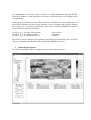
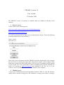
FRIOWL Version 1.0
User’s Guide
17 October 2003
The FRIOWL version 1.0 interface is available either on CD-Rom or directly on the
internet.
1. Internet Access
Click to either of the following sites:
http://www.unifr.ch/geoscience/gis/java/EsoMainImage.html
http://www.ixvision.de/friowl/java/
You will be presented with a login screen (example shown below). Enter the following
username and password (case-sensitive):
Name: esouser
Password: owl
Then click on the start button, and the FRIOWL interface should load. If the interface
does not load, try entering the login name and password again. If the webpage URLs
listed above present you with a blank white or grey screen, you probably need to upgrade
to Java version 1.4.2. You can do this by either a) installing Java from the CD-Rom (see
below) or b) going to http://java.sun.com and looking for the file j2re-1_4_2_01windows-i586.exe (windows) to download and install on your computer.
2. CD-Rom Access
A copy of the CD-Rom has been left with Marc Sarazin of ESO. To view the interface,
simply click or run the esoimageW.exe file (windows), esoimage-linux (linux), esoimage-
mac (Macintosh) or esoimage-solaris (solaris). You could alternatively copy all the files
from the CD-Rom to your hard drive and make a shortcut from your desktop to the
executable file.
If you get an error when you try to click or run the executable file, it is probable that you
do not have the latest version of Java installed on your computer (the interface requires
Java version 1.4.2 or greater). Fortunately, the new Java version installations are located
on the CD-Rom. They are as follows:
/jre/j2re-1_4_2_01-linux-i586-rpm.bin
/jre/j2re-1_4_2_01-solaris-sparc.sh
/jre/j2re-1_4_2_01-windows-i586.exe
- linux version
- sun solaris
- windows
Just click or run the relevant file listed above and follow the instructions. Once you have
Java 1.4.2 installed, you should be able to launch the FRIOWL interface
3. Launching the interface
You will be presented with a Java applet interface, such as shown below:
The interface is relatively easy to use. It consists of 5 frames within one user window.
The top-left frame houses the database, which you access and expand using simple clickand-point techniques (this frame is called “Files”). To the right is the main user windowframe (called “Main”), which displays the data file(s) you have chosen, together with a
chosen palette legend (frame called “Colors”). Below this is the user files box (frame
called “Selected Files”), in which your currently chosen files reside. At the bottom left of
the window is the “Options” frame, where you can change your operations, zoom, change
color palette or even save a map.
Navigation is simple; you just expand the database (frame “Files”) and click on the file
you are interested in. When you click on a file, it appears in your working frames
(“Selected Files”) below to the right. Each main folder has a series of subfolders, and the
data files are listed according to the month and year. You can now interrogate your
chosen files with options menu from the “Options” frame (bottom-left).
4. Description of Database
The main database has 11 different folders listed. These include the following
climatological variables (note: see Bugs in Section 8 also):
a) Longwave radiation; this is the monthly mean of outgoing longwave
radiation (olr) in Wm-2, as calculated by the NCEP / NCAR Reanalysis
model, at a grid resolution of 2.5°. The highest values are associated with
the warmest areas of the earth – because they radiate the greatest amounts
of longwave radiation to space. However, thin cirrus clouds trap a
significant amount of olr – thus, anomalously lower values of olr indicate
the higher than normal presence of cirrus clouds (e.g. compare the maps of
Jan 1998 and Jan 1999, which show a strong El Nino pattern in the Pacific
– on how to do this, see Examples in Section 6).
b) Air 2 metres (air2m); this is the mean monthly surface temperatures in
Kelvin (calculated for standard weather station height of 2m), as
determined by the NCEP / NCAR Reanalysis Model at a grid resolution of
1.875°.
c) Total cloud cover (tcc): this is the mean monthly total cloud cover in
fractions (1.0 = completely cloudy, 0.0= completely clear), as estimated
for each pixel by the ECMWF Reanalysis Model at a grid resolution of
2.5°.
d) Wind 0m (correction, this should read “0m”, not “0mb”) direction: These
are the directional frequencies of winds for 8 different compass points
(North, North-east, East, South-east, South, South-west, West and Northwest). Each map shows the wind frequency for each direction (in
fractions, 1.0= 100% frequency, 0.0= no frequency at all) e.g. clicking on
WEST for January 1979 shows the % fraction of days with a westerly
wind blowing at each pixel. The ECMWF Reanalysis model at a grid
resolution of 2.5° was used to calculate these maps.
e) Wind 0m speed: These are the mean windspeeds for each wind direction
based on the same 8 compass points (North, North-east, East, South-east,
South, South-west, West and North-west). The ECMWF Reanalysis model
f)
g)
h)
i)
j)
k)
at a grid resolution of 2.5° was used to calculate these maps; the units are
ms-1.
Wind 200mb direction; as “0m” above, but for the 200mb level. This level
is often used as an indication of jetstream or tropopause level winds.
Wind 200mb speed; as above.
Wind 850mb direction; ditto, as above.
Wind 850mb speed; ditto.
Precipitable water vapour; this is mean monthly precipitable water content
(in kg m-2, or mm), as derived from the NCEP / NCAR Reanalysis model
at a grid resolution of 2.5°.
Aerosol: these are monthly means of aerosol index (a NOAA unit, 4= sun
obscured by haze), as calculated by the satellites Nimbus-7 and Total
Ozone Mapping Spectrometer (TOMS), at a resolution of 1.25° by 1.0°.
Please note that it is best to use the BIPOL256 palette colormap, in order
to see the continental outlines.
5. Options Frame (bottom-left)
There are several different operations that can be undertaken on the data and the maps
displayed.
Firstly, using the “+” and “-“ buttons, one can zoom into areas of interest on the chosen
map, just click on the area of interest on the map. Click on the arrow button again to stop
zooming.
Secondly, you can choose different colormaps or palettes to display the maps. Please note
that the best ones for viewing aerosol data are BIPOL256, BIMOD256 or QUANT256.
Thirdly, you can choose an operation. These are simple mathematical operations
performed on the selection of maps in your user-window. The following are enacted:
a) AVERAGE: the arithmetic average of all chosen user-maps is displayed
b) SUM: the arithmetic sum of all chosen user-maps is displayed
c) MAX: the maximum pixel value of all pixels of the chosen user-maps is displayed
d) MIN: the minimum pixel value of all pixels of the chosen user-maps is displayed
e) ANOMALY: this is a special feature; firstly, you must click on the “+”sign to the
left of the file name in the “Selected files” frame, under “OP”. It will change to a
“-“ sign. When this occurs, the final map displayed is as follows;
anomaly = (average of all the “+” maps) – (average of all the “-“ maps).
f) Finally, you can save your composite maps as a “single” new map. This avoids
you having to click on the all the files again in the database window. The file is
saved in data format with the extension .ser, it can be found in the /USERFILES/
directory located in the database window (this file is saved locally when using the
CD-Rom, but on the server if using the internet).
6. An Example
Click on the total cloud cover folder, then on 1979, then on JAN. This transports the
January 1979 cloud cover file to your working window. Do the same for all Januarys
from 1979 to 1990 (this will take some time, but complete the exercise). We now have 12
individual cloud data files for 12 different Januarys. Now click on the Colormap option,
and change the colormap. Choose whichever one pleases you. Then click on the zoom
(“+”) button (in the “Options” frame) and click on the map to choose the area you want to
zoom towards. Click “-“ to zoom back out and then click the arrow button to stop the
zoom function.
Now click on the “Choose Operation” dropdown list. Choose AVERAGE. The map
displayed is now an average of all the maps displayed. Change your choice to “MAX”
and then “MIN”. The maps displayed are the maximum and minimum values of pixels of
all the maps displayed. Now choose “ANOMALY”. In order to make ANOMALY work,
you must click on the “+” sign to the left of the file name in the “Selected files” frame,
under “OP”. The plus sign will change to a “-“ sign. When this occurs, the final map
displayed is as follows;
anomaly = (average of all the “+” maps) – (average of all the “-“ maps).
Now click back to the AVERAGE function. Now save your final map as “tcc_mean_jan”
and click Save. Now go to the user window (“Selected Files” frame) again and click the
“X” on the far right of the screen, under “DEL”. This deletes maps from the current
window. Click the “X” for all the files, until you have none left in the user-window. Now
go to the database again, and look in the folder /USERFILES/. There you will find the
map you saved. This file is saved in ascii data format and resides in your local
/WINDOWS/ folder (if you are running the interface from the CD-Rom) or in an account
under your username on the server (if you are running the interface from the internet).
Click on this file, and immediately it is transported to your user-window. Note that the
new map is the average of all 12 files that you had to click individually before (this
option avoids you having to click all 12 files again).
Now delete all files from the user window, and go to the Longwave Radiation folder.
Click on Jan 1998 and Jan 1999 to transport these files to your working directory. Choose
“Anomaly” operation under “Choose Operation”. Change the “+”sign for Jan 1999 to a
“-“ sign. Note the large anomalies over the equatorial south Pacific and Indonesia,
indicative of a strong El Nino pattern.
7. Notes on the format of folders on the CD-Rom
All data files are in single column ASCII format with the extension .rst (IDRISI raster
file format). They can be found on the CD-Rom in the /rst/ folder. The reason for this
format is because the original interface was based on IDRISI file specifications.
8. Bugs to date (17/10/2003)
a) olr: please note that the data on the CD-Rom from April-December 1978
is corrupt.
b) Air2m: please note that the latitude / longitude co-ordinates are currently
back-to-front, so any analysis will be incorrect.
c) Wind 0mb: this is incorrectly labeled, it should read “0m, i.e. surface
level”, not 0mb; also, the data is currently upside down / x-reversed.
d) All wind folders: the data is currently upside down / x-reversed.
e) aerosol: please note that the data is 180° out of longitude alignment, so
any analyses at this stage is incorrect; also, the interface crashes if you try
to overlay aerosol maps with other variables (due to the different file size
resolutions).
f) Clicking on an operation while zooming doesn’t work
9. Improvements foreseen in the future
With each improvement of the FRIOWL interface, we will update the version number.
As a result of the meeting with ESO scientists in Munich on 14 October 2003, we will try
to enact the following features in later versions:
a) Fix bugs
b) Include a topographical layer
c) Ability to overlay layers, using weighting functions for each layer, in
order to create a new composite layer (e.g. choose me a place which has
less than one tenth of cloudiness, is greater than 2500m altitude and has
less than 5mm precipitable water content).
d) Change applet window size to be in accordance with user’s resolution
e) Include another frame which gives a definition of the chosen variable and
its units when user clicks on a pixel
f) Include a seismicity layer
g) Have a Root Mean Square (rms) option, made from daily data
h) To save space, possibly concentrate on 2000-5000m areas, and ignore seas
i) At a later stage, add ability to zoom into 3 or 4 pre-selected chosen areas,
which will have a new more detailed database.
j) Severe weather option: windstorms, lightning, snow
k) Ability to save image as a GIF or JPEG
l) Ability for movies (possibly)
m) Marc doesn’t want to have to click on 40 files at a time, perhaps include
an ability to multi-select (e.g. such as in Windows Explorer)
n) Delete button option for user-files
o) Get rid of SUM option
p) There is a little confusion as to when a file is saved. Perhaps clear the text
box afterwards.
q) After loading, we need to be able to look at the images individually,
therefore, include a NEUTRAL / NO OPERATION option, or SINGLE
IMAGE DISPLAY option.
r) Password change option
s) Exit button option
10. Comments, questions and discussion
Further comments and questions can be placed on the FRIOWL Discussion platform,
specially created for the FRIOWL interface, available on the web at
http://www.dynabyte.ch/cgi-bin/yabb/YaBB.cgi . This file is also available for
reading
there
at
http://www.unifr.ch/geoscience/gis/eddie/FRIOWL_version_1.0_README.doc .
Just use one of the following login usernames:
Name
Password
sarazinm
marc
esouser
owl
Alternatively, just send an email to [email protected] with your comments,
questions or suggestions.
Have fun playing!
Eddie Graham
University of Fribourg, Switzerland
17 October 2003