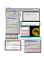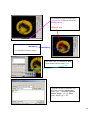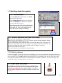
1
Bioimaging Platform
Quick Start
Zeiss LSM 510
User Manual:
Adapted from Wright: Cell Imaging Facility
Toronto Western Research Institute
Table of Contents
1
START HARDWARE.......................................................................................................................
3
2
START SOFTWARE........................................................................................................................
4
3
START LASERS .............................................................................................................................
5
4
FIND THESPECIMEN (AXIOPLAN 2) .....................................................................................................
6
5
CONFOCAL FILTER SET CONFIGURATION.................................................................................
8
6
ACQUIRE PRELIMINARY CONFOCAL IMAGE............................................................................... 9
7
OPTIMIZING THE SETTINGS........................................................................................................
10
7.1. GETTING THE DISPLAY READY....................................................................................................
7.2. SCAN CONTROL: CHANNELS WINDOW .........................................................................................
7.3. ACQUIRING YOUR FINAL IMAGE ..................................................................................................
10
12
15
8
SAVING YOUR FINAL IMAGE ......................................................................................................
17
9
ACQUIRING A Z-SERIES..............................................................................................................
18
10
ADVANCED OPTIONS ............................................................................................................
20
10.1. SINGLE-TRACK – SIMULTANEOUS ACQUISITION ............................................................................
20
10.1.1. Getting the display ready .............................................................................................
10.1.2. Optimise settings.........................................................................................................
20
20
10.2. Z-ATTENUATION COMPENSATION................................................................................................
10.3. TRANSMITTED LIGHT IMAGE.......................................................................................................
10.4. FRAP...................................................................................................................................
21
22
23
SHUTTING DOWN THE SYSTEM.............................................................................................
25
11.1. TURN OFF LASERS ...................................................................................................................
11.2. REMOVE SPECIMEN AND CLEAN MICROSCOPE ..............................................................................
11.3. EXIT THE SOFTWARE ................................................................................................................
11.4. POWER DOWN THE SYSTEM .......................................................................................................
25
25
25
25
BEAMPATH CONFIGURATION GUIDE………………………………………………………………..
26
11
12
2
1. Start Hardware
Turn on:
a) the mercury short arc lamp light switch (situated under the microscope table).
Note: Whenever the mercury lamp is turned on, it should be left on for at least 30 minutes.
Once the lamp has been turned off, it should not be turned on again for 30 minutes.
b) Remote control
c) PC power
3
2. Start software
•
•
Log on to Win2000 (you will be issued with a username and password during training).
Double click the LSM 510 desktop icon.
•
The Zeiss LSM 510 switchboard window will appear
•
Make sure Scan New Images is pressed and then click the Start expert mode button. If Scan
New Images is not pressed, the software will start but no initialize the hardware.
4
3. Start Lasers
Click the Acquire button on the
toolbar. The lower toolbar will now
change to the Acquire sub-toolbar and
show the acquisition controls.
Click the Laser button.
Turn on the desired lasers position: HeNe’s to ON, Argon to Standby. When the Status reads
Ready, click the On buttons.
Also turn OFF any lasers that have been left on for you, but you will not be using. If the previous
user has left the lasers on for you, Argon and Enterprise may already be in standby mode and
ready to be tuned on. When all the Status reads Ready, close the Laser Control window.
5
4. Find the specimen
The light path select,
focus knob
are manual controls. For security
reasons the stage can be blocked.
If this is the case press one of the
small buttons (up or down) on
the left side of the microscope
and simultaneously turn the focus
knob until you see your specimen
in focus.
The stage is motorized and
controlled by a joy stick. The rest
of the microscope Filter cubes,
light path lasers etc.) is controlled
by the software. For setup of
these controls please ask the
facility staff.
6
To set up the Axiovert microscope to locate your specimen first move the light path selector to
VIS.
Move the correct objective into place.
Do not use air-objectives after an immersion objective without wiping the
immersion liquid (water or oil) from the specimen and objective.
Once you have found your specimen, pull the light path selector out to the LSM position. The
microscope will automatically change the filter-position and shutter the light sources. If you fail to
do this you will receive an error when you try to acquire a confocal image.
7
5. Confocal filter set configuration
Click the Config button (in the Acquire sub-toolbar).
To activate multi-tracking simply chose the
MultiTrack
button in the Configuration Control window. (For single track acquisition see page…)
Load the configuration that matches
your fluorophores (referred to as
‘tracks’) by clicking the
Config button. *
* for precise instructions on how
to set a new beampath, see
‘BEAMPATH CONFIGURATION
GUIDE’ on page 26
•
Click on the drop down box and select a desired configuration, apply then close. If you cannot see the
appropriate configuration for your fluorophores, contact Facility staff.
8
6. Acquire preliminary confocal image
Set the light path selector to LSM
position
You will see an image looking something like this.
9
7. Optimizing the settings
Due to the sequential nature of ‘Multi-track’ acquisition optimizing the settings in this mode is
difficult. It is easier to set the imaging parameters for each Track individually. You can do this by
switching off each track with the checkbox along side it. Turn off all but one channel now.
7.1. Getting the display ready
This current type of display does not allow fine tuning of the imaging parameters and so needs to be
adjusted.Optimizing the confocal settings is best done with the image pseudo-colored to highlight saturated
and zero value pixels.
To do this, first click Palette on the image window tool bar and the Color Palette window will open.
Click Range Indicator and close the window
Now you will have an image where red represents the saturated pixels
(i.e. =255) and the blue represents the black pixels (i.e. zero).
10
Your image window will now look like this.
11
7.2. Scan control: Channels window
Scancontrol window.
Click on the Channels button of the
Scan control window.
The active channel will appear here.
The settings below need to be adjusted
for each channel separately.
1.) Set Pinhole of each channel:
The pinhole diameter determines the thickness of the optical
section – i.e. the axial
resolution. By increasing the pinhole diameter (and therefore
optical section) you are
also increasing the amount of out of focus fluorescence being
detected. Start with
each at the optimum (1 Airy Unit) by clicking the
1 button.
This will give different Optical Slice values for each channel.
Increase the pinholes
of the shorter wavelength channels to match the longest
wavelength.
Do not go below 1 Airy unit – you will lose signal with no
significant improvement
in axial resolution. Adjust the Pinhole for each channel so that
they have the same
optical slice (typically the green channel will be ~ 1.1 Airy
units).
2.) Check focal plane
Click the Fast scan
button to start acquiring a high-speed, low quality image. Use
this mode to focus up
and down through the specimen to get the desired focal plane.
12
You need to set the detector range to match the dimmest and brightest signal from the specimen.
Setting the detector incorrectly results in the loss of information from the specimen.
3.) Set Ampl. Offset – setting the ‘min’ signal This should be set next, but may need re-setting later.
While acquiring with the Fast scan button, adjust the Amp. Offset so that only a few of the pixels in the
background of the image are blue. If you have a lot of blue colour in the background, move the slider to the
right.
4.) Set Detector Gain and Excitation power – setting the ‘max’ signal The ‘max’ signal is set by
adjusting the detector gain and laser transmission simultaneously. You need to empirically work out
the best laser power settings – low laser power causes less bleaching but requires the detector gain to be set
high; which introduces noise.
Whilst acquiring with the Fast scan button, adjust/increase the Detector Gain so that you get a bright
image, but not too many red (saturated) pixels and not too much noise. You may need to adjust the Ampl.
Offset if you increase the Detector Gain a lot. Around 600 is a good start. This should be set in
conjunction with the excitation intensity.
5.) Set Ampl. Gain Leave as 1 unless you have a very dim signal and nothing else works. This will amplify
noise as well as signal.
13
A few red speckles; a few blue speckles
After you have set both channels, stop scanning by pressing the Stop button in the Scan Control
window. Your image will look like this (above).
Turn off the optimised
channel in the
Configuration Control
window. Turn on the next
channel and optimise these
settings for this channel
14
7.3. Acquiring your final image
Once you are satisfied that each channels detector is set optimally to the range of the image, you can create
your final image. Ensure that all Tracks are checked when acquiring the final image.
Go to the Scan control window and click the Mode button.
Change the Frame size by clicking on the Optimal button
Noise can be reduced by averaging a
number of frames and slowing the scan
speed.
In the first instance, try the following
values:
Mode: line
Method: mean
Number: 2
Scan speed: 6
Change the image Palette back to No Palette.
Click Palette
on the image window tool bar and the Color Palette window
will open
Click No Palette and close the window
15
Click on the
Single button in
the scan control
window to
collect your
final image
(bottom).
Click on the image window Info button. This will bring up a bar on the left of the image window with the
image information on it.
16
8. Saving your final image
When you are satisfied with your image you need to save it to your database. Images are
saved to Databases. A database can be single or multiple images or stacks.
Press Save as
in the image window and the Save Image and
Parameter
window will open.
You can now chose to add your image to an existing
database
(Open MDB button), or create a new database
(New MDB button)
Name the file and include any other information in
the description of
notes sections.
Do not select Compress file option.
17
9. Acquiring a Z-series
Having set the system to acquire a satisfactory image, you can acquire a z-series. It may be worthwhile
changing the frame size to 512×512 to minimize file size and to speed acquisition.
Click on the Z-Stack button in the
Scan control
Using Fast scan mode to acquire
a continuo specimen. Focus up and
do microscope focus wheel to
specimen is in the centre of the
field of view and the microscope is
focused in the middle of the
specimen.
Stop acquisition.
You can now precisely define the
depth of your z-series.
Ensure the Num Slices = 20 and
the Interval = 1 µm at this point to
ensure the top and bottom of the
specimen is located.
Click the Range
button from the Scan control
window – this will generate a side
view of you specimen. This button
is not available if the
MarkFirst/Last button is
depressed.
(LEFT) The green line
represents the middle of your
z-series. The upper red line
represents the top and the
lower red line the bottom of
the z-series. (RIGHT) Drag
the green line to the centre of
the specimen and the red
lines to just outside the top
and bottom of the specimen.
18
In the Scan control window, click the Z-slice button to bring up the Optical Slice dialog
In the Scan control window, click the
Zslice
button to bring up the Optical Slice
dialog
Click the Optimal Interval
button. Check that optical section
for each channel is the same and close. If
your optical
sections are different for each wavelength go
to
Mode/Channels and adjust the Pinhole
so that each
channel has the same optical section –
around 1 Airy
unit, but one channel will have to be slightly
larger.
Readjust the red lines that indicate the top
and bottom of the specimen (Step 7 above).
Reduce the Frame Size also if possible to
speed stack-acquisition.
To acquire your z-series stack click the Start
button.
The system will begin
scanning the specimen.
You can check progress by
selecting Gallery button
on the image window
sidebar.
19
10. Advanced Options
10.1. Single-Track – simultaneous acquisition Multi-track can solve the problem of crosstalk. Typically this occurs with bleed through of green fluorescence in to the red channel. Multi Track
avoids this by acquiring the fluorescent channels sequentially, not simultaneously as with Single Track
acquisition. In Multi Track mode the red channel detector is turned on, the green one off. Then the red
fluorophore is imaged. The red channel detector is then turned off, the green one on and the green
fluorophore
imaged. Any bleed through of fluorescence from the green fluorophore to the red detector does not register.
This switching between tracks means that there is a delay between channels. Sometimes this is
unacceptable, in particular for live cell imaging where the cell can move between channels creating
artefacts. In this case Single track mode should be used.
To load pre-designated configurations click
the Config button in the Configuration
control window.
10.1.1. Getting the display ready
For multi-label experiments, it is best to have both
channels displayed at once. To do this: In the Live
image window’s Display side-bar, click the Split xy
button This will make your image small so resize (usual
Windows mouse-drag). Then click on the Zoom button
to bring up the Zoom sidebar and select Auto button
10.1.2. Optimise settings
Unlike Sequential acquisition (Multi-Track), each channel is acquired
simultaneously during optimization – so be quick! Refer to section 7.2 for
instructions on how to optimize the channel settings.
20
10.2. Z-attenuation compensation
As images are collected deeper in to the sample there can be significant loss of signal. This can be caused
but refractive index mismatch, light scattering and absorption. This signal loss can be compensated for
collecting the attenuated slices with higher gains and/or with higher laser intensity. Two reference points are
set, one near the top where the signal is the brightest, and one near the bottom where there is still significant
signal but it has been attenuated. The laser intensity and gains are set for each reference slice (the bottom
reference slice having higher gain/laser). As the software acquires the z-series, it gradually steps up the gain
and laser as it approaches the bottom reference slice.
1. In the Scan Control: Z-settings window activate the Auto Z.Corr.
2. While in Fast XY
scan mode, focus to near the top,
of the sample where it is brightest.
You should have already set the
detector and laser settings for this
slice. If not go the Scan Control:
Channels window and set
the detector gains and laser
intensity to get adequate
signal at this focus position.
3.
In the Scan Control: Z-settings window click Set A.
4.
While in Fast XY scan, manually focus to the near the bottom of the z-series which still has
significant signal.
5. Go to the Scan Control:
Channels window and set
the detector gains and laser
intensity to get adequate
signal at this focus position.
6. Go back to the Scan Control: Z-settings window and click the Set B button.
7. Now start the Z-series acquisition by clicking Start.
21
10.3. Transmitted light image
Whilst the laser is scanning the field of
view a certain amount of the excitation
laser light passes through the specimen.
This light can be detected and its intensity
in each part of the field of view corresponds
to the transmitted light optical properties of
the specimen. In this way a “brightfield”
transmitted image can be reconstructed. It is
not a “confocal” image in that the light does
not come from a single plane.
DIC – differential interference contrast
BF – bright field
DF – dark field
For this, the microscope transmitted path needs to
be set correctly. Open the Microscope Control
panel (Toolbar Acquire then Micro)
The Field Stop iris needs to be fully opened –
100%.
The Filter at 100%
The transmitted light to be at 0%.
Click o the Condensor button to reveal the
condensor options
The Condensor Filter needs to be set to the
appropriate type of brightfield i.e. BF, DIC,
DF or Ph.
NOTE: The software keeps changing the
condensor settings back to “BF”. Keep
checking that it is set correctly.
Then, whilst in fast scan mode, adjust the transmitted light channel’s (ChD) detector gain and offset so that
the background of the image is mid-grey and the brightest part of the image is near saturation (i.e. shows red
with the Range Indicator palette).
22
10.4. FRAP
1. Click on Edit Bleach toolbar button to open up Bleach Control dialog.
2. Set Bleach parameters in Bleach Control
dialog Check Bleach after Number of Scans
Set “Scan Number” to for pre-bleach
imaging Set “Iterations” value – this may
require empirical determination. It needs to
be enough to allow complete bleaching but
few enough to allow quick return to imaging.
Try 10 as a first attempt. In “Excitation of
Bleach Track” set bleaching laser to 100%
3. Click Define Region button to select bleach
area
4. Define area to bleach then select it by ticking the
checkbox along side the ROI. Close dialog.
5. Open Time Series Control dialog by clicking the
TimeSeries button in the main toolbar.
5. Set FRAP time-course in Time Series
Control Dialog
Start Series = Manual.
Stop Series = select Time then enter the
duration of the experiment.
Enter Cycle Delay (time between frames).
7. Click “StartB” to start experiment.
23
Experimental progress shown here.
Progress bar will pause during the
bleach process.
Bleached area
7. Save experiment
8. Create ROI reference image
Turn ROI white by clicking the ROI
colour button and selecting white
Export this image for reference via
the menu command File/Export.
Image Type = “Contents of Image
Window Single”. Save in MBD
folder. Image type = TIF.
24
11. Shutting down the system
11.1. Turn off lasers
Click the Acquire toolbar button, the Laser
button in the sub-toolbar.
In the Laser control window turn each laser
Off or to Standby if somebody is using the
system within the next hour.
If you have used the UV laser, switch off the
black switch in the white frame located on the
front of the UV laser power supply. Do not
touch any of the cooling unit settings.
11.2. Remove Specimen and clean microscope
Wipe off water from objective and specimen.
Move to a low power objective (5× or 10×) objective. Raise the stage using the buttons
on the left had side of the microscope base.
If you switch off the system while the stage is lowered the ‘top’ of the focus range will
be reset to that position when the microscope is next turned on. This will mean the ‘top’
will need resetting and could result in damage to the $12,000 63× objective.
Turn off the epifluorescence lamp.
Cover the microscope avoiding the hot lamp housing.
11.3. Exit the software
Exit the Zeiss LSM .A message will come up reminding you not to power down the system until the laser
iscool. Click OK.If you have left the lasers on for the next user, you will also be asked whether you wantthe
lasers switched off. Click No.Read then close the WCIF Exit screen.Burn your data to CD or copy across
network (once installed).Once you have finished with the computer, LOGOUT. If you do not logout, the
systemwill continue to charge time to your account.
11.4. Power down the system
If nobody has booked for the next hour, please shutdown the
system If the next person is the last booking of the day, please
call them and confirm that they will be using it. This requires
that the remote control be switched off and the compressed air
shut down.
25