1
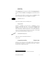
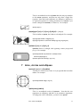
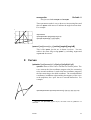
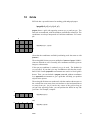
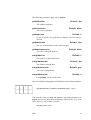
PSTricks:
leecheng
PostScript macros for Generic TeX.
M
g
m
Dripping Faucet
Mathematical Model for
a Dripping Faucet
User’s Guide
Timothy Van Zandt
12 March 1993
Version 0.93a
Author’s address:
Department of Economics, Princeton University,
Princeton, NJ 08544-1021, USA. Internet: [email protected]
Contents
Welcome to PSTricks
1
Part I
3
The Essentials
1 Arguments and delimiters
3
2 Color
4
3 Setting graphics parameters
5
4 Dimensions, coordinates and angles
7
5 Basic graphics parameters
8
Part II
Basic graphics objects
10
6 Lines and polygons
10
7 Arcs, circles and ellipses
11
8 Curves
13
9 Dots
15
10 Grids
17
11
Plots
19
Part III More graphics parameters
24
12 Coordinate systems
24
13 Line styles
24
14 Fill styles
27
15 Arrowheads and such
28
16 Custom styles
31
Part IV Custom graphics
32
17 The basics
32
18 Parameters
32
19 Graphics objects
33
Table of contents
1
20 Safe tricks
36
21 Pretty safe tricks
39
22 For hackers only
39
Part V
Picture Tools
41
23 Pictures
41
24 Placing and rotating whatever
42
25 Repetition
46
26 Axes
47
Part VI Text Tricks
52
27 Framed boxes
52
28 Clipping
54
29 Rotation and scaling boxes
55
Part VII Nodes and Node Connections
58
30 Nodes
59
31 Node connections
60
32 Attaching labels to node connections
66
Part VIII Special Tricks
70
33 Coils and zigzags
70
34 Special coordinates
71
35 Overlays
73
36 The gradient fill style
74
37 Adding color to tables
75
38 Typesetting text along a path
76
39 Stroking and filling character paths
77
40 Importing EPS files
78
Table of contents
2
41 Exporting EPS files
79
Help
82
A Boxes
82
B Tips and More Tricks
85
C Including PostScript code
86
D Troubleshooting
87
Table of contents
3
Welcome to PSTricks
PSTricks is a collection of PostScript-based TEX macros that is compatible with most TEX macro packages, including Plain TEX, LaTEX,
AMSTEX, and AMS-LaTEX. PSTricks gives you color, graphics, rotation, trees and overlays. PSTricks puts the icing (PostScript) on your
cake (TEX)!
To install PSTricks, follow the instructions in the file read-me.pst that
comes with the PSTricks package. Even if PSTricks has already been
installed for you, give read-me.pst a look over.
This User’s Guide verges on being a reference manual, meaning that it is
not designed to be read linearly. Here is a recommended strategy: Finish
reading this brief overview of the features in PSTricks. Then thumb
through the entire User’s Guide to get your own overview. Return to
Part I (Essentials) and read it carefully. Refer to the remaining sections
as the need arises.
When you cannot figure out how to do something or when trouble arises,
check out the appendices (Help). You just might be lucky enough to
find a solution. There is also a LaTEX file samples.pst of samples that is
distributed with PSTricks. Look to this file for further inspiration.
This documentation is written with LaTEX. Some examples use LaTEX
specific constructs and some don’t. However, there is nothing LaTEX
specific about any of the macros, nor is there anything that does not work
with LaTEX. This package has been tested with Plain TEX, LaTEX, AMSLaTEXand AMSTEX, and should work with other TEX macro packages
as well.
pstricks
The main macro file is pstricks.tex/pstricks.sty. Each of the PSTricks
macro files comes with a .tex extension and a .sty extension; these are
equivalent, but the .sty extension means that you can include the file
name as a LaTEX document style option.
There are numerous supplementary macro files. A file, like the one
above and the left, is used in this User’s Guide to remind you that you
must input a file before using the macros it contains.
For most PSTricks macros, even if you misuse them, you will not get
PostScript errors in the output. However, it is recommended that you
resolve any TEX errors before attempting to print your document. A
few PSTricks macros pass on PostScript errors without warning. Use
Welcome to PSTricks
1
PS
these with care, especially if you are using a networked printer, because
PostScript errors can cause a printer to bomb. Such macros are pointed
out in strong terms, using a warning like this one:
Warning: Use macros that do not check for PostScript
errors with care. PostScript errors can cause a printer to
bomb!
Keep in mind the following typographical conventions in this User’s
Guide.
• All literal input characters, i.e., those that should appear verbatim
in your input file, appear in upright Helvetica and Helvetica-Bold
fonts.
• Meta arguments, for which you are supposed to substitute a value
(e.g., angle) appear in slanted Helvetica-Oblique and HelveticaBoldOblique fonts.
• The main entry for a macro or parameter that states its syntax
appears in a large bold font, except for the optional arguments,
which are in medium weight. This is how you can recognize the
optional arguments.
• References to PSTricks commands and parameters within paragraphs are set in Helvetica-Bold.
Welcome to PSTricks
2
I
The Essentials
1 Arguments and delimiters
Here is some nitty-gritty about arguments and delimiters that is really
important to know.
The PSTricks macros use the following delimiters:
Curly braces
{arg }
Brackets (only for optional arguments)
[arg ]
Parentheses and commas for coordinates
= and , for parameters
(x , y )
par1=val1, …
Spaces and commas are also used as delimiters within arguments, but
in this case the argument is expanded before looking for the delimiters.
Always use a period rather than a comma to denote the decimal point,
so that PSTricks doesn’t mistake the comma for a delimiter.
The easiest mistake to make with the PSTricks macros is to mess up the
delimiters. This may generate complaints from TEX or PSTricks about
bad arguments, or other unilluminating errors such as the following:
! Use of \get@coor doesn’t match its definition.
! Paragraph ended before \pst@addcoor was complete.
! Forbidden control sequence found while scanning use of \check@arrow.
! File ended while scanning use of \lput.
Delimiters are generally the first thing to check when you get errors with
a PSTricks macro.
Since PSTricks macros can have many arguments, it is useful to know
that you can leave a space or new line between any arguments, except
between arguments enclosed in curly braces. If you need to insert a
new line between arguments enclosed in curly braces, put a comment
character % at the end of the line.
The Essentials
3
As a general rule, the first non-space character after a PSTricks macro
should not be a [ or (. Otherwise, PSTricks might think that the [ or ( is
actually part of the macro. You can always get around this by inserting
a pair {} of braces somewhere between the macro and the [ or (.
2 Color
The grayscales
black, darkgray, gray, lightgray, and white,
and the colors
red, green, blue, cyan, magenta, and yellow
are predefined in PSTricks.
This means that these names can be used with the graphics objects that
are described in later sections. This also means that the command \gray
(or \red, etc.) can be used much like \rm or \tt, as in
{\gray This stuff should be gray.}
The commands \gray, \red, etc. can be nested like the font commands
as well. There are a few important ways in which the color commands
differ from the font commands:
1. The color commands can be used in and out of math mode (there
are no restrictions, other than proper TEX grouping).
2. The color commands affect whatever is in their scope (e.g., lines),
not simply characters.
3. The scope of the color commands does not extend across pages.
4. The color commands are not as robust as font commands when
used inside box macros. See page 89 for details. You can avoid
most problems by explicitly grouping color commands (e.g., enclosing the scope in braces {}) whenever these are in the argument
of another command.1
1
However, this is not necessary with the PSTricks LR-box commands, expect when
\psverbboxtrue is in effect. See Section A.
Color
4
You can define or redefine additional colors and grayscales with the
following commands. In each case, numi is a number between 0 and 1.
Spaces are used as delimiters—don’t add any extraneous spaces in the
arguments.
\newgray{color }{num}
num is the gray scale specification, to be set by PostScript’s setgray
operator. 0 is black and 1 is white. For example:
\newgray{darkgray}{.25}
\newrgbcolor{color }{num1 num2 num3 }
num1 num2 num3 is a red-green-blue specification, to be set by
PostScript’s setrgbcolor operator. For example,
\newrgbcolor{green}{0 1 0}
\newhsbcolor{color }{num1 num2 num3 }
num1 num2 num3 is an hue-saturation-brightness specification,
to be set by PostScript’s sethsbcolor operator. For example,
\newhsbcolor{mycolor}{.3 .7 .9}
\newcmykcolor{color }{num1 num2 num3 num4 }
num1 num2 num3 num4 is a cyan-magenta-yellow-black specification, to be set by PostScript’s newcmykcolor operator. For
example,
\newcmykcolor{hercolor}{.5 1 0 .5}
For defining new colors, the rbg model is a sure thing. hsb is not
recommended. cmyk is not supported by all Level 1 implementations of
PostScript, although it is best for color printing. For more information on
color models and color specifications, consult the PostScript Language
Reference Manual, 2nd Edition (Red Book), and a color guide.
Driver notes:
The command \pstVerb must be defined.
3 Setting graphics parameters
PSTricks uses a key-value system of graphics parameters to customize
the macros that generate graphics (e.g., lines and circles), or graphics
combined with text (e.g., framed boxes). You can change the default
values of parameters with the command \psset, as in
Setting graphics parameters
5
\psset{fillcolor=yellow}
\psset{linecolor=blue,framearc=.3,dash=3pt 6pt}
The general syntax is:
\psset{par1=value1,par2=value2,… }
As illustrated in the examples above, spaces are used as delimiters for
some of the values. Additional spaces are allowed only following the
comma that separates par =value pairs (which is thus a good place to start
a new line if there are many parameter changes). E.g., the first example
is acceptable, but the second is not:
\psset{fillcolor=yellow, linecolor=blue}
\psset{fillcolor= yellow,linecolor =blue }
The parameters are described throughout this User’s Guide, as they are
needed.
Nearly every macro that makes use of graphics parameters allows you
to include changes as an optional first argument, enclosed in square
brackets. For example,
\psline[linecolor=green,linestyle=dotted](8,7)
draws a dotted, green line. It is roughly equivalent to
{\psset{linecolor=green,linestyle=dotted}\psline(8,7)}
For many parameters, PSTricks processes the value and stores it in a
peculiar form, ready for PostScript consumption. For others, PSTricks
stores the value in a form that you would expect. In the latter case, this
User’s Guide will mention the name of the command where the value
is stored. This is so that you can use the value to set other parameters.
E.g.,
\psset{linecolor=\psfillcolor,doublesep=.5\pslinewidth}
However, even for these parameters, PSTricks may do some processing
and error-checking, and you should always set them using \psset or as
optional parameter changes, rather than redefining the command where
the value is stored.
Setting graphics parameters
6
4 Dimensions, coordinates and angles
Whenever an argument of a PSTricks macro is a dimension, the unit is
optional. The default unit is set by the
unit=dim
Default: 1cm
parameter. For example, with the default value of 1cm, the following
are equivalent:
\psset{linewidth=.5cm}
\psset{linewidth=.5}
By never explicitly giving units, you can scale graphics by changing the
value of unit.
You can use the default coordinate when setting non-PSTricks dimensions as well, using the commands
\pssetlength{cmd }{dim}
\psaddtolength{cmd }{dim}
where cmd is a dimension register (in LaTEX parlance, a “length”), and
dim is a length with optional unit. These are analogous to LaTEX’s
\setlength and \addtolength.
Coordinate pairs have the form (x , y ). The origin of the coordinate
system is at TEX’s currentpoint. The command \SpecialCoor lets you use
polar coordinates, in the form (r ;a), where r is the radius (a dimension)
and a is the angle (see below). You can still use Cartesian coordinates.
For a complete description of \SpecialCoor, see Section 34.
The unit parameter actually sets the following three parameters:
xunit=dim
yunit=dim
runit=dim
Default: 1cm
Default: 1cm
Default: 1cm
These are the default units for x-coordinates, y-coordinates, and all
other coordinates, respectively. By setting these independently, you can
scale the x and y dimensions in Cartesian coordinate unevenly. After
changing yunit to 1pt, the two \psline’s below are equivalent:
\psset{yunit=1pt}
\psline(0cm,20pt)(5cm,80pt)
\psline(0,20)(5,80)
Dimensions, coordinates and angles
7
The values of the runit, xunit and yunit parameters are stored in the
dimension registers \psunit(also \psrunit), \psxunit and \psyunit.
Angles, in polar coordinates and other arguments, should be a number
giving the angle in degrees, by default. You can also change the units
used for angles with the command
\degrees[num]
num should be the number of units in a circle. For example, you might
use
\degrees[100]
to make a pie chart when you know the shares in percentages. \degrees
without the argument is the same as
\degrees[360]
The command
\radians
is short for
\degrees[6.28319]
\SpecialCoor lets you specify angles in other ways as well.
5 Basic graphics parameters
The width and color of lines is set by the parameters:
linewidth=dim
linecolor=color
Default: .8pt
Default: black
The linewidth is stored in the dimension register \pslinewidth, and the
linecolor is stored in the command \pslinecolor.
The regions delimited by open and closed curves can be filled, as determined by the parameters:
Basic graphics parameters
8
fillstyle=style
fillcolor=color
When fillstyle=none, the regions are not filled. When fillstyle=solid, the
regions are filled with fillcolor. Other fillstyle’s are described in Section
14.
The graphics objects all have a starred version (e.g., \psframe*) which
draws a solid object whose color is linecolor. For example,
\psellipse*(1,.5)(1,.5)
Open curves can have arrows, according to the
arrows=arrows
parameter. If arrows=-, you get no arrows. If arrows=<->, you get
arrows on both ends of the curve. You can also set arrows=-> and
arrows=<-, if you just want an arrow on the end or beginning of the
curve, respectively. With the open curves, you can also specify the
arrows as an optional argument enclosed in {} brackets. This should
come after the optional parameters argument. E.g.,
\psline[linewidth=2pt]{<-}(2,1)
Other arrow styles are described in Section 15
If you set the
showpoints=true/false
Default: false
parameter to true, then most of the graphics objects will put dots at
the appropriate coordinates or control points of the object.2 Section 9
describes how to change the dot style.
2
The parameter value is stored in the conditional \ifshowpoints.
Basic graphics parameters
9
II
Basic graphics objects
6 Lines and polygons
The objects in this section also use the following parameters:
Default: 0pt
linearc=dim
The radius of arcs drawn at the corners of lines by the \psline and
\pspolygon graphics objects. dim should be positive.
Default: 0
framearc=num
In the \psframe and the related box framing macros, the radius
of rounded corners is set, by default, to one-half num times the
width or height of the frame, whichever is less. num should be
between 0 and 1.
cornersize=relative/absolute
Default: relative
If cornersize is relative, then the framearc parameter determines
the radius of the rounded corners for \psframe, as described above
(and hence the radius depends on the size of the frame). If
cornersize is absolute, then the linearc parameter determines the
radius of the rounded corners for \psframe (and hence the radius
is of constant size).
Now here are the lines and polygons:
\psline*[par]{arrows }(x0 ,y0 )(x1,y1)… (xn,yn)
This draws a line through the list of coordinates. For example:
2
1
\psline[linewidth=2pt,linearc=.25]{->}(4,2)(0,1)(2,0)
0
0
1
2
3
4
\qline(coor0)(coor1)
Basic graphics objects
10
This is a streamlined version of \psline that does not pay attention
to the arrows parameter, and that can only draw a single line
segment. Note that both coordinates are obligatory, and there is
no optional argument for setting parameters (use \psset if you
need to change the linewidth, or whatever). For example:
1
\qline(0,0)(2,1)
0
0
1
2
\pspolygon*[par](x0 ,y0 )(x1,y1)(x2 ,y2 )… (xn,yn)
This is similar to \psline, but it draws a closed path. For example:
2
\pspolygon[linewidth=1.5pt](0,2)(1,2)
\pspolygon*[linearc=.2,linecolor=darkgray](1,0)(1,2)(4,0)(4,2)
1
0
0
1
2
3
4
\psframe*[par](x0 ,y0 )(x1,y1)
\psframe draws a rectangle with opposing corners (x0 , y0 ) and
(x1, y1). For example:
2
\psframe[linewidth=2pt,framearc=.3,fillstyle=solid,
fillcolor=lightgray](4,2)
\psframe*[linecolor=white](1,.5)(2,1.5)
1
0
0
1
2
3
4
7 Arcs, circles and ellipses
\pscircle*[par](x0 ,y0 ){radius }
This draws a circle whose center is at (x0 , y0 ) and that has radius
radius. For example:
2
1
\pscircle[linewidth=2pt](.5,.5){1.5}
0
-1
-1
0
1
2
\qdisk(coor){radius }
This is a streamlined version of \pscircle*. Note that the two
arguments are obligatory and there is no parameters arguments.
To change the color of the disks, you have to use \psset:
Arcs, circles and ellipses
11
\psset{linecolor=gray}
\qdisk(2,3){4pt}
\pswedge*[par](x0 ,y0 ){radius }{angle1}{angle2 }
This draws a wedge whose center is at (x0 , y0 ), that has radius
radius, and that extends counterclockwise from angle1 to angle2 .
The angles must be specified in degrees. For example:
2
1
\pswedge[linecolor=gray,linewidth=2pt,fillstyle=solid]{2}{0}{70}
0
0
1
2
\psellipse*[par](x0 ,y0 )(x1,y1)
(x0 , y0 ) is the center of the ellipse, and x1 and y1 are the horizontal
and vertical radii, respectively. For example:
1
0
\psellipse[fillcolor=lightgray](.5,0)(1.5,1)
-1
-1
0
1
2
\psarc*[par]{arrows }(x , y ){radius }{angleA}{angleB}
This draws an arc from angleA to angleB , going counter clockwise,
for a circle of radius radius and centered at (x , y ). You must include
either the arrows argument or the (x , y ) argument. For example:
2
1
\psarc*[showpoints=true](1.5,1.5){1.5}{215}{0}
0
0
1
2
3
See how showpoints=true draws a dashed line from the center to
the arc; this is useful when composing pictures.
\psarc also uses the parameters:
arcsepA=dim
Default: 0pt
angleA is adjusted so that the arc would just touch a line of
width dim that extended from the center of the arc in the
direction of angleA.
arcsepB=dim
Default: 0pt
This is like arcsepA, but angleB is adjusted.
Arcs, circles and ellipses
12
arcsep=dim
This just sets both arcsepA and arcsepB.
Default: 0
These parameters make it easy to draw two intersecting lines and
then use \psarc with arrows to indicate the angle between them.
For example:
3
2
\SpecialCoor
\psline[linewidth=2pt](4;50)(0,0)(4;10)
\psarc[arcsepB=2pt]{->}{3}{10}{50}
1
0
0
1
2
3
4
\psarcn*[par]{arrows }(x , y ){radius }{angleA}{angleB}
This is like \psarc, but the arc is drawn clockwise. You can
achieve the same effect using \psarc by switching angleA and
angleB and the arrows.3
8 Curves
\psbezier*[par]{arrows }(x0 ,y0 )(x1,y1)(x2 ,y2 )(x3 ,y3 )
\psbezier draws a bezier curve with the four control points. The
curve starts at the first coordinate, tangent to the line connecting
to the second coordinate. It ends at the last coordinate, tangent to
the line connecting to the third coordinate. The second and third
coordinates, in addition to determining the tangency of the curve
at the endpoints, also “pull” the curve towards themselves. For
example:
\psbezier[linewidth=2pt,showpoints=true]{->}(0,0)(1,4)(2,1)(4,3.5)
3
However, with \pscustom graphics object, described in Part IV, \psarcn is not
redundant.
Curves
13
showpoints=true puts dots in all the control points, and connects
them by dashed lines, which is useful when adjusting your bezier
curve.
\parabola*[par]{arrows }(x0 , y0 )(x1, y1)
Starting at (x0 , y0 ), \parabola draws the parabola that passes
through (x0 , y0 ) and whose maximum or minimum is (x1, y1). For
example:
3
2
\parabola*(1,1)(2,3)
\psset{xunit=.01}
\parabola{<->}(400,3)(200,0)
1
0
0
1
2
3
4
The next three graphics objects interpolate an open or closed curve
through the given points. The curve at each interior point is perpendicular to the line bisecting the angle ABC, where B is the interior point,
and A and C are the neighboring points. Scaling the coordinates does
not cause the curve to scale proportionately.
The curvature is controlled by the following parameter:
curvature=num1 num2 num3
Default: 1 .1 0
You have to just play around with this parameter to get what
you want. Individual values outside the range -1 to 1 are either
ignored or are for entertainment only. Below is an explanation of
what each number does. A, B and C refer to three consecutive
points.
Lower values of num1 make the curve tighter.
Lower values of num2 tighten the curve where the angle ABC is
greater than 45 degrees, and loosen the curve elsewhere.
num3 determines the slope at each point. If num3 =0, then the
curve is perpendicular at B to the bisection of ABC. If num3 =-1,
then the curve at B is parallel to the line AC. With this value (and
only this value), scaling the coordinates causes the curve to scale
proportionately. However, positive values can look better with
irregularly spaced coordinates. Values less than -1 or greater than
2 are converted to -1 and 2, respectively.
Here are the three curve interpolation macros:
Curves
14
\pscurve*[par]{arrows }(x1, y1) … (xn, yn)
This interpolates an open curve through the points. For example:
2
\pscurve[showpoints=true]{<->}(0,1.3)(0.7,1.8)
(3.3,0.5)(4,1.6)(0.4,0.4)
1
0
0
1
2
3
4
Note the use of showpoints=true to see the points. This is helpful
when constructing a curve.
\psecurve*[par]{arrows }(x1, y1) … (xn, yn)]
This is like \pscurve, but the curve is not extended to the first and
last points. This gets around the problem of trying to determine
how the curve should join the first and last points. The e has
something to do with “endpoints”. For example:
4
3
2
\psecurve[showpoints=true](.125,8)(.25,4)(.5,2)
(1,1)(2,.5)(4,.25)(8,.125)
1
0
0
1
2
3
4
\psccurve*[par]{arrows }(x1, y1) … (xn, yn)
This interpolates a closed curve through the points. c stands for
“closed”. For example:
1
\psccurve[showpoints=true]
(.5,0)(3.5,1)(3.5,0)(.5,1)
0
0
1
2
3
4
9 Dots
The graphics object
\psdots*[par ](x1,y1)(x2 ,y2 )… (xn,yn)
Dots
15
puts a dot at each coordinate. What a “dot” is depends on the value of
the
Default: *
dotstyle=style
parameter. This also determines the dots you get when showpoints=true.
The dot styles are also pretty intuitive:
Style
Example
Style
*
square
o
square*
+
pentagon
triangle
pentagon*
triangle*
|
Example
As with arrows, there is a parameter for scaling the dots:
dotscale=num1 num2
Default: 1
The dots are scaled horizontally by num1 and vertically by num2 . If
you only include one number, the arrows are scaled the same in both
directions.
There is also a parameter for rotating the dots:
dotangle=angle
Default: 0
Thus, e.g., by setting dotangle=45, the + dotstyle gives you an x, and
the square dotstyle gives you a diamond. Note that the dots are first
scaled and then rotated.
The unscaled size of the¨| dot style is controlled by the tbarsize parameter,
and the unscaled size of the remaining dot styles is controlled by the
dotsize. These are described in Section 15. The radius as determined
by the value of dotsize is the radius of solid or open circles. The other
types of dots are of similar size.4
The dot sizes are allowed to depend on the linewidth because of the
showpoints parameter . However, you can set the dot sizes to an absolute
dimension by setting the second number in the dotsize parameter to 0.
E.g.,
\psset{dotsize=3pt 0}
sets the size of the dots to 3pt, independent of the value of linewidth.
4
The polygons are sized to have the same area as the circles. A diamond is just a
rotated square.
Dots
16
10 Grids
PSTricks has a powerful macro for making grids and graph paper:
\psgrid(x0 ,y0 )(x1,y1)(x2 ,y2 )
\psgrid draws a grid with opposing corners (x1, y1) and (x2 , y2 ). The
intervals are numbered, with the numbers positioned at x0 and y0 . The
coordinates are always interpreted as Cartesian coordinates. For example:
2
1
\psgrid(0,0)(-1,-1)(3,2)
0
-1
0
1
2
3
-1
(Note that the coordinates and label positioning work the same as with
\psaxes.)
The main grid divisions occur on multiples of xunit and yunit. Subdivisions are allowed as well. Generally, the coordinates would be given as
integers, without units.
If the (x0 , y0 ) coordinate is omitted, (x1, y1) is used. The default for
(x1, y1) is (0,0). If you don’t give any coordinates at all, then the coordinates of the current \pspicture environment are used or a 10x10 grid is
drawn. Thus, you can include a \psgrid command without coordinates
in a \pspicture environment to get a grid that will help you position
objects in the picture.
The main grid divisions are numbered, with the numbers drawn next to
the vertical line at x0 (away from x2 ) and next to the horizontal line at
x1 (away from y2 ). (x1, y1) can be any corner of the grid, as long as
(x2 , y2 ) is the opposing corner, you can position the labels on any side
you want. For example, compare
1
\psgrid(0,0)(4,1)
0
0
1
2
3
4
and
0
1
2
3
4
1
\psgrid(4,1)(0,0)
0
Grids
17
The following parameters apply only to \psgrid:
gridwidth=dim
Default: .8pt
The width of grid lines.
gridcolor=color
Default: black
The color of grid lines.
griddots=num
Default: 0
If num is positive, the grid lines are dotted, with num dots per
division.
gridlabels=dim
Default: 10pt
The size of the numbers used to mark the grid.
gridlabelcolor=color
Default: black
The color of the grid numbers.
subgriddiv=int
Default: 5
The number of grid subdivisions.
subgridwidth=dim
Default: .4pt
The width of subgrid lines.
subgridcolor=color
Default: gray
The color of subgrid lines.
subgriddots=num
Default: 0
Like griddots, but for subdivisions.
Here is a familiar looking grid which illustrates some of the parameters:
1
0
\psgrid[subgriddiv=1,griddots=10,gridlabels=7pt](-1,-1)(3,1)
-1
-1
0
1
2
3
Note that the values of xunit and yunit are important parameters for
\psgrid, because they determine the spacing of the divisions. E.g., if the
value of these is 1pt, and then you type
\psgrid(0,0)(10in,10in)
Grids
18
you will get a grid with 723 main divisions and 3615 subdivisions!
(Actually, \psgrid allows at most 500 divisions or subdivisions, to limit
the damage done by this kind of mistake.) Probably you want to set unit
to .5in or 1in, as in
\psgrid[unit=.5in](0,0)(20,20)
11 Plots
pst-plot
The plotting commands described in this part are defined in pst-plot.tex/pstplot.sty, which you must load first.
The \psdots, \psline, \pspolygon, \pscurve, \psecurve and \psccurve
graphics objects let you plot data in a variety of ways. However, first
you have to generate the data and enter it as coordinate pairs (x , y ). The
plotting macros in this section give you other ways to get and use the
data. (Section 26 tells you how to generate axes.)
To parameter
plotstyle=style
Default: line
determines what kind of plot you get. Valid styles are dots, line, polygon,
curve, ecurve, ccurve. E.g., if the plotstyle is polygon, then the macro
becomes a variant of the \pspolygon object.
You can use arrows with the plot styles that are open curves, but there
is no optional argument for specifying the arrows. You have to use the
arrows parameter instead.
PS
Warning: No PostScript error checking is provided for
the data arguments. Read Appendix C before including
PostScript code in the arguments.
There are system-dependent limits on the amount of data
TEX and PostScript can handle. You are much less likely to
exceed the PostScript limits when you use the line, polygon
or dots plot style, with showpoints=false, linearc=0pt, and
no arrows.
Note that the lists of data generated or used by the plot commands cannot
contain units. The values of \psxunit and \psyunit are used as the unit.
Plots
19
\fileplot*[par]{file }
\plotfile is the simplest of the plotting functions to use. You just
need a file that contains a list of coordinates (without units), such
as generated by Mathematica or other mathematical packages.
The data can be delimited by curly braces { }, parentheses ( ),
commas, and/or white space. Bracketing all the data with square
brackets [ ] will significantly speed up the rate at which the data is
read, but there are system-dependent limits on how much data TEX
can read like this in one chunk. (The [ must go at the beginning
of a line.) The file should not contain anything else (not even
\endinput), except for comments marked with %.
\plotfile only recognizes the line, polygon and dots plot styles,
and it ignores the arrows, linearc and showpoints parameters.
The \listplot command, described below, can also plot data from
file, without these restrictions and with faster TEX processing.
However, you are less likely to exceed PostScript’s memory or
operand stack limits with \plotfile.
If you find that it takes TEX a long time to process your \plotfile command, you may want to use the \PSTtoEPS command
described on page 80. This will also reduce TEX’s memory requirements.
\dataplot*[par]{commands }
\dataplot is also for plotting lists of data generated by other pro-
grams, but you first have to retrieve the data with one of the
following commands:
\savedata{command }[data]
\readdata{command }{file }
data or the data in file should conform to the rules described above
for the data in \fileplot (with \savedata, the data must be delimited
by [ ], and with \readdata, bracketing the data with [ ] speeds things
up). You can concatenate and reuse lists, as in
\readdata{\foo}{foo.data}
\readdata{\bar}{bar.data}
\dataplot{\foo\bar}
\dataplot[origin=(0,1)]{\bar}
The \readdata and \dataplot combination is faster than \fileplot
if you reuse the data. \fileplot uses less of TEX’s memory than
\readdata and \dataplot if you are also use \PSTtoEPS.
Plots
20