Download Creating Flowcharts in LATEX Using the pic Language

Creating Flowcharts in LATEX
Using the pic Language ∗
Miguel Torres-Torriti
December 21th , 2008
1
Introduction
This tutorial document explains how to create flowcharts in LATEX using the pic
language developed by Brian W. Kernighan for typesetting graphics [1]. The
pic language provides an easy and flexible way to create procedural box-andarrow diagrams, state flow charts, circuit layouts and other drawings involving
repetitive uses of simple geometric forms and splines. The illustrations produced
with pic can be easily included in troff and LATEX documents. An important
advantage of using pic is that the figures are in vector form rather than bitmaps,
thus can be scaled and stored in compact files without altering the quality of
the graphs.
The purpose of this to quickly get you on the right track to producing
flowcharts that can be included in LATEX documents using. This document
is not intended to serve as a pic tutorial, but it provides references to the documentation where you may find elementary examples, sample pictures, and other
details that your are encouraged to check if you are unfamiliar with the pic
language.
2
Steps to Create Flowcharts and Other Graphs
with pic
The steps can be summarized in:
1. Write a description of your figure or flowchart using the pic language.
2. Convert your pic diagram into either of:
(a) Code containing PSTricks commands by executing the dpic interpreter as follows:
∗ Document
revision 2. (First version, July 16th , 2001).
1
dpic -p fig.pic > fig.tex
(b) Code containing tpic \special commands by executing the GNU pic
interpreter as follows:
gpic -t fig.pic
> fig.tex
or
pic -t fig.pic > fig.tex
if a newer version of groff is installed in your system.
IMPORTANT: When processing the *.pic files provided with this
document, the variable pstricks in the *.pic files must be set to 0 if
gpic is used or to 1 when dpic is used.
3. Depending on whether gpic or dpic were used in the previous step, include
fig.tex in your document respectively as follows:
(a)
\begin{document}
...
\begin{figure}[htbp]
{
\input fig.tex
\centerline{\box\graph}
}
\caption{Figure title.}
\label{fig_label}
\end{figure}
...
\end{document}
(b)
\begin{document}
\usepackage{pstricks}
...
\begin{figure}[htbp]
{
\centering
\input fig.tex
}
\caption{Figure title.}
\label{fig_label}
\end{figure}
...
\end{document}
2
The next sections briefly explain where to find the information and tools
to accomplish steps 1 and 2. Step 3 should be pretty straight forward as may
be seen from the source code for the inclusion of this document’s figures (see
file flowchart.tex).
3
Drawing Flowcharts with pic
Making figures with pic is well described in the following documents that are
available on Internet:
[1] B. W. Kernighan. PIC – A Graphics Language for Typesetting (Revised
User Manual) Bell Labs Computing Science Technical Report #116, December 1991. Available at:
http://www.cs.bell-labs.com/10thEdMan/pic.pdf.
→This is the classic pic manual and a “must read”.
[2] E. S. Raymond. Making pictures with GNU PIC, 1995. In GNUgroff
source distribution.
→This is a more complete pic manual. See reference [5] at the end of this
document for information on where to get the groff package.
[3] J. D. Aplevich. M4 Macros for Electric Circuit Diagrams in LATEX Documents, version 6.4, 2008. Available at:
http://texcatalogue.sarovar.org/entries/circuit-macros.html or
the Comprehensive TEXArchive Network (CTAN, http://www.ctan.org)
mirrors.
→This document is about the LATEXpackage circuit-macros, which is
based on M4 macros and pic. This package contains an excellent collection of PIC macros for many circuit components and other schematic
diagrams blocks. It is a “must read” because it provides a good set of references and a concise explanation about the methodology to create pic
drawings using the gpic or dpic interpreters. The circuit-macros
documentation played a key role in the preparation of this tutorial and
the flowchart macros and examples.
[4] J. D. Aplevich. Dpic package, version 29 Oct. 2008. Available at:
http://www.ece.uwaterloo.ca/ aplevich/dpic/.
→Read the README and the MAN file (manual) for more information
on the dpic interpreter.
[5] Groff for Windows, version 1.19.2. Available at:
http://gnuwin32.sourceforge.net/packages/groff.htm.
The package homepage is:
http://www.gnu.org/software/groff/groff.html.
→Read the MAN file (manual) of gpic (also known as pic) for more
information on gpic, the GNU pic interpreter.
3
There is no point in repeating the good explanations found in these references.
If you are unfamiliar with pic and cannot figure out the meaning of the drawing
commands in the *.pic files provided as examples with this document, you
should read the references in the order in which they have been listed to get a
good basis of pic’s capabilities and functionality.
Creating flowcharts with pic is not much different to the process of making
a figure with pic. To facilitate the task of making flowcharts, a set of macros
for the standard flowchart symbols was created (see Appendix A or the *.pic
files for details on the macro definitions). In order to make your own flowcharts
you must copy the macros from any of the *.pic files to a new file and write
your code right after the macros. Do not forget to end your code with the .PE
pic command. The structure of your pic file should look like:
.PS #20/25.4 # Scale drawing to 20/25.4 in =
#
=x 20/25.4[in]/25.4[mm/in] = 20 mm
# FLOWCHART - Basic flow chart blocks.
<<< HERE ARE THE MACRO DEFINITONS>>>
#--- END OF MACROS --#--- YOUR FLOWHART CODE STARTS HERE --<<< PLACE YOUR FLOWCHART CODE HERE>>>
.PE
The macros receive as arguments the scaling factors for the horizontal (sx)
and vertical (sy) dimension of the symbol. Only the connector symbol receives
one scaling factor (s) because it is a circle. The scaling factors multiply the
basic unit length defined for the macros as parameter csize (cell size). For
example, a symbol which is 12 × 8 units or cells and that has been declared with
sx set to 2, sy set to 4, will be 24 × 32 units big. By default the cell size value
is set to 2 mm, therefore, the scaled symbol will actually measure 48 × 64 mm.
The available macros are:
• process(sx,sy): makes a “process” block (rectangle).
• data(sx,sy): makes a “data input or output” block (parallelogram).
• connector(s): makes a connector symbol (circle).
• decision(sx,sy): makes a decision block (rhombus).
• preparation(sx,sy): makes a routine initialization or program preparation
block (hexagon-like block).
• sf terminator(sx,sy): makes a terminating block (“flat slim sausage” block).
4
• keying(sx,sy): makes a block to represent a process or operation that involves typing or is driven by some manual input device (“flat fat sausage”
block).
• keyboard(sx,sy): makes a block to represent a keyboard, switches or pushbuttons (quadrilateral block).
• document(sx,sy): makes a document symbol (rectangle with wavy line at
the bottom).
• display(sx,sy): makes a display symbol to represent a computer screen or
monitor, video devices, console printers, or other visual indicators.
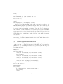
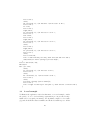
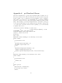
The symbols produced by these macros are shown in the figure 1, which was
created with the following lines of code (see file flow0.pic):
down;
C0: connector(1);
arrow;
H0: preparation(1,1); "\sf Preparation" at H0.c;
move to H0.B.s;
arrow;
D0: data(1,1); "\sf Data" at D0.c;
move to D0.B.s;
arrow;
P0: process(1,1); "\sf Process" at P0.c;
move to P0.B.s;
arrow;
R0: decision(1,1); "\sf Decision" at R0.c;
move to R0.B.s;
arrow;
T0: terminator(1,1); "\sf Terminator" at T0.c;
move to R0.B.w;
left;
arrow;
K0: keying(1,1); "\sf Keying" at K0.c;
move to K0.B.w;
arrow invis;
K1: keyboard(1,1); "\sf Keyboard" at K1.c;
move to K1.B.e;
right;
arrow;
move to K0.B.n;
line -> dashed up C0.w.y-K0.n.y then right C0.w.x-K0.n.x;
move to P0.B.e;
5
right;
arrow;
W0: document(1,1); "\sf Document" at W0.c;
move to D0.B.e;
right;
arrow;
S0: display(1,1); "\sf Display" at S0.c;
It is to be noted that the sizing of the symbols was made according to the
IBM flowcharting template [6], in which most symbols are 12 × 8 units long and
should also match those of the ISO standard [7]. Practically any flowchart can
be prepared with these symbols. As a matter of fact, the basic blocks: process,
data, connector, together with the processing and sequencing symbols: decision,
preparation, terminator, should be sufficient for most flowcharting needs. The
input/output and processing hardware related symbols can be replaced for data
blocks without losx of clarity, as far as the data flow or algorithmic description
are concerned.
Additional examples on the use of the macros are presented in the next
subsections. For further information and references about flowcharts please
check also [8] and references therein.
3.1
Basic Program Flow Structures
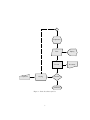
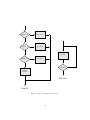
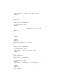
Figure 2 shows the basic program flow structures: a simple sequential execution
of three process, a conditional branching (If-Then-Else) and a program loop
(While-Do loop). These simple flowcharts were generated by the following code
(see file flowbs.pic):
#Sequence
down;
S1: [move down 30;
arrow;PA: process(1,1); "\sf Process A" at PA.c;
move to PA.B.s;
arrow;PB: process(1,1); "\sf Process B" at PB.c;
move to PB.B.s;
arrow;PC: process(1,1); "\sf Process C" at PC.c;
move to PC.B.s;
arrow;box invis "{\Large {\sf Sequence}}";
]
move to S1.ne+(60,0);
#If-Then-Else
I1: [arrow;
R1: decision(1,1); "\sf Decision" at R1.c;
move to R1.s;
arrow;
6
Preparation
Keyboard
Keying
Data
Display
Process
Document
Decision
Terminator
Figure 1: Basic flowchart symbols.
7
P1: process(1,1); "\sf Process 1" at P1.c;
move to P1.B.s;
L1: line;
move to R1.e; line -> right 20 then down R1.e.y-P1.n.y;
P2: process(1,1); "\sf Process 2" at P2.c;
move to P2.B.s;
line -> down P2.s.y-L1.end.y then left P2.s.x-L1.end.x;
down;arrow;box invis "{\Large {\sf If-Then-Else}}";
]
move to I1.s-(0,5);
#While-Do
W1: [L1: line;
arrow;
R1: decision(1,1); "\sf Decision" at R1.c;
move to R1.s;
arrow;
box invis "{\Large {\sf While-Do}}";
move to R1.e;
right;arrow;
P1: process(1,1); "\sf Process X" at P1.c;
move to P1.n;
line -> up L1.end.y-P1.n.y then left P1.n.x-L1.end.x;
]
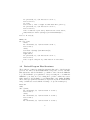
3.2
Derived Program Flow Structures
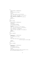
There exist two common program flow structures that can be derived from the
previous ones. These are the Case-Of, which corresponds to a series of If-ThenElse statements, and the Do-Until loop, which is derived from the While-Do
loop. The Do-Until loop is equivalent to always executing the code within the
While-Do loop at least once before exiting the loop if the condition is not met.
Other names for the Do-Until loop are Repeat-Until or the similar Do-While.
These derived program flow structures are represented by the flowcharts shown
in fig. 3, which was created with the following code (see file fileds.pic):
#Case-Of
down;
CS1: [arrow;
R1: decision(1,1); "\sf Decision 1" at R1.c;
move to R1.s;
arrow;
R2: decision(1,1); "\sf Decision 2" at R2.c;
move to R2.s;
arrow;
R3: decision(1,1); "\sf Decision 3" at R3.c;
8
Decision
Process A
Process 1
Process 2
Process B
If-Then-Else
Process C
Sequence
Decision
While-Do
Figure 2: Basic program flow structures.
9
Process X
move to R3.s;
arrow;
PD: process(1,1); "\sf Default" "\sf Process" at PD.c;
move to PD.s;
L1: line;
move to R1.e;
right;arrow;
P1: process(1,1); "\sf Process 1" at P1.c;
move to P1.e;
P1A: arrow;
move to R2.e;
right;arrow;
P2: process(1,1); "\sf Process 2" at P2.c;
move to P2.e;
arrow;
move to R3.e;
right;arrow;
P3: process(1,1); "\sf Process 3" at P3.c;
move to P3.e;
arrow;
move to P1A.end;
line -> down P1A.end.y-L1.end.y then left P1A.end.x-L1.end.x;
down;arrow;box invis "{\Large {\sf Case-Of}}";
]
move to CS1.ne+(40,-35);
#Do-Until
DU1: [L1: line;
arrow;
P1: process(1,1); "\sf Process" at P1.c;
move to P1.s;
arrow;
R1: decision(1,1); "\sf Decision" at R1.c;
move to R1.s;
arrow;
box invis "{\Large {\sf Do-Until}}";
move to R1.e;
line -> right 20 then up L1.end.y-R1.e.y then left R1.e.x+20-L1.end.x;
]
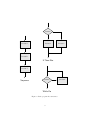
3.3
A real example
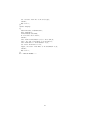
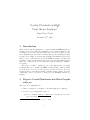
To illustrate the application of the flowchart macros on a real example, consider
the pseudocode of a color-based image segmentation process presented as algorithm 1. For every pixel p in an image, the algorithm computes a color feature
f (p) and checks if the feature is within some threshold λ with respect to all the
10
Decision 1
Process 1
Decision 2
Process 2
Process
Decision 3
Process 3
Decision
Default
Process
Do-Until
Case-Of
Figure 3: Derived program flow structures.
11
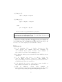
different classes’ reference feature vector fc . The two outer for-from-to-do
loops correspond to the pixel position, while the inner loop corresponds to
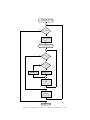
the testing with respect to each class c. This algorithm can be describe in
terms of the flowchart shown in fig. 4. In this flowchart example, the two outer
for-from-to-do loops have been represented by a single for-from-to-do loop
over the pixel position p.
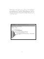
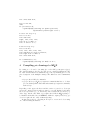
Algorithm 1: ProcessImage (Low-level Pseudocode)
input : &img (input image), &ProcessParam (process parameters)
output: &img (segmented image)
&imgaux ← &img;
—— ComputeSegmentation ——;
for row = 0 to &img.height do
for col = 0 to &img.width do
for class = 1 to &ProcessParam.Nclasses do
if kConvertToYCrCb(&imgaux(row,col ))...
−&ProcessParam.FeatureVector(class)k <Threshold then
&img ← class;
end
end
end
end
12
&imgaux←&img;
p ← (0, 0)
no
p ∈ DI
yes
Compute
feature vector
f (p)
c=0
no c < N
classes
yes
no
kf (p) − fc k < λ
yes
&img(p)=0
&img(p)=c
Increment
class
c←c+1
Update
position
p ← p + ∆p
End
13
Figure 4: Flowchart for a color-based image segmentation process.
The code that generates de flowchart in fig. 4 is (see file flowcs.pic):
alen = 25.4/4*0.8; # arrow length
crad = 1/csize/2; # connector radius in csize*2 units
# initialize the for loop on p (p is the pixel position)
down;
H0: preparation(1.5,0.5);
"\parbox{6em}{\centering \sf \&imgaux$\leftarrow$\&img;\\
$p\leftarrow (0,0)$}" at H0.c;
move to H0.B.s;
arrow alen;
C0: connector(crad);
arrow alen;
# check if the for loop on p is done
R0: decision(1,1);
"\parbox{6em}{\centering \sf $p\in\mathcal{D}_I$}" at R0.c;
move to R0.B.w; "\sf no" above rjust;
move to R0.B.s; "\sf yes" below ljust;
move to R0.B.s;
arrow alen;
P0a: process(1,0.8);
"\parbox{6em}{\centering \sf \small Compute\\
feature vector\\ $f(p)$}" at P0a.c;
move to P0a.B.s;
arrow alen;
# initialize the for loop on c (c is the class label)
H1: preparation(1.5,0.5);
"\parbox{6em}{\centering \sf $c=0$}" at H1.c;
move to H1.B.s;
arrow alen;
C1: connector(crad);
arrow alen;
# check if the for loop on c is done
R1: decision(1,1);
"\parbox{6em}{\centering \sf $c<N_{classes}$}" at R1.c;
move to R1.B.w; "\sf no" above rjust;
move to R1.B.s; "\sf yes" below ljust;
move to R1.B.s;
arrow alen;
14
# check if the feature at pixel p, f(p) can be classified
# as the class c, due to the proximity with respect to
# the class feature vector f_c
R1a: decision(1,1);
"\parbox{7em}{\centering \sf
\footnotesize $\|f(p)-f_c\|<\lambda$}" at R1a.c;
move to R1a.B.w; "\sf no" above rjust;
move to R1a.B.s; "\sf yes" below ljust;
move to R1a.B.s;
arrow alen;
P1a: process(1,0.5);
"\parbox{6em}{\centering \sf \&img($p$)=$c$}" at P1a.c;
move to P1a.B.s;
down; arrow alen;
C1e: connector(0.1);
move to R1a.B.w;
left; line; line alen;
line -> down R1a.c.y-P1a.n.y;
P1b: process(1,0.5);
"\parbox{6em}{\centering \sf \&img($p$)=$0$}" at P1b.c;
move to P1b.B.s;
line -> down P1b.s.y-C1e.c.y then right to C1e.w;
move to C1e.s;
down; arrow alen;
P1: process(1,0.8);
"\parbox{6em}{\centering \sf Increment class\\
$c\leftarrow c+1$}" at P1.c;
move to P1.B.s;
L1a: line alen;
# close for loop on c
move to L1a.end;
right; line; line;
up; line C1.c.y-Here.y;
left; line -> to C1.e;
# end for loop on c
move to R1.B.w;
left; line; line; line;
line down R1.B.w.y-P1.B.s.y+2*alen;
line right P1.B.c.x-Here.x;
15
L1b: arrow down alen;
move to L1b.end;
down;
P0: process(1,0.8);
"\parbox{6em}{\centering \sf Update position\\
$p\leftarrow p+\Delta p$}" at P0.c;
# close for loop on p
move to P0.B.s;
line down alen;
right; line; line; line;
line up C0.c.y-Here.y;
line -> left to C0.e;
# end for loop on p
move to R0.B.w;
left; line; line; line; line;
line down R0.B.w.y-P0.B.s.y+2*alen;
line right P0.B.c.x-Here.x;
L0b: arrow down alen;
T0: terminator(1,0.5);
"\parbox{6em}{\centering \sf End}" at T0.c;
4
Compiling pic drawings to LATEX
Processing pic code can be done using dpic or the GNU pic interpreter (gpic).
The output formats produced by dpic and gpic are completely different (see Ch.
12 of the circuit-macros documentation [3] or the dpic manual [4] for a complete description of the multiple formats). The differences can be summarized
in:
• dpic produces PSTricks commands.
• gpic produces tpic (TEX pic) \special commands that have to be later
processed with a printer driver that understands tpic \special commands,
such as dvips.
Depending on the approach chosen and the version of your dvi or Postscript
viewer, the output produced with gpic may be correctly displayed only under
the Postscript viewer (e.g. gv, Ghostview), but not under the dvi viewer (e.g.
Xdvi, Yap). On the other hand, dpic requires the PSTricks LATEX package to
be installed and included in your LATEX file, while the output produced by gpic
does not require the use of any additional package.
As stated in section 2, converting from *.pic to *.tex can be done using
one of the following alternatives:
16
(a) Using dpic [4]:
dpic -p fig.pic > fig.tex
(b) Using gpic [5]:
gpic -t fig.pic
> fig.tex
or with
pic -t fig.pic > fig.tex
if a newer version of groff is installed in your system.
IMPORTANT: When processing the *.pic files provided with this
document, the variable pstricks in the *.pic files must be set to 0 if
gpic is used or to 1 when dpic is used.
Once the *.tex files are produced with any of the two previous methods,
the last step is to include them into your LATEX document according to the
corresponding approach, as explained in the third point of section 2 (see also
the source code of the examples provided with this document).
References
[1] B. W. Kernighan. PIC – A Graphics Language for Typesetting (Revised User Manual) Bell Labs Computing Science Technical Report #116, December 1991. Available at:
http://www.cs.bell-labs.com/10thEdMan/pic.pdf.
[2] E. S. Raymond. Making pictures with GNU PIC, 1995. In GNUgroff source
distribution.
[3] J.
D.
Aplevich.
M4
Macros
for
Electric
Circuit
Diagrams in LATEX Documents, version 6.4, 2008. Available at:
http://texcatalogue.sarovar.org/entries/circuit-macros.html or
the CTAN http://www.ctan.org mirrors.
[4] J. D. Aplevich. Dpic package, version 29 Oct. 2008. Available at:
http://www.ece.uwaterloo.ca/ aplevich/dpic/.
[5] Groff
for
Windows,
version
1.19.2
Available
at:
http://gnuwin32.sourceforge.net/packages/groff.htm. The package
homepage is: http://www.gnu.org/software/groff/groff.html.
17
[6] International Business Machines Corporation. IBM Flowcharting
Techniques.
IBM
Technical
Publications
Dept.
Document
No.
C20-8152-1,
New
York,
1069.
Available
at:
http://www.fh-jena.de/~
kleine/history/software/...
...IBM-FlowchartingTechniques-GC20-8152-1.pdf.
[7] ISO 5807:1985 Standard: Information processing – Documentation
symbols and conventions for data, program and system flowcharts,
program network charts and system resources charts. Available at:
http://www.iso.org/iso/iso catalogue/catalogue tc/...
...catalogue detail.htm?csnumber=11955.
[8] Wikipedia. Flowchart. Visited on December, 17th , 2008.
http://en.wikipedia.org/wiki/Flowchart.
18
Appendix A
pic Flowchart Macros
The macros implemented to produce the flowcharts in this document were defined as pic language blocks. These blocks provide flowchart primitives by grouping into a single object or entity the lower level primitives of the pic language,
such as lines, boxes and arcs. Not surprisingly, the pic language primitives
grouped to form an object are called blocks in the terminology of the pic language. The following code shows the implementation of the macros developed
to plot the flowchart symbols of the examples presented in this document. The
code of these macros should be included at the beginning of your own flowcharts
as explained in section 3.
.PS #20/25.4 # Scale drawing to 20/25.4 in =
#
= 20/25.4[in]/25.4[mm/in] = 20 mm
# FLOWCHART - Basic flow chart blocks.
scale=25.4 #Scale units from inches to mm
csize=2.0 #Cell size in mm
pstricks=1
dx=0; dy=2;
#sshade(): Starts shading of an arbitrary closed curve.
define sshade
{
if pstricks==0 then
{
sprintf("\special{sh %g}",0.1)
#command "\special{sh 0.1}"
} else
{
#sprintf("\newgray{xcolor}{%s}",0.9)
command "\newgray{xcolor}{0.9}"
command "\pscustom[fillstyle=solid, fillcolor=xcolor]{"
}
}
#eshade(): Ends shading of an arbitrary close curve.
define eshade
{
if pstricks==1 then
{
command "}%"
}
}
define process
{[
w=$1*12*csize; h=$2*8*csize;
B: box wid w ht h invis;
sshade;
19
line from B.ne to B.nw to B.sw to B.se to B.ne;
eshade;
#$3 at B.c;
]}
# data(): parallelogram -> "data input/output block"
define data
{[
w=$1*12*csize; h=$2*8*csize;
dx=(h/4)/2;
B: box wid w ht h invis;
sshade;
line from B.sw-(dx,0) to B.se-(dx,0) to B.ne+(dx,0)
to B.nw+(dx,0) to B.sw-(dx,0);
eshade;
#$3 at B.c;
]}
define connector
{[
r=$1*2*csize;
sshade;
B: circle rad r;
eshade;
#$3 at B.c;
]}
# decision(): rhomboid -> "if block"
define decision
{[
w=$1*12*csize; h=$2*8*csize;
B: box wid w ht h invis;
sshade;
line from B.n to B.e to B.s to B.w to B.n;
eshade;
#$3 at B.c;
]}
define preparation
{[
w=$1*12*csize; h=$2*8*csize;
dx=(h/2)/2;
B: box wid w ht h invis;
sshade;
line from B.w to B.nw+(dx,0) to B.ne-(dx,0) to B.e
to B.se-(dx,0) to B.sw+(dx,0) to B.w;
eshade;
#$3 at B.c;
]}
define terminator
20
{[
w=$1*12*csize; h=$2*4*csize;
r=h/2;
B: box wid w ht h invis;
sshade;
line from B.sw+(r,0) to B.se-(r,0);
right; arc rad r from Here to B.ne-(r,0);
line from Here to B.nw+(r,0);
left; arc rad r from Here to B.sw+(r,0);
eshade;
#$3 at B.c;
]}
define keying
{[
w=$1*14*csize; h=$2*8*csize;
dx=(h/4)/2;
r=dx/2+(h/2)^2/(2*dx);
B: box wid w ht h invis;
sshade;
line from B.sw+(dx,0) to B.se-(dx,0);
left; arc rad r from Here to B.ne-(dx,0);
line from Here to B.nw+(dx,0);
right; arc rad r from Here to B.sw+(dx,0);
eshade;
#$3 at B.c;
]}
define keyboard
{[
w=$1*12*csize; h=$2*5*csize;
dy=(w/6)/2;
B: box wid w ht h invis;
sshade;
line from B.nw-(0,dy) to B.sw to B.se
to B.ne+(0,dy) to B.nw-(0,dy);
eshade;
#$3 at B.c;
]}
define document
{[
w=$1*12*csize; h=$2*7*csize;
dy=(w/6)/2;
r=sqrt((w/2)^2+dy^2);
B: box wid w ht h invis;
sshade;
line from B.se+(0,dy) to B.ne to B.nw to B.sw;
up; arc rad w/2 from B.sw to B.s;
21
arc cw rad r from B.s to B.se+(0,dy);
eshade;
#$3 at B.c;
]}
define display
{[
w=$1*12*csize; h=$2*8*csize;
dx=1.5*(h/4)/2;
r=dx/2+(h/2)^2/(2*dx);
B: box wid w ht h invis;
sshade;
line from B.sw+(4*dx/1.5,0) to B.se-(dx,0);
left; arc rad r from Here to B.ne-(dx,0);
line from Here to B.nw+(4*dx/1.5,0);
arc rad r from Here to B.w;
right; arc rad r from Here to B.sw+(4*dx/1.5,0);
eshade;
#$3 at B.c;
]}
#--- END OF MACROS ---
22