Download User's guide for the ROC-HJ solver: Finite Differences and Semi

Q A
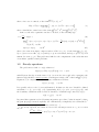
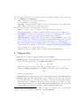
where A is a set of controls, of the form ni=1
[αi , βi ], or 2
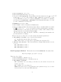
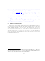
H(t, x, ∇u) := max min − f (t, x, a, b) · ∇u − `(t, x, a, b) ,
a∈A b∈B
(3)
Q A A A
Q B B B
where A and B are control sets of the form ni=1
[αi , βi ] and nj=1
[αj , βj ].
Some second order equations can also be treated, of the following type
0=
∂u
+ λ(x)u +
(4a)
∂t
1
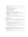
max −`(t, x, a) + r(t, x, a)u − b(t, x, a) · ∇u − T r(σ(t, x, a)σ(t, x, a)T D2 u)
a∈A
2
t ∈ [0, T ], x ∈ Rd ,
u(0, x) = u0 (x),
x ∈ Rd
(4b)
Q A
[αi , βi ]),
where A is some non empty compact subset of Rm (m ≥ 1), (of the form ni=1
d
b(t, x, a) is a vector of R , r(t, x, a) and `(t, x, a) are real-valued, and σ(t, x, a) is a d×p real
matrix (for some p ≥ 1). This problem is linked to the computation of the value function
of stochastic optimal control problems.
1.2
Steady equations
The problem is to find u = u(x) solution of
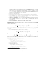
λ(x)u(x) + H(x, u(x), ∇u(x)) = 0,
x ∈ Ω,
(5)
with H given directly or in the form of (2) (or as in (4a) for second order equations), the
Q
function λ(x) should be strictly positive, Ω an hyperrectangle of Rd of the form di=1 [ai , bi ].
Equation (5) is complemented by boundary conditions as follows :
u(x) = gbord (x),
x ∈ ∂Ω.
It is possible also to solve (5) in a subdomain C. In that case the set C should be defined
such that C := {x, gdomain (x) < 0} (equivalently, Ω\C = {x ∈ Ω, gdomain (x) ≥ 0}), and
the boundary conditions at the border ∂C should be of Dirichlet type, fixed by u0 (x) :
u(x) = u0 (x),
x ∈ ∂C.
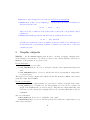
In general this equation is solved by using an iterative procedure ("value iteration"), where
the part λ(x)u(x) is treated explicitly (for a FD method) or implicitly (for a SL method). 3
2. maxa∈A minb∈B (· · · ) can be also mina∈A maxb∈B (· · · )
3. For steady equations, the scheme is based on the following iteration on n ≥ 0, for a fixed
∆t > 0 :
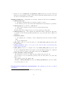
un+1 (x) − un (x)
+ λ(x)un (x) + h(x, un (x), Dun (x)) = 0, x ∈ C,
∆t
2