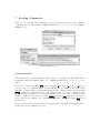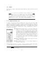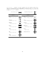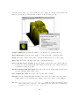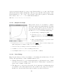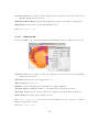
1
The ImageJ User Guide
Version 1.43 — April 2010
The ImageJ User Guide
Version 1.43
Tiago A. Ferreira
•
Wayne Rasband
April 20, 2010
Note
This document is highly enriched in hypertext links and was thought as a
fully-searchable, self-contained, annotatable, offline manual (cf. Using This
Guide).
Given ImageJ’s heavy development this guide will always remain an unfinished draft and should be considered complementary to the remaining ImageJ
documentation resources (cf. Getting Help). As such, all ImageJ users and
developers are encouraged to contribute to future editions of this manual
(cf. About this Guide).
The latest version of this document can always be obtained from http://
rsbweb.nih.gov/ij/docs/user-guide.pdf.
Table of Contents
Features Implemented in v1.43
vii
Noteworthy
viii
Macro Listings
ix
I
Getting Started
1
1
What is ImageJ?
1
2
Installation
1
3
Maintaining ImageJ
2
4
Using This Guide
4
5
Getting Help
4
II
Working with ImageJ
7
6
Shortcuts and Modifier Keys
7
7
Finding Commands
8
8
Undo and Redo
9
9
Image Types and Image Formats
10
10 Stacks, Virtual Stacks and Hyperstacks
13
11 Color Images
15
12 Selections
18
13 The Results Table
19
14 Settings and Preferences
21
15 Extending ImageJ
22
III
27
The User Interface: ImageJ Window
16 Toolbar
16.1 Status bar . . . . . . . . . . . . . . . . . . . . . . . . . . . . . . . . . . . . . . .
16.2 Progress bar . . . . . . . . . . . . . . . . . . . . . . . . . . . . . . . . . . . . . .
ii
27
27
28
17 Area selection tools
17.1 Rectangular Selection Tool .
17.2 Round Rectangular Selection
17.3 Elliptical Selection Tool . . .
17.4 Brush Selection Tool . . . .
17.5 Polygon Selection Tool . . .
17.6 Freehand Selection Tool . . .
17.7 Wand Tool . . . . . . . . . .
18 Line
18.1
18.2
18.3
.
.
.
.
.
.
.
28
28
29
29
29
30
30
30
Selection Tools
Straight Line Selection Tool . . . . . . . . . . . . . . . . . . . . . . . . . . . . .
Segmented Line Selection Tool . . . . . . . . . . . . . . . . . . . . . . . . . . . .
Freehand Line Selection Tool . . . . . . . . . . . . . . . . . . . . . . . . . . . . .
31
31
31
32
. . .
Tool
. . .
. . .
. . .
. . .
. . .
.
.
.
.
.
.
.
.
.
.
.
.
.
.
.
.
.
.
.
.
.
.
.
.
.
.
.
.
.
.
.
.
.
.
.
.
.
.
.
.
.
.
.
.
.
.
.
.
.
.
.
.
.
.
.
.
.
.
.
.
.
.
.
.
.
.
.
.
.
.
.
.
.
.
.
.
.
.
.
.
.
.
.
.
.
.
.
.
.
.
.
.
.
.
.
.
.
.
.
.
.
.
.
.
.
.
.
.
.
.
.
.
.
.
.
.
.
.
.
.
.
.
.
.
.
.
.
.
.
.
.
.
.
.
.
.
.
.
.
.
.
.
.
.
.
.
.
.
.
.
.
.
.
.
.
.
.
.
.
.
.
.
.
.
.
.
.
.
.
.
.
.
.
.
.
19 Arrow Tool
32
20 Angle Tool
32
21 Point Tool
33
22 Multi-point Tool
34
23 Text Tool
34
24 Magnifying Glass
34
25 Scrolling Tool
35
26 Color Picker
35
27 Macro Toolset Switcher
35
28 Macro Tools
36
IV
37
The User Interface: ImageJ Menus
29 File .
29.1 New... . . . .
29.2 Open... . . . .
29.3 Open Next [O]
29.4 Open Samples .
29.5 Open Recent .
29.6 Import . . . . .
29.7 Close [w] . . .
29.8 Close All . . .
29.9 Save [s] . . . .
29.10 Save As . . . .
29.11 Revert [r] . . .
29.12 Page Setup... .
. . . .
. . . .
. . . .
. . .
. . . .
. . . .
. . . .
. . . .
. . . .
. . . .
. . . .
. . . .
.
.
.
.
.
.
.
.
.
.
.
.
.
.
.
.
.
.
.
.
.
.
.
.
.
.
.
.
.
.
.
.
.
.
.
.
.
.
.
.
.
.
.
.
.
.
.
.
.
.
.
.
.
.
.
.
.
.
.
.
.
.
.
.
.
.
.
.
.
.
.
.
.
.
.
.
.
.
.
.
.
.
.
.
.
.
.
.
.
.
.
.
.
.
.
.
.
.
.
.
.
.
.
.
.
.
.
.
.
.
.
.
.
.
.
.
.
.
.
.
iii
.
.
.
.
.
.
.
.
.
.
.
.
.
.
.
.
.
.
.
.
.
.
.
.
.
.
.
.
.
.
.
.
.
.
.
.
.
.
.
.
.
.
.
.
.
.
.
.
.
.
.
.
.
.
.
.
.
.
.
.
.
.
.
.
.
.
.
.
.
.
.
.
.
.
.
.
.
.
.
.
.
.
.
.
.
.
.
.
.
.
.
.
.
.
.
.
.
.
.
.
.
.
.
.
.
.
.
.
.
.
.
.
.
.
.
.
.
.
.
.
.
.
.
.
.
.
.
.
.
.
.
.
.
.
.
.
.
.
.
.
.
.
.
.
.
.
.
.
.
.
.
.
.
.
.
.
.
.
.
.
.
.
.
.
.
.
.
.
.
.
.
.
.
.
.
.
.
.
.
.
.
.
.
.
.
.
.
.
.
.
.
.
.
.
.
.
.
.
.
.
.
.
.
.
.
.
.
.
.
.
.
.
.
.
.
.
.
.
.
.
.
.
.
.
.
.
.
.
.
.
.
.
.
.
.
.
.
.
.
.
.
.
.
.
.
.
.
.
.
.
.
.
.
.
.
.
.
.
.
.
.
.
.
.
.
.
.
.
.
.
.
.
.
.
.
.
37
37
38
39
39
40
40
44
45
45
45
49
49
29.13 Print... [p] . . . . . . . . . . . . . . . . . . . . . . . . . . . . . . . . . . . . . . . .
29.14 Quit . . . . . . . . . . . . . . . . . . . . . . . . . . . . . . . . . . . . . . . . . . .
50
50
30 Edit .
30.1 Undo [z] . . . . . . . .
30.2 Cut [x], Copy [c], Copy
30.3 Paste Control... . . . .
30.4 Clear . . . . . . . . .
30.5 Clear Outside . . . . .
30.6 Fill [f] . . . . . . . . .
30.7 Draw [d] . . . . . . . .
30.8 Invert [I] . . . . . . . .
30.9 Selection . . . . . . .
30.10 Options . . . . . . . .
. . . . . .
to System,
. . . . . .
. . . . . .
. . . . . .
. . . . . .
. . . . . .
. . . . . .
. . . . . .
. . . . . .
. . . . . .
Paste [v]
. . . . . .
. . . . . .
. . . . . .
. . . . . .
. . . . . .
. . . . . .
. . . . . .
. . . . . .
.
.
.
.
.
.
.
.
.
.
.
.
.
.
.
.
.
.
.
.
.
.
.
.
.
.
.
.
.
.
.
.
.
.
.
.
.
.
.
.
.
.
.
.
.
.
.
.
.
.
.
.
.
.
.
.
.
.
.
.
.
.
.
.
.
.
.
.
.
.
.
.
.
.
.
.
.
.
.
.
.
.
.
.
.
.
.
.
.
.
.
.
.
.
.
.
.
.
.
.
.
.
.
.
.
.
.
.
.
.
.
.
.
.
.
.
.
.
.
.
.
.
.
.
.
.
.
.
.
.
.
.
.
.
.
.
.
.
.
.
.
.
.
.
.
.
.
.
.
.
.
.
.
.
.
.
.
.
.
.
.
.
.
.
.
.
.
.
.
.
.
.
.
.
.
.
.
.
.
.
.
.
.
.
.
.
.
.
.
.
.
.
.
.
.
.
.
.
.
.
.
.
.
.
.
.
.
.
.
.
51
51
51
51
52
52
52
52
53
53
57
31 Image .
31.1 Type . . . . . .
31.2 Adjust . . . . . .
31.3 Show Info... [i] .
31.4 Properties... [P] .
31.5 Color . . . . . .
31.6 Stacks . . . . . .
31.7 Hyperstacks . . .
31.8 Crop [X] . . . . .
31.9 Duplicate... [D] .
31.10 Rename... . . . .
31.11 Scale... [E] . . .
31.12 Transform . . . .
31.13 Zoom . . . . . .
31.14 Overlay . . . . .
31.15 Lookup Tables .
.
.
.
.
.
.
.
.
.
.
.
.
.
.
.
.
.
.
.
.
.
.
.
.
.
.
.
.
.
.
.
.
.
.
.
.
.
.
.
.
.
.
.
.
.
.
.
.
.
.
.
.
.
.
.
.
.
.
.
.
.
.
.
.
.
.
.
.
.
.
.
.
.
.
.
.
.
.
.
.
.
.
.
.
.
.
.
.
.
.
.
.
.
.
.
.
.
.
.
.
.
.
.
.
.
.
.
.
.
.
.
.
.
.
.
.
.
.
.
.
.
.
.
.
.
.
.
.
.
.
.
.
.
.
.
.
.
.
.
.
.
.
.
.
.
.
.
.
.
.
.
.
.
.
.
.
.
.
.
.
.
.
.
.
.
.
.
.
.
.
.
.
.
.
.
.
.
.
.
.
.
.
.
.
.
.
.
.
.
.
.
.
.
.
.
.
.
.
.
.
.
.
.
.
.
.
.
.
.
.
.
.
.
.
.
.
.
.
.
.
.
.
.
.
.
.
.
.
.
.
.
.
.
.
.
.
.
.
.
.
.
.
.
.
.
.
.
.
.
.
.
.
.
.
.
.
.
.
.
.
.
.
.
.
.
.
.
.
.
.
.
.
.
.
.
.
.
.
.
.
.
.
.
.
.
.
.
.
.
.
.
.
.
.
.
.
.
.
.
.
.
.
.
.
.
.
.
.
.
.
.
.
.
.
.
.
.
.
.
.
.
.
.
.
.
.
.
.
.
.
.
.
.
.
.
.
.
.
.
.
.
.
.
.
.
.
.
.
.
.
.
.
.
.
.
.
.
.
.
.
.
.
.
.
.
.
.
.
.
.
.
.
.
.
.
.
.
.
.
.
.
.
.
.
.
.
.
.
.
.
.
.
.
.
.
.
.
.
.
.
.
.
.
.
.
.
.
.
.
.
.
.
.
.
.
.
.
.
.
.
.
.
.
.
.
.
.
.
.
.
.
.
.
.
.
.
.
.
.
.
.
.
.
.
.
.
.
.
.
.
.
.
.
.
.
.
.
.
.
.
.
.
.
.
.
.
.
.
.
.
.
.
.
.
.
.
.
.
.
.
.
.
.
.
.
.
.
.
.
.
.
.
.
.
.
.
.
.
.
.
.
.
.
.
.
.
.
.
.
.
65
65
66
72
73
73
76
87
89
89
89
90
90
91
93
96
32 Process .
32.1 Smooth [S] . . . . . .
32.2 Sharpen . . . . . . . .
32.3 Find Edges . . . . . .
32.4 Find Maxima... . . . .
32.5 Enhance Contrast . . .
32.6 Noise . . . . . . . . .
32.7 Shadows . . . . . . .
32.8 Binary . . . . . . . . .
32.9 Math . . . . . . . . .
32.10 FFT . . . . . . . . . .
32.11 Filters . . . . . . . . .
32.12 Batch . . . . . . . . .
32.13 Image Calculator... . .
32.14 Subtract Background...
32.15 Repeat Command [R] .
.
.
.
.
.
.
.
.
.
.
.
.
.
.
.
.
.
.
.
.
.
.
.
.
.
.
.
.
.
.
.
.
.
.
.
.
.
.
.
.
.
.
.
.
.
.
.
.
.
.
.
.
.
.
.
.
.
.
.
.
.
.
.
.
.
.
.
.
.
.
.
.
.
.
.
.
.
.
.
.
.
.
.
.
.
.
.
.
.
.
.
.
.
.
.
.
.
.
.
.
.
.
.
.
.
.
.
.
.
.
.
.
.
.
.
.
.
.
.
.
.
.
.
.
.
.
.
.
.
.
.
.
.
.
.
.
.
.
.
.
.
.
.
.
.
.
.
.
.
.
.
.
.
.
.
.
.
.
.
.
.
.
.
.
.
.
.
.
.
.
.
.
.
.
.
.
.
.
.
.
.
.
.
.
.
.
.
.
.
.
.
.
.
.
.
.
.
.
.
.
.
.
.
.
.
.
.
.
.
.
.
.
.
.
.
.
.
.
.
.
.
.
.
.
.
.
.
.
.
.
.
.
.
.
.
.
.
.
.
.
.
.
.
.
.
.
.
.
.
.
.
.
.
.
.
.
.
.
.
.
.
.
.
.
.
.
.
.
.
.
.
.
.
.
.
.
.
.
.
.
.
.
.
.
.
.
.
.
.
.
.
.
.
.
.
.
.
.
.
.
.
.
.
.
.
.
.
.
.
.
.
.
.
.
.
.
.
.
.
.
.
.
.
.
.
.
.
.
.
.
.
.
.
.
.
.
.
.
.
.
.
.
.
.
.
.
.
.
.
.
.
.
.
.
.
.
.
.
.
.
.
.
.
.
.
.
.
.
.
.
.
.
.
.
.
.
.
.
.
.
.
.
.
.
.
.
.
.
.
.
.
.
.
.
.
.
.
.
.
.
.
.
.
.
.
.
.
.
.
.
.
.
.
.
.
.
.
.
.
.
.
.
.
.
.
.
.
.
.
.
.
.
.
.
.
.
.
.
.
.
.
.
.
.
.
.
.
.
.
.
.
.
.
.
.
.
.
.
.
.
.
.
.
.
.
.
.
.
.
.
.
.
.
.
.
.
.
.
.
.
.
.
.
.
.
.
.
.
.
.
.
.
.
.
.
97
97
97
97
98
100
101
102
102
108
111
115
118
121
123
124
.
.
.
.
.
.
.
.
.
.
.
.
.
.
.
.
.
.
.
.
.
.
.
.
.
.
.
.
.
.
iv
33 Analyze .
33.1 Measure... [m] . . .
33.2 Analyze Particles... .
33.3 Summarize . . . . .
33.4 Distribution... . . . .
33.5 Label . . . . . . . .
33.6 Clear Results . . . .
33.7 Set Measurements...
33.8 Set Scale... . . . . .
33.9 Calibrate... . . . . .
33.10 Histogram [h] . . . .
33.11 Plot Profile [k] . . .
33.12 Surface Plot... . . .
33.13 Gels . . . . . . . . .
33.14 Tools . . . . . . . .
.
.
.
.
.
.
.
.
.
.
.
.
.
.
.
.
.
.
.
.
.
.
.
.
.
.
.
.
.
.
.
.
.
.
.
.
.
.
.
.
.
.
.
.
.
.
.
.
.
.
.
.
.
.
.
.
.
.
.
.
.
.
.
.
.
.
.
.
.
.
.
.
.
.
.
.
.
.
.
.
.
.
.
.
.
.
.
.
.
.
.
.
.
.
.
.
.
.
.
.
.
.
.
.
.
.
.
.
.
.
.
.
.
.
.
.
.
.
.
.
.
.
.
.
.
.
.
.
.
.
.
.
.
.
.
.
.
.
.
.
.
.
.
.
.
.
.
.
.
.
.
.
.
.
.
.
.
.
.
.
.
.
.
.
.
.
.
.
.
.
.
.
.
.
.
.
.
.
.
.
.
.
.
.
.
.
.
.
.
.
.
.
.
.
.
.
.
.
.
.
.
.
.
.
.
.
.
.
.
.
.
.
.
.
.
.
.
.
.
.
.
.
.
.
.
.
.
.
.
.
.
.
.
.
.
.
.
.
.
.
.
.
.
.
.
.
.
.
.
.
.
.
.
.
.
.
.
.
.
.
.
.
.
.
.
.
.
.
.
.
.
.
.
.
.
.
.
.
.
.
.
.
.
.
.
.
.
.
.
.
.
.
.
.
.
.
.
.
.
.
.
.
.
.
.
.
.
.
.
.
.
.
.
.
.
.
.
.
.
.
.
.
.
.
.
.
.
.
.
.
.
.
.
.
.
.
.
.
.
.
.
.
.
.
.
.
.
.
.
.
.
.
.
.
.
.
.
.
.
.
.
.
.
.
.
.
.
.
.
.
.
.
.
.
.
.
.
.
.
.
.
.
.
.
.
.
.
.
.
.
.
.
.
.
.
.
.
.
.
.
.
.
.
.
.
.
.
.
.
.
.
.
.
.
.
.
.
.
.
.
.
.
.
.
.
.
.
.
.
.
.
.
.
.
.
.
.
.
.
.
.
.
.
.
.
.
.
.
.
.
.
.
.
.
.
.
.
.
.
.
.
.
.
.
.
.
.
.
.
.
.
.
.
.
.
.
125
125
126
128
128
129
129
130
133
134
136
137
137
139
141
34 Plugins .
34.1 Macros . . . . . .
34.2 Shortcuts . . . . .
34.3 Utilities . . . . . .
34.4 New . . . . . . . .
34.5 Compile and Run...
.
.
.
.
.
.
.
.
.
.
.
.
.
.
.
.
.
.
.
.
.
.
.
.
.
.
.
.
.
.
.
.
.
.
.
.
.
.
.
.
.
.
.
.
.
.
.
.
.
.
.
.
.
.
.
.
.
.
.
.
.
.
.
.
.
.
.
.
.
.
.
.
.
.
.
.
.
.
.
.
.
.
.
.
.
.
.
.
.
.
.
.
.
.
.
.
.
.
.
.
.
.
.
.
.
.
.
.
.
.
.
.
.
.
.
.
.
.
.
.
.
.
.
.
.
.
.
.
.
.
.
.
.
.
.
.
.
.
.
.
.
.
.
.
.
.
.
.
.
.
.
.
.
.
.
.
.
.
.
.
.
.
.
.
.
.
.
.
.
.
.
.
.
.
.
148
148
149
151
153
154
35 Window
35.1 Show All [ ] ] . .
35.2 Put Behind [tab]
35.3 Cascade . . . . .
35.4 Tile . . . . . . .
.
.
.
.
.
.
.
.
.
.
.
.
.
.
.
.
.
.
.
.
.
.
.
.
.
.
.
.
.
.
.
.
.
.
.
.
.
.
.
.
.
.
.
.
.
.
.
.
.
.
.
.
.
.
.
.
.
.
.
.
.
.
.
.
.
.
.
.
.
.
.
.
.
.
.
.
.
.
.
.
.
.
.
.
.
.
.
.
.
.
.
.
.
.
.
.
.
.
.
.
.
.
.
.
.
.
.
.
.
.
.
.
.
.
.
.
.
.
.
.
.
.
.
.
.
.
.
.
.
.
.
.
.
.
.
.
.
.
.
.
.
.
.
.
155
155
155
155
155
36 Help
36.1 ImageJ Website... .
36.2 ImageJ News... . .
36.3 Documentation... .
36.4 Installation... . . .
36.5 Search Website... .
36.6 List Archives... . .
36.7 Dev. Resources... .
36.8 Plugins... . . . . .
36.9 Macros... . . . . .
36.10 Macro Functions...
36.11 Update ImageJ... .
36.12 Update Menus . .
36.13 About Plugins . .
36.14 About ImageJ... . .
.
.
.
.
.
.
.
.
.
.
.
.
.
.
.
.
.
.
.
.
.
.
.
.
.
.
.
.
.
.
.
.
.
.
.
.
.
.
.
.
.
.
.
.
.
.
.
.
.
.
.
.
.
.
.
.
.
.
.
.
.
.
.
.
.
.
.
.
.
.
.
.
.
.
.
.
.
.
.
.
.
.
.
.
.
.
.
.
.
.
.
.
.
.
.
.
.
.
.
.
.
.
.
.
.
.
.
.
.
.
.
.
.
.
.
.
.
.
.
.
.
.
.
.
.
.
.
.
.
.
.
.
.
.
.
.
.
.
.
.
.
.
.
.
.
.
.
.
.
.
.
.
.
.
.
.
.
.
.
.
.
.
.
.
.
.
.
.
.
.
.
.
.
.
.
.
.
.
.
.
.
.
.
.
.
.
.
.
.
.
.
.
.
.
.
.
.
.
.
.
.
.
.
.
.
.
.
.
.
.
.
.
.
.
.
.
.
.
.
.
.
.
.
.
.
.
.
.
.
.
.
.
.
.
.
.
.
.
.
.
.
.
.
.
.
.
.
.
.
.
.
.
.
.
.
.
.
.
.
.
.
.
.
.
.
.
.
.
.
.
.
.
.
.
.
.
.
.
.
.
.
.
.
.
.
.
.
.
.
.
.
.
.
.
.
.
.
.
.
.
.
.
.
.
.
.
.
.
.
.
.
.
.
.
.
.
.
.
.
.
.
.
.
.
.
.
.
.
.
.
.
.
.
.
.
.
.
.
.
.
.
.
.
.
.
.
.
.
.
.
.
.
.
.
.
.
.
.
.
.
.
.
.
.
.
.
.
.
.
.
.
.
.
.
.
.
.
.
.
.
.
.
.
.
.
.
.
.
.
.
.
.
.
.
.
.
.
.
.
.
.
.
.
.
.
.
.
.
.
.
.
.
.
.
.
.
.
.
.
.
.
.
.
.
.
.
.
.
.
.
.
.
.
.
.
.
.
.
.
.
.
.
.
.
.
.
.
.
.
.
.
.
.
.
.
.
.
.
.
.
.
.
.
.
.
.
.
.
.
.
.
.
.
.
.
.
.
.
.
.
.
.
.
.
.
.
.
.
.
.
156
156
156
156
156
156
156
156
157
157
157
157
157
157
158
A Keyboard Shortcuts
159
A.1 Alt Key Modifications . . . . . . . . . . . . . . . . . . . . . . . . . . . . . . . . . 161
A.2 Shift Key Modifications . . . . . . . . . . . . . . . . . . . . . . . . . . . . . . . . 162
A.3 Ctrl Key (or Cmd Key on Macs) Modifications . . . . . . . . . . . . . . . . . . . 162
v
A.4 Space Bar Modifications . . . . . . . . . . . . . . . . . . . . . . . . . . . . . . . 162
A.5 Arrow Keys . . . . . . . . . . . . . . . . . . . . . . . . . . . . . . . . . . . . . . 162
A.6 Keyboard Shortcuts for ImageJ Tools . . . . . . . . . . . . . . . . . . . . . . . . 163
B Credits
165
C ImageJ Related Publications
167
D List of Abbreviations and Acronyms
174
About this Guide
175
Index
176
vi
New Features Implemented in 1.431
Improved dimension sliders in stacks and hyperstacks . . . . . . . . . . . . . . . . 13
TIFF virtual stacks can be opened by drag and drop . . . . . . . . . . . . . . . . . 14
Round rectangular selection tool . . . . . . . . . . . . . . . . . . . . . . . . . . . . 29
Improved constrained (shift key down) elliptical selection tool . . . . . . . . . . . . 29
4 / 8 –Connected wand tool . . . . . . . . . . . . . . . . . . . . . . . . . . . . . . . 30
Arrow tool . . . . . . . . . . . . . . . . . . . . . . . . . . . . . . . . . . . . . . . . 32
Multi-point tool . . . . . . . . . . . . . . . . . . . . . . . . . . . . . . . . . . . . . 34
Improved Color Picker . . . . . . . . . . . . . . . . . . . . . . . . . . . . . . . . . . 35
Improved Drag & Drop Support . . . . . . . . . . . . . . . . . . . . . . . . . . . . . 38
File . Close All command . . . . . . . . . . . . . . . . . . . . . . . . . . . . . . . . . 45
Selections and overlays are saved in the TIFF header . . . . . . . . . . . . . . . . . 45
16–bit images can be saved as 16–bit PNGs . . . . . . . . . . . . . . . . . . . . . . 48
Transparent-zero mode now works with 16–bit and 32–bit images . . . . . . . . . . 51
Edit . Options . DICOM... command . . . . . . . . . . . . . . . . . . . . . . . . . . . 63
Image . Adjust . Color Threshold... command . . . . . . . . . . . . . . . . . . . . . . 70
Image . Stacks . Tools . submenu . . . . . . . . . . . . . . . . . . . . . . . . . . . . 85
Image . Stacks . Tools . Reduce... command . . . . . . . . . . . . . . . . . . . . . . . 85
Image . Stacks . Tools . Insert... command . . . . . . . . . . . . . . . . . . . . . . . . 86
Image . Stacks . Tools . Montage to Stack... command . . . . . . . . . . . . . . . . . 86
Image . Transform . submenu . . . . . . . . . . . . . . . . . . . . . . . . . . . . . . 90
Image . Transform . Flip Z command . . . . . . . . . . . . . . . . . . . . . . . . . . . 90
Non-destructive image overlays (Image . Overlay . submenu) . . . . . . . . . . . . . 93
Faster Process . Find Maxima... command with List output . . . . . . . . . . . . . . 98
Binary . operations with preview . . . . . . . . . . . . . . . . . . . . . . . . . . . . 107
Faster Math . commands when operating on 16–bit and float images . . . . . . . . 108
Gamma slider . . . . . . . . . . . . . . . . . . . . . . . . . . . . . . . . . . . . . . . 109
Process . Batch . submenu . . . . . . . . . . . . . . . . . . . . . . . . . . . . . . . . 118
Improved and redesigned ROI Manager . . . . . . . . . . . . . . . . . . . . . . . . 144
The Recorder generates thread safe JavaScript and Java code . . . . . . . . . . . . 148
Improved Command Finder . . . . . . . . . . . . . . . . . . . . . . . . . . . . . . . 153
1
This list is not extensive. Detailed release notes for version 1.43 are available on the ImageJ News web
site: http://rsb.info.nih.gov/ij/notes.html
vii
Noteworthy
6.1
Frontmost Window and Windows Activation . . . . . . . . . . . . . . . . . . . . . .
7
8.2
Limitations of Edit . Undo [z] . . . . . . . . . . . . . . . . . . . . . . . . . . . . . . .
9
9.3
Brightness/Contrast of High Bit–Depth Images . . . . . . . . . . . . . . . . . . . .
12
9.4
Image Types: Lossy Compression and Metadata . . . . . . . . . . . . . . . . . . . .
13
16.5 Toggling Calibrated Units . . . . . . . . . . . . . . . . . . . . . . . . . . . . . . . .
28
27.6 Opening Virtual Stacks by Drag & Drop . . . . . . . . . . . . . . . . . . . . . . . . .
35
29.7 File . Open..., File . Import . and Open by Drag & Drop . . . . . . . . . . . . . . . . .
39
29.8 Warning on JPEG compression . . . . . . . . . . . . . . . . . . . . . . . . . . . . .
46
29.9 Limitations of File . Revert [r] . . . . . . . . . . . . . . . . . . . . . . . . . . . . . . .
49
30.10 Drawing Lines Wider Than One–Pixel
. . . . . . . . . . . . . . . . . . . . . . . . .
53
30.11 Transferring Selections Between Images . . . . . . . . . . . . . . . . . . . . . . . . .
54
30.12 Converting Composite Selections . . . . . . . . . . . . . . . . . . . . . . . . . . . . .
56
31.13 Applying Auto Brightness/Contrast to Entire Stacks . . . . . . . . . . . . . . . . .
66
31.14 Display Range of DICOM Images . . . . . . . . . . . . . . . . . . . . . . . . . . . .
67
31.15 Embedding Color Annotations in Grayscale Images . . . . . . . . . . . . . . . . . .
76
31.16 Scrolling Zoomed Images . . . . . . . . . . . . . . . . . . . . . . . . . . . . . . . . .
92
31.17 Working With HEX Colors . . . . . . . . . . . . . . . . . . . . . . . . . . . . . . . .
94
32.18 Creating Binary Masks . . . . . . . . . . . . . . . . . . . . . . . . . . . . . . . . . . 104
33.19 Global Calibrations . . . . . . . . . . . . . . . . . . . . . . . . . . . . . . . . . . . . 134
33.20 Selecting Multiple ROIs in Manager . . . . . . . . . . . . . . . . . . . . . . . . . . . 146
viii
Macro Listings
1
Creating ‘MGB’ Images With the Channels... [Z] Tool . . . . . . . . . . . . . . .
17
2
Creating ‘MGB’ Images With the Image Calculator... Command . . . . . . . . . .
17
3
Ensuring Specific Settings at Launch . . . . . . . . . . . . . . . . . . . . . . . . .
21
4
Setting File . Open Samples . for off-line usage . . . . . . . . . . . . . . . . . . . .
39
5
Obtaining Histogram Lists with getHistogram() and Plot.getValues() . . . . 137
6
Assigning Keyboard Shortcuts to ImageJ Tools . . . . . . . . . . . . . . . . . . . 163
7
Cycling Through ImageJ Tools Using Keyboard Shortcuts . . . . . . . . . . . . . 164
ix
Part I
Getting Started
1
What is ImageJ?
ImageJ is a public domain Java image processing and analysis program inspired by NIH Image
for the Macintosh. It runs, either as an online applet or as a downloadable application, on any
computer with a Java 1.5 or later virtual machine. Downloadable distributions are available for
Windows, Mac OS, Mac OS X and Linux. It can display, edit, analyze, process, save and print
8–bit, 16–bit and 32–bit images. It can read many image formats including TIFF, GIF, JPEG,
BMP, DICOM, FITS and ‘raw’. It supports ‘stacks’ (and hyperstacks), a series of images that
share a single window. It is multithreaded, so time-consuming operations such as image file
reading can be performed in parallel with other operations.
It can calculate area and pixel value statistics of user-defined selections. It can measure distances
and angles. It can create density histograms and line profile plots. It supports standard image
processing functions such as contrast manipulation, sharpening, smoothing, edge detection and
median filtering.
It does geometric transformations such as scaling, rotation and flips. Image can be zoomed up to
32 : 1 and down to 1 : 32. All analysis and processing functions are available at any magnification
factor. The program supports any number of windows (images) simultaneously, limited only by
available memory.
Spatial calibration is available to provide real world dimensional measurements in units such as
millimeters. Density or gray scale calibration is also available.
ImageJ was designed with an open architecture that provides extensibility via Java plugins.
Custom acquisition, analysis and processing plugins can be developed using ImageJ’s built in
editor and Java compiler. User-written plugins make it possible to solve almost any image
processing or analysis problem.
ImageJ is being developed on Mac OS X using its built in editor and Java compiler, plus the BBEdit editor and the Ant build tool. The source code is freely available. The author, Wayne Rasband ([email protected]), is a Special Volunteer at the National Institute of Mental Health, Bethesda,
Maryland, USA.
2
Installation
Detailed information for Linux, Mac OS X, Mac OS 9 and Windows installation of ImageJ
is available at http://rsb.info.nih.gov/ij/docs/install/index.html. Specially useful are the
platform-specific Troubleshooting and Known Problems sections. This web page can also
be opened using the Help . Installation... command.
1
Other software packages based on ImageJ:
Fiji
Fiji (Fiji Is Just ImageJ ) was presented publicly for the first time on
the ImageJ User and Developer Conference in November 2008. Fiji targets image registration, stitching, segmentation, feature extraction and
3D visualization, among others. It also supports many scripting languages
(BeanScript, Clojure, Jython, Python, Ruby). For users, Fiji is easy to
install and update, bundles a set of plugins in a coherent menu structure,
bundles a Java runtime and Java3D, and has a lot of comprehensive documentation. For developers, Fiji has these benefits: it comes with the
complete source, it is properly version controlled, it bundles many useful
libraries and it has a comprehensive build system.
µManager µManager is a software package for control of automated microscopes.
It lets you execute common microscope image acquisition strategies such
as time-lapses, multi-channel imaging, z-stacks, and combinations thereof.
µManager works with microscopes from all four major manufacturers, most
scientific-grade cameras and many peripherals used in microscope imaging.
SalsaJ
SalsaJ is a software dedicated to image handling and analysis in the classroom. It is particularly adapted to professional astronomy images.
Bio7
Bio7 is an integrated development environment for ecological modelling
with a main focus on individual based modelling and spatially explicit
models.
3
Maintaining ImageJ
Once installed, updating ImageJ consists only of downloading the latest ij.jar file. This
file is installed in the ImageJ folder (on Linux and Windows) or inside the ImageJ.app
(on Mac OS X). The easiest to perform this task is to use the built in command Help .
Update ImageJ.... Note that the installation packages may not contain the latest bug
fixes so straight after a first installation it is recommended to upgrade the ij.jar file.
Releases and Updates
As mentioned, the Help . Update ImageJ... command can be used to upgrade (or downgrade) the ij.jar file to other versions, including release updates and daily builds. Release updates are announced frequently and are labeled alphabetically (e.g., v. 1.43m).
Typically, these releases contain several new features and bug fixes, described in detail on the top of ImageJ News page. Daily builds, on the other hand, are labeled
2
with numeric sub-indexes (e.g., v. 1.43n4) and are often released without documentation. Nevertheless, if available, release notes for daily builds can be found at http:
//rsb.info.nih.gov/ij/source/release-notes.html.
When a release cycle ends (v. 1.41 ended with 1.41o, v. 1.42 with 1.42q, etc.) an installation package is created, downloadable from http://rsb.info.nih.gov/ij/download.html.
Typically, this package bundles a selected list of add-ons (macros, tools, and toolsets,
scripts and plugins).
Running Help . Update ImageJ..., however, will not update any of the plugins you may
have installed1 . Plugins are add-ons that extend ImageJ’s functionality beyond its basic
core (cf. Plugins). The 500+ freely available plugins (the official distribution of ImageJ
contains only a subset) from independent contributors around the world plays a pivotal
role in ImageJ’s success [17].
You can obtain and know more about plugins on ImageJ’s plugins page (Help . Plugins...),
ImageJ Information and Documentation Portal, and in all the sites listed on the bottom
of ImageJ’s plugins page (http://rsb.info.nih.gov/ij/plugins/#more). In addition, two
ImageJ distributions can also be obtained with a pre-organized collection of plugins.
ImageJ Distributions
Fiji
As above mentioned Fiji is distributed with several plugins and libraries
that greatly simplify the use of ImageJ. Furthermore, Fiji ships with a
built in convenient updater that knows whether your files are up-to-date,
obsolete or locally modified.
MBF ImageJ The MBF ImageJ bundle — also known as ImageJ for Microscopy — is
maintained by Tony Collins at MacBiophotonics, McMaster University.
This bundle features a vast collection of plugins related to microscopy
and is described in an extensively illustrated online manual.
Note that you can use multiple distributions simultaneously, assemble your own ImageJ
‘distribution’ by organizing the plugins that best serve your needs (probably, someone
else at your institute/university already started one?) or create symbolic links to share
plugins between ‘ImageJs’ installed on your computer.
See also: Luts, Macros and Tools Updater, a macro toolset that performs live-updating of
macros listed on the ImageJ web site (http://rsb.info.nih.gov/ij/macros/)
1
Certain plugins, however, provide self-updating mechanisms (e.g., ObjectJ and the LOCI Bio-Formats
library).
3
4
Using This Guide
In this guide hypertext links to either document sections or external URLs are typed in
gray (e.g.: Section Undo and Redo, the ImageJ website).
ImageJ commands are typed in sans serif typeface with respective shortcut keys flanked
by square brackets (e.g.: Image . Duplicate... [D]). Shortcuts and modifier keys are explained in detail on page 7.
Macro functions and filenames are typed in monospaced font (e.g.: resetMinAndMax(),
StartupMacros.txt), . Example macros, and macro snippets are inserted in grayed
listings (e.g., Macro 1 on page 17). A similar syntax highlighting can be obtained within
ImageJ using Jérôme Mutterer’s IJ_ED plugin, or Fiji’s Script Editor. The full list of
macro listings is available on page ix.
Noteworthy tips, tricks and reminders are placed in ‘Noteworthy boxes’ (cf. # 1 on
page 7). The full list of these information notes is available on page viii.
Selected highlights of version 1.43 are listed on page vii and flagged with colored marginal
notes. These should be interpreted as:
New
5
A new feature implemented in ImageJ 1.43.
Improved
A routine that has been improved since version 1.42q. Typically, a faster
or more precise algorithm, a command with better usability, or a task
that can be applied to more image types.
Change
A pre-existing command that has been moved to a different Menu location in ImageJ 1.43.
Getting Help
ImageJ help resources consist of:
1. The ImageJ online documentation
Can be accessed via the Help . Documentation... command.
2. The ImageJ Information and Documentation Portal (ImageJ wiki):
http://imagejdocu.tudor.lu/doku.php
3. The Fiji wiki:
http://pacific.mpi-cbg.de/wiki/index.php/Main_Page
4. The ImageJ for Microscopy manual
http://www.macbiophotonics.ca/imagej/
5. Several online documents, most of them listed at:
http://rsb.info.nih.gov/ij/links.html
4
6. Mailing lists:
(a) ImageJ — http://rsb.info.nih.gov/ij/list.html
General user and developer discussion about ImageJ. Can be accessed via
the Help . List Archives... command. This list is also mirrored at Nabble and
Gmane. You may find it easier to search and browse the list archives on these
mirrors. Specially useful are the RSS feeds and the ‘frames and threads’ view
provided by Gmane.
(b) Fiji users — http://groups.google.com/group/fiji-users
General Fiji user discussion
(c) IJ Macro Support Group — http://listes.inra.fr/wws/info/imagejmacro
The ImageJ macro support group connects a network of ImageJ users who are
specifically interested in improving their skills in writing macros and plugins
for ImageJ. The membership base includes experienced programmers, and
new users who are interested in learning to write their very first macros.
(d) Fiji developers — http://groups.google.com/group/fiji-devel
Fiji developer discussion
(e) ImageJX — http://groups.google.com/group/imagejx
Highly technical developer discussion about ImageJ future directions
(f) ImageJDev — http://imagejdev.org/mailman/listinfo/imagej-devel
For communication and coordination of the ImageJDev project
If you are having problems with ImageJ, you should inquiry about them in the appropriated list. The ImageJ mailing list is an unmoderated forum subscribed by a knowledgeable worldwide user community with ≈2000 advanced users and developers. To have
your questions promptly answered you should consider the following:
1. Read the documentation files (Described earlier in this section) before posting.
Because there will always be a natural lag between the implementation of key
features and their documentation it may be wise to check briefly the ImageJ news
website (Help . ImageJ News...).
2. Look up the Archives (Help . List Archives...). Most of your questions may already
been answered.
3. If you think you are facing a bug try to upgrade to the latest version of ImageJ
(Help . Update ImageJ...). You should also check if you are running the latest version of the Java Virtual Machine for your operating system. Detailed instructions
on how to submit a bug report are found here.
4. Remember that in most cases you can find answers within your own ImageJ installation without even connecting to the internet. In the latest versions the heuristics
for finding commands or writing macros have been significantly improved (cf. Sections Finding Commands and Extending ImageJ).
5
5. As with any other mailing list, you should always follow basic netiquette, namely:
(a) Use descriptive subject lines – Re: Problem with Image>Set Scale command is much more effective than a general Re: Problem
(b) Stay on topic – Do not post off-topic messages, unrelated to the message
thread
(c) Be careful when sending attachments – Refrain from attaching large
files. Use, e.g., a file hosting service instead
(d) Edit replies – You should include only the minimum content that is necessary to provide a logical flow from the question to the answer, i.e., quote
only as much as is absolutely necessary and relevant.
6
Part II
Working with ImageJ
For a detailed description of all ImageJ menus and toolbar buttons (most are selfexplanatory), have a look at Parts III on page 27 and IV on page 37.
6
Shortcuts and Modifier Keys
There are three modifier keys in ImageJ:
Control
(Command Key on Apple keyboards) Denoted by ‘Ctrl’ or Ctrl in this
document. Although a control key is typically present on Apple keyboards,
on a Macintosh computer running ImageJ the Command key Cmd replaces
the functionality of the control key of other operating systems. For sake of
simplification, ‘Ctrl’ will always refer to both throughout this document.
Shift
Denoted by ‘Shift’ or Shift in this document.
Alt
Denoted by ‘Alt’ or Alt in this document. This is also the ‘Option’ or
‘Meta’ key on many keyboards.
You’ll learn more and more shortcut keys as you use ImageJ, because (almost) all shortcuts are listed throughout ImageJ menus. Similarly, in this this guide each command
has its shortcut key listed on its name (flanked by square brackets). Please note that
the notation for these key-bindings is case sensitive, i.e., shift-modifiers are not explicitly mentioned (a capital A means Shift–A) and assumes that Require control key for
shortcuts in Edit . Options . Misc... is unchecked (i.e., except when using the text editor
(page 22), you won’t have to hold down the Control key to use menu shortcuts). For
example, the command Edit . Invert [I] can be evoked by Shift ⇑ I or Ctrl Shift ⇑ I
if Require control key for shortcuts is checked. The full list of ImageJ shortcuts can be
retrieved at any time using the Plugins . Utilities . List Shortcuts... command. This list is
also available on page 159.
# 1. Frontmost Window and Windows Activation
In ImageJ, all operations are performed on the active (frontmost) image (which
has its title bar highlighted). If a window is already open it will activated when its
opening command is re-run, e.g., if the B&C window is already opened pressing
its keyboard shortcut Shift ⇑ C will activate it.
In addition, Pressing ←- on any image will bring the ImageJ window to the
foreground.
7
7
Finding Commands
There are two expedite ways of finding your way through the extensive list of ImageJ
commands, macros and plugins: Plugins . Utilities . Find Commands... [l] and Plugins .
Utilities . Search....
Plugins . Utilities . Find Commands... [l]
Plugins . Utilities . Search...
Command Finder
The quickest way to find a command without having to navigate through all the menus
is using the built-in Command Finder [C1]: Plugins . Utilities . Find Commands... [l] command.
Evoke the prompt by pressing L (as in ‘command Launcher’, ‘Locator’ or ‘List’). If
you type part of a command name, the list will only show commands that match that
substring. If only a single command matches then that command can be run by pressing
Enter . If multiple commands match, click with the mouse to select a command to run.
Alternatively pressing the up or down keys will move keyboard focus to the list and the
selected command can be run by pressing Enter . Pressing →−7 switches focus back to
the prompt. Double-clicking on a command will run that command. Pressing Esc closes
the window.
If Show full information is checked the Command Finder will display in which menu (or
.jar file) the listed command is located.
8
Search...
Plugins . Utilities . Search... searches recursively for a particular string (case sensitive or
not) contained in the file names or file contents in a chosen folder or in ImageJ/macros
folder if Search Macros Folder is checked.
Since most macros (.txt, ijm), scripts (.js) and plugins source (.java) files contain circumstanced information as commented code, you can use this utility to retrieve files
not only related to a image processing routine (e.g., background or co-localization) but
also topics related to a certain scientific context such as radiogram, cell or histology.
Indeed, the ImageJ source files contain detailed annotations useful to both developers
and regular users that want to know more about ImageJ routines and algorithms.
The results are displayed in the Log window. If the Search Contents option is checked, the
line number where the string was found is displayed. In the Log window, double click on
a file path to open that file in an editor window. There is an option to search the macros
folder and also an option to search the ImageJ source code if it has been downloaded
(from rsb.info.nih.gov/ij/download/src/) and extracted into the ImageJ folder. This
command runs the macro Search in ij.jar.
See also: Appendix A Keyboard Shortcuts and SourceCodeRetriever, a macro that searches
for a menu entry and tries to retrieve the java source file of the respective plugin
8
Undo and Redo
Probably the first thing you will notice is that ImageJ does not have a undo/redo buffer.
Undo (Edit . Undo [z]) is currently limited to the most recent image editing / filtering
operation. With time you will appreciate that this is necessary to minimize memory
overhead. If you cannot recover from a mistake, you can always use File . Revert [r] to
reset the image lo its last saved state. For selections, Edit . Selection . Restore Selection
[E] can be used to recover any misdealt selection.
In ImageJ the equivalent to ‘Redo’ is the Process . Repeat Command [R], that re-runs the
previous used command (skipping Edit . Undo [z] and File . Open... commands).
See also: Plugins . Utilities . Reset..., Multi Undo plugin
# 2. Limitations of Edit . Undo [z]
Edit . Undo [z] and File . Revert [r] are not available on operations performed on
entire stacks.
9
9
Image Types and Image Formats
Digital Images are two-dimensional grids of pixel intensities values with the width and
height of the image being defined by the number of pixels in x (rows) and y (columns)
direction. Thus, pixels (picture elements) are the smallest single components of images,
holding numeric values – pixel intensities – that range between black and white. The
characteristics of this range, i.e., the number of unique intensity (brightness) values that
can exist in the image is defined as the bit–depth of the image and specifies the level of
precision in which intensities are coded, e.g.: A 2–bit image has 22 = 4 tones: 00 (black),
01 (gray), 10 (gray), and 11 (white). A 4–bit image has 24 = 16 tones ranging from 0000
(0) to 1111 (16), etc.. In terms of bits per pixel (bpp), the most frequent types of images
that ImageJ deals with are:
8–bit
Images that can display 256 (28 ) gray levels
16–bit
Images that can display (216 ) 65, 536 gray levels
32–bit
Images that can display (232 ) 4, 294, 967, 296 gray levels. These are floating
point grayscale images. In computing, floating point describes a system for
representing numbers that would be too large or too small to be represented
as integers. Indeed, in 32–bit images a pixel can have any intensity value
including NaN (Not a Number).
RGB Color Images that can display 256 values in the Red, Green and Blue channel.
These are 24–bit (23×8 ) images. RGB color images can also be 32–bit
color images (24–bit color images with additional eight bits coding alpha
blending values, i.e., transparency).
See also: Color Images
Native Formats
Natively (i.e. without the need of third-party plugins) ImageJ opens the following formats: TIFF, GIF, JPEG, PNG, DICOM, BMP, PGM and FITS. Many more
formats are supported with the aid of plugins. These are discussed in Section Non–
native Formats.
TIFF
1
(Tagged Image File Format) images can be 1–bit, 8–bits, 16–bits (unsigned1 ),
32–bit (real) or RGB color. TIFF files with multiple images of the same
type and size open as a stack. Tiff tags are printed to the log window when
Debug Mode is enabled (Edit . Options . Misc..., cf. Settings and Preferences).
A numeric variable is signed if it can represent both positive and negative numbers, and unsigned if it
can only represent positive numbers.
10
ImageJ opens LZW and PackBits compressed TIFF files and TIFF files can
be opened and saved as ZIP archives. TIFF is the ‘default’ format of ImageJ
(cf. File . Save [s]).
DICOM (Digital Imaging and Communications in Medicine) is a standard popular
in the medical imaging community. Support in ImageJ is limited to uncompressed DICOM files. DICOM files containing multiple images open
as a stack. Use Image . Show Info... [i] to display the DICOM header information. A DICOM sequence can be opened using File . Import . Image
Sequence... or by dragging and dropping the folder on the ‘ImageJ’ window. Imported sequences are sorted by image number instead of by file
name and the tags are preserved when DICOM images are saved in TIFF
format. ImageJ supports custom DICOM dictionaries, such as the one
at http://rsb.info.nih.gov/ij/download/docs/DICOM_Dictionary.txt. More
information can be found here.
FITS
(Flexible Image Transport System) image is the format adopted by the astronomical community for data interchange and archival storage. Use Image .
Show Info... [i] to display the FITS header. More information here.
PGM
(Portable GrayMap), PBM (Portable BitMap) and PPM (Portable PixMap)
are simple image formats that use an ASCII header. More information here.
AVI
(Audio Video Interleave) is a container format which can contain data encoded in many different ways. ImageJ only supports uncompressed AVIs,
various YUV 4:2:2 compressed formats, and PNG or JPEG-encoded individual frames. Note that most MJPG (motion-JPEG) formats are not read
correctly. Attempts to open AVIs in other formats will fail.
See also: Non–native Formats, #4, #8
11
# 3. Brightness/Contrast of High Bit–Depth Images
When displayed, the intensity of each pixel that is written in the image file is
converted into the grayness of that pixel on the screen. How these intensities are
interpreted is specified by the image type. From the ImageJ website:
16–bit and 32–bit grayscale images are not directly displayable on
computer monitors, which typically can show only display 256 shades
of gray. Therefore, the data are mapped to 8–bit by windowing. The
window defines the range of gray values that are displayed: values
below the window are made black, while values above the window are
white. The window is defined by minimum and maximum values that
can be modified using Image . Adjust . Brightness/Contrast... [C].
It may happen that the initial windowing performed by ImageJ on these high
bit–depth (or HDR) images is suboptimal. Please note that windowing does not
affect image data and ImageJ’s automatic adjustments can be easily corrected.
See also: Brightness/Contrast... [C], HDRexplorerTool
Non–native Formats
When opening a file, ImageJ first checks whether it can natively handle the format. If
ImageJ does not recognize the type of file it calls for the appropriate reader plugin using
HandleExtraFileTypes, a plugin bundled with ImageJ. If that fails, it tries to open the
file using the LOCI Bio-Formats library (if present), a remarkable plugin that supports
around eighty of the most common file formats used in microscopy. If nevertheless the
file cannot be opened, an error message is displayed. Because both these plugins are
under active development, it is important that you keep them updated.
In addition and as of this writing, the ImageJ web site lists more than fifty plugins that
recognize more ‘exotic’ file formats. The ImageJ Documentation Portal maintains a list
of file formats that are supported by ImageJ.
See also: Native Formats, Import . , #4, #8, Acquisition plugins, Input/Output plugins
12
# 4. Image Types: Lossy Compression and Metadata
Two critical aspects to keep in mind when converting images:
Lossy compression Transcoding an image into a format that uses lossy compression will alter the original data, introducing artifacts. This is the
case, e.g., for JPEG formats (with the exception of some JPEG2000
images that use lossless compression). As such, these types of data
are intended for human interpretation only and are not suitable for
quantitative analyses
Metadata In ImageJ, metadata associated with the image, such as scale, gray
value calibration and user comments is only supported in tiff and zip
(compressed tiff) images. In addition, with version 1.43 selections and
overlays are also saved in the TIFF header (cf. File . Save [s]). None of
the above is saved in other formats
See also: Native Formats, #8
10
Stacks, Virtual Stacks and Hyperstacks
Stacks
ImageJ can display multiple spatially or temporally related images in a single window.
These image sets are called stacks. The images that make up a stack are called slices.
In stacks, a pixel (which represents 2D image data in a bitmap image) becomes a voxel
(volumetric pixel), i.e., an intensity value on a regular grid in a three dimensional space.
All the slices in a stack must be the same size and bit depth. A scrollbar provides
the ability to move through the slices and, in ImageJ 1.43, the slider is preceded by a
play/pause icon that can be used to start/stop stack animation. Right-clicking on this
icon runs the Animation Options... [Alt /] dialog box.
Most ImageJ filters will, as an option, process all the slices in a stack. ImageJ opens
multi-image TIFF files as a stack, and saves stacks as multi-image TIFFs. The File .
Import . Raw...command opens other multi-image, uncompressed files. A folder of images
can be opened as a stack either by dragging and dropping the folder onto the ‘ImageJ’
window or or by choosing File . Import . Image Sequence.... To create a new stack, simply
choose File . New . Image... [n] and set the Slices field to a value greater than one. The
Image . Stacks . submenu contains commands for common stack operations.
Virtual Stacks
Virtual stacks are disk resident (as opposed to RAM resident) and are the only way to
load image sequences that do not fit in RAM. There are several things to keep in mind
when working with virtual stacks:
13
Improved
–
Virtual stacks are read-only, so changes made to the pixel data are not saved when
you switch to different slice. You can work around this by using macros (e.g., Process Virtual Stack) or the Process . Batch . Virtual Stack... command implemented
in version 1.43.
–
You can easily run out of memory using commands like Image . Crop [X] because
any stack generated from commands that do not generate virtual stacks will be
RAM resident.
–
TIFF virtual stacks can usually be accessed faster than JPEG virtual stacks. A
JPEG sequence can be converted to TIFF by opening the JPEG images as a virtual
stack and using File . Save As . Image Sequence... to save in TIFF format
ImageJ appends a ‘(V)’ to the window title of virtual stacks and hyperstacks (cf. Hyperstacks). Since version 1.38 (cf. Virtual Stack Opener), several built-in ImageJ commands in the File . Import . submenu have the ability to open virtual stacks, namely:
TIFF Virtual Stack..., Image Sequence..., Raw..., Stack From List..., AVI.... In addition, in
ImageJ 1.43, TIFF stacks with a .tif extension open as virtual stacks when dragged and
dropped on the
toolbar icon (cf. #6).
New
See also: Image5D, LOCI Bio-Formats and RegisterVirtualStackSlices plugins, Process Virtual Stack and VirtualStackFromList macros
Hyperstacks
Hyperstacks are multidimensional images, extending image
stacks to four (4D) or five (5D) dimensions: x (width), y
(height), z (slices), c (channels or wavelengths) and t (time
frames). Hyperstacks are displayed in a window with three labeled scrollbars. Similarly to the scrollbar in stacks, the frame
slider (t) has a play/pause icon (cf. Virtual Stacks).
File . Open Samples . Mitosis (26MB, 5D stack) (depicted on the
left) is an example. The ‘(V)’ on the window title denotes it
has been opened as a virtual hyperstack (cf. Stacks).
See also: Image . Hyperstacks . submenu
14
Improved
11
Color Images1
ImageJ deals with color mainly in three ways: pseudocolor images, RGB images, RGB/
HSB stacks, and composite images.
Pseudocolor images
A pseudocolor (or indexed color) image is a single channel gray image (8,16,32–bit) that
has color assigned to it via a ‘lookup table’ or LUT. This is literally a table of gray values
with matching red, green and blue values. So instead of displaying a shadow of gray, the
image displays a pixel with a defined amount of each color. Differences in color in the
pseudo-colored image reflect differences in intensity of the object rather than differences
in color of the specimen that has been imaged.
See also: Image . Lookup Tables . submenu
True color images
As described in Image Types and Image Formats, true color images such as RGB images
reflect genuine colors, i.e., the green in an RGB image reflects green color in the specimen.
Color images are typically produced by color CCD cameras, in which color filter arrays
(Bayer mask) are placed over the image sensor.
Color Spaces and Color Separation
Color spaces describe the gamut of colors that image-handling devices deal with. RGB
is the most commonly-used color space. However, processing color information stored in
the form of RGB images may not be the most efficient method. There can be significant
advantages in processing colors stored in other formats, such as HSB (Hue, Saturation,
Brightness)2 .
In the HSB color space, Hue describes the attribute of pure color, and therefore distinguishes between colors. Saturation characterizes the shade of color, i.e., how much
white is added to the pure color. Brightness (also know as Value – HSV system – or
Lightness – HSL systems) describes the overall brightness of the color. In terms of digital imaging processing, using the HSB system over the traditional RGB system may be
This section is partially extracted from the MBF ImageJ online manual. The original section, Colour
Image Processing, can be found at http://www.macbiophotonics.ca/imagej/colour_image_processi.
htm.
2
Cf. Wootton R., Springall D. R., Polak J. M., Image Analysis in Histology: Conventional and Confocal
Microscopy, ISBN 0521434823, Cambridge University Press, June 1995
1
15
advantageous. E.g., since the Brightness component of an HSB image corresponds to
the grayscale version of that image, processing only the brightness channel in routines
that require grayscale images is a significant computational gain. You can read more
about the HSB color model here.
In ImageJ, conversions between image types are performed using the Image . Type . submenu. In addition, the Color Threshold... command implemented in version 143 performs
segmentation on the HSB, RGB, CIE Lab and YUV color spaces. Several other plugins
related to color processing can be obtained from the ImageJ website.
Conveying Color Information1
People see color with significant variations.
Indeed, the popular phrase “One picture is
worth ten thousand words” may not apply to
certain color images, specially those that do
not follow the basic principles of Color Universal Design.
Citing Masataka Okabe and Key Ito from the
Color Universal Design Organization (CUDO)
in Japan:
Colorblind people can recognize a wide ranges of colors. But certain
ranges of colors are hard to distinguish. The frequency of colorblindness is
fairly high. One in 12 Caucasian (8%), one in 20 Asian (5%), and one in 25
African (4%) males are so-called ‘red–green’ colorblind.
There are always colorblind people among the audience and readers.
There should be more than ten colorblinds in a room with 250 people (assuming 50% male and 50% female).
(...) There is a good chance that the paper you submit may go to colorblind reviewers. Supposing that your paper will be reviewed by three white
males (which is not unlikely considering the current population in science),
the probability that at least one of them is colorblind is whopping 22%!
One practical point defined by the Color Universal Design is the use of magenta in red–
green overlays. Magenta is the equal mixture of red and blue. Colorblind people that
have difficulties recognizing the red component can easily recognize the blue hue. The
region of double positive becomes white, which is easily distinguishable for colorblinds.
In ImageJ, RGB images can easily converted to ‘MGB’ with a simple macro (cf. Extending ImageJ). One possibility of such a macro would make use of the Channels... [Z] tool
to recolor the red channel:
1
This section is partially extracted from Masataka Okabe and Kei Ito, Color Universal Design (CUD)
– How to make figures and presentations that are friendly to Colorblind people, http://jfly.iam.utokyo.ac.jp/color/, accessed 2009.01.15
16
Macro 1: Creating ‘MGB’ Images With the Channels... [Z] Tool
1
2
// This macro replaces Red with Magenta in RGB images using the
// Edit > Color > Channels tool
3
4
5
if ( bitDepth !=24)
// Ignore non - RGB images
exit ( " This macro requires an RGB image " ) ;
6
7
8
9
10
11
12
13
14
15
setBatchMode ( true ) ;
title = getTitle ;
run ( " Make Composite " ) ;
Stack . setActiveChannels ( " 100 " ) ;
run ( " Magenta " ) ;
Stack . setActiveChannels ( " 111 " ) ;
run ( " RGB Color " ) ;
rename ( title + " ( MGB ) " ) ;
setBatchMode ( false ) ;
//
//
//
//
//
//
//
//
//
Enter ‘ Batch ’ mode
Retrieve the image title
Run Image > Color > Make Composite
Select first channel , i .e , Red
Run Image > Lookup Tables > Magenta
Select all channels
Run Image > Type > RGB Color
Rename the image
Restore ‘ GUI ’ mode
Alternatively, Process . Image Calculator... can be used to mirror the red channel ‘on the
top’ of the blue channel by adding the red component to the blue:
Macro 2: Creating ‘MGB’ Images With the Image Calculator... Command
1
2
// This macro replaces Red with Magenta in RGB images using the
// Process > Image Calculator command
3
4
5
6
7
8
9
10
11
setBatchMode ( true ) ;
title = getTitle ;
r = title + " ( red ) " ; g = title + " ( green ) " ; b = title + " ( blue ) " ;
run ( " Split Channels " ) ;
imageCalculator ( " Add " , b , r ) ;
run ( " Merge Channels ... " , " red =[&r] green =[&g] blue =[&b] " ) ;
rename ( title + " ( MGB ) " ) ;
setBatchMode ( false ) ;
In ImageJ, you can simulate color blindness on your images using the Vischeck plugin,
or, in Fiji, using the Image . Color . Simulate Color Blindness command.
Color Composites
In a composite image colors are handled through channels. The advantages with this
type of image over plain RGB images are:
1. Each channel is kept separate from the others and can be turned on and off using
the ‘Channels’ tool (Image . Hyperstacks . Channels... [Z]). This feature allows, e.g.,
to perform measurements on a specific channel while visualizing multiple.
2. Channels can be 8, 16 or 32–bit and can be displayed with any lookup table
3. More than 3 channels can be merged or kept separate
17
12
Selections
Although ImageJ can display simultaneously several selections or regions of interest
(ROIs), only one selection can be active at a time. Selections can be measured (Analyze .
Measure... [m]), drawn (Edit . Draw [d]), filled (Edit . Fill [f]) or filtered (Process . Filters .
submenu), in the case of area selections. In addition, with ImageJ 1.43 it is also possible
to create non-destructive image overlays (Image . Overlay . submenu).
Selections can be initially outlined in one of the nine ImageJ default colors (Red, Green,
Blue, Magenta, Cyan, Yellow, Orange, Black and White). Once created, selections can
be contoured or painted with any other color (cf. Edit . Selection . Properties...). Selection
Color can be changed in Edit . Options . Colors... or by double clicking on the Point Tool.
It is highlighted in the center of the Point/Multi-point Tool (cf. illustration on page 27
on which Red is the active selection color).
Most of commands that can be useful in defining or drawing selections are available
in the Edit . Selection . submenu. Listed below are the most frequent manipulations
involving selections:
Deleting
Choose any of the selection tools and click outside the selection, or use
Edit . Selection . Select None [A]. Use Edit . Selection . Restore Selection [E]
to restore a selection back after having deleted it.
Moving
Selections can be moved by clicking and dragging as long as the cursor
is within the selection and has changed to an . The status bar displays
the coordinates of the upper left corner of the selection (or the bounding
rectangle for non-rectangular selections) as it is being moved. To move
the contents of a selection, rather than the selection itself, Edit . Copy [c],
Edit . Paste [v], and then click within the selection and drag.
Adjusting
Area selections can be adjusted with the Brush Selection Tool. In addition,
vertexes of polygon selections can be adjusted by Alt/Shift-clicking (cf.
Polygon Selection Tool).
Nudging
Selections can be ‘nudged’ one pixel at a time in any direction using the
arrow keys
Managing
A selection can be transferred from one image window to another by activating the destination window and using Edit . Selection . Restore Selection
[E] Selections can be saved to disk using File . Save As . Selection... and
restored using File . Open.... Use the ROI Manager (Analyze . Tools . ROI
Manager...) to work with multiple selections.
18
Three type of area selections. Notice the cursor changes: to an arrow when it is within the
selection, to a cross-hair when outside the selection, to a hand when over a selection ‘handler’.
Notice also the filled handler in the polygon selection and the absence of point handlers in
composite selections.
Rectangular
Polygon
Composite
Cursor outside selection
Selection can be moved
Selection can be resized
Edge can be moved,
deleted or added
Composite Selections
Composite selections are non-contiguous ROIs containing more
than one cluster of pixels and/or containing internal holes.
Composite ROIs are typically originated with the Brush Selection Tool but they can be defined with any other selection
tool using key modifiers, such as the ones depicted on the left.
Modifier keys:
Shift ⇑
Drawing outside current selection while pressing Shift creates new content. To add a non-square rectangle or ellipse, the Shift key must be
released after adding the selection.
Alt
Drawing inside current selection while pressing Alt creates a hole removing content from ROI.
Note that some operations are not performed properly on these complex ROIs. Thus, it
may be useful to convert a composite into polygon using the Edit . Selection . Enlarge...
command.
See also: ROI2PolylineROI macro
13
Improved
The Results Table
Most of ImageJ analyses are printed to the Results table. In this window commands are
organized in three menus: File . , Edit . , and Font . .
19
The ImageJ Results table (version 1.43q).
File . Save As... Exports the measurements as a tab-delimited or comma-delimited text
file.
File . Options... Alias for the Edit . Options . Input/Output... command. In the I/O Op-
tions dialog box a default extension for saved tables can be set. With version 1.43,
ImageJ tables are saved in CSV format if File Extension for Tables is ‘.csv’. Custom extensions (e.g., .csv, .xls or .ods) allow these text files to be imported
seamlessly by spreadsheet applications.
The same dialog box can be used to specify if Column Headers/Row Numbers
should be copied when using Edit . Copy.
Edit . Clear Results... Alias for the Analyze . Clear Results command.
Edit . Summarize Alias for the Analyze . Summarize command.
Edit . Distribution... Alias for the Analyze . Distribution... command.
Edit . Set Measurements... Alias for the Analyze . Set Measurements... command.
Edit . Duplicate... Creates a new table containing a copy of the data. Note that ImageJ
will not output measurements to duplicated tables.
Font . This menu contains commands to adjust font size.
A contextual menu listing the majority of these commands can be accessed by rightclicking in the Results window. Columns width can be adjusted by clicking on and
dragging the vertical lines that separate the column headings. Selected lines can be
deleted by pressing →−7 .
See also: Summarize, Plugins . New . Table...
20
Improved
14
Settings and Preferences
ImageJ preferences are automatically saved in a preferences file, the IJ_prefs.txt text
file. This file is stored in the ~/Library/Preferences/ folder on Mac OS X, in the
~/.imagej/ folder on Linux and in the ImageJ folder on Windows. Several macros and
plugins also write parameters to this file. If the IJ_prefs.txt is erased, ImageJ creates
a new one the next time it is opened resetting all parameters to their default values.
Sometimes, it may be useful to override (or restore) certain settings that may have been
changed during a working session. For example, the Limit to threshold option (Analyze .
Set Measurements...) will affect most measurements performed on thresholded images.
Thus, it may be wise to check the status of this parameter before each analysis, specially
when working on multiple computers.
The setOption() macro function can be used to set this and several other ImageJ
options (cf. Built-in Macro Functions). Calling this function from the ‘AutoRun” macro
in the StartupMacros.txt file ensures preferences are set each time ImageJ starts.
So, e.g., to make sure that :
1. TIFF tag values are displayed by ImageJ (Debug Mode in Edit . Options . Misc...)
2. The name of the measured image name is recorded in the first column of the results
table (Display Label in Analyze . Set Measurements...)
3. Measurements are not restricted to thresholded pixels (Limit to Threshold in Analyze . Set Measurements...)
4. Binary images are processed assuming white objects on a black background (Black
background in Process . Binary . Options...)
5. Background color is black and foreground color is white (Edit . Options . Colors...)
are set properly at startup, the following ‘AutoRun’ macro could be appended to the
StartupMacros.txt file:
Macro 3: Ensuring Specific Settings at Launch
1
2
3
4
5
6
7
8
9
macro " AutoRun " {
setOption ( " DebugMode " , true ) ;
setOption ( " Display Label " , true ) ;
setOption ( " Limit to Threshold " , false ) ;
setOption ( " Black background " , true ) ;
se tBackgroundColor (0 ,0 ,0) ;
se tForegroundColor (255 ,255 ,255) ;
// run (" Colors ..." , " foreground = white background = black ") ;
}
See also: FAQ’s on the ImageJ Documentation Wiki
21
15
Extending ImageJ
ImageJ capabilities can be extended by loadable code modules in the form of macros,
scripts or plugins. 300+ macros, 500+ plugins and 20+ scripts are available through the
ImageJ web site. Below is a short description of these three type of ImageJ add-ons:
Macros
The easiest way to execute a series of ImageJ commands. The ImageJ macro
language – a Java-like language – contains a set of control structures, operators and built-in functions and can be used to call built-in commands and
other macros. Macro code is stored in text files (.txt and .ijm extensions).
Plugins
Much more powerful, flexible and faster than macros (most of ImageJ’s builtin menu commands are actually plugins) but harder to write and debug.
Plugins are written in the Java programming language (.java source files)
and compiled to .class files.
Scripts
ImageJ uses the Mozilla Rhino interpreter to run JavaScripts. Similarly to
plugins, scripts have full access to all ImageJ and Java APIs but do not
need to be compiled (scripts and macros run interpretively). On the other
hand, scripts lack the simplicity of macro language and ‘feel’ less integrated
in ImageJ
The ImageJ Editor
Macros, Scripts and Plugins can be opened and executed in the ImageJ editor. In
the Editor, commands are organized in five menus: File . , Edit . , Font . , Macros . and
Debug . .
File . Basic file operations (Open, Save, Print, etc.) are listed in this menu.
Edit . Similarly to any other text editor this menu contains commands related to text
handling as well as commands for locating text. Specially useful are:
G o t o Line... [l]
Ctrl L
This dialog box enables you to quickly go to a specified
line of code
Zap Gremlins This command finds and deletes the extraneous non-visible characters that sometimes appear when cutting and pasting from other sources, such as
email messages.
Copy to Image Info This command will copy the selected text (or the entire contents of the editor if no selection is present) to the image header, being available
through the Image . Show Info... [i] command. Note that the copied text will substitute any other information present in the file header and will only be available
in images saved as TIFF (cf. #4).
22
The ImageJ editor (version 1.43n)
Menu Commands
Debug Window
Main Window
Edit ▹ Go to Line…
Macros ▹ Function Finder…
Edit ▹ Find…
Font . This menu contains commands to adjust font size and type.
Macros . This menu contains commands that allow you to run, install or evaluate macro
code:
Run Macro [r]
Evaluate Line [y]
Runs the macro or the selected line(s) of code.
Ctrl R
Ctrl Y
Runs the line of code that contains the insertion point.
Abort Macro Exits the macro
Install Macros [i]
Adds the macro(s) contained in the editor to Plugins .
Macros . submenu (Plugins . Macros . Install... command).
Ctrl
Function Finder... [F]
I
[C2] Retrieves macro functions in the same
way Command Finder retrieves commands. Functions are read from the ‘functions.html’ file stored in the macros folder (a local copy of http://rsb.info.nih.gov/
ij/developer/macro/functions.html). This file is deleted by Help . Update ImageJ...
command every time ImageJ is updated to a release version (i.e., not a daily build),
forcing Function Finder to download a fresh copy the next time it is launched.
Ctrl Shift ⇑ F
Evaluate JavaScript [j] Ctrl J Runs JavaScript code in the editor window. Note
that Run Macro runs JavaScript code if the title of the file ends with ‘.js’.
Debug . This menu contains seven commands related to the macro debugging. You can
debug a macro using the commands in the Debug menu. You start a debugging
23
session initiating Debug Macro. You can then single step through the macro code
by repeatedly running Step.
Debug Macro [d]
Ctrl D (Starts running the macro in debug mode and opens
the ‘Debug’ window, which initially displays the memory usage, number of open
images, and the active image’s title. The macro stops running at the first executable line of code, which is highlighted. Use one of the following commands to
continue execution.
Step [e] Ctrl E Executes the highlighted statement and advances to the next.
The variable names and values in the ‘Debug’ window are updated.
Trace [t] Ctrl T Runs the macro, displaying variable names and values in the
‘Debug’ window as they are encountered.
Fast Trace [T]
Ctrl Shift ⇑ T
Same as above, but faster.
Run Runs the macro to completion at normal speed (similarly to Macros . Run
Macro).
Run to Insertion Point Runs the macro to a statement that was previously defined
by clicking the mouse on an executable line of code.
Abort Exits debug mode.
Macros
A macro is a simple program that automates a series of ImageJ commands. The easiest
way to create a macro is to record a sequence of commands using the command recorder
(Plugins . Macros . Record...). A macro is saved as a text file (.txt or .ijm extension) and
once installed executed by selecting the macro name in the Plugins . Macros . submenu,
by pressing a key or, in the case of Macro tools, by clicking on an icon in the ImageJ
toolbar. In addition, any macro file placed in the ImageJ/plugins folder with an ‘.ijm’
extension will be installed in the Plugins . menu like any other plugin (before version 1.41
only files with an underscore in the name would be listed).
There are more than 300 example macros, on the ImageJ Web site. To try one, open
it in a browser window and drag it directly to the ImageJ Window or, copy it to the
clipboard – Ctrl A Ctrl C –, switch to ImageJ, and run File . New . System Clipboard [V]
– Ctrl Shift ⇑ V –, pasting the macro into a new editor window (cf. The ImageJ Editor).
Run it using the editor’s Macros . Run Macro command – Ctrl R . Most of the example
macros are also available in the macros folder, inside the ImageJ folder.
The ImageJ web site has excellent tutorials on ImageJ macro language. The Builtin Macro Functions website (Help . Macro Functions...) is thoroughly documented and
constantly updated. These resources are indispensable guides to macro writing. In
24
addition, there is also a PDF version of the ImageJ macro language documentation (as
of version 1.38m), created by Uwe Walschus.
See also: Scripts, IJ_ED plugin
Scripts
ImageJ 1.41 added support for JavaScript scripting. ImageJ uses the Mozilla Rhino
interpreter built into Java 1.6 for Linux and Windows to run JavaScript. Mac users, and
users of earlier versions of Java, must download JavaScript.jar into the plugins folder.
This JAR file is available at rsb.info.nih.gov/ij/download/tools/JavaScript.jar. It is also
included with the Mac version of ImageJ 1.41 and later, in the ImageJ/plugins/tools
folder.
Example JavaScript programs are available at rsb.info.nih.gov/ij/macros/js/. With version 1.43 thread safe JavaScript code can be generated using the Recorder (Plugins .
Macros . Record...). Scripts can be opened in the editor as any other macro (cf. Macros).
Scripts with the extension ‘.js’ can be run using the Macros . Run Macro command otherwise Macros . Evaluate JavaScript ( Ctrl J ) must be used.
The ImageJ web site has growing documentation on ImageJ JavaScript scripting. In
addition, the Fiji webpage hosts a Javascript tutorial for ImageJ by Albert Cardona.
See also: Scripting comparisons on the Fiji website
Pros and cons of JavaScript in ImageJ.
JavaScript Advantages
JavaScript Disadvantages
Full access to ImageJ and Java APIs
Richer language (objects, “?” operator,
break, continue, etc.)
Extensive documentation
Standardized
a
Slower, especially starting up
No equivalent of macro sets
Cannot use most of ImageJ’s 360+ built in
macro functions
Requires knowledge of complex ImageJ
and Java APIs
No support for “batch mode”
Cannot create tools and toolbar menus
Not compatible with Function Finder and
CodeBara
No debugger
CodeBar is a convenient ‘ActionBar’ that retrieves snippets and common tasks frequently used in macro
writing. ‘ActionBars’ provide one or many easy to use button bar(s) that extend ImageJ’s graphical
user interface. You can read more about the ActionBar plugin here.
25
Plugins
Plugins are a much more powerful concept than macros and scripts and most of ImageJ’s
built-in menu commands are in fact implemented as plugins. Quoting Werner Bailer [3]:
Plugins are implemented as Java classes, which means that you can use
all features of the Java language, access the full ImageJ API and use all
standard and third-party Java APIs in a plugin. This opens a wide range of
possibilities of what can be done in a plugin.
The most common uses of plugins are filters performing some analysis or
processing on an image or image stack and I/O plugins for reading/writing
not natively supported formats from/to file or other devices. But as you can
see when looking at the plugins listed on the ImageJ plugins page, there are
many other things you can do with plugins, such as rendering graphics or
creating extensions of the ImageJ graphical user interface.
Plugins in the plugins folder are listed at the bottom of the Plugins . menu. But only
.class and .jar files in the plugins folder with at least one underscore in their name will
be installed.
More information about developing ImageJ plugins and be obtained on Developer Resources page on the ImageJ website.
26
Part III
The User Interface: ImageJ Window
Unlike most image processing programs ImageJ does not have a main work area. ImageJ’s main window is actually quite parsimonious containing only a menu bar (at the
top of the screen on the Mac), toolbar, (containing tools for making selections, zooming
and scrolling, etc.), status bar, and a progress bar. Images, histograms, profiles, etc.
are displayed in additional windows. Measurement results are displayed in the ‘Results’
window. Most windows can be dragged around the screen and resized.
The ImageJ Window (version 1.43n)
1
2
3
4
5
6
7
8
9
10
11
12
A
B
C
D
E
F
G
H
13
a
b
1.  Rectangle and Round Rectangle
selection tool
2.  Elliptical and Brush selection tool
3.  Polygon selection tool
4.  Freehand selection tool
5.  Straight, Segmented, Freehand Line
and Arrow selection tool 6.  Angle selection tool
7.  Point and Multi-point tool
8.  Wand tool
16
9.  Text tool
10.  Magnifying glass tool
11.  Scrolling tool
12.  Color Picker
13.  Macro toolset switcher

Custom tools loaded from ImageJ/
A–H.
macros/StartupMacros.txt
a.  Status bar
b.  Progress bar
Toolbar
All ImageJ tools share common features:
–
The in the bottom right corner of some icons in the toolbar depicts a contextual
menu that can be accessed by right-clicking on the on the tool icon.
–
If an ‘Options’ dialog is available for a particular tool, it can be accessed by double
clicking on the tool icon.
16.1
Status bar
When the cursor is over an image, pixel intensities and coordinates are displayed in the
status bar. After running a filter, elapsed time and processing rate (in pixels / second)
27
is also displayed. When clicking on the status bar the ImageJ version, the Java version,
memory in use, memory available and percent memory used will be displayed. As selections are created or resized, selection properties (e.g., location, width, etc.) are displayed
on the status bar.
Note that clicking on ImageJ’s status bar, forces the Java garbage collector to run, which
may help to reclaim unused memory.
See also: Plugins . Utilities . ImageJ Properties..., Help . About ImageJ...
# 5. Toggling Calibrated Units
If a spatial scale has been defined, selection properties are displayed in calibrated
units. Resizing or moving while holding down Alt forces this information to be
displayed in pixels.
16.2
Progress bar
The progress bar, located to the right of the status bar, shows the progress of timeconsuming operations. It will not appear if the operation requires less then approximately one second.
17
Area selection tools
17.1
Rectangular Selection Tool
Location, width, height, and aspect ratio are displayed in the status bar during drawing.
Modifier keys:
Shift ⇑
Selection is constrained to a square
Alt
Width / height are changed with arrow keys one pixel at a time
Ctrl
Selection is resized around the center
Ctrl Alt
Current aspect ratio is maintained while resizing
See also: Round Rectangular Selection Tool, Specify..., #5, #15
28
17.2
Round Rectangular Selection Tool
New
This tool shares the same toolbar slot and the same modifier keys with the Rectangular
Selection Tool. Corner arc size can be adjusted by double clicking on its icon. Because
its an annotation tool the round rectangle is displayed in foreground color instead of
selection color (cf. Selections, Color Picker... [K]).
See also: Rectangular Selection Tool, 15
17.3
Improved
Elliptical Selection Tool
Location, width, height, and aspect ratio are displayed in the status bar during drawing.
Modifier keys:
Shift ⇑
Selection becomes circular
Alt
Width / height are changed with arrow keys one pixel at a time
Ctrl
Selection is resized around the center
Ctrl Alt
Current aspect ratio is maintained while resizing
See also: Specify..., #5, #15
17.4
Brush Selection Tool
Adjusts the shape of any area selection using a circular ‘brush’. Clicking inside the area
selection and dragging along its boundary will expand the boundary outwards. Clicking
outside the area selection and dragging along its boundary will shrink the boundary
inwards. Brush diameter can be adjusted by double clicking on the tool icon. Location,
width, height, and aspect ratio are displayed in the status bar during drawing.
Modifier keys:
Shift ⇑
Brush is always added to the selection
Alt
Brush is always subtracted from selection
See also: Composite Selections, #5
29
17.5
Polygon Selection Tool
Creates irregularly shaped selections defined by a series of line segments. To create
a polygon selection, click repeatedly with the mouse to create line segments. When
finished, click in the small box at the starting point (or double-click), and ImageJ automatically draws the last segment. The points that define a polygon selection (edges or
vertexes) can be moved and modifier keys can be used to delete or add new vertexes to
the polygon.
Modifier keys:
Shift ⇑
Clicking on a point with with the Shift key pressed adds a new point
Alt
Clicking on a point with with the alt key pressed removes it
See also: Segmented Line Selection Tool, Enlarge..., #5, #15
17.6
Freehand Selection Tool
As with the polygon selection tool, ImageJ automatically draws the last segment. Location and intensity of starting pixel are displayed in the status bar during drawing.
See also: Polygon Selection Tool, Freehand Line Selection Tool, #5, #15
17.7
New
Wand Tool
Creates a selection by tracing objects of uniform color or thresholded objects. To trace
an object, either click inside near the right edge, or outside to the left of the object1 .
To visualize what happens, imagine a turtle that starts moving to the right from where
you click looking for an edge. Once it finds the edge, it follows it until it returns to the
starting point. Note that the wand tool may not reliably trace some objects, especially
one pixel wide lines, unless they are thresholded (highlighted in red) using Image .
Adjust . Threshold... [T].
Double clicking on the wand tool icon (or running Edit .
Options . Wand Tool...) opens the configuration dialog
box in which three modes (4–connected, 8–connected or
‘Legacy’) plus a tolerance value can be set [C4].
1
The WandAutoMeasureTool macro exemplifies how objects can be outlined and measure automatically.
30
Tolerance
The wand takes the pixel value where you click as an initial value. It
then selects a contiguous area under the condition that all pixel values in
that area must be in the range initial value − tolerance to initial value +
tolerance.
4–connected Only the four neighbors of a pixel are considered neighbors. E.g., the wand
does not follow a one-pixel wide diagonal line because the pixels of that
line are not four-connected.
8–connected Each pixel is considered to have 8 neighbors. So the wand follows a diag-
onal line if you click onto it. On the other hand, if you have an area of
constant value dissected by a one-pixel wide diagonal line, the 8–connected
wand will ‘jump over the line’ and include the other part of that area.
Legacy
18
In this mode no neighbor is checked and no tolerance is used. This is the
default mode of the Wand Tool in ImageJ 1.42 and earlier.
Line Selection Tools
Use these tools to create line selections. Double click on any line tool to specify the
line width by opening the Image . Adjust . Line Width... widget. The three line selection
tools share the same toolbar slot. To switch to a different tool, right click on the current
line tool and select the desired tool from the drop-down menu. Length and to do are
displayed in the status bar.
18.1
Straight Line Selection Tool
Modifier keys:
Shift ⇑
Forces the line to be horizontal or vertical.
Alt
Keeps the line length fixed while moving either end of the line.
Forces the two points that define the line to have integer coordinate
values when creating a line on a zoomed image.
Ctrl
While moving either end of the line rotates/resizes it about its center.
See also: Calibration Bar..., Specify..., #5, #15
18.2
Segmented Line Selection Tool
Works exactly as described for the Polygon Selection Tool: Create a segmented line
selection by repeatedly clicking with the mouse. Each click will define a new line segment.
Double-click when finished, or click in the small box at the starting point. The points
31
that define a segmented line selection can be moved or deleted, and new points can be
added:
Modifier keys:
Shift ⇑
Clicking on an existing point with the Shift key down adds a point
Alt
Clicking on an existing point with the Alt key down deletes it
See also: Polygon Selection Tool, Freehand Line Selection Tool, #5, #15
18.3
Freehand Line Selection Tool
Select this tool and drag with the mouse to create a freehand line selection.
See also: Freehand Selection Tool, #5, #15
19
New
Arrow Tool
Double-clicking on the tool icon opens the Options
prompt depicted on the left. Because its an annotation
tool Color will change foreground color and not selection color. Width and Size (in pixels) can be adjusted by
dragging the respective sliders or by direct input. Apart
from the six arrow styles listed on the left, a ‘Headless’
style is also possible.
Filled Notched Open
Single
headed
Double
headed
20
As with other tools, add arrows to a non-destructive
overlay using Image . Overlay . Add Selection... [b] or
Edit . Draw [d] to permanently draw an arrow (cf. #15).
Straight Line Selection Tool key modifiers can be used
when creating an arrow, e.g., holding down Shift ⇑ will
force the arrow to be horizontal or vertical.
See also: Straight Line Selection Tool
Angle Tool
This tool allows you to measure an angle defined by three points. The angle is displayed
in the status bar while the selection is being created or adjusted. Press M (Analyze .
Measure... [m]) to record the angle in the Results window.
32
21
Point Tool
Use this tool to create a point selection, to count objects or to record pixel coordinates.
Modifier keys:
Shift ⇑
Shift-clicking will add more points. Point count is displayed on the Status
bar.
Alt
Alt-clicking on a point will delete it. Alt-clicking and dragging with the
rectangular or oval selection tool will delete multiple points.
Double-clicking on the point tool icon (or running Edit .
Options . Point Tool...) displays its configuration dialog
box.
Mark Width If greater than zero, a mark of the specified diameter will be permanently drawn in the
current foreground color (cf. Color Picker... [K]).
Note that marks modify the image (it may be
wise to work with a copy) and color marks are
only available with RGB images (cf. #15).
Auto-Measure If checked, clicking on the image records the pixel location and intensity. Note that if Mark Width is not zero, every time a point selection is measured
a mark will be painted (cf. Measure... [m]). If unchecked, Edit . Draw [d] can be
used to paint the mark (Mark Width diameter) at the location of each point.
Auto-Next Slice If checked, ImageJ will automatically advance to the next stack slice.
Note that this feature will only allow one point per slice.
Add to ROI Manager If checked, points will be automatically added to the ROI Manager...
Label Points If checked, each point selection will be displayed with an accompanying
numeric label.
Selection Color Specifies the selection color, chosen from one of the nine ImageJ default colors: Red, Green, Blue, Magenta, Cyan, Yellow, Orange, Black and White.
Note that the selection color is highlighted in the center of the Point/MultiPoint
Tool (cf. Selections).
See also: Multi-point Tool
33
22
New
Multi-point Tool
The Multi-point Tool selects multiple points behaving as the Point Tool when Shift ⇑ is
pressed, Label Points is checked and Auto-Measure and Auto-Next Slice are deselected.
As described for the Point Tool, Alt can also be used to remove points. Similarly, when
using Edit . Draw [d] marks are painted with the diameter of Mark Width.
Double clicking on the tool icon runs the Image . Overlay . Add Selection... [b] command.
See also: Point Tool
23
Text Tool
Use this tool to add text to images. It creates a rectangular selection containing one or
more lines of text. Use the keyboard to add characters to the text and the backspace
key to delete characters. Use Image . Overlay . Add Selection... [b] to add the text nondestructively to the overlay. Use Edit . Draw [d] to permanently draw the text on the
image. Use Edit . Options . Fonts..., or double-click on the text tool, to specify the typeface, size and style.
See also: TextDemo macro
24
Magnifying Glass
Click on the image with this tool to zoom in. Right-click (or Alt-click) to zoom out. The
current magnification is shown in the image’s title bar. Double-click on the magnifying
glass icon to revert to the image’s original magnification. There are 21 possible magnification levels: 3.1, 4.2, 6.3, 8.3, 12.5, 16.7, 25, 33.3, 50, 75, 100, 150, 200, 300, 400, 600,
800, 1200, 1600, 2400 and 3200 percent.
Modifier keys:
Shift ⇑
When zooming in will prevent the window from being enlarged.
Alt
Will zoom out (right-click behavior)
See also: Zoom . , #16
34
25
Scrolling Tool
Allows you to scroll through an image that is larger than its window. When using other
tools (except the text tool), you can temporarily switch to this tool by holding down the
space bar (cf. #16).
26
Improved
Color Picker
Sets the foreground drawing color by ‘picking up’ colors from any open image. Colors can
also be ‘picked up’ from the Color Picker (CP) window (Image . Colors . Color Picker...
[K]) window using any tool. In the icon, the ‘eye dropper’ is drawn in the current
foreground color while the frame around it is drawn in the current background color.
Edit . Draw [d] and Edit . Fill [f] use the foreground color. Edit . Clear, Clear Outside and
Cut use the background color. Double-clicking on the tool icon will display the Color
Picker window.
Modifier keys:
Alt-clicking with the Color Picker Tool on an image will change the
background color
Alt
See also: Color Picker... [K], Draw [d], Fill [f], Image Types and Image Formats, #15
27
Macro Toolset Switcher
Use this drop-down menu to switch to alternative macro tool sets located in the ImageJ/
macros/toolsets folder, or to revert to the default ImageJ/macros/StartupMacros.txt
toolset [C27]. Macro toolsets can be obtained at http://rsb.info.nih.gov/ij/macros/toolsets/
or created, e.g., using Toolset Creator.
Modifier keys:
Shift ⇑
Shift-clicking on the Toolset Switcher will open the selected toolset file
(placed in the ImageJ/macros/toolsets folder)
# 6. Opening Virtual Stacks by Drag & Drop
In ImageJ 1.43 and later TIFF stacks with a .tif extension open as virtual stacks
when dragged and dropped on the
toolbar icon.
35
28
Macro Tools
The tools on the right side of the toolbar (all slots between
Color Picker and
Macro
Toolset Switcher) are defined by macros in the StartupMacros.txt file (ImageJ/macros
folder), which can be opened using the Plugins . Macros . Startup Macros... command.
These tools can be customized by editing the StartupMacros.txt file, or replaced entirely using the
menu. The macro language documentation has more information
about macro tools.
See also: Macro Toolset Switcher, Luts Macros and Tools Updater macro
Macro Toolsets distributed with version 1.43 [C27]. Note that you can use Toolset Creator
to create toolbar menus for running plugins, macros and scripts. While StartupMacros.txt
is located in the ImageJ/macros/ directory, all other toolsets must be located in the
ImageJ/macros/toolsets subfolder.
36
Part IV
The User Interface: ImageJ Menus
29
File .
As in any other Image Processing software basic file operations are listed in this menu.
Most are self-explanatory.
29.1
New... .
Contains commands for creating new images, stacks, hyperstacks or text windows.
See also: Plugins . New .
29.1.1
Image... [n]
Creates a new image window or stack. A dialog box
(depicted on the left) allows you to specify the image
title, type, dimensions and initial content.
Name is the title that will be used for the Window. Type is the image type: 8–bit grayscale, 16–
bit grayscale (unsigned), 32–bit (float) grayscale or
RGB color. Fill With (White, Black or Ramp) specifies how the image is initialized. Width and Height
specify the image dimensions in pixels. Set Slices to
a value greater than one to create a stack.
See also: Image Types and Image Formats
29.1.2
Hyperstack...
Alias for the Image . Hyperstacks . New Hyperstack... command.
29.1.3
Text Window [N]
Creates a new text window with the title ‘Untitled.txt’.
See also: Plugins . New . . Text Window.../Macro/Table...
37
29.1.4
Internal Clipboard
Opens the contents of the internal ImageJ clipboard.
See also: Edit . Cut [x], Copy [c], Copy to System, Paste [v]
29.1.5
System Clipboard [V]
Opens the contents of the operating system clipboard.
See also: Edit . Cut [x], Copy [c], Copy to System, Paste [v]
Improved
Open...
29.2
Opens an image and displays it in a separate window. Image files must be in TIFF,
GIF, JPEG, DICOM, BMP, PGM or FITS format, or in a format supported by a reader
plugin. Also opens:
–
ImageJ and NIH Image lookup tables (.lut extension).
–
Results tables (in tab-delimited text format) (.xls or .csv extension)
–
Selections (.roi or .zip extension)
–
Text files (.txt, .ijm, .js and .java extensions)
–
...
See also: File . Import . , Image Types and Image Formats, Virtual Stacks, #7
38
# 7. File . Open..., File . Import . and Open by Drag & Drop
While the File . Open... command opens formats natively supported by ImageJ
(images and non-images files), the File . Import . submenu provides access to plugins for additional file types (e.g., reading ‘raw’ files, images in ASCII format or
loading images over the network). Most of ImageJ’s Input/Output plugins are
installed on this submenu.
Note that with version 1.43 almost every format known to ImageJ can be opened by
dragging and dropping the file into the ImageJ Window. E.g., in the illustration
below a remote macro file is opened by dragging its URL directly from a Web
browser.
29.3
Open Next [O]
Closes the current image and opens the next image (if any) in its directory.
Modifier keys:
Alt
29.4
Opens the previous image (if any) in its directory.
Open Samples .
Opens example images hosted on the ImageJ Web site. These sample images are useful
for creating, testing and debugging macros since routines can be applied to the same
image, regardless of where the macro is run. Among all, probably the most used is
blobs.gif : Open Samples . Blobs (25K) [B].
Sample images can be downloaded from http://rsb.info.nih.gov/ij/images/ or, in bulk,
from http://rsb.info.nih.gov/ij/download/sample-images.zip. The ‘AutoRun’ macro in
the StartupMacros.txt file can be used to change the default path of sample images,
allowing a complete off-line usage of the File . Open Samples . submenu (cf. Macro 4).
Macro 4: Setting File . Open Samples . for off-line usage
1
2
3
4
//
//
//
//
This macro calls the Prefs . setImageURL () method to change the
default location of IJ ’s Sample Images ( http :// rsb . info . nih . gov /
ij / images /) to a subfolder of IJ ’s directory named " samples "
Note that Fiji provides this feature by default .
5
6
7
8
9
10
macro " AutoRun " {
fldr = getDirectory ( " imagej " ) + " samples " ;
path = replace ( fldr , " " , " %20 " ) ;
call ( " ij . Prefs . setImagesURL " , " file :// " + path + " / " ) ;
}
39
29.5
Open Recent .
The submenu shows a list of the 15 recently opened files. Click on a filename to open it.
29.6
Import .
This submenu lists the installed image reader plugins.
See also: Non–native Formats, Acquisition plugins, Input/Output plugins, VirtualStackFromList macro, #7
29.6.1
Image Sequence...
Opens a series of images in a folder as a stack. Images must all be the same size and type. They can be
in TIFF, JPEG, DICOM, BMP, GIF, FITS or PGM
format, or in a format supported by the HandleExtraFileTypes plugin. There are two dialog boxes: one
to select the folder and one to specify options. In the
first dialog, select any of the images in the folder and
click ‘Open’. Use the second (depicted on the left) to
specify which images to open, to reduce the image size,
to convert to a different type, or to open the images as
a virtual (disk-resident) stack. The parameters are:
Number of Images Specifies how many images to
open.
Starting Image If set to n, import will start with
the n th image in the folder.
Increment If set to ‘2’ every other image will be opened, If set to ‘3’ to every third
image will be opened, etc.
File Name Contains Enter a string into this field and ImageJ will only open files
whose name contains that string.
Enter Pattern Regular expressions (regex or regexp) can be typed here for advanced
filtering. Below are some basic examples1 :
1
The following resources provide detailed information on regular expressions:
http://www.regular-expressions.info/
http://java.sun.com/j2se/1.4.2/docs/api/java/util/regex/Pattern.html
http://www.proftpd.org/docs/howto/Regex.html
40
gray|grey
colou?r
ab*c
ab+c
matches
matches
matches
matches
gray or grey
both color and colour
ac, abc, abbc, abbbc, and so on
abc, abbc, abbbc, and so on, but not ac
Scale Images Setting a value less than 100% will reduce memory requirements. E.g.,
entering 50 reduces the amount of memory needed to open a stack by 75%.
Convert to 8–bit Grayscale When checked reduces memory requirements by 50% for
16–bit images and by 75% for 32–bit and RGB images.
Convert to RGB Allows a mixture of RGB and grayscale images to be opened.
Sort Names Numerically When checked, the stack will be opened in numeric file
name order (e.g., ‘name1.tif’, ‘name2.tif’, ‘name10.tif’) instead of alphanumeric
order (e.g., ‘name1.tif’, ‘name10.tif’, ‘name2.tif’). DICOM files in the same series
(tag# 0020, 0011) are always sorted by the image number (tag# 0020,0013). The
List Stack Tags macro, part of the ListDicomTags macro set, lists the values of
the image number and image series tags.
Use Virtual Stack When checked, images are opened as a read-only virtual (diskresident) stack using a version of the Virtual Stack Opener plugin. This allows
image sequences too big to fit in RAM to be opened, but access time is slower
and changes are lost when switching to a different image in the stack (cf. Virtual
Stacks).
Information – width×height×depth (size) – of the stack that will be created is displayed
at the bottom on the dialog box, and is updated dynamically.
See also: OpenSeriesUsingFilter macro
41
29.6.2
Raw...
Use this command to import images
that are not in a file format directly
supported by ImageJ. You will need
to know certain information about the
layout of the image file, including the
size of the image, and the offset to the
beginning of the image data.
Interleaved RGB images have pixels
stored contiguously (rgbrgbrgb...) in
a single image plane. Planar RGB images have the red, green and blue image data stored in separate 8–bit sample planes. ImageJ saves RGB images
(both TIFF and raw) in interleaved
format.
Image Type There are fourteen choices depicted above. 16–bit signed integer images are
converted to unsigned by adding 32,768. 1–bit Bitmap images are converted to 8–bit.
Image Width The number of pixel in each row of image data
Image Height The number of rows in the image
Offset to First Image The number of bytes in the file before the first byte of image
data
Number of Images The number of images stored in the file. If this value is greater
than the actual number of images the resulting stack will get truncated to the
actual size.
Gap Between Images The number of bytes from the end of one image to the beginning of the next. Set this value to width×height×bytes-per-pixel×n to skip n
images for each image read.
White is Zero Should be checked if black pixels are represented using numbers that are
less than the numbers used for white pixels. If your images look like photographic
negatives, changing this field should fix the problem.
Little-Endian Byte Order Probably needs to be checked when importing 16–bit or
32–bit grayscale images from little-endian machines such as Intel based PCs.
Open All Files in Folder If checked, ImageJ will import all the images in the folder
as a stack. The images must all be the same size and type
Use Virtual Stack Images are imported as virtual stacks
42
See also: Image Types and Image Formats
29.6.3
LUT...
Opens an ImageJ or NIH Image lookup table, or a raw lookup table. The raw LUT file
must be 768 bytes long and contain 256 reds, 256 blues and 256 greens. If no image is
open, a 256×32 ramp image is created to display the LUT. Note that lookup tables with
file names ending in ‘.lut’ can also be opened using File . Open... or drag and drop.
29.6.4
Text Image...
Opens a tab-delimited text file as a 32–bit real image (cf. illustration on page 47). The
image’s width and height are determined by scanning the file and counting the number
of words and lines. For text files with integer values no larger than 255, use Image .
Type . 8–bit to convert to 8–bits. Before converting, disable Scale When Converting in
Edit . Options . Conversions... to prevent the image from being scaled to 0–255.
See also: OpenTextImagesAsStack macro, Save As . Text Image...
29.6.5
Text File...
Opens a text file. Note that text files can also be opened using File . Open... or drag
and drop.
29.6.6
URL...
Downloads and displays known formats to ImageJ specified by a URL.
Other URLs ending with ‘/’ or ‘.html’
are opened in the user’s default
browser. Entered string is saved in the
ImageJ preferences file (IJ_Prefs.txt). Here are some example URLs:
–
http://rsb.info.nih.gov/ij/images/clown.gif
–
http://rsb.info.nih.gov/ij/images/ct.dcm
–
file:///Macintosh HD/images/Nanoprobes.tif
–
file:///D:\images\neuron.tif
–
http://rsb.info.nih.gov/ij/ (opens ImageJ website)
43
29.6.7
Results...
Improved
Opens an ImageJ Results table, or any tab or comma-delimited text file. In version 1.43
.csv and .xls files can also be opened by drag and drop.
29.6.8
Stack From List...
Opens a stack, or virtual stack, from a text file containing a list of image file paths.
The images can be in different folders but they must all be the same size and type. The
Virtual Stack From List macro demonstrates how to generate a list of images and then
use that list to open the images as a virtual stack.
29.6.9
TIFF Virtual Stack...
Opens a TIFF file as a virtual stack.
29.6.10
AVI...
Uses a built in version of the AVI reader plugin to open an
AVI file (JPEG or PNG compressed, or uncompressed) as a
stack or virtual stack (one slice per video frame). AVI files
can also be opened using File . Open... or drag and drop but
macros must use this command to gain access to the dialog
box options.
Since version 1.41b a much improved version of the plugin [C6] retrieves animation speed
from image frame rate, adds support for YUV formats, the ability to specify the starting
and ending frame, an option to convert to 8–bit grayscale, an option to open the movie
as a virtual stack, along with many bug fixes. Nevertheless, ImageJ only supports a
restricted number of AVI formats (cf. plugin source code).
29.7
Close [w]
Closes the active image.
44
29.8
New
Close All
Closes all open images. An alert (depicted
on the left) is displayed if there are unsaved
changes.
29.9
Save [s]
Saves the active image in TIFF format, the ‘default’ format of ImageJ (cf. #4). To save
only a selected area, create a rectangular selection and use the Image . Duplicate... [D]
command. Save [s] and File . Save As . Tiff... are redundant commands.
29.10
Save As .
Use this submenu to save the active image in TIFF, GIF, JPEG, or ‘raw’ format. Can
also be used to save measurement results, lookup tables, selections, and selection XY
coordinates.
29.10.1
Improved
Tiff...
Saves the active image or stack in TIFF format in redundancy with File . Save [s]. TIFF
is the only format (other than ‘raw’) that supports all ImageJ data types (8–bit, 16–bit,
32–bit float and RGB) and the only format that saves spatial and density calibration.
In addition, with version 1.43 selections and overlays are also saved in the TIFF header.
By default, 16–bit and 32–bit images are saved using big-endian byte order. Check Save
TIFF and Raw in Intel Byte Order in the Edit . Options . Input/Output... dialog box to
save using little-endian byte order.
See also: Native Formats, #4, #8
29.10.2
Gif...
Saves the active image in GIF format. RGB images must first be converted to 8–bit color
using using Image . Type . 8–bit Color. The value to be used as the transparent index (0–
255) can be set in the Edit . Options . Input/Output... dialog box. Stacks are saved as
animated GIFs. Use Image . Stacks . Tools . Animation Options... [Alt /] (or right-click on
the on the play/pause icon that precedes the stack slider) to set the frame rate.
45
29.10.3
Improved
Jpeg...
Saves the active image in JPEG format. Edit JPEG Quality in Edit . Options . Input/Output... dialog box to specify the JPEG compression level (0–100). This value is
shown on the title of the save dialog prompt. Lower values produce smaller files but
poorer quality. Larger values produce larger files but better quality. Color sub-sampling
is disabled when the value is set to 100, reducing the likelihood of color artifacts. By
default, the DPI in the JPEG header is set to 72. For a higher value, use a unit of
inch in the Analyze . Set Scale... dialog. E.g., setting Distance in Pixels to 300, Known
Distance to 1 and Unit of Length to ‘inch’ will set the DPI to 300.
Since version 1.43 displayed overlays will be embedded on the image (cf. Flatten [F])
when saving it as Jpeg.
See also: #4, #8
# 8. Warning on JPEG compression
The JPEG format uses lossy compression that can result in artifacts. This format
should not be used if you plan to make measurements on the image or to do further
processing.
29.10.4
Text Image...
Saves the active image as a spreadsheet compatible tab-delimited text file. For calibrated
images and floating-point images, the Decimal Places field in Analyze . Set Measurements... determines the number of digits to the right of the decimal point. For RGB images, each pixel is converted to grayscale using the formula gray = (red + green + blue)/3
or the formula gray = 0.299 × red + 0.587 × green + 0.114 × blue if Weighted RGB to
Grayscale Conversion is checked in Edit . Options . Conversions....
See also: Import . Text Image...
29.10.5
Zip...
Saves the active image or stack as a TIFF file inside a compressed ZIP archive.
46
Text Images: File . Import . Text Image... and File . Save As . Text Image...
29.10.6
Raw Data...
Saves the active image or stack as raw pixel data without a header. 8–bit images are saved
as unsigned bytes, unsigned 16–bit images are saved as unsigned shorts and signed 16–
bit images (e.g., File . Open Samples . CT) are saved as signed shorts. 32–bit images are
saved as floats and RGB images are saved in three bytes per pixel (24–bits interleaved)
format. 16–bit and 32–bit (float) images are saved using big-endian byte order unless
Export Raw in Intel Byte Order is checked in the Edit . Options . Input/Output... dialog
box.
29.10.7
Image Sequence...
Saves a Stack or a hyperstack as an image
sequence.
Format Specifies the output format that
can be set to either BMP, FITS,
GIF, JPEG, PGM, PNG, Raw, Text
Image, TIFF, or Zip (cf. Image
Types and Image Formats).
Name Specifies the leading string that
will be common to all numeric filenames.
Start At (Stacks only) Specifies the starting number of the sequence.
Digits (1–8) The number digits of the incremental sequence. Filenames are padded
with leading zeroes.
47
Use slice labels as filenames (Stacks only) If checked, each slice will be saved with
its own label and no numeric sequence will be used.
With hyperstacks, images are saved using ‘Name_t d_z d_c d’ in which d is the incremental number of specified Digits; t, the frame; z, the slice and c, the channel, so e.g., for
the depicted snapshot the first image would be saved as ‘mitosis_t001_z001_c001.tif’.
29.10.8
Avi...
Exports a stack or hyperstack as an AVI file
[C6].
Compression With version 1.43s, the default compression is JPEG. Uncompressed and PNG are also available
Frame Specifies frame frequency. The proposed value is read from Image . Stacks .
Tools . Animation Options... [Alt /]
See also: File . Import . AVI...
29.10.9
Improved
PNG...
Saves the active image in PNG (Portable Network Graphics) format. All image types,
except RGB, are saved as 8–bit PNGs. With 8–bit images, the value to be used as the
transparent index (0–255) can be set in the Edit . Options . Input/Output... dialog box.
With version 1.43, 16–bit images are saved as 16–bit PNGs.
29.10.10
LUT...
Saves the active image’s lookup table to a file. The 768 byte file consists of 256 red values,
256 green values and 256 blue values.
29.10.11
Measurements...
Exports the contents of the ‘Results’ window as a tab-delimited or comma-delimited
(.csv) text file.
48
29.10.12
Selection...
Saves the current area selection boundary to a file. Use File . Open... to restore the
selection. Note that with version 1.43 active selections are saved in the TIFF header by
default (cf. File . Save As . Tiff...).
29.10.13
XY Coordinates...
Exports the XY coordinates of the line selection or area selection boundary as a two
column, tab-delimited text file. Coordinates of rectangular, oval and straight line selections cannot be exported. Use the Path Writer plugin to save coordinates at evenly
spaced one pixel intervals.
29.11
Revert [r]
Reloads the active image from disk, reverting it to its last saved state. It is actually a
shortcut for closing the window without saving, and then reopening it.
See also: Undo and Redo
# 9. Limitations of File . Revert [r]
The File . Revert [r] command currently does not work with stacks.
29.12
Improved
Page Setup...
The Page Setup dialog allows you to control the size of
printed output, plus other printing options:
Scale Values less than 100% reduce the size of printed images and values greater than 100% increase the size.
100% corresponds to 72 pixels per inch (ppi), about
the unzoomed screen size of the image. The size of the
printed image is determined by the Scale value and
the width and height of the image in pixels. Spatial
calibration is ignored.
Draw border If checked, ImageJ will print a one pixel wide black border around the
image.
49
Center on page If checked, the image will be printed in the center of the page instead
of in the upper left corner.
Print title If checked, the title of the image will be printed at the top of the page.
Selection only If checked, current selection will be printed instead of the entire image.
Rotate 90 ◦ If checked, the image will be rotated 90 ◦ to the left before being printed.
Print actual size Considers the DPI information in the image header (typically 72, cf.
Jpeg...). For a higher value, use a unit of inch in the Analyze . Set Scale... dialog.
E.g., setting Distance in Pixels to 300, Known Distance to 1 and Unit of Length
to ‘inch’ will set the DPI to 300.
29.13
Print... [p]
Prints the active image. The size of the printed image will normally be slightly less its
size on the screen (unzoomed). Use the Page Setup... dialog to increase of decrease the
size of printed images. Images larger than the page are scaled to fit.
29.14
Quit
Prompts you to save all unsaved images and then exits. You can also exit ImageJ by
clicking on the close button in its window’s title bar.
50
30
30.1
Edit .
Undo [z]
Described in Undo and Redo.
30.2
Cut [x], Copy [c], Copy to System, Paste [v]
Cut [x]
Copies the contents of the current image selection to the internal clipboard
and fills it with the current background color.
Copy [c]
Copies the contents of the current image selection to the internal clipboard.
If there is no selection, copies the entire active image. The amount of image
data copied is shown in the status bar. Copy to System copies to the system
clipboard.
Paste [v]
Inserts the contents of the internal clipboard (or from the system clipboard
if the internal clipboard is empty) into the active image. The pasted image
is automatically selected, allowing it to be dragged with the mouse. Click
outside the selection to terminate the paste. Select Edit . Undo [z] to abort
the paste operation.
30.3
Improved
Paste Control...
After pasting, use the Paste Control pop-up menu
to control how the image currently being pasted is
transferred to the destination image.
Except for Blend and Transparent, the Paste Control transfer modes are the same as those listed
in the description of Process . Image Calculator....
The Blend mode is the same as the Image Calculator
Average mode. In Transparent mode, white/black
pixels are transparent and all other pixels are
copied unchanged. With version 1.43 Transparent–
zero mode works with all image types.
See also: Image . Overlay . Add Image...
51
30.4
Clear
Erases the contents of the selection to the current background color. →−7 and Del keys
are shortcuts to this command. With stacks, a dialog is displayed offering the option to
clear the selection in all stack images. Clear by pressing →−7 to avoid this dialog.
See also: Clear Outside, Fill [f], Color Picker
30.5
Clear Outside
Erases the area outside the current image selection to the background color.
See also: Clear, Fill [f], Color Picker
30.6
Fill [f]
Fills the current selection with the current foreground color. With stacks, a dialog is
displayed offering the option to fill the selection in all stack images. Fill the selection by
pressing F to avoid this dialog.
See also: Clear, Draw [d], Color Picker
30.7
Draw [d]
Outlines the current selection using the current foreground color and line width. The
foreground and background colors can also be set using the Edit . Options . Colors... command. Use the Edit . Options . Line Width... command, or double-click on the line tool,
to change the line width.
With stacks, a dialog is displayed offering the option to draw the selection in all stack
images. Draw the selection by pressing D to avoid this dialog.
See also: Label, Color Picker, #15, #10
52
# 10. Drawing Lines Wider Than One–Pixel
If the line width is an even number, the selection boundary is at the center of the
line. If the line width is odd (1, 3, ...), the center of the line drawn is displaced
from the selection edge by 1/2 pixel to the bottom right. Thus the line center (the
line in case of line width = 1) is inside the selection at the top and left borders, but
outside at the bottom and right borders. Rectangular selections (but not polygonal
selections or traced selections that happen to be rectangular) are an exception to
this rule: For rectangular selections, one–pixel wide outlines are always drawn
inside the rectangle. Thicker lines are drawn as for the other selection types.
Invert [I]
30.8
Creates a reversed image, similar to a photographic negative, of the entire image or
selection.
See also: Invert LUT
Selection .
30.9
ROI operations using the Edit . Selection . submenu commands.
Original Selection
30.9.1
Fit Spline
Fit Ellipse
Convex Hull
Create Mask
Make Inverse
Select All [a]
Creates a rectangular selection that is the same size as the image.
30.9.2
Select None [A]
Deactivates the selection in the active image.
30.9.3
Restore Selection [E]
Restores the previous selection to its original position. A selection is saved when you:
53
–
Delete the selection by clicking outside of it
–
Draw a new selection
–
De-activate the image containing the selection
–
Close the image containing the selection
–
Use a command that deletes or modifies the selection
See also: ROI Manager...
# 11. Transferring Selections Between Images
You can transfer a selection from one image to another by activating the image
with the selection, activating the destination image, then pressing Shift ⇑ E (the
keyboard shortcut for Restore Selection [E]).
30.9.4
Fit Spline
Fits a cubic spline curve to a polygon or polyline selection.
30.9.5
Fit Ellipse
Replaces an area selection with the best fit ellipse. The ellipse will have the same area,
orientation and centroid as the original selection. The same fitting algorithm is used
to measure the major and minor axis lengths and angle when Fit Ellipse is selected in
Analyze . Set Measurements....
See also: Set Measurements..., DrawEllipse macro
30.9.6
Convex Hull
Replaces a polygon of freehand selection with its convex hull, which can be thought of
as a rubber band wrapped tightly around the points that define the selection.
See also: Fit Ellipse, ConvexitySolidarity macro, Convex_Hull_Plus plugin
54
30.9.7
Make Inverse
Creates an inverse selection. What is ‘inside’ the selection will be ‘outside’, and vice
versa.
30.9.8
Create Mask
Creates a new 8–bit image called ‘Mask’ whose pixels have a value of 255 inside the
selection and 0 outside. By default, this image has an inverting LUT, so black is 255
and white is 0 unless Black Background in Process . Binary . Options... is checked.
See also: Process . Binary . Convert to Mask, #18
30.9.9
Create Selection
Creates a selection from a thresholded image or a binary mask [C7].
30.9.10
Properties...
Opens a dialog box that allows user to assign a
contour color (Stroke Color) and a contour width
(Width) to the active selection or a filling color. Note
that selections can be either filled or contoured, but
not both.
The nine default selection colors (black, blue, cyan,
green, magenta, orange, red, white, yellow) can be
typed as text, any other color must be typed in hex
notation.
See also: Selections, Add Selection... [b], ROI Manager..., #17
30.9.11
Rotate...
Rotates the selection by the specified number of degrees (negative number indicate counter-clockwise rotation). This command runs the RotateSelection macro in
ij.jar.
See also: FlipSelection macro
55
30.9.12
Enlarge...
Grows an area selection by a specified number of pixels. Enter a negative value to shrink the selection. This
command runs the EnlargeSelection macro in ij.jar.
ShrinkSelection is a variation of this macro that does not
shrink from the image edges.
See also: EnlargeSelection and ShrinkSelection macros
# 12. Converting Composite Selections
Enter zero in the Edit . Selection . Enlarge... dialog box to convert a composite
selection into a polygon selection.
30.9.13
Make Band...
Takes an area selection and creates a band with a thickness
of the specified number of pixels. If you imagine the band as
a doughnut shape, then the original selection corresponds to
the hole (i.e. the band is made by growing out the original
selection). This command runs the MakeSelectionBand macro
in ij.jar.
30.9.14
Specify...
Opens a dialog that allows your to define a rectangular or elliptical selection. Width and Height are the dimensions of the
selection. X Coordinate and Y Coordinate define the position
of the selection. Check Oval to create an elliptical selection. If
Centered is checked, the selection is positioned so X Coordinate
and Y Coordinate define the center of the selection, otherwise
they define the upper left corner.
30.9.15
Straighten...
This command straightens a curved object in an image. The curved object must first be
outlined using the segmented line tool. Use the Line Width widget, opened by double
56
clicking on the line tool icon, to adjust the width of the line selection. Check Spline Fit
in the Line Width widget to fit a cubic spline curve to the points that define the line.
Drag the points along the line selection to reposition them. Alt-click on a point to
delete it. Shift-click on a point to duplicate it. Press Shift ⇑ E (Edit . Selection .
Restore Selection [E]) to restore accidentally deleted lines.
Straighten... also works with straight line selections. In this case, the object defined by
the line selection is rotated to be horizontal.
Edit . Selection . Straighten...
30.9.16
Add to Manager [t]
Adds the current selection to the ROI Manager. If there is no selection then it opens
the ROI Manager.
See also: ROI Manager...
30.10
Options .
Use commands in this submenu to change various ImageJ user preference settings.
30.10.1
Line Width...
Displays a dialog box that allows the width of lines generated by
the Edit . Draw [d] command to be changed. This legacy command has has been superseded by the Image . Adjust . Line Width...
widget.
57
30.10.2
Input/Output...
JPEG Quality (0–100) Specifies the compression level used by the File . Save As .
Jpeg... command. Requesting a higher
degree of compression (a lower value) will
result in smaller files, but poorer image
quality. Please note that it is not a good
idea to use lossy-encoded JPEG formatted
images when doing image processing and
analysis because it alters the content of the
original image and introduces artifacts.
File Extension for Tables Sets the default extension to be used when saving tables
(e.g., the Results table). Files with ‘.txt’ and ‘.xls’ extensions are saved in tabdelimited format and files with ‘.csv’ extensions are saved in comma-delimited
format.
Use JFileChooser to Open/Save Enables versions of File . Open and File . Save As
that use the Java JFileChooser instead of the native OS file open and save dialogs.
The main advantage of JFileChooser is the ability to open multiple files by shiftclicking to select multiple contiguous files and control-clicking to select more than
one individual file. On the other hand, it is slower, uses more memory, and does
not behave like the file open and save dialogs used in other applications.
Save TIFF and Raw in Intel Byte Order Specifies the byte order used when saving 16–bit and 32–bit images using File . Save As . Raw Data..., or File . Save As .
Image Sequence... when Raw is chosen as the format. Check this option to export
images using the order used by Intel ×86 based processors (little-endian). This
Wikipedia article has more information.
Copy Column Headers / Row Numbers Specifies if Column Headers/Row Numbers
should be copied from ImageJ tables such as the Results and Summarize windows
(cf. The Results Table).
30.10.3
Fonts...
Opens a small window with three pop-up menus for specifying the type face, size and
style of the font used by the Text Tool.
58
Improved
30.10.4
Profile Plot Options...
Use this dialog to control how plots generated by ImageJ
are displayed (e.g., Image . Stacks . Plot Z-axis Profile...,
Analyze . Plot Profile [k], Analyze . Calibrate..., Analyze .
Tools . Curve Fitting..., etc.).
Plot Width and Plot Height Specify the length (in
pixels) of the X-axis (Plot Width) and Y-axis (Plot
Height).
Fixed y-axis Scale If checked, the Y-axis range is fixed
and the specified Minimum Y and Maximum Y
values are used, otherwise, plots are scaled based on
the minimum and maximum gray values.
Do not Save x–values If checked, ‘List’, ‘Save...’ and
‘Copy...’ buttons will appear in profile plot windows.
Auto–close If checked, profile plot windows will be automatically closed when ‘List’,
‘Save’ and ‘Copy’ are clicked on.
Vertical Profile If checked, row average plots of rectangular areas (or line selections
wider than 1 pixel) will be generated instead of the default column average plots.
Note that evoking Plot Profile [k] with Alt B will generate vertical profiles.
List values If checked, the list of values will be automatically opened. If Auto–close is
also checked, the plot is closed and only the list of values remains open.
Interpolate line profiles If checked, profile values will be interpolated along the line
selection
Draw grid lines If checked, gray grid lines will be drawn in the plot.
Help Opens http://rsb.info.nih.gov/ij/docs/menus/edit.html#plot-options
30.10.5
New
Arrow Tool...
See Arrow Tool.
30.10.6
Point Tool...
See Point Tool.
59
30.10.7
New
Wand Tool...
See Wand Tool.
30.10.8
Colors...
Displays a dialog box that allows you to set Foreground
Color, Background Color and Selection Color.
See also: Color Picker... [K], Point Tool..., Point Tool
30.10.9
Appearance...
This dialog contains options that control how images are
displayed, an option to display better looking toolbar
icons, and an option to set the menu font size.
Interpolate zoomed images Uses interpolation instead of pixel replication when displaying zoomed
images.
Open Images at 100% Newly open images are displayed using 100% magnification (1 image pixel =
1 screen pixel).
Black Canvas Causes the image canvas (white by default) to be rendered in black.
This is useful when looking at X-ray images in order to avoid high contrasting
intensities at the image edges.
No image border Displays images without the default one pixel wide black border.
Use inverting lookup table Causes newly opened 8–bit images to have inverted pixel
values, where white= 0 and black= 255. This is done by both inverting the pixel
values and inverting the LUT. Use the Image . Lookup Tables . Invert LUT command
to invert an image without changing the pixel values.
Double Buffer Selections Reduces flicker when working with complex selections but
it also increases memory usage and slows screen updates. It is not needed on Mac
OS X, which has built in double buffering.
Antialiased tool icons Smooths and darken the tool icons in the ImageJ window.
Since version 1.43 this option is enabled by default on all operating systems. On
60
Windows XP, enable Clear Type sub-pixel anti-aliasing to improve the quality of
text in menus.
Menu font size Specifies the size of the ImageJ window menu font. Use a size of 0
(zero) to use Java’s default menu font size. The option is ignored on Mac OS X.
Changing the font size requires a restarting ImageJ.
Help Opens http://rsb.info.nih.gov/ij/docs/menus/edit.html#appearance.
30.10.10
Conversions...
Use this dialog to set options that control
how images are converted from one type to
another.
Scale When Converting ImageJ will scale from min–max to 0–255 when converting
from 16–bit or 32–bit to 8–bit or to scale from min–max to 0–65535 when converting
from 32–bit to 16–bit. Note that Scale When Converting is always checked after
ImageJ is restarted.
Weighted RGB Conversions (0.30, 0.59, 0.11) When checked, the formula gray =
0.299×red+0.587×green+0.114×blue is used to convert RGB images to grayscale.
If it is not checked, the formula gray = (red + green + blue)/3 is used. The default
weighting factors (0.299, 0.587, 0.114), which are based on human perception, are
the ones used to convert from RGB to YUV, the color encoding system used for
analog television. The weighting factors can be modified using the setRGBWeights
macro function.
30.10.11
Memory & Threads...
Use this dialog to specify the maximum amount
of memory available to ImageJ and to specify the
number of threads used by filters when processing
stacks.
Java applications such as ImageJ will only use the
memory allocated to them but this dialog allows the
user to allocate more than the default, typically 640 MB. Note that specifying more than
75% of real RAM could result in virtual RAM being used, which may cause ImageJ to
become slow and unstable. Also note that this dialog cannot be used to set the memory
allocation if ImageJ is run from the command line or by double-clicking on ij.jar.
61
Maximum Memory 64-bit OS and a 64–bit version of Java are required to use more
than ≈1700 MB of memory. Windows users must be running a 64–bit version of
Windows and must install a 64–bit version of Java. Mac users must be running
OS X 10.5 or later and may need to use the Java Preferences utility (in /Applications/Utilities/Java) to select a 64–bit version of Java. They may also need to
switch to the ImageJ64 application. Linux users need to be running 64–bit versions of Linux and Java. The title of the Memory & Threads dialog box changes to
Memory (64–bit) when ImageJ is running on a properly configured 64–bit system.
Parallel Threads for Stacks Defaults to the number of available processors determines the number of parallel threads used by commands in the Process . Filters .
and the Process . Math . submenus when processing stacks.
Help Opens http://rsb.info.nih.gov/ij/docs/menus/edit.html#memory.
See also: FAQ’s on the ImageJ Documentation Wiki
30.10.12
Proxy Settings...
Use this dialog to modify the proxy settings of the
Java Virtual Machine. This may be required for ImageJ to connect to the internet in certain machines
running behind HTTP proxies, that otherwise, e.g.,
wouldn’t be able to open the example images ( File .
Open Samples . submenu). Settings are saved in the
ImageJ preferences file (IJ_Prefs.txt) .
30.10.13
Compiler...
Displays a dialog box with options for the Plugins .
Compile and Run... command.
Target Specifies the Java version of the class files created by Plugins . Compile and
Run.... Plugins compiled with a Target of 1.6 will not run on earlier version Java.
A Target of 1.4 should be used to create plugins capable of running on all versions
ImageJ. Target cannot be set higher than the version of Java ImageJ is currently
running on.
62
Generate Debugging Info (javac -g) If checked, information needed by Java debuggers in the class files will be included.
Help Opens http://rsb.info.nih.gov/ij/docs/menus/edit.html#compiler.
30.10.14
New
DICOM...
This dialog specifies if ImageJ should open DICOM images as
32–bit float.
See also: Image Types and Image Formats
30.10.15
Misc...
Displays a dialog box containing miscellaneous
options.
Divide by zero value Specifies the value used
when Process . Image Calculator... detects a
divide by zero while dividing one 32–bit real
image by another. The default is infinity. In
addition to numeric values, ‘infinity’ (positive or negative infinity), ‘max’ (largest positive value) and ‘NaN’ (Not-a-Number) can
be entered as the Divide by zero value.
Use pointer cursor If checked, ImageJ will use an arrow cursor instead of the default
cross-hair that is sometimes difficult to see on grayscale images in areas of medium
brightness. This option can also be used to work around a bug on Windows where
the text cursor is sometimes used in place of the cross-hair.
Hide "Process Stack?" dialog If checked, ImageJ will suppress the dialog that asks
‘Process all xx slices?’ (only the current slice will be processed).
Require control / command key for shortcuts If checked, requires the Control key
(Command key on Macs) to be pressed when using keyboard shortcuts for menu
commands.
Move isolated plugins to Misc. menu This option can reduce the size of the Plugins menu, preventing it from running off the bottom of the screen. When this
option is enabled, plugins that attempt install themselves in a submenu with only
one command are instead installed in the Plugins . Miscellaneous submenu. An example of such a plugin is TurboReg, which normally creates a Plugins . TurboReg
submenu that contains only one command.
63
Run single instance listener If checked, ImageJ will use sockets to prevent multiple instances from being launched. On Windows, this avoids the problem where
another copy of ImageJ starts each time an image is dragged and dropped on the
ImageJ icon. It also prevents multiple instances when running ImageJ from the
command line. Note that you may get a security alert the first time ImageJ starts
with this option enabled. ImageJ does not require external socket access so it is
okay to deny it access in the security alert.
Debug mode If checked, causes ImageJ to display debugging messages in the ‘Log’
window. Close the ‘Log’ window to disable display of debugging messages.
Help Opens http://rsb.info.nih.gov/ij/docs/menus/edit.html#misc.
64
Image .
31
31.1
Type .
Use this submenu to determine the type of the active image or to convert it to another
type. An attempt to perform an unsupported conversion causes a dialog box to be
displayed that lists the possible conversions. Supported conversions are listed below:
8–bit
8–bit
16–bit
32–bit
8–bit color
RGB color
RGB stack
HSB stack
I,
I,
I,
I,
S
S
S
S
16–bit
32–bit
I, S
I, S
I, S
8–bit color RGB color RGB stack HSB stack
I, S
I, S
I, S
I
I, S
I, S
I, S
I, S
I
I
I : Conversion is possible in single images; S : Conversion is possible in stacks
8–bit Converts to 8–bit grayscale. ImageJ converts 16–bit and 32–bit images and stacks
to 8–bits by linearly scaling from min–max to 0–255, where min and max are the
two values displayed in the Image . Adjust . Brightness/Contrast... [C]. Image . Show
Info... [i] displays these two values as Display range. Note that this scaling is
not done if Scale When Converting is not checked in Edit . Options . Conversions....
RGB images are converted to grayscale using the formula gray = (red + green +
blue)/3 or gray = 0.299 × red + 0.587 × green + 0.114 × blue if Weighted RGB
Conversions is checked in Edit . Options . Conversions....
16–bit Converts to unsigned 16–bit grayscale.
32–bit Converts to signed 32–bit floating-point grayscale.
8–bit Color Converts to 8–bit indexed color using Heckbert’s median-cut color quantization algorithm. A dialog box allows the number of colors (2–256) to be specified.
The active image must be RGB color.
RGB Color Converts to 32–bit RGB color.
RGB Stack Converts to a 3–slice (red, green, blue) stack. The active image must be
RGB color.
HSB Stack Converts to a 3–slice (hue, saturation and brightness) stack. The active
image must be RGB color.
65
Adjust .
31.2
This submenu contains commands that adjust brightness/contrast, threshold levels and
image size.
# 13. Applying Auto Brightness/Contrast to Entire Stacks
The Process . Enhance Contrast command can be used to adjust the brightness
and contrast of each slice in a stack, according to either the optimal for each
individual slice (if Use Stack Histogram is unchecked) or the overall stack (if Use
Stack Histogram is checked). The default behavior of the B&C tool (Image .
Adjust . Brightness/Contrast... [C]) is to use the overall stack histogram.
31.2.1
Brightness/Contrast... [C]
Use this tool to interactively alter the brightness and contrast of the active image. With
8–bit images, brightness and contrast are changed by updating the image’s lookup table
(LUT), so pixel values are unchanged. With 16–bit and 32–bit images, the display is
updated by changing the mapping from pixel values to 8–bit display values, so pixel
pixel values are also unchanged. Brightness and contrast of RGB images are changed by
modifying the pixel values.
Histogram The line graph at the top of the window, which is superimposed on the image’s histogram, shows how pixel values
are mapped to 8–bit (0–255) display values. The two numbers under the plot are the minimum and maximum displayed
pixel values. These two values define the display range, or
‘window’. ImageJ displays images by linearly mapping pixel
values in the display range to display values in the range 0–
255. Pixels with a value less than the minimum are displayed
as black and those with a value greater than the maximum
are displayed as white.
Minimum and Maximum sliders1 Control the lower and upper limits of the display range.
Brightness slider1 Increases or decreases image brightness by
moving the display range.
Contrast slider1 Increases or decreases contrast by varying the width of the display
range. The narrower the display range, the higher the contrast.
1
Holding down Shift ⇑ will simultaneously adjust all channels of a composite image (e.g., File . Open
Samples . HeLa Cells (1.3 M, 48–bit RGB))
66
Auto ImageJ will automatically optimize brightness and contrast based on an analysis
of the image’s histogram. Create a selection, and the entire image will be optimized
based on an analysis of the selection. The optimization is done by allowing a small
percentage of pixels in the image to become saturated (displayed as black or white).
Each additional click on Auto increases the number of saturated pixels and thus
the amount of optimization. A run("Enhance Contrast", "saturated=0.35")
macro call is generated if the command recorder is running.
Reset Restores the original brightness and contrast settings. The display range is set
to the full pixel value range of the image. A resetMinAndMax() macro call is
generated if the command recorder is running.
Set Allows to enter the minimum and maximum display range values in a dialog box.
A setMinAndMax() macro call is generated if the command recorder is running.
Check Propagate to all open images to apply these values to the rest of the images
currently open.
Apply Applies the current display range mapping function to the pixel data. If there
is a selection, only pixels within the selection are modified. This option currently
only works with 8–bit images and stacks and with RGB stacks. This is the only
B&C option that alters the pixel data of non-RGB images.
See also: Window/Level..., Enhance Contrast, #13, #14
# 14. Display Range of DICOM Images
With DICOM images, ImageJ sets the initial display range based on the Window Center (0028, 1050) and Window Width (0028, 1051) tags. Click Reset on the W&L (Image . Adjust . Window/Level...) or B&C (Image . Adjust .
Brightness/Contrast... [C]) window and the display range will be set to the minimum and maximum pixel values.
As an example, the File . Open Samples . CT (420K, 16–bit DICOM) image has a
Window Center of 50 and Window Width of 500, so the display range is set to -200
to 300 (center−width/2 to center+width/2). Click Reset and the display range
is set to -719 to 1402. Press H (Analyze . Histogram) and you will see that the
minimum pixel value in the image is -719 and the maximum is 1402. To display
the DICOM tags, press I (Image . Show Info...). Press R (File . Revert) to revert
to the initial display range.
67
31.2.2
Window/Level...
This command interactively adjusts the
Window – range of minimum and maximum (Contrast) – and Level – position of
that range in the grayscale intensity space
(Brightness) – of the active image in a manner closer to that implemented on medical
image terminals.
Being redundant with the Brightness/Contrast... [C] tool, if the B&C window is
opened, it will be closed and the W &L window will be opened at the same location.
See also: Brightness/Contrast... [C]
31.2.3
Color Balance...
This panel makes adjustments to the brightness
and contrast of a single color of a standard RGB
image (8–bit per color channel).
For multichannels stacks and hyperstacks it adjusts each of
the color channels independently. Use the dropdown menu to specify which color / channel will be
adjusted (the histogram is drawn for the selected
color).
Maximum and Minimum sliders, Auto, Set and
Apply work as described for Image . Adjust .
Brightness/Contrast... [C]. Similarly to the Window/Level... tool, if the B&C window is opened, it
will be closed and the Color window will be opened
at the same location.
NB: When switching from one color to another, the
changes made to one color will be lost unless Apply
is clicked before. Also, note that for 48–bit color images that load as a stack, also
Brightness/Contrast... [C] works on single stack slices, i.e., colors, and the color settings of
the Color panel are ignored.
See also: Brightness/Contrast... [C], Color . submenu
68
Image . Adjust . Threshold... [T]
Highlighted range
Thresholding methods
Holding ⇪ Shift
moves a fixed-width
thresholding window Min/Max values
Display mode
Manual input
Are objects in the image lighter
than the background?
31.2.4
Threshold... [T]
Use this tool to automatically or interactively set lower and upper threshold values,
segmenting grayscale images into features of interest and background. Use Analyze .
Measure... [m]) (with Limit to Threshold in Analyze . Set Measurements... checked) to
measure the aggregate of the selected features. Use Analyze . Analyze Particles... to measure features individually. Use the Wand Tool to outline a single feature.
Upper slider Adjusts the minimum threshold value. Hold Shift ⇑ while adjusting the
minimum to move a fixed-width thresholding window across the range of gray
values.
Lower slider Adjusts the maximum threshold value.
Method drop down menu Allows any of 16 different automatic thresholding methods
to be selected [C9]. These methods are described on Fiji’s Auto Threshold website
(http://pacific.mpi-cbg.de/wiki/index.php/Auto_Threshold). The Default method
is the modified IsoData method used by ImageJ 1.41 and earlier.
Display drop down menu Selects one of three display modes:
69
Improved
Red
Displays the thresholded values in red.
B&W
Features are displayed in black and background in white. With
version 1.43 this mode respects the Black background flag in Process . Binary . Options....
Over/Under
Displays pixels below the lower threshold value in blue, thresholded pixels in grayscale, and pixels above the upper threshold value in green. These colors can be changed from a
macro by calling the ImageProcessor.setOverColor() and
setUnderColor() methods (example).
Dark Background checkbox To be checked when features are lighter than the background.
Auto Uses the currently selected thresholding method to automatically set the threshold
levels based on an analysis of the histogram of the current image or selection.
Apply Sets thresholded pixels to black and all other pixels to white. For 32–bit float
images Apply will also run Process . Math . NaN Background.
Reset Disables thresholding and updates the histogram.
Set New threshold levels can be entered into a dialog box.
See also: #18
31.2.5
New
Color Threshold...
Thresholds 24–bit RGB images based on Hue Saturation and Brightness (HSB), Red
Green and Blue (RGB), CIE Lab or YUV components (illustration is depicted below).
Ranges of the filters can be set manually or based on the pixel value components of
a user-defined ROI (experimental). For more information refer to Threshold Color’s
built-in help. Note that the final thresholded image type is RGB, not 8–bit gray.
The Color Threshold... command [C10], implemented in version 1.43l, is a built-in version
of the Threshold Colour plugin and lacks some features that the plugin version is capable
of, such as being able to record a macro to reproduce the interactive settings and a
‘Selection button’ that creates ROIs based on the slider settings.
70
File . Open Samples . Fluorescent Cells (400K): Segmentation of DAPI stained nuclei using
Image . Adjust . Color Threshold...
See also: 3D Color Inspector/Color Histogram
31.2.6
Improved
Size...
Scales the active image or selection to
a specified Width and Height in pixels.
Check Constrain aspect ratio and ImageJ will adjust either the Height or the
Width to maintain the original aspect ratio. When applicable, other dimensions
can also be resized: Depth (images) in
stacks, Depth (slices) and Time (frames)
in hyperstacks.
Two resampling methods are possible: Bilinear and Bicubic interpolation. The
implementation of the bicubic method
(Catmull-Rom interpolation) is derived
from Burger and Burge, 2009 [11].
See also: Image . Scale... [E]
71
31.2.7
Canvas Size...
Changes the canvas size of an image or stack
without scaling the actual image. Width and
Height may be either expanded or contracted.
If the canvas size is increased, the border is
filled with the current background color, or, if
Zero Fill is checked, the border is filled with
pixels that have a value of zero. The position
of the old image within the new canvas may also
be specified.
See also: Size..., Color Picker... [K], #15
31.2.8
Line Width...
This widget is opened more easily by double
clicking on the line tool icon, and its used to
adjust the width of line selections.
Checking Spline Fit fits a cubic spline curve to the points that define the line.
See also:
31.3
Edit . Options . Line Width... and Edit . Options . Fit Spline
Show Info... [i]
Opens a text window containing information
about the active image. For DICOM and FITS
images, also displays file header information.
Use the popup menu (right-click in the Info
window) to save the information to a text file
or copy it to the system clipboard.
See also: Image . Properties... [P]
72
31.4
Improved
Properties... [P]
Use this command to display and set various properties of
the current image or stack.
The number of Channels (c), Slices (z) and Frames (t) in
the image can be changed as long as the product of c, z, and
t is equal to the number of images in the stack.
The Unit of Length (a string describing the measuring unit),
Pixel Width, Pixel Height and Voxel Depth (all in the Unit
of Length unit) can be set.
Width, Height and Depth are automatically converted if
Unit of Length is changed from one known unit (‘nm’, ‘um’,
‘µm’, ‘micron’, ‘mm’, ‘cm’, ‘meter’, ‘km’ or ‘inch’) to another.
With t–series stacks, the Frame Interval in seconds (reciprocal of the frame rate) can be
viewed and set. With version 1.43, setting the Frame Interval sets the frame rate used
by Animation Options... [Alt /] as long as the unit used is ‘sec’.
Origin (always in pixels) is the reference point (0, 0) of the image coordinate system (see
also Analyze . Set Measurements...).
Check Global to make the current settings global (i.e., apply to all images opened during
the current session, cf. #19).
See also: Image . Show Info... [i], Image . Scale... [E], Analyze . Set Scale...
31.5
Color .
This submenu contains commands that deal with color images.
31.5.1
Split Channels
Splits an RGB image (or stack) into three 8–bit grayscale images containing the red,
green and blue components of the original. The window names have an appended (red),
(green) and (blue). With composite images and / or hyperstacks (e.g., the Organ of
Corti sample image – File . Open Samples), this command splits the stack into separate
channels.
See also: Merge Channels...
73
31.5.2
Merge Channels...
Merges 1–4 grayscale images or stacks into an RGB image or
stack. Select *None* to keep a channel empty (filled with 0).
Check Create Composite to convert 2–4 grayscale images or
stacks into a composite image or hyperstack. Check Keep
Source Images if you wish to keep the originals.
See also: Channels... [Z]
31.5.3
Channels Tool... [Z]
Alias for Image . Hyperstacks . Channels... [Z].
31.5.4
Stack to RGB
Converts a two or three slice stack into an RGB image, assuming that the slices are in
R, G, B order. The stack must be 8–bit or 16–bit grayscale. Also converts composite
images (e.g., the HeLa Cells sample image – File . Open Samples) into RGB.
31.5.5
Make Composite
Converts an RGB image, a 2–7 image stack or a 2–7
channel hyperstack into a composite color image. Use
the Channels... [Z] tool ( Shift ⇑ Z ) to enable and
disable the channels of a composite image. Use Brightness/Contrast... [C] ( Shift ⇑ C ) to adjust the brightness
and contrast of the current channel.
See also: Channels... [Z]
74
31.5.6
Show LUT
Displays a plot of the active image’s lookup table (LUT) . The lookup table, or color table,
describes the color that is displayed for each of
the 256 possible pixel values. For 16 and 32–
bit images, the range of displayed pixel values
is mapped to 0–255. A bar under the plot displays the color representation of the pixel values. Note that RGB color images do not use
a lookup table. Use the List... radio button to
export the LUT as a .csv file.
See also: Edit LUT...
31.5.7
Edit LUT...
Opens the ImageJ LUT (Lookup Table) Editor.
A lookup table in ImageJ has up to 256 entries.
The entry index, and the three values (red, green
and blue) associated with it, are displayed in the
ImageJ status bar as you move the cursor over the
LUT Editor window. Click on an entry to edit the
red, green and blue values for that entry using a
Color Selector window (cf. Color Picker... [K]).
See also: Show LUT
31.5.8
Improved
Color Picker... [K]
The Color Picker tool [C8] enables the user to select foreground and background colors,
which affect Edit . Fill [f], Edit . Draw [d] and other color drawing commands. It displays
current foreground and background colors in the selection boxes at the bottom of the
window. It has two modes: Foreground and Background. To change modes, click on the
desired selection box. Clicking on the Foreground/Background Switcher button sets the
current foreground to the background and vice versa. The Black/White Reset button
sets the foreground to black and the background to white.
The color palette is based on HSB (Hue, Saturation and Brightness) color model. Hue
increases as you go down the palette while saturation and brightness values are split
horizontally. The left half of the palette varies only in brightness while the right half
varies only in saturation. At the center of the color ramp are enlarged red, green, blue,
75
The Color Picker... [K] tool
Color Ramp Algorithm
H
◀B S▶
▼
Red
Color Selectors
Yellow
Green
Black– White
Ramp
Cyan
Blue
Magenta
Foreground Color
Background Color
Foreground/Background Switcher
Black/White Reset
cyan, magenta, and yellow colors for quick selection. To the left of the color palette is a
grayscale ramp that goes from pure black to pure white.
Double-clicking on a color brings up one of the Color Selectors, shown on the right in the
illustration. Use the sliders to specify the RGB values of the foreground or background
color. To get precise colors, manually change the values in the text boxes. The title
of the Color Selector window (Foreground Color or Background Color) indicates the
current selection mode.
See also: #15, Draw [d], Fill [f], Clear, Clear Outside, Image Types and Image Formats
# 15. Embedding Color Annotations in Grayscale Images
Color marks are only available with color images or grayscale images that have
been converted to RGB. For non-RGB images, background / foreground color will
be painted in equivalent gray levels, e.g.: In a 8–bit image, if the foreground color
is red (RGB: 255, 0, 0) intensity of drawn selections will be (255 + 0 + 0)/3 = 85.
Although this issue can be overcome by converting the image into RGB (Image .
Type . submenu), the easiest way to embed true color selections in grayscale images
is to use the Image . Overlay . Add Selection... [b] command followed by Image .
Overlay . Flatten [F] (both commands were implemented in version 1.43).
31.6
Stacks .
This submenu contains commands that work with stacks.
76
31.6.1
Add Slice
Inserts a blank slice after the currently displayed slice.
Modifier keys:
Blank slice is added before the current slice.
Alt
31.6.2
Delete Slice
Deletes the currently displayed slice.
31.6.3
Next Slice [>]
Displays the slice that follows the currently displayed slice.
Modifier keys:
Pressing Alt > will skip nine slices forward
Alt
See also: Arrow Keys
31.6.4
Previous Slice [<]
Displays the slice that precedes the currently displayed slice.
Modifier keys:
Alt
Pressing Alt < will skip nine slices backward
See also: Arrow Keys
31.6.5
Set Slice...
Displays a specified slice. The user must enter a slice number greater than or equal to one and less than or equal to
the number of slices in the stack.
77
31.6.6
Improved
Images To Stack
Creates a new stack from images currently displayed in separate windows.
Method If images differ in size, a dropdown menu allows to choose a
conversion method:
Copy (center / top-left) Stack
will have the width of the widest
open image and the height of
the highest open image. Smaller
images will then be copied (either
to the center or to the upper
left corner) of the slice. Borders
are filled with pixels that have a
value of zero.
Scale (smallest / largest) Stack will have the dimensions of the smallest / largest
open image. Other images are scaled to the new slice dimensions. Bicubic interpolation is used if Bicubic interpolation is checked (cf. Image . Size... and Image .
Scale... [E]).
Name Specifies the title of the stack to be created.
Title Contains Enter a string into this field and ImageJ will only convert to stack
images whose name contains that string.
Bicubic Interpolation If checked, bicubic interpolation (cf. Adjust . Size...) will be
used if any of the Scale methods was previously chosen
Use Title as Labels If checked, image titles (without extension) will be used as stack
labels.
Keep Source Images If checked, original images are kept.
31.6.7
Stack To Images
Converts the slices in the current stack to separate image windows.
78
31.6.8
Make Montage
Produces a single image which contains the images from a stack displayed in a grid
format. This can be useful for visual comparisons of a series of images stored in a stack
and to create ‘panel figures’. With hyperstacks – that are not directly supported –,
instructions are displayed that explain how to create c, z or t montages. A dialog box
allows you to specify the magnification level at which the images are copied, and to
select the layout of the resulting grid:
Label Slices If checked, images are be labeled in the panel. If no slice metadata exists
(the setMetadata("Label", string) macro function can be used to customize
slice labels) images are labeled with slice numbers. Note that the Label... command
can also be used to draw labels in stack slices.
Use Foreground Color If checked, borders and labels are drawn in the foreground
color and blank areas of the panel are filled with the background color.
See also: Stacks . Tools . Montage to Stack... command; RC Montage plugin; Magic Montage
— a macro toolset to reorder and manipulate images in the montage (a video tutorial
can be found here)
79
31.6.9
Reslice... [/]
[C11] Reconstructs one or more orthogonal slices
through the image volume represented by the current stack or hyperstack.
A dialog allows you to specify the spacing of the reconstructed slices. The estimated size of the output
stack and the amount of available memory are displayed at the bottom of the dialog.
Increase Slice Spacing to reduce the size of the output stack.
Slice Spacing Determines the number of orthogonal slices that will be reconstructed.
Increasing Slice Spacing reduces the size of the output stack. Slice Spacing is
replaced by Slice Count if there is a line selection. With lines selections, a stack
is created by shifting (by Slice Spacing) the line down and to the left to generate
additional slices for the output stack. In this case, the size of the output stack in
determined by Slice Count.
Start At Determines the image edge (top, bottom, left or right) from which reconstruction starts.
Flip Vertically If checked, each slice in the output stack will be flipped vertically.
Rotate 90 Degrees If checked, each slice in the output stack will be rotated 90◦ .
Avoid interpolation If checked, no interpolation will be done.
See also: Dynamic Reslice and Radial Reslice plugins
80
31.6.10
Orthogonal Views
Provides an orthogonal view display of the
current stack or hyperstack [C12]. E.g., if a
stack displays sagittal sections, coronal (YZ
projection image) and transverse (XZ projection image) will be displayed through the
data-set.
The two extra planar views are displayed in
‘sticky’ panels next to original image. The
intersection point of the three views follow
the location of the mouse click with its XY
coordinates being displayed in the title of
projection panels.
Voxel dimensions can be adjusted in Image .
Properties... [P].
See also: 3D Project..., and 3D Viewer, Volume Viewer, Stack Slicer Display3_TP plugins
31.6.11
Z Project...
Projects an image stack along the axis perpendicular to image plane (the so-called z
axis) [C11]. Five different projection types
are supported:
Average Intensity projection outputs an
image wherein each pixel stores average intensity over all images in stack
at corresponding pixel location.
Maximum Intensity projection (MIP) creates an output image each of whose pixels
contains the maximum value over all images in the stack at the particular pixel
location.
Sum Slices projection creates a real image that is the sum of the slices in the stack.
Standard Deviation projection creates a real image containing the standard deviation
of the slices.
Median projection outputs an image wherein each pixel stores median intensity over
all images in stack at corresponding pixel location.
81
See also: 3D Project..., Plot Z-axis Profile...
31.6.12
3D Project...
Generates an animation sequence by projecting
through a rotating 3D data set onto a plane
[C13].
Each frame in the animation sequence is the result of projecting from a different viewing angle. To visualize this, imagine a field of parallel rays passing through a volume containing
one or more solid objects and striking a screen
oriented normal to the directions of the rays.
Each ray projects a value onto the screen, or
projection plane, based on the values of points
along its path. Three methods are available
for calculating the projections onto this plane:
nearest-point, brightest-point, and mean-value.
The choice of projection method and the settings of various visualization parameters determine how both surface and interior structures
will appear.
Projection Method Select Nearest Point projection to produce an image of the surfaces visible from the current viewing angle. At each point in the projection plane,
a ray passes normal to the plane through the volume. The value of the nearest
non transparent point which the ray encounters is stored in the projection image.
Brightest Point projection examines points along the rays, projecting the brightest
point encountered along each ray. This will display the brightest objects, such as
bone in a CT (computed tomographic) study. Mean Value projection, a modification of brightest–point projection, sums the values of all transparent points along
each ray and projects their mean value. It produces images with softer edges and
lower contrast, but can be useful when attempting to visualize objects contained
within a structure of greater brightness (e.g. a skull).
Slice Spacing The interval, in pixels, between the slices that make up the volume. ImageJ projects the volume onto the viewing plane at each Rotation Angle Increment,
beginning with the volume rotated by Initial Angle and ending once the volume
has been rotated by Total Rotation.
Lower / Upper Transparency Bound Determine the transparency of structures in
the volume. Projection calculations disregard points having values less than the
82
lower threshold or greater than the upper threshold. Setting these thresholds permits making background points (those not belonging to any structure) invisible.
By setting appropriate thresholds, you can strip away layers having reasonably uniform and unique intensity values and highlight (or make invisible) inner structures.
Note that you can also use Image . Adjust . Threshold... [T] to set the transparency
bounds.
Opacity Can be used to reveal hidden spatial relationships, specially on overlapping objects of different colors and dimensions. The (surface) Opacity parameter permits
the display of weighted combinations of nearest-point projection with either of the
other two methods, often giving the observer the ability to view inner structures
through translucent outer surfaces. To enable this feature, set Opacity to a value
greater than zero and select either Mean Value or Brightest Point projection.
Surface / Interior Depth–Cueing Depth cues can contribute to the three-dimensional
quality of projection images by giving perspective to projected structures. The
depth-cueing parameters determine whether projected points originating near the
viewer appear brighter, while points further away are dimmed linearly with distance. The trade-off for this increased realism is that data points shown in a
depth-cued image no longer possess accurate densitometric values. Two kinds of
depth-cueing are available: Surface Depth-Cueing and Interior Depth-Cueing. Surface Depth-Cueing works only on nearest-point projections and the nearest-point
component of other projections with opacity turned on. Interior Depth-Cueing
works only on brightest-point projections. For both kinds, depth-cueing is turned
off when set to zero (i.e. 100% of intensity in back to 100% of intensity in front) and
is on when set at 0 <n 100 (i.e. (100−n)% of intensity in back to 100% intensity in
front). Having independent depth-cueing for surface (nearest-point) and interior
(brightest-point) allows for more visualization possibilities.
Interpolate Check Interpolate to generate a temporary z-scaled stack that is used to
generate the projections. Z-scaling eliminates the gaps seen in projections of volumes with slice spacing greater than 1.0 pixels. This option is equivalent to using
the Scale plugin from the TransformJ package to scale the stack in the z-dimension
by the slice spacing (in pixels). This checkbox is ignored if the slice spacing is less
than or equal to 1.0 pixels.
See also: Orthogonal Views, Z Project... and 3D Viewer, Volume Viewer plugins
83
31.6.13
Plot Z-axis Profile...
Plots the ROI selection mean gray value
versus slice number. Requires a point or
area selection.
Coordinates of the upper left corner of the
selection (or the bounding rectangle for
non-rectangular selections) are displayed in
the graph title.
See also: Profile Plot Options..., Plot Profile
[k]
31.6.14
Improved
Label...
Adds a sequence of numbers (e.g., timestamps) and/or
a label to a stack. Numbers and label are drawn in
the current foreground color (cf. Image . Colors . Color
Picker... [K]).
The initial X,Y location, and Font size of the label are
based on the existing rectangular selection, if any. Slices
outside the Range are not affected. Currently this command does not work with single time-point hyperstacks.
Format Specifies the structure of the label. 0 : Unpadded sequence; 0000 : Pads each number with
leading zero(s); 00:00 : Converts the label into
a Minutes:Seconds timestamp; 00:00:00 Converts
the label into a Hours:Minutes:Seconds timestamp; Text: Stamps only the contents of the Text
field.
Starting value and Interval Specifiy the first value and the numeric steps to be applied. Note that with timestamps, metric time values must be used, e.g., an Interval
of 3600 will create 1 hour increments.
Text The string to be drawn after each number when the Format chosen is either 0 or
Text (Label without numeric sequence).
See also: Make Montage, Stacks . Tools . Insert...
84
31.6.15
31.6.15.1
Change
Tools .
Combine...
Combines
two
stacks
[Width×Height×Depth]
(W1 ×H1 ×D1 and W2 ×H2 ×D2 ) to create a new
W1 +W2 ×max(H1 ,H2 )×max(D1 ,D2 ) stack.
E.g., a
256×256×40 and a 256×256×30 stack would be
combined to create one 512×256×40 stack.
If Combine vertically is enabled, creates a new
max(W1 +W2 )×(H1 +H2 )×max(D1 ,D2 ) stack.
Unused areas in the combined stack are filled with background color (cf. Color Picker... [K]).
See also: Concatenate...
31.6.15.2
Concatenate...
Concatenates two images or stacks that have the same
width, height and data type.
See also: Combine...
31.6.15.3
New
Reduce...
Reduces the size of stacks and hyperstacks by the specified
Reduction Factor. E.g., For a 30 slices stack and a Reduction Factor of 2, the reduced stack will be be composed
of 15 slices with every second slice being removed. Virtual
stacks/hyperstacks are supported
With Hyperstacks, the default reduction is performed in
the T-Dimension, but a choice is available to Reduce in ZDimension instead.
See also: Hyperstacks . Reduce Dimensionality...
85
31.6.15.4
Reverse
Alias for the Image . Transform . Flip Z command.
31.6.15.5
New
Insert...
Inserts an image or stack into a stack
at the specified X and Y Location. The
Source Image or Stack must be of the
same type as the Destination Stack.
See also: Stacks . Label...
31.6.15.6
New
Montage to Stack...
Converts a montage image to an image stack based on the
specified number of rows and columns. This is the opposite of what the Image . Stacks . Make Montage command
does.
See also: Stacks . Make Montage; Demontager plugin
31.6.15.7
Start Animation [\]
Animates the active stack by repeatedly displaying its slices (frames) in sequence. Use
Stop Animation [\], or click with the mouse, to stop. The frame rate is displayed in the
status bar. Open the Animation Options... [Alt /] dialog box to specify the animation
speed. More than one stack can be animated at a time.
Modifier keys:
Alt
31.6.15.8
Pressing \ while holding down Alt opens the Animation Options... dialog.
Stop Animation [\]
Terminates animation of the active stack. As for the previous command \ can also be
used as a shortcut.
86
31.6.15.9
Animation Options... [Alt /]
Use this dialog to set the animation speed in frames per
second and the starting and ending frame., or to enable
‘oscillating’ animation. Selecting Start Animation animates
the stack as soon as the dialog is dismissed.
This dialog can also be accessed by right-clicking on the
play/pause icon that precedes stack sliders and hyperstack
slice sliders (cf. Stacks).
See also: Properties... [P], File . Save As . Gif..., Avi...
31.7
Hyperstacks .
This submenu contains commands that work with hyperstacks, images that have four
(4D) or five (5D) dimensions (cf. Hyperstacks).
31.7.1
New Hyperstack...
Creates a new hyperstack. Hyperstacks have Width,
Height, Channels (c dimension), Slices (z dimension) and time Frames (t dimension).
Image Type (cf. New . Type . ) and Display Mode (cf.
Channels... [Z]) can be specified.
Checking Label Images will draw the channel number, slice number and frame number on each image
in the hyperstack.
File . New . Hyperstack... is an alias of this command.
See also: Hyperstacks
87
31.7.2
Stack to Hyperstack...
Converts a stack into a hyperstack. RGB stacks
are converted into 3 channel hyperstacks.
Order is the order of the channels (c), slices
(z) and frames (t) within the stack. ImageJ
hyperstacks are always in czt order. Stacks not
in czt order will be shuffled to be in czt order.
The channel Display Mode can be Composite,
Color or Grayscale (cf. Channels... [Z]).
See also: Hyperstack to Stack
31.7.3
Hyperstack to Stack
Converts a hyperstack into a stack (in czt order).
See also: Stack to Hyperstack...
31.7.4
Reduce Dimensionality...
[C14] This command reduces the dimensionality of an hyperstack
by creating a new hyperstack with, for example, all the channels
and time points at a given z position or all the z slices for the
current channel and time point.
Uncheck Channels (n) to delete all but the current channel,
Slices (n) to delete all but the current z slice and Frames (n)
to delete all but the current time point. Check Keep Source and
the original stack will not be deleted.
The expected dimensions and size of the reduced stack are displayed in the dialog.
See also: Hyperstack to Stack
31.7.5
Channels... [Z]
Opens the ‘Channels’ window, or brings it to the front if it is already open. Shift ⇑
Z is the keyboard shortcut for this command. This tool allows to select the Display
mode of composite images. In addition, several commands hosted in the Image . Color .
submenu can easily be accessed through the More drop-down menu. The same dropdown menu also provides a convenient list of primary colors (additive: red, green and
88
blue, subtractive: cyan, magenta, yellow) that can be used to pseudocolor composite
channels. Composite images are described in more detail on page 17.
31.8
Crop [X]
Crops the image or stack based on the current rectangular selection.
31.9
Duplicate... [D]
Creates a new window containing a copy of the active image
or rectangular selection.
Modifier keys:
Hold the Alt key down to skip the dialog
box.
Alt
31.10
Rename...
Renames the active image.
89
31.11
Improved
Scale... [E]
Resizes the image or current area selection by scale
factors entered into a dialog box. As with Image .
Size..., two resampling methods are possible: Bilinear
and Bicubic interpolation.
Use integer scale factors (2, 3, 5, etc.) for the best looking results, particularly with graphics and text. With
scale factors less then 1.0, smoothing the source image
prior to scaling may produce better looking results.
Scaled image/selection are copied to a new image
named Title if Create new window is checked. If scaling
a selection that will not be copied to a new image check
Fill with Background Color to fill with the background
color instead of zero.
Entire stacks (or hyperstacks in the Z Dimension) will
be scaled if Process entire stack is checked.
See also: Image . Size...
31.12
Change
Transform .
This submenu contains commands that perform geometrical image transformation on
the active image or stack.
31.12.1
Flip Horizontally
Replaces the image or selection with a x-mirror image of the original.
31.12.2
Flip Vertically
Turns the image or selection upside down (y-mirror).
31.12.3
New
Flip Z
Reverses the order of the slices in a stack (z-mirror).
90
31.12.4
Rotate 90 Degrees Right
Rotates the entire image or stack clockwise 90◦ .
31.12.5
Rotate 90 Degrees Left
Rotates the entire image or stack counter-clockwise 90◦ .
31.12.6
Rotate...
Use this dialog to rotate the active image or selection clockwise
the specified number of degrees.
Set Grid Lines to a value greater
than zero to superimpose a grid
on the image in Preview mode.
Two resampling methods are
possible: Bilinear and Bicubic
interpolation (cf. Image . Size...).
With 8–bit and RGB images, check Fill with Background Color to fill with the background color instead of zero (cf. Color Picker... [K]). Check Enlarge to Fit Result and the
image will be enlarged as needed to avoid clipping.
31.12.7
Translate...
Translates (moves) the image in the x and y directions
by a specified number of pixels. With stacks, you can
translate either the current image or all the images in
the stack. Two resampling methods are possible: Bilinear
and Bicubic interpolation (cf. Image . Size...).
Check Preview to see how the translation will affect the
image. The background at the edges of the image will be
set to 0.
See also: Align_Slice and Align_RGB_planes plugins
31.13
Zoom .
This submenu contains commands that control how the current image is displayed. The
+ and − are the preferred way to use the In and Out commands.
91
31.13.1
In [+]
Zooms in to next higher magnification level and, if possible, enlarges the window. There
are 21 possible levels (shown in title bar): 3.1, 4.2, 6.3, 8.3, 12.5, 16.7, 25, 33.3, 50, 75,
100, 150, 200, 300, 400, 600, 800, 1200, 1600, 2400 and 3200 %.
Modifier keys:
Shift ⇑
Prevents the window from being enlarged.
# 16. Scrolling Zoomed Images
Hold down the space bar and drag to scroll a zoomed image.
31.13.2
Out [−]
Zooms out to next lower magnification level and, if needed, shrinks the window.
31.13.3
Original Scale [4]
Displays the image at the magnification used when the image was first opened. As a
shortcut, double click on the magnifying glass tool.
31.13.4
View 100% [5]
Displays the image using 100% magnification (1 image pixel = 1 screen pixel). Enable
Open Images at 100% in the Edit . Options . Appearance... dialog to have images automatically opened at 100% magnification.
31.13.5
To Selection
Zooms in based on the current selection. Note that in the absence of a selection, this
command zooms the image to a ‘Fit to Screen’ level.
31.13.6
Set...
Sets an exact zoom to any open image beyond predefined zoom levels, e.g. 37.4% [C15].
92
31.14
New
Overlay .
This submenu contains commands for creating and working with non-destructive image
overlays. An overlay consists of one or more selections (arrows, lines, points, shapes and
text). Press B (Add Selection... [b]) to add the current selection to the overlay. Press
Shift ⇑ F (Flatten [F]) to create an RGB image with the overlay embedded in it. The
overlay is preserved when an image is saved in TIFF format (cf. #4).
Outputs from Grid_Overlay, MakeOverlay and ROI Color Coder, macros that exemplify the
usage of most Image . Overlay . submenu commands. Namely, how to draw line grids, graphics,
text and particle-size heat maps as non-destructive image overlays.
31.14.1
Add Selection... [b]
Adds the current selection to the overlay, displaying the dialog
box depicted on the left. Stroke Color, Stroke Width and Fill
Color to be set. Except for text selections, the stroke (line)
color and width are ignored if a fill color is specified.
Modifier keys:
Alt
Skips the ‘Add to Overlay’ dialog
Colors are specified using the name of one of the eight default colors (black, blue, cyan, green, magenta, red, white and
yellow) or using hex notation.
Hex color codes must be given as either a 6–digit hexadecimal number in the form
#RRGGBB (opaque colors), or a 8–digit number in the form #AARRGGBB where AA
specifies the alpha blending value, RR the intensity of red, GG the intensity of green and
BB the intensity of blue. The table below provides the conversion of some RGB color
triplets into hex notation.
93
Hexadecimal equivalents of RGB colors. As for RGB triplets, alpha values range from 0 (fully
transparent) to 255 (solid color). Opacity values (%) are thus obtained using 100×(255−α)/255.
Alpha values can be omitted for fully opaque colors.
Opacity (%)
RGB Color (R, G, B)a
a
Blue
Cyan
Green
Magenta
Red
Orange
Yellow
(0, 0, 255)
(0, 255, 255)
(0, 255, 0)
(255, 0, 255)
(255, 0, 0)
(255, 200, 0)
(255, 255, 0)
#00FFFF
#00FF00
#FF00FF
#FF0000
#FFC800
#FFFF00
75
100 #0000FF
#BF0000FF
#BF00FFFF
#BF00FF00
#BFFF00FF
#BFFF0000
#BFFFC800
#BFFFFF00
50
#7F0000FF
#7F00FFFF
#7F00FF00
#7FFF00FF
#7FFF0000
#7FFFC800
#7FFFFF00
25
#3F0000FF
#3F00FFFF
#3F00FF00
#3FFF00FF
#3FFF0000
#3FFFC800
#3FFFFF00
Table generated with RGBtoHEX using ImageJ default selection colors.
Previously added overlays are removed if New Overlay is checked.
See also: Selection . Properties..., ROI Manager..., #17, ROI Color Coder and RGBtoHEX
macros
# 17. Working With HEX Colors
Hexadecimal notation (hex) is frequently used in computing because it can summarize binary code in a human-friendly manner. For example, RGB colors that
typically range from 0 to 255 can be succinctly represented as two hexadecimal
digits (ranging from 00 through FF). The following table exemplifies some dec/hex
equivalents:
Dec 0 1 2 3 4 5 6 7 8 9 10 11 12 13 14 15 16 17 18
Hex 0 1 2 3 4 5 6 7 8 9 A B C D E F 10 11 12
... 60 100 255
... 3C 64 FF
ImageJ’s built-in macro function toHex() can be used to convert RGB color values
into hex color notation. The macro RGBtoHEX uses this function to convert
current foreground color into a 8–digit hex number.
31.14.2
Add Image...
Adds an image to the overlay. A blending alpha value
can be specified in the Opacity (0–100%) field. The
initial X,Y location are based on the existing rectangular
selection, if any.
Select Create image selection to create overlay images
that can be moved around the image. Opacity of image selections can be adjusted using Edit . Selection .
Properties....
94
Image selections behave only partially as regular selections (e.g., can be added to the
ROI Manager list but cannot be resized or rotated). In addition, image selections are
not saved in the TIFF header.
See also: Paste Control..., ROI Manager...
31.14.3
Hide Overlay
Causes ImageJ to stop displaying the overlay (cf. Hide Overlay).
31.14.4
Show Overlay
Displays an overlay that was hidden by Hide Overlay.
31.14.5
From ROI Manager
Creates an overlay from the selections on the ROI Manager list (cf. ROI Manager...).
Note that previously added overlays will be removed.
31.14.6
To ROI Manager
Copies the selections and images in the current overlay to the ROI Manager, where they
can be edited (moved, resized or re-colored) (cf. ROI Manager...). Note that previous
items in the ROI Manager list will be deleted.
31.14.7
Remove Overlay
Permanently clears the overlay so that it cannot be restored using Show Overlay.
31.14.8
Flatten [F]
Creates a new RGB image that has the overlay rendered as pixel data. The RGB image is
the same size as the active image, unlike Plugins . Utilities . Capture Image, which creates a
WYSIWYG (What You See Is What You Get) image that is the same size as its window.
95
31.15
Lookup Tables .
This submenu contains a selection of color lookup tables that can be applied to grayscale
images to produce false-color images. If no image is open, a 256×32 ramp image is
created to display the color table. More than 100 additional lookup tables are available
at rsb.info.nih.gov/ij/download/luts/. They are also available as a ZIP archive at http:
//rsb.info.nih.gov/ij/download/luts/luts.zip.
See also: Macro Toolset Switcher
31.15.1
Invert LUT
Inverts the current lookup table. For 8–bit images, the value (v) of each entry in the
table is replaced by 255 − v. With inverted LUTs, pixels with a value of zero are white
and pixels with a value 255 are black. Unlike the Edit . Invert [I] command, pixels values
are not altered, only the way the image is displayed on the screen.
31.15.2
Apply LUT
Applies the current lookup table function to each pixel in the image or selection and restores the default identity function. This modifies the gray values so that when the image
is viewed using the default grayscale lookup table it will look the same as it did before.
This command is equivalent to clicking on Apply in Image . Adjust . Brightness/Contrast...
[C]. For thresholded images, it is equivalent to clicking on Apply in Image . Adjust .
Threshold... [T].
96
32
Process .
This menu lists all commands related to image processing, including point operations,
filters, and arithmetic operations between multiple images[11]. The File . Open Samples .
Blobs (25K) [B] image will be used in most of the illustrations of this section.
Process . submenu: Smooth [S], Sharpen, Find Edges and Enhance Contrast
32.1
Smooth [S]
Blurs the active image or selection. This filter replaces each pixel with the average of
its 3×3 neighborhood.
32.2
Sharpen
Increases contrast and accentuates detail in the image or selection, but may also accentuate noise. This filter uses the following weighting factors to replace each pixel with a
weighted average of the 3×3 neighborhood:
−1
−1
−1
32.3
−1
12
−1
−1
−1
−1
Find Edges
Uses a Sobel edge detector to highlight sharp changes in intensity in the active image or
selection. Two 3×3 convolution kernels (shown below) are used to generate vertical and
horizontal derivatives. The final image is produced by combining the two derivatives
using the square root of the sum of the squares.
1
0
−1
2
0
−2
1
0
−1
1
2
1
97
0
0
0
−1
−2
−1
32.4
Improved
Find Maxima...
Determines the local maxima in
an image and creates a binary
(mask-like) image of the same
size with the maxima, or one segmented particle per maximum,
marked [C16].
Analysis is performed on the existing rectangular selection or on
the entire image if no selection is
present.
For RGB images, maxima of luminance are selected, with the luminance defined as
weighted or unweighted average of the colors depending on how Weighted RGB to
Grayscale Conversion is set in Edit . Options . Conversions....
Noise Tolerance Maxima are ignored if they do not stand out from the surroundings
by more than this value (calibrated units for calibrated images). In other words,
a threshold is set at the maximum value minus noise tolerance and the contiguous area around the maximum above the threshold is analyzed. For accepting a
maximum, this area must not contain any point with a value higher at than the
maximum. Only one maximum within this area is accepted.
Output Type Can be (cf. illustration on the next page):
Single Points Results in one single point per maximum.
Maxima Within Tolerance All points within the Noise Tolerance for each maximum.
Segmented Particles Assumes that each maximum belongs to a particle and
segments the image by a watershed algorithm applied to the values of the image (in
contrast to Process . Binary . Watershed, which uses the Euclidian distance map).
Point Selection Displays a multi-point selection with a point at each maximum.
List Displays the XY coordinates of each maximum in the Results window.
Count Displays the number of maxima in the Results window.
Exclude Edge Maxima Excludes maxima if the area within the noise tolerance surrounding a maximum touches the edge of the image (edge of the selection does not
matter).
98
Process . Find Maxima... outputs:
Single Points, Maxima Within Tolerance, Segmented Particles, Point Selection, List and Count
Above Lower Threshold (Thresholded images only) Finds maxima above the lower
threshold only. The upper threshold of the image is ignored. If Segmented Particles
is selected as Output Type, the area below the lower threshold is considered a
background. This option cannot be used when finding minima (image with light
background and inverted lut).
Light Background To be checked if the image background is brighter than the objects
to be found, as it is in the Cell Colony image in the illustration below.
Points at maxima (Multi-point selection)
Output is a binary image, with foreground 255
and background 0, using an inverted or normal
LUT depending on the Black Background option
in Process . Binary . Options....
Segmented Particles (ROIs obtained with
Analyze . Analyze Particles...)
The number of particles (as obtained by Analyze . Analyze Particles...) in the output image
does not depend on the selected Output Type.
Note that Segmented Particles will usually result
in particles touching the edge if Exclude Edge
Maxima is selected. Exclude Edge Maxima applies to the maximum, not to the particle.
Find Maxima... does not work on stacks, but
the FindStackMaxima macro runs it on all the
images in a stack and creates a second stack
containing the output images. The FindMaximaRoiManager macro demonstrates how to add
particles found by Find Maxima... to the ROI Manager....
99
32.5
Enhance Contrast
Enhances image contrast by using either histogram stretching or histogram equalization. Both methods are described
in detail in the Hypermedia Image Processing Reference –
Contrast Stretching and Histogram Equalization.
This command does not alter pixel values as long as Normalize, Equalize Histogram or Normalize All n Slices (in the case
of stacks) are not checked.
Saturated Pixels Determines the number of pixels in the image that are allowed to
become saturated. Increasing this value will increase contrast. This value should
be greater than zero to prevent a few outlying pixel from causing the histogram
stretch to not work as intended.
Normalize If checked, ImageJ will recalculate the pixel values of the image so the
range is equal to the maximum range for the data type, or 0–1.0 for float images.
The contrast stretch performed on the image is similar to the ‘Auto’ option in the
Brightness/Contrast... [C] window, except that with stacks, each slice in the stack
is adjusted independently, according to the optimal for that slice alone (if Use
Stack Histogram is unchecked). The maximum range is 0–255 for 8–bit images and
0–65535 for 16–bit images.
With stacks another checkbox, Normalize All n Slices, is displayed. If checked,
normalization will be applied to all slices in the stack. Note that normalization of
RGB images is not supported, and thus this option will not be available on RGB
images.
Equalize Histogram If checked, ImageJ will enhance the image using histogram equalization [C17]. Create a selection and the equalization will be based on the histogram of the selection. Uses a modified algorithm that takes the square root of
the histogram values. Hold Alt to use the standard histogram equalization algorithm. The Saturated Pixels and Normalize parameters are ignored when Equalize
Histogram is checked.
Use Stack Histogram If checked, ImageJ will use the overall stack histogram instead
of individual slice histograms, that allow optimal adjustments for each slice alone.
This option may be specially relevant when performing enhancements based on a
ROI.
See also: Brightness/Contrast... [C], #13
100
32.6
Noise .
Use the commands in this submenu to add noise to images or remove it.
Process . Noise . submenu: Salt and Pepper, Despeckle, Add Noise and Remove Outliers...
See also: RandomJ package (Binomial, Exponential, Gamma, Gaussian, Poisson and Uniform) a Java package for image randomization by Erik Meijering
32.6.1
Add Noise
Adds random noise to the image or selection. The noise is Gaussian (normally) distributed with a mean of zero and standard deviation of 25.
32.6.2
Add Specified Noise...
Adds Gaussian noise with a mean of zero and a chosen
standard deviation.
32.6.3
Salt and Pepper
Adds salt and pepper noise to the image or selection by randomly replacing 2.5% of the
pixels with black pixels and 2.5% with white pixels. This command only works with
8–bit images.
32.6.4
Despeckle
This is a median filter. It replaces each pixel with the median value in its 3×3 neighborhood. This is a time consuming operation because, for each pixel in the selection, the
nine pixels in the 3×3 neighborhood must be sorted and the center pixel replaced with
the median value (the fifth). Median filters are good at removing salt and pepper noise.
101
32.6.5
Remove Outliers...
Replaces a pixel by the median of the pixels in the surrounding if it deviates from the median by more than a
certain value (the threshold). Useful for correcting, e.g.,
hot pixels or dead pixels of a CCD camera.
Radius Determines the area (uncalibrated, i.e., in pixels) used for calculating the median. See Process .
Filters . Show Circular Masks... to see how radius
translates into an area.
Threshold Determines by how much the pixel must deviate from the median to get
replaced, in raw (uncalibrated) units.
Which Outliers Determines whether pixels brighter or darker than the surrounding
(the median) should be replaced.
See also: Despeckle
32.7
Shadows .
Commands in this submenu produce a shadow effect, with light appearing to come from
a direction corresponding to the command name (East, North, Northeast, Northwest,
South, Southeast, Southwest and West). The commands use Convolve 3 × 3, ImageJ’s
3×3 convolution function. The Shadows Demo command uses all eight kernels to demonstrate the speed of Convolve 3 × 3. The illustration below shows four of the ‘Shadows’
convolution kernels.
Original
32.8
1
0
−1
2
1
−2
1
0
−1
−1
0
1
−2
1
2
−1
0
1
−1
−2
−1
0
1
0
1
2
1
1
2
1
0
1
0
−1
−2
−1
Binary .
This submenu contains commands that create or process binary (black and white) images. They assume that objects are black and background is white unless unless Black
Background is checked in the Process . Binary . Options... dialog box.
102
Process . Binary . commands (I).
Original
Make Binary
Adjust . Threshold... [T]
32.8.1
Erode
Dilate
Open
Close–
Outline
Skeletonize
Minimum...
(grayscale)
Maximum...
(grayscale)
Erode then
Dilate
Dilate then
Erode
1 pixel wide
outline
1 pixel wide
skeleton
Make Binary
Converts an image to black and white.
If a threshold has been set using the Image .
Adjust . Threshold... [T] tool, the depicted dialog is displayed. The value of the Black foreground, white background checkbox reflects and
sets the global Black Background value of Process . Binary . Options....
If a threshold has not been set, Make Binary will analyse the histogram of the current
selection, or of the entire image if there is no selection is present and set an automatic
threshold level to create the binary image (‘Auto-thresholding’ is displayed in the Status
bar, cf. Threshold... [T]). With stacks the Convert to Mask dialog box is displayed. Note
that for non-thresholded images and stacks Make Binary and Convert to Mask behave
similarly.
See also: Convert to Mask, Edit . Selection . Convert to Mask, #18
32.8.2
Convert to Mask
Converts an image to black and white.
The mask will have an inverting LUT (white is 0
and black is 255) unless Black Background is checked
in the Process . Binary . Options... dialog box. If a
threshold has not been set, automatic threshold levels will be calculated (cf. Make Binary). Note that
for non-thresholded images and stacks Make Binary
and Convert to Mask behave similarly.
With stacks, the depicted dialog is displayed.
Calculate Threshold for Each Image If checked, threshold levels will be calculated
for each individual slice, otherwise the calculated threshold of the currently displayed slice will be used for all slices
103
Black Background Defines whether the background is black and the foreground is
white. Note that the value of this checkbox reflects and sets the global Black
Background value of Process . Binary . Options....
See also: Make Binary, Edit . Selection . Convert to Mask, #18
# 18. Creating Binary Masks
Four ImageJ commands can be used to create binary masks:
1. Edit . Selection . Create Mask
2. Process . Binary . Make Binary
3. Process . Binary . Convert to Mask
4. Image . Adjust . Threshold... [T] (Apply)
By default these commands will produce binary images with inverted LUTs, so
that black is 255 and white is 0 (cf. Invert LUT). This behavior can be reversed by
checking Black Background in Process . Binary . Options... before running the above
commands (i.e., an inverting LUT will not be used: black will be 0 and white 255).
This choice can be confirmed when running Make Binary and Convert to Mask on
thresholded images or reset globally at startup (cf. Settings and Preferences).
32.8.3
Erode
Removes pixels from the edges of black objects. Use Filters . Minimum... to perform
grayscale erosion.
See also: Binary . Options...
32.8.4
Dilate
Adds pixels to the edges of black objects. Use Filters . Maximum... to perform grayscale
dilation.
See also: Binary . Options...
104
32.8.5
Open
Performs an erosion operation, followed by dilation. This smoothes objects and removes
isolated pixels.
See also: Binary . Options...
32.8.6
Close–
Performs a dilation operation, followed by erosion. This smoothes objects and fills in
small holes. The command has a tailing hyphen to differentiate it from File . Close [w].
See also: Binary . Options...
32.8.7
Outline
Generates a one pixel wide outline of foreground objects in a binary image. The line is
drawn inside the object, i.e., on previous foreground pixels.
32.8.8
Fill Holes
This command fills holes (4–connected background elements) in objects by filling the
background [C20].
32.8.9
Skeletonize
Repeatably removes pixels from the edges of objects in a binary image until they are
reduced to single pixel wide skeletons (topological skeletons).
See also: Skeletonize3D plugin
32.8.10
Distance Map
Generates a Euclidian distance map (EDM). Each foreground pixel in the binary image
is replaced with a gray value equal to that pixel’s distance from the nearest background
pixel. The output type (Overwrite, 8–bit, 16–bit or 32–bit) of this command can be set
in the Process . Binary . Options... dialog box. Note that when selecting ‘Overwrite’ or
‘8–bit output’, distances larger than 255 are labelled as 255.
105
32.8.11
Ultimate Points
Generates the ultimate eroded points (UEPs) of the EDM. Requires a binary image
as input. The UEPs represent the centers of particles that would be separated by
segmentation. The UEP’s gray value is equal to the radius of the inscribed circle of
the corresponding particle. The output type (Overwrite, 8–bit, 16–bit or 32–bit) of this
command can be set in the Process . Binary . Options... dialog box.
See also: Binary . Options...
32.8.12
Watershed
Watershed segmentation is a way of automatically separating or cutting apart particles
that touch. It first calculates the Euclidian distance map (EDM) and finds the ultimate
eroded points (UEPs). It then dilates each of the UEPs (the peaks or local maxima of
the EDM) as far as possible – either until the edge of the particle is reached, or the edge
of the region of another (growing) UEP. Watershed segmentation works best for smooth
convex objects that don’t overlap too much.
Enable debugging in Edit . Options . Misc... and the Watershed command will create an
animation that shows how the watershed algorithm works (cf. online example).
Original
Segmentation Movie (Watershed in Debug mode)
Watershed result
See also: Find Maxima...
32.8.13
Voronoi
Splits the image by lines of points having equal distance to the borders of the two nearest
particles. Thus, the Voronoi cell of each particle includes all points that are nearer to this
particle than any other particle. When particles are single points a Voronoi tessellation
(also known as Dirichlet tessellation) is performed.
106
The output type (Overwrite, 8–bit, 16–bit or 32–bit) of this command can be set in the
Process . Binary . Options... dialog box. In the output, the value inside the Voronoi cells
is zero; the pixel values of the dividing lines between the cells are equal to the distance to
the two nearest particles. This is similar to a medial axis transform of the background,
but there are no lines in inner holes of particles.
See also: Delaunay_Voronoi plugin
Process . Binary . commands (II).
Original
32.8.14
Distance Map
Ultimate Points
Watershed
Voronoi
Original + Voronoi
+ Ultimate Points
Improved
Options...
Specifies several settings used by Binary . commands.
Iterations Specifies the number of times erosion, dilation, opening, and closing are performed. Iterations can be aborted by pressing Esc .
Count Specifies the number of adjacent background pixels necessary before a pixel is removed from the edge of an object during
erosion and the number of adjacent foreground pixels necessary before a pixel is
added to the edge of an object during dilation.
Black background If checked, binary images will be created without using an inverted
LUT (cf. #18) and commands in the Process . Binary . submenu will assume that
images contain white objects on a black background. Macros can set this option
using the setOption("black background", true) macro function (cf. Settings
and Preferences).
107
New
Pad edges when eroding If checked, Binary . Erode does not erode from the edges of
the image. This setting also affects Binary . Close–, which erodes from the edges
unless this checkbox is selected.
EDM output Determines the output type for the Binary . Distance Map, Ultimate Points
and Voronoi commands. Set it to ‘Overwrite’ for 8–bit output that overwrites the
input image; ‘8–bit’, ‘16–bit’ or ‘32–bit’ for separate output images. 32–bit output
has floating point (subpixel) distance resolution.
Do This drop-down menu allows to test the chosen settings by previewing each binary
operation (Erode, Dilate, Open, Close–) on the active image. This option is only
available when the active image is binary.
32.9
Improved
Math .
The commands in this submenu add (subtract, multiply, etc.) a constant to each pixel
in the active image or selection. A ‘Preview’ option is available for most operations.
With stacks, the dialog depicted on the left is displayed. Choose ‘Yes’ to process entire stack or ‘No’
to process only the active slice. The dialog is not displayed if Hide "Process Stack?" dialog is checked in
Edit . Options . Misc....
See also: Memory & Threads...
32.9.1
Add...
Adds a constant to the image or selection. With 8–bit images, results greater than 255
are set to 255. With 16–bit signed images, results greater than 65,535 are set to 65,535.
32.9.2
Subtract...
Subtracts a constant from the image or selection. With 8–bit and 16–bit images, results
less than 0 are set to 0.
32.9.3
Multiply...
Multiplies the image or selection by the specified real constant. With 8–bit images,
results greater than 255 are set to 255. With 16–bit signed images, results greater than
65, 535 are set to 65, 535.
108
32.9.4
Divide...
Divides the image or selection by the specified real constant. Except for 32–bit (float)
images, attempts to divide by zero are ignored. With 32–bit images, dividing by zero
results in Infinity, -Infinity or NaN (0/0) pixels when the source pixels are positive,
negative or zero. The divide-by-zero value can be redefined using Edit . Options . Misc....
32.9.5
AND...
Does a bitwise AND of the image and the specified binary constant.
32.9.6
OR...
Does a bitwise OR of the image and the specified binary constant.
32.9.7
XOR...
Does a bitwise XOR of the image and the specified binary constant.
32.9.8
Min...
Pixels in the image with a value less than the specified constant are replaced by the
constant.
32.9.9
Max...
Pixels in the image with a value greater than the specified constant are replaced by the
constant.
32.9.10
Improved
Gamma...
Applies the function f (p) = (p/255)γ × 255 to each pixel
(p) in the image or selection, where 0.1 ≤ γ ≥ 5.0. For
RGB images, this function is applied to all three color
channels. For 16–bit images, the image min and max
are used for scaling instead of 255.
See also: GammaCorrectionTool macro
109
32.9.11
Set...
Fills the image or selection with the specified value.
32.9.12
Log
For 8–bit images, applies the function f (p) = ln(p) × 255/ ln(255) to each pixel (p) in the
image or selection. For RGB images, this function is applied to all three color channels.
For 16–bit images, the image min and max are used for scaling instead of 255. For float
images, no scaling is done. To calculate log10 of the image, multiply the result of this
operation by 0.4343 (1/ ln(10)).
32.9.13
Exp
Performs a exponential transform on the active image or selection.
32.9.14
Square
Performs a square transform on the active image or selection.
32.9.15
Square Root
Performs a square root transform on the active image or selection.
32.9.16
Reciprocal
Generates the reciprocal of the active image or selection. Only works with 32–bit float
images.
32.9.17
NaN Background
Sets non-thresholded pixels in 32–bit float images to the NaN (Not a Number) value.
For float images, the Apply option in Image . Adjust . Threshold... [T] runs this command.
Pixels with a value of Float.NaN (0f/0f), Float.POSITIVE_INFINITY (1f/0f) or Float.
NEGATIVE_INFINITY (-1f/0f) are ignored when making measurements on 32–bit float
images.
110
32.9.18
Abs
Generates the absolute value of the active image or selection. Works only with 32–bit
float or signed 16–bit image images.
32.9.19
Macro...
This command performs image arithmetic using an expression specified
by the user [C18]. It can be used
to create fully-synthetic images or
to perform precise pixel manipulations on existing images. The MathMacroDemo macro demonstrates the
usage of this command.
See also: Expression plugin
32.10
FFT .
The commands in this submenu support frequency domain display, editing and processing. They are based on an implementation of the 2D Fast Hartley Transform (FHT)
contributed by Arlo Reeves, the author of the ImageFFT spinoff of NIH Image.1
The frequency domain image is stored as 32–bit float FHT attached to the 8–bit image
that displays the power spectrum. Commands in this submenu, such as Inverse FFT, operate on the 32–bit FHT, not on the 8–bit power spectrum. All other ImageJ commands
only ‘see’ the power spectrum.
Two FFT dedicated tutorials are available on the ImageJ website: FFT Measurements
and FFT Filtering.
32.10.1
FFT
Computes the Fourier transform and displays the power spectrum. Polar coordinates of
measured point selections are recorded by Analyze . Measure... [m].
If the mouse is over an active frequency domain (FFT) window, its location is displayed
in polar coordinates. The angle is expressed in degrees, while the radius is expressed
in pixels per cycle (p/c). The radius is expressed in [units] per cycle (e.g. mm/c) if the
spatial scale of the image was defined using Analyze . Set Scale....
1
Bob Dougherty’s 3D Fast Hartley Transform plugin performs 3D FHTs
111
32.10.2
Inverse FFT
Computes the inverse Fourier transform. You can filter or mask spots on the transformed
(frequency domain) image and do an inverse transform to produce an image which only
contains the frequencies selected or which suppresses the frequencies selected. Use ImageJ’s selection tools and fill / clear commands to draw black or white areas that mask
portions of the transformed image. Black areas (pixel value = 0) cause the corresponding frequencies to be filtered (removed) and white areas (pixel value = 255) cause the
corresponding frequencies to be passed. It is not, however, possible to both filter and
pass during the same inverse transform.
Note that areas to be filtered in the frequency domain image must be zero filled and
areas to be passed must be filled with 255. You can verify that this is the case by moving
the cursor over a filled area and observing that the values displayed in the status bar
are either 0 or 255.
FFT: Creating masks that remove or pass the low frequencies of an image.
Original
Power spectrum with
mask that filters low
frequencies
Result of inverse
transform
Power spectrum with
mask that passes low
frequencies
Result of inverse
transform
With off-center selections, the same spatial frequency appears twice in the power spectrum, at points opposite from the center. It is sufficient to fill / clear only one of these.
FFT: Cleared selections in the upper half of the power spectrum have been automatically mirrored to the lower half, as shown in the power spectrum of the filtered image (courtesy of Arlo
Reeves).
Original
Edited power
spectrum
Inverse transform
112
Power spectrum after
filtering
32.10.3
Redisplay Power Spectrum
Recomputes the power spectrum from the frequency domain image (32–bit FHT). This
command allows you to start over after mis-editing the 8–bit power spectrum image.
32.10.4
FFT Options...
Displays the FFT Options dialog box. The first group of
checkboxes specifies which image(s) are created by the
FFT command:
Display FFT Window The standard output. It consists of an 8–bit image of the power spectrum and
the actual data, which remain invisible for the user.
The power spectrum image is displayed with logarithmic scaling, enhancing the visibility of components that are weakly visible. The actual data are
used for the Inverse FFT command.
Display Raw Power Spectrum The power spectrum without logarithmic scaling.
Display Fast Hartley Transform The internal format used by the command, which
is based on a Hartley transform rather than Fourier transform.
Display Complex Fourier Transform A stack with two slices for the real and imaginary parts of the FFT.
Do Forward Transform If checked, the current image is transformed immediately
when closing the FFT Options dialog.
32.10.5
Bandpass Filter...
Removes high spatial frequencies (blurring the image) and low spatial frequencies (similar to subtracting a blurred image). It can also suppress horizontal
or vertical stripes that were created by
scanning an image line by line [C19].
The Bandpass Filter uses a special algorithm to reduce edge artifacts (before the
Fourier transform, the image is extended
in size by attaching mirrored copies of
image parts outside the original image,
thus no jumps occur at the edges).
113
Filter Large Structures Down to Smooth variations of the image with typical sizes
of bright or dark patches larger than this value are suppressed (background).
Filter Large Structures Up to Determines the amount of smoothing. Objects in the
image smaller than this size are strongly attenuated. Note that these values are
both half the spatial frequencies of the actual cutoff. The cutoff is very soft, so
the bandpass will noticeably attenuate even spatial frequencies in the center of the
bandpass unless the difference of the two values is large (say, more than a factor
of 5 or so).
Suppress Stripes Select whether to eliminate Horizontal or Vertical stripes. Removal
of horizontal stripes is similar to subtracting an image that is only blurred in the
horizontal direction from the original.
Tolerance of Direction This is for Suppress Stripes; higher values remove shorter
stripes and/or stripes that are running under an angle with respect to the horizontal (vertical) direction.
Autoscale After Filtering If checked, puts the lowest intensity to 0 and the highest
intensity to 255, preserving all intensities.
Saturate Image when Autoscaling If checked, allows some intensities to go into saturation, and produces a better visual contrast. Saturate Image when Autoscaling
only has an effect when Autoscale After Filtering is enabled.
Display Filter If checked, shows the filter generated. Note that this disables Undo of
the filter operation on the original image.
32.10.6
Custom Filter...
This command does Fourier space filtering of the
active image using a user-supplied spatial domain
(non-FFT) image as the filter.
This image will be converted to 8–bit. For pixels that have a value of 0, the corresponding spatial frequencies will be blocked. Pixel with values of 255 should be used
for passing the respective spatial frequencies without attenuation. Note that the filter
should be symmetric with respect to inversion of the center: Points that are opposite
of the center point (defined as x = width/2, y = height/2) should have the same value.
Otherwise, artifacts can occur. For some examples, see the FFTCustomFilterDemo and
FFTRemoveStreaks macros.
114
32.10.7
FD Math...
This command correlates, convolves or deconvolves
two images.
It does this by converting Image1 and Image2 to
the frequency domain, performing conjugate multiplication or division, then converting the result back
to the space domain. These three operations in the
frequency domain are equivalent to correlation, convolution and deconvolution in the space domain.
Refer to the DeconvolutionDemo and MotionBlurRemoval macros for examples.
32.10.8
Swap Quadrants
FFT
Original
Swapped
Non–FFT
Original
Swapped
This command transforms between the ‘user friendly’ display of Fourier transforms with the lowest frequencies at the
center and the ‘native’ form with the lowest frequencies at
the four corners.
Swap Quadrants swaps quadrants I with III and II with IV
(counter-clockwise starting from ‘Northeast’) so that points
near the center are moved towards the edge and vice versa.
Another way to see this command is to imagine that the
image is periodically repeated and the origin is shifted by
width/2 in x and by height/2 in y direction.
For Fourier transforms, Swap Quadrants affects only the image displayed, not the actual
FHT data. Therefore, editing an image with swapped quadrants for filtering or masking
may lead to undesired results.
32.11
Filters .
This submenu contains miscellaneous filters (including those installed by the Plugins .
Utilities . Install Plugin... command).
More information on image filters can be obtained by looking up related keywords (convolution, Gaussian, median, mean, erode, dilate, unsharp, etc.) on the Hypermedia
Image Processing Reference index.
See also: Memory & Threads...
115
32.11.1
Convolve...
Does spatial convolution using a kernel entered
into a text area.
A kernel is a matrix whose center corresponds
to the source pixel and the other elements correspond to neighboring pixels. The destination
pixel is calculated by multiplying each source
pixel by its corresponding kernel coefficient and
adding the results. If needed, the input image is
effectively extended by duplicating edge pixels
outward. There is no arbitrary limit to the size
of the kernel but it must be square and have an
odd width.
Rows in the text area must all have the same number of coefficients, the rows must be
terminated with a carriage return, and the coefficients must be separated by one or more
spaces. Kernels can be pasted into the text area using Ctrl V .
Checking Normalize Kernel causes each coefficient to be divided by the sum of the
coefficients, preserving image brightness.
The kernel shown is a 9×9 “Mexican hat”, which does both smoothing and edge detection
in one operation. Note that kernels can be saved as a text file by clicking on the ‘Save’
button, displayed as an image using File . Import . Text Image..., scaled to a reasonable
size using Image . Adjust . Size... and plotted using Analyze . Surface Plot....
See also: ConvolutionDemo macro
32.11.2
Gaussian Blur...
This filter uses convolution with a Gaussian function for
smoothing [C21].
Sigma is the radius of decay to e−0.5 (≈ 61%), i.e., the standard
R
deviation (σ) of the Gaussian (this is the same as in Adobe
R
Photoshop
, but different from ImageJ versions till 1.38q, in
which radius was 2.5×σ (cf. GaussianBlur.java).
Like all ImageJ convolution operations, it assumes that out-of-image pixels have a value
equal to the nearest edge pixel. This gives higher weight to edge pixels than pixels inside
the image, and higher weight to corner pixels than non-corner pixels at the edge. Thus,
when smoothing with very high blur radius, the output will be dominated by the edge
pixels and especially the corner pixels (in the extreme case, with a blur radius of e.g.
1020 , the image will be replaced by the average of the four corner pixels).
116
For increased speed, except for small blur radii, the lines (rows or columns of the image)
are downscaled before convolution and upscaled to their original length thereafter.
See also: Accurate Gaussian Blur plugin, AnimatedGaussianBlur macro
32.11.3
Median...
Reduces noise in the active image by replacing each pixel with the median of the neighboring pixel values.
32.11.4
Mean...
Smooths the current image by replacing each pixel with the neighborhood mean.
32.11.5
Minimum...
This filter does grayscale erosion by replacing each pixel in the image with the smallest
pixel value in that pixel’s neighborhood.
See also: Binary . Erode
32.11.6
Maximum...
This filter does grayscale dilation by replacing each pixel in the image with the largest
pixel value in that pixel’s neighborhood.
See also: Binary . Dilate
32.11.7
Unsharp Mask...
Sharpens and enhances edges by subtracting a
blurred version of the image (the unsharp mask)
from the original.
Unsharp masking subtracts a blurred copy of the
image and rescales the image to obtain the same
contrast of large (low-frequency) structures as in
the input image. This is equivalent to adding a
high-pass filtered image and thus sharpens the image.
117
Radius The standard deviation (σ blur radius, cf. Gaussian Blur...) of the Gaussian
blur that is subtracted. Increasing the Gaussian blur radius will increase contrast.
Mask Weight Determines the strength of filtering, whereby M askW eight = 1 would
be an infinite weight of the high-pass filtered image that is added. Increasing the
Mask Weight value will provide additional edge enhancement.
32.11.8
Variance...
Highlights edges in the image by replacing each pixel with the neighborhood variance.
32.11.9
Show Circular Masks...
Generates a stack containing examples of the circular masks used by the Median...,
Mean..., Minimum..., Maximum... and Variance... filters for various neighborhood sizes.
32.12
New
Batch .
This submenu allows the execution of commands in a series of images without manual
intervention.
Batch . commands are non-recursive, i.e., they are applied to all the images of the chosen
Input folder but not its subfolders. Nevertheless a directory hierarchy can be transversed
using ImageJ macro language (cf. BatchProcessFolders macro).
Three critical aspects to keep in mind when performing batch operations that modify
processed images:
–
Files can be easily overwritten since the batch processor will silently override existing files with the same name.
–
The destination Output folder should have adequate disk space to receive the created images.
–
In the case of non-native formats, batch operations will be influenced by the behavior of the reader plugin or library (cf. Non–native Formats).
32.12.1
Measure...
This command measures all the images in a user-specified folder, by running the Analyze . Measure... [m] command in all images of the chosen directory.
118
In the case of TIFF images saved with active selections, Measure... [m] will be performed
on a ROI and not the whole image. Note that measurements are performed on non
thresholded images.
See also: Analyze . Set Measurements..., Batch . Macro...
32.12.2
Convert...
Batch converts and/or resizes multiple
images from a specified folder.
Input... Selects the source folder containing the images to be processed.
Output... Selects the destination folder
where the processed images will be
stored.
Output Format Specifies the output format that can be set to TIFF, 8–bit TIFF,
JPEG, GIF, PNG, PGM, BMP, FITS, Text Image, ZIP or Raw (cf. Image Types
and Image Formats and File . Save As . submenu).
Interpolation The resampling method to be used in case Scale Factor is not 1.00 (cf.
Image . Size... and Image . Scale... [E]).
Scale Factor Specifies if images should be resized (cf. Image . Scale... [E]).
119
32.12.3
Macro...
Runs a macro over all the images
in a specified folder.
Input... Selects the source folder
containing the images to be
processed.
Output... Selects the destination
folder where the processed
images will be stored.
Output Format Specifies
the
output format that can
be set to
TIFF, 8–bit
TIFF, JPEG, GIF, PNG,
PGM, BMP, FITS, Text
Image, ZIP or Raw (cf.
Image Types and Image
Formats and File . Save As .
submenu).
Add Macro Code This drop-down menu contains macro snippets that can be combined to create the processing macro. Other statements can be pasted from the
macro recorder or ImageJ’s editor while the dialog box is opened [C22]. Previously
written macros can be imported using Open.... When editing the macro beware of
any statements that may interfere with the normal operation of the batch processor
(such as Close() or Open() calls).
Test Tests the macro on the first image of the Input... folder (the processed image will
be displayed).
Open... Imports previously written macros.
Save... Saves the assembled macro.
See also: Batch . Virtual Stack...
32.12.4
Virtual Stack...
This command, that shares the same interface of Batch . Macro... (cf. BatchProcesser.java),
allows virtual stack manipulations. E.g., Cropping a virtual stack can be performed by
executing the following steps:
120
1. Open a virtual stack
2. Run Process . Batch . Virtual Stack...
3. Select an Output folder and Output format
4. Select ‘Crop’ from the Add Macro Code drop-down menu
5. Edit the macro code as needed and press the Test button to verify the macro
6. Click Process to create the cropped virtual stack
Note that cropped images are not loaded into memory but are saved to disk as they are
cropped (cf. Virtual Stacks).
32.13
Image Calculator...
Performs arithmetic and logical operations
between two images selected from popup
menus.
Image1 or both Image1 and Image2 can be
stacks. If both are stacks, they must have
the same number of slices. Image1 and Image2 do not have to be the same data type
or the same size.
Operation Selects one of the 13 available
operators.
Create New Window If checked, a new image or stack will be created to hold the
result. Otherwise, the result of the operation replaces some or all of Image1.
32–bit (float) Result If checked, the source images will be converted to 32–bit floating
point before the specified operation is performed.
With 32–bit (float) images, pixels resulting from division by zero are set to Infinity, or
to NaN (Not a Number) if a zero pixel is divided by zero. The divide-by-zero value can
be redefined in Edit . Options . Misc....
121
Image Calculator... operations. On these examples source and destination images (8–bit
grayscale) are displayed with inverted LUTs (White= 0; Black= 255) (cf. Lookup Tables . submenu). Note that calculations between images can also be performed using Copy & Paste and
the Edit . Paste Control... command.
Destination image (img2):
Source image (img1):
Operator
Result
Operator
Add:
img1 = img1 + img2
Min:
img1 = min(img1, img2)
Subtract:
img1 = img1 − img2
Max:
img1 = max(img1, img2)
Multiply:
img1 = img1 × img2
Average:
img1 = (img1 + img2)/2
Divide:
img1 = img1 ÷ img2
Difference:
img1 = |img1 − img2|
AND:
img1 = img1 ∧ img2
Copy:
img1 = img2
OR:
img1 = img1 ∨ img2
Transparent–zero
XOR:
img1 = img1 ⊕ img2
122
Result
32.14
Subtract Background...
Removes smooth continuous backgrounds from gels
and other images.
Based on the ‘rolling ball’ algorithm by Stanley
Sternberg [91]. Imagine a 3D surface with the pixel
values of the image being the height, then a ball
rolling over the back side of the surface creates the
background. If Sliding Paraboloid is checked, the
command will use a more robust implementation
of the algorithm that uses an approximation of a
paraboloid of rotation instead of a ball.
Rolling Ball Radius The radius of curvature of the paraboloid. As a rule of thumb,
for 8–bit or RGB images it should be at least as large as the radius of the largest
object in the image that is not part of the background. Larger values will also
work unless the background of the image is too uneven. For 16–bit and 32–bit
images with pixel value ranges different from 0–255, the radius should be inversely
proportional to the pixel value range (e.g., for 16–bit images (pixel values 0–65535),
typical values of the radius are around 0.2 to 5).
Light Background Allows the processing of images with bright background and dark
objects.
Separate Colors (RGB images only) If unchecked, the operation will only affect the
brightness, leaving the hue and saturation untouched.
Create Background (Don’t Subtract) If checked, the output is not the image with
the background subtracted but rather the background itself. This option is useful
for examining the background created (in conjunction with the Preview option).
Create Background can be also used for custom background subtraction algorithms
where the image is duplicated and filtered (e.g. removing ‘holes’ in the background)
before creating the background and finally subtracting it with Process . Image Calculator....
Sliding Paraboloid If checked, the ‘rolling ball’ is replaced by a paraboloid that has
the same curvature at the apex as a ball of that radius. This option allows any
value of the radius> 0.0001 (The ‘rolling ball’ algorithm requires a radius of at
least 1). The ‘sliding paraboloid’ typically produces more reliable corrections since
the ‘rolling ball’, a legacy algorithm, is prone to edge artifacts. E.g., to reduce the
computing time the ‘rolling ball’ algorithm downscales the image in a way that is
not really consistent. The ‘sliding paraboloid’ algorithm does not use downscaling
and thus produces no downscaling artifacts. Nevertheless, the ‘sliding paraboloid’
is also an approximation, since it does not really use a paraboloid (an exact implementation would require a great computing effort) but it rather slides parabolae
in different directions over the image.
123
Disable Smoothing For calculating the background (‘rolling the ball’), images are
maximum-filtered (3×3 pixels) to remove outliers such as dust and then smoothed
to reduce noise (average over (3×3 pixels). With Disable Smoothing checked, the
unmodified image data are used for creating the background. Check this option
to make sure that the image data after subtraction will never be below the background.
Subtract Background.... This command uses a ‘sliding paraboloid’ or a legacy ‘rolling ball’ algorithm that can be used to correct for uneven illuminated background (cf. plot profile – Analyze .
Plot Profile [k] – displayed below each image). The radius should be set to at least the size of
the largest object that is not part of the background.
Original Image
Corrected Image
See also: How to correct background illumination in brightfield microscopy by G. Landini,
Auto Local Threshold, Background subtractor, Rolling Ball Background Subtraction
(the plugin that implemented this command in versions up to 1.39e)
32.15
Repeat Command [R]
Reruns the previous command. The Edit . Undo and File . Open commands are skipped.
See also: Undo and Redo
124
33
Analyze .
This menu contains commands related to statistical measurements on image data, profile
and histogram plotting and plugins related to image analysis.
33.1
Measure... [m]
Based on the selection type, calculates and displays on the Results table either area
statistics, line lengths and angles, or point coordinates. Performed measurements can
be specified in the Set Measurements... dialog box.
Area statistics are calculated for the complete image if there is no selection or for a
selected subregion defined by one of the first four tools in the toolbar (cf. Area selection
tools). For linear selections (Straight, Segmented and Freehand lines, cf. Line Selection
Tools) length and angle (straight lines only) are also calculated. For Point selections
(cf. Point Tool and Multi-point Tool), the X and Y coordinates are recorded. Note that
Measure... [m] will paint (invasively) a mark over the measured point in foreground color
unless Mark Width in the Point Tool options dialog box is set to zero (cf. Point Tool).
With RGB images, results are calculated using brightness values. RGB pixels are
converted to brightness values using the formula value = (red + green + blue)/3 or
value = 0.299 × red + 0.587 × green + 0.114 × blue if Weighted RGB Conversions is
checked in Edit . Options . Conversions....
Intensity statistics (Mean, Modal, Median, Min. & Max. Gray Value, Standard Deviation
and Integrated Density) can be performed on area, line and multi-point selections.
With area selections, the following parameters can be recorded: Area, Center of Mass,
Centroid, Perimeter, Bounding Rectangle, Shape Descriptors, Fitted Ellipse, Feret’s Diameter, Skewness, Kurtosis and Area Fraction.
With line selections, the following parameters can be recorded: Length, Angle (straight
lines only), and Bounding Rectangle. The mean, standard deviation, etc. are calculated
from the values of the pixels along the line.
See also: The Results Table, Analyze Particles..., Summarize, Distribution..., Set Measurements..., Batch . Measure...
125
33.2
Analyze Particles...
This command counts and measures objects in binary or thresholded images
(Image . Adjust . Threshold... [T]). Analysis is performed on the existing area selection or on the entire image if no selection is present.
It works by scanning the image or selection until it finds the edge of an object. It then outlines the object using the
Wand Tool, measures it using the Measure... [m] command, fills it to make it
invisible, then resumes scanning until it
reaches the end of the image or selection.
Press Esc to abort this process.
Size Particles with size (area) outside the range specified in this field are ignored. Values
may range between 0 and ‘Infinity’. For spatial scaled images (cf. Set Scale...)
values are expressed in physical size square units or in pixels if Pixel Units is
checked. Enter a single value and particles smaller than that value will be ignored.
Circularity Particles with size circularity values outside the range specified in this field
[Area]
are also ignored. Circularity (4π × [P erimeter]
2 , cf. Set Measurements...) ranges from
0 (infinitely elongated polygon) to 1 (perfect circle).
Show This drop-down menu specifies which image should ImageJ display after the
analysis:
Nothing No image will be displayed
Outlines 8–bit image containing numbered outlines of the measured particles
(graylevels: Outlines: 0; Labels: 1; Background: 255).
Masks 8–bit binary image containing filled outlines of the measured particles.
Ellipses 8–bit binary image containing the best fit ellipse of each measured particle.
Count Masks 16–bit image containing filled outlines of the measured particles
painted with a grayscale value corresponding to the particle number
Display Results If checked, the measurements for each particle will be displayed in
the Results table.
126
Original (thresholded)
Outlines
Masks
Ellipses
Count Masks
Clear Results If checked, any previous measurements listed in the Results table will
be cleared.
Summarize If checked, the particle count, total particle area, average particle size,
area fraction and the mean of all parameters listed in the Set Measurements...
dialog box will be displayed in a separate Summary table. Note that while single
images ‘Summaries’ are output to the same Summary table, stack Summaries are
printed in dedicated tables (named Summary of [stack title]). Also, note that
descriptive statistics on Results measurements can be obtained at any time using
the Summarize command.
Add to Manager If checked, the measured particles will be added to the ROI Manager....
Exclude on Edges If checked, particles touching the edge of the image (or selection)
will be ignored.
Include Holes If checked, interior holes will be included. Disable this option to exclude
interior holes and to measure particles enclosed by other particles. When this
option is enabled, ImageJ finds the extent of each particle by tracing the outer
edge. When it is disabled, ImageJ finds the extent by flood filling.
Particle Analyzer: Features of thresholded images can be segregated and extracted by specifying
suitable Size and Circularity ranges and/or choosing if particles should be traced by their
outer edge or by flood filling (Include Holes checkbox).
Original
(thresholded)
Exclude on Edges
Size: 0–50
Circ.: 0.5–1.0
Include Holes
127
Size: 0–∞
Circ.: 0.0–0.5
Size: 50–∞
Circ.: 0.5–1.0
Record Starts This option allows plugins and macros to recreate particle outlines using
the doWand(x,y) macro function. The CircularParticles macro demonstrates how
to use this feature.
See also: Particle Remover plugin, 4/8–Connected Particle Analysis
33.3
Summarize
For each column in the results table, calculates and displays the mean, standard deviation, minimum and maximum of the values in that column. This command is also
available by right-clicking on the Results table (cf. The Results Table).
See also: Analyze Particles..., Distribution...
33.4
Distribution...
Produces a relative frequency histogram from the data of a chosen
column of the Results table [C23].
Use the List or Copy buttons to save
the histogram data. Mouse over the
histogram bars to read the counts
for each bin on the window’s lower
right corner. Analyze . Histogram [h]
describes in more detail ImageJ’s
histogram window.
This command is also available by
right-clicking on the Results table
(cf. The Results Table).
Parameter Specifies the parameter in the Results table to be analyzed.
128
Data points The number of rows that will be analyzed (informative)
Automatic binning If checked, ImageJ will use the method described by Scott D.,
1979 [84] to assess the optimal histogram bin width. If unchecked, the number
of bins can be set with Specify bins and the starting and ending limits of the
histogram with range.
See also: Distribution Plotter, a macro that plots relative and cumulative frequencies on a
double Y-axis graph
33.5
Label
This command labels the active selection with the current measurement counter value,
i.e., the number of rows present in the Results table. Selection outline and label (at the
selection centroid) are drawn invasively using current foreground/background colors. As
for Edit . Draw [d], Use the Edit . Options . Line Width... command, or double-click on
the line tool, to change the width of selection’s outline.
Selections can be labelled if they were previously analyzed (Analyze Particles... or Measure... [m] commands) and the parameter Centroid (cf. Set Measurements...) extracted
in the Results table.
See also: Color Picker, #15
33.6
Clear Results
Erases the results table and resets the measurement counter. This command is also
available by right-clicking on the Results table (cf. The Results Table).
129
33.7
Set Measurements...
Use this dialog box to specify which measurements are recorded by Analyze . Measure...
[m], ROI Manager’s Measure command (cf.
ROI Manager...) and Analyze . Analyze Particles.... Measurements are performed on the
current selection, the entire active image if no
selection is present. For thresholded images,
measurements can be restricted to highlighted
pixels if Limit to Threshold is checked.
This command is also available by rightclicking on the Results table (cf. The Results
Table).
The dialog contains two groups of checkboxes:
The first group controls the type of measurements that are printed to the Results table.
The second group controls measurement settings.
The eighteen checkboxes of the first group are:
Area Area of selection in square pixels or in calibrated square units (e.g., mm2 , µm2 ,
etc.) if Analyze . Set Scale... was used to spatially calibrate the image.
Mean Gray Value Average gray value within the selection. This is the sum of the
gray values of all the pixels in the selection divided by the number of pixels.
Reported in calibrated units (e.g., optical density) if Analyze . Calibrate... was
used to calibrate the image. For RGB images, the mean is calculated by converting
each pixel to grayscale using the formula gray = (red + green + blue)/3 or gray =
0.299 × red + 0.587 × green + 0.114 × blue if Weighted RGB Conversions is checked
in Edit . Options . Conversions....
Standard Deviation Standard deviation of the gray values used to generate the mean
gray value. Uses the Results table heading StdDev.
Modal Gray Value Most frequently occurring gray value within the selection. Corresponds to the highest peak in the histogram. Uses the heading Mode.
Min & Max Gray Level Minimum and maximum gray values within the selection.
Centroid The center point of the selection. This is the average of the x and y coordinates of all of the pixels in the image or selection. Uses the X and Y headings.
Center of Mass This is the brightness-weighted average of the x and y coordinates
all pixels in the image or selection. Uses the XM and YM headings. These
coordinates are the first order spatial moments.
130
Perimeter The length of the outside boundary of the selection. Uses the heading
Perim..
Bounding Rectangle The smallest rectangle enclosing the selection. Uses the headings
BX, BY, Width and Height, where BX and BY are the coordinates of the upper
left corner of the rectangle.
Fit Ellipse Fits an ellipse to the selection. Uses the headings Major, Minor and
Angle. Major and Minor are the primary and secondary axis of the best fitting
ellipse. Angle is the angle between the primary axis and a line parallel to the
X-axis of the image. The coordinates of the center of the ellipse are displayed as
X and Y if Centroid is checked. Note that ImageJ cannot calculate the major and
minor axis lengths if Pixel Aspect Ratio in the Set Scale... dialog is not 1.0.
There are several ways to view the fitted ellipse:
1. The Edit . Selection . Fit Ellipse command replaces an area selection with the
best fit ellipse.
2. The DrawEllipse macro draws (destructively) the best fit ellipse and the
major and minor axis.
3. Select Ellipses from the Show: drop-down menu in the particle analyzer and
it will draw the ellipse for each particle in a separate window.
Shape Descriptors Calculates and displays the following shape descriptors:
[Area]
Circularity 4π × [P erimeter]
2 with a value of 1.0 indicating a perfect circle. As
the value approaches 0.0, it indicates an increasingly elongated shape. Values
may not be valid for very small particles. Uses the heading Circ.
ajor Axis]
Aspect Ratio The aspect ratio of the particle’s fitted ellipse, i.e., [M
[M inor Axis] . If
Fit Ellipse is selected the Major and Minor axis are displayed. Uses the
heading AR.
Roundness 4 ×
Round.
[Area]
π×[M ajor axis]2
or the inverse of Aspect Ratio. Uses the heading
[Area]
Solidity [Convex
area] ; Note that the Edit . Selection . Convex Hull command makes
an area selection convex.
Feret’s Diameter The longest distance between any two points along the selection
boundary, also known as maximum caliper. Uses the heading Feret. The angle
(0–180 degrees) of the Feret’s diameter is displayed as FeretAngle, as well as the
minimum caliper diameter (MinFeret). The length of the object’s projection in
the X (FeretX) and Y (FeretY) direction is also displayed.
Integrated Density The sum of the values of the pixels in the image or selection.
This is equivalent to the product of Area and Mean Gray Value. The Dot Blot
131
Analysis tutorial demonstrates how to use this option to analyze a dot blot assay.
Median The median value of the pixels in the image or selection.
Skewness The third order moment about the mean. The documentation for the Moment Calculator plugin explains how to interpret spatial moments. Uses the heading Skew.
Kurtosis The fourth order moment about the mean. Uses the heading Kurt.
Area Fraction For thresholded images is the percentage of pixels in the image or selection that have been highlighted in red using Image . Adjust . Threshold... [T]. For
non-thresholded images is the percentage of non-zero pixels. Uses the heading
%Area.
Stack Position The position (slice, channel and frame) in the stack or hyperstack of
the selection. Uses the headings Slice, Ch and Frame.
nb:
For line selections the heading Length is created. For straight line selections,
Angle is recorded even if Fit Ellipse is unchecked. Also, note that measurements
that do not apply to certain selection types may be listed as NaN, Infinity or
−Infinity.
The second part of the dialog controls measurement settings:
Limit to Threshold If checked, only thresholded pixels are included in measurement
calculations. Use Image . Adjust . Threshold... [T] to set the threshold limits. This
setting affects only thresholded images (cf. Settings and Preferences).
Display Label If checked, the image name and slice number (for stacks) are recorded
in the first column of the results table, e.g., mri-stack.tif:9. For renamed selections
(Edit . Selection . Properties...) or selections measured via ROI Manager’s measure
command (cf. ROI Manager...), the selection label is appended, e.g., blobs.gif:03390163 or blobs.gif:mySelection.
Invert Y Coordinates If checked, the XY origin is assumed to be the lower left corner
of the image window instead of the upper left corner (see also Image . Properties...
[P]).
Scientif Notation If checked, measurements are displayed in scientific notation, e.g.,
1.48E2.
Redirect To The image selected from this popup menu will be used as the target for
statistical calculations done by Analyze . Measure... [m] and Analyze . Analyze Particles... commands. This feature allows you to outline a structure on one image
and measure the intensity of the corresponding region in another image.
132
Decimal Places This is the number of digits to the right of the decimal point in real
numbers displayed in the Results table and in Histogram windows.
See also: Feret’s Diameter macro
33.8
Set Scale...
Use this dialog to define the spatial scale of the active
image so measurement results can be presented in calibrated units, such as mm or µm.
Before using this command, use the straight line selection
tool to make a line selection that corresponds to a known
distance. Then, bring up the Set Scale... dialog, enter
the Known Distance and unit of measurement, then click
‘OK’.
ImageJ will have automatically filled in the Distance in
Pixels field based on the length of the line selection.
Setting Pixel Aspect Ratio to a value other than 1.0 enables support for different horizontal and vertical spatial scales, e.g., 100 pixels/cm horizontally and 95 pixels/cm vertically.
To set the Pixel Aspect Ratio:
1. Measure the width and height (in pixels) of a digitized object with a known 1:1
aspect ratio.
2. Enter the measured width (in pixels) in Distance in Pixels. Enter the known width
in Known Distance.
3. Calculate the aspect ratio by dividing the width by the height and enter it in Pixel
Aspect Ratio
When Global is checked, the scale defined in this dialog is used for all opened images
during the current session instead of just the active image (cf. #19).
Click to Remove Scale resets Distance in Pixels field and Know Distance to zero and the
Unit of Length to ‘pixel’.
See also: Three tutorials showing how to use this command: Examples of Image Analysis
Using ImageJ by Larry Reinking, Measuring DNA Contour Lengths and Spatial
Calibration (Fiji). The Copy_Pixel_Size plugin
133
# 19. Global Calibrations
Calibration settings related to spatial (pixel width, height and voxel depth), temporal (frame interval) and luminance (brightness) information can be set globally,
i.e., can be applied to all images opened during the current session instead of just
the active image. The Global flag can be set in three dialog prompts:
1. Image . Properties... [P] (pixel width, height, voxel depth, frame interval)
2. Analyze . Set Scale... (pixel width and height)
3. Analyze . Calibrate... (pixel intensity)
Once Global calibration is set, a ‘(G)’ is displayed in all image title bars until ImageJ is
closed. A warning message such as the one
depicted here is displayed when a calibrated
image with conflicting calibration details is
opened and the Global option is enabled.
Choose Disable Global Calibration to stop using global settings or Disable these
Messages to keep respecting global settings, ignoring the calibration of the newly
open image.
33.9
Calibrate...
Use this dialog box to calibrate an image to a set of density standards, for example
radioactive isotope standards or a calibrated optical density step tablet.
134
Note that to create a calibration curve, the left column must contain a list of measured
mean pixel values and the right column must contain the same number of calibration
standard values.
The ImageJ web site has a tutorial on Optical Density Calibration explaining how to
calibrate an image to an optical density step tablet.
1. Before using this command, use Analyze . Clear Results to reset the measurement
counter and use one of the selection tools and Analyze . Measure... [m] to record
the mean gray value of each of the standards.
2. When finished making the measurements, select Analyze . Calibrate... to display
the Calibrate dialog box. To calibrate the image, enter the known standard values
in the right column. The left column will be already populated with the measured
mean gray values. Select a curve fitting method from the popup menu, enter
the unit of measurement, and click ‘OK’. ImageJ will then display the calibration
function on a separate window.
3. If the calibration function is not satisfactory, bring up the Calibrate... dialog box
again and select a different curve fitting method.
In addition to the fourteen functions that can be chosen from the drop-down menu
(described in Curve Fitting...) two other functions are available that do not require any
measurement of OD standards:
Uncalibrated OD Causes ImageJ to convert gray values from 8–bit images to uncalibrated optical density values using the function Unc. OD = log10 (255/Pixel value).
Pixel Inverter Linear function defined by Inverted pixel = Bit-depth−1−Pixel value,
with Bit-depth being 255 for 8–bit images or 65535 for 16–bit images.
See also: #19, Image Types and Image Formats, Curve Fitting...
135
33.10
Histogram [h]
Calculates and displays a histogram of
the distribution of gray values in the
active image or selection. H is a convenient shortcut for this commanda .
The X-axis represents the possible
gray values and the Y-axis shows
the number of pixels found for each
gray value. The total pixel Count
is also calculated and displayed, as
well as the Mean, standard deviation
(StdDev), minimum (Min), maximum
(Max) and modal (Mode) gray value.
Use the List or Copy buttons to save the histogram data. Click on Log to display a
log-scaled version of the histogram (overlaid in gray).
Value / Count pairs (i.e., grayscale value corresponding to the X-axis cursor position / the
number of pixels that have that intensity) are displayed on the bottom right while
mousing over the histogram window.
With RGB images, the histogram is calculated by converting each pixel to grayscale using
the formula gray = (red+green+blue)/3 or gray = 0.299×red+0.587×green+0.114×blue
if Weighted RGB Conversions is checked in Edit . Options . Conversions.... With 16–bit
images, the range of gray values between the Min and Max values is divided into 256
bins. With 32–bit images, the number of bins is specified in the depicted dialog box.
With any image type, this dialog can be called with Alt H or
by holding Alt while clicking on Histogram [h].
Bins Specifies the number of bins
Use min/max If checked, the X-axis range is determined by
the minimum and maximum values in the image or selection. If unchecked, X Min and X Max values can be or
specified to fix the X-axis range.
Y Max Fixes the Y-axis range. Type type ‘Auto’ to have the
range determined by the largest bin count.
The getHistogram() and Plot.getValues() macro functions can be used to get the
2
This shortcut is not listed on Mac OS X because it conflicts with the system wide shortcut for the ‘Hide’
command. It is shown on Windows and Linux and the H shortcut (without holding down Cmd ) does
work on OS X.
136
‘value’ and ‘Count’ data displayed when you click the List button (cf. Macro 5).
Macro 5: Obtaining Histogram Lists with getHistogram() and Plot.getValues()
1
2
3
4
5
// 1. Simple images :
run ( " Blobs (25 K ) " ) ;
getHistogram ( values , counts , 256) ;
for ( i =0; i < values . length ; i ++)
print ( values [ i ] , counts [ i ]) ;
6
7
8
9
10
11
12
// 2. Entire stacks :
run ( " T1 Head (2.4 M , 16 - bits ) " ) ;
run ( " Histogram " , " stack " ) ;
Plot . getValues ( values , counts ) ;
for ( i =0; i < values . length ; i ++)
print ( values [ i ] , counts [ i ]) ;
33.11
Plot Profile [k]
Displays a two-dimensional graph of
the intensities of pixels along a line
within the image. The X-axis represents distance along the line and the
Y-axis is the pixel intensity.
Use the List, Save... or Copy... buttons to view and save the profile data.
Use Edit . Options . Profile Plot Options... to adjust how plots are generated.
For rectangular selections (or line selections wider than one pixel), displays a ‘column
average plot’, where the X-axis represents the horizontal distance through the selection
and the Y-axis the vertically averaged pixel intensity. To average horizontally, hold down
Alt or check Vertical Profile in the Edit . Options . Profile Plot Options... dialog box.
See also: Plot Z-axis Profile..., Surface Plot..., Dynamic Profiler, Oval Profile Plot, Radial
Profile Plot, Radial Profile Extended plugins, StackProfilePlot macro
33.12
Surface Plot...
Displays a three-dimensional graph of the intensities of pixels in a grayscale or pseudo
color image (non-RGB images). The plot is based on the existing rectangular selection
or on the entire image if no selection is present.
137
A stack of plots can be produced when the source image is a stack or hyperstack. In
this case, closing the plot stack window will abort the plotting process.
Polygon Multiplier Adjusts the number of profiles used to generate the plot.
Draw Wireframe If checked, the outline of each profile will be drawn in black.
Shade If checked, a shaded plot will be generated using the LUT of source image.
Draw Axis If checked, the three axis will be drawn and labeled.
Source Background is Lighter If checked, lighter areas in the source image will represent lower elevations (valleys) while darker areas in the source image will represent higher elevations (peaks).
Fill Plot Background with Black If checked, the plot is drawn with a black background, otherwise white will be used.
One Polygon Per Line If checked, all polygons will be drawn.
Smooth If checked, sharp fluctuations will be smoothed. Note that some plots can be
further improved by adjusting the contrast of the source image or smoothing it.
See also: Plot Profile [k], Interactive 3D Surface Plot plugin (it works with all image types
and viewing angle, perspective, scale, lighting and smoothing can be interactively
adjusted), 3D Color Inspector/Color Histogram
138
33.13
Gels .
Improved
Use the commands in this submenu to analyze one-dimensional electrophoretic gels.
These commands use a simple graphical method that involves generating lane profile
plots, drawing lines to enclose peaks of interest, and then measuring peak areas (i.e.,
definite integrals) using the Wand Tool. Note that this technique cannot be used to
compare bands on different gels unless gels are calibrated to known standards.
The commands listed in the Gels . submenu are:
Select First Lane 1 Requires a rectangular selection. Note that lanes are assumed to
be vertical unless the width of the initial selection is at least twice its height.
Select Next Lane 2 To be used after the first rectangular ROI is moved over the
adjacent lanes. Note that all selections must have the same dimensions.
Plot Lanes 3 Generates the lane profile plots. ImageJ assumes that only one plot
is created per analysis. As a consequence, re-running this command more than
once within the same analysis will cause a “You must first use the ‘Select First
Lane’ command” error message. To recreate plotted profiles use the Re-plot Lanes
command.
Re-plot Lanes Recreates the lane profile plots. If Plot Lanes has not yet been run a
“The data needed to re-plot the lanes is not available” error message is displayed.
Reset Resets the analysis.
Label Peaks Uses the area measurements obtained with the Wand Tool to label lane
peaks (cf. Gel Analyzer Options).
139
Gel Analyzer Options Use this dialog to control the behavior of the Gel Analyzer.
Vertical / Horizontal scale factor Specify the scale factor at which the lane
profile plots are displayed.
Uncalibrated OD If checked, ImageJ will convert gray values to uncalibrated
optical density values using the function: Unc. OD = log10 (255/pixel value). Note
that images can be calibrated to, e.g., a calibrated optical density step tablet using
the Calibrate... command.
Label With Percentages If checked, the Label Peaks command will print to the
Results table the ‘peak percentage’ and use it to label the plot. The percentage
value is obtained by dividing the area of each peak by the sum of all measured
peaks from all lanes.
Invert Peaks If checked, peaks will be inverted, i.e, bands darker than background will have positive peaks, bands lighter than background will have negative
peaks. This setting does not change the analysis (cf. Invert LUT).
For practice, refer to the video tutorial on the ImageJ wiki page and use the File .
Open Samples . Gel sample image (1–D gel) to perform the following steps. Note that a
copy of the gel image with the lane outlines can be created at any point using the Image .
Overlay . Flatten [F] command.
1. Use the rectangular selection tool to outline the first lane. This should be the left
most lane if the lanes are vertical or the top lane if the lanes are horizontal.
2. Select Gels . Select First Lane ( 1 ) and the lane will be outlined and ‘Lane 1
selected’ displayed in the status bar.
3. Move the rectangular selection right to the next lane (or down if the lanes are
horizontal) and select Gels . Select Next Lane ( 2 ). The selected lane is outlined
and labeled, and ‘Lane n selected’ is displayed in the status bar.
4. Repeat the previous step for each remaining lane.
5. Select Gels . Plot Lanes ( 3 ) to generate the lane profile plots.
6. Use the Straight Line Selection Tool to draw base lines and/or drop lines so that
each peak of interest defines a closed area (ImageJ will automatically switch to the
Straight Line tool). Note that you can hold Shift ⇑ to constrain lines to be either
horizontal or vertical. To access to all the lanes, it may be necessary to scroll the
image vertically using the Scrolling Tool (Hold down the space bar to temporarily
switch to this tool).
7. For each peak, measure the size by clicking inside the peak with the Wand Tool. If
necessary, scroll the image vertically by holding down the space bar and dragging.
140
8. Select Gels . Label Peaks to label each measured peak with its size as a percent of
the total size of the measured peaks.
See also: Calibrate..., SinglePanelGelAnalyzer macro, Video tutorial on ImageJ wiki, Luke
Miller’s tutorial, Dot Blot Analysis, Dot Blot Analyzer toolset
33.14
Tools .
This submenu provides access to various image analysis plugins.
33.14.1
Save XY Coordinates...
Writes to a text file the XY coordinates
and pixel value of all non-background pixels in the active image. Background is
assumed to be the value of the pixel at
the upper left corner of the image. For
grayscale images, writes three values per
line (x, y, and value), separated by spaces.
For RGB images, writes five values per
line (x, y, red, green and blue). The origin
of the coordinate system is at the lower
left corner of the image.
The number and percentage of non-background pixels is printed to the Log window if
Suppress Log output is not checked.
33.14.2
Fractal Box Count...
This command is used to estimate the fractal
dimension (D) of a binary image. D can be
used as a measure of pattern complexity (cell
shape, vascularization, textures, etc.) and is
specially relevant in cases in which Euclidean
measures such as diameter or length are not
good descriptors of complexity.
The command counts the number of boxes
of an increasing size needed to cover a one
pixel binary object boundary and implements
the method described in T. G. Smith, Jr., G.
D. Lange and W. B. Marks, Fractal Methods
and Results in Cellular Morphology, J Neurosci
Methods, 69:1123–126, 1996.
141
A plot is generated with the log of size on the X-axis and the log of count on the Y-axis
and the data is fitted with a straight line. The slope (S) of the line is the negative of the
fractal dimension, i.e., D= −slope. ‘Size’ (S) and ‘count’ (C) are printed to the Results
table. Refer to the source code for additional information.
See also: Fractal Dimension and Lacunarity
33.14.3
Analyze Line Graph
ImageJ can be used to recover numeric coordinate
data from scanned line graphs using the following
procedure. Steps 2 and 3 are not necessary for
binary (black and white) graphs. For practice, use
the File . Open Samples . Line Graph sample image.
1. Open the image containing the graph.
2. Open the Threshold... [T] tool ( Shift ⇑ T ).
Adjust the threshold so the graph is highlighted
in red.
3. Click on Apply (make sure foreground is black
and background is white).
4. Use the Elliptical Selection Tool as an erasor (press →−7 to erase) to isolate a single curve
(NB: background color must be white, cf. Color Picker... [K]).
5. Select the curve by clicking to the left of it with the Wand Tool.
6. Use Edit . Clear Outside to erase everything but the curve.
7. Use Analyze . Tools . Analyze Line Graph to get the XY coordinates.
33.14.4
Curve Fitting...
ImageJ’s curve fitter provides a very simple tool for fitting various functions to X- and
Y-data. The typical usage of this command is listed below.
1. Tabular data is entered or copied in the input window or alternatively, a two column
text file is opened by clicking on the Open button. Values may be separated by
spaces, tabs, commas or semicolons.
2. The function to be fit is selected from the drop-down menu. 14 built-in functions
are available. User defined functions are also possible by choosing *User-defined*.
In this case, Formula and Fitting Options must be specified by the user.
142
Analyze . Tools . Curve Fitting...
3. Once the Fit button is pressed, ImageJ displays a graph of the data with the fitted
curve as well as a log window containing information about the fit and the values
of the fitted parameters if Show Settings is checked.
4. Click Apply to create a 32–bit copy of the current image transformed with the
chosen function.
ImageJ’s curve fitter built-in functions.
Functiona
Straight Line
a
Formula
Comments
cf. Pixel Inverter (Calibrate...)
y = a + bx
2
nd
Degree Polynomial
y = a + bx + cx
3
rd
Degree Polynomial
y = a + bx + cx2 + dx3
2
4th Degree Polynomial
y = a + bx + cx2 + dx3 + ex4
Exponential
y = a × ebx
Power
y = axb
Log
y = a × ln(bx)
Gamma Variate
y = a × (x − b)c × e−(
Roadboard
y=
Exponential with Offset
y =a×e
Gaussian
y = a + (b − a) × e−
Exponential Recovery
y = a × (1 − e(−bx) ) + c
d+(a−d)
b
1+( x
c)
−(bx)
x−b
d )
Proposed by David Rodbard, NIH
+c
(x−c)2
2d2
Implemented by Stefan Wörz, DKFZ
cf. FRAP_Profiler, MBF bundle
Cf. CurveFitter documentation.
See also: Profile Plot Options..., CurveFittingDemo, RodbardSigmoidFit and PlotSigmoidDerivatives macros
143
33.14.5
ROI Manager...
Improved
The ROI (Region of Interest) Manager is a tool for working with multiple selections.
The selections can be from different locations on an image, from different slices of a
stack or from different images. All selection types, including points, lines and text, are
supported.
ROI Manager... (version 1.43p)
Show All
Show All in Edit Mode
X-coordinate
Y-coordinate
Slice number
Options…
Deselect/Select All
Show All with/without labels
More drop down menu
(also available when
right-clicking on list area)
Add Click Add to add the current selection to the list, or press T , the keyboard shortcut
for the Edit . Selection . Add to Manager [t] command. The Roi manager creates a
three part label. The first part (stacks only) is the slice number, the second is the
Y-coordinate of the selection and the third is the X-coordinate. Click on a label
to restore the associated selection to the current image. With stacks, the selection
is restored to the slice it came from.
Modifier keys:
Shift ⇑
Hold down Shift while clicking Add to ‘Add and Draw’
Alt
Hold down Alt while clicking Add to ‘Add and Rename’
Install the ROIManagerMacros macro set and you will be able to add a selection
by pressing 1 , ‘add and rename’ by pressing 2 , ‘add and draw’ by pressing 3
and ‘add and advance to the next slice’ by pressing 4 .
Update Replaces the selected ROI on the list with the current selection. This is usually
a modified version of a selection from the ROI Manager list.
Delete Deletes the selected ROIs from the list. Deletes all the ROIs if none are selected.
144
Rename... Rename the selected ROI.
Measure Measures the selected ROIs, or if none are selected, all ROIs on the list. Use
Analyze . Set Measurements... to specify the parameters to measure. With a stack,
you will be given the option to measure all the slices if all ROIs are associated
with the first slice (have labels like 0001-xxxx-yyyy) or all have labels in the form
xxxx-yyyy.
Deselect Deselects any selected ROIs on the list. Delete, Measure, More Save..., and
More Combine work with all ROIs on the list when none are selected.
Properties... See Edit . Selection . Properties....
Flatten [F] See Image . Overlay . Flatten [F].
Show All Displays a non-destructive overlay that outlines and labels all ROI Manager
selections. Click Show All a second time to remove the overlay. Click on a label
(selection number) in the overlay to activate the corresponding selection. That
selection can then be moved or edited and the overlay will be dynamically updated. The color and behavior of the Show All overlay can be changed in the
More Options dialog box.
Edit Mode Disables/enables selection labels
More Displays a drop-down menu with several additional commands (this drop-down
menu is also available when right-clicking on any listed ROI):
Open... Opens a .roi file and adds it to the list or opens a ZIP archive (.zip
file) and adds all the selections contained in it to the list. Use the Open All macro
to add all the .roi files in a folder.
Save... Saves the selected ROI as an .roi file. If no ROIs are selected, saves all
the ROI Manager selections as a ZIP archive.
Fill Alias for Edit . Fill [f].
Draw Alias for Edit . Draw [d].
Combine Uses the union operator on the selected ROIs to create a composite
selection. Combines all the ROIs if none are selected.
Split Splits the current selection (it must be a composite selection) into its component parts and adds them to the ROI Manager.
Add Particles Adds objects segmented by the particle analyzer to the ROI Manager. Requires that Record Starts be checked in the Analyze . Analyze Particles...
dialog box. Particle analyzer objects can also be added to the ROI Manager by
checking Add to Manager in the Analyze Particles dialog box.
145
Multi Measure Measures all the ROIs on all images in the stack, creating a Results table with either one row per image (if One Row Per Slice is checked in the
dialog) or one row per measurement [C24].
Sort Sorts the list in alphanumeric order.
Specify... See Edit . Selection . Specify...
Remove Slice Info removes the information in the ROI names that associates
them with particular stack slices
Help Opens http://rsb.info.nih.gov/ij/docs/menus/analyze.html#manager
Options... Displays a dialog box that allows you to set the Show All color, to
associate Show All ROIs with the stack slices, and to have the ROI Manager
restore ROIs to the center of the image.
See also: Selection . Properties..., Add Selection... [b], #17, ROI Color Coder macro
# 20. Selecting Multiple ROIs in Manager
For most ROI Manager operations Deselect works as a Select All button, e.g.,
to measure all ROIs in manager one would press Deselect then Measure. In addition,in version 1.43 it is now possible to select contiguous ROIs with a single
Shift–click in all operating systems (cf. release notes). Non-contiguous ROIs can
be selected by Ctrl–click (Command-click on Mac OS X).
33.14.6
Scale Bar...
Draws a labeled spatial calibration
bar.
Width Length of the bar in calibrated units.
Height Height of the bar in pixels.
Font Size Adjusts the labels’ font
size.
Color Adjusts the text color (cf.
#15).
Background Adjusts the filling
color of the label text box.
146
Location Adjusts the position of the calibration bar. If there is a selection, the bar is
initially drawn at the selection.
Bold Text / Serif Font Specify if label should be typeset in boldface / serif typeface.
Hide Text If checked the bar is drawn without label.
See also: Set Scale..., #19
33.14.7
Calibration Bar...
Creates an RGB copy of the current image and displays a labeled calibration bar on it.
Location Defines the position of the bar. If there is a selection, the bar is initially
drawn at the selection.
Fill Color Defines the bar’s background color.
Label Adjusts the text color.
Number of Labels Adjusts the total number of values displayed.
Decimal Places Adjust the number of decimal places present in the labels.
Font Size Adjusts labels’ font size (labels are drawn bold if Bold Text is checked)
Zoom Scale Zooms the entire calibration bar.
The Calibration Bar Macros can be used to add a calibration bar to a stack or to all the
images and stacks in a folder.
See also: Calibrate..., #19
147
Plugins .
34
Macros .
34.1
This submenu contains commands for installing, running and recording macros, as well
as any macro commands added by Plugins . Macros . Install.... Macros contained in a
file named StartupMacros.txt, in the macros folder, are automatically added to this
submenu when ImageJ starts up.
34.1.1
Install...
Adds one or more macros contained in a file to the bottom of this submenu. To install
a set of macros, and at the same time view their source code, open the macro file
with File . Open and use the editor’s Macros . Install Macros command. Macros in the
file ImageJ/macros/StartupMacros.txt are automatically installed when ImageJ starts
up.
34.1.2
Run...
Loads and runs a macro without opening it in The ImageJ Editor. To run a macro, and at
the same time view its source code, open it with File . Open and use the editor’s Macros .
Run Macro command.
34.1.3
Startup Macros...
Opens ImageJ/macros/StartupMacros.txt. The same file can be opened by holding
Shift ⇑ while selecting Startup Macros from the
drop-down menu.
34.1.4
Improved
Record...
Opens the ImageJ command recorder. To create a macro, open the recorder, use one
or more ImageJ commands, then click Create. When the recorder is open, each menu
command you use generates a macro run() function call. The run() function has one
or two string arguments. The first is the command name. The optional second argument
contains dialog box parameters. Examples:
–
Create a rectangular, oval or line selection and the recorder will generate a makeRectangle(), makeOval() or makeLine() function call.
–
Click on Auto or Set in the Image . Adjust . Threshold... [T] window to generate a
setThresold() call, and on Reset to generate a resetThresold() call.
148
–
Select an image from the Window menu to generate a selectWindow() call.
–
Click in the Image . Color . Color Picker... [K] window to generate setForegroundColor() and setBackgroundColor() calls.
Note that you can interact actively with the recorder window by deleting or commenting
lines of code or pasting text from the The ImageJ Editor. This may be specially useful
when writing your own macros or to generate simple ‘Session Logs’. In this case, you
would start the Recorder and let ImageJ keep track of the performed actions by generating macro code. When pertinent, you would annotate this output ’macro’ with your
notes, delete irrelevant processing steps, etc.. Once saved, this text file could be used as
a ‘log book’ for future reference.
34.2
Shortcuts .
This submenu contains commands for creating keyboard shortcuts and for installing and
removing plugins.
34.2.1
Change
List Shortcuts...
This command generates a table with the ImageJ keyboard
shortcuts in one column and the commands they call in another. Commands prefixed by ‘ * ’ refer to shortcuts created
with Create Shortcuts.... Commands prefixed by ‘ ^ ’ refer to
installed macros (listed in Plugins . Macros . submenu) and
override default ImageJ hotkeys.
Note that, as mentioned previously, you do not have to hold
down Ctrl to use a keyboard shortcut. E.g., to open an
image press O (File . Open...).
See also: Keyboard Shortcuts, Create Shortcuts...
149
34.2.2
Create Shortcuts...
Assigns a keyboard shortcut to an ImageJ menu
command and lists the shortcut in the Shortcuts
submenu.
Select the command from the popup menu and
enter the shortcut in the text field. A shortcut
can be a lower or uppercase letter or ‘F1’ through
‘F12’. Use Plugins . Utilities . List Shortcuts... to get
a list of shortcuts that are already being used.
34.2.3
Install Plugin...
Installs a plugin in a user-specified submenu.
Plugins with a showAbout() method are also
automatically added to the Help . About Plugins . submenu.
Use the first popup menu to select the plugin
and the second to select the submenu it is to
installed in. The command must be different
from any existing ImageJ command. Shortcut
(optional) must be a single letter or ‘F1’ through
‘F12’. Argument (optional) is the string that
will passed to the plugin’s run method.
34.2.4
Remove...
Removes commands added to the Shortcuts submenu by Create Shortcuts.... Also removes commands added by Install Plugin... and removes plugins installed in the Plugins
menu. The menus are not updated until ImageJ is restarted.
150
34.3
34.3.1
Utilities .
Control Panel...
This command [C25] opens a window containing
ImageJ commands in a hierarchical tree structure.
Click on a leaf node to launch the corresponding
ImageJ command (or plugin). Double-click on a
tree branch node (folder) to expand or collapse it.
Click and drag on a tree branch node (folder) to
display its descendants in a separate (child) window. In a child window, click on ‘Show Parent’
to re-open the parent window.
See also: Command Finder
34.3.2
ImageJ Properties...
This command displays various ImageJ properties (Java version, OS name and version,
path separator, location of directories, screen size, etc.) in a text window.
Modifier keys:
Alt
Lists all Java properties
See also: Status bar, Help . About ImageJ...
34.3.3
Threads...
This command lists, in a text window, the currently running threads and their priorities.
34.3.4
Benchmark
Runs 62 image processing operations on the current image and displays the elapsed time
in the ImageJ status bar. Additional benchmarks, test results, and source code are
available in the Benchmarks package of plugins.
See also: FAQ’s on the ImageJ Documentation Wiki
151
34.3.5
Reset...
Use this command to unlock a locked Image, or to
reclaim memory used by the clipboard and undo
buffers (cf. Undo and Redo).
34.3.6
Monitor Memory...
Displays a continuously updated graph of ImageJ’s memory
utilization, which can be useful for detecting memory leaks.
Ideally you should be able to open several images, process
them, close them, and the amount of memory used will be
the same as when you started.
Clicking on ImageJ’s status bar, which forces the Java garbage collector run, may help
reclaim unused memory (cf. Status bar).
Modifier keys:
Starting the memory monitor with the Alt key down will have it use a
640×480 window that simulates how a frame grabber plugin would work
Alt
34.3.7
Search...
Described in Finding Commands.
34.3.8
Capture Screen [g]
Copies the screen to an RGB image and displays that image a new window.
Modifier keys:
Ctrl Shift ⇑
34.3.9
Pressing Ctrl Shift ⇑ G will capture the screen while a modal dialog
box is active if the dialog is based on ImageJ’s GenericDialog class.
Capture Image
Copies a WYSIWYG version of active image to an RGB image and displays that image
a new window.
See also: Flatten [F]
152
34.3.10
Improved
Find Commands... [l]
Described in Command Finder.
34.4
New .
This submenu contains commands that open editor windows that can be used to edit
and run macros and plugins. It also has a command that opens a text window of a
specified size and a command that opens a table that macros can write to. The editor
windows opened by PlugIn, PlugInFilter and PlugInFrame contain prototype Java code
for the three types of plugins supported by ImageJ.
See also: The ImageJ Editor, Extending ImageJ
34.4.1
Macro
Opens a blank editor window with the title ‘Macro.txt’.
See also: Macros, The ImageJ Editor, Text Window..., File . New . Text Window [N]
34.4.2
JavaScript
Opens a blank editor window with the title ‘Script.js’.
See also: Scripts, The ImageJ Editor
34.4.3
Plugin
Opens an editor window containing a prototype plugin that implements the PlugIn
interface. Plugins of this type open, capture or generate images. The prototype displays
“Hello world!” in the ImageJ window. Press Ctrl R (File . Run Macro) to compile
and run it. Note that the name you choose for the plugin should include at least one
underscore. Another example is the Step Maker plugin.
34.4.4
Plugin Filter
Opens an editor window containing a prototype plugin that implements the PlugInFilter
interface. Plugins of this type process the active image. The prototype inverts the active
image twice. Another example is the Image Inverter.
153
34.4.5
Plugin Frame
Opens an editor window containing a prototype plugin that extends the PlugInFrame
class. Plugins of this type displays a window containing controls such as buttons and
sliders. The prototype opens a window containing a text area. Another example is the
IP Demo.
34.4.6
Text Window...
Opens a text window of a specified size that macros can write
to. PrintToTextWindow, Clock and ProgressBar are examples of macros that write to a text window.
See also: Plugins . New . Macro, File . New . Text Window [N]
34.4.7
Table...
Opens a blank table, similar to the Results table, that macros
can write to. SineCosineTable2 (http://rsb.info.nih.gov/ij/
macros/SineCosineTable2.txt) is an example of such a macro.
See also: Plugins . New . Text Window...
34.5
Compile and Run...
Compiles and runs a plugin. Runs a plugin if the name of the selected file ends in ‘.class’.
Requires that ImageJ be running on a Java Virtual Machine that includes the javac
compiler, which is contained in the tools.jar archive. Tools.jar is included with the
Windows and Linux versions of ImageJ bundled with Java, and it is pre-installed on
Mac OS X. Troubleshooting information can be found under ‘Compiling Plugins’ in the
Linux and Windows release notes. The Edit . Options . Compiler... command displays a
dialog box that can be used to configure the javac compiler used by Compile and Run....
154
35
Window
This menu contains four commands plus a list of open ImageJ windows. The currently
active image will have a checkmark next to its name. To activate a window, pull down
this menu and select the window by name.
35.1
Show All [ ] ]
Makes all the windows associated with ImageJ visible.
35.2
Put Behind [tab]
Displays the next open image. Repeatedly press the tab key to cycle through all open
images. Note that pressing ←- on any image will bring the ImageJ window to the
foreground.
See also: #1
35.3
Cascade
Moves all open images to the left side of the screen, slightly offset from each other, and
displayed in the order they are listed at the bottom of this menu.
35.4
Tile
Shrinks all open image windows and repositions them to fit on the screen without overlapping.
155
36
Help .
Many of the commands in this menu use ImageJ’s BrowserLauncher to open a Web
page using the user’s default browser. On Linux, BrowserLauncher looks for ’netscape’,
’firefox’, ’konqueror’, ’mozilla’, ’opera’, ’epiphany’ or ’lynx’ and uses the first one it finds.
36.1
ImageJ Website...
Opens the ImageJ home page.
36.2
ImageJ News...
Opens the News section of the ImageJ website.
36.3
Documentation...
Opens the Documentation section of the ImageJ website.
36.4
Installation...
Opens the Installation section of the ImageJ website specifically dedicated to the OS in
which ImageJ is running, i.e either Linux, Mac OS 9, Mac OS X or Windows. Worth
reading are the sections Known Problems and Troubleshooting.
36.5
Search Website...
Opens the Search page on the ImageJ website. Use this page to find plugins, macros, or
messages that have been posted to the ImageJ mailing list.
36.6
List Archives...
Opens the ImageJ Interest Group page on the NIH LISTSERV facility. Here you can
search the mailing list archives, post a message to the list, join or leave the list, or update
options.
36.7
Dev. Resources...
Opens the Developer Resources section of the ImageJ website.
156
36.8
Plugins...
Opens the Plugins page on the ImageJ website, which lists more than 500 ImageJ plugins.
36.9
Macros...
Opens the macros directory on the ImageJ website, which contains more than 400 ImageJ
macros.
36.10
Macro Functions...
Opens the Macro Functions reference page, an indispensable guide to the built in functions that can be called from the ImageJ macro language.
36.11
Update ImageJ...
Upgrades ImageJ to the latest ij.jar at
http://rsb.info.nih.gov/ij/upgrade/,
or
downgrades to one of the earlier versions at
http://rsb.info.nih.gov/ij/download/jars/.
Select daily build from the drop-down menu and
it will upgrade to the latest daily build at
http://rsb.info.nih.gov/ij/ij.jar.
See also: Maintaining ImageJ
36.12
Update Menus
Use this command to update ImageJ’s menus after adding (or removing) plugins or
macros to the plugins folder.
36.13
About Plugins .
This submenu displays information about some of the plugins in the ImageJ plugins
folder. To be included in this submenu, a plugin must be packaged as a JAR file. There
is an example at rsb.info.nih.gov/ij/plugins/jar-demo.html.
157
36.14
About ImageJ...
Opens an image containing information about the ImageJ version,
the author, the website, Java version and memory available. Note
that clicking in the status bar is a
quicker way to show this information.
See also: Plugins . Utilities . ImageJ
Properties..., Status bar
158
A
Keyboard Shortcuts
The following table summarizes the keyboard shortcuts built into ImageJ. You can create
additional shortcuts, or override built in shortcuts, by creating simple macros and adding
them to the StartupMacros.txt. You can also assign a function key to a menu command
using Plugins . Shortcuts . Create Shortcut.... Except when using the text tool, you do not
need to hold down the control key to use a keyboard shortcut. Note that this listing was
obtained from http://rsb.info.nih.gov/ij/docs/shortcuts.html.
A similar list can be obtained at any time using the Plugins . Shortcuts . List Shortcuts...
command.
See also: Shortcuts and Modifier Keys, Finding Commands, Macro Tools
Command
Shortcut
New . Image
New . Text Window
New . System Clipboard
Open
Open Next
Open Samples .
Close
Save
Revert
Print
N
Undo
Cut
Copy
Paste
Clear
Fill
Draw
Invert
Selection . Select All
Selection . Select None
Selection . Restore
Selection . Add to Manager
Z
Adjust . Contrast
Adjust . Threshold
Show Info
Shift ⇑
C
Shift ⇑
T
Shift ⇑
N
Shift ⇑
V
O
Shift ⇑
O
Shift ⇑
B
W
S
R
P
X
C
V
→−7
F
D
Shift ⇑
I
A
Shift ⇑
A
Shift ⇑
E
T
I
Description
Create new image or stack
Create new text window
Create image from system clipboard
Open TIFF, GIF, JPEG, BMP, DICOM, FITS, etc.
Open next image in folder
Opens Blobs example image
Close the active window
Save active image in Tiff format
Revert to saved version of image
Print active image
Undo last operation
Copy selection to internal clipboard and clear
Copy selection to internal clipboard
Paste contents of internal clipboard
Erase selection to background color
Fill selection in foreground color
Draw selection
Invert image or selection
Select entire image
Remove selection
Restore previous selection
Add selection to ROI Manager
Adjust brightness and contrast
Adjust threshold levels
Display information about active image
159
Command
Properties
Color . Color Picker
Stacks . Next Slice
Stacks . Previous Slice
Stacks . Reslice
Stacks . Animation
Hyperstacks . Channels
Hyperstacks .
Hyperstacks .
Hyperstacks .
Hyperstacks .
Hyperstacks .
Hyperstacks .
Crop
Duplicate
Scale
Zoom . In
Zoom . Out
Zoom . Original Scale
Zoom . View 100%
Shortcut
Shift ⇑
P
Shift ⇑
K
> or →
< or ←
/
\
Shift ⇑
Z
> or →
< or ←
Ctrl
>
Ctrl
<
Alt
>
Alt
<
Shift ⇑
X
Shift ⇑
D
E
+ or ↑
− or ↓
4
5
Smooth
Repeat Command
Shift ⇑
S
Shift ⇑
R
Measure
Histogram
Plot Profile
Gels . Select First
Gels . Select Next
Gels . Plot Lanes
M
Utilities . Capture Screen
Utilities . Find Commands
Shift ⇑
Show All
Put Behind
ImageJ
K
1
2
3
]
Tab
Enter
Display image properties
Open Color Picker
Go to next stack slice
Go to previous stack slice
Reslice stack
Start/stop stack animation
Open the ‘Channels’ tool
Next hyperstack channel
Previous hyperstack channel
Next hyperstack slice
Previous hyperstack slice
Next hyperstack frame
Previous hyperstack frame
Crop active image or selection
Duplicate active image or selection
Scale image or selection
Make image larger
Make image smaller
Revert to original zoom level
Zoom to 1:1
3×3 unweighted smoothing
Repeat previous command
Display statistics about active image or selection
Display histogram of active image or selection
Display density profile plot of current selection
Select first gel lane
Select next gel lane
Plot gel lanes
H
L
Description
G
Grab screenshot
List, find and launch commands
Make all windows visible
Switch to next image window
Bring ImageJ window to front
160
A.1
Alt Key Modifications
Analyze . Tools . Analyze Line Graph
Show intermediate image
File . Open Next
Open Previous
Analyze . Tools . Roi Manager(Add )
Name and add selection
File . Revert
Don’t show dialog
Plugins . Utilities . ImageJ Properties
List all Java properties
Edit . Copy
Copy to system clipboard
Plugins . Utilities . Monitor Memory
Simulate 640×480 frame grabber
Image . Color . Split Channels
Keep original image
Any user plugin
Load using new class loader
Image . Stacks . Add Slice
Insert before current slice
Area selection tools
Subtract this selection from the previous one
Image . Stacks . Next Slice
Skip nine slices
Image . Stacks . Previous Slice
Skip nine slices
Rectangle and Oval selection tools
Current aspect ratio is maintained
while resizing
Image . Stacks . Start Animation
Show options dialog
Polygon selection tool
Alt-click on a node to delete it
Image . Duplicate
Don’t show dialog
Straight line tool
Keeps the line length fixed while moving either end of the line. Forces the
two points that define the line to have
integer coordinate values when creating a line on a zoomed image
Image . Overlay . Add Selection
Don’t show dialog
Process . Equalize
Do classic histogram equalization
Analyze . Histogram
Show dialog
Segmented line tool
Alt-click on a node to delete it
Analyze . Plot Profile
For rectangular selections, generate
row average plot
Point tool
Alt-click on a point to delete it
Color picker tool
Alt-click to ‘pick-up’ background color
Analyze . Plot Profile
For wide straight lines, display rotated
contents
All tools
Show location and size in pixels
Analyze . Gels . Select First Lane
Assume lanes are horizontal
161
A.2
Shift Key Modifications
Area selection tool
Add this selection to previous one
Image . Adjust . Threshold
Adjusting Min also adjusts Max
Polygon selection tool
Shift-click on a node to duplicate it
Analyze . Histogram
Display log histogram
Straight line tool
Forces line to be horizontal or vertical
Installed Macros and Scripts
Open instead of run
Segmented line selection tool
Shift-click on a node to duplicate it
Rectangle and Oval selection tools
Forces 1:1 aspect ratio
A.3
Point selection tool
Shift-click to add a point
Ctrl Key (or Cmd Key on Macs) Modifications
Rectangle and Oval selection tools
Selection is resized around the center
Rectangle and Oval selection tools
(With Alt) Current aspect ratio is
maintained while resizing
A.4
Straight line tool
Rotate/resize the line about its center
Space Bar Modifications
Any Tool
Switch to the hand (scrolling) tool
A.5
Arrow Keys
stack. If there is a selection, you must
also hold Shift ⇑ .
Moving Selections
The four arrow keys move selection
outlines one pixel at a time
Hyperstacks Navigation
The ← and → keys change the
channel. Hold Ctrl to move through
the slices and Alt to move through
the frames
Resizing Selections
Rectangular and oval selections are resized by holding Alt while using the
arrow keys
Zooming
The ↑ and ↓ keys zoom the image
in and out. If there is a selection, you
must also hold either Shift ⇑ or Ctrl
Stacks Navigation
The ← and → keys substitute for
< and > for moving through a
162
A.6
Keyboard Shortcuts for ImageJ Tools
Keyboard shortcuts cannot be used directly to activate tools in the ImageJ toolbar
(with the exception of the Magnifying Glass and the Scrolling Tool). However, shortcuts
can be assigned to macros that use the setTool() function. Once copied to the to
the ImageJ/macros/StartupMacros.txt file ImageJ will automatically install them at
starts up.
The set of macros listed below (taken from the Rename and Save ROI Sets toolset)
exemplify the use of the setTool() function by assigning the numeric keys 1–4 to the
first four Area selection tools.
The macro ‘Refine selection’ activates temporarily the brush selection tool when 5 is
pressed. Once the mouse is released the previously selected tool is restored.
Macro 6: Assigning Keyboard Shortcuts to ImageJ Tools
1
2
3
// This set of macros exemplify how to use the setTool () function to
// assign hotkeys to ImageJ tools . Append this file to the Startup
// Macros and ImageJ will automatically install them at start up .
4
5
macro " Rectangle [1] " { setTool ( " rectangle " ) ;}
6
7
macro " Ellipse [2] " { setTool ( " elliptical " ) ;}
8
9
macro " Polygon [3] " { setTool ( " polygon " ) ;}
10
11
macro " Freehand [4] " { setTool ( " freehand " ) ;}
12
13
14
15
16
17
18
19
20
21
22
macro " Refine Area Selection [5] " {
if ( nImages !=0) {
tool = IJ . getToolName ;
setTool ( " brush " ) ;
while ( true ) {
getCursorLoc (x , y , z , flags ) ;
if ( flags &16!=0) { setTool ( tool ) ; exit ;}
}
}
}
This approach, however, requires the user to memorize as many shortcuts as the number
of tools in the toolbar. In addition, it may be difficult to assign so many hotkeys without
conflicting with previously defined ones (cf. List Shortcuts...). Probably, a more efficient
way to control the toolbar using the keyboard is to create macros that can cycle through
all the tools in the ImageJ toolbar.
The example on the next page demonstrates such an approach. It is composed of two
macros activated by F1 and F2 that iterate through the toolbar items from left to
right (forward cycle) and right to left (reverse cycle).
163
Macro 7: Cycling Through ImageJ Tools Using Keyboard Shortcuts
1
2
3
4
//
//
//
//
These two macros loop through the all the tools listed in the
" tools " array using " F1 " and " F2 " ( forward and reverse cycling
respectively ) . Append this file to the StartupMacros . txt file
and ImageJ will automatically install them at start up .
5
6
7
8
9
10
var tIndx = 0;
var tools = newArray ( " rectangle " , " elliptical " , " brush " , " polygon " ,
" freehand " , " line " ," polyline " , " freeline " ,
" wand " , " dropper " , " arrow " , " angle " , " point " ,
" multipoint " , " text " ) ;
11
12
13
14
15
16
17
macro " Cycle Tools Fwd [ F1 ] " {
setTool ( tools [ tIndx ]) ;
tIndx ++;
if ( tIndx == tools . length )
tIndx = 0;
}
18
19
20
21
22
23
24
macro " Cycle Tools Rwd [ F2 ] " {
tIndx - -;
if ( tIndx <0)
tIndx = tools . length -1;
setTool ( tools [ tIndx ]) ;
}
164
B
Credits
[C1]
The Command Finder was written by Mark Longair.
[C2]
The macro editor’s Function Finder (Macros . Find Functions...) was written by Jérôme
Mutterer.
[C3]
The Brush Selection Tool is based on the ROI Brush Tool plugin from Tom Larkworthy
and Johannes Schindelin.
[C4]
Michael Schmid, added 4–connected and 8–connected tracing with tolerance to the Wand
Tool.
[C5]
The File . Import . Results... command is based on Jérôme Mutterer’s Import_Results_Table macro.
[C6]
The improved versions of the AVI reader and AVI writer plugins were contributed by
Michael Schmid.
[C7]
The Edit . Selection . Create Selection command is based on the Threshold_To_Selection
plugin written by Johannes Schindelin.
[C8]
The Color Picker (Image . Color . Color Picker... [K]) was written by Gali Baler, a 2003–2004
intern from Bethesda-Chevy Chase High School.
[C9]
The 16 different thresholding methods available in the Image . Adjust . Threshold... [T] tool
were implemented by Gabriel Landini.
[C10] The Image . Adjust . Color Threshold... command implements Gabriel Landini’s Threshold
Colour plugin.
[C11] The Reslice and the ZProject plugin (Image . Stacks . Reslice... [/] and Z Project... commands) were contributed by Patrick Kelly and Harvey Karten of the University of California, San Diego.
[C12] The Image . Stacks . Orthogonal Views command is based on Dimiter Prodanov’s StackSlicer plugin and Albert Codona’s Updater class.
[C13] The Image . Stacks . 3D Project... was written by Michael Castle and Janice Keller of the
University of Michigan Mental Health Research Institute (MHRI).
[C14] The Image . Hyperstacks . Reduce Dimensionality... command is based on Jérôme Mutterer’s
Reduce HyperStack macro.
[C15] The Image . Zoom . Set... command is based on Albert Cardona’s Zoom Exact plugin.
[C16] The Process . Find Maxima... command is based on a plugin contributed by Michael Schmid.
[C17] The equalization code implemented in Process . Enhance Contrast was contributed by
Richard Kirk.
[C18] The Process . Math . Macro... command is modeled after Ulf Dittmer’s Expression plugin.
165
[C19] The Process . FFT . Bandpass Filter... is a built in version of Joachim Walter’s FFT Filter
plugin.
[C20] The Process . Binary . Fill Holes algorithm was contributed by Gabriel Landini.
[C21] The faster and more accurate version of Process . Filters . Gaussian Blur... implemented in
ImageJ 1.38r and later was contributed by Michael Schmid.
[C22] The NonBlockingGenericDialog.class used by Process . Batch . Macro... command was
added by Johannes Schindelin.
[C23] The Analyze . Distribution... command was written by Gabriel Landini.
[C24] The ROI Manager(Multi Measure) command (Analyze . Tools . ROI Manager...) is based
on Bob Dougherty’s Multi_Measure plugin.
[C25] The Control Panel (Plugins . Utilities . Control Panel...) was written by Cezar M. Tigare.
[C26] Numerous improvements / bug fixes in other commands have been contributed by:
Albert Cardona, Adrian Daerr, Alden Dima, Barry DeZonia, Christian Mol, Dimiter Prodanov, Divakar Ramachandran, Erik Meijering, Frederic Hessman, Gabriel Landini, Jay
Unruh, Joachim Wesner, Johannes Hermen, Johannes Schindelin, Julian Cooper, Kai Uwe
Barthel, Kevin Moll, Mark Longair, Matt Smith, Michael Schmid, Norbert Vischer, Olaf
Freyer, Reinhard Mayr, Robert Dougherty, Shannon Stewman, Stephan Saalfeld, Stefan
Starke, Ulf Dittmer, Wilhelm Burger.
[C27] Macro Toolsets distributed with ImageJ have been contributed by:
Gilles Carpentier (Arrow Labelling Tools.txt, Scale Bar Tools for Microscopes.txt), Jérôme
Mutterer (Example Icons.txt, Magic Montage.txt), Tiago Ferreira (Toolset Creator.txt).
166
C
ImageJ Related Publications
[1] M. Abramoff, P. Magelhaes, and S. Ram. Image Processing with ImageJ. Biophotonics
International, 11(7):36–42, 2004.
[2] L. Altomare, N. Gadegaard, L. Visai, M. C. Tanzi, and S. Farè. Biodegradable microgrooved polymeric surfaces obtained by photolithography for skeletal muscle cell orientation and myotube development. Acta biomaterialia, Dec 2009.
[3] W. Bailer. Writing ImageJ Plugins–A Tutorial. Upper Austria University of Applied Sciences Dept. of Media Technology and Design Hagenberg, Austria, http:// www.gm.fh-koeln.
de/ ~konen/ WPF-BV/ tutorial-ImageJ_V1.71.pdf , Jan 2006.
[4] D. P. Barboriak, A. O. Padua, G. E. York, and J. R. Macfall. Creation of DICOM–aware
applications using ImageJ. J Digit Imaging, 18(2):91–9, Jun 2005.
[5] D. J. Barry, C. Chan, and G. A. Williams. Morphological quantification of filamentous
fungal development using membrane immobilization and automatic image analysis. J Ind
Microbiol Biotechnol, 36(6):787–800, Jun 2009.
[6] D. S. A. Beeckman, G. Meesen, P. V. Oostveldt, and D. Vanrompay. Digital titration:
automated image acquisition and analysis of load and growth of Chlamydophila psittaci.
Microsc. Res. Tech., 72(5):398–402, May 2009.
[7] A. M. Bell, K. Parton, and E. Smith. EarthTutor: An Interactive Intelligent Tutoring
System for Remote Sensing. American Geophysical Union, 52:08, Dec 2005. (c) 2005:
American Geophysical Union.
[8] S. Bolte and F. P. Cordelières. A guided tour into subcellular colocalization analysis in
light microscopy. Journal of microscopy, 224(Pt 3):213–32, Nov 2006.
[9] K. M. Brown, D. E. Donohue, G. D’Alessandro, and G. A. Ascoli. A cross-platform freeware
tool for digital reconstruction of neuronal arborizations from image stacks. Neuroinformatics, 3(4):343–60, Jan 2005.
[10] E. Bulut and B. Sahin. A new method of assessing the size of mandibular cysts on orthopantomograms: projection area fraction. J Craniofac Surg, 20(6):2020–3, Nov 2009.
[11] W. Burger and M. J. Burge. Digital image processing: An algorithmic introduction using
Java. ISBN 978-1-84628-379-6, Springer, Jan 2008.
[12] T. Carlier, L. Ferrer, J. B. Berruchon, R. Cuissard, A. Martineau, P. Loonis, and O. Couturier. Quality controls for gamma cameras and PET cameras: development of a free
open-source ImageJ program. Medical Imaging 2005: Physics of Medical Imaging. Edited
by Flynn, 5745:1237, Apr 2005.
[13] R. Carmona, D. Macías, J. A. Guadix, V. Portillo, J. M. Pérez-Pomares, and R. MuñozChápuli. A simple technique of image analysis for specific nuclear immunolocalization of
proteins. Journal of microscopy, 225(Pt 1):96–9, Jan 2007.
167
[14] R. Cathelin, F. Lopez, and C. Klopp. AGScan: a pluggable microarray image quantification
software based on the ImageJ library. Bioinformatics, 23(2):247–248, Jan 2007.
[15] G. Chinga, P. O. Johnsen, R. Dougherty, E. L. Berli, and J. Walter. Quantification of the
3D microstructure of SC surfaces. Journal of microscopy, 227(Pt 3):254–65, Sep 2007.
[16] B. Choi, C. Nelson, Y. Tsunashima, and P. Balter. Open source, ImageJ based, web
accessible tool for treatment plan evaluation, Jan 2007.
[17] T. J. Collins. ImageJ for microscopy. BioTechniques, 43(1 Suppl):25–30, Jul 2007.
[18] C. M. Costa and S. Yang. Counting pollen grains using readily available, free image
processing and analysis software. Ann Bot, 104(5):1005–10, Oct 2009.
[19] E. C. Crawford and J. K. Mortensen. An ImageJ plugin for the rapid morphological
characterization of separated particles and an initial application to placer gold analysis.
Computers & Geosciences, 35:347, Feb 2009.
[20] S. A. W. G. Dello, R. M. van Dam, J. J. G. Slangen, M. C. G. van de Poll, M. H. A.
Bemelmans, J. W. W. M. Greve, R. G. H. Beets-Tan, S. J. Wigmore, and C. H. C. Dejong.
Liver volumetry plug and play: do it yourself with ImageJ. World J Surg, 31(11):2215–21,
Nov 2007.
[21] M. Doube. ImageJ and analysis of correlated confocal and BSE-SEM imaging, Jan 2006.
[22] J. N. Feige, D. Sage, W. Wahli, B. Desvergne, and L. Gelman. PixFRET, an ImageJ
plug-in for FRET calculation that can accommodate variations in spectral bleed-throughs.
Microsc. Res. Tech., 68(1):51–8, Sep 2005.
[23] L. Ferrer, T. Carlier, A. Lisbona, and M. Bardies. An imageJ plugin to create whole body
transmission scan using CT scanner: a validation study, Jan 2007.
[24] L. Ferrer, Y. Grealou, D. Autret, S. Gaudaire, G. Brunet, G. Delpon, A. Lisbona, B. Bridji,
I. Resche, C. Rousseau, T. Carlier, and M. BardiAs. A new ImageJ plugin to correct for
partial effect volume. Eur J Nucl Med Mol I, 31:S230–S230, Jan 2004.
[25] M. G. Forero, J. A. Pennack, A. R. Learte, and A. Hidalgo. DeadEasy Caspase: Automatic
Counting of Apoptotic Cells in Drosophila. Plos One, 4(5):e5441, Jan 2009.
[26] A. Fukushima and T. Tomita. Image analyses of the kinetic changes of conjunctival hyperemia in histamine-induced conjunctivitis in Guinea pigs. Cornea, 28(6):694–8, Jul 2009.
[27] S. T. Gammon, W. M. Leevy, S. Gross, G. W. Gokel, and D. Piwnica-Worms. Spectral
unmixing of multicolored bioluminescence emitted from heterogeneous biological sources.
Anal Chem, 78(5):1520–7, Mar 2006.
[28] E. Gering and C. T. Atkinson. A rapid method for counting nucleated erythrocytes on
stained blood smears by digital image analysis. J Parasitol, 90(4):879–81, Aug 2004.
[29] V. Girish and A. Vijayalakshmi. Affordable image analysis using NIH Image/ImageJ.
Indian J Cancer, 41(1):47, Jan 2004.
[30] N. Goodall, L. Kisiswa, A. Prashar, S. Faulkner, P. Tokarczuk, K. Singh, J. T. Erichsen,
J. Guggenheim, W. Halfter, and M. A. Wride. 3-Dimensional modelling of chick embryo
eye development and growth using high resolution magnetic resonance imaging. Exp Eye
Res, 89(4):511–21, Oct 2009.
168
[31] J. D. Gottsch, O. H. Sundin, E. V. Rencs, D. G. Emmert, W. J. Stark, C. J. Cheng, and
G. W. Schmidt. Analysis and documentation of progression of Fuchs corneal dystrophy
with retroillumination photography. Cornea, 25(4):485–9, May 2006.
[32] A. S. Green, P. R. Ohmann, N. E. Leininger, and J. A. Kavanaugh. Polarization Imaging
and Insect Vision. The Physics Teacher, 48:17, Jan 2010. (c) 2010: American Institute of
Physics.
[33] D. Grewal, R. Jain, G. S. Brar, and S. P. S. Grewal. Pentacam tomograms: a novel
method for quantification of posterior capsule opacification. Invest Ophthalmol Vis Sci,
49(5):2004–8, May 2008.
[34] J. C. Grochowsky, L. W. Alaways, R. Siskey, E. Most, and S. M. Kurtz. Digital photogrammetry for quantitative wear analysis of retrieved TKA components. J Biomed Mater Res
Part B Appl Biomater, 79(2):263–7, Nov 2006.
[35] M. Hachet-Haas, N. Converset, O. Marchal, H. Matthes, S. Gioria, J.-L. Galzi, and S. Lecat.
FRET and colocalization analyzer–a method to validate measurements of sensitized emission FRET acquired by confocal microscopy and available as an ImageJ Plug-in. Microsc.
Res. Tech., 69(12):941–56, Dec 2006.
[36] A. J. Hand, T. Sun, D. C. Barber, D. R. Hose, and S. MacNeil. Automated tracking
of migrating cells in phase-contrast video microscopy sequences using image registration.
Journal of microscopy, 234(1):62–79, Apr 2009.
[37] D. Hecker, J. Kappler, A. Glassmann, K. Schilling, and W. Alt. Image analysis of timelapse movies–a precision control guided approach to correct motion artefacts. J Neurosci
Methods, 172(1):67–73, Jul 2008.
[38] S. Hegge, M. Kudryashev, A. Smith, and F. Frischknecht. Automated classification of
Plasmodium sporozoite movement patterns reveals a shift towards productive motility
during salivary gland infection. Biotechnol J, 4(6):903–13, Jun 2009.
[39] J. Hegyi, V. Hegyi, G. Messer, P. Arenberger, T. Ruzicka, and C. Berking. Confocal laserscanning capillaroscopy: a novel approach to the analysis of skin capillaries in vivo. Skin
Res Technol, 15(4):476–81, Nov 2009.
[40] K. M. Hewitt and M. D. Stringer. Correlation between the surface area of synovial membrane and the surface area of articular cartilage in synovial joints of the mouse and human.
Surg Radiol Anat, 30(8):645–51, Nov 2008.
[41] A. Hii, T. Bloom, D. Helling, and K. J. Bloom. An algorithm for counting IHC stained
nuclei using ImageJ, a free image analysis software package, Jan 2007.
[42] A. Hii, T. Bloom, D. Helling, and K. J. Bloom. Color separation of IHC stained slides
using ImageJ, a freely available software package, Jan 2007.
[43] E. Iannuccelli, F. Mompart, J. Gellin, Y. Lahbib-Mansais, M. Yerle, and T. Boudier.
NEMO: a tool for analyzing gene and chromosome territory distributions from 3D-FISH
experiments. Bioinformatics (Oxford, England), Jan 2010.
[44] C. Igathinathane, L. O. Pordesimo, and W. D. Batchelor. Major orthogonal dimensions
measurement of food grains by machine vision using ImageJ. Food Res Int, 42(1):76–84,
Jan 2009.
169
[45] C. Igathinathane, L. O. Pordesimo, E. P. Columbus, W. D. Batchelor, and S. R. Methuku.
Shape identification and particles size distribution from basic shape parameters using ImageJ. Comput Electron Agr, 63(2):168–182, Jan 2008.
[46] B. A. Irving, J. Y. Weltman, D. W. Brock, C. K. Davis, G. A. Gaesser, and A. Weltman.
NIH ImageJ and Slice-O-Matic computed tomography imaging software to quantify soft
tissue. Obesity (Silver Spring), 15(2):370–6, Feb 2007.
[47] N. Jabbour, P. D. Krishna, J. Osborne, and C. A. Rosen. A new approach to geometrical
measurements in an animal model of vocal fold scar. J Voice, 23(1):88–94, Jan 2009.
[48] Y. Kam, A. Karperien, B. Weidow, L. Estrada, A. R. Anderson, and V. Quaranta. Nest
expansion assay: a cancer systems biology approach to in vitro invasion measurements.
BMC Res Notes, 2:130, Jan 2009.
[49] C. Karmonik, M. York, R. Grossman, E. Kakkar, K. Patel, H. Haykal, and D. King. An
image analysis pipeline for the semi-automated analysis of clinical fMRI images based on
freely available software. Computers in biology and medicine, Jan 2010.
[50] S. Kerner, D. Etienne, J. Malet, F. Mora, V. Monnet-Corti, and P. Bouchard. Root
coverage assessment: validity and reproducibility of an image analysis system. J Clin
Periodontol, 34(11):969–76, Nov 2007.
[51] G. Kilimnik, A. Kim, J. Jo, K. Miller, and M. Hara. Quantification of pancreatic islet
distribution in situ in mice. Am J Physiol Endocrinol Metab, 297(6):E1331–8, Dec 2009.
[52] Y. J. Kim, B. F. M. Romeike, J. Uszkoreit, and W. Feiden. Automated nuclear segmentation in the determination of the Ki-67 labeling index in meningiomas. Clin Neuropathol,
25(2):67–73, Jan 2006.
[53] A. Kirilova, G. Lockwood, M. Math, P. Choi, N. Bana, M. A. Haider, K. K. Brock,
C. Eccles, and L. A. Dawson. Three-dimensional motion of liver tumors using cine-magnetic
resonance imaging, Jan 2008.
[54] A. Kobayashi, T. Fujigaya, M. Itoh, T. Taguchi, and H. Takano. Technical note: a tool
for determining rotational tilt axis with or without fiducial markers. Ultramicroscopy,
110(1):1–6, Dec 2009.
[55] D. Lau, A. Seibert, D. Gandara, L. Laptalo, E. Geraghty, and C. Coulon. Computerassisted image analysis of bronchioloalveolar carcinoma. Clin Lung Cancer, 6(5):281–6,
Mar 2005.
[56] C. A. Lessman, R. Nathani, R. Uddin, J. Walker, and J. Liu. Computer-aided meiotic
maturation assay (CAMMA) of zebrafish (danio rerio) oocytes in vitro. Mol Reprod Dev,
74(1):97–107, Jan 2007.
[57] R. M. Lindley, D. B. Hawcutt, M. G. Connell, D. H. Edgar, and S. E. Kenny. Properties
of secondary and tertiary human enteric nervous system neurospheres. J Pediatr Surg,
44(6):1249–55; discussion 1255–6, Jun 2009.
[58] X. Ma and M. S. Hutson. Quantifying the intercellular forces during drosophila morphogenesis. American Physical Society, page 29003, Mar 2006.
[59] H. M. Macdonald, D. M. L. Cooper, and H. A. McKay. Anterior-posterior bending strength
at the tibial shaft increases with physical activity in boys: evidence for non-uniform geometric adaptation. Osteoporos Int, 20(1):61–70, Jan 2009.
170
[60] P. Mailly, S. N. Haber, H. J. Groenewegen, and J.-M. Deniau. A 3D multi-modal and multidimensional digital brain model as a framework for data sharing. J Neurosci Methods, Dec
2009.
[61] P. A. McAtee, I. C. Hallett, J. W. Johnston, and R. J. Schaffer. A rapid method of fruit
cell isolation for cell size and shape measurements. Plant Methods, 5:5, Jan 2009.
[62] R. B. Medeiros, K. J. Papenfuss, B. Hoium, K. Coley, J. Jadrich, S.-K. Goh, A. Elayaperumal, J. E. Herrera, E. Resnik, and H.-T. Ni. Novel sequential ChIP and simplified
basic ChIP protocols for promoter co-occupancy and target gene identification in human
embryonic stem cells. BMC Biotechnol, 9:59, Jan 2009.
[63] E. Meijering, M. Jacob, J.-C. F. Sarria, P. Steiner, H. Hirling, and M. Unser. Design
and validation of a tool for neurite tracing and analysis in fluorescence microscopy images. Cytometry. Part A : the journal of the International Society for Analytical Cytology,
58(2):167–76, Apr 2004.
[64] C. Messaoudi, N. G. de Loubresse, T. Boudier, P. Dupuis-Williams, and S. Marco. Multipleaxis tomography: applications to basal bodies from Paramecium tetraurelia. Biol Cell,
98(7):415–25, Jul 2006.
[65] C. Messaoudii, T. Boudier, C. O. S. Sorzano, and S. Marco. TomoJ: tomography software
for three-dimensional reconstruction in transmission electron microscopy. BMC Bioinformatics, 8:288, Jan 2007.
[66] K. Moodley and H. Murrell. A colour-map plugin for the open source, Java based, image
processing package, ImageJ. Computers & Geosciences, 30(6):609–618, Jan 2004.
[67] R. L. Mort. Quantitative analysis of patch patterns in mosaic tissues with ClonalTools
software. J Anat, 215(6):698–704, Dec 2009.
[68] C. A. Myrick. A low-cost system for capturing and analyzing the motion of aquatic organisms. J N Am Benthol Soc, 28(1):101–109, Jan 2009.
[69] M. L. Narro, F. Yang, R. Kraft, C. Wenk, A. Efrat, and L. L. Restifo. NeuronMetrics:
software for semi-automated processing of cultured neuron images. Brain Res., 1138:57–75,
Mar 2007.
[70] M. Noursadeghi, J. Tsang, T. Haustein, R. F. Miller, B. M. Chain, and D. R. Katz. Quantitative imaging assay for NF-κB nuclear translocation in primary human macrophages. J
Immunol Methods, 329(1-2):194–200, Jan 2008.
[71] F. Papadopulos, M. Spinelli, S. Valente, L. Foroni, C. Orrico, F. Alviano, and
G. Pasquinelli. Common tasks in microscopic and ultrastructural image analysis using
ImageJ. Ultrastruct Pathol, 31(6):401–7, Jan 2007.
[72] E. Picht, A. V. Zima, L. A. Blatter, and D. M. Bers. SparkMaster: automated calcium
spark analysis with ImageJ. Am J Physiol, Cell Physiol, 293(3):C1073–81, Sep 2007.
[73] M. Pool, J. Thiemann, A. Bar-Or, and A. E. Fournier. NeuriteTracer: a novel ImageJ
plugin for automated quantification of neurite outgrowth. J Neurosci Methods, 168(1):134–
9, Feb 2008.
[74] J. Popko, A. Fernandes, D. Brites, and L. M. Lanier. Automated Analysis of NeuronJ
Tracing Data. Cytom Part A, 75A(4):371–376, Jan 2009.
171
[75] S. Preibisch, S. Saalfeld, and P. Tomancak. Globally optimal stitching of tiled 3D microscopic image acquisitions. Bioinformatics (Oxford, England), 25(11):1463–5, Jun 2009.
[76] R. Ropolo, O. Rampado, P. Isoardi, A. Izzo, L. Savio, T. Cammarota, O. Davini, R. D.
Lucchi, and G. Gandini. Automated quality control in computed radiography. Radiol Med,
111(8):1156–67, Dec 2006.
[77] J. Roszik, D. Lisboa, J. Szöllosi, and G. Vereb. Evaluation of intensity-based ratiometric
FRET in image cytometry–approaches and a software solution. Cytometry A, 75(9):761–7,
Sep 2009.
[78] J. Roszik, J. Szöllosi, and G. Vereb. AccPbFRET: an ImageJ plugin for semi-automatic,
fully corrected analysis of acceptor photobleaching FRET images. BMC Bioinformatics,
9:346, Jan 2008.
[79] S. Saalfeld, A. Cardona, V. Hartenstein, and P. Tomancák. CATMAID: collaborative
annotation toolkit for massive amounts of image data. Bioinformatics (Oxford, England),
25(15):1984–6, Aug 2009.
[80] D. Sage, F. R. Neumann, F. Hediger, S. M. Gasser, and M. Unser. Automatic tracking of
individual fluorescence particles: application to the study of chromosome dynamics. IEEE
Trans Image Process, 14(9):1372–83, Sep 2005.
[81] S. M. D. Santos, U. Klinkhardt, R. Schneppenheim, and S. Harder. Using ImageJ for
the quantitative analysis of flow-based adhesion assays in real-time under physiologic flow
conditions. Platelets, 21(1):60–6, Feb 2010.
[82] K. M. Schartz, K. S. Berbaum, R. T. Caldwell, and M. T. Madsen. WorkstationJ: workstation emulation software for medical image perception and technology evaluation research.
Medical Imaging 2007: Image Perception, 6515:49, Mar 2007.
[83] R. Scorcioni, S. N. Wright, J. P. Card, G. A. Ascoli, and G. Barrionuevo. Point analysis in
Java applied to histological images of the perforant pathway: A user’s account, Jan 2008.
[84] D. Scott. Optimal and data-based histograms. Biometrika, 66(3):605–610, Jan 1979.
[85] J. B. Sheffield. ImageJ, a useful tool for biological image processing and analysis, Jan 2007.
[86] F. Shihana, D. M. Dissanayake, N. A. Buckley, and A. H. Dawson. A Simple Quantitative
Bedside Test to Determine Methemoglobin. Ann Emerg Med, Oct 2009.
[87] T. Shprung and I. Gozes. A novel method for analyzing mitochondrial movement: inhibition by paclitaxel in a pheochromocytoma cell model. J Mol Neurosci, 37(3):254–62, Mar
2009.
[88] S. Sieuwerts, F. A. M. de Bok, E. Mols, W. M. de Vos, and J. E. T. van Hylckama Vlieg.
A simple and fast method for determining colony forming units. Lett Appl Microbiol,
47(4):275–278, Jan 2008.
[89] A. Solé, J. Mas, and I. Esteve. A new method based on image analysis for determining cyanobacterial biomass by CLSM in stratified benthic sediments. Ultramicroscopy,
107(8):669–73, Aug 2007.
[90] D. Stepensky. FRETcalc plugin for calculation of FRET in non-continuous intracellular
compartments. Biochem. Biophys. Res. Commun., 359(3):752–8, Aug 2007.
[91] S. Sternberg. Biomedical image processing. IEEE Computer, January 1983.
172
[92] J. R. Swedlow and K. W. Eliceiri. Open source bioimage informatics for cell biology. Trends
in Cell Biology, 19(11):656–60, Nov 2009.
[93] P. Thévenaz, U. E. Ruttimann, and M. Unser. A pyramid approach to subpixel registration
based on intensity. IEEE Trans Image Process, 7(1):27–41, Jan 1998.
[94] P. Thévenaz and M. Unser. User-friendly semiautomated assembly of accurate image
mosaics in microscopy. Microsc. Res. Tech., 70(2):135–46, Feb 2007.
[95] Z. Tian, L. Q. Liu, C. Peng, Z. Chen, and C. Xu. A new development of measurement of 19Nortestosterone by combining immunochromatographic strip assay and ImageJ software.
Food Agr Immunol, 20(1):1–10, Jan 2009.
[96] E. Y. Tong, G. C. Collins, A. E. Greene-Colozzi, J. L. Chen, P. D. Manos, K. M. Judkins,
J. A. Lee, M. J. Ophir, F. M. Laliberte, and T. J. Levesque. Motion-based angiogenesis
analysis: a simple method to quantify blood vessel growth. Zebrafish, 6(3):239–43, Sep
2009.
[97] T. Vrekoussis, V. Chaniotis, I. Navrozoglou, V. Dousias, K. Pavlakis, E. N. Stathopoulos,
and O. Zoras. Image analysis of breast cancer immunohistochemistry-stained sections using
ImageJ: an RGB-based model. Anticancer Res, 29(12):4995–8, Dec 2009.
[98] T. Walter, D. W. Shattuck, R. Baldock, M. E. Bastin, A. E. Carpenter, S. Duce, J. Ellenberg, A. Fraser, N. Hamilton, S. Pieper, M. A. Ragan, J. E. Schneider, P. Tomancak, and
J.-K. Hériché. Visualization of image data from cells to organisms. Nature Methods, 7(3
Suppl):S26–41, Mar 2010.
[99] J. L. West and I. D. Cameron. Using the medical image processing package, ImageJ, for
astronomy. arXiv, astro-ph, Jan 2006.
[100] J. G. Wilson-Leedy and R. L. Ingermann. Development of a novel CASA system based on
open source software for characterization of zebrafish sperm motility parameters. Theriogenology, 67(3):661–72, Feb 2007.
[101] J. Xu and D. Chen. Desing and Implementation of the Image Format Batch-Conversion
Software Based on ImageJ. Astronomical Research and Technology. Publications of National Astronomical Observatories of China (ISSN 1672-7673), 5:270, Sep 2008.
173
D
List of Abbreviations and Acronyms
Alt . . . . . . . . . . . . . . Alt, Option or Meta key;
IJ . . . . . . . . . . . . . . . ImageJ;
API . . . . . . . . . . . . . Application Programming
Interface;
JAR . . . . . . . . . . . . . Java ARchive;
JPEG . . . . . . . . . . . Joint Photographic
Experts Group;
ASCII . . . . . . . . . . . American Standard Code
for Information
Interchange;
LUT . . . . . . . . . . . . Lookup table;
LZW . . . . . . . . . . . . Lempel-Ziv-Welch;
AVI . . . . . . . . . . . . . Audio Video Interleave;
MIP . . . . . . . . . . . . . Maximum Intensity
Projection;
bit . . . . . . . . . . . . . . Binary digit;
bpp . . . . . . . . . . . . . Bits per pixel;
MJPG . . . . . . . . . . . Motion-JPEG;
CCD . . . . . . . . . . . . Charge-coupled device;
NaN . . . . . . . . . . . . . Not a Number;
CP . . . . . . . . . . . . . . Color Picker;
OS . . . . . . . . . . . . . . Operating System;
csv . . . . . . . . . . . . . . Comma-separated values;
p/c . . . . . . . . . . . . . . Pixels per cycle;
CT . . . . . . . . . . . . . . Computed Tomography;
PBM . . . . . . . . . . . . Portable BitMap;
Ctrl . . . . . . . . . . . . . Control key. In this
document also the
Command key in Apple
keyboards;
PGM . . . . . . . . . . . . Portable GrayMap;
pixel . . . . . . . . . . . . . Picture element;
PNG . . . . . . . . . . . . Portable Network
Graphics;
DICOM . . . . . . . . . Digital Imaging and
Communications in
Medicine;
ppi . . . . . . . . . . . . . . Pixels per inch;
DPI . . . . . . . . . . . . . Dots Per Inch;
PPM . . . . . . . . . . . . Portable PixMap;
EDM . . . . . . . . . . . . Euclidian Distance Map;
RAM . . . . . . . . . . . . Random-access memory;
FAQ . . . . . . . . . . . . . Frequently Asked
Questions;
regex . . . . . . . . . . . . Regular expression;
RGB . . . . . . . . . . . . Red Green Blue;
FFT . . . . . . . . . . . . . Fast Fourier Transform;
ROI . . . . . . . . . . . . . Region of interest;
FHT . . . . . . . . . . . . Fast Hartley Transform;
Shift . . . . . . . . . . . . . Shift key;
FITS . . . . . . . . . . . . Flexible Image Transport
System;
TIFF . . . . . . . . . . . . Tagged Image File Format;
UEPs . . . . . . . . . . . . Ultimate eroded points;
fps . . . . . . . . . . . . . . Frames Per Second;
URL . . . . . . . . . . . . Uniform Resource Locator;
GIF . . . . . . . . . . . . . Graphics Interchange
Format;
voxel . . . . . . . . . . . . Volumetric pixel;
GUI . . . . . . . . . . . . . Graphical User Interface;
WYSIWYG . . . . . What You See Is What
You Get;
HDR . . . . . . . . . . . . High Dynamic Range;
HEX . . . . . . . . . . . . Hexadecimal;
HSB . . . . . . . . . . . . . Hue Saturation Brightness;
174
About this Guide
The contents of this guide have been retrieved (using html2text) from the ImageJ website
and updated where necessary using either information posted on the ImageJ mailing list,
ImageJ Documentation Portal, Fiji webpage or Tony Collins ImageJ for Microscopy manual. Nevertheless, because there has never been accompanying documentation for some
of the 300+ described commands, some parts of this guide were written from scratch
based on the relevant ImageJ source code and/or authors own experience. Legacy
nomenclature that became obsolete with version 1.43 has been intentionally omitted.
This is a free content guide. Thanks to Johannes Schindelin, the LATEX and LYX
source files of this document are available through a Git version control repository at
http://pacific.mpi-cbg.de/guide.git. Due to ImageJ’s heavy development this guide will
always remain incomplete. You are encouraged to contribute to the ImageJ documentation resources, preferentially by maturing the ImageJ Documentation Portal or by
committing changes directly to the Git repository.
To reference this document: “Ferreira, T. & Rasband, W., The ImageJ User Guide —
Version 1.43, http://rsbweb.nih.gov/ij/docs/user-guide.pdf, Apr 2010”.
About the Cover
The Hartnack microscope (ca. 1870) depicted on the front page inspired the ImageJ icon
for Mac OS X. More information about the original picture can be found on the ImageJ
website.
All other images in the guide were created with Grab 1.5 and ImageJ 1.42q–1.43u, loaded
with G. Landini’s IJ Robot and J. Schindelin’s Tutorial Maker plugins.
Comments and Suggestions:
Tiago A. Ferreira
Centre for Research in Neuroscience
McGill University, Montreal, QC, Canada
[email protected]
175
Index
A
ActionBar, 25
Add see Math, 108
Add images see Image
calculator, 121
Analyze, 125, 126
Angle tool, 32
Animation, 45, 87
Annotations, 32, 34, 75
Grayscale images, 76
Appearance, 60
Area, 130
Area under the curve see
Definite integral, 139
Arrows, 32
Aspect ratio, 28, 29, 71, 131
AutoRun, 21, 39
AVI, 11, 44, 48
B
Background see Subtract
Background, 123
Background pixels, 141
Batch, 118
Benchmark, 151
Bicubic interpolation see
Interpolation, 71
Bilinear interpolation see
Interpolation, 71
Binary, 102, 104
Bio7, 2
Bio-formats see LOCI, 12
Bitwise operations, 109
Black background, 69, 104,
107
Blend, 93, 94
Brightness/Contrast, 12, 66,
68, 100
Brush selection tool, 29
Bug (reporting) see also
Debug, 5
C
Calibration, 133
Optical density, 134, 147
Spatial, 73, 133, 146
Calibration bar, 147
Caliper length see Feret, 131
Canvas, 72
Capture image, 152
Catmull-Rom see
Interpolation 71
CCD, 15, 102
Center of mass, 130
Centroid, 130
Channels, 73, 88
CIE Lab, 16, 70
Circularity, 126, 131
Clipboard, 38, 51
CodeBar, 25
Color
Background, 35, 75
Balance, 68
Blindness, 16
Composites, 17
Foreground, 35, 75
Models, 15
Settings, 60
Threshold, 70
Color filter array, 15
Color Picker, 35
Color quantization, 65
Combine, 85
Command key, 7
Compile, 62, 154
Concatenate, 85
Control Panel, 151
Conversions, 61, 119
Convex hull, 54
Convolution, 97, 102, 115,
116
Coordinates, 27, 33, 49, 98,
132, 141
Coronal see Orthogonal
views, 81
Crop, 89, 121
CSV, 20, 44, 48
CT, 67, 82
Curve fitting see Curve
(fitting), 142
D
Dead pixels, 102
Debug, 23, 63, 64, 106
Deconvolution see
Convolution, 97
Delaunay see Voronoi, 107
Despeckle, 101
Developer resources, 156
DICOM, 11, 63, 67
Dilation, 104
Dirichlet see Voronoi, 106
Display range, 65
176
Distance map see EDM, 105
Distribution, 128
Divide see Math, 109
Divide images see Image
calculator, 121
Dot blot analysis, 132
DPI, 46, 50
Drag & Drop, 39
Duplicate, 89
E
Editor, 22
Elliptical selection, 29
Eroded points, 106
Erosion, 104
Euclidian distance map, 105
Exponential transformation,
110
Eye dropper, 35
F
Fast Fourier transform, 111
Fast Hartley Transform, 111
Feret, 131
Fiji, 2–4, 17, 25, 39
Filters, 113, 115, 117, 118
Find see Search, 8
Fit
Cubic spline, 54, 56
Curve, 142
Ellipse, 54, 130, 131
FITS, 11
Flatten, 95
Fractal box count, 141
Frame interval, 73
Freehand area selection, 30
Freehand line selection, 32
Frequency domain, 111
G
Gamma correction, 109
Gaussian Blur, 116
1–D Gel analysis, 139
GIF, 45
Global calibration see
Calibration, 133
Graph see also Plot profile,
59, 137, 142
Grayscale morphology, 104
H
HandleExtraFileTypes, 40
Heckbert’s median cut
algorithm see Color
quantization, 65
Help resources, 4, 5, 156
Hexadecimal (Hex colors),
93, 94
Histogram, 136
Histogram (measurements),
128
Holes, 105, 127
Hot pixels, 102
HSB, 15, 70
Huang see Threshold, 69
Hyperstacks, 87
I
Image calculator, 121
Image formats
Native, 10
Non–native, 12
Image sequence, 40, 47
Image types, 10, 15, 65
ImageJ for Microscopy see
MBF ImageJ, 3
Import, 40
Installation, 157
Integrated density, 132
Interpolation, 71
IsoData see Threshold, 69
J
Java, 2, 22, 26, 58, 61, 62,
151
JavaScript, 22, 25
JFileChooser, 58
JPEG, 11, 14, 46
JPEG2000, 12
K
Kurtosis, 132
L
Lanes see 1–D Gel analysis,
139
Layers see Image overlays,
94
Levels see Brightness &
Contrast, 66, 68
Li see Threshold, 69
LOCI Bio-Formats, 3, 12
Log, 110
Lossless compression see
LZW and PackBits, 11
Lossy compression, 12, 46
LUT, 15, 43, 48, 96
LZW compression, 11
M
Macro functions, 23, 157
Macro recorder, 148
Macro Tools, 36
Macro Toolset Switcher, 35
Macros, 22, 24, 111, 120, 148
Install, 148
Magenta Green Blue
(MGB), 16
Magnifying Glass Tool, 34
Mailing lists see Help
resources, 5
Mask, 55, 102–104, 118
Math, 108
Max, 109
MaxEntropy see Threshold,
69
Maxima, 98
MBF ImageJ, 3, 4, 15
Measure, 118, 125
Measurements, 130
Median cut algorithm see
Color quantization, 65
Memory, 28, 61, 152
Metadata, 12, 72
µManager, 2
Min, 109
MinError see Threshold, 69
Minima, 99
MIP see Projection, 81
MJPG, 11
Modifier Keys, 7, 159
Modifier keys, 159
Moments see Threshold, 69
Montage see Stacks
(Montage), 79
Multiply see Math, 108
Multiply images see Image
calculator, 121
Multi-point tool, 34
N
NaN, 110
Noise, 97, 98, 101, 116, 123
Non-background pixels, 141
O
Optical density see
Calibration (Optical
density), 134
Options see Settings, 21, 57
177
Orthogonal views, 81
Otsu see Threshold, 69
Outliers, 102
Outline, 105
Overlay, 93
P
PackBits compression, 11
Panel figures see Stacks
(Montage), 79
Paste, 51
Perimeter, 131
PGM, 11
Pixel size, 73
Planar views see Orthogonal
views, 81
Plot profile, 59, 84, 137
Plugins, 3, 22, 26, 157
PNG, 11, 48
Point tool, 33
Polar coordinates, 111
Polygon selection, 30
Power spectrum, 113
PPI, 49
Precision, 133
Preferences see Settings, 21,
57
Print, 49, 50
Processing, 97
Progress bar, 28
Projection, 81, 82
Proxy, 62
Q
Quit, 50
R
RAM, 61
Raw, 47, 58
Reciprocal, 110
Record see Macro recorder,
148
Rectangular selection, 28
Redo, 9
Reduce, 85, 88
Regex, 40
Renyi see Threshold, 69
Resampling see
Interpolation, 71
Reset, 152
Results, 19
Revert, 49
RGB, 15, 70
ROI see Selection, 18
ROI Manager, 95
Rolling ball, 123
Rotate, 91
Round rectangle, 29
Roundness, 131
S
Sagittal see Orthogonal
views, 81
SalsaJ, 2
Sample Images, 39
Scale, 90
Scale bar, 146
Scientific notation, 132
Screenshot, 152
Scrolling, 35
Search, 8
Segmented Line selection, 31
Selection, 18
Composite, 19, 56
Properties, 55
Refine, 29
Restore, 53
ROI Manager, 144
Settings, 21, 57, 60, 63, 107,
113
Shadows, 102
Shanbhag see Threshold, 69
Shape descriptors, 131
Sharpen, 97
Shortcuts, 7, 149, 159
64–bit, 62
Skeleton, 105
Skewness, 132
Sliding paraboloid see
Rolling ball, 123
Smooth, 97
Sobel edge, 97
Solidity, 131
Spatial scale, 133
Square root transformation,
110
Square transformation, 110
Stacks, 13
Brightness/Contrast, 66
Export, 47, 48
From List, 44
Hyperstacks, 14, 87
Labeling, 84, 86
Montage, 79, 86
Profile, 84
Tools, 85
Virtual, 13, 44, 120
StartupMacros, 35, 36, 39,
148
Statistics, 127, 128
Status bar, 27
Straight line selection, 31
Straighten, 56
Subtract see Math, 108
Subtract Background, 123
Subtract images see Image
calculator, 121
Surface, 137
Syntax highlighting, 4
Synthetic images, 111
T
Tesselation see Voronoi, 106
Text, 34
Threads, 151
3D Projection, 82
3D viewer, 81
Threshold, 69, 110, 132
Binary images, 102
Color, 70
TIFF, 10, 45
Time stamper, 84
Tolerance (Wand Tool), 31
Toolbar, 27
Tools
Angle, 32
Area Selection
Brush, 29
Ellipse, 29
Freehand, 30
Polygon, 30
Rectangle, 28
Round Rectangle, 29
Wand, 30
Color Picker, 35
178
Line Selection
Arrow, 32
Freehand Line, 32
Segmented Line, 31
Straight Line, 31
Macro Tools, 36
Macro Toolset Switcher,
35
Magnifying Glass, 34
Multi-point, 34
Point, 33
Scrolling, 35
Text, 34
Toolset, 35
Tracing see Wand tool, 30
Transform, 55, 56, 90
Translate, 91
U
Undo, 9, 49
Unsharp mask, 117
Updates, 2, 3, 157
V
Variance, 118
Virtual stacks see
Stacks (Virtual), 13
Voronoi, 106
Voxel depth, 73
W
Wand tool, 30
Watershed, 106
Web browser, 156
Window management, 155
Y
Yen see Threshold, 69
YUV, 11, 16, 70
Z
ZIP, 38, 46, 145
Compressed TIFF, 11, 46
Zoom, 34, 91
Fit to Screen, 92
Z–Profile, 84
This document was typeset with TEXLive 2009 on Mac OS 10.6.3