1
MicroMégas User Manual
Samuel Hornus
September 26, 2011
Abstract
The MicroMégas plugin for Graphite adds the possibility to
1. manipulate curves:
•
•
•
•
•
edit quadratic and cubic Bézier curves.
load interpolatory curves (a sequence of points).
display these curves in various styles including as a DNA strand.
edit the precise orientation of the base pairs around the curve.
export the obtained DNA strand in the PDB file format.
2. generate protein surfaces:
•
•
•
•
•
1
display the model-chain hierarchy of PDB files.
mesh various part of a protein with various meshing options.
specify intervals of residues and colorize these intervals.
export the surfaces in a 3D file format.
compute inter-residue distances.
Setting up MicroMégas
To enable the MicroMégas plugin, follow these steps:
1. Open the Graphite’s preferences window File→preferences.
2. Click on the [Modules] tab.
3. Make sure that the MicroMegas appears in the list. If not, type “MicroMegas” in the textfield on the
right of the [Add...] button and click on this button; then click on the [Save configuration file]
button and restart Graphite.
4. Click on the [GEL] tab.
5. Check that a file named “micromegas.gel” appears in the list. If not, add it by clicking on the small
“folder” icon below, selecting the correct file (in lib/plugins/OGF/MicroMegas/) and clicking the
[Add...] button; then click on the [Save configuration file] button and restart Graphite.
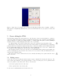
If setup correctly, a separate MicroMégas window should open when you start Graphite (Figure 1). You
can close this window at any time and reopen it from Graphite’s menu Window→Show MicroMegas window.
The bottom textfield The horizontal text field at the bottom of the MicroMégas window simply displays
information about what is going on.
1
2
Molecular surfaces
The length unit in MicroMégas is the ångström (Å)
We use the molecular surface model of
A Fast Method of Molecular Shape Comparison: A Simple Application of a Gaussian Description of
Molecular Shape. J. A. Grant, M. A. Gallardo and B. T. Pickup. Journal of Computational Chemistry,
Vol. 17, No. 14, 1653-1666 (1996)
For generating molecular surfaces, we use the [PDB
and Surfaces] tab of the MicroMégas window (Figure 1).
Opening a PDB, selecting models and chains
Click on the button [Load PDB...] for opening a
PDB file. The loaded PDB files appear in the first
column named PDB:. If you click on a PDB file name,
the list of models it contains appears in the middle
column named Models: When you click on a model
number, the list of chains it contains appears in the
right column named Chains:.
Which chains are going te be meshed? At any
given time, there is exactly one PDB selected or there
is exactly one model selected or there is exactly one Figure 1: The main window of the MicroMégas pluchain selected. This is important as this is the way to gin.
select which set of chain(s) is going to be meshed:
• if a PDB is selected, then all its chains are going to be meshed into one Graphite’s mesh object (one
surface, possibly with several connected components, see below).
• if a model is selected, then only the chains belonging to that model are going to be meshed into one
mesh object.
• if a chain is selected, then only that chain will be meshed into one mesh object.
Which residues are defined? When you select a chain (by clicking on it in the Chains: list), a text appears to the right (just above the Selected residues: caption). This texts starts with Defined residues:
and is followed by a list of integers intervals. Each number in these intervals corresponds to a residue whose
atoms are present in the PDB file. If a number is not in one interval, then you cannot select the corresponding residue for color-highlighting (see below) because there is no residue corresponding to this number in the
PDB file.
Creating a surface Use the [Mesh Surface and Colorize] button to compute a mesh of the chains. If
you change the selected residues in some chain (for showing them in special colors), click the button again:
this will only recompute the colors, not the surface (except if you change the blending (see below), or if you
force a remesh, for example after you change the Precision parameter).
After a while (look at the Info: at the bottom of the MicroMégas window), a triangular mesh of the
surface appears in the main Graphite window. The name of the generated surface depends on the selected
item and looks like mm_pdb-name[.model-name[.chain-name]], but you can change it afterwards.
2
Figure 2: Left. The two chains in 2cfa.pdb are meshed without blending (one has some blue color, the other
has some yellow color). The two meshes intersect. Right. After checking the [Blend chains:] checkbox,
the two chains are blended together.
The [ReMesh:] checkbox If a mesh with that name already exists (see paragraph above), then the surface
is not re-computed (only the colors are recomputed). If you really want to recompute the mesh, you should
either rename/delete the already-existing mesh or check the [ReMesh:] checkbox.
The [Blend chains:] checkbox If you check the [Blend chains:] checkbox and more than one chain
are going to be meshed (when you select a PDB or a model), then the chains will be blended as if it was
only one chain. This can be useful if you intend to keep these chains together with a beautiful triangular
mesh (Figure 2).
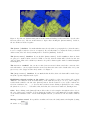
The Precision: textfield lets you enter a value between 0.01 and 3 than controls the coarseness of the
molecular surface: 3 is very tight around the atoms (but almost the same as the default value of 2.7), 0.01
gives a very coarse (bigger and smoothed) surface. See Figure 4.
The [Group surface:] checkbox If you uncheck this checkbox, then each chain will be meshed separately into separate Graphite mesh objects.
Highlighting selected residues on the surface It is possible to select some residues, and see their
“influence” or localization on the molecular surface of the chain they belong to. To do so, enter a range of
residues in the texfield to the left of the [Select] button. Use the format r:s (r,s ∈ N) to indicate the
selection of residues r,r+1, ...,s. You can enter several selections: clicking on [Select] for each, or using
the syntax r1 :s1 ,r2 :s2 ,... You will see that, in the list, the selections are numbered, starting from 0.
Color Before clicking on the [Select] button, click on the colored rectangle to the right in order to choose
the color of this group of residues. You can change the default color for the non-selected residues with the
colorbox Base surface color:. In the main Graphite window, you should see the new surface with its
colors.
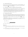
Moving a surface around It is possible to translate and rotate the (mesh) surfaces in Graphite by using
the surface tool:
.
3
Figure 3: The Distances tab (left) and the Parameters tab (right) of the MicroMégas window.
Tip I find the following settings best for visualizing molecular surface: disable the lighting in the shader
parameters and enable the Ambient Occlusion via Window→Fullscreen effect...
3
Inter-residues distances
In order to compute inter-residues distances, we use the Distances tab (Figure 3). The left part of that tab
lets the user select pairs of residues among the loaded PDB, with a self-explanatory interface. Whe the pair
is chosen, a click on the [Add pair] button will add the chosen pair of residues to the list of pairs on the
right. Two buttons below let the user [Recompute] the distances or [Remove] the pair that is selected in
the list of pairs.
While it is possible to translate and rotate the (mesh) surfaces in Graphite (in particular, those generated
by meshing a protein’s surface), the affine transformation is not (yet) applied back to the atoms positions,
and thus the distances will not change. Applying the transformation to the atoms is part of the future work.
4
Parameters tab
In this tab (Figure 3) you can set the following:
The Mesher’s distance bound roughly controls the maximum distance between the mesh approximation
of a molecular surface and the real molecular surface. A higher number results in simpler meshes. A smaller
number results in dense but ultra-smooth meshes. Default value is 0.15Å. See Figure 4.
4
B
5
0.5
0.15
0.05
Distance bound
Precision= 0.1
Figure 4: Various meshes of 2VAW.pdb.
Precision= 0.5
Precision= 2.7
Figure 5: Inside the red rectangle: the tools that the MicroMégas plugin adds to Graphite. NOTE: a
fifth button for manipulating individual base pairs of the DNA strand is not (yet) depicted on this early
screenshot.
5
Curve editing for DNA
The MicroMégas plugin adds various methods to edit 3D curves. It also provides facilities to construct a
as-rigid-as-possible moving frame at fixed arc-length intervals along the curve. Quadratic and Cubic Bézier
curve are support for creation and editing (Figure 5). A high quality interpolatory scheme [DFH09] is
available as well, for dealing with input data in the form of a point list.
No editing facilities is provided for interpolatory curves (we set this as low priority future work).
MicroMégas provides a shader for such curves, whose name is Curve. A particular interest of this shader
is that it uses the aforementionned rigidly moving frame to enable the drawing of pseudo-DNA strand, with
level-of-details (LOD) showing the atoms when the camera is sufficiently close to the curve. A DNA lines
mode makes the shader displays two ribbons in place of the DNA strand.
One motivation for these tools is to let the user coil a virtual DNA strand around proteins. Further, the
rotation of indivual base pair around the curve’s axis can be set as desired. Then, the DNA-strand can be
exported in the PDB file format.
The curves can be saved to disk and reloaded, but currently, the tuning of base pairs around the curve’s
axis are not saved.
5.1
Editing curves
A new curve is created by using the Scene→create object command and choosing the Line type. The
curve is then edited with the tools depicted in Figure 5. Two tools (blue-green) are for quadratic Bézier
curves, two (pink) for cubic Bézier curve. These tool let the user
• add control points at the end of the curve.
• delete, split and move any control point.
See the on-screen mini-manual for the details of the tools.
6
B
B
5.2
Editing DNA base pairs
Before tuning the base pairs orientation around the curve, the user must set the Curve display option to
Atoms or DNA_lines (ribbons) once, so as to generate a uniform sampling of the curve, necessary for the
tool to work properly.
• A left click is used to select a base pair which the user wants to manipulate. For technical reason,
clicking closer to the central curve works better. The selected base pair is indicated visually with a
yellow ring around it, and its number along the curve is displayed in the info text field at the bottom
of the graphite’s window.
• Clicking outside of the DNA unselects the selected base pair.
• Holding down the right mouse button and moving the mouse horizontally modifies the orientation of
the selected base pair around the curve. That orientation can be modified in the range (−π, π].
• A middle-click removes the rotation constraint on the selected base pair.
When using the Atoms display option of the Curve shader, the base pairs with a rotation constraint are
visually lighter than the other pairs, in order to make it easy for the user to see which pairs have rotation
constraints.
From the constrained base pairs, a precise orientation is computed for all every base pair, so as to keep the
DNA as “naturally twisted” as possible. For example, when exactly one base pair has a rotation constraint,
that constraint is propagated to all base pairs: when the user modifies this constraint, the whole DNA strand
can be seen to rotate around its central curve. Figure 6 illustrates DNA twisting.
6
Technical details on DNA modeling
We choose to use a smooth curve C to model DNA: at any point on the curve, the tangent vector must be
well defined. So must be the arc-length from the start of the curve to that point.
Currently in MicroMégas, two type of curves can be edited: quadratic and cubic Bézier curves.
Two point samplings of C are used: an adaptive sampling Sa of C consists of a sequence of point on
C that form a linear approximation of the curve such that the angle between two consecutive segments is
below some threshold). The adaptive sampling is used to display a visually smooth curve while minimizing
the number of segments used in the linear approximation of the curve.
We also use an uniform sampling Su of P , in which consecutive samples point on the curve are equally
spaced along the curve. We using a spacing close to 3.4 to obtain a unifom sampling Su in which the sample
points will serve as the anchor point for base-pairs of DNA.
6.1
A rigidly moving frame
From the above, we have obtained a uniform sampling Su of the curve together with the tangent vector at
every sample point. In order to coherently orient the base pairs in space, along the curve, we need to augment
this data with a normal vector, so as to obtain an orthonormal frame at each sample point. Many simple
methods to do so result in a sequence of frames exhibiting discontinuities or strong torsion (eg, the Frenet
frame). But ideally, we would like the sequence of frames to be as rigid as possible (without discontinuities
and minimizing torsion) in order to be a good start for orienting the DNA base pairs. This is not an easy
ask, but the work Wang et al. shows how one can obtain an extremely good approximation at a very low
computational cost [WJZL08]. After computing a normal vector at each sample point of Su in this way, we
store the sequence of triple {fi = (oi , ti , ni ), i ∈ [1, N ]} where ti is the tangent vector and ni is a normal
vector to the curve C at the sample point oi .
7
The initial DNA strand
One base pair is selected...
...and twisted. Note how all base pairs
have been rotated accordingly.
Another pair is selected...
...and twisted.
More pairs have been twisted.
Figure 6: Twisting DNA.
8
6.2
Drawing the DNA strand
For now we do not care about the precise nucleotides in the sequence, so the sequence will be AAA.... We
keep an atomic model of a base pair AT centered at the origin. In order to draw the full DNA strand, we
instanciate the atomic (3D) model at each sampling point oi of Su in the frame fi . Moreover, at frame fi ,
we rotate the model by 2iπ
10 to reproduce the DNA helix.
6.3
A hierarchy for interactive visualization and base-pair picking
We build a binary hierarchy over the sequence of frames {fi , i ∈ [1, N ]}. The root node consists of the entire
sequence. The subsequence at one node is split in two sub-subsequences to form the two child nodes. At
each node, a sphere bounding all the sampling point in the subsequence of the node is computed.
When drawing a long DNA strand, the hierarchy is traversed top-down, and if the bounding sphere of the
node is sufficiently far away, alternative, simpler drawing of the sub sequence are used. Our implementation
uses a double ribbon model for intermediate distances, and a simple line for faraway strands.
The hierarchy and its bounding sphere is also used to efficiently compute which base-pair has been clicked
on by the user when he wants to manipulates the DNA, see below.
6.4
Twisting the DNA strand
Since our goal is the modeling of DNA strand in interaction with some proteins, it is important that the user
user be able to fine tune the position of the DNA atoms; at least locally when there is a strong interaction
with the outside world. Allowing independent atom placement, while most powerful, would destroy the curve
model that we use to make DNA modeling easier. Instead, we allow the adjustment of the rotation of each
base-pair around the curve. That is, at each frame fi , the base pair is rotated by angle 2iπ
10 + ai . Where ai
is specified by the user.
More precisely, ai = 0 initially, and the user can then modify the angle of each base-pair individually.
To avoid the tedious task of setting the value of ai for all i, the values are interpolated where they are not
specifically defined. Suppose that the user has defined the values {ai1 , ai2 , ...aik } with i1 < i2 < ... < ik .
Then, the value of ai is computed as follows:
• if i ≤ i1 , then ai = ai1 .
• if i ≥ ik , then ai = aik .
• if ij ≤ i < ij+1 , then ai =
aij (ij+1 − i) + aij+1 (i − ij )
.
ij+1 − ij
Figure 6 illustrates DNA twisting.
References
[DFH09]
Nira Dyn, Michael S. Floater, and Kai Hormann. Four-point curve subdivision based on iterated
chordal and centripetal parameterizations. Computer Aided Geometric Design, 26(3):279–286,
2009.
[WJZL08] Wenping Wang, Bert Jüttler, Dayue Zheng, and Yang Liu. Computation of rotation minimizing
frames. ACM Transactions on Graphics, 27(1):2:1–18, March 2008.
9