Download ChipInspector 2 User Manual

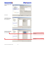
 ChipInspector 2
User Manual
For more information please contact:
Genomatix Software GmbH
Bayerstr. 85a
80335 Munich
Germany
Phone:
Fax:
Email:
WWW:
+49 89 599766 0
+49 89 599766 55
[email protected]
http://www.genomatix.de
© 2011 Genomatix Software GmbH
Table of Contents
1. Introduction to ChipInspector ...................................................................................................... 4 1.1
What is Genomatix ChipInspector? ................................................................................... 4 1.2
Which Pages in the Manual Should I Read First? ........................................................... 4 2. Theoretical Background.................................................................................................................. 5 2.1
Rationale of the Single Probe Approach........................................................................... 5 2.2
Normalization and Fold Change Calculation .................................................................... 6 2.3
Statistical Evaluation ............................................................................................................ 7 2.4
File Combinations................................................................................................................. 9 2.5
One Class Analysis (Experiment versus Control).......................................................... 10 2.6
Multiclass Analysis ............................................................................................................. 10 2.7
Absolute Expression Value ............................................................................................... 10 2.8
Projection............................................................................................................................. 10 3. Supported Microarray Platforms ................................................................................................ 11 3.1
Affymetrix Microarrays ....................................................................................................... 11 3.2
Agilent Microarrays: ........................................................................................................... 11 3.3
Illumina Microarrays ........................................................................................................... 11 3.4
Platforms and Probe Numbers ......................................................................................... 12 4. File Requirements ...................................................................................................................... 14 5. Technical Requirements............................................................................................................ 14 5.1
Operating Systems............................................................................................................. 14 5.2
Java Runtime Environment............................................................................................... 15 6. Installation and Configuration of ChipInspector ..................................................................... 17 6.1
Download............................................................................................................................. 17 6.2
Get Login and Password ................................................................................................... 19 6.2.1
Registration ................................................................................................................. 19 6.2.2 Change Password...................................................................................................... 22 6.2.3 Password Policy ......................................................................................................... 24 6.3
Installation ........................................................................................................................... 24 6.4
Configuration of ChipInspector ......................................................................................... 26 6.4.1 Proxy Configuration ................................................................................................... 26 6.4.2 Configuring automatic updates ................................................................................ 27 6.4.4. Selecting a Data Server ............................................................................................ 28 6.4.5. Configuring the Java memory settings ................................................................... 29 7 Step-by-step: Performing a ChipInspector Analysis.............................................................. 30 8 Variant: Chromatin-IP workflow ................................................................................................ 35 9 The ChipInspector Workspace Area........................................................................................ 36 9.1
The “Projects” Window ...................................................................................................... 37 9.2
The “Probes” Window ........................................................................................................ 37 9.3
The “Transcripts” Window ................................................................................................. 38 9.4
The “Genome Browser” Window ...................................................................................... 40 © 2011 Genomatix Software GmbH 2 9.5
9.6
9.7
9.8
9.9
9.10
9.11
9.12
The “Gene Information” Window ...................................................................................... 41 The “Alternative Transcripts” Window ............................................................................. 42 The “Significance Curve” Window.................................................................................... 43 The “Properties” Window................................................................................................... 43 The “Probe Filters” Window .............................................................................................. 44 The “Transcript Filters” Window ....................................................................................... 45 The “Unique Probe Statistics” Window............................................................................ 45 The “Memory Monitor” ....................................................................................................... 46 10 Projects and Analyses ............................................................................................................... 47 10.1 Creating a New Project...................................................................................................... 47 10.2 Opening an Existing Project.............................................................................................. 48 10.3 Saving the Project Tree ..................................................................................................... 48 10.4 Deleting a Project ............................................................................................................... 48 10.5 Importing Data Files into a Project................................................................................... 48 10.6 Editing a Project.................................................................................................................. 52 10.7 Creating a New Analysis ................................................................................................... 53 10.8 Committing an Analysis for a Batch Job ......................................................................... 57 10.9 Exporting Results ............................................................................................................... 58 10.9.1 Data Export ................................................................................................................. 58 10.9.2 Bed-file Export ............................................................................................................ 58 10.9.3 Transcript List Export................................................................................................. 59 © 2011 Genomatix Software GmbH 3 1. Introduction to ChipInspector
1.1 What is Genomatix ChipInspector?
ChipInspector analyzes raw data files from microarray experiments. It selects those probes
from the chip, where the signal is significantly different from the background and puts them in
their biological context.
ChipInspector extracts significant information from the expression level of single probes of
Affymetrix GeneChip© microarrays, Agilent DNA microarrays and Illumina® whole-genome
gene expression arrays. The program uses the world’s largest database of alternative
transcripts and promoters to achieve superior signal-to-noise ratios in microarray analysis. It
is unique in removing statistical and gene calling errors at the single probe level. This
annotation driven microarray analysis technology provides the basis for unmatched accuracy
in significance analysis of microarray data. It increases the number of significant features
while simultaneously reducing false positive rates by an order of magnitude. The resulting
lists of significantly regulated genes from the experiment are directly usable as input for
pathway mining tools such as Genomatix’ BiblioSphere PathwayEdition.
ChipInspector includes only a rudimentary tool set for quality assessment of microarrays.
Low level quality assessment of the hybridization and thus the success of the experiment can
be performed with a number of good and cost-free tools such as the Affymetrix TAS
software, Agilent’s Feature Extraction or Illumina’s BeadStudio.
The Genomatix approach puts its focus on the biological knowledge that is accumulated and
stored in the annotation. The annotation is made independently of the information and the
intention at the time of design of the array. Thus the data taken from the experiment is
reduced to information about hybridization signals, the biological implications are calculated
on the basis of the most current state of the genome.
1.2 Which Pages in the Manual Should I Read First?
Chapter 7 takes you through a step-by-step example of an expression array analysis. If you
wish to go to greater depths in understanding the inner workings of the program, read
Chapter 2 of this manual for theoretical considerations about the statistics and the scientific
rationale behind ChipInspector. Chapter 6 gives information about the installation and
configuration of the program and points to other resources for additional technical
information.
The “FAQ” item in the programs “Help” menu takes you to our website, where some of the
most commonly appearing issues are posted. This is continuously updated. It will also refer
you to a download area where you can obtain a pre-calculated and configured example
project.
© 2011 Genomatix Software GmbH 4 2. Theoretical Background
2.1 Rationale of the Single Probe Approach
The definition of probe sets greatly eases the handling of the large data amounts that are
produced by microarray experiments. Considerable thought has gone into the design of the
probes regarding comparable hybridization temperatures, GC content and genomic position
to create sets of single probes for one transcript. Gene expression levels are calculated as
cumulated signals from several probe expression values. The algorithms used for calculating
this cumulated signal assume that all probes in a set represent only one specific target
sequence (i.e. one transcript). In many cases, this sequence information is outdated today as
genomic annotations are becoming more and more complete. Today it can be seen from the
latest genomic annotations that most genes are flexible entities which are translated into
different mRNAs (alternative transcripts). These variants were often not or only partially
known at the time of the array design thus leading to ambiguous probe design, i.e. probes
cannot be assigned uniquely to different gene variants. Therefore the probes in a probe set
are often distributed among different (alternative) transcripts of the same gene locus. As a
consequence, the calculated signals do not reflect the expression value of the gene properly.
Figure 1: Assay sensitivity is increased by a single probe approach.
© 2011 Genomatix Software GmbH 5 With increasing computing power available to desktop/benchtop computers, the advantages
of the single probe approach can be accessed. The annotation is always up-to-date even if
some of the probes, which were originally included in a probe-set are now annotated
differently. The pooling of the single probe signals is forfeited, therefore decreasing the
chance of combining signals which are independent of each other. Consider Figure 1 to view
the difference between the single probe and the probe-set approach.
The above comments hold especially true for the new generation of tiling arrays and the
subsets of exon tiling and promoter tiling arrays. Here, the single probe approach disregards
the previously known annotation altogether, thus allowing transcript specificity and the
discovery of new splice variants when exons are assembled in a previously unknown
combination. A caveat at this point: The tiling array probes are mapped strand-specifically. A
tiling array approach using single-strand RNA would lead to a loss of detection of transcripts.
The basis for ChipInspector is the Genomatix proprietary probe to transcript assignment
based on the mapping of all probes of a microarray against the most current version of the
genome of interest. The genomic data is available in the Genomatix gene annotation browser
ElDorado. Only probes which map perfectly and uniquely in transcripts of the genome of
interest are used for the analysis. This information is saved in mapping files which are an
integral part of the program. Mapping files are updated and provided for automatic download
by ChipInspector as soon as an updated version of a genome becomes available.
2.2 Normalization and Fold Change Calculation
Initial to the significance calculation for a microarray experiment, the raw data is normalized
on the single probe level, i.e. the values are adjusted to improve consistency and reduce
bias. Each value of an array is multiplied by a constant to make the mean intensity the same
for each individual array.
Fold changes are subsequently calculated by probe wise division of the expression values
from the experimental condition by the expression values from the control condition and,
finally, a logarithmic transformation (log2) is performed for each data point.
Because values are calculated for the single probes, ChipInspector calculates differing fold
changes when compared to a probe-set-based analysis strategy. The transcripts are deemed
significant if they are detected by a user-selected number of significant probes and the fold
change value for a transcript is the mean value of the detected fold changes in the significant
single probes, not in the complete probe set. This should be kept in mind when the resulting
list of significant transcripts is further condensed by introducing a minimum fold change filter.
© 2011 Genomatix Software GmbH 6 2.3 Statistical Evaluation
The statistic algorithm in ChipInspector is a T-test with a permuted artificial background. It is
based on and enhances the original SAM algorithm by Tusher et al. (2001): Significance
analysis of microarrays applied to the ionizing radiation response. PNAS 98(9), pp 51165121.
This algorithm creates artificial background data by randomly permuting the array results.
Each probe has a score on the basis of its fold change relative to the standard deviation of
repeated measurements for this probe. Probes with scores higher than a certain threshold
are deemed significant. This threshold is the Delta value. The permutations of the data set
are then used to estimate the percentage of probes identified by chance at the identical
Delta. Thus, a relation of significant probes to falsely discovered probes can be given for
each Delta threshold. This relation is the False Discovery Rate FDR, a stringency indicator.
The FDR is a confidence value giving the user an idea of how many probes in the result
group are possibly falsely selected.
The ChipInspector algorithm calculates these numbers independently for the sets of positive
and negative data points where applicable (i.e. in a one-class assay).
The resulting curve is displayed in ChipInspector. It represents an indication of the
experiment’s success in showing the amount of probes which deviate from the signal
background. Figure 2 shows the observed (=real) values in the Y-axis over the expected
(=background) values in the X-axis. The line pictures the expected values. The single data
points are ordered by their individual significance score; values deviating downward are
displayed left of center (lower than the expected values), values deviating up are displayed
right of center (higher than the expected line). Most of the data points will deviate little from
the straight line, only in the extremes of the set is a marked change in observed versus
expected signal visible.
When the cutoff values Δpos and Δneg are changed interactively by the user, the program
recalculates the set of deviating probes, i.e. those regulated by the experimental condition.
Decreasing the Δ value yields more significant features at the cost of increasing likeliness to
find false positives. Increasing Δ diminishes the group of detected probes; the resulting set
has a higher stringency, i.e. less danger of including falsely detected probes.
A slightly different picture is obtained when the analysis is run as multi-class analysis. Here,
the features cannot be separated into down- and up-regulated groups, since the fold
changes are calculated individually for each class. Each feature may thus be up-regulated in
one and down-regulated in another class, e.g. at a different time point in the experiment.
The statistical score is therefore calculated as a deviation from the expected absolute
behavior of the average feature; there are no negative ratios in this case. The resulting curve
is shown in Figure 3.
There is no "magic number" or recommendation for Δ or the resulting FDR. This is an
experiment-specific value, a trade-off where the user has to decide on the stringency level
© 2011 Genomatix Software GmbH 7 that she requires for her results. The user chooses the statistical significance of the
calculated ratios from the statistics curve. All the selected probes and thus the resulting
projected transcripts are then significant with this FDR. With increasing Δ, the curve diverges
away from the linear gradient. Experience shows that there is often a point where a sudden
distinct decrease in the number of significant features happens and this is usually a good
point to set the cutoff. It cannot be stressed too often that microarray analysis needs to be
complemented by a biological evaluation of the results.
Observed
equals
expected – the
„null
hypothesis“
Positive
significant
features
Δpos
The majority of
values is grouped
near zero
(no difference
between expected
and observed
ratio
Δneg
Negative
significant
features
Figure 2: Graphic output of the ChipInspector statistical calculation for a Treatment/Control
analysis. The plot shows the observed (=actual) relative fold change ratios in the Y-axis over
the expected (=background) ratios in the X-axis. The features with deviating values (i.e. > Δ)
are regulated by the experimental condition.
© 2011 Genomatix Software GmbH 8 Figure 3:
Graphic output of the
ChipInspector
statistical calculation
for a multi-class
analysis.
Significant
features
Δ
„null
hypothesis“
2.4 File Combinations
Due to the fact that the statistical evaluation of the experimental data is carried out with the
data from single probes, replicates are needed to create enough data points. ChipInspector
cannot be used with only one replicate. We strongly recommend a minimum of three
replicates per experimental point, although it is possible to work with two replicates. If only 2
samples and 2 controls are available, the array parameter for file combination can be set to
"exhaustive pairing" to create 4 combinations (S1/C1, S1/C2, S2/C1, S2/C2). This is
statistically tolerable and will be sufficient to run the analysis. The results will still have less
confidence (higher False Discovery Rates) than when 3 samples are used.
Exhaustive matching of the experiments introduces a second level of data volume
enhancing. This means it is using the complete set of available data points by matching the
values from every condition experiment to the values from every control experiment. With
pair-wise matching, only a subset of this data is used. Since the background data volume is
thus increased, the individual outliers from each experiment are leveled out and therefore
signal is separated more sharply from background noise. This gives the results greater
confidence and therefore increases the number of values that are recognized as significant
(higher number of significant genes with lower FDR). This is feasible when not comparing
individuals (e.g. patient samples).
© 2011 Genomatix Software GmbH 9 2.5 One Class Analysis (Experiment versus Control)
This analysis is suited for the comparison of two experimental groups such as "knockout
versus wild-type", “treated versus untreated", or "diseased versus healthy".
2.6 Multiclass Analysis
This analysis is suited for kinetic or titration experiments with more than two data points.
2.7 Absolute Expression Value
This analysis is suited for comparing individual probe signals against the average chip
expression value.
2.8 Projection
The approach to microarray analysis in ChipInspector is annotation driven. In contrast to
most other software packages, ChipInspector does not rely on the predefined probe to
transcript assignment done by the chip manufacturer at the time of the chip design.
ChipInspector includes a new probe to transcript association performed by the Genomatix
proprietary mapping pipeline based on an up-to-date genome (ElDorado).
Significant probes are projected to transcripts using pre-calculated mapping files. As default
value, three significant probes are needed to detect a transcript as significant. This figure of
three probes was determined empirically via spike-in experiments and proved to produce a
low false positive rate while maintaining high sensitivity. However, the number of probes to
define a transcript can be adapted by the user.
The restriction of the number of transcripts marked as significant by requiring a minimum
number of significant probes to match this transcript is a form of biological quality checking.
More than one transcript can be annotated at a locus, therefore many (if not most) probes
are mapped to multiple transcripts.
© 2011 Genomatix Software GmbH 10 3. Supported Microarray Platforms
3.1 Affymetrix Microarrays
Array formats from Affymetrix (Affymetrix Inc., Santa Clara, CA, USA) are recognized
automatically when the corresponding raw data files (“CEL”-files) are imported into a
ChipInspector project.
3.2 Agilent Microarrays:
The unique identifier for Agilent (Agilent Technologies Inc., Santa Clara, CA, USA) probe
sequences is the “featureNum” entity, which is displayed in column 2 of the Agilent scanner
output. If the output comes from a GenePix scanner, the corresponding unique identifier is
the “RefNumber” in column 57.
3.3 Illumina Microarrays
The unique identifier for Illumina (Illumina Inc., San Diego, CA, USA) probe sequences is the
ArrayAddressID, which is displayed in the Bead Studio output.
For array formats from Agilent and Illumina automatic recognition is not implemented. During
file import, you are asked to identify the chip type and the column of your tab-delimited raw
data file, where the unique probe identifier is marked. In addition, these array formats do not
use the probe-set approach. The coverage should therefore be set to 1 (cf. chapter 9.10).
Genomatix calculates a proprietary annotation for the database ElDorado. ChipInspector
data is based on this. For the currently supported chips, more than 85% of the perfect match
probes are used to calculate the statistics. The following tables show the data for each chip.
© 2011 Genomatix Software GmbH 11 3.4 Platforms and Probe Numbers
Affymetrix exon arrays
Number of
columns / rows
Human Exon 1.0 ST
Human Gene 1.0 ST
Human Gene 1.1 ST Plate
Mouse Exon 1.0 ST
Mouse Gene 1.0 ST
Mouse Gene 1.1 ST Plate
Rat Gene 1.0 ST
Soy Gene 1.0 ST
2560
1050
1190/990
2560
1050
1190/990
1050
2166
Affymetrix tiling arrays
Number of
columns / rows
Human Promoter 1.0 R
Mouse Promoter 1.0 R
Arabidopsis Tiling 1.0R
Arabidopsis Tiling 1.0F
Drosophila Tiling 2.0R
2166
2166
2560
2560
2560
Affymetrix expression arrays
Number of
columns /
rows
Arabidopsis ATH1 Genome
Bovine Genome
C. elegans Genome
Canine Genome Ver 2
Chicken Genome
Human Genome U133Plus2.0
Human Genome U133A
Human Genome U133A 2.0
Human Genome U133B
Human Genome U95Av2
Human Genome FL (6800)
Human Genome U219 Plate
500K_Sty
500K_Nsp
Maize Genome
Mouse Expression Set 430 A
Mouse Expression Set 430 B
Mouse Genome 430 2.0
Mouse Genome 430A 2.0
Murine Genome U74v2 A
Chimpanzee on HGU133Plus2.0
Poplar Genome
© 2011 Genomatix Software GmbH Perfect match
probes (Genomatix
optimized)
4983374
732795
744981
4406226
752965
750883
169630
1155742
Species
Perfect match
probes (Genomatix
optimized)
3967233
3943515
2888551
2888550
2726143
Species
H. sapiens
M. musculus
R. norvegicus
G. max
H. sapiens
M. musculus
A. thaliana
D. melanogaster
Transcripts
(Genomatix
annotated)
Species
712
732
712
732
984
1164
712
732
712
640
536
744
2560
2560
730
712
712
1002
732
640
1164
Perfect match
probes
(Genomatix
optimized)
220039
199713
213496
383133
315499
525438
207689
207689
222339
169901
103884
472423
1610660
1612024
188040
207750
220386
427307
207750
141087
398160
29840
16861
20501
39164
15996
61158
39876
39876
22693
24755
15267
143190
12329
10303
64195
62161
34676
89895
62161
37949
76364
A. thaliana
B. taurus
C. elegans
C. familiaris
G. gallus
1162
355285
27395
P. trichocarpa
12 H.sapiens
Z. mays
M.musculus
P. troglodytes
Affymetrix expression arrays
cont’d
Number of
columns /
rows
Perfect match
probes
(Genomatix
optimized)
144141
284875
100954
590073
513875
276821
146487
426244
152434
Transcripts
(Genomatix
annotated)
Rat Expression Set 230 A
Rat Genome 230 2.0
Rat Genome U34 A
Rhesus Macaque Genome
Rice Genome
Soybean Genome
Vitis vinifera Genome
Xenopus tropicalis Genome
Zebrafish Genome
602
834
534
1164
1164
1164
730
1162
712
Other Array providers
Number of
identifiers
Perfect match
probes
(Genomatix
optimized)
Transcripts
(Genomatix
annotated)
41675
29678
106485
43376
1379
82289
62972
474411
473123
47281
22185
21448
78853
24526
23750
81826
48702
45347
88337
48804
45480
92754
48803
25697
45775
24972
135472
90332
45281
43331
116468
22523
20968
39569
18676
26353
8056
40644
55024
31938
8892
33458
8716
Species
R.norvegicus
M. mulatta
O. sativa
G. max
V.vinifera
X. tropicalis
D. rerio
Species
Agilent
Human Genome, 12391
(G4112A)
Human Genome, 14850
(G4112F)
SurePrint G3 Human 8x60k
Human Promoter,
014706/014707 (G4489A)
H. sapiens
Illumina
Human RefSeq 8, Version
2.0
Human RefSeq 8, Version
3.0
Human Whole Genome 6,
Version 2.0
Human Whole Genome 6,
Version 3.0
Human HT 12.0 Version 3
Mouse RefSeq 8, Version
2.0
Mouse Whole Genome 6,
Version 2.0
Rat RefSeq 12
© 2011 Genomatix Software GmbH 13 H. sapiens
M. musculus
R. norvegicus
4. File Requirements
ChipInspector has a number of requirements for the data files. The files as they are produced
in the experiment usually meet all of them, but if the files cannot be analyzed, it might be
advisable to check the following list:
1. The chip type given in the data file must be compliant with the (currently) 69 chips
supported (cf. the list of accepted chip types).
2. The files should be stored locally or on a mounted drive. Please be aware that,
depending on the file format and your network protocol, remote storage could cause
increased time demand.
3. File extension: ChipInspector analyzes files with the .cel or .CEL extensions in case
of Affymetrix microarrays. For other chip providers, tab-delimited files are expected
and a data import interface is displayed.
We recommend a minimum of three replicates per experimental point. It is possible to work
with two replicates, but the statistical evaluation should be considered with caution. It is not
possible to have less than two replicates per experimental point, because this makes
statistics non-utilizable.
5. Technical Requirements
5.1 Operating Systems
The application has been tested on the following operating systems:
Windows:
Windows XP, Windows Vista
Macintosh
At least MacOS X 10.4
Linux/Unix systems:
SuSE Linux 8.0 or above, or equivalent version of other distributors
Minimum system requirements:
•
•
•
5 GB hard disc space
1 GB RAM (recommended 2GB)
1 GHz processor speed
If you do not have any of these operating systems, or if you are not sure about your
operating system, please contact the Genomatix customer support ([email protected]).
© 2011 Genomatix Software GmbH 14 5.2 Java Runtime Environment
In order to run the ChipInspector application, you will need Java 1.6 or higher.
To test if you have an appropriate Java version already installed on your system, type
“java –version” on command line.
Here is an example for windows users how to check the installed java version:
Click on Start/All Programs/Accessories/Command Prompt (see screenshot below).
© 2011 Genomatix Software GmbH 15 A command window will pop up:
Type in java –version and press Enter.
If Java is installed, you will get an output like:
If Java is not yet installed on your computer, or if you have a Java version older than 1.6.0,
please follow the link http://www.java.com/ to download and install the newest version of
Java (at least version 1.6.0).
© 2011 Genomatix Software GmbH 16 6. Installation and Configuration of ChipInspector
ChipInspector is a JAVA program which must be installed locally on your computer. Please
proceed for download and installation as follows.
6.1 Download
To download ChipInspector, please follow the following steps:
1.
2.
3.
4.
Create a folder on you hard disk where you want to store the installer
Switch to http://www.genomatix.de/products/ChipInspector/ChipInspector6.html
Choose your operating system from the download
Click on the download button next to your operating system
Clicking on the download-icon will result in the following screen:
Choose the option “save to disk” and click “ok”
© 2011 Genomatix Software GmbH 17 A window will show up, where you can choose a folder to save the file. Choose the folder
where you would like to save the installer and press ok.
Mac users will find a folder named "GenomatixApplications" on their desktop or in their
designated download folder. It contains an installer package, a ReadMe and the license file.
Double clicking the "GenomatixApplications" installer package will start the installation of the
software.
© 2011 Genomatix Software GmbH 18 6.2 Get Login and Password
To apply the ChipInspector application you require a Genomatix user account with login and
password. Registration for a two-week trial account is free of charge. An e-mail with your
personal username and password will be sent to you immediately.
6.2.1. Registration
Open your internet browser and navigate to www.genomatix.de.
Click on “Login” in the left frame of the webpage.
© 2011 Genomatix Software GmbH 19 If you do not have an account yet, please click on “Register”.
Fill in the form – please enter your e-mail correctly.
© 2011 Genomatix Software GmbH 20 Check your e-mail. A mail with your login data should be sent to you right away.
The login and password is not only valid for ChipInspector but for all Genomatix products.
© 2011 Genomatix Software GmbH 21 6.2.2
Change Password
Open your internet Browser and switch to www.genomatix.de.
Click on “Login” on the webpage (see above)
Enter your login and password which was sent to you via e-mail.
© 2011 Genomatix Software GmbH 22 After login you will see the following page. Click on “Password”.
Fill in the form and click on “Change Password” to change your password.
© 2011 Genomatix Software GmbH 23 6.2.3
Password Policy
Genomatix’ password policy requires all passwords to be at least 6 characters long and must
contain at least one non-alphabetic or capital character. No blanks or tabs are allowed.
6.3 Installation
Switch to the folder on your hard disk where the installer was saved. Execute the installer
(see below) and follow the instructions.
Please note that the Genomatix licensing model for ChipInspector is a single-user floating
license. This means that you may install the program on any number of machines, however
not run several instances of the program at the same time. If a second instance of
ChipInspector is started while another instance is running, the user is given the choice of
ending the concurring session. This can lead to data loss on the first instance if the analysis
results have not been stored yet. The above said is true also for parallel instances of
ChipInspector 2 and older versions. The programs may be run alternately, but not at the
same time.
© 2011 Genomatix Software GmbH 24 If you run a windows system, the following screen will pop up:
Click “Next >” and follow the instructions.
After ChipInspector is installed successfully, you can start the application either from the
program group “Genomatix” with the executable “ChipInspector” by double-clicking the
“ChipInspector” icon on your desktop.
© 2011 Genomatix Software GmbH 25 6.4 Configuration of ChipInspector
Before you start working with ChipInspector, please take a minute to configure the
application concerning the proxy configuration for internet access and the application update
behavior to get the latest program version automatically.
6.4.1
Proxy Configuration
Many companies and institutions use proxies and firewalls for secure and fast access to the
Web. ChipInspector will try to learn the appropriate settings from your preferred browser
application (InternetExplorer or Firefox), but it may be necessary to configure these settings
to allow the application to pass your local proxy or firewall.
In ChipInspector, go to the "Tools"
menu and select "Options".
In the “General” tab, tell the
application whether to use
the proxy known to your
computer or to use a manual
setting which you will be
able to receive from your
institution’s
system administrator.
© 2011 Genomatix Software GmbH 26 6.4.2
Configuring automatic updates
Periodically Genomatix provides important ChipInspector updates. The Genomatix Update
Service helps you to keep your application current.
In ChipInspector, go to the "Tools" menu
and select "Plugins".
In the “Settings” tab,
set the interval of
automatic update
checks.
If you select “Never”,
then the application
will only update itself
if you manually start
this process.
© 2011 Genomatix Software GmbH 27 When an updated
version of the
program is
available, you will
be notified by a
symbol in the
bottom right corner
of the screen
Click this icon to
update
ChipInspector
automatically or go
to the "Help" menu
and select "Check
For Updates".
6.4.4. Selecting a Data Server
If data downloads are slow, a different data server may be closer to your geographical
location. Configure the data server which you want to use by going to the “Tools” menu and
selecting “Options”.
In the “Download”
tab, choose the
server for data
download.
© 2011 Genomatix Software GmbH 28 6.4.5. Configuring the Java memory settings
Every Java program such as ChipInspector runs within a defined environment, the Java
Virtual Machine (JVM). When a Java program is started, the computer allocates a portion of
its main memory (its RAM) to the JVM. When ChipInspector is first installed, the amount of
allocatable RAM is calculated. However, this calculation may be off or new hardware RAM
may have been added subsequently. It is possible to increase the portion of RAM for the
JVM, thus giving ChipInspector more memory:
Step 1: Find out how much RAM your computer has. Under Windows, this parameter can
e.g. be found in the System Properties Control Panel. Here, you can also find out whether
you have a x64 operating system.
Step 2: Find out which Java machine is installed. See page 15 for details.
Step 3: Calculate the portion of RAM for the Java Machine.
If you have a x64 operating system and a suitable x64 Java installed, then the maximum
memory manageable by the JVM lies between 3000 and 3400 Megabyte. If this is not the
case, the limit is between 1500 and 1700 Megabyte. Leave at least 200 Megabyte for internal
computer processes.
Step 4: Edit the file which starts ChipInspector accordingly:
Under Windows, right-click the ChipInspector
icon and choose "Properties". In the
"Shortcut" tab, edit the last number in the
"Target" box accordingly. For example, if you
decide that 1300 Megabyte of RAM can be
allocated to the JVM, the end of the line
should read:
...\chipinspector.exe -J-Xmx1300m
Step 5: When the RAM portion size is not compatible with your computer setup, the JVM
(and thus ChipInspector) will not start. Redo step 3 until ChipInspector is functional again.
© 2011 Genomatix Software GmbH 29 7
Step-by-step: Performing a ChipInspector Analysis
When the program starts,
a login screen asks for
your Genomatix account
credentials. If you have no
account with Genomatix
yet, please refer to page
20 of this manual for
instructions on how to
activate an account.
Enter username and
password and click “Ok”.
On the welcome page, a
wizard is provided to guide
you through the creation of
a project, the data import
and the analysis.
All steps are also
accessible via the program
interface.
If you previously
deactivated the “Welcome”
page, you can re-enable it
in the Help menu.
Click the “ChipInspector”
logo in the “Available
modules” column.
In Step 1, an input form is
displayed, which asks for
a project name.
Enter a name for the new
project and click “Finish”.
© 2011 Genomatix Software GmbH 30 In the next step, the raw
data files are imported.
The wizard opens this
dialog automatically.
Depending on the type
of data choose “CELFile Import” for
Affymetrix or “Tabular
File Import” for other
platforms.
Click “Next”.
Use the upper
“Browse…” button to
navigate to the folder
where the data files are
located.
Choose the appropriate
data files in the
FileChooser dialog and
click “Open”.
© 2011 Genomatix Software GmbH 31 The program will
attempt to recognize
the chip type.
You may have to select
the chip type manually
if it is not recognizable
from the data file. In
this case, please select
the chip type from the
list of supported chips.
Click “Next”.
The data files are
imported into the
project.
Click “Finish”.
The wizard now
presents the “New
Analysis” workflow.
In the first step, you are
asked to choose the
appropriate statistical
assay form (see p. 9 for
explanations of the
various statistical
assays possible):
Click “Next”.
© 2011 Genomatix Software GmbH 32 Provide a name for the
analysis.
Click “Next”.
The data files for the
project are presented in
the central file list.
Select the control files
and associate them with
the “Control” list.
Christian Zinser 15.7.08 16:36
Kommentar: Screenshot paßt nicht – das sind Treatment Files Christian Zinser 15.7.08 15:48
Kommentar: © 2011 Genomatix Software GmbH 33 Select the files that
represent the experimental
condition and associate
them with the “Treatment”
list.
Click “Next”.
Choose the file
combinations for the
statistical analysis (see p.9
for an explanation of the
possible variants).
Christian Zinser 15.7.08 16:47
Kommentar: Anderer Screenshot ; Normalization type kann nicht mehr gewählte werden Click “Next”.
The time required for an
analysis depends on the
size of the microarray, the
size of the data set and the
hardware.
The program gives an
overview of the progress.
When the analysis is
finished,
click “Finish”.
© 2011 Genomatix Software GmbH 34 ChipInspector
displays a table with
the analysis results.
The “Probes” table
shows the significant
single probes
detected on the chip
ordered by
chromosomal
position.
The program allows various views on the data. In section 9, each view is explained in detail.
Click the “Window” menu item to see a list of display options.
8
Variant: Chromatin-IP workflow
ChipInspector can be used for the evaluation of Chromatin-IP experiments. In this case, the
workflow is amended. Chromatin-IP experiments are targeted towards sharply defined
regions of the genome, where the immunoreaction produces a signal.
It is therefore not advisable to use the transcript list view to see annotated genomic regions
defined by single probes. Instead, use the Probe Filters (section 8.9) to define the size of the
significant regions in basepairs and the minimum number of probes that this region should
contain.
Export the resulting significant regions as
a .bed-file (File – Export). Use this bedfile as input in Genomatix’ RegionMiner, a
program found on our webserver.
RegionMiner provides information on
Transcription Factor binding sites
independent of annotation and strand
specificity and is thus optimally suited for
Chromatin-IP evaluation.
© 2011 Genomatix Software GmbH 35 9
The ChipInspector Workspace Area
The Menu item “Window” shows a list of different data view options, which can be turned on
and off and are explained in detail in this section. Each view presents various aspects of the
data:
Projects
projects and analyses which
are currently open.
Genome Browser
probes graphically in the
genomic environment
Gene Information
known annotation of a
selected gene
Transcript View
alternative transcripts for
the selected locus
Significance
Curve
result curve of the statistical
calculation for the
experiment
Properties
properties of the selected
project or analysis
Probe Filters
parameters used for
selecting subsets of the
data
Transcript Filters
Size and screen position of all windows are manageable.
© 2011 Genomatix Software GmbH 36 9.1 The “Projects” Window
The project management panel shows the currently
open projects and analyses in a tree structure.
Right-clicking on an item in the tree opens a context
menu for performing actions on the respective
object such as data import or starting a new
analysis.
Only the menu items with a meaningful function for
the current state of the object will be activated.
9.2 The “Probes” Window
ChipInspector displays a table with the analysis results. The “Probes” table shows the
significant single probes detected on the chip ordered by chromosomal position. For each
single probe, the following information is displayed from left to right:
•
chromosome number
•
start position of the probe on the chromosome
•
length of the probe
•
strand where the probe is mapped to
•
statistical significance score of the probe in the experiment
•
significant region into which this probe is grouped
•
the transcripts to which this probe is assigned
•
the fold change (log2) that this probe shows in the experiment
When a table cell is selected, the corresponding information is updated correspondingly in
the other windows.
The list is filtered according to the filter settings in the “Probe Filters” window. Clicking the
“transcripts” tag in the table header toggles the view to display the transcripts that are
associated with the probes in the list.
© 2011 Genomatix Software GmbH 37 9.3 The “Transcripts” Window
The result list lists the significantly regulated transcripts and their probe coverage (i.e. the
number of significant probes that map to the transcript exons from left to right:
•
the NCBI GeneID
•
the official gene symbol
•
the RefSeq Accession Number
•
the coverage of this transcript by significant probes
•
the average fold change of all significant probes for this transcript
Clicking the accession number will update the “Alternative Transcripts” window and display
all alternative transcripts at this locus. If there is significant evidence for both up and down
regulation of a transcript, two entries are listed for it, displaying the according positive and
negative fold changes.
The list can be sorted by any column by clicking on its header.
When a table cell is selected, the corresponding information is updated correspondingly in
the other windows.
© 2011 Genomatix Software GmbH 38 The list is filtered according to the filter settings in the “Transcript Filters” window. Clicking
the “transcripts” tag in the table header toggles the view to display the transcripts that are
associated with the probes in the list.
Clicking the button “ElDorado” at the bottom of this window opens a browser with a view of
the selected transcript in Genomatix’ annotation browser ElDorado.
This is especially helpful when the analysis is based on an older version of ElDorado,
therefore disabling the graphic view in ChipInspector. The ElDorado view can then still be
used to see the genomic environment of the selected transcript.
© 2011 Genomatix Software GmbH 39 9.4 The “Genome Browser” Window
The Genome Browser shows the genome annotation at the specified locus. It automatically
repositions the view if a probe or a transcript is selected in another view. The following
elements are extracted from Genomatix’ ElDorado database and displayed in the graph:
Element Color
Element Description
Primary transcript
Exon
Promoter
3’ UTR
Transcription start region, based on CAGE
tag evidence
Up-regulated probe significant / nonsignificant
Down-regulated probe significant / nonsignificant
/
/
The elements on the forward strand are displayed above the black line; the elements on the
reverse strand are located beneath the black line. The vertical size of the probe reflects the
fold change in the experiment. Tool tip texts give additional information about the elements.
The following graph explains the various functions:
Zoom in Zoom out Select a region Show / hide elements Display selected region in ElDorado Display selected region in MatInspector © 2011 Genomatix Software GmbH 40 A region that is selected by clicking and drawing the mouse can be displayed in the genome
annotation browser ElDorado by clicking the corresponding button.
A comprehensive overview over all the transcription factor binding sites that are located in
the selected region can be obtained by clicking the MatInspector button.
A browser window is opened in both cases taking you directly to the corresponding
Genomatix webpage.
Please note that this feature depends on synchronized genome versions in ChipInspector
and ElDorado and is therefore disabled, when an analysis is based on an older version of the
genome.
9.5 The “Gene Information” Window
A digest of the comprehensive annotation
from ElDorado is presented. The link behind
the GeneID leads to a complete overview of
the information in the various databases on
the Genomatix servers while the button
“ElDorado” leads directly to the “More Gene
Info” page of ElDorado.
© 2011 Genomatix Software GmbH 41 9.6 The “Alternative Transcripts” Window
The Transcript View shows the various alternative transcripts at the specified locus. It
automatically repositions the view if a transcript is selected in another view. The following
elements are extracted from Genomatix’ ElDorado database and displayed in the graph:
Element Color
Element Description
Primary transcript
Exon
Promoter
3’ UTR
Transcription start region, based on CAGE
tag evidence
Up-regulated probe significant / nonsignificant
Down-regulated probe significant / nonsignificant
/
/
The elements on the forward strand are displayed above the black line; the elements on the
reverse strand are located beneath the black line. The vertical size of the probe reflects the
fold change in the experiment. Tool tip texts give additional information about the elements.
The NCBI GeneID and the RefSeq accession number are shown for each alternative
transcript; the Genomatix LocusID and the gene symbol are shown at the bottom of the
window.
The following graph explains the various functions:
Zoom in Show / hide elements Zoom out Display selected region in ElDorado © 2011 Genomatix Software GmbH 42 9.7 The “Significance Curve” Window
For an explanation of the
statistical algorithm which is
applied in ChipInspector, please
refer to page 9 in this manual.
The resulting significance curve
is displayed for each analysis.
The observed ratio values are
plotted against the expected ratio
values.
The color intensity of the curve
mirrors the number of features
with the corresponding
Observed/Expected coordinates,
scaled in the bar on the right.
Most of the features will be
grouped around the center of the
graph near Zero.
By right-clicking the graph, you have access to zooming functions.
9.8 The “Properties” Window
A right-click on any object in the program opens
a “Properties” window. Here, the parameters,
description texts and file locations for the
selected object are displayed.
In the case of an analysis, this includes e.g. the
chip type, the file combination and the ElDorado
database version, on which this analysis is
based.
© 2011 Genomatix Software GmbH 43 9.9 The “Probe Filters” Window
Each single probe in the analysis has a
statistical score and a defined position in
the genome.
The list of probes can thus be restricted
either by the significance score or by their
proximity to other significant probes.
Please refer to p. 9 in this manual for an
explanation of the Delta value and False
Discovery Rate. The sliders in theProbe
Filters window are used to vary this
parameter in the analysis. The “Significant
Feature” number is an estimation at this
point and the numerical value may
deviate in the resulting probe list,
especially at low Delta settings.
In general, a more stringent statistic score
(a higher Delta) results in less significant
features with a higher confidence (lower
FDR).
To define regions of significant probes, a sliding window approach is utilized, the parameters
here are the window size (in basepairs) and the number of required significant probes within
this region.
© 2011 Genomatix Software GmbH 44 9.10 The “Transcript Filters” Window
Each transcript which is included in the microarray is
detected by one or more single probes. This filter is
used to select the number of significant single
probes that detect a transcript before this transcript is
deemed significant. The default of 3 should be set to
1 for non-Affymetrix arrays.
This filter is also used to restrict the number of
transcripts in the result list by a minimum fold
change. The parameter refers to the average fold
change of all significant probes which detect this
transcript.
9.11 The “Unique Probe Statistics” Window
By selecting one or more imported data files in the “Projects” Window and right-clicking, you
can select the action “Show Unique Probe Statistics” and view a low-level assessment of the
raw data.
The displayed values
give an estimate
whether the raw data
files in the analysis
are on comparable
expression levels.
By right-clicking the graph, you have access to zooming functions.
© 2011 Genomatix Software GmbH 45 9.12 The “Memory Monitor”
Click “View – Toolbars –
Memory” to display a
memory monitor in the
toolbar field.
Click the memory monitor to free unused memory.
© 2011 Genomatix Software GmbH 46 10 Projects and Analyses
10.1 Creating a New Project
To create a new project, select “File – New Project…” from the menu, or click on the “New
Project” toolbar button.
A form is displayed which
asks for a project type.
Currently, only one type of
project is supported, the
“New Project”.
Click “Next”.
An input form is displayed,
asking for a project name.
Enter a name for the new
project and click “Finish”.
© 2011 Genomatix Software GmbH 47 10.2 Opening an Existing Project
To open a previously saved project, select “File - Open Project…” from the menu, or click on
the Open Project toolbar button, and select a project tree file from the dialog.
10.3 Saving the Project Tree
To save the project tree, including all projects, analyses and results, select “Save” from the
File menu, or click on the Save All toolbar button.
10.4 Deleting a Project
To delete a project, including all analyses and results, right-click the project in the projects
window and select “Delete” from the context menu.
10.5 Importing Data Files into a Project
To import data files into
your project, click the
“New Action” button in
the task bar or rightclick the appropriate
project and select “New”
from the context menu.
Select “Cel-File Import” from, the context menu.
© 2011 Genomatix Software GmbH 48 In the next step, the raw
data files are imported.
The wizard opens this
dialog automatically.
Depending on the type
of data, choose “CELFile Import” for
Affymetrix or “Tabular
File Import” for other
platforms.
Click “Next”.
Use the upper
“Browse…” button to
navigate to the folder
where the data files are
located.
Choose the appropriate
data files in the File
Chooser dialog and
click “Open”.
© 2011 Genomatix Software GmbH 49 The program will
attempt to recognize the
chip type.
You may have to select
the chip type manually if
it is not recognizable
from the data file. In this
case, please select the
chip type from the list of
supported chips.
Click “Next”.
If non-CEL files are imported, a preview step is interposed allowing you to select the data
rows and columns which are relevant for the subsequent analysis.
Choose the separator, which marks the columns, identify the first row where data is located
and finally select those columns, which hold the relevant data.
Only one column may be designated as holding the feature ID. ChipInspector expects the
identifier for the unique and singular tag sequence.
© 2011 Genomatix Software GmbH 50 The unique identifier for Agilent probe sequences is the “featureNum” entity, which is
displayed in column 2 of the Agilent scanner output. If the output comes from a GenePix
scanner, the corresponding unique identifier is the “RefNumber” in column 57.
The unique identifier for Illumina probe sequences is the ArrayAddressID, which is displayed
in the Bead Studio output. This not the Illumina ProbeID (starting with “ILMN_”), but rather
the strictly numeric ArrayAddressID.
The number of columns that can hold expression data from the experiment is not restricted.
The data files are
imported into the
program.
Click “Finish”.
© 2011 Genomatix Software GmbH 51 10.6 Editing a Project
Right-click on the project node in the “Projects Window” to perform a number of tasks on the
project:
• New
o Importing additional data files for analysis
o Starting a new analysis on imported data files
• Renaming
• Deleting
• Copying to another directory (i.e. for sharing the result with collaborators)
• Closing
• Moving to another location on your computer
• Set As Main Project: this project will be suggested as the default project when a new
analysis is started
• Editing the project Properties (i.e. adding a description text)
© 2011 Genomatix Software GmbH 52 10.7 Creating a New Analysis
To create a new
analysis, right-click
on a project node
and select “New” –
“Other Action”.
Choose an analysis type from the selection; please refer to page 9 for a more in-depth
explanation. Available types are:
Treatment/Control Pairing
Use this option if you want to perform a one-class analysis, which compares a treated
sample to a control. A single sided permutation T-test analysis is performed.
Time Course/Titration Experiment
Select this option if you want to compare a set of data points in a multi-class analysis, e.g. for
subsequent cluster analysis of the results in other programs. In this case a multi-class
permutation T-test analysis is performed.
Presence/Absence Calling
Choose this option if you want to measure expression values relative to the average
expression on the chip, e.g. for gene expression values in one specific tissue. In this case a
permutation T-test analysis detecting probes which are significantly above the experiment
average is performed. Biological replicates with n>=2 are still required.
Click “Next”.
© 2011 Genomatix Software GmbH 53 Provide a name for the
analysis.
Click “Next”.
The data files for the
project are presented in
the central file list.
If “Treatment/Control” is
selected, two windows
are displayed to which
the respective files are
assigned.
Select the control files
and associate them with
the “Control” list.
© 2011 Genomatix Software GmbH 54 Select the files that
represent the experimental
condition and associate
them with the “Treatment”
list.
Click “Next”.
If “time Course/Titration” is
selected, you are
additionally asked to
choose the number of
experimental conditions,
which are relevant for this
analysis.
Assign the files accordingly;
control files may be
associated with more than
one experimental class,
while each treatment file
may be associated with
only group.
Click “Next”.
Accordingly, when
“Presence/Absence” is
chosen, there is only field
displayed which accepts
all the files for the current
analysis.
Click “Next”.
© 2011 Genomatix Software GmbH 55 Choose the file
combinations for the
statistical analysis (see p.9
for an explanation of the
possible variants).
The program will display
the combination of the files
accordingly, when the
combination type is
selected.
Click “Next”.
If you select “Finish” at this point, the analysis is stored for later inclusion into a batch job, i.e.
when more than one analysis is run in one continuous process.
The time required for an
analysis depends on the
size of the microarray, the
size of the data set and
the hardware.
The program gives an
overview of the progress.
When the analysis is
finished,
Click “Finish”.
Please refer to page 38 for a description of the various data views which are presented by
the program.
© 2011 Genomatix Software GmbH 56 10.8 Committing an Analysis for a Batch Job
Right-click the project or
select “New Action” from
the menu bar to display the
possible actions and select
“Analysis Batch Job” from
the list.
Click “Next”.
Select
those
analyses
which you want to run in
one continuous process,
e.g. over night.
Click “Next”.
© 2011 Genomatix Software GmbH 57 10.9 Exporting Results
You can export the results in different formats for further analysis. To do so, click on “File Export” in the menu and choose from the available export options:
10.9.1 Data Export
Both the transcript list and the probe list can be exported as a table for MS Excel or other
spreadsheet programs. This table will contain the following data:
•
•
•
•
•
•
•
•
Chromosome
Position
Length
Strand
Significance Score
Region
Transcript
Fold Change (log2)
10.9.2 Bed-file Export
The probe list
can be
exported as a
.bed-file for
further
downstream
analysis in
Genomatix’
RegionMiner
or other
annotation
programs. It
will show the
significant
regions:
•
•
•
Chromosome
Start position
End position
© 2011 Genomatix Software GmbH 58 10.9.3 Transcript List Export
If the table of transcripts
is exported and the fold
changes for every data
combination are required,
additional columns for
these
data
will
be
included in the output file.
Alternatively, the transcript list can be exported in a format which is compliant with
Genomatix’ BiblioSphere and PathwaySystem.
© 2011 Genomatix Software GmbH 59