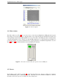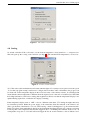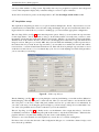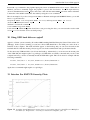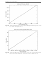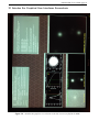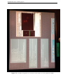
1
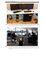
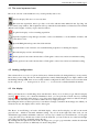
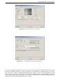
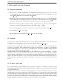
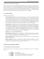
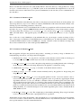
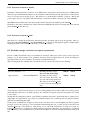
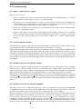
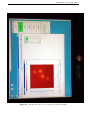
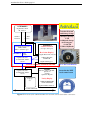
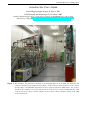
AstraLux Sur User’s Guide page 1
AstraLux Sur User’s Guide
Stefan Hippler, [email protected], May 6, 2013
Felix Hormuth, [email protected], November 2007
AstraLux Sur Homepage: http://www.mpia-hd.mpg.de/ASTRALUX/sur_index.html
Observatory webpages: http://www.eso.org/sci/facilities/lasilla/
Figure 1. The AstraLux Sur instrument mounted at the Nasmyth B focus of the NTT. The AstraLux Sur
camera is attached to the adapter/rotator flange. A filter wheel in black sits between the camera
and the flange. The EFOSC2 instrument has been separated from the NTT rotator. One of the 3
AstraLux Sur computers sits in the rack shown on the lower left. A dedicated Gigabit fiber links
connects the local camera control computer to the remote camera computer sitting in the NTT
local control room.
AstraLux Sur User’s Guide page 2
Figure 2. A view inside the old NTT local control room: the Astralux Sur remote camera computer is shown
on the left half, next to the AstraLux Sur pipeline machine (right half). The image shows the fiber
cable on the left and the white switch to the right of the computer monitors.
Figure 3. A view inside the new observations building (NOB): An X-terminal with 1 monitor connects to
the remote camera computer in the old NTT local control room. Another X-terminal with 2 monitors connects to the pipeline machine in the old NTT control room. Observers prepare for night
observations.
AstraLux Sur User’s Guide page 3
Contents
1 Introduction
1.1 Purpose of this document . . . . . . . . . . . . . . . . . . . . . . . . . . . . . . . . . . . .
1.2 Recommended reading . . . . . . . . . . . . . . . . . . . . . . . . . . . . . . . . . . . . .
4
4
4
2 The AstraLux Sur network: computers and accounts
4
3 Filter Setup
3.1 Standard filters . . . . . . . . . . . . . . . . . . . . . . . . . . . . . . . . . . . . . . . . .
3.2 Filter GUI . . . . . . . . . . . . . . . . . . . . . . . . . . . . . . . . . . . . . . . . . . . .
5
5
6
4 Camera operation
4.1 The most important icons
4.2 Loading configurations .
4.3 Live display . . . . . . .
4.4 Slider window . . . . . .
4.5 Shutter . . . . . . . . . .
4.6 Cooling . . . . . . . . .
4.7 Acquisition setup . . . .
.
.
.
.
.
.
.
.
.
.
.
.
.
.
.
.
.
.
.
.
.
.
.
.
.
.
.
.
.
.
.
.
.
.
.
.
.
.
.
.
.
.
.
.
.
.
.
.
.
.
.
.
.
.
.
.
.
.
.
.
.
.
.
.
.
.
.
.
.
.
.
.
.
.
.
.
.
.
.
.
.
.
.
.
.
.
.
.
.
.
.
.
.
.
.
.
.
.
.
.
.
.
.
.
.
.
.
.
.
.
.
.
.
.
.
.
.
.
.
.
.
.
.
.
.
.
.
.
.
.
.
.
.
.
.
.
.
.
.
.
.
.
.
.
.
.
.
.
.
.
.
.
.
.
.
.
.
.
.
.
.
.
.
.
.
.
.
.
.
.
.
.
.
.
.
.
.
.
.
.
.
.
.
.
.
.
.
.
.
.
.
.
.
.
.
.
.
.
.
.
.
.
.
6
7
7
7
8
8
9
10
5 Quick guide to Lucky Imaging
5.1 Filename conventions . . . . . . . . . .
5.2 Flat-fields . . . . . . . . . . . . . . . .
5.3 To bias or not to bias . . . . . . . . . .
5.4 Use the right FoV . . . . . . . . . . . .
5.5 Finding the right gain and exposure time
5.6 How many frames to acquire . . . . . .
5.7 Photometry: a thorny issue . . . . . . .
.
.
.
.
.
.
.
.
.
.
.
.
.
.
.
.
.
.
.
.
.
.
.
.
.
.
.
.
.
.
.
.
.
.
.
.
.
.
.
.
.
.
.
.
.
.
.
.
.
.
.
.
.
.
.
.
.
.
.
.
.
.
.
.
.
.
.
.
.
.
.
.
.
.
.
.
.
.
.
.
.
.
.
.
.
.
.
.
.
.
.
.
.
.
.
.
.
.
.
.
.
.
.
.
.
.
.
.
.
.
.
.
.
.
.
.
.
.
.
.
.
.
.
.
.
.
.
.
.
.
.
.
.
.
.
.
.
.
.
.
.
.
.
.
.
.
.
.
.
.
.
.
.
.
.
.
.
.
.
.
.
.
.
.
.
.
.
.
.
.
.
.
.
.
.
.
.
.
.
.
.
.
.
.
.
.
.
.
.
.
.
.
.
.
.
.
12
12
12
12
13
13
13
13
.
.
.
.
.
.
.
.
.
.
.
.
.
.
.
.
.
.
.
.
.
.
.
.
.
.
.
.
.
.
.
.
.
.
.
.
.
.
.
.
.
.
.
.
.
.
.
.
.
6 Preparing the control desktops
13
7 The
7.1
7.2
7.3
14
14
15
15
AstraLux Sur applications & windows
AstraLux File Receiver . . . . . . . . . . . . . . . . . . . . . . . . . . . . . . . . . . . . .
AstraLux Data Transfer Monitor . . . . . . . . . . . . . . . . . . . . . . . . . . . . . . . .
Pipeline Windows . . . . . . . . . . . . . . . . . . . . . . . . . . . . . . . . . . . . . . . .
8 Data types, pipeline products
8.1 Data directories and data products . . . . . . . . . .
8.1.1 Contents of AstraLux input . . . . . . . . .
8.1.2 Contents of AstraLux output . . . . . . . . .
8.1.3 Contents of AstraLux header . . . . . . . . .
8.1.4 Contents of AstraLux calib . . . . . . . . . .
8.2 Available storage, minimum free space requirements
9 Troubleshooting
9.1 Help! I cannot find my target! . . . . .
9.2 Camera software crashes . . . . . . . .
9.3 Reasons and cures for pipeline crashes .
9.4 Reasons and cures for receiver problems
.
.
.
.
.
.
.
.
.
.
.
.
.
.
.
.
.
.
.
.
.
.
.
.
.
.
.
.
.
.
.
.
.
.
.
.
.
.
.
.
.
.
.
.
.
.
.
.
.
.
.
.
.
.
.
.
.
.
.
.
.
.
.
.
.
.
.
.
.
.
.
.
.
.
.
.
.
.
.
.
.
.
.
.
.
.
.
.
.
.
.
.
.
.
.
.
.
.
.
.
.
.
.
.
.
.
.
.
.
.
.
.
.
.
.
.
.
.
.
.
.
.
.
.
.
.
.
.
.
.
.
.
.
.
.
.
.
.
.
.
.
.
.
.
.
.
.
.
.
.
.
.
.
.
.
.
.
.
.
.
.
.
.
.
.
.
.
.
.
.
.
.
.
.
.
.
.
.
.
.
.
.
.
.
.
.
.
.
.
.
.
.
.
.
.
.
.
.
.
.
.
.
.
.
.
.
.
.
.
.
.
.
.
.
.
.
.
.
.
.
.
.
.
.
.
.
.
.
.
.
.
.
.
.
15
15
16
16
17
17
17
.
.
.
.
18
18
18
18
18
10 Using USB hard disks on apipe2
19
11 Astralux Sur EMCCD Linearity Plots
19
12 Astralux Sur Graphical User Interfaces Screenshots
21
AstraLux Sur User’s Guide page 4
1 Introduction
1.1 Purpose of this document
AstraLux Sur is the La Silla NTT 3.5 m Lucky Imaging camera. With a pixel scale of 31 mas it allows nearly
diffraction limited imaging at wavelengths longwards of 800 nm over a field of view of 512×512 pixels. The
heart of the instrument is an electron multiplying high speed CCD (EMCCD) with virtually zero readout
noise.
This document does not intend to give a thorough description of the instrument or the Lucky Imaging observing technique. For more information about these topics you may look into the diploma thesis of Felix
Hormuth which had AstraLux (the Calar Alto Lucky Imaging Camera) as its main topic or read the PhD theses of Bob Tubbs and Nicholas Law which describe similar instruments and give valuable information about
the Lucky Imaging technique in general and specific data processing steps.
For a description of the daily task to be performed during / before observations, please see the separate
checklists.
1.2 Recommended reading
For a general introduction to Lucky Imaging and the AstraLux Sur instrument, you may have a look at the
following sections of the AstraLux diploma thesis, which is available as PDF file at the AstraLux homepage
http://www.mpia.de/ASTRALUX:
Section
Pages
Topic
1.5.3
14–18
Lucky Imaging: what is it, why does it work,
which filters make sense to use.
3.2
28–31
EMCCDs: how do they work, peculiarities.
3.3.2
32–43
AstraLux camera characteristics: gain, linearity, noise, etc.
4.3
50–53
Pipeline steps, e.g. quality assessment, image reconstruction.
5.2.5
65–66
Atmospheric dispersion effects.
5.4.1-5.4.2
68–71
Temporal characteristics, correlation times.
5.5.1
75
Isoplanatic angle.
5.5.2
76
Reference star magnitude requirements.
6.4
86–87
Recommendations for the astrometric calibration of AstraLux.
Astronomers who want to know more about the data quality and examples of observational results might read
Chapters 5 and 7 in full length.
The PhD theses of Bob Tubbs and Nicholas Law can be found via the Cambridge LuckyCam Homepage at
http://www.ast.cam.ac.uk/~optics/Lucky_Web_Site/references.htm.
2 The AstraLux Sur network: computers and accounts
See separate sheet for passwords!
The AstraLux Sur hardware can be split into three segments: one is made up by the camera computer and
electronics at the Nasmyth B focal station, the second by one Windows XP computer and the Linux pipeline
machine inside the ”old” local control room of the NTT building. The third segment is actually not exclusively
attributed to AstraLux Sur, but consists of usually two X-terminals, which connect to wg5pl and wg5off in
the new observations building, NOB, which is used for observations with e.g. FEROS, GROND, WFI, and
HARPS also.
AstraLux Sur User’s Guide page 5
In the current layout (see Fig. 17), data transfer between the camera and the other machines in the dome is
accomplished by an exclusive 1 GBit duplex fibre connection between the camera computer asterope2 and the
Windows machine pleione2. This connection is only used for raw data transfer and remote control. No other
machine in the network than pleione2 can see the camera computer asterope2, and only a private network is
used.
The built-in 1 GBit copper Ethernet port of pleione2 is connected to an 4-port 1 GBit switch in the local
control room. The pipeline computer apipe2 connects to the same switch. This switch also provides the
connection to the general La Silla network. There are a few visitor LAN cables available, one of them should
be connected to the AstraLux Sur switch.
Using the fibre link exclusively for the raw data transfer and remote control of the camera guarantees sufficient
network performance, even if the pipeline computer accesses data on pleione2 during a running acquisition.
It ensures that the camera computer cannot be disturbed or slowed down by external network traffic.
Here is a summary of the machines, which are used in the context of AstraLux Sur observations, the tasks of
these machines, and which usernames apply:
Name
Location
OS
Login
Purpose
wg5off
NOB
Linux
astro
wg5pl
NOB
Linux
pipeline
Local account, only used to connect to apipe2 and
start the pipeline software there.
Local account, only used to connect to apipe2 and
the to pleione2, and eventually to asterope2.
apipe2
”old” NTT local
control room
Linux
astraobs
Pipeline, data storage, connection point for external
USB harddisks.
pleione2
”old” NTT local
control room
Windows
user
Raw data storage, remote connection to camera
computer
asterope2
NTT Nasmyth B
Windows
user
Direct camera control. Can only be connected via
pleione2. Has a local monitor for maintenance purposes.
IMPORTANT NOTE! IMPORTANT NOTE! IMPORTANT NOTE!
A crucial point for the automatic processing of raw data by the quicklook pipeline is the network connection
between apipe2 and pleione2. The raw data directory on pleione2 has to mounted at /pleione2 in the
pipeline machine’s filesystem. This may not be the case after a reboot!
At the beginning of an observing run you should therefore do a ls /pleione2 on the pipeline machine. If
you can see the directory AstraLux input and the file lastfilter.txt, everything is fine. If not, execute
the command mount shares as the pipeline user astraobs on apipe2. If this does not succeed, it may be
necessary to reboot both the Windows machined pleione2 as well as the pipeline machine before retrying.
IMPORTANT NOTE! IMPORTANT NOTE! IMPORTANT NOTE!
3 Filter Setup
3.1 Standard filters
The filter wheel of Astralux Sur holds up to 6 filters with 25.4 mm diameter. Please note: the filters are in the
original f/11 beam, hence filters with different thickness require refocusing.
Lucky Imaging observations are performed in the SDSS i’ and z’ band. Though the camera is sensitive at
wavelengths well shorter than 385 nm, using a completely open filter position should be avoided to limit
atmospheric dispersion effects to an acceptable level.
The suggested standard configuration of the filter wheel is:
AstraLux Sur User’s Guide page 6
Pos.
Spectral
band
GUI name
Thickness [mm]
λcen [nm ]
λcut−on [nm ]
FWHM [nm]
A
B
C
D
E
F
y
z’
y1000
SDSSz
OPEN
RG1000
SDSSi
CLOSED
6.3
3
3
3
3
3
1000 (cut-on)
912
—
1000 (cut-on)
766
—
> 1200
100
—
> 800
136
—
y
i’
Table 1. Standard filters for AstraLux Sur as of January 2012. Central wavelengths and FWHM refer to the
convolution of filter transmission with camera quantum efficiency and atmospheric transmission
profile. See also Appendix B of the AstraLux thesis for filter curves. The GUI name refers to the
correct entry in the wheel control GUI filter list. Only these names are recognised by the pipeline
and correctly attributed to the corresponding filter properties.
3.2 Filter GUI
The filter GUI is pretty straightforward. The only configuration task that has to be performed is to let the GUI
know which filters are installed. The filter names are stored on the local hard-disk of the camera computer
asterope2 in the file C:\orielfilters.txt. This file contains one filter name per line for each filter
position A to H. The last line should be followed by a carriage return (press enter). The filter names are
displayed in the filter GUI and will also appear in the FITS headers containing the telescope data.
The properties of the filters listed in Table 1 are known to the pipeline in the sense that approximate Strehl
values can be computed on an absolute scale, at least for the i’ and z’ filters. You have to stick to the filter
names given in Table 1 for this purpose. If you use other filters, the pipeline will on default fall back to SDSS
z’. This will affect the accuracy of the absolute Strehl measurements but not the image selection process.
4 Camera operation
Foreword: this section will not cover all possible settings and options of the camera software, but only the
ones you will need for Lucky Imaging observations. Feel free to play around with the software and to use
the online help to get acquainted with it. You cannot damage anything. Just one word of caution: if you are
prompted to save something, just say no... Otherwise you might overwrite configuration files or produce large
data files where they are not supposed to be saved.
AstraLux Sur User’s Guide page 7
4.1 The most important icons
Here is an overview of the menubar icons you will probably want to use:
Start live display. This does not save any data.
This starts the acquisition, data is spooled to a fits cube with the name defined in the ’Spooling’ tab
in the camera setup window. The acquisition will stop when the desired number of frames has been reached
(Kinetic series length) or when you press the abort button.
Stop the live display or abort a running acquisition.
Open the acquisition setup dialogue, needed to set the save filename, to set the number of frames, and
to chose the field of view.
Open the EM-gain and exposure time slider window.
Open the shutter control window. Not available during acquisition or running live display.
Reset the display section to the full image.
Fix the greylevel cuts at the current values. Click again to release cuts and restore min/max scaling.
Fix the greylevel cuts at the current values. Click again to release cuts and restore min/max scaling.
4.2 Loading configurations
The software allows to set a lot of options. In fact most of them should not be changed unless you very exactly
know what you are doing. For the two main applications, namely Lucky Imaging in low light conditions and
flat-fielding with high SNR, there are two readily available configurations. They can be accessed via the menu
by choosing Files --> Configuration Files --> Load. See also extended checklist document.
4.3 Live display
This is probably the most useful thing about AstraLux Sur: what you see is what you get. The live display
(see Fig. 4) also allows you to check the illumination level: you can point the crosshair cursor by clicking
with the mouse somewhere in the image to see position and counts in the bottom status bar of the live display.
You may use the cursor keys to move the crosshair cursor by single pixel steps.
By holding the left mouse button pressed you can draw a rectangle somewhere in the image area. When you
release the mouse, the display will zoom in to this region.
The ’Reset’ icon will bring you back to full field display. Above the live display you will see the actual
greyscale cuts – default is automatic min/max scaling. If you look at the right end of the scale you can
determine the approximate maximum count level – an easy way to check if you should increase or lower gain
or exposure time. If you fix the cuts via the icon in the menu bar, you can use the arrows at the left and right
end of the greyscale bar to manually change the cuts.
By clicking with the right mouse button into the image area, you get a pop menu that contains the submenu
’Palettes’. Here you can choose differently coloured lookup tables.
AstraLux Sur User’s Guide page 8
Figure 4. The live display
4.4 Slider window
The slider window (see Fig. 5 gives you easy access to the electron multiplication (EM) gain and exposure
time setting. You can use the mouse to drag the sliders or type values directly into the fields below them. You
can in principal switch off the EM amplifier here, but you shouldn’t. The EM gain slider is disabled if the
conventional amplifier is in use. Please note that the EM setting here is not the physical gain and that it is
not linearly related to it! See the AstraLux thesis for typical gain curves for different temperatures. See also
Fig. 11 and Fig. 12 for with and without electron multiplication linearity.
Figure 5. The slider control window for exposure time and EM gain.
4.5 Shutter
In the shutter control window (see Fig. 6), opened via the shutter icon, only two settings are of interest:
either ’Permanently open’ or ’Permanently closed’. The latter is used for dark/bias acquisitions, otherwise
the shutter can be left open. Do not change any other settings here!
AstraLux Sur User’s Guide page 9
Figure 6. The shutter control window
4.6 Cooling
To switch on/off the CCD cooler and to set the desired temperature, select Hardware -> Temperature.
This will open up the cooling control window (see Fig. 7). The standard CCD temperature to be used is -
Figure 7. Cooler control window
75◦ C. This value can be maintained even in warm summer nights. For security reasons, please leave the option
’Cooler On at program startup’ unselected. Cooling down from +20◦ C takes ≈10 minutes, the progress can
be monitored via the temperature display in the lower left corner of the camera software. A red background
means that the current temperature is different from the requested one or that it is not stabilised yet. Wait until
the background turns to blue before starting with acquisitions. Please note that the temperature display is not
updated during acquisition or while the live display is running.
If the temperature display turns to ’OFF’ or shows a different value than -75◦ C during the night, there may
be a hardware problem. Either the power supply of the camera has been disconnected or the camera is not
able to get the heat of the Peltier cooler out of the housing – which could happen if e.g. the camera fan fails.
In this case please check immediately directly at the instrument what happened. In case you hear a persistent
loud beep, this is the temperature fuse that has triggered due to overheating and switched off the cooler. At
a temperature set-point of –75◦ C this will never happen in free air even in summer, so this is indicator for a
AstraLux Sur User’s Guide page 10
serious problem with the cooling system. Especially after very long acquisition sequences the background
colour of the temperature display may sometimes change to red for a couple of minutes.
At the end of observations, please set the temperature to 0◦ C. Do not simply switch off the cooler.
4.7 Acquisition setup
The acquisition setup dialogue offers a lot of options and has multiple tabs. In fact, only few have to be ever
touched and it is recommended to leave all other settings unchanged. All options not mentioned in the following should not be touched! In case you mess something up, you can reload the appropriate configuration.
The tab ’Setup CCD’ (see Fig. 8) offers three important options. Firstly, you can set here the exposure time
for the single frames – this is equivalent to doing so in the slider window. Secondly, here you have to enter
the number of desired frames in the field ’Kinetic series length’. Thirdly, you can switch off and on the Frame
Transfer mode of the camera. In frame transfer mode, the imaging area of the CCD is exposed while the last
image is read out. This gives you nearly 100% duty cycle, but limits the minimum possible exposure time to
the readout time. If you need shorter exposure times, you can either use a smaller FoV, because this will be
read out faster, or switch off the Frame Transfer mode. This will allow in principle exposure times as short
as 10 microseconds, but at a cost of a reduced duty cycle. Do not touch anything else in this dialogue unless
you are sure what you are doing!
Figure 8. CCD setup dialogue
The tab ’Binning’ (see Fig. 9) allows you in principle to activate pixel binning – not useful at all for diffraction
limited imaging. The important part is on the left side. Here you can select either to use the full FoV with
512×512 pixel or a sub-array of 256×256 pixel (smaller areas are also possible but not recommended). If
you select a sub-array you can drag the green rectangle to position it freely on chip. It is recommended to use
one of the right quadrants and to stick to it whenever you use the small FoV.
The tab ’Spooling’ (see Fig. 10) is finally used to set the filename of the output data cube(s). See below
for filename conventions. Never change the path in this window, only the field ’File Name’! Otherwise the
pipeline will have a very hard time finding your data. Don’t touch anything else here.
You have to use a new filename for each acquisition you start! Do not overwrite existing files!
Feel free to have a look at the other tabs of the configuration dialogue or to consult the software’s help to read
more about the possibilities.
AstraLux Sur User’s Guide page 11
Figure 9. The sub-array selection dialogue.
Figure 10. Set your filename in the Spooling dialogue.
If you have configured everything as desired, you can now start the acquisition with the camera-like icon from
the menu bar. During acquisition you will see the number of acquired frames counting up in the bottom status
bar of the camera software. Sometimes this display will not appear or seem to be frozen. In this case it will
help to click once somewhere in the menu (e.g. on ’Files’) without actually selecting anything. Especially
when using the full FoV the counter may get updated more frequently if you resize the live display a bit, it
will eat up all available display bandwidth if it is too large.
AstraLux Sur User’s Guide page 12
5 Quick guide to Lucky Imaging
5.1 Filename conventions
• Important rule: NEVER OVERWRITE AN EXISTING FILE! The pipeline/receiver will not be able
to deal with this. If you have to abort and restart an acquisition, use a new filename (e.g. mytarget 2ndtry SDSSi after you aborted my-target SDSSi).
• Put the filter name in the filename! Firstly, this will make it much easier for you to find the right files
later on hard-disk, secondly the pipeline relies to some extent on this information. Just add a filtername
to each spooling filename, were filtername is the name that appears in the filter wheel GUI.
• If you don’t want the pipeline to attempt to reduce a specific dataset (e.g. because you just acquired a
few images of a photometric standard), then use the suffixes ’ test’ or ’ phot’.
• If you want the pipeline to produce a master bias from a dark cube, then add the suffix ’ Bias’.
• For flat-fields, use ’ Flat’ accordingly.
• If you take the bias for a flat-field, use Flat Bias (see also checklist).
5.2 Flat-fields
If you want a bias frame for the flat field, take it first, ie use the flat field configuration, close the shutter, and
use 300 frames with the minimum exposure time. Save the file ending with Flat Bias.
You should obtain a flat-field cube with at least 50 frames in it for each filter you want to use later. Sky-flats
are superior to dome-flats. Please remember that you have very small pixels – you have to start right after
sunset with flat-fielding if you want to have a good SNR in the z’ band! A good SNR is usually reached if
you have at least 4000 counts in the live display.
Since flat-fielding is done in high SNR conditions, you should use the conventional amplifier – a suitable
configuration file is provided, see checklist. The flat-fields can safely applied to data obtained through the
electron amplifier output. But please note that the horizontal readout direction is reversed between these two
outputs! The quicklook pipeline accounts for this effect and will also automatically select the right region of
the flat-field when observing with a sub-array of the chip. You therefore only need flat-fields for the full field
of view.
5.3 To bias or not to bias
If you take flat-fields you will certainly need an accurate bias acquisition – otherwise you will have a hard
time with applying this flat-field, and the pipeline will refuse to generate a master-flat anyway if it cannot find
an appropriate bias cube.
In the case of science cubes obtained in Lucky Imaging mode, it is however usually not necessary to obtain
a dedicated bias cube for each science target. In fact most pixels of your science cube will contain nothing
else than blank sky, and these are perfectly suited to determine bias level and bias structure from the science
data itself – see Nicholas Law’s PhD thesis for a prescription how to do this. Bias frames should be taken in
the same mode as the science data are taken, that means all CCD parameters should be the same as for Lucky
Imaging. 300 frames with the shortest exposure time is a good choice for full frames.
AstraLux Sur User’s Guide page 13
5.4 Use the right FoV
Only if you absolutely need the full 16×1600 FoV you may use it! Otherwise you are better off by using only
256×256 pixels. This will allow shorter exposure times, give you less blank sky and hence less raw data to
handle with, and the quicklook pipeline will be much faster. Do not use smaller fields, since this can cause
problems when the reference star gets too close to the image border.
Use one of the right side quadrants of the CCD for the small FoV and stick to your choice throughout your run.
Changing as few parameters as possible is always good. Best is to check while flat-fielding which quadrant
is least affected by dust.
5.5 Finding the right gain and exposure time
Golden rule: use the shortest possible exposure time in frame transfer mode. This will give you a better
temporal sampling of the speckle pattern. This is one more reason why you should prefer the small FoV if
possible: you can use 15 ms instead of 29 ms minimum exposure time. Of course, if you target is rather dim
and you are already using the maximum EM gain setting of 1000, then you have to increase the exposure
time. As a rule of thumb, the maximum count value should be around 10000 ADU, i.e. the greyscale bar in
the live display should only occasionally show the number 10000. You can also open a histogram display, as
this will show the maximum count value. To do so, start first the live display. Then click on the icon with
the two read peaks in the right part of the icon bar (image to be added above...). At the low flux end it is not
so simple. Also as a rule of thumb, your reference target should always be easily visible on the live display.
Otherwise you will get a very strange PSF with all noise coherently added to the central pixel. Be encouraged
to test with a faint target what happens if you choose different exposure times. Try to get a feeling for the
signal levels you need to get a useful result. You might e.g. experiment with a known binary to see how the
exposure time selection affects resolution, PSF shape, and Strehl ratio.
If you need to observe very bright targets, you might have to switch off the Frame Transfer mode in the
Acquisition Setup dialogue. This will allow you to use exposure times down to <1 ms at the cost of a reduced
duty cycle of the camera.
5.6 How many frames to acquire
This is basically determined by the effective exposure time you want to achieve. At a 10% selection rate and
with 10000 frames with 30 ms exposure time you will have e.g. 30 s worth of integration time in your final
result. At the lower end, you should avoid to acquire less than 2000 frames. Doing so guarantees that you
sample a reasonable span of atmospheric turbulence variation and will reduce any static aberrations in the
final results.
5.7 Photometry: a thorny issue
The electron gain setting is not linearly related to the physical electron gain, and the actual gain also depends
on the temperature. If you want to determine e.g. the i’–z’ colour of an object, it is there best first to observe
it in i’, since you usually get more counts here, and then to observe it in z’ without changing the gain. If you
need not only the colour, but also the magnitude, the optimum strategy would be to observe a photometric
standard using the same gain afterwards.
You can also calibrate the EM gain curve by observing the same star with different EM gain settings. This
should allow you to do all-sky photometry with at least 10 % accuracy.
6 Preparing the control desktops
!!! See also extended checklist for daily preparation !!!
AstraLux Sur User’s Guide page 14
• Login to apipe2 using the pipeline account on wg5pl and the astraobs account on apipe2.
– Connect to pleione2 with the command: rdesktop -a 16 -g 1280x1024 -u user pleione2
& or just type pleione2. Once the pleione2 screen appears, log in as user.
– On the remote desktop of pleione2, double-click the icon named “asterope2.RDP”. This opens
again a remote desktop connection, this time to the camera control computer at the Nasmyth B
focal station. Again log in as user.
– On the desktop of asterope2, start the filter-wheel GUI via the icon named “FILTER.py”. A log
window and the actual control window (you will recognise it, it is the one with large, friendly
buttons) pop up. Place the control GUI at the right side of asterope2’s desktop.
– Start the camera software via the icon named “Andor iXon”. A splash screen will appear for up
to 15 seconds, then you should see the camera control software window. Resize it so that it fills
the part of the desktop not occupied by the filter GUI (do not care about the filter log window, you
will not need to see it).
– NEVER EVER START ANY OTHER SOFTWARE ON THE WINDOWS MACHINES
DURING OBSERVATIONS!.
Of course, during daytime you can do what you want, but: the real-time display and data transfer during observations need quite some resources, and any other software can heavily interfere.
Don’t complain if your acquisition crashes because you started “just” the Windows explorer...
• Login to apipe2 using the astro account on wg5off and the astraobs account on apipe2.
– Start the whole holy suite of IDL programs with just one command:
start astralux
• If you did all as told, your screens should now look approximately like in Fig. 14, Fig. 15, and Fig. 16.
7 The AstraLux Sur applications & windows
This is a brief overview of the pipeline & helper applications started with the last command. Please note that
they can be individually started/stopped, see Troubleshooting section.
7.1 AstraLux File Receiver
The receiver monitors the raw data directory on the windows machine pleione2. Each time a new FITS file
is created, the message >>>ACQSTART<<< is printed, a sound is played (not in the NOB), and all vital
telescope parameters are retrieved. These are saved as FITS header in the AstraLux header directory, using
TELHDR as prefix in front of the FITS file name specified in the camera software. If a new FITS cube of the
same acquisition is started, a short sound (not in the NOB) will be played, and a message printed. When an
acquisition is finished, you will see the message <<< ACQEND >>>, and – guess what – hear a sound (not
in the NOB). Each time a FITS file is finished (not only after the complete acquisition), the header of this file
is extracted and stored away in the header directory with the prefix CAMHDR. What is more important: each
finished FITS file is scheduled for FTP transfer to the pipeline machine. If all cubes belonging to a specific
observations have been received, the quicklook pipeline will be triggered. If you abort an acquisition in the
camera software, the receiver will recognise this when you start the next one (and of course: play a sound!,
but unfortunately not in the NOB).
AstraLux Sur User’s Guide page 15
7.2 AstraLux Data Transfer Monitor
This logs the the activity of the so-called FIFO command execution script. This piece of software watches a
directory for the arrival of time-stamped text files and simply executes the commands saved in these files in
the correct temporal order – one at a time. The FTP transfer of the raw data is handled by this script, ensuring
that only one file is retrieved at the same time, and that the quicklook pipeline is not started before all files
have been received. The messages you see in this window belong to the wget processes retrieving the raw
data files. Of some interest is the transfer speed, this should be on average >18MB/s
7.3 Pipeline Windows
The pipeline windows in detail:
• AstraLux Reference Pick: this shows a stack of the first two seconds of the data cube currently
processed. The pipeline will automatically pick the brightest object as the Lucky Imaging reference
position and draw a red circle around it. If you see the message ’Click on reference!’ at the bottom
of this window, the pipeline was not able to find a sufficiently bright reference object. This can be the
case if your target is very faint. You have to select a reference manually by clicking with the left mouse
button in the window. The content of the reference pick window is saved as a PNG image file for each
processed data cube, allowing you to easily reconstruct which object was used as reference.
• Stacked image: After the pipeline has measured the image quality of each single frame it will show a
plain stack without any tip/tilt correction or bias / flat-field processing in this window. This image is also
saved as FITS file. A 2D Gauss-fit is performed on the brightest object, and the short-axis FWHM is
used to estimate the equivalent seeing in V-band, printed at the bottom of this window. This value may
be quite different from the one measured by the DIMM. Especially in summer it can be significantly
better, while dome seeing may give you much worse values in winter. In any case, it is the seeing that
is relevant for your observation and that you can state in the night report.
• Tip/Tilt corrected: NOT YET IMPLEMENTED!
• Strehl & Reference Statistics: Here you see a histogram of the Strehl measurements for your reference
object, a cumulative plot giving you the cutoff Strehl value, i.e. the lowest Strehl contained in a selection
of 10%, 2%, and 1%, and a scatter plot of the reference peak position.
• Quicklook Pipeline Result: After final processing this window displays the sqrt-scaled Lucky Imaging
result for a 10% selection.
• Quicklook Pipeline Log: Here you find diagnostic output which will most likely not be of great
interest for the average user. However, if you see nasty IDL error messages, followed by the prompt
’AstraLux>’ here, the pipeline has crashed and needs to be restarted.
8 Data types, pipeline products
8.1 Data directories and data products
The following directories are located in the home directory of the pipeline user astrobs on the machine
apipe2:
AstraLux
AstraLux
AstraLux
AstraLux
input
output
calib
header
raw data cubes
quicklook pipeline result files
master flat and master bias files generated by the pipeline
camera and telescope header files for each data cube
AstraLux Sur User’s Guide page 16
Please note that these directories are symbolically linked to the home directory of the pipeline user. Doing
an ’cp -rv’ of such an directory to e.g. a FAT file system on an external hard-disk might therefore only work
from the real locations of these directories (/disk-b/ASTRALUX/ for the raw data, /disk-a/ASTRALUX/ for
the other files).
8.1.1 Contents of AstraLux input
Here you will find the unmodified raw data cubes as they have been retrieved directly from the primary raw
data storage directory on pleione2. These are ordinary 3D FITS files with camera information header, summarising exposure and timing parameters of the CCD.
Since the maximum file size for an individual cube is 2 GB, long acquisitions will be broken down into multiple files. If you e.g. requested 10000 full frames and chose the filename my-image in the camera software,
you will get three files: myimage.fits, my-image. X2.fits, and my-image. X3.fits, containing 4096,
4096, and 1808 frames. The pipeline pretty well knows how to handle this and how to locate a specific
frame.
Note: A file size of only 532800 bytes is the minimum file size, just enough to contain one image of 512 x
512 x 2 bytes plus 2 x 2880 bytes for the FITS header, in total 529988 bytes. To make this number of multiple
of 2880, the FITS standard, results in 532800 bytes. Usually, a data file of this size indicates an empty data
file, because Astralux data are cubes with typically 10000 frames.
8.1.2 Contents of AstraLux output
Here the pipeline will place the quicklook data products. Assuming you used my-image as filename for a
Lucky Imaging observation, you will get the following files:
• SELECTION my-image 000.png: this is a screenshot of the reference selection window, allowing you
to reconstruct easily later on, which object was used as Lucky Imaging reference.
• STACK my-image 000.fits: this is the plain seeing and telescope tracking limited stack of all images
in the data cube, identical to the image displayed by the pipeline to estimate the seeing.
• STREHLSTATS my-image 000.png: a screenshot of the Strehl statistics window.
• RATES my-image 000.xdr: an IDL structure internally used by the pipeline for image rating and
image selection.
• TDRIZZLE xxxx my-image 000.fits: the pipeline quicklook result. ’xxxx’ here stands for the selection rate, expressed in 0.1%. The quicklook pipeline results are produced by applying the drizzle
algorithm to the best 1%, 2.5%, 5%, and 10% to all frames. Please note that the pixel scale of the output
files is half the physical pixel scale of ≈47 mas/px! The signal level in these files is normalised to the
single frame exposure time. The bias level is estimated from the science data, and flat-fielding is applied if you obtained a master-flat for the used filter before (see extended checklist for information about
taking flat-fields). For a detailed description of the drizzle algorithm, please refer to Fruchter & Hook
2002, PASP 114, 144.
• WEIGHTS my-image 000.xdr: The weight maps produced during drizzling. They can give information how uniform the pixels in the output grid have been “populated”.
All filenames end in a three-digit number. This will usually be 000, but will increment in case the pipeline
is forced to re-reduce a dataset. Please note that the FITS files have only rudimentary headers. Camera and
telescope information is stored in external header files.
AstraLux Sur User’s Guide page 17
8.1.3 Contents of AstraLux header
Each time a data acquisition is started or a new FITS cube is started, the receiver will retrieve a FITS header
with telescope and ambient information from a machine on the La Silla network. The data are retrieved from
wt5tcs:/diska/vltdata/tmp/pctcs. This directory is automatically available on apipe2. The mount
point is /pctcs. In case of problems with this interface, contact the La Silla software group or the NTT TIO.
This FITS header will have the same name as the camera data cube, but with the prefix TELHDR .
Each time a data cube is finished, the camera information FITS header will be extracted and saved with the
prefix CAMHDR in this directory.
8.1.4 Contents of AstraLux calib
This directory contains the master-bias and master-flat file produced and used by the pipeline. They retrieve the prefix ’MASTERBIAS ’ and ’MASTERFLAT ’, respectively. The pipeline applies a simple sigmaclipping algorithm to the calibration data cubes to filter out cosmics.
8.2 Available storage, minimum free space requirements
In total ≈3 GB of hard-disk storage are available for AstraLux. This space can be used to create temporary
backups of your data, but there is no guarantee that these will last longer than your actual observing run,
especially if there are more AstraLux observations scheduled afterwards.
The following disks are available in the AstraLux network – but not all can be used for backup:
Computer
Mount Point
Purpose
Total
Minimum free
pleione2 (Windows)
S:
Incoming raw data storage
Never use this for backup!
1000GB
500GB
apipe2 (Linux)
/disk-b/ASTRALUX/
Incoming raw data storage
You can create directories and
save raw data temporarily here.
The directory AstraLux input
is reserved for the incoming raw
data.
1500GB
500GB
You can freely use the network storage aserv for creating backups. In case these disks are not empty, please
check with the staff before you delete any data! Also check how long this data can be kept there if you want
to rely on this.
Though the incoming data partition on the Windows machine pleione2 is larger than what is required for a
single night, it is in general not a good idea to put additional data on it, as this may decrease disk performance
and cause trouble during the night.
Under /disk-b/ASTRALUX on apipe2 you may create own directories to save the nightly raw data or pipeline
products. In case the copying of your raw data has failed during the day, you may just move the files from
AstraLux input into a new directory. This allows you to start with observations as usual (as a clean AstraLux input directory is required every night) without losing time and/or data. You should try to get all data
from this disk to your own media before you leave the mountain, as it will be certainly deleted before the next
run.
AstraLux Sur User’s Guide page 18
9 Troubleshooting
9.1 Help! I cannot find my target!
Here are the top reasons:
• Telescope pointing is not accurate. Search around the nominal position with the paddle, use coordinate
difference display of the telescope control to do it systematically.
• The dome is out of sync and vignettes or totally covers the aperture. Check if the dome azimuth and
elevation make sense regarding the telescope coordinates. Ask support astronomer for possible cures
to this problem. Report in the night report if it happens annoyingly often.
• Shutter closed. Taken a bias and forgotten to re-open the shutter? Loaded a camera configuration file
and forgot to check shutter status?
• Target too faint. Well. you may change to the first filter position, which is usually close to a clear filter
any try with longer exposure times. Use the maximum electron gain. But if you cannot see your target
in the Sloan filters with reasonably short exposure times <200 ms, it is too faint for Lucky Imaging
anyway.
9.2 Camera software crashes
This virtually never happens. Only when severe network problems occur the camera software will not be able
to write data in real time to the hard-disk and may crash. You can then try to restart it.
What probably may happen more often is that the remote desktop connection to the Windows machines breaks
down and the window disappears from the left screen. The camera software will perfectly continue to run on
the Windows machines, and a running acquisition will continue without problems. You can re-establish the
remote desktop connection like described in the setup procedures. If the connection is terminated more than
once per night you should report this in the night report as it may indicate problems with the La Silla network
performance.
9.3 Reasons and cures for pipeline crashes
The top reasons for pipeline crashes are reference sources that are too close to the image border or vanishing
references due to some movements or clouds. You will usually get a bunch of IDL error messages in the
quicklook pipeline log window. While it is in principal possible to gently restart the pipeline from within this
window, the following sequence can be executed from the astraobs shell prompt and is more reliable.
The pipeline can be stopped and started independently of the receiver or any running acquisitions by using the
command kill pipeline. By typing start pipeline it will be restarted. Any observations that have been finished
since the pipeline stopped/crashed will not be reduced, the pipeline will continue with the next completed
dataset.
9.4 Reasons and cures for receiver problems
If the file receiver does not acknowledge the start or end of an acquisition with appropriate ACQSTART
or ACQEND message and sounds (not in the NOB), then it is probably stuck in the attempt to retrieve the
telescope information for the last cube from the wt5tcs NTT telescope control computer.
Before restarting the receiver you should wait until any pending data transfers (check the Data Transfer
Monitor window) have been completed. It is better not to start any new acquisitions, but first to solve the
receiver problem. The first step is to kill the receiver with a kill receiver command at the astraobs
pipeline user’s shell prompt. This should close the two receiver windows on the left screen. Now you have
to manually copy all raw data files that have been missed by the receiver. On the pipeline machine, go to the
directory /pleione2/AstraLux input. Look for the data cubes that belong to the last observation. Copy
AstraLux Sur User’s Guide page 19
them with a cp command to the pipeline input path /disk-b/ASTRALUX/AstraLux input. When this is
finished, you have to manually trigger the pipeline to process this observation. Go to the input directory
/disk-b/ASTRALUX/AstraLux input and create a file with the name READY cubename where cubename
is the name of the datafile without the .fits suffix by using the touch command.
Here is an example: if you chose Trapezium SDSSi as filename and requested 10.000 full frames, you would
have to copy first the files
Trapezium SDSSi.fits, Trapezium SDSSi. X2.fits, and Trapezium SDSSi. X3.fits to
/disk-b/ASTRALUX/AstraLux input
and then to execute the command
touch READY Trapezium SDSSi
in this directory. While the pipeline should now start processing the data, you can restart the receiver with
start receiver from the astraobs shell prompt.
10 Using USB hard disks on apipe2
apipe2 is a Linux system currently (November 2008) running Red Hat Enterprise Linux Client release 5.2
(Tikanga). If the system is running you can just connect USB hard disks to the USB ports on the front or
backside of the computer. The disks will then appear on the Desktop and you can access them from the
terminal shell. To find their mount point just type mount in the terminal shell and spot the name /media.
To disconnect any USB hard disk, eject it from the Desktop. Alternatively, you can umount the mount point
of the USB disk (this might require root privileges). If USB disks are already connected and you reboot the
computer remotely, you have to manually mount the USB disks again. This can be done for example with the
following commands:
• mount /dev/sdc1 -o rw,user,umask=0000 /media/usbdisk1 or
• mount /dev/sdd1 -o rw,user,umask=0000 /media/usbdisk2.
Again, these commands might require root privileges.
11 Astralux Sur EMCCD Linearity Plots
Figure 11. AstraLux Sur CCD Linearity, mean counts vs. integration time for a fixed Electron Multiplication Gain of 3. Temperature: -72.75 degree Celsius. Pre amplifier gain: 5.1.
AstraLux Sur User’s Guide page 20
Figure 12. AstraLux Sur CCD Linearity as a function of Electron Multiplication Gain. Temperature: -74.05
degree Celsius. Pre amplifier gain: 5.1.
Figure 13. AstraLux Sur CCD Linearity, standard deviation vs mean counts. At around 11000 counts the
camera starts saturating. Temperature: -74.05 degree Celsius. Pre amplifier gain: 5.1.
AstraLux Sur User’s Guide page 21
12 Astralux Sur Graphical User Interfaces Screenshots
Figure 14. AstraLux Sur pipeline screen layout on the left screen of wg5off in the NOB.
AstraLux Sur User’s Guide page 22
Figure 15. AstraLux Sur pipeline screen layout on the right screen of wg5off in the NOB.
AstraLux Sur User’s Guide page 23
Figure 16. AstraLux Sur camera screen layout on wg5pl in the NOB.
AstraLux Sur User’s Guide page 24
ASTEROPE2
Gigabit Fiber Link
IP: 10.0.0.2
SC Fiber
Transmit
Astralux Network
and Storage Setup
SC Fiber
Receive
PLEIONE2
Camera Control
D−Link Media Converter
DMC−700SC
Fiber to Cat5/6 Copper
OPTIONAL
Storage Capacity:
3 TB
Additional Storage
for Transport:
4 x 1.0 TB
USB 2.0 MyBooks
(via rdp to asterope2)
Real−time Display
RJ45
Cat5/6
Gigabit Fiber Link (10.0.0.1)
Gigabit Switch #1
D−Link DGS−1005D
5 Ports
DMC 700SC
1 TB RAW DATA
STORAGE
Gigabit Link Copper
ASTRALUX REAL−TIME NETWORK
iXon+ DU 897BV EMCCD
APIPE2
Gigabit Switch #2
D−Link DGS−1008D
8 Ports
Laptops
etc.
Dual Xeon 5355, 2.66 GHz
Quad Core
Astralux
Quicklook Pipeline
Located in the NTT
local control room
Lucky Display
2 TB RAW/REDUCED
DATA STORAGE
Gigabit Link IP: 10.0.0.49
La Silla, NTT LAN
Figure 17. Layout of the current AstraLux Sur network with exclusive fibre connection.