1
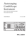
$XWRUDQJLQJ
&RPEL6FRSH
,QVWUXPHQW
I
30%30%30%
30%30%
Users Manual
2/1- Nov-1998
®
II
IMPORTANT
In correspondence concerning this instrument please give the model number and
serial number as located on the type plate on the rear of the instrument.
NOTE: The design of this instrument is subject to continuous development and
improvement. Consequently, this instrument may incorporate minor
changes in detail from the information provided in this manual.
Fluke Corporation
P.O. Box 9090
Everett WA
98206-9090, USA
Fluke Industrial B.V.
P.O. Box 680
7600 AR Almelo
The Netherlands
Copyright 1997, 1998 Fluke Corporation
All rights reserved. No part of this manual may be reproduced by any means or in
any form without written permission of the copyright owner.
Printed in the Netherlands
III
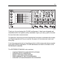
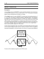
Thank you for purchasing this FLUKE oscilloscope. It has been designed and
manufactured to the highest quality standards to give you many years of trouble
free and accurate measurements.
The powerful measuring functions listed below have been combined with an easy
and logical operation to let you use the full power of this instrument each and
every day.
If you have any comments on how this product could be improved, please contact
your local FLUKE organization. FLUKE addresses are listed in the back of the
REFERENCE MANUAL.
The REFERENCE MANUAL also contains:
-
CHARACTERISTICS AND SPECIFICATIONS
PRINCIPLES OF OPERATION
BRIEF CHECKING PROCEDURE
PERFORMANCE TEST PROCEDURES
PREVENTIVE MAINTENANCE PROCEDURES
IV
MAIN FEATURES
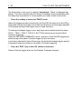
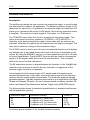
There are five models in this family of FLUKE oscilloscopes. Each of these
models is a combination of an analog real-time oscilloscope and a fully featured
digital storage oscilloscope. By pressing a single key, you can switch the
instrument from the analog mode to the digital mode and back. This allows each
of the units to be used in an optimum operating mode for all kinds of signal
conditions. Complex data streams, modulated waveforms, and video signals can
often best be seen in the analog mode of operation. The digital mode of operation
is more suited for single events, signals with low repetition frequencies, and when
automatic measurements need to be performed.
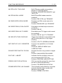
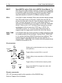
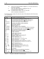
In this family there is a choice of five models. Two models have a bandwidth of
200 MHz, two have a bandwidth of 100 MHz and one has a bandwidth of 60 MHz.
Beside the 2 channel models with EXT TRIG input, there is a choice of two models
with four fully featured channels, all shown in the following table:
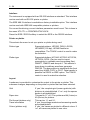
Type Number
Bandwidth
Sample rate
Number of
Channels
Input
Impedance
PM3370B
60 MHz
200 MS/s
2
1 MΩ
PM3380B
100 MHz
200 MS/s
2
1 MΩ
PM3384B
100 MHz
200 MS/s
4
1 MΩ
PM3390B
200 MHz
200 MS/s
2
1 MΩ/50Ω
PM3394B
200 MHz
200 MS/s
4
1 MΩ/50Ω
In the same instrument family, there are two 200-MHz and two 100-MHz analog
oscilloscopes that have specifications similar to the above-mentioned analog/
digital combination oscilloscopes operating in analog mode.
All analog/digital combination oscilloscopes listed above have the following features:
- Autoranging attenuators.
- Realtime clock.
- 32K sample acquisition memory in 4 channel versions.
- 8K sample acquisition memory, expandable to 32K in 2 channel versions.
- Up to 40 waveforms stored in memory or 204 waveforms with optional
memory extension.
- Autoset function for an instant optimized signal display at the touch of a button.
- Autoranging timebase.
- Cursor measurements with 1% accuracies.
- Extensive set of fully automated voltmeter and time measurement functions.
- Probe operated ’Touch Hold and Measure’ function freezes the display and
instantly displays the signal frequency, amplitude and dc voltage level.
V
-
Peak detection for the capture of glitches as narrow as 5 ns.
Pattern, State and Glitch triggering (2 ns) (2 channel models; 4ns Glitch
triggering only)
Event delay and pretriggering and posttriggering.
TV triggering including HDTV and TV line selection.
Serial interface for printing and plotting.
Averaging to reduce signal noise and to increase the vertical resolution from
8 to 16 bits.
Advanced mathematics, including digital low-pass filtering. A Math+ option
adds integration, differentiation, histogramming, and FFT.
Sine interpolation and magnification which enables true to life four channel
single shot acquisitions with a timebase up to 625 ns/div (32x magnified)
A delayed timebase with full trigger features.
An RS-232 (EIA-232-D) interface (standard) and an GPIB/IEEE-488 interface
(optional).
Autocal for automatic fine tuning of all circuitry to achieve maximum accuracy
under all user conditions.
Closed case calibration for efficient maintenance of traceable calibration at
minimum cost.
The following options are available:
-
-
A MATH+ option with more automated measurement functions including
envelope and measurement pass/fail testing. Also included in this option are
Integration, Differentiation, Histogramming, and FFT.
Memory extension offering 32K acquisition length and the ability to store 156
traces (of 512 samples each) in memory for 2 channel versions.
IEEE-488.2 interface using the new SCPI (Standard Commands for
Programmable Instruments) industry standard for remote control of test and
measurement equipment.
VI
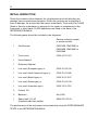
INITIAL INSPECTION
Check the contents of the shipment for completeness and note whether any
damage has occurred during transport. When the contents are incomplete or
there is damage, file a claim with the carrier immediately. Then notify the FLUKE
Sales or Service organization to arrange for the repair or replacement of the
instrument or other parts. FLUKE addresses are listed in the back of the
REFERENCE MANUAL.
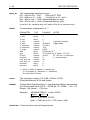
The following parts should be included in the shipment:
Service ordering number
or model number
1
Oscilloscope
PM3370B, PM3380B or
PM3390B, PM3384B or
PM3394B
1
Front cover
5322 447 70121
1
Users Manual
1
Reference Manual
1
Line cord (European type) or
5322 321 21616
1
Line cord (North American type) or
5322 321 10446
1
Line cord (British type) or
5322 321 21617
1
Line cord (Swiss type) or
5322 321 21618
1
Line cord (Australian type)
5322 321 21781
2
Probes 10:1
2
Batteries
AA (LR6)
1
Spare fuse 3.15 AT
(located inside fuse holder)
4822 070 33152
The performance of the instrument can be tested by using the PERFORMANCE
TESTS in the REFERENCE MANUAL.
VII
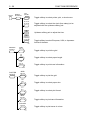
INSIDE THIS MANUAL
This operating guide contains information on all of the oscilloscope’s features. It
starts with a general introduction, a summary of main capabilities, initial
inspection note and a front and rear view.
Operators safety
Chapter 1 should be read before unpacking,
installing, and operating the instrument.
Installation instructions
Chapter 2 describes grounding, line cord, fuses,
and backup batteries.
Getting started
Chapter 3 provides a 10-minute tutorial intended
for those who are not familiar with Fluke
oscilloscopes.
How to use more advanced
functions of the instrument
Chapter 4 provides the more experienced user
with a detailed explanation of the major functions
of the oscilloscope.
Function reference
Chapter 5 contains an alphabetized description of
each function. Each description includes an
explanation of local and remote control functions.
CPL protocol
Chapter 6 provides the CPL commands with an
example of each.
Function index
The Function Index lists all implemented
functions in alphabetical order.
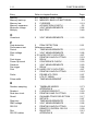
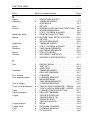
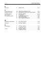
Index
The overall index contains all function names
and reference words in alphabetical order. It
includes the relevant chapter and page number
where more detailed information can be found.
IN THE APPENDICES
Menu structures
RS-232
Cable configurations
VIII
CONTENTS
CONTENTS
1 OPERATORS SAFETY
Page
. . . . . . . . . . . . . . . . . . . . . . . . . . . . . . . . 1-1
1.1 INTRODUCTION . . . . . . . . . . . . . . . . . . . . . . . . . . . . . . . . . . . . . . . 1-1
1.2 SAFETY PRECAUTIONS . . . . . . . . . . . . . . . . . . . . . . . . . . . . . . . . 1-1
1.3 CAUTION AND WARNING STATEMENTS . . . . . . . . . . . . . . . . . . 1-1
1.4 SYMBOLS . . . . . . . . . . . . . . . . . . . . . . . . . . . . . . . . . . . . . . . . . . . . 1-2
1.5 IMPAIRED SAFETY PROTECTION . . . . . . . . . . . . . . . . . . . . . . . . 1-2
1.6 MEASURING EARTH . . . . . . . . . . . . . . . . . . . . . . . . . . . . . . . . . . . 1-2
2 INSTALLATION INSTRUCTIONS
. . . . . . . . . . . . . . . . . . . . . 2-1
2.1 SAFETY INSTRUCTIONS . . . . . . . . . . . . . . . . . . . . . . . . . . . . . . . . 2-1
2.1.1
Protective earthing . . . . . . . . . . . . . . . . . . . . . . . . . . . . . . . 2-1
2.1.2
Mains voltage cord, mains voltage range and fuses . . . . . 2-1
2.2 MEMORY BACK-UP BATTERIES . . . . . . . . . . . . . . . . . . . . . . . . . 2-3
2.2.1
General information . . . . . . . . . . . . . . . . . . . . . . . . . . . . . . 2-3
2.2.2
Installation of batteries . . . . . . . . . . . . . . . . . . . . . . . . . . . . 2-3
2.3 THE FRONT COVER . . . . . . . . . . . . . . . . . . . . . . . . . . . . . . . . . . . . 2-3
2.4 HANDLE ADJUSTMENT AND OPERATING
POSITIONS OF THE INSTRUMENT . . . . . . . . . . . . . . . . . . . . . . . . 2-4
2.5 IEEE 488.2/IEC 625 BUS INTERFACE OPTION . . . . . . . . . . . . . . 2-4
2.6 RS-232-C SERIAL INTERFACE . . . . . . . . . . . . . . . . . . . . . . . . . . . 2-5
2.7 RACK MOUNTING . . . . . . . . . . . . . . . . . . . . . . . . . . . . . . . . . . . . . 2-5
2.8 VERSIONS . . . . . . . . . . . . . . . . . . . . . . . . . . . . . . . . . . . . . . . . . . . . 2-5
CONTENTS
IX
3 GETTING STARTED . . . . . . . . . . . . . . . . . . . . . . . . . . . . . . . . . . . 3-1
3.1 FRONT-PANEL LAYOUT . . . . . . . . . . . . . . . . . . . . . . . . . . . . . . . . 3-1
3.2 SWITCHING ON THE INSTRUMENT . . . . . . . . . . . . . . . . . . . . . . . 3-2
3.3 SCREEN CONTROLS . . . . . . . . . . . . . . . . . . . . . . . . . . . . . . . . . . . 3-3
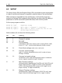
3.4 AUTO SETUP . . . . . . . . . . . . . . . . . . . . . . . . . . . . . . . . . . . . . . . . . 3-4
3.5 MODE SWITCHING BETWEEN ANALOG AND
DIGITAL OPERATING MODES . . . . . . . . . . . . . . . . . . . . . . . . . . . . 3-6
3.6 VERTICAL SETUP . . . . . . . . . . . . . . . . . . . . . . . . . . . . . . . . . . . . . . 3-8
3.7 TIMEBASE SETUP . . . . . . . . . . . . . . . . . . . . . . . . . . . . . . . . . . . . 3-11
3.8 MAGNIFY (EXPAND) . . . . . . . . . . . . . . . . . . . . . . . . . . . . . . . . . . . 3-12
3.9 DIRECT TRIGGER SETUP . . . . . . . . . . . . . . . . . . . . . . . . . . . . . . 3-13
3.10 PRE-TRIGGER VIEW . . . . . . . . . . . . . . . . . . . . . . . . . . . . . . . . . . 3-15
3.11 MORE ADVANCED FEATURES . . . . . . . . . . . . . . . . . . . . . . . . . . 3-16
3.12 CURSOR OPERATION . . . . . . . . . . . . . . . . . . . . . . . . . . . . . . . . . 3-17
3.13 MORE ADVANCED TRIGGER FUNCTIONS . . . . . . . . . . . . . . . . 3-19
3.14 MORE SIGNAL DETAIL WITH THE DELAYED TIMEBASE . . . . 3-20
3.15 TRACE STORAGE . . . . . . . . . . . . . . . . . . . . . . . . . . . . . . . . . . . . 3-22
4 HOW TO USE MORE ADVANCED FUNCTIONS
OF THE INSTRUMENT . . . . . . . . . . . . . . . . . . . . . . . . . . . . . . . . 4-1
4.1 INTRODUCTION . . . . . . . . . . . . . . . . . . . . . . . . . . . . . . . . . . . . . . . 4-1
4.2 DISPLAY AND PROBE ADJUSTMENTS . . . . . . . . . . . . . . . . . . . . 4-5
4.3 ANALOG AND DIGITAL MODES . . . . . . . . . . . . . . . . . . . . . . . . . . 4-9
4.4 VERTICAL DEFLECTION . . . . . . . . . . . . . . . . . . . . . . . . . . . . . . . 4-13
4.5 HORIZONTAL DEFLECTION AND TRIGGERING . . . . . . . . . . . . 4-22
X
CONTENTS
4.6 DIGITAL ACQUISITION AND STORAGE . . . . . . . . . . . . . . . . . . . 4-30
4.7 ADVANCED VERTICAL FUNCTIONS . . . . . . . . . . . . . . . . . . . . . 4-31
4.8 ADVANCED HORIZONTAL AND TRIGGER FUNCTIONS . . . . . 4-34
4.9 MEMORY FUNCTIONS . . . . . . . . . . . . . . . . . . . . . . . . . . . . . . . . . 4-39
4.10 CURSORS FUNCTIONS . . . . . . . . . . . . . . . . . . . . . . . . . . . . . . . . 4-44
4.11 MEASUREMENT FUNCTIONS . . . . . . . . . . . . . . . . . . . . . . . . . . . 4-49
4.12 PROCESSING FUNCTIONS . . . . . . . . . . . . . . . . . . . . . . . . . . . . . 4-54
4.13 DISPLAY FUNCTIONS . . . . . . . . . . . . . . . . . . . . . . . . . . . . . . . . . 4-57
4.14 DELAYED TIMEBASE . . . . . . . . . . . . . . . . . . . . . . . . . . . . . . . . . . 4-63
4.15 HARD COPY FACILITIES . . . . . . . . . . . . . . . . . . . . . . . . . . . . . . . 4-68
4.16 AUTOSET AND SETUP UTILITIES . . . . . . . . . . . . . . . . . . . . . . . 4-71
4.17 OTHER FEATURES . . . . . . . . . . . . . . . . . . . . . . . . . . . . . . . . . . . 4-75
5 FUNCTION REFERENCE
. . . . . . . . . . . . . . . . . . . . . . . . . . . . . 5-1
6 THE CPL PROTOCOL . . . . . . . . . . . . . . . . . . . . . . . . . . . . . . . . .
6-1
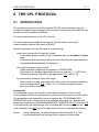
6.1 INTRODUCTION . . . . . . . . . . . . . . . . . . . . . . . . . . . . . . . . . . . . . . . 6-1
6.2 EXAMPLE PROGRAM FRAME . . . . . . . . . . . . . . . . . . . . . . . . . . . 6-3
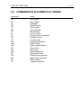
6.3 COMMANDS IN FUNCTIONAL ORDER . . . . . . . . . . . . . . . . . . . . . 6-4
6.4 COMMANDS IN ALPHABETICAL ORDER . . . . . . . . . . . . . . . . . . 6-5
6.5 COMMAND REFERENCE . . . . . . . . . . . . . . . . . . . . . . . . . . . . . . . . 6-6
6.6 ACKNOWLEDGE . . . . . . . . . . . . . . . . . . . . . . . . . . . . . . . . . . . . . 6-47
6.7 STATUS . . . . . . . . . . . . . . . . . . . . . . . . . . . . . . . . . . . . . . . . . . . . . 6-48
6.8 SETUP . . . . . . . . . . . . . . . . . . . . . . . . . . . . . . . . . . . . . . . . . . . . . . 6-50
CONTENTS
XI
Appendix A
ACQUIRE menu structure . . . . . . . . . . . . . . . . . . . . . . A-1
Appendix B
CURSORS menu structure . . . . . . . . . . . . . . . . . . . . . B-1
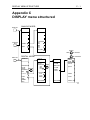
Appendix C
DISPLAY menu structured . . . . . . . . . . . . . . . . . . . . C-11
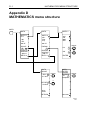
Appendix D
MATHEMATICS menu structure . . . . . . . . . . . . . . . . . D-1
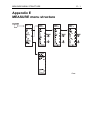
Appendix E
MEASURE menu structure . . . . . . . . . . . . . . . . . . . . . E-1
Appendix F
DTB (DEL’D TB) menu structure . . . . . . . . . . . . . . . . F-1
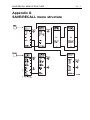
Appendix G
SAVE/RECALL menu structure . . . . . . . . . . . . . . . . . G-1
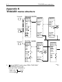
Appendix H
SETUPS menu structure . . . . . . . . . . . . . . . . . . . . . . . H-1
Appendix J
TB MODE menu structure . . . . . . . . . . . . . . . . . . . . . . . J-1
Appendix K
TRIGGER menu structure . . . . . . . . . . . . . . . . . . . . . . K-1
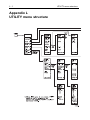
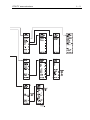
Appendix L
UTILITY menu structure . . . . . . . . . . . . . . . . . . . . . . . . L-1
Appendix M
VERTICAL menu structure . . . . . . . . . . . . . . . . . . . . . M-1
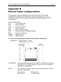
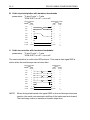
Appendix N
RS-232 Cable configurations . . . . . . . . . . . . . . . . . . . N-1
Appendix P
. . . . . . . . . . . . . . . . . . . . . . . . . . . . . . . . . . . . . . . . . . . . P-1
FUNCTION INDEX (see Chapter 5)
INDEX
. . . . . . . . . . . . . . . . . . . . . . I-1
. . . . . . . . . . . . . . . . . . . . . . . . . . . . . . . . . . . . . . . . . . . . . . . . . . . . . I-3
XII
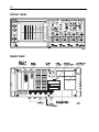
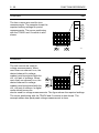
FRONT VIEW
REAR VIEW
XIII
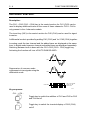
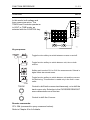
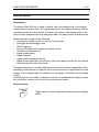
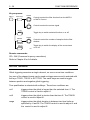
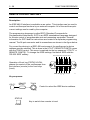
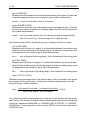
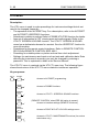
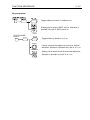
FRONT PANEL CONNECTIONS
Probe Adjust
Squarewave output signal for e.g. probe calibration.
Amplitude is calibrated.
CH1
BNC input socket for vertical channel 1 with probe
indication contact.
CH2
BNC input socket for vertical channel 2 with probe
indication contact.
CH3
BNC input socket for vertical channel 1 with probe
indication contact. (only in 4 channel models)
CH4
BNC input socket for vertical channel 1 with probe
indication contact. (only in 4 channel models)
EXT TRIG
BNC input socket used as an extra external trigger
input with probe indication contact (only in 2 channel
models)
Ground socket (banana): same potential as safety
ground.
The measuring ground socket and the external
conductor of the BNC sockets are internally
connected to the protective earth conductor of the
three-core mains cable. The measuring ground
socket or the external conductor of the BNC-sockets
must not be used as a protective conductor terminal.
XIV
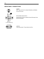
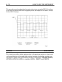
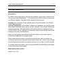
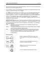
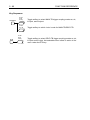
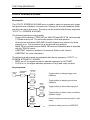
REAR PANEL CONNECTIONS
Z-MOD
BNC input socket for external intensity-modulation
of the CRT trace.
NC TXD
RXD DTR
RS-232 BUS (EIA-232-D)
Input/output socket to connect the oscilloscope to an
RS-232 Interface.
5
1
6
9
RTS NC
DSR CTS
NC=NOT CONNECTED
ST6065
FUSE
LINE IN
Line input socket. Fuse holder is built in.
XV
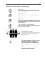
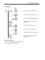
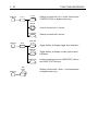
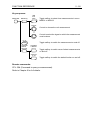
OPTIONAL REAR PANEL CONNECTIONS
CH1 Y-OUT
BNC output socket with a signal derived from the
Channel 1 input signal.
MAIN TB GATE
BNC output socket with a signal that is "high" when
the Main Timebase is running and "low" for the other
conditions.
DTB GATE
BNC output socket with a signal that is "high" when
the Delayed Timebase is running and "low" for the
other conditions.
EXT TRIG (only in 4 channel models)
BNC input socket used as an extra external trigger
input for the Main Timebase
SHIELD SRQ NDAC DAV DIO4 DIO2
NR
ATN IFC FD EO1 DIO3 DIO1
12
1
24
13
GND GND GND REN DIO7 DIO5
11
9
7
LOGIC GND GND GND DIO8 DIO6
GND 10
8
6
IEEE 488.2 BUS OPTION
If installed you will find here the input/output
socket to connect the oscilloscope to an
IEEE 488 interface.
ST6064
The external conductor of the BNC sockets
and the screening of the interface bus
connectors are internally connected to the
protective earth conductor of the three-core
mains cable. The external conductor of the
BNC sockets and the screening of the
interface bus connectors must not be used as
a protective conductor terminal.
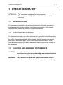
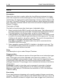
OPERATORS SAFETY
1-1
1 OPERATORS SAFETY
ATTENTION:
The instrument is designed for indoor use only.
Read this page carefully before installation and use of the
instrument.
1.1 INTRODUCTION
The instrument described in this manual is designed to be used by proper-lytrained personnel only. Adjustment, maintenance and repair of the exposed
equipment shall be carried out only by qualified personnel.
1.2 SAFETY PRECAUTIONS
For the correct and safe use of this instrument it is essential that both operating
and service personnel follow generally-accepted safety procedures in addition to
the safety precautions specified in this manual. Specific warning and caution
statements, where they apply, will be found throughout the manual. Where
necessary, the warning and caution statements and/or symbols are marked on
the apparatus.
1.3 CAUTION AND WARNING STATEMENTS
CAUTION:
Is used to indicate correct operating or maintenance
procedures in order to prevent damage to or destruction of the
equipment or other property.
WARNING:
Calls attention to a potential danger that requires correct
procedures or practices in order to prevent personal injury.
1-2
OPERATORS SAFETY
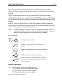
1.4 SYMBOLS
Read the safety information in the manual.
Earth.
Conformité Européenne.
Recycling information.
1.5 IMPAIRED SAFETY PROTECTION
The use of the instrument in a manner not specified may impair the protection
provided by the equipment. Before use, inspect the instrument and accessories
for mechanical damage!
Whenever it is likely that safety-protection has been impaired, the instrument
must be made inoperative and be secured against any unintended operation. The
matter should then be referred to qualified technicians. Safety protection is likely
to be impaired when, for example, the instrument fails to perform the intended
measurements or shows visible damage.
1.6 MEASURING EARTH
The measuring earth socket and the external conductor of the BNC sockets are
internally connected to the protective earth conductor of the three-core mains
cable. The measuring earth socket or the external conductor of the BNC-sockets
must not be used to connect a protective conductor.
INSTALLATION INSTRUCTIONS
2-1
2 INSTALLATION INSTRUCTIONS
Attention:
You are strongly advised to read this chapter thoroughly before
installing your oscilloscope.
2.1 SAFETY INSTRUCTIONS
2.1.1
Protective earthing
Before any connection to the input connectors is made, the instrument shall be
connected to a protective earth conductor via the three-core mains cable; the
mains plug shall be inserted only into a socket outlet provided with a protective
earth contact. The protective action shall not be negated by the use of an
extension cord without protective conductor.
WARNING:
Any interruption of the protective conductor inside or outside
the instrument is likely to make the instrument dangerous.
Intentional interruption is prohibited.
WARNING:
When an instrument is brought from a cold into a warm
environment, condensation may cause a hazardous
condition. Therefore, make sure that the grounding
requirements are strictly adhered to.
2.1.2
Mains voltage cord, mains voltage range and fuses
Before inserting the mains plug into the mains socket, make sure that the
instrument is suitable for the local mains voltage.
NOTE: When the mains plug has to be adapted to the local situation, such
adaption should be done by a qualified technician only.
WARNING:
The instrument shall be disconnected from all voltage
sources when a fuse is to be renewed.
The oscilloscope has a tapless switched-mode power supply that covers most
nominal voltage ranges in use: ac voltages from 100 ... 240 V (r.m.s.). This
obviates the need to adapt to the local mains (line) voltage. The nominal mains
(line) frequency range is 50 Hz ... 400 Hz.
Line fuse rating: 3.15 AT delayed action, 250 V (for ordering code see
"INITIAL INSPECTION").
2-2
INSTALLATION INSTRUCTIONS
The mains (line) fuseholder is located on the rear panel in the mains (line) input
socket. When the mains (line) fuse needs replacing, proceed as follows:
- disconnect the oscilloscope from the mains (line).
- remove the cover of the fuseholder by means of a small screwdriver.
- fit a new fuse of the correct rating and refit the cover of the fuseholder.
WARNING:
Make sure that only fuses with the required rated current and
of the specified type are used for replacement. The use of
makeshift fuses and the short-circuiting of fuse holders are
prohibited.
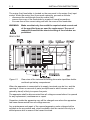
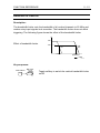
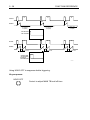
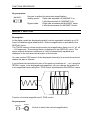
REAR VIEW
Figure 2.1
Rear view of the instrument showing the mains input/fuse-holder
and back-up battery compartment.
When the apparatus is connected to its supply, terminals may be live, and the
opening of covers or removal of parts (except those to which access can be
gained by hand) is likely to expose live parts.
The apparatus shall be disconnected from all voltage sources before it is opened
for any replacement, maintenance or repair.
Capacitors inside the apparatus may still be charged even when the apparatus
has been disconnected from all voltage sources.
Any maintenance and repair of the opened apparatus under voltage shall be
avoided as far as possible and, when inevitable, shall be carried out only by a
skilled person who is aware of the hazard involved.
INSTALLATION INSTRUCTIONS
2-3
2.2 MEMORY BACK-UP BATTERIES
2.2.1
General information
Memory backup is provided to store the oscilloscope’s settings when switched off
so that the instrument returns to the same settings when turned on. Two AA (LR6)
Alkaline batteries are used.
Note:
The batteries are not factory installed and must be installed at the
customer’s site.
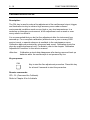
Note:
This instrument contains batteries. Do not dispose of these batteries with
other solid waste. Used batteries should be disposed of by a qualified
recycler or hazardous materials handler. Contact your authorized Fluke
Service Center for recycling information.
2.2.2
Installation of batteries
Proceed as follows:
- Remove all input signals and disconnect the instrument line power.
- Remove the plastic cover of the battery compartment so that the battery
holder becomes accessible.
- Install two penlight batteries (AA) in the battery holder as indicated on the
battery holder.
- Reinstall the cover of the battery compartment.
Note:
Frontsettings and autocalibration data disappear after exchange of the
batteries with the instrument disconnected from the line power. After
battery exchange, it is necessery to press the CAL key after the
recommended warming up time.
CAUTION: Never leave the batteries in the oscilloscope at ambient temperatures outside the rated range of the battery specifications because of possible damage that may be caused to the
instrument. To avoid battery damage, do not leave the batteries
in the oscilloscope when it is stored longer than 30 days.
2.3 THE FRONT COVER
For ease of removal and reinstallation, the front cover has been designed to snap
on to the front of the instrument.
The front can be removed as follows:
- Fold the carrying handle down so that the oscilloscope occupies a sloping
position (refer to Chapter 2.4 for how to proceed).
- Pull the clamping lip at the top side of the cover slightly outwards.
- Lift the cover off the instrument.
2-4
INSTALLATION INSTRUCTIONS
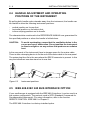
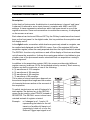
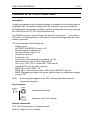
2.4 HANDLE ADJUSTMENT AND OPERATING
POSITIONS OF THE INSTRUMENT
By pulling both handle ends outwards away from the instrument, the handle can
be rotated to allow the following instrument positions:
-
vertical position on its rear feet;
horizontal position on its bottom feet;
in three sloping positions on its handle.
The characteristics mentioned in the REFERENCE MANUAL are guaranteed for
the specified positions or when the handle is folded down.
CAUTION:
To avoid overheating, ensure that the ventilation holes in the
covers are free of obstruction. Do not position the instrument
in direct sunlight or on any surface that produces or radiates
heat.
In the rear panel of the instrument there is storage space for the mains cable.
There is also a clamping device to fix the end of the mains cable to the rear panel.
The mains plug then fits in the area where the RS232 connector is present. In this
way the instrument can also stand on its rear feet.
MAT4221
Figure 2.2
Instrument positions
2.5 IEEE 488.2/IEC 625 BUS INTERFACE OPTION
If your oscilloscope is equipped with the IEEE 488.2 interface, it can be used in a
bus system configuration. The protocol used is SCPI (Standard Commands for
Programmable Instruments). For setup information, refer to the function
REMOTE CONTROL IEEE 488.2 in Chapter 5.
The IEEE 488.2 interface is a factory-installed option.
INSTALLATION INSTRUCTIONS
2-5
2.6 RS-232-C SERIAL INTERFACE
Your oscilloscope is equipped with an RS-232-C interface as standard. The
interface can be used in a system for serial communication. The protocol used is
CPL (Compact Programming Language). CPL is a small set of very powerful
commands that can be used for full remote control. Detailed information about this
interface and the CPL protocol is given in Chapter 6 in this manual. For setup
information, refer to the REMOTE CONTROL RS-232 function in Chapter 5
’Function Reference’.
2.7 RACK MOUNTING
The rackmount kit (PM 8960/04) allows you to install the oscilloscope in a
standard 19 inch rack.
It is not necessary to open the oscilloscope itself to mount the rackmount kit.
Installation can be done easily by the user.
2.8 VERSIONS
The model number of your oscilloscope (e.g. PM33...) is indicated on the text strip
above the CRT. This model number is also represented by the digits 6, 7, 8 and 9
of the 12- digit code on the type plate on the rear panel. The ’A’ or ’B’ series is
indicated by a 1 or 2 on the 5th digit.
The instrument’s serial number is also given on the type plate. This number
consists of a six digit code preceeded by the characters ’DM’.
The instrument version can also be displayed on the CRT after having pressed
menu key UTILITY and then softkey MAINTENANCE.
GETTING STARTED
3-1
3 GETTING STARTED
This chapter provides a 10-minute tutorial intended for those who are not familiar
with Fluke oscilloscopes. Those who are already familiar can skip this chapter and
continue to Chapter 4.
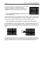
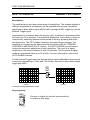
3.1 FRONT-PANEL LAYOUT
This oscilloscope is a combination of an analog oscilloscope and a digital storage
oscilloscope in the same instrument. The basic signal acquisition and display
functions are identical in both operating modes. Differences will be explained in
the text. Switching between the two operating modes is done with the yellow
ANALOG key.
The front panel of the oscilloscope is organized into functional areas. The areas
are discussed in order of typical operation.
Figure 3.1
Front panel layout
Note that the front panel shown is that with the most functions. Differences are
explained in Section 4.1. For this getting started procedure, only CH1 and CH2
are used. These are identical for all models.
3-2
Typical operation of your instrument will be:
- Switching on the instrument
- Initial standard setup
- Screen controls
- Auto setup
- Analog-Digital mode switching
- Vertical setup
- Timebase setup
- Magnify (Expand)
- Direct trigger setup
- Pretrigger view
- More advanced features
- Cursor operation
- More advanced trigger functions
- More signal detail with the DTB
- Trace storage
GETTING STARTED
(see Section 3.2)
(see Section 3.2)
(see Section 3.3)
(see Section 3.4)
(see Section 3.5)
(see Section 3.6)
(see Section 3.7)
(see Section 3.8)
(see Section 3.9)
(see Section 3.10)
(see Section 3.11)
(see Section 3.12)
(see Section 3.13)
(see Section 3.14)
(see Section 3.15)
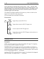
3.2 SWITCHING ON THE INSTRUMENT
Connect the power cord and set the front panel power switch to ON. For any line
source between 100V to 240V nominal, 50/400 Hz, the instrument automatically
turns on. After performing the built-in power-up routine, the instrument is
immediately ready for use. The instrument’s settings will be identical to those
when the oscilloscope was switched off (with the batteries installed).
To ensure that you will get the same setup in all cases, press the STATUS key
and TEXT OFF key simultaneously. This will set the instrument in a predefined
default condition (STANDARD SETUP) and a trace will appear on the screen.
Text is also displayed at the bottom of the screen.
GETTING STARTED
3-3
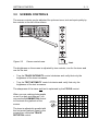
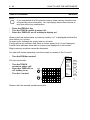
3.3 SCREEN CONTROLS
The screen controls can be adjusted for optimum trace, text and spot quality by
the controls to the left of the screen.
Figure 3.2
Screen control area
The brightness on the screen is adjusted by two controls, one for the trace and
one for the text.
•
Turn the TRACE INTENSITY control clockwise and verify that only the
brightness of the trace increases.
•
Turn the TEXT INTENSITY control clockwise and verify that only the
brightness of the text increases.
The sharpness of the trace and text is optimized by the FOCUS control.
When you are making photographs
or are in a dark environment, you
can use the ILLUMINATION control
to illuminate the graticule of the
screen.
The trace is adjusted in parallel with
the horizontal graticule lines by the
screwdriver-controlled TRACE
ROTATION control.
TRACE
ROTATION
ST5975
9303
3-4
GETTING STARTED
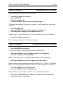
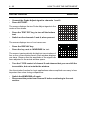
3.4 AUTO SETUP
The best way to start each measurement is by using the AUTOSET key. This
automatically finds and scales all relevant parameters on all channels.
AUTO SET
1
2
3
4
ST6659
9303
Figure 3.3
Measuring setup
Step 1
Connect the probe as shown in figure 3.3.
NOTE:
AUTOSET is programmable. Because you have set the instrument in the
"standard setup" before (see Section 3.2), all programmable features are
set to a predefined condition and the instrument is set in the analog mode.
Programming of AUTOSET is explained in Chapters 4 and 5.
Step 2
Press the AUTOSET key.
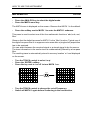
The scope flashes the message ’AUTO SETTING...’ on the screen. In
a few seconds the front-panel settings are adjusted for an optimized
display of the applied signal in the analog mode.
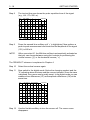
Step 3
The calibration signal is clearly displayed.
The parameters of the channel and the timebase settings are
displayed at the bottom of the screen.
CH1 200mV
MTB 200µs
CH1
ST6704
GETTING STARTED
Step 4
3-5
To prevent measurement errors, check the pulse response before any
measurement. If the pulse shows overshoot or undershoot, you can
correct this by using the trimmer in the probe’s body. Chapter 4
describes how to adjust the pulse response.
ST5952
In most cases, using AUTO SETUP is sufficient for a good initial display of the
signal(s). After the initial AUTOSET, and to optimize the signal for a more detailed
view, continue with the paragraphs below.
NOTE:
If you get lost when adjusting your instrument, just press AUTOSET.
3-6
GETTING STARTED
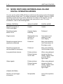
3.5 MODE SWITCHING BETWEEN ANALOG AND
DIGITAL OPERATING MODES
You can use the yellow ANALOG key to switch from the analog mode to the digital
mode and back at any time. The signal acquisition and display functions of both
operating modes are very similar. However, the nature of the signals you are
using may determine which operating mode you prefer to use. For more
information, refer to the following table:
SIGNAL CRITERIA
ANALOG MODE
DIGITAL MODE
Repetitive signals of
30 Hz and higher
Usable
Usable
Repetitive signals
below 30 Hz
Causes display
flickering
Preferred
Single events
Displayed for the
duration of
the event
Can capture and
display for long
term display
Repetitive signals that are
amplitude modulated
Preferred
May cause alaising
Use Peak detect or
Envelope mode
Repetitive signals that
are modulated in frequency
Preferred
May cause aliasing.
Use Envelope mode.
Long serial data streams
Preferred when
Delayed sweep
is not used.
When using delayed
sweep to observe
details, Digital mode
provides better
light output.
Video signals
Preferred when
Delayed sweep
is not used.
When using delayed
sweep to observe
details, Digital mode
provides better
light output.
Not possible
Up to full acquisition
length
OTHER CRITERIA
Need to see pretrigger
information
GETTING STARTED
3-7
SIGNAL CRITERIA
ANALOG MODE
DIGITAL MODE
You need to make adjustments
to the circuitry and watch
the signal change
Fastest
display
update
Slower
display
update
Automatic measurements
Can’t use
Fully implemented
Signal
Math
Add, Subtract, Multiply
Add, Subtract
All functions
Signal
Analysis
Integration,
Differentiation, FFT
Not available
Full analysis
(optional)
Automatic Pass/Fail test
Not available
Fully implemented
(optional)
Autorange attenuator
Not available
Results in a displayed
signal with an amplitude of 2 to 6.4 divisions
Autorange timebase
Not available
Results in a signal
display of 2 to 6
waveform periods
ANALOG
1
2
3
4
RUN/STOP
ST6680
9312
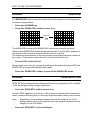
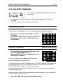
Figure 3.4
Analog-Digital switching setup
Step 1
Press AUTOSET. The scope performs an AUTOSET in analog mode.
Step 2
Press the ANALOG key to change over to the digital mode. Check that
the picture is identical to the one in the analog mode. The text ’DIGITAL
MODE’ is displayed briefly at the bottom of the screen.
3-8
GETTING STARTED
Step 3
Press AUTOSET again. This time the scope performs the autoset in
digital mode.
Step 4
Press the RUN/STOP key and observe that the trace is frozen and
stays on screen even after removing the probe.
Step 5
Press the RUN/STOP key to display the actual input signal again.
Reconnect the probe to display the Probe Adjust signal again.
Step 6
Press the ANALOG button once again to return to the analog mode. In
the bottom of the screen, the text ’ANALOG MODE‘ is briefly displayed.
3.6 VERTICAL SETUP
This section deals with setting of the input circuits of the four channels. The main
adjustments are AMPLitude, POSition, and the channel input coupling selection
for GND, DC, and AC.
Figure 3.5
Step 1
Vertical setup
Adjust the absolute ground level by disconnecting the signal and using
the POS control to position the trace in the middle of the screen. A
marker with the channel number (’1-’) at the left of the screen indicates
the ground reference.
POS
1
1
MAT4191
Step 2
Reconnect the probe to the Probe Adjust signal for display.
GETTING STARTED
Step 3
3-9
You can change the amplitude of the signal in a 1, 2, 5 sequence by
pressing one of the AMPL keys. Note that the bottom of the screen
shows the AMPL/DIV setting of CH1.
CH1 500mV
CH1 100mV
ST6681
Step 4
Press the ON button of CH2 and observe that a second trace is now
visible. The position and amplitude of this channel can be adjusted
similar to the adjustment of CH1. The channel settings are also
displayed in the bottom of the screen.
Press the ON key of CH2 once again to turn this channel off.
Step 5
Press the AC DC/GND key of CH1 so that a ’⊥’ sign is displayed in the
bottom text line. This interrupts the input signal and connects the input
to the ground. In this case, only the ’base’ line is visible.
Press the AC DC/GND key once again for ac input coupling; the
bottom text line now displays ’~’.
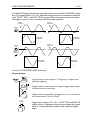
In most cases, dc input coupling is used to show ac as well as dc components of
the signal. However, in some cases where a small ac signal is superimposed on
a large dc voltage, ac input coupling must be used. Then only the ac component
is visible on the screen. The text line shows a ’=’ or ’~’ sign to indicate dc or ac
coupling. Because the calibration signal is a square wave with a low level of 0V
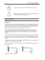
and a high level of +600 mV, the screen shows either of the following two displays:
AC INPUT COUPLING
ZERO
LEVEL
DC INPUT COUPLING
ZERO
LEVEL
1
CH1 200mV
MTB 200µs
CH1
1
CH1 200mV
MTB 200µs CH1
ST6682
3 - 10
GETTING STARTED
Step 6
Press the ANALOG key to enter the digital mode
Step 7
Press the top one (mV) of the AMPL keys, so that the signal has
maximum amplitude.
Press AUTO RANGE and see the signal change to a suitable
attenuator value. When AUTO RANGE is active, the attenuators
automatically adjust when the signal amplitude changes, to keep the
trace on screen.
Step 8
Press the key labeled AVERAGE. Noise in the input signal can be
reduced by using the average function. The random noise is reduced
by calculating the average over the last n scans (average factor can be
set between 2 and 4096)
NOTE:
Refer to Chapter 4 for an explanation of the CH1+CH2, TRIG1, and
INV keys.
GETTING STARTED
3 - 11
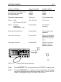
3.7 TIMEBASE SETUP
The next step is the adjustment of the main timebase controls (TIME/DIV, X
POSition, and MAGNIFY keys).
MAGNIFY
1
2
3
X POS
AUTO
RANGE
4
s
TIME/DIV
VAR
ns
ST6435
9312
Figure 3.6
Timebase setup
Step 1
Press the AUTOSET key.
Step 2
Use the TIME/DIV keys on the right hand side of the instrument to
decrease or increase the number of periods of the signal on the
screen.
TIME/DIV
MTB 500µs
MTB 100µs
ST6683
Step 3
Select a timebase of 1 ms/div.
Step 4
Press AUTO RANGE and see the signal display change to a more
suitable timebase. The AUTO RANGE function automatically selects a
timebase that displays 2 to 6 signal periods.
Step 5
Press the ANALOG key to switch the scope to the analog mode.
Step 6
Turn the X POS control to shift the signal horizontally (left or right)
across the screen.
3 - 12
GETTING STARTED
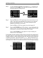
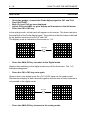
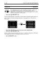
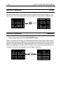
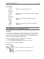
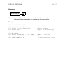
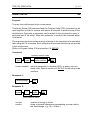
3.8 MAGNIFY (EXPAND)
Step 1
You can use the MAGNIFY keys to expand the signal on the screen.
The ’MGN’ indication and the corrected timebase setting are displayed
in the text line.
In the analog mode, magnification is limited to *10. The right key will
activate the magnification. The left key will turn off the MAGNIFY
function. On or off is indicated by ’MGN’ in the bottom of the screen.
Step 2
Press the ANALOG key to switch the scope to the digital mode.
Step 3
In the digital mode, pressing the right MAGNIFY key expands the
signal in *1, *2, *4 ...steps to a maximum of *32 times. Pressing the
left MAGNIFY key compresses the signal to 1 again. When you
*
operate the MAGNIFY buttons, or when you turn the X POSition
control, a bargraph is displayed showing which part of the digital trace
is expanded.
NOTE:
The MAGNIFY key and X POS control can also be used after the
oscilloscope is STOPped.
5.00µs
10 DIV
1.25µs 4
10 DIV
*
START OF TIME WINDOW CAN BE VARIED WITH
X POS OVER THE WHOLE SWEEP RANGE.
1.00ms
40 DIV
ST6684
GETTING STARTED
3 - 13
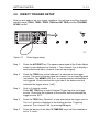
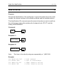
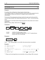
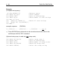
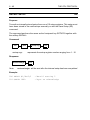
3.9 DIRECT TRIGGER SETUP
Now you are ready to set your trigger conditions. You will use one of the channel
selection keys (TRIG1, TRIG2, TRIG3, TRIG4 or EXT TRIG) and the TRIGGER
LEVEL control.
Figure 3.7
Direct trigger setup
Step 1
Press the AUTOSET key. The square-wave signal of the Probe Adjust
output is now displayed on channel 1. Turn channel 2 on to display a
second horizontal trace (channel 2 has no input signal).
Step 2
Press the TRIG2 key so that channel 2 is selected as the trigger
source. The result is that the signal on channel 1 is no longer triggered
(not stable). The ARM’D LED is on, to indicate that the oscilloscope is
not triggered. Check also that the right side of the bottom text line
indicates the trigger source (’ch2’).
Step 3
Only in 2 channel models
Press EXT TRIG key to select External Trigger input as the trigger
source. Check that the rightside of the bottom textline indicates the
trigger source ’EXT’.
Step 4
Press the TRIG1 key. Channel 1 is now selected as the trigger source.
The ’ch1’ symbol is displayed in the bottom text line. Triggering
resumes. Turn channel 2 off, by pressing ON again.
Step 5
Press the ns key of the MainTB TIME/DIV keys until the timebase is
set to ’2 µs/div’.
3 - 14
Step 6
GETTING STARTED
The same TRIG1 key that was used to select the trigger source is also
used to select the trigger slope. Repeatedly pressing the TRIG1 button
changes the triggering so that it occurs on the leading or trailing edge
of the input signal. Note that the slope is also displayed in the bottom
text line.
TRIG1
CH1 200mV
MTB 2µs
CH1
CH1 200mV
MTB 2µs
CH1
ST6685
Step 7
For repetitive signals, you obtain a stable display when each
successive timebase sweep is triggered at the same stable level of the
input signal. You use the TRIGGER LEVEL control to adjust the level.
Turn the control. The precise position in relation to the maximum signal
amplitude (between +100 % and -100 %) is displayed on the screen.
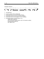
SUMMARY
The previous steps covered the basic adjustments. Now you are ready to look
at the special features of the oscilloscope. This includes the use of the cursors,
advanced trigger functions and using the second (delayed) timebase for signal
details.
GETTING STARTED
3 - 15
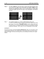
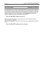
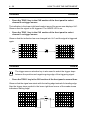
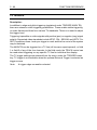
3.10 PRE-TRIGGER VIEW
One of the powerful features in the digital mode is the ability to capture and view
signal contents prior to the actual trigger. The amount of pretrigger information
can be as long as one full acquisition/record. The trigger position is adjusted with
the TRIGGER POSITION control.
Step 1
Turn the TRIGGER POSITION control counter clockwise. Now the
triggering edge shifts to the center of the screen. A trigger point marker
(s) indicates the trigger point. The part to the left of the marker is called
pretrigger view. The pretrigger view is indicated in the bottom of the
screen (in divisions)
TRIGGER
POSITION
1
1
DELAY=−5.00dV
ST6686
PRE-TRIGGER
VIEW
Step 2
The TRIGGER POSITION control can also be used to adjust time
delay. Rotate the TRIGGER POSITION control clockwise until the
readout displays "0". When you continue to turn the TRIGGER
POSITION control clockwise, a positive delay between trigger point
and acquisition is set. The delay is no longer read out in divisions of
pretrigger information, but in seconds, or fractions of seconds to
indicate how much delay is used.
3 - 16
GETTING STARTED
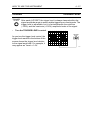
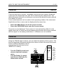
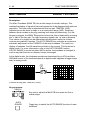
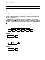
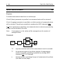
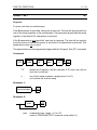
3.11 MORE ADVANCED FEATURES
All basic functions are accessed by dedicated keys for fast and easy operation.
Some of the more advanced features are menu operated. Menus are called up by
pressing one of the keys identified with blue text on the front panel. After you
press one of these keys, a menu is displayed on the right side of the screen. This
menu gives you access to the more advanced functions of the oscilloscope. Use
the blue softkeys to the right of the screen to select the desired functions; the
selected function is indicated by the highlighted text.
TRIGGER WITH
MENUKEY
TRIGGER
1
3
2
4
ST6433
9303
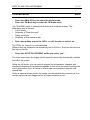
SOFTKEYS
Figure 3.8
Step 1
Menu keys and softkeys
Press the key marked TRIGGER.
Check that the ’TRIGGER MAINTB’ menu is displayed at the right side
of the screen.
After changing the setting, you can deactivate the menu again to use
the full screen for the signal.
There are two ways to do this:
- Press the TRIGGER key once again.
- Press the TEXT OFF key.
The TEXT OFF key operates in a 1-2-3 cycle, and allows you to blank
the bottom text line as well.
TRIGGER
MAIN TB
edge tv
logic
ch1
line
CH1 200mV
MTB 200µs
CH1
TEXT OFF
TEXT OFF
CH1 200mV
MTB 200µs
CH1
TEXT OFF
ST6679
Step 2
Use both methods to familiarize yourself with turning the menus and
the bottom text line on and off.
GETTING STARTED
3 - 17
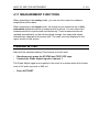
3.12 CURSOR OPERATION
Cursors are used for accurate amplitude or time measurements of the signal.
TRACK
1
2
3
CURSORS
∆
4
ST6431
9303
Figure 3.9
Cursor setup
Step 1
Before you continue, reset the instrument with the STANDARD
SETUP. To do this, press the STATUS key and TEXT OFF key
simultaneously. Now the instrument is set in the default condition and
operates in analog mode.
Step 2
Press the AUTOSET key.
Step 3
Press the CURSORS key to enter the cursors menu.
The menu is now displayed on the screen and the
cursors are turned on.
Step 4
Use the second blue softkey from the top to select
one of the three cursor modes:
- Amplitude cursor measurements, indicated by ’=’.
- Time cursor measurements, indicated by ’||’ for
measuring time or frequency.
- Amplitude and time measurements, indicated by
’#’. The top text line displays the result of the
measurements (∆V or ∆T).
CURSORS
on off
#
READ OUT
ST6430
Step 5
Press the second bluesoft key until ’||’ is highlighted.
Step 6
The TRACK control moves both cursors at the same time. For
example, to measure the period time of the input signal, set the left
(reference) cursor to a rising edge of the signal.
Step 7
The ∆ control moves the right cursor only. Set this cursor the next rising
edge of the signal.
3 - 18
Step 8
GETTING STARTED
The top text line now shows the pulse repetition time of the signal
(e.g., ch1: ∆T= 500 µs).
ch1:
∆T= 500µs
CURSORS
on off
#
READ OUT
CH1
200mV
MTB 200µs
CH1
ST6687
Step 9
Press the second blue softkey until ’=’ is highlighted. Now perform a
peak-to-peak measurement and check that the amplitude of the signal
(’∆V’) is 600 mV.
NOTE:
When you select ’#’, the fifth blue softkey is automatically activated so
that you can choose between using the controls for positioning the
vertical cursors (’||’) or the horizontal cursors (’=’).
The ’READOUT’ submenu is explained in Chapter 4.
Step 10
Select the vertical cursors again.
Step 11
Now switch to the digital mode. Notice the changing readout and the
’X’ indicating where the trace and the cursors intersect. Since the trace
is digitized, the cursors can be really smart. In the digital mode you can
measure time differences (∆T) and amplitude differences (∆V) at the
same time.
ch1:
∆T= 500µs
∆V= 600mV
CURSORS
on off
#
ch1
-
READ OUT
CH1
200mV
MTB 200µs
CH1
ST6688
9303
Step 12
Use the first blue softkey to turn the cursors off. The cursor menu
disappears.
GETTING STARTED
3 - 19
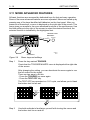
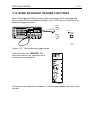
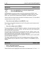
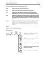
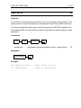
3.13 MORE ADVANCED TRIGGER FUNCTIONS
Most of the trigger functions (source, slope, and level) can be controlled with
direct access to the functions (see Section 3.9). A CRT menu is used for more
advanced trigger functions.
TRIGGER
ARM’D
1
2
3
4
TRIGGER
LEVEL
TB MODE
ST6432
9303
Figure 3.10
More advanced trigger setup
Press the menu key TRIGGER. This
turns the menu on. An extensive set of
functions is now displayed.
All functions are explained in Chapter 4. For most applications, this menu is not
needed.
3 - 20
GETTING STARTED
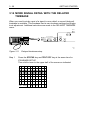
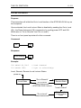
3.14 MORE SIGNAL DETAIL WITH THE DELAYED
TIMEBASE
When you need to study a part of a signal in more detail, a second (delayed)
timebase is available. This timebase has its own timebase settings and trigger
level adjustment. Additional selections are made in the DELAYED TIMEBASE
menu.
DISPLAY
MAGNIFY
DELAYED TIMEBASE
DTB
2
1
3
s TIME/DIV ns
DELAY
TRIGGER
POSITION
TB MODE
4
ST6439
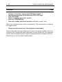
9303
Figure 3.11
Step 1
Delayed timebase setup
Press the STATUS key and TEXT OFF key at the same time for
STANDARD SETUP.
Then shift to trace to the upper half of the screen as indicated.
CH1
50mV
MTB 1.00ms
ch1
ST6690
GETTING STARTED
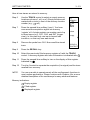
Step 2
3 - 21
Press the DTB key. The DELAYED TIME BASE menu is now displayed
on screen. Turn the delayed time base on with the first softkey.
DELAYED
TIME BASE
DEL’D TB
on off
MAIN TB
on off
starts
trig’d
TRACE
SEP
CH1
50mV
MTB1.00ms
DTB 100µs 4.882ms
T
ch1
ST6689
The upper trace is the main timebase trace. This first trace shows an intensified
part. Adjust the TRACE INTENSITY with the control as necessary. The lower
trace is the delayed timebase trace and is an expanded representation of the
intensified part in the upper trace.
Step 3
Turn the DELAY knob to shift the intensified part and to select which
part of the main timebase you want to magnify.
Step 4
The delayed timebase TIME/DIV keys are used to select the
’magnification factor’. Notice the changing delayed timebase ’TIME/
DIV’ readout at the bottom of the screen.
Step 5
The ’T’ symbol at the fourth blue softkey indicates that the cursor
TRACK control can be used to make adjustments. In this menu the
cursor TRACK control is used to change the TRACE SEParation, which
is the distance between the main timebase and the delayed timebase.
The delayed timebase can be used in the triggered mode. The triggered mode is
selected with the STARTS/TRIG’D softkey. The function of the triggered mode will
be explained in Chapter 4. For this part of "Getting Started", remain in the
STARTS mode.
Step 6
Switch the menu off with the TEXT OFF key. Notice that the delayed
timebase is still active and that the most important functions (DELAY
control and TIME/DIV key pair) still allow you to operate the delayed
timebase.
3 - 22
GETTING STARTED
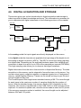
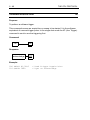
3.15 TRACE STORAGE
In the digital mode you not only have the ability to store traces on the screen
(using the RUN/STOP key), but also to store traces in memory for later use.
ANALOG
1
2
3
SAVE
RECALL
4
RUN/STOP
ST6691
9312
Figure 3.12
Digital memory setup
Store traces on screen:
Step 1
Press AUTOSET.
Step 2
Make sure that the scope is in the digital mode. If not, press the
ANALOG key to enter the digital mode.
Step 3
With the RUN/STOP key, new acquisitions are stopped and the display
is frozen. Removing the input signal or pressing a key has no effect on
the display. Stopping the acquisition is very useful to do measurements
on the signal or to make a hard copy.
Step 4
Press the RUN/STOP key to reactivate the acquisition.
Store traces in memory:
Step 5
For this step-by-step introduction you will first clear all memory
locations so that all unnecessary traces are removed.
- press the SAVE menu key.
- select CLEAR & PROTECT.
- select CLEAR ALL.
- in the confirm menu, select YES.
Sometimes there will be a second confirm menu. Select YES again to
clear protected traces as well.
Press the TEXT OFF key to turn the menu off.
GETTING STARTED
3 - 23
Here is how traces are stored in memory:
Step 6
Use the TRACK control to select an empty memory
location such as m1, m2, or m3. Empty locations are
marked with a circle in front of the memory location
number (e.g.,
m3).
Step 7
Press the second blue softkey (’save’). You have
now saved the acquisition signal into memory
’register’ m3. A single register can contain a set of up
to three traces (e.g., CH1, CH2, and EXT (trigger
view)). In this case only one input channel was
turned on, so that only one was stored.
Step 8
Remove the probe from CH1. Now recall the stored
trace.
SAVE ACQ
TO
MEMORY
m2
m3
m4
save
clear
copy
CLEAR &
PROTECT
Step 9
Press the RECALL key.
Step 10
Select the previously filled memory register m3 with the TRACK
control. A memory register with trace information is indicated with
Step 11
Press the second blue softkey to turn on the display of this register.
Indicated by
Step 12
Turn the ∆ control to separate the acquisition (live signal) and the trace
recalled from memory.
NOTE:
You are now able to operate nearly all the oscilloscope’s functions in
most routine applications. Please continue with Chapter 4 for a more
detailed description of the oscilloscope’s many advanced features.
Memory indications:
Empty register
Filled register
Displayed register
ST6705
HOW TO USE THE INSTRUMENT
4-1
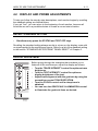
4 HOW TO USE MORE ADVANCED
FUNCTIONS OF THE INSTRUMENT
This chapter allows more experienced oscilloscope users to learn more about the
advanced features of this instrument and how to use them. For a complete
description of each function, refer to the next chapter in this manual: "Function
Reference".
This chapter explains the basics of each function and gives examples are given
in a step by step sequence.
Less experienced oscilloscope users should read Chapter 3 before beginning this
chapter.
4.1 INTRODUCTION
All of the oscilloscope models in the PM337xB, PM338xB and PM339xB family
combine the features and operation of an analog oscilloscope with that of a fullfeatured Digital Storage Oscilloscope (DSO). Switching between one mode of
operation to the other is done by pressing one (yellow) push button.
Most signal acquisition functions are identical for both modes of operation, even
though the digital mode allows for pretrigger acquisition and display, plus more
powerful logic triggering.
Delayed sweep operation is available in both operating modes.
Cursors operate in both modes.
The digital mode provides access to many powerful calculated measurement and
signal analysis functions.
It also has a completely new feature called AUTO RANGE.
AUTO RANGE automatically adjusts the attenuator or the timebase setting when
the amplitude or the frequency of the signal has changed.
This family of oscilloscopes is available with a 60 MHz, 100 MHz or 200 MHz
bandwidth. There are full four-channel instruments as well as 2+2 channel
models.
The economy version have 2 full channels and an external trigger channel.
PM3394B 200 MHz Full Four Channel Oscilloscope.
The PM3394B offers a 200 MHz bandwidth. Four channels provide equal
bandwidth, and sensitivity ranges. Each channel has full AC/DC/GND coupling
capabilities.
In VERTMENU each channel is set to 50Ω or 1 MΩ input impedance.
4-2
HOW TO USE THE INSTRUMENT
PM3390B 200 MHz 2 Channel Oscilloscope
The PM3390B has the same capabilities as the PM3394B on the channels 1 and
2. The channels 3 and 4 are replaced by an external trigger channel. This channel
can only be used as an additional trigger input channel. Signal manipulation as in
the full channels 1 and 2 is not possible. The external trigger signal can be
displayed by using the function TRIG VIEW.
PM3384B 100 MHz Full Four-Channel Oscilloscope
Bandwidth is 100 MHz.
The PM3384B has the same capabilities as the PM3394B. VERT MENU only
offers BW LIMIT selection.
PM3380B 100 MHz 2 Channel Oscilloscope
The PM3380B has the same capabilities as the PM3384B on the channels 1 and
2. The channels 3 and 4 are replaced by an external trigger channel as in the
PM3390B. VERT Menu offers only BWLIMIT selection.
PM3370B 60 MHz 2 Channel Oscilloscope
The PM3370B has a bandwidth of 60 MHz. All other features are equal to those
of the PM3380B.
HOW TO USE THE INSTRUMENT
4-3
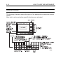
FRONT PANEL LAYOUT
The controls on the front panel are grouped by function. In this chapter, a
description for each group of controls is given in the following sequence:
-
Display and probe adjustment
Analog and digital modes
Vertical deflection
Horizontal deflection and triggering
Digital acquisition and storage
Advanced vertical functions
Advanced horizontal and trigger functions
Memory functions
Cursor functions
Measurement functions
Processing functions
Display functions
Delayed timebase
Hard copy facilities
AUTOSET and other utilities
(see section 4.2)
(see section 4.3)
(see section 4.4)
(see section 4.5)
(see section 4.6)
(see section 4.7)
(see section 4.8)
(see section 4.9)
(see section 4.10)
(see section 4.11)
(see section 4.12)
(see section 4.13)
(see section 4.14)
(see section 4.15)
(see section 4.16)
4-4
HOW TO USE THE INSTRUMENT
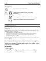
Study the front panel of your oscilloscope and observe what functions the different
controls and push buttons (keys) perform. There are three different styles of push
buttons, plus the blue softkeys adjacent to the screen. The push button functions
are as follows:
Direct function key. These keys provide direct access to specific
functions as labeled on the front panel. Examples include
AUTOSET for automatic setup of the oscilloscope and AC DC
(GND) for selection of the instrument’s input coupling.
Menu initialization key, with blue text. Press to produce a menu on
the screen from which you can select functions that are related to
the function name of this key.
Key pair. These pairs serve as up/down controls. They are used to
select a value from a range.
Softkey. Press to select a function from the menu that has been
initialized by pressing one of the menu initialization keys.
Rotary control. Used for continuously variable control of a function.
HOW TO USE THE INSTRUMENT
4-5
4.2 DISPLAY AND PROBE ADJUSTMENTS
To help you follow the step-by-step descriptions, each section begins by recalling
the standard setting as outlined below.
If you get "lost", you can return to the beginning of each section, because all
functions are set to a predefined state to create a correct start situation.
RECALL STANDARD SETTING
-
Simultaneously press the STATUS and TEXT OFF keys.
Recalling the standard setting always results in a trace on the display, even with
no signal applied to the oscilloscope inputs. Refer for a list of the standard setting
to the section "STANDARD SETUP/FRONT PANEL RESET" of Chapter 5.
DISPLAY ADJUSTMENT
Before going through the examples that introduce you to
features of this oscilloscope, adjust the display as follows:
- Turn the TRACE INTENSITY control for optimum trace
brightness.
- Turn the TEXT INTENSITY control for optimum
display brightness of the text.
- Adjust trace alignment with the graticule by using the
screwdriver control TRACE ROTATION.
- Turn the FOCUS control until a sharp trace is
obtained.
- You can turn the GRATICULE ILLUMINATION control
to illuminate the graticule lines as desired.
4-6
HOW TO USE THE INSTRUMENT
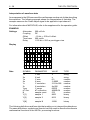
DISPLAY LAYOUT
The following illustration shows the layout of the display with a maximum amount
of text.
Most text is active only when specific functions are activated.
HOW TO USE THE INSTRUMENT
MENUS
4-7
TEXT OFF
A menu appears when a key with blue text is pressed.
The menu functions can be selected by pressing the blue softkeys to the right side
of the screen.
-
Press the ANALOG key to select the digital mode.
Press the DISPLAY key to activate the menu.
DISPLAY
WINDOWS
on off
VERT
MAGNIFY
off
T
X vs Y
Each menu starts with a menu name, which
corresponds with the key that was used to select the
menu. This is sometimes followed by a second name of
the softkey that initialized a submenu.
The windows function can be switched on and off by
pressing the corresponding blue softkey.
T indicates that a selection must be made with the
TRACK control.
The arrow ( ) behind TEXT indicates that there is a
submenu.
TEXT
dots
linear
sine
ST7415
9312
The bottom softkey switches (toggles) between the
three functions.
You can turn off the text by pressing the TEXT OFF key. This can be done to free
up the display area.
-
Press the TEXT OFF key three times.
Observe that the text mode follows the following sequence: menu off, settings off,
both on.
4-8
HOW TO USE THE INSTRUMENT
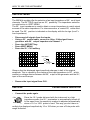
CAL SIGNAL AND PROBE ADJUSTMENT
Each measuring probe has been checked and adjusted before delivery. However,
to match the probe to your oscilloscope, you must perform the following
procedure to optimize the pulse response of the combination of oscilloscope input
and probes.
-
Connect the probe body to channel 1.
Connect the probe tip to the Probe Adjust output of the oscilloscope.
Press the AUTOSET key.
If the display looks like one of the two displays shown on the left, you must adjust
your probe to get the display shown on the right.
The probe output impedance can be adjusted through a hole in the compensation
box of the probe to obtain optimum pulse response. Refer to the following figure.
ST6024
9303
-
Adjust the probe until the screen shows the correct compensation.
The probe is now adjusted for optimum pulse response with this oscilloscope. If
you connect the probe to another channel or oscilloscope, it must be adjusted
again to that oscilloscope input.
-
Repeat this adjustment for the second probe.
HOW TO USE THE INSTRUMENT
4-9
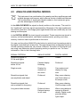
4.3 ANALOG AND DIGITAL MODES
ANALOG
This instrument is a combination of an analog real-time oscilloscope and
a digital storage oscilloscope, which offers a variety of additional features.
The combination of analog and digital modes in one instrument gives
you the advantages of both modes.
In the ANALOG MODE the signal is directly written on the screen. The result is
the "traditional" real-time signal representation. Because of the high update rate
and infinite resolution, this image gives signal details that are visible only on true
analog oscilloscopes.
In the DIGITAL MODE the input signal is sampled. These samples are stored in
memory so that mathematics, calculated measurements, printing, and other
memory functions can be performed on the trace.
You can use the yellow ANALOG push button to switch from the analog mode to
the digital mode and back at any time. The signal acquisition and display functions
of both operating modes are very similar. However, the nature of the signals you
are using may determine which operating mode you prefer to use. For more
information, refer to the following table:
SIGNAL CRITERIA
ANALOG MODE
DIGITAL MODE
Repetitive signals of
30 Hz and higher
Usable
Usable
Repetitive signals
below 30 Hz
Causes display
flickering
Preferred
Single events
Display for
duration of
the event
Can capture and
display for long
term
Repetitive signals that
are amplitude modulated
Preferred
May cause aliasing.
Use Peak detect or
Envelope mode
Repetitive signals that
are modulated in frequency
Preferred
May cause aliasing.
Use Envelope mode.
Long serial data streams
Preferred when
Delayed sweep
is not used.
When using delayed
sweep to observe
details, Digital mode
provides better
light output.
4 - 10
HOW TO USE THE INSTRUMENT
SIGNAL CRITERIA
ANALOG MODE
DIGITAL MODE
Video signals
Preferred when
Delayed sweep
is not used.
When using delayed
sweep to observe
details, Digital mode
provides better light
output.
Need to see pretrigger
information
Not possible
Up to one screen
You need to make adjustments
to the circuitry and watch
the signal change
Fastest
display update
Slower display
update
Automatic measurements
Can’t use
Fully implemented
Signal
Math
Add, Subtract, Multiply
Add, Subtract only
All functions
Signal
Analysis
Integration,
Differentiation, FFT
Not available
Full analysis, with
Math Plus option
installed
Automatic Pass/Fail test
Not available
Fully implemented,
with Math Plus option
installed
Autorange attenuator
Not available
Results in a
displayed signal with
an amplitude of 2 to
6.4 divisions
Autorange timebase
Not Available
Results in a signal
display of 2 to 6
waveform periods
OTHER CRITERIA
HOW TO USE THE INSTRUMENT
4 - 11
STANDARD SETTING
-
Simultaneously press the STATUS and TEXT OFF keys.
Connect the Probe Adjust signal to channel 1.
The Probe Adjust signal, now supplied to the input, is a square wave with a lower
level of 0V and a top level of 600 mV. The oscilloscope always operates in analog
mode after a recall of the standard setting.
-
Press the AUTOSET key for optimum signal display.
ANALOG TO DIGITAL MODE SWITCHING
Switching from analog to digital mode and vice-versa can be done by pressing the
yellow ANALOG key. If no Digital mode-only features were activated, you can
switch between the modes with no changes in the display.
-
Press the ANALOG key again.
The oscilloscope is automatically set in the digital mode. This is indicated by a
message ’DIGITAL MODE’ that appears briefly on the screen.
4 - 12
HOW TO USE THE INSTRUMENT
TRACE STORAGE
RUN/STOP
The digital mode offers a set of powerful features. One of the most important
advantages is that you can store one or more traces in memory or on screen.
-
Press the RUN/STOP key to stop the signal acquisition and freeze the
display on the screen.
The trace is frozen and stays on the screen. Observe that the signal stays stored
even when you remove the probe.
Now the instrument has been STOPped, and most keys have been disabled. The
only keys that continue to function are those directly related to display functions.
This includes trace shift using the POS control. All measurement functions are still
operable.
A frozen trace can be used for comparisons with other traces, mathematics,
cursor measurements, automatic measurements and more.
The RUN/STOP key is used to end the STOP mode and start the aquisition again.
-
Press the RUN/STOP key.
This starts the acquisition again so that the actual input signal is displayed. You
can use the RUN/STOP key at any time.
RUN/STOP
RUNNING
FROZEN
ST6482
9312
NOTE: The following section explains the basic functions regardless of
operating mode. The oscilloscope will react almost identically in either
mode. Where necessary, different behavior will be explained.
HOW TO USE THE INSTRUMENT
4 - 13
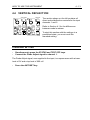
4.4 VERTICAL DEFLECTION
VERT MENU
1
AVERAGE
2
POS
POS
TRIG1
V
ON
AC DC
GND
AUTO
AMPL RANGE
mV
INV
VAR
VAR
AUTO
AMPL RANGE CH1+CH2
mV
TRIG2
AC DC
GND
ON
V
ST6437
9312
The section shown on the left contains all
direct vertical deflection controlls for the input
channels 1 and 2.
Refer to Section 4.1 for the differences
between model numbers.
To start this section with the settings in a
predefined state, you must recall the
standard setting.
STANDARD SETTING
-
Simultaneously press the STATUS and TEXT OFF keys.
Connect the Probe Adjust signal to channel 1.
The Probe Adjust signal, now supplied to the input, is a square wave with a lower
level of 0V and a top level of 600 mV.
-
Press the AUTOSET key.
4 - 14
HOW TO USE THE INSTRUMENT
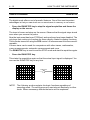
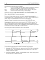
VERTICAL COUPLING
AC, DC, GND
The input coupling after AUTOSET is ac. Since the Probe Adjust signal is a pulse
type signal with a 50% duty cycle, its mean value is at the signal’s 50% amplitude
level. When the input is ac coupled, the mean value will be displayed at the
ground level of the oscilloscope. As a result of this, the displayed waveform is
centered on the screen.
AC coupling can be used to examine small ac components that are superimposed
on large dc voltages.
-
Press the AC DC GND key once for DC input coupling.
Since the Probe Adjust signal is a pulse-type signal with a lower level of 0V, and
a higher level of 600 mV, and since the oscilloscope adjusts the display position
of the ground level to coincide with the screen center, switching from ac coupling
to dc coupling results in an upward shift of the display position of the signal.
The coupling sign in the lower left hand corner of the screen changes from ∼ (ac)
to = (dc).
The ground level for each of the channels is indicated by a dash after the channel
identifier, i.e., ’1-’ for the ground level of channel 1.
0.5ms
600mV
0V
Input Signal
AC DC
GND
AC DC
GND
AUTO SET
1-
1-
1-
AC DC
GND
CH1 200mV
AC Coupled
CH1 200mV
CH1 200mV
DC Coupled
GND Coupled
ST6708
-
Press the AC DC GND key to obtain ground coupling.
A straight line is now displayed. This is the 0V (ground) level of the input. This
level serves as the 0 volt reference for amplitude measurements.
The coupling sign ’⊥’ now indicates ground coupling.
HOW TO USE THE INSTRUMENT
4 - 15
VERTICAL
POSITION
Use the POS control to adjust the ground level to any desired vertical
position on the screen.
POS
ST6158
9303
1
POS
1
MAT4171
-
Use the position control to position the line in the middle of the screen.
Observe that the channel identifier ’1-’ shifts with the trace.
-
Press the AC DC GND key again to obtain ac input coupling.
Since the Probe Adjust signal is a pulse type signal with a 50% duty cycle, its
mean value is at the 50% amplitude level of the input signal. When the input is ac
coupled, the mean value will be displayed at the ground level of the oscilloscope.
As a result of this, the displayed waveform is centered on the screen.
4 - 16
HOW TO USE THE INSTRUMENT
VERTICAL
-
AMPLITUDE
Press the upper key of the AMPL keys
Pressing the upper key increases the amplitude of the displayed
waveform. As the amplitude of the displayed waveform changes, the
screen readout of the input sensitivity changes as well.
If you adjust the displayed amplitude to 6 divisions, you will notice that
the readout in the lower left hand corner of the screen reads 100 mV/div.
The amplitude of the signal is then: 100 mV/div times 6 div = 600 mV.
AMPL
ST6159
AMPL
CH1
100mV
AMPL/div
CH1
500mV
AMPL/div
MAT4165
Try other sensitivity settings as follows :
-
Use the AMPL keys to step through the attenuator range.
Observe that the sensitivity readout changes in steps following a 1, 2, 5
sequence. The AMPL keys allow you to step up and down through the
sensitivities from 5 V/div to 2 mV/div and vice-versa. This sequence enables a
quick selection between the oscilloscope’s sensitivity positions and are such that
almost every input signal can be made visible with sufficient amplitude.
-
Adjust AMPL to 100 mV.
A waveform with an amplitude of six divisions is displayed.
HOW TO USE THE INSTRUMENT
4 - 17
VERTICAL
AUTO
RANGE
-
AUTO RANGE
The AUTO RANGE function results in an amplitude display of 2 to 6
divisions.
Press the AUTO RANGE key.
Observe that the amplitude of the signal changes from 6 divisions to 3 divisions.
In the upper right corner of the display ATT 1 is displayed. This indicates that the
AUTO RANGE function is active on input channel 1.
-
Press the upper AMPL key once.
The AUTO RANGE function is switched off and the ATT 1 indication disappears
The attenuator is now back in manual control.
VERTICAL
AMPL
VAR
mV
V
ST5971
-
VARIABLE AMPLITUDE
Press both AMPL buttons simultaneously to select the VARiable
mode. This mode is used to make fine adjustments of the input
amplitude settings between the 1-2-5 steps.
When the VARiable mode is turned off, the oscilloscope selects the
nearest ’1-2-5’ value.
Enter the VAR mode by simultaneously pressing both AMPL keys.
Adjust amplitude with either AMPL key.
Observe that the sensitivity steps that can be selected are much finer than before
and that the displayed amplitude is continuously adjustable.
Note:
-
The VAR values are calibrated amplitude settings as well. This enables
you to make accurate measurements and readouts even when
intermediate settings are used.
Adjust AMPL to 220 mV.
Press both AMPL keys to turn the VARiable mode off.
4 - 18
HOW TO USE THE INSTRUMENT
VERTICAL
-
CH1+CH2
Using two probes, connect the Probe Adjust signal to Ch1 and Ch2.
Press AUTOSET.
Both Ch1 and Ch2 are now displayed.
Adjust POS and AMPL to get a display as illustrated on the left below.
Press the CH1+CH2 key.
In the analog mode, a third trace will appear on the screen. This trace has twice
the amplitude of the Probe Adjust signal. The position of the third trace is affected
by the position controls of both Ch1 and Ch2.
The display mode is indicated in the screen as ’1+2’.
1-
1-
CH1+CH2
2CH1
CH2
2500mV
500mV
CHP MTB
200µs
CH1
CH2
ch1
500mV
500mV
1+2
CHP MTB
200µs
ch1
ST5970
-
Press the ANALOG key to switch to the Digital mode.
Observe that switching to the digital mode turns off the third trace. The ’1+2’
indication disappears.
-
Press the CH1+CH2 key once again.
Observe that in the digital mode the (CH1+CH2) trace can be used as well.
Simultaneous display of both channels together with the sum of both channels is
not possible in the digital mode.
1-
CH1+CH2
2CH1
CH2
500mV
500mV
1+2
MTB
200µs
ch1
CH1
CH2
500mV
500mV
ALT MTB
200µs
ch1
ST6720
-
Press the ANALOG key to return to the analog mode.
HOW TO USE THE INSTRUMENT
4 - 19
VERTICAL
INVERT
The INVERT function in Channel 2 can be used to make it easier to do out-ofphase signal comparisons. The most common use of the INVERT function is to
obtain the display or make the acquisition of the voltage difference between two
channels. This is done by displaying or capturing the sum of Ch1 and Ch2 as
follows. (This is referred to as the differential mode.)
-
Using two probes, connect the Probe Adjust signal to Ch1 and Ch2.
Press AUTOSET.
Both Ch1 and Ch2 are now displayed.
Adjust POS and AMPL to get a display as illustrated on the left below.
Press the CH1+CH2 key.
Press the INV key of channel 2.
Since channel 2 is inverted before it is added to channel 1, the result will be CH1CH2. This is indicated as ’1-2’ on the screen. The signals on both inputs are the
same, resulting in a straight line at ground level.
(If the line is not straight, this may be an indication that the probes are not correctly
adjusted. When one of the probes is not properly adjusted, the input signals at the
input connectors of the oscilloscope will be unequal. The difference of the two
input signals shows up in the differential mode).
1-
1-
CH1+CH2
INV
2CH1
CH2
2200mV
200mV
1+2
CHP MTB
200µs
ch1
CH1 200mV
CH2↓ 200mV
1-2
CHP MTB
200µs
ch1
ST5969
4 - 20
HOW TO USE THE INSTRUMENT
VERTICAL MENU
BANDWIDTH LIMITER
The Bandwidth Limiter reduces the bandwidth of the vertical channels to 20 MHz.
This is done by activating a filter in the vertical channels. This feature can be used
both in analog mode and in digital mode to suppress high frequency noise. For
repetitive signals and when in the digital mode, averaging is the preferred
method to reduce noise without limiting the bandwidth.
-
Press the ’BW LIMIT’ softkey to turn it on.
Observe that the displayed line becomes "thinner" as an indication that the
amount of noise is reduced.
The text ’BWL’ appears in the bottom of the screen to indicate that the function is
active.
-
Press the ’BW LIMIT’ softkey to turn it off again.
HOW TO USE THE INSTRUMENT
4 - 21
50Ω
VERTICAL MENU
The 200 MHz models offer the selection of an input impedance of 50Ω on all input
channels. The EXTTRIG input has no 50Ω possibility. The impedance selection
is a subfunction in VERT MENU.
The 50Ω input impedance is used to obtain a correct impedance to match signal
sources of the same impedance. For interconnection, a coaxial 50Ω cable must
be used. The 50Ω position is indicated on the display with the Lz sign (Low Z =
Low Impedance).
-
Disconnect all signals from the inputs.
Using a 50Ω coaxial cable, connect a 4 Vpp, 2 kHz signal from a
generator with 50Ω output impedance to channel 1.
Press the AUTOSET key.
Press VERT MENU.
Press the 50Ω CH1 softkey.
VERT MENU
50Ω CH.
ON
OFF
CH1
1V
CH1
1V
LZ
ST5968
9312
Observe that the displayed signal amplitude changes to half of the original
amplitude. This is caused by the change of the input impedance to 50Ω, which
results in a voltage division between the 50Ω output of the generator and the 50Ω
input of the oscilloscope.
-
Remove the input signal from CH1.
VERTICAL
-
PROBE RANGE INDICATOR
Connect the probe again.
Since the 10:1 probe delivered with the instrument is a high
impedance probe, the 50Ω termination is automatically turned off.
At the same time, the sensitivity readout is adjusted automatically
detector
when a 10:1 or 100:1 probe is used. This way you don’t have to
multiply the displayed amplitude by 10 or 100 when you use a Fluke probe with
range indication.
CHx
ST6021
4 - 22
HOW TO USE THE INSTRUMENT
4.5 HORIZONTAL DEFLECTION AND TRIGGERING
Before starting with the horizontal deflection functions, you must set the
instrument to a predefined state to create a correct start situation.
STANDARD SETTING
-
Simultaneously press the STATUS and TEXT OFF keys.
Connect the Probe Adjust signal to channel 1.
The Probe Adjust signal, now supplied to the input, is a square wave with a lower
level of 0V and a top level of 600 mV.
-
Press AUTOSET.
TIMEBASE
TIME/DIV
TIME/DIV
4 periods/cycles of the square wave are displayed on the screen.
ST6839
-
Press the ’s’ (left) key of the MainTB TIME/DIV key pair a few times.
The more you press the left (’s’) key, the slower the timebase will run. This results
in the number of displayed periods/cycles of the input signal to increase.
-
Press the ’ns’ (right) key of the MainTB TIME/DIV key pair a few times.
The number of displayed periods/cycles decreases as the timebase speed
increases.
Observe that the timebase speeds are adjustable in steps following a 1-2-5
sequence.
TIME/DIV
MTB 500µs
MTB 100µs
ST6709
-
Set the timebase to 200 µs.
The signal is displayed with four periods on the screen.
HOW TO USE THE INSTRUMENT
TIMEBASE
AUTO
RANGE
-
4 - 23
AUTO RANGE
The AUTO RANGE function continuously adjusts the timebase to a
display of 2 to 6 waveform periods.
Press the AUTO RANGE key.
Observe that the timebase of the signal display changes to display 2 to 6 signal
periods. AUTO TB in the upper right corner of the display indicates that the AUTO
RANGE timebase function is active.
-
Press one of the TIME/DIV keys.
The AUTO RANGE function is switched off and the AUTO TB indication
disappears.
TIMEBASE
MAIN TB VAR
TIME/DIV
Fine adjustment of timebase speeds between the 1-2-5 steps
can be made by simultaneously pressing the MainTB TIME/DIV
keys.
ST6710
-
Activate the VAR function by simultaneously pressing the TIME/DIV keys.
Press one key of the MainTB VAR keys.
Observe that the timebase indication is now changing continuously instead of
following the 1-2-5 step sequence.
The VAR timebase readout values are calibrated values. This enables accurate
timing measurements using VAR timebase settings.
-
Adjust MainTB VAR to 850 µs/div.
Turn off the VAR function by pressing the MainTB TIME/DIV key pair
simultaneously.
Observe that the timebase is set to the nearest step value (1 ms/div).
In the Digital mode, the timebase speeds are determined by an XTal oscillator.
4 - 24
HOW TO USE THE INSTRUMENT
TIMEBASE
MAGNIFY
ST6711
-
MAGNIFY
The displayed signal can be expanded horizontally so that more
signal detail becomes visible. In the analog mode, a 10
*
magnification is possible and the entire sweep length can be made
visible by turning the X POS control.
Press the right MAGNIFY key.
The text ’MGN’ appears in the bottom of the screen to indicate that the function is
active. Observe that the timebase indication is changed from 1.00 ms/div to
100 µs/div.
MAGNIFY
CH1 200mV
MGN
MTB 100µs
ch1
CH1 200mV
MTB
100µs
ch1
ST6504
-
Press the ANALOG key to set the scope in the digital mode.
Press the right MAGNIFY key.
Observe that the signal expands in 1, 2, 4 ... steps to a maximum of 32 times.
* * *
This magnification factor is displayed briefly on the screen.
-
Set the MAGNIFY to 4.
*
HOW TO USE THE INSTRUMENT
4 - 25
TIMEBASE
X POS
-
X POS
With X POS the displayed signal is shifted horizontally across the
display.
Turn the X POS control clockwise.
X POS
1
1
MAT4199
Observe that a bar graph (
) is displayed.The block on the bar graph
shows which part of the digital trace is displayed as expanded. This block on the
bar graph moves as you use the XPOS control.
-
Press the RUN/STOP key.
Observe that the MAGNIFY key and the X POS control can still be used after the
acquisition has STOPped. This allows you to look at signal details even after the
signal has been acquired.
-
Press the RUN/STOP key.
TRIGGERING
-
Simultaneously press the STATUS and TEXT OFF keys.
Press AUTOSET.
4 - 26
HOW TO USE THE INSTRUMENT
TRIGGER
-
SOURCE
Press the TRIG 2 key in the CH2 section of the front panel to select
channel 2 as trigger source.
The indication in the lower right hand readout area of the screen now displays ’ch2’.
Observe that the signal is not triggered. The ARM’D LED is on.
-
Press the TRIG 1 key in the CH1 section of the front panel to select
channel 1 as trigger source.
Observe that the indication has now changed into ’ch1’ and the signal is triggered
again.
TRIG2
TRIG1
CH1
ch2
CH1
ch1
ST5955
TRIGGER
TRIG1
-
SLOPE
The trigger source selection key is also used to select the trigger slope
between the positive-and negative-going edge of the triggering signal.
Press the TRIG 1 key in the CH1 section of the front panel a second time.
Observe that the signal now starts with the trailing edge instead of a leading edge.
Also the trigger slope symbol in the lower right hand corner of the readout area
indicates a trailing edge.
TRIG1
ch1
ch1
ST6025
HOW TO USE THE INSTRUMENT
4 - 27
TRIGGER
TRIGGER LEVEL
TRIGGER
After each AUTOSET, the trigger level is always clamped within the
LEVEL
signal amplitude range to assure stable triggering on most signals. The
trigger level is adjustable, but it is limited between the minimum
(-100%) and the maximum (+100%) amplitude levels of the signal.
-
Turn the TRIGGER LEVEL control.
As you turn the trigger level control, the
trigger level readout in the bottom of the
screen shows the trigger level relative
to the signal amplitude. For example, it
may appear as ’Level=+ 14%’.
TRIGGER
LEVEL
1-
LEVEL=+17%
ST6547
4 - 28
HOW TO USE THE INSTRUMENT
TRIGGER
TRIGGER
POSITION
TRIGGER POSITION
-
Press the ANALOG key to select the digital mode.
Turn the TRIGGER POSITION control counterclockwise.
One of the outstanding capabilities of a Digital Storage Oscilloscope is the ability
to capture and display signal details before the trigger moment.
When you turn the TRIGGER POSITION control counterclockwise, the trigger
point ( ) is shifted to the right. This allows you to look at the signal before the
trigger point. The pretrigger view is displayed in the bottom of the screen, and
calibrated in divisions. The trigger point is indicated on the screen with an arrow.
Pretrigger recording can be adjusted and is limited to one full screen, or -10
divisions.
-
Turn the TRIGGER POSITION control clockwise.
When the control is rotated clockwise, delay is added. The trigger point shifts to
the left. The delay can be adjusted to a maximum of1000 divisions, so that it is
outside the screen. Positive trigger delay is indicated in seconds or in fractions of
seconds.
-
Set the delay to 0 with TRIGGER POSITION
HOW TO USE THE INSTRUMENT
4 - 29
TRIGGER
-
SINGLE SHOT
Make sure the instrument is in the Digital Mode.
Press AUTOSET.
This sets up the scope with the proper amplitude and timebase settings.
-
Remove the probe tip from the Probe Adjust output.
Turn the TRIGGER POSITION to mid-screen (counterclockwise).
Press the SINGLE key.
This automatically prepares the scope for a single acquisition.
Observe that the screen has been cleared, and that the ARM’D LED is on. This
indicates that the scope is armed and waits for a trigger. The trigger level is
automatically set to .5 divisions (indicated by ’T-’).
-
Look at the screen and touch the Probe Adjust output with the probe tip.
Observe that the oscilloscope ’runs’ once and that a signal appears on the screen.
The ARM’D LED is turned off. At the moment you touched the Probe Adjust output
with the probe, the scope was triggered. The trigger moment is displayed in the
center of the screen. The left side of the screen displays the part of the signal
before triggering (pretrigger information).
T−
Probe Adjust
T−
ST6505
9303
In SINGLE SHOT also ’Dual Slope’ triggering is possible. See chapter 5
TRIGGER MAIN TB function.
4 - 30
HOW TO USE THE INSTRUMENT
4.6 DIGITAL ACQUISITION AND STORAGE
This section gives you a short introduction to digital acquisition and storage in
order to provide the basic knowledge and terms. This information is necessary for
you to understand all digital statements in the following sections of the manual.
ANALOG:
INPUT
STAGE
DISPLAY
DIGITAL:
INPUT
STAGE
signal
data
ADC
ACQUISITION
MEMORY
DISPLAY
REGISTER
MEMORY
ST6721
In the analog mode the input signals are directly displayed on the screen.
In the digital mode the channels are applied to the input stage of the digital circuit:
the analog-to-digital convertors (ADC’s). The ADC’s convert the analog signal(s)
into digital data. Depending on the selected timebase speed, this sa2pling and
conversion is done at a rate of up to 200 million samples per second (200 MS/s).
This high sampling rate allows you to observe fast signal variations.
Digital information from the adc is then stored in a Acquisition Memory. The data
acquisition in this memory can be stopped to freeze the trace on the screen. You
can also store (save) complete registers or separate signals into a "background"
memory, called Register Memory. Traces can be stored as long as you like and
can be recalled at any time.
The CombiScopes in this range have a standard memory of 8K. The record length
for each trace is the maximum number of samples divided by the number of
traces. With the standard scope, the memory depth of 8K is available for two
channels. The memory is partitioned so that 1x8K, 2x4K or 4x2K records can be
captured. For maximum update rate, records can be made as short as 512 points.
If the memory expansion option is installed, the record length can be adjusted
between 32K and 512 points.
HOW TO USE THE INSTRUMENT
4 - 31
4.7 ADVANCED VERTICAL FUNCTIONS
All basic functions of the oscilloscope are accessible via direct action front panel
keys.
More advanced functions are easily accessible via the menus behind the menu
initialization keys (keys with their function name in blue text).
STANDARD SETTING
Before continuing with the advanced vertical functions, you must set the
instrument to a predefined state to ensure a correct start situation.
-
Simultaneously press the STATUS and TEXT OFF keys.
Connect the Probe Adjust signal to channel 1.
The Probe Adjust signal, now supplied to the input, is a square wave with a lower
level of 0V and a top level of 600 mV.
-
Press AUTOSET.
4 - 32
HOW TO USE THE INSTRUMENT
ACQUIRE
AVERAGE
The average function averages the input data over a number of successive
acquisitions. The average function is used to reduce the influence of random
noise in the input signal. There is no loss of bandwidth when the average function
is activated, but the signal must be repetitive. The number of samples over which
the average is calculated can be selected by the user.
-
Use the probe to connect Ch1 to the Probe Adjust output.
Press AUTOSET.
Connect the second probe to channel 2, but do not connect it to a signal!
Press the CH1+CH2 key to add Ch1 and Ch2 together.
Press the mV key of the CH2 AMPL keys so that the noise picked up by
the probe tip of the second probe appears on the CH1+CH2 trace.
Press the AVERAGE key.
For maximum ease of use, the scope offers direct access to the important
average feature.
The text ’Average = 8’ appears in the bottom of the screen to indicate that the
function is active. The default value is 8. The indication changes into ’AVG’.
Observe that the noise on the trace is reduced.
-
To change the Average constant, press the ACQUIRE key.
Turn the TRACK control clockwise.
The Average factor increases when the TRACK control is turned clockwise.
Observe that this reduces noise on the trace even more.
TRACK
Average=2
AVG
Average=256
AVG
ST6481
-
Turn the TRACK control counterclockwise so that the Average factor is
8 again.
HOW TO USE THE INSTRUMENT
4 - 33
ACQUIRE
ENVELOPE
The ENVELOPE mode records the minimum and the maximum of the signal over
a number of acquisitions.
-
Press the ACQUIRE key.
Press the ’ENVELOPE’ softkey to turn it on.
ENVELOPE
on
ENV
ST6480
The AVERAGE mode and the ENVELOPE modes are mutually exclusive.
Observe that AVERAGE is automatically switched off. The text ’ENV’ appears in
the bottom of the screen to indicate that the function is active.
The minimum and maximum of the input signal is stored and becomes visible on
the screen. This process continues until it is turned off by the user.
-
Turn the POS control of Ch1.
Observe that every time you change the settings of the scope (like trace POS) the
ENVELOPE process automatically starts again.
-
Press the ’ENVELOPE’ softkey to turn off the ENVELOPE mode.
ACQUIRE
PEAK DETECTION
PEAK DETection automatically catches peak values (up to glitches of 10 ns width)
of the input signal during a single acquisition.
-
Press the ’PEAK DET’ softkey to turn it on.
The text ’PKD’ appears in the bottom of the screen to indicate that the function is
active. Observe that any glitch on the input signal becomes visible on the screen.
Note:
-
Regardless of the timebase speed selected, the scope is set to the
highest sample rate, so that glitches up to the sample frequency can be
caught (5 ns at 200 MS/s).
Press the ’PEAK DET’ to turn it off again.
4 - 34
HOW TO USE THE INSTRUMENT
4.8 ADVANCED HORIZONTAL AND TRIGGER
FUNCTIONS
All basic timebase and trigger functions of the oscilloscope are accessible via
direct action front panel keys. More advanced functions are easily accessible via
the menus behind the menu initialization keys (keys with the function in blue text).
STANDARD SETTING
Before continuing with the advanced functions, you must set the instrument to a
predefined state to ensure a correct start situation.
-
Simultaneously press STATUS and TEXT OFF.
Connect the Probe Adjust signal to channel 1.
Press the AUTOSET key.
TRIGGER
-
MODE
Press the TRIGGER key.
On the screen the ’TRIGGER MAIN TB’ menu is displayed. The menu functions
can be selected by pressing the blue softkeys to the right of the screen. The top
softkey selects the trigger mode (’edge’ or ’tv’). The lower part of the menu is
optimized for the selected trigger modes.
-
Press the first softkey to select ’tv’ trigger mode.
Observe that the lower part of the menu is optimized for tv applications.
-
Press the first softkey to return to ’edge’.
Note :
In the Digital mode, an additional selection is available. This is called
"logic" or "glitch". A full description of the Logic and Glitch triggering
functions can be found in Chapter 5.
HOW TO USE THE INSTRUMENT
4 - 35
TRIGGER
-
LEVEL
Press the ’level-pp’ softkey to turn it off.
TRIGGER The automatic level detection circuitry is turned off. The trigger level is
LEVEL
no longer clamped within the peak-peak range of the signal. You must
adjust the proper trigger level. While you turn the TRIGGER LEVEL
control, the actual trigger level is displayed in (m)V.
An indicator ’T-’ is displayed next to the channel identifier when the combination
of trigger coupling and channel input coupling is useful (both ac coupled or both
dc coupled).
When the ’T-’ is within the signal range, a stable display of the signal is obtained.
When proper triggering takes place, the ARM’D LED is off.
Use the TRIGGER LEVEL control to move the indicator (T-) vertically.
TT-
TRIGGER
LEVEL
ST6738
When the trigger level indicator (T-) is outside the signal range, triggering is lost.
Because of the nature of the (Probe Adjust) input signal, it appears that only two
lines are drawn. The timebase is not properly triggered, as is indicated by the
ARM’D LED being turned on.
Note:
’T-’ is an indication for reference only. Its position can differ slightly from
the actual trigger level.
4 - 36
HOW TO USE THE INSTRUMENT
TRIGGER MODE
-
Press the TB MODE key.
TB MODE
-
TRIGGERED
In the screen, the timebase mode (TB MODE) menu appears. ’auto’ is
intensified. With the "auto" mode turned on, the timebase will run free as
soon as no triggering signal is detected, in order to provide a base line.
The ’Auto’ mode works well with most signal that have frequencies of
30 Hz or higher.
Press the softkey next to the ’auto trig single’ function to select ’trig’.
In the triggered mode, a signal is visible only when proper triggering occurs.
-
Move the indicator (T-) in and out of the signal range.
T−
T−
TRIGGER
LEVEL
ST6737
In the Analog mode, the result is a stable and triggered signal when the indicator
is inside the signal range, and no trace appears on the screen when the indicator
is outside the signal range.
Disabling the ’auto’ function by selecting ’trig’ can be useful for displaying very low
frequency signals. The scope waits for a real trigger before the sweep starts even
if the signal frequency is very low.
In the Digital mode, the same criteria exist for the use of the ’auto’ function and
the ’trig’ function, but there is a difference. When the scope is in the ’trig’ mode
and triggering is lost, the acquisition will stop, but the display will reflect the last
information before the triggering stopped. This may lead you into thinking that the
scope is properly triggered because the display appears to be stable, while in fact,
you are displaying stored information only. Watch the ARM’D LED !
HOW TO USE THE INSTRUMENT
TRIGGER MODE
-
4 - 37
ROLL
Press the ANALOG key to select the digital mode.
Press the TB Mode key to enter the TB mode menu
The TB MODE menu is extended with extensive timebase modes. The
differences are as follows:
• A Roll mode
• Selection of ’Real-time only’
• Delay by events
• Selection of Acquisition length
-
Press the softkey next to the ’ROLL on off’ function to select ’on’.
The ’ROLL on’ function is now intensified.
Observe that the timebase is automatically set to 200 ms. The trace moves from
the right to the left.
-
Press the ’STOP ON TRIGGER’ softkey to select ’yes’.
The trace stops when the trigger (in this case the start of the first period) reaches
the left of the screen.
Using the roll mode, you can monitor signals like temperature changes and
chemical processes at low timebase speeds. In this mode the scope operates like
a four-pen plotter. Over 36 hours of events can be recorded in memory and
plotted later.
Unlike a paper and pen plotter, the scope can record glitches as narrow as 5 ns,
and the record can be stopped when a trigger condition is met.
4 - 38
HOW TO USE THE INSTRUMENT
TRIGGER
-
LINE
Connect a sine-wave signal of 4 V/300 Hz to channel 1.
Simultaneously press the STATUS and TEXT OFF keys.
Press AUTOSET.
Select a timebase speed of 1 ms/div.
Press the TRIGGER key.
Press the softkey next to the function ’ch1 line’ to select ’line’.
When ’line’ is selected, this function is intensified. The line frequency is used as
the trigger source.
-
Slowly vary the frequency of the sine-wave input signal.
Observe that when the input frequency is close to an integer multiple of the line
frequency, the running sine wave slows down or even stands still. Line triggering
can be used to display signals or signal components that are related to the line
frequency (e.g., hum or power supply ripple).
HOW TO USE THE INSTRUMENT
4 - 39
4.9 MEMORY FUNCTIONS
The next section deals with storing and recalling traces in memory for later use.
Functions related to trace storage and recall are easily accessible via the menus
selection keys labeled ’SAVE" and ’RECALL’.
STANDARD SETTING
Before continuing with the memory functions, you must first set the instrument to
the default setting to ensure a correct start situation.
-
Simultaneously press the STATUS and TEXT OFF keys.
Connect the Probe Adjust signal to channel 1.
Press AUTOSET.
The Probe Adjust signal, now supplied to the input, is a square wave with a lower
level of 0V and a top level of 600 mV.
TRACE STORAGE
SAVE
-
CLEAR & PROTECT
Press the ANALOG key to select the digital mode.
Press the SAVE key to enter the ’SAVE ACQ TO MEMORY’ menu.
To be sure that all unnecessary stored traces are removed, you first will clear all
memory locations.
-
Press the ’CLEAR & PROTECT’ softkey.
Press the ’clear all’ softkey.
The scope now displays the confirmation submenu to prevent you from removing
traces you did not want to remove.
-
Press the ’yes’ confirm softkey.
If any memory locations were protected (’PROTECT ON’ in CLEARS PROTECT
MEMORY submenu), a second confirmation must be given.
-
Press the ’yes’ confirm softkey again.
4 - 40
HOW TO USE THE INSTRUMENT
TRACE STORAGE
-
SAVE
Turn the TRACK control to select the memory location in which to store
the trace data.
Observe that eight memory locations ’m1 to m8’ (or 50 memory locations when
extended memory is installed) scroll through the menu. All locations are marked
with a circle before the memory number.
-
Select memory location ’m1’.
Press the ’save’ softkey.
The signal is saved in memory location m1.
Observe that the circle before ’m1’ is solid now to indicate that this memory
location is occupied.
-
Set the MainTB to 500 µs.
Select location ’m2’.
Press the ’save’ softkey.
Set the MainTB to 200 µs/div.
Select location ’m3’.
Press the ’save’ softkey.
Observe that memory locations ’m2’ and ’m3’ are now solid bullets as well.
TRACE STORAGE
You can also clear a memory location.
-
Select location ’m2’.
Press the ’clear’ softkey.
This clears memory location 2. This is indicated by the open circle.
CLEAR
HOW TO USE THE INSTRUMENT
TRACE STORAGE
4 - 41
COPY
A trace can be copied from one memory location to another.
-
Press the ’COPY’ softkey.
The ’COPY MEMORY’ is now displayed. The source (’FROM’) and destination
(’TO’) memory locations can be selected in this submenu.
-
Turn the TRACK control to select ’m3’ as source from.
Turn the ∆ control to select ’m2’ as destination to.
Press the ’copy’ softkey.
The contents of ’m3’ have now been copied into ’m2’ without destroying the data
in ’m3’.
4 - 42
HOW TO USE THE INSTRUMENT
TRACE STORAGE
RECALL
-
RECALL
If you completed all of the previous steps, three memory locations are
occupied by trace information. You can display these stored traces at
any time and in any combination.
Press the RECALL key.
Turn the TRACK control to select ’m1’.
Press the ’DISPLAY on off’ softkey to display m1.
Observe that the stored trace on memory location ’m1’ is displayed and that the
circle before m1 is solid.
An open circle indicates an empty memory location.
A circle with a dot indicates that there is a trace stored, but it is not displayed.
A solid circle indicates trace data in memory are displayed on the screen.
Empty memory locations cannot be displayed.
You can shift traces separately over the screen by means of the ∆ control.
-
Turn the POSition control.
RECALL
REGISTER
MEMORIES
The live trace shifts.
-
Turn the TRACK
control to select ’m2’.
Press the ’DISPLAY on
off’ softkey to on.
Turn the ∆ control.
POS
∆
acq
m1 T
m2
DISPLAY
on off
CLEAR
DISPLAY
Y-POS ∆
−2.30D
trace
register
ST6722
9303
Observe that the second stored trace shifts.
HOW TO USE THE INSTRUMENT
TRACE STORAGE
4 - 43
SAVING MULTIPLE TRACES
Each memory location can store two channels.
-
Connect the probe to channel 1.
Press AUTOSET.
Switch on channel 2.
Turn the channel 2 POS control counterclockwise.
The upper trace displays the signal of channel 1, and the lower line represents
channel 2.
-
Press the SAVE key.
Turn the TRACK control to select memory location ’m1’.
Press the ’save’ softkey to store two traces in ’m1’.
Observe that m1 was already filled, so the confirmation submenu is displayed.
-
Press the softkey next to ’yes’.
This overwrites memory ’m1’ with the new traces.
TRACE STORAGE
-
RECALLING MULTIPLE TRACES
Press the RECALL menu key.
The memory location is already preset to the last saved (m1).
-
Press the ’DISPLAY on off’ softkey so that ’m1’ is displayed.
Turn the ∆ control counterclockwise.
Observe that both traces are displayed and shifted to the lower screen.
-
Press the softkey next to ’trace register’ to select ’trace’.
Observe that the menu displays both traces of register 1 (m1.1 and m1.2). Both are
filled: m1.1 with the signal of channel 1 and m1.2 with the signal from channel 2.
-
Turn the TRACK control to select m1.1.
Press the ’DISPLAY on off’ softkey to off.
Observe that the stored trace of channel 1 is not displayed any more.
-
Press the ’CLEAR DISPLAY’ softkey to clear all stored traces before
continuing to the next section.
4 - 44
HOW TO USE THE INSTRUMENT
4.10 CURSORS FUNCTIONS
Cursors are provided to make fast and accurate amplitude
and time measurements. These can be done in digital
mode as well as in analog mode.
The analog mode of the oscilloscope is often used to accurately display complex
waveforms, such as in AM, FM, and Video.
The digital mode will often be the preferred operating mode for single accuracies
which have to be studied or analyzed.
TRACK
CURSORS
∆
ST6171
9303
When operating in digital mode, the cursors are always set to the optimum place
for that particular measurement and the readout is directly displayed on the
screen.
This is the fastest and easiest way for most of the measurements .
But for measurements on very complex signals with different waveforms in a
trace, the analog cursor measurements gives you a very helpful tool to find your
measurement.
STANDARD SETTING
Start with the standard setting. This ensures you have the correct start condition.
-
Press the STATUS and TEXT OFF keys simultaneously.
Connect the Probe Adjust signal to channel 1.
The Probe Adjust signal now supplied to the input is a square wave with a lower
level of 0V and a top level of 600 mV.
-
Press the AUTOSET key.
HOW TO USE THE INSTRUMENT
4 - 45
CURSORS
ON/OFF
There are two sets of cursors : amplitude cursors and time cursors. Amplitude
cursors are two horizontal lines, and Time cursors are two vertical lines. The
dashed lines are referred to as reference cursors and the dotted lines are referred
to as delta (∆) cursors.
Cursor measurements can be made in both operating modes of the instrument.
Amplitude and time cursors can be displayed at the same time.
-
Press the ANALOG key to set the scope in mode.
Press the CURSORS key to enter the cursors menu.
The menu is now displayed. Time cursors (’||’) are selected by default. In the
digital mode, two ’x’s mark the actual measuring point where the cursors intersect
with the signal. In the analog mode these ’x’ indicators are not available.
CURSORS
TIME
Using the TRACK and ∆ controls, you can adjust the position of the cursors. The
time and amplitude difference between the cursors is read in the top of the screen.
Cursor readout parameters can be
changed and are selected via the
CURSORS
’READ OUT’ softkey.
on off
TRACK
-
-
Turn the TRACK control and
observe that both cursors
move.
Turn the Delta (∆) control
and observe that only the
delta cursor moves.
#
ch1
ch1: ∆T= 354µs ∆V= 584mV
READOUT
ST6730
9303
CH1
200mV
MTB 200us
∆
ch1
4 - 46
HOW TO USE THE INSTRUMENT
CURSORS
-
VOLT
Use the softkeys, to select the amplitude cursors (’=’ intensified).
Two amplitude cursors will appear in the display.
The menu permits the channel to be selected for which the amplitude cursors
apply.
When channel 1 is the only channel displayed, ’ch1’ is the only selection.
CURSORS
on off
-
Turn the TRACK
control to move both
cursors, and turn the
Delta (∆) control to
move only the ∆
cursor.
#
∆
ch1
ch1: ∆T=
s ∆V=360mV
TRACK
READOUT
ST6731
9303
CH1
CURSORS
200mV
MTB 200us
ch1
AMPLITUDE & TIME
Amplitude and Time cursors can be displayed at the same time. When both
amplitude and time cursors are displayed, you must select which cursors are
affected by the TRACK and ∆ controls. This selection is made by toggling the
softkey ’CONTROL’.
Channel selection applies only to the voltage cursors. The time cursor always
applies to all channels.
To use both types of cursors at the same time, do the following:
-
Press the softkey next to ’= || #’ so that ’#’ is intensified.
Press the CONTROL softkey so that ’=’ is intensified.
Turn the TRACK control and observe that only the amplitude cursors
move.
Press the CONTROL softkey so that ’||’ is intensified.
Turn the TRACK control and observe that only the time cursors move.
HOW TO USE THE INSTRUMENT
4 - 47
CURSORS
-
READOUT
Press the softkey next to ’READOUT’.
The ’CURSOR READOUT’
selection menu for horizontal and
vertical measurements is now
displayed. You can make the
following selections from this menu:
∆T, 1/∆T, ∆T-ratio, T-trg and phase
for time measurements.
∆V, V1, V2, ∆V-ratio for voltage
measurements.
CURSORS
READOUT
∆T 1/∆T
∆T-ratio
ph T-trg
∆V
V1&V2
∆V-ratio
ch1: ∆T= 460s ∆V= 600mV
RETURN
ST6732
9312
∆T is the time difference between the time cursors. The readout is in seconds (s)
or fractions of seconds.
1/∆T results in the inverted value of the time difference, and is displayed in Hz.
When the time cursors are set exactly one period apart this represents the
frequency of the signal.
∆T-ratio allows for a relative measurement of two cursor readings. It is displayed
as a percentage.
Phase is used to measure a phase difference between two signals, or to
determine the phase of a detail within one signal.
T-trg gives the timedifference between the cursors and the trigger point.
∆V is the voltage difference between the voltage cursors (readout: ∆V=...V).
V1, V2 displays the absolute voltages for each voltage cursor in relation to ground
(readout: V1=Vreference, V2=Vdelta).
∆V-ratio allows for a relative measurement of two cursor readings. It is displayed
as a percentage.
4 - 48
HOW TO USE THE INSTRUMENT
∆T-RATIO/PHASE
CURSORS READOUT
First, the reference distance between the two cursors is set. This then is set to
100 % (360°) by pressing the ∆T=100 % (360°) softkey. Changing the distance
between the cursors now results in a % (°) reading of the reference.
-
Press the softkey next to ∆T until ∆T-ratio (phase) is intensified.
Set the time cursors to be exactly one signal period apart.
Press the softkey next to ∆T=100% (360°).
In the cursor readout line of the screen, the value for ∆T is now ’∆T=100%’
(∆T=360°)
Observe that the 100% (360°) reference does not change when the TRACK
control is turned.
100%
50%
ch1: ∆T=100% ∆V=600mV
TRACK
ch1: ∆T=50% ∆V=600mV
∆
TRACK
∆
∆T=100%
-
Adjust the cursors to a distance of half a signal period.
Now the ∆T in the readout area will read ’∆T= 50%’ (∆T=180°)
This is the way to use the cursors for duty cycle measurements.
ST6733
HOW TO USE THE INSTRUMENT
4 - 49
4.11 MEASUREMENT FUNCTIONS
When operating in the analog mode, you can use the cursors to measure
amplitude and time data.
When operating in the digital mode, the scope has an extensive set of fully
automated amplitude and time measurement functions. You can select two
measurements to be performed simultaneously. These measurements are
updated automatically, so that when signals change, the measured values
automatically changed at the same time. The read- outs are displayed in the
upper section of the screen.
STANDARD SETTING
Start with the standard setting.This ensures a correct start.
-
Simultaneously press the STATUS and TEXT OFF keys.
Connect the Probe Adjust signal to channel 1.
The Probe Adjust signal now supplied to the input is a square wave with a lower
level of 0V and a top level of 600 mV.
-
Press AUTOSET.
4 - 50
HOW TO USE THE INSTRUMENT
MEASURE
MEASURE
-
MEAS1-PKPK
Press the ANALOG key to select the digital mode.
Press the MEASURE key.
The displayed menu gives access to the two measurements MEAS 1 and
MEAS 2. Each measurement can be independently turned on and off. In this
menu, you can select the measurement in MEAS 1 and MEAS 2 function.
Observe that the measurements are linked to the active channel. The two default
measurements are ’pkpk’ and ’freq’.
-
Press the second softkey to turn MEAS1 to ’on’.
The screen automatically displays the result of the peak-to-peak measurement:
’ch1: pkpk= ....mV’.
-
Press the softkey next to ’MEAS1’.
The menu displays the ’SELECT MEAS 1" submenu. You can choose from three
main measurements: volt, time, or delay. The lower part of the menu optimizes to
the selected main measurement.
The actual type of measurement is selected by using the ’TRACK’ control. The
following voltage measurements are available : dc, root- mean square, minimum
peak, maximum peak, peak-to-peak, low level, high level.
The following time measurements are available : frequency, period, pulse width,
rise time, fall time, duty cycle.
The ’delay’ measurements include the time delay between leading or trailing
edges between any two channels or traces. (Channel or trace must be on the
display)
MEASURE
-
MEAS1-RMS
Select ’volt’ measurements.
Turn the TRACK control to select ’rms’.
Observe that the screen displays the result of the rms measurement: ’ch1 rms = ....V’.
HOW TO USE THE INSTRUMENT
4 - 51
MEASURE
-
MEAS 2-FREQ
Press the ’RETURN’ softkey to return to the ’MEASURE’ menu.
Turn on MEAS 2.
MEAS 2 performs a frequency measurement on the same signal. The screen
displays this result as : ’ch1 freq= ....kHz’.
-
Remove the Probe Adjust signal from channel 1
Because of the absence of an input signal, no frequency can be measured. This
results in the display ’ch1 freq= ----Hz’.
MEASURE
-
DELAY
Connect the Probe Adjust signal to channels 1 and 2.
Turn on channel 2.
Shift the signal on channel 1 to the upper half of the screen and the
signal on channel 2 to the lower half of the screen.
Press the softkey next to MEAS1.
The SELECT MEAS1 submenu is displayed.
-
Press the first softkey to select ’delay’
The delay measurement is
performed automatically.
Observe that the first
measurement is linked to the
channel 1 signal (on positive
slope) and the second is listed to
the channel 2 signal (on
negative slope).
The delay is displayed in the top
corner of the screen
’ch1: del = .... µs’.
SELECT
MEAS 1
volt
time
delay
1−
ch1
ch2
T
ch1
ch2
-
∆
RETURN
2−
ST6723
9303
DELAY
-
Press the RETURN softkey to return to the MEASURE menu.
This measurement is very useful when you must compensate unequal cable delays.
4 - 52
MEASURE
HOW TO USE THE INSTRUMENT
CURSOR LIMIT
With cursor limited measurements it is possible to perform measurements on a
part of the waveform.
-
Press the softkey next to CURSOR LIMIT& STATIST.
Set CURSOR LIMITED to ’yes’.
Turn the ∆ control to reduce the area between the cursors.
Notice that the measurement result shows dashes when the area between the
cursors gets too small.
-
Press the RETURN softkey to return to the MEASURE menu.
Turn off the measurements MEAS1 and MEAS2.
Disconnect the probe from channel 2 before continuing to the next
section.
HOW TO USE THE INSTRUMENT
4 - 53
MEASURE
TOUCH, HOLD & MEASURE ™
The probes delivered with the oscilloscope offer a unique and innovative way to
perform a number of functions directly from a push button mounted on the side of
the probe. One of these functions is called ’TOUCH HOLD and MEASURE ™’.
The TOUCH HOLD & MEASURE ™ function is a very quick way to instantly
display the four main measurements. You need only one single push button. This
push button is located nearest to the place of measurement on the probe;
therefore, this button is referred to as COMMAND switch.
1
2
3
4
Before using the COMMAND
switch on the probe, you must
first adapt the instrument’
reaction to this function. This is
done in the ’UTILITY >>
PROBE’ menu.
COMMAND
ST6837
9303
The procedure to set up for TOUCH, HOLD and MEASURE ™ is:
-
Press the UTILITY key.
Press the softkey labeled ’PROBE’.
Select ’q.meas’.
-
Press the COMMAND push button on the probe.
Observe that the screen displays the signal frequency and amplitude dc voltage
level (dc, pkpk, rms, and freq) measurements.
The probe COMMAND switch gives you the fastest and easiest method of
trouble-shooting. You can keep your eyes on the circuit to be measured without
having to move your eyes to press a push button on the scope.
NOTE: The probe COMMAND switch can also be used for other functions.
Programming of other functions is done in the UTILITY menu
(see section 5)
4 - 54
HOW TO USE THE INSTRUMENT
4.12 PROCESSING FUNCTIONS
MATH
Most oscilloscopes, including most Digital Storage Oscilloscopes, limit
their capabilities to the display of amplitude (in volts), versus time.
In addition to those traditional oscilloscope functions, this range offers capabilities
to mathematically change the contents of each memory location. To do so, the
functions under ’MATHEMATICS’ allow you to calculate new waveforms from
existing other traces serving as input data.
If your oscilloscope is equipped with the MATH + option, more functions are
available than the ones described in this section. Additional information on the
additional functions is described in a separate manual.
The section below describes the mathematical functions implemented in the
standard oscilloscopes versions.
Two mathematical functions MATH 1 and MATH 2 can be used as two
independent processes. They can be used in series or in parallel.
The result of MATH 1 is always stored in memory location ’m1’.
The result of MATH 2 is always stored in memory location ’m2’.
When used for mathematical functions, existing memory locations are
overwritten. (Use the ’Copy’ function to save important traces in another memory
location, before using the mathematical functions.)
STANDARD SETTING
Start with the standard setting to ensure that you have the correct start condition.
-
Simultaneously press the STATUS and TEXT OFF keys.
Connect the Probe Adjust signal to channel 1.
Press AUTOSET.
The Probe Adjust signal now supplied to the input is a square wave with a lower
level of 0V and a top level of 600 mV.
HOW TO USE THE INSTRUMENT
4 - 55
MATHEMATICS
-
FILTER
Press the ANALOG key to select the digital mode.
Press the MATH menu key.
The MATH menu is displayed on the screen. Observe that MATH 1 is the default.
-
Press the softkey next to MATH 1 to enter the MATH 1 submenu.
This menu is used to select one of the four mathematic functions: ’add, sub, mul,
filter’.
Observe that the default process for MATH 1 is the ’filter’ function. Typical use of
the digital low-pass filter is to suppress noise even after a (single shot) acquisition
has to be captured.
You can select between the acquired signal or a stored signal to be the source.
The trace information in the source trace is mathematically filtered by a low-pass
filter.
The resulting trace is automatically stored in memory location ’m1 and displayed
on the screen.
-
Turn the TRACK control to select ’acq’.
Press the ’ENTER’ softkey.
Press the key next to ’on off’ to turn MATH 1 on.
TRACK
1-
CH1 200mV
1-
3dB=4.25kHz
MTB 200µs
ch1
CH1 200mV
3dB=11.2kHz
MTB 200µs
ch1
ST6745
-
Turn the TRACK control to change the cut-off frequency.
Switch off MATH 1 again before continuing to the next section.
4 - 56
HOW TO USE THE INSTRUMENT
MATHEMATICS
MULTIPLY
You can activate a second process MATH 2. This way, two processes can run at
the same time.
-
Connect the Probe Adjust signal to channel 1 and channel 2 and turn on
both channels.
Press the ’MATH 2’ softkey in the MATH menu.
The menu displays the MATH 2 functions. MATH 2 offers the same functions and
parameters as MATH 1.
For MATH 2 the default parameter is ’mult’.
Using ’MULT’ means that two selected traces are multiplied together and that the
result is stored in ’m2’.
-
Press the softkey next to MATH 2 to enter the MATH 2 submenu.
Observe that the submenu is now optimized for the multiplying process. You can
select between all active traces or memory locations to be the source traces.
-
Turn the TRACK control to select ch1.
Turn the ∆ control to select ch2.
Press the ENTER softkey to return to the main menu.
Press the softkey next to ’on off’ to turn MATH 2 on.
The multiplied trace of channel 1 and channel 2 is instantly displayed on the
screen. At this time the resulting trace is stored in memory location ’m2’.
One example of this process is to multiply voltage across a component and
current through that component to find dissipated instantaneous power.
-
Switch MATH 2 off again.
HOW TO USE THE INSTRUMENT
4 - 57
4.13 DISPLAY FUNCTIONS
When operating in the analog mode, you can set the scope to display XY displays
by selecting ’X DEFLECTION’ mode. In this mode the horizontal deflection is
obtained from one of the input signals, while the analog timebase generator is
turned off.
In the digital mode the ’DISPLAY’ menu is extended.
STANDARD SETTING
Start with the standard setting. This ensures that you have the correct start.
-
Simultaneously press the STATUS and TEXT OFF keys.
Connect the Probe Adjust signal to channel 1.
Press AUTOSET.
The Probe Adjust signal now supplied to the input is a square wave with a lower
level of 0V and a top level of 600 mV.
ANALOG DISPLAY
X-DEFL
In X-DEFLection mode, ’XY’ displays are used for direct comparisons of two or
more signals : one as a function of one or more others.
Vertical deflection is selected in the same way as for ’normal’ displays using the
timebase. Horizontal deflection is obtained by selecting one of the sources as
displayed in the X-DEFL menu on the screen.
-
Connect a sine wave of approx 300 Hz to channel 2.
Press AUTOSET.
Observe that the scope displays the two traces on the screen in analog mode.
-
Press the DISPLAY key to enter the analog DISPLAY MENU.
Press the X-DEFL softkey to enter the X-DEFL sub menu.
Press the ’on off’ softkey so that ’on’ is intensified.
Two vertical lines appear on the screen.
The menu now displays the source for the X-axis intensified (’X=ch1’).
4 - 58
HOW TO USE THE INSTRUMENT
The signal on channel 1 is a square wave. Consequently,
there will be only two vertical levels to display.
The signal on channel 2 is a sine wave, which is now
displayed as a function of the square wave on channel 1.
-
2
1
CH1 200mV
CH2 1.00V
Press the X SOURCE softkey so that ’line’ is intensified.
Turn off channel 1.
X=ch1
ST6739
Horizontal deflection is now obtained from the line voltage. On the screen channel
2 (sine-wave) is displayed against the line voltage. The signals on the horizontal
deflection (line) and the vertical deflection (ch2) have different frequency.
-
Vary the frequency of the generator to get an almost stable picture.
The displayed figure is called a Lissajous figure. This lissajous figure has 5 (60 Hz
line) or 6 (50 Hz line) tops depending on the line frequency. The number tops
multiplied by the horizontal (line) frequency results in the frequency of the vertical
signal.
ch1
ch2
ch3
ch4
line
2
CH2
1V
X=lne
50Hz
2
60Hz
CH2
1V
X=lne
ST6006
If the generator is equal or close to the line frequency, the Lissajous figure is an
ellips whose shape depends on the phase difference. Measuring phase difference
using the X Deflection mode is one of the typical applications for this mode.
HOW TO USE THE INSTRUMENT
4 - 59
DIGITAL DISPLAY
X versus Y
Similar to the analog mode, the digital mode allows you to display one trace as a
function of another.
The source for vertical direction (Y) is selected by the TRACK control. It can be
the acquired trace or a saved track in a memory location (e.g., m3).
For horizontal direction (X) you can choose from an active channel signal saved
in memory (e.g., m3.1).
-
Press the ANALOG key to select the digital mode.
Press the DISPLAY key.
Press the X vs Y softkey.
Press the ’on off’ softkey to turn it on.
Press the X SOURCE softkey to select ’ch1’.
Now two horizontal lines (Ch 1 against Ch 2) are
displayed. Horizontal deflection is determined by the
amplitude of the sine wave.
2−
CH2 50mV
X= CH1 200mV
ST6724
9303
The X vs Y submenu displays the selection menu for the X and Y sources.
Observe that you can select the Y source (REGISTER) using the TRACK control.
Use the softkeys to choose the X source.
-
Remove the signal from channel 2.
4 - 60
HOW TO USE THE INSTRUMENT
DIGITAL DISPLAY
VERT MAGNIFY
In the digital mode, the displayed signal can be expanded vertically after it has
been captured. This allows you to look to signal details. Please note that the
magnified representation of the signal has the same resolution as the originally
acquired signal.
-
Press the ANALOG key to select the digital mode.
Press AUTOSET.
Remove the probe tip from the Probe Adjust output.
Turn the TRIGGER POSITION control to mid screen (counterclockwise).
Press the SINGLE key to prepare the scope for a single acquisition.
Touch the probe tip to the Probe Adjust output.
The scope ’runs’ once and a signal appears on the screen.
-
Press the DISPLAY key.
Press the VERT MAGNIFY softkey to turn it on.
Turn the TRACK control clockwise.
The signal magnifies a maximum of 32 times. The magnification factor is
displayed in the DISPLAY menu. At the same time the vertical deflection in the
bottom text area reflects the expanded deflection factor.
-
Use the TRACK control to adjust VERT MAGNIFY to 8.
Observe that you can observe
the signal in more detail. It has
the same vertical resolution as
when captured. Notice the adc
noise being displayed.
Vertical magnify is very useful
when you want to observe a
signal detail with very high
resolution. You can use it in
combination with the horizontal
MAGNIFY function.
Note:
DISPLAY
WINDOWS
on off
VERT
MAGNIFY
8
T
X vs Y
T−
TEXT
dots
linear
sine
CH1 25.0mV
MTB 200µs 5.00dv ch1
ST6725
9303
If you want to adjust the displayed position of the magnified trace, you
must enter the Recall menu, and use the ∆ control to make any
adjustments to the Y position.
HOW TO USE THE INSTRUMENT
4 - 61
DIGITAL DISPLAY
INTERPOLATION
Interpolation is a mathematical way to calculate displayed dots between actually
captured signal samples. Interpolated displays help in the recognition of trace
waveforms, even when the number of samples is too low to render an accurate
representation of the signal.
Use the bottom key in the DISPLAY menu to control whether or not interpolation
is used. You can choose between dots, linear, and sine interpolation.
The default is linear interpolation. Linear interpolation fills the spaces between
each sample on the screen with additional dots that are interpolated linearly. This
is used to obtain a smoothed display.
-
Use the MAGNIFY keys to set the horizontal magnify to 4.
*
Turn the X POS control clockwise to display the adc noise only.
The noise is displayed as continuous trace. This is because the space between
the samples is interpolated with additional dots and this filled with a continuous
line.
LINEAR
-
DOTS
SINE
ST6736
Press the bottom softkey to select ’dots’.
Observe that only the sample dots are displayed and the space between the dots
is blanked.
-
Press the bottom softkey to select ’sine’.
Observe that the trace is smoothed again, but because of a different calculation,
it is ’roundedoff’ as compared to the linear interpolation.
Sine interpolation is recommended for signals primarily containing sine waves or
combinations.
4 - 62
HOW TO USE THE INSTRUMENT
DIGITAL DISPLAY
-
WINDOWS
Connect the Probe Adjust signal to channels 1 and 2.
Press AUTOSET.
The screen displays the two Probe Adjust signals in the
center of the screen.
-
Press the TEXT OFF key, to turn off the bottom
text.
Switch on the channels 3 and 4, when present.
The screen displays two or four traces now.
1
-
Press the DISPLAY key.
Press the key next to ’WINDOWS’ to ’on’.
2
3
The screen is automatically divided into two windows of
four or four of two divisions each. Each window displays
one trace. Observe that the amplitude of the signal has
been adjusted to the actual window space.
-
4
ST6740
Turn the Y POS control of channel 2 and observe that you can shift the
trace within, but not outside the window.
Use the window function for logic applications where amplitude accuracy is less
important than clear timing comparisons.
-
Switch the WINDOWS off again.
Disconnect the probe from channel 2 before continuing to the next
section.
HOW TO USE THE INSTRUMENT
4 - 63
4.14 DELAYED TIMEBASE
DELAYED TIME BASE
DTB
DELAY
s TIME/DIV ns
The Delayed Timebase (DEL’DTB) has two basic
functions:
ST6719
9303
•
•
To magnify and display any detail of the signal displayed with the main
timebase.
To permit more accurate timing measurements.
STANDARD SETTING
To start from a predefined state, you must recall the standard front setting.
-
Simultaneously press the STATUS and TEXT
OFF keys.
Connect the Probe Adjust signal to channel 1.
Shift the trace to the upper half of the screen
as indicated.
1-
CH1 500mV
MTB 1ms
ch1
ST6715
DELAYED TIMEBASE
-
Press the Delayed Timebase DTB key to enter
the DELAYED TIMEBASE menu.
Press the ’DEL’D TB on off’ softkey to turn on
the Delayed Timebase.
The main timebase trace and delayed timebase
trace are displayed simultaneously.
MainTB and Del’dTB
DELAYED
TIME BASE
DEL’D TB
on off
1-
MAIN TB
on off
starts
trig’d
TRACE
SEP
CH1 500mV
MTB 1ms
DTB 0.1ms 4.300ms
T
ch1
ST6716
The upper trace is the Main Timebase trace. The Main Timebase trace shows an
intensified portion. It may be necessary to adjust the trace intensity with the
TRACE INTENSITY control to the left of the screen.
The lower trace is the Delayed Timebase trace. This represents the intensified
part of the upper trace.
Since all primary functions have dedicated keys and controls on the front panel,
the menu can now be turned off.
-
Press the TEXT OFF button to turn off the menu.
4 - 64
HOW TO USE THE INSTRUMENT
DELAYED TIMEBASE
DELAY
Use the DELAY control to select the start of intensified part of the signal in the
upper trace. The intensified part acts like a window over the Main Timebase trace.
DELAY
CH1
500mV
MTB 1.00ms
CH1
DTB 100µs 2.675ms
CH1
500mV
MTB 1.00ms
CH1
DTB 100µs 6.225ms
ST6726
DELAYED TIMEBASE
-
TIMEBASE
Press either key of the Del’dTB TIME/DIV keys.
When you press the left key, the intensified part of this signal gets longer. More
periods of the signal are displayed on the Delayed Timebase. When you press the
right key, the intensified part of this signal gets shorter and fewer periods of the
signal are displayed on the Del’dTB. This way you can select any small portion of
a signal and capture and display it with a higher resolution.
s TIME/DIV ns
MTB 1.00ms
DTB 500us
MTB 1.00ms
DTB 50.0µs
ST6727
9303
HOW TO USE THE INSTRUMENT
4 - 65
DELAYED TIMEBASE
TRACE SEP
The traces displayed by the Main Timebase and Delayed Timebase can be
separated with TRACE SEP.
If the DELAYED TIMEBASE menu is activated, you will see the T symbol next
to the TRACE SEP text. The T indicates that the TRACK control can be used to
adjust the trace separation.
-
Turn the TRACK control and observe that the DTB trace shifts.
dtb
TRACK
ST6728
DELAYED TIMEBASE
TRIGGER
Using the Delayed Timebase (Del’d) to select, capture, and display a small portion
of the Main Timebase display results in a magnification of the intensified part.
Depending on the ratio between the MainTB and Del’dTB settings, this
magnification can be very significant.
If the input signal contains jitter or any other form of timing instability, this jitter will
be magnified in the same ratio. This can be so much, that the display becomes
unusable. To address such a problem, the Delayed Timebase (Del’dTB) can be
made to trigger on the input signal after the delay time has passed.
Start with the STANDARD SETUP.
-
Connect the Probe Adjust signal to the
Channel 1 input.
Simultaneously press the STATUS and
TEXT OFF keys.
Switch channel 1 to AC coupling ( ).
Shift the trace to the upper half of the screen.
Press the Delayed Timebase (DTB) key to
enter the DELAYED TIMEBASE menu.
Turn on the Delayed Timebase.
DELAYED
TIME BASE
DEL’D TB
on off
1-
MAIN TB
on off
starts
trig’d
TRACE
SEP
LEVEL
+0V
ac dc
lf-rej
hf-rej
CH1 500mV
T
∆
MTB 1ms
ch1
DTB 0.1ms >4.300ms ch1
ST6717
4 - 66
HOW TO USE THE INSTRUMENT
The third softkey in the menu is labeled ’starts/trig’d’. ’Starts’ is highlighted as
default. This is an indication that the Delayed Timebase starts immediately after
the delay time has passed. For most signals, the ’starts’ mode can be used.
-
Press the softkey to select the TRIG’D mode.
When the triggered mode is selected for the Del’dTB, the start of the Del’dTB is
postponed until the first trigger occurs after the delay time. A valid trigger depends
on the proper setting of the trigger source, slope and level.
The delayed timebase trigger source and slope can be selected with the same
TRIG 1, TRIG 2, TRIG 3, TRIG 4 or EXT TRIG buttons as are used for Main
Timebase triggering.
When the DELAYED TIMEBASE is active, operation of the Del’dTB triggering is
similar to that of the Main Timebase trigger source and slope.
In the lower right hand corner of the screen, the delayed timebase trigger readout
is displayed under the readout for the Main Timebase triggering.
-
Press the TRIG 1 key in the CH1 section a few times.
Observe that the trigger slope for the Delayed Timebase changes.
HOW TO USE THE INSTRUMENT
4 - 67
DELAYED TIMEBASE
TRIGGER LEVEL
Just as is the case for Main Timebase triggering, proper triggering of the Delayed
Timebase depends on the selection of the proper trigger level.
The ∆ symbol in the Delayed Timebase trigger menu indicates the ∆ control to be
used to adjust the trigger level.
If the coupling for the vertical channel and the triggering are the same, a trigger
level indicator is visible (D-).
If you have set up for triggered operation of the Del’dTB as described in the
previous section, and the Del’dTB trace is not displayed, the trigger level needs
adjustment.
Adjust the ∆ control until the Del’dTB signal is visible.
1- D-
1-
∆
D-
D−: DTB TRIGGER LEVEL INDICATOR
DELAYED TIMEBASE
ST6729
COUPLING
The Del’dTB permits the same trigger coupling selection as for the MainTB (ac,
dc, LF-rej, HF-rej). The level indication ’D-’ (for Del’dTB) is present only when the
combination of the Del’dTB trigger coupling and the input coupling is useful.
4 - 68
HOW TO USE THE INSTRUMENT
4.15 HARD COPY FACILITIES
The oscilloscope offers the capabilities to make a hard copy of the screen
information on a printer or a plotter. The hard copy can include the recorded
waveform(s), the relevant scope settings, trace identification, cursors,
measurement results and screen graticule.
Before you are able to print or plot a hard copy of the information on the CRT it is
necessary to make some preparations:
• Oscilloscope and printer/plotter must be connected through a suitable cable.
• The oscilloscope and the printer/plotter must be set up to the correct interface
parameters.
All setup actions are done in the UTILITY menu.
SET STANDARD
First set the instrument to the standard setting.
-
Simultaneously press the STATUS and TEXT OFF keys.
Connect the Probe Adjust signal to channel 1.
The Probe Adjust signal, now supplied to the input, is a square wave with a lower
level of 0V and a top level of 600 mV.
-
Press AUTOSET.
HOW TO USE THE INSTRUMENT
UTILITY
4 - 69
PRINT SETUP
The oscilloscope must first be set to the correct interface parameters. Your
instrument is always equipped with an RS 232 interface as standard. The
following procedure describes how to set up the oscilloscope to use a printer
through the RS 232 interface.
-
Press the ANALOG key to select the digital mode.
Press the UTILITY key.
Press the softkey ’PRINT&PLOT&CLK’.
Select ’print’ with the first softkey.
Using the TRACK control, you can choose from the following models or
emulations: HP 2225, FX 80, LQ 1500, HPLASER and HP540 Deskjet.
-
Turn TRACK to select the printer you wish to use.
Press the softkey next to ’RS 232/IEEE’ to select RS 232.
The RS 232 settings of the oscilloscope and the printer must match. To set the
RS 232 parameters do the following:
-
Press RETURN to go to the UTILITY main menu.
Press the ’RS 232 SETUP’ softkey.
If the IEEE option is present, the RS 232 SETUP softkey is reached via the
REMOTE SETUP softkey.
-
Set the RS 232 parameters (baud rate, data bits, parity, connector type,
and XON/XOFF).
Press the RETURN softkey.
If you don’t know what to choose, the mostly used "default" parameters are:
9600, 8, N, 3wire, XON/XOFF=ON.
To set up the layout of the printer hard copy.
-
Press the LAYOUT softkey.
Set the layout parameters (grid, paper length and trace info).
Press the RETURN softkey.
Now you are ready to make the hard copy.
-
Press the HARD COPY key.
The printer starts printing.
Observe that the screen displays : ’HARDCOPY BUSY : ..% DONE’ to indicate
the progress of the printing.
4 - 70
HOW TO USE THE INSTRUMENT
The preceding section describes the setup of a printer using the RS 232 interface.
If you wish to use an IEEE-488 equipped printer, all steps are the same, except
for the RS 232 setup.
9303
UTILITY
PLOT SETUP
For a hard copy with a plotter, please refer to the previous section on how to set
up the oscilloscope to be used with a printer. Instead of selecting a printer, you
can select a plotter from the following models or emulations : HP7440, HP7550,
HP7475A, HP7470A, HPGL (= standard HPGL), PM8277 and PM8278.
HOW TO USE THE INSTRUMENT
4 - 71
4.16 AUTOSET AND SETUP UTILITIES
This oscilloscope has a number of utilities that assist you to quickly get to the
setup you need.
One utility is the SET STANDARD utility to set the oscilloscope to a factorydefined, known state.
The most frequently used utility will be AUTOSET. AUTOSET is user
programmable as outlined below.
SET STANDARD
-
Simultaneously press the STATUS and TEXT OFF keys.
The standard setting feature resets all functions to a predefined state. At this time it
must be used to ensure that the standard setup condition applies before proceeding.
SET STANDARD also resets the autoset function to the standard autoset condition.
AUTOSET
STANDARD
AUTO SET
The AUTOSET function automatically sets all relevant functions of the
oscilloscope as they apply to the input signal. This includes the
selection of channels, input sensitivity, timebase setting, trigger
source, trigger slope, and trigger level for an optimum trace.
-
Connect the Probe Adjust output to channel 1.
Press the AUTOSET key.
The result is a stable display with a number of signal periods. The amplitude is
well within the display range. In this example the Probe Adjust signal is displayed
with four periods/cycles on the screen and an amplitude of three divisions. This
operating mode is referred to as AUTOSET after the SET STANDARD.
STATUS
AUTO SET
1-
1-
TEXT OFF
CH1 500mV
MTB 1.00ms
ch1
CH1 200mV
MTB 200µs
ch1
ST6734
4 - 72
HOW TO USE THE INSTRUMENT
AUTOSET
USER PROGRAMMABLE
The AUTOSET function can also be programmed so that certain functions switch
to a predefined position after an AUTOSET.
USERPROG allows the user to customize the AUTOSET function for specific
applications.
Example:
-
To program the AUTOSET function for dc coupling of the inputs, do
the following:
Press the UTILITY key.
Press the softkey labeled ’AUTOSET’.
Select ’userprog’
Press the ’VERT >’ softkey; select ’dc’, and press RETURN.
Press the AUTOSET key.
The Probe Adjust signal is now displayed as dc coupled, instead of ac coupled as
would be the case after a STANDARD AUTOSET.
SETUPS
SETUPS
All settings of all controls can be stored in any of 10 memory locations.
This is a useful feature when performing routine tasks involving complex
setup procedures. Rather than changing all parameters to go from one
measurement to another, the oscilloscope can recall even the most complex
settings combinations with the touch of one button.
The SETUPS key is used to store and recall previously defined instrument
settings.
First clear all memory locations.
-
Press the SETUPS key.
Press the ’CLEAR&PROTECT’ softkey.
Press the ’clear all’ softkey.
Press the ’yes’ confirm softkey.
Example:
-
Set the attenuator to 500 mV/div, and set the timebase to 500 µs/div.
Position the trace in the bottom of the screen.
HOW TO USE THE INSTRUMENT
4 - 73
This setup can be saved in memory as follows:
-
Turn the TRACK control until memory location ’s7’ is selected.
Press the softkey ’save’.
FRONTS
s6
s7
s8
T
recall
The actual setting of the front is
now stored in memory location
’s7’. The indication in front of
memory location number ’s7’
changes from an open circle to a
closed circle.
undo
save
TEXT
CLEAR &
PROTECT
CH1 500mV
MTB 500µs
ch1
ST6735
9303
To recall a previously stored setting :
-
Press the AUTOSET key.
The signal is displayed again with an amplitude of three divisions and with four
periods.
-
Press the SETUPS key.
Use the TRACK control to select the same front number ’s7’ as in the
previous example.
Press the softkey next to ’recall’.
The stored settings are recalled and the trace is displayed in the same way as
when the setup was stored.
A STANDARD FRONT setup can be recalled at any time by pressing the STATUS
and TEXT OFF keys simultaneously.
4 - 74
HOW TO USE THE INSTRUMENT
SETUP
TEXT LABEL
In the setup menu each stored setups can be given a label of user defined text.
This is done in the submenu TEXT of the SETUP menu. The cursor controls are
used for editing text. The TRACK control is used as "cursor", The ∆ control is used
for selecting the character.
SETUP
RECALL A SEQUENCE
You can create a sequence of setups by storing setups to successive locations
(e.g. s1, s2, s3) and clearing the next location (e.g. s4). The AUTOSET key then
can be programmed to step through this sequence. This is very useful for semi
automated manufacturing. To program the AUTOSET to be used for STEP-TONEXT-SETUP-IN-THE-SEQUENCE select the UTILITY >> AUTOSET submenu
and select setups.
AUTOCAL
The AUTOCAL function is used for fine adjustment of the oscilloscope’s input,
trigger, and timebase circuitry. This allows you to achieve the high accuracies
specified for this instrument, even under extreme environmental conditions like
very high or very low temperatures.
When the oscilloscope is always kept under the same environmental conditions
(e.g. in a workshop or lab.), it is sufficient to perform this AUTOCAL once every
month.
It is recommended that you perform an AUTOCAL after the instrument has
warmed up.
To perform an AUTOCAL :
-
Press the CAL key for at least 2 seconds.
The calibration is fully automatic and takes about 4 minutes.
For purposes of full traceability, an official calibration in a fully equipped and
traceable calibration laboratory should be done once a year or after every 2000
hours of use.
HOW TO USE THE INSTRUMENT
4 - 75
OTHER FEATURES
You are now an experienced user of this Fluke oscilloscope.
The following features were not covered by this step-by-step introduction:
- Trigger and ground level indicators
- TV and HDTV trigger modes and line selection
- Trigger filters
- State pattern and glitch triggering (Glitch only in 2 ch. models)
- Event counter delay
- Record length selection 8k/4k/2k/512 samples
- User text
- Intensity ratio Main/Delayed Timebase
- Probe correction
- Beep and click signals
- Noisy signal triggering
- Confidence check
Most of these functions can be operated via the UTILITY menu.
For further information on all of these features, refer to the cross- reference index
and Chapter 5. This chapter describes all oscilloscope functions in alphabetical
order.
This oscilloscope has been designed to give you many years of dependable
service. We are sure that you will feel confident with your Fluke oscilloscope.
Fluke is in the process of constantly improving products and documentation. For
any problems or suggestions, please contact the Fluke Service Center nearest you.
A complete listing of addresses for the Fluke Service Centers can be found in the
Reference Manual.
FUNCTION REFERENCE
5-1
5 FUNCTION REFERENCE
This chapter contains an alphabetized description of each oscilloscope function.
For easy reference, the functions are organized in the following order:
1. The Function description
Explanation and detailed information about the function.
2. Key sequence
Tells the operator which keys/controls to use to select the desired function.
The first key/control mentioned is always one of the front panel menu selection
keys, and the other keys are the softkeys.
3. Remote commands
Gives information about the command to be programmed for the operation of
the relevant function via a remote control interface. For more detailed
programming information, see Chapter 6.
Note 1:
Finding your way through the menus.
Some functions are attained via successive steps through a tree structure of
menus. An example is how to activate the key CLICK function:
- Press the UTILITY menu key.
- Press the SCREEN & SOUND softkey.
- Press the SOUND softkey.
- Press the CLICK softkey to activate ’on’.
The shortform annotation for these steps is ’UTILITY >> SCREEN & SOUND
>> SOUND >> CLICK on’.
Note 2:
A complete function index is part of this Operating Manual. This
function index contains all function names and reference words in
alphabetical order including the relevant chapter and page number
where more detailed information can be found. It can be found at the
end of this manual.
5-2
FUNCTION REFERENCE
ACQUISITION LENGTH
Description:
The oscilloscope allows the user to select the acquisition length, or record length
that best suits the needs of the application. The default acquisition length is 512
data points for each trace. It is possible to increase the length of a trace from 512
points up to a maximum 8K points (or 32K points if the memory expansion option
is installed). This results in a trace length of 16 screens, or 160 divisions.
The TB MODE menu offers four choices to select the acquisition length. This
menu is accessed via the key sequence ’TB MODE >> ACQ LENGTH >> ..’
Selection of the desired acquisition length is then made with the soft keys as
indicated. Note that all registers will be cleared when the length is changed. The
user must confirm the change of the acquisition length.
The X POS control is used to move the trace in horizontal direction and to display
any desired part. A bar graph shows which part of the trace is displayed on the
screen. By using the MAGNIFY key pair, you can expand the trace up to 32 times
to look at signal details. The MAGNIFY keys can also be used to compress the
signal to fit the display width and look at the total waveform. This is realized
without the loss of vertical information.
The 8K acquisition memory is shared between all channels. In the ’2ch@4K pts’
mode the entire memory is used for the two channels, so triggerview of the
external trigger channel is not possible.
In the standard mode the trace length is 512 samples and all channels can be
acquired simultaneously. In this mode, more traces can be stored in the reference
memory, and the screen update rate increases. This mode also supports delayed
timebase operation. This way, acquisition can consist of up to eight traces, four Main
TB and four Delayed TB traces ( for the 2 channel models: six traces, two Main TB
traces, two Delayed Time Base traces and two Trigger View (MTB+DTB) traces).
The following table shows the selection possibilities for a standard oscilloscope
with 8K acquisition memory.
Acquisition length
Reference memory
Traces )
8K
4K
2K
512
2 registers of 1 trace each
2 registers of 2 traces each
2 registers of 4 (3) traces each
8 registers of 4 (3) traces each
3 (3)
6 (6)
12 (9)
40 (30)
*) memory plus acquisition; 2 ch. models between brackets
*
FUNCTION REFERENCE
5-3
MEMORY EXPANSION
With the Extended Memory Option installed, the acquisition memory can be made
as long as 32K. When shorter acquisitions are selected, more traces can be
stored in memory with a maximum of 208 (156) traces.
Acquisition
Reference memory
Traces *)
1 x 32K
2 x 16K
3 x 8K
3 x 512
2 registers of 1 traces each
2 registers of 2 traces each
2 registers of 4 (3) traces each
50 registers of 4 (3) traces each
3 (3)
6 (6)
12 (9)
208 (156)
*) memory plus acquisition; 2 ch. models between brackets
Key sequence:
TB MODE
ACQ
LENGHT
4ch@
512 pts
Softkey to select 512 points with confirm menu.
4ch@
2k pts
Softkey to select 2K points with confirm menu.
2ch@
4k pts
Softkey to select 4K points with confirm menu.
1ch@
8k pts
Softkey to select 8K points with confirm menu.
ST6751
9303
5-4
FUNCTION REFERENCE
ADD INVERT SUBTRACT
Description:
The CH1 + CH2 (CH3 + CH4) key in the control section for CH1 (CH3) can be
used to display additional traces of the sums of these channels. CH3 + CH4 is
only present in the 4 channels models.
The invert key (INV) in the control section for CH2 (CH4) can be used for signal
inversion.
A differential mode is provided by adding CH1 (CH3) and ’Inv’ CH2 (CH4) together.
In analog mode the two channel and the added trace are displayed at the same
time. In digital mode however channel and added trace are displayed separately.
Switching between both is done with the CH1+CH2 (CH3 + CH4) toggle key.
Activating the function will turn off AUTO RANGE AMPL.
CH1
Suppression of common mode
components in two signals using the
differential mode.
CH2
CH1-CH2
Key sequence:
ONLY THE SQUARE
WAVE WILL BE
DISPLAYED.
MAT4202
CH... + CH...
Toggle key to switch the addition of CH1 and CH2 or CH3
and CH4 on/off
INV
Toggle key to switch the inverted display of CH2 (CH4)
on/off
FUNCTION REFERENCE
5-5
ADD (MATHEMATICS)
Description:
The ADD function performs a point-to-point addition of two traces, related to the
two ground levels (indicated as ‘-’). The result of the ADD function is a new trace
in a different register. This trace can be scaled and positioned.
Scaling is the correction of the resultant trace to fit in the screen. The TRACK
control adjusts scaling.
Vertical positioning is called offset. It offsets each sample in the resultant trace
with a value so that the trace can be "moved" vertically. The ∆ control adjusts the
vertical positioning. The scale factor and the offset factor are displayed in the
‘MATH SCALE’ menu. Pressing the ‘autoscale’ softkey automatically selects the
settings so the trace fits the screen.
When you add signals with different amplitude settings, the smaller signal is
automatically adapted to the larger signal.
Either newly acquired traces or previously stored traces can be used as the
sources for this process and each can be selected with the control. The resulting
trace is automatically written in a register memory (m1 for math1 or m2 for math2).
To see the result more clearly, you can use the DISPLAY SOURCE on/off softkey
to turn off the two source traces.
Mathematical description:
Result = S1 + S2
5-6
FUNCTION REFERENCE
Key sequence:
MATH
add
substract
multiply
filter
MATH1(2)
Control to select the ADD process.
∆
Control to select the first source trace.
∆
Control to select the second source trace.
on off
Toggle softkey to switch the ADD
function on.
SCALE
∆
T
TRACK
Control to adjust the scale factor.
∆
Control to adjust the offset factor.
auto
scale
DISPLAY
SOURCE
yes no
ST7271
9303
Remote commands:
CPL: QW (Command to query a waveform).
Refer to Chapter 6 for full details
Toggle softkey to select the autoscaling.
Toggle softkey to switch the source
traces on and off.
FUNCTION REFERENCE
5-7
ALT/CHOP
Description:
In the analog mode, when two or more channels are selected, the oscilloscope
displays multiple channels in a ‘time shared’ mode. This implies that a fast
electronic switch connects each input signal to the output amplifier in turn. This
can be done at the end of every sweep, or at a high frequency. The display modes
are referred to as Alternate or Chop modes.
Alternate mode: After each sweep of the time base has been completed, the
channel switch selects the next channel to be displayed during the next sweep.
The result is that each channel is displayed one after the other. At fast timebase
speeds this mode assures maximum intensity, while slow timebase speeds in
alternate mode result in a flickering display.
Chopped mode: In this mode, the channel selector switch operates at a high
frequency, and is no coupled to the time base sweep. This mode is recommended
for slow timebase speeds. The display switches very fast (1 MHz) between the
channels, which results in what appears to be a simultaneous display of all
channels.
ALT/CHOP is not available with single trace display.
In the digital mode channel 1 and channel 2 each have their own digitizer for
simultaneous sampling on both channels. In this two-channel mode ALT/CHOP is
not active.
If a combination of channel 1 or 2, and channel 3 or 4 is selected, the ALT/CHOP
is active and functions in the following way:
ALT results in a complete memory acquisition of channel 1 or 2 simultaneously
sampled, followed by a complete memory acquisition of channel 3 or 4, also
simultaneously sampled.
CHOP results in a single sample being made on channel 1 or 2 followed by a
single sample on channel 3 or 4. This continues until the acquisition memory for
each channel is filled. This ALT/CHOP function is valid only for the real-time
sampling timebase speeds.
NOTE: For further details on three or four channel operation, also refer to the
ACQUISITION LENGTH and PEAK DETECTION functions.
5-8
FUNCTION REFERENCE
The alternate and chopped modes are shown in the figures below.
ALTERNATE MODE
.....
MAT4203
CHOPPED MODE
.....
Key sequence:
TB MODE
alt chop
Toggle softkey to select ALTernate or CHOPped mode.
ST6845
9303
ANALOG MODE
Description:
You can use the yellow ANALOG key to switch from the analog mode to the digital
mode and back at any time. The signal acquisition and display functions of both
operating modes are very similar. Depending on the nature of the signal used or
the choice of the measurement, you may prefer the analog mode.
This is especially true for the following types of signals:
• amplitude modulated signals
• frequency modulated signals
• fast sweeps
• long serial data streams
• most video signals
• observing signal changes (e.g., adjustments)
The same waveform is usually displayed in the same manner, whether you select
the analog or the digital mode. However, some functions are not implemented in
both modes. For instance, the digital mode permits the viewing of pre-trigger
information. The digital mode also offers auto-range for main time base and
vertical channels. These functions are not available in the analog mode.
FUNCTION REFERENCE
5-9
If switching from one mode to another results in an unsatisfactory display, press
the yellow key a second time to return to the original situation.
Key sequence:
ANALOG
Toggle key to switch between analog mode and digital
mode.
AUTO RANGE
Description:
The AUTO RANGE function automatically selects the input sensitivity of the
vertical channels and time/div of the main timebase to obtain an optimum display
of the input signal(s). AUTO RANGE is a continuous function: vertical channel or
time/div settings are adapted if the input signal changes.
The AUTO RANGE function of the vertical channels automatically selects the
input sensitivity. The result is that the input signal is displayed with 2 to 6.4
divisions of amplitude. The amplitude is between 1 and 3.2 divisions with
DISPLAY WINDOWS on. AUTO RANGE can be turned on separately for each
vertical channel. AUTO RANGE functions at input sensitivities between 5V and
50 mV/div. Input coupling is put to ac if AUTO RANGE is switched on: dc or
ground coupling can be selected manually. AUTO RANGE is switched off after
operation of the AMPL key, the AUTOSET key, the channel’s AUTORANGE key,
channel ADD key or changing Acquisition length.
The AUTO RANGE function of the main timebase (MAIN TB) adjusts the
timebase automatically so that 2 to 6 waveform periods are displayed. To turn off
AUTO RANGE, press the TIME/DIV key, the AUTOSET key, or the main timebase
AUTORANGE key.
In VARiable timebase mode the AUTO RANGE function tries to keep the
displayed trace unchanged.
Key sequence:
AUTO RANGE
Toggle key to switch the AUTO RANGE function of main
timebase and vertical channels.
5 - 10
FUNCTION REFERENCE
AUTOSET
Description:
The AUTOSET function sets the oscilloscope so that an optimum display of the
input signals is obtained within the same mode analog or digital. Operating the
AUTOSET key results in:
- Channels with an input signal are switched on; others are switched off.
- Input coupling is set to ac; because of this autoset does not function at very
low signal frequencies.
- Input impedance is set to 1 MΩ
- Input attenuator settings are optimized; VAR function off.
- Bandwidth limiter and INVert are switched off.
- ALT or CHOP mode selected to most optimal display.
- Vertical POS selection in center screen.
- Edge triggering on positive slope is activated.
- Trigger source is the channel with the lowest frequency; at equal frequency
the lower channel number is selected. Trigger source is EXT TRIG input when
a signal is present, and Trigger View becomes active.
- Trigger coupling is set to ac and level-pp on.
- Horizontal mode is switched to MAIN TB only.
- Cursors and usertext are switched off; settings display is switched on.
These settings are suitable for most signal conditions. You can also customize
AUTOSET to your own application or preference. For information about
AUTOSET programming, refer to AUTOSET USERPROG.
Key sequence:
AUTOSET
Key to start the autoset
Remote commands:
CPL: AS (Command for Auto Setup)
Refer to Chapter 6 for full details.
FUNCTION REFERENCE
5 - 11
AUTOSET SEQUENCE
Description:
If front panel settings are stored in memory locations ‘s1 to s5’ and ‘s6’ is cleared,
then the range of ‘s1 to s5’ becomes a sequence of front panel settings. Such a
sequence can be used as (part of) a step-by-step testing procedure. The two
following methods can be used to quickly step through such a sequence. This
saves time by not without having to recall each setting from a menu:
-
Programming the AUTOSET key to be used as the ‘recall next setup’ key. This
selection is done in the UTILITY >> AUTOSET menu.
-
Using a special probe with a COMMAND switch. Two probes with COMMAND
switch are delivered with each oscilloscope as standard accessory. The
appropriate mode for this probe command can be selected in the UTILITY >>
PROBE menu.
To return to the ‘normal’ oscilloscope mode, press the STATUS and TEXT OFF
key simultaneously to recall the STANDARD SETUP.
5 - 12
FUNCTION REFERENCE
AUTOSET USERPROG
Description:
A number of instrument settings after AUTOSET can be customized to your
special needs when the standard default settings do not fit on your application.
The selections are reached via the key sequence ’UTILITY >> AUTOSET >>
userprog’. This gives access to VERT, TRIG and PROBE submenus where the
selections are made. The following table shows possible selections. Unaffect
means that existing selections are not overruled by AUTOSET.
1)
Description
Standard
AUTOSET
Userprog
alternatives
Channel selection
volt/div, on/off
unaffect
VERT
Input coupling
ac
dc, unaffect
VERT
Input Impedance
1 MΩ
50Ω, unaffect 1)
VERT
Bandwidth limiter
off
on, unaffect
VERT
Triggering
edge, ac,
level-pp on,
auto, LEVEL
MTB center
unaffect
TRIG
Probe
manual probe
selection set
to 1:1
unaffect
manual probe
selections
PROBE
200 MHz models only
Menu
UTILITY>>AUTOSET
>>userprog>>.
FUNCTION REFERENCE
5 - 13
Key sequence:
UTILITY
AUTOSET
AUTOSET
off
default
userprog
setups
Toggle softkey to activate userprog
VERT
CHANNELS
scan
unaffect
ac dc
unaffect
1MΩ 50Ω
unaffect
BWL
on off
unaffect
TRIG
PROBE
UNAFFECT
yes no
PROBE
1:1
unaffect
ST6066
9303
Remote commands:
CPL: AS (Command for an Auto Setup)
Refer to Chapter 6 for full details.
Toggle softkey to preset channels
on/off and input attenuator after
AUTOSET.
Toggle softkey to preset input
coupling after AUTOSET
Toggle softkey to preset input
impedance after AUTOSET
Toggle softkey to preset reaction of
bandwidth limiter after AUTOSET.
Toggle softkey to preset trigger
settings after AUTOSET.
Toggle softkey to preset probe
attenuation factor (for probes
without indication ring) after
AUTOSET.
5 - 14
FUNCTION REFERENCE
AVERAGE
Description:
Valid in digital mode only.
Averaging is a process to reduce random noise without losing bandwidth.
Averaging can only be used for repetitive signals.
Every sample point is calculated after every subsequent acquisition as follows:
measured – previous
new = previous + -----------------------------------------------------------C
In this formula "previous" is the result of the average function after the previous
acquisition, on the same sample position as the measured one. "C" is the
average-factor. Noise is reduced by a factor which is equal to the square root of "C".
Average values for "C" can be selected from 2 to 4096 in a binary sequence. To
do so, use the TRACK control in the ACQUIRE menu.
Averaging also results in a higher vertical resolution resulting in higher
measurement accuracy.
Averaging can be quickly switched on and off with the direct access key
(AVERAGE) on the front panel, or via the ACQUIRE menu. Once activated,
average is a continuous process until it is switched off. However, whenever the
display is changed (e.g. POS, AMPL/DIV) the average process will restart.
AVERAGE is mutually exclusive with ENVELOPE. If the ENVELOPE mode is
selected, AVERAGE is automatically switched off.
Key sequence:
AVERAGE
Key to switch the AVERAGE function on or off.
ACQUIRE
TRACK
Control to select the AVERAGE factor.
ST6555
9303
FUNCTION REFERENCE
5 - 15
BANDWIDTH LIMITER
Description:
The bandwidth limiter cuts the bandwidth of all vertical channels to 20 MHz and
makes noisy input signals look smoother. The bandwidth limiter does not affect
triggering. The following figure shows the effect of the bandwidth limiter.
0dB
Effect of bandwidth limiter
−3dB
BWL
ON
20MHz
BWL
OFF
FULL
BANDWITH
FREQ.
MAT4204
Key sequence:
VERT MENU
BW LIMIT
on off
ST6556
9312
Toggle softkey to switch the vertical bandwidth limiter
on/off
5 - 16
FUNCTION REFERENCE
CALIBRATION AUTOCAL
Description:
The CAL key is used to make a fine adjustment of the oscilloscope’s input, trigger,
and timebase circuitry to achieve high accuracy even under extreme
environmental conditions such as very high or very low temperatures. In a
workshop or laboratory environment, a fine adjustment once a week or even
every month is sufficient.
It is recommended that you do the fine adjustment after the instrument has
warmed up. For a complete calibration (advised once a year or every 2000
service hours), a special submenu is available in the maintenance menu.
Calibration data are protected by a keyword and a seal. Calibration should be
done by qualified personnel only. For details, refer to the chapter ’Calibration
Adjustment Procedure’ in the service manual.
Attention:
Calibration autocal data disappears after having removed back up
batteries while the oscilloscope is not powered by line.
Key sequence:
CAL
Key to start the fine adjustment procedure. Press this key
for at least 2 seconds to start the procedure.
Remote commands:
CPL: CL (Command for Calibrate)
Refer to Chapter 6 for full details
FUNCTION REFERENCE
5 - 17
CHANNEL/TRACE SELECTION
Description:
In this family of instruments, the distinction is made between ‘channel’ and ‘trace’.
A channel is referred to as an input channel, complete with AMPL and POS
settings. A trace represents a waveform which has been stored in one of the
register memories. Once such a waveform is recalled from memory, it is displayed
on the screen as a trace.
Each channel can be turned ON and OFF by the ON key located near the channel
keys on the front panel. In the digital mode, this key switches the acquisition and
the display on/off.
In the digital mode, a waveform which has been previously stored in a register, can
be recalled and displayed via the RECALL menu. One of the registers (M0) is the
acquisition register, where the newly acquired data from the input channels is stored.
The RECALL function only switches on and off the display of the trace and does
not influence the acquisition. It allows the running acquisition to be hidden to give
a better view of the processed results calculated from an acquisition running in
the ‘background’.
In addition to the acquisition register (M0), the scope provides eight different
register memory locations (50 for the extended memory version). Each memory
location can hold a maximum of one of the following:
4 (3) waveforms of 512 samples.
4 (3) waveforms of 2K samples.
2 (2) waveforms of 4K samples.
1 (1) waveform of 8K samples.
The number of stored waveforms depends on
the selected acquisition length and the number
of channels that were active at the moment of
the acquisition.
To switch single traces on and off instead of a
total register, the bottom key in the RECALL
menu can be used to select TRACE instead of
REGISTER. The RECALL menu is then trace
oriented instead of register oriented.
Example :
m1 changes in m1.1 and m1.2,
representing the labels for the ch1
trace in m1 and the ch2 trace in m1,
respectively. Label m1.e is for the
External Trigger input signal in m1.
5 - 18
FUNCTION REFERENCE
Key sequence:
ON
RECALL
Key to switch a channel ON or OFF.
TRACK
Control to select a register or a trace to be recalled
from memory.
DISPLAY
on
off
Toggle softkey to turn the display of the selected
trace or register ON or OFF.
trace
register
Toggle softkey to deselect traces or deselect registers.
ST6557
9303
CONFIDENCE CHECK
Description:
After turning the oscilloscope on, a confidence check starts automatically. The
following is tested in sequence:
- The instrument’s internal control bus.
- The communication between front panel and internal microprocessor.
- The settings in the memory (with backup batteries installed only).
- Interface to digitizer circuitry.
The selftest takes less than a second. A message appears on the screen when
errors are found.
The settings stored in memory become active with backup batteries installed.
These are the same settings present when the instrument was last switched off.
With no batteries present, the standard default setting ’std’ is activated. Refer to
STANDARD SETUPS for details.
Key sequence:
POWER ON OFF
Toggle key to switch the oscilloscope on/off. Starts
confidence check
FUNCTION REFERENCE
5 - 19
CURSORS
Description:
Cursors are on-screen measuring lines. They can be moved using the TRACK
and ∆ controls. Cursors can be positioned on signal details of interest and can be
used for accurate measurements.
Basically there are two types of cursors: vertical lines (||) called time cursors and
horizontal lines (=) called volt cursors. A simultaneous display of both cursor
types (#) is possible.
If the acquisition length in digital mode is more than 10 horizontal screen
divisions, it is possible to position the cursors horizontally along the complete
acquisition. When a cursor that is visible on the screen is moved outside the
screen, it will drag the trace with it. This means that the X POSition is changed. A
bar graph shows the display window and cursor positions in relation to the total
acquisition length. The cursors are trace oriented rather than display oriented.
The acquisition length can be selected via the TB MODE menu.
The readout of the delta between the cursor lines is shown in the cursor display
area (upper part of the CRT viewing area). In analog mode the display can be in
voltage or time, and is in digital mode in voltage and time at the same time. In this
way cursors can be used for accurate on-screen measurements without using the
graticule. Additional readout information can be selected under the READOUT
softkey. For details see the CURSOR READOUT function.
The cursors are activated via the menus under the CURSORS menu key. The
structure of the menu is shown in Appendix B.
Activating the cursors is made with the ’CURSORS on/off’ menu selection.
5 - 20
FUNCTION REFERENCE
CURSORS
The time cursors are used for time
measurements. The example shows the
required softkey settings for period
measurements. The cursor positioning
with the TRACK and ∆ controls is also
shown.
TIME
CURSORS
on
off
#
ch... ∆T=...
READOUT
TRACK
∆
ST6553
9303
CURSORS
VOLT
CURSORS
The volt cursors are used for
voltage measurements. When
off
on
more than one channel is on, the
#
desired channel for voltage
ch1
ch2
readout must be selected with the
ch2 ∆V=...
∆
ch1, ch2 pair of softkeys. When
more than one channel is on, the
READOUT
TRACK
desired channel for voltage
readout must be selected with the
ch1, ch2 pair of softkeys. In digital
mode stored traces can
also be used for voltage measurements. The figure shows the required settings.
The cursor positioning with the TRACK and ∆ controls is also shown. The
example shows how peak-peak voltage measurement is done.
ST6552
9303
FUNCTION REFERENCE
5 - 21
CURSORS
BOTH
In this mode, both voltage and
time cursors are active. The
TRACK and ∆ controls operate as
in VOLT or TIME mode, as
selected with the CONTROL key.
CURSORS
on
∆
off
ch1
ch2
-
ch2 ∆T=... ∆V=...
CONTROL
READOUT
TRACK
TRACK
∆
ST6554
9303
Key sequence:
Toggle function softkey to switch between cursors on and off.
Toggle function softkey to switch between volt, time or both
cursors.
Softkey pair to select CH1 or CH2 for measurements. Selects in
digital mode also stored traces.
Toggle function softkey to switch between volt and time cursors
for positioning. This selection is usable only in the ’both’ cursor
mode.
TRACK
Control to shift both cursors simultaneously, or to shift the
track cursor only. Selection in the CURSORS READOUT
menu determines one of the two.
∆
Control to shift the ∆ cursor.
Remote commands:
CPL: QM (command to query measured values)
Refer to Chapter 6 for full details.
5 - 22
FUNCTION REFERENCE
CURSORS READOUT
Description:
The cursors offer a wide variety of voltage and time readouts. For comparison of
signal details the ratio mode is very suitable. When in analog mode time or volt
cursors have been selected, only the relevant readouts are displayed in the
READOUT menu. In digital mode all readouts are displayed at the same time.
The various readout selections for time, volt and ’both’ are reached via the key
sequence ’CURSORS >> READOUT’.
CURSORS READOUT
TIME
Three time interval readouts can be selected:
- ∆T: Gives the time between the cursors.
- 1/∆T: This results is a frequency readout. The readout is correct when the
distance between the cursors equals one signal period.
- ∆T-ratio: The readout is a percentage
ch ... :∆V=100%
that can be reset by using the
’∆T=100 %’ softkey. This mode can be
used for time comparisons. The figure
shows an example of a duty cycle
measurement. First the cursors are
positioned at the period and the readout
is set to 100%. Then the pulse width is
-POSITION CURSORS
ON 1 SIGNAL PERIOD
∆
TRACK
measured.
-PRESS ∆T=100%
- Phase (ph): The readout is a number of
degrees that can be reset using the
ch ... :∆T=25%
’∆T=360 °’ softkey.
- T-trg (time to trigger): The readout gives
the time between the trigger point and
each time cursors.
∆
-POSITION ∆ CURSOR
ON NEGATIVE SLOPE
OF PULSE
MAT4210
FUNCTION REFERENCE
5 - 23
CURSORS READOUT
VOLT
Three readouts can be selected:
- ∆V: Gives the voltage difference
between the cursors.
- V1 V2: Gives the absolute voltage
with respect to ground for each
cursor. V1 and V2 have to be
selected separately.
- ∆V-ratio: The readout is a
percentage that can be reset
using the ’∆=100 %’ softkey. This
can be used for amplitude
comparisons. The figure shows an
example: the percentage of
overshoot compared with 100 %
pulse amplitude is determined.
ch ... :∆V=100%
TRACK
∆
-POSITION CURSORS ON TOP/BOTTOM OF SIGNAL
-PRESS ∆V=100%
ch ... :∆V=12.5%
∆
-POSITION ∆ CURSOR ON TOP OF OVERSHOOT
MAT4211
Key sequence:
CURSORS
∆T 1/∆T
∆T-ratio
ph T-trg
READ
OUT
BOTH
∆V
V1&V2
∆V-ratio
∆V=100%
∆T=100%
∆T=360°
cursor
track
yes no
Softkey pair to switch between time readout ∆T,
1/∆T, ∆T-ratio, phase, and T-trg.
Toggle function softkey to switch between
voltage readout ∆V, V1, V2 or ∆V-ratio.
Softkey to reset ∆V-ratio to 100%, ∆T-ratio to
100% or phase to 360°.
Toggle function softkey to link the TRACK control
to both cursors or to the track cursor only.
CONTROL
Toggle function softkey to switch between time or
volt cursor for 100% reset and positioning.
ST6846
9312
Remote commands:
CPL: QM (command to query measured values)
Refer to Chapter 6 for full details.
5 - 24
FUNCTION REFERENCE
DELAY
Description:
Delay is the term that is used to define the time difference between the trigger
point of an acquisition and the starting point of the resulting trace. In an analog
oscilloscope, the trigger point is at the beginning of a trace, and the delay is said
to be zero. The use of a Delayed Timebase introduces a delay between the trigger
point of the Main Timebase and the start of the trace which is displayed with the
Delayed Timebase.
Three types of Delay.
This family of oscilloscopes has three types of adjustable delay :
1. Delay controlled by the DELAY control on the front panel. This is the amount of
time delay between the start of the Main Timebase and the Delayed Timebase.
This delay applies to the Analog mode, as well as to the Digital mode.
2. A delay between the trigger point and a signal acquisition. This delay is used
to ‘position’ the acquired input signal with respect to the trigger point. This type
of delay can be ‘positive’, as well as ‘negative’. The result is the acquisition of
posttrigger or pretrigger waveform data, respectively.
This delay is available in the digital mode only and is controlled with the
TRIGGER POSITION control.
3. Delay caused by counting EVENTS. Available in the digital mode only. The
use of EVENTS delay causes the acquisition to start after a user selectable
number of events has been counted.
Delay
A full description is given under Delayed Timebase.
Trigger position
Pretrigger is used to observe a portion of the signal that occurs before the trigger
point. This trigger point is then indicated in the screen by a marker (s). The
maximum pretrigger is the acquisition length. In this case, the trigger point marker
is positioned on the right side of the screen and the entire record contains
pretrigger information. The pretrigger view is indicated (in divisions) in the bottom
of the screen.
Posttrigger is used for time delay and is expressed in seconds or fractions
thereof. The maximum delay depends on the setting of the main timebase.
Maximum trigger delay is 100 divisions; the resolution is 1/50 of the timebase
TIME/DIV setting.
Event delay
Event delay postpones triggering until a specific number of trigger events have
occurred. The trigger event is defined in the EVENT DELAY sub menu of the TB
MODE. Its definition consists of a signal source and a trigger level (event level).
FUNCTION REFERENCE
5 - 25
Every time the signal crosses this level the event counter is incremented by one.
When the event counter reaches the selected delay value, the scope triggers and
a new signal acquisition is started. The number of events to be counted before the
acquisition starts is selected by using the ∆ control in the EVENT DELAY sub
menu.
Event delay and trigger position can be used in combination to offer powerful
delay capabilities.
CH1
CH2
ACQUISITION:
CH1: SLOPE
CH2: EVENT, COUNT=8
TRIGGER POSITION: .... ms
TRIGGER
POSITION
ST6768
Key sequence:
Control to adjust of the trigger position.
Toggle softkey to switch the Event mode on and off.
When the Event mode is turned on, further menu
selections are displayed
Control to change the number of events. Readout in
the menu is called ‘COUNT’.
Toggle softkey to select the channel on which the
events must be counted.
Control to set the events level. Readout in the menu is
called ‘LEVEL’.
Toggle softkey to select the positive or negative slope.
5 - 26
FUNCTION REFERENCE
DELAY MEASUREMENT
Description:
In the digital mode, the MEASURE menu provides a ‘delay’ measurement. This
is an automatic measurement of the time between two 50% levels ("mesials") of
the first leading or trailing edge of two signals. The menu is reached with the key
sequence ‘MEASURE >> MEAS1(2) >> delay’ The lower part of the menu is then
automatically changed to the delay measurement.
Newly acquired signals or signals stored in memory can be used as sources for
this measurement. The ∆ and TRACK controls are used to select the two sources.
Sources have to be traces in the same register memory to avoid any possible
error of making delay measurements between traces that were not part of the
same acquisition.
For each source there is a softkey to select the slope of the edge (leading edge
or trailing edge).
The delay is displayed in the top left corner of the screen (‘del = ....µs’).
Delay = (leading/trailing edge S1 - leading/trailing edge S2)
where:
S1 and S2 are source signals S1 and S2
Refer to section MEASURE MENU for details of signal parameters.
S1:
S2:
DELAY
ST6658
FUNCTION REFERENCE
5 - 27
Key sequence:
MEASURE
delay
MEAS1(2)
Toggle softkey to select the delay measurement in
menu DELAY 1 or DELAY 2.
TRACK
Control to select the reference waveform.
Toggle softkey to select the slope of the reference
waveform. Referred to "zero" delay.
∆
Control to select the second waveform.
Toggle softkey to select the slope of the second
waveform.
on off
ST6754
9303
Toggle softkey to switch the delay measurement
on and off.
Remote commands:
CPL: QM (Command to query a measurement)
Refer to Chapter 6 for full details.
DELAYED TIMEBASE (DEL’D TB)
Description:
The Delayed Timebase (DEL’D TB) is used to examine a signal detail of interest.
The detail to be examined is indicated as an intensified part of the MAIN TB trace
and is displayed on the full screen width using the DEL’D TB time scale.
The DELAY control adjusts the delay between the start of the MAIN TB and DEL‘D
TB sweep. Refer to the TRIGGER DEL’D TB function for more details.
The DEL’D TB time scale is adjusted in steps with the delayed timebase
TIME/DIV key pair.
5 - 28
FUNCTION REFERENCE
In the DELAYED TIMEBASE menu, which is selected with the DTB key, the
delayed timebase can be switched on. This is done with the first softkey called
‘DEL’D TB on/off’. Once activated, the delayed timebase trace is displayed. The
main timebase trace can be switched off using the ‘MAIN TB on/off’ softkey. If both
main and delayed time bases are displayed, you can separate them by using the
TRACE SEP function.
DELAY
DTB START DIRECTLY AFTER DELAY TIME (STARTS)
DELAY TIME
Function of ’mtb+dtb’, DELAY
and TRACE SEP.
TRACK
ST6750
Key sequence:
DTB
DEL’ DTB
on off
MAIN TB
on off
Toggle softkey to switch the delayed timebase on or off.
Toggle softkey to switch the main timebase on or off.
TRACK
Control to adjust the vertical distance (TRACE SEP)
between MAIN TB and DEL’D TB traces.
ST6756
9303
s TIME/DIV ns
Key pair to adjust the DEL’D TB time scale.
DELAY
Control to adjust delay time between start of MAIN TB and DEL’D
TB sweeps.
FUNCTION REFERENCE
5 - 29
DIGITAL MODE
Description:
The yellow ANALOG key is used to switch from the analog mode to the digital
mode and back at any time. The signal acquisition and display functions of both
operating modes are very similar. However, the nature of the signal used or the
choice of the measurement may determine when it is best to use the digital mode.
Digital storage is used for the following:
• recording of single events, or very low frequencies
• pretrigger and posttrigger view
• glitch triggering
• saving, recalling and comparing multiple traces
• automatic measurements
• signal mathematics
• signal analysis
• making hard copies (plot/print)
• digital mode offers the convenience of the auto range function for the vertical
channels and the main time base.
The same waveform is usually displayed in the same manner, regardless of the
operating mode selected. However, some functions are not implemented in both
modes. In the analog mode, for instance, no ‘pretrigger’ information can be made
visible.
If switching from one mode to another results in an unsatisfactory display, press
the yellow key once more to return to the previous situation.
Key sequence:
ANALOG
Toggle switch to switch between analog mode and digital
mode.
5 - 30
FUNCTION REFERENCE
DISPLAY MENU
Description:
The DISPLAY menu offers a set of powerful display functions for the analog mode
and the digital mode.
In the analog mode, the scope can be set to the X DEFLECTION mode. In this
mode XY displays can be generated from a combination of any of the input
channels for X and Y, while the analog timebase generator is turned off.
In the digital mode, the display menu is extended with additional display functions
such as: WINDOWS, VERTICAL MAGNIFY, X vs Y, TEXT GENERATOR and
INTERPOLATION.
For the X DEFLECTION function for the analog mode, refer to X DEFLECTION
further on in this chapter.
WINDOWS automatically separates the traces on the screen when more than one
trace is displayed. Each trace is then displayed in a window.
When two channels are displayed, one is displayed in the upper half of the
screen, and the other is displayed in the bottom half. When three traces from
different channels are displayed, the screen is divided into four windows of two
divisions each.
Even when only two divisions are allocated to a trace, for each trace is displayed
with the full dynamic range of 8 bits and the full 256 ADC levels are still used. The
displayed amplitude of the signal and its screen readout, has however, been
adapted to the new window space. Also the range of the POS controls is limited
to the new window. The windows mode is especially useful in multichannel
applications. It eliminates trace positioning and scaling, while retaining maximum
resolution, accuracy and trigger sensitivity.
VERT MAGNIFY is used to vertically expand signals without changing the
AMPL/DIV setting of the input channels. It can be used to study signal details in
high resolution acquisitions such as an averaged waveform. The signals can be
expanded up to 32 times, and the magnification factor is displayed in the
DISPLAY menu. At the same time the vertical deflection (volts/div) in the bottom
text area is adjusted.
X versus Y is an XY display capability in the digital mode. It is similar to X deflection
in the analog operating mode. The TRACK control is used to select the source for
vertical direction (Y). The source can be any newly acquired trace but it can also be
a saved trace in a memory location (e.g., m3). For horizontal direction (X) you can
choose from any active channel or a signal saved in memory (e.g., m3.1) as well.
FUNCTION REFERENCE
5 - 31
Horizontal source selection is made with softkeys. X and Y sources must always be
traces from the same register memory.
This is done to avoid errors because the traces have to be sampled simultaneously
to give a useful and correct X vs Y display.
The TEXT submenu allows you to display ‘user text’ as additional information in
the viewing area. This can be very useful when making photographs or hard
copies on printers or plotters. For a detailed description, refer to the USER TEXT
function. The submenu is also used for on/off switching of the trigger level
indicators for MAIN TB-, DEL’D, TB- and EVENT- triggering, and the ground level
indicators for each channel.
INTERPOLATION determines if and how the spaces between sample points are
displayed. The choices can be dots (samples only - interpolation tuned off), linear
or sine interpolation activated. Linear interpolation is the default. The following
description applies:
dots:
The space between the sample points is blanked. Only the real
samples are shown.
linear:
The space between the sample points is interpolated linearly. Straight
lines are drawn between sample points.
sine:
The space between the sample points is interpolated using a sine
wave interpolation algorithm. This mode is used to obtain a more
accurate display of mainly sinusoidal signals which were
undersampled.
Key sequence:
DISPLAY
X-DEFL
DISPLAY
WINDOWS
on off
DISPLAY
VERT
MAGNIFY
Softkey to select the X-DEFLection mode, refer
to the X- DEFLECTION function (in analog mode
only).
Separates the displayed signals and sets them in
a window (in digital mode only).
Softkey to turn on the vertical magnification
(in digital mode only).
TRACK
Control to determine the magnification factor.
ST6784
9303
5 - 32
DISPLAY
FUNCTION REFERENCE
X vs Y
on off
Softkey to select the X vs Y mode, see function
X-DEFLECTION (in digital mode only).
TRACK
Control to select the Y source.
X SOURCE
Softkey to select the X source.
ST6785
9303
DISPLAY
TEXT
TRIG IND
on off
Toggle softkey to display trigger level indication.
GND IND
on off
USERTEXT
Toggle softkey to display or blank ground level
indicators.
Access to editing menu for USERTEXT (refer to
the USER TEXT function).
ST6786
9303
DISPLAY
dots
linear
sine
ST6755
9303
Softkey to select sine-, linear-, or no interpolation
(in digital mode only).
FUNCTION REFERENCE
5 - 33
ENVELOPE
Description:
If a waveform is changing over time (because of drift, jitter, or intermittent faults),
the ‘history’ of the changing waveform can be collected using the envelope mode.
In the envelope mode the minimum and maximum signal values are stored, taking
the values of a large number of successive waveform acquisitions. If an
interpolation mode is switched on, the area between the maximum and minimum
values is shaded.
Each time the settings of the scope are changed (like trace POS), the envelope
process is restarted by clearing the acquisition register. A new envelope process
starts and continues until stopped or until a change of settings is made.
ST6788
Display of signal with
amplitude variation (AM).
ST6789
Display of signal with frequency
variation (FM or jitter).
ENVELOPE and AVERAGE functions are mutually exclusive. When the AVERAGE
function is selected, the ENVELOPE mode is automatically switched off.
Key sequence:
ACQUIRE
ENVELOPE
on off
ST6790
9303
Toggle softkey to switch Envelope on or off.
5 - 34
FUNCTION REFERENCE
EXTERNAL TRIGGER (2 CHANNELS MODELS ONLY)
Description:
The External Trigger input provides an extra input that can be used as the trigger
source for the Main Time Base (MTB).
The External Trigger input chargacteristics are simular to those of the input
channels 1 and 2. The input has probe range indication detection and two
attenuator positions (0.1 V/div. and 1 V/div.). If External is selected as trigger
source the same trigger modes (Edge, TV and Glitch) are availlable as for the
trigger sources CH1 and CH2.
When the External Trigger input is selected as trigger source , the signal on this
input can be made visible by pressing the function key TRIG VIEW. When another
Trigger source is selected, Trigger View is automatically switched off.
Trigger View can be used in Single- and Multiple shot in timebases up to 10µs/div.
In the other timebase modes Trigger View automatically selects Alternating mode
for timebases faster than 10µs/div. This result in the simultaneous acquisition of
the External Trigger input.
Key sequence:
EXT TRIG
Key to select the external trigger input as trigger source.
Selects trigger slope when External trigger is selected.
TRIG VIEW
Key to turn on and off the display of the external trigger
signal.
AMPL
Toggle key to switch between the attunuator settings
1 V/div and 0.1 V/div.
FUNCTION REFERENCE
5 - 35
FILTER
Description:
The FILTER function is a waveform MATH function. It is a post- acquisition
algorithm which can be used to simulate the effect of a low-pass filter process on
a trace. The cut-off frequency of the low-pass filter can be adjusted and the result
trace is stored as a new trace in a separate register. This implies that the original
waveform or trace is never disturbed by the process, allowing you to "experiment"
with different filter factors.
A typical use of this digital low pass filter is to suppress noise even after a signal
acquisition. Since the FILTER function is a post acquisition process, it can also be
used on single event waveforms.
Any newly acquired trace or previously stored trace can be used as the source for
the filter process.
The result trace is automatically written in memory location m1 for MATH1 and m2
for MATH2 and instantly displayed on the screen.
For each sample point of the trace, a (1 - cos X) weighted sum is calculated over
a window of N samples (convolution). N is adjusted with the ∆ control. The window
value is displayed in the ‘MATH FILTER PARAM’ menu. The resulting cut-off
frequency is the result of the sample rate set by the time base and N. The -3 dB
point is displayed in the bottom area of the screen.
5 - 36
FUNCTION REFERENCE
Key sequence:
MATH
MATH1(2)
TRACK
Control to select the filter function from the MATH 1
or MATH 2 menu.
∆
Control to select the source signal.
on off
Toggle key to switch selected function on or off.
PARAM
TRACK
Control to select the number of samples for the filter
window.
DISPLAY
SOURCE
yes no
ST6757
9303
Toggle key to switch the display of the source trace
on or off.
Remote commands:
CPL: QW (Command to query a waveform)
Refer to Chapter 6 for full details.
GLITCH TRIGGER
Glitch triggering examines a single channel, on one or more time conditions.
Any one of the channel inputs can be used as trigger source and is selected with
the keys ‘TRIG1, TRIG2’ or EXT TRIG. The same keys are used to toggle
between positive and negative glitch triggering.
Time qualification is selected with softkeys. These time conditions are:
n>t1
triggers when the glitch is longer than the selected time t1. The
TRACK control is used to adjust t1.
n<t2
triggers when the glitch is shorter than the time t2. The TRACK
control is used to adjust t2.
range
triggers when the glitch duration is between two time limits as
specified by t1 and t2. The TRACK control is used to adjust t1 and
the control is used to adjust t2.
FUNCTION REFERENCE
5 - 37
Key sequence:
Toggle key to select positive or negative
glitch detection.
Toggle softkey to select positive or
negative glitch detection.
Softkey pair to select the additional trigger
condition.
Control to adjust the conditional time or the
beginning of the range.
Control to adjust the end of the range.
HOLD OFF
Description:
The HOLD OFF control determines the hold off time.
In the analog mode, the hold off time is an additional ‘dead’ time after each
timebase sweep during which the MAIN TB trigger is inhibited. Variable HOLD
OFF enables the user to synchronize the display rate to the signal being
examined. This eliminates the problem of ‘double’ triggering on pulse train
information as shown in the figure.
For most signals the hold off must be minimal (0%), so that the sweep repetition
rate can be the highest permitted by the trigger signal. Turning the HOLD OFF
control clockwise increases the hold off time. When the hold off time is set longer
than is necessary to synchronize the signal, loss of light output will result.
In the digital mode, the variable hold off time serves a similar function, and the
extra time is used for processing previously captured data.
In digital mode, triggering on certain pulses can be achieved via the logic trigger
mode ’pattern’. For details refer to the LOGIC TRIGGER function.
5 - 38
SIGNAL
FUNCTION REFERENCE
1
2
1
2
TRIG
TRIG
1
2
TRIG
SWEEP
HOLD OFF
(no triggers
accepted)
HOLD OFF
(no triggers
accepted)
HOLD OFF
(no triggers
accepted)
WAVEFORM 1
ON SCREEN
SIGNAL
1
2
1
2
TRIG
TRIG
1
2
TRIG
SWEEP
HOLD OFF
HOLD OFF
WAVEFORM 1
ON SCREEN
(DOUBLE
TRIGGERING)
HOLD OFF
2
MAT4213
Using HOLD OFF to suppress double triggering.
Key sequence:
HOLD OFF
Control to adjust MAIN TB hold off time.
FUNCTION REFERENCE
5 - 39
INPUT ATTENUATOR
MANUAL + AUTOMATIC
Description:
The oscilloscope’s input has a wide range of sensitivities. This enables signals of
different amplitudes to be displayed on the available screen area. Sensitivity
adjustment is done with key pair AMPL/VAR or a single AMPL toggle key (for the
External Trigger input).
Input sensitivity increases when the top key (mV) is pressed; it decreases when
the lower key (V) is pressed. The sensitivity adjustment can be done in steps or
continuously; switching between these modes is done by pressing both keys
simultaneously. The CRT readout resolution correspondingly changes. The
amplitude of a signal can be determined as described under the ’SCREEN
CONTROLS AND GRATICULE’ function. The AUTO RANGE key activates a
continuous automatic adjustment of input sensitivity. The result is a signal
amplitude on the screen between 2 and 6.4 divisions. This functions in digital
mode for input sensitivities up to 50 mV/div. For more information, refer to the
AUTO RANGE function.
For the External Trigger input, the input sensitivity can be adjusted to the two most
commonly used settings (1 V/div and 100 mV/div). Selection is done with a single
toggle key AMPL.
AUTO
RANGE
AMPL
100mV
CH1
CH1
AMPL/div
500mV
AMPL/div
Function of key pair AMPL/VAR
Key sequence:
AMPL
Key pair to adjust the vertical input sensitivity
in coarse or fine steps.
ST6182
MAT4165
9312
5 - 40
FUNCTION REFERENCE
AUTO
RANGE
AMPL
Toggle key to switch the AUTO RANGE function on/off
Toggle key to switch between two vertical input sensitivities
of the External Trigger input channel.
INPUT COUPLING
Description:
The characteristics of the oscilloscope’s inputs can be selected for each channel.
A channel can be switched on/off with the toggle key ON. Display of the External
Trigger input signal is switched on/off with the toggle key TRIG VIEW. CH1 is
always switched on when all other channels are switched off.
In the dc coupled mode the complete signal including dc components and
extremely low frequencies (<10 Hz) are displayed. In the ac coupled mode, dc
components are suppressed. This results in a display of the ac components
(≥10 Hz).
Ground coupling (GND) interrupts the input signal. The position of the trace is at
the 0 volt level. A continuous ground level indication for each channel can also be
activated. Refer to the description of the UTILITY>>SCREEN&SOUND MENU
function.
The selections are made with the toggle keys AC/DC/GND for the channel inputs,
or AC/DC for the External Trigger input.
The type of coupling is given in the readout area using the symbols
and ⊥ (GND).
0dB
(ac), = (dc)
0dB
−3dB
AC-COUPLING
10Hz
FULL BANDWITH
FREQ.
−3dB
DC
DC-COUPLING
FULL BANDWITH
FREQ.
MAT4219
Effect of ac/dc input coupling
FUNCTION REFERENCE
5 - 41
Key sequence:
ON
Toggle key to switch a channel on/off.
TRIG VIEW
Toggle key to switch the display of the External Trigger
signal on/off.
AC/DC/GND
Toggle key for vertical input coupling of the input
channels.
AC/DC
Toggle key for vertical input coupling of the External
Trigger input.
INPUT IMPEDANCE (200 MHZ MODELS ONLY)
Description:
For high-frequency measurements the input impedance can be switched from
1 MΩ to 50Ω. Input impedance is automatically adapted to the type of probe.
Manual switching is done with the toggle key 50Ω in the VERT MENU menu.
The 50Ω input is not available for the EXT TRIG.
The input is protected in the 1 MΩ as well as the 50Ω setting:
- 1 MΩ: protected for signals up to 400V.
- 50Ω: protected for peak voltages up to 50V or up to 5V rms.
For details, refer to the Reference Manual.
Key sequence:
Toggle key to switch 50Ω input impedance of CH1.
..
Toggle key to switch 50Ω input impedance of CH..
5 - 42
FUNCTION REFERENCE
LOGIC TRIGGER (4 CHANNELS MODELS ONLY)
Description:
Logic triggering enables triggering on a combination of the four input signals.
Each input is compared with a trigger level and is recognized as being either
HIGHer or LOWer than the trigger level. The four input signals together can be
regarded to be a 4-bit digital ‘word’. If this ‘word’ matches a certain pattern
triggering occurs. The 4-bit trigger pattern can be edited with the TRIG buttons in
each of the channel sections and is displayed in the lower right hand corner of the
screen with each input being identified as H=High, L=Low, or X=Don’t care.
(Example: HHxL).
There are three logic trigger modes: pattern, state, and glitch.
To enter the logic trigger mode select ‘logic’ from the TRIGGER MAIN TB menu.
The menu now displays the choices, and you use a softkey to select one of the
three logic trigger modes: pattern, state, or glitch.
- State
State triggering, sometimes called conditional triggering, is used in applications
with clocked or synchronous systems. One of the four input signals must be
selected as the ‘clock’ signal. Triggering occurs on this clock edge, when the other
3-inputs match the selected three bit pattern (i.e., are TRUE). The clock edge may
be chosen as a rising or falling clock edge. In this menu you use a softkey pair to
select the trigger slope in combination with the keys TRIG1 through TRIG4 that
give the state (HIGH, LOW, or don’t care) for the three other trigger sources.
Example of a STATE trigger word: HLL, in which ch1 is used as positive clock
edge.
- Pattern
The PATTERN mode is used to trigger the oscilloscope when a combination of up
to four signals is true for a specified amount of time. In other words, triggering
occurs only when two conditions are met; the combination and the time limits.
The trigger pattern is set as a combination of HIGH, LOW, or don’t care, of the
four input channels of the oscilloscope.
Example of a PATTERN: HHxL.
The PATTERN condition is set or edited with the TRIG buttons in each of the
vertical channel sections.
When the PATTERN condition is true for a specified amount of time, the
oscilloscope triggers.
FUNCTION REFERENCE
5 - 43
The time condition can be set in the softkey menu.
enter
triggers when the pattern becomes true.
exit
triggers when the pattern changes from true to false.
if>t1
triggers when the pattern is true and its duration exceeds a
specified time. The TRACK control is used to adjust time limit t1.
if<t2
triggers when the pattern condition exists for a time which is shorter
than t2. Triggering actually occurs when the pattern changes from
true to false in a time shorter than t2. The TRACK control is used
to adjust t2.
range
triggers when pattern remains true for a time longer than t1 and
shorter than t2. Triggering actually occurs when the pattern
changes from true to false within the specified time limits. The
TRACK control is used to adjust t1, and the control is used to
adjust t2.
Glitch
Refer to GLITCH TRIGGER function.
Key sequence:
TRIGGER
edge tv
logic
state
pattern
glitch
TRIG
Toggle key to select the logic state for
CH1, CH2, CH3 and CH4.
CLOCK
ch1 ch4
ch3 ch4
Softkey pair to select the trigger source
CH1 ... CH4 as clock input.
enter
exit
if>t1
if<t2
Softkey pair to select the additional trigger
condition.
TRACK
Control to adjust the conditional time or the
beginning of the range.
∆
Control to adjust the end of the range.
ST6758
9303
5 - 44
FUNCTION REFERENCE
MAGNIFY HORIZONTAL
Description:
In the analog mode, the MAGNIFY key pair switches between the normal trace
and horizontal expansion of the trace by a factor of 10. The maximum timebase
speed is then increased from 20 ns/div to 2 ns/div.
In the digital mode, the same MAGNIFY key pair gives horizontal expansion of
x1, x2, x4 up to 32 times for detailed viewing of captured signals. This results in
an expansion of the timebase range from 2 ns/div to 62.5 ps/div. The MAGNIFY
keys also allow horizontal compression of up to 32 times so that full records of 8K
(32K optional) can be displayed on a single screen without loss of information.
The current magnification factor is temporarily displayed on the screen when you
are making a change. When the magnify function is active, the magnification
factor is permanently displayed on the screen.
In both analog and digital modes, the X POS control positions the trace with respect
to the screen to display the part of interest. When you adjust X POS, a bargraph is
temporarily displayed to show which part of the trace is currently being displayed.
*4
*2
*2
XPOS
Function of the timebase magnifier and X POS control
*4
ST6672
FUNCTION REFERENCE
5 - 45
Key sequence:
Key pair to adjust the horizontal magnification.
Analog mode:
Right side switches x10 MAGNIFY on.
Left side switched x10 MAGNIFY off.
Digital mode:
Right side increases the MAGNIFY factor.
Left side decreases the MAGNIFY factor.
MAGNIFY
ST6711
MAGNIFY VERTICAL
Description:
In the digital mode the displayed signal(s) can be expanded vertically up to 32
times for detailed signal examination. Vertical magnification is activated in the
DISPLAY menu.
The TRACK control is then used to select the magnification factor in a x1, x2, x4
... x32 sequence. The selected factor is displayed in the DISPLAY menu. The
actual vertical deflection coefficient in V/div is automatically updated and
displayed in the text area at the bottom of the screen.
You can use the POS control of the displayed channel(s) to move the trace and
display the part of interest.
If you selected a trace stored in one of the memory locations m1 ... mn, using the
RECALL menu, to be displayed and magnified, you can change the position of
such magnified traces using the Y POS control as indicated in the RECALL menu.
POS
ST6671
Function of vertical magnifier and Y POS control
Key sequence:
DISPLAY
TRACK
Control to select the vertical magnification.
ST6759
9303
5 - 46
FUNCTION REFERENCE
MAIN TIMEBASE
MANUAL + AUTOMATIC
Description:
The Main Timebase (MAIN TB) has a wide range of time/div settings. This
enables the display of signals of various frequencies to be displayed with optimum
resolution. The time scale is adjusted with the key pair TIME/DIV (VAR).
Adjustment can be done in steps or in a continuous range (VAR). Switching
between these modes is done by pressing both keys simultaneously. For low
frequency signals, the MAIN TB speed must be slow; this is obtained by pressing
the ’s’ side of the key pair. For high frequency signals, the ’ns’ side is pressed.
Time values of a signal can be determined as described under the ’screen
controls and graticule’ function. The AUTO RANGE key activates a continuous
automatic adjustment of the TIME/DIV of the main timebase. The result is a
display of between 2 and 6 waveform periods on the screen. This functions in
digital mode. For more information, refer to the AUTO RANGE function.
If AUTO RANGE is turned on when VAR is active, the timebase is changed in
such a way that the trace on display is kept unchanged.
In the digital mode, the timebase speeds are determined by an XTal oscillator.
VARiable control of the timebase speeds in digital mode happens in bigger steps
than in analog mode
AUTO
RANGE
TIME/DIV
ST6838
9312
Function of key pair TIME/DIV (VAR).
Key sequence:
s
TIME/DIV
VAR
ns
AUTO
RANGE
Key pair to adjust the MAIN TB time scale for fine or
coarse steps
Toggle key to switch the AUTO RANGE function of main
timebase.
FUNCTION REFERENCE
5 - 47
MATHEMATICS
Description:
Two mathematical functions (MATH 1 and MATH 2) are independent waveform
processes. These can be used separately, or be chained together if required.
Each offers a choice of four mathematical functions (add, subtract, multiply, filter).
The result of each function is always placed in a separate register.
Independent operation allows two separate processes to be performed at the
same time. By placing the result of a mathematical function in a register memory,
it is possible to chain functions together. An example is Ch1xCh2 with its result
being filtered to remove noise. In this example, MATH 1 is the multiply function
with the product placed in m1 and MATH 2 is the filter process, filtering the
contents of m1 and placing its results in m2.
Appendix D gives the complete menu structure of the MATH menu.
When the oscilloscope has been delivered with the optional ‘MATH +’ menu, the
set of functions is expanded with integration, differentiation, Fast Fourier
Transformation (FFT) analysis, and histogram analysis processes. For more
details of these, see the separate MATH PLUS manual.
MEASURE MENU
Description:
In the digital mode the oscilloscope can perform two calculated measurements
(MEAS1 and MEAS2) simultaneously. These measurements are in addition to the
cursor measurements described under CURSORS. Each calculated
measurement can be individually selected. Once selected, the results are
automatically updated with each new signal acquisition and the result is displayed
in the top left corner of the screen.
Measurements can be performed on live signals or signals stored in any of the
registers. It is possible to perform measurements on the part of the waveform
between the two cursors. This function is called cursor-limited measurements and
is turned on via the key sequence MEASURE >> CURSOR LIMIT & STATIST >>
CURSOR LIMITED yes. Cursor operation is done via the TRACK and ∆ controls
and via the CURSOR menu.
There are three measurement dimensions: amplitude (volt), time, and delay. The
lower part of the menu reflects the type of measurement selected.
5 - 48
FUNCTION REFERENCE
The following measurements are available:
volt:
dc, rms, min peak, max peak, pk-pk, low level, high level, overshoot
(positive and negative), preshoot (positive and negative)
time:
frequency, period, pulse width, rise time, fall time, duty cycle
delay:
channel to channel on leading or trailing edges
Refer to the functions TIME MEASUREMENT, VOLT MEASUREMENT, and
DELAY MEASUREMENT for more information.
Execution of these measurements can also be controlled by pressing the
command switch on the measuring probe in the TOUCH, HOLD & MEASURE
mode. (Refer to the appropriate function for more information.)
Appendix E gives the complete menu structure of the MEASURE menu.
All calculated measurements are made using the HISTOGRAM method. The
HISTOGRAM method is used to assure that measurements on signals with
distortion, overshoot, ringing, or noise, establish the most probable signal levels
as references for the 0 % and 100 % amplitude levels.
The next figure shows all parameters used in this method.
MAX
HIGH
1st DISTAL
1st MESIAL
1st PROXIMAL
2nd DISTAL
2nd MESIAL
2nd PROXIMAL
3rd DISTAL
3rd MESIAL
3rd PROXIMAL
90%
50%
10%
LOW
MIN
ST6743
All calculated measurements are made following a fixed sequence:
1. Using the HISTOGRAM algorithm, determine the HIGH-LOW levels and the
MIN-MAX levels. These parameters are used to define the 0% and 100%
voltage levels of the signal.
2. Calculate the MESIAL, DISTAL, and PROXIMAL levels. These voltage levels
are derived from the HIGH and LOW.
FUNCTION REFERENCE
5 - 49
3. Calculate all other signal parameters. The formulas for all time and volt
measurements are given in the sections for DELAY MEASUREMENT, TIME
MEASUREMENT, and VOLT MEASUREMENT.
The HISTOGRAM method determines the voltage levels. This method is as follows:
-
The input data (= trace) is used to create a histogram. This histogram
evaluates all signal amplitude values that occur in a given signal, plus the
number of occurrences for each amplitude value found in the trace. The
highest number of occurrences at the high end of amplitude range determines
the HIGH level, when the count is over 5% of the total number of samples.
Under the same condition, the highest count in the low end of the amplitude
range determines the LOW level..
-
If the 5% limit is not reached by any count, the HIGH level is set to the MAX level
and LOW is set to the MIN level. MAX and MIN are the highest and the lowest
detected amplitude levels. This occurs for example when the signal is a sinewave.
-
The DISTAL, MESIAL, and PROXIMAL level are now derived as follows:
DISTAL = 0.9 * (HIGH-LOW)
MESIAL = 0.5 (HIGH-LOW)
*
PROXIMAL = 0.1 (HIGH-LOW)
*
Remote commands:
CPL: QM (Command to query a measurement)
Refer to Chapter 6 for full details.
MULTIPLY (MATHEMATICS)
Description:
The MULTIPLY function performs a point-to-point multiplication of two traces. The
value of each data point is related to ground. The result of the MULTIPLY function
is a trace in a register.
The result trace can be scaled and positioned.
Scaling is the correction of the resulted trace to fit in the screen. The TRACK
control us used to adjust scaling.
Vertical positioning is called offset. It offsets each sample in the resulting trace
with a certain value so that the trace can be "moved" vertically. The ∆ control is
used to adjust vertical positioning.
The scale factor and the offset factor are displayed in the ‘MATH SCALE’ menu.
Pressing the ‘autoscale’ softkey automatically selects the settings for the trace to
fit in the screen.
5 - 50
FUNCTION REFERENCE
Newly acquired traces or previously stored traces can be used as source for this
process and can be selected with the ∆ control. The resulting trace is
automatically written in a register memory (m1 for math1 or m2 for math2).
To see the result more clearly, use the ‘DISPLAY SOURCE on/off’ softkey to turn
off the two source traces.
One example of using the MULTIPLY function is the measurement of dissipated
power, by taking the voltage across a device and multiplying it by the current
through the same device.
Mathematical description:
Result = S1 x S2
Key sequence:
MATH
add
substract
multiply
filter
MATH1(2)
Control to select the MULTIPLY process.
∆
∆
on off
Control to select the first source trace.
Control to select the second source trace.
Toggle softkey to switch the MULTIPLY function on.
SCALE
∆
T
TRACK
Control to adjust the scale factor.
∆
Control to adjust the offset factor.
auto
scale
Toggle softkey to select the autoscaling.
DISPLAY
SOURCE
yes no
Toggle softkey to switch the source traces on and off.
ST7271
9303
Remote commands:
CPL: QW (Command to query a waveform)
Refer to Chapter 6 for full details.
FUNCTION REFERENCE
5 - 51
PEAK DETECTION
Description:
This function is available only in the digital mode.
In the acquisition system of a Digital Storage Oscilloscope, the sample distance
is determined by the time base speed. At higher time base speeds, the distance
between the samples is short; at lower time base speeds, the sample distance is
longer.
To capture high frequency signals, or signal details of short duration, a high time
base speed is usually selected. A high time base speed captures a time ‘window’
that is usually equivalent to the length of the screen. So at higher time base
speeds, the time ‘window’ is shorter than at lower time base speeds.
Some applications require the time ‘window’ to be long. This is then achieved by
selecting a slow time base speed, to fit the requirement. But at lower time base
speeds, the time distance between the actual samples increases. The result is,
that signal details shorter than the sample distance will be missed.
The peak detection mode allows the Analog to Digital Convertors (ADC) to
operate at their highest speed, even when a lower time base speed has been
selected. The result is that, even at lower time base speeds, the maximum or
minimum peaks of the signals are placed in memory and displayed. This
technique is referred to as oversampling.
Using peak detection (PEAK DET) allows you to capture peak values of the input
signal which may otherwise occur between the samples. PEAK DET operates on
repetitive signals as well as on signals taken in a single acquisition.
The shortest events (or ‘glitches’) that can be captured are 5 ns in the single
channel mode and 10 ns in the dual channel mode. Selection of peak detection is
made from the ACQUIRE menu.
The following is an overview of peak detection possibilities:
Mode of use
Description
Peak detection speed
one channel
two channels
three channels
any channel
Ch1 & Ch2 or Ch3 & Ch4
ALT mode
CHOP mode
ALT mode
CHOP mode
5 ns
10 ns
10 ns
not applicable
10 ns
not applicable
four channels
5 - 52
FUNCTION REFERENCE
See the function ACQUISITION LENGTH for additional information
SIGNAL
DETAIL
MAX SAMPLE RATE
EFFECTIVE SAMPLES
GLITCH OFF
MAX
MIN
MAX
MIN
EFFECTIVE SAMPLES
GLITCH ON
1 SAMPLE PERIOD
ST6660
Key sequence:
ACQUIRE
PEAK DET
Toggle key to switch the peak detection on/off.
ST6760
9303
POSITION
Description:
Position controls allow the signals to be shifted across the screen to align signals
with the measuring graticule to make time and voltage measurements.
Vertical positioning is done for each channel with the POS controls.
Horizontal positioning of all signals is done with the X POS control.
Key sequence:
Control to adjust vertical position of a channel.
V
V
V POS
W
X POS
Control to adjust the horizontal position of all the channels
FUNCTION REFERENCE
5 - 53
POWER SUPPLY
Description:
The instrument can be used at any nominal line voltage between 100 Vac and
240 Vac, with no switching and no fuse changes. After the instrument is turned on
by pressing the POWER ON/OFF switch, an automatic power-up test is started.
For detailed information, refer to the ’CONFIDENCE CHECK’ function.
The oscilloscope starts up with its previous settings when backup batteries are
installed. In the absence of batteries, the standard default setting ’std’ becomes
active. Refer to STANDARD FRONT for details.
Key sequence:
POWER ON OFF
Toggle key to switch the oscilloscope on/off.
PRINTING AND PLOTTING
Description:
In the digital mode a hard copy of the information on the CRT can be made to a
printer or a plotter. The hard copy can consist of trace(s), the trace settings, trace
identification, cursors, measurement results, and the screen graticule.
The oscilloscope and printer/plotter must be interconnected via a suitable cable
and must be set up to the correct interface parameters. The setup of the print or
plot action is made in the UTILITY >> PRINT & PLOT & CLOCK menu. The setup
of the interface parameters is made in the UTILITY >> REMOTE SETUP or the
UTILITY >> RS232 SETUP menu. This is described under the REMOTE
CONTROL IEEE 488.2 and RS-232 functions. The settings of the printer or plotter
are described in the manual that comes with the printer or plotter.
The front panel key HARDCOPY is used to start a print or plot. During the plot
action, the screen shows the message ‘HARDCOPY BUSY: ..% DONE,’ and
during a print or plot action, all front panel keys except HARDCOPY are inactive.
Pressing the HARDCOPY key again stops the hard copy action. Before
continuing, wait for the message ‘HARDCOPY DONE’.
5 - 54
FUNCTION REFERENCE
Interface
The instrument is equipped with an RS-232 Interface as standard. This interface
can be used with an RS-232 printer or plotter.
The IEEE 488.2 Interface is available as factory installable option. This interface
can be used with IEEE-488 compatible printers or plotters.
For correct functioning, correct interface parameters must be set. This is done in
the menu UTILITY >> PRINT&PLOT&CLOCK.
Press the IEEE / RS232 softkey to select the IEEE or the RS232 interface.
Printer or plotter
This selects the menu to set up a printer or plotter being used.
Printer type
Supported printers: HP2225, FX80, LQ1500,
HPLASER (150 dpi), HP540 DeskJet or
compatibles. The TRACK control is used to make
the selection.
Plotter type
Supported plotters: HP7440, HP7550, HP7475A,
HP7470A, HPGL (Can be used to import
screenplots in a suitable word processing files),
PM8277, PM8278 and dump-m1. This selects a
trace dump to arbitrary waveform generator
PM5150. The dump action is started with the front
panel key HARD COPY or PLOT. Data transfer is
possible via RS232 or IEEE option. The TRACK
control is used to make the selection.
Layout
A submenu is provided to customize the output to the printer or plotter. This
submenu changes, depending on the printer or plotter that has been selected.
Grid
Paper size
Plot format (plotters only)
Trace information
Colors (plotters only)
If ‘yes’, the complete grid (screen graticule) with
divisions is printed/plotted. If ‘no’, only the square
border in printed/plotted.
This can be 11" or 12" for printer and A4 (A size) or
A3 (B size) for plotters.
This can be 1:1 and 2:1.
If ‘yes’, the settings readout and measuring results
are printed/plotted.
If ’yes’, the traces are plotted in different colors. If
‘no’, all traces are plotted in one color.
FUNCTION REFERENCE
5 - 55
Real-time clock
The real-time clock is used to make time stamps on a hardcopy. Hardcopies will
be stamped with two timestamps: the time of operation of the HARD COPY key
and the time of trigger of the acquisition.
Adjust block
Three softkeys are used to adjust the clock. The
softkey in the middle determines if the adjustment
is done for day, month, year, hour, minutes or
seconds. The item to be adjusted is displayed
intensified. The adjustment is done with the upper
and lower softkey. The upper softkey s gives an
increase, the lower softkey t a decrease.
Date format
The date can be selected to be in the European
format (day:month:year), USA format
(month:day:year) or Japanese format
(year:month:day).
Confirm
The adjusted time becomes active after pressing
the softkey ENTER & RETURN.
Key sequence:
UTILITY
PRINT&
PLOT&CLK
print
plot clk
Toggle softkey to select printer, plotter or
clock menu.
TRACK
Control to select printer (plotter) type.
LAYOUT
...
IEEE
RS232
ST7410
9312
Access to LAYOUT menu for printer or
plotter.
Toggle softkey to select IEEE or RS-232
interface (only visible if IEEE interface is
present).
5 - 56
UTILITY
FUNCTION REFERENCE
print
plot clk
PRINT&
PLOT&CLK
Toggle softkey to select printer, plot, or clock menu.
30:11:93
16:17:00
Toggle softkey to select the clock (time stamp) to be
adjusted with the up/down softkey pair.
Up/down softkey pair to adjust the time.
dd:mm:yy
mm:dd:yy
yy:mm:dd
Toggle softkey to select European, USA, or Japanese
format of the date.
ST7413
9312
PRINTER
LAYOUT
GRID
yes no
Toggle softkey to print the grid.
11"
12"
Toggle softkey to select paper length.
TRACE
info
yes no
Toggle softkey to print trace information.
ST6763
9303
PLOTTER
LAYOUT
GRID
yes no
Toggle softkey to plot the grid.
A3
A4
Toggle softkey to select paper size.
1:1
2:1
Toggle softkey to select plot format.
TRACE
INFO
yes no
Toggle softkey to plot trace information.
COLORS
yes no
Toggle softkey to plot traces in colors.
ST6764
9303
FUNCTION REFERENCE
5 - 57
PROBE UTILITIES
Description:
The ’PROBE SWITCH’ setting of the ’UTILITY >> PROBE’ menu determines the
instrument’s reaction when you press the command button on the probe. You can
select between the start of AUTOSET, performing a TOUCH, HOLD & MEASURE™,
selecting the next setup or switching between analog and digital mode.
For non-Fluke probes or probes without an indication ring, the attenuation factor
can be programmed. As a result, the combined input sensitivity of the probe and
oscilloscope is given in the readout area. The selections in the UTIL PROBE
CORR menu are reached via the key sequence ’UTILITY >> PROBE >> PROBE
CORR’. Attenuation factors 1:1, 10:1, 20:1, 50:1 and 100:1 can be selected. This
can be done for each channel individually.
Key sequence:
Softkey pair to select oscilloscope’s reaction
on pressing pushbutton on probe
Softkey pair to select for which channel the
probe attenuation is valid (ch1, ch2, ch3, ch4
or Ext Trig)
Softkey pair to select probe attenuation factor
(1:1, 10:1, 20:1, ...)
5 - 58
FUNCTION REFERENCE
REMOTE CONTROL IEEE 488.2
Description:
An IEEE 488.2 Interface is available as an option. This interface can be used to
control oscilloscope functions by an external computer. All of the oscilloscope’s
current settings can be read by the computer.
The programming language is called SCPI (Standard Commands for
Programmable Instruments). SCPI is an IEEE standardized language designed
for remote control of programmable test and measuring equipment. General
information for SCPI and the instructions are located in a separate programming
manual. The 24-pole connector and its connections are shown in the figure below.
For correct functioning in a IEEE 488 environment, the oscilloscope’s device
address must be selected. This is done in the UTILITY REMOTE CONTRL menu
with the TRACK control. This menu is reached via the key sequence ’UTILITY >>
REMOTE CONTRL’. To change the IEEE settings, first select IEEE with the
’RS-232 IEEE’ softkey.
SHIELD SRQ NDAC DAV DIO4 DIO2
NR
ATN IFC FD EO1 DIO3 DIO1
Operation of front key STATUS LOCAL
passes the control of the oscilloscope from
the interface (remote) to the front keys
(local).
12
1
24
13
GND GND GND REN DIO7 DIO5
11
9
7
LOGIC GND GND GND DIO8 DIO6
GND 10
8
6
ST6064
Key sequence:
UTILITY
REMOTE
SETUP
TRACK
Control to select the IEEE device address.
ST6075
9303
STATUS
Key to switch from remote to local
LOCAL
FUNCTION REFERENCE
5 - 59
REMOTE CONTROL RS-232
Description:
The oscilloscope is equipped with an RS-232 Interface as standard. This can be
used for remote control or for setting the readout using an external controller or PC.
The language used is called CPL (Compact Programming Language) and is
described in Chapter 6. CPL is a small set of very powerful commands for full
remote control of all oscilloscope functions. The male 9-pin connector and its
connections are shown in the figure below.
For correct functioning Communication parameters must be adjusted. This is
done in the menu UTILITY RS-232 SETUP. This menu is reached via the key
sequence ’UTILITY >> RS-232 SETUP >> ......’. Possible Selections are:
- Baud rate. To be selected with the TRACK control.
- Number of DATAbits and PARITY. Combinations are
dataBITS:
7
7
8
8
8
PARITY:
Odd Even Odd Even No
There is always one stopbit.
- Hardware handshake is selected with ’3-wire/7-wire’. In the 7 wire position the
hardware handshake signals DSR/DTR and CTS are active.
- Software handshake is selected with ’XON-XOFF on off’.
NC TXD
RXD DTR
Operation of the front panel key STATUS LOCAL
passes the control of the oscilloscope from the
interface (remote) to the front panel keys (local).
5
1
6
9
RTS NC
DSR CTS
NC=NOT CONNECTED
ST6065
5 - 60
FUNCTION REFERENCE
Key sequence:
UTILITY
WITH IEEE:
REMOTE
SETUP
RS232
SETUP
RS232
SETUP
TRACK
Control to adjust baud rate.
NO IEEE
BITS
7
8
Toggle softkey to select number of
databits.
PARITY
no odd
even
Toggle softkey to select parity.
3 wire
7 wire
Toggle softkey to select hardware
handshake.
XON-XOFF
on off
Toggle softkey to select software
handshake.
ST6076
9303
STATUS
Key to switch from remote to local.
LOCAL
Remote commands:
CPL: PC (Command to program communication parameters)
GL (Has same result as operation of STATUS LOCAL key)
LL (Inhibits front key STATUS LOCAL)
Refer to Chapter 6 for full details.
FUNCTION REFERENCE
5 - 61
RUN/STOP
Description:
The RUN/STOP button operates in the digital mode only. When the STOP
function is active, any new signal acquisition is stopped and the trace is ‘frozen’.
The status of the STOP function is displayed in the bottom right side of the screen.
With the acquisitions STOPped, the following actions are still possible:
- Plot actions
- Display changes (also Y POS)
- Cursor measurements
- Calculated measurements
- Mathematics and signal analysis
- Settings of the acquisition system (actions that influence the contents of the
register are not possible).
- Data can be saved in memory
- Front settings actions (also recalls)
Pressing the RUN/STOP key returns the oscilloscope to the acquisition mode that
was in effect before the key was pressed.
Key sequence:
RUN/STOP
Key to stop the acquisition and to freeze the trace and to
start the acquisition again.
5 - 62
FUNCTION REFERENCE
SCREEN CONTROLS AND GRATICULE
Description:
The screen controls are located to the left of the CRT viewing area.
Brightness of trace(s) and text can be adjusted separately with the TRACE
INTENSITY and TEXT INTENSITY controls. Intensity of the trace(s) can also be
determined by a voltage applied to the rear panel socket Z MOD. Refer to
’Characteristics’ Chapter 1 of the Reference Manual for input amplitudes.
The FOCUS control is used to optimize display sharpness.
A graticule is a provided with 1cm x 1cm divisions. Each vertical centimeter
equals the indicated channel sensitivity. A horizontal centimeter equals the
indicated timebase setting. The graticule has 0, 10, 90, and 100 % lines that can
be used for risetime measurements. For these, the signal peaks are exactly
positioned on the 0 and 100 % lines. The risetime of the pulse is readout between
the 10 and 90 % lines as shown in the following figure. Intensity of graticule
illumination is controlled with the GRATICULE ILLUMINATION control.
Trace alignment is done with the screwdriver operated TRACE ROTATION control.
TRACE
BRILLIANCE
Screen controls and function of
TRACE ROTATION.
TEXT
BRILLIANCE
TRACE
INTENSITY
TEXT
INTENSITY
100
90
TRACE
ROTATION
FOCUS
DISPLAY
SHARPNESS
0%
GRATICULE
ILLUMINATION
CH1
20mV
MTB
0.2ms
}
GRATICULE
ILLUMINATION
{ 10
MAT4216
9303
100
90
Rise time measurement using the graticule.
10
0%
RISE
TIME
MAT4217
FUNCTION REFERENCE
5 - 63
Key sequence:
TRACE INTENSITY
Control for trace intensity.
TEXT INTENSITY
Control for text intensity.
TRACE ROTATION
Srewdriver operated control to align the trace with the
graticule
FOCUS
Control for focusing of trace, text and cursors.
GRATICULE
ILLUMINATION
Control for illumination intensity of measuring graticule
SCREEN MESSAGES
Description:
User messages show up in the center of the CRT viewing area. Messages warn
of incorrect settings and error conditions. The following table shows the important
messages.
Message
Meaning
Refer to function ’...’
ALWAYS PARITY IF 7 BITS
Always parity in case of 7 bits.
Function ’REMOTE CONTROL RS-232’.
AUTOCAL...(approx4 min)
Indicates that autocalibration has started.
Function ’CALIBRATION AUTOCAL’.
AUTOCAL NECESSARY
Indication that scope is out of its specified
temperature range and that an
autocalibration is necessary.
Function ’CALIBRATION AUTOCAL’.
AUTO SETTING...
Indicates that instrument performs an
autoset.
Function AUTOSET’.
5 - 64
FUNCTION REFERENCE
AUTO SETTING (USERPROGRAM)
Indicates that instrument performs an
userprogrammed autoset.
Function ’AUTOSET USERPROG’.
CALIBRATION COMPLETED
Autocalibration is completed.
Function ’CALIBRATION AUTOCAL’.
CALIBRATION ERROR ...
Autocal not successfully completed.
Function ’CALIBRATION AUTOCAL’.
CH. 50Ω OVERLOAD
Input voltage at 50Ω input impedance is
too high.
Function ’INPUT IMPEDANCE’
DESTINATION PROTECTED
MATH1 (2) is activated while register M1
(2) is protected.
Functions ’ADD’, ’FILTER’,
’MATHEMATICS’, ’MULTIPLY’ and
’SUBTRACT’.
FUNCTION ONLY IN ANALOG
Function activated in digital mode, but is
only present in analog mode.
Function ’ANALOG MODE’.
HARDCOPY ABORTED
Print or plot action has been aborted.
Function ’PRINTING AND PLOTTING’.
HARDCOPY BUSY : ..% DONE
Instrument is busy with a print/plot action.
Function ’PRINTING AND PLOTTING’.
HARDCOPY DONE
Print/plot or abort action has been done.
Function ’PRINTING AND PLOTTING’.
INVALID REGISTER SELECTION
Copying to the same register is not
possible.
INVALID SELECTION
Selected source is not valid.
FunSELECTIONctions ’ADD’, ’FILTER’,
’MATHEMATICS’, ’MULTIPLY’ and
’SUBTRACT’.
KEY INACTIVE WHEN STOPPED
Pressed key is inactive when trace is
frozen.
Function ’RUN/STOP’.
NO AVERAGE IN ROLL MODE
Average and Roll modes cannot be
combined.
Function ’AVERAGE’ and TB MODE’.
NO BATTERY BACKUP
Battery backup not possible because of
absence of batteries.
FUNCTION REFERENCE
5 - 65
NO DTB, ACQ. TOO LONG
Del’d TB only possible at acquisition
length of 512 sample points.
Functions ’ACQUISITION LENGTH’ and
’DEL’D TB’.
NO DTB IN ROLL MODE
Del’d TB and Roll modes cannot be
combined.
Function ’DEL’D TB’ and ’TB MODE’.
NO ENVELOPE IN ROLL MODE
Envelope and Roll modes cannot be
combined.
Function ’ENVELOPE’ and ’TB MODE’.
NO EVENT DELAY, DUAL SLOPE
Event delay and dual slope cannot be
combined.
Function ’DELAY’.
NO EVENT DELAY IN TV MODE
Event delay and TV trigger mode cannot
be combined.
Function ’DELAY’ and ’TV TRIGGER’.
NO IND WITH THIS COUPLING
Trigger level indication not possible at dc
input coupling and ac or lf-rej trigger
coupling.
Function ’UTILITY SCREEN & SOUND.
NOT PART OF X VS Y REGISTER
X-source only possible out of chosen
register.
Functions ’DISPLAY MENU’ and
’X-DEFLECTION’.
PLEASE FIRST SWITCH TO DSO
Activated function only possible in digital
mode.
Function ’ANALOG/DIGITAL MODE’.
PLOT KEY = ABORT
Indicates that the print/plot action can
only be aborted with PLOT key.
Function ’PRINTING AND PLOTTING’.
PRESS 2 SEC FOR AUTOCAL
CAL key must be pressed for more then
two sec to start autocalibration.
Function ’CALIBRATION AUTOCAL’.
PROBE DETECTED, NO CHANGE
The automatic probe detection overrules
manual selection when a probe with
indication ring is used.
Function ’PROBE UTILITIES’.
5 - 66
FUNCTION REFERENCE
REGISTER EMPTY
Recalling traces from an empty register is
not possible. Protection of an empty
register is impossible.
Function ’RECALL’.
REGISTER PROTECTED
Register cannot be saved in protected
memory location.
Function ’SAVE’.
REGISTER USED FOR MATH
Trace cannot be saved in register M1 or
M2, because it is in use for a MATH
function.
Function ’MATHEMATICS’.
SETUP EMPTY
Recalling settings from an empty memory
location is not possible. Protection of an
empty front is impossible.
Function ’SETUPS’.
SETUP PROTECTED
Settings cannot be saved in protected
memory location.
Function ’SETUPS’.
STD SETUP = RECALL ONLY
Save settings in the ’std’ front is not
possible.
Function ’SETUPS’.
TIME/DIV ADJUSTED
FOR ROLL
Set timebase to fastest Roll mode
position.
Function ’TB MODE’.
TOO MANY TRACES
Maximum allowed traces is eight.
SETUPS
Description:
Ten complete front panel settings can be saved into a battery backed-up memory.
This feature is useful for routine measurements. Setups are stored in memory
location labeled s1 .... s10. These memories are accessible under the menu key
SETUPS. The menu structure is shown in Appendix H.
Selection of the memories s1 ... s10 is done with the TRACK control. Memory
location ’std’ is a factory-stored set of standard settings that can be used to put
the instrument in a defined state. For a detailed specification, refer to the
STANDARD FRONT function.
FUNCTION REFERENCE
5 - 67
save: The actual set of settings is saved in the selected memory location.
recall: The settings saved in the selected memory location become the actual
settings.
undo: The settings previous to the last recall action become active again.
CLEAR & PROTECT: in the CLEAR & PROTECT SETUPS submenu ’PROTECT
on off’ can be used to protect a memory location by prohibiting save actions to this
location.
clear all: in the CLEAR & PROTECT SETUPS submenu ’clear all’ leads to a
confirm menu. The memory locations s1 to s10 are emptied altogether when ’yes’
is selected. Selecting ’no’ stops the clear action.
Note:
Screen messages are given in the CRT viewing area when incorrect
commands are given and the action is prohibited. Example: When one
attempts to save settings to a protected memory location.
Key sequence:
SETUPS
TRACK
Settings memory selection.
save
Softkey to recall settings in selected memory
location
recall
Softkey to recall settings from before the last recall
action
undo
Softkey to save the actual front settings.
CLEAR&
PROTECT
ST6766
9303
Softkey that leads to a dedicated menu to switch
the memory protection of the settings and to clear
memory contents.
Remote commands:
CPL: SS (To save a front in a desired memory)
RS (To recall a front from a desired memory)
PT (To program text into a setup register)
QT (To query text from a setup register)
Refer to Chapter 6 for details
5 - 68
FUNCTION REFERENCE
SETUPS SEQUENCE
Description:
If front panel settings are stored in memory locations ‘s1 to s5’ and ‘s6’ is cleared,
then the range of ‘s1 to s5’ is referred to as a sequence. Such a sequence can be
used as (part of) a step-by-step testing procedure. There are two possible ways
to step through a sequence without have to recall each individual setup using the
menus:
-
By programming the AUTOSET key to be used as the ‘recall next setup’ key.
This selection can be done in the UTILITY >> AUTOSET menu.
-
By using a probe with a COMMAND switch. Each instrument is delivered with
two such probes, as standard accessory. The appropriate mode for this probe
command can be selected in the UTILITY >> PROBE menu.
To return to the ‘normal’ oscilloscope mode, recall the STANDARD SETUP by
simultaneously pressing the STATUS and TEXT OFF key.
FUNCTION REFERENCE
5 - 69
STANDARD SETUP / FRONT PANEL RESET
Description:
A factory-programmed set of default settings is available to put the instrument in
a defined state. The default settings (std) are reached in the menu under the
SETUPS menu key. Another method to perform a front panel reset is by pressing
the STATUS and TEXT OFF keys simultaneously.
The TRACK control is used to Select ’std’ and the memories s1 ... s10 (refer to
SETUPS). The settings saved in ’std’ become the actual settings when the ’recall’
softkey is pressed.
The most important ’std’ settings are:
- Analog mode.
- AUTOSET USERPROG is set to ’off’.
- Setting readout is switched on.
- Ground indicator is set to ’on’.
- Usertext is set to ’off’.
- Cursors are ’off’.
- Input is dc coupled and input impedance is 1 MΩ.
- Input sensitivity is set to 50mV and VAR off.
- CH1 is on. CH2, CH3, CH4 and EXT TRIG are off.
- Vertical POS is set to center of screen.
- MAIN TB on and X-DEFL ’off’.
- MAIN TB in 1 ms and auto mode. VAR and 10x MAGNIFY are off.
- MAIN TB triggering in edge, level-pp on, positive slope, ac coupled and trigger
source CH1.
Note:
Error messages appear in the CRT viewing area when incorrect
commands are given.
Key sequence:
SETUPS
TRACK
std memory selection
recall
softkey to recall ’std’ settings.
ST6767
9303
Remote commands:
CPL: DS (Command for a front panel reset).
Refer to Chapter 6 for full details
5 - 70
FUNCTION REFERENCE
STATUS SCREEN
Description:
Normally a maximum of four lines of setting information are given in the lower
screen area. More extensive setting information can also be displayed. The
STATUS toggle key switches between normal and extensive settings information.
The status screen gives the following additional setting readouts:
- Channel input coupling is indicated by AC, DC, or GND instead of symbols.
- Settings of inactive channels are given in addition to the active channels.
- Channel off or on is displayed.
- The probe type is given for each channel.
- A continuous indication of HOLD OFF, LEVEL MAIN TB and LEVEL DEL’D TB
is given.
- MAIN TB and DEL’D TB trigger coupling are indicated.
- The trigger position is displayed.
- TV mode settings are displayed.
When the SAVE or RECALL menu is active, the STATUS SCREEN will show the
X and Y settings of the displayed traces.
Note:
The STATUS key has a third function when the oscilloscope is under
remote control. This second function is called ’go to LOCAL’ and is
indicated in small text below the STATUS key. For more information,
refer to the ’REMOTE CONTROL RS-232’ and ’REMOTE CONTROL
IEEE 488.2’ functions.
Key sequence:
STATUS
Toggle key to select amount of settings information on
screen
LOCAL
FUNCTION REFERENCE
5 - 71
SUBTRACT (MATHEMATICS)
The subtract mode is available in the digital mode of operation.
Description:
The SUBTRACT function performs a point-to-point subtraction of two traces.
Each point related to the respective ground levels (indicated as ‘-’). The result of
the SUBTRACT function is a new trace in a different register. This trace can be
scaled and positioned.
Scaling is the correction of the resultant trace to fit in the screen. Scaling can be
adjusted by using the TRACK control.
Vertical positioning is called offset. It offsets each sample in the resultant trace
with a certain value so that the trace can be "moved" vertically. It is adjusted with
the ∆ control.
The scale factor and the offset factor are displayed in the ‘MATH SCALE’ menu.
Pressing the ‘autoscale’ softkey automatically selects the settings for the trace to
fit the screen.
When subtracting signals with different amplitude settings, the size of the smaller
signal is automatically adjusted to match the size of the larger signal.
Newly acquired traces or previously stored traces can be used as the source for
this process and can be selected with the ∆ control. The resulting trace is
automatically written in a register memory (m1 for math1 or m2 for math2).
To see the result more clearly, you can turn off the two source traces by pressing
the ‘DISPLAY SOURCE on/off softkey’.
Mathematical description:
Result = S1 - S2
5 - 72
FUNCTION REFERENCE
Key sequence:
MATH
add
substract
multiply
filter
MATH1(2)
Control to select the SUBTRACT process.
∆
Control to select the first source trace.
∆
Control to select the second source trace.
on off
Toggle softkey to switch the SUBTRACT
function on.
SCALE
∆
T
TRACK
Control to adjust the scale factor.
∆
Control to adjust the offset factor.
auto
scale
DISPLAY
SOURCE
yes no
Toggle softkey to select the autoscaling.
Toggle softkey to switch the source traces
on and off.
ST7271
9303
Remote commands:
CPL: QW (Command to query a waveform)
Refer to Chapter 6 for full details.
TEXT OFF
Description:
Toggle key to select information in the CRT viewing area. This way, more space
is available on screen for trace display. There are three steps in the cycle:
- Softkey menu turned off.
- Instrument settings turned off.
- Both softkey menu and instrument settings turned on again.
FUNCTION REFERENCE
5 - 73
Key sequence:
TEXT OFF
Toggle key to cycle through three states of information
given in CRT viewing area.
TIMEBASE MODES
Description:
The Main Timebase (MAIN TB) can function in three different modes : AUTO,
TRIG, or SINGLE. The choice is mainly determined by the frequency of the trigger
signal. The modes are explained below.
AUTO
In ‘auto’ mode, the MAIN TB always gives a display, even when
no signal is present. It checks for the occurrence of the trigger
signal for some 100 ms, but if none is found, it automatically
starts a new sweep or acquisition. On repetitive signals this mode
is most common except for signal frequencies lower than 10 Hz
where unstable displays will occur.
TRIG
In the triggered (trig) mode, traces are displayed only when the
MAIN TB is actually triggered by a signal. This mode is
recommended for frequencies lower than 10 Hz because it
assures a stable display. The ARM’D indicator indicates if no
trigger occurs.
SINGLE
In single shot mode, the MAIN TB runs only once after a trigger.
Pressing the SINGLE key resets the scope for single shot
operation; the trigger level is automatically set to 0.5 division
above ground (indicated by T-). The ARM’D indicator lights when
the MAIN TB is waiting for a trigger (MAIN TB armed). The single
mode is used to capture and observe (photograph) events that
happen only once.
In the digital mode the single mode can be used in combination with pre-triggering
to observe and store single events, along with signal information occurring before
the trigger point.
Auto, trig, and single can be chosen in the menu under the TB MODE menu key.
In the digital mode the TB MODE menu is expanded to include MULTI (only with
the optional MATH+ functions installed), ROLL and REAL TIME ONLY mode.
5 - 74
FUNCTION REFERENCE
MULTI
Part of MATH+ option. Refer also to MATH+ Users Manual. The
MULTIple shot mode enables a number of single shot acquisitions
to be made in rapid succession. It is basically the same as SINGLE
but with automatic rearming following each acquisition. Each
acquired waveform is stored in a different memory location.
ROLL
In the ROLL mode, the MAIN TB can be used with sweep speeds
from 200 ms/div down to 200 s/div. Initially the trace fills the
screen from the right to the left. Once the screen is full, the trace
flows ‘through’ the screen from left to right. When ROLL is
selected, the TB MODE menu provides a ‘STOP ON TRIGGER’
choice. If this is set to ‘off’, the trace flows through the screen
continuously until you press the STOP key. If ‘STOP ON
TRIGGER’ is set to ‘on’, the trace stops when the scope is
triggered and the trigger point reaches the left of the screen.
REAL TIME
ONLY
In the digital mode the scope operates in random sampling mode
for sweep speeds 200 ns and faster. Setting ‘REAL TIME ONLY’
to ‘on’ means that these MAIN TB positions are inhibited. This
measuring errors on signals that are not truly repetitive or
identical. REAL TIME ONLY also inhibits alternating acquisitions
of MAIN TB and DEL’D TB.
Key sequence:
TB MODE
auto
trig
single
multi
Softkey pair to select between auto, trig, single and
multi (optional).
ROLL
on off
Toggle softkey to switch ROLL on and off.
ROLL
on off
STOP ON
TRIGGER
yes no
REALTIME
ONLY
yes no
Toggle softkey to stop acquisition in ROLL mode on
a trigger.
ST6769
9303
Toggle softkey to inhibit random sampling mode.
SINGLE
ARM’D
Key to reset MAIN TB in single shot mode, with
ARM’D indicator.
Remote commands:
CPL: AT (has same result as the operation of the SINGLE key)
Refer to Chapter 6 for full details.
FUNCTION REFERENCE
5 - 75
TIME MEASUREMENTS
Description:
Time measurements can be made using the cursors or using automated,
calculated measurement routines. Cursors operate in the analog mode as well as
in the digital mode.
Calculated time measurements are available in the digital mode only.
Using the cursors, three time interval readouts can be selected:
- ∆T gives the time interval (seconds) between the cursors.
- 1∆T gives an inverted readout of the time interval, and is read in Hz.
- ∆T-ratio gives a percentage (%) that can be reset by using the ∆T=100% softkey.
For more details, refer to CURSORS READOUT.
In the digital mode, the MEASURE menu accesses automatic time
measurements. This menu is reached via the key sequence ‘MEASURE >>
MEAS 1(2) >> time’. The TRACK control us used to select the type of
measurement and the ∆ control is used to select the waveform.
The result of the measurement is displayed in the top left corner of the screen.
PERIOD
PULSE
DISTAL
MESIAL
PROXIMAL
1−
RISE
-
FALL
The following measurements are
possible:
(Refer to section MEASURE MENU
for details of signal parameters).
ST6744
freq (FREQUENCY).
Measures the reciprocal of the PERIOD of the signal. Frequency is calculated
between the first and third mesial of the signal. At least one complete signal
period must be acquired to get a valid measurement.
freq =
1
time of 3rd mesial - time 1st mesial
5 - 76
-
period (PERIOD).
Measures the time between the first and third mesial of the signal. At least one
complete signal period must be acquired to get a valid measurement.
period
-
FUNCTION REFERENCE
= time of 3rd mesial - time of 1st mesial
pulse (PULSE WIDTH).
Measures the minimum time of the positive part and negative part of the first
period of the signal. At least one complete signal period must be acquired to
get a valid measurement.
pulse = min {(time 2nd mesial- time 1st mesial) pos part of signal period},
{(time 2nd mes- time 1st mes) neg part of signal period}
Note that the part with the shortest duty cycle is always defined as ‘pulse’.
-
rise (RISE TIME).
Measures the rise time of a signal. It is calculated between the proximal and
distal of the first rising slope of the input signal. At least one rising slope must
be displayed on the screen to get a valid measurement.
rise =
-
fall (FALL TIME).
Measures the fall time of a signal. It is calculated between the proximal and
distal of the first falling slope of the input signal. At least one falling slope must
be displayed on the screen to get a valid measurement.
fall =
-
time of distal of first rising slope - time of proximal of first rising slope
time of proximal of first falling slope - time of distal of first falling slope
duty (= DUTY CYCLE).
Measures the percentage time of the positive part of the first period of the signal
as compared to the period time. At least one complete signal period must be
acquired to get a valid calculation.
duty =
2nd mesial of pos part - 1st mesial of pos part
time of 3rd mesial - time 1st mesial
* 100%
It is possible to perform measurements on the part of the waveform between the
two cursors. This function is called cursor-limited measurements and is turned on
via the key sequence MEASURE >> CURSOR LIMIT & STATIST >> CURSOR
LIMITED yes. Cursor operation is done via the TRACK and ∆ controls and via the
CURSOR menu.
FUNCTION REFERENCE
5 - 77
Results of the measurements MEAS1 and MEAS2 are displayed in the top left
corner of the screen. When you press the key sequence MEASURE >> CURSOR
LIMIT & STATIST >> STATIST on, the screen displays three values per MEAS
function. These values are measured over the total number of acquisitions for that
particular measurement and are updated instantly. The statistic measurement
values are as follows:
-
absolute minimum value
absolute maximum value
mean value
Key sequence:
MEASURE
MEAS1(2)
volt
time
delay
Toggle softkey to select time measurements in menu
MEAS1 or MEAS 2.
TRACK
Control to choose the time measurement.
∆
on off
CURSOR
LIMIT&
STATIST
Control to select the signal on which the measurement
must be made.
Toggle softkey to switch the measurement on and off.
CURSOR
LIMIT
yes no
STATIST
on off
Toggle softkey to switch cursor limited measurements
on and off.
Toggle softkey to switch the statist function on and off.
ST6770
9312
Remote commands:
CPL: QM (Command to query a measurement)
Refer to Chapter 6 for full details.
5 - 78
FUNCTION REFERENCE
TOUCH, HOLD & MEASURE ™ MODE
Description:
The TOUCH, HOLD & MEASURE.™ mode is a quick way to freeze the trace and
to display four main measurements instantly. This is done by pressing the
COMMAND switch on the measuring probe of the required channel.
The four measurements are: dc voltage level, peak-to-peak value, rms value, and
frequency. The four values are displayed in the upper left corner of the screen.
This function is a fast and easy way of troubleshooting. The COMMAND switch is
always where it should be: near the place to be measured (not on the
oscilloscope). This feature enables accurate signal probing and display freezing
without having to reach and touch the oscilloscope control.
NOTE: The ‘PROBE SWITCH’ setting of the ‘UTILITY >> PROBE’ menu must
first be set to ‘q.meas’ in order to obtain a reading on the oscilloscope
when you press the COMMAND switch on the measuring probe.
Press the COMMAND switch again to go to RUN mode. TOUCH, HOLD &
MEASURE ™ results are deleted from display.
Key sequence:
Toggle softkey to select the TOUCH, HOLD &
MEASUREMENT ™ mode reaction of the oscilloscope on
pressing the COMMAND switch on the measuring probe.
COMMAND
ST6771
COMMAND switch on the measuring probe to activate
and leave the TOUCH, HOLD & MEASURE ™ mode.
FUNCTION REFERENCE
5 - 79
TRIGGER COUPLING
Description:
Trigger coupling is used to optimize the trigger stability for different signal types.
The filter modes ac and dc are identical to those of the vertical inputs. Refer to
function INPUT COUPLING.
Lf-reject cuts off lower frequencies; triggering occurs on signals between 30 kHz
and full bandwidth.
Hf-reject cuts off higher frequencies; triggering occurs on signal frequencies lower
then 30 kHz. The following figure explains ac, lf-reject, and hf-reject.
Noise ’on’ improves trigger stability for noisy signals. By enlarging the trigger gap
(of MAIN TB and DEL’D TB) the triggering becomes less sensitive to noise.
The MAIN TB trigger coupling can be selected in the menu under the TRIGGER
menu key. For DEL’D TB, the menu under the DTB menu key is used; the
selection is possible in ’triggered’ mode (ch1, ch2 and ext trig) only.
lf-reject
ac-coupled
hf-reject
0dB
0dB
0dB
−3dB
−3dB
−3dB
10Hz
FULL
BANDWITH
30kHz
FULL
BANDWITH
FREQ.
30kHz
FREQ.
FULL
BANDWITH
FREQ.
MAT4218
Effect of trigger coupling modes
Presence of trigger level indicators (T-, D-) as a function of trigger coupling and
other oscilloscope settings:
Trigger
coupling
Vertical
input coupling
Trigger level indicator
ac
dc
lf-rej
hf-rej
dc
dc
dc
dc
off
on
off
on
all settings
ac
on
if level-pp is on
off
5 - 80
FUNCTION REFERENCE
Key Sequence:
TRIGGER
ac dc
lf-rej
hf-rej
noise
on off
Toggle softkey to select MAIN TB trigger coupling modes ac, dc,
lf-reject, and hf-reject.
Toggle softkey to switch ’noise’ mode for MAIN TB/DEL’D TB.
ST6772
9303
DTB
ac dc
lf-rej
hf-rej
ST6773
9303
Toggle softkey to select DEL’D TB trigger coupling modes ac, dc,
lf-reject and hf-reject. Not selectable when ’starts’ is active in the
menu under the DTB key.
FUNCTION REFERENCE
5 - 81
TRIGGER DEL’D TB
Description:
The Delayed Timebase has two operating modes: starts and triggered. In both
modes the main timebase must be triggered first, and the delay time must have
expired. The Del’d Time Base modes are selected in the DELAYED TIMEBASE
menu after switching the delayed timebase on.
In the "STARTS" mode, the DEL’D TB starts immediately after the DELAY time.
This is explained under DEL’D TB. When signal jitter is present, the effect will be
magnified by using the DEL’D TB. The jitter is eliminated by changing from the
‘starts’ to the triggered mode. The start of the DEL’D TB sweep is then ‘postponed’
to the first DEL’D TB trigger after the delay time.
The triggered mode is activated in the DELAYED TIMEBASE menu by selecting
the trigger source (ch1, ch2 and ext trig). For stable triggering, the DEL’D TB
trigger level must be adjusted to a proper level. The trigger level for the Del’d Time
Base is adjusted with the ∆ control. The figure shows the difference between
‘starts’ and ‘trig’d’.
For more explanation of trigger functions, refer to ‘TRIGGER MAIN TB’ function.
For details about trigger coupling, see the appropriate section.
DELAY
DTB START DIRECTLY AFTER DELAY TIME (STARTS)
DELAY TIME
DEL’D TB ‘starts’ and
‘trig’d’ modes
DELAY
DTB START AFTER DELAY TIME UPON TRIGGER PULSE (CH1...CH4)
WAITING FOR TRIGGER
DELAY TIME
DTB
TRIGGER
MAT4214
The DEL’D TB trigger source and slope can be selected when:
- The menu is active.
- The ‘trig’d’ mode is selected.
5 - 82
FUNCTION REFERENCE
Source and slope are selected with the same TRIG 1, TRIG .., and EXT TRIG
keys that are used for the main timebase trigger source and slope selection. The
delayed timebase source and slope have their own readout. This readout can be
found at the bottom right corner of the screen, below the readout for the main
timebase trigger source and slope.
If the channel and trigger coupling are the same (e.g., both ac or both dc), the
trigger level is indicated on the screen by D-.
For more details refer to the DEL’D TB section.
Key sequence:
DTB
DEL’D TB
on off
Toggle softkey to switch DEL’D TB ’on’.
starts
trig’d
Toggle softkey to select the DEL’D TB trigger mode.
∆
Control to adjust the DEL’D TB trigger level.
ac
dc
lf-rej
hf-rej
Toggle softkey to select the DEL’D TB trigger coupling modes ac, dc,
lf- reject and hf- reject.
ST6774
9303
TRIGGER LEVEL
Description:
LEVEL selects the signal level at which the timebase will trigger. For triggering,
the level must be within the peaks of the signal.
TRIGGER LEVEL sets the trigger level for the main timebase. In level-pp ’on’
mode, the level range is clamped within the peak-peak values of the signal. Then
the MTB will always be triggered as shown in the following figure. When level-pp
is ’off’, the level range is from -8 ... +8 divisions.
Leveling in DEL’D TB is adjusted with the ∆ control. It is activated in the triggered
DEL’D TB mode. The range is from -8 ... +8 divisions.
FUNCTION REFERENCE
5 - 83
Leveling in DEL’D TB is adjusted with the ∆ control. It is activated in the triggered
DEL’D TB mode. The range is from -8 ... +8 divisions.
Trigger levels for MAIN TB and DEL’D TB can be displayed. Refer to the
description of the UTILITY SCREEN & SOUND function.
ARM’D
TRIGGER
LEVEL
TRIGGER
LEVEL
TRIGGER
LEVEL
RANGE
=
PEAK PEAK
SIGNAL
VALUE
TIME BASE
TRIGGERED
ARM’D
level −pp
on
level −pp
off
ST6791
TRIGGER LEVEL control ranges in level-pp on and off
Key sequence:
TRIGGER
LEVEL
Control for MAIN TB trigger level.
TRIGGER
level-pp
on off
DTB
starts
trid’d
Toggle softkey to switch MAIN TB level-pp on and off.
∆
Control for DEL’D TB trigger level.
ST6775
9303
Remote commands:
CPL: TA (Command for trigger Acquisition)
Refer to chapter 6 for more details.
5 - 84
FUNCTION REFERENCE
TRIGGER MAIN TB
Description:
This section deals only with ‘edge’ triggering of the MAIN TB. For TV triggering,
Logic triggering or DEL’D TB triggering, refer to the appropriate sections.
In the analog mode triggering determines the start point of the MAIN TB sweep.
The sweep starts at the moment the signal crosses the trigger level in positive or
negative direction. The slope is selectable (
), as is shown in the figure below.
In the digital mode, the trigger system determines which part of the trace is
acquired and placed in memory. As in every other Digital Storage Oscilloscope,
signal acquisition through the ADC system is a continuous process, until it is
stopped by the trigger signal. If nothing else would be done, the signal placed in
memory would be the signal prior to the trigger moment and the trigger moment
would be displayed at the end of the screen. For most oscilloscope users this
would be confusing, since most users were taught that the trigger point
determines the beginning of a sweep (as is the case for an analog scope).
Therefore, in actuality, a delay time equivalent to the time of one sweep length is
added, so that it appears as if the trigger moment is displayed at the beginning of
the screen.
The TRIGGER POSITION control allows you to change the time delay between
the trigger point and the digital acquisition. If set to zero, the acquisition is stopped
after a time equivalent to one sweep length has been added so that the trigger
point appears at the beginning of the trace.
Any of the inputs can be used as the trigger source. The source is selected with
the keys ‘TRIG1, TRIG.. or EXT TRIG’ in the respective control sections. The
same keys are used to toggle between the positive ( ) and negative ( ) slope.
In the digital mode, dual slope ( ) is available. The oscilloscope must be set to
’REAL TIME ONLY’ = yes in the TB MODE menu. Dual slope triggering can be
selected only by the TRIGGER menu key and is restricted to the single shot
modes. The medium level is adjusted by the TRIGGER LEVEL knob. The trigger
gap between positive and negative slope is adjusted by the TRACK knob. For line
frequency related signals, a Line trigger source is available. The Line trigger
source is selected by a softkey under the TRIGGER menu key. The External
Trigger input provides an extra trigger input. This input can be used as the trigger
source for the Main TimeBase (MTB) and Delayed Time Base (DTB). The input
characteristics are simular to the input channels. To reduce the effect on triggering
on noisy signals, trigger filters can be used. For this, lf-rej or hf-rej can be
selected.
Refer to TRIGGER COUPLING and TRIGGER LEVEL for details.
FUNCTION REFERENCE
5 - 85
The MAIN TB trigger settings are selected in the menu under the TRIGGER menu
key. The toggle softkey ‘ch...line’ selects the trigger source in combination with the
keys TRIG1, TRIG.. and EXT TRIG that give direct front panel access to select
the trigger source. This is combined with the slope selection.
SLOPE:
POSITIVE
SLOPE:
NEGATIVE
TRIGGER
LEVEL
WAVEFORM
ON SCREEN
WAVEFORM
ON SCREEN
SLOPE:
NEGATIVE
TRIGGER
LEVEL
SLOPE:
POSITIVE
WAVEFORM
ON SCREEN
WAVEFORM
ON SCREEN
ST6749
Function of TRIGGER LEVEL and slope
Key sequence:
Toggle softkey to select edge or TV triggering. In digital mode
also logic triggering.
Toggle softkey to select positive or negative trigger edge (slope).
In digital mode also dual slope.
Toggle softkey to select MAIN TB trigger source. CH1 to CH4 are
to be selected with TRIG1 to TRIG4.
. . TRIG . .
Toggle key to select CH1, CH.. or EXTTRIG as MAIN TB
trigger source. Subsequent key presses cause the trigger
slope to change between positive and negative trigger
edge.
5 - 86
FUNCTION REFERENCE
TV TRIGGER
Description:
In addition to edge and glitch triggering (explained under TRIGGER MAIN TB),
there are extensive video triggering possibilities. These enable stable triggering
on video frames and lines from various TV standards. There is no need to adjust
the trigger level.
Triggering is possible on video signals with positive (pos) or negative (neg) signal
polarity. Supported video standards include NTSC, PAL, SECAM, and HDTV. For
HDTV systems a three- level sync trigger is used, and the line count of the system
may be selected.
The MAIN TB can be triggered on a TV line (all lines are superimposed), or field
1 or field 2 of any of the four channels. In the field mode, the TRACK control can
be used select triggering on any specific TV line for individual line display.
The TV trigger settings are selected from the menu under the TRIGGER menu
key. TV trigger is not available when the optional External Trigger is selected as
trigger source.
Note:
A trigger edge can not be selected
FUNCTION REFERENCE
5 - 87
Key sequence:
Toggle softkey to switch between edge and tv triggering.
In digital mode also glitch triggering.
Toggle softkey to switch between TV triggering on field 1,
field 2, or line sync pulses.
Control to select the line number.
Toggle softkey to select between pos(itive) and
neg(ative) signal polarity.
Softkey pair for video system selection.
Softkey pair for selection of max. number of HDTV lines.
Selects the channel and toggles between pos(itive) and
neg(ative) signal polarity (no edge selection)
5 - 88
FUNCTION REFERENCE
USERTEXT
Description:
Two lines of user-definable text can be displayed in the CRT viewing area. The
text may be useful as additional information when taking photographs. The
selections are reached via the key sequence ’UTILITY >> SCREEN & SOUND >>
USERTEXT >> on’.
The EDIT USER TEXT menu gives the following editing modes:
- The TRACK control determines the position where text has to be edited. The
position is indicated by a flashing cursor.
- The ∆ control is used for character selection.
- Softkey ’space’ changes the character under the cursor into a space.
- Softkey ’delete’ erases text under the cursor.
- Softkey ’insert’ adds a space under the cursor.
Key sequence:
UTILITY
SCREEN&
SOUND
USER
TEXT
on off
Toggle softkey to activate user text.
TRACK
Control to determine the position where
text has to be edited.
∆
Control to determine the character to be
added.
space
Softkey to make space.
delete
Softkey to delete a character.
insert
Softkey to insert a character.
ST6085
9303
Remote commands:
CPL: PT (command to program user text)
QT (command to query user text)
Refer to Chapter 6 for full details.
FUNCTION REFERENCE
5 - 89
UTILITY MAINTENANCE
Description:
The UTILITY MAINTENANCE menu is used to calibrate the oscilloscope and for
repair and testing. Calibration data is protected by a password and by operation
of a pinhole switch that can be sealed. Calibration is of vital importance for the
instrument’s high accuracy. The menu is meant for calibration and for use by
service technicians, and is therefore not explained in this Users Manual.
An extensive description can be found in the Service Manual.
5 - 90
FUNCTION REFERENCE
UTIL MENU
Description:
The UTIL menu is used to make presettings for instrument settings that do not
need to be changed frequently:
- The operation of the AUTOSET key. For a description, refer to the AUTOSET
and AUTOSET USERPROG functions.
- Selections in relation to probes. Refer to PROBE UTILITIES function for details.
- Amount of information in CRT viewing area and audio signals. Refer to the
UTILITY SCREEN & SOUND function. The UTILITY SCREEN & SOUND
menu has a dedicated submenu for usertext. See the USERTEXT function for
more information.
- Presettings for the remote control interfaces. Refer to REMOTE CONTROL
RS-232 and REMOTE CONTROL IEEE 488.2
- Presetting for suitable printer or plotter and real time clock adjustment.
- Settings for maintenance and repair such as tests and calibration data. Data
affecting the instrument’s accuracy can only be changed by entering a
password. This is explained in detail in the Service Manual.
The UTILITY menu is reached via the UTILITY menu key. The following figure
shows the structure of the UTILITY menu related to instrument operation.
Key sequence:
UTILITY
AUTOSET
...
Access to AUTOSET programming.
...
Access to PROBE functions.
...
Access to UTILITY SCREEN & SOUND functions.
PROBE
SCREEN&
SOUND
RS232
SETUP
(’REMOTE CONTROL’ when IEEE 488 option is present)
...
PRINT&
PLOT&CLK
...
MAINTENANCE
...
ST6779
9312
Access to interface settings (REMOTE functions).
Access to PRINT & PLOT & CLOCK settings menu.
Access to UTILITY MAINTENANCE functions (for service
technicians only).
FUNCTION REFERENCE
5 - 91
UTILITY SCREEN & SOUND
Description:
The UTILITY SCREEN & SOUND menu is used to select on-screen text, trigger
and ground level indicators, and user text. Settings for acoustic feedback (beep
and click) are set in this menu. The menu can be reached with the key sequence
’UTILITY >> SCREEN & SOUND’.
The following selections are possible:
- Trigger level indicators (TRIG IND) for MAIN TB and DEL’D TB. Level-pp and
TV mode must be off. The horizontal marker is the level position.
- Ground level indicators (GND IND) for each channel are visible only when
channel is on. The horizontal line is the ground level position.
- MAIN TB-int contrast between MAIN TB trace and intensified part is adjusted
with the TRACK control.
- USERTEXT leads to a submenu for usertext. Refer to the function
USERTEXT for more information.
The following audio signals are activated with the key sequence ’UTILITY >>
SCREEN & SOUND >> SOUND’:
- BEEP on off, the signal sounds to indicate messages or AUTOSET.
- CLICK on of, the signal indicates operation of keys and rotary controls.
Key sequence:
UTILITY
SCREEN&
SOUND
TRIG IND
on off
Toggle softkey to display trigger level
indication.
GND IND
on off
SOUND
Toggle softkey to display ground level
indication.
BEEP
on off
Toggle softkey to select warning signal.
CLICK
on off
Toggle softkey to select rotary control/key
operation signal.
TRACK
Control to adjust the intensity ratio in ’mtbi’
mode.
USERTEXT
...
Access to editing menu for USERTEXT.
ST6087
9303
5 - 92
FUNCTION REFERENCE
VOLT MEASUREMENTS
Description:
Voltage measurements can be made using the cursors or using automated,
calculated measurement routines. Cursors operate in the analog mode as well as
in the digital mode.
Calculated volt measurements are available in the digital mode only.
Using the cursors, three voltage readouts can be selected:
- ∆V gives the voltage difference between the cursors.
- V1&V2 gives the absolute voltage with respect to ground for each cursor.
- ∆V-ratio gives a percentage that can be reset by using the ∆V=100% softkey.
For more details refer to the section CURSOR READOUT.
In the digital mode, the MEASURE menu provides automatic voltage
measurements.
This menu is reached via the key sequence ‘MEASURE >> MEAS 1(2) >> volt’.
The TRACK control is used to select the type of measurement, and the ∆ control
is used to select the waveform.
The result of the measurement is displayed in the top left corner of the screen.
PRESHOOT
OVERSHOOT
MAX
HIGH
RMS
DC
1−
PKPK
LOW
The following
measurements are possible:
(Refer to section MEASURE
MENU for details of signal
parameters).
MIN
UNDERSHOOT
ST6670
-
dc (DC VOLTAGE)
Measures the absolute dc level, related to the ground level of the signal. This
is the average voltage of all samples in one period. If no full period is present,
all input samples in the signal are included in the calculation.
1
dc = ------------------- × S ( n )
k–j+1
where:
j = 1st mesial crossing [first sample if no full period]
k = 3rd mesial crossing [last sample if no full period]
S(n) = nth sample (j<=n<=k)
FUNCTION REFERENCE
-
rms (ROOT MEAN SQUARE VOLTAGE)
Measures the rms value within one period, related to the ground level of the
signal. If no full period is present, all input samples are included in the
calculation.
rms =
where:
-
5 - 93
1
------------------- × S ( n ) 2
k–j+1
j = 1st mesial crossing [first sample if no full period]
k = 3rd mesial crossing [last sample if no full period]
S(n) = nth sample (j<=n<=k)
min (MINIMUM VOLTAGE)
Measures the minimum voltage level of the signal, including undershoot. It is
calculated over all samples of the displayed signal.
min = min {S(n)}
where:
-
S(n) = nth sample
max (MAXIMUM VOLTAGE)
Measures the maximum voltage level of the signal, including overshoot. It is
calculated over all samples of the displayed signal.
max = max {S(n)}
where:
-
S(n) = nth sample
pkpk (PEAK-TO-PEAK VOLTAGE)
Measures the peak-to-peak voltage (the difference between the absolute
minimum voltage and absolute maximum voltage of the signal).
pkpk = max - min
-
low (LOW LEVEL)
Measures the low level of the signal. The number of samples for each
amplitude level is counted. A peak in the number of samples at one level
indicates the low level and is referred to 0% level. If no such point is present
(e.g., sine wave), it is equal to the minimum voltage.
-
high (HIGH LEVEL)
Measures the high level of the signal. The number of samples at each
amplitude level is counted. A peak in the number of samples at one level
indicates the high level and is referred to the 100% level. If no such point is
present (e.g., sine wave), the high level is equal to the maximum voltage.
5 - 94
-
-
FUNCTION REFERENCE
oversh (OVERSHOOT)
Measures the overshoot (in %), related to the amplitude of the signal. There are
two types of overshoot: rising overshoot and falling overshoot (undershoot).
rising oversh =
max (of 1st rising slope) -high
high - low
*100%
falling oversh =
low - min (of 1st falling slope)
high - low
*100%
presh (PRESHOOT)
Measures the preshoot (in %), related to the amplitude of the signal. There are
two types of preshoot: rising preshoot and falling preshoot.
rising presh =
falling presh =
low - min (of 1st rising slope)
high - low
*100%
max (of 1st falling slope) -high
*100%
high - low
It is possible to perform measurements on the part of the waveform between the
two cursors. This function is called cursor limited measurements and is turned on
via the key sequence MEASURE >> CURSOR LIMIT & STATIST >> CURSOR
LIMITED yes. Cursor operation is done via the TRACK and ∆ controls and via the
CURSOR menu.
Results of the measurements MEAS1 and MEAS2 are displayed in the top left
corner of the screen. When you press the key sequence MEASURE >> CURSOR
LIMIT & STATIST >> STATIST on, the screen displays three values per MEAS
function. These values are measured over the total number of acquisitions for that
particular measurement and are updated instantly. The statistic measurement
values are as follows:
-
absolute minimum value
absolute maximum value
mean value
FUNCTION REFERENCE
5 - 95
Key sequence:
MEASURE
MEAS1(2)
volt
time
delay
Toggle softkey to select time measurements in menu
MEAS1 or MEAS2.
TRACK
Control to choose the volt measurement.
∆
Control to select the signal on which the measurement
must be done.
on off
Toggle softkey to switch the measurement on and off.
CURSOR
LIMIT&
STATIST
CURSOR
LIMITED
yes no
Toggle softkey to switch cursor limited measurements
on and off.
STATIST
on off
Toggle softkey to switch the statist function on and off.
ST6780
9312
Remote commands:
CPL: QM (Command to query a measurement)
Refer to Chapter 6 for full details.
5 - 96
FUNCTION REFERENCE
X-DEFLECTION (X-DEFL, X vs Y)
Description:
X-deflection creates X-Y displays in which one input signal is displayed as
function of another. To obtain X-Y displays in the analog mode, the oscilloscope
can be set to X-DEFLection mode. In the digital mode a similar function is called
X vs Y mode. In both cases a display of amplitude vs amplitude instead of the
display of amplitude vs time is visible.
In the analog mode, X-DEFL uses a signal from one of the input channels for
horizontal direction. Also the line voltage or EXT TRIG channel can be used for
X-deflection. Any of the input channels can be selected for vertical deflection.
In the digital mode, X vs Y also uses a signal from one of the input channels.
X vs Y displays can also be displayed from signals previously stored in memory.
In this case the memory register (e.g., m3) must first be selected with the TRACK
control. The horizontal deflection source can then be any of the active trace
registers (e.g., m3.2).
The selections are made in the DISPLAY menu under the X-DEFL or X vs Y menu
softkey. After the function is switched ‘on’, the source selection becomes visible.
In all cases the active X deflection source is displayed at the bottom right of the
screen and the Y deflection source(s) at the bottom left of the screen.
To achieve correct scaling and positioning, use the channel AMPL front panel key
pair, their POS controls and the XPOS control in the analog mode. For the digital
mode, use the VERT MAGNIFY under the DISPLAY menu and the XPOS control.
FUNCTION REFERENCE
5 - 97
Key sequence:
Toggle softkey to switch X- Deflection on.
Softkey pair to select X-DEFL source. Selection is
possible only with X- DEFLection on.
DIGITAL MODE:
DISPLAY
X vs Y
on off
Toggle softkey to switch X vs Y on.
TRACK
Control to select the register as source for vertical
deflection. Selection is possible only with X vs Y on.
X-SOURCE
Softkey pair to select source for horizontal deflection.
Selection is possible only with X vs Y on.
ST6782
9303
THE CPL PROTOCOL
6-1
6 THE CPL PROTOCOL
6.1 INTRODUCTION
The oscilloscope can be controlled via the RS-232 serial interface using the
Compact Programming Language (CPL) protocol. In this protocol a small but very
powerful set of commands is defined.
The main characteristics of the CPL protocol:
It is kept simple and straightforward and is fully tailored to use simple
communication facilities like those of BASIC.
Special emphasis is put on the ease of programming:
-
easy input format with a ’forgiving’ syntax:
Commands always consist of two characters that can be upper or lower
case.
Parameters that sometimes follow the command may be separated from
it by one or more separation characters.
-
strict and consistent output format:
Alpha character responses are always in UPPERCASE.
Parameters are always separated by only one comma ("," = ASCII 44).
Responses always end with a carriage return (CR = ASCII 13).
-
synchronization between input and output
After receipt of every command, CPL returns an acknowledge character
and a carriage return (CR = ASCII 13), to indicate reception and/or
execution of the command.
Commands
All commands consist of a header of two alpha characters. Some of the
commands are followed by parameters to give the oscilloscope more information.
The parameters are separated from one another by a PROGRAM DATA
SEPARATOR <pds>. At the end of the complete command (i.e., header and
parameters) comes the PROGRAM MESSAGE TERMINATOR CR. After the CR
is recognized by the oscilloscope, the command will be executed. Then an
<acknowledge> and CR is sent to signal the end of the command processing.
Notes:
- Literal characters are placed between double quotes, e.g. "AS".
- Literal characters may be specified in upper and lower case.
6-2
THE CPL PROTOCOL
There are several IMPLICIT QUERY commands, which means that the
oscilloscope will send data back (i.e., respond) to the computer after receiving
and executing the command.
Acknowledge
The <acknowledge> is an automatic response from the oscilloscope to let the
computer know that the received command has been executed. The
<acknowledge> also contains information about how the command was
executed.
An <acknowledge> is always followed by a CR. For more information, see section
6.6 ACKNOWLEDGE.
Responses
The format of the response data depends on the command which invoked the
response. When several values or strings are returned they are always separated
with a RESPONSE DATA SEPARATOR which is a comma ("," = ASCII 44). To
signal the end of the response a RESPONSE MESSAGE TERMINATOR
CR (ASCII 13) is sent.
Data Separators
Data Separators are used between parameters sent to the oscilloscope and
between values and strings received back from the oscilloscope. The following list
gives the possibilities for data separators:
program data separator
space SP (ASCII 32)
tab
HT (ASCII 9)
comma ,
(ASCII 44)
*)
*))
*
more than one space or more than one tab can be used as a
separator
response data separator
comma ,
(ASCII 44)
Message Terminators:
At the end of a command or response a terminator must be sent. For both
programming and response messages the terminator has been defined as:
program message terminator
carriage return CR (ASCII 13)
response message terminator
carriage return CR (ASCII 13)
THE CPL PROTOCOL
6-3
6.2 EXAMPLE PROGRAM FRAME
In the COMMAND REFERENCE SECTION a very short programming example is
given for each command. All examples are written in GW-Basic and able to run
on an IBM-compatible PC. The example program expects the oscilloscope to be
connected via COM1 port (RS-232) with a RS-232 null modem cable and to be
setup at 9600 baud, 8 databits, no parity, 3 wire, xon/xoff = off (Menu UTILITY).
The following program lines are an example frame work. The frame work lets you
embed any of the example programs shown in the COMMAND REFERENCE
SECTION.
Program frame:
10 OPEN "COM1:9600,N,8,1, CS0, DS0, CD0" AS #1:’open serial port
... Insert Example Programs Here
999
1000
1010
1020
1030
1040
1050
1060
1070
1080
1090
1100
1110
END
’- synchronize on acknowledge &
INPUT#1,ACK
IF (ACK=0) THEN GOTO 1110
IF (ACK<0) OR (ACK>4) THEN GOTO
PRINT "ERROR: ";ACK;
ON ACK GOTO 1060,1070,1080,1090
PRINT "SYNTAX ERROR"
:
PRINT "EXECUTION ERROR"
:
PRINT "SYNCHRONISATION ERROR" :
PRINT "COMMUNICATION ERROR"
:
PRINT "UNKNOWN ACKNOWLEDGE"
:
RETURN
handle error:
1100
END
END
END
END
END
First the serial port of the PC is opened (line 10) with the settings of the
oscilloscope communication parameters **)
Following that, the example program lines from the COMMAND REFERENCE
SECTION can be executed.
The subroutine to synchronize on the <acknowledge> returned from the
oscilloscope starts at line 1000.
) The oscilloscope communication parameters are stored in battery backup
*memory
when the oscilloscope is turned off. On power-up the parameters are
restored.
*)
6-4
THE CPL PROTOCOL
6.3 COMMANDS IN FUNCTIONAL ORDER
group
name
command
Communication
Program Communication
PC
Setup
Auto Setup
Default Setup
Program Setup
Program text
Query Setup
Query text
Recall Setup
Save Setup
Calibrate
AS
DS
PS
PT
QS
QT
RS
SS
CL
States
Go to Local
Go to Remote
Local Lockout
GL
GR
LL
Measurement
Arm Trigger
Program Wavefrom
Query measurement
Query Wavefrom
Trigger Acquisition
Query Print
AT
PW
QM
QW
TA
QP
Miscellaneous
IDentification
Reset Instrument
STatus query
ID
RI
ST
THE CPL PROTOCOL
6-5
6.4 COMMANDS IN ALPHABETICAL ORDER
command
name
AS
AT
CL
DS
GL
GR
ID
LL
PC
PS
PT
PW
QS
QM
QP
QT
QW
RI
RS
SS
ST
TA
Auto Setup
Arm Trigger
Calibrate
Default Setup
Go to Local
Go to Remote
IDentification
Local Lockout
Program Communication
Program Setup
Program text
Program Wavefrom
Query Setup
Query measurement
Query Print
Query text
Query Wavefrom
Reset Instrument
Recall Setup (internal)
Save Setup (internal)
STatus query
Trigger Acquisition
6-6
THE CPL PROTOCOL
6.5 COMMAND REFERENCE
In this section all commands of the CPL protocol available in the oscilloscope are
described in alphabetical order.
All command descriptions have the same layout:
NAME
NM
Purpose:
Explains the command, its parameters and limitations.
Command:
Shows the syntax for the programming command. The parameters are separated
by one or more PROGRAM DATA SEPARATORS <pds>. Commands are
terminated by a Carriage Return (CR).
Response:
Shows the format of the response coming from the oscilloscope. Responses are
terminated by a Carriage Return (CR).
The oscilloscope will <acknowledge> after the receipt of each programmed
command. This acknowledgment indicates the status of the oscilloscope after
command execution. For more information refer to section 6.6 (ACKNOWLEDGE).
To obtain a more detailed status description, the status can be fetched with the
ST command.
Example:
Example lines of programming code are used to demonstrate the function of the
CPL commands. The examples as shown can be embedded in the Program
Frame mentioned in section 6.2.
THE CPL PROTOCOL
6-7
AUTOSET
AS
Purpose:
To start the AUTOSET function. With this command the oscilloscope will select
the optimum settings (volts, time base, trigger mode, etc.) for the connected
signal(s).
The AutoSet (AS) command performs the same function as pressing the front
panel AUTOSET button.
Command:
"AS"
CR
Response:
acknowledge
Note:
CR
The <acknowledge> will be sent after the AUTOSET has been fully
completed.
Example:
100 PRINT #1,"AS"
110 GOSUB 1000
:’Send command
:’Sync on acknowledge
6-8
THE CPL PROTOCOL
ARM TRIGGER
AT
Purpose:
Will reset the timebase and rearm the triggering for a new timebase trigger.
Issuing this command during a time base sweep will immediately stop the sweep,
reset the timebase and rearm the triggering.
The Arm Trigger (AT) command performs the same function as pressing the
frontpanel SINGLE-ARM’D button.
Command:
"AT"
CR
Response:
acknowledge
CR
Example:
100 PRINT #1,"AT"
110 GOSUB 1000
:’Send command
:’Sync on acknowledge
THE CPL PROTOCOL
6-9
CALIBRATE
CL
Purpose:
To start the internal Auto-Calibration procedure. This procedure optimizes the
input, trigger and time base circuitry of the oscilloscope. This calibration takes
approximately one minute and completion is signalled by the acknowledge.
The Calibrate (CL) command performs the same function as pressing the front
panel CAL button for more than 2 seconds.
Command:
"CL"
CR
Response:
acknowledge
Note:
CR
The <acknowledge> will be sent after the calibration has been fully
completed. A detailed error report may be queried for using the ST
command (only if acknowledge is not zero).
Example:
100 PRINT #1,"CL"
110 GOSUB 1000
:’Send command
:’Sync on acknowledge
6 - 10
THE CPL PROTOCOL
DEFAULT SETUP
DS
Purpose:
Sets the oscilloscope to the default setup conditions.
The Default Setup (DS) command performs the same function as pressing the
TEXT OFF and STATUS/LOCAL buttons simultaneously.
The communication interface parameters will not be changed.
Command:
"DS"
CR
Response:
acknowledge
Note:
CR
The <acknowledge> is sent after the completion of the change to the
default setups.
Example:
100 PRINT #1,"DS"
110 GOSUB 1000
:’Send command
:’Sync on acknowledge
THE CPL PROTOCOL
6 - 11
GO to LOCAL
GL
Purpose:
Puts the oscilloscope in the Local State. In the Local State, all oscilloscope
functions are accessible via the front panel buttons and knobs.
The Go to Local (GL) command performs the same function as pressing the
STATUS/LOCAL key on the front panel of the oscilloscope, when the oscilloscope
is in the Remote State (Refer also to "Go to Remote" and "Local Lockout").
Command:
"GL"
CR
Response:
acknowledge
CR
Example:
100 PRINT #1,"GL"
110 GOSUB 1000
:’Send command
:’Sync on acknowledge
Local, Remote, Remote+Local Lockout States
power-on
Local State
"Go to Remote"
"Go to Local"
"Reset Instrument"
<STATUS/LOCAL button>
"Go to Local"
"Reset Instrument"
Remote State
"Local Lockout"
Remote with
Local Lockout
State
6 - 12
THE CPL PROTOCOL
GO to REMOTE
GR
Purpose:
Puts the oscilloscope in the Remote State. In the Remote State none of the
oscilloscope functions are accessible via the front panel buttons and knobs.
Going back to the Local State is achieved by sending the Go to Local (GL)
command or by pressing the STATUS/LOCAL key on the frontpanel (Refer also
to "Local Lockout" and "Go to Local").
Command:
"GR"
CR
Response:
acknowledge
CR
Example:
100 PRINT #1,"GR"
110 INPUT #1,ACK
:’Send command
:’Sync on acknowledge
Local, Remote, Remote+Local Lockout States
power-on
Local State
"Go to Remote"
"Go to Local"
"Reset Instrument"
<STATUS/LOCAL button>
"Go to Local"
"Reset Instrument"
Remote State
"Local Lockout"
Remote with
Local Lockout
State
THE CPL PROTOCOL
6 - 13
IDENTIFICATION
ID
Purpose:
Returns the identification of the oscilloscope. It gives information about the model
number, the version numbers of all software modules and the installed options.
This Identification (ID) command gives the same information as can be read from
the oscilloscope screen after pressing the frontpanel knob UTILITY and the
softkey MAINTENANCE.
Command:
"ID"
CR
Response 1:
acknowledge
CR
Response 2:
identity string
Note:
CR
The items in the identity string are separated by a ’;’(ASCII 59)
Example:
100
110
120
130
PRINT
GOSUB
INPUT
PRINT
#1,"ID"
1000
#1,ID$
ID$
:’Send command
:’Sync on acknowledge
:’Input Identity string
:’Print Identity string
6 - 14
THE CPL PROTOCOL
example response:
FLUKE;PM 3380B;0;SW3394BI V4.0 1996-10-02;UHM V1.0;UFO V2.0;IEEE;EMCR
1
2
3
4
5
6
1
2
3
4
5
6
- manufacturer
- model number of the oscilloscope
- information about the oscilloscope software
- information about the micro-controller software
- information about the frontpanel control software
- information about installed options, e.g.:
• IEEE (IEEE interface)
• EXT (External Trigger option; only in 4 channel models)
• EM (Extended Memory)
• MP (Math Plus)
THE CPL PROTOCOL
6 - 15
LOCAL LOCKOUT
LL
Purpose:
This instruction will inhibit the Go to Local function of the STATUS/LOCAL key on
the frontpanel.
Once activated, the Local Lockout State is disabled by sending the Go to Local
(GL), the Reset Instrument (RI) command or by cycling power OFF and ON.
(Refer also to "Go to Remote" and "Go to Local").
There is no front panel equivalent for this command.
Command:
"LL"
CR
Response:
acknowledge
CR
Example:
100 PRINT #1,"LL"
110 GOSUB 1000
:’Send Command
:’Sync on acknowledge
Local, Remote, Remote+Local Lockout States
power-on
Local State
"Go to Remote"
"Go to Local"
"Reset Instrument"
<STATUS/LOCAL button>
"Go to Local"
"Reset Instrument"
Remote State
"Local Lockout"
Remote with
Local Lockout
State
6 - 16
THE CPL PROTOCOL
PROGRAM COMMUNICATION
PC
Purpose:
To program baudrate, parity mode, number of data and stopbits and the
handshake method for computer communication.
After the command is sent, an <acknowledge> will be returned with the old
communication parameters still active.
If the <acknowledge> = 0, the new communication parameters will be valid
approximately 0.5 seconds later. The communication parameters are stored in
battery backup memory and restored on power-up.
This command performs the same function as the UTILITY + RS232 SETUP menu.
Command:
"PC"
pds
baud
pds
parity
pds
data bits
to bypass handshake
pds
<baud>
<parity>
<data bits>
<stopbits>
<handshake>
stop bits
pds
handshake
CR
= 75, 110, 150, 300, 600, 1200, 2400, 4800, 9600, 19200,
38400
= O, E or N
= 7 or 8
= 1
= XONXOFF to enable Xon/Xoff handshake
HWL
to enable hardwareline handshake
If left out, both handshake methods are disabled.
THE CPL PROTOCOL
6 - 17
Response:
acknowledge
Note:
CR
approx. 0.5 sec after an <acknowledge> = 0 is received, the
communication parameters are changed to the new values.
Example:
100
110
120
130
140
150
160
170
180
PAR$="2400,N,8,1"
:’comm parameters
CTL$=",XONXOFF"
:’XONXOFF handshake
PRINT #1,"PC",PAR$,CTL$
:’Send command
GOSUB 1000
:’Sync on acknowledge
CLOSE #1
:’Close the COM Port,
WT=TIMER
WHILE (TIMER-WT) < .5 : WEND
:’Wait 0.5 second
COMM$ = "COM1:"+PAR$+",CS0,DS0,CD0"
OPEN COMM$ AS #1
:’Reprogram COM Port
6 - 18
THE CPL PROTOCOL
PROGRAM SETUP
PS
Purpose:
To configure the oscilloscope using compact setup strings.
This Program Setup (PS) command and the Query Setup (QS) command can be
used together to restore and retrieve a complete setup or partial of the
oscilloscope.
The format of the programming strings must be the same as the format of the
received setup strings. Each setup string describes a "node" in the oscilloscope
setup.
It is possible to send back partial setups because the setup nodes can be send
individually.
(Refer to "Query Setup" and section 6.8 SETUP)
Command:
"PS"
pds
count
pds
node
CR
send more nodes
<count>
<node>
number of node strings to follow.
string of hexadecimal characters (0..9,A..F) representing a
setup node in the oscilloscope.
Response:
acknowledge
Note:
CR
The <acknowledge> is sent after the setup has been completed.
Example:
100
110
120
130
140
150
160
PRINT #1,"PS";
PRINT #1,N;
FOR I=1 TO N
PRINT #1," ";SETUP$[I];
NEXT I
PRINT #1,""
GOSUB 1000
:’Setup command
:’# of strings
:’Send strings sep’d by SP **)
:’Send CR to end the setup
:’Sync on acknowledge
**) These are the strings that are received after a Query Setup (QS) command
THE CPL PROTOCOL
6 - 19
PROGRAM TEXT
PT
Purpose:
To program text to an oscilloscope.
If the S parameter is specified, setup text is programmed. The text will be set into
one of the setup registers of the oscilloscope. The parameter n specifies the setup
register. A maximum number of 22 characters is allowed. The remainder of the
text field is set to ’spaces’.
If the S parameter is not specified, user text is programmed. The text will be
displayed on the screen of the oscilloscope. A maximum number of 64 characters
is allowed. The remainder of the text field is set to ’spaces’. The parameter n may
not be used.
The programmed text can be read with the Query Text (QT) command.
Command 1:
"PT"
pds
"S"
Response 1:
acknowledge
CR
Command 2:
char
CR
Response 2:
acknowledge
CR
pds
n
CR
6 - 20
THE CPL PROTOCOL
"S"
n
char
setup text will be specified for register n; if "S" and n are left out,
user text is specified
one of the setup registers, ranging from 0 to 10;
n=0 selects the current setup
a character byte; range = 0 to 12, 14 to 255
(refer to character code table 6.1)
The following table contains the decimal codes of the character set for the screen
of an oscilloscope:
CHAR
CHARACTER DESCRIPTION
0 .. 12
13
14
15 and 16
17 and 18
19
20
21, 22, 23
24 and 25
26 and 27
28 and 29
30
31
32
33 .. 35
36
37 .. 39
40 .. 47
48 .. 57
58 .. 64
65 .. 77
78 .. 90
91 .. 95
96
97 .. 109
110 .. 122
123
124
125 and 126
127
128 .. 255
Control up/down character (conform char. 127)
Command terminator ASCII CR (may not be used)
Control up/down character (conform char. 127)
Positive and negative slope characters
Positive and negative pulse characters
Dual slope character
Special marker (X)
Delta, degrees, micro characters
Low impedance (low_z) and omega (Ohm) characters
Arrow up and down (char. 27 is also ESC character)
AC and ground (channel coupling) characters
Register off (but filled) character
Filled o character
ASCII space character
ASCII characters ! " #
External Trigger char character ET
ASCII characters % & ’
ASCII characters ( ) + , - . /
*
ASCII characters 0 1 2 3 4 5 6 7 8 9
ASCII characters : ; < = > ? @
ASCII characters A B C D E F G H I J K L M
ASCII characters N O P Q R S T U V W X Y Z
ASCII characters [ \ ] ^ _
Menu selection indication
ASCII characters a b c d e f g h i j k l m
ASCII characters n o p q r s t u v w x y z
Menu return indication
| character
Menu rocker key up and down characters
Control up/down character ( )
Control up/down character (conform char. 127)
Table 6.1
Character code table for oscilloscopes.
THE CPL PROTOCOL
6 - 21
Examples: (of user text)
1)
Program the following user text to be displayed on the screen of the
oscilloscope: Measurement 15
100
110
120
130
2)
PRINT
GOSUB
PRINT
GOSUB
#1,"PT"
:’Program user Text command
1000
:’Sync on acknowledge
#1,"Measurement 15":’Send user text
1000
:’Sync on acknowledge
In the next example user text, containing non-keyboard characters (Ω=25
decimal and s =125 decimal), is programmed to be displayed on the screen
of the oscilloscope, e.g.: Ohm(Ω),Up(s).
100 PRINT #1,"PT"
:’Program user Text command
110 GOSUB 1000
:’Sync on acknowledge
120 PRINT #1,"Ohm(";CHR$(25);"),Up(";CHR$(125);")."
:’Send user text
130 GOSUB 1000
:’Sync on acknowledge
Example: (of setup text)
Program the following text to set up register 7 of the oscilloscope:
1.25 kΩ (CH1)
100
110
120
130
140
PRINT
GOSUB
PRINT
GOSUB
PRINT
#1,"SS 7"
:’Save Setup command
1000
:’Sync on acknowledge
#1,"PT S 7"
:’Program setup Text command
1000
:’Sync on acknowledge
#1,"1.25 k";CHR$(25);" (CH1)"
:’Send setup text
150 GOSUB 1000
:’Sync on acknowledge
6 - 22
THE CPL PROTOCOL
PROGRAM WAVEFORM
PW
Purpose:
To send a waveform to the oscilloscope. This function is referred to as to Program
a complete Waveform in the oscilloscope.
A waveform is sent (programmed) in two command sequences. The first
sequence selects the waveform register number, programs the waveform
administration data, and programs the number of samples. The second sequence
programs the samples, including a checksum. Each sequence is synchronized by
an acknowledge response.
You can use the PW command to send the data received with the QW command
back to the oscilloscope.
Note:
The number of data bits of the RS-232 interface must be 8 (not 7),
otherwise, an execution error will occur.
Command 1:
"PW"
pds
wave_nr
pds
Response 1:
acknowledge
CR
Command 2:
sample
checksum
Response 2:
acknowledge
CR
admin
pds
count
CR
THE CPL PROTOCOL
6 - 23
wave_nr
The oscilloscope waveform destination:
011 - 084 for m1.1 - m8.4
01e - 08e for m1.e - m8.e
091 - 504 for m9.1 - m50.4 (Extended Memory only)
09e - 50e for m9.e - m50.e (Extended Memory only)
(xx.e for 2 ch. models only; xx.3 and xx.4 for 4 ch. models only)
admin
16 parameters, separated by a "pds":
PARAMETER
TYPE
EXAMPLE
ACTION BY
OSCILLOSCOPE NOTES
trace_name
Y_unit
X_unit
Y_zero
X_zero
Y_resolution
X_resolution
Y_range
date
time
dT-corr
min/max
mult_shot_tot
mult_shot_nr
reserved
reserved
string
string
string
number
number
number
number
number
string
string
number
number
number
number
string
string
m4.1
V
s
+3
-8.625E-6
78.13E-3
1E-6
65535
25-01-1994
17:10:25:40
375E-3
0
32
5
0
0
ignored
interpreted
interpreted
interpreted
ignored
interpreted
interpreted
ignored
interpreted
interpreted
interpreted
interpreted
interpreted
interpreted
ignored
ignored
Notes:
count
*
3)
4)
1)
2)
1) dT = dT-corr X-resolution
2) 1 = min/max trace envelopes 0 = waveform trace
3) date format: European = E25-01-1994
American = A01-25-1994
Japanees = J1994-01-25
for compatibility reasons (initial versions)
European format without leading character can
be used.
4) for compatibility reasons (initial versions) hundreds of
seconds can be omited
The number of samples in the waveform:
512, 1024, 2048, 4096, 8192, 16384 or 32768
(Extended Memory: 2048 and higher)
6 - 24
sample
THE CPL PROTOCOL
2 bytes (Most Significant Byte + Least Significant Byte), representing
the 16 bit sample value (bit 16 = -32768, bit 15 = 16384, ..., bit 1 = 1).
Range: -32k (down) to +32k (up)
Example:
1000000011000111 = value -32569
byte 1
byte 2
byte 1 = 128 (value -32768)
byte 2 = 128+64+4+2+1 = 199 (value +199)
checksum 1 byte checksum of all sample bytes
(add one by one; result modulus 256)
Example:
In this example, a waveform of 512 points is generated in the computer and sent to
the oscilloscope. The display of the waveform on the oscilloscope screen consists
of two sine waves (amplitude = ± 3 vertical divisions and period (2π) = 5 horizontal
divisions). The Y-scale will be set at 500 Volts per division, and the X-scale at
50.0 µs per division. The following values can be calculated from these settings:
-
The number of waveform amplitude points = 3 divisions * 6400 points/div. = 19200
(used in the example program)
-
The number of waveform time points = trace length (512) / 2 2π) = 40.744
*
(used in the example program)
-
<Y_resolution> =
-
<X_resolution> =
500 V/div.
= 78.13E-3V
6400 dots/div.
50 µ/div.
50 dots/div.
= 1E-6s
After running the example program, perform the following:
Select the default setup by pressing the front panel keys STATUS and TEXT
OFF at the same time.
Select the digital mode by pressing the ANALOG key.
Select the recall menu by pressing the RECALL key.
Use the TRACK button and the software keys to turn the m4 register display
on and the acq display off.
Press the STATUS key.
THE CPL PROTOCOL
6 - 25
Example program:
100
110
120
130
140
150
160
170
180
190
200
210
220
230
240
250
260
270
280
290
300
310
320
330
340
350
360
370
380
390
400
410
420
430
440
450
460
COUNT=512
:’Number of samples
PRINT "Generating trace samples ..." :’Display operator message
DIM WAVE(2*COUNT)
:’Declare waveform array
FOR I=1 TO COUNT
:’For all samples
SAMPLE = INT(19200*SIN(I/40.744))
:’Generate sine value
LSB = SAMPLE AND &HFF
:’Calculate Least Sign. Byte
MSB = ((SAMPLE-LSB) / 256) AND &HFF :’Calculate Most Sign. Byte
WAVE(2*I) = LSB
:’Put LSB in array
WAVE(2*I-1) = MSB
:’Put MSB in array
NEXT
PRINT "Transmitting trace administration ..."
:’Display operator message
PRINT #1,"PW",41,
:’Program waveform (m4.1)
PRINT #1,"m4.1",
:’Trace_name (ignored)
PRINT #1,"V",
:’Y_unit (Volts)
PRINT #1,"s",
:’X_unit (seconds)
PRINT #1,+3,
:’Y_zero (3 V offset)
PRINT #1,-8.625E-6,
:’X_zero (ignored)
PRINT #1,78.13E-3,
:’Y_resolution
PRINT #1,1E-6,
:’X_resolution
PRINT #1,65535,
:’Y_range (ignored)
PRINT #1,"E25-01-1994",
:’Date
PRINT #1,"14:32:56:00",
:’Time
PRINT #1,375E-3,
:’Delta T correction
PRINT #1,0,
:’Min Max trace off
PRINT #1,32,
:’Mult_shot_tot
PRINT #1,5,
:’Mult_shot_nr
PRINT #1,"0","0",
:’Reserved field 1,2
(ignored)
PRINT #1,COUNT
:’Number of 16 bit samples
GOSUB 1000
:’Sync on acknowledge
SUM=0
PRINT "Transmitting trace samples ..."
:’Display operator message
FOR I=1 TO 2*COUNT
:’2 bytes per sample
PRINT #1,CHR$(WAVE(I));
:’Send each sample byte
SUM=(SUM+WAVE(I))MOD(256)
:’Calculate checksum
NEXT I
PRINT #1,CHR$(SUM);
:’Send checksum
GOSUB 1000
:’Sync on acknowledge
6 - 26
THE CPL PROTOCOL
QUERY MEASUREMENT
QM
Purpose:
To obtain measurement data from an oscilloscope.
If the V (Value) parameter is specified, one measured value will be returned.
If the L (Logging) parameter is specified, an infinite number of measured values
will be returned. Cancelling is possible by sending the ASCII character ESC.
If no V or L parameter is specified, one measured value is returned, preceded by
its type, and concluded by its suffix.
Note:
If averaging is on, the values will be averaged over the number of
average counts.
Command:
"L"
"QM"
n
"V"
CR
"V"
only the numerical value of the measurement result is returned
"L"
the numerical values of an infinite number of measurement
results is returned; cancelling is possible by sending ASCII
character ESC (= 27 decimal)
n
decimal number, specifying the type of measurement to perform
(see table on next page)
THE CPL PROTOCOL
n
1
2
10
11
12
13
20
21
30
40
51
52
60
61
Notes:
6 - 27
meas_type 1)
suffix_unit 1)
variable
variable
dV
V1
V2
Vdc
dT
F
dX
dPh
T1-trg
T2-trg
FFT_freq
FFT_ampl
variable
variable
V
V
V
V
s
Hz
V
o
s
s
Hz
dB/dBm/
dBµV/Vrms
Note:
measurement 1
measurement 2
delta Voltage between cursors
Volt cursor 1
Volt cursor 2
Volt dc
delta Time between cursors 2)
Frequency (1/dT)
delta X 3)
Phase difference
Time between cursor 1 and trigger
Time between cursor 2 and trigger
Frequency at cursor 4)
Amplitude at cursor 4)
1) The meas_type and suffix_unit of the measurement 1 and 2 values
depend on the selections, made with the MEASURE MENU via the
front-panel key MEASURE. Refer to the MEASURE MENU of
chapter 5 "FUNCTION REFERENCE".
2) Delta T can only be obtained, if X-Deflection is off.
3) Delta X can only be obtained, if X-Deflection is on.
4) FFT only when MATH+ option is availlable.
Response 1:
acknowledge
CR
Response 2:
","
meas_value
meas_type
","
meas_value
","
suffix_unit
CR
Response 2:
Condition:
type,value,unit
value
value{,value}
No V or L parameter
V parameter specified
L parameter specified
6 - 28
THE CPL PROTOCOL
meas_type
string of characters, specifying the type of the measured value,
e.g. "Tr"
meas_value
string of characters, specifying the measured value in floating
point notation, e.g. "98934E-09"
suffix_unit
string of characters, specifying the unit of the measured value:
"V", "s" or "Hz"
Example: (of a single measurement)
100 PRINT #1,"QM",21
:’Query for frequency
measurement
110 GOSUB 1000
:’Sync on acknowledge
120 INPUT #1,TYPE$,MEAS$,SUFFIX$ :’Read measured frequency
130 PRINT "Measurement: ";TYPE$;MEAS$;SUFFIX$
:’Print measured frequency
Example: (of multiple measurements)
100 PRINT #1,"QM",10,"L"
110 GOSUB 1000
120 INPUT #1,MEAS$
130 PRINT "Measurement
140 IF INKEY$="" THEN GOTO 120
150 PRINT #1,CHR$(27)
:’Query for deltavoltage measurement
:’Sync on acknowledge
:’Read measured
delta-voltage
:";MEAS$:’Print measured
delta-voltage
:’Do next measurement
until a key is pressed
:’Send ESC character
THE CPL PROTOCOL
6 - 29
QUERY PRINT
QP
Purpose:
To obtain the graphical data of the display from the oscilloscope.
The Query Print (QP) command can be used to retrieve a complete display
picture, which can be stored as a HPGL file in the PC. This file can then be used
in for example FLUKEVIEW, Word Perfect or Word files.
Command:
"QP"
1
CR
Response 1:
acknowledge
CR
Response 2:
print data
null
print data HPGL data bytes.
In the example below the print data is read byte after byte by the PC
and appended to the HPGL.HGL file
null
When input buffer stays empty data transfer has ended
6 - 30
Example:
THE CPL PROTOCOL
Written in Quick Basic;
CLS
CLOSE
OPEN “COM2:19200,N,8,1, CS0, DS0, CD0” FOR RANDOM AS #1
OPEN “HPGL.HGL” FOR OUTPUT AS #2 : ‘Open output file
PRINT #1, “QP”; 1
: ‘Query print
Start! = TIMER
WHILE ((TIMER < Start! + 1) AND (LOC(1) = 0))
WEND
IF LOC(1) > 0 THEN
: ‘Sync on data
PRINT “Response = “;
DO
Byte$ = INPUT$(LOC(1),#1)
:’Read each data byte
PRINT Byte$;
:’Display databyte
PRINT #2, Byte$;
:’Append databyte to file
Start! = TIMER
WHILE ((TIMER < Start! + 1) AND (LOC(1) = 0))
WEND
LOOP WHILE LOC(1) > 0
ELSE
: ‘Error message
PRINT “No Response”
END IF
CLOSE
THE CPL PROTOCOL
6 - 31
QUERY SETUP
QS
Purpose:
To query the oscilloscope for its current setup.
This Query Setup (QS) command and the Program Setup (PS) command can be
used together in order to retrieve and restore a complete or partical setup of the
oscilloscope. Optionally a parameter can be added to the command to query a
particular part of the setup. When this parameter is omitted, the complete setup
is returned.
The response can be stored as an array of strings in the computer to be sent back
later using the PS command. Each string that is received describes a setup node
in the oscilloscope.
(Refer to Program Setup (PS) and section 6.8 SETUP)
Command:
bypass to ask all nodes
"QS"
pds
node number
CR
<node number> optional parameter, in decimal ASCII, to query only one
setup node. Refer to section 6.8 SETUP for the setup node
numbers.
Response 1:
acknowledge
CR
Response 2:
count
","
node
CR
more nodes to follow
<count>
<node>
number of strings to follow
string of decimal characters representing a setup node in
the oscilloscope, e.g. 16 (=10 hex.)
6 - 32
THE CPL PROTOCOL
Example:
(Complete setup query)
90
100
110
120
130
140
150
160
DIM SETUP$[25]
:’Reserve space
PRINT #1,"QS"
:’Send command
GOSUB 1000
:’Sync on acknowledge
INPUT #1,N
:’Read number of node strings
FOR I=1 TO N
INPUT #1,SETUP$[I]
:’Read all node strings
PRINT "N= ";I;SETUP$[I]
NEXT I
example response:
(PM3394)
11,0106hlhl.....,0206hlhl......,0306hlhl......CR
**)
**
)
These SETUP$ array elements can be stored and sent back later to the
oscilloscope with the "PS" command.
(Optional setup query to read only one setup node)
100
110
120
130
140
PRINT
GOSUB
INPUT
INPUT
PRINT
#1,"QS";4
1000
#1,N
#1,SETUP$
SETUP$
:’Query setup node 4
:’Sync on acknowledge
:’Read number of setup nodes
:’Read the setup node
:’Print the setup string
THE CPL PROTOCOL
6 - 33
QUERY TEXT
QT
Purpose:
To query text from an oscilloscope.
If the S parameter is specified, setup text is returned. The text will be queried from
one of the setup registers of the oscilloscope. The parameter n specifies the setup
register. A text field of 22 characters is returned.
If the S parameter is not specified, user text is returned. The text will be queried
from the screen of the oscilloscope. A text field of 64 characters is returned. The
parameter n may not be used.
The queried text can be programmed again with the Program Text (PT) command.
Command:
"QT"
pds
"S"
pds
n
CR
"S"
setup text of register n will be returned; if "S" and n are left out,
user text is returned
n
one of the setup registers, ranging from 0 to 10;
n=0 selects the current setup
Response 1:
acknowledge
CR
Response 2:
char
char
CR
a character byte; range = 15 to 127
(refer to PROGRAM TEXT character code table 6.1)
6 - 34
THE CPL PROTOCOL
Example: (of user text)
Read the user text from the screen of an oscilloscope:
90
100
110
120
130
DIM USERTXT$ (64)
PRINT #1,"QT"
GOSUB 1000
LINE INPUT #1,USERTXT$
PRINT USERTXT$
:’Query user Text command
:’Sync on acknowledge
:’Read text characters
:’Print user text
The text on the screen of the oscilloscope will be printed, e.g.:
Measurement 15
Note:
The ASCII presentation of the oscilloscope character set is
printed, e.g. :
• dec 25 = oscilloscope character Ω
• dec 25 = ASCII character ↓
Example: (of setup text)
Read the text from setup register 7 of an oscilloscope:
90
100
110
120
130
DIM SETUP$ (22)
PRINT #1,"QT S 7"
GOSUB 1000
LINE INPUT #1,SETUP$
PRINT SETUP$
:’Query setup Text command
:’Sync on acknowledge
:’Read text characters
:’Print setup text
THE CPL PROTOCOL
6 - 35
QUERY WAVEFORM
QW
Purpose:
To obtain a complete waveform from the oscilloscope.
You can use the PW command to send the data received with the QW query back
to the oscilloscope.
The option ",A" can be used to recall the date and time in the customized format.
When compatibility with initial versions of these oscilloscopes is required this ",A"
option should be omitted.
Note:
The number of data bits of the RS-232 interface must be 8 (not 7);
otherwise an execution error will be given.
Command:
"QW"
pds
wave_nr
",A"
CR
Response 1:
acknowledge
CR
Response 2:
admin
Note:
","
count
","
sample
checksum
A trace transfer can be canceled by sending the ESC character
(= 27 decimal).
6 - 36
THE CPL PROTOCOL
wave_nr
The oscilloscope waveform source:
001 - 004 for CH1 - CH4
00e for EXT TRIG
011 - 084 for m1.1 - m8.4
01e-08e for m1.e - m8.e
091 - 504 for m9.1 - m50.4 (Extended Memory only)
09e - 50e for m9.e - m50.e (Extended Memory only)
(xx.e for 2 ch. versions only; xx3 and xx4 for 4 ch. versions only)
admin
16 parameters, separated by a ",":
PARAMETER
TYPE
EXAMPLE
trace_name
Y_unit
X_unit
Y_zero
X_zero
Y_resolution
X_resolution
Y_range
date
time
dT-corr
min/max
mult_shot_tot
mult_shot_nr
reserved
reserved
string
string
string
number
number
number
number
number
string
string
number
number
number
number
string
string
m4.1
V
s
3
Y-position (reverse)
-8.625E-6
Trigger delay
78.13E-3
1E-6
65535
[F]1994-01-25 1)
17:11:25:40 no",A" option: 17:11:25
375E-3
dT = dT-corr * X-resolution
0
1 = min/max trace
32
5
0
0
NOTES
1) When ’A’ option is added; F = date format
(E = European, A = American, J = Japanese)
No option then E format.
count
The acquisition length: 512, 8192, 16384 or 32768
(Extended Memory: 8192 and higher)
sample
2 bytes (Most Significant Byte + Least Significant Byte), representing
the 16-bit sample value (bit 16 = -32768, bit 15 = 16384, ..., bit 1 = 1).
Range: -32k (down) ... +32k (up)
Example:
1000000011000111 = value -32569
byte 1
byte 2
byte 1 = 128 (value -32768)
byte 2 = 128+64+4+2+1 = 199 (value +199)
checksum 1 byte checksum over all sample bytes
THE CPL PROTOCOL
6 - 37
Example:
100
110
120
130
140
150
160
170
180
190
200
210
220
230
240
250
260
270
280
290
300
310
320
330
340
350
360
370
380
390
PRINT #1,"QW";74
GOSUB 1000
INPUT #1,NM$
INPUT #1,YUNIT$
INPUT #1,XUNIT$
INPUT #1,YZERO
INPUT #1,XZERO
INPUT #1,YRESOL
INPUT #1,XRESOL
INPUT #1,YRANGE
INPUT #1,DT$
INPUT #1,TM$
INPUT #1,DTC
INPUT #1,MINMAX
INPUT #1,RES1$
INPUT #1,RES2$
INPUT #1,RES3$
INPUT #1,RES4$
INPUT #1,COUNT
DIM WAVE(2*COUNT)
SUM=0
PRINT "Reading trace samples ..."
FOR I=1 TO 2*COUNT
WAVE(I)=ASC(INPUT$(1,#1))
SUM=(SUM+WAVE(I))MOD(256)
NEXT I
CHECKSUM=ASC(INPUT$(1,#1))
IF SUM <> CHECKSUM THEN GOTO 380
END
PRINT "*** Checksum error ***"
:’Query waveform (m7.4)
:’Sync on acknowledge
:’Trace_name
:’Y_unit
:’X_unit
:’Y_zero
:’X_zero
:’Y_resolution
:’X_resolution
:’Y_range
:’Date
:’Time
:’Delta T correction
:’Min Max trace
:’Reserved field
:’Reserved field
:’Reserved field
:’Reserved field
:’Sample_count
:’Declare waveform array
:’Display operator message
:’2 bytes per sample
:’Read each sample byte
:’Calculate checksum
:’Read checksum
:’Test checksum
:’Display error message
6 - 38
THE CPL PROTOCOL
Interpretation of waveform data
As a response to the QW command the oscilloscope sends a set of data describing
the waveform. The following example shows the interpretation of that data. The
example assumes the Probe Adjust signal to be applied to input channel 1.
For information about MATHPLUS, refer to the supplement for the operation guide.
EXAMPLE:
Settings
Attenuator
Coupling
Offset
Time base
Delay
200 mV/div
DC
-1.5 div = -300 mV offset.
200 us/div
-2.50 div = 500 us pre-trigger view
Display
1−
CH1
200mV
MTB 200µs −2.5dv
ch1
ST6994
Data
SYMBOL
PARAMETER
VALUE
TYPE
Yu
Xu
Yz
Xz
Yr
Xr
Yrng
dT-corr
N
Y[1]
Y[2]
....
Y[N]
Y-unit
X-unit
Y-zero
X-zero
Y-resolution
X-resolution
Y-range
dT-correction
sample count
sample 1
sample 2
.....
sample N
V
s
0.3
-0.0005
3.125e-005
4e-006
65535
4688E-04
512
9603
9612
.....
-9599
string
string
number
number
number
number
number
number
number
binary
binary
....
binary
The following definitions and formula’s that enable you to interpret the data above.
The same definitions, symbols and formula’s will be used to describe the discrete
mathematical functions of the MATH+ processing functions.
THE CPL PROTOCOL
6 - 39
Definitions
A waveform can be described as a set of two one dimensional arrays: S[1...N]
and T[1...N]. The index n corresponds with the number of the samples and is an
integer value in the range 1...N. The waveform of a sampled signal describes for
a range of sample moments (T[1]...T[N]; usually expressed in seconds) the value
of the signal at these moments (S[1]...S[N]; usually expressed in volts).
A waveform is sometimes expressed in other units. An FFT waveform for example
gives for a range; of frequencies (T[1]...T[N]; expressed in Hz) the signal
amplitude of these frequency components (S[1]...S[N]; expressed in dB). Another
example is the possibility to multiply an input voltage with a floating point value of
another dimension.
Formula’s
S[n]
S[n] is the value of sample n, expressed in Y-units.
Y-units are usually expressed in volts.
S[n] = (Yz + (Y[n]
Sensitivity
* Yr)) * Yu
Usually the sensitivity is expressed in volt/div. In the oscilloscope,
the range of the Y[n] values (Yrng) always equals 2^16 = 65535,
which corresponds with 10.24 divisions on the screen. This gives a
maximum vertical resolution of 6400 ’levels’ per division.
Sensitivity is expressed in Y-units/division.
Sensitivity = 6400
Offset
Offset is the vertical screen position of the signal ground level,
indicated by "1-" (excluding Y-pos shift). The offset can be adjusted
with the front panel Y POS controls. For calculated traces the offset
can be adjusted with the delta-controls in the MATHematics menu.
Offset is expressed in Y-units (volts).
Offset = -Yz
Note:
T[n]
* Yr * Yu/div
* Yu
Traces can also be positioned with the Y-pos control in the
RECALL menu, but this does not affect the offset. The
reason is that Y-pos is a pure display function, which
therefore does not affect the signal sampling, nor the
calculation of a trace using a mathematics function.
T[n] is the sample moment, expressed in X-units.
X-units are usually expressed in seconds.
T[n] = (Xz + (n-1)
* Xr) + (dT-corr * Xr)) * Xu
6 - 40
Time base
THE CPL PROTOCOL
In case of a sampled signal the horizontal scale is called the time
base. The time base setting is usually expressed in
seconds/division. Without magnification or compression the
oscilloscope always displays 50 samples per horizontal division.
Note:
The horizontal scale as well as the FFT scale can differ. In
that case it is expressed in X-units per division.
Time base = 50
Delay
* Xr * Xu/div
Delay is the time delay between the trigger moment and the
moment that the first sample is taken. If the delay is negative, the
first sample is taken before the trigger moment. This is called pretrigger view. In case of pre-trigger view the trigger point (horizontal
position of which T[n]=0) is indicated on the screen. The delay or
the position of the trigger point can be adjusted by means of the
TRIGGER POSITION control.
Delay is usually expressed in X-units (seconds).
Note:
Traces can also be positioned in horizontal direction with
the X- POS control, but this does not affect the delay. The
reason is that X-POS is a pure display function and
therefore does not affect the signal sampling.
Delay = -(Xz + (dT-corr
* Xr)) * Xu
Trigger pos = (Xz + (dT-corr Xr)) Xu
* *
These values can also be expressed in divisions :
Delay = ( -(Xz + (dT-corr
* Xr)) / Xr ) * 1/50 * div
* Xr)) / Xr ) * 1/50 * div
Trigger pos = ( (Xz +(dT-corr
Notes:
•
The mathematic functions only give useful results, if there is no conflict
between the units. For example, it makes no sense to add amperes to volts.
•
The trigger delay and the time base setting of the two traces must be equal.
This is always guaranteed, if the traces were acquired at the same time,
because the trace elements are from the same register.
•
Consider the following useful example of a mathematics function:
- Perform the multiplication of two traces with different units, i.e. a trace
representing volts over time and a trace with amperes over time.
- The resulting trace is expressed in watts and gives the power over time.
- After integration this gives the Pulse Power in joules.
THE CPL PROTOCOL
6 - 41
RESET INSTRUMENT
RI
Purpose:
Resets all of the software of the oscilloscope, including the CPL protocol handler
and all of the input and output buffers.
Oscilloscope settings remain the same. Interface parameters are not changed in
order to keep the communication alive.
When the Reset has been completed the oscilloscope responds with an
<acknowledge>.
There is no frontpanel equivalent for this command.
Command:
"RI"
CR
Response:
acknowledge
Note:
CR
<acknowledge> will be sent after the Reset has been completed
Example:
100 PRINT #1,"RI"
110 GOSUB 1000
:’Send command
:’Sync on acknowledge
6 - 42
THE CPL PROTOCOL
RECALL SETUP
RS
Purpose:
To recall an internally stored setup from one of 10 setup registers. This setup must
have been stored in the oscilloscope manually or with the Save Setup (SS)
command.
The command performs the same as the frontpanel key SETUPS together with
the softkey RECALL.
Command:
"RS"
pds
<setup reg>
setup reg
CR
represents the setup register number ranging from 1...10
Response:
acknowledge
Note:
CR
<acknowledge> will be sent after the internal setup has been completed.
Example:
100 PRINT #1,"RS";5
110 GOSUB 1000
:’Recall setting 5
:’Sync on acknowledge
THE CPL PROTOCOL
6 - 43
SAVE SETUP
SS
Purpose:
To save the current oscilloscope setup in one of 10 internal setup registers. This
setup can be recalled manually or by sending the Recall Setup (RS) command.
The command performs the same as the frontpanel key SETUPS together with
the softkey SAVE. An execution error will be returned if the setup register is write
protected.
Command:
"SS"
pds
<setup reg>
setup reg
CR
represents the setup register number, ranging from 1 ... 10
Response:
acknowledge
CR
Example:
100 PRINT #1,"SS";3
110 INPUT#1,ACK
:’Save setup in reg 3
: Sync on acknowledge
6 - 44
THE CPL PROTOCOL
STATUS
ST
Purpose:
To obtain a more detailed status report. The response gives more information
about the conditions, causing a wrong acknowledge.
The status is returned as one or more signed decimal integers.
Each bit of the equivalent 16-bit binary status word represents a status condition.
If a bit is set, the corresponding status event has occurred.
The 16-th (sign) bit of a status word indicates that another status word follows.
The last status word is the error status.
After the reply, the value of the status is reset to zero. The complete description
of the status word can be found in section 6.7 (STATUS).
The function of the front panel key STATUS has no relation with this ST command.
Command:
"ST"
CR
Response:
acknowledge
CR
when acknowledge=0 followed by:
status
","
CR
*)
<status> = signed integer,
between -32768 ... 32767
*) when status is negative
THE CPL PROTOCOL
6 - 45
Example:
100
110
120
130
140
PRINT #1,"ST"
GOSUB 1000
INPUT #1,STATUS
IF STATUS < 0 THEN GOTO 120
GOSUB 2000
:’Send command
:’Sync on acknowledge
:’Read Status word
:’Fetch next status
:’Display Status )
example status:
6CR (= 0000000000000110 in binary)
which means: (because bit 2 and bit 1 are set)
- data out of range and
- data format of the body is wrong
*) See section 6.7 (STATUS) for program example.
*
6 - 46
THE CPL PROTOCOL
TRIGGER ACQUISITION
TA
Purpose:
To perform a software trigger.
This command causes an acquisition or sweep to be started. It is the software
equivalent of a normal trigger pulse. In the single shot mode the AT (Arm Trigger)
command is sent to arm the triggering first.
Command:
"TA"
CR
Response:
acknowledge
CR
Example:
100 PRINT #1,"TA"
110 GOSUB 1000
:’Send Trigger Acquisition
:’Sync on acknowledge
THE CPL PROTOCOL
6 - 47
6.6 ACKNOWLEDGE
The <acknowledge> is a synchronization reply that is returned after each
command sent to the oscilloscope, signalling correct or incorrect operation:
"0"
"1"
"2"
"3"
"4"
Ok, normal situation
Syntax error
(ST query may give more info)
Execution error
(ST query may give more info)
Synchronization error
Communication error
Explanation and examples of the errors:
Syntax Error:
returned when the command is not understood by the oscilloscope for one of the
following reasons:
*
*
Unknown header, wrong instructions
Data format of body is wrong, e.g. alpha characters when decimal data
expected
Execution Error:
returned when internal processing is not possible:
*
*
Data out of (internal) range
Conflicting oscilloscope settings
Synchronization Error:
returned when the oscilloscope receives a new command while it is still executing
the previous one:
*
a new command is sent without waiting for the <acknowledge>
synchronization.
Communication Error:
returned when any framing, parity or overrun error occurs in the received data.
When an error is detected during the execution of the command:
-- the oscilloscope sends an <acknowledge>,
-- the oscilloscope terminates further execution of the command and returns
to the idle state,
-- the oscilloscope is then ready for a new command.
6 - 48
THE CPL PROTOCOL
6.7 STATUS
The Status word gives more information when the acknowledge is non- zero. A
certain bit in the word can be found by performing a logical AND of the status word
with the mask defined below.
(Logical AND: the words are compared bitwise and only when both bits are 1, the
result bit is 1)
Example:
Status = 38 and must be checked for ’data out of range’ (4)
38
= 0000 0000 0010 0110
4
= 0000 0000 0000 0100
logical AND
0000 0000 0000 0100
First status word: CPL status
Bit
Position
Mask
hex
0
1
2
3
4
5
6
7
8
9
10
11
12
13
14
15
&H0001
&H0002
&H0004
&H0008
&H0010
&H0020
&H0040
&H0080
&H0100
&H0200
&H0400
&H0800
&H1000
&H2000
&H4000
&H8000
Value
dec
1
2
4
8
16
32
64
128
256
512
1024
2048
4096
8192
16384
32768
Meaning
Unknown header
Data format of body is wrong
Data out of range
Invalid instruction
-- reserved, normally zero
Invalid number of parameters
Wrong number of databits
Flash ROM not present
Invalid Flash software
Conflicting oscilloscope settings
User request, front panel key pressed
Flash write error
-- reserved, normally zero
Invalid password entered
-- reserved, normally zero
Next status available
Second status word: Auto calibration status
Third status word: Acquisition status
THE CPL PROTOCOL
6 - 49
Example program to investigate status:
2000
2010
2020
2030
2040
2050
2060
2070
2080
2090
2100
PRINT "STATUS IS: ";STATUS
PRINT "MEANING: ";
IF (STATUS AND &H0001) > 0 THEN PRINT "UNKNOWN HEADER"
IF (STATUS AND &H0002) > 0 THEN PRINT "WRONG DATA FORMAT"
IF (STATUS AND &H0004) > 0 THEN PRINT "DATA OUT OF RANGE"
IF (STATUS AND &H0020) > 0 THEN PRINT "INVALID # PARAMS"
IF (STATUS AND &H0040) > 0 THEN PRINT "WRONG # DATABITS"
IF (STATUS AND &H0200) > 0 THEN PRINT "CONFLICT SETTING"
IF (STATUS AND &H0400) > 0 THEN PRINT "USER REQUEST"
IF ABS (STATUS AND &H8000) > 0 THEN PRINT "MORE STATUS"
RETURN
6 - 50
THE CPL PROTOCOL
6.8 SETUP
The Query Setup (QS) and Program Setup (PS) commands can be used together
in order to retrieve and restore a complete or partical setup of the oscilloscope.
When a setup is requested from the oscilloscope, it will send its setup as a
sequence of strings. Each separate string describes a setup node. By adding a
parameter to the QS command a particular setup node can be queried.
So the query program could be:
PRINT #1,"QS"
PRINT #1,"QS",2
PRINT #1,"QS",S
Complete setup
Only node 2 (channel 2 settings)
Only node S, where S must be one of the
values specified below.
Node numbers (S) can have the following values:
hex
dec
meaning
01
02
03
04
1
2
3
4
Channel 1 settings
Channel 2 settings
Not used
Ext trig settings
(nodes above: attenuator, display on/off, coupling DC/AC, GND,
Invert, 50Ω/1 MΩ, continuous(var)/discrete, position control)
0E
14
0F
15
Probe Scale settings (scale value, scale unit)
Common vertical settings
(add 1+2, alt/chop, bandwidth limiter on/off, number of traces,
average, envelope).
10
16
Common horizontal settings
(X-deflection on/off, mode auto/trig/single/multiple, X-deflection
source, magnify, acquisition length, X-position.
11
17
Main Timebase settings
(timebase speed, triggering edge/TV, MTBI on/off, MAIN TB on/off,
trigger slope pos/neg, TV trigger F1/F2/line, noise suppression
on/off, continuous(var)/discrete, level-pp on/off, trigger source,
trigger coupling, TV trigger normal/hdtv)
12
18
Delayed Timebase settings
(timebase speed, trigger mode edge/tv, DEL’D TB on/off, edge
trigger slope pos/neg, edge trigger source, trigger coupling)
THE CPL PROTOCOL
hex
dec
13
19
6 - 51
meaning
Events Trigger Delay settings
(event counter low/high, trigger level low/high, trigger source, event
bits, trigger coupling)
14
20
20
32
SCPI Trigger Settings (SCPI trigger source low/high)
Cursor settings
(V cursors on/off, T cursors on/off, rise time on/off, control V/T, Vpp
on/off, rise time 10-90/20-80, readout Vpp/V+V-, cursors on/off, V
readout delta/absolute/ratio, T readout delta/1/delta/ratio, channel
FFT read out dBm/dBµV/Vrms, FFT reference impedance)
21
33
Cursor autosearch settings
(on/off, flank selection, reference selection, abs/rel)
31
32
49
50
Measurement 1 settings
Measurement 2 settings
(Measure bits, measure type, source 1 low/high, source 2 low/high)
33
51
Pass/fail test settings
(on/off, define, action, menu on/off, hardware on/off)
41
42
65
66
Mathematics 1 settings
Mathematics 2 settings
(Mathematics bits, mathematics type, source 1 low/high, source 2
low/high, scale low/high, scale minimum low/high, offset low/high,
window width low/high)
50
80
Display settings
(settings display on/off, ground level indicator on/off, trigger level
indicator on/off, dots join on/off, x versus Y on/off, status view
on/off, backup status view, window on/off))
51
81
Trace intensity settings
(analog trace intensity low/high, mtb/dtb intensity ratio)
52
82
Display trace position setting (X position, Y position)
60
96
Setup label text (max 22 characters)
70
112
Real time clock setting (format)
F0
240
Special node for service purposes
It is NOT necessary to send all strings to the oscilloscope, when a setting must
be changed.
6 - 52
THE CPL PROTOCOL
Applications:
The setup nodes for different timebase settings can be stored
separately. They can be used afterwards as fixed ’templates’ to
change only the oscilloscope timebase setup.
The layout of each setup node string is:
nnllxxxxxx.......xx
where all characters are in the hexadecimal range (0..9,A..F).
Each pair forms the hexa-decimal representation of a byte, in high-low order
(eg. hex:2A = bin:00101010 = dec:42)
nn
ll
xx
the setup node number
the number of bytes in the setup node
(each byte is represented by two characters)
the actual setup node
ACQUIRE MENU STRUCTURE
Appendix A
ACQUIRE menu structure
DIGITAL MODE:
ACQUIRE
ACQUIRE
TRACK
AVERAGE
256
T
PEAK DET
on off
ENVELOPE
on off
ST6565
9312
A-1
B-1
CURSORS menu structure
Appendix B
CURSORS menu structure
ANALOG
DIGITAL
ANALOG
CURSORS
#
CURSORS
CURSORS
on off
on off
#
ch2
ch3
ch4
CURSORS
on off
#
ch2
ch3
ch4
#
ch2
ch3
ch4
CONTROL
READOUT
READOUT
READOUT
CURSORS
READOUT
CURSORS
READOUT
CURSORS
READOUT
∆T 1/∆T
∆T-ratio
ph T-trg
∆T=100%
∆T 1/∆T
∆T-ratio
ph T-trg
∆T=360°
∆V
V1&V2
∆V-ratio
∆V
V1&V2
∆V-ratio
∆V=100%
∆V=100%
cursor
track
yes no
cursor
track
yes no
RETURN
RETURN
CONTROL
RETURN
ST6567.1
9312
CURSORS menu structure
CURSORS
B-2
#
CURSORS
CURSORS
on off
on off
#
ch2
ch3
ch4
CURSORS
on off
#
#
ch2
ch3
ch4
select
∆ cursor
trace
ch2
ch3
ch4
select
∆ cursor
trace
READOUT
READOUT
READOUT
CURSORS
READOUT
CURSORS
READOUT
CURSORS
READOUT
∆T 1/∆T
∆T-ratio
ph T-trg
∆T=100%
∆T 1/∆T
∆T-ratio
ph T-trg
∆T=360°
∆T 1/∆T
∆T-ratio
ph T-trg
∆T=100%
∆V
V1&V2
∆V-ratio
∆V
V1&V2
∆V-ratio
∆V
V1&V2
∆V-ratio
∆V=100%
∆V=100%
∆V=100%
CONTROL
cursor
track
yes no
cursor
track
yes no
RETURN
RETURN
CONTROL
RETURN
ST6567.2
9312
DISPLAY MENU STRUCTURE
C-1
Appendix C
DISPLAY menu structured
DISPLAY
ANALOG MODE:
DISPLAY
X-DEFL
on off
ANALOG
X-SOURCE
X-DEFL
TEXT
ch1
ch2
ch3
ch4
line
RETURN
TRACK
USE:
for Position
∆
DISPLAY
for Character
DIGITAL MODE:
DISPLAY
WINDOWS
on off
TRACK
VERT
MAGNIFY
off
T
X vs Y
TEXT
dots
lineair
sine
X vs Y
TEXT
EDIT
USER
TEXT T
on off
TRIG IND
on off
on off
GND IND
on off
space
REGISTER TRACK
acq
m1 T
m2
USER
TEXT
X SOURCE
delete
m3.1
m3.2
m3.3
RETURN
insert
RETURN
ENTER
ST6560
9303
D-1
MATHEMATICS MENU STRUCTURE
Appendix D
MATHEMATICS menu structure
MATH
MATH
MATH
MATH n
MATH 1
m1=
MATH 2
m2=
filter
acq
add
sub
mul
filter
ch1
*
ch2
on off
on off
SCALE
T
∆
DISPLAY
SOURCE
yes no
PARAM
T
DISPLAY
SOURCE
yes no
MATH 2
MATH 1
TRACK
OFFSET ∆
26.8mU
T
ch2
∆
∆
ENTER
MATH
SCALE
1 DIV= T
21.3mU
ch1
TRACK
MATH
FILTER
PARAM
WINDOW
31
T
samples
TRACK
∆
autoscale
RETURN
RETURN
ST6748
9303
MEASURE MENU STRUCTURE
Appendix E
MEASURE menu structure
E-1
F-1
DTB (DEL’D TB) menu structure
Appendix F
DTB (DEL’D TB) menu structure
(TB MODE)
EVENTS
DELAY
OFF
ON
DTB
DELAYED
TIMEBASE
(TRIGGER)
TV
OFF
ON
DELAY TB
on off
MAIN TB
on off
starts
trig’d
TRACE
T
SEP
LEVEL
125mV ∆
ac dc
lf-rej
hf-rej
DELAYED
TIMEBASE
DELAY TB
on off
MAIN TB
on off
TRACK
∆
TRACK
TRACE T
SEP
ST6564
9303
SAVE/RECALL MENU STRUCTURE
Appendix G
SAVE/RECALL menu structure
G-1
H-1
SETUPS MENU STRUCTURE
Appendix H
SETUPS menu structure
SETUPS
FRONT
SETUPS
TRACK
std
s1 T
s2
recall
CLEAR&
PROTECT
SETUPS TRACK
std
s1 T
s2
PROTECT
on off
CLEAR
SETUPS
CONFIRM
undo
yes
save
clear
TEXT
clear
all
CLEAR&
PROTECT
RETURN
CLEAR
SETUPS
CONFIRM
yes
ARE YOU
SURE ?
OVERRULE
PROTECT?
no
no
TRACK
USE:
SETUP
TEXT T
∆
EDIT
USE:
space
for Position
for Character
delete
insert
ENTER
ST6746
9303
TB MODE MENU STRUCTURE
J-1
Appendix J
TB MODE menu structure
TB MODE
ANALOG:
TB MODE
EVENT
DELAY
auto
trig
single
on off
COUNT T
1022
LEVEL ∆
+99.8mV
ANALOG
alt chop
TB MODE
RETURN
ACQ
LENGTH
ACQ
LENGTH
CONFIRM
4ch @
512 pts
auto
trig
single
multi 1)
ROLL
on off
REALTIME
ONLY
yes no
EVENT
DELAY
ACQ
LENGTH
1) OPTIONAL
∆
RETURN
DIGITAL :
TB MODE
on off
TRACK
CHANNEL
1 2 EXT
3 4
TB MODE
EVENT
DELAY
4ch @
2k pts
ROLL
on off
STOP ON
TRIGGER
yes no
ACQ
LENGTH
2ch @
4k pts
1ch @
8k pts
RETURN
yes
ARE YOU
SURE ?
no
ST6563
9303
K-1
TRIGGER menu structure
Appendix K
TRIGGER menu structure
TRIGGER
ANALOG MODE:
TRIGGER
MAIN TB
TRIGGER
MAIN TB
TRIGGER
MAIN TB
edge tv
edge tv
edge tv
ch3
line
field 1
field 2
lines
field 1
field 2
lines
TRACK
LINE NBR
32 T
level-pp
on off
ANALOG
noise
on off
ac dc
lf-rej
hf-rej
TRIGGER
pos neg
VIDEO
SYSTEM
hdtv
DIGITAL MODE:
TRIGGER
MAIN TB
edge tv
logic
ch3
line
level-pp
on off
noise
on off
1)
1)
ac dc
lf-rej
hf-rej
1)
pos neg
VIDEO
SYSTEM
hdtv
TRIGGER
MAIN TB
edge tv
logic
field 1
field 2
lines
TRACK
LINE NBR
32 T
pos neg
TRACK
edge tv
logic
state
pattern
glitch
LH↑H
CLOCK
ch1
ch2
ch3
ch4
VIDEO
SYSTEM
hdtv
only in SINGLE mode, when ’REAL TIME ONLY’
in TB MODE menu is yes.
level-pp is then replaced by:
trigger gap
0.50 div T
TRIGGER
MAIN TB
ST6566.1
9303
TRIGGER menu structure
K-2
VIDEO
SYSTEM
hdtv
ntsc
pal
secam
LINES
1050
1125
1250
ENTER
TRIGGER
MAIN TB
TRIGGER
MAIN TB
TRIGGER
MAIN TB
edge tv
logic
state
pattern
glitch
edge tv
logic
state
pattern
glitch
edge tv
logic
state
pattern
glitch
LHxH
LHxH
enter
exit
if >t1
if <t2
range
t1 =
T
x.xxxms
enter
exit
if >t1
if <t2
range
TRACK
TRACK
TRACK
RANGE
RANGE
x.xxxms T
xx.xxms ∆
>t1
<t2
range
∆
x.xxxms T
xx.xxms ∆
∆
ST6566.2
9303
L-1
Appendix L
UTILITY menu structure
UTILITY menu structure
UTILITY menu structure
L-2
M-1
VERTICAL MENU STRUCTURE
Appendix M
VERTICAL menu structure
VERT MENU
VERTICAL
MENU
BW LIMIT
on off
50Ω CH1
on off
50Ω CH2
on off
50Ω CH3
on off
50Ω CH4
on off
ST7412
9312
RS-232 CABLE CONFIGURATIONS
N-1
Appendix N
RS-232 Cable configurations
This appendix supplies additional information about the RS-232 cable
configurations between the oscilloscope and a connected device. The
oscilloscope and most of the devices are Data Terminal Equipment (DTE)
configurated.
Communication lines:
TxD
= Transmitted Data
RxD
= Received Data
RTS
= Request To Send
CTS
= Clear To Send
DTR
= Data Terminal Ready
DSR
= Data Set Ready (= Modem Ready)
DCD
= Data Carrier Detect
S.GND = Signal ground
F.GND = Safety ground
A. Cable to printer/plotter/controller with software handshake
parameters: "3-wire/7-wire" = 3-wire
"XON-XOFF on off" = on
OSCILLOSCOPE
(DTE)
DEVICE
(DTE)
SIGNAL
9 PIN
(female)
9 PIN
25 PIN
TxD
3
3
2
RxD
2
2
3
RfR
7
7
4
CTS
8
8
5
DTR
4
4
20
DSR
6
6
6
DCD
1
1
8
S.GND
5
5
7
F.GND
CASE
CASE
1
ST6930
ATTENTION:
The maximum Baud rate for the PM8277 and PM8278 plotters is
4800 baud. For a higher Baud rate you must use a hardware
handshake configuration.
NOTE:
The LQ1500 printer can have a 6-pole DIN connector with the
following connections:
TxD on pin 1
DTR on pin 2
RxD on pin 3
S.GND on pin 5
N-2
RS-232 CABLE CONFIGURATIONS
B. Cable to printer/plotter with hardware handshake
parameters: "3-wire/7-wire" = 7-wire
"XON-XOFF on off" = on or off
OSCILLOSCOPE
(DTE)
PRINTER/PLOTTER
(DTE)
SIGNAL
9 PIN
(female)
9 PIN
(male)
25 PIN
(male)
TxD
3
3
2
RxD
2
2
3
RfR
7
7
4
CTS
8
8
5
DTR
4
4
20
DSR
6
6
6
DCD
1
1
8
S.GND
5
5
7
F.GND
CASE
CASE
1
ST6921
C. Cable to controller with hardware handshake
parameters: "3-wire/7-wire" = 7-wire
"XON-XOFF on off" = on or off
The communication is confirm the RfR protocol. This means that signal RfR is
active when the oscilloscope can receive data.
OSCILLOSCOPE
(DTE)
CONTROLLER
(DTE)
SIGNAL
9 PIN
(female)
9 PIN
(female)
25 PIN
(female)
TxD
3
3
2
RxD
2
2
3
RfR
7
7
4
CTS
8
8
5
DTR
4
4
20
DSR
6
6
6
DCD
1
1
8
S.GND
5
5
7
F.GND
CASE
CASE
1
ST6920
NOTE: When during data transfer the signal DSR on the oscilloscope becomes
inactive, the serial communication buffers of the instrument are cleared.
The hard copy action or waveform transfer stops then.
APPENDIX P
P-1
Appendix P
CHANNELS SIMULTANEOUSLY SAMPLED AT 100 MS/s
The scope has two 8-bit flash analog-to-digital converters (ADCs), each with a
maximum sample rate of 100 MS/s. This allows two channels to be captured
simultaneously in single shot mode, with sample rates of up to 100 MS/s for each
channel. The horizontal resolution is then 10 ns (i.e., 1/100 MS/s).
DOUBLE SAMPLING MODE FOR 200 MS/s SINGLE CHANNEL ACQUISITIONS
Input stage switching expands the capability of both ADCs so they can be
interleaved, allowing a maximum sample rate of 200 MS/s on a single channel.
The entire acquisition memory can be used so that the record length for a single
channel acquisition is can be equal to the full memory of the instrument (i.e., 8K
for the standard instrument, and 32 K for an instrument equipped with Memory
Expansion). The interleaving is done by feeding the input signal of a single
channel to both ADCs that are sampling at a phase difference of 5 ns.
GLITCH DETECTION
The sampling rate of a DSO decreases when you lower the timebase setting. As
long as the glitch capture feature is activated, the ADCs continue to sample at
their maximum speed. A fast digital circuit analyzes all of these samples at realtime speed (100-MHz signal processing).
Only the maximum and minimum values (i.e., an envelope of min/max pairs) are
stored in memory. Such a glitch detection circuit allows very narrow glitches to be
captured even at low timebase settings and even if they occur only once.
The glitch capture circuit can also be used to avoid aliasing. The upper curve and
the lower curve of an AM modulated signal appear on screen as an envelope of
min/max pairs, and the area in between is shaded.
In the two-channel mode, glitches down to 10 ns (i.e., 1/100 Ms) can be captured.
In single-channel mode, even glitches down to down to 5 ns can be captured.
GLITCH CAPTURE IN FOUR CHANNEL MODE
If more than two channels are activated and the glitch detector is switched on, the
scope automatically selects the alternating mode. Since the alternate mode
allows each ADC to run at full speed, 10 ns glitch detection is now possible on all
four channels.
Single-shot acquisition with glitch detection is possible only in one- and twochannel modes.
P-2
APPENDIX P
CHANNEL ACQUISITIONS
For three- or four-channel acquisition, the ADCs are used in conjunction with the
chopped mode or alternate mode.
In the chopped mode the first ADC takes a single sample on channel 1, then one
on channel 3, then one on channel 1 again and so on. The second ADC chops
between channels 2 and 4. The chopping rate is so high that the effective sample
rate is 5 MS/s on four channels in parallel. This is more than adequate for single
shot capture in most applications (power switching, audio, process control, etc.)
and certainly for electro/mechanical applications, which are typically in the kHz
range.
The advantage of a high speed chopper is that it allows single shot acquisitions
to be taken on four channels simultaneously. The chopper is also an advantage
for acquisitions at low timebase speeds.
ALTERNATING ACQUISITION
Some applications require the use of an alternating signal acquisition mode. In
this mode each ADC can be used to its highest speed. Channels are acquired in
the following sequence :
Channels 1 and 2 are acquired in parallel, with synchronized ADC acquisition,
followed by channels 3 and 4. Because each ADC can be used up to 100 MS/s,
glitch capture is now possible for glitches down to 10 ns.
RANDOM SAMPLING FOR FULL 200 MHz ACQUISITIONS AT HIGH TIME/DIV
AND FOR FOUR CHANNELS IN PARALLEL.
For high timebase settings (200 ns/div to 2 ns/div), real-time signal acquisition
would require a real-time sampling rate of 25 GigaSamples/second. Such sample
rate is not achievable.
The oscilloscope can be used with time base speeds exceeding the capabilities
of the ADCs. For such acquisitions repetitive signals are required. A sampling
method known as random sampling is used.
This sampling method is automatically selected at higher time base speeds. In the
random sampling mode, the chopper is used to acquire four signals
simultaneously without restriction. The glitch detection circuit is not needed at
these high timebase speeds because the sample distance is smaller than the
glitch capture capability of 10 ns would allow (40 picoseconds at 2 ns/div).
APPENDIX P
P-3
EXPANSION AND INTERPOLATION
Sometimes there is a need to look at a single shot or low repetition rate signal at
high timebase speed. This can be done by selecting the ‘real time sampling only’
mode in the Main Time Base menu. In this mode the scope never switches to
random sampling.
In order to capture a longer time ‘window’ than would be accessible with the given
time base speed, the Main Time Base mode menu allows you to select a longer
acquisition length.
By means of horizontal magnification (2x, 4x, 8x, up to 32x) you can expand the
signal, giving you a higher effective time base speed. In the DOTS mode, single
samples become visible, and SINE and LINEAR interpolation can be used to
reconstruct a true-to-life waveform. In four channel single shot mode with its
maximum sample rate of 5 MS/s, a timebase speed close to 1 µs/div is no
problem. The 8x magnified waveform is then reconstructed out of 62 samples.
FUNCTION INDEX
FUNCTION INDEX (see Chapter 5)
ACQUISITION LENGTH
ADD INVERT SUBTRACT
ADD (MATHEMATICS)
ALT/CHOP
ANALOG MODE
AUTO RANGE
AUTOSET
AUTOSET RECALL SEQUENCE
AUTOSET USERPROG
AVERAGE
BANDWITH LIMITER
CALIBRATION AUTOCAL
CHANNEL TRACE SELECTION
CONFIDENCE CHECK
CURSORS
CURSORS READOUT
DELAY
DELAY MEASUREMENT
DEL’D TB
DIGITAL MODE
DISPLAY MENU
ENVELOPE
EXTERNAL TRIGGER
FILTER
GLITCH TRIGGER
HOLD OFF
INPUT ATTENUATOR
INPUT COUPLING
INPUT IMPEDANCE
LOGIC TRIGGER
I-1
I-2
MAGNIFY HORIZONTAL
MAGNIFY VERTICAL
MAIN TB TIME/DIV
MATHEMATICS
MEASURE MENU
MULTIPLY
PEAK DETECTION
POSITION
POWER SUPPLY
PRINTING AND PLOTTING
PROBE UTILITIES
REMOTE CONTROL
RUN/STOP
SCREEN CONTROLS AND GRATICULE
SCREEN MESSAGES
SETUPS
SETUPS RECALL SEQUENCE
STANDARD FRONT/FRONT PANEL RESET
STATUS SCREEN
SUBTRACT (MATHEMATICS)
TB MODE
TEXT OFF
TIME MEASUREMENTS
TOUCH,HOLD & MEASURE MODE
TRIGGER COUPLING
TRIGGER DEL’D TB
TRIGGER LEVEL
TRIGGER MAIN TB
TV TRIGGER
USERTEXT
UTILITY MENU
UTILITY SCREEN & SOUND
UTILITY MAINTENANCE
VOLT MEASUREMENTS
X-DEFLECTION
FUNCTION INDEX
FUNCTION INDEX
I-3
INDEX
The overall index contains all function names and reference words in alphabetical
order. It refers to the relevant section and page number, mainly of Chapter 5
(Function Reference). In this chapter more detailed information can be found.
Entry
Refer to chapter/function
Page
50Ω
1 MΩ
5
5
INPUT IMPEDANCE. . . . . . . . . . . . . . . . . . 5-41
INPUT IMPEDANCE. . . . . . . . . . . . . . . . . . 5-41
5
5
5
5
5
5
5
5
4.3
5
5
5
5
5
5
5
5
4.16
5
5
5
5
INPUT COUPLING . . . . . . . . . . . . . . . . . . . 5-40
TRIGGER COUPLING . . . . . . . . . . . . . . . . 5-79
ACQUISITION LENGTH. . . . . . . . . . . . . . . . 5-2
CHANNEL/TRACE SELECTION . . . . . . . . 5-17
ADD INVERT SUBTRACT . . . . . . . . . . . . . . 5-4
ADD (MATHEMATICS) . . . . . . . . . . . . . . . . . 5-5
PRINTING AND PLOTTING . . . . . . . . . . . . 5-55
ALT/CHOP . . . . . . . . . . . . . . . . . . . . . . . . . . 5-7
ANALOG AND DIGITAL MODES . . . . . . . . . 4-9
ANALOG MODE . . . . . . . . . . . . . . . . . . . . . . 5-8
INPUT ATTENUATOR . . . . . . . . . . . . . . . . 5-39
CALIBRATION AUTOCAL . . . . . . . . . . . . . 5-16
AUTO RANGE . . . . . . . . . . . . . . . . . . . . . . . 5-9
INPUT ATTENUATOR . . . . . . . . . . . . . . . . 5-39
AUTO RANGE . . . . . . . . . . . . . . . . . . . . . . . 5-9
MAIN TIMEBASE . . . . . . . . . . . . . . . . . . . . 5-46
AUTO RANGE . . . . . . . . . . . . . . . . . . . . . . . 5-9
AUTOSET AND SETUP UTILITIES . . . . . . 4-70
AUTOSET. . . . . . . . . . . . . . . . . . . . . . . . . . 5-10
AUTOSET SEQUENCE . . . . . . . . . . . . . . . 5-11
AUTOSET USERPROG . . . . . . . . . . . . . . . 5-12
AVERAGE. . . . . . . . . . . . . . . . . . . . . . . . . . 5-14
5
5
BANDWIDTH LIMITER. . . . . . . . . . . . . . . . 5-15
CURSORS . . . . . . . . . . . . . . . . . . . . . . . . . 5-19
A
a.c.
Acquisition
Add
Adjusting the clock
Alternate
Analog
Attenuator
Autocal
Automatic attenuators
Automatic timebase
Auto range
Autoset
Average
B
Bandwidth
Bar graph
C
Calibration
Channel
Characteristics
Checking
Chop
5
CALIBRATION AUTOCAL . . . . . . . . . . . . . 5-16
5
CHANNEL/TRACE SELECTION . . . . . . . . 5-17
Reference manual
5
CONFIDENCE CHECK . . . . . . . . . . . . . . . 5-18
5
ALT/CHOP . . . . . . . . . . . . . . . . . . . . . . . . . . 5-7
I-4
FUNCTION INDEX
Entry
Refer to chapter/function
Clock
Command switch
Common mode
Confidence
Cursor limited
measurements
5
5
5
5
PRINTING AND PLOTTING. . . . . . . . . . . . 5-55
TOUCH, HOLD & MEASURE ™ MODE . . 5-78
ADD INVERT SUBTRACT . . . . . . . . . . . . . . 5-4
CONFIDENCE CHECK . . . . . . . . . . . . . . . 5-18
5
5
5
0
5
5
MEASURE MENU . . . . . . . . . . . . . . . . . . . 5-47
TIME MEASUREMENS . . . . . . . . . . . . . . . 5-76
VOLT MEASUREMENTS . . . . . . . . . . . . . . 5-93
. . . . . . . . . . . . . . . . . . . . . . . . . . . . . . . . . . . . XI
CURSORS . . . . . . . . . . . . . . . . . . . . . . . . . 5-19
CURSORS READOUT. . . . . . . . . . . . . . . . 5-22
5
5
5
5
4.14
5
5
5
4.3
5
4.2
4.13
5
5
5
5
INPUT COUPLING . . . . . . . . . . . . . . . . . . . 5-40
VOLT MEASUREMENTS . . . . . . . . . . . . . . 5-91
DELAY . . . . . . . . . . . . . . . . . . . . . . . . . . . . 5-24
DELAY MEASUREMENT . . . . . . . . . . . . . . 5-26
DELAYED TIMEBASE . . . . . . . . . . . . . . . . 4-62
DELAYED TIMEBASE . . . . . . . . . . . . . . . . 5-27
TRIGGER DEL’D TB . . . . . . . . . . . . . . . . . 5-81
ADD INVERT SUBTRACT . . . . . . . . . . . . . . 5-4
ANALOG AND DIGITAL MODES . . . . . . . . . 4-9
DIGITAL MODE . . . . . . . . . . . . . . . . . . . . . 5-29
DISPLAY AND PROBE ADJUSTMENT . . . 4-06
DISPLAY FUNCTIONS. . . . . . . . . . . . . . . . 4-56
DISPLAY MENU . . . . . . . . . . . . . . . . . . . . . 5-30
TRIGGER MAIN TB . . . . . . . . . . . . . . . . . . 5-84
PRINTING AND PLOTTING. . . . . . . . . . . . 5-54
TIME MEASUREMENTS . . . . . . . . . . . . . . 5-76
5
5
5
5
5
ENVELOPE . . . . . . . . . . . . . . . . . . . . . . . . 5-33
DELAY . . . . . . . . . . . . . . . . . . . . . . . . . . . . 5-24
ACQUISITION LENGTH . . . . . . . . . . . . . . . 5-2
APPENDIX N . . . . . . . . . . . . . . . . . . . . . . . . N-1
EXTERNAL TRIGGER . . . . . . . . . . . . . . . . 5-34
5
5
5
4.1
5
TIME MEASUREMENTS . . . . . . . . . . . . . . 5-76
FILTER . . . . . . . . . . . . . . . . . . . . . . . . . . . . 5-35
TIME MEASUREMENTS . . . . . . . . . . . . . . 5-75
. . . . . . . . . . . . . . . . . . . . . . . . . . . . . . . . . . . 4-2
STANDARD FRONT. . . . . . . . . . . . . . . . . . 5-69
Connections
Cursors
Page
D
d.c.
DC voltage
Delay
Delay measurement
Delayed timebase
Differential mode
Digital mode
Display
Dual slope trigger
dump-m1
Duty cycle
E
Envelope
Event delay
Expansion
External trigger
F
Fall time
Filter
Frequency
Front
FUNCTION INDEX
Entry
I-5
Refer to chapter/function
Page
G
Glitch
Glitch trigger
GND
5
5
5
PEAK DETECTION . . . . . . . . . . . . . . . . . . 5-51
GLITCH TRIGGER . . . . . . . . . . . . . . . . . . . 5-36
INPUT COUPLING . . . . . . . . . . . . . . . . . . . 5-40
5
5
5
4.5
4.8
PRINTING AND PLOTTING . . . . . . . . . . . . 5-53
VOLT MEASUREMENT . . . . . . . . . . . . . . . 5-92
HOLD OFF . . . . . . . . . . . . . . . . . . . . . . . . . 5-37
HORIZONTAL DEFLECTION . . . . . . . . . . . 4-21
ADVANCED HORIZONTAL FUNCTIONS . 4-34
5
5
5
5
5
5
2
5
5
PRINTING AND PLOTTING . . . . . . . . . . . . 5-54
REMOTE CONTROL IEEE 488.2. . . . . . . . 5-58
INPUT ATTENUATOR . . . . . . . . . . . . . . . . 5-39
INPUT COUPLING . . . . . . . . . . . . . . . . . . . 5-40
INPUT IMPEDANCE. . . . . . . . . . . . . . . . . . 5-41
DISPLAY MENU . . . . . . . . . . . . . . . . . . . . . 5-30
INSTALLATION INSTRUCTIONS. . . . . . . . . 2-1
APPENDIX N . . . . . . . . . . . . . . . . . . . . . . . . N-1
ADD INVERT SUBTRACT . . . . . . . . . . . . . . 5-4
5
5
LOGIC TRIGGER . . . . . . . . . . . . . . . . . . . . 5-44
VOLT MEASUREMENTS . . . . . . . . . . . . . . 5-92
5
5
5
5
5
4.12
5
5
4.11
5
5
5
5
MAGNIFY HORIZONTAL . . . . . . . . . . . . . . 5-44
MAGNIFY VERTICAL. . . . . . . . . . . . . . . . . 5-45
UTIL MAINTENANCE. . . . . . . . . . . . . . . . . 5-88
HOLD OFF . . . . . . . . . . . . . . . . . . . . . . . . . 5-37
MAIN TIMEBASE . . . . . . . . . . . . . . . . . . . . 5-46
PROCESSING FUNCTIONS . . . . . . . . . . . 4-52
MATHEMATICS . . . . . . . . . . . . . . . . . . . . . 5-47
VOLT MEASUREMENTS . . . . . . . . . . . . . . 5-92
MEASUREMENT FUNCTIONS . . . . . . . . . 4-49
DELAY MEASUREMENT . . . . . . . . . . . . . . 5-26
MEASURE MENU . . . . . . . . . . . . . . . . . . . 5-47
TIME MEASUREMENTS . . . . . . . . . . . . . . 5-75
VOLT MEASUREMENTS . . . . . . . . . . . . . . 5-91
H
Hard copy
High level
Hold off
Horizontal deflection
Horizontal functions
I
IEEE 488.2
Input attenuator
Input coupling
Input impedance
Interpolation
Installation
Invert
L
Logic trigger
Low level
M
Magnify
Maintenance
Main Timebase
Mathematics
Maximum voltage
Measure
I-6
FUNCTION INDEX
Entry
Refer to chapter/function
Page
Memory
Memory back-up
Memory bar
Memory expansion
Minimum voltage
Multiply
4.9
2.2
5
5
5
5
MEMORY FUNCTIONS . . . . . . . . . . . . . . . 4-49
MEMORY BACK-UP BATTERIES . . . . . . . . 2-3
CURSORS . . . . . . . . . . . . . . . . . . . . . . . . . 5-19
ACQUISITION LENGTH . . . . . . . . . . . . . . . 5-2
VOLT MEASUREMENTS . . . . . . . . . . . . . . 5-92
MULTIPLY . . . . . . . . . . . . . . . . . . . . . . . . . 5-49
5
VOLT MEASUREMENTS . . . . . . . . . . . . . . 5-93
O
Overshoot
P
Peak detection
Performance test
Period
Pkpk voltage
Plot
Post-trigger
Power up check
Preshoot
Pre-trigger
Print
Probe
Pulse width
5
PEAK DETECTION . . . . . . . . . . . . . . . . . .
Reference manual
5
TIME MEASUREMENTS . . . . . . . . . . . . . .
5
VOLT MEASUREMENTS . . . . . . . . . . . . . .
4.15 HARD COPY FACILITIES . . . . . . . . . . . . .
5
PRINTING AND PLOTTING. . . . . . . . . . . .
5
DELAY . . . . . . . . . . . . . . . . . . . . . . . . . . . .
5
CONFIDENCE CHECK . . . . . . . . . . . . . . .
5
VOLT MEASUREMENTS . . . . . . . . . . . . . .
5
DELAY . . . . . . . . . . . . . . . . . . . . . . . . . . . .
4.15 HARD COPY FACILITIES . . . . . . . . . . . . .
5
PRINTING AND PLOTTING. . . . . . . . . . . .
5
PROBE UTILITIES . . . . . . . . . . . . . . . . . . .
5
UTILITY MENU . . . . . . . . . . . . . . . . . . . . .
5
TIME MEASUREMENT . . . . . . . . . . . . . . .
5-51
5-76
5-92
4-67
5-53
5-24
5-18
5-93
5-24
4-67
5-53
5-57
5-89
5-76
R
Random sampling
5
Readout
Real time clock
Recall
5
5
5
5
5
5
5
5
5
Rise time
RMS voltage
RS-232
Run
RS-232 cables
TIMEBASE MODES . . . . . . . . . . . . . . . . . . 5-73
APPENDIX N . . . . . . . . . . . . . . . . . . . . . . . . N-1
CURSOR READOUT . . . . . . . . . . . . . . . . . 5-22
PRINTING AND PLOTTING. . . . . . . . . . . . 5-55
CHANNEL/TRACE SELECTION . . . . . . . . 5-17
SETUPS . . . . . . . . . . . . . . . . . . . . . . . . . . . 5-67
TIME MEASUREMENTS . . . . . . . . . . . . . . 5-76
VOLT MEASUREMENTS . . . . . . . . . . . . . . 5-92
PRINTING AND PLOTTING. . . . . . . . . . . . 5-54
REMOTE CONTROL RS-232 . . . . . . . . . . 5-59
RUN/STOP . . . . . . . . . . . . . . . . . . . . . . . . . 5-61
APPENDIX N . . . . . . . . . . . . . . . . . . . . . . . . N-1
FUNCTION INDEX
Entry
I-7
Refer to chapter/function
Page
S
Safety
Sampling
Save
Screen
Setting the clock
Setups
Single shot
Sound
Statistics
Status
Subtract
1
5
OPERATORS SAFETY. . . . . . . . . . . . . . . . . 1-1
TIMEBASE MODES . . . . . . . . . . . . . . . . . . 5-73
APPENDIX N . . . . . . . . . . . . . . . . . . . . . . . . N-1
5
SETUPS . . . . . . . . . . . . . . . . . . . . . . . . . . . 5-67
5
SCREEN CONTROLS AND GRATICULE . 5-62
5
SCREEN MESSAGES . . . . . . . . . . . . . . . . 5-63
5
UTILITY SCREEN & SOUND . . . . . . . . . . . 5-90
5
PRINTING AND PLOTTING . . . . . . . . . . . . 5-55
4.16 AUTOSET AND SETUP UTILITIES . . . . . . 4-70
5
SETUPS . . . . . . . . . . . . . . . . . . . . . . . . . . . 5-66
5
SETUPS SEQUENCE . . . . . . . . . . . . . . . . 5-68
5
TIMEBASE MODES . . . . . . . . . . . . . . . . . . 5-73
5
UTILITY SCREEN & SOUND . . . . . . . . . . . 5-90
5
TIME MEASUREMENTS . . . . . . . . . . . . . . 5-77
5
VOLT MEASUREMENTS . . . . . . . . . . . . . . 5-93
5
STATUS SCREEN . . . . . . . . . . . . . . . . . . . 5-70
5
ADD INVERT SUBTRACT . . . . . . . . . . . . . . 5-4
5
SUBTRACT (MATHEMATICS) . . . . . . . . . . 5-71
T
Text
Timebase
Time cursors
Time measurements
Time to trigger
Touch, Hold & Measure
Trace
Trace separation
Trigger
Trigger position
Trigger View
T-trg
TV
5
5
5
5
5
5
5
5
5
5
4.11
5
5
5
5
5
5
5
5
5
5
5
DISPLAY MENU . . . . . . . . . . . . . . . . . . . . . 5-31
TEXT OFF . . . . . . . . . . . . . . . . . . . . . . . . . 5-74
USER TEXT . . . . . . . . . . . . . . . . . . . . . . . . 5-88
TIMEBASE MODES . . . . . . . . . . . . . . . . . . 5-75
DELAYED TIMEBASE . . . . . . . . . . . . . . . . 5-27
CURSORS . . . . . . . . . . . . . . . . . . . . . . . . . 5-19
CURSORS READOUT . . . . . . . . . . . . . . . . 5-22
MEASURE MENU . . . . . . . . . . . . . . . . . . . 5-47
TIME MEASUREMENTS . . . . . . . . . . . . . . 5-77
CURSORS READOUT . . . . . . . . . . . . . . . . 5-22
TOUCH, HOLD & MEASURE MODE . . . 4-52
TOUCH, HOLD & MEASURE MODE . . . 5-78
CHANNEL/TRACE SELECTION . . . . . . . . 5-17
DELAYED TIMEBASE . . . . . . . . . . . . . . . . 5-28
TRIGGER COUPLING . . . . . . . . . . . . . . . . 5-79
TRIGGER DEL’D TB. . . . . . . . . . . . . . . . . . 5-81
TRIGGER LEVEL . . . . . . . . . . . . . . . . . . . . 5-82
TRIGGER MAIN TB . . . . . . . . . . . . . . . . . . 5-84
DELAY . . . . . . . . . . . . . . . . . . . . . . . . . . . . 5-24
EXTERNAL TRIGGER . . . . . . . . . . . . . . . . 5-34
CURSORS READOUT . . . . . . . . . . . . . . . . 5-22
TV TRIGGER . . . . . . . . . . . . . . . . . . . . . . . 5-86
I-8
FUNCTION INDEX
U
User text
5
USER TEXT . . . . . . . . . . . . . . . . . . . . . . . . 5-87
4.4
4.7
5
5
5
5
5
VERTICAL DEFLECTION . . . . . . . . . . . . .
ADVANCED VERTICAL FUNCTIONS . . . .
DISPLAY MENU . . . . . . . . . . . . . . . . . . . . .
CURSORS . . . . . . . . . . . . . . . . . . . . . . . . .
CURSORS READOUT. . . . . . . . . . . . . . . .
MEASURE MENU . . . . . . . . . . . . . . . . . . .
VOLT MEASUREMENTS . . . . . . . . . . . . . .
6
5
CPL PROTOCOL . . . . . . . . . . . . . . . . . . . . 6-36
DISPLAY MENU . . . . . . . . . . . . . . . . . . . . . 5-30
5
5
5
5
DISPLAY MENU . . . . . . . . . . . . . . . . . . . . .
X-DEFLECTION . . . . . . . . . . . . . . . . . . . . .
DISPLAY MENU . . . . . . . . . . . . . . . . . . . . .
X-DEFLECTION . . . . . . . . . . . . . . . . . . . . .
V
Vertical deflection
Vertical functions
Vertical magnify
Volt cursors
Volt measurements
4-13
4-29
5-30
5-19
5-22
5-47
5-91
W
Waveform parameters
Windows
X
X-Deflection
X vs Y
5-30
5-94
5-30
5-94