Download MATLAB TARGET SUPPORT PACKAGE - RELEASE NOTES User manual

Dymola
Dynamic Modeling Laboratory
Dymola Release Notes
Dymola 2015 FD01
The information in this document is subject to change without notice.
Document version: 1
© Copyright 1992-2014 by Dassault Systèmes AB. All rights reserved.
Dymola® is a registered trademark of Dassault Systèmes AB.
Modelica® is a registered trademark of the Modelica Association.
Other product or brand names are trademarks or registered trademarks of their respective holders.
Dassault Systèmes AB
Ideon Science Park
SE-223 70 Lund
Sweden
Support:
URL:
Phone:
http://www.3ds.com/support
http://www.Dymola.com
+46 46 2862500
Contents
1
2
3
Important notes on Dymola .................................................................................................... 5
About this booklet ................................................................................................................... 6
Dymola 2015 FD01 .................................................................................................................. 7
3.1 Introduction ...................................................................................................................................................... 7
3.1.1
Additions and improvements in Dymola ................................................................................................ 7
3.1.2
New and updated libraries ...................................................................................................................... 8
3.2 Developing a model ......................................................................................................................................... 9
3.2.1
Extended connection dialog .................................................................................................................... 9
3.2.2
Infinite diagram layer ........................................................................................................................... 10
3.2.3
Support of favorite packages ................................................................................................................ 10
3.2.4
Improved bus signal tracing.................................................................................................................. 11
3.2.5
Improved export of images of diagram/icon layer ................................................................................ 14
3.2.6
Minor improvements ............................................................................................................................ 14
3.3 Simulating a model ........................................................................................................................................ 17
3.3.1
Simulation speed-up ............................................................................................................................. 17
3.3.2
Interactive parameter tuning ................................................................................................................. 19
3.3.3
Plot window .......................................................................................................................................... 19
3.3.4
Animation window ............................................................................................................................... 20
3.3.5
Scripting ............................................................................................................................................... 21
3.3.6
Minor improvements ............................................................................................................................ 25
3.4 Installation ...................................................................................................................................................... 26
3.4.1
Installation on Windows ....................................................................................................................... 26
3.4.2
Installation on Linux ............................................................................................................................. 27
3.5 Other Simulation Environments ..................................................................................................................... 28
3.5.1
Dymola – Matlab interface ................................................................................................................... 28
3.5.2
Real-time simulation............................................................................................................................. 29
3.5.3
JavaScript interface for Dymola on Windows available ....................................................................... 30
3.5.4
Report generator ................................................................................................................................... 31
3.5.5
FMI Support in Dymola ....................................................................................................................... 38
3.6 Updated libraries ............................................................................................................................................ 41
3.6.1
Air Conditioning Library ...................................................................................................................... 41
3.6.2
DataFiles Library .................................................................................................................................. 42
3.6.3
Dymola Commands Library ................................................................................................................. 42
3.6.4
Electric Power Library.......................................................................................................................... 42
3
3.6.5
Engine Dynamics Library ..................................................................................................................... 43
3.6.6
Fuel Cell Library .................................................................................................................................. 43
3.6.7
Heat Exchanger Library........................................................................................................................ 44
3.6.8
Hydraulics Library ................................................................................................................................ 45
3.6.9
Hydro Power Library ............................................................................................................................ 46
3.6.10
Liquid Cooling Library ......................................................................................................................... 46
3.6.11
Model Management Library ................................................................................................................. 47
3.6.12
Modelica_LinearSystems2 Library....................................................................................................... 47
3.6.13
Pneumatics Library ............................................................................................................................... 47
3.6.14
PowerTrain Library .............................................................................................................................. 47
3.6.15
Thermal Power Library ........................................................................................................................ 47
3.6.16
Vapor Cycle Library ............................................................................................................................. 48
3.6.17
Vehicle Dynamics Library.................................................................................................................... 49
3.7 Documentation ............................................................................................................................................... 51
3.8 Appendix – Installation: Hardware and Software Requirements ................................................................... 52
3.8.1
Hardware requirements/recommendations ........................................................................................... 52
3.8.2
Software requirements .......................................................................................................................... 52
4
1
Important notes on Dymola
Installation on Windows
For users of Windows XP and Windows Vista, specific conditions apply. Please see
section “Support for Windows XP and Windows Vista” on page 26.
To translate models on Windows, you must also install a supported compiler. The compiler
is not distributed with Dymola. Note that administrator privileges are required for
installation. Two types of compilers are supported on Windows in Dymola 2015 FD01:
Microsoft Visual Studio C++
This is the recommended compiler for professional users. Note that free Microsoft compiler
versions earlier than Microsoft Visual Studio Express 2008 are not supported (concerning
full versions, some earlier versions are supported). Refer to section “Compilers” on page 52
for more information.
GCC
Dymola 2015 FD01 has limited support for the MinGW GCC compiler. Note:
•
To be able to use other solvers than Lsodar and Dassl, you must also add support for
C++ when installing the GCC compiler. Usually you can select this as an add-on when
installing GCC.
•
There are currently some limitations with GCC:
•
Only ordinary simulation, and DLL, is currently supported (no FMU
Export, DDE or OPC servers).
•
Only 32-bit simulation is supported
•
Commercial libraries: Only limited testing has been done; no support for
external library resources.
•
No support for run-time license.
Installation on Linux
To translate models, Linux relies on a GCC compiler, which is usually part of the Linux
distribution. Refer to section “Supported Linux versions and compilers” on page 53 for
more information.
Dymola 2015 FD01 Release Notes
5
2
About this booklet
This booklet covers Dymola 2015 FD01. The disposition is similar to the one in Dymola
User Manual Volume 1 and 2; the same main headings are being used (except for, e.g.,
Libraries and Documentation).
6
3
3.1
Dymola 2015 FD01
Introduction
3.1.1 Additions and improvements in Dymola
A number of improvements and additions have been implemented in Dymola 2015 FD01. In
particular, Dymola 2015 FD01 provides:
• Support for FMI 2.0 (page 38)
• Extended FMI support:
o On Windows, the handling of external resources is now also supported
for FMI 2.0. (It was previously already supported for FMI 1.0.) (page
38).
o On Windows, Co-simulation export of FMUs with Dymola solvers is
now also supported for FMI 2.0. (It was previously already supported
for FMI 1.0.) (page 38).
o 64-bit export of FMUs on Linux (page 38).
• Simulation speed-up:
o Multi-core support (page 17).
o More efficient event handling (page 19).
• Interactive parameter tuning (page 19).
• Infinite diagram layer (page 10).
• Extended connection dialog (in particular for connection of instances with many scalar
input/outputs) (page 9).
• Improved bus signal tracing (page 11).
• Support of favorite packages (page 10).
• Improved scripting (page 21).
• Improved export
o Diagram/icon layer as SVG (page 14).
o Plots as SVG (page 19).
o Animation as X3D (page 20).
o Improved VRML export (page 20).
• Extended Linux support
o 64-bit Dymola distribution (page 27).
o 64-bit FMU Export (page 38).
o FLEXnet license server upgraded to 11.11 (page 28).
• Visual Studio 2013 supported (page 26).
Dymola 2015 FD01 Release Notes
7
•
•
•
•
•
JavaScript interface to Dymola (page 30).
Report generator (page 31).
Support of Windows 8.1 (page 26).
GCC compiler support extended on Windows (page 27):
o DLL export supported
For users of Windows XP and Windows Vista, specific conditions apply (page 26).
3.1.2 New and updated libraries
New libraries
No new libraries are released in Dymola 2015 FD01.
Updated libraries
The following libraries have been updated:
• Air Conditioning Library, version 1.9.
• DataFiles Library, version 1.0.2.
• Dymola Commands Library, version 1.1.
• Electric Power Library, version 2.2.
• Engine Dynamics Library, version 1.2.2.
• Fuel Cell Library, version 1.3.
• Heat Exchanger Library, version 1.2.
• Hydraulics Library, version 4.1.
• Hydro Power Library, version 2.4.1.
• Liquid Cooling Library, version 1.3.
• Model Management Library, version 1.1.3.
• Modelica_LinearSystems2, version 2.3.2.
• Pneumatics Library, version 1.6.3.
• Power Train Library, version 2.3.0.
• Thermal Power Library, version 1.9.
• Vapor Cycle Library, version 1.2.
• Vehicle Dynamics Library, version 2.0.
For more information about the updated libraries, please see the section “Updated libraries”
starting on page 41.
8
3.2
Developing a model
3.2.1 Extended connection dialog
The connection dialog has been extended to support overlapping (stacked) connectors. The
subcomponents selected by the user are shown at the bottom of the dialog.
Below is an example how to use this feature when connecting FMUs with stacked
connectors.
Note 1: Only overlapping connectors of the same parent component are supported by this
feature.
Note 2: The feature “Smart Connect” is presently not supported when connecting
overlapping connectors.
Dymola 2015 FD01 Release Notes
9
For information about the automatic stacking of connectors when importing FMUs, see
section “Improved import of FMUs with many inputs/outputs” on page 41.
3.2.2 Infinite diagram layer
In Dymola 2015 FD01, infinite diagram layer is implemented.
You can move the diagram/icon layer by pressing Ctrl while moving the mouse. Scrollbars
are no longer needed, and are removed when using this feature.
The feature is by default active, but can be disabled by setting the flag
Advanced.InfiniteDiagramLayer=false
3.2.3 Support of favorite packages
It is possible to create a package containing “favorite” classes, by right-clicking on a class in
the package browser, and selecting Add as Favorite…,
This opens a simplified class creation dialog:
10
Here you can select name and package. To create a new package, click the marked icon.
This opens the normal Create New Package dialog. The newly created package gets
preselected after creation.
To add a currently open class as a favorite, right-click the background of the diagram layer
and select Add as Favorite….
As an example, consider a package of favorites: Favorites.
The Favorites package looks like an ordinary package, but behaves differently:
•
When you open the Favorites package, the favorite classes in it will not be loaded
(except that Modelica Standard Library will be opened).
•
If you have a favorite (made from Modelica.Blocks.Math.Gain), drag-and-drop
of this class will insert a Modelica.Blocks.Math.Gain component, not a
Favorites.Gain component.
•
A favorite package is similar, if you have as favorite the package Math (made from
Modelica.Blocks.Math),
drag-and-drop of its Gain will insert a
Modelica.Blocks.Math.Gain component, not a Favorites.Math.Gain
component.
3.2.4 Improved bus signal tracing
The tracing of bus signals (expandable connectors) has been improved; by setting Log bus
signal sets in the simulation setup. This setting is reached by the command Simulation >
Setup…, the Translation tab.
Dymola 2015 FD01 Release Notes
11
This setting is by default not activated. Activating this setting corresponds to setting the flag
Advanced.LogBusSignalSets=true.
When the setting is active, you get a new entry in the Translation tab of the Command log
(if the model has expandable connectors, like for example the Robot demo).
12
Expanding this display several instances like:
Source means that a causal signal originates at that place, and Use that the signal is used at
that place. Clicking on a link highlights both components of connect-statement in the
diagram layer.
The node can be opened to show detailed content (this information is also shown for some
errors in order to help with localizing the error).
Note:
•
Source without Use means that the signal is not used.
•
Use without Source means:
o
o
For a physical signal (pin, flange) this is normal.
For a causal signal this means that the model in incomplete (except that
it the model has a public top level bus it will automatically get one
external input).
Dymola 2015 FD01 Release Notes
13
•
Neither Source nor Use: The signal is only present in the connector definition and is
not used.
3.2.5 Improved export of images of diagram/icon layer
In Dymola 2015 FD01, images of diagram layer/icon layer can be exported also to SVG
files, using the command File > Export > Image…:
3.2.6 Minor improvements
Extended UNC path support
The current directory can now be an UNC path on Windows. Note: Compilation is handled
by copying to a temporary directory.
Improved “Copy to Model” alternative when using “Split Model”
The Copy to Model alternative when using Split Model now has Dynamic typing
selections:
14
The options are:
•
No change (default). No special treatment of inner/outer components.
•
All inner: Intended to make a model that can be run directly. All inner components
•
visible from the selected sub-components are included.
Make outer: Intended to make a reusable sub-system. Any used inner component is
replaced by a corresponding outer component.
This Dynamic typing choice is remembered between calls, and is also available as:
Advanced.SplitModelDynamicVariant.
The Dynamic typing choice is only available for Copy to model.
The alternative Move to base class has no special treatment of inner/outer components.
The alternative Create submodel already had similar treatment as Make outer, since it is
intended to create re-usable sub-systems.
String parameter input can be quoted by a context command
Having entered a value in the input box for a string parameter in the parameter dialog, the
input can be quoted by right-clicking and selecting Quote String.
Adjustable default value of max line length for the Modelica text editor
The default value of the maximum line length in the Modelica text editor can now be set
using the command Edit > Options…, in the Appearance tab:
Dymola 2015 FD01 Release Notes
15
Values
less
than
50
cannot
be
set.
The
setting
corresponds
to
the
flag
Advanced.MaxLineLength.
The value can be stored in the setup together with other setting in the Appearance tab, by
using the Save Setting tab.
16
3.3
Simulating a model
3.3.1 Simulation speed-up
Multi-core support
Dymola can parallelize the evaluation of model equations for calculation of the derivatives
for continuous-time integration.
This feature is activated by setting the flag
Advanced.ParallelizeCode = true
Dymola automatically inquires the number of cores.
Notes:
• Hyper-threading is included in this number, i.e. a dual-core processor is seen as 4
cores, and a quad-core as 8 cores.
• The Dymola calculated number of cores is seen in the command log (see below).
If a certain number of cores are to be used (including hyper-threading as above), the flag
Advanced.NumberOfCores can be set to any wanted (positive) number of cores, this value
overrides the automatically calculated value. An example of using this flag is when you
want to create code for a machine with a higher number of cores that the machine you work
on. To go back to using the automatically calculated number of cores instead, set this flag to
0. (This is also the default value of the flag.)
Notes:
• The compiler used must support OpenMP. For Visual Studio this means that you must
use Visual Studio Professional 2010 or later, or Visual Studio Express 2012 or later.
On Windows, the GCC version that Dymola supports, also supports OpenMP.
• Multi-core simulation is currently only supported for dassl, lsodar, euler and rkfix,
when neither using DLL nor embedded server (DDE).
• For source code generation the generated C-code will contain standard OpenMPpragmas that are supported by many compilers (see their documentation).
At translation Dymola finds out which equations that can be executed in parallel. The result
is a sequence of layers, where the layers have sections that can be executed in parallel.
The translation produces a log to be found in the log window.
Dymola 2015 FD01 Release Notes
17
The log reports that the calculation of the derivatives (the DynamicsSection) includes
413717 operations, while for the parallelization using 4 cores the longest path is 110030
operations, which means an estimated speed-up of 3.76.
The critical path is estimated to have 26131 operations, i.e., the Amdahl speed-up factor is
413717/26131 = 15.3, which indicates an upper limit of what could be obtained having
many cores and neglecting overhead.
The log then reports the structure of the parallelization obtained. First there is a sequential
part calculating 119 unknowns followed by 3 parallel layers, a sequential part and finally a
parallel layer. The log for the parallel layer 4 is opened up and it reports that there are 4
parallel sections.
Dymola supports profiling. It is activated by setting Advanced.GenerateBlockTimers =
true as usual. If parallelization has been activated at translation, the profiling result will
also include timing results for the sequences and the parallel layers as well as for the
individual sections. These are identified by Seq[i], Par[i] and Sec[i:j] where i and j are the
numbers given in the log above.
18
The method for parallelization is described in the paper: H. Elmqvist, S.E. Mattsson and H.
Olsson: “Parallel Model Execution on many cores”, Proceedings of the 10th Internal
Modelica Conference:
https://www.modelica.org/events/modelica2014/proceedings/html/submissions/ECP140963
63_ElmqvistMattssonOlsson.pdf
This paper includes successful uses from the thermodynamic and the electrical domains
giving speed-ups of 2.9-3.4 on a quad-core machine.
It should be noted that for many kinds of models the internal dependencies don’t allow
efficient parallelization for getting any substantial speed-up.
More efficient event handling
Setting the flag
Advanced.EfficientMinorEvents = true;
activates more efficient handling of “minor” events.
These are events that either do not influence the continuous model at all (these events will
be skipped; this is likely to occur when sub-sampling signals in synchronous models), or
events that do not require a new Jacobian (sampled input to a continuous model; not
implemented yet for lsodar and dassl).
The efficient event handling is not approximate in itself, but due to fewer Jacobians and
slight changes in the simulation intervals for the numerical solvers, the results may change
within the tolerance.
3.3.2 Interactive parameter tuning
Dymola now supports interactive tuning of parameters during simulation runs. The
functionality is enabled setting the flag
Advanced.OnlineParameterChanges = true;
Setting this flag allows synchronized online parameter tuning changes both from the
variable browser and from the parameter dialog of the diagram view in simulation mode.
Note. A tunable parameter is an interactive parameter that influences simulation parameters
(parameters that appear in simulation equations), but that does not influence parameters
which either specify fixed=false or that appear in equations differentiated by Pantelides’
algorithm.
3.3.3 Plot window
Improved export of plot images
In Dymola 2015 FD01, images of plots can be exported also to SVG files, using the
command File > Export > Image…; see “Improved export of images of diagram/icon layer”
on page 14 for image.
Dymola 2015 FD01 Release Notes
19
3.3.4 Animation window
Export of animation as X3D supported
In Dymola 2015 FD01, exporting animations in X3D format is supported, by using the
command File > Export > Animation…:
There are two possibilities to export to X3D files:
• Pure XML.
• As XHTML (HTML/JS). When exporting to this file format, an external library,
X3DOM, is used.
Improved VRML export
The export to VRML files has been improved:
• Objects are seen in the same view as in the animation window.
• “Follow” is implemented.
20
3.3.5 Scripting
The library DymolaCommands reviewed and updated, and automatically
opened
New command group “Documentation” added
A new subpackage Documentation has been added in DymolaCommand, to support export
of, for example, diagram and equations, to create dynamic reports.
Improved documentation of the commands
The documentation of a number of commands in DymolaCommands has been improved, for
most commands examples are given in the documentation.
New commands
The commands in the “New commands” section below have been added to the
DymolaCommands library.
The commands have been added in the following groups in DymolaCommands:
Group
Commands
SimulatorAPI
getExperiment
Comment
setClassText
Plot
clearPlot
signalOperatorValue
Animation
exportAnimation
Documentation
exportDiagram
New group
exportDocumentation
exportEquations
exportIcon
getClassText
More commands included
Apart from the new commands introduced, the previously available command
listfunctions(filter="*") has been added to DymolaCommands, to the
SimulatorAPI group. The function is used to list built-in functions. The wildcards * and ?
can be used in the filter.
Dymola 2015 FD01 Release Notes
21
Commands removed from DymolaCommands
The following commands have been removed from DymolaCommands due to low usability;
they are however still accessible in Dymola.
• continue
• experiment
• SetVariable
• readDataFromFile
• RestoreWindow
• writeToFile
Automatic opening of library
In Dymola 2015 FD01, DymolaCommands is automatically opened, like the Modelica
Standard Library.
Different functionality of the two documentation commands
A difference between the commands help and document has been introduced; help
displays a short description of the command, while document displays more information.
Example: Typing help importFMU in the command input line of the Command log window,
and pressing Enter, gives:
Typing document(“importFMU”), and pressing Enter, gives:
22
New commands
A number of new commands (built-in functions) have been added, for example to support
the report generator:
clearPlot
clearPlot(id=0)
Erase curves and annotations in the diagram. Id is identity of window (0 means last).
exportAnimation
exportAnimation(path, width=-1, height=-1)
Exports an animation to file. Supported file formats are AVI, VRML, and X3D. The file
format is determined by the file extension. Use wrl as file extension for VRML.
If there is more than one animation window, the last window is used.
width and height are only applicable for X3D files.
exportDiagram
exportDiagram(path, width=400, height=400, trim=true)
Export the diagram layer to a file. Supported file formats are PNG and SVG. The file format
is determined by the file extension. To export in SVG, the diagram layer must exist.
exportDocumentation
exportDocumentation(path, className)
Export the documentation for a model to an HTML file.
Dymola 2015 FD01 Release Notes
23
exportEquations
exportEquations(path)
Export the equations to file. Supported file formats are PNG and MathML. The file format is
determined by the file extension. Use mml as file extension for MathML.
exportIcon
exportIcon(path, width=80, height=80, trim=true)
Export the icon layer to a file. Supported file formats are PNG and SVG. The file format is
determined by the file extension. To export in SVG, the icon layer must exist.
getClassText
getClassText(fullName, includeAnnotations=false,
formatted=false, classText)
Return the Modelica Text (as a string classText) for a given model, and also if the model
is read-only (the output readOnly=true if so). fullName is the name of the model, for
"Modelica.Mechanics.Rotational.Components.Clutch".
example
includeAnnotations specify if annotations should be included, formatted if the text
should be returned as HTML (formatted=true) or as plain text.
getExperiment
getExperiment()
Get the current experiment (simulation) setting. Outputs from this command are
StartTime, StopTime, NumberOfIntervals, OutputInterval, Algorithm,
Tolerance, and FixedStepSize.
setClassText
setClassText(parentName, fullText)
Set the Modelica text for an existing or new class. parentName is the package in which to
add a class, fullText is the Modelica text to add. If the class specified by parentName
does not exist, it is created. If parentName is an empty string, a top level class is created.
signalOperatorValue
signalOperatorValue(variablePath, SignalOperator, startTime=1e100, stopTime=1e100)
The command signalOperatorValue returns the value of a signal operator for a given
variable. An example of a call:
signalOperatorValue("J1.w", SignalOperator.ArithmeticMean);
The following signal operators are presently supported:
Signal operators:
SignalOperator.Min
24
SignalOperator.Max
SignalOperator.ArithmeticMean
SignalOperator.RectifiedMean
SignalOperator.RMS
SignalOperator.ACCoupledRMS
SignalOperator.SlewRate
Note that First Harmonic and Total Harmonic Distortion are not supported by this function,
startTime has default value -1e100 and stopTime has default value 1e100, if the
startTime is before the simulated interval the start of the simulation is used instead, and if
the stopTime is after the simulated interval the stop time of the simulation is used instead.
3.3.6 Minor improvements
Copy Path available for signals in variable browser and plots
The command Copy Path is selectable by right-clicking:
• A variable in the variable browser.
• A curve in the plot window.
• A legend in the plot window.
The two first alternatives are illustrated below:
The path is copied to the clipboard.
Dymola 2015 FD01 Release Notes
25
Extended support for result file name and sequence name in variable
path
Variable paths with result file name and sequence name (in brackets) was previously
supported only for the plot expression feature. Now this is supported also for the built-in
functions createPlot, plot, and signalOperatorValue. Commands created when
adding signal operators in the GUI now also generate this longer path alternative.
The above commands also support the shorter path alternative. An example of long and
short path alternatives is: "CoupledClutches[end].J1.w" and "J1.w".
(For the longer name, the sequence name end and end-1 corresponds to the latest and
second latest result files; the absolute sequence number can be used in other cases. The
shorter name refers to the latest result file.)
3.4
Installation
For the current list of hardware and software requirements, please see chapter “Appendix –
Installation: Hardware and Software Requirements” starting on page 52.
3.4.1 Installation on Windows
Operating systems
Windows 8.1 supported
Windows 8.1 is now supported.
Support for Windows XP and Windows Vista
A 32-bit version of Dymola 2015 FD01 supporting Windows XP and Windows Vista is
available on request. Please contact your support channel/sales representative for access to
download.
Dymola 2015 FD01 will be the final release to support Windows XP and Windows Vista. In
the following Dymola releases, support for Windows XP and Windows Vista will be
discontinued.
Compilers
New compiler supported
The new compiler Microsoft Visual Studio 2013 is now supported, both the Professional
edition and the Express edition.
For more information on compilers, please see www.Dymola.com/compilers. Note that you
need administer rights to install the compiler.
26
Note that although the Visual Studio 2013 and 2012 compiler are fully supported, these
compilers by default generate a bit less efficient code than previous versions of the
compiler, with the selected optimization settings. As a temporary work-around you can set
the flag
Advanced.Define.GlobalOptimizations = 2;
before generating code, to activate global optimization in the compiler. (The default value of
the flag is 0.)
This flag works the same for all Visual Studio compilers, but the effect on compilers of
previous versions is small. For the Visual Studio 2013 and 2012 compiler, however, the
simulation performance is restored, but the compilation of the code might take substantially
longer for large models. The setting corresponds to the compiler command /Og.
Extended GCC compiler support
DLL mode is now supported for GCC.
3.4.2 Installation on Linux
Dymola now available as a 64-bit application on Linux
Dymola 2015 FD is available as a 64-bit application on Linux. It is included in the
distribution. 64-bit export and import of FMUs is also supported.
Note some general requirements concerning jpg files and 32-bit compilation, see section
“Supported Linux versions and compilers” on page 53.
Changed directory structure
From Dymola 2015 FD01, version and architecture are included in the default path for
installation and user:
/opt/dymola-<version>-<architecture>
and
Dymola 2015 FD01 Release Notes
27
/usr/local/bin/dymola-<version>-<architecture>
The architecture is RPM standard, and is for 32-bit i586, and for 64-bit x86_64. This gives
for example the default directory for a Dymola 2015 FD01 64-bit installation:
/opt/dymola-2015FD01-x86_64
Note that it is however still possible to start the latest installation of Dymola by dymola
from a terminal, since a soft link is also created. As an example, if the 2015 FD01 64-bit
Linux was the last installed version,
/usr/local/bin/dymola
corresponds to
/usr/local/bin/dymola-2015FD01-x86_64
Upgraded FLEXnet license server
The Dymola program and the vendor daemon have been upgraded to version 11.11 of
FLEXnet on Linux.
3.5
Other Simulation Environments
3.5.1 Dymola – Matlab interface
Compatibility
The Dymola – Simulink interface now supports Matlab releases from R2009a (ver. 7.8) up
to R2014a (ver. 8.3). Only Visual Studio C++ compilers are supported to generate the
DymolaBlock S-function. The LCC compiler is not supported.
Updated dymtools utility
An improved and extended version of the dymbrowse command is available in
Program Files (x86)\Dymola 2015 FD01\Mfiles\dymtools
A Browse button has been added to open new result files together with an option to plot
variables in a new Matlab figure. The new version is supported with Matlab R2009b and
later.
28
3.5.2 Real-time simulation
Compatibility – dSPACE
Dymola 2015 FD01 generated code has been verified for compatibility with the following
combinations of dSPACE and Matlab releases.
dSPACE DS1005 and DS1006 platforms
• dSPACE Release 6.4 with Matlab R2009a
• dSPACE Release 6.6 with Matlab R2010a
• dSPACE Release 7.0 with Matlab R2009bSP1 and R2010bSP1
• dSPACE Release 7.1 with Matlab R2011a
• dSPACE Release 7.2 with Matlab R2011b
• dSPACE Release 7.3 with Matlab R2012a
• dSPACE Release 7.4 with Matlab R2012b
• dSPACE Release 2013-A with Matlab R2013a
• dSPACE Release 2013-B with Matlab R2013a and R2013b
• dSPACE Release 2014-A with Matlab R2013a, R2013b, and R2014a
SCALEXIO
• dSPACE Release 7.4 with Matlab R2012b
• dSPACE Release 2013-A with Matlab R2013a
• dSPACE Release 2013-B with Matlab R2013a and R2013b
• dSPACE Release 2014-A with Matlab R2013a, R2013b, and R2014a
The selection of supported dSPACE releases focuses on releases that introduce support for a
new Matlab release and dSPACE releases that introduce a new version of a cross-compiler
Dymola 2015 FD01 Release Notes
29
tool. In addition, Dymola always support the three latest dSPACE releases with the three
latest Matlab releases. Although not officially supported, it is likely that other combinations
should work as well.
Compatibility – xPC Target
Compatibility with Matlab xPC Target has been verified for all Matlab releases that are
supported by the Dymola – Simulink interface, which means R2009a (xPC Target ver. 4.1)
to R2014a (Simulink Real-Time ver. 6.0). Only Microsoft Visual C compilers have been
tested.
3.5.3 JavaScript interface for Dymola on Windows
available
The class DymolaInterface provides a JavaScript API for accessing the most useful built-in
functions in Dymola.
To use the JavaScript interface, Dymola must be started specifying server port 8082, for
example by adding this port as the last part of Target in a shortcut for starting Dymola:
…\Dymola.exe" –serverport 8082
There is a one-to-one correspondence between the parameters in a Dymola command and
the parameters in the corresponding JavaScript method. Note that JavaScript does not
support named parameters.
If you want to execute a command that is not part of the Java interface, you can use the
method ExecuteCommand. It takes a string parameter that can contain any command or
expression. For example:
dymola.ExecuteCommand("a=1");
The command is not type checked so you are responsible for making sure that the command
is valid. It is not possible to retrieve the output from the command.
Note! The JavaScript interface is currently only supported on Windows.
The JavaScript interface has been tested on Firefox, Google Chrome, and Internet Explorer
11.
Below an example of how to use the JavaScript interface:
30
try {
var dymola = new DymolaInterface();
var result =
dymola.simulateModel("Modelica.Mechanics.Rotational.Examples.CoupledClutches");
if (result) {
result = dymola.plot(["J1.w", "J2.w", "J3.w", "J4.w"]);
if (result) {
result = dymola.ExportPlotAsImage("C:/temp/plot.png");
}
} else {
alert("Simulation failed.");
var log = dymola.getLastError();
alert(log);
}
} catch (e) {
alert("Exception: " + e);
}
For
more
information
about
the
JavaScript
interface,
open
the
file
DymolaInterface.html, located in
Program Files (x86)\Dymola 2015 FD01\Modelica\Library\
java_interface\doc
with your favorite browser.
3.5.4 Report generator
Fundamentals
In Dymola 2015 FD01 a report generator is available. It is based on Dymola running as a
server. It enables a HTML page loaded in a browser to call Modelica functions using
JavaScript. It is possible to insert a model diagram, change parameters, simulate a model,
show plots, show animations, etc. It can be used as a “notebook” since it´s possible to reexecute function calls, for example to make a simulation with changed parameters and
observe the changed plots. The resulting report can then be stored and sent to anyone (the
reader does not need Dymola to read the report).
XHTML can be used, as well as HTML5, SVG, WebGL, MathML and X3D (successor
standard for VRML). For example, 3D animations can be made directly in a browser using
X3DOM which renders 3D animations represented as X3D. It is written in JavaScript and
uses WebGL. For animation commands available in the animation, see section “Mouse and
keyboard commands available for animation in reports” on page 37 below.
In order to allow calling Modelica functions from HTML, a web server version of Dymola
has been developed. All functions available in the package DymolaCommands are possible
to call from JavaScript in the client web browser. An automatic JavaScript generator has
been developed. It creates the code for the parameter exchange.
Important.
To support the report generator, Dymola must be started specifying server port 8082, for
example by adding this port as the last part of Target in a shortcut for starting Dymola:
Dymola 2015 FD01 Release Notes
31
…\Dymola.exe" –serverport 8082
Note! The report generator is currently only supported on Windows.
The report generator has been tested on Firefox, Google Chrome, and Internet Explorer 11.
JavaScript functions
A set of special report JavaScript functions has been developed which are suitable to include
in the HTML code. When the HTML page is opened, the browser communicates with
Dymola to retrieve various information, such as model diagrams, plots, and animations. This
information is inserted in the HTML page. It is possible to save the HTML code including
this information for use without having Dymola running. It is also possible to re-execute a
function call, for example to re-run a simulation after changing parameters.
The functions add content (innerHTML) of HTML div-blocks. The structure of the
functions is:
insertXXX(result_block, model, ...);
The id of the div-block is a parameter block-_id. The model path is given as the
parameter model. A typical structure of a HTML page is thus:
<p>Text</p>
<div id="diagram"></div>
<script type="text/javascript">insertDiagram(diagram, "MyModel", "svg");
</script>
The functions are:
insertDiagram(result_block, model, format, width, height)
Inserts a Modelica diagram.
The format is either "PNG" or "SVG". The dimensions in pixels are given by width and
height.
insertIcon(result_block, model, format, width, height)
Inserts a Modelica icon.
The format is either "PNG" or "SVG". The dimensions in pixels are given by width and
height.
insertText(result_block, model)
Inserts pretty printed Modelica text.
The annotations are omitted from the Modelica text.
insertClass(result_block, model, width, height)
Inserts a Modelica text editor for a given model.
32
The text of the model can be edited and submitted to Dymola. If the model is read-only, the
editor is disabled and the model is not possible to edit.
The dimensions in pixels are given by width and height.
insertEquations(result_block, model, format)
Inserts the equations and algorithms of a Modelica model.
The format is either "PNG" or "MathML".
insertDocumentation(result_block, model, width, height)
Inserts the formatted documentation of a Modelica model.
The dimensions in pixels are given by width and height.
insertParameterDialog(result_block, model)
Inserts an editor for the top-level parameters in a model.
The parameter values can be changed and submitted to Dymola.
insertCommand(result_block, width, height)
Inserts a command window.
The bottom part is a command-line where any command may be entered. The top part
shows the result.
The dimensions in pixels are given by width and height.
insertPlot(result_block, model, variables, format, width, height)
Inserts a plot.
The array of variables to plot is given by variables.
The format is either "PNG" or "SVG". The dimensions in pixels are given by width and
height.
insertVariableValue(model, variable, time)
Inserts a variable value. The value is read from the result file.
The variable path is given by variable. The time in seconds is given by time.
insertSignalOperatorValue(model, variable, signalOperator)
Inserts a signal operator value.
The variable path is given by variable. The signalOperator is an enumeration value.
Here is a list of available signal operators:
SignalOperator.Min
SignalOperator.Max
Dymola 2015 FD01 Release Notes
33
SignalOperator.ArithmeticMean
SignalOperator.RectifiedMean
SignalOperator.RMS
SignalOperator.ACCoupledRMS
SignalOperator.SlewRate
SignalOperator.THD
SignalOperator.FirstHarmonic
insertAnimation(result_block, model, format, width, height)
Inserts an animation.
The animation is automatically running. You can rotate the animation object by pressing left
button and moving the mouse. Pan by also pressing Ctrl. Zoom by pressing Alt.
The format supported is "X3D". The dimensions in pixels are given by width and height.
The following utility function is also available:
setClassText(package_path, Modelica_text);
Creates or changes a Modelica class.
The complete text definition of a Modelica class is given. It can be inserted in a package. If
the package_path is an empty string, a top level class is created.
Example of HTML report sections
Below a small example of how a HTML report can look like:
<?xml version="1.0" encoding="UTF-8" ?>
<!DOCTYPE html PUBLIC "-//W3C//DTD XHTML 1.1//EN"
"http://www.w3.org/TR/xhtml11/DTD/xhtml11.dtd">
<html xmlns="http://www.w3.org/1999/xhtml" xml:lang="en">
<head>
<meta http-equiv="Content-Type" content="application/xhtml+xml; charset=utf-8"/>
<title>Dymola Report</title>
<link rel="stylesheet" type="text/css" href="dymola_report.css"/>
<script type="text/javascript" src="utils.js"></script>
<script type="text/javascript" src="dymola_interface.js"></script>
<script type="text/javascript" src="dymola_report.js"></script>
<script type="text/javascript"
src="http://cdn.mathjax.org/mathjax/latest/MathJax.js?config=TeX-AMSMML_HTMLorMML"></script>
</head>
<body>
<h1>Dymola Report</h1>
<p>This is a sample report to demonstrate the Dymola Report features.</p>
<h2>Diagram</h2>
<p>The model diagram for the Modelica.Blocks.Examples.PID_Controller is shown
below:</p>
34
<div id="dymola_example_diagram"></div>
<script
type="text/javascript">insertDiagram(document.getElementById("dymola_example_diagram
"), "Modelica.Blocks.Examples.PID_Controller", "svg");</script>
<h2>Plot</h2>
<p>The angular velocities of
Modelica.Mechanics.Rotational.Examples.CoupledClutches are shown below:</p>
<div id="dymola_example_plot"></div>
<script
type="text/javascript">insertPlot(document.getElementById("dymola_example_plot"),
"Modelica.Mechanics.Rotational.Examples.CoupledClutches", ["J1.w", "J2.w", "J3.w",
"J4.w"], "svg", 600, 350);</script>
<h2>Animation</h2>
<p>The animation view of
Modelica.Mechanics.MultiBody.Examples.Systems.RobotR3.fullRobot is shown below:</p>
<div id="dymola_example_animation"></div>
<script
type="text/javascript">insertAnimation(document.getElementById("dymola_example_anima
tion"), "Modelica.Mechanics.MultiBody.Examples.Systems.RobotR3.fullRobot", "xhtml",
600, 300);</script>
<div id="dymola_report_created"></div>
</body>
</html>
This example only includes a model diagram, a plot and an animation. For an example with
more features, please open the file dymola_report_example.xhtml in the folder
Modelica\Library\javascript_interface in the distribution (preferred browsers are
Firefox or Google Chrome). Note that this file also displays the resulting report.
For more information about the report generator, open, with your favorite browser, the file
global.html, located in
Program Files (x86)\Dymola 2015 FD01\Modelica\Library\
java_interface\doc_report
An example of how a report could look like when generated is:
Dymola 2015 FD01 Release Notes
35
36
Mouse and keyboard commands available for animation in reports
The implementation of X3DOM for animation in reports provides some generic interaction
and navigation methods. Navigation is controlled by specific predefined modes.
Examine mode (activate with key “e”)
Function
Button
Rotate
Left Button / Left Button + Shift
Pan
Mid Button / Left Button + Ctrl
Zoom
Right Button / Wheel / Left Button + Alt
Set center of rotation
Left Button double-click
Walk mode (activate with key “w”)
Function
Button
Move forward
Left Button
Move backward
Right Button
Fly mode (activate with key “f”)
Function
Button
Move forward
Left Button
Move backward
Right Button
Look at mode (activate with key “l”)
Function
Button
Move closer
Left Button
Move back
Right Button
Non-interactive movement
Function
Button
Reset view
R
Show all
A
Upright
U
Dymola 2015 FD01 Release Notes
37
3.5.5 FMI Support in Dymola
Unless otherwise stated, features are available both for FMI version 1.0 and version 2.0.
Support for FMI 2.0
Dymola 2015 FD01 supports FMI 2.0. For details about FMI 2.0, see the FMI 2.0
specifications, available using Help > Documentation
Improved handling of external resources for FMU export
On Windows
On Windows the handling of external resources is now also supported for FMI 2.0. (It was
previously already supported for FMI 1.0.)
On Linux
On Linux the handling of external resources is now supported both for FMI 1.0 and 2.0.
All Dymola solvers supported for FMU Co-simulation export for FMI 2.0
on Windows
On Windows FMU export with Dymola solvers is supported also for FMI 2.0. (It was
previously already supported for FMI 1.0.)
Support for Dymola license options and FMU Export options in FMI 2.0
Support for Dymola license options in FMI 2.0
The following export options are supported:
38
Export options
Model Exchange
Co-simulation using
Cvode
Co-simulation using
Dymola solvers
Binary Export
TRUE
TRUE
TRUE
Source code export
TRUE
TRUE
false
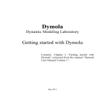
Support for optional FMI Export options in FMI 2.0
The following tables list Dymola support for optional export options in FMI 2.0. Since both
“True” and “False” can be a limitation, the cells are color coded: green means “underlying
feature supported in Dymola”, yellow means “underlying feature not supported in Dymola”.
Furthermore, capital letters are used for “underlying feature supported”.
The order of the features is the order they appear in the specification.
Optional FMI 2.0 features
Model
Exchange
Model
Exchange
with inline
integration
Cosimulation
using
Cvode
Cosimulaton
with inline
integration
Cosimulation
using
Dymola
solvers
needsExecutionTool
FALSE
FALSE
FALSE
FALSE
FALSE
completedIntegratorStepNotNeeded
false
false
NA
NA
NA
canBeInstantiatedOnlyOncePerProcess
true
true
true
true
true
canNotUseMemoryManagementFunctions
FALSE
FALSE
FALSE
FALSE
true
canGetAndSetFMUState
TRUE
TRUE
TRUE
TRUE
false
canSerializeFMUState
false
false
false
false
false
providesDirectionalDerivative
TRUE
TRUE
TRUE
TRUE
false
canHandleVariableCommunicationStepSize
NA
NA
TRUE
false
TRUE
canInterpolateInputs
NA
NA
TRUE
false
false
maxOutputDerivativeOrder
NA
NA
1
0
0
canRunAsynchronuously
NA
NA
false
false
false
Dymola 2015 FD01 Release Notes
39
Support for Dymola license options and FMI Export options in FMI 1.0
Support for Dymola license options in FMI 1.0
The following export options are supported:
Export options
Model Exchange
Co-simulation using
Cvode
Co-simulation using
Dymola solvers
Binary Export
Yes
Yes
Yes
Source code export
Yes
Yes
No
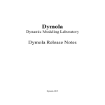
Support for optional FMI Export options in FMI 1.0
The following tables list Dymola support for optional export options in FMI 1.0. Since both
“Yes” and “No” can be a limitation, the cells are color coded: green means “underlying
feature supported in Dymola”, yellow means “underlying feature not supported in Dymola”.
Furthermore, capital letters are used for “underlying feature supported”.
The order of the features is the order they appear in the specification.
40
Optional FMI 1.0 Co-simulation features
Cosimulation
using
Cvode
Cosimulation
with inline
integration
Cosimulation
using
Dymola
solvers
canHandleVariableCommunicationStepSize
YES
false
YES
canHandleEvents
YES
YES
YES
canRejectSteps
false
false
false
canInterpolateInputs
YES
false
false
maxOutputDerivativeOrder
1
0
0
canRunAsynchronuously
false
false
false
canSignalEvents
false
false
false
canBeInstantiatedOnlyOncePerProcess
true
true
true
canNotUseMemoryManagementFunctions
FALSE
FALSE
true
Improved import of FMUs with many inputs/outputs
The import of FMUs with many inputs/outputs has been further improved; now the
connectors of the same parent component are automatically stacked when imported, if there
are 10 (default) or more connectors.
This number can be changed by changing the value of the flag
Advanced.FMI.OverlappingIOThreshold
The default value of the flag is 10.
The connection of stacked connectors has also been improved, see section “Extended
connection dialog” on page 9.
64-bit export/import of FMUs on Linux
Dymola 2015 FD01 supports 64-bit export and import of FMUs on Linux.
Note that for the 64-bit version of Dymola, it is required to set the flag
Advanced.CompileWith64=2 when compiling applications (dymosim.exe) that contains
imported 64-bit FMUs.
Importing Simulink models using FMI
The package for Simulink FMU export that can be used together with the Dymola support
for FMU import to facilitate simulation of Simulink models in Dymola only supports FMI
version 1.0.
The package does currently not support FMI version 2.0, and the package may be removed
in some future version of Dymola.
3.6
Updated libraries
Below is a short description of updated libraries. For a full description, please refer to the
libraries documentation.
3.6.1 Air Conditioning Library
A new version 1.9 of the Air Conditioning Library is available. Some improvements:
• Improved robustness for the refrigerant CO2 (R744) at the critical point.
• A refrigerant flow source (Reservoirs.FlowSourceCharge) is introduced as an optional
component in the liquid receiver model. This makes it more convenient to reach
steady-state operating points in charge experiments, since the additional refrigerant is
usually stored there and does not have to travel through the system.
• Chens correlation for evaporative heat transfer is added. It is not dependent on the heat
flux and therefore avoids this iterative loop in the non-linear equation systems. On the
other hand it is known to be a little less accurate than other correlations
Dymola 2015 FD01 Release Notes
41
•
•
The parameter p_ambient, which is used in all air models, is propagated to the top
level of all heat exchangers. For numerical and efficiency reason this property is
constant and not the time-varying downstream pressure. Making this parameter
available at the component tops level makes it easier to simulate pressure levels
different to the atmospheric pressure. The default behavior of the models is not
influenced by this change.
Stability state as advanced feature included in refrigerant channel models. The variable
twoPhaseFraction, which describes the fraction of a volume covered by two-phase
fluid, is turned into an additional state with an artificial delay. This can in some cases
avoid oscillations, which may occur for the hard-coupled dependency of the heat
transfer coefficient on the amount of evaporated or condensed refrigerant in the
volume. Note that activating this advanced feature may change the overall dynamic
behavior of the component. The default behavior of the affected components is not
influenced.
A conversion script is necessary (opens automatically) for used evaporation heat transfer
correlations, see note below.
3.6.2 DataFiles Library
A minor version 1.0.2 has been released.
3.6.3 Dymola Commands Library
A major version 1.1 has been released. For changes and improvements, see section “The
library DymolaCommands reviewed and updated, and automatically opened” starting on
page 21.
3.6.4 Electric Power Library
Version 2.2 of Electric Power library contains a number of improvements. Some examples:
TurboGroups package replaces Mechanics package
The package Mechanics has been replaced with a TurboGroups package. The reason for the
new package is that the Mechanics package was dedicated to construction of turbo groups
(turbines including a generator rotor) The Turbo groups are however used in all 3-phase
representations. This change should motivate the user to use dedicated mechanic libraries
for mechanics modeling.
The new TurboGroups package has the following structure:
• Actuators: Components used in experiments, e.g. tabular torque sources. No
equivalents are available in MSL (Modelica Standard Library).
• Gears: The gear components are of a specialized type, and cannot be replaced by the
MSL gear components.
• Shafts:
o ShaftNoMass is modelled as a spring, it now extends its MSL
equivalent Modelica.Mechanics.Rotational.Components.Spring.
42
Shaft is modeled as an inertia connected to a spring. It is built up using
MSL components.
Rotors: Two rotor types are available, one corresponding to an inertia, and one
including connectors to generator rotor, stator and friction.
Examples: Examples of turbo groups. Data records are included in the package.
o
•
•
Components that had equivalent components in Modelica Standard Library have been
replaced with those MSL components.
Flanges are named according to the standard in Modelica Standard Library.
The Mechanics.Translation package is now obsolete and will be removed in next release.
Enumerations extensively applied
The old integer versions of SourceType, IniType etc., have been replaced by enumerations.
A conversion script is needed for conversion.
3.6.5 Engine Dynamics Library
Version 1.2.2 is a minor update of the Engine Dynamics Library. Examples of
improvements:
• The simplified heat exchanger components based on efficiency (table based and epsNTU models) have been improved in that the maximum transferable heat is now
correctly computed from the enthalpy difference and flow rates of both sides.
Previously this assumed uniform specific heat capacity which in rare cases could result
in non-physical solutions.
• All user calibration factors for heat transfer and pressure drop has been converted from
parameters to inputs. Users may still assign them with fixed values in the parameter
dialog, but can now also use variable expressions to define calibration factors.
• Improved flexibility of discretized pipe models. The component can now be
configured to expose a flow or control volume behavior at the component boundaries.
Automatic conversion from Engine Dynamics library 1.2.1 is supported using the included
conversion script.
3.6.6 Fuel Cell Library
Version 1.3 is a major update of the Fuel Cell Library with new manifold structure for
modeling of complex stack configurations and new system example. In addition,
improvements of simulation speed and documentation has been made.
Major improvements:
• New manifold structure with support for both external and internal manifolds.
Predefined manifolds with inlet/outlet at the top, bottom or in the middle of the stack.
• Updated FullStack template to make use of the new manifold structure. The manifold
structure allows for modeling of different flow configurations: U-flow, Z-flow, Midflow, equally distributed flows or combinations.
Dymola 2015 FD01 Release Notes
43
•
•
•
•
•
•
•
•
Support for both co-flow and counter flow in FullStack template
Support for stack insulation in FullStack template
New example: SOFC system with energy recovery (micro-gas turbine)
SOFC system examples now use FastMedia with linear cp instead of NASA media to
avoid nonlinear systems of equations and improve simulation speed.
Added new predefined media: steam (H2O) hydrogen mixture both as ideal gas (in
NASA and Fast representation) and as ideal gas with condensated mass fraction of
water.
Added pump model
Removed SimpleManifold as a consequence of the new manifold structure. Replaced
by the new external manifold.
Added parameter frictionDistribution to ReactionChannel. The option can be used to
control the type of model exposed in the fluid connector and facilitates creation of
numerically sound system models with alternating control volume and flow resistance
models.
3.6.7 Heat Exchanger Library
The Heat Exchanger library version 1.2 includes a number of new features and
improvements.
New features
• Added support for moist air and condensation on the ambient side of the heat
exchanger
• Added an optional, more detailed representation of the air side pressure drop and heat
transfer. This option is selectable from the heat exchanger parameter dialog, and is
optimized for simulation of stand-alone heat exchangers with high resolution gridded
boundary conditions. The original implementation is also available and is
recommended for use in heat exchanger stack models.
• Added the possibility of computing the total internal liquid or working fluid volume
and mass. When included in a system model based on the Liquid Cooling Library or
Vapor Cycle Library, the total properties will be computed for the whole system
including the heat exchanger.
Examples of improvements
• All user calibration factors for heat transfer and pressure drop has been converted from
parameters to inputs. Users may still assign them with fixed values in the parameter
dialog, but can now also use variable expressions to define calibration factors.
• Improved in library documentation.
Automatic conversion of user libraries is supported using the included conversion script.
44
3.6.8 Hydraulics Library
Hydraulics 4.1 is a major release with the following enhancements compared to 4.0.
Examples of enhancements and improvements:
• The documentation is now improved throughout the library.
o The information section (Hydraulics.Information) has been updated.
o Each main-component have detailed documentation of usage,
assumptions and extending classes.
o The information section for the templates (see e.g. Templates.TwoPort),
displays what kind of equations that has to added to classes using this
template.
• The package structure is improved throughout the library. Examples:
o A separate icons package (Utilities.Icons) is created with the most
common Hydraulics Library Icons.
o Mechanical components and actuators are now located in the
Utilities.Mechanics.
o The Visualizer package is located in Utilities.Visualizers.
o Many of the component and example names were abbreviations. Most
of the names are now changed to the full name.
o Many components were old and deprecated. They are now placed in the
package Utilities.Deprecated and will be removed after a year from the
release when they were put in the deprecated package. These
components are marked with a red cross and if they are used, a warning
message will appear in the message log. If the user wants to keep using
the component, it has to be copied to the local library. But they will no
longer be supported by Modelon.
o Basic components now have a different look. A grey thick dashed line is
placed around the components, to easily identify basic components.
o Pump and motor components are now merged and put into a new
package: RotatyActuators.
o The new component RotaryActuator represents the following pump
components: SimplePump, VariablePump, TabularPump and
PumpWithLoss the following motor components: SimpleMotor and
VariableMotor.
o The Sources package is now cleaned up and some components are
merged.
• A few new components, examples and features have been added to the library.
o An example visualizing usage of a Modelon Base Library (MBL) Heat
Exchanger, see Examples.ThermoHydraulicsGuide.HXTableEfficiency.
This
is
possible
using
the
new
adaptor
component
Interfaces.ThermoFluidAdaptor.
o An example visualizing temperature rise in a closed system due to pump
losses, see Examples.ThermoHydraulicsGuide.ClosedPumpCircuit.
Dymola 2015 FD01 Release Notes
45
o
o
o
o
o
All two-port components with volumes now have conditional
conductance if using thermal hydraulics.
The
component
Valves.SpoolValve
and
RotaryActuators.CentrifugalPump now also exists as a main component
and not just as a basic equivalent.
Excavator and LoadSensingControlSystem are cleaned up and now
easier to overview.
The tabular oil has different extrapolation options, for instance "hold
last point" and "extrapolate linearly between two last points".
Aggregated mass and volume are now calculated within the oil
component. Using the parameter "include_in_aggregate", the user can
simply include or exclude a volume or chamber from the aggregated
mass/volume.
Conversion scripts will only support conversion from the previous release to the current
release. Note that the conversion script cannot handle some of the bug fixes. See the release
notes in the library for more information.
3.6.9 Hydro Power Library
A minor release 2.4.1 is available. The focus is on improving the Modelica compliance and
remove tool dependent implementations. As an example, all models now pass Dymola 2015
FD01 Modelica Pedantic check.
Models using Hydro Power version 2.4 will automatically be converted to version 2.4.1
when loaded into Dymola.
3.6.10
Liquid Cooling Library
Liquid Cooling library version 1.3 contains a number of new features and improvements.
New features
• New component models with geometry based pressure drop correlations.
• Added heat exchanger stack templates with 7 and 8 included heat exchangers.
Example of Improvements
• The simplified heat exchanger components based on efficiency (table based and epsNTU models) have been improved in that the maximum transferable heat is now
correctly computed from the enthalpy difference and flow rates of both sides.
Previously this assumed uniform specific heat capacity which in rare cases could result
in non-physical solutions.
• All user calibration factors for heat transfer and pressure drop has been converted from
parameters to inputs. Users may still assign them with fixed values in the parameter
dialog, but can now also use variable expressions to define calibration factors.
• Improved flexibility of discretized pipe models. The component can now be
configured to expose a flow or control volume behavior at the component boundaries.
46
•
•
Table based heat exchangers can now be configured to use table data from file directly
from the parameter dialog.
The aggregate volume base classes have been moved to the Modelon Base Library to
allow computation of total liquid volume when the system includes components from
other libraries.
Automatic conversion of user libraries is supported using the included conversion script.
3.6.11
Model Management Library
A minor release 1.1.3 of the Model Management library is now available.
3.6.12
Modelica_LinearSystems2 Library
A minor release 2.3.2 of the Modelica_LinearSystems2 library is now available.
3.6.13
Pneumatics Library
A new version 1.6.3 of the Pneumatics library is now available. Examples of improvements:
• The packages throughout the library are rearranged and restructured. Some packages
are located inside Utilities and some top level packages are separated into two.
• The library has a new top level icon.
• Environment now have a new icon, displaying both pressure and temperature.
• Aggregated mass and volume are now calculated within the environment component.
Using the parameter "include_in_aggregate", the user can simply include or exclude a
volume or chamber from the aggregated mass/volume.
• Some components were old and deprecated. They are now placed in the package
Utilities.Deprecated and will be removed after a year from the release when they were
put in the deprecated package. These components are marked with a red cross and if
they are used, a warning message will appear in the message log. If the user wants to
keep using the component, it has to be copied to the local library. But they will no
longer be supported by Modelon.
3.6.14
PowerTrain Library
The version 2.3.0 of Power Train has been released; in this version heat ports are used in all
electric drives and all shafts.
The version 2.3.0 is backward compatible to all 2.x.y versions.
3.6.15
Thermal Power Library
Thermal Power version 1.9 is a major release with a number of additions and improvements.
Some examples:
• New system component System_TPL. It's used to set global system settings such as
T_ambient. It also automatically sums up volumes, energy and mass in
twophaseMedia components and energy and mass in wall models.
Dymola 2015 FD01 Release Notes
47
•
•
•
•
•
•
New pre heater model, ThermalPower.TwoPhase.Condensers.Condenser_3_zones.
The 3-zones make it possible to simulate sub-cool and super-heat effects.
New parameter in Benson separator that specifies the outlet vapor quality.
Fixed mass conservation in ThermalPower.TwoPhase.FlowChannels.Pipe_lumpedP
(valid for positive flow), the conservation laws were not fulfilled during transients.
Note that there might be a minor difference in dynamics compared to result using
older versions.
More efficient implementation of two-phase lumped pipe, better simulation
performance.
More efficient implementation of gas lumped pipe, better simulation performance.
Improved Modelica compliance.
Models using Thermal Power version 1.8 will automatically be converted to version 1.9
when loaded in Dymola.
3.6.16
Vapor Cycle Library
A new version 1.2 of the Vapor Cycle Library is available.
New features
• A static reversible valve, which can be used in architectures that change operation
mode.
• A turbine model parametrized with a mass flow lookup table and an efficiency look up
table.
• A compressor model with a parametrisation suitable for dynamic compressors. It is
parametrised with an isentropic efficiency table and a mass flow table.
• An ORC example experiment has been added to the library
• A bend component has been added to the library.
• A counterflow internal heat exchanger has been added to the library.
• Visualizers for all working fluids have been added to the library.
• The library contains a new User's Guide and two Tutorials.
Examples of improvements
• Turbine or the compressor face correct inlet density also for two-phase inlet now. The
default characteristics however do not take into account performance deterioration
because of liquid at the inlet.
• All heat transfer correlations and pressure drop correlations for pipes have been moved
in order to improve user friendliness when working with a combination of different
Modelon libraries. Their description and information is updated. Running the included
conversion script is necessary for this update.
• The default two phase medium model has been changed from R134a, reference
properties by Tillner-Roth to R134a, short form Helmholtz EOS by Span. Its accuracy
is slightly lower but still more than sufficient for most applications. The simulation
speed is increased significantly with the simpler model.
48
•
•
•
•
Both the receiver and accumulator can be initialized using a liquid level.
Adding specific interfaces to the heat exchanger models increased replaceability and
reusability of the models in a system context.
The default air model is replaced with one, which is better suited for challenging
steady-state initialization. Basically the same assumptions apply except that the new
model neglects the liquid volume in case liquid water droplets are transported by the
air stream and assumes that they do not influence the specific heat capacity. The
previously used model can still be selected from a drop-down list.
The medium model for CO2 has an improved robustness around the critical point.
Existing models can be converted to this version using the supplied conversion script.
3.6.17
Vehicle Dynamics Library
A new version 2.0 of the Vehicle Dynamics Library is available.
New features
Pacejka '94 Tire Contact Force Model
Support for the Pacejka '94 'Magic Formula' contact force model has been added. The
Pacejka '94 contact force model provides the benefit that it requires fewer coefficients than
newer models; is more commonly used than the Pacejka '02 model; and is used in many
other vehicle dynamics software products. By supporting this contact force model natively
in VDL, the Pacejka '94 tire coefficients can be shared between VDL and other simulation
tools.
Suspension Wheel Test Rig
A new live tire suspension test rig has been added that allows the application of external
forces and torques at either the contact patch or wheel center/hub. In physical kinematics
and compliance tests, it is quite common to have a wheel and tire mounted on the
suspension. It is the intent of this new rig to be able to better mimic the actual physical tests.
Dymola 2015 FD01 Release Notes
49
Example suspension experiments using this new rig can be found in: Examples.WheelRig.
Chassis Kinematics & Compliance Experiments
Two new chassis-level kinematics and compliance experiments have been added:
FourPostNoWheels & KinematicsCompliance. These rigs not only allow vertical excitation
of the chassis, they also allow the application of external forces and torques at either the
contact patch or wheel center/hub.
Ground Proximity Sensors
Ground proximity information is commonly required in vehicle dynamics simulations. Most
commonly, this information is used in the contact calculations for wheels. Other
applications include ride heights for aerodynamics calculations and ground impacts. Three
new sensors have been added to report the proximity of a frame to ground:
50
•
•
•
ClosestPoint - outputs the closest point located on the ground surface to the sensor
ClosestPointInPlane - outputs a point located on the ground surface at the point of
intersection of a plane and ground
IntersectionAlongLine - outputs a point located on the ground surface at the point of
intersection of a line and ground
Existing ground sensors that were previously located in Chassis.Sensors have been moved
to Ground.Sensors. This includes the following sensors:
• FrameInPlaneThreePoints
• FrameOnGround
• GroundCurvature
• GroundHeight
• VelocityOfGround
Ride Height Dependent Aerodynamics Models
Four new aerodynamics models have been added that are dependent on front/rear ride
heights. The different models demonstrate how to represent lift/drag/side aerodynamic
forces using either a polynomial or tabular data:
• PitchPolynomialLD
• PitchPolynomialLDS
• PitchTabularLD
• PitchTabularLDS
Some models will automatically be converted from version 1.9 to version 2.0 when loaded.
3.7
Documentation
In the software distribution of Dymola 2015 FD01 Dymola User Manuals of version
“September 2014” will be present; these manuals include all relevant features/improvements
of Dymola 2015 FD01 presented in the Release notes.
Dymola 2015 FD01 Release Notes
51
3.8
Appendix – Installation: Hardware and Software
Requirements
Below the current hardware and software requirements for Dymola 2015 FD01 are listed.
3.8.1 Hardware requirements/recommendations
Hardware requirements
• At least 1 GB RAM
• At least 400 MB disc space
Hardware recommendations
At present, it is recommended to have a system with an Intel Core 2 Duo processor or better,
with at least 2 MB of L2 cache. Memory speed and cache size are key parameters to achieve
maximum simulation performance.
A dual processor will be enough if not using multi-core support; the simulation itself, by
default, uses only one execution thread so there is no need for a “quad” processor. If using
multi-core support, you might want to use more processors/cores.
Memory size may be significant for translating big models and plotting large result files, but
the simulation itself does not require so much memory. Recommended memory size is 2-4
GB of RAM for 32-bit architecture and 3-6 GB of RAM for 64-bit architecture.
3.8.2 Software requirements
Microsoft Windows
Dymola versions on Windows and Windows operating systems versions
Dymola 2015 FD01 is supported, as 32- and 64-bit application, on Microsoft Windows 7
and Windows 8.1. Since Dymola does not use any features supported only by specific
editions of Windows (“Home”, “Professional”, “Enterprise” etc.), all such editions are
supported if the main version is supported.
For users of Windows XP and Windows Vista, specific conditions apply. Please see section
“Support for Windows XP and Windows Vista” on page 26.
Compilers
Please note that for the Windows platform, a Microsoft C/C++ compiler, or a GCC
compiler, must be installed separately. The following compilers are supported for Dymola
2015 FD01 on Windows:
Microsoft C/C++ compilers, free editions:
• Visual Studio 2008 Express Edition (9.0)
52
•
•
•
Visual C++ 2010 Express (10.0)
Visual Studio 2012 Express Edition (11.0)
Visual Studio 2013 Express Edition (12.0)
Microsoft C/C++ compilers, professional editions:
• Visual Studio 2005 (8.0)
• Visual Studio 2008 (9.0)
• Visual Studio 2010 (10.0)
• Visual Studio 2012 (11.0)
• Visual Studio 2013 (12.0)
GCC compilers
Dymola 2015 FD01 has limited support for the MinGW GCC compiler, with a GCC version
compatible with 4.8. Note the present limitations, and a demand for an add-on, refer to
section “GCC” on page 5.
Dymola license server
For a Dymola license server on Windows, all files needed to set up and run a Dymola
license server on Windows, except the license file, are available in the Dymola distribution.
(This includes also the license daemon, where Dymola presently supports FLEXnet
Publisher version 11.11. This version is part of the Dymola distribution.)
Linux
Supported Linux versions and compilers
Dymola 2015 FD01 runs on SUSE Linux (Release 11), 32-bit and 64-bit, with gcc version
4.3.4, and compatible systems. In addition to gcc, the model C code generated by Dymola
can also be compiled by clang. To change compiler, change the variable CC in
/opt/dymola-<version>-<architecture>/insert/dsbuild.sh,
where
<architecture> is i586 for 32-bit application, and x86_64 for 64-bit application. As
an example, for a 64-bit Dymola 2015 FD01 application:
/opt/dymola-2015FD01-x86_64/insert/dsbuild.sh
Dymola 2015 FD01 is supported as a 32-bit and 64-bit application on Linux.
Notes
• For rendering of jpg files, libjpg62 must be installed.
• 32-bit compilation might require explicit installation of 32-bit libc. E.g. on Ubuntu:
sudo apt-get install g++-multilib libc6-dev-386
Note on Optimization library
Please note that you have to use the Optimization library version 2.x or higher to use multicriteria design optimization on Linux; the older Design.Optimization package does not
support multi-criteria design optimization on Linux.
Dymola 2015 FD01 Release Notes
53
Dymola license server
For a Dymola license server on Linux, all files needed to set up and run a Dymola license
server on Linux, except the license file, are available in the Dymola distribution. (This also
includes the license daemon, where Dymola presently supports FLEXnet Publisher version
11.11.)
54