Download Casio fx-5800P User`s guide

100

101

102

103

104

105

106

107

108

109

110

111

112

113

114

115

116

117

118

119

120

121

122

123

124

125

126

127

128

129

130

131

132

133

134

135

136

137

138

139

140

141

142

143

144

145

146

147

Transcript

E
fx-5800P
User's Guide
http://world.casio.com/edu/
RJA516644-001V01
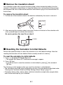
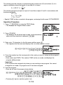
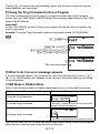
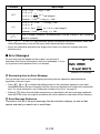
k Remove the insulation sheet!
Your calculator comes with a special insulation sheet, which isolates the battery from the
contacts in the battery compartment, to keep the battery from running down during storage
and shipment. Be sure to remove the insulation sheet before trying to use the calculator for
the ﬁrst time.
To remove the insulation sheet
1. Pull the tab of the insulation sheet in the direction indicated by the arrow to remove it.
Pull to remove
引き抜いてください
2. After removing the insulation sheet, press the P button on the back of the calculator with
a thin, pointed object to initialize the calculator.
Be sure to perform this step! Do not skip it!
P
P button
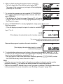
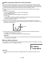
k Resetting the Calculator to Initial Defaults
Perform the operation below to return the calculator to its initial default settings. Note that
resetting the calculator will also delete all data currently stored in its memory.
To reset the calculator to initial defaults
1. Press Nc3(SYSTEM)3(Reset All).
• This causes the “Reset All?” conﬁrmation message to appear.
2. Press E(Yes).
• If you do not want to reset the calculator to initial defaults, press J(No) instead of
E(Yes).
The following is what happens when you reset the calculator to initial defaults.
• The calculation mode and setup conﬁguration return to the initial defaults described under
“Clearing the Calculation Mode and Setup Settings (Reset Setup)” (page 13).
• Calculation history data, memory data, statistical calculation sample data, program data,
and all other data input by you is deleted.
E-1
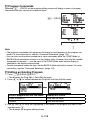
k About this Manual
• Most of the keys perform multiple functions. Pressing 1 or S and then another key
will perform the alternate function of the other key. Alternate functions are marked above
the keycap.
Alternate function
sin–1{D}
Keycap function
s
Alternate function operations are notated in this manual as shown below.
–1
Example: 1s(sin )1E
The notation in parentheses indicates the function executed by the preceding key
operation.
• The following shows the notation used in the manual for menu items that appear on the
display.
Example: z – {PROG} – {/}
The notation in braces ({ }) indicates the menu item being selected.
• The following shows the notation used in the manual for menu items that appear on the
display (which are executed by pressing a number key).
Example: z – {MATH}1(∫dX)
The notation in parentheses indicates the menu item accessed by the preceding number
key.
• The displays and illustrations (such as key markings) shown in this User’s Guide are for
illustrative purposes only, and may differ somewhat from the actual items they represent.
• The contents of this manual are subject to change without notice.
• In no event shall CASIO Computer Co., Ltd. be liable to anyone for special, collateral,
incidental, or consequential damages in connection with or arising out of the purchase or
use of this product and items that come with it. Moreover, CASIO Computer Co., Ltd. shall
not be liable for any claim of any kind whatsoever by any other party arising out of the use
of this product and the items that come with it.
• Company and product names used in this manual may be registered trademarks or
trademarks of their respective owners.
k Symbols Used in Examples
Various symbols are used in the examples of this manual to alert you to settings that need
to be conﬁgured in order to perform the example operation correctly.
• A mark like the ones shown below indicates that you need to change the calculator’s
display format setting.
If you see this:
B
Change the display
format setting to:
If you see this:
b
Natural Display
Change the display
format setting to:
Linear Display
For details, see “Selecting the Display Format (MthIO, LineIO)” (page 11).
E-2
• A mark like the ones shown below indicates that you need to change the calculator’s
angle unit setting.
If you see this:
v
Change the angle unit
setting to:
If you see this:
V
Deg
Change the angle unit
setting to:
Rad
For details, see “Specifying the Angle Unit” (page 12).
Safety Precautions
Be sure to read the following safety precautions before using this calculator. Be sure to keep
all user documentation handy for future reference.
Caution
This symbol is used to indicate information that can result in personal injury or material
damage if ignored.
Battery
• After removing the battery from the calculator, put it in a safe place where it will not
get into the hands of small children and accidentally swallowed.
• Keep batteries out of the reach of small children. If accidentally swallowed, consult
with a physician immediately.
• Never charge the battery, try to take the battery apart, or allow the battery to become
shorted. Never expose the battery to direct heat or dispose of it by incineration.
• Improperly using a battery can cause it to leak and damage nearby items, and can
create the risk of ﬁre and personal injury.
• Always make sure that the battery’s positive k and negative l ends are facing
correctly when you load it into the calculator.
• Remove the battery if you do not plan to use the calculator for a long time.
• Use only the type of battery speciﬁed for this calculator in this manual.
Disposing of the Calculator
• Never dispose of the calculator by burning it. Doing so can cause certain components
to suddenly burst, creating the risk of ﬁre and personal injury.
E-3
Operating Precautions
• Be sure to press the P button on the back of the calculator before using the
calculator for the ﬁrst time. See page 1 for information about the P button.
• Even if the calculator is operating normally, replace the battery at least once a year.
A dead battery can leak, causing damage to and malfunction of the calculator. Never
leave a dead battery in the calculator.
• The battery that comes with this unit discharges slightly during shipment and
storage. Because of this, it may require replacement sooner than the normal
expected battery life.
• Do not use an oxyride battery or any other type of nickel-based primary battery with
this product. Incompatibility between such batteries and product speciﬁcations can
result in shorter battery life and product malfunction.
• Low battery power can cause memory contents to become corrupted or lost
completely. Always keep written records of all important data.
• Avoid use and storage of the calculator in areas subjected to temperature extremes.
Very low temperatures can cause slow display response, total failure of the display,
and shortening of battery life. Also avoid leaving the calculator in direct sunlight, near a
window, near a heater or anywhere else it might be exposed to very high temperatures.
Heat can cause discoloration or deformation of the calculator’s case, and damage to
internal circuitry.
• Avoid use and storage of the calculator in areas subjected to large amounts of
humidity and dust.
Take care never to leave the calculator where it might be splashed by water or exposed to
large amounts of humidity or dust. Such conditions can damage internal circuitry.
• Never drop the calculator or otherwise subject it to strong impact.
• Never twist or bend the calculator.
Avoid carrying the calculator in the pocket of your trousers or other tight-ﬁtting clothing
where it might be subjected to twisting or bending.
• Never try to take the calculator apart.
• Never press the keys of the calculator with a ballpoint pen or other pointed object.
• Use a soft, dry cloth to clean the exterior of the calculator.
If the calculator becomes very dirty, wipe it off with a cloth moistened in a weak solution
of water and a mild neutral household detergent. Wring out all excess liquid before wiping
the calculator. Never use thinner, benzene or other volatile agents to clean the calculator.
Doing so can remove printed markings and can damage the case.
E-4
Contents
Remove the insulation sheet! ............................................................................................. 1
Resetting the Calculator to Initial Defaults.......................................................................... 1
About this Manual............................................................................................................... 2
Symbols Used in Examples................................................................................................ 2
Safety Precautions ...................................................................................3
Operating Precautions .............................................................................4
Before starting a calculation... ...............................................................9
Turning On the Calculator................................................................................................... 9
Key Markings ...................................................................................................................... 9
Reading the Display ........................................................................................................... 9
Calculation Modes and Setup ...............................................................10
Selecting a Calculation Mode ........................................................................................... 10
Calculator Setup ............................................................................................................... 11
Clearing the Calculation Mode and Setup Settings (Reset Setup)................................... 13
Using the Function Menu.......................................................................14
Inputting Calculation Expressions and Values ....................................14
Inputting a Calculation Expression (Natural Input) ........................................................... 14
Using Natural Display ....................................................................................................... 16
Editing a Calculation......................................................................................................... 19
Finding the Location of an Error ....................................................................................... 21
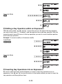
Displaying Decimal Results while Natural Display is Selected
as the Display Format ............................................................................21
Example Calculations ....................................................................................................... 22
Using the f Key (S-D Transformation) ............................................... 22
Examples of S-D Transformation ...................................................................................... 22
Basic Calculations..................................................................................23
Arithmetic Calculations ..................................................................................................... 23
Fractions ........................................................................................................................... 24
Percent Calculations......................................................................................................... 26
Degree, Minute, Second (Sexagesimal) Calculations ...................................................... 27
Calculation History and Replay.............................................................28
Accessing Calculation History .......................................................................................... 29
Using Replay .................................................................................................................... 29
Using Multi-statements in Calculations ...............................................30
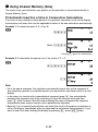
Calculator Memory Operations .............................................................31
Using Answer Memory (Ans) ............................................................................................ 32
Using Independent Memory ............................................................................................. 33
Using Variables ................................................................................................................ 34
Clearing All Memory Contents ......................................................................................... 35
E-5
Reserving Variable Memory ...................................................................35
User Memory Area ........................................................................................................... 35
Using Extra Variables ....................................................................................................... 36
Using π and Scientiﬁc Constants..........................................................37
Pi (π) ................................................................................................................................. 37
Scientiﬁc Constants .......................................................................................................... 38
Scientiﬁc Function Calculations ...........................................................40
Trigonometric and Inverse Trigonometric Functions ......................................................... 40
Angle Unit Conversion ...................................................................................................... 41
Hyperbolic and Inverse Hyperbolic Functions .................................................................. 41
Exponential and Logarithmic Functions ........................................................................... 41
Power Functions and Power Root Functions .................................................................... 42
Integration Calculation ...................................................................................................... 43
Derivative.......................................................................................................................... 45
Second Derivative ............................................................................................................ 46
Σ Calculation .................................................................................................................... 46
Coordinate Conversion (Rectangular ↔ Polar) ................................................................ 47
Random Number Functions ............................................................................................. 49
Other Functions ................................................................................................................ 50
Using Engineering Notation ..................................................................53
3
Using 10 Engineering Notation (ENG) ............................................................................ 53
ENG Conversion Examples .............................................................................................. 54
Using Engineering Symbols ............................................................................................. 54
Complex Number Calculations (COMP) ...............................................55
Inputting Complex Numbers ............................................................................................. 55
Complex Number Display Setting..................................................................................... 56
Complex Number Calculation Result Display Examples .................................................. 56
Conjugate Complex Number (Conjg) ............................................................................... 57
Absolute Value and Argument (Abs, Arg) ......................................................................... 57
Extracting the Real Part (ReP) and Imaginary Part (ImP) of a Complex Number ............ 58
Overriding the Default Complex Number Display Format................................................. 58
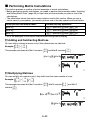
Matrix Calculations (COMP) ..................................................................59
Matrix Calculation Overview ............................................................................................. 59
About the Mat Ans Screen ............................................................................................... 59
Inputting and Editing Matrix Data ..................................................................................... 59
Performing Matrix Calculations......................................................................................... 62
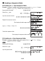
Sequence Calculations (RECUR) ..........................................................65
Sequence Calculation Overview ...................................................................................... 65
Creating a Sequence Table .............................................................................................. 68
Sequence Calculation Precautions .................................................................................. 69
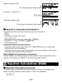
Equation Calculations (EQN).................................................................69
Equation Calculation Overview ........................................................................................ 69
Selecting an Equation Type .............................................................................................. 71
Inputting Values for Coefﬁcients ....................................................................................... 71
E-6
Viewing Equation Solutions .............................................................................................. 72
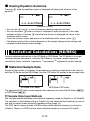
Statistical Calculations (SD/REG) .........................................................72
Statistical Sample Data .................................................................................................... 72
Performing Single-variable Statistical Calculations .......................................................... 75
Performing Paired-variable Statistical Calculations .......................................................... 77
Statistical Calculation Examples ...................................................................................... 84
Base-n Calculations (BASE-N) ..............................................................86
Performing Base-n Calculations ....................................................................................... 86
Converting a Displayed Result to another Number Base ................................................. 87
Specifying a Number Base for a Particular Value ............................................................. 88
Performing Calculations Using Logical Operations and Negative Binary Values ............. 89
CALC........................................................................................................90
Using CALC...................................................................................................................... 90
SOLVE ......................................................................................................92
Expressions Supported by SOLVE ................................................................................... 92
Using SOLVE.................................................................................................................... 92
Creating a Number Table from a Function (TABLE) ............................94
TABLE Mode Overview..................................................................................................... 94
Creating a Number Table .................................................................................................. 96
Number Table Creation Precautions ................................................................................. 97
Built-in Formulas ....................................................................................97
Using Built-in Formulas .................................................................................................... 97
Built-in Formula Names .................................................................................................... 99
User Formulas ................................................................................................................ 102
Program Mode (PROG).........................................................................104
Program Mode Overview ................................................................................................ 105
Creating a Program ........................................................................................................ 105
Running a Program ........................................................................................................ 109
File Screen Operations ................................................................................................... 111
Deleting a Program......................................................................................................... 112
Command Reference............................................................................113
Program Commands ...................................................................................................... 113
Statistical Calculation Commands .................................................................................. 121
Other PROG Mode Commands...................................................................................... 122
Data Communication (LINK) ................................................................124
Connecting Two fx-5800P Calculators to Each Other .................................................... 124
Transferring Data Between fx-5800P Calculators........................................................... 124
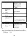
Memory Manager (MEMORY)...............................................................126
Deletable Data Types and Supported Delete Operations ............................................... 127
Using Memory Manager ................................................................................................. 127
E-7
Appendix ...............................................................................................128
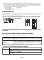
Calculation Priority Sequence ........................................................................................ 128
Stack Limitations ............................................................................................................ 130
Calculation Ranges, Number of Digits, and Precision .................................................... 130
Error Messages .............................................................................................................. 132
Before assuming malfunction of the calculator... ........................................................... 135
Lower Battery Indicator ................................................................................................. 135
Power Requirements ............................................................................136
Speciﬁcations .......................................................................................137
E-8
Before starting a calculation...
k Turning On the Calculator
Press o. This displays the same screen that was on the display when you last turned off
the calculator.
A Adjusting Display Contrast
If the ﬁgures on the display become hard to read, try adjusting display contrast.
1. Press Nc3(SYSTEM)1(Contrast).
• This displays the contrast adjustment screen.
2. Use d and e to adjust display contrast.
3. After the setting is the way you want, press J.
Note
You can also use d and e to adjust contrast while the calculation mode menu that
appears when you press the N key is on the display.
A Turning Off the Calculator
Press 1o(OFF).
k Key Markings
% BIN [
Function
Key Marking Color
To perform the function:
1
ln
2
%
Orange
Press 1 and then press the key.
3
[
Red
Press S and then press the key.
4
BIN
Green
In the BASE-N Mode, press the key.
Press the key.
k Reading the Display
A Input Expressions and Calculation Results
This calculator can display both the expressions you input and calculation results on the
same screen.
E-9
Input expression
Calculation result
A Display Symbols
The symbols described below appear on the display of the calculator to indicate the current
calculation mode, the calculator setup, the progress of calculations, and more.
The nearby sample screen shows the 7 symbol.
The 7 symbol turns on when degrees (Deg) are selected for
the default angle unit (page 12).
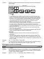
Calculation Modes and Setup
k Selecting a Calculation Mode
Your calculator has 11 “calculation modes”.
A Selecting a Calculation Mode
1. Press N.
• This displays the calculation mode menu. Use c and f to switch between menu
screen 1 and screen 2.
Screen 1
Screen 2
2. Perform one of the following operations to select the calculation mode you want.
To select this calculation mode:
Go to this screen:
And press this key:
COMP (Computation)
1(COMP)
BASE-N (Base n)
2(BASE-N)
SD (Single Variable Statistics)
3(SD)
REG (Paired Variable Statistics)
Screen 1
PROG (Programming)
4(REG)
5(PROG)
RECUR (Recursion)
6(RECUR)
TABLE (Tables)
7(TABLE)
EQN (Equations)
8(EQN)
E-10
To select this calculation mode:
Go to this screen:
And press this key:
1(LINK)
LINK (Communication)
MEMORY (Memory Management)
Screen 2
2(MEMORY)
3(SYSTEM)
SYSTEM (Contrast Adjustment, Reset)
• To exit the calculation mode menu without changing the calculation mode, press N.
k Calculator Setup
The calculator setup can be used to conﬁgure input and output settings, calculation
parameters, and other settings. The setup can be conﬁgured using setup screens, which
you access by pressing 1 N(SETUP). There are two setup screens, and you can use
f and c to navigate between them.
A Selecting the Display Format (MthIO, LineIO)
You can select either natural display (MthIO) or linear display (LineIO) for expressions you
input and for calculation results.
Natural Display (MthIO)
Natural display displays fraction, square root, derivative, integral, exponential, logarithmic,
and other mathematical expressions just as they are written. This format is applied both for
input expressions and for calculation results. When natural display is selected, the result of
a calculation is displayed using fraction, square root, or π notation whenever possible.
1
1
For example, the calculation 1 ÷ 2 produces the result , while π ÷ 3 results in
π.
2
3
Linear Display (LineIO)
With linear display, expressions and functions are input and displayed using a special format
1
deﬁned by your calculator. For example,
would be input as 1 { 2, and log24 would be
2
input as log(2,4).
When linear display is selected all calculation results, except for fractions, are displayed
using decimal values.
To select this display fomat:
Perform this key operation:
Natural Display (MthIO)
1N1(MthIO)
Linear Display (LineIO)
1N2(LineIO)
Note
For information about the input procedures when using the natural display and linear
display, see “Inputting Calculation Expressions and Values” on page 14 of this manual and
the sections of this manual that explanation of each type of calculation.
E-11
A Specifying the Angle Unit
To select this angle unit:
Perform this key operation:
Degrees
1N3(Deg)
Radians
1N4(Rad)
Grads
1N5(Gra)
(90˚ =
A Specifying the Display Digits
To specify this display digit setting:
π
radians = 100 grads)
2
Perform this key operation:
Number of Decimal Places
1N6(Fix)0(0) to 9(9)
Signiﬁcant Digits
1N7(Sci)1(1) to 9(9), 0(10)
Exponential Display Range
1N8(Norm)1(Norm1) or
2(Norm2)
The following explains how calculation results are displayed in accordance with the setting
you specify.
• From zero to nine decimal places are displayed in accordance with the number of decimal
places (Fix) you specify. Calculation results are rounded off to the speciﬁed number of
digits.
Example: 100 ÷ 7 = 14.286 (Fix = 3)
14.29 (Fix = 2)
• After you specify the number of signiﬁcant digits with Sci, calculation results are
displayed using the speciﬁed number of signiﬁcant digits and 10 to the applicable power.
Calculation results are rounded off to the speciﬁed number of digits.
–1
(Sci = 5)
Example: 1 ÷ 7 = 1.4286 × 10
–1
(Sci = 4)
1.429 × 10
• Selecting Norm1 or Norm2 causes the display to switch to exponential notation whenever
the result is within the ranges deﬁned below.
–2
10
Norm1: 10 > x, x > 10
–9
10
Norm2: 10 > x, x > 10
Example: 100 ÷ 7 = 14.28571429 (Norm1 or Norm2)
–3
(Norm1)
1 ÷ 200 = 5. × 10
0.005
(Norm2)
A Specifying the Fraction Display Format
To specify this fraction format for
display of calculation results:
Perform this key operation:
Mixed Fractions
1Nc1(ab/c)
Improper Fractions
1Nc2(d/c)
E-12
A Specifying the Engineering Symbol Setting
This setting lets you turn engineering symbols on and off. For more information, see “Using
Engineering Symbols” on page 54.
To do this:
Perform this key operation:
Turn engineering symbols on
1Nc3(ENG)1(EngOn)
Turn engineering symbols off
1Nc3(ENG)2(EngOff)
While engineering symbols are turned on (EngOn), engineering symbols are used when a
calculation result is outside of the range of 1 < x < 1000.
A Specifying the Complex Number Display Format
You can specify either rectangular coordinate format or polar coordinate format for complex
number calculation results.
To specify this complex number format
for display of calculation results:
Perform this key operation:
Rectangular Coordinates
1Nc4(COMPLX)1(a+bi)
Polar Coordinates
1Nc4(COMPLX)2(r∠Ƨ)
ENG conversion (page 53) is not possible while polar coordinate format is selected.
A Specifying the Statistical Frequency Setting
Use the key operations below to turn statistical frequency on or off during SD Mode and
REG Mode calculations (page 72).
To select this frequency setting:
Perform this key operation:
Frequency On
1Nc5(STAT)1(FreqOn)
Frequency Off
1Nc5(STAT)2(FreqOff)
A Changing the BASE-N Mode Negative Value Setting
You can use the key operations below to enable or disable use of negative values in the
BASE-N Mode.
To specify this setting:
Perform this key operation:
Negative values enabled
1Nc6(BASE-N)1(Signed)
Negative values disabled
1Nc6(BASE-N)2(Unsigned)
k Clearing the Calculation Mode and Setup Settings
(Reset Setup)
Perform the following key operation to reset the calculation mode and setup settings.
Nc3(SYSTEM)2(Reset Setup)E(Yes)
If you do not want to reset the calculator’s settings, press J(No) in place of E(Yes) in
the above operation.
E-13
Calculation Mode ..................................... COMP
Setup Settings
Display Format .................................... MthIO
Angle Unit ............................................ Deg
Exponential Display ............................. Norm1
Fraction Format .................................. d/c
Complex Number Format .................... a+bi
Engineering Symbol ............................ EngOff
Statistical Frequency ........................... FreqOff
BASE-N Negatives .............................. Signed
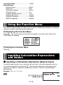
Using the Function Menu
The function menu provides you with access to various mathematical functions, commands,
constants, symbols, and other special operations.
A Displaying the Function Menu
Press z. The function menu shown below will appear if you press z while in the
COMP Mode for example.
A Exiting the Function Menu
Press J.
Inputting Calculation Expressions
and Values
k Inputting a Calculation Expression (Natural Input)
The natural input system of your calculator lets you input a calculation expression just as
it is written and execute it by pressing E. The calculator determines the proper priority
sequence for addition, subtraction, multiplication, division, fractions and parentheses
automatically.
Example: 2 (5 + 4) – 2 × (–3) =
b
2(5+4)2*-3E
E-14
A Inputting Scientiﬁc Functions with Parentheses (sin, cos, ',
etc.)
Your calculator supports input of the scientiﬁc functions with parentheses shown below.
Note that after you input the argument, you need to press ) to close the parentheses.
–1
–1
–1
–1
–1
–1
sin(, cos(, tan(, sin (, cos (, tan (, sinh(, cosh(, tanh(, sinh (, cosh (, tanh (, log(, ln(,
3
2
2
e^(, 10^(, '(, '(, Abs(, Pol(, Rec(, ∫(, d/dx(, d /dx (, Σ(, P(, Q(, R(, Arg(, Conjg(, ReP(,
ImP(, Not(, Neg(, Det(, Trn(, Rnd(, Int(, Frac(, Intg(, RanInt#(
Example: sin 30 =
b
s30)E
Note
Some functions require a different input sequence when using natural input. For more
information, see “Inputting Calculation Expressions Using Natural Display” on page 17.
A Omitting the Multiplication Sign
You can omit the multiplication sign in the following cases.
• Immediately before an open parenthesis: 2 × (5 + 4)
• Immediately before a scientiﬁc function with parentheses: 2 × sin(30), 2 × '(3)
• Before a preﬁx symbol (excluding the minus sign): 2 × h123
• Before a variable name, constant, or random number: 20 × A, 2 × π, 2 × i
A Final Closed Parenthesis
You can omit one or more closed parentheses that come at the end of a calculation,
immediately before the w key is pressed.
Example: (2 + 3) (4 − 1) = 15
b
(2+3)
(4-1E
A Calculation Expression Wrapping (Linear Display)
When using linear display, calculation expressions that are longer than 16 characters
(numbers, letters, and operators) are wrapped automatically to the next line.
Example: 123456789 + 123456789 = 246913578
b
123456789+
123456789E
E-15
A Number of Input Characters (Bytes)
As you input a mathematical expression, it is stored in memory called an “input area,”
which has a capacity of 127 bytes. This means you can input up to 127 bytes for a single
mathematical expression.
When linear display is selected as the display format, each function normally uses one or
two bytes of memory. With the natural display format, each function use four or more bytes
of memory. For more information, see “Inputting Calculation Expressions Using Natural
Display” on page 17.
Normally, the cursor that indicates the current input location on the display is either a
ﬂashing vertical bar (|) or horizontal bar ( ). When the remaining capacity of the input area
is 10 bytes or less, the cursor changes to a ﬂashing box (k).
If this happens, stop input of the current expression at some suitable location and calculate
its result.
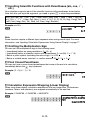
k Using Natural Display
While natural display is selected as the display format (page 11), you can input fractions
and some scientiﬁc functions just as they are written.
A Natural Display Basics
The table below lists the types of scientiﬁc functions that you can input using natural display
format.
• The *1 column shows the number of bytes of memory used up by each scientiﬁc function.
See “Number of Input Characters (Bytes)” (page 16) for more information.
• For information about the *2 column, see “Using Values and Expressions as Arguments”
(page 18).
Scientiﬁc Functions that Support Natural Display
Function
Improper Fraction
*1
*2
'
Key Operation
9
Yes
Mixed Fraction
1'(()
14
No
log(a,b)
z – {MATH}c7(logab)
7
Yes
10^x
1l($)
4
Yes
e^x
1i(%)
4
Yes
Square Root (')
!
4
Yes
Cube Root ( ')
1((#)
9
Yes
Square
x
4
No
Reciprocal
1)(x )
5
No
3
–1
Power
6
4
Yes
Power Root
16(")
9
Yes
Absolute Value (Abs)
z – {MATH}c1(Abs)
4
Yes
Integral
z – {MATH}1(∫dX)
8
Yes
E-16
Function
Key Operation
*1
*2
7
Yes
Derivative
z – {MATH}2(d/dX)
Second Derivative
z – {MATH}3(d /dX )
7
Yes
Σ Calculation
z – {MATH}4(Σ()
11
Yes
2
2
Note
If you include values or expressions in parentheses (( and )) while using natural
display, the height of the parentheses will adjust automatically depending on whether they
enclose one line or two lines. Regardless of their height, opening and closing parentheses
take up one byte of memory each.
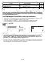
Inputting Calculation Expressions Using Natural Display
1. To input a speciﬁc function, perform the operation in the “Key Operation” column of the
“Scientiﬁc Functions that Support Natural Display” table.
2. At the input ﬁelds indicated by , input the required values and expressions.
• Use the cursor keys to move between the input ﬁelds of the expression.
1+2
Example: To input
2×3
B
Specify fraction input:
'
Input the numerator:
1+2
Move the cursor to the denominator: c
Input the denominator: 2*3
Execute the calculation: E
Important!
• Certain types of expressions can cause the height of a calculation formula to be greater
than one display line. The maximum allowable height of a calculation formula is two
display screens (31 dots × 2). Further input will become impossible if the height of the
calculation you are inputting exceeds the allowable limit.
• Nesting of functions and parentheses is allowed. Further input will become impossible if
you nest too many functions and/or parentheses. If this happens, divide the calculation
into multiple parts and calculate each part separately.
E-17
A Scrolling the Screen Left and Right
The screen will show up to 14 characters when inputting with natural display. When you
input more than 14 characters, the screen will scroll automatically. If this happens, the ]
symbol will turn on to let you know that the expression runs off the left side of the display.
B
Input expression
1111 + 2222 + 3333 + 444
Displayed expression
Cursor
• While the ] symbol is turned on, you can use the d key to move the cursor to the left
and scroll the screen.
• Scrolling to the left causes part of the expression to run off the right side of the display,
which is indicated by the ' symbol on the right. While the ' symbol is on the screen, you
can use the e key to move the cursor to the right and scroll the screen.
A Using Values and Expressions as Arguments
When inputting with natural display, in certain cases you can use a value or an expression
that is enclosed in parentheses that you have already input as the argument of a scientiﬁc
function (such as '), the numerator of a fraction, etc. For the sake of explanation here,
a natural display function that supports the use of previously input values or parenthetical
expressions is called an “insertable natural display function”.
Example: To insert the natural display function ' into the parenthetical expression in the
following calculation: 1 + (2 + 3) + 4
B
(Move the cursor immediately to the left of
the parenthetical expression.)
1Y(INS)
!
Note
• Not all natural display functions are insertable. Only the scientiﬁc functions for which
“Yes” appears in the column of the table under “Scientiﬁc Functions that Support Natural
Display” (page 16) are insertable.
• The cursor can be immediately to the left of a parenthetical expression, a numeric value,
or a fraction. Inserting an insertable function will make the parenthetical expression, value,
or fraction the argument of the inserted function.
• If the cursor is located immediately to the left of a scientiﬁc function, the entire function
becomes the argument of the inserted function.
E-18
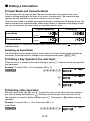
k Editing a Calculation
A Insert Mode and Overwrite Mode
The calculator has two input modes. The insert mode inserts your input at the cursor
location, shifting anything to the right of the cursor to make room. The overwrite mode
replaces the key operation at the cursor location with your input.
Only the insert mode is available when natural display is selected as the display format. You
cannot change to the overwrite mode. When linear display is selected as the display format,
you can choose either the insert mode or overwrite mode for input.
Pressing +
Original Expression
Insert Mode
Overwrite Mode
Cursor
Cursor
A vertical cursor (|) indicates the insert mode, while a horizontal cursor ( ) indicates the
overwrite mode.
Selecting an Input Mode
The initial default input mode setting is insert mode. If you have linear display selected as
the display format and want to change to the overwrite mode, press: 1Y(INS).
A Editing a Key Operation You Just Input
When the cursor is located at the end of the input, press Y to delete the last key operation
you performed.
Example: To correct 369 × 13 so it becomes 369 × 12
Bb
369*13
Y
2
A Deleting a Key Operation
With the insert mode, use d and e to move the cursor to the right of the key operation
you want to delete and then press Y. With the overwrite mode, move the cursor to the
key operation you want to delete and then press Y. Each press of Y deletes one key
operation.
Example: To correct 369 × × 12 so it becomes 369 × 12
Insert Mode
Bb
369**12
E-19
dd
Y
Overwrite Mode
b
369**12
ddd
Y
A Editing a Key Operation within an Expression
With the insert mode, use d and e to move the cursor to the right of the key operation
you want to edit, press Y to delete it, and then perform the correct key operation. With the
overwrite mode, move the cursor to the key operation you want to correct and then perform
the correct key operation.
Example: To correct cos(60) so it becomes sin(60)
Insert Mode
Bb
c60)
dddY
s
Overwrite Mode
b
c60)
dddd
s
A Inserting Key Operations into an Expression
Be sure to select the insert mode whenever you want to insert key operations into an
expression. Use d and e to move the cursor to the location where you want to insert the
key operations and then perform them.
E-20
k Finding the Location of an Error
If your calculation expression is incorrect, an error message will appear on the display
when you press E to execute it. Pressing the J, d, or e key after an error message
appears will cause the cursor to jump to the location in your calculation that caused the
error so you can correct it.
Example: When you input 14 ÷ 0 × 2 = instead of 14 ÷ 5 × 2 =
(The following examples use the insert mode.)
b
14/0*2E
J (or e, d)
Location of Error
D5
E
• Instead of pressing J, e or d while an error message is displayed to ﬁnd the
location of the error, you could also press o to clear the calculation.
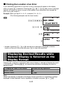
Displaying Decimal Results while
Natural Display is Selected as the
Display Format
Pressing E to execute a calculation while natural display is selected will display the result
in natural format. Pressing 1E will execute the calculation and display the result in
decimal format.
To display the result in this format:
Perform this key operation:
Natural Format
E
Decimal Format
1E
Note
When linear display is selected as the display format, execution of a calculation is always
displayed in linear (decimal) format, regardless of whether you press E or 1E.
E-21
k Example Calculations
Example: '
2 +'
8 = 3'
2
B
!2e+!8E
Produce the result in decimal format:
!2e+!81E
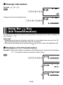
Using the f Key
(S-D Transformation)
You can use the f key to transform a value between its decimal (D) form and its standard (S)
form (fraction, ', π).
Important!
• Depending on the type of calculation result that is on the display when you press the f
key, the conversion process may take some time to perform.
• With certain calculation results, pressing the f key will not convert the displayed value.
k Examples of S-D Transformation
Example 1: While linear display is selected as the display format, to perform the calculation
111 ÷ 33, and then convert the result to fraction format
b
111/33E
f
f
E-22
Note
• Each press of the f key toggles the displayed result between the two forms.
• The format of the fraction depends on which fraction display format (improper or mixed) is
currently selected (page 12).
Example 2: While natural display is selected as the display format, to perform the
calculation 111 ÷ 33, and then convert the result to decimal format
B
111/33E
f
f
Example 3: While natural display is selected as the display format, to perform the π
calculation shown below, and then convert the result to decimal format
B
15(π)*'2c5E
f
Basic Calculations
Unless otherwise noted, the calculations in this section can be performed in any of the
calculator’s calculation mode, except for the BASE-N Mode.
k Arithmetic Calculations
Arithmetic calculations can be used to perform addition (+), subtraction (-),
multiplication (*), and division (/).
E-23
Example 1: 2.5 + 1 − 2 = 1.5
b
2.5+1-2E
Example 2: 7 × 8 − 4 × 5 = 36
b
7*8-4*5E
• The calculator determines the proper priority sequence for addition, subtraction,
multiplication, and division automatically. See “Calculation Priority Sequence” on page 128
for more information.
k Fractions
Keep in mind when inputting fractions on your calculator that the input procedure you need
to use depends on whether natural display or linear display is selected as the display format
(page 11), as shown below.
Natural Display:
Key Operation
Display
7
3
Improper Fraction
'7c3
Mixed Fraction
1'(()
2e1c3
2
1
3
Linear Display:
Key Operation
Improper Fraction
Display
7{3
7'3
Numerator Denominator
Mixed Fraction
2'1'3
2{1{3
Integer Numerator Denominator
As you can see above, natural display lets you input fractions as they appear in your
textbook, while linear display requires input of a special symbol ({).
Note
• Under initial default settings, fractions are displayed as improper fractions.
• Fraction calculation results are always reduced automatically before being displayed.
Executing 2 { 4 =, for example, will display the result 1 { 2.
E-24
A Fraction Calculation Examples
Example 1:
B
2
1
7
+
=
3
2
6
'2c3
e+
'1c2
E
b
2'3+1'2
E
Example 2: 3
b
1
2
11
+1 =4
(Fraction Display Format: ab/c)
4
3
12
3'1'4+
1'2'3E
B
1'(()3e1c4e+
1'(()1e2c3E
E-25
Note
• If the total number of elements (integer digits + numerator digits + denominator digits
+ separator symbols) that make up a mixed fraction expression is greater than 10, the
calculation result will be displayed in decimal form.
• If an input calculation includes a mixture of fraction and decimal values, the result will be
displayed in decimal format.
• You can input integers only for the elements of a fraction.
A Switching between Improper Fraction and Mixed Fraction
Format
To convert an improper fraction to a mixed fraction (or a mixed fraction to an improper
b
d
fraction), press 1f( a —
c ⇔—
c ).
A Switching between Fraction and Decimal Format
Use the procedure below to toggle a displayed calculation result between fraction and
decimal format.
3 3
Example: 1.5 = ,
= 1.5
2 2
b
1.5E
f
The current fraction display format setting determines if an improper or mixed fraction is displayed.
f
Note
The calculator cannot switch from decimal to fraction format if the total number of elements
(integer digits + numerator digits + denominator digits + separator symbols) that make up a
mixed fraction is greater than 10.
k Percent Calculations
Inputting a value and with a percent (%) sign makes the value a percent. The percent (%)
sign uses the value immediately before it as the argument, which is simply divided by 100 to
get the percentage value.
A Percent Calculation Examples
All of the following examples are performed using linear display (b).
E-26
Example 1: 2% = 0.02
(
2
)
100
21,(%)E
Example 2: 150 × 20% = 30
(150 ×
20
)
100
150*201,(%)E
Example 3: What percent of 880 is 660?
660/880
1,(%)E
Example 4: Increase 2500 by 15%.
2500+2500*
151,(%)E
Example 5: Reduce 3500 by 25%.
3500-3500*
251,(%)E
k Degree, Minute, Second (Sexagesimal) Calculations
You can perform calculations using sexagesimal values, and you can convert between
sexagesimal and decimal.
A Inputting Sexagesimal Values
The following is basic syntax for inputting a sexagesimal value.
{Degrees}${Minutes}${Seconds}$
Example: To input 2°30´30˝
b
2e30e30eE
• Note that you must always input something for the degrees and minutes, even if they are
zero.
Example: To input 0°00´30˝, press 0$0$30$.
E-27
A Sexagesimal Calculation Examples
• The following types of sexagesimal calculations will produce sexagesimal results.
- Addition or subtraction of two sexagesimal values
- Multiplication or division of a sexagesimal value and a decimal value
Example 1: 2°20´30˝ + 39´30˝ = 3°00´00˝
b
2e20e30e+
0e39e30eE
Example 2: 2°20´00˝ × 3.5 = 8°10´00˝
b
2e20e*
3.5E
A Performing a Decimal Calculation to Obtain a Sexagesimal
Result
You can use the “'DMS” command to execute a decimal calculation and obtain a
sexagesimal result. The “'DMS” command can be used in the COMP Mode only.
Example: Perform the calculation 100 ÷ 3 so it produces a sexagesimal result
b
100/3E
z – {ANGLE}4('DMS)E
A Converting between Sexagesimal and Decimal
Pressing $ while a calculation result is displayed will toggle the value between
sexagesimal and decimal.
Example: To convert 2.255 to sexagesimal
b
2.255E
e
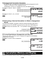
Calculation History and Replay
You can use calculation history in the COMP and BASE-N Modes.
E-28
k Accessing Calculation History
The ` symbol in the upper right corner of the display indicates that there is data stored in
calculation history. To view the data in calculation history, press f. Each press of f will
scroll upwards (back) one calculation, displaying both the calculation expression and its
result.
Example:
B
1+1E2+2E
3+3E
f
f
While scrolling through calculation history records, the $ symbol will appear on the display,
which indicates that there are records below (newer than) the current one. When this symbol
is turned on, press c to scroll downwards (forward) through calculation history records.
Important!
• Calculation history records are all cleared when you change to a different calculation
mode, or when you change the display format.
• Calculation history capacity is limited. Whenever you perform a new calculation while
calculation history is full, the oldest record in calculation history is deleted automatically to
make room for the new one.
Note
A calculation that contains any of the following functions is not stored in calculation history
when it is executed.
CALC, SOLVE, Built-in Formulas, User Formulas
k Using Replay
While a calculation history record is on the display, press d or e to display the cursor
and enter the editing mode. Pressing e displays the cursor at the beginning of the
calculation expression, while d displays it at the end. After you make the changes you
want, press E to execute the calculation.
Example: 4 × 3 + 2.5 = 14.5
4 × 3 – 7.1 = 4.9
b
4*3+2.5E
E-29
d
YYYY
-7.1E
Using Multi-statements in
Calculations
A multi-statement is a statement that is made up of multiple calculation expressions
separated by special separator codes (: and ^). The following examples show how the two
separator codes differ from each other.
{expression 1} : {expression 2} : .... : {expression n}
Pressing E executes each expression in sequence, starting with {expression 1} and
ending with the ﬁnal expression in the series. After that, the result of the ﬁnal expression
appears on the display.
Example: To perform the calculation 123 + 456, and then subtract its result from 1000
b
123+4561!(:)
1000-1-(Ans)
E
{expression 1} ^ {expression 2} ^ .... ^ {expression n}
In this case, pressing E starts execution starting with {expression 1}. When execution
reaches a ^ separator, execution pauses and the calculation result up to that point appears
on the display. Pressing E again will resume execution from the expression below the ^
separator.
Example: To display the result of the calculation 123 + 456, and then subtract it from 1000
b
123+4561x(^)
1000-1-(Ans)
E-30
E
E
Note
• The Q symbol turns on in the upper right corner of the display when execution of a
multi-statement calculation has been paused by a ^ separator.
• When performing a multi-statement calculation, Ans (Answer Memory) (page 32) is
updated each time any of the statements that makes up a multi-statement produces a
result.
• You can mix “^” and “:” separators within the same calculation.
Calculator Memory Operations
Your calculator includes the types of memory described below, which you can use for
storage and recall of values.
Memory Name
Description
Answer Memory
Answer Memory contains the result of the last calculation you
performed.
Independent Memory
Independent memory comes in handy when adding or subtracting
multiple calculation results.
Variables
The letters A through Z can be assigned different values
individually and used in calculations. Note that variable M is also
used for storing independent memory values.
Extra Variables
You can create extra variables when you need storage for more
values than provided by the 26 letters from A through Z. You can
reserve up to 2372 extra variables, which are named Z[1], Z[2],
etc.
Formula Variables
The following literal variables are used by the calculator’s built-in
formulas or user formulas.
• Lower-cast alphabetic characters: a through z
• Greek characters: α through ω, Α through Ω
• Subscripted alphabetic and Greek characters: A1, a0, ωt, ∆x, etc.
For details about built-in formulas and formula variables, see
“Built-in Formulas” (page 97).
The types of memory described above are not cleared when you press the o key, change
to another mode, or turn off the calculator.
E-31
k Using Answer Memory (Ans)
The result of any new calculation you perform on the calculator is stored automatically in
Answer Memory (Ans).
A Automatic Insertion of Ans in Consecutive Calculations
If you start a new calculation while the result of a previous calculation is still on the display,
the calculator will insert Ans into the applicable location of the new calculation automatically.
Example 1: To divide the result of 3 × 4 by 30
b
3*4E
(Next) /30E
Pressing / inputs Ans automatically.
2
2
Example 2: To determine the square root of the result of 3 + 4
b
3x+4xE
!E
Note
• As in the above examples, the calculator automatically inserts Ans as the argument of
any calculation operator or scientiﬁc function you input while a calculation result is on the
display.
• In the case of a function with a parenthetical argument (page 15), Ans automatically
becomes the argument only in the case that you input the function alone and then
press E. Note, however, that with natural display Ans may not become the argument
automatically when using a function with a parenthetical argument.
• Basically, Ans is inserted automatically only when the result of the previous calculation is
still on the display, immediately after you executed the calculation that produced it. If you
want to insert Ans after clearing the display by pressing o, press 1-(Ans).
E-32
A Inserting Ans into a Calculation Manually
You can insert Ans into a calculation at the current cursor location by pressing 1-(Ans).
Example 1: To use the result of 123 + 456 in another calculation as shown below
123 + 456 = 579
789 – 579 = 210
b
123+456E
789-1-(Ans)E
2
2
Example 2: To determine the square root of 3 + 4 and then add 5 to the result
b
3x+4xE
!1-(Ans))+5E
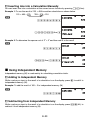
k Using Independent Memory
Independent memory (M) is used mainly for calculating cumulative totals.
A Adding to Independent Memory
While a value you input or the result of a calculation is on the display, press l to add it to
independent memory (M).
Example: To add the result of 105 ÷ 3 to independent memory (M)
b
105/3l
A Subtracting from Independent Memory
While a value you input or the result of a calculation is on the display, press 1l(M–) to
subtract it from independent memory (M).
E-33
Example: To subtract the result of 3 × 2 from independent memory (M)
b
3*21l(M–)
Note
Pressing l or 1l(M–) while a calculation result is on the display will add it to or
subtract it from independent memory.
Important!
The value that appears on the display when you press l or 1l(M–) at the end of a
calculation in place of E is the result of the calculation (which is added to or subtracted
from independent memory). It is not the current contents of independent memory.
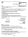
A Viewing Independent Memory Contents
Press ~9(M).
A Clearing Independent Memory Contents (to 0)
01~(STO)9(M)
A Calculation Example Using Independent Memory
Press 01~(STO)9(M) to clear independent memory contents before performing the
following operation.
Example:
23+9m
23 + 9 = 32
−)
53 – 6 = 47
53-6m
45 × 2 = 90
45*21m(M–)
99 ÷ 3 = 33
99/3m
(Total) 22
t9(M)
(Recalls value of M.)
k Using Variables
Your calculator supports the use of 26 variables, named A through Z.
A Assigning a Value or Calculation Result to a Variable
Use the procedure shown below to assign a value or a calculation expression to a variable.
Example: To assign 3 + 5 to variable A
3+51~(STO)0(A)
A Viewing the Value Assigned to a Variable
To view the value assigned to a variable, press ~ and then specify the variable name. You
could also press S, specify the variable name, and then press E.
Example: To view the value assigned to variable A
~0(A) or S0(A)E
E-34
A Using a Variable in a Calculation
You can use variables in calculations the same way you use values.
Example: To calculate 5 + A
5+S0(A)E
A Clearing the Value Assigned to a Variable (to 0)
Example: To clear variable A
01~(STO)0(A)
A Clearing All Variables (to 0)
Use the MEMORY Mode screen to clear the contents of all the variables. See “Memory
Manager (MEMORY)” on page 126 for more information.
k Clearing All Memory Contents
Perform the operation below when you want to clear all variables (including variable M) and
Answer Memory (Ans) to zero.
z – {CLR} – {Memory}E
Reserving Variable Memory
If you ﬁnd that the calculator’s default variables (A through Z) are not enough for your
purposes, you can reserve variable memory and create “extra variables” for storage of
value.
Extra variables work like array variables of an array named “Z” when assigning or recalling
their values. An extra variable name consists of the letter “Z” followed by a value in brackets,
like Z[5].
k User Memory Area
Your calculator has a 28500-byte user memory area that you can use to reserve variable
memory and add extra variables.
Important!
• You can perform the procedure to reserve variable memory in the COMP Mode or in a
COMP Mode program. All of the sample operations in this section are performed in the
COMP Mode (N1).
• The 28500-byte user memory is used for storage of extra variables and programs. This
means that increasing the number of extra variables reduces the amount of memory
available for storing programs. So also, storing programs in memory reduces the amount
of memory available for storing extra variables.
E-35
A Adding Extra Variables
Example: To increase the number of variables by 10
b
10z – {PROG} – {/}1.(Dim Z)E
• When “Done” appears on the display, it means that the number of extra
variables you speciﬁed has been added. At this point, zero is assigned to all of
the extra variables.
(To check the value of Z[10])
oS5(Z)
Si([)10S6(])E
Note
Reserving variable memory uses up a basic 26 bytes, plus 12 bytes for each of the extra
variables that you add. Note that storing a complex number of an extra variable uses up 22
bytes. Adding 10 extra variables as shown above, for example, uses up 26 + (12 × 10) = 146
bytes of the user memory area. Since user memory has a total capacity of 28500 bytes, the
limit on the number of extra variables you can add is 2372 (assuming you do not have any
complex numbers assigned to the extra variables).
k Using Extra Variables
After creating extra variables, you can assign values to them and insert them into
calculations just as you do with the default valuables (from A through Z). Just remember that
extra variable names consist of the letter “Z” followed by a value in brackets, like Z[5].
Note
• The closing bracket ( ] ) of the extra variable name can be omitted.
• In place of a value inside the brackets of an extra variable name, you can use a calculation
expression or a default array name (A to Z).
• Note that the value in the brackets of an extra variable name must be in the range of
1 and the number of extra variables that have been added. Trying to use a value that
exceeds the number of extra variables will cause an error.
A Assigning a Value or Calculation Result to an Extra Variable
You can assign a value to an extra variable using the following command syntax: {value or
expression} / Z[{extra variable value}] E.
Example: To assign 3 + 5 to variable Z[5]
b
3+5z – {PROG} – {/}
S5(Z)Si([)5S6(])E
E-36
Important!
You can write data to extra variables in the COMP Mode or in a COMP Mode program.
A Recalling the Contents of an Extra Variable
Input the name (Z[n]) of the extra variable whose contents you want to recall, and then
press E.
Example: To recall the contents of extra variable Z[5]
b
S5(Z)Si([)5a6(])E
A Using an Extra Variable in a Calculation
You can use extra variables in calculations the same way you use values.
Example: To calculate 5 + Z[5]
b
5+S5(Z)Si([)5S6(])E
A Clearing Extra Variable Contents (to 0)
Example: To clear extra variable Z[5]
0z – {PROG} – {/}S5(Z)ai([)5S6(])E
A Clearing All Extra Variables
Perform the operation below when you want delete all extra variables that are currently in
calculator memory.
0z – {PROG} – {/}1.(Dim Z)E
Note
You can also use the MEMORY Mode screen to delete all the extra variables. See “Memory
Manager (MEMORY)” on page 126 for more information.
Using π and Scientiﬁc Constants
k Pi (π)
Your calculator supports input of pi (π) into calculations. Pi (π) is supported in all modes,
except for the BASE-N Mode. The following is the value that the calculator uses for π.
π = 3.14159265358980 (1Z(π))
E-37
k Scientiﬁc Constants
Your calculator has 40 often-used scientiﬁc constants built in. Like π, each scientiﬁc constant
has a unique display symbol. Scientiﬁc constants are supported in all modes, except for the
BASE-N Mode.
A Inputting a Scientiﬁc Constant
1. Press z to display the function menu.
2. On the menu, select “CONST”.
• This displays page 1 of the scientiﬁc constant menu.
• There are ﬁve scientiﬁc command menu screens, and you can use c and f to
navigate between them. For more information about scientiﬁc constants, see “List of
Scientiﬁc Constants” on page 39.
3. Use c and f to scroll through the pages and display the one that contains the
scientiﬁc constant you want.
4. Press the number key (from 1 to 8) that corresponds to the scientiﬁc constant you
want to select.
• This will input the scientiﬁc constant symbol that corresponds to the number key you
press.
1
• Pressing E here will display the value of the scientiﬁc constant whose symbol is
currently on the screen.
A Example Calculations Using Scientiﬁc Constants
Example: To calculate the constant for the speed of light in a vacuum ( c0 = 1/ ε 0µ 0 )
b
1/!
z – {CONST}ccc8(ε0)
E-38
z – {CONST}cccc1(ƫ0))
E
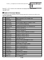
A List of Scientiﬁc Constants
The numbers in the “No.” column show the scientiﬁc constant menu page number on the left
and the number key you need to press to select the constant when the proper menu page is
displayed.
No.
1-1
Scientiﬁc Constant
No.
Scientiﬁc Constant
Proton mass
3-5
Muon magnetic moment
1-2
Neutron mass
3-6
Faraday constant
1-3
Electron mass
3-7
Elementary charge
1-4
Muon mass
3-8
Avogadro constant
1-5
Bohr radius
4-1
Boltzmann constant
1-6
Planck constant
4-2
Molar volume of ideal gas
1-7
Nuclear magneton
4-3
Molar gas constant
1-8
Bohr magneton
4-4
Speed of light in vacuum
2-1
Planck constant, rationalized
4-5
First radiation constant
Second radiation constant
2-2
Fine-structure constant
4-6
2-3
Classical electron radius
4-7
Stefan-Boltzmann constant
2-4
Compton wavelength
4-8
Electric constant
2-5
Proton gyromagnetic ratio
5-1
Magnetic constant
2-6
Proton Compton wavelength
5-2
Magnetic ﬂux quantum
2-7
Neutron Compton wavelength
5-3
Standard acceleration of gravity
2-8
Rydberg constant
5-4
Conductance quantum
3-1
Atomic mass constant
5-5
Characteristic impedance of vacuum
3-2
Proton magnetic moment
5-6
Celsius temperature
3-3
Electron magnetic moment
5-7
Newtonian constant of gravitation
3-4
Neutron magnetic moment
5-8
Standard atmosphere
• The values are based on CODATA Recommended Values (2000). For details, see <#01>
in the separate Supplement.
E-39
Scientiﬁc Function Calculations
Unless otherwise noted, the functions in this section can be used in any of the calculator’s
calculation modes, except for the BASE-N Mode.
Scientiﬁc Function Calculation Precautions
• When performing a calculation that includes a built-in scientiﬁc function, it may take
some time before the calculation result appears. Do not perform any key operation on the
calculator until the calculation result appears.
• To interrupt an on-going calculation operation, press @.
Interpreting Scientiﬁc Function Syntax
• Text that represents a function’s argument is enclosed in braces ({ }). Arguments are
normally {value} or {expression}.
• When braces ({ }) are enclosed within parentheses, it means that input of everything
inside the parentheses is mandatory.
k Trigonometric and Inverse Trigonometric Functions
–1
–1
–1
sin(, cos(, tan(, sin (, cos (, tan (
A Syntax and Input
sin({n}) (Other functions may be used in argument.)
–1
Example: sin 30 = 0.5, sin 0.5 = 30
bv
s30)E
–1
1s(sin )0.5)E
A Remarks
The angle unit you need to use in a calculation is the one that is currently selected as the
default angle unit.
E-40
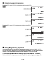
k Angle Unit Conversion
You can convert a value that was input using one angle unit to another angle unit.
After you input a value, select z – {ANGLE} to display the menu screen shown below.
1(°): Degrees
2(r): Radians
3(g): Grads
Example: To convert
bv
π
radians to degrees
2
(15(π)/2)
z – {ANGLE}2(r)E
k Hyperbolic and Inverse Hyperbolic Functions
–1
–1
–1
sinh(, cosh(, tanh(, sinh (, cosh (, tanh (
A Syntax and Input
sinh({n}) (Other functions may be used in argument.)
Example: sinh 1 = 1.175201194
b
z – {MATH}cc1(sinh)1)
A Remarks
To input a hyperbolic or inverse hyperbolic function, perform the following operation to
display a menu of functions: z – {MATH}cc.
k Exponential and Logarithmic Functions
10^(, e^(, log(, ln(
A Syntax and Input
10^({n}) .......................... 10 n
log({n}) ........................... log10{n}
log({m},{n}) ..................... log{m}{n}
ln({n}) ............................. loge{n}
{ }
(Same as e^()
(Common Logarithm)
(Base {m} Logarithm)
(Natural Logarithm)
E-41
Example 1: log216 = 4, log16 = 1.204119983
b
l2,16)E
l16)E
Base 10 (common logarithm) is assumed when no base is speciﬁed.
B
z – {MATH}c7(logab)
2e16E
Example 2: ln 90 (= loge 90) = 4.49980967
b
i90)E
k Power Functions and Power Root Functions
x2, x–1, ^(, '(, 3'(, x'(
A Syntax and Input
2
2
{n} x ............................... {n}
–1
–1
{n} x ............................. {n}
{ }
{(m)}^({n}) ....................... {m} n
'({n}) .......................... {n}
3
3
'({n}) ......................... {n}
{ }
({m})x'({n}) .................. m {n}
(Square)
(Reciprocal)
(Power)
(Square Root)
(Cube Root)
(Power Root)
Example 1: ('
2 + 1) ('
2 – 1) = 1, (1 + 1)
2+2
b
= 16
(!2)+1)
(!2)-1)E
E-42
(1+1)62+2)E
B
(!2e+1)
(!2e-1)E
(1+1)62+2E
2
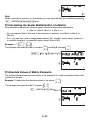
Example 2: (–2) 3 = 1.587401052
b
(-2)6(2'3)E
k Integration Calculation
Your calculator performs integration using Gauss-Kronrod integration for approximation. The
calculator uses the following function for integration.
∫(
A Syntax and Input
∫( f(x), a, b, tol)
f(x): Function of x (Input the function used by variable X.)
• All variables other than X are viewed as constants.
a: Lower limit of region of integration
b: Upper limit of region of integration
tol: Error tolerance range (Can be input only when linear display is being used.)
–5
• This parameter can be omitted. In that case, a tolerance of 1 × 10 is used.
Example: ∫(ln(x), 1, e) = 1
B
(tol value not input)
z – {MATH}1(∫dX)
iS0(X))c1f1i(%)1E
E-43
b
z – {MATH}1(∫dX)
iS0(X)),1,1i(%)1))E
A Remarks
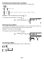
• Use of ∫( is supported in the COMP, SD, REG, and EQN Modes only.
• The following functions cannot be input for the f(x), a, b, and tol parameters: ∫(, d/dx(,
d2/dx2(, Σ(. In addition, the Pol( and Rec( functions, and the random number functions
cannot be input for the f(x) parameter.
• The integration result will be negative when the limit of region of integration parameters
are within the range a < x < b and f(x) < 0.
2
Example: ∫(0.5X – 2, –2, 2) = –5.333333333
• In the case of integration of a trigonometric function, select Rad for the angle unit.
• Integration calculations can take a long time to complete.
• Specifying a smaller value for the tol parameter tends to improve precision, but it also
–14
causes the calculation to take more time. Specify a tol value greater than 1 × 10 .
• You will not be able to input a tol value while using natural display.
• The type of function being integrated, positive and negative values within the region of
integration, and the region of integration being used can cause large error in integration
values and errors.
• You can interrupt an ongoing integration calculation operation by pressing o.
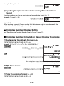
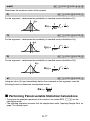
A Tips to for Successful Integration Calculations
• For periodic functions, and for positive and negative f(x) values due to the region of
integration being used
/ Divide the integration into parts for each period, or between positive and negative
parts, obtain integration values for each, and then add the values.
S Positive
S Negative
∫
b
a
f(x)dx =
∫
c
a
f(x)dx + (–
Positive Part
(S Positive)
∫
b
c
f(x)dx)
Negative Part
(S Negative)
• For widely ﬂuctuating integration values due to a minutely shifting region of integration
/ Divide the integration interval into multiple parts (in a way that breaks areas of wide
ﬂuctuation into small parts), perform integration on each part, and then combine the
results.
E-44
∫
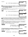
b
a
f(x)dx =
∫
x1
a
f(x)dx +
∫
x2
x1
f(x)dx + .....+
∫
b
x4
f(x)dx
k Derivative
Your calculator performs differential calculations by approximating the derivative based on
centered difference approximation. Calculation is performed using the function shown below.
d/dx(
A Syntax and Input
d/dx( f (x), a, tol)
f(x): Function of x (Input the function used by variable X.)
• All variables other than X are viewed as constants.
a: Value of point (derivative point) of desired derivative coefﬁcient
tol: Error tolerance range (Can be input only when linear display is being used.)
• This parameter can be omitted. In that case, a tolerance of 1 × 10
–10
is used.
π
Example: To obtain the differential coefﬁcient at point x =
for the function y = sin(x)
2
(tol value not input)
V
z – {MATH}2(d/dX)sS0(X)).....1
B
b
(Continuing from 1, above)
e'1Z(π)c2E
(Continuing from 1, above)
,1Z(π)'2)E
A Remarks
• Use of d/dx( is supported in the COMP, SD, REG, and EQN Modes only.
2
2
• The following functions cannot be input for the f(x), a, and tol parameters: ∫(, d/dx(, d /dx (,
Σ(. In addition, the Pol( and Rec( functions, and the random number functions cannot be
input for the f(x) parameter.
• In the case of differentiation of a trigonometric function, select Rad for the angle unit.
• Specifying a smaller value for the tol parameter tends to improve precision, but it also
–14
causes the calculation to take more time. Specify a tol value greater than 1 × 10 .
• You will not be able to input a tol value while using natural display.
• Non-consecutive points, abrupt ﬂuctuation, extremely large or small points, inﬂection
points, and the inclusion of points that cannot be differentiated, or a differential point or
E-45
differential calculation result that approaches zero can cause poor precision or error.
• You can interrupt an ongoing differential calculation operation by pressing o.
k Second Derivative
2
2
Your calculator lets you calculate the second derivative coefﬁcient (d /dx ( f (x))|x=a) for f (x)
where x = a. Your calculator uses approximation based on the second order value differential
equation of the Newton interpolation polynomial. Calculation is performed using the function
shown below.
d2/dx2(
A Syntax and Input
d 2/dx2( f (x), a, tol)
f (x): Function of x (Input the function used by variable X.)
• All variables other than X are viewed as constants.
Value of point (second derivative point) of desired second derivative
coefﬁcient
tol: Error tolerance range (Can be input only when linear display is being used.)
–10
• This parameter can be omitted. In that case, a tolerance of 1 × 10 is used.
a:
3
2
Example 1: To obtain the second derivative coefﬁcient for the function y = x + 4x + x – 6
when x = 3
B
2
2
z – {MATH}3(d /dX )S0(X)63e
+4S0(X)x+S0(X)-6e3E
Example 2: To perform the same procedure as Example 1, specifying tol = 1 × 10
–12
Since you want to specify a value for tol, you will need to perform this calculation using
linear display.
b
2
2
z – {MATH}3(d /dX )S0(X)63)+4
S0(X)x+S0(X)-6,3,1Z12)E
A Remarks
See the remarks for derivative on page 45.
k Σ Calculation
This function determines the sum of an input f (x) for a speciﬁed range. Calculation is
performed using the function shown below.
Σ(
E-46
The following shows the calculation formula used for Σ calculations.
Σ( f (x), x, a, b) = f (a) + f (a+1) + .... + f (b)
A Syntax and Input
Σ( f (x), x, a, b)
f (x): Function of x (parameter variable speciﬁed below)
x: Parameter variable (Any letter from A through Z)
• If the variable name you specify here does not match the variable name
used within the function of x, the variable in the function will be treated as a
constant.
a: Start point of calculation range
b: End point of calculation range
10
10
• a and b are integers in the range of –1 × 10 < a < b < 1 × 10 .
• The step for this calculation is ﬁxed as 1.
Example: Σ( X + 1, X, 1, 5) = 20
B
z – {MATH}4(Σ()S0(X)
+1ea0(X)e1e5E
b
z – {MATH}4(Σ()S0(X)
+1,a0(X),1,5)E
A Remarks
• Use of Σ( is supported in the COMP, SD, REG, and EQN Modes only.
2
2
• The following functions cannot be input for the f(x), a, and b parameters: ∫(, d/dx(, d /dx (,
Σ(. In addition, the Pol( and Rec( functions, and the random number functions cannot be
input for the f(x) parameter.
• You can interrupt an ongoing Σ calculation operation by pressing o.
k Coordinate Conversion (Rectangular ↔ Polar)
Pol(, Rec(
Your calculator can convert between rectangular coordinates and polar coordinates.
o
o
Rectangular Coordinates (Rec)
E-47
Polar Coordinates (Pol)
A Syntax and Input
Rectangular-to-Polar Coordinate Conversion (Pol)
Pol(x, y)
x: Rectangular coordinate x-value
y: Rectangular coordinate y-value
Polar-to-Rectangular Coordinate Conversion (Rec)
Rec(r, Ƨ)
r : Polar coordinate r-value
Ƨ: Polar coordinate Ƨ-value
2, '
2 ) to polar coordinates
Example 1: To convert the rectangular coordinates ('
bv
1+(Pol)!2)
,!2))E
Bv
1+(Pol)!2e
,!2e)E
Example 2: To convert the polar coordinates (2, 30˚) to rectangular coordinates
bv
1-(Rec)2,
30)E
A Remarks
• These functions can be used in the COMP Mode.
• The r-value or x-value produced by the calculation is assigned to variable I, while the
Ƨ-value or y-value is assigned to variable J (page 34).
• The values obtained for Ƨ when converting from rectangular coordinates to polar
coordinates is within the range –180° < Ƨ < 180°.
• When executing a coordinate conversion function inside of a calculation expression, the
calculation is performed using the ﬁrst coordinate that the conversion produces (r-value or
x-value).
2, '
2)+5=2+5=7
Example: Pol ('
E-48
k Random Number Functions
Your calculator comes with functions for generating ten-digit non-sequential random
numbers, ten-digit sequential random numbers, or random integers within a speciﬁc range.
The following are the random number generation functions.
Ran#, RanInt#(
A Non-sequential Random Numbers (Decimal Values)
The following generates ten-digit non-sequential fractional numbers in the range of 0 to 1.
Syntax: Ran#
Example: To generate ten-digit non-sequential random numbers
B
z – {MATH}6(Ran#)E
E
E
The above values are provided for example only. The actual values produced
by your calculator for this function will be different.
A Sequential Random Numbers (Decimal Values)
In this case, ten-digit sequential random numbers are generated in the range of 0 to 1 in
accordance with nine sequences numbered from 1 through 9. The sequence is speciﬁed by
the integer argument (1 through 9) of Ran#. The random numbers generated in accordance
with the argument are generated in a ﬁxed sequence.
Syntax: Ran#{n} (n is an integer from 1 to 9.)
Example: To generate sequential random numbers
B
Initialize the sequence:
z – {MATH}6(Ran#)0E
E-49
z – {MATH}6(Ran#)1E
E
E
A Random Integers
This function generates random integers within a speciﬁc range.
Syntax: RanInt#({m}, {n}) (m and n are integers. m < n; |m|, |n| < 1E10; n – m < 1E10)
Example: To generate random integers in the range of 0 to 5
B
z – {MATH}c8(RanInt)0,5)E
E
E
The above values are provided for example only. The actual values produced
by your calculator for this function will be different.
k Other Functions
x!, Abs(, nPr, nCr, Rnd(, Int(, Frac(, Intg(
E-50
A Factorial (!)
Syntax: {n}! ({n} must be a natural number or 0.)
Example: (5 + 3)!
b
(5+3)
z – {MATH}5(X!)E
A Absolute Value (Abs)
Syntax: Abs({n})
Example: Abs (2 – 7) = 5
B
z – {MATH}c1(Abs)2-7E
b
z – {MATH}c1(Abs)2-7)E
A Permutation (nPr)/Combination (nCr)
Syntax: {n}P{m}, {n}C{m}
Example: How many four-person permutations and combinations are possible for a group
of 10 people?
b
10z – {MATH}7(nPr)4E
10z – {MATH}8(nCr)4E
A Rounding Function (Rnd)
You can use the rounding function (Rnd) to round the value, expression, or calculation result
speciﬁed by the argument. Rounding is performed to the number of signiﬁcant digits in
accordance with the number of display digits setting.
E-51
Display Digit Setting: Norm1 or Norm2
The mantissa is rounded off to 10 digits.
Display Digit Setting: Fix or Sci
The value is rounded to the speciﬁed number of digits.
Example: 200 ÷ 7 × 14 = 400
b
200/7*14E
(3 decimal places)
1N(SETUP)6(Fix)3E
(Internal calculation uses 15 digits.)
200/7E
*14E
Now perform the same calculation using the rounding (Rnd) function.
o200/7E
(Calculation uses rounded value.)
10(Rnd)E
(Rounded result)
*14E
A Integer Part Extraction (Int)
The Int( function extracts the integer part of the real number input as its argument.
E-52
Syntax: Int({n})
Example: To extract the integer part of –1.5
b
z – {MATH}c2(Int)-1.5)E
A Fractional Part Extraction (Frac)
The Frac( function extracts the fractional part of the real number input as its argument.
Syntax: Frac({n})
Example: To extract the fractional part of –1.5
b
z – {MATH}c3(Frac)-1.5)E
A Largest Integer (Intg)
The Intg( function determines the largest integer that does not exceed the real number input
as its argument.
Syntax: Intg({n})
Example: To determine the largest integer that does not exceed –1.5
b
z – {MATH}c4(Intg)-1.5)E
Using Engineering Notation
3
k Using 10 Engineering Notation (ENG)
Engineering notation (ENG) expresses quantities as a product of a positive number between
1 and 10 and a power of 10 that is always a multiple of three. There are two functions that
you can use to convert a number to engineering notation, ENG/ and ENG,.
Function
Key Operation
ENG/
1/(ENG)
ENG,
1*(ENG)
E-53
k ENG Conversion Examples
Example 1: To convert 1234 to engineering notation using ENG/
B
1234E
1/(ENG)
1/(ENG)
Example 2: To convert 123 to engineering notation using ENG,
B
123E
1*(ENG)
1*(ENG)
k Using Engineering Symbols
Your calculator supports the use of ten engineering symbols (m, ƫ, n, p, f, k, M, G, T, P)
that you can use for input of value or for calculation result display. You can use engineering
symbols in calculations in all calculation modes, except for the BASE-N Mode.
A Displaying Calculation Results with Engineering Symbols
Use the calculator’s setup screens to select “EngOn” for engineering symbols (page 13).
E-54
A Inputting Values Using Engineering Symbols
Example: To input 500 k
500
z – {MATH}ccc
6(k)
A Using ENG (10 ) Conversion while Engineering Symbols
Turned on (EngOn)
3
Performing ENG conversion while “EngOn” is selected for engineering symbols (page 13)
will move the decimal point three places to the right, and change the engineering symbol
accordingly (from M to k, for example). Conversely, performing ←ENG conversion will move
the decimal point three places to the left, and change the engineering symbol accordingly
(from k to M, for example).
Example: To calculate 999 k (kilo) + 25 k (kilo) = 1.024 M (Mega) = 1024 (kilo)
b
999z – {MATH}ccc6(k)+
25z – {MATH}ccc6(k)E
1/(ENG)
(ENG conversion)
Complex Number Calculations
(COMP)
To perform the example operations in this section, ﬁrst select COMP (N1) as the
calculation mode.
k Inputting Complex Numbers
A Inputting Imaginary Numbers (i)
Use the i key to input imaginary number i.
E-55
Example: To input 2 + 3i
2+3i
A Inputting Complex Number Values Using Polar Coordinate
Format
Complex numbers can also be input using polar coordinate format (r ∠ Ƨ).
Example: To input 5 ∠ 30
51i(∠)30
Important!
When inputting argument Ƨ, enter a value that indicates an angle in accordance with the
calculator’s current default angle unit setting.
k Complex Number Display Setting
See “Specifying the Complex Number Display Format” (page 13).
k Complex Number Calculation Result Display Examples
A Rectangular Coordinate Format (a+bi)
1N(SETUP)c4(COMPLX)1(a+bi)
3 + i) = 2'
3 + 2i = 3.464101615 + 2i
Example 1: 2 × ('
Bv
2*(!3e+i)E
b
2*(!3)+i)E
When using linear display format, calculation results are displayed
in two lines showing the real part and imaginary part.
Example 2: '
2 ∠ 45 = 1 + i
Bv
!2e1i(∠)45E
A Polar Coordinate Format (r ∠ Ƨ)
1N(SETUP)c4(COMPLX)2(r∠Ƨ)
E-56
Example 1: 2 × ('
3 + i) = 2'
3 + 2i = 4 ∠ 30
Bv
2*(!3e+i)E
b
2*(!3)+i)E
When using linear display format, calculation results are displayed
in two lines showing the absolute value and argument.
Example 2: 1 + i = '
2 ∠ 45
Bv
1+iE
k Conjugate Complex Number (Conjg)
You can perform the operation below to obtain conjugate complex number ¯z = a – bi for the
complex number z = a + bi.
Example: Obtain the conjugate complex number of 2 + 3i
B
z – {COMPLX}3(Conjg)2+3i)E
k Absolute Value and Argument (Abs, Arg)
You can use the procedure shown below to obtain the absolute value (|z|) and argument
(Arg(z)) on the Gaussian plane for a complex number in the format z = a + bi.
Example: To obtain the absolute value and
argument of 2 + 2i
Imaginary axis
b=2
bv
o
Absolute Value:
z – {COMPLX}1(Abs)2+2i)E
E-57
a=2
Real axis
Argument:
z – {COMPLX}2(Arg)2+2i)E
k Extracting the Real Part (ReP) and Imaginary Part (ImP)
of a Complex Number
You can use the following operations to extract the real part (a) or imaginary part (b) of
complex number a + bi.
Example: Obtain the real part and imaginary part of 2 + 3i
B
z – {COMPLX}4(ReP)2+30)E
z – {COMPLX}5(ImP)2+30)E
k Overriding the Default Complex Number Display Format
You can use the procedures described below to override the default complex number
display format and specify a particular display format for the calculation you are currently
inputting.
A Specifying Rectangular Coordinate Format for a Calculation
Input z – {COMPLX}7('a+bi) at the end of the calculation.
2 ∠ 45 = 2 + 2i (Angle Unit: Deg)
Example: 2'
Bv
2!2e10(∠)45
z – {COMPLX}7('a+bi)E
A Specifying Polar Coordinate Format for a Calculation
Input z – {COMPLX}6('r∠Ƨ) at the end of the calculation.
2 ∠ 45
Example: 2 + 2i = 2'
Bv
2+20z – {COMPLX}6('r∠Ƨ)E
E-58
Matrix Calculations (COMP)
To perform the example operations in this section, ﬁrst select COMP (N1) as the
calculation mode.
k Matrix Calculation Overview
Matrix calculations are performed by ﬁrst storing the matrices in one of six matrix memory
areas named Mat A through Mat F, and then using the matrix area variables to perform the
20
12
+
actual calculation. To perform a matrix calculation like
, for example, you would
02
34
12
20
into Mat A and
into Mat B, when perform the calculation Mat A + Mat B.
input
34
02
Matrix calculation results are displayed on a Mat Ans screen.
k About the Mat Ans Screen
Any calculation result that is a matrix is stored in Matrix Answer memory named “Mat Ans”.
You can use the Mat Ans screen to view the matrix that is currently stored in Mat Ans.
• Each of cells on the Mat Ans screen shows up to six digits of the value currently stored in
the cell.
• To check the value stored in a cell, use the cursor keys to move the highlighting to the cell.
This will cause the full value contained to appear in the value display area at the bottom of
the screen.
• If a cell contains a fraction or sexagesimal value, the applicable cell on the Mat Ans
screen will show the decimal format equivalent. When you move the highlighting to the
cell, the value will appear in the applicable fraction or sexagesimal format in the value
display area.
• Though the Mat Ans screen looks very similar to the matrix editor screen, you cannot edit
a matrix on the Mat Ans screen.
• Pressing E while the Mat Ans screen is on the display will switch to the calculation
screen.
• You can press +, -, or another operator key while the Mat Ans screen is on the
display to start a calculation that uses the current Mat Ans contents (like “Mat Ans+”). This
is similar to Answer Memory operations (page 32). For more information, see “Performing
Matrix Calculations” (page 62).
k Inputting and Editing Matrix Data
You can input data for up to six matrices, named Mat A through Mat F, and then use the
matrix names as variables in calculations. There are two methods you can use to input data
into a matrix: using the matrix editor screen and using the value assignment command (/).
E-59
A Using the Matrix Editor Screen to Input Matrix Data
1. Press z – {MATRIX}1(EDIT) to display the matrix
memory area menu.
• A memory area that already contains a matrix will show
the dimensions of its matrix (like 2 × 2), while an area that
is empty will be indicated by “None”.
2. Use c and f to move the highlighting to the matrix you want to use for data input.
3. Press E.
• This displays a screen for specifying the dimensions of
the matrix. m is the number of rows, while n is the number
of columns.
Note
If you select a memory area that already contains a matrix in step 2, pressing E
will display the matrix editor screen so you can edit the matrix. If you want to delete
the existing matrix and make a new one with different dimensions, press e or
z1(Dim) in place of E in step 3.
4. Specify the dimensions of the matrix you want to create, up to a maximum of 10 rows
and 10 columns.
• To specify the number of rows, move the highlighting to m, input a value and then press
E. This will cause the highlighting to move to n.
• Input a value for n to specify the number of columns and then press E.
• You can use c and f to move the highlighting between m and n.
5. After inputting the row and column values you want, press
E.
• This will display the matrix editor screen.
Cursor
6. On the matrix editor screen, input values into the cells of the matrix.
• Use the cursor keys to move the cursor to the cell you want and then input a value.
After inputting a value, press E to register it.
7. After inputting all the values you want, press J.
A Using the Value Assignment Command (/) to Input Matrix
Data
...
...
...
1. On the COMP Mode calculation screen, use the following syntax to input the matrix you
want to input into matrix memory.
a11 a12 ... a1n
a21 a22 ... a2n
[[a , a , ..., a ][a , a , ..., a ] ... [a , a , ..., a ]]
11
12
1n
21
22
2n
m1
m2
mn
am1 am2 ... amn
• Inputting 1 2 , for example, can be performed using the following key operation.
34
Si([)Si([)1,2S6(])
Si([)3,4S6(])S6(])
E-60
2. Input the value assignment command (/).
z – {PROG} – {/}
3. Specify the matrix memory (Mat A to Mat F or Mat Ans) where you want to store the
matrix.
• To store it in Mat A, for example, perform the following key
operation: z – {MATRIX}2(Mat)Si(A).
Important!
If you specify a matrix memory that already contains matrix data, the existing data will be
overwritten with the data you input here.
4. To store the matrix, press E.
• This displays the stored matrix on the screen. The display
format is the same as that of the matrix editor screen, but
you cannot edit the matrix on this screen.
• Pressing J will return to the COMP Mode calculation
screen.
Note
You can assign the contents of Matrix Answer memory to a matrix variable (such as Mat A)
by executing the following: Mat Ans→Mat A.
A Viewing the Contents of a Matrix
1. On the COMP Mode calculation screen, press z – {MATRIX}1(EDIT) to display the
matrix memory area menu.
2. Use c and f to move the highlighting to the matrix whose contents you want to view,
and then press E.
3. Now you can edit the cell contents of the matrix, if you want.
• Use the cursor keys to move the cursor to the cell whose value you want to change and
then input the new value. After inputting a value, press E to register it.
4. After you ﬁnish making the changes you want, press J.
A Deleting the Contents of a Particular Matrix Memory Area
1. On the COMP Mode calculation screen, press z – {MATRIX}1(EDIT) to display the
matrix memory area menu.
2. Use c and f to move the highlighting to the matrix memory whose contents you want
to delete.
3. Press Y or z2(Del).
• This causes a conﬁrmation message to appear.
4. To delete all programs currently stored in calculator memory, press E(Yes). To cancel
the operation without deleting anything, press J(No).
E-61
k Performing Matrix Calculations
This section presents a number of actual examples of matrix calculations.
• Before performing matrix calculations, you need to perform the procedure under “Inputting
and Editing Matrix Data” (page 59) to input data into the matrices you plan to use in the
calculations.
• The table below shows the matrix name notation used in this section. When you see a
matrix name in a procedure, you need to perform one of the key operations shown below.
When you see this matrix name:
Perform this key operation:
Mat A
z – {MATRIX}2(Mat)S0(A)
Mat B
z – {MATRIX}2(Mat)S'(B)
Mat C
z – {MATRIX}2(Mat)S$(C)
• All of the examples in this section are performed using natural display.
A Adding and Subtracting Matrices
You can add or subtract matrices only if their dimensions are identical.
Example: 2 0 + 1 2
34
02
This example assumes that Mat A contains 2 0 and Mat B contains 1 2 .
02
34
Mat A + Mat B
E
A Multiplying Matrices
You can multiply two matrices only if they both have the same number of rows.
Example: 2 0 + 1 2 × 3
02
34
5
This example assumes that Mat A contains 2 0 , Mat B contains 1 2 , and Mat C
34
02
contains 3 .
5
Mat A + Mat B E
* Mat C
E-62
E
Note
While a calculation screen is on the display, you can input the Mat Ans variable by pressing
z – {MATRIX}2(Mat)1-(Ans).
A Calculating the Scalar Multiplication of a Matrix
Your calculator supports the following types of scalar multiplication calculations.
n × Mat A, n Mat A, Mat A × n, Mat A ÷ n
• You can replace “Mat A” with any of the calculator’s matrices, from Mat A to Mat F, or
Mat Ans.
• For n, you can use a value, independent memory (M), variable, matrix name, constant (π
or scientiﬁc constant), or scientiﬁc function value (like sin(30)).
20
12
+
Example: 3 ×
02
34
This example assumes that Mat A contains 2 0 and Mat B contains 1 2 .
02
34
3*( Mat A + Mat B )
E
A Absolute Values of Matrix Elements
The following determines absolute values of the elements of a matrix and places them onto
the Mat Ans screen.
Example: To determine the absolute values of the matrix 1 –2 .
5 0
This example assumes that Mat C contains 1 –2 .
5 0
z – {MATH}c1(Abs) Mat C
E
E-63
A Obtaining the Determinant of a Matrix
The det( function can be used to obtain the determinant of a square matrix.
det a11 = a11
det
a11 a12
= a11a22 – a12a21
a21 a22
a11 a12 a13
det a21 a22 a23 = a11a22a33 + a12a23a31 + a13a21a32 – a13a22a31 – a12a21a33 – a11a23a32
a31 a32 a33
Example: To obtain the determinant of the matrix 1 –2 .
5 0
This example assumes that Mat C contains 1 –2 .
5 0
z – {MATRIX}3(det) Mat C )
E
A Transposing a Matrix
Transposing a matrix basically means to change its rows in to columns and its columns into
rows. Calculation is performed using the Trn( function as shown below.
Example: To transpose the matrix 1 2 3 .
456
This example assumes that Mat B contains 1 2 3 .
456
z – {MATRIX}4(Trn) Mat B )
E
A Inverting a Matrix
You can use the procedure shown below to invert a square matrix.
a11 –1 =
1
a11
a22 –a12
a11 a12 –1 –a21 a11
=
a21 a22
a11a22 – a12a21
E-64
a11 a12 a13
a21 a22 a23
a31 a32 a33
–1
=
a22a33 – a23a32 –a12a33 + a13a32 a12a23 – a13a22
–a21a33 + a23a31 a11a33 – a13a31 –a11a23 + a13a21
a21a32 – a22a31 –a11a32 + a12a31 a11a22 – a12a21
a11a22a33 + a12a23a31 + a13a21a32 – a13a22a31 – a12a21a33 – a11a23a32
Important!
• Matrix inversion is supported for a non-zero square matrix only.
–1
–1
• Use the !)(x ) key to input “ ”.
1
–2
Example: To invert the matrix
.
5 0
This example assumes that Mat C contains 1 –2 .
5 0
–1
Mat C !)(x )E
A Squaring a Matrix
You can use the procedure shown below to square a matrix.
Important!
Use the x key to specify the squaring operation.
Example: To square the matrix 1 –2 .
5 0
This example assumes that Mat C contains 1 –2 .
5 0
Mat C xE
Sequence Calculations (RECUR)
To perform the example operations in this section, ﬁrst select RECUR (N6) as the
calculation mode.
k Sequence Calculation Overview
You can use either of the two following sequence types to create a sequence table.
1 an Type Sequence
With this sequence type, you input the general term of the sequence (an = f (n)), along
with a sequence start value and end value.
2 an+1 Type Sequence
With this sequence type, you input the recursion formula for two-term recursion (an+1 =
f (an)), along with a sequence start value and end value.
E-65
A Selecting the Sequence Type
To select this sequence type:
Perform this key operation:
an Type
z – {TYPE}1(an)
an+1 Type
z – {TYPE}2(an+1)
A Sequence Editor Screen
Either of the sequence editor screens shown below appears immediately after you enter the
RECUR Mode and select the sequence type. Use this screen to input the expression that
deﬁnes the expression (general term or recursion formula).
an Type
an+1 Type
Inputting a Formula on the Sequence Editor Screen
Example 1: To input an+1 = an + n + 1
z – {TYPE}2(an+1)
z2(an)+z1(n)+1
Example 2: To input an = n + 5
z – {TYPE}1(an)
z1(n)+5
Note
To clear the screen during input, press o.
A Table Range Screen
Pressing E to register the formula you input on the sequence editor screen displays either
of the table range screens shown below.
an Type Sequence
an+1 Type Sequence
Use this screen to specify the start value (Start) and end value (End) of n for sequence
table creation.
Specifying the Initial Term, Start Value, and End Value
1. On the table range screen, use c and f to move the highlighting to the setting you
want to change.
2. Input the values or expressions you want.
• To clear the screen during input, press o.
• Pressing J during input will discard everything you have input up to that point, and
restores the values that were previously input on the screen.
E-66
3. After inputting everything you want, press E.
• This registers your input. If you input expressions, the calculation result of the
expression is registered.
• While any setting is highlighted, press E to display the sequence table screen (page
67).
Returning to the Sequence Editor Screen from the Table Range
Screen
Press J.
A Sequence Table Screen
When you press E in step 3 under “Specifying the Initial Term, Start Value, and End
Value”, the calculator will perform the sequence calculation in accordance with the formula
(general term or recursion formula), initial term, start value, and end value that you have
input, and display the result on the sequence table screen.
an Type Sequence
an+1 Type Sequence
• Each of cells on the sequence table screen shows up to six digits of the value currently
stored in the cell.
• To see the full value in a cell, move the highlighting to it. The full value contained in the
cell will appear in the value display area at the bottom of the screen.
• While a value is in the value display area, you can convert it using ENG conversion (page
53), sexagesimal-decimal conversion (page 27), or decimal-fraction format conversion
(page 22).
• Note, however, that you cannot input into the value display area or edit the values
displayed there.
Sequence Table Columns
This column:
Contains this data:
n
Value from the start value to the end value speciﬁed for n on the
table range screen.
an
Value of an for the n-value in the same line.
Σan
Sum of an from start value of n up to the n-value in the same line
n+1
Value from the start value to the end value speciﬁed for n+1 on the
table range screen.
an+1
Value of an+1 for the n+1 value in the same line.
Σan+1
Sum of an+1 from a1 to n+1 in the same line.
Returning to the Table Range Screen from the Sequence Table Screen
Press J.
E-67
k Creating a Sequence Table
A Creating an an+1 Type Sequence Table
Example: To create a sequence table with the recursion formula an+1 = an+ n + 1 using a
range of 1 < n < 10 (n = integer). Note, however, that a1 = 2.
N6(RECUR)
Enter the RECUR Mode:
Select the an+1 type:
z – {TYPE}2(an+1)
Input the recursion formula:
z2(an)+z1(n)+1
Register the recursion formula:
E
(This displays the table range screen.)
Input a1 = 2, Start = 1, End = 10:
2E1E10E
Create the sequence table:
E
(This displays the sequence table screen.)
A Creating an an Type Sequence Table
1 2
Example: To create a sequence table with the general term an = ( )n + 2n – 3 using a
2
range of 2 < n < 6 (n = integer).
B
Enter the RECUR Mode:
Select the an type:
N6(RECUR)
z – {TYPE}1(an)
Input the general term:
'1c2ez1(n)x+
2z1(n)-3
E-68
Register the general term:
E
(This displays the table range screen.)
Input Start = 2 and End = 6:
2E6E
Create the sequence table:
E
(This displays the sequence table screen.)
k Sequence Calculation Precautions
The following functions cannot be used during sequence calculations.
• CALC
• SOLVE
• Coordinate conversion (Pol(, Rec()
2
2
• d/dx(, d /dx (, ∫(, Σ(
• Independent memory add and subtract (l, 1l(M–))
• Assignment of values to variables (1~(STO))
• Multi-statement input
Sequence Table Generation Errors
• A sequence table can have up to 199 lines. A Range ERROR occurs if a table range
setting causes this to be exceeded.
• A “Memory Full” error also occurs if the calculator runs out of calculation result memory
while performing a sequence table calculation.
Math ERROR during Sequence Calculation
If a Math ERROR occurs during sequence table calculation, the sequence table screen
appears on the display with “ERROR” in the cell that generated the error.
Equation Calculations (EQN)
k Equation Calculation Overview
This section shows the general operational procedure for solving simultaneous linear
equations with two unknowns. Natural display is used for this procedure.
X + 0.5Y = 3
2X + 3Y = 4
E-69
1. Press N8(EQN).
• This displays an initial EQN type menu like the one shown below.
2. Press 1(aX+bY=c) to select simultaneous linear equations with two unknowns.
• This displays a coefﬁcient editor screen like the one shown below. You can use this
screen to input values for the equation’s coefﬁcients.
3. Input values for the coefﬁcients.
1E0.5E3E2E3E4E
X + 0.5Y = 3
2X + 3Y = 4
These values will produce the simultaneous equations shown above.
4. To display the solutions, press E.
• This displays the solution for X.
• Use c and f to switch the display between the solutions for X and Y.
• To exit the solution screen and return to the coefﬁcient editor screen, press J.
E-70
k Selecting an Equation Type
The following shows the operations you can use to select an equation type.
To select this equation type:
Perform this key
operation:
EQN type menu item:
Simultaneous Linear Equations
with Two Unknowns
N8(EQN)1
aX+bY=c
Simultaneous Linear Equations
with Three Unknowns
N8(EQN)2
aX+bY+cZ=d
Simultaneous Linear Equations
with Four Unknowns
N8(EQN)3
aX+bY+cZ+dT=e
Simultaneous Linear Equations
with Five Unknowns
N8(EQN)4
aX+bY+cZ+dT+eU=f
Quadratic Equation
N8(EQN)c1
aX +bX+c=0
Cubic Equation
N8(EQN)c2
aX +bX +cX+d=0
2
3
2
Note
Changing the equation type after you are already using the EQN Mode to perform a
calculation will cause all values currently input on the coefﬁcient editor screen to be cleared.
k Inputting Values for Coefﬁcients
Use the coefﬁcient editor for inputting values for the coefﬁcients of an equation. The
coefﬁcient editor screen has cells that you can use to input values for each coefﬁcient. The
number of cells that appear on the coefﬁcient editor screen depends on the equation type
you selected.
A Inputting and Editing Coefﬁcient Values
• Use the cursor keys to move the cursor to the cell you want and then input a value. As you
input a value or expression, it appears in the lower left corner of the display.
• To clear the contents of the cell where the cursor is currently located, press o.
• You must press E to ﬁnalize input into the cell where the cursor is located. This will
register your input and move the cursor to the next cell. Up to six digits of the input value
will be displayed in the cell when you press E.
• You can input a value or calculation expression into each cell. If you input a calculation
expression, pressing E will execute the calculation and display only the result in the
applicable cell.
• To edit the contents of a cell, use the cursor keys to move the cursor to the cell and then
input what you want.
E-71
k Viewing Equation Solutions
Pressing E while the coefﬁcient editor is displayed will display the solutions of the
equation.
Equation solution
• You can use c and f to scroll forward and back through the solutions.
• You can also press E while a solution is displayed to cycle through all of the other
available solutions. Pressing E while the ﬁnal solution is displayed will return to the
coefﬁcient editor screen.
• To exit the solution screen and return to the coefﬁcient editor screen, press J.
• The display format of the solutions depends on the setup’s display format settings and
complex number display format settings.
Statistical Calculations (SD/REG)
Perform statistical calculations in the SD Mode or REG Mode. The SD Mode is for singlevariable statistical calculations, while the REG Mode is for paired-variable regression
calculations (linear, quadratic, logarithmic, e exponential, ab exponential, power, inverse).
k Statistical Sample Data
Except for the number of variables, the procedure for inputting sample data is the same for
both the SD Mode and the REG Mode. Use the STAT editor list screen to input sample data.
SD Mode STAT editor
REG Mode STAT editor
The applicable STAT editor screen appears ﬁrst whenever you enter the SD Mode (,3)
or REG Mode (,4).
A Sample Data Input Methods
You can input sample data either with statistical frequency turned on (FreqOn) or off (FreqOff).
The calculator’s initial default setting is FreqOff. You can select the input method you want to
use with the setup screen statistical frequency setting (page 13).
The STAT editor screens include a FREQ column when statistical frequency is turned on
(FreqOn). There is no FREQ column when statistical frequency is turned off (FreqOff).
E-72
A Inputting Sample Data
The following example shows how to input the following sample data in the SD Mode.
Class Value (X)
Frequency (FREQ)
24.5
4
25.5
6
26.5
2
Enter the SD Mode:
N3(SD)
Input the class values in the X column:
24.5E25.5E26.5E
The initial default for all frequencies is 1.
Move the cursor to the top cell of the FREQ column:
ce
Input the frequency values in the FREQ column:
4E6E2E
The only difference when inputting sample data in the REG Mode is that the STAT editor
screen has three columns named X, Y, and FREQ.
Note
• In the SD Mode, one set of sample data consists of an X value and FREQ value, while
one set of REG Mode sample data consists of an X value, Y value, and FREQ value.
Whenever you start input of a sample data set by inputting a value for any one of its
columns on the STAT editor screen, the remaining column(s) in the same sample data set
change(s) to their initial defaults (X = 0, Y = 0, FREQ = 1).
• Inputting a calculation expression into a cell and pressing E will register the result of the
calculation.
• In both the SD Mode and REG Mode, you can input up to 199 STAT editor lines of sample
data.
• Sample data you input is retained in memory until you delete it or reset the calculator.
Changing to another calculation mode, changing the statistical frequency setting, or
turning off the calculator does not affect sample data.
E-73
• Even though Y-data is not used and there is no indication of Y-data on the screen in the
SD Mode, the calculator still maintains a Y-value (always zero) internally for each X-data.
Because of this, if you perform a statistical calculation operation that involves Y-data (such
as Σy) after inputting single-variable data in the SD Mode, the calculator will produce a
result without displaying an error.
A Editing Sample Data
You can use the procedures in this section to perform the following STAT editor screen
editing operations: replace cell contents, insert a line, insert a cell, delete a cell, and delete
all STAT editor screen data.
Replacing the Contents of a Cell
Use the cursor keys to move the cursor to the cell whose contents you want to replace and
then input the value or calculation expression you want. After you are ﬁnished, press E to
register your input.
Inserting a Line
1. Move the cursor to the location where you want to insert the line.
2. Press z5(STAT)1(Edit)1(Ins Row).
• This shifts the line where the cursor is located and everything below it downwards, and
inserts a new line.
• All of the columns in the newly inserted lines are ﬁlled in with the applicable initial
default values (X = 0, Y = 0 if applicable, FREQ = 1).
Deleting all STAT Editor Data
1. Press z5(STAT)1(Edit)2(Del All).
• This causes the “Delete All Data?” conﬁrmation message to appear.
2. To delete all STAT editor data, press E(Yes). To cancel the operation without deleting
anything, press J(No).
Inserting a Cell
1. Move the cursor to the location where you want to insert the cell.
2. Press z5(STAT)1(Edit)3(Ins Cell).
• This shifts the cell where the cursor is located and everything below it downwards, and
inserts a new cell. The cell at the bottom of the column where the new cell is inserted is
deleted automatically.
(Ins Cell)
• The inserted cell is ﬁlled in with the applicable initial default value (X = 0, Y = 0, or
FREQ = 1).
Deleting a Cell
1. Move the cursor to the cell you want to delete.
E-74
2. Press z5(STAT)1(Edit)4(Del Cell).
• This deletes the cell where the cursor is located and shifts everything below it upwards.
A new cell is inserted at the bottom of the column where the cell is deleted.
(Del Cell)
• The new cell that is inserted at the bottom of the column is ﬁlled in with the applicable
initial default value (X = 0, Y = 0, or FREQ = 1).
k Performing Single-variable Statistical Calculations
• To perform the example operations in this section, ﬁrst select SD (N3) as the
calculation mode.
• The following operation assumes that the sample data under “Inputting Sample Data” on
page 73 is already input.
A Displaying the Statistical Calculation Result Screen
While the STAT editor screen (containing the sample data) is on the display, perform the
following key operation.
z6(RESULT)
(Use c and f to scroll.)
This is one example of possible calculation results.
Note
• Calculation results can be displayed up to 10 digits.
• To return to the STAT editor screen, press J.
• For the meanings of the values that appear on the statistical calculation result screen and
the formulas used to produce them, see “SD Mode Statistical Command Reference” (page
76).
A Performing a Speciﬁc Statistical Calculation
1. While the STAT editor screen is on the display, press z1(/COMP).
• This displays the initial COMP Mode calculation screen.
2. Input the command for the statistical calculation you want to perform and then press E.
• To determine the mean value (o) of the currently input sample data, for example,
perform the operation shown below.
E-75
z7(STAT)2(VAR)
2(o)E
This is one example of possible calculation results.
For more information about statistical calculation commands, see the following section.
A SD Mode Statistical Command Reference
z7(STAT)2(VAR)1
n
Obtains the number of samples.
n = (number of xi-data items)
z7(STAT)2(VAR)2
x¯
Σx
o= ni
Obtains the mean.
xσn
z7(STAT)2(VAR)3
Obtains the population standard deviation.
Σ(xi – o)2
n
xσn =
xσn–1
z7(STAT)2(VAR)4
Obtains the sample standard deviation.
xσn –1 =
Σ(xi – o)2
n–1
z7(STAT)2(VAR)c1
ƙx2
Obtains the sum of squares of the sample data.
Σx2 = Σxi2
z7(STAT)2(VAR)c2
ƙx
Obtains the sum of the sample data.
Σx = Σxi
z7(STAT)2(VAR)cc1
minX
Determines the minimum value of the samples.
E-76
z7(STAT)2(VAR)cc2
maxX
Determines the maximum value of the samples.
z7(STAT)3(DISTR)1
P(
For the argument t, determines the probability of standard normal distribution P(t).
P (t)
P (t) =
1
2π
∫ ∞t e
−
x2
dx
2
−
0 t
z7(STAT)3(DISTR)2
Q(
For the argument t, determines the probability of standard normal distribution Q(t).
Q (t)
Q (t) =
1
2π
∫
 t −
0
e
x2
2
dx
0 t
z7(STAT)3(DISTR)3
R(
For the argument t, determines the probability of standard normal distribution R(t).
R (t)
R(t) =
1
2π
∫t
+∞
e
−
x2
2
dx
0 t
z7(STAT)3(DISTR)4
't
Using the value (X) input immediately before the command as the argument, uses the
following formula to determine standardized variate t.
X't = X – o
k Performing Paired-variable Statistical Calculations
• To perform the example operations in this section, ﬁrst select REG (N4) as the
calculation mode.
• The following operation assumes that the sample data under “Inputting Sample Data” on
page 73 is already input.
E-77
A Displaying the Statistical Calculation Result Screen
In the REG Mode, you can display a screen that lists the results of standard deviation and
sum calculations. You can also display results for a speciﬁc type of regression calculation.
Note
• Calculation results can be displayed up to 10 digits.
• To return to the STAT editor screen from the calculation result screen, press J.
• For the meanings of the values that appear on the result screen and the formulas used to
produce them, see “REG Mode Statistical Command Reference” (page 80).
Displaying the Standard Deviation and Sum Calculation Result
Screen
While the STAT editor screen (containing the sample data) is on the display, perform the
following key operation.
z6(RESULT)1(S-Var)
(Use c and f to scroll.)
This is one example of possible calculation results.
Displaying Regression Calculation Results
1. While the STAT editor screen (containing the sample data) is on the display, perform the
following key operation.
z6(RESULT)2(Reg)
• This displays the regression type menu.
E-78
2. Press the key that corresponds to the type of regression whose results you want to
display.
To display the results of this type of
regression calculation:
Press this key:
Linear (y = ax + b)
1(Line)
2
Quadratic (y = ax + bx + c)
2(Quad)
Logarithmic (y = a + b ln x)
3(Log)
e Exponential (y = aebx)
4(eExp)
ab Exponential (y = abx)
5(abExp)
Power (y = axb)
6(Power)
Inverse (y = a + b/x)
7(Inv)
(Example screen when 1 is pressed)
This is one example of possible calculation results.
A Performing a Speciﬁc Statistical Calculation
1. While the STAT editor screen is on the display, press z1(/COMP).
• This displays the initial COMP Mode calculation screen.
2. Input the command for the statistical calculation you want to perform and then press E.
• To determine the mean (o and p) values of the current input sample data, for example,
perform the operation shown below.
z7(STAT)2(VAR)
2(o)E
z7(STAT)2(VAR)5(p)E
This is one example of possible calculation results.
E-79
A Performing a Speciﬁc Regression Calculation
Example: To use the statistical data shown below to perform logarithmic regression to
obtain the correlation coefﬁcient and the estimated value of y when x = 100
x
y
29
50
74
103
118
1.6
23.5
38.0
46.4
48.9
1. Display the logarithmic regression calculation result screen.
z6(RESULT)2(Reg)3(Log)
2. Press J to return to the STAT editor screen.
3. Press z1(/COMP) to display the COMP Mode calculation screen.
4. Determine correlation coefﬁcient r and the estimated value of y when x = 100.
• Correlation Coefﬁcient
z7(STAT)2(VAR)
ccc4(r)E
• Estimated Value of y when x = 100
100z7(STAT)2(VAR)
ccc7(n)E
Note
• The r and n values produced by this example are for logarithmic regression because
we ﬁrst displayed the logarithmic regression calculation screen in step 1 before using
the commands to calculate the values were wanted. If you do not display a particular
regression calculation result screen ﬁrst, the values produced by the commands are for
linear regression by default.
• For details about statistical calculation commands, see “REG Mode Statistical Command
Reference” (page 80).
A REG Mode Statistical Command Reference
Mean and Standard Deviation Commands
z7(STAT)2(VAR)1
n
Obtains the number of samples.
n = (number of xi-data items)
E-80
z7(STAT)2(VAR)2
x¯
Obtains the mean of the sample x-data.
Σx
o= ni
xσn
z7(STAT)2(VAR)3
Obtains the population standard deviation of the sample x-data.
Σ(xi – o)2
n
xσn =
xσn–1
z7(STAT)2(VAR)4
Obtains the sample standard deviation of the sample x-data.
xσn –1 =
Σ(xi – o)2
n–1
z7(STAT)2(VAR)5
y¯
Obtains the mean of the sample y-data.
Σy
p = ni
yσn
z7(STAT)2(VAR)6
Obtains the population standard deviation of the sample y-data.
yσn =
Σ(yi – y)2
n
yσn–1
z7(STAT)2(VAR)7
Obtains the sample standard deviation of the sample y-data.
yσn –1 =
Σ(yi – y)2
n–1
Sum Commands
z7(STAT)2(VAR)c1
ƙx2
Obtains the sum of squares of the sample x-data.
Σx2 = Σxi2
z7(STAT)2(VAR)c2
ƙx
Obtains the sum of the sample x-data.
Σx = Σxi
E-81
z7(STAT)2(VAR)c3
ƙy2
Obtains the sum of squares of the sample y-data.
Σy2 = Σyi2
z7(STAT)2(VAR)c4
ƙy
Obtains the sum of the sample y-data.
Σy = Σyi
z7(STAT)2(VAR)c5
ƙxy
Obtains the sum of products of the sample x-data and y-data.
Σxy = Σxiyi
z7(STAT)2(VAR)c6
ƙx
3
Obtains the sum of cubes of the sample x-data.
Σx3 = Σxi3
z7(STAT)2(VAR)c7
ƙx2y
Obtains the sum of squares of the sample x-data multiplied by the sample y-data.
Σx2y = Σxi2yi
z7(STAT)2(VAR)c8
ƙx4
Obtains the sum of the fourth power of the sample x-data.
Σx4 = Σxi4
Minimum and Maximum Value Commands
z7(STAT)2(VAR)cc1
minX
Obtains the minimum value of the sample x-data.
z7(STAT)2(VAR)cc2
maxX
Obtains the maximum value of the sample x-data.
z7(STAT)2(VAR)cc3
minY
Obtains the minimum value of the sample y-data.
z7(STAT)2(VAR)cc4
maxY
Obtains the maximum value of the sample y-data.
E-82
Regression Coefﬁcient and Estimated Value Commands
The values obtained by the following commands depend on the regression formula used for
the calculation. The regression formula used is the one that is applicable for the regression
calculation result screen (page 78) that was last displayed in the REG Mode.
z7(STAT)2(VAR)ccc1
a
Obtains coefﬁcient a of the regression formula.
z7(STAT)2(VAR)ccc2
b
Obtains coefﬁcient b of the regression formula.
z7(STAT)2(VAR)ccc3
c
This command is supported for quadratic regression only.
It obtains coefﬁcient c of the regression formula.
z7(STAT)2(VAR)ccc4
r
Obtains correlation coefﬁcient r.
This command is not supported for quadratic regression.
z7(STAT)2(VAR)ccc5
xˆ 1
Obtains the estimated value of x for a value of y, which is assumed to be the value input
immediately before this command.
z7(STAT)2(VAR)ccc6
xˆ 2
This command is supported for quadratic regression only.
It obtains the second estimated value of x for a value of y, which is assumed to be the value
input immediately before this command. When used in a calculation that is not a quadratic
regression calculation, this command produces the same results as the m1 command.
z7(STAT)2(VAR)ccc7
yˆ
Obtains the estimated value of y for a value of x, which is assumed to be the value input
immediately before this command.
A Regression Coefﬁcient and Estimated Value Calculations
The formulas used by the regression coefﬁcient and estimated value commands depend
on the regression calculation type. For details about regression calculation formulas, see
<#02> and <#08> in the separate Supplement.
For more information about this type of regression calculation:
Go here:
Linear Regression
<#02>
Quadratic Regression
<#03>
Logarithmic Regression
<#04>
e Exponential Regression
<#05>
ab Exponential Regression
<#06>
E-83
For more information about this type of regression calculation:
Go here:
Power Regression
<#07>
Inverse Regression
<#08>
k Statistical Calculation Examples
This section provides some actual examples of statistical calculation examples as they are
performed on your calculator.
Example 1: The nearby table shows the pulse rates of 50
students who attend a high school for boys that
has a total enrollment of 1,000 students.
1 Determine the mean and standard deviation of the sample
data.
2 Assuming that the population distribution is a normal
distribution, determine the distribution probability of students
with pulse rates of 70 of greater.
Pulse Rate
Students
54 – 56
56 – 58
58 – 60
60 – 62
62 – 64
64 – 66
66 – 68
68 – 70
70 – 72
72 – 74
74 – 76
1
2
2
5
8
9
8
6
4
3
2
Operation Procedure
Select the SD Mode: N3(SD)
Select FreqOn for the statistical frequency setting:
1N(SETUP)c5(STAT)1(FreqOn)
Input the pulse rate data into the X-column:
55E57E59E61E63E65E
67E69E71E73E75E
Input the number of students data into the FREQ-column:
ce1E2E2E5E8E
9E8E6E4E3E2E
(1) Mean and Standard Deviation
Obtain the mean:
z1(/COMP)
z7(STAT)2(VAR)2(o)E
Obtain the sample standard deviation:
z7(STAT)2(VAR)4(xσn–1)E
(2) Distribution Probability
z7(STAT)3(DISTR)3(R()70
z7(STAT)3(DISTR)4('t))E
E-84
Example 2: The nearby data shows how the weight of a
newborn at various numbers of days after birth.
Number
of Days
Weight
(g)
1 Obtain the regression formula and correlation coefﬁcient
produced by linear regression of the data.
2 Obtain the regression formula and correlation coefﬁcient
produced by logarithmic regression of the data.
3 Predict the weight 350 days after birth based on the
regression formula that best ﬁts the trend of the data in
accordance with the regression results.
20
50
80
110
140
170
200
230
260
290
320
3150
4800
6420
7310
7940
8690
8800
9130
9270
9310
9390
Operation Procedure
Select the REG Mode: N4(REG)
Select FreqOff for the statistical frequency setting:
1N(SETUP)c5(STAT)2(FreqOff)
Input the number of day data into the X-column:
20E50E80E110E140E170E
200E230E260E290E320E
Input the weight data into the Y-column:
ce3150E4800E6420E7310E
7940E8690E8800E9130E
9270E9310E9390E
(1) Linear Regression
Display the linear regression calculation result screen:
z6(RESULT)2(Reg)1(Line)
(2) Distribution Logarithmic Regression
Display the logarithmic regression calculation result screen:
Jz6(RESULT)2(Reg)3(Log)
(3) Weight Prediction
The absolute value of correlation coefﬁcient r is close to 1, so logarithmic regression is used
for its calculation.
Obtain n when x = 350:
Jz1(/COMP)350z7(STAT)
2(VAR)ccc7(n)E
E-85
Base-n Calculations (BASE-N)
To perform the example operations in this section, ﬁrst select BASE-N (N2) as the
calculation mode.
k Performing Base-n Calculations
When you press N2 to enter the BASE-N Mode, the current setup appears on the
display as shown below.
Number base indicator
Negative value setting indicator
Number base indicator: Indicates the current number base (see table below).
Negative value setting indicator: Indicates whether the use of negative values is allowed (see
“Changing the BASE-N Mode Negative Value Setting” on
page 13).
A Specifying the Number Base
Use the keys shown below to specify the number base.
^ DEC $ HEX
w l
To select this number
base:
% BIN [ "
i
Press this key:
OCT]
6
Which displays this
screen indicator:
Decimal
x(DEC)
Dec
Hexadecimal
l(HEX)
Hex
Binary
i(BIN)
Bin
Octal
6(OCT)
Oct
A Example Base-n Calculations
Example: To select binary as the number base and calculate 12 + 12
oi(BIN)1+1E
• Inputting an invalid value causes a Syntax ERROR.
• In the BASE-N Mode, input of fractional (decimal) values and exponential values is not
supported. Anything to the right of the decimal point of the calculation results is cut off.
E-86
A Hexadecimal Value Input and Calculation Example
Use the following keys to input the letters required for hexadecimal values (A, B, C, D, E, F).
∠ {A} ( {B} , {C}
i '
$
sin–1{D} cos–1{E} tan–1{F}
s
c
t
Example: To select hexadecimal as the number base and calculate 1F16 + 116
ol(HEX)1t(F)+1E
A Effective Calculation Ranges
When the setup’s negative value setting is “Signed”
Number Base
Effective Range
Binary
Positive: 00000000000000000000000000000000
< x < 01111111111111111111111111111111
Negative: 10000000000000000000000000000000
< x < 11111111111111111111111111111111
Octal
Positive: 00000000000 < x < 17777777777
Negative: 20000000000 < x < 37777777777
Decimal
–2147483648 < x < 2147483647
Hexadecimal
Positive: 00000000 < x < 7FFFFFFF
Negative: 80000000 < x < FFFFFFFF
When the setup’s negative value setting is “Unsigned”
Number Base
Effective Range
Binary
00000000000000000000000000000000
< x < 11111111111111111111111111111111
Octal
00000000000 < x < 37777777777
Decimal
0 < x < 4294967295
Hexadecimal
00000000 < x < FFFFFFFF
• A Math ERROR occurs when a calculation result is outside of the applicable range for the
current default number base.
k Converting a Displayed Result to another Number Base
Pressing x(DEC), l(HEX), I(BIN), or 6(OCT) while a calculation result is displayed
will convert the result to the corresponding number base.
E-87
Example: To convert the decimal value 3010 to binary, octal, and hexadecimal format
ox(DEC)30E
i(BIN)
6(OCT)
l(HEX)
k Specifying a Number Base for a Particular Value
You can specify a number base that is different from the current default number base while
inputting a value.
A Specifying the Number Base during Input
Inputting a decimal value of 3, for example, can be performed using the following key
operation.
z1(BASE-N)
1(d)3
E-88
A Example Calculation Using Base-n Speciﬁcation
Example: To perform the calculation 510 + 516, and display the result in binary
oi(BIN)
z1(BASE-N)1(d)5+
z1(BASE-N)2(h)5E
k Performing Calculations Using Logical Operations and
Negative Binary Values
Your calculator can perform 32-digit (32-bit) binary logical operations and negative value
calculations. All of the examples shown below are performed with binary (i(BIN)) set as
the default number base.
Note
Negative binary, octal, and hexadecimal values are produced by taking the binary two’s
complement and then returning the result to the original number base. With the decimal
number base, negative values are displayed with a minus sign.
A Logical Product (and)
Returns the result of a bitwise product.
Example: 10102 and 11002 = 10002
1010z1(BASE-N)
c3(and)1100E
A Logical Sum (or)
Returns the result of a bitwise sum.
Example: 10112 or 110102 = 110112
1011z1(BASE-N)
c4(or)11010E
A Exclusive Logical Sum (xor)
Returns the result of a bitwise exclusive logical sum.
Example: 10102 xor 11002 = 1102
1010z1(BASE-N)
c5(xor)1100E
A Exclusive Logical Sum Negation (xnor)
Returns the result of the negation of a bitwise exclusive logical sum.
E-89
Example: 11112 xnor 1012 = 111111111111111111111111111101012
1111z1(BASE-N)
c6(xnor)101E
A Complement/Inversion (Not)
Returns the result of a complement (bitwise inversion).
Example: Not(10102) = 111111111111111111111111111101012
z1(BASE-N)c2(Not)
1010)E
A Negation (Neg)
Returns the two’s complement of a value. Negation is supported only when the negative
value setting is “Signed”.
Example: Neg(1011012) = 111111111111111111111111110100112
z1(BASE-N)c1(Neg)
101101)E
CALC
CALC makes it easy to solve an expression that contains variables. After you input the
expression, simply enter values for the variables to calculate the result. You can change the
values of the variables as many times as you like.
CALC can be used only in the COMP Mode (N1).
k Using CALC
Inputting an expression that contains variables and pressing the s key displays a “value
assignment screen”, which you can use to assign values to each variable. After inputting the
values, press E to execute the calculation.
A Performing Calculation with CALC
Important!
• In the CALC mode, a calculation that contains variables can use variables A through Z
only. Extra variables (Z[1], Z[2], etc.) cannot be used as variables. If you try to use an
extra variable in a calculation in the CALC mode, it will be treated as a constant using the
current value assigned to it.
E-90
Example: To assign the values A = 5, B = 3 and A = 5, B = 10 for the expression 3 × A + B
b
3*S0(A)+S'(B)
s
(This displays the value assignment screen.)
Assign A = 5 and B = 3:
5E3E
Execute the calculation:
E
Display the value assignment screen again:
s
Leave A the way it is, and assign 10 to B:
c10E
Execute the calculation:
E
Note
• If natural display is selected for the calculator’s display format, the value assignment
screen shows only one variable at a time.
• Use c and f to move the highlighting between variables and select the one you want
to input.
Important!
The following functions cannot be used on the value assignment screen.
• Input and display of complex numbers
• SOLVE
E-91
A Displaying Comment Text on the Value Assignment Screen
You can use the following syntax to add comment text to an expression you input with
CALC: "comment text" : {calculation expression}. The comment text will appear in the top
line of the value assignment screen in place of the expression.
Example: To use CALC and input "AREA": S = A × B ÷ 2, assign the values A = 7, B = 8,
and then perform the calculation
B
1S(;-LOCK)!(")i(A)/(R)c(E)
i(A)!(")1!(:)S1(S)S~(=)
S0(A)*S'(B)/2
s
7E8E
E
SOLVE
SOLVE uses approximation based on Newton’s Law to solve equations. SOLVE can be
used only in the COMP Mode (N1).
k Expressions Supported by SOLVE
SOLVE supports input of equations of the following formats
Examples: Y = X + 5, X = sin(M), X + 3 = B + C, XY + C (Treated as XY + C = 0)
Important!
• The following is not supported by SOLVE equations.
- Input of integration, differential, Σ(, Pol( and Rec( functions
- Multi-statement input
• SOLVE does not support input of complex number coefﬁcients or display of complex
number solutions.
k Using SOLVE
Inputting an equation and pressing the . key displays a “value assignment screen”,
which you can use to assign values to each variable. After assigning values to the variables,
move the highlighting to the variable you want to solve for and then press E to solve.
A Using SOLVE to Solve an Equation
2
Example: To solve the equation y = ax + b for x, when y = 0, a = 1, b = –2
B
S.(Y)S~(=)S0(A)
S0(X)x+S'(B)
E-92
.
(This displays the value assignment screen.)
0E
1E
1E
-2E
Assign 0 to Y:
Assign 1 to A:
Input an initial value for X (Here, input 1):
Assign –2 to B:
Specify the variable you want to solve for:
f
(Here we want to solve for X, so move the highlighting to X.)
Solve the equation:
.
• Press E to return to the value assignment screen. Then you can assign different values
to the variables, change the initial value, and solve again.
• An error message (Can’t Solve) will appear if SOLVE is unable to solve the equation.
Note
• If natural display is selected for the calculator’s display format, the value assignment
screen shows only one variable at a time.
• Use c and f to move the highlighting between variables and select the one you want
to input.
A Scrolling the Equation on the Value Assignment Screen
If an equation is too long to ﬁt on the variable assignment screen, you can scroll it left and
right to bring other parts of it into view. To enable scrolling, press z6(LOOK).
Use the e and d keys to scroll the equation right and left.
To return the equation to its initial view after scrolling, press J.
A SOLVE Precautions
• Depending on the initial value you input for the equation, SOLVE may not be able to
produce a solution. If this happens, input a different initial value that you estimate is close
to the actual value of the variable you are solving for, and try again.
• SOLVE may not be able to produce a solution for an equation, even though one actually
exists.
E-93
• Due to the characteristics of Newton’s Law, the following scientiﬁc functions tend to make
it difﬁcult to obtain solutions.
- Periodic functions (like y = sin(x))
1
- Functions that produce steep slopes when graphed (like y = ex, y = x )
x )
- Discontinuous functions (like y = '
A Solution Screen Contents
The SOLVE solution screen displays the information shown below.
b
Equation
(The equation you input.)
Variable solved for
Solution
(Left Side) – (Right Side) result
• Solutions are always displayed in decimal format.
• When natural display is selected as the calculator’s display format, the two lines “X=” and
“L–R” are displayed in one line. If any of the data in a line does not ﬁt on the screen, use
e and d to scroll.
• “(Left Side) – (Right Side) result” shows the result when the right side of the equation
is subtracted from the left side, after assigning the obtained value to the variable being
solved for. The closer this result is to zero, the higher the accuracy of the solution.
A Convergence in Progress Screen
The convergence in progress screen like the one shown below will appear on the display
when SOLVE is unable to obtain a solution after a certain number of calculations. Pressing
E while this screen is displayed will resume with the calculation.
b
To interrupt an on-going calculation operation, press o.
Creating a Number Table from a
Function (TABLE)
To perform the example operations in this section, ﬁrst select TABLE (N7) as the
calculation mode.
k TABLE Mode Overview
The TABLE Mode lets you create an x and f (x) number table by specifying a range of values
to be substituted for the function f (x) and for x.
E-94
A Expression Editor Screen
The expression editor screen appears ﬁrst when you enter the TABLE Mode. You can use
this screen to input the function of variable X, which will be used for generation of a number
table.
Inputting on the Expression Editor Screen
2
Example: To input f (x) = x +
B
1
2
S0(X)x+'1c2
Note
• To clear the screen during input, press o.
• Any other variable other than X that is input on the expression editor screen is treated as
a value (in accordance with the value currently assigned to it).
A Table Range Screen
Pressing E to register the expression you input on the expression editor screen displays
the table range screen shown below.
Use this screen to specify the start value (Start), end values (End), and the step (Step) of
the x value, which will be used to generate the number table.
Specifying the Start Value, End Value, and Step
1. On the table range screen, use c and f to move the highlighting to the setting you
want to change.
2. Input the values or expressions you want.
• To clear the screen during input, press o.
• Pressing J during input will discard everything you have input up to that point, and
restores the values that were previously input on the screen.
3. After inputting everything you want, press E.
• This registers your input. If you input expressions, the calculation result of the
expression is registered.
• While any setting is highlighted, press E to display the number table screen (page
96).
Returning to the Expression Editor Screen from the Table Range
Screen
Press J.
E-95
A Number Table Screen
When you press E in step 3 under “Specifying the Start Value, End Value, and Step”,
the calculator will perform the number table calculation in accordance with the function
expression, start value, end value, and step that you have input, and display the result on
the number table screen.
• Each of cells on the number table screen shows up to six digits of the value currently
stored in the cell.
• To see the full value in a cell, move the highlighting to it. The full value contained in the
cell will appear in the value display area at the bottom of the screen.
• While a value is in the value display area, you can convert it using ENG conversion (page
53), sexagesimal-decimal conversion (page 27), or decimal-fraction format conversion
(page 22).
• Note, however, that you cannot input into the value display area or edit the values
displayed there.
Number Table Columns
This column:
Contains this data:
X
x-values calculated in accordance with the start value, end value,
and step speciﬁed on the table range screen
Value of x for the f (x) value in the same line
F(X)
Returning to the Table Range Screen from the Number Table Screen
Press J.
k Creating a Number Table
Example: To calculate the total principal and interest at the end of one year, three years,
and ﬁve years on an original principal amount of $100,000 with an annual
interest rate of 3%, compounded annually
Total principal and interest after x years can be calculated using the formula 100000 × (1 +
x
0.03) . Input the above function, specify a start value of 1 for x, 5 for the end value, and 2 for
the step, and then create the number table.
Enter the TABLE Mode:
N7(TABLE)
Input the function expression f (x) = 100000 × (1 + 0.03)x:
100000(1+0.03)
6S0(X)
E-96
Register the function expression:
E
(This displays the table range screen.)
Input Start = 1, End = 5, and Step = 2:
1E5E2E
Create the number table:
E
(This displays the number table screen.)
k Number Table Creation Precautions
The precautions for number table creation are identical to the RECUR Mode precautions.
For more information, see “Sequence Calculation Precautions” on page 69.
Built-in Formulas
Your calculator comes with 128 different mathematic and scientiﬁc formulas. Built-in
formulas can be used only in the COMP Mode (N1).
k Using Built-in Formulas
A Searching for a Built-in Formula by Inputting a Character
1. Press G.
• This displays an alphabetic menu of built-in formulas.
2. Input the ﬁrst letter of the name of the built-in formula you want.
• If you want to recall the Sector Area formula for example, press 1(S). This will jump
to the section of the formula menu where the names start with the letter you speciﬁed
(“S” in this example). The ﬁrst formula with a name that starts with the letter will be
highlighted, indicating that it is selected. Use c and f to scroll the highlighting to the
formula you want (“Sector Area” in this example).
1(S)
• The formula names that appear on the display are abbreviated due to space limitations.
For a full list of formulas, their abbreviated names, and their full names, see “Built-in
Formula Names” (page 99).
E-97
A Searching for a Built-in Formula by Scrolling through the Menu
1. Press G.
2. Use c and f to scroll through the built-in formula names until the one you want to
recall is selected.
A Performing Calculation with a Built-in Formula
The following example shows how to use Heron’s formula to determine the area of a triangle
when the lengths of its three sides (8, 5, 5) are known.
Operation Procedure
b
Search for Heron’s formula:
G)(H)c(HeronFormula)
Start the calculation:
E
(This displays a prompt for input of the first variable value.)
Input a = 8, b = 5, and c = 5:
8E5E5E
E
(This displays the calculation result.)
• As shown above, the calculation result appears after you assign values to all of the
required variables.
• In the case of a formula that produces multiple results (such as /Y Conversion), the
Q symbol will turn on when the ﬁrst calculation result is on the display. Press E to
display the other result(s) produced by the formula. The Q symbol will turn off when the
ﬁnal result is on the display.
• Pressing E while the ﬁnal calculation result is on the display (Q symbol turned off)
will re-execute the formula from the beginning.
A Displaying a Built-in Formula
While a prompt for input of a value for a formula variable is on the display, you can display
the entire formula by pressing z6(LOOK).
E-98
Use the e and d keys to scroll the formula right and left.
Press J or w to return to the screen that was displayed before you pressed
z6(LOOK).
k Built-in Formula Names
For details about the calculation formula used by each built-in formula, see <#09> in the
separate Supplement.
No.
1
2
3
4
5
6
7
8
9
10
11
12
13
14
15
16
17
18
19
20
21
22
23
24
25
26
27
28
29
Displayed Name
2-Line Int
Acceleration
Advance Dist
Area&IntAngl
ArithProgSum
AvgGasMolSpd
AxisMov&Rota
Bernoulli 1
Bernoulli 2
Bernoulli 3
Binomial PD
C-PointCoord
CarnotCycEf1
CarnotCycEf2
CentriForce1
CentriForce2
ChordWarVel
CircCone Lat
CircCone Vol
CircCylinLat
CircCylinVol
CircMotCyc 1
CircMotCyc 2
CircMotCyc 3
Circle Area
ConductResis
Cont Equa 1
Cont Equa 2
Conv Y/
Formula Name
Angle of Intersect for Two Straight Lines
Acceleration
Distance of Advance
Area and Interior Angle of a Triangle (3 Sides)
Sum of Arithmetic Progression
Average Gaseous Molecular Speed
Movement and Rotation of a Coordinate Axis
Bernoulli’s Theorem (1)
Bernoulli’s Theorem (2)
Bernoulli’s Theorem (3)
Probability Function of Binomial Distribution
Coordinate of a Center Point
Efﬁciency of Carnot’s Cycle (1)
Efﬁciency of Carnot’s Cycle (2)
Centrifugal Force (1)
Centrifugal Force (2)
Velocity of Wave Transmitted by a Chord
Lateral Area of a Circular Cone
Volume of a Circular Cone
Lateral Area of a Circular Cylinder
Volume of a Circular Cylinder
Cycle of Circular Motion (1)
Cycle of Circular Motion (2)
Cycle of Circular Motion (3)
Area of a Circle
Resistance of a Conductor
Equation of Continuity (1)
Equation of Continuity (2)
Y/ Conversion
E-99
No.
30
31
32
33
34
35
36
37
38
39
40
41
42
43
44
45
46
47
48
49
50
51
52
53
54
55
56
57
58
59
60
61
62
63
64
65
66
67
68
Displayed Name
Conv /Y
Coord Calc
CosinTheorem
Coulomb’sLaw
Cubes Sum
Current Gain
Deviation
Dist&DirecAn
Doppler
DropDistance
Elastic Enr
ElecCap ES 1
ElecCap ES 2
ElecCap ES 3
ElecFidEDS 1
ElecFldEDS 2
ElecFldStren
ElecOsciFreq
Ellipse Area
Enthalpy
Exponent PD
Geom PD
GeomProg Sum
HeatQuantity
HeronFormula
HyperGeom PD
I E Force
IdlGasStaEq1
IdlGasStaEq2
IdlGasStaEq3
IdlGasStaEq4
IncCritAngle
InducMagnEnr
IntsecCoord1
IntsecCoord2
Joule Law 1
Joule Law 2
Kinetic Enr
LC S-Cir CR
Formula Name
/Y Conversion
Coordinate Calculation (Direction Angle and Distance)
Cosine Theorem
Coulomb’s Law
Sum of Cubes
Current Gain
Deviation
Distance and Direction Angle (Coordinates)
Doppler Effect
Distance of Drop
Elastic Energy
Energy Stored in Electrostatic Capacity (1)
Energy Stored in Electrostatic Capacity (2)
Energy Stored in Electrostatic Capacity (3)
Energy Density Stored in Electrostatic Field (1)
Energy Density Stored in Electrostatic Field (2)
Strength of Electric Field
Frequency of Electric Oscillation
Area of an Ellipse
Enthalpy
Probability Function of Exponential Distribution
Probability Function of Geometric Distribution
Sum of Geometric Progression
Quantity of Heat
Heron’s Formula
Probability Function of Hyper-geometric Distribution
Induced Electromotive Force
Equation of State of Ideal Gas (1)
Equation of State of Ideal Gas (2)
Equation of State of Ideal Gas (3)
Equation of State of Ideal Gas (4)
Critical Angle of Incidence
Magnetic Energy of Inductance
Intersection Coordinate (4 Points)
Intersection Coordinate (3 Points and 1 Distance)
Joule’s Law (1)
Joule’s Law (2)
Kinetic Energy
Composite Reactance in LC Series Circuit
E-100
No.
69
70
71
72
73
74
75
76
77
78
79
80
81
82
83
84
85
86
87
88
89
90
91
92
93
94
95
96
97
98
99
100
101
102
103
104
105
106
107
108
Displayed Name
LR S-CirImp
LRC P-CirImp
LRC S-CirImp
MagPolFrcExr
Magn Fld EKE
Magn Force
MinLossMatch
Module 1
Module 2
Module 3
Module 4
Normal Dist
P-Reson Cir
ParalleArea
PlateElecCap
Point-Line
Point-Point
Poisson PD
PotentialEnr
Power Factor
Power Gain
Pyramid Vol
Pythagorean
Quad Area
R T-VoltChng
RC S-CirImp
RadiTraverse
RefracRelInd
Repeat Combi
RepeatPermut
Reynolds Num
RotatBodyEnr
S-Reson Cir
Scir&ArcArea
Sector Area
ShearStress1
ShearStress2
Simp Pend 1
Simp Pend 2
SimpHarmMot1
Formula Name
Impedance in LR Series Circuit
Impedance in LRC Parallel Circuit
Impedance in LRC Series Circuit
Force Exerting on Magnetic Pole
Electronic Kinetic Energy in Magnetic Field
Magnetic Force
Minimum Loss Matching
Module (1)
Module (2)
Module (3)
Module (4)
Normal Distribution (Probability Density Function)
Parallel Resonance Circuit
Area of a Parallelogram
Electrostatic Capacity between Parallel Plates
Distance Between Point and Straight Line
Distance Between Two Points
Probability Function of Poisson’s Distribution
Potential Energy
Power Factor
Power Gain
Volume of a Pyramid
Pythagorean
Area of a Quadrangle (Coordinates)
Change in Terminal Voltage of R in RC Series Circuit
Impedance in RC Series Circuit
Radiation Traverse
Relative Index of Refraction
Repeated Combination
Repeated Permutation
Reynolds Number
Energy of Rotational Body
Series Resonance Circuit
Area of a Segmental Circle and Arc (Chord and Radius)
Area of a Sector
Shearing Stress (1)
Shearing Stress (2)
Simple Pendulum (1)
Simple Pendulum (2)
Simple Harmonic Motion (1)
E-101
No.
109
110
111
112
113
114
115
116
117
118
119
120
121
122
123
124
125
126
127
128
Displayed Name
SimpHarmMot2
SimpPendCyc
SineTheorem1
SineTheorem2
SineTheorem3
Single Curve
Sound Intens
SphereS-Area
SphereVolume
SprngPendCyc
Squares Sum
Stadia Calc
T-Zoid Area
Tension&Comp
Triangle 1
Triangle 2
Uniform PD
UnivGravitat
V-Line&Dist
Voltage Gain
Formula Name
Simple Harmonic Motion (2)
Cycle of Simple Pendulum
Sine Theorem (1)
Sine Theorem (2)
Sine Theorem (3)
Single Curve
Sound Intensity
Surface Area of a Sphere
Volume of a Sphere
Cycle of Spring Pendulum
Sum of Squares
Calculations Using a Stadia
Area of a Trapezoid
Tension and Compression
Area of a Triangle
Area of a Triangle (Coordinates)
Probability Function of Uniform Distribution
Law of Universal Gravitation
Vertical Line and Distance (3 Points)
Voltage Gain
k User Formulas
In addition to the calculator’s built-in formula, you can also input your own formulas for later
recall when you need them. You can also store built-in formulas under different names and
edit their contents if you want. Formulas you create and save under the name you want are
called “user formulas”.
Important!
A user formula actually is a program whose run mode is “Formula.” When performing the
following procedure also refer to “Program Mode (PROG)” (page 104).
A Saving a Built-in Formula Under a Different Name
1. Press G to display the built-in formula menu.
• For details about this procedure, see “Using Built-in Formulas” (page 97).
2. Press z2(Save formula).
• This will display the ﬁle name input screen, and
automatically alpha-lock the calculator’s keyboard
(1S).
3. Enter up to 12 characters for the ﬁle name and then press w.
• This saves the speciﬁed built-in formula as a program (user formula) and displays the
Fmla List screen with the user formula you just saved highlighted.
E-102
• Here you can execute the user formula you just saved by pressing w.
4. Press J to close the Fmla List screen.
5. Press ,5(PROG) to enter the PROG Mode.
6. Press 3(EDIT).
• This displays the Prog Edit or Fmla Edit ﬁle menu.
• If the Prog Edit ﬁle menu is displayed, press e to change to the Fmla Edit ﬁle menu.
→
7. Use c and f to move the highlighting to the name of the
program you entered in step 3, and then press w.
• This displays the formula editing screen.
8. Use e and d to move the cursor around the formula, and perform the required
operations to edit it.
9. After program contents are the way you want, press J.
• This returns to the Fmla Edit ﬁle menu.
A Creating and Saving a New Formula
1. Press N5(PROG) to enter the PROG Mode.
2. Press 1(NEW).
• This will display the ﬁle name input screen, and automatically alpha-lock the
calculator’s keyboard (1S).
3. Enter up to 12 characters for the ﬁle name and then press
E.
• This will register the ﬁle name and display the run mode
selection screen.
4. Press 3(Formula) to select the Formula Mode.
• This displays the formula editing screen.
5. Input the formula.
• See “Formula Editing Screen Operations” (page 104) for information about the
expressions, variables, and characters that can be input.
6. After you are ﬁnished with your input, press J.
• This changes to the PROG Mode Fmla Edit ﬁle menu, which now displays the ﬁle name
of the saved formula.
A Editing an Existing User Formula
See “Editing an Existing Program” (page 108).
E-103
A Formula Editing Screen Operations
The formula editing screen is used for saving a built-in formula under a new name, for
editing a formula, and for creating a new formula. You can perform the following operations
on the formula editing screen.
• The formula editing screen supports input for calculation formulas that can be input using
CALC (page 90). As with CALC, you can also input comment text that appears when you
display the calculation formula. For more information, see “Displaying Comment Text on
the Value Assignment Screen” on page 92.
• The following types of character names can be used in a formula.
- 1-character alphabetic or Greek character variables (like z or α)
- 2-character variables with indexes
To input a variable like this, press z4(ALPHA) to display the menu shown below.
To input this character:
Press this key:
Lower-case Alphabetic
1(abc)
Upper-case Greek
2(ΑΒΓ)
Lower-case Greek
3(αβγ)
Numeric Index
4( 1 2 3)
Upper-case Alphabetic Index
5(ABC)
Lower-case Alphabetic Index
6( a b c)
To input upper-case alphabetic characters, use normal upper-case input operations like S
i(A).
A Performing Calculation with a User Formula
Since user formulas are saved as programs, they are executed using the same procedures
as those for program execution. For details about the procedure, see “Running a Program
from the Prog List or Fmla List Screen” (page 109).
Operation (assignment of values to variables) after executing a user formula is the same as
those for the built-in formulas.
Program Mode (PROG)
You can use the PROG Mode (N5) to create and store programs for calculations you
need to perform on a regular basis. You can assign a name to a program when you store it,
which simpliﬁes recall, editing, deletion, and other ﬁle management operations.
E-104
k Program Mode Overview
A Specifying a Program Run Mode
Whenever you create a new program, you need to specify its “run mode”, which is the
calculator mode where the program will run. There are three run modes: COMP, BASE-N,
and Formula.
When your program contains this:
Select this run mode:
Calculations performed in the COMP Mode (including
matrix, complex number, and statistical calculations)
COMP
Calculations performed in the BASE-N Mode
BASE-N
Built-in formula type calculations
Formula
The run mode of each program is indicated on ﬁle list screens (page 111). There are two
types of ﬁle list screens, a “Prog List” screen that shows programs whose run mode is
COMP or BASE-N, and the “Fmla List” screen that shows programs whose run mode is
Formula.
Prog List screen
Fmla List screen
File name
Run modes (No indicator: COMP, BN: BASE-N, FM: Formula)
The examples use COMP or BASE-N as the run mode. For information about programs (user
formulas) that use Formula as the run mode, see “User Formulas” (page 102).
A Program Memory
Your calculator has 28500 bytes of program memory.
Important!
The 28500-byte user memory is used for storage of extra variables and programs. This
means that increasing the number of extra variables reduces the amount of memory
available for storing programs. So also, storing programs in memory reduces the amount of
memory available for storing extra variables.
k Creating a Program
A Creating a New Program
Example: To create a program that determines the surface area and volume
of three regular octahedrons, the length of one side for each is
7 cm, 10 cm, and 15 cm
A
E-105
The following are the formulas for determining the surface area (S) and volume (V) of a
regular octahedron when the length of one side (A) is known.
2 3
2
S = 2'
3A ,V='A
3
The following program prompts for input of A and then outputs S and V in accordance with
the above programs.
"A" ?→A
2
2 × '(3) × A ^
3
'(2) ÷ 3 × A
• Specify COMP as the run mode for the program, and assign the ﬁle name “OCTAHEDRON”.
Operation Procedure
1. Press N5(PROG) to enter the PROG Mode.
• This displays the Program Menu screen.
2. Press 1(NEW).
• This displays the ﬁle name input screen, and automatically
alpha-lock the calculator’s keyboard (1S).
3. Enter up to 12 characters for the ﬁle name and then press E.
• This registers the ﬁle name and displays the run mode selection screen.
5(O)$(C)2(T)i(A))(H)c(E)s(D)
/(R)5(O)4(N)E
4. Press the number key that corresponds to the mode you want to assign as the program’s
run mode.
• Here, press 1(COMP). This selects COMP as the run mode, and displays the
program editing screen.
Important!
A run mode can be assigned only when you are creating a new program. You cannot
change the run mode of a program once it has been assigned.
5. Input the program.
• Here we will input the program shown below.
S!(")Si(A)S!(")
z3(PROG)1(?)z3(PROG)2(→)Si(A)E
2*!3)*Si(A)x1x(^)
!2)/3*Si(A)63)
• Pressing E inputs a newline symbol (_).
E-106
6. After you ﬁnish inputting the entire program, press J.
• This will display the Prog Edit ﬁle menu (page 108).
The name of the program you just input will be highlighted
(selected) on the screen.
7. Try running the program you just created (OCTAHEDRON).
Press J to display the Program Menu screen, and then
press 2(RUN).
• This displays the Prog List screen. Pressing E will run the
program whose name is currently highlighted (selected) on
the Prog List screen.
8. Since “OCTAHEDRON” is already highlighted, simply press E to run it.
Run the program:
E
(This will display a prompt for input of a value for variable A.)
Input 7 for A:
7E
(This displays the calculated result of surface area S.)
The ^ command in the program causes it to pause and
display the calculation result up to that point.
Resume the program to perform the next calculation:
E
(This displays the calculated result of volume V,
and ends the program.)
9. To calculate the surface area and volume of the second octahedron, press J or E
to return to the Prog List screen, and repeat step 8, inputting 10 for A. Do this one more
time for the third octahedron, inputting 15 for A.
• You can return to the normal calculation screen by pressing N1(COMP) to enter
the COMP Mode any time at the end of step 8.
Note
• If the ﬁle name you input in step 3 of the above procedure is already used by another
program, pressing E will display the editing screen for the existing program.
• There are a number of different ways to run a program in addition to the method described
in this procedure. For more information, see “Running a Program” (page 109).
E-107
A Program Commands
Selecting z – {PROG} on the program editing screen will display a menu of program
commands that you can use for command input.
z – {PROG}
c
f
c
f
Note
• The program commands that appear on the menu for input depend on the program run
mode. For more information, see the “Command Reference” (page 113).
• You can also use the above procedure to input commands while the COMP Mode or
BASE-N Mode calculation screen is on the display. Note, however, that only the variable
assignment command (/) can be input in the COMP Mode when natural display is
selected for the display format setting.
• Certain commands cannot be input on the BASE-N Mode calculation screen. For more
information, see the “Command Reference” (page 113).
A Editing an Existing Program
1. Press N5(PROG)3(EDIT).
• This displays the Prog Edit or Fmla Edit ﬁle menu.
2. Press e or d to switch between the Prog Edit and Fmla Edit ﬁle menu.
To edit a program with this run mode:
Display this screen:
COMP or BASE-N
Prog Edit ﬁle menu
Formula
Fmla Edit ﬁle menu
3. Use c and f to move the highlighting to the name of the program you want to edit
and then press E.
• This displays the program editing screen.
E-108
4. Use e and d to move the cursor around the program, and perform the required
operations to edit the contents of the program or to add new contents.
• You can press 1f to jump to the beginning of the program, while 1c jumps to
the end.
5. After program contents are the way you want, press J.
k Running a Program
An existing program can be executed from the COMP Mode, BASE-N Mode, or PROG
Mode.
Note
• If you run a program from the PROG Mode, pressing E or J after the program is
complete will return to the Prog List or Fmla List screen. Since the name of the program
you just ran will be highlighted on the Prog List or Fmla List screen, you can run it again
by pressing E.
• If you run a program from the COMP Mode or BASE-N Mode, pressing E after the
program is complete will run the same program again. Pressing J will not perform any
operation.
• To interrupt ongoing program execution, press o.
A Running a Program from the Prog List or Fmla List Screen
1. Perform either of the following operations.
- While the Program Menu screen is on the display in the PROG Mode, press 2(RUN).
- In the COMP or BASE-N Mode, press /.
• This displays the Prog List screen or Fmla List screen.
2. Press e or d to switch between the Prog List and Fmla List screen.
To run a program with this run mode:
Display this screen:
COMP or BASE-N
Prog List screen
Formula
Fmla List screen
3. Use c and f to move the highlighting to the name of the program you want to run
and then press E.
• This runs the program.
Note
After you run a program, you can press the o key to manually interrupt program
execution. This displays a screen like the one shown below.
E-109
Pressing J will display the program editing screen, with the cursor located at the point
where execution was interrupted.
A Using the Prog Command to Run a Program
The Prog command can be used to specify a program ﬁle name and run that program
directly from the COMP Mode or BASE-N Mode. Perform the procedure below in the COMP
Mode or BASE-N Mode.
Important!
An error (Go ERROR) will occur if there is no program with the ﬁle name you specify with
the Prog command.
Example: To use the Prog command to execute the program named “OCTAHEDRON”
b
o1/(Prog)
1S(;-LOCK)!(")
5(O)e(C)2(T)0(A))(H)c(E)
s(D)/(R)5(O)4(N)!(")
E
(This runs the program.)
A What to do if an error message appears
If an error message appears, you can press any one of the following keys to clear it: J,
d, or e. What happens next depends on the calculator mode from which you are trying
to run the program.
COMP Mode or BASE-N Mode
Either of the following screens will appear, depending on how you executed the program.
If you executed the program this way:
This screen will appear:
Using the Prog command
From the Prog List screen
The cursor is located at the end of the name of the
program ﬁle that was being run.
From the Fmla List screen
The cursor is located at the end of the user formula.
Now you can enter the PROG Mode and display the program editing screen of the program
where the error occurred, and correct the cause of the error.
E-110
Note
The mode that the calculator will enter automatically when you clear an error message
depends on the program’s run mode, as shown below.
Program Run Mode
Calculation Mode
COMP Mode or Formula Mode
COMP Mode
BASE-N Mode
BASE-N Mode
PROG Mode
Clearing an error message will display the editing screen for the program, with the cursor
located at the location where the error was generated so you can correct the problem.
k File Screen Operations
The Program Menu of the PROG Mode lets you select from among the following screens.
• Prog List screen/Fmla List screen: 2(RUN)
Use these screens to select a program or user formula, and run it.
• Prog Edit ﬁle menu/Fmla Edit ﬁle menu: 3(EDIT)
Use these menus to select a program or user formula, and edit it.
• Prog Delete ﬁle menu/Fmla Delete ﬁle menu: 4(DELETE)1(One File)
Use these menus to select a program or user formula, and delete it.
All of the operations in this section can be performed while any one of the above screens is
on the display.
Important!
The operations in this section assume that one of the six ﬁle screens is already on the
display.
A Searching for a Program
Searching for a File Name by Inputting a Character
On a ﬁle screen, input the ﬁrst letter of the name of the program you want.
Example: To search for the ﬁle named “OCTAHEDRON”
Press 5(O).
5(O)
This will jump to the section of the ﬁle screen where the names start with the letter you
speciﬁed (“O” in this example). The ﬁrst program with a name that starts with the letter
will be highlighted, indicating that it is selected. You can use c and f to scroll the
highlighting to the program you want (“OCTAHEDRON” in this example).
Searching for a Program by Scrolling through the List
On a ﬁle screen, use c and f to scroll through the program names until the one you
want is highlighted.
E-111
A Adding a File Name to “Favorites”
You can add the ﬁle name of an often-used program to “Favorites”, which will cause the
name to be displayed at the top of the ﬁle screens.
Operation Procedure
1. On a ﬁle screen, highlight the name of the ﬁle you want to add to “Favorites”.
2. Press z1(Favorite-Add).
• This displays the ﬁle name at the top of the ﬁle screens.
Note
• A ﬁle name added to “Favorites” is displayed both at the top of the ﬁle screens, and at its
normal alphabetic location in the ﬁle screens.
• The names of the ﬁles in “Favorites” are not checked when you search for a ﬁle by
inputting the ﬁrst character of its ﬁle name.
• “Favorites” ﬁle names at the top of the ﬁle screens are separated from the other names by
a line.
• File name added to “Favorites” are displayed in the order they are added (not in
alphabetical order).
A Removing a File Name from “Favorites”
1. In the “Favorites” ﬁle name list (above the separator line) of a ﬁle screen, highlight the ﬁle
name you want to remove.
2. Press z1(Favorite-Off).
A Renaming a Program File
1. On a ﬁle screen, select the name of the ﬁle you want to rename.
2. Press z2(Rename).
• This displays a ﬁle name input screen.
3. Input the new name and then press E.
Important!
An error message will appear if the ﬁle name you input already used for another program. If
this happens, press o, J, d, or e to return to the ﬁle name input screen, and input
a different name.
k Deleting a Program
A Deleting a Speciﬁc Program
1. Press N5(PROG)4(DELETE)1(One File).
• This displays the Prog Delete or Fmla Delete ﬁle menu.
2. Press e or d to switch between the Prog Delete and Fmla Delete ﬁle menu.
E-112
To delete a program with this run mode:
Display this screen:
COMP or BASE-N
Prog Delete ﬁle menu
Formula
Fmla Delete ﬁle menu
3. Use c and f to move the highlighting to the name of the program you want to delete
and then press E.
• This will cause the “Delete File?” conﬁrmation message to appear.
4. To delete the speciﬁed program, press E(Yes). To cancel the operation without deleting
anything, press J(No).
A Deleting All Programs
1. Press N5(PROG)4(DELETE)2(All Files).
• This will cause the “Delete All Files?” conﬁrmation message to appear.
2. To delete all programs currently stored in calculator memory, press E(Yes). To cancel
the operation without deleting anything, press J(No).
Command Reference
This section provides details on each of the commands that you can use in programs.
Note
• When you see <variable> in a command syntax, it speciﬁes any variable from A to Z, or
an array (like Z[5]).
• When inputting commands on the program editing screen, you can use a newline symbol
(_) or output command (^) in place of any separator code (:) within a syntax or example.
To input a <newline> character into the program editing screen, press E.
• Except for the separator code (:) and output command (^), none of the commands
explained in this reference can be input into a program (user formula) that uses Formula
as the run mode. For information about creating a user formula, see “User Formulas” on
page 102.
k Program Commands
There are two types of program commands: Those you input from the menu that appears
when you select z – {PROG}, and those you input using key operations: separator code
(:) (1!), output command (^) (1x), and Prog (1/). This section provides
details for each program command.
Note
“(COMP)” to the right of a command name indicates a command that can be input only into
a program that uses COMP as the run mode or onto the COMP Mode calculation screen
(while linear display is selected as the display format).
A Basic Operation Commands
: (Separator Code)
Syntax
Function
(1!)
<statement> : <statement> : ... : <statement>
Separates statements. Does not stop program execution.
E-113
Example
2
2
? → A : A : Ans
^ (Output Command)
Syntax
Function
Example
Note
(1x)
<statement>^<statement>
Pauses program execution and displays the result of the current execution.
The Q symbol is turned on while program execution is paused by this
command.
2
2
? → A : A ^ Ans
Program execution paused by the ^ command can be resumed by pressing
the E key, which will resume execution from the command following the ^
command.
? (Input Prompt)
Syntax 1
Function 1
Example 1
Syntax 2
Function 2
Example 2
? → <variable>
"<character string>"? → <variable>
Assigns a value to a variable. An input prompt “?” or “<character string>?”
appears on the display when program execution reaches this command.
?→A
?<variable>
"<character string>"?<variable>
Assigns a value to a variable. The input prompt “<variable>?” or “<character
string>?” appears on the display when program execution reaches this
command.
Unlike the ? → <variable> syntax, this syntax displays the current value of
the variable along with prompt. If E is pressed without inputting anything
in response to the prompt, program execution will proceed using the current
value of the variable.
?A
→ (Variable Assignment)
Syntax
Function
Example
<expression> → <variable>
Assigns the value obtained by the element on the left to the variable on the
right.
A+5→A
A Relational Operators
=, ≠, >, >, <, <
Syntax
Function
Example
<expression> <relational operator> <expression>
These commands evaluate the expressions on either side and return a value
of true (1) or false (0). These commands are used in combination with the
branching command S, and when structuring the <conditional expression>
of If, While, and Do statements.
See the entries for S (page 115), If statement (page 116), While statement
(page 117) and Do statement (page 117).
E-114
Note
These commands evaluate the expressions on either side, and return 1 if
true and 0 if false.
A Jump Commands
Goto ~ Lbl
Syntax
Function
Example
Important!
Goto n : .... : Lbl n or Lbl n : .... : Goto n (n is an integer from 0 to 9, or a
variable name from A through Z.)
Execution of Goto n jumps to corresponding Lbl n.
? → A : Lbl 1 : ? → B : A × B ÷ 2 ^ Goto 1
A Go ERROR occurs if there is no corresponding Lbl n in the same program
where Goto n is located.
Dsz (Decrement and Skip on Zero)
Syntax
Function
Example
Dsz <variable> : <statement 1> : <statement 2> : ...
Decrements the value of <variable> by one. Then if the <variable> value
is non-zero, <statement 1> is executed, followed by <statement 2> and
everything after it in succession. If the <variable> value is zero, <statement
1> is skipped, and <statement 2> and everything after it is executed.
10 → A : 0 → C : Lbl 1 : ? → B : B + C → C : Dsz A : Goto 1 : C ÷ 10
Isz (Increment and Skip on Zero)
Syntax
Function
Isz <variable> : <statement 1> : <statement 2> : ...
Increments the value of <variable> by one. Then if the <variable> value
is non-zero, <statement 1> is executed, followed by <statement 2> and
everything after it in succession. If the <variable> value is zero, <statement
1> is skipped, and <statement 2> and everything after it is executed.
S
Syntax
Function
1 <expression> <relational operator> <expression> S <statement 1> :
<statement 2> : ...
2 <expression> S <statement 1> : <statement 2> : ...
This is a conditional branching command. Conditional branching command
used in combination with relational operators (=, ≠, >, >, <, <).
Syntax 1: <statement 1> is executed if the condition to the left of the S
command is true, and then <statement 2> and everything after it is executed
in sequence. <statement 1> is skipped if the condition to the left of the
S command is false, and then <statement 2> and everything after it is
executed.
Syntax 2: A non-zero evaluation result of the condition to the left of the S
command is interpreted as “true”, so <statement 1> is executed, followed
by <statement 2> and everything after it in succession. A zero evaluation
result of the condition to the left of the S command is interpreted as “false”,
so <statement 1> is skipped, and <statement 2> and everything after it is
executed.
E-115
Example
Lbl 1 : ? → A : A > 0 S '(A) ^ Goto 1
A Control Structure Commands: If Statements
The If statement is used to control program execution branching according to whether the
expression following If (which is the branching condition) is true or false.
If Statement Precautions
• An If statement must always be accompanied by a Then statement. Using an If without a
corresponding Then will result in a Syntax ERROR.
• An expression, Return, or Stop command can be used for the <expression*> following
Then and Else.
If ~ Then (~ Else) ~ IfEnd
Syntax
Function
Example 1
Example 2
If <conditional expression> : Then <expression*> : Else <expression*> :
IfEnd : <statement> : ...
• The statements following Then are executed up to Else, and then the
statements following IfEnd are executed when the conditional statement
following If is true. The statements following Else and then the statements
following IfEnd are executed when the conditional statement following If is
false.
• “Else<expression>” may be omitted.
• Always include the “IfEnd”. Omitting it will not cause an error, but certain
program contents can cause unexpected execution results by everything
after the If statement.
? → A : If A < 10 : Then 10A ^ Else 9A ^ IfEnd : Ans×1.05
? → A : If A > 0 : Then A×10 → A : IfEnd : Ans×1.05
A Control Structure Commands: For Statements
The For statement repeats execution of the statements between For and Next as long as
the value assigned to the control variable is within the speciﬁed range.
For Statement Precautions
A For statement must always be accompanied by a Next statement. Using a For without a
corresponding Next will result in a Syntax ERROR.
For ~ To ~ Next
Syntax
Function
Example
(COMP)
For <expression (start value)> → <variable (control variable)> To <expression
(end value)> : <statement> : ... <statement> : Next : ...
Execution of the statements from For to Next repeats as the control variable
is incremented by 1 with each execution, starting from the starting value.
When the value of the control value reaches the ending value, execution
jumps to the statement following Next. Program execution stops if there is no
statement following Next.
2
For 1 → A To 10 : A → B : B ^ Next
E-116
For ~ To ~ Step ~ Next
Syntax
Function
Example
(COMP)
For <expression (start value)> → <variable (control variable) >
To <expression (end value)> Step <expression (step value)> : <statement> :
... <statement> : Next : ...
Execution of the statements from For to Next repeats as the control variable
is incremented by the step amount with each execution, starting from the
starting value. Except for that, this command is the same as For~To~Next.
2
For 1 → A To 10 Step 0.5 : A → B : B ^ Next
A Control Structure Commands: While Statements
While ~ WhileEnd
Syntax
Function
Example
Note
(COMP)
While <conditional statement> : <statement> : ... <statement> : WhileEnd : ...
The statements from While to WhileEnd are repeated while the conditional
expression following While is true (non-zero). When the conditional
expression following While becomes false (0), the statement following
WhileEnd is executed.
2
? → A : While A < 10 : A ^ A + 1 → A : WhileEnd : A ÷ 2
• If the condition of the While statement is false the ﬁrst time this command
is executed, execution jumps directly to the statement following WhileEnd
without executing the statements from While to WhileEnd even once.
• To input the WhileEnd command, select “W·End” on the function menu.
Do ~ LpWhile
Syntax
Function
Example
Note
(COMP)
Do : <statement> : ... <statement> : LpWhile <conditional statement>
The statements from Do to LpWhile are repeated while the conditional
expression following LpWhile is true (non-zero). Since the condition is
assessed following execution of LpWhile, the statements from Do to LpWhile
are executed at least once.
Do : ? → A : A × 2 → B : B ^ LpWhile B > 10
To input the LpWhile command, select “Lp·W” on the function menu.
A Subroutine Call Commands
Prog
Syntax
(1/)
... : Prog "ﬁle name" : ...
E-117
Function
Executes another separate program (subroutine) from the current program
(main routine).
Subroutines
Main Routine
Level 1
Level 2
Level 3
Level 4
• A subroutine can be called up as many times as you like from the main
routine. A subroutine can be called up from any number of main routines.
• Execution of the Prog "ﬁle name" command jumps to the subroutine and
runs it from the beginning. When the end of the subroutine is reached,
processing jumps back to the main routine and continues from the
statement following the Prog "ﬁle name" command.
• You can use the Prog command inside of a subroutine to cause process
to jump to another subroutine. This is called “nesting”. You can nest
subroutines up to 10 levels. Attempting to nest more than 10 levels causes
an error (Ne ERROR).
• Note that a Goto ~ Lbl jump within a subroutine can be performed only
within the same subroutine.
• An error (Go ERROR) will occur if the program speciﬁed by the Prog "ﬁle
name" command cannot be found for some reason.
Important!
• A program that uses Formula as the run mode cannot be used as a
subroutine.
• The main routine and the subroutine must be the same run mode. This
means, for example, that a subroutine that is a program whose run mode
is BASE-N cannot be called by a main routine that is a program whose run
mode is COMP.
Example
Note
Ans → A : Prog "SUB1" : Prog "SUB2"
For information about using the Prog command outside of the PROG Mode,
see “Using the Prog Command to Run a Program” (page 110).
A Program Control Commands
Break
(COMP)
Syntax
Function
... : Break : ...
This command forces a break in a For, While, or Do loop, and jumps to the
next command. Normally, this command is used inside of a Then statement
in order to apply a Break condition.
While A > 0 : If A > 2 : Then Break : IfEnd : WhileEnd : A ^
Example
E-118
Return
Syntax
Function
Example
(COMP)
... : Return : ...
Returns from a subroutine to the program from the program that called the
subroutine. In a main routine, this command terminates the program.
Main Routine
Subroutine (File Name: SB)
1 → A : Prog "SB" : C^
For A → B To 10 :
B + 1 → C : Next : Return
Stop
Syntax
Function
Example
(COMP)
... : Stop : ...
Forces termination of program execution. Execution of this command in a
subroutine terminates all execution, including all subroutines and the main
routine.
For 2 → A To 10 : If A=5 : Then "STOP" : Stop : IfEnd : Next
A Input/Output Commands
Getkey
Syntax
Function
... : Getkey : ...
Returns one of the codes shown below, which corresponds to the last key
pressed. 0 is returned when no key was pressed.
84
81
Note
Example
86
83
82
85
71
72
73
74
75
76
61
62
63
64
65
66
51
52
53
54
55
56
41
42
43
44
45
46
31
32
33
34
21
22
23
24
35
36
37
77
67
25
26
27
57
47
87
The Getkey command can be inserted into an expression the same as a
mathematical function.
Do : Cls : Locate 1,1, Ran# : Locate 1,2, "PRESS 0" : LpWhile Getkey ≠ 25
A Display Screen Commands
" "
Syntax
Function
... : "<character string>" : ...
Displays the alphanumeric characters, command, or other text enclosed in
the quotation marks (" ") as comment text.
If there are more than 16 characters, the text is wrapped to the next line. If
the current line is the bottom line on the screen, screen contents will scroll
upwards when text wrapping is performed.
E-119
Cls
Syntax
Function
... : Cls : ...
Clears all expressions and calculation results from the display.
Locate
Syntax
Function
Example
Locate <column number> , <row number> , <value>
Locate <column number> , <row number> , <expression>
Locate <column number> , <row number> , "<character string>"
(1 < row number < 4, 1 < column number < 16)
Displays the speciﬁed value or character string at the speciﬁed screen
location.
• Screen location is speciﬁed as (<column number>, <line number>), with
the location of the upper left corner being (1, 1) and the lower right corner
(16, 4). An error (Argument ERROR) occurs if you specify a location that is
outside of the range deﬁned above.
• Specifying <expression> will cause the result of the expression to appear
at the speciﬁed location. If the expression is a variable, the value assigned
to the variable will appear. Note that an error (Math ERROR or Syntax
ERROR) will occur if the calculation result is a complex number, list, or
matrix.
Locate 5 , 2 , "CASIO fx"
A Logical Operator Commands
And
Syntax
Function
Example
(COMP)
<expression> And <expression>
Evaluates the expressions (equality or inequality) on either side and returns
true or false based on their logical product.
? → A : ? → B : If A = 2 And B > 0 : Then A ÷ B : Else B : IfEnd
Or
Syntax
Function
Example
(COMP)
<expression> Or <expression>
Evaluates the expressions (equality or inequality) on either side and returns
true or false based on their logical sum.
While A < 10 Or B < 5 : A + B ^ A + 1 → A : B + 1 → B : WhileEnd
Not
Syntax
Function
Example
(COMP)
Not <expression>
Evaluates the expression (equality or inequality) immediately following and
returns its negation.
Do : ? → A : A × 2 → B : B ^ LpWhile Not B < 10
E-120
A Clear Commands
You can input data clear commands from the menu that appears when you select z –
{CLR}.
ClrStat
Syntax
Function
ClrStat
Clears all list data (List X, List Y, List Freq).
ClrMemory
Syntax
Function
Note
ClrMemory
Clears all variables (A through Z) and Ans memory to zero.
To clear a speciﬁc variable, use 0 → <variable>.
ClrMat
Syntax
Function
ClrMat
Clears the contents of all matrix memories (Mat A to Mat F, and Mat Ans).
ClrVar
Syntax
Function
ClrVar
Clears all formula variables.
k Statistical Calculation Commands
You can input statistical calculation commands from the menu that appears when you select
z – {STAT}.
Note
For information about individual commands for calculating the mean, standard deviation,
and other individual statistical values, see “Statistical Calculations (SD/REG)” (page 72).
x List Commands: z – {STAT}1(LIST)
{ } (Input List)
Syntax
Function
Example
(COMP)
... : {<expression> , <expression> , .... , <expression>} →
List <X , Y , Freq> : ...
Assigns list data to a list.
See the List command, below.
List (List Operations)
Syntax
(COMP)
..... (Assigns list data to a list.)
1 ... : <list data> → List <X , Y , Freq> : ...
2 ... : <expression> → List <X , Y , Freq> [<value (cell location)>] : ...
.............. (Assigns a value to a particular cell in a list.)
3 ... : List <X , Y , Freq> [<value (cell location)>] : ...
........... (Recalls a value from a particular cell in a list.)
E-121
Function
Example
Important!
List X, List Y, and List Freq correspond respectively to the X-column,
Y-column, and the FREQ-column of the STAT Mode’s STAT editor screen.
The List command is used in combination with X (S0), Y (S.),
Freq (z – {STAT}1(LIST)2) to perform the operations described in
parentheses, above.
1 ? → A : {A , A + 2 , A + 3} → List X
2 ? → A : ? → B : A → List Y [B]
3 ? → A : List X [A] ^ List X [A + 1]
A Regression Commands: z – {STAT}4(Reg)
LinearReg, etc.
Syntax
Function
(COMP)
... : LinearReg : ...
(Linear Regression)
... : QuadReg : ...
(Quadratic Regression)
... : LogReg : ...
(Logarithmic Regression)
... : eExpReg : ...
(e Exponential Regression)
... : abExpReg : ...
(ab Exponential Regression)
... : PowerReg : ...
(Power Regression)
... : InverseReg : ...
(Inverse Regression)
These commands perform the speciﬁed regression calculation based on
the data input in the STAT editor (List X, List Y, List Freq). The screens that
appear when these commands are executed are identical to those described
under “Displaying Regression Calculation Results” (page 78).
k Other PROG Mode Commands
This section describes commands that can be used in the PROG Mode only. Note that each
command can be used only in a program that uses the run mode indicated by “(COMP)” or
“(BASE-N)” to the right of the command names.
A Setup Commands
These commands function the same way as the calculator’s various setup settings. For
more information, see “Calculator Setup” on page 11.
Important!
With some setup commands, the settings you conﬁgure remain in effect even after you
ﬁnish running the program.
Angle Unit Setting Commands
Deg, Rad, Gra
Syntax
Function
(COMP)
... : Deg : ...
... : Rad : ...
... : Gra : ...
These commands specify the angle unit setting.
E-122
Display Format Setting Commands
Fix
Syntax
Function
(COMP)
... : Fix <n> : ...(n is an integer from 0 to 9.)
Fixes the number of decimal places (from 0 to 9) for output of calculation
results.
Sci
Syntax
Function
(COMP)
... : Sci <n> : ...(n is an integer from 0 to 9.)
Fixes the number of signiﬁcant digits (from 1 to 10) for output of calculation
results. 0 for n (Sci 0) will specify 10 signiﬁcant digits.
Norm
Syntax
Function
(COMP)
... : Norm <1 ; 2> : ...
Speciﬁes either Norm 1 or Norm 2 for output of calculation results.
ab/c, d/c
Syntax
Function
(COMP)
... : ab/c : ...
... : d/c : ...
Speciﬁes whether mixed fraction format (ab/c) or improper fraction format (d/c)
should be used as the display format for a calculation results.
EngOn, EngOff
Syntax
Function
(COMP)
... : EngOn : ...
... : EngOff : ...
These commands turn engineering symbols on (EngOn) or off (EngOff).
a+bi, r∠Ƨ
Syntax
Function
(COMP)
... : a+bi : ...
... : r∠Ƨ : ...
Speciﬁes whether rectangular coordinate format (a+bi) or polar coordinate
format (r∠Ƨ) should be used as the display format for a complex number
calculation results.
Statistical Frequency Setting Command
FreqOn, FreqOff
Syntax
Function
(COMP)
... : FreqOn : ...
... : FreqOff : ...
These commands turn statistical frequency on (FreqOn) or off (FreqOff).
E-123
A Base-n Commands
Dec, Hex, Bin, Oct
Syntax
Function
(BASE-N)
... : Dec : ... / ... : Hex : ... / ... : Bin : ... / ... : Oct : ...
These commands specify the number base for Base-n calculations.
Signed, Unsigned
Syntax
Function
(BASE-N)
... : Signed : ...
... : Unsigned : ...
These commands specify whether Base-n calculation values are signed
(negative values allowed) or unsigned (negative values not allowed).
A Rounding (Rnd) Command
Rnd(
(COMP)
Syntax
Function
... : <expression> : Rnd(Ans : ...
Rounds the calculation result currently in Ans to the number of digits
speciﬁed by the display format setting.
Data Communication (LINK)
Data communication can be used to transfer program data between two fx-5800P
calculators.
k Connecting Two fx-5800P Calculators to Each Other
An optionally available data communication cable (SB-62) is required to connect two
calculators.
A Connecting the Calculators
Connect the data communication cable as shown in the illustration below.
k Transferring Data Between fx-5800P Calculators
After connecting the two fx-5800P calculators, perform the procedure below to transfer data.
E-124
A Transferring All Programs
1. Perform the following operation on the receiving calculator (Receiver).
Nc1(LINK)2(Receive)
• This will put the Receiver into receive standby, which is indicated by “Receiving...” on its
display.
2. Perform the following operation on the sending calculator (Sender).
Nc1(LINK)1(Transmit)1(All)
3. To start data transfer, press the Sender’s E key.
• During data transfer, the screen of the Sender will show
the message shown to the right. The screen of the
Receiver continues to shows the screen that appeared in
step 1.
• After data transfer is complete, the screen of the both the
Sender and Receiver will change to the message shown
to the right.
A Transferring Speciﬁc Programs
1. Perform the following operation on the receiving calculator (Receiver) to put it into
receive standby.
Nc1(LINK)2(Receive)
2. On the sending calculator (Sender), perform the following operation.
Nc1(LINK)1(Transmit)2(Select)
E-125
3. On the Sender, use c and f to move the highlighting to the program you want to
transfer, and then press 1(SEL).
• This will cause a “'” mark to appear to the left of the ﬁle name, indicating that it is
selected for transfer. Each press of 1(SEL) will toggle display of the “'” mark next to
the ﬁle name on (selected) and off (not selected).
• Repeat step 3 until there is a “'” mark next to the names of all the programs you want
to transfer.
4. After selecting all the ﬁles you want, press 0(TRAN) on the Sender.
• This will cause “Transmit OK?” to appear on the Sender’s display.
5. To start transfer of the programs, press E on the Sender.
• During data transfer, the screen of the Sender will show
the message shown to the right. The screen of the
Receiver continues to shows the screen that appeared in
step 1.
• After data transfer is complete, the screen of the both the
Sender and Receiver will change to the message shown
to the right.
A Interrupting an Ongoing Data Transfer Operation
On either the sending or receiving fx-5800P calculator, press o.
A When there is already a program with the same ﬁle name on
the receiving calculator
If the sending calculator (Sender) ﬁnds that the receiving
calculator (Receiver) already has a program with the same
name in its memory during data transfer, the Sender will
display a message like the one shown to the right.
To overwrite the program currently in Receiver memory with the program being transferred
from the Sender, press 1(Yes). If you do not want to overwrite the ﬁle in Receiver memory,
press 0(No). This will cause transfer of the applicable program to be skipped and start
transfer of the next program.
Memory Manager (MEMORY)
Memory Manager is a tool for deleting data stored in the memory of your calculator.
Note
Here, the term “delete” has the following meanings.
• Initialization of Alpha Memory (to zeros) and Setup
• Deletion of all other data type and memory ﬁles
E-126
To perform the example operations in this section, ﬁrst select
MEMORY (Nc2) as the mode.
• This will display the Memory Manager screen, which provides
a menu of the different types of data in memory.
k Deletable Data Types and Supported Delete Operations
The following lists the types of data you can delete using Memory Manager.
Data Type
Data Name
Supported Delete
Operations
Programs
<PROGRAM>
Delete all or delete speciﬁc
User Formulas
<FORMULA>
Delete all or delete speciﬁc
Formula Variables
<FMLA Variable>
Delete all or delete speciﬁc
Matrix Data
<MATRIX>
Delete all or delete speciﬁc
Setup
Setup
Delete all
Variables
Alpha Memory
Delete all
Extra Variables
DimZ Memory
Delete all
Statistical Sample Data
STAT
Delete all
Recursion Data
Recursion
Delete all
Table Data
Table
Delete all
Equation Data
Equation
Delete all
• The “Data Name” column of the above table shows the data name that appears on the
Memory Manager menu.
• Angle brackets (< >) around a data name indicates a data folder that supports both delete
all and delete speciﬁc. Delete all deletes all of the data in the applicable folder, while
delete speciﬁc deletes speciﬁc data items selected by you.
k Using Memory Manager
A Selecting the Data You Want to Delete
1. Use c and f to move the highlighting to the name of the data or data folder you want
to delete.
2. Press 1(SEL).
• This will cause a “'” mark to appear to the left of the
name, indicating that it is selected for deletion.
• Each press of 1(SEL) will toggle display of the “'” mark next to the name on (selected)
and off (not selected).
• A data name enclosed in angle brackets (< >) indicates a data folder. Selecting a data
folder here will delete all of the data in the folder.
E-127
3. Repeat steps 1 and 2 as required to select all of the data names you want.
A Selecting Speciﬁc Data Items within a Folder
1. Use c and f to move the highlighting to the name of
the data folder that contains the data want to delete.
2. Press E to enter the folder.
• This will display a menu of all the data items contained in
the folder.
3. Use c and f to move the highlighting to the name of the data you want to delete, and
then press 1(SEL).
• This will cause a “'” mark to appear to the left of the name, indicating that it is selected
for deletion.
4. Repeat step 3 as required to select all of the data names you want.
5. To exit the folder and return to Memory Manager screen, press J.
Note
• If a folder name is selected (which is indicated when “'” is in front of it) on the Memory
Manager screen, all of the data inside the folder will be selected for deletion when you
enter the folder in step 2 of the above procedure.
• When you enter a folder in step 2 of the above procedure, all currently selected data (except
for the folder itself) becomes deselected automatically.
• The data you select inside of a folder becomes deselected when you exit the folder.
A Deleting the Currently Selected Data
After using the above procedures to select the data or folders you want to delete, display
the Memory Manager screen and then press 0(DEL).
Appendix
k Calculation Priority Sequence
The calculator performs calculations you input in accordance with the priority sequence shown
below.
• Basically, calculations are performed from left to right.
• Calculations enclosed in parentheses are given priority.
E-128
Sequence
Operation Type
Description
1
Parenthetical Functions
Pol(, Rec(
2
2
∫(, d/dx(, d /dx (, Σ(, P(, Q(, R(
–1
–1
–1
sin(, cos(, tan(, sin (, cos (, tan (, sinh(, cosh(,
–1
–1
–1
tanh(, sinh (, cosh (, tanh (
3
log(, ln(, e^(, 10^(, '(, '(
Arg(, Abs(, ReP(, ImP(, Conjg(
Not(, Neg(, Det(, Trn(, Rnd(
Int(, Frac(, Intg(
2
Functions Preceded by Values
Power, Power Root
Standardized Variate
Percent
ENG Notation
x2, x–1, x!, °’ ”, °, r, g
^(, x'(
't
%
m, ƫ, n, p, f, k, M, G, T, P
3
Fractions
a b/c
4
Preﬁx Symbols
(–) (minus sign)
d, h, b, o (Base-n symbols)
5
Statistical Estimated Value
Calculations
m, n, m1, m2
6
Permutation, Combination
Complex Number Symbol
nPr, nCr
∠
7
Multiplication, Division
Omitted Multiplication Sign
×, ÷
Multiplication sign can be omitted immediately
before π, variables, scientiﬁc constants (2π, 5A,
πA, 3mp, 2i, etc.), and parenthetical functions
(2'(3), Asin(30), etc.)
8
Addition, Subtraction
+, −
9
Relational Operators
=, ≠, >, <, >, <
10
Logical Product
and (bitwise operator)
And (logical operation command)
11
Logical Sum, Exclusive Logical or (bitwise operator)
Or (logical operation command)
Sum, Exclusive Negative
xor (bitwise operator)
Logical Sum
xnor (bitwise operator)
Note
• If a calculation contains a negative value, you may need to enclose the negative value in
2
parentheses. If you want to square the value –2, for example, you need to input: (–2) . This is
2
because x is a function preceded by a value (Priority 2, above), whose priority is greater than
the negative sign, which is a preﬁx symbol (Priority 4).
-2wE
(-2)wE
2
–2 = –4
2
(–2) = 4
E-129
• Multiplication and division, and multiplication where the sign is omitted are the same priority
(Priority 7), so these operations are performed from left to right when both types are mixed in the
same calculation. Enclosing an operation in parentheses causes it to be performed ﬁrst, so the
use of parentheses can result in different calculation results.
b/c0w
b/(c0)w
1 ÷ 2i = 0.5i
1 ÷ (2i) = – 0.5i
k Stack Limitations
This calculator uses memory areas called “stacks” for temporary storage of lower calculation priority
sequence values, commands, and functions. The “numeric stack” has 10 levels and the “command
stack” has 26 levels as shown in the illustration below.
In the TABLE and RECUR Modes, the command stack has only 25 levels (one less than normal).
Numeric Stack
1
2
3
2
1
1 2 3
4
4
5 6
5
7
Command Stack
1
2
3
2
3
4
3
4
5
4
5
4
5
6
7
A Stack ERROR occurs when the calculation you are performing causes the capacity of a stack to
be exceeded.
k Calculation Ranges, Number of Digits, and Precision
The following table shows the general calculation range (value input and output range), number of
digits used for internal calculations, and calculation precision.
–99
99
Calculation Range
±1×10
Internal Calculation
15 digits
Precision
In general, ±1 at the 10th digit for a single calculation. Error in the
case of a calculation result in exponential format is ±1 at the least
signiﬁcant digits of the mantissa. Errors are cumulative in the case of
consecutive calculations.
to ±9.999999999×10
and 0
A Function Calculation Input Ranges and Precision
Functions
sinx
Input Range
DEG
0 < | x | < 9×109
RAD
0 < | x | < 157079632.7
GRA
0 < | x | < 1×1010
E-130
Functions
cosx
tanx
sin–1x
cos–1x
tan–1
x
sinhx
coshx
Input Range
DEG
0 < | x | < 9×109
RAD
0 < | x | < 157079632.7
GRA
0 < | x | < 1×1010
DEG
Same as sinx, except when | x | = (2n–1)×90.
RAD
Same as sinx, except when | x | = (2n–1)×π/2.
GRA
Same as sinx, except when | x | = (2n–1)×100.
0<|x|<1
0 < | x | < 9.999999999×1099
0 < | x | < 230.2585092
sinh–1x
0 < | x | < 4.999999999×1099
cosh–1x
1 < x < 4.999999999×1099
tanhx
0 < | x | < 9.999999999×1099
tanh–1
0 < | x | < 9.999999999×10–1
logx/lnx
0 < x < 9.999999999×1099
x
10x
–9.999999999×1099 < x < 99.99999999
ex
'
x
x2
1/x
3
'
x
x!
–9.999999999×1099 < x < 230.2585092
0 < x < 1×10100
| x | < 1×10
50
| x | < 1×10
100
| x | < 1×10
100
;xG0
0 < x < 69 (x is an integer)
nPr
0 < n < 1×1010, 0 < r < n (n, r are integers)
1 < {n!/(n–r)!} < 1×10100
nCr
0 < n < 1×1010, 0 < r < n (n, r are integers)
1 < n!/r! < 1×10100 or 1 < n!/(n–r)! < 1×10100
Pol(x, y)
Rec(r, θ )
°’ ”
| x |, | y | < 9.999999999×1099
x2+y2 < 9.999999999×1099
0 < r < 9.999999999×1099
θ: Same as sinx
| a |, b, c < 1×10100
0 < b, c
| x | < 1×10100
Decimal ↔ Sexagesimal Conversions: 0°0´0˝ < | x | < 9999999°59´59˝
E-131
Functions
Input Range
x > 0: –1×10100 < ylog x < 100
x = 0: y > 0 m
x < 0: y = n, 2n+1 (m, n are integers)
However: –1×10100 < ylog | x | < 100
y > 0: x G 0, –1×10100 < 1/x logy < 100
y = 0: x > 0
y < 0: x = 2n+1, 2n+1 (m G 0; m, n are integers)
^(xy)
x'
y
m
However: –1×10100 < 1/xlog | y | < 100
Total of integer, numerator, and denominator must be 10 digits or less (including
separtor symbols).
a b/c
y , ', x!, nPr, nCr type functions require consecutive internal calculation, which can
• ^(xy), x'
result in accumulation of errors that occur within each individual calculation.
• Errors are cumulative and tend to be large in the vicinity of a function’s singular point and
inﬂection point.
3
k Error Messages
An error message will appear on the screen if you perform a
calculation that causes a calculator’s limit to be exceeded, or if you
try to perform some operation that is not allowed.
Sample Error Message
A Recovering from an Error Message
You can recover from an error message by performing the key operations described below,
regardless of the error type.
• Press J, d or e to display the editing screen for the calculation expression you input
immediately before the error occurred, with the cursor positioned at the location that caused the
error. For more information, see “Finding the Location of an Error” on page 21.
• Pressing o clears the calculation expression you input before the error message appeared.
Note that in this case, the original calculation will not be retained in calculation history memory.
A Error Message Reference
This section lists all of the error messages that the calculator displays, as well as their
causes and what you need to do to avoid them.
E-132
Error Message
Math ERROR
Cause
Action
• An intermediate or the ﬁnal result
of the calculation falls outside of
the allowable calculation range.
• An input value is outside the
allowable input range.
• You are trying to perform an illegal
mathematical operation (such as
division by zero).
• Check your input values and
reduce the number of digits, if
required.
• When using independent memory
or a variable as the argument
of a function, make sure that
the memory or variable value is
within the allowable range for the
function.
• Complex numbers cannot be used
as arguments of trigonometric
functions and other functions.
Change the argument to a real
number.
• You input a complex number as an
argument of a function.
Stack ERROR
• The calculation has causes the
capacity of the numeric stack
or the command stack to be
exceeded.
• The calculation includes more
than 10 matrices.
• Simplify the calculation expression
so it does not exceed the capacity
of the stacks.
• Try splitting the calculation into
two or more parts.
Syntax ERROR
• The syntax of the calculation
expression is wrong.
• Check the syntax and make the
required corrections.
Argument ERROR
• The calculation is using the wrong
argument.
• Check how arguments are being
used and make the required
corrections.
Dimension ERROR • The matrix used in a calculation
does not contain anything.
• You are trying to perform an
addition or other operation
with two matrices of different
dimensions, or some other illegal
matrix operation.
• Change the matrix to one that
contains data.
• Check the matrices and make
sure they are within the limits
for the type of calculation being
performed.
Can’t Solve
• SOLVE (page 92) could not obtain
a solution. (Example: X = X + 1)
• Check the equation to make sure it
does not contain any errors.
• Input an initial value that is close to
the solution and try again.
Time Out
• Integration or differential calculation • Increase the tol value to loosen the
executed, but the solution does not
solution conditions and try again.
satisfy end conditions.
Solution precision will be lower in
this case.
• In the case of differentiation of a
trigonometric function, select Rad
for the angle unit.
E-133
Error Message
Cause
Action
Memory ERROR
• An attempt was made to recall data • Check to make sure that the name
of the data you are trying to recall
(list, matrix, extra variable, formula
is correct.
variable, etc.) that does not exist.
Go ERROR
• A “Goto n” in the program being
executed does not have a
corresponding “Lbl n”.
• The ﬁle name being called up by
the Prog command does not exist.
• Either add a “Lbl n” for the “Goto n”
command, or delete the applicable
“Goto n” command.
• Check to make sure that the ﬁle
name that way input following the
Prog command is correct.
Ne ERROR
• The number of nested If (page
116), For (page 116), While (page
117) or Do statements (page 117),
or subroutines (page 117) in the
program being executed exceeds
10.
• Too many nested functions or
parentheses in a calculation.
• Edit the program so the number of
nested statements or subroutines
is 10 or fewer.
• Divide the calculation into multiple
parts and calculate each part
separately.
Transmit ERROR,
Receive ERROR
• LINK Mode data communication
was interrupted during send
(Transmit ERROR) or receive
(Receive ERROR).
• Make sure that the cable is
connected correctly.
• Check to make sure that the
receiving calculator is in the receive
standby mode.
Memory Full
• Operation or memory storage
operation exceeds remaining
memory capacity.
• Keep the number of memories you
use within the currently speciﬁed
number of memories.
• Simplify the data you are trying to
store to keep it within the available
memory capacity.
• Delete no longer needed data to
make room for the new data.
Already Exists
• During data communication, a
program or ﬁle name in the data
being sent already is used in
receiving unit memory.
• To overwrite the ﬁle currently in
receiving unit memory with the
program or ﬁle being sent, press
1(Yes).
Range ERROR
In the TABLE or RECUR Mode:
• The table range speciﬁcation is
wrong.
• An attempt is being made to
create a table with more than 199
lines.
• Check the range speciﬁcation and
make the required corrections.
No Variable
• There is no variable to be solved
for in the equation you input for a
SOLVE calculation.
• Change the equation to one that
has a variable to be solved for.
E-134
k Before assuming malfunction of the calculator...
Perform the following steps whenever an error occurs during a calculation or when calculation
results are not what you expected. If one step does not correct the problem, move on to the next
step. Note that you should make separate copies of important data before performing these steps.
1 Check the calculation expression to make sure it does not include any errors.
2 Make sure that you are using the correct mode for the type of calculation you are trying to
perform.
3 Perform the following steps.
(1) Press Nc3(SYSTEM) to enter the SYSTEM Mode.
(2) Press 2(Reset Setup).
(3) On the conﬁrmation screen that appears, press E(Yes).
(4) Press J.
(5) Press N to display the calculation mode menu, and select the appropriate calculation
mode for the type of calculation you want to perform.
(6) Perform the calculation again.
4 Press the P button on the back of the calculator with a thin, pointed object to initialize the
calculator. If you perform this procedure correctly, the calculator will return to the state it was in
the last time you turned it off.
P
P button
5 If step 4 does not restore normal operation, initialize all modes and settings by pressing
Nc3(SYSTEM)3(Reset All)E(Yes).
• For details, see “To reset the calculator to initial defaults” (page 1).
Important!
• Calculation history data, memory data, statistical calculation sample data, program data, and
all other input data is deleted.
k Lower Battery Indicator
The message shown below appears when battery power goes low. When this happens, stop using
the calculator, turn it off, and replace its battery.
Important!
• The calculator’s data transfer function is disabled while the Low Battery message is on the
display.
E-135
• Normally when you replace the calculator’s battery, it stores its current memory contents in
ﬂash memory and restores them after battery replacement is complete. If you continue to use
the calculator without replacing the battery after the above message appears, the calculator will
eventually lose its ability to store data to ﬂash memory. When this happens, the calculator will not
be able to restore memory contents after battery replacement.
Power Requirements
Your calculator runs on a single AAA-size alkaline battery (LR03).
Using the wrong type of battery can result in greatly reduced battery life and calculator
malfunction.
A Replacing the Battery
The Low Battery message will appear when battery power goes low. When this happens,
stop using the calculator, turn it off, and replace its battery. You should also regularly replace
the battery at least once a year, even if the calculator is operating normally.
Note
Your calculator uses ﬂash memory to store data, so memory data is not lost when you
remove the battery.
1. Press 1o(OFF) to turn off the calculator.
• Be sure to turn off the calculator before replacing the battery. Replacing the battery with
power on will cause data in memory to be deleted.
• Close the calculator cover before replacing the battery. This will help prevent turning on
calculator power accidentally.
2. On the back of the calculator, loosen the screw that
secures the battery cover in place.
• The screw is designed so it can be loosened, without
being removed from the cover. Loosen the screw as much
as it can be loosened.
3. Slide the battery cover in the direction indicated by the
arrow to remove it.
4. Remove the old battery.
5. Referring to the illustration inside the battery compartment,
load a new battery so its positive k and negative l ends
are facing correctly.
E-136
LR03 OR “AAA” SIZE(ALKALINE)
6. Slide the battery cover back into its original position, and secure it in place with the
screw.
7. Press the P button on the back of the calculator with a thin, pointed object to initialize the
calculator. Be sure to perform this step! Do not skip it!
A Auto Power Off
Your calculator will turn off automatically if you do not perform any operation for about 10
minutes. If this happens, press the o key to turn the calculator back on.
Speciﬁcations
Power Requirements: AAA-size battery (ALKALINE): LR03 × 1
Approximate Battery Life: 1 year (based on 1 hour of operation per day)
Power Consumption: 0.12W
Operating Temperature: 0˚C to 40˚C (32˚F to 104˚F)
Dimensions: 15.1 (H) × 81.5 (W) × 163 (D) mm
5
1
3
/8" (H) × 3 /4" (W) × 6 /8" (D)
Approximate Weight: 150g (5.3 oz)
E-137
MEMO
E-138
MEMO
E-139
MEMO
E-140
MEMO
E-141
MEMO
E-142
MEMO
E-143
MEMO
E-144
CASIO Europe GmbH
Bornbarch 10, 22848 Norderstedt,
Germany
This mark applies in EU countries only.
CASIO COMPUTER CO., LTD.
6-2, Hon-machi 1-chome
Shibuya-ku, Tokyo 151-8543, Japan
SA0606-A
Printed in China

Top types

Top brands

Top types

Top brands

Top types

Top brands

Top types

Top brands

Top types

Top brands

Top types

Top brands

Top types

Top brands

Top types

Top brands

Top types

Top brands

Top types

Top brands

Top types

Top brands

Top types

Top brands

Top types

Top brands

Download Casio fx-5800P User`s guide