1
ISCE Documentation
Release 0.3
JPL
February 12, 2013
CONTENTS
1
Installation
1.1 With Installation Script . . . . . . . . . . . . . . . . . . . . . . . . . . . . . . . . . . . . . . . . . .
1.2 Manual Installation . . . . . . . . . . . . . . . . . . . . . . . . . . . . . . . . . . . . . . . . . . . .
1.3 Special Notes on Creating Documentation . . . . . . . . . . . . . . . . . . . . . . . . . . . . . . . .
1
1
4
8
2
Running ISCE
2.1 Interferometry with insarApp . . . . . . . . . . . . . . . . . . . . . . . . . . . . . . . . . . . . . .
2.2 Comparison Between ROI_PAC and ISCE Parameters . . . . . . . . . . . . . . . . . . . . . . . . .
2.3 Process Workflow . . . . . . . . . . . . . . . . . . . . . . . . . . . . . . . . . . . . . . . . . . . .
9
9
13
17
3
Ionospheric Faraday Rotation
3.1 Background . . . . . . . . . . . . . . . . . . . . . . . . . . . . . . . . . . . . . . . . . . . . . . . .
3.2 Running ISSI . . . . . . . . . . . . . . . . . . . . . . . . . . . . . . . . . . . . . . . . . . . . . . .
3.3 ISSI in Detail . . . . . . . . . . . . . . . . . . . . . . . . . . . . . . . . . . . . . . . . . . . . . . .
31
31
32
34
4
Module Documentation
4.1 ISCE Structure . . . . . . . . . . . . . . . . . . . . . . . . . . . . . . . . . . . . . . . . . . . . . .
4.2 Modules . . . . . . . . . . . . . . . . . . . . . . . . . . . . . . . . . . . . . . . . . . . . . . . . .
43
43
65
5
Extending ISCE
5.1 C Extension . . . . . . . . . . . . . . . . . . . . . . . . . . . . . . . . . . . . . . . . . . . . . . .
5.2 Application to ISCE . . . . . . . . . . . . . . . . . . . . . . . . . . . . . . . . . . . . . . . . . . .
77
77
81
Bibliography
83
Python Module Index
85
Index
87
i
ii
CHAPTER
ONE
INSTALLATION
Obtain the ISCE source code from the download-site. Unpack the tarball in a temporary folder, referred to below as
ISCE_SRC. You can delete that folder after the complete installation of ISCE.
Before installing ISCE, several software packages - called dependencies - need to be installed. These packages can be
installed manually or with an installation script included in the ISCE distribution.
Note: To install ISCE and its dependencies, you will need approximately 3.1 GB of free space on the hard drive, or
400 MB after removing the source and build directories.
1.1 With Installation Script
This distribution includes a script that is designed to download, build and install all relevant packages needed for ISCE.
The installation script is a bash script called install.sh, located in the setup directory of ISCE_SRC. Before running it,
you should first cd to the setup directory. To get a quick help, issue the following command:
./install.sh -h
Note: To build all the dependencies, you need the following packages to be preinstalled on your computer: gcc, g++,
make, m4. Use your favorite package manager to install them (see Tested Platforms).
1.1.1 Quick Installation
It is recommended to install ISCE and all its dependencies at the same time by means of the installation script. For
quick installation, use install.sh with the -p option (-p as in prefix):
./install.sh -p INSTALL_FOLDER
where INSTALL_FOLDER is the ISCE root folder where everything will be installed. INSTALL_FOLDER should be
a local directory away from the system areas to avoid conflicts and so that administration privileges are not needed.
Warning: Do not use ISCE_SRC or any directory within the source tree as the installation folder.
1.1.2 Understanding the Script
The install.sh bash script checks some system parameters before installing the dependencies and then ISCE.
1
ISCE Documentation, Release 0.3
1. The script checks for gcc, g++, make and m4, needed to build other packages. Your system should already
come with both compilers gcc and g++. Any version will do. The required version of gcc (and g++) will be
installed later by the script. m4 is needed to create makefiles and make to run them. If you do not have any of
those packages, you need to install it manually before using the installation script (see Tested Platforms).
2. The script checks that you have Python installed and that its version is later than the required one. The script will
also look for the Python.h file to make sure that you have the development package of Python. If not, Python
will be installed by the script.
3. The script downloads, unpacks, builds and installs all the relevant packages needed for ISCE (see ISCE Prerequisites). The file setup_config.py contains a list of places where the packages currently exist (i.e. where they
should be downloaded from). By commenting out a particular package with a # at the beginning of the line, you
can prevent that package from being installed, for example because an appropriate version is already installed
on your system elsewhere. If the specified server for a particular package in this file is not available, then you
can simply browse the web for a different server for this package and replace it in the setup_config.py file.
4. After checking some system parameters, the script generates a config file for scons to install ISCE, called
SConfigISCE, located in the directory $HOME/.isce.
5. The script calls scons to install ISCE, using parameters from the SConfigISCE file.
6. Once ISCE is installed, a .isceenv file is placed in the directory $HOME/.isce. You have to source that file to
export the environment variables each time you want to run ISCE: source ~/.isce/.isceenv
Note: If an error occurs during the installation, the script exits and displays an error message. Try to fix it or send a
copy of the message to the ISCE team. Once the error is fixed, you can run the script again (see Adding Options).
1.1.3 Adding Options
You can pass some options to the script so that the installation does not start from the beginning. You might want to
download or install some packages only, especially after an abnormal script termination. Or you might want to install
ISCE only, if all the dependencies are already installed. Again, it is recommended to use the quick installation step ;
add options to the script only if you want to save time or reinstall a few packages.
Choosing Your Dependencies
By default, the script will download, unpack and install all the dependencies given in the setup_config.py file. If at
some point, any of the dependencies has already been downloaded, unpacked or installed in the INSTALL_FOLDER,
you can control the behaviour of the script with three extra options: -d -u -i, along with the -p option.
• -d DEP_LIST: download the list of dependencies
• -u DEP_LIST: unpack the list of dependencies
• -i DEP_LIST: install the list of dependencies
where DEP_LIST can be ALL | NONE | dep1,dep2... (a comma-separated string, with no space). The dependencies
can be: GMP,MPFR,MPC,GCC,SCONS,FFTW,SZIP,HDF5,NUMPY,H5PY
You can thus customize the installation with the following command: ./install.sh -p INSTALL_FOLDER
-d DEP_LIST -u DEP_LIST -i DEP_LIST
Note that if an option is omitted, it defaults to NONE. But at least one of the three options (-d -u -i) has to be given,
otherwise it equals to a quick installation.
-d) If a package has already been dowloaded to the INSTALL_FOLDER, you do not need to download it again. Specify
only the packages you want to download with the -d option (those packages will then be untarred and installed).
2
Chapter 1. Installation
ISCE Documentation, Release 0.3
-u) It might take time to untar some packages. You might want to skip that step if it has already been done inside the
INSTALL_FOLDER. Specify only the dependencies that you want to unpack with the -u option (those dependencies
will then be installed too). You do not need to pass those already given with the -d option.
-i) To install specific packages, pass them to the -i option. You do not need to pass those already given with the -d and
-u options.
Note: At each step (download, unpack, install), the script processes all the specified packages before moving to the
next step. If the script fails somewhere, you can just start from that step after fixing the bug.
Note: After installing the dependencies, the script will go on with the installation of ISCE, based on the generated
SConfigISCE file.
Possible Combinations
The following table shows how you can combine the three options -d, -u and -i to customize the installation of the
dependencies. In any case, ISCE will be built after the specified dependencies are installed.
-d
NONE
NONE
NONE
NONE
NONE
NONE
NONE
list D
list D
list D
list D
list D
list D
list D
ALL
-u
NONE
NONE
NONE
list U
list U
list U
ALL
NONE
NONE
NONE
list U
list U
list U
ALL
*
-i
NONE
list I
ALL
NONE
list I
ALL
*
NONE
list I
ALL
NONE
list I
ALL
*
*
download
nothing
nothing
nothing
nothing
nothing
nothing
nothing
list D
list D
list D
list D
list D
list D
list D
everything
unpack
nothing
nothing
nothing
list U
list U
list U
everything
list D
list D
list D
lists D & U
lists D & U
lists D & U
everything
everything
install
nothing
list I
everything
list U
lists U & I
everything
everything
list D
lists D & I
everything
lists D & U
lists D & U & I
everything
everything
everything
Note: Where NONE is present, you can just omit that option... except when all three are NONE: give at least one
option with NONE to restrict the installation to the ISCE package. For example, the following combinations are
equivalent: -d NONE -u NONE -i NONE and -d NONE -i NONE and -i NONE
Note: The symbol * means that the argument for that particular option does not matter.
Installing ISCE Only
If you have all the dependencies already installed, you might want to install the ISCE package only. Two possibilities
are offered:
1. Pass NONE to the three options -d, -u and -i (see note in previous section):
INSTALL_FOLDER -i NONE
./install.sh -p
Here the script generates a SConfigISCE based on your system configuration and sets up the environment for the
installation.
1.1. With Installation Script
3
ISCE Documentation, Release 0.3
2. Pass the SConfigISCE file as an argument to the -c option: ./install.sh [-p INSTALL_FOLDER] -c
SConfigISCE_FILE
Here the environment variables are supposed to have been set up for the installation so that the script can find all it
needs. You might need to pass the INSTALL_FOLDER with the -p option so the script knows where the dependencies
have been installed.
Use the -c option if you have edited the SConfigISCE file generated by the script, e.g. to add path to X11 or Open
Motif libraries. Or if you have created the SConfigISCE file manually, e.g. after a manual installation.
1.1.4 Tested Platforms
Warning: The following packages need to be preinstalled on your computer: gcc, g++, make, m4. If not, use a
package manager to do so (check examples in the third column of the table below).
Warning: On a 64-bit platform, you need to have the C standard library so that gcc can generate code
for 32-bit platform. To get it: sudo apt-get install libc6-dev-i386 or sudo yum install
glibc-devel.i686 or sudo zypper install glibc-devel-32bit
Operating system
Ubuntu 10.04 lucid
Ubuntu 12.04 precise
Linux Mint 13 Maya
openSUSE 12.1
Fedora 17 Desktop Edition
Mac OS X Lion 10.7.2
CentOS 6.3
Platform
32-bit
64-bit
64-bit
32-bit
64-bit
64-bit
64-bit
Installing prerequisites
sudo apt-get install gcc g++ make m4
sudo apt-get install gcc g++ make m4
sudo apt-get install gcc g++ make m4
sudo zypper install gcc gcc-c++ make m4
sudo yum install gcc gcc-c++ make m4
install Xcode
sudo yum install gcc gcc-c++ make m4
Results
OK
OK
OK
OK
OK
OK
OK
1.2 Manual Installation
If you would prefer to install all the required packages by hand, read carefully the following sections and the installation guides accompanying the packages.
1.2.1 ISCE Prerequisites
To compile ISCE, you will first need the following prerequisites:
• gcc >= 4.3.5 (C, C++, and Fortran compiler collection)
• fftw 3.2.2 (Fourier transform routines)
• Python >= 2.6 (Interpreted programming language)
• scons >= 2.0.1 (Software build system)
• For COSMO-SkyMed support
– hdf5 >= 1.8.5 (Library for the HDF5 scientific data file format)
– h5py >= 1.3.1 (Python interface to the HDF5 library)
Many of these prerequisites are available through package managers such as MacPorts, Homebrew and Fink on the
Mac OS X operating system, yum on Fedora Linux, and apt-get/aptitude on Ubuntu. The only prerequisites that
require special build procedures is fftw 3.2.2, the remaining prerequisites can be installed using the package managers
4
Chapter 1. Installation
ISCE Documentation, Release 0.3
listed above. At the very minimum, you should attempt to build all of the prerequisites, as well as ISCE itself with a
set of compilers from the same build/version. This will reduce the possibility of build-time and run-time issues.
Building gcc
Building gcc from source code can be a difficult undertaking.
http://gcc.gnu.org/install/ for further help.
Refer to the detailed directions at
On a Mac OS operating system, you can install Xcode to get gcc and some other tools.
https://developer.apple.com/xcode/
See
Building fftw-3.2.2
• Get fftw-3.2.2 from http://www.fftw.org/fftw-3.2.2.tar.gz
• Untar the file fftw-3.2.2.tar.gz using tar -zxvf fftw-3.2.2.tar.gz
• Go into the directory that was just created with cd fftw-3.2.2
• Configure the build process by running ./configure --enable-single --enable-shared
--prefix=<directory> where <directory> is the full path to an installation location where you have
write access.
• Build the code using make
• Finally, install fftw using make install
Building python
• Get the Python source code from http://www.python.org/ftp/python/2.7.2/Python-2.7.2.tgz
• Untar the file Python-2.7.2.tgz using tar -zxvf Python-2.7.2.tgz
• Go into the directory that was just created with cd Python-2.7.2
• Configure the build process by running ./configure --prefix=<directory> where <directory> is
the full path to an installation location where you have write access.
• Build Python by typing make
• Install Python by typing make install
Building scons
Warning: Ensure that you build scons using the python executable built in the previous step!
• Get scons from http://prdownloads.sourceforge.net/scons/scons-2.0.1.tar.gz
• Untar the file scons-2.0.1.tar.gz using tar -zxvf scons-2.0.1.tar.gz
• Go into the directory that was just created with cd scons-2.0.1.tar.gz
• Build scons by typing python setup.py build
• Install scons by typing python setup.py install
1.2. Manual Installation
5
ISCE Documentation, Release 0.3
Building hdf5
Note: Only necessary for COSMO-SkyMed support
• Get the source code from http://www.hdfgroup.org/ftp/HDF5/releases/hdf5-1.8.8/src/hdf5-1.8.8.tar.gz
• Untar the file hdf5-1.8.8.tar.gz using tar -zxvf hdf5.1.8.8.tar.gz
• Go into the directory that was just created with cd hdf5-1.8.8
• Configure the build process by running ./configure --prefix=<directory> where <directory> is
the full path to an installation location where you have write access.
• Build hdf5 by typing make
• Install hdf5 by typing make install
Building h5py
Note: Only necessary for COSMO-SkyMed support
Warning: Ensure that you have Numpy and HDF5 already installed
Warning: Ensure that you build h5py using the python executable built in a few steps back!
• Get the h5py source code from http://h5py.googlecode.com/files/h5py-1.3.1.tar.gz
• Untar the file h5py-1.3.1.tar.gz using tar -zxvf h5py-1.3.1.tar.gz
• Go into the directory that was just created with cd h5py-1.3.1
• Configure the build process by running python setup.py configure -hdf5=<HDF5_DIR>
• Build h5py by typing python setup.py build
• Install h5py by typing python setup.py install
Note: Once all these packages are built, you must setup your PATH and LD_LIBRARY_PATH variables in the unix
shell to ensure that these packages are used for compiling and linking rather than the default system packages.
Note: If you use a pre-installed version of python to build numpy or h5py, you might need to have write access to the
folder dist-packages or site-packages of python. If you are not root, you can install a python package in another folder
and setup PYTHONPATH variable to point to the site-packages of that folder.
1.2.2 Building ISCE
Creating SConfigISCE File
Scons requires that configuration information be present in a directory specified by the environment variable
SCONS_CONFIG_DIR. First, create a build configuration file, called SConfigISCE and place it in your chosen
SCONS_CONFIG_DIR. The SConfigISCE file should contain the following information, note that the #-symbol denotes a comment and does not need to be present in the SConfigISCE file.:
6
Chapter 1. Installation
ISCE Documentation, Release 0.3
# The directory in which ISCE will be built
PRJ_SCONS_BUILD = $HOME/build/isce-build
# The directory into which ISCE will be installed
PRJ_SCONS_INSTALL = $HOME/isce
# The location of libraries, such as libstdc++, libfftw3
LIBPATH = $HOME/lib64 $HOME/lib
# The location of Python.h
CPPPATH = $HOME/include/python2.7
# The location of your Fortran compiler
FORTRAN = $HOME/bin/gfortran
# The location of your C compiler
CC = $HOME/bin/gcc
# The location of your C++ compiler
CXX = $HOME/bin/g++
#libraries needed for mdx display
MOTIFLIBPATH = /opt/local/lib
X11LIBPATH = /opt/local/lib
MOTIFINCPATH = /opt/local/include
X11INCPATH = /opt/local/include
utility
# path to
# path to
# path to
# path to
libXm.dylib
libXt.dylib
location of the Xm directory with .h files
location of the X11 directory with .h files
Warning: The C, C++, and Fortran compilers should all be the same version to avoid build and run-time issues.
Installing ISCE
Untar the file isce.tar.gz to the folder ISCE_SRC
Now, ensure that your PYTHONPATH environment variable includes the ISCE configuration directory located in the
ISCE source tree e.g.
export PYTHONPATH=<ISCE_SRC>/configuration
Create the environment variable SCONS_CONFIG_DIR that contains the path where SConfigISCE is stored:
export SCONS_CONFIG_DIR=<PATH_TO_SConfigISCE_FOLDER>
Warning: The path for SCONS_CONFIG_DIR should not end with ‘/’
Note: The configuration folder and SCONS_CONFIG_DIR are only required during the ISCE build phase, and is not
needed once ISCE is installed.
Once everything is setup appropriately, issue the command
scons install
from the root of the isce source tree. This will build the necessary components into the directory specified in the
configuration file as PRJ_SCONS_BUILD and install them into the location specified by PRJ_SCONS_INSTALL.
Setting Up Environment Variables
After the installation, each time you want to run ISCE, you need to setup PYTHONPATH and add a new environment
variable ISCE_HOME:
export ISCE_HOME=<isce_directory> where <isce_directory> is the directory specified in the configuration file as PRJ_SCONS_INSTALL
1.2. Manual Installation
7
ISCE Documentation, Release 0.3
export PYTHONPATH=$ISCE_HOME/components; <parent_of_isce_directory>
ent_of_isce_directory> is the parent directory of ISCE_HOME.
where
<par-
1.3 Special Notes on Creating Documentation
1.3.1 Generating Documentation
ISCE documentation is generated from rst files that are based on the markup syntax called reStructuredText.
To generate the documentation, navigate to the docs/manual folder inside the ISCE source tree. There, use the Makefile: make html or make latexpdf according to the type of output you want. Issue the command make to have
a list of available output types.
1.3.2 Prerequisites
To convert rst files, you need to have Sphinx installed (get it with your package manager or from Sphinx website).
If you want to build Sphinx from source, you might need to have Python compiled with zlib and the Python module
setuptools. To generate LaTex files, install first the LaTex software.
8
Chapter 1. Installation
CHAPTER
TWO
RUNNING ISCE
Once everything is installed, you will need to set up a few environment variables to run the scripts included in ISCE
(see Setting Up Environment Variables):
export ISCE_HOME=<isce_directory>
export PYTHONPATH=$ISCE_HOME/applications:$ISCE_HOME/components
where <isce_directory> is the directory specified in the SConfigISCE file as PRJ_SCONS_INSTALL, usually
$HOME/isce
If you have installed ISCE using the installation script, you can simply source the .isceenv file located in the
$HOME/.isce folder.
2.1 Interferometry with insarApp
The standard interferometric processing script is insarApp.py, which is invoked with the command:
$ISCE_HOME/applications/insarApp.py insar.xml
where insar.xml (or whatever you would like to call it) contains input parameters (known as “properties”) and names
of supporting input xml files (known as “catalogs”) needed to run the script.
Warning: Before issuing the above command, navigate first to the output folder where all the generated files will
be written to.
2.1.1 Input Xml File
The input xml file that is passed to insarApp.py describes the data needed to generate an interferogram, which basically
are:
• a pair of images taken from the same scene, one is called master and the other slave,
• a digital elevation model (DEM) of the same area.
The input data are restricted to image products as provided by the vendor (mostly Level 0 products), accompanied by
their metadata i.e., header files. ISCE supports the following sensors: ALOS, COSMO_SKYMED, ERS, ENVISAT,
JERS, RADARSAT1, RADARSAT2, TERRASARX, GENERIC. The DEM is not mandatory since the application
can download a suitable one from the SRTM database.
In the ISCE distribution, there is a subdirectory called “examples/” that contains sample xml input files specific to
insarApp.py for several of the supported satellites.
9
ISCE Documentation, Release 0.3
Describing the Input Data
Even though the overall structure of the xml file is fixed, the information needed to describe the input data depends on
the sensor that is used.
For example, for the ALOS satellite, insar.xml would look as follows:
<?xml version="1.0" encoding="UTF-8"?>
<insarApp>
<component name="insar">
<property name="Sensor Name">
<value>ALOS</value>
</property>
<component name="Master">
<property name="IMAGEFILE">
<value>../ALOS2/IMG-HH-ALPSRP028910640-H1.0__A</value>
</property>
<property name="LEADERFILE">
<value>../ALOS2/LED-ALPSRP028910640-H1.0__A</value>
</property>
<property name="OUTPUT">
<value>master.raw</value>
</property>
</component>
<component name="Slave">
<property name="IMAGEFILE">
<value>../ALOS2/IMG-HH-ALPSRP042330640-H1.0__A</value>
</property>
<property name="LEADERFILE">
<value>../ALOS2/LED-ALPSRP042330640-H1.0__A</value>
</property>
<property name="OUTPUT">
<value>slave.raw</value>
</property>
</component>
<component name="Dem">
<catalog>dem.xml</catalog>
</component>
</component>
</insarApp>
insarApp accepts the following properties in the insar.xml file:
Property
Sensor Name
Doppler Method
Azimuth Patch Size
Number of Patches
Patch Valid Pulses
Posting
Unwrap
useHighResolutionDem
Note
M
D
C
C
C
D
D
D
Description
Name of the sensor (ALOS, ENVISAT, ERS...)
Doppler calculation method. Can be: useDOPIQ (default), useCalcDop, useDoppler
Size of overlap/save patch size for formslc
Number of patches to process of all available patches
Number of good lines per patch
Pixel size of the resampled image (default: 15)
If True (default), performs the unwrapping
If True (default), will download high resolution dems
Notes:
M: This property is mandatory.
C: This property is optional and its value is calculated by insarApp, if not specified.
10
Chapter 2. Running ISCE
ISCE Documentation, Release 0.3
D: This property is optional and takes a default value, if not specified.
The following components are also accepted by the application:
Property
Master
Slave
Dem
Note
S
S
O
Description
Description of the first image
Description of the second image
Description of the DEM
Notes:
S: The Master and Slave components are mandatory. Their properties (e.g. IMAGEFILE, LEADERFILE, etc.)
depend on the sensor type.
O: The DEM component is optional. If not specified, the application will try to download one from the SRTM
database.
Describing the DEM
The file dem.xml is a catalog that specifies the parameters describing a DEM which is to be used to remove the
topographic phase in the interferogram. Presently ISCE supports only one format for DEM (short integer equiangular
projection). The xml file should contain the following information:
<component>
<name>Dem</name>
<property>
<name>DATA_TYPE</name>
<value>SHORT</value>
</property>
<property>
<name>TILE_HEIGHT</name>
<value>1</value>
</property>
<property>
<name>WIDTH</name>
<value>3601</value>
</property>
<property>
<name>FILE_NAME</name>
<value>SaltonSea.dem</value>
</property>
<property>
<name>ACCESS_MODE</name>
<value>read</value>
</property>
<property>
<name>DELTA_LONGITUDE</name>
<value>0.000833333</value>
</property>
<property>
<name>DELTA_LATITUDE</name>
<value>-0.000833333</value>
</property>
<property>
<name>FIRST_LONGITUDE</name>
<value>-117.0</value>
2.1. Interferometry with insarApp
11
ISCE Documentation, Release 0.3
</property>
<property>
<name>FIRST_LATITUDE</name>
<value>34.0</value>
</property>
</component>
If a DEM component is given and the DEM is referenced to the EGM96 datum (which is the case for SRTM DEMs),
the DEM component will be converted into WGS84 datum. A new DEM file with suffix wgs84 is created. If the given
DEM is already referenced to the WGS84 datum no conversion occurs.
If a DEM compoenent is not given in the input file, insarApp.py attempts to download a suitable DEM from the
publicly available SRTM database. After downloading and datum-converting the DEM, there will be two files, a
EGM96 SRTM DEM with no suffix and a WGS84 SRTM DEM with the wgs84 suffix. If no DEM component is
specified and no SRTM data exists, insarApp.py cannot produce any geocoded or topo-corrected products.
There are a number of optional input parameters that are specifiably in the input file. They control how the processing
is done. insarApp.py picks reasonable defaults for these, and for the most part they do not need to be set by the user.
See the examples directory for specification and usage.
In order to run the interferometric application, the user is assumed to have gathered all needed data (master and slave
images, with their metadata, and optionnally a DEM) and generated the xml files (insar.xml and, if a DEM is given,
dem.xml). In the near future (as of July 2012), the distribution will include a script to guide the user in the generation
of xml input files.
2.1.2 Input Arguments
Alternatively, the user can choose to pass arguments and options directly in the command line when calling insarApp.py:
python $ISCE_HOME/applications/insarApp.py LIST_OF_ARGS
where LIST_OF_ARGS is a list of arguments that will be parsed by the application.
The arguments have to be passed as a pair of key and value in this form: key=value where key represents the name
of the attribute whose value is to be specified, e.g. insarApp.sensorName=ALOS. The above xml file parameters
would look like this in the command line:
python $ISCE_HOME/applications/insarApp.py insarApp.sensorName=ALOS
insarApp.Master.imagefile=../ALOS2/IMG-HH-ALPSRP028910640-H1.0__A
insarApp.Master.leaderfile=../ALOS2/LED-ALPSRP028910640-H1.0__A
insarApp.Master.output=master.raw
insarApp.Slave.imagefile=../ALOS2/IMG-HH-ALPSRP042330640-H1.0__A
insarApp.Slave.leaderfile=../ALOS2/LED-ALPSRP042330640-H1.0__A
insarApp.Slave.output=slave.raw
insarApp.Dem.dataType=SHORT
insarApp.Dem.tileHeight=1
insarApp.Dem.width=3601
insarApp.Dem.filename=SaltonSea.dem
insarApp.Dem.accessMode=read
insarApp.Dem.deltaLongitude=0.000833333
insarApp.Dem.deltaLatitude=-0.000833333
insarApp.Dem.firstLongitude=-117.0
insarApp.Dem.firstLatitude=34.0
As it can be seen, passing all the arguments might be painstaking and requires the user to know the private name of
each attribute. That is why it is recommended to use an xml file instead.
12
Chapter 2. Running ISCE
ISCE Documentation, Release 0.3
2.2 Comparison Between ROI_PAC and ISCE Parameters
The following table, valid as of July 1, 2012, shows the parameters used within ROI_PAC and their equivalents in
ISCE.
ROI_PAC Name
<no equivalent>
ISCE Name
Sensor Name
Type
property
Description
Name of satellite from
which data was taken
<no equivalent>
Debug
property
<no equivalent>
Posting
property
im1
Image Raw Data File
property
im2
Image Raw Data File
property
SarDir1
<no equivalent>
N/A
SarDir2
<no equivalent>
N/A
IntDir
<no equivalent>
N/A
SimDir
<no equivalent>
N/A
DEM
Dem
Component
needs xml description
file
Catalog
<no equivalent>
N/A
Switch to enable debugging logging
Output posting of the
Geocoded file
File name of the master raw data file
File name of the slave
raw data file
Directory containing
master raw data file
and derived products
Directory containing
slsave raw data file
and derived products
Directory containing
interferometric data
produces
Directory
containing simulations to
be used; create if
necessary
Component that allows different DEM
file types to be imported
Separate file that describes the DEM and
its properties
alternatively specify
all DEM properties,
including file name,
datum,
coordinate
system etc, bounding
box, etc. in top-level
catalog
Directory containing
geocoded output create if necessary
GeoDir
Defaults
None
(could
be
“ERS1”,
“ERS2”,
“Envisat”, “ALOS”,
“Terrasar-X”,
“Cosmo-Skymed”,
“Radarsat-1”,
“Radarsat-2”)
None
None (use DEM natural posting)
None
None
N/A
N/A
N/A
N/A
None
None
N/A
Continued on next page
2.2. Comparison Between ROI_PAC and ISCE Parameters
13
ISCE Documentation, Release 0.3
ROI_PAC Name
FilterStrength
UnwrappedThreshold
OrbitType
BaselineType
Rlooks_sim*
Rlooks_int*
Rlooks_unw*
Rlooks_sml**
Alooks_sml**
pixel_ratio*
usergivendop1
usergivendop2
unw_seedx*
unw_seedy*
x_start*
y_start*
Table 2.1 – continued from previous page
Type
Description
Filter property
Goldstein-Werner
adaptive filter alpha
weight
Unwrapping Correla- property
Correlation value betion Threshold
low which to not unwrap
Orbit Type
property of Frame
Format of orbit file
used to process data
Baseline Type
N/A
Format of baseline
Range Looks for Sim- property
Number of range
ulation
looks to take relative
to SLC spacing in
simulation
Range Looks for In- property
Number of range
terferogram
looks to take relative
to SLC spacing in
interferogram
Range Looks for Un- property
Number of range
wrapping
looks to take relative
to SLC spacing in
unwrapped
Range Looks for property
Number of range
Thumbnails
looks to take for
thumbnail images
Azimuth Looks for property
Number of range
Thumbnails
looks to take for
thumbnail images
Pixel Aspect Ratio
property
Intrinsic aspect ratio
for all interferometric
data
(Azimuth looks /
Range looks)
<no equivalent>
property
Actually not used, but
a method to set a fixed
Doppler for processing
<no equivalent>
property
Actually not used, but
a method to set a fixed
Doppler for processing
Unwrapping Seed Co- property
Range,Azimuth pixel
ordinates
coordinate to place
unwrapping seed
Would be a coordinate
pair in ISCE
Coarse Offset be- property
Range, Azimuth pixel
tween SLC Images
offset to coarsely
align two SLC images
Would be a coordinate
pair in ISCE
ISCE Name
Adaptive
Weight
Defaults
0.5 (must be > 0)
0.1 (0-1)
None
$OrbitType
4
$Rlooks_sim
$Rlooks_sim
16
$Rlooks_sml*$pixel_ratio
5 (should be sensor/mode dependent)
0
0
None
None
Continued on next page
14
Chapter 2. Running ISCE
ISCE Documentation, Release 0.3
ROI_PAC Name
Threshold_mag**
Threshold_ph_grd**
sigma_thresh**
slope_width**
smooth_width**
concurrent_roi
mapping
cleanup
CO_MODEL**
INTER_MODEL**
Table 2.1 – continued from previous page
ISCE Name
Type
Description
Magnitude Threshold property
Magnitude threshold
for Unwrapping
to use in creating a
mask for unwrapping
Phase
Gradient property
Magnitude threshold
Threshold for Unto use in creating a
wrapping
mask for unwrapping
Phase Sigma Thresh- property
Magnitude threshold
old for Unwrapping
to use in creating a
mask for unwrapping
Slope Resolution for property
Magnitude threshold
Thresholding
to use in creating a
mask for unwrapping
Smoothing Resolutino property
Magnitude threshold
for Thresholding
to use in creating a
mask for unwrapping
<no equivalent>
N/A
If yes, kick off two roi
jobs simultaneously
<no equivalent>
N/A
Uses a DEM to computer mapping from
DEM to radar coordinates
<no equivalent>
N/A
Remove large intermediate files if set to
yes
Coseismic Model
component
Component
that
allows various CoSeismic model files to
be imported
needs xml description catalog
Separate file that defile
scribes the model and
its properties
alternatively specify
all model properties,
including file name,
datum,
coordinate
system etc, bounding
box, etc. in top-level
catalog
Interseismic Model
component
Component that allows various interseismic model files to be
imported
needs xml description catalog
Separate file that defile
scribes the model and
its properties
alternatively specify
all model properties,
including file name,
Defaults
5.0e-5
5.0e-5
5.0e-5
5.0e-5
5.0e-5
no
dem_based (other option: “inverse”)
no
None
None
None
None
Continued on next page
2.2. Comparison Between ROI_PAC and ISCE Parameters
15
ISCE Documentation, Release 0.3
ROI_PAC Name
Filt_method*
unw_method
flattening
do_sim
do_mod
<no equivalent>
unw_mod
MAN_CUT
BaselineOrder
MPI_PARA
NUM_PROC
ROMIO
ref_height**
before_z_ext*
after_z_ext*
near_rng_ext*
far_rng_ext*
Table 2.1 – continued from previous page
Type
Description
datum,
coordinate
system etc, bounding
box, etc. in top-level
catalog
Adaptive
Filter property
Version smoothing of
Method
interferogram to employ
Unwrapping Method
property
Unwrapping method
to use
<no equivalent>
N/A
In ROIPAC, selects either to use TOPO or
reference surface to
flatten
Topo Simulation File property
If file name is speciName
fied, use it as source
for simulation output
Coseismic Simulation property
If file name is speciFile Name
fied, use it as source
for simulation output
Interseismic Simula- property
If file name is specition File Name
fied, use it as source
for simulation output
Not sure what this is
yes (other option:
“no”)
Unwrapping Cuts File property
Filename of man_cut
Name
(for SIM)
Polynomial Order for property
Self explanatory
Baseline Fit
<no equivalent>
N/A
Unsupported parallelization flag
<no equivalent>
N/A
Unsupported number
of parallel cores to use
<no equivalent>
N/A
Unsupported parallel
IO specification variable
Reference Height
property
Reference height to
use for initial flattening and mocomp
Azimuth Processing property
Percent of synthetic
Advancement
aperture length to extend earlier in time
Azimuth Processing property
Percent of synthetic
Extension
aperture length to extend later in time
Range Processing Ad- property
Percent
of
chirp
vancement
length to extend
earlier in time
Range Processing Ex- property
Percent
of
chirp
tension
length to extend later
in time
ISCE Name
Defaults
psfilt (other options:
“adapt_filt”, “Nons”)
old (other options are
“icu”, “snaphu”)
topo (other option:
“orbit”)
None
None
None
None
QUAD (other option:
“LIN”)
N/A
N/A
N/A
0.
None (0-100%)
None (0-100%)
None (0-100%)
None (0-100%)
Continued on next page
16
Chapter 2. Running ISCE
ISCE Documentation, Release 0.3
ROI_PAC Name
valid_samples
patch_size
number_of_patches*
<no equivalent>
geo_files
geo_intfiles
Table 2.1 – continued from previous page
ISCE Name
Type
Description
Valid Pulses in Patch
property
Number of pulses of
azimuth circular convolution to save
Patch Size
property
Power of 2 size of
patch for azimuth circular convolution processing
Number of Patches
property
Total
number
of
patches to compute
even if there are more
available
Doppler
component
<no equivalent>
property
Flag to decide if
all files should be
geocoded or only
some
<no equivalent>
property
Flag to decide if interferograms should be
geocoded
Defaults
None (up to Patch
Size)
None (2k, 4k, 8k, etc.)
None (1-N)
twopass (other option:
“all”)
no (other
“yes”)
Legend:
** Not yet implemented in ISCE.
* Implemented in ISCE, but hardcoded at a lower level; not yet exposed to user.
N/A not applicable in ISCE
Types:
“property” is the ISCE name for an input parameter
“component” is the ISCE name for a collection of input parameters and other components that configure a function to
be performed
“catalog” is the ISCE name for a parameter file
2.3 Process Workflow
Once the input data are ready (see previous sections), the user can run the insarApp application, which will generate
an interferogram according to parameters given in the xml file.
The process invoked by insarApp.py can be broken down into several simple steps:
• Preparing the application to run
• Processing the input parameters
• Preparing the data to be processed
• Running the interferometric application
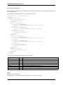
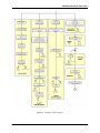
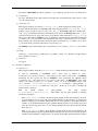
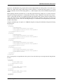
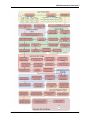
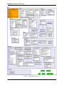
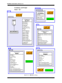
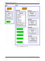
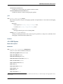
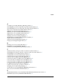
The following diagram gives an overview of the steps taken by the insarApp script to generate an interferogram,
including the initial part under the user’s control (in green).
2.3. Process Workflow
17
option:
ISCE Documentation, Release 0.3
18
Chapter 2. Running ISCE
ISCE Documentation, Release 0.3
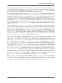
Figure 2.1: insarApp workflow diagram
2.3. Process Workflow
19
ISCE Documentation, Release 0.3
Convention: In the next sections where we describe the process more in detail, we use the following emphasis
convention:
• path/to/folder/ : path to a folder or a file (relative to $ISCE_HOME)
• file.ext: file name (the file path should be easily deduced from context)
• variableName: name of a variable used in the Python code
• function(): name of a function or a method
• Class: class name (if not given, the name of the file that implements it should be class.py)
2.3.1 Preparing the Application to Run
Once the required data have been gathered, the user can call insarApp.py with insar.xml as argument, where the xml
file is an ASCII-file describing the input parameters. The python code starts by preparing the application to run while
implementing all the methods needed to generate an interferogram.
When the user issues the command:
python $ISCE_HOME/applications/insarApp.py insar.xml
python starts by executing the __main__ block inside insarApp.py. The first line of that block creates an Insar object
called insar:
insar = Insar()
Note: The above command creates an instance of the Insar class (also known as an Insar object) and calls its
__init__() method.
The Insar class, defined in insarApp.py, is a child class of Application that inherits from Component, which in
turn derives from ComponentInit. Hence, when instantiated through its method __init__(), insar has all the
properties and methods of its ancestors.
An object _insar of type InsarProc is then added to insar:
self._insar = InsarProc.InsarProc()
That object holds the properties, along with the methods (setters and getters) to modify and return their values, which
will be useful for the interferometric process.
Using the RunWrapper class and the functions defined in Factories.py, the application will then wrap all the methods
needed to run insar, e.g.:
self.runPreprocessor = InsarProc.createPreprocessor(self)
Note: The above command calls the function createPreprocessor(), found in Factories.py (imported by
__init__.py inside components/isceobj/InsarProc/ ). It takes the function runPreprocessor() defined in components/isceobj/InsarProc/runPreprocessor.py and attaches it to the object insar by means of a RunWrapper object.
Now, insar has an attribute called runPreprocessor which is linked to a function also called runPreprocessor().
The methods thus defined become methods of insar and will be called later, directly from insar, to process the data.
Once the initialization is done, the code calls the method run() defined in Application, insar‘s parent class:
insar.run()
20
Chapter 2. Running ISCE
ISCE Documentation, Release 0.3
2.3.2 Processing the Input Parameters
After the initialization of the application, the command line is processed to extract the argument(s) passed to insarApp.py. The application needs parameters to be given in order to run. Those input parameters can be passed
directly in the command line or via an xml file (called e.g. insar.xml) and are used to initialize the properties and the
facilities of the application.
Note: Only xml files are supported in the current distribution.
The command line is processed by Application‘s method _processCommandLine(), which gets the command
line and parses it through the method commandLineParser() of a Parser object PA. Since the passed argument
refers to an xml file, PA calls the method parse() of an XmlParser instance.
The parsing is facilitated by the ElementTree XML API (module xml.etree.ElementTree) which reads the xml file and
stores its content in an ElementTree object called root. root is then parsed recursively by a Parser object to extract
the components and the properties inside the file (parseComponent(), parseProperty()). When done, we
get a dictionary called catalog, containing a cascading set of dictionaries with all the properties included in the xml
file(s). In our example, catalog‘s content would look like this:
{ ’sensor name’: ’ALOS’,
’Master’: { ’imagefile’: ’../ALOS2/IMG-HH-ALPSRP028910640-H1.0__A’,
’leaderfile’: ’../ALOS2/LED-ALPSRP028910640-H1.0__A’,
’output’: ’master.raw’ },
’Slave’: { ’imagefile’: ’../ALOS2/IMG-HH-ALPSRP042330640-H1.0__A’,
’leaderfile’: ’../ALOS2/LED-ALPSRP042330640-H1.0__A’,
’output’: ’slave.raw’ },
’Dem’: { ’data_type’: ’SHORT’,
’tile_height’: 1,
’width’: 3601,
’file_name’: ’SaltonSea.dem’,
’access_mode’: ’read’
’delta_longitude’: 0.000833333,
’delta_latitude’: -0.000833333,
’first_longitude’: -117.0,
’first_latitude’: 34.0 } }
Then, the application parameters are defined through insar‘s method _parameters(): those are the parameters that
can be configured in the input xml file. For each parameter, the following information is needed: private name (known
to the application only), public name (disclosed to the user), type (int, string, etc.), units, default value (if parameter is
omitted), mandatoriness (the parameter must be present in the xml file or not), description. Each and everyone of those
parameters are represented by an attribute of the insar object, whose name is the parameter’s private name and whose
value is given by the parameter’s default value. Also, we end up with several dictionaries (descriptionOfVariables,
typeOfVariables and dictionaryOfVariables) and lists (mandatoryVariables and optionalVariables) that help organize
the parameters according to their characteristics.
With the configurable parameters thus defined, the code calls initProperties() which checks catalog‘s content
and assigns the user’s values to the given parameters.
Then, the application facilities are defined through insar‘s method _facilities(). Facilities are objects whose
class can only be determined when the code reads the user’s parameters. Their nature cannot be hardcoded in advance,
so that they will be created by the code at runtime using modules called factories. For insarApp.py, those facilities are
master (master sensor), slave (slave sensor), masterdop (master doppler), slavedop (slave doppler) and dem. For each
facility, the following information is needed: private name (known to the application only), public name (disclosed to
the user), module (package where the factory is present), factory (name of the method capable of creating the facility),
args and kwargs (additional arguments that the factory might need in order to create the facility), mandatoriness,
description. Each and everyone of those facilities are represented by an attribute of the insar object, whose name is
the facility’s private name and whose value is an object of class EmpytFacility. The dictionaryOfFacilities is updated
2.3. Process Workflow
21
ISCE Documentation, Release 0.3
to reflect the list of facilities that can be configured in the input xml file.
Finally, the facilities are given their actual type and properties according to the user’s parameters, with the method
_processFacilities().
2.3.3 Preparing the Data to Be Processed
The application needs to read and ingest the pair of image products with their header files and the given doppler
method to produce raw data which will be processed later. If a dem has not been given, the application proceeds to
download one from the SRTM database (make sure that you have an internet connection).
At this step, run() executes insar‘s main() method which calls help() to output an initial message about the
application and creates a Catalog object for logging purposes:
self.insarProcDoc = isceobj.createCatalog(’insarProc’)
The current time is also recorded in order to assess the duration of the following steps, the first of which is
runPreprocessor().
runPreprocessor() takes the four input facilities (master, slave, masterdop and slavedop) and generates one raw
image for each pair of Sensor and Doppler objects: master.raw and slave.raw (the output names can be configured in
the xml file). First, runPreprocessor() passes the pair master/masterdop to a make_raw() method - to avoid
confusion, let’s call it insar.make_raw(), which returns a make_raw object. To do that, insar.make_raw()
creates a make_raw object (whose class is defined in applications/make_raw.py), wires the pair of facilities as input
ports to that object and executes its make_raw() method - called make_raw.make_raw() to avoid confusion.
make_raw.make_raw() starts by activating the make_raw object’s ports, i.e., adding master as its sensor attribute and masterdop as its doppler attribute. Then, it extracts the raw data from master. Here it is assumed that
each supported sensor has implemented a method called extractImage(). For example, the ALOS class, defined
in components/isceobj/Sensor/ALOS.py, expects four parameters, of which three are mandatory, to be given in the
input xml file: IMAGEFILE, LEADERFILE, OUTPUT and RESAMPLE_FLAG (optional). extractImage()
parses the leaderfile and the imagefile, extracts raw data to output (with resampling or not), creates the appropriate metadata objects with populateMetadata() (Platform, Instrument, Frame, Orbit, Attitude and Distortion) and generates a .aux file (master.raw.aux) with readOrbitPulse(). Once the raw data has been extracted, make_raw.make_raw() calculates the doppler values and fits a polynomial to those values by calling masterdop‘s method calculateDoppler() and fitDoppler(). The Doppler polynomial coefficients
and the pulse repetition frequency are then transferred to a Doppler object called dopplerValues. The spacecraft height and height_dt (calculateHeighDt()), velocity (calculateVelocity()) and squint angle
(calculateSquint()) are also computed whereas the sensing start is adjusted according to values in the pulse
timing .aux file (adjustSensingStart()).
Most of the attributes in the make_raw object are copied to a RawImage object, called masterRaw: filename, Xmin,
Xmax, number of good bytes (Xmax - Xmin), width (Xmax). The same steps are done with the pair slave/slavedop as
well. Finally, the following values are assigned to _insar‘s attributes: _masterRawImage, _slaveRawImage, _masterFrame, _slaveFrame, _masterDoppler, _slaveDoppler, _masterSquint, _slaveSquint.
Once runPreprocessor() has been executed, insar‘s main() method checks if a dem has been given. If not,
it assesses the common geographic area between the master and slave frames, taking into account the master and
slave squint angles, with the method extractInfo(). Then, createDem() downloads a DEM from the STRM
database, generates an xml file and creates a DemImage object assigned to _insar as _demImage.
2.3.4 Running the Interferometric Application
Now that all the data and metadata are ready to get processed, we can proceed to the core of the interferometric
application with the following steps:
22
Chapter 2. Running ISCE
ISCE Documentation, Release 0.3
1. data focussing
2. interferogram building
3. interferogram refining
4. coherence computing
5. filter application
6. phase unwrapping
7. geocoding
1. Data Focussing
(a) runPulseTiming
This wrapper is linked to the method runPulseTiming() which generates an interpolated orbit for
each image (master and slave).
From the master frame, the method pulseTiming() generates an Orbit object containing a list of
StateVector objects - one for each range line in the frame. The state vectors are interpolated from the
original orbit, using the Hermite interpolation scheme (a C code). The satellite’s position and velocity are
evaluated at the time of each pulse.
Idem for the slave frame.
The pair of pulse Orbit objects generated are assigned to _insar as _masterOrbit and _slaveOrbit.
(b) runEstimateHeights
This wrapper is linked to the method runEstimateHeights() which calculates the height and the
velocity of the platform for each image (master and slave).
For the master image (and then for the slave image), the code starts by instantiating a
CalcSchHeightVel object using the function createCalculateFdHeights() defined
in components/stdproc/orbit/__init__.py.
The CalcSchHeightVel class is defined in components/stdproc/orbit/orbitLib/CalcSchHeightVel.py. Three input ports are wired to the CalcSchHeightVel
object: _masterFrame (_slaveFrame for the slave image), _masterOrbit (_slaveOrbit) and planet. planet
is extracted from _masterFrame. The CalcSchHeightVel object’s method calculate() is then called,
computing the height and the velocity of the platform.
The computed master and slave heights are assigned to _insar as _fdH1 (with setFirstFdHeight())
and _fdH2 (with setSecondFdHeight()) respectively.
(c) runSetmocomppath
This wrapper is linked to the method runSetmocomppath() which selects a common motion compensation path for both images.
The method begins with the instantiation of a Setmocomppath object using the function
createSetmocomppath() found in components/stdproc/orbit/__init__.py. The Setmocomppath
class is defined in Setmocomppath.py, located in the same folder. Three input ports are wired to the
Setmocomppath object: planet, _masterOrbit and _slaveOrbit. Then, the method setmocomppath()
of that object is executed: using a Fortran code, it takes the pair of orbits and picks a motion compensation
trajectory. It returns a Peg object (representing a peg point with the following information: longitude,
latitude, heading and radius of curvature), which is the average of the two peg points computed from the
master orbit and the slave orbit. It gives also the average height and velocity of each platform.
The computed peg, average heights and velocities are assigned to _insar as _peg, _pegH1 (with
setFirstAverageHeight()), _pegH2 (with setSecondAverageHeight()), _pegV1 (with
setFirstProcVelocity()) and _pegV2 (with setSecondProcVelocity()).
2.3. Process Workflow
23
ISCE Documentation, Release 0.3
(d) runOrbit2sch
This wrapper is linked to the method runOrbit2sch() which converts the orbital state vectors of the
master and slave orbits from xyz to sch coordinates.
For the master orbit (and then for the slave orbit), the method starts by instantiating an Orbit2sch object using the function createOrbit2sch() found in components/stdproc/orbit/__init__.py. The Orbit2sch
class is defined in Orbit2sch.py, located in the same folder. The mean value of _pegH1 and _pegH2 (first
and second average heights) is assigned to the Orbit2sch object while three input ports are wired to it:
planet, _masterOrbit (_slaveOrbit for the slave image) and _peg. Then, the orbit2sch() method converts the coordinates of the orbit into the sch coordinate system, using a Fortran code. It returns an Orbit
object with a list of StateVector objects whose coordinates are now in sch.
The two newly-computed orbits replace _masterOrbit and _slaveOrbit in _insar.
(e) updatePreprocInfo
This wrapper is linked to the method runUpdatePreprocInfo() that calls runFdMocomp() to
calculate the motion compensation correction for Doppler centroid: here, it returns fd, the average correction for masterOrbit and slaveOrbit. fd is used as the fractional centroid of averageDoppler, which
is the average of _masterDoppler and _slaveDoppler (the doppler centroids previously calculated in
runPreprocessor()).
averageDoppler is then assigned to _insar as _dopplerCentroid.
(f) runFormSLC
This wrapper is linked to the method runFormSLC() which focuses the two raw images using a rangedoppler algorithm with motion compensation.
For the master raw image (and then for the slave raw image), the method starts by instantiating a Formslc
object using the function createFormSLC() found in components/stdproc/stdproc/formslc/__init__.py.
The Formslc class is defined in Formslc.py, located in the same folder. Seven input ports are wired to the
Formslc object: _masterRawImage (_slaveRawImage), masterSlcImage (slaveSlcImage), _masterOrbit
(_slaveOrbit), _masterFrame (_slaveFrame), planet, _masterDoppler (_slaveDoppler) and _peg. The
spacecraft height is set to the mean value of _fdH1 (first Fd Height) and _fdH2 (second Fd Height), and its
velocity to the mean value of _pegV1 (first Proc Velocity) and _pegV2 (second Proc Velocity). The method
formslc() of the Formslc object is then called, which generates a .slc file (master.slc and slave.slc).
The two generated SlcImage objects are assigned to _insar as _masterSlcImage and _slaveSlcImage, along
with _patchSize, _numberValidPulses and _numberPatches. The two Formslc objects used to generate the
slcs are also assigned to _insar as _formSLC1 and _formSLC2.
2. Interferogram Building
(a) runOffsetprf
This wrapper is linked to the method runOffsetprf() which calculates the offset between the two slc
images.
It starts by instantiating an Offsetprf object using the function createOffsetprf() found in components/isceobj/Util/__init__.py. The Offsetprf class is defined in Offsetprf.py, located in the same folder.
The method offsetprf() of the Offsetprf object is then called, with _masterSlcImage and _slaveSlcImage passed as arguments. It returns, via a Fortran code, an OffsetField object which compiles a list of
Offset objects, each describing the coordinates of an offset, its value in both directions (across and down)
and the signal-to-noise ratio (SNR).
The computed OffsetField object is assigned to _insar twice: as _offsetField and _refinedOffsetField.
(b) runOffoutliers
24
Chapter 2. Running ISCE
ISCE Documentation, Release 0.3
This wrapper is linked to the method runOffoutliers() which culls outliers from the previously
computed offset field. The offset field is approximated by a best fitting plane, and offsets are deemed to be
outliers if they are greater than a user selected distance.
It is executed three times with a distance value set to 10, 5 then 3 meters. For each iteration, it
makes use of an Offoutliers object, created by the function createOffoutliers() found in components/isceobj/Util/__init__.py. The Offoutliers class is defined in Offoutliers.py, located in the same
folder. One input port is wired to the Offouliers object: _refinedOffsetField. The SNR is fixed to 2.0 while
the distance is the value set at each iteration. The method offoutliers() of the Offoutliers object is
then called and returns a new OffsetField object, replacing _refinedOffsetField in _insar.
(c) prepareResamps
This wrapper is linked to the method runPrepareResamps() which calculates some parametric values
for resampling (slant range pixel spacing, number of azimuth looks, number of range looks, number of
resamp lines) and fixes the number of fit coefficients to 6.
(d) runResamp
This wrapper is linked to the method runResamp() which resamples the interferogram based on
the provided offset field.
It begins with the instantiation of a Resamp object, using the function createResamp() found
in components/stdproc/stdproc/resamp/__init__.py. The Resamp class is defined in Resamp.py, located in the same folder. Two input ports are wired to the Resamp object: _refinedOffsetField and
instrument, along with some more parameters. The method resamp() is then called with four input
arguments: the two slcs as well as AmpImage and IntImage objects. Through a Fortran code, the
two slcs are coregistered and processed to form an interferogram that is then multilooked according to the values calculated in the previous step. Two files are generated: resampImage.amp and
resampImage.int.
The AmpImage and IntImage objects are assigned to _insar as _resampAmpImage and _resampIntImage.
(a) runResamp_image
This wrapper is linked to the method runResamp_image() which plots the offsets as an image.
It begins with the instantiation of a Resamp_image object using the function
createResamp_image() found in components/stdproc/stdproc/resamp_image/__init__.py.
The Resamp_image class is defined in Resamp_image.py, located in the same folder. Two input
ports are wired to the Resamp_image object: _refinedOffsetField and instrument, along with some
more parameters. Then, the method resamp_image() of that object is called with two OffsetImage objects as arguments (one accross and one down): using a Fortran code, that method takes the
offsets and plots them as an image, generating two files: azimuthOffset.mht and rangeOffset.mht.
The accross OffsetImage and down OffsetImage objects are assigned to _insar as _offsetRangeImage and _offsetAzimuthImage respectively.
(a) runMocompbaseline
This wrapper is linked to the method runMocompbaseline() which calculates the mocomp
baseline. It iterates over the S-component of the master image and interpolates linearly the SCH
coordinates at the corresponding S-component in the slave image. The difference between the master
SCH coordinates and the slave SCH coordinates provides a 3-D baseline.
It begins with the instantiation of a Mocompbaseline object using the function
createMocompbaseline() found in components/stdproc/orbit/__init__.py.
The Mocompbaseline class is defined in Mocompbaseline.py, located in the same folder. Four input ports
are wired to the Mocompbaseline object: _masterOrbit, _slaveOrbit, ellipsoid and _peg, along with
some more parameters. Then, the method mocompbaseline() of that object is called: using
2.3. Process Workflow
25
ISCE Documentation, Release 0.3
a Fortran code, that method gets the insar baseline from mocomp and position files, updating the
properties of the Mocompbaseline object.
The Mocompbaseline object is assigned to _insar as _mocompBaseline.
(a) runTopo
This wrapper is linked to the method runTopo() which approximates the topography for each pixel of
the interferogram.
At this step, _resampIntImage is duplicated as _topoIntImage inside _insar.
Then the code
starts by instantiating a Topo object using the function createTopo() found in components/stdproc/stdproc/topo/__init__.py. The Topo class is defined in Topo.py, located in the same folder.
Five input ports are wired to the Topo object: _peg, _masterFrame, planet, _demImage and _topoIntImage, along with some more parameters. Then, the method topo() of that object is called: using a Fortran
code, it approximates the topography and generates temporary files giving, for each pixel, the following
values: latitude (lat), longitude (lon), height in SCH coordinates (zsch), real height in XYZ coordinates (z)
and the height in XYZ coordinates rounded to the nearest integer (iz).
The Topo object is assigned to _insar as _topo.
(b) runCorrect
This wrapper is linked to the method runCorrect() which carries out a flat earth correction of the
interferogram.
It starts by instantiating a Correct object using the function createCorrect() found in components/stdproc/stdproc/correct/__init__.py. The Correct class is defined in Correct.py, located in the same
folder. Four input ports are wired to the Correct object: _peg, _masterFrame, planet, and _topoIntImage,
along with some more parameters. Then, the method correct() of that object is called: using a Fortran code, it reads the interferogram and the SCH height file, and removes the topography phase from the
interferogram. It generates two files: topophase.flat (the flattened interferogram) and topophase.mph (the
topography phase).
(c) runShadecpx2rg
This wrapper is linked to the method runShadecpx2rg() which combines a shaded relief from the
DEM in radar coordinates and the SAR complex magnitude image into a single two-band image.
It begins with the instantiation of a Shadecpx2rg object using the function
createShadecpx2rg() found in components/isceobj/Util/__init__.py. The Shadecpx2rg
class is defined in Shadecpx2rg.py, located in the same folder. After initializing some parameters,
the method shadecpx2rg() of that object is called with four arguments: a DemImage object
referencing the height file (iz), an IntImage object referencing the resampled amplitude image
(resampImage.amp), an IntImage object referencing the Rg Dem image to be written (rgdem) and a
shade factor equal to 3. Using a Fortran code, that method computes, for each pixel, a shade value
and multiplies that factor to the magnitude value. It generates a file called rgdem.
The RgImage object referencing the file rgdem and the DemImage referencing the file iz are assigned
to _insar as _rgDemImage and _heightTopoImage respectively.
13. Interferogram Refining
(a) runRgoffset
This wrapper is linked to the method runRgoffset() which estimates the subpixel offset between two
images stored as one rg file.
It starts by instantiating an Rgoffset object using the function createRgoffset() found in components/isceobj/Util/__init__.py. The Rgoffset class is defined in Rgoffset.py, located in the same folder.
After initializing some parameters, the method rgoffset() of that object is called with an RgImage
object as argument, referencing the file rgdem.
26
Chapter 2. Running ISCE
ISCE Documentation, Release 0.3
It generates an OffsetField object that is assigned to _insar, replacing _offsetField and _refinedOffsetField.
(b) runOffoutliers
See step 8. This method culls outliers from the offset field. It is executed three times with a distance value
set to 10, 5 then 3 meters.
(c) runResamp_only
This wrapper is linked to the method runResamp_only() which resamples the interferogram.
It begins with the instantiation of a Resamp_only object using the function createResamp_only()
found in components/stdproc/stdproc/resamp_only/__init__.py. The Resamp_only class is defined in Resamp_only.py, located in the same folder. Two input ports are wired to the Resamp_only object: _refinedOffsetField and instrument, along with some more parameters. Then, the method resamp_only() of
that object is called with two IntImage objects as arguments (one referencing the resampled interferogram
resampImage.int to be read, and the other referencing a file called resampOnlyImage.int to be written):
using a Fortran code, that method takes the interferogram and resamples it to coordinates set by offsets
(_refinedOffsetField), generating a file called resampOnlyImage.int.
The IntImage object referencing the file resampOnlyImage.int is assigned to _insar as _resampOnlyImage.
(d) runTopo
At this step, _resampOnlyImage is duplicated as _topoIntImage inside _insar. Then the code approximates
the topography as in step 13.
(e) runCorrect
See step 14.
16. Coherence Computation
(a) runCoherence
This wrapper is linked to the method runCoherence() which calculates the interferometric correlation.
It starts by instantiating a Correlation object, whose class is defined in components/mroipac/correlation/correlation.py. Two input ports are wired to that object: an IntImage
referencing the file topophase.flat and an AmpImage object referencing the amplitude image
resampImage.amp. One output port is also wired to that object: an OffsetImage object referencing a file called topophase.cor to be written. Then, one of the Correlation object’s methods is executed: calculateEffectiveCorrelation() if method is ‘phase_gradient’, or
calculateCorrelation() if method is ‘cchz_wave’. Both rely on C codes to calculate the
interferometric correlation.
Here
the
default
method
is
calculateEffectiveCorrelation().
the effective correlation:
‘phase_gradient’:
the
script
executes
That method uses the phase gradient to calculate
• First, phase_slope() is called to calculate the phase gradient. It takes nine arguments: the interferogram filename (topophase.flat), the phase gradient filename (a temporary file to be written), the
number of samples per row (interferogram width), the size of the window for the gradient calculation
(default: 5), the gradient threshold for phase gradient masking (default: 0), the starting range pixel
offset (0), the last range pixel offset (-1), the starting azimuth pixel offset (0) and the last azimuth
pixel offset (-1).
• Then, phase_mask() is called to create the phase gradient mask. It takes eleven arguments: the
interferogram filename, the phase gradient filename (the temporary file previously created), the phase
standard deviation filename (a temporary file to be written), the standard deviation threshold for phase
2.3. Process Workflow
27
ISCE Documentation, Release 0.3
gradient masking (default: 1), the number of samples per row, the range and azimuth smoothing
window for the phase gradient (default: 5x5), the starting/last range/azimuth pixel offsets.
• Finally, magnitude_threshold() is called to threshold the phase file using the magnitude values
in the coregistered interferogram. It takes five arguments: the interferogram filename, the phase standard deviation filename (the temporary file previously created), the output filename (topophase.cor),
the magnitude threshold for phase gradient masking (default: 5e-5) and the number of samples per
row.
The other method calculateCorrelation() uses the maximum likelihood estimator to calculate
the correlation. It calls cchz_wave() which takes nine arguments: the interferogram filename, the
amplitude filename (resampImage.amp), the output correlation filename (topophase.cor), the width of
the interferogram file, the width of the triangular smoothing function (default: 5 pixels), the starting/last
range/azimuth pixel offsets.
21. Filter Application
(a) runFilter
This wrapper is linked to the method runFilter() which applies the Goldstein-Werner power-spectral
filter to the flattened interferogram.
It starts by instantiating a Filter object, whose class is defined in components/mroipac/filter/Filter.py. One
input port and one output port are wired to that object: an IntImage referencing the flattened interferogram (topophase.flat), and another IntImage object referencing the filtered interferogram to be created
(filt_topophase.flat), respectively. Then, the method goldsteinWerner() is called with an argument
alpha, representing the strength of the Goldstein-Werner filter (default: 0.5). That method applies a powerspectral smoother to the phase of the interferogram:
• First, separate the magnitude and phase of the interferogram and save both bands.
• Second, apply the power-spectral smoother to the original interferogram.
• Third, take the phase regions that were zero in the original image and apply them to the smoothed
phase.
• Fourth, combine the smoothed phase with the original magnitude, since the power-spectral filter distorts the magnitude.
The first steps are done with the method psfilt() while the last one is done with the method
rescale_magnitude(). Both methods are based on C code.
Now _topophaseFlatFilename in _insar is set to filt_topophase.flat.
22. Phase Unwrapping
(a) runGrass
This wrapper is linked to the method runGrass() which unwraps the filtered interferogram using the
grass algorithm.
This step is executed only if required by the user in the xml file. It starts by instantiating a Grass object,
whose class is defined in components/mroipac/grass/grass.py. Two input ports are wired to that object:
an IntImage referencing the filtered interferogram (filt_topophase.flat) and an OffsetImage object referencing the coherence image to be created (filt_topophase.cor). One output port is also wired to the Grass
object: an IntImage object referencing the unwrapped interferogram to be created (filt_topophase.unw).
Then, the method unwrap() is called:
• First, it creates a flag file for masking out the areas of low correlation (default threshold: 0.1) calling
the following C functions: residues(), trees() and corr_flag().
• Then, it unwraps the interferogram using the grass algorithm with the C function grass().
28
Chapter 2. Running ISCE
ISCE Documentation, Release 0.3
23. Geocoding
(a) runGeocode
This wrapper is linked to the method runGeocode() which generates a geocoded interferogram.
It begins with the instantiation of a Geocode object using the function createGeocode() found
in components/stdproc/rectify/__init__.py. The Geocode class is defined in Geocode.py, located in
the subfolder components/stdproc/rectify/geocode/. Five input ports are wired to the Geocode object:
_peg, _masterFrame, planet, _demImage and an IntImage object referencing the filtered interferogram
(filt_topophase.flat), along with some more parameters. Then, the method geocode() of that object is
called: using a Fortran code, that method takes the interferogram and orthorectifies it (i.e., correcting its
geometry so that it can fit a map with no distortions).
Two files are generated at this step: a geocoded interferogram (topophase.geo) and a cropped dem
(dem.crop).
After the interferometric process is done, the application stops the timer and returns the total time required to finish all
the operations. Finally, it dumps all the metadata about the process into an insarProc.xml file:
self.insarProcDoc.renderXml()
2.3. Process Workflow
29
ISCE Documentation, Release 0.3
30
Chapter 2. Running ISCE
CHAPTER
THREE
IONOSPHERIC FARADAY ROTATION
3.1 Background
3.1.1 Motivation
Inhomogeneities in ionospheric structure such as plasma irregularities lead to distortions in low frequency (L-band
and lower) Synthetic Aperture Radar (SAR) images [FreSa04]. These inhomogeneities hamper the interpretation of
ground deformation when these SAR images are combined to form interferograms. To mitigate the effects of these
distortions, [Pi12] outlined a methodology for the estimation and removal of ionospheric artifacts from individual,
fully-polarimetric SAR images. The estimation methodology also provides a way to create temporal snapshots of
ionospheric behavior with large (40km) spatial extent. To demonstrate these capabilities for fully polarimetric spaceborne SAR to provide images of the ionosphere, we have developed computer software to implement the methodology
outlined in [Pi12].
3.1.2 Methodology behind ISSI
The measured scattering matrix from an L-band polarimetric SAR can be written as:
M = A(r, θ)eiφ RT RF SRF T + N,
(3.1)
with
M
R
T
RF
S
T
Mhh
Mvh
1
δ2
cos Ω
− sin Ω
Shh
Svh
1
δ4
=
=
=
=
=
δ1
f1
Mhv
Mvv
sin Ω
cos Ω
Shv
Svv
δ3
f2
where Sij is the scattering matrix, A(r, θ) is the gain of the radar as a function of range and elevation angle, δi are the
cross-talk parameters, fi are the channel imbalances, and Ω is the Faraday rotation [Fre04]. By rearranging equation
(3.1), we can apply the cross-talk and channel imbalance corrections while preserving the effects of Faraday rotation,
yielding.
1
1
f1 −δ2
f2 −δ3
M 0 = RF SRF =
M
.
−δ1
1
−δ4
1
f1 − δ1 δ2 f1 − δ3 δ4
31
ISCE Documentation, Release 0.3
We can now use M 0 , the partially-polarimetrically calibrated data matrix, to estimate the Faraday rotation using the
method outlined in [Bick65]. We begin by transforming M 0 into a circular basis, yielding,
Z11 Z12
1 i
1 i
0
=
M
.
(3.2)
Z21 Z22
i 1
i 1
The Faraday rotation can then be calculated as,
Ω = arg(Z12 Z ∗21 )
(3.3)
Given a measurement of Faraday rotation and an estimate of the strength of the Earth’s magnetic B-field, one can then
estimate the Total Electron Count (TEC) using the relationship,
Z
Ωf 2
(3.4)
ne B cos θds =
,
k
3
where k = 8π2|e|
c0 m2e with e being the elementary charge, c is the speed of light 0 is the permittivity of free space, me
is the electron mass, ne is the electron density, θ is the angle between the SAR signal propagation direction and the
B-field and f is the carrier frequency of the radar. Since the the angle $theta$, does not change much along the path
through the ionosphere, we can move the B cos θ term out of the integral in equation (3.4). This allows us to rewrite
equation (3.4) as,
T EC =
where T EC =
R
Ωf 2
kB cos θ
(3.5)
ne ds.
Ideally, we would calculate the strength of the Earth’s B-field along the path from the radar to the ground at each pixel
in the SAR image. Since, at the scale of a typical SAR image, the B-field is smoothly varying, we will make the
assumption that we can approximate the effect of the magnetic field by using the average B-field value over the area of
the SAR image. Additionally, we will make the assumption that B-field is homogeneous enough to allow us to replace
the line-of-sight path integration with a vertical integration through the ionosphere. This is an assumption that can
easily be changed in the future. We begin by calculating the geographic coordinates of the corners of our SAR image.
Then, we estimate the total strength of the magnetic B-field in the direction of the radar line-of-sight in a vertical
column above each geographic location. The average total strength of the magnetic B-field in radar line-of-sight is
then used to calculate the TEC at each pixel in the SAR image using equation (3.5).
Finally, the phase change contribution to the SAR image from the Faraday rotation can be calculated using the estimate
of TEC found from equation (3.5) as,
Z
ω
φI = −
Xds
2c
Z
2π
e2
= −
ne ds
c 8π 2 0 me f
8.45 × 10−7
=
T EC
f
ω
, where X = ωp , and ωp =
the SAR image.
ne e 2
0 me
21
is the angular plasma frequency. This value can be calculated at each pixel in
3.2 Running ISSI
SAR data can be acquired from ground processing facilities as raster images of focused or unfocused radar echos. ISSI
can accept either data format and produce images of Faraday rotation, TEC and phase delay. The most straightforward
32
Chapter 3. Ionospheric Faraday Rotation
ISCE Documentation, Release 0.3
application of the ISSI methodology begins with focused and aligned SAR data, which typically comes in the form of
single-look complex (SLC) images. These images are first rotated into a circular basis using equation (3.2), and an
estimate of Faraday rotation is formed using equation (3.3). TEC and phase delay are then calculated using subsequent
results.
When beginning with unfocused radar echos, we must first prepare SLC images, taking care to focus the radar echos
using the same Doppler parameters for each transmit and receive polarity combination. Once SLC’s have been produced, we must align each SLC by resampling the SAR data transmitted with vertical polarization such that it lies
on the same pixel locations as the SAR data transmitted with horizontal polarization. Once these steps have been
completed, we may proceed as before in converting the images to a circular basis and forming Faraday rotation, TEC
and phase delay images.
As input to the ISSI scripts, we require a set of XML files. Begin by creating a file called FR.xml and put the following
information in it:
<component>
<property>
<name>HH</name>
<factoryname>createALOS</factoryname>
<factorymodule>isceobj.Sensor</factorymodule>
<value>HH.xml</value>
</property>
<property>
<name>HV</name>
<factoryname>createALOS</factoryname>
<factorymodule>isceobj.Sensor</factorymodule>
<value>HV.xml</value>
</property>
<property>
<name>VH</name>
<factoryname>createALOS</factoryname>
<factorymodule>isceobj.Sensor</factorymodule>
<value>VH.xml</value>
</property>
<property>
<name>VV</name>
<factoryname>createALOS</factoryname>
<factorymodule>isceobj.Sensor</factorymodule>
<value>VV.xml</value>
</property>
</component>
Next, we will specify our output file names and options. Create a file called output.xml and put the following information in it:
<component>
<property>
<name>FILTER</name>
<value>None</value>
</property>
<property>
<name>FILTER_SIZE_X</name>
<value>21</value>
</property>
<property>
<name>FILTER_SIZE_Y</name>
<value>11</value>
</property>
<property>
3.2. Running ISSI
33
ISCE Documentation, Release 0.3
<name>TEC</name>
<value>tec.slc</value>
</property>
<property>
<name>FARADAY_ROTATION</name>
<value>fr.slc</value>
</property>
<property>
<name>PHASE</name>
<value>phase.slc</value>
</property>
</component>
Finally, create four XML files, one for each polarity combination, HH.xml, HV.xml, VH.xml and VV.xml, and place the
following information in them:
<component>
<property>
<name>LEADERFILE</name>
<value>LED-ALPSRP016410640-P1.0__A</value>
</property>
<property>
<name>IMAGEFILE</name>
<value>IMG-HH-ALPSRP016410640-P1.0__A</value>
</property>
</component>
We can now produce estimates of Faraday rotation, TEC and phase delay by running
$ISCE_HOME/applications/ISSI.py FR.xml output.xml
The code will create the Faraday rotation output in a file named fr.slc, TEC output in a file named tec.slc, and phase
delay in a file named phase.slc.
3.3 ISSI in Detail
This section details the structure and usage of ISSI.py, an application within ISCE that performs polarimetric processing. It assumes that the user has already installed Python and ISCE successfully. ISSI.py was written over a year
ago by a computer scientist, no longer contributing to the project at NASA JPL. As a result it is structured differently
from most other scripts written by the current software developers. Unfortunately, this means that understanding the
processing flow of ISSI.py is difficult, and other applications within ISCE do not serve as templates to help with the
task. Also, the structure of this program is extremely object oriented, where executing a function in ISSI.py may
call methods from up to five different Python scripts located elsewhere within ISCE’s file structure. Thus, this task
ultimately devolves to tracing out the processing flow as it takes you from script to script. Throughout this journey
into ISSI.py we limit the depth of understanding to processing tasks directly relevant to polarimetric processing. Other
components such as the wrapping process, the wrapped C and Fortran code itself, and computer resource management
are worthy of mention, but we do not dig into the specifics of their operation. We treat these portions of the code as
black boxes whose functionality is well understood.
The following diagram gives an overview of the steps taken by the ISSI scripts to calculate Faraday rotation, TEC and
phase delay.
34
Chapter 3. Ionospheric Faraday Rotation
ISCE Documentation, Release 0.3
3.3. ISSI in Detail
Figure 3.1: ISSI workflow diagram
35
ISCE Documentation, Release 0.3
3.3.1 Extracting Information from Xml Files
ISSI.py begins by running its main() method. It first creates an object called fi which is an instance of the class
FactoryInit. FactoryInit is a class in FactoryInit.py whose methods and attributes allow the program to extract information found in the six xml files required for processing (FR.xml, output.xml, HH.xml, HV.xml, VH.xml, VV.xml;
see Running ISSI). Whenever the program creates an instance of a Python class, it always runs the __init__()
method found within that class’ script. The FactoryInit class’ __init__() method simply defines the attributes of
the object and then returns to ISSI.py. In the remainder of the document, we gloss over this initialization process for
other objects because they all follow identical procedures.
ISSI.py then extracts information from the first input argument, FR.xml. To do this it sets two attributes of
fi, fileInit and defaultInitModule, to ‘FR.xml’ and ‘InitFromXmlFile’, respectively, and then runs the method
initComponentFromFile(). FactoryInit.py contains the definition of initComponentFromFile() because it is a method of the FactoryInit class; it returns a dictionary with all information found within FR.xml. The
function getComponent(), again inside FactoryInit.py, searches that dictionary and returns an instance of the
Sensor (i.e., the satellite) class responsible for creating that particular data file defined as the input argument of
getComponent(). ISSI.py supports different Sensor classes, and this guide follows the processing path assuming all four raw images are products of the ALOS/PALSAR mission. We therefore indicate by hh, hv, vh and vv the
four instances of the class ALOS, found in ALOS.py.
At this point, ISSI.py moves to the second input argument, output.xml. Frustratingly, extracting information from this
xml file requires a completely new object of class InitFromXmlFile, found in InitFromXmlFile.py. One of its methods
called init() (NOT to be confused with __init__()) extracts information from output.xml and returns it to an
attribute local to ISSI.py called variables. ISSI.py then distributes the information found in variables to other different
local attributes, including filter size and file names to be used later, that serve as input variables to an instance of the
class Focuser called focuser. main() in ISSI.py concludes by setting the filter and filterSize attributes of focuser and
then running focuser(), a method in the Focuser class that begins processing the raw images.
focuser() begins by calling the function useCalcDop(), found in __init__.py, that instantiates and returns an
instance, called doppler, of the class Calc_dop, found within Calc_dop.py. We see that useCalcDop() simply
redirects the program to the class Calc_dop. The object doppler later provides the attributes and methods necessary to
calculate Doppler information about the processed radar images.
3.3.2 Extracting Data from Input Files
Extraction of raw data from the input files begins with the creation of objects, called hh.raw, hv.raw, vh.raw and
vv.raw, which hold the output raw data from the extraction process. Following this the program runs the method
make_raw(), in ISSI.py, with both the raw data and Doppler objects passed as input arguments. The method
make_raw() immediately creates an instance of the class make_raw, called mr. The class make_raw resides in
another ISCE application named make_raw.py.
During the initialization of this class the program creates two input port objects. Port objects essentially serve as
conduits between Python objects, allowing one to access the attributes of another. After generating mr, the method
make_raw(), back in ISSI.py, finalizes the input ports by running the method wireInputPort(). The relevance
of this method lies only with Python object communication rather than polarimetric radar processing, so we will not
examine it in detail here. Finally, the object mr runs its own method called make_raw().
Note: We pause here to show the importance of constant vigilance when working with ISCE components. Follow
closely: we just ran ISSI.py’s method called make_raw(), which then created an instance of the class make_raw,
found in make_raw.py, which then ran make_raw(), a method of the class make_raw located in make_raw.py.
36
Chapter 3. Ionospheric Faraday Rotation
ISCE Documentation, Release 0.3
Then, in the make_raw() method of make_raw.py, the method extractImage() runs. The sensor class of the
image file, in our case ALOS for all four polarized images, contains the method extractImage(). Note that the
script ALOS.py contains definitions for not one but four different classes. The user must therefore look closely to see
which methods in ALOS.py fall under which classes; this will become relevant soon.
extracImage() begins with if statements designed to ensure that the user passed correct xml and image files
to ISSI.py. The first if statement ensures that the attributes _imageFileList and _leaderFileList are lists rather than
strings. The second quits the program if the number of leader and image files is not the same. The final if statements
protect against the case that an image file contains more than one image; if the user operates ISSI.py as instructed,
these if statements should be inconsequential. The program then creates instances of three new classes: an instance
of Frame, in Frame.py, called frame, and instances of the classes LeaderFile and ImageFile, called leaderFile and
imageFile, respectively, both in ALOS.py. The input argument to initialization of the LeaderFile class is the leader file
in memory.
The program then attempts to parse the leader file by running parse() on leaderFile. After opening the leader
file in read mode, parse() then creates an instance of the class CEOSDB, in CEOS.py, called leaderFDR. An
xml file containing the ALOS leader file record (also known as CEOS data file), provided already by ISCE, and the
leader file itself serve as input arguments for the initialization of CEOSDB. During initialization a local variable called
rootChildren stores an element tree of the information stored in the ALOS leader file record xml file. If the image file
being processed comes from a spacecraft with no leader file record, rootChildren simply becomes an empty list.
With leaderFDR completely initialized, it runs its method parse(). parse() opens the ALOS leader file record
and extracts any information it contains via an element tree; this user manual does not look any more closely at
how ISSI.py parses xml files. Find documentation on element trees for more information. If values found within
leaderFDR’s recently parsed metadata indicate to, the final lines of parse(), the method acting upon leaderFile,
perform the same element tree parsing process on scene header, platform position, spacecraft attitude, and spacecraft
calibration xml files, also all provided within ISCE. After closing the leader file, we return to extractImage()
where imageFile submits itself to a similar parsing process, also called parse() but found under the class ImageFile.
Then, we open the image file and, just like before, create an instance of the class CEOSDB called imageFDR, run parse() on this object, set the number SAR channels as found in imageFDR’s metadata, and run
_calculateRawDimensions() if the input argument calculateRawDimensions is true. For the ALOS case, calculateRawDimensions is false so the program skips over _calculateRawDimensions(). Finally, we close the
image file and return to extractImage().
The next portion of code decides whether the image ought to be resampled; it currently does not resample the image. Instead it moves on to run extractImage(), a method of the class ImageFile, on the image file itself.
extractImage() checks the data type of the image file. If the data is Level 1.5, it raises an exception and exits the
program. If the data is Level 1.1, a single-look-complex (SLC) image, it runs the method extractSLC(). Finally,
if the data is Level 1.0, the original raw image, the program runs extractRaw(). Level 1.0 data is the most basic
form of radar image, so we will explore this branch in order to ensure complete coverage of ISSI.py. If the processing
facility for the image file is ERSDAC, the program runs the method alose_Py() to extract the raw image. If not, it
runs alos_Py().
Note: Whenever you encounter a method whose name ends with _Py, you have found the beginning of the wrapping process described elsewhere in ISCE.pdf. In the current case, alos_Py ultimately refers to a function found in
ALOS_pre_process.c, one of the many pieces of original scientific software that inspired the ISCE project. Other
sections of ISCE.pdf describe in detail the Python wrapping process, and understanding the source code is left to radar
scientists. Therefore here we go no further into any method ending in _Py.
The methods alos_Py() and alose_Py() both perform the actual image extraction; look closely at
ALOS_pre_process.c to understand how. After they run, the program sets some local variables and then runs a method
createRawImage(). createRawImage() returns an instance of the class RawImage, in RawImageBase.py,
called rawImage. The RawImage class serves as ISSI.py’s means of storing and manipulating a raw image. The program creates a new instance of this class every time it needs to process a raw image in any way. After setting some
attributes of rawImage with information from the raw image’s metadata, it sets the raw image to be the image in the
3.3. ISSI in Detail
37
ISCE Documentation, Release 0.3
frame of the original ALOS sensor object. Frames can hold more than one image, however the design of ISSI.py
ensures that each frame holds only one.
3.3.3 Pre-Focusing Calculations
Minor bookkeeping as well as orbit and Doppler calculations follow the data extraction procedure.
populateMetadata(), a method of the ALOS class, first creates and fills metadata objects from the CEOS format metadata generated earlier. It is worth noting here that one of the methods in populateMetadata(), called
_populateDistortions(), creates the transmit and receive polarimetric calibration distortion matrices. The
polarimetric calibration process later implements these matrices during the formation of the SLC image.
The method readOrbitPulse(), with the leader file, image file, and image width as input parameters, prepares
to calculate the ALOS positions and times of the raw image. The method creates instances of three image classes,
RawImage, StreamImage, and Image, called rawImage, leaImage and auxImage, respectively. The class StreamImage holds and manipulates the leader file in memory while the Image class creates a generic image object. Each
image object has an associated image accessor, which it passes to other objects, allowing them to access the image in
memory. Finally, readOrbitPulse() runs three separate methods called setNumberBitesPerLine_Py(),
setNumberLines_Py() and readOrbitPulse_Py(). These methods wrap Fortran source code that fills auxImage with an auxiliary file of file extension .raw.aux, containing the ALOS positions and times of the raw image.
After this process, the method finalizes the three image objects and returns to extractImage(). The program
appends the frame created earlier to the list of frames in memory and then returns to make_raw() to begin Doppler
calculations.
If the image extracted earlier is Level 1.0 data, make_raw() wires three input ports to doppler so that it may access
attributes of the instrument, raw image, and frame objects. doppler then calculates the Doppler fit for the raw image
using calculateDoppler(), a method of the Calc_dop class. This method creates yet another RawImage object
to access the image, and then passes that object’s accessor to calc_dop_Py(), a method that wraps the source
code calc_dop.f90. As with all methods that include wrapped source code, calculateDoppler() contains a
significant amount of pre-processing steps, including setting the state of Fortran compatible parameters necessary for
the wrapped source code as well as allocating memory for its processes. After calc_dop.f90 calculates the Doppler
fit for the image, calculateDoppler() deallocates memory and runs getState(), a method that grabs the
information calc_dop.f90 calculated and loads it into attributes of the Python object doppler.
Next, doppler runs its method fitDoppler(), whose original purpose is to fit a polynomial to the Doppler values.
Inside the fitDoppler() method itself, however, we find that rather than perform a polynomial fit, it simply sets
the first Doppler coefficient to the zero order term found earlier, leaving all others at zero. To conclude Doppler
processing, make_raw() establishes both pulse repetition frequency and the Doppler coefficients as local variables
and then loads them directly into an object called dopplerValues, an instance of the class Doppler found in Doppler.py.
If the original input data is Level 1.1, an SLC image, the program does not calculate Doppler values and instead loads
all zeros into dopplerValues. Doppler coefficients allow the generation of an SLC image from a raw image; if the data
comes in as an SLC image, the Doppler coefficients are unnecessary.
Following Doppler processing, make_raw() comes to a close by calculating the velocity, squint angle, and change
in height of the spacecraft. Each calculation requires a different method, and each method gets certain parameters
of the image and uses them to calculate the desired result in Python. The only method worth investigating here
is calculateHeightDt() because it implements the method interpolateOrbit(). Found in Orbit.py,
interpolateOrbit() offers three ways of interpolating the state vector of an orbit; it performs linear interpolation, interpolation with an eighth order Legendre polynomial, or Hermite interpolation. The math of these different
interpolation techniques lies beyond the scope of this user guide. After interpolating the orbit at both the start and
mid-times of the image capture, calculateHeightDt() calculates the height of the spacecraft using a method in
Orbit.py called calculateHeight(). calculateHeight() itself runs a method called xyz_to_llh() that
converts the spacecraft ellipsoid from Cartesian coordinates to latitude, longitude, and height, and returns height. The
method calculateHeightDt() concludes using the height and time parameters just calculated to determine the
change in height over time.
38
Chapter 3. Ionospheric Faraday Rotation
ISCE Documentation, Release 0.3
Finally, make_raw() concludes with renderHdr(), a method in Image.py that creates an xml file containing
important parameters of the raw image.
3.3.4 Focusing the Raw Image
The process of creating an SLC image begins with estimating an average Doppler coefficient fd for all of the polarized
images. It adds all four coefficients together and divides by four. ISSI.py then runs focus(), with the raw image
object and average Doppler coefficient as input arguments.
The first step in focus(), after getting parameters necessary for processing, calculates a value called peg point. Also
found in ISSI.py, calculatePegPoint() passes the frame, planet, and orbit and returns peg, height, and velocity
values. It also makes heavy use of both the interpolateOrbit() and xyz_to_llh() methods to calculate
points in both location and time. It also implements geo_hdg(), another method in Ellipsoid.py, that calculates the
spacecraft’s heading given its start and middle locations. An instance of the class Peg, in Peg.py, called peg, stores the
peg point information; calculatePegPoint() returns the Peg object as well as height and speed.
Interpolating and returning the spacecraft’s orbit comes next, beginning with the method createPulsetiming().
This method returns an instance of the class Pulsetiming, in Pulsetiming.py, called pt, which runs the method
pulsetiming(). pulsetiming() interpolates the spacecraft orbit and calculates a state vector for each line
of the image. It appends each successive state vector together in order to return the complete orbit of the spacecraft.
The program then converts this complete orbit to SCH coordinates with an instance of the class Orbit2sch, found in
Orbit2sch.py, called o2s. It wires a few input ports, sets the average height of the spacecraft, and then performs the
conversion with its method orbit2sch(). After setting parameters and allocating memory, orbit2sch() runs
orbit2sch.F, source code wrapped by the method orbit2sch_Py().
Back now in ISSI.py, focus() creates instances of the RawImage and SlcImage classes called rawImage and slcImage, respectively. While rawImage provides access to the raw image in memory, slcImage facilitates the creation of
the SLC image in memory. The program also creates an instance of the class Formslc, found in Formslc.py, called
focus, which contains the attributes and methods necessary to process raw data into an SLC image. With these objects
prepared, focus() wires input ports and sets variables necessary for generating the SLC image. Notice that, while
focus() has many lines, the vast majority of its commands simply get and set data calculated elsewhere; most of
focus() simply prepares for the actual SLC generation, executed in method called formslc().
formslc() finishes wiring the ported objects, allocates memory, sets parameters, and runs formslc_Py(), the
method that wraps formslc.f90. This Fortran code completely generates the SLC image, and after it finishes, another
wrapping function called getMocompPositionSize_Py() returns information about motion compensation performed in formslc.f90. formslc() concludes by setting a few more local variables, running getState(), which
returns more motion compensation parameters from the Fortran processing, deallocating memory, and creating an xml
header file for the new SLC image.
Once more in focus(), both rawImage and slcImage run their finalizeImage() methods. Now only one last
step remains for focus(), to convert the SLC image from writeable to readable. It accomplishes this by creating
another SlcImage object identical to that created earlier, but setting it as readable rather than writeable. Finalizing this
image object and defining local variables of image length and width conclude the conversion process from raw data to
SLC image.
3.3.5 Resampling the SLC Image
focuser() next runs the method resample(), in ISSI.py, on the VH and VV polarized SLC images. As usual,
resample() begins by getting and setting parameters and objects relevant to the resampling process. It creates two
SlcImage objects called slcImage, which refers to the SLC image currently in memory, and resampledSlcImage, which
facilitates the creation of a resampled SLC image file. Following this, it creates an instance of the class OffsetField, in
Offset.py, called offsetField, that represents a collection of offsets defining an offset field. The program then proceeds
to create an instance of the class Offset, also in Offset.py, called offset, with a constant 0.5 pixel shift in azimuth. This
offset adds to the offset field, ready for use later in the resampling process.
3.3. ISSI in Detail
39
ISCE Documentation, Release 0.3
An instance of the class Resamp_only, found in Resamp_only.py, called resamp, enables the resampling process. After
setting local parameters and establishing ports, resamp runs the method resamp_only() on the two SlcImage
objects. As usual, the method imports objects from ports, establishes parameters, allocates memory, and runs the
wrapping method, in this case resamp_only_Py(), which points to resamp_only.f90. Resamp_only.f90 concludes,
getState() runs, and resamp_only() deallocates memory before returning to resample(). It finalizes
both image objects, renames the resampled image files to be the new SLC images, and returns to the focuser()
processing flow.
Once more in focuser(), if the original input data is Level 1.1, the program changes the extracted files’ extensions
from .raw to .slc. This step is necessary because the extraction process detailed earlier gives the files .raw extensions
by default. And finally, just before beginning polarimetric processing, focuser() checks the endianness of the
image files and swaps it if necessary.
3.3.6 Polarimetric Processing
The final line of focuser() executes the method combine(), which combines all four polarized images to form
Faraday rotation (FR), total electron content (TEC) and phase images. The method combine() begins with an
instance of the class FR, found in FR.py, called issiObj. All of the SLC images as well as size parameters and
objects to hold the ouput of polarimetric processing pass as input arguments to the initialization of FR. If the input
data to ISSI.py is Level 1.0, as we assume, issiObj runs the method polarimetricCorrection(), with the
distortion matrices as its input arguments.
Before this point in ISSI.py, nearly all the wrapped source code is Fortran. For polarimetric processing, however, nearly
all the source code is compiled C code. Fortunately for us, Python interacts well with C and requires a much simpler
wrapping process. This process consists of converting Python parameters, such as strings, characters, floats, etc., into
C compatible parameters via built in Python functions such as c_char_p() or c_float(), and then executing
the wrapped code itself. Such a straightforward wrapping procedure greatly simplifies understanding ISSI.py, and
therefore this user guide.
polarimetricCorrection() creates the appropriate ctype parameters, including file names and distortion matrices, and runs polcal(), found in polcal.c. Interestingly, polcal.c performs only part of the calibration process,
calling upon yet another wrapped file polarimetricCalibration.f to perform the calibration computation. The interconnection of C and Fortran code is beyond the scope of this section. After the source code completes its tasks,
polarimetricCorrection() shifts the results to the output files and returns to combine() in ISSI.py.
The program next calculates Faraday rotation (FR) via the method calculateFaradayRotation(), also in
FR.py. This method begins with _combinePolarizations(), which itself creates necessary ctype parameters
and then runs the wrapping method cfr(), which points to cfr.c. Using the Bickel and Bates 1965 method, cfr.c
calculates complex FR from the four polarized images. Following this, calculateFaradayRotation() calls
_filterFaradayRotation(), a method that utilizes the filter parameters found in output.xml to filter the FR.
After generating an instance of the class Filter, found in Filter.py, the method runs one of three possible filter types,
medianFilter, gaussianFilter, and meanFilter. Each of these filter methods establishes important parameters and then
runs a Python wrapping method, medianFilter_Py(), gaussianFilter_Py(), or meanFilter_Py(),
that actually performs the filtering process. These filtering methods actually call upon more than one piece of source
code. See the appendix workflow for more detail.
Calculation of the average real valued FR follows next. The program generates the appropriate ctype parameters and
then runs cfrToFr(), a Python method that wraps cfrToFr.c. After cfrToFr() calculates and returns the average
real valued FR at each pixel (in radians), calculateFaradayRotation() generates a resource for the new FR
file and then returns to combine().
The final portion of polarimetric processing requires calculation of the geodetic corners of the images. To this end the
program sets the date and radar frequency as local parameters and then executes calculateLookDirections(),
in ISSI.py, which calculates the satellite’s look direction at each corner of the image. To do this it first calculates
the satellite heading at mid-orbit with the function calculateHeading(). Calculate heading gets the orbit and
40
Chapter 3. Ionospheric Faraday Rotation
ISCE Documentation, Release 0.3
ellipse parameters of the images and, as before, interpolates the orbit and converts the state vector outputs to latitude, longitude and height. The function geo_hdg() uses that information to calculate the satellite’s heading, and
calculateHeading() returns this information in degrees. calculateLookDirections() takes the heading value, adds to it the yaw value plus 90 degrees, and returns it as the look direction.
Next, the program calculates the corner locations via calculateCorners(). This method sets the image planet
as a local parameter, ports an instance of the class Geolocate, found in Geolocate.py, and sets many more local
parameters before running geolocate() on each corner. geolocate() creates the necessary ctypes and calls
geolocate_wrapper(), a Python method that wraps geolocate_wrapper.c. The C code calls geolocate(),
which itself derives from source code called geolocate.f; this Fortran calculates the corners and look angle at each
corner. Back in geolocate() in Geolocate.py, the Python script creates an instance of the class Coordinate, which
stores the latitude, longitude, and height of the corner just calculated. It returns the coordinate object, as well as the
look and incidence angles, to calculateCorners() in ISSI.py, which itself returns the parameters for all four
corners to combine().
The program next calls makeLookIncidenceFiles() to create files containing look and incidence angles in
order to test antenna pattern calibration. This method also ports an instance of the Geolocate class, sets planet,
orbit, range, etc. as local parameters, and opens the two files meant to store the new angle information. It then
gets the time of the acquisition and uses interpolateOrbit() to return a state vector which is itself used as
each pixel in the range direction (width of the image) to calculate the coordinate, look angle, and incidence angle
via geolocate(), the method used earlier to calculate corners. The program then stores the look and incidence
angle values, calculated for each pixel in the range direction, in every pixel of the column located at that width.
makeLookIncidenceFiles() closes the two files and returns to combine().
The second to last polarimetric processing method is frToTEC(). Given a coordinate, look angle, and look direction, frToTEC() calculates the average magnetic field value in the radar line-of-sight. It starts by, for each
corner, setting a local parameter k to be the look vector, calculated from look angle and look direction, via the
method _calculateLookVector(). Then it appends the result of performing the dot product of k, the look
vector, and magnetic field, via the method _integrateBVector(), to a list of such dot products at each corner. _integrateBVector() creates a vector of altitude information and at each height in that vector calculates the magnetic field vector with _calculateBVector(). _calculateBVector() establishes necessary ctypes and runs calculateBVector(), a Python method that wraps calculateBVector.c, which itself calls
upon igrf2005_sub.f. This Fortran code calculates and returns the magnetic field value at each input coordinate,
and _calculateBVector() returns the North, East, and down components of the magnetic field at each point.
_integrateBVector() then performs the dot product between the magnetic field and look vector and calculates
and returns the average dot product value for all points in the height vector. Given the mean value of the dot product
and the radar frequency, _scaleFRToTEC() applies a scaling factor to FR in order to arrive at TEC. With the correct ctypes, _scaleFRToTEC() calls upon frToTEC.c to perform the actual scaling conversion. After arriving at
TEC, ftToTEC() creates a resource file for the TEC file, and returns to combine() in ISSI.py.
Finally, combine() executes the final method of ISSI.py and runs tecToPhase(), also found in FR.py,
which applies a scalar value to TEC in order to return phase. With the correct ctypes, tecToPhase() calls
convertToPhase(), a method that wraps tecToPhase.c, which applies the scaling factor. The program concludes
by creating a resource file for the phase file. Here lies the end of ISSI.py. [Zeb10] [LavSim10]
3.3. ISSI in Detail
41
ISCE Documentation, Release 0.3
42
Chapter 3. Ionospheric Faraday Rotation
CHAPTER
FOUR
MODULE DOCUMENTATION
4.1 ISCE Structure
4.1.1 Python Terminology
In Python terminology, a module is the basic block of code that can be imported by some other code. There are three
main types of modules: packages, pure Python modules and external modules.
A package is a module that contains other modules. It is basically a directory in the filesystem, distinguished from
other directories by the presence of a file __init__.py. That file might be empty but it can also execute initialization
code for the package.
Note: Even empty, the file __init.py__ is required for a directory to be treated as a containing package. Otherwise,
it is considered as a normal directory in the filesystem. For example, the folder bin in the ISCE tree is not a Python
package.
A pure Python module (or a pure module) is written in Python and contained in a single .py file. For example, the
package applications in the ISCE tree contains only pure modules. Since ISCE is object-oriented, many of its pure
modules implement classes of objects with their attributes and methods. Whenever possible, classes are also shown in
the following diagrams.
Finally, an external module contains code written in languages other than Python (e.g. C/C++, Fortran, Java...) and
is typically packed in a single dynamically loadable file (e.g. a shared object .so or a dynamic-link library .dll).
4.1.2 Module Diagrams
The diagrams shown in this section reflect the structure of ISCE, as of July 1, 2012.
The first figure (Overall structure of ISCE) gives an overview of ISCE packages and modules. The root package of
ISCE contains 3 packages: applications, components and library. The package components holds 5 subpackages that
are detailed in the other figures:
• ISCEOBJ package
• ISCESYS package
• STDPROC package
• CONTRIB package
• MROIPAC package
43
ISCE Documentation, Release 0.3
Figure 4.1: Overall structure of ISCE
44
Chapter 4. Module Documentation
ISCE Documentation, Release 0.3
Figure 4.2: ISCEOBJ package
4.1. ISCE Structure
45
ISCE Documentation, Release 0.3
Figure 4.3: ISCEOBJ package (2/7)
46
Chapter 4. Module Documentation
ISCE Documentation, Release 0.3
Figure 4.4: ISCEOBJ package (3/7)
4.1. ISCE Structure
47
ISCE Documentation, Release 0.3
Figure 4.5: ISCEOBJ package (4/7)
48
Chapter 4. Module Documentation
ISCE Documentation, Release 0.3
Figure 4.6: ISCEOBJ package (5/7)
4.1. ISCE Structure
49
ISCE Documentation, Release 0.3
Figure 4.7: ISCEOBJ package (6/7)
50
Chapter 4. Module Documentation
ISCE Documentation, Release 0.3
Figure 4.8: ISCEOBJ package (7/7)
4.1. ISCE Structure
51
ISCE Documentation, Release 0.3
Figure 4.9: ISCESYS package
52
Chapter 4. Module Documentation
ISCE Documentation, Release 0.3
Figure 4.10: ISCESYS package (2/3)
4.1. ISCE Structure
53
ISCE Documentation, Release 0.3
Figure 4.11: ISCESYS package (3/3)
54
Chapter 4. Module Documentation
ISCE Documentation, Release 0.3
4.1. ISCE Structure
Figure 4.12: STDPROC package
55
ISCE Documentation, Release 0.3
Figure 4.13: STDPROC package (2/6)
56
Chapter 4. Module Documentation
ISCE Documentation, Release 0.3
Figure 4.14: STDPROC package (3/6)
4.1. ISCE Structure
57
ISCE Documentation, Release 0.3
Figure 4.15: STDPROC package (4/6)
58
Chapter 4. Module Documentation
ISCE Documentation, Release 0.3
Figure 4.16: STDPROC package (5/6)
4.1. ISCE Structure
59
ISCE Documentation, Release 0.3
Figure 4.17: STDPROC package (6/6)
60
Chapter 4. Module Documentation
ISCE Documentation, Release 0.3
Figure 4.18: CONTRIB package
4.1. ISCE Structure
61
ISCE Documentation, Release 0.3
Figure 4.19: MROIPAC package
62
Chapter 4. Module Documentation
ISCE Documentation, Release 0.3
Figure 4.20: MROIPAC package (2/3)
4.1. ISCE Structure
63
ISCE Documentation, Release 0.3
Figure 4.21: MROIPAC package (3/3)
64
Chapter 4. Module Documentation
ISCE Documentation, Release 0.3
4.2 Modules
4.2.1 ISCE Objects
Module Descriptions
Orbit
class isceobj.Orbit.StateVector
This module provides a basic representation of an orbital element.
get/setTime()
A Python datetime.datetime object indicating the time
get/setPosition()
A three element list indicating the position
get/setVelocity()
A three element list indicating the velocity
getScalarVelocity()
Calculate the scalar velocity from the velocity vector
calculateHeight(ellipsoid)
Calculate the height of the StateVector above the provided ellipsoid object.
•Notes Comparison of StateVector objects is done with reference to their time attribute.
class isceobj.Orbit.Orbit
This module provides the basic representation of an orbit.
set/getOrbitQuality()
A string representing the quality of the orbit (e.g. Preliminary, Final).
set/getOrbitSource()
A string representing the source of the orbital elements (e.g. Header, Delft)
set/getReferenceFrame()
A string representing the reference frame of the orbit (e.g. Earth-centered Earth-Fixed, Earth-centered
inertial)
addStateVector(stateVector)
Add an Orbit.StateVector object to the Orbit.
interpolateOrbit(time, method)
Interpolate the orbit and return an Orbit.StateVector at the specified time using the specified method. The
variable time must be a datetime.datetime object, and method must be a string. Currently, the interpolation
methods include ‘linear’, ‘hermite’, and ‘legendre’.
selectStateVectors(time, before, after)
Select a subset of orbital elements before and after the specified time. The variable time must be a datetime.datetime object, and before and after must be integers.
trimOrbit(startTime, stopTime)
Select a subset of orbital elements using the time bounds, startTime and stopTime. Both startTime and
stopTime must be datetime.datetime objects.
4.2. Modules
65
ISCE Documentation, Release 0.3
Attitude
class isceobj.Attitude.StateVector
This module provides the basic representation of a spacecraft attitude state vector.
get/setTime()
A Python datetime.datetime object indicating the time
get/setPitch()
The pitch
get/setRoll()
The roll
get/setYaw()
The yaw
class isceobj.Attitude.Attitude
This module provides the basic representation of the spacecraft attitude.
get/setAttitudeQuality()
A string representing the quality of the spacecraft attitude (e.g. Preliminary, Final)
get/setAttitudeSource()
A string representing the source of the spacecraft attitude (e.g. Header)
addStateVector(stateVector)
Add an Attitude.StateVector object to the Attitude.
interpolate(time)
Interpolate the attitude and return an Attitude.StateVector at the specified time. The variable time must be
a datetime.datetime object. Currently, the interpolation method is ‘linear’.
Doppler
class isceobj.Doppler.Doppler
This module provides a basic representation of the Doppler variation with range.
get/setDopplerCoefficients(inHz=False)
A list representing the cubic polynomial fit of Doppler with respect to range. The variable inHz is a boolean
indicating whether the coefficients are expressed in Hz, or Hz/PRF.
average(doppler)
Average two sets of Doppler polynomial coefficients. The variable doppler should be another Doppler
object.
Coordinate
class isceobj.Location.Coordinate.Coordinate(latitude=None,
height=None)
This module provides a basic representation of a geodetic coordinate.
longitude=None,
get/setLatitude()
get/setLongitude()
get/setHeight()
66
Chapter 4. Module Documentation
ISCE Documentation, Release 0.3
Peg
class isceobj.Location.Peg.PegFactory
static fromEllipsoid(coordinate=None, heading=None, ellipsoid=None)
Create an isceobj.Location.Peg object from an isceobj.Location.Coordinate object, a
heading and an isceobj.Planet.Ellipsoid object.
class isceobj.Location.Peg.Peg(latitude=None, longitude=None, heading=None, radiusOfCurvature=None)
A class to hold Peg point data used in the definition of the SCH coordinate system.
get/setHeading()
get/setRadiusOfCurvature()
Offset
class isceobj.Location.Offset.Offset(x=None, y=None, dx=None, dy=None, snr=0.0)
A class to represent a two-dimensional offset
setCoordinate(x, y)
setOffset(dx, dy)
setSignalToNoise(snr)
getCoordinate()
getOffset()
getSignalToNoise()
class isceobj.Location.Offset.OffsetField
A class to represent a collection of offsets
addOffset(offset)
Add an isceobj.Location.Offset.Offset object to the offset field.
cull(snr=0.0)
Remove all offsets with a signal to noise lower the snr
unpackOffsets()
A convenience method for converting an offset field to a list of lists. This is useful for interfacing with
Fortran and C code. The order of the elements in the list is: [[x,dx,y,dy,snr],[x,dx,y,dy,snr], ... ]
SCH
class isceobj.Location.SCH.SCH(peg=None)
A class implementing SCH <-> XYZ coordinate conversions.
isceobj.Location.Peg.Peg object.
The variable peg should be a
xyz_to_sch(xyz)
Convert from XYZ to SCH coordinates. The variable xyz should be a three-element list of cartesian
coordinates.
sch_to_xyz(sch)
Convert from SCH to XYZ coordinates. The variable sch should be a three-element list of SCH coordinates.
4.2. Modules
67
ISCE Documentation, Release 0.3
vxyz_to_vsch(sch, vxyz)
Convert from a Cartesian velocity vxyz, to an SCH velocity relative to the point sch.
vsch_to_vxyz(sch, vsch)
Convert from an SCH velocity vsch, to a Cartesian velocity relative to the point sch.
class isceobj.Location.SCH.LocalSCH(peg=None, sch=None)
A class for converting between SCH coordinate systems with different peg points.
xyz_to_localsch(xyz)
localsch_to_xyz(sch)
Planet
class isceobj.Planet.AstronomicalHandbook.Const
A class encapsulating numerous physical constants.
pi
G
AU
c
class isceobj.Planet.Ellipsoid.Ellipsoid(a=1.0, e2=0.0)
A class for defining a planets ellipsoid
get_a()
Return the semi-major axis
get_e()
Return the eccentricity
get_e2()
Return the eccentricity squared
get_f()
Return the flattening
get_b()
Return the semi-minor axis
get_c()
Return the distance from the center to the focus
set_a(a)
set_e(e)
set_e2(e2)
set_f(f )
set_b(b)
set_c(c)
xyz_to_llh(xyz)
Convert from Cartesian XYZ coordinates to latitude, longitude, height.
llh_to_xyz(llh)
Convert from latitude, longitude, height to Cartesian XYZ coordinates
68
Chapter 4. Module Documentation
ISCE Documentation, Release 0.3
geo_dis(llh1, llh2)
Calculate the distance along the surface of the ellipsoid from llh1 to llh2.
geo_hdg(llh1, llh2)
Calculate the heading from llh1 to llh2.
radiusOfCurvature(llh, hdg=0.0)
Calculate the radius of curvature at a given point in a particular direction.
localRadius(llh)
Compute the equivalent spherical radius at a given coordinate.
class isceobj.Planet.Planet.Planet(name)
A class to represent a planet
get_elp()
Return the isceobj.Planet.Ellipsoid.Ellipsoid object for the planet.
get_GM()
get_name()
get_spin()
Platform
class isceobj.Platform.Platform.Platform
planet
mission
pointingDirection
antennaLength
spacecraftName
Radar
class isceobj.Radar.Radar
platform
An isceobj.Platform.Platform.Platform object
pulseLength
rangePixelSize
PRF
rangeSamplingRate
radarWavelength
radarFrequency
incidenceAngle
inPhaseValue
quadratureValue
4.2. Modules
69
ISCE Documentation, Release 0.3
beamNumber
Scene
class isceobj.Scene.Frame.Frame
A class to represent the smallest SAR image unit.
instrument
An isceobj.Radar.Radar.Radar object.
orbit
An isceobj.Orbit.Orbit object.
attitude
An isceobj.Attribute.Attribute object.
image
An object that inherits from isceobj.Image.BaseImage.
squint
polarization
startingRange
farRange
sensingStart
sensingMid
sensingStop
trackNumber
orbitNumber
frameNumber
passDirection
processingFacility
processingSystem
processingLevel
processingSoftwareVersion
class isceobj.Scene.Frame.Track
A collection of Frames.
combineFrames(output, frames)
addFrame(frame)
70
Chapter 4. Module Documentation
ISCE Documentation, Release 0.3
Image
Image Format Descriptions
File name
amp
int
mht
slc
raw
dem
Bands
2
1
2
1
1
1
Size
real*4
complex*8
real*4
complex*8
complex*2
int*2
Interleaving
BIP
Single
BIP
Single
Single
Single
class isceobj.Image.BaseImage.BaseImage
The base class for image objects.
width
length
accessMode
filename
byteOrder
class isceobj.Image.AmpImage.AmpImage
A band-interleaved-by-pixel file, containing radar amplitude images in each band.
class isceobj.Image.DemImage.DemImage
A single-banded 2-byte integer file, representing a Digital Elevation Model (DEM).
class isceobj.Image.IntImage.IntImage
A single-banded, complex-valued interferogram.
class isceobj.Image.MhtImage.MhtImage
A band-interleaved-by-pixel Magnitude (M) and height (ht) image.
class isceobj.Image.RawImage.RawImage
A single-banded, 2-byte, complex-valued image. Typically used for unfocussed SAR data.
class isceobj.Image.RgImage.RgImage
A band-interleaved-by-pixel Red (r), Green (g) image.
class isceobj.Image.SlcImage.SlcImage
A single-banded, 8-byte, complex-valued image. Typically used for focussed SAR data.
4.2.2 Stdproc Modules
Module Descriptions
Pulsetiming
class stdproc.orbit.pulsetiming.pulsetiming
This pure-Python module resamples the orbital state vectors using a Hermite interpolation scheme. The satellite’s position and velocity are evaluated at each range line.
•Input
–frame: an isceobj.Scene.Frame object
4.2. Modules
71
ISCE Documentation, Release 0.3
•Output
–orbit: The interpolated orbital elements
Setmocomppath
class stdproc.orbit.setmocomppath.setmocomppath
This module selects a peg point for the SCH coordinate system using the geometry of the orbits for each satellite.
•Input
–foo
•Output
–bar
Orbit2sch
class stdproc.orbit.orbit2sch.orbit2sch
This module converts orbital state vectors from cartesian to SCH. The SCH coordinate system is defined through
the Peg object on input
•Input
–orbit: an isceobj.Orbit.Orbit object in ECEF coordinates
–planet: an :py:clas::isceobj.Planet.Planet object
–peg: an isceobj.Location.Peg object
•Output
–orbit: an isceobj.Orbit.Orbit object in SCH coordinates
Formslc
class stdproc.stdproc.Formslc.Formslc
This module focuses SAR data using a range-doppler algorithm with motion compensation.
•Input
–foo
•Output
–bar
Cpxmag2rg
class stdproc.util.Cpxmag2rg.cpxmag2rg
This is a data preparation step in which the amplitudes from two SAR images are combined into a single twoband image. The resulting image is band-interleaved by pixel.
•Input
–foo
•Output
72
Chapter 4. Module Documentation
ISCE Documentation, Release 0.3
–bar
Rgoffsetprf
class stdproc.util.Rgoffsetprf.rgoffsetprf
This module calculates the offset between two images using a 2-D Fourier transform method. The initial guess
for the bulk image offset is derived from orbital information.
Offoutliers
class stdproc.util.Offoutlier.offoutlier
This module removes outliers from and offset field. The offset field is approximated by a best fitting plane, and
offsets are deemed to be outliers if they are greater than a user selected distance.
resamp
class stdproc.stdproc.resamp.resamp.resamp
This module resamples an interferogram based on the provided offset field.
Mocompbaseline
class stdproc.orbit.mocompbaseline.mocompbaseline
This module utilizes the S-component information from the focusing step to line up the master and slave images.
This is done by iterating over the S-component of the master image and then linearly interpolating the SCH
coordinate at the corresponding S-component in the slave image. The difference between the SCH coordinate
of the master and slave is then calculated, providing a 3-D baseline.
Topocorrect
class stdproc.stdproc.topocorrect.topocorrect.topocorrect
This module implements the algorithm outlined in section 9 of 1 to remove the topographic signal in the interferogram.
shadecpxtorg
class stdproc.util.shade2cpx.shade2cpx
Create a single two-band image combining shaded relief from the DEM in radar coordinates and a SAR amplitude image.
Rgoffsetprf
class stdproc.util.rgoffsetprf.rgoffsetprf
Estimate the subpixel offset between two interferograms.
1
Zebker, H. A., S. Hensley, P. Shanker, and C. Wortham (2010), Geodetically accurate insar data processor, IEEE T. Geosci. Remote.
4.2. Modules
73
ISCE Documentation, Release 0.3
Rgoffset
class stdproc.util.rgoffset.rgoffset
Estimate the subpixel offset between two images.
Geocode
class stdproc.rectify.geocode.geocode
•Input
–foo
•Output
–bar
Citations
4.2.3 MROIPAC Modules
Module Descriptions
filter
class mroipac.filter.filter
This module provides access to the Goldstein-Werner power spectral filter from ROI_PAC. The algorithm behind
the Goldstein-Werner filtering is explained in 2 .
•Input Ports
–inteferogram: isceobj.Image.IntImage
•Output Ports
–filtered inteferogram: isceobj.Image.IntImage
goldsteinWerner(alpha=0.5)
Apply the Goldstein-Werner filter with a smoothing value of alpha.
correlation
class mroipac.correlation.correlation.Correlation
This module encapsulates the correlation methods from ROI_PAC and phase gradient correlation methods.
•Input Ports
–interferogram: isceobj.Image.IntImage
–amplitude: isceobj.Image.AmpImage
•Output Ports
–correlation: isceobj.Image.MhtImage
2
74
Goldstein, R. M., and C. L. Werner (1998), Radar interferogram filtering for geophysical applications, Geophys. Res. Lett., 25(21), 4035–4038.
Chapter 4. Module Documentation
ISCE Documentation, Release 0.3
calculateCorrelation()
Calculate the correlation using the standard correlation formula.
calculateEffectiveCorrelation()
Calculate the effective correlation using the phase gradient
grass
class mroipac.grass.grass.Grass
This module encapsulates the grass unwrapping algorithm, an implementation of the branch-cut unwrapping
outlined in 3 .
•Input Ports
–interferogram: an isceobj.Image.IntImage object
–correlation: an isceobj.Image.MhtImage object
•Output Ports
–unwrapped interferogram: an isceobj.Image.FOO
unwrap(x=-1, y=-1, threshold=0.1)
Unwrap an interferogram with a seed location in pixels specified by x (range) and y (azimuth) and an
unwrapping correlation threshold (default = 0.1).
Citations
4.2.4 ISCE System
Module Descriptions
MathModule
class isceobj.Util.mathModule.MathModule
A class for some common mathematical functions.
static multiplyMatrices(mat1, mat2)
static invertMatrix(mat)
static matrixTranspose(mat)
static matrixVectorProduct(mat, vec)
static crossProduct(v1, v2)
static normalizeVector(v1)
static norm(v1)
static dotProduct(v1, v2)
static median(list)
static mean(list)
static linearFit(x, y)
3 Goldstein, R. M., H. A. Zebker, and C. L. Werner (1988), Satellite radar interferometry: two-dimensional phase unwrapping, Radio Science,
23(4), 713– 720.
4.2. Modules
75
ISCE Documentation, Release 0.3
static quadraticFit(x, y)
DateTimeUtil
class iscesys.DateTimeUtil.DateTimeUtil.DateTimeUtil
A class containing some useful, and common, date manipulations.
static timeDeltaToSeconds(td)
static secondsSinceMidnight(dt)
static dateTimeToDecimalYear(dt)
Component
class iscesys.Component.Component.Port(name=None, method=None, doc=None)
get/setName()
get/setMethod()
get/setObject()
class iscesys.Component.Component.PortIterator
add(port)
getPort(name=None)
hasPort(name=None)
class iscesys.Component.Component.InputPorts
class iscesys.Component.Component.OutputPorts
class iscesys.Component.Component.Component
wireInputPort(name=None, object=None)
listInputPorts()
getInputPort(name=None)
activateInputPorts()
wireOuputPort(name=None, object=None)
listOutputPorts()
getOutputPort(name=None)
activateOutputPorts()
76
Chapter 4. Module Documentation
CHAPTER
FIVE
EXTENDING ISCE
It is possible to extend the functionality of ISCE with existing Fortran, C, or C++ code, or pure Python. For pure
Python code, the process is straightforward. However, if you are choosing to extend ISCE’s functionality with Fortran
or C code, you have two options, C extensions or pure Python extensions.
5.1 C Extension
There are two primary ways of extending ISCE with existing C code, using the built-in ctypes module, or writing a
Python extension. The topics covered here extend straightforwardly to Fortran extensions as well. To create a Fortran
extension, one needs to provide a light C wrapper and then use one of the two methods explained below to provide
the bridge between Python and Fortran via the light C wrapper. First, we’ll cover ctypes extensions, since they are the
most straightforward to create.
5.1.1 ctypes
First Steps
We’ll begin by creating a HelloWorld program in C. First, create a file called helloWorld.c with the following contents:
#include <stdio.h>
void helloWorld() {
printf("Hello World\n");
}
Compile this function into a shared object file called hello.so. Using the GNU C compiler, the invocation is:
gcc -fPIC -shared -o hello.so hello.c
Now, lets call this C-function from Python using the ctypes module. Create a Python file called helloWorld.py with the
following contents:
#!/usr/bin/env python
import os
import ctypes
class Hello(object):
def __init__(self):
pass
77
ISCE Documentation, Release 0.3
def callHelloC(self):
helloC = ctypes.cdll.LoadLibrary(os.path.dirname(__file__)+’/hello.so’)
helloC.helloWorld();
if __name__ == "__main__":
hello = Hello()
hello.callHelloC()
The line:
helloC = ctypes.cdll.LoadLibrary(os.path.dirname(__file__)+’/hello.so’)
loads the library file created from your C code, while the line:
helloC.helloWorld();
calls the helloWorld() function in the hello.so library. Now, running the script helloWorld.py, will result in the message
“Hello World” appearing on your screen.
Passing and Retrieving Values
Let’s add a function to our hello.c file to demonstrate passing data in to C from Python, and getting a result back. Add
the calculateSQRT function to hello.c to calculate a square root. hello.c should now look like this:
#include <stdio.h>
#include <math.h>
void helloWorld() {
printf("Hello World\n");
}
int calculateSQRT(double val, double *ans) {
int retval;
*ans = sqrt(val);
if (isnan(*ans)) {
retval = 1;
} else {
retval = 0;
}
return retval;
}
This overly pedantic example will demonstrate how to retrieve both the result of the call, and the return value of the
function. We can now change our Python interface in helloWorld.py to:
#!/usr/bin/env python
import os
import ctypes
class Hello(object):
def __init__(self):
pass
def callHelloC(self):
78
Chapter 5. Extending ISCE
ISCE Documentation, Release 0.3
helloC = ctypes.cdll.LoadLibrary(os.path.dirname(__file__)+’/hello.so’)
helloC.helloWorld();
def callSqrtC(self,val):
helloC = ctypes.cdll.LoadLibrary(os.path.dirname(__file__)+’/hello.so’)
val_C = ctypes.c_double(val)
ans_C = ctypes.c_double()
success = helloC.calculateSQRT(val_C,ctypes.byref(ans_C))
if (success != 0):
raise ValueError("math domain error")
return ans_C.value
if __name__ == "__main__":
hello = Hello()
hello.callHelloC()
print hello.callSqrtC(4.0)
print hello.callSqrtC(-4.0)
Recompile hello.so and run helloWorld.py. You’ll notice that the first call to hello.callSqrtC() returns a valid answer,
however, the second call, raises a exception. One of the benefits of using ctypes is that we are essentially delegating
the memory management of variables passed in to the C code to Python through the calls to ctypes.c_double(). Python
will now track these resources and reclaim them using it’s garbage collector when they fall out of scope. Using this
approach reduces the chance of a memory leak.
5.1.2 Python Extension
Writing a C-based Python extension is the most powerful and most complicated way of extending ISCE. For starters,
we’ll begin with the basics of writing Python extensions. To begin, we need to create a directory tree like:
+-helloworld/
+-Makefile
+-helloWorld.py
+-bindings/
| +-helloworldmodule.cpp
+-src/
| +-hello.c
+-include/
+-helloworldmodule.h
For this example, we can resuse the hello.c file from the ctypes example. We’ll begin with helloworldmodule.cpp:
#include <Python.h>
#include "helloworldmodule.h"
extern "C" void inithelloworld() {
Py_InitModule3("helloworld",hello_methods,moduleDoc);
}
PyObject *hello_C(PyObject *self,PyObject *args) {
helloWorld();
return Py_BuildValue("i",0);
}
5.1. C Extension
79
ISCE Documentation, Release 0.3
PyObject *sqrt_C(PyObject *self,PyObject *args) {
int retval;
double val,*ans;
PyObject *result;
if(!PyArg_ParseTuple(args,"d",&val)) {
return NULL;
}
ans = new double[1];
retval = calculateSQRT(val,&ans);
result = Py_BuildValue("d",*ans);
delete[] ans;
return result;
}
Now, we need to create the helloworldmodule.h header file:
#ifndef helloworldmodule_h
#define helloworldmodule_h
#include <Python.h>
extern "C" {
PyObject *hello_C(PyObject *self,PyObject *args);
PyObject *sqrt_C(PyObject *self,PyObject *args);
int calculateSQRT(double val,double *ans);
void helloWorld();
}
static char *moduleDoc = "module for exploring Python extensions";
static PyMethodDef hello_methods[] =
{
{"callHelloC",hello_C,METH_VARARGS,"Say Hello"},
{"callSqrtC",sqrt_C,METH_VARARGS,"Calculate a square root"},
{NULL,NULL,0,NULL}
};
#endif helloworldmodule_h
We now need to compile our C extension. The way in which this is done varies from platform to platform, but
something along the lines of the following Makefile should work:
CC=gcc
CXX=g++
CFLAGS=-fPIC -shared
CPPFLAGS=-I/usr/include
LDFLAGS=-L/usr/lib
LIBS=-lpython
VPATH=src bindings
helloworldmodule.so: hello.o helloworldmodule.o
$(CXX) $(CFLAGS) $^ -o $@ $(LIBS)
.c.o:
$(CC) $(CPPFLAGS) -c $<
80
Chapter 5. Extending ISCE
ISCE Documentation, Release 0.3
.cpp.o:
$(CXX) $(CPPFLAGS) -c $<
clean:
/bin/rm helloworldmodule.so \*.o
Finally, we can create helloWorld.py:
#!/usr/bin/env python
import helloworld
helloworld.callHelloC()
print helloworld.callSqrtC(4.0)
print helloworld.callSqrtC(-4.0)
Running helloWorld.py results in the same output as the ctypes program, but, compared the the ctypes approach, much
of the memory management and low-level program control had to be written by us.
5.2 Application to ISCE
We can take the lessons learned from our simple Hello World modules and extend them straightforwardly to ISCE. To
do so, we’ll need to learn how to use scons, ISCE’s build system.
As an example, lets add a quadratic interpolation method to our Orbit object.
5.2. Application to ISCE
81
ISCE Documentation, Release 0.3
82
Chapter 5. Extending ISCE
BIBLIOGRAPHY
[FreSa04] Freeman, A., and S. S. Saatchi (2004), On the detection of Faraday rotation in linearly polarized L-band
SAR backscatter signatures, IEEE T. Geosci. Remote, 42(8), 1607–1616.
[Pi12] Pi, X., A. Freeman, B. Chapman, P. Rosen, and Z. Li (2012), Imaging ionospheric inhomogeneities using
spaceborne synthetic aperature radar, J. Geophys. Res.
[Fre04] Freeman, A. (2004), Calibration of linearly polarized polarimetric SAR data subject to Faraday rotation, IEEE
T. Geosci. Remote, 42(8), 1617–1624.
[Bick65] Bickel, S. H., and R. H. T. Bates (1965), Effects of magneto-ionic propagation on the polarization scattering
matrix, pp. 1089–1091.
[Zeb10]
8. Zebker, S. Hensley, P. Shanker, and C. Wortham, Geodetically Accurate InSAR Data Processor, IEEE
Transactions on Geoscience and Remote Sensing, 2010.
[LavSim10] 13. Lavalle and M. Simard, Exploitation of dual and full PolInSAR PALSAR data, in 4th Joint ALOS
PI Symposium, Tokyo, Japan, Nov. 2010.
83
ISCE Documentation, Release 0.3
84
Bibliography
PYTHON MODULE INDEX
i
isceobj.Attitude, 66
isceobj.Doppler, 66
isceobj.Image.AmpImage, 71
isceobj.Image.BaseImage, 71
isceobj.Image.DemImage, 71
isceobj.Image.IntImage, 71
isceobj.Image.MhtImage, 71
isceobj.Image.RawImage, 71
isceobj.Image.RgImage, 71
isceobj.Image.SlcImage, 71
isceobj.Location.Coordinate, 66
isceobj.Location.Offset, 67
isceobj.Location.Peg, 67
isceobj.Location.SCH, 67
isceobj.Orbit, 65
isceobj.Planet.AstronomicalHandbook, 68
isceobj.Planet.Ellipsoid, 68
isceobj.Planet.Planet, 69
isceobj.Platform.Platform, 69
isceobj.Radar, 69
isceobj.Scene.Frame, 70
isceobj.Util.mathModule, 75
iscesys.Component.Component, 76
iscesys.DateTimeUtil.DateTimeUtil, 76
stdproc.util.Offoutlier, 73
stdproc.util.rgoffset, 74
stdproc.util.rgoffsetprf, 73
stdproc.util.Rgoffsetprf, 73
stdproc.util.shade2cpx, 73
m
mroipac.correlation.correlation, 74
mroipac.filter, 74
mroipac.grass.grass, 75
s
stdproc.orbit.mocompbaseline, 73
stdproc.orbit.orbit2sch, 72
stdproc.orbit.pulsetiming, 71
stdproc.orbit.setmocomppath, 72
stdproc.rectify.geocode, 74
stdproc.stdproc.Formslc, 72
stdproc.stdproc.resamp.resamp, 73
stdproc.stdproc.topocorrect.topocorrect,
73
stdproc.util.Cpxmag2rg, 72
85
ISCE Documentation, Release 0.3
86
Python Module Index
INDEX
A
accessMode (isceobj.Image.BaseImage.BaseImage attribute), 71
activateInputPorts() (iscesys.Component.Component.Component method), 76
activateOutputPorts() (iscesys.Component.Component.Component method), 76
add() (iscesys.Component.Component.PortIterator method), 76
addFrame() (isceobj.Scene.Frame.Track method), 70
addOffset() (isceobj.Location.Offset.OffsetField method), 67
addStateVector() (isceobj.Attitude.Attitude method), 66
addStateVector() (isceobj.Orbit.Orbit method), 65
AmpImage (class in isceobj.Image.AmpImage), 71
antennaLength (isceobj.Platform.Platform.Platform attribute), 69
Attitude (class in isceobj.Attitude), 66
attitude (isceobj.Scene.Frame.Frame attribute), 70
average() (isceobj.Doppler.Doppler method), 66
B
BaseImage (class in isceobj.Image.BaseImage), 71
beamNumber (isceobj.Radar.Radar attribute), 70
byteOrder (isceobj.Image.BaseImage.BaseImage attribute), 71
C
calculateCorrelation() (mroipac.correlation.correlation.Correlation method), 74
calculateEffectiveCorrelation() (mroipac.correlation.correlation.Correlation method), 75
calculateHeight() (isceobj.Orbit.StateVector method), 65
combineFrames() (isceobj.Scene.Frame.Track method), 70
Component (class in iscesys.Component.Component), 76
Const (class in isceobj.Planet.AstronomicalHandbook), 68
Const.AU (in module isceobj.Planet.AstronomicalHandbook), 68
Const.c (in module isceobj.Planet.AstronomicalHandbook), 68
Const.G (in module isceobj.Planet.AstronomicalHandbook), 68
Const.pi (in module isceobj.Planet.AstronomicalHandbook), 68
Coordinate (class in isceobj.Location.Coordinate), 66
Correlation (class in mroipac.correlation.correlation), 74
cpxmag2rg (class in stdproc.util.Cpxmag2rg), 72
crossProduct() (isceobj.Util.mathModule.MathModule static method), 75
cull() (isceobj.Location.Offset.OffsetField method), 67
D
dateTimeToDecimalYear() (iscesys.DateTimeUtil.DateTimeUtil.DateTimeUtil static method), 76
DateTimeUtil (class in iscesys.DateTimeUtil.DateTimeUtil), 76
87
ISCE Documentation, Release 0.3
DemImage (class in isceobj.Image.DemImage), 71
Doppler (class in isceobj.Doppler), 66
dotProduct() (isceobj.Util.mathModule.MathModule static method), 75
E
Ellipsoid (class in isceobj.Planet.Ellipsoid), 68
F
farRange (isceobj.Scene.Frame.Frame attribute), 70
filename (isceobj.Image.BaseImage.BaseImage attribute), 71
filter (class in mroipac.filter), 74
Formslc (class in stdproc.stdproc.Formslc), 72
Frame (class in isceobj.Scene.Frame), 70
frameNumber (isceobj.Scene.Frame.Frame attribute), 70
fromEllipsoid() (isceobj.Location.Peg.PegFactory static method), 67
G
geo_dis() (isceobj.Planet.Ellipsoid.Ellipsoid method), 68
geo_hdg() (isceobj.Planet.Ellipsoid.Ellipsoid method), 69
geocode (class in stdproc.rectify.geocode), 74
get_a() (isceobj.Planet.Ellipsoid.Ellipsoid method), 68
get_b() (isceobj.Planet.Ellipsoid.Ellipsoid method), 68
get_c() (isceobj.Planet.Ellipsoid.Ellipsoid method), 68
get_e() (isceobj.Planet.Ellipsoid.Ellipsoid method), 68
get_e2() (isceobj.Planet.Ellipsoid.Ellipsoid method), 68
get_elp() (isceobj.Planet.Planet.Planet method), 69
get_f() (isceobj.Planet.Ellipsoid.Ellipsoid method), 68
get_GM() (isceobj.Planet.Planet.Planet method), 69
get_name() (isceobj.Planet.Planet.Planet method), 69
get_spin() (isceobj.Planet.Planet.Planet method), 69
getCoordinate() (isceobj.Location.Offset.Offset method), 67
getInputPort() (iscesys.Component.Component.Component method), 76
getOffset() (isceobj.Location.Offset.Offset method), 67
getOutputPort() (iscesys.Component.Component.Component method), 76
getPort() (iscesys.Component.Component.PortIterator method), 76
getScalarVelocity() (isceobj.Orbit.StateVector method), 65
getSignalToNoise() (isceobj.Location.Offset.Offset method), 67
goldsteinWerner() (mroipac.filter.filter method), 74
Grass (class in mroipac.grass.grass), 75
H
hasPort() (iscesys.Component.Component.PortIterator method), 76
I
image (isceobj.Scene.Frame.Frame attribute), 70
incidenceAngle (isceobj.Radar.Radar attribute), 69
inPhaseValue (isceobj.Radar.Radar attribute), 69
InputPorts (class in iscesys.Component.Component), 76
instrument (isceobj.Scene.Frame.Frame attribute), 70
interpolate() (isceobj.Attitude.Attitude method), 66
interpolateOrbit() (isceobj.Orbit.Orbit method), 65
IntImage (class in isceobj.Image.IntImage), 71
invertMatrix() (isceobj.Util.mathModule.MathModule static method), 75
88
Index
ISCE Documentation, Release 0.3
isceobj.Attitude (module), 66
isceobj.Doppler (module), 66
isceobj.Image.AmpImage (module), 71
isceobj.Image.BaseImage (module), 71
isceobj.Image.DemImage (module), 71
isceobj.Image.IntImage (module), 71
isceobj.Image.MhtImage (module), 71
isceobj.Image.RawImage (module), 71
isceobj.Image.RgImage (module), 71
isceobj.Image.SlcImage (module), 71
isceobj.Location.Coordinate (module), 66
isceobj.Location.Offset (module), 67
isceobj.Location.Peg (module), 67
isceobj.Location.SCH (module), 67
isceobj.Orbit (module), 65
isceobj.Planet.AstronomicalHandbook (module), 68
isceobj.Planet.Ellipsoid (module), 68
isceobj.Planet.Planet (module), 69
isceobj.Platform.Platform (module), 69
isceobj.Radar (module), 69
isceobj.Scene.Frame (module), 70
isceobj.Util.mathModule (module), 75
iscesys.Component.Component (module), 76
iscesys.DateTimeUtil.DateTimeUtil (module), 76
L
length (isceobj.Image.BaseImage.BaseImage attribute), 71
linearFit() (isceobj.Util.mathModule.MathModule static method), 75
listInputPorts() (iscesys.Component.Component.Component method), 76
listOutputPorts() (iscesys.Component.Component.Component method), 76
llh_to_xyz() (isceobj.Planet.Ellipsoid.Ellipsoid method), 68
localRadius() (isceobj.Planet.Ellipsoid.Ellipsoid method), 69
LocalSCH (class in isceobj.Location.SCH), 68
localsch_to_xyz() (isceobj.Location.SCH.LocalSCH method), 68
M
MathModule (class in isceobj.Util.mathModule), 75
matrixTranspose() (isceobj.Util.mathModule.MathModule static method), 75
matrixVectorProduct() (isceobj.Util.mathModule.MathModule static method), 75
mean() (isceobj.Util.mathModule.MathModule static method), 75
median() (isceobj.Util.mathModule.MathModule static method), 75
MhtImage (class in isceobj.Image.MhtImage), 71
mission (isceobj.Platform.Platform.Platform attribute), 69
mocompbaseline (class in stdproc.orbit.mocompbaseline), 73
mroipac.correlation.correlation (module), 74
mroipac.filter (module), 74
mroipac.grass.grass (module), 75
multiplyMatrices() (isceobj.Util.mathModule.MathModule static method), 75
N
norm() (isceobj.Util.mathModule.MathModule static method), 75
normalizeVector() (isceobj.Util.mathModule.MathModule static method), 75
Index
89
ISCE Documentation, Release 0.3
O
offoutlier (class in stdproc.util.Offoutlier), 73
Offset (class in isceobj.Location.Offset), 67
OffsetField (class in isceobj.Location.Offset), 67
Orbit (class in isceobj.Orbit), 65
orbit (isceobj.Scene.Frame.Frame attribute), 70
orbit2sch (class in stdproc.orbit.orbit2sch), 72
orbitNumber (isceobj.Scene.Frame.Frame attribute), 70
OutputPorts (class in iscesys.Component.Component), 76
P
passDirection (isceobj.Scene.Frame.Frame attribute), 70
Peg (class in isceobj.Location.Peg), 67
PegFactory (class in isceobj.Location.Peg), 67
Planet (class in isceobj.Planet.Planet), 69
planet (isceobj.Platform.Platform.Platform attribute), 69
Platform (class in isceobj.Platform.Platform), 69
platform (isceobj.Radar.Radar attribute), 69
pointingDirection (isceobj.Platform.Platform.Platform attribute), 69
polarization (isceobj.Scene.Frame.Frame attribute), 70
Port (class in iscesys.Component.Component), 76
PortIterator (class in iscesys.Component.Component), 76
PRF (isceobj.Radar.Radar attribute), 69
processingFacility (isceobj.Scene.Frame.Frame attribute), 70
processingLevel (isceobj.Scene.Frame.Frame attribute), 70
processingSoftwareVersion (isceobj.Scene.Frame.Frame attribute), 70
processingSystem (isceobj.Scene.Frame.Frame attribute), 70
pulseLength (isceobj.Radar.Radar attribute), 69
pulsetiming (class in stdproc.orbit.pulsetiming), 71
Q
quadraticFit() (isceobj.Util.mathModule.MathModule static method), 75
quadratureValue (isceobj.Radar.Radar attribute), 69
R
Radar (class in isceobj.Radar), 69
radarFrequency (isceobj.Radar.Radar attribute), 69
radarWavelength (isceobj.Radar.Radar attribute), 69
radiusOfCurvature() (isceobj.Planet.Ellipsoid.Ellipsoid method), 69
rangePixelSize (isceobj.Radar.Radar attribute), 69
rangeSamplingRate (isceobj.Radar.Radar attribute), 69
RawImage (class in isceobj.Image.RawImage), 71
resamp (class in stdproc.stdproc.resamp.resamp), 73
RgImage (class in isceobj.Image.RgImage), 71
rgoffset (class in stdproc.util.rgoffset), 74
rgoffsetprf (class in stdproc.util.Rgoffsetprf), 73
rgoffsetprf (class in stdproc.util.rgoffsetprf), 73
S
SCH (class in isceobj.Location.SCH), 67
sch_to_xyz() (isceobj.Location.SCH.SCH method), 67
secondsSinceMidnight() (iscesys.DateTimeUtil.DateTimeUtil.DateTimeUtil static method), 76
selectStateVectors() (isceobj.Orbit.Orbit method), 65
90
Index
ISCE Documentation, Release 0.3
sensingMid (isceobj.Scene.Frame.Frame attribute), 70
sensingStart (isceobj.Scene.Frame.Frame attribute), 70
sensingStop (isceobj.Scene.Frame.Frame attribute), 70
set_a() (isceobj.Planet.Ellipsoid.Ellipsoid method), 68
set_b() (isceobj.Planet.Ellipsoid.Ellipsoid method), 68
set_c() (isceobj.Planet.Ellipsoid.Ellipsoid method), 68
set_e() (isceobj.Planet.Ellipsoid.Ellipsoid method), 68
set_e2() (isceobj.Planet.Ellipsoid.Ellipsoid method), 68
set_f() (isceobj.Planet.Ellipsoid.Ellipsoid method), 68
setCoordinate() (isceobj.Location.Offset.Offset method), 67
setmocomppath (class in stdproc.orbit.setmocomppath), 72
setOffset() (isceobj.Location.Offset.Offset method), 67
setSignalToNoise() (isceobj.Location.Offset.Offset method), 67
shade2cpx (class in stdproc.util.shade2cpx), 73
SlcImage (class in isceobj.Image.SlcImage), 71
spacecraftName (isceobj.Platform.Platform.Platform attribute), 69
squint (isceobj.Scene.Frame.Frame attribute), 70
startingRange (isceobj.Scene.Frame.Frame attribute), 70
StateVector (class in isceobj.Attitude), 66
StateVector (class in isceobj.Orbit), 65
stdproc.orbit.mocompbaseline (module), 73
stdproc.orbit.orbit2sch (module), 72
stdproc.orbit.pulsetiming (module), 71
stdproc.orbit.setmocomppath (module), 72
stdproc.rectify.geocode (module), 74
stdproc.stdproc.Formslc (module), 72
stdproc.stdproc.resamp.resamp (module), 73
stdproc.stdproc.topocorrect.topocorrect (module), 73
stdproc.util.Cpxmag2rg (module), 72
stdproc.util.Offoutlier (module), 73
stdproc.util.rgoffset (module), 74
stdproc.util.Rgoffsetprf (module), 73
stdproc.util.rgoffsetprf (module), 73
stdproc.util.shade2cpx (module), 73
T
timeDeltaToSeconds() (iscesys.DateTimeUtil.DateTimeUtil.DateTimeUtil static method), 76
topocorrect (class in stdproc.stdproc.topocorrect.topocorrect), 73
Track (class in isceobj.Scene.Frame), 70
trackNumber (isceobj.Scene.Frame.Frame attribute), 70
trimOrbit() (isceobj.Orbit.Orbit method), 65
U
unpackOffsets() (isceobj.Location.Offset.OffsetField method), 67
unwrap() (mroipac.grass.grass.Grass method), 75
V
vsch_to_vxyz() (isceobj.Location.SCH.SCH method), 68
vxyz_to_vsch() (isceobj.Location.SCH.SCH method), 67
W
width (isceobj.Image.BaseImage.BaseImage attribute), 71
wireInputPort() (iscesys.Component.Component.Component method), 76
Index
91
ISCE Documentation, Release 0.3
wireOuputPort() (iscesys.Component.Component.Component method), 76
X
xyz_to_llh() (isceobj.Planet.Ellipsoid.Ellipsoid method), 68
xyz_to_localsch() (isceobj.Location.SCH.LocalSCH method), 68
xyz_to_sch() (isceobj.Location.SCH.SCH method), 67
92
Index