1
1
CS 342
Fall 2014
Database Project
Orchards Harvest Database
I - Conceptual Database Design and ER model
II - Relational Model and Relational Algebra/Calculus
III - Normalization of Relations
IV - Common Features of PL/SQL and T-SQL
V - Graphics User Interface & Design and Implementation
Team Members
Jason Chi - CS Major
Moises Ayala - CS Major
Database System Project
2
Table of Contents
Phase 1.......................................................................................4
1. Fact-Finding Techniques and Information Gathering.............4
1.1 Introduction to Enterprise/Organization................................4
1.2 Description Fact-Finding Techniques...................................4
1.3 Project and Database Scope/1.4 Entity sets and relationship
sets..............................................................................................5
1.5 User Groups, Data views and Operations............................6
2.Conceptual Database Design..................................................7
2.1 Entity Set Description............................................................7
2.2 Relationship Set Description...............................................15
Phase 2.....................................................................................19
3. ER-Model vs. Relational Model.............................................19
3.1 Description of E-R model and relational model..................19
3.2 Comparisons.......................................................................21
3.3 Converting Entity Types to Relations..................................21
3.4 Converting Relationship Types to Relations.......................22
3.5 Database Constraints..........................................................23
4 Relational Model.....................................................................24
4.1 Relation Schema.................................................................24
4.2 Sample Data........................................................................26
4.3 Queries................................................................................30
Phase 3.....................................................................................36
3
5. Normalization of Relations....................................................36
5.1 What is normalization?........................................................36
5.3 Check Your Relations.........................................................38
5.4 What is SQL * PLUS?.........................................................39
5.5 Oracle/Schema Objects......................................................40
5.6 Relation Schema.................................................................44
5.7 SQL Queries........................................................................56
Phase 4.....................................................................................64
6.1 Common Features of PL/SQL and T-SQL..........................64
6.2 Purpose of Stored Subprograms........................................65
6.3 Benefits of calling stored subprogram over sending a
dynamic SQL.............................................................................66
6.4 Oracle PL/SQl.....................................................................66
6.5 Oracle PL/SQL Subprogram...............................................73
Phase 5.....................................................................................75
7.1 Description of Daily activities..............................................75
7.2 Relation...............................................................................76
7.3 Screenshots........................................................................81
7.4 Major steps of designing a user interface...........................85
7.5 Descriptions of major classes.............................................86
7.6 Learning a new development tool in a new language.........88
7.7 Major Steps of Designing and Implementing a Database. .89
4
Phase 1
1. Fact-Finding Techniques and Information Gathering
1.1 Introduction to Enterprise/Organization
We have taken the task of developing a database for an agriculture automation
and analytics company. The software will be deploy at farms to record various data.
The purpose of the software is to allow the farm owners to be able to accurately see
and follow various set of data. The current method that the farms employ to gather data
is not accurate due to it being based on estimation which are often very different from
the actual value. This will cause various problems. For example, the farm will estimate
how much fruit that they will harvest in a day and ask the packing house to prepare for
the the fruit. However, if the estimate is too low then the packing house has not
sufficiently prepare for all the fruit. This database will allow the farms to view accurate
data and generate accurate reports based on that data.
1.2 Description Fact-Finding Techniques
Our database will be designed to to be able to print out reports on any employee
and keep track on the amount of cherries that the employee picks over time. Our
database will also keep track of the coordinates location of the bin which will allow the
5
user to generate yield maps. Yield maps are a graphical overlay on a map which shows
the area of the field which are the most productive.
Data will be sent from the fields to our database in a text based file which the
extracted data will insert into the database. The data will contain the amount fruit that
each employee deposited into the bin, employee identification number, and a time
stamp. This data can be delivered either wireless over the internet or it will be delivered
using a usb drive. How the data is delivered will depend on whether or not the field
where the bin is located at has wifi.
As part of data gathering, we have been talking to many ranch owners, and also
have talked to employees that have experience with crops in order to gain knowledge of
how the whole harvesting system functions.
1.3 Project and Database Scope/1.4 Entity sets and relationship sets
This database will only generate reports for the specified field of cherries.
Usually ranches will have more than one field/orchard of cherries and also they will
contain more than one variety of cherries, for example, one field might contain bright
sour red cherries, while the other one might contain bing cherries which are two
different kinds of cherries. Therefore, our database will keep records for the field
specified. We have came up with five major entities which are, Farm, Employee, Fields,
Bin, and Crops.
6
We have a relationship between the Farm entity and the Fields entity which we
call “Owns” because a farm owns fields (Pieces of land, usually about 155 acres). We
have a relationship from fields to crops named “grows” because fields grow one type
and variety of crops. Farm is also related to employee, we call the relationship “Hires”
because a farm hires the employee to do all the labor work around the lands. Employee
has a relationship with the Crops entity set named “Picks” because employees pick the
crops that are grown. The Bin entity set is related to the “Picks” relationship making this
a ternary relationship, whenever an employee picks up crops it dumps them into an
huge bin, therefore we managed to make bin its own entity set and relate it to the
relationship.
1.5 User Groups, Data views and Operations
The groups that will use our database will be the managers, or farm owners
whenever they want to know know the coordinates of the bin, in order to generate the
maps that will show the trees in the field that gave the most cherries. They would want
to know them in order so that they can analyze how good is the soil they are planting in.
People in the farm offices will also use our database to generate the reports of the
employees number of buckets picked and the amount of weight picked, that way there
is solid proof of the work done by the employee.
7
2.Conceptual Database Design
2.1 Entity Set Description
Farm
The farm entity is to distinguish who is its respective owner, where is the farm located
and also what is the name of the farm. This entity has three attributes which will be
described below.
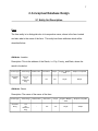
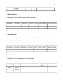
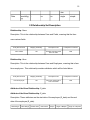
Attribute: Location
Description: This is the address of the Ranch, i.e. City, County, and State, where the
ranch is located at.
Domain/Type
Value-Range
Default Value
Null Value?
Unique
Single or Multiple
Value
Simple or Composite
Character
String
A-Z 0-9
(100
Characters
long)
..
Yes
Yes
Single
Simple
Attribute: Owner
Description: The name of the owner of the farm.
Domain/Type
Value-Range
Default Value
Null Value?
Unique
Single or Multiple
Value
Simple or Composite
Character
String
A-Z
(30
characters
long)
..
Yes
Yes
Single
Simple
8
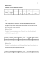
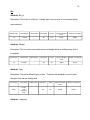
Attribute: Name
Description: This is the name of the farm/ranch.
Domain/Type
Value-Range
Default Value
Null Value?
Unique
Single or Multiple
Value
Simple or Composite
Character
String
A-Z 0-9
(30 characters
long)
..
Yes
Yes
Single
Simple
Fields
Fields are also referred to as orchards, and these are huge pieces of land usually
averaging 155 acres, where the farm owner and his staff will plant one type of crop per
field. Farms usually contain many fields.
Attribute: Field_id
Description: Farmers usually have a map of their entire farm where they distinguish
each field with its respective field ID.
Domain/Type
Value-Range
Default Value
Null Value?
Unique
Single or Multiple
Value
Simple or Composite
Int
0-10,000
..
No
Yes
Single
Simple
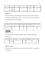
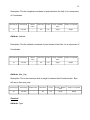
Attribute: Crop
Description: As mentioned before, each field grows different types of crops therefore we
need to know what type of crop we are working with.
Domain/Type
Value-Range
Default Value
Null Value?
Unique
Single or Multiple
Simple or Composite
9
Value
String
A-Z
(35
characters
long)
..
Yes
No
Single
Simple
Attribute: Type
Description: Each crop has a different type of variety, for example, when a field grows
grapes, there are different types of grapes. You have the big ones with seeds, and then
you have green grapes, and purple grapes.
Domain/Type
Value-Range
Default Value
Null Value?
Unique
Single or Multiple
Value
Simple or Composite
String
A-Z
(35
characters
long)
..
Yes
No
Single
Simple
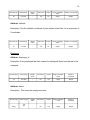
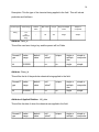
Coordinates
Attribute: Field_Id
This number will be used to identify the field for whom the longtitude and latitude
corresponds to.
Domain/Typ
e
Value-Range
Default
Value
Null Value?
Unique
Single or Multiple
Value
Simple or Composite
..
No
Yes
Single
Simple
0-99999
int
Attribute: Longitude
Description: This the Longitude coordinate of point related to the field. It is a component
of Coordinates.
10
Domain/Type
Value-Range
Default
Value
Null Value?
Unique
Single or Multiple
Value
Simple or Composite
Int
0-10,000
..
Yes
No
Single
Simple
Attribute: Latitude
Description: This the Latitude coordinate of point related to the field. It is a component of
Coordinates.
Domain/Type
Value-Range
Default
Value
Null Value?
Unique
Single or Multiple
Value
Simple or Composite
Int
0-10,000
..
Yes
No
Single
Simple
Employee
Attribute: Employee_Id
Description: Every employee has their unique id to distinguish them from the rest of the
employee.
Domain/Type
Value-Range
Default
Value
Null Value?
Unique
Single or Multiple
Value
Simple or
Composite
Int
0-10,000
..
No
Yes
Single
Simple
Attribute: Name
Description: This stores the employees name.
Domain/Type
Value-Range
String
A-Z
(35
Default
Value
Null Value?
Unique
Single or Multiple
Value
Simple or
Composite
..
No
Yes
Single
Simple
11
characters
long)
Attribute: Phone
Description: This is used to store the phone number.
Domain/Type
Value-Range
Default Value
Null Value?
Unique
Single or Multiple
Value
Simple or Composite
Int
0-10,000
..
Yes
Yes
Single
Simple
Attribute: Wage
Description: Wage will represent the amount of money that the employee earns per
pound of cherries picked.
Domain/Type
Value-Range
Default Value
Null Value?
Unique
Single or Multiple
Value
Simple or Composite
Float
0-100.00
..
No
No
Single
Simple
Attribute: Address
Description: This is the address of the Employee.
Domain/Type
Value-Range
Default Value
Null Value?
Unique
Single or Multiple
Value
Simple or Composite
String
A-Z 0-9
(100
characters
long)
..
No
No
Single
Simple
12
Bin
Attribute: Bin_id
Description: This is the id of the bin. Usually kept in the records to know where the bin
was located at.
Domain/Type
Value-Range
Default Value
Null Value?
Unique
Single or Multiple
Value
Simple or Composite
Int
0-10,000
..
No
Yes
Single
Simple
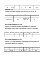
Attribute: Weight
Description: This is used to record the amount of weight the bin is holding every time it
is updated.
Domain/Type
Value-Range
Default Value
Null Value?
Unique
Single or Multiple
Value
Simple or Composite
Int
0-10,000
..
No
No
Single
Simple
Attribute: Type
Description: There are different types of bins. Therefore this attribute is used to save
the type of bin we are dealing with.
Domain/Type
Value-Range
Default Value
Null Value?
Unique
Single or Multiple
Value
Simple or Composite
String
A-Z 0-9
(100
characters
long)
..
No
No
Single
Simple
Attribute: Longitude
13
Description: This the Longitude coordinate of point related to the field. It is a component
of Coordinates.
Domain/Type
Value-Range
Default
Value
Null Value?
Unique
Single or Multiple
Value
Simple or Composite
Int
0-10,000
..
Yes
No
Single
Simple
Attribute: Latitude
Description: This the Latitude coordinate of point related to the field. It is a component of
Coordinates.
Domain/Type
Value-Range
Default
Value
Null Value?
Unique
Single or Multiple
Value
Simple or Composite
Int
0-10,000
..
Yes
No
Single
Simple
Attribute: Max_Cap
Description: This is the maximum limit of weight of cherries that fit inside the bin. Bins
will vary in their max_cap.
Domain/Type
Value-Range
Default Value
Null Value?
Unique
Single or Multiple
Value
Simple or Composite
Int
0-10,000
..
No
Yes
Single
Simple
Chemical
Attribute: Type
14
Description: This the type of the chemical being applied to the field. This will include
pesticides and fertilizers.
Domain/Type
Value-Range
String
A-Z
(35
characters
long)
Default
Value
Null Value?
Unique
Single or Multiple
Value
Simple or
Composite
..
No
Yes
Single
Simple
Attribute: Field_Id
This will be used as a foreign key and the parent will be Fields.
Domain/T
ype
valuerange
default
value
null
value?
unique
single or
multiple
vlue
simple or
composite
int
0-99999
..
no
no
single
simple
Attribute: Chem_id
This will be the id of the particular chemical being applied to the field.
Domain/T
ype
valuerange
default
value
null
value?
unique
single or
multiple
vlue
simple or
composite
int
0-99999
..
no
no
single
simple
Attribute of Applied Relation: Util_date
This will be the date of when the chemical was applied to the field.
Domain/T
ype
valuerange
default
value
null
value?
unique
single or
multiple
simple or
composite
15
vlue
Date
mm/dd/yy
yy
..
no
no
single
simple
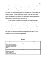
2.2 Relationship Set Description
Relationship: Owns
Description: This is the relationship between Farm and Fields, meaning that the farm
owns various fields.
Entity Sets Involved
Mapping Cardinality
Descriptive Field
Participation Constraint
Farm & Field
1:M
Knowing how many fields
are in the Farm
Total
Relationship: Hires
Description: This is the relationship between Farm and Employees, meaning that a farm
hires employees. This relationship contains attributes which will be listed below.
Entity Sets Involved
Mapping Cardinality
Descriptive Field
Participation Constraint
Farm & Employee
1:M
Farm hires employees to
work on its lands
Total
Attribute of the Hires Relationship: S_date
Attribute of the Hires Relationship: E_date
Description: These attributes are the start date of the employee (S_date) and the end
date of the employee (E_date).
Domain/Type
Value-Range
Default Value
Null Values?
Unique
Single or Multiple
Single or Composite
16
Value
Date
Time and
Date
..
Yes
No
Single
Simple
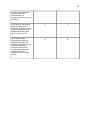
Relationship: Picks
Description this is a ternary relationship between Employee, Crops, and Bin. This
represents an employee picking up crops and dumping them into a bin.
Entity Sets Involved
Mapping Cardinality
Descriptive Field
Participation Constraint
M:1
Employee picks crops
deposits into a bin;
therefore, many
employees will pick one
crop into one bin
Total
Employee, Crops, Bin
Attribute of the Picks Relationship: Date
Description: This attribute is used to know what days and time that the employees
deposited up the crops into the bin. This information will be analyzed to create graphs.
Domain/Type
Value-Range
Default Value
Null Value?
Unique
Single or Multiple
Value
Simple or Composite
Date
Date and time
..
Yes
No
Single
Simple
Attribute of the Picks Relationship: Weight
Description: Will be used to determine the amount of cherries picked at any time, can be
used to evaluate the employees’ working pace.
Domain/Type
Value-Range
Default Value
Null Value?
Unique
Single or Multiple
Value
Simple or Composite
Int
0-10,000
..
No
Yes
Single
Simple
Relationship: Applied
17
Description: This is the relationship between fields and chemicals, meaning that fields
have applied chemicals.
Entity Sets Involved
Fields & Chemicals
Mapping Cardinality
Descriptive Field
Participation Constraint
1:M
A Field can have many
chemical applied
Partial
18
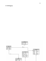
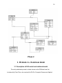
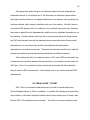
2.3 E-R Diagram
19
Phase 2
3. ER-Model vs. Relational Model
3.1 Description of E-R model and relational model
The entity-relationship model or better known as the ER-Model was first
introduced by Peter Chen, who received his Ph.D in Computer Science and Applied
20
Mathematics from Harvard. This brilliant mind brought the idea of the ER Model to the
Enterprise Data World which was held in 1976. Ever since then, it has became a
popular high-level conceptual data model in the world of databases. Like mentioned
before, and ER model is a high level data model, meaning that the developer will grab
all the data that will be stored in the database and include detailed descriptions of entity
types, relationships and constraints. This model can also be used to communicate with
nontechnical users and to make sure that all the requirements that the user, or the
person for whom the database is being developed for are met.
The ER model describes the data as entities, relationships, and attributes.
Entities are an object in the real world with an independent existence. An object with a
physical existence like a house, person, etc. Or even an object with a conceptual
existence like an employee. Every entity will consist of attributes which are the
properties that describe an entity, for example, employee name can be considered an
attribute to the entity Employee because every employee has a name. There is a
special type of attribute known as the key attribute which values are distinct for all the
entities on the entity set. This type of attribute is unique, meaning that no two entities
will have the same value for the entity. Usually each entity will have at least one key
attribute, otherwise it is considered a weak entity . A relationship can be considered an
association of two entities, because a relationship will link the entities it is related to.
Just like entities, relationships can also contain attributes.
The relational model was first formulated by the mathematician Edgar F. Codd in
1969 .The relational model can be derived from a high-level design, like the ER model.
Relational model is considered to be a logical database design, or the data model
21
mapping step of a database design. In this model, all data is represented as tuples, and
grouped into relations. From the ER model we can get all the strong entities and make
a relation for each entity E in the ER model. The key attributes in the entity will be
represented as primary keys for the respective relation. In relational models, we have
Foreign keys, which will provide a link between two relations.
3.2 Comparisons
The ER model is easier to develop and also it provides a lot of information about
the structure of the database. This type of high-level design is a great way to start that
way the developer can make sure he has covered the whole enterprise/company,
before he dives into the development of the database. Whereas the relational model is
more complicated to understand because it is a logical database design meaning that it
is widely based on predicate calculus, tuples, and relations. The ER model might be
easier to the non technical guys to understand, but once you get into querying and
designing the back end of a database, the relational model will make things much more
easier for you.
3.3 Converting Entity Types to Relations
To map a strong entity type from an ER-model to a relational model you will
create a relation R that will include all the simple attributes of E. You will choose one of
the key attributes of the entity as the primary key for your relationship R. However, if
the key attribute happens to be composite, then all the attributes that form it will all be
22
the primary key. If the entity happens to have many keys, then you will place the keys
in order to preserve uniqueness.
Another type of entity that we must worry about are the weak type entities. We
convert these type of entities by first creating a relation R for the weak entity type. The
relation R attributes will be the same as the weak entities’ attributes and R will also
contain an attribute that will serve as a foreign key that will be used to link the weak
entity to the owner entity.
For each multi valued attribute we will create a relation R. The relations will
include an attribute that corresponds to the multivalued attribute, and it will also include
the primary key attribute of the relation for which the multivalued attribute corresponds
to.
3.4 Converting Relationship Types to Relations
When it comes to converting relationship types to relations we must take
inconsideration if the relationship is one-to-one, one-to-many, or many-to-many. The
first approach we will look at is at the one-to-one mapping. In this particular type of
relationship there are 3 approaches we can take. The first one is by using a foreign
key, in this strategy we take the primary key in one relation and use it as a foreign key in
another relation, that way we can have a link between the two relations. The second
approach is the merged relation approach, which means to grab the relationship and the
two entities that correspond to it and throw all of them in a relation. The final one is the
cross-reference also known as the relationship relation approach. In this method we set
up a relation R in order to cross reference the primary keys of the two entities/relations
23
that it belongs to. The primary key of R will be one of the foreign keys from the entities,
and the other foreign key will be the unique key.
In order to map a binary one-to-many relationship we will use the entity of one
side of the relationship and call it S and we will use the primary key from the other
entity, which will also be a relation R, as a foreign key.
The other type of mapping we the many-to-many relationship type. To convert
the relationship we will create a relation S for the relationship, and we will include as
foreign keys all the primary keys in both entities that correspond to the relationship.
Another type of mapping is the N-ary relationships. This means that the
relationship now maps more than two entities. We first start by creating a relation that
will represent S. The foreign key attributes for S will be all of the primary keys of the
relations that represent the entities that participate in the N-ary relationship.
3.5 Database Constraints
The entity constraint says that no primary key can be NULL, because having
NULL values will means that there is no way for us to identify some tuples. Another
important constraint is the primary key and unique key constraints. An entity must have
an attribute that will distinguish it from other entities, however, sometimes an entity can
contain more than one attribute that makes it unique, which we call a composite key.
This means that the key will include all of the attributes.
The referential integrity constraint is another type of constraint that states that a
tuple in one relation that refers to another relation must refer to an existing tuple in that
relation.
24
Check constraints is another type of integrity constraint that specifies a
requirement that must be met by each row in the database table. This constraint must
be a predicate and it can refer to a single or multiple columns of the table.
The other type of constraint that also exists is the business rule, which cannot be
expressed by schemas and must be enforced by the applications programs.
4 Relational Model
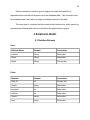
4.1 Relation Schema
Farm
Attribute Name
Domain
Constraints
Location
String
Referential
Owner
String
Referential
Name
String
Primary Key
Attribute
Domain
Constraints
Field_ID
int
Primary Key
Variety
string
Referential
longitude
int
Referential
Latitude
int
Referential
Fname
string
Referential
Crop
string
Referential
Fields
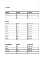
25
Coordinates
Attribute
Domain
Constraint
Field_Id
int
Foreign Key
Longitude
Double
Referential
Latitude
Double
Referential
Attribute
Domain
Constraints
Emp_ID
int
Primary Key
Name
string
Referential
Phone
int
Referential
Wage
Float
Referential
Address
string
Referential
F_name
string
Referential
S_date
date
Referential
E_date
date
Referential
Attribute Name
Domain
Constraints
Bin_ID
int
Primary Key
Weight
int
Referential
Bin_Type
String
Referential
Max_Cap
int
Referential
Employee
Bin
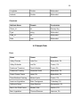
26
Longitude
Double
Referential
Latitude
Double
Referential
Attribute Name
Domain
Constraints
Chem_Id
int
Primary Key
Type
string
Referential
Field_id
int
Referential
Date
date
Referential
Chemicals
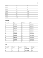
4.2 Sample Data
Farm
Name
Owner
Location
Valley Cherries
John Doe
Bakersfield, CA
Valley Orchards
Joe Dirt
Fresno, CA
Sunkissed Tomatoes
David Valadao
Fresno,CA
Paramount Farming
Alexander Smith
Bakersfield, CA
Cesar Chavez Farms
Jason Chi
Bakersfield, CA
Three Brothers Farming
Moises Ayala
Fresno, CA
Americas Vegetables
Brian Castagneda
Tehachapi, CA
California Farms
Omar Ramirez
Sacramento, CA
Best in the West Farms
Michael Watt
Hanford, CA
Best Vegetables
Thomas Sherman
Lemoore, CA
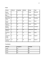
27
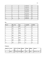
Fields
Fname
Field_id
longitude
latitude
Crops
Type
Jason
Farming
1
0
0
Grape
Big Seed
Best
Tomatoes
2
0
0
Tomato
Cherry
Bakersfield
Farms
3
50
53
Grape
Seedless
Fresno
Farms
4
51
50
Cherry
Black
Farms of
California
5
50
50
Peach
White
Moises
Farming
6
50
50
Watermelon
Seedless
Farms Of
America
7
52
50
Watermelon
Seeds
Americas
Ag
8
51
50
Melon
White
Agriculture
for the
people
9
54
50
Tomato
Regular
Paramount
Farming
10
50
50
Peach
Regular
Coordinates
Field_Id
Longitude
Latitude
10000
10
20
20000
25
50
30000
35
60
28
40000
45
70
50000
55
80
60000
65
90
70000
75
100
80000
85
110
90000
95
120
11000
105
130
Chemicals
Chem_Id
Type
Field_id
Date
1
Pesticide
1
6/1/2014
2
Fertilizer
2
6/4/2014
3
Medicine
3
6/5/2014
4
Fertilizer
4
6/7/2014
5
Medicine
5
6/9/2014
6
Pesticide
6
6/10/2014
7
Fertilizer
6
6/11/2014
8
Medicine
6
6/15/2014
9
Pesticide
8
6/18/2014
10
Medicine
8
6/21/2014
Picks
Field_ID
Bin_Id
Emp_Id
Date
Weight
1
1
5
6/13/2014
20
2
2
2
6/17/2014
40
29
3
3
3
6/19/2014
32
4
4
4
6/20/2014
54
5
5
1
6/11/2014
21
6
6
8
6/23/2014
32
7
7
7
6/27/2014
54
8
8
6
6/28/2014
23
9
9
9
6/29/2014
22
10
10
10
6/30/2014
44
Bin_Id
Max_Cap
Type
Longitude
Latitude
1
200
steel
50
50
2
250
wood
52
50
3
200
wood
55
55
4
215
Steel
55
51
5
210
Wood
50
50
6
200
wood
50
50
7
205
wood
50
50
8
210
Steel
50
50
9
225
Steel
53
50
10
220
Wood
55
52
Bin
Employee
Emp_ID
F_Name
S_Da
te
1
Jason
1/7/20 6/1/2014 Juan
E_date
Name
Phone
Wage
Address
321-
8.00
6787 W. C++ ave.
30
Bakersfield, CA
Farming
14
7895
2
Best
Tomatoes
6/1/20 NULL
14
Moises
1234567
8.25
1254 W. Database
ave.
Bakersfield, CA
3
Bakersfield
Farms
7/18/2 NULL
014
Jason
3216548
8.67
9856 W. CS ave.
Bakersfield, CA
4
Fresno
Farms
7/31/2 12/12/14 Brian
014
7898523
9.00
8523 W. Code ave.
Bakersfield, CA
5
Farms of
California
8/25/1 1/15/15
4
Abraha
m
9512541
9.25
1235 W. Javascript
ave.
Bakersfield, CA
6
Moises
Farming
1/20/1 3/5/15
5
Cesar
9875265
9.75
5261 W. HTML5
ave.
Bakersfield, CA
7
Farms Of
America
1/31/1 NULL
5
Jose
8529638
10.00
7532 W. Pascal ave.
Bakersfield, CA
8
Americas
Ag
2/14/1 3/30/15
5
Juan
9874523
10.00
7852 W. Python ave.
Bakersfield, CA
9
Agriculture
for the
people
2/28/1 NULL
5
Maria
8529874
10.25
7856 W. Java ave.
Bakersfield, CA
10
Paramount
Farming
3/1/15 NULL
Monica
7531452
10.75
1254 W. C# ave.
Bakersfield, CA
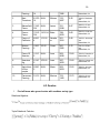
4.3 Queries
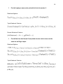
1.
Find all farms who grew cherries with seedless variety type
Relational Algebra:
Tuple Relational Calculus:
31
Domain Relational Calculus:
{<N,O>|Farm<N,O>
2.
crop, type(Fields(Cherry,Seedless,O,-,-,-,-,-)}
Find all the fields owned by Big Run Farm who planted tomatoes type big
and were picked by employee Philiip Flores.
Relational Algebra:
(Farm(F)
Tuple Relational Calculus:
(f|field(f) ⋀ ∃fa∃p∃e(farm(fa) ⋀ Picks(p) ⋀ Employee(e) ⋀ fa.owner =”Big Run Farm”
⋀ f.fname=”Big Run Farm” ⋀ f.crop=”Tomatoes” ⋀ f.type=”Big” ⋀ e.name=”Moises” ⋀
p.Emp_id=e.Emp_id ⋀ p.field_id = f.field_id))
Domain Relational Calculus:
{<f>|fields(-,-,-,f,-,-,-,-)⋀
(Farm(-,Big Run Farm,Jason)) ⋀
⋀
⋀ (Picks(f,-,t,-,-)}
32
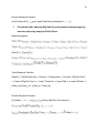
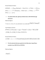
3.
Find all employee names who picked fruit into bin number 3.
Relational Algebra:
Tuple Relational Calculus:
Domain Relational Calculus:
{<N>|Employee(I,-,-,-,N,-,-,-)
4.
3(Pick(I,3,-,-,-) }
Find all the bins that Norma Cook picked cherries into but were not the
same bin as Roger Lopez.
Relational Algebra:
Tuple Relational Calculus:
(B|Bins(B) ⋀
e1
e2.name=”Robert Lopez”
p2.Bin_id))
=p.emp_id
p2.Emp_Id=e2.Emp_Id B.bin_id=p1.Bin_id p1.bin_id !=
33
Domain Relational Calculus
{<B>|Bin(B,-,-,-,-,-)
(Cherry,-,-,i,-,-,-,-)
(Employee(i,-,-,-,Norma Cook,-,-,-) Picks(i,-,-,-,-)
(Employee(j,-,-,-,Robert Lopez,-,-,-)
Picks(j,-,-,-,-)
(Cherry,-,-,j,-,-,-,-) i != j}
5.
Find all the fields who applied pesticides between 06/01/2014 through
06/15/2014.
Relational Algebra:
Tuple Relational Calculus:
(f|Fields(f)
c.Date<=”06/15/2014”))
Domain Relational Calculus:
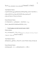
6.
Find the chemicals that were applied to the fields where Jason Burns
worked in from 06/01/2014 to 06/21/2014.
Relational Algebra:
34
Tuple Relational Calculus:
(c.type|Chemicals(c)
f e p(Employee(e) Field(f) Pick(p) e.name=”Jason Burns”
p.Date>=06/01/2014
p.Date<=06/01/2014 e.Emp_Id=p.Emp_Id
p.field_Id=f.Field_Id
f.Field_Id=c.Field_Id))
Domain Relational Calculus:
{<T>|Chemicals(T,n,-)
(Employee(t,-,-,-,Jason Burns,-,-,-))
(Picks(f,-,j,Date>06/01/2014 && Date<06/21/2014,-)) n=j }
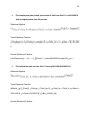
7.
Find all employees who did not pick cherries in field 4.
Relational Algebra:
Tuple Relational Calculus:
(e|Employee(e)
f(Picks(f)
f.field_id!=’9’ f.crop=”Cherries” f.emp_id=e.emp_id))
Domain Relational Calculus:
{<N>|Employee(Ei,-,-,-,N,-,-,-)
(Picks(Field_Id!=9,-,I,-,-) Ei=I }
35
8.
Find employees who picked up buckets of fruit from field 11 on 06/09/2014
with a weight greater than 25 pounds.
Relational Algebra:
Tuple Relational Calculus:
))
Domain Relational Calculus:
{<N>|Employee(j,-,-,-,N,-,-,-)
9.
(Picks(11,-,i,date=06/09/2014,weight=25) j=i ) }
Find which bin was used on field 11 during 06/01/2014-06/20/2014
Relational Algebra:
Tuple Relational Calculus:
(b|Bin(b)
p
“06/01/2014”
(Field(f)
Picks(p)
f.Field_Id=12
p.Field_Id = f.Field_Id
p.Date<=”06/20/2014” p.Bin_Id=b.Bin_Id))
Domain Relational Calculus:
p.Date >=
36
{<B>|Bin(B,-,-,-,-,-)
(Picks(11,-,-,Date>=06/01/2014 && Date<=06/20/2014,-))
(Field(-,-,-,11,) ) }
10.
Which fields were worked by Philip Flores and by Thomas Wilson that
were not worked by Sarah Henry.
Relational Algebra:
)
Tuple Relational Calculus:
(f|Fields(f)
f.Area>30
e p(Employee(e)
Picks(p)
p.Date >= “9/25/2014”
e.Name=”John”
p.Date <= “10/10/2014”
p.Emp_Id=e.Emp_Id
f.Crop=”Cherries”))
Domain Relational Calculus:
{<I>|Field(-,-,-,I,-,-,-)
f(Field(Cherries,-,-,j,area>30,-,-,-))
(Picks(d,-,Ei,Date>=9/25/2014 && Date<=10/10/2014))
j=d
(Employee(Ed,-,-,-,John,-,-,-))
Ei=Ed }
Phase 3
5. Normalization of Relations
5.1 What is normalization?
37
Normalization of data is the process of analyzing the relation schemas based on
their primary keys in order to minimize the redundancy and minimize the insertion,
deletion, and update anomalies. In other words, one can think of this process of the
filtering, because it will make the design have better quality. If our relation is not
normalized then it might contain redundant data storage, and once our database has
been fully developed, it will not organize the data in the most efficient way.
Normalization plays an important role that can determine the performance of our
database. The types of normalization forms that exist are first normal form (1NF),
second normal form (2NF), third normal form (3NF), and Boyce-Codd Normal Form
(BCNF) all these forms are described below.
1NF- Also known as first normal form, which is also known as the basic relational
model. This form doesn’t allow multivalued attributes, composite attributes, and their
combinations. It also states that the domain of an attribute must include only atomic
values and that the value in any attribute in a tuple must be a single value from the
domain of that attribute. If there are any attributes that are multivalued, or any nested
relations then we will form new relations for them. 1NF also disallows relations within
relations or relations as attribute values within tuples. It will only permit single atomic
values.
2NF- (Second Normal Form) is based on the concept of full functional dependency.
Any relation schema R is said to be in 2NF if every non-prime attribute A in R is fully
functionally dependent on the primary key of R. In order to normalize to this form we
will set up a new relation for each partial key with its dependent attributes. However, we
38
must make sure to keep a relation with the original primary key and any attributes that
are fully functionally dependent on it.
3NF-(Third Normal Form) which is the form that is based on the concept of transitive
dependency. Transitive dependency means if there is a functional dependency, X onto
Y in a relation schema then there exists a set of attributes Z in the relation R that is not
a candidate key or a subset of R and X maps onto Z and Z maps onto Y. A relation is
said to be in 3NF if it satisfies 2NF and no non prime attribute of R is transitively
dependent on the primary key. In order to normalize our relation into this form, we must
non key attributes.
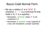
BCNF- (Boyce-Codd Normal Form) This form was suppose to be a simpler form of 3NF
but it ended up being stricter than 3NF. Which means that every relation in BCNF is set
up a relation that includes the non key attributes that functionally determine other also in
3NF; but not every relation in 3NF is in BCNF. A relation schema R is said to be in
BCNF form if whenever a non trivial functional dependency X onto A holds in R, then X
is a superkey of R.
If the relations are not normalized then our database will run the risk of becoming
inconsistent, which is also known as modification anomalies. What this means is that if
we update a tuple in our table then we must make sure to update every tuple who
depends on the tuple we updated otherwise our data will be unorganized or inconsistent
like mentioned before.
5.3 Check Your Relations
39
After going back and looking at our relational schema we have analyzed and
determined that all of our relations are in 1NF because our attributes in each relation
are single valued and there is no repeated attributes in our relations, also a primary key
has been defined, which uniquely identifies each row in the relation. We didn’t have to
worry about 2NF because all of our relations only contained one primary key, therefore
there was no partial function dependencies, and the non key attributes depended on our
key attribute. Usually relations who have two or more primary keys will usually violate
the 2NF rules because there will be instances where some attributes will have partial
dependencies on one primary key and the other attributes will have partial
dependencies on another primary key. Therefore the developer would have to split the
primary keys and their partial dependencies attributes into different relations.
After making sure all of our relations where in 1NF and in 2NF we checked if any
of them had any transitivity because having transitivity in our relations would violate the
3NF rules. None of our relations had any transitivity associated with them therefore
they all meet the 3NF requirements. Unfortunately none of our relation met the BCNF
requirements.
5.4 What is SQL * PLUS?
SQL *Plus is an interactive and batch query tool that is installed with every
Oracle Database Server or Client installation. It contains the following a command-line
user interface, a Windows Graphical Interface which is also known as a GUI and it also
has the iSQL *Plus web-based user interface. This utility is commonly used by users,
40
administrators, and programmers. SQL*Plus understands five categories of text which
are:
1.
SQL statements
2.
PL/SQL blocks
3.
SQL *Plus internal commands which are:
1) environment control commands like SET
2) environment monitoring commands such as SHOW
4.
Comments
5.
External Commands prefixed by the exclamation point.
5.5 Oracle/Schema Objects
A schema is a logical set of logical data structures. These are stored in an
Oracle table space, which may exist in one or many physical files. The schema is
owned by a database user and has the same name as the user. Once the data is
stored in the tablespaces, data structures can be ran to manipulate data. The following
data structures used are:
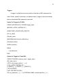
Tables- This is the basic unit of data storage in an Oracle database. The table is
defined with a table name, and the data stored into this table is stored in rows and
columns. The columns will also have a column name and a data type which contains a
domain for it. A row is a collection of the column information corresponding to a single
record.
An example of using sqlplus in oracle to create a new table.
CREATE TABLE table_name (
Attribute_Name_1
Variable_Type_1,
41
Attribute_Name_2
Attribute_Name_3
Table_Constraint_1,
Table_Constraint_2
Variable_Type_2,
Variable_Type_3,
);
Views- Whenever you run a query on your database you will be shown a view takes
the output of the query and treats it as a table. This view can be a one or more tables
combined together showing any info that the query retrieves.
An example of the sqlplus command to create the database.
CREATE VIEW view_name AS
SELECT column_name(s)
FROM table_name
WHERE condition
Dimensions- This will define the hierarchical relation between pairs of columns or
column sets.
Sequence Generator- Provides sequential series of numbers. This is really useful in
multiuser environments for generating sequential numbers without the overhead of disk
I/O or transaction locking. The sequence automatically generates correct values for
each user.
CREATE SEQUENCE sequence_name (
MINVALUE minimum_value,
MAXVALUE maximum_value,
START WITH initial_value,
INCREMENT BY increment_value,
CACHE amount_to_cache);
42
Synonyms- Is an alias for any table, view, sequence,procedure,function, or package.
This requires no storage other than its definition in the data dictionary because it is only
an alias.
Indexes- These are optional structures who are associated with tables and clusters.
Usually indexes are created on one or more columns in a table in order to speed the
SQL statement of the table. By indexing it will help you locate the information faster.
However, you cannot create an index that references only one column in a table if
another such index already exists.
CREATE INDEX emp_ename ON emp(ename);
Stored Procedures/Functions- These type of functions are similar to those from any
high level language (C++,C,Java) because they will accept arguments and return
values. Stored procedures also accept arguments, and they can return actual result
sets.
CREATE OR REPLACE PROCEDURE procedure_name(var1 in var_type)
Database Linkage- This allows the data to be read-only, which means that one can’t
edit the data or delete it. This is usually used to see data on another DBMS without
needing to login as a user in that database.
43
Packages- This will group logically related schema types, items and subprograms.
The packages contain a specification, declared data types, variables, subprograms, and
exceptions. The packages might sometimes contain a body but this is usually
unnecessary.
Our database currently consists of tables, which are named:
Farm, Fields, Employee, Coordinate, Picks, Bin, and Chemicals. We have also
implemented stored procedures, to retrieve the data we wish to extract, for example, the
employees working at a certain farm. Another schema object we have implemented is
the database/linkage because we are able to pull up the table but it is only read-only,
which means we can’t edit it.
Insert Into Statement- This is used to insert new records into the table.
INSERT INTO table_name (column1,column2,column3,...)
VALUES (value1,value2,value3,...);
SQL Join-
ins are used to combine rows from two or more tables.
Max()- Will return the maximum value from the column
SELECT MAX(column_name) FROM table_name;
Having clause- This is similar to the where command but is compatible with
aggregated functions.
HAVING aggregate_function(column_name) operator value;
Group by- statement is used in conjunction with the aggregate functions to group
the result-set by one or more columns
GROUP BY column_name;
Select- This statement is used to select data from a database
44
SELECT column_name,column_name
FROM table_name;
Where- This statement is used to filter records.
WHERE column_name operator value;
Drop-The DROP INDEX statement is used to delete an index in a table.
DROP INDEX index_name
Purge Recyclebin- This cleans out the recycle bin which will remove any junk
tables from the database.
Purge Recyclebin;
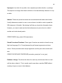
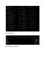
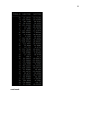
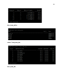
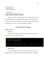
5.6 Relation Schema
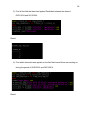
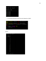
Shown below are the responses from SELECT and DESC queries done on our
table.
select * from jcma_farm;
desc jcma_farm;
45
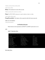
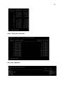
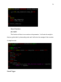
select * from jcma_field
desc jcma_field
46
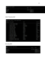
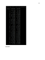
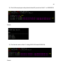
select * from jcma_employee
continued…
47
desc jcma_employee
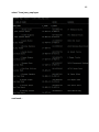
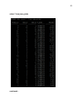
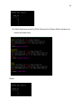
select * from jcma_coordinates
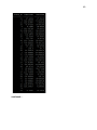
48
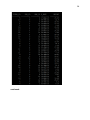
continued……
49
continued….
50
continued….
51
continued..
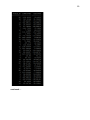
52
select * from jcma_chemicals
desc jcma_chemicals
53
select * from jcma_picks
continued…
54
continued..
55
desc jcma_picks;
select * from jcma_bin;
desc jcma_bin
56
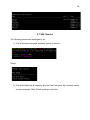
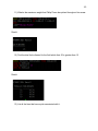
5.7 SQL Queries
The following queries were developed by us.
1) Find all the farms that grew ‘seedless’ variety of cherries.
Result:
2) Find all the fields that is owned by ‘Big Run Farm’ that grew ‘big’ tomatoes variety
and had employee ‘Philip Flores’ working on that field.
57
Result:
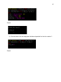
3) Find the name of all the employees that have deposited fruit into bin number 3.
Result:
58
4) Find all the fields that ‘Norma Cook’ has work on but exclude the fields that
‘Roger Lopez’ has work on.
Result:
59
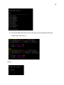
5) Find all the field that have had applied Pesticides between the dates of
06/01/2014 and 06/15/2014.
Result:
6) Find which chemicals was applied on the field that Jason Burns was working on
during the period of 06/01/2014 and 06/21/2014.
Result:
60
7) Find all the employees who did not pick cherries in field 9.
Result:
61
8) Find all the employees who picked at least 25 pounds on field 11 on 06/09/2014
Result:
9) Find the bin used on field 11 during 06/01/2014 and 06/20/2014.
Result:
62
10) Which fields were worked by Philip Flores and by Thomas Wilson that were not
worked by Sarah Henry.
Result:
63
11) What is the maximum weight that Philip Flores has picked throughout his career.
Result:
12) Find the total fruit collected for the field which their ID is greater than 15
Result:
13) List all the bins that have a pick associated with it.
64
Result:
Phase 4
6.1 Common Features of PL/SQL and T-SQL
Procedural Language/SQL(PL/SQL) and Transact SQL(T-SQL) both have many
similarities because they are based on the original SQL. However, since they are being
developed by competing companies, Oracle and Microsoft respectively, these
65
languages can have differing implementation of similar features. For example, both
languages have similar support query commands like the select command or join
command. Another commonality between the two languages is that they store the
trigger and procedures to be stored on the server. Since both languages are based on
SQL, they include clauses, expressions, predicates, queries, and statements from SQL.
The differences between the two languages can vary a lot from small syntax
differences to large differences like supporting differing functions. One large difference
between PL/SQL and Transact SQL is that Oracle has Packages as subroutines. There
are no packages in Transact SQL. Packages are an object that encapsulates
statements, object, subprograms, and variables. They are similar in concept to classes
in C# or C++ because it allows functions within the package to use shared variables.
To implement functionality similar to packages in Transact SQL, the user would have
duplicate data within the implementation due to not having shared variables. Packages
are also stored in the database along with the other subroutines.
6.2 Purpose of Stored Subprograms
In PL/SQL, subprograms includes functions, procedures and packages. They
have the ability to take arguments in and can be comprised of a set of complicated
commands. The purpose of subprograms is to allow the user to encapsulate
complicated procedures to improve reusability of code. It can also provide control of
how certain actions are performed. For example, in the current database there are
insert procedures that contain sequences that increment the ID for each new row.
Subprograms are more efficient when compared to running commands by statements.
66
6.3 Benefits of calling stored subprogram over sending a dynamic
SQL
It is more efficient to use stored subprograms due to to the fact that
subprograms are precompiled on the server and can take a single transaction call to
complete a procedure. In comparison, if a same instruction set is sent over dynamic
SQL then each statement is considered a transaction. So, it takes more transactions to
complete and that will take more time. Subprograms can make common procedures or
automated calls more efficient. In addition to this, subprograms also provide reusability
and maintainability, because once validated, a subprogram can be used with confidence
in any number of applications.
6.4 Oracle PL/SQl
PL/SQL consists of program structure, control statements, and cursors. A
program structure is a block that consists of three parts which are:
1.
Declaration-declare the variables, constraints, cursors, and user-defined
expressions.
2.
Executable-which consists of SQL/SQLPLUS statements.
3.
Exception Handling- A predefined or user-defined warning or error that is
handled by the PL/SQL program.
The control statement consists of conditional, iterative, and sequential controls.
Conditional controls are “if/else if” statements, whereas iterative controls are loops like
the “while” and the “for” loop.
67
Cursors are used by database programmers to retrieve specified rows based on
the database system queries. A cursor will enable the manipulation of whole result sets
all at once.
Stored Procedure:
A stored procedure will perform one or more specified tasks. It contains a
header and a body. The header consists of the name of the procedure and the
parameters or variables passed to the procedure. The body consists the execution
section and the exception section. A stored procedure may or may not return a value.
Syntax For Stored Procedure In PL/SQL:
CREATE [OR REPLACE] PROCEDURE proc_name [list of parameters]
IS
Declaration section
BEGIN
Execution section
EXCEPTION
Exception section
END;
Syntax For Stored Procedure in Trans-SQL:
CREATE PROC [ EDURE ] procedure_name [ ;number ]
[ { @parameter data_type }
[ VARYING ] [ =default ] [ OUTPUT ]
] [ ,... ]
[ WITH
68
{
RECOMPILE
| ENCRYPTION
| RECOMPILE, ENCRYPTION
}
]
[ FOR REPLICATION ]
AS
sql_statement
Stored Procedures in PL/SQL vs Trans-SQL Syntax:
In the Trans-SQL syntax, there is the Recompile, Encryption, and the Recompile
Encryption and this is not included in the syntax for the PL/SQL. However in the
PL/SQL we have the the Exception block, which can output an error to the screen
whenever an exception happens.
Stored Function:
A stored function is similar to a stored procedure, but the main difference
between these two, is that a function must always return a value and a procedure may
or may not return a value.
Syntax For Stored Function In PL/SQL:
CREATE [OR REPLACE] FUNCTION function_name [parameters]
RETURN return_datatype;
IS
Declaration_section
69
BEGIN
Execution_section
Return return_variable;
EXCEPTION
exception section
Return return_variable;
END;
Stored Function in Trans-SQL:
CREATE FUNCTION [ schema_name. ] function_name
( [ { @parameter_name [ AS ][ type_schema_name. ] parameter_data_type
[ = default ] [ READONLY ] }
[ ,...n ]
]
)
RETURNS return_data_type
[ WITH <function_option> [ ,...n ] ]
[ AS ]
BEGIN
function_body
RETURN scalar_expression
END
[;]
Stored Function in PL/SQL vs. Trans-SQL syntax:
In the Trans-SQL syntax, one must provide the name of the schema before the
function name. Also the Trans-SQL does not provide us with the “OR REPLACE”
command. PL/SQL also has a place for the exception that will print out an error
whenever an exception is fired.
Package:
70
A package is a schema object that groups logically related PL/SQL types, items,
and subprograms. Packages usually have two parts a specification and a body. The
specification declares the types, variables, constants, exceptions, cursors, and
subprograms available for use. The body fully defines cursors and subprograms, and so
implements the specifications.
Syntax For Package In Pl/SQL:
Defining Package Specification Syntax
CREATE [OR REPLACE] PACKAGE package_name
[AUTHID {CURRENT_USER | DEFINER}]
{IS | AS}
[PRAGMA SERIALLY_REUSABLE;]
[collection_type_definition ...]
[record_type_definition ...]
[subtype_definition ...]
[collection_declaration ...]
[constant_declaration ...]
[exception_declaration ...]
[object_declaration ...]
[record_declaration ...]
[variable_declaration ...]
[cursor_spec ...]
[function_spec ...]
[procedure_spec ...]
71
[call_spec ...]
[PRAGMA RESTRICT_REFERENCES(assertions) ...]
END [package_name];
Creating Package Body Syntax In PL/SQL
[CREATE [OR REPLACE] PACKAGE BODY package_name {IS | AS}
[PRAGMA SERIALLY_REUSABLE;]
[collection_type_definition ...]
[record_type_definition ...]
[subtype_definition ...]
[collection_declaration ...]
[constant_declaration ...]
[exception_declaration ...]
[object_declaration ...]
[record_declaration ...]
[variable_declaration ...]
[cursor_body ...]
[function_spec ...]
[procedure_spec ...]
[call_spec ...]
[BEGIN]
sequence_of_statements]
END [package_name];]
Reminder: We can’t create packages in Trans-SQl.
72
Triggers:
A trigger is a pl/sql block structure which is fired when a DML statements like
Insert, Delete, Update is executed on a database table. A trigger is fired automatically
when an associated DML statement is executed.
Syntax For Triggers In PL/SQL:
CREATE [OR REPLACE ] TRIGGER trigger_name
{BEFORE | AFTER | INSTEAD OF }
{INSERT [OR] | UPDATE [OR] | DELETE}
[OF col_name]
ON table_name
[REFERENCING OLD AS o NEW AS n]
[FOR EACH ROW]
WHEN (condition)
BEGIN
--- sql statements
END;
Syntax for Triggers in Trans-SQL:
CREATE TRIGGER [ schema_name . ]trigger_name
ON { table | view }
[ WITH <dml_trigger_option> [ ,...n ] ]
{ FOR | AFTER | INSTEAD OF }
{ [ INSERT ] [ , ] [ UPDATE ] [ , ] [ DELETE ] }
[ WITH APPEND ]
[ NOT FOR REPLICATION ]
AS { sql_statement [ ; ] [ ,...n ] | EXTERNAL NAME <method specifier [ ; ] > }
73
<dml_trigger_option> ::=
[ ENCRYPTION ]
[ EXECUTE AS Clause ]
<method_specifier> ::=
assembly_name.class_name.method_name
Syntax for Triggers in PL/SQL vs. Trans-SQL
Triggers in Trans-SQL are different than the ones in PL/SQL because in TransSQL the triggers can’t be used with the “BEFORE” command. The Trans-SQL only
contains an “AFTER” and an “INSTEAD OF” command. The Syntax for the Trans-SQL
also contains an “Encryption” and an “Execute As Clause” command.
6.5 Oracle PL/SQL Subprogram
Stored Procedures:
Insert farm
This procedure takes 3 parameters that are the same data type as the fields of
the farm table and will be inserted as a new row.
Delete chemical
This procedure will take in one parameter(p_id) which will be the id number of
the chemical, and it will delete the chemical corresponding to that id from our database.
74
Stored Functions
get_avg(n)
This function will take in one number as its parameter. It will order the weight in
the jcma_picks table, by descending order and it will return the average of the n number
of weight records.
Stored Trigger
75
This trigger will be fired when a record of the jcma_farm table is updated or
deleted. The trigger will convert the old record and new record as strings and save the
old record string and the new record string into a table defined as logTable.
Phase 5
7.1 Description of Daily activities
The orchard database is meant for the field owners only. The field owner will be
able to analyze the performance of the employees hired by looking at the reports of
76
employee performance and employee contribution generated by our database. Farm
owners will also be able to keep track of all their fields performance. They will be able
to accomplish this by pulling up monthly, and/or yearly reports for the amount of crop
collected for their fields. We have also integrated two date/time pickers, which are used
as parameters in reports, in order to view data between the dates selected.
Besides generating reports for fields and employees, the farm owner will have
access to all his field and employee records. Therefore, he has the ability to add,
update and delete records from the database.
7.2 Relation
Our final relational model contains 7 tables. We ended up using 2 procedures
which are the insert and the delete procedures. We used a “Before” delete trigger for
our “Fields” table, because it contains a parent key that is used by other tables,
therefore we had to make sure the foreign key was deleted before the parent key.
77
78
The following trigger implemented in our database will take effect before any row
from the “Fields” table is deleted. We made a before trigger on this table because it
contains the Field_ID column which happens to be a parent key for the
Picks,Coordinates and Chemicals table.
The following trigger takes place when the user inserts a new field into the
database. It will take the value passed in as the field_id which happens to be the
primary key and it will replace the value with the next number in our sequence
79
generator. The reason why we implemented this was because we didn’t want the user
to insert a repeated field_id otherwise we would have repeated primary keys.
This triggered is executed when the user inserts a new employee into our
database. The functionality to this trigger is the same as the field insert trigger, because
it will take the emp_id entered by the user and replace it with the next number in our
sequence generator that way there are no repeated primary keys.
The following procedure is used when the user inserts a new employee into the
fields table. This procedure takes in four parameters and will insert the values into a
new field row.
80
The following procedure that we use in our front end is the “insert_farm”
procedure. This procedure takes in three parameters which will be our columns for the
new added row to the farm table.
The last procedure that we use in our front end is called whenever the user
inserts a new employee. This procedure will take 7 parameters and insert them as the
values of the new employee row that is being added.
81
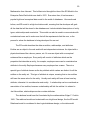
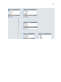
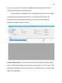
7.3 Screenshots
Main Form: This is the form that will show as soon as our program gets executed. We
display the farm data in our data grid view, which shows the field_ids, crop, and variety.
We included a tab in our UI which is the Employee tab. By clicking on the tab the user
will be able to view all the employees that work, and have worked for the farm that has
been selected. The employee tab will show the employee ID, name, address, phone
number, the starting date for when they first got hired, and the end date which is the
date they left, however, if the value is null it means the employee is still working for the
farm.
We give the option for the user to add a new farm by clicking on the “Add New
Farm” button, which will call another form, where the user will enter the farm. We also
have three buttons on the far right side of the form. Two of the buttons will generate a
report, one of them is a yearly report, and the other is a monthly report. The “save
changes” button will save the changes made on the datagridview.
We also allow the user to view the all the picks in a particular field by right
clicking any of the rows in the farm table. By right clicking the gridview allow the user to
82
choose from 2 options. One of those are generating a report and the other one is
viewing the picks related to the selected field.
By right clicking on the datagrid view of the Employee tab, the user has a choice
of viewing either the employee performance, or the Employee Picks report. By
choosing the view this employees picks option, the user can view the picks the
employee has had throughout his career.
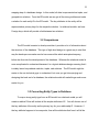
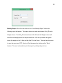
Choose A Month Form: This form will show after the user clicks the “Monthly Report”
button. The user will choose a month and also input the year in a (YYYY) format. After
filling up the requirements, the user will click the “View Monthly Report” and the monthly
report will be generated.
83
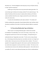
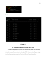
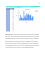
Monthly Report: Once the user clicks on the “View Monthly Report” button the
following report will appear. The report shows us a table which has a Field_ID and a
Weight column. The Field_ID column shows all the IDs and the Weight column will
show the total weight picked on that particular field. We also provided a bar graph
shows the weight on the Y-Axis and the field ID in the X-axis. The user has the option
to save the report as a PDF, Excel, or Word document by clicking on the “Save”
function. The user is also able to print the report by clicking the print icon.
84
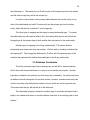
Add A Farm Form: The following form will be show when the user clicks the “Add New
Farm” button. The user will add as many new farms as he wishes and once he is done
editing/adding he/she will click the save button to send the new farms to the database.
Before the program inserts the new added farms to the database, it will first check to
see if any of the farm names in the form are repeated with the ones in the database. If
it finds a repeated farm name it will not insert it in the database because the farm name
is our primary key, therefore there can not be any repeated primary keys.
85
7.4 Major steps of designing a user interface
When designing a user interface, it is important to keep the user in mind. The
developer often has extreme familiarity due to the fact that he created it; however, the
user will not have the same familiarity. The developer will often be satisfied by just
having the functionality in the program and do not always take into account how the
user will use the program. Some procedure may not be intuitive to the user but it is
functionality complete in the programs. User will not like to do complicated procedure to
do a task if it can be simplified. It is important to consider how the user will use the
86
program and the typical operation of the program. This is the most important point of
user interface design.
Designing the user interface can be complicated and difficult to predict. Some
very large companies have a difficult time designing good user interfaces. The best way
to improve the user interface is to have people test the program to get feedback. The
best feedback come from users who have little familiarity with the programs and would
be using the programs on a consistent basis. These users can provide valuable
feedback to improve the program. Another good feedback is to grab people who have
no familiarity with the program and get their feedback. Another tester for the program is
to force the developer to use their own program consistently for a period of time. If the
developer is forced to use the program daily, then he can see the parts of the user
interface that can be improved.
Prototyping is a popular tool to give the users an approximation of how the
project will look and the behavior can be planned. For example, Microsoft Sketchpad is
a prototype tool that allows scripting of of mock up to simulate usage. This will allow the
user to get feedback before building the main program.
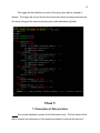
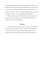
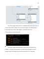
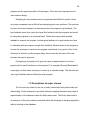
7.5 Descriptions of major classes
The Gui was very reliant on the use of entity framework's entity data model and
data binding. Entity framework is an object relational mapping framework that create a
representation of the database called the Entity data model. The Entity data model is
an extension of the entity relation model and allows the developer to develop application
without referring to the database.
87
Entity framework has many powerful features and it can handle the create,
replace, drop, and updates procedures to the database. It can be used as general
connection to the main database and create classes that can be binded to various
controls within winform. The changes to the bound object will also be reflected on the
controls. Entity framework automatically generates classes based on Entity data model.
Important classes generate by Entity framework include JCMA_FARM, JCMA_FIELDS,
JCMA_CHEMICALS, JCMA_COORDINATES, JCMA_EMPLOYEE, JCMA_PICKS, and
JCMA_BIN. The Entity data Model is shown below.
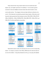
Each relation classes contains the information from one row in the corresponding
relation. For example, an instance of the JCMA_FARM class will contain the data from
one row in the relations. Using entity framework and Linq, you can query the database
88
and return dataset to the programs. The main forms are mainly used to display the data
and manipulate the form. Data binding is the main device to transfer data to the forms
and the second device used was queries. All grids, text box, and combo boxes uses
one of these two devices. An example of using entity frameworks is given below.
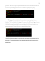
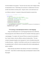
7.6 Learning a new development tool in a new language
Using a new development tool in a new language did present various difficulties.
Every language has various differences that need to be learned to effectively program in
a new language. For example, both Java and C# have a concept of an enhanced for
loop / foreach; however, they have different syntax and implementation. The basic
concepts of programming apply across languages but it can be frustrating learning how
to relearn the syntax. In addition, Visual Studio controls have a lot of properties that can
be manipulated and it is difficult to achieve the desired effect without understanding the
system completely.
Entity Framework was difficult to learn because of the lack of understanding of
how it works. It was difficult to bind the data properly and manipulate the data set within
the program.
89
7.7 Major Steps of Designing and Implementing a Database
Designing and implementing an end-to-end database is not an easy task. It
takes a lot of effort, research, and patience. Keep in mind, many times throughout the
project there will be a lot of refining and redesigning.
The first step a developer should take when it comes to designing a database is
to research the company, organization, and business for whom the database is being
designed for. One should consider talking to the employees, CEOs, and any other staff
that will be using this database that way, one can define the requirements that the
database must meet, because it is harder to change them later on.
After we have done our intense research, we are now ready to take all of the
information gathered and design and create our E-R(Entity-Relationship) model. An ER model is a basic model that is intended for managers and other non-technical persons
and therefore it can easily be explained to them to make sure your database has
covered all of the requirements needed. This step is very important because it plays a
big role when it comes to designing the relational model.
Once we have established a sturdy E-R model we are ready to convert it into a
relational model. Many DBMS are based on relational models. This process requires
converting our entities into relations and having primary and foreign keys inside our
relations in order to have access to other relations. It is really important to carefully
design the relations in our relational model because the model can be directly applied to
our database.
90
After we have finished designing our relational model, we are now ready to write
the subprograms and the triggers that will be used in our database.
The last step on developing a database is the software interface. We must make
sure that the GUI is simple enough that way the users won’t have a hard time when they
utilize our program.
Having a good looking GUI plays a huge role, not only does it
make it more appealing to the user’s eye but it also makes it easier to understand and
the functionality of our program will be clear to the user.
It is very important to follow and revise each and every step of designing a
database because we must try to fix any errors before moving on. Sometimes a small
error at a certain step may not seem critical, but it might come and haunt us later on in
other steps. There was many times where we had to go back and refine our E-R and
relational models, because we had to fix errors. Encountering these errors and fixing
them served us a major learning experience and also served as a lesson to avoid
similar errors in any of our future database designs.
Survey
Outcome
Jason
Moises
(3b) An ability to analyze a
problem, and identify and define
the computing requirements and
specifications appropriate to its
solution
10
10
(3e) An ability to design,
implement and evaluate a
computer-based system,
process, component, or
program to meet desired needs.
10
9
91
An ability to understand the
analysis, design, and
implementation of a
computerized solution to a reallife problem.
(3f) An ability to communicate
effectively with a range of
audiences. An ability to write a
technical document such as a
software specification white
paper or a user manual.
7
7
(3j) An ability to apply
mathematical foundations
algorithmic principles, and
computer science theory in the
modeling and design of
computer-based systems
in a way that demonstrates
comprehension of the
tradeoffs involved in design
choices.
9
9