1
Console
Acceptance
Tests &
Specifications
UNITY
INOVA NMR Spectrometer Systems
Pub. No. 01-999120-00, Rev. B0800
Console Acceptance Tests & Specifications
INOVA NMR Spectrometer Systems
Pub. No. 01-999120-00, Rev. B0800
UNITY
Applicability of manual:
INOVA NMR Spectrometer Systems consoles
UNITY
Revision history:
A0699 – Initial release, E.R. 2751
B0200 – Update autotest and phone list; updated AutoTest for VNMR 6.1C
Technical contributors: George Gray, Everett Schreiber, Lisa Deuring
Technical writers: Dan Steele, Mike Miller
Copyright ©2000 by Varian, Inc.
3120 Hansen Way, Palo Alto, California 94304
http://www.varianinc.com
All rights reserved. Printed in the United States.
The information in this document has been carefully checked and is believed to be
entirely reliable. However, no responsibility is assumed for inaccuracies. Statements in
this document are not intended to create any warranty, expressed or implied.
Specifications and performance characteristics of the software described in this manual
may be changed at any time without notice. Varian, Inc. reserves the right to make
changes in any products herein to improve reliability, function, or design. Varian, Inc.
does not assume any liability arising out of the application or use of any product or circuit
described herein; neither does it convey any license under its patent rights nor the rights
of others. Inclusion in this document does not imply that any particular feature is
standard on the instrument.
UNITY
INOVA, UNITYplus, UNITY, and VXR are registered trademarks of Varian, Inc.
Sun is a registered trademark of Sun Microsystems, Inc. SPARC and SPARCstation are
registered trademarks of SPARC International, Inc. Ethernet is a registered trademark of
Xerox Corporation Other product names are trademarks of their respective holders.
Table of Contents
SAFETY PRECAUTIONS .................................................................................... 7
Chapter 1. Installation Tests and Demonstrations ....................................... 11
1.1
1.2
1.3
1.4
1.5
1.6
1.7
1.8
1.9
Acceptance Testing .............................................................................................
Computer Audit ..................................................................................................
Installation Checklist ..........................................................................................
System Documentation Review ..........................................................................
Basic System Demonstration ..............................................................................
Magnet Demonstration ...............................................................................
Console and Probe Demonstration .............................................................
General Acceptance Testing Requirements ........................................................
General Requirements .................................................................................
Probe Installation Policies ..........................................................................
AutoTest Automated Instrument Testing ............................................................
Test Design .................................................................................................
Scope of Test ...............................................................................................
Test Output ..................................................................................................
AutoTest Directory Structure ......................................................................
AutoTest Macros .........................................................................................
Standard Tests Performed by AutoTest .......................................................
Details of AutoTest Experiments ................................................................
Varian Sales Offices ............................................................................................
Posting Requirements for Magnetic Field Warning Signs .................................
Warning Signs .............................................................................................
11
11
12
12
12
12
12
13
13
14
15
15
15
16
16
19
21
24
34
35
35
Chapter 2. Console and Magnet Test Procedures ........................................ 37
2.1 Automated Test Procedures—Running AutoTest ...............................................
Installing Autotest .......................................................................................
Sample for AutoTest ...................................................................................
Setting Up for AutoTest ..............................................................................
Running AutoTest .......................................................................................
Saving Data and FID Files from Previous Runs .........................................
Creating Probe-Specific Files .....................................................................
Tests Performed by AutoTest ......................................................................
2.2 Manual Test Procedures Required to Demonstrate Console Operation .............
Homonuclear Decoupling ...........................................................................
Lock Frequency Stability ............................................................................
Basic Variable Temperature Operation .......................................................
Magnet Drift ...............................................................................................
01-999120-00 B0800
UNITYINOVA
Acceptance Tests Procedures and Specifications
37
37
38
38
38
39
40
40
42
43
43
44
45
3
WALTZ 1H Decoupling—Preprogrammed Phase Modulation ..................
WALTZ 1H Decoupling—High-Performance RF Waveform Generator ....
2.3 Procedures for Contracted Custom Console Specifications ...............................
Temperature Accuracy for VT Systems ......................................................
Stability Calibration for High-Stability VT Accessory ...............................
Homospoil Demonstration ..........................................................................
Sucrose Anomeric 1H Signal-to-Noise Ratio .............................................
Aqueous Phenylalanine Water Suppression ................................................
46
47
48
48
50
51
52
54
Chapter 3. Consoles and Magnets Specifications ....................................... 57
3.1 Specifications for AutoTest .................................................................................
3.2 Specifications for Manual Console Tests ............................................................
Lock Frequency Stability ............................................................................
Homonuclear Decoupling ...........................................................................
Variable Temperature Operation .................................................................
Magnet Drift Specifications ........................................................................
WALTZ 1H Decoupling Using Preprogrammed Phase Modulation ...........
WALTZ 1H Decoupling Using High-Performance Waveform Generators .
3.3 Contracted Custom Console Specifications ........................................................
Temperature Accuracy for VT Accessories .................................................
Stability Calibration for High-Stability VT Accessory ...............................
Homospoil Demonstration ..........................................................................
57
60
61
62
63
64
65
66
67
68
69
70
Chapter 4. Acceptance Test Results.............................................................. 71
4.1
4.2
4.3
4.4
4.5
Computer Audit ..................................................................................................
System Installation Checklist
.........................................................................
Supercon Shim Values ........................................................................................
Console and Magnet Test Results .......................................................................
Consoles and Magnets Custom Specifications Form .........................................
Custom Specification ..................................................................................
Sample Requirements .................................................................................
Name of Procedure Required for Custom Specification: ............................
73
75
77
79
81
81
81
81
Index .................................................................................................................. 83
4
UNITY
INOVA Acceptance Tests Procedures and Specifications
01-999120-00 B0800
List of Figures
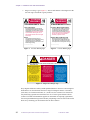
Figure 1. 10-Gauss Warning Sign ..................................................................................................
Figure 2. 5-Gauss Warning Sign ....................................................................................................
Figure 3. Magnet Area Danger Sign ..............................................................................................
Figure 4. AutoTest Program ...........................................................................................................
5
UNITY
INOVA Acceptance Tests Procedures and Specifications
01-999120-00 B0800
36
36
36
39
6
UNITY
INOVA Acceptance Tests Procedures and Specifications
01-999120-00 B0800
SAFETY PRECAUTIONS
The following warning and caution notices illustrate the style used in Varian manuals for
safety precaution notices and explain when each type is used:
WARNING: Warnings are used when failure to observe instructions or precautions
could result in injury or death to humans or animals, or significant
property damage.
CAUTION:
Cautions are used when failure to observe instructions could result in
serious damage to equipment or loss of data.
Warning Notices
Observe the following precautions during installation, operation, maintenance, and repair
of the instrument. Failure to comply with these warnings, or with specific warnings
elsewhere in Varian manuals, violates safety standards of design, manufacturing, and
intended use of the instrument. Varian assumes no liability for customer failure to comply
with these precautions.
WARNING: Persons with implanted or attached medical devices such as
pacemakers and prosthetic parts must remain outside the 5-gauss
perimeter from the centerline of the magnet.
The superconducting magnet system generates strong magnetic fields that can
affect operation of some cardiac pacemakers or harm implanted or attached
devices such as prosthetic parts and metal blood vessel clips and clamps.
Pacemaker wearers should consult the user manual provided by the pacemaker
manufacturer or contact the pacemaker manufacturer to determine the effect on
a specific pacemaker. Pacemaker wearers should also always notify their
physician and discuss the health risks of being in proximity to magnetic fields.
Wearers of metal prosthetics and implants should contact their physician to
determine if a danger exists.
Refer to the manuals supplied with the magnet for the size of a typical 5-gauss
stray field. This gauss level should be checked after the magnet is installed.
WARNING: Keep metal objects outside the 10-gauss perimeter from the centerline
of the magnet.
The strong magnetic field surrounding the magnet attracts objects containing
steel, iron, or other ferromagnetic materials, which includes most ordinary
tools, electronic equipment, compressed gas cylinders, steel chairs, and steel
carts. Unless restrained, such objects can suddenly fly towards the magnet,
causing possible personal injury and extensive damage to the probe, dewar, and
superconducting solenoid. The greater the mass of the object, the more the
magnet attracts the object.
Only nonferromagnetic materials—plastics, aluminum, wood, nonmagnetic
stainless steel, etc.—should be used in the area around the magnet. If an object
is stuck to the magnet surface and cannot easily be removed by hand, contact
Varian service for assistance.
01-999120-00 B0800
UNITYINOVA
Acceptance Tests Procedures and Specifications
7
SAFETY PRECAUTIONS
Warning Notices (continued)
Refer to the manuals supplied with the magnet for the size of a typical 10-gauss
stray field. This gauss level should be checked after the magnet is installed.
WARNING: Only qualified maintenance personnel shall remove equipment covers
or make internal adjustments.
Dangerous high voltages that can kill or injure exist inside the instrument.
Before working inside a cabinet, turn off the main system power switch located
on the back of the console, then disconnect the ac power cord.
WARNING: Do not substitute parts or modify the instrument.
Any unauthorized modification could injure personnel or damage equipment
and potentially terminate the warranty agreements and/or service contract.
Written authorization approved by a Varian, Inc. product manager is required to
implement any changes to the hardware of a Varian NMR spectrometer.
Maintain safety features by referring system service to a Varian service office.
WARNING: Do not operate in the presence of flammable gases or fumes.
Operation with flammable gases or fumes present creates the risk of injury or
death from toxic fumes, explosion, or fire.
WARNING: Leave area immediately in the event of a magnet quench.
If the magnet dewar should quench (sudden appearance of gasses from the top
of the dewar), leave the area immediately. Sudden release of helium or nitrogen
gases can rapidly displace oxygen in an enclosed space creating a possibility of
asphyxiation. Do not return until the oxygen level returns to normal.
WARNING: Avoid liquid helium or nitrogen contact with any part of the body.
In contact with the body, liquid helium and nitrogen can cause an injury similar
to a burn. Never place your head over the helium and nitrogen exit tubes on top
of the magnet. If liquid helium or nitrogen contacts the body, seek immediate
medical attention, especially if the skin is blistered or the eyes are affected.
WARNING: Do not look down the upper barrel.
Unless the probe is removed from the magnet, never look down the upper
barrel. You could be injured by the sample tube as it ejects pneumatically from
the probe.
WARNING: Do not exceed the boiling or freezing point of a sample during variable
temperature experiments.
A sample tube subjected to a change in temperature can build up excessive
pressure, which can break the sample tube glass and cause injury by flying glass
and toxic materials. To avoid this hazard, establish the freezing and boiling
point of a sample before doing a variable temperature experiment.
8
UNITYINOVA
Acceptance Tests Procedures and Specifications
01-999120-00 B0800
SAFETY PRECAUTIONS
Warning Notices (continued)
WARNING: Support the magnet and prevent it from tipping over.
The magnet dewar has a high center of gravity and could tip over in an
earthquake or after being struck by a large object, injuring personnel and
causing sudden, dangerous release of nitrogen and helium gasses from the
dewar. Therefore, the magnet must be supported by at least one of two methods:
with ropes suspended from the ceiling or with the antivibration legs bolted to
the floor. Refer to the Installation Planning Manual for details.
WARNING: Do not remove the relief valves on the vent tubes.
The relief valves prevent air from entering the nitrogen and helium vent tubes.
Air that enters the magnet contains moisture that can freeze, causing blockage
of the vent tubes and possibly extensive damage to the magnet. It could also
cause a sudden dangerous release of nitrogen and helium gases from the dewar.
Except when transferring nitrogen or helium, be certain that the relief valves are
secured on the vent tubes.
WARNING: On magnets with removable quench tubes, keep the tubes in place
except during helium servicing.
On Varian 200- and 300-MHz 54-mm magnets only, the dewar includes
removable helium vent tubes. If the magnet dewar should quench (sudden
appearance of gases from the top of the dewar) and the vent tubes are not in
place, the helium gas would be partially vented sideways, possibly injuring the
skin and eyes of personnel beside the magnet. During helium servicing, when
the tubes must be removed, carefully follow the instructions and safety
precautions given in the manual supplied with the magnet.
Caution Notices
Observe the following precautions during installation, operation, maintenance, and repair
of the instrument. Failure to comply with these cautions, or with specific cautions elsewhere
in Varian manuals, violates safety standards of design, manufacturing, and intended use of
the instrument. Varian assumes no liability for customer failure to comply with these
precautions.
CAUTION:
Keep magnetic media, ATM and credit cards, and watches outside the
5-gauss perimeter from the centerline of the magnet.
The strong magnetic field surrounding a superconducting magnet can erase
magnetic media such as floppy disks and tapes. The field can also damage the
strip of magnetic media found on credit cards, automatic teller machine (ATM)
cards, and similar plastic cards. Many wrist and pocket watches are also
susceptible to damage from intense magnetism.
Refer to the manuals supplied with the magnet for the size of a typical 5-gauss
stray field. This gauss level should be checked after the magnet is installed.
01-999120-00 B0800
UNITYINOVA
Acceptance Tests Procedures and Specifications
9
SAFETY PRECAUTIONS
Caution Notices (continued)
CAUTION:
Keep the PCs, (including the LC STAR workstation) beyond the 5gauss perimeter of the magnet.
Avoid equipment damage or data loss by keeping PCs (including the LC
workstation PC) well away from the magnet. Generally, keep the PC beyond the
5-gauss perimeter of the magnet. Refer to the Installation Planning Guide for
magnet field plots.
CAUTION:
Check helium and nitrogen gas flowmeters daily.
Record the readings to establish the operating level. The readings will vary
somewhat because of changes in barometric pressure from weather fronts. If
the readings for either gas should change abruptly, contact qualified
maintenance personnel. Failure to correct the cause of abnormal readings could
result in extensive equipment damage.
CAUTION:
Never operate solids high-power amplifiers with liquids probes.
On systems with solids high-power amplifiers, never operate the amplifiers
with a liquids probe. The high power available from these amplifiers will
destroy liquids probes. Use the appropriate high-power probe with the highpower amplifier.
CAUTION:
Take electrostatic discharge (ESD) precautions to avoid damage to
sensitive electronic components.
Wear a grounded antistatic wristband or equivalent before touching any parts
inside the doors and covers of the spectrometer system. Also, take ESD
precautions when working near the exposed cable connectors on the back of the
console.
Radio-Frequency Emission Regulations
The covers on the instrument form a barrier to radio-frequency (rf) energy. Removing any
of the covers or modifying the instrument may lead to increased susceptibility to rf
interference within the instrument and may increase the rf energy transmitted by the
instrument in violation of regulations covering rf emissions. It is the operator’s
responsibility to maintain the instrument in a condition that does not violate rf emission
requirements.
10
UNITYINOVA
Acceptance Tests Procedures and Specifications
01-999120-00 B0800
Chapter 1.
Installation Tests and Demonstrations
Sections in this chapter:
• 1.1 “Acceptance Testing” this page
• 1.2 “Computer Audit” this page
• 1.3 “Installation Checklist” page 12
• 1.4 “System Documentation Review” page 12
• 1.5 “Basic System Demonstration” page 12
• 1.6 “General Acceptance Testing Requirements” page 13
• 1.7 “AutoTest Automated Instrument Testing” page 15
• 1.8 “Varian Sales Offices” page 34
• 1.9 “Posting Requirements for Magnetic Field Warning Signs” page 35
Following each installation of a Varian UNITYINOVA NMR spectrometer system, an
installation engineer tests and demonstrates the instrument’s operation. Chapter 4,
“Acceptance Test Results,” outlines the procedures for the acceptance tests. The forms for
recording test results in that chapter follow the same sequence as the tests.
1.1 Acceptance Testing
The objectives of the acceptance tests procedures are twofold:
• To identify the tests to be performed during system installation.
• To identify the precise methods by which these tests are performed.
The procedures are ordered in a sequence designed to efficiently and logically evaluate the
performance of the instrument. These procedures cover the basic specifications of the
instrument, that is, signal-to-noise (S/N), resolution, and lineshape, and are not intended to
reflect the full range of operating capabilities or features of a research NMR spectrometer.
Note: Performance of any additional tests beyond those described herein must be agreed
upon in writing as part of the customer contract. Test samples for these contracted
tests are not supplied by Varian.
1.2 Computer Audit
“Computer Audit,” page 73, includes a computer audit form. The information from this
form will help Varian personnel assist you better in making future software upgrades and
avoiding hardware compatibility problems. You will be asked for information about all
computers directly connected to the spectrometer or used to process NMR data.
01-999120-00 B0800
UNITYINOVA
Acceptance Tests Procedures and Specifications
11
Chapter 1. Installation Tests and Demonstrations
1.3 Installation Checklist
“System Installation Checklist,” page 75, includes an installation checklist form.
1.4 System Documentation Review
Following the completion of the acceptance tests and computer audit, the following system
documentation will be reviewed with the customer:
• Software Object Code License Agreement
• Varian and OEM manuals
• Warranty coverage and where to telephone for information
1.5 Basic System Demonstration
The basic operation of the system is demonstrated to the primary user. The objective of the
demonstration is to familiarize the customer with system features and safety requirements,
as well as to assure that all mechanical and electrical functions are operating properly.
Detailed specifications and circuit descriptions will not be covered.
Note: Varian installation engineers are not responsible for nor trained to run any spectra
not described in the acceptance tests procedures.
Magnet Demonstration
The magnet demonstration includes the following items:
• Posting requirements for magnetic field warning signs
• Cryogenics handling procedures and safety precautions
• Magnet refilling
• Flowmeters
• Homogeneity disturbances
Console and Probe Demonstration
The console and probe demonstration includes the following items:
• Loading programs and operating the streaming magnetic tape unit.
• Experiment setup, including mounting the probe in the magnet.
• Basic instrument operation to obtain typical spectra, including probe tuning, magnet
homogeneity shimming, and printer/plotter operation.
• Demonstration of broadband operation.
• Demonstration of homonuclear and heteronuclear decoupling.
Formal training in the operation and maintenance of the spectrometer is conducted by
Varian NMR Systems at periodically scheduled training seminars held in most Varian
Application Laboratories. On-site training is available in some geographic locations.
Contact your sales representative for further information on availability and pricing for
these courses.
12
UNITYINOVA
Acceptance Tests Procedures and Specifications
01-999120-00 B0800
1.6 General Acceptance Testing Requirements
To make the system demonstration most beneficial, the customer should review Varian and
OEM manuals before viewing the demonstration.
1.6 General Acceptance Testing Requirements
Each Varian UNITYINOVA spectrometer is designed to provide high-resolution performance
when operated in an environment as specified in the UNITYINOVA NMR Spectrometer
Systems Installation Planning Guide. Unless both the specific requirements of this manual
and the general requirements specified in the UNITYINOVA Installation Planning Guide are
met, Varian cannot warrant that the NMR spectrometer system will meet the published
specifications.
General Requirements
• The UNITYINOVA performance specifications in effect at the time the system is ordered
are used to evaluate the system.
• The appropriate quarter-wavelength cable must be used for each nucleus.
• Homogeneity settings must be optimized for each sample (manual shimming may be
required in any or all cases). The shim parameters for resolution tests on each probe
should be recorded in a log book and in a separate file (in the /vnmr/shims
directory) for each probe. For example, for a 5-mm switchable probe, the shim
parameters can be saved with the command svs('/vnmr/shims/sw5res').
These values can then be used as a starting point when adjusting the homogeneity on
unknown samples, by using rts('sw5res').
• The probe must be tuned to the appropriate frequency.
• The spinning speed used is the following:
Sample (mm)
Nuclei
Speed (Hz)
5
all
20–26
10
all
15
Note: Making 10-mm tubes spin faster than 15 Hz may cause vortexing in samples,
severely degrading the resolution.
• All test parameters are stored in the disk library /vnmr/tests and can be recalled
by entering rtp('/vnmr/tests/xxx'), where xxx is the name of the test, for
example, rtp('/vnmr/tests/H1sn'). To see the parameter sets available for
the standard tests, enter ls('/vnmr/tests').
• For all sensitivity tests, the value of pw must be changed to the value of the 90°
pulse found in the pulse width test on the same probe.
• For all direct observe pulse width tests, an appropriate array of pw values must
be entered to determine the 180° pulse. The 180° pulse is the first non-zero pulse
that gives minimum intensity of the spectrum. The 180° pulse is usually
determined by interpolation between a value that gives a positive signal, and a
value that gives a negative signal. The 90° pulse width is one half the 180° pulse.
• Signal-to-noise (S/N) is measured by the computer as follows:
S/N =
maximum amplitude of peak
2 x root mean square of noise region
01-999120-00 B0800
UNITYINOVA
Acceptance Tests Procedures and Specifications
13
Chapter 1. Installation Tests and Demonstrations
• Lineshape should be measured with the aid of the system software. The properly scaled
spectra should also be plotted and retained.
• Software determination of lineshape:
a.
Display and expand the desired peak.
b.
Enter nm, then dc for drift correction to ensure a flat baseline. Set
vs=10000. Press F7 until Thresh is displayed on axis f2. Press the F2 key
to display the horizontal threshold cursor. Set th=55 (the 0.55% level).
c.
Press the F1 key to display two vertical cursors, and align them on the
intersections of the horizontal cursor and the peak. Enter delta? to see the
difference, in Hz, between the cursors.
d.
Set th=11 (the 0.11% level) and repeat the first three steps.
• Determination of lineshape from a plot:
a.
Use a large enough plot width to allow accurate determination of the baseline.
The baseline should be drawn through the center of the noise, in a region of
the spectrum with no peaks.
b.
The 0.55% and 0.11% levels are then measured from the baseline and
calculated from the height of the peak and the value of vs. For example, if a
peak is 9.0 cm high with vs=200, the 0.55% level on a 100-fold vertical
expansion (vs=20000) is 9.0 × 0.55, or 4.95 cm from the baseline.
If the noise is significant at the 0.55% and 0.11% levels, the linewidth should be
measured horizontally to the center of the noise.
• For all sensitivity tests, a noise region free of any anomalous features should be chosen
with the cursors. Neither cursor should be placed any closer to an edge of the spectrum
than 10 percent of the value of sw. This should produce the best possible signal-tonoise that is representative of the spectrum.
• The results of all tests should be plotted as a permanent record. Include a descriptive
label and a list of parameters. These plots can then be saved as part of the acceptance
tests documentation.
Probe Installation Policies
The following policies are in effect at installation:
• Custom Specifications Policy – For custom specifications that have been purchased,
record test results in “Consoles and Magnets Custom Specifications Form,” page 81.
• Specifications Policy for Probes Used in Systems other than UNITYINOVA – For probes
purchased for use in systems other than Varian UNITYINOVA systems, no guarantee is
given that these probes meet current specifications.
• Testing Policy for Indirect Detection Probes for Direct Observe Broadband
Performance – Probes designed for indirect detection applications are tested for
indirect detection performance only.
• Sample Tubes Policy – Tests are performed with the following sample tubes:
3-mm probes: 3-mm tubes with 0.30-mm wall (Wilmad 327-PP, or equivalent).
5-mm probes: 5-mm tubes with 0.38-mm wall (Wilmad 528-PP, or equivalent).
8-mm probes: 8-mm tubes with 0.51-mm wall (Wilmad 513A-7PP, or equivalent).
10-mm probes: 10-mm tubes with 0.46-mm wall (Wilmad 513-7PP, or equivalent).
Using sample tubes with thinner wall thickness (e.g., Wilmad 5-mm 545-PPT, or
equivalent; Wilmad 10-mm 513-7PPT, or equivalent) increases signal-to-noise.
14
UNITYINOVA
Acceptance Tests Procedures and Specifications
01-999120-00 B0800
1.7 AutoTest Automated Instrument Testing
1.7 AutoTest Automated Instrument Testing
AutoTest is a test suite designed as an instrument performance tracking tool for UNITYINOVA
NMR spectrometers. “Automated Test Procedures—Running AutoTest,” page 37, describes
how to install AutoTest and how to use it for automated instrument testing.
After AutoTest is installed, the user can establish benchmark values for a spectrometer and
use these values to track the system’s performance characteristics at regular intervals. The
test is completely automated and can be performed in about 40 to 90 minutes, depending
on the options chosen.
Significant deviations from the norm can provide an indication of a hardware failure or slow
degradation, each of which might be hard to identify using normal spectra. Tests have been
designed to test only one aspect of performance and one piece of hardware at a time, as
much as possible. Historical trends in performance can be displayed.
This section contains the following topics:
• “Test Design,” this page
• “Scope of Test,” this page
• “Test Output,” page 16
• “AutoTest Directory Structure,” page 16
• “AutoTest Macros,” page 19
• “Standard Tests Performed by AutoTest,” page 21
• “Details of AutoTest Experiments,” page 24
Test Design
The test is designed to quantitate instrument performance on an unbiased statistical basis.
The average values and standard deviations from stability and reproducibility
measurements are determined. Other tests produce a regular intensity output (exponential
or linear, such as when an attenuator or modulator value is varied). Correlation coefficients
and standard deviations from a regression analysis are reported.
Calibrations are made of parameters such as 1H pw90 using channels 1 and 2, 13C pw90,
and high- and low-band amplifier compressions. Probe rf homogeneity (1H 450/90, 810/90,
and 13C 360/0, 720/0) values are determined. Sensitivity, T1, and T2 are measured.
Scope of Test
Various hardware aspects are checked, including:
• Lock performance (measured by phase-cycle cancellation efficiency)
• Image cancellation
• Built-in phase modulator decoupling (MLEV-16, WALTZ-16, XY-32, and GARP-1)
• Waveform generation (WFG) based decoupling (WURST and STUD)
• Heating under 13C decoupling and 1H spinlocks
• Variable temperature response
Functionality of receiver gain, small-angle phase shifters, pulse turn-on, attenuators,
modulators, and pulse shaping is measured. The lock channel power and gain control is
checked and quantified.
01-999120-00 B0800
UNITYINOVA
Acceptance Tests Procedures and Specifications
15
Chapter 1. Installation Tests and Demonstrations
Gradient performance is checked on all active axes specified by the pfgon parameter. The
tests include signal amplitude stability following a pulse done 100 µs after a gradient pulse,
or a pulse followed by a bipolar gradient pair generating a gradient echo. Field recovery is
measured by doing a gradient followed by a variable delay and an rf pulse. Gradient DAC
values to generate 10 G/cm strengths are determined. Gradient stability is measured by
measuring a CPMGT2 experiment with and without gradients within the spin echoes.
Test Output
AutoTest results are plotted (if specified), FIDs are stored, and results are logged in
appropriate text files. At the end of the test a single-page report is printed, summarizing the
test results. If desired, the test can be made to repeat until aborted to acquire multiple runs.
After several runs have been completed, histograms showing all previous values of a
parameter can be viewed, for example, all previous z-axis gradient calibrations, along with
the average of all the results and their standard deviations. Of particular interest is any
parameter exhibiting a sudden change in value or a steady increase or decrease. These
results can give an early indication for a hardware problem.
AutoTest Directory Structure
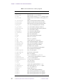
AutoTest uses the ~/vnmrsys/autotest directories listed in Table 1.
Table 1. AutoTest Directories.
Directory
Contents
data
FIDs from the recent AutoTest run(s)
data.failed
FIDs from any failed Auto Test experiments
history
History files for the various tests
reports
Copies of the report generated each time AutoTest is run
parameters
Parameter files—default entry is standard.par
texts
Copies of the text files attached to the AutoTest experiments
atdb
AutoTest database
data Directory
The ~/vnmrsys/autotest/data directory contains FIDs collected in previous
AutoTest experiments. As each experiment finishes, the macro specified by the wexp
parameter executes, and as part of that macro, a svf command is performed that saves the
FID under a file name specified by the parameter at_currenttest (if it contains a
name). The macro first removes any file by the same name (the results of the test from the
last time it was run) and then executes svf. Thus, the data directory may contain FIDs
obtained during different AutoTest runs if those runs were not full runs.
Any data files stored in the data directory can be recalled by normal VNMR commands
such as rt. The data may then be transformed and displayed. The wexp parameter will
contain the name of the macro normally used for data processing, so that the wexp
command can be used to duplicate the actions normally done in an automatic manner.
CAUTION: If file ~/vnmrsys/autotest/atdb/at_selected_tests is
empty, only processing and no further acquisition is done.
16
UNITYINOVA
Acceptance Tests Procedures and Specifications
01-999120-00 B0800
1.7 AutoTest Automated Instrument Testing
This result is normally the case if the last AutoTest run came to a normal completion.
However, if the last AutoTest run was aborted and no new entry into the AutoTest Program
was done, this file will contain entries and an acquisition may start up following the wexp
command. If so, just abort the acquisition.
data.failed Directory
The ~/vnmrsys/autotest/data.failed directory contains any data from any
failed experiment. Failure results when a calculated result falls outside limits defined in the
~/vnmrsys/autotest/atdb/at_spec_table file. Varian specifications are
indicated in the ~/vnmrsys/autotest/atdb/at_spec_table file. Users can
modify this file by supplying upper and lower limits. Any user-modified
at_spec_table file should be saved outside ~/vnmrsys/autotest, since this file
can be deleted later.
parameters Directory
The ~/vnmrsys/autotest/parameters directory contains any parameter set used
by AutoTest macros, including any put there by the user. Normally, only standard.par
is present. This parameter set has all parameters necessary for the AutoTest macros. Values
of parameters may be displayed by using dg in the text window. Some parameters are only
displayed when certain variables are nonzero, or 'y' if a string parameter; however, these
parameters are printed and displayed if used in an experiment. The AutoTest macro Atrtp
is used to recall a parameter set from this directory.
reports Directory
The ~/vnmrsys/autotest/reports directory contains text files from previous
AutoTest runs, by date. Each run produces a report, whether plotting is requested or not.
The report file for a currently proceeding AutoTest run is ~/vnmrsys/autotest/
REPORT. At the end of an AutoTest run, this file is copied to the reports directory under a
title that includes the date and time. If AutoTest is repeated, automatically a new report is
written out for each complete AutoTest run. The existing ~/vnmrsys/autotest/
REPORT file is renamed as ~/vnmrsys/autotest/LASTREPORT whenever an
AutoTest run begins. Similar actions are executed for the atrecord_report.
texts Directory
The ~/vnmrsys/autotest/texts directory contains mainly text files that are
printed on some spectral plots and most parameter set printouts. These files explain the
purpose of the test.
history Directory
The ~/vnmrsys/autotest/history directory contains text files that record the
values determined in AutoTest runs. They are generated automatically by the ATrecord
macro which is used in any AutoTest macro that obtains a numerical result from an NMR
experiment. Each result is written on a new line and is date-stamped. Tests that have a
Varian specification listed in this manual will be denoted as having passed or failed.
If the history file has more than one result per line, any one failure will cause a fail result
for the whole line. When the history file is viewed using the History display (after using
the macro autotest), failure is indicated by a red data point in graphical output and a
colored entry in the text output.
01-999120-00 B0800
UNITYINOVA
Acceptance Tests Procedures and Specifications
17
Chapter 1. Installation Tests and Demonstrations
atdb Directory
The ~/vnmrsys/autotest/atdb directory contains mainly the following text files
used by the Auto Test program to create the AutoTest interface:
at_tests_file
The at_tests_file file defines all the tests that AutoTest can perform. Tests are
specified by a macro name and description. Normally, these are grouped and separated by
a line starting with Label. The word following will be displayed as a heading for a group
of tests. The test descriptions are displayed in the Test Library display (after entering the
macro autotest or by using a menu calling this macro). The macro names are not shown
in the display; checkboxes are displayed next to the test description.
New tests may be added to the at_tests_file by specifying a group title (use the
Label keyword as the first word on the line, followed by a descriptive phrase). Specify a
macro name and then a test description, one per line.
at_groups_file
The at_groups_file file defines test packages that have been assembled for
convenience. Each package has a line that gives a description (in double quotes) followed
by a list of macros to be used in the order of acquisition. There are no restrictions on the
placement of these macros in the text file, only the order matters. When the next doublequoted entry appears, a new group is set.
The AutoTest interface display shows these packages as checkbox entries in the
Configuration display. Selection of one or more of these causes their execution in the order
of selection, once the Begin Test button is selected. When this happens, the
at_selected_tests file is fixed. Selection of the All Tests checkbox disables all
the other selections because they will be done as part of the All Tests run.
Users may add new packages to the Configuration display list by adding appropriate lines
to the at_groups_file in the same format.
at_selected_tests
The at_selected_tests file contains the names of the macros to be run as part of the
AutoTest procedure and is fixed at the time the Begin Test button is selected. The format is
one line per macro with each line containing the name of a macro, in the order of
acquisition.
As AutoTest proceeds, each line is deleted as the specified macro finishes its activity. Thus,
completion of the AutoTest run is defined as when this file is empty. The single exception
is the case of automatic repeating of AutoTest, as specified by the Repeat Until Stopped
checkbox in the Configuration display and as indicated by the value of the global parameter
at_cycletest('y'). In this case, at the completion of the AutoTest run, the contents
of the file at_cycled_tests are copied into at_selected_tests and the process
then continues.
at_cycled_tests
The at_cycled_tests file is updated when the Begin Test button is selected. If the
Repeat Until Stopped checkbox is selected in the Configuration display, the global
parameter at_cycletests is set to 'y' and the file at_selected_tests is copied
to at_cycled_tests. If no test cycling is requested, this file is emptied.
18
UNITYINOVA
Acceptance Tests Procedures and Specifications
01-999120-00 B0800
1.7 AutoTest Automated Instrument Testing
at_spec_table
The at_spec_table file is written out when the ~/vnmrsys/autotest directory is
created and is spectrometer-dependent. The appropriate file is copied from the directory
/vnmr/autotest, depending on spectrometer frequency. It contains a list of macros
used in AutoTest. For each macro the following is specified:
• The history file affected by the macro.
• The column number (not counting date) containing the result.
• The lower limit for the result.
• The upper limit for the result.
• A text description of the result. This text description is used for the graphical displays
and plots. A comment line above each macro serves to describe the test.
All results specified in this manual have upper and lower limits specified numerically in this
file. Those not having Varian specifications have asterisks (*) as entries for upper and lower
limits and these results will have no indication of pass or fail in their history files, or colored
indication of failure in the graphical displays of the history files.
Users may wish to set their own upper and lower limits for many, if not all, of the results.
They may do so by replacing the asterisks with numbers. Of course, this should only be
done after a good statistical base is obtained, such as more than 20 complete AutoTest runs.
Once this base is obtained, the numbers put into the at_spec_table file should have
a reasonable margin of error built in.
It is a good idea to make a copy of the file at_specs_table file prior to changing
it, as well as the modified file, because deletion or renaming of the autotest directory
will result in a default at_spec_table being copied from /vnmr/autotest/atdb.
AutoTest Macros
To help users who may want to add tests or modify tests, this section describes some of the
macros used by AutoTest. These macros are in /vnmr/maclib/maclib.autotest.
ATglobal Macro
The ATglobal macro is run when the AutoTest program begins. The macro checks for
the existence of autotest parameters in the user file ~/vnmrsys/global. These
parameters are used to store calibrations and results that are used by autotest macros.
If the parameters are not present, ATglobal creates them. Otherwise, the parameters are
left unchanged. A partial list of these parameters is given in Table 2.
ATstart Macro
The ATstart macro is run after the Begin Test button is selected in the Configuration
display. The macro sets the global parameters to reflect the current state of the hardware
and aborts under certain circumstances, such as if requested tests are not compatible with
the current hardware settings.
Messages are displayed indicating the source of the problem. The reports are initialized
with relevant information and the ATnext macro is executed.
ATnext Macro
The ATnext macro checks the at_selected_tests file and copies the first entry into
the global parameter at_cur_smacro, deletes the top line in at_selected_tests
01-999120-00 B0800
UNITYINOVA
Acceptance Tests Procedures and Specifications
19
Chapter 1. Installation Tests and Demonstrations
Table 2. Selected Parameters Created by ATglobal.
20
Parameter
Contains
at_currenttest
Name under which the FID is stored
autotestdir
Full path of the autotest directory
at_user
Name of the user running autotest (printed in report)
at_coilsize
length (in mm) of active window in coil (typically 16 or
18 mm)
at_consoletype
Name of console entered in AutoTest window
at_consolesn
Number of console entered in AutoTest window
at_probetype
Name entered for probe used in AutoTest window
at_wntproc
y or n (for processing/display after each FID)
at_cycletest
y or n (for automatic repeating of AutoTest)
at_printparams
y or n (for parameter list/pulse sequence printouts)
at_plotauto
y or n (for automatic plotting)
at_graphhist
y or n (for history graphs plotting)
at_locktests
y or n (for lock power/gain tests)
at_T1
Value of last determined T1
at_gain
Value of gain determined by autogain
at_tof
Value of tof for water
at_fsq
Value of fsq parameter
at_dsp
Current value of dsp at start of run
at_ampl_compr
Value of high-band amplifier compression
at_LBampl_compr
Value of low-band amplifier compression
at_decHeating
Temperature increase from decoupling
at_linewidth
Linewidth of water resonance
at_pw90
90° pw at power specified in AutoTest display
at_tpwr
Power specified in AutoTest display
at_pw90Lowpower
90° pw at reduced power
at_tpwrLowpower
Power level at reduced power
at_pw90_ch2
90° pw on channel 2
at_pwx90
13C
pw90 determined at at_pwx90lvl
at_pwx90lvl
13C
power level for approximately 15-µs pwx90
at_pwx90Lowpower
13C
pw90 at reduced power
power level at reduced power
at_pwx90Lowpowerlvl
13C
at_vttest
y or n (for VT test)
at_temp
Current temperature
at_vttype
Current value of global parameter vttype
at_tempcontrol
Value reflects usage of temp tcl/tk panel
at_gradtests
y or n (for gradient tests)
at_pfgon
Current value of pfgon
at_gmap
y or n (for gradient mapping/shimming)
at_gzcal
Value of G/cm per DAC unit for z-axis gradient
at_gxcal
Value of G/cm per DAC unit for x-axis gradient
at_gycal
Value of G/cm per DAC unit for y-axis gradient
UNITYINOVA
Acceptance Tests Procedures and Specifications
01-999120-00 B0800
1.7 AutoTest Automated Instrument Testing
and executes the macro specified by at_cur_smacro. If the at_selected_tests
file is empty, ATnext either finishes the AutoTest run or calls the ATrestart macro
which copies the at_cycled_tests file to at_selected_tests, permitting
repeated AutoTest runs until manually aborted by the user.
ATnext is usually found at the bottom of each macro defining a particular test. This
permits the linking of one test to another, in a general fashion.
ATxxx Macros
Specific tests usually have the designation of AT, followed by a number or group of letters.
Each macro is self-contained, having the ability of setting up parameters, performing
acquisition, processing the acquired data, possibly setting up new experiments and
processing the data acquired from those experiments, creating plots, parameter printouts,
archiving the raw data, performing statistical analyses of the data, and writing results to
history files and reports.
A new MAGICAL capability is used that makes the macro easier to read and write, the
elseif statement. This removes the need for multiple endif statements if multiple calls
to the same macro are used.
To better illustrate the structure of these macros, Table 3 gives the source code for macro
AT16, the turn-on test (channel 1). A column of descriptive comments has been added to
clarify the statements.
The AutoTest macros can be run as independent macros if a specific test is desired. This is
done by entering the macro in the VNMR command line. Again, if the file
at_selected_tests is not empty, the ATnext macro will start a new acquisition.
Standard Tests Performed by AutoTest
Automated Console Tests
• 90° pulse stability channel 1 and channel 2
• 30° amplitude stability channel 1 and channel 2
• Pulse turnon time channel 1 and channel 2
• Phase cycle cancellation (2-scan test is run as demonstration, no specification is set)
• Quadrature image: 1 scan and 4 scans
• Frequency-shifted quadrature image: 1 scan
• Phase stability test (13° test) channel 1 and channel 2
• Attenuator test channel 1 and channel 2
Full power correlation coefficient and standard deviation
Reduced power correlation coefficient and standard deviation
• Modulator linearity channel 1 and channel 2
tpwr=40: standard deviation
tpwr=-16: standard deviation
• Temperature increase in spinlock test
• Lock power test correlation coefficient
• Lock gain test correlation coefficient
• Variable temperature test
01-999120-00 B0800
UNITYINOVA
Acceptance Tests Procedures and Specifications
21
Chapter 1. Installation Tests and Demonstrations
Table 3. Source Code for AT16 Macro Example.
Code
Comment
if ($#=0) then
First time AT16 is run it has no arguments.
ATrtp('standard')
Recalls standard parameter set.
text('Pulse Turnon Test')
at_currenttest=turnon_ch1
Puts name of test in global variable.
tpwr=tpwr-6 ph
array('pw',37,0.1,.025)
Sets up pulse width array.
ss=2
wnt='ATwft select(celem) aph0 vsadj dssh dtext'
Specifies what to do every FID
wexp='AT16(`PART1`)'
Specifies what to do at end of experiment.
ATcycle
Disables wnt processing if in repeat mode.
au
Begins acquisition and specifies wnt/wexp
processing to occur.
write('line3','Pulse Turnon Test (channel 1)')
dps
elseif ($1='PART1') then
This part executes at end of experiment.
if (at_plotauto='y') then
if (at_printparams='y') then
pap ATpltext
If parameter printout requested.
pps(120,0,wcmax-120,90)
page
endif
endif
select(arraydim) aph0
f peak:$ht,cr rl(0) sp=-1p wp=2p vsadj dssh dtext
ATreg6
Fits to straight line and displays/plots data.
ATpl3:$turnon,$corrcoef
Determines turn-on time and correlation
coefficients
$turnon=trunc($turnon) $corrcoef=
trunc(1000*$corrcoef)/1000
Limits number of decimal places.
ATrecord('TURNONch1','Pulse Turnon Time (nsec)
(channel 1)','time ',$turnon,'
corr_coef.',$corrcoef)
Writes out results to history file.
write('file',autotestdir+'/REPORT',
'Pulse Turnon Time (channel 1): %2.0f
nsec.-Corr. Coef. = %1.3f ',$turnon,$corrcoef)
Writes results to report.
if (at_plotauto='y') then
ATpltext(100,wc2max-5)
full wc=50 pexpl page
Plots regression fit
endif
ATsvf
Removes old data set and stores FID under
name in at_currenttest.
ATnext
Starts next macro in at_selected_tests file, if
present.
Closes elseif part
endif
22
UNITYINOVA
Acceptance Tests Procedures and Specifications
01-999120-00 B0800
1.7 AutoTest Automated Instrument Testing
Automated Tests with Shaped RF
• Gaussian 90° stability, channel 1 and channel 2
• Gaussian phase stability test, channel 1 and channel 2
• Gaussian SLP phase stability test, channel 1 and channel 2
Automated Decoupling Performance Tests
•
13C
phase modulation decoupling profiles
GARP decoupling profile
13C WALTZ-16 decoupling profile
13C XY-32 decoupling profile
13C MLEV-16 decoupling profile
13C
•
13C
adiabatic decoupling profiles (if waveform generator present on decoupling
channel):
13C STUD decoupling profile
13C WURST decoupling profile
• Sample heating during 13C broadband decoupling
90° Pulse Width Calibrations (PW90)
•
1H
•
13C
90° pulse width calibrations on channels 1 and 2
90° pulse width calibrations (PW90)
RF Homogeneity Tests
•
1H
•
13C
rf homogeneity test
rf homogeneity test
Gradient Calibrations and Performance Tests
• Gradient level for 10 G/cm along the following:
Z axis for all gradient probes
X axis for triax probes
Y axis for triax probes
• Gradient echo stability for the following:
Z axis at 30 G/cm
X axis at 10 G/cm
Y axis at 10 G/cm
Z axis at 10 G/cm
• Gradient recovery stability for the following:
X axis at 10 G/cm
Y axis at 10 G/cm
Z axis at 10 G/cm
• Gradient recovery for the following:
X axis at ± 10 G/cm
Y axis at ± 10 G/cm
Z axis at ± 10 G/cm
• Cancellation after gradient.
01-999120-00 B0800
UNITYINOVA
Acceptance Tests Procedures and Specifications
23
Chapter 1. Installation Tests and Demonstrations
Console Demonstration Tests
• High-band amplifier compression
• 1 µsec pulse amplitude stability channel 1 and channel 2
• Low-band amplifier compression
• Temperature rise in decoupler heating test
• AutoGain result for 90° pulse.
• Receiver gain (normal sampling 10-kHz sweep width)
• Receiver gain (oversampling 100-kHz sweep width)
• Folded noise reduction with large spectral width
• Phase switch settling time
CPMG T2 result for the following:
• Gradient level = 10 G/cm
• Without gradients
• 1% gradient mismatch
Shaped RF Demonstrations
• Shaped pulse accuracy—waveform generator gaussian profile
• RF amplitude predictability using a gaussian pulse
• Amplitude scaling of shaped pulses using a gaussian pulse
• RF excitation predictability using a variety of shaped pulses.
Details of AutoTest Experiments
This section provides descriptions of the experiments performed by AutoTest.
All units of the rf system (transmitters, linear modulators, rf attenuators, amplifiers,
receivers, and probes) must be in the standard configuration when AutoTest is run. If the
system configuration has been changed, it must be returned to the standard configuration
before running AutoTest for acceptance testing.
All data is stored, and both plots and statistical analyses are provided as part of the
acceptance testing. Plots and statistical analyses are made concurrently with acquisition.
RF Performance Test (Nonshaped Channels 1 and 2)
Pulse Stability
Experiment – A single-scan pulse experiment is repeated 20 times and the spectra plotted
in a horizontal stack. The average peak amplitude and rms deviation are measured and
reported. This test is run for the following:
• 90° flip pulses
• 30° flip pulses
• 1 µsec pulses
Purpose of 90° Pulse Stability – Modern experiments require very high pulse
reproducibility to minimize cancellation residuals and T1 noise in 2D experiments. This test
checks amplitude reproducibility by comparing a series of spectra obtained with the signal
24
UNITYINOVA
Acceptance Tests Procedures and Specifications
01-999120-00 B0800
1.7 AutoTest Automated Instrument Testing
following a single 90° pulse. The statistical analysis produces an rms deviation, in percent
of the average peak height.
Purpose of 30° Pulse Stability – The sinusoidal nature of the excitation profile makes the
signal generated following a 90° pulse less sensitive to error than signal following a much
smaller flip angle pulse (the top of a sine wave is broad and changes in amplitude less for
small changes in flip angle than for a smaller pulse). A 0° flip angle would have the highest
sensitivity to flip angle, but would give no signal, of course. A compromise between the
extremes of large signal following a 90° pulse, and no signal following a 0° pulse is to use
a 30° pulse. The rms deviation is measured from an array of spectra obtained using 30°
pulses.
Purpose of 1 µsec Pulse Stability – This test emphasizes the turnon characteristics of the
pulse. Any instability of the pulse rise should give a corresponding reduction of measured
stability. Since the flip-angle is much less than a 90° or 30° pulse, the measured stability
may be lower. The rms deviation is measured from an array of spectra obtained using 1 µsec
pulses.
Cancellation Test
Experiment – Four single-scan, 4 two-scan, and 4 four-scan 90° pulse spectra are acquired
in which the transmitter phase is held fixed and the receiver is phase-cycled 0, 2, 1, 3. Data
are plotted in a horizontal stack with the single-scan spectra on scale. The vertical scale is
increased by 100 times and plotted in the same manner. Average residual signal for 2-scan
and 4-scan cancellation are determined.
Purpose – Modern experiments (HMQC, HSQC, NOE-difference, etc.) often rely on
phase-cycling to achieve desired results. This test compares single-transient response
versus two- and four-transient response in which the phase-cycling is set to achieve
cancellation.
Phase Stability (13° Phase Error) Test
Experiment – The 90° pulse stability test is repeated but uses a 90° pulse–1 ms—90° pulse
train with the carrier positioned 37 Hz off-resonance from the water.
Purpose – Phase stability is essential for high-performance modern experiments. Poor
phase stability would produce poorer water suppression and increase T1 noise in 2D NMR.
The most robust tests of phase stability are solids tune-up sequences used for verifying
performance for line-narrowing sequences, such as WAHUHA or MREV-8, because these
sequences are fairly independent of amplitude stability.
Another test is the 13° test in which two 90° pulses separated by 1 ms are applied with the
transmitter placed 37 Hz off-resonance. The resulting NMR response stability is a product
of both rf amplitude stability and phase stability because variations in phase between the
pulses induce an amplitude change. The observed amplitude error should be divided by a
factor of 7.1 to obtain a measure of phase error, in degrees.
Pulse Turn-on Time
• Experiment – Single-scan experiments are taken in which the pulse is varied from 0 to
1–2 µs in minimum pulse-width steps at low enough power so that the response is
linear. The response is fitted to a straight line and the turn-on time is determined.
Because of differences in implementation, turn-on times for channel 2 are usually
longer than for channel 1, even though the hardware is identical.
• Purpose – The quality of modern rf is good enough that examination of pulse shapes
using an oscilloscope is not as informative as well-designed and executed NMR tests.
01-999120-00 B0800
UNITYINOVA
Acceptance Tests Procedures and Specifications
25
Chapter 1. Installation Tests and Demonstrations
The turn-on and turn-off characteristics of a very short pulse are properties that can be
measured sensitively by NMR.
• The turn-on test measures the amplitude of a signal following a short variable-length
pulse. In the limit of a small flip angle, this dependence is linear. The data are analyzed
and least-squares fitted to a straight line. The intercept is the pulse turn-on time.
Attenuator Linearity
Experiment – For a small flip angle pulse, the rf coarse power is varied from maximum to
minimum in single-scan mode. The data are plotted in a horizontal stack to facilitate visual
inspection. The data are fitted to a linear regression and plotted in phased mode to show any
phase change as a function of power.
Purpose – Overall power control is accomplished using PIN diode-controlled rf
attenuators. These attenuators are precision devices that should have negligible phase
change throughout their full range. The amplitude response should also be logarithmic. A
log regression analysis should show the extent of fit to the ideal. The phase change as a
function of power is examined. Raw, uncorrected output should be examined without
software adjustment of phase and amplitude.
This test does not permit a full assessment of the cause of the phase error, because the
amplifier might be in compression at the maximum power output.
Attenuator Linearity at Reduced Power
Experiment – The attenuator linearity test is repeated but with output of the transmitter
reduced by the linear modulator. This is done to isolate the effect of the rf amplifier.
Purpose – The attenuator linearity test is performed, but with reduced power input to the
attenuator (using the linear modulator to reduce the output power from the transmitter).
Raw, uncorrected output should be examined without software adjustment of phase and
amplitude corrections.
Linear Modulator Linearity Tests
Experiment – With the coarse rf amplitude set at a value 23 dB down from maximum, the
rf power is varied using the linear modulator. The linear modulator is used for fine power
control and shaped rf excitation. The rf amplitude is varied, over a range of 60 dB, in 100
equally-spaced steps over the whole range. This should produce a linear ramp of signal
response following a small flip-angle pulse. Spectra are plotted in a horizontal stack of
spectra in phased mode with the highest signal full scale. The width of the plotted region
around the water is set narrow enough to clearly show the base of the water peak. The data
are fitted to a straight line using a linear regression analysis and plotted.
Purpose – Further power control is possible using the linear modulator present on the NMR
transmitter board. This test produces a series of experiments in which the pulse power is
changed over the full range of the modulator. The linear nature is tested by a linear leastsquares fit of the data.
Predictable power control is essential for delivering accurate shaped pulses and for precise
power level control in Hartmann-Hahn experiments in both solids and liquids. Raw,
uncorrected output should be examined without software adjustment of phase or amplitude.
Linear Modulator Linearity Tests with Attenuators Set to Full Attenuation
Experiment – The linear modulator linearity test is repeated, with the coarse rf amplitude
control set for minimum power (resulting in a maximum attenuation of 139 dB). The pulse
width is increased correspondingly to obtain comparable signal-to-noise as in the linear
26
UNITYINOVA
Acceptance Tests Procedures and Specifications
01-999120-00 B0800
1.7 AutoTest Automated Instrument Testing
modulator linearity test. The data are fitted to a straight line using a linear regression
analysis and plotted.
Pulse Shape Test—DANTE
Experiment – The rf amplitude is set for a 20 µs 90° pulse, and the result is compared to
that for a single-scan spectrum:
• 10 pulses, 2 µs each
• 20 pulses, 1 µs each
• 25 pulses, 800 µs each
• 50 pulses, 400 µs each
• 100 pulses, 200 µs each
For all except the first 20 µs pulse, a 1 µs delay is inserted between each pulse. The data are
plotted in a horizontal stack to permit comparison of amplitudes. The amplitudes are
measured and printed.
Purpose – A DANTE-type test is performed in which the signal response following a 20µs pulse is measured. This is compared with a series of experiments in which the pulse is
increasingly divided into series of pulses spaced by 1 µs. The sum of the pulses is held
constant at 20 µs.
If the pulse shape is ideal and the total time of the pulse train is short compared to T2, the
rotation of magnetization should be identical. As the pulse length shortens, any non-ideality
of pulse shape is revealed as a reduction in intensity.
Phase Switch Settling Time
Experiment – Parameters p1 and pw are set to the same value (1 µs) and 30 spectra are
acquired using a 2-pulse sequence, with the first and second pulses separated by a delay of
20 µs. The phase of the second pulse is shifted 180° from the first pulse at a variable time
prior to the second pulse. A single-pulse spectrum is also acquired. The arrayed 2-pulse
spectra and the single-pulse spectrum are plotted, with the single-pulse spectrum last. This
last spectrum serves as a reference. The phase shift should be accomplished in 100 ns or
less.
Purpose – This test exercises the phase-shift hardware by finding the time needed to
perform a 180° phase shift. The pulse sequence is a version of jump-and-return in which
two 1-µs pulses are executed just 20 µs apart. Ideally, because the second pulse has a 180°
phase shift with respect to the first pulse, there should be no excitation. By varying the time
before the second pulse, at which the phase shift is done, from 0 to 20 µs, an estimate of
the phase switch and settling time can be made. The last spectrum is that from just a single,
1-µs pulse, and serves as a reference.This phase shift should be accomplished in 100 ns or
less.
RF Homogeneity
1
H RF Homogeneity Experiment – One hundred experiments are run in which the pulse
width is incremented from 1 to 100 µs. The spectra are plotted in a horizontal stack in
phased mode and sufficiently expanded so that the base of the water can be examined using
the same phase settings for each spectrum (use channel 1).
13C
RF Homogeneity Experiment – In the pulse sequence
delay—pw90(1H)—delay(1/2JCH)—pw(13C)
the pw(13C) is varied from 0 to a flip angle greater than 900° while observing the 13Ccoupled protons. The 0-flip-angle spectrum is adjusted to full scale and the data expanded
01-999120-00 B0800
UNITYINOVA
Acceptance Tests Procedures and Specifications
27
Chapter 1. Installation Tests and Demonstrations
to show only the 13C-bound protons side-by-side to permit measurement of X-coil rf
homogeneity. The results are plotted and displayed in magnitude mode showing one of the
lines of the methanol doublet.
Purpose – This test checks the homogeneity of the rf field strength throughout the active
region of the sample. In an ideal case, for nuclei having reasonable T2 values, the signal
generated following a 360° + 0° pulse should match that following a 0° pulse. The signal
strength as a function of flip angle should be sinusoidal. The amount of drop off is related
to the inhomogeneity of the rf field.
High rf homogeneity is important because many important pulse sequences use a large
number of pulses. The signal losses accumulate with each pulse such that, in worst cases,
all the desired signal is lost. Most heteronuclear, indirect detection experiments on large
molecules use HSQC pulse sequence components. These contain 6 to 10 1H pulses,
including 4 to 8 X nucleus 180° pulses. High rf homogeneity is especially important in
these cases.
Receiver Test
Experiment – Single scan spectra are collected that span the range of receiver gain and
divide that range into at least 25 evenly spaced values of gain, including the highest and
lowest gain values.The data are plotted with the highest signal on scale so that the heights
can be easily compared.
The results are fitted to a straight line using linear regression, and the fitted data are plotted.
Next, the data are normalized and plotted with the water signal held to a constant height so
that the noise levels are easily compared (a few mm of noise in the baseline are provided).
The signal-to-noise ratios for the water line in all spectra are measured with a spectral width
of 10000 Hz and no oversampling. Channel 1 is used for the acquisition. With oversampling
×10, the experiment is repeated. Processing, plotting, and quantization of the oversampled
data are the same as for the data from the 10000-Hz experiment.
Purpose – Receiver gain is selectable in a logarithmic manner (in dB). In an ideal case,
variation of receiver gain should produce a logarithmic dependence of signal strength. As
the gain is lowered, the noise becomes dominated by noise generated in the ADCs, not in
the preamplifier and probe. Regardless of the signal strength, operation in this range of gain
will produce poorer signal-to-noise.
Image Rejection Test
Experiment – Plot the data from the following tests first in a horizontal stack, with the
single-scan data on-scale, and then with the vertical scale increased 100 times. Quantitate
the average image and center glitch.
• Four single-scan and four 4-scan 90° pulse spectra are acquired in which the carrier
frequency is shifted 1000 Hz from the water. The carrier position is not changed during
the pulse sequence and acquisition, and digital filtering is not used.
• The test is repeated using frequency-shifted quadrature detection (FSQD) with single
scans. FSQD is described FSQD is described with the digital filtering information in
the Getting Started manual.
Purpose – This test checks the inherent balance in the two quadrature channels and the
ability of phase cycling to eliminate any quadrature image. Four single-transient and 4 fourtransient responses are collected and compared.
Quadrature images can also be eliminated using digital filtering techniques. The FSQD test
measures image rejection under these conditions.
28
UNITYINOVA
Acceptance Tests Procedures and Specifications
01-999120-00 B0800
1.7 AutoTest Automated Instrument Testing
Shaped Pulse Test (Channels 1 and 2)
Gaussian-Shaped Pulse Excitation
Experiment – A gaussian-shaped pulse, with excitation bandwidth at 50% amplitude about
200 Hz, is applied (e.g., a 12-ms, 90° pulse length). Single-scan spectra are taken with the
transmitter stepped over the range ±250 Hz from resonance, in 5–Hz steps.
The data are plotted in a horizontal stack, with the on-resonance spectrum at full scale to
illustrate the gaussian shape of excitation. The vertical scale is increased by ×10 and plotted
again to show the wings.
Purpose – The most demanding test of shaped pulse accuracy is the ideality of the NMR
data following a shaped pulse. This test determines the accuracy of a gaussian pulse by
examination of the off-resonance excitation. This is done by repeating the same singlepulse excitation while varying the transmitter position through a wide range.
A stacked array of data should show the magnitude of excitation as a function of offset from
resonance. In the ideal case, this excitation envelope would also be gaussian. Any nongaussian nature of the pulse, as delivered to the probe, would be represented by a
convolution of excitation envelopes. For example, if the power were not delivered in a
linear manner, producing some rectangular nature, the excitation envelope would have
some sinx/x nature, producing characteristic sinc wiggles. The lack of such non-gaussian
behavior is a direct measure of the accuracy with which the hardware can deliver an ideal
shape to the nuclei.
Gaussian 90° Pulse Stability
Experiment – The rf 90° pulse stability test is repeated using a gaussian pulse at the same
peak power.
The data are plotted in a horizontal stack, with the on-resonance spectrum at full scale to
illustrate the gaussian shape of excitation.
Purpose – Modern experiments require very high pulse reproducibility to minimize
cancellation residuals and T1 noise in 2D experiments. This tests amplitude reproducibility
by comparing a series of spectra obtained with the signal following a single 90° pulse. The
statistical analysis produces an rms deviation, in percent of the average peak height.
Gaussian 13° Phase Error
Experiment – The rf 13° test is repeated using a gaussian pulse at the same peak power as
in the phase stability test.
The data are plotted in a horizontal stack, with the on-resonance spectrum at full scale.
Purpose – The rf 13° test can be done using shaped pulses. In this case, a gaussian pulse is
used at high peak power.
Gaussian SLP 13° Phase Error (Phase-Ramped Gaussian Pulses)
Experiment – This 13° test is repeated using a phase-ramped gaussian pulses. The rf carrier
should be 37 Hz off-resonance from water, but the center of excitation of the gaussian
phase-ramped pulses should be 1000 Hz from the carrier. The amplitude of the gaussian
pulses is set high enough to exert a 90° pulse on the water.
Purpose – The 13° test can be done using phase-modulated pulses. These types of pulses
provide single- or multiple-frequency selective excitation through the use of both amplitude
and phase modulation.
01-999120-00 B0800
UNITYINOVA
Acceptance Tests Procedures and Specifications
29
Chapter 1. Installation Tests and Demonstrations
Shaped Pulse Settability
Experiment – Single-pulse, single-scan spectra are collected. The rf power is dropped in
eight successive spectra by 3 dB each time and the pulse width increased so that a 90° flip
angle is maintained. The spectra are plotted in a horizontal stack for easy amplitude
comparison.
Purpose – An rf attenuator should permit accurate power control. In this case, the pulse
length is repeatedly incremented while appropriately reducing power levels. The NMR
response should be identical.
Shaped Pulse Test – Rectangular, Gaussian, and EBURP-1
Experiment – Single-scan, one-pulse excitation spectra are collected using rectangular,
gaussian, and EBURP-1 pulses at the same peak amplitude (note the power value and pulse
lengths). Constant peak amplitude is maintained; therefore, pulse width ratios of
1.0:2.4:16.0 for the rectangular:gaussian:EBURP-1 pulses, respectively, are used to obtain
the same flip angle. Spectra are plotted side-by-side in absolute intensity mode at full
vertical scale.
At any constant power, the 90° pulse lengths should reflect their theoretical ratios. Here, the
pulse lengths are set in a ratio of 1:2.4:16. The resulting NMR responses should be identical
in amplitude.
Shaped Pulse Test—Constant Bandwidth for a Variety of Shapes
Experiment – Single-scan, one-pulse excitation spectra are collected using a variety of
shapes that are automatically calculated using Pbox, based on a single pulse calibration
using a rectangular pulse, for a constant 4000 Hz bandwidth. The shaped pulses have
different peak amplitudes and pulse widths (note the power value and pulse lengths).
Spectra are plotted side-by-side in absolute intensity mode at full vertical scale. The
resulting NMR responses should be identical in amplitude.
Shaped Pulse Scalability
Experiment – A small flip-angle gaussian pulse is used for a single-transient, one-pulse
spectrum. The linear modulator is used to scale down the amplitude of the pulse in 100 steps
over a range of 60 dB. Plot widths are set small enough to show the base of the water and
plot all spectra in a horizontal stack in phased mode with the maximum signal spectrum at
full scale.
Purpose – The linear nature of the system is graphically tested by measuring NMR
response when the amplitude is under full control, both by the rf attenuator and by the linear
modulator.
13C Test
X-coil rf homogeneity can be determined using an indirect detection pulse sequence.
Sensitivity in many indirect detection experiments is markedly affected by X-coil
performance because of the large number of 180° pulses used.
X-decoupling is tested for various modulation schemes at constant amplitude (WALTZ-16,
GARP-1, etc.) as well as more powerful adiabatic pulse techniques. Efficiency is measured
by varying the 13C decoupling frequency while observing the proton spectrum under
broadband decoupling.
30
UNITYINOVA
Acceptance Tests Procedures and Specifications
01-999120-00 B0800
1.7 AutoTest Automated Instrument Testing
13C
90° Pulse Width Calibration
The power level for a 90° flip of approximately 15 µs on the X-coil of the probe is
determined. Amplifier compression is determined by lowering power by 12 dB and
redetermining the 90° pulse width. Both results are reported.
X-Phase Modulation Decoupling Profiles
13C power level is reduced 20 dB from the level used to obtain a 15 µs 90° (approximately
1.8 kHz), and the 13C decoupling efficiency is determined for the following phase-
modulated, constant-amplitude broadband decoupling sequences:
• WALTZ-16
• GARP-1
• XY-32
• MLEV-16
The 13C decoupling frequency is varied over a range of ± 80 ppm in a series of single-scan,
proton-observe experiments. Only the 13C-bound protons are shown in the expanded
spectrum, which is plotted with spectra side-by-side in absolute intensity mode to illustrate
decoupling efficiency.
X-Adiabatic Decoupling Profiles
The decoupling profile experiment is repeated with the following adiabatic decoupling
schemes: STUD modulation and WURST modulation
Decoupler Heating
The same test as in the variable temperature test is performed but this time using a 75-ms
decoupling period prior to acquisition within a total recycle time of 1.5 seconds,
including acquisition. One-hundred, single-scan spectra are collected with 13C decoupling
followed by 100 identical spectra with no decoupling. The spectra are plotted in a stacked
manner to permit examination of the rate of change of temperature, the homogeneity of
temperature, and the length of time necessary to reach equilibrium. The rf field strength
should be sufficient to decouple over a 160 ppm range using garp-1. (Note that
decoupling over 160 ppm at 1H frequencies over 750 MHz (200-MHz 13C) require efficient
broadband adiabatic decoupling schemes.)
13C
Gradient Tests
Gradient Profile
Experiment – A spectrum with a 100 kHz spectral width is acquired using a gradient echo
(collect echo during a Z-axis gradient). This acquisition is repeated for both positive and
negative gradients that are sufficient to spread the pattern greater than 50 kHz at the base.
Gradient strength and duration as well as the size of the active length of the coil are noted.
The experiment is repeated for both the X-axis and Y-axis gradients if available.
Purpose – This test uses pulsed field gradients (PFGs) to quantitate the gradient field
strength. The width of the pattern is directly proportional to the gradient strength. The
width at 20% of maximum is used to calculate the gradient strength. Both positive and
negative gradients are used. This should be done for all orthogonal axes available.
Field Recovery Stability
Experiment – The 90° pulse stability test is performed but, preceding the rf pulse, is a 1-ms,
30-G/cm Z-axis gradient pulse, which is then followed by a 100−µs field stabilization
01-999120-00 B0800
UNITYINOVA
Acceptance Tests Procedures and Specifications
31
Chapter 1. Installation Tests and Demonstrations
delay. This test is repeated with a 10 G/cm gradient pulse. If X and Y gradients are
available, the test is repeated with a 10 G/cm gradient pulse for each gradient.
Purpose – A gradient is applied prior to a measuring pulse. The stability of the signal
response is used to measure the ability and reproducibility of the system to recover from
the gradient pulse.
Field Recovery
Experiment – The gradient 90° pulse stability test is repeated with the field recovery delay
varied from 0 to 1000 µs, using a positive 10 G/cm Z-axis gradient pulse. The spectra are
plotted in a horizontal stack with the 1000 µs data at full scale. The test is repeated using a
negative 10 G/cm gradient and, if available, for both the X and Y gradients. Rectangular
and half sine gradients are used. Recovery is defined as the time it takes to recover to 95%
or more of the amplitude.
Purpose – A gradient is applied prior to a measuring pulse and the time before the pulse is
varied. The rate of recovery determines how soon a pulse may be applied.
Gradient Echo Stability
Experiment – The 90° pulse stability test is run, this time with a positive gradient for 1 ms,
a 500 µs delay, and a negative gradient for 1 ms following the rf pulse. The following
gradient strengths and axes are used.
• 30 G/cm—Z axis only
• 10 G/cm—Z axis and, if present, X and Y axes
Purpose – Following a single pulse, a pair of opposite-signed gradients is applied. The
stability of the resulting refocused signal measures any instability in the gradient amplitude,
as well as the accuracy of the gradient level control. This should be done for all orthogonal
axes available.
Gradient Effect on Cancellation Test
Experiment – Four 1-scan, four 2-scan and four 4-scan 90° pulse spectra are acquired, with
a 10 G/cm Z-axis gradient pulse 100 µs prior to the rf pulse and the transmitter phase held
constant while the receiver is phase-cycled 0, 2, 1, 3. The spectra are plotted in a horizontal
stack with the single-scan spectra on scale. Vertical scale is increased by 100 times and
plotted in the same manner. The average residual signal for the 4-scan cancellation is
quantitated and the results plotted and analyzed as above.
Purpose – The cancellation test is done with a gradient pulse applied 100 µs before the rf
pulse. If the lock circuitry and field recovery characteristics are favorable, no deterioration
in cancellation efficiency should be noted.
CPMG T2
Experiment – A CPMG T2 experiment is performed with 2 ms between 180° pulses for total
echo pulse trains ranging from a few milliseconds out to at least 2*T1. This experiment is
repeated for the case where 500 µs 10 G/cm rectangular pulses are placed around the 180°
pulses in each echo, as well as the case in which no gradients are used. The values for T2
are reported for all cases. The experiment is repeated for the case of a 1% mismatch in
gradient amplitude.
Purpose – Following a single pulse, pairs of same-signed gradients are applied within the
echoes of a CPMG T2 pulse echo train. The measured T2 gives a measure of any instability
in the gradient amplitudes as well as the accuracy of the gradient level control. This
measurement is compared to an identical experiment in which the gradient amplitudes are
32
UNITYINOVA
Acceptance Tests Procedures and Specifications
01-999120-00 B0800
1.7 AutoTest Automated Instrument Testing
set to zero or mismatched by 1%. More rapid diffusion at higher temperature will cause the
gradient/no gradient comparison to worsen. Therefore, performance over time should be
compared for the same temperature. (Measurements done at ~4° C have showen no
difference in measured T2 for the gradient/no gradient cases, indicating that diffusion is
responsible for the difference in these cases at higher temperatures).
Other Tests
Heating During Spin Lock Test
Experiment – The same test as in the variable temperature test is performed using a 70-ms
1H pulse at an rf field strength of 10 kHz with a total recycle time of 1.5 seconds, including
acquisition. The data are plotted in the same way as in the VT test.
Purpose – Many modern experiments use spin locks or decoupling within their pulse
sequences. Often, rf fields can cause significant sample heating. Depending on the nature
of the probe, this heating can be a problem causing baseline artifacts and t1 noise. It is
important to quantify the amount of sample heating, the speed in attaining a new
equilibrium temperature, the homogeneity of temperature throughout the sample during the
heating period, and the final change in temperature.
This test imposes a rather strong (10 kHz) rf field for a period of time often used in TOCSY
experiments, using a recycle time of 1.5 seconds (including acquisition). Single transients
are acquired, at a rate of one per 1.5 seconds. The data show any temperature change at the
expected 0.01 ppm/degree. The intensity and/or linewidth can be used to measure
temperature homogeneity. The number of transients needed to attain a new equilibrium
temperature measures the ability of the probe to stabilize the effects of internal sample
heating. The final shift value indicates the total temperature change. This can be used to
reduce the requested temperature value so as to obtain the desired equilibrium. Of course,
the amount of heating is a function of the sample itself, primarily its salt content. The same
approach may be used to follow the actual temperature in the sample under the influence of
X-nucleus decoupling.
Lock Tests
Experiment – Lock power is varied over a 30 dB range and the lock level recorded. The
experiment is repeated for the lock gain. A log regression analysis is performed to confirm
the relationship between the lock signal and power/gain.
Purpose of Lock Gain Test – Lock gain is selectable in a logarithmic manner (in dB). In an
ideal case, variation of receiver gain should produce a logarithmic dependence of signal
strength.
Purpose of Lock Power Control Using an RF Attenuator – Overall lock power control is
accomplished using computer-controlled rf attenuators. The amplitude response should
also be logarithmic. A log regression analysis should show the extent of fit to the ideal.
Spectral Purity Test
Experiment – Four single-scan 100 kHz spectral width spectra are acquired with no pulse.
Each spectrum is plotted with a few millimeters of noise.
Purpose – RF purity of the transmitter and receiver can be tested by recording data without
any excitation pulse. The spectrum reveals any artifactual signals.
Variable Temperature Test
Experiment – Single-scan spectra are acquired during an increase of 5°C in sample
temperature. Spectra are recorded sequentially. Spectra are taken every 2 seconds until the
01-999120-00 B0800
UNITYINOVA
Acceptance Tests Procedures and Specifications
33
Chapter 1. Installation Tests and Demonstrations
sample reaches equilibrium, as reflected in a stable chemical shift of a methyl proton.
Spectra are plotted in a stacked manner to permit examination of the rate of change of
temperature, the homogeneity of temperature, and the length of time necessary to reach
equilibrium.
Purpose – The sample temperature is increased by 5o C while recording spectra every 2
seconds. Most methyl resonances show a chemical shift of (sfrq/100) Hz/oC and this
shift, therefore, indicates the actual temperature distribution within the sample. The methyl
resonance should move quickly and homogeneously to its new equilibrium position. The
rate of change and homogeneity of change demonstrate the VT performance of the probe
and regulation hardware.
Small-Angle Phase Shift Test
Experiment – Single-scan spectra are acquired in which the phase of the pulse is
incremented by 10° in each spectrum through a full 360° at constant receiver phase. Spectra
are plotted in a horizontal stack to show a smooth phase rotation of the spectrum. The test
is repeated using pulses generated from channel 2.
Purpose – Small-angle phase adjustment is used in multiple-quantum selection (q>2),
phase-modulated pulses, and a variety of complex pulse sequences. This test exercises the
phase-shift hardware by varying the pulse phase in small increments over 360°.
1.8 Varian Sales Offices
For product sales and service information, contact one of the Varian sales offices:
• Argentina, Buenos Aires, (114) 783-5306
• Australia, Mulgrave, Victoria, (3) 9566-1138
• Austria, Vösendorf, (1) 699 96 69
• Belgium, Brussels, (2) 721 48 50
• Brazil, Sao Paulo, (11) 829-5444
• Canada, Ottawa, Ontario, (613) 260-0331
• China, Beijing, (10) 6846-3640
• Denmark, Herlev, (42) 84 6166
• France, Orsay, (1) 69 86 38 38
• Germany, Darmstadt, (6151) 70 30
• Italy, Milan, (2) 921351
• Japan, Tokyo, (3) 5232 1211
• Korea, Seoul, (2) 3452-2452
• Mexico, Mexico City, (5) 523-9465
• Netherlands, Houten, (30) 635 0909
• Norway, Oslo, (9) 86 74 70
• Russian Federation, Moscow, (95) 241-7014
• Spain, Madrid, (91) 472-7612
• Sweden, Solna, (8) 445 1601
• Switzerland, Zug, (41) 749 88 44
• Taiwan, Taipei, (2) 2698-9555
34
UNITYINOVA
Acceptance Tests Procedures and Specifications
01-999120-00 B0800
1.9 Posting Requirements for Magnetic Field Warning Signs
• United Kingdom, Walton-on-Thames, England (1932) 898 000
• United States, Palo Alto, California,
Varian, Inc., NMR Systems
Customer Sales Support, (650) 424-5145
Service Support, Palo Alto, California, 1 (800) 356-4437
E- mail: [email protected]
North American Service Manager
6440 Dobbin Rd, Ste D, Columbia, MD 21045
(410) 964-3065
• Venezuela, Valencia (41) 257608
1.9 Posting Requirements for Magnetic Field Warning Signs
The strong magnetic fields that surround a superconducting magnet are capable of causing
death or serious injury to individuals with implanted or attached medical devices such as
pacemakers or prosthetic parts. Such fields can also suddenly pull nearby magnetic tools,
equipment, and dewars into the magnet body with considerable force, which could cause
personal injury or serious damage. Moreover, strong magnetic fields can erase magnetic
media such as tapes and floppy disks, disable the information stored on the magnetic strip
of automated teller machine (ATM) and credit cards, and damage some watches.
To warn of the presence and hazard of strong magnetic fields, the customer is responsible
for posting clearly visible signs warning of magnetic field hazards. This responsibility
includes measuring stray fields with a gaussmeter.
Radio-frequency emissions may also pose a danger to some individuals. The rf emission
levels from Varian NMR equipment have been measured and compared to the IEEE/ANSI
C95.1-1991 standard. For further information, refer to the RF Environment section of the
Installation Planning Guide.
Warning Signs
Varian provides signs to help customers meet this posting responsibility. These signs must
be posted according to the following requirements before the magnet is energized:
1.
10-gauss warning signs (Figure 1) – Post along the 10-gauss perimeter of the magnet
so that a sign can be easily seen by any person about to enter the 10-gauss field from
any direction. Refer to the manuals supplied with the magnet for the size of a typical
10-gauss stray field. Check this gauss level after the magnet is installed.
Note that the stray field may extend vertically to adjacent floors, and additional signs
may be needed there. A sign is not required if the 10-gauss field extends less than 30
cm (12 in.) beyond a permanent wall or less than 61 cm (24 in.) beyond the floor
above the magnet.
2.
5-gauss warning signs (Figure 2) – Post along the 5-gauss perimeter of the magnet
so that a sign can be easily seen by any person about to enter the 5-gauss field from
any direction. Refer to the manuals supplied with the magnet for the size of a typical
5-gauss stray field. Check this gauss level after the magnet is installed. Note that the
stray field may extend vertically to adjacent floors, and additional signs may be
needed there.
01-999120-00 B0800
UNITYINOVA
Acceptance Tests Procedures and Specifications
35
Chapter 1. Installation Tests and Demonstrations
3.
Magnet area danger signs (Figure 3) – Post at each entrance to the magnet area. Be
sure each sign is outside the 5-gauss perimeter.
10-GAUSS
WARNING
5-GAUSS
WARNING
STRONG MAGNETIC FIELD
STRONG MAGNETIC FIELD
Tools and Equipment
Pacemaker, Metallic Implant Hazard
Strong magnetic fields are present that can
make magnetic items suddenly fly towards the
magnet, which could cause personal injury or
serious damage. Do not take tools, equipment,
or personal items containing steel, iron, or
other magnetic materials closer to the magnet
than this sign.
Dewars
Strong magnetic and rf fields are present that
can cause serious injury or death to persons
with implanted or attached medical devices,
such as pacemakers and prosthetic parts. Such
persons must not go closer to the magnet than
this sign until safety at a closer distance is
identified by a physician or device
Magnetic Media, ATM/Credit Cards
The stray field of the magnet can pull a
magnetic dewar into the magnet body, causing
serious damage. Use only nonmagnetic
stainless steel dewars. Do not use iron or steel
dewars during servicing.
Strong magnetic fields are present that can
erase magnetic media, disable ATM and credit
cards, and damage some watches. Do not take
such objects closer to the magnet than this sign.
Pub. No. 87-250303-00 B0694 5-Gauss Warning Sign
Pub. No. 87-250302-00 B0694 10-Gauss Warning Sign
Figure 1. 10-Gauss Warning Sign
Figure 2. 5-Gauss Warning Sign
DANGER
STRONG MAGNETIC AND RADIO-FREQUENCY FIELDS ARE PRESENT
Pacemaker and
Metallic Implant Hazard
Magnetic Media and
ATM/Credit Cards
Tools and Equipment
Strong magnetic and radiofrequency fields are present that
could cause serious injury or
death to persons with implanted
or attached medical devices,
such as pacemakers and
prosthetic parts.
Strong magnetic fields are
present that could erase
magnetic media such as
floppies and tapes, disable ATM
and credit cards, and damage
some watches.
Strong magnetic fields are
present that could make some
magnetic items suddenly fly
towards the magnet body, which
could cause personal injury or
serious damage.
Do not take such objects closer
to the magnet than the
5-GAUSS WARNING signs.
Do not take tools, equipment,
or personal items containing
steel, iron, or other magnetic
materials closer to the
magnet than the
10-GAUSS WARNING signs.
Such persons must not go
closer to the magnet than the
5-GAUSS WARNING signs until
safety at a closer distance is
identified by a physician or
medical device manufacturer.
Pub. No. 87-250301-00 B0694
Magnet Area Entrance Danger Sign
Figure 3. Magnet Area Danger Sign
Stray magnetic fields can reach beyond the published distances when two or more magnetic
fields intersect or when the field extends over large ferromagnetic masses or structures
(steel doors, steel construction beams, etc.). In this case, the customer must measure the
stray field using a gaussmeter to determine how the 5- and 10-gauss fields are altered
(contact a scientific instrumentation supplier for information on acquiring a gaussmeter).
You can request additional signs from Varian by telephoning 1-800-356-4437 in the United
States or by contacting your local Varian office in other countries.
36
UNITYINOVA
Acceptance Tests Procedures and Specifications
01-999120-00 B0800
Chapter 2.
Console and Magnet Test Procedures
Sections in this chapter:
• 2.1 “Automated Test Procedures—Running AutoTest” this page
• 2.2 “Manual Test Procedures Required to Demonstrate Console Operation” page 42
• 2.3 “Procedures for Contracted Custom Console Specifications” page 48
This chapter contains the procedures for testing UNITYINOVA NMR consoles and magnets.
These procedures are required to demonstrate the specifications listed in Chapter 3,
“Consoles and Magnets Specifications,” for UNITYINOVA NMR consoles and magnets.
2.1 Automated Test Procedures—Running AutoTest
The AutoTest automated test procedures software features a series of automated tests for
both the console and the probe. These tests demonstrate the console performance and its
compliance with the acceptance test specifications as well as some of the probe acceptance
tests and its compliance with the specifications listed in Chapter 3. AutoTest tests only
channels 1 and 2.
The automated tests write the results to a text file and plot the resulting spectra. Although
plotting is optional, plotting should be activated for acceptance testing and customer
review. A hard copy of the AutoTest report should be attached to the appropriate acceptance
test results in Chapter 4.
Refer to “Details of AutoTest Experiments,” page 24, for detailed descriptions of the tests
performed by AutoTest.
Installing Autotest
AutoTest is available beginning with the VNMR 6.1B. AutoTest can be installed at any
time, but it is most convenient to install it when VNMR is installed. If AutoTest is not
already installed, use these steps to install it now.
CAUTION: Remove any files used for previous versions of AutoTest from your
vnmrsys directories, particularly any ~/vnmrsys/seqlib/AT* or
~/vnmrsys/maclib/AT* files. Remove AT*.DEC, gauss32.RF,
gauss.RF and eburp1.RF from ~/vnmrsys/shapelib, if present.
Make sure that ~/vnmrsys/maclib/autotest is not present.
1.
Mount the VNMR CD-ROM, change to the CD-ROM directory, and enter
./load.nmr. The VNMR installation menu appears.
2.
Select the UNITYINOVA system at the top of the menu. The VNMR installation menu
for UNITYINOVA appears.
01-999120-00 B0800
UNITYINOVA
Acceptance Tests Procedures and Specifications
37
Chapter 2. Console and Magnet Test Procedures
3.
Select the AutoTest checkbox. Click on install.
Refer the manual VNMR and Solaris Software Installation for further details.
Sample for AutoTest
As the sample, AutoTest uses 0.1% 13C-enriched methanol in 1% H2O/99% D2O. The
sample is doped with gadolinium chloride at a concentration of 0.30 mg/ml, which
produces a 1H T1 relaxation time of about 50 to 75 ms. The resulting line width is
considerable larger than the magnet-determined line width because of the paramagnetic
relaxation contribution.
Setting Up for AutoTest
To set up for autotest:
1.
Make sure all units of the rf system (transmitters, linear modulators, rf attenuators,
amplifiers, receivers, and probes) are in the standard configuration.
2.
If the system has a PFG accessory installed, make sure that the gradient amplifier is
on and pfgon is set correctly for the number of gradients available:
• pfgon='nny' for Z-axis only.
• pfgon='yyy' for triax.
Allow sufficient time for stabilization. AutoTest calibrates the gradients.
3.
Insert the AutoTest sample.
4.
Set the VT to 25° C. Allow the temperature of the sample to regulate and equilibrate.
While specifications are determined at 25° C, normal day-to-day AutoTest runs may
be done at other temperatures.
5.
Tune the probe, and lock on the D2O resonance.
6.
Shim the field on the sample to give a nonspinning half-height that is dominated by
the paramagnetic relaxation agent. Because the H2O line is quite broad, this should
not require much time.
7.
Note the tpwr value necessary to produce a 1H 90° pulse width that is within
specification (8 to 10 µs), but does not cause probe arcing.
AutoTest uses this tpwr value in determining the 1H 90° pulse width and calculates
the amplifier compression at this tpwr value.
8.
To save the results of a previous AutoTest run, rename the history and data
directories. For further information, refer to the manual System Administration.
Running AutoTest
To run AutoTest, you enter values and make selection in the AutoTest window and then
select the Begin Test button. Be sure to press the Return key after entering each value.
38
1.
Enter the macro autotest. The AutoTest window opens, similar to Figure 4. .
2.
Select the Configuration tab at the top of the window, if not already selected.
3.
Fill in the fields for the Operator Name, Console type, etc. at the top of the
window. In the pw90 field, enter an approximate 1H pw90 for the value of tpwr
that you entered (10 µs is recommended)
UNITYINOVA
Acceptance Tests Procedures and Specifications
01-999120-00 B0800
2.1 Automated Test Procedures—Running AutoTest
Figure 4. AutoTest Program
4.
Select the options desired in the checkboxes in the middle and lower part of the
window.
A full AutoTest run including all available options must be run before any single test
or partial set of tests is specified. Most of these tests rely on calibrations that are
performed as part of the full AutoTest run. This option is specified by the All Tests
checkbox.
5.
Click the Begin Test button at bottom of the window to start the test(s).
AutoTest begins. The total time for the test(s) depends on the test(s) specified and on
plotting, and CPU speed.
As AutoTest runs, FIDs are stored in the data directory and the results from the
tests are stored in the history directory.
6.
After AutoTest finishes, inspect the reports and compare the results to the
specifications.
Saving Data and FID Files from Previous Runs
As AutoTest executes, data and FID files are written into the history and data
directories, which are located in the autotest directory. The autotest directory is
usually located in the directory vnmrsys of a user’s home directory. The contents of the
data directory are progressively overwritten as AutoTest continues.
Before starting a new AutoTest run, do the following to save the data from a previous run:
1.
Open a UNIX window. and enter cd ~/vnmrsys/autotest.
2.
Change the name of the history directory by entering, for example,
mv history history.old.
01-999120-00 B0800
UNITYINOVA
Acceptance Tests Procedures and Specifications
39
Chapter 2. Console and Magnet Test Procedures
3.
Change the name of the data directory by entering, for example,
mv data data.old
Creating Probe-Specific Files
If you run AutoTest with different probes, you might want to keep separate autotest
directories. Use the following steps to create probe-specific files.
1.
After you have run AutoTest using a specific probe, change the name of the
autotest directory by using the mv command, for example:
cd ~/vnmrsys
mv autotest autotest_probe_1
Where probe_1 is the name of the probe that was tested, for example,
5mmTriplePFG or 5mmID.
Any new AutoTest run automatically creates a new autotest directory in the
user’s vnmrsys directory. The only file that needs to be updated would be
~/vnmrsys/autotest/parameters/standard.par. This can either be
copied from the saved autotest file or the parameter set may be retrieved using
rt or rtp, the parameters updated and then saved, replacing the standard.par
file. This should be safe for any parameters displayed in the dg window, but there
are several parameters dealing with gradients and indirect detection that must also
be checked. It is safest to do an All Tests run the first time a new probe is used.
Once a calibrated standard.par parameter set is present, autotest
directories may be renamed whenever a probe is changed. In this way, history
files may be kept specific to a probe.
2.
To change the file name back to probe_1 (or the name you have chosen), enter,
for example:
cd ~vnmrsys
mv autotest autotest_probe_2
Where probe_2 is the name you have chosen for the probe last tested.
mv autotest_probe_1 autotest
Where probe_1 is the name you have chosen for the probe you now want to test.
If you need to repeat any individual test, you can do so by recalling the appropriate
FID from the data directory. The experiment can then be started with the go
command without overwriting the previous data. Or the test may be selected from
the Test Library after using the autotest macro or a menu calling this macro.
Tests Performed by AutoTest
This section provides an outline of the tests run by AutoTest. A full description of each test
is provided in “AutoTest Automated Instrument Testing,” page 15.
Automated Console Acceptance Tests
AutoTest performs the following automated console acceptance tests:
• 90° pulse stability channel 1 and channel 2
• 30° amplitude stability channel 1 and channel 2
• Pulse turnon time channel 1 and channel 2
• Phase cycle cancellation (2-scan test is run as demonstration, no specification is set)
• Quadrature image: 1 scan and 4 scans
40
UNITYINOVA
Acceptance Tests Procedures and Specifications
01-999120-00 B0800
2.1 Automated Test Procedures—Running AutoTest
• Frequency-shifted quadrature image: 1 scan
• Phase stability test (13° test) channel 1 and channel 2
• Attenuator test channel 1 and channel 2
Full power correlation coefficient and standard deviation (standard deviation is
provided for reference, no specification is set)
Reduced power correlation coefficient and standard deviation
• Modulator linearity channel 1 and channel 2
tpwr=40: standard deviation.
tpwr=-16: standard deviation.
• Temperature increase in spinlock test
• Lock power test correlation coefficient
• Lock gain test correlation coefficient
• Variable temperature test
Automated Console Acceptance Tests Using Shaped RF
AutoTest performs the following automated acceptance tests with shaped rf:
• Gaussian 90° stability, channel 1 and channel 2
• Gaussian phase stability test, channel 1 and channel 2
• Gaussian SLP phase stability test, channel 1 and channel 2
Automated Heteronuclear Decoupling Performance Tests
AutoTest performs the following automated decoupling performance tests:
•
13C
phase modulation decoupling profiles:
GARP decoupling profile
13C WALTZ-16 decoupling profile
13C
•
13C
13C
•
XY32 decoupling profile
MLEV-16 decoupling profile
13C adiabatic decoupling profiles (if waveform generator is present on the decoupling
channel):
13C STUD decoupling profile
13C WURST decoupling profile
• Sample heating during 13C broadband decoupling
Automated Probe Performance Tests
Note: Individual probe acceptance test procedures and specifications specify probe
acceptance tests and specifications. The automated tests do not form the basis of a
probe’s acceptance or rejection.
AutoTest performs the following 90° pulse width calibrations (PW90):
•
1
•
13C
H 90° pulse width calibrations on channels 1 and 2
90° pulse width calibrations (PW90)
AutoTest performs the following rf homogeneity tests:
•
1H
•
13C
rf homogeneity test
rf homogeneity test
01-999120-00 B0800
UNITYINOVA
Acceptance Tests Procedures and Specifications
41
Chapter 2. Console and Magnet Test Procedures
AutoTest performs the following gradient calibrations and performance tests:
• Gradient level for 10 G/cm along the following:
Z axis for all gradient probes
X axis for triax probes
Y axis for triax probes
• Gradient echo stability for the following:
Z axis at 30 G/cm
X axis at 10 G/cm
Y axis at 10 G/cm
Z axis at 10 G/cm
• Gradient recovery stability for the following:
X axis at 10 G/cm
Y axis at 10 G/cm
Z axis at 10 G/cm
• Gradient recovery for the following:
X axis at ± 10 G/cm
Y axis at ± 10 G/cm
Z axis at ± 10 G/cm
• Cancellation after gradient.
Automated Console Acceptance Demonstration Tests
AutoTest performs the following console demonstration tests:
• High-band amplifier compression
• Low-band amplifier compression
• Temperature rise in decoupler heating test
• AutoGain result for 90° pulse.
• Receiver gain (normal sampling 10-kHz sweep width)
• Receiver gain (oversampling 100-kHz sweep width)
• Folded noise reduction with large spectral width
• Phase switch settling time
2.2 Manual Test Procedures Required to Demonstrate
Console Operation
This section contains the required manual test procedures:
• “Homonuclear Decoupling,” this page
• “Lock Frequency Stability,” page 43
• “Basic Variable Temperature Operation,” page 44
• “Magnet Drift,” page 45
• “WALTZ 1H Decoupling—Preprogrammed Phase Modulation,” page 46
• “WALTZ 1H Decoupling—High-Performance RF Waveform Generator,” page 47
42
UNITYINOVA
Acceptance Tests Procedures and Specifications
01-999120-00 B0800
2.2 Manual Test Procedures Required to Demonstrate Console Operation
For optional or custom-contracted tests, refer to “Procedures for Contracted Custom
Console Specifications,” page 48.
Homonuclear Decoupling
Sample
0.1% ethylbenzene, 0.01% TMS, 99.89% deuterochloroform (CDCl3)
Part No.
Sample Tube
00-968120-70
5 mm
00-968123-70
10 mm
Probe and Hardware Requirements
A 5-mm probe capable of 1H direct observe is recommended.
Test Procedure:
1.
Enter rtp('/vnmr/tests/H1sn') su to retrieve the test parameter set to the
current experiment. Check that the 1H quarter-wavelength cable is installed (200MHz, 300-MHz, and 400-MHz systems) and the probe is tuned.
2.
Enter nt=1 dm='n' and ga to acquire a normal spectrum without decoupling.
3.
Move the cursor to the central line of the triplet, and enter sd to move the decoupler
to that frequency.
4.
Enter dm='n','y' dpwr=20 homo='y' and ga to acquire two spectra; the
first spectrum is without decoupling, and the second is with homodecoupling.
The best values of dpwr must be found by experiment. Start with the dpwr=20.
Too much power can show increased noise; too little fails to decouple the quartet.
Lock Frequency Stability
The stability of the lock is judged by the phase response of a Hahn echo. Run 20 small,
single-scan echo experiments at 1 minute intervals and record the phase variations.
Sample
Doped 2-Hz H2O/D2O (0.1 mg/ml GdCl3 in 1% H2O in D2O), Part No. 01-901855-01 for
5-mm samples.
Probe and Hardware Requirements
A 5-mm probe capable of 1H direct observe is recommended. This test also requires a Lock
Module on the spectrometer.
Test Procedure
1.
Check that the 1H quarter-wavelength cable is installed (200-, 300-, and 400-MHz
systems), the probe is tuned, 1H linewidth shimmed to within 2.5 to 3.5 Hz at the
50% level, and the 90° pulse width determined for the 1% H2O/99% D2O sample.
Set pw to the 90° pulse width value.
01-999120-00 B0800
UNITYINOVA
Acceptance Tests Procedures and Specifications
43
Chapter 2. Console and Magnet Test Procedures
2.
Enter rtp('/vnmr/tests/shmd2o') to retrieve the test parameter set to the
current experiment. Acquire a normal spectrum and shim the water signal to less
than 3-Hz linewidth at 50%.
3.
Place the cursor close to the water signal and enter movetof to move the
transmitter offset to within 50 Hz of the water peak.
4.
Set the following parameters: hom2dj ph sw=2000 lb=1.0 spin='n'
d2=1.000 ni=0 sb='n' fn=32k nt=1 ss=0 at=1.
5.
Set pw to the 90° pulse width value, p1 to the 180° pulse width value.
6.
Create an array of 20 d1 values by entering array('d1',20,60,0).
7.
Enter ga to acquire the spectrum. Phase the first spectrum by entering ds(1) to
display the first spectrum of the array and by entering aph0 to apply a first-order
phase correction to the spectrum.
8.
Enter ai to scale all of the spectra to the same vertical scale and enter dssh to
display the arrayed spectra horizontally.
9.
Enter analyz to use the analyz macro to process the 20 spectra for average
height, phase deviation, and frequency shift.
The lock frequency stability is displayed as the standard deviation (degrees). When
the prompt Plot Results? (n/y) appears, answer y to print the results.
Basic Variable Temperature Operation
For the basic variable temperature (VT) accessory (Varian Part No. 00-992957-00), this test
demonstrates that the VT accessory and probe go to the desired temperature as registered
on the window of the VT controller. VT accessory operation is described in detail in the
VNMR manuals. For the high-stability VT accessory, refer to “Stability Calibration for
High-Stability VT Accessory,” page 50.
Dry nitrogen is required as the VT gas if the requested temperature is over 100° C or below
10° C. Otherwise, air can be used. For temperatures below –40° C, dry nitrogen gas is
recommended for cooling the bearing, spinner, and decoupler. This gas prevents moisture
condensation in the probe and spinner housing.
CAUTION: The use of air as the VT gas for temperatures above 100° C is not
recommended. Such use destructively oxidizes the heater element
and the thermocouple.
Demonstration Limitations
The VT range varies from probe to probe. VT will be demonstrated only at temperatures
within the specified range of the probe in use.
If dry nitrogen gas and liquid nitrogen are not available at the time of installation, the range
of VT demonstration is limited to temperatures between 30°C and 100°C.
Sample
An empty sample tube with spinner.
Probe and Hardware Requirements
Any variable temperature probe.
44
UNITYINOVA
Acceptance Tests Procedures and Specifications
01-999120-00 B0800
2.2 Manual Test Procedures Required to Demonstrate Console Operation
Test Procedure
1.
Set N2 gas flow to 9.5 to 10.0 LPM. For temperatures below –100° C, set N2 flow to
12 LPM.
2.
Enter a value for temp, then enter su. For values below room temperature, the heat
exchanger must be in place. Maintain the requested temperature for 5 minutes.
3.
Operate the VT unit within the specifications of the probe. Test the temperature at
set points that correspond to the following:
• Maximum, minimum, and midpoint of the allowed temperature. For example,
probes with a VT range of –150 to 200 could be tested as follows: 95, 80, 60 if
air is used; 120, 30, 20 if dry nitrogen is used; 120, –100, 40 if a heat exchanger
is used.
• Ambient temperature.
Adjust the temperature by no more than 50°C, enter su, and wait for the temperature
to equilibrate.
Magnet Drift
The magnet drift test is an overnight test.
Sample
For 200- and 300-MHz systems, use 1H lineshape sample 20% CHCl3 in 80%
deuteroacetone (CD3)2CO, Part No. 00-968120-76.
For 400-, 500-, 600-, 750-, and 800-MHz systems, use 1% CHCl3 in 99% deuteroacetone
(CD3)2CO, Part No. 00-968120-89
Probe and Hardware Requirements
A 5-mm probe capable of 1H direct observe is recommended.
Test Procedure
1.
Enter rtp('/vnmr/tests/H1lshp') to retrieve the test parameter set to the
current experiment.
2.
Check that the 1H quarter-wavelength cable is installed (200-MHz, 300-MHz, and
400-MHz systems) and the probe is tuned. Acquire a normal spectrum and shim the
chloroform signal to less than 1 Hz linewidth at 50%.
3.
Connect to the acqi window, turn the lock off, turn the spinner off, and set the
spinner speed to 0. Make sure the lock signal is on-resonance (the lock signal display
should be flat). Disconnect the acqi window.
4.
Enter in='n' spin='n' nt=1 array('d1',11,3600,0) d1[1]=60.
This sets up an array of d1 values, with the first spectrum to be collected after 1
minute and subsequent spectra to be collected at one-hour intervals.
5.
Enter ga to acquire the spectra.
The test takes about 10 to 11 hours to finish.
6.
After the spectra are acquired, phase the first spectrum by entering ds(1) to display
the first spectrum of the array and by entering aph0 to apply a first-order phase
correction to the spectrum.
01-999120-00 B0800
UNITYINOVA
Acceptance Tests Procedures and Specifications
45
Chapter 2. Console and Magnet Test Procedures
7.
Enter ai to scale all of the spectra to the same vertical scale, and enter dssa to
display the arrayed spectra stacked vertically.
8.
Compare the frequency shift of the chloroform peak of the arrayed spectra to the
frequency of the first spectrum in the array.
WALTZ 1H Decoupling—Preprogrammed Phase Modulation
Sample
Doped 40% p-dioxane in benzene-d6.
Part No.
Sample Tube
00-968120-91
5-mm
00-968123-91
10-mm
Probe and Hardware Requirements
A 5-mm or 10-mm broadband observe, 1H decouple probe is recommended (i.e. 5-mm or
10-mm broadband probes, 5-mm switchable probes, or 4-nucleus Auto•nmr probes). This
test requires the results from the γH2 calibration that gives a dpwr of 1 watt at the probe.
Test Procedure
1.
Enter rtp('/vnmr/tests/gamah2') su to retrieve the test parameter set to
the current experiment. Check that the appropriate quarter-wavelength cable for 13C
is installed and the probe is tuned.
2.
Set pw to the 13C 90° pulse width value and tpwr to the power value used to achieve
the 13C 90° pulse width.
3.
Enter dmm='nny' dpwr=30 d1=10 (for the doped ASTM) or d1=30 (for the
dioxane/deuterobenzene sample) and ga to acquire the spectra.
Each spectrum shows a triplet. Using two cursors, measure the distance in Hz
between the center peak and one of the outer peak. Use the same outer peak (either
the one on the right or the one on the left) for the measurements for both spectra. The
two measurements, in Hz, are used as input for the h2cal command, which
calculates the γH2 for a given decoupler power level.
46
4.
Enter h2cal to calculate γH2. Record the result.
5.
Set dmf to the 4*γH2 value. Set dmm='w' lb=1 and enter the command
array('dof',9,–2000,500) to set up the experiment. Enter ga to acquire
the data. Enter ds(1) aph0 dssh to phase and display the spectra. To plot the
spectra and acquisition parameters, enter pap pl('all') page.
UNITYINOVA
Acceptance Tests Procedures and Specifications
01-999120-00 B0800
2.2 Manual Test Procedures Required to Demonstrate Console Operation
WALTZ 1H Decoupling—High-Performance RF
Waveform Generator
Sample
Doped 40% p-dioxane in benzene-d6.
Part No.
Sample Tube
00-968120-91
5-mm
00-968123-91
10-mm
Probe and Hardware Requirements
A 5-mm or 10-mm broadband observe, 1H decouple probe is recommended (i.e. 5 mm or
10 mm broadband probes, 5 mm switchable probes, or 4-nucleus Auto•nmr probes). This
test requires the presence of waveform generator boards. This test also requires the results
from the γH2 calibration that gives a dpwr of 1 watt at the probe.
Test Procedure
If you completed the previous test (“WALTZ 1H Decoupling—Preprogrammed Phase
Modulation,” page 46), skip to step 5 in the following procedure.
1.
Enter rtp('/vnmr/tests/gamah2') su to retrieve the test parameter set to
the current experiment.
2.
Check that the appropriate quarter-wavelength cable for 13C is installed and the
probe is tuned.
3.
Set pw to the 13C 90° pulse width and tpwr to the power used to achieve the 13C
90° pulse width
4.
Set dm='nny' dpwr=30 d1=10 (for the doped ASTM) or d1=30 (for the
dioxane/deuterobenzene sample), and enter ga to acquire the spectra.
Each spectrum shows a triplet.
5.
Using two cursors, measure the distance in Hz between the center peak and one of
the outer peak. Use the same outer peak (either the one on the right or the one on the
left) for the measurements for both spectra. The two measurements in Hz are used
as input for the h2cal command, which calculates the γH2 for a given decoupler
power level.
6.
Enter h2cal to calculate γH2. Record the result.
7.
Set dmf to 4* γH2 value. Set dmm='ccp' dseq='waltz16' dres=90 lb=1
and enter array('dof',9,–2000,500) to set up the experiment using the first
decoupler.
If it is the second decoupler that is capable of programmable decoupling using the
waveform generator, set dmm2='ccp' dseq2='waltz16' dres2=90.
Enter ga to acquire the data. Enter ds(1) aph0 dssh to phase and display the
spectra. To plot the spectra and acquisition parameters, enter pap pl('all')
page.
01-999120-00 B0800
UNITYINOVA
Acceptance Tests Procedures and Specifications
47
Chapter 2. Console and Magnet Test Procedures
2.3 Procedures for Contracted Custom Console
Specifications
The following procedures are described in this section:
• “Temperature Accuracy for VT Systems,” this page
• “Stability Calibration for High-Stability VT Accessory,” page 50
• “Homospoil Demonstration,” page 51
• “Sucrose Anomeric 1H Signal-to-Noise Ratio,” page 52
• “Aqueous Phenylalanine Water Suppression,” page 54
These procedures are not required as part of the acceptance testing but may be performed
during the installation of the Varian NMR spectrometer system if mutually agreed to before
the installation. Users are encouraged to perform these procedures on their own as further
familiarization and evaluation of the instrument performance.
Temperature Accuracy for VT Systems
The tests in this section check temperature accuracy calibrations for high and low
temperatures using ethylene glycol and or methanol, respectively.
Sample
Table 4 lists the samples for low-temperature and high-temperature tests.
Table 4. Samples for VT Calibration Curve
Temperature Range
(°C)
Sample Tube
Test Sample
(mm)
Sample Part
Number
–50 to +25 (Low)
5
100% methanol (reagent grade)
00-968120-80
+25 to +100 (High)
5
100% ethylene glycol (reagent grade)
00-968120-79
Probe and Hardware Requirements
The variable temperature accessory and a VT probe are required.
VT tests should be run using a 5-mm probe that is capable of 1H direct observe over the
temperature range of -150°C to +200°C. For probes that have a more limited temperature
range (particularly PFG probes), run the test at two or three temperatures that fall within
the VT range of the probe. These tests can also be run using the 1H decoupling coil of the
5-mm broadband probe as 1H direct observe.
Test Procedure for High-Temperature Calibrations
1.
Check that the 1H quarter-wavelength cable is installed and the probe is tuned. Use
the following sample e for shimming up the probe prior to the VT calibrations:
• Doped 2-Hz H2O/D2O (0.1 mg/ml GdCl3 in 1% H2O in D2O), Part No. 01901855-01 for 5-mm samples.
2.
48
Enter rtp('/vnmr/tests/shmd2o') to retrieve the test parameter set to the
current experiment. Acquire a normal spectrum and shim the water signal to about
3 to 4 Hz linewidth at 50%.
UNITYINOVA
Acceptance Tests Procedures and Specifications
01-999120-00 B0800
2.3 Procedures for Contracted Custom Console Specifications
3.
Replace the 99.8% D2O sample with the 100% ethylene glycol sample (Part No.
00-968120-79). Set the following parameters: pw=2 gain=5 (or some value that
doesn’t overload the receiver) sw=10000 at=2 nt=1 in='n'.
In the acqi window, set the lock to Off. The test is run unlocked, because the
sample has no deuterated solvent to lock on. Enter su and check the probe tuning
for the ethylene glycol sample. Enter ga to acquire the spectrum. Place the cursor
between the two peaks and enter movetof to move the transmitter offset.
4.
Click the mouse on the Box menu button to call up right and left cursors. Position
the right and left cursors on the right and left peaks. Enter tempcal('glycol').
5.
Record the temperature reading from the VT controller (displayed on the remote
status module or on the front face of the VT controller) and the computer-calculated
temperature based on the chemical shift frequencies of the two peaks.
CAUTION: Extreme temperatures can damage the probe. The high and low
temperatues must be within the specified range of the probe.
6.
Enter temp=50 su to change the temperature to 50°C. Allow the sample to
stabilize at 50° C for at least 10 minutes after the VT controller has reached the final
temperature and regulated. Enter ga to acquire a spectrum. Repeat step 3 above and
record the two temperatures.
7.
Make sure that the VT gas flow and cooling air flow levels are between 9.5 to 10
LPM and gas flow to the probe is not restricted in any way. Enter temp=100 su to
change the temperature to 100°C.
8.
Allow the sample to stabilize at 100°C for at least 10 minutes after the VT controller
has reached the final temperature and regulated. Enter ga to acquire a spectrum.
Repeat step 3 above and record the two temperatures.
Test Procedure for Low-Temperature Calibrations
CAUTION: For low-temperature calibrations, fill the VT dewar with liquid
nitrogen. If a chemical mixture is used instead of liquid nitrogen for
low-temperature calibrations, choose the chemical slurry carefully.
A mixture of crushed dry ice and acetone is not recommended,
because it will dissolve the polystyrene VT dewar.
1.
Check that the 1H quarter-wavelength cable is installed and the probe is tuned. Use
the following sample for shimming up the probe prior to the VT calibrations:
• Doped 2-Hz H2O/D2O (0.1 mg/ml GdCl3 in 1% H2O in D2O), Part No. 01901855-01 for 5-mm samples.
2.
Enter rtp('/vnmr/tests/shmd2o') to retrieve the test parameter set to the
current experiment. Acquire a normal spectrum and shim the water signal to about
3 to 4 Hz linewidth at 50%.
3.
Replace the 99.8% D2O sample with the 100% methanol sample (Part No.
00-968120-80). Set the following parameters: pw=2 gain=5 (or some value that
doesn't overload the receiver) sw=10000 at=2 nt=1 in='n'.
In the acqi window, set the lock to Off. The test is run unlocked because the sample
lacks deuterated solvent to lock on.
01-999120-00 B0800
UNITYINOVA
Acceptance Tests Procedures and Specifications
49
Chapter 2. Console and Magnet Test Procedures
Enter su and check the probe tuning for the methanol sample. Enter ga to acquire
the spectrum. Place the cursor between the two peaks and enter movetof to move
the transmitter offset.
4.
Click on the Box menu button to call up right and left cursors. Position the right and
left cursors on the right and left peaks, and enter tempcal('methanol').
5.
Record the temperature reading from the VT controller (displayed on the remote
status module or on the front face of the VT controller). Record also the computercalculated temperature based on the chemical shift frequencies of the two peaks. If
low-temperature calibrations are performed immediately following hightemperature calibrations, allow the probe to cool to room temperature before
continuing with the rest of the procedure.
6.
Enter temp=–20 su to change the temperature to –20° C. Allow the sample to
stabilize at –20° C for at least 10 minutes after the VT controller has reached the final
temperature and regulated. Enter ga to acquire a spectrum. Repeat step 3 above and
record the two temperatures.
7.
Enter temp=–80 su to change the temperature to –80° C. Allow the sample to
stabilize at –80° C for at least 10 minutes after the VT controller has reached the final
temperature and regulated. Enter ga to acquire a spectrum. Repeat step 3 above and
record the two temperatures.
8.
After finishing the low-temperature test, enter temp='n' su to turn off the
temperature regulation. While keeping the dry nitrogen gas flowing to the probe and
upper barrel, remove the polystyrene VT dewar containing liquid nitrogen. The flow
of dry nitrogen gas to the probe will prevent condensation inside the probe. Allow
the dry nitrogen gas to flow through the probe and upper barrel for at least 15 minutes
while the probe warms up to room temperature.
9.
Plot a graph of the VT controller reading (horizontal axis) as compared with the
calculated VT reading from the chemical-shift differences between the two peaks
(vertical axis). Draw a straight line through the points.
Stability Calibration for High-Stability VT Accessory
This test is for high-stability VT units only (Part No. 00-992953-00). It demonstrates that
the VT unit can hold the temperature within ± 0.1°C. The test requires preconditioning of
the laboratory air and applies restrictions on the room temperature fluctuations.
Sample
Doped 2-Hz H2O/D2O (0.1 mg/ml GdCl3 in 1% H2O in D2O), Part No. 01-901855-01 for
5-mm samples.
Alternatively, the customer can use a 10-mM DSS in D2O (sample volume of 0.6 ml in a 5mm NMR tube) DSS= 3-(trimethylsilyl)-1-propane sulfonic acid. The customer must make
this sample using DSS and deuterium oxide (99.8 or 99.9 atom%D). Upon request, Varian
can make this sample if DSS is not available at the customer site.
Probe and Hardware Requirements
High-stability variable temperature accessory and a 5-mm probe capable of 1H direct
observe are required.
50
UNITYINOVA
Acceptance Tests Procedures and Specifications
01-999120-00 B0800
2.3 Procedures for Contracted Custom Console Specifications
Test Procedure
1.
Enter rtp('/vnmr/tests/shmd20') to retrieve the test parameter set to the
current experiment.
2.
Enter temp=40 at=10 sw=10000. Set pw to the 1H 90° pulse width for the
probe, and then enter spin='n' su.
Allow the VT controller to regulate to 40° C, which should be about 10° higher than
the room temperature. Check that the 1H quarter-wavelength cable is installed
(200-, 300-, and 400-MHz systems) and the probe is tuned.
3.
Acquire a normal spectrum by entering ga. Move the cursor to the DSS signal
(right-most peak). Enter movetof sw=1000 at=10.
4.
Acquire a normal spectrum and shim the DSS signal to about 0.6 Hz or less
linewidth at 50%. The sample of DSS in D2O should equilibrate at 40° C for at least
2 hours before the next step.
5.
Enter in='n' spin='n' nt=1 and array('d1',73,600,0) d1[1]=0.
This sets up an array of d1 values with the first spectrum to be collected at time 0
minutes, and subsequent spectra to be collected at 10 minute intervals for up to 12
hours. Enter ga to acquire the spectra. The test takes 10 to 11 hours to complete.
6.
After the spectra are acquired, phase the first spectrum by entering ds(1) to display
the first spectrum of the array, and by entering aph0 to apply a first-order phase
correction to the spectrum.
7.
Enter ai to scale all of the spectra to the same vertical scale, and enter dssa to
display the arrayed spectra stacked vertically.
8.
Measure the difference between the left-most peak and the right-most peak in Hz.
Homospoil Demonstration
Sample
Doped 2-Hz H2O/D2O (0.1 mg/ml GdCl3 in 1% H2O in D2O), Part No. 01-901855-01 for
5-mm samples.
Probe and Hardware Requirements
A 5-mm probe capable of 1H direct observe is recommended.
Test Procedure—Part 1
1.
Enter rtp('/vnmr/tests/shmd20') to retrieve the test parameter set to the
current experiment. Enter solvent='d2o' pw=0 hst=0.005 sw=6000
d1=60 d2=0.055; then set p1 to the 1H 90° pulse width value and enter su.
Check that the appropriate quarter-wavelength cable for 1H is installed (200-, 300-,
and 400-MHz systems) and the probe is tuned.
2.
Enter ga to acquire a normal spectrum. Shim the water signal to about 3 Hz or less
linewidth at 50%. Set tof to be about 100 Hz off resonance from the water peak.
3.
Array the homospoil parameter by entering hs='nn','ny'. Enter ga to acquire
the arrayed spectra. Enter ds(1) to display the first spectrum. Phase the spectrum
by entering aph0. Display both spectra by entering dssh.
01-999120-00 B0800
UNITYINOVA
Acceptance Tests Procedures and Specifications
51
Chapter 2. Console and Magnet Test Procedures
The second spectrum should be considerable smaller than the first spectrum.
4.
Measure the amplitude of the first spectrum by moving the cursor on top of the peak
and entering nl.
The height of the peak (in mm) and the frequency are displayed in the status window.
Record the height of the peak for the first spectrum. Measure the amplitude of the
second spectrum by displaying the second spectrum using ds(2). Make sure the
first and second spectra are displayed using the same values of vs (vertical scale).
Move the cursor on top of the peak and enter nl. Record the height of the peak for
the second spectrum.
5.
Calculate the residual signal amplitude of the second spectrum as follows:.
h 2 × 100
------------------- = Percentage of residual signal amplitude
h1
Where h2 is the height of the second spectrum and h1 is the height of the first
spectrum.
Test Procedure—Part 2
1.
Enter rtp('/vnmr/tests/shmd20') p1=0 hst=0.005 sw=6000 d1=60
d2=0.055; then set pw to the 1H 90° pulse width value and enter su. Check that
the appropriate quarter-wavelength cable for 1H is installed (200-, 300-, and 400MHz systems) and the probe is tuned.
2.
Enter ga to acquire a normal spectrum. Shim the water signal to about 3 Hz or less
linewidth at 50%. Set the tof to be about 100 Hz off resonance from the water peak.
3.
Array the homospoil parameter by entering hs='nn','ny'. Enter ga to acquire
the arrayed spectra. Enter ds(1) to display the first spectrum. Phase the spectrum
by entering aph0. Display both spectra by entering dssh. The second spectrum
should be considerably smaller than the first spectrum.
4.
Measure the amplitude of the first spectrum by moving the cursor on top of the peak
and entering nl. The height of the peak (in mm) and the frequency are displayed in
the status window. Record the height of the peak for the first spectrum. Measure the
amplitude of the second spectrum by displaying the second spectrum using ds(2).
Make sure the first and second spectra are displayed using the same values of vs
(vertical scale). Move the cursor on top of the peak and enter nl. Record the height
of the peak for the second spectrum.
5.
Calculate the residual signal amplitude of the second spectrum as follows:.
h 2 × 100
-------------------- = Percentage of residual signal amplitude
h1
Where h2 is the height of the second spectrum and h1 is the height of the first
spectrum.
Sucrose Anomeric 1H Signal-to-Noise Ratio
This test measures signal-to-noise ratio for anomeric proton of 1.46 mM sucrose in D2O
(with and without 250 mM NaCl) for 500-, 600-, 750-, and 800-MHz systems.
52
UNITYINOVA
Acceptance Tests Procedures and Specifications
01-999120-00 B0800
2.3 Procedures for Contracted Custom Console Specifications
Samples
The samples are the following:
• 300 µg sucrose in 0.6 mL of D2O
• 300 µg sucrose, 250 mM NaCl in 0.6 mL of D2O
• 0.6 mL sample volume in a standard 5-mm NMR sample tube (Wilmad 535-PP)
These samples can be made up by the customer or specially prepared samples from Varian
can be sent for the test.
Probe and Hardware Requirements
This test requires 5-mm triple-resonance, indirect detection, and proton probes (probes
capable of 1H direct observe). The tests are designed to be performed at a power level
giving rise to a 90° pulse width less than or equal to 10 µs (for the no-salt sample).
This test requires excellent B0 homogeneity. As a prerequisite, the probe should be
shimmed well enough to meet 1H non-spin lineshape specifications. The sucrose 1H signalto-noise test is performed with the sample not spinning.
Test Procedure
1.
Insert sample A into the magnet, tune the probe, and adjust the homogeneity using
the lock signal.
2.
Enter rtp('/vnmr/tests/shmd2o') and presat to retrieve the test
parameter set to the current experiment.
3.
Set nt=1 spin='n' sw=6000 at=5.0 gain=40 pw=10 (1H 90° pulse
width) tpwr=57 (or whatever tpwr was used to give a 1H 90° pulse width of 10
µs or less) dm='nnn' satpwr=4 satfrq=tof presat=2.0 tnsat='y'
composit='n' lb=1.0.
4.
Enter ga to acquire the spectrum.
If the receiver or the ADC overloads, reduce gain and reacquire the spectrum.
5.
Phase the spectrum (using manual phasing), and place the cursor on the water signal.
6.
Enter nl rl(4.8p) movetof satfrq=tof and reaquire the spectrum. Then
adjust gain to the highest level without ADC overload.
The sucrose anomeric proton peak will be at 5.3 ppm. Determine the 1H 90° pulse
width for the sample by arraying pw to determine the optimum pw.
7.
Expand the spectral region between 5 to 7 ppm. The 1H signal-to-noise of the
anomeric proton of sucrose is measured using a 200-Hz noise region between 5.4 to
7.0 ppm.
8.
Write the results on the forms provided in “Consoles and Magnets Custom
Specifications Form,” page 81.
9.
Insert sample B into the probe, tune the probe, and adjust the homogeneity using the
lock signal.
10. Determine the 1H 90° pulse width for the sample by arraying pw. Use the same
tpwr value as used for the no-salt test.
11. Repeat the procedure for sample C.
01-999120-00 B0800
UNITYINOVA
Acceptance Tests Procedures and Specifications
53
Chapter 2. Console and Magnet Test Procedures
The 1H 90° pulse width for sample B is increased 20% to 25% over the sucrose with
no salt sample.
12. Write the results for each probe in the forms provided in “Consoles and Magnets
Custom Specifications Form,” page 81.
Aqueous Phenylalanine Water Suppression
Sample
1 mM phenylalanine, 10-mM NaOAc, 10-mM TSP, 90% H2O/10% D2O (600 µl sample
volume, Wilmad 535-PP) for 500-, 600-, 750-, and 800-MHz systems.
This sample can be made up by the customer can be specially prepared by Varian and sent
for the test.
Probe and Hardware Requirements
Water suppression tests should be run using a 5-mm probe capable of 1H direct observe.
The tests are designed to be performed at a power level giving rise to a 10 µs 90° pulse
width.
This test requires excellent B0 homogeneity. As a prerequisite, the probe should be
shimmed well enough to meet 1H nonspin lineshape specifications.
Test
Use the following procedure:
1.
Check that the probe is tuned and the 90° pulse width determined for a doped 2-Hz
D2O sample.
The 90° pulse width determined from the doped D2O sample (for example, 10 µs at
tpwr=58) is used for the pw value for the water suppression test.
2.
Obtain the correct frequency for the presaturation of the water peak as follows:
a.
Enter rtp('/vnmr/tests/shmd2o') to retrieve the test parameter set
into the current experiment.
b.
Enter nt=4 sw=7500 at=0.8 tpwr=10 gain=20. Change pw to the
90° value and enter ga to acquire the spectrum.
If the receiver or the ADC overloads, reduce gain and reacquire the
spectrum.
c.
Phase the spectrum (using manual phasing), and place the cursor near the
water signal. Enter nl rl(4.8p) movetof dof=tof.
d.
Enter presat d1=0.01 ss=2 nt=4 gain=20 lb=1 satfrq=tof
presat=2 satpwr=4 (or the tpwr-type power level provides a 50 Hz
field on the transmitter, see step 3 for the calibration procedure) tpwr=63
pw=8 (or whatever is the tpwr and pw values meet the 1H 90° pulse width
calibration specification for the probe).
e.
Enter ga to acquire the spectrum.
The spectrum should show that the water peak is suppressed. The water peak
should be roughly the same amplitude or smaller than the acetate (about 2
ppm) and the TSP (at 0 ppm) peaks.
54
UNITYINOVA
Acceptance Tests Procedures and Specifications
01-999120-00 B0800
2.3 Procedures for Contracted Custom Console Specifications
If the water peak is not suppressed, the satpwr level may need to be
calibrated to give a 50-Hz γH2 field or the tof may need to be moved so that
it is directly on the water peak.
3.
The γH2 field calibration is made by calibrating the 90° pulse. If the water peak is
used to calibrate the 90° pulse, the water signal would overload the system. A better
way is to apply a pulse to the TSP (0 ppm) line. Calibrate the γH2 field as follows:
a.
Place the cursor on the TSP resonance (the line furthest to the right as you
look at the spectrum from the previous steps).
b.
Enter nl movetof.
c.
Set d1=10 nt=1 pw=5000.
The relationship between the desired γH2 field and pw is pw= 1/(4*γH2 field).
For a 50-Hz γH2 field, pw=5000.
d.
Array tpwr over a range of values that span the desired power level (a
suggested array is tpwr=4,6,8,10,12,14,16,18,20).
Enter wexp='wft dssh' au.
e.
Select the tpwr value that gives the maximum signal amplitude from the
previous step.
f.
Enter setlimit('pw',50000,0,0.025) to allow the software limit
for pw to exceed 8192.
g.
Array pw around the 360° pulse (4 * 90° pulse). A suggested array is
pw=16000,18000,20000, 22000,24000,26000.
h.
Select the γH2 value that gives the best null signal. The exact γH2 field is
1/360° pulse width. Substitute the tpwr value that gives the desired γH2 field
for the value of satpwr in step 2d.
4.
With the tpwr that gives the desired γH2 field substituted for the satpwr, move the
cursor near the water peak and enter nl rl(4.8p) movetof dof=tof. Enter
ga to acquire the spectrum. Measure the width of the suppressed water peak at the
height of the phenylalanine multiplet near 4 ppm.
5.
Write the results for each probe on the forms provided in “Consoles and Magnets
Custom Specifications Form,” page 81.
01-999120-00 B0800
UNITYINOVA
Acceptance Tests Procedures and Specifications
55
Chapter 2. Console and Magnet Test Procedures
56
UNITYINOVA
Acceptance Tests Procedures and Specifications
01-999120-00 B0800
Chapter 3.
Consoles and Magnets Specifications
Sections in this chapter:
•
•
•
3.1 “Specifications for AutoTest” this page
3.2 “Specifications for Manual Console Tests” page 60
3.3 “Contracted Custom Console Specifications” page 67
Each section contains the published specifications for UNITYINOVA consoles and magnets.
Chapter 2 contains the corresponding acceptance test procedures.
3.1 Specifications for AutoTest
All AutoTest data is stored, and plots and statistical analyses are provided as part of the
acceptance testing. Plots and statistical analyses are made concurrently with acquisition.
Sample
The AutoTest sample is 0.1% 13C enriched methanol in 1% H2O/99% D2O.
The sample is doped with gadolinium chloride at a concentration of 0.30 mg/ml, which
produces a 1H T1 relaxation time of about 50 to 75 ms. The resulting linewidth is between
6 and 10 Hz.
Hardware Requirements
The rf system (transmitters, linear modulators, rf attenuators, amplifiers, receivers, and
probes) must be in the standard configuration when AutoTest is run. If the system
configuration has been changed, it must be returned to the standard configuration before
running AutoTest for acceptance testing.
Basic Specifications
Table 5 lists the specifications and demonstrations generated by AutoTest. Gradient pulses
are rectangular except where noted. Oversampling and/or digital filtering is disabled except
when doing the frequency-shifted image and receiver gain tests.
Note 1 – Specifications for 90° pulse stability and 30° amplitude stability are given in
“% instability,” which is 100% minus the standard deviation of the intensity (in %).
Note 2 – Phase cycle cancellation and gradient phase cycle cancellation specifications
depend on floor vibrations not exceeding the levels specified in the UNITYINOVA Installation
Planning manual.
01-999120-00 B0800
UNITYINOVA
Acceptance Tests Procedures and Specifications
57
Chapter 3. Consoles and Magnets Specifications
For attenuator linearity tests, the standard deviation (std. dev.) value is provided as a
reference but is not a specification for the test.
Table 5. AutoTest Specifications and Demonstrations
Test
AutoTest Specification
RF homogeneity test: 1H
1H
RF homogeneity test:
13C
rf homogeneity spec. for probe
13C
rf homogeneity spec. for probe
Water resonance frequency
value reported
T1
value reported
1H
PW90 determination for channels 1 and 2
13C
PW90 determination
1H
PW90 spec. for probe
13C
PW90 spec. for probe
High-band amplifier compression
measure
Low-band amplifier compression
measure
Temperature rise in decoupler heating test
demonstration
AutoGain test for 90° pulse
demonstration
Signal-to-noise (normal and oversampled)
demonstration
Folded noise reduction with large SW
demonstration
Average signal-to-noise (20 trials)
demonstration
13C
phase modulation decoupling profile (using phase modulator)
GARP-1 modulation
demonstration
WALTZ-16 modulation
demonstration
XY-32 modulation
demonstration
MLEV-16 modulation
demonstration
13C
adiabatic decoupling profiles (using waveform generator)
STUD modulation
demonstration
WURST modulation
demonstration
Receiver gain tests (normal and oversampled)
demonstration
Small-angle phase test (channels 1 and 2)
demonstration
90° pulse stability (channels 1 and 2) (see Note 1)
≥ 99.9%
Phase cycle cancellation – 2 scans (see Note 2)
measure
Phase cycle cancellation – 4 scans (see Note 2)
≤ 0.25%
Quadrature images and spurious signals – 1 scan
≤ 0.4%
Quadrature images and spurious signals – 4 scans
≤ 0.04%
Frequency-shifted quadrature image – 1 scan
0.05%
Frequency-shifted quadrature image – 4 scans
0.05%
30° amplitude stability (channels 1 and 2) (see Note 1)
≥ 99.9%
Pulse turnon time for channel 1
≤ 0.05 µs
Pulse turnon time for channel 2
≤ 0.05 µs
Attenuator linearity tests (channels 1 and 2; full power)
400 MHz systems and above
corr. coef. = 0.95 ±0.03, std. dev. = 0.007*
200 and 300 MHz systems
corr. coef. = 0.92 ±0.05, std. dev. = 0.01*
Attenuator linearity test (channels 1 and 2; reduced power)
58
400 MHz systems and above
corr. coef. = 0.98 ±0.03, std. dev. = 0.007*
200 and 300 MHz systems
corr. coef. = 0.92 ±0.05, std. dev. = 0.02*
UNITYINOVA
Acceptance Tests Procedures and Specifications
01-999120-00 B0800
3.1 Specifications for AutoTest
Table 5. AutoTest Specifications and Demonstrations (continued)
Test
AutoTest Specification
Modulator linearity (channel 1; tpwr = 40)
std. dev. ≤0.25
Modulator linearity (channel 2; tpwr = 40)
std. dev. ≤0.25
Modulator linearity (channel 1; tpwr = –16)
std. dev. ≤ 0.50
Modulator linearity (channel 2; dpwr = –16)
std. dev. ≤ 0.50
13° phase error (channels 1 and 2)
≤ 0.09°
Gradient level for 10 G/cm along Z
value reported
Gradient level for 10 G/cm along X
value reported
Gradient level for 10 G/cm along Y
value reported
Z-gradient echo stability (30 G/cm)
≥ 99.9%
X-gradient echo stability (10 G/cm)
≥ 99.9%
Y-gradient echo stability (10 G/cm
≥ 99.9%
Z-gradient echo stability (10 G/cm)
≥ 99.9%
CPMG T2 calculation (gradients on, mismatched, and off)
demonstration
Z-gradient recovery stability (10 G/cm)
≥ 99.9%
X-gradient recovery stability (10 G/cm)
≥ 99.9%
Y-gradient recovery stability (10 G/cm)
≥ 99.9%
Z-axis signal recovery (rect)
≤ 50 µs
Z-axis signal recovery (sine)
≤ 50 µs
X-axis signal recovery (rect)
≤ 30 µs
X-axis signal recovery (sine)
≤ 30 µs
Y-axis signal recovery (rect)
≤ 30 µs
Y-axis signal recovery (sine)
≤ 30 µs
Gradient phase cycle cancellation – 4 scans (see note 2)
≤ 0.5%
Gaussian 90° stability (channels 1 and 2)
≥ 99.9%
Gaussian 13° phase error (channels 1 and 2)
≤ 0.09°
GaussianSLP 13° phase error (channels 1 and 2)
≤ 0.09°
Temperature rise in spinlock test
demonstration
Lock power test: corr. coef.
≥ 0.85
Lock gain test: corr. coef.
≥ 0.9
* standard deviation (std. dev.) provided as reference, but is not a specification for the test.
01-999120-00 B0800
UNITYINOVA
Acceptance Tests Procedures and Specifications
59
Chapter 3. Consoles and Magnets Specifications
3.2 Specifications for Manual Console Tests
This section contains the following specifications:
“Lock Frequency Stability,” this page
“Homonuclear Decoupling,” this page
“Variable Temperature Operation,” page 63
“Magnet Drift Specifications,” page 64
“WALTZ 1H Decoupling Using Preprogrammed Phase Modulation,” page 65
“WALTZ 1H Decoupling Using High-Performance Waveform Generators” page 66
60
UNITYINOVA
Acceptance Tests Procedures and Specifications
01-999120-00 B0800
3.2 Specifications for Manual Console Tests
Lock Frequency Stability
Sample
99% D2O/1% H2O in a 5-mm sample tube (0.7 µl volume)
Probe and Hardware Requirements
A 5-mm probe capable of 1H direct observe is recommended. This test also requires a Lock
Module on the spectrometer.
Basic Specifications
The lock is stable to within 0.01 Hz, as judged by the phase response of a Hahn echo in 99%
D2O/ 1% H2O with 500 ms echo interval (0.1 Hz = 36° zero-order phase change). The
maximum phase variation in the twenty experiments must not exceed ±3.6°.
01-999120-00 B0800
UNITYINOVA
Acceptance Tests Procedures and Specifications
61
Chapter 3. Consoles and Magnets Specifications
Homonuclear Decoupling
Sample
0.1% ethylbenzene, 0.01% TMS, 99.89% deuterochloroform (CDCl3)
Part No.
Sample Tube
00-968120-70
5 mm
00-968123-70
10 mm
Probe and Hardware Requirements
A 5-mm probe capable of 1H direct observe is recommended.
Basic Specifications
The quartet shows a single peak with no remaining evidence of splitting.
62
UNITYINOVA
Acceptance Tests Procedures and Specifications
01-999120-00 B0800
3.2 Specifications for Manual Console Tests
Variable Temperature Operation
For basic variable temperature (VT) accessories (Varian Part No. 00-992957-00),
demonstrate that the VT unit and probe go to the desired temperature as registered on the
window of the VT controller. If the system is equipped with a VT unit, the system user
should read through the VT operation instructions before the demonstration.
Dry nitrogen is required as the VT gas if the requested temperature is over 100°C or below
10°C. Otherwise, air can be used. For temperatures below –40°C, dry nitrogen gas is
recommended for cooling the bearing, spinner, and decoupler. This prevents moisture
condensation in the probe and spinner housing.
CAUTION: The use of air as the VT gas for temperatures above 100°C is not
recommended. Such use destructively oxidizes the heater element
and the thermocouple.
CAUTION: Extreme temperatures can damage the probe. The high and low
temperature must be within the specified range of the probe.
Demonstration Limitations
If dry nitrogen gas and liquid nitrogen are not available at the time of installation, the range
of VT demonstration is limited to temperatures between 30°C and 100°C.
Sample
Insert an empty sample tube with spinner into the probe.
Probe and Hardware Requirements
Any variable temperature probe is used.
Basic Specifications
The specifications for variable temperature ranges are listed with each probe.
01-999120-00 B0800
UNITYINOVA
Acceptance Tests Procedures and Specifications
63
Chapter 3. Consoles and Magnets Specifications
Magnet Drift Specifications
Sample
For 200- and 300-MHz systems, use 1H lineshape sample 20% CHCl3 in 80%
deuteroacetone (CD3)2CO, Part No. 00-968120-76.
For 400-, 500-, 600-, and 750-MHz systems, use 1% CHCl3 in 99% deuteroacetone
(CD3)2CO, Part No. 00-968120-89
Probe and Hardware Requirements
A 5-mm probe capable of 1H direct observe is recommended.
Basic Specifications
Table 6 lists the drift specifications for magnets. Specifications for nominal field decay rate
are less than or equal to the values listed in the table.
Table 6. Magnet Drift Specifications
64
System
(MHz/mm)
Field Strength
(T)
Nominal Field Decay Rate
(Hz/hr)
200/54, 200/89
4.70
2
300/54, 300/89
7.05
3
400/54
9.40
8
400/89
9.40
10
500/51
11.75
10
600/51
14.10
10
750/51
17.60
15
UNITYINOVA
Acceptance Tests Procedures and Specifications
01-999120-00 B0800
3.2 Specifications for Manual Console Tests
WALTZ 1H Decoupling Using Preprogrammed Phase Modulation
This test is performed using the phase modulator and not the waveform generators.
Sample
Doped 40% p-dioxane in benzene-d6.
Part No.
Sample Tube
00-968120-91
5-mm
00-968123-91
10-mm
Probe and Hardware Requirements
A 5-mm or 10-mm broadband observe, 1H decouple probe is recommended (i.e. 5-mm or
10-mm broadband probes, 5-mm switchable probes, or 4-nucleus probes). This test
requires the results from the γH2 calibration that gives a dpwr of 1 watt at the probe.
Basic Specifications
All of the spectra in the array show a single peak. With the exception of the first and last
spectrum, the remaining spectra do not vary in amplitude by more than 10% of the average
amplitude.
01-999120-00 B0800
UNITYINOVA
Acceptance Tests Procedures and Specifications
65
Chapter 3. Consoles and Magnets Specifications
WALTZ 1H Decoupling Using High-Performance Waveform
Generators
This test is performed by generating shaped pulses using the waveform generators.
Sample
Doped 40% p-dioxane in benzene-d6.
Part No.
Sample Tube
00-968120-91
5-mm
00-968123-91
10-mm
Probe and Hardware Requirements
A 5-mm or 10-mm broadband observe, 1H decouple probe is recommended (i.e. 5 mm or
10 mm broadband probes, 5 mm switchable probes, or 4-nucleus probes). This test requires
the presence of waveform generator boards. This test also requires the results from the γH2
calibration that gives a dpwr of 1 watt at the probe.
Basic Specifications
All of the spectra in the array show a single peak. With the exception of the first and last
spectrum, the remaining spectra do not vary in amplitude by more than 10% of the average
amplitude.
WALTZ decoupling using programmable decoupling should be comparable to the nonprogrammable (hardware) WALTZ. Compare the results obtained in this test to those
obtained from the test “WALTZ 1H Decoupling Using Preprogrammed Phase Modulation,”
page 65.
Note that files with other modes of decoupling can be found in the /vnmr/shapelib
directory as pulseshape.DEC.
66
UNITYINOVA
Acceptance Tests Procedures and Specifications
01-999120-00 B0800
3.3 Contracted Custom Console Specifications
3.3 Contracted Custom Console Specifications
This section contains the following specifications:
“Temperature Accuracy for VT Accessories,” this page
“Stability Calibration for High-Stability VT Accessory,” page 69
“Homospoil Demonstration,” page 70
Before testing to specifications in this section, refer to“Consoles and Magnets Custom
Specifications Form,” page 81, for any custom acceptance test specifications.
Note: Specifications on a Custom Specifications Form are done only by prior contract
agreement and supersede the specifications shown in this manual.
01-999120-00 B0800
UNITYINOVA
Acceptance Tests Procedures and Specifications
67
Chapter 3. Consoles and Magnets Specifications
Temperature Accuracy for VT Accessories
Sample
For high-temperature work—100% ethylene glycol (reagent grade)
Part No. 00-968120-79 for 5-mm sample tubes
For low-temperature work—100% methanol (reagent grade)
Part No. 00-968120-80 for 5-mm sample tubes
Table 7 lists which sample to use with a temperature range for VT calibration curve.
Table 7. Samples for VT Calibration Curve
Temperature Range
(°C)
Sample Tube
(mm)
Test Sample
Sample Part No.
–50 to +25 (Low)
5
methanol
00-968120-80
+25 to +100 (High)
5
ethylene glycol
00-968120-79
Probe and Hardware Requirements
A VT Unit and a VT probe are required fore these tests.
For best results, run the VT tests using a 5-mm probe that is capable of 1H direct observe
over the temperature range of –150°C to +200°C. For probes that have a more limited
temperature range (particularly PFG probes), run the test at two or three temperatures that
fall within the VT range of the probe. These tests can also be run using the 1H decoupling
coil of the 5-mm broadband probe as 1H direct observe.
CAUTION: Before performing variable temperature calibrations, check that
the VT unit is correctly installed according to the instructions in the
installation manual. Dry nitrogen gas should be used for the gas
flow to the probe and upper barrel for both the high- and lowtemperature calibrations.
CAUTION: For the low-temperature calibrations, fill the VT dewar with liquid
nitrogen. If a chemical mixture is used instead of liquid nitrogen for
the low-temperature calibrations, be careful about the choice of the
chemical slurry. A mixture of crushed dry ice and acetone is not
recommended, because it dissolves the polystyrene VT dewar.
Basic Custom Specifications
The temperature reading displayed on the VT unit display panel should be within ±1° C of
the actual temperature reading, as measured from the chemical shift.
68
UNITYINOVA
Acceptance Tests Procedures and Specifications
01-999120-00 B0800
3.3 Contracted Custom Console Specifications
Stability Calibration for High-Stability VT Accessory
Sample
Doped 2-Hz H2O/D2O (0.1 mg/ml GdCl3 in 1% H2O in D2O), Part No. 01-901855-01 for
5-mm samples.
Alternatively, the customer can request 10-mM DSS in D2O (sample volume of 0.6 ml in a
5-mm NMR tube) DSS= 3-(trimethylsilyl)-1-propane sulfonic acid. The customer must
make this sample using DSS and deuterium oxide (99.8 or 99.9 atom%D). Upon request,
Varian can make the sample if DSS is not available at the customer site.
Probe and Hardware Requirements
The high-stability VT Accessory and a 5-mm probe capable of 1H direct observe are
required. The high-stability VT tests have the following customer site prerequisites:
1.
Room temperature regulation to within ±1°C, as described in the manual UNITYINOVA
Installation Planning.
2.
Dry nitrogen for the air supply for temperatures below 10°C, per the guidelines in
the manual UNITYINOVA Installation Planning.
3.
A preconditioned VT air supply, with the VT air cooled to ≤ 10°C below the desired
sample temperature.
4.
The air flow to the probe for VT regulation in accord with the Varian probe manuals.
Specifications for High-Stability VT Units
The high-stability VT accessory holds the set temperature to within ±0.1°C. (±0.1°C =
0.001 ppm: 600 MHz, ±0.6 Hz; 500 MHz, ±0.5 Hz; 400 MHz, ±0.4 Hz)
01-999120-00 B0800
UNITYINOVA
Acceptance Tests Procedures and Specifications
69
Chapter 3. Consoles and Magnets Specifications
Homospoil Demonstration
Sample
Doped 2-Hz H2O/D2O (0.1 mg/ml GdCl3 in 1% H2O in D2O), Part No. 01-901855-01 for
5-mm samples.
Probe and Hardware Requirements
Use a 5-mm probe capable of 1H direct observe.
Specifications
Part 1: The residual signal amplitude of the second spectrum is less than 5% of the signal
amplitude of the first spectrum.
Part 2: The residual signal amplitude of the second spectrum is greater than or equal to 95%
of the signal amplitude of the first spectrum.
70
UNITYINOVA
Acceptance Tests Procedures and Specifications
01-999120-00 B0800
Chapter 4.
Acceptance Test Results
Sections in this chapter:
•
•
•
•
•
4.1 “Computer Audit” page 73
4.2 “System Installation Checklist” page 75
4.3 “Supercon Shim Values” page 77
4.4 “Console and Magnet Test Results” page 79
4.5 “Consoles and Magnets Custom Specifications Form” page 81
This chapter contains forms for recording system information and acceptance test results.
01-999120-00 B0800
UNITYINOVA
Acceptance Tests Procedures and Specifications
71
Chapter 4. Acceptance Test Results
Notes:
72
UNITYINOVA
Acceptance Tests Procedures and Specifications
01-999120-00 B0800
4.1 Computer Audit
4.1 Computer Audit
Information about your site (please print):
Company/University
Address
Principal User
Phone
Spectrometer type
Fax
Console S/N
Sales Order No.
Delivery (month/day)
Information on each computer (additional forms are on the back of this page). Include
computers directly attached to the spectrometer, computers (networked or non-networked, on-site
or off-site) used to process NMR data using Varian’s VNMR software, and computers (on-site and
off-site) used to process data collected on this spectrometer with software from other vendors.
Information on computer ____ of ____ (e.g., 1 of 3)
Manufacturer
Model no.
Computer S/N
Purchased from
Memory (Mbytes)
Screen size (in.)
Peripherals: Internal hard disk (Mbytes)
External hard disk (Mbytes)
Serial no.
Tape drive size
Serial no.
CD-ROM drive model
Serial no.
Printer model
Serial no.
Plotter model
Serial no.
Terminal model
Serial no.
Other peripheral
Serial no.
Computer function: NMR host
Workstation running VNMR
on-site or off-site
Workstation running other NMR software
on-site or off-site
Workstation running VNMR and other NMR software
on-site or off-site
VNMR version
Operating system
The above computer audit was performed during installation of the system.
Varian Representative
Date
I certify that the information on this form is accurate and that all computers to be used to run
VNMR software (including variants VnmrS, VnmrX, VnmrI, VnmrSGI, and VnmrV), or to run
other software to process data obtained on this spectrometer, have been included in the audit
(including those previously registered as part of purchases of other Varian NMR spectrometers).
Customer Representative
01-999120-00 B0800
Date
UNITYINOVA
Acceptance Tests Procedures and Specifications
73
Chapter 4. Acceptance Test Results
Use these forms for additional computers. If more forms are needed, copy this page. Attach
all copies to the Computer Audit.
Information on computer ____ of ____ (e.g., 2 of 3)
Manufacturer
Model no.
Computer S/N
Purchased from
Memory (Mbytes)
Screen size (in.)
Peripherals: Internal hard disk (Mbytes)
External hard disk (Mbytes)
Serial no.
Tape drive size
Serial no.
CD-ROM drive model
Serial no.
Printer model
Serial no.
Plotter model
Serial no.
Terminal model
Serial no.
Other peripheral
Serial no.
Computer function: NMR host
Workstation running VNMR
on-site or off-site
Workstation running other NMR software
on-site or off-site
Workstation running VNMR and other NMR software
on-site or off-site
VNMR version
Operating system
Information on computer ____ of ____ (e.g., 3 of 3)
Manufacturer
Model no.
Computer S/N
Purchased from
Memory (Mbytes)
Screen size (in.)
Peripherals: Internal hard disk (Mbytes)
External hard disk (Mbytes)
Serial no.
Tape drive size
Serial no.
CD-ROM drive model
Serial no.
Printer model
Serial no.
Plotter model
Serial no.
Terminal model
Serial no.
Other peripheral
Serial no.
Computer function: NMR host
Workstation running VNMR
on-site or off-site
Workstation running other NMR software
on-site or off-site
Workstation running VNMR and other NMR software
on-site or off-site
VNMR version
74
UNITYINOVA
Acceptance Tests Procedures and Specifications
Operating system
01-999120-00 B0800
4.2 System Installation Checklist
4.2 System Installation Checklist
Company/University
Address
Principal User
Phone
Spectrometer type
Fax
Console S/N
Sales Order No.
Magnet S/N
Shipment Damage:
Preinstallation Preparation:
Line voltage measured (Vac):
console
accessory
air
N2
LHe
LN
Line pressure:
Air conditioning:
Cryogens (liters):
Testing and Customer Familiarization:
1.
Acceptance tests and computer audit
Acceptance tests procedures finished
Test results form completed and signed
Computer audit completed and signed
2.
System documentation review
Software Object Code License Agreement (acceptance of product constitutes acceptance
of object code license regardless of whether agreement is signed or not)
Varian and OEM manuals
Explanation of warranty and where to telephone for information
3.
Magnet demonstration
Posting requirements for magnetic field warning signs
Warning signs posted
Cryogenics handling and safety
Magnet refilling
Flowmeters
Homogeneity disturbances
4.
Console and probe demonstration
CAUTION! To avoid possible preamplifier damage, make sure the probe is connected and
tuned to resonance.
Loading programs, operating the streaming tape unit
Experiment setup
Basic operation to obtain typical spectra
Demonstration of broadband operation
Demonstration of homonuclear and heteronuclear decoupling
01-999120-00 B0800
UNITYINOVA
Acceptance Tests Procedures and Specifications
75
Chapter 4. Acceptance Test Results
Notes:
76
UNITYINOVA
Acceptance Tests Procedures and Specifications
01-999120-00 B0800
4.3 Supercon Shim Values
4.3 Supercon Shim Values
Fill in the following information:
Magnet Frequency and Serial Number:
Magnet Frequency
Serial Number
Measurement in:
Helipot
Amps
Measurement
1. Date:
2. Date:
3. Date:
Z0
Z1
Z2
Z3
Z4
X
Y
ZX
ZY
XY
X2–Y2
Drift
Spacers
Main Field Current
Customer
Signature:
Varian
Representative
Signature:
01-999120-00 B0800
UNITYINOVA
Acceptance Tests Procedures and Specifications
77
Chapter 4. Acceptance Test Results
Notes:
78
UNITYINOVA
Acceptance Tests Procedures and Specifications
01-999120-00 B0800
4.4 Console and Magnet Test Results
4.4 Console and Magnet Test Results
Fill in the following information.
Homonuclear Decoupling:
Lock Frequency Stability:
Basic Variable Temperature Operation:
Magnet Drift:
WALTZ 1H Decoupling—Preprogrammed Phase Modulation:
WALTZ 1H Decoupling—High-Performance RF Waveform Generator:
Varian Representative
Date
Customer Representative
Date
01-999120-00 B0800
UNITYINOVA
Acceptance Tests Procedures and Specifications
79
Chapter 4. Acceptance Test Results
Notes
80
UNITYINOVA
Acceptance Tests Procedures and Specifications
01-999120-00 B0800
4.5 Consoles and Magnets Custom Specifications Form
4.5 Consoles and Magnets Custom Specifications Form
Fill in the following information.
Custom Specification
Sample Requirements
Name of Procedure Required for Custom Specification:
If there is a test in this manual that can be modified for this custom specification, attach
the necessary procedure to this form.
01-999120-00 B0800
UNITYINOVA
Acceptance Tests Procedures and Specifications
81
Chapter 4. Acceptance Test Results
82
UNITYINOVA
Acceptance Tests Procedures and Specifications
01-999120-00 B0800
Index
Index
E
Numerics
180° pulse, 13
ethylene glycol, 48
experiment setup, 12
90 degree pulse width calibrations (PW90), 23
90° pulse value for pw, 13
F
A
acceptance tests documentation, 14
acceptance tests objectives, 11
automated console acceptance tests using shaped
rf, 41
automated console tests, 21
automated decoupling performance tests, 23
automated tests with shaped rf, 23
automatic teller machine (ATM) cards caution, 9
AutoTest
13C 90 degree Pulse Width Calibration, 31
13C test descriptions, 30
CPMG T2, 32
creating probe-specific files, 40
directory structure, 16
experiment details, 24
gradient tests descriptions, 31
macros, 19
other test descriptions, 33
RF performance test descriptions (nonshaped
channels 1 and 2), 24
sample requirement, 38
saving data and FID files from previous runs,
39
standard tests, 21
B
basic system operation, 12
broadband operation, 12
G
gradient calibrations and performance tests, 23
H
H1sn test file, 43
Hahn echo, 43
helium contact with body, 8
helium gas flowmeters caution, 10
heteronuclear decoupling performance tests, 41
high-power amplifiers cautions, 10
high-stability VT units, 50
homogeneity disturbances, 12
homogeneity settings, 13
homonuclear decoupling test, 43
homospoil demonstration, 51
I
installation checklist, 12
installation engineer, duties, 11
installation of AutoTest, 37
installation planning guide, 13
L
lineshape measurements, 14
linewidth measurement, 14
liquid nitrogen, 44, 63
loading programs, 12
lock stability manual test procedures, 43
C
cautions defined, 7
computer audit, 11
computer audit form, 73
console acceptance demonstration tests, 42
console acceptance tests, 37
console acceptance tests using AutoTest, 40
console demonstration, 12
console demonstration tests, 24
credit cards caution, 9
cryogenics handling procedures, 12
M
magnet acceptance tests, 37
magnet demonstration, 12
magnet quench warning, 8
magnet refilling, 12
magnetic media caution, 9
metal objects warning, 7
methanol, 48
modifying the instrument, 8
D
decoupling, 12
demonstrate console operation, 42
demonstration of system, 12
demonstration of the system, 12
01-999120-00 B0800
flammable gases warning, 8
flowmeters, 12
N
90° pulse, 13
nitrogen contact with body, 8
nitrogen gas, 44, 63
nitrogen gas flowmeters caution, 10
UNITYINOVA
Acceptance Tests Procedures and Specifications
83
Index
noise region, 14
U
upper barrel warning, 8
O
objectives of acceptance tests, 11
OEM manuals, 12
180° pulse, 13
P
pacemaker warning, 7
parameters for tests, 13
phase stability, 29
preinstallation checklist, 75
probe demonstration, 12
probe performance tests, 41
prosthetic parts warning, 7
H1sn test file, 43
pw parameter, 13
V
variable temperature (VT) units, 44
Varian manuals, 12
vortexing, 13
VT controller, 44
VT experiment warning, 8
W
warnings defined, 7
warranty coverage, 12
Q
quarter-wavelength cable, 13
R
radio-frequency emission regulations, 10
relief valves warning, 9
removable quench tubes warning, 9
RF homogeneity tests, 23
rtp command, 13
rts command, 13
running AutoTest, 38
S
safety precautions, 7, 9
sensitivity tests, pw parameter, 13
set up of AutoTest, 38
shaped pulse test descriptions (channels 1 and 2), 29
shaped rf demonstrations, 24
shim parameters, 13
shipment damage, 75
signal-to-noise, 13
Software Object Code License Agreement, 12
solids high-power amplifiers caution, 10
spinning speed, 13
streaming magnetic tape unit, 12
svs command, 13
system demonstration, 12
system documentation review, 12
system installation checklist, 75
T
temperature accuracy for VT systems, 48
test conditions, 13
test parameters, 13
tests library, 13
tpwr value for AutoTest, 38
training seminars, 12
84
UNITYINOVA
Acceptance Tests Procedures and Specifications
01-999120-00 B0800