Download Epi Info 7 User Manual

Epi Info 7 User Manual
Table of Contents
Contents
1.
Getting Started _____________________________________________________________________________ 1
Introduction to Epi Info 7
Epi Info 7 Tools Overview
Analysis
Map
Options
General
Conventions Used in this Manual
Navigate Epi Info 7
Tech Support and Contact Information
Acknowledgements
2.
1
2
2
2
3
3
4
7
9
10
Form Designer ____________________________________________________________________________ 15
Introduction
Navigate the Form Designer Workspace
Available Field or Variable Types
Field Properties
Check Code Program Editor
How To:
Create a New Project and Form
Edit a Field in a Form
Set a Field or Prompt Font
Change Workspace Settings
Set the Tab Order
Set a Default Font
Align Fields
Insert a Background Image or Color
Work with Pages in a Form
Save Page as Template
Create a Mirror Field
Create an Option Box
Create Legal Values
Create a Comment Legal
Codes
Create Codes with Existing Table
Match Fields
Insert a Line as an Image
Insert an Image in a Record
Editing Related Forms
Delete an Existing Data Table Without Deleting the Form
Check Code
Overview
Create a Skip Pattern with GOTO
Create a Dialog
Use Autosearch
Set a European Date Format
Concatenate Fields
Create Check Code for Option Box Fields
15
16
17
23
24
25
25
29
30
31
32
33
35
36
37
40
46
47
48
49
50
52
53
56
57
60
61
62
62
66
69
70
71
74
77
iii
Table Of Contents
How to use EpiWeek Function
3.
Enter Data ________________________________________________________________________________ 81
Introduction
How To
Enter Data in a Form
Save a Page or Record
Find Records
4.
79
81
83
83
84
85
Classic Analysis ___________________________________________________________________________ 88
Introduction
Navigate the Classic Analysis Workspace
How to Manage Data
Use the READ Command
Use Related Forms
Use the WRITE Command
Use the MERGE Command
Delete File/Table
Delete Records
Use the ROUTEOUT Command
Use the CANCEL SORT Command
Undelete Records
How to Manage Variables
Use the DEFINE Command
How to Use Undefine
Use the ASSIGN Command
How to Use Recode
Use the DISPLAY Command
How to Select Records
Use the SELECT Command
Use the IF Command
Use the Sort Command
CANCEL SORT
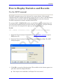
How to Display Statistics and Records
Use the LIST Command
Use the FREQ Command
Use the TABLES Command
Use the SUMMARIZE Command
Use the GRAPH Command
How to Manage Output
Header
TypeOut
Closeout
Printout
Storing Output
How to Use User-Defined Commands
Define Command (CMD)
Run Saved Program
Execute File
How to Create User Interaction
DIALOG
BEEP
QUIT
SET
88
89
91
91
96
98
99
104
107
109
111
112
113
113
118
119
121
123
124
124
127
129
130
131
131
133
136
144
147
151
151
153
156
157
158
160
160
161
165
167
167
171
172
174
iv
Table Of Contents
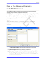
How to Use Advanced Statistics
Use the REGRESS Command
Use the LOGISTIC Command
Use the KMSURVIVAL Command
Use the COXPH Command
Complex Sample Frequencies
Complex Sample Means
Complex Sample Tables
5.
Translation ______________________________________________________________________________ 195
Features
How To Translate Epi Info 7
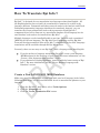
Create a New LANGUAGE .MDB Database
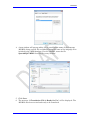
Use an Existing LANGUAGE .MDB Database
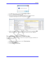
Choose a Language
6.
176
176
180
183
186
192
193
194
195
196
196
198
201
Nutritional Anthropometry
_________________________________________________________________________________________ 202
Introduction
Using the Nutrition Project
Opening the Nutrition Form
Using the Nutrition Form
Customizing the Nutrition Forms
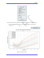
Creating Growth Charts
Using the Nutrition Functions
The ZSCORE Function
The PFROMZ Function
7.
StatCalc _________________________________________________________________________________ 213
Introduction
How to Use StatCalc
Opening StatCalc
Analysis of Single and Stratified Tables
Population Survey or Descriptive Study
8.
202
202
202
204
206
206
209
209
211
213
214
214
215
220
Command Reference ______________________________________________________________________ 222
Introduction
Check Commands
ASSIGN
AUTOSEARCH
BEEP
CLEAR
COMMENTS (*)
DEFINE
DEFINE DLLOBJECT
AFTER and END-BEFORE
BEFORE and END-BEFORE
EXECUTE
GOTO
UNHIDE
IF THEN ELSE
NEWRECORD
Analysis Commands
222
223
223
225
227
228
230
231
234
235
236
237
239
241
243
246
247
v
Table Of Contents
ASSIGN
BEEP
CANCEL SELECT or SORT
CLOSEOUT
COXPH
DEFINE
DEFINE DLLObject
Define Group Command (Analysis Reference)
DELETE FILE/TABLES
DELETE RECORDS
DIALOG
DISPLAY
EXECUTE
FREQ
GRAPH
Program Specific Feature
IF THEN ELSE
KMSURVIVAL
LIST
LOGISTIC
MEANS
MERGE
PRINTOUT
QUIT
READ
RECODE
REGRESS
RELATE
ROUTEOUT
RUNPGM
SELECT
SET
SORT
SUMMARIZE
TABLES
TYPEOUT
UNDEFINE
UNDELETE
WRITE
9.
247
249
250
251
252
254
256
257
258
259
260
266
268
270
272
273
275
278
279
280
281
283
285
286
287
289
292
293
295
296
297
299
301
302
303
305
306
307
308
Functions and Operators __________________________________________________________________ 311
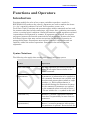
Introduction
Syntax Notations
Operators
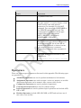
Operator Precedence
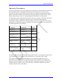
& Ampersand
= Equal Sign
Addition (+)
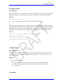
AND
ARITHMETIC
COMPARISONS
LIKE Operator
NOT
OR
XOR (eXclusive OR)
311
311
312
313
314
314
315
316
316
318
320
320
321
322
vi
Table Of Contents
Functions
ABS Function
DAY
DAYS
EXISTS
EXP
FILEDATE
FINDTEXT
FORMAT
HOUR
HOURS
LN
LOG
MINUTES
MONTH
MONTHS
NUMTODATE
NUMTOTIME
RECORDCOUNT
RND
ROUND
SECONDS
SIN, COS, TAN
SUBSTRING
SYSTEMDATE
SYSTEMTIME
TRUNC
LIST Trc1 ADDSC
TXTTODATE
TXTTONUM
UPPERCASE
YEAR
YEARS
324
324
325
325
326
326
327
327
328
332
332
333
333
334
334
335
335
337
339
340
341
342
342
343
343
345
346
346
346
347
347
348
349
10.
Glossary _________________________________________________________________________________ 350
11.
Appendix _________________________________________________________________________________ 353
Data Quality Check
Date Validation
Numeric Data Validation – Lower and Upper Bound
Legal Values
Comment Legal Values
Auto Search
Skip Logic/Patterns
Update Data
Must Enter
Calculated Age
Analysis
Check for Duplicate Records
Delete Duplicate Records
Missing Data
Check for Completeness
353
353
354
354
355
355
355
355
356
356
356
356
356
357
357
vii
Getting Started
Introduction to Epi Info 7
Epi Info 7 is a series of freely-distributable tools and utilities for Microsoft Windows
for use by public health professionals to conduct outbreak investigations, manage
databases for public health surveillance and other tasks, and general database and
statistics applications. It enables physicians, epidemiologists, and other public
health and medical officials to rapidly develop a questionnaire or form, customize
the data entry process, and enter and analyze data.
Epi Info 7 is free of charge and can be downloaded from the Centers for Disease
Control and Prevention (CDC) website at http://www.cdc.gov/epiinfo.
Epi Info Tools
Form Designer - Create the questionnaire, form, or form to collect and
view data.
Enter - Enter data and show existing records in the form.
Classic Analysis - Run statistical analyses, lists, tables, graphs, charts,
etc.
Map - Create maps from Map Server or ShapeFiles.
Options - User custom configuration of Epi Info.
General - Set default values for data format, Map server, etc.
Language - Use Epi Info 7 tools in languages other than English.
Analysis - Set default Boolean values, HTML output format, etc.
Plug-ins - Import new Dashboard Gadgets and Data Sources.
Additional Utilities
StatCalc - Epidemiologic calculators for statistics of summary data.
1
Getting Started
Epi Info 7 Tools Overview
Form Designer
The Form Designer module can be accessed by clicking on the Create Forms button
on the main menu or through the Tools/Create Forms option available from the top
menu. The Form Designer module allows you to place prompts and data entry fields
on one or more pages of a form. Since this process also defines the database(s) that
are created, Form Designer can be regarded as the database design environment.
The Check Code editor within Form Designer customizes data entry providing many
commands and functions. It enables operators to validate data as they are entered,
auto-calculate fields, provide skip patterns, and deliver messages to the data entry
user. For more information, see Introduction to Form Designer.
Enter
The Enter module can be accessed by clicking on the Enter Data button on the
main menu or through the Tools/Enter Data option available from the top menu.
Enter displays the form that was constructed in Form Designer. It can construct a
data table, control the data entry process using the settings and check code specified
in Form Designer, and provide a search function to locate records that match values
specified for any combination of variables or fields on the form. In Enter, the cursor
moves from field-to-field and page-to-page automatically saving data. Navigation
buttons provide access to new, previous, next, first, and last records, and to their
related tables. For more information, see Introduction to Enter.
Analysis
Analysis is the Epi Info 7 tool that allows you to manipulate, manage and analyze
data. The Analysis module offers two interfaces; Classic and Visual Dashboard.
Both of these interfaces can be accessed by clicking on the Classic or Visual
Dashboard button on the main menu or through the Tools/Analyze Data option
available from the top menu. These data may have been collected using Epi Info 7
or another type of database. Currently, Analysis can read data formats in MS
Access, Excel, SQL server, and ASCII. It offers simple and intuitive tools to produce
many forms of useful statistics and graphs for epidemiologists and other public
health professionals. For more information, see Introduction to Analysis.
Map
The mapping component of Epi Info 7, Map, can be accessed by clicking on the
Create Maps button on the main menu or through the Tools/Create Maps option
located on the top menu. Epi Info 7 Map shows data from multiple data formats by
relating data fields to shape files or through point locations containing X and Y
coordinates in various symbols, colors, and sizes. Choropleth and Case-Based are
supported. For more information, see Introduction to Map.
2
Getting Started
Options
General
Sets background images, default database formats, and map service keys for
mapping and geocoding.
Language
Translates completed Epi Info 7 programs into non-English languages by creating
and importing translation definition files. Translation can be done without changing
the names of files, and individual translations can be installed or uninstalled
without affecting the main programs. Switching from one language to another can
be done from the main menu.
Analysis
Displays the current values of Analysis option settings and provides various options
that affect the performance and output of data in Analysis. Settings are used
whenever the Classic Analysis module is used.
Plug-ins
All of the analysis in the Visual Dashboard module is done using gadgets, which
always appear by default. Currently, the record count, data filtering, data recoding,
and formatting gadgets are automatically incorporated in the Visual Dashboard
module. Additional gadgets can be added with future releases of Epi Info 7.
3
Getting Started
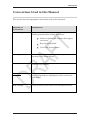
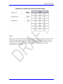
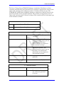
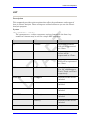
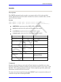
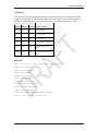
Conventions Used in this Manual
This section describes typographic conventions used in this document.
Example of
Convention
Explanation
Boldface type
Emphasizes heading levels, column headings, and the
following literals when writing procedures:
Names of options and elements that appear
on screens.
Keys on the keyboard.
User input for procedures.
Italic type
Accentuates words or phrases that have special
meaning or are being defined.
Courier New
Used for code samples.
Hyperlink
Provides quick and easy access to cross-referenced
topics. Hyperlinks are highlighted in blue and may be
underlined.
File > Print...
Used to identify menu choice and command selection.
4
Getting Started
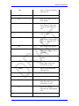
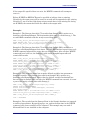
Syntax Notations
The following rules apply when reading this document and using syntax:
Syntax
Explanation
ALL CAPITALS
Epi Info 7 commands and reserved words are shown in
all capital letters.
<parameter>
Information to be supplied to a command or function.
Parameters are enclosed with less-than and greaterthan symbols. Each valid parameter is described
following the statement of syntax for the command.
Parameters are required by the command unless they
are enclosed in braces { }. Do not include the < > or { }
symbols in the code.
[<variable(s)>]
Brackets [ ] around a parameter indicate the possibility
of more than one parameter.
{<parameter>}
Braces { } around a parameter indicate an optional
parameter. Do not include the { } symbols in the code.
|
The pipe symbol '|' denotes a choice and is usually used
with optional parameters. An example is seen in the
LIST command.
*
An asterisk in the beginning of a line of code, as shown
in some code examples, indicates a comment. Comments
are skipped when a program is run.
""
Quotation marks must surround all text values.
DIALOG "Notice: Date of birth is invalid."
5
Getting Started
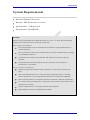
System Requirements
Microsoft Windows XP or above
Microsoft .NET Framework 3.5 or above
Recommended - 1 GHz processor
Recommended - 256 MB RAM
NOTES
Epi Info 7 may be downloaded in two different formats: As a “zip” or a “setup” file. The following
explains what scenarios may be best suited for each format.
ZIP (.zip file) Installation
Can be downloaded to most user desktops and run without requiring administrative or
elevated privileges.
Can be extracted to and run from any folder that the user has read/write/execute privileges
on (including thumb drives).
Assumes that the machine already has Microsoft .NET 3.5 and other prerequisites
installed.
Recommended for disconnected laptops and other emergency use if IT support or
infrastructure is unavailable.
Setup (.msi file) Installation
Traditional setup mechanism that deploys Epi Info™ 7 to the location required by IT
policy.
Allows network administrators to centrally manage and push Epi Info™ 7, including
updates and patches, to users using Microsoft System Center Configuration Manager.
Ensures that the machine's configuration matches the software’s minimum requirements.
Pre-compiles and registers Epi Info™ 7 components on the machine which enables certain
components to run faster.
Requires administrative or elevated privileges during installation.
Recommended for centrally managed IT environments.
6
Getting Started
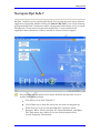
Navigate Epi Info 7
Epi Info 7 modules can be opened individually by accessing the main menu after the
application is installed. Double-clicking the Launch Epi Info 7 icon on the desktop
will open the Epi Info 7 main menu where all programs and utilities can be accessed.
The Epi Info 7 main menu also provides the Epi Info 7 version number and
application date information, which is needed to contact technical support.
Selecting from the navigation menu opens modules and provides access to
utilities and custom settings.
File allows you to “Exit” Epi Info 7.
View allows you to show the status bar and view the program log.
Tools allow you to access the main Epi Info 7 modules: Form
Designer, Enter, Classic Analysis, the Visual Dashboard, and Maps.
The Tools menu also enables you to set default options which
include Language Translations.
7
Getting Started
StatCalc is a sample size calculator.
Help provides access to the online help videos, an Epi Info
discussion forum, instructions on how to contact the Help Desk, and
an About Epi Info page.
Clicking the menu buttons allows easy access to the most used modules:
Form Designer, Enter, Classic Analysis, the Visual Dashboard, Maps, the
Epi Info website (requires Internet connection), and the ability to exit the
application.
8
Getting Started
Tech Support and Contact Information
CDC provides funding for the Epi Info Help Desk, which offers free technical support
to all Epi Info users from 8:30 a.m. to 4:30 p.m.
If you have any questions or issues with Epi Info systems, contact the Epi Info Help
Desk:
Epi Info Help Desk:
404-498-6190
Epi Info E-mail:
[email protected]
Website
The latest version of the Epi Info software, shapefiles for Epi Map, comprehensive
tutorials, and translations can be downloaded from the Epi Info website.
Epi Info User Community Website
The Epi Info User Community Website provides a forum for user questions and
answers. Join the group by creating a user account at
http://www.phconnect.org/group/epiinfo. Complete the instructions for joining.
9
Getting Started
Acknowledgements
A Database and Statistics Program for Public Health Professionals
CDC Core Team (in alphabetical order):
José Aponte
Harold Collins
John Copeland
James Haines (McKing Consulting)
Asad Islam (Team Leader)
Gerald Jones
Erik Knudsen
David McKing (McKing Consulting)
Roger Mir
David Nitschke
Carol Worsham
Special thanks to:
Sara Bedrosian
Doug Bialecki
Karl August Brendel, III
Andy Dean
Robert Fagan
Gabriel Rainisch
Donald Chris Smith
Enrique Nieves
10
Getting Started
Suggested citation: Dean AG, Arner TG, Sunki GG, Friedman R,
Lantinga M, Sangam S, Zubieta JC, Sullivan KM, Brendel KA, Gao Z,
Fontaine N, Shu M, Fuller G, Smith DC, Nitschke DA, and Fagan RF.
Epi Info™, a database and statistics program for public health
professionals. CDC, Atlanta, GA, USA, 2011.
Additional thanks to:
EIS Epi Info 7 Workgroup
Sudhir Bunga
Timothy Cunningham
Nancy Fleischer
Alyson Goodman
Asha Ivy Jeffrey Miller
Timothy Minniear (Chairperson)
Diane Morof
Cyrus Shahpar
Danielle Tack
Christopher Taylor
Ellen Yard
PHPS Epi Info 7 Workgroup
Tegan L. Callahan
Sarah Elkerholm
Coby E. Jansen
Amy V. Neuwelt
Cristina M. Rodriguez Hart
Tina J. Sang
Anna S. Talman (Chairperson)
Angela s. Tang
Sharron H. Wyatt
11
Getting Started
Special thanks to past contributions:
Previous versions produced in collaboration with the World Health Organization
(WHO), Geneva, Switzerland, by Andrew G. Dean, Jeffrey A. Dean, Denis
Coulombier, Anthony H. Burton, Karl A. Brendel, Donald C. Smith, Richard C.
Dicker, Kevin M. Sullivan, Thomas G. Arner, and Robert F. Fagan.
Manual by Andrew G. Dean, Juan Carlos Zubieta, Kevin M. Sullivan, Cecile
Delhumeau, Ralph H. Lord, Jr., Shonna Luten, and Shannon Jones.
Tutorial exercises by Juan Carlos Zubieta, Consuelo M. Beck-Sagué, G. Allen
Tindol, Karen DeRosa, Jinghong Ma, and Shannon Jones.
Division of Epidemiology and Analytic Methods
Epidemiology and Analysis Program Office
Office of Surveillance, Epidemiology, and Laboratory Services
Centers for Disease Control and Prevention (CDC)
1600 Clifton Road, (Mail Stop E-33)
Atlanta, GA 30333
This manual and the programs are in the public domain and may be freely copied,
translated, and distributed. All are available at www.cdc.gov/epiinfo.
Epi Info Help Desk for Technical Assistance
[email protected]
(404) 498-6190 voice
12
Getting Started
Additional Acknowledgements
StatClac algorithms and formulas provided by OpenEpi.com.
Aberration detection algorithms provided by the CDC’s Early Aberration Reporting
System (EARS). For more information on EARS visit:
http://emergency.cdc.gov/surveillance/ears/
Equations Acknowledgements
We thank Drs. David Martin and Harland Austin for use of their source code for
computing exact and mid-p exact statistical tests and confidence intervals for the
odds and rate ratios. Thanks to reviewers of this chapter who provided comments,
and to the software testers.
Epi Info's Nutrition Project File (replaces NutStat)
Acknowledgements
Special thanks to Kevin Sullivan, Ph.D., Department of Pediatrics, School of
Medicine and Department of Epidemiology, Rollins School of Public Health, Emory
University, Atlanta, GA; Nathan Gorstein, WHO; Phillip Neibrug, M.D., M.P.H.,
Norman Staehling, M.S., Ronald Fichtner, Ph.D., and Frederick Trowbridge, M.D.,
CDC, for their assistance in preparing the Epi Info™ 6 manual upon which portions
of this manual are based.
Notes
These programs are provided in the public domain to promote public health. We
encourage you to provide copies of the programs and the manual to friends and
colleagues. The programs may be freely translated, copied, distributed, or even sold
without restriction except as noted below. No warranty is made or implied for use of
the software for any particular purpose.
"Epi Info" is a trademark of the CDC. Please observe the following requests:
The programs can be translated and the examples altered for regional use, but must
be distributed in essentially the form supplied by CDC.
Epi Info is written in C# .NET and runs on version 3.5 of the Microsoft .NET
Framework.
Microsoft, Windows, Word, and Visual Basic are registered trademarks of Microsoft
Corp. Trade names are used for identification or examples; no endorsement of
particular products is intended or implied. The use of trade names or trademarks in
this manual does not imply that such names, as understood by the Trade Marks and
Merchandise Marks Act, may be used freely by anyone.
13
Getting Started
Technical Support
For new versions of the software and answers to commonly asked questions, please
visit the Epi Info website at http://www.cdc.gov/epiinfo. Technical assistance is
provided by e-mail or telephone. Information for obtaining Epi Info technical
assistance is provided on the title page.
The Epi Info WebBoard provides a forum for user questions and answers. Join the
group by creating a user account at http://phconnect.org/group/epiinfo. Follow the
instructions to join.
Contact Us
Please send comments and suggestions for future versions to:
Epi Info Hotline
[email protected]
(404) 498-6190 voice
14
Form Designer
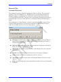
Introduction
Epi Info 7 may use the Microsoft Access database format or a SQL server database
to create projects. Each project contains one or more forms, and each form may have
one or more data tables. Form Designer allows you to place prompts and data entry
fields on one or more pages within the form. Since this process also defines the
database(s) that are created, Form Designer can be regarded as the database design
environment.
The form and the data table are located inside an Epi Info 7 project. An unlimited
amount of forms may be contained inside a project. When data are entered into a
form through the Enter module, it will be populated into the form’s corresponding
data table.
Inside each form, fields (called variables in Analysis) are created to hold data. The
Check Code Editor component of the Form Designer can be used to add intelligence
to a form (e.g., allowing for skip patterns, hiding fields from view, and performing
math calculations). It can also be used to implement data validation checks.
Functions are provided for importing files from Epi Info 3.5.x, aligning fields, and
placing a layout grid on the workspace. Fields can also be grouped for display and
used in Classic Analysis or Visual Dashboard.
15
Form Designer
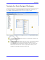
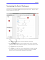
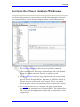
Navigate the Form Designer Workspace
To open Form Designer, click Create Forms from the Epi Info 7 main menu, or
select Tools > Create Forms from the main page navigation menu.
The Form Designer page panel allows you to insert pages, controls, and
templates into a form.
The Make/Edit Form window is the form, survey, or questionnaire design
space. Fields are created, edited, and designed from this area of the
application using the Field Definition dialog box. You can customize the
work space by selecting fonts, colors, and grid options. Surveys can be
customized by creating code tables or Check Code.
16
Form Designer
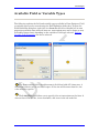
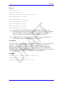
Available Field or Variable Types
The following explains the field and variable types available in Form Designer. Field
or variable types can be created using the Field Definition dialog box. To open the
Field Definition dialog box, right click in a form. Each field or variable has its own
properties available when selected; however, some options may not be shown or may
be disabled (grayed out) depending on the variable or field type selected. Field or
Variable Type Properties can also be selected.
1
The Text variable field is an alphanumeric field that holds 255 characters. A
maximum field size can be set to save space. If the size will be more than five, the
value must be typed in.
2
The Label/Title field allows you to specify titles or instructions on the form. It
does not have Check Code, is not searchable, and is not in the tab order list.
17
Form Designer
3
The Text [Uppercase] field is a forced uppercase field. All information typed
in this field will appear in uppercase. A maximum field size can be set to save space.
If the size is more than five, you must type in the value.
4
The Multiline field is an alphanumeric field with the capacity to store up to 1
gigabyte of information in the field or approximately two million characters.
5
The Number field is a numeric field with six predefined value patterns. You
can create a new pattern by typing the pattern into the Pattern field.
6
The Phone Number field is a pre-determined mask field for phone numbers
only. Phone extensions or international numbers cannot be used in this field.
18
Form Designer
7
The Date field is an alphanumeric field with pre-set date patterns selected
from the pattern drop-down list. It cannot be altered.
8
The Time field is an alphanumeric field with pre-set time patterns selected
from the pattern drop-down list. It cannot be altered.
9
The Yes/No field is a pre-determined field in which the only selected values
can be yes or no. The yes or no answer is stored in the database as a 1 or 0. 1 = Yes
and 0 = No. When performing Check Code, use the (+) or (–) to register a yes or no
response. (+) = Yes and (–) = No. A Yes/No field can also store a missing value
represented by (.).
10
The Checkbox field is treated like a Yes/No field. There is no missing value; it
only has two values.
19
Form Designer
11
The Option field creates radio button selection fields for the form. It is for
mutually exclusive choices; only one choice can be made. If more than one choice is
required, use the Checkbox option.
12
The Command Button creates an executable button on the form. For
example, execute Classic Analysis or another program (e.g., Microsoft Excel).
13
The Image field allows an image to be inserted per record (i.e., patient, rash or
bacteria picture). The accepted image file types are: Graphics Interchange Format
(.GIF), Joint Photographic Expert Group (.JPG or .JPEG), Windows Bitmap Format
(.BMP), Windows Icon File Format (.ICO), Windows Metafile Format (.WMF), and
Enhanced Metafile Format (.EMF).
14
The Mirror type field only works with multiple pages in a form (i.e., if a
Patient ID is on page one, the value of Patient ID can be mirrored onto another
page using the mirror field). It will be Read Only.
20
Form Designer
15
The Date/Time field is an alphanumeric field with pre-set date/time patterns
selected from the pattern drop-down list. It cannot be altered.
16
17
The Unique Identifier type creates values unique to a specific record.
The Legal Values field type creates a drop-down list of values.
18
The Comment Legal Values field type creates a drop-down list of values
with a comment associated with each value. Only the value and not the comment
associated with the value is saved to the database.
21
Form Designer
19
The Codes field creates a linked drop-down list where the selected value
populates other fields on the form.
20
The Relate field creates relationships between your main form ("parent" form)
with sub forms ("child" forms) only within the same .PRJ.
Related forms are relationships between the main or parent form with sub or
child forms, which are linked to a parent form automatically by unique keys
generated by the application. They are made accessible through buttons in the
form. Buttons can be created on a conditional basis to become available only
under specified conditions (i.e., when additional information is needed about a
particular disease).
22
Form Designer
Field Properties
Select Field types by right-clicking on the Form Designer canvas by using the New
Field option. Each field has a set of available field properties; however, some options
may not be shown or may be disabled (grayed out) depending on the field type
selected.
A Required field is mandatory. It cannot be used in combination with Read
Only because the properties are mutually exclusive. If a page contains a
Required field, the Enter module will not allow further page navigation until
a value has been entered. To avoid gridlock, use this property sparingly.
A Read Only field does not allow the placement of the cursor in the field or
data entry. It is particularly useful for calculated fields that will not be
changed directly. Read Only cannot be used in combination with Required
because those properties are mutually exclusive.
Retain Image Size maintains the size of the original image and does not
alter the size to fit the image box in the form.
The Range property can be applied to Number or Date field types. It allows
for a specified value between one setting and another. Values falling outside
a specified range will prompt the user with a warning message in the Enter
module. Missing values are accepted unless the field is designated Required.
23
Form Designer
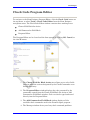
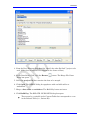
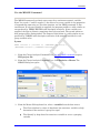
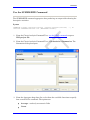
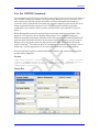
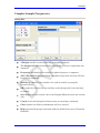
Check Code Program Editor
To navigate to the Form Designer Program Editor, click the Check Code button on
the top menu, or select Tools > Check Code Editor from the Form Designer
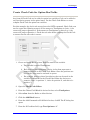
navigation menu. The Check Code Editor window contains three working areas:
Choose Field Block for Action
Add Command to Field Block
Program Editor
The Program Editor can be closed and the form opened by clicking OK, Cancel, or
the close X button.
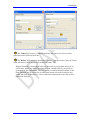
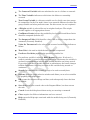
1. The Choose Field for Block Action tree allows you to select fields
and sets when the actions designated by the Check Commands occur
during data entry.
2. The Program Editor window displays the code generated by the
commands created from the Choose Field Block for Action or Add
Command to Field Block window. Code can also be typed and saved
directly into the Program Editor.
3. The Add Command to Field Block window displays all the
available check commands used in the Form Designer program. .
4. The Message window alerts you of any check command problems.
24
Form Designer
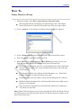
How To:
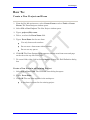
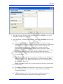
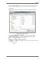
Create a New Project and Form
1. From the Epi Info main menu, select Create Forms or select Tools > Create
Forms. The Form Designer window opens.
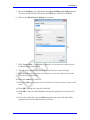
2. Select File > New Project. The New Project window opens.
3. Type a project (file) name.
4. Tab to, or select the Form Name field.
5. Type a Form Name for the new form.
Use only letters and numbers.
Do not start a form name with a number.
Do not use any spaces.
6. Click OK. The Form Designer page appears with the new form name and page
on the tab at the top left of the page.
7. To create fields, right click in the workspace to open the Field Definition dialog
box.
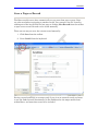
Create a New Form in an Existing Project
1. Select File > New Form. The Name the form dialog box opens.
2. Type a Form Name.
3. Click OK. The new form appears in the workspace.
A new form is created in the existing project.
25
Form Designer
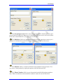
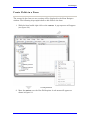
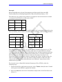
Create Fields in a Form
The canvas for the form you are creating will be displayed in the Form Designer
window. The following steps explain how to add fields to the form.
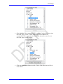
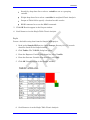
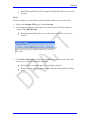
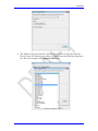
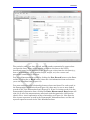
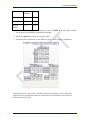
1. With the form loaded right-click on the canvas. A pop-up menu will appear
(see figure 2.0).
Creating Fields 2.0
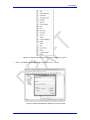
2. Move the mouse over the New Field option. A sub-menu will appear as
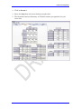
shown in figure 2.1.
26
Form Designer
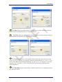
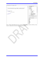
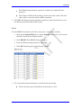
Figure 2.1: The list of field types that you can add to your form
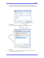
3. Select a Field or Variable Type from the list (i.e., Text).
Figure 2.2: The field definition dialog box for Text fields
27
Form Designer
4. Type in the Question or Prompt for the field.
5. Press the Tab key on the keyboard. The cursor jumps to the field and
automatically filled it in for you based on the prompt.
6. Click OK. The field is created and displayed on the canvas.
At the most basic level, that’s all there is to adding fields – simply select the type of
field you want to add, give it a prompt, and you’re done!
The steps above outlined how to create a text field. Other field types are also
available, including number fields (which restrict the user to entering just valid
numbers), date fields, checkboxes, and drop-down lists.
Delete a Field
1. Right-click on the field. The pop-up menu opens.
2. Click Delete. The field is removed from the form.
Warning: The field and any data previously collected are deleted from the
form and database. Deletions occur immediately. There is no prompt to
verify the deletion before it occurs, and the only way to recover the field is by
using the “undo” feature.
28
Form Designer
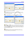
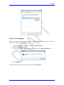
Edit a Field in a Form
To edit a field, right-click on the field. The Field Definition dialog box
appears for that field/variable.
If a data table has not been created in Form Designer, or if no records exist in
it, use the Field Definition dialog box to change names, field types, and
patterns.
Once the data table contains entries, the field name cannot be changed, but
the field type can. Form Designer will attempt to transfer the data into the
new type. In some cases, however, it will discard incompatible data items.
Changing the type of a text field to a numeric field will transfer numeric
data, but Form Designer cannot handle certain numbers (i.e., "M0111") and
will assign a missing value. Since both contain text, a text field can safely be
changed to a multi-line field.
Delete an Existing Data Table without Deleting the Form
1. From the Form Designer navigation menu, select Tools > Delete Data
Table. The Form Designer warning message appears.
2. Click Yes.
If the data table is deleted, any entered data associated with the form
is deleted from the project. Before accepting the warning, be absolutely
sure you do not need the data previously entered.
29
Form Designer
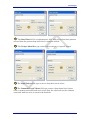
Set a Field or Prompt Font
Default prompt and field fonts can be overwritten using Field Font and Prompt
Font buttons in the Field Definition dialog box. Prompt Font and Field Font are
applied per field. To apply fonts to future fields, set a default font for the project
using the Format menu.
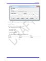
1. From the Field Definition dialog box, click Prompt Font or Field Font. The
Font dialog box opens.
2. Select a font, font style, and sizes.
3. Click OK. The Field Definition dialog box appears.
4. Click OK. The font is applied to the question/prompt or field.
30
Form Designer
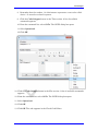
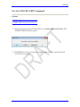
Change Workspace Settings
Use the Format settings to customize the Form Designer workspace.
1. From the Form Designer navigation menu, select Format. The drop-down menu
opens allowing you to customize your workspace.
2. Select Format>Grid Settings to open the grid settings dialog box.
Check the Snap to Grid box to force fields in the form to snap to the grid
nearest the field edge.
Check the Show Grid box to see the grid as the workspace background.
Use the up and down arrows in the character widths between grid lines
field to alter the displayed widths between grid lines.
Select either the Snap prompt to grid or Snap entry field to grid
radio button depending on whether you want prompts or fields aligned.
3. Click OK. The Form Designer page appears with new settings.
31
Form Designer
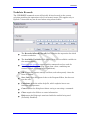
Set the Tab Order
Initially, the order in which the cursor visits fields is set automatically based on
each field’s position in order from right to left, then top to bottom. If another tab
order is desired, (when fields are arranged in vertical columns), right click in the
canvas area of the page you want to customize the tab order.
Manually Change the Tab Order
1. Click Tab > Show Tab Order to show the current order of field entry.
2. Click Tab > Start New Tab Order to arrange order of field entry according to
the defaults.
3. Click Tab > Continue Tab Order to continue the tab order of fields you have
selected by left clicking and dragging the selection box over the desired fields.
All fields within the selection box will be ordered starting with the next field tab
number after the last field in your current tab order.
32
Form Designer
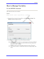
Set a Default Font
If set prior to creating fields on the form, default fonts facilitate a consistent look to
your fields.
1. From the Form Designer navigation bar, select Format > Set Default Prompt
Font or Set Default Field Font. The Font dialog box opens.
2. Select a new font, font style, or size.
3. Click OK. A new default font is set.
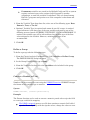
The default font settings affect new prompts created using the Field
Definition box and not update any existing field fonts in the form.
The default font is set at the Form Designer level, and not just the form
level. The default font will appear in all forms/fields created with Form
Designer.
Default fonts can be overwritten using Font for Prompt option in the Field
Definition dialog box.
33
Form Designer
Copy, Cut, and Paste Fields
1. Left click, hold, and drag a rectangle around the fields to be copied or cut.
2. From the Form Designer navigation menu, select Edit > Copy or Cut from the
drop-down list.
3. Click in the new section of the form or select a new page in the project.
4. Select Edit > Paste. The copied fields appear in the form.
Note: You can also use the right-click pop-up menu to copy, cut, or paste instead of
using the Edit menu.
Note: If copied to the same page, the copied fields will be placed directly over the
original fields. Drag the new fields to a new position on the page. The new field will
have the same name as the original with a number '1' appended to the name. If the
name already has a number appended to it, it will be incremented by one or have an
additional number appended to it.
34
Form Designer
Align Fields
Fields can be aligned vertically or horizontally.
1. Click and hold the left mouse button to draw a rectangle around the fields to be
aligned.
2. Select Format > Alignment > As Stack (vertical alignment) or
Format > Alignment > As Table (horizontal arrangement with rows). The
selected fields align based on the selection.
35
Form Designer
Insert a Background Image or Color
Insert a Background Image on a Form
1. From the Form Designer navigation menu, select Format > Background. The
Background dialog box opens.
2. From the Background Image section, click Choose Image. The Background
Image box opens.
3. Locate the image file. Click Open. The selected image appears in the
Background Image dialog box. Image formats include bitmap (.bmp), picture
(.ico), and JPEG (.jpg).
4. Use the Image Layout drop down selection to customize the image on the
screen (None, Tile, Center, and Stretch).
5. From the Image and Color section, use the radio buttons to Apply to all pages
or Apply to the current page only.
6. Click OK. The image appears in the form.
To remove the image, select Clear Image from the Background Image
box.
Insert a Background Color to a Form
1. From the Form Designer navigation menu, select Format > Background. The
Background dialog box opens.
2. From the Background Image section, click Change Color. The Color dialog box
opens.
3. Select a background color from the palette or select Define Custom Colors
to enter a more specific color request.
4. Click OK. The selected color previews in the background box.
5. From the Image and Color section, use the radio buttons to Apply to all pages
or Apply to the current page only.
6. Click OK. The color appears in the form as a background.
To remove the color, select Clear Color from the Background Color box.
36
Form Designer
Work with Pages in a Form
Add a New Page
1. From the Form Designer page panel, highlight the form where you want to
add a page.
2. Click Add Page. The page appears in the Form Designer window and at the
end of the existing pages listed in the Page Names window.
Delete a Page
1. From the Form Designer page panel, highlight the page you want to delete.
2. Click Delete Page. The Confirming Deletion pop-up opens.
3. Click Yes. The page is deleted from the list.
37
Form Designer
Insert a New Page
1. From the Form Designer page panel, highlight the page where you want to
insert a page.
2. Click Insert Page. The page appears in the Form Designer window above
the selected page in the Page Names window.
Delete a Page
1. From the Form Designer page panel, highlight the page you want to delete.
2. Click Delete Page.
3. Click Yes. The page is deleted from the list.
38
Form Designer
Name a Page
1. Right click the page from the Page Names window. The Page Name dialog box
opens.
1. Type a name in the Page Name field.
2. Click OK. The page name appears in the list of pages.
39
Form Designer
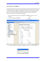
Save Page as Template
Using page templates allows you to develop a library of pre-formatted pages that can
be used in any form or applications being built. This makes it easy for you to rapidly
customize data collection forms. Templates may also be useful in reordering the
pages in a form (save each page as a template, then drag each template to the
canvas in the order you want the pages to appear).
1. From the Form Design page panel, highlight the page you want to save as a
template.
2. Click Save Page as Template.
3. In the Page Names window type a name you want to use for the template.
40
Form Designer
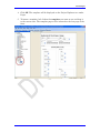
4. Click OK. The template will be displayed on the Project Explorer tree under
Pages.
5. To insert a template, left click on the template you want to use and drag it
to the canvas area. The template page will be inserted as the last page of the
form.
41
Form Designer
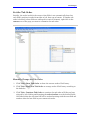
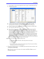
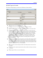
View a Data Dictionary
The Data Dictionary displays form(s) and defined variables for an open project.
Fields or variables are sorted and displayed by page number in the form with
defined variables appearing at the end of the listing. Information retrieved from the
form includes Page Number, Prompt, Field Name, Variable Type, Format, and
Special Info.
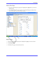
1. From the Form Designer navigation menu, select Tools > Data Dictionary.
The Variables table is displayed in the form window.
42
Form Designer
Page Number values are developed each time a page is added from the Form
Designer Page panel.
Column values for Prompt, Field Type, Name and Variable type are
developed when fields are created from the Field Definition dialog box.
Format column values include selected patterns for number and date fields
and sorted for combo boxes.
Special Info column values include all properties available from the Field
Definition dialog box. Properties include Read Only, Legal Value, Repeat
Last, Code Table, Groups, Required, Range, and Image Size. The Special Info
column also holds the defined variables values of Standard, Global, or
Permanent. The Special Info column includes information on related fields to
indicate whether they contain one record or an unlimited number of records.
This is developed when the related field is created. The default is Unlimited
Records. If the Return to the Parent Form after One Record has been Entered
box is checked, the format will appear as one record.
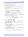
Note: To view a data table located in another form:
 Click Select Form. The Select Form drop-down menu opens.
 Locate a form.
 The Data Dictionary for the selected form opens. Note that only the Data
Dictionary for the selected form opens.
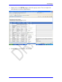
2. To open the Data Dictionary as an HTML page inside the browser window, click
View/Print as Web Page.
Note: From the browser, the data can be printed with File > Print, or saved
with File > Save As.
43
Form Designer
3. Right click on the HTML page to show the pop-up menu. You can export the
data directly to an Excel spreadsheet.
5. Click Close to exit the Data Dictionary.
44
Form Designer
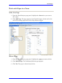
Create a Group
In the Classic Analysis or Visual Dashboard module, statistics can be run on a group
of variables as a whole or on the individual variables inside the group.
1. Left click, hold, and drag a rectangle around the fields slated to be grouped. A
line rectangle appears around the selected fields.
2. From the Form Designer navigation menu, select Insert > Group. The Group
Properties dialog box appears.
3. Type a group name in the Question or Prompt box.
4. Click Font to change the font type and size.
5. Click OK to accept the group options. The fields appear in the group box.
Move the group by clicking and holding the group name with the mouse.
Resize the group box by double-clicking inside the group to change the
cursor to the resize arrows. If the new size includes additional fields, they
become members of the group.
Edit a Group
The following steps delete the group, ungroup variables, or change the group name:
1. Right click on the group name. Select Properties. The Edit Group window
opens.
2. Change the Group Name by typing a new name in the Group Name field.
3. Click OK. The group appears with the selected edits.
4. To delete a group box, right click anywhere on the box to open the pop-up
box. Click Delete to delete the group box.
Note: This will not delete your fields.
45
Form Designer
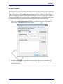
Create a Mirror Field
A mirror field is used to mirror or echo data from another field onto one or more
pages of a project. They can be used across pages, but cannot be included in Related
Forms.
To create a mirror field:
1. Open a project that contains at least two pages.
2. From the page that requires a mirror field, right-click on the canvas. The popup menu will appear.
3. Move the mouse over the New Field option. A sub-menu will appear. Select
Mirror as the variable type.
4. The Assign Variable to Mirror Field dialog box opens.
5. Enter a value in the Question or Prompt box. (This will populate the Field Name
when you tab or click out of the Question or Prompt box).
6. Click the drop-down box for the Assigned Variable in the Attributes Group to
show a list of variables that can be mirrored.
7. Select the variable to be mirrored. (Field and Prompt font may also be edited in
this group).
8. Click OK. The new variable appears on the current page.
Mirror fields are Read Only.
When data are entered into the original field, the value of that field will
be reflected in the newly-created mirror field.
Mirror fields can be copied and pasted to subsequent pages.
Command buttons cannot be selected as source fields to mirror.
46
Form Designer
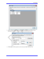
Create an Option Box
Option boxes should be used when the choices presented to you are mutually
exclusive. If you make more than one choice, use checkboxes.
To create an option box field:
1. Open the page where you want the Option Box field to be placed.
2. From the page that requires an Option Box field, right-click on the canvas.
The pop-up menu will appear.
3. Move the cursor over the New Field option. A sub-menu will appear.
4. Select Option as the field type. The Option dialog box appears.
5. In the Number of Choices field, enter a number (the option definition fields
will increase with an increase in the number of choices).
6. Select Right or Left for the placement of the Option box (radio button).
7. Type the option information in each field.
8. Click OK. The Option box appears in the form.
47
Form Designer
Create Legal Values
A Legal Values field is a drop-down list of choices on the questionnaire. These items
cannot be altered by the user during entry. The only values for entry are the ones in
the list.
To create a Legal Values field:
1. Open the page where you want the field to be placed.
2. Right-click on the canvas. The pop-up menu will appear.
3. Move the cursor over the New Field option. A sub-menu will appear.
4.
Select Legal Values as the variable type to display the Legal value dialog box.
5. Enter the Question or Prompt for the Legal Values field.
6. Click the ellipses (…) button to the right of the Data Source box.
7. Click Create New to enter the legal values to answer the question. Existing
tables can also be used to create legal values.
7. Enter the first value (i.e., Married). Press Enter or Tab to advance to the next
value.
8. Values will appear in alphabetical order unless you select Do Not Sort.
8. Click OK.
9. From the Field Definition box, click OK. The new field appears in the form as a
drop-down list of values.
48
Form Designer
Create a Comment Legal
Comment Legal fields are similar to Legal Values. They are text fields with
character(s) typed in front of the text (with a hyphen). During data entry, the
character and the text (i.e., M-Male) are displayed. However, only the character
value is stored in the table (i.e., M). In the Classic Analysis module, statistics will be
calculated if all values are numeric.
To create Comment Legal fields:
1. Open the page where you want the field to be placed.
2. Right-click on the canvas. The pop-up menu will appear.
3. Move the mouse over the New Field option. A sub-menu will appear.
4. Select Comment Legal as the variable type to display the Comment Legal
value dialog box.
5. Enter the Question or Prompt for the Comment Legal field.
6. Click the ellipses (…) to the right of the Data Source box.
7. Click Create New to enter the Comment Legal values (separated with
hyphen) for the field. Existing tables can also be used to create Comment
Legal fields.
8. Enter the first value (i.e., 1-Male). Press Tab to advance to the next value.
Values will appear in alphabetical order unless you select Do Not Sort.
9. Click OK.
10. From the Field Definition box, click OK. The new field appears as a dropdown list of values.
49
Form Designer
Codes
A Codes field allows you to choose a value from a drop-down list. Based on the value
selected, another field(s) is populated with predetermined values. At least two fields
must exist; one which holds the selection code, and another to receive the value of
the code. The first field holds the selection code in a drop-down list while subsequent
ones are Read Only, which populates based on assignments set in the code table.
Create a New Code Table
Code tables provide values to select from a drop-down list. When a value is selected
in Code fields from a drop-down list, based on that choice, another field populates
from a set of predetermined values.
New code tables can be created or existing code tables can help create code table
selections. When a list of values is specified, an entry must match one of a specified
list of values or be rejected.
To create a new code table:
1. Open the page where you want the code table field to be placed.
2. Right-click on the canvas. A pop-up menu will appear.
3. Move the mouse over the New Field option. A sub-menu will appear. Select
Codes as the variable type.
4. The Field Definition dialog opens for the field. Enter the Question or
Prompt for the field.
50
Form Designer
5. Select the field(s) to be linked from the Select field(s) to be linked section.
To select multiple fields, hold down the CTRL key and click each field.
6. Click on the Data Source ellipsis (…) button.
7. Click Create New. A spreadsheet opens for you to enter the values for the
Codes field and Linked fields.
8. The left-most column displays the selection field you chose in Step 4.
9. Each column to the right lists the field(s) to receive the codes based on the
value of the selection field.
10. Enter the codes for each field.
11. Press the Tab key to move to the next field, or to the next row if at the end of
a row.
12. Click OK to accept the codes for each field.
13. Click OK to close the Field Definition dialog box and place the fields in the
form.
14. To test the code table, open the Enter module and verify that both fields
populate based on the drop-down list selection.
51
Form Designer
Create Codes with Existing Table
A code table can be used for more than one field in a form (i.e., values of “agree” and
“disagree.”) If you click on the Data Source ellipsis button after creating a new
Codes field, an option to Use Existing is displayed. Follow the steps below to set up
an existing code table for a different Codes field.
To create a Codes field using an existing code table:
1. Open the page where you want to place the code table field.
2. Right-click on the canvas. The pop-up menu will appear.
3. Move the mouse over the New Field option. A sub-menu will appear. Select
Codes as the variable type.
4. The Field Definition dialog opens for the field. Enter the Question or
Prompt for the field.
5. Select the field(s) to be linked from the Select field(s) to be linked to above
field list box.
6. To select multiple fields, hold down the CTRL key and click each field.
7. Click on the Data Source ellipsis button.
8. Click Use Existing. The Tables dialog box opens.
9. Select a table from the list. Click OK.
10. Follow the instructions to make the associations in the Match Fields section.
52
Form Designer
Match Fields
Text fields created from your form are displayed on this dialog. From the right-hand
side of the screen, select a value from the drop-down list. At least two fields must
exist; one holds the selection code, and one or more receives the value of the code(s).
The first field holds the selection code in a drop-down menu, and all subsequent ones
are Read Only, which populates based on assignments set in the code table.
1. Select the required drop-down field to be linked to the code table. Once you
select a link, the OK button becomes active.
2. Click Preview Table to view the link association. You can see the table and
determine if you want to keep your selection. Select Back to return to the Match
Fields dialog box.
53
Form Designer
3. Create additional links for the other fields using the Form and Table Fields
drop-down lists. Select one field from the form fields drop down list
4. Click Link to add the matches to the Associated Link Fields list box.
54
Form Designer
Links can be deleted by selecting from the list and clicking Unlink.
Fields removed from the Link list box return to the Form and Table
Fields drop-down lists.
5. Click OK to accept the Match Field selection. The Code Table selection appears
in a grid format for review.
6. Click OK to accept the selection or click Back to return to the Match Field
dialog box and edit the code table selections.
55
Form Designer
Insert a Line as an Image
1. Open a field definition dialog box for a Label/Title field on the page you want
to insert the line.
2. In the Question or Prompt field, hold the SHIFT key and type an underscore
to create a line.
3. Click Font for Prompt. The Font dialog box opens.
4. Select a font size and bold.
5. Click OK.
6. Create a Field Name for the variable.
7. Click OK. The line appears in the form.
8. The line can be resized, moved, copied and pasted as needed.
56
Form Designer
Insert an Image in a Record
1. Open a field definition dialog box for an Image field on the page you want to
insert the Image.
2. From the New Field drop-down list, select Image.
3. Enter the Question or Prompt in the Image dialogue box. If the image does
not have to be resized, click the Retain Image Size checkbox.
3. Click OK. The Image box appears in the form. Image boxes can be resized by
selecting the grid and dragging the blue bounding boxes.
Note: This is only a place holder on the form. The actual image is entered into
the record from the Enter Data module during the data entry process.
57
Form Designer
4. From the Form Designer navigation menu, select File > Enter Data. The
newly-created image field displays in the Enter Data window.
5. Click the Image Field. The Select the Picture File dialog box opens.
6. Select an image file.
7. Click Open. The selected image appears in the field.
58
Form Designer
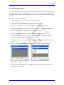
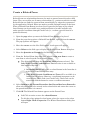
Create a Related Form
Related forms are relationships between the main or parent form with sub or child
forms. They are used for one-to-many relationships (i.e., patient record/visit records).
Related forms are linked to a parent form automatically by unique keys generated
by the application. Related Forms are made accessible through buttons in the form.
When a Related Form Button is selected it will open the first page of the related
form. Buttons can be accessible on a conditional basis to become available only
under specified conditions through Check Code (i.e., to show a special form for a
particular disease).
1. Open the page where you want the Related Form Button to be placed.
2. From the page that requires a Related Form Button, right-click on the canvas.
The pop-up menu will appear.
3. Move the cursor over the New Field option. A sub-menu will appear.
4. Select Relate as the field type to display the Related Form Button dialog box.
5. Enter the Question or Prompt for the Related Form Button.
6. From the Related Form drop down box , select Create new form to create a
new form or select from the list of existing forms.
The dialog box will show the Accessible always button selected. The
Only When Certain Conditions are True selection is not available in
this version of Epi Info 7.
 Accessible always will create a related button in the form that is
active at all times during data entry.
 Only When Certain Conditions are True will be available in a
future Epi Info release. However, a conditional statement can be
created using Check Code (see Check Code). Check Code can be
associated with the button to create a condition statement.
6. Select Return to the Parent Form after One Record has been Entered to
allow only one record to be entered in the related table and return the cursor to
the parent form after it is entered.
7. Click OK. The Related Form button appears on the Parent Form.
Left Click to resize or move the related button.
To edit the relate options for that button, place the cursor on the relate
button Right Click >Properties. The Related Form Button dialog box
will open.
59
Form Designer
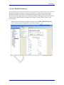
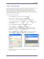
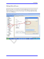
Editing Related Forms
Related form pages can be edited by selecting the page under the form in the Project
Explorer pane. The screen below shows how the button Hepatitis opens the related
form/view “RHepatitis). To edit the related page, click on Person and Clinic Info
under the form RHepatitis.
60
Form Designer
Delete an Existing Data Table Without Deleting the Form
To delete an existing data table without deleting the form, perform the following
steps:
1. From the Form Designer navigation menu, select Tools > Delete Data Table.
The Form Designer warning message appears.
2. Click Yes. The data table associated with your form is deleted. The form
remains intact. A new data table will be made next time you use it in Enter.
If the data table is deleted, any entered data associated with the form are
deleted from the project. Be absolutely sure you do not need the records.
WARNING!
This function should be used only if you want to delete the data. All data
will be deleted.
61
Form Designer
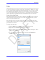
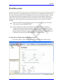
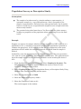
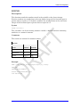
Check Code
Overview
To create Check Code, open the Program Editor by selecting the Check Code
button located on the toolbar, or select Tools > Check Code Editor from the Form
Designer navigation menu.
Check Code validates data entry and enters data faster and more accurately. With
advance planning, code can be created to perform calculations, skip questions based
on prior answers, prompt the user with dialog boxes, and populate fields across
pages and records. Basically, Check Code is a set of rules for you to follow while
entering data. It helps eliminate errors that can occur when you enter large
amounts of information. Check Code is created using the Check Code Editor.
Check Commands must be placed in a block of commands corresponding to a
variable in the database. Special sections are provided to execute commands
before or after you display a form, page, or record.
Comments preceded by two forward slashes ("//") may be placed within blocks
of commands.
Commands in a block are activated before or after you make an entry in the
field. By default, commands are performed after an entry has been completed
with <Enter>, <PgUp>, <PgDn>, or <Tab>, or another command causes the
cursor to leave the field (e.g., GOTO).
Check commands for each field are stored in the form in a record associated
with a particular field.
Commands are inserted automatically through interaction with the dialog
boxes. Text versions appear in the Check Code Editor when generated by the
dialogs. Text can also be edited and saved there.
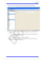
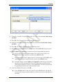
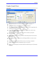
Before commands can be inserted into the Check Code Editor, a Check Code
Block corresponding to a form, page, record, or field can be created. Check
Code Blocks are created using the following steps:

Select the form, page, record, or field that will receive the commands.
62
Form Designer

Select before if the commands will be executed before data entry into
the form, page, record, or field. Otherwise, select after if the
commands will be executed after data entry when the cursor leaves
the form, page, record, or field.

Click the Add Block button to add a Check Code Block to the Check
Code Editor.
63
Form Designer
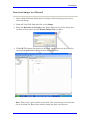
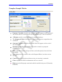
After a Check Code Block has been created for a form, page, record, or field, you can
execute commands and insert them within the block.
64
Form Designer
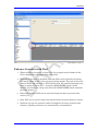
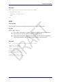
Delete a Row of Code from the Check Code Editor
To delete a row from the Check Code Editor:
1. Highlight the text.
2. On the keyboard, press Delete.
3. From the Check Code Editor toolbar, click Save.
Be sure of all deletions. No confirmation prompt or undo button will appear
prior to deletion.
65
Form Designer
Create a Skip Pattern with GOTO
You can create skip patterns by changing the tab order and setting a new cursor
sequence through a questionnaire, or by creating Check Code using the GOTO
command. Skip patterns can also be created based on the answers to questions using
an IF/THEN statement.
1. Open a form that contains at least three fields.
2. Click Check Code. The Check Code Editor opens.
3. Select the first field from the Choose Field Block for Action list box.
4. Select after from the Before or After Section.
5. Click the Add Block button. This creates code to run after the first field is
entered and accepted.
6. Click GoTo from the Add Command to Field Block list box. The GOTO dialog
box opens.
7. Select a field for the cursor to jump to after you enter the first field. The code
will run after the cursor leaves the field.
8. Click OK. The code appears in the Check Code Editor.
9. Click Save.
10. Click Close to return to the form.
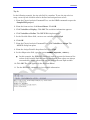
To test the skip pattern, open the form in the data entry module. Use the
tab key to ensure that upon leaving the field with the GOTO command, the
cursor goes to the specified field.
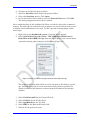
Create a Skip Pattern Using IF/THEN and GoTo
Use IF/THEN statements to create skip patterns based on the answers to questions
in the survey or questionnaire. This example creates code which states that if the
person answered Yes (+) to being ill, then the cursor jumps to a field that asks for
the diagnosis. If the person answered No (-), the cursor subsequently jumps to (or
skips) to the field for vaccination information.
1. Click Check Code. The Check Code Editor opens.
2. From the Choose Field Block for Action list box, select the field which
contains the action. For this example, select Ill.
3. The action needs to occur after data are entered into the Ill field. Select after
from the Before or After section.
66
Form Designer
4. Click the Add Block button. This creates code to run after the first field is
entered and accepted.
5. Click If from the Add Command to Field Block list box. The IF dialog box opens.
6. From the Available Variables drop-down list, select the field to contain the
action. For this example, select Ill. The selected variable appears in the If
Condition field.
7. From the Operators, click =.
8. From the Operators, click Yes. The If Condition field will read Ill=(+).
7. Click the Code Snippet button in the Then section. A list of available
commands appears.
8. From the command list, select GoTo. The GOTO dialog box opens.
9. Select the field for the cursor to jump to based on a Yes answer from the list of
variables. For this example, select Diagnosis.
10. In the GOTO dialog box, click OK to return to the IF dialog box.
11. Click the Code Snippet button in the Else section. A list of available commands
appears.
12. From the command list, select GoTo. The GOTO dialog box opens.
13. Select the field for the cursor to jump to based on a No answer from the list of
variables. For this example, select Vaccinated.
14. In the GOTO dialog box, click OK to return to the IF dialog box.
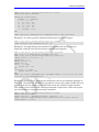
15. Click OK. The code appears in the Check Code Editor. The example code
appears as:
IF Ill = (+) THEN
GOTO Diagnosis
ELSE
GOTO Vaccinated
END-IF
16. Click Save from the Check Code Editor.
67
Form Designer
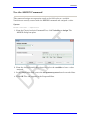
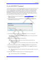
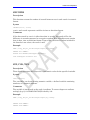
Assign a Date
To program a mathematical function, use the Program Editor and the ASSIGN
command. Check Code can be created to calculate and enter the age of a respondent
based on the date of birth and the date the survey was completed, or the system date
of the computer when data were entered.
This example uses a field called DateOfBirth and a field called Age to demonstrate
the use of the ASSIGN command and the function YEARS.
1. From the Form Designer, click Check Code or select Tools > Check Code
Editor. The Check Code Editor opens.
2. Select the DateOfBirth field from the Choose Field Block for Action list box.
3. Select after from the Before or After Section.
4. Click the Add Block button. This creates code to run after the DateOfBirth
field is entered and accepted.
5. Click Assign from the Add Command to Field Block list box. The Assign dialog
box opens.
3. From the Assign Variable drop-down, select the field where the calculated value
should appear. For this example, select the Age field.
4. In the = Expression field, type the function YEARS.
5. Type or click the left parenthesis (. Do not put a space before it.
Statements of a function must be enclosed in parentheses. Use the
Operator buttons or type them in from your keyboard.
7. From the Available Variables drop-down list, select the DateOfBirth field.
8. Type a comma.
9. Type the survey date in a MM/DD/YYYY format or type the function
SYSTEMDATE to calculate using the computer clock.
10. Type or click the right parenthesis).
11. Click OK. Check Code can appear in the Check Code Editor in two ways.
ASSIGN Age = YEARS(DateOfBirth, 06/21/2010)
ASSIGN Age = YEARS(DateOfBirth, SYSTEMDATE)
12. Click the Save button in the Check Code Editor.
Always save Check Code. Code will not update unless saved. The Save
feature also verifies syntax.
68
Form Designer
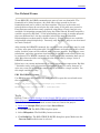
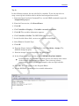
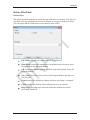
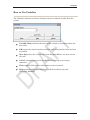
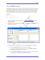
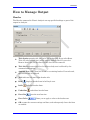
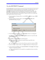
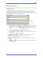
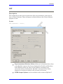
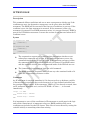
Create a Dialog
The DIALOG command provides interaction with data entry personnel from within
a program. Dialogs can display information, ask for and receive input, and offer lists
to make choices.
In this example, you can use the DIALOG command to create a reminder that all
fields on page two of the survey must be completed.
1. From the form, click Check Code or select Tools > Check Code Editor. The
Check Code Editor opens.
2. From the Choose Field Block for Action list box, select Page 2. The action
should occur after the cursor leaves the page.
3. Select after from the Before or After Section.
4. Click the Add Block button.
5. From the Add Command to Field Block list box, select Dialog. The DIALOG box
opens.
3. In the Title field, type Alert. The Dialog Type radio button should be Simple.
5. In the Prompt field, type All fields on page two must be completed.
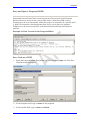
6. Click OK. The code appears in the Check Code Editor.
DIALOG "All fields on page two must be completed."
TITLETEXT="Alert"
7. Click Save in the Check Code Editor.
69
Form Designer
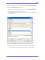
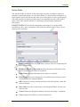
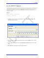
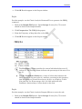
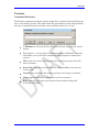
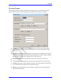
Use Autosearch
During data entry, fields with Autosearch Check Code are automatically searched
for one or more matching records. A match can be displayed and edited or be
ignored. Data entry can continue on the current record. Autosearch can alert you to
potential duplicate records, not prevent them from being entered.
1. Open a form. Click Check Code. The Check Code Editor opens.
2. From the Choose Field Block for Action list box, select the field to be searched.
3. Select After from the Before or After Section.
4. Click the Add Block button.
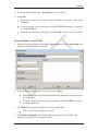
5. From the Add Command to Field Block list box, click Autosearch. The
Autosearch window opens.
6. Select the variable(s) to be searched during data entry. This selection should
match the variable selected from the Choose Field Block for Action list box.
7. Click OK. The code appears in the Check Code Editor window.
8. Click Save.
9. Click Close to return to the form.
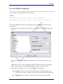
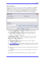
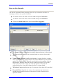
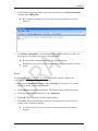
When a duplicate record is entered from the data entry module, the
Autosearch dialog box opens with all the matching records listed.
To view the potential duplicate record, double-click the arrow that
appears next to the record. The field where the potential duplicate was
entered is cleared.
Alternatively, click Cancel to remain on the current record and accept
the duplicate value.
Note: For more information on using Autosearch, please see the Autosearch topic in
the Command Reference.
70
Form Designer
Set a European Date Format
Date literals in Check Code and Analysis Programs (.PGMs) must use fourdigit years. If not, an error message will appear once per session.
Date literals with two-digit years are treated according to the computer's
local settings.
71
Form Designer
Copy the Value of a Field from a Main to a Related Form
Check Code must be created for a value from a field in the main form to appear in a
related form (i.e., there may be an ID Number or Name that needs to be visible in
the Parent and Child Forms).
The following instructions assume the Parent and Child Forms already exist. The
field to be copied needs to exist in the main form or be created in the main form prior
to beginning.
1. Note the name of the field on the Parent form whose value will be copied to the
Child form.
2. Open the Child form.
3. Create a new field. The new field must be the same field type as the field being
copied from the Parent form.
3. Select the Read Only option.
4. Click OK. The new field appears in the form. This is where the Parent form
values will be assigned and appear in data entry.
5. Click Check Code. The Check Code Editor appears.
6. From the Choose Field Block for Action list box, select the variable just created
in the Child form.
7. Select before from the Before or After Section.
8. Click the Add Block button.
8. From the Add Command to Field Block list box, click Assign. The ASSIGN
dialog box appears.
9. From the Assign Variable drop-down list, select the new variable.
10. In the = Expression area, type the field name from Step 1.
If the Child Form already has a field with the same name as the one
being copied from the Parent Form, it is important to distinguish the
parent’s field name. This field name must be prefixed by the Parent
Form’s name followed by a period in the Assign expression:
Demographics.PatientID
11. Click OK. The code appears in the Check Code Editor.
If the Child form does not have a field with the same name as the one
being copied from the Parent form, the Check Code may appear as
follows:
72
Form Designer
ASSIGN VisitsPatientID = PatientID
If the Child form already has a field with the same name as the one
being copied from the Parent form, it is important to distinguish the
Parent’s field name. In this example, Visits is the name of the form for
the child while Demographics is the name of the form for the parent.
The Check Code will appear as follows:
ASSIGN Visits.PatientID = Demographics.PatientID
12.
13. Click Save.
73
Form Designer
Concatenate Fields
If you write field concatenation code in Check Code Editor, future records will be
programmed. The code will not go back and populate previously entered data. If
previously entered data need to be concatenated, use concatenation commands from
the Analysis module.
Concatenate Fields with the Ampersand '&' Operator
This example illustrates how to join data from two fields and assign it into a third
field using the ‘&’ operator. In this case, Patient Full Name will be assigned the
concatenation of First Name and Last Name.
1. From the Form Designer, click Check Code. The Check Code Editor opens.
2. From the Choose Field Block for Action list box, select the field that the code
should run after. In this example, the code needs to run after you complete the
Last Name field.
3. Select after from the Before or After Section.
4. Click the Add Block button.
3. From the Add Command to Field Block list box, click Assign. The ASSIGN
dialog opens.
4. From the Assign Variable drop-down list, select the field to contain the
concatenated value.
5. Create the = Expression using the '&' operator.
ASSIGN TargetField = FieldA & FieldB & … & FieldZ.
In this example, ASSIGN PatientFullName = FirstName &
LastName.
If in Enter, FirstName was entered the name "Carl" and LastName
was entered the name "Gao", the result of PatientFullName would be
"CarlGao." There are no spaces between the names. To add a space
between the names, simply modify the ASSIGN statement by adding a
blank space in quotes between the first and last names as in the
following statement:
ASSIGN PatientFullName = FirstName & " " & LastName
74
Form Designer
Concatenate Fields with the Substring Function
This example illustrates how to join parts of two variables to create a unique text
ID. In this case, you will create a Patient ID made up of parts of the patient's last
and first name. The ampersand (&) operator is used to join the two parts together.
1. From the Form Designer, click Check Code. The Check Code Editor opens.
2. From the Choose Field Block for Action list box, select the field that the
code should run after. In this example, the code needs to run after you enter
the first name variable.
3. Select after from the Before or After Section.
4. Click the Add Block button.
5. From the Add Command to Field Block list box click Assign. The ASSIGN
dialog box opens.
6. From the Assign Variable drop-down list, select the field to contain the
concatenated value.
7. Create the =Expression using the SUBSTRING syntax.
SUBSTRING(<variable>, position #, character #)
<variable> is the field or variable.
position # is the position of the first character to be extracted from the
variable.
character # is the number of characters to extract.
In this example, the ID variable contains a combination of the first position and
four characters of the last name plus the first position and three characters of
the first name.
ASSIGN ID = SUBSTRING(LName, 1, 4) & SUBSTRING(FName, 1, 3)
75
Form Designer
8. Click OK. The code appears in the Check Code Editor window.
9. Click Save.
10. Test the code in the Enter Data module.
The example functions as such:
Last Name: Smith
First Name: Meg
Patient ID: SmitMeg
The Patient ID field being calculated is Read Only.
76
Form Designer
Create Check Code for Option Box Fields
Any form of Check Code can be added to option box variables. Code can be added to
any line/choice present in the option boxes. Use the Check Code Editor to create
complex Check Code for option box variables.
For this example, the check code created uses the GOTO command. Check Code was
used to create the following scenario. If the answer to TestOptions is choice 1, the
cursor will jump to Question 2. If the answer to TestOptions is choice 2 or 3, the
cursor will jump to Question 1. Check the tab order before creating the Check Code
to ensure that the tab order is correct.
1. Create an Option Box in a form. Note the name of the variable.
a. The variable is named TestOptions.
b. Each text line that represents a choice in the form represents a
numeric position in the Check Code Editor. Since the positions are
text values, they must be enclosed in quotes.
c. For example, there are three lines/choices that can be made in the
variable TestOptions. In the Check Code Editor the choices are
numeric, choice 1= position '1', choice 2= position '2', and choice 3=
position '3'.
2. Open the Check Code Editor.
3. From the Choose Field Block for Action list box, select TestOptions.
4. Select after from the Before or After Section.
5. Click the Add Block button.
6. From the Add Command to Field Block list box, click If. The IF dialog box
opens.
7. From the If Condition field, type Test Options = ‘1’.
77
Form Designer
8. Remember that the number 1 in this instance represents a text value called
choice 1. It must be enclosed in quotes.
9. Click the Code Snippet button in the Then section. A list of available
commands appears.
10. From the command list, select GoTo. The GOTO dialog box opens.
11. Select Question2.
12. Click OK.
10. Click the Code Snippet button in the Else section. A list of available commands
appears.
10. From the command list, select GoTo. The GOTO dialog box opens.
11. Select Question1.
12. Click OK.
13. Click OK. The code appears in the Check Code Editor.
78
Form Designer
How to use EpiWeek Function
Epi Info 7 allows the use of the Epi Week function which allows users to the
epidemiologic week. Epidemiological weeks are usually complete weeks. The
ministries of health around the world define the day of the week to be considered the
first epidemiologic day. As a result, some countries may consider the first day of the
week Sunday while others may consider the first day of the week Saturday or
Monday. Currently the Epi Info 7 Epi Week function does not allow changing any
property to allow users to decide which day of the week is considered to be the
beginning of the epidemiologic week. We will incorporate this functionality in a
future release. As a result, epidemiologic week’s calculations in Epi Info 7 are based
on Sunday being the starting day of the week.
If the year of occurrence is not relevant, you can use the Epiweek method instead.
The advantage of using Epiweek is that the value is returned as a number and it can
be stored in a numeric field. Epiweek takes one required parameter that must be a
date. The week is calculated relative to the year of the date provided. We calculated
the Epidemiological week using the following code:
ASSIGN week = EpiWeek(OnsetDate)
79
Enter Data
Introduction
The Enter program displays Forms constructed in Form Designer. Enter controls the
data entry process using settings and Check Code specified in Form Designer.
Information entered into the form is stored in MS Access .MDB or MS SQL server
data tables.
You can access the Enter program by clicking the Enter Data button on the Epi
Info main menu. It can also be accessed from the Tools>Enter Data sub menu
option. In Form Designer, you can access Enter Data by clicking the Enter Data
button. This button is a convenient method to switch between designing a form and
entering data to test your form design.
Enter can be used to enter new data, modify existing data, or search for records.
When data are entered into a form, the data table inside the project is populated.
The Find function allows records to be located based on a series of matched
variables. As data are entered, the cursor moves from field-to-field, page-to-page,
and saves data as you move to a new page. If you try to exit a page before data is
saved, you will be prompted to save the data (Yes or No).
Navigation is provided for using the New Record button and navigation buttons for,
next ( ), previous ( ), first (
), and last (
) records. When entering data
into a child form you will also have the “Back” button to take you back to the parent
form.
81
Translation
Navigating the Enter Workspace
Open Enter by clicking Enter Data from the Epi Info main menu. The Enter Data
screen consists of four main areas.
1. The Page panel lists all pages associated with the current form.
2. The Linked Records panel is used to conduct contact tracing. It contains
information about which records have exposed to, or from the current record.
3. The Canvas shows the current page.
4. The Toolbar at the top of the screen contains buttons to navigate through
the records, create new records, open the Dashboard, open the mapping
module, save the current record, and print the current page.
82
Translation
How To
Enter Data in a Form
1. From the toolbar, select File > Open Form or Recent Forms.
Selecting Open Form will display the Open dialogue box. The ellipsis
button allows you to search for the project (.prj file) you want to open.
2. Select a project. A list of forms available within that project appears.
3. Select a form from the list of available forms. The selected form opens.
4. Place the cursor in the first data entry field.
5. Enter data into each field. Use the Tab or Enter key to move to the next
field. Moving from one field to another will execute Check Code.
As records are navigated, data are saved automatically. After completing
the last field on a page, the cursor automatically jumps to the next page
in the sequence.
Field properties that were defined in Form Designer, (e.g., Read Only,
Required Range) are enforced during data entry.
Drop-down lists and code tables created in Form Designer are enforced.
Multiline Fields automatically scroll when filled with text to hold up to 1
gigabyte of information.
Plain text fields automatically scroll when filled with text to hold up to
128 characters per field.
Note: Check Code will execute as you move through the fields. All Check Code in
the fields between the field being left and the one being entered (according to tab
order) will be executed.
83
Translation
Save a Page or Record
The Enter module saves data automatically as you move from page-to-page. Data
are also saved when navigating to another record. You can move out of a record by
tabbing out of the last field of the last page or clicking New Record from the toolbar
to open a new record. Records can be saved manually.
There are two ways to save the current record manually:
1. Click Save from the toolbar.
2. Press Ctrl+S from the keyboard.
Saving a record manually is necessary only if you view an unsaved record and want
to use the linked records functionality in the dashboard or the maps module from
within Enter, and want that record to be included.
84
Translation
Find Records
Find can search for a record matching any field value or combination of field values.
If a form has more than 255 fields and more than one associated data table, only the
first data table will be used for the FIND. As a result, only the fields in the first
table will be listed in the field list and only the field values in the first table will be
displayed in the results grid. Advanced search features can be used in the Find
window.
When using Find from the Enter module, date fields can only be searched
with the date format MM/DD/YYYY.
Find is linked to the process setting for including deleted or undeleted
records in the Classic Analysis module. Find will include both deleted and
undeleted records when the statement SET PROCESS = BOTH is issued in
Classic Analysis; Deleted records only for SET PROCESS = DELETED; and
Undeleted records only for SET PROCESS = UNDELETED.
To Find Records Matching a Specified Criteria
1. From the toolbar, select the Find icon. The Find Records window opens.
85
Translation
2. Select one or more field names from the Choose Search Fields section.
2. Enter search criteria and click Search. Results appear in a grid in the Find
window.
Click Reset to begin a new search. Note that more than one field can
be searched at a time.
Click Back to return to the Enter workspace.
4. Open a record by double-clicking the arrow on the chosen row. The record
displays in the Enter Data workspace.
86
Translation
Enhance Searches with Find
1. When searching a numeric or date field, the accepted search format for the
field is displayed to the right of the entry field.
2. Embedded text items in multiline and text fields can be found by searching
for *word* where "word" is the text string being sought. This type of search is
called a Wild Card search. In a Wild Card search, the asterisk represents any
letter or string of letters (i.e., a search for DIAGNOSES *heart* would
identify all records for a large text field called DIAGNOSES which contained
the word "heart)."
3. Dates and numeric fields can be searched using less than or greater than
values (<>).
4. Only “OR” can be used to search for matches based on more than one criteria.
5. Searches are not case sensitive and are designed to be more inclusive than
exclusive. Spelling variations are automatically accommodated.
87
Translation
Classic Analysis
Introduction
Classic Analysis manipulates, manages, and analyzes data. It acts as a statistical
toolbox providing many ways to transform data and perform statistical Classic
Analysis. Data can be selected, sorted, listed, or manipulated with a series of
commands, functions, and operators. Available statistics include frequencies, means,
and more advanced processes (i.e., Kaplan-Meier Survival Classic Analysis and
Logistic Regression). Classic Analysis can be accessed by clicking Classic from the
Epi Info™ main window or by selecting Tools > Analyze Data>Classic . It reads
data files created in Form Designer and other types of databases (e.g., MS Access,
MS Excel, SQL Server, and ASCII). Classic Analysis can also produce graphs to
present graphic representations of data.
Classic Analysis provides access to existing data directly or through forms created in
Form Designer. It reads data from files and tables created in Epi Info 7, Microsoft
Access, Microsoft Excel, SQL Server, and ASCII.
88
Translation
Navigate the Classic Analysis Workspace
The Classic Analysis module contains four areas: the Classic Analysis Command
Tree, Program Editor, Classic Analysis Output window, and the Message Area.
1. The Command Explorer contains a list of available commands
separated into folders by command type. Commands are generated,
edited, and executed. Selecting a command opens the corresponding
dialog box for that command, function, or statistic to run.
2. The Program Editor displays the commands and code created using
the Classic Analysis Command Tree. Commands can also be typed
directly into the Program Editor. Programs or .PGM files written in
Classic Analysis can be stored in the current .PRJ or as text files.
Saved programs can be run against new data, or shared with others.
3. The Output window acts as a browser and displays information
generated from commands run in Program Editor. The buttons allow
you to navigate through program scripts that run and display in the
output screen.
89
Translation
4. The Message window alerts you if any problems occur with any
executed commands.
90
Translation
How to Manage Data
Use the READ Command
To analyze data, it must be read or imported into Classic Analysis. The READ
command allows you to select a project and/or data table to run statistics. The
READ command is used almost every time you open Classic Analysis.
Warning! Never manipulate the Form table in a software application outside of Epi
Info 7. The database may become corrupt and render the form unusable.
1. From the Classic Analysis Command Tree Data folder, click Read. The READ
dialog box opens.
91
Translation
The Database Type field indicates the database file to be loaded (.PRJ,
.MDB, .XLS). Specify the data format for the data to be read. Unless
otherwise specified, output files created from these data are stored in this
destination folder.
The Data Source field indicates the file location/path. If you use an SQL
Server database, the Data Source field will require server and database
names.
2. The Recent Data Sources field provides a list of recently-accessed databases
in Classic Analysis or Visual Dashboard. By selecting one of the data sources
available on the list, you do not need to provide Database Type or Data Source
information. Only data tables or forms will need to be selected again. If you are
reading an Epi Info 7 project file from the Data Source section, select the
Forms checkbox to view available forms in the project, or select the Tables
checkbox to view all project tables.
3. From the Forms section, select a form in your project. This reads the data
table associated with your form.
4. Click OK. The READ command is saved in the Program Editor and run
simultaneously. The current form file location, Record Count, and Date appear
in the Classic Analysis Output window; the READ command appears in the
Program Editor.
Click Save Only to save the command in the Program Editor. The
command does not run and the Record Count is not displayed.
92
Translation
Read a Microsoft Excel File
1. From the Classic Analysis Command Tree, click Read. The READ dialog box
opens.
2. From the Data Formats drop-down list, select either MS Excel 97-2003
Workbook or MS Excel 2007 Workbook.
3. In the Data Source field, click on the ellipsis
button to browse and select
the workbook (.xls or .xlsx) to import into Classic Analysis.
4. Click Open.
First Row Contains Field Names is checked by default. If the first row of
the spreadsheet does not contain field names, deselect the checkbox.
5. Click OK
6. Select a Worksheet from the list provided in the Data Source Explorer.
7. Click OK. The Record Count and file information appear in the Classic Analysis
Output window.
93
Translation
Read a Microsoft Access File
1. From the Classic Analysis Command Tree, click Read. The READ dialog box
opens.
2. From the Data Formats drop-down list, select either MS Access 2002-2003
(.mdb) or MS Access 2007(.accdb).
3. In the Data Source field, click on the ellipsis
the file to import into Classic Analysis.
button to browse and select
4. Click OK.
5. Select a data table from the list provided in the Data Source Explorer.
6. Click OK. The Record Count and file information appear in the Classic Analysis
Output window.
Read an ASCII Text File
1. From the Classic Analysis Command Tree, click Read. The READ dialog box
opens.
2. From the Data Formats drop-down list, select Flat ASCII File.
3. In the Data Source field, click the ellipsis
button to browse.
4. Click the ellipsis button again. Select directory of the file to import into
Classic Analysis.
5. Click OK.
6. Select the file from the list provided in the Data Source Explorer
7. Click OK.
Note: There are two forms of text files. Since both have only one table per file, you
do not have to specify a table. Both put the data for one record on a single line. The
difference is in how the fields are indicated.
94
Translation
Read an SQL Server Database
1. From the Classic Analysis Command Tree, click Read. The READ dialog box
opens.
2. From the Data Formats drop-down list, select Microsoft SQL Server
Database.
3. In the Data Source field, click the ellipsis
button to browse.
4. When the Connect to SQL Server Database dialog opens, specify the server
name and database name to connect and import into Classic Analysis.
5. Click OK.
6. From the list provided in the Data Source Explorer, select a data table.
7. Click OK. The Record Count and file information appear in the Classic Analysis
Output window.
95
Translation
Use Related Forms
To use RELATE, the READ command must open at least one form/table. The
form/table to be linked requires a key field that relates records in the two
forms/tables and can be used to join them together. The keys in the main and
related tables or forms do not require the same name. If the table was created in
Form Designer and the data entry completed using Enter, Classic Analysis can
establish a relationship automatically using the Global Record ID and Foreign Key
variables created by Epi Info 7. If the relationship was created in another program
that uses different keys, the key variables in both files must be identified.
Relationships are represented by double colons (::). Classic Analysis can establish
relationships using multiple keys. Currently, only Epi Info 7 projects can be related
in Classic Analysis.
After issuing the RELATE command, the variables in the related table may be used
as if they were part of the main table. Variable names are duplicated in the related
tables; variable names will be suffixed with a sequence number. Frequencies, crosstabulations, and other operations involving data in the main and related tables can
be performed. The WRITE command can create a new table containing both sets of
data. More than one table can be related to the main table by using a series of
RELATE commands.
Relate keys can contain mathematical or string concatenation expressions. Epi Info
7 functions can be used to determine relationships. It may be easier, however, to
write out a new file in which the complex key is included as a single variable. Use
this single variable as a key.
PRJ File RELATE Syntax
Use READ to open the first PRJ file, and RELATE to open the second and create
the relationship.
READ {C:\My_Project_Folder\Sample\Sample.prj}:Surveillance
RELATE RHepatitis GlobalRecordId :: GlobalRecordId
Try It
Epi Info 7 has a related database in the Sample.PRJ file which contains two forms:
Surveillance and RHepatitis. The variable GLOBAL RECORD ID is the internal
Epi Info 7 identification key located in more than one form in the project.
1. Read in the Sample.PRJ project. Open Surveillance.
2. Click RELATE. The RELATE dialog box opens.
3. Select RHepatitis. The Build Key button activates.
4. Click Build Key. The RELATE-BUILD KEY dialog box opens. Make sure the
Current Table radio button is selected.
96
Translation
5. From the Available Variables drop-down list, select GLOBALRECORDID.
6. Select the Related Table radio button.
7. From the Available Variables drop-down list, select GLOBALRECORDID.
8. Click OK. The Related Tables field populates.
9. Click OK. The RELATE dialog box opens and the Key field populates with the
join information.
10. Click OK. The related form information appears in the Output window.
Data from the two tables can now be used to compute statistics.
97
Translation
Use the WRITE Command
Use to create a new file with selected variables.
Syntax
WRITE <METHOD> {<output type>} {<project>:}table {[<variable(s)>]}
WRITE <METHOD> {<output type>} {<project>:}table * EXCEPT {[<variable(s)>]}
To use the WRITE command, open a project using the READ command. Follow
these steps:
1. From the Classic Analysis Command Tree, click Write. The WRITE dialog box
opens.
2. Keep the default setting All (*) unchecked to write all the variables to a new
file.
Note: You can also choose individual variables from the file list by clicking on
the variable name or select All (*) Except to exclude specific variables.
3. From the Output Mode section, click the Replace radio button.
Replace creates a new file and overwrites any existing variables and
records. To overwrite or replace data in a table, use the Replace selection.
Append adds new variables and records to the end of existing data.
98
Translation
4. Using the drop-down list, select the desired Output Format.
Available output formats are the same as ones that can be imported
using the READ command (i.e., MS Access, MS Excel, SQL Server and
Flat ASCII file).
5. Click the ellipsis
name and location.
button in the Connection Information field to specify file
6. Click OK.
7. Establish a name for the Destination Table or select a table name from the
drop down list (if the table already exists).
8. Click OK.
To see the data, use the READ command to open the newly-created
project.
The WRITE command will not create a form and cannot create a data
table to work with a form. To preserve forms, use the MERGE command.
Not all output formats support all possible input formats.
Use the MERGE Command
Use the MERGE command to join records. MERGE is only supported if the READ
data source is an Epi Info 7 project. A merge requires a key, called the GLOBAL
RECORD ID, which represents an internal matching variable inside both sets of
data.
Syntax
MERGE <table specification>
<key(s)> <type>
1. From the Classic Analysis Command Tree, use the READ command to open a
PRJ project file.
2. From the Classic Analysis Command Tree, click Data > Merge. The MERGE
dialog box opens.
99
Translation
3. From the Data Formats drop-down list, specify the other Epi Info 7 project to be
read. (Other data sources will be supported in a future release).
4. In the Data Source field, click the Browse
dialog box opens.
button. The Merge File Name
5. Select the project file that contains the data to be merged.
6. Click Open. The MERGE dialog box populates with available tables or
worksheets.
7. Merge a data table or worksheet. The Build Key button activates.
8. Click Build Key. The RELATE - BUILD KEY dialog box opens.
There must be a variable in the Current Table that corresponds to a one
in the Related Table (i.e., Patient ID).
100
Translation
9.
From the Available Variables drop-down list, select the current table merge
variable.
10. Click OK. The Current Table field shows the selection.
11. From the Available Variables drop-down list, select the related table merge
variable.
12. Click OK. The Related Tables field shows the selection.
13. Click OK to accept the Build Key designations. The MERGE dialog box opens.
14. Make Update and Append selections from the corresponding checkboxes.
For matching records, Update replaces the value of any field in the
READ table whose build key matches the MERGE table.
For unmatched records, Append creates a new record in the READ table
with values only for those fields that exist in the MERGE table.
For most merges, select Update and Append records. If you select both
options, records containing the same selected merge variables will be
updated (overwritten) if there is new information. All other records will
be appended (added) to the end of the data table.
15. From the Merge dialog box, click OK.
If the MERGE table is the same project as the READ table, the Record
Count in the Output window updates to reflect any new records added to
the table.
101
Translation
Use the ASSIGN Command
This command assigns an expression result or the field value to a variable.
Variables are usually created with the DEFINE command and assigned a value.
Syntax
ASSIGN <variable> = <expression>
1. From the Classic Analysis Command Tree, click Variables > Assign. The
ASSIGN dialog box opens.
2. From the Assign Variable drop-down list, select the variable to have a value
assigned.
3. In the =Expression field, create the assignment syntax based on needed data.
4. Click OK. The code appears in the Program Editor.
102
Translation
Try It
In the following example, the zip code field is a number. To use the zip code in a
map, a new zip code variable must be defined and assigned text values.
1. From the Classic Analysis Command Tree, use the READ command to open the
Sample.PRJ project.
2. From the Form section, click Surveillance.
3. Click OK.
4. Click Variables > Display.>--Variables currently available.
5. Click OK. The variables information appears.
6. Click Variables > Define. The DEFINE dialog box opens.
7. In the Variable Name field, create a new variable named Zip2.
8. Select Text for Variable Type
9. Click OK.
10. From the Classic Analysis Command Tree, click Variables > Assign. The
ASSIGN dialog box opens.
11. From the Assign Variable drop-down list, select Zip2.
12. In the =Expression field, type the syntax FORMAT(ZipCode,"00000").
In this example, the FORMAT function converts the format of the values
of the variable ZipCode into text format. Text values are always
surrounded by double quotes and assigned to the new Zip2 variable.
10. Click OK. The code appears in the Program Editor.
11. Use the DISPLAY command to view variable information.
103
Translation
Delete File/Table
Delete Files
The file(s) specified explicitly or implicitly (via wildcards) are deleted. If no files are
specified, or if any specified files cannot be deleted, a message is produced unless
you select Run Silent. Wildcards are not allowed in the suffix.
File Name contains the name of the file to be deleted.
Run Silent causes the command to run without any warning or error
messages from the Program Editor.
OK accepts the current settings and data, and subsequently closes the
form or window.
Save Only saves the created code to the Program Editor, but does not
run the code.
Cancel closes the dialog box without saving or executing a command.
Clear empties the fields to allow information to be re-entered.
Help opens the Help topic associated with the module being used
(Currently Disabled).
104
Translation
Delete Table
The specified table is deleted. If the table does not exist or cannot be deleted, a
message is produced unless you select Run Silent. To delete tables with spaces in
their names, specify the file and the table even if the table is in the current project.
The table must be enclosed in single quotes. It is possible to read a table with a
space in its name and then delete it, resulting in errors during subsequent
procedures.
DELETE TABLES will not delete and produce messages if any of the tables
specified are data, grid, or program. Code tables are deleted only if they are not
referenced by any form.
Data Format specifies the data source format of the file containing the
table to be deleted.
Database (Blank or Current) specifies the name and location of the
dataset containing the table to be deleted.
Table Name specifies the name of the table to be deleted.
Run Silent causes the command to run without any warning or error
messages from the Program Editor.
OK accepts the current settings and data, and subsequently closes the
form or window.
Save Only saves the created code to the Program Editor, but does not
run the code.
Cancel closes the dialog box without saving or executing a command.
Clear empties the fields to re-enter information.
105
Translation
Help opens the Help topic associated with the module being used.
(Currently Disabled).
106
Translation
Delete Records
Delete Records may not be used with related tables. For DELETE * and DELETE
TABLES, space will not be reclaimed. You can run the Epi Info 3.5.3 Compact
Database utility to reclaim space. All records in the current selection matching the
expression are set to deleted status, or if PERMANENT is specified, physically
deleted. Unless you select RUNSILENT, a confirmation message is displayed.
Permanent Deletion causes records to be inaccessible after deletion.
Mark for Deletion marks the selected records as to be deleted, and
permits you to undelete. This feature can only be applied to Epi Info 7
projects.
The Records Affected (* for all) field specifies which records to delete.
Run Silent causes the command to run without any warning or error
messages from the Program Editor.
The Available Variables drop down allows you to select variables
available in the current project.
Functions and operators appear within commands and are used for common
tasks (e.g., extracting a year from a date, combining two numeric values, or
testing logical conditions).
OK accepts the current settings and data, and subsequently closes the form
or window.
Save Only saves the created code to the Program Editor, but does not run
the code.
Cancel closes the dialog box without saving or executing a command.
107
Translation
Clear empties the fields to re-enter information.
Help opens the Help topic associated with the module being used.
(Currently Disabled).
108
Translation
Use the ROUTEOUT Command
You can locate output by using the ROUTEOUT command. If no directory exists,
the file is placed in the current project’s directory. Results accumulate until you
execute a CLOSEOUT command. Output files can be placed in any folder. The
ROUTEOUT command selects a path and filename. If no output file is selected,
Classic Analysis uses the default value. In each folder, Classic Analysis creates a
new index table that contains links to the files created.
1. From the Classic Analysis Command Tree, use the READ command to open a
PRJ project file.
2. From the Classic Analysis Command Tree, click Output > RouteOut. The
ROUTEOUT dialog box opens.
3. In the Output Filename field, enter a file name to locate an existing file.
If necessary, select Replace Existing File to write over any files with
the same name.
4. Click OK. Create Output on the existing project.
Notice the title bar contains the output filename specified in the
ROUTEOUT command.
The new file is placed in the selected directory with the extension .HTM.
5. From the Output window toolbar, click Open. The Browse dialog box opens.
6. Locate and select the file created with ROUTEOUT. Click Open. The Output
appears in the Output window.
The saved Output file can be opened by any application that can read an
HTML file.
To end the ROUTEOUT command, choose one of the following options.
From the Output folder, click Closeout.
109
Translation
READ in a new project.
Close Epi Info 7.
110
Translation
Use the CANCEL SORT Command
Syntax
CANCEL SORT Command Generator
CANCEL SORT Command Reference
1. From the Classic Analysis Command Tree, click Select/If > Cancel Sort. The
CANCEL SORT dialog box opens.
2. Click OK. The selection criteria are removed from the data, and the original
record count is restored.
111
Translation
Undelete Records
The UNDELETE command causes all logically deleted records in the current
selection matching the expression to be set to normal status. This applies only to
Epi Info 7 forms and may not be used when using related tables.
The Records Affected (*for all) field contains the expression for which
records to undelete.
The Available Variables field allows you to select available variables in
the current project.
Functions and operators appear within commands and are used for
common tasks (e.g., extracting a year from a date, combining two
numeric values, or testing logical conditions).
OK accepts the current settings and data, and subsequently closes the
form or window.
Save Only saves the created code to the Program Editor, but does not
run the code.
Functions opens the online help file, which explains how to use
functions and operators.
Cancel closes the dialog box without saving or executing a command.
Clear empties the fields to re-enter information.
Help opens the Help topic associated with the module being used.
(Currently Disabled).
112
Translation
How to Manage Variables
Use the DEFINE Command
This command creates new variables.
Syntax
DEFINE <variable> {<scope>} {<type indicator>} {("<prompt>")}
1. From the Classic Analysis Command Tree, click Variables > Define. The
DEFINE Variable dialog box opens.
2. From the Scope section, select one of the following variables:
Standard variables remain in a current project and are one variable in
that form. They can assume new values with each record during a file
query (e.g., a LIST or FREQ).
Global variables persist throughout program execution. They pass
values from one form to a related form, and do not change during a file
query.
113
Translation
Permanent variables are stored in the EpiInfo.Config.xml file or system
registry and retain any value assigned until changed by another
assignment, or until the variable is undefined. They are shared among
Epi Info 7 programs and persist even if the computer is shut down and
restarted.
3. From the Variable Type drop-down list, select one of the following types: Date,
Numeric, Text, or Yes-No.
4. Optional: Variable Type is required and cannot be used if <scope> is omitted.
<type indicator> is the data type of the new variable and must be one of the
following reserved words: NUMERIC, TEXTINPUT, YN, or DATEFORMAT. If
omitted, the variable type will be inferred based on the data type of the first
value assigned to the variable. However, omitting field type is not
recommended.
5. Click OK.
Define a Group
To define a group, take the following steps:
1. From the Classic Analysis Command Tree, click Variables > Define Group.
The DEFINE GROUP dialog box opens.
2. In the Group Variable field, type a name.
3. From the Variables list box, select the variables to be included in the group.
4. Click OK.
Convert a Number to Text
Numbers can be converted to text using the FORMAT function. FORMAT changes
the format of one variable type to another.
Syntax
FORMAT(<variable>, {"<format specifcation>"})
Example
The Format function can be used to convert a numeric postal code or zip code field
to a text type variable for mapping.
The READ command opens a new file that contains a numeric field called
zipcode. To use Epi Map with the zipcode values, change the values to text.
114
Translation
The DEFINE command creates a new variable called NewZip. The variable
NewZip will hold the values of zipcode in a text format. The code appears in
the Program Editor as DEFINE NewZip.
The ASSIGN command formats the variable NewZip with the values of
ZipCode and the format of text. Text values are enclosed in quotes. The code
appears in the Program Editor as:
ASSIGN NewZip=FORMAT(ZipCode,"00000")
The variable NewZip can now be used as a geographic variable in Epi Map
because it is a text type variable that contains numeric data.
Try It
For this example, use the Classic Analysis Program Editor to create the code.
1. Read in the Sample.PRJ project. Open Oswego. Seventy five (75) records
should be listed in the Output window.
2. In the Program Editor window, place the cursor under the created Read
command. Type DEFINE MyAge TEXTINPUT
Do not press the Enter key. Leave your cursor on the line of code you just
created.
3. In the Program Editor window, type the following: ASSIGN
MyAge = FORMAT(Age, "00").
4. From the Program Editor navigation menu, click Run Commands. The code
will turn gray to indicate a syntax review.
5. From the Classic Analysis Command Tree, click Statistics > List. Click OK.
The records appear.
Notice that the values in ‘MyAge’ are all two characters with a leading ‘0’
before each single digit year. The leading zero is present because of the
‘00’ format specification.
7. From the Classic Analysis Command Tree, click Variables > Display. Click
OK. The variable types appear.
The variable MyAge now contains the values of Age and the format type
of Text.
Program Editor Code SCREEN SHOT TO BE ADDED
115
Translation
Use IF Statements with Permanent or Global Variables
If the condition of an IF statement depends on global or permanent
variables, the value is computed immediately and only the true or false
branch, as appropriate, is followed.
If the condition of an IF statement depends on a field variable, neither
branch is followed. However, computations within the branches are saved
for execution as appropriate on each record. In the second case, noncomputational commands (e.g., READ, SELECT, SORT, HEADER, and
ROUTEOUT) are never executed.
116
Translation
Handle Date Fields
Date formats are often determined by default computer settings. To access Regional
Settings in a Windows environment, click Start > Control Panel > Regional and
Language Options.
Date fields in forms are entered in European, American, or ISO format as
specified in Form Designer. They are stored in the database in a neutral
format.
Date fields in Excel, and Text files are read into Classic Analysis
according to the date format found in Regional Settings, and stored in a
neutral format. Excel files prepared with one date format often do not
import properly on machines with a different date format.
Date fields in forms are displayed in European, American, or ISO format
as specified in Form Designer by the following Classic Analysis
commands: LIST, LIST GRIDTABLE, TABLES, and FREQ.
Date fields in forms are displayed according to the date format found in
Regional Settings in the following Classic Analysis commands: DISPLAY,
and GRAPH.
Date fields in tables without forms are displayed according to the date
format found in Regional Settings.
Date fields written to Excel or Text files are written according to the date
format in Regional Settings.
Date literals in Form Designer, Check Code, or Classic Analysis
Programs; and date-type permanent variables in the EpiInfo.Config.xml
file, should be in American format unless enclosed in braces or pipe
symbols. European date format (DD/MM/YYYY) literals must be enclosed
in braces (i.e., {23/11/2007}). ISO date literals (YYYY/MM/DD) must be
enclosed in pipe symbols (i.e.,|.,2007/11/23|.
Dates formatted with the FORMAT function are formatted according to
the date format found in Regional Settings when no format is specified as
a second argument.
Dates converted from text with TXTTODATE are converted to a neutral
format according to the date format found in Regional Settings. For
multi-national applications, it may be safer to use the NUMTODATE
function.
If you are not sure, conduct experiments and examine the results.
117
Translation
How to Use Undefine
The Undefine command in Classic Analysis removes a defined variable from the
system.
Variable Name indicates the name of the variable to be removed from the
data table.
OK accepts the current settings and data, and subsequently closes the form
or window.
Save Only saves the created code to the Program Editor, but does not run
the code.
Cancel command generation window without saving or executing a
command.
Clear empties fields so that information can be re-entered.
Help opens the Help topic associated with the module being used.
(Currently Disabled).
118
Translation
Use the ASSIGN Command
This command assigns the result of an expression or the field value to a variable.
Variables are usually created with the DEFINE command and subsequently
assigned a value.
Syntax
ASSIGN <variable> = <expression>
<variable> = <expression>
1. From the Classic Analysis Command Tree, click Variables > Assign. The
ASSIGN dialog box opens.
2. From the Assign Variable drop-down list, select the variable to have a value
assigned.
3. In the =Expression field, create the assignment syntax based on the needed
data.
4. Click OK. The code appears in the Program Editor.
119
Translation
Try It
In the following example, the zip code field is a number. To use the zip code in a
map, a new zip code variable must be defined and assigned text values.
1. From the Classic Analysis Command Tree, use the READ command to open the
Sample.PRJ project.
2. From the form section, click Surveillance. Click OK.
3. Click Variables > Display. Click OK. The variables information appears.
4. Click Variables > Define. The DEFINE dialog box opens.
5. In the Variable Name field, create a new variable named Zip2.
6. Click OK.
7. From the Classic Analysis Command Tree, click Variables > Assign. The
ASSIGN dialog box opens.
8. From the Assign Variable drop-down list, select Zip2.
9. In the =Expression field, type the syntax FORMAT(ZipCode,"00000").
In this example, the FORMAT function is used to convert the format of the
values of the variable ZipCode into the text format. Text values are always
surrounded by double quotes and are assigned to the new Zip2 variable.
10. Click OK. The code appears in the Program Editor.
11. Use the DISPLAY command to view variable information.
120
Translation
How to Use Recode
The Recode command allows grouping of data for age and other variables, or
changing code from one system to another.
To insert a line in the table, select the row and press Ctrl-Insert.
To delete a line in the table, select the row and press Ctrl-Delete.
Delete any blank rows prior to selecting OK or Save Only.
The From drop down identifies the variable whose values are to be recoded.
The To drop down identifies the variable slated is to receive the recoded
values.
Value (blank = other) identifies the bottom of a range of values, a single
value, or all remaining values slated to be recoded. Enclose text in quotation
marks. The word LOVALUE may be used to indicate the smallest value in
the database. HIVALUE may be used to indicate the largest. To recode a
single value instead of a range, use only this column. To recode all
unspecified values, leave this column and the To column blank.
To Value (if any) identifies the top of a range of values that will be recoded.
Recoded Value identifies the value to be assigned to the destination
variable for the specified values of the source variable. Enclose text in
quotation marks.
121
Translation
Fill Ranges allows you to redefine recoded ranges of equal
distribution.
OK accepts the current settings and data, and closes the form or
window.
Save Only saves the created code to the Program Editor, but does not
run the code.
Cancel command generation window without saving or executing a
command.
Clear empties fields so information can be re-entered.
Help opens the Help topic associated with the module being used.
(Currently Disabled).
122
Translation
Use the DISPLAY Command
This command displays table, form, and database information.
Syntax
DISPLAY <option> [<sub-option>] [OUTTABLE=<tablename>]
1. From the Classic Analysis Command Tree, use the READ command to open a
PRJ project file.
If a .PRJ file is not opened, only language is shown for selected variables.
2. From the Classic Analysis Command Tree, click Variables > Display. The
DISPLAY dialog box opens.
3. From the Information for section, select one of the following form data options:
Variables displays information about all of the variables in the dataset;
the defined, field, and selected variables.
Forms displays the forms in the current dataset or a selected dataset.
Information about forms and other Epi Info-specific tables is shown.
Tables displays information about tables in a database. Information
about tables and other Epi Info-specific or generic tables is shown.
4. If needed, type an Output to Table name.
5. Click OK. The information is displayed in the Output window.
123
Translation
How to Select Records
Use the SELECT Command
Use SELECT to view or analyze specific records based on selection criteria.
Syntax
SELECT <expression>
1. From the Classic Analysis Command Tree, click Select/If > Select. The
SELECT dialog box opens.
2. Use the Available Variables drop-down list to select variables from the open
dataset.
3. Use the Select Criteria field and the Functions and Operators buttons to
create selection code.
4. Click OK. The Record Count in the Output window should alter based on the
number of records meeting the new criteria.
5. From the Classic Analysis Command Tree, click Statistics > List to view the
records matching the selection criteria.
6. From the Classic Analysis Command Tree Select/If folder, click Cancel
Select to cancel the selection criteria and return the Record Count to all
records in the dataset.
124
Translation
Select a Date Range
1. From the Classic Analysis Command Tree, use the READ command to open a
PRJ project file.
2. From the Classic Analysis Command Tree, click Select/If > Select. The
SELECT dialog box opens.
3. From the Available Variables drop-down list, select a date variable.
In this example, DateVar is a date variable used in the data table. The
DateVar has to be a date field or be converted into a date field using the
NUMTODATE or TXTTONUM functions.
4. In the Select Criteria field, create the date range selection code by using the
greater than >, less than <, and AND operators.
Note: Unless the date literal is enclosed in braces or pipe symbols, literal dates in
PGMs are always in U.S. date format. European date format (DD/MM/YYYY)
literals must be enclosed in braces (i.e., {23/11/2007}). ISO date literals
(YYYY/MM/DD) must be enclosed in pipe symbols (i.e.,|.,2007/11/23|).
Create the following example using the project called Sample.PRJ and the
data from Surveillance.
125
Translation
Use the CANCEL SELECT Command
SELECT
CANCEL SELECT Command Generator
CANCEL SELECT Command Reference
1. From the Classic Analysis Command Tree, click Select/If > Cancel Select. The
CANCEL SELECT dialog box opens.
2. Click OK. The selection criteria are removed from the data and the original
record count is restored.
126
Translation
Use the IF Command
The IF command defines a condition. True causes the THEN code block to be
executed; false causes the ELSE code block (if present) to be executed.
The If Condition field specifies the condition to determine which statement
that follows it is executed.
The Available Variables field allows you to select variables available in the
current project.
The Then button is part of the If Condition statement. It starts the section of
code executed when the If condition is true.
The Else button is part of the If Condition and works as follows: If the
condition is true, the first statement is executed. If false, the statement is
bypassed, and if an else statement exists, it is executed instead.
127
Translation
Functions and operators appear within commands and are used for
common tasks (e.g., extracting a year from a date, combining two
numeric values, or testing logical conditions).
OK accepts the current settings and data, and subsequently closes the
form or window.
Save Only saves the created code to the Program Editor, but does not
run the code.
Functions opens the online Help file which explains the functions and
operators. (Currently Disabled).
Cancel closes the dialog box without saving or executing a command.
Clear empties the fields so information can be re-entered.
Help opens the Help topic associated with the module being used.
(Currently Disabled).
128
Translation
Use the Sort Command
The Sort command allows you to specify a sequence for records to appear when using
the LIST, GRAPH, and WRITE commands.
The Available Variables field allows you to select variables available in the
current project.
Sort Order allows variables to be sorted in ascending (A to Z) or descending
(Z to A) order. If the order is not specified, the sort order will be ascending. To
sort one or more variables in descending order, the descending parameter (--)
must be after each variable.
Select Remove from Sort to remove the variables selected from the list.
Sort Variables contains a list of variables selected for the sort.
OK accepts the current settings and data, and subsequently closes the form
or window.
Save Only saves the created code to the Program Editor, but does not run
the code.
Cancel closes the dialog box without saving or executing a command.
Clear empties the fields so that information can be re-entered.
Help opens the Help topic associated with the module being used. (Currently
Disabled).
129
Translation
CANCEL SORT
How to Use the CANCEL SORT command
The Cancel Sort command in Classic Analysis cancels a previous SORT command.
OK accepts the current settings and data, and subsequently closes the form
or window.
Save Only saves the created code to the Program Editor, but does not run
the code.
Cancel closes the dialog box without saving or executing a command.
Help opens the Help topic associated with the module being used. (Currently
Disabled).
130
Translation
How to Display Statistics and Records
Use the LIST Command
The LIST command creates a line listing of the current dataset. Select specific
variables from the Variables drop-down to narrow the list or select * (the Wild Card)
to display all the variables. Check the All (*) Except box and select from the
Variables drop-down to exclude variables from the list.
To navigate LIST * GRIDTABLE results, use the Tab key to move forward one cell
at a time and the Shift+Tab keys to move back one cell at a time. Navigate through
the records and cells using the left, right, up, and down arrow keys.
Syntax
LIST {* EXCEPT} [<variable(s)>] LIST {* EXCEPT} [<variable(s)>] {GRIDTABLE}
1. From the Classic Analysis Command Tree, use the READ command to open a
PRJ project file.
2. From the Classic Analysis Command Tree, click Statistics > List. The LIST
dialog box opens.
3. Click OK to accept the default settings. The variables in the dataset appear in a
grid table inside the Output Window.
Grid output is not embedded. An Output file is not created.
131
Translation
Create a Web Format List
1. From the Classic Analysis Command Tree, click Statistics > List. The LIST
dialog box opens.
2. From the Display Mode section, select the Printable / Exportable radio
button.
3. Click OK. The List appears in the Output window in a web table format. Web
display mode creates an embedded output file.
132
Translation
Use the FREQ Command
The FREQ command produces a frequency table that shows how many records have
a value for each variable, the percentage of the total, and a cumulative percentage.
The command FREQ * creates a table for each variable in the current form other
than unique identifiers. This command is used to begin analyses on a new data set.
Syntax
FREQ [<variable(s)>]
FREQ * {EXCEPT [<variable(s)>]}
1. From the Classic Analysis Command Tree, use the READ command to open a
PRJ project file.
2. From the Classic Analysis Command Tree, click Statistics > Frequencies. The
FREQ dialog box opens.
3. From the Frequency of drop-down list, select a variable from the data table.
Click the All (*) Except checkbox to exclude variables.
Use the corresponding drop-down lists to select a Weight variable or a
Stratify by variable from the data source.
Use the Output to Table field to specify a location for table results. The
new table can be accessed using the READ command.
133
Translation
4. Click OK. Results appear in the Output window.
Try It
For this example, use the Classic Analysis Command Tree to generate the FREQ
command.
1. Read in the Sample.PRJ project. Open Oswego. Seventy five (75) records
should be listed in the Output window.
2. Click Frequencies. The FREQ dialog opens.
3. From the Frequency of drop-down list, select ILL.
4. Click OK. Results appear in the Output window.
The Frequency column provides the count of individuals that were ill
and not ill. The Percent column indicates the percentage of who were ill or
not ill.
The 95% Confidence Limits are a range of values that indicates the
likely location of the true value of a measure, meaning (in this instance)
that the number of ill could be as low as 49.38%, or as high as 72.36%.
Note that the Yes Ill percentage of 61.33% falls within the 95%
Confidence Limits range of values based on the data.
Try It
For this example, use the Classic Analysis Program Editor to create the code.
1. Read in the Sample.PRJ project. Open Oswego. Seventy five (75) records
should be listed in the Output window.
134
Translation
2. In the Program Editor window, place the cursor under the Read command
created. Type FREQ ILL.
Do not press the Enter key. Leave the cursor on the line of code just
created.
3. Click Run Commands from the Program Editor navigation menu. The code
turns green indicating syntax review and execution.
Results of the command appear in the Output window.
Results are the same as those created using the Command Tree dialog
boxes.
Try It
A program or PGM can be saved and run repeatedly against a dataset for
continuously updated statistics and analyses.
1. Read in the Sample.PRJ project. Open Oswego. Seventy five (75) records
should be listed in the Output window.
2. Click Open from the Program Editor. The Read Program dialog box opens.
3. From the Program drop-down list, select Statistics.
4. Click OK. The PGM opens in the Program Editor.
5. Click Run. The Program Editor runs the code and output is placed in the
Classic Analysis Output window.
Use the scroll bar to review all the results computed to the Output
window.
135
Translation
Use the TABLES Command
The Tables command examines the relationship between two or more categorical
values. For 2x2 tables, the Tables command produces odds and risk ratios. A 2x2
table is created when each selected variable has a yes or no answer.
Syntax
TABLES <exposure> <outcome> {STRATAVAR=[<variable(s)>]} {WEIGHTVAR=<variable>}
{PSUVAR=<variable>} {OUTTABLE=<table>} }
1. From the Classic Analysis Command Tree, use the READ command to open a
PRJ project file.
2. From the Classic Analysis Command Tree, click Statistics > Tables. The
TABLES dialog box opens.
3. From the Exposure Variable drop-down list, select a variable from the data to
indicate a risk factor exists.
4. From the Exposure Variable drop-down list, select a variable from the data to
indicate the presence of an outcome. Use the:
136
Translation
Stratify by drop-down list to select a variable to act as a grouping
variable.
Weight drop-down list to select a variable for weighted Classic Analysis.
Output to Table field to specify a location for table results.
READ command to access the READ command.
5. Click OK. Results appear in the Output window.
6. Scroll down to view the Single Table Classic Analysis.
Try It
Create a 2x2 table using data from the Sample.MDB project.
1. Read in the Sample.PRJ project. Open Oswego. Seventy five (75) records
should be listed in the Output window.
2. Click Tables. The TABLES dialog box opens.
3. From the Exposure Variable drop-down list, select Vanilla.
4. From the Outcome Variable drop-down list, select ILL.
5. Click OK. Results appear in the Output window.
6. Scroll down to view the Single Table Classic Analysis.
137
Translation
Try It
For this example, use the Classic Analysis Program Editor to create the code.
1. Read in the Sample.PRJ project. Open Oswego
2. In the Program Editor window, place the cursor under the Read command
created. Type TABLES Chocolate ill.
Do not press the Enter key. Leave the cursor on the line of code just
created.
3. Click Run Commands from the Program Editor navigation menu. The code
turns gray indicating syntax review and execution.
Results of the command appear in the Output window.
138
Translation
Results are the same as those created using the Command Tree dialog
boxes.
Try It
A program or PGM can be saved and run repeatedly against a dataset for
continuously updated statistics and analyses.
1. To see an example of a PGM, read in the Sample.PRJ project. Open
Oswego.
2. From the Program Editor, click Open Pgm. The Read Program dialog box
opens.
3. From the Program drop-down list, select Statistics.
4. Click OK. The PGM opens in the Program Editor.
5. Click Run Commands. The Program Editor runs the code and output is
placed in the Classic Analysis Output window. Use the scroll bar to review all
the results computed to the Output window.
139
Translation
Use the MEANS Command
The MEANS command can obtain an average for a continuous numeric variable.
Since Yes equals ‘1’ and No equals ‘0’, the mean of a yes-no variable is the proportion
of respondents answering yes. For this situation, use the FREQ command. It has
two formats. If only one variable is supplied, the program produces a table similar to
one produced by FREQUENCIES with descriptive statistics. If two variables are
supplied, the first is numeric containing data to be analyzed. The second indicates
how groups will be distinguished. The output of this format is a table similar to one
produced by TABLES with descriptive statistics of the numeric variable for each
group variable value.
Syntax
MEANS <variable 1> {<variable 2>} {STRATAVAR=<variable(s)>}
{WEIGHTVAR=<variable>} {OUTTABLE=<tablename>}
1. From the Classic Analysis Command Tree, use the READ command to open a
PRJ project file.
2. From the Classic Analysis Command Tree, click Statistics > Means. The
MEANS dialog box opens.
3. From the Means Of drop-down list, select a variable from the data source.
The Cross-tabulate by value of drop-down list contains a variable to help
determine if the means of a group are equal.
The Stratify by drop-down list contains a variable to act as a grouping
variable.
140
Translation
The Weight drop-down list contains a variable for weighted Classic
Analysis.
The Output to Table field specifies a location for table results. The new
table can be accessed using the READ command.
4. Click OK. The Output window populates with the results. Scroll down to view
the Mean and Standard Deviation results.
Try It
Use the MEANS command to find the average for a continuous variable.
1. Read in the Sample.PRJ project. Open Oswego. Seventy five (75) records
should be listed in the Output window.
2. Click MEANS. The MEANS dialog box opens.
3. From the Means of drop-down list, select Age.
4. Click OK. Results appear in the Output window.
5. To view the Descriptive Statistics, scroll down the Age listing.
Notice the mean age of individuals in the dataset is 36.8.
141
Translation
Try It
For this example, use a numeric variable and a Yes/No variable to determine the
MEANS for a group.
1. Read in the Sample.PRJ project.
2. Click MEANS. The MEANS dialog box opens.
3. From the Means of drop-down list, select Age.
4. From the Cross-Tabulate by Value of drop-down list, select ILL.
5. Click OK. Results appear in the Output window.
6. To view the Descriptive Statistics, scroll down the Age listing.
Notice the Mean Age of those answering yes to ill is 39.2. Those
answering no to ill is 32.9.
Other available statistics include:
ANOVA, a Parametric Test for Inequality of Population Means.
Bartlett's Test for Inequality of Population Variances.
142
Translation
Mann-Whitney/Wilcoxon Two-Sample Test (Kruskal-Wallis test for two
groups).
Try It
For this example, use the Classic Analysis Program Editor to create the code.
1. Read in the Sample.PRJ project. Open Oswego.
2. In the Program Editor window, place the cursor under the Read command
created. Type MEANS Age.
Do not press the Enter key. Leave the cursor on the line of code just
created.
3. Click Run Commands from the Program Editor navigation menu. The code
turns gray to indicate execution of syntax.
Results of the command appear in the Output window.
Results are the same as those created using the Command Tree dialog
boxes.
143
Translation
Use the SUMMARIZE Command
The SUMMARIZE command aggregates data producing an output table showing the
descriptive statistics.
Syntax
SUMMARIZE varname::aggregate(variable) [varname::aggregate(variable) ...] TO
tablename STRATAVAR=variable list {WEIGHTVAR=variable}
1. From the Classic Analysis Command Tree, use the READ command to open a
PRJ project file.
2. From the Classic Analysis Command Tree, click Statistics > Summarize. The
Summarize dialog box opens.
3. From the Aggregate drop-down list, select from the available functions to specify
how records will be combined. The options are:
Average - used only on numeric fields.
Count
144
Translation
First - based on sorts order.
Last - based on sorts order.
Maximum
Minimum
StdDev - Standard Deviation.
StdDev(Pop)
Sum - only used on numeric fields.
Var- Variance - only used on numeric fields.
Var(Pop)
4. From the Variable drop-down list, select from the variables in the dataset.
5. In the Into Variable field, type a name to title the summarized variable.
6. Click Apply. The code appears in the open field.
If grouping is necessary, use the Group By drop-down list to select a
variable to group the aggregated data.
If a weight variable exists, use the Weight drop-down list to select a
variable to weight the aggregated data.
7. In the Output to Table field, type a name for the new data table.
8. Click OK. The following message appears in the Output window: Output table
created: location listed.
9. Click Read/Import. The READ dialog box opens.
10. Click the All radio button. All the tables in the dataset appear in a list.
11. Locate and select the summary table just created.
12. Click OK. The Output window populates with the Record Count for the
summary table.
13. Use the LIST command to view the summary table.
Try It
1. Read in the Sample.PRJ project. Open ADDFull. Three hundred and fifty nine
(359) records should be listed in the Output window.
2. Click Statistics > Summarize. The SUMMARIZE dialog box opens.
145
Translation
3. From the Aggregate drop-down list, select Average.
4. From the Variable drop-down list, select the variable GPA.
5. In the Into Variable field, type AverageGPA.
6. Click Apply. The code appears in the open field.
7. From the Group By drop-down list, select the variable GENDER.
8. In the Output to Table field, type DATATABLE1.
9. Click OK. The following message appears in the Output window:
SUMMARIZE AverageGPA :: Avg(GPA) TO DATATABLE1 STRATAVAR = GENDER
10. Click Read/Import. The READ dialog box opens.
11. Click the Tables checkbox. All the tables in your dataset appear in a list.
12. Select the summary table DATATABLE1.
13. Click OK. The Output window populates with a record count of two for the
summary table.
14. Use the LIST command to view the summary table.
146
Translation
Use the GRAPH Command
The following steps create a basic graph containing one main variable. The GRAPH
command opens the Epi Graph application and creates a variety of graph types
based on the types of data available in the project.
Syntax
GRAPH [<Variable(s)>] GRAPHTYPE ="<GraphType>" [<OptionName>=OptionValue]
GRAPH [<Variable(s)>] * <Crosstab> GRAPHTYPE ="<GraphType>"
[<OptionName>=OptionValue]
GRAPH [<Variable(s)>] GRAPHTYPE="<GraphType>" XTITLE="<string>"
YTITLE="<string>"
1. From the Classic Analysis Command Tree, use the READ command to open an
Epi Info 7 .PRJ file.
2. From the Classic Analysis Command Tree, click Statistics > Graph. The
GRAPH dialog box opens.
The default graph selection is Bar.
147
Translation
3. From the Graph Type drop-down list, select a type of graph from the list.
4. From the Main Variable(s) drop-down list, select the X-Axis value to graph.
Use the:
Show Value Of drop-down list to select an aggregate when multiple
records need to be displayed as a group.
Weight Variable drop-down list to select a variable for weighted Classic
Analysis.
Bar for Each Value Of drop-down list to select a variable to generate
multiple series from a single data source, each with a different color or
style.
One Graph for Each Value of drop-down list to select a variable to
generate a multiple series from a single data source, each displayed on a
separate set of axes.
X-Axis Label box to type a label to appear in the graph.
5. Click OK. Epi Graph opens.
148
Translation
6. View the graph. Graphs can be saved by clicking on the floppy disk icon located
on the top right hand side of the graph.
7. The graph is now embedded in the Output window as part of your output file.
Try It
Create a bar graph using data from the Sample.MDB project.
1. Read in the Sample.PRJ project. Open Oswego. Seventy five (75) records
should be listed in the Output window.
2. Click Statistics > Graph. The GRAPH dialog box opens.
3. From the Graph Type drop-down list, select Column.
4. From the Main Variable drop-down list, select the variable Age to use for the XAxis.
5. Click OK. Epi Graph opens.
149
Translation
6. The bar graph is now embedded in the Output window and part of the output
file.
Notice the Graph code that appears in the Program Editor.
150
Translation
How to Manage Output
Header
The Header command in Classic Analysis sets up specific headings as part of the
output in Analysis.
Title Option permits title lines to be set or changed. If you select Reset
Title, the selected title level will be reset to default titles. If you select
Remove Last Line, the last line of a title level will be removed.
Title Line indicates which level of titles or body text is affected by the
command and settings.
Append Text adds a new line of text to an existing header. If not selected,
the current title is replaced.
Title indicates the text in the header title.
Bold
displays header fonts in bold style text.
Italic
italicizes header fonts.
Underline
underlines header fonts.
Font Size
sets the text font size.
Font Color
allows you to apply a color to the header text.
OK accepts the current settings and data, and subsequently closes the form
or window.
151
Translation
Save Only saves the created code to the Program Editor, but does not run
the code.
Cancel closes the dialog box without saving or executing a command.
Clear empties the fields so information can be re-entered.
Help opens the Help topic associated with the module being used. (Currently
Disabled).
152
Translation
TypeOut
The TypeOut command in Classic Analysis inserts text, either a string or the
contents of a file, into the output. Typical uses may include comments or
boilerplates.
Selecting “Filename” opens the Windows File Explorer to allow you to select a file to
be included in your output.
153
Translation
The Text or Filename field contains the text or file name to be inserted in
the output file.
Bold
Italic
displays type fonts in bold style text.
italicizes type fonts.
Underline
underlines type fonts.
Font Size
sets the type text font size.
Font Color
allows you to apply a color to the type text.
Type a filename or click the ellipse to locate a file (e.g., HTM, JPEG,
XML).
OK accepts the current settings and data, and subsequently closes the form
or window.
Save Only saves the created code to the Program Editor, but does not run
the code.
Cancel closes the dialog box without saving or executing a command.
Clear empties the fields so information can be re-entered.
Help opens the Help topic associated with the module being used. (Currently
Disabled).
154
Translation
Use the ROUTEOUT Command
The ROUTEOUT command enables you to locate output. If no directory exists, the
file is placed in the current project’s directory. Results accumulate until a
CLOSEOUT command is executed. Output files can be placed in any folder. The
ROUTEOUT command selects a path and filename. If no output file is selected,
Analysis uses the default value. In each folder, Analysis creates a new index table
that contains links to the files created.
1. From the Analysis Command Tree, use the READ command to open a PRJ
project file.
2. From the Analysis Command Tree, click Output > RouteOut. The
ROUTEOUT dialog box opens.
3. In the Output Filename field, enter a file name to locate an existing file.
If necessary, select Replace Existing File to write over any files with
the same name.
4. Click OK. Create Output on the existing project.
Notice the title bar contains the output filename specified in the
ROUTEOUT command.
The new file is placed in the selected directory with the extension .HTM.
5. From the Output window toolbar, click Open. The Browse dialog box opens.
6. Locate and select the file created with ROUTEOUT. Click Open. The Output
appears in the Output window.
The saved Output file can be opened by any application that can read an
HTML file.
155
Translation
To end the ROUTEOUT command, choose one of the following options.
From the Output folder, click Closeout.
READ in a new project.
Close Epi Info.
Closeout
The Closeout command closes the current output file.
OK accepts the current settings and data, and subsequently closes the
form or window.
Save Only saves the created code to the Program Editor, but does not
run the code.
Cancel closes the dialog box without saving or executing a command.
Help opens the Help topic associated with the module being used.
(Currently Disabled).
156
Translation
Printout
Command Reference
The Printout command sends the current output file, or another file specified by the
user, to the default printer. This differs from the print button on the output window
because a command is generated that causes printing whenever it is run.
If Filename is selected, the file will print. If blank, it prints the current
output.
The ellipses (…) to the right of the filename opens a Windows dialog box
and allows you to search the computer for the program or command to
execute.
OK accepts the current settings and data, and subsequently closes the
form or window.
Save Only saves the created code to the Program Editor, but does not
run the code.
Cancel closes the dialog box without saving or executing a command.
Clear empties the fields so information can be re-entered.
Help opens the Help topic associated with the module being used.
(Currently Disabled).
157
Translation
Storing Output
The Storing Output command defines how output files are stored in the current
project directory with a name composed of a prefix and a sequence number.
Output File Prefix contains the first part of the filename of the output
files. It is used with the Output File Sequence to store output files in the
directory.
Output File Sequence contains the second part of the filename for output
files. This number is automatically incremented for each file. Along with the
Output File Prefix, it stores output files in the directory.
Results Folder locates the Results index file in the project directory.
The Archive Folder allows you to locate the Archive file in the directory.
Archive opens the Archive Results window, and allows specific output files
to be selected and archived to the current directory.
Delete opens the Delete Results window and allows you to delete specific
files from the directory.
158
Translation
Age in Days marks output files older than the indicated number of days in
the form window if Flags are active. If output file limits are placed on
number of days, it appears in the Flag Files operation.
Number of Results marks output files in excess of the number indicated in
the form window if Flags are active.
File Size marks output files in excess of the size indicated in the form
window if Flags are active. Enter output file size limits in this field.
OK accepts the current settings and data, and subsequently closes the form
or window.
Apply accepts the current settings and data, and subsequently closes the
form or window.
Cancel exits the dialog box without saving or executing a command.
159
Translation
How to Use User-Defined Commands
Define Command (CMD)
The User Define Command allows you to create a block of code that can be invoked
by name, like a subroutine. This is useful for sequences of commands that will be
called more than once.
This command will be available in a future version of Epi Info 7.
160
Translation
Run Saved Program
Command Reference
The Run Saved Program command in Classic Analysis transfers control to the
second program returning to the first automatically, beginning with the line
following the RUN statement. A program being run from another program is similar
to an INCLUDE or subroutine in other systems.
Filename indicates the database or text file containing the program. If the
path or filename contains a space, it must be enclosed in double quotes. If
the program to be run is in the current project, the path does not need to be
supplied.
Program indicates the program name if it’s in the database.
OK accepts the current settings and data, and subsequently closes the form
or window.
Cancel closes the dialog box without saving or executing a command.
Clear empties the fields so information can be re-entered.
Save Only saves the created code to the Program Editor, but does not run
the code.
Help opens the Help topic associated with the module being used. (Currently
Disabled).
161
Translation
Save and Open a Program (PGM)
Commands entered into Classic Analysis generate lines of code in the Program
Editor and can be stored in the current data source (.mdb file or SQL server).
Programs can be saved internally within the project or externally as a text file with
a .pgm7 file extension. Saved programs that can be run as data are updated.
Programs can be saved as text files, and shared without sharing data tables or
projects.
Example of Code Created in the Program Editor
Save Code as a PGM
1. From the Program Editor Navigation bar, click the Save Pgm icon. The Save
Program dialog box opens.
2. In the Program field, type a name for the program.
3. In the Author field, type a name or initials.
162
Translation
4. In the Comments field, type a description of the program.
5. Click OK.
When code is saved, it is written to a special table in the current .mdb, called
Programs.
A saved program can be executed with the RUNPGM command, or opened in
the Program Editor.
From the Save Program dialog box, click Text File to save code to a text file.
Open and Run a Saved PGM
1. From the Program Editor, select File > Open Pgm or click the Open Pgm icon.
The Read Program dialog box opens.
2. From the Program drop-down list, select a saved Pgm.
Information about the program automatically populates the open fields in
the dialog box.
To open a program that was saved externally, click Text File to view all
available .pgm files.
3. Click OK. The program code opens in the Program Editor.
Code can now be run, edited, or saved.
4. Click Run Commands. The Program Editor runs all the code listed and
displays the results in the Output window.
163
Translation
To run individual commands, use the cursor to highlight the commands you
want to run. Click Run Commands.
164
Translation
Execute File
Command Reference
This command executes a Windows program in Classic Analysis. You can either
explicitly name the command (e.g., WinWord.exe) or one designated within the
Windows registry as appropriate for a document with the named file extension
(C:\Temp\MyDocument.doc). This provides a mechanism for bringing up whatever
word processor or browser is the default on a computer without first knowing its
name.
If the pathname is a long filename, it must be surrounded in single quotes. If the
command takes parameters, surround the command and the parameters with a
single set of double quotes. Do not use single quotes.
Filename is the file name, program name, or command to execute. Enter a
path and program name for .EXE and .COM files along with any desired
command line arguments.
Wait for command to execute indicates whether the program should run
before or after the command is executed.
OK accepts the current settings and data, and subsequently closes the form
or window.
Cancel closes the dialog box without saving or executing a command.
Clear empties the fields so information can be re-entered.
Save Only saves the created code to the Program Editor, but does not run
the code.
Help opens the Help topic associated with the module being used. (Currently
Disabled).
165
Translation
Syntax
EXECUTE <filename>
EXECUTE <program-name>
EXECUTE "<fprogram-name><command-line parameters>"
EXECUTE NOWAITFOREXIT <filename>
EXECUTE NOWAITFOREXIT '<filename>'
EXECUTE NOWAITFOREXIT "<filename>"
EXECUTE WAITFOREXIT <filename>
EXECUTE WAITFOREXIT '<filename>'
EXECUTE WAITFOREXIT "<filename>"
The <program name> represents the path and program name for .exe
(filename for registered Windows programs) and .com (any Internet address)
files, along with any desired command line arguments. If a parameter is
added, the whole string should be enclosed within double quotes.
If EXECUTE is run modally, permanent variables are written before the
command is executed, and reloaded after it is executed.
Comments
If the given name is not a program, but a file with an extension (the three characters
after the ".") registered by Windows for displaying the document, the correct
program to display the file will be activated (i.e., WRITEUP.DOC might cause
Microsoft Word to run and load the file on one computer). Usually .TXT will run
NOTEPAD.EXE or WORDPAD.EXE, and image files will appear either in a browser
or graphics program. An .HTM file will bring up the default browser.
Example
EXECUTE "C:\Epi_Info_7\Enter.exe sample.prj:oswego"
EXECUTE "C:\ Epi_Info_7\OUT120.htm'
EXECUTE "C:\windows\notepad.exe c:\Test1.txt"
166
Translation
How to Create User Interaction
DIALOG
How to Use the DIALOG Command
The DIALOG command provides user interaction from within a program. Dialogs
can display information, ask for and receive input, and offer lists to make choices.
DIALOG Type Simple
Title holds the text of the heading title.
Prompt contains the text to be used in the dialog as a message.
OK accepts the current settings and data, and subsequently closes the form
or window.
Cancel closes the command generation window without saving or executing
a command.
Clear empties fields so information can be re-entered.
Save Only saves the command in the Program Editor, but does not run the
command.
Help opens the Help topic associated with the module being used. (Currently
Disabled).
167
Translation
DIALOG Type Get Variable
This form of dialog displays a combo box of databases or form variables.
Title holds the text of the heading title.
Prompt contains the text to be used in the dialog as a message.
Input Variable allows you to select a variable from the current data table.
Variable Type allows you to select the dialog format to receive the value.
Formats include Text, Number, Date, and Yes-No-Cancel. This field defaults
to any previously assigned types. If the Variable Type is Text, the Dialog
Type drop down allows you to select Text Entry, Multiple Choice, Variable
List, Form List, Database List, File Open, and File Save. Database List
options are not restricted to databases, but can include any file type. The
Multiple Choice selection opens another set of dialog boxes to set up the
choice selection.
Pattern and/or Length create the pattern or size that allows input to follow
when entered into the variable. Pattern options are based on Variable and
Dialog Type selections. Number Type patterns consist of pound signs (#) and
can contain one decimal place with a boundary. Date pattern options are DDMM-YYYY, MM-DD-YYYY, or YYYY-MM-DD.
OK accepts the current settings and data, and subsequently closes the form
or window.
Cancel closes the command generation window without saving or executing
a command.
Clear empties fields to re-enter information.
168
Translation
Save Only saves the command in the Program Editor, but does not run the
command.
Help opens the Help topic associated with the module being used (Currently
Disabled).
DIALOG Type List of Values
This dialog type displays a combo box of distinct values of the specified variable in
the specified database.
Title holds the text of the heading title.
Prompt contains the text to be used in the dialog as a message.
Input Variable allows you to select a variable from the current data table.
Variable Type allows you to select the dialog format to receive the value.
Options are Text, Number, Date, and Yes-No-Cancel.
Show Table contains a list of available forms or tables in the current project.
Show Variable contains a list of available fields that act as selection criteria
for the input variable in the current project.
OK accepts the current settings and data, and subsequently closes the form
or window.
Cancel closes the command generation window without saving or executing
a command.
Clear empties fields to re-enter information.
169
Translation
Save Only saves the command in the Program Editor, but does not run the
command.
Help opens the Help topic associated with the module being used (Currently
Disabled).
170
Translation
BEEP
The Beep command generates a sound when a function is performed.
OK accepts the current settings and data, and subsequently closes the form
or window.
Cancel closes the dialog box without saving or executing a command.
Save Only saves the created code to the Program Editor, but does not run
the code.
Help opens the Help topic associated with the module being used (Currently
Disabled).
171
Translation
QUIT
The Quit command closes the current data files and terminates the current program,
closing Analysis.
OK accepts the current settings and data, and subsequently closes the form
or window.
Cancel closes the dialog box without saving or executing a command.
Save Only saves the created code to the Program Editor, but does not run
the code.
Help opens the Help topic associated with the module being used (Currently
Disabled).
172
Translation
Use IF Statements with Permanent or Global Variables
If an IF statement condition depends on global or permanent variables, the
value is computed immediately and only the true or false branch, as
appropriate, is followed.
If an IF statement condition depends on a field variable, neither branch is
followed. However, computations within the branches are saved for execution,
as appropriate, on each record. In the second case, non-computational
commands (e.g., READ, SELECT, SORT, HEADER, and ROUTEOUT) are
never executed.
173
Translation
SET
Description
This command provides various options that affect the performance and output of
data in Classic Analysis. These settings are utilized whenever the Classic Analysis
program is used.
Syntax
SET [<parameter> = <value>]
Representation of Boolean Values allows you to determine how values
in the Epi Info 7 projects line list are displayed for Yes/No and Checkbox
fields. Boolean Values are stored in the database according to the
convention used by that database. Epi Info 7 converts the line listing
displayed in analysis according to the selection in this menu.
HTML Output Options are not available in this version of Epi Info 7.
174
Translation
Statistics settings are not available in this version of Epi Info 7. The
grayed-out display indicates analysis statistics are advanced. The None,
Minimal and Intermediate settings will be available in a future release.
Precision setting is not available in this version of Epi Info 7.
Include Missing Values allows you to determine if you want missing
values to be included if statistical calculations are made.
Process Records selects how records marked for deletion (deleted) will
be processed. The normal default is to process only the undeleted records.
OK accepts the current settings and data, and subsequently closes the
form or window.
Cancel closes the dialog box without saving or executing a command.
Reset clears (removes) any changes and returns all values to their
default settings.
Save Only saves the created code to the Program Editor, but does not
run the code.
Help opens the Help topic associated with the module being used.
(Currently Disabled).
175
Translation
How to Use Advanced Statistics
Use the REGRESS Command
The REGRESS command performs linear regression and contains support for
automatic dummy variables and multiple interactions.
REGRESS can be used for simple linear regression (only one independent variable),
for multiple linear regression (more than one independent variable), and for
quantifying the relationship between two continuous variables (correlation).
Regression is used when you want to predict one dependent variable from one or
more independent variables.
Syntax
REGRESS <dependent variable> = <independent variable(s)> [NOINTERCEPT]
[OUTTABLE=<tablename>] [WEIGHTVAR=<weight variable>] [PVALUE=<PValue>]
Dialog Box
The Outcome Variable is the dependent variable for the regression.
Other Variables appear in the predictor variables list.
Interaction Terms are defined with the Make Interaction button. Make
Interaction appears if two or more variables are selected from the Other
Variables list box. If you click Make Interaction, the relationship populates
the Interaction Terms list box.
176
Translation
Make Dummy is activated if you select a predictor variable. If you select a
numeric variable, it will be treated as discrete rather than continuous; the
variable is enclosed in parentheses to indicate that dummy variables are
being created. If a predictor variable enclosed in parentheses is selected in
the list, the Make Dummy button changes to Make Continuous. Selecting it
results in the variable being treated as continuous. If you select more than
one predictor variable, the Make Dummy button changes to Make
Interaction. Selecting it results in all possible combinations of the selected
variables being added to the regression as interaction terms.
A Weight variable may selected to use in weighted analyses.
Confidence Limits specifies the probability level at which confidence limits
are computed (default=.05).
The Output to Table field identifies a table to receive output from the
command. (Currently Disabled).
If you select No Intercept, the regression is performed without a constant
term, forcing the regression line through the origin.
OK accepts the current settings and data, and subsequently closes the form
or window.
Save Only saves the created code to the Program Editor, but does not run
the code.
Cancel closes the dialog box without saving or executing a command.
Clear empties the fields so information can be re-entered.
Help opens the Help topic associated with the module being used. (Currently
Disabled).
How to Use
1. From the Analysis Command Tree, use the READ command to open a PRJ
project file. Select a form or table.
2. From the Analysis Command Tree, click Advanced Statistics > Linear
Regression. The REGRESS dialog box opens.
177
Translation
3. From the Outcome Variable drop-down list, select a variable to be the
dependent variable for regression.
4. From the Other Variables drop-down list, select the variable(s) to be the
predictors.
If you select any predictor variables, Make Dummy will be activated.
Selecting one will allow a numeric variable to become discrete rather than
continuous; the variable is enclosed in parentheses to indicate that
dummy variables are created. If a predictor variable enclosed in
parentheses is selected, the Make Dummy button changes to Make
Continuous. Selecting it makes the variable continuous. If you select more
than one, the Make Dummy button changes to Make Interaction.
Selecting it adds all possible selected combinations to the regression as
interaction terms.
Make Interaction appears if you select two or more variables from the
Other Variables list box. Interaction Terms are defined with the Make
Interaction button. Click Make Interaction. The relationship populates
the Interaction Terms list.
The Output to Table field identifies a data table to receive output from
the command. Results can be sent to an output table for graphing.
(Currently Disabled).
If No Intercept is selected, the regression is performed without a constant
term, forcing the regression line through the origin.
5. Click OK. Results appear in the Output window.
178
Translation
Try It
1. Read in the project Sample.PRJ. Open BabyBloodPressure.
2. Click Linear Regression. The REGRESS dialog box opens.
3. From the Outcome Variable drop-down list, select SystolicBlood.
4. From the Other Variables drop-down list, select AgeInDays.
5. From the Other Variables drop-down list, select Birthweight.
6. Click OK. Results appear in the Output window.
Linear Regression
Variable
Coefficient Std Error
F-test P-Value
AgeInDays
5.888
0.680
74.9229 0.000002
Birthweight
0.126
0.034
13.3770 0.003281
CONSTANT
53.450
4.532 139.1042 0.000000
Correlation Coefficient: r^2= 0.88
Source
df Sum of Squares Mean Square F-statistic
Regression
2
591.036
295.518
Residuals
13
79.902
6.146
Total
15
670.938
48.081
179
Translation
Use the LOGISTIC Command
The Logistic Regression command performs conditional or unconditional
multivariate logistic regression with automatic dummy variables and support for
multiple interactions.
The dependent (Outcome) variable must have a Yes/No value. Records with missing
values are excluded from the analyses.
Independent (Other Variables) can be numeric, categorical, or Yes/No variables.
Missing is interpreted as missing, 0 is false, and any other response is true.
Independent variables are controlled by the Include Missing setting. If Include
Missing is used with missing values and true and false, dummy variables will be
made automatically, which contribute Yes vs. Missing and No vs. Missing.
Independent variables of text type are automatically turned into dummy variables,
which compare each value relative to the value lowest in the sort order. Date or
numeric type Independent variables are treated as continuous variables unless
surrounded by parentheses in the command. If that occurs, they automatically turn
into dummy variables which compare each value relative to the lowest value.
Syntax
LOGISTIC <dependent variable> = <independent variable(s)> [MATCHVAR=<match
variable>] [NOINTERCEPT] [OUTTABLE=<tablename>] [WEIGHTVAR=<weight variable>]
[PVALUE=<PValue>]
Dialog Box
1. From the Analysis Command Tree, use the READ command to open a PRJ
project file. Select a form or table.
2. From the Analysis Command Tree, click Advanced Statistics > Logistic
Regression. The LOGISTIC dialog box opens.
180
Translation
3. From the Outcome Variable drop-down list, select a variable to act as the
dependent variable for regression.
4. From the Other Variables drop-down list, select the variable(s) to act as the
predictors.
If you select any predictor variables, Make Dummy will be activated.
Selecting one will allow a numeric variable to become discrete rather than
continuous; the variable is enclosed in parentheses to indicate that
dummy variables are created. If a predictor variable enclosed in
parentheses is selected, the Make Dummy button changes to Make
Continuous. Selecting it makes the variable continuous. If you select more
than one, the Make Dummy button changes to Make Interaction.
Selecting it adds all possible selected combinations to the regression as
interaction terms.
Make Interaction appears if two or more variables are selected from the
Other Variables list box. Interaction Terms are defined with the Make
Interaction button. Click Make Interaction. The relationship populates
the Interaction Terms list.
Match Variable identifies the variable indicating the group membership
of each record.
The Output to Table field identifies a data table to receive output from
the command. Results can be sent to an output table for graphing.
(Currently Disabled).
If No Intercept is selected, the regression is performed without a
constant term forcing the regression line through the origin.
181
Translation
5. Click OK. Results appear in the Output window.
Try It
1. Read in the project Sample.PRJ. Open Oswego
2. Click Logistic Regression. The LOGISTIC dialog box opens.
3. From the Outcome Variable drop-down list, select ILL.
4. From the Other Variables drop-down list, select BROWNBREAD,
CABBAGESAL, WATER, MILK, CHOCOLATE, and VANILLA.
5. Click OK. Results appear in the Output window.
Unconditional Logistic Regression
Term
Odds
Ratio
BROWNBREAD
(Yes/No)
1.7803 0.3932
8.0614
0.5768 0.7706
0.7485 0.4542
CABBAGESAL
(Yes/No)
1.1342 0.2818
4.5647
0.1259 0.7104
0.1772 0.8593
WATER (Yes/No)
1.1122 0.2670
4.6326
0.1063 0.7280
0.1460 0.8839
MILK (Yes/No)
0.1342 0.0068
2.6635
-2.0086 1.5246
-1.3174 0.1877
CHOCOLATE
(Yes/No)
1.0975 0.3024
3.9829
0.0930 0.6577
0.1415 0.8875
26.0016 5.4707 123.5818
3.2582 0.7953
4.0968 0.0000
-2.1277 0.9733
-2.1861 0.0288
VANILLA
(Yes/No)
95%
C.I.
CONSTANT
*
Convergence:
Converged
Final -2*Log-Likelihood:
Test
*
S. E.
ZPStatistic Value
5
Iterations:
Cases included:
*
Coefficient
69.2504
74
Statistic D.F. P-Value
182
Translation
28.0180
6
0.0001
Likelihood Ratio 29.8484
6
0.0000
Score
Use the KMSURVIVAL Command
The KMSURVIVAL command performs Kaplan-Meier (KM) Survival Analysis. The
objective of this methodology is to estimate the probability of survival of a defined
group at a designated time interval. KM uses a non-parametric survival function for
a group of patients (their survival probability at time t) and does not make
assumptions about the survival distribution.
What distinguishes survival analysis from most other statistical methods is the
presence of “censoring” for incomplete observations. In a study following two
different treatment regimens, analysis of the trial typically occurred well before all
patients died. For those still alive at the time of analysis, the true survival time was
known only to be greater than the time observed to date. These observations are
called “censored.” Two other sources of incomplete observation are patients “lost to
follow-up,” and the appearance of an event other than the event being studied.
Survival analysis requires censored and time variables, the units of time, and the
groups being compared.
Syntax
KMSURVIVAL <TimeVar> = <GroupVar> * <CensorVar> (<Value>)
[TIMEUNIT="<TimeUnit>"] [OUTTABLE=<TableName>] [GRAPHTYPE ="<GraphType>"]
[WEIGHTVAR=<WeightVar>]
Dialog Box
1. From the Analysis Command Tree, use the READ command to open a PRJ
project file. Select a form or table.
2. From the Analysis Command Tree, click Advanced Statistics > KaplanMeier Survival. The Kaplan-Meier Survival dialog box opens.
3. From the Censored Variable drop-down list, select the variable that
indicates whether the case is a failure or a censored case.
4. From the Value for Uncensored drop-down list, select the value of the
censored variable that indicates a failure.
5. From the Time Variable drop-down list, select the variable that indicates at
which time the failure or censorship occurred.
6. From the Test Group Variable drop-down list, select the discrete variable
used to divide cases into groups.
183
Translation
7. Click OK. Results appear in the Output window.
A Survival Probability graph is produced by default. Use the Graph Type
drop-down list to select the Log-Survival graph type or None to view the
results in a table.
Try It
1. Read in the Sample.PRJ project. Open the Addicts table.
2. Click KAPLAN-MEIER SURVIVAL. The Kaplan-Meier Survival dialog box
opens.
3. From the Censored Variable drop-down list, select Status.
4. From the Value for Uncensored drop-down list, select 1.
5. From the Time Variable drop-down list, select Survival_Time_Days.
6. From the Test Group Variable drop-down list, select Clinic.
7. Click OK. Results appear in the Output window.
184
Translation
185
Translation
Use the COXPH Command
The COXPH command performs Cox Proportional Hazards survival analysis. This
form of survival analysis relates covariates to failure through hazard ratios. A
covariate with a hazard ratio less than one suggests improved survival for the level
being compared with the reference level. COXPH output includes regression
coefficients, test statistics with p-values, hazard ratios, and cumulative survival
plots.
What distinguishes survival analysis from most other statistical methods is the
presence of “censoring” for incomplete observations. In a study following two
different treatment regimens, analysis of the trial typically occurred well before all
patients died. For those still alive at the time of analysis, the true survival time is
known only to be greater than the time observed to date. These observations are
called “censored”. Two other sources of incomplete observation are patients “lost to
follow-up”, and the appearance of an event other than the event being studied.
Survival analysis requires censored and time variables, the units of time, and the
groups being compared.
Syntax
COXPH <time variable>= <covariate(s)>[: <time function>:] * <censor variable>
(<value>) [TIMEUNIT="<time unit>"] [OUTTABLE=<tablename>] [GRAPHTYPE="<graph
type>"] [WEIGHTVAR=<weight variable>] [STRATAVAR=<strata variable(s)>]
[GRAPH=<graph variable(s)>]
Dialog Box
186
Translation
The Censored Variable indicates whether the case is a failure or censored.
The Time Variable indicates at which time the failure or censorship
occurred.
Test Group Variable is a discrete variable used to divide cases into groups
for comparison. In the Cox model, there is no essential difference between the
group variable and other predictor terms. For this reason, its use is optional.
A Weight variable is selected for use in weighted analyses. The weight
variable applies to all aggregation clauses.
Confidence Limits indicate the probability level at which confidence limits
should be computed (default=.05).
The Output to Table field identifies a data table to receive output from the
command. (Currently Disabled).
Value for Uncensored is the value of the censored variable that indicates a
failure.
Time Unit is the unit in which the time variable is expressed.
Predictor Variables populates the predictor variables list.
If a predictor variable is selected, Make Dummy is active. If selected, a
numeric variable is treated as discrete rather than continuous; the variable is
enclosed in parentheses to indicate that dummy variables are being created.
If you select a predictor variable enclosed in parentheses, the button changes
to Make Continuous. Selecting it results in the variable being treated as
continuous.
Stratify by identifies the variable (if any) to be used to stratify data.
Options opens the graph selection window and allows you to select variables
for graphing and graph types.
OK accepts the current settings and data, and subsequently closes the form
or window.
Save Only saves the created code to the Program Editor, but does not run
the code.
Cancel closes the dialog box without saving or executing a command.
Clear empties the fields so information can be re-entered.
Help opens the Help topic associated with the module being used. (Currently
Disabled).
187
Translation
Try It
1. From the Analysis Command Tree, use the READ command to open a PRJ
project file. Select a form or table.
2. From the Analysis Command Tree, click Advanced Statistics > Cox
Proportional Hazards. The Cox Proportional Hazards dialog box opens.
3. From the Censored Variable drop-down list, select the variable that
indicates whether the case is a failure or a censored case.
4. From the Value for Uncensored drop-down list, select the value of the
censored variable that indicates a failure.
5. From the Time Variable drop-down list, select the variable that indicates at
which time the failure or censorship occurred.
6. From the Time Unit drop-down list, select the unit in which the time
variable is expressed, if needed.
7. From the Test Group Variable drop-down list, select the discrete variable
used to divide cases into groups.
In the Cox model, there is no essential difference between the group
variable and other predictor terms. For this reason, using the group
variable is optional.
8. From the Other Variables drop-down list, select the predictor variables.
If you select any predictor variables, Make Dummy will be activated.
Selecting will allow a numeric variable to become discrete rather than
continuous; the variable is enclosed in parentheses to indicate that
dummy variables are created. If a predictor variable enclosed in
parentheses is selected in the list, the Make Dummy button changes to
Make Continuous. Selecting it makes the variable continuous. If you
select more than one, the Make Dummy button changes to Make
Interaction. Selecting it results in all possible combinations of the selected
variables being added to the regression as interaction terms.
9. Click Graph Options. The Cox Graph Options dialog box opens.
10. From the Plot Variables drop-down list, select a graph type.
11. From the list box, select a variable(s) to graph.
12. Clear the Customize Graph checkbox.
13. Click OK. The Cox Proportional Hazards dialog box opens.
14. Click OK. Results appear in the Output window.
188
Translation
Try It
1. Read in the Sample.PRJ project. Open the Addicts table.
2. Click Cox Proportional Hazards. The Cox Proportional Hazards dialog box
opens.
3. From the Censored Variable drop-down list, select Status.
4. From the Value for Uncensored drop-down list, select 1.
5. From the Time Variable drop-down list, select Survival_Time_Days.
6. From the Test Group Variable drop-down list, select Clinic.
7. From the Predictor Variables drop-down list, select
Methadone_dose__mg_day and Prison_Record.
8. Click Options. The Cox Graph Options dialog box opens.
9. From the Plot Variables drop-down list, select Survival Observed.
10. From the list box, select Clinic.
11. Clear the Customize Graph checkbox.
12. Click OK. The Cox Proportional Hazards dialog box opens.
13. Click OK. Results appear in the Output window.
189
Translation
190
Translation
Complex Sample Frequencies, Tables, and Means
The Frequencies (FREQ), Tables (TABLES), and Means (MEANS) commands in the
Classic Analysis program perform statistical calculations that assume the data
comes from simple random (or unbiased systematic) samples. More complicated
sampling strategies are used in many survey applications. These may involve
sampling features (i.e., stratification, cluster sampling, and the use of unequal
sampling fractions). Surveys that include some form of complex sampling include the
coverage surveys of the WHO Expanded Program on Immunization (EPI)
(Lemeshow and Robinson, 1985) and CDC’s Behavioral Risk Factor Surveillance
System (Marks et al., 1985).
The CSAMPLE functions compute proportions or means with standard errors and
confidence limits for studies where the data did not come from a simple random
sample. If tables with two dimensions are requested, the odds ratio, risk ratio, and
risk difference are also calculated.
Data from complex sample designs should be analyzed with methods that account
for the sampling design. In the past, easy-to-use programs were not available for
analysis of such data. CSAMPLE provides these facilities. It can form the basis of a
complete survey system with an understanding of sampling design and analysis.
191
Translation
Complex Sample Frequencies
Dialog Box
A Weight variable is selected for use in weighted analyses.
The Output to Table field identifies a data table to receive output from the
command.
Frequency of identifies the variable(s) whose frequency is computed.
All (*) Except indicates that all the variables except those selected will have
frequencies computed.
Stratify by identifies the variable to be used to stratify or group the
frequency data.
OK accepts the current settings and data, and subsequently closes the form
or window.
Save Only saves the created code to the Program Editor but does not run the
code.
Cancel closes the dialog box without saving or executing a command.
Clear empties the fields so information can be re-entered.
Help opens the Help topic associated with the module being used. (Currently
Disabled).
192
Translation
Complex Sample Means
Dialog Box
Means of identifies the variable whose mean is to be computed
A Weight variable is selected for use in weighted analyses.
The Output to Table field identifies a data table to receive output from the
command. (Currently Disabled).
Cross-Tabulate by Value of identifies the variable to be used to crosstabulate the main variable.
Stratify by identifies the variable to be used to stratify or group the
frequency data.
OK accepts the current settings and data, and subsequently closes the form
or window.
Save Only saves the created code to the Program Editor, but does not run
the code.
Cancel closes the dialog box without saving or executing a command.
Clear empties the fields so information can be re-entered.
Help opens the Help topic associated with the module being used. (Currently
Disabled).
193
Translation
Complex Sample Tables
Dialog Box
Exposure Variable identifies the variable that will appear on the horizontal
axis of the table. It is considered to be the risk factor (or * for all variables).
A Weight variable is selected for use in weighted analyses.
The Output to Table field identifies a data table to receive output from the
command.
Outcome Variable identifies the variable that will appear on the vertical
axis of the table.
Stratify by identifies the variable to be used to stratify or group the
frequency data.
OK accepts the current settings and data, and subsequently closes the form
or window.
Save Only saves the created code to the Program Editor, but does not run
the code.
Cancel closes the dialog box without saving or executing a command.
Clear empties the fields so information can be re-entered.
Help opens the Help topic associated with the module being used. (Currently
Disabled).
194
Translation
Translation
Features
Translation of Epi Info 7 programs, help files, and exercises into non-English
languages is formulated by placing the translated phrase of all English phrases used
in the programs in an MS Access .MDB database. This database can be placed in
any directory accessible by Epi Info 7. It is recommended that you create a
“Translation” subdirectory under the main directory of Epi Info (usually \Epi Info
7). All translation .MDB database files can be placed under \Epi Info 7\Translation
to make them easy to install and distribute. You can have additional translated
phrases, help files, and exercises placed in sub-directories named after the relevant
language (e.g., SPANISH). Translation can be done without changing file names,
and individual translations can be installed or uninstalled without affecting the
main programs. Switching from one language to another can be made from the main
menu, and is changed by setting the LANGUAGE under Tools>Options.
How to:
Translate Epi Info.
Create a New LANGUAGE .MDB Database.
Use an Existing LANGUAGE .MDB Database.
Choose a Language.
195
Translation
How To Translate Epi Info 7
Epi Info 7 is designed for easy translation into languages other than English. All
the English phrases that can safely be translated are contained in a table in the
language database. Commands and other reserved words in the Analysis and Check
Command programming languages should not be translated, however, you can
translate the screen prompts that lead to their generation. Each Epi Info 7
component/object has its own row in a translation database. Each language has its
own database, and needs to be installed into Epi Info 7.
Multiple languages can be installed/loaded at one time. You will need a translated
.MDB file for the new language. The Epi Info User Community and the Epi Info
Team will develop translation files as Epi Info 7 is distributed to the field. Language
translations will be available through the Epi Info website.
Currently, there are two ways to use Epi Info 7 with a language other than English.
If you do not have a language translation file to use, create a new language
.MDB database for the language of your choice. For more information, see the
“Create a New Language.mdb Database” section.
If you obtained a Language database, install it with the latest version of Epi
Info 7. For more information, see the “Use an Existing Language.mdb
Database” section.
Create a New LANGUAGE .MDB Database
Make sure your Windows Locale setting is set with your local language locale before
following these steps. You will need Microsoft Access to translate the phrases to your
language.
1. From the Epi Info 7 main menu, select Tools>Options
2. Click the Language tab.
3. Click the Create Translation File button.
196
Translation
4. A new window will pop up asking you to establish the name of the language
.MDB file being created. We recommend using the name of the language to be
included in the .MDB database. For this example, name the file
SpanishEpi7.MDB. Save the file to any location.
5. Click Save.
6. The message “A Translation File is Ready for Use” will be displayed. The
.MDB file has been created and ready to be translated.
197
Translation
1. Use Microsoft Access to open the SpanishEpi7.mdb file.
2. Open the Cultural Resources table.
3. The phrases/contents in the RESOURCEVALUE column need to be
translated from English into the corresponding language.
4. After you translate each of the rows contained in the table, install the .MDB
file and run Epi Info 7 using the language translated into the .MDB file.
Use an Existing LANGUAGE .MDB Database
You must have an .MDB file, which contains the completed language translation, to
complete this section.
1. From the Epi Info 7 main menu, select Tools>Options.
2. Click the Language tab.
3. Select Import Translations.
198
Translation
4. The Import Language Database window opens. Select a language from the
Please choose the language or culture to import from the following drop down
list. For this example, select Spanish (Mexico).
199
Translation
5. Click on the Connect to Data Source button. Select the location of the
.MDB file. In this example, the translation file is named SpanishEpi7.mdb.
6. Click Open
7. Select CulturalResources from the Data Source Explorer list.
8. Click OK.
9. The newly-created language is listed from the list of available languages
under the Options>Language submenu.
200
Translation
Choose a Language
After you import the desired language, select the language imported to be used with
Epi Info 7. Complete the following steps:
1. From the Epi Info 7 main menu, select Tools>Options.
2. Click the Language tab.
3. Select the language desired. In this example, select Spanish (Mexico).
4. Click Apply.
For the language to take effect, close and reopen Epi Info 7.
201
Translation
Nutritional Anthropometry
This chapter provides an overview on how to use the nutritional anthropometry
functions. The following topics are included:
Introduction to Nutritional Anthropometry in Epi Info 7.
Using the Nutrition project.
Using the growth charts in the Visual Dashboard.
Using the nutrition functions.
Introduction
Epi Info 7 contains several nutritional anthropometry tools that you can use to
collect, analyze, and graph child growth data. Among these tools are a data entry
form to calculate z-scores and percentiles as data are entered, growth charting
capabilities in the Visual Dashboard, and several nutrition functions in Classic
Analysis that you can use to add z-scores and percentiles to existing sets of data.
Four growth references are available for use: CDC/WHO 1978, CDC 2000, WHO
Child Growth Standards, and the WHO Reference 2007. Except for the Nutrition
project, all nutritional anthropometry tools in Epi Info 7 allow you to easily select
the growth reference.
Users familiar with Epi Info 3 may notice the absence of the NutStat module. The
tools outlined above will replace it.
Using the Nutrition Project
The Nutrition Project is a special data entry form that can be opened in the Enter
module. You can type in a child’s age, height, weight, and other measurements for
each clinic or doctor’s office visit. As you enter the measurements, the appropriate zscores and percentiles are automatically calculated and added to the data set. The
WHO Child Growth Standards are used to calculate z-scores for children 0 to 2 years
of age and the CDC 2000 reference is used to calculate z-scores for children 2 years
of age and older. For more information, see www.cdc.gov/growthcarts.
Opening the Nutrition Form
To open the Nutrition project:
1. From the Epi Info 7 menu, click the Enter Data button. The Enter module
loads.
2. From the toolbar, click the Open Form button. The Open Form dialog box
appears.
202
Translation
3. Click the ellipsis button (…) next to the Current Project text box. A Select a
Project dialog box appears. To open a form, you must select an Epi Info 7
project first.
4. Navigate to the /Projects subfolder. A list of projects appears as shown in
Figure 6.1.
Figure 6.1: The Projects subfolder
5. Select the Nutrition folder. Click Open. A list of project files appears.
6. Select the Nutrition project file. Click Open. The Open Form dialog
reappears with a list of available forms to select.
7. From the list of forms, highlight Nutrition.
8. Click OK. The Nutrition form appears in the Enter Data window as shown in
Figure 6.2.
203
Translation
Figure 6.2: The Nutrition data entry form
Using the Nutrition Form
After the Nutrition Form is displayed (Figure 6.2), data can be entered, modified,
and deleted in the same manner as other Epi Info 7 forms. Each record in the
Nutrition form represents a single child. The form also contains the optional
capability to ‘geocode’ the child’s home address into latitude and longitude
coordinates when you press the Get Coordinates button. See the Enter Data chapter
to learn more about the data entry process.
Although the data entry form contains only one record per child, each child may
have been measured at multiple points in time. Capturing each of the child’s
measurements is essential to generate statistics and graphs. The Nutrition form has
a “related” form, called PatientVisits, to store measurement information. A child
record may have one or more associated visit records. Clicking the Enter
Measurement Data button will present you with the PatientVisits form (Figure
6.3).
204
Translation
Figure 6.3: The PatientVisits data entry form
The patient’s name, sex, date of birth, and ID number automatically appear when
you open the form. These values link the records in this form to the child’s
nutritional record in the Nutrition form. As you type values into the visit form (e.g.,
date of measurement, age in months, height, weight, etc.) the z-scores and
percentiles automatically calculate.
You can add measurement records by clicking the New Record button on the Enter
toolbar. Clicking the <- Back button closes the visit information form and returns
you to the Nutrition form (Figure 6.2).
You must understand the relationship between these two forms. For each record in
the Demographic Information form (Figure 6.2), there may be one or more linked
records in the Visit Information form (Figure 6.3). If one is viewing record #1 in the
Demographic Information form, clicking the Enter Measurement Data button will
take you to all of the measurements associated with that particular child (and no
others). For a visual explanation of the relationship, see Figure 6.4. Note that the
blue squares represent records in the Demographic Information form, and the red
squares represent records in the Visit Information form.
205
Translation
Figure 6.4: The relationship between a child’s base record (blue, top) and their
measurement records (red, bottom).
If you want to see child #1’s measurement information on 1/6/2001, navigate to child
#1’s record in the Demographic Information form. Click Enter Measurement Data
and navigate to the record that has 1/6/2001 as the date of measurement.
Customizing the Nutrition Forms
The data entry forms (Figures 6.2 and 6.3) can be customized to include or exclude
anything that is shown. For example, if the nutritional surveys are being conducted
at a school, new fields could be created to capture the child’s teacher and their grade.
Or, if geocoding the child’s address into latitude and longitude is not necessary,
those fields could be deleted. The form’s title could also be changed from Nutritional
Survey to match whatever organization captures this data. Caution should be used
when removing fields or changing field names because this may cause the
underlying z-score and percentile calculations to no longer work.
For more information on adding, removing, and modifying fields, see the Form
Designer chapter.
Creating Growth Charts
After a child’s measurements have been captured, you can generate a growth chart
that can be used to track an individual child’s progress. (Showing multiple children
on a single chart is not supported). All growth charting is done using the Visual
Dashboard module. Nutritional data must first be loaded into the dashboard before
any charting can take place. Follow the steps below to load the data associated with
the Nutrition form into the dashboard.
1.
2.
3.
4.
Open the Epi Info 7 main menu.
Click the Visual Dashboard button. The Dashboard module appears.
Right-click on the dashboard canvas. A context menu appears.
Select Set Data Source… from the right-click context menu. The Select
Data Source dialog appears.
5. Click the … button next to the Data Source text box. A file open dialog
appears.
206
Translation
6.
7.
8.
9.
Navigate to the Epi Info projects folder.
Open the Nutrition folder within the projects folder.
Select the Nutrition project. Click Open.
In the Select Data Source dialog, select the PatientVisits form. Click OK.
The dialog disappears and the data is loaded.
After completing Step 9, the dashboard will have cached the data in the computer’s
memory. Various types of statistical tools or gadgets can now be added to the canvas
to display useful information to the user. To add a growth charting gadget, follow
these steps.
1. Right-click on the dashboard canvas. A context menu appears.
2. Select Add NutStat Growth Chart > CDC 2000 Growth Reference >
Body Mass Index (BMI) for Age from the list of opens in the context menu.
A growth charting gadget appears on the canvas (Figure 6.5).
Figure 6.5: The growth chart gadget for body mass index-for-age
The gadget must know what fields to use for the patient ID number, gender,
age, and body mass index. It also must know what patient to produce the
charts for because this database contains growth information for multiple
children.
3.
4.
5.
6.
7.
Select VisitPatientID for the Patient ID field.
Select VisitSex for the Gender field.
Select AgeMonths for the Age field.
Select BMI for the Body mass index field.
Select 1 for the patient to chart.
207
Translation
Figure 6.6: The growth chart gadget for body mass index-for-age, after completing step 7
8. Click the Generate Chart button. The chart will appear as shown below
(Figure 6.7).
Figure 6.7: The growth chart
208
Translation
9. To collapse the panel and show only the chart, click the up arrow at the topright-corner of the properties panel. You can use the down arrow to expand
the properties panel.
It is important to note some aspects of the growth charting capabilities. First, there
must be a patient ID field to identify a single person within the database. In the
example above, we charted all of the records from the patient with an ID value of 1.
Second, the field storing gender information must code that information as M and F.
The dashboard has data recoding capabilities that can be used to change gender
information to other formats. No matter what format represents male and female, it
can be converted. In the example above, it was in the right format so no conversion
was necessary. Third, the field storing the age values must store those age values in
months. Similar to gender, the dashboard can convert ages stored in days and years
into months. Fourth, these properties can be changed and the chart re-generated.
However, changing the chart to anything other than body mass index-for-age or to
use a reference other than the CDC 2000 Reference is not possible. Another chart
would have to be added if we wanted to show (i.e., height-for-age using the WHO
reference. Finally, the growth charts can also be used with non-Epi Info 7 projects,
including projects that do not have the z-scores and percentiles already calculated.
Using the Nutrition Functions
There may be cases where you have already collected the nutritional data in another
program (e.g., Microsoft Excel) and want to add the z-scores and percentiles to it. Reentering all of this data into the Epi Info 7 Nutrition project in order to add the
scores would be inefficient and time-consuming.
Epi Info 7’s Analysis module contains two specialized functions, ZSCORE and
PFROMZ, that you can use to add z-scores and percentiles to an existing set of data
very quickly. If the reader is not familiar with using analysis program editor code or
functions, reading the Analysis chapter(s) is highly recommended.
The ZSCORE Function
The ZSCORE function takes a series of parameters and returns a z-score based on
those parameters. These parameters include the:
1.
2.
3.
4.
Growth reference set to use (i.e., the CDC 2000 Growth Reference).
Type of z-score to calculate (i.e., body mass index-for-age).
Name of the column that stores the primary measurement (i.e., BMI).
Name of the column that stores the secondary measurement (i.e.,
AgeMonths).
5. Name of the column that stores the child’s gender, stored as 1s and 2s.
209
Translation
Each parameter is separated by a comma, and the entire series of parameters are
enclosed in parenthesis. If the intention was to calculate body mass index-for-age
using the CDC 2000 Growth Reference where the child’s raw BMI is stored in a
column called BMI, the child’s age in months is stored in a column called
AgeMonths. The child’s gender is stored in a column called Gender. The function
would look like the following:
ZSCORE("CDC 2000", "BMI", BMI, AgeMonths, Gender)
The first parameter is “CDC 2000”. Notice the quotes that surround it. These are
required for the first parameter to be accepted. It tells the program to calculate the
z-score using the CDC 2000 Growth Reference. The full set of valid references that
can be used for this parameter include those shown in Table 6.1.
Parameter value
Reference
CDC 2000
WHO CGS
WHO 2007
NCHS 1977
CDC 2000 Growth References
WHO Child Growth Standards (0-5 years)
WHO Reference 2007 (5-19 years)
CDC/WHO 1977 Growth Reference
Table 6.1: The valid values for the first parameter
The second parameter is “BMI”, which tells the program to calculate a z-score for
body mass index-for-age. The quotes for this second parameter are also required.
The full set of valid z-score types that can be used for the second parameter include
those shown in table 6.2. Not all growth references support all types of z-score
calculations (i.e., “BMI” may be valid for the second parameter, but it is not
supported when using the NCHS 1977 growth reference).
Parameter value
Type of z-score
BMI
HtAge
WtAge
WtHt
WtLgth
HeadCircum
LgthAge
Ssf
Tsf
Body mass index-for-age
Height-for-age
Weight-for-age
Weight-for-height
Weight-for-length
Head circumference-for-age
Length-for-age
Subscapular skinfold-for-age
Triceps skinfold-for-age
Table 6.2: The valid values for the second parameter
The third parameter is also BMI, but does not contain any quotes because this
parameter is the name of the column (or field) in the current data set that contains
the child’s raw BMI calculation. For this example, it is assumed that the raw BMI
score is stored in a column called BMI.
The fourth parameter is AgeMonths. It is critical to note that this parameter
assumes the specified column is numeric and the numbers represent the child’s age
in months.
The fifth parameter is Gender. It assumes the genders are stored in the database as
1s (male), and 2s (female).
210
Translation
Different databases may contain different column names than the example above.
The final three parameters may vary considerably depending on what database is
being read. However, the first two parameters will only ever accept the limited set of
inputs displayed in Tables 6.1 and 6.2.
To run this calculation, the ZSCORE function must be paired with an ASSIGN
command. For example:
ASSIGN BMIZ = ZSCORE("CDC 2000", "BMI", BMI, AgeMonths, Gender)
The above code tells Analysis to assign the z-score for body mass index-for-age using
the CDC 2000 Growth Reference to the BMIZ column. It will do this for every row in
the current dataset, effectively batch-processing all the rows. This should only take a
few seconds even on very large data sets.
The PFROMZ Function
The second Nutritional Anthropometry function included with Epi Info 7 is called
PFROMZ. You can use it after a z-score has been calculated and convert the z-score
into a percentile. It is simple to use: Simply pass in the column name that contains a
z-score as a parameter, and the corresponding percentile is returned. For example:
PFROMZ(BMIZ)
The above code assumes the BMIZ column contains the z-scores for body mass indexfor-age. Note that the PFROMZ function does not need to know the reference, z-score
type, gender, etc., of the data. To use it effectively, it must be combined with the
ASSIGN command. For example:
ASSIGN BMIP = PFROMZ(BMIZ)
The above code tells Analysis to assign to the BMIP column the percentile associated
with the values stored in the BMIZ column. It will do this for every row in the
current data set, effectively batch-processing all of the rows and adding percentiles
to each of them.
211
StatCalc
Introduction
StatCalc is an epidemiologic calculator that produces statistics from summary data.
Three types of calculations are offered:
Statistics from 2-by-2 to 2-by-9 tables similar to those produced in Analysis.
Both single and stratified 2-by-2 tables can be analyzed to produce odds
ratios and risk ratios (relative risks) with confidence limits, several types of
chi square tests, Fisher exact tests, Mantel-Haenszel summary odds ratios
and chi squares, and associated p-values.
Sample size and power calculations include Population Survey, Cohort or
Cross-Sectional, and Unmatched Case-Control Study.
Chi-square for trend by the Mantel extension of the Mantel-Haenszel
summary odds ratio and chi square. This tests for the presence of a trend in
dose response or other case control studies where a series of increasing or
decreasing exposures is being studied.
213
Functions and Operators
How to Use StatCalc
Opening StatCalc
1. From the Epi Info 7 main menu, select StatCalc.
2. Select one of the following calculations using the up and down arrow keys or
click: Sample Size & Power, Chi Square for Trend, Tables (2X2, 2Xn),
Poisson (rare event vs. std.) or Binomial (proportion vs. std.).
You can also select calculations by pressing the corresponding key on the
keyboard that matches the highlighted letter on the menu. If you select a
calculation using the keyboard, the calculation appears immediately.
If you select the Sample size and power calculation, the following
calculation options appear: Population Survey, Cohort or Cross-Sectional,
Unmatched Case-Control.
Use the tab key or return key to move around the different cells available
for data entry
4. Enter data for each calculation type. Calculations are performed when you enter
data...
5. To modify values already entered, use the Tab key or click on the cell and enter
the new information.
Right click and select the Print option in order to print the results.
Right click and select the Save as Image option to save a screen shot of
your results as an image file.
214
Functions and Operators
Analysis of Single and Stratified Tables
These tables are similar to those produced in Classic Analysis. Both single and
stratified 2-by-2 tables can be analyzed to produce odds ratios and risk ratios
(relative risks) with confidence limits, several types of chi square tests, Fisher exact
tests, Mantel-Haenszel summary odds ratios and chi squares, and associated p
values
Assumptions

The values in the cells must be counts representing the number of records
meeting the specifications in the marginal and stratum labels.

A case-control study is one in which the ill and well individuals are selected and
the number of exposed and unexposed is subsequently ascertained. In a cohort
study, the exposed and unexposed are selected and the number of ill in each
group is subsequently ascertained. A cross-sectional study starts with neither
illness nor exposure determined, and ascertains both during the study.

In cohort studies, the relative risk may be calculated from the results. In casecontrol studies, the odds ratio may be used as an approximation of the relative
risk if the disease is rare in the general population from which cases and
controls are selected. Fewer than one case in 20 individuals might be taken as a
starting point. Thus, in a foodborne outbreak, selecting cases and controls from
those who ate at a particular restaurant in a given week, the odds ratio could
not be used to approximate relative risk if half of the individuals became ill. The
odds ratio would, however, be an indicator of the degree of association between
illness and the consumption of a particular food.

For the results to be valid, the outcomes in each record must be independent of
those in other records. The values for one individual do not predict those for
another. Confounding must be removed by stratifying on confounding variables.
Single 2-by-2 Tables
Two-by-two tables are frequently used in epidemiology to explore associations
between exposure to risk factors and disease or other outcomes. The table in
StatCalc has Exposure on the left and Disease across the top. Not all textbooks and
articles use the same conventions. Carefully observe the labels and transpose data
items if necessary.
Given a yes-no or other two-choice question describing disease and another
describing exposure to a risk factor, StatCalc produces several kinds of statistics
that test for relationships between exposure and disease. Generally, an association
is suggested by an odds ratio or relative risk larger or smaller than 1.0. The further
the odds ratio or relative risk is from 1.0, the stronger the apparent association.
Statistical significance can be assessed by p-values for the Chi square tests that are
small <.05 if often used, Fisher exact test with a small p value; or confidence limits
for the odds ratio that do not include 1.0.
215
Functions and Operators
The expected value of a cell is the product of the marginal totals for that cell divided
by the grand total for the table. If any expected value is less than five, it is
recommended you use the Fisher Exact test results and the Exact confidence limits.
If the numbers in the table are all large, the other tests should indicate nearly the
same result.
Stratified Analysis of 2-by-2 Tables
If confounding is present, associations between disease and exposure can be missed
or falsely detected. A confounding factor is one that is associated with the disease
and the exposure. Age is a frequent confounder, although any factor other than the
main exposure being considered can be treated as a confounder.
Stratification means making a separate table of disease by exposure for each
possible confounder combinations. In the simplest case, this could mean separate
male and female tables if sex is the potential confounder. If Age, Sex, and City are
confounders, separate tables would be made for each possible combination of age
group, sex, and city.
The Mantel-Haenszel weighted odds ratio, relative risk, summary Chi square, and
p-value combine results from different strata to remove confounding caused by the
variables used for stratification. If tables are entered for male and female,
confounding by sex is removed. The degree of confounding can be judged by
comparing the crude and weighted odds ratios; if they are identical, there was no
confounding by sex.
The Approximate (Cornfield and Greenland/Robins) and Exact confidence limits
provide additional measures. If the weighted odds ratio or relative risk (not for casecontrol studies) has confidence limits that do not include 1.0, there is a statistical
association with 95% confidence between the disease and the exposure without
confounding by the stratifying factor.
If the odds ratio or relative risks for strata in a series of stratified tables for the tests
are not similar, then interaction between the stratifying factor and the risk factor
are present. Logistic regression or other multivariate methods may be indicated (or
the number of subjects is too small to draw definite conclusions). Alternatively, it
may be advisable to present the stratum-specific estimates separately.
Experts in logistic regression recommend you thoroughly explore the data using
stratified analysis before undertaking the regression analysis. If the number of
confounding factors is fairly small and the odds ratios are homogeneous from
stratum to stratum, stratified analysis may be all you need.
Example
A study of bladder cancers cases used randomly selected controls to explore the
history of artificial sweetener use in the two groups.
216
Functions and Operators
Bladder
Cancer
Sweetener
Yes
No
Ever Used
1293
2455
Never
Used
1707
3321
1. From the StatCalc application main page, select Tables <2 x 2, 2 x n>. A blank
table opens in the StatCalc application window.
2. Enter the data from the above sample table.
3. Results will be generated as the different values in the cells are populated.
1.
The odds ratio of 1.02 and the confidence limits that include 1.0 fail to provide
evidence of any association between sweetener use and bladder cancer (cited by
Schlesselman, p. 38-39).
217
Functions and Operators
Example
Relationship Between Alcohol Consumption and Myocardial Infarction (MI):
Confounding Due to Smoking Hypothetical Data from Schlesselman, p. 182
The following case-control study indicates an apparent association between alcohol
consumption and MI with an odds ratio of 2.26.
MI
Alcohol
Yes
No
Yes
71
52
No
29
48
Smoking is known to be associated with MI and alcohol consumption. Stratifying the
data by smoking status creates two tables, one for smokers, and one for nonsmokers.
Nonsmokers
Smokers
MI
MI
Alcohol
Yes
No
Alcohol
Yes
No
Yes
8
16
Yes
63
36
No
22
44
No
7
4
The odds ratio for each table is 1.0, and the Mantel summary odds ratio is 1.0. The
crude odds ratio and the Mantel summary odds ratio are quite different (4.0 and
1.0), concluding that smoking was a confounding factor and there appears (with this
over simplified analysis) to be no association (odds ratio= 1.0) between alcohol and
MI. Note that the odds ratio in the two strata are the same (1.0); there is no
interaction or effect modification between smoking and alcohol. In other words, the
effect of alcohol on MI is the same for smokers and nonsmokers. When the effect
varies in the different strata (the odds ratios are different), interaction or effect
modification is present.
To view and create a Stratified Analysis Summary of 2-by-2 Tables, take the
following steps:
1. From the StatCalc application main page, select Tables <2 x 2, 2 x n>. A blank
table opens in the StatCalc application window.
2. Enter the data from the above Nonsmokers sample table in the first Strata tab
(Strata 1).
218
Functions and Operators
3. Click on Strata 2
4. Enter the data from the above Smokers sample table.
5. The Stratified Analysis Summary of 2 Tables window gets populated as you
enter data.
219
Functions and Operators
Population Survey or Descriptive Study
Assumptions
The sample to be taken must be a simple random or representative. A
systematic sample (e.g., every fifth person on a list) is acceptable if the
sample is representative. Choosing every other person from a list of couples,
however, would not give a representative sample because it might select only
males or only females.
The question being asked must have a Yes-No or other two-choice answer,
leading to a proportion of the population (those answering Yes) as the final
result.
Example
Suppose you want to investigate whether the true prevalence of HIV antibody in a
population is 10%. A random or systematic sample of the population is planned to
estimate the prevalence. A 95% confidence that the true proportion in the entire
population will fall within the confidence interval calculated from the sample is
desired.
In StatCalc, enter the population size of 5,000, the estimate of the true prevalence
10%, and 10% as the Confidence Limit.Worst Acceptable value. The application will
show the sample size for several different confidence levels including the desired
95%.
1. From the StatCalc application main page, select Sample size & power. The
following calculation options appear: Population survey, Cohort or crosssectional, Unmatched case-control.
2. Select Population Survey. The Population Survey or Descriptive Study Using
Random (Not Cluster) Sampling window opens.
3. Enter the Population Size of 5,000.
4. Enter the Expected Frequency of 10%.
5. Enter the Confidence Limits as 6%.
The results appear in the window.
220
Functions and Operators
Notes
Sample size determination is only a rough guide, based on assuming a specific value
for the true population proportion, the variability in the sample estimate and its
confidence limit. Many other factors (i.e.,cost, number of available subjects, rate of
nonresponse, and the accuracy of answers and data transcription) must be
considered in study design.
221
Functions and Operators
Command Reference
Introduction
Epi Info 7 is easy to operate in interactive mode, but complex or repeated operations
require saving the steps as programs. Programs (similar to “scripts” in other
software) can be used to set up menus, guide and limit the data entry process,
restructure data, and do analyses.
In Form Designer and Classic Analysis, programming consists of interacting with a
series of dialogs that produce the actual program statements. Experienced users
may want to edit the statements or type them directly in the Program Editor. For
this reason, the details of command syntax are provided and include a definition of
each command and its operation because a single command (e.g., EXECUTE) may be
found in Form Designer, Classic Analysis, and Visual Dashboard. Commands are in
module based chapters with notation of differences that may exist between program
implementation. Some commands are only available in one or two programs. Check
Commands are saved in Form Designer and executed in Enter. Classic Analysis
commands are generated, edited, executed, and may be saved with the Program
Editor from Classic Analysis.
Functions and operators appear within commands and are used for common tasks
(i.e., extracting a year from a date, combining two numeric values, calculating
duration between two dates, or converting numbers to text and vice versa).
222
Functions and Operators
Check Commands
ASSIGN
Description
This command assigns the result of an arithmetic or string expression to a variable.
Syntax
ASSIGN <variable> = <expression>
ASSIGN <variable> = <defined DLLOBJECT>!<script function>({<parameters>})
The <variable> represents a variable in a database or a defined variable
created in a program.
The <expression> represents any valid arithmetic or string expression.
The <defined DLLOBJECT> represents any variable defined as a DLL object.
The <script function> represents the name of a class or method inside the
DLL or WSC that returns the desired value to be assigned.
The <parameters> represent one or more optional function parameters to be
passed into the DLL or WSC (do not include the {} or <> symbols in the code;
parenthesis are required).
Comments
This command assigns the value of an expression to a variable. The variable may be
a database variable in a form or Data Table, a user-defined variable created by the
DEFINE command, or a system variable.
Examples
Example 1: The patient's age is calculated using the date of birth and the date the
survey was last updated. The example assumes a form exists with the following
fields: DOB (Date), SurveyDate (Date), and Age (Numeric). The code below would
appear in the AFTER section of the second date field to be filled in by the user.
IF NOT BirthDate = (.) AND NOT SurveyDate = (.) THEN
ASSIGN Age = YEARS(BirthDate, SurveyDate)
END
Example 2: The code below will automatically set the checkbox field 'Minor' to true
when the value of the field 'Age' is below 18. The example assumes a form exists that
has the following fields: Minor (Checkbox) and Age (Numeric). The code below would
appear in the AFTER section of the Age field.
223
Functions and Operators
IF Age < 18 THEN
ASSIGN Minor = (+)
END
Example 3: A field is assigned the value of a mathematical expression that is used to
calculate body mass index. The example assumes a form exists with the following
fields: BMI (Numeric), Weight (Numeric), and Height (Numeric). The code below
would appear in the AFTER section of the last field to be entered. Note that Weight
and Height in this formula are being measured in pounds and inches, respectively.
ASSIGN BMI = (Weight / (Height * Height)) * 703
Example 4: A patient ID field is automatically generated using the patient's last
name, gender, and middle initial. The example assumes a form exists with the
following fields: ID (Text), LastName (Text), Sex (Text), and MI (Text). The code
below would appear in the AFTER section of the last of the above fields to be
entered.
ASSIGN ID = LastName & " - " & Sex & " (" & MI & ")"
224
Functions and Operators
AUTOSEARCH
Description
AUTOSEARCH causes Enter to search for records with values in the specified fields
that match ones in the current record. If a match is found, it can be displayed,
edited, or ignored, and the current record can continue to be entered.
Syntax
AUTOSEARCH [<field(s)>]
The <field(s)> represents one or more fields to search.
Comments
The results are displayed as a spreadsheet. If you have more records than can be
viewed in a single screen, a scroll bar appears to the right of the spreadsheet. Use
the mouse to see the additional matched records.
To quickly navigate to one of the matched records returned, double-click the
intended row. Alternatively, move the cursor to the desired row and press Enter or
click OK. Navigating to a matched record will discard any data entered to the new
record. All fields will show data from the selected record. The record number
indicator at the lower left will show the record number of the selected record. To
avoid selecting any of the matched records, press Esc or click Cancel to return to
the current new record. Data entry will continue for the new record.
Fields displayed from a search are determined as follows:
If a single field is the key field, it will be displayed with as many other fields
as possible.
Multiple key fields (if any) will be displayed before any others.
Example
The AUTOSEARCH command is used to find duplicate entries during data entry. In
this example, duplicates are identified by a matching first and last name as in a
name-based registry system. The example assumes a form exists with the following
fields: FirstName (Text) and LastName (Text). The code below would appear in the
AFTER section of the second field to be filled in by the user.
AUTOSEARCH FirstName LastName
225
Functions and Operators
Note: When searching on multiple fields, put the AUTOSEARCH command in
Check Code for a field after all the key values have been entered. In the example
above, both FirstName and LastName are key fields and LastName is the last of the
key fields to be entered. The AUTOSEARCH command should appear in the Check
Code for LastName.
226
Functions and Operators
BEEP
Description
This command causes the computer to generate a beep sound. It is often used to
emphasize a customized message or warning dialog during data entry.
Syntax
BEEP
Comments
Command must be typed into the Program Editor since it is not available using the
Command Tree.
Example
The computer emits a beep when invalid data is detected in the Age field. This code
should appear in the AFTER section of the Age field.
IF Age > 5 THEN
BEEP
DIALOG "Do not include records for children over 5."
END
227
Functions and Operators
CLEAR
Description
CLEAR sets the field named to the missing value, as if it had been left blank. The
command is used to clear a previous entry when an error has been detected or a
change occurs. More than one field may be specified. CLEAR is frequently followed
by a GOTO command, which places the cursor in position for further entry after an
error.
Note: More than one field can be used with the CLEAR command.
Syntax
CLEAR [<field(s)>]
The <field> represents the name of a field on the form. If more than one field
is specified, a space will separate them.
Comments
CLEAR will delete the value only for the current record. CLEAR cannot be used in
grid tables. In Classic Analysis, you must clear a variable to use the ASSIGN
command to assign it a value of null (.).
Examples
Example 1: The code below prevents invalid data from being saved to the current
record by erasing it as soon as it is detected. The example assumes a form exists
with the following field: Age (Numeric). The code below would appear in the AFTER
section of the Age field.
IF Age >= 18 THEN
BEEP
DIALOG "Do not include records for adults."
CLEAR Age
END
Example 2: The code below prevents an invalid date from being saved to the current
record by erasing it as soon as it is detected. The example assumes a form exists
with the following fields: DOB (Date) and SurveyDate (Date). The code below would
appear in the AFTER section of the SurveyDate field.
IF (DOB > SurveyDate) OR (SurveyDate > SYSTEMDATE) THEN
CLEAR DOB SurveyDate
DIALOG "Invalid date detected. Please try again."
END
228
Functions and Operators
Example 3: The code below prevents an invalid date from being saved to the current
record by erasing it as soon as it is detected. By using a GOTO command to move the
cursor back to the SurveyDate field, you are forced to keep entering data until valid
data are detected. The example assumes a form exists with the following fields: DOB
(Date) and SurveyDate (Date). The code below would appear in the AFTER section
of the SurveyDate field.
IF DOB > SurveyDate THEN
CLEAR SurveyDate
GOTO SurveyDate
DIALOG "Survey date invalid. Please try again."
END
229
Functions and Operators
COMMENTS (*)
Description
In Check Code and Classic Analysis, the combination of backslash and asterisk in
the beginning of a line of code and an asterisk and backslash at the end, as shown in
some code samples, indicates a comment. Commented lines are not executed. This
allows you to enter user-defined comments to identify tasks, describe variable names
or code blocks for documentation, and to assist with trouble-shooting or debugging.
Syntax
/* <text>
*/
The <text> represents any alphanumeric text as a comment or a block of code
slated to be ignored.
Comments
The /* character must be placed in the first column of a line to be recognized as
comment mark. For comments longer than one line, the */ characters should be
added at the end of the code. Use comments to disable commands.
Examples
Example 1: Comments are used to note the date of the code's generation date,
purpose, and author.
/* Written by Jason D. Veloper, MPH – 06/30/2010
The block of code below uses the YEARS function
*/
ASSIGN AGE = YEARS(DOB, SYSTEMDATE)
Example 2: Comments are used to disable certain commands from executing.
/* The next few lines are incomplete and are commented for later
DEFINE PatientID Numeric – Note: need to determine ID should be a
Text type variable.
LIST – ToDo: need to add the variables to list
*/
230
Functions and Operators
DEFINE
Description
This command creates a new variable. In Check Code, all user defined variables are
saved in the DEFINEDVARIABLES section.
Syntax
DEFINE <variable> {<scope>} {<type indicator>}
<variable> represents the name of the variable to be created. The name of the
newly defined variable cannot be a reserved word. For a list of reserved
words, see the List of Reserved Words section.
<scope> is optional and is the level of visibility and availability of the new
variable. <scope> must be one of the reserved words: STANDARD, GLOBAL,
or PERMANENT. If omitted, STANDARD is assumed and a type indicator
cannot be used. For information on defining a variable as a DLL OBJECT,
see the DEFINE DLLOBJECT command.
<type indicator> is required and cannot be used if <scope> is omitted. <type
indicator> is the data type of the new variable and must be one of the
following reserved words: NUMERIC, TEXTINPUT, YN, or DATEFORMAT.
If omitted, the variable type will be inferred based on the data type of the
first value assigned to the variable. However, omitting field type is not
recommended. Once field type is defined, the variable type cannot be
changed. An error will occur if you attempt to assign data of a different type
to the variable.
Comments
A custom variable defined in Epi Info 7 might not have a predefined data type if the
<type indicator> is omitted when the variable is defined. If the variable does not
have a predefined type and has not been used, the variable will accept a value in any
of the four data types (Text, Number, Date, Yes/No [Boolean]) that is assigned to the
variable the first time. Thereafter, the variable takes on the data type of the value
assigned and it’s data type cannot be changed. However, omitting field type is not
recommended. An error will occur if you attempt to assign data of a different data
type. Various functions can be used to manipulate data, changing data type of values
to match the data type of the variable. Some of these functions include FORMAT,
TXTTONUM, TXTTODATE, and NUMTODATE.
Variable Scope
STANDARD variables retain their value only within the current record and
are reset when you load a new record. Standard variables are used as
temporary variables behaving like other fields in the database. In Classic
Analysis, Standard variables lose their values and definitions with each
READ statement.
231
Functions and Operators
GLOBAL variables retain values across related forms and when the program
opens a new form, but are removed when you close the Enter program. Global
variables persist while the program is executed. Global variables are also
used in Classic Analysis to store values between changes of data source.
PERMANENT variables are stored in the EpiInfo.Config.xml file and retain
any value assigned until the value is changed by another assignment or the
variable is undefined. They are shared among Epi Info programs (i.e., Enter,
Classic Analysis, etc.) and persist even if the computer is shut down.
Permanent variables in Classic Analysis may not have values that depend
directly or indirectly on table fields. A <prompt/description> created for a
permanent variable will exist for one session, and must be re-established
each time it is used.
Type Indicators
TEXTINPUT - Variables of this data type can receive any alpha-numeric
characters including symbols and the output of functions (e.g., FORMAT).
NUMERIC - Variables of this data type can receive numbers and the output
of functions (e.g., TXTTONUM).
DATEFORMAT - Variables of this data type can receive date values
including the output of functions (e.g., TXTTODATE and NUMTODATE).
YN - Variables of this data type can receive the Boolean values of (+) for Yes
and (-) for No. Until an assignment is made, YN type variable values are (.) or
missing.
Examples
Example 1: A variable is defined without <scope>, <type indicator>, and
<prompt/description>. Standard scope thus becomes the default scope. As no type is
specified, the variable can be assigned number, date, text, or Boolean data. However,
once assigned a value, the data type of the variable becomes the data type of the
value that has been assigned and may not be changed.
DEFINE BodyMassIndex NUMERIC
Example 2: A variable with standard scope and of type YN is defined.
DEFINE DoYouSmoke YN
IF DateSmokingStarted = (+) THEN
ASSIGN DoYouSmoke = (+)
ELSE
ASSIGN DoYouSmoke = (.)
END
Example 3: A variable with standard scope and in date format is defined.
DEFINE DateOfBirth DATEFORMAT
232
Functions and Operators
Example 4: A variable with permanent scope is defined, but with no <type
indicator>. As described in Example 1, the variable data type will be set with the
first assignment of data and cannot be changed thereafter.
DEFINE StateID PERMANENT
Example 5: A variable with global scope and of type text is defined.
DEFINE PatientID GLOBAL TEXTINPUT
233
Functions and Operators
DEFINE DLLOBJECT
Description
This command creates a variable that represents an ActiveX object and a class
within an ActiveX DLL (dynamic link library) file, ActiveX EXE (executable file), or
a Windows Scripting Component (WSC) file.
Syntax
ActiveX DLL File
DEFINE <variable> DLLOBJECT "<ActiveX name>.<class>"
Windows Scripting Component (WSC) File
DEFINE <variable> DLLOBJECT "<filename>"
The <variable> represents the name of the variable to be created. <variable>
cannot be a reserved word.
The <ActiveX name> represents the internal name of the ActiveX object that
contains the class object for the DLL or EXE file.
The <class> represents an internal class name that is defined within the
ActiveX component.
The <filename> represents the name of the Windows Scripting Component
(WSC) file where the script component resides.
Comments
The ActiveX name may not be the same as the actual name of the dll (dynamic link
library) or executable (exe) file. An ActiveX object is given a name when it’s
developed. This name is required to create the object. The ActiveX object (executable
or dll) must be registered before it can be used. Windows Scripting Component
(WSC) objects can also be used.
Examples
Example 1: A variable is created that points to a class object within the Epiweek
DLL file. This variable can subsequently be used to find the Epi Week for any given
date.
DEFINE Week DLLOBJECT "EIEpiwk.Epiweek"
Example 2: A variable is created that points to a class object within the
GetGlobalUniqueID.WSC file. You can use this variable to assign a field a unique
ID.
DEFINE Global_ID DLLOBJECT "GetGlobalUniqueID.WSC"
234
Functions and Operators
AFTER and END-BEFORE
Description
This command divides Check Commands to be executed after data entry. All
commands in the AFTER and END-AFTER block are executed after entering data to
the field, page, or form.
Syntax
AFTER

AFTER-BEFORE is only used in Check Code. Command buttons will not
take END-AFTER since all code inserted will be executed when you click the
button.
Comments
This command enables actions to occur after accessing a form, page, or field. The
default time to execute commands associated with a variable is after entry.
AFTER must start in the first position of the line and end with END-AFTER.
Example
The following commands represent the Check Code for a variable called Demo1.
BEFORE
DIALOG ”This is Before entry”
END-BEFORE
AFTER
DIALOG ”This is After entry”
END-AFTER
235
Functions and Operators
BEFORE and END-BEFORE
Description
This command divides Check Commands to be executed before data entry from those
executed after entry. All commands in the BEFORE and END-BEFORE block are
executed before data entry to the field, page, or form.
Syntax
END-BEFORE

ENDBEFORE is only used in Check Code. Command buttons will not take
ENDBEFORE since all code inserted will be executed when you click the
button.
Comments
This command enables actions to occur before accessing a form, page, or field. The
default time to execute commands associated with a variable is before entry.
BEFORE must start in the first position of the line and end with END-BEFORE.
Example
The following commands represent the Check Code for a variable called Demo1.
BEFORE
DIALOG ”This is Before entry”
END-BEFORE
AFTER
DIALOG ”This is After entry”
END-AFTER
236
Functions and Operators
EXECUTE
Description
Executes a Windows or DOS program - either one explicitly named in the command
or one designated within the Windows registry as appropriate for a document with a
named file extension. This provides a mechanism for bringing up the default word
processor or browser on a computer without first knowing its name. The EXECUTE
command accepts a series of paths, separated by semicolons:
EXECUTE c:\epi_info\myfile.exe;d:\myfile.exe
If the first is not found, the others are tried in succession. In Check Code, the
EXECUTE command can be placed in any command block, but is often used with a
button. A button does not have a Before Entry section.
Syntax
EXECUTE <filename>
EXECUTE "<filename> <command-line parameters>"
EXECUTE NOWAITFOREXIT <filename>
EXECUTE NOWAITFOREXIT '<filename>'
EXECUTE NOWAITFOREXIT "<filename>"
EXECUTE WAITFOREXIT <filename>
EXECUTE WAITFOREXIT '<filename>'
EXECUTE WAITFOREXIT "<filename>"
The <filename> represents the path and program name for .exe (filename for
registered Windows programs) and .com (filename for MS-DOS binary
executable) files.
The <command-line parameters> represent any additional command-line
arguments that the program can accept.
When Wait for Command to Execute (modal) is specified, the command
should run and Enter should continue running. When Wait for Command to
Execute is not specified (non-modal), Enter should wait until the executed
program closes before continuing. When EXECUTE is run modally,
permanent variables are written before the command is executed and
reloaded after it is executed.
Comments
If the name of an executable program, (e.g., ENTER.EXE, MYBATCH.BAT, or
MYWEB.HTM) is given, the program will be run in a separate window. The window
closes when the program terminates.
237
Functions and Operators
If the name given is not a program, but a file with an extension (the three characters
after the ".") registered by Windows for displaying the document, the correct
program to display the file will be activated (i.e., WRITEUP.DOC might cause
Microsoft Word© to run and load the file on one computer). Usually .TXT will run
NOTEPAD.EXE© or WORDPAD.EXE©, and image files will appear in a browser or
in a graphics program. An .HTM file will bring up the default browser.
You will not need to supply the location or even the name of the program that will be
run. These details are stored in the Windows registry for common file extensions.
The same concept applies to Internet addresses (URLs). Give a URL (Universal
Resource Locator) that ends in .HTM or begins with HTTP://
“http://www.cdc.gov/epiinfo/” and Windows brings up the default browser, connects
to the Internet (if possible), and goes directly to the site indicated.
Examples
Example 1: A text file on the C drive is opened. The operating system will select an
application to open the file.
EXECUTE “C:\logfile.txt”
Example 2: An executable file is run.
EXECUTE "C:\Windows\Notepad.exe"
Example 3: Windows Internet Explorer is run and passed http://www.cdc.gov/epiinfo
as a command-line parameter. Because WAITFOREXIT is specified, Enter will not
allow you to continue entering data until the browser window is closed.
EXECUTE WAITFOREXIT "http://www.cdc.gov/epiinfo"
238
Functions and Operators
GOTO
Description
This command can be used alone or in an IF statement to transfer the cursor to a
named variable field.
Syntax
GOTO <event>

The <event> can be a +1, -1, page number, or a variable.
Event and Description
+1 Automatically saves the current page if changes have been made, and goes
to the next page.
-1 Automatically saves the current page if changes have been made, and goes
to the previous page.
<page number> Automatically saves the current page if changes have been
made, and goes to the page indicated by the number.
<variable name> Goes to the variable indicated. Automatically saves the
current page if changes have been made, if the variable is on another page.
Comments
GOTO will be ignored if it is in the Before or After Record event. The GOTO
command skips all the variables in between unavailable for data entry or Read Only.
Examples
Example 1: The form will skip directly from one field to another based on certain
user input. The example assumes a form exists that has the following fields:
DoYouSmoke (Yes/No), PacksPerDay (Numeric), and HeartDisease (Yes/No). The
code below would appear in the AFTER section of the DoYouSmoke field.
IF DoYouSmoke = (+) THEN
GOTO HeartDisease
ELSE
GOTO PacksPerDay
END
Example 2: You will be taken to the second page on the form based upon an answer
provided to a question on lung disease. The example assumes a form exists that has
two pages and the following fields: LungDisease (Yes/No). The code below would
appear in the AFTER section of the LungDisease field.
IF LungDisease = (-) THEN
GOTO 2
END
239
Functions and Operators
Example 3: You will be taken to the page immediately following the one they are on
currently. The example assumes a form exists that has two pages and the following
fields: DOB (Date) on page 1. The code below would appear in the AFTER section of
the DOB field.
IF NOT DOB = (.) THEN
GOTO +1
END
240
Functions and Operators
UNHIDE
Description
HIDE - This command hides a field from the form and prevents data entry.
UNHIDE - This command makes a field visible and returns it to the status before it
was hidden.
Syntax
HIDE [<field(s)>]
UNHIDE [<field(s)>]
The <field(s)> represents one or more valid field names.
Comments
If no field name is specified, the current field (the one to which the Check Code block
pertains) is assumed. Text fields can be hidden or unhidden to position messages on
the screen, and the display of alternate messages. Label/Title fields cannot be
hidden.
Examples
Example 1: Questions relating to pregnancy will not be displayed if the patient is
male. The ELSE section of the IF command allows the fields to be unhidden if you go
back and change your answer in the Sex field. The example assumes a form exists
with the following fields: Sex (Text), Pregnant (Yes/No), and ChildBirth (Yes/No).
The code below would appear in the AFTER section of the Sex field.
IF Sex = "M" THEN
HIDE Pregnant
HIDE ChildBirth
ELSE
UNHIDE Pregnant
UNHIDE ChildBirth
END
Example 2: The field that has the HIDE command will be hidden. The example
assumes a form exists with two pages and the following fields: LungDisease
(Yes/No). The code below would appear in the AFTER section of the LungDisease
field.
IF LungDisease = (-) THEN
HIDE
END
Example 3: Questions relating to pregnancy will not be displayed if the patient is a
male. The example assumes a form exists with the following fields: Sex (Text),
Pregnant (Yes/No), Complications (Yes/No), and ChildBirth (Yes/No). The code below
would appear in the AFTER section of the Sex field.
241
Functions and Operators
IF Sex = "M" THEN
HIDE Pregnant ChildBirth Complications
END
Note: When hiding a field, it is important that be unhidden (with an
If…Then…Else…) if the value entered is changed.
242
Functions and Operators
IF THEN ELSE
Description
This command defines conditions and one or more consequences which occur when
the conditions are met. An alternative consequence can be given after the ELSE
statement to be realized if the first set of conditions is not true. The ELSE statement
is optional.
Syntax
IF <expression> THEN
[command(s)]
END
IF <expression> THEN
[command(s)]
ELSE
[command(s)]
END
The <expression> represents a condition that determines whether or not
subsequent commands will be run. If the condition evaluates to true, the
commands inside of the IF block will run. If the condition evaluates to false,
the commands inside of the ELSE block will run instead. If no ELSE exists
and the condition is false, then no commands inside of the IF block are run.
The (command[s]) represents at least one valid command.
The ELSE statement is optional and will run any code contained inside of it
when the <expression> evaluates to false.
Comments
The IF statement is executed immediately if it does not refer to a database variable,
any characteristic or attribute that can be measured, or if any defined variables
have been assigned literal values. If the statement YEAR = 97 has already occurred,
then an IF statement dependent on it e.g., IF YEAR = 97 THEN ….) will be executed
immediately.
Examples
Example 1: If you select "Male" for the patient's sex then the fields named
Pregnancy and ChildBirth are hidden. The example assumes a form exists with the
following fields all on the same page: Sex (Text), Pregnancy (Yes/No), and ChildBirth
(Yes/No). The code below would appear in the AFTER section of the Sex field.
IF (Sex = "Male") THEN
HIDE Pregnancy Childbirth
END
243
Functions and Operators
Example 2: If the date of birth supplied by the user occurs prior to January 1, 1900,
the Enter module provides a warning beep and a warning dialog indicating invalid
input. However, if the date of birth supplied is on or after January 1, 1900, the
GOTO command is executed instead taking you to the following page. The example
assumes a form exists with the following fields: DOB (Date). It also assumes a page
exists following the page where DOB resides. The code below would appear in the
AFTER section of the DOB field.
IF DOB < 01/01/1900 THEN
BEEP
DIALOG "Warning: Invalid date of birth detected"
ELSE
GOTO +1
END
Example 3: The date of birth field is validated to ensure correct input. The date of
birth field must not be less than January 1, 1900, must not be greater than the
current time, and must not be greater than the date of the survey. If any of these
conditions is not met, a warning dialog is displayed and the invalid input erased.
The example assumes a form exists with that has the following fields: DOB (Date)
and SurveyDate (Date). The code below would appear in the AFTER section of either
DOB or SurveyDate, depending on whichever one will be filled in last.
IF (DOB < 01/01/1900) OR (DOB > SYSTEMDATE) OR \
(DOB > SurveyDate) THEN
BEEP
DIALOG "Warning: Invalid date of birth detected"
CLEAR DOB
END
The backward slash "\" is used to indicate continuation of a long line.
Example 4: An IF command is used to check if a field has been left blank. The
example assumes a form exists with the following field: LastName (Text). The code
below would appear in the AFTER section of the LastName field.
IF NOT LastName = (.) THEN
BEEP
DIALOG "Last name field should not be blank."
END
Example 5: Multiple IF commands are used to generate more than two possible
outcomes. The example assumes a form exists with the following fields: AgeType
(Text), AgeYears (Numeric), and Age (Numeric). The code below would appear in the
AFTER section of AgeType or Age, depending on which one will be filled in last.
IF AgeType = "Days" THEN
ASSIGN AgeYears = Age / 365.25
END
IF AgeType = "Months" THEN
ASSIGN AgeYears = Age / 12
END
IF AgeType = "Years" THEN
ASSIGN AgeYears = Age
END
244
Functions and Operators
Example 6: The AND operator requires both Sex to be "F" and Pregnancy to be true
in order for the GOTO command to be executed. The example assumes a form exists
with the following fields: Sex (Text), Pregnancy (Yes/No), and ChildBirth (Yes/No).
The code below would appear in the AFTER section of either Sex or Pregnancy,
depending on which one is filled in last.
IF (Sex = "F") AND (Pregnancy = (+)) THEN
GOTO ChildBirth
END
Example 7: Several IF commands are used to determine if a patient is ill. If any one
of the symptoms listed in the form are true, the field ill is assigned true. The
example assumes a form exists that has the following fields: Ill (Yes/No), Vomiting
(Yes/No), Fever (Yes/No), and Diarrhea (Yes/No). The code below would appear in
the AFTER section of the ill field.
ASSIGN Ill = (-)
IF Vomiting = (+) THEN
ASSIGN Ill = (+)
END
IF Diarrhea = (+) THEN
ASSIGN Ill = (+)
END
IF Fever = (+) THEN
ASSIGN Ill = (+)
END
Example 8: Several IF commands are used to determine the number of symptoms a
patient is presenting with. If the number of symptoms is greater than or equal to
two, the Case variable is assigned true. If the number of symptoms is less than two,
the Case variable is assigned false. The example assumes a form exists that has the
following fields: MajorSymp (Numeric), Vomiting (Yes/No), Fever (Yes/No), Diarrhea
(Yes/No), and Case (Yes/No).
ASSIGN MajorSymp = 0
IF Diarrhea = (+) THEN
ASSIGN MajorSymp = MajorSymp + 1
END
IF Fever = (+) THEN
ASSIGN MajorSymp = MajorSymp + 1
END
IF Vomiting = (+) THEN
ASSIGN MajorSymp = MajorSymp + 1
END
IF MajorSymp >= 2 THEN
ASSIGN Case = (+)
ELSE
ASSIGN Case = (-)
END
245
Functions and Operators
NEWRECORD
Description
This command saves the current records data and opens a new record for data entry.
Syntax
NEWRECORD
Example
DIALOG "This is the last field in my form."
NEWRECORD
246
Functions and Operators
Analysis Commands
ASSIGN
Description
This command assigns numeric or string expression results to a variable. It may be
a database variable in a form or data table, or a user-defined variable created by the
DEFINE command in a program.
Syntax
ASSIGN <variable> = <expression>
LET <variable> = <expression>
(ASSIGN and LET may be omitted)
<variable> = <expression>
The <variable> represents a variable in a database or a defined variable
created in a program.
The <expression> represents any valid arithmetic or string expression.
Program Specific Feature
If the right side of the assignment does not contain a field variable (one in a
database table), or a variable that depends on a field variable, the assignment is
made immediately.
DEFINE YEAR NUMERIC
ASSIGN YEAR = 2000
The following code contains two view variables, ONSETDATE and
EXPOSUREDATE.
DEFINE INCUBATION NUMERIC
ASSIGN INCUBATION = ONSETDATE-EXPOSUREDATE
In this example, INCUBATION is only calculated during current dataset processing.
It is calculated for each record and may be used similar to a dataset variable in
procedures (i.e., TABLES, FREQ, and GRAPH). Prior to and after processing a
dataset, INCUBATION will have a "missing" value, although it could be assigned a
value with another statement (e.g., INCUBATION = 999).
The value is calculated each time a record that meets the conditions of SELECT is
read from the dataset. Any legal expression can be used that combines functions or
literal values and operators (i.e., &, +, -, *, /, ^, and MOD). Boolean expressions are
not supported in assign commands. Standard variables that depend on database
fields must be saved to a table using WRITE before they can be edited using LIST
UPDATE.
247
Functions and Operators
Comments
Temporary variables must be defined before being used and will accept any type of
data (i.e., text, numeric, or date). Once they have been assigned a non-missing value
or an expression, their type cannot change.
If an attempt is made to assign an invalid expression to a variable, it retains any
previous assignment.
Examples
Example 1: The ASSIGN command is used to assign values to defined variables and
database variables. Note that literal values (e.g., 42, other variables, and functions)
can be used on the right side of the = operator.
READ {C:\My_Project_Folder\Sample\Sample.prj}:Surveillance
DEFINE State TEXTINPUT
ASSIGN City = "Atlanta"
ASSIGN State = "GA"
ASSIGN Address = City & ", " & State
DEFINE Now DATEFORMAT
ASSIGN Now = SYSTEMTIME
DEFINE Duration NUMERIC
ASSIGN Duration = YEARS(01/01/1998, ReportDate)
DEFINE Ill YN
ASSIGN Ill = (-)
ASSIGN Age = 42
ASSIGN Occupation = "Doctor"
LIST Address City State Duration Now Ill Occupation Age GRIDTABLE
248
Functions and Operators
BEEP
Description
This command generates a sound.
Syntax
BEEP
Example
If the number of records in the database is greater than 1,000, a beep is generated
and a dialog box appears.
READ {C:\My_Project_Folder\Sample\Sample.prj}:Surveillance
IF RECORDCOUNT > 4 THEN
BEEP
DIALOG "Database greater than 4 records."
END
249
Functions and Operators
CANCEL SELECT or SORT
Description
This command cancels a previous SELECT or SORT command.
Syntax
SORT
SELECT
Comments
The Cancel Select and Cancel Sort commands automatically close the current output
file.
Example
The commands below should be run one-by-one to better understand how the cancel
sort and cancel select commands function.
READ {C:\My_Project_Folder\Sample\Sample.prj}:Oswego
SELECT Ill = (+)
LIST Age Ill Sex
SELECT
SORT Age
LIST Age Ill Sex
SORT
250
Functions and Operators
CLOSEOUT
Description
This command closes the current output file. It is normally used after a ROUTEOUT
command when all the information to be included in the ROUTEOUT file has been
produced.
Syntax
CLOSEOUT
Example
READ {C:\My_Project_Folder\Sample\Sample.prj}:Oswego
ROUTEOUT “C:\ My_Project_Folder \Outbreak1.htm” REPLACE
TABLES Vanilla Ill STRATAVAR=Sex
MEANS Age Ill
CLOSEOUT
251
Functions and Operators
COXPH
Description
This command performs Cox-Proportional Hazards and Extended Cox-Proportional
Hazards survival analysis. This form of survival analysis relates covariates to
failure through hazard ratios. A covariate with a hazard ratio greater than one
causes failure. A covariate with a hazard ratio less than one improves survival.
Some of the subjects may be unavailable prior to failure; the term "censored" is
applied to them. COXPH is especially constructed to deal with this situation.
Statistics showing the risk set by group and time can be written to an OUTTABLE
for later formatting.
Syntax
COXPH <time variable>= <covariate(s)>[: <time function>:] * <censor variable>
(<value>) [TIMEUNIT="<time unit>"] [OUTTABLE=<tablename>] [GRAPHTYPE="<graph
type>"] [WEIGHTVAR=<weight variable>] [STRATAVAR=<strata variable(s)>]
[GRAPH=<graph variable(s)>]
The <time variable> represents a numeric or date variable, specifying when
failure or censorship occurred.
The <covariate(s)> represent a numeric variable, a non-numeric variable, or a
variable specified as non-numeric by parenthesis. Any non-numeric variable,
even a variable specified as non-numeric by surrounding with parenthesis, is
automatically recoded into dummy variables. For all but one of the levels of a
variable, a dummy variable will be created. It measures the contribution of
its level to the excluded level. A covariate may be followed by a time function.
This causes COXPH to run the Extended Cox procedure.
The <time function> represents a numeric expression involving the time
variable.
The <censor variable> indicates whether the event is a failure or a censor.
The <value> indicates which value of the CensorVar represents failure.
The <strata variable(s)> represents a list of variables indicating the different
levels of strata.
The <weight variable> represents a variable to specify the contribution each
data row has on the output.
The <time unit> represents a value for labeling the time axis.
The <tablename> represents a valid table name.
The <graph type> generates one of the indicated graphs:
252
Functions and Operators
1. Survival Probability shows the adjusted survival curves.
2. Observed shows the observed survival curves.
3. Survival-Observed shows the adjusted and observed survival curves.
4. Log-log Survival shows the logarithm of the negative of the logarithm
of the adjusted survival curve.
5. Log-log Observed shows the logarithm of the negative of the logarithm
of the observed survival curve.
6. Hazard Function shows the adjusted hazard function.
7. None
The <graph variable(s)> represent a list of variables used to generate
survival curves. Graph variables that are covariates or strata
variables create curves adjusted by the covariates at all possible
combinations of these graph variables. If a variable is numeric, it is
plotted at its average value. Otherwise the graph variable splits the
data into separate groups, each with its own curve.
Comments
COXPH uses the Breslow method to handle ties in the data.
Example
In this example, we will use the Anderson dataset from a clinical trial of leukemia
patients to compare the treatment and placebo group survival.
READ {C:\My_Project_Folder\Sample\Sample.prj}:Anderson
COXPH STIME = (Rx) * Status ( 1 ) TIMEUNIT="Weeks" PVALUE=95% GRAPH=Rx
GRAPHTYPE="Survival Probability"
253
Functions and Operators
DEFINE
Description
This command creates a new variable.
Syntax
DEFINE <variable> (<scope>) (<type indicator>)
<variable> represents the name of the variable to be created.
<scope> is the level of visibility and availability of the new variable and must
be one of the reserved words STANDARD, GLOBAL, or PERMANENT. If
omitted, STANDARD is assumed and a type indicator may not be used.
<type indicator> is required and cannot be used if <scope> is omitted. <type
indicator> is the data type of the new variable and must be one of the
following reserved words: NUMERIC, TEXTINPUT, YN, or DATEFORMAT.
If omitted, the variable type will be inferred based on the data type of the
first value assigned to the variable. However, omitting field type is not
recommended. Once field type is defined, the variable type cannot be
changed. An error will occur if you attempt to assign data of a different type
to the variable.
Comments
A custom variable defined in Epi Info 7 might not have a predefined data type if the
<type indicator> is omitted when the variable is defined. If the variable does not
have a predefined type and has not been used, the variable will accept a value in any
of the four data types (Text, Number, Date, Yes/No [Boolean]) that is assigned to the
variable the first time. Thereafter, the variable takes on the data type of the value
assigned and it’s data type cannot be changed. However, omitting field type is not
recommended. An error will occur if you attempt to assign data of a different data
type. Various functions can be used to manipulate data, changing data type of values
to match the data type of the variable. Some of these functions include FORMAT,
TXTTONUM, TXTTODATE, and NUMTODATE.
Variable Scope
STANDARD variables retain their value only within the current record and
are reset when a new record is loaded. Standard variables are used
temporarily behaving like other fields in the database. In Classic Analysis,
Standard variables lose their values and definitions with each READ
statement.
254
Functions and Operators
GLOBAL variables retain values across related forms and when the program
opens a new form, but are removed when the Classic Analysis program is
closed. Global variables persist during program execution. Global variables
are also used to store values between changes of data source (e.g., when the
READ command is used). Global variables in Classic Analysis may not
depend directly or indirectly on table fields.
PERMANENT variables are stored in the EpiInfo.Config.xml file and retain
any value assigned until the value is changed by another assignment or the
variable is undefined. Permanent variables are shared among Epi Info 7
programs (i.e., Menu, Enter, Classic Analysis, etc.) and persist even if the
computer shuts down. Permanent variables in Classic Analysis may not have
values that depend directly or indirectly on table fields. A
<prompt/description> created for a permanent variable will exist for one
session and must be re-established each time it is used.
Type Indicators
TEXTINPUT - Variables of this data type can receive any alpha-numeric
characters including symbols and the output of functions (e.g., FORMAT).
NUMERIC - Variables of this data type can receive numbers and the output
of functions (e.g., TXTTONUM).
DATEFORMAT - Variables of this data type can receive date values
including the output of functions (e.g., TXTTODATE and NUMTODATE).
YN - Variables of this data type can receive the Boolean values of (+) for Yes
and (-) for No. Until an assignment is made, YN type variable values are (.) or
missing.
Example
READ {C:\My_Project_Folder\Sample\Sample.prj}:Surveillance
DEFINE Birthday DATEFORMAT
ASSIGN Birthday = 01/01/2006
DEFINE HospitalCode NUMERIC
ASSIGN HospitalCode = 854
DEFINE Smoke YN
ASSIGN Smoke = (+)
LIST Birthday HospitalCode Smoke
255
Functions and Operators
DEFINE DLLObject
Description
This command allows you to create an ActiveX (dynamic link library or executable)
object.
Syntax
DLL File
DEFINE <variable> DLLOBJECT "<ActiveX name>.<class>"
WSC File
DEFINE <variable> DLLOBJECT "<filename>"
The <variable> represents the name of the variable to be created.
The <ActiveX name> represents the internal name of the ActiveX object that
contains the class object for DLL files.
The <class> represents a class name defined within the DLL.
The <filename> represents the name of the WSC file where the script
component resides.
Comments
The ActiveX name may not be the same as the actual name of the dll (dynamic link
library) or executable. When an ActiveX object is developed, it is given a project
name. This name is required to create the object. The ActiveX object (executable or
dll) must be registered before it can be used. Windows Scripting Component (WSC)
objects can also be used.
Example
DEFINE Week DLLOBJECT "EIEpiwk.Epiweek"
256
Functions and Operators
Define Group Command (Analysis Reference)
Description
This command allows you to create temporary group variables
Syntax
DEFINE <variable> GROUPVAR <variable 1> [<variable 1> ...]
<variable> represents the new group variable being defined.
<variable 1> ... represent the existing variables to which the new group
variable will be equivalent.
Program Specific Feature
Field variables, not defined variables must be in the group. Variables in the group
may be from different pages of the same or different forms, in any combination. They
may themselves be group variables, but each variable will be represented in the new
group only once no matter how many times it appears in the variable list or in group
variables in the variable list.
If the group variable being defined exists and is not a group variable, an error
message is displayed and the command is not processed. If it is a group variable, the
new variable list replaces the existing variable list until the next READ or MERGE
command or until it is redefined again. Group variables cannot be undefined.
Comments
This command is useful when there are many variables so that the use of * is
impractical or invalid. Group variables can be used in the LIST and WRITE
commands and in some statistical commands (e.g., FREQ, TABLES, and MEANS).
Group variables cannot be used in Complex Sample commands.
Example
READ {C:\My_Project_Folder\Sample\Sample.prj}:Oswego
DEFINE Exposure GROUPVAR JELLO CAKES VANILLA CHOCOLATE
LIST Exposure
257
Functions and Operators
DELETE FILE/TABLES
Description
This command deletes files, tables, and forms.
Syntax
DELETE filename | wildcard {RUNSILENT}
DELETE TABLES tablename | filename:tablename {RUNSILENT | SAVEDATA}
Comments
Delete file specifies explicitly or implicitly (via wildcards) files to be deleted. If no
files are specified, or if some of the specified files cannot be deleted, a message is
produced unless RUNSILENT is specified. Wildcards are not permitted in the suffix.
Delete table specifies a table to be deleted. If the table does not exist or cannot be
deleted, a message is produced unless RUNSILENT is specified. Unless
RUNSILENT is specified, a confirmatory message is displayed prior to deletion.
To delete tables with spaces in their names, specify both the file and the table even
if the table is in the current project. The table must be enclosed in single quotes. You
can read a table with a space in its name, delete it, causing errors during
subsequent procedures. To delete a table with space in its name, specify the
database even if the table is in the current database.
DELETE TABLES will not delete, and produce a message if any of the specified
tables are data, grid, or program. Code tables are deleted only if they are not
referenced by any view.
SAVEDATA does not delete the data tables, but removes the RECStatus property
from the table.
Space is not reclaimed until the Compact utility is run.
Analysis will not delete the current project MDB or any table in use by the current
form.
Example
DELETE TABLES Backup2005
258
Functions and Operators
DELETE RECORDS
Description
This command deletes selected records.
Syntax
DELETE * {PERMANENT | RUNSILENT}
DELETE expression {PERMANENT | RUNSILENT}
Comments
All records in the current selection are set to deleted status, or if PERMANENT is
specified, physically deleted. A confirmation message is displayed unless
RUNSILENT is selected. This applies to Access tables and may not be used when
using related tables. Use Epi Info 3.5.3 Compact Database utility to reclaim space
after deleting tables.
Examples
Example 1: The code below will permanently erase all records in the current data
source where the AgeInDays variable contains a value greater than five. Permanent
deletions cannot be undone.
DELETE AgeInDays > 5 PERMANENT
Example 2: The code below will mark all records in an Epi Info 7 database for
deletion. The UNDELETE Command can restore records that have been marked for
deletion.
DELETE *
259
Functions and Operators
DIALOG
How to Use the DIALOG Command
Description
This command provides interaction with the user from within a program. Dialogs
can display information, ask for and receive input, and offer lists for making choices.
Syntax
Simple Form
DIALOG "<prompt>" {TITLETEXT="<title>"}
<prompt> represents the text to be displayed as message.
<title> represents the text to be used as the caption for the dialog window. If
<title> is omitted in the Dialog command, "Analysis" will be displayed on the
dialog box's title bar.
Get Variable Form
DIALOG "<prompt>" <variable> <entry type>
DIALOG "<prompt>" <variable> "<value 1>",
n>" {TITLETEXT="<title>"}
DIALOG "<file type selection>" <variable>
DIALOG "<file type selection>" <variable>
{TITLETEXT="<title>"}
"<value 2>", "<value 3>", … ,"<value
READ {TITLETEXT="<title>"}
WRITE {TITLETEXT="<title>"}
<variable> represents the variable to store value entered.
<entry type> represents a reserved word and/or mask that defines the type of
input to be accepted and stored in the variable. The following are valid entry
types:

TEXTINPUT specifies the input as text.

YN specifies the input as Boolean.

DATEFORMAT ("<date mask>") specifies the input as a date; if a
date mask is not specified, the system short date is used.

"<numeric mask>" specifies the input as numeric. This option is
identified as "Number Only". The numeric mask should be a text
string (e.g., "####" or "##.###") that indicates the type of data to be
entered. # indicates a digit.

If no <entry type> is specified, the input variable is interpreted as a
number if possible. If the value is not a valid number, but is a valid
date, it is interpreted as a date. Otherwise, an error occurs.
260
Functions and Operators
<value> represents a value in a drop-down list of choices. Each value
included in the command will be shown as a single item in the list.
<file type selection> controls the type of files that are displayed for selection.
It consists of alternating description and filter elements separated by vertical
bars. The description is displayed for you to select. The corresponding filter
element selects the files. If this element is left blank, all files can be selected.
Syntax is created using the File Open and File Save options from the Dialog
Format drop down menu.
List of Values Form
DIALOG "<prompt>" <variable> [<list type>] {TITLETEXT="<title>"}
DIALOG "<prompt>" <variable> DBVALUES <table name> {TITLETEXT="<title>"}
The [<list type>] are DATABASES and DBVIEWS
Comments
The Simple form of DIALOG places a dialog box on the screen, using the text
provided, with an OK button.
The Get Variable form of DIALOG displays the text prompt and provides a means
for entering a value.

If YN is specified, "Yes," "No" and "Cancel" buttons are presented and the
specified variable is set to (+), (-), or (.).

If TEXTINPUT or no entry type is specified, an entry field for user response
is provided with OK and Cancel buttons. The variable is assigned the value of
the input with a missing value if Cancel is chosen.

The Get Variable form of the DIALOG command can also display a file
selection dialog. If READ is used, only existing files are displayed. If WRITE
is used and an existing file is selected, you will see the Overwrite? prompt.

The Multiple Choice form of DIALOG displays the text prompt and
provides a combo box for selecting among the values with OK and Cancel
buttons. The variable is assigned the value of the input with a missing value
if Cancel is chosen. Variable will text type.

The Date form of the DIALOG command uses a special control for accepting
input. Each section of the date (year, month, and day) can be increased or
decreased independently using the drop down calendar. Using this control, it
is impossible to select an invalid date.
261
Functions and Operators
The List of Values form of DIALOG displays a combo box of databases or form
variables with OK and Cancel presented. The variable is assigned the value of your
input with a missing value if Cancel is chosen. Variable will be text type. The
VARIABLE VALUE form of DIALOG displays a combo box of distinct values of the
specified variable in the specified database. The variable is assigned the value of
input with a missing value if Cancel is chosen. The variable will be of the same type
as the database variable.
Date Mask
*
System Time Format
!
System Long Date
Numeric Mask
#
Digit placeholder (Entry
required).
.
Decimal placeholder. The
actual character used is the one
specified as the decimal
placeholder in the computer's
international settings.
,
Thousand separator. The
actual character used is the one
specified as the thousands
placeholder in the computer's
international settings.
9
Digit placeholder. (Entry
optional).
Punctuation
Included in the display.
1. Custom Formats
D
One- or two-digit day.
Dd
Two-digit day. Single-digit
day values are preceded
by a zero.
262
Functions and Operators
Ddd
Three-character weekday
abbreviation.
dddd
Full weekday name.
H
One- or two-digit in a 12hour format.
Hh
Two-digit hour in a 12hour format. Single digit
values are preceded by a
zero.
H
One- or two-digit hour in
24-hour format.
HH
Two-digit hour in a 24hour format. Single digit
values are preceded by a
zero.
M
One- or two-digit minute.
Mm
Two-digit minute. Single
digit values are preceded
by a zero.
M
One- or two-digit month
number.
MM
Two-digit month number.
Single digit values are
preceded by a zero.
MMM
Three-character month
abbreviation.
MMMM
Full month name.
S
One- or two-digit seconds.
Ss
Two-digit seconds. Singledigit day values are
preceded by a zero.
T
One-letter AM/PM
abbreviation. AM displays
as A.
Tt
Two-letter AM/PM
263
Functions and Operators
abbreviation. AM displays
as AM.
Y
One-digit year. 1997
displays as 7.
Yy
Last two digits of the
year. 1997 displays as 97.
Yyyy
Full year. 1997 displays
as 1997.
Punctuation
Included in the display
Examples
Example 1: A prompt is displayed letting you know that the following commands
may take several minutes to complete because of their complexity.
DIALOG "Warning: This script may take several minutes to complete"
TITLETEXT="Warning"
Example 2: The DIALOG command is used to obtain a user-supplied date to
calculate the patient's age. If you do not supply a date (press the Cancel button), the
default ending date contained in the survey data source is used instead.
READ {C:\My_Project_Folder\Sample\Sample.prj}:Surveillance
DEFINE UpdateDate DATEFORMAT
DEFINE SubmitDate Dateformat
ASSIGN SubmitDate = EventDate
DIALOG "Enter a new ending date for survey data:" UpdateDate DATEFORMAT "MM-DDYYYY"
DEFINE NewAge NUMERIC
ASSIGN NewAge = YEARS(SubmitDate, UpdateDate)
GRAPH NewAge GRAPHTYPE="Column"
Example 3: You will see a drop-down list of choices. The list contains part of the
command; in this case, several counties in the state of Georgia. Your selection is
temporarily assigned to all records in the form.
READ {C:\My_Project_Folder\Sample\Sample.prj}:Oswego
DEFINE NewCounty TEXTINPUT
DIALOG "Select a county" NewCounty "Fulton", "Baldwin", "DeKalb", "Cobb"
ASSIGN CountyName = NewCounty
LIST CountyName
Example 4: A drop-down list of choices is displayed. Each list item is retrieved from
the X_COORD column of the SohoDead data table.
READ {C:\My_Project_Folder\Sample\Sample.prj}::SohoDead
DEFINE Coordinates TEXTINPUT
264
Functions and Operators
DIALOG "Select Coordinates" Coordinates DBVALUES SohoDead X_COORD
TITLETEXT="Coordinates"
Example 5: A dialog box prompts you for an image file in JPG or bitmap format.
Upon choosing the file, the full path and filename of the file are saved to the
specified variable.
DEFINE FileName TEXTINPUT
DIALOG "Image files|*.bmp;*.jpg;|Allfiles|*.*" FileName READ TITLETEXT="Get
image files"
Example 6: A dialog box is displayed that allows you to enter a number. An input
mask is used to force your input to three whole digits and one decimal digit. Your
input is temporarily assigned to each record in the form.
READ {C:\My_Project_Folder\Sample\Sample.prj}:Oswego
DEFINE NewAge NUMERIC
DIALOG "Enter patient age" NewAge "###.#"
ASSIGN Age = NewAge
LIST Age
Example 7: A dialog box is displayed that allows you to enter a number. An input
mask is used in order to force your input to either one or two whole digits and one
decimal digit. (The 9 represents an optional digit.) Your input is temporarily
assigned to each record in the form.
READ {C:\My_Project_Folder\Sample\Sample.prj}:Oswego
DEFINE NewAge NUMERIC
DIALOG "Enter patient age" NewAge "9##.#"
ASSIGN Age = NewAge
LIST Age
265
Functions and Operators
DISPLAY
Command Generator
How to Use the DISPLAY Command
Description
This command displays table, form, and database information.
Syntax
DISPLAY <option> [<sub-option>] [OUTTABLE=<tablename>]
The <option> determines the type and source of information displayed.
The <tablename> represents the name of the data output table to receive
results (optional).
The [<sub-option>] refers to the type of displayed information.
1. Option DBVARIABLES - displays information about variables. Suboption DEFINE displays only defined variables. Sub-option
FIELDVAR displays only table/view variables for the current READ
and RELATE tables. Sub-option LIST followed by a list of variable
names displays only the specified variables.
2. Option DBVIEWS - displays information about forms and other Epi
Info 7 specific tables in a database. The sub-option is the path of the
database. Omitting the sub-option displays information for the current
project database.
3. Option TABLES - displays information about tables in a database,
whether Epi Info 7 specific or generic. The sub-option is the path of
the database. Omitting the sub-option displays information for the
current project database.
Examples
Example 1: The DISPLAY command is used to show the tables, forms, and variables
from an existing data source.
READ {C:\My_Project_Folder\Sample\Sample.prj}:Oswego
DISPLAY TABLES
DISPLAY DBVIEWS
DISPLAY DBVARIABLES
Example 2: All forms in the Sample database are displayed.
DISPLAY DBVIEWS 'C:\My_Project_Folder\Sample\Sample.prj’
266
Functions and Operators
Example 3: All tables in the Sample database are displayed.
DISPLAY TABLES 'C:\My_Project_Folder\Sample\Sample.prj’
Example 4: All variables in Oswego are written to a new table in the Sample
database called VarInfo.
READ {C:\My_Project_Folder\Sample\Sample.prj}:Oswego
DISPLAY DBVARIABLES OUTTABLE=VarInfo
267
Functions and Operators
EXECUTE
Description
This command executes a Windows program; one explicitly named in the command,
or one designated within the Windows registry as appropriate for a document with a
named file extension. This provides a mechanism for bringing up whatever word
processor or browser is the default on a computer without first knowing its name.
If the pathname is a long filename, it must be surrounded in single quotes. If the
command takes parameters, surround the command and the parameters with a
single set of double quotes. Do not use single quotes.
Program Specific Feature
Link and Activate are not valid command names.
Syntax
EXECUTE
EXECUTE
EXECUTE
EXECUTE
EXECUTE
EXECUTE
EXECUTE
EXECUTE
<filename>
"<filename> <command-line parameters>"
NOWAITFOREXIT <filename>
NOWAITFOREXIT '<filename>'
NOWAITFOREXIT "<filename>"
WAITFOREXIT <filename>
WAITFOREXIT '<filename>'
WAITFOREXIT "<filename>"
The <filename> represents the path and program name for .exe (filename for
registered Windows programs) and .com (filename for MS-DOS binary
executable) files.
The <command-line parameters> represent any additional command-line
arguments that the program can accept. When used, the entire string should
be enclosed within double quotes.
When Wait for Command to Execute (modal) is specified, the command and
Analysis should run. When Wait for Command to Execute is not specified
(non-modal), Classic Analysis should wait until the executed program closes
before continuing. When EXECUTE is run modally, permanent variables are
written before the command is executed, and reloaded after the command is
executed.
268
Functions and Operators
Comments
If the name given is not a program, but a file with an extension (the three characters
after the ".") registered by Windows for displaying the document, the correct
program to display the file will be activated (i.e., WRITEUP.DOC might cause
Microsoft Word © to run and load the file on one computer). On another machine,
however, .DOC might correspond to Corel WordPerfect©. Usually .TXT will run
NOTEPAD.EXE© or WORDPAD.EXE©, and image files will appear in a browser or
in a graphics program. An .HTM file will bring up the default browser.
Examples
Example 1: The EXECUTE command is used to start the Enter module. The
command-line parameter is used to load the Oswego Form from the Sample
database.
EXECUTE "C:\Epi Info 7\
Epi Info 7\Enter.exe"
Example 2: The output file generated (in this case, Outbreak1.htm) is opened in the
computer's default web browser.
READ {C:\My_Project_Folder\Sample\Sample.prj}:Oswego
ROUTEOUT “C:\Epi Info 7\Epi Info 7\Output\Outbreak1.htm' REPLACE
SET STATISTICS=COMPLETE
TABLES Vanilla Ill STRATAVAR=Sex
MEANS Chocolate Ill
CLOSEOUT
EXECUTE “C:\Epi Info 7\Epi Info 7\Outbreak1.htm”
269
Functions and Operators
FREQ
Description
FREQ produces a table from the table(s) specified in the last READ statement,
showing how many records have each value of the variable. Exact Confidence limits
for each proportion are included.
Syntax
FREQ [<variable(s)>] {<settings>}
FREQ * {EXCEPT [<variable(s)>]} {<settings>}
<variable(s)> represents one or more variable names. Group variables may be
used.
<settings> represent clauses from the SET command indicating a value of a
setting (except PROCESS and HYPERLINKS) which will be used for the
duration of the statistical command only.
Comments
Records may be included or excluded from the count by using SELECT statements.
Those marked as deleted in Enter will be handled according to the current setting
for SET PROCESS. If more than one variable name is given, FREQ makes a
separate table for each variable. Confidence limits for the binomial proportions are
produced.
If a WEIGHTVAR is specified, the value of the WEIGHTVAR variable is treated as a
count of instances of the variable being computed in the frequency (i.e., in the
following command a record containing the value 30 for AGE and 15 for COUNT
would give a result equivalent to 15 individuals of age 30).
FREQ AGE WEIGHTVAR = COUNT
If STRATUM is specified, a separate frequency is produced for each stratifying
variable value.
FREQ ILL STRATAVAR=SEX, produces a table showing ILL (Yes/No/Unknown)
for males and another for females. The same numbers can be obtained using
TABLES ILL SEX, but the latter produces results in one table rather than in
separate tables, and produces statistics to test for an association between ILL and
SEX.
FREQ * makes a table for each variable in the current form other than unique
identifiers. It is often used to begin analyses of a new data set.
To do frequencies of all variables except a few, use FREQ * EXCEPT VarName(s)
followed by the names of the variables to be excluded.
270
Functions and Operators
Multiline (memo) variables cannot be used in Frequencies. To use a Multiline
variable, define a new variable and assign to it the value SUBSTRING(<old
variable>,1,255) and use it in the frequency.
Examples
Example 1: The number of ill and healthy people are displayed along with their
percentages and the total.
READ {C:\My_Project_Folder\Sample\Sample.prj}:Oswego
FREQ Ill
Example 2: In this case, the variable 'Desserts' is a group variable containing the
Yes/No variables Chocolate, Vanilla, and Cakes. Running a frequency on a group
variable automatically runs a frequency on every variable contained in the group.
READ {C:\My_Project_Folder\Sample\Sample.prj}:Oswego
FREQ Desserts
Example 3: A frequency on two variables is produced. In this case, BakedHam and
Milk.
READ {C:\My_Project_Folder\Sample\Sample.prj}:Oswego
FREQ BakedHam Milk
Example 4: A frequency on every variable in the current data source is produced.
READ {C:\My_Project_Folder\Sample\Sample.prj}:Oswego
FREQ *
Example 5: A frequency on every variable in the current data source (except Age,
Code_RW, DateOnset, Name and TimeSupper) is produced.
READ {C:\My_Project_Folder\Sample\Sample.prj}:Oswego
FREQ * EXCEPT Age Code_RW DateOnset Name TimeSupper
Example 6: A frequency of ill people is produced, stratified by sex. Using the
stratification option will produce two frequencies. In this case, males and females.
READ {C:\My_Project_Folder\Sample\Sample.prj}:Oswego
FREQ Ill STRATAVAR=Sex
Example 7: A weighted frequency is conducted. For each record, the value stored in
Count is used to represent that record's weight.
READ {C:\My_Project_Folder\Sample\Sample.prj}:Lasum
FREQ Outcome WEIGHTVAR=Count
Example 8: A complex sample frequency is run using the Epi1 data set.
READ {C:\My_Project_Folder\Sample\Sample.prj}:Epi1
SET STATISTICS=COMPLETE
FREQ VAC PSUVAR=Cluster
271
Functions and Operators
GRAPH
Description
This command produces graphs from data in Classic Analysis.
Syntax
GRAPH [<variable(s)>] GRAPHTYPE="<graph type>" [<option name>=option value]
GRAPH [<variable(s)>] * <crosstab> GRAPHTYPE="<graph type>"
GRAPH [<variable(s)>] GRAPHTYPE="<graph type>" XTITLE="<string>"
YTITLE="<string>"
The <variable(s)> represents the (main) variable(s) to be graphed.
The <crosstab> represents a variable to be used to classify the main
variable(s).
The <graph type> represents one of the graph types described below.
STRATAVAR=<variable> generates a graph for each value of VarName.
When saving a template, the template stores the current graph's background
including the main title and the subtitle if it exists. However, if the sub-title
is stratified (under "One Graph for Each Value of" in the dialog screen), it
will be filtered out.
WEIGHTVAR=<variable> weights each record by the value of <VarName>.
WEIGHTVAR=<agg func>(<variable>) allows multiple records referring
to the same values of the main variable, crosstab variable (if any), and strata
variable (if any) are represented by the aggregate of VarName. Permissible
AggFunc values are MIN (minimum), MAX (maximum), AVG (average),
STDEV (standard deviation), SUM, SUMPCT (percent based on total of
VarName), COUNT (number of records), or PERCENT (percent based on
number of records).
TITLETEXT="<string>" represents a title for each page of graphs. This title
is in addition to the title for each graph, which is set by customization.
DATEFORMAT="<format string>" is used when a main variable is a date
variable to determine the format in which it will be displayed. Uses the same
coding scheme as the FORMAT function.
XTITLE="<string>", YTITLE="<string>" are used to pass X- and Y-axis
labels from the GRAPH command.
272
Functions and Operators
Program Specific Feature
Multiline (memo) fields cannot be graphed. To use a Multiline variable, define a new
variable, assign to it the value SUBSTRING(<old variable>,1,255), and use it in the
graph.
The following are the graph types capable of being generated by the GRAPH
command along with type-specific information ("series" refers to the values of a main
variable for a specific value of any crosstab and strata variables):
Line graphs connect X-Y points with lines. The main variables are the X
and Y variables. Each series is represented by a different style of line. Both
variables must be numeric. To generate a line graph with categorical data,
generate a Bar graph and use customization.
Column graphs use vertical bars to represent the count or weight for each
value of the main variable(s). Each series results in an additional vertical bar
at each point; the bars are distinguished by their style.
Bar graphs use horizontal bars to represent the count or weight of each
value of the main variable(s). Each series creates an additional horizontal bar
at each point.
Epi Curve use vertical bars to represent the count or weight for each value
of the main variable. Each series creates an additional vertical bar at each
point. The main variable must be numeric. This graph differs from the bar
graph because adjacent bars represent equal ranges of the main variable.
Pie in which each series is represented by a circle, and each value of the
main variable has a slice of the circle proportional to the value associated
with it.
Area is similar to a line, except that the area below the line contains a solid
fill.
Scatter graphs display X-Y points as a scatter gram. The main variables are
X and Y variables. Each series is represented by a different style of point.
Bubble graphs are a variation of a Scatter chart in which the data points
are replaced with bubbles. A Bubble chart can be used instead of a Scatter
chart if your data has three data series.
Examples
Example 1: A graph showing the age of all survey respondents is displayed.
READ {C:\My_Project_Folder\Sample\Sample.prj}:Oswego
GRAPH Age GraphType="Column"
Example 2: A pie chart showing age categories is displayed.
273
Functions and Operators
READ {C:\My_Project_Folder\Sample\Sample.prj}:Oswego
DEFINE AgeCategory TEXTINPUT
RECODE Age TO AgeCategory
LOVALUE - 0 = "Unknown"
0 - 10 = "0 - 10"
10 - 20 = "11 - 20"
20 - 30 = "21 - 30"
30 - 50 = "31 - 50"
50 - 70 = "51 - 70"
70 - HIVALUE = ">70"
END
GRAPH AgeCategory GRAPHTYPE="Pie" TITLETEXT="Church Supper Attendees"
Example 3: A scatter graph is displayed showing age by time of supper.
READ {C:\My_Project_Folder\Sample\Sample.prj}:Oswego
GRAPH TimeSupper Age GRAPHTYPE="Scatter XY"
Example 4: A graph showing the number of ill persons and vanilla eaters is
displayed using the form for the Oswego outbreak investigation.
READ {C:\My_Project_Folder\Sample\Sample.prj}:Oswego
FREQ Vanilla Ill STRATAVAR=Sex OUTTABLE=VanillaOut
READ {C:\My_Project_Folder\Sample\Sample.prj}:VanillaOut
SELECT Vanilla = (+) OR Ill = (+)
SET Missing = (-)
DEFINE Vanilla2 YN
DEFINE Ill2 YN
IF Ill = (+) THEN
ASSIGN Ill2 = Sex
END
IF Vanilla = (+) THEN
ASSIGN Vanilla2 = Sex
END
GRAPH Ill2 Vanilla2 GRAPHTYPE="Bar" TITLETEXT="Number of Ill Persons and Vanil
la Eaters by Sex" WEIGHTVAR=Count
Example 5: An Epi Curve showing the incubation time for an unknown pathogen is
displayed. Note that the DIALOG=(-) parameter ensures the graph window does not
appear. Instead, the graph is generated and sent to the Analysis output window.
This option can be useful when running automated scripts since it does not require
user interaction to continue processing commands.
READ {C:\My_Project_Folder\Sample\Sample.prj}:Oswego
DEFINE Incubation NUMERIC
ASSIGN Incubation = MINUTES(TimeSupper, DateOnset) / 60
GRAPH Incubation GRAPHTYPE="Epi Curve" XTITLE="Incubation Period (Hours)"
YTITLE="Number of Cases"
274
Functions and Operators
IF THEN ELSE
Description
This command defines conditions and one or more consequences which occur if the
conditions are met. An alternative consequence can be given after the ELSE
statement. The ELSE will be executed if the first set of conditions is not true. If the
condition is true, the first statement is executed. If the statement is false, the
statement is bypassed. If an ELSE statement exists, it is executed instead. THEN is
part of the If Condition statement. It starts the section of code executed when the If
condition is true.
Syntax
IF <expression> THEN
[command(s)]
END
IF <expression> THEN
[command(s)]
ELSE
[command(s)]
END
The <expression> represents a condition that determines whether or not
subsequent commands will be run. If the condition evaluates to true, the
commands inside of the IF block will run. If the condition evaluates to false,
the commands inside of the ELSE block will run instead. If no ELSE exists
and the condition is false, then no commands inside of the IF block are run.
The [command(s)] represents at least one valid command.
The ELSE statement is optional and will run any code contained inside of it
when the <expression> evaluates to false.
Comments
An IF statement is executed immediately if it does not refer to a database variable,
if characteristic or attribute that can be measured, or if any defined variables have
been assigned literal values. If the statement, YEAR = 97 has already occurred, then
an IF statement dependent on it, such as IF YEAR = 97 then …., is executed
immediately.
IF Age > 15 THEN
ASSIGN Group = "ADULT"
ELSE
ASSIGN Group = "CHILD"
END
It is important to cover all the conditions in IF statements to avoid gaps in the logic
and results. Sometimes it is important to have an ELSE condition that covers
conditions not included in other IF clauses. This effect is best achieved by setting the
variable initially to something other than missing.
275
Functions and Operators
DEFINE ILL YN
ASSIGN ILL = (-)
IF Vomiting = (+) THEN
ASSIGN ILL = (+)
END
IF Diarrhea = (+) THEN
ASSIGN ILL = (+)
END
IF Fever = (+) THEN
ASSIGN ILL = (+)
END
Set Ill = (+) only if one or more symptoms are present.
The same result could be achieved with this code:
IF (Diarrhea = (+)) OR (Vomiting = (+)) OR (Fever = (+)) THEN
ASSIGN ILL = (+)
ELSE
ASSIGN ILL = (-)
END
Examples
Example 1: The Group variable for all records in the data set is assigned the value of
"Young Adult" if the Age variable has a value between (but not including) 17 and 30.
If the value in Age falls outside of this range, no value is assigned to Group.
READ {C:\My_Project_Folder\Sample\Sample.prj}:Oswego
DEFINE Group TEXTINPUT
IF Age < 30 AND Age > 17 THEN
ASSIGN Group = "Young Adult"
END
LIST Group
Example 2: Several different values are assigned to the Group variable depending on
the value of the Age variable.
READ {C:\My_Project_Folder\Sample\Sample.prj}:Oswego
DEFINE Group TEXTINPUT
IF Age < 30 AND Age > 17 THEN
ASSIGN Group = "Young Adult"
END
IF Age <= 17 THEN
ASSIGN Group = "Minor"
END
IF Age >= 30 THEN
ASSIGN Group = "Adult"
END
LIST Group
Example 3: If the patient ate chocolate or vanilla ice cream, the variable IceCream is
assigned a value of true. Otherwise, it is assigned a value of false.
276
Functions and Operators
READ {C:\My_Project_Folder\Sample\Sample.prj}:Oswego
DEFINE IceCream YN
IF Vanilla = (+) OR Chocolate = (+) THEN
ASSIGN IceCream = (+)
ELSE
ASSIGN IceCream = (-)
END
LIST Vanilla Chocolate IceCream
277
Functions and Operators
KMSURVIVAL
Description
This command performs the Kaplan-Meier Survival Analysis and produces graphs
and statistics for one or several groups of subjects being followed in a clinical study.
At any given time, some of the subjects may be "censored," not having information
available on their status. KMSurvival is especially constructed to deal with this
situation. Statistics showing the risk set by group and time can be written to an
OUTTABLE for later formatting.
Syntax
KMSURVIVAL <time variable>=<group variable> * <censor variable> (<value>)
[TIMEUNIT="<time unit>"] [OUTTABLE=<tablename>] [GRAPHTYPE="<graph type>"]
[WEIGHTVAR=<weight variable>]
The <time variable> represents the variable specifying the time of the
event.
The <group variable> represents the variable that indicates to which
treatment or control group the subject belongs.
The <censor variable> represents the variable to describe an event as
failure or censored.
The <value> represents the value of the censor variable indicating
uncensored (failure).
The <time unit> represents a value for labeling the time axis.
The <graph type> represents the following:

Survival Probability is the observed survival over the different
groups.

Log-Log Survival is the log of the negative log of the survival
probability.

None does not produce a graph. If no graph type is specified, the
default Survival Probability curve is plotted.
The <weight variable> represents a variable in the database that specifies
the contribution or each data row to the output.
Example
The commands below show a comparison between two groups.
READ {C:\My_Project_Folder\Sample\Sample.prj}:Addicts
KMSURVIVAL Survival_Time_Days = Clinic * Status ( 1 ) TIMEUNIT="Days"
278
Functions and Operators
LIST
Description
This command does a line listing of the current dataset. If variable names are given,
LIST displays only these variables. LIST * displays all variables of all active
records. LIST * EXCEPT displays all variables of all active records except those
named.
Syntax
LIST {* EXCEPT} [<variable(s)>] LIST {* EXCEPT} [<variable(s)>] {GRIDTABLE}
The * asterisk is used to represent all variables
The <variable(s)> represents one or more variable names.
The keyword GRIDTABLE specifies that data is displayed as a grid for
viewing only, instead of HTML format.
Comments
Adding an EXCEPT Variable list excludes all the named variables from a LIST or
LIST *.
If the dataset has been sorted with the SORT command, the records are listed in
sorted order. Otherwise, they are listed in an order determined by the database.
Examples
Example 1: All variables are listed using the grid format.
READ {C:\My_Project_Folder\Sample\Sample.prj}:Oswego
LIST * GRIDTABLE
Example 2: The Age variable is listed using the web (HTML) format.
READ {C:\My_Project_Folder\Sample\Sample.prj}:Oswego
LIST Age
Example 3: The variables Sex, Vanilla, Chocolate, Ill, and Age are listed using the
grid format.
READ {C:\My_Project_Folder\Sample\Sample.prj}:Oswego
LIST Sex Vanilla Chocolate Ill Age GRIDTABLE
279
Functions and Operators
LOGISTIC
Description
This command performs conditional or unconditional multivariate logistic regression
with automatic dummy variables and support for multiple interactions.
Syntax
LOGISTIC <dependent variable> = <independent variable(s)> [MATCHVAR=<match
variable>] [NOINTERCEPT] [OUTTABLE=<tablename>] [WEIGHTVAR=<weight variable>]
[PVALUE=<PValue>]
The <dependent variable> represents the dependent variable.
The <independent variable(s)> represents an independent variable that can
be a numeric variable, a non-numeric variable, or a variable surrounded by
parenthesis. Any text or yes-no variable, or a variable surrounded with
parenthesis, is automatically recoded into dummy variables. A dummy
variable is created for all but one of the levels of a variable. The variable
measures the contribution of its level relative to the excluded level.
Interactions are specified by * between variables.
The <weight variable> represents a variable to specify the contribution each
data row has to the output.
The <match variable> represents a variable to specify the different groups for
a conditional analysis. If a match variable is specified, a conditional analysis
will be performed
The <tablename> represents a table where the residuals are stored. If no
table name is present, no residuals are produced.
The <PValue> represents the size of the confidence intervals; this may be
specified as percent or decimal. If greater than .5, 1-PValue is used. The
default is 95%.
Comments
LOGISTIC uses the Newton-Rhapson method for maximizing likelihood.
Example
To do an unconditional regression, run the following:
READ {C:\My_Project_Folder\Sample\Sample.prj}:Oswego
LOGISTIC Ill = BrownBread CabbageSal Water Milk Chocolate Vanilla
280
Functions and Operators
MEANS
Description
This command is used to compute descriptive statistics for a continuous (numeric)
variable. When used with a cross-tabulation variable, it also computes statistics
showing the likelihood that the means of the groups are equal. The mean of a yes-no
variable is the proportion of respondents answering yes.
Syntax
MEANS <variable 1> {<variable 2>} {STRATAVAR=<variable(s)>}
{WEIGHTVAR=<variable>} {OUTTABLE=<tablename>}
<variable 1> represents a numeric variable to be used to calculate means (or
* for all numeric variables).
<variable 2> represents any variable used for cross-tabulation (optional).
<variable(s)> represent variable(s) to be used for stratified analysis.
<variable> represents a variable containing the frequency for the event.
<tablename> represents a name for a table to be created.
Comments
The MEANS command has two formats. If only one variable is supplied, the
program produces a table similar to one produced by FREQUENCIES, plus
descriptive statistics. If two variables are supplied, the first is a numeric variable
containing data to be analyzed and the second is a variable that indicates how
groups will be distinguished. The output of this format is a table similar to one
produced by TABLES, plus descriptive statistics of the numeric variable for each
value of the group variable.
Multiline (memo) variables cannot be used in MEANS. To use a Multiline variable,
define a new variable and assign to it the value SUBSTRING(<old variable>,1,255)
and use it in the means.
The f-test which is generated from MEANS is a generalization of the t-test. The ttest only works with two groups while the f-test works with any number of groups.
MEANS produces the following statistical tests:
Parametric
ANOVA (for two or more samples)
Student's t-test (for two samples)
Non-parametric
281
Functions and Operators
Kruskal-Wallis one-way analysis of variance (for two or more samples)
Mann-Whitney U = Wilcoxon Rank Sum Test (for two samples)
Examples
Example 1: Descriptive statistics for the age variable are displayed, including the
number of observations, the total, the mean, variance, standard deviation, 25%,
median, 75%, maximum, minimum, and mode.
READ {C:\My_Project_Folder\Sample\Sample.prj}:Oswego
MEANS Age
Example 2: The MEANS command is used to compare two means. An independent ttest and one-way analysis of variance (ANOVA) is performed.
READ {C:\My_Project_Folder\Sample\Sample.prj}:EvansCounty
MEANS CHL CHD
Example 3: The average number of cigarettes smoked between males and females is
determined.
READ {C:\My_Project_Folder\Sample\Sample.prj}:Smoke
MEANS NumCigar Sex STRATAVAR=Strata WEIGHTVAR=SampW PSUVAR=PSUID
282
Functions and Operators
MERGE
Description
This command merges records in one dataset with those in another the Global
Record Identifier contained in every Epi Info 7 project to establish the match
between records. Records in the second dataset that do not have matching keys can
be appended to the end of a dataset. Records in the second dataset that do have
matching keys can be used to update records in the main dataset. Records in the
second dataset can be used as the parent in defining an Epi Info 7 parent-child
relationship after records have been merged into the parent and child forms.
Syntax
MERGE <table specification> {LINKNAME=<text>} [<key(s)>] <type>
The <table specification> represents the type and name of a data table to be
read as the Merge file.
The <key(s)> represent the Global Record Identifier on which the match or
relate will be performed. These are in the form:
<ExpressionCurrntTable>::<ExpressionMergeTable>
The <MergeType>, may be APPEND, UPDATE or RELATE. If no type is
specified, APPEND and UPDATE are performed. For matching records,
UPDATE replaces the value of any field in the READ table whose name
matches in the MERGE table with the value from the MERGE table unless it
has a missing value. For unmatched records, APPEND creates a new record
in the READ table with values only for those fields which exist in the
MERGE table.
Currently, Merge is only supported when the READ and MERGE data source
is an Epi Info 7 project.
Comments
APPEND adds unmatched records in the Merge table to the currently active dataset.
Only fields found in both datasets are added.
UPDATE replaces fields of records in the active table with those in the Merge table
if the key expressions match. Only fields found in both datasets with a non-empty
value in the Merge table are replaced.
RELATE moves the unique key of the current table to the foreign key of the related
table to make a permanent relationship. The related (Merge) table must be an
Access/Epi2000 table. The READ table and the RELATE tables must be Epi Info
forms. READ {C:\My_Project_Folder\Sample\Sample.prj}:
283
Functions and Operators
Example
MERGE {C:\My_Project_Folder\Sample\Sample.prj}:Surveillance GlobalRecordId ::
GlobalRecordId
284
Functions and Operators
PRINTOUT
Description
This command sends the contents of the current output file (the one visible in the
output window) or some other specified file to the default printer.
Syntax
PRINTOUT <filename>
Example
The output file Oswego.txt is sent to the printer.
READ {C:\My_Project_Folder\Sample\Sample.prj}:Oswego
WRITE REPLACE "Text" 'C:\Epi_Info\Oswego.txt' *
PRINTOUT 'C:\Epi_Info\Oswego.txt'
285
Functions and Operators
QUIT
Description
This command closes the current data files and terminates the current program,
closing Classic Analysis.
Syntax
QUIT
Program Specific Features
Quit will stop the execution of a program and close Classic Analysis. If there is no
QUIT at the end of a .PGM program, Classic Analysis continues to run and offer
user-interaction.
Example
You are presented with a dialog box asking if you want to close Analysis. Selecting
'Yes' closes Classic Analysis.
DEFINE Results YN
DIALOG "Do you wish to close Analysis?" Results YN
IF Results = (+) THEN
QUIT
END
286
Functions and Operators
READ
Description
This command makes one or more forms the active dataset. It also removes any
previously active datasets and associated defined variables and dataset-specific
commands (e.g., RELATE, SORT, SELECT or IF statements).
Syntax
READ <table specification> FMT="<file format>" UID="<username>"
PWD="<password>" END
The <table specification> and FILESPEC are referred to in the following
paragraphs:
The READ, RELATE, and MERGE commands can operate on many different
types of data. Each type requires a different table specification, and some types
required additional information in a file specification. Table specifications
usually consist of a data type (contained in double quotes), a space, a file path
(which may be enclosed in single quotes, and must be if it includes a space), a
colon, and a table name.
The various file types that can be used are:
Epi Info 7 Forms and Tables
Microsoft Access 97-2003 and MS Access 2007
Microsoft Excel 97-2003 and Excel 2007
SQL Server – Server name and Database name will be required
when accessing tables within an SQL Server database.
287
Functions and Operators
Text Files – There are two basically different forms of text files.
Both forms have only one table per file, so there is no need to
specify a table. Both forms put the data for one record on a single
line. The difference is in how the fields are indicated. One form,
called "delimited," uses designated characters to separate fields.
The second form, shown in the fourth example, is called "fixed"
because each field occupies the same positions in each line. All
character positions through the last field must be accounted for
even if they do not contain useful data (the command generator
will automatically generate filler fields as required). Even if the
first line of the file contains field names (HDR="YES"), the names
specified in field definitions will be used. The text file driver
actually reads the file into the database, so changes made to the
file after the READ will not be saved and changes made through
Epi Info will not be saved to the text file (unless it is rewritten
with the WRITE REPLACE command, which is available only in
CSV format).
Examples
Example 1: If the file/form was previously accessed, the Oswego Form is read
READ {config:Sample.prj}:Oswego
Example 2: The Oswego Form is read. Unlike in example 1, the full path to the
database file is specified.
READ {C:\Epi Info 7\Epi Info 7\Projects\Sample\Sample.prj}:Oswego
Example 3: If a space appears in the table name in Access, it must be enclosed in
square brackets.
READ {C:\Epi Info 7\Epi Info 7\MyData}:[Table Name with Spaces]
Example 4: An Excel spreadsheet is read.
READ {C:\Epi Info 7\Epi Info 7\PlagueData.xls}:[Plague$]
288
Functions and Operators
RECODE
Description
This command is used to change some or all the values of a variable. New values can
be stored in the same variable or in a new one. It can also be used to convert a
numeric variable into a character variable or the reverse, or to create a new variable
based on recoded values of an existing variable.
Syntax
RECODE <variable1> TO <variable2>
value1 - value2 = <recoded value>
value1 – HIVALUE = <recoded value>
LOVALUE - value2 = <recoded value>
value3 = <recoded value>
ELSE = <recoded value>
END
The <variable1> represents the donor variable (where the values are).
The <variable2> represents the receiver variable (where recoded values will
be).
Comments
Text values must be enclosed in quotation marks; numeric, date; yes/no values must
not. All recoded values must be of the same type. Numeric ranges are separated by a
space, hyphen, and space, as in 1 - 5. Negative values are permitted (i.e.,-10, -9, and
-8). The words LOVALUE and HIVALUE may be used to indicate the smallest and
largest values representable in the database. The word ELSE may be used to
indicate all values not falling in the preceding ranges. Recodes take place in the
order stated; if two ranges overlap, the first in order will apply. Analysis cannot
RECODE more than about 12 levels of values. If this is a problem, do as many
recodes as possible, write a new table, READ it, and do more recodes.
Examples
Example 1: The RECODE command is used to generate an age range.
289
Functions and Operators
READ {C:\My_Project_Folder\Sample\Sample.prj}:Oswego
DEFINE AgeRange TEXTINPUT
RECODE Age TO AgeRange
LOVALUE - 0 = "<=0"
0 - 10 = ">0 - 10"
10 - 20 = ">10 - 20"
20 - 30 = ">20 - 30"
30 - 40 = ">30 - 40"
40 - 50 = ">40 - 50"
50 - 60 = ">50 - 60"
60 - 70 = ">60 - 70"
70 - 80 = ">70 - 80"
80 - 90 = ">80 - 90"
90 - 99 = ">90 - 99"
99 - HIVALUE = ">99"
END
LIST Age AgeRange
Example 2: The RECODE command is used to generate an age range. The ELSE
clause ensures that any values not captured in the recoding process are assigned a
default value. In this case, any values greater than 60 are assigned "Senior."
READ {C:\My_Project_Folder\Sample\Sample.prj}:Oswego
DEFINE AgeRange TEXTINPUT
RECODE Age TO AgeRange
LOVALUE - 0 = "<=0"
0 - 10 = ">0 - 10"
10 - 20 = ">10 - 20"
20 - 30 = ">20 - 30"
30 - 50 = ">30 - 50"
50 - 65 = ">50 - 65"
ELSE = "Senior"
END
LIST Age AgeRange
Example 3: The RECODE command is used to generate a detailed age range from 0
to 70 in increments of three. Note that a single RECODE command is limited to
approximately 12 conditions because of query size limitations inherent in the Access
database format. The desired age categories would require more than 12 recodes. To
work around this problem, only 10 recodes are done at a time and are separated by a
series of SELECT, WRITE, and READ commands. The first WRITE command
creates a new temporary table (or overwrites an existing one) that stores only
records that contain recoded values. The remaining records are not written out
because of the SELECT command. Each subsequent block of recoded values is
written to the same file using the APPEND parameter. By the time the code is done
executing, the table T1 contains all of the recoded data.
READ {C:\My_Project_Folder\Sample\Sample.prj}:Oswego
DEFINE AgeRange TEXTINPUT
RECODE AGE TO AgeRange
LOVALUE - 0 = "<=0"
0 - 3 = ">0 - 3"
3 - 6 = ">3 - 6"
6 - 9 = ">6 - 9"
9 - 12 = ">9 - 12"
12 - 15 = ">12 - 15"
15 - 18 = ">15 - 18"
18 - 21 = ">18 - 21"
290
Functions and Operators
21 - 24 = ">21 - 24"
24 - 27 = ">24 - 27"
END
SELECT NOT AgeRange = (.)
WRITE APPEND "Epi7" {Provider=Microsoft.Jet.OLEDB.4.0;Data
Source="{C:\My_Project_Folder\Sample\Sample.prj}: T1 *
READ {C:\My_Project_Folder\Sample\Sample.prj}:Oswego
DEFINE AgeRange TEXTINPUT
RECODE Age TO AgeRange
27 - 30 = ">27 - 30"
30 - 33 = ">30 - 33"
33 - 36 = ">33 - 36"
36 - 39 = ">36 - 39"
39 - 42 = ">39 - 42"
42 - 45 = ">42 - 45"
45 - 48 = ">45 - 48"
48 - 51 = ">48 - 51"
51 - 54 = ">51 - 54"
54 - 57 = ">54 - 57"
END
SELECT NOT AgeRange = (.)
WRITE APPEND "Epi7" {Provider=Microsoft.Jet.OLEDB.4.0;Data
Source="{C:\My_Project_Folder\Sample\Sample.prj}: T1 *
READ {C:\My_Project_Folder\Sample\Sample.prj}:Oswego
DEFINE AgeRange TEXTINPUt
RECODE Age TO AgeRange
57 - 60 = ">57 - 60"
60 - 63 = ">60 - 63"
63 - 66 = ">63 - 66"
66 - 69 = ">66 - 69"
69 - 70 = ">69 - 70"
70 - HIVALUE = ">70"
END
SELECT NOT AgeRange = (.)
WRITE APPEND "Epi7" {Provider=Microsoft.Jet.OLEDB.4.0;Data
Source="{C:\My_Project_Folder\Sample\Sample.prj}: T1 *
READ {C:\My_Project_Folder\Sample\Sample.prj}:T1
LIST Age AgeRange
291
Functions and Operators
REGRESS
Description
This command performs multivariate linear regression with support for automatic
dummy variables and multiple interactions. If a variable has more than two values,
it is automatically turned into a series of 'yes/no' variables called 'dummy variables',
one for each extra value.
Syntax
REGRESS <dependent variable> = <independent variable(s)> [NOINTERCEPT]
[OUTTABLE=<tablename>] [WEIGHTVAR=<weight variable>] [PVALUE=<PValue>]
<dependent variable> represents the dependent variable.
<independent variable(s)> is an independent variable that can be a
numeric variable, a non-numeric variable, or a variable surrounded by
parenthesis. Any text or yes-no variable, or a variable surrounded with
parenthesis, is automatically recoded into dummy variables. A dummy
variable is created for all but one of the levels of a variable. This dummy
variable measures the contribution of its level relative to the excluded level.
Interactions are specified by * between variables.
<weight variable> represents a variable describing each data row's
contribution to the regression
<tablename> is the table to store the residuals. If no table name is present,
no residuals are produced.
<PValue> represents the size of the confidence intervals; may be specified as
percent or decimal; if greater than .5, 1-PValue is used. The default is 95%.
Comments
REGRESS uses the least-squares method for determining coefficients.
Example
READ {C:\My_Project_Folder\Sample\Sample.prj}:BabyBloodPressure
REGRESS SystolicBlood = AgeInDays Birthweight
292
Functions and Operators
RELATE
Description
This command links one or more tables to the current dataset during analysis, using
a common identifier to find matching records. The identifier may span several fields,
in which case values in each of the fields must match.
Syntax
RELATE <table specification> [<key(s)>] {ALL}
The <table specification> represents the type and name of a data table to be
read as the Related file.
The <key(s)> represent one or more expressions that designate keys on which
the match or relate will be performed. When multiple expressions are used,
they are connected with AND. These following are in the form:
<ExpressionCurrentTable> :: <ExpressionRelateTable>
The ALL represents records in the table(s) already READ or related for which
there is no corresponding record in the RELATE table will be included in the
data with null values for variables in the RELATE table. If absent, only
records with corresponding records in the RELATE table will be included in
the data.
Program Specific Features
Analysis
If the relationship was created in Form Designer, Classic Analysis can relate the two
tables without need of a key expression.
Form Designer
Grid tables and relate buttons help create parent-child relationships.
Grid tables have a prefix of recgrid table.
Comments
To use RELATE, at least one table must have been made active with the READ
command. The table to be linked must have a key field that identifies related records
in the other table. In Epi Info 7, the keys in the main and related tables or files
might not have to have the same name.
The expressions in the key are the names of variables in the tables that will be used
to determine which records match each other. More than one key pair ("multiple
keys") can be designated, separated by AND.
293
Functions and Operators
After issuing the RELATE command, the variables in the related table may be used
as if they were part of the main table. Where variable names are duplicated in the
related tables, the variable names will be suffixed with a sequence number. In
referring to a variable in a related table, you may (optionally) use the form
HOUSE.AGE to represent the variable AGE in the form HOUSE. This will
distinguish it from another variable AGE that might be in the main table.
Frequencies, cross-tabulations, and other operations involving data in both the main
and related tables can be performed. To preserve the linked structure, the WRITE
command may be used to create a new table. More than one table may be related to
the main table or related table by using successive RELATE commands.
Example
The records from the RHepatitis data tables are related to the Surveillance data
table.
READ {C:\My_Project_Folder\Sample\Sample.prj}:Surveillance
RELATE RHepatitis GlobalRecordId :: [FKEY]
294
Functions and Operators
ROUTEOUT
Description
This command directs output to the named file until the process is terminated by
CLOSEOUT. Output from commands (e.g., FREQ and LIST) is appended to the
same output file as it is produced.
Syntax
ROUTEOUT <filename> {REPLACE | APPEND}
The <filename> represents an HTM document where the output will be
stored. If no directory is specified, use the directory of the current project.
The REPLACE | APPEND keyword controls what happens to an existing file
with the same name. If REPLACE is specified, any existing file of the same
name is deleted prior to writing. If APPEND is specified, new output is
appended to any existing file with the same name.
Comments
Epi Info 7 sends output to an HTML document that any browser can be read. If no
output is selected, Epi Info 7 creates a new file (typically called OUTXXX.HTM)
where XXX is a sequential number. Output files are placed in the same directory as
the current project. The prefix for output files and a starting sequence number can
be changed from the Storing Output command located in the Output folder.
If no path is specified, or if the directory does not exist, the output file is created in
the directory of the current project.
Example
The output generated by running the commands below is sent to the file
Outbreak1.htm in the C:\My_Project_Folder\folder.
READ {C:\My_Project_Folder\Sample\Sample.prj}:Oswego
ROUTEOUT “C:\My_Project_Folder\Outbreak1.htm” REPLACE
SET STATISTICS=COMPLETE
TABLES Vanilla Ill STRATAVAR=Sex
MEANS Chocolate Ill
CLOSEOUT
295
Functions and Operators
RUNPGM
Description
This command runs a stored Classic Analysis program. This command is similar to
an INCLUDE file or subroutine in other systems.
Syntax
RUNPGM '<file name>':"<program>"
RUNPGM '<file name>'
The <file name> represents the path and filename for the MDB or PGM file
where the program is stored. If the path or filename contains a space, it must
be enclosed in single quotes. If the program to be run is in the current project,
the path need not be supplied.
The <program> represents the Program name. If the program name contains
a space, it must be enclosed in double quotes. This is not used for text files.
Comments
Since the filename can include any path and database name, the program to be
executed can be stored in a different database.
Examples
Example 1: The program editor code contained in the Statistics.pgm file is run.
RUNPGM "C:\MyProject_Folder\Sample\Sample.prj":Statistics
296
Functions and Operators
SELECT
Description
This command allows an expression to be specified that must be true to process a
record. It can also be called a data filter. If the current selection is Age>35, then only
those records with age greater than 35 are selected. SELECT used alone without an
expression cancels all previous SELECT statements. SELECT statements are
cumulative until canceled. Therefore, Select Age > 34, Select Sex = “Male" will
choose males over the age of 34. Cancel Select before doing Select Sex = “Female"
because you will get only records that are male and female, or none at all.
Syntax
SELECT <expression>
The <expression> represents any valid Epi Info 7 expression.
Comments
SELECT expressions are cumulative so that the two expressions:
SELECT Age > 35
SELECT Sex = "F"
are equivalent to
SELECT (Age > 35) AND (Sex = "F")
Examples
Example 1: A subset of the data contained in the Food History table is selected. In
this case, only records where the patient is female and interviewed after 04/15/2011,
or where the patient is male and interviewed after 06/01/2011 are selected to be in
the subset. Note the use of parentheses to show relationships.
READ {C:\My_Project_Folder\Ecoli\EColi.prj}:FoodHistory
SELECT ((DateofInterview > 04/15/2011) AND (Sex =”F-Female")) OR
((DateofInterview > 05/15/2011) AND (Sex = "M-Male"))
LIST * GRIDTABLE
Example 2: A subset of the data contained in the Food History data table is selected.
In this case, only records where the patient's first name is "Pam" are selected to be
in the subset. Note that "Huber" is not case sensitive, and the SELECT command
would have also selected "HUBER" and "huber”.
READ {C:\My_Project_Folder\Ecoli\EColi.prj}:FoodHistory
SELECT LastName = "Huber"
LIST * GRIDTABLE
297
Functions and Operators
Example 3: A subset of the data contained in the Food History data table is selected.
In this case, only records where the patient's last name starts with the letters "Sch"
and ends with the letter "r" are selected to be in the subset.
READ 'C:\Epi_Info\Refugee.mdb':Patient
SELECT LastName LIKE "Sch*r"
LIST LastName
Example 4: A subset of the data contained in the Oswego data table is selected. In
this case, only records where the patient is ill are selected to be in the subset.
READ {C:\My_Project_Folder\Sample\Sample.prj}:Oswego
SELECT Ill = (+)
LIST Name Age Ill
Example 5: A subset of the data contained in the Oswego data table is selected. In
this case, all records except those that do not have a value for the TimeSupper
variable (the field was left blank during data entry) will be selected to be in the
subset.
READ {C:\My_Project_Folder\Sample\Sample.prj}:Oswego
SELECT NOT TimeSupper = (.)
LIST TimeSupper DateOnset Sex Ill
Example 6: A subset of the data contained in the Oswego data table is selected. Two
SELECT commands have a cumulative effect so that the two expressions are
equivalent to SELECT (Age > 30) AND (Sex = "Male"). Only records where the age is
greater than 30 and the sex is male will be selected.
READ {C:\My_Project_Folder\Sample\Sample.prj}:Oswego
SELECT Age > 30
SELECT Sex = "Male"
LIST Age Sex
Example 7: A subset of the data contained in the Oswego data table is selected. Two
SELECT commands have a cumulative effect making the two expressions equivalent
to SELECT (Age > 30) AND (Age < 20). Only records where the age is greater than
30 and less than 20 are selected. Because these two conditions are mutually
exclusive, the LIST command produces no output. A CANCEL SELECT command
may be issued to clear the current selection criteria.
READ {C:\My_Project_Folder\Sample\Sample.prj}:Oswego
SELECT Age > 30
SELECT Age < 20
LIST Age Sex
298
Functions and Operators
SET
Description
This command provides various options that affect the performance and output of
data in Classic Analysis. These settings are utilized whenever you use the Classic
Analysis program.
Syntax
SET [<parameter> = <value>]
The <parameter> = <value> represents various elements on the form. Any
number of elements may be used in a single SET statement.
Parameter
Values
Response
(-)
"<Text>"
In Boolean variables,
NO will be represented
as <Text>.
(.)
"<Text>"
Variables with missing
values will be
represented as <Text>.
(+)
"<Text>"
In Boolean variables,
YES will be represented
as <Text>.
YN
"<Text1>"
Sets displayed text for
Yes, No, and Missing to
Text1, Text2, and Text3
respectively.
PROCESS
NORMAL
Deleted records are not
included.
DELETED
Only deleted records are
included.
BOTH
Deleted records are
included.
YES or (+)
Deleted records are
included.
NO or (-)
Deleted records are not
included.
ONLY
Only deleted records are
DELETED
299
Functions and Operators
included.
MISSING
(+) or ON
Include missing values
for analysis.
(-) or OFF
Do not include missing
values for analysis.
Program Specific Feature
In the command generator, selecting Save All generates a SET command, which
contains all current settings. Selecting Save Only or OK generates a SET command,
which contains only changed settings. To force a SET command to be generated for a
current value of a setting, change its value and change it back again.
Example
SET MISSING=(-)
300
Functions and Operators
SORT
Description
This command allows a sequence to be specified for records to appear in LIST,
GRAPH, and WRITE commands. If no variable names are specified after the SORT
command, the current sort is cleared, and subsequent record outputs will be in the
order of the original data table. If one variable name is given, records are sorted
using that variable as the "key". If more than one variable is specified, records will
be put in order by the first variable, then within a group with the same value of
variable 1, the ordering will be by variable 2, etc.
Syntax
SORT <variable> {DESCENDING}

<variable> represents the variable to be sorted by.

DESCENDING indicates that the sort order is descending; if not specified,
ascending order will be used.
Comments
The parameter DESCENDING must be placed next to the variable to be sorted in
descending order. Should several variables be sorted in descending order, one
DESCENDING should be included for each of them.
Examples
Example 1: The data is sorted by Age in ascending order.
READ {C:\My_Project_Folder\Sample\Sample.prj}:Oswego
SORT Age
LIST Age Sex Ill GRIDTABLE
Example 2: The data is sorted by Age in descending order. If two or more records
have the same value for Age, the records are sorted by Ill in descending order. If two
or more records have the same value for Ill, the records are sorted by Sex in
descending order.
READ {C:\My_Project_Folder\Sample\Sample.prj}:Oswego
SORT Age DESCENDING Ill DESCENDING Sex DESCENDING
LIST Age Sex Ill GRIDTABLE
301
Functions and Operators
SUMMARIZE
Description
This command creates a new table containing summary statistics for the current
dataset or its strata.
Syntax
SUMMARIZE varname::aggregate(variable) [varname::aggregate(variable) ...] TO
tablename STRATAVAR=variable list {WEIGHTVAR=variable}
Available aggregates are COUNT, MIN, MAX, SUM, FIRST, LAST, AVG,
VARiance and STandardDEViation (Sum, Avg, Var and StDev available only
for numeric fields). COUNT may be used without a variable in parenthesis to
indicate that a count of the number of records in the table or strata is desired.
You can also use COUNT with a variable in parenthesis to indicate that the
number of records in the table or strata with non-missing values of the
specified group is desired. FIRST and LAST are based on the current sort
order.
Comments
Classic Analysis creates a new table or appends to an existing table (tablename)
containing variables (varname) which represent aggregates of variables in the
current data source (aggregate[variable]). The aggregates are computed for each
group of records, determined by the STRATAVARs, which are also included in the
table. Available aggregates are COUNT, MIN, MAX, SUM, AVG, VARiance and
STandardDEViation (Sum, Avg, Var and StDev available only for numeric fields).
COUNT may be used without a variable in parenthesis to indicate that a count of
the number of records in the group is desired, or with a variable in parenthesis to
indicate that the number of records in the group with non-missing values of the
specified group is desired.
This command solves some recurring problems for programmers. One is computing
percents; it is difficult to get a denominator. Another is determining the earliest or
latest date in a list of relevant dates, or the highest or lowest of a series of
measurements. Many problems can be solved with the OUTTABLE from a TABLES
or FREQ command, or with self-joins, but this provides a straightforward method to
achieve these results.
Note: Multi-line (memo) fields are not permitted.
Example
READ {C:\My_Project_Folder\Sample\Sample.prj}:EvansCounty
SUMMARIZE Average_Age :: Avg(AGE) Average_DBP :: Avg(DBP) Number_Records ::
Count(AGE) Std_Age :: StDev(AGE) Std_DBP :: StDev(DBP) TO SUMMARY_TABLE
READ {C:\My_Project_Folder\Sample\Sample.prj}:Summary_Table
LIST *
302
Functions and Operators
TABLES
Description
This command cross-tabulates specified variables in two or three dimensions. Values
of the first variable appear across the top of the table while those of the second
variable appear in the left margin of the table. Unique values of additional variables
are represented as strata. Normally, cells contain counts of records matching the
values in the corresponding marginal labels. If a WEIGHTVAR parameter is given,
the cells represent sums of the weight variable. TABLES DISEASE COUNTY
WEIGHTVAR=COUNT provide the same results as SUMTABLES COUNT
DISEASE COUNTY in Epi6.
Syntax
TABLES <exposure> <outcome> {STRATAVAR=[<variable(s)>]} {WEIGHTVAR=<variable>}
{PSUVAR=<variable>} {OUTTABLE=<table>}
<exposure> represents the variable in the database to be considered the risk
factor (or * for all variables).
<outcome> represents the variable in the database considered disease of
consequence (or * for all variables).
<variable> represents the variable in the database.
<table> represents a valid table name to be used to store output.
Comments
For every possible combination of values of the strata variables, a separate table
(stratum) for variable 1 by variable 2 is produced. TABLES BAKEDHAM ILL
STRATAVAR=SEX produces a table of BAKEDHAM by ILL for each value of sexone for M and one for F. TABLES BAKEDHAM ILL STRATAVAR=SEX RACE
produces a separate table of BAKEDHAM by ILL for each combination of SEX and
RACE-female/black, female/white, male/black, male/white, etc.
If * is given instead of a variable name, each variable in the dataset is substituted
for * in turn. To analyze each variable by illness status, use the command TABLES *
ILL which produces tables of SEX by ILL, AGE by ILL, etc.
It is important to consider using * or requesting multidimensional tables if the
dataset is large (thousands of records), since it may produce more tables than
needed in terms of time, paper, and other costs. Press Ctrl-Break to exit from a
lengthy procedure.
303
Functions and Operators
For 2x2 tables, the command produces odds and risk ratios. For these values to have
their accepted epidemiological meanings, the value representing presence of the
exposure and outcome conditions must appear in the first row and column of the
table. Epi Info yes/no variables are automatically sorted properly. The STATISTICS
setting controls the detail to which the statistics are reported. For tables other than
2x2, Chi-square statistics are computed. If an expected value is < 5, the message
Chi-square not valid appears. The mid-p and Fisher exact are preferred, especially
in this case.
Multiline (memo) variables cannot be used in tables. To use a Multiline variable,
define a new variable and assign to it the value SUBSTRING(<old variable>,1,255)
and use it in the table.
Examples
Example 1: A 2x2 table is generated showing coronary heart disease (CHD) by
Catecholamine Level (CAT).
READ {C:\My_Project_Folder\Sample\Sample.prj}:EvansCounty
TABLES CAT CHD
Example 2: A 2x2 table is generated showing coronary heart disease (CHD) by
Catecholamine Level (CAT), stratified by an age group variable of type yes/no.
READ {C:\My_Project_Folder\Sample\Sample.prj}:EvansCounty
TABLES CAT CHD STRATAVAR=AgeG1
Example 3: A 2x2 table is generated for every variable in the database using Ill as
the outcome variable for table.
READ {C:\My_Project_Folder\Sample\Sample.prj}:Oswego
TABLES * Ill
Example 4: A 2x2 table is generated and saved to a separate table in the Sample
database using the OUTTABLE parameter.
READ {C:\My_Project_Folder\Sample\Sample.prj}:Oswego
TABLES Vanilla Ill OUTTABLE = T1
READ {C:\My_Project_Folder\Sample\Sample.prj}:T1
LIST * GRIDTABLE
Example 5: A 2x2 table is generated showing obesity and disease outcome. The
analysis is weighted by the value contained in the COUNT column.
READ {C:\My_Project_Folder\Sample\Sample.prj}:Lasum
TABLES OB OUTCOME WEIGHTVAR=COUNT
Example 6: A complex sample table is generated using a stratified cluster survey.
READ {C:\My_Project_Folder\Sample\Sample.prj}:Epi10
TABLES Prenatal VAC STRATAVAR=Location WEIGHTVAR=POPW PSUVAR=Cluster
304
Functions and Operators
TYPEOUT
Description
This command inserts text, a string or file contents, into the output. Typical uses
might include comments or boilerplate.
Syntax
TYPEOUT "text" ([<font property>]) {TEXTFONT <color> <size>}
<text> represents the text to be displayed.
<font property> represents the properties Underline, Bold, or Italic
separated by commas.
<color> represents Aqua, Lime, Red, Black, Silver, Maroon, Blue, Navy,
Teal, Fuchsia, Olive, White, Grey, Purple, Yellow, or Green. Color can also be
represented by hexadecimal digits ###### with pairs of digits representing
the amount of red, green, and blue on a scale of 0–255.
Comments
TYPEOUT with a text string is similar to TITLE except that TYPEOUT places the
text once when the command is encountered. HEADER appears at the top of each
segment of output until cleared.
If no text in quotation marks follows the TYPEOUT command, TYPEOUT sends the
file contents specified to the current output. It can be in text or HTML.
Examples
Example 2: Displays the word "Confidential" underlined and in bold.
TYPEOUT "Confidential" (BOLD,UNDERLINE)
305
Functions and Operators
UNDEFINE
Description
This command removes a defined variable and any assigned values from the system.
Syntax
UNDEFINE <variable>
The <variable> represents a defined variable.
Program Specific Feature
Permanent variables cannot be undefined from the Undefine dialog box. To undefine
a permanent variable, type the syntax into the Program Editor and run the
command.
Comments
A variable that already exists in the database cannot be undefined. To remove a
database variable from the database, use the WRITE command with the EXCEPT
modifier.
Example
UNDEFINE NewVar
306
Functions and Operators
UNDELETE
Description
This command will mark logically deleted records as normal.
Syntax
UNDELETE *
UNDELETE expression
Comments
Undelete * or expression causes all logically deleted records in the current selection
matching the expression to be set to normal status. This applies only to Epi Info 7
forms and may not be used when using related tables.
Example
UNDELETE AgeInDays > 5
307
Functions and Operators
WRITE
Description
The WRITE command sends records to an output table or file in the specified
format. Specifications include which variables are written, variable order, and the
type of file to be written.
Syntax
WRITE <METHOD> {<output type>} {<project>:}table {[<variable(s)>]}
WRITE <METHOD> {<output type>} {<project>:}table * EXCEPT {[<variable(s)>]}
<METHOD> represents either REPLACE or APPEND
<project> represents the path and filename of the output.
<variable(s)> represents one or more variable names.
<output type> represents the following allowable outputs:
Database Type
Specifier
Element
Epi Info 7
" Epi Info 7
<path:<table>
MS Access 97-2003
MS Access 972003
<path>
MS Access 2007
MS Access 2007
<path>
Excel 97-2003
MS Access 972003
<path>
Excel 2007
MS Access 2007
<path>
SQL Server
Text (Delimited)
Server Name &
Database Name
"Text"
<path>
Comments
Records deleted in Enter or selected in Classic Analysis are handled as in other
Analysis commands. Defined variables may be written to allow you to create a new
Epi Info 7 file to make permanent changes. Unless explicitly specified, global and
permanent variables will not be written.
To write only selected variables, the word EXCEPT may be inserted to indicate all
variables except those following EXCEPT.
308
Functions and Operators
If the output file specified does not exist, the WRITE command will attempt to
create it.
Either APPEND or REPLACE must be specified to indicate that an existing
file/table by the same name will be erased or records will be appended to the existing
file/table. If not all of the fields being written match those in an existing file during
an APPEND, the unmatched fields are added to the output table.
Examples
Example 1: The Oswego data table (75 records) from Sample.PRJ is written to a
database called SampleOutput. The destination table name is called Oswego_1. The
second READ command reads the newly-created data table.
READ {C:\My_Project_Folder\Sample\Sample.prj}:Oswego
WRITE REPLACE "Epi 2000" 'C:\Epi_Info\SampleOutput.mdb':Oswego_1 *
READ {C:\My_Project_Folder\Sample\Sample.prj}:Oswego_1
Example 2: The Oswego data table (75 records) from Sample.PRJ is written to a
database called SampleOutput three times. The APPEND method ensures that each
WRITE command appends the entire data set several times. After all three WRITE
commands have been run, the Oswego_2 table inside SampleOutput.mdb will
contain 225 records.
READ {C:\My_Project_Folder\Sample\Sample.prj}:Oswego
WRITE APPEND "Epi7" {Provider=Microsoft.Jet.OLEDB.4.0;Data
Source="C:\My_Project_Folder\SampleOutput.mdb"} : OSWEGO_2 *
WRITE APPEND "Epi7" {Provider=Microsoft.Jet.OLEDB.4.0;Data
Source="C:\My_Project_Folder\SampleOutput.mdb"} : OSWEGO_2 *
WRITE APPEND "Epi7" {Provider=Microsoft.Jet.OLEDB.4.0;Data
Source="C:\My_Project_Folder\SampleOutput.mdb"} : OSWEGO_2 *
READ {C:\My_Project_Folder\SampleOutput.mdb”}:OSWEGO_2
Example 3: This example shows how to make defined variables into permanent
database variables. The Oswego data table from Sample.PRJ is written to a
database called SampleOutput. Notice that the defined variable IncubationTime
does not exist in Sample.PRJ, but after the WRITE command has executed, it is now
a part of the newly-created data table Oswego_3.
READ {C:\My_Project_Folder\Sample\Sample.prj}:Oswego
DEFINE IncubationTime NUMERIC
ASSIGN IncubationTime = HOURS(TimeSupper, DateOnset)
LIST IncubationTime
WRITE REPLACE "Epi7" {Provider=Microsoft.Jet.OLEDB.4.0;Data
Source="C:\My_Project_Folder\SampleOutput.mdb"} : OSWEGO_3 *
READ {C:\My_Project_Folder\SampleOutput.mdb”}:OSWEGO_3
LIST * GRIDTABLE
Example 4: The records from the Oswego Form in the Sample database are exported
to an Excel spreadsheet. By specifying age, sex, and incubation time in the WRITE
command, only those variables will be exported. This example may not work if
Microsoft Excel is not installed on the computer.
309
Functions and Operators
READ {C:\My_Project_Folder\Sample\Sample.prj}:Oswego
DEFINE IncubationTime
ASSIGN IncubationTime = HOURS(TimeSupper, DateOnset)
WRITE REPLACE "Epi7" {Provider=Microsoft.Jet.OLEDB.4.0;Data
Source="C:\My_Project_Folder\Oswego.xls";Extended Properties="Excel
8.0;HDR=Yes;IMEX=1"} : OSWEGO_1 Age Sex IncubationTime*
READ {C:\My_Project_Folder\Oswego.xls}:[OSWEGO_1$]
LIST * GRIDTABLE
Example 5: The records from the Oswego Form in the Sample database are exported
to a text file.
READ {C:\My_Project_Folder\Sample\Sample.prj}:Oswego
WRITE REPLACE "Epi7" {Provider=Microsoft.Jet.OLEDB.4.0;Data Source="C:\
My_Project_Folder ";Extended Properties="text;HDR=Yes;FMT=Delimited"} :
[OSWEGO#txt] *
310
Functions and Operators
Functions and Operators
Introduction
Functions modify the value of one or more variables to produce a result (i.e.,
ROUND(2.33333) produces the value 2). Operators are used to combine two items
(i.e., the + operator combines Var1 and Var2 to produce a sum, as in
Var3=Var1+Var2). Functions and operators appear within commands and are used
for common tasks that include extracting a year from a date, combining two numeric
values, or testing logical conditions. Almost all functions require arguments enclosed
in parentheses and separated by commas. If arguments are required, do not place
any spaces between the function name and the left parenthesis. Syntax rules must
be followed. Quotes that must enclose text strings are displayed in question or
prompt dialog boxes. Parentheses must enclose arithmetic expressions and can
explicitly control the order of operations. Parentheses also enclose function
arguments.
Syntax Notations
The following rules apply when reading this manual and using syntax:
Syntax
Explanation
ALL CAPITALS
Epi Info commands and reserved words are
shown in all capital letters similar to the
READ command.
<parameter>
A parameter is information to be supplied to
the command. Parameters are enclosed with
less-than and greater-than symbols or angle
brackets < >. Each valid parameter is
described following the statement of syntax
for the command. Parameters are required
by the command unless enclosed in braces {
}. Do not include the < > symbols in the code.
[<variable 1>]
Brackets [ ] around a parameter indicates
that there can potentially be more than one
parameter.
{<parameter>}
Braces { } around a parameter indicate that
the parameter is optional. Do not include the
311
Functions and Operators
Syntax
Explanation
{ } symbols in the code.
|
The pipe symbol ’|’ is used to denote a choice
and is usually used with optional
parameters. An example is in the LIST
command. You can use the GRIDTABLE or
the UPDATE option, but not both. The
syntax appears as follows with the pipe
symbol between the two options:
LIST {* EXCEPT} <VarNames>
{GRIDTABLE | UPDATE}
/*
*/
The combination of backslash and asterisk
in the beginning of a line of code and an
asterisk and backslash, as shown in some
code samples, indicates a comment.
Comments are skipped when a program is
run.
""
Quotation marks must surround all text
values as in:
DIALOG "Notice: Date of birth is invalid."
Operators
There are various types of operators discussed in this appendix. The following types
are provided:
Arithmetic Operators are used to perform mathematical calculations.
Assignment Operators are used to assign a value to a property or variable.
Assignment Operators can be numeric, date, system, time, or text.
Comparison Operators are used to perform comparisons.
Concatenation Operators are used to combine strings.
Logical Operators are used to perform logical operations and include AND,
OR, or NOT.
Boolean Operators include AND, OR, XOR, or NOT and can have one of
two values, true or false.
312
Functions and Operators
Operator Precedence
If several operations occur in an expression, each part is evaluated and resolved in a
predetermined order called Operator Precedence. Parentheses can be used to
override the order of precedence and evaluate some parts of an expression before
others. Operations within parentheses are always performed before those outside.
Within parentheses, however, normal Operator Precedence is maintained.
If expressions contain operators from more than one category, arithmetic operators
are evaluated first, comparison operators next, and logical operators last.
Comparison operators all have equal precedence; they are evaluated in the left-toright order in which they appear. Arithmetic and logical operators are evaluated in
the following order of precedence:
Arithmetic
Comparison
Logical
Negation (-)
Equality (=)
Not
Exponentiation (^)
Inequality (<>)
And
Multiplication and
division (*, /)
Less than (<)
Or
Integer division (\)
Greater than (>)
Xor
Modulus arithmetic
(Mod)
Less than or equal to
(<=)
Addition and
Subtraction (+, -)
Greater than or equal
to (>=)
String concatenation
(&)
Is
Table 37. Arithmetic and Logical Operators
If addition and subtraction, multiplication and division, occur together respectively
in an expression, each operation is evaluated as it occurs from left to right.
The string concatenation operator (&) is not an arithmetic operator, but in
precedence, it does fall after all arithmetic operators and before all comparison
operators. The Is operator is an object reference comparison operator. It does not
compare objects or their values; it checks only to determine whether two object
references refer to the same object.
313
Functions and Operators
& Ampersand
Description
This operator forces text string concatenation of two expressions. Text concatenation
operator connects or concatenates two values to produce a continuous text value.
Syntax
<expression> & <expression>
The <expression> represents any valid logical expression.
Whenever an expression is not a string, it is converted to a String subtype. If both
expressions are Null, the result is Null. However, if only one expression is Null, that
expression is treated as a zero-length string ("") when concatenated with the other
expression. Any expression that is Empty is also treated as a zero-length string.
Example
READ {C:\My_Project_Folder\Sample\Sample.prj}:Oswego
DEFINE NameVar TEXTINPUT
ASSIGN NameVar=LastName&FirstName
LIST NameVar LastName FirstName
= Equal Sign
Description
This operator assigns a value to a variable or property. Comparison operator also
used as an equal to; the result of comparison operators is usually a logical value,
either true or false.
Syntax
<variable> <operator> <value>
The <variable> represents any variable or any writable property.
The <value> represents any numeric or string literal, constant, or
expression.
Comments
314
Functions and Operators
The name on the left side of the equal sign can be a simple scalar variable or an
element of an array. Properties on the left side of the equal sign can only be those
writable properties at run time.
Example
READ {C:\My_Project_Folder\Sample\Sample.prj}:Oswego
DEFINE Newvar NUMERIC
ASSIGN Newvar =Age
LIST Newvar Age
Addition (+)
Description
This operator provides the sums of two numbers. Basic arithmetic operator used for
addition; the result of an arithmetic operator is usually a numeric value.
Syntax
[expression1] <operator> [expression2]
Comments
Although the + operator can be used to concatenate two character strings, the &
operator should be used for concatenation to eliminate ambiguity and provide selfdocumenting code. If + operator is used, there may be no way to determine whether
addition or string concatenation will occur. The underlying subtype of the
expressions determines the behavior of the + operator in the following way:
If
Then
Both expressions are numeric
Add
Both expressions are strings
Concatenate
One expression is numeric and the
other is a string
Add
If one or both expressions are Null expressions, the result is Null. If both
expressions are Empty, the result is an integer subtype. However, if only one
expression is Empty, the other expression is returned unchanged as a result.
Example
READ {C:\My_Project_Folder\Sample\Sample.prj}:Oswego
DEFINE Newvar NUMERIC
ASSIGN Newvar = Age + 5
315
Functions and Operators
LIST Age Newvar
AND
Description
This operator performs logical conjunction on two Boolean expressions. If both
expressions evaluate to True, the AND operator returns True. If either or both
expressions evaluate to False, the AND operator returns False.
Syntax
[Logical Expression] AND [Logical Expression]
Comments
The expression is any valid logical expression in Epi Info.
Example
READ {C:\My_Project_Folder\Sample\Sample.prj}:Smoke
DEFINE Result TEXTINPUT
IF Age > 75 AND Sex = 2 THEN
ASSIGN Result="Senior"
END
SELECT Result = "Senior"
LIST Result Age Sex
In this case, the value of "Senior" is assigned to all records that meet both criteria
Age>65 and Sex=2.
ARITHMETIC
Description
These basic arithmetic operators can be used in combination with other commands.
The result is a numeric value.
Syntax
[Expression] <Operator> [Expression]
[Expression] is a numeric value or a variable containing data in
numeric format.
316
Functions and Operators
Comments
The results are expressed in numeric format. The basic mathematical operators that
can be used in Epi Info are as follows:
Addition + Basic arithmetic operator used for addition; the result of
an arithmetic operator is usually a numeric value (i.e., EX. 3 + 3).
Subtraction - (Used for subtraction or negation.) Basic arithmetic
operator used for subtraction or negation; the result of an arithmetic
operator is usually a numeric value (i.e., EX. 3 – 1).
Multiplication * (Asterisk) Basic arithmetic operator used for
multiplication; the result of an arithmetic operator is usually a
numeric value.
Division / Basic arithmetic operator used for division; the result of
an arithmetic operator is usually a numeric value.
Exponentiation ^
Modulus or Remainder MOD
Arithmetic operators are shown in descending order of precedence. Parentheses can
be used to control the order in which operators are evaluated. The default order,
however, frequently achieves the correct result.
While it is possible to do date math with dates considered as a number of days (e.g.,
IncubationDays = SymptomDateTime - ExposureDateTime), the behavior of the
database services underlying Epi Info makes it more efficient to use time interval
functions (e.g., IncubationDays = MINUTES(ExposureDateTime, Symptom
DateTime)/[24*60]). For doing date math, the following rules apply:
Date + Date produces Date
Date - Date produces Days
Date * Date not permitted
Date / Date not permitted
Date ^ Date not permitted
Date + Number produces Date
Number + Date produces Number
The last two rules apply as well to other math operations: -, *, /, ^
The "zero day" for date math is December 30, 1899.
317
Functions and Operators
Example
READ {C:\My_Project_Folder\Sample\Sample.prj}:Surveillance
DEFINE var1 NUMERIC
ASSIGN var1=1250 MOD 100
DEFINE var2 NUMERIC
ASSIGN var2=1+1
DEFINE var3 NUMERIC
ASSIGN var3=2-1
DEFINE var4 NUMERIC
ASSIGN var4=1*1
DEFINE var5 NUMERIC
ASSIGN var5=8/4
DEFINE var6 NUMERIC
ASSIGN var6=5^2
LIST var1 var2 var3 var4 var5 var6
COMPARISONS
Description
These comparison operators can be used in If, Then, and Select statements in Check
Code and Analysis programs. Yes/No variables can only be tested for equality
against other Yes/No constants (+), (-), and (.).
Operator
Description
=
Equal to Comparison operator used for equal to; the result of
comparison operators is usually a logical value, either True or
False. EX. A1 = B1
>
Greater than comparison operator. Compares a value greater
than another value; the result of comparison operators is usually
a logical value, either True or False. Comparison operator used
for comparing a value greater than another value; the result of
comparison operators is usually a logical value, either True or
False. EX. A1 > B1.
<
Less than comparison operator. Compares a value less than
another value; the result of comparison operators is usually a
logical value, either True or False. Comparison operator used for
318
Functions and Operators
comparing a value less than another value; the result of
comparison operators is usually a logical value, either True or
False. EX. A1< B1
>=
Greater than or equal to
<=
Less than or equal to
<>
Not equal to
LIKE
Left side variable matches right side pattern; in pattern, ’*’
matches any number of characters, ’?’ matches any one character.
Table 38. Comparison Operators
Syntax
[Expression] <Operator> [Expression]
[Expression] is any valid expression.
Comments
Comparison operators are executed from left to right. There is no hierarchy of
comparison operators. The <> operator can be used only with numeric variables. For
non-numeric variables, use NOT.
Example
READ {C:\My_Project_Folder\Sample\Sample.prj}:Surveillance
SELECT Age>20
LIST Age Disease
READ {C:\My_Project_Folder\Sample\Sample.prj}:Surveillance
SELECT Age<45
LIST Age Disease
READ {C:\My_Project_Folder\Sample\Sample.prj}:Surveillance
SELECT Age>=38
LIST Age Disease
READ {C:\My_Project_Folder\Sample\Sample.prj}:Surveillance
SELECT Age<>77
LIST Age Disease
319
Functions and Operators
LIKE Operator
Description
This operator is used with the SELECT command to locate subsets of information
using a wildcard search. LIKE can be used only to locate data in text variables and
uses asterisks (*) to define the select value. It can also be used to create IF/THEN
statements.
Syntax
SELECT <variable> LIKE "*value*"
SELECT <variable> LIKE "*val*"
SELECT <variable> LIKE "v*"
SELECT <variable> LIKE "*v"
The select variable must be a text type. The value can be a whole or
partial text value. Text variables must be enclosed in quotes.
Comments
The results appear in the Output window. Use LIST to view the selected records.
Examples
READ {C:\My_Project_Folder\Sample\Sample.prj}:Surveillance
DEFINE Sick NUMERIC
IF Disease LIKE "h*" THEN
ASSIGN Sick = 0
END
SELECT Disease LIKE "h*"
LIST Age Disease DateAdmitted Sick GRIDTABLE
NOT
Description
This operator reverses the True or False value of the logical expression that follows.
320
Functions and Operators
Syntax
NOT [Expression]
The expression represents any valid logical expression in Epi Info.
Comments
If the value of an expression is True, Not returns the value False. If the expression
is False, Not <expression> is True.
Example
READ {C:\My_Project_Folder\Sample\Sample.prj}:Oswego
DEFINE NoVanilla YN
IF NOT Vanilla = (+) THEN
NoVanilla = (+)
ELSE
NoVanilla = (-)
END
FREQ NoVanilla Vanilla
VANILLA
NOVANILLA
Yes
No
No
Yes
OR
Description
This operator returns True if one or the other or both expressions are True. If either
expression evaluates to True, Or returns True. If neither expression evaluates to
True, Or returns False.
Syntax
[Logical Expression] OR [Logical Expression]
[Logical Expression] represents any valid logical expression in Epi Info.
Example
READ {C:\My_Project_Folder\Sample\Sample.prj}:Oswego
DEFINE IceCream YN
321
Functions and Operators
IF VANILLA=(+) OR CHOCOLATE=(+) THEN
IceCream=(+)
ELSE
IceCream=(-)
END
FREQ IceCream
VANILLA
CHOCOLATE
ICE CREAM
Yes
Yes
Yes
No
Yes
Yes
Yes
No
Yes
No
No
No
Yes
Yes
Yes
XOR (eXclusive OR)
Description
This operator performs a logical exclusion on two expressions.
Syntax
[Logical Expression] XOR [Logical Expression]
The [Logical Expression] represents any valid logical expression in Epi Info 7 for
Windows.
Comments
If one, and only one, of the expressions evaluates to True, the result is True.
However, if either expression is Null, the result is also Null. When neither
expression is Null, the result is determined according to the following table:
If
expression1
is
And
expression2
is
Then result
is
322
Functions and Operators
True
True
False
True
False
True
False
True
True
False
False
False
Example
READ {C:\My_Project_Folder\Sample\Sample.prj}:Oswego
DEFINE Oneicecream YN
IF Vanilla = (+) XOR Chocolate = (+) THEN
Oneicecream = (+)
ELSE
Oneicecream = (-)
END
LIST Vanilla Chocolate Oneicecream GRIDTABLE
323
Functions and Operators
Functions
Do not put a space before the first parenthesis. Functions take the value of one or
more variables and return the result of a calculation or transformation.
ABS Function
Description
The ABS function returns the absolute value of a variable by removing the negative
sign, if any.
Syntax
ABS<variable>
The <variable> can be an existing numeric variable, a defined variable
containing numbers, or a numeric constant.
Comments
Results will be numeric.
Value
ABS
Function
-2
2
1
1
0
0
-0.0025
0.0025
Example
READ {C:\My_Project_Folder\Sample\Sample.prj}:Oswego
DEFINE Age2 NUMERIC
DEFINE Age3 NUMERIC
ASSIGN Age2 = Age * -1
ASSIGN Age3 = ABS(Age2)
LIST Age Age2 Age3
324
Functions and Operators
DAY
Description
The DAY function extracts the day from the date.
Syntax
DAY (<variable>)
The <variable> is in date format.
Comments
If the date is stored in a text variable, the function will not be processed, and will be
null.
Example
READ {C:\My_Project_Folder\Sample\Sample.prj}:Oswego
DEFINE CurrentDay NUMERIC
ASSIGN CurrentDay = DAY(01/15/2007)
LIST CurrentDay
DAYS
Description
The DAYS function returns the number of days between <var2> and <var1>. If any
of the variables or values included in the formula is not a date, the result will be
null.
Syntax
DAYS(<var1>, <var2>)
The <variable> is in a date format.
Comments
If the date stored in <var1> is more recent than that in <var2>, the result is the
difference in days expressed as a negative number.
Example
READ {C:\My_Project_Folder\Sample\Sample.prj}:Oswego
DEFINE SickDays NUMERIC
325
Functions and Operators
ASSIGN SickDays = DAYS(04/18/1940, DateOnset)
LIST SickDays GRIDTABLE
EXISTS
Description
This function returns True if a file exists. Otherwise, it returns False.
Syntax
EXISTS(<variable>)
<variable> represents the complete file path and name in text format.
Comments
If you do not have permission to access the file, a False may be returned.
Example
READ {C:\My_Project_Folder\Sample\Sample.prj}:Oswego
DEFINE var1 TEXTINPUT
ASSIGN var1="C:\epi_info\epimap.exe"
IF EXISTS(Var1) =(+) then
DIALOG "Hello"
END
IF Exists("C:\Epi_Info\EpiInfo.mnu")=(+) then
DIALOG "File epiInfo.mnu exists"
END
EXP
Description
This function raises the base of the natural logarithm (e) to the power specified.
Syntax
EXP(<variable>)
Comments
This variable can be an existing numeric variable, a defined variable containing
numbers, or a numeric constant.
326
Functions and Operators
Example
READ {C:\My_Project_Folder\Sample\Sample.prj}:Oswego
DEFINE ExpA NUMERIC
ASSIGN ExpA=EXP(Age)
LIST ExpA Age
FILEDATE
Description
This function returns the date a file was last modified or created. If FILEDATE is
specified with a file path that lacks a directory, the current directory is used. If
FILEDATE is specified without a file, or with a file that does not exist, the function
returns missing.
Syntax
FILEDATE(<variable>)
The <variable> represents the complete file path and the name is text format.
Comments
This function is useful when several users are updating a large database.
Example
READ {C:\My_Project_Folder\Sample\Sample.prj}:RHepatitis
DEFINE NewUpdate DATEFORMAT
ASSIGN NewUpdate=FILEDATE("C:\epi_info\Sample.mdb")
IF FILEDATE("C:\epi_info\Sample.mdb") > NewUpdate THEN
DIALOG "This information may be out of date. Please check the source."
TITLETEXT="Warning"
END
LIST NewUpdate
FINDTEXT
Description
This function returns the position in a variable in which the string is located.
Syntax
FINDTEXT(<variable1>,<variable2>)
327
Functions and Operators
The <variable1> represents the string of characters to be found. The <variable2>
represents the string to be searched.
Comments
If the sting is not found, the result is 0; otherwise it is a number corresponding to
the position of the string starting from the left. The first character is 1. If the result
is 0, the test was not found.
Example
READ {C:\My_Project_Folder\Sample\Sample.prj}:Surveillance
DEFINE Var11 NUMERIC
VAR11=FINDTEXT("M",LASTNAME)
LIST LASTNAME Var11
FORMAT
Description
This function changes the format of one variable type to text in a specified format. If
no format is specified it returns text and converts a number to text.
Syntax
FORMAT(<variable>,["Format Specification"])
The <variable> represents a variable in any format and the [Format Specification]
can represent any of the following:
2. Format
Specification
Description
Date Formats
General Date
11/11/1999 05:34
Long Date
System's long date format
Medium Date
System's medium date format
Short Date
System's short date format
Long Time
System's long time format
328
Functions and Operators
Medium Time
System's medium time format
Short Time
System's short time format
Number Formats
General Number
No thousand separator
Currency
Thousand separator plus two decimal places (based on system
settings)
Fixed
At least #.##
Standard
#,###.##
Percent
Number multiplied by 100 plus a percent sign
Scientific
Standard scientific notation
Yes/No
Displays NO if number = 0, else displays Yes
True/False
False if number = 0
On/Off
True if number <> 0
Displays 0 if number = 0, else displays 1
Custom Format
Allows for the creation of customized formats
Table 39. Format Specification
329
Functions and Operators
Comments
Output may vary based on the specific configuration settings of the local
computer.
Format(Time, "Long Time")
MyStr = Format(Date,"Long Date")
MyStr = Format(MyTime,"h:m:s")
Returns "17:4:23"
MyStr = Format(MyTime,"hh:mm:ssAMPM")
Returns "05:04:23 PM"
MyStr = Format(MyDate,"dddd, mmm yyyy")
Returns "Wednesday, ' Jan 27 1993". If format is not supplied, a string is
returned.
MyStr = Format(23)
Returns "23".
User-defined formats
MyStr = Format(5459.4, "##,##0.00")
Returns "5,459.40"
MyStr = Format(334.9, "###0.00")
Returns "334.90"
MyStr = Format(5, "0.00%")
Returns "500.00%"
MyStr = Format("HELLO", "<")
Returns "hello"
MyStr = Format("This is it", ">")
Returns "THIS IS IT"
MyStr = Format("This is it", ">;*")
Returns "THIS IS IT"
330
Functions and Operators
Examples
READ 'C:\Epi_Info\Refugee.MDB':Patient
DEFINE var2 NUMERIC
DEFINE var3 NUMERIC
DEFINE var4 NUMERIC
DEFINE var5 NUMERIC
DEFINE var6 NUMERIC
DEFINE var7 YN
DEFINE var8 Boolean
DEFINE var9
DEFINE var10
var2=FORMAT(BOH, "Currency")
var3=FORMAT(BOH, "fixed")
var4=FORMAT(BOH, "Standard")
var5=FORMAT(BOH, "Percent")
var6=FORMAT(BOH, "Scientific")
var7=FORMAT(BOH, "Yes/No")
var8=FORMAT(BOH, "True/false")
var9=FORMAT(BOH, "On/Off")
var10=FORMAT(BOH, "VB\s #,###.##")
LIST dob var2 var3 var4 var5 var6 var7 var8 var9 var10
331
Functions and Operators
HOUR
Description
This function returns a numeric value that corresponds to the hour recorded in a
date/time or time variable.
Syntax
HOUR(<variable>)
The <variable> represents a variable in date format.
Comments
If the time is stored in a text variable, the function will not be processed, and the
result will be null.
Example
READ {C:\My_Project_Folder\Sample\Sample.prj}:Oswego
DEFINE Local DATEFORMAT
ASSIGN Local = SYSTEMTIME
LIST Local
DEFINE hour1 NUMERIC
ASSIGN hour1=hour(local)
LIST Local hour1
HOURS
Description
This function returns the number of hours between <var1> and <var2> in numeric
format.
Syntax
HOURS(<var1>, <var2>)
<var1> and <var2> represent variables in time or date/time format.
Comments
If the date stored in <var1> is older than that in <var2>, the result will be the
difference in hours expressed as a negative number. Both variables must contain
data in date, time, or date/time format. If any of the variables or values included in
the formula is not a date, the result will be null.
Example
READ {C:\My_Project_Folder\Sample\Sample.prj}:Oswego
DEFINE hour1 NUMERIC
332
Functions and Operators
ASSIGN hour1=HOURS(Timesupper,Dateonset)
LIST hour1
LIST hour1 Timesupper Dateonset
LN
Description
The function LN returns the natural logarithm (logarithm in base e) of a numeric
value or variable. If the value is zero or null, it returns a null value.
Syntax
LN(<variable>)
The <variable> can be an existing numeric variable, a defined variable containing
numbers, or a numeric constant.
Example
READ {C:\My_Project_Folder\Sample\Sample.prj}:Oswego
DEFINE Natlogofage NUMERIC
ASSIGN Natlogofage = LN(AGE)
LIST Age Natlogofage
LOG
Description
This function returns the base 10 logarithm (decimal logarithm) of a numeric value
or variable. If the value is 0 or null it returns a null value.
Syntax
LOG(<variable>)
The <variable> can be an existing numeric variable, a defined variable containing
numbers, or a numeric constant.
Comments
The results will be numeric.
Example
READ {C:\My_Project_Folder\Sample\Sample.prj}:Oswego
DEFINE Declog NUMERIC
ASSIGN Declog = LOG(Age)
LIST Age Declog
333
Functions and Operators
MINUTES
Description
This function returns the number of minutes between <var1> and <var2> in
numeric format.
Syntax
MINUTES(<var1>, <var2>)
<var1> and <var2> represent variables in time or date/time format.
Comments
If the date stored in <var1> is older the one in <var2>, the result will be the
difference in minutes expressed as a negative number. Both variables must contain
data in date, time, or date/time format. If any of the variables or values included in
the formula is not a date, the result will be null.
Example
READ {C:\My_Project_Folder\Sample\Sample.prj}:Oswego
DEFINE Min1 NUMERIC
ASSIGN Min1=MINUTES(timesupper,dateonset)
LIST Min1
MONTH
Description
This function extracts the month from the date.
Syntax
MONTH(<variable>)
The <variable> represents a variable in date format.
Comments
If the date is stored in a text variable, the function will not be processed, and the
result will be null.
334
Functions and Operators
Example
READ {C:\My_Project_Folder\Sample\Sample.prj}:Oswego
DEFINE CurrMonth NUMERIC
ASSIGN CurrMonth = MONTH(01/01/2005)
LIST CurrMonth
MONTHS
Description
This function returns the number of months between <var1> and <var2>. If any of
the variables or values included in the formula is not a date, the result will be null.
Syntax
MONTHS(<var1>, <var2>)
<var1> and <var2> represent variables in date format.
Comments
If the date stored in <var1> is older than that in <var2>, the result will be the
difference in months expressed as a negative number.
Example
READ {C:\My_Project_Folder\Sample\Sample.prj}:Surveillance
DEFINE AgeMonths NUMERIC
ASSIGN AgeMonths = MONTHS(BirthDate,01/01/2000)
LIST AgeMonths
NUMTODATE
Description
This function transforms three numbers into a date format.
Syntax
NUMTODATE(<year>, <month>, <day>)
<year> represents a numeric variable or a number representing the year.
<month> represents a numeric variable or a number representing the
month.
<day> represents a numeric variable or a number representing the day.
335
Functions and Operators
Comments
If the date resulting from the conversion is not valid (e.g., December 41, 2000), the
date is recalculated to the corresponding valid value (e.g., January 10, 2001). When
<Year> ranges between 0 and 29, it is represented as the respective year between
2000 and 2029. Values from 30 to 99 are represented as the respective year between
1930 and 1999. The earliest date that can be recorded is Jan 01, 100.
Day
Month
Year
Date
Created
02
02
1999
02/02/1999
60
01
1999
03/01/1999
15
18
2000
03/18/2001
99
99
99
06/07/0107
20
74
74
08/20/1974
Example
READ {C:\My_Project_Folder\Sample\Sample.prj}:Surveillance
DEFINE day1 NUMERIC
DEFINE month1 NUMERIC
DEFINE year1 NUMERIC
ASSIGN day1= day(BirthDate)
ASSIGN month1 = month(BirthDate)
ASSIGN year1 = year(BirthDate)
define date2 DATEFORMAT
ASSIGN date2= NUMTODATE(year1,month1,day1)
LIST month1 day1 year1 date2 BirthDate GRIDTABLE
336
Functions and Operators
NUMTOTIME
Description
This function transforms three numbers into a time or date/time format.
Syntax
NUMTOTIME(<hour>, <minute>, <second>)
<hour> represents a numeric constant or variable representing hours.
<minute> represents a numeric constant or variable representing minutes.
<second> represents a numeric constant or variable representing seconds.
337
Functions and Operators
Comments
Time must be entered in 24-hour format. Invalid dates will be recalculated to the
respective valid time. If the number of the hour exceeds 24, the resulting variable
will have a date/time format and the default day 1 will be December 31, 1899.
Hour
Minute
Second
Time Created
00
00
00
12:00:00 AM
00
00
90
12:01:30 AM
15
84
126
04:26:06 PM
25
00
00
12/31/1899 1:00:00 AM
150
250
305
01/05/1900 10:15:05
AM
15999
7500
8954
09/21/1901 07:29:14
AM
Example
READ {C:\My_Project_Folder\Sample\Sample.prj}:Surveillance
DEFINE Var3 DATEFORMAT
ASSIGN Var3=SYSTEMTIME
DEFINE Hour1 NUMERIC
DEFINE Minute1 NUMERIC
DEFINE Second1 NUMERIC
ASSIGN Hour1=HOUR(VAR3)
ASSIGN Minute1=MINUTE(VAR3)
ASSIGN Second1=SECOND(VAR3)
DEFINE Time2 DATEFORMAT
ASSIGN Time2=NUMTOTIME(HOUR1,MINUTE1,SECOND1)
LIST Var3 Hour1 Minute1 Second1 Time2
338
Functions and Operators
RECORDCOUNT
Description
This function returns the number of records in the current View. In Analysis, this
takes into account any SELECT statement and value of the Process (Deleted)
setting.
Syntax
RECORDCOUNT
339
Functions and Operators
Example
READ {C:\My_Project_Folder\Sample\Sample.prj}:Oswego
IF RECORDCOUNT=0 THEN
DIALOG "No records found."
QUIT
END
RND
Description
This function generates a random number between <var1> and <var2>.
Syntax
RND(<min>, <max>)
The <min> represents a number or numeric variable that corresponds to
the lowest value of the random number to be generated.
The <max> represents a number or numeric variable that corresponds to
the highest possible value for the random number to be generated.
Example
READ {C:\My_Project_Folder\Sample\Sample.prj}:Oswego
DEFINE Random1 NUMERIC
DEFINE Random2 NUMERIC
DEFINE Random3 NUMERIC
ASSIGN Random1=RND(1,100)
ASSIGN Random2=RND(1,100)
ASSIGN Random3=RND(1,100)
LIST Random1 Random2 Random3
340
Functions and Operators
ROUND
Description
This function rounds the number stored in the variable to the closest integer.
Positive numbers are rounded up to the next higher integer if the fractional part is
greater than or equal to 0.5. Negative numbers are rounded down to the next lower
integer if the fractional part is greater than or equal to 0.5.
Syntax
ROUND(<variable>)
The <variable> can be an existing numeric variable, a defined variable containing
numbers, or a numeric constant.
Comments
The results are returned in numeric format.
Differences Between TRUNC and
ROUND
Value
TRUNC
ROUND
0.123456
0
0
7.99999999
7
8
45.545
45
46
Example
READ {C:\My_Project_Folder\Sample\Sample.prj}:Oswego
FREQ AGE
DEFINE Decade NUMERIC
ASSIGN Decade=ROUND(AGE/10)+1
LIST AGE Decade
341
Functions and Operators
SECONDS
Description
This function returns the number of seconds between <var1> and <var2> in numeric
format.
Syntax
SECONDS(<var1>, <var2>)
<var1> and <var2> represent variables in time or date/time format.
Comments
If the date stored in <var1> is older than that in <var2>, the result will be the
difference in seconds expressed as a negative number. Both variables must contain
data in date, time or date/time format. If any of the variables or values included in
the formula is not a date, the result is null.
Example
READ {C:\My_Project_Folder\Sample\Sample.prj}:Oswego
DEFINE Sec1 NUMERIC
ASSIGN Sec1=SECONDS(Timesupper,DateOnset)
LIST Timesupper DateOnset Sec1
SIN, COS, TAN
Description
These functions return the respective trigonometric value for the specified variable.
Syntax
SIN(<variable>)
The <variable> can be an existing numeric variable, a defined variable containing
numbers, or a numeric constant.
Comments
The variable is interpreted as the angle in radians. To convert degrees to radians,
multiply by pi (3.1415926535897932) divided by 180.
Example
READ {C:\My_Project_Folder\Sample\Sample.prj}:Oswego
DEFINE SinA NUMERIC
DEFINE SinB NUMERIC
342
Functions and Operators
DEFINE CosA NUMERIC
DEFINE TanA NUMERIC
ASSIGN SinA=SIN(AGE)
ASSIGN SinB=SIN(AGE)*3.14/180
ASSIGN CosA=COS(AGE)
ASSIGN TanA=TAN(AGE)
LIST SinA CosA TanA SinB
SUBSTRING
Description
This function returns a string that is a specified part of the value in the string
parameter.
Syntax
SUBSTRING(<variable>, [First], [Length])
The <variable> represents a variable in text format.
The [First] represents the position of the first character to extract from the
file.
The [Length] represents the number of characters to extract.
Comments
This function cannot be used with non-string variables.
Example
READ {C:\My_Project_Folder\Sample\Sample.prj}:Oswego
DEFINE Text1 TEXTINPUT
ASSIGN Text1 ="James Smith"
DEFINE LName TEXTINPUT
ASSIGN LName = SUBSTRING(Text1,7,5)
LIST Text1 LName
SYSTEMDATE
Description
This function returns the date stored in the computer's clock.
Syntax
SYSTEMDATE
343
Functions and Operators
Comments
The SYSTEMDATE cannot be changed (assigned) from Classic Analysis. To use the
SYSTEMDATE for computations, a new variable must be defined.
344
Functions and Operators
Example
To calculate next week's date:
READ {C:\My_Project_Folder\Sample\Sample.prj}:Surveillance
DEFINE TodayDate DATEFORMAT
ASSIGN TodayDate =SYSTEMDATE + 7
LIST TodayDate
SYSTEMTIME
Description
This function returns the time stored in the computer’s clock at the time the
command is executed.
Syntax
SYSTEMTIME
Comments
The SYSTEMTIME cannot be changed from Classic Analysis (assigned). To use the
system time for computations, a new variable must be defined.
Example
To calculate a time two hours after the current time:
READ {C:\My_Project_Folder\Sample\Sample.prj}:Surveillance
DEFINE Later DATEFORMAT
ASSIGN Later =SYSTEMTIME
LIST Later
ASSIGN Later =SYSTEMTIME+(120)
LIST Later
345
Functions and Operators
TRUNC
Description
This function removes decimals from a numeric variable, returning the integer part
of the number. This follows the same logic as rounding toward zero.
Syntax
TRUNC(<variable>)
The <variable> can be an existing numeric variable, a defined variable containing
numbers, or a numeric constant.
Comments
The result will be returned in numeric format.
Example
READ {C:\My_Project_Folder\Sample\Sample.prj}:ADDFull
DEFINE Trc1 Numeric
ASSIGN Trc1 = TRUNC(ADDSC)
LIST Trc1 ADDSC
TXTTODATE
Description
This function returns a date value that corresponds to the string.
Syntax
TXTTODATE(<variable>)
The <variable> represents a variable in text format.
Comments
The text variable can be in any format that can be recognized as a date (e.g., "Jan 1,
2000", "1/1/2000").
Example
READ {C:\My_Project_Folder\Sample\Sample.prj}:Surveillance
DEFINE Var1 TEXTINPUT
ASSIGN Var1="05/20/2006"
DEFINE Var2 DATEFORMAT
ASSIGN Var2=TXTTODATE(Var1)
DISPLAY DBVARIABLES
346
Functions and Operators
LIST Var1 Var2
TXTTONUM
Description
This function returns a numeric value that corresponds to the string.
Syntax
TXTTONUM(<variable>)
The <variable> represents a variable in text format.
Example
READ {C:\My_Project_Folder\Sample\Sample.prj}:Oswego
DEFINE Var1 TEXTINPUT
ASSIGN Var1="12345"
DEFINE Var2 NUMERIC
ASSIGN Var2=TXTTONUM(Var1)
LIST Var1 Var2
DISPLAY DBVARIABLES
UPPERCASE
Description
This function returns a string (text) variable that has been converted to uppercase.
Syntax
UPPERCASE(<variable>)
The <variable> represents a variable in text format.
347
Functions and Operators
Comments
Only lowercase letters are converted to uppercase; all uppercase letters and nonletter characters remain unchanged.
Example
READ {C:\My_Project_Folder\Sample\Sample.prj}:Surveillance
DEFINE LastName2 TEXTINPUT
ASSIGN LastName2 = UPPERCASE(LASTNAME)
LIST LastName2 LASTNAME
YEAR
Description
This function extracts the year from a date.
Syntax
YEAR(<variable>)
The <variable> represents a variable in date format.
Comments
The date argument is any expression that can represent a date. If the date variable
contains null, null is returned.
Example
READ {C:\My_Project_Folder\Sample\Sample.prj}:Surveillance
DEFINE CurrentYear NUMERIC
ASSIGN CurrentYear =YEAR(01/01/2006)
LIST CurrentYear
348
Functions and Operators
YEARS
Description
This function returns the number of years from <var1> to <var2> in numeric format.
If any of the variables or values included in the formula is not a date, the result will
be null.
Syntax
YEARS(<var1>, <var2>)
<var1> and <var2> are represented in date format.
Comments
If the date stored in <var1> is more recent than that in <var2>, the result will be the
difference in years expressed as a negative number.
Example
READ {C:\My_Project_Folder\Sample\Sample.prj}:Surveillance
DEFINE SurveyDate DATEFORMAT
ASSIGN SurveyDate=05/15/2001
DEFINE AgeYears NUMERIC
ASSIGN AgeYears =YEARS(BirthDate,SurveyDate)
MEANS AgeYears
LIST AgeYears BirthDate SurveyDate
349
Glossary
#
.CHK: EpiData was developed for data entry as an update of the principles used
in the DOSprogram Epi Info v6. It is an all-in-one program (one exe file) for
Windows (95/98/NT/2000) and Macintosh (with RealPc emulation). EpiData
uses Epi Info v6 format for files (Qes, Rec, and Chk). Data can be exported to
CSV, (comma separated data), dBase, Exceland Stata v4-6. Simple (range,
legal, date) and enhanced control of logical consistency across variables,
jumps based on the value of entry, and calculations during data entry is easy
to define. Lists of data and overall frequency tables can be produced.
Compare two files and get a list of differences in data (validate).
.QES: EpiData was developed for data entry as an update of the principles used
in the DOSprogram Epi Info v6. It is an all-in-one program (one exe file) for
Windows (95/98/NT/2000) and Macintosh (with RealPc emulation). EpiData
uses Epi Info v6 format for files(Qes, Rec, and Chk). Data can be exported to
CSV, (comma separated data), dBase, Exceland Stata v4-6. Simple (range,
legal, date) and enhanced control of logical consistency across variables,
jumps based on the value of entry, and calculations during data entry is easy
to define. Lists of data and overall frequency tables can be produced.
Compare two files and get a list of differences in data (validate).
.REC: EpiData was developed for data entry as an update of the principles used
in the DOSprogram Epi Info v6. It is an all-in-one program (one exe file) for
Windows (95/98/NT/2000) and Macintosh (with RealPc emulation). EpiData
uses Epi Info v6 format for files (Qes, Rec and Chk). Data can be exported to
CSV, (comma separated data), dBase, Exceland Stata v4-6. Simple (range,
legal, date) and enhanced control of logical consistency across variables,
jumps based on the value of entry, and calculations during data entry is easy
to define. Lists of data and overall frequency tables can be produced.
Compare two files and get a list of differences in data (validate).
95% Confidence Limits: A range of values for a variable that indicates the
likely location of the true value of a measure.
A
Association: Statistical relationship between two or more events,
characteristics, or other variables.
Average: Average of the values in the numeric expression.
C
Case: In epidemiology, a countable instance in the population or study group of a
particular disease, health disorder, or condition under investigation.
Sometimes, an individual with the particular disease.
Case Based: An advanced display process that allows users to show different
symbols based on levels of classification (e.g., Confirmed, Probable,
Discarded, Suspected).
Chi Square: A test of statistical significance used to determine how likely an
observed association between an exposure and a disease could have occurred
because of chance alone, if the exposure was not actually related to the
disease. Tests for the presence of a trend in dose response or other case
control studies where a series of increasing or decreasing exposures is being
studied.
Conditional Probability: Estimate of the probability of survival of a defined
group at a designated time interval.
Control: In a case-control study, comparison group of persons without disease.
Count: Number of values in the expression or number of selected rows.
D
DLL: Dynamic Link Library
E
Elementary outcomes: All possible results of a random experiment.
Epi Info: Epi Info for Windows
Epidemic: The occurrence of more cases of disease than expected in a given area
or among a specific group of people over a particular period of time.
Epidemiology: The study of the distribution and determinants of health-related
states or events in specified populations, and the application of this study to
the control of health problems.
Evaluation: A process that attempts to determine as systematically and
objectively as possible the relevance, effectiveness, and impact of activities in
the light of their objectives.
F
Frequency: The count in any given interval. The relative frequency is the
proportion of weights in each interval.
G
GIS: Geographic Information System
H
Histogram: A graphical representation of the frequency of data values within
small data ranges which are created by dividing the total range of data into 5
to 20 equal subintervals. The most common histogram form is the Bell Curve,
also known as a Normal Distribution.
I
Interaction: The odds ratio (OR) for a variable varies with the value of another
variable.
M
Maximum: Highest value in the expression.
Mean: Equal to the average of the data. Add all data together and divide by the
number of observations.
Median: The measure of central location which divides a set of data into two
equal parts. A center or mid-point of the data. Order the data from the
smallest to the largest and the center point is the median. For odd numbers,
it is the center number. For even numbers, it is the average of the center
numbers.
Minimum: Lowest value in the expression.
O
ODBC: Open Database Connectivity
Odds Ratio: A measure of association that quantifies the relationship between
an exposure and health outcome from a comparative study. Also known as
the cross-product ratio.
Outbreak: Synonymous with epidemic. Sometimes the preferred word because it
may escape sensationalism. Alternatively, a localized as opposed to
generalized epidemic.
Outliers: The number of data values that are much smaller or larger than the
rest of the data values.
P
P-Value: The probability that an observed association between an exposure and
a disease could have occurred because of chance alone, if the exposure was
not actually related to the disease.
PGM Files: Commands entered into Classic Analysis generate lines of code in
the Program Editor and can be stored in the current PRJ file. Programs can
be saved internally within the project or externally as a text file with a .pgm7
file extension. This makes a neat package of data and programs that can be
copied to another system or sent by email for use elsewhere.
R
Random experiment: The process of observing the outcome of a chance event.
Ratio: The value obtained by dividing one quantity by another.
Risk: The probability that an event will occur (e.g., an individual will become ill
or die within a stated period of time or age).
Risk Ratio: A comparison of the risk of some health-related event (e.g., disease
or death in two groups).
S
Sample space: The set or collection of all elementary outcomes.
Standard Deviation: A statistical summary of how dispersed the values of a
variable are around its mean. The average of all distances of each data point
from the mean.
Standard Error: (of the mean) The standard deviation of a theoretical
distribution of sample means of a variable around the true population mean
of that variable.
Strata: A population subgroup defined by any number of demographic
characteristics (e.g., age, gender, race, etc.).
Sum: Total of the values in the numeric expression.
V
Variable: Any characteristic or attribute that can be measured.
Variance: A measure of the dispersion shown by a set of observations.
Appendix
Data Quality Check
Date Validation
The Date field is an alphanumeric field with pre-set date patterns selected from
the pattern drop-down list. It cannot be altered.
The date field offers Range property, which can be applied to Date variable
types. Range allows for a specified value between one setting and another.
Values falling outside a specified range will prompt you with a warning message
in the Enter module. Unless the field is designated Required, missing values are
accepted.
How to:
Use Form Designer to open the data entry form.
Select Oswego from “C:\Epi Info
7\Projects\Sample\Sample.prj\Oswego”.
Right click on the Date Onset field.
Select Properties option from the popup menu.
Click on Range option.
Enter the Lower and Upper date.
Numeric Data Validation – Lower and Upper Bound
The Number field is a numeric field that has six predefined value patterns (e.g.,
xxx.xx). A new pattern can be created by simply typing the pattern into the
Pattern field.
The Number field offers Range property. The Range property can be applied to
Number or Numeric types. The Range allows for a specified value between one
setting and another. Values falling outside a specified range will prompt the user
with a warning message in the Enter module. Missing values are accepted unless
the field is also designated Required.
How to:
Use Form Designer to open the data entry form:
Select Oswego from “C:\Epi Info
7\Projects\Sample\Sample.prj\Oswego”.
Right click on the Age field.
Select Properties option from the popup menu.
Click on Range option.
Enter the Lower and Upper values.
Legal Values
A Legal Values field is a drop-down list of choices on the questionnaire. These
items cannot be altered by the person entering data. The only values legal for
entry are the ones in the list.
How to:
See the Legal Value section
Comment Legal Values
Comment Legal variables are similar to Legal Values. Comment Legal fields are
text fields with a code typed in front of text (with a hyphen) so that in populating
fields, the code is entered instead of the text. In the Classic Analysis module, the
statistics are displayed with the codes only.
How To
See the Comment Legal section
Auto Search
During data entry, fields with Autosearch Check Code are automatically
searched for one or more matching records. If found, a match can be displayed
and edited or be ignored and data entry can continue on the current record.
Autosearch is used as an alert to potential duplicate records. However, the
Autosearch command does not restrict users from entering duplicate records.
How To
See the AutoSearch section
Skip Logic/Patterns
Skip patterns can be created by changing the tab order and setting a new cursor
sequence through a questionnaire, or by creating Check Code using the GOTO
command. Skip patterns can also be created based on the answers to questions
using an IF/THEN statement.
How To
See the Skip section.
Update Data
This technique allows users to search for existing records and re-enter or update
data.
How To
See the Data Entry sections.
Must Enter
A Must Enter/Required field is a mandatory field. Since the properties are
mutually exclusive, Required cannot be used in combination with Read Only. If a
page contains a Required variable, the Enter module will prevent further page
navigation until a value has been entered. Use this property sparingly to avoid
gridlock.
How To
See the Must Enter section.
Calculated Age
If possible, always use the Years command to calculate from the birth and the
data entry date.
How To
See the YEARS function
Analysis
Check for Duplicate Records
Using Frequency, check for duplicate records.
How to:
READ {C:\Epi Info 7\Projects\Sample\Sample.prj}:Oswego
FREQ CODE
SELECT CODE = "P55"
LIST * GRIDTABLE
Delete Duplicate Records
Helps you delete or remove duplicate records.
How To:
READ {C:\Epi Info 7\Projects\Sample\Sample.prj}:Oswego
FREQ CODE
SELECT CODE = "P55"
LIST * GRIDTABLE
DELETE UNIQUEKEY = 1 PERMANENT
Missing Data
Using the SELECT command, this technique allows you to find missing records
for specific fields or variables.
How to:
READ {C:\Epi Info 7\Projects\Sample\Sample.prj}:Oswego
SELECT DATEONSET = (.)
LIST * GRIDTABLE
Check for Completeness
This technique allows users to find out number of records received verses
expected from a specific district or health facility.
How to:
READ {C:\Epi Info 7\Projects\Sample\Sample.prj}:Oswego
FREQ CODE