Download User manual (pdf, 3083 Кб)

Multifunctional Reference Instrument
ENERGOMONITOR 3.3T1
User's Manual
МС3.055.028 UM
Edition 5
2014
CONTENTS
LIST OF ABBREVIATIONS ........................................................................................... 4
INTRODUCTION .............................................................................................................. 5
1. SAFETY REQUIREMENTS ........................................................................................ 6
2. DESCRIPTION AND OPERATION PRINCIPLE .................................................... 7
2.1. Purpose ..................................................................................................................... 7
2.2. Operating conditions ............................................................................................... 7
2.3. Delivery package ...................................................................................................... 7
2.4 Specifications ............................................................................................................. 8
2.5. Design and operation ............................................................................................. 20
3. PUTTING INTO OPERATION ................................................................................. 22
3.1. Operating restrictions ........................................................................................... 22
3.2. Unpacking............................................................................................................... 22
3.3 Preparing for operation ......................................................................................... 22
3.3.1 Controls and Connectors .............................................................................22
3.3.2. Turning on ..................................................................................................23
4. OPERATION PROCEDURE ..................................................................................... 25
4.1. Operator Interface................................................................................................. 25
4.2 Measurements ......................................................................................................... 27
4.2.1. General .......................................................................................................27
4.2.2 Measuring Voltages and Currents ...............................................................27
4.2.3. Measuring power........................................................................................29
4.2.4. Measuring energy .......................................................................................33
4.2.5 Measuring phase angles ..............................................................................33
4.2.6 Measuring harmonics ..................................................................................34
4.2.7 Measuring power of harmonics ...................................................................36
4.2.8 Waveforms ...................................................................................................37
4.3. Logging and PQP ................................................................................................... 37
4.3.1 Introduction .................................................................................................37
4.3.2. Logging ......................................................................................................39
4.3.3. Log formats ................................................................................................42
4.3.4. Current PQP values ...................................................................................45
4.4. Calibration of meters ............................................................................................ 48
4.4.1. "Calibration of meters" mode .....................................................................48
4.4.2. Pulse Former ..............................................................................................52
4.4.3. Photoelectric Scanning Heads ...................................................................53
4.5. Calibration of voltage transformers .................................................................... 54
4.5.1. General .......................................................................................................54
4.5.2. Setting up VT data ......................................................................................55
4.5.3. Zero correction ...........................................................................................57
4.5.4. Calibration of VTs ......................................................................................58
4.6. Calibration of current transformers.................................................................... 59
4.6.1. General .......................................................................................................59
2
МС3.055.028 UM
4.6.2. Setting up CT data ..................................................................................... 60
4.6.3. Zero correction .......................................................................................... 62
4.6.4. Calibration ................................................................................................ 63
4.6.5. Current Transformer Calibration Switch .................................................. 65
4.7. Measuring burden of instrument transformers with TMBD ........................... 66
4.8. Voltage Peak/Amplitude ....................................................................................... 68
4.8.1. Peak detector ............................................................................................. 69
4.8.2. Amplitude detector ..................................................................................... 70
4.8.3. Average amplitude ..................................................................................... 72
4.8.4. Voltage scaling factors .............................................................................. 75
4.8.5. Settings ...................................................................................................... 75
4.9. Data exchange with PC ......................................................................................... 76
4.10. Settings ................................................................................................................. 77
4.10.1. General .................................................................................................... 77
4.10.2. Circuit connections .................................................................................. 77
4.10.3. Measuring range selection....................................................................... 77
4.10.4. Password ................................................................................................. 78
4.10.5. Data Transfer Rate (RS-232 interface) .................................................... 79
4.10.6. Averaging time ......................................................................................... 79
4.10.7. Language ................................................................................................. 79
4.10.8. Display illumination ................................................................................ 80
4.11. Extra Settings ...................................................................................................... 80
4.11.1. Introduction ............................................................................................. 80
4.11.2. NPL and UPL correction ......................................................................... 81
4.11.3. Clock setting ............................................................................................ 82
4.11.4. Memory .................................................................................................... 83
5. USER MAINTENANCE ............................................................................................. 85
6. STORAGE CONDITIONS ......................................................................................... 86
7. TRANSPORTATION ................................................................................................. 86
8. MARKING AND SEALING ...................................................................................... 87
9. WARRANTY ............................................................................................................... 88
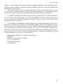
10. PACKING FORM ..................................................................................................... 90
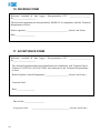
11. ACCEPTANCE FORM ............................................................................................ 90
12. WARRANTY CLAIM .............................................................................................. 91
13. CALIBRATION PROCEDURE .............................................................................. 92
APPENDIX A: RS-232 CABLE SCHEMATICS ......................................................... 93
APPENDIX B: CONNECTING CURRENT CLAMPS TO THE EМ-3.3Т1 .......... 94
APPENDIX C: CONNECTION SCHEMATICS ........................................................ 99
3
LIST OF ABBREVIATIONS
ADC - Analogue-to-Digital Converter
CTB — Current Transformers Block
NPL — Normal Permissible Limits
UPL — Utmost Permissible Limits
PQP — Power Quality Parameters
VT — instrument voltage transformer
CT — instrument current transformer
RPS — Rechargeable Power Supply
Accessories
TMBD — Transformer Burden Measuring Device
PF — Pulse Former
VTCS — Voltage Transformer Calibration Switch
CTCS — Current Transformer Calibration Switch
SH-I — Scanning Head for testing induction meters
SH-E — Scanning Head for testing electronic meters
4
МС3.055.028 UM
INTRODUCTION
This User Manual (the UM) covers a portable reference standard and data logger Energomonitor 3.3T1 (hereinafter referred to as “the EM-3.3T1” or “the Device”). The UM describes
its operation, maintenance, transportation, storage, and manufacturer's warranty conditions. The
UM also includes information about its calibration procedure, packing form and acceptance
form.
EM3.3T1 comes in 2 modifications:
N Energomonitor 3.3T1 (fully functional option);
N Energomonitor 3.3T1-C (option with no PQP measurement and logging).
In terms of metrological characteristics, the Device comes in various versions distinguished for their measurement accuracy depending on input current converters (see Table 2.2).
The legend below explains EM-3.3T1 options to be specified in purchase order
Energomonitor-3.3T1-Х — ХХХХC-ХХХХCp-ХХCTB-ХTR
1
2
3
4
5
6
1 – Name of product;
2 – Range of functions (can be either omitted or specified as “С”):
Omission of this field — indicates full-range option;
С
— character “С” stands for the instrument inoperable as PQP
meter and logger;
3, 4, 5, 6 — specify rated currents of input scaling converters supplied as EM-3.3T1 accessories:
ХХХХC
— Nominal (rated) values of current for a current clamps kit of
basic accuracy included in the basic delivery package (separated by commas);
ХХХХCp — Nominal (rated) values of current for a precision current
clamps kit included in the basic delivery package (separated
by commas);
ХХCTB
— Nominal (rated) values of current for the Current Transformers Block included in the basic delivery package (separated
by commas);
ХTR
— Nominal values of current for the CTCS (Current Transformer Calibration Switch) and TMBD (Transformer Burden
Measurement Device) (separated by commas).
5
1. SAFETY REQUIREMENTS
1.1. When the Device is operated, “Interbranch Rules for Labor Safety (Safety Rules)
When Operating Electrical Systems" (POT РМ-016-2001, RD 153-34.0-03.150–00) must be
observed.
The symbol
!
placed on the panel of the Device is intended to alert the user to the presence of the important
operating instructions specified in the UM (see "Warning!" clause, section "3.3.2 Turning on").
Warning notices are used in the text as follows: NOTE: [important information on the topic discussed in a given section or paragraph]; Caution! [Affects equipment – if not followed may
cause damage to the Device]; Warning! [Affects personnel safety – if not followed may cause
bodily injury or death.]
1.2. The EM3.3T1 is compliant with IEC 61010-1:2001 "Safety requirements for electrical
equipment for measurement, control and laboratory use": category of measurements — II
300V, pollution grade — 1, double reinforced insulation. The Device shall be operated in controlled environment.
Ingress protection rating: IP40. If the Device is used in a manner NOT specified, the protection provided by the Device may be impaired.
1.3 The maximum value of phase-to-neutral voltages at the measuring inputs shall not exceed 400 V. The maximum value of line voltages between the measuring inputs shall not exceed 600 V.
Note!
Please consider the correspondence between phases L1, L2, L3 stenciled on the EM 3.3T1
panels and phases A, B, C mentioned in the document:
L1 → A
L2 → B
L3 → C
6
МС3.055.028 UM
2. DESCRIPTION AND OPERATION PRINCIPLE
2.1. Purpose
Purpose of the Device is:
N measurement and logging of power quality parameters (PQP);
N measurement and logging of electrical parameters (AVG) in single- and three-phase
networks (RMS of voltages and currents, no matter what their waveforms may be (sinusoidal or not); active, reactive and apparent electric power);
N in-situ testing / calibration of single- or three-phase meters of active or reactive electric
power; performance testing and control of meters accuracy characteristics (correctness
of their connection as well), without breaking into current circuits;
N in-situ testing / calibration of voltage and current instrument transformers;
N measurement of electric parameters in secondary circuits (load power), as applied to
metering and billing systems;
N in-situ testing / calibration of measuring instruments and/or instrument-class converters
of voltage, current, active and reactive power;
N measurement of amplitude (peak) AC voltage values up to 500 Hz frequency in
one/three channels or in a differential channel;
N testing / calibration of amplitude/peak voltmeters.
With such a wide variety of functions the Device can be used for:
N inspecting enterprises involved in electric power generation or consumption (electric
energy audit);
N conducting test procedures established for electric power certification;
N long term monitoring and analysis of electric power quality;
N equipping various metrological units (mobile testing labs in that number).
As nationally recognized tool, the EM-3.3T1 has been registered under N 39952-08 with
National Registry of Measuring Instruments, and granted certifications as follows: Pattern Approval Certificate of Measuring Instruments RU.C.34.001.А N 34446.
2.2. Operating conditions
Environmental conditions for the EМ-3.3Т1 shall be as follows:
N Ambient temperature, °C ................................................... From - 20 to 55;
N Relative humidity, % ......................................................... 90 at 30 °C
N Atmospheric pressure, kPa (mm Hg) ................................ 70–106.7 (537–800).
The EМ-3.3Т1 shall typically be connected to mains (85-264 V AC, 50 ± 5 Hz) via Power
adapter and Rechargeable power supply. The Device will accept being powered from either of
the said accessories. A delivery package may be agreed to include both.
Warning!
You must not power the EM3.3T1 from any power supply unit other than that supplied by
the manufacturer.
2.3. Delivery package
Particular delivery package for the Device may be agreed to contain items specified in Table 2.1.
7
Table 2.1
Delivery package
Item description
Notes
Qty
Standard Accessories
Energomonitor-3.3Т1 Basic
1
Power adapter with mains cable 220V
(Uout = 16V, Iout = 1.2A)
1
PC connection cable, RS-232 interface
1
PC connection cable, USB interface
1
Rechargeable power supply
1
Test leads (4 colors)
4
Shunt 1000A
1
Shunt 100A
1
Scanning Head SH-E for testing electronic meters
1
Scanning Head SH-I for testing induction meters
1
Pulse Former PF
1
*
"Energomonitoring" software
1 CD
User's Manual
1
Carrying bag
2
Optional Accessories
Current clamps:
10 A
3
1000A
3
_____________
*
PC programs of "Energomonitoring" software family presently compatible with the Energomonitor-3.3Т1
2.4 Specifications
2.4.1. The Device’s technical characteristics correspond to the type of input current converters (i.e. scaling converters of the current to be measured).
Current measurement channels of the Device are connected via scaling converters included in the delivery package. These may be current transformers or current clamp kits, complete with suitable shunts and/or cables (see Appendices B and C). The EM-3.3T1 is provided
with three current measurement channels that support measurement sub-ranges with nominal
values as follows:
N 0.1 A with current transformers;
N 1 A with current transformers;
N 0.5 A with current transformers;
N 5 A with current transformers;
N 50 A with current transformers;
N 5 A with current clamp kit 5 A;
N 10 A with current clamp kit 10 A;
8
МС3.055.028 UM
30 A with flexible current clamp kit 30/300/3000 A
50 A with current clamp kit 50 A;
N 100 A with current clamp kit 100 A;
N 300 A with flexible current clamp kit 30/300/3000 A;
N 500 A with current clamp kit 500 A;
N 1000 A with current clamp kit 1000 A;
N 3000 A with flexible current clamp kit 30/300/3000 A;
N 5000 A with current clamp kit 5000 A.
Voltage measurement channels are connected to the network under control directly or via
scaling converters (i.e. voltage transformers, dividers etc.). The EМ-3.3Т1 is provided with
three channels for direct measurement of phase-to-neutral (phase-to-phase) voltages with nominal values of 60 V (100 V), 120 V (200 V), 240 V (415 V).
N
N
2.4.2. The EМ-3.3Т1 is capable of measuring, besides other parameters of electric power,
the basic power quality parameters (PQP). See Table 2.2 for measuring ranges and permissible
limits of measurement errors.
Monitored values are continuously measured, calculated, graphically displayed on the Device’s LCD screen and logged for further transfer to a PC.
Measurement results from ADC are processed programmatically by firmware. Calculations over the sampled data are based on 4096 ADC readings taken over 0.32 s. Thus, at 50 Hz
frequency, the sampling rate of 256 samples per period is provided. Momentary value of each
signal monitored is recalculated every 0.16 s, using 2048 samples from previous measurement
and 2048 samples from the next one.
Logging function of the EМ-3.3Т1 covers the following data and events:
N PQP: the most important totals show how many PQP measurements (based upon one
ADC reading per 0.32 s) lie within Normal Permissible Limits (NPL), within Utmost
Permissible Limits (UPL), or outside UPL. Data are averaged over the interval of: 60 s
for steady-state voltage deviation; 20 s for frequency deviation; 3 for other PQP.
N Voltage dips and swells;
N Flicker short-term perceptibility values for measurement periods of 10 min, 5 min, or 1
min;
N Values of PQP and averaged network parameters (AVG). Logging may be based on
AVG averaging periods of 3 s, 1 min, or 30 min. Alternatively, EМ-3.3Т1 logging
function may operate in “oscilloscope” mode, instead of data averaging. In such a
mode, network parameters (3 phase voltages and 3 phase currents only) are taken directly from the ADC at 12.8 kHz frequency;
N Archive of meters calibration tests. The EМ-3.3Т1 may store results for as many as 200
tests, up to 10 measurements per test.
EМ-3.3Т1 graphic display makes visible the results of measurements, including:
N Values of basic PQP;
N Network parameters, their averaging time being 1.25 s, 2.5 s, 5 s, 10 s, 1 min, 15 min,
or 30 min (see section 4.10.6);
N Measurement error values for meters tested;
N Measurement error values for instrument transformers tested (with use of CTCS for current transformers, and VTCS for voltage transformers).
Data length of measured values of current on the display is five significant digits and a polarity sign (represented as: ±х.хххх, ±хх.ххх, ±ххх.хх, ±хххх.х). Data length of measured voltage values on the display is five significant digits and a polarity sign (represented as: ±х.хххх,
±хх.ххх, ±ххх.хх). Measured values of power are represented by at least four significant digits
9
and a polarity sign (represented as: ±х.ххх, ±хх.ххх, ±ххх.ххх, ±хххх.хх, ±ххххх.х, ±хххххх,
±ххххххх).
10
МС3.055.028 UM
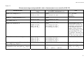
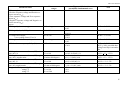
Table 2.2
Measurement ranges and permissible values of measurement error stated for EM3.3T1
Measured values
Measurement
ranges
1 RMS of AC voltage (U), V
0.01UN to 1.5UN
2 RMS of 1st voltage harmonic (U1), V
3 DC voltage (UDC), V
0.01UN to 1.5UN
0.01UN to 1.5UN
4 RMS of AC current (I), A
*
0.005IN to 1.5IN
0.05IN to 1.5IN **
0.05IN to 1.5IN ***
5 RMS of 1st current harmonic (I1), А
0.01IN to 1.5IN *
0.05IN to 1.5IN **
0.05IN to 1.5IN ***
0 to 360
6 Phase angle between the 1st harmonics of
phase voltages (ϕU), degrees
7 Phase angle between 1st voltage and 1st cur0 to 360
rent harmonics in the same phase (ϕUI), degrees
Types and limits of
permissible fundamental error
relative
±[0.1+0.01((UN /U)–1)]%
relative
±[0.1+0.01((UN /U)–1)]%
relative
±[0.2+0.02((UN /U)–1)]%
relative
±[0.1+0.01((IN /I)–1)]% *
±[0.5+0.05((IN /I) –1)]% **
±[1.0+0.05((IN /I)–1)]% ***
relative
±[0.2+0.02((IN /I)–1)]% *
±[0.5+0.05((IN /I) –1)]% **
±[1.0+0.05((IN /I)–1)]% ***
absolute
±0.1
absolute
±0.2 *
±0.5 **
±0.5 ***
Note
UN = 60 (100),
120 (200),
240 (415) V
Nominal RMS values of
measured AC current are determined by, and correspond
to, the nominal values of
primary current converters
(CTB, current clump, CTCS)
taken from EM-3.3T1 delivery package. The range is as
follows: 0.1, 1, 0.5, 5, 10, 50,
100, 300, 500, 1000, 3000 А.
0.2UN < U < 1.5 UN
0.2 IN < I < 1.5IN
0.2 UN < U < 1.5 UN
11
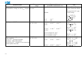
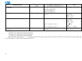
Measured values
Measurement
ranges
8 Phase angle between nth voltage and nth current harmonics, n being 2 to 40, (φUI(n)), degrees 0 to 360
9 Active power (Р), W
0.01IN UN
to 1.5IN 1.2UN
Types and limits of
permissible fundamental error
absolute
Only for EM-3.3T1 with
Current Transformer Block,
or
Precision EM-3.3T1 with
Current clamps
±1.0 *
±3.0 *
relative
±0.1% *
±0.2% *
Р(N ) > 0.003IN UN
0.1 IN < I < 1.5 IN
2% < K(n) < 15%
2 < n < 10
11 < n < 40
PF = 1
0.1 IN < I < 1.5 IN
0.01 IN < I < 0.1 IN
±3.0 **
±6.0 **
±0.5% **
*
±0.15%
±0.25% *
10 Reactive power (Q), var, calculated with one 0.01IN UN
of three methods:
to 1.5IN 1.2UN
2 2
Q1=√(S -P ) – geometrical method;
Q2=UIsinφ – phase shift method;
Q3=UIcos(φ+90°) – method of cross-connection
(for three-phase networks).
12
Note
±1.0%
**
±1.0% ***
±2.0%
***
±[0.25+0.02((PN /P)–1)]% *
±[1.0+0.1((PN /P) –1)]% **
±[2.0+0.1((PN /P)–1)]% ***
relative
±0.3% *
±0.5 % *
±1.0% **
±2.0% **
PF 0.5L…1… 0.5C
0.1 IN < I < 1.5 IN
0.02 IN < I < 0.1 IN
±2.0% ***
PF 0.2L…1… 0.2C
0.1 IN < I < 1.5 IN
PF 0.45L…0…-0.45C
PF 0.45C…0…-0.45L
0.1 IN < I < 1.5 IN
±4.0% ***
PF 0.86L…0…-0.86C
PF 0.86C…0…-0.86L
0.1 IN < I < 1.5 IN
МС3.055.028 UM
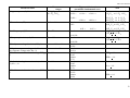
Measured values
11 Apparent power (S), VA
Measurement
ranges
0.01IN UN
to 1.5IN 1.2UN
Types and limits of
permissible fundamental error
relative
±0.2% * ±1.0% ** ±2.0% ***
±2,0% *
12 Power factor (PF)
–1.0 to +1.0
±2.0% **
absolute
0.02 *
13 AC frequency (f), Hz
45 to 75
absolute
14 Frequency deviation (Δf), Hz
-5 to +25
±0.01 Hz
absolute
-100 to +40
16 Negative sequence voltage ratio, K2U, %, and
0 to 50
Zero sequence voltage ratio, K0U, %
17 Total harmonic distortion of voltage THDU), 0 to 49.9
%
18 Individual voltage harmonic ratio (n = 2 to
40), KU(n ), %
0 to 49.9
19 Total harmonic distortion of current (THDI), 0 to 49.9
%
±0.01 Hz
absolute
±0.2%
absolute
±0.2 %
absolute
±0.05
relative
±5 %
absolute
±0.05
relative
±5 %
absolute
±0.1%
relative
±10%
0.1IN UN to 1.5IN 1.2UN
0.01 IN UN to 0.1 IN UN
0.05 IN UN to 0.1 IN UN
0.01IN UN to 1.5IN 1.5UN
0.05 **
15 Steady-state voltage deviation (δUs), %
±4.0% ***
Note
0.05 ***
0.05IN UN to 1.5IN 1.5UN
0.1IN < I < 1.5IN
0.1UN < U < 1.5UN
0.1IN < I < 1.5IN
0.1UN < U < 1.5UN
THDU < 1.0
THDU > 1.0
KU(n) < 1.0
KU(n) > 1.0
THDI < 1.0
THDI > 1.0
13
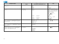
Measured values
20 Individual current harmonic ratio (n = 2 to
40), KI(n), %
21 Active power of nth harmonic (n = 1 to 40),
Р(n), W
Measurement
ranges
0 to 49.9
0.003IN UN
to 0.1IN UN
Types and limits of
permissible fundamental error
absolute
±0.1
relative
±10%
22 Positive sequence current (I1(1)), Zero sequence current (I0(1)), and Negative sequence
current (I2(1)), A
0 to IN
23 Positive sequence voltage (U1(1)), Zero se- 0 to UN
quence voltage (U0(1)) , and Negative sequence
voltage (U2(1)), V
24 Positive sequence active power (P1(1)), Zero 0.01IN UN
sequence active power (P0(1)), and Negative
to 1.,5IN UN
sequence active power (P2(1)), W
14
±10.0% **
±5.0% *
±10.0% **
±10.0% * ±20.0% **
absolute
±0.002 IN А *
±0.01 IN А **
±0.02 IN А ***
absolute
±0.002 UN
absolute
±0.0025PN *
±0.01PN **
±0.02PN***
KI(n) < 1.0
KI(n) > 1.0
Only for EM-3.3T1 with
Current Transformer Block,
or EM-3.3T1 with Precision
Current clamps
0.1 IN < I < 1.5 IN
2% < K(n)
relative
±5.0% *
Note
PF = 1
PF 0.5L…1… 0.5C
2 < n < 10
11 < n < 40
0.01 IN < I < 1.5 IN
0.1 IN < I < 1.5 IN
МС3.055.028 UM
Measured values
25 Phase angles between
a) Positive sequence voltage and Positive sequence current (φ1UI);
b) Zero sequence voltage and Zero sequence
current (φ0UI);
c) Negative sequence voltage and Negative sequence current (φ2UI);
degrees
26 Voltage dip duration (Δtd), s
Measurement
ranges
0 to 360
Types and limits of
permissible fundamental error
not standardized
0.02 or longer
absolute
±0.02
relative
±10.0 %
relative
±2.0 %
absolute
±0.02
relative
±5.0 %
27 Voltage dip depth (Udip),%
10 to 100
28 Voltage swell height
(over-voltage factor) Usw ,%
29 Voltage swell duration (Δtsw), s
110 to 799
0.01 or longer
30 Flicker short-term perceptibility (Pst)
0.25 to 10
31 Voltage instrument transformer (VT) ratio
error (ΔfU), %
32 Voltage instrument transformer (VT) angle
error (ΔδU), angular units
33 Current instrument transformer (CT) ratio
error (ΔfI), %
34 Current instrument transformer (CT) angle
error (ΔδI), angular units
35 Apparent load power (S), VA
using CT
using VT
0.1 to 100
0.1min to180 degrees
0.1 to 100
0.2 min to180 degrees
12 to 100
10 to 1200
absolute
±(0.02 +0.02|ΔfU |) %
absolute
±(1.0 + 0.1|ΔδU|) min
absolute
±(0.02 +0.02|ΔfI |) %
absolute
± (1.0 + 0.1|ΔδI |) min
relative
2.0 %
2.0 %
Note
49 Hz < f < 51 Hz
49 Hz < f < 51 Hz
49 Hz < f < 51 Hz
49 Hz < f < 51 Hz
49 Hz < f < 51 Hz
∆U/U ≤ 20%, provided that
voltage envelope is meanderlike.
0.8 UN < U < 1.5 UN
0.8 UN < U < 1.5 UN
0.01 IN < I < 1.5 IN
0.01 IN < I < 1.5 IN
15
36 Tangent ϕ
Measurement
ranges
0 to 8
37 Voltage peak value, V
0.1UN to 2.1UN
38 Voltage amplitude value, V
0.1UN to 2.1UN
Measured values
39 Accuracy of time keeping (daily rate of realtime clock)
N/A
Types and limits of
permissible fundamental error
absolute
±[0.005+0.003(tg ϕ )2]*
±[0.02+0.015(tg ϕ )2]**
±[0.02+0.015(tg ϕ )2]***
referred
±0.2 %
Note
0.01INUN to 1.5IN 1.2UN
±[0.2 + 0.02|2 UN /U-1|] %
Within the bandwidth of 0.6
to 2.0 kHz:
THDU < 30 %,
KU(n) < 10 %
Within the bandwidth of 0.6
to 2.0 kHz:
THDU < 30 %,
KU(n) < 10 %
f < 400 Hz
±[0.5 + 0.05|2 UN /U-1|] %
absolute
±2 s/day
400 Hz < f < 600 Hz
Within temperature range of
10 оC to 35 оC
relative
________________
*
for EM-3.3T1 with Current Transformers Block.
for EM-3.3T1 with Precision Current clamp kit.
***
for EM-3.3T1 with a basic Current clamp kit.
Data not marked with asterisks *, **, *** are valid regardless of the type of input current converters (for EM3.3T1 with Precision current clamps, Basic current clamps, or with Current Transformers Block).
**
16
МС3.055.028 UM
2.4.3. Additional real-time clock inaccuracy within operating temperature range is no
more than ±0.05 s/(24 hours · °С).
2.4.4. When input signal does not constitute a sine waveform, the EM-3.3T1 still supports
measurement of network parameters and PQP, provided that amplitude values of current and
voltage never exceed twice the nominal values for measurement sub-ranges (see section 2.4.1).
2.4.5. 5 For the purpose of PQP monitoring, the EM-3.3T1 calculates and logs upper/lower and maximum/minimum parameter values determined from the parameter averages
per a day. It also maintains daily totals for each PQP that show how many PQP measurements
has fallen within Normal Permissible Limits (NPL), within Utmost Permissible Limits (UPL),
and outside UPL. Continuous logging for 8 days is supported without rewriting.
For the purpose of monitoring the Averaged Network Parameters (AVG), the EM-3.3T1
calculates and logs AVG continuously during:
N 9.5 hours at 3 s averaging time;
N 8 days at 1 min averaging time (PQP values included);
N 7.5 months at 30 min averaging time.
EМ-3.3Т1 logging function may operate in “oscilloscope” mode to log data (3 phase voltages and 3 phase currents only) taken directly from the ADC at 12.8 kHz. The Device’s memory size permits such logging to last for 9 minutes without rewriting the data.
The EM-3.3T1 provides for calculation and logging of magnitudes and durations of voltage dips/swells. 80 000 events of the kind may be logged continuously before being overridden.
The EM-3.3T1 provides for calculation and logging of flicker short-term perceptibility
values for measurement periods of 10 min, 5 min, or 1 min. Continuous logging for 8 days is
supported without rewriting.
The EМ-3.3Т1 may store results for as many as 200 meter calibration tests, up to 10 measurements per test.
The EМ-3.3Т1 archives measurement results in its internal non-volatile memory. Data storage time is unlimited when the Device is powered off.
2.4.6. The EМ-3.3Т1 supports data transfer to a PC via serial interfaces RS-232 or USB.
2.4.6 The built-in real time clock makes it possible to record the time of data logging over
all parameters measured, as they are stored in the Device's internal memory (in the dedicated
logs). Date and time setting to a new value is available. The clock is powered by a built-in battery with at least 2 years life-time.
2.4.8. The Device uses two-level protection system based on passwords. Depending on the
level, the user gains access to certain operation modes and settings. Password length on first
level is 8 digits; second level requires 9 digits.
2.4.9. The EМ-3.3Т1 remains operational when 0.5 s overload occurs on its measurement
channels, provided that RMS value of measured phase voltage never exceeds 600 V, and RMS
value of measured current never exceeds 2IN A. The Device will regain its accuracy characteristics within 15 minutes after the overload removal.
2.4.10. Apparent power consumed by each current measurement channel is 0.5 VA or less
(for measured current as per Table 2.2).
Apparent power consumed by each voltage measurement channel is 1.0 VA or less.
17
2.4.11. The EМ-3.3Т1 is provided with frequency output Fout generating pulse signal as
follows:
N pulse duration, microseconds ....................................14 ± 2;
N pulse height, V ..........................................................4.5 ± 0,5 (U ≤ 0.2 V; U ≥ 4.5 V).
0
1
Частота f (kHz) is in proportion to measured power, as defined by the applicable Instrument Constant.
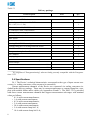
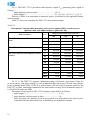
Table 2.3 shows the constants for EМ-3.3Т1 measurement ranges.
Table 2.3
Instrument Constant while measuring active power (pulses/kWh), reactive power
(pulses/kvarh), and apparent power (pulses/kVAh)
EM3.3T1 option
EM-3.3T1 with Current Transformers
Block
EM-3.3T1 with Precision Current clamp
kit
EM-3.3T1 with Current clamp kit of basic
accuracy
IN, A
Voltage measurement range selected, V
240
120
60
0.5
120000000
240000000
480000000
5
12000000
24000000
48000000
50
1200000
2400000
4800000
5
12000000
24000000
48000000
10
6000000
12000000
24000000
5
12000000
24000000
48000000
10
6000000
12000000
24000000
50
1200000
2400000
4800000
100
600000
1200000
2400000
300
200000
400000
800000
500
120000
240000
480000
1000
60000
120000
240000
3000
20000
40000
80000
5000
12000
24000
48000
2.4.12. 11 The EМ3.3Т1 supports calibration/testing of electronic type meters (Class 0.5
or less accurate, with pulse output), as well as induction disk type meters. In both cases photoelectric scanning heads (SH-E or SH-I) or pulse formers (PF) are used to generate pulses for the
EМ3.3Т1 to count. Instrument constant for the meter under test may be set within the range of 1
to 999 999 999 pulses per kWh.
Parameters of the signal on EМ-3.3Т1 frequency input shall be as follows:
N pulse height, V .................................................................. 5÷15;
N pulse duration, microseconds, at least .............................. 10;
N pulse repetition rate (number of pulses per second) is in proportion to the value of power measured by the meter under test, as defined by its instrument constant.
18
МС3.055.028 UM
Supplied complete with photoelectric scanning heads (SH) and pulse formers (PF), the
EМ3.3Т1 provides for testing of both metrological characteristics and correctness of meters
connection, without breaking into meter’s current circuit. SHs and PFs are applied as follows:
N Electronic type meters with optical pulse output are tested using SH-E photoelectric
scanning head or Pulse Former PF
N Electronic type meters with current pulse output are tested using just a Pulse Former PF
N Induction disk type meters are tested using a SH-I photoelectric scanning head or a
pulse former PF.
2.4.13. One more type of auxiliary equipment is included in the Device’s delivery package
for the purpose of instrument transformers calibration. These are Current Transformer Calibration Switch (CTCS) and Voltage Transformer Calibration Switch (VTCS). When equipped with
a CTCS, the EМ-3.3Т1 supports testing of Class 0.2S (or less accurate) current instrument
transformers with secondary current of up to 5 A. Equipped with a VTCS, the Device supports
testing of Class 0.2 (or less accurate) voltage instrument transformers.
2.4.14. While operating in the peak voltmeter mode, the EM3.3T1 supports calibration/testing of peak voltmeters of 0.2 accuracy class or less accurate.
2.4.15. The Device is considered set for stable operation in 30 minutes after applying
power. From that point on its technical characteristics are as specified in Table 2.2.
2.4.16. The EМ-3.3Т1 retains both its settings and stored data in case of either failure of
its 10-17 V DC power supply, or voltage dip down to the depth of 100 %. If connected to mains
via the Power adapter and Rechargeable power supply, the EМ-3.3Т1 remains operational in
case of external power failure (see sections 2.4.17).
Each time a shutdown occurs in logging mode, the Device automatically restarts as soon
as it regains power. Then the Device resumes logging according to the parameters set before
shutdown (see section 4.3.2).
2.4.17. Time of continuous operation of the EM3.3T1 powered from the Rechargeable
power supply 12V (after 1 charging cycle, in case of no mains supply) is no less than 2 hours.
Time of continuous operation of the EM3.3T1 powered from the fully charged Rechargeable
power supply is no more than 5 hours.
2.4.18. Power consumption from mains is 20 VA or less; DC power consumed by the Device itself is within 8 VA at 12 V.
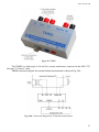
2.4.19. Dimensions of the Device (height, width, depth) are within 250x280x80 mm.
Weight of the Device (not including accessories) does not exceed 2 kg.
2.4.20. Mean Time to First Failure (MTFF) of the Device is at least 44 000 hours. Average
lifetime -10 years or longer.
19
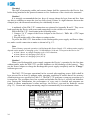
2.5. Design and operation
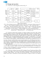
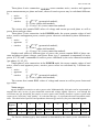
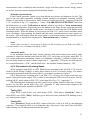
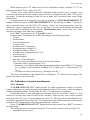
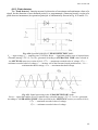
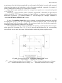
2.5.1. The Device’s block diagram is shown in Fig. 2.1.
Fig. 2.1. Block diagram:
SCU— Unit of Scaling Converters; voltage scaling converters SCU) and current scaling converters SCI;
ADCU — Unit of Analogue-to-Digital Converters; voltage ADCs — ADCU and current ADCs —
ADCI); DPB — Data Processing Block; FAMU, FAMI — "Former of Array" modules (they create data
arrays of voltage (U) and current (I) instantaneous values); CMUrms, CMIrms — Calculating modules for
RMS values of U and I; MP,Q,S — module calculating active, reactive and apparent power;
FFTMU, FFTMI — Fast Fourier Transform Modules; DDU — Data Display Unit (graphic display and
keyboard); MU — Memory Unit; PCC — PC Connection unit.
2.5.2. The Device shares basic principles of Analog-to-Digital Conversion (ADC) and the
Sampling Method. In the SCU, three-phase input voltages and currents are converted into 1V
level voltage signals compliant with U and I measurement ranges of ADC U and ADC I. Instantaneous signal values are converted into digital codes by six ADCs and routed to the DPB. In
the DPB, the arrays of sampled instantaneous values of voltage UUj and current UIj are created
(j — is the number of a sample). Programmatically calculated values of the measured parameters are shown on Data Display, stored in the Memory Unit and may be transferred to a PC, if
necessary. Program modules obtain each measured parameter by calculating measurement results from the array of sampled data. This method (called “incoherent sampling”) does not require frequency synchronization between sampling process and measured signal. Such a measuring technique enables to view values of the measured parameters for all three phases on one
screen at the same time.
The EМ-3.3Т1 can determine all of the AC network parameters simultaneously, namely
current, voltage, frequency, angles, current and voltage individual harmonics (1st to 40th), power (active, reactive and apparent). It operates with all types of circuit connections applied to single- and three-phase network measurements.
2.5.3. The Unit of Scaling Converters (SCU) includes Current Transformers Block (CTB)
or set of current clamps (3 psc., each one individually calibrated to match a measuring channel)
and three voltage dividers. SCU relays are processor-controlled. The processor issues commands (in the form of a potential) to select an input range for voltage or current. The controller
20
МС3.055.028 UM
outputs the value of an active measuring range on the graphical display. The relays serve to
switch among voltage measuring ranges for the input transformers.
2.5.4. The ADC Block, or Measuring Board, has six identical channels. They operate independently converting ±1.5V analogue input signals into 16-bit binary data (a sign bit
+ 15 significant bits). Each data word represents instantaneous value of an input signal. At the
heart of each channel are two chips available from Analog Device, one for the input amplifier, the
other for ADC itself. Type AD177 chip, the input amplifier, matches the input transformers due to
its low offset output voltage drift, negligible temperature drift, and ultra-low input currents.
Channel’s input impedance is over 50 MOhm. Signal taken from the amplifier is fed into type
AD977 chip, the ADC. The latter performs complete 16-bit conversion without signal quality degradation, and transmits the result in serial code to the controller upon request. It takes 40 ns (so
called “aperture time”) for AD conversion to come to an end internally. As to the entire Measuring board, it takes voltages fed into ADC inputs, digitizes them, and passes the results onto the
Processor board.
2.5.5 Data Processing Block, otherwise called the Processor board or the Controller board,
exercises full control over the EМ-3.3Т1. It provides that calculations be done over the arrays of
digitized samplings, the results be stored in non-volatile memory and displayed on LCD screen,
time be kept and intervals marked as per real-time clock, data exchange be supported with external devices (PCs), commands and data be received from operator’s keyboard. The Controller
board bears the ultimate responsibility for smooth operation of the entire EМ-3.3Т1. At the
heart of the controller are a Texas Instruments signal processor, and an FPGA available from
Xilinx. Such a solution makes possible prompt upgrading of Device’s firmware, keeping its
hardware intact.
Data from ADC are processed programmatically and shown on Data Display. Calculations
over the sampled data are based on 4096 ADC readings taken over 0.32 s. Thus, at 50 Hz frequency, the sampling rate of 256 samples per period is provided. Momentary value of each signal monitored is recalculated every 0.16 s., using 2048 samples from previous measurement and
2048 samples from the next one.
2.5.6 The Memory Unit provides storage space for measurement results, settings, etc.
2.5.7 The Power Supply Unit generates voltages for the Processor and Measuring boards.
2.5.8 Operator’s membrane keyboard and LCD graphic display are both mounted on the
Device's front panel and connected to the Processor Board. The keyboard is used to select operation and display modes, enter data upon request, configure the Device etc.
21
3. PUTTING INTO OPERATION
3.1. Operating restrictions
If the Device has been moved from a cold environment (with ambient temperature below -5°
C) into a warm one, it shall be left to stand for at least 4 hours at room temperature before applying
power, to make sure that no condensation remains inside. In case of a drop in ambient temperature
for 10° C or more, the Device shall be kept for at least 30 minutes under operating conditions not
connected to power.
Warning!
The Device shall not be used under the ingress of moisture inside its body.
The contrast of LCD screen image can be impaired under the temperature below -10° C.
However, this does not affect the Device’s performance.
3.2. Unpacking
Check that the delivery package contains all items specified in the Supply Agreement.
Remove the garnish plugs and check to see if the manufacturer’s seal is intact. Should anything
in the package is found damaged, contact the supplier immediately.
3.3 Preparing for operation
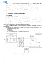
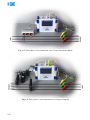
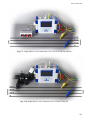
3.3.1 Controls and Connectors
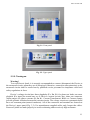
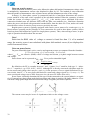
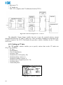
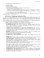
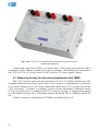
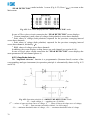
Front and upper panels of the EM 3.3T1 are shown in Fig. 3.1 and Fig. 3.2. The controls
and connectors are listed in Table 3.1.
Table 3.1
Key
Name and Function
“0”, ..., “9” Numeric keypad: press to type in numeric values or to browse through the screens
i, j
Up and down arrow keys: press to scroll through various menu items or data fields
g, h
Left and right arrow keys: press to scroll through various menu items or data fields
“ENT”
Press to
- activate a menu item;
- confirm data typed in (with saving the value);
- enable selected mode
“ESC”
Press to
- return to an upper-level menu without saving changes;
- return to the Main menu
- leave some current menu item for an upper level menu
“F”
‰
22
"Function": press
- as a hot key to exit from any menu item and enable “Measuring range selection”
mode;
- to enter/exit “character entry” mode when typing in some names
- press to insert a symbol while entering names
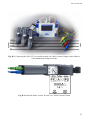
МС3.055.028 UM
Fig. 3.1. Front panel
Fig. 3.2. Upper panel
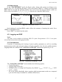
3.3.2. Turning on
Warning!
To avoid electric shock, it is strongly recommended to connect (disconnect) the Device to
the measured circuits when they are de-energized. Otherwise, connection (disconnection) to the
measured circuits shall be carried out by qualified service personnel in compliance with local
safety regulations in force.
Device’s voltage circuits have three plugholes (UA, UB, UC) for phase test leads, one more
plughole (UN input) for neutral one; as to Device's current circuits, they share one connector
(input-output) for phase currents (IA, IB, IC). Current Transformers Block or Current clamps
provide galvanic isolation between the current circuits. The voltage circuits are symmetrical and
have one common point (neutral conductor). All of the connectors and terminals are located on
the Device’s upper panel (Fig. 3.2). Use manufacturer-supplied cables only. Inspect the cables.
Ensure all joints are made properly to avoid overheating and excessively high resistance.
23
Warning!
The clips of measuring cables and current clamps shall be connected to the Device first,
before being attached to the powered contacts or live conductors of the circuit to be measured.
Caution!
It is strongly recommended that jaw faces of current clamps be kept clean and free from
any dirt or oxidizing to ensure the jaws are fully closed. If there is a tight clearance between the
clamped jaws, the measured current may be considerably in error.
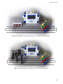
A multitude of the EМ-3.3Т1 connections are pictured in Appendix B and C. They cover
both supplying the Device with power and connecting it to the circuits to be measured.
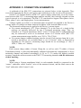
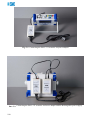
Power the EМ-3.3Т1 from mains in the following order:
1. Connect “16 V” output of the Power Adapter to the Device’s "DC= 10 … 17V" input
(see Fig. C-1).
2. Plug the mains cable of the adapter to mains socket.
To power the EМ-3.3Т1 from mains via the Rechargeable power supply and Power Adapter, make a serial connection to mains as shown in Fig. C-3.
Note
Time of battery-powered operation (via Rechargeable Power Supply 12V; without mains supply)
depends on the number of charging cycles. Ni-Mh batteries 2100 mA · h can power the Device for:
N at least 2 hours at a single charging cycle of 4.5 h duration;
N at least 4 hours at 2 charging cycles (4.5 h);
N at least 5 hours at 3 charging cycles (4.5 h).
Caution!
When your Rechargeable power supply supports the Device’s operation for the first time
without mains, make the EМ-3.3Т1 run into shutdown (to full discharge of the battery). Then
use the Power Adapter to charge the Rechargeable power supply completely until its “Charge”
indicator goes out.
The EМ-3.3Т1 becomes operational in few seconds after applying power. Still it shall be
kept powered for at least 30 minutes under operating conditions to ensure that all its accuracy
characteristics are as specified in Table 2.2. The EМ-3.3Т1 performs a warm-up procedure as it
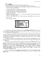
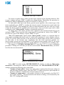
is turned on. The procedure lasts few seconds and includes the Device’s self-test and initialization. During the initialization, the performance of every unit is checked and programs are
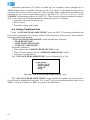
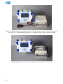
loaded. It shows manufacturer’s name and logo, the Device’s type and its firmware version
(Fig. 3.3). Current and voltage measuring ranges are automatically set to maximum values.
Fig. 3.3. "Power up" screen
24
МС3.055.028 UM
4. OPERATION PROCEDURE
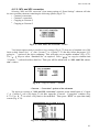
4.1. Operator Interface
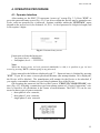
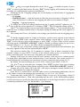
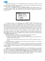
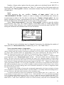
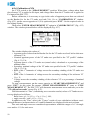
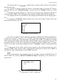
After turning on, the EM3.3T1 represents “power up” screen (Fig. 3.3). Press "ENT" to
get to the password entry screen (Fig. 4.1). User access within the Device may be granted at two
levels, each one protected by a password. Options available within the "SETTINGS” menu
depend on the access level (see sections 4.10, 4.11). 1st level password is 8 digits in length; 2nd
level requires 9 digits.
Fig. 4.1. Password entry screen
Passwords set from the factory are:
N 1st (lower) level — 00000000;
N 2nd (higher) level — 222222222.
Note
While the factory preset 1st level password (00000000) is valid, it is possible to get 1st level
access by pressing "ENT" (without typing in any password).
Digits entered in the fields are displayed with "*". Password entry is finished by pressing
"ENT". If you fail to enter a correct password 50 times (the attempt number 50 is displayed),
the Device will be blocked. The manufacturer will arrange for the Device to be unlocked, if
you supply a reasonable evidence of your being legitimate user of the Device.
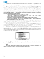
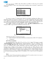
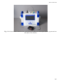
On accepting the password, the Device takes you to "CIRCUIT CONNECTIONS" window (Fig. 4.2). Selecting a connection type from among options of “Circuit Connections” window is crucial to all calculations in the course of measurements. The EМ-3.3Т1 can be connected to three types of power networks:
N three-phase 4-wire network;
N three-phase 3-wire network;
N single-phase 2-wire network.
Fig. 4.2. “Circuit Connections” screen
25
Typical EМ-3.3Т1 connections to circuits under review are pictured in Appendixes B and
C.
Operator interface of the EМ-3.3Т1 was designed on the model of nested menus and windows. To navigate to a desired screen or menu item six keys are used: ENT, ESC, j, i, g, h.
Their functions and locations on the keyboard are explained in Table 3.1 and Fig. 3.2. Wherever
within menu hierarchy you might be, the Device’s current date and time are always indicated on
the top of your screen, while its bottom line shows active measurement ranges and the circuit
connection type. Active measurement ranges are represented on the bottom line as two alphanumeric fields and a separator “/” between them. Active range for current is indicated on the separator’s right and may be one of the following:
N if the Device is connected via CTs: T0,5A, Т5A, Т50A;
N if the Device is connected via current clamps: C5A, C10A, C30A, C50A, C100A,
C300A, C500A, C1000A, C3000A, C5000A;
N if the Device is connected via precision current clamps: Cp5A, Cp10A, Cp1000A;
N if the Device is connected via CTCS (CT Calibration Switch) or TMBD (Transformer
Burden Measurement Device): D0.5А, D5А.
Active measurement range indicator for voltage appears to the left of “/” separator as
“60V”, “120V”, or “240V”. Besides, in the “Logging and PQP” mode the bottom line reflects
actual status of logging function (enabled, disabled, or timed).
Measuring range and circuit connection options are available via “SETTINGS” menu (see
sections 4.10.2, 4.10.3). Instead, the “Measuring range selection” function may be called up
promptly from no matter what menu or item, just by pressing “F” hotkey.
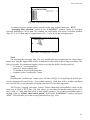
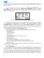
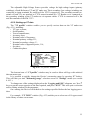
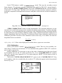
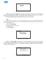
Each option of the Main menu (pictured below) corresponds to a mode of operation or a setting procedure (Fig. 4.3). Access to the "EXTRA SETTINGS" options is given only if the user
opened the Main Menu via the second level password. The 1st level password gives access to 8 basic options of the “SETTINGS” menu.
Fig. 4.3. Main Menu
Use j and i keys to select from among items of the Main menu. Enter the selected item
by pressing "ENT".
Note
The operator interface may be modified with respect to the order of displaying information. The
changes do not affect the Device’s accuracy and technical characteristics.
26
МС3.055.028 UM
4.2 Measurements
4.2.1. General
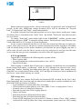
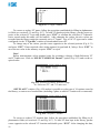
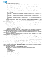
The "MEASUREMENTS" screen is shown in Fig. 4.4.
Fig. 4.4. "MEASUREMENTS" menu
The "MEASUREMENTS" menu contains seven options, the use and selection of which
is dependent on user need: power; current and voltage; harmonics; phase angles; etc. Press j
or i to cycle through the options. Press "ENT" to enable an option, press "ESC" to return to
the Main Menu.
Except for “WAVEFORMS”, “MEASUREMENT” modes specified in the menu show
“real time” parameters on their respective screens. Data on the screens are updated as per averaging time preset in the “AVERAGING TIME” window of the “SETTINGS” menu (see section 4.10.6). “WAVEFORMS” mode is described in section 4.2.7. If the preset averaging time
exceeds 10 seconds, the ANGLES, HARMONICS and HARMONICS POWER data are updated each 10 seconds.
Progress bar reflecting elapsed time in the course of averaging appears at the left top part
of the screen (unless averaging time is set to 1.25 s default value).
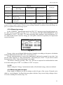
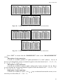
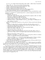
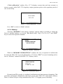
4.2.2 Measuring Voltages and Currents
In the “VOLTAGES AND CURRENTS” measuring mode, one screen is available (see
Fig. 4.5).
Press ESC to return from the mode to the “MEASUREMENTS” menu.
Three-phase 4-wire connection
Values displayed: RMS of phase and phase-to-phase voltages and currents, Averagerectified values of phase voltages and currents, Average values (DC component) of phase voltages.
Three-phase 3-wire connection
Values displayed: RMS of phase currents and RMS of phase-to-phase voltages; averagerectified values of phase currents.
Single-phase 2-wire connection
Values displayed: RMS of current and voltage; average-rectified values of current and voltage; average value (DC component) of voltage.
If a signal has no AC voltage component, its average voltage value (DC component)
equals DC voltage supplied.
27
Fig. 4.5. “Current and Voltage” screen for different circuit connections
Note
The screen line showing average values of current is informative for technical service personnel only, as DC current component cannot pass through the input transformers and current
clamps.
Note
Physically speaking, the effective (root mean square or RMS) values of voltage and current relate
to power (heat energy) dissipated through an active load (e.g., a bulb or a water heater), where
2
2
P = U RMS I RMS = U RMS
R = I RMS
R,
IRMS, URMS are the effective (root mean square) values of voltage and current; P is the active power dissipated through an active load; R is the active load resistance.
The EM3.3T1 algorithm of calculating RMS of voltage (current) may be simplistically phrased as
follows: instantaneous voltage (current) values measured by the ADC are squared and averaged, and
then the square root is extracted.
Average voltage (current) value is calculated from the weighted sum of voltage (current) instantaneous samples. The sign is determined by DC component.
Certain physical quantities (e.g. the magnetic force of attraction between a solenoid and a core)
are proportional to the average-rectified values of voltage (current). The algorithm of calculating Average-Rectified values of voltage (current) may be simplistically described as averaging over the weighted
sum of instantaneous samples coming from the ADC. All voltage (current) samples are considered
positive.
28
МС3.055.028 UM
In case of DC voltage (current), its RMS, Average and Average-Rectified values are equal in
magnitude.
For a pure sinusoidal signal, the Average value equals zero; the RMS and Average-Rectified values are related by a constant factor.
If a signal is not sinusoidal, its RMS, Average, and Average-Rectified values may differ.
Let’s consider rectangular pulses with 10 V amplitude and pulse period-to-pulse duration ratio of
10.
RMS voltage value for such a pulse train would be:
10 2 V
≈ 3.16V
10
Average and Average-Rectified voltage values are:
10V
U average = U average-rectified =
= 1V
10
When this voltage is applied to a 1 Ohm resistor, the power dissipated in the resistor would be:
P = U RMS I RMS = 3.16 ⋅ 3.16 = 10 W
There are a number of RMS-scaled instruments that actually measure average-rectified values of
voltage (current), e.g. the instruments based on an electrodynamic measuring principle. It is important
to consider that such instruments display correct values of voltage (current) only in case of a pure sinusoidal signal.
U RMS =
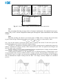
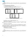
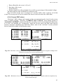
4.2.3. Measuring power
The POWER mode gives access to 3 screens: “Active POWER” (Fig. 4.6), “Reactive
POWER” (Fig. 4.7) and “Apparent POWER” (Fig. 4.8). Use g, h keys to cycle through
these screens or 1, 2, 3 numeric keys to select any particular one. The frequency at the Device’s
frequency output Fout is proportional to the measured power of a selected type (active, reactive
or apparent). While in “Reactive POWER” screen, you may select the desired calculation method for reactive power (there are 3 of them on the screen). Just place the heading “At Fout:
(↑↓)” above one of the methods displayed.
29
Fig. 4.6. “Active Power” screen for different circuit connections
Fig. 4.7. “Reactive Power” screen for different circuit connections
Fig. 4.8. “Apparent Power” screen for different circuit connections
Press ESC to return from the POWER MODE to the MEASUREMENTS menu.
30
МС3.055.028 UM
Three-phase 4-wire connection: POWER screen contains active, reactive and apparent
power measurements per phase and total; values of reactive power may be calculated differently:
N active
P;
N apparent
S;
N reactive
Q = S 2 − P 2 (geometrical method),
Q = UI sin ϕ (phase-shift method),
Q = UI cos(ϕ + 90) (cross-connection method).
The screens also contain RMS values of voltage and current per each phase as well as
power factor and tg φ values.
Three-phase 3-wire connection: in the POWER mode, the screen contains values of total
active, reactive and apparent power, reactive power values are calculated by three different methods:
N active
P;
N apparent
S;
N reactive
Q = S 2 − P 2 (geometrical method),
Q = UI sin ϕ (phase-shift method),
Q = UI cos(ϕ + 90) (cross-connection method).
Besides total values of different types of power, the screens contain RMS of phase currents and phase-to-phase voltages, total power factor, tg φ, 2 summands (components) of active
power (P1, P2) and 3 summands of reactive power calculated by the cross-connection method
(per phases L1, L2, L3).
Single-phase 2-wire connection: in the POWER mode, the screen contains values of total
active, reactive and apparent power, reactive power values are calculated by 2 different methods:
N active
P;
N apparent
S;
N reactive
Q = S 2 − P 2 (geometrical method),
Q = UI sin ϕ (phase-shift method).
The screens also contain RMS values of voltage and current as well as power factor and
tg φ values.
Notes on tg φ:
tg φ is defined as reactive to active power ratio. Mathematically, this ratio can be represented as
tangent ratio only in case of pure sinusoidal current and voltage signals. However, even though the
waveforms are not sinusoidal, the reactive to active power ratio clearly describes a power system with
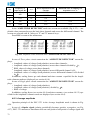
respect to its "efficiency" and "quality". It is obvious that tg φ = 0 represents the most favourable conditions. The table below specifies correspondence between tg φ and cos φ for pure sinusoidal signals:
φ,
degrees
0
5
15
30
45
60
75
83
cos φ
1
0.996
0.966
0.866
0.707
0.5
0.259
0.121
tg φ
0
0.0875
0.268
0.577
1
1.73
3.73
8.14
The Device calculates tg φ by three methods as determined by the reactive power calculation method.
31
Notes on reactive power:
When calculation of reactive power value follows the phase shift method, instantaneous voltage value
is multiplied by instantaneous current value displaced in phase by 90°. The method of cross-connection
takes the product of instantaneous value of phase current, and the instantaneous value of line voltage.
In theory, if a three-phase system is symmetrical and free of non-linear distortions, the reactive
power would be of the same value, regardless of the calculation method. When the symmetry is broken
within the system of voltage vectors (UАВ ≠ UВС ≠ UСА), the reactive power calculated with crossconnection method turns out different from what the other two methods give. Non-linear distortion
makes the power calculated with geometrical method differ from the other two. Thus, under real conditions the three values of reactive power are never precisely the same.
Regular power system is typically equipped with reactive power meters of a certain type (e.g., in
Russia meters operating on the principle of cross-connection are used in three-phase systems; meters
based on phase shift method are typical for single-phase systems). Thus, when testing a meter, its principle of operation should be taken into account.
Note!
Each time the RMS value of voltage or current is found less than 1 % of its nominal
range, the reactive power is not calculated with phase shift method: zeroes (0) are displayed instead of measured values.
Notes on power factor:
For pure sinusoidal signal, active, reactive and apparent powers are computed from the formulae:
P = U RMS I RMS cos ϕ , Q = U RMS I RMS sin ϕ , S = U RMS I RMS ,
where IRMS, URMS are effective (RMS) values of voltage and current, φ is phase angle between current
and voltage.
Power factor can be expressed as PF = P S . For a perfect sinusoidal signal
cos ϕ
P U I
PF = = RMS RMS
= cos ϕ.
S
U RMS I RMS
By definition, the PF is a number between 1 and -1 (letters L or C stand for load type: L – inductive; C – capacitive, e.g. 0.52L, 0.83C, -0.92C). Although PF is directly concerned with phase angle between current and voltage, there may be a case (e.g. in the presence of severe signal distortion in a current circuit), that PF < 1 at zero phase shift between current and voltage signals (φ = 0, cos φ = 1). The
more current and voltage curves differ from pure sine, the more PF differs from cos φ.
Power Factor is basically determined by the type of loads connected to the system (inductive or capacitive). If current lags voltage (phase angle between current and voltage is positive), the load is inductive. If current leads voltage (phase angle between current and voltage is negative), the load is capacitive.
The current vector may be in one of 4 quadrants relative to the voltage vector:
32
МС3.055.028 UM
Interval
Quadrant
Angle between current
and voltage
Active power
Reactive Power
Load type
I
0° to 90°
URMSIRMS to 0
0 to URMSIRMS
Inductive
II
90° to 180°
0 to –URMSIRMS
URMSIRMS to 0
Capacitive
(negative)
III
180° to 270°
(–180° to –90°)
–URMSIRMS to 0
0 to –URMSIRMS
Inductive
(negative)
IV
270° to 360°
(–90° to 0°)
0 to URMSIRMS
–URMSIRMS to 0
Capacitive
Positive active power (energy) relates to energy import, negative active power (energy) corresponds to energy export. Positive reactive power (energy) indicates an inductive load with energy import, or a capacitive load with energy export.
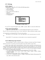
4.2.4. Measuring energy
In the “ENERGY” measurement mode, the EM 3.3T1 operates as an electrical energy meter. One screen is available (see Fig. 4.8.1). On selecting “START MEASUREMENT” item
(confirmed by “ENT”), the EM 3.3T1 starts measuring and cumulative total calculation of active (kW·h) and reactive (kvar·h) energy per each phase connected (separately for import and
export directions).
Fig. 4.8.1.
Energy values are calculated following three formulae (according to the power calculation
methods implemented in the EM 3.3T1, see section 4.2.3).
Energy measurements are carried out continuously and may be stopped at any time. Just
put the cursor opposite to “Stop measurement” option and press “ENT”. If you need to restart
measurements, select “Start measurement” once again.
The mode is exited by pressing “ESC” key. The user is requested to confirm that he wants
to exit the mode (press “ENT” to confirm or “ESC” to reject).
NOTE!
When exiting the “Energy” measurement mode, all calculated energy values are deleted.
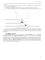
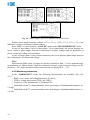
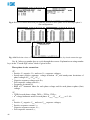
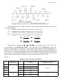
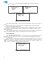
4.2.5 Measuring phase angles
Phase angles in degrees are put in column on the left part of the screen. Pictured on its
right is a vector diagram. It reflects the same phase relations, long vectors being voltages, shorter vectors standing for currents (Fig. 4.9).
33
Fig. 4.9. “Phase Angles” screen for different circuit connections
Positive phase angles between voltages ∠(UA(1), UB(1)), ∠(UB(1), UC(1)), ∠(UC(1), UA(1)) are
indicative of correct (clockwise) phase rotation.
Press “ESC” to return from the “ANGLES” mode to the “MEASUREMENTS” menu.
In case of three-phase 4-wire or three-phase 3-wire connections, the screen displays numeric values of phase angles between 1st harmonics of phase voltages and 1st harmonics of
phase current and voltage per each phase.
In case of single phase 2-wire circuit connection, the screen displays phase angle between
the 1st harmonics of current and voltage.
Note!
Each time the RMS value of voltage or current is found less than 1 % of its nominal range,
no parameters in “Phase Angles” mode are calculated. Instead, angles between voltages are displayed as ~ 90°, angles between voltages and currents are displayed as ~ - 90°.
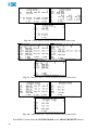
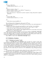
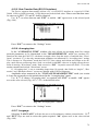
4.2.6 Measuring harmonics
In the “HARMONICS” mode, the following measurements are available (Fig. 4.10,
4.11):
N RMS of 1st current and voltage harmonics (U and I);
N THD of voltage and current (THD and THD );
U
I
st
N Frequency of the fundamental (1 ) harmonic (F);
th
N Individual (each n ) voltage harmonic ratios (percentages of fundamental harmonic; n =
1 to 40);
th
N Individual (each n ) current harmonic ratios (percentages of fundamental harmonic; n =
1 to 40).
34
МС3.055.028 UM
Fig. 4.10. “Voltage harmonics” screens for different circuit connections
Fig. 4.11. “Voltage harmonics” screens for different circuit connections
Press “ESC” to return from the “HARMONICS” mode to the “MEASUREMENTS”
screen.
Three-phase 4-wire connection:
6 screens are available (product of 2 phase parameters (U, I) and 3 phases). Use g, h
keys to cycle through the screens, or numeric keypad to select the desired one 1 — UА, 2 — UВ,
3 — UС, 6 — IА, 7 — IВ, 8 — IС.
Three-phase 3-wire connection:
6 screens are available (3 phase-to-phase voltages plus 3 phase currents). Use g, h keys
to cycle through the screens and numeric keypad to select the desired one 1 — UАB, 2 — UВC,
3 — UСA, 6 — IА, 7 — IВ, 8 — IС.
Single-phase 2-wire connection:
2 screens are available (U and I). Use g, h keys to alternate between the screens, or numeric keys to select either (1 — U, 6 — I).
35
Note!
Each time the RMS value of voltage or current is found less than 1 % of its nominal range, the
“HARMONICS” mode related parameters are not calculated: zeroes (0) are displayed instead of measured values.
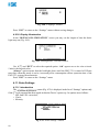
4.2.7 Measuring power of harmonics
The “HARMONICS POWER” mode determines by phase (Fig. 4.12):
st
th
N Active power of each harmonic from 1 to 40 ;
th
th
N Angles between n voltage harmonic and n current harmonic (n = 1 to 40).
Fig. 4.12. “Harmonics Power” window for different circuit connections
Press “ESC” to return to the “MEASUREMENTS” menu.
Three-phase 4-wire connection:
Three screens are available, one for each phase (A, B and C). Use g, h keys to cycle
through the screens, or number keys to select anyone (1 — phase A, 2 — phase B, 3 — phase
C).
Three-phase 3-wire connection:
Three screens are available as well. Use g, h keys to cycle through the screens, or numeric
keypad to select as follows: 1 — harmonics power totals for the entire three-phase system, 2 —
1st summand of harmonics power totals for the entire three-phase system, 3 — 2nd summand of
harmonics power totals for the entire three-phase system.
Single phase 2-wire connection:
one screen (phase A) is available.
Use j, i keys to view all of 40 harmonics by tens.
Note!
Each time the RMS value of voltage or current is found less than 1 % of its nominal range, the
“HARMONICS” mode related parameters are not calculated: zeroes (0) are displayed instead of measured values.
36
МС3.055.028 UM
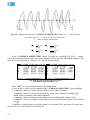
4.2.8 Waveforms
In the “WAVEFORMS” mode, the Device plots voltage and current waveforms on its
display (Fig. 4.13). On entering the mode, LCD screen shows “phase A” voltage waveform with
RMS value on its right. By pressing number keys (1, 2, 3, 6, 7, 8), the user makes visible (or
hides) other waveforms (UA, UB, UC, IA, IB, IC respectively) with their RMS values.
Fig. 4.13. “Waveforms” screen
Each displayed waveform/RMS couple reflects the moment of entering the mode. Press
“ENT” to refresh the screen.
Press “ESC” to return from the mode.
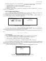
4.3. Logging and PQP
Note!
The mode is only available for full-range EM3.3T1 option. Energomonitor 3.3T1-C is an option
with no PQP measurement and logging functions.
4.3.1 Introduction
Functions of measuring and viewing of power quality parameters as well as recording
measurement results and averaged values of electric quantities into the non-volatile memory
(logging mode) are enabled from “LOGGING AND PQP” main menu option (Fig. 4.14).
Fig. 4.14. “LOGGING AND PQP” screen
The “LOGGING AND PQP” menu includes the following options:
N Current PQ values;
N Logging (PQP and AVG);
N Nominal values of voltage and frequency (by default U
N phase = 219.4 V, UN line = 380V
and FN = 50Hz);
N Set of PQ limits (threshold values) against which measurement results are compared
(you can select any of standard or customer defined sets).
37
Press j andi to navigate through the screens. Press “ENT” to enable an option, or press
“ESC” to return to the Main menu. Pressing “ESC” during logging will terminate the logging
procedure (on confirming the request for termination).
Following the list of logging settings, the screen displays an actual status of logging that
may be as follows:
N No logging;
N Waiting for start — what this means is either the preset start time of logging is still to
come, or the Device is about to start logging and waits for next minute to begin;
N Logging — logging in progress.
To change one of the four settings displayed on the “Logging and PQP” submenu, use j
or i keys to put the cursor opposite to it, and press “ENT”. This will open an editing window
Only 2nd level password gives access to all of the editing windows. 1st level password does not
enable the user to change nominal values or PQ limits setting (he cannot put the cursor opposite to
these options).
On a startup, the Device will default to the settings specified before the last logging procedure.
To change nominal values of voltage or frequency, put the cursor opposite to the selected
option and press ENT. Enter required values using numeric keypad and g, h keys. Press
“ENT” to save the new value in the memory or press “ESC” to reject. Either of these actions
will bring up the “LOGGING AND PQP” window. Should you change setting for one of two
nominal voltages (UN line, UN phase), the other will be recalculated automatically.
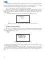
To select the type of PQ limit settings applied to PQP measurement and calculation, put
the cursor opposite to the selected option and press “ENT”.
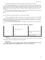
The selection window (Fig. 4.3.2) contains six options. Four of them correspond to four
nominal voltages (as per GOST 13109-97) of the network under review, as measured at the
probe connection point. Two more sets of PQ limits are customer-defined.
Settings of all types are stored in the Device's memory, each one in two variant records:
for single phase / three-phase 4-wire and three-phase 3-wire networks. The variant record is selected automatically according to the actual type of circuit connection (see section 4.11.2).
By default, the custom settings are set to 0.38 kV values (as per GOST 13109-97).
Use j or i keys to select the type of settings. Press “ENT” to select a new type of settings
and “ESC” to reject. Either of these actions will bring up the “LOGGING AND PQP” window.
Custom sets of PQ Limits (NPL and UPL) can only be managed (created, modified etc.)
on a PC. The Standard sets cannot be changed.
If the Device is connected to a network under review via instrument transformers, the set
of PQ Limits is selected according to the network type (6÷20, 35, or 110÷330kV).
At the same time, in the EM3.3T1, nominal voltage is set so as to fit secondary voltage of
the instrument transformers. Then, after uploading logs into a PC, in the EmWorkNet program,
it will be necessary to specify the data of the transformers to let the logged results be recalculate
considering transformer ratio (see EmWorkNet User Manual).
Fig. 4.15. "PQ sets" selection screen
38
МС3.055.028 UM
4.3.2. Logging
In the “LOGGING” mode, the screen contains (Fig. 4.16):
N Name of the object (site) under review (to which the logged data belongs);
N Start and stop time of logging (by default logging would start as it is enabled and stop
that very moment a month later);
st
st
N 1 peak load start time (1 off-peak load stop time);
st
st
N 1 peak load stop time (1 off-peak load start time);
nd
N 2
peak load start time (2nd off-peak load stop time);
nd
N 2
peak load stop time (2nd off-peak load start time);
N PQP log zone selection;
N Selection of averaging interval (3 s, 1 or 30 min) for logging of averaged network data
(AVG) or "oscilloscope" data;
N Selection of averaging interval for Flicker short-term perceptibility values (10 min, 5
min, or 1 min);
N "Start logging" command.
Fig. 4.16. "Logging" window
To change one of the settings displayed on the “LOGGING AND PQP” submenu, use j
or i to put the cursor opposite to the line required, and press “ENT”. This will open a selection
and/or editing window for the parameter.
On confirming "Start logging" request, the Device starts to measure and calculate power
quality parameters comparing them against settings (tolerances) of the selected type, and starts
to measure and calculate network parameters averaged over the selected interval. Power Quality parameters are calculated according to the formulae specified in Russian Power Quality
Standard GOST 13109-97.
A logging session can be started immediately. This is indicated by “Logging” status in the
bottom screen line, and the session begins from an adjacent time point that is a multiple of the
averaging time.
Alternatively, you can define a timed start. This is indicated by “Waiting for start” message. On achieving the preset start time, “Logging” message replaces the previous one. “No
logging” message shows that a logging session is stopped. Suppose no logging takes place at
the moment. To request an immediate logging session, mark “START LOGGING” as a selected item and press “ENT”. “STOP LOGGING” message appears instead of “START
LOGGING”. Logging session may be stopped at any time by placing the cursor opposite to
“STOP LOGGING” command and pressing “ENT”. Press “ESC” to return to the
“LOGGING AND PQP” menu.
To view “real-time” voltage and current components as they are measured (with or without logging), you may activate “CURRENT PQ VALUES” option in the “LOGGING AND
PQP” screen.
39
By default logging starts as it is enabled and stops that very moment a month later. To edit
the default values of logging parameters, put the cursor opposite to the parameter to be changed
and press “ENT” to open an editing window.
If you need to change the contents of “OBJECT NAME” field, mark the field as a selected item and press “ENT”. This will display the actual list of objects that can be downloaded
from a PC in advance. Select the required name and press “ENT” to open the name entry window (Fig. 4.17).
Fig. 4.17. Name entry window
To declare the name as it is on this screen, press “ENT” or “ESC”. Both keystrokes will
take you back to the upper-level “LOGGING” screen. Alternatively, you may want to return
with another name (corrected or replaced). In such a case, proceed as follows: use g, h to position the cursor exactly where you want to replace a character. Press “F” key to enter the character mode and start selection of characters (as the prompt suggests on the screen). Use j, i, g,
h to mark one location in the table as a selected character. Press ‰ key to insert a character into
object name field (cursor will leave the table and reappear on the next character position of the
object name). Numbers are entered by pressing number keys on the keypad. If you made a mistake typing in the name, press “F” key once again and repeat the procedure described above.
Press “ENT” to save a new name and “ESC” to reject. Either of these actions will bring up the
“LOGGING AND PQP” screen.
The PQP storage area is arranged as a circular buffer made up of 8 log zones.
Each log zone is kept active and collects the following PQ data:
N Number of measurements lying inside their Normal Permissible Limits (NPL) and Utmost Permissible Limits (UPL);
N Number of measurements falling outside their NPLs and UPLs throughout a day (24
hours).
Averaging periods are as follows: 60 s for steady state voltage deviation; 20 s for frequency deviation, and 3 s for the other PQP.
Each log zone houses a daily log. Log zones are changed automatically at the beginning
of a new logging session. In the case of several logs created for one day, a new log zone is assigned to each new log. When logging lasts for several days, log zones are changed automatically each midnight.
Suppose you want to ensure that a particular zone be used for logging (e.g. to keep data
from different objects separate from each other). In such a case select a log zone before making
the request for logging. Enter “PQP log zone selection” option in the "LOGGING" window,
select the log zone required and press “ENT”. "PQP log zone selection" window looks like
shown in Fig. 4.18. The window shows the complete list of log zones, one at a line. Each line
specifies a corresponding object name and start date/time of the recording.
40
МС3.055.028 UM
Fig. 4.18. "PQP log zone selection" window
To select a log zone, put the cursor opposite to the zone required and press “ENT”.
“Averaging time selection” option in the “LOGGING” window relates to Averaged
Network Parameters (AVG) data. By enabling the said option you open a selection window
(Fig. 4.3.3). AVG data may be logged based on 3 s, 1 min, or 30 min averaging time.
Рис. 4.19. “Averaging time” window
Note!
On selecting the averaging time, the user should take into account that his choice determines how long the logged data will be maintained in the buffer before being overridden. The
Device provides for continuous logging (before recycling the buffer) for the period of:
N 9.5 hours at 3 s averaging time;
N 8 days at 1 min averaging time;
N 7.5 months at 30 min averaging time;
N 9 minutes in the “oscilloscope” mode.
Note!
Enabling the “oscilloscope” mode erases all data on PQP, AVG and Dips & Swells previously maintained in the Device’s non-volatile memory. Such data will be neither calculated
nor recorded till you set particular averaging time instead of oscilloscope mode.
The Device’s logging procedure collects Flicker short-term perceptibility values in the
same way as PQP or AVG data. The said values are calculated for measurement period of 10
min, 5 min, or 1 min, and then stored in non-volatile memory. To set the measurement time as
desired, click on “Flicker observation period” field in the "LOGGING" window and press
“ENT”. This will take you to the screen pictured below (Fig. 4.20).
41
Fig. 4.20. “Flicker observation period”
window
Before starting a logging session , the user can specify "on-peak load" and "off-peak load"
periods. In this case, steady-state voltage deviation ((δUs) will be calculated for "On-peak
load", "Off-peak load" and "Daily" modes independently.
If on-peak (off-peak) load start and stop times are set to equal values, steady-state voltage
deviation ((δUs) is calculated on the "daily" basis. By default, "Peak load" start and stop times
are set to 00:00.
To change “Peak load” option fields while in the “LOGGING” window, put the cursor
accordingly and press “ENT” to open the editing window. Peak load start (stop) times are specified within 00:00 to 23:30 range in 30 min increments.
In case of power shutdown, the Device will close the current log following its regular procedure. After power recovery, the Device resumes operation and restarts logging in accordance
with all settings being in force before shutdown, provided that the preset logging stop time is
still to come. In such a case the Device creates a new log, and goes to a new log zone (the same
occurs when the user gives the command to exit and re-enter the logging mode).
4.3.3. Log formats
Logged data is arranged in the following three separate blocks:
N Power Quality data;
N Averaged parameters of the network under review (AVG);
N Dips & Swells data.
When logging is enabled, data of each type is separately recorded into the corresponding
block (storage area) unless “oscilloscope” mode for AVG data has been selected in the “Averaging time” window. Enabling this mode means that only "oscilloscope" data coming directly
from ADC are recorded and all data on PQP, AVG and Dips & Swells previously maintained in
the Device’s non-volatile memory are erased.
PQP storage area
This storage area contains PQP totals and measured PQP recorded for the last 8 days.
Based upon these data, decisions may be taken about whether power quality standards are complied with. PQP log format is as follows:
N Type (Standard or Custom) and values of settings;
N Circuit connection (three-phase 4-wire, three-phase 3-wire, or single-phase 2-wire);
N Nominal values of voltage and frequency;
N Start and stop date/time of the logging interval;
N Object (site) name;
N Peak load start time (Off-peak load stop time);
N Peak load stop time (Off-peak load start time).
N Totals of PQP monitoring over the period of 24 hours or shorter. These “daily” statistics
(collected for each PQ) show how many measurements (based upon one ADC reading
42
МС3.055.028 UM
per 0.32 s) lie within Normal Permissible Limits (NPL), within Utmost Permissible
Limits (UPL), etc. They are stored in the following order:
N Number of measurements lying inside the parameter’s NPL;
N Number of measurements lying inside its UPL;
N Number of measurements falling outside the UPL;
N Maximum (Minimum) parameter value (to be checked against UPL);
N Upper (Lower) parameter value (to be checked against NPL.
Items listed below are measured power quality parameters stored as described above (each
parameter is averaged over 3s period except for δUs (1 min averaging interval) and Δf (20s
averaging interval):
N Frequency deviation Δf;
N Steady-state voltage deviation (phase, line and positive sequence) taken on a daily
basis (δUs), on-peak (δUs'), and off-peak δUs'';
N Total Harmonic Distortion THD per each phase;
U
N Negative sequence voltage ratioK
2U and Zero sequence voltage ratio K0U;
th
N Individual (each n ) voltage harmonic ratios K
U(n) (percentages of fundamental voltage by phase; n=2 to 40);
N Statistics on voltage Dips & Swells over the period of 24 hours stored in the following
format:
N Number of voltage dips for each phase and for the entire three-phase system, N ;
N Total time in voltage dips for each phase and for the entire three-phase system, T
total;
N Duration of the longest voltage dip, T
max;
N Depth of the longest voltage dip, δU, relative to nominal voltage;
N Depth of the deepest voltage dip, δU
max;
N Duration of the deepest voltage dip, T;
N Number of voltage swells for each phase and for the entire three-phase system, N ;
N Total time in voltage swells for each phase and for the entire three-phase system, T
tot;
al
N Duration of the longest voltage swell, T
max;
N Maximum swell height, U , while in the longest swell period, (relative to nominal
sw
voltage, see Appendix D for the calculation formula);
N Largest swell height, U
sw max, detected over the logging period of 24 hours or shorter,
(relative to nominal voltage, see Appendix D for the calculation formula);
N Duration of the largest voltage swell, T;
N Flicker short-term perceptibility P
St over the logging period of 24 hours taken for measurement periods of 0; 5 or 1 min, per each phase.
The above data are only available for viewing on a PC. Flicker long-term perceptibility
PLt values are also calculated on a PC (on the basis of PSt data). User-oriented reports on power
quality for the system under review may be written automatically.
PQ values are stored in 8 separate log zones. The Device automatically goes to a new log
zone when a logging period exceeds 24 hours or when the Device gets the command to exit and
re-enter the logging mode (even if the logging period is shorter than 24 hours). The log zones
are used in rotation: on quitting the 8th zone, logging makes a swap for the 1st one, overriding
old data. Suppose you want to ensure that a particular zone be used for logging (e.g. to keep data from different objects separate from each other). In such a case select a log zone before making the request for logging (Fig.4.18).
43
Averaged values of power quality parameters and electrical network parameters
(AVG log)
This storage area collects Averaged Network Parameters (AVG) data. They may be logged
based on 3 s, 1 min, or 30 min intervals. Record format is as follows:
N RMS of AC voltages (phase, phase-to-phase);
st
N RMS of 1 voltage harmonics (phase, phase-to-phase);
N RMS of AC currents;
st
N RMS of 1 current harmonics;
st
N Angles between 1 harmonics of phase voltages;
st
st
N Angles between 1 voltage and 1 current harmonics;
N Per phase and total powers (active, reactive and apparent). Three values of reactive
power are stored, each calculated in a separate method;
N Per phase and total power factor (PF);
N AC frequency;
N Frequency deviation;
N Steady-state voltage deviation ((phase, phase-to-phase and positive sequence);
N Zero sequence voltage ratio (К , %) and negative sequence voltage ratio (К ,%);
0U
2U
N THD and THD per each phase;
U
I
N Positive, negative and zero sequence currents;
N Positive, negative and zero sequence voltages;
N Positive, negative and zero sequence active power;
N Phase angle between voltage and current for positive, negative and zero sequences;
th
th
N Per phase n voltage harmonic and n current harmonic ratios (n= 2 to 40);
th
N Active power of n harmonic (n= 1 to 40);
th
N Phase angle between n
phase voltage harmonic and nth phase current harmonic (n= 2
to 40).
Alternatively, EМ-3.3Т1 in the logging mode may operate in “oscilloscope” mode, instead
of data averaging. In such a mode, network parameters (3 phase voltages and 3 phase currents
only) are taken directly from the ADC at 12.8 kHz frequency.
The above data stored in the logs are only available for viewing on a PC. In the PC environment, the changes in circuit parameters can be evaluated and analyzed over the entire observation period. “Oscilloscope” mode of logging makes it possible to restore voltage and current
waveforms for each phase.
Typical AVG storage area is built up of uniform records. It is arranged as a circular buffer
with a capacity of 11884 records (new data override the oldest record in the buffer). One record
includes all values averaged over one averaging interval.
AVG storage area provides for continuous logging (before recycling the buffer) for the period of:
N 7.5 months at 30 min averaging time;
N 8 days at 1 min averaging time;
N 9.5 hours at 3 s averaging time;
N 9 min for "oscilloscope" data.
Based on this data, user-oriented reports for the system under review may be created on a
PC automatically.
Dips & Swells log.
This storage area collects data on voltage dips and swells (otherwise called “events”). An
event description is formatted as follows:
N Event type: dip or swell;
44
МС3.055.028 UM
Phase affected by the event: A, B, or C;
Start time of the event;
N Event duration;
N Relative depth (for a dip) or height (for a swell) as a percentage of the nominal voltage.
The above data are only available for viewing on a PC.
Dips & Swells storage area is arranged as a circular buffer with a capacity of 80 000
events. The storage area is used in rotation (the latest record overwrites the oldest data).
N
N
4.3.4. Current PQP values
“Real-time” PQP, voltages and currents as they are measured can be viewed on the screen
with or without logging. Selecting “CURRENT PQP VALUES” from among options of
“LOGGING AND PQP” window will take the user into a set of screens linked in a chain ((fig.
4.21–4.24). On enabling the “oscilloscope” mode the Device erases old PQP data from its
memory and stops calculating new PQP data. Hence, none of the “real-time” screens pictured
below would be available in oscilloscope mode
Fig. 4.21. Real-time views of steady-state voltage deviation, negative and zero sequence voltages and
frequency deviation; by circuit connection type
Fig. 4.22. Real-time views of current and power values for positive, negative and zero sequences; by
circuit connection type
45
Fig. 4.23.View of flicker short-term perceptibility screens for three-phase 4-wire and single-phase 2wire configurations
Fig. 4.24. Real-time views of THD values and individual harmonic ratios; by circuit connection type
Use g, h keys or number keys to cycle through the screens. Explanation on using number
keys in the "Current PQP values" mode is given below.
Three-phase 4-wire connection:
“5”:
N Positive U , negative U
s
2(1) and zero U0(1) sequence voltages;
N Steady-state positive sequence voltage deviation δU and steady-state deviations of
s
phase voltages δUsA, δUsB, δUsC;
N Negative sequence voltage ratio K ;
2U
N Zero sequence voltage ratio K ;
0U
N Frequency deviation Δf;
st
N RMS of 1 harmonic taken for each phase voltage and for each phase-to-phase (line)
voltage.
“4”:
N THD for each phase voltage THD
UA, THDUB, THDUC;
th
N n voltage harmonic ratios for each phase K
UA(n), KUB(n), KUC(n), n=2...40.
“0”:
N Positive U , negative U
s
2(1) and zero U0(1) sequence voltages;
N Positive sequence current I
1(1);
N Negative sequence current, I
2(1);
N Zero sequence current I
0(1);
46
МС3.055.028 UM
N
N
N
RMS of 1st harmonic taken for each phase current;
Active power of positive P1, negative P2 and zero P0 sequences;
Phase angles between 1st voltage and current harmonics of positive φ1UI, negative φ2UI
and zero φ0UI sequences.
“9”:
THD for each phase current THDIA, THDIB, THDIC;
N Current harmonic ratios per each phase K
IA(n), KIB(n), KIC(n), n =2...40.
N
“3”:
N Flicker short-term perceptibility P per each phase.
St
Three-phase 3-wire connection:
“5”:
N Positive U and negative U
s
2(1) sequence voltages;
N Steady-state positive sequence voltage deviation δU and steady-state deviations of
s
line voltages δUsAB, δUsBC, δUsCA;
N Negative sequence voltage ratio K ;
2U
N Frequency deviation Δf;
st
N RMS of 1 harmonics of phase voltages.
“4”:
THD for each phase-to-phase voltage THDUAB, THDUBC, THDUCA;
h
N Nt phase-to-phase voltage harmonic ratios K
UAB(n), KUBC(n), KUCA(n), n = 2...40.
N
“0”:
N Positive U and negative U
s
2(1) sequence voltages;
N Positive sequence current I
1(1);
N Negative sequence current, I
2(1);
st
N RMS of 1 harmonic taken for each phase current;
N Active power of positive P and negative P sequences;
1
2
N Phase angles between 1st current and voltage harmonics of positive φ
1UI and negative
φ2UI sequences.
“9”:
N THD for each phase current THD , THD , THD ;
IA
IB
IC
N Current harmonic ratios per each phase K
IA(n), KIB(n), KIC(n), n =2...40.
“3”:
N Empty screen: flicker short-term perceptibility P
St is not measured for three-phase 3wire connection.
Three-phase 2-wire connection:
“5”:
st
N Positive sequence voltage U (i.e. RMS of 1 harmonic U
s
A(1));
N Steady-state voltage deviation δU (δU );
s
sA
N Frequency deviation Δf.
47
“4”:
N Voltage THD THD ;
U
N Voltage harmonic ratios K
U(n), n = 2...40.
“0”:
N Positive sequence voltage U ;
s
st
N Positive sequence current I
1(1) (i.e. RMS of 1 harmonic I(1));
N Positive sequence active power P ;
1
st
N Phase angle between 1 harmonics of positive sequence voltage and positive sequence
current φ1UI.
“9”:
N Current THD THD ;
I
N Current harmonic ratios K
I(n), n = 2...40.
“3”:
N Flicker short-term perceptibility P .
St
To scroll through all of 40 harmonic ratios, press j, i keys.
Flicker short-term perceptibility is only defined for three-phase 4-wire and single-phase 2wire connection types.
In addition to the flicker short-term perceptibility PSt the "real-time" screen displays:
N Flicker short-term perceptibility observation period (10 min, 5 min, or 1 min);
N Time before the end of current flicker observation period;
N Flicker short term perceptibility values updated at the end of each flicker observation
period (10, 5 or 1 min, see Fig. 4.20).
Flicker measurement and calculation is started upon enabling “LOGGING AND PQP”
mode, and stopped on quitting the mode. First measured Pst value appears on the “real-time”
screen with 2-minute delay, as compared to the length of an observation period. Further measurements are updated at intervals equal to the time of measurement.
Press “ESC” to return to the “LOGGING AND PQP” menu.
4.4. Calibration of meters
4.4.1. "Calibration of meters" mode
While in “CALIBRATION OF METERS” mode, the EM-3.3T1 follows certain established methods and operates as energy reference standard and pulse comparator. It provides for
either performance testing or accuracy testing (calibration) of electric energy meters (class 0.5
or less accurate). Results of calibration are recorded and stored in the Device's memory. Each
log may keep calibration results acquired from up to 200 meter tests (up to 10 measurements
per test). The logs may be uploaded and converted into appropriate form using a PC. Test reports based on test results may be created on a PC automatically using "Energomonitoring"
software.
To test a meter with current pulse output, connect the meter’s pulse output to the Device’s
pulse input Fin (Fig. C.10, Appendix C) via a Pulse Former (section 4.4.2).
To test a meter with optical pulse output, use SH-E scanning head or Pulse Former. SH-E
is mounted onto the meter and connected to the Device's pulse input Fin as shown in Fig. C11 of
Appendix C. Pulse Former (section 4.4.2) is connected to the Device's pulse input Fin as shown
in Fig. C13 of Appendix C.
48
МС3.055.028 UM
To test an induction disk (Ferraris) meter, use SH-I scanning head or Pulse Former. SH-I
is mounted onto the meter and connected to the Device's pulse input Fin as shown in Fig. C12 of
Appendix C. Pulse Former (section 4.4.2) is connected to the Device's pulse input Fin as shown
in Fig. C13 of Appendix C.
Select “CALIBRATION OF METERS” item from the Main menu to get to the "Meter
profile" screen pictured below (Fig. 4.25). The screen contains meter data fields to be specified
before calibration. Use j and i keys to scroll through the items. Press “ESC” to return to the
Main menu, or select “ENTER CALIBRATION N” item and press “ENT” to go to the next
calibration screen.
The "Meter profile" window (Fig. 4.25) enables you to key in various data on the meter
under test, including:
N Meter type or name (a key data field used as a library name);
N Serial number;
N Year of manufacture;
N Accuracy class;
N Meter constant;
N CT’s turns ratio (i.e. conversion factor of current instrument transformer; this field is
specified only if a whole unit consisting of a meter together with CTs is tested);
N Meter's nominal current and voltage;
N Type of power to be measured during calibration: active, apparent or reactive (calculated by one of three methods).
Fig. 4.25. "Meter profile" window
The bottom item of “Meter profile” window may be used to delete old logs with archived
data on meter tests.
It is possible to quickly change the Device’s measuring range by pressing “F” hotkey.
This will take you into "Measuring range" selection screen of "Settings" menu (see section
4.10.3.).
To change one of the settings displayed on the “Logging and PQP” submenu, use g or h
to put the cursor opposite to the line required, and press “ENT”. This will open a selection
and/or editing window for the parameter.
On a startup, the Device will default to the settings specified before the last logging procedure.
For example, “METER TYPE” window enables you to enter a new meter name or
choose one of the names declared earlier (Fig. 4.26).
49
Fig. 4.26. “Meter type” window
To correct or replace meter’s name, put the cursor opposite to the selected position in “Meter type” window and press “ENT” to enable the editing window. Then follow the procedure established for filling in alphanumeric fields (see section 4.3.2 and Fig. 4.17).
To load meter's data kept in the library, put the cursor opposite to the selected type of the
meter and double press “ENT” to confirm the selection (meter's characteristics stored under this
name will be loaded). After changing the values of meter parameters, the new values are recorded into the library under the currently active meter name. Any of 10 meter types can be either
configured via the "Meter profile" window or downloaded from a PC.
To change any of the values, put the cursor opposite to the selected position (Fig. 4.25)
and press “ENT”. Enter required values using numeric keypad and g, h keys. Press “ENT” to
save the new value in the memory or press “ESC” to reject.
“Inst. CT’s turns ratio” option within “Meter profile” window is a required field. Its
value equals something other than 1 only if a whole unit consisting of a meter together with external CTs is tested. If the external CTs are not used, one and the same current value is specified
on both sides of the fraction sign considering that this field represents primary current/secondary current ratio of instrument CTs. If a meter is tested together with CTs, the meter
is connected to the primary side of the CT, and the EM3.3T1 is connected to its secondary side.
The purpose of “ENTER CALIBRATION N” item (Fig. 4.27) is to start a calibration
procedure. Clicking on it will take you into the screen named “Measurement entry” just initialized for the next measurement:
Fig. 4.27. "Measurement entry" window
Press “ESC” to return to the “METER PROFILE” window, or click on "Enter measurement N" field and press “ENT” to start measurement. The “MEASUREMENT ENTRY”
window contains the following pulse count fields:
N "Number of input pulses" shows how many pulses (coming from the meter under test
and reflecting common energy flow) the EM-3.3T1 shall accept on its pulse input Fin to
be able to calculate a reliable value of meter-under-test error;
N "Number of output pulses" is the number of pulses to be generated by the EM-3.3T1
on its pulse output Fout and proportional to the amount of energy to be measured by the
EM-3.3T1 during meter testing.
50
МС3.055.028 UM
Number of input pulses (pulses from the meter under test) calculated by the EM3.3T1 is
based on EM 3.3T1 instrument constant (see Table 2.3), accuracy class of the meter under test
(specified in the "Meter profile" window), instrument constant of the meter and CTs turns ratio
(if applicable).
Note!
When necessary, the user modifies “Number of input pulses” field in the
“MEASUREMENT ENTRY” window, in order to change error calculation time. However,
account must be taken of the fact that by reducing the “Number of input pulses” the user
makes calculation of meter’s measurement error less accurate. Meter’s error determined at reduced calculation time will hardly fit the accuracy class of the meter tested.
Select “Enter measurement N” item from “Meter profile” window to open the window
pictured below (Fig. 4.28): The window displays actual RMS values of voltage and current,
values of power factor and power of a certain type measured by both the meter and EM 3.3T1
during the calibration and estimated time of error calculation.
Fig. 4.28. "Meter calibration" window
The time of error calculation may be changed (if necessary) by adjusting the number of
input pulses in “Measurement entry” window (Fig. 4.4.3). See “Note” above.
Notes on optimal number of input pulses
To generate an error value, the EM-3.3T counts and compares pulses from the meter under test
(pulses coming with Fin frequency) and pulses generated on its own (pulses coming with Fout frequency) where pulse repetition ratios are proportional to the power measured by the meter and by the
EM3.3T1 respectively. In other words, the EM 3.3T1measures the ratio of frequencies Fout/Fin.
The first pulse from the meter opens a gate for (n + 1) input pulses, where n — number of input
pulses indicated in the "Measurement entry" window. The gate is filled with the reference (Fout)
pulses. The ratio of the two frequencies determines the meter error. Minimum number of input pulses
(n) taken for the gate from the meter under test is based on instrument constant and accuracy class of the
meter and active voltage and current measurement ranges of the EM 3.3T1. Number of output pulses
(pulses generated by the EM 3.3T1 on its pulse output Fout is selected so as to guarantee that the resolution when measuring the meter error will be enough to conform with the meter accuracy class. In fact,
this means that the resolution during meter error calculation should be one order of magnitude better
than the declared meter error.
The greater is the number of input and consequently output pulses, the better resolution of meter
error calculation is achieved and the smaller is spread of EM3.3 T1 readings while determining the meter error. However, this leads to the increase in error calculation time.
To rate the resolution of meter error calculation in percent, find the ratio 1/nout * 100% ( nout – the
actual number of output pulses). For example, if nout = 1000, the EM 3.3T1 error calculation resolution
is 0.1 %, and the meter under test error is δm = (δ ± 0.1) %, where δ is the error indicated by EM 3.3T1.
Accordingly, the spread of two adjacent values of δ may reach 0.2%. If the accuracy class of a meterunder-test is 1, such a rate is sufficient. In case of 0.5 meter accuracy class, this rate is admissible. But
51
in case of 0.2 meter accuracy class, this rate is unacceptable. So the possibility to change the number of
input pulses enables you to select the resolution of meter error calculation different to the one specified
by the manufacturer.
To start a measurement, put the cursor opposite to “START MEASUREMENT N” and
press “ENT”. At this point, the prompt “START MEASUREMENR N” turns to “STOP
MEASUREMENT N”. The field below the prompt keeps count of time still to measure the
meter’s error. See Fig. 4.29.
Fig. 4.29. "Meter calibration" window (measurement in progress)
On completing the measurement, the meter-under-test (or CT– meter-under-test unit) error
(%) is displayed. A measurement can be stopped at any time by clicking on “STOP
MEASUREMENT N” prompt, which will turn to “SAVE MEASUREMENT N”. By clicking
on “SAVE...” you may record the result into the EM 3.3T1 memory. Before the next measurement, you may change values of currents, voltages, PF, etc. applied to the meter-under-test and
repeat the measurement procedure with other test conditions.
Press “ESC” to get back to the "Meter profile" window.
Data on each meter calibrated are archived according to the following format:
N Meter type or name;
N Serial number;
N Year of manufacture;
N Accuracy class;
N Meter constant С ;
mt
N Meter's nominal voltage U (V) and current I (A);
N
N
N Actual power type;
N CT’s turns ratio;
N Date/time of the calibration;
N Up to 10 records of calibration results. Each record contains:
N Data on test signal applied to the meter while determining meter error;
N Calculated error.
The above information in the edited form is included in meter calibration test reports. The
reports can only be viewed on a PC.
4.4.2. Pulse Former
As an auxiliary device, Pulse Former is used for generating pulses in “Calibration of meters” mode. The EM-3.3T1 receives the pulses on its pulse input Fin and keeps count of them, in
order to calculate the meter-under-test error. Pulse Former generates pulses either automatically
(as a repeater of the pulses coming from the meter), or in respond to operator’s stroke of a button on the Pulse Former. Example: the operator watches disk revolve and pushes the button at
each passage of the mark. Thus, Pulse Former may be used together with EM 3.3T1 to calculate
52
МС3.055.028 UM
measurement errors of induction and electronic, single- and three phase electric energy meters
as well as electronic meters equipped with telemetry output.
Manually operated mode
Pulse Former generates a pulse every time that the user presses red button on its side. This
may be the case when automatic scanning of mark passages (or automatic scanning of LED
flashes) is impossible or inconvenient. Pulse Former is connected to the Fin connector of the EM
3.3 T1 as shown in Fig. C13, Appendix C. Select “CALIBRATION OF METERS” item from
the Main menu, go to the "Calibration of meters" window and click on "Start measurement
N" to begin test procedure. Repeatedly press the button on the Pulse Former each time the mark
on the disk edge aligns with that on the meter’s enclosure (or each time the LED flashes on an
electronic meter). When the button is first pressed, the EM-3.3T1 emits a beep and starts meter
error calculation. Keep pushing the button until the result (calculated meter error) appears on
the screen. .This will happen when the actual count of your button-strokes runs into the recommended number of input pulses (displayed in “Measurement entry” window).
Note!
When it takes less than 2 s for the meter to make one disk revolution (or one flash of its LED), it
is recommended to use a scanning head (SH-E or SH-I).
Automatic mode
In the automatic mode, the Pulse Former converts each pulse coming from meter’s pulse
(telemetry) output into another pulse that the EM-3.3T1 can accept on its pulse input (Fin). To
test a meter with optical (telemetry) output, use additional “telemetry” (red/black) cable to connect the Pulse Former to meter’s pulse output (Fig. C., Appendix C). Plug the red lead into meter’s terminal marked “+ TM”, and the black one – into another terminal marked “- TM”.
4.4.3. Photoelectric Scanning Heads
When equipped with SH-E or SH-I Photoelectric scanning heads, the EM-3.3T1 may be
used for in-situ testing of single- or three-phase meters of active or reactive energy. The meters
are tested in automatic mode (described above), no manual operation is required.
SH-E Photoelectric scanning head is an EM-3.3T1 accessory for testing electronic type
meters with optical pulse output. This is done by mounting the SH-E on such a meter, then attaching SH-E’s pulse output to EM-3.3T1 pulse input Fin (Fig. C.11, Appendix C).
SH-I Photoelectric scanning head was conceived for testing induction disc type (Ferraris)
meters. Set the SH-I on the meter (Fig. C12, Appendix C) and connect pulse output of the
Scanning Head into pulse input Fin of the EM 3.3T1.
Tuning SH-E
Align SH-E’s optical lens even with meter’s LED. Then adjust “Sensitivity” knob to
make SH-E's own LED ("Pulse" indicator) go on and out in time with the LED flashing on meter's optical pulse output.
Tuning SH-I
Turn “Sensitivity” knob on the SH-I counter-clockwise as far as it will go (for minimum
response). Then align the SH-I so as to bring the edge of the meter’s disc into focus of the SH-I
light emitting lens (scanning beam must hit the mark).
53
Turn “Sensitivity” knob of the SH-I gently clockwise until “Pulse” indicator on the SH-I
starts responding to disk mark passages across the beam. Then adjust the sensitivity so as to ensure reliable SH-I response with neither false triggering no misfiring.
Note!
The SH-I is provided with auto-tuning function that corrects its behavior for light intensity. Auto-tuning causes some 20...40-second follow-up delay in sensitivity control.
If the "Pulse" indicator is still on, turn “Sensitivity” knob slightly clockwise. Please adjust SH-I considering the delay in sensitivity control.
4.5. Calibration of voltage transformers
4.5.1. General
“CALIBRATION OF VTS” mode provides for either performance testing or accuracy
testing (calibration) of voltage instrument transformers of up to 0.2 accuracy class according to
certain established methods. In this mode, the EM 3.3T1 operates as a comparator.
Permissible limits of ratio and angle measurement errors are specified in Table 2.2. Test
results are recorded and stored in the Device's memory. Each log may store results acquired
from up to 200 VTs (up to 10 measurements per each VT). The logs may be uploaded and converted into appropriate form using a PC. Test reports based on the measurement results may be
created on a PC automatically using "Energomonitoring" software.
Select “CALIBRATION OF VTS” option from the main menu. Press “ESC” to return to
the main menu.
The following units are included in a typical VT test system (wired as shown in Fig.4.30):
N Adjustable high-voltage source;
N Reference VT;
N VT burden set;
N EM 3.3T1 complete with VT calibration Switch (VTCS).
Fig. 4.30. Connection diagram of a VT test set
54
МС3.055.028 UM
The adjustable High-Voltage Source provides voltage for high-voltage inputs (primary
windings) of both Reference VT and VT under test. Their secondary (low-voltage) windings are
connected to input terminals UA and UB of the VTCS respectively. The secondary neutral terminals of both VTs are attached to VTCS neutral terminal UN. VT Burden set is connected to
the secondary winding of the VT under test via separate cables. VTCS is connected to UA, UB
and UN terminals of the EM 3.3T1.
4.5.2. Setting up VT data
The "VT profile" window enables you to specify various data on the VT under test
(Fig. 4.31), including:
N VT type or name;
N Serial number;
N Year of manufacture;
N Accuracy class;
N Nominal value of frequency;
N Nominal primary voltage, kV;
N Nominal secondary voltage, V;
N Nominal value of apparent power, VA;
N Set place;
N Connection phase.
Fig. 4.31. "VT profile" window
The bottom item of “VT profile” window may be used to delete old logs with archived
data on meter tests.
It is possible to quickly change the Device’s measuring range by pressing “F” hotkey.
This will take you into "Measuring range" selection screen of "Settings" menu (see section
4.10.3.).
To change one of the settings displayed on the “Logging and PQP” submenu, use j or i
keys to put the cursor opposite to the line required, and press “ENT”. This will open a selection
and/or editing window for the parameter.
On a startup, the Device will default to the settings specified before the last logging procedure.
For example, “VT TYPE” window (Fig. 4.32) enables you to select one of 10 types stored
in the library or enter a new name.
55
Fig. 4.32. “VT type” window
To correct or replace VT name, follow the procedure established for filling in alphanumeric fields (see section 4.3.2 and Fig. 4.17). To load VT data kept in the library, put the cursor opposite to the selected VT type and double press “ENT” to confirm the selection (VT characteristics stored under this name will be loaded). After changing the values, the new values are
recorded into the library under the currently active VT name. Any of 10 VT types can be either
configured via the "VT profile" window or downloaded from a PC.
To change any of the values, put the cursor opposite to the selected position (Fig. 4.31)
and press “ENT”. Enter required values using numeric keypad and g, h keys. Press “ENT” to
save the new value in the memory or press “ESC” to reject.
Note!
Before measurement, select nominal value for secondary voltages of both Reference VT
and VT under test. Click on “SELECT NOMINAL Unom.2” option (Fig. 4.33) and set the required value.
Fig. 4.33. Selecting secondary nominal voltage
for “Reference VT” and “VT under test”
“SET PLACE” window (Fig. 4.34) makes it possible to select one of 10 options stored in
the library, or enter a new location data (including a phase to which VT under test is connected).
Fig. 4.34. “Set place” window
To correct or replace VT location data, follow the procedure established for filling in alphanumeric fields (see section 4.3.2 and Fig. 4.17). To load VT data kept in the library, put the
cursor opposite to the selected VT location and double press “ENT”. After changing the data,
56
МС3.055.028 UM
new values are recorded into the library under the currently active VT location. Any of 10 options can be either configured via the "Meter profile" window or downloaded from a PC.
Press “ESC” to return to the Main menu, or select “ENTER CALIBRATION N” item
and press “ENT” to go to the next calibration screen (Fig. 4.35).
Fig. 4.35. "Calibration of VTs" entry window
Calibration procedure is carried out in 2 steps:
N 1 — "Zero correction" (correction of differences in characteristics of EM 3.3T1 channels);
N 2 — "Calibration" .
4.5.3. Zero correction
To make zero correction, enable “ENTER CALIBRATION N” item (Fig. 4.35) and open
"Enter measurement N" screen (Fig. 4.37) where measurement results are displayed. Manually
adjust the variable HV source to obtain the required test voltage across primary windings of
both reference VT and that under test. While doing this, watch secondary voltage of Reference
VT (displayed as voltage in phase B (UB(1)) on the screen)
On the VTCS, position "Correction / Measurement" switch to enable “CORRECTION”
mode. This applies output voltage from the reference VT (reference voltage) to UA and UB inputs of the EM 3.3T1. Enable “CORRECTION” option in the "Enter calibration N" screen
(see Fig. 4.35, 4.36). The EM-3.3T1 will carry out zero correction, namely it will electronically
compensate both amplitude difference and phase shift between voltages in channels A and B.
Fig. 4.36. “Correction” window with “Processing…” message in it
“ZERO CORRECTION” mode is exited automatically. The measured differences in characteristics are saved in the memory to be considered in further measurements . To achieve the
highest accuracy, it is recommended that the second step of the calibration procedure (described below) be taken under the same operating conditions (mains voltage, ambient temperature) within
next 10 minutes immediately after zero correction. To check the results of zero correction, enable
the next calibration procedure and look at the calibration results screen (Fig. 4.37). Make sure that
two inequalities below are satisfied:
(U
A (1)
− U B (1) )
U B (1)
< 0.01 %,
∠(UA(1), UB(1)) < 0.1'. If the values displayed exceed the above, repeat zero correction.
57
4.5.4. Calibration of VTs
Set VTCS switch to the “MEASUREMENT” position. When done, voltage taken from
the reference VT is applied to UB input, and voltage taken from the VT under test is applied to
UA input of the EM 3.3T1.
Before calibration, it is necessary to type in the value of apparent power that was selected
on the Burden Set for the VT under test load (VA). Go to “CALIBRATION N” window
(Fig. 4.35), put the cursor opposite to S (VA) option and press “ENT”. Set the required value in
the editing window.
Then select “ENTER MEASUREMENT N” option in “CALIBRATION N” (Fig. 4.35)
window. The window pictured below will be displayed (Fig. 4.37).
Fig. 4.37. "VT Calibration results" window
The window displays the values of:
N Apparent power selected on the Burden Set for the VT-under-test load before this measurement, VA;
N Nominal apparent power of the VT under test specified in the "VT profile" window
(Fig. 4.31), VA;
N Apparent power of the VT under test (actual value) calculated as a percentage of the
nominal value;
N Secondary nominal voltage of the VT under test specified in the "VT profile" window
(Fig. 4.31), VA;
st
N RMS of the 1 harmonic of voltage across the secondary winding of the VT under test
UA(1), V;
st
N RMS of the 1 harmonic of voltage across the secondary winding of the reference VT
UB(1), V;
N Voltage across the secondary winding of the reference VT as a percentage of nominal
voltage.
To start a measurement, put the cursor opposite to “START MEASUREMENT N” and
press “ENT”. At this point, the prompt “START MEASUREMENR N” turns to “STOP
MEASUREMENT N”. The EM 3.3T1 will determine measurement errors and take you to the
"VT calibration results" screen (Fig. 4.37).
Well-determined or "Fine" (considering zero correction results) values of VT under test errors are displayed as follows:
N Ratio error Δf , %: [(U
U
A(1) – UB(1)) / UB(1)] · 100;
N angle error Δδ , min: ∠(U
U
A(1), UB(1)).
In addition to the "Fine" values, the "Coarse" results of error calculation (without considering differences in characteristics of A and B channels) are displayed in the next column.
Fine ratio and angle errors are considered representative within the ranges of ±1° for angle
error and/or ±2 % for ratio error.
58
МС3.055.028 UM
When actual errors of VT under test do not lie within these ranges, asterisks (*****) are
displayed instead of "Fine" values (Fig. 4.37).
"Coarse" error values shall be taken as calibration results in such a case. Owing to zero
correction, measurement in this mode is fairly accurate, as compared to other EM-3.3T1 operating modes. To take the advantage of this, be sure to make zero correction before each voltage
measurement.
A measurement can be stopped at any time by clicking on “STOP MEASUREMENT N”
prompt, which will turn to “SAVE MEASUREMENT N”. By clicking on “Save...” option you
may record the result in to the EM 3.3T1 memory. Before the next measurement, you may
change the value of apparent power (VA) by selecting a new one on the Burden Set (then the
new value shall be manually specified in the "Measurement entry" screen (Fig. 4.35). Then
repeat the procedure with other test conditions.
Press “ESC” to get back to the "VT profile" window.
Data on each VT calibrated are archived according to the following format:
N VT type;
N Serial number;
N Year of manufacture;
N Accuracy class;
N Nominal value of frequency;
N Nominal primary voltage, kV;
N Nominal secondary voltage, V;
N Nominal value of apparent power, VA;
N Location (place);
N Connection phase.
N Date/time of the calibration;
N Up to 10 records of calibration results. Each record contains:
N Nominal value of apparent power, VA;
st
N Parameters of test signal while determining measurement errors (RMS of 1 harmonics of voltage across secondary windings of VT under test UA(1) and reference VT
UB(1));
N VT-under-test errors (ratio error ∆f and angle error ∆δ ).
U
U
The above information in the edited form is included in VT calibration test reports. The
reports can only be viewed on a PC.
4.6. Calibration of current transformers
4.6.1. General
“CALIBRATION OF CTS” mode provides for either performance testing or accuracy
testing (calibration) of current instrument transformers of up to 0.2S accuracy class according to
certain established methods. In this mode, the EM 3.3T1 operates as a comparator.
Permissible limits of ratio and angle measurement errors are specified in Table 2.2. Test
results are recorded and stored in the Device's memory. Each log may store results acquired
from up to 200 CTs (up to 10 measurements per each CT). The logs may be uploaded and converted into appropriate form using a PC. Test reports based on the measurement results may be
created on a PC automatically using "Energomonitoring" software.
Select “CALIBRATION OF CTS” option from the main menu. Press “ESC” to return to
the main menu.
The following units are included in typical CT test system (wired as shown in Fig.4.38):
N Adjustable current source;
59
N
N
N
Reference CT;
CT burden set;
EM 3.3T1 complete with CT calibration Switch (CTCS).
Fig. 4.38. Connection diagram of a CT test set
The adjustable Current Source enables the user to pass the required primary current
through both Reference CT and CT under test. Their secondary windings are connected to the
respective inputs of the CTCS. The Burden Set provides a choice of burdens for the CT under
test to bear.
4.6.2. Setting up CT data
The "CT profile" window enables you to specify various data on the CT under test
(Fig. 4.39), including:
N CT type;
N Serial number;
N Year of manufacture;
N Accuracy class;
N Nominal value of frequency, Hz;
N Nominal primary current, A;
N Nominal secondary current, A;
N Nominal value of apparent power, VA;
N Location (place);
N Connection phase.
Fig. 4.39. "CT profile" window
60
МС3.055.028 UM
The bottom item of “CT profile” window may be used to delete old logs with archived
data on meter tests.
It is possible to quickly change the Device’s measuring range by pressing “F” hotkey.
This will take you into "Measuring range" selection screen of "Settings" menu (see section
4.10.3.).
To change one of the settings, use j or i keys to put the cursor opposite to the line required and press “ENT”. This will open a selection and/or editing window for the parameter.
On a startup, the Device will default to the settings specified before the last logging procedure.
For example, “CT TYPE” window enables you to enter a new name or choose one of the
names declared earlier (Fig. 4.40).
Fig. 4.40. “CT type” window
To correct or replace CT name, follow the procedure established for filling in alphanumeric fields (see section 4.3.2 and Fig. 4.17). To load CT data kept in the library, put the cursor opposite to the selected type of the transformer and double press “ENT” to confirm the selection
(CT's characteristics stored under this name will be loaded). After changing the values of CT
parameters, the new values are recorded into the library under the currently active CT name.
Any of 10 CT types can be either configured via the "CT profile" window or downloaded from
a PC.
To change any of the values, put the cursor opposite to the selected position (Fig. 4.39)
and press “ENT”. Enter required values using numeric keypad and g, h keys. Press “ENT” to
save the new value in the memory or press “ESC” to reject.
Note!
Before measurement, select nominal values for secondary voltages of both Reference CT
and CT under test. Click on “SELECT NOMINAL Inom.2” option (Fig. 4.41) and set the required value.
Fig. 4.41. Selecting secondary nominal voltage
for “Reference CT” and “CT under test”
61
“CT LOCATION” window (Fig. 4.42) makes it possible to select one of 10 options
stored in the library, or enter a new location data (including a phase to which CT under test is
connected).
Fig. 4.42. “CT location” window
To correct or replace CT location data, follow the procedure established for filling in alphanumeric fields (see section 4.3.2 and Fig. 4.17). To load CT data kept in the library, put the
cursor opposite to the selected CT location and double press “ENT”. After changing the data,
new values are recorded into the library under the currently active CT location. Any of 10 options can be either configured via the "CT profile" window or downloaded from a PC.
Press “ESC” to return to the Main menu, or select “ENTER CALIBRATION N” item
and press “ENT” to go to the next calibration screen (Fig. 4.43).
Fig. 4.43. "Calibration of CTs" selection window
Calibration procedure is carried out in 2 steps:
N 1 — "Zero correction" (correction of differences in characteristics of EM 3.3T1 channels);
N 2 — "Calibration" .
4.6.3. Zero correction
Set measuring range of the EM-3.3T1 at D 5A or D 1A. Push CTCS button to enable
“MEASUREMENT” mode ("Measurement" indicator lights up). Click on "Calibration" item
in the “CALIBRATION OF CTS” selection window (Fig. 4.43) to enable a new measurement
(Fig. 4.45). Manually adjust variable transformer to pass the required primary (test) current
through primary windings of both reference CT and that under test. While doing this, watch
secondary currents on the screen of the EM 3.3T1. The CT-under-test secondary current is displayed as IA(1) and Reference CT output current is displayed as IB(1). If the secondary current is
less than 0.6A (for a CT with 5A output) or less than 0.12A (for a CT with 1A output), manually set current measurement ranges of the CTCS and EM 3.3T1 to D 0.5A or D 0.1A respectively.
Note!
Circuitry of the CTCS provides that the continuity of both CTs secondary circuits is in no way affected by swapping measurement ranges or operating modes.
62
МС3.055.028 UM
Push CTCS button to enable “CORRECTION” mode. This way the secondary current
from reference CT (reference current) is simultaneously applied to EM-3.3T1 current inputs IA
and IB. Click on “ZERO CORRECTION” item in the "Calibration of CTs" selection window
of the EM 3.3T1 (Fig. 4.44). The EM-3.3T1 will carry out zero correction, namely it will electronically compensate both amplitude difference and phase shift between currents in channels A
and B.
Fig. 4.44. “Zero Correction” window with “Processing…” message in it
“ZERO CORRECTION” mode is exited automatically. The measured differences in characteristics are saved in the memory to be considered in further measurements. To achieve the highest accuracy, it is recommended that the second step of the calibration procedure (described below)
be taken under the same operating conditions (mains voltage, ambient temperature) within next 10
minutes immediately after zero correction. To check the results of zero correction, enable the next
calibration procedure and look at the calibration results screen (Fig. 4.45). Make sure that two
inequalities below are satisfied:
I A(1) − I B (1)
I B (1)
< 0.01 %,
∠(IA(1), IB(1)) < 0.1'. If the values displayed exceed the above, repeat zero correction.
4.6.4. Calibration
Push CTCS button to enable “MEASUREMENT” mode. This way the secondary currents from CT under test and reference CT are simultaneously applied to EM-3.3T1 current inputs IA and IB respectively.
Before calibration, it is necessary to type in the value of apparent power that was selected
on the Burden Set for the CT under test load (VA). Go to “CALIBRATION N” window
(Fig. 4.43), put the cursor opposite to S (VA) option and press “ENT”. Set the required value in
the editing window.
Then select “ENTER MEASUREMENT N” option in the “CALIBRATION N” (Fig.
4.43) window. After few seconds delay the results of CT calibration appear in the form pictured
below (Fig. 4.45).
Fig. 4.45. "Calibration of CTs" window
63
The window displays the values of:
N Apparent power selected on the Burden Set for the CT-under-test load before this measurement, VA;
N Nominal apparent power of the CT under test specified in the "CT profile" window
(Fig. 4.39), VA;
N Apparent power of the CT under test (actual value) calculated as a percentage of the
nominal value;
N Secondary nominal voltage of the CT under test specified in the "CT profile" window
(Fig. 4.39), VA;
st
N RMS of the 1 harmonic of current in the secondary winding of the CT under test I
A(1),
A;
st
N RMS of the 1 harmonic of current in the secondary winding of the reference CT I
B(1),
A;
N Current in the secondary winding of the reference CT as a percentage of nominal voltage.
To start a measurement, put the cursor opposite to “START MEASUREMENT N” and
press “ENT”. At this point, the prompt “START MEASUREMENR N” turns to “STOP
MEASUREMENT N”.
The EM 3.3T1 will determine measurement errors and take you to the "CT calibration
results" screen (Fig. 4.45).
Well-determined or "Fine" (considering zero correction results) values of CT under test errors are displayed as follows:
N Ratio error δ , %: [(I
fi
A(1) – IB(1)) / IB(1)] · 100;
N Angle error ∆δ , min: ∠(I
i
A(1), IB(1)).
In addition to the "Fine" values, the "Coarse" results of error calculation (without considering differences in characteristics of A and B channels) are displayed in the next column.
Fine ratio and angle errors are considered representative within the ranges of ±1° for angle
error and/or ±2 % for ratio error.
When actual errors of CT under test do not lie within these ranges, asterisks (*****) are displayed instead of "Fine" values (Fig. 4.45).
"Coarse" error values shall be taken as calibration results in such a case. Owing to zero correction, measurement in this mode is fairly accurate, as compared to other EM-3.3T1 operating
modes. To take the advantage of this, be sure to make zero correction before each current measurement.
A measurement can be stopped at any time by clicking on “STOP MEASUREMENT N”
prompt, which will turn to “SAVE MEASUREMENT N”. By clicking on “Save...” option you
may record the result in to the EM 3.3T1 memory. Before the next measurement, you may change
the value of apparent power (VA) by selecting a new one on the Burden Set (then the new value
shall be manually specified in the "Measurement entry" screen (Fig. 4.43). Then repeat the procedure with other test conditions.
Press “ESC” to get back to the "CT profile" window.
Data on each CT calibrated are archived according to the following format:
N CT type;
N Serial number;
N Year of manufacture;
N Accuracy class;
N Nominal value of frequency, Hz;
N Nominal primary current, A;
N Nominal secondary current, A;
64
МС3.055.028 UM
Nominal value of apparent power, VA;
Location (place);
N Connection phase.
N Date/time of the calibration;
N Up to 10 records of calibration results. Each record contains:
N Nominal value of apparent power, VA;
st
N Parameters of test signal while determining measurement errors (RMS of 1 harmonics of current in the secondary windings of CT under test IA(1) and reference CT IB(1));
N CT under test errors (ratio error δ and angle error ∆δ .
fi
i
The above information in the edited form is included in CT calibration test reports. The
reports can only be viewed on a PC.
N
N
4.6.5. Current Transformer Calibration Switch
The CTCS is included in EM-3.3T1 delivery package as an auxiliary device that can be
applied to the calibration of Class 0.2S (or less accurate) instrument current transformers, provided that their output current is rated 1A or 5A. Depending on calibration steps and modes,
CTCS completes various current circuits between CTs and the EM-3.3T1. Ranges and permissible errors for measured CT characteristics are specified in Table 2.2.
Controls, connectors and indicators of a CTCS are pictured in Fig. 4.46.
CTCS terminals to be connected to external devices are as follows:
N ENERGOMONITOR socket is used to connect the secondary windings of the reference CT and CT under test to A and B current inputs of the EM 3.3T1 (via T-Current
cable from the basic delivery package );
N CURRENT TRANSFORMERS CT under TEST / REFERENCE CT: each pair of
terminals shall be connected to the secondary circuit of its respective CT: red terminal
is attached to “source” (otherwise called “lead-in”) wire, black terminal to “load” (otherwise called “return”) wire;
N BURDEN terminals are connected to a set of burdens. When CT’s secondary circuit
bears no load, it shall be closed by strapping these two terminals.
CTCS front panel controls and indicators:
N CORRECTION / MEASUREMENT button toggles CTCS modes as the name suggests;
N CORRECTION indicator lights up in Zero Correction mode, namely when test signal
from the Reference CT is applied to both EM-3.3T1 current inputs IA and IB;
N MEASUREMENT indicator lights up in Measurement (Calibration) mode, namely
when two different test signals (from the Reference CT and CT under test) are passed
through EM-3.3T1 current inputs IA and IB, respectively;
N 0.5 А / 5 А button toggles CTCS current ranges (0.5 A range shall be set when secondary current is found less than 0.6 A for a CT with 5A output);
N 0.5 А indicator lights up when 0.5A measurement range is active. The range is needed
to test the CT in 10% test point (10% of nominal secondary current).
N 5 А indicator lights up when 5A measurement range is active. The range is needed to
test the CT in the nominal secondary current test point.
N SWITCHING indicator lights up when CTCS modes or ranges are being swapped
(CORRECTION / MEASUREMENT modes or 0.5 A / 5 A ranges). The light shows
that the CTCS provides short-circuits between the lead-in (red) and return (black) CT
terminals to keep current circuits closed.
65
Fig. 4.46. CTCS (5 A): Terminals to be connected to external devices;
controls and indicators
Controls and connectors of STCS (1 A) are the same. CTCS is powered (connector +12 V)
from mains via the Adaptor included in the delivery package. Maximum power consumed by
the CTCS is 12 VA (AC circuit) and 4 VA (DC circuit; at 12V power supply voltage).
4.7. Measuring burden of instrument transformers with TMBD
EM-3.3T1 user may want to measure parameters of VT or CT burden with the aim of determining burden current, voltage, power factor, active, reactive or apparent power. In such cases a Current Clamp kit (10 A) or Current Transformers Block (0.5A or 5A) can be used as EM3.3T1 accessories. If neither is available, but the Current Transformer Calibration Switch
(CTCS, see section 4.6.5) is included in EM-3.3T1 delivery package, IT burden measurements
are still feasible with the aid of Transformer Burden Measuring Device (TBMD) pictured below.
Controls, connectors and indicators of TMBD are pictured in Fig. 4.47.
66
МС3.055.028 UM
Fig. 4.47. TMBD
The TBMD is a dual range (0.5A and 5A) current transformer connected to the EM-3.3T1
through “T-Current” cable.
TBMD connection diagram for external burden measurements is shown in Fig. 4.48.
Fig. 4.48. Connection diagram for IT burden measurements
67
Instrument transformer (IT) under test shall pass its secondary current through one of
TBMD lead-in (source) terminals. This may be red 5A or red 0.5A, depending on what value is
expected. The current returns trough NT black terminal. Make connections accordingly and
manually set the current measurement range in the EM-3.3T1 (D 0.5A or D 5A). Select
“POWER” measurement mode in the EM 3.3T1. Then you may browse through the windows
(Fig. 4.6–4.8) and read IT burden parameters displayed in phase C including:
N Apparent, active and reactive power;
N Power Factor;
N Secondary voltage and current.
4.8. Voltage Peak/Amplitude
In the “VOLTAGE PEAK/AMPLITUDE” mode, the EM 3.3T1 measures amplitude and
peak values, as applied to AC voltages of up to 500Hz frequency, across its one / three channels
(including differential channel).
“VOLTAGE PEAK/AMPLITUDE” mode includes three functions:
N “PEAK DETECTOR”;
N “AMPLITUDE DETECTOR”;
N “AVERAGE AMPLITUDE”.
Selectable parameters:
N Time constant for “AMPLITUDE DETECTOR” mode;
N Time of bounce suppression for “AVERAGE AMPLITUDE” mode;
N Selection of scaling factors.
The “VOLTAGE PEAK/AMPLITUDE” screen is shown in Fig. 4.49.
Fig. 4.49. "VOLTAGE PEAK/AMPLITUDE " menu
The “VOLTAGE PEAK/AMPLITUDE” menu contains five options, the use and selection of which is dependent on user need. Use j and i keys to navigate through the items. Press
“ENT” to enable an option, or “ESC” to return to the Main Menu.
68
МС3.055.028 UM
4.8.1. Peak detector
The "Peak detector" function meant for detection of maximum and minimum values of a
signal for the duration of user-defined period is a programmatic (firmware-based) version of a
peak detector instrument (its operation principle is schematically shown in Fig. 4.50 and 4.51).
Fig. 4.50. Operation principle of “PEAK DETECTOR” mode:
Uin — input voltage; fs — sampling rate (12.8 kHz); Reset — signal that enables reset of captured data,
selectable among 1.25; 2.5; 5 or 10 s; generated according to AVERAGING TIME value selected in
H
L
the SETTINGS menu (see section 4.10.6); U peak — maximum recorded value of voltage; U peak —
minimum recorded value of voltage; C — memory sell of the firmware-based peak detector; –Uthr —
minimum threshold voltage; +Uths — maximum threshold voltage
Fig. 4.51. Signal processing in the “PEAK DETECTOR” mode:
Reset — signal that enables reset of captured data, selectable among 1.25; 2.5; 5 or 10 s; generated
according to “AVERAGING TIME” value specified in the “SETTINGS” menu (see section 4.10.6);
H
U peak
— maximum recorded value of voltage;
L
U peak
— minimum recorded value of voltage
69
“PEAK DETECTOR” mode includes 1 screen (Fig. 4.52). Press “ESC” to return to the
Main menu.
Fig. 4.52. Peak values displayed in the “PEAK DETECTOR” mode
In case of Three-phase circuit connection the “PEAK DETECTOR” screen displays:
N Current (temporary) peak values of voltage (both polarities) across three channels;
N Peak values of voltage (both polarities) captured for the previous averaging interval
across three channels;
N Peak values of voltage (both polarities) captured for the previous averaging interval
across three channels, divided by 2 ;
N RMS values of voltage across three channels.
In addition, the screen displays scaling factors per each channel (see section 4.8.4).
In case of Single-phase circuit connection the “PEAK DETECTOR” screen displays the
same parameters for one channel (phase A).
4.8.2. Amplitude detector
The "Amplitude detector" function is a programmatic (firmware-based) version of the
corresponding analogue instrument (its operation principle is schematically shown in Fig. 4.53
and 4.54).
Fig. 4.53. Operation principle of “AMPLITUDE DETECTOR” mode:
Uin — input voltage; fs — sampling rate (12.8 kHz);
H
U — values of upper envelope curve of voltage; U L — values of lower envelope curve of voltage;
τ = RC — time constant (selectable within 0.1 to 100s range);
–Uthr — minimum threshold value of voltage; +Uthr — maximum threshold value of voltage
70
МС3.055.028 UM
Fig. 4.54. Signal processing in the “AMPLITUDE DETECTOR” mode:
The following values of voltage calculated within the measurement interval (time gate) of
0.16 s are displayed:
H
U max
— maximum value of upper envelope curve (see Fig. 4.54);
H
U min — minimum value of upper envelope curve (see Fig. 4.54);
L
U max
— maximum value of lower envelope curve (see Fig. 4.54);
L
U min
— minimum value of lower envelope curve (see Fig. 4.54).
H
H
U max
+ U min
UH =
,
2
UL =
L
L
U max
+ U min
,
2
H
H
U max
+ U min
,
2 2
L
U L + U min
.
= max
2 2
U H2 =
U L2
Then the values calculated for U H , U H2 , U L , U L2 are averaged over 1.25; 2.5 or 5 s interval (according to “AVERAGING TIME” value specified in the “SETTINGS” menu (section 4.10.6)) and displayed. Parameter τ corresponds to time constant of programmatically realized RC circuit. Thus, by selecting the value of time constant, you can achieve the balance between the rate of tracking of amplitude values and dynamic (discharge related) measurement
error. Table 4.1 contains dynamic errors (caused by the RC discharge time and by the rate of
taking samples) theoretically calculated for some sine waveforms (see Fig. 4.54).
Table 4.1
Dynamic errors for some waveforms
No
Frequency of
input signal, Hz
1
2
3
50
4
5
6
400
τ, s
Error dependent on time
constant
0.1
9
1
1
10
0.1
100
0.01
0.1
1.25
1
0.125
Maximum value of sampling rate
dependent error, %
0.0019
0.12
71
No
7
8
Frequency of
input signal, Hz
400
τ, s
Error dependent on time
constant
10
0.0125
100
0.00125
Maximum value of sampling rate
dependent error, %
9
12.5
10
0.4
10
500
1
0.1
0.19
11
1000
1
0.05
0.75
In the “AMPLITUDE DETECTOR” mode two screens are available (Fig. 4.55) — amplitude values measured across the basic three channels and across the differential channel. The
screens are selected with g, h keys or "1" and "2" numeric keys..
Press ESC to return to the main menu.
Fig. 4.55. Amplitude values measured in the “AMPLITUDE DETECTOR” mode
In case of Three-phase circuit connection the “AMPLITUDE DETECTOR” screen displays:
N Amplitude values of voltage (both polarities) across three channels;
N Amplitude values of voltage (both polarities) across three channels divided by
2;
N RMS values of voltage across three channels;
N Amplitude values of voltage (both polarities) across differential channel А–В;
N Amplitude values of voltage (both polarities) across differential channel А–В divided
by 2 .
In addition, scaling factors per each channel and time constant τ specified for the Amplitude voltmeter mode are displayed (see section 4.8.4).
In case of Single-phase circuit connection the “AMPLITUDE DETECTOR” screen displays:
N Amplitude values of voltage (both polarities);
N Amplitude values of voltage (both polarities), divided by
2;
N RMS of voltage.
In addition, scaling factor (see section 4.8.4) and time constant τ (see section 4.8.5.2) specified for the Amplitude voltmeter mode are displayed (see section 4.8.4).
4.8.3. Average amplitude
Operation principle of the EM 3.3T1 in the Average Amplitude mode is shown in Fig.
4.56.
In case of a bipolar signal (polarity periodically becomes positive or negative, see Fig.
4.57), EM 3.3T1 measures a maximum value on each positive half-period of voltage signal and
72
МС3.055.028 UM
a maximum value (in absolute magnitude) on each negative half-period, records each measured
value into the memory and calculates a value of average amplitude (separately for signals of
positive and negative polarity) over a time gate of 160 ms.
Then the average amplitude values are averaged once again over a user-selected period
(1.25, 2.5 or 5s).
Parameter Tb (user-specified “time of bounce suppression”) determines a time interval
within which EM 3.3T1 ignores changes in signal polarity to suppress voltage fluctuations
about zero (if present). Tb is selected within 0.1…100 ms range (see “Settings” submenu of
“VOLTAGE/PEAK AMPLITUDE” mode).
In case of a unipolar signal (there are no changes in signal polarity during the specified
averaging time (1.25, 2.5 or 5s) or the changes are within Tb interval), EM 3.3T1 records the
maximum signal value for positive signal or the maximum signal value (in absolute magnitude)
for negative signal detected within each 160 ms gate.
Then the unipolar voltage values recorded into the memory at 160 ms intervals are sequentially passed for averaging over 1.25, 2.5 or 5s intervals and displayed in the corresponding
screen fields. At this time, the screen fields related to undetected polarity display zeroes.
Fig. 4.56. Operation principle of “AVERAGE AMPLITUDE” mode:
Uin — input voltage fs — sampling rate (12.8 kHz);
U H — values of upper envelope curve of voltage; U L — values of lower envelope curve of voltage;
–Uthr — minimum threshold value of voltage; +Uthr — maximum threshold value of voltage
73
H
Fig. 4.57. Signal processing in the “AVERAGE AMPLITUDE” mode: U i — values of upper
envelope curve; U iL — values of lower envelope curve;
Тb — time of bounce suppression
1 K H
1 K H
Ui , U H2 =
∑
∑U i ,
K i =1
2 K i =1
1 M L
1 M L
UL =
U
,
U
=
∑ i
∑U i .
L2
M i =1
2 M i =1
UH =
In the “AVERAGE AMPLITUDE” mode 2 screens are available (Fig. 4.58) — amplitude values measured across the basic three channels and across the differential channel. The
screens are selected with g, h keys or “1” and “2” numeric keys.
Fig. 4.58. Amplitude values measured in the
“AVERAGE AMPLITUDE” mode
Press “ESC” to return from the mode to the Main menu.
In case of three-phase circuit connection the “AVERAGE AMPLITUDE” screen displays:
N Amplitude values of voltage (both polarities) across three channels;
N Amplitude values of voltage (both polarities) across three channels divided by 2 ;
N RMS values of voltage across three channels;
N Amplitude values of voltage (both polarities) across differential channel А–В;
N Amplitude values of voltage (both polarities) across differential channel А–В divided
by 2 .
In addition, scaling factors per each channel (see section 4.8.4) and time of bounce suppression Tb (see section 4.8.5.1) are displayed.
74
МС3.055.028 UM
In case of single-phase 2-wire connection, the “AVERAGE AMPLITUDE” screen displays:
N Amplitude values of voltage (both polarities);
N Amplitude values of voltage (both polarities) divided by 2 ;
N RMS value of voltage.
In addition, scaling factor (section 4.8.4) and time of bounce suppression Tb (see section 4.8.5.1) are displayed.
4.8.4. Voltage scaling factors
In the “VOLTAGE PEAK/AMPLITUDE” mode, the EM 3.3T1 displays measured values considering scaling factors (turns ratios) of external voltage dividers.
Scaling factors can be specified separately per each channel within 0.00001 to
99999.99999 range in 0.00001 increments (Fig. 4.59).
Fig. 4.59. “Scaling factor” entry window
All values measured in the “VOLTAGE PEAK/AMPLITUDE” mode are automatically
displayed in appropriate measurement units (V, kV, or MV).
Voltage measured across the differential channel is also displayed considering scaling factors:
U A −B = K A ⋅U A − K B ⋅U B .
4.8.5. Settings
In the “VOLTAGE PEAK/AMPLITUDE” mode 2 parameters are selectable:
N Time of bounce suppression (“AVERAGE AMPLITUDE” submenu);
N Time constant (“AMPLITUDE DETECTOR” submenu).
4.8.5.1. Time of bounce suppression (“AVERAGE AMPLITUDE” submenu)
In the “AVERAGE AMPLITUDE” mode (see section 4.8.3), time of bounce suppression
Tb represents a time interval within which EM 3.3T1 ignores changes in signal polarity to suppress voltage fluctuations about zero (if present).
Tb can be selected within 0.01 to 999.99 ms range in 0.01increments (Fig. 4.60).
Fig. 4.60. “Time of bounce suppression” selection window,
“AVERAGE AMPLITUDE” mode
75
If no changes in signal polarity have occurred during 160 ms, or the signal has changed its
polarity within Tb interval, and thus such changes have not been registered, EM 3.3T1 records
amplitude values measured on the unipolar part of signal curve into the memory.
4.8.5.2. Time constant (“AMPLITUDE DETECTOR” submenu)
Parameter τ (“Time constant”) corresponds to time constant of programmatically realized
RC circuit (see section 4.8.2). Thus, by selecting the value of time constant, you can achieve the
balance between the rate of tracking of amplitude values and dynamic (discharge related) measurement error.
τ is selectable within the range of 0.01 to 999.99 in 0.01 increments (Fig. 4.61).
Fig. 4.61 “Time constant” selection window, “AMPLITUDE DETECTOR” mode
4.9. Data exchange with PC
The EM-3.3T1 is equipped with one RS-232 and one USB serial ports supporting data exchange
with a PC. The port is enabled by selecting its option in “DATA EXCHANGE WITH PC”
screen of the main menu (Fig. 4.62):
N RS-232;
N USB.
Fig. 4.62 “Data exchange with PC” window
Select the required option with j, i keys, confirm the selection with “ENT”, or press
“ESC” to return to the main menu.
To establish connection between EM3.3T1 and PC, connect proper interface cable (see RS232 cable schematics in Appendix A). “Energomonitoring” software package supports data exchange on
the PC side of the cable. The package shall therefore be installed on the PC before enabling EM-3.3T1
port.
76
МС3.055.028 UM
4.10. Settings
4.10.1. General
“SETTINGS” menu (Fig. 4.63) offers the following options:
N Circuit Connections;
N Measuring Range;
N Password Changing;
N Data Exchange Speed via RS-232;
N Language;
N Display illumination;
N Averaging time.
Fig. 4.63. “Settings” menu
Use j , i to navigate through the items, “ENT” to enable, “ESC” to return to the Main menu.
4.10.2. Circuit connections
“CIRCUIT CONNECTION” is a screen displayed at power up (see section 4.1,
Fig. 4.2). The user also may want to enter “Circuit Connection” window and declare another connection type gently, not forcing the EМ-3.3Т1 power down and up.
Three phase 4-wire, three phase 3-wire, and single phase 2-wire connection types are available.
Typical EМ-3.3Т1 connections to circuits under review are pictured in Appendix C.
4.10.3. Measuring range selection
“Measuring Range” window is called up either by clicking on its name (specified in “Settings”
upper-level menu), or by pressing “F” hot key while in any other window or menu item.
Explicit range setting trough “Measuring Range” window makes it possible to select between automatic and manual voltage ranging, in the latter case the user may choose among 60 V, 120 V and 240
V ranges. As for currents, the ranges included in menus depend on what optional accessories have been
ordered with the EM-3.3T1. The Device is delivered preset so as to show its current ranges accordingly.
The complete set of current ranges is as follows:
N
N
N
N
via Current Transformers Block (direct measurements): T0.5A, T5A, T50A;
via current clamps: C5A, C10A, C30A, C50A, C100A, C300A, C500A, C1000A,
C3000A, C5000A;
via precision current clamps: Ch5A, Ch10A, Ch1000A;
via CTCS (CT calibration switch) or TMBD (Transformer Burden Measurement Device): D0.1A, D1A, D0.5A, D5A.
77
Use j, i and “ENT” to browse through the windows and set ranges as required.
Fig. 4.64. “Measuring range” windows
Active measurement ranges are represented in the bottom line of each screen (in the left
corner).
If the measured voltage exceeds the limit of its manually preset range, an automatic
swap is made for the highest voltage range.
If the active voltage range limit is exceeded in automatic ranging mode, a swap is made
for the highest voltage range 240V, followed (within next two seconds) by another swap to
obtain optimal range.
In the automatic mode, as well as in the manual, the Device never makes swaps for lower
ranges, even if the measured voltage or current drops below its active range limit.
4.10.4. Password
In the “PASSWORD CHANGING” screen, you may set new entry password, provided
that its access level is equal or less to that of your current password (entered following the
EM-3.3T1 power-up).
Press number keys to type-in your new password, then press “ENT” (Fig. 4.65). You will
be prompted (“Confirm…” message) to reenter the password. Repeat your type-in and press
“ENT”. On accepting this change, the Device takes you back to “Settings” window. Press
“ESC” to return to “Settings” window without saving changes.
Fig. 4.65. “Password Changing” window
78
МС3.055.028 UM
4.10.5. Data Transfer Rate (RS-232 interface)
The Device supports data transfer to/from a PC via its RS-232 interface at a speed of 115200,
38400, 19200, or 9600 bit/second. 115200 bit/second is the default value. Please note that data trans-
fer rates set in EM 3.3T1 and PC shall be identical.
Use j, i to select data rate and “ENT” to enable. “OK” appears next to the selected speed
(Fig. 4.66).
Fig. 4.66. “Data Transfer Rate” window
Press “ESC” to return to the “Settings” menu.
4.10.6. Averaging time
In the “AVERAGING TIME” window, the user selects an averaging time for various
network parameters to be determined in the “MEASUREMENTS” mode (see section 4.2).
Based on this time the EM-3.3T1 calculates averaged values from the arrays of sampled data. “Waveforms” (section 4.2.7) is the only measurement technique not influenced by “Averaging time” setting.
This is because in “Waveforms” mode the EM-3.3T1 plots voltage and current waveforms on its display, much like an oscilloscope does. Such a waveform (with RMS value on its right) reflects the moment of entering “Waveforms” mode. Each successive “ENT” keystroke causes the EM-3.3T1 to take
another snapshot and refresh “Waveforms” screen.
If “Averaging time” is set to something longer than 10 seconds, data fields on “Angles”, “Harmonics” and “Harmonics Power” screens are updated with 0.10 Hz frequency.
Amplitude values measured in the “VOLTAGE PEAK/AMPLITUDE” mode (see section
4.8) are also averaged over the period selected in the “Averaging time” menu.
Use j, i to choose “Averaging time” as required and “ENT” to enable. “OK” appears
next to the value selected (Fig. 4.67). 1.25 s is the default value.
Fig. 4.67 “Averaging time” window
Press “ESC” to return to the “Settings” menu.
4.10.7. Language
Selecting “LANGUAGE” will take the user to self-explanatory window pictured below. j, i
and “ENT” keys are used to select the option required. “OK” appears next to the value selected
(Fig. 4.68).
79
Fig. 4.68. “Language” window
Press “ESC” to return to the “Settings” menu without saving changes.
4.10.8. Display illumination
In the “DISPLAY ILLUMINATION” screen you may set the length of time the backlight stays on (Fig. 4.69).
Fig. 4.69. “Backlight time” selection window
Use j, i and “ENT” to select the required option. “OK” appears next to the value selected.
5 min is the default value.
“Always” option means that the backlight glows until the EM3.3T1 is turned off. Please
note that, when this mode is active, increased power consumption affects operation time of the
EM3.3T1 powered from batteries.
Press “ESC” to return to the “Settings” menu.
4.11. Extra Settings
4.11.1. Introduction
The “EXTRA SETTINGS” menu (Fig. 4.70) is displayed in the list of “Settings” options only
if the 2nd level password has been typed-in after the Device’s power up. Its options are as follows:
N NPL and UPL correction;
N Clock;
N Memory.
Fig. 4.70. “Extra Settings” window
80
МС3.055.028 UM
4.11.2. NPL and UPL correction
Selecting “NPL and UPL correction” from among options of “Extra Settings” submenu will take
the user to another submenu containing the following options (Fig.4.71):
N
N
N
N
Custom 1correction;
Custom 2 correction;
Copying to Custom 1;
Copying to Custom 2.
Fig. 4.71.”NPL and UPL correction” window
Two bottom options make it possible to copy settings (Fig. 4.72) from any of standard sets of PQ
limits (called “Stand. Set 1…4”) into “Custom 1” or “Custom 2”. To do this, select the proper “Co-
pying to…” option of the above submenu. This will take you to another window (Fig. 4.72).
Use j , i keys to select “Standard Set” as required. Press “ENT” to copy its contents into
“Custom…” (selected earlier) data box. Then you will be taken back to “NPL and UPL correction” window.
Fig. 4.72. “Copy to Custom…” window
“Custom … Correction” options of the submenu
The upper two options of “NPL and UPL correction” submenu permit modification of “Custom
1” or “Custom 2” sets of PQ limits. To do this, open the “Custom …Correction” window (Fig.
4.73). Use j , i to select a PQ limit to be modified. Then press “ENT” to open data entry
screen (Fig. 4.74).
Fig. 4.73. “Custom …Correction” window
81
Fig. 4.74. NPL and UPL entry window
Enter the required value with numeric keypad and g, h, ‰ keys (use ‰ key to type/remove the
minus sign). When ready, press “ENT” to declare what you have entered as new PQ limit, or press “ESC”
to reject. Either of the keystrokes takes you back to NPL and UPL selection window.
Values of PQ limits may be entered within the range of -50% to +50%.
Note!
When entering “Custom 1” or “Custom 2” PQ limits, be sure to set each Utmost Permissible
Limit strictly greater in magnitude than its corresponding Normal Permissible Limit. This implies that
|UPL| > |NPL| for all time.
4.11.3. Clock setting
The menu consists of 2 options:
N Clock setting;
N Clock calibration.
Fig. 4.75. “Clock” window
While in “Clock setting” window (Fig. 4.7.6), the user may set new values for current
date and time kept by the EM-3.3T1 internal clock. Just enter the values required from numeric
keypad and press “ENT”. The Device will return to “Clock” submenu with new date and time
on the top line of the screen.
Fig. 4.76. “Clock setting” window
82
МС3.055.028 UM
“Clock calibration” window (Fig. 4.7.7) displays current date and time accurate to
nearest second, while EM-3.3T1 frequency output generates pulses with repetition period of
one second sharp.
Fig. 4.77. “Clock calibration” window
Press “ESC” to return to “Clock” submenu.
4.11.4. Memory
Selecting “MEMORY” from among “Settings” options makes it possible to format the
Device’s internal memory or view the “Bad Blocks Map” (Fig. 4.78). Use j, i and “ENT”
keys to select the required command.
Fig. 4.78. “Memory” submemu
While in “MEMORY FORMATTING” window, the user is requested to confirm that
he wants the EM-3.3T1 log to be deleted (Fig. 4.79). Press “ESC” to reject formatting and return to “Memory” submenu with EM-3.3T1 memory intact.
.
Fig. 4.79. Confirmation request
Decimal point ‰ keystroke is considered confirmation and starts memory formatting. This
procedure incorporates initialization and check on the entire EM-3.3T1 non-volatile memory.
Hence, it deletes all types of logs maintained by EM-3.3T1 logging system, including:
83
N
N
N
N
N
Daily totals of PQP monitoring (statistics on voltage Dips & Swells as well);
Dips & Swells history (describing each voltage dip or swell, for each phase independently);
Flicker short-term perceptibility values;
Values of PQP and Averaged network parameters (AVG).
Log of meters calibration tests.
When formatting of memory is over, the EM-3.3T1 returns to “Memory” submenu automatically.
If “BAD BLOCKS MAP” is selected, the screen displays addresses of bad blocks detected in EM 3.3T1 non-volatile memory.
Press “ESC” to return into “Memory” submemu.
84
МС3.055.028 UM
5. USER MAINTENANCE
5.1. Maintenance is the care and servicing that the user provides for keeping his equipment operational over its life cycle.
5.2. Every maintenance operation shall meet safety requirements described in Sections 1
and 3.3.2 of this Manual.
5.3. If the Device is used appropriately, it does not require occasional maintenance. Routine
maintenance includes minor operations, such as:
N cleaning the display and keyboard with a damp cloth;
N cleaning the oxidized contacts and checking the reliability of their fixing;
N
cleaning the jaw faces of current clamps with a soft damp cloth; any dirt may cause malfunction of the clamps; do not use abrasives, solvents, alcohol.
5.4. Troubleshooting:
No
Fault
Correction
1
EM3.3T1 does not start up
Check that the batteries are inserted in the battery compartment.
Power the Device from mains via Power Adapter. It is highly
recommended to fully charge the batteries.
Check that Power Adapter cable is reliably connected.
2
EM3.3T1 spontaneously shuts down.
Charge the batteries.
3
The batteries are discharged too soon.
See section 3.3.2
Change the faulty batteries and fully charge the new ones following the procedure described in section 3.3.2.
4
No connection between EM3.3T1 and Check connection settings both in EM3.3T1 and PC.
PC via serial interface
Check the connection cable.
85
6. STORAGE CONDITIONS
6.1. EM 3.3T1 storage conditions shall comply with National Standard GOST 15150-69.
6.2. The Device shall be stored indoor, in a heated storeroom.
Storage conditions in the manufacturer’s package:
N Ambient temperature ........................................................ 0 to 40 °C;
N Relative humidity .............................................................. 80 % at 35 °С.
Storage conditions without the package:
N Ambient temperature ........................................................ 10 to 35 °С;
N Relative humidity .............................................................. 80 % at 25 °С.
6.3. The storeroom should be free from current-conductive dust, acid or alkali fumes and
other aggressive substances.
7. TRANSPORTATION
The Device should be transported packed in the manufacturer’s box. The Device can be
transported in any enclosed vehicle including air-tight heated plane cargo compartment.
Ambient conditions allowed during transportation:
Ambient temperature ........................................................ - 40 to 50 °С;
N Relative humidity .............................................................. 90 % at 25 °С.
N
86
МС3.055.028 UM
8. MARKING AND SEALING
8.1. Marking
The Device’s front panel bears:
N Model name (Energomonitor-3.3T1);
N Manufacturer’s trade mark;
N Sign of the Type Approval Certificate;
N Sign of the Certificate of Conformity.
The manufacturer’s stamp stenciled on the Device’s lower panel contains:
N Manufacturer’s name and trade mark;
N Device’s serial number;
N Date of manufacture;
N Power supply type, nominal power supply voltage.
The Device’s upper panel bears the double reinforced insulation sign according to Russian
State Standard (GOST) P 51350 (Class II) on electrical protection.
8.2. Side and face walls of the transportation box bear handling symbols: “Fragile”, “Keep
dry” and “Top”.
8.3. The seal is installed in the hole of a fastening screw on the front panel under the garnish plug.
After opening the Device for repair, the seal should be reinstalled by the authorized Service Companies only.
87
9. WARRANTY
9.1. All products of ESME are warranted against defects in manufacture or material for
a period of 2 (two) years from the date of purchase from ESME. Warranty period for the batteries is 6 (six) months from the date of purchase from ESME. Equipment believed to be defective may be sent within the warranty period to ESME for inspection (Warranty Claim enclosed, transportation prepaid). If the inspection by ESME confirms that the product is defective, it will be repaired or replaced (at ESME option) at no charge, within the underlisted limitations (paragraph 9.3), and returned prepaid to the location specified in the buyer’s Warranty
Claim. All replaced parts become the property of ESME.
Conditions
9.2 In the event of any Device’s failure or defect in manufacture or material during the
warranty period (provided that the transportation, storage and operating conditions outlined in
this Manual are fulfilled), send the Device to ESME along with the sales invoice or other
proof of Device's ownership and date of purchase. If the documents outlined in the previous
section are absent, the warranty period is calculated from the date of Device manufacture.
ESME retains the right to reject a warranty claim, if the documents listed in the previous
section are filled out incompletely, incorrectly or illegibly. This warranty will not be applicable for the Devices whose serial number has been altered, removed or made illegible.
This warranty will not be applicable for damages to your Device caused during shipment
to and from ESME location.
This warranty will not be applicable:
1) For parts requiring regular maintenance or replacement due to natural wear;
2) For consumable parts (parts, the nature of which is to become worn or depleted
with use, such as batteries);
3) For damages to the Device caused by:
a) Any use other than correct use described in the User manual including:
N Handling the Device resulting in mechanical damages, cosmetic defects, Device modification, or damages to the LCD;
N Damages caused by incorrect installation;
N Damages caused by any maintenance other than correct maintenance described in the
User manual;
N Damages caused by installation and use inconsistent with the technical and safety
standards in force in the country where the Device has been installed and used;
b) Damages caused by computer virus infection or by use of software not supplied by
ESME, or damages caused by incorrect software installation;
c) Damages caused by condition or defects of a system or its elements with which or as
part of which the Device was used, excluding the other ESME products intended for use with
the Device;
d) Damages caused by accessories or ancillary equipment not made or authorized by
ESME with respect to their type, condition or characteristics;
e) Damages caused by repairs or attempts to repair the Device executed by an unauthorized person or company;
f) Damages caused by adjustments or modifications made to the Device without prior
written consent of ESME;
g) Damages caused by negligent handling;
h) Damages caused by accidents, fire, ingress of liquids, chemicals or other materials,
flood, vibration, heat, improper ventilation, variations of supply voltage, improper power
88
МС3.055.028 UM
supply or input voltage, electrostatic discharge including lightning, or any other impacts or
external actions beyond the reasonable control of ESME and not covered by the technical documentation for the Device.
The present warranty only covers hardware failures. This warranty does not cover failures of software (produced either by ESME or by other manufacturers ), which are the subject
of express or implied end user license agreements, separate warranties, or exclusions.
9.3 ESME establishes the lifetime for the products outlined above (excluding the batteries) of 4 (four) years from the date of purchase from ESME. Lifetime period for the batteries
is 2 (two) years from the date of purchase from ESME. Please note that warranty period and
lifetime differ from each other.
9.4 It is highly recommended to make a backup copy of the data from the Device's internal memory and store it on another (external) media. ESME shall in no circumstances be liable for any direct or indirect damages or losses, whether incidental, consequential or otherwise, including but not limited to loss of profits, loss of use or any deletion, corruption, destruction or removal of data, disclosure of confidential information or infringement of privacy,
data recovery expenses, losses arising out of interruption of commercial, production or other
activities based on use or loss of use of the Device.
Manufacturer’s address for warranty claims follows.
ESME OÜ
Kalda tn. 9, 20103, Narva, Estonia
Tel. +372 56 809 999
E-mail: [email protected]
www.esme.ee
89
10. PACKING FORM
Reference standard & data logger “Energomonitor-3.3T1” ___________________
№_____________________
The aforesaid equipment has been packed by ESME OU in compliance with the Technical
Requirements in force.
Packer signature: ______________________________________ (Initials and Name)
Date: _________________
11. ACCEPTANCE FORM
Reference standard & data logger “Energomonitor-3.3T1” ___________________
№_____________________
The aforesaid equipment has been manufactured in compliance with Technical Specifications TS 4220-011-49976497-2005 and conforms to the Technical Requirements
in force.
Head of Quality Control Department: _____________________ (Initials and Name)
Corporate Seal:
Date: ________________
Date of sale: __________________
(Corporate Seal)
90
__________________________________ (Initials and Name)
МС3.055.028 UM
12. WARRANTY CLAIM
In the event of any Device’s failure or defect in manufacture or material during the warranty period (provided that the transportation, storage and operating conditions outlined in this
Manual are fulfilled), send the Device to ESME along with the Warranty Claim containing the
following information:
1) Device’s Model and Serial number;
2) Date of manufacture;
3) Date of putting the Device into operation;
4) Condition of the manufacturer’s seals (in place, destroyed, absent). See section 8 for the
location of the seals.
5) Description of the failure or defect;
6) Buyer details (Company name, address, etc., including name and phone number of
whom the reply may concern).
Find the Device’s Serial number and Date of manufacture on the nameplate located on the
lower panel.
91
13. CALIBRATION PROCEDURE
Energomonitor-3.3Т1 № _______________________________
The Device’s calibration procedure shall be carried out in compliance with the calibration
methods established by D.I. Mendeleev Institute for Metrology (VNIIM, Saint-Petersburg, Russia). The Device undergoes primary post-manufacture calibration, and then it is calibrated after
each repair. Regular calibration is performed during operation. A period of two calendar years
is considered maximum time between calibrations
Date
of Calibration
92
Type of Calibration
Calibration
Results
Calibrator's Signature,
Initials and Name
МС3.055.028 UM
APPENDIX A: RS-232 CABLE SCHEMATICS
EM 3.3T1 (DB-9)
Personal Computer (DB-9)
Circuit
Pin
Pin
Circuit
TX
2
2
RX
RX
3
3
TX
RTS
8
8
СTS
CTS
7
7
RTS
GND
5
5
GND
Fig. A.1. RS-232 connection cable
93
APPENDIX B: CONNECTING CURRENT CLAMPS
TO THE EМ-3.3Т1
The 10A Current Clamps are connected to the EМ-3.3Т1 via 10A Shunt (see Fig. B-1).
The Device’s current measuring range shall be set to “C 10A”.
When connecting the Device to the circuit under test, take into account that current clamps
are directional. Be sure to plug the “lead-in” wire from the Device into the “source” socket of
the clamp (see Fig. B-2). The “return” wire from the Device is correspondingly plugged into
the “load” socket of the clamp. An arrow embossed next to the clamp sockets stands for the direction “Source → Load” (in other words, “lead-in wire → return wire”).
The direction is also meaningful when jaws are clamped around the current carrying conductor. There is another “source → load“ arrow embossed on the jaws and pointing along the
conductor (see Fig. B-2). If the jaws are clamped correctly, the pointer shows which way the
power is transmitted.
The 100A Current Clamps are connected to the EМ-3.3Т1 via 100A Shunt. This depends
on what accessories are found delivered with the Device. The Device’s current measuring range
shall be set to “C 100A”.
When connecting the Device to the circuit under test, take into account that current clamps
are directional. Be sure to plug the “lead-in” wire from the Device into the “source” socket of
the clamp (see Fig. B-2). The “return” wire from the Device is correspondingly plugged into
the “load” socket of the clamp. An arrow embossed next to the clamp sockets stands for the direction “Source → Load” (in other words, “lead-in wire → return wire”).
The direction is also meaningful when jaws are clamped around the current carrying conductor. There is another “source → load“ arrow embossed on the jaws and pointing along the
conductor (see Fig. B-2). If the jaws are clamped correctly, the pointer shows which way the
power is transmitted.
The 1000A Current Clamps are connected to the EМ-3.3Т1 via a Shunt (see Fig. B-3).
This depends on what accessories are found delivered with the Device. The 1000A Current
Clamps can support both 1000A mode (if connected via 1000A Shunt) and 100A mode (if connected via 100A Shunt). Depending on the mode, the Device’s current measuring range “C
1000A” or “C 100A” shall be set (see section 4.7.3).
When connecting the Device to the circuit under test, take into account that current clamps
are directional. Be sure to plug the “lead-in” and “return” wires from the Device into the `S1`
and `S2` sockets of the clamp, respectively (see below Fig. B-8).
The direction is also meaningful when jaws are clamped around the current carrying conductor. There is “A~” pointer (lateral arrow) stenciled on the jaws and pointing along the conductor (see Fig. B-8). `P1` and `P1` marks on its sides stand for “source” and “load”, respectively. If the jaws are clamped correctly, the pointer shows which way the power is transmitted.
30A /300A / 3000A Flexible Current Clamps with amplifier (integrator)
The 30A /300A/3000A current clamps are of frameless design with flexible loops and a
three-range (30A /300A/3000A) amplifier (range selection module included, see Fig. B.10) .
Use the amplifier to attach the 30A /300A/3000A current clamps to the EМ-3.3Т1, as pictured below (Fig. B.5). Depending on the range activated in the three-range amplifier, the EМ3.3Т1 current measuring range shall be set to “C 3000A” or “C 300A” or “C 30A. To enable the
required range in the amplifier, short press the red button on its front panel. Each pressing of the
button enables the next range (30 А → 300 А → 3000 А → 30 A etc.).
94
МС3.055.028 UM
To switch the amplifier off, press the red button for approximately 2 seconds.
When connecting the EМ-3.3Т1 to the circuit under test, take into account that current
clamps are directional. When clamping each flexible loop around the respective network’s conductor, take into account the pointer embossed on the loop’s connector (see Fig. B-5). This
pointer looks like an arrow and, in case of flexible clamps, indicates the direction “Load →
Source“.
NOTE: To achieve the highest accuracy, be sure to keep the measuring loop’s connector in
the point most distant from the current carrying conductor.
NOTE!
Arrows on flexible current clamps indicate “Load Æ Source” direction).
The 30A /300A/3000A amplifier (integrator) is powered either from two Ni-Cd or Ni-MH
1.25V rechargeable batteries of AA type or from two expendable AA batteries (1.5V). Time of
battery-powered operation depends on type and capacity (mA·h) of the batteries. The guaranteed time of continuous operation is 8 days.
The 30A /300A/3000A amplifier shows low charge level of the batteries (see the table below).
Low charge indication in 30 / 300 / 3000 A amplifier
Mode
Indication
State of the EM 3.3T1
No power applied
Normal operation
All LEDs are off
One of the measurement range indicators is
on, “charge” indicator is off
“Charge” indicator flashes once in 3 s periods
Instrument is off
Instrument works correctly
Caution
Alarm
“Charge” indicator flashes 3 times in 3 s
periods
Instrument works correctly however
charging/replacement of the batteries
is required
Instrument stops measurements,
charging/replacement of the batteries
must be done urgently
Caution!
It is strongly recommended to disconnect the clamps from measured circuits and switch
the amplifier off before opening the battery compartment.
CAUTION!
Do not connect the Power Adapter (used to charge rechargeable batteries) to the 30A
/300A/3000A amplifier with expendable batteries (AA type, 1.5V) inside it!
95
Fig. B.1. Connecting the EM 3.3T1 to a tested network via 10A (100A) Current Clamps (with 10A
(100A) Shunt) and voltage test leads
Fig. B.2. Flow direction marks “source Æ load” on the 10A- and 100A-Current Clamps
96
МС3.055.028 UM
Fig. B.3. Connecting the EM 3.3T1 to a tested network via 1000A Current Clamps (with 1000A or
100A Shunt) and voltage test leads
Fig. B.4. Stenciled marks “source Æ load” on a 1000A Current Clamp
97
Fig. B.5. Connecting 30 / 300 / 3000 A Flexible Current Clamps to the EМ-3.3Т1
NOTE!
Arrows on flexible current clamps indicate “Load Æ Source” direction)
98
МС3.055.028 UM
APPENDIX C: CONNECTION SCHEMATICS
A multitude of the EМ-3.3Т1 connections are pictured below in this Appendix. They
cover both supplying the Device with power and connecting it to the circuits to be measured.
Section 3.3.2 contains details on EМ-3.3Т1 power supply connections. As to the connections between EМ-3.3Т1’s measuring inputs and the network, they basically depend on what
type of network is to be monitored. The EМ-3.3Т1 can therefore support Three-phase 4-wire,
Three -phase 3-wire, and Single-phase 2-wire measurements.
Voltage signals (up to 400 V as measured phase-to-neutral) are applied to the Device’s
voltage inputs via voltage test leads connected to phases of the network under review.
The measured currents may be applied to the Device’s current inputs:
„ Via current transformers (CT). Three identical CTs in the form of a single-in-line
package are typically delivered for one CT-oriented measuring range. They are
referred to as “Current transformer block”. Each CT in the block is independent and
may be connected in series to its measured circuit via T-Current cable (EM 3.3T1
current measurement range shall be set to T0.5А, T5A, T50A).
„ Via current clamps (without breaking into the circuit). Each current clamp kit is connected to the Device via a suitable shunt or via “C-Current” cable, as instructed in
Appendix B. The Device’s measuring range should be set accordingly (C 10A, C
100A, C 300A, or C 3000A).
NOTE:
Each current clamp within a Current Clamp kit, as well as each CT within a Current
Transformers Block, is delivered individually calibrated (electronically compensated) to fit its
measuring channel and marked accordingly (A, B, or C). To ensure the highest possible
accuracy, attach the said accessories to the EМ-3.3Т1 measuring channels with the observance
of their marking.
NOTE:
When using a Current transformer block, its red terminals should be connected to the
“source” (otherwise called “lead-in”) wire of the measured circuit, and the black ones to the
“load” (otherwise called “return”) wire.
99
Fig. C.1. Connecting the EМ-3.3Т1 to mains via power adapter
Рис. C.2. Connecting the EМ-3.3Т1 to mains via Power adapter and the Rechargeable power supply
100
МС3.055.028 UM
Fig. C.3. Three-phase 4-wire connection via a Current Transformer Block
Fig. C.4. Three-phase 4-wire connection via a Current Clamp kit
101
Fig. C.5. Three-phase 3-wire connection via a Current Transformer Block
Fig. C.6. Three-phase 3-wire connection via a Current Clamp kit
102
МС3.055.028 UM
Fig. C.7. Single-phase 2-wire connection via a Current Transformer Block
Fig. C.8. Single-phase 2-wire connection via a Current Clamp kit
103
Fig. C.9. Connecting a meter with pulse output via the Pulse Former (red wire of the Pulse Former is
connected to (+) terminal and black wire to (-) terminal of meter’s pulse (telemetry) output)
Fig. C.10. Attaching a meter with optical pulse output via SH-E scanning head
104
МС3.055.028 UM
Fig. C.11. Pulse Former connected for testing meters of induction (disk) type (a pulse is generated on
each press of the button)
105