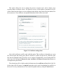
1
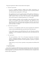
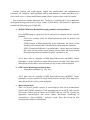
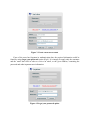
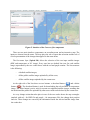
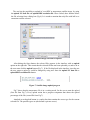
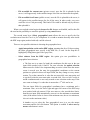
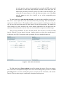
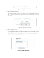
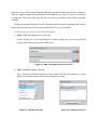
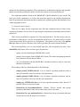
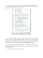
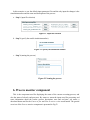
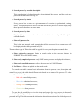
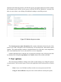
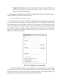
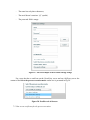
GreenView
A Grid based application for satellite
image processing
Acknowledgments
This research is supported by SEE-GRID-SCI (SEE-GRID eInfrastructure for regional
eScience) project, funded by the European Commission through the contract nr RI-211338.
Climate change data have been retrieved from the PRUDENCE data archive, funded by the
EU through contract EVK2-CT2001-00132.
MODIS data have been produced and distributed by NASA through the EOS Data Gateway
system.
Biome-BGC version 4.1.1 was provided by the Numerical Terradynamic Simulation Group
(NTSG) at the University of Montana. NTSG assumes no responsibility for the proper use of
Biome-BGC by others.
Partners engaged in the GreenView research project
1. Technical University of Cluj-Napoca (UTCN)
2. National Center for Information Technology (NCIT) Bucharest
3. West University of Timisoara (UVT)
4. National Research Institute in Informatics (ICI) Bucharest
5. Eötvös Loránd University (ELU) from Budapest (Hungary)
6. Research and Educational Networking Association of Moldova (RENAM)
Contents
1. Introduction
1.1. General overview
1.2. Existing versions of the application
1.3. Project requirements
1.4. Specific problems
2. User Login
3. Coarse to fine component
3.1. Method presentation
3.2. Input and output dataset
3.3. Start a new processing on the Grid infrastructure
4. Fine to coarse component
4.1. Method presentation
4.2. Input and output dataset
4.3. Start a new processing on the Grid infrastructure
5. Calibration component
5.1. Method presentation
5.2. Input and output dataset
5.3. Start a new processing on the Grid infrastructure
6. Process monitor component
7. User options
7.1.
How to modify the current user settings
7.2.
How to use certificates for the process execution
7.3.
How to configure my proxy settings for process execution
8. Conclusions and future work
1. Introduction
This paper is structured in eight chapters, and could be used for a better understanding and a
correct usage of the application, just like a user manual. There is also a pdf version of this
manual that could be downloaded by the users.
The first chapter (Introduction) provides a general overview of the GreenView application
and the characteristics of the applicability domain. Also, this section covers the main
requirements based on user and specialist’s feedback.
The second chapter (User login) presents the login steps into GreenView application and
some other issues like: creating a new account or what to do when you forgot your password.
The core of the application is represented by functionalities presented in the next three
chapters (Coarse to fine component, Fine to coarse component, Calibration component).
The meaning of the input and output dataset, the way to choose these sets, some user scenarios
containing the required steps for a new processing are just a few example of what can be found
in these three chapters.
The sixth chapter (Process monitor component) shows how someone can analyze the
previous launch process executions, by using different search options and apply different filter
on the results of the search.
There are several possibilities for process execution. All these are presented in the seventh
chapter (User options), that also contains information on how to modify the user settings.
The last chapter presents GreenView related conclusions and other applications that could be
integrated in GreenView.
1.1. General overview
GreenView is a Grid based environmental application that is using satellite images taken for
specific geographical locations over the entire Globe. These satellite images contain lots of
information, organized in bands (like Landsat) or levels (MODIS, MERIS, Thunderbird, etc.). In
order to correct the satellite measurement errors, some ground collect data are used also.
GreenView is a client server application. The server side relies on Java technology and
includes classes, methods and web services. The client side relies on the Flex technology for
creating the interface components and to associate them with different functionalities.
The main goal of GreenView is to be used as an application for monitoring temperatures and
vegetation growth over worldwide geographical areas. These monitoring values represent a start
point for domain field specialists, for predicting temperature and vegetation distribution in a long
run period of time. Because a large data volume is used in every processing step, GreenView
works on Grid infrastructure.
Grid infrastructure is a very powerful community at Global level, formed by Virtual
Organizations (VO). Each VO has a random number of work stations and a huge resource
volume that could be accessed only by authorized members. The identity validation is based on
certificates emitted by a certain Certificate Authority (CA). Every execution is done on the
stations of the Grid (called nodes), where the job distribution is realized automatically by
different middleware platforms.
1.2. Existing versions of the application
Our team has released the 3rd version of GreenView application. This version reveals new
approaches, both at the interface level and at backdoor functionality. Some of the most important
changes from the previous versions are:
a. Easy to use interface for the clients;
b. New functionality for user authenticity;
c. Redesigning (at interface and server level) Coarse to fine component;
d. Introducing a new search mechanism (for all the components) for the processes
launched by the logged in user, and the possibility to filter the search results;
e. Individual development of GreenLand regarding GreenView;
f. The possibility for the user to change the account setting;
g. Update the user manual, for a better understanding of the application usage by the
clients.
There is a description catalog for this application on the wiki server that presents the general
overview, the main goals and the basic approaches for GreenView. The web addresses for the
GreenView versions are:
http://wiki.egee-see.org/index.php/GreenView (wiki page for GreenView)
http://c5.mediogrid.utcluj.ro:4331/interpolation2.1/ (2nd version)
http://c5.mediogrid.utcluj.ro:4331/interpolation3.1/ (3rd version)
1.3. Project requirements
The project requirements could be classify in three main categories:
a. Functional requirements
-
In case of vegetation parameters obtained from satellite measurements, the
application should be able to produce rescaled fields of given vegetation parameters
on a arbitrarily chosen regular grid over CEE region.
-
This application will provide vegetation-related model parameters optimized to a
Hungarian measuring site for further calculations. As future work a geographical
region extension is taken into account. These calculations will hopefully produce
more accurate estimates on vegetation productivity over a wider region.
-
Fields of atmospheric pollutants, such as tropospheric ozone, sulfur-dioxide, nitrous
oxides are also produced from satellite measurements. This application can be
interesting for both the scientific and social community. GreenView must have the
ability to compare and verify satellite field with ground based measurements in those
points where those are available.
b. Non-functional requirements
-
GreenView is a web application, and the user accesses by Internet the computation
resources and environmental data that are provided by the Grid infrastructure.
-
For the satellite image processing ESIP platform will be used. The gProcess platform
is going to be used for managing the communication between Grid infrastructure and
GreenView.
c. User requirements
-
The main beneficiaries of this VO are Government Organizations, Environment
Agencies, Hydrological Institutes, and Research Groups involved in environment
supervision and behavior prediction of natural phenomena, especially in vegetation
related studies.
-
Simple and easy to use by all users, specialists or non-specialists from different field
domains.
1.4. Specific problems
One of the most important problems that appear regards the large processing volume of data
contained in the satellite images. For a single machine obtaining the results in a reasonable time
is almost impossible. So, our attention focused on the Grid infrastructure that is designed to deal
with these kinds of applications.
Another problem that might appear, regards the parallelization and implementation
techniques. For example a certain algorithm could be implemented as a simple procedure or as a
Grid or web service. A better parallelization means a better execution time on the Grid nodes.
Data acquisition is another important issue. Testing is an essential part of every application
development strategy that involves a large volume of pilot dataset. The GreenView application
considers the following types of input data:
a. MODIS (MODerate Resolution Imaging Sounder) related products:
Every MODIS image is organized in levels, and one level contains data for a specific
parameter.
- Land cover: contains values for different parameters used for ground cover
recognition;
- FPAR (Fraction of Photoshyntetically Active Radiation): the fraction of the
incoming solar radiation that is absorbed by the photosynthetic organisms;
- NDVI (Normalized Difference Vegetation Index): simple numerical indicator
that can be used to analyze remote sensing measurements and assess whether
the target being observed contains live green vegetation or not.
All of these data are originally in HDF (http://hdf.ncsa.uiuc.edu/HDF5/) format.
Optionally it can be converted to simple binary format if needed. These data can be
ordered from NASA (https://wist.echo.nasa.gov/api) so they can be multiplied.
b. OMI (Ozone Monitoring Instrument) data
- Atmospheric pollutants (O3, SO2, NO2)
All of these data are originally in HDF (http://hdf.ncsa.uiuc.edu/HDF5/) format.
Optionally it can be converted to simple binary format if needed. These data can be
ordered from NASA so they can be multiplied.
c. Meteorological data
There are several possible sources of meteorological data (local measurements,
GMAO and ECMWF reanalysis). Local measurements are in ASCII with a specific
file format, GMAO data are binary and ECMWF data are NetCDF. Chosing the
appropriate meteorological data needs further discussions considering all
circumstances – data availability, - and users’ needs. These data (except for local
measurements) cannot be redistributed.
2. User Login
The authenticity of the user can be validated by using the login component (Fig.1). For this
operation a username and a password should be provided by the user. If the information
contained in the input textboxes don’t match the user identity, some error message is displayed
(Fig.2). If the cancel button is clicked, then the username and the password fields are set to null.
Figure 1. Login component
Figure 2. Error message example
If a user wants to create a new account in the GreenView database, then the new user link
should be clicked. At this action a form is expanding below the main login window, form that
contains some personal information: name of the client, the login username, an email address, a
password and a short description (Fig.3). It is worth to mention that every user has a unique
username that differentiate it from others. When creating a new account the main login window
is disabled, for security reasons.
Figure 3. Create a new user account
If one of the users has forgotten its authentication data, the required information could be
found by using forgot your password option (Fig.4). It is enough to supply only the username
and the email data field in order to receive an email, at the given address, containing the
password and other important user information.
Figure 4. Forgot your password option
At every one of the three main operations (login, creating account, forgot your password
form completion) could appear some error messages, due to some misspelling errors, skip to
complete some required fields, or try to provide an already existing username. Only one
component is enabled at a certain moment, meaning that when creating a new user account the
main login window and forgot your password options are not enabled.
To logout of the GreenView application the user must click the username that appears in the
right top side of the application window.
3. Coarse to fine component
GreenView application has three main components based on satellite images: coarse to fine,
fine to coarse (used for monitoring the temperature over SEE) and satellite image calibration
(used for monitoring the growth and vegetation distribution over some specific geographical
areas).
3.1. Method presentation
Coarse to fine component uses some static input datasets (including satellite images) in order
to provide a temperature map for a chosen geographical area. It is based on a non-linear
weighted interpolation technique for computing the temperature values in the output map.
The main goal of this component is to generate a map of the temperature distribution over a
geographical area. For this, some satellite images (NC coarse resolution image and HDF fine
resolution image) are used, images that contain information about specific geographical area and
information about temperature values from another area. The interpolation algorithm is applied
on the region obtained by overlapping the two geographical areas. The meaning of every
interface component will be detailed in the next section.
3.2. Input and output dataset
The general view of this component at interface level is presented in Fig.5. As can be seen
every tab in the interface is associated with one of the components that are detailed in this user
manual (e.g. 3rd tab corresponds to the calibration component).
Figure 5. Interface of the Coarse to fine component
There are two main interface components: an accordion menu and an interactive map. The
inputs are chosen from the menu. The map plays the role of input data selection and the role of
visual representation of the changes that appears in the menu items.
The first menu layer (Upload file) allows the selection of the two input satellite images
(HDF and temperature or NC image). Every user has two default lists (one for each satellite
image) represented by the two combo boxes with the red and purple contour. The lists structure
is the following:
-
A default satellite images;
-
All the public satellite images uploaded by all the users;
-
All the satellite images uploaded by the current user.
At the right side of the lists there are two buttons: a download button (
) and a delete
button (
). The download button is used for downloading the selected HDF or temperature
image. The delete button is active only for current user uploaded satellite images, meaning that
the default and the public files uploaded by other users could not be deleted by the current user.
At every change action that takes place in one of the two combo boxes the map rectangles
(marked with red – for HDF file and purple – for temperature file) also change their position
and size. These changes are caused by the information inside the selected satellite image from
the combo box.
The user has the possibility to upload its’ own HDF or temperature satellite image, by using
the upload NC data file and upload HDF resolution file. Once clicked, these buttons allows
the file selection from a dialog box (Fig.6). It is worth to mention that only files with hdf or nc
extension could be selected.
Figure 6. Satellite image selection for upload
After hitting the Open button, the selected files appears in the interface with an upload
option on the right side. This means that the selected file has not been uploaded yet, and to do so
the user must click the upload button (Fig.7). If the file displayed in the interface is not the one
the user wants to upload, it could be changed by using once more the upload NC data file or
upload HDF resolution file button.
Figure 7. Satellite image upload progress
Fig.7 shows that the temperature file is in a waiting mode, for the user to start the upload
(first file from Fig.7). Every upload action has a progress component that shows the upload
percentage of the file (second file from Fig.7).
Attached to each upload button is a combo box that contains the access type for the current
selected file. The possible types are (the default is private access):
-
File accessible for current user (private access): once the file is uploaded to the
server, it will appear only in the satellite images list of the user that make the upload;
-
File accessible for all users (public access): once the file is uploaded to the server, it
will appear in the satellite images list for all the users. In other words, every user
could use it in a Grid processing. This kind of file could be deleted only by the user
that uploaded it.
When a new upload action begins the browse for file buttons are disabled, and for that file
the user has the possibility to cancel the upload, by using cancel button.
The second menu layer (Select geographical area) allows the user to specify the fine
resolution area from the Coarse to fine component. It is worth to mention that only areas inside
the HDF map region (marked with red) could be selected.
There are two possible solutions in choosing the geographical area:
-
Apply interpolation on the entire HDF region: meaning that for a Grid processing,
the entire geographical area, specify in the HDF file, is used. On the map this is
highlight by filling that region with a grey filter;
-
Select subarea from the HDF region: this option give two possibilities in
geographical area selection.
a. The first one is to enter (by hand) the coordinates for this area, in the text
input fields marked with A and B. For area selection the update selection
button must be clicked. One important thing to notice is that when the mouse
cursor is moved over the map, the geographical coordinates at the current
position are placed in these text input fields, but they change at every mouse
motion. To set the content for A value the user must click on a map point, and
to set the B value the user must make a second click. Now we have set the A
and B coordinates and we are ready to make a new selection on the map. If the
user wants to change A’s value then it must make a 3rd click and so on.
The text input fields for geographical coordinates have a minimum and a
maximum value, set to the lower right and upper left corner of the HDF map
area (marked with red contour). If the user enters a value outside these limits,
then the text input field automatically corrects it to the minimum or maximum
value (if the entered value is closer to the minimum one, the set it to minimum,
else set it to the maximum value).
b. Another way to select the fine geographical area is to use the mouse
movement and the left click button. This option is enabled if select area by
mouse radio button is active.
As in the previous option, only geographical areas inside the HDF region could
be selected. To start a new map selection, just make a click, keep your left
button down and move the mouse. When you want to end the selection, just
release the left mouse button. At click and mouse movement, even if the select
area by mouse is active, the A and B are set to the corresponding map
coordinates.
The third menu layer (time interval selection) gives the user the possibility to specify the
last Coarse to fine input that is the time interval used for processing. This time interval is
expressed as month’s interval. The months and the years are stored in combo boxes, and in this
way the user can select much easier the time interval for the Grid processing. The combo box
values change every time when the user selects another temperature file. In other words the
minimum and maximum time interval values are stored inside the temperature satellite images.
There are two possibilities for time selection interval. The first one is to select a month
interval, followed by a year interval selection. Another option is to select only a month interval
for the same year (Fig.8). An output result is generated for every month in the interval.
Figure 8. Time interval selection
The firth menu layer (Process options) is used for naming the process. Every new process
has a name and a description that improve the search action among other processes. The start
processing button is used for starting the process execution on the Grid nodes, and remains
inactive if the user does not give a name and a description for this process.
It is important to notice that all the required inputs have some default assigned values. The
HDF and temperature (NC) inputs have as default value the first file selected in the two combo
boxes and the interpolation algorithm is applied for the entire HDF area. There is also a default
value for the time interval. The lower and upper boundaries of the year interval are both equal to
the minimum value in the years related combo box and the month interval is set to January (e.g.
1961, January – 1961, January). Even though there are default values for every input data, the
process execution could not begin until it has a name and a description. The left image from Fig.
9 presents an example when the start processing button is disabled, meaning that the process
execution could not begin. On the other hand, the right image represents a valid example of a
Grid process execution.
Figure 9. Process name and description
Another important component for the Coarse to fine method is the interactive map of the
entire Globe. Because the GreeView application is used only for European geographical regions,
the map is limited in size at the European continent. Because is an interactive map, drag and
select action could be used. The general view of the map is presented in Fig. 10.
Figure 10. Map component
The most important interactive techniques available are:
a. The red rectangle on the map represents the geographical area from the HDF file,
selected in the corresponding combo box. The purple rectangle represents the
geographical area from the temperature file. When the user selects another HDF or
temperature file, the two rectangles modify according to the areas contained in the
selected files;
b. Map region selection is available only if the select subarea from the HDF file option,
from the second menu layer, is active. The selection of the geographical region is made
with the left mouse button. For this the user clicks once to set the starting position of the
selection and keeps the left button down and moves the mouse. When it wants to end the
selection just release the left mouse button;
c. On every mouse click on the map the text inputs for A and B, from the second menu
layer, change their values according to the current geographical coordinates of the
mouse;
d. Using the drag mouse event, the map moves according to the mouse position, but it
cannot exceed the boundaries of the European continental platform;
e. Zooming option is another important feature of the map. It can be done by using the
zoom in ( ) and zoom out ( ) buttons. A 17 zoom level is accepted, meaning that in
some geographical areas the map scale is 1:1875Km (on zoom out) and 1:50m (on zoom
in);
f. Map resizing in useful sometimes when we are dealing with very small area selection
options. For placing the map on the entire application window, the full screen button
could be used. When we are in a full screen mode, the button name will change into
normal mode, that allows us to return to the default map position and size;
g. There are different views of the map, specify through the Map, Satellite and Hybrid
buttons, situated on the upper right side of the map;
3.3. Start a new processing on the Grid infrastructure
This section presents a scenario of the Coarse to fine input data selection in order to execute
a new process on the Grid infrastructure.
a. Step 1 (select the HDF and temperature input files)
Step 1.1
Step 1.2
Step 1.3
Figure 11. HDF and temperature file selection
b. Step 2 (select geographical area)
In this scenario we apply the interpolation method on the entire HDF area, in order to
reduce the complexity of the scenario. In a real time execution, the user could specify its
own geographical area by using the techniques mentioned above.
Figure 12. Geographical area selection
c. Step 3 (time interval selection)
This scenario takes into account a 1961, January – 1963, March time interval. This is
only an example, meaning that for other processes the time interval could be different
from this one.
Figure 13. Time interval selection
d. Step 4 (naming the process)
In this case the process name is Test and its description is set to Coarse to fine scenario.
After all the four steps are completed the user can click the start processing button for
starting the process execution on the Grid nodes.
Figure 14. Naming the process
4. Fine to coarse component
This is the second core component of the GreenView application, used for monitoring the
temperature over European geographical regions. It is very similar with the Coarse to fine
component, described above. For details regarding the significance and importance of the
interface components see the section 4.2. Input and output dataset. The general view of the Fine
to coarse component is presented in Fig.15.
Figure
Naming
thecomponent
process
Figure
15.14.
Fine
to coarse
4.1. Method presentation
It is based on an arithmetic mean interpolation technique. In order to determine the values for
the interpolated pixels, this method takes into account the values of the pixels from a virtual
rectangle that is a part of the entire geographical area. As the previous component, Fine to coarse
method is based on two satellite images (HDF – fine resolution image and temperature file –
coarse resolution image).
The main goal of this component is to generate a coarse resolution image (available in
different formats: JPG, ASCII, NC, etc) given a fine resolution image as input.
4.2. Input and output dataset
This method has three inputs: HDF satellite image, temperature satellite image and a
processing metadata, that could be found in the temperature file. The satellite image selection is
similar to the selection described for the Coarse to fine component and it makes no sense to
repeat these steps. The metadata from the HDF file represents the third input of this component.
There is a single metadata structure that has several attributes (e.g. Fpar, Lai, Ndvi, etc) stored in
a combo box. From this combo box the user can select one attribute in the process execution
workflow.
Giving a name and a description to the execution process is another important issue. All the
aspects related to this case have been presented for the Coarse to fine method.
4.3. Start a new processing on the Grid infrastructure
a. Step 1 (HDF and temperature file selection)
In this scenario we are not uploading new satellite images, but we are using already
existing ones from the two related combo boxes.
Figure 16. HDF and temperature file selection
b. Step 2 (Metadata attribute selection)
Fig.17 presents the metadata structure for the MOD17.hdf file. From this list we select
the Fpar_1km attribute that will be used for further processing.
Figure 17. Metadata selection
Figure 18. Naming the process
c. Step 3 (Naming the process)
For this process we choose a Test name and Fine to coarse scenario as a description
(Fig.18).
5. Calibration component
This is the last main component of the GreenView application, hierarchically speaking. As
the previous two components, this one is also based on satellite images. The general overview of
is presented in Fig.19.
Figure 19. Calibration component
5.1. Method presentation
Calibration component has a different approach that the first two. It is based on satellite
measurements, but also on ground measurements for the same list of parameters. The insight of
the calibration notion presumes some sort of comparisons between some measured values
(satellite obtained values) and given values (ground based values).
The calibration method applies on a list of vegetation parameters. Every parameter has an
interval of possible values. In order to filter the results, some mathematical relations could be
attached to the calibration component. These relations have mathematical operator and operands,
and the user has the possibility to modify of add extra relation to an already defined set.
The calibration method is based on the BIOME-BGC (BioGeochemical Cycles) model. The
main goal of this component is to correct the errors that appear in the satellite measurement,
based on ground made measurements and to monitor the vegetation growth and distribution over
certain geographical areas.
5.2. Input and output dataset
There are five inputs for this component: three files that contain the interval values for the
vegetation parameters and two files for specifying the mathematical relationship between these
parameters.
There are two possibilities to input the five files mentioned above. The first one give the user
the freedom in choosing its’ own files on upload them on the server. The upload action is similar
to the one presented for the previous two components. This option is active only if the upload
files radio button is selected. Because of the lack of pilot data, this option remains disabled.
The second possibility is to use some default input files and correspond to the state of the
default files radio button. There are three types of parameters:
-
spinup: used for initializing the BIOME-BGC model;
-
normal: used as inputs in the BIOME-BGC model. The normal and spinup parameter
list is identical, only the interval differs;
-
epc: in combination with the BIOME-BGC simulation results are used to correct the
satellite measurements.
The meaning of the five default input files is the following:
-
sample_normal_INTERVALS.ini: a list of normal vegetation parameters and an
interval of possible values for each one of the parameters;
-
sample_spinup_INTERVALS.ini: a list of spinup vegetation parameters and an
interval of possible values for each one of the parameters;
-
sample_epc_INTERVALS.dat: a list of epc vegetation parameters and a interval of
possible values for each one of them;
-
Restrictions_for_ini_mathematical.txt: relations between normal and spinup
parameters that must be taken into account in the process execution;
-
Restrictions_for_epc_mathematical.txt: relations between epc parameters that must
be taken into account in the process execution.
All the files have a view button on the right side and by clicking this button the content of the
file is displayed in the text area (Fig.20). It is worth to mention that for default files the user can
only view the file content and cannot modify the file.
Figure 20. Content of the spinup parameters default file
The calibration method is based on random value generation for the vegetation
parameters, values that must be inside the parameter’s interval. In order to obtain a better
calibration we must simulate the BIOME-BGC model as many times as possible (at least 1000).
Taken this into account the simulation number is another input parameter for the Calibration
component. The user can specify this value in the no.of model simulation text input.
The process name and process description have the same meaning as in the previous two
components. If both the name and the description attributes have been set by the user, the process
execution could begin.
5.3. Start a new processing on the Grid infrastructure
In this scenario we use the default input parameter files and the only input the changes is the
simulation number and the name and description of the process.
a. Step 1 (input file selection)
Figure 21. Input file selection
b. Step 2 (specify the model simulation number)
Figure 22. Specify the simulation number
c. Step 3 (naming the process)
Figure 22. Naming the process
6. Process monitor component
This is the component used for displaying the status of the current executing process, and
also the status of already end processes. By status we mean the inputs used for processing and
some information about the results: process description, start and end time, job status, a
download button and for the Coarse to fine and Fine to coarse a view result button. The general
overview of the Process monitor component is presented in Fig.23.
Figure 23. Process monitor component
This component is personalized for each user, meaning that only the processes created by the
current user are return by the search actions. Fig.23 shows that the current login username is
testuser.
There are five search options for the user that will be presented in this paragraph:
a. Search process by name
Is the first search option, that allows the user to focus its’ search on the name of the
process. All processes that contain that name will be displayed in the table below. Fig.24
shows the search result for “test” process name.
Figure 24. Search result for “test”
b. Search process by words in description
This search action is looking through the description of the process, and the results are
placed in the same table as in Fig.24.
c. Search process by status
Every process has a status at a given moment of execution (e.g. submitted, running,
done). This option allows the user to filter the current user process list and to display only
those processes that have the same status.
d. Search process by date
Display all the processes that have the start time in the time interval specified through the
calendar buttons.
e. Show all processes for
This is the most general search, meaning that all the processes for the current users will
be displayed in the table presented in Fig.24.
There are three types of filters that could be applied for every search option presented above:
a. Show only active processes: limits the search results to the processes that are in
SUBMITTED or RUNNING status;
b. Show only completed processes: only DONE status processes are displayed to the user;
c. Show only cancelled processes: refers to the processes in CANCEL status;
d. No filters: no filters are applied on the search result.
The search result table contains basic information about the process: name, description and
status. Every row in the table has a different color based on the status of the process. The color
meaning is the following:
-
Red color: cancelled processes;
-
Blue color: submitted processes;
-
Orange color: running processes;
-
Green color: done processes.
The user has the possibility the view the inputs and outputs for every process in the search
result table by clicking on the process name, marked with blue. The effect of such an action is
presented in Fig.25. At this moment the information about the execution of the clicked process is
displayed in the following structure: the ID of the process, the inputs and the lower table contains
the execution results. In this case the process with the ID=830 has finished its’ execution, but
there are cases when we are dealing with submitted, running or cancelled processes.
Figure 25. Monitor the process status
The Current process status information table contains information about the jobs of the
process, like: name, description, start execution time, end execution time, status and an option
attribute. This option attribute contains a download button (for all the three main components)
and a view button only for Coarse to fine and Fine to coarse component.
Another important aspect is that the user can stop the execution of any of the processes that
he submitted, by clicking the stop button in the Cancel column of the search result table.
7. User options
The user has the possibility to change some of the account settings or to change the process
execution mode. There are three types of users in this application, based on the process execution
type:
-
Guest: it uses a set of default certificate in order to execute process on the Grid;
-
Using its’ own certificates: only users with a valid certificate could try this option;
-
Using the My Proxy server: this means that the user has uploaded its’ own
certificate on another server, and it can generate a proxy in order to execute the
processes on the Grid infrastructure.
Changing one of the attribute in the database is automatically followed by a logout action, in
order to refresh the modifications made by the user.
7.1. How to modify the current user setting
This option gives the user the possibility to change the account settings. It can change its’
name, password, email, description or it can specify another CE (Computing Element) on the
Grid infrastructure for job processing. All the time, the current user knows what status has in the
process execution (Guest, Certificate owner or proxy owner). What is more interesting is that it
can change this status by simply selecting another status form the combo box presented in
Fig.26. The content of the combo box is different for every user, because not every user owns a
certificate or a my proxy certificate.
Figure 26. Changing the account settings
For a user that doesn’t have a valid certificate or a valid My Proxy the only available
status is the Guest one. Every text input in the Fig.26 must be at least 4 characters long. The save
button becomes active when the user makes at least one change on the default settings. The
example is Fig.27 in not a valid one, because of the following reasons:
-
The name has only three characters;
-
The email doesn’t contain a “@” symbol;
-
The password field is empty.
Figure 27. An bad example of the account settings change
For a user that has a certificate on the GreenView server and on a MyProxy server the
content of the Select the process execution mode combo box is presented in Fig.28.
Figure 28. Possible role of the user
7.2. How to use certificates for the process execution
This option allows the user to change the process execution style, and to obtain a new
execution status (certificate owner). The general overview of this option is presented in Fig.29.
All the fields from this figure are auto completed with default values taken from the database for
the current user. If no certificate was uploaded then these fields will be set to null.
Figure 29. Certificate settings form
Only valid certificates could be used with this option. This certificate is formed by two .pem
file (usercert.pem and userkey.pem) that are similar to a public and private key. Both the .pem
files must be uploaded to the GreenView server, and once uploaded they are not made public for
other users. By clicking the Browse for user certificate and Browse for user key buttons we
accomplish the upload action.
The selected pem file is display under the button near the certificate and key labels (Fig.30).
On the right of the file name is an upload button that can be used for uploading the certificate to
the server. In every moment the user can cancel the upload action, by using the cancel button.
Figure 30. Certificate upload
For this option all the fields must be completed and the user must agree with the conditions
impose by the GreenView development team (meaning that the I agree the terms box must be
selected).
An
example
for
the
woms
proxy
field
is
https://wms.ipp.acad.bg:7443/glite_wms_wmproxy_server.
7.3. How to configure my proxy settings for process execution
Another users’ role for the process execution is by owning a valid proxy, generated from the
certificates. This means that the user has to upload its’ certificates on a My Proxy server and to
generate its’ own proxy. Then, in the interface (Fig.31) the user has to complete the fields with
the correct information based on the proxy generation.
Figure 31. My proxy form
All the fields are required, except the MyProxy port. Before updating the user account, the
information is validated at interface level. The possible error messages that could appear are:
-
The field is empty: all the field must have a non null value, and it’s content must be
different from the “ “ (space) character;
-
The information has less than four characters;
-
The field accepts only integer values: for Myproxy port and Myproxy lifetime
fields only numerical values are accepted;
8. Conclusions
GreenView is a useful Grid application for monitoring the vegetation growth and distribution
over certain geographical areas. Another approach is regarding the temperature distribution over
Central Eastern Europe regions, where non-linear interpolation algorithm was used for output
temperature map generation. The spatial limitation of the GreenView application is due to the
input datasets. By collecting new HDF and NC satellite images, the GreeView’s functionality
could be easily extended to other geographical areas.
It is worth to mention that the interpolation algorithms were chosen on a compromise basis
between precision and implementation complexity. Another interesting thing, regarding this
application, is to use other interpolation techniques and to compare the obtaining results (e.g.
linear, bicubic, polynomial interpolation algorithms).