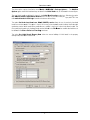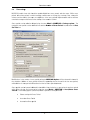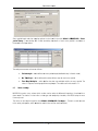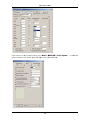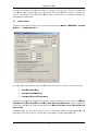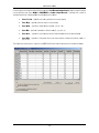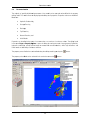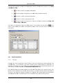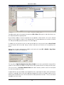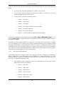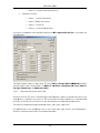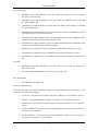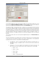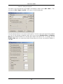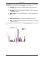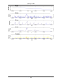
1
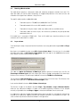
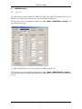
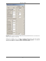
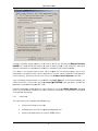
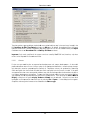
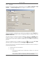
THIS PAGE HAS BEEN LEFT INTENTIONALLY BLANK 50371/P3-R3 FINAL Schlumberger Water Services DTIRIS NSW) NAMOI CATCHMENT WATER STUDY INDEPENDENT EXPERT MODEL USER MANUAL July 2012 50371/P3-R3 FINAL Prepared for: Department of Trade and Investment, Regional Infrastructure and Services, New South Wales, (DTIRIS NSW) Locked Bag 21 Orange NSW 2800 Prepared by: Schlumberger Water Services (Australia) Pty Ltd Level 5, 256 St Georges Terrace Perth WA 6000 Australia 50371/P3-R3 FINAL Schlumberger Water Services DTIRIS NSW) REPORT REVIEW SHEET Report no: Client name: Namoi Catchment Water Study Independent Expert Model User Manual 50371/P3-R3 FINAL Client contact: Department of Trade and Investment, Regional Infrastructure and Services, New South Wales, (DTIRIS NSW) Mr Mal Peters, Chairman, Ministerial Oversight Committee (MOC) SWS Project Manager: Sean Murphy SWS Technical Reviewer: Mark Anderson Main Author: Gareth Price Date Issue No Revision SWS Approval 17/02/2012 1 Draft Mark Anderson 27/07/2012 2 Final Mark Anderson 50371/P3-R3 FINAL Schlumberger Water Services DTIRIS NSW) CONTENTS Page 1 INTRODUCTION 2 GROUNDWATER MODEL 2.1 Introduction 2.2 Groundwater Vistas files 2.3 Domain, grid and rotation 2.4 Layer surfaces 2.5 MODFLOW settings 2.5.1 BCF / LPF 2.5.2 Initial heads 2.6 Time settings 2.7 Solver settings 2.8 Output settings 2.9 Parameterisation 2.10 Boundary conditions 2.10.1 Recharge 2.10.2 Mine inflow (drain boundaries) 2.10.3 Rivers / streams 2.10.4 Abstraction wells (background) 2.10.5 Abstraction and injection wells (CSG) 2.10.6 Irrigation (injection) wells 2.10.7 Connective cracking / permeability enhancement 2.11 Model and translation and run 2.12 Post processing results 2.12.1 Importing model results 2.12.2 Contours 2.12.3 Hydrographs 2.12.4 Historical surface water / groundwater interaction 2.12.5 Predictive period mass balance 2 2 2 3 3 4 4 6 8 9 11 13 14 14 16 18 20 21 24 27 27 27 27 28 29 31 32 3 HYDROLOGIC MODEL 3.1 Introduction 3.2 Domain and sub-catchment selection 3.3 Parameterisation 3.3.1 Soil settings 3.3.2 Surface water storage settings 3.3.3 Land use settings 3.3.4 Rainfall settings 3.3.5 Evaporation settings 3.4 Time settings 3.5 Specific run settings 35 35 37 37 37 38 39 40 42 42 43 50371/P3-R3 FINAL 1 Schlumberger Water Services DTIRIS NSW) Contents 3.6 LASCAM runs and post processing results REFERENCES 50371/P3-R3 FINAL 44 50 Schlumberger Water Services DTIRIS NSW) THIS PAGE HAS BEEN LEFT BLANK INTENTIONALLY 50371/P3-R3 FINAL Schlumberger Water Services DTIRIS NSW) 1 INTRODUCTION Schlumberger Water Services (Australia) Pty Ltd (SWS) has been appointed as the Independent Expert for the Namoi Catchment Water Study (the Study) and has been charged with the development of an integrated suite of models (the Model) for the assessment of the nature and extent of potential effects from coal and gas developments on the water resources of the catchment. The purpose of the Study is to collate and analyse quality data to assist in identifying and quantifying risks associated with the coal mining and coal seam gas (CSG) developments on water resources. The numerical modelling tools were developed as part of Phase 3 of the Study. Two numerical models were constructed that together have the ability to simulate those parts of the hydrological system that are pertinent to the simulation of the interaction between coal and gas development and the surface water and groundwater resources of the Namoi catchment. The two models constitute the Model and are: A lumped parameter Hydrologic Model. This was constructed with the LASCAM (Viney and Sivapalan, 2000) package and is used to simulate the fate of rainfall in the catchment, particularly the portion that forms runoff and the portion that percolates downwards into the sediments and recharges the groundwater system. This model includes the simulation of the impact of mining and CSG development on these processes. A groundwater flow model (the Groundwater Model). This was constructed using the numerical code MODFLOW 2000 (Harbaugh et al, 2000) and is used to simulate the processes governing groundwater flow in and between the alluvial aquifers and hydrostratigraphic units pertinent to the prediction of the impact of coal and gas developments on the groundwater resources and the interaction between surface water and groundwater. The model therefore includes representation of the abstraction of groundwater associated with CSG development and the flow of groundwater to mine voids, both underground and open cut. It also uses predictions from the Hydrologic Model to define groundwater recharge inputs and changes to these in response to mining and CSG development. According to the Study Request for Tender (Section G.3.7.1.g.ii) a User Manual must be produced that provides full details on how to operate the Model including updating the Model to include additional or improved data and the locations for mines or gas extraction developments. This document represents the User Manual. Section 2 provides details of the operation of the Groundwater Model and Section 3 the operation of the Hydrologic Model. 50371/P3-R3 FINAL Schlumberger Water Services 1 DTIRIS NSW) 2 2.1 GROUNDWATER MODEL Introduction The MODFLOW 2000 numerical code (Harbaugh et al, 2000) along with the user interface Groundwater Vistas, Version 6 (ESI, 2011) is used to simulate groundwater flow and surface water / groundwater interaction in the Groundwater Model. The modelling has been undertaken assuming saturated, single phase, temperature independent and single density groundwater flow. 2.2 Groundwater Vistas files Nine Groundwater Vistas files and a single results file have been provided. They are: Namoi_Historical.gwv Namoi_Historical.hds Namoi_Sc0.gwv Namoi_Sc1.gwv Namoi_Sc2.gwv Namoi_Sc3.gwv Namoi_Sc4.gwv Namoi_Sc5.gwv Namoi_Sc6.gwv Namoi_Sc7.gwv These files contain all of the data required to run the historical and predictive scenario models. The results file “Namoi_Historical.hds” forms the initial heads for all of the scenario runs. When running any of these scenarios for the first time the link to the “Namoi_Historical.hds” file must be defined within Groundwater Vistas. 50371/P3-R3 FINAL Schlumberger Water Services 2 DTIRIS NSW) Gro roundwater Model Mo 2.3 Domain, gridd and rotatio on c a rectangular r m odel grid, rottated by 30 degrees clockw wise from norrth. This The moodel domain comprises aligns tthe model cells with the Basin B morphollogy, as the general g dip direction of thee hard rock units and orientattion of the Upper Namoi Allluvium is alon g this axis. The speecific model properties are detailed d below w: Thee model originn is at 745,0000E, 6,410,000N N (MGA Zone 55, GDA94). Thee model extennds 310 km to the NW and 180 1 km to the NE. Thee model cell size (plan view w) is 1,000 m byy 1,000 m (3100 rows and 1880 columns). Thee model contaains 20 vertic al layers, with thicknesses provided by the geologicaal model desscribed in Section 2. model layer is composed of 55,800 cellss. There are 20 model layers thereforee resulting inn a total Each m numberr of cells for thhe model of 1,,116,000. 2.4 Layer surfacces Tasks innvolving the setup s of layerss and vertical discretization are mostly peerformed usingg the Grid and Props menus. a using the t menu Griid > Insert > Layer above e, if the new layer is to be added New laayers can be added above tthe current layyer, or Grid > Insert > Layyer below, iff the new layeer is to be addded below thee current layer. Inn either case, the following dialog will apppear: mbo box Option for Thickness of Neew Layer proovides optionss for insertingg layers, the first f one The com (Percentage of Currrent Layer) splits the currrent layer in two t assigningg a percentagee of the curreent layer w layer. The percentage is deefined in the text box Thick kness or Perccentage. thickness to the new C thickness, assignns a constant thickness for the new layerr. The thicknesss of the The seccond option, Constant new layyer can be speecified in the Thickness T orr Percentage e text box. Layers ccan be deleted in the menu Grid > Delet ete > Current layer. The thickness of layeers can be edited in the meenu Props > Top elevatio on or Props > Bottom ele evation, where the top and bottom elevaations of layeers can be edited respectively. Elevatioons can be assigned a manually or importedd via the menuu Props > Impport... where several s differeent formats caan be used. It is impportant to notte that assigniing the bottom m elevation off one layer doees not automaatically assignn the top elevatioon of the layeer below, requuiring that botth top and boottom elevations are assignned for all layers. The same iss valid for top elevation and bottom elevaation of the layyer above. 50371/P3--R3-FINAL Schlumbeerger Water Servicees 3 DTTIRIS (NSW) Gro roundwater Model Mo 2.5 2.5.1 MODFLOW settings s BCF / LPF The chooice between the Block Ceentred Flow (BBCF) and Layeer Property Floow (LPF) packa kages affects the way MODFLLOW formulatees interblock conductances c and confined//unconfined behaviour. M Model > MODFLOW W > Package es... The The BCCF package caan be activateed/deactivatedd using the Menu followinng dialog will appear: nd To activvate the BCF package, p click the check boxx next to the BCF B package (22 line). The LPFF package cann be activated/deactivated tthrough the menu m Model > MODFLOW W 2000 > Pack kages... A new dialog will appear (see beloow) and the paackage can bee toggled by clicking on the check box nexxt to the LPF linee. 50371/P3--R3-FINAL Schlumbeerger Water Servicees 4 DTTIRIS (NSW) Gro roundwater Model Mo a MODFLOW will nnot work whenn both or Importtant: Make sure that only onne (LPF or BCFF) package is activated. neither of the two paackages are acctivated. Specificc layer paraameters such as averaginng, confined//unconfined behaviour annd vertical leakance calculattions can be modified m usingg the menu Mo Model > MODFFLOW > Pack kages optionns... A new diaalog will appear and the param meters can be edited in the BCF-LPF tab, illustrated below. 50371/P3--R3-FINAL Schlumbeerger Water Servicees 5 DTTIRIS (NSW) Gro roundwater Model Mo Parameeters regarding vertical leaakance can bee found in thhe top box. Checking the CCompute Leakance (VCON NT) box makees MODFLOW W calculate thhe vertical leaakance basedd on cell thiccknesses and vertical hydraulic conductivities as specifieed in the modeel (this is the option o used in the Namoi M Model). If this ooption is not selected, leakance values will be assiggned from the Leakance prooperty, whichh can be represeented as raw leakance l values, vertical coonductivity of the layer, verttical conductivvity of the aquuitard or vertical anisotropy. The T leakance format can be chosen in the Leakance Zones Repressent combo boox. Layer cconfined/unconfined behaviour can be deefined in the Layer Types box. For eachh layer defineed in the mn Layer Typ pe (LAYCON)). Layer type ooptions availaable will model, there will bee a combo boxx in the colum dependd on the selectted flow packaage (BCF or LPPF). mn BCF3/4 Avveraging. Avveraging Interbloock conductannce averagingg options cann be defined in the colum optionss can be indiviidually assigned for each laayer through the combo boxxes. Averagingg options also depend on the sselected flow package. 2.5.2 Initial headds The inittial heads can be assigned in i three differeent ways: c valuees for each layyer; Using constant Assigniing values manually in the pproperty editinng mode; and Importing simulated heads from a previous MOD DFLOW row. 50371/P3--R3-FINAL Schlumbeerger Water Servicees 6 DTTIRIS (NSW) Gro roundwater Model Mo The thrree options caan be found inn the menu M Model > MOD DFLOW > Package Optioons... . The Modflow M Optionns appear and initial heads settings s are foound in the Initial Heads tab, as illustratted in the nexxt figure. The waay initial headds are defined is chosen in the Initial Head H Location combo box.. Selecting the option Use Deefault Headss in Spreadssheet Below w allows the use u of one inittial value per layer, defined in the table D Default headss in Each Layyer located at the bottom off the dialog. The opttion Set Heads from Hea ad-save, BAS SIC, SURFER,, matrix allow ws the use off previously simulated heads ffrom another model. m This opption is useful , for instance,, when hydrauulic heads from m the historicaal model need too be used as innitial heads foor the predictivve runs, and thhis is the way it is done in tthe Namoi moodel. The file conntaining the prreviously simuulated heads ccan be definedd in the File Name N box andd the desired time t can be definned in the Strress Period and a Time Stepp text boxes. The option Use Inittial Heads Property P Dataa allows the manual editinng of initial hheads in the property editing mode, describbed in Sectionn 2.8. 50371/P3--R3-FINAL Schlumbeerger Water Servicees 7 DTTIRIS (NSW) Gro roundwater Model Mo 2.6 Time settinggs mulation periood divided intto stress periods and timee steps. While stress MODFLLOW models have their sim periodss define time periods in which w boundaryy conditions do d not change (e.g. recharrge rates, absstraction volumes and river levvels), time steeps are subdivvisions of the stress periodss implementedd in order to facilitate f numericcal convergence and increase the stabilitty of the numeerical solution. Stress periods can be b added or deleted d using the menu Mo odel > MOD DFLOW > Pacckage option ns... The m in the text box Num mber of Stresss Periods loccated below the Data numberr of stress periods can be modified Set Tittles box. Modificcations in the number of stress periods uusing the MODFLOW Options will be oobserved in thee end of the sim mulation. Addittion of stress periods will rresult in appeending them at the end of tthe last stresss period, while ddeletion of streess periods wiill be done fro m the last streess period bacckwards. Stress pperiods can bee inserted or deleted d in thee middle of thee simulation, as a opposed too the previous method which aaffect only thhe final stresss period, usinng the menu Model > MO ODFLOW > IInsert/delete e Stress Periodds... A new diaalog appears (see below) whhere 3 operatiions can be peerformed: Delete starting with Stress Period Insert after a Stress Peeriod Insert before b Stress period p 50371/P3--R3-FINAL Schlumbeerger Water Servicees 8 DTTIRIS (NSW) Gro roundwater Model Mo Stress period length and time steepping optionss can be founnd in the menu Model > M MODFLOW > Stress n dialog with w a table ccontaining thee details of each stress peeriod is activaated, as periodd Setup... A new illustratted in the figuure below. a follows: The tabble presents thhree columns as 2.7 Periodd Length – whhich defines dee stress periodd length (definned in days in Namoi modell) No. Tim me Steps – which w defines tthe number off time steps foor each stress period Time Step S Multiplier – which ddefines the tim me step multiplier within tthe stress period. The value of 1 equates too having equall time step lenngths. The valuue used in thiss model is 1.1. Solver settinngs MODFLLOW contains many solverss which can bbe used to soolve the differential equatiions formulateed for a given m model. The chhoice of solver relies on thee type and coomplexity of models, m with PPCG2 being the most commonly used. The solver can be choosen through the menu Moodel > MODFL FLOW > Pack kages... . Theree is a combo box b next to the ssolver packagee line, which determines d whhich solver will be used (seee below). 50371/P3--R3-FINAL Schlumbeerger Water Servicees 9 DTTIRIS (NSW) Gro roundwater Model Mo b changed using the men u Model > MODFLOW M > Solver Optio ions... . A new w dialog Solver settings can be w: with the settings for the several soolvers will apppear and is illuustrated below 50371/P3--R3-FINAL Schlumbeerger Water Servicees 10 DTTIRIS (NSW) Gro roundwater Model Mo Each taab on the dialoog correspondds to the settinngs of a specific solver. The solver PCG22 was the solvver used in the N Namoi model,, although othher solvers caan be used. Thhe solver PCG G4/PCG5 cann ot be used since this solver is only preseent in the MODFLOW-SURRFACT model. The LMG solver s is propprietary and must m be purchassed prior to beeing used. 2.8 Output settings s dialog can be acc essed throughh the menu Model M > MO ODFLOW > Package P The default output settings t Optionns... in the Outtput Control tab. The outtput frequencyy for hydraulic heads, drawddown and cell-by-cell flows can be set ussing the text boxes: Print/S Save Heads Every E Print/S Save Drawdo own Every Print/S Save Cell-by--Cell Flows EEvery e of the sim mulation can be saved by marking the ccheck boxes Always A Outputss from the beeginning and end Save D Data at Last Time T Step off Run and Alw ways Save Data at First Time T of Run. Outputs from the end of eachh stress periodd can be saved marking thee check box Always A Save Data at Lastt Time Step of o each Stress Period. c often be too large in terms of storrage space, leeading to slow w reading tim mes and Simulattion outputs can difficultt post processsing. In order to overcome thhat, custom ouutput can be defined in MODDFLOW. 50371/P3--R3-FINAL Schlumbeerger Water Servicees 11 DTTIRIS (NSW) Gro roundwater Model Mo Custom m outputs can be generated ticking the chheckbox Use Custom C Outpu ut Control. Cuustom output settings can be defined in thhe menu Mod del > MODFL FLOW > Custo tom Output Control... C A ddialog with a table of settingss (see below) is displayed with w the follow wing main coluumns: Stress Period – speecifies the streess period for the custom ouutput. Time Step S – specifiees the time st ep for custom output Save Head H – specifies if heads w will be saved (11 = yes, 0 = noo) Save Ddn D – specifiees if drawdow n will be saveed (1 = yes, 0 = no) Save Conc. C – speciffies if concenttration will be saved. Not reelevant to the Namoi Modell Save CBC C – specifiies if cell-by-ccell flows (forr water balance calculationns) will be savved (1 = yes, 0 = no) maining colum mns refer to output to the MO ODFLOW list file f and are noot relevant to tthe Namoi Moodel. The rem 50371/P3--R3-FINAL Schlumbeerger Water Servicees 12 DTTIRIS (NSW) Gro roundwater Model Mo 2.9 Parameterissation The maajority of spatially-distributeed parameterss of the modeel can be acceessed and moodified in the property editing mode. This mode m allows thhe displaying aand editing off all properties. Properties rrelevant to thee Namoi Model aare: Hydraulic Conductivitty; Storagee/Porosity; Rechargge; Top Eleevation; Bottom Elevation; and Initial Heads. H Propertties can be edited using zonnes of constannt value or as matrices of continuous valuues. The dialoog found in the m menu Props > Property Op ptions... open s the dialog foor setting the mode of everyy property. By default, hydraulic conductivitty, storage and recharge arre treated witth zone distribbutions, whilee layer elevations and initial hheads are defined by continuuous matricess. The prooperty zones distribution cann be edited ussing the editing mode by preessing the The prooperty to be eddited can be selected in the combo box neext to the 50371/P3--R3-FINAL Schlumbeerger Water Servicees 13 button. button. DTTIRIS (NSW) Gro roundwater Model Mo Once thhe property haas been selectted, the follow wing options can c be accesseed from the tooolbar or menu Props > Set V Value or Zonee. Thhis button activates the propperty editing mode m This button definnes the defaullt zone to be defined d by the editing comm mands z Thiis button is used to assign a rectangular zone Thiis button is used to assign a polygon zonee. This button transsposes a prop erty zone. Thee same can bee done using thhe menu Prop ps > Set Value or Zone > Tra ranspose... button), Zone vaalues for eachh property cann be accessedd through the Zone Databasse Informationn Dialog ( where a table includding zone num mbers and resspective param meter values are a shown annd can be edited (see figure bbelow). 2.10 2.10.1 c Boundary conditions Recharge Rechargge zones werre assigned inn the Namoi Model to match the sub-ccatchment struucture defined in the LASCAM M model, so that infiltratiion values froom LASCAM could be asssigned directlyy to MODFLO OW. The distribuution of recharrge zones can be edited in the property editing e mode previously desscribed. Specific zone values ccan be accesssed and editedd in the Zone Database Infformation diaalog. ASCAM outpuut values weree converted too a monthly MODFLOW M form mat using a sppecially written script. Daily LA Monthly historical reecharge from LASCAM waas factored to an average catchment c wiide recharge value v of w the rechharge assignedd to the calibbrated and accepted Upperr Namoi groundwater 20 mm//yr to match with model ((McNeilage, 2006). 2 The facttoring processs was completted in Excel, with w the steps aas follows: 50371/P3--R3-FINAL Schlumbeerger Water Servicees 14 DTTIRIS (NSW) Gro roundwater Model Mo 1. Remove anyy negative recharge values aand replace thhem with a zerro value. o the recharge depths to a volume per month m by multiplying by the ssub-catchment area 2. Convert all of and the num mber of days inn the month ment volumetr ic recharges for each year and a divide the total by the total 3. Sum all of the sub-catchm area of the Hydrologic Moodel then 365 to get an average rechargee depth per yeaar (in mm/yr) 4. Calculate thhe average annnual recharge over the years calculated (11990 - 2009) t initial rechharge depths uuntil the average 5. Repeat stepps 2 to 4 using a multiplicatiion factor on the annual recharge equals 20 mm/yr. In thhe current moddel this requireed a factoringg value of x 0.2225 6. Output these new rechargge values for uuse in the histtorical MODFLOW model t any Rechargge calculationns for the scenario and sennsitivity modells were factorred by this saame value so that changes to recharge would only bee from changees to model inpputs. Average recharge wass therefore allowed to becomee higher or low wer than 20 mm/yr m dependi ng on the sceenario being ruun. Three zonees showed anoomalous rechargge values in thhe LASCAM files and thesee were given fixed recharge values of 20 mm/yr (Zoness 48 and 52), andd 29.2 mm/yr (Zone 38). Thhese values w were then allowed to changge in the samee way as otheer zones with miining or CSG developments. d . s of the histtorical sub-catchment Open-cut mines weree introduced to the predictivve models by reducing the size maximum footprint area of the mine from m the start of the simulation. Recharge w was factored by b 0.225 by the m and theen also factoreed by the new (reduced) catcchment area. For the predictive moodels monthly outputs weree retained unttil 2030, from then until 21000 the monthly values were coonverted into annual averagges by summinng the monthly values for each year and dividing by 3665 to get rechargge in m/d. ASCAM can bbe inserted dirrectly in to thhe model usinng the menu Props P > Rechargge values calculated by LA Importt > Databasee.... LASCAM output o files haave the following format, onne header line , followed by one line with the number of zones z defined in the MODFLLOW model and one line peer zone includ ing the recharrge zone t transient run, r the numbber of zones annd value numberr and respectivve recharge value (in m/dayy). In case of the lines arre present forr every stress period of thee simulation. An A illustration of the formaat of the rechaarge file generatted by LASCAM is provided below. 50371/P3--R3-FINAL Schlumbeerger Water Servicees 15 DTTIRIS (NSW) Gro roundwater Model Mo The LA ASCAM outpuut can be coonverted intoo the correctt format for import to M MODFLOW ussing the ‘Recharrge_adjuster’ EXCEL file. Thhe following stteps are required: _recharge' with the new LAASCAM recharge *.dat 1. Update coluumns A to D inn the worksheeet 'modflow_ file 2. If required update u the subb-catchment aarea sizes in Column AX in 'm modflow_rechharge' worksheet 3. Refresh the pivot table onn 'pivot' workssheet 4. Copy the addjusted data from Columns Y and Z in 'moodflow_recharge' worksheett to a new csvv file maining periodds in case connstant recharge values Rechargge values of a given stress period can bee copied to rem are to bbe used in the model (not the case of N Namoi model). The menu Props P > Propperty Values > Copy Transiient Data... opens a dialogg which allow ws the operation to be condducted for on e specific zonne or all zones ssimultaneouslyy. Mine infloow (drain bounndaries) 2.10.2 Drain bboundary condditions can be edited in Grooundwater Vistas using thee boundary coondition editinng mode clickingg the button and seleecting Drain in the comboo box next to it. The editinng mode can also be accesseed through thee menu BCs > Drain.. The buttons for editing are the same as pressented in the property mode. a for every e stress peeriod of the simulation, eithher by assigninng and copyinng to the The draains must be assigned followinng periods, or assigning eacch stress periood separately. o cut The datta used to deffine the drain boundary connditions used to simulate groundwater fl ows to both open and undderground minnes in Groundw water Vistas iin the predictive scenarios is generated uusing the spreeadsheet “Namoi_CSG_Inputss_140512.xlsb”. Data neeeds to be inpputted or moddified in severral of the tabss in the spreaadsheet to prooduce and conntrol the mine drrain boundaryy condition filee. The tabs re late either to drain cell speecifics (conducctance, stress periods etc) or tto the model layer surfaces. The tabs are : Drain boundary condition data: Drain cell conductancce (Conductannce tab) Groundwater Vista row and coluumn coordinates of the mine drain cellls, list of thee mines a the targeteed seam (Hypoothetical_Minnes_Data tab) includinng their type and The moodel stress perriods (SP tab) Layer surface data Groundwater Vista exxport file of laayer 12 (Hoskisssons seam) top elevation ( Elevations_L12 tab). Groundwater Vista exxport file of laayer 14 (Melville seam) top elevation (Elevvations_L14 tab). Groundwater Vista export file of layer 17 1 (Maules Creek formaation) top elevation e (Elevatiions_L18 tab). How thhe spreadsheet et works 50371/P3--R3-FINAL Schlumbeerger Water Servicees 16 DTTIRIS (NSW) Groundwater Model The file includes five working tabs based on the seam targeted and the mine type: Hoskissons open cut mine, Hoskissons underground mine, Maules Creek open cut mine, Maules Creek underground mine and Melville open cut. In the 6 Scenarios there were no Melville underground mines. The user chooses in the list of mine drain cells a particular seam target and mine type and then copy and pastes the data (mine numbers, row and column coordinates) to the appropriate tab. The data relative to the different mine will then be assigned a stress period and head corresponding to the top elevation of the cells. For an open cut mine, all the mine drain cells are active from the first layer to the targeted seam layer since the beginning of the production. For an underground mine, six stages (each of 5 years duration) of production have been assumed. The underground mine drain cells are only active in the targeted seam layer. How to use the spreadsheet Set the conductance values for the mine drain cells in the “Conductance” tab. Set the start and end times of the mines in columns B to D in the “SP” tab. Only the dates are required as the lookup functions determine the stress periods for use in the Groundwater Vistas input file. Once these tasks are complete the final, and most involved task, is to define which mines will target which coal seams / formation and the time variant development of the underground mines. This is done by the following method (an example of a Hoskissons Seam open cut and underground mine is given, but the process is identical for Melville Seam and Maules Creek Formation mines). 1. Open cut mines Hypothetical_Mines_Data tab: Filter columns A to C for the mine number in column A. Chose which mine numbers to filter based on the data in columns F to H. In the template spreadsheet provided mine numbers 10, 11, 15, 18, 20, 22, 23, 25 and 28 are open cut and within the Hoskissons Seam. Therefore to define the open cut Hoskissons Seam mines filter for these mine numbers. Copy the filtered results. Hoskissons_OC tab: Paste the mine numbers, row and column coordinates (from above) to column A, B and C (zone in blue). If additional mine cells are included, the calculations need to be extended to further rows. Column J corresponds to the input data for the groundwater numerical model. 2. Underground mines Hypothetical_Mines_Data tab: Filter columns A to C for the mine number in column A. Chose which mine numbers to filter based on the data in columns F to H. In the template spreadsheet provided mine numbers 13, 16, 21, 24, 29 and 31 to 34 are underground mines targeting the Hoskissons Seam. Therefore to define the underground Hoskissons Seam mines filter for these mine numbers. Copy the filtered results. Hoskissons_UG tab: Paste the mine numbers, row and column coordinates (from above) to column A, B and C (zone in blue). If additional mine cells are included, the calculations need to be extended to further rows. Column J corresponds to the input data for the groundwater numerical model. Column D is used to define the development schedule of each underground mine. The development is split into 6 stages of 5 years each, and the active cells during each of these stages is defined by putting the stage number next to each mine cell in this column. This is done manually. 50371/P3-R3-FINAL Schlumberger Water Services 17 DTIRIS (NSW) Gro roundwater Model Mo When ffinished, dataa for the Grouundwater Visttas input file is generated in the “Imporrt” tab. This must be copied and pasted into another blank b spreadssheet which is then saved as a *.csv. TThis file can then be importeed to Groundw water Vistas. The texxt file (*.csv) contains eight columns (see figure below) described as follows: First column (R) – Inddicates the row w index of thee cell where thhe constant heead will be applied Secondd column (C) – Indicates thhe column inddex of the cell where the cconstant headd will be appliedd Third coolumn (L) – Inddicates the layyer index of thhe cell where the t constant hhead will be applied Fourth column (Head) – Indicatess the head elevation for thhe constant heead to be applied (in mAHD for the Namoi model) Fifth coolumn (Reach h) – Reach inddex used by Groundwater G Vistas, V and ussed here to inndex the differennt mines Sixth coolumn (S) – Indicates the sttarting stress period p for the constant headd Seventhh column (E) – Indicates thee ending stress period for thhe constant heead Eighth column c (Cond d) – Indicates tthe boundary conductance (not relevant ffor constant heeads). mported usingg the menu BC Cs > Import > Text File... . The texxt file can be im 2.10.3 Rivers / sttreams Similar to constant heads, h the riveer boundary coonditions can be accessed entering in thhe boundary condition editing mode using thhe 50371/P3--R3-FINAL buttonn and selectinng River in thee combo box, as a illustrated bbelow: Schlumbeerger Water Servicees 18 DTTIRIS (NSW) Gro roundwater Model Mo The ediiting mode cann also be acceessed using thhe menu BCs > River. Editing options annd toolbar buttons are the sam me presented in i the propertyy mode. b assigned foor all stress periods p of thee simulation. TThis can be achieved a River boundary condditions must be editing one stress peeriod at a timee, or if this booundary does not change thhroughout the simulation, assigning one streess period andd copying thesse settings to the remainingg ones. For editting one stress period at a time, the streess period to be b set can be accessed usinng the Stress Period text box located to the t left tool bar. b Typing a number in thee text box will lead to the corresponding stress period. c be copiedd to another using u the mennu BCs > Moodify > Copyy Stress Settings from one sttress period can Periodd... which openns the followinng dialog: od) sets the sttress period w which settingss will be The firsst textbox (Coopy Boundaryy Data from Stress Perio copied. The next twoo text boxes deefine the initiaal and final strress periods too which the seettings will be copied. The two text boxes in Use Reach Number Frrom define which w boundary condition reeaches will bee copied from onne stress periood to the otherrs. Compleex definition of o river boundaary may be reequired at times, especiallyy when highly spatial and temporal variability is requiredd. Similar to constant c headds described previously, p thee river boundaary conditionss can be edited outside Grounndwater Vistas and once finnished can bee imported intoo the model. This was the method adoptedd for the Namoi model. 50371/P3--R3-FINAL Schlumbeerger Water Servicees 19 DTTIRIS (NSW) Groundwater Model The file must obey the river package format defined for USGS MODFLOW 2000. The format is barfly described below: First line contains the number equating to the number of lines in the file; For each stress period, one header line containing the number of record lines for the stress period, followed for one line for each record; For each record, six columns are defined as follows: o Column 1 – Row index; o Column 2 – Column index; o Column 3 – Layer index; o Column 4 – River head (in mAHD for the Namoi model); o Column 5 – Boundary conductance; o Column 6 – River bottom elevation; o Column 7 – Auxiliary variables not applicable to Namoi Model. Once the file is prepared it can be imported using the menu BCs > Import > MODFLOW Package.... In the combo box Files or type:, located at the bottom of the dialog, choose the river option and select the file to be imported accordingly. The generation of river boundary conditions for a model of this size and this many stress periods is a complex task. It has required the use of several macros and large complex spreadsheets used to interpolate between river gauges and between missing temporal data. Now that the process of building these inputs has been completed the most efficient method of making any changes to these inputs will be via the Groundwater Vistas interface, using the methods described above. Single river cell settings (stage, river bottom elevation and conductance) can be modified in this way or entire reaches. Abstraction wells (background) 2.10.4 The background abstractions (irrigation, public water supply etc) have been simulated in the Groundwater Model as MNW wells. The transient data has been compiled into a comma delimited file (.csv). Each 3 abstraction point has a header line followed by a rate (m /d) for each of the 304 stress periods, even if that rate is zero. The following architecture is used: Well header line (values assigned to columns not mentioned below are not used in the file import and are therefore not important): 50371/P3-R3-FINAL o Column 1 – Well name o Column 2 – Well easting o Column 3 – Well northing o Column 5 – Top layer of well o Column 6 – Bottom layer of well o Column 9 – Well Rw value Schlumberger Water Services 20 DTIRIS (NSW) Gro roundwater Model Mo o Column 13 – number of trransient data points Abstracction rate liness o Column 1 – Starting stresss period o Column 2 –EEnding stress period o Column 3 – Rate (m /d) o Column 4 – Concentrationn (default 0) 3 Once thhe file is prepaared it can be imported usinng the menu AE A > Import > Well text fi le.... which oppens the followinng dialog: The diaalog should be filled in as shhown above. TThe option Se et as a Fractu ure Well or M MNW well shhould be selected and the column numberss filled in for N Name, X coo ordinate, Y coordinate, c N No. Trans. Da ata Pts, Top Laayer, Bottom Layer and Co onductance ((Rw). 2.10.5 Abstractioon and injectioon wells (CSG) G) Abstracction from the CSG wells is simulated usiing the WEL package. p Injecction of treateed water back into the model ddomain is sim mulated in the same way. TThe transient data has beenn compiled intto a comma delimited text filee (.csv) with thhe same characteristics as tthat described above for thee background aabstractions. SG_Inputs_1400512.xlsb”. The inpput file is geneerated using thhe spreadsheeet “Namoi_CS User deefined inputs to the spreaddsheet relate to one of thrree types; layyer surfaces, CCSG field geoometry / abstracction and stresss period set-uup. These are ddescribed beloow: 50371/P3--R3-FINAL Schlumbeerger Water Servicees 21 DTTIRIS (NSW) Groundwater Model Layer surface inputs Groundwater Vista grid coordinates of the cells where only Hoskissons seam is observed (GV_points_Hoskissons tab) Groundwater Vista grid coordinates of the cells where only Melville seam is observed (GV_points_Melville tab) Groundwater Vista grid coordinates of the cells where only Maules Creek formation is observed (GV_points_Maules tab) Groundwater Vista grid coordinates of the cells where both Hoskissons and Melville seam are observed (GV_points_Hoskissonsmelville tab) Groundwater Vista grid coordinates of the cells where both Hoskissons seam and Maules Creek formation are observed (GV_points_Hoskissonsmaules tab) Groundwater Vista grid coordinates of the cells where both Melville seam and Maules Creek formation are observed (GV_points_Maulesmelville tab) Groundwater Vista export file of layer 12 (Hoskissons seam) thickness (Elevations_L12 tab). Groundwater Vista export file of layer 14 (Melville seam) thickness (Elevations_L14 tab). Groundwater Vista export file of layer 18 (Maules Creek formation) thickness (Elevations_L18 tab). CSG inputs Groundwater Vista grid coordinates of the cells within the coal seam gas project area. (CSG_Field_Pts tab) The yearly average field production or injection rates (QC_Inputs tab) Stress period inputs The model stress periods (SP tab) How the spreadsheet works Every model cell within a CSG field is defined as being one of the following based on the thickness of the coal seams or formations they intercept: “Hoskissons”. Only the Hoskissons Seam is present at a thickness of 5 m or greater in this cell “Melville”. Only the Melville Seam is present at a thickness of 5 m or greater in this cell “Maules Creek”. Only the Maules Creek Formation is present at a thickness of 5 m or greater in this cell “Hoskissons-Melville”. Both the Hoskissons and Melville Seams are present in this cell, both at a thickness of 5 m or greater “Hoskissons-Maules”. Both the Hoskissons Seam and Maules Creek Formation are present in this cell, both at a thickness of 5 m or greater 50371/P3-R3-FINAL Schlumberger Water Services 22 DTIRIS (NSW) Groundwater Model “Melville-Maules”. Both the Melville Seam and Maules Creek Formation are present in this cell, both at a thickness of 5 m or greater Cells where all three seams / formations were present are limited and were therefore discounted from this analysis. There is therefore no “Hoskissons- Melville-Maules” class. If there is no thickness of coal seam or formation in any particular model cell then it is not assigned to any of these groups. This data is used directly to assign wells in a CSG field to the correct layer and to apportion the abstraction accordingly. A single well can only target one of the three geological units. Therefore a cell where two or more coal seams / formations are present will have two or three wells assigned. If a cell contains only one well, the well production (or injection) rate corresponds to the cell production (or injection) rate. If a cell contains two wells, the well production (or injection) rates are calculated based on the cell production (or injection) rates proportionally to the targeted unit thickness. The calculations described above are undertaken in the Field_Cells_Calc, Bando_Hoskissons, Bando_Melville, Bando_Maules tabs and the results are amalgamated in the CSG_Field_GV_Input tab. How to use the spreadsheet In order to produce a full CSG abstraction input file for Groundwater Vistas the following tabs require inputs. 3 1. QC_Inputs tab: Input the yearly average field production (or injection) rates in m /d in columns A and B. Input positive values for a production project (abstraction) and negative values for injection project. 2. CSG_Field_Pts tab: Input cell coordinates (from Groundwater Vista model grid – X, Y, row and column – highlighted in yellow) of all model cells falling within the CSG field area. 3. Field_Cells_Calc tab: Check if all the CSG field cells (see step 2) are taken into account and if they are not extend row 1822 down (which holds the calculations) 4. Hoskissons tab: In Field_Cells_Calc tab select all cells beneath and including row 5, columns A to P and filter column C for the definitions “Hoskissons”, “Hoskissons-Maules” and “HoskissonsMelville”. Copy and transpose paste the following: a. Column M to cell G3 in the Bando_Hoskissons tab b. Column N to cell G4 in the Bando_Hoskissons tab c. Column J to cell G5 in the Bando_Hoskissons tab 5. Melville tab: In Field_Cells_Calc tab select all cells beneath and including row 5, columns A to P and filter column C for the definitions “Hoskissons”, “Hoskissons-Maules” and “Hoskissons-Melville”. Copy and transpose paste the following: a. Column M to cell G3 in the Bando_Melville tab b. Column N to cell G4 in the Bando_Melville tab c. 50371/P3-R3-FINAL Column J to cell G5 in the Bando_Melville tab Schlumberger Water Services 23 DTIRIS (NSW) Groundwater Model 6. Maules tab: In Field_Cells_Calc tab select all cells beneath and including row 5, columns A to P and filter column C for the definitions “Hoskissons”, “Hoskissons-Maules” and “Hoskissons-Melville”. Copy and transpose paste the following: a. Column M to cell G3 in the Bando_Maules tab b. Column N to cell G4 in the Bando_Maules tab c. Column J to cell G5 in the Bando_Maules tab 7. QC_Inputs tab: Quality check the results. Column D should be equalled to 0% as this is where the input (and desired) total yearly average abstraction for the entire CSG field is compared against the final product of the spreadsheet calculations. 8. CSG_Field_GV_Input: If more wells than currently in the file are considered, extend columns F, P and Z. Copy and paste columns G, Q and AA (one under the other) to a *.csv file. This is the final input file for the CSG abstractions for Groundwater Vistas. If additional wells are included, check in the tabs above that all the data are taken into account in the calculations. If not, the calculations need to be extended to further rows or columns. Once the file is prepared it can be imported using the menu AE > Import > Well text fie... which opens the dialog displayed above. On this occasion, as MNW wells are not to be used, leave the option Set as a Fracture Well or MNW well unselected and specifying a column number for Conductance (Rw) is not required. These wells are therefore imported as analytical elements, but when datasets are created the data is passed into a WEL package file, rather than an MNW package file. 2.10.6 Irrigation (injection) wells Groundwater recharge from irrigation is simulated using the WEL package. This boundary condition was set up directly in Groundwater Vistas using the process described below. Activation of the WEL editing menus is accomplished by using the menu BCs > Well.... Once this has been selected wells can be assigned directly to model cells by selecting the relevant layer (for irrigation recharge this was always Layer 1), locating the mouse arrow over the desired cell and pressing the right mouse button. This action opens the following dialog: 50371/P3-R3-FINAL Schlumberger Water Services 24 DTIRIS (NSW) Gro roundwater Model Mo f month too month the innput cannot be treated as ssteady state. For this As the irrigation rechharge varies from B Co ndition should be unselectted. Once thiss has been doone time reason the option Stteady-state Boundary variant rates of rechaarge can be asssigned by leftt clicking on thhe Transient Data option. The sprreadsheet “Naamoi_Transiennt_Irrigation.xxlsx” has beenn set up to allow productionn of both timee variant historiccal (based on 306 3 equal lenggth stress periiods) and timee variant predictive (based oon 304 unequaal length stress pperiods) input files. To change the irrigatiion rates on which w the inputts are calculatted change the values in cells H2 (currentlyy equal to 30 mm/yr) or cel l I2 (currently equal to 70 mm/yr). m Recal culate by pressing F9 and thee data required as input to the t Groundwaater Vistas boundary conditions is displayyed in columnns T to V (30 mm m/yr historical)), X to Z (70 mm/yr m historiccal), AD to AFF (30 mm/yr predictive) andd AH to AJ (700 mm/yr predictiive). c then be ccopied and pasted p directlyy into the Traansient Data a dialog The data within theese columns can described above. The proocess describeed above was undertaken onnce for the hisstorical model and once for the predictivee model. To allow this input to be used inn the creationn of other scenarios and sensitivities, s iit was exportted from Groundwater Vistas as a a text file. The text file hhas the follow wing attributes: Four heeader lines. The first 2 corrrespond to weells and the seecond two corrrespond to rivvers. As the irrigation recharge is simulatted as wells it is the first two lines thhat are relevant here. Followeed by; Well daata lines. For each stress pperiod a rate iss supplied for each irrigatioon recharge well. w The data is organised as follows (only tthose options used in the im mport process are describedd): 50371/P3--R3-FINAL o Column 1 – Row o Column 2 – Column o L Column 3 - Layer o Column 5 - Rate R o Column 7 – Starting stresss period Schlumbeerger Water Servicees 25 DTTIRIS (NSW) Gro roundwater Model Mo o Column 8 – Ending stresss period The texxt file can be imported by first f activatingg the well bouundary condition options (B BCs > Well...). Then, using thhe menu BCs > Import > Text T file... wh ich opens the following dialog box: Using this dialog boxx browse to the location of tthe input file. The lines to skip at the topp of the file shhould be c are required, r but tthe options att the bottom (Coordinate Data and Bo oundary set to 44. No other changes Data) m must be enterred and filled out so that thhe import coluumns match thhe text file. FFor example, once o the Boundary Data opttion has beenn selected thee following diialog box will open and shhould be filledd out as indicateed: 50371/P3--R3-FINAL Schlumbeerger Water Servicees 26 DTTIRIS (NSW) Gro roundwater Model Mo 2.10.7 Connective ve cracking / permeability pe ennhancement Changees to model parameters in order to simuulate connective cracking above undergroound mines has been undertaaken manuallyy. Shapefiles were createdd delineating zones z where changes c were required. In order to do this the shapefilees need to be imported as m maps. Once the t file is prepared it can bbe imported using the menu FFile > Map > Shapefile.... The file musst then be seleected. Grounddwater Vistas will then use this file to produce a file in itts own format (.map). A nam me for this filee must be provvided. mported and can be seen in Groundwaterr Vistas the hyydraulic param meters can be changed c Once thhe maps are im by firstt selecting Props P > Hydraulic Cond uctivity.... This activates the optionss for controlling this parameeter. If changes to storage are required Storage/Porrosity must be selected insstead. Once this has been done changes to the param meters can bee made simplyy by right cliccking on relevvant model ceells. To mber attributed to the cell w when this is done, d simply select s Props > Default Va alues.... control the zone num mber to equal the zone thatt is required. Then, inn the dialog boox that opens,, set the Defaault Zone Num 2.11 Model and translation and run Once m model setup iss finished, the model inputss need to be translated t to MODFLOW innput files form mat. This operation is done pressing the button or thhrough the menu Model > MODFLOW W > Create Da atasets. With thhe model filess translated, thhe model can be set to run wither using Groundwaterr Vistas or witth native USGS M MODFLOW thrrough the com mmand promptt. From Groundwater Vistas, V the moddel can be runn using the meenu Model > MODFLOW > Run MODFFLOW. A new dialog will apppear showing the running pprogress and verbose messages. The m model should carry c on a stress peeriods until it gets to the end. e At this point it will say the runningg through the time steps and Modflow has finished and model results will be ready to be post-processedd. 2.12 2.12.1 Post proceessing resultss Importing model resultss Prior too any post-pprocessing the model ressults generateed by MODFFLOW have tto be importted into Groundwater Vistas. Model resultts can be imp orted using thhe button or using the menu Plot > Import ts... . A new diialog will appeear and it is illlustrated in thhe following figure. Results 50371/P3--R3-FINAL Schlumbeerger Water Servicees 27 DTTIRIS (NSW) Gro roundwater Model Mo t the desiredd stress periodd and time steep in the textt boxes locateed in the Type thhe numbers coorresponding to box Read Data for This T Time Pe eriod and preess the OK buutton. By defauult, Groundwaater Vistas will import hydraulic head results, however, drawdown annd cell-by-celll flows can also be loadedd marking the Import wn File and Ceell-by-Cell Fllow text boxes. checkbooxes next to thhe Drawdow ODFLOW and, therefore, only these Importtant: Only results specified in the outpu t control are saved by MO results can be importted into Grounndwater Vistass. 2.12.2 Contours For the most part moodel results are reported ass drawdown from f coal and gas developm ments. As the model predictss drawdown from f all sorts of things on ttop of this (baackground absstraction, natuural recharge changes etc) thee results musst be compareed against Sccenario 0. Drrawdown contours are prooduced by subbtracting Surfer aascii grids froom the Scenarrio 0 model froom Surfer asccii grids from the Scenario 3 model. If the grids are expported from thhe same stresss period and ttime step, thiss calculation provides p the ddrawdown only due to coal and gas developpments at thatt time. To expport the grids the head resuults from the sstress period and a time quired must b be imported fo ollowing the ned above. T hen selecting g the Plot > What W to step re process outlin ad must be seelected. Oncee this has been done Display... dialog box the option Display Conttours of Hea head grrids can be exxported for thee active layer by selecting File > Exportt.... In the diaalog box that appears Shapefiles and manyy other formatss can be seleccted as the Sa ave as type. 50371/P3--R3-FINAL Schlumbeerger Water Servicees 28 DTTIRIS (NSW) Gro roundwater Model Mo Hydrograpphs 2.12.3 Hydrographs for the observation targets t can bee exported using the menu Reports > CCalibration > Target arget Report dialog will apppear as illustrrated in the neext figure. Residuuals... . The Calibration Ta L box. Targetss to be exportted can be filttered by layerr, simulation time, group annd zone using the Target List Summaarized statisticcs by layers, group g and zonne can be gennerated by tickking the checkkboxes locateed in the Summaarize Statistiics box. SV file contai ning the hydrrographs is deefined in the File Name text t box The loccation and name of the CS locatedd at the bottoom of the dialog. Checkinng the optionn Launch Te ext Editor too View Report will automaatically open the report oncee it is generatted. To generaate report, press the OK buttton located inn the top right coorner. Targetss can be definned manually in Groundwaater Vistas ussing the button b or the menu AE > Target. Alternaatively, targetss can be imporrted using the menu AE > Im mport > Targ get from Textt File... t targets is described in G Groundwater Vistas V documeentation and cconsists basically of a The format used for the CSV filee containing thhe following: One inittial head line with column i dentifiers; For each target : 50371/P3--R3-FINAL o One line with the targett information including nam me, coordinattes, row, coluumn and layer indexees, etc... o One line forr every observvation containing time, obseerved value annd weight (irreelevant). Dummy observation valuees can be usedd to generate the target hyddrographs. Schlumbeerger Water Servicees 29 DTTIRIS (NSW) Gro roundwater Model Mo The folllowing figure illustrates thee format used by the target text t files: Calibrat ation spreadshheets Two sppreadsheets are used to compare the preedicted groundwater levelss from the hisstorical model against the obsserved grounddwater levels. The first “Naamoi_Modflow w_Calibration_General.xlsbb” includes the public data tthat was used to assess the ca libration in the Upper Namoi Alluuvium. The second “Namoi_Modflow_CCalibration_Miines.xlsb” inccludes monitoring associateed with mininng projects. Both B are described in more deetail below: Namoi__Modflow_Caalibration_Genneral.xlsb The tarrget file “Targget_Calibration_General_088092011.csv” must first be imported intoo Groundwateer Vistas so that predicted grooundwater levvels through t ime can be exxported at thee correct locattions from thee model. This proocess is descrribed above. To update the calibbration hydroggraphs paste all of the Grroundwater Vistas exportedd data (includding the header line) into cell A6 of the tabb “GWVOutpu t”. Then presss F9 to recalcuulate and the graphs locateed in the other taabs will updatte. Namoi__Modflow_Caalibration_Minnes.xlsb a of thee model predictions against mine relatedd groundwateer levels. The proocess is the same for the analysis The tarrget data file is called “Taarget_Calibrattion_mines__ _241011.csv”. The exportedd groundwateer levels from thhese targets can be pasted into cell A2 oof the tab “GW WVOutput. Thhen press F9 tto recalculate and the graphs located in thee other tabs will update. Thee hydrographss used in the calibration are found in red coloured c tabs (“N Narrabri”, “Roocglen”, “Sunnnyside” and “BBoggabri”). Other hydrograpphs that were available are found in the unccoloured tabs. Predictition hydrograpph - alluvial mulated draw wdown at As withh the calibratioon hydrographhs, the initial sstep in reproduucing the hydrrographs of sim targets the hypothetical alluvial monitorinng locations is to imporrt the water Vistas. Once the sttandard proceedure of (“Namooi_Hypotheticaal_Targets_Alluvium.csv“) into Groundw importing the targetss and model results r has beeen completedd the results can c be exportted at these loocations and thhe results imported intoo columns B to K of the tab “S ScX_Results” found in the t file “Namoi_Predictive_H Hypothetical_ _Alluvium_Hyddrographs.xlsbb”. If backgrouund settings ( recharge, bacckground abstracction, irrigationn etc, or any more m fundameental model chhanges made) then the updaated Scenario 0 model results must also bee exported in this t format annd pasted intoo columns B to t K of the tabb “Sc0_Results”. The differennce between the t Scenario 0 and Mining / CSG scenario run (the drrawdown due to coal and / or CSG developpment) is thenn displayed in the t hydrograpphs in the tab “Plots”. “ Predictition hydrograpphs - hard rock (HR) hydrograaphs 50371/P3--R3-FINAL Schlumbeerger Water Servicees 30 DTTIRIS (NSW) Groundwater Model The file containing the HR target locations and data is called “Namoi_Hypothetical_Targets_HR.csv”. A single spreadsheet is devoted to each hypothetical location due to the size of the output data. These spreadsheets are called: Namoi_Predictive_Hypothetical_Hydrographs-Bando1.xlsx Namoi_Predictive_Hypothetical_Hydrographs-Bando2.xlsx Namoi_Predictive_Hypothetical_Hydrographs-Bando3.xlsx Namoi_Predictive_Hypothetical_Hydrographs-Bando4.xlsx Namoi_Predictive_Hypothetical_Hydrographs-Narrabri1.xlsx Namoi_Predictive_Hypothetical_Hydrographs-Narrabri2.xlsx Namoi_Predictive_Hypothetical_Hydrographs-Narrabri3.xlsx Namoi_Predictive_Hypothetical_Hydrographs-Narrabri4.xlsx The configuration of each spreadsheet is the same and the exported data must be pasted into columns K to T of the “Results” tab. If Scenario 0 has also changed, this data can be pasted into columns A to J. The difference between Scenario 0 and the coal and gas development scenario is then calculated in column U and the hydrograph presented in the tab “Plot”. 2.12.4 Historical surface water / groundwater interaction The difference between Scenario 0 and the coal and gas development scenario predictions of interaction flows between groundwater and surface water are analysed using three spreadsheets: Namoi_river_Accretion-2030.xlsx Namoi_river_Accretion-2030.xlsx Namoi_river_Accretion-2030.xlsx Following the method above, the predictive data can be pasted directly into the relevant column in each “Reach” tab in the spreadsheet (there are 14 of these tabs, one for each modelled reach). Results for any coal and gas scenario can be pasted into cell B3 and a re-run scenario 0 into cell C3. The results are then displayed in the hydrographs in the “Plots” tab. Results from surface/water groundwater flow exchanges can be extracted using the menu Plot > Import Results... as described in section 2.11.1. In this case the check box for importing cell-by-cell flow must be marked. With the results imported, the calculations can be made through the menu Plot > Mass Balance > BC Flow Accretion Curve... The dialog in illustrated in the next figure appears. 50371/P3-R3-FINAL Schlumberger Water Services 31 DTIRIS (NSW) Gro roundwater Model Mo The com mbo box Boundary Type allows a the sel ection of boundary type used for the cal culations. Forr surface water/ groundwater interaction, thhe option Riveer must be chosen. Select the t option Dow wnstream Distance in the X Axis repreesents combo box and typee the desired river reach ID in the text bbox Reach (Segment for Streams). The reeach id is defined during thhe setup of thhe river boundary conditionss described inn section 2.9.3. w with a plott of flux rates against With all options seleected pressingg the OK buttton displays a chart window downsttream distancee. To copy thee numeric valuues, right-click on the graph and select tthe Copy option. The data wiill be sent to Windows W clipbboard and can be pasted as a spreadsheeet in Excel or aas text. Predictivee period mass balance b 2.12.5 The Grooundwater Vistas files are set up with hydrostratigraaphic propertyy zones for usse with mass balance analysis. The zones are: a Zone 1:: Lower Namoi Alluvium (layyer 2) Zone 2:: Upper Namoi Alluvium – N Narrabri Formaation (layer 1) Zone 3:: Upper Namoi Alluvium – G Gunnedah Form mation (layer 2) 2 Zone 4:: Unused Zone 5:: Hard rock forrmations (layeers 2 to 20) 50371/P3--R3-FINAL Schlumbeerger Water Servicees 32 DTTIRIS (NSW) Groundwater Model Once the cell by cell flow data (the *.cbb file) has been imported to Groundwater Vistas the flows calculated at boundary conditions within these zones and flows between neighbouring zones can be exported. The mass balance data can be exported by using the menu Plot > Mass Balance > HydroStratigraphic Units > Export HSU Report... which opens a simple dialog box. A file name must be chosen (*.csv) and then when prompted “Summarize Mass Balance for All Times” select “yes”. The exported data can then be pasted directly into the Sc0 or ScX tabs of the analysis spreadsheets depending on requirements. The results are displayed in the tab “Plot”. The process is the same for mass balance, groundwater / surface water interaction and flow spreadsheets, which are detailed below: Namoi_Mass_Balance.xlsx Namoi_Interaction.xlsx Namoi_flows.xlsx 50371/P3-R3-FINAL Schlumberger Water Services 33 DTIRIS (NSW) Groundwater Model THIS PAGE HAS BEEN LEFT BLANK INTENTIONALLY 50371/P3-R3 FINAL Schlumberger Water Services 34 DTIRIS NSW) 3 3.1 HYDROLOGIC MODEL Introduction The Large Scale Catchment Model (LASCAM) developed by Viney and Sivalapan (2000) was the selected code to simulate the surface water processes occurring in the catchment. While providing a robust simulation of processes such as infiltration and run-off with a relatively small number of parameters, LASCAM does not have a graphical user interface for pre and post processing of model inputs and results. In order to allow the use of LASCAM in an optimized way and accelerate workflows related to model settings and results processing, additional scripts were developed using Matlab. Matlab is a high-level language and interactive environment for technical computing developed by Mathworks. The Matlab scripts help translating the inputs stored in spreadsheets into the LASCAM input files, as well as processing LASCAM results and generating ready-to-use outputs such as charts, spreadsheets and MODFLOW package files (recharge in this case). The input files, Matlab scripts and LASCAM executables were built in an enclosed folder structure as illustrated below. The structure contains 3 main folders, namely input, matlab and output. The input folder contains the inputs created by the user. The folder matlab contains matlab scripts, the input files translated to LASCAM format (once the input files are translated) and LASCAM executable, while the folder output contains the post-processed LASCAM results. Important: The folder structure must not be modified otherwise the Matlab scripts will not operate properly. 50371/P3-R3 FINAL Schlumberger Water Services 35 DTIRIS NSW) Hy Hydrologic moddel m are sa ved in the foolder Input. The T several iinputs are divvided in All the inputs of thhe LASCAM model subfoldders according to its nature, as follows: Catchm ment – this suubfolder contaains informatioon about sub-ccatchments; Climatte – this subfoolder contains climate inform mation, such as a rainfall and evaporation; Flow – this folder coontains flow oobservations used in the model calibrationn; Lake – this folder coontains inform ation about laakes and reserrvoirs; Master – this folderr contains inpuuts that controol running timee and outputs;; Parameter – this folder contains parameter inpputs that are common to all sub-catchmennts; Rainfall – this folder contains rainnfall data; Soil – this folder conntains informaation regardingg soil parametters; and Vegetaation – this foolder contains information on o the vegetation and imperrvious surfacess. The filees in the folder matlab relate to internal operation of the models andd therefore muust not be modified in any way. Details on the t output folder and post pprocessing aree presented inn Section 3.6. 50371/P3--R3-FINAL Schlumbeerger Water Servicees 36 DTTIRIS (NSW) Hydrologic model 3.2 Domain and sub-catchment selection The LASCAM model domain and sub-catchment selection is defined in the file catchment.csv located in the Catchment folder. The file consists of a header line containing the column identifiers followed by one line per sub-catchment in the model. The sub-catchment input consists of 9 parameters, namely: Link – indicates the sub-catchment ID, starting from 1 for the most downstream catchment up to the total number of catchments (99 in the Namoi LASCAM model); Dslink – indicates the ID of the downstream sub-catchment. For the most downstream subcatchment, Dslink must be assigned as 0; DistToOF – distance along the river from the centroid of the sub-catchment to the most downstream point of the basin; BasinArea – total area of all sub-catchments located upstream of the current sub-catchment; LinkArea – area of the sub-catchment; DrainDensity – ratio between stream length within the sub-catchment and its corresponding area; Y – northern coordinate of the sub-catchment centroid; X – eastern coordinate of the sub-catchment centroid; and Projection – coordinate projection system used to define the centroid coordinates. Important: Downstream sub-catchments must always have a lower index that those located upstream, and the most downstream sub-catchment must have index 1. 3.3 3.3.1 Parameterisation Soil settings Soil settings can be accessed and modified in the CSV file soil.csv in the soil folder. This file consists of one header line with column names followed by one line per sub-catchment where the parameters are set. The required parameters are: Link – corresponds to the sub-catchment ID; Dmin – minimum soil depth (m); Dmean – average soil depth (m); Poroup – top-soil porosity (-); FieldCap – top-soil field capacity (-); PoroZNS – deep soil porosity (-); DepthBR – depth to bedrock (m); Psif – bubbling pressure (mm); 50371/P3-R3-FINAL Schlumberger Water Services 37 DTIRIS (NSW) Hy Hydrologic moddel Lambdda – soil indexx; SpecY Yield – specific yield (-); andd AlphaG GW – fractionn of the sub-caatchment undeerlain by contrributing aquifeers. The subb-catchment liines have to be in ascendingg order by ID. A typical soil file format is shown below. 3.3.2 Surface waater storage seettings Parameeters of surface water storage such as lakes and reeservoirs are defined in thhe CSV file la ake.csv locatedd in the lake folder. f Similaar to the soil ffile, the lake file consists of o one headerr line followedd by one line perr lake/storage structure. Required parameeters are desccribed as follow ws: Sub – Id of the sub-ccatchment wh ere the lake/sstorage is locaated; LakAM Max – Maximuum area of stoorage (km ); LakvA – Parameter relating r storagge volume andd area; LakVDead – Dead volume v of storaage (ML); LakVA AMax – Storagge volume at LLakAMax (ML); LakVM Max – Maximuum storage voolume (ML); LakQM Max – Maximuum storage disscharge; LakvQ – Parameter relating r volum me and downsttream discharge (-); NAMEE – Text containing the namee of the storagge (optional). 2 50371/P3--R3-FINAL Schlumbeerger Water Servicees 38 DTTIRIS (NSW) Hy Hydrologic moddel An exam mple of the lake.csv file is presented p beloow: 3.3.3 Land use seettings meters are deefined in Land usse settings are restricted too vegetation pparameters in LASCAM. Vegetation param six CSVV files located in the vegeta ation folder, nnamely: Grn.cssv – contains information onn deep-rooted vegetation fraaction; Imp.cssv – contains information onn the impervioous soil fractioon; Max.csv – contain initial conditioons for groundw water elevatioons; Rip.csvv – contains innformation onn riparian vegeetation fractionn; Sc.csm m – contains innformation onn leaf area indexes (LAI’s); and Sea.cssv – contains information onn seasonal disstribution of thhe LAI’s. The filee grn.csv connsists of two columns, one for the sub-ccatchment ID and the seco nd for the fraaction of deep roooted vegetatiion (%). The first line is a hheader with thhe column identifiers with oone additionall line for each simulated sub-ccatchment. Ann example of t his file is pressented below: 50371/P3--R3-FINAL Schlumbeerger Water Servicees 39 DTTIRIS (NSW) Hy Hydrologic moddel The im mp.csv file haas a similar structure to tthe grn.csv file, f with the first columnn containing the t subcatchment identifier and the seccond column containing the impervious fraction (%).. A column iddentifier header is followed byy one additionnal line per subb-catchment, as illustrated below: The filees max.csv annd rip.csv havve the same f ormats of imp p.csv files. Thhe sc.csv file contains the spatially s distribuuted values for Leaf Area Inndex (LAI). It cconsists of onee header line with the colu mn identifier and one additionnal line for each sub-catchm ment, containi ng the followiing parameters: Catchm ment – refers to the sub-cattchment ID; GRN – Leaf Area Inddex for the deeep-rooted vegeetation; and L Area Indeex for the riparrian vegetation. RIP – Leaf mple of the scc.csv file is prresent below: An exam 3.3.4 Rainfall setttings Rainfall data is definned in three files. The first ttwo files are rain.csv r and siteselectionn.xls and are located in the ffolder rainfall.. The file rain n.csv containss the raw observed data froom rainfall staations and connsists of one heaader line with one additionaal line per rainnfall record. Inputs required for each rainffall record are: X – easstern coordinaate of the rainffall station; Y – norrthern coordinate of the rainnfall station; Stationn_Number – rainfall statioon identificatioon number; Date_TTime – date and a time of thee rainfall record; Year1 – year of the rainfall r recordd; 50371/P3--R3-FINAL Schlumbeerger Water Servicees 40 DTTIRIS (NSW) Hy Hydrologic moddel Month1 – month of the t rainfall reccord; Day1 – day of the rainfall record; aand Precipp – recorded precipitation inn mm. Rainfall records are required to bee in a daily baasis. The records must also be ordered bby station num mber and date. A An example of the file is included below: The filee siteselectioon.xls containns the stationss that will be used by LASCAM, if only a sub-set of thee rainfall record is planned too be used. This file is reddundant if the option Use e User Definned Rain in the file runtime.xls is set too “no”. w column iddentifiers, folllowed by one line per The forrmat of site selection.xls consists of a header line with w be used inn model. The foollowed inputs are required for each statiion: rainfall station that will Site ID D – Rainfall station Id. It muust match the Station_Number field prresent in the rain.csv r file; Y – norrthern coordinate of the rainnfall station; X – easstern coordinaate of the rainffall station; Projecction – coordinnate system uused for the rainfall station coordinates c mple of the sitte selection file is presente d in the follow wing figure: An exam 50371/P3--R3-FINAL Schlumbeerger Water Servicees 41 DTTIRIS (NSW) Hy Hydrologic moddel The file climate.cssv is presentt in the clim mate folder and contains annual averaages for rainffall and ate.csv file is described in tthe following section. s evaporaation for each sub-catchmennt. The formatt of the clima 3.3.5 Evaporationn settings Parameeters required for evaporation are restriccted to a singlle value of avverage annual evaporation per subcatchment. These parameters are set in the clim mate.csv file (same file whhere average rrainfall per catchment e folder. The ffile consists of o one header line, followedd by one line for each is definned) located inn the climate sub-cattchment, with the following parameters: Link – represents the sub-catchmeent ID; Evap – average annuual evaporatioon (mm); Rai – average a annuaal rainfall (mm ); The folllowing figure illustrates thee climate.csvv format: 3.4 Time settinggs M models aree simulated in daily time steps. Time settings s are restricted to bbeginning andd end of LASCAM simulattion dates. Theese settings can be accesseed and modifieed in the spreaadsheet runti me.xls locateed in the masterr folder. 50371/P3--R3-FINAL Schlumbeerger Water Servicees 42 DTTIRIS (NSW) Hy Hydrologic moddel The fiellds StartDatee and EndDate e (displayed inn yellow in thee next figure) control the daates for beginnning and end of the simulation, respectively. The fields Start Flow In nput and End d Flow Inputt control the period p in which oobservation daata will be useed for calibrattion purposes. The use of suub-sets is usefful in some situations where an initial simulation periodd is assigned tto the model stabilize numerically to ini tial conditions before sensible results can be b provided. 3.5 Specific runn settings me.xls file annd are highlighhted in yellow w in the Other sspecific run seettings can allso be found in the runtim screen print below. The T specific run settings aree: OutputtDirectory – defines the naame of the output directory which is creaated (when it does d not exist) during the LASCAM run from m Matlab; Converrt Raw Data – defines wh ether the rainfall and obserrvation inputs need to be coonverted to LASSCAM binary format prior to the modeel run. The raw data connversion can be time consum ming depending on the amouunt of data involved in the simulation, soo if the data has h been previouusly converted, it is recomm ended to set this t option to “no”; “ Use Usser Defined Rain R – define s the rainfall data d to be useed in the simullation. If this option o is set as “no”, LASCAM M will use thee entire rainfaall dataset for generation oof spatially disstributed values. If the option is set as “yes ”, only the raiinfall stations specified in t he siteselecttion.xls u spreadssheet will be used; Run Caalibrator – deefines whetheer the calibratoor is to be useed. When set tto “no”, LASC CAM will conductt one single run with the sppecified param meters. Whenn set to “yes”,, LASCAM will be run many times and atteempt to obtainn the best maatch between the model ressults and observation data vaarying the paraameters speciffied in the filee calibration..dat; Monthly B Store – defines whetther a specific output containing infiltrattion, evaporattion and net balaance for each sub-catchme nt is to be written. If set to “yes” Matlabb post-processsing will generatte a series of charts and sppreadsheets foor each sub-caatchment. If seet to “no”, outtput will be ignoored; and Run Vaalidation – defines d whethher additionall plots compaaring observedd and simulatted flow rates arre generated. 50371/P3--R3-FINAL Schlumbeerger Water Servicees 43 DTTIRIS (NSW) Hy Hydrologic moddel 3.6 LASCAM runns and post processing p rresults m can be run from Mattlab. Firstly thee current foldeer of Matlab must be Once thhe input files are set, the model set to the matlab folder describedd in section 3. 1. To change the current foolder, type thee folder locatioon in the mbo box locateed at the top oof Matlab Winndow, or press the button located neext to it, Currennt Folder: com as presented in the following figurre. c folder, go to the Coommand Win ndow in Matlab, type lasccam and presss Enter. After seelecting the current This command startss the Matlab scripts that w will translate the t input files and call the LASCAM exeecutable. Charts and plots willl be displayedd showing the observation data d as the simulation goess and, once thhe run is finishedd, another series of plots will be displayeed. 50371/P3--R3-FINAL Schlumbeerger Water Servicees 44 DTTIRIS (NSW) Hy Hydrologic moddel All the plots and spreeadsheets gennerated by Maatlab post processing scripts are saved inn the subfoldeer 2.post locatedd within the Ouutput folder. The T 2.post follder contains 3 subfolders, namely: n BStoree; Flow; and a Validation. Store folder stores s the results regardingg infiltration and a evaporatioon into deep aquifer, the recharge r The BS package file that goees into the Moodflow model is saved in this folder. The CSV subfoldeer contains a series s of ore.xlsx file contains cumulative monnthly values for evaporation and spreadssheets. The Master_Bsto rechargge into the aquifer. This filee contains thee data for all the catchments and entire simulated peeriod. An example of the file iss illustrated beelow. M re.xlsx file, aadditional filees containing individual va lues of rechaarge and In addition to the Master_Bstor re.xlsx, wheree XXX is evaporaation for eachh sub catchment are createdd. The general file name is scXXX_store the corrresponding caatchment numbber. These filees have the saame format as the master fille. The Floow folder conttains charts and spreadsheeets comparingg results from LASCAM aga inst observation data. The subbfolder Plots contain charrts with hydroographs of sim mulated and observed o flow w rates, as illustrated below. One plot for each e observattion point is geenerated. 50371/P3--R3-FINAL Schlumbeerger Water Servicees 45 DTTIRIS (NSW) Hy Hydrologic moddel The CS SV folder withhin Flow contains spreadshheets containing the data used u to generaate the plots. The file masterrFlow.xlsx contains c all the observattion data andd corresponding LASCAM M result values. The spreadssheet containss 5 columns naamely: StationnID: contains the name of t he observation point; X: contains the easteern coordinatee of the observvation; Y: contain the northeern coordinatee of the observvation; Raw: contains c the obbservation datta (in ML/day)); Model: contains the model resultss (ML/day); Additional files with the same format are gene rated individuually for each station. The ffile name corresponds to the sstation ID. Thee format of thee flow files is illustrated below: 50371/P3--R3-FINAL Schlumbeerger Water Servicees 46 DTTIRIS (NSW) Hy Hydrologic moddel The vaalidation foldder contains additional p lots used to assess the consistency of model results at catchments where obbservations arre present. Thee subfolder Pllots contains the t following plots: Annual Runoff – whhich comparess simulated annd observed ruunoff values inn an yearly bassis; Cumulative Total – plotting cumuulative observved and simulaated runoff rattes; Flow Duration D – which comparess simulated and observed values v of runooff against perrcentage of time equalled or exceeded; Monthly Average – which plot monthly averraged values for observed and simulated runoff rates; Monthly Flow – which w plot monnthly simulateed runoff valuues against coorresponding monthly averageed observationns; Monthly Average Recharge R –w which presentss monthly average infiltratioon values (mm m). Storess – which pressent time seriees of storage volumes for the A, B, D andd F stores (as defined in LASCCAM) in millim metres; w the These 7 plots are geenerated for eaach observatioon station. Thhe files are names as mentiioned above, with station name appendd at the end. Illustrative I exaamples of thee Annual Run noff and Storees plot are prresented below. 50371/P3--R3-FINAL Schlumbeerger Water Servicees 47 DTTIRIS (NSW) Hy Hydrologic moddel 50371/P3--R3-FINAL Schlumbeerger Water Servicees 48 DTTIRIS (NSW) Hydrologic model THIS PAGE HAS BEEN LEFT BLANK INTENTIONALLY 50371/P3-R3 FINAL Schlumberger Water Services 49 DTIRIS NSW) REFERENCES ESI 2011, Guide to Using Groundwater Vistas Version 6. Environmental Simulations, Inc. Harbaugh, AW, Banta, ER, Hill, MC & McDonald, MG 2000, MODFLOW-2000, The U.S. geological survey modular ground-water model – User guide to modularisation concepts and the ground-water flow process, Open- File Report 00-92, pp. 121 United States Geological Survey, USA. Viney, NR, & Sivapalan, M 2000, Modelling catchment processes in the Swan-Avon River Basin. Hydrol. Process., 15(13), 2671-2685. 50371/P3-R3 FINAL Schlumberger Water Services 50 DTIRIS NSW)