1
Measurement System Design and
Experimental Study of Drive Train Test Rig
Master’s Thesis in the International Master’s Programme in Applied Mechanics
JOSHUA CHRISTOPHER SQUIRES
Department of Applied Mechanics
Division of Dynamics
CHALMERS UNIVERSITY OF TECHNOLOGY
Göteborg, Sweden 2014
Master’s thesis 2014:36
MASTER’S THESIS IN INTERNATIONAL MASTER’S PROGRAMME IN APPLIED
MECHANICS
JOSHUA CHRISTOPHER SQUIRES
Department of Applied Mechanics
Division of Dynamics
CHALMERS UNIVERSITY OF TECHNOLOGY
Göteborg, Sweden 2014
CHALMERS, Applied Mechanics, Master’s Thesis 2014:36
I
Measurement System Design and Experimental Study of Drive Train Test Rig
JOSHUA CHRISTOPHER SQUIRES
© JOSHUA CHRISTOPHER SQUIRES, 2014
Master’s Thesis 2014:36
ISSN 1652-8557
Department of Applied Mechanics
Division of Dynamics
Chalmers University of Technology
SE-412 96 Göteborg
Sweden
Telephone: + 46 (0)31-772 1000
Chalmers Reproservice
Göteborg, Sweden 2014
CHALMERS, Applied Mechanics, Master’s Thesis 2014:36
II
To my loving family, for your ever continued support in all my adventures
CHALMERS, Applied Mechanics, Master’s Thesis 2014:36
III
CHALMERS, Applied Mechanics, Master’s Thesis 2014:36
IV
Measurement System Design and Experimental Study of Drive Train Test Rig
Master’s Thesis in the International Master’s Program in Applied Mechanics
JOSHUA CHRISTOPHER SQUIRES
Department of Applied Mechanics
Division of Dynamics
Chalmers University of Technology
Abstract
Of recent, there has been much research taken into the efficiency of extracting mechanical
energy from renewable energy sources, in particular from the wind. Wind turbines have made
much advancement in their operational uses, performance, longevity and efficiencies over the
last couple of decades. Still however there is an underlying problem with the functional
components of Drive Train System including the shafts, gearing and transmission.
Chalmers University of Technology has developed a modular test rig of a scaled down model
simulating a direct drive wind turbine in partnership with leading industries. From this
calibration of academia, industry and experienced professionals the test rig has been
developed to its initial setup, a high speed subsystem. The rig was developed through study of
existing test facilities included the National Renewable Energy Laboratory (NREL).
The test rig has been used by students from Masters level through to PHD level to analyse the
performances and responses of a wind turbine under certain conditions and further research
will continue to be undertaken for the foreseeable future.
Particular consideration has been taken into researching the dynamics of the system with
particular attention made into the impacts of misalignment and the condition monitoring of
the Drive Train System. Test rig properties were developed in AutoCAD® and Adams® and
the computational understanding using Matlab® and SKF @ptitude Observer®. Paired with
the use of accelerometers, displacement sensors and non-contact torque sensors allows for a
wide range of studies to be undertaken.
KEY WORDS: Misalignment, Dynamics, Instrumentation, Vibrations.
CHALMERS, Applied Mechanics, Master’s Thesis 2014:36
I
CHALMERS, Applied Mechanics, Master’s Thesis 2014:36
II
Preface
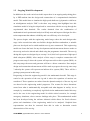
The aim of this report is to deal with the advancements in wind turbine development at
Chalmers University. It forms part of the ongoing research into wind turbine functionality that
is supported by the Swedish Wind Power Technological Centre (SWPTC). This thesis focal
point is on the implementation of instrumentation onto the operational test rig. In this setup
the rig resembles a high speed shaft subsystem unit, simulating the stage of power generation
present in a wind turbine. The design of this development has been conducted using both
academic research and industry leading professionals, highlighting the key direction for its
progression.
ERASMUS students are welcomed to the University of Chalmers openly and excellent effort
and provisions are made to make them feel welcomed to the Swedish educational system. My
appreciation is shown to the professors that helped to get my thesis up a running as well as all
the PHD students that made my time enjoyable. A very special thank you goes to my
supervisors, Professor Dr. Viktor Berbyuk and Lecturer Dr. Håkan Johansson for their ever
continued support and mentoring throughout the project. The author express’s thanks to
Research Engineer Jan Möller whose experience and patience helped my project to progress
smoothly. Appreciation is also given to Saeed Asadi who in addition to being the PHD
research student on this test rig has also become a very good friend during my stay in Sweden.
Gratefulness is given to ABB® and SKF® for their kind contribution to the project, in the
form of frequency controllers, two motors, a range of sensors, Multilog system and
compatible software which will all serve as the mainframe to the test rig.
I would also like to express my gratitude to the staff members at the University of Aberdeen
for making this academic exchange possible and providing the necessary transitional support
that was necessary. My final thanks goes to all of my family and friends back home for giving
me confidence to study abroad and support during my stay.
Göteborg June 2014
Joshua Christopher Squires
CHALMERS, Applied Mechanics, Master’s Thesis 2014:36
III
CHALMERS, Applied Mechanics, Master’s Thesis 2014:36
IV
Contents
Abstract ....................................................................................................................................... I
Preface ...................................................................................................................................... III
Table of Figures ......................................................................................................................VII
1
2
Introduction ......................................................................................................................... 1
1.1
Background .................................................................................................................. 1
1.2
Ongoing Model Development ..................................................................................... 3
1.3
Objective ...................................................................................................................... 4
Hardware Available ............................................................................................................ 5
2.1
3
4
5
6
7
Sensor Choices .......................................................................................................... 10
Software Available............................................................................................................ 11
3.1
SKF @ptitude ............................................................................................................ 11
3.2
Labview ..................................................................................................................... 12
3.3
Matlab ........................................................................................................................ 13
Development Routes ......................................................................................................... 14
4.1
SKF ............................................................................................................................ 14
4.2
National Instruments.................................................................................................. 15
4.3
Both Routes Combined .............................................................................................. 16
Software Development...................................................................................................... 17
5.1
SKF ............................................................................................................................ 17
5.2
Labview ..................................................................................................................... 18
Hardware Connections and Testing .................................................................................. 20
6.1
Motor Controller Connection .................................................................................... 20
6.2
DAQ Connections...................................................................................................... 25
Sensor Testing ................................................................................................................... 31
7.1
Pre-Testing................................................................................................................. 31
7.1.1
Accelerometers ................................................................................................... 31
7.1.2
Displacement Probes and Drivers ...................................................................... 33
8
Hardware Additions: Safety frame and Bracket Arm ....................................................... 39
9
Accelerometer Measurements ........................................................................................... 41
9.1
Accelerometer Robustness Tests ............................................................................... 42
9.2
Accelerometer Response for Varying Motor Speed .................................................. 44
10 Knock Tests ...................................................................................................................... 46
11 Displacement Probe Analysis ........................................................................................... 50
CHALMERS, Applied Mechanics, Master’s Thesis 2014:36
V
12 Shaft Tests ......................................................................................................................... 53
12.1
Shaft end .................................................................................................................... 55
12.2
Mid shaft .................................................................................................................... 57
12.3
Shaft Symmetry Test ................................................................................................. 59
13 Conclusion ........................................................................................................................ 62
15 Future Outlook .................................................................................................................. 64
References ................................................................................................................................ 65
Table of Appendices................................................................................................................. 66
CHALMERS, Applied Mechanics, Master’s Thesis 2014:36
VI
Table of Figures
Figure 1: NREL.......................................................................................................................................... 2
Figure 2: CAD model of test rig ............................................................................................................... 5
Figure 3: ABB motor [5] ........................................................................................................................... 6
Figure 4: ABB ACS355 motor controller [1] ............................................................................................. 6
Figure 5: IMx-P Multilog system [8] ........................................................................................................ 8
Figure 6: SKF displacement probe & driver [9] ....................................................................................... 8
Figure 7: Low sensitivity accelerometer [10] .......................................................................................... 9
Figure 8: High sensitivity accelerometer [10].......................................................................................... 9
Figure 9: NI Compact DAQ [12] ............................................................................................................... 9
Figure 10: SKF software connections .................................................................................................... 15
Figure 11: Full connection schematic .................................................................................................... 16
Figure 12: Final data acquisition Labview VI ......................................................................................... 19
Figure 13: Motor controller connection schematic .............................................................................. 20
Figure 14: Field bus module .................................................................................................................. 21
Figure 15: MTAC-01 module.................................................................................................................. 21
Figure 16: Motor wiring - delta setup ................................................................................................... 21
Figure 17: Encoder connection.............................................................................................................. 22
Figure 18: Encoder- open....................................................................................................................... 22
Figure 19: Encoder- detailing ................................................................................................................ 22
Figure 20: Fully connected motor controller......................................................................................... 23
Figure 21: Wired setup 2 ....................................................................................................................... 24
Figure 22: Compact DAC connecticvity schematic............................................................................... 25
Figure 23: NI9923 module wiring .......................................................................................................... 26
Figure 24:NI-MAX to NI9923 module connection ................................................................................. 26
Figure 25: NI-MAX to NI9923 module testing ....................................................................................... 26
Figure 26: NI9923 module response ..................................................................................................... 27
Figure 27: NI9401 module wiring .......................................................................................................... 27
Figure 28: NI-MAX to NI9401 module connection ................................................................................ 28
Figure 29: NI-MAX to NI9401 module testing ....................................................................................... 28
Figure 30: NI9401 module response ..................................................................................................... 28
Figure 31: NI-MAX to NI9263 module connection ................................................................................ 29
Figure 32: NI-MAX to NI9263 module testing ....................................................................................... 29
Figure 33:Labview motor output control VI .......................................................................................... 30
Figure 34: Three module analysis Labview VI ....................................................................................... 30
Figure 35: Magnetic foot plates ............................................................................................................ 31
Figure 36: Accelerometer connection ................................................................................................... 32
Figure 37: Accelerometer testing VI ...................................................................................................... 32
Figure 38: Accelerometer graphical response....................................................................................... 33
Figure 39: Thandar voltage generator ................................................................................................... 33
Figure 40: Displacement probe and driver wiring ................................................................................. 34
Figure 41: Vertical probe analysis ......................................................................................................... 35
Figure 42: Vertical probe analysis response .......................................................................................... 35
Figure 43: Curvature probe analysis...................................................................................................... 36
Figure 44: Curvature probe analysis response ...................................................................................... 36
CHALMERS, Applied Mechanics, Master’s Thesis 2014:36
VII
Figure 45: Key lock testing setup ........................................................................................................... 37
Figure 46: Key lock testing VI ................................................................................................................ 38
Figure 47: Key lock graphical response ................................................................................................. 38
Figure 48: Virtual bracket arm design ................................................................................................... 39
Figure 49: Actual bracket arm design .................................................................................................... 40
Figure 50: Safety frame virtual design .................................................................................................. 40
Figure 51: 2k sampling rate ................................................................................................................... 41
Figure 52: 10k sampling rate ................................................................................................................. 41
Figure 53: Obtained vertical acceleration data ..................................................................................... 41
Figure 54: Obtained lateral acceleration data....................................................................................... 41
Figure 55: Processed vertical acceleration data .................................................................................... 42
Figure 56: Processed lateral acceleration data ..................................................................................... 42
Figure 57: Motor input - stepped function ........................................................................................... 43
Figure 58: Vertical accelerometer robustness response ....................................................................... 43
Figure 59: Lateral accelerometer robustness response ........................................................................ 43
Figure 60: Vertical accelerometer location response ........................................................................... 44
Figure 61: Lateral accelerometer location response ............................................................................. 44
Figure 62: Knock test Labview VI ........................................................................................................... 47
Figure 63: Knock test 1 .......................................................................................................................... 47
Figure 64: Knock test 2 location ............................................................................................................ 48
Figure 65: Knock test 2 results .............................................................................................................. 48
Figure 66: Knock test 3 location ............................................................................................................ 49
Figure 67: Knock test 3 results .............................................................................................................. 49
Figure 68: Static shaft test results ......................................................................................................... 50
Figure 69: Shaft hand rotation results................................................................................................... 51
Figure 70: Stepped motor input ............................................................................................................ 53
Figure 71: Ramped motor input ............................................................................................................ 53
Figure 72: System prediction 1 diagram................................................................................................ 53
Figure 73: Vertical stepped NE response .............................................................................................. 54
Figure 74: Vertical stepped E response ................................................................................................. 54
Figure 75: Vertical ramped NE response ............................................................................................... 54
Figure 76: Vertical ramped E response ................................................................................................. 54
Figure 77: Shaft end displacement probe ............................................................................................. 55
Figure 78: System prediction 2 diagram................................................................................................ 56
Figure 79: NE shaft response ................................................................................................................. 56
Figure 80: 74.4g shaft response ............................................................................................................ 56
Figure 81: 353.6g shaft response .......................................................................................................... 56
Figure 82: Mid shaft displacement probe ............................................................................................. 57
Figure 83: System prediction 3 diagram................................................................................................ 58
Figure 84:NE shaft response.................................................................................................................. 58
Figure 85: 74.4g shaft response ............................................................................................................ 58
Figure 86: 353.6g shaft response .......................................................................................................... 58
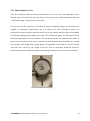
Figure 87: Ironside mechanical gauge ................................................................................................... 59
Figure 88: Shaft misalignment results ................................................................................................... 60
Figure 89: Angular maximum position response .................................................................................. 61
CHALMERS, Applied Mechanics, Master’s Thesis 2014:36
VIII
1
Introduction
1.1 Background
It is imperative that further advancements be made in the field of renewable energy, in
particular when it is extracted from the wind. A wind turbine operates to convert the
potential energy of the wind into mechanical energy that can be used as power. High
levels of research are currently taking place globally, both through academia and
industry, all with a view of improving the lifespan and efficiencies of this conversion
process.
Chalmers University of Technology has conducted research over the past decade into
analysing the wind turbine in many differing ways. Particular attention has been
directed to the impact of vibrations on the dynamics of the turbines operation. This
has led to the development of a mounted modular test rig located in the Vibrations and
Smart Structures Laboratory of the Division of Dynamics at Chalmers.
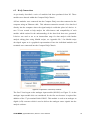
The wind energy market is emerging at a rapid rate both nationally and globally.
Wind power accounted for 32% of the total new renewable power generation installed
within Europe during the year of 2013 [2]. The European Union has already set in
motion strategic plans to raise the share of renewable energy sources in the final
energy consumption of the Union from 8.5% in 2005 to 20% in 2020 [3]. The annual
investments in offshore wind farms averaged 5.5 billion Euros in the year of 2013, an
increase of nearly 750% compared with a decade ago[2]. In the month of March 2014
it was reported that two projects involving the construction total of 326 wind turbines
has been given approval off the coast of Scotland, it will stand as the third largest
wind farm in the world. Expected to provide 2.5GW of electricity which it will deliver
to more than a million homes while creating employment for 4,600 staff and
generating around £2.5 Billion for the Scottish economy [4]. The European Wind
Energy Associations announced in a recent report that Europe was the global leader in
offshore wind energy in 2011 with 90% of the world’s installed capacity. They are
predicting that one quarter of all Europe’s energy could be produced offshore [23].
It is clear that at this rate of development, technological advancements also have to be
made. An advancement that has made considerable progression was developed in
CHALMERS, Applied Mechanics, Master’s Thesis 2014:36
1
response to the vast investments being made, a condition monitoring system that can
assess the performance and reliability of the wind turbines operation through
analysing the dynamics of the system over varying time periods. To operationally
function, sensors are implemented onto and into varying components around the wind
turbine which synchronously relay their data to the monitoring system. This system
then analyses this data and creates performance reports for the technicians. The
motivation for “condition monitoring systems” stemmed from several factors.
Gearboxes in wind turbines have not been achieving their expected design life;
however, they commonly meet and exceed the design criteria specified in current
standards in the gear, bearing, and wind turbine industry as well as third-party
certification criteria. Complete gearbox failures within a wind turbine are not too
common, but are very costly to repair and rectify. This means that if there was a
system that can detect faults at an earlier stage, complete failures can be avoided and
some repairs can be planned ahead of time with minimal downtime, saving money.
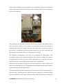
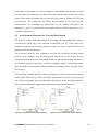
The National Renewable Energy Lab (NREL) located in Colorado is leading the way
in renewable energy initiatives. Funded by the United States Department of Energy
the NREL received $328 million in 2009 [21], of which $55 million was directed
towards the National Wind Technology Centre (NWTC) [22]. This centre is working
towards identifying how gearbox misalignments can affect wind turbines operations
[20]. Figure 1 shows a schematic for their test rig, although there work is on an
international level it is important to highlight that having their research combined into
a condition monitoring system would help alleviate the costly downtime reparation
hours currently incurred across this energy sector.
Figure 1: NREL [21]
CHALMERS, Applied Mechanics, Master’s Thesis 2014:36
2
1.2 Ongoing Model Development
In addition to the work carried out in this report there is an ongoing study taking place
by a PHD student into the design and construction of a computational simulation
model. This model aims to simulate the high speed shaft test rig dynamics with focus
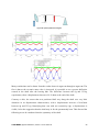
on misalignment analysis. EMC is the three step strategy that highlights how this
simulation model is being developed and its connection with the test rig through the
experimental data obtained. The results obtained from the combination of
mathematical and experimental analysis will help new and improved designs for drive
train components that enhance reliability and cost efficiency to be developed.
The process begins with the engineering model stage where the main design takes
stage. After research into other test facilities designs had been undertaken, a suitable
plan was developed and a scaled modular test rig was constructed. This engineering
model now forms the basis for any developments and advancements that are made on
the test rig and can be altered and edited using the programme Autocad®. The test rig
during this report was designed up to a setup 1 level; this level represents a high speed
shaft subsystem (HSSS). After analysis of this setup is complete construction will
progress onto setup 2 where the system will represent a direct drive system (DDS). At
this setup stage the motor and generator will have a direct connection. Post analysis
design and construction advancements will be made to progress the test rig onto setup
3 whereby the system will represent an indirect drive system (IDS). There will be a
gearing system present in this setup.
Progressing on from the engineering model is the mathematical model. This stage is
crucial to the operation of the test rig and is where the equations of motions are
considered. These equations are taken from the dynamic analysis of the test rig and
are altered as the engineering model progresses. The reasons for these alterations
stems from what is mathematically acceptable and what happens in reality. As an
example, by considering a completely rigid shaft in the mathematical model this may
not be the case in the engineering model in which critical scenarios, for example
emergency shutdown, where extreme loadings take place. This mathematical model
has been developed using the software Adams® which allows for fixed reference
points and simulations of the engineering model to be analysed. Graphical data
representation can then be extracted from this in order to determine certain
characteristics of the test rig.
CHALMERS, Applied Mechanics, Master’s Thesis 2014:36
3
In addition to using the mathematical model it is also important to consider the
computational model. This model forms the basis of the analysis and is used as a data
interpretation process. Using a developed script in Matlab® it is possible to
numerically analyse the response of the mathematical model. It is at this stage that
will depict if the progress made has been successful. If for example the script creates
graphical data that shows erratic behavioural response of the system then it identifies
that alterations need to be made to the engineering model and the whole process
repeated again.
1.3 Objective
The main motivation of this project is to understand the reason why faults and failures
happen within the Drive Train System of a wind turbine and its functional
components including shafts, coupling and gears. Utilising condition monitoring
systems to Detect – Predict – Prevent is one key way to reduce the number of
downtime hours that a wind turbine will face when faults and failures occur. The test
rig is being developed in order to support the advancement of the mechanical models
that can be used to improve existing CMS systems and develop newer and better ones.
This thesis is a continuation in the development of a scaled modular test rig. The
direction is to develop and implement a measurement system, while ensuring that it
delivers data which will be used for model validation and experimental investigation
of the drive train system test rig. This includes the installation of probes, probe
calibration and data acquisition routes setup. The use of tools for data analysis,
experimental investigation of test rig frame response and the investigation into the
assumptions made for previously developed mathematical models will be
incorporated.
CHALMERS, Applied Mechanics, Master’s Thesis 2014:36
4
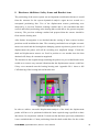
2
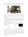
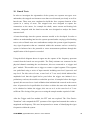
Hardware Available
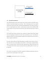
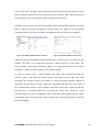
The main hardware at this stage can be considered in groups from three perspective
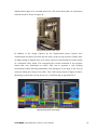
providers, ABB®, SKF® and National Instruments®, see Figure 2 for the labelled
CAD model and physical model.
Figure 2: Details of test rig
ABB® has provided a considerable amount of equipment in donation to the projects
development. A pair of 400V, 3 phase, and 6 pole induction motors act as the motor
and generator in the wind turbine setup, see Figure 3. Capable of delivering shaft
rotational speeds up to 1500rpm they are able to replicate the rotational speeds
experienced with the main frame of a wind turbine [5].
CHALMERS, Applied Mechanics, Master’s Thesis 2014:36
5
Figure 3: ABB motor [5]
These motors are controlled by a pair of ACS355 motor controllers, see Figure 4.
These controllers have been selected for their performance and longevity capabilities.
They have been designed to deliver a range of variable parameters that will enable
intricate analysis of the test rig to take place. Incorporated into this is the ability to
conduct ‘extreme limit testing’, the motor controller has the capabilities to deliver up
to 75Hz to the motor allowing for a rotational shaft speed in excess of 1500rpm [1].
An operational scenario to this effect would simulate an ‘extreme’ condition in reality.
The creation of a “common DC link” between the generator and motor was also
another setup requirement. The concept of this “link” is that the power generated
during the transition from motor to generator can be recirculated back into the motor.
This prevents the need to “energy dump” which usually takes place in the form of
heating resistors.
Figure 4: ABB ACS355 motor controller [1]
CHALMERS, Applied Mechanics, Master’s Thesis 2014:36
6
A fieldbus module acts as a plug-in module that allows for multiple system
connections to be incorporated into the setup [6], see Figure 14. This unit will act to
connect the motor controller with the National Instruments system route. An MTAC01 extension module was also incorporated into the controller; this module serves the
purpose of offering a pulse encoder interface allowing for motor rotational speed to be
measured through data acquisition from the encoder, located on the back plate of the
motors [7], see Figure 15.
Since this report is focussing on the development of the high speed shaft, one motor
and controller is being used.
SKF® also exists as an industrial partner with Chalmers University of Technology
and has equally donated a vast array of instrumentation towards the projects
development. A set of six displacement probes and drivers, two high sensitivity
accelerometers and two standard accelerometers, and all respective cabling were
among the donation package. In addition to the sensors they generously gifted a
Multilog system with corresponding software package (SKF @ptitude Observer®).
Their full contribution forms one of the analysis routes being used within this project.
A six day training and installation package was also offered, this enables Chalmers
Test Rig project users to connect with SKF engineers to fully understand the
installation, maintenance and operational uses of this system.
The IMx-P Multilog system [8] that SKF donated is an adaptable device that is used
by many wind turbine operators around the globe. Also given the pseudonym “black
box”, it is a portable system that is used as an online data acquisition and analysis
system. Containing 16 analog and 8 digital inputs it is a versatile device that assists in
troubleshooting, condition monitoring and vibration analysis, see Figure 5.
CHALMERS, Applied Mechanics, Master’s Thesis 2014:36
7
Figure 5: IMx-P Multilog system [8]
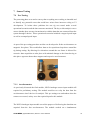
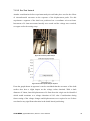
SKF’s donations of 6 * CMSS-65 5mm probes with the 6 * CMSS-665 drivers act as
displacement sensors to the system and can be fitted in any position and direction to
monitor the movements of any metal object [9], see Figure 6. They are contactless and
have a read limit over a distance of 2mm from the measurement surface. They work
using a magnetic field that is created around the surface of the probe, as the target
object encroaches into this field, eddy currents are generated on its surface that
decrease the field strength thus decreasing the drivers voltage output. It is this change
in output voltage that can be graphically represented as the displacement of the
examined member.
Figure 6: SKF displacement probe & driver [9]
In addition to the displacement sensing equipment it is also important to consider the
accelerations that are occurring. To identify the occurrences of these accelerations
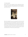
SKF also contributed a pair of CMSS-799LF accelerometers and a pair of CMSS2200 accelerometers. The CMSS-799LF set are highly sensitive, with a sensitivity
level of 500mV/g, ideal for areas of the test rig that may experience small but notable
vibrations, see Figure 8. Meanwhile the CMSS-2200’s are a standard sensor operating
with a sensitivity level of 100mV/g [10] see Figure 7.
CHALMERS, Applied Mechanics, Master’s Thesis 2014:36
8
Figure 7: Low sensitivity accelerometer [10]
Figure 8: High sensitivity accelerometer [10]
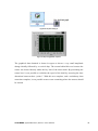
National Instruments® (NI) currently isn’t an active external partner so the hardware
listed was purchased from them using recommendations NI engineers had made. A
Compact Data Acquisition (DAQ) system was used as the data acquisition base with a
number of modules purchased to assist in the data extraction. One digital input/output
module which should be used to relay the digital encoder signals, one analogue output
module that acts as a digital to analogue converter used to carry the analogue motor
controller signals, one analogue input module that acts as an analogue to digital
converter used for the transmission of the analogue encoder signals and finally
another analogue input module that would collate the four accelerometer signals. The
compact DAQ system features an ethernet connection which connects directly into the
computer for signal analysis [11], see Figure 9.
Figure 9: NI Compact DAQ [12]
Although this project features many items from a wide range of companies the main
aim is still clear. To deliver a dual directional instrumented system, incorporating both
the “Black Box” strategy that the SKF offer with the Multilog system, and the “NI
System” strategy incorporating an array of modules and virtual interfaces in Labview,
in order to analyse and assess the overall response of the HSS.
CHALMERS, Applied Mechanics, Master’s Thesis 2014:36
9
2.1 Sensor Choices
A total of ten sensors, including six displacement sensors, two high sensitivity
accelerometers and two standard accelerometers, were received as part of the SKF
donation package. As an initial plan a total of six of these sensors will be used,
leaving the other 4 available for use when the DTS test rig is developed further.
The selection of sensors that were chosen was based on several factors, industrial
recommendations, forming the first factor. It was important to consider all parties in
the decision making process and identifying that the supporting external partners all
specialise in the products that they manufacture. Their ideas were therefore very
important when considering the progression of the test rig through each setup
advancement made.
The next factor for consideration was the usability of the product. Requiring hard
wearing, easy maintenance and reliable equipment was paramount. All equipment
selected had to serve a multiple compatibility role because it was imperative that all
systems could operate simultaneously and synchronously during the data acquisition
process. It was important therefore that the products chosen prevented any data
acquisition conflicts.
The final factor considered was financial. Although two of the operating systems
being used were external partners to the project (ABB and SKF), the third system
produced by National Instruments was not. This meant that as important as key
component selection was, appreciation had to be given to the budget available for this
project.
CHALMERS, Applied Mechanics, Master’s Thesis 2014:36
10
3
Software Available
There are currently three software packages that analyse the system and its responses,
SKF @ptitude, Labview and Matlab.
3.1 SKF @ptitude
SKF @ptitude Observer forms part of a family of condition monitoring systems that
SKF offer under their Windcon branch of operations [13]. The purpose of this branch
within SKF is to extend the life of wind turbines through a number of operational
capabilities. These operations achieve extended turbine longevity through predicting
failures before they occur and by planning more effective maintenance schedules, thus
reducing overall maintenance costs. By implementing sensors inside and around the
wind turbine, data acquisition can take place relating to its operations. This data is
stored and logged in the monitoring system, the IMxP-Multilog, which when
connected with the @ptitude Observer software is capable of tracking many
operational scenarios including gear damage, blade vibrations, misalignment,
lubrication errors and bearing conditions. This @ptitude Observer software is at the
forefront of analysis and has the capability to allow its users access to a fleet of wind
turbines for periodic analysis in any remote location.
Its features include a vast array of analysis techniques, including FFT (fast Fourier
transform) which uses a vibration signal as a function of frequency to identify faults.
Time waveform analysis allows for the detection of waveform signature patterns in
order to avoid error. Another analysis technique that is available is DPE (digital peak
enveloping); this method can be used to detect very small but notable impulses that
are occurring within a noisy environment. These analysis techniques along with all the
others available within the @ptitude Observer software package work in unity to
deliver the highest level of data interpretation and accuracy possible.
In conjunction with the many forms of analysis techniques available there is also a
wide range of user interface displays contained within the Observer software. These
act to graphically display the data either as a live feed or as a post processing
technique. The author has listed several of these capabilities below;
CHALMERS, Applied Mechanics, Master’s Thesis 2014:36
11
Spectra: allows for fault comparison at specific event settings, for example it is
possible to compare the faults occurring on the generator vertical bearing with any of
the other bearings.
History/3D Plots: these methods display the variation in machine condition over time
by allowing the comparison between visualization charts to take place helping to
identify any impending faults.
Orbit/Profiling: these features will play an important role in future work carried out on
this test rig. The concept is that two or three axis sensors can be mounted around a
shaft in order to graphically determine unbalance and alignment problems.
All of these interfaces allow the users to clearly identify faults that occur around the
turbine
in
a
variety
of
scenarios
and
independently
of
one
another.
3.2 Labview
Laboratory Instrument Engineering Workbench (Labview) [14] is a variable platform
analysis software designed and developed by National Instruments (NI). It is
identified as being a visual programming language that’s functionality allows its
operators to perform a variety of control and acquisition operations.
By utilising the data obtained from the bank of sensors located on the test rig,
Labview has the capability to deliver graphical and numerical representations of this
to give a visual understanding of the processes taking place.
The face of Labview is broken down into two interface sections, the first is the block
diagram and the second is the front panel. The block diagram contains the graphical
code used to operate the system, it is within this that modules, functions, terminals
and wiring can take place. The concept is to create an operable system using a variety
of tools that executes sequential operations creating a dataflow from start to finish. A
complete selection of tools are available within the tool palette, it is from here that the
code can be created that incorporates all the necessary terminals, controls, indicators,
acquisition modules, timers and wires to create the VI. The front panel acts as a visual
CHALMERS, Applied Mechanics, Master’s Thesis 2014:36
12
for the block diagram created, it is here that the input and output displays can be
coordinated.
3.3 Matlab
Matlab (Matrix Laboratory) is a software package for numerical analysis with
programming capabilities, used globally for a range of purposes, which was
developed by MathWorks [15]. The use of Matlab within this project will form the
post testing analysis of the data as it is predicted that the data accumulated could far
exceed the computational abilities of other software’s such as Microsoft Excel.
CHALMERS, Applied Mechanics, Master’s Thesis 2014:36
13
4
Development Routes
As previously mentioned the instrumentation development of the project will take the
form of two separate directions. One path follows the SKF system and the other, using
the National Instruments system. Both paths were developed separately in order to
allow for comparison of data analysis when experimental results are obtained.
4.1 SKF
The development of the SKF system began with the installation of the SKF @ptitude
Observer Software onto the system. As previously mentioned, this software forms part
of a network of SKF applications that unify as a monitoring suite. Its purpose is to
provide a platform for engineers globally to conditionally monitor rotating machinery.
This software is a comprehensive analysis package that allows its users to view a
complete overview of the status of the wind turbine [13].
This software required a direct feed into a Microsoft SQL Express Server offering a
10GB storage database for the system.
The final stage of the SKF monitoring system is the Multilog IMx-P On-line System.
Offering 16 analogue inputs and 8 digital inputs, this hardware will allow for
simultaneous data acquisition to take place from the test rig and the sensors located on
this. The hardware along with the @ptitude software package will provide several
enhancing features to the operations of the HSS. The first is a fault detection function
that activates through the use of alarms and warning icons to indicate to the operator
that the system is experiencing dynamic instability. Secondly a fault prevention
function that provides advice on correcting existing or impeding problematic
conditions. Finally they will provide condition based maintenance analysis that will
allow for improved reliability and performance. All of these systems operate
simultaneously to give values for real time operational scenarios.
This route is used by many renewable power operators globally. Having it included in
the operation of the test rig will help to identify key data parameters which can then
be analysed on a secondary level by the National Instruments system.
See Figure 10 for a concise connection diagram of the SKF software listed above.
CHALMERS, Applied Mechanics, Master’s Thesis 2014:36
14
Figure 10: SKF software connections
4.2 National Instruments
The NI measurement system route begins at the sensors, similar to the SKF system,
which are positioned around the test frame. These sensors then deliver the signals
required for analysis from frame vibrations and displacements. This data is fed into a
series of signal splitters that enable a connection to be made into the Multilog SKF
system and also into the Compact DAQ Chassis. This forms the first stage of the NI
route.
The second stage of this route takes place within the Compact DAQ Chassis which
acts as an eight port terminal used in the data acquisitions process. This DAQ has
installed a number of varying acquisition modules and terminals that are all used for a
range of signals acquisitions.
From the Compact DAQ the signal data transport concludes in the software Labview.
The connection between the hardware and software is made using a standard ethernet
cable. It is in this software where all the data calibration and analysis takes place and
it is predicted that similar responses to them found in the SKF @ptitude software can
be achieved.
The software development of both SKF @ptitude and National Instruments Labview
are discussed in a later chapter of this report.
CHALMERS, Applied Mechanics, Master’s Thesis 2014:36
15
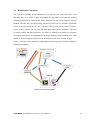
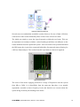
4.3 Both Routes Combined
The reason for running an operational test rig with the two routes that have been
discussed here is to create a fully examinable test rig, which uses both the leading
technology that can be found in the field (Windcon) as well as the indirect analysis
method (NI) that has been specifically tailored for this test rig. Another significant
factor for incorporating the NI route is that the SKF system doesn’t allow for direct
motor control, whereas the NI route has both input and output capabilities, allowing
for motor control and data extraction. The idea is to identify as accurately as possible
the causes and effects of misalignment on the performance and reliability of a wind
turbine in order to identify improvements that can be made to its existing design.
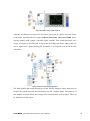
Figure 11 shows a full connection setup diagram that incorporates all three industrial
contributors together.
Figure 11: Full connection schematic
CHALMERS, Applied Mechanics, Master’s Thesis 2014:36
16
5
Software Development
This chapter will focus on the development of the two analysis software packages
available, Labview and SKF @ptitude.
5.1 SKF
Installation of this software began under the supervision of an SKF software engineer
who emphasised the importance of correct installation to avoid any malfunctions
during the operational stages. The data acquired by the monitoring system can stretch
the storage requirements into the gigabytes of data. In order to deal with this
effectively it was recommended that a connection was established with an online
server. Initially due to budgeting restrictions, this server took the form of a free
Express SQL Server provided by Microsoft, this selection was made based on its ease
of accessibility and the 10 GB of storage, per database, available [16]. The
functionality of this allowed for immediate data recovery and a storage system that
could be accessible anywhere and at any time. Once the test rig has reached its final
setup then this server will be upgraded to a premium account with larger storage
capabilities.
Post installation of @ptitude, access was made into the demonstration model account,
this model acts as a template to allow its users to familiarise themselves with the
software. Contained within this model were data sets that had been obtained by SKF
from a BONUS 600kW turbine between the 4th May 2004 and 17th April 2005. This is
a 44m tall turbine with an ABB Async driver unit that has been described as being
one of the industry’s most reliable turbines with over 2,700 operating around the
globe [17]. This demonstration account also allowed the author to develop a better
understanding and knowledge of the software’s operations and how to use the
integrated analysis tools contained within.
As part of the contributions to the development of this project, SKF have made
considerable donations to its progress. As previously discussed a 6 day training
package has been donated that will allow all operators of the test rig to spend 3 days
in the laboratory with an engineering installation team from SKF, once completed a
CHALMERS, Applied Mechanics, Master’s Thesis 2014:36
17
further 3 days will be allocated to the software and data acquisition development.
During this time a team of software engineers will begin the operation of the IMxP
system. Upon training completion the SKF system will be fully functional and
operational.
5.2 Labview
The development of Labview took place over a series of stages due to the level of
complexity required for a full system acquisition. The initial development used was to
develop the Author’s understanding of this software. A basic VI was created
containing a signal simulation and a graphical indicator, the idea was to understand
the data flow using wiring and probes to graphically visualise the simulated signal.
This VI was later enhanced to contain a series of numerical indicators, controllers,
timers and loops. This development helped to intuitively identify more advanced
software operations and highlight key improvement areas.
The idea was to take a systematic and methodical approach to the software
development and so therefore further enhancement in this software occurred
continuously throughout this project. In order to identify these key development areas,
the aim is to systematically discuss these as they took place chronologically during
this project.
One of the very first VI’s created was constructed to allow for the testing of the
accelerometers and displacement sensors. It comprised of a DAQ assistant pair and a
set of waveform graphs that acted as a visual interpretation of the results obtained.
This VI then progressed onto the capability of writing data to a file while extracting
the frequency response of the data obtained. This development occurred as a means of
assessing the motor rotational speed.
It was decided that in order to efficiently select specific rotational speeds for analysis,
an input controller should be incorporated into the VI. The use of a while loop in this
VI also allowed for a continually varying input from the controller to be used.
CHALMERS, Applied Mechanics, Master’s Thesis 2014:36
18
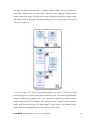
The final development incorporated a “simulate arbitrary signal” into the system and a
third DAQ assistant that was physically connected to the analogue output module
used to control the motor. Having both systems contained within two separate while
loops allowed for both stepped and ramped functions to be used as inputs, the final VI
is shown in Figure 12.
Figure 12: Final data acquisition Labview VI
A series of single VI’s were developed throughout the course of this project that
served the purpose of testing other system parameters. The first one developed had the
purpose of allowing the knock tests to be carried out, containing a DAQ assistant,
trigger and gate and a FFT module. This allowed for the creation of the knock test
graphs seen later in the report. The other single VI used acted as an indicator for the
shaft symmetry assessment that can be found later in this report.
CHALMERS, Applied Mechanics, Master’s Thesis 2014:36
19
6
Hardware Connections and Testing
The connections of the hardware into a the test setup took place over a series of
developments, initially beginning with the testing and connection of the ABB
controller and then progressing onto implementing the National Instruments setup.
6.1 Motor Controller Connection
The ABB ACS355 controller acted as a crucial piece of equipment within the system.
It was therefore important to analyse the capabilities and performance of this
controller before it was implemented into the full system setup. The motor controller
connections are shown in Figure 15: MTAC-01 moduleFigure 13.
Figure 15: MTAC-01 moduleFigure 13: Motor controller connection schematic
To efficiently analyse the controller it was connected into the high speed shaft
subsystem. The controller acted to process the signals and also as the power
transmission from the mains power supply. It was important that it was therefore
installed as instructed in the manual.
For the controller to perform to the requirements of this test rig additional modular
units were required, see Figure 14 Figure 15.
CHALMERS, Applied Mechanics, Master’s Thesis 2014:36
20
Figure 14: Field bus module
Figure 15: MTAC-01 module
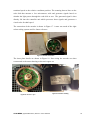
The preliminary wiring of this system began with the installation of power input from
the mains and the power output from the controller to the motor. This wiring took the
form of a quad-core shielded cable which was used to reduce interference from other
neighbouring electrical/mechanical machinery. Figure 16 is an image of the Delta
setup that was required when connecting the power source to the motor.
Figure 16: Motor wiring - delta setup
After the connection of the power to the controller unit the next stage was the
connection of the controller to the motor’s encoder. The Leine-Linde encoder uses
photoelectric scanning on a graduated code disk to deliver dual purpose information
to the controller unit [18]. The information generated can relate to the measured
CHALMERS, Applied Mechanics, Master’s Thesis 2014:36
21
rotational speed or the relative coordinate position. The scanning detects lines on the
code disk that measure a few micrometers wide and generates signals based on
whether the light passes through the code disk or not. The generated signal is then
directly fed into the controller unit which processes these signals and generates a
visual value for shaft speed.
The connection of the encoder is shown in Figure 17. A note was made of the eight
colour coding system used for future reference.
Figure 17: Encoder connection
The inner plate details are shown in Figure 18. Post wiring the encoder was then
reconnected to the motor housing as shown in Figure 19.
Figure 18: Encoder- open
CHALMERS, Applied Mechanics, Master’s Thesis 2014:36
Figure 19: Encoder- detailing
22
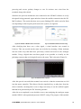
With all the preliminary wiring completed, it was important to focus on the controller
wiring. Figure 20 below shows the wiring of the controller with the power output and
the encoder connected.
Figure 20: Fully connected motor controller
The powering from the mains is shown in the far left connecter and situated next to
this is the power delivery to the motor. As previously described the encoder is
connected into the MTAC module using the same eight colour coded wires noted on
the encoder. An additional connection required that power was also connected from
the controller unit into the MTAC-01 using single core wiring.
The hardware development to this stage was considered an initial phase. This
development allowed for significant testing of the controller including its interface,
pre/programmable features and also its basic operations to be conducted. The motor
could be turned on, speed up/down and stopped in this configuration.
Importance was stressed on the analysis into the performance of the controller unit
and the only achievable way of reaching this was to adapt this current setup to allow a
measurement system to be implemented.
The idea progressed into the connection of an oscilloscope and DC function generator
onto this setup. Connecting the DC function generator allowed for a controlled signal
delivery to take place to the motor via the controller. The DC generator was connected
CHALMERS, Applied Mechanics, Master’s Thesis 2014:36
23
into channel one of the oscilloscope and the encoder input “Sref” (in this instance
Brown) was connected into channel two. It was imperative that the voltage delivery to
the motor remained positive to prevent damage and this was controlled using the DC
frequency generator. Figure 21 shows the setup that was achieved.
Figure 21: Wired setup 2
The hardware development to this stage was a secondary level stepping point. It was
concluded that the frequency controller was very versatile in its usability and
functionality containing a wide range of parameters. The problem that arose from this
setup related to the performance analysis in the oscilloscope. The oscilloscope
contained a very small recordable memory which meant that it was impossible to
justify the performance level from the immeasurable number of encoder pulses
achieved per revolution.
This led to the conclusion that in order to analyse the system fully, the next step was
to develop and run this operational scenario from a Labview VI programme. This
would allow for an infinite recording time and a greater accuracy when analysing the
controllers’ performance. Before this was carried out it was important to consider the
other hardware that was going to be used in conjunction with the motor controller,
such as the Compact DAQ.
CHALMERS, Applied Mechanics, Master’s Thesis 2014:36
24
6.2 DAQ Connections
As previously described a series of modules had been purchased from NI. These
modules were housed within the Compact DAQ Chassis.
All four modules were connected into the Compact DAQ were then connected to the
computer using an Ethernet cable. This ethernet connection created a live data feed
directly into the computer where the signal analysis could take place in Labview. A
new VI was created to help analyse the effectiveness and compatibility of each
module which assisted in the understanding of the data feeds that were generated.
Labview was used to act as an intermediate stage for data analysis with further
analysis taking place using Matlab scripts, see Appendix file 3 for Matlab script
developed. Figure 22 is a graphical representation of how the individual modules and
terminals were connected into the Compact DAQ Chassis.
Figure 22: Compact DAC connecticvity schematic
The first VI test began on the analogue input module (NI9205) see Figure 23. As the
analogue input module this was considered for the first test because it required the
addition of the 37 pin terminal block NI9923. This module is used as an analogue to
digital (A/D) convertor which is used to deliver the analogue sensor signals into the
analysis software.
CHALMERS, Applied Mechanics, Master’s Thesis 2014:36
25
The aim of this initial test was to deliver a signal from the DC generator into the NI
9923 terminal block, through the A/D convertor module, into the compact DAQ and
then to Labview where the signal could be verified and visually displayed.
Figure 23: NI9923 module wiring
Terminal 29 (black wire) was connected to the ground port on the DC generator and
terminal 2 (red wire) was connected to the +Ve port. The system was delivered with
100Hz from the generator, see Figure 23. The testing was now able to progress onto
the Labview stage.
Initially using National Instruments Measure and Automation Explorer (NI-MAX)
software the author was able to test the overall setup for signal delivery. This showed
a successful signal delivery from all devices connected in the loop. Figure 24 below
shows the module connection into the NI-MAX software and Figure 25 shows the
first basic “on-off” test explored.
Figure 24:NI-MAX to NI9923 module connection
Figure 25: NI-MAX to NI9923 module testing
After clarifying that there was a clear signal a visual interface was created in Labview.
Using a while loop, DAQ assistant and a waveform graph it was possible to visually
interpret the signal that was being sent from the DC generator to the Compact DAQ
and through the use of a while loop, this meant the data acquisition was continuous, so
CHALMERS, Applied Mechanics, Master’s Thesis 2014:36
26
the graph acted as a “live feed” when the frequency was altered. Figure 26 shows this
result:
Figure 26: NI9923 module response
After this test proved to be a success analysis into the NI9401 module was made.
Similar to before this module also had the addition of a 25 pin terminal block NI9924.
The module will be used to deliver the digital encoder signals into the analysis
software.
The purpose of this second test was to test the digital signal flow of the system. This
terminal block and module would be used in connection with the encoder so its
operation was vital to analyse the motors operation. The wiring for this module is
shown in Figure 27.
Figure 27: NI9401 module wiring
This module was also connected to the DC frequency generator which was used to
deliver the same signal that the analog module was receiving. The terminal line DIO0
terminal 14 (green) was connected to the +Ve port of the generator and COM terminal
1 (yellow) was connected to the ground port of the generator. Before the two wires
were connected into the terminal it was important to protect the system from over
CHALMERS, Applied Mechanics, Master’s Thesis 2014:36
27
powering and reverse polarity changes so two 1k resistors were wired into the
terminals along with a diode.
Similar to the previous method this was connected to the NI-MAX software to verify
the signals being generated, Figure 28 below shows the module connection into the NIMAX software. The results this time was a green flashing LED, which varied in flash
rate depending on the frequency delivered to the system, see Figure 29
Figure 28: NI-MAX to NI9401 module connection
Figure 29: NI-MAX to NI9401 module testing
After clarifying that there was a clear signal, a visual interface was created in
Labview. This was carried out the same was as before by inserting a DAQ Assistant
into the while loop that had been previously created and used for the analogue
module. Using a digital data waveform graph it was possible to visually see the
pulsating response that was being delivered to the setup. This is shown in Figure 30.
Figure 30: NI9401 module response
After this proved successful the terminal was rewired so that the connection was fed
into the motor controller. This allowed for the signal delivery to take place from the
motor controller, meaning that it was no longer necessary to use the artificial signals
that had been generated by the DC function generator.
After this was completed it was decided to move onto analysing the analogue output
module NI9263 with operational protector NI9927 casing. The purpose of this module
CHALMERS, Applied Mechanics, Master’s Thesis 2014:36
28
was to deliver the analogue motor controller signals from the analysis software to the
motor controller which in turn was connected to the encoder. This could be described
as allowing the user to control the motor operation from Labview.
Similar to the previous cases this was initially tested in the NI Max software to clarify
that the signal was active through the Compact DAQ. See Figure 31 for the module
connection into the NI-MAX software and Figure 32 show the first test conducted.
Figure 31: NI-MAX to NI9263 module connection
Figure 32: NI-MAX to NI9263 module testing
After this clarification another DAQ Assistant was created to act as a control for this
module. This time it was required to generate a signal to deliver to the motor. The
idea was that in delivering an analogue signal as an output from Labview it would be
possible to visually see the response of the motor rotating.
In order to achieve this, a signal module and slider were incorporated into the
Labview while loop which was then wired as the data feed into this new DAQ
Assistant. The decision for this was to deliver a variety of signals from this module to
the motor. Altering the wave type, frequency, amplitude and offset were just some of
the variations that could be used as inputs to the motor. Before the signal was fed into
the data feed a waveform chart was wired into the circuit, this allowed a visual
representation to be given in addition to the visual and audio changes that the motor
was making. Figure 35 shows this visual response and virtual wiring that was used in
the block diagram.
CHALMERS, Applied Mechanics, Master’s Thesis 2014:36
29
Figure 33:Labview motor output control VI
After this test had proved successful a decision was made to replace all of the inputs
to the DAQ Assistant shown in Figure 33Error! Reference source not found. above
into this module with a single “simulate signal” module. This would then allow for a
variety of signals to be delivered to the motor including saw tooth, square and sine
waves. Figure 34 is a photo showing the combined VI in Labview used to test the first
3 modules.
Figure 34: Three module analysis Labview VI
The final module that required analysis was the NI9234 analogue sensor input used to
transfer the signals from the accelerometers into the Compact DAQ. The analysis of
this module occurred during the testing of the accelerometer sensors phase. This can
be found later in this report.
CHALMERS, Applied Mechanics, Master’s Thesis 2014:36
30
7
Sensor Testing
7.1 Pre-Testing
The pretesting phase was used to survey that everything was working as intended and
to identify any potential errors that could have arisen from incorrect wiring or VI
development. To isolate these problems the test rig was tested under several
operational scenarios and the data outcome monitored. The key to this analysis was to
assess whether there was any inconsistencies with the data that was extracted from the
system through Labview. These operational scenarios included a stepped speed input
as well as a ramped speed input.
As part of the pre-testing procedure an idea was developed to fit the accelerometers to
magnetic foot plates. This would allow them to be repositioned anywhere around the
rig during testing. By allowing for relocations around the test frame it allowed for
extensive data acquisition to take place with minimal damage to the frame having to
take place. Figure 35 shows these magnets and respective accelerometers.
Figure 35: Magnetic foot plates
7.1.1 Accelerometers
As previously discussed the final module, NI9234 analogue sensor input module still
required its preliminary testing. The module would act to relay the data from the
accelerometers into Labview for analysis. This pre-testing was undertaken when the
sensors were tested, as they were the required input for this module.
The NI9234 analogue input module served the purpose of delivering the data that was
acquired from the four accelerometers. The module worked on a simultaneous
CHALMERS, Applied Mechanics, Master’s Thesis 2014:36
31
acquisition level from the four sensors, meaning that all data was collated in the same
instance.
For this pre-test of this module a CMSS 2200 Standard Accelerometer was attached to
a magnetic foot and was connected into the module using one of the CMSS 932
cables. The author decided that because this was a testing stage that it was important
to maximize the vibrations, so a lateral hand movement was made to ensure that large
vibrations were achieved. A photo of this connection is shown in Figure 36.
Figure 36: Accelerometer connection
Unlike previous test procedures, this setup didn’t require an NI Max pre-state test,
instead a new DAQ Assistant was wired into the while loop as with similar cases.
This was then linked to the physical channel “ai0” which was the connection port
located on the module, the configuration method was for acceleration responses and a
waveform graph was wired into the assistant. This configuration is shown in Figure 37.
Figure 37: Accelerometer testing VI
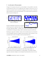
The system was then initiated and the VI was run to acquire the data feed, the
accelerometer was held and moved laterally at a rapid rate. The idea behind this was
to maximise the vibrations within the accelerometer, this would then accentuate the
graphical representation.
After this had been conducted, the magnet was positioned on the foot plate of the
motor. This was now an area of significantly lower vibrations compared to the hand
CHALMERS, Applied Mechanics, Master’s Thesis 2014:36
32
movement, so it was crucial to test how responsive the accelerometers were. The
graphical data that was fed back is shown in Figure 38.
Figure 38: Accelerometer graphical response
With all modules having been tested on the National Instruments setup it was time to
progress onto testing the SKF probes and displacement sensors.
7.1.2 Displacement Probes and Drivers
In order to assess the usability and effectiveness of the displacement sensors it was
decided that they should be tested in a controlled scenario where all factors could be
monitored. The process of this preparation is listed below.
Development began with the wiring of the probe to the driver and to the voltage
generator. The driver required a voltage of 24V, since none of the other systems
operated with this voltage, a generator was required. Figure 39 shows this unit.
Figure 39: Thandar voltage generator
The unit was set to deliver a voltage of 24V and a current of 0.12 amps; this was the
required current to overcome the impedance of the system. The positive and negative
terminals of this generator were then connected to the driver ports. The negative
terminal wired to the -24V port and the positive terminal to the GND port. With the
driver now receiving the required voltage it was time to consider the wiring into the
Compact DAQ.
CHALMERS, Applied Mechanics, Master’s Thesis 2014:36
33
The operating voltage limit for the Compact DAQ was 10 Volts so it was important
that the voltage was stepped down before being connected into the DAQ. Using a
voltage divider rule from Ohms Law, see equation 1, was the way of achieving this.
(𝐸𝑞𝑛 1)
𝑉𝑜𝑢𝑡 = 𝑉𝑖𝑛 ∗
𝑅2
𝑅1 + 𝑅2
Knowing that a Vout value of greater then 10V couldn’t be exceeded, a 15kΩ and
10kΩ were wired in series with the two output terminals. This would allow the 9.6V
input to the Compact DAQ to be achieved. See Figure 40 for the wiring.
Figure 40: Displacement probe and driver wiring
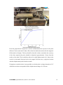
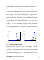
7.1.2.1 Pre-Test Vertical
In order to better understand the probe response, a test was carried out that varied the
probe displacement whilst recording the voltage obtained. This was undertaken to
help identify the response of a probe to movement through its magnetic field in the
vertical direction. The results of this could then be used to assess at which
displacement the most accurate data acquisition would occur. Figure 41 shows this
testing setup.
CHALMERS, Applied Mechanics, Master’s Thesis 2014:36
34
Figure 41: Vertical probe analysis
Figure 42: Vertical probe analysis response
From the graph shown in Figure 42 it can be concluded that the response of the probe
follows a linear trend until 2.4mm offset when the shafts interaction with the magnetic
field started to dissipate. The key identifier from this is that to maximise the accuracy
of the data acquired the probe should be displaced approximately 1.2mm from the
surface of the shaft. This would then allow for a shaft displacement of ±1.2mm in the
vertical or horizontal direction before the magnet field was lost, or physical contact
with the displacement probe head was made.
Using these recorded values it was possible to calculate that a voltage alteration of 1V
within the test data corresponded with a displacement change of 0.361mm.
CHALMERS, Applied Mechanics, Master’s Thesis 2014:36
35
7.1.2.2 Pre-Test Lateral
Another consideration before experiment analysis could take place was for the effects
of circumferential curvature on the response of the displacement probe. For this
experiment a segment of the shaft was positioned on a coordinate axis test frame.
Increments of 0.1mm movement laterally were made and the voltage was recorded,
see Figure 43 for the testing setup.
Figure 43: Curvature probe analysis
Figure 44: Curvature probe analysis response
From the graph shown in Figure 44 it can be concluded that the curvature of the shaft
surface does have a slight impact on the voltage values obtained. With a shaft
diameter of 30mm, lateral displacements of 0.5mm from the origin can be identified
which would constitute to a voltage alteration of 0.03 volts. Consideration during
future testing of the voltage changes and displacements were required to see if these
correlated to any significant alteration in the shafts lateral positioning.
CHALMERS, Applied Mechanics, Master’s Thesis 2014:36
36
7.1.2.3 Key Lock Test
With the preliminary tests now completed it was time to install the probe onto the
DTS setup to test its usability. Using the following setup of brackets and magnets it
was possible to get the probe to be positioned within 1.2mm of the rotating shaft.
Figure 45 shows this setup.
Figure 45: Key lock testing setup
With all of the equipment now into its correct wiring state, the software setup could
then be altered to allow for correct data acquisition. The first step was to alter the
existing analogue input module two DAQ Assistant to allow the flow of data through
the system. The internal settings of this were altered so that the data acquisition could
take place from “ai3” which was the channel line this sensor had been wired into. The
rest of the Labview setup was left at its current state. The reason for this was that
existing graphs could be used to perform the same visualisation response as was used
on previous module tests. The Labview setup is shown in Figure 46.
CHALMERS, Applied Mechanics, Master’s Thesis 2014:36
37
Figure 46: Key lock testing VI
Figure 47: Key lock graphical response
The graphical data obtained is shown in Figure 47 shows a very small amplitude
change initially followed by a vertical drop. The reason behind this was because the
sensor was located directly under the key lock of the motor shaft. By positioning the
sensor here it was possible to calculate the speed of the shaft by assessing the time
alterations between these “pulses”. With this test complete, and a satisfactory data
extraction complete, it was possible to move onto examining where the sensors should
be located.
CHALMERS, Applied Mechanics, Master’s Thesis 2014:36
38
8
Hardware Additions: Safety frame and Bracket Arm
The positioning of the sensor system was an important consideration because it would
form the structure for the system dynamical analysis. Figure 48 was created as a
conceptual positioning idea. Two of the displacement sensors positioning were
analysed by a previous Erasmus exchange student and it was concluded that their
vertical and lateral positioning at the bearing hub would deliver the greatest response
accuracy. The previous exchange student had proposed that the sensors should be
fixed onto the bearing unit.
After further investigation it was decided that the seating of these sensors in these
positions would invalidate the data. The reasoning concluded was as higher eccentric
masses are tested and the bearing house damping system experiences greater levels of
displacements the probes will still be recording zero amplitude change. If both the
shaft and displacement sensors are fixed in position to one another then the data
obtained will always be constant in magnitude.
The alteration to the original design, attaching the probes to a pre-welded bracket arm,
would act to remove any external vibrations that the displacement sensors could face
if they were mounted onto the bearing housing unit. Appendix file 1 shows a full
CAD drawing of the bearing hub and bracket arm.
Figure 48: Virtual bracket arm design
In order to achieve successful displacement analysis of the shaft, the displacement
probes will have to be positioned within the 2mm required range specified on their
data sheets. In conjunction with the Vertical test that had been previously undertaken
it was concluded that a 1.2mm positioning from the shaft would allow for the widest
CHALMERS, Applied Mechanics, Master’s Thesis 2014:36
39
displacement ranges to be recorded effectively. The actual frame that was constructed
from the model is shown in Figure 49.
Figure 49: Actual bracket arm design
In addition to the design required for the displacement probes bracket arm,
consideration also had to be made into the safety of the test rig operators. With a mass
of 20kg rotating at 900rpm there were safety concerns created which led to the design
of a structural safety frame. The conceptual idea created consisted of two separate
frames that were positioned on rollers. This was to generate a safe working
environment whilst allowing maintenance and alterations to be made to the test rig
easily by sliding the casing on its rollers. The CAD concept shown in Figure 50 shows
the design created; this can also be seen as a CAD drawing in Appendix file 2.
Figure 50: Safety frame virtual design
CHALMERS, Applied Mechanics, Master’s Thesis 2014:36
40
9
Accelerometer Measurements
Using the VI developed, discussed in a previous chapter, it was possible to extract the
raw data that the sensors were recording from the responses of the test rig. As an
initial test assessment into the acquisition sampling rate (Hz) was made, to determine
what would deliver the best data representation. The results from this experiment are
shown in Figure 51 and Figure 52.
-3
x 10
Acc sensor 3
Acc sensor 3
0.05
5
0
-5
0
-0.05
-10
20.538 20.54 20.542 20.544 20.546 20.548 20.55 20.552 20.554 20.556
time (s)
20.538
20.54
20.542
20.544
time (s)
20.546
20.548
20.55
Figure 52: 10k sampling rate
Figure 51: 2k sampling rate
In Figure 51 and Figure 52 an increase in acquisition rate from 2k to 10k is shown. This
alteration generates a significant improvement in the validity of the results, instead of
the signal appearing random; a periodic wave form can be identified. It could be
concluded that all subsequent testing would be undertaken using the 10,000 Hz rate.
Identifing an appropriate method to analyse the data obtained by the accelerometers
was also important. Figure 53 and Figure 54 show the plots of the raw data as it was
recorded from the sensors in both the vertical and lateral directions.
Figure 53: Obtained vertical acceleration data
Figure 54: Obtained lateral acceleration data
The very first analysis method calculated, the Root Mean Square (RMS), is a
statistical measure into the magnitude of a varying quantity. The problem with this
approach was that the readings were becoming heavily distorted by the noise level on
CHALMERS, Applied Mechanics, Master’s Thesis 2014:36
41
the system, higher orders of vibrations from the motor were exciting the eigenmodes
at higher frequencies. This should have been visible in the RMS results however the
general noise was “blurring” the response.
As a secondary analysis method the Frequency Response Function (FRF) was taken,
the results are shown in both the vertical (Figure 55) and the lateral (Figure 56)
directions. This is the response of the system for a specific frequency and is a type of
transfer function, i.e. input to output relation as a function of excitation frequency.
The specific frequency corresponded to the motor input frequency. Eigenmodes, i.e.
resonances, are particularly sensitive, and are seen as spikes or mountains in the FRF.
Excitation at such frequency is expected to give large vibrations (steel frame = low
damping), which can affect the sensors or the whole system, if there is little noise in
the signal, and there is a pronounced eigenmode. The problem is likely that the
excitation is not just a single frequency. It probably contains many different
frequencies, and the sensors pick up different kinds of noise. An alternative to the
stepped function input that acts as a frequency sweep is to have a wide-spectrum
excitation, also known as a “knock test”, this will be discussed in a later chapter.
2.5
x 10
Vertical at hub
-3
Lateral at hub
0.02
2
0.015
H((f))
H((f))
1.5
0.01
1
0.005
0.5
0
0
200
600
400
Angular Velocity (RPM)
0
0
800
Figure 55: Processed vertical acceleration data
200
400
600
Angular Velocity (RPM)
800
Figure 56: Processed lateral acceleration data
9.1 Accelerometer Robustness Tests
Before full operational testing was carried out it was important to consider the
accelerometers abilities and performance capabilities. It was important to assess the
performance of the accelerometers under varying operational scenarios, including
relocations and disturbances. It was from this that a series of sensor robustness checks
were undertaken. A stepped function, shown in Figure 57, was delivered to the test rig
CHALMERS, Applied Mechanics, Master’s Thesis 2014:36
42
as the operational scenario using a predefined VI developed in Labview and all
analysis was then conducted using Matlab.
Figure 57: Motor input - stepped function
A preliminary set of tests were conducted that sought to identify the robustness of the
accelerometers. An input of a twenty stepped function from 100rpm to 900rpm was
inputted to the system and varying disturbances were made on the accelerometers.
The first set of results indicated as ‘Orig data’ in Figure 58 and Figure 59 below acted
as a base set of values for the next tests. The second test that was undertaken aimed to
identify the implication of a disturbance to the sensors. All sensors were lifted and
repositioned in the same locations as they were for the first test. The recorded data is
plotted as ‘Replace’ in Figure 58 and Figure 59. The third test that was carried out
aimed to identify whether there was any noticeable difference in the recording
capabilities between the high sensitivity (500mV/g) and low sensitivity (100mV/g)
sensors. All three tests had data recorded in the lateral and vertical direction and the
recording sensors where positioned on the top and side of the bearing hub.
Figure 58: Vertical accelerometer robustness
response
Figure 59: Lateral accelerometer robustness response
CHALMERS, Applied Mechanics, Master’s Thesis 2014:36
43
From Figure 58 and Figure 59, a close correlation is identifiable from the data recorded
over the series of preliminary tests show. There are small deviations in the lower rpm
values on the lateral recording however the two focal points at 600rpm and 780 rpm
are consistent. The preliminary test allows the conclusion to be made that the
accelerometers are recording very similar data as one another and that a full
disturbance (such as removal and replacement) had very little alterations to the
recording effectiveness.
9.2 Accelerometer Response for Varying Motor Speed
The next set of tests undertaken aimed to investigate the data comparison between
accelerometers when they were positioned around the test rig. These tests were
conducted using the pair of high sensitivity sensors, one in the vertical direction and
the other in the lateral direction.
The prediction made for this experiment was that the vibrations recorded would
decrease as the distance from the bearing hub was increased. The reason for this
expectation stemmed from the idea that the shaft is contacting the bearing hub first, so
all vibrations originate from there. Another assumption drawn is that objects shake
more the further away from their point of fixation, particularly if they are light, which
the test rig is.
The first data recorded had the sensors positioned on the vertical and horizontal
bracket arms of the test rig. These were then repositioned the sensors on the top and
side of the bearing hub, before moving them onto the test frame and finally onto the
table. The data obtained is graphically represented in Figure 60 and Figure 61.
Figure 60: Vertical accelerometer location response
Figure 61: Lateral accelerometer location response
CHALMERS, Applied Mechanics, Master’s Thesis 2014:36
44
By analysing the results of the lateral direction data first, it can be identified that the
hypothesis made was accurate. Higher accelerations are visible on the bracket arm and
the smallest accelerations were recorded on the table. Controversially the data
measured in the vertical direction, only matches the hypothesis made up to 600rpm.
Beyond this value it is clearly identifiable that a reverse in the predictions made
occurs with the highest accelerations being found at the test frame and table with very
small recorded values being obtained on the bracket arm and the bearing hub.
An explanation for these results could be drawn from the excitation force that is being
applied to the system. In the vertical direction a presumption can be made that the
excitation force is no longer from the shaft and is in fact from the motor itself. This is
located on top of the test frame which is then connected to the table before its
connection to the bearing hub. This first connection to the table could be acting as a
nodal point creating the next highest recorded amplitudes on the table, after the
vibrations have transferred through the system to the bracket arm and bearing hub
they have reduced significantly in amplitude.
It can be concluded from the tests, that the sensors all perform to a similar
performance level despite the clear differences in sensitivity ratings. It can also be
suggested that the location choices of these sensors with respect to their sensitivity
levels can be ignored. Consideration however, must be given to the data recorded in
the vertical direction in future tests.
CHALMERS, Applied Mechanics, Master’s Thesis 2014:36
45
10 Knock Tests
In order to investigate the eigenmodes of the system, two separate test types were
undertaken, the stepped accelerometer tests that were discussed previously as well as
knock tests. These tests were conducted to build the force response function of the
system in a variety of areas. The stepped tests were designed to capture the
connections to the motor, for example the shafts, motor mount and bearing hub
structure, compared with the knock tests that were designed to analyse the frame
structure itself.
A better knowledge into the systems structure needed to be developed. In order to
achieve an understanding into how the system operated under varying cyclical loading
tests a series of knock tests were undertaken to analyse the systems eigen frequencies.
Any eigen frequencies that are contained within the structure and are excited by
system in balances have the potential to cause measurement problems through the
amplification of the frequencies recorded.
Using the block diagram shown in Figure 62, the capture of the frequency spectrum
created from the knock test was possible. The DAQ assistant was connected to the
physical channel containing the accelerometer, this was connected to a “trigger and
gate” module. This module uses a trigger to extract a signal segment. This segment
was predefined using a series of input controls including start level, hysteresis and
stop level. For this series of tests, a start level of 5 was used, which indicated the
amplitude level that the signal had to pass before the trigger was initiated. As a
preliminary read out, the module recorded the previous 10 samples before the trigger
opened, this was used as a visual validation that initiation had occurred at the correct
time. A hysteresis level specified the level above or below the start value that needed
to be obtained to initiate the trigger; this was set to 0 as the start level of 5 was
sufficient. The closing of the gate was set using the sample number required of 1000.
After the Trigger and Gate module, the FFT unit was explored. The “Fast Fourier
Transform” unit computed the FFT spectrum of the signal and returned the results as
magnitude and frequency. This was incorporated as a means of identifying the eigen
frequencies within the system.
CHALMERS, Applied Mechanics, Master’s Thesis 2014:36
46
Figure 62: Knock test Labview VI
Several tests were undertaken around the system, however for ease of data collection,
a discussion of the results obtained by three of these tests will now be made.
The initial test aimed to assess the eigen frequencies within the test frame. This was
an important test to analyse whether vertical bending would have an influence on the
results obtained from the operational system. An accelerometer was positioned behind
the HSS motor the rig was then contacted behind the disconnected motor allowing for
a full test frame analysis. The results from this experiment are shown in Figure 63.
Figure 63: Knock test 1
The action of the motor engaging will deliver a range of frequencies into the system
from 0Hz to 50Hz. It is identifiable from the Figure 63 that there is no notable
eigenmodes recorded at these frequency levels and therefore no concern about the
system being excited by the bending of the frame.
CHALMERS, Applied Mechanics, Master’s Thesis 2014:36
47
The second test undertaken was an analysis into the eigen frequencies contained
within the bearing hub and their effect on future acceleration tests on the bracket arm.
Figure 64: Knock test 2 location
Figure 65: Knock test 2 results
Similar conclusions can be drawn to the first test carried out, in that the eigen
frequencies obtained are far higher than the motor delivery frequencies.
The third and final test carried out followed a similar strategy to the second test.
Understanding needed to be made into the eigen frequencies contained within the
bearing hub in order to identify their effects on acceleration recordings made on the
vertical bracket arm. Figure 66 is a photograph identifying the positioning and the
point where impact was made; a yellow ring highlights the accelerometer location.
The graphical results obtained are shown in Figure 67.
CHALMERS, Applied Mechanics, Master’s Thesis 2014:36
48
Figure 66: Knock test 3 location
Figure 67: Knock test 3 results
Having eigen frequencies that exceeded the motor output level meant that there was
no excitation occurring. The values obtained relate very closely to the second test
conducted on the horizontal bracket arm. Under a “perfect” sinusoidal motor, one
main eigenmode should be notable, it is however important to identify that the motor
will exhibit certain overtones that can be integer multiples of the excitation. These
corresponding to motor speed, creating these higher order frequencies required to
excite the frame eigenmodes >750 Hz.
As a conclusion to the results obtained and all the other tests carried out, it can be said
that the frame is stiff enough so that it is free from low frequency eigenmodes,
therefore no impact will be made on the experimental results obtained.
CHALMERS, Applied Mechanics, Master’s Thesis 2014:36
49
11 Displacement Probe Analysis
The results from the previous tests involving the accelerometer responses and knock tests
were a way of ensuring that the displacement sensors would give reasonable results with little
influence from other factors. The data obtained from the displacement probes would be used
in the evaluation of the computational model so the analysis of the displacement probes
formed another key evaluation area. The preliminary tests were developed in order to enhance
the understanding of what was actually happening at the displacement sensors.
These series of tests were designed to analyse the effectiveness of the voltage displacement
probes. With the results obtained, analysis could then be made into the contribution of noise
of the system under various operational scenarios.
After the results of the vertical probe test, discussed in a previous chapter, were analysed, it
could be concluded that an alteration in the voltage reading of 1V corresponded to a
displacement of 0.361mm for the shaft. The first test undertaken was a static shaft test, with
the aim of highlighting what voltage alterations could be associated with system noise. Noise
on a static shaft system would still correspond to displacement values being obtained.
The first test scenario ran for 20 seconds and the displacement probes recorded all the data
relating to a static shaft. The results are shown in Figure 68.
Figure 68: Static shaft test results
When analysing this data in Matlab, a command was used that plotted the sliding average.
This method took a sliding average for the data points and could be used as a technique of
CHALMERS, Applied Mechanics, Master’s Thesis 2014:36
50
removing the noise from the system. An appropriate value for this plot was to use an N-Slide
value of between 25 and 50. It was deduced from other assessments that a value <25 then
noise still dominated the signal response and a value >75 lost the signal detailing. A value of
50 was used in all subsequent analysis so that each data point in the displacement data was
replaced by the mean of the 50 preceding recorded points and 50 subsequent points. This
value of 50 corresponds to 0.005 seconds which relates to the sampling rate of 10,000 per
second (10k). If the value of sampling rate is altered then the value of n-slide will also need to
be altered, for example a 1k sample rate would require the n-slide value to be changed to 5.
I also calculated the standard deviation, which is the spread from the sliding average values
for a series of data, the smaller the value the greater the central tendency meaning that the
data is concentrated around mean, the higher the value the greater spread of data. The results
from this static test show a small value indicating that the data is concentrated around the
mean. The response from the graphical data presented in Figure 69 is that noise on the system
accounts for roughly 40 mV alterations (standard deviation = 6 mV) in the X-axis
displacement probe and around 30mV (standard deviation = 5 mV) in the Y-axis displacement
probe. It is expected that the “visual noise” level and the standard deviation values should be
proportional.
A second test was developed as an identifier to see if very slow rotation on the shaft would
have an effect on the noise experienced on the system. The shaft was hand rotated three times
over a period of 25 seconds and the data recorded. Matlab analysis generated the graphical
data shown in Figure 69.
Figure 69: Shaft hand rotation results
The graphical data shown in Figure 69 identifies that the voltage alterations appear similar in
magnitude to the static shaft test performed previously. Noise represented alterations of
CHALMERS, Applied Mechanics, Master’s Thesis 2014:36
51
around 50mV in the X-axis (standard deviation = 8.8 mV) and 35mV in the Y-axis (standard
deviation = 13.1 mV). The standard deviation results were not as expected and did not agree
with the predictions that were made about the proportionality increase from the previous
experiment.
The series of further test were undertaken with the priority to identify how much noise was
accountable by a motor that had brakes engaged. A motor that had the brakes applied gave the
same response scenario as a static shaft but with the addition of noise interference from the
motors electrical cabling. The results obtained indicated a significantly larger noise level on
the system with the motor incorporated into the system. Observing displacement voltage
readings of around 150mV in both axial directions identifies that an approximate addition of
100mV of noise has been added into the system by the introduction of a braking motor.
The final noise analysis test acted as a combination test where the shaft was being slowly
driven by the motor. This incorporated aspects of the still shaft, braking and rotation into one
experiment. The Labview VI controlled the motor to spin at one revolution per fifteen
seconds, while the data was being acquired. In this instance an addition of approximately
150mV has been added into the system on top of the static motor noise by having the
inclusion of shaft rotation.
The outcome of these experiments is that the factoring of noise into the results must be
actively considered within the data analysis phase.
CHALMERS, Applied Mechanics, Master’s Thesis 2014:36
52
12 Shaft Tests
After the completion and analysis of the static tests, it was time to test the rig under an
eccentric load conditions. The eccentric (E) load conditions were developed in parallel to the
computer model development, allowing for both the model and reality to be compared
together.
The initial test consisted of two inputs to the system, a stepped function and a ramped
function. Both tests together would cover a wide range of operation scenarios that could be
present on an operational wind turbine out in the field. These inputs are graphically displayed
in Figure 70 and Figure 71 below.
Figure 70: Stepped motor input
Figure 71: Ramped motor input
The stepped function was created with a stepping time of 5 seconds creating a total run time
of 110 seconds. The ramps were predetermined to allow a range of gradients to be achieved.
They all ran from 0rpm to 900rpm with a transit time of 20 seconds, 10 seconds and 5 seconds
respectively and a trail time of 10 seconds.
The hypothesis from this test was based on the same hypothesis used in the design of the
computational model. That the system behaves with a rigid shaft and a damping spring system
that operates in the bearing hub. Figure 72 gives a visual interpretation of this prediction.
Figure 72: System prediction 1 diagram
The first test was the 20 step function initially with no eccentricity (NE) followed by an
eccentric (E) mass of 74.4g added to the system. The results were recorded for both the X-
CHALMERS, Applied Mechanics, Master’s Thesis 2014:36
53
Axis displacement probe as well as the Y-Axis displacement probe. For analysis purposes
consider the Y-axis displacement probe shall be considered. NE is shown in Figure 73 and E in
Figure 74.
Figure 73: Vertical stepped NE response
Figure 74: Vertical stepped E response
Through analysis of the signal it is identifiable that the responses in the Y-Axis displacement
sensor are nearly identical with and without eccentric mass. Thus suggesting that even with an
eccentric mass, the system isn’t creating significant displacements at the bearing house. The
calculated displacement, with and without eccentric mass, equated to an alteration between
the maximum and minimum values of 0.029mm.
The next test undertaken consisted of the same setup as the first test, this time the input was a
ramped function. The ramped function was used for analysis purposes because it is a ramped
function that is used in the computational model. Analysis was made using the 20 seconds to
900rpm ramp. The analysis between the time frame of 12.5 and 13 seconds has been selected
because in the stepped test this is the point where the motor has achieved approximately
500rpm NE is shown in Figure 75 and E shown in Figure 76.
Figure 75: Vertical ramped NE response
CHALMERS, Applied Mechanics, Master’s Thesis 2014:36
Figure 76: Vertical ramped E response
54
Again it is clear that similar results to the stepped assessment have been achieved with very
little displacement alterations with the eccentric mass addition. This time similar
displacements were recorded of 0.028mm. This could relate to the fact that the mass addition
of 74 g is too insufficient to be noticeable, it was therefore concluded that heavier masses
should be incorporated into future tests carried out.
The conclusion drawn, the initial prediction of a rigid shaft and spring damper system was in
fact inaccurate.
12.1 Shaft end
The next test undertaken was to identify whether or not the shaft was being subject to bending
after the bearing hub. To do this another displacement sensor was positioned behind the
bearing house as shown in Figure 77. This time the test would be conducted under a constant
frequency. It was decided that 28Hz was appropriate, equating to 560rpm. This value sat just
below the critical speed of 600rpm where there was considerable visual shaking on the test
rig.
Figure 77: Shaft end
displacement probe
The hypothesis for this experiment was that the system would show characteristics of bending
after the bearing hub, indicating that the shaft was acting as a rigid body. Also that the
damping system was rigid, forcing the shaft to deflect after the bearing hub. This is depicted
in Figure 78.
Each arrow depicts the displacement sensors positioning on the test rig. The test was
conducted using no eccentricity (0g), 74.4g and 353.6g in order to determine whether higher
CHALMERS, Applied Mechanics, Master’s Thesis 2014:36
55
masses would cause displacements at the bearing hub. The plotted results for varying
eccentric masses are shown in Figure 79 through to Figure 81.
Figure 78: System prediction 2 diagram
Figure 79: NE shaft response
Figure 80: 74.4g shaft response
Figure 81: 353.6g shaft response
The conclusion that can be made about the results shown in Figure 79 through to Figure 81 is
that the shaft is showing significant signs of bending after the bearing hub. The voltage
alteration of 1.1V shown between 0g and 353.6g equates to a displacement of 0.397mm which
is a significant alteration when compared with the voltage change at the vertical (y axis)
displacement probe which showed virtually no alteration in the voltage change at all.
CHALMERS, Applied Mechanics, Master’s Thesis 2014:36
56
12.2 Mid shaft
After the previous test, there was now concern about the shaft pre-bearing hub (between
coupling and bearing house). The third and final system test that was carried out aimed to
identify if the shaft was bending before the bearing hub, over the length of shaft connecting
the motor with the coupling and onto the bearing hub.
To do this another displacement sensor as then positioned the middle of the test shaft (near to
coupling), this is shown in Figure 82.
Figure 82: Mid shaft displacement probe
For this test an input frequency of 27 Hz was used equating to 540 rpm. This value was
selected because now there was a new critical speed of 560 rpm. The probable cause for the
alteration from previous test was due to the structural change required to conduct this test.
The hypothesis for this experiment was that the system would show characteristics of bending
after and before the bearing hub. During the transition through the bearing hub it is predicted
that the shaft will remain rigid so small displacements will occur. This will verify that the
damping system is rigid which is forcing the shaft to deflect before and after the bearing hub.
This prediction is depicted in Figure 83 where the arrows indicate where the additional sensor
was positioned. The same tests that were previously carried out were undertaken again and the
results with varying eccentric masses are shown in Figure 84 through to Figure 86.
CHALMERS, Applied Mechanics, Master’s Thesis 2014:36
57
Figure 83: System prediction 3 diagram
Figure 84:NE shaft response
Figure 85: 74.4g shaft response
Figure 86: 353.6g shaft response
Many conclusions can be drawn from the results shown in Figure 84 through to Figure 86. The
first is that as the eccentric mass value is increased, it is possible to see a greater deflection
created in the shaft after the bearing hub. The difference between the 0g and 353.6g
experiments, show a displacement increase of 0.314mm at the end of the shaft.
Contrary to this, the sensor that was positioned half way along the shaft sees very little
alteration in its displacement characteristics, with a displacement increase of 0.063mm
between 0g and 353.6g. Identifying that even with no eccentricity (0g), a displacement is
visible, led to the suggestion that the shaft may in fact be permanently bent. This directed the
following test to be conducted into the symmetry of the shaft.
CHALMERS, Applied Mechanics, Master’s Thesis 2014:36
58
12.3 Shaft Symmetry Test
After the conclusions that were drawn from the previous set of tests it was important to now
identify why it was that in the previous tests a non-eccentric test yielded results that indicated
a ‘half shaft length’ displacement of 0.063mm.
In order to assess the symmetry of the shaft an Ironside mechanical gauge was used that was
capable of measuring displacements up to 0.01mm [19]. This mechanical gauge was
positioned at points along the shaft, the shaft was slowly rotated and the point corresponding
to the highest displacement change was noted. The mechanical gauge was then moved 10cm
along the shaft and the test was repeated. The prediction for this test related to the results of
the previous eccentric test, in order to identify the shaft bend the dots should be in a straight
line along the shaft length with varying degrees of magnitude. If the shaft was “ideal”, and the
only bend was caused by the weight of the disc then no maximum deflection would be
detected. Figure 87 the mechanical gauge used and Figure 88 shows the result values obtained.
Figure 87: Ironside mechanical gauge
CHALMERS, Applied Mechanics, Master’s Thesis 2014:36
59
Figure 88: Shaft misalignment results
From the results depicted in Figure 88 it is clear to see that the shaft has been significantly bent
before bearing hub. A bend is identifiable post bearing hub with a deflection magnitude of
0.05mm present. One problem with this testing method is that each recorded point is being
measured with relation to the centreline of that object. If it is in fact the centrelines that are
not aligned then this test will give very inaccurate data. As a future test consideration, these
displacements should be recorded with relation to each individual component. Alterations to
the test rig could then be made to reduce this level of centreline misalignment.
The next test carried out aimed to asses at what rotational positioning these maximum
displacement readings had taken place. A clock face was attached to the motor face plate and
a corresponding angular value was recorded from the vertical position for each of the data
points on the shaft. The results of this test have been plotted in Figure 89.
CHALMERS, Applied Mechanics, Master’s Thesis 2014:36
60
Figure 89: Angular maximum position response
Figure 89 highlights a considerable twist on the system. From the main shaft start to finish
there is a recorded angular alteration of 180 degrees between these two maximum
displacement points. The cause for such a twist is unknown, however proposals, that this
occurred during the production process, have been suggested. Future analysis should be made
into this anomaly to identify the cause.
CHALMERS, Applied Mechanics, Master’s Thesis 2014:36
61
13 Conclusion
The initial design and fabrication of this test rig was conducted by another student and the
design team at Chalmers, further progression from this basic setup was required in order to
enhance the operational capabilities of the test rig.
This development began with the priority of identifying the key areas for improvement.
Initiating with the development route strategy, this assisted in the projects progression,
following with the hardware and software development.
Further structural enhancements were required for the test rig, with designs for sensor
positioning allowing for this. An in-depth understanding and knowledge of the sensors
calibration and capabilities has since been developed, with an indication for their usable
parameters being available for all future test rig operators and researchers.
A range of probes have since been connected onto the test rig and data acquisition routes have
been developed and incorporated into the overall system. Analysis into the test frame
responses under varying operational scenarios has been undertaken with a view to identifying
vibrational causes of misalignment.
A full shaft investigation helped to identify key induced misalignment areas of the system that
will be used in the future work of the mathematical model development.
The project, following the guidelines of the master’s programme, can be considered to be
multidisciplinary in its orientation. It is important to identify that a considerable level of
electrical understanding was required for the project. Expressed in the form of hardware
testing, knowledge of oscilloscope operations, voltage dividers and motorised machinery.
Heavy project direction was emphasised as being mechanically related, with engineering
topics such as system dynamics, statics and condition monitoring were all utilised in the
development of this test rig.
A series of engineering software packages have also been integrated into this project.
Mathematical calculations were undertaken in both Matlab® and Excel®, 2D and 3D models
were constructed in AutoCad®, data acquisition took place using National Instruments
Labview® and the SKF @ptitude Observer®. All these packages will continue to be used in
the development of this test rig, with the incorporation of other software such as ADAMS®
for the mathematical model development.
CHALMERS, Applied Mechanics, Master’s Thesis 2014:36
62
This report, Chalmers, Applied Mechanics, Master’s Thesis 2014:36, will serve to educate
future test rig operators, users and other readers on the appropriate methods for data
acquisition from this test rig and other drive train systems. Aspects will prove insightful for
research conducted in the energy and design industries as well as in academia.
Professionalism was maintained throughout the course of this project. Seminars were
scheduled once a week for 90 minutes to discuss the projects development, direction and key
target areas. A series of meetings and discussions were also held with the industrial partners
of this project to identify the scope and requirements. A proficient manner was also taken to
address paper work and document unity. All parties associated with the projects progression
and development were given access to the Dropbox® file sharing service where all relevant
documents, designs, order sheets and conformity papers were uploaded, this helped to
integrate everyone with the projects progression.
It can be considered that the initial objective set out at the project initiation has been achieved.
It is however important that the overall project progression is maintained in keeping with the
overall deadline plan. Consideration therefore has to be given to the future requirements.
CHALMERS, Applied Mechanics, Master’s Thesis 2014:36
63
15 Future Outlook
After undertaking the development of the test rig to its current stage it is important to consider
the future developments that can be undertaken.
Beginning with the completion of the safety casing frame, it is important that this is
completed before the WindCon system is installed during the training package that will be
delivered by SKF. It is imperative that safety in maintained during this training because there
are many hazards present with the laboratory.
The next level of progression should be directed to completing the installation of the second
analysis path, the SKF route. Beginning with the installation of the IMxP-multi-log system
and incorporating the signal dividers to keep the NI system operational, simultaneously with
the SKF system. This future enhancement should be closely combined with the development
of software sets, Labview and @ptitude Observer.
The next development is the progression of the test rig into its second setup phase, it is this
setup that will act as a model for the direct drive wind turbine. At this stage, analysis can take
part on a number of dynamical aspects, including shaft torque, bending moments and the
effects of angular misalignment.
Progressing further on from this could be the development and analysis of setup three. At this
stage is where all of the finite analysis can be made which is directly comparable to a full
scale wind turbine. By incorporating a modular and interchangeable gearing system, analysis
could be made into the effects and efficiencies of power transmission using parallel spool
gears or a planetary gear set. Coupling with the effects of misalignment on the system and a
very in-depth analysis can be made.
As another future consideration, studies could be taken into the effects of the interaction of
mechanical components (coupling, shaft, etc.) and electrical components (motor, etc.) within
the system. Particular attention could be made into the effects of stray currents passing
through the bearing housing and the effects this has on the performance of the rotational
capabilities of the system.
As a final reflection, the results obtained from this report and all future analysis can be used
as a prediction into the impact of full scale wind turbine operations. Pairing this towards the
CMS currently in operation, to develop further improvements and enhancements.
CHALMERS, Applied Mechanics, Master’s Thesis 2014:36
64
References
[1]
ABB ACS355 drives User’s manual, 2012 49-310 pp. Catalog
[2]
Report: Pineda, I., Azau, S., Moccia, J. and Wilkes, J. Wind in Power - 2013 European
Statistics. 2014, 12 pp.
[3]
Commission, E. Renewable Energy: Progressing towards the 2020 target. 2011. Catalog
[4]
BBC (2014), 'Massive offshore wind farm in Outer Moray
<http://www.bbc.com/news/uk-scotland-highlands-islands-26645997>,
20/03/2014.
[5]
ABB Low voltage Process performance motors according to EU MEPS, 2013 27 pp. Catalog
[6]
ABB ABB F-series fieldbus adapter modules. ACS355, ACS850, ACQ810, ACSM1 and ACS880,
2013. Catalog
[7]
ABB ABB Drives Pulse Encoder Interface Module MTAC-01. 2006, ABB Oy: Helsinki. Pamphlet
[8]
SKF SKF Multilog On-line System IMx-P Condition Monitoring Center 2013. Catalog
[9]
SA, V.-M. CMSS 65/CMSS 665 Series 2010. Catalog
[10]
Inc., S.U. SKF Vibration Sensors 2013 19, 104, 129 pp. Catalog
[11]
Instruments, N. (2014), 'Installing and Configuring NI CompactDAQ Chassis',
<http://www.ni.com/gettingstarted/setuphardware/dataacquisition/compactdaq.htm#NI >,
accessed 15/03/2014.
[12]
Instruments,
N.
(2014),
'NI
CompactDAQ',
acquisition/compactdaq/>, accessed 02/06/14.
[13]
SKF @ptitude Observer User manual. 2012 16-139 pp. Catalog
[14]
Instruments, N. (2014), 'LabVIEW System Design Software', <http://www.ni.com/labview/>,
accessed 25/02/14.
[15]
MathWorks (2014), <http://www.mathworks.com/>, accessed 03/05/14.
[16]
Microsoft (2014), 'Server and Cloud Platform - SQL Server', <http://www.microsoft.com/enus/server-cloud/products/sql-server>, accessed 02/04/14.
[17]
Solutions, R. [RE]built wind turbine - BONUS 600kW. 2012 6-10 pp. Catalog
[18]
Linde, L. HEAVY DUTY 800 SERIES - ENCODER MODELS. Catalog
[19]
Mikrometer (2014), 'Mikrometer.se katalogen', <http://www.mikrometer.se/>, accessed
10/06/14.
[20]
National Renewal Energy Laboratory (2014), <www.NREL.gov>, accessed 29/02/14.
CHALMERS, Applied Mechanics, Master’s Thesis 2014:36
Firth
approved',
accessed
<http://www.ni.com/data-
65
[21]
U.S Department of Energy, <www.energy.gov>, accessed 05/03/14
[22]
National Wind Technology Centre, <http://www.nrel.gov/wind/nwtc.html>, accessed
02/03/14
[23]
European WInd Energy Associations, <www.ewea.org>, accessed 13/03/14
Table of Appendices
Number
1
2
3
Description
Bearing Hub Model
Test Setup 1
Matlab Code
CHALMERS, Applied Mechanics, Master’s Thesis 2014:36
File Name
MENG_BH_2014
MENG_TR_2014
plotDataTest2
66
2014-06-16 10:47
C:\THESIS\New Files\plotDataTest2.m
clear
close all
clc
fclose('all');
%% Read data from file.
%DataInXlsFile=true;
DataInXlsFile=false;
% set true to read from xls file
% set false to read from text (lvm) or from mat file
if DataInXlsFile
%load AccData2
[data,textdata] = xlsread('Data 10.xlsx');
% Assumes 3 displacement sensors and arbritraty many accelerometers
% each sensor has two columns, one for time and second for value
data(:,1:2:end)=data(:,1:2:end)-min(data(1,1:2:end));
data(:,1:2:end)=data(:,1:2:end)*3600*24;
else
filename='test400';
try
load([filename '.mat']);
catch
fp=fopen([filename '.lvm'],'r');
NoHeaderLines=23;
NoColumns=14;
for i=1:NoHeaderLines
str=fgetl(fp);
end
data=nan(5000,NoColumns);
k=0;
str=fgetl(fp);
while str~=-1
k=k+1;
str(strfind(str,','))='.';
vals=str2num(str);
data(k,NoColumns-length(vals)+1:end)=vals;
if mod(k,5000)==0
fprintf('k=%u - increasing size \n',k)
data=[data;nan(5000,NoColumns)];
end
str=fgetl(fp);
if k==150000
1 of 5
2014-06-16 10:47
C:\THESIS\New Files\plotDataTest2.m
2 of 5
break
end
if isempty(str)
for j=1:10
str=fgetl(fp);
end
end
end
data(k+1:end,:)=[];
% trimming last part
fclose(fp);
save([filename '.mat'],'data');
end
end
% Call sensor 1 - 2 Bearinghub (displacement)
BearingHub=data(:,1:4);
BearingHub(isnan(BearingHub))=[];
BearingHub=reshape(BearingHub,[],4);
% Call sensor 3 KeyLock (displacement) for speed measurement
keyLock=data(:,5:6);
keyLock(isnan(keyLock))=[];
keyLock=reshape(keyLock,[],2);
% Call sensor 4 AccMeters (accelerometers)
AccMeters=data(:,7:end);
%% Find sliding average of displacement sensor and plot.
n_slide=25;
BearingHub_slide=BearingHub;
for i=1:n_slide
BearingHub_slide(i,[2 4])=mean(BearingHub(1:i,[2 4]),1);
end
for i=n_slide+1:length(BearingHub(:,1))-n_slide
BearingHub_slide(i,[2 4])=mean(BearingHub(i-n_slide:i+n_slide,[2 4]),1);
end
for i=length(BearingHub(:,1))-n_slide+1:length(BearingHub(:,1))
BearingHub_slide(i,[2 4])=mean(BearingHub(i:length(BearingHub(:,1)),[2 4]),1);
end
figure
plot(BearingHub(:,1),BearingHub(:,2),'b-')
title('Disp. sensor 1')
hold on
plot(BearingHub_slide(:,1),BearingHub_slide(:,2),'r-','LineWidth',2)
figure
plot(BearingHub(:,3),BearingHub(:,4),'r-')
2014-06-16 10:47
C:\THESIS\New Files\plotDataTest2.m
3 of 5
title('Disp. sensor 2')
hold on
plot(BearingHub_slide(:,3),BearingHub_slide(:,4),'b-','LineWidth',2);
xlim([60 60.5])
%ylim([-3.8 -4.2])
ylabel('Voltage (V)')
xlabel('time (s)')
title('E Stepped')
Noise_Hub=BearingHub(:,[2 4])-BearingHub_slide(:,[2 4]);
figure
%new figure because different scale
plot(BearingHub(:,1), Noise_Hub(:,1),'b+-',BearingHub(:,3), Noise_Hub(:,2),'rx-')
legend('Disp. sensor 1', 'Disp. sensor 2')
ylabel('V')
StdStr=sprintf('std(noise_1)=%f V, std(noise_2)=%f V',std(Noise_Hub(:,1)) ,std
(Noise_Hub(:,2)));
title(StdStr)
disp(StdStr)
%% Determine speed if sensor 3 is at KeyLock
if true% change to true for speed measureing
figure
subplot(3,1,1)
plot(keyLock(:,1),keyLock(:,2),'ro-')
a=(min(keyLock(:,2))+max(keyLock(:,2)))/2;
inds1=find(keyLock(1:end-1,2)>a & keyLock(2:end,2)<a );
inds2=1+find(keyLock(1:end-1,2)<a & keyLock(2:end,2)>a );
if inds2(1) < inds1(1)
inds2(1)=[]; % remove if starting on key lock
elseif inds1(end) > inds2(end)
inds1(end)=[]; % remove if ending on key lock
end
hold on,
plot(keyLock(inds1,1),keyLock(inds1,2),'ko')
plot(keyLock(inds2,1),keyLock(inds2,2),'ko')
t_pass=(keyLock(inds1,1)+keyLock(inds2,1))/2;
subplot(3,1,2)
plot((t_pass(1:end-1)+t_pass(2:end))/2,diff(t_pass))
ylabel('T_{pass}')
xlabel('time (s)')
subplot(3,1,3)
plot((t_pass(1:end-1)+t_pass(2:end))/2,60./diff(t_pass))
ylabel('Shaft RPM')
xlabel('time (s)')
end
%% Plot and determine vibration level from accelerometers for each speed step
NoSteps=20;
t_end=AccMeters(end,1);
t_starts=t_end/NoSteps*(0:NoSteps-1)+t_end/NoSteps/3;% choose middle 1/3
2014-06-16 10:47
C:\THESIS\New Files\plotDataTest2.m
t_ends=t_end/NoSteps*(0:NoSteps-1)+t_end/NoSteps*2/3;% of step
freqs=zeros(NoSteps,1);
H=zeros(NoSteps,3);
H2=zeros(NoSteps,3);
for i=1:length(t_starts)
pass_inds=find(t_pass>t_starts(i) & t_pass<t_ends(i) );
freqs(i)=1/mean(diff(t_pass(pass_inds)));
for j=1:size(AccMeters,2)/2
t=AccMeters(:,2*j-1);
step_inds=find(t>t_starts(i) & t<t_ends(i) );
t=t(step_inds);
u=AccMeters(step_inds,2*j);
H(i,j)=sqrt(sum( ( (u(1:end-1)+u(2:end))/2).^2.*diff(t) ) );
figure(50+j)
subplot(5,ceil(NoSteps/5),i)
L=length(step_inds);
Fs=L/(t(end)-t(1));
NFFT = 2^nextpow2(L);
Y = fft(u,NFFT)/L;
f = Fs/2*linspace(0,1,NFFT/2+1);
plot(f,2*abs(Y(1:NFFT/2+1)))
hold on
harms=freqs(i):freqs(i):f(end);
plot(harms,zeros(1,length(harms)),'rx')
legend(sprintf('f_e=%f',freqs(i)))
[v,kk]=min(abs(f-freqs(i)));
plot(f,2*abs(Y(1:NFFT/2+1)))
H2(i,j)=abs(Y(kk));
end
end
for j=1:size(AccMeters,2)/2
figure
subplot(2,1,1)
plot(AccMeters(:,2*j-1),AccMeters(:,2*j))
ylabel(sprintf('Acc sensor %u',j))
xlabel('time (s)')
subplot(2,1,2)
plot(freqs*60,H2(:,j),'+-'),xlabel('freq f (RPM)'), ylabel('H((f))')
end
%% Various plots of displacement at bearing hub
x_hub=(BearingHub(:,2)-mean(BearingHub(:,2)))*0.361188165;
y_hub=(BearingHub(:,4)-mean(BearingHub(:,4)))*0.361188165;
figure
plot(BearingHub(:,1),x_hub)
ylabel('Displacement (mm)')
xlabel('time (s)')
hold on
plot(BearingHub(:,3),y_hub,'r')
ylabel('Displacement (mm)')
xlabel('time (s)')
4 of 5
2014-06-16 10:47
C:\THESIS\New Files\plotDataTest2.m
5 of 5
figure
plot(BearingHub(:,1),sqrt(x_hub.^2+y_hub.^2))
figure
plot(BearingHub(:,1),(BearingHub(:,2)-mean(BearingHub(:,2)))*0.361188165)
%% Saving to mat.file for analysis
save([filename '_H2.mat'],'freqs','H','H2','x_hub','y_hub', 'BearingHub', 'AccMeters')