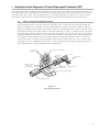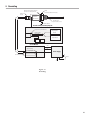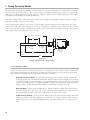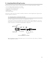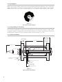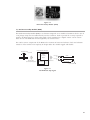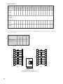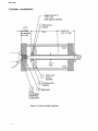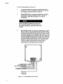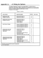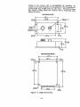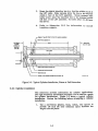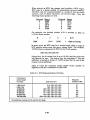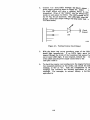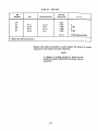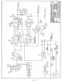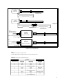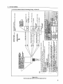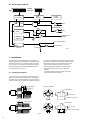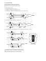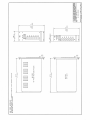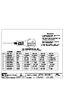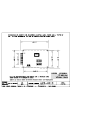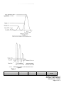
1
MTS Temposonics®
Linear Position Sensors
Archive Manuals
l
SENSORS
G R O U P
l
T
P
e
o
s
m
i
t
i
p
o
n
o
S
s
e
n
s
o
o
r
n
s
i
a
n
c
d
Part No. 550033 Rev. E
Te m p o s o n i c s ® I I
P o s i t i o n S e n s o r s
Installation & Instruction Manual
11-98 550055 Revision E
s
S
y
s
®
t
e
m
s
GENERAL INFORMATION
MTS PHONE NUMBERS
Application questions:
Repair Service:
Fax:
SHIPPING ADDRESS
MTS Systems Corporation
Sensors Division
3001 Sheldon Drive
Cary, North Carolina 27513
HOURS
Monday - Thursday
7:30 a.m. to 6:30 p.m. EST/EDT
Friday
7:30 a.m. to 5:00 p.m. EST/EDT
800-633-7609
800-248-0532
919-677-0200
TABLE OF CONTENTS
Section
1
2
Page
INTRODUCTION
1
1.1
Theory of Operation/Magnetostriction
1
1.2
Temposonics II LDT Specifications for Sensors <180 inches
2
1.3
Temposonics II LDT Specifications for Sensors ³ 200 inches
2
TEMPOSONICS II LDT INSTALLATION
3
2.1
Types of Transducer Supports
5
2.1.1
Loop Supports
5
2.1.2
Channel Supports
6
2.1.3
Guide Pipe Supports
6
2.2
Open Magnets
7
2.3
Spring Loading and Tensioning
7
2.4
Cylinder Installation
7
2.5
Installing Magnets
10
3
TEMPOSONICS II WIRING
11
4
GROUNDING
13
1. Introduction to the Temposonics II Linear Displacement Transducer (LDT)
The Temposonics™II Linear Displacement Transducer precisely senses the position of an external magnet to measure displacement with a high degree of resolution. The system measures the time interval between an interrogation pulse and a return pulse. The interrogation pulse is transmitted through the transducer waveguide, and the
return pulse is generated by a movable permanent magnet representing the displacement to be measured.
1.1
Theory of Operation/Magnetostriction
The interrogation pulse travels the length of the transducer by a conducting wire threaded through the
hollow waveguide. The waveguide is spring loaded within the transducer rod and exhibits the physical
property of magnetostriction. When the magnetic field of the interrogation pulse interacts with the stationary magnetic field of the external magnet, a torsional strain pulse or "twist" is produced in the waveguide.
This strain pulse travels in both directions, away from the magnet. At the end of the rod, the strain pulse
is damped within the "dead zone". At the head of the transducer, two magnetically coupled sensing coils
are attached to strain sensitive tapes. The tapes translate the strain pulse through coils to an electrical
"return pulse". The coil voltage is then amplified in the head electronics before it is sent to various measuring devices as the conditioned "return pulse". See the Temposonics II Analog and Digital manuals for
more information on analog and digital system configurations.
External reference magnet
Reference
magnetic field
Strain tape
Waveguide
twist
Interaction of magnetic
fields causes
waveguide to twist
Bias magnet
Waveguide
Sensing coil
Conducting element
Magnetic field from interrogation pulse
Waveguide enclosure
Figure 1-1
Waveguide Interaction
1
1.2 Temposonics II LDT Specifications for Sensors <180 Inches
Parameter
Input Voltage:
Current Draw:
Displacement:
Dead Zone:
Electronics Enclosure:
Non-linearity:
Repeatability:
Hysteresis:
Temperature Coefficient:
Transducer (length dependent):
Electronics:
Operating Temperature:
Head Electronics:
Transducer Rod:
Operating Pressure:
Output Impedance:
Specifications
± 12 to ± 15 Vdc
Transducer Only:
± 15 Vdc at 100 mA maximum, 25 mA minimum
(current draw varies with magnet position, maximum draw occurs when magnet is at 2 in.
(50.6 mm) from the flange and minimum update time is being utilized)
Up to 25 feet (7620 millimeters)
2.5 inches (63.5 millimeters)
IP-67
< ± 0.05% of full scale or ± 0.002 inch (±0.05 mm), whichever is greater
< ± 0.001% of full scale or ± 0.0001 inch (±0.002 mm), whichever is greater
0.0008 inch (0.02 mm) maximum
3 ppm/°F (5.4 ppm/°C)
<0.00011 in./°F (<0.00503 mm/°C)
- 40 to 150°F (- 40 to 66°C)
- 40 to 185°F (- 40 to 85°C)
3000 psi continuous, 8000 psi static
47½
Specifications are subject to change without notice. Consult MTS for verification of specifications critical to your application.
1.3 Temposonics II LDT Specifications for Sensors ³180 Inches
Below is a list of specifications that pertain to Temposonics II transducers with active stroke lengths of
180 inches (4572 mm) to 300 inches (7620 mm). The below specifications apply only to sensors 180 to
300 inches in length. Specifications not listed below may be found in section 1.2, above.
Parameter
Parameter
Input Voltage:
Dead Zone:
Cable Length:
Magnet Requirement:
2
Specification
Specifications
• Maximum: ± 15 Vdc, ± 5% at 100 mA
• Minimum: ± 15 Vdc at 25 mA
(current draw varies with magnet position, maximum draw occurs when magnet is 2 inches
(50.8 mm) from the flange and minimum update time is being used)
3 in. (76.2 mm)
• Maximum cable length for neuter version transducer (i.e., Temposonics II without an
integrated Personality Module) which requires the use of external interface electronics
(Analog Output Module, Digital Interface Box or other signal conditioners) is 250 ft.
Part Numbers: 201554, 201553, 251416, 201542
2. Temposonics II LDT Installation
Before beginning installation, be sure you know the following dimensions (as illustrated in Figures 2-1 to 2-3a-c.):
• Null Space
• Stroke
• Dead Zone
Flange to Tip
Dead Zone
2.50 in.
(63.50 mm)
for stroke
lengths up to
179.9 in;
Stroke Length
(specified by customer)
Standard Null
(2.0 in., 50 mm)
2.50 in.
(63.50 mm)
1.36 in.
(34.54 mm)
0.03 in. (0.76 mm)
3 in. (76.2 mm)
for strokes
³180 in.
0.38 in. (9.65 mm)
2.13 in.
(54 mm)
0.38 in. DIA
(9.65 mm)
1.57 in. dia.
(39.87 mm)
End Plug,
Flush 0.375 in.
(9.65 mm)
1.75 in. dia.
(44.45 mm)
3/4-16 UNF-3A Thread
Hex
1.75 in. (44.45 mm) across flats
Figure 2-1
Temposonics II Dimensions
2.5 in. minimum
(clearance for connector
and cable bend)
Temposonics II with
Molded Connector/Cable Assembly
Temposonics II with
Field Instalable Connector
1.25 in.
minimum
Temposonics II with
Integral Cable
Figure 2-2
Temposonics II Connector/Cable Clearance Requirements
3
1. Use the 3/4 inch (19 mm), 16 UNF thread of the transducer to mount it at the selected location. Leave room to
access the hex head. If a pressure or moisture seal is required, install an O-ring (type MS 28778-8 is recommended) in the special groove. Use the hex head to tighten the transducer assembly.
2. Install the permanent magnet over the LDT rod. Mount the permanent magnet to the movable device whose displacement will be measured. To minimize the effect of magnetic materials (i.e. iron, steel, etc.) on the magnetic
field of the permanent magnet, ensure the minimum spacing requirements are met as shown in Figure 2-3a-c.
(Any non-magnetic materials can be in direct contact with the permanent magnet without affecting performance.)
Ferromagnetic Material
1/8 in.
1/8 in. Minimum
Minimum
5/8 in.
Minimum
Tip
Head
Magnet
Figure 2-3a
Minimum Magnet Clearance Using Magnetic Supports
Ferromagnetic Support
NON-Ferromagnetic Support
Threads
Magnet
5/8 in.
Minimum
Magnet
A
A = 1 in., minimum to clear threads
Figure 2-3b
Minimum Null Space Using Non-Magnetic Support
A
A = 5/8 in. plus support thickness
Figure 2-3c
Minimum Null Space Using Magnetic Support
Notes:
1. The magnet must not contact ferromagnetic materials (such as iron or steel). Clearances are required between the surface of the magnet
and ferromagnetic material, as shown. Non-ferrous material (such as copper, brass, or 300 series stainless steel) may contact the magnet
without affecting transducer performance.
2. Standard Null Space is 2 inches. There is no maximum limit for Null Space. Less then 2 inches can be specified if magnet clearances meet
requirements illustrated above.
4
NOTE:
Clearance between the magnet and the
transducer rod is not critical. However,
contact between the components will
cause wear over time. The installation of
supports or readjustment of the supports
is recommended if the magnet contacts
the transducer rod.
3. Move the permanent magnet full-scale to check that it moves freely and does not rub against the transducer. If
the magnet does not move freely, you can correct this by mounting a support bracket to the end of the tranducer. Long transducers may need additional supports to be attached to the transducer rod. Transducer supports
are described later in this section.
2.1 Types of Transducer Supports
Long transducers (48 inches or longer) may require supports to maintain proper alignment between the
transducer rod and the permanent magnet. When transducer rod supports are used, special, open-ended
permanent magnets are required.
Transducer supports attached to the active stroke length must be made of a non-ferrous material, thin
enough to permit the permanent magnet to pass without obstruction. Because the permanent magnet
does not enter the dead zone, supports connected within the dead zone may be made of any material.
The main types of supports are loop, channel, and guide pipe supports.
2.1.1 Loop Supports
Loop supports are fabricated from non-ferrous materials, thin enough to permit free movement of
the magnet. Loop supports are recommended for straight transducers and may be spaced apart
approximately every three feet. They may be used alone or with channel supports. Figure 2-4
illustrates the fabrication of a loop support.
Front View
Side View
0.38 in.
0.375
in.
I.D.
I.D.
Transducer Rod
Figure 2-4
Loop Support
NOTE:
When open magnets are used, ensure the
transducer rod remains within the inside
diameter of the magnet throughout the
length of the stroke. If the transducer rod
is allowed to enter the cut out area of an
open magnet, the transducer signal
could attenuate or be lost. See Figure 2-7.
5
2.1.2 Channel Supports
Channel supports, being typically straight, are normally used with rigid transducers. A channel
support consists of a straight channel with loop supports mounted at intervals. The loop supports
are required to keep the transducer within the channel. Figure 2-5 shows a channel support.
Channel supports are available from various manufacturers or may be fabricated.
Magnet
• Part No.: 201553 or
• Part No.: 251416
Rod
Loop Support
Figure 2-5
Channel Support
2.1.3 Guide Pipe Supports
Guide pipe supports are normally used for flexible transducers. A guide pipe support is constructed of non-ferrous material, straight or bent to the desired shape. As shown in Figure 2-6, both
inside and outside dimensions of the pipe are critical:
• Because the transducer rod is installed inside the pipe, the inside diameter of the pipe must be
large enough to clear the rod.
Magnet
• Part No.: 201553 or
• Part No.: 251416
Rod
Guide Pipe
Figure. 2-6
Guide Pipe Support
• The outside diameter of the pipe must be small enough to clear the magnet.
Refer to pipe manufacturers’ specifications and dimensions (schedule 10, 40, etc.) to select the
appropriate size pipe. Guide pipe is typically supported at each end of the pipe.
6
2.2 Open Magnets
When using an open magnet, make sure the rod is positioned at all times within the “active” zone of the magnet.
The transducer cannot operate properly unless the entire stroke of the transducer rod is located within this zone.
The active zone, as shown in Figure 2-7, lies within the inside diameter of the magnet.
Magnet
Active Zone
e
on
eZ
iv
ct
a
In
Figure 2-7
Active Zone for Open Magnets
2.3 Spring Loading or Tensioning
The transducer rod can be spring loaded or tensioned using a stationary weight. Attach a spring mechanism or
weight to the dead zone of the transducer rod with a clamping device which will not deform the transducer rod.
The maximum weight or spring tension is 5 to 7 lbs.
2.4 Cylinder Installation
Dead Zone:
2.50 in. (63.5 mm)
for stroke lengths
up to 179.9 in;
Null (as specified)
Minimum: 2 in. (50mm)
3
Active Stroke
3 in. (76.2 mm)
for stroke lengths
³180 in.
Minimum: 5 in. (127 mm)
1/8 in.
min.
0.5 in (12.7 mm) Bore
Pipe O.D. 0.38 in.
4
O-ring (MS 28778-8 or equivalent)
Part No.: 560315
Piston Head and Rod Assembly
2
1
NON-ferrous Spacer, Part No.: 400633
Magnet, Type SR-12
Part No.: 201542
(1.29 in. (32.76 mm) O.D.
(other options available)
5
Chamfered Rod Bushing
Figure 2-8
Typical Cylinder Installation
7
Figure 2-8 shows a typical cylinder installation. Review the following before attempting this type of
installation.
• Use a non-ferrous (plastic, brass, Teflon®, etc.) spacer [1] to provide 1/8 inch (32 mm) minimum space
between the magnet and the piston.
• An O-ring groove [2] is provided at the base of the transducer hex head for pressure sealing. MTS uses
mil-standard MS33514 for the O-ring groove. Refer to mil-standard MS33649 or SAE J514 for machining
of mating surfaces.
• The null space [3] is specified according to the installation design and cylinder dimensions. The analog
output module provides a null adjustment. Make sure that the magnet can be mounted at the proper
null position.
• The piston head [4] shown in Figure 2-8 is typical. For some installations, depending on the clearances,
it may be desired to countersink the magnet.
• A chamfered rod bushing [5] should be considered for stokes over 5 feet (1.5 meters) to prevent wear
on the magnet as the piston retracts. The bushing should be made from Teflon or similar material.
• The recommended bore for the cylinder rod is 1/2 inch (13 mm). The transducer rod includes a 0.375 inch
(9.53 mm) diameter end plug mounted flush. Use standard industry practices for machining and mounting
of all components. Consult the cylinder manufacturer for applicable SAE or military specifications.
2.250 in. Minimum Dia
Specifies Surface B
2.250 in. Minimum Dia
Specifies Surface B
A 0.005 in. Dia., FIM
A 0.005 in. Dia., FIM
0.875 in. Dia.
+.0.015
-0.000
32
32 min.
32 min.
0.875 in. Dia.
+.0.015
-0.000
0.769 in. Dia.
+.0.015
-0.000
0.769 in. Dia.
+.0.015
-0.000
min
120° ±0° 30'
.
3/4-16 UNIF-3B Thread
See Notes 3 And 4
32
125 min.
min
.
-B-
0.094 in. +.0.015
-0.000
120° ±0° 30'
125 min.
-B-
0.094 in. +.0.015
-0.000
See Note 7
1.105 in.
Minimum
Full Thread
Depth
See Detail C
See Detail C
Thru Thread Design
0.030 in. ±0.010 R
See Note 8
0.500
Dia.
0.094 in. REF
Blind Thread Design
45° ±5°
0.020 in. R
Maximum
Detail C
NOTES:
1. Dimensions and tolerances based on ANSI Y14.5-1982.
2. MTS has extracted all pertinent information from MS33649 to Generate this document.
3. PD must be square with surface B within 0.005 FIM across 2.250 dia minimum.
4. PD must be concentric with 2.250 dia within 0.030 FIM and with 0.769 dia within 0.005 FIM.
5. Surface texture ANSI B46.1-1978
6. Use o-ring MTS part number 560315 for correct sealing.
7. The thread design shall have sufficient threads to meet strength requirements of material used.
8. Finish counter-bore shall be free from longitudinal and spiral tool marks. Annular tool marks up to 32 microinches maximum will be permissible.
Figure 2-9
O-ring Boss Detail
8
3/4-16 UNJF-3B Thread
See Notes 3 and 4
Key:
FIM = Full Indicator Movement
PD = Pitch Diameter
1.180 in.
Recommended
Minimum
Spotface
Diameter
See Note 1
0.004 A
0.008 A
ø0.866 in.
Minimum
See Note 2
ø0.813 in.
±0.002 in.
R 0.008 in.
0.004 in.
0.094 in. Max.
0.125 min.
.
25 min
0.1
R0.015 in.
Max.
0.106 in.
±0.008 in.
1.100 in.
See Note 4
45° ±5°
1.250 in.
See Note 3
See Note 4
15° ±1°
Pitch A
Dia.
3/4-16 UNF-2B Thread
ø0.500 in.
Ref.
See Note 4
NOTES:
1. If face of port is on a machined surface, dimensions 1.180 and 0.094 need not apply as
long as R0.008/0.004 is maintained to avoid damage to the O-ring during installation.
2. Measure perpendicularity to A at this diameter.
3. This dimension applies when tap drill cannot pass through entire boss.
4. This dimension does not conform to SAE J1926/1.
Figure 2-10
Port Detail (SAE J1926/1)
9
2.5 Installing Magnets
Figure 2-11 below shows the standard magnet types and dimensions. The circular magnet with an outside
diameter of 1.29 inches and 0.53 inch inside diameter (Part No. 201542) is the most common and is suitable for most applications. Larger magnets, with an outside diameter of 2.5 inches are typically only used
with Temposonics transducers that exceed 180 inches in stroke length. Magnets with a 90 degree cut-out
are used in applications that require intermediate supports along the transducer rod.
If upon installation, the null adjustment is inadequate, you can design a coupler with adjustments to
mount the magnet to the measured member.
Part No. 201554
Part No. 201553
1 of 2 holes
0.177 in. dia. (4.5 mm)
120° apart
on 1.625 in. dia. (41.3 mm)
0.44 in. (11.2 mm) opening
90° cut-out
1 of 4 holes
each 0.182 in. dia. (4.6 mm)
I.D.: 0.75 in. (19.05 mm) on 1.625 in. dia. (41.3 mm)
O.D.: 2.49 in. (63.25 mm)
Thickness: 0.375 in. (9.5 mm)
Part No. 251416
I.D.: 0.625 in. (15.9 mm)
O.D.: 2.46 in. (63.25 mm)
Thickness: 0.375 in. (9.5 mm)
Part No. 201542
1 of 2 holes
0.15 in. dia. (3.9 mm)
120° apart
on 0.94 in. dia. (23.9 mm)
90° cut-out
4 holes
each 0.15 in. dia. (3.9 mm)
on 0.94 in. dia. (23.9 mm)
I.D.: 0.53 in. (13.5 mm)
O.D.: 1.29 in. (32.8 mm)
Thickness: 0.312 in. (7.9 mm)
Part No. 400533
I.D.: 0.53 in. (13.5 mm)
O.D.: 1.29 in. (32.8 mm)
Thickness: 0.312 in. (7.9 mm)
Part No. 400633
Part No. 401032
4 Holes
each 3.9 mm dia. (0.15 in.)
90° apart on 23.9 mm dia.
(0.94 in.)
I.D.: 0.53 in. (13.5 mm)
O.D.: 1.0 in. (25.4 mm)
Thickness: 0.312 in. (7.9 mm)
I.D.: 0.532 in. (13.5 mm)
O.D.: 0.685 in. (17.4 mm)
Thickness: 0.312 in. (7.9 mm)
For use with stroke lengths
£ 60 in.
Magnet Spacer
ID: 14.3 mm (0.563 in.)
OD: 31.75 mm (1.25 in.)
Thickness: 3.175 mm (0.125
Part No. 251298-1
1.1 in.
Ref.
0.75 in.
Ref.
0.30 in. max.
S
Aluminum Plate
(bonded to magnet)
0.52 in.
Ref.
N
Figure 2-11
Magnet Dimensions
10
0.80 in.
Ref.
3. Temposonics II Wiring
Table 3A Connections - Temposonics II Transducer with Personality Modules
Temposonics II Cable Color Code (See Note 1)
Pin No.
1
2
3
Wire Color
(Striped leads)
White/Blue Stripe
Blue/White Stripe
White/Orange Stripe
Wire Color
(Solid Leads)
White
Brown
Gray
4
5
Orange/White Stripe
White/Green Stripe
6
7
8
9
10
Temposonics II Configurations:
• Neuter - No Personality Module
• RPM - RS422 Personality Module
• DPM - Digital Personality Module
• APM - Analog Personality Module
Neuter
DPM
RPM
APM
DC Ground
Frame
Not Used
DC Ground
Frame
(-) Gate Out
Pink
Red
Not Used
+ VDC
(+) Gate Out
+ VDC
Green/White Stripe
White/Brown Stripe
Brown/White Stripe
White/Gray Stripe
Blue
Black
Violet
Yellow
Gray/White Stripe
Green
- VDC
Output Pulse Return
Output Pulse
+ Interrogation
(See Notes 2, 3)
- Interrogation
(See Notes 2, 3)
- VDC
Not Used
Not Used
+ Interrogation
(See Notes 2, 4)
- Interrogation
(See Notes 2, 4)
DC Ground
Frame
(-) Start/Stop Pulse
DC Ground
Frame
Displacement
Return (GND)
(+) Start/Stop Pulse Displacement Out
+ VDC
+ VDC
(See Note 6)
- VDC
- VDC
Not Used
Not Used
Not Used
Not Used
+ Interrogation
Not Used
(See Notes 2, 4, 5)
- Interrogation
Not Used
(See Notes 2, 4, 5)
NOTES:
1. Verify if the cable has striped or solid color leads and make connections accordingly.
2. 1 to 4 microseconds maximum pulse duration.
3. WARNING: Under no condition should both the positive (+) and negative (-) interrogation leads be connected at the same time
when using the "NEUTER" version Temposonics II transducer. The unused interrogation lead must be connected to DC ground.
4. When using a Temposonics II transducer with a Digital Personality Module (DPM) or an RS422 Personality Module (RPM), it is
recommended that both the positive and negative interrogation leads are used to produce a differential interrogation signal.
5. For external interrogation mode ONLY.
6. Temposonics II w/APM requires +/-13.5 to +/-15 Vdc. All others require +/-12 Vdc to +/-15 Vdc.
1
9
9
5
3
10 1 8
6
5
3 2
7
10
7
8
6
2
4
4
Temposonics II 10-Pin Connector
Table 3B Connections - Original Temposonics Transducer
Original Temposonics Connector
Pin Number
Wire Color Code
A
Green or Gray
B
Black
C
Orange or Brown
D
Blue
E
White
F
Red
Signal Function
+ 15 Vdc
DC Ground
Return Pulse (from LDT)
- 15 Vdc
Interrogation Pulse
+ 12 Vdc
11
Table 3C Connections - Temposonics II Transducer to Analog Output Module (AOM)
Temposonics II Cable Color Code (See Note 5)
Pin No. Wire Color
(Striped leads)
Wire Color
(Solid Leads)
Function
1
2
3
4
5
6
7
8
9
White/Blue Stripe
Blue/White Stripe
White/Orange Stripe
Orange/White Stripe
White/Green Stripe
Green/White Stripe
White/Brown Stripe
Brown/White Stripe
White/Gray Stripe
White
Brown
Gray
Pink
Red
Blue
Black
Violet
Yellow
10
Gray/White Stripe
Green
DC Ground
Frame (see note 1)
Not Used
Not Used
+Vdc
-Vdc
Output Pulse Return
Output Pulse
+ Interrogation
(See notes 2, 4)
- Interrogation
(See notes 3, 4)
AOM Connections:
(Stroke Lengths < 180 in.)
Terminal
Military Style
Blocks
Connectors
AOM Connections
(Stroke Lengths > 180 in.)
Terminal
Military Style
Blocks
Connectors
TB2-B
TB2-B
Not Used
Not Used
TB2-F
TB2-D
TB2-B
TB2-C
TB2-E
J2 Pin B
J2 Pin B
Not Used
Not Used
J2 Pin F
J2 Pin D
J2 Pin B
J2 Pin C
J2 Pin E
TB2-B
TB2-B
Not Used
Not Used
TB2-A
TB2-D
TB2-B
TB2-C
TB2-E
J2 Pin B
J2 Pin B
Not Used
Not Used
J2 Pin A
J2 Pin D
J2 Pin B
J2 Pin C
J2 Pin E
TB2-E
J2 Pin B
TB2-E
J2 Pin B
NOTES:
1. Frame ground is isolated from circuit ground inside the transducer head.
2. For retrofitting AOMs or DIBs with strooke lengths greater than 12 inches (+ interrogation pulse).
3. For retrofitting AOMs or DIBs with stroke lengths of 12 inches or less (-interrogation pulse).
4. IMPORTANT: under no condition should both the positive (+) and negative (-) interrogation leads be connected at the same time. The
unused interrogation lead must be connected to DC ground.
5. Verify if the cable has striped or solid color leads and make connections accordingly.
Table 3D Connections - Temposonics II to Digital Interface Box (DIB)
Temposonics II Cable Color Code (See Note 1)
Pin No. Wire Color
Wire Color
(Striped leads)
(Solid Leads)
Function
1
2
3
4
5
DC Ground
Frame (see note 2)
Not Used
Not Used
+Vdc
White/Blue Stripe
Blue/White Stripe
White/Orange Stripe
Orange/White Stripe
White/Green Stripe
White
Brown
Gray
Pink
Red
DIB Connections:
J2 Pin Connections
J2 Pin B
J2 Pin B
Not Used
Not Used
J2 Pin F
(Pin A if stroke
length is > 180 in.)
J2 Pin D
J2 Pin B
J2 Pin C
J2 Pin E
J2Pin B
Retrofit connections to
Mating Connector
(P/N 370160, See Note 2)
A
J
K
G
H
6
Green/White Stripe
Blue
-Vdc
B
7
White/Brown Stripe
Black
Return (Gnd.)
Not Used
8
Brown/White Stripe
Violet
Output (return pulse)
Not Used
9
White/Gray Stripe
Yellow
+ Interrogation
E
10
Gray/White Stripe
Green
- Interrogation
D
NOTES:
1. Frame ground is isolated from circuit ground inside the transducer head.
2. Verify if the cable has striped or solid color leads and make connections accordingly.
3. Connections to existing mating connector when replacing a Digital Interface Box with a Temposonics II LDT with a Digital Personality
Module.
12
4. Grounding
Ground connection between bracket
and outer cover made by threads
Flange
(electrically isolated from threads)
Connector
(10 pins)
Bracket
(internal to
head enclosure)
Transducer Rod
(3/8 in. stainless steel)
Machine Ground
Head Assembly Grounding Diagram
Cable Shield (no connection)
Driver/Amplifier
Module
Signals Return(s)
Power Return
Frame
Option Module
Bracket
Cover
Control Module
+Vcc
(AOM, DIB, Counter Card or other)
-Vee
Signals Return(s)
Power Return
Frame
Power Return
Power Supply
Shield Ground
(non current carrying)
AC Line
Figure 4-1
Grounding
13
l
MTS Systems Corporation
Sensors Division
3001 Sheldon Drive
Cary, NC 27513
Phone: 800-633-7609
Fax: 919-677-0200
Internet: www.temposonics.com
MTS Sensor Technologie GmbH and Co. KG
Auf dem Schuffel 9, D-58513 Lüdenscheid, Germany
Postfach 8130 D-58489 Lüdenscheid, Germany
Phone: + 49-2351-95870
Fax: + 49-2351-56491
Temposonics sensors are a registered trademark of MTS Systems Corporation
All Temposonics sensors are covered by US patent number 5,545,984 and others.
Additional patents are pending.
Part Number: 11-98 550055 Revision E
© 1998 MTS Systems Corporation
MTS Sensors Technology Corporation
Izumikan Gobancho
12-11 Gobancho
Chiyoda-ku
Tokyo 102
Japan
Phone: + 813 3239-3003
Fax: + 813 3262-7780
l
T
P
e
o
s
m
i
t
i
p
o
n
o
S
s
e
n
s
o
o
r
n
s
i
a
n
c
d
Part No. 550033 Rev. E
Te m p o s o n i c s ® I I
P o s i t i o n S e n s o r s
Installation & Instruction
Manual for Analog Systems
11-98 550032 Revision F
s
S
y
s
®
t
e
m
s
GENERAL INFORMATION
MTS PHONE NUMBERS
Application questions:
Repair Service:
Fax:
SHIPPING ADDRESS
MTS Systems Corporation
Sensors Division
3001 Sheldon Drive
Cary, North Carolina 27513
HOURS
Monday - Thursday
7:30 a.m. to 6:30 p.m. EST/EDT
Friday
7:30 a.m. to 5:00 p.m. EST/EDT
800-633-7609
800-248-0532
919-677-0200
TABLE OF CONTENTS
Section
1
2
Page
INTRODUCTION
1
1.1
Theory of Operation/Magnetostriction
1
1.2
Temposonics II LDT Specifications for Sensors <180 Inches
2
1.3
Temposonics II LDT Specifications for Sensors ³ 180 inches
2
TEMPOSONICS II LDT INSTALLATION
3
2.1
Types of Transducer Supports
5
2.1.1
Loop Supports
5
2.1.2
Channel Supports
6
2.1.3
Guide Pipe Supports
6
2.2
Open Magnets
7
2.3
Spring Loading and Tensioning
7
2.4
Cylinder Installation
7
2.5
Installing Magnets
10
3
TEMPOSONICS II WIRING
11
4
TROUBLESHOOTING THE LINEAR DISPLACEMENT TRANSDUCER
12
5
GROUNDING
13
6
INTRODUCTION TO ANALOG SYSTEMS
14
6.1
Specifications of Analog System Components
15
6.1a
Analog Personality Module (APM)
15
6.1b
Analog Output Module (AOM) and Analog Output Card
15
7
ANALOG PERSONALITY MODULE
16
7.1
Performance Modes
16
7.2
APM Programming Procedure
18
8
INSTALLING THE ANALOG OUTPUT MODULE (AOM)
21
9
ANALOG OUTPUT MODULE ADJUSTMENTS
22
9.1
Nominal Range of Adjustments
22
9.2
Null and Full-Scale Adjustments
23
9.3
Velocity Null Adjustments
24
10
11
12
ANALOG OUTPUT MODULE/WIRING PROCEDURES
25
10.1
Preparing Cable for Connection to the AOM
25
10.2
J1 Installation Wiring
26
10.3
J1 Connections for AOM
27
10.4
J1 Connection to AOM with MS Connectors
29
10.5
J1 Connections
29
TROUBLESHOOTING THE ANALOG OUTPUT MODULE
32
11.1
General
32
11.2
Power Supply Check
32
11.3
Grounding
33
11.4
Connections
33
11.5
LDT Signals
33
ANALOG OUTPUT CARD
36
1. Introduction to the Temposonics II Linear Displacement Transducer (LDT)
The Temposonics II LDT precisely senses the position of an external magnet to measure displacement with a
high degree of accuracy and resolution. Using the principle of magnetostriction (see Section 1.1, below), the
Temposonics II LDT measures the time interval between the initiation of an interrogation pulse and the detection
of a return pulse. A variety of interface devices use the data derived from these two pulses and generates an analog
or digital output to represent position.
1.1 Theory of Operation/Magnetostriction
The interrogation pulse travels the length of the transducer by a conducting wire threaded through a hollow waveguide. The waveguide is spring loaded within the transducer rod and exhibits the physical property of magnetostriction. When the magnetic field of the interrogation pulse interacts with the stationary
magnetic field of the external magnet, a torsional strain pulse or “twist” is produced in the waveguide.
This strain pulse travels in both directions, away from the magnet. At the end of the rod, the strain pulse
is damped within the “dead zone”. At the head of the transducer, two magnetically coupled sensing coils
are attached to strain sensitive tapes. The tapes translate the strain pulse through coils to an electrical
“return pulse”. The coil voltage is then amplified in the head electronics before it is sent to various measuring devices as the conditioned “return pulse”.
External reference magnet
Reference
magnetic field
Strain tape
Waveguide
twist
Interaction of magnetic
fields causes
waveguide to twist
Bias magnet
Waveguide
Sensing coil
Conducting element
Magnetic field from interrogation pulse
Waveguide enclosure
Figure 1-1
Waveguide Interaction
1
1.2 Temposonics II LDT Specifications for Sensors <180 Inches
Parameter
Input Voltage:
Current Draw:
Displacement:
Dead Zone:
Electronics Enclosure:
Non-linearity:
Resolution:
Repeatability:
Hysteresis:
Update Time:
Operating Temperature
Head Electronics:
Transducer Rod:
Operating Pressure:
Analog Outputs (absolute)
Specifications
± 12 to ± 15 Vdc
Transducer Only:
± 15 Vdc at 100 mA maximum, 25 mA minimum
(current draw varies with magnet position, maximum draw occurs when magnet is at 2 in.
(50.6 mm) from the flange and minimum update time is being utilized)
Transducer with:
• Analog Personality Module (APM):
± 13.5 Vdc to ±15 Vdc at 190 mA maximum, 115 mA minimum
• Analog Output Module (AOM):
+ 15 Vdc at 250 mA, -15 Vdc at 65 mA
Up to 25 feet (7620 millimeters)
2.5 inches (63.5 millimeters) for stroke lengths up to 179.9 in.
IP-67
< ± 0.05% of full scale or ± 0.002 inch (±0.05 mm), whichever is greater
1 ÷ [gradient x crystal freq. (mHz) x circulation]; maximum resolution: 0.006 mm or 0.00025 in.
Equals resolution
0.0008 inch (0.02 mm) maximum
Resolution and Stroke dependent
Minimum = [Stroke (specified in inches) + 3] x 9.1 µs
- 40 to 150°F (- 40 to 66°C)
- 40 to 185°F (- 40 to 85°C)
3000 psi continuous, 8000 psi static
Standard 0 to10 Vdc (other voltage outputs are available)
Optional: 4-20 mA (AOM)
Specifications are subject to change without notice. Consult MTS for verification of specifications critical to your application.
1.3 Temposonics II LDT Specifications for Sensors ³180 Inches
Below is a list of specifications that pertain to Temposonics II transducers with active stroke lengths of
180 inches (5083 mm) to 300 inches (7620 mm). The below specifications apply only to sensors 180 to
300 inches in length. Specifications not listed below may be found in section 1.2, above.
Parameter
Parameter
Input Voltage:
Dead Zone:
Cable Length:
Magnet Requirement:
Specification
Specifications
• Maximum: ± 15 Vdc, ± 5% at 100 mA
• Minimum: ± 15 Vdc at 25 mA
(current draw varies with magnet position, maximum draw occurs when magnet is 2 inches
(50.8 mm) from the flange and minimum update time is being used)
3 in. (76.2 mm)
• Maximum cable length for neuter version transducer (i.e., Temposonics II without an
integrated Personality Module) which requires the use of external interface electronics
(Analog Output Module, Digital Interface Box or other signal conditioners) is 250 ft.
• APM: 150 ft.
AOM: 250 ft.
Part Numbers: 201554, 201553, 251416, 201542
Specifications are subject to change without notice. Consult MTS for verification of specifications critical to your application.
2
2. Temposonics II LDT Installation
Before beginning installation, be sure you know the following dimensions (as illustrated in Figures 2-1 to 2-3a-c.):
• Null Space
• Stroke
• Dead Zone
Flange to Tip
Dead Zone
2.50 in.
(63.50 mm)
for stroke
lengths up to
179.9 in;
Stroke Length
(specified by customer)
Standard Null
(2.0 in., 50 mm)
2.50 in.
(63.50 mm)
1.36 in.
(34.54 mm)
0.03 in. (0.76 mm)
3 in. (76.2 mm)
for strokes
³180 in.
0.38 in. (9.65 mm)
2.13 in.
(54 mm)
0.38 in. DIA
(9.65 mm)
1.57 in. dia.
(39.87 mm)
End Plug,
Flush 0.375 in.
(9.65 mm)
1.75 in. dia.
(44.45 mm)
3/4-16 UNF-3A Thread
Hex
1.75 in. (44.45 mm) across flats
Figure 2-1
Temposonics II Dimensions
2.5 in. minimum
(clearance for connector
and cable bend)
Temposonics II with
Molded Connector/Cable Assembly
Temposonics II with
Field Instalable Connector
1.25 in.
minimum
Temposonics II with
Integral Cable
Figure 2-2
Temposonics II Connector/Cable Clearance Requirements
3
1. Use the 3/4 inch (19 mm), 16 UNF thread of the transducer to mount it at the selected location. Leave room
to access the hex head. If a pressure or moisture seal is required, install an O-ring (type MS 28778-8 is
recommended) in the special groove. Use the hex head to tighten the transducer assembly.
2. Install the permanent magnet over the LDT rod. Mount the permanent magnet to the movable device whose
displacement will be measured. To minimize the effect of magnetic materials (i.e. iron, steel, etc.) on the
magnetic field of the permanent magnet, ensure the minimum spacing requirements are met as shown in
Figures 2-3a-c. (Any non-magnetic materials can be in direct contact with the permanent magnet without affecting performance.)
Ferromagnetic Material
1/8 in.
1/8 in. Minimum
Minimum
5/8 in.
Minimum
Tip
Head
Magnet
Figure 2-3a
Minimum Magnet Clearance Using Magnetic Supports
Ferromagnetic Support
NON-Ferromagnetic Support
Threads
Magnet
5/8 in.
Minimum
Magnet
A
A = 1 in., minimum to clear threads
Figure 2-3b
Minimum Null Space Using Non-Magnetic Support
A
A = 5/8 in. plus support thickness
Figure 2-3c
Minimum Null Space Using Magnetic Support
NOTES:
1. The magnet must not contact ferromagnetic materials (such as iron or steel). Clearances are required between the surface of the magnet
and ferromagnetic material, as shown. Non-ferrous material (such as copper, brass, or 300 series stainless steel) may contact the magnet
without affecting transducer performance.
2. Standard Null Space is 2 inches. There is no maximum limit for Null Space. Less then 2 inches can be specified if magnet clearances meet
requirements illustrated above.
4
NOTE:
Clearance between the magnet and the
transducer rod is not critical. However,
contact between the components will
cause wear over time. The installation of
supports or readjustment of the supports
is recommended if the magnet contacts
the transducer rod.
3. Move the permanent magnet full-scale to check that it moves freely. If not (if the magnet rubs on the transducer) you can correct this by mounting a support bracket to the end of the transducer. Long transducers may
need additional supports to be attached to the transducer rod. Transducer supports are described later in this
section.
2.1 Types of Transducer Supports
Long transducers (48 inches or longer) may require supports to maintain proper alignment between the
transducer rod and the permanent magnet. When transducer rod supports are used, special, open-ended
permanent magnets are required.
Transducer supports attached to the active stroke length must be made of a non-ferrous material, thin
enough to permit the permanent magnet to pass without obstruction. Because the permanent magnet
does not enter the dead zone, supports connected within the dead zone may be made of any material.
The main types of supports are loop, channel, and guide pipe supports.
2.1.1 Loop Supports
Loop supports are fabricated from non-ferrous materials, thin enough to permit free movement of
the magnet. Loop supports are recommended for straight transducers and may be spaced apart
approximately every three feet. They may be used alone or with channel supports. Figure 2-4
illustrates the fabrication of a loop support.
Front View
Side View
0.38 in.
0.375
in.
I.D.
Transducer Rod
Figure 2-4
Loop Support
NOTE:
When open magnets are used, ensure the
transducer rod remains within the inside
diameter of the magnet throughout the
length of the stroke. If the transducer rod
is allowed to enter the cut out area of an
open magnet, the transducer signal
could attenuate or be lost. See Figure 2-7.
5
2.1.2 Channel Supports
Channel supports, being typically straight, are normally used with rigid transducers. A channel
support consists of a straight channel with loop supports mounted at intervals. The loop supports
are required to keep the transducer within the channel. Figure 2-5 shows a channel support.
Channel supports are available from various manufacturers or may be fabricated.
Magnet
• Part No.: 201553 or
• Part No.: 251416
Rod
Loop Support
Figure 2-5
Channel Support
2.1.3 Guide Pipe Supports
Guide pipe supports are normally used for flexible transducers. A guide pipe support is constructed of non-ferrous material, straight or bent to the desired shape. As shown in Figure 2-6, both
inside and outside dimensions of the pipe are critical:
• Because the transducer rod is installed inside the pipe, the inside diameter of the pipe must be
large enough to clear the rod.
Magnet
• Part No.: 201553 or
• Part No.: 251416
Rod
Guide Pipe
Figure. 2-6
Guide Pipe Support
• The outside diameter of the pipe must be small enough to clear the magnet.
Refer to pipe manufacturers’ specifications and dimensions (schedule 10, 40, etc.) to select the
appropriate size pipe. Guide pipe is typically supported at each end of the pipe.
6
2.2 Open Magnets
When using an open magnet, make sure the rod is positioned at all times within the “active” zone of the
magnet. The transducer cannot operate properly unless the entire stroke of the transducer rod is located
within this zone. The active zone, as shown in Figure 2-7, lies within the inside diameter of the magnet.
Magnet
Active Zone
e
on
eZ
iv
ct
a
In
Figure 2-7
Active Zone for Open Magnets
2.3 Spring Loading or Tensioning
The transducer rod can be spring loaded or tensioned using a stationary weight. Attach a spring mechanism or weight to the dead zone of the transducer rod with a clamping device which will not deform the
transducer rod. The maximum weight or spring tension is 5 to 7 lbs.
2.4 Cylinder Installation
Dead Zone:
2.50 in. (63.5 mm)
for stroke lengths
up to 179.9 in;
Null (as specified)
Minimum: 2 in. (50mm)
3
Active Stroke
3 in. (76.2 mm)
for stroke lengths
³180 in.
Minimum: 5 in. (127 mm)
1/8 in.
min.
0.5 in (12.7 mm) Bore
Pipe O.D. 0.38 in.
4
O-ring (MS 28778-8 or equivalent)
Part No.: 560315
Piston Head and Rod Assembly
2
1
NON-ferrous Spacer, Part No.: 400633
Magnet, Type SR-12
Part No.: 201542
(1.29 in. (32.76 mm) O.D.
(other options available)
5
Chamfered Rod Bushing
Figure 2-8
Typical Cylinder Installation
7
Figure 2-8 shows a typical cylinder installation. Review the following before attempting this type of
installation.
• Use a non-ferrous (plastic, brass, Teflon®, etc.) spacer [1] to provide 1/8 inch (32 mm) minimum space
between the magnet and the piston.
• An O-ring groove [2] is provided at the base of the transducer hex head for pressure sealing. MTS uses
mil-standard MS33514 for the O-ring groove. Refer to mil-standard MS33649 or SAE J514 for machining
of mating surfaces.
• The null space [3] is specified according to the installation design and cylinder dimensions. The analog
output module provides a null adjustment. Make sure that the magnet can be mounted at the proper
null position.
• The piston head [4] shown in Figure 2-8 is typical. For some installations, depending on the clearances,
it may be desired to countersink the magnet.
• A chamfered rod bushing [5] should be considered for stokes over 5 feet (1.5 meters) to prevent wear
on the magnet as the piston retracts. The bushing should be made from Teflon or similar material.
• The recommended bore for the cylinder rod is 1/2 inch (13 mm). The transducer rod includes a 0.375
inch (9.53 mm) diameter end plug mounted flush. Use standard industry practices for machining and
mounting of all components. Consult the cylinder manufacturer for applicable SAE or military specifications.
2.250 in. Minimum Dia
Specifies Surface B
2.250 in. Minimum Dia
Specifies Surface B
A 0.005 in. Dia., FIM
A 0.005 in. Dia., FIM
0.875 in. Dia.
+.0.015
-0.000
32
32 min.
32 min.
0.875 in. Dia.
+.0.015
-0.000
0.769 in. Dia.
+.0.015
-0.000
0.769 in. Dia.
+.0.015
-0.000
min
120° ±0° 30'
.
3/4-16 UNIF-3B Thread
See Notes 3 And 4
32
125 min.
min
.
-B-
0.094 in. +.0.015
-0.000
120° ±0° 30'
125 min.
-B-
0.094 in. +.0.015
-0.000
See Note 7
1.105 in.
Minimum
Full Thread
Depth
See Detail C
See Detail C
Thru Thread Design
0.030 in. ±0.010 R
See Note 8
0.500
Dia.
0.094 in. REF
Blind Thread Design
45° ±5°
0.020 in. R
Maximum
Detail C
NOTES:
1. Dimensions and tolerances based on ANSI Y14.5-1982.
2. MTS has extracted all pertinent information from MS33649 to Generate this document.
3. PD must be square with surface B within 0.005 FIM across 2.250 dia minimum.
4. PD must be concentric with 2.250 dia within 0.030 FIM and with 0.769 dia within 0.005 FIM.
5. Surface texture ANSI B46.1-1978
6. Use o-ring MTS part number 560315 for correct sealing.
7. The thread design shall have sufficient threads to meet strength requirements of material used.
8. Finish counter-bore shall be free from longitudinal and spiral tool marks. Annular tool marks up to 32 microinches maximum will be permissible.
Figure 2-9
O-ring Boss Detail
8
3/4-16 UNJF-3B Thread
See Notes 3 and 4
Key:
FIM = Full Indicator Movement
PD = Pitch Diameter
1.180 in.
Recommended
Minimum
Spotface
Diameter
See Note 1
0.004 A
0.008 A
ø0.866 in.
Minimum
See Note 2
ø0.813 in.
±0.002 in.
R 0.008 in.
0.004 in.
0.094 in. Max.
0.125 min.
.
25 min
0.1
R0.015 in.
Max.
0.106 in.
±0.008 in.
1.100 in.
See Note 4
45° ±5°
1.250 in.
See Note 3
See Note 4
15° ±1°
Pitch A
Dia.
3/4-16 UNF-2B Thread
ø0.500 in.
Ref.
See Note 4
NOTES:
1. If face of port is on a machined surface, dimensions 1.180 and 0.094 need not apply as
long as R0.008/0.004 is maintained to avoid damage to the O-ring during installation.
2. Measure perpendicularity to A at this diameter.
3. This dimension applies when tap drill cannot pass through entire boss.
4. This dimension does not conform to SAE J1926/1.
Figure 2-10
Port Detail (SAE J1926/1)
9
2.5 Installing Magnets
Figure 2-11 below shows the standard magnet types and dimensions. The circular magnet with an outside
diameter of 1.29 inches and 0.53 inch inside diameter (Part No. 201542) is the most common and is suitable for most applications. Larger magnets, with an outside diameter of 2.5 inches are typically only used
with Temposonics transducers that exceed 180 inches in stroke length. Magnets with a 90 degree cut-out
are used in applications that require intermediate supports along the transducer rod.
If upon installation, the null adjustment is inadequate, you can design a coupler with adjustments to
mount the magnet to the measured member.
Part No. 201554
Part No. 201553
1 of 2 holes
0.177 in. dia. (4.5 mm)
120° apart
on 1.625 in. dia. (41.3 mm)
0.44 in. (11.2 mm) opening
90° cut-out
1 of 4 holes
each 0.182 in. dia. (4.6 mm)
I.D.: 0.75 in. (19.05 mm) on 1.625 in. dia. (41.3 mm)
O.D.: 2.49 in. (63.25 mm)
Thickness: 0.375 in. (9.5 mm)
Part No. 251416
I.D.: 0.625 in. (15.9 mm)
O.D.: 2.46 in. (63.25 mm)
Thickness: 0.375 in. (9.5 mm)
Part No. 201542
1 of 2 holes
0.15 in. dia. (3.9 mm)
120° apart
on 0.94 in. dia. (23.9 mm)
90° cut-out
4 holes
each 0.15 in. dia. (3.9 mm)
on 0.94 in. dia. (23.9 mm)
I.D.: 0.53 in. (13.5 mm)
O.D.: 1.29 in. (32.8 mm)
Thickness: 0.312 in. (7.9 mm)
Part No. 400533
I.D.: 0.53 in. (13.5 mm)
O.D.: 1.29 in. (32.8 mm)
Thickness: 0.312 in. (7.9 mm)
Part No. 400633
Part No. 401032
4 Holes
each 3.9 mm dia. (0.15 in.)
90° apart on 23.9 mm dia.
(0.94 in.)
I.D.: 0.53 in. (13.5 mm)
O.D.: 1.0 in. (25.4 mm)
Thickness: 0.312 in. (7.9 mm)
I.D.: 0.532 in. (13.5 mm)
O.D.: 0.685 in. (17.4 mm)
Thickness: 0.312 in. (7.9 mm)
For use with stroke lengths
£ 60 in.
Magnet Spacer
ID: 14.3 mm (0.563 in.)
OD: 31.75 mm (1.25 in.)
Thickness: 3.175 mm (0.125
Part No. 251298-1
1.1 in.
Ref.
0.75 in.
Ref.
0.30 in. max.
S
Aluminum Plate
(bonded to magnet)
0.52 in.
Ref.
N
Figure 2-11
Magnet Dimensions
10
0.80 in.
Ref.
3. Temposonics II Wiring
Table 3A
Temposonics II Connections (Neuter Version and with APM)
Pin No.
1
2
3
4
5
6
7
8
9
10
Temposonics II Integrated
or Extension Cable
(see Note 1)
Wire Color Code
Wire Color Code
White/Blue Stripe
White
Blue/White Stripe
Brown
White/Orange Stripe
Gray
Orange/White Stripe
Pink
White/Green Stripe
Red
Green/White Stripe
Blue
White/Brown Stripe
Black
Brown/White Stripe
Violet
White/Gray Stripe
Yellow
Gray/White Stripe
Green
Temposonics II Configurations:
• Neuter - No Personality Module
• APM - Analog Personality Module
Neuter
APM Option
DC Ground
DC Ground
Frame
Frame
Not Used
Displacement Return
Not Used
Displacement Out
+Vdc
+Vdc
-Vdc
-Vdc
Output Pulse Return
Not Used
Output Pulse
Not Used
(+) Interrogation (Notes 2, 3)
Not Used
(-) Interrogation (Notes 2, 3)
Not Used
NOTES:
1. Verify if the cable has striped or solid color leads and make connections accordingly.
2. 1 to 4 microseconds maximum pulse duration.
3. WARNING: Under no condition should both the positive (+) and negative (-) interrogation leads be connected at the same time
when using the "NEUTER" version Temposonics II transducer. The unused interrogation lead must be connected to DC ground.
4. Temposonics II w/APM requires +/-13.5 to +/-15 Vdc. All others require +/-12 Vdc to +/-15 Vdc.
1
9
7
10
5
8
3
6
2
4
Temposonics II 10-Pin Connector
(connections styles RB or RC)
Table 3B
Connections - Original Temposonics Transducer
Original Temposonics
Connector Pin Number
A
B
C
D
E
F
Wire Color Code
Signal Function
Green or Gray
Black
Orange or Brown
Blue
White
Red
+ 15 Vdc
DC Ground
Return Pulse (from LDT)
- 15 Vdc
Interrogation Pulse
+ 12 Vdc
11
4. Troubleshooting the Linear Displacement Transducer
NOTE:
The following checklist is for general
diagnostic purposes. Purchase of replacement components should not be based
solely on this checklist. Consult MTS
Sensors Division for recommendations
and factory service before ordering
replacement components.
Use the below checklist when operational problems are encountered. The possible causes of faulty output are listed below in order of probability of occurrence, and should be checked in order.
1.
2.
3.
4.
5.
6.
7.
8.
Improper power supply/power connection
Mismatched system components*
Ground loops/improper grounding*
Improper wiring
Incorrect receiver device or software*
Improper magnet mounting
EMI noise, affecting transducer or transducer cable
Circuit fault within transducer
* Will cause erratic or unstable output
Update Time
(-) Interrogation pulse sent to LDT (Pin 10)
1ms
1ms
1ms
(+) Interrogation pulse sent to LDT (Pin 9)
Return pulse from LDT (pin 8)
20ms
15ms
20ms
Figure 4-1
Temposonics II Transducer Signals
12
5. Grounding
Ground connection between bracket
and outer cover made by threads
Flange
(electrically isolated from threads)
Connector
(10 pins)
Bracket
(internal to
head enclosure)
Transducer Rod
(3/8 in. stainless steel)
Machine Ground
Head Assembly Grounding Diagram
Cable Shield (no connection)
Driver/Amplifier
Module
Signals Return(s)
Power Return
Frame
Option Module
Bracket
Cover
Control Module
+Vcc
(AOM, DIB, Counter Card or other)
-Vee
Signals Return(s)
Power Return
Power Supply
Power Return
Frame
Shield Ground
(non current carrying)
AC Line
Figure 5-1
Grounding
Customer Interface
Analog Output Module
TB1 A
+
Customer Interface
Analog Output Module
TB1 A
A
TB1 B
4-20 mA Grounded Loop
Figure 5-2
4-20mA Grounded Loop
250 to
400 W
(max.)
+
V
+
A
1 - 8 Volts
TB1 B
100 W
250 to
400 W
(max.)
+
V
1 - 8 Volts
4-20 mA Ungrounded Loop
Figure 5-3
4-20mA Ungrounded Loop
NOTES FOR FIGURES 5-2 & 5-3:
1. Selecting the grounding scheme is dependent upon the controller interface.
2. The current loop path must be completed for the system to operate.
3. The ungrounded loop is not truly isolated from ground. Isolators are required if this configuration is needed by the controller interface.
13
6. Introduction to Analog Systems
Temposonics II Analog Systems include a Linear Displacement Transducer (LDT), a magnet, and an Analog
Personality Module (APM), Analog Output Module (AOM), or an Analog Output Card. See Figures 6-1, 6-2 and 63. The APM, AOM and Analog Output Card generate the interrogation pulse, sense the return pulse, and develop
the analog output displacement signal (voltage or current).
The Analog Personality Module (Figure 6-1) is installed in the electronics enclosure of the Temposonics II transducer. The Analog Output Module and Analog Output Card are both separate interface devices.
POWER SUPPLY
± 13.5 to ±15 Vdc@ 190 mA
(bipolar)
Magnet
APM
Output:
To be specified
Range: - 10 to + 10 Vdc
Temposonics II LDT
USER'S
CONTROL
SYSTEM
Analog Personality Module
Figure 6-1
Analog System Configuration with Analog Personality Module
ANALOG
OUTPUT
MODULE
(AOM)
J2
J1
POWER SUPPLY
+ 15 Vdc / 250 mA
- 15 Vdc / 65 mA
OPTIONAL
24 Vdc@ 340 mA
Analog Displacement Output
Belden YR8105 or equivalent (5 pairs)
T1
Magnet
T2
Temposonics II LDT
Figure 6-2
Analog System Configuration
with Analog Output Module (AOM)
ANALOG
OUTPUT
CARD
POWER SUPPLY
+ 15 Vdc / 250 mA
- 15 Vdc / 65 mA
OPTIONAL
24Vdc @ 340 mA
Analog Displacement Output
Belden YR8105 or equivalent (5 pairs)
T1
Magnet
T2
Temposonics II LDT
Figure 6-3
Analog System Configuration
with Analog Output Card
14
6.1 Specifications of Analog System Components
6.1a Analog Personality Module (APM)
Parameter
Power Requirements:
Output Impedance:
Output:
Temperature Requirements:
Storage:
Operating:
Coefficient:
Maximum Cable Length:
Standard Features:
Specification
± 13.5 Vdc to ± 15 Vdc at 190 mA maximum, 115 mA minimum
10 K½ minimum load for voltage output
Specified by user; Range: - 10 Vdc to + 10 Vdc, forward or reverse acting
- 40 to 150°F (- 40 to 70°C)
- 32 to 150°F (-30 to 70°C)
10 ppm/°F (18 ppm °C)
150 ft.
Field programmable
Specifications are subject to change without notice. Consult MTS for verification of specifications critical to your application.
6.1b Analog Output Module (AOM) and Analog Output Card
Parameter
Power Requirements:
Standard:
Optional:
Output Impedance:
Velocity Output:
Temperature Requirements:
Storage:
Operating:
Coefficient:
Standard Features:
Specification
+ 15 Vdc (±2%) at 250 mA, < 1% ripple
- 15 Vdc (±2%) at 65 mA, < 1% ripple
+ 24 Vdc (±2%) at 340 mA, < 1% ripple
5 K½ minimum load for voltage output, 400½ maximum for 4-20 mA output
0 to ± 10 Vdc at 1 to 400 in. per second
Positive voltage output as magnet travels away from the transducer's head assembly, negative
voltage output as the magnet travels toward the transducer's head assembly.
- 40 to 180°F (- 40 to 82°C)
- 40 to 180°F (- 40 to 82°C)
20 ppm/°F (36 ppm/°C)
Non-volatile memory permanently stores set-up information. Surface mounted components
reduce moment of inertia and enhance shock and vibration resistance of the module.
Specifications are subject to change without notice. Consult MTS for verification of specifications critical to your application.
15
7. Analog Personality Module
The Analog Personality Module (APM) is mounted inside the electronics housing of the Temposonics II linear displacement transducer and produces a direct analog output. No additional interfacing electronics are required. The
APM processes digital data into an analog output via a digital to analog converter (DAC). MTS uses a 16-bit DAC
to provide the best available resolution performance.
Typically the APM will be ordered with the Temposonics II transducer. The APM is installed, and the set points
and output voltages are pre-set at the factory.
In the example below (Figure 7-1) we have a 60 inch stroke, note the indicated active stroke range. Set points
cannot be set within the null or dead space area, they can only be set within the active stroke area. The 13 inch
stroke selected in the example is defined by Set Point 1 (set at 4.000 volts) and Set Point 2 (set at 7.538 volts). Set
Point voltage values can range from -10 to +10 Vdc.
Stroke can be anywhere within this range
13 in.
SP 1
Set Point 2
7.538 V
2.5 in.
Dead
Space
SP 2
RPM
Set Point 1
4.000 V
60 in.
Available Active Stroke
2 in.
Null
Analog
Personality
Module
64.5 in.
Figure 7-1
Voltage & Displacement - 100% Scalable.
7.1 Performance Modes
Update time (or response time) for analog systems is based upon the active stroke of the transducer and
the resolution desired. To get the best mix of update time and resolution for your particular application,
three modes are available with the APM. These modes are as follows:
Resolution-Preferred Mode - In this mode the APM generates a high resolution output while
sacrificing update time. The Resolution Preferred Mode is limited to stroke lengths up to 48 inches and will provide an output resolution of approximately 0.001 inches. In applications exceeding
48 inches, the APM must be set for Balanced Mode or Update Preferred Mode. In the programming procedure, the Resolution Preferred Mode is indicated by an output of 0 volts.
Balanced Mode - In this mode the APM offers a "balance" between update time and resolution.
For stroke lengths up to 250 inches, the output resolution will be approximately 0.003 inches. In
the programming procedure, this mode is indicated by an output of +8.4 volts.
Update Preferred Mode - In this mode the APM produces the fastest possible update time while
sacrificing resolution. For stroke lengths up to 300 inches, the output resolution will be approximately 0.007 inches. In the programming procedure, this mode is indicated by an output of -8.4
volts.
16
The mode desired is selected at the time of order and factory pre-set. The following charts identify the
update time and resolution for each mode.
Resolution Preferred Mode
Update Time
Resolution
0.005
0.008
0.004
Resolution
(inches per step)
0.007
0.003
0.002
0.006
0.005
0.004
0.003
0.002
0.001
0.001
0.000
0.000
8
16
24
32
40
8
48
Sensor Stroke Length (inches)
Balanced Mode
Update Time
0.008
0.004
0.007
Resolution
(inches per step)
0.005
0.003
0.002
0.000
0.003
150
200
250
40
48
Resolution
300
50
Sensor Stroke Length (inches)
100
150
200
250
300
Sensor Stroke Length (inches)
Update Preferred Mode
Update Time
32
0.005
0.004
100
24
0.006
0.001
50
16
Sensor Stroke Length (inches)
0.009
0.003
0.008
Resolution
(inches per step)
0.004
0.002
0.001
0.000
Resolution
0.007
0.006
0.005
50
100
150
200
250
Sensor Stroke Length (inches)
300
50
100
150
200
250
300
Sensor Stroke Length (inches)
17
7.2 APM Programming Procedure
! CAUTION !
If the APM is being programmed for
the first time, the analog output at
power-up will be near zero volts. The
programming steps are the same in
this case, but the analog output will
return to zero volts until valid information is stored for both Set Point 1
and Set Point 2. When both Set
Points have been programmed, the
transducer will enter normal operating mode and produce an analog
output scaled according to the information permanently stored in the
APM's memory.
SW1
SW2
Figure 7-2
APM, Top View
! CAUTION !
IMPORTANT: Before beginning the
programming procedures, supply
power to the APM for a full 5 minutes.
This will allow all components to stabilize and ensure set point accuracy.
The output range of the APM is determined by choosing two endpoints within the active stroke length of
the transducer and using the two push-buttons to assign a voltage to each point. The two endpoints are
called Set Point 1 (SW1) and Set Point 2 (SW2). Any voltage from -10 volts to +10 volts may be assigned
to either point; the APM will automatically scale the output to the specified range. Set Point 1 must be the
set point closest to the head electronics.
18
In addition, the APM can be programmed for one of three performance modes, as described earlier.
During the programming procedure, each mode is represented by a particular output voltage. They are as
follows:
Resolution-Preferred Mode - In the programming procedure, the Resolution Preferred Mode is
indicated by an output of 0 volts.
Balanced Mode - In the programming procedure, this mode is indicated by an output of +8.4 volts.
Update Preferred Mode - In the programming procedure, this mode is indicated by an output of
-8.4 volts.
The number of recirculations shown will also indicate which mode the APM is programmed, see
Mode Table below.
Mode Table
Mode Select Voltages*
Resolution Mode = 0.0 V
Balance Mode = + 8.4 V
Update Mode = - 8.4 V
* Voltages are approximate values.
Recirculations
8 recirculations
2 recirculations
1 recirculation
When programming the APM, use the table below as a reference.
APM Programming Reference Guide
Press
SW1 (for 3 seconds)
SW2
SW1
SW1 (setpoint 1)
or
SW2 (setpoint 2)
SW1 or SW2
at setpoint 1 or 2
SW1 and SW2
Approx. Output voltage
+4.2 Vdc
see mode table
-4.2 Vdc
-2.1 Vdc
Function
Start program mode
Select mode
Locks mode in
Select setpoint 1 to program
Reference
Step 1
Step 2
Step 3
Step 4
+2.1 Vdc
Desired output voltage
voltage needed at setpoint 1
Setpoint voltage
Select setpoint 2 to program
Select desired output
Step 10
Step 5 or 11
Lock in program
Step 6 or 12
NOTES:
1. Always program setpoint 1 first, lock in program, then complete the steps to program setpoint 2.
2. When adjusting the output voltage (step 4) make sure the magnet is in the position of the setpoint.
3. Setpoint 1 will always be the setpoint closest to the transducer head.
4. If a mistake is made during programming, turn off power, wait a few seconds, turn power on and start over.
It is necessary to monitor the analog output with a digital voltmeter while performing the following steps.
1. Move the permanent magnet to the desired position for Set Point 1. Press the SW1 push-button until
the APM enters the programming mode (3 seconds) and acknowledges by producing an output voltage
of about +5 volts. Release the SW2 button.
2. Press and release the SW2 button to enter the performance-mode setup mode. The APM will acknowledge by producing an output voltage which corresponds to the currently stored performance mode
(see below). If the APM has never been programmed, the default mode will be resolution-preferred
(that is, the output voltage will be 0 volts).
• Resolution Preferred Mode = 0 volts
• Balanced Mode = +8.4 volts
• Update Preferred Mode = -8.4 volts
19
3. At this point, repeated presses of the SW2 button will cause the APM to cycle through the three performance modes. Continue to press and release the SW2 button until the voltage output indicates the
voltage associated with the correct mode for your application. Once the correct voltage is displayed,
press and release the SW1 button to accept the mode setting. The APM acknowledges by producing an
output voltage of approximately -4.2 volts.
4. Press and release the SW1 button to enter the Set Point 1 setup mode. The APM will acknowledge by
producing an output voltage of about -2.1 volts.
5. At this point, you can use the SW1 and SW2 buttons to choose the voltage to assign to Set Point 1.
Pressing and holding the SW1 button causes the output voltage to move in the positive direction;
pressing and holding the SW2 button causes the output voltage to move in the negative direction. If
either button is held for more than five seconds, the output voltage will begin to change more quickly.
Release the button when the desired output voltage is displayed on the digital volt meter. (For testing
purposes, it is not necessary to perform this step. It can be skipped entirely since it only assigns the
final voltage to the Set Point.)
6. To complete the setup for Set Point 1, press and release both buttons simultaneously. Move magnet
while looking at the output voltage. If output voltage changes, program has been locked in successfully. If output voltage does not change, put magnet back to the setpoint position and press both
buttons simultaneously. If the transducer has been previously programmed, it will resume operation
with the new voltage assigned to SW1. If it has not been previously programmed, it will return to the
same voltage it had prior to entering the programming mode (near 0 volts).
7. Move the permanent magnet to the desired position for Set Point 2. Press the SW1 push-button until
the APM enters the programming mode (3 seconds) and acknowledges by producing an output voltage
of approximately +4.2 volts. Release the SW1 button.
8. Press and release the SW2 button to enter the performance-mode setup mode. The APM will acknowledge by producing an output voltage which corresponds to the currently stored performance mode. If
the APM has never been programmed, the default mode will be resolution-preferred (that is, the output
voltage will be 0 volts).
9. At this point, repeated presses of the SW2 button will cause the APM to cycle through the three performance modes. Continue to press and release the SW2 button until the voltage output indicates the
voltage associated with the correct mode for your application. Once the correct voltage is displayed,
press and release the SW1 button to accept the mode setting. The APM acknowledges by producing an
output voltage of approximately -4.2 volts. (Note that the mode chosen in this step should be the same
as the one chosen in step 3. If a different mode is chosen, it will overwrite the one chosen previously.)
10. Press and release the SW2 button to enter the Set Point 2 setup mode. The APM will acknowledge by
producing an output voltage of +2.1 volts.
11. At this point, you can use the SW1 and SW2 buttons to choose the voltage to assign to Set Point 2.
Pressing and holding the SW1 button causes the output voltage to move in the positive direction;
pressing and holding the SW2 button causes the output voltage to move in the negative direction. If
either button is held for more than five seconds, the output voltage will begin to change more quickly.
Release the button when the desired output voltage is displayed on the digital volt meter. (For testing
purposes, this step may be skipped completely.)
12. To complete the setup for Set Point 2, press and release both buttons simultaneously. Move magnet
while looking at the output voltage. If output voltage changes, program has been locked in successfully. If output voltage does not change, put magnet back to the setpoint position and press both
buttons simultaneously. If the transducer was previously programmed, it will resume operation with
the new voltage assigned to Set Point 2.
20
8. Installing the Analog Output Module (AOM)
Dimensions of the AOM are shown below in Figure 8-1. The mounting hole dimensions shown are also stamped
on the back of the module. Mount the AOM as shown, using two socket head cap-screws.
TB3
A B C D E F G
H J K
4.35 in.(110.5 mm)
TB1
3.31 in.(84.1 mm)
(Shown with Cover Removed)
TB2
A B C D E F
0.24 in.(6.1 mm)
3.88 in.(98.6 mm)
4.35 in.(110.5 mm)
0.52 in.
(13.2 mm)
2.25 in. (57.1 mm)
with Cover
0.5625 in.
(14.3 mm)
Socket Head Cap Screw (2)
10-32 UNF-2A thread x 3/4 in. lg. (Recommended)
Figure 8-1
AOM Dimensions
1. Mount the AOM in a location within reach of the LDT assembly cable. Standard systems allow the AOM to be
mounted 250 feet from the LDT assembly.
2 Connect cable from AOM to the LDT assembly.
3. Adjust the AOM null and full-scale potentiometers (as described in Section 9) to compensate for any offsets due
to mechanical installation.
21
9. Analog Output Module Adjustments
This section explains how to adjust and calibrate the Temposonics II LDT system using an AOM.
The AOM includes adjustments for null (zero), and full-scale (span). The adjustments compensate for the
following:
• Differences between transducer gradients.
• Small offsets in the magnet position due to mounting.
• Wear in the moving parts of the mechanical system to which the magnet is attached.
In cases where a coupler device is used for adjusting the magnet, the coupler is used for coarse adjust
ments of both null and scale, while the AOM is used for fine adjustments.
9.1 Nominal Range of Adjustment
Null:
Full-scale:
Minimum: ± 3/8 in.
Maximum: Up to 10% of total stroke or ±2 inches, whichever is smaller
± 2% of total stroke
Figure 9-1 (next page) shows the location of position adjustments and terminal boards on the AOM.
NOTE:
Null adjustment has an overall effect on
total scale adjustment. However, scale
adjustment has no effect on null
adjustment.
22
9.2 Null and Full-Scale Adjustments
The following procedures calibrate the null position and the full-scale position to the required output levels.
Refer to Figure 9-1 for the adjustment locations.
NOTE:
The following procedure assumes the
standard full-scale 0 to 10 Vdc output is
supplied. When other output signals are
supplied, use the appropriate signal levels
and test equipment for the following
adjustments.
Null Adjustment R20
Scale Adjustment R24
Figure 9-1
Location of Null & Scale Adjustments
and Terminal Boards on the AOM.
1. Disconnect all power from the system. Loosen the four screws securing the AOM cover, and remove
the cover.
2. Note the location of terminal board TB1 on the AOM (Refer to Figure 9-1). Connect a DVM (digital
voltmeter) across pins A and B of terminal board TB1 to monitor the displacement signal. Apply power
to the system
3. Position the permanent magnet at the specified null position. The null position is specified when the
LDT assembly is ordered (typically 2 inches from the transducer head).
4. Use a screwdriver to adjust the null potentiometer (R20) to increase or decrease the value, until you
obtain a DVM reading of 0.000 Vdc.
5. Position the permanent magnet for full-scale position (typically 2 inches from the end of the LDT
assembly).
6. Use a screwdriver to adjust the scale potentiometer (R24) to increase or decrease the value, until you
obtain a DVM reading of +10.000 Vdc.
7. Repeat steps 3 to 6 to check the null and full-scale settings. Readjust as necessary.
8. Disconnect the DVM and check overall system operation. If no more adjustments are necessary, replace
the AOM cover.
23
9.3 Velocity Null Adjustment
The AOM can be provided with an optional velocity output. For those units, velocity zero and span
adjustments are provided. The velocity zero and velocity span adjustments are factory set and should not
require readjustment. A velocity output signal of 0 (zero) volts represents a static displacement (no
motion). A velocity output of 10 volts represents a dynamic displacement or a customer-specified maximum velocity (maximum velocity must be specified at time of order). The direction of motion is indicated
by the polarity of the velocity signal; a positive output signal typically indicates that the permanent magnet is moving away from the transducer head (unless otherwise specified for this system). A negative output signal typically indicates that the permanent magnet is moving towards the transducer head.
Velocity Scale Adjustment R41
Velocity Null Adjustment R40
Option Board
Factory Pre-set
Do Not Adjust
Figure 9-2
Velocity Adjustments on the AOM
24
10. Analog Output Module/ Wiring Procedures
This section describes wiring procedures for analog systems that use the Analog Output Module, including:
•
•
•
•
•
•
0 to 10 V displacement (forward and reverse acting)
-10 to +10 V displacement (forward and reverse acting)
Ungrounded 4 to 20 mA displacement
Grounded 4 to 20 mA displacement
Velocity Outputs
Dual Channel Outputs
Connections are made between the transducer assembly, the AOM, the customer-supplied power supply, and the
customer-supplied receiving device.
10.1 Preparing Cable for Connection to the AOM
The AOM is equipped with two strain relief or two MS (mil-spec) connectors.
A strain relief is used for an un-terminated cable. Prepare the cable as shown in Figure 10-1. It is recommended that you tin the exposed leads to ensure a good connection. Mount the cable to the AOM, ready
to make connections to the terminal boards (TB1, TB2, or TB3) inside.
AOM Enclosure
0.25 in.
3 in.
Male Threaded Nipple
(Do not remove)
1 in.
Strain Relief
Split Ring Cable Clamp
Cable Seal
Figure 10-1
Cable Preparation for Strain Relief
When the AOM box is used an optional MS connector can be used with the cable. Cables are available in
various lengths from inventory.
25
10.2 J1 Installation Wiring
The J1 cable provides the AOM voltage inputs from the DC power supply. It also provides displacement
outputs to the receiving device.
Take the following steps to connect J1:
1. One of the screws securing the cover of the AOM has a raised head. Connect a ground wire from
that screw head to a central earth ground or to the power supply ground (if it is grounded). Only
one circuit earth ground should be used to prevent ground loops. (Refer to Figure 5-1 of this manual
for a full system grounding diagram.)
2. Strain Relief Only: Fabricate the J1 cable, and prepare the cable as described earlier. Identify the
connections to TB1 and TB3. Refer to section 10.3 to determine the appropriate J1 connections.
3. MS Connector Only: Fabricate the J1 cable. Refer to section 10.4 to determine the appropriate J1
connections. Solder the connections to the MS type connector (Part No. 370017). Use any cable capable
of maintaining the signals for the required length. Ensure the solder connections are clean and free of
excessive solder. Use heat-shrink over the solder connections to prevent the pins from shorting.
4. Identify the wires at the other end of the cable for connections to the power supplies and the
receiving device. Test the cable for shorts.
NOTE:
Make sure that the power supply can provide +15 Vdc at 250 mA and -15 Vdc at
65 mA (use a bipolar power supply). The
power supply should provide less than 1%
ripple with 2% regulation. The power
supply should be dedicated to the transducer system to prevent noise and external loads from affecting the system
performance.
5. Make sure the power supply is off. Complete the cable connections at the power supply.
! CAUTION !
The input to the receiver electronics
should be a passive, resistive device to
prevent damage to the AOM.
6. First, make sure there is no voltage present on the receiving device input connections. Then,
complete the cable connections to the receiving device.
NOTE:
Do not route the J1 cable near high
voltage sources.
7. Strain Relief Only: Connect the cable to the TB1 and TB3 terminals on the AOM.
8. MS Connector Only: Connect the cable to the J1 connector on the AOM.
26
10.3 J1 Connections for AOM
The AOM is provided with either a strain relief connector, which accepts a pigtailed connection directly
into terminals blocks located inside the AOM enclosure, or a threaded MS connectors. Tables 10A through
10F, below, indicate the appropriate connection to make for either configuration. Make sure that you follow the appropriate table for your specified options.
AOM w/MS Connectors
AOM w/Strain Relief Connectors
TB1
TB3
ABCDEFG
HJK
J2
TB1
ABCDEFG
J1
A
F
E
TB3
J2
A
B
HJK
J1
B
E
D
C
D
C
J1
J2
Figure 10-2
AOM w/ Strain Relief and MS Connectors
Table 10A Standard J1 Connections
Strain Relief Connection
TB1
A
B
TB3
H
J
K
MS Connector Pin Designation (J1)
Function
D
E
Displacement Output
Displacement Output Return (ground)
A
B
C
+ 15 Vdc
- 15 Vdc
DC Common
Table 10B J1 Connections w/Velocity Output Option
Strain Relief Connection
TB1
A
B
C
D
TB3
H
J
K
MS Connector Pin Designation (J1)
Function
D
E
-
Displacement Output
Displacement Output Return (ground)
Velocity Output
Velocity Output Return (ground)
A
B
C
+ 15 Vdc
- 15 Vdc
DC Common
27
Table 10C J1 Connections w/24 V Power Supply Option
Strain Relief Connection
TB1
A
B
TB3
H
J
K
MS Connector Pin (J1)
Function
D
E
(+) Displacement Output
(-) Displacement Output
A
No Connection
C
24 Vdc
N/A
DC Common
Table 10D J1 Connections w/ 24 V Power Supply & Velocity Output Options
Strain Relief Connection
TB1
A
B
C
D
TB3
H
J
K
MS Connector Pin (J1)
Function
D
E
-
(+) Displacement Output
(-) Displacement Output
(+) Velocity Output
(-) Velocity Output
A
No Connection
C
24 Vdc
N/A
DC Common
Table 10E AOM J1 Connections w/Dual Channel Option
Strain Relief Connection
TB1
A
E
TB3
H
J
K
MS Connector Pin (J1)
Function
D
E
Channel 1 (+) Displacement Output
Channel 2 (+) Displacement Output
A
B
C
+ 15 Vdc
- 15 Vdc
DC Common
Table 10F J1 Connections w/Dual Channel & 24 V Power Supply Options
Strain Relief Connection
TB1
A
E
TB3
H
J
K
28
MS Connector Pin (J1)
Function
D
E
Channel 1 (+) Displacement Output
Channel 2 (+) Displacement Output
A
No Connection
C
24 Vdc
N/A
DC Common
10.4 J1 Connection to AOM with MS Connectors
Table 10G Voltage Output
Terminal Block
Connections *
TB3-H
TB3-J
TB3-K
TB3-A
TB1-B
Pin Connection (J1)
A
B
C
D
E
Function #1
(w/Standard ± 15 Vdc P.S.)
+ 15 Vdc
- 15Vdc
DC Common
Displacement Output
Optional: velocity output
Function #2
(w/Optional + 24 Vdc P.S.)
+ 24 Vdc
DC Common
Displacement Output
Optional: velocity output
Function #1
(w/Standard ± 15 Vdc P.S.)
+ 15 Vdc
- 15 Vdc
DC Common
Current Output (source)
Function #2
(w/Optional + 24 Vdc P.S.)
+ 24 Vdc
DC Common
Current Output (source)
DO NOT ground or damage may result
Maximum load resistance: 400½
DO NOT ground or damage may result.
Maximum load resistance: 400½
Current Output (return)
Current Output (return)
Table 10H Ungrounded 4-20 mA Current Output
Terminal Block
Connections *
TB3-H
TB3-J
TB3-K
TB1-A
TB1-B
Pin Connection (J1)
A
B
C
D
E
Table 10I Grounded 4-20 mA Current Output
Terminal Block
Connections *
TB3-H
TB3-J
TB3-K
TB1-A
-
Pin Connection (J1)
Function #1
Function #2
(w/Standard ± 15 Vdc P.S.)
(w/Optional + 24 Vdc P.S.)
A
+ 15 Vdc
+ 24 Vdc
B
- 15 Vdc
C
DC Common
DC Common
D
Current Output (source)
Current Output (source)
E
Not Used
Not used
Maximum load resistance: 500½ Maximum load resistance: 500½
* Terminal blocks are located inside the AOM housing and are accessed via strain relief connectors J1 and J2 on the face of the AOM.
10.5 J2 Connections
The J2 cable provides connections between the AOM and the transducer assembly.
Cables up to 250 feet (76 meters) can be fabricated with any high quality multi-conductor cable with an
overall shield (Belden equivalent).
Take the following steps to connect J2:
1. It is recommended that you apply an earth ground to the transducer rod. This is typically accomplished by mounting the transducer head to a bracket or machine.
2. Strain Relief Only: If necessary, fabricate the J2 cable, and prepare the cable as described earlier.
Identify the connections to TB2. Refer to Table 10J (next page) for the J2 connections.
NOTE:
Ensure the solder connections are clean
and free of excessive solder. Use heatshrink over the solder connections to prevent the pins from shorting.
29
3. MS Connector Only:
If necessary, fabricate the J2 cable. Be sure to use the recommended cable for the required length. The
color code refers to cables supplied with the system. Solder the connections to the MS connector
supplied with the AOM. Use any cable capable of maintaining the signals for the required length.
Ensure the solder connections are clean and free of excessive solder. Use heat-shrink over the solder
connections to prevent the pins from shorting.
AOM w/MS Connectors
TB1
ABCDEFG
Optional AOM outputs
TB3
TB2
ABCDEF
HJK
Cable Ground
(connect at or
near AOM)
No Connection TB2-A
DC Common/GRD TB2-B
Return Pulse TB2-C
- 15 Vdc TB2-D
Interrogation Pulse TB2-E
+ 12 Vdc TB2-F
TB3-K DC Common
TB3-J - 15 Vdc
TB3-H + 15 Vdc (Optional +24 Vdc)
TB1-B (-) Displacement Output
TB1-A (+) Displacement Output
J2
J1
NOTE:
The connections to TB3 represent wiring for a typical system configuration (i.e., ±15 Vdc power supply and strain-relief connectors). If the
AOM is configured with other options (i.e., 24 Vdc power supply, velocity output, MS connectors) refer to sections 10.3 and 10.4 for proper wiring.
Figure 10.3
AOM J1 and J2 Connections
Table 10J AOM J2 Connections
J2 Connection (TB 2 A - F or J2 Pin A - F)
Pin Connection
Terminal Block Connection
J2 Pin A
TB2-A
J2 Pin B
TB2-B
J2 Pin C
J2 Pin D
J2 Pin E
J2 Pin F (see note 1)
TB2-C
TB2-D
TB2-E
TB2-F
Wire Color Code *
Not Used
White/Blue Stripe
Blue/White Stripe
White/Brown Stripe
Gray/White Stripe
Brown/White Stripe
Green White Stripe
White/Gray Stripe
White/Green Stripe
Wire Color Code
Not Used
White
Brown
Black
Green
Violet
Blue
Yellow
Red
*Function
No Connection
DC Common/GND
Frame
Output Pulse
- 15 Vdc (- 13.5 to - 14.5 Vdc)
Interrogation Pulse
+12 Vdc
*Verify if the cable has striped or solid color leads and make connections accordingly.
NOTES:
1. Connect to TB2 Pin A if the stoke length exceeds 180 inches.
4. Strain Relief Only: Connect the cable to the TB2 terminals on the AOM and to the transducer.
5. MS Connector Only: Connect the cable to the J2 connector on the AOM, and to the transducer.
6. Apply power and check the displacement readings at the system electronics.
30
Table 10K Retrofit Connections Temposonics II Replacement of Existing Temposonics I with AOM
Temposonics II Integrated or Extension Cable (Notes 1, 2)
Pin No. Wire Color Code
Wire Color Code
Functional Description
1
2
3
4
5
6
7
8
9
White/Blue Stripe
Blue/White Stripe
White/Orange Stripe
Orange/White Stripe
White/Green Stripe
Green/White Stripe
White/Brown Stripe
Brown/White Stripe
White/Gray Stripe
10
Gray/White Stripe
White
Brown
Gray
Pink
Red
Blue
Black
Violet
Yellow
(See warning, below)
Green
(See warning, below)
DC Ground
Frame (Note 3)
Not Used
Not Used
+Vdc
-Vdc
Return (GND)
Output (return pulse)
(+) Interrogation (Note 5)
Analog Output Module (AOM)
Terminal Blocks Military Style (MS)
Connectors
TB2-B
J2 Pin B
TB2-B
J2 Pin B
Not Used
Not Used
Not Used
Not Used
TB2-F (Note 4)
J2 Pin F (Note 4)
TB2-D
J2 Pin D
TB2-B
J2 Pin B
TB2-C
J2 Pin C
TB2-E
J2 Pin E
(-) Interrogation (Note 6)
TB2-B
J2 Pin B
NOTES:
1. Verify if the cable has striped or solid color leads and make connections accordingly.
2. Cable: Belden #8105 or equivalent
3. Frame ground is isolated from circuit ground inside the electronics enclosure or head of the transducer.
4. Connect to TB2 Pin A if the stoke length exceeds 180 inches.
5. For retrofitting AOMs with stoke lengths greater than 12 inches in stroke length and positive (+) interrogation.
6. For retrofitting AOMs with stoke lengths greater than 12 inches in stroke length and negative (-) interrogation.
7. Shield: Connect extension cable shield at TB2-B or J2 Pin B.
!WARNING!
Under no condition connect both the
positive (+) and negative (-) interrogation wires to TB2-E at the same time. The
unused interrogation lead MUST be
connected to DC Ground.
31
11. Troubleshooting the Analog Output Module
Use the troubleshooting procedures in this section when operational problems are encountered. The procedures
are listed in order of frequency of occurrence, and should be completed in the order shown.
NOTE:
The following procedures are for general
diagnostic purposes. Purchase of replacement components should not be based
solely on these procedures. Consult MTS
Sensors Division for recommendations
and factory service before ordering
replacement components.
11.1 General
Make sure the magnet is positioned to move freely along the LDT rod. Trace all wiring from the J1
connector to ensure proper routing.
11.2 Power Supply Check
Perform the following procedure to check the power supply voltages.
1. Remove power and disconnect connector J1 to check open circuit power supply voltages (as described
in steps 2 and 3).
NOTE:
If voltage is not present in steps 2 and 3,
a problem with wiring or the power supply is indicated.
2. Connect a DVM (digital voltmeter) to pins A and C of cable connector J1 if you have MS type connectors,
or TB3 pins H and K if you have strain relief connectors. Apply power. The voltage should be +15 Vdc.
3. Connect the DVM to pins B and C of cable connector J1 if you have MS type connectors, or TB3 pins
J and K if you have strain relief connectors. The voltage should be -15 Vdc.
NOTE:
A low voltage reading in steps 4 and 5
indicates a power supply with an inadequate rating or an excessive voltage drop
in the cabling (i.e. improper wire sizes).
4. If the voltage readings are correct, check the power supply voltages under load (as described in steps
5 and 6).
32
5. Connect a 60 ½ to 75 ½ resistor across Pins A and C of the MS connector or pins H and K of TB3. The
voltage across the resistor should be +14.7 Vdc (minimum).
6. Connect a 230 ½ to 250 ½ resistor across Pins B and C. The voltage across the resistor should
be -14.7 Vdc (minimum).
11.3 Grounding
Trace all ground and power supply common connections. A single earth ground should be connected to
the power supply common (circuit ground). An additional ground is connected to the case of the analog
output module (AOM). If the AOM is suspect, remove the mounting screws and place the box on insulating material (i.e. wood) then recheck the output readings.
11.4 Connections
Check the solder connections in the J1 cable. Ensure no cold solder joints are present. Perform a continuity check between the J1 connections to ensure no shorts are present.
11.5 LDT Signals
Disconnect connector J2 from the AOM. Apply power and check the J2 readings, using Figure 11-1. If the
voltages are correct, connect J2 and check the signals at pins B and C with an oscilloscope.
33
3
10
5
2
4
9
7
6
11
8
1
12
Figure 11-1
Test Point (TP) Locations
5 Volts at Test Point 1
0 Volts, TB3-K
A
1 ms
Update
Time
B
3 - 5 Volt Interrogation
pulse sent to TB2-E
C
Pulse returned from TB2-C
(approximately 2-3 Volts)
20ms
15ms
20ms
D
TTL level pulse, 3-5 Volts
located at Test Point 3
E
Pulse-width modulated output
3-5 Volts at Test Point 2
F
6 Volts at Test Point 6
G
Test Point #9: 0 to 10 Volts as the magnet moves back and forth.
H
Test Point #12: 0 to10 Volts or ±10 volts as the magnet moves back and forth.
(The 4-20 mA Ungrounded option is 0 to 2 Volts)
I
TB1-A: Same as H, above.
Figure 11-2
AOM Signals
34
NOTE:
Do not interchange transducers and
AOMs with differing model numbers,
without first consulting MTS Sensors
Division.
A. If a spare transducer of the same stroke and model number is available, connect the spare transducer
to the AOM and check the displacement readings at the system electronics.
B. If a spare AOM of the same stroke model number is available, connect J1, J2 and the ground wire to
the spare AOM and check the displacement readings at the system electronics.
35
12. Analog Output Card
The Analog Output Card is a plug-in type electronics card that performs the same functions as the Analog Output
Module (AOM) and can be used as a direct replacement (physically and functionally) for the "old style"
Temposonics Electronics Card.
4.5 in.
0.187 in.
3.8 in.
5.0 in.
5.375 in.
• •
R20 R24
1.008 in.
2.484 in.
0.375 in.
Figure 12-1
Analog Output Card Dimensions
The displacement output options available from the Analog Output Cards are as follows:
Voltage Outputs:
• 0 to 10 Vdc (forward and reverse acting)
• 0 to -10 Vdc (forward and reverse acting)
• -10 to +10 Vdc (forward and reverse acting)
Current Outputs:
• 4 to 20 mA ungrounded (forward and reverse acting)
• 4 to 20 mA grounded (forward and reverse acting)
Null (R20) and scale (R24) adjustments are available on the Analog Output Card.
Null Adjustment:
Using a digital voltmeter, turn potentiometer (R20) to increase or decrease the voltage output until null is
set at 0.000 Vdc.
Scale Adjustment:
Using a digital voltmeter, turn potentiometer (R24) to increase or decrease the voltage output until full
scale output is set at 10.000 Vdc.
36
The Analog Output Card has a 15 pin edge card connector, the function of each pin is as follows:
Table 12A
Analog Output Card Pin Identification
Pin No.
1
2
3
4
5
6
7
8
9
10
11
12
13
14
15
Function
DC Ground (Current return for grounded systems)
+5 Vdc input (optional)
- 15 Vdc input
+12 Vdc to transducer (for strokes < 180 in.)
+15 Vdc input (+24 Vdc is optional)
+15 Vdc to transducer (for strokes ³ 180 in.)
External reference input (optional)
-15 Vdc to transducer
+ Pulse width modulated signal (optional)
Dependent upon unit configuration. Options include:
• 4-20 mA ungrounded velocity return, or
• Channel 2 return for dual channel displacement
Dependent upon unit configuration. Options include:
• Velocity output (current source), or
• Channel 2 output for dual channel displacement
Analog displacement output (current source)
Displacement return for 4-20 mA ungrounded output systems
Output pulse
+ Interrogation pulse to transducer
NOTE:
The mating edge connector is MTS p/n 370034, and may be ordered by contacting the factory.
The connections from the Temposonics II transducer to the Analog Output Card are as follows:
Table 12B
Temposonics II Connection to Analog Output Card
Temposonics II Integrated or Extension Cable (see Note 1)
Pin No.
Wire Color Code
Wire Color Code
1
White/Blue Stripe
White
2
Blue/White Stripe
Brown
5
White/Green Stripe
Red
6
Green/White Stripe
Blue
7
White/Brown Stripe
Black
8
Brown/White Stripe
Violet
9
White/Gray Stripe
Yellow
10
Gray/White Stripe
Green
Analog Output Card Pin No.
1
1
4
8
1
14
15
1
NOTES:
1. Verify if the cable has striped or solid color leads and make connections accordingly.
2. Shield wire (drain) can be connected to Pin 1 on the Analog Output Card.
37
l
MTS Systems Corporation
Sensors Division
3001 Sheldon Drive
Cary, NC 27513
Phone: 800-633-7609
Fax: 919-677-0200
Internet: www.temposonics.com
MTS Sensor Technologie GmbH and Co. KG
Auf dem Schuffel 9, D-58513 Lüdenscheid, Germany
Postfach 8130 D-58489 Lüdenscheid, Germany
Phone: + 49-2351-95870
Fax: + 49-2351-56491
Temposonics sensors are a registered trademark of MTS Systems Corporation
All Temposonics sensors are covered by US patent number 5,545,984 and others.
Additional patents are pending.
Part Number: 11-98 550032 Revision F
© 1998 MTS Systems Corporation
MTS Sensors Technology Corporation
Izumikan Gobancho
12-11 Gobancho
Chiyoda-ku
Tokyo 102
Japan
Phone: + 813 3239-3003
Fax: + 813 3262-7780
l
Sensors Division
Te m p o s o n i c s I I
®
Linear Displacement Transducer
Installation and Instruction Manual for
DIGITAL SYSTEMS
P/N 550033 Rev. F
Part No. 550033 Rev. E
1
GENERAL INFORMATION
MTS PHONE NUMBERS
Application questions:
Service:
Fax:
SHIPPING ADDRESS
MTS Systems Corporation
Sensors Division
3001 Sheldon Drive
Cary, North Carolina 27513
HOURS
Monday - Thursday
7:30 a.m. to 6:30 p.m. EST/EDT
Friday
7:30 a.m. to 5:00 p.m. EST/EDT
2
800-633-7609
800-248-0532
919-677-0200
TABLE OF CONTENTS
Section
1
2
Page
INTRODUCTION
1
1.1
Theory of Operation/Magnetostriction
1
1.2
Temposonics II LDT Specifications
2
1.3
Specifications for Temposonics II LDTs over 180 inches
3
TEMPOSONICS II LDT INSTALLATION
4
2.1
Types of Transducer Supports
6
2.1.1
Loop Supports
6
2.1.2
Channel Supports
7
2.1.3
Guide Pipe Supports
7
2.2
Open Magnets
8
2.3
Spring Loading and Tensioning
8
2.4
Cylinder Installation
8
2.5
Installing Magnets
11
3
GROUNDING
12
4
DIGITAL SYSTEM CONFIGURATIONS
13
4.1
Specifications of Digital System Components
14
4.2
Digital Personality Module
15
4.2.1
Synchronous (External Interrogating) Mode
15
4.2.2
Asynchronous (Internal Interrogating) Mode
16
4.2.3
Operation During Loss of Signal
16
4.3
RS422 Personality Module
17
4.4
Digital Counter Card
18
4.4.1
Scaling
19
4.4.2
Spare Parts/Inventory Considerations
19
5
DIGITAL SYSTEM ADJUSTMENTS
20
6
ELECTRONIC CONNECTIONS
21
6.1
General
21
6.2
Transducer Connections
22
6.3
Digital Counter Card Connections
24
6.3.1
Latch Pulse
25
6.3.2
Protocol
25
6.3.3
Latch Inhibit Input
25
6.4
Counter Cards - Natural Binary Output
26
6.5
Counter Cards - BCD Output
29
6.6
System Calibration
32
6.6.1
Re-zeroing the Digital Counter Card
32
6.6.2
Scaling the Digital Counter Card
37
APPENDICES
A
How to Specify Systems with Digital Output
38
B
Digital Personality Module (DPM) Programming Procedure (Asynchronous Mode)
45
C
Modification to the Digital Interface Box
49
D
Troubleshooting
51
3
1. Introduction to the Temposonics II Linear Displacement Transducer (LDT)
The Temposonics II LDT precisely senses the position of an external magnet to measure displacement with a high
degree of accuracy and resolution. Using the principle of magnetostriction (see Section 1.1, below), the
Temposonics II LDT measures the time interval between the initiation of an interrogation pulse and the detection
of a return pulse. A variety of interface devices use the data derived from these two pulses and generates an analog or digital output to represent position.
1.1 Theory of Operation/Magnetostriction
The interrogation pulse travels the length of the transducer by a conducting wire threaded through a hollow waveguide. The waveguide is spring loaded within the transducer rod and exhibits the physical property of magnetostriction. When the magnetic field of the interrogation pulse interacts with the stationary
magnetic field of the external magnet, a torsional strain pulse or “twist” is produced in the waveguide.
This strain pulse travels in both directions, away from the magnet. At the end of the rod, the strain pulse
is damped within the “dead zone” (2.5 inches in length). At the head of the transducer, two magnetically
coupled sensing coils are attached to strain sensitive tapes. The tapes translate the strain pulse through
coils to an electrical “return pulse”. The coil voltage is then amplified in the head electronics before it is
sent to various measuring devices as the conditioned “return pulse”.
External reference magnet
Reference
magnetic field
Strain tape
Waveguide
twist
Interaction of magnetic
fields causes
waveguide to twist
Bias magnet
Waveguide
Sensing coil
Conducting element
Magnetic field from interrogation pulse
Waveguide enclosure
Figure 1-1
Waveguide Interaction
1
1.2 Temposonics II LDT Specifications
Parameter
Input Voltage:
Current Draw:
Displacement:
Dead Space:
Electronics Enclosure:
Non-linearity:
Resolution:
Repeatability:
Hysteresis:
Update Time:
Operating Temperature
Head Electronics:
Transducer Rod:
Operating Pressure:
Digital Outputs (absolute)
Specifications
± 12 to ± 15 Vdc
Transducer Only:
± 15 Vdc at 100 mA maximum, 25 mA minimum
(current draw varies with magnet position, maximum draw occurs when magnet is at 2 in.
(50.6 mm) from the flange and minimum update time is being utilized)
Transducer with:
• RS-422 Personality Module (RPM): ± 12 to ±15 Vdc at 140 mA maximum
• Digital Personality Module (DPM): + 15 Vdc at 150 mA maximum, 75 mA minimum, - 15 Vdc
at 100 mA maximum, 25 mA minimum
Up to 25 feet (7620 millimeters)
2.5 inches (63.5 millimeters) for stroke lengths up to 179.9 in.
3 inches (76.2 millimeters) for stroke lengths ≥ 180 in.
IP-67
< ± 0.05% of full scale or ± 0.002 inch (±0.05 mm), whichever is greater
1 ÷ [gradient x crystal freq. (mHz) x circulation]; maximum resolution: 0.006 mm or 0.00025 in.
Equals resolution
0.0008 inch (0.02 mm) maximum
Resolution and Stroke dependent
Minimum = [Stroke (specified in inches) + 3] x 9.1 µs
- 40 to 150°F (- 40 to 66°C)
- 40 to 185°F (- 40 to 85°C)
3000 psi continuous, 8000 psi static
TTL level, nominal 0 and 5V, true high, parallel transmission
Specifications are subject to change without notice. Consult MTS for verification of specifications critical to your application.
2
1.3 Specifications for Temposonics II LDTs over 180 Inches
Below is a list of specifications that pertain to Temposonics II transducers with active stroke lengths of
180 inches (4572 mm) to 300 inches (7620 mm). Special versions of the Analog Output Modules (AOM)
and Digital Interface Boxes (DIB) are required to interface with transducers over 180 inches in length.
Contact an MTS Applications Engineer for details before ordering.
Parameter
Parameter
Input Voltage:
Dead Space:
Cable Length:
Magnet Requirement:
Specification
Specifications
• Maximum: ± 15 Vdc, ± 5% at 100 mA
• Minimum: ± 15 Vdc at 25 mA
(current draw varies with magnet position, maximum draw occurs when magnet is 2 inches
(50.8 mm) from the flange and minimum update time is being used)
3 in. (76.2 mm)
• Maximum cable length for neuter version transducer (i.e., Temposonics II without an
integrated Personality Module) which requires the use of external interface electronics
(Analog output Module, Digital Interface Box or other signal conditioners) is 250 ft.
• Maximum cable length for Temposonics II transducers with Personality Modules
RPM: 1640 feet (500 meters) using external interrogation
DPM: 300 feet (90 meters) using external interrogation
Part Number: 201554 or 201553 ONLY
3
2. Temposonics II LDT Installation
Before beginning installation, be sure you know the following dimensions (as illustrated in Figures 2-1 to 2-3a-c.):
• Null Space
• Stroke
• Dead Zone
Flange to Tip
Dead Zone
2.50 in.
(63.50 mm)
for stroke
lengths up to
179.9 in;
Stroke Length
(specified by customer)
Standard Null
(2.0 in., 50 mm)
2.50 in.
(63.50 mm)
1.36 in.
(34.54 mm)
0.03 in. (0.76 mm)
3 in. (76.2 mm)
for strokes
≥180 in.
0.38 in. (9.65 mm)
2.13 in.
(54 mm)
0.38 in. DIA
(9.65 mm)
1.57 in. dia.
(39.87 mm)
End Plug,
Flush 0.83 in.
(9.65 mm)
3/4-16 UNF-3A Thread
Hex
1.75 in. (44.45 mm) across flats
Figure 2-1
Temposonics II Dimension
2.5 in. minimum
(clearance for connector
and cable bend)
Temposonics II with
Molded Connector/Cable Assembly
Temposonics II with
Field Instalable Connector
1.25 in.
minimum
Temposonics II with
Integral Cable
Figure 2-2
Temposonics II Connector/Cable Clearance Requirements
4
1.75 in. dia.
(44.45 mm)
1. Use the 3/4 inch (19 mm), 16 UNF thread of the transducer to mount it at the selected location. Leave room to
access the hex head. If a pressure or moisture seal is required, install an O-ring (type MS 28778-8 is recommended) in the special groove. Use the hex head to tighten the transducer assembly.
2. Install the permanent magnet over the LDT rod. Mount the permanent magnet to the movable device whose
displacement will be measured. To minimize the effect of magnetic materials (i.e. iron, steel, etc.) on the magnetic field of the permanent magnet, ensure the minimum spacing requirements are met as shown in Figure 24. (Any non-magnetic materials can be in direct contact with the permanent magnet without affecting performance.)
Ferromagnetic Material
1/8 in.
Minimum
5/8 in.
Minimum
Tip
Head
Magnet
Figure 2-3a
Minimum Magnet Clearance Using Magnetic Supports
Ferromagnetic Support
NON-Ferromagnetic Support
Threads
Magnet
5/8 in.
Minimum
Magnet
A
A = 1 in., minimum to clear threads
Figure 2-3b
Minimum Null Space Using Non-Magnetic Support
A
A = 5/8 in. plus support thickness
Figure 2-3c
Minimum Null Space Using Magnetic Support
Notes:
1. The magnet must not contact ferromagnetic materials (such as iron or steel). Clearances are required between the surface of the magnet
and ferromagnetic material, as shown. Non-ferrous material (such as copper, brass, or 300 series stainless steel) may contact the magnet
without affecting transducer performance.
2. Standard Null Space is 2 inches. There is no maximum limit for Null Space. Less then 2 inches can be specified if magnet clearances meet
requirements illustrated above.
5
NOTE:
Clearance between the magnet and the
transducer rod is not critical. However,
contact between the components will
cause wear over time. The installation of
supports or readjustment of the supports
is recommended if the magnet contacts
the transducer rod.
4. Move the permanent magnet full-scale to check that it moves freely. If not (if the magnet rubs on the transducer) you can correct this by mounting a support bracket to the end of the transducer. Long transducers may
need additional supports to be attached to the transducer rod. Transducer supports are described later in this
section.
2.1 Types of Transducer Supports
Long transducers (48 inches or longer) may require supports to maintain proper alignment between the
transducer rod and the permanent magnet. When transducer rod supports are used, special, open-ended
permanent magnets are required.
Transducer supports attached to the active stroke length must be made of a non-ferrous material, thin
enough to permit the permanent magnet to pass without obstruction. Because the permanent magnet
does not enter the dead zone, supports connected within the dead zone may be made of any material.
The main types of supports are loop, channel, and guide pipe supports.
2.1.1 Loop Supports
Loop supports are fabricated from non-ferrous materials, thin enough to permit free movement of
the magnet. Loop supports are recommended for straight transducers. They may be used alone or
with channel supports. Figure 2-4 illustrates the fabrication of a loop support.
Front View
Side View
0.375 in.
I.D.
Transducer Rod
Figure 2-4
Loop Support
NOTE:
When open magnets are used, ensure the
transducer rod remains within the inside
diameter of the magnet throughout the
length of the stroke. If the transducer rod
is allowed to enter the cut out area of an
open magnet, the transducer signal
could attenuate or be lost. See Figure 2-7.
6
2.1.2 Channel Supports
Channel supports, being typically straight, are normally used with rigid transducers. A channel
support consists of a straight channel with loop supports mounted at intervals. The loop supports
are required to keep the transducer within the channel. Figure 2-5 shows a channel support.
Channel supports are available from various manufacturers or may be fabricated.
Magnet
• Part No.: 201553 or
• Part No.: 251416
Rod
Loop Support
Figure 2-5
Channel Support
2.1.3 Guide Pipe Supports
Guide pipe supports are normally used for flexible transducers. A guide pipe support is constructed of non-ferrous material, straight or bent to the desired shape. As shown in Figure 2-6, both
inside and outside dimensions of the pipe are critical:
• Because the transducer rod is installed inside the pipe, the inside diameter of the pipe must be
large enough to clear the rod.
Magnet
• Part No.: 201553 or
• Part No.: 251416
Rod
Guide Pipe
Figure. 2-6
Guide Pipe Support
• The outside diameter of the pipe must be small enough to clear the magnet.
Refer to pipe manufacturers’ specifications and dimensions (schedule 10, 40, etc.) to select the
appropriate size pipe. Guide pipe is typically supported at each end of the pipe.
7
2.2 Open Magnets
When using an open magnet, make sure the rod is positioned at all times within the “active” zone of the
magnet. The transducer cannot operate properly unless the entire stroke of the transducer rod is located
within this zone. The active zone, as shown in Figure 2-7, lies within the inside diameter of the magnet.
In
ac
tiv
eZ
on
e
Active
Zone
Figure 2-7
Active Zone for Open Magnets
2.3 Spring Loading or Tensioning
The transducer rod (flexible or rigid) can be spring loaded or tensioned using a stationary weight. Attach
a spring mechanism or weight to the dead zone of the transducer rod with a clamping device which will
not deform the transducer rod. The maximum weight or spring tension is 5 to 7 lbs.
2.4 Cylinder Installation
Dead Zone:
2.50 in. (63.5 mm)
for stroke lengths
up to 179.9 in;
Null (as specified)
Minimum: 2 in. (50mm)
3
Active Stroke
Minimum: 5 in. (127 mm)
0.5 in (12.7 mm) Bore
4
O-ring (MS 28778-8 or equivalent) 2
Part No.: 560315
Nylok® Insert
Piston Head and Rod Assembly
6
1
NON-ferrous Spacer, Part No.: 400633
Magnet, Type SR-12
Part No.: 201542
(1.29 in. (32.76 mm) O.D.
(other options available)
5
Chamfered Rod Bushing
Figure 2-8
Typical Cylinder Installation
8
3 in. (76.2 mm)
for stroke lengths
≥180 in.
Figure 2-8 shows a typical cylinder installation. Review the following before attempting this type of installation.
• Use a non-ferrous (plastic, brass, Teflon®, etc.) spacer [1] to provide 1/8 inch (32 mm) minimum space
between the magnet and the piston.
• An O-ring groove [2] is provided at the base of the transducer hex head for pressure sealing. MTS uses
mil-standard MS33514 for the O-ring groove. Refer to mil-standard MS33649 or SAE J514 for machining
of mating surfaces.
• The null space [3] is specified according to the installation design and cylinder dimensions. The analog
output module provides a null adjustment. Make sure that the magnet can be mounted at the proper
null position.
• The piston head [4] shown in Figure 2-8 is typical. For some installations, depending on the clearances,
it may be desired to countersink the magnet.
• A chamfered rod bushing [5] should be considered for stokes over 5 feet (1.5 meters) to prevent wear
on the magnet as the piston retracts. The bushing should be made from Teflon or similar material.
• A Nylok self locking insert [6] is provided on the transducer threads. An O-ring groove is provided at
the base of the transducer hex head for pressure sealing.
• The recommended bore for the cylinder rod is 1/2 inch (13 mm). The transducer rod includes a 0.375
inch flush (9.53 mm) end plug. Use standard industry practices for machining and mounting of all components. Consult the cylinder manufacturer for applicable SAE or military specifications.
2.250 in. Minimum Dia
Specifies Surface B
2.250 in. Minimum Dia
Specifies Surface B
A 0.005 in. Dia., FIM
A 0.005 in. Dia., FIM
0.875 in. Dia.
+.0.015
-0.000
32
32 µin.
32 µin.
0.875 in. Dia.
+.0.015
-0.000
0.769 in. Dia.
+.0.015
-0.000
0.769 in. Dia.
+.0.015
-0.000
µin
120° ±0° 30'
.
3/4-16 UNIF-3B Thread
See Notes 3 And 4
32
125 µin.
µin
.
-B-
0.094 in. +.0.015
-0.000
120° ±0° 30'
3/4-16 UNJF-3B Thread
See Notes 3 and 4
125 µin.
-B-
0.094 in. +.0.015
-0.000
See Note 7
1.105 in.
Minimum
Full Thread
Depth
See Detail C
See Detail C
Thru Thread Design
0.030 in. ±0.010 R
See Note 8
0.500
Dia.
0.094 in. REF
Blind Thread Design
45° ±5°
0.020 in. R
Maximum
Key:
FIM = Full Indicator Movement
PD = Pitch Diameter
Detail C
NOTES:
1. Dimensions and tolerances based on ANSI Y14.5-1982.
2. MTS has extracted all pertinent information from MS33649 to Generate this document.
3. PD must be square with surface B within 0.005 FIM across 2.250 dia minimum.
4. PD must be concentric with 2.250 dia within 0.030 FIM and with 0.769 dia within 0.005 FIM.
5. Surface texture ANSI B46.1-1978
6. Use o-ring MTS part number 560315 for correct sealing.
7. The thread design shall have sufficient threads to meet strength requirements of material used.
8. Finish counter-bore shall be free from longitudinal and spiral tool marks. Annular tool marks up to 32 microinches maximum will be permissible.
Figure 2-9a
O-ring Boss Detail
9
1.180 in.
Recommended
Minimum
Spotface
Diameter
See Note 1
0.004 A
0.008 A
ø0.866 in.
Minimum
See Note 2
ø0.813 in.
±0.002 in.
R 0.008 in.
0.004 in.
0.094 in. Max.
0.125 µin.
.
25 µin
0.1
R0.015 in.
Max.
0.106 in.
±0.008 in.
1.100 in.
See Note 4
45° ±5°
15° ±1°
Pitch A
Dia.
3/4-16 UNF-2B Thread
ø0.500 in.
Ref.
See Note 4
NOTES:
1. If face of port is on a machined surface, dimensions 1.180 and 0.094 need not apply as
long as R0.008/0.004 is maintained to avoid damage to the O-ring during installation.
2. Measure perpendicularity to A at this diameter.
3. This dimension applies when tap drill cannot pass through entire boss.
4. This dimension does not conform to SAE J1926/1.
Figure 2-9b
Port Detail (SAE J1926/1)
10
1.250 in.
See Note 3
See Note 4
2.5 Installing Magnets
Figure 2-10 below shows the standard magnet types and dimensions. The circular magnet with an outside
diameter of 1.29 inches and 0.53 inch inside diameter (Part No. 201542) is the most common and is suitable for most applications. Larger magnets, with an outside diameter of 2.5 inches are typically only used
with Temposonics transducers that exceed 180 inches in stroke length. Magnets with a 90 degree cut-out
are used in applications that require intermediate supports along the transducer rod.
If upon installation, the null adjustment is inadequate, you can design a coupler with adjustments to
mount the magnet to the measured member.
Part No. 201554
Part No. 201553
1 of 2 holes
0.177 in. dia. (4.5 mm)
120° apart
on 1.625 in. dia. (41.3 mm)
0.44 in. (11.2 mm) opening
90° cut-out
1 of 4 holes
each 0.182 in. dia. (4.6 mm)
I.D.: 0.75 in. (19.05 mm) on 1.625 in. dia. (41.3 mm)
O.D.: 2.49 in. (63.25 mm)
Thickness: 0.375 in. (9.5 mm)
I.D.: 0.625 in. (15.9 mm)
O.D.: 2.46 in. (63.25 mm)
Thickness: 0.375 in. (9.5 mm)
Part No. 251416
90° cut-out
Part No. 201542
1 of 2 holes
0.15 in. dia. (3.9 mm)
120° apart
on 0.94 in. dia. (23.9 mm)
4 holes
each 0.15 in. dia. (3.9 mm)
on 0.94 in. dia. (23.9 mm)
I.D.: 0.53 in. (13.5 mm)
O.D.: 1.29 in. (32.8 mm)
Thickness: 0.312 in. (7.9 mm)
Part No. 400533
I.D.: 0.53 in. (13.5 mm)
O.D.: 1.29 in. (32.8 mm)
Thickness: 0.312 in. (7.9 mm)
Part No. 251298-1
Part No. 401032
1.1 in.
Ref.
0.75 in.
Ref.
0.30 in. max.
I.D.: 0.53 in. (13.5 mm)
O.D.: 1.0 in. (25.4 mm)
Thickness: 0.312 in. (7.9 mm)
Max. Length: 120 in. (3050 mm)
I.D.: 0.532 in. (13.5 mm)
O.D.: 0.685 in. (17.4 mm)
Thickness: 0.312 in. (7.9 mm)
Max Length: 60 in. (1535 mm)
Aluminum Plate
(bonded to magnet)
0.52 in.
Ref.
0.80 in.
Ref.
Figure 2-10
Magnet Dimensions
11
3. Grounding
Flange
(electrically isolated from threads)
Ground connection between bracket
and outer cover made by threads
Connector
(10 pins)
Bracket
(internal to
head enclosure)
Transducer Rod
(3/8 in. stainless steel)
Machine Ground
Head Assembly Grounding Diagram
Cable Shield (no connection)
Driver/Amplifier
Module
Signals Return(s)
Power Return
Frame
Option Module
Bracket
Cover
Control Module
+Vcc
(AOM, DIB, Counter Card or other)
-Vee
Signals Return(s)
Power Return
Power Return
Power Supply
Frame
Shield Ground
(non current carrying)
AC Line
Figure 3-1
Grounding
12
4. Digital System Configurations
The typical digital system configurations are shown in Figures 4-1, 4-2, and 4-3. Figure 4-1 is a “full” digital system. A full digital system includes a Temposonics II LDT with an integrated Digital Personality Module (DPM) and
a Digital Counter Card and supplies either a Binary Coded Decimal (BCD) or Natural Binary output. When
ordered as a scaled system, the components are matched and factory calibrated and will provide an exact, discrete
resolution.
Figures 4-2 and 4-3 illustrate other system configurations which use the output from either the Digital Personality
Module (DPM) or the RS422 Personality Module (RPM) as direct input into a control system. The DPM provides a
pulse duration output and the RPM provides an RS422 interface.
Power Supply Requirements
• ±12 to ±15Vdc
@ 150mA (bipolar)
• + 5Vdc
@ 1.2A req. for Counter Card
TTL Level
0
TTL Level
0
Pulse Duration Output
Belden YR8105 or equivalent (5 pair)
Digital Personality Module
Digital
Counter
Card
DPM
Natural Binary or BCD Output
+5Vdc
Figure 4-1
Digital System Configuration with DPM, LDT and Digital Counter Card
Power Supply Requirements
• ±12 to ±15Vdc @ 140mA (bipolar)
Belden YR8105 or equivalent (5 pair)
RPM
User's
Control
System
1µs
RS422 Personality Module
Figure 4-2
Temposonics II Digital System Configuration
with RS422 Personality Module
13
Power Supply Requirements
• ±12 to ±15Vdc @ 140mA (bipolar)
Belden YR8105
or equivalent (5 pair)
User's
Control
System
Pulse Width Output
DPM
Digital Personality Module
Figure 4-3
Half Digital System Configuration
with an LDT and a DPM
4.1 Specifications/Digital System Components (Temposonics II with TCS Counter Card)
Parameter
Digital Counter Card
Power Requirements
Voltage:
Current:
Specification
+5 Vdc
800 mA
Output
TTL Compatible, nominal 0 & 5 Vdc, parallel, true high.
Source Current: 0.8 A
Sink Current: 16 mA
(up to 18 bits natural binary, 4 1/4 digit BCD; up to 22 bits binary
and 6 digit BCD can be achieved with a second counter card)
Mounting Distance
300 ft. maximum from Digital Personality Module (DPM)
Digital Personality Module
Recirculations
Interrogation
Power Requirements
Voltage:
Current:
Temperature Requirements
Storage:
Operating:
RS422 Personality Module
Interrogation
Power Requirements
Voltage:
Current:
Temperature Requirements
Storage:
Operating:
Selectable from 1 to 127
Internal
External (1 to 4µs pulse)
± 15 Vdc
50 mA
- 40°F to 180°F (- 40°C to 83°C)
- 40°F to 180°F (- 40°C to 83°C)
External
± 15 Vdc
40 mA
- 40°F to 180°F (- 40°C to 83°C)
- 40°F to 180°F (- 40°C to 83°C)
Temposonics II Power Supply
Power Supply Requirements
±15 Vdc at 175 mA maximum, 25 mA minimum
[current draw varies with magnet position, maximum draw occurs
when the magnet is 2 inches (50.8 mm) from the flange and the
minimum update time is being utilized]
14
4.2 Digital Personality Module (DPM)
The Digital Personality Module (DPM) replaces the functions provided by the digital interface box. The
DPM, which is roughly the size of a US postage stamp, is installed directly into the transducer head and
provides electronics for pulse shaping, digital recirculations, auto interrogation, and cable interfacing.
NOTE:
Call MTS Sensors Division when replacing a Digital Interface Box with an integrated Digital Personality Module (DPM)
Inside Temposonics LDT Head
1 µs, nominal
Digital
Personality
Module
RS422
Excitation Pulse
(IF externally interrogated)
Waveguide
Driver Board
TTL Level
0V
TTL Level
0V
Return Pulse
Pulse Duration Output
Displacement
Figure 4-4
Excitation Pulse
The waveguide driver board detects a logic level excitation pulse from the DPM. If the device is externally interrogated, an RS422 excitation pulse is fed from an external control system.
The Temposonics linear displacement measurement systems are available with either synchronous or
asynchronous options. These options are available by the configuration of three miniature rotary switches
(SW1, SW2 and SW3).
4.2.1 Synchronous (External Interrogating) Mode
In synchronous operation, an interrogation pulse is supplied to the linear displacement transducer
from an external counter module. After supplying the pulse, the counter module waits until the
recirculation electronics return a termination pulse, and then ends the cycle. The time between
the interrogation and termination pulses is proportional to the distance between the transducer
head assembly and the movable magnet.
In this synchronous mode, SW1 and SW2 are set to the hexadecimal value of the desired number
of recirculations plus 80 (i.e. 81 to FF hex or 129 to 255). SW1 is the least significant digit and
SW2 is the most significant digit. Permissible settings are 81 to FF corresponding to 1 to 127 recirculations.
SW3 is ignored in this mode.
15
Update Time
User Defined
External InterrogationTiming
+ Gate
DPM Output
- Gate
Figure 4-5
Timing for Two Circulations
4.2.2 Asynchronous (Internal Interrogating) Mode
In asynchronous operation the transducer interrogates itself. The DPM uses a fixed interrogation
frequency. Switches SW1 and SW2, located on the DPM board, are set to the hexadecimal value
of the desired number of recirculations. Permissible settings are 01 to 7F corresponding to 1 to
127 recirculations.
The update rate in this mode is determined by the following formula:
U = (N + 1) * (SW3 + 1) * .2 ms
Where:
U = Update rate in ms
N = # of recirculations selected on SW1 and SW2 (1 to 127)
SW3 = Setting of SW3 (0 to 15)
Refer to the Addendum in the back of this manual for DPM programming procedures.
4.2.3 Operation During Loss of Signal
It is the responsibility of the Digital Counter Card to detect a loss of signal in the system (such as
when the magnet is removed from the rod). The DPM supports this mode by supporting a restart
mode if the Digital Counter Card negates its interrogation cycle before the end of a data acquisition cycle.
16
Figure 4-6
RS422 Personality Module (RPM)
4.3 RS422 Personality Module (RPM)
The RS422 Personality Module (RPM) is an alternate integrated circuit module. The RPM is also the size of
a US postage stamp and is installed directly into the transducer head to provide the circuitry required to
produce an RS422 start/stop output. This signal is then transmitted to a digital counter card or various
other devices. The RPM must be interrogated by an external source.
The surface mount components of the RPM reduce moment of inertia and enhance shock and vibration
resistance of the module. The simplicity of design makes the module rugged and reliable.
Inside Temposonics LDT Head
Interrogation Pluse
1 µs, nominal
RS422
Personality
Module
Excitation Pulse
(IF externally interrogated)
Waveguide
Driver Board
TTL Level
0V
TTL Level
0V
Return Pulse
RS422
Displacement
1 µs pulse width
Figure 4-7
The RPM Start/Stop Signal
17
4.4 Digital Counter Card
The digital counter card measures the on-time of the DPM pulse duration signal. This is accomplished by
using a crystal oscillator with frequency selected to provide the desired resolution (counts per inch). A 2728 MHz crystal is typically used.
The leading edge of the pulse duration signal enables the counter registers, and the trailing edge triggers
a “latch pulse” to download the count into the output registers. The latch pulse is normally available for
the receiver device to interpret as a “data valid” signal: normally low = data valid, TTL level high = data
invalid. The latch pulse frequency is the same as the interrogation frequency, and the duration is nominally 1 microsecond.
Scaling of the counter card is accomplished by matching the counter card crystal frequency to the gradient of the transducer to provide 0.001 inch, 0.0005 inch, etc. per count. Unscaled systems may require
scaling within the receiver device, depending upon desired accuracy.
4.5 in. (114.3 mm)
0.35 in. (8.9 mm)
5.85 in. (148.6 mm)
3.8 in. (96.5 mm)
Notch
0.95 in. (24.1 mm)
2.60 in. (66 mm)
0.40 in.
(10.2 mm)
Figure 4-8
TCS Digital Counter Card
18
6.250 in. (158.75 mm)
0.175 in.
(4.4 mm)
4.4.1 Scaling
In most cases, the system supplied is a scaled system. Scaling refers to the selection of system
component variables so that the natural binary output represents a discrete number of inches per
count, such as 0.002 inch, 0.001 inch, or 0.0005 inch per count. For BCD outputs, scaling means
that the output reads directly in inches (mm, etc.), and need not be corrected mathematically.
The system variables that are matched include the transducer stroke, the number of recirculations,
the null point, and the counter card crystal oscillator clock. The transducer, DPM, and counter
card are factory calibrated to provide the desired resolution. The counter card crystal frequency is
calculated based upon the transducer velocity gradient, which is unique to the transducer serial
number. The zero is factory set on the counter card, and is also matched to the transducer. To
maintain a scaled output, the user should use a transducer and counter card with the same serial
number. Substitution of DPMs with the same number of recirculations does not affect the output
reading.
An unscaled system is provided upon request. An unscaled system may require calibration to
mathematically correct the digital output to read in inches, millimeters, etc. The scale factor for
unscaled systems is not a discrete number of inches per count, but should be within 0.2% of the
specified resolution for 27-28 MHz systems. For example, an unscaled system specified for 0.001
inches per count may have a scale factor of 0.00002 inches per count (approximately). Similarly,
an unscaled BCD output may have a scale factor of 1.002 inches per inch of reading. This does
not effect resolution but will vary the counts at any particular point on the stroke. Interchanging
system components which do not have the same serial number will also result in an unscaled
output.
4.4.2 Spare Parts and Inventory Considerations
The zero can be set on the counter card using DIP switches. An externally interrogated DPM or a
counter card can be used as a common spare. However, a system calibration should be performed after any system component change.
19
5. Digital System Adjustments
The Temposonics measurement systems do not require service or re-calibration under normal use. The systems’
sensing elements are non-contacting and the components are solid state. Performance will not degrade, or drift
over time.
Digital systems have a zero-adjustment only. They do not have field adjustments for scale purposes. The output is
factory set during final calibration by selection of the counter card crystal frequency and zero-preset. If a system
configuration change requires a alternate resolution, the system must be returned to the factory. In some cases,
the customer provided receiver device software may be reprogrammed to adjust to the new settings.
20
6. Electronic Connections
6.1 General
Figure 6-1 (below) illustrates the interconnections of a typical digital system comprised of a Temposonics
II transducer, an integrated Digital Personality Module (DPM) and a Digital Counter Card.
Function
Temposonics II
Pin Numbers
+12 to +15Vdc
5
- 12 to -15Vdc
6
Power Return
1
+12 to +15 Vdc
Power Supply
• + 12 to + 15 Vdc, 0.8A
• - 12 to - 15 Vdc, 0.8A
• + 5 Vdc, 3A
-12 to -15 Vdc
Common
+5V
Frame Ground
2
Earth
Ground 1
- Gate Output
+ Gate Output
3
4
(+) Gate Pulse
+ Interrogation
9
(+) Interrogation Pulse
- Interrogation 2
(optional )
10
(- ) Interrogation Pulse
Digital Counter Card
Pin 1 DC Common with Edge Connector
Pin 2 + 5 Vdc
Pin 3 Latch Pulse
Pin 4 (-) Gate Pulse
Pin 5 (+) Gate Pulse
Pin 6 No Connection
S1
Pin 7
Pin 8
S2
Pin 9
Pin 10
W23
•
W22
W21
•
W20
•
Pin 24 Latch Inhibit (Note 2)
Pin 25
(- ) Gate Pulse
Binary Outputs
Receiver
with Interrogation Capability 2
(optional)
NOTES:
1. It is common practice to apply earth ground to power supply common terminals near power supply. Refer to Section 3 for grounding diagram.
2. Jumpers W20 and W22 make Pin 24 inhibit and Pin 3 Latch Pulse
Jumpers W21 and W23 make Pin 24 Latch Pulse and Pin 3 inhibit.
Figure 6-1
Typical Digital System Connections
21
To ensure system performance to published specifications, wiring procedures and system configuration
guidelines must be carefully followed.
NOTE:
The following recommendations are supplied for “full digital” systems, which
include a Temposonics Digital Counter
Card. For systems which use a digital
counting device in the receiver computer,
the counter card is not supplied. Use the
following procedures in conjunction with
the receiver device manufacturer’s recommendations.
6.2 Transducer Connections
The cable from the transducer has 10 conductors (5 pair Belden YR8105 or equivalent). Standard available
lengths are 5, 15, and 25 feet. (Consult MTS Sensors Division for custom lengths.) It is recommended to
keep the transducer cable as short as possible to avoid possible noise or temperature effects on accuracy.
Table 6A (below) identifies the cable leads from the Temposonics II transducer. Note the three version
indicated in the table: Neuter Temposonics II, Temposonics II with an integrated Digital Personality
Module (DPM), and a Temposonics II with an integrated RS422 Personality Module (RPM).
Table 6A Temposonics II Transducer Connections
Pin No.
Temposonics II
Integrated or Extension Cable
(see Note 1,2)
Color Code
Color Code
1
2
3
4
5
6
7
8
9
(Striped Leads)
White/Blue Stripe
Blue/White Stripe
White/Orange Stripe
Orange/White Stripe
White/Green Stripe
Green/White Stripe
White/Brown Stripe
Brown/White Stripe
White/Gray Stripe
(Solid Leads)
White
Brown
Gray
Pink
Red
Blue
Black
Violet
Yellow
10
Gray/White Stripe
Green
Temposonics II Configurations: • Neuter: No Personality Module
• DPM: Digital Personality Module
• RPM: RS422 Personality Module
Neuter
DPM Option
RPM Option
DC Ground
Frame
VCC
VEE
Not Used
Not Used
(+) Interrogation
(Note 3)
(-) Interrogation
(Note 3)
DC Ground
Frame
(-) Gate
(+) Gate
VCC
VEE
Not Used
Not Used
(+) Interrogation
(Notes 4, 5)
(-) Interrogation
(Notes 4, 5)
DC Ground
Frame
(-) Start/Stop Pulse
(+) Start/Stop Pulse
VCC
VEE
Not Used
Not Used
(+) Interrogation
(Note 5)
(-) Interrogation
(Note 5)
Notes:
1. Verify if the cable has striped or solid color leads and make connections accordingly.
2. Cable : Belden YR8105 or equivalent
3. IMPORTANT: Connect the unused interrogation lead to ground.
4. Connect both positive and negative interrogation leads to ground when using a DPM programmed for internal interrogation.
5. When using external interrogation, connect both the positive and negative interrogation leads to provide differential interrogation.
22
Use Table 6B (below) when:
1. Replacing an original Temposonics transducer (connected to a Digital Interface Box) with a
Temposonics II transducer.
2. Replacing an original Temposonics transducer and a Digital Interface Box with a Temposonics II transducer and integrated Digital Personality Module (DPM)
Table 6B Temposonics II Retrofit Wiring Connections
(For direct replacement of Original Temposonics transducer using an existing DIB)
Pin No.
1
2
3
4
5
Temposonics II Cable Color Code
(see Note 1,2)
Wire Color
Wire Color
(Striped Leads)
(Solid Leads)
White/Blue Stripe
Blue/White Stripe
White/Orange Stripe
Orange/White Stripe
White/Green Stripe
White
Brown
Gray
Pink
Red
DIB Connections
Functional Description
DC Ground
Frame (Note 3)
Not Used
Not Used
VCC
J2
Pin Connections
J2 Pin B
J2 Pin B
Not Used
Not Used
J2 Pin F
Retrofit connections to
R3 connector
(P/N 370160, See Note 7)
A
J
K
G
H
(Pin A if stroke length
exceeds 200 in.)
6
7
8
9
10
Green/White Stripe
White/Brown Stripe
Brown/White Stripe
White/Gray Stripe
Gray/White Stripe
Blue
Black
Violet
Yellow
Green
VEE
Amp Return (Gnd.)
Amp Output (Return pulse)
+ Interrogation (Note 4, 6)
- Interrogation (Note 5, 6)
J2 Pin D
J2 Pin B
J2 Pin C
J2 Pin E
J2 Pin B
B
Not Used
Not Used
E
D
Notes:
1. Verify if the cable has striped or solid color leads and make connections accordingly.
2. Cable : Belden YR8105 or equivalent
3. Frame ground is isolated from circuit ground inside the transducer head.
4. For retrofitting DIBs with strokes greater than 12 inches (+ interrogation)
5. For retrofitting DIBs with strike lengths less than 12 inches (- interrogation)
6. IMPORTANT: Connect the unused interrogation lead to ground.
7. Connections to existing mating connector when replacing a Digital Interface Box with a Temposonics II LDT with a DPM
8. Shield: Connect Extension cable shield at J2 Pin B
Table 6C (below) identifies the cable leads of an original Temposonics transducer.
Table 6C Original Temposonics I Transducer Cable
Signal/Function
+ 15 Vdc
DC Ground
Return Pulse from LDT
- 15 Vdc
Interrogation Pulse
+ 12 Vdc
Wire Color Code
Green or Gray
Black
Orange or Brown
Blue
White
Red
23
Table 6D (below) identifies the terminations to make with the positive and negative interrogation lines
(Pin 9 and 10) depending on the Temposonics II configuration being used in your application. It is important note that when using a “neuter” version Temposonics II, DO NOT connect both the positive and negative interrogation leads at the same time — the unused lead must be tied to ground.
Table 6D Temposonics II Interrogation Configurations
Transducer Pin No.
Functional Description
Personality Module Interrogation Mode
9
(+) Interrogation
Neuter Temposonics II, Temposonics II w/RPM
10
(-) Interrogation
or Temposonics II w/DPM (external interrogation, See Note)
9
(+) Interrogation
Neuter Temposonics II (positive interrogation), Temposonics II w/RPM
10
DC Common
or Temposonics II w/DPM (external positive interrogation)
9
DC Common
Neuter Temposonics II (negative interrogation), Temposonics II w/RPM
10
(-) Interrogation
or Temposonics II w/DPM (external negative interrogation)
9
DC Common
Temposonics II w/DPM (internal interrogation)
10
DC Common
Temposonics II w/APM (all modes)
Note:
1. It is recommended that both the positive and negative interrogation leads be connected when using a Temposonics II with a DPM (external
interrogation ONLY). This will provide a differential interrogation signal which is preferred over a single ended interrogation.
6.3 Digital Counter Card Connections
See Appendix A of this manual for an in-depth explanation on how to specify systems with digital output.
Tables 6E, 6F, and 6G show the counter card output connection tables. In order to select the proper table,
the following order variables must be known.
Stroke:
Resolution:
Recirculation:
Output Format:
Output:
Input:
24
inches (mm)
inches (mm)
(1 - 127)
BCD or Natural Binary
Latch Pulse (standard: 1µs, optional: 12 µs)
Latch Inhibit (Standard)
NOTE:
The latch pulse is offered on Pin 3 and
the latch inhibit is offered on Pin 24, but
can be switched via jumpers on the
board.
6.3.1 Latch Pulse
The latch pulse is a nominal 1µs wide pulse that is used as a “data valid” signal. Data is invalid
when the signal is high. Data is valid and can be read when the signal is low. The standard latch
pulse can be “gated” with a read type pulse generated at the receiver device. The user performs
the gating logic external of the counter card. The latch pulse is available on pin 3 of the digital
counter card. (An optional 12µs wide latch pulse is available if the 1µs pulse is too fast.)
TTL Level
+ Gate
- Gate
Connect complementary gates from the
Digital Interface Box (DIB)
or Digital Personality Module (DPM) to
Digital Counter Card -- Pins 4 and 5
Date INVALID
(during Latch Pulse)
TTL Level
Pin 3 of Digital Counter Card
Latch Pulse
Data VALID
Figure 6-2
Latch Pulse
6.3.2 Protocol
The recommended protocol for assuring that valid count data is received from the counter card is
as follows:
• Poll the data-valid output for a logic 1, indicating that data is currently invalid, but will soon be
valid.
• Poll the same output for a logic 0, indicating that new, valid count data is present at the outputs of the counter card.
• Bring the latch-inhibit input of the counter card low. This prevents the outputs of the counter
card from changing.
• When ready, accept the data into the user control system processing
• After sampling, bring the latch-inhibit input high.
If this protocol is followed, data presented to the user control system from the input module will
be valid count data, and the effects of electrical noise and signal transitions will be minimized.
6.3.3 Latch Inhibit Input
The latch inhibit input is available on the digital counter card to “freeze” the binary output signal.
The users’ receiver provides an inhibit signal to pin 24 on the counter card. The signal must be a
low TTL level to inhibit downloading of the updated displacement information into the output
registers; the receiver is then provided unchanging data.
25
6.4 Counter Cards - Natural Binary Output
Table 6E is based upon a counter card with [÷1] divider (factory set). A single card is capable of 18 bits
natural binary output maximum.
For the 27-28 MHz crystal, the resulting resolution and recirculations versus stroke are as follows:
Resolution
0.000125
0.00025
0.0005
0.001
0.002
0.004
Circulations
32
16
8
4
2
1
Stroke Length
Up to 32 inches
Up to 65 inches
Up to 131 inches
Up to 262 inches
Up to 300 inches
Up to 300 inches
Table 6E Counter Card Output (÷1)
Pin No.
10
Bit Weight
LSB1
9
8
7
14
13
12
11
18
17
16
15
20
21
22
19
23
25
MSB2
Decimal Value
Bit
Maximum Counts vs.
Number of Bits
20
21
1 = 1 bit
22
23
7 = 3 bits
24
25
31 = 5 bits
26
27
127 = 7 bits
28
29
511 = 9 bits
210
211
2047 = 11 bits
212
213
8191 = 13 bits
214
215
32,767 = 15 bits
216
217
131,071 = 17 bits
3 = 2 bits
15 = 4 bits
63 = 6 bits
255 = 8 bits
1023 = 10 bits
4095 = 12 bits
16,383 = 14 bits
65,535 = 16 bits
262,143 = 18 bits
NOTES:
1. LSB = Least Significant Bit
2. MSB = Most Significant Bit. MSB is determined by dividing the stroke length by the resolution and comparing to the maximum count.
For Example: 25 in./0.001 = 25,000; this requires a maximum count of 32,767, thus yielding an MSB at Pin 22.
26
NOTE:
When using more than 18 bits Natural
Binary or 17 bits BCD, a second counter
card is required.
Table 6F is based upon a counter card with [÷2] divider (factory set). A single card is capable of 17 bits
natural binary output maximum.
For the 27-28 MHz crystal, the resulting resolution and recirculations versus stroke are as follows:
Resolution
0.000125
0.00025
0.0005
0.001
0.002
0.004
0.008
Circulations
64
32
16
8
4
2
1
Stroke Length
Up to 16 inches
Up to 32 inches
Up to 65 inches
Up to 131 inches
Up to 262 inches
Up to 300 inches
Up to 300 inches
Table 6F Counter Card Output (÷2)
Pin No.
9
Bit Weight
LSB1
8
7
14
13
12
11
18
17
16
15
20
21
22
19
23
15
MSB2
Decimal Value
Bit
Maximum Counts vs.
Number of Bits
20
21
1 = 1 bit
22
23
7 = 3 bits
3 = 2 bits
15 = 4 bits
24
25
31 = 5 bits
26
27
127 = 7 bits
28
29
511 = 9 bits
210
211
2047 = 11 bits
212
213
8191 = 13 bits
214
215
32,767 = 15 bits
216
131,071 = 17 bits
63 = 6 bits
255 = 8 bits
1023 = 10 bits
4095 = 12 bits
16,383 = 14 bits
65,535 = 16 bits
NOTES:
1. LSB = Least Significant Bit
2. MSB = Most Significant Bit. MSB is determined by dividing the stroke length by the resolution and comparing to the maximum count.
For Example: 25 in./0.001 = 25,000; this requires a maximum count of 32,767, thus yielding an MSB at Pin 19.
27
Table 6G is based upon a counter card with [÷4] divider (factory set). A single card is capable of 16 bits
natural binary output maximum.
For the 27-28 MHz crystal, the resulting resolution and recirculations versus stroke are as follows:
Resolution
0.000125
0.00025
0.0005
0.001
0.002
0.004
0.008
0.016
Circulations
125
64
32
16
8
4
2
1
Stroke Length
Up to 8 inches
Up to 16 inches
Up to 32 inches
Up to 65 inches
Up to 131 inches
Up to 262 inches
Up to 300 inches
Up to 300 inches
Table 6G Counter Card Output (÷4)
Pin No.
8
Bit Weight
LSB1
7
14
13
12
11
18
17
16
15
20
21
22
19
23
15
MSB2
Decimal Value
Bit
Maximum Counts vs.
Number of Bits
20
21
1 = 1 bit
22
23
7 = 3 bits
24
25
31 = 5 bits
26
27
127 = 7 bits
28
29
511 = 9 bits
210
211
2047 = 11 bits
212
213
8191 = 13 bits
214
215
32,767 = 15 bits
3 = 2 bits
15 = 4 bits
63 = 6 bits
255 = 8 bits
1023 = 10 bits
4095 = 12 bits
16,383 = 14 bits
65,535 = 16 bits
1. LSB = Least Significant Bit
2. MSB = Most Significant Bit. MSB is determined by dividing the stroke length by the resolution and comparing to the maximum count.
For Example: 25 in./0.001 = 25,000; this requires a maximum count of 32,767, thus yielding an MSB at Pin 15.
28
6.5 Counter Card - BCD Output
The Digital Counter Card can be provided with Binary Coded Decimal (BCD) output. BCD code is a binary method of representing decimal numbers. The BCD code for a decimal number is a string of four-bit
binary numbers, each of which represents one decimal digit. Only the following binary groups are used:
Decimal No. Binary No.
0
0000
1
0001
2
0010
3
0011
4
0100
Decimal No. Binary No.
5
0101
6
0110
7
0111
8
1000
9
1001
For example, the decimal number 8.74 is encoded in BCD as a 12-bit binary number:
Decimal No. 8
Binary No.
1000
7
0111
4
0100
=
=
8.74
1000.01110100
In many cases, the BCD code for a stroke length yields a range of BCD numbers where some bits never
change value. For example, 19.999 inches is represented in BCD by the following 20-bit number:
00011001.100110011001
Notice that, for all values from 0 up to 19.999, the first three bits will like- wise be zero. This means that
the remaining 17 bits are sufficient to encode a stroke of 19.999 inches; that is, one 18-bit counter card is
sufficient.
Table 6H (below) lists the maximum stroke length versus number of significant bits for a resolution of
0.001 inch.
Table 6H BCD Representations of Stroke
X
(maximum stroke reading)
7.999 (8)
9.999 (10)
19.999 (20)
39.999 (40)
79.999 (80)
99.999 (100)
199.999 (200)
BCD Value of ‘X’
Required
Number of Bits
0111 . 1001 1001 1001
15
1001 . 1001 1001 1001
16
0001 1001 . 1001 1001 1001
17
0011 1001 . 1001 1001 1001
18*
0111 1001 . 1001 1001 1001
19*
1001 1001 . 1001 1001 1001
20*
0001 1001 1001 . 1001 1001 1001
21*
* A second Digital Counter Card is required for all values requiring 18 bits or more.
29
Table 6I (below) can be used to determine connections for Digital Counter Cards with BCD output.
To determine the applicable connections, you must know the stroke length and resolution. Subtract the
resolution from the stroke length to obtain a maximum reading (column 1). Refer to column 7 to determine the decimal equivalent of each digit, knowing the desired decimal position. An example is worked
out on the following page.
Table 6I BCD Output Connections
1
Max.
Reading
2
No. of
Active Bits
3
Active
Digits
1
2
999
1999
3999
7999
9999
19999
39999
79999
99999
199999
399999
799999
999999
12
13
14
15
16
17
18
19
20
21
22
23
24
3
3 1/4
3 1/2
3 3/4
4
4 1/4
4 1/2
4 3/4
5
5 1/4
5 1/2
5 3/4
6
4
Pin Connectors
Card A
8
7
14
13
12
11
18
17
16
15
20
21
22
19
23
25
93
5
Binary
Weight
6
Digit
1
2
4
8
1
2
4
8
1
2
4
8
1
2
4
8
1
2
4
8
1
2
4
8
1
(LSD)1
7
Check Appropriate
Column Resolution
Card B
8
7
14
13
12
11
18
17
other
0.000
1
0.001
0.01
0.001
0.01
0.1
0.01
0.1
1
0.1
1
10
1
10
100
10
100
1000
2
3
4
5
6
(MSD)2
NOTES:
1. LSD = Least Significant Digit
2. MSD = Most Significant Digit
3. Used ONLY with 4 1/4 digits. For 4 1/2 digits or more, a second Digital Counter Card is required (5th digit is on second card).
30
Example: Stroke = 200 in., Resolution = 0.001 in.
Results: • Maximum Reading: 199.99 or 200 inches (See column 1)
• Digits: 5 1/4 (1 is considered 1/4 digit)
• Digital Counter Card Connections: Per column 4 (Pin Connections)
• Least Significant Digit (LSD) Connections: Pins 8, 7, 14, 13 (Card A)
• Most Significant Digit (MSD) Connections: Pin 12 (Card B)
The next MSD connections are Pins 8, 7, 14, 13 on Card B,
Pin 9 on Card A is NOT USED (see Note 3, below).
Resolution:
1/4 Digit, Pin 12 (Card B): 100
5th Digit: 10
4th Digit: 1
3rd Digit: 0.1
2nd Digit: 0.001
1st Digit: 0.001
Example Table: BCD Output Connection Table
1
Max.
Reading
2
No. of
Active Bits
3
Active
Digits
4
Pin Connectors
Card A
Card B
5
Binary
Weight
6
Digit
1
2
4
8
1
2
4
8
1
2
4
8
1
2
4
8
1
2
4
8
1
2
4
8
1
(LSD)1
7
Check Appropriate
Column Resolution
other
1
2
999
1999
3999
7999
9999
19999
39999
79999
99999
199999
399999
799999
999999
12
13
14
15
16
17
18
19
20
21
22
23
24
3
3 1/4
3 1/2
3 3/4
4
4 1/4
4 1/2
4 3/4
5
5 1/4
5 1/2
5 3/4
6
8
7
14
13
12
11
18
17
16
15
20
21
22
19
23
25
93
8
7
14
13
12
11
18
17
0.000
0.001
0.01
0.001
0.01
0.1
0.01
0.1
1
0.1
1
10
1
10
100
10
100
1000
2
3
4
5
6
(MSD)2
NOTES:
1. LSD = Least Significant Digit
2. MSD = Most Significant Digit
3. Used ONLY with 4 1/4 digits. For 4 1/2 digits or more, a second Digital Counter Card is required (5th digit is on second card).
31
6.6 System Calibration
There are no adjustments on the Digital Personality Module or on the transducer. Instead, the system is
calibrated at the Counter Card or by external means. The scaling (inches per count) is determined by a
fixed frequency crystal oscillator, while the zero point is determined by re-settable DIP switches on the
counter card. Generally, the system components do not show shift, age, or drift over time, and re-calibration is not necessary. However, calibration may be used to compensate for mechanical wear on external
mechanical parts connected to the magnet or the transducer.
6.6.1 Re-zeroing the Digital Counter Card
On the Counter Cards, the zero point is preset at the factory, using a pair of DIP switches, S1 and
S2. Zero is set at 2 inches from the hex flange of the transducer, or at a distance specified by the
customer. If reverse output is specified, the zero point is set at 2.5 inches from the tip of the
transducer rod.
There are three ways of changing the zero setting:
1. Mechanical Offset
The zero position can be adjusted by changing the mechanical offset of the magnet relative to the
transducer rod. This requires a coupler device which permits a screw adjustment of the magnet.
Fabricate a coupler device to hold the magnet. The coupler should include adjustment screws that
allow fine adjustments of the magnet along the transducer rod. Move the magnet to obtain a zero
reading.
If the coupler does not allow magnet position adjustment, it can sometimes be used to lock the
magnet in place, while shims or washers are used to move the transducer relative to the magnet.
(Do not attempt this if the unit is installed in a hydraulic cylinder).
2. Software Programming
In some applications it is possible (and preferable) to maintain a zero offset in software at the
receiver. This permits quick re-zeroing without adjusting the magnet or resetting the DIP switches.
For the detailed procedure, consult the manual for the receiver device. Move the magnet to the
desired zero position and set the receiver reading to zero.
In most cases, the zero offset is determined by adding the binary complement to the reading
observed with the magnet in the desired zero position.
32
3. Resetting the Counter Card with DIP Switches
For this procedure, the receiver device must be capable of reading each of the Counter Card output bits. For example, the System CRT or LED display may be connected to each bit connection
on the input module. If this is not possible, a string of LEDs must be connected to the counter
card connector to read each active bit (Refer to Figure 7-1 for a typical connection). Figures 6-5
and 6-6 show DIP switches S1 and S2, along with tables for determining the switch settings.
Circuit
Ground
LED
Figure 6-3
Testing Counter Card Output
a. Binary Output
Take the following steps (Refer to Figure 6-4, next page):
1. Before changing any DIP switch positions, record the factory-set positions for reference.
2. Move the magnet to the desired null position. Clamp it in place to prevent movement.
3. Reset all switch segments to the LO (closed) position, taking note of alignment marks on the
board.
4. If a PLC or readout device indicates the equivalent counts, write this value in row A of the diagram in Figure 6-4. Then convert this number to binary and write it in row B. To ensure that
the count is correct, move the magnet through its stroke and observe the count change. For
example, a 24 inch stroke unit with 0.001 resolution should yield a 24,000 count change.
Alternatively, read each active bit on the counter card output and record into row B of the diagram.
5. Determine the complement of the binary number in row B, by changing 1s to 0s and 0s to 1s.
Write this complement in row C.
6. Use the number from row C to mark the columns E and F. If the corresponding bit from C is 1,
mark and X in column F (open or HI). If the corresponding bit is 0, mark an X in column E
(closed or LO).
7. Turn off power, then set each switch segment to the value (HI or LO) indicated by the Xs in
columns E and F.
8. Apply power to the system and check that the output is now zero.
33
Edge Card Connector
Pin No.
Bit
217
216
215
214
213
212
211
210
29
28
27
26
25
24
23
22
A. Reading
in Counts
(If available)
B. Reading
in Binary
(From LEDs or
Binary of ‘A’)
C. Complement
(Complement
of ‘B’)
E
F
E
23
F
214
8
8
25
216
7
217
6
28
29
27
LO = 0
5
4
COUNTER
CARD
3
215
CLOSED
26
OPEN
CLOSED
22
210
212
213
2
211
1
S1
HI = 1
S2
LO = 0
S1
34
5
4
3
2
1
HI = 1
S2
Figure 6-4
Setting DIP Switches (Binary System)
6
OPEN
7
24
21
20
b. BCD Output
Take the following steps (Refer to Figure 6-5, next page):
1. Before changing any DIP switch positions, record the factory-set positions for reference.
2. Move the magnet to the desired null position. Clamp it in place to prevent movement.
3. Reset all switch segments to the LO (closed) position, taking note of alignment marks on the
board.
4. If a CRT or other readout device indicates a decimal value (in inches, mm, or other units) convert this value from decimal to BCD binary, and record it in row B of the diagram in Figure 6-5
(next page).
Alternatively, read each active bit on the counter card output and record this BCD number in
row A of the Diagram. Then convert row A to decimal, and record it in row B.
5. Subtract each digit in row B from 9, and record the result in row C.
6. Convert row C into BCD binary and record the result in row D.
7. Use the number from row C to mark the columns E and F. If the corresponding bit from C is 1,
mark an X in column F (open or HI). If the corresponding bit is 0, mark an X in column E
(closed or LO).
8. Turn off power, then set each switch segment to the value (HI or LO) indicated by the Xs in
columns E and F.
9. Apply power to the system and check that the output is now zero.
35
Edge Card Connector
Digit
103
Pin No.
2
Bit
25
3
2
2
102
2
2
2
19
22
21
1
23
0
3
101
2
2
20
15
2
2
1
2
0
16
3
17
2
100
2
2
18
1
11
2
2
12
13
0
3
2
Not Used
2
1
2
2
14
7
8
0
9
10
A. Reading
in BCD
(from LEDs,
if used)
B. Reading
in Decimal
(From BCD
Indicator, if used)
C. Complement
(Subtract
B from 9)
D. Converted
to BCD
(Convert C to BCD)
If a second Counter Card is provided (required for 5 or 6 digit BCD) use the following table in addition
to the table above.
104
2
13
3
2
14
21
7
2
E
20
8
F
E
7
F
22
8
8
13
23
7
7
14
25
6
6
OPEN
5
12
4
19
CLOSED
CLOSED
8
5
16
4
COUNTER
CARD
18
3
20
3
17
21
2
2
11
15
1
LO = 0
S1
HI = 1
1
S2
LO = 0
S1
Figure 6-5
Setting DIP Switches (BCD System)
36
HI = 1
S2
OPEN
Digit
Bit
Pin No.
A. Reading in BCD
B. Reading in Decimal
C. Complement
D. Converted to BCD
6.6.2 Scaling Digital Counter Cards
1. Scaling is not normally required for digital counter cards because most digital systems are supplied as scaled systems. (Refer to the earlier Subsection 6.4.1, page 18 for a discussion of scaling.)
2. Scaling is required for systems supplied as “unscaled” systems, or if the counter card is not
matched to the transducer serial number. Scaled systems will have a discrete scale factor, such
as 0.001 inches per count, and do not require scale factor determination.
To determine the scale factor (or to check system performance), move the magnet to a known
measured position on the transducer near full stroke. Observe the output and record it.
The scale factor is determined by dividing the measurement by the observed number of counts
or the observed output in BCD. As an example,
Measurement = 36.000 inches
Reading =
35,420 counts (or 35.420 in BCD)
Scale Factor =
36 = 0.0010163 inches per count
(35,420 counts per inch in BCD)
3. For systems that will be used for only one or more discrete positions, move the magnet to the
known measured positions that will be repeated during system operation. Observe and record
each reading.
Compare each observed reading to the measured reading and record results. Use the observed
readings in software programming as the set point or control points.
For greater system accuracy, repeat this step and average the readings.
NOTE:
To obtain maximum system accuracy
perform the above procedures at or near
the actual system operating conditions.
4. For systems that are used for continuous readings or variable set points, apply the scale factor
in Step 2 to software programming so that each reading is multiplied by the scale factor (consult receiver device manual). Continue to Step 5.
5. Move the magnet to a known, measured position at or near half of stroke. Observe the reading and compare to the measurement. If the reading varies by more than ±0.05% full stroke,
repeat Step 2 using a different measurement near full stroke. Check the new scale factor by
performing Step 5 again.
NOTE:
To obtain maximum system accuracy,
several scale factors should be calculated
using different measurements and the
factors should be averaged. Readings
should be taken at or near actual system
operation conditions.
6. If the readings do not relate to the stroke position, or appear erratic, refer to Appendix D for
troubleshooting information.
37
APPENDIX A How to Specify Systems with Digital Outputs
A.1 General
To order a transducer with digital output, you must first determine the stroke length, the resolution, and
the maximum acceptable update time for your application, and then select the appropriate options. Four
sizing procedures are provided:
I.
II.
III.
IV.
Natural Binary Output, using the standard 27-28 MHz clock.
Natural Binary Output, using non-standard clocks.
BCD Output, using the standard 27-28 MHz clock.
BCD Output, using non-standard clocks.
Note that procedures I and III, based upon a 27-28 MHz counter card clock crystal, offer a scaled output
with the standard shipping schedule. If the combinations of options available do not match the resolution
or update needs of your application, MTS Sensors Division can (by special order) modify the clock crystal
rate to improve resolution or shorten update time. Refer to procedures II and IV to select a non-standard
counter card clock crystal.
A.2 Natural Binary Output Selection
PROCEDURE I
System Sizing for Natural Binary Output (Scaled Output, 27-28 MHz Clock Crystal)
This procedure is for 95% of all applications, and provides a scaled output with best possible
manufacturing lead time. (For applications requiring a shorter update time or a non-standard resolution, use procedure II.) From the stroke length, resolution, and maximum acceptable update
time, we can determined the number of TTL level parallel bits supplied by the Digital Counter
Card(s), the number of circulations required in the Digital Personality Module (or Digital Interface
Box), and the actual update time using a standard 27 MHz clock crystal.
Take the following steps:
1. Divide the stroke length by the resolution. This number gives the minimum number of counts
required. Use Table 1A to determine how many bits are required to accommodate this number.
2. Use Table 2A to determine how many circulations are required for the specified resolution.
NOTE:
The following additional steps are recommended, to increase output stability:
a. Divide the required resolution by 2
b. Select the number of bits from Table
1A, using the new resolution.
c. Discard or do not connect to the least
significant bit.
d. Do not exceed 18 bits (to avoid using
an additional counter card.)
3. Use the graph in Figure A-1 to determine the update time, based upon the stroke and circulations.
38
4. If the update time is unacceptable, adjust the resolution and circulations to lower the update time.
You can make a note of the parameters as you go along:
Number of bits required:
Resolution (R):
Circulations (N):
Update Time:
less than
ms.
Table 1A Calculations for Required Binary Bits
Binary Bits
Maximum Count
14
15
16
17
18
19
20
16,383
32,767
65,535
131,071
262,143
524,287
1,048,575
Maximum Stroke (in.),
w/0.001 in. Resolution
16
32
65
131
262
524
-
Maximum Stroke (in.),
w/0.0005 in. Resolution
8
16
32
65
131
262
-
Table 2A Circulations vs. Resolutions
Resolution
Circulations (N)
0.004
1
0.002
2
0.001
4
0.0005
8
0.00025
16
0.000125
32
NOTE:
Values in Table 2A are based on 27-28 MHz clock.
Example 1
Given:
• Stroke: 48 in.
• Resolution: 0.001 in.
N = 32
25 ms
N = 16
15 ms
N=8
10 ms
7.5 ms
7 ms
• Maximum Update Time: 3 milliseconds
6 ms
1. 48 ÷ 0.001 = 48000 counts. From Table 1A, this requires 16 bits.
2. From Table A-2, N = 4.
3. The graph (Figure A-1) indicates an update time of approximately 2.3 milliseconds (which is acceptable).
4. Repeat Steps 1 to 3 for half the resolution (0.0005 in.), to provide increased stability for the 0.001 in. least significant bit.
Notice that for 0.0005 in. resolution, N = 8 and the update time
exceeds the specified maximum of 3 ms. Therefore, specify
N=4 and 0.001 inch resolution.
5 ms
N=4
UPDATE TIME
(milliseconds)
4 ms
3 ms
N=2
2 ms
N=1
1 ms
Specify:
Number of bits required: 16
10
20
30
40
50
60
70
80
90
100
STROKE LENGTH (inches)
Resolution: 0.001 in.
(Re)circulations: 4
Update Time: less than 3 ms
Figure A-1
Update Times (external interrogation)
39
PROCEDURE II
System Sizing for Natural Binary Output (Special Clock Frequency)
Procedure I above is for 95% of all applications, and provides a scaled output with best possible
manufacturing lead time. For applications requiring a shorter update time or a non-standard resolution, use the following procedure to determine an approximate crystal frequency, number of
circulations, and update time. Note that systems requiring a special clock frequency can add 2-4
weeks to manufacturing time and slight additional cost.
The crystal frequency versus circulations for a given resolution is approximated by the following
formula:
FORMULA:
fc = (0.11 x D) ÷ [R (inches) x N] or
where
fc = Counter Card clock frequency in MHz
fc = (2.8 x D) ÷ [R (mm) x N]
(maximum 56 MHz)
R = Resolution (inches or millimeters)
N = Number of circulations
D = Counter Card divider (1, 2, or 4 only)
Take the following steps:
1. Divide the stroke length by the resolution. This number gives the minimum number of counts
required. Use Table 1A to determine how many bits are required to accommodate this number.
NOTE:
The following additional steps are preferred, to increase output stability:
a. Divide the required resolution by 2
b. Select the number of bits from Table
1A, using the new resolution.
c. Discard or do not connect to the least
significant bit.
d. Do not exceed 18 bits (to avoid using
an additional counter card.)
2. Use the above formula to determine the clock frequency, fc, assuming N=1 and D = 1.
3. If the calculated frequency is greater than 40 MHz, divide by N = 2, 4, 8, 16, 32, etc., until you
find a value for N which determines an fc between 11 and 40 MHz.
4. Taking the N value from Step 3 and the given stroke, use the graph in Figure A-1 to determine
the update time.
5. If the update time is unacceptable, select a lower N value which yields a clock frequency fc of
56 MHz or less. Then recheck the update time.
You can make a note of the parameters as you go along:
Number of bits required:
Resolution (R):
Circulations (N):
Update Time:
less than
ms.
40
Example 2
1. 48 ÷ 0.0001 = 480,000 counts. From Table A-1,
this requires 19 bits.
2. fc = 0.11/0.0001 = 1100 MHz
Given
• Stroke: 48 in.
• Resolution: 0.0001 in.
• Maximum Update Time: 30 milliseconds
Specify
Number of bits required: 18
Resolution (R): 0.0001 in.
(Re)circulations: 32
Update Time: less than 25 ms.
fc: 34 MHz
3. Try N = 2, and divide fc by N: 1100/2 = 550. This
is greater than 56 MHz
4. Try N = 4, and divide: 1100/4 = 275. This is also
greater than 56 MHz.
5. Try N = 8, 16, and 32. For N = 32, the clock crystal
value is 34.4 MHz.
6. The graph in Figure A-1 indicates an update time
of less than 25 milliseconds (which is acceptable).
7. Repeat Steps 1-6, using half the resolution, and
note that the update time is unacceptable.
Note that this application can also be satisfied in some cases with 0.000125 inch resolution and a
standard 27-28 MHz clock crystal.
A.3 BCD Output Selection
Notes on BCD Output
When specified, digital systems can provide BCD (Binary Coded Decimal) output. BCD code is a
binary method of representing decimal numbers. In BCD notation, each decimal digit is converted
into a four-bit binary number. The BCD code for a decimal number is a string of four-bit binary
numbers, each representing one decimal digit. Only the following binary groups are used:
Decimal
0
1
2
3
4
Binary
000
0001
0010
0011
0100
Decimal
5
6
7
8
9
Binary
0101
0110
0111
1000
1001
For example, the decimal number 8.74 is encoded in BCD as a 12-bit binary number:
Decimal
BCD
8
1000
.
.
7
0111
4
0110
=
=
8.74
1000.01110100
In many cases, the BCD code for a stroke length lies within a range of BCD numbers where
some bits never change value. For example, 19.999 inches can be represented in BCD by the 20bit number
00011001.100110011001
Notice that, for all values from 0 up to 19.999, the first three bits will always be zero. This means
that the remaining 17 bits are sufficient to encode a stroke of 19.999 inches; that is, one counter
card is sufficient. Table 3A lists the maximum stroke length versus number of significant bits (for
a resolution of 0.001 inch). By moving the decimal point, the number of bits required for all other
resolutions can be determined.
41
Table 3A
Maximum Stroke Length vs. Number of Significant Bits
X
BCD Value
Required
of ‘X’
Number of Bits
7.999 (8)
0111 . 1001 1001 1001
15
9.999 (10)
1001 . 1001 1001 1001
16
19.999 (20)
0001 1001 . 1001 1001 1001
17
39.999 (40)
0011 1001 . 1001 1001 1001
18 *
79.999 (80)
0111 1001 . 1001 1001 1001
19 *
99.999 (100)
1001 1001 . 1001 1001 1001
20 *
199.999 (200)
0001 1001 1001 . 1001 1001 1001
21 *
* A second Digital Counter Card is required for all values requiring 18 bits or more.
(maximum stroke reading)
PROCEDURE III
System Sizing/BCD Output - “Standard” Resolutions (Using a 27-28 MHz Clock Crystal)
A 27-28 MHz clock crystal can be used to generate 0.001 in. and 0.1 mm resolutions, satisfying
the following resolution requirements: 0.1 in., 0.01 in., 0.001 in, 1 mm, and 0.1 mm. For other resolutions, use procedure IV.
Take the following steps to determine the number of bits, circulations, update time, and counter
card divider:
1. Select the circulation number N from Table 4A, using the calculated values. Begin by using the
values in the first column (for counter card divider D = 2).
Table 4A
Recirculation Values for Selected Resolution
Resolution (R)
0.1 in.
0.01 in.
0.001 in.
1 mm
0.1 mm
Recirculations (N)
D=2
D=1
Remarks
N/A
N/A
Use 0.001 in. resolution and discard the two least significant digits.
N/A
N/A
Use 0.001 in. resolution and discard the least significant digit.
8
4
N/A
N/A
Use 0.1 mm resolution and discard the least significant digit.
2
1
2. Using the N value selected, look up the update time in the graph, Figure A-1. If this update
time is acceptable, record the values for N, R, D, and update time, and go on to Step 3. If this
update time is not acceptable, try Step 1 again, using the values for D = 1. The divider D = 2 is
preferred, to prevent instability of the least significant digit (LSD). If one or more digits are discarded, however, D = 2 offers only marginal improvement over D = 1.
3. Use Table 3A to determine the number of BCD bits required to generate the given resolution.
NOTE:
If the number of bits required is 18 or
more (requiring two counter cards), and
the desired resolution is 0.1 inch, 0.01
inch, or 1 mm, then consider the alternate procedure in Section IV.
42
You can make a note of the parameters as you go along:
Number of bits required:
Resolution (R):
Circulations (N):
Update Time:
less than
ms.
PROCEDURE IV
System Sizing for BCD Output - Other Resolutions/Non-Standard Clock Crystal
For 0.1 in., 0.0001 in., 0.01 mm, and 0.001 mm, a non-standard counter card clock crystal must be
estimated using the following procedure.
NOTE:
Procedure IV should be used only when
absolutely necessary. Ordering a nonstandard clock crystal will add approximately four weeks to normal manufacturing lead times. An additional nominal charge also applies. Procedure III
above should be used whenever possible.
The crystal frequency for a given resolution versus circulations is approximated by the following
formula.
FORMULA:
fc = (0.11 x D) ÷ [R (inches) x N]
where
fc = Counter Card clock frequency in MHz
or
fc = (2.8 x D) ÷ [R (mm) x N]
R = Resolution (inches or millimeters)
N = Number of circulations
D = Counter Card divider (1, 2, or 4 only)
Take the following steps:
1. Select an N (circulation) value using Table 5A for the resolutions shown. These pre-calculated
values are normally sufficient. As an alternative, N values can be calculated using the formulas
above. Begin by using the values from the first column (for counter card divider D = 4). If
none are available under D = 4, then use values from the next column (D = 2).
2. Using the N selected, look up the update time in the graph, Figure A-1. If this update time is
acceptable, record the values for N, R, D, and update time, and go on to Step 3. If this update
time is not acceptable, use the formula above to calculate values for N and try Step 1 again,
using the values for D = 2, then, if necessary, D = 1. The higher divider numbers are preferred,
to prevent instability of the least significant digit (LSD). If one or more digits are discarded,
however, D = 2 offers only marginal improvement over D = 1.
3. Use Table 3A to determine the number of BCD bits required to generate the given resolution.
43
Table 5A
Recirculation Values for Resolutions
Resolution (R)
0.1 in.
0.01 in.
0.001 in.
1 mm
0.1 mm
Recirculations (N)
D=2
D=1
Remarks
N/A
N/A
Use 0.001 in. resolution and discard the two least significant digits.
N/A
N/A
Use 0.001 in. resolution and discard the least significant digit.
8
4
N/A
N/A
Use 0.1 mm resolution and discard the least significant digit.
2
1
You can make a note of the parameters as you go along:
Number of bits required:
Resolution (R):
Circulations (N):
Update Time:
less than
ms.
44
APPENDIX B
DPM Programming Procedure (Asynchronous Mode)
NOTE:
DPM programming switches are pre-set
at the factory. Only authorized OEMs are
permitted to program this device. Call
MTS before making any adjustments to
the switches.
REMOVING THE TRANSDUCER COVER
VOIDS THE WARRANTY.
WARNING!
The DPM is a static sensitive device and
should be treated as such. MTS recommends that a static wrist strop be worn
during installation and programming.
Also, these procedures are to be conducted in a clean (dust and moisture-free)
environment.
A small flat head screwdriver should be
used to program the switches. See Figure
B-1 for switch locations.
SW 1
SW 2
SW 3
Figure B-1
DPM Switch Locations
B.1 Setting Number of Recirculations
SW1 and SW2 are programming switches that are used to set the number of recirculations (1 through
127). Refer to Table 2B (next page).
NOTE:
The number of recirculations are specified by the customer at time of order.
This number is based on resolution and
frequency. You can use Table 1B to
choose the number of recirculations
based on resolution using a 27 - 28 MHz
crystal.
45
Hexadecimal numbers 01 to 7F (for internal interrogation) and 81 to FF (for external interrogation) are
printed on the switches. Choose the desired number of recirculations from Table 2B and set SW1 and
SW2 to the corresponding hexadecimal numbers.
Table 1B
Resolution vs. Recirculations
Resolution
Recirculation
0.004
0.002
0.001
0.0005
0.00025
0.000125
1
2
4
8
16
32
Values are calculated using a 27-28 MHz Crystal.
Table 2B
Recirculation Switch Settings
Internal Interrogation
SW 2
0
0
0
0
1
2
4
7
SW 1
1
2
4
8
0
0
0
F
Recirculations
1
2
4
8
16
32
64
127
External Interrogation
SW 2
8
8
8
8
9
A
C
F
SW 1
1
2
4
8
0
0
0
F
B.2 Setting Update Time (Internal Interrogation)
SW3 is the programming switch that is used to set the update time for internal interrogation.
NOTE:
SW2 disables SW3 in external interrogation. That is, setting SW2 to any hexadecimal number past 7 will disable SW3.
SW3 is pre-programmed for external
interrogation from the factory.
46
Update time is programmed with SW3 using hexadecimal numbers 0 - F. Refer to Table 3B (next page).
To find the minimum required update time (Umin) use the following procedure:
FORMULA #1:
U(min) = (2.5 + NULL + STROKE) x .01086 ms/in. x N
where
NULL = Null length in inches
STROKE = Stroke length in inches (1 to 300 inches)
N = Number of recirculations
1) Select from Table 3B the switch setting for SW3 that yields the closest update time greater or equal to
Umin.
2) Verify the exact update time of the transducer with the following formula:
FORMULA #2:
U = (N + 1) x (SW3 + 1) x 0.2 ms
where
N = Number of recirculations
SW3 = Switch setting in decimal
B.3 Example:
Given
• Null = 2 in.
• Stroke Length = 20 in.
• Resolution = 0.001 in.
Solution
1) From Table 1B, the corresponding resolution to
number of recirculations is N = 4.
2) The minimum required update time using Formula
#1 (previous page) is:
Umin. = (2.5 + 2 + 20) x .01086 x 4 = 1.064 ms
3) Table 3B shows that the closest update time
greater or equal to Umin corresponding to N = 4 is
2.00 ms; therefore, SW3 = 1.
4) The exact update time using Formula #2 (previous
page) is:
U = (4 + 1) x (1 + 1) x .2 ms = 2 ms
47
Table 3B
SW 3 Setting Update Time as a Function of Stroke and Recirculation
(Internal Interrogation Only)
Recirculations
48
SW3 Setting (according to stroke length in inches)
1-32
32.1-65
65.1-102
102.1-135 135.1-175
175.1-215
215.1-250
250.1-290
290.1-300
6
7
8
1
0
1
2
3
4
5
2
1
2
3
5
6
7
9
A
B
4
1
3
4
6
7
9
B
C
E
8
1
3
5
6
8
A
C
E
F
16
1
3
5
7
9
B
D
F
F
32
1
3
5
7
9
B
E
F
F
64
1
3
5
7
9
B
D
F
F
127
1
3
5
7
9
B
D
F
F
APPENDIX C
Modifications to the Digital Interface Box
C.1 Modifying the Polarity of the Interrogation Pulse
Consult drawings 650110 and 250068 before performing the following procedure.
From INTERNAL to EXTERNAL interrogation
From EXTERNAL to INTERNAL Interrogation
1. Remove the 4 cover screws from the DIB.
1. Remove the 4 cover screws from the DIB.
2. Remove cover with PCB connected. Turn component side
up with J1 to the left and J2 to the right as you face the
board.
2. Remove cover with PCB connected. Turn component side
up with J1 to the left and J2 to the right as you face the
board.
3. Remove the 555 timer from the bottom of the 16-pin DIP
socket (position U1B— Pins 1-4 and 13-16).
3. Remove the 9637 IC from the top side of the 16-pin DIP
socket (position U1B Pins 5-8 and 9-12).
4. Install a 9637 IC* on the top side of the same 16-pin DIP
socket (position U1 Pins 5-8 and 9-12).
4. Install a 555 timer** on the bottom side of the same 16pin DIP socket (position U1 Pins 1-4 and 13-16).
5. Install a 100Ω resistor between Pins D and E of J1 10-pin
connector (or E1 and E2).
5. Install the proper value resistor (or next highest available
value) in R1 location. Use the following formula to determine the resistor value:
R1 (KΩ) - [T(msec) x 14.43] - 1
6. Install R2 (499Ω), C1 (0.1µF) and C13 (0.01µF) if R1 is not
present.
C.2 Changing Recirculations
1. Remove the 4 cover screws on the DIB.
2. Locate the jumper wire in the center of the PCB attached to “0” and some other number ranging from
1 to 8. There are 8 possible points.
3. Use the chart below to change from 0 to X to get N (number of desired (re)circulations).
4. Install U3 (74161) for recirculations above 8.
Jumper
N
(From 0 to X)
0 to 1
0 to 2
0 to 3
0 to 4
0 to 5
0 to 6
0 to 7
0 to 8
(No. of circulations)
1
2
4
8
16
32
64
128
NOTE:
Any DIB having a high number of circulations can be changed to a lower number without having an effect on the interrogation pulse timing.
49
C.3 Changing Polarity of Interrogation Signal
This procedure is used when connecting a negative pulse transducer to a positive pulse DIB, or when
connecting a positive pulse transducer to a negative pulse DIB.
NOTE:
The only transducers with a negative
interrogation pulse are original
Temposonics I transducers with stroke
lengths of 12 inches or less (the serial
number indicated on the transducer
label ends with “N” to denote a negative
interrogation pulse).
Temposonics II transducers can provide either a positive or a negative
interrogation pulse. The positive pulse
is available on Pin 9 of the transducer
connector (white/gray stripe or yellow
wire of pigtail connection). The negative
interrogation pulse is available on Pin
10 of the transducer connector
(gray/white stripe or green wire of pigtail connection).
1. Remove the 4 cover screws on the DIB.
2. Remove cover with PCB connected. Turn component side up with J1 to the left and J2 to the right as
you face the board.
3. Make one connection to Pin-E on the J2, 6-pin connector, which represents the positive (+) or negative
(-) pulse.
Example:
• Post E14 to J2 Pin-E is (+) polarity
• Post E13 to J2 Pin-E is ( -) polarity
Digital Interface Box PCB Board
(Component Side Up)
E1 E2 E3 E4 E5
J1
E6 E7
E8 E9 E10
E11 E12 E13 E14
J2
Figure C-1
Digital Interface Box - Posts E1 - E14
50
APPENDIX D
Troubleshooting
This section consists of troubleshooting procedures to be used when operational problems are encountered.
NOTE:
The following procedures are for general
troubleshooting purposes. Purchase of
replacement components should not be
determined solely upon results of these
tests. Consult MTS Sensors Division for
recommendations before purchasing
replacement system components.
D.1 General
If the output signal is erratic or unchanging, turn off power and recheck mechanical and electrical installation. Once all steps have been checked, continue with diagnostic test procedures to determine the cause
of fault. The possible causes of faulty output are listed below in order of probability of occurrence, and
should be checked in order.
1. Improper power supply/power connection
2. Mismatched system components*
3. Ground loops/improper grounding*
4. Improper wiring for counter card connections*
5. Incorrect receiver device or software*
6. Improper magnet mounting*
7. EMI noise, affecting transducer, transducer cable, or counter card cable*
8. Circuit fault within transducer
9. Circuit fault within counter card
* Will cause erratic or unstable output
The equipment required for diagnostic testing is:
1. Analog or digital voltmeter
2. Circuit tester or ohmmeter
3. Oscilloscope, 50 MHz (15 MHz minimum) — dual channel preferred
51
D.2 Power Supply Check
IMPORTANT NOTE:
This procedure is for checking the power
supply voltage to the Digital Interface
Box (DIB). The DIB is a discontinued
product, but this procedure is included
in this manuals to support prior installations.
This procedure will determine if the power supply rating is sufficient, or if there is a voltage drop occurring in the field wiring.
Perform the following procedure to check power supply voltage and connections at the interface box.
1. Remove power and disconnect J-1 10 pin connector from the Digital Interface Box (DIB). Also remove
edge connector from counter card. Turn power on and check open circuit voltages at the connector
pins of the Digital Interface Box’ mating connector.
2. Pin H should read +15 Vdc with respect to Pin A.
Pin B should read -15 Vdc with respect to Pin A.
Pin C should read +5 Vdc with respect to Pin A.
3. Check power supply voltages under load by connecting a 150 ohm resistor (or similar 1.5 watt, 12-15
Vdc load*) between pins H and A and read the voltage across the resistor. The value should be 14.25
Vdc minimum.
4. Connect a 220 ohm resistor (or similar 1 watt, 12-15 Vdc load*) between pins B and A and read the
voltage across the resistor. The value should be -14.25 Vdc minimum.
5. Connect a 10 to 12 ohm resistor (or similar 2 watt, 5-6 Vdc load*) between pins A and B and read the
voltage across the resistor. The voltage should read +4.75 Vdc minimum.
Perform the following procedure to check the power supply voltage and connections at the 5 volt power
supply.
1. Connect a 4 ohm, 5 watt resistor (or similar 1.2 amp load* across the +5 Vdc terminals of the power
supply. The voltage should be +4.75 Vdc minimum.
2. Reconnect the counter card and digital interface box. Read the voltage at the counter card edge connector, pin 2 with respect to pin 1. The voltage should read +4.75 Vdc minimum.
* Automotive 12 or 6 Vdc bulbs of the proper wattage are acceptable alternatives.
52
D.3 Temposonics II Digital System Signals
(+) Interrogation pulse sent to LDT (pin 10)
(-) Interrogation pulse sent to LDT (Pin 9)
Return Pulse from LDT (pin 8)
20µs
15µs
RS422 (-) Start/Stop (pin 3)
RS422 (+) Start/Stop (pin 4)
DPM (-) Gate Out (pin 3)
DPM (+) Gate Out (pin 4)
Figure D-1
Digital System signals
D.4 Wiring Check
Improper wiring can cause either an erratic output or complete loss of output signal. The following
instructions should be followed to check all connections.
1. Disconnect or remove DC power to the system.
2. Trace all wiring from the counter card to the transducer. Ensure that maximum cable length and type is
observed.
3. Check system grounds. Figure D-3 shows a typical circuit diagram with the required and optional
grounds. Ensure that circuit ground is made at only one location to avoid ground loops. If erratic or
unstable output is encountered, recheck all earth grounds and cable grounds.
4. Disconnect transducer from the DIB while the power is off.
5. Connect the J1 connector to the DIB and restore power.
6. Check for the voltages listed below on the J2 (6-pin) connector on the DIB with respect to J2, pin-B
(Ground).
A = +12 to +15 Vdc
D = -13 to -15 Vdc
F = +11.5 to +12 Vdc
53
7. Connect an oscilloscope to J2 pin-E with respect to J2 pin-B to see the 1µs, TTL, interrogation pulse
(see Figure D-4). Transducers with stroke lengths ≤ 12 inches should have a negative signal and transducers with stroke lengths 13 inches or longer will have a positive signal.
8. Disconnect power and connect transducer back to the DIB and look for the same voltage and signal
levels as in step 6 and 7 with the power restored.
9. Connect the oscilloscope to J2 pin-C with respect to J2 pin-B to see the transient return pulse along
with the recirculations (see Figure D-5). If these signals are not present, go to the next step.
10. Disconnect power and isolate J2 pin-C (return pulse) from the DIB. Connect the oscilloscope to pin-C
on the transducer side and restore the power. The signals should look like Figure D-5. If not, send the
transducer to MTS Sensors for repair.
D.5 Counter Card Digital Output Test Procedure
The Counter Card output, (14-18 bits typical), is a true high TTL level signal nominal 0 to 5 volts DC.
The receiver device must be selected to interface with the TTL level signal of the Counter Card. Most
devices offer a TTL input option or a specific model selection designed for TTL only. If the user suspects
an improperly selected or malfunctioning receiver device, the Counter Card output may be tested using
LEDs.
Perform the following procedure:
1. Disconnect the receiver device from the binary output of the Counter Card. This is usually performed at
the receiver device input terminals.
2. Connect 4 or more LEDs (rated for 3-5 Vdc, 50 mA maximum) between the binary output and power
supply ground as shown in Figure 9-1. Select the bits (or digit) which will give a reading which is easily interpreted. (Four of the “middle” bits for natural binary; tenths or units place for BCD). The LEDs
light when the bit is high. (Note that output voltage will drop under load - refer to a TTL data book
for details.)
3. With the above test set-up procedure, some of the LEDs should light immediately. If no LEDs light,
move the magnet through the stroke of the transducer and ensure that one or more LEDs light. If
none respond, recheck the wiring of the LEDs and the power supply connections to the Digital
Counter Card (Pins 1 and 2).
Circuit
Ground
LED
Figure D-2
Testing Counter Card Output
4. To check the Counter Card reading, move the magnet between two measured positions on the stroke,
and record the LED readings, as “HI” or “LO”. Take the complement of the readings, and calculate the
decimal equivalent of the readings. Refer to Table 1D (next page).
54
Table 1D LED Test
Bit Number
20
LED
Complement (A)
Decimal Weight (B)
AxB
0.001
29
210
HI = 1
LO = 0
0.512
0
LO = 0
HI = 1
1.024
1.024
211
212
HI = 1
LO = 0
2.048
0
LO = 0
HI = 1
Sum =
4.096
5.120
4.096
(inches of stroke)
Repeat the procedure for position 2, and compare the inches of stroke measured to the inches of stroke
observed. A change in reading between 2 points on the stroke is a general indication of proper system
operation.
Temposonics II Transducer Connections
FUNCTION
WIRE COLOR
Vcc
White/Green Stripe
PIN NUMBER
5
Vee
Green/White Stripe
6
Common
White/Blue Stripe
1
Frame Ground
Blue/White Stripe
2
- Gate Output
White/Orange Stripe
3
+ Gate Output
Orange/White Stripe
4
+ 12 to + 15 Vdc
- 12 to - 15 Vdc
•
Earth
Ground *
•
•
Common
POWER SUPPLY
• + 12 to + 15 Vdc @ 0.8 A
• - 12 to - 15 Vdc @ 0.8 A
• + 5 Vdc @ 3 A
•
Pin 1 DC Common
Pin 2 + 5 Vdc
Pin 3 Latch Pulse
Pin 4 (-) Gate Pulse
Pin 5 (+) Gate Pulse
Pin 6 No Connection
Pin 7
Pin 8
Pin 9
Pin 10
COUNTER CARD
S1
S2
W 23
W 22
W 21
W 20
Pin 24 Latch Inhibit **
Pin 25
NOTES:
* It is common practice to apply earth ground to power supply terminals near power supply.
** Jumpers W 20 and W 22 make P1 Pin 24 inhibit and P1 Pin 3 latch pulse
Jumpers W 21 and W 23 make P1 Pin 24 latch pulse and P1 Pin 3 inhibit.
Figure D-3
Signal and Power Wiring, Digital Systems
55
IMPORTANT NOTE:
The MTS Customer Service Department
should be consulted before attempting
any repairs in the field. Failure to consult MTS will void the warranty.
D.5 Digital Interface Box (DIB)
1. Turn power OFF.
2. Disconnect transducer from DIB.
3. Turn power ON.
4. Check the following voltages on Pin-B (Gnd.) on J2 (6-pin) of the DIB.
Pin A = +12 to +15 Vdc
Pin D = -13.5 to -15 Vdc
Pin F = +11.5 to +12 Vdc
3. If any voltage is missing or is not within specification, send the DIB to the factory for repair. If voltages
are correct go to Step 4.
4. With power on, use an oscilloscope to check the interrogation signal to the transducer on J2 Pin-E on
the DIB. If no signal is present, send the box to the factory for repair. If the signal looks like the example below, go to step 5.
Positive (+) Pulse Transducer
Negative (-) Pulse Transducer
1µs
4v ±.5
Figure D-4
Interrogation Signal
5. Connect oscilloscope to Pin-C on the transducer cable. The return pulse and recirculations should be
present. Go to Step 6 if these signals are present. Return the DIB to the factory for repair if the signals
are not present. Below is an example of a DIB with 4 recirculations.
Volts/div: 1v
Time/div: 5µs (delay mode)
1
2
3
Figure D-4
(4) Recirculation Pulses
56
4
Return Pulse
6. Observe the gate signals on Pins G(+) and K(-) on the J1 connector. A complimentary TTL level output
(0 volts low, 5 volt high) should be present. Return the DIB to the factory for repair if gate signals are
not present.
57
l
MTS Systems Corporation
Sensors Division
3001 Sheldon Drive
Cary, NC 27513
Phone: 800-633-7609
Fax: 919-677-0200
Internet: www.temposonics.com
MTS Sensor Technologie GmbH and Co. KG
Auf dem Schuffel 9, D-58513 Lüdenscheid, Germany
Postfach 8130 D-58489 Lüdenscheid, Germany
Phone: + 49-2351-95870
Fax: + 49-2351-56491
Temposonics sensors are a registered trademark of MTS Systems Corporation
All Temposonics sensors are covered by US patent number 5,545,984 and others.
Additional patents are pending.
Part Number: 03-98 550033 Revision F
© 1998 MTS Systems Corporation
58
MTS Sensors Technology Corporation
Izumikan Gobancho
12-11 Gobancho
Chiyoda-ku
Tokyo 102
Japan
Phone: + 03 3239-3003
Fax: + 03 3262-7780
T E M P O S O N I C S
®
INSTALLATION
A P M
I N S T R U C T I O N S
I N S T A L L I N G
A N
A N A L O G
P E R S O N A L I T Y
M O D U L E
550409 C
( A P M )
CAUTION!
The APM is a static sensitive device and should be
treated as such. MTS recommends a static wrist
wrap be worn during installation and that these
procedures are conducted in a clean environment.
1. Place the transducer hex in a vise.
2. Unscrew the cover using hand pressure only. Note that cover has right-hand threads.
A specially designed cover wrench is available from MTS.
CAUTION!
Hands must be clean. Ensure that no foreign
material contacts the inside components.
To assure full coverage under
warranty and error-free future
replication orders, install this
label as instructed in Step 9.
3. Once the cover is removed, clean the inner threads of the cover and bracket with a lint free cloth. Spray ONLY the cover threads with Sherwin Williams
number 00217 Teflon® spray.
4. Remove APM from the static sensitive bag by holding the module by its edges, being careful that the plastic does not contact the transducer mechanism.
The old coil block design has a key that can interfere with a new APM. If an APM is being installed on a transducer with the old coil block design, be sure
to cut off the key before installing the new APM as indicated in the drawing below. Refer to the programming procedures on the next page if the APM
needs to be reprogrammed.
Figure 1
5. Align the 12-pin connector on the interconnect board with the socket on the APM, ensure the pins are straight, and press gently until the module is securely
inserted.
6. Once the module is inserted, secure the APM with hardware provided until they are snug. DO NOT OVER TIGHTEN!
m
I N S T A L L I N G
A N
A N A L O G
P E R S O N A L I T Y
M O D U L E
( A P M )
8. Carefully align the cover to the threads and hand tighten until snug against the gasket.
DO NOT OVER TIGHTEN COVER.
9. Once cover is secure, attach the label provided as shown in Figure 2.
Figure 2
10. Connect transducer and verify proper operation.
A P M
P R O G R A M M I N G
P R O C E D U R E
CAUTION!
IMPORTANT: Before beginning the programming
procedures, supply power to the APM for a full 5
minutes. This will allow all components to stabilize
and ensure set point accuracy.
The output range of the APM is determined by choosing two endpoints within the active stroke length of the transducer and using the two push-buttons to
assign a voltage to each point. The two endpoints are called Set Point 1 (SP1) and Set Point 2 (SP2). Any voltage from -10 volts to +10 volts may be assigned
to either point; the APM will automatically scale the output to the specified range. Set point 1 must be the set point closest to the head electronics.
In addition, the APM can be programmed for one of the three performance modes. During the programming procedure, each mode is represented by a
particular output voltage. The three modes are as follows:
Resolution Preferred Mode:
In this mode the APM generates a high resolution output while sacrificing update time. The Resolution Preferred Mode is limited to stroke lengths up to 48
inches and will provide an output resolution of approximately 0.001 inches. In applications exceeding 48 inches, the APM must be set for Balanced Mode or
Update Preferred Mode. In the programming procedure, the Resolution Preferred Mode is indicated by an output of 0 volts.
Balanced Mode:
In this mode the APM offers a “balance” between update time and resolution. For stroke lengths up to 250 inches, the output resolution will be approximately
0.003 inches. In the programming procedure, this mode is indicated by an output of +10 volts.
Updated Preferred Mode:
In this mode the APM produces the fasts possible update time while sacrificing resolution. For stroke lengths up to 300 inches, the output resolution will be
approximately 0.007 inches. In the programming procedure, this mode is indicated by an output of -10 volts.
2
A P M
P R O G R A M M I N G
P R O C E D U R E
The following charts identify the Update Time versus the Resolution for stroke lengths up to 300 inches for each of the three mode selections.
Resolution Preferred Mode
Resolution
Resolution
(inches per step)
Update Time
Sensor Stroke Length (inches)
Sensor Stroke Length (inches)
Balanced Mode
Resolution
Resolution
(inches per step)
Update Time
Sensor Stroke Length (inches)
Sensor Stroke Length (inches)
Updated Preferred Mode
Resolution
Resolution
(inches per step)
Update Time
Sensor Stroke Length (inches)
Sensor Stroke Length (inches)
It is necessary to monitor the analog output with a digital volt meter while performing the following steps.
1. Move the permanent magnet to the desired position for Set Point 1. Press the SP1 push-button until the APM enters the programming mode (3 seconds)
and acknowledges by producing an output voltage of about +5 volts. Release the SP1 button.
3
A P M
P R O G R A M M I N G
P R O C E D U R E
2. Press and release the SP2 button to enter the performance-mode setup mode. The APM will acknowledge by producing an output voltage which
corresponds to the currently stored performance mode (see below). If the APM has never been programmed, the default mode will be resolution preferred
(that is, the output voltage will be 0 volts).
• Resolution Preferred Mode = 0 volts
• Balanced Mode = +10 volts
• Updated Preffered Mode = -10 volts
3. At this point, repeated presses of the SP2 button will cause the APM to cycle through the three performance modes. Continue to press and release the
SP2 button until the voltage output indicates the voltage associated with the correct mode for your application. Once the correct voltage is displayed,
press and release the SP1 button to accept the mode setting. The APM acknowledges by producing an output voltage of a approximately -5 volts.
4. Press and release the SP1 button to enter the Set Point 1 setup mode. The APM will acknowledge by producing an output voltage of about -2.5 volts.
5. At this point, you can use the SP1 and SP2 buttons to choose the voltage to assign to Set Point 1. Pressing and holding the SP1 button causes the output
voltage to move in the positive direction; pressing and holding the SP2 button causes the output voltage to move in the negative direction. If either button
is held for more than five seconds, the output volatge will begin to change more quickly. Release the button when the desired output voltage is displayed
on the digital volt meter. (For testing purposes, it is not necessary to perform this step. It can be skipped entirely since it only assigns the final voltage to
the Set Point.).
6. To complete the setup for Set Point 1, press and release both buttons simultaneously. If the transducer has been previously programmed, it will resume
operation with the new voltage assigned to SP1. If it has not been previously programmed, it will return to the same voltage it had prior to entering the pro
gramming mode (near 0 volts).
7. Move the permanent magnet to the desired position for Set Point 2. Press the SP1 push-button until the APM enters the programming mode (3 seconds)
and acknowledges by producing an output voltage of approximately +5 volts. Release the SP1 button.
8. Press and release the SP2 button to enter the performance-mode setup mode. The APM will acknowledge by producing an output voltage which
corresponds to the currently stored performance mode. If the APM has never been programmed, the default mode will be resolution preferred (that is, the
output voltage will be 0 volts).
9. At this point, repeated presses of the SP2 button will cause the APM to cycle through the three performance modes. Continue to press and release the SP2
button until the voltage output indicates the voltage associated with the correct mode for your application. Once the correct voltage is displayed, press and
release the SP1 button to accept the mode setting. The APM acknowledges by producing an output voltage of approximately -5 volts. (Note that the mode
chosen in this step should be the same as the one chosen in step 3. If a different mode is chosen, it will overwrite the one chosen previously.)
10. Press and release the SP2 button to enter the Set Point 2 setup mode. The APM will acknowledge by producing an output voltage of +2.5 volts.
11. At this point, you can use the SP1 and SP2 buttons to choose the voltage to assign to Set Point 2. Pressing and holding the SP1 button causes the output
voltage to move in the positive direction; pressing and holding the SP2 button causes the output voltage to move in the negative direction. If either button
is held for more then five seconds, the output voltage will begin to change more quickly. Release the button when the desired output voltage is displayed
on the digital volt meter. (For testing purposes, this step may be skipped completely.).
12. To complete the setup for Set Point 2, press and release both buttons simultaneously. If the transducer was previously programmed, it will resume
operation with the new voltage assigned to Set Point 2.
4
A P M
P R O G R A M M I N G
P R O C E D U R E
CAUTION!
If the APM is being programmed for the first time, the
analog output at power-up will be near zero volts. The
programming steps are the same in this case, but the
analog output will return to zero volts until valid
information is stored for both Set Point 1 and Set Point 2.
When both Set Points have been programmed, the
transducer will enter normal operating mode and produce
an analog output scaled according to the information
permanently stored in APM’s memory.
Figure 3
APM, Top View
m
Pioneers,
Innovators,
Leaders in
Magnetostrictive
Sensing
SENSORS
G
R
O
U
P
UNITED STATES
GERMANY
JAPAN
MTS Systems Corporation
Sensors Division
3001 Sheldon Drive
Cary, NC 27513
Tel: 800.633.7609
Fax: 800.498.4442
Email: [email protected]
Web: www.temposonics.com
MTS Systems Corporation
Sensors Technologie
Auf dem Schuffel 9, D-58513 Lüdenscheid, Germany
Postfach 8130 D-58489 Lüdenscheid, Germany
Tel: + 49.2351.95870
Fax: + 49.2351.56491
Web: www.mtssensor.de
MTS Systems Corporation
Sensors Technologie Japan
Ushikubo Bldg.
737 Aihara-cho, Machida-shi
Tokyo 194-0211, Japan
Phone: + 81 (42) 775.3838
Fax: + 81 (42) 775.5512
Temposonics® is a registered trademark of MTS Systems Corporation.
© 2000 MTS Systems Corporation
All Temposonics sensors are covered by US patent number 5,545,984 and others. Additional patents are pending.
Part Number: 10-00 550409 Revision C
l
INSTALLATION INSTRUCTIONS
DIGITAL PERSONALITY MODULE
Installing an Digital Personality Module (DPM)
ATTENTION:
Attach an updated label
to this document before
shipment to customer
! CAUTION !
The DPM is a static sensitive device
and should be treated as such. MTS
recommends a static wrist wrap be
worn during installation and that these
procedures are conducted in a clean
environment.
1. Place the transducer hex in a vise.
2. Unscrew the cover using hand pressure only. Note that cover has right hand
threads. A specially designed cover wrench is available from MTS.
To assure full coverage under
warranty and error-free future
replication orders, install this
label as instructed in Step 9.
! CAUTION !
Hands must be clean. Ensure that no
foreign material contacts the inside
components.
3. Once the cover is removed, clean the inner threads of the cover and bracket with a lint free cloth. Spray
ONLY the cover threads with Sherwin Williams #00217 Teflon® spray.
4. Remove DPM from the static sensitive bag by holding the module by its edges, being careful that the plastic
does not contact the transducer mechanism. The old coil block design has a key that can interfere with a
new DPM (if a DPM is being installed on a transducer with the old coil block design, be sure to cut off the
key before installing the new DPM as indicated in the drawing below. Refer to the programming procedures on the next page if the DPM needs to be reprogrammed.
Key to be cut off, 2
Key removed
The keys can be detached using either an
Exacto® knife or side cutting wire cutters.
Figure 1
5. Place provided insulator on the bracket.
6. Align the 12 pin connector on the interconnect board with the socket on the RPM, ensure pins are straight,
and press gently until PM is securely inserted.
7. Once the module is inserted, secure with the 2 provided
Plastite screws until snug. DO NOT OVER-TIGHTEN!
05/94 550093 REVISION B (5 PAGES)
1
8. Carefully align the cover to the threads and hand tighten
until snug against the gasket.
9. Once cover is secure, attach the provided label as shown in Figure 2.
Temposonics II Label (already attached)
Apply new
label here.
Figure 2
10. Connect transducer and verify proper operation.
DPM Programming Procedure (Asynchronous Mode)
NOTE
DPM programming switches are set
from the factory. Call MTS before making any adjustments to the switches. A
small flat head screw driver should be
used to program the switches. (See
Figure 1, next page, for switch locations).
! CAUTION !
The DPM is a static sensitive device
and should be treated as such. MTS
recommends a static wrist wrap be
worn during installation and programming. These procedures are to be conducted in a clean environment.
1. SW1 and SW2 are programming switches used to set the number of recirculations from hexadecimal numbers 01 to 7F or from 81 to FF (refer to Table 2). Table 1 indicates the resolutions that are attainable with a
given number of recirculations; these numbers assume a standard 27 to 28 MHz crystal is being used.
2. SW3 is the switch used to program, or set, the update time for internal interrogation. Update Time is programmed using hexadecimal numbers 0 to F (refer to Table 3). Follow the steps below to program Update
Time.
Step A: Knowing the stroke length, the null, and the resolution desired, use Table 1 to find the corresponding number of
recirculation required.
Step B: Find the minimum required update time (Umin) using the formula below:
U(min) = (2.5 + Null + Stroke) (.01086 ms/in. x N)
Where:
Stroke = stroke length in inches (1 to 300 inches)
N = number of recirculations
Null = null length in inches
2
05/94 550093 REVISION B (5 PAGES)
Step C: Go to Table 3 to select the switch setting SW3 that yields the closest update time which is greater than or equal to Umin.
Step D: Use the following formula to verify the exact update time of the transducer.
Update Time = (N + 1) (SW3 + 1) (0.2 ms)
Where:
N = number of recirculations
SW3 = switch setting in decimal
EXAMPLE:
Given:
Stroke Length = 20 inches
Null = 2 inches
Resolution = .001 inch
SOLUTION:
a. From Table 1, the corresponding recirculation is N = 4.
b. From Step B, above, the minimum required update time is:
Umin = (2.5 + 2 + 20) (.01086) (4) = 1.064 ms
c. The programming table shows that the closest update time greater than or equal to Umin
corresponding to N = 4 is 2.00 ms; and SW3 = 1.
d. Verifying the update time, from Step 2, the exact update time is:
Update Time = (4 + 1) (1 + 1) (0.2 ms) = 2 ms
Switch Settings
Table 1
Resolution vs. Recirculations w/27-28 MHz Crystal
Resolution
Recirculation
0.004
1
0.002
2
0.001
4
0.0005
8
0.00025
16
0.000125
32
SW1
SW2
SW3
Figure 3
Switch Locations
Table 2
Recirculation Switch Settings
Internal Interrogation
SW 2
SW 1 Recirculation
0
1
1
0
2
2
0
4
4
0
8
8
1
0
16
2
0
32
4
0
64
7
F
127
l
External Interrogation
SW 2 SW 1
8
1
8
2
8
4
8
8
9
0
A
0
C
0
F
F
MTS SYSTEMS CORPORATION
Sensors Division
3001 Sheldon Drive
Cary, North Carolina 27513
Phone: 800-633-7609
Fax: 919-677-0200
05/94 550093 REVISION B (5 PAGES)
3
Table 3-a: INTERNAL INTERROGATION DPM PROGRAMMING.
SW2 SW1 N
SW3
U
U
U
U
0
1
1
0
0.40
1 0.80
2 1.20
3
1.60
0
2
2
0
0.60
1 1.20
2 1.80
3
2.40
0
3
3
0
0.80
1 1.60
2 2.40
3
3.20
0
4
4
0
1.00
1 2.00
2 3.00
3
4.00
0
...
...
0
8
8
0
1.80
1 3.60
2 5.40
3
7.20
0
...
...
0
F
15
0
3.20
1 6.40
2 9.60
3 12.80
1
0
16
0
3.40
1 6.80
2 10.20
3 13.60
1
...
...
1
F
31
0
6.40
1 12.80
2 19.20
3 25.60
2
0
32
0
6.60
1 13.20
2 19.80
3 26.40
2
...
...
2
F
47
0
9.60
1 19.20
2 28.80
3 38.40
3
0
48
0
9.80
1 19.60
2 29.40
3 39.20
3
...
...
3
F
63
0
12.80
1 25.60
2 38.40
3 51.20
4
0
64
0
13.00
1 26.00
2 39.00
3 52.00
4
..
..
4
F
79
0
16.00
1 32.00
2 48.00
3 64.00
5
0
80
0
16.20
1 32.40
2 48.60
3 64.80
5
...
...
5
F
95
0
19.20
1 38.40
2 57.60
3 76.80
6
0
96
0
19.40
1 38.80
2 58.20
3 77.60
6
...
...
6
F
111
0
22.40
1 44.80
2 67.20
3 89.60
7
0
112
0
22.60
1 45.20
2 67.80
3 90.40
7
1
113
0
22.80
1 45.60
2 68.40
3 91.20
7
...
...
7
F
127
0
25.60
1 51.20
2 76.80
3 102.40
Update time: U = (N +1) * ( SW3 +1 ) * .2 ms
c:\prjs\dpm\dpmprg4.xls
4
4
4
4
4
4
4
4
4
4
4
4
4
4
4
4
4
112.00
113.00
114.00
96.00
97.00
80.00
81.00
64.00
65.00
48.00
49.00
32.00
33.00
16.00
17.00
9.00
U
2.00
3.00
4.00
5.00
5
5
5
5
5
5
5
5
5
5
5
5
5
5
5
5
5
5
5
5
5
153.60
134.40
135.60
136.80
115.20
116.40
96.00
97.20
76.80
78.00
57.60
58.80
38.40
39.60
19.20
20.40
10.80
U
2.40
3.60
4.80
6.00
6
6
6
6
6
6
6
6
6
6
6
6
6
6
6
6
6
6
6
6
6
179.20
156.80
158.20
159.60
134.40
135.80
112.00
113.40
89.60
91.00
67.20
68.60
44.80
46.20
22.40
23.80
12.60
7
7
7
7
7
7
7
7
7
7
7
7
7
7
7
7
7
204.80
179.20
180.80
182.40
153.60
155.20
128.00
129.60
102.40
104.00
76.80
78.40
51.20
52.80
25.60
27.20
14.40
Page 4 of 5
SW3
U
7
3.20
7
4.80
7
6.40
7
8.00
4
4
4
128.00
550093 B
U
2.80
4.20
5.60
7.00
4
Table 3-b: INTERNAL INTERROGATION DPM PROGRAMMING.
SW2 SW1 N
SW3
U
U
U
0
1
1
8
3.60
9
4.00
A
4.40
0
2
2
8
5.40
9
6.00
A
6.60
0
3
3
8
7.20
9
8.00
A
8.80
0
4
4
8
9.00
9
10.00
A 11.00
0
...
...
0
8
8
8
16.20
9
18.00
A 19.80
0
...
...
0
F
15
8
28.80
9
32.00
A 35.20
1
0
16
8
30.60
9
34.00
A 37.40
1
...
...
1
F
31
8
57.60
9
64.00
A 70.40
2
0
32
8
59.40
9
66.00
A 72.60
2
...
...
2
F
47
8
86.40
9
96.00
A 105.60
3
0
48
8
88.20
9
98.00
A 107.80
3
...
...
3
F
63
8
115.20
9 128.00 A 140.80
4
0
64
8
117.00
9 130.00 A 143.00
4
..
..
4
F
79
8
144.00
9 160.00 A 176.00
5
0
80
8
145.80
9 162.00 A 178.20
5
...
...
5
F
95
8
172.80
9 192.00 A 211.20
6
0
96
8
174.60
9 194.00 A 213.40
6
...
...
6
F
111
8
201.60
9 224.00 A 246.40
7
0
112
8
203.40
9 226.00 A 248.60
7
1
113
8
205.20
9 228.00 A 250.80
7
...
...
7
F
127
8
230.40
9 256.00 A 281.60
Update time: U = (N +1) * ( SW3 +1 ) * .2 ms
c:\prjs\dpm\dpmprg4.xls
U
4.80
7.20
9.60
12.00
C
C
C
C
C
41.60
44.20
23.40
U
5.20
7.80
10.40
13.00
D
D
D
D
D
D
D
89.60
92.40
44.80
47.60
25.20
U
5.60
8.40
11.20
14.00
E
E
E
E
E
E
E
E
E
96.00
99.00
48.00
51.00
27.00
F
F
F
F
F
F
F
SW3
F
F
F
F
153.60
156.80
102.40
105.60
51.20
54.40
28.80
U
6.40
9.60
12.80
16.00
Page 5 of 5
B
B
B
B
21.60
C
C
D
D
144.00
147.00
550093 B
U
6.00
9.00
12.00
15.00
B
38.40
40.80
83.20
85.80
E
E
B
B
C
C
134.40
137.20
204.80
208.00
76.80
79.20
D
D
F
F
B
B
124.80
127.40
192.00
195.00
C
C
E
E
115.20
117.60
179.20
182.00
B
B
D
D
256.00
259.20
166.40
169.00
F
F
C
C
240.00
243.00
153.60
156.00
E
E
B
B
224.00
226.80
B
B
D
D
307.20
310.40
208.00
210.60
F
F
C
C
288.00
291.00
192.00
194.40
E
E
268.80
271.60
230.40
232.80
D
D
B
B
249.60
252.20
358.40
361.60
364.80
C
C
336.00
339.00
342.00
E
E
E
C
C
C
313.60
316.40
319.20
268.80
271.20
273.60
291.20
293.80
296.40
B
B
B
409.60
F
F
F
F
F
384.00
332.80
E
C
358.40
307.20
D
D
D
D
D
B
l
Sensors Division
Temposonics®
Intrinsically Safe Position Sensors
Ordering Guide &
Installation and Instruction Manual
Part Number 550420
Revision D 2/20/98
Section
TABLE OF CONTENTS
1
2
INTRODUCTION...............................................................................................................
SYSTEM COMPONENTS..............................................................................................
2.1 System Specifications..................................................................................................
HOW TO ORDER SYSTEM COMPONENTS............................................................
3.1 Temposonics Intrinsically Safe Position Sensor....................................................
3.2 Extension Cable............................................................................................................
3.3 Analog Output Module...............................................................................................
3.4 Digital Interface Box.....................................................................................................
3.5 MK 292 Digital Output Module..................................................................................
MECHANICAL INSTALLATION..................................................................................
4.1 Installing a Temposonics Position Sensor..............................................................
4.2 Types of Sensor Supports..........................................................................................
4.2.1 Loop Supports.......................................................................................................
4.2.2 Channel Supports................................................................................................
4.2.3 Guide Pipe Supports...........................................................................................
4.3 Open Magnets..............................................................................................................
4.4 Spring Loading or Tensioning..................................................................................
4.5 Cylinder Installation.....................................................................................................
4.6 Installing Magnets.......................................................................................................
SYSTEM WIRING............................................................................................................
5.1 Factory Mutual Control Drawing...............................................................................
5.2 Analog Systems/Power Supply and Sensor Connections.................................
5.2.1 Analog output Module Output Connections (TB1)........................................
5.3 Digital Systems/Power Supply and Sensor Connections...................................
5.4 MK 292 Digital Output Module Connections..........................................................
3
4
5
Page
1
2
3
4
4
4
6
8
9
10
10
11
11
12
12
12
12
13
14
15
15
17
21
22
23
GENERAL INFORMATION
MTS PHONE NUMBERS
To place orders: Contact your local distributor or call:
1-800-633-7609 or 919-677-0100
Application questions: 1-800-633-7609
Service: 1-800-248-0532
Fax: 919-677-0200
SHIPPING ADDRESS
HOURS
MTS SYSTEMS CORPORATION
Monday - Thursday
Sensors Division
8:00 a.m. to 6:30 p.m. EST or EDT
3001 Sheldon Drive
Friday
Cary, North Carolina 27513
8:00 a.m. to 4:30 p.m. EST or EDT
ii
1. INTRODUCTION
Temposonics position sensors can be used in hazardous environments when
connected to approved safety barriers. Factory Mutual approval permits the use
of intrinsically safe Temposonics position sensors in Class I, Division 1, Groups A,
B, C, and D hazardous locations (see Table 1A below).
Table 1A Hazardous Location Classifications
Class I
Flammable Gases or Vapors
Division 1
May exist because of repair or maintenance operations, or leakage
• Release concentration because of breakdown or faulty operation of equipment or process
• Faulty operation of process which causes simultaneous failure of electrical equipment
Group A
Group B
Group C
Group D
Atmospheres such as:
Atmospheres such as:
Atmospheres
Atmospheres such as:
containing Acetylene
• Acetone
• Cyclopropane
• Butadiene
• Alcohol
• Ethyl Ether
• Ethylene Oxide
• Ammonia
• Ethylene
• Propylene Oxide
• Benzene
• Acrolein
• Benzol
• Hydrogen
• Butane
• Gasoline
• Hexane
• Lacquer Solvent
Vapors
• Naptha
• Natural Gas
• Propane
Intrinsic Safety (IS) is based on the principle of restricting the electrical energy
transmitted into a hazardous area, thereby ensuring that any sparks or heated
surfaces that may occur as a result of electrical failures are insufficient to cause
ignition. With intrinsically safe systems, a safe operating environment is
provided for personnel and equipment -- voltages are low and no threat of an
explosion exists.
1
2. SYSTEM COMPONENTS
COMPONENTS -- INTRINSICALLY SAFE SYSTEMS:
• Temposonics I Linear Displacement Transducer
• (1 ea.) MTL-728 Shunt Diode Safety Barrier (P/N 370140)
• (2 ea.) MTL-710 Shunt Diode Safety Barrier (P/N 370141)
• 24-28 Vdc Power Supply (P/N 380009)
• ± 15 Vdc Power Supply -- required with digital systems and some analog system configurations
• 5 Vdc power Supply -- required with digital systems
• A signal conditioning interface module (see Figure 1.1 -- 'Signal Conditioning')
MTL-728 or
Stahl 9001/01-280-100-10
MTL-710 or
Stahl 9001/01-086-150-10
26 Vdc
DC Ground
1
+ 15, - 15, 5 Vdc
Power Supply
Optional
2
+ 15, - 15, 5 Vdc
Power Supply
3
+ 15, - 15, 5 Vdc
Power Supply
SIGNAL CONDITIONING
Analog Output (voltage or current)
MTL-710 or
Stahl 9001/01-086-150-10
Safety Barriers
Analog
Output
Module
Pulse Duration Output
Digital
Interface Box
l
MK 292
Digital
Interface Box
Hazardous Area
Safe Area
RUN
REC
ZERO
RE
MR
SC
S1
S2
S3
S4
S5
S6
Natural Binary, BCD, or
Gray Code Output
Figure 1.1
Typical System Configuration
2
2.1 System Specifications
Parameter
Specification
Input Voltage:
Displacement:
Dead Space:
Sensor Styles:
Non-linearity:
Repeatability:
Frequency Response:
Temperature Coefficient:
Transducer (length dependent):
Electronics:
Operating Temperature
Head Electronics:
Transducer Rod:
Analog Output Module:
Digital Interface Module
MK 292 Digital Output Module
Sensor Operating Pressure:
Outputs (absolute)
Analog:
• Position Sensor: 26 Vdc
• Interface Modules: ± 12 to ± 15 Vdc
• Counter Card: 5 Vdc
Up to 25 feet (7620 millimeters)
For stroke lengths up to 200 inches: 5 inches (127 millimeters)
For stroke lengths over 200 inches: 7 inches (177.8 millimeters)
3 Styles:
1) Standard, dust-tight
2) Ruggedized, dust-tight (similar to NEMA 1)
3) Ruggedized, splash-proof (similar to NEMA 4)
< ± 0.05% of full scale or ± 0.002 inch (±0.05 mm), whichever is greater
± 0.001% of full scale or ± 0.0001 inch (± 0.002 mm)), whichever is greater
Stroke dependent, 200 to 50 Hz for strokes ranging from 12 to 100 inches (305 to 2540
mm). Wider response is available. For digital systems, output is updated at discreet
intervals.
3 ppm/°F (5.4 ppm/°C)
< 0.00011 in./°F (< 0.00503 mm/°C)
- 40 to 150 °F (- 40 to 66 °C)
- 40 to 185 °F (- 40 to 85 °C)
- 40 to 180 °F (- 40 to 82 °C)
35 to 150°F (2 to 65°C)
32 to 140°F (0 to 60°C)
Factory Mutual certified to 3000 psi continuous, 8000 psi static
Standard: 0 to 10 Vdc (others voltage outputs are available),
Optional: 4 - 20 mA
Digital: Natural Binary, BCD, Gray Code
Velocity Output (optional) 0 to ± 10 Vdc, polarity of output defines direction of travel
(optional 4-20 mA velocity output is available -- contact MTS for details)
Magnet Requirement: Part Number: 201542 (standard) or 201554 if sensor stroke length is over 200 inches
Mounting Distances: • Temposonics position sensor to safety barriers: 200 feet maximum
• Temposonics position sensor to Digital Interface Box: up to 200 feet with Belden
9931 cable
• Digital Interface Box to MK 292 Module up to 300 feet with Belden 8227 cable
• Temposonics position sensors to Analog Output Module: up to 200 feet with
Belden 9931 cable
Specifications are subject to change without notice. Consult MTS for verification of specifications critical to your application.
3
3. HOW TO ORDER SYSTEM COMPONENTS
3.1
Temposonics Intrinsically Safe Position Sensor
I6
Enclosure Style
1 = Standard, dust-tight (similar to NEMA 1)
2 = Ruggedized, dust-tight (similar to NEMA 1)
3 = Ruggedized, splash-proof (similar to NEMA 4)
Stroke Length Units
U = U.S. Customary (inches and tenth -- xxx.x inches)
M = Metric (millimeters)
Stroke Length
The value to enter depends on stroke length units indicated above.
For example:
0120 = 12.0 inches or 120 mm
1200 = 120.0 inches or 1200 mm
Null/Dead Space
5 = 5 in. dead space, 2 in. null—standard for strokes up to 200 inches
7 = 7 in. dead space, 2 in. null—standard for strokes over 200 inches
9 = Special (must be specified at time of order)
Cable/Connector (See IMPORTANT NOTE below)
1 = 5 ft. cable with standard, 6-pin connector (for use with Enclosure Style "1")
2 = 5 ft. cable with pigtail connection (for use with Enclosure Style "1")
3 = No cable -- extension cable required, connector attached directly to head assembly (for use with Enclosure Styles "2" or "3")
4 = 25 ft. cable with standard, 6-pin connector (for use with Enclosure Style "1")
IMPORTANT NOTE
Consult Applications Engineering for any installation
with cable lengths that exceed 200 feet of total
distance between the position sensor and the external
conditioning module (analog or digital).
3.2 Extension Cables
IS
Cable Type
S = Standard (Belden 9931)
H = Heavy Duty (Belden 9730)
Length (ft.)
Examples: 25 ft. = 025; 100 ft. = 100
Maximum Length: 200 ft.
Mating Connector
1 = Standard, PN 370018
(For use with sensor Enclosure Style "1")
2 = Ruggedized, P/N 370011
(For use with sensor Enclosure Style "2", refer to Section 3.1 above and Figure 3.1 on next page)
3 = Ruggedized, P/N 370062
(For use with sensor Enclosure Style "3", refer to Section 3.1 above and Figure 3.1 on next page.
Also, this connector is available with standard cable only—not compatible with Heavy Duty cable)
4
Standard
Intrinsically Safe
Position Sensor
Pigtal Connection or
Connector (P/N 370015)
Integral Cable (5 or 25 ft.)
Standard
Intrinsically Safe
Position Sensor
Connector (P/N 370015)
Connector (P/N 370018)
Integral Cable (5 or 25 ft.)
Cable:
Belden #9931 (standard) or
Belden #9730 (heavy duty)
Mating Connector (P/N 370011)
Pigtail Connection
to Safety Barriers
Extension Cable, 200 ft. maximum)
Standard: Belden 9931
Heavy Duty: Belden 9730
Ruggedized
Intrinsically Safe
Position Sensor
Dust-tight, similar to NEMA 1
MS3102A14S-6P
Cable:
Belden #9931 (standard) ONLY
Ruggedized
Intrinsically Safe
Position Sensor
Splashproof, similar to NEMA 4
Mating Connector (P/N 370062)
DT1H-10-6PN
Figure 3.1
Temposonics Intrinsically Safe
Position Sensor Configurations
NOTES:
1. Safety Barriers are hard-wired using a pigtail connection.
2. Maximum cable length between the Temposonics position sensor and the safety barrier is 200 feet.
Table 3A Position Sensor Cable Connections
A
B
Belden 9931
(standard)
Red
Black
C
D
Brown
Blue
E
F
White
Green
Connector Pin #
C AB L E
Belden 9730
(heavy duty)
Red
Black
(twisted with Red wire)
Green
Black
(twisted with Green wire)
White
Black
(twisted with White wire)
Functional
Description
26 V
Common
Return Pulse
Common
Interrogation Pulse
Common
5
3.3
Analog Output Module for Intrinsically Safe Systems
Position Sensor Code
I
6
Enclosure Style
31 = Standard, Strain-relief Connectors
32 = 5 & 6 Pin MS Style Connectors
35 = Plug-in Card, rack mountable
Note: Style '35' requires a 15-pin edge connector (P/N 370034) or card holder (P/N 370170
Displacement Output
Voltage Outputs:
10 = 0 to 10 Vdc
20 = 0 to 10 Vdc, reverse acting
50 = -10 to +10 Vdc
60 = -10 to +10 Vdc, reverse acting
01 = 0 to -10 Vdc
02 = 0 to -10 Vdc, reverse acting
Intrinsically Safe Sensor
Current Outputs:
03 = 4 to 20 mA ungrounded
04 = 4 to 20 mA ungrounded, reverse acting
05 = 4 to 20 mA grounded
06 = 4 to 20 mA grounded, reverse acting
Style
1 = Standard, dust-tight (similar to NEMA 1)
2 = Ruggedized, dust-tight (similar to NEMA 1)
3 = Ruggedized, splashproof (similar to NEMA 4)
Special Outputs:
09 = Dual Channel
90 = Differential Output
Unit of Measurement
U = US Customary (inches and tenths)
M = Metric (millimeters)
DC Power Supply Requirement
0 = ± 15 Vdc (for retrofits)
1 = 26 Vdc
Stroke Length
__ __ __ __ = Stroke Length
Note: This 4 digit code represents either inches and tenths or
millimeters depending in the Unit of Measurement selected)
Velocity Option
0 = None
1 = Forward acting voltage output
2 = Reverse acting voltage output
3 = Forward acting current output (grounded)
4 = Reverse acting current output (grounded)
5 = Forward acting current output (ungrounded)
6 = Reverse acting current output (ungrounded)
Maximum Velocity
__ __ __ = Maximum Velocity, range = 1 to 400 inches/second or 0.01 to 9.99
meters/second
Note: The 3 digit code represents either inches/second or meters/second depending upon the Stroke Length Units selected.
3.3.1 Accessories for AOM
• 5 pin female MS connector (P/N 370017)
• 6 pin female MS connector (P/N 370015)
6
TB3
A B C D E F G
A B C D E F
0.24 in.(6.1 mm)
4.35 in.(110.5 mm)
TB1
3.31 in.(84.1 mm)
(Shown withCover Removed)
H J K
TB2
3.88 in.(98.6 mm)
0.52 in.
(13.2 mm)
4.35 in.(110.5 mm)
2.25 in. (57.1 mm)
with Cover
0.5625 in.
(14.3 mm)
Socket Head Cap Screw (2)
10-32 UNF-2A thread x 3/4 in. lg. (Recommended)
Figure 3.2
Analog Output Module Dimensions
7
3.4
Digital Interface Box for Intrinsically Safe Systems
I
6
D
Digital Interface Box for Intrinsically Safe System
Interrogation
I = Internal Interrogation
E = External Interrogation
Recirculation Count
0 = 1 Circulation
1 = 2 Recirculations
2 = 4 Recirculations
3 = 8 Recirculations
4 = 16 Recirculations
5 = 32 Recirculations
6 = 64 Recirculations
7 = 128 Recirculations
9 = Other
Style
0 = Standard, ±15 Vdc P.S.; Temp. Range: 35 to 150°F (1.67 to 66°C)
2 = ±12 Vdc P.S.; Temp. Range: 35 to 150°F (1.67 to 66°C)
9 = Special
Unit of Measurement (Sensor Length)
U = US Customary (inches and tenths)
M = Metric (millimeters)
Stroke Length of Sensor
__ __ __ __ = Stroke Length
Note: This 4 digit code represents either inches and tenths or millimeters depending in the Unit of
Measurement selected)
1.75 in.
1.31 in. (44.5 mm)
(33.3 mm)
0.06 in. (1.5 mm)
5.38 in (136.7 mm)
4.88 in (124 mm)
J2
J1
1.5 in.
(38.1 mm) 1.75 in.
(44.5 mm)
MS3102A14S - 6P MS3112E12S - 10P
Connector
Connector
4 Holes
each 0.177 in. dia. (4.5 mm)
0.44 in. (11.2 mm)
0.25 in. (6.3 mm)
Figure 3.3
Digital Interface Box Dimensions
3.4.1
Accessories for Digital Interface Box
• 10-pin female MS connector (P/N 370013)
• 6-pin female MS connector (P/N 370015)
8
3.5 MK 292 Digital Output Module for Intrinsically Safe System
MK 292
0
1
MK 292 Digital Output Module
Hardware
10 = Card
11 = Card with Analog Sub-board Assembly
(Sub-board assembly: AK294, 0 to 10 Vdc or 10 to 0 Vdc output)
50 = Module
51 = Module with Analog Sub-board Assembly
(Sub-board assembly: AK294, 0 to 10 Vdc or 10 to 0 Vdc output)
Software
01 = For use with Intrinsically Safe Sensor and Digital Interface Box
170 mm
50.4 mm
l
MK 292
RUN
REC
ZERO
RE
MR
SC
S1
MK 292
19 " Rack Mountable Module
128.4 mm
S2
S3
S4
S5
S6
170 mm
30.2 mm
l
MK 292
RUN
REC
ZERO
MK 292
19" Card
RE
MR
SC
S1
S2
128.4 mm
S3
S4
S5
S6
Figure 3.4
MK 292 Module Dimensions
9
4. MECHANICAL INSTALLATION
4.1 Installing a Temposonics Position Sensor
Before beginning installation, be sure you know the following dimensions (as illustrated in Figures
4-1 to 4-3.):
• Null Space
• Stroke
• Dead Zone
Ruggedized Enclosure (Styles '2' and '3')
1.75 in. Hex (across flats)
3/4 - 16 Thread
2.5 in.
(63.4 mm)
1.65 in.
(41.91 mm)
3/8 O.D. Stainless Steel Rod
End Plug
(0.44 in. O.D.)
Standard Enclosure
(Style '1')
3.875 in. (98.42 mm)
Null
6.25 in. (158.8 mm)
Active Stroke
Dead
Zone
Length specified by customer
Figure 4.1
Temposonics Intrinsically Safe Position Sensor Dimension
1. Use the 3/4 inch (19 mm), 16 UNF thread of the position sensor to mount it at the
selected location. Leave room to access the hex head. If a pressure or moisture seal is
required, install an O-ring (type MS 28778-8 is recommended) in the special groove. Use
the hex head to tighten the position sensor assembly.
2. Install the permanent magnet over the sensor rod. Mount the permanent magnet to the
movable device whose displacement will be measured. To minimize the effect of
magnetic materials (i.e. iron, steel, etc.) on the magnetic field of the permanent magnet,
ensure the minimum spacing requirements are met as shown in Figures 4.2a-c. (Any nonmagnetic materials can be in direct contact with the permanent magnet without affecting
performance.)
Ferromagnetic Material
1/8 in.
Minimum
5/8 in.
Minimum
Tip
Head
Magnet
Figure 4.2a
Minimum Magnet Clearance Using Magnetic Supports
10
NON-Ferromagnetic Support
Ferromagnetic Support
5/8 in.
Minimum
Threads
Magnet
Magnet
A
A
A = 1 in., minimum to clear threads
Figure 4.2b
Minimum Null Space Using Non-Magnetic Support
A = 5/8 in. plus support thickness
Figure 4.2c
Minimum Null Space Using Magnetic Support
Notes:
1. The magnet must not contact ferromagnetic materials (such as iron or steel). Clearances are required between the
surface of the magnet and ferromagnetic material, as shown. Non-ferrous material (such as copper, brass, or 300 series
stainless steel) may contact the magnet without affecting sensor performance.
2. Standard Null Space is 2 inches. There is no maximum limit for Null Space. Less then 2 inches can be specified if magnet
clearances meet requirements illustrated above.
NOTE
Clearance between the magnet and the sensor rod is
not critical. However, contact between the
components will cause wear over time. The
installation of supports and/or readjustment of the
supports is recommended if the magnet contacts the
sensor rod.
3. Move the permanent magnet full-scale to check that it moves freely. If not (if the magnet
rubs on the sensor rod) you can correct this by mounting a support bracket to the end
of the position sensor. Long sensors may need additional supports to be attached to the
sensor rod. Transducer supports are described later in this section.
4.2 Types of Sensor Supports
Long sensors (48 inches or longer) may require supports to maintain proper alignment between
the sensor rod and the permanent magnet. When sensor rod supports are used, special, openended permanent magnets are required.
Transducer supports attached to the active stroke length must be made of a non-ferrous material,
thin enough to permit the permanent magnet to pass without obstruction. Because the permanent
magnet does not enter the dead zone, supports connected within the dead zone may be made of
any material. The main types of supports are loop, channel, and guide pipe supports.
4.2.1 Loop Supports
Loop supports are fabricated from nonferrous materials, thin enough to permit
free movement of the magnet. Loop
supports are recommended for straight
position sensors. They may be used alone
or with channel supports. Figure 4.3
illustrates the fabrication of a loop support.
Front View
Side View
0.375 in.
I.D.
Transducer Rod
Figure 4.3
Loop Support
11
NOTE
When open magnets are used, ensure the sensor rod
remains within the inside diameter of the magnet
throughout the length of the stroke. If the sensor rod is
allowed to enter the cut out area of an open magnet, the
output signal could attenuate or be lost. See Figure 4.6.
4.2.2 Channel Supports
Magnet
• Part No.: 201553 or
• Part No.: 201552
Channel supports, being typically straight, are
normally used with rigid sensors. A channel
support consists of a straight channel with loop
supports mounted at intervals. The loop supports
are required to keep the sensor rod within the
channel. Figure 4.4 shows a channel support.
Channel supports are available from various
manufacturers or may be fabricated.
Rod
Loop Support
Figure 4.4
Channel Support
4.2.3 Guide Pipe Supports
A guide pipe support is constructed of nonferrous material, straight or bent to the desired
shape. As shown in Figure 4.5, both inside and
outside dimensions of the pipe are critical:
• Because the sensor rod is installed inside the
pipe, the inside diameter of the pipe must be
large enough to clear the rod.
• The outside diameter of the pipe must be
small enough to clear the magnet.
Magnet
• Part No.: 201553 or
• Part No.: 201552
Rod
Guide Pipe
Figure. 4.5
Guide Pipe Support
Refer to pipe manufacturers' specifications and
dimensions (schedule 10, 40, etc.) to select the
appropriate size pipe. Guide pipe is typically
supported at each end of the pipe.
Active
Zone
In
ac
tiv
e
When using an open magnet, make sure the rod is positioned at all
times within the “active” zone of the magnet. The position sensor
cannot operate properly unless the entire stroke of the sensor rod is
located within this zone. The active zone, as shown in Figure 4.6, lies
within the inside diameter of the magnet.
Zo
ne
4.3 Open Magnets
Figure 4.6
Active Zone for Open Magnets
4.4 Spring Loading or Tensioning
The sensor rod can be spring loaded or tensioned using a stationary weight. Attach a spring
mechanism or weight to the dead zone of the sensor rod with a clamping device -- make sure that
the clamp does not deform the rod. The maximum weight or spring tension is 5 to 7 lbs.
12
4.5 Cylinder Installation
3
4
2
6
1
5
Figure 4.7
Typical Cylinder Installation
Figure 4.7 shows a typical cylinder installation. Review the following before attempting this type of
installation.
• Use a non-ferrous (plastic, brass, Teflon®, etc.) spacer [1] to provide 1/8 inch (32 mm)
minimum space between the magnet and the piston.
• An O-ring groove [2] is provided at the base of the hex for pressure sealing. MTS uses
mil-standard MS33514 for the O-ring groove. Refer to mil-standard MS33649 or SAE J514
for machining of mating surfaces.
• The null space [3] is specified according to the installation design and cylinder
dimensions. The analog output module provides a null adjustment. Make sure that the
magnet can be mounted at the proper null position.
• The piston head [4] shown in Figure 4.7 is typical. For some installations, depending on
the clearances, it may be desired to countersink the magnet.
• A chamfered rod bushing [5] should be considered for stokes over 5 feet (1.5 meters) to
prevent wear on the magnet as the piston retracts. The bushing should be made from
Teflon or similar material.
• A Nylok self locking insert [6] is provided on the threads. An O-ring groove is provided at
the base of the hex head for pressure sealing.
• The recommended bore for the cylinder rod is 1/2 inch (13 mm). The 0.375 in. sensor
rod includes a 0.44 in. (12 mm) end plug. Use standard industry practices for machining
and mounting of all components. Consult the cylinder manufacturer for applicable SAE
or military specifications.
13
NOTES:
1. Dimensions and tolerances based on ANSI Y14.5-1982.
2. MTS has extracted all pertinent information from MS33649 to generate this document.
3. PD must be square with surface B within 0.005 FIM across 2.250 dia minimum.
4. PD must be concentric with 2.250 dia within 0.030 FIM and with 0.769 dia within 0.005 FIM.
5. Surface texture ANSI B46.1-1978.
6. Use o-ring MTS part number 560315 for correct sealing.
7. The thread design shall have sufficient threads to meet strength requirements of material used.
8. Finish counter-bore shall be free from longitudinal and spiral tool marks. Annular tool marks up to 32 micro-inches maximum will be permissible.
Figure 4.8
O-ring Boss Detail
4.6 Installing Magnets
If the null adjustment is inadequate, you can design a coupler with adjustments to mount the
magnet to the measured member.
14
5.2 Analog Systems -- Power Supply and Sensor Connections
SYSTEM
• Temposonics Position Sensor
• Analog Output Module w/Strain-relief Connectors
• 26 Vdc Power Supply
• ±15 Vdc Power Supply
26 Vdc
Power
+ Supply
Temposonics
Intrinsically Safe
Position Sensor
Red
3
1
MTL-728 or
Stahl 9001/01-280-100-10
4
2
Black
White
Common
+
-
3
1
MTL-710 or
Stahl 9001/01-086-150-10
4
2
Green
Brown or Orange
Blue
Common
+/- 15 Vdc
Power
Supply
1
MTL-710 or
Stahl 9001/01-086-150-10
2
4
3
Hazardous Area
Analog Output Module
with M S Connectors
Safe Area
J2
Pin E
Pin B
Pin C
J1
Pin C
Pin B
Pin A
Figure 5.2
Analog Output Module w/ Strain-relief Connectors
17
SYSTEM
• Temposonics Position Sensor
• Analog Output Module w/MS-Style Connectors
• 26 Vdc Power Supply
• ±15 Vdc Power Supply
+/- 15 Vdc
Power
Supply
26 Vdc
Power
+ Supply
Temposonics
Intrinsically Safe
Position Sensor
Red
Black
White
Green
Brown or Orange
Blue
3
1
MTL-728 or
Stahl 9001/01-280-100-10
4
2
Common
Common
+
-
3
1
MTL-710 or
Stahl 9001/01-086-150-10
4
2
Analog Output Module
with M S Connectors
1
MTL-710 or
Stahl 9001/01-086-150-10
2
4
3
Hazardous Area
Safe Area
J2
Pin E
Pin B
Pin C
J1
Pin C
Pin B
Pin A
Figure 5.3
Analog Output Module w/MS Style Connectors
18
SYSTEM
• Temposonics Position Sensor
• Analog Output Module w/Strain-relief Connector and 24 Vdc
power supply option
• 26 Vdc Power Supply
26 Vdc
Power
+ Supply
Common
Temposonics
Intrinsically Safe
Position Sensor
Red
Black
White
Green
Brown or Orange
Blue
3
MTL-728 or
1
Stahl 9001/01-280-100-10
4
2
3
1
MTL-710 or
Stahl 9001/01-086-150-10
4
2
1
MTL-710 or
Stahl 9001/01-086-150-10
2
4
3
TB2 Pin E
Analog Output Module
with Strain-relief Connectors
TB1
Outputs
TB3
TB2
Hazardous Area
ABCDEFG
Safe Area
ABCDEF
TB2 Pin B
TB2 Pin C
HJK
TB3 Pin K
(Ground)
TB3 Pin H
(26 Vdc)
Figure 5.4
Analog Output Module w/ Strain-relief Connectors and 24 V Power Supply Option
19
SYSTEM
• Temposonics Position Sensor
• Analog Output Module w/MS-Style Connectors and 24 Vdc power
supply option
• 26 Vdc Power Supply
26 Vdc
Power
+ Supply
Common
Temposonics
Intrinsically Safe
Position Sensor
Red
Black
White
Green
Brown or Orange
Blue
3
4
MTL-728 or
Stahl 9001/01-280-100-10
1
2
3
1
MTL-710 or
Stahl 9001/01-086-150-10
4
2
1
MTL-710 or
Stahl 9001/01-086-150-10
2
4
3
Hazardous Area
Analog Output Module
with M S Connectors
Safe Area
J2
Pin E
Pin B
Pin C
J1
Pin C
(Ground)
Pin A
(26 Vdc)
Figure 5.5
Analog Output Module w/MS Style Connectors and 24 V Power Supply Option
20
5.2.1 Analog Output Module (AOM) Output Connections (TB1)
Table 5A Standard AOM
Strain Relief
Connection
TB1
A
B
C
D
MS Connector
Pin Designation
D
E
n/a
n/a
Function
(+) Displacement Output
(-) Displacement Output Return
n/a
n/a
Table 5B AOM w/Velocity Output Option
Strain Relief
Connection
TB1
A
B
C
D
MS Connector
Pin Designation
D
E
-
Function
(+) Displacement Output
(-) Displacement Output Return
(+) Velocity Output
(-) Velocity Output
Table 5C AOM w/Dual Channel Option
Strain Relief
Connection
MS Connector
Pin Designation
TB1
A
D
E
E
C
D
n/a
n/a
Function
Channel 1
(+) Displacement Output
Channel 2
(+) Displacement Output
n/a
n/a
21
5.3 Digital Systems -- Power Supply and Sensor Connections
SYSTEM
• Temposonics Position Sensor
• Digital Interface Box
• 26 Vdc Power Supply
• Power Supplies: + 15, - 15, and 5 Vdc
Power Supply
26 Vdc
Power
Supply
+
Temposonics
Intrinsically Safe
Position Sensor
Red
Common
Common
+15 Vdc
-15 Vdc
+5 Vdc
3
MTL-728 or
1
Stahl 9001/01-280-100-10
4
2
Black
White
3
1
MTL-710 or
Stahl 9001/01-086-150-10
4
2
Green
To J1 Pin A
Pin E
Pin B
Brown or Orange
Blue
3
MTL-710 or
Stahl 9001/01-086-150-10
4
1
Pin C
2
6-pin connector
J2
J1
10-pin connector
Digital Interface Box
Hazardous Area
Safe Area
Pulse Duration Signal
To MK 292 or customer provided counter card
Figure 5.6
Digital System
5.3.1 Digital Systems -- Digital Interface Box J1 Connections
Table 5D Digital Interface Box J1 Connections
J1/Pin #
A
B
C
D
E
G
H
J
K
Function
DC Common
- 15 Vdc Power
+ 5 Vdc Power
(-) External Interrogation Pulse
(+) External Interrogation Pulse
(+) Gate Output
+ 15 Vdc Power
Case Ground
(-) Gate Output
22
5.4 MK 292 Digital Output Module Connections
Temposonics
Intrinsically Safe
Position Sensor
Pulse Duration Output from
Digital Interface Box
Power Supply
24Vdc
3 Safety Barriers
MK 292 Digital Output Module
<<<< Interrogation Pulse
Pulse Duration Output >>>>
Digital Interface Box
Selectable BCD, Binary, or Gray Code Output
Optional Voltage Output: (0 to 10 Vdc or 10 to 0 Vdc)
Figure 5.7
Typical System Configuration -Intrinsically Safe Position Sensor, Digital Interface Box,
and MK 292 Module
NO T IC E:
Refer to document number 550414 (MK 292
Digital Output Module Installation Manual and
Ordering Guide) for details on the installation,
wiring, and programming of the MK 292 Module.
23
P
l
TEMPOSONICS
R
O
D
U
C
T
S
P
E
C
I
F
I
C
A
T
I
O
®
Temposonics Display Unit (TDU)
Model TDU-100
®
Features:
• Zero Reset (along
entire stroke)
• Scaled Outputs
- Inches
- Millimeters
- Centimeters
- Meters
• Compatible with
Temposonics II &
Temposonics LP
• Large 5 1/4 digit LED
characters
The Temposonics Display
Unit (TDU) provides a
large, clear, LED readout of
accurate measurement data.
The TDU is ideal for use in
applications where immediate visual verification of
position is required, such as
plastic and woodworking
applications.
The TDU is designed to
work with both the
Temposonics II and
Temposonics LP transducers with Start/Stop output.
Together, the TDU and
Temposonics transducers
provide a highly accurate,
reliable, and easy to use
position display system.
If you want to find out
more about the TDU or any
of the other Temposonics
products, please call MTS
Sensors Division at (800)
633-7609.
N
Specifications
Temposonics Display Unit (Model TDU-100)
Parameter
Specifications
Supply Voltage:
• w/Temposonics II: ± 15 Vdc
• w/Temposonics LP: + 20 to 24 Vdc
Sensor Product Life:
• Active Sensing Element - 4 x 10⁶ MTBF
Display Electronics Enclosure:
• Drip, dust and rust resistant
Non Linearity (transducer):
• Temposonics II: < ±0.05% F.S. or ±0.0001 inch (±0.0025 mm)*
• Temposonics LP: ± 0.1% of F.S., minimum of ± 0.004 in. (0.10 mm)*
Repeatability (transducer):
• ± 0.001% of full stroke, or ± 0.0001 in. (± 0.0025 mm)
Measuring Range (transducer):
• Temposonics II: Up to 25 feet
• Temposonics LP: Up to 48 inches
Operating Temperature:
• 32 to 158°F (0 to 70°C)
Output:
• 5 1/4 digit LED display; Outputs selected via internal dip switch
Inches: 199.995
• 0.005 in.
Millimeters: 5080.00
• 0.1 mm
Centimeters: 508.00
• 0.01 cm
Meters: 5.0800
• 0.0001 m
Zero Reset:
• Available on front of display panel
Specifications are subject to change without notice. Contact MTS for verification of specifications critical to your needs.
* Measurements are independent Best Straight Line (BSL)
+ 24 V
+ 15 V
- 15 V
GND
INT +
INT Gate Gate +
GND
- 15 V
+ 15 V
+ 24 V
Connections
J1
J2
For more detailed literature on Temposonics
products, or to talk with an MTS
representative, call toll free.
1-800-633-7609
l
MTS Systems Corporation
Sensors Division
3001 Sheldon Drive
Cary, North Carolina 27513
Telephone: 800-633-7609
Fax: 919-677-0200
MTS Sensor Technologie GmbH and Co.
Auf dem Schüffel 9
D-58513 Ludensheid
Federal Republic of Germany
Telephone: +49-23-5195870
Fax: +49-23-5156491
Temposonics is a registered trademark of MTS Systems Corporation
Temposonics products are covered by US patents 3,898,555; 4,726,226; 4,721,902; 4,298,861; 4,952,873 and additional
patents pending.
MTS Sensors Technology Corporation
Lions Plaza 805
1-1-8 Shin-Yokohama
Kohoku-ku, Yokohama 222 Japan
Telephone: +8145-475-2401
Fax: +8145-475-0641
P
l
TEMPOSONICS
R
O
D
U
C
T
S
P
E
C
I
F
I
C
A
T
I
O
®
Temposonics Digital Output Module
Model MK292
®
Features:
• Microprocessorcontrolled
• External
synchronization
• Output selections:
- BCD
- Natural Binary
- Gray Code
• Program settings:
- Zero point
- Resolution
- Active stroke length
- Output orientation
• Error feedback
• Noise rejection
• Data ready/Data hold
• Master/Slave operaThe Temposonics MK292
Digital Output Module provides an interface between
a Temposonics position
sensor and a system controller. The selection of displacement outputs from the
MK292 allows almost universal compatibility; they
include: BCD, Binary, and
Gray Code.
'DATA READY' and
'ERROR' feedback, as well
as logic inputs (DATA
HOLD, EXTERNAL START,
MASTER/SLAVE, and TRISTATE) are standard with
the MK292. If required, an
optional sub-board assem-
bly provides an analog output (range: 0 to 10 Vdc or
10 to 0 Vdc).
Two mounting configurations are available (see
above photograph). Both
are designed for installation
in a standard 19 inch
mounting rack. The module
version (left) provides a
thermal shield against other
electronic components and
mechanical protection.
Connections to the MK292
from the position sensor
and other sources are made
via a 64-pin DIN edge connector (an optional 64-pin
card holder is also available).
The format of the input signal from the Temposonics
position sensor, and attainable system resolution, is
determined by the type of
position sensor selected:
1 ) Temposonics II
• w / Digital Personality Module
- Output: Pulse-width modulated
- Resolution: 0.0002 in. (0.005 mm)
• w / RS422 Personality Module
- Output: Start/Stop
- Resolution: 0.002 in. (0.05 mm)
2 ) Temposonics LP
- Output: Start/Stop
- Resolution: 0.002 in. (0.05 mm)
N
Specifications
Temposonics Digital Output Module (Model MK292)
Parameter
Specifications
Supply Voltage:
• 24 Vdc (- 15%/+ 20%)
Input Requirement:
• Temposonics II with integrated Digital Personality Module (DPM) -- Pulse-width modulated (PWM)
• Temposonics II with integrated RS422 Personality Module (RPM) -- Start/Stop output
• Temposonics LP with Start/Stop output
Output Format:
• Selectable: BCD, Binary, or Gray Code; 24 bits data output and 1 parity bit
Resolution:
• 0.002 in. (0.05 mm) when using Temposonics II position sensor with RS422 Personality Module (RPM) or
Temposonics LP position sensor
• 0.0002 in. (0.005 mm) when using Temposonics II position sensor with Digital Personality Module (DPM)
Update Frequency:
• Stroke and resolution dependent
Optional Voltage Output:
• 0 to 10 Vdc or 10 to 0 Vdc (with additional sub-print AK 294)
Programming Parameters:
• Zero, Resolution, Stroke Length, Measuring Direction
Connection:
• 64-pin edge connector (DIN 41612); Optional 64-pin card holder available (Part No. 370292)
Cable Requirement:
• 8 x 24 AWG, twisted pairs, shielded (Belden 8104 recommended)
Maximum Cable Length:
• 500 meters
Dimensions:
• 19 in. standard European board (Front panel: 30.2 x 128.4 mm)
• 19 in. module for rack mounting (Front panel: 50.4 x 128.4 mm)
Specifications are subject to change without notice. Contact MTS for verification of specifications critical to your needs.
* Measurements are independent Best Straight Line (BSL)
System Configuration
Temposonics II Position Sensor
(will also function with a Temposonics LP
Position Sensor with Start/Stop output)
Digital Personality Module (DPM)
or
RS422 Personality Module (RPM)
Power Supply
24Vdc
Interrogation
Sensor Output
MK 292 Digital Output Module
Magnet
Start/Stop Output from Temposonics II with RPM
or Temposonics LP with Start/Stop Output
Maximum Resolution: 0.002 in. (0.05 mm)
Pulse Duration Output from Temposonics II with DPM
Maximum Resolution: 0.0002 in. (0.005 mm)
Sensor Outputs
Selectable BCD, Binary, or Gray Code Output
Optional Voltage Output: (0 to 10 Vdc or 10 to 0 Vdc)
For more detailed literature on Temposonics
products, or to talk with an MTS
representative, call toll free.
1-800-633-7609
l
MTS Systems Corporation
Sensors Division
3001 Sheldon Drive
Cary, North Carolina 27513
Telephone: 800-633-7609
Fax: 919-677-0200
MTS Sensor Technologie GmbH and Co.
Auf dem Schüffel 9
D-58513 Ludensheid
Federal Republic of Germany
Telephone: +49-23-5195870
Fax: +49-23-5156491
MTS Sensors Technology Corporation
Lions Plaza 805
1-1-8 Shin-Yokohama
Kohoku-ku, Yokohama 222 Japan
Telephone: +8145-475-2401
Fax: +8145-475-0641
Temposonics is a registered trademark of MTS Systems Corporation
Temposonics products are covered by US patents 3,898,555; 4,726,226; 4,721,902; 4,298,861; 4,952,873 and additional patents pending.
03/97 550451 REVISION B DAP Printed in USA ©COPYRIGHT MTS Systems Corporation, 19947
l
T e m p o s o n i c s
P o s i t i o n
®
S e n s o r s
MK292 Digital Output Module
Users Manual
0797 550414 Revision B
GENERAL INFORMATION
P h o n e / F a x
N u m b e r s
Phone: 919-677-0100
800-633-7609
Fax:
919-677-0200
S h i p p i n g
A d d r e s s
MTS SYSTEMS CORPORATION
Sensors Division
3001 Sheldon Drive
Cary, North Carolina 27513
O f f i c e
H o u r s
Mon. - Thurs.: 7:30 a.m. to 6:30 p.m. EST
Friday: 7:30 a.m. to 5:00 p.m. EST
T e c h n i c a l
S u p p o r t
( 2 4 - H r . )
Call: 800-633-7609 (after hours, press 5)
T a b l e
o f
C o n t e n t s
S e c t i o n
P a g e
1
INTRODUCTION
1
1.1
System Configuration
2
2
SPECIFICATIONS
3
2.1
MK292 Specifications
3
2.2
Temposonics Position Sensor Specifications
4
3
SYSTEM COMPONENTS
5
3.1
MK292-Compatible Temposonics Position Sensors
5
3.1.1
Temposonics Position Sensor with Start/Stop Output
5
3.1.2
Temposonics Position Sensor with Pulse Width Modulated Output 5
3.1.3
Temposonics Position Sensor with Synchronous Operation
5
4
CONNECTIONS
6
4.1.1
Temposonics II Position Sensors with DPM or RPM
6
4.1.2
SE-based Temposonics LP Position Sensors with Start/Stop Output 6
4.1.3
Temposonics L Series Position Sensors with Start/Stop Output
7
4.2
System Connections
9
4.3
Functional Inputs/Outputs
10
4.3.1
Error Output (Loss of Feedback)
10
4.3.2
Data-Ready Output (Latch Pulse)
10
4.3.3
Data-Hold Input (Latch Inhibit)
11
4.3.4
External Start Input
11
4.3.5
Master/Slave Input
11
5
SYSTEM PARAMETERS
12
6
SHORT FORM PROGRAMMING PROCEDURE
14
7
DETAILED PROGRAMMING PROCEDURE
15
7.1
(RUN) Programming Mode
15
7.2
(REC) Pulse Duration
15
7.3
(SC) Scale Factor
17
7.4
(RE) Resolution
18
7.5
(MR) Measuring Range
19
7.6
(ZERO) Null Adjust
20
7.7
(ZERO) Offset
20
7.8
(RUN) Operation Mode
22
8
OPTIONAL ANALOG OUTPUT FOR THE MK292
23
8.1
Operation Mode 1 (Normal)
23
8.2
Operation Mode 2 (Programmable Adjustment)
24
1. Introduction to the MK292 Digital Output Module
The MK292 Digital Output Module provides an interface between a Temposonics position sensor with
a pulse-width modulated or start/stop output and a system controller. A selection of outputs from the
MK292 (BCD, binary, or Gray Code) gives this device nearly universal compatibility.
The MK292 is compatible with many Temposonics position sensors, as follows:
Compatible Position Sensors:
•
SE-based Temposonics LP sensor with start/stop output
•
Temposonics II sensors with a pulse-width modulated or start/stop output
•
Temposonics L Series sensors with a pulse-width modulated or start/stop output
In addition to position data, the MK292 generates logic outputs: DATA READY and ERROR; and logic
input: DATA HOLD. An optional sub-board assembly provides an analog output for recording purposes (output range: 0 to 10 Vdc or 10 to 0 Vdc).
The MK292 can be configured as either a rack-mountable card or module that can be installed in a
standard 19 inch mounting rack.
Figure 1-1
MK292 (Module version, left; card version, right)
1
6.7 in.
170 mm
1.98 in.
50.4 mm
l
MK 292
RUN
REC
ZER
R
E
M
S
MK 292
Module
5.06 in.
128.4 mm
S
S
S
S
S
6.7 in.
170 mm
1.19 in.
30.2 mm
l
MK 292
RUN
REC
ZER
MK 292
Card
R
E
M
S
S
S
5.06 in.
128.4 mm
S
S
S
Figure 1-2
MK292 Digital Output Module Dimensions
1.1 System Configuration
24 Vdc
Power Suppy
Required
Magnet
5 Vdc
Required for
TTL Output
Temposonics Sensor with
Start/Stop or PWM Output
MK292
Module
Start/Stop Output
Max. Resolution: 0.002 in. (0.05 mm)
Selectable: BCD, Binary, or Gray Code Displacement Output
Optional Voltage Output (0 to 10 Vdc or 10 to 0 Vdc)
for recording purposes only
PWM Output
Max. Resolution: 0.0002 in. (0.005 mm)
Figure 1-3
Typical System Configuration
2
NOTE:
BCD outputs are limited to a maximum
stroke length of 99.99 inches (2540 mm)
2. Specifications
2.1 MK292 Digital Output Module Specifications
Parameter
Input Voltage:
Current Draw:
Input Requirement:
Output Format: (Selectable):
Specification
24 Vdc (-15%/+20%); Ripple: < 5%
NOTE:
An additional 5V power supply is required for the optional TTL level outputs;
dual power supply (24/5 Vdc) is available from MTS, P/N 380066
250 mA maximum
SE-based Temposonics LP with start/stop output*
Temposonics II with PWM or start/stop output
Temposonics L Series with PWM or start/stop output*
Up to 24 bit:
• BCD (maximum stroke length with BCD output scaled in millimeters is 7500 mm. When utilizing
inches, strokes may be up to 300 inches)
• Natural Binary
• Gray Code
Resolution:
0.002 in. (0.05 mm) with start/stop input
0.0002 in. (0.005 mm) with PWM input
Update Frequency:
Stroke and resolution dependent
Optional Analog (Recorder) Output : Range: -10 to +10 Vdc (used for recording; option board required - must be specified upon initial order)
12 bit resolution
5mv ripple
Fully adjustable
Programming Parameters:
Zero
Resolution
Stroke Length
Measuring Direction
Analog Output (used for recording; option board required - must be specified upon initial order)
Operating Temperature:
0 to 60°C (32 to 140°F)
Connection:
64 pin edge connector (DIN 41612; provided with circuit card)
Cable Requirements:
8 x 24 AWG, twisted pairs, shielded low capacitance cable (BELDEN 8105 or equivalent)
w/appropriate number of conductors for sensor used
Maximum Cable Length:
Sensor with RS422 output: 500 meters (1640 ft.)
Sensor with PWM output: 152.4 meters (500 ft.)
Dimensions:
MK292 Card, Front Panel: 30.2 x 128.4 mm (1.19 x 5.06 in.)
MK292 Module, Front Panel: 50.4 x 128.4 mm (1.98 x 5.06 in.)
* When using the MK292 with a Temposonics LA or LP sensor, please contact Applications Engineering.
Specifications are subject to change without notice. Consult MTS for verification of specifications critical to your application.
3
2.2 Temposonics Position Sensor Specifications
For detailed specifications and installation requirements for the position sensors, refer
to the appropriate document, as follows:
• Temposonics II Sensor Installation and Instruction Manual (P/N 550055)
• SE-based Temposonics LP Installation Guide (P/N 550582)
• Temposonics L Series/Digital Product Specification (P/N 550539)
NOTE (Zero Points):
Before ordering an MK292 with a Temposonics LA
or LP sensor, consult an MTS Sensors Division
Applications Engineer for details regarding the
positioning of the sensor’s ZERO point.
Parameter
Input Voltage:
Stroke Length:
Non-linearity:
Repeatability:
Operating Temperature:
Operating Pressure:
Outputs (absolute):
Mounting Distances:
Specification
Powered from MK292 Module
Temposonics II: Up to 300 inches (7620 mm)
SE-based Temposonics LP: Up to 48 inches (1219 mm)
Temposonics L Series: Up to 120 inches (3048 mm)
Temposonics II: < ± 0.05% of full scale or ± 0.002 inch (±0.05 mm), whichever is greater
SE-based Temposonics LP: ± 0.1% of full scale or ± 0.004 in. (± 0.10 mm), whichever is greater
Temposonics L Series: 0.03% of full scale
± 0.001% of full scale or ± 0.0001 inch (± 0.002 mm), whichever is greater
Head Electronics: - 40 to 150°F (- 40 to 66°C)
Sensor Rod: - 40 to 185°F (- 40 to 85°C)
Temposonics II Rod-Style Sensors: 3000 psi continuous, 8000 psi static typical
Temposonics L Series Rod-Style Sensors (Model LH): 5000 psi continuous, 10,000 psi static
Start/stop or PWM configured for external interrogation
Sensor with RS422 output to MK292: 500 meters (1640 ft.)
Sensor with PWM output to MK292: 152.4 meters (500 ft.)
MK292 to PLC: 25 meters (82 ft.)
Specifications are subject to change without notice. Consult MTS for verification of specifications critical to your application.
4
3. System Components
3.1 MK292-Compatible Temposonics Position Sensors
To interface with the MK292, a start/stop or pulse-width modulated output (see figure
3.1) is required from the Temposonics position sensor. The MK292 will convert these
signals into a parallel BCD, Gray Code, or binary output.
COMPATIBLE SENSORS
3.1.1. Temposonics Position Sensor with Start/Stop Output
Temposonics L Series and LP position sensors provide a direct RS422 compatible
start/stop output. Temposonics II position sensors require an RS422 Personality
Module (RPM), installed in the sensor head, to produce a start/stop output.
3.1.2. Temposonics Position Sensor with Pulse-Width Modulated (PWM) Output
Temposonics L Series position sensors provide a direct pulse-width modulated output.
Temposonics II position sensors require a Digital Personality Module (DPM) to generate a pulse-width modulated output. The DPM is installed in the head of the sensor's
electronics enclosure.
When using a Temposonics sensor with a PWM output, "external interrogation" is
required to interface with the MK292. External interrogation is an option selected at
the time of order and is pre-set at the factory.
3.1.3. Temposonics Position Sensor with Synchronous Operation (External
Interrogating)
In synchronous operation, an interrogation pulse is supplied to the position sensor
from the MK292 module. After supplying the interrogation pulse, the MK292 waits for
the sensor's return pulse, then ends the cycle. The time between the launching of the
interrogation pulse and the receipt of the return pulse is proportional to the distance
between the null or zero position and the movable magnet.
RS422 Compatible
Start/Stop Output
Stop
Pulse Duration Output
Start
Distance between Start and Stop pulse
is proportional to magnet position
Temposonics Position Sensor
To MK292 Module
Pulse duration is
proportional to position
To MK292 Module
Temposonics Position Sensor
Figure 3-1
Start/stop and PWM Outputs
5
4. Connections
4.1.1 Temposonics II Position Sensors with DPM or RPM
Table 4-A Connections - Temposonics II Position Sensor
MK292
Connections
Pin No.
C32
1
C32
2
C28
3
C27
4
C30
5
C31
6
No Connection
7
No Connection
8
C24
9
C25
10
Wire Color
(Striped Leads)
White/Blue Stripe
Blue/White Stripe
White/Orange Stripe
Orange/White Stripe
White/Green Stripe
Green/White Stripe
White/Brown Stripe
Brown/White Stripe
White/Gray Stripe
Gray/White Stripe
Wire Color
(Solid Leads)
White
Brown
Gray
Pink
Red
Blue
Black
Violet
Yellow
Green
Function
w/PWM Output
DC Ground
Frame
(-) Gate Out
(+) Gate Out
+ 15 Vdc
- 15 Vdc
Not Used
Not Used
(+) Interrogation
(-) Interrogation
Function
w/Start/Stop Output
DC Ground
Frame
(-) Start/Stop Pulse
(+) Start/Stop Pulse
+ 15 Vdc
- 15 Vdc
Not Used
Not Used
(+) Interrogation
(-) Interrogation
NOTE: Verify if the cable has striped or solid color leads and make connections accordingly.
1
9
10
7
8
5
2
3
6 4
Figure 4-1
10 Pin 'RB' Style Connector
(Mating Connector: P/N 400755-3)
4.1.2 SE-based Temposonics LP Position Sensors with Start/Stop Output
Table 4-B Connections - SE-based Temposonics LP Position Sensor
MK292
Connections
C28
C27
C25
C24
C30
C32
No Connection
No Connection
Sensor
Pin No.
1
2
3
4
5
6
7
8
Wire Color
Blue
Green
Yellow
Orange
Red
Black
Drain
N/A
Function
Gate (-)
Gate (+)
Interrogation (-)
Interrogation (+)
Power, provided by MK292 (+15, ± 10%)
Ground
Shield Drain Wire
N/A
1
1
2
4
3
6
5
8
2
4
3
6
5
8
7
7
Figure 4-2a
Integral Connector
Connection Type C,
External View
6
Figure 4-2b
Hanging Connector
Connection Type H or J,
External View
4.1.3 Temposonics L Series Position Sensors with Start/Stop Output
CAUTION!
When wiring Temposonics L Series sensors, DO NOT
connect DC ground to the cable shield or drain wire.
Table 4-C.1 Connections - Temposonics L Series Position Sensor with RG Connector
MK292
Connection
C28
C27
C24
C25
C2
C32
Pin No.
1
2
3
4
5
6
7
Wire Color
Gray
Pink
Yellow
Green
Red or Brown
White
-
Function
(-) Gate
(+) Gate
(+) Interrogation
(-) Interrogation
Power supplied by MK292 (+ 24 Vdc)
DC Ground
No Connection
3
2
4
7
1
5
6
Figure 4-3
RG Connector
Table 4-C.2 Connections - Temposonics L Series Position Sensor with MS Connector
MK292
Connection
C32
C28
C27
C2
C24
C25
Pin No.
A
B
C
D
E
F
G
H
J
K
Wire Color
White
Gray
Pink
Red
Yellow
Green
A
H
B
G
F
Function
DC Ground
No Connection
(-) Gate
(+) Gate
Power supplied by MK292 (+ 24 Vdc)
No Connection
No Connection
No Connection
(+) Interrogation
(-) Interrogation
J C
K
E
D
Figure 4-4
MS Connector
(Mating Connector: P/N 370013)
7
Table 4-C.3 Connections - Temposonics L Series Position Sensor with RB Connector
MK292
Connection
C32
C28
C27
C2
C24
C25
Pin No.
1
2
3
4
5
6
7
8
9
10
Wire Color
White
Gray
Pink
Red
Yellow
Green
Function
DC Ground
No Connection
(-) Gate
(+) Gate
Power supplied by MK292 (+ 24 Vdc)
No Connection
No Connection
No Connection
(+) Interrogation
(-) Interrogation
1
9
10
7
8
5
3
2
6 4
Figure 4-5
RB Connector
(Mating Connector: P/N 400755-3)
Table 4-C.4 Connections - Temposonics L Series Position Sensor with RO Integral Cable
MK292
Connection
C28
C27
C24
C25
C2
C32
Wire Color
Gray
Pink
Yellow
Green
Red or Brown
White
Function
(-) Gate
(+) Gate
(+) Interrogation
(-) Interrogation
Power supplied by MK292 (+ 24 Vdc)
DC Ground
Table 4-C.5 Connections - Temposonics L Series Position Sensor with HO Integral Cable*
MK292
Connection
C28
C27
C24
C25
C2
C32
Wire Color
White
Black twisted w/white
Blue
Black twisted w/blue
Red
Black twisted w/red
Function
(-) Gate
(+) Gate
(+) Interrogation
(-) Interrogation
Power supplied by MK292 (+ 24 Vdc)
DC Ground
*The HO Integral Cable [maximum length 30 feet (9.14 m)] was not available at the time
this manual was printed. Please contact the factory for status.
8
4.2 System Connections
0V
24 V
Vin
DC Common c1
c2
c3
BCD
0 V DC Common c1
24 V
c2
c3
For 5 - 24 V input
IMPORTANT: 5 V required for TTL
(Note 1)
DC Common
+ 24V Input to MK292
5-24V Input for TTL Output
EXAMPLE:
Controller with 24 V inputs
c1 or a1
c2 or a2
c3 or a3
Error
Data Ready
Master/Start Output
c5
c6
c7
PWM or Start/Stop
c10
MK 292
Digital
Output
Module
c11
c12
c13
c14
c15
c16
c17
c19
c20
Displacement Output Format
Master/Slave Input
mm/Inch
Output Logic (+/-)
External Start Input
Data Hold Input
Optional Analog Output
DC Common
Sensor Connections
(Wire color is sensor dependent refer to Section 4.1 of this manual)
(+) Interrogation
(-) Interrogation
c24
c25
(+) Gate or (+) Start/Stop Pulse
(-) Gate or (-) Start/Stop Pulse
c27
c28
Output
Input
Output
Output Logic
0V
Unit of Measurement
0V
+ 15 Vdc
- 15 Vdc
DC Ground
Frame
c1 or a1
c1 or a1
c2 or a2
c15
Positive
Vin
c14
Millimeter
Vin c2 or a2
c11
c12
Parallel
BCD Output
(Note 2)
1
a4
2
a5
3
a6
4
a7
1
1
a8
2
a9
3
a10
4
a11
2
4
5
6
7
1
a12
2
a13
3
a14
4
a15
3
8
9
10
11
1
a16
2
a17
3
a18
4
a19
4
12
13
14
15
1
a20 2
a21 3
a22 4
a23
5
16
17
18
19
a24
a25
a26
a27
c30 or a30
c31 or a31
c32 or a32
Natural Binary
or Gray Code
1
2
3
4
6
a28
c15
Negative
c14
Inches
c11
c12
Parallel
Binary Output
c10
PWM
(Note 3)
LSB
MSB
0
1
2
3
20
21
22
23
Polarity (+/-)
When high, output is negative (-);
when low, output is positive (+)
Displacement
Output Format
c2 or a2
Vin
c1 or a1
0V
0V
c1 or a1
0V
Vin
c1 or a1
c2 or a2
c11
c12
Parallel
Gray Output
PWM or Start/Stop
0V
c1 or a1
c10
Start/Stop
Vin c2 or a2
NOTES:
1. Logic inputs and outputs are relative to voltage level connected to Vin (Pin c3). For example, set Vin to 5 Vdc for TTL, or 24
Vdc for controller with 24 Vdc inputs/outputs.
2. The five digit BCD outputs are limited to stroke lengths 7500 mm when measuring in millimeters. When measuring in
inches, BCD output is available for stroke lengths up to 300 inches.
3. When using a PWM output, the sensors must be configured for external interrogation.
Figure 4-6
System Connections
9
4.3 Functional Inputs/Outputs
OUTPUTS:
Voltage Level: TTL level to 24 Vdc
Maximum Current Load: 20 mA (high level)
INPUTS:
Control Signal Level: applied Vin level
Current Load per Input: < 1 mA
4.3.1 Error Output (Loss of Feedback)
Pin: c5
Logic: HIGH: No Error; LOW: Error
c5
HIGH = No Error
LOW = Error
Figure 4-7 Error Outputs
Errors:
• No sensor magnet
• Sensor magnet not positioned within the active range of sensor
• Malfunction or failure of sensor or module
• Electronic interference
4.3.2 Data-Ready Output (Latch Pulse)
Pin: c6
Logic: HIGH
Ensures that parallel data transfer does not occur during data update
(i.e., during change in magnet position). In addition, the data ready
output confirms that the data is up-to-date.
The timing of data transfer is illustrated below.
Cycle
Time
60 µs
Data
Ready
60 µs
Data
Changing
Figure 4-8 Data Ready
10
4.3.3 Data-Hold Input (Latch Inhibit)
Pin: c17
Logic: HIGH
Data Hold is another means, besides Data Ready, to ensure that parallel data transfer does not occur during data update. When Data Hold
(C17) is high, data does not update.
4.3.4 External Start Input (Features)
Pin: c16
Logic: HIGH
The External Start Input permits the timing of the measuring cycle
(i.e., the interrogation pulses) to originate from an outside source.
The Master/Slave Input (see below) logic must be HIGH before the
sensor can be interrogated, normally it is set LOW.
Start signals must be between 6 to 10 microseconds in duration and
repetition period must exceed the minimum cycle time -- refer to programming section of the manual: (MR) Measuring Range.
Minimum
Cycle Time
6 - 10 µs
Figure 4-9 External Start
4.3.5 Master/Slave Input (Features)
Pin: c13
Logic: HIGH
If an application requires that more than one Temposonics position
sensor provide position data simultaneously, the Master/Slave Input
may be used. It is essential to identify the longest position sensor as
the master device since it possesses the longest cycle time. The master "start" command is switched to output 'c7' and linked to slave output 'c16' (External Start Input).
Vin
Master
c7
c13
Slave
c16
c13
Slave
c16
Figure 4-10 Master/Slave
11
5. System Parameters
After the MK292 Digital Output Module is installed and connected to the Temposonics position sensor,
system parameters must be set before start-up. When setting the system parameters, you must be
aware which electronics module is installed in the Temposonics position sensor. Verify that the sensor
has either a start/stop or PWM output. If the sensor has a PWM output, also verify that it is configured for external interrogation. Contact an MTS Applications Engineer if you have any questions
regarding the configuration of your sensor or how to interface to the MK292 unit.
The system parameters for each configuration are indicated below:
SYSTEM PARAMETERS
(Sensor with PWM Outputs)
SYSTEM PARAMETERS
(Sensor with Start/Stop Outputs)
RUN
<
Programming Mode
<
RUN
REC
<
Pulse Duration
<
N/A
NOTE: Pulse Duration (REC) only applies to systems that are using sensors with a PWM output.
SC
<
Scaling Factor
<
SC
RE
<
Resolution
<
RE
MR
<
Measuring Range
<
MR
ZERO
<
Null Adjustment
<
ZERO
System parameters are set via the front panel of the MK292 using the programming and BCD switches.
• Programming Switch
This momentary toggle switch is located at the bottom of the front panel. It has two activation positions: #1 and #2. Programming Modes are accessed by manipulation of this switch as defined in the
Programming section of this manual.
Position #1
Normal
Position
Position #2
Figure 5-1
Programming Switch Positions
When the Programming Switch is pushed into either Position #1 or Position #2 it will automatically
return to the center (normal) position when released.
12
• BCD Switches (S1-S6)
The six rotary switches, S1 (least significant digit) to S6 (most significant digit), are used to set parameter values. A screw driver or adjusting tool is used to set the switches.
The input values are checked against the actual values as indicated by the customer provided controller display.
MK 292
RUN
REC
ZERO
RE
MR
SC
LEDs
S1
S2
S3
2
Figure 5-2
Front Panel of MK292 Module
0 1
9
S6
1
8
4 5 6
S5
Programming Switch
2 3
S4
7
BCD Switches
Figure 5-3
BCD Switch
• LEDs
There are six LEDs, one red and five green, which give visual indication of the operating condition and
programming mode of the MK292.
1.
2.
3.
4.
RED (continuous light) = System in operation mode
RED (flashing light) = Transition to programming mode
GREEN (continuous light) = Indication of selected parameter
GREEN (flashing light) = Programming mode is activated – parameter settings can be
changed via BCD switches S1-S6.
5. GREEN (fast flashing light) = Input error
13
6. Short Form Programming Procedure
• Programming Mode
Hold the programming switch in Position #1 (see Fig. 6.1) until the 'RUN' LED begins to
flash ( 3 sec.) Programming Mode is set up.
• Selection of System Parameters
To select desired parameter, momentarily toggle the programming switch to Position #1 and
release; an LED will light. Repeat until the LED is lit next to desired parameter.
NOTE:
You may cycle through and check the parameters by
observing the controller display as you repeatedly put
the programming switch in Position #1.
To change a parameter: Select desired parameter, then
simply hold the programming switch in Position #2
until the LED flashes ( 3 sec.). Change parameter
using the BCD switches.
• Parameter Adjustment
Enter desired values using BCD switches S1-S6 (S1 represents the least significant digit). Rapid
flashing of the green LED indicates input error.
• Parameter Setup
To store a newly set parameter, hold the programming switch in Position #2 (see Fig. 6.1)
until the LED of the next parameter is activated ( 3 sec.)
NOTE:
If the value cannot be stored, momentarily hold the
programming switch in Position #1, and repeat, until
you cycle through to the desired parameter.
• Operation Mode
Hold the programming switch in Position #1 until the red "RUN" LED is activated. This indicates that the Programming Mode has been exited and the Operation Mode is ready.
Position #1
Normal
Position
Position #2
Figure 6-1
Programming Switch Positions
For detailed instructions on programming the MK292 Digital Output Module, refer to Section 7 of this
manual.
14
7. Detailed Programming Procedure
7.1 (RUN) Programming Mode / Red LED
During initial start-up, the red 'RUN' LED will flash. This indicates that the MK292 is in
the programming mode and input parameters are required for operation.
If the 'RUN' LED is on, but not flashing, this means that parameters have already been
set. If parameters must be changed, the programming mode must be accessed, as follows:
RUN
Hold programming switch in Position #1 until 'RUN' LED flashes ( 3 sec.)
ADJUST
7.2 (REC) Pulse Duration / Green LED
NOTE:
This parameter only applies to systems that have a
Temposonics position sensor with a PWM output. In
the procedure, this step will not occur if the MK292 is
configured for a start/stop output.
Temposonics sensors with a PWM output are capable of “circulations”, meaning that
the interrogation and return signals can be recirculated a specific number of times.
This lengthens the duration of the PWM output from the sensor and the counting time
of the MK292; the result is increased resolution.
The number of circulations is determined at the time of order and is reflected in the
sensor’s model number. Refer to the appropriate ordering guide for the sensor that
you are using to determine the circulation count. If you have any questions regarding
this, contact an MTS Applications Engineer.
15
REC
1) Hold the programming switch in Position #2 until the 'REC' LED is flashing ( 3 sec.)
2) Enter the Pulse Duration (recirculation value) using BCD switches S1-S6.
ADJUST
Example:
NOTE:
The chart below defines the MK292-programmable resolutions. It is important to note that with resolution
finer than 0.0002 in., instabilities will be detected on
the Least Significant Bits.
Resolution vs. Circulations
Maximum
See note above
0.00025
0.0005
0.001
0.002
Minimum
0.00025
0.0005
0.001
0.002
0.004
Circulation Count
16
8
4
2
1
Maximum Resolution Formulas:
• Resolution in millimeters = (0.0508 ÷ Circulation Count)
• Resolution in inches = (0.002 ÷ Circulation Count)
Switch Setting: PWM Output (circulations)
BCD Switch
S1
S2
S3
S4
S5
S6
REC
Circulations: 4
4
0
0
0
0
0
Circulations: 16
6
1
0
0
0
0
1) Hold the programming switch in Position #2 until the 'SC' LED is flashing ( 3 sec.)
ADJUST
The MK292 is now ready to accept the next parameter – Scale Factor (SC).
16
7.3 (SC) Scaling Factor / Green LED
Each Temposonics position sensor has its own specific scale factor (gradient) which
describes the velocity of the torsional strain pulse through the waveguide medium
(refer to 'Principle of Operation'). The gradient is indicated on the sensor's label. Upon
initial start-up or when replacing sensors, this value must be set to recalibrate system.
I M P O R T A N T
Scale Factor or Gradient
For stroke lengths defined in inches (Pin c14 set for inches), the
scale factor or gradient is described in microseconds per inch.
This value is indicated on the sensor's label (see Fig. 7.3).
For stroke lengths defined in millimeters (Pin c14 set for millimeters), the scale factor or gradient is described in meters per second.
The formula to convert µs/in, to m/s is as follows:
(Scale in m/s) = 25,400 ÷ (Scale in µs.in.)
Example:
Scale (Gradient) = 8.94371 µs/in.
25,400 ÷ 8.94371 µs/in = 2839.98 meters/second
SC
ADJUST
1) Momentarily tap the programming switch to Position #1, the 'SC' LED will light.
2) Hold the programming switch in Position #2 until the 'SC' LED begins to flash ( 3 sec.)
3) Enter the scale factor indicated on the sensor label using the BCD switches (S1 - S6).
Example: Gradient = 8.94371
BCD Switch #
S1
S2
S3
S4
S5
S6
Settings
1
7
3
4
9
8
17
SC
Hold the programming switch in Position #2 until the 'RE' LED is lighted ( 3 sec.)
SETUP
The MK292 is now ready to accept the next parameter – Resolution (RE).
7.4 (RE) Resolution / Green LED
The resolution that can be achieved by the MK292 is dependent on the input from the
Temposonics position sensor. The chart below indicates the range of resolutions
depending on sensor type. Note that sensors with PWM output must be set for the
appropriate number of circulations to achieve desired output resolution.
RESOLUTION
Start/Stop Output
Range: 0.1 in. to 0.002 in. or 2.54 mm to 0.05 mm
PWM Output
Range: 0.1 in. to 0.0002 in. or 2.54 mm to 0.005 mm
(Note: Refer to Resolution vs. Circulation Chart, page 16)
RE
ADJUST
1) Hold the programming switch in Position #2 until the 'RE' LED begins to flash ( 3 sec.)
2) Enter the desired resolution using BCD switches S1 - S6.
Table 7A
SWITCH SETTINGS / RESOLUTION IN INCHES
Switches
0.0002 in. 0.0004 in. 0.002 in.
S1 (0.000X)
2
4
0
S2 (0.00X)
0
0
2
S3 (0.0X)
0
0
0
S4 (0.X)
0
0
0
S5
0
0
0
S6
0
0
0
0.004 in.
0
4
0
0
0
0
0.02 in.
0
0
2
0
0
0
0.039 in.
0
9
3
0
0
0
SWITCH SETTINGS / RESOLUTION IN MILLIMETERS
Switches
0.005 mm
0.01 mm
0.05 mm
0.1 mm
S1 (0.000X)
0
0
0
0
S2 (0.00X)
5
0
0
0
S3 (0.0X)
0
1
5
0
S4 (0.X)
0
0
0
1
S5
0
0
0
0
S6
0
0
0
0
0.5 mm
0
0
0
5
0
0
1.0 mm
0
0
0
0
1
0
Table 7B
RE
Hold the programming switch in Position #2 until the 'MR' LED begins to flash ( 3 sec.)
SETUP
The MK292 is now ready to accept the next parameter – Measuring Range (MR)
18
7.5 (MR) Measuring Range / Green LED
The measuring range or "stroke length" of the sensor must be set accurately to optimize the interdependence of the other parameters. This value is indicated on the sensor label as "stroke" and will be in either inches or millimeters.
NOTE:
Pin c14 of the MK292 permits you to select the unit of
measurement (i.e., inches or millimeters) and must be
wired accordingly (refer to section 4.2).
MR
ADJUST
1) Hold the programming switch in Position #2 until the 'MR' LED begins to flash ( 3 sec.)
2) Enter the measuring range using BCD switches S1 - S6.
Example:
INCHES
Measuring Range: 120.5 inches
Switch (in.)
Setting
S1 (0.1)
5
S2 (1.0)
0
S3 (10)
2
S4 (100)
1
S5 (n/a)
0
S6 (n/a)
0
MILLIMETERS
Measuring Range: 1525 millimeters
Switch (mm)
Setting
S1 (1.0)
5
S2 (10)
2
S3 (100)
5
S4 (1000)
1
S5 (n/a)
0
S6 (n/a)
0
NOTE:
When the measuring range is set, the measuring frequency and system update time is also set. Refer to the
tables below to see the relationship of measuring
range, frequency, and update time.
Update Time Formula:
Tud = [(Lm + 120 mm) (13) (N)] ÷ 36
Where:
Update Time (in milliseconds) = Tud
Length in mm = Lm
Circulation Count = N
MR
NOTE:
When using inches, use the following
formula to convert inches to millimeters:
Inches x 25.4
1) Hold the programming switch in Position #2 until the 'ZERO' LED begins to flash ( 3 sec.)
SETUP
The MK292 is now ready to accept the next parameter -- Null Adjust (ZERO).
19
7.6 (ZERO) Null Adjust / Green LED
Null adjust allows you to set the mechanical ZERO position anywhere within the
active measuring range of the position sensor. Move the sensor magnet to the desired
ZERO position and proceed as follows:
ZERO
1) Hold the programming switch in Position #2 until the 'ZERO' LED begins to flash ( 3 sec.)
ADJUST
The displacement output indicates position without the offset calculation
2) Set switches S1-S6 to ZERO position.
ZERO
1) Hold the programming switch in Position #2 to restart programming sequence. ( 3 sec.)
SET UP
NOTE:
If a set value is overwritten, the programming mode
has to be set again by repeatedly tapping the dip
switch to position #1.
7.7
(ZERO) Offset
As an alternative to the ZERO/NULL adjust, a ZERO/NULL offset can be programmed
within a range of -49.9999 to +49.9999 inches. The value depends on the pre-set resolution of the position sensor. The offset is set by using S6 only.
Positive Offset
0 = +0
1 = +1
2 = +2
3 = +3
4 = +4
Negative Offset
5 = -0
6 = -1
7 = -2
8 = -3
9 = -4
Forward Acting - Positive offset counts down when magnet is moved to the head and
counts up when moved to the tip.
Reverse Acting - Negative offset counts up when magnet is moved to the head and
counts down when moved to the tip.
20
Move the magnet to the desired mechanical start position and calibrate the offset as
follows:
OFFSET
1) Hold the programming switch in Position #2 until the 'ZERO' LED begins to flash ( 3 sec.)
ADJUST
The displacement output indicated position without the offset calculation
2) Enter the desired offset value using BCD switches S1-S6.
EXAMPLE: Switch Settings S1-S6 for Offset Value
POSITIVE OFFSET (in inches)
BCD Switch +00.3571
+04.5841
S1
1
1
S2
7
4
S3
5
8
S4
3
5
S5
0
4
S6
0
0
+03.5705
5
0
7
5
3
0
+45.8405
5
0
4
8
5
4
NEGATIVE OFFSET (in inches)
BCD Switch
-00.3571
-04.5841
S1
1
1
S2
7
4
S3
5
8
S4
3
5
S5
0
4
S6
5
5
-03.5705
5
0
7
5
3
5
-45.8405
5
0
4
8
5
9
OFFSET
1) Hold the programming switch in Position #2 to restart programming sequence. ( 3 sec.)
SET UP
NOTE:
If a set value is overwritten, the programming mode
has to be set again by repeatedly tapping the dip
switch to Position #1.
21
7.8 (RUN) Operation Mode / Red LED
RUN
1) Hold the programming switch in Position #1 until the 'RUN' LED begins to flash ( 3 sec.)
SETUP
The Programming Mode is exited and all parameter settings are stored in an EEPROM
within the MK292 module. You are now in Operation Mode.
22
8. Optional Analog Output for the MK292 (for Recording Purposes Only)
NOTE:
The analog output is available as an option and must
be specified at the time of order. An additional analog
sub-print is required.
The analog output option functions in two operational modes:
1. Normal (NORM)
2. Programmable Adjustment (PROG)
WARNING!
When powering down during analog operation, switch
must remain in programming mode or all parameters
will be lost.
Operation mode is selected with the switch on the analog sub-print board (see Fig. 8.1).
Analog
Subprint
MK 292
Module
NORM
c19
c20
- 10 to + 10 Vdc
0 Vdc
PROG
Figure 8-1
8.1 Operation Mode 1 (Normal)
Analog Sub-print Switch (S1) = NORM
The analog output configuration is defined by the zero position and measuring range
of the sensor. The three possible configurations are illustrated in Fig. 8.2.
Null Set-Up
Null Set-Up
+10 V
0V
Null Set-Up
+5 V
0V
0V
-10 V
No. 1
No. 2
-5 V
No. 3
Figure 8-2
23
If the magnet leaves the defined measuring range of the sensor, the system will indicate the following outputs:
1. If the magnet leaves the measuring range moving towards the end of the sensor
rod, the output voltage will be NEGATIVE.
2. If the magnet leaves the measuring range moving toward the electronics head of
the sensor, the output will be a constant +10V.
8.2 Operation Mode 2 (Programmable Adjustment)
The analog output configuration can be set-up by defining the desired output range of
the sensor with two set-points (SP1 and SP2).
IMPORTANT NOTES:
• SP1 and SP2 must be within the valid measuring range
• SP1 must be located nearer the sensor head than SP2
• SP1 and SP2 can have output values between -10 V
and +10 V
Switch S1 = ON (PROG)
SP1 Programming:
1.) Move the magnet to the desired SP1 position.
2.) Hold the programming switch in Position #1 until the RUN LED begins to flash ( 3 seconds)
Programming Mode is set up.
3.) Momentarily toggle the programming switch to Position #1 and release and repeat until ZERO + SC become lit.
4.) Hold the programming switch in Position #2 until SC begins to flash ( 3 seconds). ZERO is also lit.
5.) Enter the desired analog out at SP1 using the BCD switches (S1 = least significant bit, S5 = most significant bit).
6.) Hold the programming switch in Position #2 until SC is lit ( 3 seconds). ZERO is also lit.
7.) The output value at SP1 is now stored.
NOTE:
Setting up a value outside the valid voltage range will
be detected and SC will flash rapidly to indicate an error.
SP2 Programming:
1.) Move the magnet to the desired SP2 position
2.) Hold the programming switch in Position #1 until the RE LED begins to flash ( 3 seconds). ZERO is also
lit.
3.) Enter the desired analog out at SP2 using the BCD switches (S1 = least significant bit, S5 = most significant bit).
4.) Hold the programming switch in Position #2 until SC is lit ( 3 seconds). ZERO will no longer be lit.
5.) Hold the programming switch in Position #1 until the RUN LED is lit ( 3 seconds).
The output value at SP2 is now stored and the system has entered the Operations Mode.
NOTE:
Setting up a value outside the valid voltage range will
be detected and RE will flash rapidly to indicate an error.
24
EXAMPLE, BCD Switch Settings
SP1 = + 7.565 V
S1 = 5
S2 = 6
S3 = 5
S4 = 7
S5 = 0
S6 = 0
SP2 = - 9.480 V
S1 = 0
S2 = 8
S3 = 4
S4 = 9
S5 = 0
S6 = 9
NOTE:
To configure a negative setpoint value: S6 5.
25
l
MTS Systems Corporation
Sensors Division
3001 Sheldon Drive
Cary, NC 27513 USA
Phone: 800-633-7609
Fax: 919-677-0200
Temposonics is a registered trademark of MTS Systems Corporation.
All Temposonics products are covered by US patent number 5,545,984.
Other patents pending.
0797 550414 Revision B
© 1997 MTS Systems Corporation
MTS Sensor Technologie
Gmb and Co. KG
Auf dem Schüffel 9
D-58513 Ludensheid
Federal Republic of Germany
Phone: +49-23-5195870
Fax: +49-23-5156491
MTS Sensors Technology Corp.
Izumikan Gobancho
12-11 Gobancho
Chiyoda-ku, Tokyo 102
Japan
Phone: +3-3239-3003
Fax: +3-3262-7780
®
TEMPOSONICS
Position Sensors
®
550912A
User's Manual
Analog Position Sensor System
with Separate Electronic Interface
1. Position Sensor Temposonics-II
2. Analog Board AK 288
Table of Contents
1.
2.
3.
4.
5.
MTS Sensor Technologie
GmbH & Co.KG
P.O. Box 8130
D-58489 Lüdenscheid, Germany
Tel. 02351/9587-0
Fax 02351/56491
eMail: mtssensor@t-online
http://www.mtssensor.com
Introduction
Analog Board AK 288
Installation
Troubleshooting
System Calibration
MTS Systems Corporation
Sensors Division
3001 Sheldon Drive, USA
Cary, N.C. 27513
Tel. 919-677-0100
Fax 919-677-0200
eMail: [email protected]
http://www.mtssensors.com
Page
1
1
2
5
7
MTS Sensors Technology
Izumikan Gobancho
12-11 Gobancho
Chiyoda-ku, Tokyo 102, Japan
Tel. 813-3239-3003
Fax 813-3262-7780
1. Introduction
The absolute and linear TEMPOSONICS Position Sensing system is an analog measuring device with highest
resolution. Consisting of a sensor TEMPOSONICS-II
with built-in R-Module in the sensor head and the separate evaluation interface AK 288.
The TEMPOSONICS system measures the time interval
between a Start and a Stop signal. In the sensor, a torsional strain pulse is induced in a specially designed magnetostrictive waveguide by the interaction of two magnetic
fields under the positioning head.
The running time, proportional to the displacement will be
converted into an analog voltage or current output (Fig 1).
V
mA
mm
0
R-Module
START
t~s
Start
STOP
Analog Board AK 288
Stop
Temposonics-II
Voltage / Current Output
±15 V / 24 Vdc
Power Supply
Fig. 1
2. Analog Board AK 288
2.1 Design and Operations
The AK 288 card in Europe format 100 x 160 mm is
suitable for installation in a 19" sub-rack, for 32-pin
insert card blocks of structural shape C (DIN 41612)
or Snap-in card housing.
The board consists of the following function units:
1.
2.
3.
4.
Control Logic and Start/Stop-pulse processing
Measuring Length Calibration
Noise Rejection
Analog Output with
• Reference Voltage
• Analog Switch
• Filter and Amplifier for Null and Span
5. Error Output
The card generates the measuring repeat frequency and
generates a pulse width from the start/stop signal which
is proportional to the position of the magnet head. The
pulse duration controls a precision analog switch used to
switch an internal reference voltage to an active filter. The
filter forms an analog voltage from the gate which is directly proportional to the magnet position.
The Error Output of board AK 288 shows " Low "
level, if
•
•
•
•
•
the magnet on the sensor is missing
no sensor is connected
the power supply of sensor is missing
the board is defective
the Error-Input Pin a16 is not connected
The Error Output requires an additional power supply of
+15V or +24Vdc on Pin a16. Pin c16 shows that voltage
output if the board AK 288 has no fault.
Magnet
2.2 Block Diagram AK 288
S2
0 9 8 7 6 5 4 3 2 1
Coding
Switches
5 4 3 2 1
Sensor Length
(Cycle time)
Set
S1
Noise
Rejection
Crystal
Oscillator
Start
Reset
Flip/Flop
Differential driver
Precision
Switch
Stop
Displacement
Output
Internal
Reference
Error-Input Voltage
D
Clock
Error-Output
Flip/Flop
1,5 KOhms
825 Ohms
Fig. 2
3. Installation
Measuring and control technology as a component of
modern production facilities are often surrounded by interference factors which can impair the function of the electronic system. For this reason the measuring technology
should be installed very carefully and attention paid to
the following items ( see fig 3. )
3.1 Installing the Sensor
For mechanical installation see the below figures illustrating minimum clearances of transducer magnets and note
following items for the very best function of the device.
• Use non-ferrous material (screws, supports etc.)
• Using ferromagnetic materials, the magnet needs
spaces between the surface of the magnet and
material
• Long Sensors (above 1000 mm measuring stroke)
may require mechanical supports
The sensor has to be mounted to the machine in any position. The measuring point is definated by the position
magnet that has to be connected to the moving machine
part and it slides over the transducer rod without wearing.
15 5 min.
Position Magnet
Mounting examples:
Nonferrous
Spacer
Position Magnet
Sensor Rod
Nonferrous Guide pipe
Ferromagnetic Material
30
Position Magnet
Position Magnet
Sensor Rod
Nonferrous Loop support
Nonferrous Material
Fig. 3
3.2 Installing the Board
The analog displacement board AK 288 has the European
standard format 100 x 160 mm for mounting in 19"-racks.
For mounting in control cabinets it is also possible to use
standard card holders, form C, 32 pins, a + c row. Over
the terminal block the sensor interface can be wired directly to the sensor.
Temposonics
AK 288
N
S
AK 288
Fig. 4
TP
3.3 Cable
Electrical faults are often caused by the long data lines
with defective and incorrect cable laying. The Start/Stop
pulse is transmitted as a differential signal.
Cable connection between sensor and card of
500 meters are possible.
Attention! All connections are measuring
cable and must be treated as such.
• Do not lay cable near and parallel to sources of interference such as engine lines, frequency converters,
valve lines or other lines with high switching inductivity
• Lay low-impedance cable
• Avoid earth circuits
• Use twisted cable with a shield
• The shielding of the sensor feed should be
matched to the overall concept of the control.
Possible shields are
• One-sided sheath to machine ground ( standard )
• One-sided sheath to 0 volts
• Two-sided sheath to machine ground
• External sheath to machine ground. Internal shield to
0 V power supply (applies only to double shielded
cable of type LiYCY-CY.... )
• We recommended following cable type:
8 x 0,25 mm² / twisted pairs / shielded
e.g. LiYCY 4 x 2 x 0,25 mm² or
LiYCY-CY 4 x 2 x 0,25 mm²
3.4 Power Supply
Power units can also cause interference to the measuring
system. This often happens in facilities on which joint
power supplies are used which then transmit interference
peaks from other components.
Only stabilized power supplies guarantee trouble-free
functioning of the Temposonics measuring device.
Please note the connected loads right.
Attention! Do not connect other voltages.
That can damage electronic components
of sensor or board.
Input: ±15 V dc ( ± 0,5 V )
•
•
•
•
+15 V current consumption: 250 mV max.
Ripple: 200 mV max.
-15 V current consumption: 100 mV max.
Ripple: 200 mA max.
Input: 24 Vdc ( ± 1,2V )
• Current consumption: 250 mA max.
• Ripple: 200 mV max.
3.5 Connections of Sensor Temposonics-II
Connector
Connector
Pin No.
1
9 7 5 3 2
Cable color
TEMPOSONICS-II / Series TTA; TTM and TTS
Type TTA/TTM/TTS-RB-M-rrrr-R (Integral connector)
Type TTA/TTM/TTS-R0-M-rrrr-R (Integral cable)
Cable type K 32
4 x 2 pairs
Power Supply
1
2
5
6
white
brown
red
blue
3
4
7
8
9
10
gray
pink
DC Ground (0V)
Machine Ground (Frame)
+15V
-15V
Pulse Transmission
Stop ( - )
Stop ( + )
yellow
Start ( + )
green
Start ( - )
10 8 6 4
10-pin MTS-Connector
type RB (male)
External view
3.6 Wiring Sensor - Analog Board
Following TEMPOSONICS components can be connect to an analog sensor system
Position Sensor
1. Type TTA; TTM and TTS - RB - M - xxxx- R (Connector version)
2. Type TTA; TTM and TTS - R0 - M - xxxx - R (Cable version)
Analog Board
1. Type AK 288 - xx - 0 - xxxx ( ±15 Vdc Input )
2. Type AK 288 - xx - 1 - xxxx ( 24 Vdc Input )
Do not carry out any connection with power on !
The Start/Stop pulse transmission between Sensor and Board is a differential signal.
Cable length: Maximum of 500 meters ( see page 3 )
Cable type: Shielded Cable with twisted pairs
e.g. LiYCY 4 x 2 x 0,25 mm2 or
LiYCYCY 4 x 2 x 0,25 mm 2
SENSOR
Start (-)
Start (+)
AK 288
Cable type K 32
4 x 2 x 0,25mm²
10
9
green
yellow
6
5
4
3
2
1
blue
red
pink
gray
brown
white
-15V
+15V
Stop (+)
Stop (-)
Machine Grd (Frame)
DC Ground (0V)
a 30
c 30
a/c 28
a/c 22
c 26
a 26
a/c 24
EINGANG
+15V
-15V
0V
Input
±15 V
a/c 4
a/c 6
a/c 2
+24V
N.C.
0V
Input
24 V
+15V or 24Vdc
for Error-Output
Fig. 5
a 16
c 16
a/c 14
a/c 10
a/c 12
Error
0V
Voltage ( V )
Current ( mA )
1. w/o electrical isolation:
Maximum load:
600 Ohms at ±15V
1000 Ohms at +24V
2. with electrical isolation:
Maximum load: 750 Ohms
0V ( a/c 14 ) is electrically isolated
of 0V input
4. Operational Check
4.1 Adjustment Start-Position and End-Position
Note: All boards are factory-set to the following customized parameters
• Sensor Length
• Noise rejection
• Measuring direction
• Position of Setpoints SP1 and SP2
• Output
A difference is made between standard and customized adjustments.
1. Standard adjustment
Setpoint
Setpoint
SP 1
SP 2
mA/V
forward
2. Customized adjustment
0
mm
Setpoint
Setpoint
SP 1
SP 2
SP 2
SP 1
mA/V
mA/V
revers
mm
51
0
Stroke length
0
30
63,5
Mounting zone
1. Bring Position magnet to the factory adjusted ZERO
and SPAN position ( Setpoints SP1 and SP2 ) and
check the outputs with help of a digital voltmeter or
the connected controller.
2. Adjust START position ( NULL ) if necessary by
potentiometer " N "
3. Adjust END position ( SPAN ) if necessary by the
potentiometer " S "
To guarantee the high accuracy of the TEMPOSONICS
analog measuring device, that adjustments of 'N' and 'S'
are only possible in the small range of ±1% of full stroke.
Important! Independent of measuring direction, valid is:
The Start Position will be adjusted always with pot 'N'
The End Position will be adjusted always with pot 'S'
mm
Available stroke length
Mounting zone
Fig. 6
Small offsets in the magnet position due to mounting or
wear in the moving parts of the mechanical system to
which the magnet is attached can be compensate by the
adjustments of 2 potentiometers in the card front panel:
Examples of
customized calibration
63,5
4.2 Troubleshooting
Use the troubleshooting procedure in this section when
operational problems are encountered. Note, that the
following checks are only for general diagnostic purposes.
1. Check the cable connections
2. Check the power supply of the board AK 288
3. Check the Power supply board to displacement sensor
4. Check the START - SIGNAL on the multipoint plug of the card with an oscilloscope
Minimum 2,4 V
Pin c 30
= START
depends of cycle time
Pin a 30
Minimum 2,4 V
5. Check the STOP - SIGNAL on the card ' s multipoint plug
Minimum 2 V
Pin c 26
depends of
magnet position
= STOP
Pin a 26
Minimum 2 V
6. The following signals must be measured at the pins of the test socket " BU 1 " (see fig. 7 / page 7)
Hight about 3-5 V
Pin 5
Hight about 3-5 V
Pin 7
depends of
magnet position
Pin 9
Hight about 5 V
depends of
magnet position
7. At the 2 testpoints " TP " on the board frontpanel (right) the actual
DISPLACEMENT VALUE can be measured as an analog voltage output.
Please use this signal output for testing only !
14
12
10
8
6
4
2
13
11
9
7
5
3
1
BU 1
depends of cycle time
Test Socket
Component side
5. System Calibration
ATTENTION! All Boards are factory adjusted. Following
detailed instructions are for scaling to altered local conditions
only or for a new setting of a neutral spare part board.
5.1 Sensor Length and Cycle Time
5.2 Noise Rejection
5.3 Measuring Direction
5.4 Output of Start and End Points
are variable parameters. For changements of the factory
calibration note the adjustment items on following pages.
Position of calibration components you can find on the
board component side below.
Temposonics
R 32
AK 288
R 34
N
S
S
14
BU 1
N
S2
BR 1
S1
TP
2
1
Fig. 7
5.1 Sensor Length and Cycle Time
To optimize the cycle time (measuring frequency), the
AK 288 must always be adjusted to the Sensor Length
of the connected Temposonics-II transducer.
The Sensor Length is the addition of labled stroke
length, mounting zone (51 mm) and a fixed value of
46 mm (see below).
Example of Scaling Sensor Length
SP 1
Example
Sensor Lable
MTS Sensor Technologie
GmbH & Co. KG
Auf dem Schüffel 9
D-58513 Lüdenscheid
SP 2
300 mm Stroke length
51
Mounting zone
Temposonics
Stroke length + 51mm mounting zone + 46 mm
TTA-RB-M-0150-R
Stroke
Scale
FK
Grd
FN
GW =
• Put in the values of above sketch
300 + 51 + 46
GW =
The Sensor Length must be programmed with the dip
switches No. 0-9 of the code switch S2 (fig.8) in On/Off
position.
ON
OFF
0
9
8
7
6
5
4
17,9 mm
Stroke length
150 mm
64840
281972 / A
9.00805
93-39065
3
2
= 22,18
17,9
• Round up that calculated value to 23
• Add the Single Values from table 1 to that calculated
Total Value of 23 and setup the corresponding dip
switches (see table 1) in position ON. All others in
position OFF.
1
EW 16 + 4 + 2 + 1 = 23
Fig. 8 - Code switch S2
Switch #
6
8
0 = ON
9
5.1.1 Calculation of Total Value ( GW ):
GW =
Stroke length + 51mm Mounting zone + 46 mm
ON
17,9 mm
OFF
0
Always round up the calculated value !
5.1.2 Setup Code switch S 2
• Each of the dip-switches 0 - 9 of code switch S2 has a
Single Value ( EW ) as shown in table 1.
• EW (Single Value) which is closest to the calculated
GW (Total Value) read from the table 1 and add EW`s
until GW is reached.
ON
• Set the slide switches 0 - 9, with the single
value ( EW ) to position ON.
OFF
• All other switches must be in position OFF.
Cycle Time
Sensor
Dip
Single
( µsec ) Length ( mm )
Value (EW) Switch
1
2
4
8
16
32
64
128
256
512
0
9
8
7
6
5
4
3
2
1
6.4
12.8
25.6
51.2
102.4
204.8
409.6
819.2
1638.4
3264.8
Table 1
17.9
35.8
71.6
143.2
286.4
572.8
115.6
2291.2
4582.4
9164.8
9
8
7
6
5
4
3
2
1
• Table 1 can also be used to obtain the cycle time or
measuring frequency for the individual sensor length.
The cylcle time is calculated by the addition of the
individual cycle times + 6,2 µs.
5.2 Noise Rejection
TEMPOSONICS sensor device needs a perfect STOP
signal. Noises out of interferences on the connecting
cable can be rejected on the Analog Board AK 288 with
code switch S1 by programming a " time window ". The
STOP signal must be within this window.
Using this calculated time window, the required programming of Switch S1, can read from table below.
Time window
in µs
Switch S2
Switch S1
5 4 3 2 1
OFF
OFF
5
4
3
1
2
0 9 8
ON
1) No noise rejection
ON
2) 1.4 µsec
Code switch S1
3) 1.4 µsec
Start
Stop
Start
4) Factory preset
up to 150 mm
time
window
Noise rejection
6) 3.1 µsec
Noise rejection
7) Factory preset
150...300 mm
Fig. 9
8) 4.6 µsec
The pulse duration - measured in µs - is adjusted dynamically to the STOP signal in each case. If a setting other
than the factory scaling is desired, the duration must be
programmed on starting up in dependence on the maximum speed of the position magnet
9) Factory preset
above 300 mm
10) 6.2 µsec
11) 8.0 µsec
Following noise rejections has been factory set:
• Stroke length up to 150 mm
( time window = 3,1 µs )
12) 9.6 µsec
13) 11.2 µsec
ON
OFF
5
4
3
2
14) 12.8 µsec
1
• Stroke length of 150-300 mm
( time window = 4,6 µs )
ATTENTION!
Switch positions as
right are prohibited !
ON
OFF
5
4
3
2
STOP
1
• Stroke length above 300 mm
( time window = 6,2 µs )
If the calculated value is below the lowest table 2 value,
switch S1 is set for a time window = 1.4 µs as follows:
ON
OFF
5
4
3
2
Table 2
1
ON
OFF
5
4
3
2
1
5.2.1 Scaling Noise Rejection
The position of the single switches # 1 - 5 of S1 is determined according to the formula as follows
IMPORTANT! Sliding switch No. 5 of S1 and switch
No. 0 of S2 are connected with one other.
Both sliding switches must be switched ON or OFF!
Time Window (µsec) =
max. speed (m/s) x setup stroke length* + 17
7840
*) see page 8; item 5.1
5.3 Scaling Measuring Direction
The measuring direction is determined or changed on the
analog card using the 3 pin code-bridge BR 1 (see page 7).
Measuring direction
Code bridge BR 1
End Position
Start Position
forward
SP1
SP2
End Position
Start Position
revers
SP1
SP2
Fig. 10
5.4 Setpoint Adjustment
Independent of measuring direction:
Setpoint SP 1 is always at sensor head
Setpoint SP 2 is always at sensor rod end
For calibration of the Start and End position you need
2 decimal resistors or multispeed helical pot. Setups
are done using the resistors R32 and R34 (see page 7,
fig. 7) as following:
1. Turn potentiometers NULL " N " and SPAN " S "
(page 7, fig 7) to the middle position.
2. For R32 and R34 connect compensating resistors in
the form of decimal resistors or helical potentiometers.
Start Position Setup
R 32
R 34
Fig. 11
End Position Setup
3. Attention! It is imperative that R 34 is wired with a resistor (average value appx. 10 KOhms), as the power
stages otherwise work without feedback.
4. Connect a Digitalmultimeter to the output of the
analog board.
5. Bring the position magnet to the Start Position SP1
or SP2 and set the desired output using the decimal
resistor or helical potentiometer at R32.
6. Read the resistance value off or measure the potentiometer value and connect as fixed resistor for R32
7. Check the output by approaching the start point
from both sides several times, and correct where
necessary using " N ".
8. Bring the position magnet to the End Position SP1
or SP2 and determine the fixed resistance for R34 in
the same manner as described for R32.
9. Check the output by approaching the end point
from both sides several times, and correct where
necessary using " S ".
10. If there is only 1 decimal resistor or 1 helical potentiometer, before R 32 is set, R 34 must be provided with
a 10 KOhms fixed resistor.
m
APD-0046
Sensors Division
Title: Tempo 2 Manual Trim Procedure 1" (25mm) to 300" (7620mm) E.S.
Revision Notes:
A First Realease
07/07/00
Reviewed & Approved By: Mike O’Gorman
Tooling Requirements: Oscilloscope with dual trace and delay sweep capabilities ( 35 MHz
bandwidth ), Tempo 2 cable test set, Flat, smooth, non-magnetized surface, 2" and 3" gauge block,
Resistor Decade Box, Hand Held Calculator, Felt Tip Pen and Resistor Lead Former.
CAUTION ! When the cover is OFF, the Tempo 2 transducer is a static sensitive device and
should be treated as such. A Static Wrist Wrap or Heel Wrap must be worn during Testing.
Procedure:
1)
The Model Number will specify the configuration, and electrical stroke of the transducer and
output style. Connect the transducer to the Trim Station using the correct Tempo 2 cable test
set. NOTE: the connectors on the transducer are pinned and keyed to a certain pattern and will
go on only one way.
2)
Connect the Decade box leads to the gain resistor hole on the Waveguide/Driver Amplifier
PCB. Reference Figure 1.
Mfg Inst No: APD-0046 Rev: A
Doc Owner: Mike O’Gorman
Effective Date: 07/07/00
Page: 1 of 6
Fig 1
3)
Be sure the oscilloscope is turned ON and the oscilloscope lead is connected to the test box.
Adjust which ever channel the oscilloscope lead is connected.
4)
Slide the Trim Magnet to within 2" of the hex. Reference Fig 2. Two signals like that shown in
Figure 4 should be present on the oscilloscope screen.
Fig 2
Doc No: APD-0046 Rev: A
Doc Owner: Mike O’Gorman
Effective Date: 07/07/00
Page: 2 of 6
5)
Slide the Trim Magnet to within 3" of the end of the transducer tip Reference Fig 4. Adjust
the resistor decade box so that the *Vpeak MIN/MAX of the RETURN signal is in accordance
with Figure 5 and Table 1.
Figure 4.
Mfg Inst No: APD-0046 Rev: A
Doc Owner: Mike O’Gorman
Effective Date: 07/07/00
Page: 3 of 6
Figure 5
Table 1
Version
Vpeak, MIN
Vpeak, MAX
Vpeak, DROOP
1" (25mm) to 300" (7620mm) E.S.
2.20
2.70
2.20
Vpeak, MAX along
Stroke
4.20
Doc No: APD-0046 Rev: A
Doc Owner: Mike O’Gorman
Effective Date: 07/07/00
Page: 4 of 6
6)
Move the test magnet along the entire length of the waveguide so it comes to rest next to the.
2.000" gauge block as shown in Figure 2. Verify that
a) the return signal does not drop below the Vpeak (DROOP) level
b) the Vnoise level does not exceed 0.70V after 15 usec from the Vtrigger point on the return
signal
c) the Vnoise level does not exceed 0.70V after 20 usec from the trigger point on the
interrogation signal.
7)
Read the display on the resistor decade box. If the value displayed on the resistor decade box
is greater than the values noted in TABLE 2 for the stroke length being trimmed then the value
is invalid and there is something "WRONG" with the.
Table 2 Maximum Allowable Trim Resistor Value
Electrical Stroke Length
180" (4572mm) to 300" (7620mm) E.S.
8)
Maximum Allowable Value in OHMS
N/A
Turn the power to the transducer OFF. Solder a trim resistor (with a value that is within 5% of
the value noted in step above into the Waveguide/Driver Amplifier PCB Reference Fig 6.
Figure 6
Mfg Inst No: APD-0046 Rev: A
Doc Owner: Mike O’Gorman
Effective Date: 07/07/00
Page: 5 of 6
9)
Turn the power to the transducer ON. Move the test magnet along the entire length of the
waveguide. Verify that the return signal is still compliant to spec. Note: it is normal for the
return signal to go above the Vpeak MAX level when the magnet is moved toward the HEX,
BE SURE NOT to exceed the Vpeak MAX Along Stroke.
10)
If the transducer meets all the requirements up to this point it is ready to have GRADIENT and
LINEARITY TEST run on it.
Doc No: APD-0046 Rev: A
Doc Owner: Mike O’Gorman
Effective Date: 07/07/00
Page: 6 of 6
m
APD-0048
Sensors Division
Title: Adjustment Procedure for the Set Slave Address Command for
the Profibus P202 (Husky) Sensor
Revision Notes:
A Initial Release
12/13/01
Reviewed & Approved By:
Uwe Viola
Purpose:
The purpose of this application note is to redefine the procedure for adjustment of the
Temposonics R Series Profibus version P202 slave address in the field for transducer
serial numbers 10123000 and above.
Restrictions:
For the Set Slave Address command we have the following restriction:
The Slave Address can only be permanently stored in the internal EEPROM after
power up and before entering Data Exchange Mode.
Even if the sensor responds to the Set Slave Address Command and appears to be
working with the new address, if the sensor was not taken out of Data Exchange Mode
before programming, it will not retain the new address.
Doc No: APD-0048 Rev: A
Doc Owner: Uwe Viola
Effective Date: 12/13/01
Page: 1 of 2
Procedure:
In order to program the sensor with a new address the following steps are required:
1.
Make sure that the sensor is working under the expected address (default
address is 126).
2.
Leave Data Exchange Mode (change address of the projected slave in the
actual configuration if necessary).
3.
Restart your Profibus system (do not enter Data Exchange Mode).
4.
Switch off and on the supply voltage for the sensor.
5.
Change the Slave Address as in the normal procedure.
Doc No: APD-0048 Rev: A
Doc Owner: Uwe Viola
Effective Date: 12/13/01
Page: 2 of 2