
1
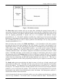
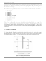
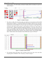
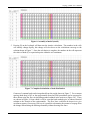
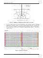
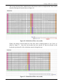
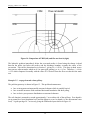
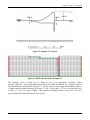
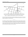
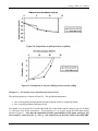
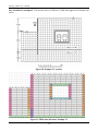
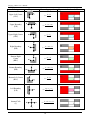
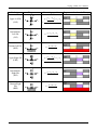
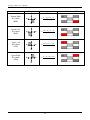
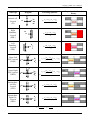
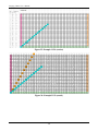
Seepage_CSM8 A spreadsheet tool implementing the Finite Difference Method (FDM) for the solution of twodimensional steady-state seepage problems. USER’S MANUAL J. A. Knappett (2012) This user’s manual and its associated spreadsheet (‘Flownet_CSM8.xls’) accompanies Craig’s Soil Mechnics, 8th Edition (J.A. Knappett & R.F. Craig). The spreadsheet ‘Flownet_CSM8’ is an implementation of the methodology outlined in: Williams, B.P., Smyrell, A.G. and Lewis, P.J. (1993) Flownet diagrams – the use of finite differences and a spreadsheet to determine potential heads, Ground Engineering, 25(5), 32–8. Seepage_CSM8: User’s Manual 1. INTRODUCTION This manual will explain how to use the spreadsheet analysis tool ‘Seepage_CSM8.xls’ to solve a wide range of two-dimensional steady-state seepage problems. This spreadsheet is an implementation of the Finite Difference Method (FDM) described in Section 2.7 of the main text. Spreadsheets offer a number of advantages for solving such problems, namely: The tabular layout is particularly suited for forming a two-dimensional mesh, in which each cell represents a node of the mesh. The problem as laid out on screen will therefore bear a strong visual resemblance to the problem being addressed; As the total head at each node depends on the values of the nodes around it, it is required to solve a large number of simultaneous equations. This can be done effectively and efficiently using the iterative calculation techniques embedded within modern spreadsheets; Spreadsheet software is a standard component of most suites of office applications which are installed as standard on most computers (e.g. Microsoft Excel, within the Microsoft Office suite, or Calc, within the Open Office suite). They are therefore almost universally accessible to students and practicing engineers without the need to buy additional expensive software. This manual is structured as follows: Section 2 The basic structure of both the workbook (Seepage_CSM8.xls) and the worksheet used to perform the analyses will be described and the principle of operation will be highlighted. Section 3 This section will describe, step-by-step, how to use the basic worksheet to analyse a new seepage problem. The resulting values of head will be used to derive equipotentials which will be compared to those obtained using a flow net sketch. Section 4 The spreadsheet tool has further been used to analyse other worked examples from the main text. These are compared with the solutions obtained by flow net sketching to validate the method. These examples demonstrate how different types of boundary conditions (e.g. structural elements, soil layering) may be implemented within models. Section 5 This section describes the library of different FDM nodes implemented within the spreadsheet tool and provides further detail of the governing equations. Appendix Describes the modelling of drains within a body of soil, with reference to the backfilled retaining wall problem in Example 11.5. 2. PROGRAMME DESCRIPTION The spreadsheet analysis tool essentially consists of a single worksheet in which all calculations are conducted and which contains all of the necessary information for solving a problem by the FDM. The worksheet consists of four sections, as shown schematically in Figure 1. 2 Seepage_CSM8: User’s Manual Figure 1: Worksheet structure The Basic data section contains cells for user input data, including the spacing between nodes (a square grid with uniform spacing in both horizontal and vertical spacing is implemented in the current version of the software), the depth at which the datum for head measurement has been selected, and cells for inputting permeability if layered soils are to be modelled with different isotropic permeabilities (k1, k2). Note that for problems in which only a single layer of soil is present, the head distribution is independent of the permeability of the soil, and the permeability cells may be left blank. The spreadsheet may also be used to analyse problems with anisotropic soils by using equivalent isotropic permeabilities (k′1, k′2). Below the Basic data section is the FDM node library. As the formulation of the basic equation governing the head at any node depends on the cells around it, for nodes on the boundary of an impermeable element (e.g. some sheet piling or the bottom of a foundation) some of the adjacent cells will be inactive (e.g. ‘within’ the impermeable boundary). As a result, special versions of the basic node formula (Equation 2.31 from the main text) are required to correctly model the boundary conditions within the model. The formulae employed are described in more detail in Section 5 of this manual. The FDM node library section contains one example of each formula, which may be copied into appropriate cells in the Drawing area (see below) to build up a complete FD mesh. An example of this is provided in Section 3. The drawing area may be extended if necessary by inserting additional columns between columns BQ and BR and inserting additional rows after row 57. This may be necessary for problems in which a fine grid spacing is required to give a high level of detail in a large problem. The Depth scale section auto-calculates the depth in metres of each row of nodes using the grid spacing entered in Basic data. The depth scale fixes zero at the level of the uppermost row of nodes used in the problem. The uppermost row of nodes should therefore be entered in row 7 within the drawing area. The examples in Section 4 include problems where soil levels may be unequal within the problem (e.g. for an exacavtion) for guidance. This section also uses the input datum level to provide an alterantive scale which is the elevation head (z) above the datum. Note that positive values of z indicate nodes which are above the datum. As the elevation head is the same for all nodes within a row, the worksheet provides the user with both values of h (by calculation – see Section 3) and z at all nodes within the model. The distribution of 3 Seepage_CSM8: User’s Manual pore pressure within the model can therefore be obtained by application of Equation 2.1 from the main text at each node. This may be efficiently conducted for a given problem using the remaining cells in the worksheet as necessary. The workbook Seepage_CSM8.xls contains a series of worksheets which are named as shown below: New analysis… Example 2.1 Example 2.2 Example 2.3 Example 2.5 (Lw=Lb=0) Example 2.5 (Lw=9.1) Example 2.5 (Lb=9.1) Example 11.5a Example 11.5b Each of these worksheets has the structure described previously, though in all cases except ‘New analysis…’ a completed solution is presented (the ‘New analysis…’ sheet having been used in each case to analyse a worked example from the main text). The use of the ‘New analysis…’ sheet to solve a seepage problem will be described in Section 3 of this manual; the remaining sheets will be discussed in Section 4. 3. WORKED EXAMPLE To illustrate how the FD mesh is assembled and analysed, this section will consider the example presented in Section 2.4 of the main text, which was used to describe the flow net sketching technique. The example is shown in Figure 2. The steps required to solve the problem are illustrated below. Figure 2: Example problem (section) 4 Seepage_CSM8: User’s Manual 1. For this problem a grid spacing of 0.5 m is selected. This means that almost all of the dimensions in Figure 2 can be represented exactly by whole numbers of nodes. The depth of 8.6 m between the soil surface and the lower impermeable layer will here be approximated as 8.5 m, which is expected to have a negligible influence on the resulting seepage. The value of 0.5 is entered into the grid spacing cell in the Basic data section as shown in Figure 3. As in the main text, the datum will be selected at -0.5 m depth (i.e. the downstream water level). The spreadsheet is programmed to calculate the results of formulae only when requested by the user. After entering the grid spacing and datum level, pressing F9 will calculate the depth scale and elevation heads in the Depth scale section. Figure 3: Data entry 2. The FD mesh may now be assembled. As in the example from the main text, the soil domain extends approximately 8 m either side of the sheet piling. This requires 17 nodes (at 0.5 m spacing) from one edge of the soil domain up to and including the nodes along one side of the sheet piling. As the pressures/head along either side of the wall may be different, nodes are required for both sides of the piling, even though it has a negligible thickness. A total of 34 nodes will therefore be required horizontally (i.e. 34 columns). 18 nodes are required vertically to model the 8.5 m depth of soil (i.e. 18 rows). The uppermost nodes, representing the upper surface of the soil, represent the recharge (left hand side) and discharge (right hand side) boundaries. Values of head (relative to the datum) are known at these nodes and are entered in metres as shown in Figure 4. The left and right boundaries are then formed by copying the formulae for these boundary conditions from the FDM node library to the drawing area (i.e. LB and RB respectively). Note that of the 18 nodes required on this boundary, the top node is on the discharge boundary (value = 0.5 m) and the bottom node will be part of both the right boundary and the bottom boundary, i.e. a bottom right corner (BRC). Only the 16 nodes in between should therefore have the RB 5 Seepage_CSM8: User’s Manual formula copied in. The left boundary and bottom boundary (BB) can similarly be copied in as shown in Figure 4. Figure 4: Assembly of model 3. The nodes on either side of the sheet piling can similarly be incorporated using LB and RB nodes as shown in Figure 5. The nodes beneath the sheet piling are a special case, as due to the small thickness of the sheet pile wall, the nodes below each side of the sheet piling essentially represent the same point within the soil and so require special formulae to ensure that the heads calculated at these nodes will be consistent. These formulae are given in the central column of the node library (‘NODES AROUND & BENEATH PILING’). The nodes at the toe of the wall (i.e. at 6 m depth) are represented by Upper-Right Pile (URP) and Upper-Left Pile (ULP) on the right and left sides of the wall respectively. The nodes below this are modelled using the intermediate nodes (IRP and ILP) and those on the bottom boundary using the BRP and BLP nodes. Further details on the formulation of these FDM nodes are given in Section 5. Figure 5: Assembly of model (contd.) 4. The remaining nodes in the interior of the soil body on either side of the wall are then filled using the generic ‘INTERNAL CELL’ formula (I), as shown in Figure 6. 6 Seepage_CSM8: User’s Manual Figure 6: Assembly of model (contd.) 5. Pressing F9 on the keyboard will then start the iterative calculation. The numbers in the cells will initially change rapidly; this change will slow down as the calculations converge to the solution shown in Figure 7. Once the calculation is complete, the numbers in the cells represent the values of head (h) at a particular point within the soil continuum. Figure 7: Completed calculation of head distribution Contours of constant head can be interpolated from the results shown in Figure 7. For a contour spacing (head drop) of 0.5 m, the equipotentials from the FDM spreadsheet can be compared to those drawn using the flow net sketching method outlined in the main text (Figure 2.8). These are shown in Figure 8, from which it will be seen that both methods give an almost identical solution to the location of the equipotentials. The flow lines could then be drawn in to give curvilinear squares if necessary, however it is possible to determine the amount of seepage from the change in head along the discharge boundary without drawing flow lines. 7 Seepage_CSM8: User’s Manual Figure 8: Comparison of FDM equipotentials with flow net sketch 6. The flow of pore water must become perpendicular to the discharge boundary as the fluid approaches the boundary. Each set of vertical nodes in this region therefore represent flow lines. The change in head (h) at the discharge boundary is therefore found at a given distance from the right edge of the wall as by entering the formula shown in Figure 9. This is then copied as shown. Figure 9: Calculation of flow rate 8 Seepage_CSM8: User’s Manual The average amount of flow within the flow tube between each set of adjacent flow lines is then found by entering the formula shown in Figure 10. Figure 10: Calculation of flow rate (contd.) Finally, the change in head within all of the flow tubes is added together to give h), as shown in Figure 11. Once this last formula has been entered, F9 must be pressed on the keyboard to perform all of the calculations entered during this step. Figure 11: Calculation of flow rate (contd.) 9 Seepage_CSM8: User’s Manual Performing the calculations gives h = 1.4. The flow rate (q) can then be found as described in Section 2.7/Example 2.3 of the main text: qk h This gives q = 1.4k, which compares favourably to the value of q = 1.5k found from the flow net sketch in Section 2.4 of the main text. It can readily be seen by this example that use of the FDM in this way provides a very quick and simple way to determine total head (and hence pore pressures if necessary) and flow quantities for a seepage problem, and is less subjective than the sketching of a flow net. 4. APPLICATION TO WORKED EXAMPLES IN MAIN TEXT This section demonstrates how the FDM spreadsheet may be applied to the other worked examples included in Chapter 2 of the main text. These are included as complete worksheets within Seepage_CSM8.xls. Note that this implementation of the FDM is not suited to problems involving unconfined seepage (e.g. flow through embankment dams). As such, only Examples 2.1 – 2.3 will be considered here. These examples will demonstrate the use of the full range of nodal formulations included in the FDM node library, including applications to sheet piling, layered soils and buried structures. Example 2.1 – Flow into a cofferdam The problem geometry is shown in Figure 12. This problem is similar to the worked example in Section 3; however, it demonstrates: how to tackle problems with varying ground level; how to tackle problems involving symmetry; how to extract hydraulic gradient information from the FDM. The soil domain is assumed to extend 8 m on either side of the excavation. Zero depth is set at the level of the soil outside the excavation and the datum is set at 2.5 m depth (i.e. the water level within the excavation). A grid spacing of 0.5 m is used, giving the FDM node layout shown in Figure 13. 10 Seepage_CSM8: User’s Manual Figure 12: Example 2.1 (section) Figure 13: FDM node allocation, Example 2.1 The resulting head distribution within the model may be found in the appropriate worksheet within Seepage_CSM8.xls. It will be seen that the solution is symmetric and validates the symmetry assumptions made in the main text when sketching the flow net. A half FDM model could equally-well have been used, which would have given the same solution. Equipotentials have been derived from head distribution and are compared with those obtained from the flow net sketch in the main text in Figure 14. 11 Seepage_CSM8: User’s Manual Figure 14: Comparison of FDM (left) and flow net sketch (right) The hydraulic gradient immediately below the excavated surface is found using the change in head between the nodes just below the surface and the discharge boundary towards the centre of the excavation. This can be determined as in Section 3, giving h = 0.26 m. This drop in head occurs between two adjacent nodes which are 0.5 m apart (grid spacing), so s = 0.5 m. Therefore, i = h/s = 0.52 which compares favourably with the value of 0.5 derived from the flow net sketch in the main text. Example 2.2 – seepage beneath a dam spillway The problem geometry is shown in Figure 15. This problem demonstrates: how to incorporate an impermeable structural element which is partially buried; how to model structures with combined horizontal boundaries and sheet piling; how to derive pore pressure distributions on structural elements. The soil domain is assumed to extend approximately 5 m on either side of the spillway. Zero depth is set at ground level (not foundation level) and the datum is set at 0 m depth (i.e. the downstream water level). A grid spacing of 0.7 m is used, giving the FDM node layout shown in Figure 16. 12 Seepage_CSM8: User’s Manual Figure 15: Example 2.2 (section) Figure 16: FDM node allocation, Example 2.2 The resulting values of head may be found in the in the appropriate worksheet within Seepage_CSM8.xls. The equipotentials derived from the FDM calculations are compared with the flow net sketched in the main text in Figure 17. The flow rate of water seeping underneath the spillway is found using the method described in Section 3. h = 1.48 m and k = 2.5×10⁻⁵ m/s (see main text) so that q = 3.7×10⁻⁵ m3/s (per m length). This compares favourably with the value of 3.75×10 -5 m3/s (per m length) determined from the flow net sketch. 13 Seepage_CSM8: User’s Manual Figure 17: Comparison of FDM (dashed lines) and flow net sketch (solid lines) The values of head at the nodes along the underside of the spillway may be copied out. The elevation head (z) from column Z for each node may then be used to determine the uplift pressures acting on the spillway using Equation 2.1 from the main text: u w h z This method may similarly be applied for the nodes along either side of the sheet piling to determine the net pore pressures acting on the piling. Note that this is the same method used in the main text ; however, the FDM is particularly suitable for this application as the heads are automatically determined at the same points along each side of the wall. The uplift pressure distribution on the underside of the spillway and the net pore pressures on the sheet piling are compared with those determined from the flow net sketch (main text) in Figures 18 and 19 respectively. 14 Seepage_CSM8: User’s Manual Figure 18: Comparison of uplift pressures on spillway Figure 19: Comparison of net pore (fluid) pressures on sheet piling Example 2.3 – Excavation next to buried tunnel in layered soil The problem geometry is shown in Figure 20. This problem demonstrates: how to incorporate an impermeable structural element which is completely buried; how to model problems with layered soils. Zero depth is set at ground level on the right hand side of the model and the datum is set at 6 m depth (i.e. the water level in the excavation). A grid spacing of 1 m is used, giving the FDM node layout shown in Figure 21. Note that the equivalent isotropic permeabilities of the upper and lower soil layers must be entered in the ‘k1’ and ‘k2’ cells respectively in the Basic Data section BEFORE 15 Seepage_CSM8: User’s Manual any calculation is attempted. The current version of Flownet_CSM8 only supports two distinct soil layers. Figure 20: Example 2.3 (section) Figure 21: FDM node allocation, Example 2.3 16 Seepage_CSM8: User’s Manual The resulting values of head may be found in the in the appropriate worksheet within Seepage_CSM8.xls. The values of head may be extracted from the nodes representing the tunnel walls and the method described in the previous example may be used to convert these values into pore pressures. The resulting pore pressure distribution is shown in Figure 22. Figure 22: Pore pressure distribution around tunnel (all values in kPa) The flow rate is found as in the previous example, by considering the change of head (h) just below the level of the excavation. From the spreadsheet, this is found to be h = 3.30 m. At this level, the water is flowing through soil 1 with permeability k1, so: q k1 h This gives q = 3.3×10⁻⁹ m3/s (per m length). 5. FDM NODE LIBRARY This section describes the different nodal formulae which are available within Seepage_CSM8.xls and provides the theoretical formulation of each. These are split into four separate tables over pages 18 – 21 inclusive: p.18: Basic nodes for modelling impermeable boundaries and general soil nodes p.19: Nodes for modelling soil beneath thin impermeable elements (e.g. sheet piling) p.20: Nodes at the corner of an impermeable buried structure p.21: Advanced nodes for modelling horizontal soil layer boundaries where there is a change in permeability. 17 Seepage_CSM8: User’s Manual Node type Diagram Governing equation h1 Upper-Left Corner (ULC) h h1 h4 2 h4 Upper Boundary (UB) h3 h1 h h1 h3 2h4 4 h4 h3 Upper-Right Corner (URC) h h3 h4 2 h4 h2 Right Boundary (RB) h h3 h2 2h3 h4 4 h4 h2 Bottom-Right Corner (BRC) h h3 h2 h3 2 h2 Bottom Boundary (BB) h h3 h1 h1 2h2 h3 4 h2 Bottom-Left Corner (BLC) h h1 h1 h2 2 h2 Left Boundary (LB) h h1 2h1 h2 h4 4 h4 h2 Internal Cells (I) h3 h1 h h1 h2 h3 h4 4 h4 18 Representation in node library Seepage_CSM8: User’s Manual Node type Diagram Governing equation h2L h2R Upper-Left Pile (ULP) h3 h1 h h2 R h1 2 L 2 h 4 h3 h4 h4 h2 IntermediateLeft Pile (ILP) h3 h1 h h1 h2 h3 h4 4 h4 h2 Bottom-Left Pile (BLP) h3 h1 h h1 2h2 h3 4 h2L h2R Upper-Right Pile (URP) h3 h1 h h2 R h1 2 L 2 h 4 h3 h4 h4 h2 IntermediateRight Pile (IRP) h3 h1 h h1 h2 h3 h4 4 h4 Bottom-Right Pile (BRP) h2 h3 h1 h h1 2h2 h3 4 19 Representation in node library Seepage_CSM8: User’s Manual Node type Diagram Governing equation h2 Bottom-Right Re-entrant (BRR) h3 h1 h h1 2h2 2h3 h4 6 h1 h 2h1 2h2 h3 h4 6 h1 h 2h1 h2 h3 2h4 6 h1 h h1 h2 2h3 2h4 6 h4 h2 Bottom-Left Re-entrant (BLR) h3 h4 h2 Upper-Left Re-entrant (ULR) h3 h4 h2 Upper-Right Re-entrant (URR) h3 h4 20 Representation in node library Seepage_CSM8: User’s Manual Node type Diagram Governing equation h2 Internal cell, Layered (IL) k1 h3 h h1 k2 h1 1 h2 h3 2 h4 4 h4 h2 Right Boundary, Layered (RBL) k1 h h3 1 h2 2h3 2 h4 4 k2 h4 h2 Left Boundary, Layered (LBL) k1 h h1 k2 2h1 1 h2 2 h4 4 h4 h2L h2R Upper-Left Pile, Layered (ULPL) h h2 R h1 1 2 L 2 h 4 k1 h3 h1 k2 h3 2 h4 h4 h2L h2R Upper-Right Pile, Layered (URPL) h h2 R h1 1 2 L h3 2 h4 2 h 4 k1 h3 h1 k2 h4 h2 IntermediateLeft Pile, Layered (ILPL) k1 h3 h1 h h1 1 h2 h3 2 h4 4 h h1 1 h2 h3 2 h4 4 k2 h4 h2 IntermediateRight Pile, Layered (IRPL) k1 h3 h1 k2 h4 1 2k1 2k 2 ; 2 k1 k 2 k1 k 2 21 Representation in node library Seepage_CSM8: User’s Manual APPENDIX This appendix demonstrates the use of Seepage_CSM8.xls for analysing the drained backfill in the retaining wall problem of Example 11.5. This problem demonstrates: how to incorporate a linear drain within models ; how to determine the resultant pore water pressure thrust on a plane within the soil (for use in the Coulomb wedge method of analysis, Section 11.5). Only the retained soil is modelled in this case (assuming that the underlying soil is relatively impermeable). Zero depth is set at the top of the retained soil and the datum is set at 6 m depth (i.e. the bottom of the retained soil). The head along the top surface of the soil is therefore 6 m (pore pressure = 0, elevation = 6 m). A grid spacing of 0.25 m is used. Example 11.5(a): vertical drain behind retaining wall The upper, right hand side and bottom boundaries are set as before. The drain is vertical and runs along the back of the retaining wall. Within the drain the pore pressure must always be zero, so the head will always be equal to the elevation head (i.e. is independent of the adjacent cells). This can be modelled by setting each of the cells on the left hand boundary equal to the value of elevation in that row, giving the FDM node layout shown in Figure 23. Figure 23: Example 11.5a (section) The calculation then proceeds as normal by pressing F9. For the Coulomb wedge analysis, the resultant pore water thrust along a plane inclined at p = 45 + ′/2 = 64° to the horizontal is to be found. Starting from the bottom left hand corner, a point close to the failure plane is found by going up two cells for every one across. These cells are highlighted in dark orange in Figure 24. 22 Seepage_CSM8: User’s Manual Figure 24: Example 11.5a (contd.) The distance along the slip plane from one orange cell to the next is found by Pythagoras’ Theorem (one cell across = 0.25 m, two up = 0.5 m so L = 0.56 m). The values of h and z can then be extracted for each orange cell; the pore water pressure at each point is then found using Equation 2.1. These values are then numerically integrated along the slip plane using the trapezium rule, to give U = 36.8 kN/m (per metre length) Example 11.5(b): sloping drain behind retaining wall The sloping drain in Example 11.5(b) is modelled in the same way, except that the cells representing the drain now fall on a 45° line as shown in Figure 25. The left hand boundary is now impermeable (representing the back of the concrete retaining wall; starting from the bottom left hand corner the internal cells within the mesh are replaced with the value of elevation head in each row. The calculation then proceeds as normal by pressing F9. The resultant pore water thrust is to be found along the same plane as before. Starting from the bottom left hand corner, a point close to the failure plane is found by going up two cells for every one across. These cells are highlighted in dark orange in Figure 26. The values of h and z can then be extracted for each orange cell; the pore water pressure at each point is then found using Equation 2.1. These values are then numerically integrated along the slip plane using the trapezium rule, to give U = 0.43 kN/m 0 (per metre length) 23 Seepage_CSM8: User’s Manual Figure 25: Example 11.5b (section) Figure 26: Example 11.5b (contd.) 24


![RessqM, Enhanced Version of RESSQ [Javandel et al., 1984]](http://vs1.manualzilla.com/store/data/005674408_1-e8a4b9f66c80cdc83d847a710e5b4b1f-150x150.png)