Download Shrimp Partial Harvesting Model: Decision Support System

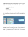
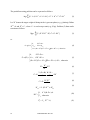
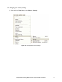
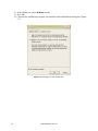
CTSA Publication No. 153
Shrimp Partial Harvesting Model:
Decision Support System
User Manual
Lotus E. Kam, Run Yu, and PingSun Leung
Department of Molecular Biosciences and Bioengineering
College of Tropical Agriculture and Human Resources
University of Hawai`i at Mānoa, Honolulu, USA
Paul Bienfang
Department of Oceanography
School of Ocean and Earth Science and Technology
University of Hawai`i at Mānoa, Honolulu, USA
CENTER
FOR
TROPICAL
AND
SUBTROPICAL
AQUACULTURE
User Information & Program Requirements
This Shrimp Partial Harvesting Model, often hereafter referred to as “Model,” includes worksheets
to simplify data entry and navigation. This manual describes the data entry procedures, equations
unique to the Model, and a simplified financial analysis.
Users of the Model should have a general working knowledge of Microsoft Excel®. For a detailed
description of the program, its functions and commands, consult a Microsoft Excel® manual or one
of the many books describing Microsoft Excel®.
This beta version of the Model requires a Windows PC or compatible that runs Microsoft Excel®
2002, 2003, or 2007. Free space of 1MB is required.
This application requires the Solver® add-in available with Microsoft Excel®. This application is
not compatible with the Premium version of the Solver® available through Frontline Systems Inc.
If you have installed the Premium Solver, you must uninstall the advanced version of the add-in in
order to use this Model software. The providers are not responsible for conflicts between versions
of the Solver® and Microsoft Excel®.
Limits of Liability and Disclaimer of Warranty
The authors of this manual have used their best efforts to prepare this manual and the program it
supports. The authors make no warranty of any kind, expressed or implied, with regard to these
programs or the documentation contained herein. The authors shall not be held liable for incidental
or consequential damages in connection with, or arising from, the furnishing, performance or use
of the program.
Shrimp Partial Harvesting Model: Decision Support System User Manual
i
Contact
Please direct inquiries regarding this publication and associated software to PingSun Leung
through either e-mail or regular mail using the below contact information:
PingSun Leung
Department of Molecular Biosciences and Bioengineering
University of Hawai`i at Mānoa
3050 Maile Way, Gilmore 111
Honolulu, HI 96822, USA
[email protected]
Trademarks
Microsoft® and Excel® are trademarks of the Microsoft Corporation.
Copyright
©2008
ii
CTSA Publication No. 153
Acknowledgements
Many people contributed to the development of this Shrimp Partial Harvesting Model. The
authors thank Mr. James N. Sweeney and Mr. David Godin of the former Ceatech USA Inc. for
their various forms of support for and assistance with the validation of this Model. The Model
and software development was made possible by the generous support of the Center for Tropical
and Subtropical Aquaculture through grant nos. 2003-38500-13092 and 2002-38500-12039
from the U.S. Department of Agriculture Cooperative State Research, Education, and Extension
Service.
Shrimp Partial Harvesting Model: Decision Support System User Manual
iii
Shrimp Partial Harvesting Model
Decision Support System
User Manual
1. Introduction
In traditional shrimp culture and other intensive aquaculture systems, an entire crop can be harvested
at one time. However, since growth and survival are density-dependent, single-batch harvesting can
lead to competitive pressures that lower individual growth and increase mortalities. In comparison
to single-batch harvesting, a partial harvesting approach can enhance growth rates and total yield,
since a reduction in total biomass reduces competitive pressure. In partial harvesting, a crop can be
partially-harvested so that only a portion of the crop is extracted. This Shrimp Partial Harvesting
Model was created to simulate the effects of partial harvesting and assist farm managers in deciding
the most profitable harvesting schedule.
This Shrimp Partial Harvesting Model, often hereafter referred to as “Model,” is a decision support
system based on a network-flow approach. This Model determines the optimal harvesting times that
maximize the overall net revenue based on biological and economic factors (e.g., survival, growth,
and price). This Model was implemented in a spreadsheet form using Microsoft Excel. The model
requires the use of the Solver add-in. See Part B of the Appendix for instructions on installing the
standard Solver. Details of the Model development also can be found in the Appendix.
Click Begin on the introduction screen to begin using the Partial Harvesting Model (Figure 1-1).
Figure 1-1. View of the introduction screen.
1
2. Main Menu
The Main Menu of this spreadsheet Model provides access to worksheets to enter information
about farm operations (Operations), market price and demand information (Market Info), and
bioproduction technology performance (Bioproduction). Use the Analysis button to determine
the optimal harvesting strategy. Use the Results button to find the production schedule and overall
net revenue solution for the most recent analysis.
In compatible versions of Excel, a navigation toolbar is located at the top of the screen. The
navigation toolbar provides access to the worksheets, file, viewing, and printing options. The
navigation toolbar is not available in Microsoft Office® 2007.
Figure 2-1. View of the Main Menu used for navigation.
3. Operations
Information about farm operations is needed to estimate the operating expenses that a farm will
incur.
2
CTSA Publication No. 153
The total pond area must be specified in acres. The total pond area refers to the size of a single
pond. Multiple ponds are not considered in this simplified partial-harvesting model. Multiple ponds
introduce a more complex scheduling problem (Yu and Leung 2005).
Key farm costs are required, including the expenses listed as examples below:
• weekly maintenance cost ($/week),
• feed cost ($/lb),
• harvest cost ($/harvest),
• and seed cost ($/1000).
This Model is designed to determine if it is more advantageous to engage in multiple small “partial
harvests” in comparison to a single (or few) very large harvests. In order to investigate the benefits
of the partial-harvest strategy, users must specify the cost for a traditional full harvest and a partial
harvest.
Figure 3-1. View of the input screen for Operations.
In this partial harvesting software, users specify the maximum size of the partial harvest (partial
harvest limit) in lbs/harvest. The partial harvest limit should be greater than 0 and indicates the
maximum amount that can be harvested at the partial harvest cost ($/harvest).
In Figure 3-1, for example, the cost to harvest any amount over 1,000 lb. is $1,000. For harvests
less than or equal to 1,000 lb., the cost is $250.
Shrimp Partial Harvesting Model: Decision Support System User Manual
3
Specify the seed size in grams. The seed cost must be specified in conventional units of dollars per
thousand pieces ($/1,000). The cost is converted into $/lb based on the seed size entered.
Note: If there is no distinction between a partial harvest and large harvest, the harvest cost should
be the same. Do not leave either of these cells blank. For large pond sizes, it may make sense to
increase the partial harvest limit accordingly.
4. Market Information (Input)
Information about the market size and demand is needed to determine the potential revenue
available to the farm enterprise.
Figure 4-1. View of the Market Information input screen.
4
CTSA Publication No. 153
4.1. Market Size (B1)
This spreadsheet divides the market demand for shrimp products into seven common count sizes.
Since market sizes are specified as ranges corresponding to the number of shrimp per pound,
a farmer can specify his target weight criteria. In particular, a farmer may choose to meet the
minimum, average, maximum, or other weight criteria corresponding to each range. In this
example, the farmer has chosen to meet the minimum shrimp sizes, which are 9.07 g (40–50
count), 10.08 g (41–45 count) … and 22.68 g (16–20 count).
The minimum setting is the most conservative and recommended for most production systems.
High criteria require more efficient bioproduction technologies. This Model will not be able to
provide a harvest solution if bioproduction technology (discussed in Section 5) cannot achieve
the size criteria specified. Therefore, if you have difficulty running your model, you may want to
revise your Market Size information.
The count ranges are based on current market demand but can be customized by a user. As
illustrated in Figure 4-2, a user can customize the range settings by modifying the maximum
count corresponding to each growout phase and the overall minimum count (i.e., the largest
shrimp). The maximum count of shrimp for each market range should be decreased for successive
ranges. The length of a growout period corresponds to shrimp size and shrimp count. Specifically,
extending the length of growout means increasing shrimp size and reducing shrimp counts. This
Model requires consecutive ranges such that the maximum counts for each range decrease for later
growout phases. This Model will verify whether sizes are sequential before conducting analysis.
A user can specify target sizes in the Other column. When selecting “Other” for criteria, weights
must be specified for each range in the far right column. These target weights should fall between
the minimum and maximum count sizes for each size range. The values in the Other column cells
are only active when the target weight criteria is set to “Other” from the drop down menu.
Figure 4-2. Specifiying target weight criteria and
market size range.
Shrimp Partial Harvesting Model: Decision Support System User Manual
5
4.2. Market Demand
The Target Size (in grams) should reflect the weight corresponding to your target weight criteria.
Enter the Minimum Production corresponding to each size. If no production is required for a
size category, enter 0. In Figure 4-5, no minimum production is required. Enter the Maximum
Demand corresponding to each size. If demand is unknown or not very large, type “=MaxValue”
and the maximum default value will appear.
Figure 4-3. Default Minimum Production and
Maximum Demand (Partial Harvest Scenario).
Farms may be required to fulfill a minimum production level if they have contracts with shrimp
wholesalers. If a minimum level of production is required, the Minimum Production amount
must reflect the required production for each size. Figure 4-4 illustrates the case where a farm is
required to produce a minimum volume of 5,000 lb. of 36–40 count and 14,000 lb. 16–20 count
shrimp.
For the single-batch harvest scenario, the Minimum Production for all product sizes should be
set to 0. The Maximum Demand should also be equal to 0 for all growout sizes except for the final
harvest size (see Figure 4-5). The minimum production required must be less than the carrying
capacity. The Maximum Demand for the final harvest (growout phase) cannot be equal to zero.
Figure 4-4. Specifying a production requirement
(Partial Harvest Scenario with Production
Requirement).
6
Figure 4-5. Single-batch harvest scenario (baseline
scenario).
CTSA Publication No. 153
5. Bioproduction (Input)
In order to measure the financial performance of a shrimp farm, information about bioproduction
technology is needed. Recommended bioproduction performance data is available in the
Bioproduction worksheet. Values are based on data collected from a commercial shrimp farm in
Hawai`i, which operated 40 one-acre intensive shrimp ponds (Yu, Leung, and Bienfang 2007).
Growth and mortality information is based on traditional single-batch harvest practices.
Figure 5-1. View of input screen for Bioproduction Technology.
Bioproduction performance values may be changed based on your farm’s production
specifications:
Indicate the carrying capacity for your pond (kg/m2). The carrying capacity is assumed to be the
same for all phases and is based on the value you specify.
• Provide the initial stocking density for the first growout period in shrimp per square
meter (i.e., first row in the current density column). Estimate the density for subsequent
phases based on your pond performance. These density estimates should be based on
single-batch harvest practices.
• Estimate the weekly growth rate (g/week) for each growout phase.
• Provide the current survival rate for each phase (% survival).
Shrimp Partial Harvesting Model: Decision Support System User Manual
7
• Enter the maximum growth rate for each phase (g/week). Current growth rates should
always be less than maximum growth rates.
• Enter the feed rate as a percentage of pond biomass.
The worksheet also provides a summary about the growth curve, time required to reach market
weight, and growth limits based on the production technology specified.
Figure 5-2. Bioproduction growth and limit summary.
6. Analysis
To run a partial harvest analysis based on your input, click the Analysis button.
Some validation has been built into this Model. This worksheet verifies that entered values
are consistent or acceptable within the workbook. This program will verify that the following
constraints are met:
• Count sizes should decrease for subsequent phases.
• Maximum growth is less than the growth limit for each phase.
Please be patient as the analysis runs through a sequence of six different algorithm settings. If your
analysis is successful, you will be directed to a summary report. The optimal solution is compared
to the single-batch harvesting solution in this report.
8
CTSA Publication No. 153
Figure 6-1. Beginning the analysis.
Note: If the program is not able to run successfully based on your input, a partial-harvest solution
will not be given. You will receive a message that requests revision of your inputs.
Shrimp Partial Harvesting Model: Decision Support System User Manual
9
7. Results
Results include summary information about bioproduction performance (D1), market summary
(D2), revenue and expenses (D3), and net revenue (D4).
Figure 7-1. Results spreadsheet.
7.1. Bioproduction Performance
Information about Bioproduction Performance includes initial density, duration of each phase,
weekly growth rates, harvest weight, and harvest schedule. The optimal partial harvesting solution
for a scenario with no production requirement and unlimited demand is indicated in Figure 7-2.
According to these results, the stocking density should be 112.9 shrimp/m2 with harvests after 7.4
weeks (1,000 lb. of 36–40 count shrimp), 9.0 weeks (1,000 lb. of 31–35 count shrimp), 14.9 weeks
(102 lb. of 21–25 count shrimp), and 20.6 weeks (14,738 lb. of 16–20 count shrimp). The total
weight harvested by the end of the 20.6 weeks is 16,840 lb. of shrimp.
7.2. Market Demand
In the Market section, the minimum demand (required production) and maximum demand values
entered earlier by a user in the Bioproduction sheet input are displayed. These demand ranges
indicate market constraints imposed on the farm. The count ranges used in this analysis are also
displayed for reference. This market information is illustrated in Figure 7-2.
10
CTSA Publication No. 153
Figure 7-2. Bioproduction performance and market information.
7.3. Revenue and Expenses
Operating costs, profit from sales (revenue – operating costs), and harvest costs are listed in
the results worksheet (D3). Profit from sales (revenue – production costs) is calculated for each
growout phase (Figure 7-2).
7.4. Net Revenue Summary
The Net Revenue Summary provides information on revenue from sales, expenses (operating
costs and harvest costs), and net revenue for each growout phase.
The Pond Summary is based on user-entered information on operations, bioproduction, and
market. The partial harvest solution is always compared to the single-batch, full-harvest optimal
solution. In the example above (Figure 7-3), the partial harvest solution is expected to generate an
overall net revenue of $58,119 in comparison to the single-batch harvest of $57,239 at 19.9 weeks.
Therefore, the partial harvest method is expected to increase overall net revenue by $880.
Figure 7-3. Partial harvest result compared to singlebatch baseline scenario.
Shrimp Partial Harvesting Model: Decision Support System User Manual
11
7.5. Production Requirement Example
The following example (Figure 7-4) illustrates the impact of market constraints on the partial harvest
solution. In contractual business relationships, a farm may be required to produce a minimum level
of production for a certain market size of shrimp. Given these constraints, a producer is forced to
harvest a minimum volume of product at specific times during the growout period.
In this production requirement (PR) example, the farm is required to produce 5,000 lb. of 36–40
count shrimp and 14,000 lb. of 16–20 count shrimp. The market demand inputs for this scenario
are entered as illustrated earlier in Figure 4‑4.
Note: Whenever changes are made to input values, the analysis must be run in order to determine
the harvest schedule based on the new information.
Using the Shrimp Partial Harvesting Model on this example produces the following analysis.
Optimal stocking is 158.5 animals per square meter. Shrimp should be harvested as follows: 5,000
lb. at 10.7 weeks (36–40 count), 102 lb. at 18.0 weeks (21–25 count) and 14,738 lb. at 23.7 weeks
(16–20 count). The result of this production schedule is overall net revenue of $53,317 and a total
harvest of 19,840 lb. These production requirements, then, result in a loss of $3,921 in comparison
to the traditional single-batch harvest method.
In comparison to the optimal partial harvest solution with no production requirement exhibited in
Figure 7-3, the projected loss is $4,801 (= $58,119 - $53,317). This example illustrates the case
where a farmer is disadvantaged by a wholesaling contract that imposes production requirements.
Figure 7-4. Partial harvest result for required production
compared to the single-batch baseline scenario.
12
CTSA Publication No. 153
8. References
R. Yu and P.S. Leung. 2005. Optimal harvesting strategies for a multi-pond and multi-cycle shrimp
operation: a practical network model. Mathematics and Computers in Simulation 68(4): 339–
354.
R. Yu, P.S. Leung, and P. Bienfang. 2007. Modeling partial harvesting in intensive shrimp
culture: a network-flow approach. European Journal of Operational Research. doi:10.1016/j.
ejor.2007.10.031.
APPENDIX
A. The Mathematical Model
Suppose a shrimp production cycle is comprised of N growout phases. Let H i and Psi denote the
amount of shrimp harvested at the ith growout phase in kg and its associated shrimp price ($/kg),
N
N
N
∑ P ⋅ H - ∑ (C +C )-∑ HC
i=1
s.t.
i
s
i
i=1
i
HC =0,
i
i
f
i
m
i
i=1
i
if H =0
(1)
i
HC =Ch , if H > 0
H imax ≥ H i ≥ H imin
respectively. The overall net revenue from this production cycle can be estimated as follows:
where Cif , Cim , HCi are feed cost, maintenance cost , and harvest cost occurring in the ith growout
phase, respectively. Only a quasi-fixed harvest cost, Ch , is considered in the present model. In
other words, if the producer decides to do a harvest, it will result in a fixed expenditure; Ch .
H imax and H imin are the maximum and minimum amount of shrimp that can be extracted by the ith
harvest.
Let Di and Bi denote the density of shrimp stock (e.g., kg/m2) at the beginning and end of the
ith growout phase, respectively. Define V as the total area (or volume) of the water body of the
growout facility (e.g., m2). Assume there is no restocking between two successive growout phases.
The amount of shrimp that is extracted by the ith harvest at the end of the ith growout phase, H i
, then can be estimated as H i =VBi -VDi+1 , i.e., the difference between the biomass at the end of
the ith growout phase and that at the beginning of the i+1th growout phase. Since all the shrimp will
be harvested at the end of the growout cycle, it implies H N =VBN . Assume the objective of the
producer is to maximize overall net revenue.
Shrimp Partial Harvesting Model: Decision Support System User Manual
13
The partial harvesting problem can be expressed as follows:
N-1
Max
∑ [Psi ⋅ V ⋅ (Bi -Di+1 )-Cif -Cim -HCi ] + PsN ⋅ V ⋅ BN -CfN -CmN -HC N
i
D
(2)
i=1
Let W i denote the target weight of shrimp in the ith growout phase (e.g., g/shrimp). Define
D N+1 =0 and Ps0 = Cs , where Cs is seed cost per unit (e.g., $/kg). Problem (2) then can be
rewritten as follows:
Max
i
D
N
∑ [V ⋅ (P ⋅ B -P
i
s
i=1
i
i-1
s
⋅ Di )-Cif -Cim -HCi ]
(3)
s.t.
0,
if Di >D max

G i =g(Di )= G max , if Di <Dimin

i
i
i
i
G max -(D max -D )(G max -G current ) (D max -Dcurrent ), otherwise
(4)
0,
if Di >D max

Si =s(Di )=  S max , if Di <Dicurrent

i
i
i
i
i
(D max -D )(Scurrent -Smin ) (D max -Dcurrent )+Smin , otherwise
(5)
Bi =
Cif =Pf
Wi i i
DS
W i-1
V ⋅ (Di +Bi ) W i -W i-1
⋅ FR i
i
2
G
(7)
W i -W i-1
Gi
(8)
Cim =Pm
H imax ≥ V ⋅ (Bi -Di+1 ) ≥ H imin
0, if V(Bi -Di+1 )=0
HCi = 
Ch , otherwise
Ps0 = Cs , D N+1 =0,
14
(6)
CTSA Publication No. 153
(9)
(10)
(11)
where G i and Si are the growth (e.g., g/week) and survival rates (%) of shrimp in the ith growout
phase and equations (4) and (5) are the corresponding density-dependent growth and survival
functions used to estimate the impacts of density on growth and survival. As illustrated in Figures
1 and 2, D max is the density at the carrying capacity (e.g., kg/m2), Dicurrent is the density under
the current practice, and G imax and Dimin are the maximum possible growth (e.g., g/week) and
its associated minimum possible density. Similarly, Sicurrent is the survival rate under the current
density level ( Dicurrent ) and Simin is the survival rate at the carrying capacity ( D max ). Equation (6)
defines that the density at the end of the ith growout phase ( Bi ) is the product of the density at the
beginning of the ith growout phase ( Di ), the associated survival rate ( Si ), and the rate of increased
shrimp weight ( W ). Equation (7) estimates total feed costs in the ith growout phase, where Pf
W
and FR i are, respectively, feed cost per unit (e.g., $/kg) and average feeding rate in terms of
i
i-1
percentage of the prevailing biomass. Equation (8) calculates total maintenance costs, where Pm
is maintenance cost per unit (e.g., $/week). Equation (9) specifies the maximum and minimum
possible amount of shrimp that can be harvested by the ith harvest. Equation (10) is the quasi-fixed
harvest cost function.
Figure A-1. Density-dependent growth.
Note: Dmax denotes the density at the carrying capacity (e.g., kg/m2); Dcurrent and Gcurrent denote the
density (e.g., kg/m2) and growth (e.g., g/week) under the current practice; Gmax and Dmin denote the
maximum possible growth (e.g., g/week) and associated minimum possible density (e.g., kg/m2).
Shrimp Partial Harvesting Model: Decision Support System User Manual
15
Figure A-2. Density-dependent survival.
Note: Dmax denotes the density at the carrying capacity (e.g., kg/m2), Dcurrent and Scurrent denote the
density (e.g., kg/m2) and survival rate (%) under the current practice, and Smin denotes the survival
rate (%) at carrying capacity.
16
CTSA Publication No. 153
B. Installing the Solver
The Frontline Solver is required in order to run this Shrimp Partial Harvesting Model. If the Solver
add-in has already been activated in your Microsoft Excel software, it will appear in your Tools
drop-down menu.
Figure B-1. Solver appears in the Tools
menu of Excel.
Shrimp Partial Harvesting Model: Decision Support System User Manual
17
B.1. Solver is not located in the Tools menu
If the Solver is not located in the Tools menu, the following steps will assist you in loading the
Solver add-in.
1) Start Excel and click on Tools on the menu. Then click on Add-ins...
2) A box should appear with a list of add-ins.
If there is no checkbox for “Solver Add-in,” go to B.2. on the next page.
3) Check the checkbox for the Solver add-in
4) Click OK.
5) The Solver should now be listed on the Tools menu in Excel (see Figure B-1).
Figure B-2. Select the Solver add-in.
18
CTSA Publication No. 153
B.2. Solver is not located in the list of available add-ins.
If the Solver is not located in your list of add-ins, you will need your Microsoft Office CD-ROM.
The following steps will assist you in installing the Solver add-in.
1) Insert the Microsoft CD-ROM. If the CD does not run the setup program automatically,
open My Computer, locate and double-click the setup.exe file on the CD.
2) Click the Add or Remove Features button.
3) In the graphic that then appears, click the little plus sign next to Microsoft Excel for
Windows. This opens up the outline under that box.
4) Click the plus sign next to “Add-ins” in order to expand the list. The Solver should be listed
in the expanded list of add-Ins.
5) Click on Solver and choose Run from My Computer, so that the box is white, with no
yellow “1.” This picture illustrates how it should look when you’re done.
6) Then click Update Now to proceed with the installation. Depending on your version of
Microsoft Office, your screen may be different, but this procedure will be similar.
7) Go to step B.1 on the previous page.
Figure B-3. Installing the Excel Solver add-in.
Shrimp Partial Harvesting Model: Decision Support System User Manual
19
C. Macros used in the Model
This Shrimp Partial Harvesting Model contains macros and executable VBA script. Macros must
be enabled in order to use this Model. When opening this Model in Microsoft Excel, the following
warning about macros may appear:
C.1. Enabling macros
Click on the Enable Macros options in order for this Model to run properly.
Figure C-1. Enable Macros dialog box.
If you open the file and the Enable Macros dialog box does not appear, please change your security
settings in Excel (see C.2. on the next page).
20
CTSA Publication No. 153
C.2. Changing your security settings
1) From the Excel Tools Menu, select Macro > Security.
Figure C-2. Changing Macro Security settings.
Shrimp Partial Harvesting Model: Decision Support System User Manual
21
2) In the Dialog box, select Medium security
3) Press OK.
4) Close the file, and then open it again. You should see the Enable Macros dialog box (Figure
C-1)
Figure C-3. Changing the macro security level.
22
CTSA Publication No. 153
For more information, please contact the
Center for Tropical and Subtropical Aquaculture
[email protected]
www.ctsa.org
Oceanic Institute
41-202 Kalaniana`ole Hwy.
Waimanalo, HI 96795
Tel: (808) 259-3168
Fax: (808) 259-8395
University of Hawai`i
3050 Maile Way, Gilmore 124
Honolulu, HI 96822
Tel: (808) 956-3529
Fax: (808) 956-5966