1
User Manual Version 11
Quick Reference Guide ....................................................................................................................... 14
Introduction ......................................................................................................................................... 17
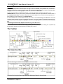
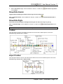
The Toolbar....................................................................................................................................... 18
The Selection Bar… .......................................................................................................................... 18
The Status Bar…............................................................................................................................... 19
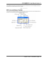
The Import Toolbar ............................................................................................................................ 19
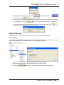
The Export Toolbar............................................................................................................................ 19
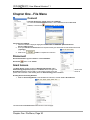
Chapter One - File Menu ..................................................................................................................... 20
Connect............................................................................................................................................. 20
Disconnect ........................................................................................................................................ 20
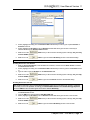
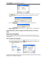
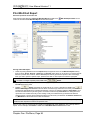
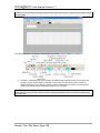
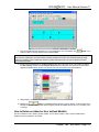
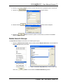
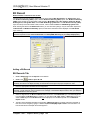
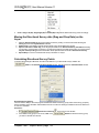
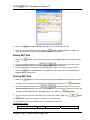
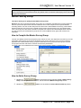
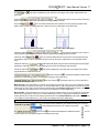
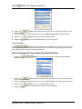
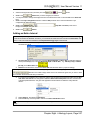
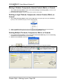
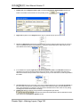
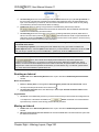
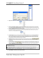
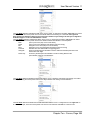
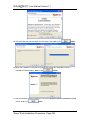
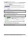
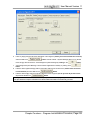
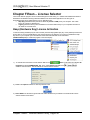
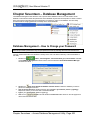
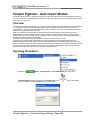
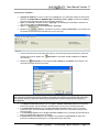
Grant Access..................................................................................................................................... 20
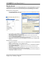
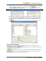
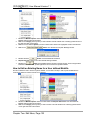
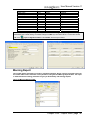
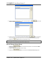
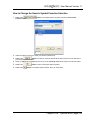
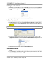
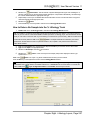
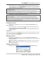
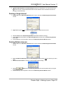
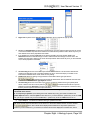
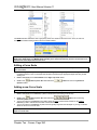
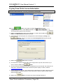
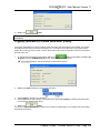
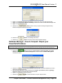
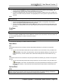
Revoke Access.................................................................................................................................. 22
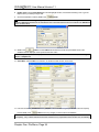
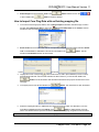
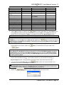
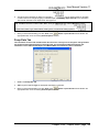
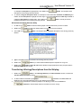
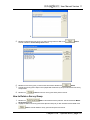
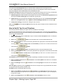
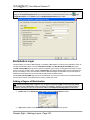
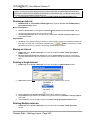
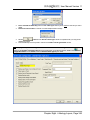
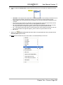
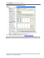
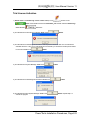
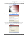
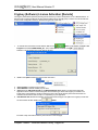
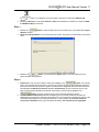
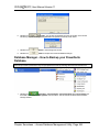
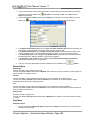
New Log ............................................................................................................................................ 23
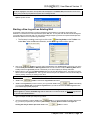
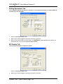
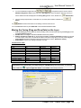
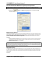
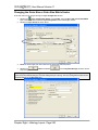
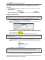
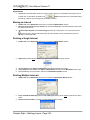
Starting a New Log with an Existing Well ....................................................................................... 25
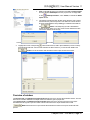
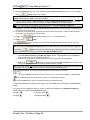
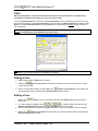
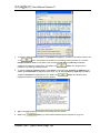
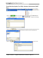
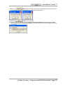
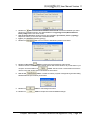
How to Change the API code or the Unique Well Identifier (UWI)................................................... 26
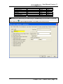
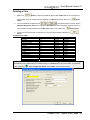
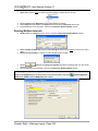
Open ................................................................................................................................................. 27
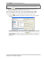
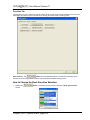
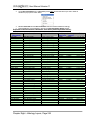
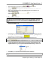
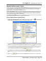
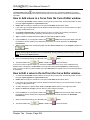
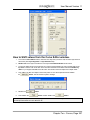
How to Sort the Well List................................................................................................................ 28
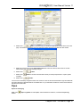
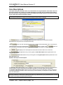
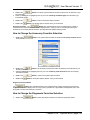
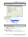
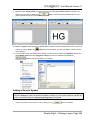
How to Query the Well List (By String Search) ............................................................................... 29
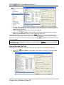
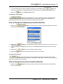
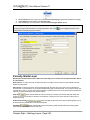
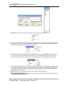
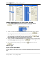
How to Query the Well List (By DLS or NTS Survey Systems) ....................................................... 30
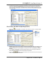
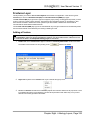
Close................................................................................................................................................. 31
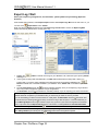
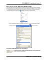
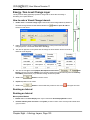
Export Log / Well ............................................................................................................................... 32
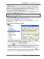
Exporting the Geological Expansion Dictionary, User defined Symbols or all your User defined
Generic Category choice list…....................................................................................................... 34
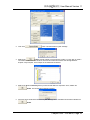
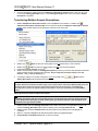
Exporting all the Well Data at one time… ....................................................................................... 34
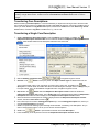
Exporting everything at one time… ................................................................................................ 36
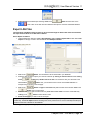
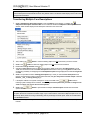
Import Log/Well ................................................................................................................................. 40
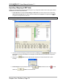
LAS Import ........................................................................................................................................ 41
How to Import an LAS data File ..................................................................................................... 42
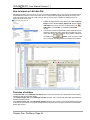
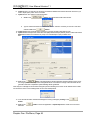
Overview of window....................................................................................................................... 42
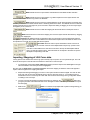
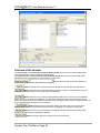
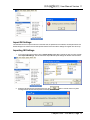
Importing / Mapping of LAS Curve data.......................................................................................... 43
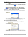
Importing LAS data with an Existing mapping file. .......................................................................... 44
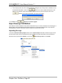
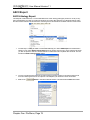
Export LAS Files................................................................................................................................ 45
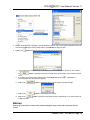
Import Surveys New Method.............................................................................................................. 47
Overview of the window. ................................................................................................................ 48
Importing / Mapping of Survey data................................................................................................ 49
Import Surveys Old Method ............................................................................................................... 50
Importing Surveys.......................................................................................................................... 50
How to Import a Survey Data with an Existing mapping file. ........................................................... 53
Export Surveys.................................................................................................................................. 55
Import AGS (Only relative to Apple Core Data files that are Version 9.2D)...................................... 56
Import Core Plug Data ....................................................................................................................... 56
How to import Core Plug data ........................................................................................................ 56
Overview of the window. ................................................................................................................ 57
Importing / Mapping of Core Plug data. .......................................................................................... 58
How to Import Core Plug Data with an Existing mapping file........................................................... 59
ASCII Import - How to Import an ASCII data file ................................................................................. 60
Overview of window....................................................................................................................... 61
Importing / Mapping of ASCII Curve data. ...................................................................................... 62
Importing ASCII Curve data with an Existing mapping file. ............................................................. 63
Import Dip Meter Data ....................................................................................................................... 64
Overview of the window. ................................................................................................................ 66
Importing / Mapping of Dip Meter data. .......................................................................................... 67
How to Import Dip Meter Data with an Existing mapping file. .......................................................... 68
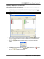
Import Modular Dynamic Tester (MDT) Data...................................................................................... 70
Overview of the window. ................................................................................................................ 71
Table of Contents, Page 1
User Manual Version 11
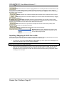
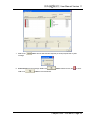
Importing / Mapping of MDT data................................................................................................... 72
How to Import MDT Data with an Existing mapping file................................................................... 73
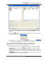
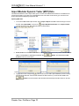
Export INI Settings......................................................................................................................... 74
Exporting INI Settings .................................................................................................................... 74
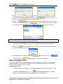
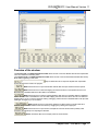
Import INI Settings......................................................................................................................... 75
Importing INI Settings .................................................................................................................... 75
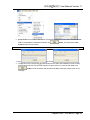
ASCII Export ..................................................................................................................................... 76
ASCII Lithology Export................................................................................................................... 76
Slide / Rotate Export...................................................................................................................... 78
Export ASE Format........................................................................................................................ 78
Backup .............................................................................................................................................. 79
Print Log............................................................................................................................................ 81
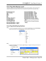
Print Morning Report.......................................................................................................................... 83
Print Well End Report ........................................................................................................................ 86
Print “Well End and AM” Reports to Word Format .............................................................................. 89
How to Print Well End Reports to Word Format.................................................................................. 90
How to Print Morning Reports to Word Format. .................................................................................. 92
Print Setup ........................................................................................................................................ 93
Exit.................................................................................................................................................... 93
Chapter Two – Edit Menu.................................................................................................................... 94
Undo ................................................................................................................................................. 94
How to Undo:................................................................................................................................. 94
Redo ................................................................................................................................................. 94
How to Redo:................................................................................................................................. 94
Log.................................................................................................................................................... 94
How to Delete a Log ...................................................................................................................... 95
Well................................................................................................................................................... 95
Det. Lith Button:............................................................................................................................. 96
Abstract Button.............................................................................................................................. 97
Curve Button ................................................................................................................................. 98
How to Change the Digital Curve Attributes (Curve Units, Depth Units, Null Value and Remarks)... 98
How to Delete a Well ..................................................................................................................... 98
Print Sections .................................................................................................................................. 101
Log Configuration ............................................................................................................................ 101
Track Configuration ......................................................................................................................... 103
Layer Configuration ......................................................................................................................... 104
How to Edit a Layer Configuration Window .................................................................................. 106
Display Settings Tab........................................................................................................................ 106
How to Display a different Wells data on a layer of an Existing Log from another UWI or well....... 107
Curve Definitions Tab ...................................................................................................................... 108
How to select a different Curve to display on a Curve layer .......................................................... 109
How to change the Curve Attributes (Curve and Units, Null Value and Remarks) ......................... 110
Layer Scales Tab............................................................................................................................. 110
Data Group ID’s Tab........................................................................................................................ 112
Annotation Group Button ............................................................................................................. 113
Generic Category Button ............................................................................................................. 113
MDT Run Number Button ............................................................................................................ 113
Directional Survey Button ............................................................................................................ 113
Graphics Button........................................................................................................................... 113
Detailed Lithology Group Button .................................................................................................. 113
Dip Meter Group Button............................................................................................................... 114
Visual Range Button .................................................................................................................... 114
Generic Symbols Button .............................................................................................................. 114
How to select a different Group to display on a layer.................................................................... 114
Formation Age Display Tab ............................................................................................................. 115
Table of Contents, Page 2
User Manual Version 11
Dip Meter Definitions Tab ................................................................................................................ 115
Metafile Options .............................................................................................................................. 117
How to Edit an Existing Metafile................................................................................................... 117
How to Add a New Metafile.......................................................................................................... 119
How to Delete an Added or User defined Metafile ........................................................................ 121
How to Edit an Existing Name for a User defined Metafile ............................................................ 122
Delete Generic Groups .................................................................................................................... 123
Generic Group Sorting..................................................................................................................... 124
How to sort a Generic Group List ................................................................................................. 124
Core / Sample Header ..................................................................................................................... 126
How to Edit a Core / Sample Header ........................................................................................... 127
Well Record Data portion of the Core / Sample Header window ................................................... 128
How to Delete a Core / Sample Header ....................................................................................... 128
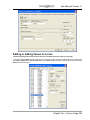
Log Layer Annotations..................................................................................................................... 129
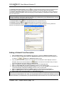
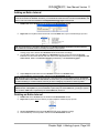
Adding Annotations...................................................................................................................... 129
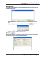
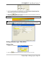
Drawing a Line… ......................................................................................................................... 130
Globally Changing Annotation Font Properties….......................................................................... 132
Chapter Three - View Menu............................................................................................................... 133
Depth View Mode ............................................................................................................................ 133
Go To Depth.................................................................................................................................... 133
Log Scales ...................................................................................................................................... 134
Screen Accuracy ............................................................................................................................. 135
Layers Organizer............................................................................................................................. 135
Show All Layers............................................................................................................................... 136
Show Active Layer........................................................................................................................... 136
Show/Hide Header .......................................................................................................................... 137
Show/Hide Digits ............................................................................................................................. 137
Toolbar............................................................................................................................................ 137
Import Toolbar................................................................................................................................. 137
Export Toolbar................................................................................................................................. 138
RTF Font Toolbar ............................................................................................................................ 138
Status Bar ....................................................................................................................................... 138
Mouse Cross hairs........................................................................................................................... 138
RTF Line and Boxes Toolbar ........................................................................................................... 139
Chapter Four - Reports Menu ........................................................................................................... 140
Sample Description ......................................................................................................................... 140
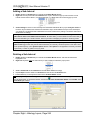
Adding a Sample Description....................................................................................................... 141
Editing a Sample Description ....................................................................................................... 142
Deleting a Sample Description… ................................................................................................. 142
Core Descriptions............................................................................................................................ 143
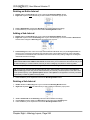
Adding a Core Description ........................................................................................................... 144
Editing a Core Description ........................................................................................................... 145
Deleting a Core Description ......................................................................................................... 145
Abandonment Plug .......................................................................................................................... 146
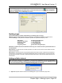
Adding an Abandonment Plug ..................................................................................................... 146
Editing an Abandonment Plug...................................................................................................... 146
Deleting an Abandonment Plug.................................................................................................... 146
Bit Record ....................................................................................................................................... 148
Adding a Bit Record..................................................................................................................... 148
Bit Records Tab........................................................................................................................... 148
Pump Data Tab ........................................................................................................................... 149
Drilling Parameters Tab ............................................................................................................... 150
Bit Grading Tab ........................................................................................................................... 150
Editing a Bit Record..................................................................................................................... 151
Deleting a Bit Record................................................................................................................... 151
Table of Contents, Page 3
User Manual Version 11
Aligning All Bit Records................................................................................................................ 151
Moving Bit Records (Drag and Drop In / Out Info) on the Layer. ................................................... 152
Casing Strings................................................................................................................................. 154
Adding a Casing String ................................................................................................................ 154
Editing a Casing String ................................................................................................................ 154
Deleting a Casing String .............................................................................................................. 154
Moving the Casing (Drag and Drop Data) on the Layer. ............................................................... 155
Core ................................................................................................................................................ 156
Adding a Core ............................................................................................................................. 156
Editing a Core.............................................................................................................................. 156
Deleting a Core............................................................................................................................ 157
Core Descriptions............................................................................................................................ 158
Adding a Core Description ........................................................................................................... 159
Editing a Core Description ........................................................................................................... 159
Deleting a Core Description ......................................................................................................... 159
Core Plugs Report Window.............................................................................................................. 160
Adding an Core Plug record manually.......................................................................................... 160
Editing an Core Plug.................................................................................................................... 161
Deleting an Core Plug.................................................................................................................. 161
Directional Survey ........................................................................................................................... 161
Adding a Directional Survey Group .............................................................................................. 162
Editing a Directional Survey Group .............................................................................................. 162
Deleting a Directional Survey Group ............................................................................................ 163
Master Survey Group Button........................................................................................................ 163
How to Compile the Master Survey Group ................................................................................... 163
How to Add a Survey Group to the Master Survey Group............................................................. 163
How to Delete a Survey Group..................................................................................................... 165
How to Calculate the Master Survey Group Survey Points ........................................................... 165
Directional Survey Portion ........................................................................................................... 166
Calculate Master Survey Portion:................................................................................................. 166
Well Path Portion......................................................................................................................... 167
TVD Attributes Portion ................................................................................................................. 167
Directional Survey Point Window ..................................................................................................... 168
Adding a New Record.................................................................................................................. 168
Editing a Directional Survey Point ................................................................................................ 169
Deleting a Directional Survey Point .............................................................................................. 169
Indicating a Misrun ...................................................................................................................... 169
Aligning All Directional Survey Points........................................................................................... 169
Moving the Directional Survey data (Drag and Drop Data) on the Layer. ...................................... 170
Calculating Directional Survey Points........................................................................................... 170
Well Path Portion......................................................................................................................... 171
TVD Attributes Portion ................................................................................................................. 171
Formation........................................................................................................................................ 173
Well Formation Window - Overview ............................................................................................. 173
Adding a Formation Top .............................................................................................................. 175
Editing a Formation Top............................................................................................................... 175
Deleting a Formation Top ............................................................................................................ 175
Aligning All the Formation Tops ................................................................................................... 175
Moving the Formation Top Data (Drag and Drop) on the Layer. ................................................... 176
MDT ................................................................................................................................................ 178
Adding a MDT Run ...................................................................................................................... 178
Editing a MDT Run ...................................................................................................................... 178
Deleting a MDT Run .................................................................................................................... 178
MDT Data Window ...................................................................................................................... 179
Adding an MDT record manually.................................................................................................. 179
Editing MDT Data ........................................................................................................................ 180
Table of Contents, Page 4
User Manual Version 11
Deleting MDT Data ...................................................................................................................... 180
Morning Report................................................................................................................................ 181
Adding a Morning Report ............................................................................................................. 182
Editing a Morning Report ............................................................................................................. 182
Deleting a Morning Report ........................................................................................................... 182
Lithology Summary...................................................................................................................... 183
Adding a Lithology Summary ....................................................................................................... 183
Editing a Lithology Summary ....................................................................................................... 183
Deleting a Lithology Summary ..................................................................................................... 184
Transferring a Sample Description............................................................................................... 184
Transferring Lithology Descriptions from the Striplog.................................................................... 185
Gas Summary ............................................................................................................................. 187
Adding a Gas Summary............................................................................................................... 187
Editing a Gas Summary............................................................................................................... 187
Deleting a Gas Summary............................................................................................................. 187
Mud Type ........................................................................................................................................ 188
Adding a Mud Type...................................................................................................................... 188
Editing a Mud Type...................................................................................................................... 188
Deleting a Mud Type.................................................................................................................... 189
Sidewall Cores ................................................................................................................................ 190
Adding a Sidewall Core Run ........................................................................................................ 190
Editing a Sidewall Core Run ........................................................................................................ 190
Deleting a Sidewall Core Run ...................................................................................................... 190
Sidewall Core Descriptions .............................................................................................................. 191
Adding a Sidewall Core Description ............................................................................................. 192
Editing a Core Description ........................................................................................................... 193
Deleting a Core Description ......................................................................................................... 193
Test................................................................................................................................................. 195
Adding a Test .............................................................................................................................. 195
Editing a Test .............................................................................................................................. 195
Deleting a Test ............................................................................................................................ 196
Adding a Test Period ................................................................................................................... 197
Editing a Test Period ................................................................................................................... 197
Deleting a Test Period ................................................................................................................. 197
Well Abstract ................................................................................................................................... 199
Wireline Logging.............................................................................................................................. 199
Adding a Wireline Logging Run.................................................................................................... 200
Editing a Wireline Logging Run.................................................................................................... 200
Deleting a Wireline Logging Run.................................................................................................. 200
Adding a Wireline Trip ................................................................................................................. 200
Editing a Wireline Trip.................................................................................................................. 201
Deleting a Wireline Trip................................................................................................................ 201
Work Schedule ................................................................................................................................ 203
Adding a Work Schedule ............................................................................................................. 203
Editing a Work Schedule.............................................................................................................. 203
Deleting a Work Schedule ........................................................................................................... 203
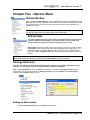
Chapter Five - Options Menu ............................................................................................................ 205
Refresh Window .............................................................................................................................. 205
Refresh Data ................................................................................................................................... 205
Geology Dictionary .......................................................................................................................... 205
Adding an Abbreviation................................................................................................................ 205
Editing an Abbreviation................................................................................................................ 206
Deleting an Abbreviation.............................................................................................................. 206
Curve Maintenance ......................................................................................................................... 206
Mapping a Curve to an Existing Layer.......................................................................................... 207
Table of Contents, Page 5
User Manual Version 11
Changing and Adding Curve Scales............................................................................................. 207
Editing the Active Track Configuration.......................................................................................... 208
Editing a Layer Configuration....................................................................................................... 208
Changing Curve Units, Names, Null Values, or Remarks ............................................................. 208
Adding a Curve Layer to a Track on your Log .............................................................................. 209
Log Configuration Builder ................................................................................................................ 210
Showing or Hiding a Track........................................................................................................... 211
Moving a Track or Layer .............................................................................................................. 212
Adding Tracks to a Log................................................................................................................ 212
Adding Layers to a Track on your Log.......................................................................................... 213
Deleting a Track .......................................................................................................................... 213
Deleting a Layer .......................................................................................................................... 214
Changing the Width of a Track..................................................................................................... 214
Sample / Core Description Transfer ................................................................................................. 214
Transferring one Sample Description ........................................................................................... 215
Transferring Multiple Sample Descriptions ................................................................................... 216
Transferring Core Descriptions .................................................................................................... 217
Transferring a Single Core Description......................................................................................... 217
Transferring Multiple Core Descriptions ....................................................................................... 218
Master Survey Group....................................................................................................................... 219
How to Compile the Master Survey Group ................................................................................... 219
How to Add a Survey Group ........................................................................................................ 219
How to Change a Survey Group .................................................................................................. 220
How to Delete a Survey Group..................................................................................................... 221
How to Calculate the Master Survey Group Survey Points ........................................................... 222
Master Survey Portion ................................................................................................................. 222
Well Path Portion......................................................................................................................... 222
TVD Attributes Portion ................................................................................................................. 223
Shift Data ........................................................................................................................................ 223
Lithology Integrity Check.................................................................................................................. 224
Use Default Printer Settings............................................................................................................. 225
Sidetrack ......................................................................................................................................... 225
Unwrap LAS .................................................................................................................................... 226
How to unwrap a wrapped LAS file format.................................................................................... 226
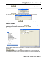
System Options ............................................................................................................................... 227
General Tab .................................................................................................................................... 227
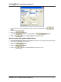
Fonts Tab........................................................................................................................................ 228
How to Set your Fonts ................................................................................................................. 229
How to restore the System default Fonts...................................................................................... 230
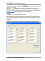
Display Tab ..................................................................................................................................... 231
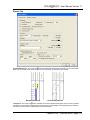
Favorites Tab .................................................................................................................................. 234
How to Change the Rock Favorites Selection............................................................................... 234
How to Change the Accessory Favorites Selection ...................................................................... 235
How to Change the Diagenesis Favorites Selection ..................................................................... 235
How to Change the % Lithology Sort Order.................................................................................. 236
How to Change the Sedimentary Favorites Selection................................................................... 237
How to Change the Fractures Favorites Selection........................................................................ 237
How to Change the Trace Fossil Favorites Selection.................................................................... 238
How to Change the Generic Symbol Favorites Selection.............................................................. 239
Chapter Six - Window Menu.............................................................................................................. 240
Cascade .......................................................................................................................................... 240
Tile.................................................................................................................................................. 240
Arrange Icons.................................................................................................................................. 240
Chapter Seven - Toolbar Functions.................................................................................................. 241
Layer Selection List ......................................................................................................................... 241
Table of Contents, Page 6
User Manual Version 11
Data Editing Tools of Active Layer ................................................................................................... 241
Activating a Layer's Data Editing Tool .......................................................................................... 241
Layers Organizer............................................................................................................................. 242
Show All Layers............................................................................................................................... 242
Show Active Layer........................................................................................................................... 243
Show/Hide Header .......................................................................................................................... 243
Show/Hide Digits ............................................................................................................................. 243
Depth View Mode ............................................................................................................................ 243
Log Scales ...................................................................................................................................... 243
Changing the Scale of the Screen (Two Methods)… .................................................................... 243
Go to Depth..................................................................................................................................... 243
Depth Offset of Active Layer ............................................................................................................ 243
Offsetting Layer Data… ............................................................................................................... 244
Screen Accuracy ............................................................................................................................. 244
Changing the Screen Accuracy of the Mouse Pointer................................................................... 244
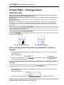
Chapter Eight - Lithology Layers...................................................................................................... 246
Grain Size Layer.............................................................................................................................. 246
How to Change the Grain Size Scale Type (Wentworth, Canstrat or Amstrat) .............................. 246
Adding an Entire Interval.............................................................................................................. 247
Deleting an Entire Interval............................................................................................................ 248
Adding a Sub-interval .................................................................................................................. 248
Deleting a Sub-Interval ................................................................................................................ 248
Changing the Grain Size or Grain Size Matrix Scales................................................................... 250
Grain Size Matrix Layer ................................................................................................................... 251
How to Change the Grain Size Display from a Solid Color to a Hatching Pattern on your log. ....... 251
How to Change the Grain Size Scale Type (Wentworth, Canstrat or Amstrat) .............................. 252
Adding an Entire Interval.............................................................................................................. 252
Deleting an Entire Interval............................................................................................................ 253
Adding a Sub-interval .................................................................................................................. 253
Deleting a Sub-Interval ................................................................................................................ 253
Porosity Type Layer......................................................................................................................... 255
Adding Porosity Types................................................................................................................. 255
Deleting Porosity Types............................................................................................................... 255
Porosity Grade Layer....................................................................................................................... 256
Adding an Entire Interval.............................................................................................................. 257
Deleting an Entire Interval............................................................................................................ 258
Adding a Sub-Interval .................................................................................................................. 258
Deleting a Sub-Interval ................................................................................................................ 258
Changing the Porosity Grade Scale and grid pattern.................................................................... 258
Framework Layer............................................................................................................................. 260
Adding an Entire Interval.............................................................................................................. 260
Deleting an Entire Interval............................................................................................................ 261
Adding a Sub-Interval .................................................................................................................. 261
Deleting a Sub-Interval ................................................................................................................ 262
Oil Show Layer ................................................................................................................................ 262
Adding an Entire Interval.............................................................................................................. 263
Deleting an Entire Interval............................................................................................................ 263
Adding a Sub-Interval .................................................................................................................. 264
Deleting a Sub-Interval ................................................................................................................ 264
Rounding Layer ............................................................................................................................... 265
Adding an Entire Interval.............................................................................................................. 265
Deleting an Entire Interval............................................................................................................ 266
Adding a Sub-Interval .................................................................................................................. 266
Deleting a Sub-Interval ................................................................................................................ 266
Sorting Layer................................................................................................................................... 267
Table of Contents, Page 7
User Manual Version 11
Adding an Entire Interval.............................................................................................................. 267
Deleting an Entire Interval............................................................................................................ 268
Adding a Sub-interval .................................................................................................................. 268
Deleting a Sub-Interval ................................................................................................................ 269
Interpreted Lithology Layer - Rock Type Builder............................................................................... 270
Overview of Rock type builder window............................................................................................. 270
Drafting an Interpreted Lithology Interval...................................................................................... 271
Drafting an Interpreted Lithology Interval with Interbedding. ......................................................... 272
How to draw with an already drawn Interbedded Interval.............................................................. 274
Deleting an Interpreted Lithology Interval with Interbedding.......................................................... 274
Drafting an Interpreted Lithology Interval with No Data................................................................. 275
Inserting Thin beds ...................................................................................................................... 275
Resizing an Existing Rock Type or Bed........................................................................................ 275
Deleting an Existing Rock Type or Bed ........................................................................................ 276
Interpreted Lithology Layer - Rock Accessory Builder ...................................................................... 276
Drawing Accessories ................................................................................................................... 276
Drawing an Internal Bedding Contact........................................................................................... 277
Moving a Thinbed, Components, Internal Contact, Matrix, or Cement .......................................... 278
Deleting a Single Thin bed, Components, Internal Contact, Matrix, or Cement ............................. 278
Deleting Multiple Thin beds, Components, Internal Contacts, Matrix, or Cements......................... 279
Detailed Lithology Layer - Rock Type Builder................................................................................... 280
Drawing Detailed Lithology .......................................................................................................... 280
Overview of the Detailed Rock Type Builder ................................................................................ 281
Deleting a Detailed Lithology ....................................................................................................... 282
Detailed Lithology Layer - Rock Accessory Builder........................................................................... 282
Drawing Accessories ................................................................................................................... 282
Moving a Thinbed, Components, Internal Contact, Matrix, or Cement .......................................... 284
Deleting a single Thinbed, Components, Internal Contact, Matrix, or Cement............................... 284
Deleting Multiple Thin beds, Components, Matrix, or Cements..................................................... 284
Percent (%) Lithology Layer............................................................................................................. 285
Drafting a Percent (%) Lithology Interval ...................................................................................... 285
Resizing an Existing Interval ........................................................................................................ 286
Deleting an Existing Interval......................................................................................................... 286
How to Update an Existing % Lithology Record............................................................................ 286
How to Delete an Existing % Lithology Record............................................................................. 286
How to Enter a No Sample into the % Lithology Track.................................................................. 287
Curve Fill Layer ............................................................................................................................... 288
How to Add a Curve Fill layer to an existing log............................................................................ 288
How to Set (1) One Curve Fill options .......................................................................................... 288
How to Set (2) Two Curve Fill options .......................................................................................... 290
How to Add a New Curve Fill ID................................................................................................... 291
Curve Fill Layer (Well Path Option on Single Curve) ........................................................................ 292
How to Set the Well Path Curve Fill options ................................................................................. 293
Well Path Curve Fill Layer – Bedding Angle Contacts builder........................................................... 295
Single Value Data Entry............................................................................................................... 295
Multiple Value Data Entry ............................................................................................................ 296
Drilling Schedule Layer / Date Editor................................................................................................ 297
Adding a Date.............................................................................................................................. 297
Deleting a Date............................................................................................................................ 298
Editing a Date.............................................................................................................................. 298
Slide / Rotate Layer ......................................................................................................................... 299
Drawing a Slide ........................................................................................................................... 299
Deleting a Slide ........................................................................................................................... 299
Resizing a Slide........................................................................................................................... 299
Annotation Layers............................................................................................................................ 300
Overview of RTF Font Toolbar buttons......................................................................................... 300
Table of Contents, Page 8
User Manual Version 11
Overview of RTF Lines and Boxes Toolbar buttons. ..................................................................... 301
Adding Annotations / Lithology Descriptions… ............................................................................. 302
Drawing a Line… ......................................................................................................................... 303
Editing Annotations/Lithology Descriptions… ............................................................................... 303
Resizing Annotations/Lithology Descriptions…............................................................................. 303
Moving Annotations/Lithology Descriptions…............................................................................... 304
Deleting Annotations/Lithology Descriptions… ............................................................................. 304
Deleting Lines associated with Annotations… .............................................................................. 304
Using the List functionality to copy, move to and delete annotations............................................. 305
Globally Change the Annotation Font Properties. ......................................................................... 306
Globally Change the Annotation Font Color. ................................................................................ 306
Globally Change the Annotation Box Alignments.......................................................................... 307
Globally Change the Annotation Display Scale............................................................................. 308
Globally Change the Box placements to fit in the Track width....................................................... 308
Oil Staining Layer ............................................................................................................................ 309
Adding an Oil Staining type over an Entire Interval....................................................................... 309
Adding an Oil Staining type and interval....................................................................................... 310
Resizing an Interval ..................................................................................................................... 311
Deleting an interval...................................................................................................................... 311
Carbonate Texture Layer................................................................................................................. 312
How to Change the Carbonate Texture Pattern from a Solid Color to a Hatching Pattern on your log.
.................................................................................................................................................... 312
Adding an Entire Interval.............................................................................................................. 313
Deleting an Entire Interval............................................................................................................ 314
Adding a Sub-Interval .................................................................................................................. 314
Deleting a Sub-Interval ................................................................................................................ 314
Changing the Carbonate Texture and Carbonate Texture Matrix Scale ........................................ 315
Carbonate Texture Matrix Layer....................................................................................................... 315
Adding an Entire Interval.............................................................................................................. 316
Deleting an Entire Interval............................................................................................................ 317
Adding a Sub-Interval .................................................................................................................. 317
Deleting a Sub-Interval ................................................................................................................ 318
Ages Layer ...................................................................................................................................... 318
Ages Layer ...................................................................................................................................... 319
Adding a Formation / Age ............................................................................................................ 319
To Change the Display ................................................................................................................ 319
Formations Expanded Layer............................................................................................................ 320
Adding a Formation ..................................................................................................................... 320
To Change the Display ................................................................................................................ 320
Diagenesis Layer............................................................................................................................. 321
Adding a Diagenesis.................................................................................................................... 321
Resizing an Interval ..................................................................................................................... 323
Moving an Interval ....................................................................................................................... 323
Deleting a Single Interval ............................................................................................................. 323
Deleting Multiple Intervals............................................................................................................ 324
Fractures Layer ............................................................................................................................... 325
Adding a Fracture ........................................................................................................................ 325
Resizing an Interval ..................................................................................................................... 326
Moving an Interval ....................................................................................................................... 327
Deleting a Single Interval ............................................................................................................. 327
Deleting Multiple Intervals............................................................................................................ 327
Sedimentary Structures Layer.......................................................................................................... 329
Adding a Sedimentary Structure .................................................................................................. 329
Resizing an Interval ..................................................................................................................... 330
Moving an Interval ....................................................................................................................... 330
Deleting a Single Interval ............................................................................................................. 331
Table of Contents, Page 9
User Manual Version 11
Deleting Multiple Intervals............................................................................................................ 331
Bioturbation Layer ........................................................................................................................... 332
Adding a Degree of Bioturbation .................................................................................................. 332
Resizing an Interval ..................................................................................................................... 333
Moving an Interval ....................................................................................................................... 334
Deleting a Single Interval ............................................................................................................. 334
Deleting Multiple Intervals............................................................................................................ 334
Trace Fossils Layer ......................................................................................................................... 335
Adding a Trace Fossil .................................................................................................................. 335
Resizing an Interval ..................................................................................................................... 337
Moving an Interval ....................................................................................................................... 337
Deleting a Single Interval ............................................................................................................. 337
Deleting Multiple Intervals............................................................................................................ 337
Rock Accessories Layer .................................................................................................................. 339
Adding a Rock Accessory ............................................................................................................ 339
Resizing an Interval ..................................................................................................................... 340
Moving an Interval ....................................................................................................................... 340
Deleting a Single Interval ............................................................................................................. 341
Deleting Multiple Intervals............................................................................................................ 341
Sneider’s Rock Type (Geo) Layer .................................................................................................... 342
Adding a Sneider’s Rock type ...................................................................................................... 342
Resizing an Interval ..................................................................................................................... 344
Moving an Interval ....................................................................................................................... 344
Deleting a Single Interval ............................................................................................................. 344
Deleting Multiple Intervals............................................................................................................ 344
Sneider’s Rock Type (Core) Layer ................................................................................................... 346
Adding a Sneider’s Rock type (C) ................................................................................................ 346
How to edit or change a Sneider’s Rock Type (C) interval ............................................................ 346
Deleting a Sneider’s Rock Type (C) interval ................................................................................. 347
Graphics Layer ................................................................................................................................ 348
Adding a Graphic or Picture to a Log ........................................................................................... 348
Modifying a Picture or Graphic..................................................................................................... 349
Moving a Graphic ........................................................................................................................ 349
Changing a Group ....................................................................................................................... 349
Deleting a Picture or Graphic ....................................................................................................... 350
Saving an Existing Graphic or Picture to a file. ............................................................................. 350
Generic Category Layer................................................................................................................... 351
How to add a Generic Category Track / Layer to your Log ........................................................... 351
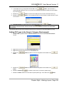
Adding Fill Types to the Generic Category (Environment) ............................................................ 353
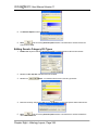
Editing Generic Category Fill Types ............................................................................................. 354
Deleting Generic Category Fill Types........................................................................................... 355
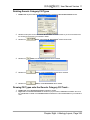
Drawing Fill Types onto the Generic Category Fill Track…........................................................... 355
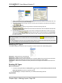
Modifying Fill Types..................................................................................................................... 356
Resizing Fill Types ...................................................................................................................... 356
Deleting Fill Types ....................................................................................................................... 357
Percent Layer.................................................................................................................................. 357
How to Add a Percent Track ........................................................................................................ 357
Drawing Percents ........................................................................................................................ 358
Deleting Percents ........................................................................................................................ 360
Changing the Percent Scale ........................................................................................................ 360
Core Box Data Layer ....................................................................................................................... 361
How to Enter Core Box Data........................................................................................................ 361
Editing an Core Box Data ............................................................................................................ 361
Deleting an Core Box Data .......................................................................................................... 362
Core Plug Data Display Layers ........................................................................................................ 363
Core Plug Data Display Options....................................................................................................... 363
Table of Contents, Page 10
User Manual Version 11
Multi Array Data Layer ..................................................................................................................... 364
How to Add a Multi Array Track.................................................................................................... 364
Setting up the Layer using the Dialogue Window.......................................................................... 365
Generic Symbol Layer / Track.......................................................................................................... 367
How to Add a Generic Symbol Track ........................................................................................... 367
Adding a Generic Symbol ............................................................................................................ 369
Resizing an Interval ..................................................................................................................... 371
Moving an Interval ....................................................................................................................... 371
Deleting a Single Interval ............................................................................................................. 371
Deleting Multiple Intervals............................................................................................................ 372
Energy / Sea Level Change Layer ................................................................................................... 374
How to enter a Visual Change interval. ........................................................................................ 374
Resizing an Interval ..................................................................................................................... 374
Resizing an Interval ..................................................................................................................... 374
Moving an Interval ....................................................................................................................... 375
Deleting an Interval...................................................................................................................... 375
Chapter Nine - Database Navigational Tools ................................................................................... 377
The Editing and Database Navigational Tools.................................................................................. 377
Save (ALT-S)............................................................................................................................... 377
Undo ........................................................................................................................................... 378
New (ALT-N) ............................................................................................................................... 378
Delete.......................................................................................................................................... 378
Move to First Record ................................................................................................................... 379
Move to Previous Record............................................................................................................. 379
Query .......................................................................................................................................... 379
Move to Next Record ................................................................................................................... 379
Move to Last Record.................................................................................................................... 379
Chapter Ten - Curves ........................................................................................................................ 380
Adding Curves................................................................................................................................. 380
Adding a Curve Layer .................................................................................................................. 380
Adding a Curve to the New Curve Layer ...................................................................................... 381
Adding a New Curve.................................................................................................................... 382
Editing or Adding Values to Curves.................................................................................................. 385
How to Add values to a Curve from the Curve Editor window. .......................................................... 386
How to Edit a value in the list from the Curve Editor window............................................................. 386
How to Shift values from the Curve Editor window. .......................................................................... 387
How to delete values in the Curve Editor window. ............................................................................ 388
Curve Layer..................................................................................................................................... 388
Digital Curve Pop-Out Menu ........................................................................................................ 388
Editing a Curve Scale .................................................................................................................. 390
Adding a new Curve Scale........................................................................................................... 390
Right Click ASCII Import (Single Curve) ....................................................................................... 392
Right Click LAS Imports (Single Curve)........................................................................................ 393
Changing Digital Curve Attributes (Units / Null Value) ...................................................................... 395
Chapter Eleven - Core ....................................................................................................................... 398
Creating, Describing, and Illustrating Core Data............................................................................... 398
Adding, Editing and Deleting a Core ............................................................................................ 398
Adding a Core Rate curve layer to the log.................................................................................... 399
The Add Curve window................................................................................................................ 399
Changing the Color of the Core Rate curve.................................................................................. 400
Adding values to the Core Rate curve.......................................................................................... 400
Core Description.............................................................................................................................. 400
Adding a Core Description ........................................................................................................... 401
Editing a Core Description ........................................................................................................... 402
Table of Contents, Page 11
User Manual Version 11
Deleting a Core Description ......................................................................................................... 402
Transferring Core Descriptions ........................................................................................................ 403
Transferring a Single Core Description......................................................................................... 403
Transferring Multiple Core Description ......................................................................................... 403
Editing Core Descriptions ................................................................................................................ 404
Editing Annotations/Lithology Descriptions… ............................................................................... 404
Resizing Annotations/Lithology Descriptions…............................................................................. 405
Moving Annotations/Lithology Descriptions…............................................................................... 405
Deleting Annotations/Lithology Descriptions… ............................................................................. 405
Drawing Interpreted Lithology on a Core Log ................................................................................... 406
Adding Annotations to an Annotation layer................................................................................... 406
Printing out a Core Log.................................................................................................................... 407
Chapter Twelve - System Help.......................................................................................................... 409
Index: .............................................................................................................................................. 409
Using Help:...................................................................................................................................... 409
About Power*Log / Core & Curve:.................................................................................................... 409
Show Registration: .......................................................................................................................... 409
Current Access Flags: ..................................................................................................................... 410
Check for Updates:.......................................................................................................................... 410
Useful Topics:.................................................................................................................................. 410
Context Sensitive Help button:......................................................................................................... 410
Chapter Thirteen - Power*Suite Installation Procedures................................................................. 411
1Power*Suite Installation Procedure.................................................................................................. 411
Hasp Device Driver Installation Procedures ................................................................................. 419
Hasp Key License Activation........................................................................................................ 421
Crypkey Power*Suite License Authorization................................................................................. 422
Trial License Activation................................................................................................................ 423
ASCII to LAS Builder Installation Procedures ............................................................................... 424
ASCII to LAS Builder Trial License Activation............................................................................... 429
Crypkey Authorization for the ASCII to LAS Builder...................................................................... 430
Hasp (Hardware Key) License Activation ..................................................................................... 431
HASP Key Upgrade Procedures .................................................................................................. 432
Chapter Fourteen - Authorization..................................................................................................... 433
PowerSuite License Configuration Utility: Software Authorization..................................................... 433
How to initially authorize a program once it has been installed ..................................................... 433
License Configuration: Floppy Disk Transfer ................................................................................ 434
PowerSuite Hasp Update Tool Utility: Hardware Authorization (HASP Key).................................. 436
Chapter Fifteen – License Selector .................................................................................................. 438
Hasp (Hardware Key) License Activation ......................................................................................... 438
Crypkey (Software) License Activation [Local].................................................................................. 439
Crypkey (Software) License Activation [Remote].............................................................................. 440
Chapter Sixteen – ASCII to LAS Builder Module.............................................................................. 442
Introduction ..................................................................................................................................... 442
How to Build an LAS file from an ASCII file (No current configuration file present)............................ 442
How to Generate a LAS file from An ASCII file (With a valid configuration file already saved for a
particular ASCII file set) ................................................................................................................... 447
Chapter Seventeen – Database Management .................................................................................. 452
Database Management – How to Change your Password................................................................ 452
Database Manager – How to Compact / Repair your PowerSuite Database. .................................... 453
Database Manager – How to Backup your PowerSuite Database..................................................... 454
Chapter Eighteen - Auto Import Module........................................................................................... 456
Overview ......................................................................................................................................... 456
Table of Contents, Page 12
User Manual Version 11
Operating Procedures...................................................................................................................... 456
Appendix A – Geological Expansion Dictionary
A printed version of the Power*Log / Curve on-line expansion dictionary
Appendix B – Power*Log / Curve / Core Reports
An example of various Power*Log / Curve / Core Reports and Types and saved in the PS and TV Report directories
Appendix C – Power*Log / Curve / Core System Logs
A hard copy version of the Power*Log / Curve / Core System Logs
Power*Log / Curve / Core Tutorials
A printed version of the Power*Log / Curve /Core Tutorials
Table of Contents, Page 13
User Manual Version 11
Quick Reference Guide
Annotations:
Adding an annotations to an annotation layer
Drawing a line in an annotation window
Adding an annotation to the log layer
300
301
127
Carbonate Texture Layer
How to change the Carbonate Texture Design pattern
How to change the Carbonate Texture Scale
310
313
Core:
Creating, Describing and Illustrating Core Data
Power*Core Tutorial
396
Addendum
Core Descriptions:
Adding a core description
Transferring core descriptions
Transferring multiple core descriptions
Automatic Core Description Transfer
157, 399
142, 213, 401
216, 401
142
Curves:
Adding curves
Adding/changing curve scales
Changing curve attributes
Editing curves
Right Click ASCII Import (Single Curve)
Right Click LAS Import (Single Curve)
ASCII Curve Import (Multiple Curves)
LAS Curve Import (Multiple Curve)
378
388
96, 108 393
383
390
391
58
39
Curves Fills:
Adding curve fill layers to your log
How to set up a 1 curve fill layer
How to set up a 2 curve fill layer
How to set up a Well Path Curve Fill (Power*Curve)
286
286
288
293
Dates:
Adding a date
Date Format
295
225
Geological Dictionary:
Using the geological expansion dictionary
203
Grain Size Layer
How to change the Grain Size Design pattern
How to change the Grain Size Scale
How to change the Grain Size Scale from Wentworth to Canstrat / Amstrat
Quick Reference Guide, Page 14
249
248
244
User Manual Version 11
Favorites Toolboxes / Right Click Favorites:
How to Change the Rock Favorites Selection
How to Change the Accessory Favorites Selection
How to Change the % Lithology Sort Order
How to Change the Trace Fossil Favorites Selection
How to Change the Sedimentary Favorites Selection
How to Change the Fractures Favorites Selection
How to Change the Diagenesis Favorites Selection
How to Change the Generic Symbol Favorites Selection
232
233
234
236
235
235
234
237
Graphics:
How to change a graphic group
347
Importing ASCII Data
Importing ASCII Survey Data
Importing ASCII Core Data
Import ASCII Curve Data
Import Dip Meter Data
Import MDT Data
45, 48
54
58, 390
62
68
Interpreted Lithology:
Drafting interpreted lithology
Drafting interpretive lithology interbedded intervals
Resizing an existing interpreted lithology
269
270
273
LAS:
Exporting LAS Curve data
Importing LAS Curve data
ASCII Lithology Export
Import ASCII Curve Data
Layers:
Adding layers
Deleting layers
Editing the layer configuration
Moving a layer
Offsetting/Shifting layers
Layers Organizer
43
39, 391
74
58, 390
211
212
104
210
106
133
Lithology Descriptions:
Editing a lithology description
Globally changing lithology annotation font properties
Moving a lithology description
301
309-306
302
Logs:
Changing the scale of a log
Deleting a log
Editing the log configuration (log header color & grid formats)
Exporting logs/wells
Importing logs/wells
Printing out Strip logs
Printing out Core logs
Shifting log data selectively or globally
Starting a log with an existing well
Starting a new log/well
132, 241
93
99
32
38
79
405
221
25
23
Quick Reference Guide, Page 15
User Manual Version 11
Metafiles / System Symbols:
How to edit existing symbols
How to add new symbols
115
117
Porosity Grade Layer
How to change the Porosity Grade Design pattern
How to change the Porosity Grade Scale
255
256
Sample Descriptions:
Transferring sample descriptions into the morning report
Transferring lithology descriptions into the morning report
Adding a sample description
Transferring a sample description
Transferring multiple sample descriptions
182
183
139
23
214
System Options:
Changing system options
225
Tracks:
Adding a track
Adding track headers
Changing track width
Deleting a track
Editing the track configuration
Moving a track
Offsetting/Shifting tracks
Showing/Hiding a track
210
101
212
211
101
210
101
209
Wells:
Deleting a well
Exporting a well
Importing a well
Starting a new well
How to change a wells UWI / API Code
How to sidetrack a well
96
32
38
23
26
223
Well End Reports:
Previewing the printout of a report
Printing the report to a Word file
Quick Reference Guide, Page 16
81
87
User Manual Version 11
Introduction
Power*Log / Core & Curve™ (Petrographical Office and Wellsite Evaluation and Reporting) is a chip sample and
core logging program that utilizes single-entry data capturing to produce geological striplogs and corelogs. The
geological data is entered into the system through the use of intuitive data entry forms to ensure standardization of
data. This data is stored in an RDBMS (Relational Database Management System) to allow data manipulation using
SQL (Structured Query Language) access tools.
Power*Log / Core & Curve™ Software consists of Four (4) Main Sections:
1.
2.
3.
4.
A log editor module that allows you to change the striplogs to suit your needs and preferences.
A data transfer module.
Report printing modules.
An on-line help system that is designed to familiarize you with the commands and functions available in
Power*Log / Core & Curve™ and lead you through many of the processes involved in creating logs.
Starting Power*Log / Core & Curve™…
1.
1.
2.
Double click on the Power*Log / Core & Curve™
icon. This brings you into the Power*Log / Core
& Curve™ program. The first window to appear will be the Security window with the registration and
button to acknowledge the window. A Connect Database
copyright information. Click on the
window will immediately appear. See the “Connect” section, later in this User Manual to learn more about
how to connect to a database.
Highlight the Pgeology V9.0 Metric (Microsoft Access Driver [*.mdb]) database by clicking on it once, if
it is not already highlighted.
Move your mouse pointer to the User ID data field and click once to activate a flashing cursor in the User
ID field. Then, type pgeology in the User ID field. Press the Tab key on the keyboard.
3.
Type pgeology in the Password field and then click on the
load various dictionaries and will activate an Open Log window.
4.
Double click on a log to open an existing log or click on the New Log
You are now in the Power*Log / Core & Curve™ environment.
button. The program will now
button to start a new log/well.
Navigating through Power*Log / Core & Curve™:
When you are entering information into data forms, you may move between boxes/fields by pressing the Tab key to
go forward and Shift +Tab to move backwards. To exit forms that do not have an Exit, OK, or Cancel button, press
the Esc key on the keyboard.
The various fields located in the Power*Log / Core & Curve™ dialog boxes have character restrictions. “Field
Restriction Tables” are provided in this manual that provide a useful reference to help you enter the appropriate
amount of characters or numbers in each field.
Reading the Field Restriction Tables:
The tables have four columns each and resemble the example table shown below:
For numeric fields, the maximum amount of numbers allowed is represented on the table as a decimal. The number
that precedes the decimal indicates how many numbers you may place before a decimal point and the number
following the decimal represents how many numbers may follow the decimal point.
Introduction, Page 17
User Manual Version 10
For example: If the number on the Field Restriction Table is 5.2. You may place five (5) digits before the decimal
point and two(2) digits after the decimal point. The range of numbers available, in this particular case, is -99999.99 to
99999.99. If you enter too many numbers in a field, your current record will not be saved. Instead, the offending field
is highlighted and an error message appears in the lower left side of the Status Bar.
Any key on the keyboard is considered a character, so you may place letters, numbers, and symbols in any
CHARACTER field. You may enter as many characters as that field allows (this is represented as a whole number on
the Field Restriction Table). If the field is categorized as DATE FORMAT, then you must use the proper date and
time format that you have selected in your System Options.
If a field is MANDATORY, it must be filled in before you can save a record. Power*Log / Core & Curve™ uses these
mandatory fields to identify records in the database. Therefore, if you have not filled in a mandatory field and you try
to save the record, the offending field is highlighted and an error message appears in the lower left side of the Status
Bar.
Accessing the On-line Help System in Power*Log / Core & Curve™:
You can make use of the context sensitive help by pressing the F1 key when you are in a dialog box. A pertinent help
file will appear, opened to the topic relevant to the dialog box you are in.
The Toolbar
The Selection Bar…
Selection Bar Using the Default American Style Inches Screen Scale
Selection Bar Using the Metric Style Selection Utilizing a Ratio for Screen Scale
Introduction, Page 18
User Manual Version 11
The Status Bar…
The Status Bar displays system status messages and any error message (associated with a field entry),
in the far left corner. The KB elevation is displayed in the lower right corner of the Status Bar.
The Import Toolbar
This toolbar is dock able and can be moved to different places on the screen.
The Power*Log / Core & Curve™ Import Toolbar…
The Export Toolbar
This toolbar is dock able and can be moved to different places on the screen.
The Power*Log / Core & Curve™ Export Toolbar…
Button, Check box and drop box types.
The Four (4) Main On-line Help System Categories:
Commands - Descriptions of each menu command within Power*Log / Core & Curve™.
Toolbar - Shortcuts to common commands are explained.
Database Table Operations - Commands or functions related to the Database Table are described.
Quick Reference Guide - The portion of the On-line Help System that quickly refers you to some of the more
commonly performed tasks.
Introduction, Page 19
User Manual Version 11
Chapter One - File Menu
Connect
Connects Power*Log / Core & Curve™ to a database.
To access the Connect Database window, click on Connect, under the File menu
selection, or click on the
Connect button on the Toolbar.
Connecting to a Database
1. When this window is displayed, highlight the PGEOLOGY V11 IMPERIAL {Microsoft Access
Driver)*.mdb)] database.
2. Enter your User ID and Password in their respective fields (your default User ID and Passwords are both
"pgeology").
3.
Click on the
button to complete the connection.
Disconnect
Disconnects Power*Log / Core & Curve ™ from a database.
Disconnect
button on the Toolbar
Grant Access
The Grant Access window provides the Network Administrator and/or
Power*Geology Superuser(displayed in the Granter field in the upper left
Grant Access window), with the ability to control which network users gain
specific well information or data residing within the Power*Geology network database.
corner of the
access to
Granting Access to existing Grantees
1. Click on Access Registration, under the File menu selection, and then click on Grant Access.
This will activate the Grant Access window shown on the next page:
Chapter One- File Menu, Page 20
User Manual Version 11
2.
3.
Select (highlight) the well(s) from the Granter's Well List field that you wish to give a specific Grantee or
Grantees access to.
Select (highlight) the Grantee(s) from the Grantees list field that will be given access to the well you
selected earlier from the Granter's Well List field.
4.
Click once on the
want to GRANT access?"
button and you will receive the following system message, "Do you really
5.
Click once on the
button to give the selected Grantee(s) access to the selected well(s).
Note: Use PUBLIC, in the Grantees list field, to give ALL of the Grantees access to selected well(s).
Granting Access to a new Grantee
1. Click on Access Registration, under the File menu selection, and then click on Grant Access to activate
the Grant Access window.
2. Select (highlight) the well(s) from the Granter's Well List field that you wish to give the new Grantee access
to.
3. Type the name of the new Grantee into the New Grantee field.
4.
Click once on the
want to GRANT access?"
button and you will receive the following system message, "Do you really
5.
Click once on the
button to give the new Grantee access to the selected well(s).
Granting Access to a new well
Note: Situations will arise in which existing Power*Log/Curve users have not yet been given access to a well that
was recently or soon to be spudded. Accordingly, the Network Administrator and/or Power*Geology Superuser
will use the UWI from the new well to grant access to the selected Grantee(s).
1. Click on Access Registration, under the File menu selection, and then click on Grant Access to activate
the Grant Access window.
2. Type the UWI of the new well into the New Well (UWI) field.
3. Select (highlight) the Grantee(s) from the Grantees list field that will be given access to the new well.
4.
Click once on the
want to GRANT access?"
button and you will receive the following system message, "Do you really
5.
Click once on the
button to give the selected Grantee(s) access to the new well.
Chapter One - File Menu, Page 21
User Manual Version 11
Revoke Access
The Revoke Access window provides the Network Administrator and/or Power*Geology Superuser (displayed in
the Granter field in the upper left corner of the Revoke Access window), with the ability to revoke the access of
specific network users to specific well information or data residing within the Power*Geology network database.
Revoking Access to existing Grantees…
1.
Select Access Registration, under the File menu selection, and then click on Revoke Access to activate
the Revoke Access window shown below:
2.
Select (highlight) a specific Grantee from the Grantees list field to determine what wells in the Grantee's
Well List field the Grantee currently has access to.
Select (highlight) the well(s) from the Grantee's Well List field you wish to revoke access to for the
previously selected (highlighted) Grantee.
Click on the Revoke Access (Grantee View) button and you will receive the following system message,
"Do you really want to REVOKE the selected wells from the selected user?"
Click on "Yes" to revoke the access of the selected Grantee to the selected well(s) in the Grantee's Well
List field.
3.
4.
5.
Revoking Access to a selected well
1.
2.
3.
4.
5.
6.
Select Access Registration, under File, and then click on Revoke Access to activate the Revoke Access
window.
Click on the Well Name button to activate the Well List window.
Double click on the desired Well from the Well List window to display it in the Well Name and UWI fields
within the Revoke Access window.
Select (highlight) the Grantee(s) from the Grantees field for whom you wish to revoke access to the
selected well.
Click on the Revoke Access (Well View) button and you will receive the following system message, "Do
you really want to REVOKE the selected users from the selected well?"
Click on the “Yes” button to revoke the access of the selected Grantee(s) to the selected well displayed in
the Well Name and UWI fields, respectively.
Chapter One- File Menu, Page 22
User Manual Version 11
New Log
1.
The first step in creating a new log is to click on the
New Log button on the Toolbar, or to select New
from the File menu selection. This will open the New Log window shown below:
2.
The Cursor will be active in the Well / Log Name field. Type in the Well Name into the Well / Log Name field
(maximum of 50 characters). On a new well the well name and the log name will be the same.
3.
Click on the
4.
The default is a flashing cursor is placed in the API Code / Name field, awaiting your data entry.
5.
Click on the
button when you have finished entering the UWI. An extended UWI is created by
Power*Log / Core & Curve ™ from the many small boxes that you just filled in. You will now be in the New Log
window again.
6.
Click on the
7.
button. You may also
Click once on the format you wish to use for your log and then click on the
double click on the desired format, where upon you will be returned to the New Log window.
button to activate the UWI Format window shown below:
button to activate the Log Format List window shown below:
Note: Log Formats with the letter "V" in front of their names are Vertical logs, and can only be used within
Power*Log™. Log Formats with the letter "H" in front of their names are Horizontal logs, and can only be used within
Power*Curve™.
Chapter One - File Menu, Page 23
User Manual Version 11
8.
Double Click in the Log Start Depth field. This will highlight the Zero, and activate a flashing cursor. Type the
depth at which you want your log to start.
9.
Once the information is entered, click on the
button.
Note: This will initiate a New Log. During this process, the curves associated with the selected log format will be
added and Add Curve windows may be activated for each curve within that log format. An example of an Add Curve
window is shown below.
10. Click on the
button for each Add Curve window and you will have just added curves to the
database that are displayed on the layers with the same name.
Note: You may edit any of the curve’s properties in the Add Curve window. For more information, see “Adding
Curves” in Chapter Ten.
11. You can now edit, or add information in the Well Header Information window.
12. Select Well, under the Edit menu selection, to activate the Well window, shown below
13. Fill in the information you feel is necessary (the picture above is filled in to give you an idea of what is required),
and then click on the
button to save any changes you have made to the database.
Note: Some of the fields in the Edit Well window have character restrictions or mandatory requirements.
Consequently, if any of these restrictions have been violated or if any requirements have not been met, the offending
Chapter One- File Menu, Page 24
User Manual Version 11
field will be highlighted, the nature of the problem will be displayed on the Status Bar (lower left hand corner of the
screen), and you will be prompted with a system error message window.
14. If the record has been successfully saved, click on the appropriate button when prompted with the Shortcut
Options system window.
Starting a New Log with an Existing Well
An example of doing this would be to create a Horizontal Log presentation for an existing vertical well in the
database. You would use the vertical presentation (either MD, SSL. or TVD) and when the well reached 90 degrees
you would start up a Horizontal. Also you could have a wellsight sample log and then incorporate the Samples with
the Wireline data to have a composite log presentation.
1. The first step in creating a new log is to click on the
New Log button on the Toolbar or to
select New, under the File menu selection, and the New Log window will be opened.
2.
3.
Click on the
button to view the wells in the database. Then, double click on the well of your choice
to automatically fill in the UWI and Well/Log Name fields. The user can then modify the Well/Log Name field to
suitably reflect the Log Format (Vertical or Horizontal), to be used to display the existing well’s data.
Type a name for your log in the Well/Log Name field (no more than 50 characters long). The original Log name
will be viewed in the Log/Name field. The Log name must be unique in the database. The user must modify the
name by adding / removing or creating a new name.
Note: This does not change the well name; it only changes the log name.
4.
Click on the
button to activate the Log Format List window.
5.
Click on the Log Format you wish to use for your log and then click on the
button. Alternatively,
you can simply double click on the desired Log Format and you will be returned to the New Log window with
your selection appropriately displayed.
Note: Available Logs with the letter "V" in front of their names are Vertical logs and can only be used within
Power*Log/Core™. Likewise, Available Logs with the letter "H" in front of their names are Horizontal logs and can
only be used within Power*Curve™.
6.
Double Click in the Log Start Depth field to highlight the numeral zero (0) and activate a flashing cursor. Then,
type in the depth at which you want your log to start.
7.
button. If you have associated an existing well with the
Once the information is entered, click on the
log, you will be prompted with yet another system message, “You are about to create a new log for an
existing well. Do you want to proceed?” Click on the
button to confirm.
Chapter One - File Menu, Page 25
User Manual Version 11
Note: This will initiate a New Log. During this process, the curves associated with the selected log format will may be
added in the form of Add Curve windows, for each curve within that log format, with their associated units and
scales.
8.
Click on the
button for each Add Curve window and you will have just added curves to the
database that are displayed on the layers with the same name in/on your log.
How to Change the API code or the Unique Well Identifier (UWI)
This procedure will guide the user through the appropriate steps to change the API code or the UWI.
1.
Click on the
Log window.
2.
Highlight the Well Name that you wish to change the UWI / API, in the Well List portion of the window, and
the logs for that well will appear in the Log List portion of the window. Highlight or click on any of the logs
3.
Open Log button or select Open, under the File menu selection, to activate the Open
button and the selected well / log
available for that well in the Log List. Then, click on the
will open accordingly
Click on the Well selection, located under the Edit menu selection on the Menu bar. This will activate the
Well Window.
Chapter One- File Menu, Page 26
User Manual Version 11
4.
Click on the
button in the Well window to activate the appropriate window shown on the next
page: This window will be filled in with the original information when the Log / Well were first created.
5.
Click your mouse cursor into the appropriate fields either in the DLS section, NTS section or the API /
Name section and make the necessary changes.
6.
Click on the
7.
Click on the
message.
8.
Click on the
button.
button. If the well record has been saved you will be prompted with a 4 option system
button.
You have now successfully changed the UWI or API Code for a well. We have automated all the logs associated with
the original Well to be reallocated with the new Wells UWI. For your information all data for a well is stored under the
UWI and not the well name.
Open
Opens an existing log
Click on the
window.
Open Log button or select Open, under the File menu selection, to activate the Open Log
Chapter One - File Menu, Page 27
User Manual Version 11
1.
2.
Locate the well you wish to open either by querying or scrolling through the Well List portion of the window
and Click on the Well Name so it becomes highlighted, and the logs available for that well will appear in the
Log List portion of the window.
Click on the log name you want to open. It will become highlighted.
button and the selected log will open accordingly. Please keep in mind that
Click on the
Power*Log / Core & Curve™ allows you to have multiple logs open at once.
The Recent Logs portion of the window indicates the last 10 logs / wells opened. You may wish to select one of
these rather than looking through the well list. Also if you are reopening the last well used it is already highlighted in
3.
button or by depressing your enter
the Recent Logs list and can be reopened easily by clicking on the
key on your keypad.
Note: Logs with the letter "V" in front of their names are Vertical logs, and can only be used within Power*Log™ or
Power*Core™. Likewise, Logs with the letter "H" in front of their names are Horizontal logs, and can only be used
within Power*Curve™.
How to Sort the Well List
(Well Name, UWI, Spud Date, Total Depth, Field, Pool, Hole Direction, Province/State, License #)
1.
Click on the
Log window.
Open Log button or select Open, under the File menu selection, to activate the Open
Chapter One- File Menu, Page 28
User Manual Version 11
2.
The default sorting in the Open Log window is on Well Name. If you wish to sort on any other criteria, you
simply have to click on its heading indicator at the top of the Well List. By doing so, you will sort the
window with respect to that criterion. The Example above is sorted by spud date in ascending order. If you
click on the heading indicator again it will reverse the order as shown in the example below with Spud date
in descending order.
How to Query the Well List (By String Search)
1.
Click on the
Log window.
2.
Choose the field to search criteria by clicking on the drop arrow in the search portion of the window. This will
activate a drop list and click on your selection. You have many field strings to search with. Then type in
your search criteria in the Enter String field. The example shown above is any Well Name with ANY in it
anywhere.
You can choose a search type in the drop box beside the Search string you have type or selected. The
default is like so if in this case the ANY can be anywhere in the well name.
3.
4.
Open Log button or select Open, under the File menu selection, to activate the Open
button. This will redo the Well List with those Well Names that meet the specific
Click on the
criteria. The search results are shown below.
Chapter One - File Menu, Page 29
User Manual Version 11
5.
Click on the
button to refresh the list with all the Wells in the database.
How to Query the Well List (By DLS or NTS Survey Systems)
1.
Click on the
window.
Open Log button or select Open, under the File menu selection, to activate the Open Log
2.
Type in the fields to search by utilizing either the DLS or NTS Survey system that was used to create the UWI.
th
The example shown above is Township 84 Range 11 and the 6 Meridian
3.
Click on the
button. This will redo the Well List with those Well Names that meet the specific
criteria. The search results are shown below.
Chapter One- File Menu, Page 30
User Manual Version 11
4.
Click on the
button to refresh the list with all the Wells in the database.
Close
Closes the currently active log
Click on Close, under the File menu selection, to close the current or active well or click on the
icon.
Note: You do not have to save any changes prior to closing a log, because all work performed on a log is
automatically saved to the Power*Geology database.
Chapter One - File Menu, Page 31
User Manual Version 11
Export Log / Well
Allows you to export log configurations, well information, system symbols and your Geology Expansion
Dictionary
Under the File menu selection, select Import / Export and then select Export Log / Well from the sub-menu. Or, you
Export button on the Toolbar.
can click on the
When you enter the Export window from the main Power*Log / Core & Curve™ screen, the Export Log/Well
window automatically defaults to the currently active log.
1.
2.
3.
Click on the
button to activate a list of logs in your database. Then, select the log for export by double
clicking on it.
If the log has a Primary Well associated with it, the Well field will default to the Primary Well. If there is no
Primary Well or you wish to export a different well, select the well to be exported by clicking on the
button to activate a list of the Wells available in your database. Then, double click on the well that you wish to
export.
should be activated (checked), when you are exporting a log for the first
The Log Configuration check box
time or if you have changed the log's track or layer configurations.
should also be activated (checked), if you are exporting your well for the first time.
The Entire Well check box
4.
Note: This is a good way to back-up your well's information and should be done on a daily basis, so that if your
database becomes corrupted or your hard drive fails, you have a way to restore or recover your data.
If you are transmitting your files to another location on a daily basis, the Entire Well check box
should be used
until the file size (and resulting transmission time), becomes too large. After this point, it is recommended that you
use the Morning Report check box , instead, to export only a portion of your well's morning data and should be
used in conjunction with the Export Interval portions of the window, including Interval and Record Based Data.
5. Activate the Today's Interval check box
and then enter a set of values into Today's Interval.
Note: The values entered into Today's Interval, within the Export Log/Well window, will automatically be displayed
in the Today's Section print interval part of the Print Log window when the log/well is imported.
6.
If you activated the Entire Well check box
, please proceed to Step 11.
Chapter One- File Menu, Page 32
User Manual Version 11
7.
You may now also wish to activate the Morning Report check box
from the Morning Reports by clicking on the
from the Morning Date From list window.
8.
9.
and then select a single date for export
button and then double clicking on the selected Date
button to activate the Morning Date
To select a range of dates for export, however, simply click on the
To list window and then double click on the final Date to be exported. Then, every Date between this one and
the one selected in Step 7 will then be exported.
Enter the intervals of the Well that you wish to export in the Export Interval fields. After you have typed in the
two (2) intervals, press the Tab key. This will cause the interval range you have just entered, to be displayed in
the list window. The numbers you enter here will determine which Interval Based Data is exported.
**Note that multiple interval ranges can be added to this interval list box. **
10. From the lists of Interval and Record Based Data, highlight the data that you wish to export.
Note: If you are only exporting intervals, it is recommended that you choose the
Record Based Data.
buttons on the Interval and
If you are exporting a specific interval, your window should now look like the window shown below.
Interval Based Data:
Annotation: Any annotation on the log over the exported intervals.
Date: The information in the Date layer of the well over the exported intervals.
Detailed Lithology: The Detailed Lithology on the log over the exported intervals.
Graphics: Any graphics inserted onto the log over the exported intervals. Theses graphic files can be pretty large so
the user must be careful about sending these on a daily basis.
Lithology: Includes all lithology-related tracks and layers over the exported intervals.
Lithology Description: The Lithology Descriptions on the log over the exported intervals.
MDT Runs: The information that is captured in the MDT Reports.
NBR Symbology: The information that is captured on the core logs that have non bed restricted layers such as
Trace Fossils, Bioturbation, Sedimentary Structures, Diagenesis, Fractures, Accessories.
Oil Staining: The Oil staining data entered onto the log over the exported intervals
Percent: Any of the Generic Percent Layers data.
Sample / Core Descriptions: The Sample Descriptions you have entered into the Sample or Core Description
Reports over the exported intervals.
Slide / Rotate: The Slide / Rotate data entered onto the log over the exported intervals.
Sneider Rock Type (G): The information in the Sneider Rock Type (Geo) layer of the well over the exported
intervals.
Chapter One - File Menu, Page 33
User Manual Version 11
Sneider Rock Type (C): The information in the Sneider Rock Type (Core) layer of the well over the exported
intervals.
Record Based Data:
Double click on Curves, Core, and Formation in the Record Based Data list to show a list of curves, cores, and
formations. Highlight the specific curves, cores and formations to export them. To export all Curves, Cores, or
Formations, just highlight "Curves," "Core," and "Formation."
To add all data from a list, click on the
button located above the appropriate list. If you decide not to add any
button above the appropriate list.
data from a list, click on the
11. If you want to encrypt the file, enter the same password into the Password and Again fields.
12. Type any comments about the file/well/log to be included with the export header information.
button and then select a destination and a filename.
13. Name the export file by clicking on the
Do not type in a file extension other than .EXP. If you omit the extension, an .EXP file extension will be
added, automatically, to your filename by Power*Log, Core and Curve™.
button.
14. Click on the
Important Note: If your file is too large to fit on a floppy disk, you may have to export the file to your hard drive and
then use a compression utility to fit the file onto a single disk. Common compression utilities include Microsoft
Backup, PKZip by PKWare, and Norton Utilities.
Also, if you have limited free hard disk space, you may not be able to save a file directly to a floppy, because
Power*Log / Core & Curve ™ first writes data to the hard drive and then sends it to the floppy drive.
Exporting the Geological Expansion Dictionary, User defined
Symbols or all your User defined Generic Category choice list…
It is possible to export your geology dictionary, user defined symbols, or all your user defined generic category
choices to another computer, so that any alterations you have made to the standard dictionary will translate properly,
when you export logs to another location.
1. In the Export window, select a file name for the exported version of your dictionary. Do this by clicking on
the
2.
3.
button, and selecting a file name from your computer, or creating a new one.
a.) Click on the
button and you will be prompted to verify the export.
b.) Click on the
button and you will be prompted to verify the export.
c.) Click on the
button and you will be prompted to verify the export.
Click on the
button to export your selection.
Important note: If you are importing a Geological Dictionary from another location, be sure to export your own
Geological Dictionary to another directory or floppy, so that you will be able to access your own Geological
Dictionary at a later time. Otherwise, your existing or original Geological Dictionary will be overwritten by the
imported Geological Dictionary.
Important note: If you are importing a System symbol set from another location, be sure to export your own
System symbols to another directory or floppy, so that you will be able to access your own System symbol set at a
later time. Otherwise, your existing or original System symbol will be overwritten by the imported System symbol.
Exporting all the Well Data at one time…
1.
Select Import/Export, under the File menu selection, and then select Export Log/Well from the sub-menu.
Or, you can click on the
Export Log / Well button on the Toolbar.
Chapter One- File Menu, Page 34
User Manual Version 11
button. This will activate a system message.
2.
Click on the
3.
Click on the
button. This will activate a Choose Directory window. You may wish to create a
new folder for these well. This cannot be done from this window and must be done through Windows
Explorer or My Computer. In the example an old wells folder is selected.
4.
Click on the drive and directory where you wish the well data to be exported to. Then, click on the
button. This will activate the Exporting window.
5.
When the export all well data is finished a System Message will be activated as shown below. Click on the
button.
Chapter One - File Menu, Page 35
User Manual Version 11
Exporting everything at one time…
This would include all the Well data, Generic Categories, Well Symbols, Geological Expansion Dictionary,
Favorites and all the Power*Suite initialization files .
1.
Select Import/Export, under the File menu selection, and then select Export Log/Well from the sub-menu.
Or, you can click on the
Export Log / Well button on the Toolbar.
Chapter One- File Menu, Page 36
User Manual Version 11
2.
Click on the
button. This will activate a system message.
Chapter One - File Menu, Page 37
User Manual Version 11
3.
Click on the
button. This will activate a Choose Directory window. You may wish to create a
new folder for these well. This cannot be done from this window and must be done through Windows
Explorer or My Computer. In the example an old wells folder is selected.
4.
Click on the drive and directory where you wish the well data to be exported to. Then, click on the
button. This will activate the Exporting window.
5.
When the export all well data is finished a System Message will be activated as shown below. Click on the
button. Below you will view the folder created in the PowerSuite V11 \ Backup \ Todays
backup with files and their names.
Chapter One- File Menu, Page 38
User Manual Version 11
You will notice that the well export will have the log names, and the other exports associated with this backup all
feature will have a time stamp after the file type.
Chapter One - File Menu, Page 39
User Manual Version 11
Import Log/Well
Allows you to import a file into your database
Select Import/Export, under the File menu selection, and then select Import Log/Well from the sub-menu. Or, you
can use the
Import button on the Toolbar. This will activate the Import window
Importing a Log/Well…
button to browse through your drives/directories for the file(s) you wish to import. Note
1. Click on the
that files available for importing will have an .EXP file extension. Any of the files that you select will then be
added to the File list. Please make sure that the files you wish to import are highlighted (selected), in the list prior
to importing.
Note: In situations where numerous Export files are all being imported at once, click on the
highlight all of the Export files displayed in the Import window.
button to
2. If any of the files are encrypted, a window will appear, stating that the file format is not recognized (if the files are
not encrypted, proceed to Step 5). Click on the
button in this window and a Password box will
then appear with the filename and an empty field for you to enter the correct Password into.
3. Type in the Password, using UPPERCASE letters only.
4. After entering the Password, click on the
button to decrypt the file and place it in the File list with
the file's contents displayed in the File Header list field.
5. The Import Log/Well window will now be displayed with the details of the file(s) to be imported. Select/highlight
button to select all of the files or use the
button to select
the file(s) to be imported. Use the
none of the files. Note that you can select or turnoff individual files by simply clicking on them with your mouse.
Note: The
button will remove the selected/highlighted files from the import list, but will not delete
them. The
button, on the other hand, will completely erase the selected/highlighted files from their
directory. Once deleted, these files will no longer be recoverable.
6.
Click on the
the highlighted files?”
7. Click on the
button to activate the following system message, “Do you really want to IMPORT
button to proceed with the import.
Chapter One- File Menu, Page 40
User Manual Version 11
Note: If you click on the “Yes” button, and the file you are importing contains the information from an Entire
Well, the following system message will be activated, “About to IMPORT ENTIRE WELL data. All information
associated with this well in the database will be OVERWRITTEN. Continue?”
8. Click on the
button.
9. Upon completion of the import, the following system message will then be activated, “Data has been imported
successfully.”
10. Click on the
The
button to confirm the successful import of the data.
button will take you to the Export Project/Well window.
LAS Import
Allows you to import Log ASCII Standard (LAS) formatted files into the database. We have separated these
import procedures into 2 sections. The first section is How to Import an LAS data File. The second section is
How to Import an LAS data file with a saved mapping file.
The user can also import a single curve into an existing curve by referring to the Right Click import method.
If the ASCII files you receive looks like the file shown on the next page it is an LAS file. The ASCII data can be
directly imported into the database as long as the Well exists in the database. You can now proceed with “How to
import an LAS data File”. If it does not look similar you will have to proceed with “How to Import an ASCII data file”.
~Version Information
VERS.
2.00
:CWLS LOG ASCII STANDARD - VERSION 2.00
WRAP.
NO
:One line per depth step
~WELL INFORMATION
#MNEM.UNIT
DATA
DESCRIPTION
STRT.ft
178.46040
:START DEPTH
STOP.ft
2206.44720
:STOP DEPTH
STEP.ft
0.15240
:STEP LENGTH
NULL.
-999.22000
:Null value
COMP.
ABC Exploration Company
:Company
WELL.
ABC et al Anywhere
:Well
FLD.
Anywhere
:Field
LOC.
111/09-12-015-5W4M
:Location
PROV.
Alberta
:Province
DATE.
14-MAR-96
:Run Date
UWI.
111012601505W400
:Unique Well ID
LIC.
12356
:License Number
SRVC.
Anywhere Logging Company :SERVICE COMPANY
~CURVE INFORMATION
#MNEM.UNIT
API CODE
CURVE DESCRIPTION
DEPT
.M
00 001 00 00
: 1 Depth
GR
.GAPI
01 310 01 00
: 2 Gamma Ray
DT
.US/M
01 520 80 00
: 3 DELTA-T
SP
.MV
01 010 01 00
: 4 Spontaneous Potential
LLD
.OHMM
01 220 10 00
: 5 Latero-Log Deep (Resistivity)
LLS
.OHMM
01 220 09 00
: 6 Latero-Log Shallow (Resistivity)
HD
.MM
01 280 01 00
: 7 Hole Diameter
TDEP
.M
01 636 00 00
: 8 Tide Depth
~PARAMETER INFORMATION
#MNEM.UNIT
VALUE
DESCRIPTION
RUN.
ONE
:Run Number
PDAT.
GROUND LEVEL :Permanent Datum
~OTHER INFORMATION
#MNEM.UNIT
VALUE
DESCRIPTION
~A
DEPT
GR
DT
SP
LLD
LLS
HD
TDEP
178.4604 52.4498 182.4146
96.9375 3.8158 0.1481 210.3713
178.46042
If the well does not exist in your please refer to “Starting a New Log/Well” to create a new well so that you can import
the curve data.
Chapter One - File Menu, Page 41
User Manual Version 11
How to Import an LAS data File
This method will allow you to import one or more curves into the database and your log. If the curve already exists in
the database and is shown on a curve layer then the curve and its’ data will appear automatically on the log. If the
curve does not exist the user must create a layer for that curve to be shown or replace an existing curve on an
existing layer with a new curve.
1.
2.
Click on the File pull down menu selection and click on Import /
Export and then click on Import / Export LAS and then select
LAS Import from the pop out-menu or simply click on the
LAS button, on the Toolbar, to activate the LAS Reader
window.
This will then activate the Open window which allows the user to
select the LAS file they wish to import the curve data from. Find
the file and directory and highlight the file by click on it once and
button. If your log is open at the
then click on the
time you will see something similar to the window shown below.
Overview of window
The left hand side of the LAS Reader window allows the user to see the tree view of the data file format including
the different data and information blocks.
The right hand upper side of the LAS Reader window allows the user to see the data associated with the different
data and information blocks.
The right hand lower side of the LAS Reader window allows the user to see the curve names description and units
for the curves as well as the curve layers associated with the log that is open and active at the time the LAS Reader
window was invoked.
Chapter One- File Menu, Page 42
User Manual Version 11
Button allows the user to open another LAS file after the LAS Reader window has been
opened.
Button allows the user to open another Log / Well to replace the curve layers with the new
ones associated with a different Log / Well in the database.
Button allows the user to save the mapping between curves and layers when it has been done
so that if you have to use a similar LAS file and/or a similar log format in the future. This enables the user to utilize the
mapping that was done for the original so you do not have to repeat the clicking of dragging of curves to layers again
and again if you do not want to.
Button allows the user to utilize the mapping file saved from above to remap the curves to
layers.
Button allows the user to undo all the mapping from curves to layers that was done either by dragging
or by utilizing the mapping file.
Check box will default the import to append the data. So it will check to see if the data exists and then
will replace or append the data. If this is unchecked then the default will be replace which will delete the entire curve
and replace the curve with the LAS data that will be imported.
Check box allows the user to import all the data in the file. If the box is
unchecked then you can enter new from and to depths fields to import only a portion of the
LAS data file
If the box is unchecked then the user will have access to the top and base depths fields to
type in an interval of data to import. This interval has do correspond to the lesser or equal to
the depths corresponding in the data.
Importing / Mapping of LAS Curve data.
The log portion of the window must have a log open to directly map or import a curve to a particular layer. The LAS
file must also be open on the left side of the window to view a list of curves to import.
1.
On the left side of the window Click and drag the curve you wish to import to the curve layer on the right
side and release it when the layer becomes highlighted.
N.B. The user can Right click on the Curve Layer ID to remove the mapping or switch the action from append to
replace. Note the legend of the mapping techniques.
2.
Repeat the Clicking and Dragging of curves to curve layers until all have been mapped. The user can also
bring over new curves to the well without having a layer to show the curves on. You would then have to
associate that curve to a new layer at a later date. This would be done through the log configuration builder
on adding a new curve layer.
3.
button and
The user can save this mapping procedure at this time by clicking on the
giving this procedure a file name and folder to be used again at a later date when you would have to import
this data again.
4.
button. You will then be prompted with a system message asking you
Click on the
if the actions done beforehand in the mapping procedure are correct.
Chapter One - File Menu, Page 43
User Manual Version 11
5.
Click on the
button if you wish to proceed with the import. You will view the processing
going on in your status bar on the lower left of your screen. When the data is importing you will be prompted
with a system message.
6.
Acknowledge the Finished Import message. Click on the
button and then click on the
to exit or click on the File menu and select the Exit option to close the LAS Reader Window.
Importing LAS data with an Existing mapping file.
The log portion of the window must have a log open to directly map or import a curve to a particular layer. The LAS
file must also be open on the left side of the window to view a list of curves to import.
1.
On the middle portion between the LAS curve names and the curves from the open log click on the
button. This will activate an open file window.
2.
Select the mapping file with the *.cvm saved from previous imports of similar data to similar logs. You may
have some messages popping up indicating some of the possible errors that may have occurred.
N.B. The user can Right click on the Curve Layer ID to remove the mapping or switch the action from append to
replace. Note the legend of the mapping techniques being performed.
3.
The user can map more curves on the left side of the window by Clicking and dragging the curve you
wish to import to the curve layer on the right side and release it when the layer becomes highlighted.
4.
button. You will then be prompted with a system message asking you
Click on the
if the actions done beforehand in the mapping procedure are correct.
5.
Click on the
button if you wish to proceed with the import. You will view the processing
going on in your status bar on the lower left of your screen. When the data is importing you will be prompted
with a system message.
Chapter One- File Menu, Page 44
User Manual Version 11
6.
Acknowledge the Finished Import message. Click on the
button and then click on the
to exit or click on the File menu and select the Exit option to close the LAS Reader Window.
Export LAS Files
The Power*Suite LAS Export Utility program can be accessed through the Power*Suite folder and facilitates
the export of Power*Suite curve data into an LAS File.
How to Export an LAS File
1. Under the File menu selection, click on Import/Export, click on Import / Export LAS and then select LAS
Import from the pop out menu. This will activate the LAS Export window.
2.
3.
Click on the
button. This will activate a list of all the wells in your Database.
Select the well you wish to export your LAS Curve data for by clicking on the well name and then clicking
on the
button or by double click on the well. You should now see your well name in the
button. Also, you should see a list of curves in the Curve List field. An
field beside the
example of this is shown on the next page.
button and type in a file name and path for that file in the window. Click on the
4.
Click on the
5.
button when you have done.
Select the Curves you wish to create a file for by click on the curve name in the Curve name field or by
6.
button to select all the curves.
clicking on the
Select the step type you wish to use for the export.
Extrapolate will give you the best incremental data utilizing a constant step extrapolating the data to replicate this
constant step. The Curve depths selection will merge the curves (if more than one curve is selected) and will export
the data as it has been collected into the database.
7.
Type in an appropriate step (depth increment) or utilize the default 1 m depth increment.
Chapter One - File Menu, Page 45
User Manual Version 11
8.
9.
Optional Type in an interval in the From and To fields and deselect the Extract Interval All check box if you
wish to export just a portion of the curve data.
Optional If the user wishes to Change Null Value.
button. This will activate a Null Value window.
a.
Click on the
b.
Type in another Null value if the default null value of –999.25 is not what you want for a null value
and then click on the
button.
10. Optional Select the reverse direction check box if you want the data in descending order.
11. Optional Select the depth unit values other than (MD) Measured Depth (default). Click on either radio button
beside the other such selections as (TVD) True Vertical Depth or (SSL) Subsea Level.
12. Click on the
button. This will activate a LAS file generation window indicating which curves
are being exported. Then the process amalgamates all the curve data into a single LAS File. When the file
generation has been completed a System Message will be generated.
There may be a message box encountered during this process indicating some of the curves selected have no data.
You will have a choice of not including these curves in the LAS Export file.
13. Once the File has been created acknowledge the ensuing message by clicking on the
button.
14. Click on the
data files.
button to Close the application or repeat steps 2-13 to create more LAS Curve
Chapter One- File Menu, Page 46
User Manual Version 11
Import Surveys New Method
The new method will allow the user to import ASCII or csv file format into our database. We cannot import xls or any
other type of spreadsheet format. If the data comes that way you must resave it in another format before attempting
to import the data. If the data has not been formatted correctly and the ASCII file has any non numeric characters
such as Easting (E) or Northing (N) the user should utilize the old method of importing. The older method only imports
the measured depth inclination and azimuth columns.
Importing Surveys
1.
To access the Directional Survey Import window, click
on Import / Export under File to activate the pop-out
menu and then select Import Surveys to activate a pop
out menu and select New Method or click on the
Import Survey button on the Toolbar. This will
activate another pop out menu and select new method.
This will open Directional Survey file window as shown
below.
2.
Select the file from the folder or drive with the corresponding navigational tools provided and either double
button. This will activate the Set
click on the file name or click once and click on the
delimiter window as shown below.
N.B. The one on the left the delimiter is set correctly the one on the right the delimiter is set incorrectly.
Correct
3.
Not Correct
button beside Comma, TAB or Space delimiter (if shown correctly
Highlight the correct corresponding
the Example should read <column-break> between the data columns. If you see this then click on the
button to close this window and activate the Directional survey import window shown on the
next page.
Chapter One - File Menu, Page 47
User Manual Version 11
Overview of the window.
The left hand side of the Directional Survey Point Import window allows the user to view the different data
columns represented in the file numbered in ascending order.
The right hand side of the Directional Survey Point Import window allows the user to see the data fields
associated with the Directional Survey Table supplied by Power*Suite.
Drop box allows the user to import the surveys into
unique survey groups that have been made in the program.
Button allows the user to open another Survey file after the Import window has been opened.
Button allows the user to utilize the mapping file saved from above to remap data columns in the
survey file to database fields in the survey point table in the database.
Button allows the user to save the mapping between data columns in the survey file to database
fields in the survey point table in the database. Once the initial mapping has been done and saved, the user can
utilize this mapping file so you do not have to repeat the clicking of dragging of data columns to database fields in the
survey point table again and again if you do not want to.
Button allows the user to undo all the mapping from data columns in the survey file to
database fields in the survey point table that was done either by dragging or by utilizing the mapping file.
Button allows the user to open the file in Wordpad to look at the file format and possibly make
changes to the data file prior to importing the files data.
Button reloads the data into the sample portion of the file window.
Chapter One- File Menu, Page 48
User Manual Version 11
Importing / Mapping of Survey data.
The survey group must exist in the database to be able to import survey data.
1.
On the left side of the window Click and drag the data column you wish to import to the corresponding
table field on the right side and release it when the field becomes highlighted. If mapped the field
turn green on the right and red on the left.
will
N.B. The user can Right click on the Field to remove the mapping.
2.
Repeat the Clicking and Dragging of data columns to fields until all the columns that you want have been
mapped.
N.B. The minimum requirement for us to calculate Minimum Curvature is the measured depth, Inclination and
Azimuth and Measured Depth and Inclination for Drift Angle calculations. The user can import all the fields if they are
available and no survey calculations are necessary unless you wish to update the well path or TVD fields in other
windows.
3.
The user can save this mapping procedure at this time by clicking on the
button and giving
this procedure a file name and folder to be used again at a later date when you would have to import this
data again.
4.
Click on the
message.
5.
Acknowledge the Import message. Click on the
to exit or click on the
button. After the data has been imported you will be prompted with a system
button and then click on the
button to close the Window.
Chapter One - File Menu, Page 49
User Manual Version 11
6.
This will prompt the user with a System Message asking the user if they wish to calculate the TVD
button if you need to update the well path or TVD
and Well Path Calculations. Click on the
fields or if you imported only the minimum fields and do not have any TVD on the import. Click on the
button if you have all the information you require on the import.
If you Clicked on the
button move ahead to page46.
Import Surveys Old Method
If the data has not been formatted correctly and the ASCII file has any non numeric characters such as Easting (E) or
Northing (N) the user should utilize the old method of importing. This method is better because it only imports the
measured depth, inclination and azimuth columns and does not read the rest of the file.
Importing Surveys
To access the Directional Survey Import window, click on Import / Export under File to activate the pop-out menu
and then select Import Surveys to activate another pop out selection and select Old method. This will activate the
Directional Survey Import window. Method or click on the
Chapter One- File Menu, Page 50
Import Survey button on the Toolbar.
User Manual Version 11
1.
2.
3.
4.
5.
6.
Click on the
button, and select the data file provided by the directional drillers.
The next step is to select which Survey Group you want to Import the surveys into. The Default is Group 1.
If you wish to Import the surveys into a different group click on the
button and then select
the Survey Group form the List provided.
The next step is to select the correct delimiter for your file. Select one from the right hand drop down box.
When you have selected the correct delimiter for your file, the curves should fill the individual columns.
From the top window, choose a start depth by clicking the first line of data you wish to import.
Select the columns that represent the measured depth, Inclination and azimuth values from the drop down
boxes on the right hand side of the columns.
Click on the
button.
After a successful import, the directional surveys should contain the values of the measured depth,
inclination and azimuth from the directional survey data file.
The next thing will be a System message asking the user
7.
button only if you have the required fields filled in within the Directional Survey
Click on the
Report window. Otherwise, you will not be able to calculate the surveys.
Chapter One - File Menu, Page 51
User Manual Version 11
TVD Calculations
The TVD Calculations window will perform either Minimum Curvature calculations if all the survey data has an
azimuth or direction or can do Drift Angle calculations if the survey data only has a measured depth and an angle for
both the Survey group imported into as well as the Master Survey group. This Master Survey group can consist of
survey data from several groups of surveys that have been used throughout the drilling process. The Master Survey
group must be chosen in the Directional Survey window. Also, this window we can update a Well path curve from the
survey points in either TVD or SSL values starting at a desired measured depth. Also, if you would like to change or
update any of the TVD fields scattered through the different report windows can also be done in this window.
If a Master Survey group is built this survey data is utilized to perform all the TVD and SSL views for a specific well.
This would only be applicable if there are multiple survey groups for a well and they cover different portions of the
wells profile.
Directional Survey Portion:
The User has the ability to have the program calculate the Directional Survey group, select which survey group they
wish to calculate, which calculation method either minimum curvature or drift angle calculations and from either tie-in
or kick off co-ordinates.
Procedure…
1.
If the user wishes to calculate a Survey Group, activate the Check box
in this portion of the window.
button and select the survey group you
If the default survey group is not correct, click on the
wish to calculate from the List.
3. Select the Calculation method from the drop box. (Minimum curvature must have an azimuth and will fill in
all the fields in the Survey Points Window, otherwise use drift angle to get only the TVD field completed in
the Survey Points Window.)
4. Select the From Tie-In or Kick-Off co-ordinantes
The defaults are picked up from the User defined TVD Calculation portion of the ‘Directional Surveys Report’, found
under the Reports menu selection. Kick Off is selected by default if not filled in. Remember that the data required for
the Kick Off or Tie In reference is entered in the ‘Directional Surveys Report’, found under the Reports menu
selection. Kick Off is selected by default.
2.
Calculate Master Survey Portion:
The User has the ability to have the program calculate the Directional Surveys in the Master Survey group, which
calculation method either minimum curvature or drift angle calculations and from either tie-in or kick off co-ordinates.
The Master Survey Group can be compiled from points from different Survey Groups. The Master Survey group is
built in the Directional Survey window. If there is only one survey group this procedure is not required. The Master
Survey group if built is then used to perform all TVD / SSL Calculations within the application.
Procedure…
1. Select the Calculation method from the drop box. (Minimum curvature must have an azimuth and will fill in
all the fields in the Survey Points Window, otherwise use drift angle to get only the TVD field completed in
the Survey Points Window.)
2. Select the From Tie-In or Kick-Off co-ordinates.
Well Path Portion:
Chapter One- File Menu, Page 52
User Manual Version 11
The Well Path for lack of better terms will update any curve on your log with either TVD or SSL data and will start at
any depth required. It basically plots a curve with respect to measured depth and the survey data’s TVD calculations
which can also be converted to SSL if a KB elevation has been entered into the Well Record located under the Edit
menu selection.
Procedure…
1.
If the user wishes to calculate or update the Well path curve activate the Check box
the window.
in this portion of
button and
Select which curve you wish to populate with this data by clicking on the
selecting the curve from the existing curve in the database.
3. Type in the Start depth for which the curve will first appear on the log.
4. Select which units you would like this curve to be plotted or updated with from the Units selection box. TVD
is the direct calculations from the survey points. SSL are converted with respect to the wells Kelly Bushing
Elevation.
TVD Attributes Portion
Procedure…
2.
1.
If the user wishes to calculate or update the specified TVD fields within the various windows throughout the
Reports activate the Check box
in this portion of the window.
The program is only able to determine the TVD at any depth covered by the directional surveys. Power*Log and
Power*Curve have several windows in which the measured depth and corresponding true vertical depth are asked
for. If you have directional surveys over that interval, the program will calculate the exact TVD for you. If it is outside
the range of your surveys, it will be left as a manual entry.
2.
Select or click on which fields (highlight) you wish to calculate for or recalculate if you have changed the
survey data. Remember you have the ability to select all or unselect all.
3.
Click on the
button.
How to Import a Survey Data with an Existing mapping file.
1.
To access the Directional Survey Import window, click on Import / Export under File to activate the pop-out
Import Survey button on the Toolbar. This will
menu and then select Import Surveys or click on the
activate the open Directional Survey file window as shown below.
2.
Select the file from the folder or drive with the corresponding navigational tools provided and either double
click on the file name or click once and click on the
delimiter window as shown below.
button. This will activate the Set
N.B. The one on the left the delimiter is set correctly the one on the right the delimiter is set incorrectly.
Correct
Not Correct
Chapter One - File Menu, Page 53
User Manual Version 11
3.
Highlight the correct corresponding
button beside Comma, TAB or Space delimiter (if shown correctly
the Example should read <column-break> between the data columns. If you see this then click on the
button to close this window and activate the Directional survey import window shown below.
button. This will activate an open file window.
4.
In the upper portion of the window click on the
5.
Select the mapping file with the *.dsm saved from previous imports of similar survey data files to your
button or double clicking
directional survey table by highlighting the file and clicking on the
on the file name. Once the file has been opened it will refresh with the current mapping configuration as
shown below.
N.B. The user can Right click on the Field to remove the mapping.
6.
The user can map more data columns on the left side of the window by Clicking and dragging the column
you wish to import to the field on the right side and release it when the layer becomes highlighted.
7.
Click on the
message.
button. After the data has been imported you will be prompted with a system
Chapter One- File Menu, Page 54
User Manual Version 11
8.
Acknowledge the Import message. Click on the
to exit or click on the
9.
button and then click on the
button to close the Window.
This will prompt the user with a System Message asking the user if they wish to calculate the TVD and Well
Path Calculations. Click on the
button if you need to update the well path or TVD fields or if
you imported only the minimum fields and do not have any TVD on the import. Click on the
button if you have all the information you require on the import.
Export Surveys
This utility exports your survey data into 3 file formats which can then be used by other applications.
Exporting Surveys
To access the Export Directional Surveys window, click on Import / Export under File to activate the pop-out menu
and then select Export Surveys. This will activate the Export Directional Surveys window.
1.
2.
Click on the Choose Survey Group drop down arrow and select a survey group.
Click on the radio button next to the type of the file that you would like to create.
3.
Click on the
button. This will activate a Specify Survey Export File Name window.
Chapter One - File Menu, Page 55
User Manual Version 11
4.
Type in a file name and select the drive and directory you wish the survey to be exported to. Then, click on
the
proceed.
button. This will activate the System Information window asking you if you wish to
5.
Click on the
button. This will activate the Survey Export File Created window.
6.
Click on the
Surveys window.
button and then click on the
button to exit Export Directional
Import AGS (Only relative to Apple Core Data files that are Version
9.2D)
Import Core Plug Data
This method will allow the user to import ASCII or csv file formats into our database. We cannot import xls or any
other type of spreadsheet format. If the data comes that way you must resave it in another format before attempting
to import the data.
How to import Core Plug data
1.
To access the Core Plug Import window, click on Import / Export under File to activate the pop-out menu
Import Core Data button on the Toolbar. This will
and then select Import Core Data or click on the
activate the open Core Plug data file window as shown below.
Chapter One- File Menu, Page 56
User Manual Version 11
2.
Select the file from the folder or drive with the corresponding navigational tools provided and either double
click on the file name or click once on the file name and click on the
activate the Set delimiter window as shown below.
button. This will
N.B. The one on the left the delimiter is set correctly the one on the right the delimiter is set incorrectly.
Correct
3.
Not Correct
Highlight the correct corresponding
button beside Comma, TAB or Space delimiter (if shown correctly
the Example should read <column-break> between the data columns. If you see this then click on the
button to close this window and activate the Directional survey import window shown on the
next page.
Overview of the window.
The left hand side of the Core Plug Data Import window allows the user to view the different data columns
represented in the file numbered in ascending order.
The right hand side of the Core Plug Data Import window allows the user to see the data fields associated with the
Core Plug Data Table supplied by Power*Suite.
Button allows the user to open another Core Plug data file after the Import window has been opened.
Button allows the user to utilize the mapping file saved from above to remap data columns in the
survey file to database fields in the survey point table in the database.
Chapter One - File Menu, Page 57
User Manual Version 11
Button allows the user to save the mapping between data columns in the survey file to database
fields in the Core Plug table in the database. Once the initial mapping has been done and saved, the user can utilize
this mapping file so you do not have to repeat the clicking of dragging of data columns to database fields in the
survey point table again and again if you do not want to.
Button allows the user to undo all the mapping from data columns in the survey file to
database fields in the survey point table that was done either by dragging or by utilizing the mapping file.
Button allows the user to open the file in Wordpad to look at the file format and possibly make
changes to the data file prior to importing the files data.
Button reloads the data into the sample portion of the file window.
Importing / Mapping of Core Plug data.
1.
On the left side of the window Click and drag the data column you wish to import to the corresponding
table field on the right side and release it when the field becomes highlighted. If mapped the field
turn green on the right and red on the left.
will
N.B. The user can Right click on the Field to remove the mapping.
2.
Repeat the Clicking and Dragging of data columns to fields until all the columns that you want have been
mapped.
3.
The user can save this mapping procedure at this time by clicking on the
button and giving
this procedure a file name and folder to be used again at a later date when you would have to import this
data again.
4.
Click on the
message.
button. After the data has been imported you will be prompted with a system
Chapter One- File Menu, Page 58
User Manual Version 11
5.
Acknowledge the Import message. Click on the
to exit or click on the
button and then click on the
button to close the Window.
How to Import Core Plug Data with an Existing mapping file.
1.
To access the Core Plug Import window, click on Import / Export under File to activate the pop-out menu
Import Core Data button on the Toolbar. This will
and then select Import Core Data or click on the
activate the open Core Plug data file window as shown below.
2.
Select the file from the folder or drive with the corresponding navigational tools provided and either double
click on the file name or click once on the file name and click on the
activate the Set delimiter window as shown below.
button. This will
N.B. The one on the left the delimiter is set correctly the one on the right the delimiter is set incorrectly.
Correct
3.
Not Correct
button beside Comma, TAB or Space delimiter (if shown correctly
Highlight the correct corresponding
the Example should read <column-break> between the data columns. If you see this then click on the
button to close this window and activate the Directional survey import window shown on the
next page.
button. This will activate an open file window.
4.
In the upper portion of the window click on the
5.
Select the mapping file with the *.cdm saved from previous imports of similar core data files to your core
button or double clicking on the file
plug table by highlighting the file and clicking on the
name. Once the file has been opened it will refresh with the current mapping configuration as shown below.
N.B. The user can Right click on the Field to remove the mapping.
Chapter One - File Menu, Page 59
User Manual Version 11
6.
The user can map more data columns on the left side of the window by Clicking and dragging the column
you wish to import to the field on the right side and release it when the layer becomes highlighted.
10. Click on the
message.
button. After the data has been imported you will be prompted with a system
11. Acknowledge the Import message. Click on the
to exit or click on the
button and then click on the
button to close the Window.
ASCII Import - How to Import an ASCII data file
This method will allow you to import one or more curves into the database and your log. If the curve already exists in
the database and is shown on a curve layer then the curve and its’ data will appear automatically on the log. If the
curve does not exist the user must create a layer for that curve to be shown or replace an existing curve on an
existing layer with a new curve.
This method will allow you to import one or more curves into the database. However, right click method may be
easier if you only have one curve to import. Refer to page 9 within chapter 10
Also refer to Right Click ASCII Import Method.
Chapter One- File Menu, Page 60
User Manual Version 11
1.
Click on the File pull down menu selection and click on Import / Export
and then click on ASCII Import from the pop out-menu or simply click
ASCII Import button, on the Toolbar, to activate the ASCII
on the
Import window.
2.
This will then activate the Open window which allows the user to select
the ASCII file they wish to import the curve data from. Find the file and
directory and highlight the file by clicking on it once and then click on
button. This will prompt you with a Set delimiter
the
window as shown below. If you see <column break> between the data
columns the delimiter is set correctly.
Not correct
Correct
3.
Highlight the correct corresponding
button beside Comma, TAB or Space delimiter (if shown correctly
the Example should read <column-break> between the data columns. If you see this then click on the
button to close this window and activate the ASCII Import window shown below.
Overview of window
The left hand side of the ASCII Curve Import window allows the user to see the ASCII file data columns. The first
data column has been defaulted to the depth column and has been given a purple color.
The right hand side of the ASCII Curve Import window allows the user to see their log and the curve layers
associated with the log that is open and active at the time the ASCII Curve Import window was invoked.
Button allows the user to open another ASCII file after the ASCII Curve Import window has been
opened.
Chapter One - File Menu, Page 61
User Manual Version 11
Button allows the user to save the mapping between curves and layers when it has been done so that
if you have to use a similar ASCII file and/or a similar log format in the future. This enables the user to utilize the
mapping that was done for the original so you do not have to repeat the clicking of dragging of curves to layers again
and again if you do not want to.
Button allows the user to utilize the mapping file saved from above to remap the curves to layers.
Button allows the user to undo all the mapping from curves to layers that was done either by dragging
or by utilizing the mapping file.
Check box will default the import to append the data. So it will check to see if the data
exists and then will replace or append the data. If this is unchecked then the default will be replace which will delete
the entire curve and replace the curve with the ASCII data that will be imported.
Button allows the user to open the file in Wordpad to look at the file format and possibly make
changes to the data file prior to importing the files data.
Button reloads the data into the sample portion of the file window.
Drop box allows the user to determine which column is the
depth column in the data file. When it is chosen the color of
the curve will change to purple.
Importing / Mapping of ASCII Curve data.
The log portion of the window must have a log open to directly map or import a curve to a particular layer. The ASCII
file must also be open on the left side of the window to view a list of curves to import.
1.
On the left side of the window Click and drag the data column you wish to import to the curve layer on the
right side and release it when the layer becomes highlighted.
N.B. The user can Right click on the Curve Layer ID to remove the mapping or switch the action from append to
replace. Note the legend of the mapping techniques.
2.
Repeat the Clicking and Dragging of curves to curve layers until all have been mapped. The user can also
bring over new curves to the well without having a layer to show the curves on. You would then have to
associate that curve to a new layer at a later date. This would be done through the log configuration builder
on adding a new curve layer.
Chapter One- File Menu, Page 62
User Manual Version 11
3.
The user can save this mapping procedure at this time by clicking on the
button and giving
this procedure a file name and folder to be used again at a later date when you would have to import this
data again.
4.
button. If done successfully you will be prompted with a System Message indicating
Click on the
Import done successfully as shown below.
5.
Acknowledge the Import message. Click on the
to exit or click on the
button and then click on the
button to close the ASCII Curve Import Window.
Importing ASCII Curve data with an Existing mapping file.
The log /well must be open for you to import ASCII Curve data into the well.
1.
2.
Click on the File pull down menu selection and click on Import / Export and then click on ASCII Import
ASCII Import button, on the Toolbar, to activate the
from the pop out-menu or simply click on the
ASCII Import window.
This will then activate the Open window which allows the user to select the ASCII file they wish to import the
curve data from. Find the file and directory and highlight the file by clicking on it once and then click on the
button. This will prompt you with a Set delimiter window as shown below. If you see <column
break> between the data columns the delimiter is set correctly.
Chapter One - File Menu, Page 63
User Manual Version 11
Correct
Not correct
3.
Click on the correct delimiter radio button. Click on the
time you will see something similar to the window shown below.
4.
button This will activate a open ASCII Curve Mapping file dialogue window.
Click on the
Select the correct or previously saved *. acm file saved from previous imports of similar data to similar logs
by highlighting the file and clicking on the
button. If your log is open at the
button or double clicking on the file name.
N.B. The user can Right click on the Curve Layer ID to remove the mapping or switch the action from append to
replace. Note the legend of the mapping techniques being performed.
5.
The user can map more curves on the left side of the window by Clicking and dragging the curve you
wish to import to the curve layer on the right side and release it when the layer becomes highlighted.
6.
button. If done successfully you will be prompted with a System Message indicating
Click on the
Import done successfully as shown below.
7.
Acknowledge the Import message. Click on the
to exit or click on the
button and then click on the
button to close the ASCII Curve Import Window.
Import Dip Meter Data
This method will allow the user to import ASCII, space, comma or tab delimited file formats into our database. We
cannot import EXCEL or any other type of spreadsheet format. If the data comes that way you must resave it in
another format before attempting to import the data.
Importing Dip Meter Data
1.
To access the Dip Meter Import window, click on Import / Export under File to activate the pop-out menu
Import Dip Meter data button on the Import
and then select Import Dip Meter or click on the
Toolbar. This will activate the open Dip Meter Data file window as shown below.
Chapter One- File Menu, Page 64
User Manual Version 11
2.
Select the file from the folder or drive with the corresponding navigational tools provided and either double
button. This will activate the Set
click on the file name or click once and click on the
delimiter window as shown below.
N.B. The one on the left the delimiter is set correctly the one on the right the delimiter is set incorrectly.
Correct
3.
Not Correct
Highlight the correct corresponding
button beside Comma, TAB or Space delimiter (if shown correctly
the Example should read <column-break> between the data columns. If you see this then click on the
button to close this window and activate the Dip Meter Data Import window shown on the
next page.
Chapter One - File Menu, Page 65
User Manual Version 11
Overview of the window.
The left hand side of the Dip Meter Data Import window allows the user to view the different data columns
represented in the file numbered in ascending order.
The right hand side of the Dip Meter Data Import window allows the user to see the data fields associated with the
Dip Meter Table supplied by Power*Suite.
Drop box allows the user to import the dip data into unique dip
meter groups that have been made in the program.
Button allows the user to open another Dip meter file after the Import window has been opened.
Button allows the user to utilize the mapping file saved from above to remap data columns in the dip
meter file to database fields in the dip meter table in the database.
Button allows the user to save the mapping between data columns in the Dip meter survey file to
database fields in the Dip meter table in the database. Once the initial mapping has been done and saved, the user
can utilize this mapping file so you do not have to repeat the clicking of dragging of data columns to database fields in
the dip meter table again and again if you do not want to.
Button allows the user to undo all the mapping from data columns in the dip meter file to
database fields in the dip meter table that was done either by dragging or by utilizing the mapping file.
Button allows the user to open the file in Wordpad to look at the file format and possibly make
changes to the data file prior to importing the files data.
Button reloads the data into the sample portion of the file window.
Chapter One- File Menu, Page 66
User Manual Version 11
Importing / Mapping of Dip Meter data.
A Dip Meter Layer should already have been added through the Log configuration builder so that a Dip Meter group
exists in the database to be able to import Dip Meter data.
1.
On the left side of the window Click and drag the data column you wish to import to the corresponding
table field on the right side and release it when the field becomes highlighted. If mapped the field
turn green on the right and red on the left.
will
N.B. The user can Right click on the Field to remove the mapping.
2.
Repeat the Clicking and Dragging of data columns to fields until all the columns that you want have been
mapped.
3.
The user can save this mapping procedure at this time by clicking on the
button and giving
this procedure a file name and folder to be used again at a later date when you would have to import this
data again.
4.
Click on the
message.
5.
Acknowledge the Import message. Click on the
click on the
button. After the data has been imported you will be prompted with a system
button and then click on the
to exit or
button to close the Window.
Chapter One - File Menu, Page 67
User Manual Version 11
How to Import Dip Meter Data with an Existing mapping file.
1.
To access the Dip Meter Data Import window, click on Import / Export under File to activate the pop-out
menu and then select Import Dip Meter or click on the
Import Dip Meter button on the Import
Toolbar. This will activate the open Dip Meter Data file window as shown below.
2.
Select the file from the folder or drive with the corresponding navigational tools provided and either double
click on the file name or click once and click on the
delimiter window as shown below.
button. This will activate the Set
N.B. The one on the left the delimiter is set correctly the one on the right the delimiter is set incorrectly.
Correct
3.
Not Correct
Highlight the correct corresponding
button beside Comma, TAB or Space delimiter (if shown correctly
the Example should read <column-break> between the data columns. If you see this then click on the
button to close this window and activate the Dip Meter Data Import window shown on the
next page.
button. This will activate an open file window.
4.
In the upper portion of the window click on the
5.
Select the mapping file with the *.dmm saved from previous imports of similar dip meter data files to your dip
button or double clicking on the file
meter table by highlighting the file and clicking on the
name. Once the file has been opened it will refresh with the current mapping configuration as shown below.
N.B. The user can Right click on the Field to remove the mapping.
6.
The user can map more data columns on the left side of the window by Clicking and dragging the column
you wish to import to the field on the right side and release it when the layer becomes highlighted.
Chapter One- File Menu, Page 68
User Manual Version 11
7.
Click on the
message.
8.
Acknowledge the Import message. Click on the
click on the
button. After the data has been imported you will be prompted with a system
button and then click on the
to exit or
button to close the Window.
Chapter One - File Menu, Page 69
User Manual Version 11
Import Modular Dynamic Tester (MDT) Data
This method will allow the user to import ASCII, space, comma or tab delimited file formats into our database. We
cannot import EXCEL or any other type of spreadsheet format. If the data comes that way you must resave it in
another format before attempting to import the data.
Importing MDT Data
1.
To access the MDT Data Import window, click on Import / Export under File to activate the pop-out menu
Import Dip Meter data button on the Import Toolbar.
and then select Import MDT or click on the
This will activate the open MDT Data file window as shown below.
2.
Select the file from the folder or drive with the corresponding navigational tools provided and either double
click on the file name or click once and click on the
delimiter window as shown below.
button. This will activate the Set
N.B. The one on the left the delimiter is set correctly the one on the right the delimiter is set incorrectly.
Correct
3.
Not Correct
Highlight the correct corresponding
button beside Comma, TAB or Space delimiter (if shown correctly
the Example should read <column-break> between the data columns. If you see this then click on the
button to close this window and activate the MDT Data Import window shown on the next
page.
Chapter One- File Menu, Page 70
User Manual Version 11
Overview of the window.
The left hand side of the MDT Data Import window allows the user to view the different data columns represented
in the file numbered in ascending order.
The right hand side of the MDT Data Import window allows the user to see the data fields associated with the Dip
Meter Table supplied by Power*Suite.
Drop box allows the user to import the dip data into unique MDT
groups that have been made in the program.
Button allows the user to open another MDT data file after the Import window has been opened.
Button allows the user to utilize the mapping file saved from above to remap data columns in the
MDT data file to database fields in the MDT table in the database.
Button allows the user to save the mapping between data columns in the MDT data file to database
fields in the MDT table in the database. Once the initial mapping has been done and saved, the user can utilize this
mapping file so you do not have to repeat the clicking of dragging of data columns to database fields in the dip meter
table again and again if you do not want to.
Button allows the user to undo all the mapping from data columns in the dip meter file to
database fields in the MDT table that was done either by dragging or by utilizing the mapping file.
Button allows the user to open the file in Wordpad to look at the file format and possibly make
changes to the data file prior to importing the files data.
Button reloads the data into the sample portion of the file window.
Chapter One - File Menu, Page 71
User Manual Version 11
Importing / Mapping of MDT data.
An MDT Layer should already have been added through the Log configuration builder so that an MDT group exists in
the database to be able to import MDT data.
1.
On the left side of the window Click and drag the data column you wish to import to the corresponding
table field on the right side and release it when the field becomes highlighted. If mapped the field
turn green on the right and red on the left.
will
N.B. The user can Right click on the Field to remove the mapping.
2.
Repeat the Clicking and Dragging of data columns to fields until all the columns that you want have been
mapped.
3.
The user can save this mapping procedure at this time by clicking on the
button and giving
this procedure a file name and folder to be used again at a later date when you would have to import this
data again.
4.
Click on the
message.
5.
Acknowledge the Import message. Click on the
click on the
button. After the data has been imported you will be prompted with a system
button to close the Window.
Chapter One- File Menu, Page 72
button and then click on the
to exit or
User Manual Version 11
How to Import MDT Data with an Existing mapping file.
1.
To access the MDT Data Import window, click on Import / Export under File to activate the pop-out menu
and then select Import MDT or click on the
Import MDT button on the Import Toolbar. This will
activate the Open MDT Data file window as shown below.
2.
Select the file from the folder or drive with the corresponding navigational tools provided and either double
click on the file name or click once and click on the
delimiter window as shown below.
button. This will activate the Set
N.B. The one on the left the delimiter is set correctly the one on the right the delimiter is set incorrectly.
Correct
3.
Not Correct
Highlight the correct corresponding
button beside Comma, TAB or Space delimiter (if shown correctly
the Example should read <column-break> between the data columns. If you see this then click on the
button to close this window and activate the MDT Data Import window shown on the next
page.
button. This will activate an open file window.
4.
In the upper portion of the window click on the
5.
Select the mapping file with the *.mdt saved from previous imports of similar MDT data files to your dip
meter table by highlighting the file and clicking on the
button or double clicking on the file
name. Once the file has been opened it will refresh with the current mapping configuration as shown below.
N.B. The user can Right click on the Field to remove the mapping.
6.
The user can map more data columns on the left side of the window by Clicking and dragging the column
you wish to import to the field on the right side and release it when the layer becomes highlighted.
Chapter One - File Menu, Page 73
User Manual Version 11
6.
Click on the
message.
button. After the data has been imported you will be prompted with a system
7.
Acknowledge the Import message. Click on the
click on the
button and then click on the
to exit or
button to close the Window.
Export INI Settings
This will allow the user to export all the user’s favorites’ lists, the placement of the toolbars, window placements and
default settings for another user to import to have all the settings the original user has set up.
Exporting INI Settings
1.
To access the INI Export window, click on Import / Export under File to activate the pop-out menu and then
select Export INI Settings. This will activate the Export INI Settings file window as shown below and tells
you the folder it has been saved into as IBF file extension.
Chapter One- File Menu, Page 74
User Manual Version 11
Import INI Settings
This will allow the user to import all the user’s favorites’ lists, the placement of the toolbars, window placements and
default settings from another user who has exported this file and to have all the settings the original user has set up.
Importing INI Settings
1.
To access the INI Import window, click on Import / Export under File to activate the pop-out menu and then
select Import INI Settings. This will activate the Open INI Backup file Settings file window as shown below.
2.
Select the file that has been exported and click on the
button. This will result in a system
message that the file has been imported successfully as shown below.
Chapter One - File Menu, Page 75
User Manual Version 11
ASCII Export
ASCII Lithology Export
This utility will create ASCII files, or comma delimited files of certain lithology data types (other than curves) for any
well in the database. The utility can create a single file of the chosen data categories or multiple files with the same
file name entered and their own file extensions. The file types and file extensions are listed at the end of this section.
1.
The first step in creating an ASCII or comma delimited file(s) is to select ASCII Export from the File menu
selection. Then, select ASCII Lithology Export from the ensuing pop-out menu. Then, select the file format
you wish to export the data into. We have tailored our ASCII files to be compatible with Landmark. This will
activate the ADCII Lithology Export window.
2.
The user can select the file format for the ASCII Lithology export by clicking on the Select Output format
arrow and selecting the file from the output list. This will place your selection in the file format field.
3.
Click on the
button to activate the Well list window. This will activate the Well List window.
Chapter One- File Menu, Page 76
User Manual Version 11
4.
Select the well by double clicking on the Well Name / UWI that you wish to make a Lithology ASCII dump
for. The user can also click on the Well Name / UWI to highlight it and then click on the
button. This selection will then be populated in the Well field in the Log Dump window.
button and this will activate the Choose filename window.
5.
Click on the
6.
Type in a file name and select the drive and directory you wish the file(s) to be exported to. Then, click on
7.
button. This will fill in the Choose file field in the Log Dump window with the drive,
the
directory and file name.
Select the data types you wish to populate your ASCII lithology export file(s) with by clicking on them once
to make them highlighted. The user can deselect the data types by clicking on them again. Also, the user
can click on the
clear all your selections.
button to select all the data categories or click on the
8.
If you want only one data type in each file created click on the Save as multiple files check box
deselected or unchecked the dump will populate a single file.
9.
Click on the
10. Click on the
11. Click on the
of ASCII Data Files.
button to
. If
button to initiate the export. This will activate a System Message.
button to acknowledge the message.
button to escape the Log Dump window or repeat steps 3-6 to create another set
List of multiple files exported if file name that was used was dump
Bedding Contacts
Carbonate Texture Matrix
Carbonate Texture
Core Box Data
Diagenesis
Diagenesis - NBR
Dip Meter Data
Fractures
Fractures - NBR
dump.bdc
dump.cbm
dump.cbt
dump cbx
dump dg1
dump dg2
dump.dip
dump.fr1
dump.fr2
Chapter One - File Menu, Page 77
User Manual Version 11
Framework
Generic Fills
Grain Size
Grain Size Matrix
Lithology
Lithology Interbeds
Lithology Rock Accessories
Oil Shows
Oil Stains
Percents
Porosity Grade
Porosity Type
Rock Accessory Symbols
Rock Accessory Symbols - NBR
Rounding
Sample Descriptions
Sedimentary structures
Sedimentary structures - NBR
Sidewall Cores
Sneider’s Permeability - Core
Sneider’s Permeability - Geo
Sneider’s Permeability – Geo - NBR
Sorting
Trace Fossils
Trace Fossils - NBR
NBR = Non Bed Restricted
dump.fwk
dump.gsf
dump.gsz
dump.gsm
dump.ilg
dump.itb
dump.acc
dump.oil
dump.stn
dump.pct
dump.por
dump.pty
dump.nra
dump.brs
dump.rnd
dump.dsc
dump.nss
dump.brs
dump.swc
dump.snc
dump.nss
dump.brs
dump.srt
dump.nfs
dump.brs
Slide / Rotate Export
This utility will create an ASCII file, or a comma delimited file for the slide rotate intervals of the log / well that is active
at the time of the export.
1.
2.
3.
4.
The first step in creating an ASCII or a comma delimited
file is to select ASCII Export from the File menu
selection. Then select the Slide / Rotate Export from the
ensuing pop-out menu. This will open the Specify File
Name window.
Type in a file name (without extension) and select the
drive and directory you wish the file to be exported to.
button. This will
Then click on the
activate a System Info – Slide / Rotate Extract window.
The System Info – Slide / Rotate Extract Window will
notify you that a file called (file name from step 2) will be
create in directory (directory specified in step 2). Do you
button to
wish to proceed? Click on the
initiate the export.
The file will be found in the location where was directed
and can be opened in notepad / wordpad or into an Excel
spreadsheet.
Export ASE Format
This utility will create dbl files, or comma delimited files of certain lithology data types (other than curves) for any well
in the database. The utility can create a single file of the chosen wells or multiple files with the file name resulting
from the well names.
1.
The first step in creating a dbl file format is to select ASCII Export from the File menu selection. Then, select
Export ASE Format from the ensuing pop-out menu or by utilizing the Export DBL
will activate the DBL Export window.
Chapter One- File Menu, Page 78
icon on the toolbar. This
User Manual Version 11
2.
Click on the Well Names to highlight or activate the Wells in the list. Click on them again to deselect from the list.
Hold down the Shift key to access multiple wells or the CTRL Key to single out wells.
3.
Click on the
4.
button and this will activate the Save DBL Export File window.
Type in a file name and select the drive and directory you wish the file(s) to be exported to. Then, click on
the
name.
button. This will fill in the field in the DBL Export window with the drive, directory and file
5.
If you want only one well per file created click on the Multiple files check box
unchecked the Export will populate a single file.
6.
Click on the
button to initiate the export. This will activate a System Message.
7.
Click on the
button to acknowledge the message.
8.
Click on the
of DBL Data Files.
. If deselected or
button to escape the Export DBL window or repeat steps 2-7 to create another set
Backup
Power*Log / Core & Curve™ allows you to create a backup file of your active well or any other well you
choose.
Chapter One - File Menu, Page 79
User Manual Version 11
Creating a Backup of a Well…
1.
With the well open at the time, Click on Backup, under the File menu
selection, to activate the Backup To window.
2.
Select the directory to which you wish to send your backup file: The
C:\Powersuite_V11\Backup directory is created by Power*Log / Core &
Curve™ for the backup files, while the A:\ and B:\ drives represent the floppy
drives on your computer.
Click on any one of the directories to activate the Export window shown on
the next page.
3.
Notice that the Export window automatically activates the Log Configuration and the Entire Well check boxes
to ensure that all of your data is backed-up properly.
Note: If you had a log open and active, when you began the backup steps, please proceed to Step 7.
4.
If you closed your log before exiting from Power*Log / Core & Curve™ and you wish to make a backup,
you will have to select a log and a well to back up. To do this, simply click on the
activate the Open Log window.
Chapter One- File Menu, Page 80
button to
User Manual Version 11
5.
Then, double click on the Available Log you wish to back up and the Export window will be filled in
accordingly.
6.
button to begin the backup procedure. Note that the backup file will
Click on the
automatically be given a file name, based on the date and the number of times you have backed up wells in
one day. The example shown in the Export window above is for May 5, 2000 and was the second backup of
that day.
7.
The following message then appears, “Data has been exported successfully.” Click on the
button to proceed.
8.
Press the Esc key on the keyboard to exit from the Export window or click on the
button.
Print Log
Prints all or part of your log/well along with the Title page, legends, individualized cores and formation tops
on a continuous or single sheet basis
1.
Under the File menu selection, click on Print Log or click on the
activate the Print Log window shown below:
Print button on the Toolbar to
Note: The Title bar and all depths associated with the Print Log window are defaulted to the Depth View that
Power*Log or Power*Curve are in at the time of the activation of the Print Log window.
2.
Select the appropriate paper orientation from this drop box
field and the Title Page, Legend, and Formation Tops will automatically conform to the selected
orientation. There are four (4) types of paper orientation to choose from: letter portrait or landscape and
legal portrait or landscape settings.
Chapter One - File Menu, Page 81
User Manual Version 11
Note: The letter or legal landscape or portrait settings selected from within the Print Log window will NOT override
the paper orientation settings selected in the printer's Properties window. Therefore, you must also modify the paper
orientation settings in your printer's Properties window to letter or legal landscape.
3.
Activate this check box
, if you wish to printout a full Wellsight Version of the Title
Activate this check box
, if you wish to printout an abbreviated version of the Core
Page.
4.
Log Title Page.
5.
6.
Activate this check box , if you wish to printout an abbreviated version of the
Core Log alternate title Page.
Activate this check box , if you wish to printout an abbreviated version of the
Sample Log Title Page.
7. Activate this check box , if you wish to printout a logo, and then select a logo
from the Logo drop box field.
Note: Any bitmap image may be printed out as a logo. However, the bitmap image must be an equally sided square
image, because Power*Suite will shrink or expand the image to fit the logo space on the Title Page. This bitmap
should be placed in the Powersuite_V9\logo directory.
8. Type any pertinent comments into the Title Page Remarks field and they will be displayed accordingly on
the Strip Log Title Page only.
Activate this check box , if you wish to have our entire legend printed out.
9.
10.
Activate this check box , if you wish to have the legend reflect only the symbols
printed on the log or core portions of the printed intervals defined in the log and core portions of the
print log window.
In the Log portion of the Print Log window
Select or type in the Scale for the main log to be printed out at, in the Scale drop
11.
box field.
Activate this check box
to have the track headers printed out with the main log.
Activate this check box
to have the track footers printed out with the main log.
Activate this check box
to have the core accessories printed out on the main log.
15. Highlight the main log printing options in the selection box. The user
can select either None, User-defined Interval (requires that you
manually enter the desired print interval depths), Today Section,
Well Section, or Lithology Section.
12.
13.
14.
Note: Today Section interval is derived from the From and To Depth values entered into the Today’s Section
portion of the Power*Log Data Transfer: Export window.
The Well Section interval is derived from the Top and Base Depth values entered into the Print Sections window
(see Print Sections).
The Lithology Section interval is derived from what has been drawn into the interpretive lithology track of the well
that is being printed.
16. If user defined interval is chosen the user can select which depth type, either measured depth, true
vertical depth or subsea level depth from the depth measurement drop box. The user must also type
in the depth interval to be printed.
Note: The log itself must be displayed in whatever depth view you wish to print before you activate the print log
window. To change the log to the desired format, refer to depth view under the view pull down menu.
In the Cores portion of the Print Log Window
17. If you are printing out a Core log on the tail of the striplog, select the Cores you wish to print by highlighting
them.
Select or type in the Scale for the core log to be printed out at in the Scale drop box
18.
field.
Chapter One- File Menu, Page 82
User Manual Version 11
19.
20.
Activate this check box
Activate this check box
to have the track headers printed out with the core log.
to have the track footers printed out with the core log.
Note: A separate Header Information Box is automatically printed out with every Core and includes the Core
Scale, Core Date, Core Number, Cored Interval, Amount Cut, Amount Recovered, and Percentage.
**A value must be entered into the Core Scale field in order to printout anything. **
21.
Activate this check box
if you wish to printout Formation Tops and the Formation
Tops will be included on a separate page at the end of the log printout.
The page margin field is available, primarily, when you are printing to Adobe Acrobat writer.
When a numerical value in inches is typed into this field it will initiate a top and left margin for the templates
(Title Page, Legend and Formation Tops) as well as a left margin for the main log.
Activate this check box
if you are printing on single sheets. This will force the printer to include an
additional 1/4 inch of the log at the top and bottom of each page, so that you can cut-and-paste pages manually, if
you so desire.
forces Power*Log / Core & Curve to use a raster or bitmap graphic printing
Activating the Default radio button
method. This printing method is generally used with Laser printers but not exclusively so.
Activating the Meta File radio button
forces Power*Log / Core & Curve to use the meta file
technology printing method. This printing method was developed for the newer models of
printers on the market today as well as using the Adobe Acrobat Distiller or pdf printing
technology.
forces Power*Log / Core & Curve to use the settings from the printer driver
Auto Activating the Auto radio button
to printout the log.
forces Power*Log / Core & Curve to override the
Color Activating the Color radio button
printer driver settings and consequently Power*Log / Core & Curve assumes that you are
using a color printer.
forces Power*Log / Core & Curve to override the
Mono Activating the Mono radio button
printer driver settings and consequently Power*Log / Core & Curve assumes that you are using a monochrome
(black and white) printer.
22. Click on the
settings are in effect.
button to activate the Print Setup window and confirm that the correct printer
Note: If you are printing out logs in color, you must activate the Diffusion or Error Diffusion option normally found
under Graphics in the Properties window for most printers.
23. Interval per page field indicates how many meters of log will fit on a page of selected paper size and
orientation selected in the setup as well as what log scale you are printing at. This will help indicate to
the user how many pages will be required by the print job.
Activate this check box
if the user wishes to have a blank page before the logs starts.
24.
This could be useful if utilizing continuous paper when you want the title page oriented on the
correct side of the prefolded paper.
25. When you are ready to print your log, click on the
button.
Note: If you do exit from the Print Log window, you will be asked if you wish to save the print settings. If you
click on Yes, the program will remember every setting that you made to the Print Log window and then will default
to those settings the next time you enter the Print Log window
Print Morning Report
Prints Morning Reports
Under the File menu selection, click on Print Morning Report or click on the
Toolbar to activate the Print Morning Report window shown below:
Morning Report button on the
Chapter One - File Menu, Page 83
User Manual Version 11
Printing Morning Reports…
1.
2.
3.
Select the printing destination from the Output field (in the upper left corner of the Morning Report window),
drop box arrow: Printer, Preview, or Disk File. The Preview option allows you to see what your report looks like
before it is printed. Note, however, that the Preview option will only preview one report at a time. Accordingly,
when you wish to preview a specific report, please be sure that no other reports are selected / highlighted.
If printing to a Disk File (on your hard drive or to a floppy diskette), select the file format from the Disk File
Format field drop box arrow
Click on
and a Save As window will pop up. Type in the in a five (5) character (or less)
button. Power*Log / Core & Curve ™ will then attach an extra two (2)
filename and click on the
characters to the end of your filename to create a seven (7) character filename--preceding the standard three (3)
character file extension. The two (2) characters added by Power*Log / Core & Curve ™ on to the end of the five
(5) characters you have typed in are used as a reference by Power*Log / Core & Curve ™ to distinguish which
reports are to be included in the files you are creating. Finally, the standard three (3) character file extension
following the dot or period, will be selected according to the file format you selected in the Disk File Format field,
e.g. MS Word documents will use the .DOC file extension.
For example, if the five (5) characters you chose for a file name were "Trial" and you chose to print all Morning
Reports with multiple days (and your Disk File Format was MS Word), you would end up with the following six (6)
files:
TRIALLT.DOC
TRIALTG.DOC
TRIALGS.DOC
TRIALFM.DOC
TRIALSC.DOC
TRIALSG.DOC
Summary and Lithology Report
Total Gas Summary Report
Gas Chromatography Summary Report
Formation Report
Formation, Lithology Summary and Chromatography
Formation, Lithology Summary and Total Gas
Note: You can then use a word processor, like MS Word, to access these files.
4.
Select a Well that includes your Morning Report(s) by clicking on the
button and then double click on
the desired Well from the ensuing Well List window. Please note that you may select numerous Wells, from the
Well List window, for printing. Once you have selected your Well(s), you will then be returned to the Morning
Report window.
Chapter One- File Menu, Page 84
User Manual Version 11
Note: Only one well can be printed at one time, but you may print multiple days and reports for a single well all at
once.
**Only the selected/highlighted wells and their selected/highlighted reports will be printed. **
To highlight a Well, click on it once. To remove a Well from the Well List field, highlight the Well and click on the
button. To remove all of the Wells from the Well List field, click on the
button. Note that these
buttons will not remove any of the Wells from the database. These buttons will only remove the Wells from the list of
Wells currently available for printing.
5. Highlight the appropriate Morning Report (listed by Date), and the related reports that you wish to print. You
may click on the
button to print all of the Morning Reports from that Well. Conversely, to deactivate all of
the Morning Reports, simply click on the
6.
Click on the
button.
button to activate the Report Format window.
Using the Format field drop down arrow, click on the style of Report Format that you wish to use. Then, click on the
button, when you are finished.
Note: Report Formats are useful, when you are printing reports for various clients, who prefer specific Report
Formats. The formats store reports in their own directories, which Power*Log / Core & Curve ™ refers to when you
choose to print reports in the specific formats.
7.
Click on the
button and then select the 8.5” x 11” Portrait paper size.
8. Click on the
button in the main window.
Formation Tops are automatically created in a Morning Report, if the depths specified fall within the range of the
Morning Reports, two days prior to the day of printing. In order to have the Formation Tops printed, you must enter
data into at least two Morning Report Date and Depth fields, prior to printing. Power*Log/Curve™ searches for the
Depth information to locate the Formation Tops it should include for the Date selected.
**The Well End Report button will take you to the Well End Report window.**
Note: When you exit from the Print Morning Report window, you will be asked if you want to save the print
configuration. If you click on Yes, the program will remember every setting that you made to the window and will
default to these settings the next time you enter the window.
Chapter One - File Menu, Page 85
User Manual Version 11
Print Well End Report
Prints the reports for the end of a well
Under the File menu selection, select Print Well End Report or click on the
Toolbar to activate the Print Well End Report window shown below:
Well End Report button on the
Printing a Well End Report…
1. Select the printing destination from the Output field (in the upper left corner of the Well End Report window),
drop box arrow: Printer, Preview, or Disk File. The Preview option allows you to see what your report looks like
before it is printed. Note, however, that the Preview option will only preview one report at a time. Accordingly,
when you wish to preview a specific report, please be sure that no other reports are selected / highlighted.
Note: To select or configure a specific printer, click on the
button.
2.
If printing to a Disk File (on your hard drive or to a floppy diskette), select the file format from the Disk File
Format field drop box arrow
3.
Click on
button and a Save As window will pop up. Type in a filename and click on the
button. Power*Log / Core & Curve™ will then attach an extra two (2) characters to the end of your filename-preceding the standard three (3) character file extension. The two (2) characters added by Power*Suite™ on to
the end of the filename that you have typed in are used as a reference by Power*Suite™ to distinguish which
reports are to be included in the file you are creating. Finally, the standard three (3) character file extension
following the dot or period, will be selected according to the file format you selected in the Disk File Format field,
e.g. MS Word documents will use the .DOC file extension.
Note: The Rich Text File currently gives you the best formatting. We have a separate directory in reports especially
formatted for RTF reports that can then be opened in word.
Below is a list of two (2) character file name additions that Power*Log / Core & Curve™ uses to identify different
reports. For this example, a File Name of "Trial" with an MS Word Disk File Format will be used:
Chapter One- File Menu, Page 86
User Manual Version 11
Report Name
Title Page
Well Summary
Casing Strings
Bit Record Summary
(TBG)
Core Descriptions
File Output Name
trialtt1.doc
trialws1.doc
trialcs1.doc
trialbd1.doc
Report Name
Well Abstract
Daily Drilling Summary
Bit Record Summary (IADC)
Bit Record Summary
File Output Name
trialwa1.doc
trialdr1.doc
trialbs1.doc
trialbr1.doc
trialcd1.doc
trialct1.doc
Logging Reports
Directional Surveys
Deviation Survey Points
Mud Data
Formation Tops
Sample Descriptions
Sidewall Cores
Core Plugs
Geology Dictionary
triallg1.doc
trialsv1.doc
trialds1.doc
trialfl1.doc
trialtp1.doc
trialst1.doc
trialsw1.doc
trialcp1.doc
trialgd1.doc
Core Description / Report
Core Header
Test Reports
Directional Survey Points
Master Survey Group
Abandonment Plugs
Work Schedule
Formation Evaluation
Sample Description / Tops
MDT Run
Table of Contents
4.
trialts1.doc
trialsp1.doc
trialmg1.doc
trialpg1.doc
trialwk1.doc
trialfm1.doc
trialfs1.doc
trialmdt1.doc
trialtc1.doc
button and then double click on the desired Well from the
Select a Well for printing by clicking on the
ensuing Well List window. Please note that you may select numerous Wells, from the Well List window, for
printing. Once you have selected your Well(s), you will then be returned to the Well End Report window
Note: Only the selected / highlighted wells and their selected/highlighted reports will be printed**
To highlight a Well, click on it. To remove a Well from the Well List field, highlight the Well and then click on the
button. To remove all Wells from the Well List field, click on the
button. Note that these buttons
will not remove any of the Wells from the database. These buttons will only remove the Wells from the list of Wells
currently available for printing.
5. Select/highlight and/or deactivate any of the reports in the Reports field by clicking on them once. To
select/highlight all of the reports, click on the
button. To deactivate all of the reports, click on the
button.
Note: Daily Drilling Summary Report Update… If your Daily Drilling Summary Report is not up-to-date or is
missing Progress and Average P.R. (Penetration Rate) data you must select Print Morning Report under File on
the Selection Bar. This will activate the Print Morning Report window, then exit from the Print Morning Report
window (without performing any tasks), and return to the Well End Report window to printout your newly updated
Daily Drilling Summary Report.
6.
If you are printing Sample Descriptions, you may print all or a portion of the descriptions. To print all of the
intervals, activate the All check box . To print specific intervals only, enter the start and end points, i.e.
Measured Depth intervals, in the appropriate interval fields and then deactivate the All check box
7.
If you are printing the Title Page, click on the
information is only used on the Title Page of the report.
.
button and fill in the required information. This
Note: In order to have the Formation Evaluation Report printed out, there are two fields that must be filled in on
your Well Formation window. These are the Boundary Type field and the Period field. If these two fields are left
blank, the Formation Evaluation Report for that Formation will not be printed out.
8.
Click on the
button to activate the Report Format window shown below:
Chapter One - File Menu, Page 87
User Manual Version 11
9.
Using the Format field drop down arrow, click on the style of Report Format that you wish to use. Then, click
button, when you are finished.
on the
Note: Report Formats are useful when you are printing reports for various clients, who prefer specific Report
Formats. The formats store reports in their own directories.
10. If you only want to printout a Table of Contents, activate the Table of Contents Only check box
make sure that the reports you want to include on the Table of Contents are selected/highlighted.
and then
Note: You can start printing at any page by typing the page number in the Start Printing at Page # field.
11. The user has a choice of paginating by section number (18 – 1, 2, 3 etc), or paginating by section name (Sample
Description – 1, 2, 3 etc). The Table of Contents will reflect these choices if you print the table of Contents with all
the reports at the time of printing.
12. The user also now has the choice of paginating the reports continuously pages 1 - infinity, and with this option
you can also use the start printing at page # option.
13. Click on the
button and then select the 8.5” x 11” Portrait paper size.
14. Click on the
button.
**The
button, in the upper right corner of the Print Well End Report window, will take you to the
Print Morning Report window. **
Note: Upon closing the Print Well End Report window, you will be asked if you want to save the print configuration.
If you click on
button, the program will remember every setting that you made to the window and will
default to these settings the next time you enter the Print Well End Report window.
Print to Preview
1. In the Print Well End Report or Print Morning Report windows, select "Preview" from the Output field
drop box in the upper left corner of the given window.
2. Select the report you wish to preview by clicking on it and the report will then be highlighted.
3.
button and you will be launched into the Print Preview mode, where you will
Click on the
see your report displayed on screen exactly as it will look when it is printed.
Note: You can only preview one report at a time. If numerous reports are highlighted, only the first one on the list will
be previewed. Also, you can only printout one report at a time from within the preview mode.
When in the Preview mode, you have some tools available to you at the bottom of the screen.
This is the Zoom text field. It allows you to zoom in and out of the report to display it in different sizes.
This is the Print button. Click on this button to print your previewed report to paper.
This is the Export button. It lets you reproduce the report to another file format.
To exit from the Preview mode without printing, simply click on the Close button at the bottom of the Print Preview
window.
You are able to view multiple page reports by using the navigational tools(similar to the Database Navigational
Tools), at the lower left side of the Print Preview screen:
First Page
One Page Forward
Last Page
One Page Backward
Chapter One- File Menu, Page 88
User Manual Version 11
Print “Well End and AM” Reports to Word Format
This printing method has been implemented to facilitate the printing of the Geological reports to a different
format other than the Crystal Reports generated to this point in time. Most of the reports are very similar but
are not just text fields that our users have had some problems with when they are printed to word format.
This new geration of reports should be easily formatted to their particular reporting format.
1.
Click on Print Reports to Word, under the File menu selection, to activate the Print Reports to Word
window shown below. The user can also click on the Shortcut button
located on the toolbar.
Overview of Well End Reports Tab Window
Prepared for Fields are to be filled in for the Title page report. Type in the Company Name
you are working for in the company field and the Person’s name you are working for or is
receiving the reports in the Name field
Chapter One - File Menu, Page 89
User Manual Version 11
Prepared by Fields are to be filled in for the Title page report as well. Type in your
Company Name in the company field and your name in the Name field
This field defaults to the well that is
open when you enter into this application. The user can utilize the drop arrow to pick any well they have in their
database.
The Depth Range fields are available to print a portion or depth interval of the
Sample or Core descriptions as well as Devon Malibu Format Moring Reports. Leave
these fields blank to print them all.
Activate this check box if you want to include the Formation tops in the Sample or Core
Descriptions report.
This field gives the user to identify which well end reports they would like to print and
they can also identify multiple reports to print at once. Click on the report name to
activate or highlight the report to be printed and Click again to deactivate the report.
Scroll through the list to identify which reports you wish to print.
Activate this check box if you wish to print multiple reports to a single file. Or conversely deactivate
this check box if you want multiple files created.
This button will highlight / select all the reports and you can activate the reports you do not wish to
print.
This button will dehighlight / deselect all the reports and you can activate the reports you wish to
print.
This button will activate the printing process and create either single or multiple files. The documents
created will be Document 1 Document 2 etc.
How to Print Well End Reports to Word Format.
1.
2.
3.
Click on Print Report to Word, under the File menu selection, to activate the Print Reports to Word
window. The user can also click on the shortcut
button located on the toolbar.
Choose the well you wish to create a report for from the selection box if the default well is not the one you
want to print.
Highlight the reports you wish to print in the Reports field by clicking on them once. To select/highlight all of
button. To deactivate all of the reports, click on the
the reports, click on the
button. . If you are printing sample or core Descriptions select if you wish to print tops or all the
descriptions.
4.
button to create the reports. This will activate your copy of MS Word application
Click on the
and you can view, customize and save these reports.
Chapter One- File Menu, Page 90
User Manual Version 11
Overview of Morning Reports Tab Window
This field defaults to the well that is open when you enter into this application. The
user can utilize the drop arrow to pick any well they have in their database.
This field gives the user the ability to identify which Morning reports date they
would like to print. The user has the ability to print one or more report dates. Select
or deselect them by clicking on them once.
This identifies which portion of the report they would
like to print. The choices will be activated with a
check box. This information is entered into the
Morning reports located under the Reports pull
down menu in Power*Log / Core or Curve.
This portion of the window allows the user the ability to pick and choose which of
the Well End reports they would like to include with the printed am report. They
include Bit records Casing Formations and Surveys. All these records default to
the depth interval from the previous morning report but can be modified by the
user.
Chapter One - File Menu, Page 91
User Manual Version 11
button activates the Set depth range window so the user can
This
decide what ranges of well end report data to include with the AM report printing.
The default is the depth from the previous Am report and the one you have selected
to print.
Activate this check box if you wish to print multiple report dates to a single file. Or conversely
deactivate this check box if you want multiple files created.
The
button will highlight all the am report dates.
The
button will deselect all the am report dates.
The
button will activate the printing process and create either single or multiple files. The documents
created will be Document 1 Document 2 etc.
How to Print Morning Reports to Word Format.
1.
2.
3.
4.
Click on Print Report to Word, under the File menu selection, to activate the Print Reports to Word
button located on the toolbar.
window. The user can also click on the shortcut
Click on the Morning Reports tab to activate that portion of the window.
Choose the well you wish to create a report for from the selection box if the default well is not the one you
want to print.
Highlight the report dates you wish to print in the Dates field by clicking on them once. To select/highlight
all of the reports, click on the
5.
6.
7.
button. To deactivate all of the reports, click on the
button.
Select the report options from the appropriate check boxes.
Select from the Single Report Options which data from the well end reports you would like to include in this
printed AM report.
If you have selected some Well End report data to be included with the AM report printing and you would like
to change the default depths to search for a different interval of data then you would Click on the
button to activate the window and change the depths accordingly.
8.
Click on the
9.
Click on the
button to print the AM report to word format. This will activate your copy of MS
Word application and you can view, customize and save these reports.
button to return to the main window.
Chapter One- File Menu, Page 92
User Manual Version 11
Print Setup
This command allows you to customize your printing options.
Click on Print Setup, under the File menu selection, to activate the Print Setup window shown below:
1.
2.
3.
If you wish to use a printer other than the default printer, then select an available printer from the drop down
menu.
Define the Paper Orientation by selecting either the Portrait or Landscape radio button .
Select a Paper Size(generally Letter 8.5 x 11), and Source from the appropriate drop boxes.
4.
To modify settings that are specific to the printer, click on the
button.
Note: All reports are printed out in Portrait (Letter 8.5 x 11), however, logs may be printed in any format you wish.
5.
If you are printing the log in color, then select Diffusion or Error Diffusion, under Dithering, via the
Graphics tab from within the printer's Properties window. Conversely, if you are printing the log in black &
white, then select Coarse, under Dithering, via the Graphics tab from within the printer's Properties
window. Moreover, select Print True Types as Graphics via the Fonts tab from within the printer’s
Properties window, regardless of whether you are printing in black & white or color.
Exit
Closes current logs/wells, closes Power*Log / Curve / Core™, and returns to the Windows Desktop.
Click on Exit, under the File menu selection, to exit from Power*Log / Curve / Core™.
Shortcut:
Click on the
shown below, at the far right of the Title Bar
Note: You do not have to save any of your changes prior to exiting from Power*Log / Curve / Core™, because all
changes to the log/well are automatically saved to the Power*Geology database.
Chapter One - File Menu, Page 93
User Manual Version 11
Chapter Two – Edit Menu
Undo
The Undo selection allows the user to undo any or all of the striplog manipulations, with
respect to the layer functionalities, performed on the striplog. This includes adding, deleting,
resizing, moving etc. of any of the individual layers functionalities. The undo comments
changes with each function performed to indicate what undo action can be performed.
How to Undo:
1.
Click on Undo, under the Edit menu selection, to undo the last Log action or the
button on the toolbar.
N.B. This functionality does not undo anything that has been done in the data entry windows such as the Sample
Description report etc.
Redo
The Redo selection allows the user to redo any or all of the striplog manipulations,
with respect to the layer functionalities, performed on the striplog. This includes
adding, deleting, resizing, moving etc. of any of the individual layers functionalities.
The redo comments changes with each function performed to indicate what redo
action can be performed.
How to Redo:
2. Click on Redo, under the Edit menu selection, to redo the last Log action
or the
button on the toolbar.
N.B. This functionality does not undo anything that has been done in the data entry windows such as the
Sample Description report etc.
Log
Allows you to add, delete, and edit log information.
A log can be defined as a series of tracks and their layers that have been specifically configured to meet the needs of
the individual user. Power*Log / Core & Curve provides the user with seventeen (17) preconfigured SYSTEM Logs
ranging in size from 8.5” to 14” wide.
When a new log is first created, it has the same name as the Well/Log Name that you entered into the Well/Log
Name field of the New Log window. This log name can be changed at a later date in the Log field within the Log
window, as can the Primary Well, that is identified by the UWI(Unique Well Identifier) originally entered into the New
Well window.
Start Date and Storage Unit values are also derived from the information you originally entered into the New Well
window.
The Log Type is determined by the program in which the log was created: if the log was created with Power*Log or
Power*Core, then the Log Type will be vertical (vert). Conversely, if the log was created with Power*Curve, then the
Log Type will be horizontal (horz).
The Remarks portion of the Log window, shown below, allows you to comment about your log configuration and its
various unique characteristics.
Chapter Two- Edit Menu, Page 94
User Manual Version 11
How to Delete a Log
1.
Click on Log, under the Edit menu selection, to activate the Log window.
2.
3.
Click on the
button to activate the Log List window.
Double click on the log you wish to delete and its attributes will be displayed accordingly within the Edit Log
window.
4.
Delete button and a confirmation message will appear asking, "Would you like to
Click on the
delete the current record?"
5.
Click on the
button to delete the log from the Log List and from the database.
Note: When you delete a log, you are not deleting the Primary Well or well data associated with that log. However, if
you also wish to delete the Primary Well or well data associated with the log, see "How to Delete a Well" in the Edit
Well section of the User Manual.
Field Restriction Table:
Log (ID)
Type
Start Date
Finish Date
Primary Well (UWI)
Lithology Input
Lithology Output
Remarks
50
10
DATE FORMAT
DATE FORMAT
20
20
20
100
Character
Character
Mandatory
Optional
Character
Character
Character
Character
Mandatory
Optional
Mandatory
Optional
Optional
Optional
Well
Lets you edit existing wells, and delete a well. The majority of this information is usually filled in at the start of
a well, but should be updated with new information at the completion of a well.
The information associated with each well is entered into the Well window, along with the well's UWI (Unique Well
Identifier). Note that each well and the information that it contains must be associated with a UWI (Unique Well
Identifier) in order to distinguish it from the other wells residing within the Power*Log / Core & Curve database.
However, the only way in which a well’s information can then be displayed is by associating it with a log and then
having that log open.
1.
Click on Well, under the Edit menu selection, to activate the Well window shown below:
Chapter Two - Edit Menu, Page 95
User Manual Version 11
Note: The well window has been filled in to give you an idea of how to complete the different fields.
2. Change or add to the different fields by typing in the fields. Certain fields have restrictions to what
data they accept. If an error occurs while saving refer to the status bar for instructions.
3. Click on the
button or press ALT-S and the well data that you have just entered will be
saved to the database.
Note: The Well Name field should be highlighted after you have clicked on the
button or press ALT-S, as
an indication of a properly saved record. Some of the fields in the Edit Well window have character restrictions or
mandatory requirements. Consequently, if any of these restrictions have been violated or if any requirements have not
been met, the offending field will be highlighted and the problem will be displayed on the Status Bar, at the lower left
hand corner of your screen. Remember to save your work again, after the problem has been rectified.
4.
If the record has been successfully saved, click on the
Shortcut Options system window.
button, when prompted with the
Det. Lith Button:
The
Detailed Lithology button allows you to add Detailed Lithology Groups to your well as well
as get access to the Detailed Lithology Scales. The Scales sometimes are entered wrong when initiating a log
and can cause a floating point error in the program. The user can get access to the detailed lithology scales
without opening the log.
1.
2.
Click on Well, under Edit, to activate the Well window and it will default to the active well.
Click on the Well Name drop box to activate a list of well names and double click on the Well Name you
wish to display within the Well window.
3.
Click on the
window shown below:
button within the Well window to activate the Detailed Lithology Group
Chapter Two- Edit Menu, Page 96
User Manual Version 11
4.
5.
Click on the
button or press ALT-N to prepare the window for the entry of a new record.
Then, type a Group ID name for your new Detailed Lithology Group into the Group ID field.
button or press ALT-S.
Click on the
If the record has been successfully saved, click on the appropriate button, when prompted with the Shortcut
Options system window.
*Now that you have added a Detailed Lithology Group to the log, you must associate it with a layer.*
Associating an Existing Detailed Lithology Group with the Active Layer…
6.
7.
1.
Make sure that the Detailed Lithology layer you wish to use is the active layer by selecting it from the Layer
Selection List.
2.
Select Layer Configuration, under the Edit menu selection, or click on the
on the Toolbar to activate the Layer Configuration window.
3.
button to activate the Detailed Lithology Group List window which lists all of
Click on the
the available Detailed Lithology Groups in the database for that well.
Double click on the Detailed Lithology Group you wish to associate with the currently active layer and you
will be returned to the Layer Configuration window.
4.
Layer Configuration button
button or press ALT-S to save the changes to the active layer and exit from the
Click on the
window.
Deleting a Detailed Lithology Group…
5.
1.
Click on Well, under the Edit menu selection, to activate the Edit Well window.
2.
Click on the
3.
Use the
4.
When the Detailed Lithology Group name is displayed in the window, click on the
Delete button
and you will be prompted with the following message, "Would you like to delete the current record?"
5.
Click on the
button to activate the Detailed Lithology Group window.
button to find the Detailed Lithology Group you wish to delete.
button and the selected Detailed Lithology Group will be deleted accordingly.
Abstract Button
This button allows you to access the Well Abstract window, so that you may document an overview or maybe
important facts regarding the well.
Adding Well Data to the Well Abstract window…
1.
2.
3.
Click on Well, under the Edit menu selection, to open the Well window and it will default to the active well.
This can also be found under the report menu selection.
Click on the Well Name drop box to activate the Well List window and then double click on the Well Name
you wish to work on.
Click on the
button within the Well window to activate the Well Abstract window.
Chapter Two - Edit Menu, Page 97
User Manual Version 11
4.
Type in whatever information you feel is pertinent to the well you are currently working on and remember to
keep your comments factual and concise.
5.
When you are finished, click on the
Well window.
button within the Well Abstract window to return to the
6.
Click on the
button or press ALT-S within the Well window to save your work and then click on
the appropriate button when prompted with the Shortcut Options system window.
Note: You may return to the Well Abstract window as many times as you wish in order to update your well
information.
Curve Button
The
button activates the Digital Curve window and the user can edit the curve attributes as well as
get at a secondary window to edit or view the curve scales. There are only two ways to change the Curve Attributes.
One is through the Layer Configuration window and the other is Well Window and is located under the Edit pull down
menu
How to Change the Digital Curve Attributes (Curve Units, Depth Units,
Null Value and Remarks)
1.
Click on the
button in the lower right corner of the Well of the window. This will activate
Digital Curve window. The user can also right click on an active curve layer and select the Edit Curve
selection.
2.
3.
The Default Curve name will be the curve name first in the Alphabet. The user can click on the
button to see a list of the curves associated with the primary well.
You can now rename, or type in, new units, change the null value, or add/change the remarks.
4.
Click on the
button or press ALT-S. The user can also change the curve scales by clicking on the
button and editing the curve scales here.
How to Delete a Well
1.
Click on the Edit menu selection and Click on Well to activate the Well window.
2.
Click on the
button to activate the Well List window.
Chapter Two- Edit Menu, Page 98
User Manual Version 11
3.
Double Click on the well name you wish to delete and its attributes will be displayed in the Well window. Or
click on the well name so that it goes into the upper field and click on the
button.
4.
Click on the
button and a confirmation message will appear asking, "Would you like to delete the
current record?"
5.
Click on the
button to delete the well from the Well List and from the database.
Note: When you delete a well, you are not deleting the log that the well is associated with. If you wish to delete the
log, see "How to Delete a Log"
Chapter Two - Edit Menu, Page 99
User Manual Version 11
Field Restriction Table:
Bottom Hole Latitude
Bottom Hole Longitude
Bottom Hole EW
Bottom Hole NS
Intermediate Casing Latitude
Intermediate Casing Longitude
Intermediate Casing EW
Intermediate Casing NS
Casing Flange Elevation
Country
County
Cut
Driller's TD (Strap) MD
Driller's TD (Strap) TVD
Driller’s TD (Tally) MD
Driller’s TD (Tally) TVD
Drilling Contractor
Field (Assigned Field)
Fill
Ground Elevation
Hole Direction
Hole ID
KB Elevation
KB to Ground
Licensee
Location
Logger’s TD MD
Logger’s TD TVD
Operator
Plugback Depth
Province/State
Reference Elevation
Rig Release Date
Spud Date
Storage Units
Surface EW
Surface NS
Surface Latitude
Surface Longitude
T.D. Date
UTM East Coordinates
UTM North Coordinates
UWI
Water Depth
Water Depth Reference
Well Abstract
Well Name
SideTrack Depth
Well Status
60
60
100
100
60
60
100
100
5.5
50
50
5.5
5.5
5.5
5.5
5.5
50
50
5.5
5.5
12
15
5.5
5.5
50
50
5.5
5.5
50
5.5
50
12
DATE
FORMAT_24:00
DATE
FORMAT_24:00
12
100
100
60
60
DATE
FORMAT_24:00
11.2
11.2
20
5.5
4
40000
50
5.5
100
Chapter Two- Edit Menu, Page 100
Character
Character
Character
Character
Character
Character
Character
Character
Numeric
Character
Character
Numeric
Numeric
Numeric
Numeric
Numeric
Character
Character
Numeric
Numeric
Character
Character
Numeric
Numeric
Character
Character
Numeric
Numeric
Character
Numeric
Character
Character
Optional
Optional
Optional
Optional
Optional
Optional
Optional
Optional
Optional
Optional
Optional
Optional
Optional
Optional
Optional
Optional
Optional
Optional
Optional
Optional
Optional
Optional
Optional
Optional
Optional
Optional
Optional
Optional
Optional
Optional
Optional
Optional
Optional
Optional
Character
Character
Character
Character
Character
Mandatory
Optional
Optional
Optional
Optional
Optional
Numeric
Numeric
Character
Numeric
Character
Character
Character
Numeric
Character
Optional
Optional
Mandatory
Optional
Optional
Optional
Mandatory
Optional
Optional
User Manual Version 11
Print Sections
The Print Sections window allows the Power*Log / Core & Curve user to preset the Well Section and Today
Section print intervals within the Print Log window for a specific log/well. To activate the Print Sections window
shown below, click on Print Sections, under the Edit menu selection.
Vertical Print Section - Allows the user to enter the Top Depth and Base Depth values representing the specific
print intervals for a given vertical log/well within Power*Log/Core, which will then be automatically displayed as values
in the Well Section within the Print Log window. This also controls the thumb on the scroll bar. Pull the thumb over ½
way along and it will go to the top of the log. It is the same for the base.
Note: The Top Depth and Base Depth print interval values may represent an interval that is larger than the lithologic
interval, due to the presence of Annotations above and below the actual lithologic section.
Horizontal Print Section - Allows the user to enter the Top Depth and Base Depth values representing the specific
print intervals for a given horizontal log/well within Power*Curve, which will then be automatically displayed as values
in the Well Section within the Print Log window. This also controls the thumb on the scroll bar. Pull the thumb over ½
way up and it will go to the top of the log. It is the same for the base.
Today Print Section - The values displayed in the Top Depth and Base Depth fields were originally entered as
Today's Interval values within the Export Log/Well window and will also be automatically displayed as Today
Section values within the Print Log window.
Log Configuration
Allows you to specify and customize Colors, Grids, Header lengths, and Axes within the striplog.
A log consists of at least 1 track and may contain as many tracks as you wish. The log configuration window allows
the user to configure the Line types, Colors (foreground and background), and Header* length by adjusting the
necessary fields.
*The Header is used to identify the layers within each of the tracks, both on the screen and on hard copy
presentations.
Shortcut:
Toolbar:
Chapter Two - Edit Menu, Page 101
User Manual Version 11
Editing the Active Log Configuration…
1.
Open the log that you wish to edit.
2.
Click on Log Configuration under the Edit menu selection, or use the
the Toolbar to activate the Log Configuration window.
Note: You may also access the Log Configuration window by clicking on the
Configuration Builder window.
3.
Log Configuration button on
button within the Log
Make any changes in the following manner:
Grid Color - Select the desired Grid Color from the FG (foreground) Color field drop box.
Background Color - Select the desired Background Color from the BG (background) Color field drop box.
Grid Lines - Select the styles of your Majors, Minors, and Increments by selecting from the available styles in the
drop boxes. Then, select the line width by entering a value in the Width fields.
Depth Axis Spacings - Select a Linear or Ruler style for the grid from the Type field drop box. Then, insert values
into the Major, Minor, and Increment fields within the Depth Axis Spacings portion of the window.
Note: Select values that best fit the log screen and hard copy scales.
Log Scales
5" (Imperial)
1:240 (Metric)
Core Log Scales
1:120 or less
1:120 or less
Major
50
10
Major
4
4
Minor
10
5
Minor
1
1
Increment
2
1
Increment
0.4 (For Grid Patterns displayed in 1/5ths)
0.5 (For Grid Patterns displayed in 1/4trs)
Note: Implementing one of the Core Log Scale settings described above is only applicable to the printout of a Core
Log. Once you have finished printing out your Core Log, you must change the Depth Axis Spacing values back to
the default Log Scale of 1:240 and its associated settings.
Header Length - Type the length of the header (in inches) into the Header Length field. Make sure that the header is
long enough to fully display the titles of each track and the layers within each track.
4.
5.
After completing the changes, click on the
button or press ALT-S.
Press Exit from the window that pops up to tell you your record was saved successfully and the changes will
be displayed on the active log.
Field Restriction Table:
Name
30
Character
Mandatory
Width
3.2
Numeric
Optional
Current Track
30
Character
Optional
Remarks
100
Character
Optional
Chapter Two- Edit Menu, Page 102
User Manual Version 11
Depth Axis Type
Depth Axis Major
Depth Axis Minor
Depth Axis Increment
Major Style
Major Width
Minor Style
Minor Width
Increment Style
Increment Width
Log Scale
Log Depth Increment
Header Length
Current Depth
15
5.5
5.5
5.5
5
1.2
5
1.2
5
1.2
5.0
5.5
3.2
5.2
Character
Numeric
Numeric
Numeric
Character
Numeric
Character
Numeric
Character
Numeric
Numeric
Numeric
Numeric
Numeric
Optional
Optional
Optional
Optional
Optional
Optional
Optional
Optional
Optional
Optional
Optional
Optional
Optional
Optional
Track Configuration
This is the only window that allows you to offset tracks* and add information to individual track headers. This window
will also allow the user to turn off the outside border of any Track.
A track is a portion of the log that contains one or more layers of information. The track configuration window can be
used to edit the name of the track, the track header, and the track's depth offset in relation to the rest of the tracks
within the log. The user must keep in mind that any track can be offset with respect to its actual depth. A positive
integer will increase the depth of the track, while a negative integer will decrease the depth of the track. To be able to
work within or on a track, the track must be ACTIVE: highlighted with a green border. The Track configuration will also
allow the user to turn off or on the track borders between tracks.
*Track Offsetting is only available to those users possessing the Correlational Module.
Shortcut:
This is the Track Configuration window:
Editing the Active Track Configuration…
1.
Click on the desired track to make it active: highlighted with a green border.
2.
Click on Track Configuration, under the Edit menu selection, or click on the
Track Configuration
button on the Toolbar to activate the Track Configuration window shown above.
Note: You may also access the Track Configuration window by clicking on the
Configuration Builder window, once you have highlighted the track you wish to edit.
button within the Log
Adding a Track Header
3.
Type the desired Header information into the Heading fields within the window.
Offsetting or Depth Shifting a Track: (Correlation Module only)
4.
Type the offset figure into the Depth Offset field within the window.
Chapter Two - Edit Menu, Page 103
User Manual Version 11
Note that a positive integer will increase the depth of the track (move it down), while a negative integer will decrease
the depth of the track (move it up).
Changing Track Borders for the main log
5.
The user can turn off and on the borders between tracks on any log. The Track border is turned on when the
is activated or selected and is turned off when the check box is deactivated or unselected
check box
.
Changing Track Borders for the track header
6.
The user can turn off and on the borders between tracks on any log. The Header border is turned on when
is activated or selected and is turned off when the check box is deactivated or
the check box
unselected
.
Note: To turn off the border between two tracks the left or bottom selection of one track and the right or top selection
from the adjacent track must be deactivated or unchecked.
7.
Click on the
button or press ALT-S.
8. A system message will appear telling the user “Record saved successfully. Do you wish to Exit?” Click on
the
button to exit the window and view your changes.
Field Restriction Table:
Name
Sequence
Width
Depth Offset
Current Layer
Remarks
Heading (1, 2, & 3)
30
5.0
3.2
5.2
30
100
30
Character
Numeric
Numeric
Numeric
Character
Character
Character
Mandatory
Optional
Optional
Optional
Optional
Optional
Optional
Layer Configuration
The Layer is the lowest level of a log. A layer is part of a track, which in turn is part of a log. The Layer The
Layer is the lowest level of a log. A layer is part of a track, which in turn is part of a log. The Layer
Configuration window allows you to edit all aspects of any given layer. You have access to all layer attributes,
including curve attributes, layer grid styles and patterns and layer display controls. You may also control the
display format and depth offset of layers in this particular window. None of the layer data types use all the
layer controls.
A layer is a set of information that is displayed on a track. A track can consist of one or more layers. The layers are
positioned within a track and are superimposed or stacked on top of one another, if there are multiple layers in a track.
You are able to show/hide the layers and adjust the layering order. This can be done in the Layers Organizer window
located under the view pull down menu.
You can only work with one layer at a time and we call this the active layer on an active track. Layer information is
restricted to the Primary Well of your log, unless you have the Correlational Module, which allows a layer to be
pointed at any well in the database. A layer can access any type of information in the Primary Well or any other well
in the database and display it within the log. A layer can be offset on its depth axis to make correlations between wells
relatively simple.
In the Layer Configuration window, you are able to associate specific Annotation Groups with Annotation layers
via their Annotation Group ID. The user can also associate specific Data Groups with a specified layer.
Note: The Correlational Module allows you to access all of the UWI's or wells in the database in order to display
their information in comparison with the current Primary Well on the same log.
There are numerous Data Types for Layer Configurations. Each data type viewed below are shown in the data
type field of each layer and it represents what type of data each layer can show. For instance a Curve layer
can only show curves. The directional survey layer can only show survey data. These data types are listed on
the next page.
Chapter Two- Edit Menu, Page 104
User Manual Version 11
Accessories
Age (Era/Series/Stage)
Annotation (Track)
Annotation (Log)
Bedding Contacts
Bioturbation
Bit Record
Carbonate Texture
Carbonate Texture Matrix
Casing Data
Change Energy / Sea Level
Core
Core Box Data
Core Bulk Density
Core Grain Density
Core Permeability Kmax
Core Permeability K90
Core Permeability KV
Core Permeability K Air
Core Porosity Calculated
Core Porosity Helium
Core Porosity Measured
Core Sample Code
Curves
Curve Fills
Date / Drilling Schedule
Depth
Detailed Lithology
Diagenesis
Dip Meter Data
Directional Survey
Formation (Group /
Formation / Member)
Formation (Short Name)
Formation (Long Name)
Fractures
Framework
Generic Category
Generic Symbol
Grain Size
Grain Size Matrix
Graphics
Hole Dip Meter Data
Interpretive Lithology
% Lithology
Lithology Descriptions
MDT Data
Multi Array Curve layer
Oil Show
Oil Staining
Percent
Porosity Grade
Porosity Type
Rounding
Core Saturated Bulk Mass – Fluids
Core Saturated Bulk Mass – Oil
Core Saturated Bulk Mass – Water
Core Saturated Bulk Mass – Solids
Core Saturated Bulk Mass – Totals
Core Saturated Grain Mass – Oil
Core Saturated Grain Mass – Water
Core Saturated Pore Volume – Oil
Core Saturated Pore Volume – Water
Core Saturated Pore Volume (Frc)- Oil
Core Saturated Pore Volume (Frc)- Water
Sedimentary Structures
Sidewall Cores
Slide / Rotate
Snieder’s Rock Type Geology
Snieder’s Rock Type Core
Sorting
Surveys
Tests
Trace Fossils
Shortcut:
This is an example of our Tab Dialogue Configuration window for a Curve Data Type Layer:
Chapter Two - Edit Menu, Page 105
User Manual Version 11
How to Edit a Layer Configuration Window
1.
2.
3.
Make the desired layer active by clicking once on the track containing the layer to make the track active
(Highlighted in Green).
Click on the Layer Selection List located on the Selection Bar (top left corner) and select the desired layer
name contained within the currently active track that you wish to edit or make changes to.
Click on the Edit pull down menu and select Layer Configuration or click on the
Configuration button on the Toolbar to activate the Layer Configuration window.
Note: You may also access the Layer Configuration window by clicking on the
Configuration Builder window, once you have highlighted the layer that you wish to edit.
4.
5.
Layer
button within the Log
Edit the Layer Configuration window, according to the specific requirements of each individual layer or data
type as to what you would like the layer to look like, as outlined in various sections of the User Manual and
button when finished.
then click on the
A system message will appear telling the user “Record saved successfully. Do you wish to Exit?” Click on
the
button to exit the window and view your changes.
Display Settings Tab
This tab in the layer configuration window allows the user to change the display setting for each individual layer. An
example is shown below:
Once a field in this Layer Configuration Tab dialogue window has been changed the user must then click on the
button or press ALT-S.
The
field in yellow is a mandatory field. This is the name that is displayed for a
layer or a curve irregardless of the Curve you have identified to show on this layer within the Curve Definition Tab of
this dialogue window.
Chapter Two- Edit Menu, Page 106
User Manual Version 11
If this box is checked (default), indicates that the Curve Scale or Layer
heading will be displayed in the track header.
- If this box is checked (default), indicates that the layer is being displayed.
If this box is checked indicates that the Layer heading will be displayed
vertically in the track header. If unchecked it will be displayed horizontally.
If this box is checked (default), any time a curve goes off scale or wraps the curve is
hatched and the backup scale is viewed on the Layer.
If this box is checked (default), any time the user changes scale a line will run
across the layer (color and size to be found in the right click curve menu only) indicating a scale change.
If this box is checked (default), it will display the scales (including scale changes)
for a curve on the log will be shown regardless of which layer is active at the time.
If this check box is activated it will display all the major cycles will be labeled. If this is
unchecked or deactivated only the two end borders of the scale will be activated.
If this box is checked (default), it will display the Depth Axis Grid (X-axis), Horizontal grid
lines in Power*Log and Vertical grid lines in Power*Curve as defined in the Log Configuration Layer Scale Tab
Dialogue window.
If this box is checked (default) it will display the Data Axis Grid (Y-axis) Vertical grid lines in
Power*Log and Horizontal grid lines in Power*Curve, as defined in the Log Configuration Layer Scale Tab Dialogue
window Data Axis Grid Style.
UWI Button
Normally, the UWI field within the Layer Configuration window should be blank, because the layer normally exhibits
data from the Active or Primary Well on the current log. This Button or field (if you have the Correlational Module) will
allow you to exhibit another wells data.
Note: If you decide to use this log as a template for creating future logs and refrain from clearing the UWI field(s) in
the Layer Configuration window(s), then all future logs created from this template will contain layers pointing to
another UWI.
If you possess the Correlational Module, you can use the
within the database.
button to access data from other UWIs or wells
How to Display a different Wells data on a layer of an Existing Log
from another UWI or well.
1.
2.
To access other wells within the database, click on the
button. This will activate a Well List window.
Double click on the Well you wish to display on this layer. This will select the well you wish to retrieve the
data from. You will now view the UWI of the well you chose in the UWI field of the Layer Configuration
window. However, keep in mind that the type of well data that you are able to retrieve is dependent upon
what layer was active at the time you attempted to retrieve the well data from within the Layer Configuration
window.
For example: If the active layer within the Layer Configuration window, at the time of the retrieval, was a Curve
layer. Then, the only well data you would be able to retrieve from another well in the database, via the
would be Curve layer data.
button,
This field will change the color of individual items with a fill
pattern, such as Grain Size, Carbonate Texture, and Porosity Grade and MDT Data Layers
Chapter Two - Edit Menu, Page 107
User Manual Version 11
(Correlational Module only), This field allows you to offset a layer
by typing the depth you want to offset the layer by into the Depth Offset field.
Note: A positive (+) number will move the layer DOWN the striplog, while a negative (-) number will move the layer UP
the striplog.
The Every Field indicates the frequency (at either 1:240 or
5”) at which the curve scale will be indicated for that curve
layer on the log. If all curve layers on a track have this
same frequency and start depth they will be staggered
according to the scales on the track header for that track.
The Start At field indicates where the first scale for the
curve will be placed and then it will add whatever is in the Every field and place the curve scale for that curve on the
layer. There will be no curve scale it there is no data over that particular interval on the log.
Example. Every field 50, Start at field 250. You will have a scale placed on the log for that curve layer at 250, 300,
350, 400 etc.
Note: If the Start at and Every fields are Blank the default for the scale placement will be at the top of the screen or
the top of every printed page. But they will only show if the Curve layer is the active layer on the track at the time of
printing or viewing regardless of if the Scale on non-active layers is checked.
Once a field in this Layer Configuration Tab dialogue window has been changed the user must then click on the
button or press ALT-S.
Curve Definitions Tab
This tab in the layer configuration window allows the user to change the curve attributes for each individual curve
layer. An example is shown below:
Once a field in this Layer Configuration Tab dialogue window has been changed the user must then click on the
button or press ALT-S.
Chapter Two- Edit Menu, Page 108
User Manual Version 11
The
button in the Curve Definitions tab of the Layer Configuration window activates a list of the
curves associated with the active layers well. These Curves have been created through the Add Curve window when
new Curve layers have been added to a log or when a new log has been started. The user has the ability to show any
Curve and its values that has been added to the database as long as the data type for the layer is Curve.
button activates the Digital Curve window and the user can edit the curve attributes as
The
well as get at a secondary window to edit or view the curve scales. There are three ways to change the Curve
Attributes. One is through the Layer Configuration window and the other is in the Well Window and is located under
the Edit pull down menu. The last way is to right click on a curve layer and select Edit Curve from the pop out menu
selection.
The Curve Field between the Curve and Curves Button shows the curve that is being displayed on that particular
curve layer.
The Width Field indicates the width of the curve in pixels. To change, click in the Width field and typing in a new curve
width (Values [1-9]).
The Pattern Field indicates the line pattern associated with the curve. The user has five (5) patterns to choose from.
PtoP
point to point curve (stop curve at null values)
PtoP2
point to point curve (disregard null values [continuous curve])
Box
histogram or box curve (stop curve at null values)
Box2
histogram or box curve (disregard null values [continuous curve])
Track Fill
fills track with color determined in the pgeology32.ini
Histogram
draws a colored histogram the width of the line width from the data point back to the lowest
value track edge.
Points Only
shows only the data points and defaults to circles if nothing defined in the
point indicator portion of curve definitions
The Style Field indicates the line style associated with the curve. The user has five (5) styles to choose from. They are
Solid, Dash, Dot, Dash Dot, and Dash Dot Dot. This field can be changed by clicking on the style field and selecting a
new style from the drop down list.
The Color Field indicates the line color associated with the curve. The user has a lot of curve colors to choose from.
This field can be changed by clicking on the style field and selecting a new style from the drop down list
The Point Indicator Field indicates if the data points for the curve selected will be marked with some kind of indicator
demonstrating where the actual curve data points are that make up the curve representation. The user has a lot of
curve point indicators to choose from. This field can be changed by clicking on the style field and selecting a new point
indicator or none from the drop down list.
Once a field in this Layer Configuration Tab dialogue window has been changed the user must then click on the
button or press ALT-S.
How to select a different Curve to display on a Curve layer
1.
2.
Click on the track containing the Curve layer to make the track active (Highlighted in Green).
Click on the Layer Selection List located on the Selection Bar (top left corner) and select the desired
Curve layer contained within the currently active track that you wish to edit or make changes to.
3.
Layer
Click on the Edit pull down menu and select Layer Configuration or click on the
Configuration button on the Toolbar to activate the Layer Configuration window or right click on the layer
and select Edit options and then Edit Layer from the pop out menus.
Click on the Curve Definitions tab
4.
5.
6.
button. This will activate a list of all the Curves that have been created for
Click on the
this well.
Select the Curve you wish to display on this layer by double clicking on the desired Curve. If selected the
Curve Name will show in the field beside the
7.
Click on the
button.
button or press ALT-S, when you are finished.
Chapter Two - Edit Menu, Page 109
User Manual Version 11
8.
A system message will appear telling the user “Record saved successfully. Do you wish to Exit?” Click on
the
button to exit the window and view your changes.
How to change the Curve Attributes (Curve and Units, Null Value and
Remarks)
1.
2.
3.
Click once on the track containing the Curve layer to make the track active (Highlighted in Green).
Click on the Layer Selection List located on the Selection Bar (top left corner) and select the desired
Curve layer contained within the currently active track that you wish to edit or make changes to.
Right Click on the Layer and select Edit Options and then click on the Edit Layer selection or click on
4.
Layer Configuration button on
Edit pull down menu and select Layer Configuration or click on the
the Toolbar to activate the Layer Configuration window or Select the Edit Curve selection.
Click on the Curve Definitions Tab
5.
Click on the
6.
The Default Curve name will be the one in the Layer Window but the user can access any curve associate
7.
button to see a list of the curves associated with
with the active well. The user can click on the
the primary well.
You can now rename, or type in new units, change the null value, or add/change the remarks.
8.
button. This will activate Digital Curve window:
button or press ALT-S. The user can also change the curve scales by clicking on the
Click on the
Curve Scales button and editing the curve scales here, and then, click on the appropriate button when
prompted with the Shortcut Options system window.
Layer Scales Tab
This tab in the layer configuration window allows the user to change the scale on non curve layers as well as curve or
layer attributes that utilize grid attributes for each individual layer. The six data layer types that would utilize this tab
would be all curves, Grain Size, Carbonate texture, Porosity Grade, Percent and Dip meter layers. An example of a
grain size layer is shown below:
Chapter Two- Edit Menu, Page 110
User Manual Version 11
Once a field in this Layer Configuration Tab dialogue window has been changed the user must then click on the
button or press ALT-S.
Grain Size, Carbonate texture, Porosity Grade,
Percent and Dip meter layers Left and Right scale
fields.
These two fields are used to define the scales for the
layers defined above. Any other scales are handled by
the digital curve attributes and scales The Grain size and Carbonate Texture scales can also be defined from the
verbal setting selector. On the horizontal log the left scale is the bottom and the right scale is the top.
This is an
easy way to set your grain size scale for either the Grains Size or Grain size matrix layers. When this verbal selector is
utilized it will automatically set up the natural log cycles for you.
This is an
easy way to set your Carbonate texture scale for either the Carbonate Texture or Carbonate Texture matrix layers.
When this verbal selector is utilized it will automatically set up the linear cycles for you.
This is the only way to reset the Dip Meter Quality Scale range is by utilizing this feature. The default is 0 to 1. This
would depend on the data that has been imported or input manually through our report window. Quality ranges would
either be 0 to 1 or 0 to 100 depending on the vendor.
The Depth-Axis grid represents the X-axis on the log (Horizontal lines on Power*Log/Core or Vertical Lines on
Power*Curve). You can edit the Depth Axis grid or Frequency of Depth Lines and Depth Track Numbers in the Log
Configuration window. This is located in the Edit Pull Down menu
Style - Select from Full or Ruler styles for your grid lines. A Full style goes across
the entire width of the layer while a Ruler style only goes partially across the layer
The Data-Axis grid represents the Y-axis on the log (Vertical lines on Power*Log/Core or Horizontal Lines on
Power*Curve).
Data Axis Grid Type - Select from Logarithmic, Linear, and Natural (LN) grid
types or lines. This LN type (Natural log Base 2) can only be used with the Grain
Size or Grain Size Matrix Layer.
Chapter Two - Edit Menu, Page 111
User Manual Version 11
If you choose Logarithmic or LN you must fill in the number of Log Cycles. If you choose Linear you must fill in the
Linear cycles or grid pattern you wish to use on this layer.
The Units field is used to display the units used in the layer header for the Grain Size,
Carbonate texture, Porosity Grade, Percent and Dip meter layers.
Linear Cycle Fields - Alters how the grid lines are displayed on a layer. You
can set the occurrence of major divisions (lines) on a layer and minor divisions
(lines) as well as the number of increments divisions (lines) on a particular layer.
In this case the layer will be divided in two with a major line, divided into 5 with minor lines and divided in 10 with
increment lines. The grid lines styles and thickness are determined in the Log Configuration window located under the
Edit pull down menu. The Scale markings numbers are dictated in this portion of the window as well. The Minor linear
cycles takes precedent so in this case you would have 5 markings on the scale. The frequency of the scale is
determined in the Display options tab.
Log Cycles – The number of Log cycles is directly dependent on the Scale of the curve that is
represented on this layer. The system does not mandate any values and will attempt to display the curve scale with
the Log Cycles entered into this field but there is no guarantee as to the correctness of the curve scale represented in
the Curve Header Scale. The frequency of the scale is determined in the Display options tab.
Remember that for Logarithmic scales, the left and right values must be values according to the Log Based 10 (0.1,
1.0, 10.0, 100.0 etc). Therefore, if your left and right values are 0.001 and 100 respectively, then the Log Cycle field
should have a value of 5 cycles. Moreover, if the left and right values are 1.0 and 1000 respectively, then the Log
Cycle field should have a value of 3 cycles.
Grain Size LN (Natural Log) cycles are best determined utilizing the grain size Verbal setting selector. Otherwise to
determine the left/right values and grid cycle, you should refer to the grain chart that is produced on the log legend.
This will help you find out the upper (coarse) and lower (fine) limits of your Grain Sizes.
For example: If the lower limit is Coarse Silt at 0.03125mm and the upper limit is Very Coarse Sand at 2mm, then
you should have 6 Log Cycles for the grid (on a natural log scale) and also have a LN as a Data Axis Grid Type.
Data Group ID’s Tab
This tab in the layer configuration window allows the user to change the specific data groups available for
each Layer type. An example is shown below:
Chapter Two- Edit Menu, Page 112
User Manual Version 11
Once a field in this Layer Configuration Tab dialogue window has been changed the user must then click on the
button or press ALT-S.
Annotation Group Button
The
button allows you to associate an existing Annotation Group with the Annotation layer active
within the Layer Configuration window at the time. Each Annotation Group has a unique Group ID as they are
assigned when a new log is created for a well. So for every annotation layer that is associated with a well there is a
new Annotation group created. Accordingly, if you have multiple Annotation layers associated with a single well, then
you will have to assign a unique Group ID number to each of the Annotation layers within each of their respective
Layer Configuration windows.
For example: "Comments" is an Annotation layer, that when a well/log was first created was assigned an Annotation
Group ID of Comments1 with its own Layer Configuration window. Meanwhile, "Remarks" is another Annotation
layer in that same well/log creation, that has been assigned Annotation Group ID Remarks1 within its own Layer
Configuration window. If another log is created for the same well that has both a Remarks and Comments Layers
they each will be assigned Group ID’s of Remarks2 and Comments2. The new log will not show the same comments
as the original log. You can show any group of annotations on any annotation layer and this is shown below.
Generic Category Button
You can use the
Generic Category button only when the Data Type field
displays, "Generic Category.". The user can use this button to associate a Generic Category Group and its associated
data with a layer. Generic Category Groups are listed by their Name.
MDT Run Number Button
You can use the
MDT Run Number button only when the Data Type field
displays, "MDT."
The user can use this button to associate a MDT Run Group Numbers and its associated data with a layer. A layer
can be associated with only one MDT Run Number Group and its associated data. MDT’s are listed by their Run
Number and can be selected by utilizing the drop box and selecting the according number from the List. Then click on
the
button.
Directional Survey Button
You can use the
Directional Survey button only when the Data Type field
displays, "Directional Survey." The user can use this button to associate a Directional Survey Group and its associated
points with a layer Directional Survey Groups are listed by their Start Date and their Survey Group ID. The default for
any Directional Survey Layer is for it to display the Survey Group ID 1and its associated points.
Graphics Button
The
Graphics Groups button is used, when a Graphics layer is the
currently active layer within the Layer Configuration window. The Graphics Group button allows you to
associate an existing Graphics Group to the currently active layer. Graphic Groups are listed by their
Group Number / Name and can be selected by utilizing the drop box and selecting the according number
from the List. Then click on the
button.
Detailed Lithology Group Button
The
Detailed Lithology Group button is used, when a Detailed Lithology layer
is the currently active layer within the Layer Configuration window. The Detailed Lithology Group button allows you
to associate an existing Detailed Lithology Group to the currently active layer.
Chapter Two - Edit Menu, Page 113
User Manual Version 11
Each Detailed Lithology Layer added when creating new logs for a well or adding a Detailed Lithology layer/track to
a log is assigned a unique Detailed Lithology Group ID. So for every Detailed Lithology layer that is associated with
a well there is a new Detailed Lithology group created. Accordingly, if you have multiple Detailed Lithology layers
associated with a single well, then the system will have to assign a unique Group ID number to each of the Detailed
Lithology layers within each of their respective Layer Configuration windows.
For example: The First Detailed Lithology layer added to a well/log is assigned a Detailed Lithology Group ID of
Detlith1 with its own Layer Configuration window. Meanwhile, if another Detailed Lithology layer is added in a new
log creation that will be assigned another Detailed Lithology Group ID Detlith2. Etc. Etc. Etc.
Dip Meter Group Button
The
Dip Meter Group button is used, when a Dip Meter layer is the currently
active layer within the Layer Configuration window. The Dip Meter Group button allows you to associate an existing
Dip Meter Group to the currently active layer. Dip Meter Groups are listed by their Group Name and can be selected
by utilizing the drop box and selecting the according name from the List. Then click on the
button.
Visual Range Button
The
Visual Range Group button is used, when a Visual Range layer is the
currently active layer within the Layer Configuration window. The Visual range Group button allows you to
associate an existing Visual range Group to the currently active layer. Dip Visual range are listed by their Group
Name and can be selected by utilizing the drop box and selecting the according name from the List. Then click on the
button.
Generic Symbols Button
The
Generic Symbols Group button is used, when a Generic Symbol layer is
the currently active layer within the Layer Configuration window. The Generic Symbols Group button allows you to
associate an existing Generic Symbols Group to the currently active layer. The Generic Symbols Group are listed
by their Group Name and can be selected by utilizing the drop box and selecting the according name from the List.
Then click on the
button.
How to select a different Group to display on a layer
1.
Click on the track containing a Multiple Group layer to make the track active (Highlighted in Green).
2.
Layer
Click on the Edit pull down menu and select Layer Configuration or click on the
Configuration button on the Toolbar to activate the Layer Configuration window.
Click on the Data Group ID’s Tab.
Click on the appropriate Group button. This will activate a list of all the groups that have been created for
this well.
Select the Group you wish to display on this layer by double clicking on the desired Group Name. If
selected the Group Name will show in the field below the Group button in the Layer Configuration window.
3.
4.
5.
6.
7.
button or press ALT-S, when you are finished.
Click on the
A system message will appear telling the user “Record saved successfully. Do you wish to Exit?” Click on
the
button to exit the window and view your changes.
Chapter Two- Edit Menu, Page 114
User Manual Version 11
Formation Age Display Tab
This tab in the layer configuration window allows the user to change the display of the Formation in either the Long /
Short / or Extended as well as the Ages layers.
Once a field in this Layer Configuration Tab dialogue window has been changed the user must then click on the
button or press ALT-S.
Formation Display
This portion of the window is only applicable to the Expanded Formation Track / Layer that displays the Group,
Formation and Member information that is entered into the Formation Report.
Group – This track can be divided into as many as 3 portions. If this box is checked, indicates that the
Group information will be displayed on the Formation Track / Layer.
Formation – This track can be divided into as many as 3 portions. If this box is checked, indicates that
the Formation information will be displayed on the Formation Track / Layer.
Member – This track can be divided into as many as 3 portions. If this box is checked, indicates that the
Member information will be displayed on the Formation Track / Layer.
Display at top – If this box is checked, indicates that the Group / Formation / Member information will be
displayed at the top of the interval instead of the middle of the interval.
Age Display
This portion of the window is only applicable to the Ages Track / Layer that displays the Era, Period/series and stage
information that is entered into the Formation Report.
Era – This track can be divided into as many as 3 portions. If this box is checked, indicates that the Era
information will be displayed on the Ages Track / Layer.
Period – This track can be divided into as many as 3 portions. If this box is checked, indicates that the
Period information will be displayed on the Ages Track / Layer.
Stage – This track can be divided into as many as 3 portions. If this box is checked, indicates that the
Stage information will be displayed on the Ages Track / Layer.
Display at top – If this box is checked, indicates that the Era / Period / Stage information will be displayed at the top
of the interval instead of the middle of the interval.
The Format field indicates which format you wish to display the top on the log (either short name [1] or long name [2])
Format 1 indicates the Formation top with a line and its appropriate Depth above the line and a short form for Age
and Formation below the line.
Format 2 displays the Member/Formation (in long form), along with True Vertical Depth (TVD) and Sub Sea Depth
(SSL) and is typically used in the Formation Long Name Layer.
Dip Meter Definitions Tab
This tab in the layer configuration window allows the user to change the display of the Dip Meter Data on the Dip
meter and hole dip layers. An example is shown below:
Chapter Two - Edit Menu, Page 115
User Manual Version 11
Set Color for Dips Azimuth selection allows the user to make a color differential between dips
from 0-180°and dip azimuths from 180- 360°
To change a color Click on the
button and this will activate the Color Picker. Click on a
color or Use custom defined color picker and then click on the
button.
Dip Line Color selector allows the user to define the line and circle color of the
dip data so that you can utilize multiple groups on a single track and you can differentiate between them.
3D Look check box when activated will give the dot or indicator a 3 Dimensional look rather than a flat
look.
Quality by Size check box when activated will allow the user to identify the quality of the dip reading
by size rather than a color fill lood. Examples of both are shown below.
Quality by Size checked
Quality by Size not checked
Once a field in this Layer Configuration Tab dialogue window has been changed the user must then click on the
button or press ALT-S.
Field Restriction Table:
Name
Sequence
Remarks
UWI
Annotation Group
Directional Survey
Depth Grid Style
Data Axis Type
Data Axis Style
Log Cycles
Major Linear Cycles
Minor Linear Cycles
Increment Cycles
Scale Left
Scale Right
Scale Units
Curve ID
Curve Line Width
Curve Line Pattern
Curve Line Style
Depth Offset
30
5.0
100
20
30
30
5
15
5
5.0
5.0
5.0
5.0
10.5
10.5
10.5
30
1.2
5
10
5.2
Chapter Two- Edit Menu, Page 116
Character
Numeric
Character
Character
Character
Character
Character
Character
Character
Numeric
Numeric
Numeric
Numeric
Numeric
Numeric
Numeric
Character
Numeric
Character
Character
Numeric
Mandatory
Optional
Optional
Optional
Optional
Optional
Optional
Optional
Optional
Optional
Optional
Optional
Optional
Optional
Optional
Optional
Optional
Optional
Optional
Optional
Optional
User Manual Version 11
Metafile Options
This option allows the users to edit any existing metafiles or symbols within the PowerSuite applications (i.e.
rock types, accessories, structures etc.) or add new Metafiles or symbols to our lists for the more
sophisticated users.
How to Edit an Existing Metafile
1.
Click on the Metafile Options selection located under the Edit pull down menu. This will activate the
Metafile Options window.
2.
3.
Click on the category of the symbol you wish to modify or edit. This will activate a list of existing symbols
shown on the right hand side of the window.
Click on the Symbol you wish to edit. It will become highlighted and fill in the edit field.
4.
Click on the
button. This will activate a System Message window shown below.
Note: A (two) 2- pane window shows the metafile in regular and expanded views. A single pane window shows the
metafile in an expanded view only.
5.
Click on either the
or
button and the Power Metafile Editor will open with the
selected symbol in the window that you had selected.
Note: The Rock Type window shown below is a two pane window and is different from any other Metafile window. The
upper pane shows the actual screen or print size. The difference with the rock type window is that the upper pane
shows the metafiles repeatability. The upper pane is placing the same metafile staked on top of each other and left to
right attempting to show the user the metafiles repeatability. This is essential when creating or editing rock types
because they should be repeatable so when printed they will appear seamless when drawn on the screen or printouts
when the region is larger than the metafile.
Chapter Two - Edit Menu, Page 117
User Manual Version 11
The toolbar functionality’s are defined in the illustration shown below.
Note: Lines on sedimentary structures / trace fossils will change color if line width is 1.
6.
The lower or expanded portion of the window is the editable portion. With the mouse you can select a line,
rectangle, polyline or other shape tool and draw in this window. You can move the lines or shapes by
dragging the shapes, copy or delete by using the toolbar or keyboard keys or buttons. Use the drop down
menus or the toolbars to select the different options the user can utilize.
7.
Once the metafile has been modified to your specifications the user must click on the
the toolbar or click on the File pull down menu and select Save.
Save button on
Note: There are two save choices. The Save Mono is done automatically for you when you save the metafile. In other
words the color metafiles are converted to black and white metafiles and saved to the Powersuite/symbolm folder.
These mono metafiles come in useful when printing to a black and white printer. The color symbols are saved to
Powersuite/symbol folder.
8.
9.
Exit the Power Metafile Editor by clicking on the X in the upper right hand corner of the window or click on
the Exit selection located under the File pull down menu. This will put the user back into the PowerSuite
Application Metafile options window.
Repeat steps 2-8 to edit more existing metafiles.
button in the Metafile Options window to exit this window. All the changes will be
10. Click on the
reflected in the Choice lists, printed legends and on the screen and printed metafiles.
Chapter Two- Edit Menu, Page 118
User Manual Version 11
How to Add a New Metafile
1.
2.
Click on the Metafile Options selection located under the Edit pull down menu. This will activate the
Metafile Options window shown below.
Click on the category of the symbol you wish to add a new symbol to. This will activate a list of existing
symbols shown on the right hand side of the window.
button. This will activate the Metafile Options (Add Metafile) window.
3.
Click on the
4.
If you have selected the components category the user must select the appropriate accessory, fossil, grain
or texture Sub Category drop box.
Type in a short name and a long name into their respective fields for your new metafile. These will appear
in the choice lists and will be exported in the ASCII Lithology export file.
5.
6.
button. This will activate a System Message window if you have selected any
Click on the
other category other than rock.
Note: A (two) 2-pane window shows the metafile in regular and expanded views. A single pane window shows the
metafile in an expanded view only.
7.
Click on either the
or
button and the Metafile editor will open a blank Power
Metafile Editor window with a file name that is a combined short name and category name.
Note: The Rock Type window shown below is different to any other Metafile window. The upper pane shows the
actual screen or print size The difference with the rock type window is that the upper pane shows the metafiles
repeatability. The upper pane is placing the same metafile staked on top of each other and left to right attempting to
show the user the metafiles repeatability. This is essential when creating or editing rock types because they should be
Chapter Two - Edit Menu, Page 119
User Manual Version 11
repeatable so when printed they will appear seamless when drawn on the screen or printouts when the region is larger
than the metafile.
The toolbar functionality’s are defined in the illustration shown below.
8.
The lower or expanded portion of the window is the editable portion. With the mouse you can select a line,
rectangle, polyline or other shape tool and draw in this window. You can move the lines or shapes by
dragging the shapes, copy or delete by using the toolbar or keyboard keys or buttons. Use the drop down
menus or the toolbars to select the different options the user can utilize.
Note: The Polyline and Polygon drawing tools require a double click to finish the action. The text tool font size is
determined by the height of the field. Once an action is performed the default reaction is to place the emphasis back
on the select tool.
Chapter Two- Edit Menu, Page 120
User Manual Version 11
9.
Once the metafile has been designed to your specifications the user must click on the
toolbar or click on the file pull down menu and select Save.
button on the
Note: There are two save choices. The Save Mono is done automatically for you when you save the metafile. In other
words the color metafiles are converted to black and white metafiles and saved to the Powersuite/symbolm folder.
These mono metafiles come in useful when printing to a black and white printer. The color symbols are saved to
Powersuite/symbol folder.
10. Exit the Power Metafile Editor by clicking on the X in the upper right hand corner of the window or click on
the Exit selection located under the File pull down menu. This will put the user back into the PowerSuite
Application Metafile options window. You will now view you new creation in the appropriate list.
11. Repeat steps 2-10 to add more metafiles.
12. Click on the
button in the Metafile Options window to exit this window. All the changes will be
reflected in the Choice lists, printed dynamic legends and will be available to draw with on your existing, new
or old logs.
How to Delete an Added or User defined Metafile
We will not allow the user to delete a system metafile. You are able to modify or edit a system metafile but the
deletions of these symbols are not allowed.
Chapter Two - Edit Menu, Page 121
User Manual Version 11
1.
3.
Click on the Metafile Options selection located under the Edit pull down menu. This will activate the
Metafile Options window shown below.
Click on the category of the symbol you wish to delete. This will activate a list of existing symbols shown on
the right hand side of the window.
Click on the user defined Symbol you wish to delete and it will become highlighted and fill in the edit field.
4.
Click on the
5.
6.
Click on either the
button and the Metafile will be deleted.
Repeat steps 2-5 to delete more users defined existing metafiles.
7.
button in the Metafile Options window to exit this window. All the changes will be
Click on the
reflected in the Choice lists, printed legends and on the screen and printed metafiles.
2.
button. This will activate a System Message window.
How to Edit an Existing Name for a User defined Metafile
We will not allow the user to rename a system metafile. You are able to modify or edit a system metafile but the
renaming or deletions of these symbols are not allowed.
8.
9.
Click on the Metafile Options selection located under the Edit pull down menu. This will activate the
Metafile Options window shown below.
Click on the category of the symbol you wish to rename. This will activate a list of existing symbols shown
on the right hand side of the window.
Chapter Two- Edit Menu, Page 122
User Manual Version 11
10. Click on the user defined Symbol you wish to rename and it will become highlighted and fill in the edit field.
11. Click on the
button. This will activate the Rename Symbol window.
12. Click on either the
button and the Metafile rename confirmation window will appear
.
13. Click on the
Options window.
button to rename the symbol. This action will put you back into the Metafile
Delete Generic Groups
The Delete Generic Groups window allows you to delete a generic group.
1.
Click on the Delete Generic Groups selection located under the Edit pull down menu. This will activate the
Generic Groups window shown below.
2.
click on the
Click on the Generic Group Name that you wish to delete, and
button. This will activate the Database Data Warning window.
Chapter Two - Edit Menu, Page 123
User Manual Version 11
3.
Click on the
button, and the Generic Group will be deleted.
Generic Group Sorting
The Generic Group Sorting allows the user to view all the generic groups and order the group list into a format that is
sensible to the user rather than our default that would be alphabetically.
How to sort a Generic Group List
1.
Click on Generic Group Sorting, under the Edit menu selection. If any Generic Groups have been
added to the Database to activate the generic group selection window shown below.
2.
Click once on the Group Name (Interpretation) you wish to resort and then click on the
button or Double Click on the Group Name. This will activate a window that allows you to resort the
Fill list as shown below.
Before Move
During Move
Result of Move
3.
Click and drag on the Generic fill you wish to resort and move it above or below the generic fill you
want it beside.
4.
Repeat step 3 as many times as you like.
5.
Once you have finished Click on the
Chapter Two- Edit Menu, Page 124
button.
User Manual Version 11
6.
The user can either select a different group by clicking on the
this window by clicking on the
button or you can close
button.
Chapter Two - Edit Menu, Page 125
User Manual Version 11
Core / Sample Header
The Core / Sample Header window allows you to edit the information being displayed when the core or Borehole log
header is printed. It also allows you to delete the core log header.
Core Log Header
Alternate Core Log Header
Sample / Borehole Log header
Chapter Two- Edit Menu, Page 126
User Manual Version 11
How to Edit a Core / Sample Header
1.
Click on the Core / Sample Header selection located under the Edit pull down menu and then either Select
Standard Format or Alternate Format.
2.
3.
In the Logged by field, type in the name of the person who the core is logged by.
In the Top Depth and Base Depth fields, type in the Top Depth and Base Depth of the core / sample
interval.
In the Depth Corrected Remark field, type in the remark related to depth change that you wish to appear at
the core log header.
Activate the Slabbed check box , if you wish the core log header to be cut in half. This is not applicable to
the Sample Log abbreviated Header.
In the Quality Remark field, type in the remark related to quality that you wish to appear at the core log
header.
In the Remarks field, type in any other remarks that you wish to appear on the Core Log header.
4.
5.
6.
7.
N.B. The Remarks field is limitless as the Core Header Expands to the appropriate size to accommodate
the entire Remarks Field.
Chapter Two - Edit Menu, Page 127
User Manual Version 11
Well Record Data portion of the Core / Sample Header window
1.
Click on the
button to enter KB and Ground Elevation. The Well window will be shown.
2.
In the KB field, enter the KB. In the Ground / Collar, enter the ground elevation as well as the UTM
coordinates and the Hole ID if you have them.
3.
button or press ALT-S. This will activate the Core Header window showing the KB
Click on the
and Ground Elevation that you have just entered.
4.
button. If the record has been successfully saved, click on the appropriate button
Click on the
when prompted with the Shortcut Options system window.
How to Delete a Core / Sample Header
1.
Click on the Core / Sample Header selection located under the Edit pull down menu. This will activate the
Core / Sample Header and select the Alternate or standard selections window.
2.
Click on the
button, and the Confirmation window will be shown.
3.
Click on the
button, and the Core Header will be deleted.
Field Restriction Table:
Date
Logged By
Core Interval Top Depth
DATE FORMAT
50
5.5
Chapter Two- Edit Menu, Page 128
Default=Current Date
Character
Numeric
Optional
Optional
Mandatory
User Manual Version 11
Core Interval Bottom Depth
Depth Corrected Remark
Quality Remark
Remark
5.5
20
20
40,000
Numeric
Character
Character
Character
Mandatory
Optional
Optional
Optional
Log Layer Annotations
The Log Layer Annotation builder window allows you to add, edit, resize and move an annotation anywhere within
the log.
Adding Annotations
1.
Click on Log Layer under the Edit menu selection to activate the Annotation Builder window.
2. Click on the
button or press ALT-N to enter a new Annotation.
If you wish to select a Font Size that is different from the default Font Size (set in the System Options window,
under Options), then select a new Font Size from the Font Size drop box field.
If you wish to modify the Annotation further, you can use the Heading, Color, Bold, Italicize, and Underline
fields to modify the appearance of the Annotation header and/or text. For example, The Bold b check
box
can be activated to bold the Annotation header and/or text, the Italic i check box
can be used to
italicize the Annotation header and/or text, and the Underline u check box
can be used to underline the
Annotation header and/or text. Moreover, the Annotation header and/or text may also be assigned different
colors selected from the Color drop box fields.
Decide how Power*Log / Core & Curve will distinguish what portion of the Annotation is the header and what
portion is the text by inserting a character, most often a colon”:”, in the Heading: field to indicate the
separation of the header from the Annotation text. This is applicable to every line in the Annotation and you
can have numerous headers as a result.
For example: If you used the colon ( : ) displayed in the Heading: field by default, as your header and then typed
"Lithology : no data" in the main text field. The "Lithology" would inherit whatever modifications, if any,
were made to the Color, Bold, Italicize, and Underline fields located to the right of the Heading: field, while
the "no data" would inherit whatever modifications, if any, were made to the Color, Bold, Italicize, and
Underline fields located to the right of the word Text:.
3. Type the text of your Annotation into the Annotation Builder window’s main text field.
in the Annotation
If you wish to have a box drawn around the Annotation, activate the Box check box
Builder window.
4. Define the area of the layer where the Annotation will appear by: a) placing the mouse pointer at the desired
depth; b) clicking and dragging the left mouse button from the upper left corner to the lower right corner of
the desired area to form a rectangular shape; c) releasing the left mouse button.
is activated to display the red dot overlying each of the
Show Select Box - The Show Select Box check box
Annotations. The red dots are displayed to help the user click on specific Annotations for editing within the
Annotation Builder window. The Show Select Box check box
is activated by right clicking once
anywhere within the log to activate the pop-up menu and then selecting Display followed by Select Box.
Chapter Two - Edit Menu, Page 129
User Manual Version 11
Note: You can make changes to the Annotations at any time by clicking once on the Annotation itself in order to
display it in the Annotation Builder window for editing purposes.
5.
Press the Esc key on the keyboard to exit from the Annotation Builder window.
Drawing a Line…
**A Line can be associated with an existing Annotation or it can exist on its own.**
1. Click on Log Layer, under the Edit menu selection, to activate the Annotation Builder window.
Right click anywhere within the log to activate the pop-up menu.
2.
Select Line Mode from the pop-up menu and the Line radio button
Annotation Builder window will be activated.
and check box
within the
Note: The Text and Line radio buttons are used simply to prevent the user from working on both the Text and the
Line functions at the same time, i.e. the user can only work on the function that has had its radio button activated.
3.
4.
Click on the spot where you wish for the Line to begin, hold down the mouse button and then drag the
mouse pointer to the spot where you wish for the Line to stop.
Release the left mouse button and the Line will be drawn accordingly.
Note: Every Line, whether it exists on its own or is affiliated with a given Annotation, must originate from within a
new Annotation Builder window each time.
5.
Press the Esc key on the keyboard to exit from the Annotation Builder window.
Editing Annotations
1.
Click on Log Layer, under the Edit menu selection, to activate the Annotation Builder window.
2.
button to activate a list of all the annotations that have been created in a log layer and
Click on the
double click on the desired annotation. OR Click on the Annotation itself to display it in the Annotation
Builder window
To change the Font Size of the Annotation now being displayed in the Annotation Builder window, simply
3.
select a new Font Size from the Font Size drop box , click on the
Font Size of the selected Annotation will be changed accordingly.
button or press ALT-S, and the
Note: The Change Font Size selection in the pop-up menu should only be used to change the Font Size for multiple
Annotations.
4.
To change the text of the Annotation now being displayed in the Annotation Builder window, simply edit
the Annotation within the Annotation Builder window’s large text field and then click on the
or press ALT-S when you are finished.
button
Note: If you wish to edit any other Annotation parameters, including the Display Scale, Line Thickness, and Line
Style, simply make the necessary changes within the Annotation Builder window, click on the
press ALT-S and the Annotation will be changed accordingly.
Chapter Two- Edit Menu, Page 130
button or
User Manual Version 11
If you wish to modify the Annotation further, you can use the Heading, Color, Bold, Italicize, and Underline
fields to modify the appearance of the Annotation/Lithology Description header and/or text. For example,
The Bold b check box
can be activated to bold the Annotation header and/or text, the Italic i check
box
can be used to italicize the Annotation header and/or text, and the Underline u check box
can be
used to underline the Annotation header and/or text. Moreover, the Annotation header and/or text may also
be assigned different colors selected from the Color drop box fields.
Decide how Power*Log / Core & Curve will distinguish what portion of the Annotation is the header and what
portion is the text by inserting a character, most often a colon”:”, in the Heading: field to indicate the
separation of the header from the Annotation text. This is applicable to every line in the Annotation and you
can have numerous headers as a result.
For example: If you used the colon ( : ) displayed in the Heading: field by default, as your header, and then
typed "Lithology : no data" in the main text field. "Lithology" would inherit whatever modifications, if any,
were made to the Color, Bold, Italicize, and Underline fields located to the right of the Heading: field, while
the "no data" would inherit whatever modifications, if any, were made to the Color, Bold, Italicize, and
Underline fields located to the right of the word Text:.
5. Press the Esc key on the keyboard to exit from the Annotation Builder window, when you are finished.
Resizing Annotations
1.
Click on Log Layer, under the Edit menu selection, to activate the Annotation Builder window.
button to activate a list of all the annotations that have been created in the log layer and
Click on the
double click on the desired annotation. OR Click on the Annotation itself to display it in the Annotation
Builder window
3. Place the mouse pointer over one of small boxes () used to define the outline around the Annotation and
the mouse pointer will transform into a double arrow (Ú).
4. Click and drag the mouse pointer to define the new size for the Annotation, release the mouse button and
the Annotation will be redrawn within its newly defined area.
5. Press the Esc key on the keyboard to exit from the Annotation Builder window, when you are finished.
Moving Annotations
2.
1.
Click on Log Layer, under the Edit menu selection, to activate the Annotation Builder window.
2.
button to activate a list of all the annotations that have been created in a log layer and
Click on the
double click on the desired annotation.
3.
OR Click on the Annotation itself to display it in the Annotation Builder window
Place the mouse pointer inside the outline surrounding the selected Annotation on the Log and the mouse
pointer will transform into the shape of a cross with four (4) arrows.
5. Click and drag the mouse pointer to the Annotation's new position, release the mouse button, and the
Annotation will be redrawn at its new location.
6. Press the Esc key on the keyboard to exit from the Annotation Builder window, when you are finished.
Deleting Annotations
4.
1.
Click on Log Layer, under the Edit menu selection, to activate the Annotation Builder window.
2.
button to activate a list of all the annotations that have been created in a log layer
Click on the
and double click on the desired annotation. OR Click on the Annotation itself to display it in the
Annotation Builder window
Note: If the Annotation you wish to delete is displayed in the Annotation Builder window, simply click on the
Delete button to delete the selected Annotation.
3.
4.
Right click anywhere within the log to activate the pop-up menu.
Click on Delete selection and you will receive the following system message, "Do you really want to
DELETE?"
5.
6.
button and the selected Annotation will be deleted accordingly.
Click on the
Press the Esc key on the keyboard to exit from the Annotation Builder window, when you are finished.
Chapter Two - Edit Menu, Page 131
User Manual Version 11
Globally Changing Annotation Font Properties…
1.
2.
Click on Log Layer, under the Edit menu selection, to activate the Annotation Builder window.
Right click anywhere within the log to activate the pop-up menu.
3.
Select Change Font Properties from the pop-up menu and the Change Annotation Font Properties
window shown above will be activated.
Enter specific values into the Interval (From) and Interval (To) fields, if you are changing the font size for a
specific interval of Annotations. Otherwise, leave the Interval (From) and Interval (To) fields defaulted to
the numeral zero (0) for every Annotation on the log.
4.
5.
6.
Select a new font size for the Annotation(s) from the Font Size drop box .
The user can change the heading indicator, the color of the heading and text fonts as well as changing the
font type to bold (b), italic (I) and underline (u)
7.
Click on the
button to modify the font properties of the selected Annotation(s).
Chapter Two- Edit Menu, Page 132
User Manual Version 11
Chapter Three - View Menu
Depth View Mode
Changes the depth view of Power*Log according to your needs. The log can be viewed and printed in
Measured Depth, Subsea Level or True Vertical Depth. These views are dependant on whether you have
survey data entered and if you have calculated or entered in the TVD fields in the Survey points window.
There are two ways to change your depth views but these views are only applicable to Power*Log. They are
both outlined below.
Procedure 1
1. Click on Depth View Mode, under the View menu selection, to activate the pop out menu and then click on the
desired depth view MD (Measured Depth), TVD (True Vertical Depth) or SSL (Sub Sea Level) you want for
the active Log. This will change the logs screen presentation. You will notice that the depth layer shows the
depths with either an “m or ft” followed by “(ssl)” in subsea level view or “(tvd)” in true vertical depth view.
Note: The SSL and TVD views are calculated from the directional surveys entered into the wells data. You must also
have the KB elevation if you wish to view the log in the SSL view. The user has the ability to setup which survey
groups / survey sets they wish to utilize for these views.
Procedure 2
1. Click on the down arrow on the
Depth View mode selection on the Selection Bar and select the desired
depth view for your Log.
Note: Once SSL or TVD is activated the mouse pointer now indicates the view mode you are in as well as the
measured depth that the mouse pointer is now pointing at.
Go To Depth
This allows you to go to a specific depth on the active log. There are two ways to do this procedure, as listed
below:
Procedure 1
1. Click on Go to Depth, under the View menu selection, to activate the Go to Depth window for the active log.
Chapter Three - View Menu, Page 133
User Manual Version 11
2. Type in a depth in the depth field and then click on the
button. This will place the depth specified at
the top of the screen in Power*Log/Core or the left of your screen in Power*Curve.
Procedure 2
1. Click in the Go to Depth field.
2. Type in the depth of the log that you wish to view, in the Go to Depth field.
3. Once you have entered the desired depth, press the Tab key to exit from the Go to Depth field and the depth
that you entered will then be displayed at the top of the log.
Log Scales
Allows the user to change the depth scale of the active log. Screen Log depth scales can be chosen from the
menu and can also be type in the second method. The screen depth scales vary from 1:5 to 1:5000 (metric).
There are two ways to do this procedure. They are both outlined below.
Procedure 1
Click on Log Scales, under the View menu selection, to activate the pop out menu and then click on the log scale
you want for the active Log. This will refresh your log with the new Scale.
Note: This list is a partial list of the scales that can be displayed. To get the ability to display the log at any scale
between 1:5 and 1:5000 refer to Procedure 2.
Chapter Three - View Menu, Page 134
User Manual Version 11
Procedure 2
1. Click in the Log Scales field.
2. Select a scale from the list by clicking on it, or by typing in a scale in the Log Scales field.
3. Depress the Tab key on your keypad. This will refresh your log with the new Log Scale.
Screen Accuracy
Varies the depth increment of the log according to your specifications. This increases or decreases the
accuracy of your mouse pointer, while locating more specific depths with your mouse. There are two ways to
do this procedure. They are both outlined below.
Procedure 1
1. Click on Screen Scale Accuracy, under the View menu selection, to activate the pop out menu and then click
on the screen scale accuracy you want for the active Log. This will change the mouse’s accuracy on the log.
Procedure 2
1. Click on the Screen Accuracy field to activate the drop down menu.
2. Select an available increment from the Screen Accuracy drop down menu by clicking once on the desired
increment and your selection will be displayed within the Screen Accuracy field accordingly.
Layers Organizer
Allows you to choose which layers of the active track are active or inactive and shown or hidden.
Click on the track for which you wish to view the layers and the selected track will be highlighted with a green border.
Click on Layers Organizer, under the View menu selection, or click on the
Toolbar to activate the Layers Organizer window for the active track.
Layers Organizer button on the
Chapter Three - View Menu, Page 135
User Manual Version 11
The order of the layers on this list determines the order in which the layers are drawn on the track. The layer at the
top of the list is drawn last and the layer at the bottom is drawn first. It's a good idea to put the most important layers
nearest the top of the list, so that when drawn they are on the top. Remember that the active layer displays its grid
pattern.
The layers that are shown on the track are marked with a "Y", the hidden layers are marked with an "N", and the
active layer is denoted with a ">".
To show all layers, click on the
button. To hide all layers, click on the
specific layer between show and hide, highlight the layer and click on the
button. To toggle a
button. You may also double
click on a layer to change its current state. To make a layer active, highlight it and click on the
button.
Moving a Layer…
button, which will then display,
Highlight the layer and click on the
Then, click on the layer that you wish to position the moved layer above.
Moving the Grid for an Active Curve layer…
1. Make a curve layer active by highlighting a curve layer and clicking on the
2. Highlight the Movable Grid selection and click on the
button
button, which will then display,
3. Click on the layer over which the grid pattern will be placed and the Movable Grid selection will then move one
line above the selected layer.
4. Click on the
button to exit from the Layers Organizer window.
Show All Layers
Displays every log layer that exists in your active track
To Show All the Layers of a given Track…
1. Click on the track you wish to view to make it active and it will be highlighted with a green border.
2. Click on Show All Layers, under the View menu selection, or click on the
Show All Layers button on the
Toolbar.
Show Active Layer
Enables only the active layer, within the currently active track, to be seen on screen
1. Click on the track you wish to view to make it active and it will be highlighted with a green border.
Chapter Three - View Menu, Page 136
User Manual Version 11
2. Click on Show Active Layer, under the View menu selection, or click on the
Show Active Layer button
on the Toolbar.
Show/Hide Header
Toggles between displaying the Header and removing it from the viewing area
Click on Show/Hide Header, under the View menu selection, or click on the
the Toolbar.
Show/Hide Header button on
Show/Hide Digits
This function will either display or hide digits from the grid of an active curve layer on your log.
Click on Show/Hide Digits, under the View menu selection, or click on the
Toolbar.
Show/Hide Digits button on the
Note: This function only works for Curve layers on the log.
Toolbar
Turns the Toolbar on and off. This toolbar is dock able and can be moved to different places on the screen.
The Power*Log / Core & Curve™ Toolbar…
Import Toolbar
Turns the Import Toolbar on and off. This toolbar is dock able and can be moved to different places on the screen.
The Power*Log / Core & Curve™ Import Toolbar…
Chapter Three - View Menu, Page 137
User Manual Version 11
Export Toolbar
Turns the Export Toolbar on and off. This toolbar is dock able and can be moved to different places on the screen.
The Power*Log / Core & Curve™ Export Toolbar…
RTF Font Toolbar
Turns the RTF Font Toolbar on and off. This toolbar is dock able and can be moved to different places on the screen.
This is used with the New RTF Annotations used on the Log.
Status Bar
Turns the Status Bar, located at the bottom of the Power*Log / Core & Curve™ screen, on and off.
This is the Power*Log / Core & Curve™ Status Bar…
The Status Bar displays system status and any error messages in the lower left corner of the screen. If there are no
errors the status bar will indicate "For Help, press F1".
Note: The KB Elevation is displayed in the lower right corner of the Status Bar
Mouse Cross hairs
Chapter Three - View Menu, Page 138
User Manual Version 11
Turns the Mouse Cross hairs on and off that follow the mouse around the screen. This can be helpful when the user
would like to line up certain aspects of the core / striplog.
RTF Line and Boxes Toolbar
Turns the RTF Line and Boxes Toolbar on and off. This toolbar is dock able and can be moved to different places on
the screen. This is used with the New RTF Annotations used on the Log.
Chapter Three - View Menu, Page 139
User Manual Version 11
Chapter Four - Reports Menu
Sample Description
This report allows you to describe a Sample. The long descriptions will be used in the Sample Description Report that
is printed out in the Well End Report. We have added an Ascending Check box so that user can either log up or down
with respect to the depth intervals.
This window will now populate the % Lithology layer if it is utilized on your log as well. This % Lithology
Layer will be populated if a % (percentage) is used as well as a Rock Type is selected in the % Lithology Rock
Type drop down box.
Note: If the descriptions are then transferred to the Striplog and then edited on the striplog the descriptions entered in
the Sample Description reports remain unchanged.
The
button activates the Geology Dictionary window that allows you to add, edit and delete
abbreviations and long forms from the expansion dictionary.
button takes the last value saved to the Interval (To) field and places it in the Interval (From) field.
The
Then, it places the cursor in the empty Interval (To) field and waits for the user to enter a new value.
button adds the amount entered into the Auto Increment field (the default is 5m), to the Interval
The
(From) and Interval (To) fields.
The
check box when activated will advance the Top Depth with the Base depth value. This will only be
implemented when the record is saved and the
option is chosen and then the
or
the
buttons are activated. If the
check box is not activated the descending order will be
implied and the Top depth will be place in the Base depth field.
Note: The
or the
buttons should only be activated, when the window has been cleared. This
would mean selecting either the
button or the
in the save options window. If a Rock
Type is present in the Rock Type field, prior to using these buttons, that Rock Type and its associated data will be
associated with the new depths.
The
button displays a list of descriptions that have been entered to date for the current well.
button takes the correct Rock Type abbreviation and places the rock type in its associated field. If
The
the abbreviation is not correct according to our expansion dictionary, the rock type will not be placed. Then, the user
can choose the rock type from the drop down box.
Chapter Four – Report Menu, page 140
User Manual Version 11
The
button expands the text you have typed in the Short Description field and places them in the
Long Description field.
button abbreviates the text you have typed in the Long Description field and places them in the
The
Short Description field.
Automatic Sample Description Transfer Options
The Automatic Description transfer check box
when activated will automatically transfer the sample description
to the log when it is saved. It will transfer with the options specified in the transfer Options discussed below.
The Transfer to Annotation Group selection drop box indicates which group the description is being transferred to.
This window will default to Lithtext1. If this is not the group you wish to transfer you descriptions to, select a different
group from this drop box.
Note: The first log created for a well will have a lithology description layer identified with a group called lihtext1, the
second log created for a well will have a lithology description layer identified with a group called lihtext2 etc. The user
can select any annotation group that exists for that well.
The Transfer Depth Range check box
when activated will transfer the from and to depth interval to the log.
The Transfer Top Depth Only check box
when will transfer only the from depth interval to the log.
The Transfer % check box
when activated will transfer the rock % to the log.
The Transfer Short Form check box
when activated will transfer the short description to the log. When this
selection is unchecked the samples long sample description will be transferred to the log.
Adding a Sample Description
1.
2.
3.
4.
5.
6.
7.
Click on Sample Description, under the Reports menu selection. If any descriptions have been entered for the
current well, the last description will be displayed. Click on the
button. The intervals are set to zero (0) and
the cursor is placed in the Interval(From) depth field.
Type the Interval (From) and Interval (To) depth values into their respective fields and press the Tab key on the
keyboard to move to the next field.
Type in the Rock Type and press the Tab key.
Type in a Percentage (%), if you require one, and Tab out of the field.
button active. The user can press the Enter Key with this button active and if
This will make the
the Rock Type abbreviation is correct the rock type will show in its associate field. Or The User can click on the
button and the rock type will show in its associate field.
If the rock type does not show in the field the user can pick their own rock type from the drop down box
provided. The reason why it would not be populated is either the rock type symbol does not exist or the Short
Form was not abbreviated correctly for this field to be populated. Tab to the Short Description field.
Type the Short (abbreviated) Description into the Short Description field. Note that any abbreviations that are
misspelled or are not found in the Geology Dictionary will not be expanded.
Note: When you type your abbreviations in ALL CAPS, your long description will be ALL CAPS as well. Similarly, if
you use all lower case letters in your abbreviations, your expanded description will be all lower case. You are also
able to use capital letters to begin your abbreviations and leave the remaining letters in lower case. This will produce
lower case words that are capitalized in the long description.
Note: You also have the option of typing out the non-abbreviated form of the Sample Descriptions into the Long
Description field and then clicking on the
button to display the abbreviated form of the Sample
Descriptions in the Short Description field. Moreover, you may also type out the Sample Descriptions
(abbreviated or non-abbreviated), using a Window's program, such as Notepad or Word, and then Copy/Cut and
Paste the Sample Descriptions into either the Short or Long Description fields within the Sample Description
window.
Chapter Four – Report Menu, page 141
User Manual Version 11
8.
Click on the
button or press ALT-S.
9.
To enter another description at the same interval, click on the
to 8.
button or press ALT-N, then click on
10. To add a description to a new interval, click on the
the
button or the
button and repeat Steps 3
button, and repeat Steps 3 to 8.
Note: IT IS IMPORTANT TO SAVE EVERY RECORD!! You must click on the
time you finish entering a new record.
button or press ALT-S every
Editing a Sample Description
1.
Use the Database Navigational Tools
to navigate through the records. See the
Database Navigational Tools section later in this User Manual for more information.
2.
button to view a list of Sample Descriptions and then double click on the
Or, Click on the
interval that you wish to edit.
Once the selected interval is displayed in the Sample Description window, make any changes you feel are
3.
button or press ALT-S and then click on the appropriate button when prompted
necessary. Click on the
with the Shortcut Options system window.
Deleting a Sample Description…
1. Use the Database Navigational Tools
to navigate through the records. See the
Database Navigational Tools section later in this User Manual for more information.
button to view a list of Sample Descriptions and then double click on the
2. Or, Click on the
interval that you wish to delete.
3. Click on the
Delete button.
4. The user will be prompted with a confirmation “Do you really want to delete?” Click on the
button.
The
button will restore the window to the settings of the last saved record.
You can Tab between fields or press Shift + Tab to move backwards between fields.
Field Restriction Table:
Intervals (From & To)
Rock Type
Percentage
Short Description
7.5
50
3
65,535
Numeric
Character
Numeric
Character
Mandatory
Mandatory
Optional
Optional
For other ways on how to transfer Sample Descriptions to a log, see the “Sample/Core Description Transfer”
section in Chapter Five of the User Manual.
Chapter Four – Report Menu, page 142
User Manual Version 11
Note: When you add any layer to a log, it is always associated with a Data Type. Every data type in Power*Log /
Core & Curve has a default setting. The default settings for a Lithology Description layer are shown below. To
access this window, click on the
Layer Configuration button on the Toolbar, when the layer is active.
Core Descriptions
This report allows you to describe a Core on an interval basis. The long descriptions will be used in the Core
Description Report that is printed out in the Well End Report print window. We have modified the window to
get rid of some of the confusing buttons and we have added an Ascending Check box so that user can either
log up or down with respect to the depth intervals.
Note: If the descriptions are entered into this Core Description report and transferred to the Striplog and then edited
on the striplog the descriptions entered in this Core Description reports remain unchanged.
The
button activates the Geology Dictionary window that allows you to add, edit and delete
abbreviations and long forms from the expansion dictionary.
The
check box when activated will advance the Top Depth with the Base depth value. This will only be
option is chosen. If the
check box
implemented when the record is saved and the
is not activated the descending order will be implied and the Top depth will be place in the Base depth field.
Chapter Four – Report Menu, page 143
User Manual Version 11
The
button displays a list of descriptions that have been entered to date for the current well.
The
button expands the text you have typed in the Short Description field and places them in the
Long Description field.
button abbreviates the text you have typed in the Long Description field and places them in the
The
Short Description field.
Automatic Description Transfer Options
The Automatic Description transfer check box
when activated will automatically transfer the sample description
to the log when it is saved. It will transfer with the options specified in the transfer Options discussed below.
The Transfer to Annotation Group selection drop box indicates which group the description is being transferred to.
This window will default to Lithtext1. If this is not the group you wish to transfer you descriptions to select a different
group from this drop box.
Note: The first log created for a well will have a lithology description layer identified with a group called lithtext1, the
second log created for a well will have a lithology description layer identified with a group called lithtext2 etc. The user
can select any annotation group that exists for that well.
The Transfer Depth Range check box
when activated will transfer the from and to depth interval to the log.
The Transfer Top Depth Only check box
when activated will transfer only the from depth interval to the log.
The Transfer Short Form check box
when activated will transfer the short description to the log. When this
selection is unchecked the samples long sample description will be transferred to the log.
Adding a Core Description
1.
2.
3.
4.
5.
Click on Core under the Reports menu selection to activate the Well Core window.
The user must fill in the Mandatory fields in the core window and save this record before you can click on Core
Description Button in the Well Core window. If any descriptions have been entered for the current well, the last
description will be displayed. Otherwise, the intervals are set to zero (0) and the cursor is placed in the Interval
(From) depth field.
Type the Interval (From) and Interval (To) depth values into their respective fields and press the Tab key on the
keyboard to move to the next field.
Type in the Rock Type and press the Tab key.
Type the Short (abbreviated) Description into the Short Description field.
Note that any abbreviations that are misspelled or are not found in the Geology Dictionary will not be expanded.
When you type your abbreviations in ALL CAPS, your long description will be ALL CAPS as well. Similarly, if you
use all lower case letters in your abbreviations, your expanded description will be all lower case. You are also
able to use capital letters to begin your abbreviations and leave the remaining letters in lower case. This will
produce lower case words that are capitalized in the long description.
6.
Click on the
button or press ALT-S, and then click on the appropriate button when prompted with the
Shortcut Options system window.
Note: You also have the option of typing out the non-abbreviated form of the Core Descriptions into the Long
Description field and then clicking on the
Descriptions in the Short Description field.
7.
Repeat Steps 3 to 6.
Chapter Four – Report Menu, page 144
button to display the abbreviated form of the Core
User Manual Version 11
Note: IT IS IMPORTANT TO SAVE EVERY RECORD!! You must click on the
every time you finish entering a new record.
button or press ALT-S
Editing a Core Description
1.
Use the Database Navigational Tools
to navigate through the records. See the
Database Navigational Tools section later in this User Manual for more information
2.
button to view a list of Core Descriptions and then double click on the interval
Or, Click on the
that you wish to edit.
Once the selected interval is displayed in the Core Description window, make any changes you feel are
3.
button or press ALT-S and then click on the appropriate button when prompted
necessary. Click on the
with the Shortcut Options system window.
Deleting a Core Description
1.
Use the Database Navigational Tools
to navigate through the records. See the
Database Navigational Tools section later in this User Manual for more information
2.
Or, Click on the
that you wish to delete.
3.
Click on the
4.
The user will be prompted with a confirmation “Do you really want to delete?” Click on the
button to view a list of Core Descriptions and then double click on the interval
Delete button.
button.
Field Restriction Table:
Intervals (From & To)
Rock Type
Short Description
7.5
50
63,535
Numeric
Character
Character
Mandatory
Mandatory
Optional
For another way on how to transfer Core Descriptions to a log, see the “Transferring Core Descriptions”
section in Chapter Five of the User Manual.
Note: When you add any layer to a log, it is always associated with a Data Type. Every data type in Power*Log /
Core & Curve has a default setting. The default settings for a Core Description layer are shown below. To access
this window, click on the
Layer Configuration button on the Toolbar, when the layer is active.
Chapter Four – Report Menu, page 145
User Manual Version 11
Abandonment Plug
This is where you record Abandonment Plug data. This information can be printed in your Well End Report,
but cannot be displayed on the log at this point in time.
This is the Abandonment Plug Report window:
Adding an Abandonment Plug
1.
Click on Abandonment Plug under the Reports menu selection.
2.
Click on the
3.
When you have finished adding your data, click on the
button or press ALT-S and then click on the
appropriate button when prompted with the Shortcut Options system window.
button or press ALT-N and then fill in the report window with your data.
Editing an Abandonment Plug
1.
Click on the
button to view a list of Abandonment Plugs to date and then double click on the
record that you wish to edit.
2.
to navigate through the records. See the
Or, use the database navigational tools
Database Navigational Tools section later in this User Manual for more information.
Once the selected interval is displayed in the Abandonment Plug window, make any changes you feel are
3.
button or press ALT-S and then click on the appropriate button when prompted
necessary. Click on the
with the Shortcut Options system window.
Deleting an Abandonment Plug
1.
Click on the
button to view a list of Abandonment Plugs to date and then double click on the
record that you wish to delete. Once the selected record is displayed in the Abandonment Plug window, click
on the
Delete button.
Chapter Four – Report Menu, page 146
User Manual Version 11
2.
Or, use the database navigational tools
to navigate through the records. See the
Database Navigational Tools section later in this User Manual for more information. Select the record you wish
to delete and it will be displayed in the Abandonment Plug window. Then, click on the
3.
The
The user will be prompted with a confirmation “Do you really want to delete?” Click on the
Delete button.
button.
button will restore the window to the settings of the last saved record.
You can Tab between fields or press Shift + Tab to move backwards between fields.
Field Restriction Table:
Plug Number
Top Depth
Base Depth
Cement Amount
Cement Volume
Cement Density
Cement Blend
Plug Down Date
Logging Company
Logging Rep.
Plug Felt Depth
Plug Felt Date
Remarks
10
5.2
5.2
6.2
6.2
6.0
40000
DATE FORMAT
30
30
5.2
DATE FORMAT
40000
Character
Numeric
Numeric
Numeric
Numeric
Numeric
Character
Character
Character
Numeric
Character
Mandatory
Mandatory
Mandatory
Optional
Optional
Optional
Optional
Optional
Optional
Optional
Optional
Optional
Optional
Chapter Four – Report Menu, page 147
User Manual Version 11
Bit Record
Bit Record data is entered into this window.
The data entered into this window is used to generate three separate Well End Reports: the "Bit Records" report,
the "Bit Record Summary (IADC)" report, and the “Bit Record Summary (TBG)” report. The "Bit Record Summary
(IADC)" report is made up of select fields of data including: Bit #, Make, Type, Size, Depth In, Depth Out, Drilled,
Rotating Hours, Average Drill Rate, and the IADC Bit Grading System fields. The “Bit Record Summary (TBG)”
report is made up of the same fields of data, however, it also includes the Size and TBG Grading System fields.
When entering this data into the Bit Record window, you can save time by filling in only the information required for
the Bit Record and Bit Record Summary reports, as well as the information that is displayed on the Bit Record
layer on the log.
Note: The Pump Data tab section of the Bit Record window only needs to be filled in once per well. The only
information required for each additional Bit Record is the Pump SPM, Efficiency (%), and Pump Output (l/min).
Adding a Bit Record
Bit Records Tab
1.
Click on Bit Record under the Reports menu selection.
2.
Click on the
button or press ALT-N.
Note: In the event of a “plugback” or redirected well, the Seq# field can be used to override the Bit order (normally
dictated by the values in the Depth Out field), so that the Bits can be kept in the proper sequence or order.
3.
Enter any appropriate information into the empty fields.
Note: Please leave the Rotating Hours field blank or empty, if you wish to indicate a zero(0) value for Rotating Hours.
Otherwise, you will receive an “Error in formula” error message, in the Well End Report window, when you attempt to
printout the Bit Record Summary reports.
4.
Select an alignment for the Bit In and Bit Out data to be shown on the Bit Record layer. The default alignment
is to the right of the Bit Record layer. However, you can select a left, right, center, or blank alignment. If you
select a blank alignment the Bit Record will not be displayed, but it will still be printed out in the Well End
Report window.
5.
from the depth entered into the depth in
The Bit In data is defaulted to display the information
field. That can be changed by typing in a different depth in the Display Depth In field for the information. The
bow ties will remain at the depth the bit was tripped in.
Chapter Four – Report Menu, page 148
User Manual Version 11
6.
The Bit Out data is defaulted to display the information
from the depth entered into the depth
out field. That can be changed by typing in a different depth in the Display Depth Out field for the information.
The bow ties will remain at the depth the bit was tripped out.
Note: The Bit In information consists of Bit #, Make, and Type
, while the Bit Out information
consists of Bit #, Make, Type, Meters Drilled, Rotating Hours, and either Bit Grading Systems
7.
.
When you have finished adding your data, Click on the
button or press ALT-S and then click on the
appropriate button out of the ensuing Shortcut Options window.
Pump Data Tab
This information is stored and remembered for the entire well. You may wish to change the average strokes
per minute and the output otherwise all should be good. The only Bit Record Report that utilizes this
information is the Full Bit Record Report. The TBG and IADC do not utilize any of this information.
1.
Click on the Pump Data Tab
2.
Tab through the fields and type the appropriate information in each field.
3.
button or press ALT-S and then click on the
When you have finished adding your data, Click on the
appropriate button out of the ensuing Shortcut Options window.
Chapter Four – Report Menu, page 149
User Manual Version 11
Drilling Parameters Tab
The only Bit Record Report that utilizes this information is the Full Bit Record Report. The TBG and IADC do
not utilize any of this information.
1.
Click on the Drilling Parameters Tab
2.
Tab through the fields and type the appropriate information in each field.
3.
button or press ALT-S and then click on the
When you have finished adding your data, Click on the
appropriate button out of the ensuing Shortcut Options window.
Bit Grading Tab
This information is utilized in all Bit Record Reports.
1.
Click on the Drilling Parameters Tab
2.
Tab through the fields and type the appropriate information in each field.
Chapter Four – Report Menu, page 150
User Manual Version 11
3.
When you have finished adding your data, Click on the
button or press ALT-S and then click on the
appropriate button out of the ensuing Shortcut Options window.
Editing a Bit Record
1.
Click on Bit Record under the Reports menu selection.
2.
Click on the
wish to edit.
3.
to navigate through the records. See the
Or, use the database navigational tools
Database Navigational Tools section later in this User Manual for more information.
Once the selected interval is displayed in the Bit Record window, make any changes you feel are necessary.
Click on each Tab to view all the information entered for this bit.
4.
5.
button to view a list of Bit Records to date and then double click on the record that you
button or press ALT-S and then click on the appropriate button when prompted with the
Click on the
Shortcut Options system window.
Deleting a Bit Record
1.
Click on Bit Record under the Reports menu selection.
2.
Click on the
button to view a list of Bit Records to date and then double click on the record that you
wish to delete. Once the selected record is displayed in the Bit Record window, click on the
button.
3.
to navigate through the records. See the
Or, use the database navigational tools
Database Navigational Tools section later in this User Manual for more information. Select the record you wish
to delete and it will be displayed in the Abandonment Plug window. Then, click on the
4.
Delete
The user will be prompted with a confirmation “Do you really want to delete?” Click on the
Delete button.
button.
Aligning All Bit Records
1.
2.
Make the Bit Record layer active within the Drilling Progress track by clicking on the track and then selecting
the Bit Record layer from the Layer Selection List field.
Right click anywhere within the Bit Record layer to activate the pop-up menu.
3.
Select IN Alignment from the pop-up menu to activate a pop out menu and select Left, Right or Center to align
the bit in records accordingly.
4.
Select OUT Alignment from the pop-up menu to activate a pop out menu and select Left, Right or Center to
align the bit out records accordingly.
Chapter Four – Report Menu, page 151
User Manual Version 11
Moving Bit Records (Drag and Drop In / Out Info) on the Layer.
1.
2.
3.
4.
Make the Bit Record layer active within the Drilling Progress track by clicking on the track and then selecting
the Bit Record layer from the Layer Selection List field.
Double click on the Layer to activate the Bit Record Data entry window.
Depress and Hold the CTRL key (on the keypad) and click on the Bit record In or Out information and drag
your mouse to a new location on the layer. You will see the outline of the data moving with your mouse pointer.
Let your mouse pointer go and the information will be placed at that new location. Release the Ctrl key.
Repeat Step 3 to move more Bit Record In / Out Information on a layer.
Field Restriction Table:
Bit Number
Make
Type
Size
Serial Number
IADC Series
IADC Type
Nozzle Size 1
Nozzle Size 2
Nozzle Size 3
Nozzle Size 4
Number of Nozzle 1
Number of Nozzle 2
Number of Nozzle 3
Number of Nozzle 4
TFA
Depth In
Depth Out
Display Depth In
Display Depth Out
Drilled
Rotating Hours
Average Drill Rate
Total Rotating Hrs
FOB Min
FOB Max
RPM Min
RPM Max
SPP Min
SPP Max
Mud Density Min
Mud Density Max
Funnel Vis Min
Funnel Vis Max
Drift Angle Min
Drift Angle Max
TBG Teeth
TBG Bearing
TBG Gage
Pump Model (1&2)
Pump Size (1&2)
Pump Type (1&2)
Pump Rod Di(1&2)
Liner Size (1&2)
Stroke Length (1&2)
SPM (1&2)
Efficiency (1&2)
Output (1&2)
Formations Drilled
Annular Vel DC
Annular Vel HWDP
Annular Vel DP
Bottoms Up Depth
Bottoms Up Theor.
Bottoms Up Actual
IADC Inner Rows
IADC Outer Rows
10
15
10
5.3
15
2.0
2.0
2.1
2.1
2.1
2.1
1.0
1.0
1.0
1.0
4.1 (Calculated)
5.2
5.2
5.2
5.2
Calculated
3.2
3.2
5.2
6.0
6.0
6.0
6.0
6.0
6.0
6.0
6.0
6.0
6.0
3.3
3.3
1
1
6.0
15
10
10
6.0
6.0
6.0
6.0
3.0
5.2
254
6.0
6.0
6.0
5.2
6.0
6.0
1
1
Chapter Four – Report Menu, page 152
Character
Character
Character
Numeric
Character
Numeric
Numeric
Numeric
Numeric
Numeric
Numeric
Numeric
Numeric
Numeric
Numeric
Numeric
Numeric
Numeric
Numeric
Numeric
Mandatory
Optional
Optional
Optional
Optional
Optional
Optional
Optional
Optional
Optional
Optional
Optional
Optional
Optional
Optional
Optional
Optional
Optional
Optional
Optional
Numeric
Numeric
Numeric
Numeric
Numeric
Numeric
Numeric
Numeric
Numeric
Numeric
Numeric
Numeric
Numeric
Numeric
Numeric
Character
Character
Numeric
Character
Character
Character
Numeric
Numeric
Numeric
Numeric
Numeric
Numeric
Character
Numeric
Numeric
Numeric
Numeric
Numeric
Numeric
Character
Character
Optional
Optional
Optional
Optional
Optional
Optional
Optional
Optional
Optional
Optional
Optional
Optional
Optional
Optional
Optional
Optional
Optional
Optional
Optional
Optional
Optional
Optional
Optional
Optional
Optional
Optional
Optional
Optional
Optional
Optional
Optional
Optional
Optional
Optional
Optional
Optional
User Manual Version 11
IADC Major Dull C
IADC Location
IADC Show Cone #
IADC Non-sealed B
IADC Sealed Bearing
IADC Gage
IADC Other Dull C
IADC Pulled Reasons
IADC Remarks
2
1
4
1
1
6.0
2
3
50
Character
Character
Character
Character
Character
Numeric
Character
Character
Character
Optional
Optional
Optional
Optional
Optional
Optional
Optional
Optional
Optional
Note: When you add any layer to a log, it is always associated with a Data Type. Every Data Type in Power*Log /
Core & Curve™ has a default setting. The default settings for a Bit Record layer are shown below. To access this
window, click on the
Layer Configuration button on the Toolbar, when the layer is active.
Chapter Four – Report Menu, page 153
User Manual Version 11
Casing Strings
All information involving Casing Strings is entered into this window. This information can be printed in your
Well End Report, but cannot be displayed on the log at this point in time.
Adding a Casing String
1.
Click on Casing String under the Reports menu selection.
2.
Click on the
3.
When you have finished adding your data, Click on the
button or press ALT-S and then click on the
appropriate button out of the ensuing Shortcut Options window.
button or press ALT-N and then fill in the report window with your data.
Editing a Casing String
1.
Click on the
that you wish to edit.
2.
to navigate through the records. See the
Or, use the database navigational tools
Database Navigational Tools section later in this User Manual for more information.
Once the selected interval is displayed in the Casing String window, make any changes you feel are
necessary.
3.
4.
button to view a list of Casing Strings to date and then double click on the record
button or press ALT-S and then click on the appropriate button when prompted with the
Click on the
Shortcut Options system window.
Deleting a Casing String
1.
Click on the
button to view a list of Casing Strings to date and then double click on the record
that you wish to delete. Once the selected record is displayed in the Casing Strings window, click on the
Delete button.
Chapter Four – Report Menu, page 154
User Manual Version 11
2.
Or, use the database navigational tools
to navigate through the records. See the
Database Navigational Tools section later in this User Manual for more information. Select the record you
wish to delete and it will be displayed in the Casing String window. Then, click on the
3.
The
Delete button.
The user will be prompted with a confirmation “Do you really want to delete?” Click on the
button.
button will restore the window to the settings of the last saved record.
You can Tab between fields or press Shift+Tab to move backwards between fields.
Moving the Casing (Drag and Drop Data) on the Layer.
1.
2.
3.
4.
Make the Casing layer active within the track by clicking on the track and then selecting the Casing layer from
the Layer Selection List field.
Double click on the Layer to activate the Bit Record Data entry window.
Depress and Hold the CTRL key (on the keypad) and click on the Casing information and drag your mouse
to a new location on the layer. You will see the outline of the data moving with your mouse pointer. Let your
mouse pointer go and the information will be placed at that new location. Release the Ctrl key.
Repeat Step 3 to move more Casing Information on a layer.
Field Restriction Table:
String Number
Type
Hole Size
Casing Size
Joint Info
Total Joints
Landed Depth
Casing Date
Plug Down Date
Cementing Details
Remarks
4.0
30
5.2
5.2
40000
4.0
5.2
DATE FORMAT
DATE FORMAT
40000
40000
Numeric
Character
Numeric
Numeric
Character
Numeric
Numeric
Character
Character
Mandatory
Mandatory
Optional
Optional
Optional
Optional
Optional
Optional
Optional
Optional
Optional
Note: When you add any layer to a log, it is always associated with a Data Type. Every Data Type in Power*Log /
Core & Curve™ has a default setting. The default settings for a Bit Record layer are shown below. To access this
window, click on the
Layer Configuration button on the Toolbar, when the layer is active.
Chapter Four – Report Menu, page 155
User Manual Version 11
Core
Well Core information is entered into the window shown below. This information fills in the header of the
Core Report and indicates the location of a cut core on the Core layer.
The actual Core Descriptions are entered into the Core Description window, located in the lower left corner of the
Well Core Report Window. These Core Descriptions will then be used in the Well End Report print window’s “Core
Report”, if the Core Description Interval (To) and Interval (From) depth values fall between the top and bottom of
the cored interval.
Note: The Core Report will not print out, until you have completed at least one (1) Core Description that falls
between the Core’s Interval (To) and Interval (From) depth values.
Note: The Recovered field should be filled in with a Recovery Length and not a Percentage. The percentage is
calculated for you on the final report and on the Core layer on the log.
Adding a Core
1. Click on Core under the Reports menu selection.
2. Click on the
button or press ALT-N in the Well Core Window shown above and then fill in the report
window with your data.
button or press ALT-S and then click on the
3. When you have finished adding your data, Click on the
appropriate button when prompted with the Shortcut Options system window.
Editing a Core
1.
Click on the
wish to edit.
2.
to navigate through the records. See the
Or, use the database navigational tools
Database Navigational Tools section later in this User Manual for more information.
Once the selected interval is displayed in the Well Core window, make any changes you feel are necessary.
3.
4.
button to view a list of Cores to date and then double click on the record that you
button or press ALT-S and then click on the appropriate button when prompted with the
Click on the
Shortcut Options system window.
Chapter Four – Report Menu, page 156
User Manual Version 11
Deleting a Core
1.
Click on the
button to view a list of Cores to date and then double click on the record that you
wish to delete. Once the selected record is displayed in the Well Core window, click on the
button.
2.
Delete
to navigate through the records. See the
Or, use the database navigational tools
Database Navigational Tools section later in this User Manual for more information. Select the record you
wish to delete and it will be displayed in the Well Core window. Then, click on the
Delete button.
3.
The user will be prompted with a confirmation “Do you really want to delete?” Click on the
button.
Field Restriction Table:
Core Number
Coring Date
Top Depth
Base Depth
Recovered (meters)
Core Outside Diameter
Hole Size
Formation
Coring Company
Service Rep.
Bit Make
Bit Type
Bit Serial Number
Bit Size
Remarks
Digital Curve
20
DATE FORMAT
5.2
5.2
5.2
5.3
5.3
50
50
50
15
10
15
5.3
40000
30
Character
Numeric
Numeric
Numeric
Numeric
Numeric
Character
Character
Character
Character
Character
Character
Numeric
Character
Character
Mandatory
Optional
Mandatory
Mandatory
Mandatory
Optional
Optional
Optional
Optional
Optional
Optional
Optional
Optional
Optional
Optional
Optional
Note: When you add any layer to a log, it is always associated with a Data Type. Every Data Type in Power*Log /
Core & Curve™ has a default setting. The default settings for a Bit Record layer are shown below. To access this
window, click on the
Layer Configuration button on the Toolbar, when the layer is active.
Chapter Four – Report Menu, page 157
User Manual Version 11
Core Descriptions
This report allows you to describe a Core on an interval basis. The long descriptions will be used in the Core
Description Report that is printed out in the Well End Report print window. We have modified the window to
get rid of some of the confusing buttons and we have added an Ascending Check box so that user can either
log up or down with respect to the depth intervals.
Note: If the descriptions are entered into this Core Description report and transferred to the Striplog and then edited
on the striplog the descriptions entered in this Core Description reports remain unchanged.
The
button activates the Geology Dictionary window that allows you to add, edit and delete
abbreviations and long forms from the expansion dictionary.
The
check box when activated will advance the Top Depth with the Base depth value. This will only be
option is chosen. If the
check box
implemented when the record is saved and the
is not activated the descending order will be implied and the Top depth will be place in the Base depth field.
The
button displays a list of descriptions that have been entered to date for the current well.
The
button expands the text you have typed in the Short Description field and places them in the
Long Description field.
button abbreviates the text you have typed in the Long Description field and places them in the
The
Short Description field.
Automatic Description Transfer Options
The Automatic Description transfer check box
when activated will automatically transfer the sample description
to the log when it is saved. It will transfer with the options specified in the transfer Options discussed below.
The Transfer to Annotation Group selection drop box indicates which group the description is being transferred to.
This window will default to Lithtext1. If this is not the group you wish to transfer you descriptions to select a different
group from this drop box.
Note: The first log created for a well will have a lithology description layer identified with a group called lithtext1, the
second log created for a well will have a lithology description layer identified with a group called lithtext2 etc. The user
can select any annotation group that exists for that well.
Chapter Four – Report Menu, page 158
User Manual Version 11
The Transfer Depth Range check box
when activated will transfer the from and to depth interval to the log.
The Transfer Top Depth Only check box
when activated will transfer only the from depth interval to the log.
The Transfer Short Form check box
when activated will transfer the short description to the log. When this
selection is unchecked the samples long sample description will be transferred to the log.
Adding a Core Description
1.
2.
3.
4.
5.
Click on Core under the Reports menu selection to activate the Well Core window.
The user must fill in the Mandatory fields in the core window and save this record before you can click on Core
Description Button in the Well Core window. If any descriptions have been entered for the current well, the last
description will be displayed. Otherwise, the intervals are set to zero (0) and the cursor is placed in the Interval
(From) depth field.
Type the Interval (From) and Interval (To) depth values into their respective fields and press the Tab key on the
keyboard to move to the next field.
Type in the Rock Type and press the Tab key.
Type the Short (abbreviated) Description into the Short Description field.
Note that any abbreviations that are misspelled or are not found in the Geology Dictionary will not be
expanded.
When you type your abbreviations in ALL CAPS, your long description will be ALL CAPS as well. Similarly, if you
use all lower case letters in your abbreviations, your expanded description will be all lower case. You are also
able to use capital letters to begin your abbreviations and leave the remaining letters in lower case. This will
produce lower case words that are capitalized in the long description.
6.
Click on the
button or press ALT-S, and then click on the appropriate button when prompted with the
Shortcut Options system window.
Note: You also have the option of typing out the non-abbreviated form of the Core Descriptions into the Long
Description field and then clicking on the
Descriptions in the Short Description field.
7.
button to display the abbreviated form of the Core
Repeat Steps 3 to 6.
Note: IT IS IMPORTANT TO SAVE EVERY RECORD!! You must click on the
every time you finish entering a new record.
button or press ALT-S
Editing a Core Description
1.
Use the Database Navigational Tools
to navigate through the records. See the
Database Navigational Tools section later in this User Manual for more information
2.
button to view a list of Core Descriptions and then double click on the interval
Or, Click on the
that you wish to edit.
Once the selected interval is displayed in the Core Description window, make any changes you feel are
3.
button or press ALT-S and then click on the appropriate button when prompted
necessary. Click on the
with the Shortcut Options system window.
Deleting a Core Description
1.
Use the Database Navigational Tools
to navigate through the records. See the
Database Navigational Tools section later in this User Manual for more information
2.
Or, Click on the
button to view a list of Core Descriptions and then double click on the interval
that you wish to delete. Then Click on the
Delete button.
Chapter Four – Report Menu, page 159
User Manual Version 11
3.
The user will be prompted with a confirmation “Do you really want to delete?” Click on the
button.
Field Restriction Table:
Intervals (From & To)
Rock Type
Short Description
7.5
50
63,535
Numeric
Character
Character
Mandatory
Mandatory
Optional
For another way on how to transfer Core Descriptions to a log, see the “Transferring Core Descriptions”
section in Chapter Five of the User Manual.
Core Plugs Report Window
The Core Plugs Report will display the each individual data field on individual layers. You will find these tracks and
layers associated with this report on the SYSTEM log. You can add some or all of these layers to any of your existing
logs. The values can be entered into the report manually or can be imported through the Import Core Data Utility.
Refer to Import Core Data Utility
Adding an Core Plug record manually
1.
Click on Core Plugs under the Reports menu selection.
2.
Click on the
3.
When you have finished adding your data, click on the
button or press ALT-S and then click on the
appropriate button when prompted with the Shortcut Options system window.
button or press ALT-N and then fill in the report window with your data.
Chapter Four – Report Menu, page 160
User Manual Version 11
Editing an Core Plug
1.
Click on the
that you wish to edit.
2.
to navigate through the records. See the
Or, use the database navigational tools
Database Navigational Tools section later in this User Manual for more information.
Once the selected interval is displayed in the Core Plug window, make any changes you feel are necessary.
3.
4.
button to view a list of Core Plugs to date and then double click on the record
button or press ALT-S and then click on the appropriate button when prompted with
Click on the
the Shortcut Options system window.
Deleting an Core Plug
1. Click on the
button to view a list of Core Plugs to date and then double click on the record
that you wish to delete. Once the selected record is displayed in the Core Plug window, click on the
Delete button.
to navigate through the records. See the
2. Or, use the database navigational tools
Database Navigational Tools section later in this User Manual for more information. Select the record you
wish to delete and it will be displayed in the Core Plug window. Then, click on the
Delete button.
3. The user will be prompted with a confirmation “Do you really want to delete?” Click on the
button.
The
button will restore the window to the settings of the last saved record.
You can Tab between fields or press Shift + Tab to move backwards between fields.
Directional Survey
Information regarding Directional Surveys is entered into this window. This information can then be printed
out in the Print Well End Report window. Also this information is utilized to build a True Vertical Depth and
Subsea Level Depth view log presentations in Power*Log and Power*Core. The tie-in and kick-off information
is critical to these calculations as well as the Target Azimuth and the Dog Leg Severity characteristics. Also
the choosing of which survey group/groups you wish to use to do these calculations with in the Master
Survey Group.
The information entered into can be used to produce four (4) separate reports as well as the TVD and SSL depth view
Power*Log/Core presentations. The “Directional Surveys” report uses both the Groups information and its survey
points. The “Directional Survey Points” report and the "Deviation Survey Points" uses the survey points only with
two pieces of information (Survey Type & Mode) out of the group data entry window. The User can also print out the
Master Survey Groups Survey points.
Chapter Four – Report Menu, page 161
User Manual Version 11
The Survey Points can be added through the
layer Toolbox.
button or directly through the Directional Survey
Note: The Survey Group number is used to identify which group of survey points is associated with a specific
Directional Survey layer on a log. Each Directional Survey layer can be associated with a specific group of survey
points. This is done through the Directional Survey Layer Configuration window and selecting the group through its
button.
The
button allows the user to build or compile the survey points from multiple or specific survey
groups other than the default group 1.
The User Defined TVD Calculation portion of the window allows the user to define the default calculation method
when the survey group’s survey points are calculated.
button activates the TVD calculations window which can calculate the survey group, calculate
The
the Master Survey group, update the well path, and calculate all the TVD fields in the various report window.
Adding a Directional Survey Group
1. Click on Directional Survey under the Reports menu selection or click on the
button located on the toolbar.
2. Click on the
Directional Survey
button or press ALT-N and then fill in the report window with your data.
3. When you have finished adding your data, click on the
button or press ALT-S and then click on the
appropriate button when prompted with the Shortcut Options system window.
Editing a Directional Survey Group
1.
Click on the
button to view a list of Directional Survey Groups to date and then double
click on the record that you wish to edit.
2.
to navigate through the records. See the
Or, use the database navigational tools
Database Navigational Tools section later in this User Manual for more information.
Chapter Four – Report Menu, page 162
User Manual Version 11
3.
Once the selected interval is displayed in the Directional Survey window, make any changes you feel are
necessary.
4.
button or press ALT-S and then click on the appropriate button when prompted with the
Click on the
Shortcut Options system window.
Deleting a Directional Survey Group
1.
Click on the
button to view a list of Directional Survey Groups to date and then double
click on the record that you wish to delete. Once the selected record is displayed in the Directional Survey
window, click on the
Delete button.
2.
to navigate through the records. See the
Or, use the database navigational tools
Database Navigational Tools section later in this User Manual for more information. Select the record you
wish to delete and it will be displayed in the Directional Survey window.
3.
Then, click on the
4.
The user will be prompted with a confirmation “Do you really want to delete?” Click on the
button.
Delete button.
Master Survey Group Button
Definition: The user can imagine the master survey group as a compilation of multiple survey groups to define the
well from spud to total depth. Power*Suite has enabled the user to enter multiple set of surveys from different
measuring devises. The user can then take points from all the sets to build a Master Set of survey points that best
defines the well path. This group is then compiled and then used to represent Power*Log/Core in the TVD/SSL depth
views. This survey set is also used to calculate or interpolate TVD values for all measured depth fields. If the user
only has one survey set and has kept the group name as 1 then the Master Survey group does not have to be
assembled.
How to Compile the Master Survey Group
The user must identify which Survey Groups they want used for the TVD / SSL depth views of Power*Log/Core. The
user must identify which group(s) of surveys and the starting survey point in that survey group. Once this is done the
application then creates a Master Survey group that contains all the survey points from all the groups and there
surveys points and then uses these to create the TVD and SSL presentations.
The Tie In or Kick of the shallowest survey points Survey group is used as a starting or reference point.
How to Add a Survey Group to the Master Survey Group
1. Click on the
Group window.
button in the Directional Survey Window. This will activate the Master Survey
Chapter Four – Report Menu, page 163
User Manual Version 11
2. Click on the
button. This will activate the Choose Directional Survey window.
3. Click on the Directional Survey group you wish to Add and then click on the
activate the Choose Survey Point Window.
button. This will
button. This will place
4. Click on the Survey point you wish to start with and then click on the
survey point’s depth in the top depth field the Survey Group ID selected into the Survey Group ID field.
5. Click on the
button and the Survey will be placed in the list.
Note: This Survey and all subsequent surveys in this groups list will be added to the Master Survey Groups survey
points until another Survey Group and its top depth has been added to the list.
How to Change a Survey Group top Survey Point
button in the Directional Survey Window. This will activate the Master
1. Click on the
Survey Group window.
2. Highlight or click on the survey point you wish to change.
3. Click on the
button. This will activate the Choose Directional Survey window.
Chapter Four – Report Menu, page 164
User Manual Version 11
4. Click on the Directional Survey group you wish to Change and then click on the
will activate the Choose Survey Point Window.
button. This
5.
6.
Click on the new Survey point you wish to start with and then click on the
button.
This will place survey point’s depth in the top depth field and the Survey Group ID selected into the Survey
Group ID field.
7.
Click on the
button and the new Survey point will be placed in the list.
How to Delete a Survey Group
1.
2.
Click on the
button in the Directional Survey Window. This will activate the Master
Survey Group window.
Highlight or Click on the Survey points Start depth and Group ID you wish to Delete and then click on the
button. This will delete the survey point and Groups ID from the list.
How to Calculate the Master Survey Group Survey Points
If the Master Survey group has been altered in any way and the user exits the window they will be prompted with a
calculation window. The user will have to recalculate the master survey group for your changes to take affect.
1. Click on the
Survey Group window.
button in the Directional Survey window. This will activate the Master
Chapter Four – Report Menu, page 165
User Manual Version 11
2. Click on the
button. This will activate the TVD Calculation window.
Directional Survey Portion
The User has the ability to have the program calculate the Directional Survey group, select which survey group they
wish to calculate, which calculation method either minimum curvature or drift angle calculations and from either tie-in
or kick off co-ordinates.
Procedure…
activate the Check box
in
1.
If the user wishes to calculate a Survey Group
this portion of the window.
2.
button and select the survey group you
If the default survey group is not correct click on the
wish to calculate from the List.
Select the Calculation method from the drop box. (Minimum curvature calculation method must have an
azimuth filled in for every survey point and will calculate all the fields in the Survey Points Window, otherwise
use drift angle to get only the TVD field completed in the Survey Points Window.)
Select the From Tie-In or Kick-Off co-ordinates
3.
4.
The defaults are picked up from the User defined TVD Calculation portion of the ‘Directional Surveys Report’, found
under the menu item “Reports”. Kick Off is selected by default if not filled in. Remember that the data required for the
Kick Off or Tie In reference is entered in the ‘Directional Surveys Report’, found under the menu item “Reports”.
Kick Off is selected by default.
Calculate Master Survey Portion:
The program will calculate the Directional Surveys into a Master Survey [SYSTEM] group. The user can determine
which calculation method to use. The choices are either minimum curvature (all surveys have an azimuth) or drift
angle calculations and from either tie-in or kick off co-ordinates. The Master Survey Group can be compiled with
points from different Survey Groups. The Master Survey group is built in the Directional Survey window. If there is
only one survey group this procedure is not required. The Master Survey group will be built, utilizing Group 1
(one) surveys and if that does not exist then the first survey group record in the table. Those default surveys
will then be used to perform all TVD / SSL Calculations within the application.
Procedure…
1. Select the Calculation method from the drop box. (Minimum curvature calculation method must have an
azimuth entry for every Survey Point, otherwise use drift angle to get only the TVD field completed in the
Survey Points Window.)
2. Select the From Tie-In or Kick-Off co-ordinates.
Chapter Four – Report Menu, page 166
User Manual Version 11
The defaults are picked up from the User defined TVD Calculation portion of the ‘Directional Surveys Report’
window from the survey group that has the shallowest survey point, Kick Off is selected by default if not filled in.
Remember that the data required for the Kick Off or Tie In reference is entered in the ‘Directional Surveys Report’,
found under the menu item “Reports”. Kick Off is selected by default.
Well Path Portion
The Well Path for lack of better terms will update any curve on your log with either TVD or SSL data and will start at
any depth required. It basically plots a curve with respect to measured depth and the survey data’s TVD calculations
which can also be converted to SSL if a KB elevation has been entered into the Well Record located under the Edit
menu.
Procedure…
activate the Check box
1. If the user wishes to calculate or update the Well path curve
in this portion of the window.
2.
3.
4.
5.
button and
Select which curve you wish to populate with this data by clicking on the
selecting the curve from the existing curve in the database.
Type in the Start depth for which the curve will first appear on the log.
Select which units you would like this curve to be plotted or updated with from the Units selection box. TVD is
the direct calculations from the survey points. SSL are converted with respect to the wells Kelly Bushing
Elevation.
Select the Survey Indicators Check box
degrees to the selected well path curve.
If the user wishes to have the survey points displayed at 45
TVD Attributes Portion
Procedure…
1. If the user wishes to calculate or update the specified TVD fields within the various windows throughout the
activate the Check box
Reports
in this portion of the window.
The program is only able to determine the TVD at any depth covered by the directional surveys. Power*Log / Core &
Curve have several windows in which the measured depth and corresponding true vertical depth are asked for. If you
have directional surveys over that interval, the program will calculate the exact TVD for you. If it is outside the range
of your surveys, it will be left as a manual entry.
2.
Select or click on which fields (highlight) you wish to calculate for or recalculate if you have changed the
survey data. Remember you have the ability to select all or unselect all.
3.
Click on the
button.
Field Restriction Table:
Survey Group
Service Company
Directional Driller
MWD Hands
Survey Type
Survey Mode
Survey Date
Calculation Method
Kick-off MD
Kick-off TVD
Kick-off Inclination
Kick-off Azimuth
Kick-off East meters
Kick-off North meters
Kick-off Section meters
30
30
50
50
20
20
DATE
FORMAT
20
10.5
10.5
10.5
10.5
10.5
10.5
10.5
Character
Character
Character
Character
Character
Character
Default=Current
Date
Character
Numeric
Numeric
Numeric
Numeric
Numeric
Numeric
Numeric
Mandatory
Optional
Optional
Optional
Optional
Optional
Optional
Optional
Required for calculations
Required for calculations
Required for calculations
Required for calculations
Required for calculations
Required for calculations
Required for calculations
Chapter Four – Report Menu, page 167
User Manual Version 11
Kick-off Dog Leg
Kick-off Latitude
Kick-off Longitude
Kick-off N/S
Kick-off E/W
Tie-in MD
Tie-in TVD
Tie-in Inclination
Tie-in Azimuth
Tie-in East meters
Tie-in North meters
Tie-in Section meters
Tie-in Dog Leg
Tie-in Latitude
Tie-in Longitude
Tie-in N/S
Tie-in E/W
Dog Leg Characteristic
Target Azimuth
Remarks
10.5
5.7
5.7
100
100
10.5
10.5
10.5
10.5
10.5
10.5
10.5
10.5
5.7
5.7
100
100
4.0
5.2
254
Numeric
Numeric
Numeric
Character
Character
Numeric
Numeric
Numeric
Numeric
Numeric
Numeric
Numeric
Numeric
Numeric
Numeric
Character
Character
Numeric
Numeric
Character
Required for calculations
Optional
Optional
Optional
Optional
Required for calculations
Required for calculations
Required for calculations
Required for calculations
Required for calculations
Required for calculations
Required for calculations
Required for calculations
Optional
Optional
Optional
Optional
Required for calculations
Required for calculations
Optional
Directional Survey Point Window
This window is accessed through the Directional Survey Report window, the Well window, or through the
Directional Survey layer Toolbox. These points can be viewed on the log through a Directional Survey layer or can
be printed from the Print Well End Report window. Directional Surveys can be imported from ASCII files supplied by
Directional Drillers.
Use the Database Navigational Tools to scroll through the existing records or click on the Measured Depth button
to view a list of the survey points, that already exist within the database.
Adding a New Record
1. Click on Directional Survey under the Reports menu selection. Then click on the
activate the Directional Survey Point window shown above.
button to
button or press ALT-N.
2. Click on the
3. Enter any appropriate information into the empty fields.
Note: If you have information for the Measured Depth, Drift Angle and Azimuth fields, the rest of the fields can be
calculated for you.
See Chapter Five - Options Menu: Directional Survey Import - Overview
4. Select an Alignment, if you want to view the Directional Survey Point(s) on the track that contains the survey
layer. The default Alignment is always right. However, if you select a blank Alignment from the Alignment field
drop box, your Directional Survey Point(s) will not be displayed on the survey layer, but they will still be printed
out through the Print Well End Report window.
Chapter Four – Report Menu, page 168
User Manual Version 11
5. The user can display the Survey data at a different depth than what the survey was take at if that depth is not
the best place to show that data. Type in a display depth in the Display depth field and the information will be
shown according t the above alignment and the display depth field. The line where the survey data stays
where the survey was taken.
Note: The information that is shown on the Directional Survey layer is a line that is always placed on the right side of
the track at the Measured Depth, Drift Angle, Azimuth, and TVD. The rest of the information goes to the Print Well
End Report.
6. Click on the
button or press ALT-S and then click on the appropriate button when prompted with the
Shortcut Options system window.
button to perform either Drift
7. After the record has been saved the user can then select the
Angle or Minimum Curvature calculations from either the tie-in or kick-off points.
Note: The drift angle calculations uses minimum curvature but we assume an azimuth for all the survey points so we
can do some TVD calculation’s to produce interpolated TVD’s as well as produce a TVD / SSL log.
Editing a Directional Survey Point
1.
Click on the
button to view a list of Directional Survey Points to date and then double
click on the record that you wish to edit.
2.
s to navigate through the records. See the
Or, use the database navigational tools
Database Navigational Tools section later in this User Manual for more information.
Once the selected interval is displayed in the Directional Survey Point window, make any changes you feel
are necessary.
3.
4.
button or press ALT-S and then click on the appropriate button when prompted with the
Click on the
Shortcut Options system window.
Deleting a Directional Survey Point
1. Click on the
button to view a list of Directional Survey Points to date and then double
click on the record that you wish to delete.
to navigate through the records. See the
2. Or, use the database navigational tools
Database Navigational Tools section later in this User Manual for more information. Select the record you
wish to delete and it will be displayed in the Directional Survey Point window. Then, click on the
Delete button.
3. The user will be prompted with a confirmation “Do you really want to delete?” Click on the
button.
Indicating a Misrun
To indicate a Misrun, enter in the measured depth (MD) of the survey and simply check the Misrun check box
to
flag this survey as a misrun. Misruns will be excluded from any calculations performed on the surveys, and will be
labeled in the appropriate End of Well reports.
Aligning All Directional Survey Points
1.
2.
Make the Directional Survey Points layer active within the track by clicking on the track and then selecting the
Directional Survey Points layer from the Layer Selection List field.
Right click anywhere within the Directional Survey Points layer to activate the pop-up menu.
Chapter Four – Report Menu, page 169
User Manual Version 11
3.
Click on Align Left (All), Align Right (All) or Center (All) to align all the directional survey points accordingly.
Moving the Directional Survey data (Drag and Drop Data) on the
Layer.
1.
2.
3.
4.
Make the Directional Survey layer active within the track by clicking on the track and then selecting the
Casing layer from the Layer Selection List field.
Double click on the Layer to activate the Directional Survey Points Data entry window.
Depress and Hold the CTRL key (on the keypad) and click on the Directional Survey information and drag
your mouse to a new location on the layer. You will see the outline of the data moving with your mouse pointer.
Let your mouse pointer go and the information will be placed at that new location. Release the Ctrl key.
Repeat Step 3 to move more Directional Survey Information on a layer.
Calculating Directional Survey Points
To perform the Drift angle or Minimum Curvature calculations on your directional surveys, click on the
button in the Directional Survey Points window. This will activate the TVD Calculation window.
Directional Survey Portion:
The User has the ability to have the program calculate the Directional Survey group, select which survey group they
wish to calculate, which calculation method either minimum curvature or drift angle calculations and from either tie-in
or kick off co-ordinates.
Procedure…
1.
Activate the Check box
2. If the default survey group is not correct, click on the
you wish to calculate from the List.
Chapter Four – Report Menu, page 170
in this portion of the window.
button and select the survey group
User Manual Version 11
3. Select the Calculation method from the drop box. (Minimum curvature must have an azimuth and will fill in all
the fields in the Survey Points Window, otherwise use drift angle to get only the TVD field completed in the
Survey Points Window.)
4. Select the From Tie-In or Kick-Off co-ordinates
The defaults are picked up from the User defined TVD Calculation portion of the ‘Directional Surveys Report’, found
under the menu item “Reports”. Kick Off is selected by default if not filled in. Remember that the data required for the
Kick Off or Tie In reference is entered in the ‘Directional Surveys Report’, found under the menu item “Reports”.
Kick Off is selected by default
Calculate Master Survey Portion:
The program will calculate the Directional Surveys into a Master Survey [SYSTEM] group. The user can determine
which calculation method to use. The choices are either minimum curvature (all surveys have an azimuth) or drift
angle calculations and from either tie-in or kick off co-ordinates. The Master Survey Group can be compiled with
points from different Survey Groups. The Master Survey group is built in the Directional Survey window. If there is
only one survey group this procedure is not required. The Master Survey group will be built, utilizing Group 1
(one) surveys and if that does not exist then the first survey group record in the table. Those default surveys
will then be used to perform all TVD / SSL Calculations within the application.
1.
2.
Select the Calculation method from the drop box. (Minimum curvature calculation method must have an
azimuth entry for every Survey Point, otherwise use drift angle to get only the TVD field completed in the
Survey Points Window.)
Select the From Tie-In or Kick-Off co-ordinates.
The defaults are picked up from the User defined TVD Calculation portion of the ‘Directional Surveys Report’
window from the survey group that has the shallowest survey point, Kick Off is selected by default if not filled in.
Remember that the data required for the Kick Off or Tie In reference is entered in the ‘Directional Surveys Report’,
found under the menu item “Reports”. Kick Off is selected by default
Well Path Portion
The Well Path for lack of better terms will update any curve on your log with either TVD or SSL data and will start at
any depth required. It basically plots a curve with respect to measured depth and the survey data’s TVD calculations
which can also be converted to SSL if a KB elevation has been entered into the Well Record located under the Edit
menu.
Procedure…
activate the Check box
1. If the user wishes to calculate or update the Well path curve
in this portion of the window.
2.
3.
4.
5.
Select which curve you wish to populate with this data by clicking on the
button and
selecting the curve from the existing curve in the database.
Type in the Start depth for which the curve will first appear on the log.
Select which units you would like this curve to be plotted or updated with from the Units selection box. TVD is
the direct calculations from the survey points. SSL are converted with respect to the wells Kelly Bushing
Elevation.
If the user wishes to have the survey points displayed at 45
Select the Survey Indicators check box
degrees to the selected well path curve on their horizontal log.
TVD Attributes Portion
Procedure…
1. If the user wishes to calculate or update the specified TVD fields within the various windows throughout the
activate the Check box
in this portion of the window.
Reports
The program is only able to determine the TVD at any depth covered by the directional surveys. Power*Log and
Power*Curve have several windows in which the measured depth and corresponding true vertical depth are asked
for. If you have directional surveys over that interval, the program will calculate the exact TVD for you. If it is outside
the range of your surveys, it will be left as a manual entry.
Chapter Four – Report Menu, page 171
User Manual Version 11
2.
Select or click on which fields (highlight) you wish to calculate for or recalculate if you have changed the
survey data. Remember you have the ability to select all or unselect all.
3.
Click on the
button.
Directional Survey Points Window Field Restriction Table:
Measured Depth
Drift Angle
Azimuth
TVD Depth
N/S Distance
E/W Distance
Vertical Section
Dog Leg Severity
5.2
4.6
4.6
5.2
13.2
13.2
13.2
4.2
Numeric
Numeric
Numeric
Numeric
Numeric
Numeric
Numeric
Numeric
Mandatory
Optional
Optional
Optional
Optional
Optional
Optional
Optional
Note: When you add any layer to a log, it is always associated with a Data Type. Every Data Type in Power*Log /
Core & Curve has a default setting. The default settings for a Directional Survey layer are shown below. To access
this window, click on the
Layer Configuration button on the Toolbar, when the layer is active. Notice that this
Directional Survey is directed at Reference ID 1 and its associated Survey Points.
Chapter Four – Report Menu, page 172
User Manual Version 11
Formation
Enter the details of any Formation into this window. This information is then printed out in 3 different reports
and can be place on the striplog in 4 different formats. The reports this information generates would be a
Formation Top Summary, Formation Evaluation Report and the Sample Description report with Tops and the
Morning Report Formation report. These reports can be printed using the Print Well End Report and the Print
Morning Report windows. The Formations can also go on the striplog as a Short Name, Long Name with TVD
and SSL Depths and expanded format along with the Ages. The user can also choose between showing the
Prognosis, Sample or Log tops on the Striplog
Well Formation Window - Overview
K.B., Ground, and Casing - This information is displayed based on the Well information that you entered in the Well
window. The Well window can be located under the Edit Menu Selection.
Button - Click on the
button to display the list of Formations and Sample Tops that have
been entered to date. Double click on the Formation or highlight the Formation and click on the Select button to
edit or view the Formation.
Group, Formation, and Member (short and long) - Type in the short and long name for the Group, Formation, and
Member names. Only the Formation long name is a mandatory field. The short name will be added to the formation
short name layer display on the log coupled with the short period name and the measured depth.
Chapter Four – Report Menu, page 173
User Manual Version 11
Formation Tops Long Name
Short Name
Expanded Layer
Ages Layer
Sequence Number - The Seq # field can be used to override the order that the formations are printed out in the well
end and morning reports.
Era, Series, Period, and Stage - Use the drop box methods to access the various Eras on the lists. Note that the
Period chosen will affect the list in the Stage drop box.
Age – You may enter the estimated geological age of this formation in this field.
Thickness MD– The user may enter the measured depth thickness of this formation into this field.
Thickness TVD – The user may enter the true vertical depth thickness of this formation into this field.
Button calculates the Measured Depth and True Vertical Depth thickness between this formation and
the next formation in the list.
Tops Depth section - You may enter the Measured Depths and True Vertical
Depths in these fields. If you have entered survey point data and have filled in or
calculated the TVD fields and you have a survey point above and below the depth
of this formation the True Vertical depths will be calculated for the user.
Note: Formations are normally ordered by their depths starting with Log Tops TVD, then MD followed by Sample Top
TVD, then MD and lastly by Prognosis Tops TVD in all the well end and morning reports where the tops are
generated.
Subsea - This is calculated from the depths entered in the Tops section and the K.B. elevation that you entered in
the Well window.
Subsea is calculated successively using the following data respectively: Prognosis depth, Sample Top (MD), Sample
Top (TVD), Log Top (MD), and finally Log Top (TVD).
Alignment - This is used to align the Formation Top in a Formation (long name) layer, using Format 2 in the Layer
Configuration window. The following choices are available from this drop box: Left, Middle, Right, and Blank.
Leave this box blank, if you don't want the Formation Top to be shown on the layer, but still want the Formation
Top to be printed out via the Well End Report window. If you are using the Formation layer in more than one track,
you should beware of layer overlapping. You will discover which the best alignment for all layers is. You have one
selection for all layers using this format.
Long Name Display Depth field is defaulted to empty (Display Long name data at the sample top measured depth).
The user can change the display depth for the Long Name by typing in a depth in this field.
Display Options on the tops allows the user to show the Prognosis top, the Sample
top or the Log top on the Log. This applies to all the display options on the
Formations and Ages Layers
Button - Click on the
button to activate the Transfer Sample Description window from which
you may copy Sample/Core Descriptions into either the Evaluation and/or Conclusion fields. See “Copying a
Sample/Core Description” in the Table of Contents for more information.
Chapter Four – Report Menu, page 174
User Manual Version 11
Button – Click on the
Button to activate the Transfer Annotations window from which
you may copy Lithology Descriptions into either the Evaluation and/or Conclusion fields. See “Transfer annotation” in
the Table of Contents for more information.
Evaluation - Type in the Formation Evaluation pertaining to the lithology, etc…. You may use the short forms and
then click on the
button to lengthen the descriptions.
Conclusion - Type in the Formation Conclusion pertaining to hydrocarbon potential. You may use the short forms
and then click on the
button to lengthen the descriptions.
Adding a Formation Top
1.
Click on Formation under the Reports menu selection.
2.
Click on the
3.
button or press ALT-S and then click on the
When you have finished adding your data, click on the
appropriate button when prompted with the Shortcut Options system window.
button or press ALT-N and then fill in the report window with your data.
Editing a Formation Top
1.
Click on the
you wish to edit.
2.
to navigate through the records. See the
Or use the Database Navigational Tools
Database Navigational Tools section later in this User Manual for more information.
Once the selected interval is displayed in the Formation window, make any changes you feel are necessary.
3.
button to view a list of Formations to date and then double click on the record that
button or press ALT-S and then click on the appropriate button when prompted with the
Click on the
Shortcut Options system window.
Deleting a Formation Top
1.
Click on the
button to view a list of Formations to date and then double click on the record that
you wish to delete. Once the selected record is displayed in the Formation window, click on the
button.
2.
to navigate through the records. See the
Or use the Database Navigational Tools
Database Navigational Tools section later in this User Manual for more information. Select the record you wish
to delete and it will be displayed in the Formation window. Then, click on the
3.
Delete
Delete button.
The user will be prompted with a confirmation “Do you really want to delete?” Click on the
button.
Aligning All the Formation Tops
1.
Make the Formation Tops layer active within the track by clicking on the track and then selecting the Formation
Tops layer from the Layer Selection List field.
2. Right click anywhere within the Formation Tops layer to activate the pop-up menu.
Chapter Four – Report Menu, page 175
User Manual Version 11
3.
Click on Align Left (All), Align Right (All) or Center (All) to align all the Formation Tops accordingly.
Moving the Formation Top Data (Drag and Drop) on the Layer.
1.
2.
3.
4.
The
Make the Formation Top layer active within the track by clicking on the track and then selecting the Formation
Top layer from the Layer Selection List field.
Double click on the Layer to activate the Directional Survey Points Data entry window.
Depress and Hold the CTRL key (on the keypad) and click on the Formation Top information and drag your
mouse to a new location on the layer. You will see the outline of the data moving with your mouse pointer. Let
your mouse pointer go and the information will be placed at that new location. Release the Ctrl key.
Repeat Step 3 to move more Formation Top Information on a layer.
button will restore the window to the settings of the last saved record.
You can Tab between fields or press Shift + Tab to move backwards between fields.
Field Restriction Table:
Group (short)
Group
Formation (short)
Formation
Member (short)
Era
Series
Period
Stage
Age
Boundary Type
Fault Type
MD Sample
MD Log
TVD Prognosis
TVD Sample
TVD Log
Evaluation
Conclusion
Thickness MD
Thickness TVD
5
30
5
30
5
30
30
30
30
7.3
30
30
5.2
5.2
5.2
5.2
5.2
40000
40000
10.5
10.5
Character
Character
Character
Character
Character
Character
Character
Character
Character
Numeric
Character
Character
Numeric
Numeric
Numeric
Numeric
Numeric
Character
Character
Numeric
Numeric
Optional
Optional
Optional
Mandatory
Optional
Optional
Optional
Optional
Optional
Optional
Optional
Optional
Optional
Optional
Optional
Optional
Optional
Optional
Optional
Optional
Optional
Note: In order to have the Formation Evaluation report printed, there are two fields that must be filled in: Boundary
Type and Period. If these fields are left blank, the Formation Evaluation Report for that Formation will NOT be
printed.
Note: Format 1 displays Period (short name), Formation (short name field), a Bedding Line, and the last two digits
of the Sample Top.
Format 2 gives the Formation Name in long form True Vertical Depth TVD and Sub Sea Value SSL. This format
data can be viewed in the Layer Configuration window with Formation data types. The Display depth field will only
alter the Long Name format.
Chapter Four – Report Menu, page 176
User Manual Version 11
Also, the Ages (Era / Period / Stage) [Ages Track] as well as tops (Group / Formation / Member) [Formations Track]
can be displayed along the log.
Formation Tops are automatically generated in the Morning Report from the Formation Tops that are entered into
the Well Formation window. The depths entered into the Morning Report window are used to generate the Morning
Formation Top report list. However, before a list can be generated, two (2) reports must be filled in to initiate a
range. If your Sample Tops are located between these two (2) depths, the Formation Tops will then come out in the
Morning
Note: When you add any layer to a log, it is always associated with a Data Type. Every Data Type in Power*Log /
Core & Curve™ has a default setting. The default settings for a Formations layer are shown below. To access this
window, click on the
Layer Configuration button on the Toolbar, when the Formations layer is active.
Format 1: Short Names
Format 2: Long Names
Note: When you add any layer to a log, it is always associated with a Data Type. Every Data Type in Power*Log /
Core & Curve™ has a default setting. The default settings for a Formation layer are shown below. To access this
window, click on the
Layer Configuration button on the Toolbar, when the Formation layer is active and
then click on the Formation and Age Display Tab.
Note: When you add any layer to a log, it is always associated with a Data Type. Every Data Type in Power*Log /
Core & Curve™ has a default setting. The default settings for an layer are shown below. To access this window,
click on the
Layer Configuration button on the Toolbar, when the Ages layer is active and then click on the
Formation and Age Display Tab.
Chapter Four – Report Menu, page 177
User Manual Version 11
MDT
MDT Report window information is entered into the window shown below. This information fills in the header
of the MDT Test report. The indications for the MDT Test Locations are handled through the MDT Data Entry
windows. The MDT Run #1 is added automatically when you add the MDT Layer to your striplog.
button, located in the upper right side of the MDT Runs
The actual MDT Data is entered through the
Window. . The values can be entered into the report manually or can be imported through the Import MDT Data
Utility. Refer to Import MDT Data Utility
Adding a MDT Run
1.
Click on MDT, under the Reports menu selection, to activate the MDT Runs window.
2.
3.
4.
Click on the
button or press ALT-N.
Type in the Run Number Field press the Tab key to advance the cursor to the next field.
Type and Tab between all the fields and Fill in the appropriate information.
5.
button or press ALT-S and then click on the
When you have finished entering your data, click on the
appropriate button when prompted with the Shortcut Options system window.
Editing a MDT Run
1.
Click on the
wish to edit.
2.
to navigate through the records. See the
Or, use the Database Navigational Tools
Database Navigational Tools section later in this User Manual for more information.
Once the selected interval is displayed in the Sidewall Core Runs window, make any changes you feel are
3.
drop box to view a list of MDT Runs to date and then click on the record that you
button or press ALT-S and then click on the appropriate button when prompted
necessary. Click on the
with the Shortcut Options system window.
Deleting a MDT Run
1.
Click on the
drop box to view a list of MDT Runs to date and then click on the record that you
wish to delete. Once the selected record is displayed in the MDT Runs window, click on the
button.
Chapter Four – Report Menu, page 178
Delete
User Manual Version 11
2.
Or, use the Database Navigational Tools
to navigate through the records. See the
Database Navigational Tools section later in this User Manual for more information. Select the record you wish
to delete and it will be displayed in the MDT Runs window. Then, click on the
3.
Delete button.
The user will be prompted with a confirmation “Do you really want to delete?” Click on the
button.
Field Restriction Table:
Run Number
Service Company
Service Representative
Tool Type.
Date
Geologist
Remarks
4
160
160
254
DATE FORMAT
60
40,000
Numeric
Character
Character
Character
Default=Current Date
Character
Character
Mandatory
Optional
Optional
Optional
Optional
Optional
Optional
MDT Data Window
This report allows you to enter MDT Data manually or view the data once it has been imported through the
Import MDT Data Utility. The MDT locations can be viewed on the MDT layer.
Adding an MDT record manually
1.
Click on MDT under the Reports menu selection.
2. Click on the
button. This will activate the MDT Data window.
Chapter Four – Report Menu, page 179
User Manual Version 11
3. Click on the
button or press ALT-N and then fill in the report window with your data.
4. When you have finished adding your data, click on the
button or press ALT-S and then click on the
appropriate button when prompted with the Shortcut Options system window.
Editing MDT Data
1.
Click on the
to edit.
2.
to navigate through the records. See the
Or, use the Database Navigational Tools
Database Navigational Tools section later in this User Manual for more information.
Once the selected interval is displayed in the Core Plug window, make any changes you feel are necessary.
3.
button to view a list of MDT Data to date and then double click on the record that you wish
button or press ALT-S and then click on the appropriate button when prompted with the
Click on the
Shortcut Options system window.
Deleting MDT Data
1.
Click on the
button to view a list of MDT Data to date and then double click on the record that you wish
to delete. Once the selected record is displayed in the Core Plug window, click on the
2.
to navigate through the records. See the
Or, use the Database Navigational Tools
Database Navigational Tools section later in this User Manual for more information. Select the record you wish
to delete and it will be displayed in the Core Plug window. Then, click on the
3.
The
Delete button.
Delete button.
The user will be prompted with a confirmation “Do you really want to delete?” Click on the
button will restore the window to the settings of the last saved record.
You can Tab between fields or press Shift + Tab to move backwards between fields.
Field Restriction Table:
Seq No.
4
Numeric
Chapter Four – Report Menu, page 180
Mandatory
button.
User Manual Version 11
Depth (MD)
Depth (TVD)
Depth (SSL)
Display Depth (MD)
EFW Estimated Fluid Weight
Hydrostatic Pressure Before
Hydrostatic Pressure After
Formation Pressure
Temperature
Mobility
Formation
Comments
10.4
10.4
10.4
10.4
10.4
10.4
10.4
10.4
10.4
10.4
254
40,000
Numeric
Numeric
Numeric
Numeric
Numeric
Numeric
Numeric
Numeric
Numeric
Numeric
Character
Character
Mandatory
Optional
Optional
Optional
Optional
Optional
Optional
Optional
Optional
Optional
Optional
Optional
Note: When you add any layer to a log, it is always associated with a Data Type. Every data type in Power*Log /
Core & Curve has a default setting. The default settings for a MDT layer are shown below. To access this window,
click on the
Layer Configuration button on the Toolbar, when the layer is active.
Morning Report
This window gathers information to include in your Morning Reports. Simply enter the requested criteria into
the window and then this information can be printed out, using the Print Morning Report window. This report
is combined with the Lithology information to give you the Summary and Lithology Reports.
This is the Morning Report window:
Chapter Four – Report Menu, page 181
User Manual Version 11
Adding a Morning Report
1.
Click on Morning Report under the Reports menu selection.
button or press ALT-N and then fill in the report window with your data.
2. Click on the
Note: If the Directional Survey points are already calculated, the Morning Depth [TVD] field will be calculated as soon
as you type in a value in the Morning Depth [MD] field. Otherwise, the Morning Depth [TVD] field will show the same
value that has been typed in the Morning Depth [MD] field.
3.
When you have finished adding your data, click on the
button or press ALT-S and then click on the
appropriate button when prompted with the Shortcut Options system window.
Editing a Morning Report
1.
Click on the
button to view a list of Morning Reports classified by date and then double click on the
record that you wish to edit.
2.
to navigate through the records. See the
Or, use the Database Navigational Tools
Database Navigational Tools section later in this User Manual for more information.
Once the selected interval is displayed in the Morning Report window, make any changes you feel are
necessary.
3.
4.
button or press ALT-S and then click on the appropriate button when prompted with the
Click on the
Shortcut Options system window.
Deleting a Morning Report
1.
Click on the
button to view a list of Morning Reports classified by date and then double click on the
record that you wish to delete. Once the selected record is displayed in the Morning Report window, click on
the
2.
Delete button.
Or, use the Database Navigational Tools
to navigate through the records. See the
Database Navigational Tools section later in this User Manual for more information. Select the record you wish
to delete and it will be displayed in the Morning Report window. Then Click on the
3.
The
Delete button.
The user will be prompted with a confirmation “Do you really want to delete?” Click on the
button will restore the window to the settings of the last saved record.
You can Tab between fields or press Shift+Tab to move backwards between fields.
Field Restriction Table:
Date
Morning Depth
Morning Depth (TVD)
Morning Depth (SSL)
Report Time
Hours Drilling
Daily Cost
Formation
Operational Status
Operational Summary
Remarks
DATE FORMAT
5.2
5.2
5.2
4.0
2.1
8.2
50
40000
40000
40000
Chapter Four – Report Menu, page 182
Default=Current Date
Numeric
Numeric
Numeric
Default=800 Hrs
Numeric
Numeric
Character
Character
Character
Character
Mandatory
Mandatory
Optional
Optional
Optional
Optional
Optional
Optional
Optional
Optional
button.
User Manual Version 11
Lithology Summary
This is the window that appears when you click on the
button. This information can be printed out in
the Morning Report. The Lithology Report is combined with the Morning Report to give you a Summary and Lithology
Report.
The
button gets you to the Transfer Annotations window. Here the user can transfer single or
multiple lithology descriptions or annotations from their striplog into their AM Lithology Summary report.
button gets you to the Transfer Sample Description window. Here the user can transfer single
The
or multiple sample descriptions into their AM Lithology Summary report.
button expands the abbreviated text you have typed in the Lithology Description field.
The
Adding a Lithology Summary
1.
Click on Morning Report under the Reports menu selection. Then click on the
the Lithology Summary window shown above.
button to activate
2.
Click on the
3.
When you have finished adding your data, click on the
button or press ALT-S and then click on the
appropriate button when prompted with the Shortcut Options system window.
button or press ALT-N and then fill in the report window with your data.
Transferring a Sample/Core Description into the Morning Lithology Report
See “Transferring a Sample/Core Description” on the following page for more information.
Editing a Lithology Summary
1.
Click on the
button to view a list of Lithology Summaries to date and then double click on the
record that you wish to edit.
2.
to navigate through the records. See the
Or, use the Database Navigational Tools
Database Navigational Tools section later in this User Manual for more information.
Once the selected interval is displayed in the Formation window, make any changes you feel are necessary.
3.
4.
button or press ALT-S and then click on the appropriate button when prompted with the
Click on the
Shortcut Options system window.
Chapter Four – Report Menu, page 183
User Manual Version 11
Deleting a Lithology Summary
1.
Click on the
button to view a list of Lithology Summaries to date and then double click on the
record that you wish to delete. Once the selected record is displayed in the Lithology Summary window, click
on the
2.
Delete button.
to navigate through the records. See the
Or, use the Database Navigational Tools
Database Navigational Tools section later in this User Manual for more information. Select the record you wish
to delete and it will be displayed in the Lithology Summary window. Then Click on the
3.
The
The user will be prompted with a confirmation “Do you really want to delete?” Click on the
Delete button.
button.
button will restore the window to the settings of the last saved record.
You can Tab between fields or press Shift+Tab to move backwards between fields.
Field Restriction Table:
Top Depth
Base Depth
Lithology Description
5.2
5.2
40000
Numeric
Numeric
Character
Mandatory
Optional
Optional
Transferring a Sample Description
1.
Click on the
button, in the Lithology Summary or the Well Formation window, to activate the
Transfer Sample Description window.
2.
If you want to transfer Core Descriptions activate the
descriptions.
3.
To transfer a single description Click on a Description to highlight the description in this window and then
check box and you will see your core
button. This will place the description in the Lithology Summary Window. Or, to
click on the
transfer multiple description, Click on a Description in this window then hold down the CTRL Key and click
Chapter Four – Report Menu, page 184
User Manual Version 11
on subsequent descriptions to highlight them. Then click on the
descriptions in the Lithology Summary Window
4.
button. This will place all the
To Transfer a range of descriptions Click on a Description in this window then hold down the SHIFT Key and
click on the last descriptions to highlight the entire range. You can also hold down the CTRL Key and click on
subsequent descriptions to highlight them. Then, click on the
highlighted descriptions in the Lithology Summary Window.
button. This will place all the
OR the Alternate Range Selection Utility
1.
Or click on the
button to select the starting depth of the first interval that you wish to transfer.
2.
Click on the
3.
Then click on the
Window.
5.
Type in the From and To Interval fields in this Lithology Summary window.
6.
Click on the
7.
Click on the
button or press ALT-S and then click on the appropriate button when prompted with the
Shortcut Options system window.
button and select the starting depth of the last interval to be transferred.
button. This will place all the highlighted descriptions in the Lithology Summary
button if you want the abbreviated descriptions expanded to a long form.
Transferring Lithology Descriptions from the Striplog.
1.
Click on the
button, in the Lithology Summary or the Well Formation window, to activate the
Transfer Sample Description window.
2.
and Click on the down arrow and
To Select a different Annotation group
select from any group associated with your log. The default group is lithtext1.
If the User has not transferred or utilized any Depths on the striplog you may want to activate the
3.
check box to add the depth where the annotation is found on the log.
Chapter Four – Report Menu, page 185
User Manual Version 11
4.
To transfer a single annotation, Click on an annotation to highlight the annotation in this window and then click
button. This will place the annotation in the Lithology Summary Window. Or, to transfer
on the
multiple annotation, Click on a annotation in this window then hold down the CTRL Key and click on
subsequent annotations to highlight them. Then click on the
annotation in the Lithology Summary Window
5.
button. This will place all the
To Transfer a range of annotation Click on a annotation in this window then hold down the SHIFT Key and
click on the last annotation to highlight the entire range. You can also hold down the CTRL Key and click on
subsequent annotations to highlight them. Then, click on the
highlighted annotations in the Lithology Summary Window.
8.
Type in the From and To Interval fields in this Lithology Summary window.
9.
Click on the
button. This will place all the
button if you want the abbreviated descriptions expanded to a long form.
Chapter Four – Report Menu, page 186
User Manual Version 11
10. Click on the
button or press ALT-S and then click on the appropriate button when prompted with the
Shortcut Options system window.
Gas Summary
This is the window that appears when you click on the
each report date, in the Morning Report.
button. The Gas information can be printed out, for
Note: All gasses are entered in percentage (%) form and the C4's and C5's will be totaled for you in the final
Morning Gas Report
Adding a Gas Summary
1.
Click on Morning Report under the Reports menu selection. Then click on the
Gas Summary window shown above.
button to activate the
2.
Click on the
3.
When you have finished adding your data, click on the
button or press ALT-S and then click on the
appropriate button when prompted with the Shortcut Options system window.
button or press ALT-N and then fill in the report window with your data.
Editing a Gas Summary
1.
Click on the
that you wish to edit.
2.
to navigate through the records. See the
Or Use the Database Navigational Tools
Database Navigational Tools section later in this User Manual for more information.
Once the selected interval is displayed in the Gas Summary window, make any changes you feel are necessary.
3.
4.
button to view a list of Gas Summaries to date and then double click on the record
button or press ALT-S and then click on the appropriate button when prompted with the
Click on the
Shortcut Options system window.
Deleting a Gas Summary
1.
Click on the
button to view a list of Gas Summaries to date and then double click on the record
that you wish to delete. Once the selected record is displayed in the Gas Summary window, click on the
Delete button.
2.
to navigate through the records. See the
Or, use the Database Navigational Tools
Database Navigational Tools section later in this User Manual for more information. Select the record you wish
to delete and it will be displayed in the Gas Summary window. Then, click on the
Delete button.
Chapter Four – Report Menu, page 187
User Manual Version 11
3.
The user will be prompted with a confirmation “Do you really want to delete?” Click on the
The
button.
button will restore the window to the settings of the last saved record.
You can Tab between fields or press Shift+Tab to move backwards between fields.
Field Restriction Table:
Top Depth
Base Depth
All fields
Remarks
5.2
5.2
3.3
40000
Numeric
Numeric
Numeric
Character
Mandatory
Optional
Optional
Optional
Mud Type
This window allows you to detail the depths used for each drilling fluid type. There are two ways of accessing this
report: in the Well window, as described in Steps 1 - 3 below, or under Reports on the Menu Bar.
Adding a Mud Type
1.
Click on Well, under the Edit menu selection, to open the Well window and it will default to the active well.
2.
Click on the
to work on.
button to activate a list of well names and then double click on the well you wish
3.
Click on the
button, in the Well window, to activate the Mud Type window shown below:
4. Click on the
button or press ALT-N and then fill in the report window with your data.
button or press ALT-S and then click on the
5. When you have finished adding your data, click on the
appropriate button when prompted with the Shortcut Options system window.
Note: The information entered into this window creates the Mud Type report generated within the Print Well End
Report window
Editing a Mud Type
1.
Click on the
you wish to edit.
2.
to navigate through the records. See the
Or, use the Database Navigational Tools
Database Navigational Tools section later in this User Manual for more information.
Once the selected interval is displayed in the Mud Type window, make any changes you feel are necessary.
3.
4.
button to view a list of Mud Types to date and then double click on the record that
button or press ALT-S and then click on the appropriate button when prompted with the
Click on the
Shortcut Options system window.
Chapter Four – Report Menu, page 188
User Manual Version 11
Deleting a Mud Type
1.
Click on the
button to view a list of Mud Types to date and then double click on the record that
you wish to delete. Once the selected record is displayed in the Mud Type window, click on the
button.
2.
to navigate through the records. See the
Or, use the Database Navigational Tools
Database Navigational Tools section later in this User Manual for more information. Select the record you
wish to delete and it will be displayed in the Mud Type window. Then Click on the
3.
Delete
Delete button.
The user will be prompted with a confirmation “Do you really want to delete?” Click on the
button.
button will restore the window to the settings of the last saved record.
The
You can Tab between fields or press Shift + Tab to move backwards between fields.
Field Restriction Table:
Top Depth
Base Depth
Mud Type Used
5.5
5.5
50
Numeric
Numeric
Character
Optional
Optional
Optional
Chapter Four – Report Menu, page 189
User Manual Version 11
Sidewall Cores
Sidewall Core information is entered into the window shown below. This information fills in the header of the
Sidewall Core. The indications for the sidewall cores are handled through the Sidewall Cores window.
button, located in the upper right
The actual Sidewall Core Descriptions are entered through the
corner of the Sidewall Core Runs Window. These Sidewall Core Descriptions will then be used in the Well End
Report print window’s “Sidewall Core Report”.
Note: The Sidewall Core Report will not print out, until you have completed at least one (1) Core Description that
falls between the Core’s Interval (Top of Run) and Interval (Base of Run) depth values.
Adding a Sidewall Core Run
6. Click on Sidewall Core, under the Reports menu selection, to activate the Sidewall Core Runs window.
7.
8.
9.
10.
button or press ALT-N.
Click on the
Type in a Run number and then press the Tab key to advance the cursor to the Top of Run field.
Type in the Top of Run depth and then press the Tab key to advance the cursor to the Base of Run field.
Type in the Base of Run depth and tab through the other fields filling in the necessary information.
button or press ALT-S and then click on the
11. When you have finished entering your data, click on the
appropriate button when prompted with the Shortcut Options system window.
Editing a Sidewall Core Run
1.
Click on the
that you wish to edit.
2.
to navigate through the records. See the
Or, use the Database Navigational Tools
Database Navigational Tools section later in this User Manual for more information.
Once the selected interval is displayed in the Sidewall Core Runs window, make any changes you feel are
necessary.
3.
4.
drop box to view a list of Sidewall Cores Runs to date and then click on the record
button or press ALT-S and then click on the appropriate button when prompted with the
Click on the
Shortcut Options system window.
Deleting a Sidewall Core Run
1. Click on the
drop box to view a list of Sidewall Cores Runs to date and then click on the record
that you wish to delete. Once the selected record is displayed in the Sidewall Core Runs window, click on the
Delete button.
Chapter Four – Report Menu, page 190
User Manual Version 11
2. Or, use the Database Navigational Tools
to navigate through the records. See the
Database Navigational Tools section later in this User Manual for more information. Select the record you wish
to delete and it will be displayed in the Sidewall Core Runs window. Then Click on the
3. The user will be prompted with a confirmation “Do you really want to delete?” Click on the
Delete button.
button.
Field Restriction Table:
Run Number
Top of Run
Base of Run
Cores Requested
Cores Obtained
Cores Lost
Service Company
Tool Type.
Date
Geologist
4
10.5
10.5
4
4
4
60
30
DATE FORMAT
60
Numeric
Numeric
Numeric
Numeric
Numeric
Numeric
Character
Character
Character
Mandatory
Mandatory
Mandatory
Optional
Optional
Optional
Optional
Optional
Optional
Optional
Sidewall Core Descriptions
This report allows you to describe a Sidewall Core. The long descriptions will be used in the Sidewall Core
Description Report that is printed out in the Well End Report print window. The descriptions can also be
transferred to the Striplog and the core locations can be viewed on the Sidewall Core layer.
Note: If the descriptions are entered into this Sidewall Core Description report and transferred to the Striplog and then
edited on the striplog the descriptions entered in this Sidewall Core Description reports remain unchanged.
The
drop box displays a list of descriptions that have been entered to date for the Sidewall coring run
for the active well.
button expands the text you can type in the Short Description field and places them in the Long
The
Description field
button abbreviates the text you can type in the Long Description field and places them in the
The
Short Description field. The Long descriptions are automatically updated from the short Description field when the
short description is typed in.
Automatic Description Transfer Options
Chapter Four – Report Menu, page 191
User Manual Version 11
The Automatic Description transfer check box
when activated will automatically transfer the sample description
to the log when it is saved. It will transfer with the options specified in the transfer Options discussed below.
The Transfer to Annotation Group selection drop box indicates which group the description is being transferred to.
This window will default to Lithtext1. If this is not the group you wish to transfer you descriptions to select a different
group from this drop box.
Note: The first log created for a well will have a lithology description layer identified with a group called lithtext1, the
second log created for a well will have a lithology description layer identified with a group called lithtext2 etc. The user
can select any annotation group that exists for that well.
The Transfer Depth check box
when activated will transfer the core depth to the log.
The Transfer % check box
when activated will transfer the core recovery % to the log.
The Transfer Short Form check box
when activated will transfer the short description to the log. When this
selection is unchecked the samples long sample description will be transferred to the log.
Adding a Sidewall Core Description
1. Click on Sidewall Cores, under the Reports menu selection, to activate the Sidewall Core Runs window.
2. The user must fill in the Mandatory fields in the Sidewall Core Runs window and save this record before you
button in the Sidewall Core Runs window.
can click on
3. If any descriptions have been entered for the current well, the last description will be displayed. If there is a
description then the user must first click on the
button to clear the form and make it ready to accept a
new record. Otherwise, the cursor will be in the Core No field.
4. Type in the Core No. and press the Tab key to advance to the Core depth (MD) field.
5. Type in the Core Depth (MD) and press the Tab key to advance to the TVD depth field.
6. If the survey data has been entered this field will be filled in for you. If not you may type in the Core Depth TVD
or leave the field blank and press the Tab key to advance to the % recovery field.
7. Type in the % Recovered and press the Tab key to advance to the Rock type short description.
8. Type in the Rock Type short name and press the Tab key to advance to the Short description field.
9. Type the Short (abbreviated) Description into the Short Description field.
Note: Any abbreviations that are misspelled or are not found in the Geology Dictionary will not be expanded.
When you type your abbreviations in ALL CAPS, your long description will be ALL CAPS as well. Similarly, if you use
all lower case letters in your abbreviations, your expanded description will be all lower case. You are also able to use
Chapter Four – Report Menu, page 192
User Manual Version 11
capital letters to begin your abbreviations and leave the remaining letters in lower case. This will produce lower case
words that are capitalized in the long description.
10. Click on the
button or press ALT-S and then click on the appropriate button when prompted with the
Shortcut Options system window.
Note: You also have the option of typing out the non-abbreviated form of the Sidewall Core Descriptions into the
Long Description field and then clicking on the
Sidewall Core Descriptions in the Short Description field.
11. To add a new description, click on the
button to display the abbreviated form of the
button or press ALT-N and repeat Steps 4 to 10.
Note: IT IS IMPORTANT TO SAVE EVERY RECORD!! You must click on the
time you finish entering a new record.
button or press ALT-S every
Editing a Core Description
1. Click on the
drop box to view a list of Sidewall Core Descriptions to date and then click on the
record that you wish to edit.
to navigate through the records. See the
2. Or, use the Database Navigational Tools
Database Navigational Tools section later in this User Manual for more information.
3. Once the selected interval is displayed in the Sidewall Cores window, make any changes you feel are
necessary.
button or press ALT-S and then click on the appropriate button when prompted with the
4. Click on the
Shortcut Options system window.
Deleting a Core Description
1.
Click on the
drop box to view a list of Sidewall Core Descriptions to date and then click on
the record that you wish to delete. Once the selected record is displayed in the Sidewall Core Runs window,
click on the
2.
Delete button.
Or, use the Database Navigational Tools
to navigate through the records. See the
Database Navigational Tools section later in this User Manual for more information. Select the record you
wish to delete and it will be displayed in the Sidewall Cores window. Then Click on the
button.
3.
Delete
The user will be prompted with a confirmation “Do you really want to delete?” Click on the
button.
Field Restriction Table:
Core No.
Depth (MD)
Depth (TVD)
% Recovered
Rock Type (SD)
Short Description
Rock Type (LD)
Long Description
4
10.5
10.5
5.2
50
40000
50
40000
Numeric
Numeric
Numeric
Numeric
Character
Character
Character
Character
Mandatory
Mandatory
Optional
Optional
Optional
Optional
Optional
Optional
Chapter Four – Report Menu, page 193
User Manual Version 11
Note: When you add any layer to a log, it is always associated with a Data Type. Every data type in Power*Log /
Core & Curve has a default setting. The default settings for a Sidewall Core layer are shown below. To access this
window, click on the
Layer Configuration button on the Toolbar, when the layer is active.
Chapter Four – Report Menu, page 194
User Manual Version 11
Test
This window is used to capture Well Test data. This data can be printed out, using the Print Well End Report
window.
Note: The Test Interval is used to show the interval in the Test layer on the log, however, if the Misrun check box
is activated the interval will not be shown on the log.
Adding a Test
1.
Click on Test under the Reports menu selection.
2.
Click on the
3.
Click on the
button or press ALT-S and then click on the appropriate button when prompted with the
Shortcut Options system window.
button or press ALT-N and then fill in the report window with your data.
Note: A Test Record will only be partially printed if no test periods are filled in. Click on the
to enter at least 1 (one) test period for every test unless it is a misrun.
button
Editing a Test
1.
Click on the
to edit.
2.
to navigate through the records. See the
Or, use the Database Navigational Tools
Database Navigational Tools section later in this User Manual for more information.
Once the selected interval is displayed in the Well Test window, make any changes you feel are necessary.
3.
4.
button to view a list of Tests to date and then double click on the record that you wish
button or press ALT-S and then click on the appropriate button when prompted with the
Click on the
Shortcut Options system window.
Chapter Four – Report Menu, page 195
User Manual Version 11
Deleting a Test
1. Click on the
button to view a list of Tests to date and then double click on the record that you wish
to delete. Once the selected record is displayed in the Well Test window, click on the
Delete button.
2. Or, use the Database Navigational Tools
to navigate through the records. See the
Database Navigational Tools section later in this User Manual for more information. Select the record you
wish to delete and it will be displayed in the Well Test window. Then, click on the
3. The user will be prompted with a confirmation “Do you really want to delete?” Click on the
button.
You can Tab between fields or press Shift + Tab to move backwards between fields.
Field Restriction Table:
Well Test Window
Run Number
Test Number
Test Date
Test Type
Top MD
Base MD
Total MD
Top TVD
Base TVD
Total TVD
Top Formation
Base Formation
Testing Company
Testing Rep.
Truck Number
Closed Chamber Co.
Closed Chamber Rep.
String Equipment
Gas/Liquid Cushions
Tool Chased Dist.
Mud Level Drop
Bottom Hole Temp
Hole Conditions
Drilling Fluid Prop.
Fluid Recovery
Fluid/Gas Analysis
Remarks
4.0
4
DATE FORMAT
30
5.2
5.2
5.2
5.2
5.2
5.2
30
30
30
30
10
30
30
40000
100
3.1
3.2
3.2
40000
40000
40000
40000
40000
Chapter Four – Report Menu, page 196
Numeric
Character
Character
Numeric
Numeric
Numeric
Numeric
Numeric
Numeric
Character
Character
Character
Character
Character
Character
Character
Character
Character
Numeric
Numeric
Numeric
Character
Character
Character
Character
Character
Mandatory
Mandatory
Optional
Mandatory
Mandatory
Optional
Optional
Optional
Optional
Optional
Optional
Optional
Optional
Optional
Optional
Optional
Optional
Optional
Optional
Optional
Optional
Optional
Optional
Optional
Optional
Optional
Optional
Delete button.
User Manual Version 11
The following window appears when you click on the
button:
A typical period is a sequential series of letters or numbers (1, 2, 3... or a, b, c...).
Adding a Test Period
1.
Click on Test under the Reports menu selection. Then click on the
Test Periods window shown above.
button to activate the
2.
Click on the
3.
Click on the
button or press ALT-S and then click on the appropriate button when prompted with the
Shortcut Options system window.
button or press ALT-N and then fill in the report window with your data.
Editing a Test Period
1.
Click on the
that you wish to edit.
2.
to navigate through the records. See the
Or, use the Database Navigational Tools
Database Navigational Tools section later in this User Manual for more information.
Once the selected interval is displayed in the Test Periods window, make any changes you feel are
necessary.
3.
4.
button to view a list of Test Periods to date and then double click on the record
button or press ALT-S and then click on the appropriate button when prompted with the
Click on the
Shortcut Options system window.
Deleting a Test Period
1.
Click on the
button to view a list of Test Periods to date and then double click on the record
that you wish to delete. Once the selected record is displayed in the Test Periods window, click on the
Delete button.
Chapter Four – Report Menu, page 197
User Manual Version 11
2.
Or, use the Database Navigational Tools
to navigate through the records. See the
Database Navigational Tools section later in this User Manual for more information. Select the record you
wish to delete and it will be displayed in the Test Periods window. Then, click on the
3.
The
Delete button.
The user will be prompted with a confirmation “Do you really want to delete?” Click on the
button.
button will restore the window to the settings of the last saved record.
You can Tab between fields or press Shift + Tab to move backwards between fields.
Field Restriction Table:
Test Period:
Period Number
Period Type
Start Pressure
End Pressure
Duration
Flow Description
Surface Choke Type
Inside Diameter
Rate Units
Flow Rates
4.0
30
6.2
6.2
4.0
40000
10
5.2
10
40000
Numeric
Character
Numeric
Numeric
Numeric
Character
Character
Numeric
Character
Character
Mandatory
Optional
Optional
Optional
Optional
Optional
Optional
Optional
Optional
Optional
Note: When you add any layer to a log, it is always associated with a Data Type. The default settings for a Test layer
are shown below. To access this window, click on the
Test layer is active.
Chapter Four – Report Menu, page 198
Layer Configuration button on the Toolbar, when the
User Manual Version 11
Well Abstract
This window is used to allow the user to enter Well Abstract data. This data can be printed out, using the
Print Well End Report window.
1.
Click on Well Abstract under the Reports menu selection to activate the Well Abstract window shown
above.
2.
Add, edit or delete comments regarding the particular well and click on the
activate the Confirmation window.
3.
Click on the
button. This will
button to save the current record.
Wireline Logging
Wireline Logging descriptions are entered into this window and then this information, accompanied by the
Trips data, can be printed out in your Print Well End Report window.
Chapter Four – Report Menu, page 199
User Manual Version 11
Adding a Wireline Logging Run
1.
Click on Wireline Logging under the Reports menu selection.
2.
Click on the
3.
button or press ALT-S and then click on the appropriate button when prompted with the
Click on the
Shortcut Options system window.
button or press ALT-N and then fill in the report window with your data.
Editing a Wireline Logging Run
1.
Click on the
you wish to edit.
2.
to navigate through the records. See the
Or, use the Database Navigational Tools
Database Navigational Tools section later in this User Manual for more information.
Once the selected interval is displayed in the Wireline Logging window, make any changes you feel are
necessary.
3.
4.
button to view a list of Wireline Logs to date and then double click on the record that
button or press ALT-S and then click on the appropriate button when prompted with the
Click on the
Shortcut Options system window.
Deleting a Wireline Logging Run
1. Click on the
button to view a list of Wireline Logs to date and then double click on the record that
you wish to delete. Once the selected record is displayed in the Wireline Logging window, click on the
Delete button.
to navigate through the records. See the
2. Or, use the Database Navigational Tools
Database Navigational Tools section later in this User Manual for more information. Select the record you
wish to delete and it will be displayed in the Wireline Logging window. Then, click on the
button.
Delete
3. The user will be prompted with a confirmation “Do you really want to delete?” Click on the
button.
Adding a Wireline Trip
1.
Click on Wireline Logging under the Reports menu selection. Then click on the
the Wireline Trips window.
Chapter Four – Report Menu, page 200
button to activate
User Manual Version 11
4.
Click on the
button or press ALT-N and then fill in the report window with your data.
5.
button or press ALT-S and then click on the appropriate button when prompted with the
Click on the
Shortcut Options system window.
Editing a Wireline Trip
1. Click on the
button to view a list of Wireline Log Trips to date and then double click on the
record that you wish to edit.
to navigate through the records. See the
2. Or, use the Database Navigational Tools
Database Navigational Tools section later in this User Manual for more information.
3. Once the selected interval is displayed in the Wireline Trips window, make any changes you feel are
necessary.
button or press ALT-S and then click on the appropriate button when prompted with the
4. Click on the
Shortcut Options system window.
Deleting a Wireline Trip
1.
Click on the
button to view a list of Wireline Log Trips to date and then double click on the
record that you wish to delete. Once the selected record is displayed in the Wireline Trips window, click on
the
2.
Delete button.
to navigate through the records. See the
Or, use the Database Navigational Tools
Database Navigational Tools section later in this User Manual for more information. Select the record you
wish to delete and it will be displayed in the Wireline Trips window. Then, click on the
The user will be prompted with a confirmation “Do you really want to delete?”
3.
Click on the
Delete button.
button.
Chapter Four – Report Menu, page 201
User Manual Version 11
Field Restriction Table:
Wireline Logging
Job Number
Logging Date
Logging Company
Logging Engineer
Witness
District
Unit Number
Bit Size
Casing Size
Lost Time
Logger Down Time
Job Time
Max Deviation
Driller Total Depth
Driller Total TVD
Driller Casing Depth
Driller Casing TVD
Logger Casing Depth
Logger Casing TVD
Steel Line Depth
20
DATE
FORMAT
30
30
30
30
10
3.2
4.2
4.2
4.2
4.2
3.1
5.2
5.2
5.2
5.2
5.2
5.2
5.2
Character
Default=Current
Date
Character
Character
Character
Character
Character
Numeric
Numeric
Numeric
Numeric
Numeric
Numeric
Numeric
Numeric
Numeric
Numeric
Numeric
Numeric
Numeric
3.0
DATE
FORMAT
DATE
FORMAT
40000
4.1
3.0
2.1
3.1
4.4
3.2
4.4
3.2
4.4
3.2
4.4
3.2
20
20
5.2
5.2
3.2
40000
40000
40000
Numeric
Optional
Optional
Optional
Optional
Optional
Optional
Optional
Optional
Optional
Optional
Optional
Optional
Optional
Optional
Optional
Optional
Optional
Optional
Optional
Optional
Wireline Trips
Run Number
Trip Date
On Bottom Date
Drilling Fluid
Density
Viscosity
pH
Fluid Loss
Rm
Rm Temperature
RmF
RmF Temperature
RmC
RmC Temperature
Rm BH
Rm BH Temp
RmF Source
RmC Source
Max. Depth
Max. TVD
Max. Temp
Logging Tools
Hole Conditions
Remarks
Chapter Four – Report Menu, page 202
Mandatory
Optional
Optional
Character
Numeric
Numeric
Numeric
Numeric
Numeric
Numeric
Numeric
Numeric
Numeric
Numeric
Numeric
Numeric
Character
Character
Numeric
Numeric
Numeric
Character
Character
Character
Optional
Optional
Optional
Optional
Optional
Optional
Optional
Optional
Optional
Optional
Optional
Optional
Optional
Optional
Optional
Optional
Optional
Optional
Optional
Optional
Optional
User Manual Version 11
Work Schedule
This window allows you to identify the Dates and Depths of the striplog that each author has created. There are two
ways of accessing this report: in the Well window or under Reports on the Menu Bar.
Adding a Work Schedule
1.
Click on Work Schedule, under the Reports menu selection, to activate the Work Schedule window shown
below.
2.
Click on the
3.
Click on the
button or press ALT-S and then click on the appropriate button when prompted with the
Shortcut Options system window.
button or press ALT-N and then fill in the report window with your data.
Editing a Work Schedule
1.
Click on the
that you wish to edit.
2.
to navigate through the records. See the
Or, use the Database Navigational Tools
Database Navigational Tools section later in this User Manual for more information.
Once the selected interval is displayed in the Work Schedule window, make any changes you feel are
necessary.
3.
4.
button to view a list of Work Schedules to date and then double click on the record
button or press ALT-S and then click on the appropriate button when prompted with the
Click on the
Shortcut Options system window.
Deleting a Work Schedule
1.
Click on the
button to view a list of Work Schedules to date and then double click on the record
that you wish to delete. Once the selected record is displayed in the Work Schedule window, click on the
Delete button.
2.
Or, use the Database Navigational Tools
to navigate through the records. See the
Database Navigational Tools section later in this User Manual for more information. Select the record you
wish to delete and it will be displayed in the Work Schedule window. Then, click on the
button.
Delete
3.
The user will be prompted with a confirmation “Do you really want to delete?” Click on the
button.
Note: Be sure to return to the Work Schedule window to enter the final date of the well, once it is finished. Also, the
information entered into this window creates the Work Schedule report in the Print Well End Report window.
Chapter Four – Report Menu, page 203
User Manual Version 11
Field Restriction Table:
Type
Top Depth
Base Depth
Start Date
End Date
Contractor
Worker
Remark
10
5.5
5.5
DATE FORMAT
DATE FORMAT
30
50
254
Character
Numeric
Numeric
Default=Current Date
Character
Character
Character
Chapter Four – Report Menu, page 204
Mandatory
Mandatory
Optional
Optional
Optional
Optional
Optional
Optional
User Manual Version 11
Chapter Five - Options Menu
Refresh Window
When you click on Refresh Window, under the Options menu selection, Power*Log / Core &
Curve will redraw the layers displayed on the screen. This is utilized to redraw the log when the
screen doesn't look normal. This option will not retrieve information from the database and
populate the log with it.
Note for Network users: Since this function doesn't retrieve information from the database,
you will not be able to see any changes made by other network users.
Refresh Data
This option updates the log/well with all of the new/updated data that has been edited,
entered or imported into the database. It can also be used if you have made some
changes and you don't believe that they are being reflected on the log.
Refresh Data is particularly helpful, when you are working on numerous logs with the same
Primary Well and the current log has been updated, while the inactive log(s) have not. To
update the inactive log(s) with the latest information, make one of the previously inactive
logs active, click on the Refresh Data option, and then repeat this procedure for the rest of
the logs.
Note: If you are using a network version of Power*Log / Core & Curve, the Refresh Data option will update the
database with changes, that have been made to the same Primary Well by another workstation.
Geology Dictionary
There are over 1500 terms listed in the Geology Dictionary. Definitions are organized alphabetically in their
long form. You may add your own terms to the dictionary or modify existing terms.
Click on Geology Dictionary, under the Options menu selection, to activate the Geology Dictionary window
shown below. You can also get access to the Geology Dictionary through the Sample and Core Description
windows under the Reports pull down menu.
Adding an Abbreviation
1. Click on Geology Dictionary under the Options menu selection.
Chapter Five – Options Menu, page 205
User Manual Version 11
2. Click on the
button or press ALT-N to clear the Short Form and Long Form fields.
3. Enter the desired abbreviation into the Short Form field and press the Tab key to advance to the Long
Form field.
4. Enter the long form of the new abbreviation into the Long Form field.
5. Click on the
button or press ALT-S and then click on the appropriate button when prompted with
the Shortcut Options system window.
Editing an Abbreviation
1. Click on the
button and a list of abbreviations will appear.
2. Then, click on the empty field at the top of Geology Dictionary Terms window and begin typing out the full
word.
3. Click on the
4.
button and the list of Geology Dictionary terms will advance alphabetically. You
may also scroll down the list to find the word, if you so desire.
Either double click on the word you were searching for in the list or click once on the word and then click
on the
window.
button. The word and its abbreviation will then appear in the Geology Dictionary
5. Make any necessary changes to the abbreviation, Click on the
button or press ALT-S and then
click on the appropriate button when prompted with the Shortcut Options system window.
Deleting an Abbreviation
1. Click on the
button and a list of abbreviations will appear.
2. Then, click on the empty field at the top of the Geology Dictionary Terms window and begin typing out the
full word.
3. Click on the
4.
button and the list of Geological terms will advance alphabetically. You may also
scroll down the list to find the word, if you so desire.
Either double click on the word you were searching for or click on the word and then click on the
button. The word and its abbreviation will then appear in the Geology Dictionary window.
5. Click on the
Delete button and you will receive the following system message, "Do you really want
to delete the current record?"
6. Click on the
The
button to delete the abbreviation and select the appropriate shortcut option.
button will restore the window to the settings of the last saved record.
You can Tab between fields or press Shift+Tab to move backwards between fields.
Curve Maintenance
The Curve Maintenance window is designed to provide the user with access to every curve layer configuration tool
within Power*Log / Core & Curve. Click on Curve Maintenance, under the Options menu selection, or simply click
on the
Curve Maintenance button to activate the Curve Maintenance window shown below:
Chapter Five – Options Menu, page 206
User Manual Version 11
Mapping a Curve to an Existing Layer
1. Click on Curve Maintenance under the Options menu selection.
2. Select (highlight) a layer you wish to associate the curve data with and the layer's name will be displayed in
the Selected Layer field.
3. Scroll through the list of curves to find the curve data you wish to map to the previously selected layer,
select (highlight) the desired curve, and its scale will be displayed in the Curve Scales field.
4. Click on the
button. The selected curve and its data will be associated with the selected
layer and displayed accordingly on the log.
5. Click on the
button to save and make changes to the curve displays. If this is an imported
curve, the scales associated with this curve could be wrong. Refer to Changing and Adding Curve Scales
section.
Changing and Adding Curve Scales
1. Click on the Curve name that you wish to edit.
2. Click on the
button to activate the Curve Scale window shown below:
Notice that the Interval (From) and Interval (To) values, respectively, have defaulted to "0" to "0" with the Scale
(Left), Scale (Right), and Backup Scale defaulting to the values last entered by the user.
**Note that an interval of 0 to 0 represents the entire curve. **
3. Enter a new value into the Interval (To) field to indicate where the existing scale will stop.
4. Click on the
5.
button or press ALT-S and then click on the appropriate button when prompted with
the Shortcut Options system window.
Type a new value into the Interval (From) field (must be the same value that was entered into the original
Interval (To) field to indicate where the first curve scale ended.)
Chapter Five – Options Menu, page 207
User Manual Version 11
6. Type a new value into the Interval (To) field, which is typically larger than the last depth on your log, to
indicate where the second curve scale ends.
7. Enter the new Scale (Left) and Scale (Right) values, including a Backup Scale (typically Straight Shift),
from the Backup Scale field drop box
8. Click on the
button or press ALT-S and then click on the appropriate button when prompted with
the Shortcut Options system window to close the Curve Maintenance window.
Note: Always fill in all the fields in the Curve Scale window. Never leave any depth intervals uncovered by the curve
scales intervals. The data at those intervals will not be able to be shown.
Editing the Active Track Configuration
1. Click on the Track name that you wish to edit.
2. Click on the
button to activate the Track Configuration window.
3. Edit the Track Configuration window, as outlined below.
Adding a Header to a Track
a. Type the desired Header information into the Heading fields within the window and click on the
button or press ALT-S.
Offsetting a Track - (Correlational Module only)
b.
Type the offset figure into the Depth Offset field within the window and click on the
button
or press ALT-S and then click on the appropriate button when prompted with the Shortcut
Options system window. to exit the window and return to the Track Configuration window.
Note: A positive integer will increase the depth of the track(move it down), while a negative integer will decrease the
depth of the track(move it up).
4. Click on the
button or press ALT-S to save your work and exit from the Curve Maintenance
window.
Editing a Layer Configuration
1. Click on the Layer name that you wish to edit.
2. Click on the
button to activate the Layer Configuration window.
3. Edit the Layer Configuration window, using the instructions outlined for you in the On-Line Help System
(generated by pressing the F1 key, when you are inside the Layer Configuration window).
4. Click on the
button or press ALT-S and then click on the appropriate button when prompted with
the Shortcut Options system window.
Changing Curve Units, Names, Null Values, or Remarks
1. Click on the
button to activate the Digital Curve window shown below:
Chapter Five – Options Menu, page 208
User Manual Version 11
2. Use the Database Navigational Tools to view all of the curves available in the database and select the one
that you wish to use OR
3. Click on the
4.
button to see a list of the curves associated with the primary well or other wells in
the database, if you used the UWI field in the Layer Configuration window to associate the layer with curve
data in another well within the database.
You can now rename, select (or type in), new units, change the null value, or add/change the remarks.
5. Click on the
button or press ALT-S and then click on the appropriate button when prompted with
the Shortcut Options system window.
Note: You can add a new curve by clicking on the
button or press ALT-N and filling in the blank fields. Click
on the
button or press ALT-S and then click on the appropriate button when prompted with the Shortcut
Options system window.
Adding a Curve Layer to a Track on your Log
When you add a curve layer to your log, you must assign it to a specific track.
1. Click on the
button in the Curve Maintenance window.
2. On the left side of the window, click on the track (Generic Curve / Single Curve or Mud Gas) containing the
3.
4.
curve layer you wish to add to your log and the layers contained in the selected track will then be displayed
below in the Layers section.
The left side of the window, click on the specific curve layer, that you wish to add to your log, within the
Layers section on the left side of the Log Configuration Builder window.
On the right side of the window, highlight the track that you wish to add the selected curve layer to.
5. Click on the
button to add the selected curve layer to the track on your log and the
following system message will be activated, "Do you want to ADD the selected <LAYER> from the
available log to the active log?"
6. Click on the
button. This will activate the Get Name window.
7. You now have the option of either renaming the curve layer or simply leaving it with its original name.
8. Click on the
button to add the curve layer to your log and place its name in the active Layers
list on the right side of the Log Configuration Builder window.
9. Click on the
button to close the Log Configuration Builder window and return to the Curve
Maintenance window.
10. Click on the
button to close the Curve Maintenance window.
Chapter Five – Options Menu, page 209
User Manual Version 11
Log Configuration Builder
This window allows you to add tracks/layers, delete tracks/layers, alter track width, and move tracks. You
can also access all log, track and layer configurations for your log.
To activate this window Click on Log Configuration Builder, under the Options menu selection in this window, or
use the
Log Configuration Builder button on the Toolbar to activate the Log Configuration Builder window.
This is the heart of the Power*Log / Core & Curve program and as such controls the way your well’s information is
displayed on the log.
The well may have a lot of information stored in the database, but that information cannot be shown graphically on
the log, until the necessary layers are built to illustrate that information.
The left side of the Log Configuration Builder: Available Logs
The Available Logs section or left side of the Log Configuration Builder window allows you to take any track or
layer from Available Logs and add it to the log you are currently creating/building. On the left side of the window,
radio button is a list of the tracks available for adding to the Active Log.
below the
The Available Logs section or left side of the window contains the track and layer configuration of the SYSTEM
[SYSTEM] log, when the window first opens. You have the option of using any of the existing Tracks and their
associated layers or any of the existing Layers that are associated with any of the logs in the log database. The user
button on the left side of the screen to activate a selection list of all
can click on the
log formats that are in your database. The list is comprised of two (2) names with the first name in the list being the
system Log Name and the second name (in brackets), being the UWI of its primary well. Double click on the log
format you wish to copy from.
radio button, on the left side of the window, is a list of the layers available in the track
Below the
highlighted above. They will be added all at once, if you add their parent track. However, they can also be added on
an individual basis, if you only want to add one (1) layer to an existing Active Log track.
The right side of the Log Configuration Builder window: Active Log
The Active Log section or the right side of the window displays the tracks and layers of the Active Log (the log that
is open), in the main Power*Log/Core/Curve window that is open. The name of the log is viewed in the Log field. In
radio button on the right side of the window, is a list of
this case, it will be “Horizontal Test.” Below the
the tracks that are currently found within the Active Log. The track at the top of this list is drawn on the left side of
the log, while the track on the bottom of the list is drawn on the far right of the log with all of the other tracks drawn in
radio button, on the right side of the window, is a list of the layers that
between, respectively. Below the
are associated with the track highlighted above.
The middle of the Log Configuration Builder window: Selection Buttons
Chapter Five – Options Menu, page 210
User Manual Version 11
The selection buttons, found in the middle column of the window, are for adding layers or tracks from the Available
Logs to the Active Log, activating/deactivating the Active Log’s tracks, deleting active log tracks or layers, and
moving tracks or layers within the Active Log.
The
button adds all of the available tracks, along with their associated layers, on the left side of the
Log Configuration Builder window to your log. Once added to your log, the tracks will appear on the right side of
the Log Configuration Builder window in the Tracks list.
Note: A new track will not be created, if you try to add a new track to your log that contains the same name as an
existing track on your log. However, the layers associated with the added track will be added to the existing track,
provided that they possess unique layer names.
The
button will enable all of the tracks listed on the right side of the Log Configuration Builder
window to be seen on your log. The letter "Y", placed next to the track names, indicates that they are being shown on
the log.
button will configure your log, so that all of the tracks on your log are hidden from sight. The
The
letter "N", placed next to the track names, indicates that they are not being shown on the log.
button adds the highlighted track or layer, on the left side of the Log Configuration Builder
The
window, to your log. Once added, this track and/or layer will be visible in either the Tracks or the Layers list on the
right side of the window.
Note: If you add a track and/or layer to your log containing the same name as an existing track and/or layer, the new
track and/or layer will not be created. Therefore, you must rename your track and/or layer prior to adding it to your
log.
The
Builder window.
button deletes the track or layer that is highlighted on the right side of the Log Configuration
button will toggle between Show and Hide for the highlighted track on the right side of the
The
window. You can also show and hide tracks by double clicking on them:
The letter "Y" (yes) signifies that the track is being shown on the log.
The letter "N" (no) signifies that the track is hidden.
Showing or Hiding a Track
1. Click on (highlight) the track name from your log that you wish to Show/Hide.
Chapter Five – Options Menu, page 211
User Manual Version 11
2. Click on the
button and the letter "Y" at the beginning of the track name will change to the
letter "N" signifying that the track is no longer displayed on your log. To Show or display the track on the log
again, simply repeat the procedure.
Note: The Show/Hide button feature only works for tracks and not layers.
button allows the user to move a track or layer. The button is used to move tracks and/or layers
The
up or down within the Tracks or Layers lists on the right side of the Log Configuration Builder window. The order of
the tracks and layers within their respective lists is the order in which they will appear on the striplog: tracks situated
at the top of the list will be placed on the left side of the striplog, while those tracks found at the bottom of the list will
be found on the right side of the striplog. Layers situated at the top of the list will be drawn on the track last, while
layers found at the bottom of the list will be drawn first on the track.
Moving a Track or Layer
1. Click on Log Configuration Builder, under the Options menu selection, or use the
2.
Log
Configuration Builder button on the Toolbar to activate the Log Configuration Builder window.
Click on (highlight) the track or layer that you wish to move on the right side of the Log Configuration
Builder window.
3. Click on the
button and the Move button will then display
.
4. Click on the track or layer that you wish to place the movable track/layer above and the track/layer will be
moved above the track or layer you clicked upon.
Adding Tracks to a Log
1. Click on Log Configuration Builder, under the Options menu selection, or use the
Log
Configuration Builder button on the Toolbar to activate the Log Configuration Builder window.
2. Click on the
3.
4.
5.
button at the upper left corner of the Log Configuration Builder window to activate
the Log Format List window.
Select a Log from which to take available tracks or layers by double clicking on one of the SYSTEM Logs
in the Log Format List window.
On the right side (active log) highlight the track that you wish the new track to be added above.
Click on the track from the list of tracks on the left side of the Log Configuration Builder window that you
wish to add to your log.
6. Next, click on the
button to add the selected track to your log and this will activate the
following system message, "Do you want to ADD the selected <TRACK> from the available log to the
active log?"
Note: When you add a track to your log, you will get the track and all of the layers associated with that track.
7. Click on the
button to activate the Get Name window.
8. You now have the option of either renaming the track or simply leaving it with its original name.
Note: Two tracks cannot share the same name. Accordingly, no tracks will be added to your log, if they share the
same name as a track that already exists on the active (your) log.
9. Click on the
button to add the track to your log and place its name in the active Tracks list on
the right side of the Log Configuration Builder window and place the Track above the Track Name that
was highlighted on the Right side.
Chapter Five – Options Menu, page 212
User Manual Version 11
**Note that the track will be moved to your log with all of its associated layers. Also, you may use the
button to add every track listed on the left side of the Log Configuration Builder window to your active log. **
All new tracks added to the active log will be added above the highlighted Track on the right hand side of the Log
Configuration Builder window. Please note that the tracks nearest to the top of the Tracks list are placed nearest to
the left or top on the actual log.
Adding Layers to a Track on your Log
When you add a layer to your log, you must assign it to a specific track.
1. Click on Log Configuration Builder, under the Options menu selection, or use the
Log
Configuration Builder button on the Toolbar to activate the Log Configuration Builder window.
2. Click on the
3.
4.
5.
6.
button at the upper left corner of the Log Configuration Builder window to
activate the Log Format List window.
Select a Log from which to take available tracks or layers by double clicking on one of the SYSTEM Logs
in the Log Format List window.
On the left side of the window, click on the track containing the layer(s) you wish to add to your log and the
layers contained in the selected track will then be displayed below in the Layers section.
Click on the specific Layer that you wish to add to your log, within the Layers section on the left side of the
Log Configuration Builder window.
On the right side of the window, highlight the track that you wish to add the selected layer to.
7. Click on the
button to add the selected layer to the track on your log and the following
system message will be activated, "Do you want to ADD the selected <LAYER> from the available log
to the active log?"
8. Click on the
button to activate the Get Name window.
9. You now have the option of either renaming the layer or simply leaving it with its original name.
Note: Two layers cannot share the same name. Accordingly, no layer will be added to your track if they share the
same name as a layer that already exists on the active (your) track.
10. Click on the
button to add the layer to your log and place its name in the active Layers list on
the right side of the Log Configuration Builder window.
Note: The
button only works for tracks. You cannot use it to add all layers.
Deleting a Track
1. Click on Log Configuration Builder, under the Options menu selection, or use the
Log
Configuration Builder button on the Toolbar to activate the Log Configuration Builder window.
2. On the right side of the window, there is a list of all the tracks in your active log. Highlight the track that you
wish to delete or highlight the track that contains a layer you wish to delete.
Note: When a track is highlighted, its layers will be displayed below in the Layers section.
3. Click on the
button and you will be prompted with the following system message, "Do you
want to DELETE the selected <TRACK/LAYER> in the active log?"
4. Click on the
button to confirm the deletion.
**Note that if you delete a track, all of its layers will also be deleted. **
Chapter Five – Options Menu, page 213
User Manual Version 11
Deleting a Layer
1. Click on Log Configuration Builder, under the Options menu selection, or use the
2.
3.
Log
Configuration Builder button on the Toolbar to activate the Log Configuration Builder window.
On the right side of the window, there is a list of all the tracks in your active log. Click on (highlight) the track
that contains the layer you wish to delete.
Click on the Layer you wish to delete so that it become highlighted and the
radio button is
activated.
Note: When a track is highlighted, its layers will be displayed below in the Layers section.
4. Click on the
button and you will be prompted with the following system message, "Do you
want to DELETE the selected <TRACK/LAYER> in the active log?"
5. Click on the
button to confirm the deletion.
Changing the Width of a Track
These widths are used for both screen display and printing purposes.
1. Click on Log Configuration Builder, under the Options menu selection, or use the
2.
3.
4.
Log
Configuration Builder button on the Toolbar to activate the Log Configuration Builder window.
On the right side of the window, click on the track whose width you wish to modify and the current width of
the track will then be displayed in the Track Width field, underneath the list of tracks.
Click in the Track Width field and enter in the new Track Width field value.
Press the Tab key on the keyboard to exit from the field and input the new track width.
Note: The total width of the log is determined only by the tracks that are active (indicated with a "Y"). The printable
range for most printers is approximately 8" when printing in Portrait on 8.5" paper. Therefore, do not make the total
width of your log greater than the range of your printer. You may have to experiment with your printer to
determine its precise margin settings.
Sample / Core Description Transfer
This utility can be used to transfer Sample and Core Descriptions entered into the Sample and Core
Description Report windows to an annotation layer on the log.
The
button activates a list of all descriptions that are entered into the current well.
Chapter Five – Options Menu, page 214
User Manual Version 11
The
and
buttons allow you to select an interval or range of Sample or Core Descriptions to be
transferred. If you utilize these buttons, the user must deactivate (uncheck) the Single Transfer check box . You
may also then disregard whatever information is being displayed within the Interval (From), Interval (To), and the
Description fields. See "Transferring Multiple Sample Descriptions" on the following page.
only allows for the transfer of the single description currently
When activated, the Single Transfer check box
being displayed within the Sample/Core Description Transfer window.
When the Single Transfer is deactivated (unchecked) it will allow the user to transfer Multiple Descriptions to the log
The Core Section check box , when activated, sets the display scale of the Descriptions selected to be
transferred onto the Lithology Description layer to 1:120.
Note: The Core Section check box
does not have to be activated (checked) in order to transfer a Core
Description to the log. It is only used to modify the display scale from 1:240 to 1:120 in order to limit the overlapping
of descriptions within the standard 1:240 log scale.
The Transfer Depth Range check box
when activated will transfer the From and To Depth Interval to the log.
The Transfer % check box
when activated will transfer the rock % to the log.
The Transfer Short Form check box
when activated will transfer the short description to the log. When this
selection is unchecked the samples long sample description will be transferred to the log.
when activated will transfer the only the From Interval (or Top of the interval
The Top Depth Only check box
described) to the log.
Transferring one Sample Description
1.
Click on Sample/Core Description Transfer, under the Options menu selection, or click on the
Sample/Core Description Transfer button on the Toolbar to activate the Sample/Core Description Transfer
window, which will then display the last description entered into the current well.
2.
Use the database navigational tools
3.
Or, Click on the
button within the Sample/Core Description Transfer window to activate the
Sample/Core Description List window. Then, double click on the desired description within the Sample/Core
Description List window in order to display it in the Sample/Core Description Transfer window.
4.
OR Click on the
to navigate through the records.
button to enter query mode. The Depth and Rock Type text fields will become red.
Start
Type in either a depth value or rock type where you want to start a query from, and click on the
Query button. This will refresh the window with all the records starting from the depth value or rock type that you
have just entered. Then, use the database navigational tools to navigate through the records.
Chapter Five – Options Menu, page 215
User Manual Version 11
5.
Once the description is displayed within the Sample/Core Description Transfer window, click once on a spot
on the active Lithology Description layer, on the Lithology Description track, where you want the Sample
Description to be placed.
Transferring Multiple Sample Descriptions
1.
Click on Sample/Core Description Transfer, under the Options menu selection, or click on the
Sample/Core Description Transfer button on the Toolbar to activate the Sample/Core Description Transfer
window, which will then display the last description entered into the current well.
2.
Click on the
button to select the starting depth of the first interval that you wish to transfer.
3.
Click on the
4.
5.
Deactivate the Single Transfer check box .
Click on the desired spot within the Lithology Description layer where you want the first description transferred
and the following system message will be activated, “Do you really want to transfer sample / core text
between _ and _ to the log starting at _?”
6.
If the depths outlined in the system message are correct, then click on the
Sample Descriptions will be transferred to the log.
button and select the starting depth of the last interval to be transferred.
button and the
Note: The depth difference between the position of the first description and the actual start depth interval of the first
description will remain constant for the entire range of your current transfer. If there are multiple descriptions for one
interval they will be placed on the log one meter apart in descending order of percentage, or alphabetically if
percentage was not used in the original sample/core descriptions. These can be edited later in the Annotation
window.
Editing Previously Transferred Sample Descriptions
Note: The user must first close down the Sample Core Description Transfer window before you start editing
the sample descriptions that have been transferred to the log. Otherwise every time you click on the layer
(with the Sample Core Description Transfer window open) you will either transfer a new description or be
prompted to see if you want to transfer.
1. Click anywhere within the Lithology Description track to make it the active track: highlighted in green. Then,
make the Lithology Description layer active by selecting it from the Layer Selection List.
2. Click anywhere inside the Annotation field. This will activate the RFT Editing boxes and highlight the
annotation.
3. Make any necessary changes to the Sample Description within the highlighted Region.
4. Click outside the annotation field to finish or save the changes.
Chapter Five – Options Menu, page 216
User Manual Version 11
Note: If you wish to edit any other Sample Description parameters, including the Display Scale, simply make the
necessary changes within the RFT Toolbars and then click outside the annotation field to finish or save the
changes.
Transferring Core Descriptions
Before transferring Core Descriptions, it is recommended that you expand the main log screen to the same scale
that you will be using to printout your Core Log. Normally, Core Logs are printed on a log scale of 1:120 or less. To
select your scale, click on the Log Scales field drop box, located on the Toolbar in the main Power*Log / Core &
Curve window, and select a Log Scale of 1:120 or less, e.g. 1:96 or 1:48.
Transferring a Single Core Description
1. Click on Sample/Core Description Transfer, under the Options menu selection, or click on the
Sample/Core Description Transfer button on the Toolbar to activate the Sample/Core Description Transfer
window, which will then display the last description entered into the current well.
2. Use the database navigational tools
3. OR Click on the
to navigate through the records.
button to enter query mode. The Depth and Rock Type text fields will become red.
Start
Type in either a depth value or rock type where you want to start a query from, and click on the
Query button. This will refresh the window with all the records starting from the depth value or rock type that you
have just entered. Then, use the database navigational tools to navigate through the records.
4. OR, Click on the
5.
6.
7.
button within the Sample/Core Description Transfer window to activate the
Sample/Core Description List window. Then, double click on the desired description within the Sample/Core
Description List window in order to display it in the Sample/Core Description Transfer window
When the desired Core Description for transfer is displayed within the Sample/Core Description Transfer
window, activate the Core Section check box .
Next, select a spot on the active Lithology Description layer, on the Lithology Description track, where you
want the Core Description to be placed.
Click on a spot and the following system message will be activated, “Transferring Core Descriptions. Do you
wish to change screen scale to 1:120 so you can see the core descriptions?”
8. Click on the
button to proceed with the transfer of the Core Description.
9. Press the Esc key on the keyboard to exit from the Sample/Core Description Transfer window.
Chapter Five – Options Menu, page 217
User Manual Version 11
Note: You may now wish to change the Log Scale back to the default of 1:240. When the scale is changed back to
1:240 the descriptions transferred will be turned off by default. Refer to Annotation builder display scale to see how to
manage these annotations.
Transferring Multiple Core Descriptions
1. Click on Sample/Core Description Transfer, under the Options menu selection, or click on the
Sample/Core Description Transfer button on the Toolbar to activate the Sample/Core Description Transfer
window, which will then display the last description entered into the current well.
2. Then, click on the
button to select the starting depth of the first interval that you wish to transfer.
3. Click on the
button and select the starting depth of the last interval to be transferred.
4. Deactivate the Single Transfer check box .
5. Activate the Core Section check box to ensure that the display scale for the Core Descriptions is set at
6.
1:120. This will ensure that all of the Core Descriptions will be seen on the log at a Log Scale of 1:120, while
avoiding any possibility of overlapping with the Sample Descriptions being displayed at the standard Log Scale
of 1:240.
Click on a spot within the active Lithology Description layer, where you want the Core Descriptions to be
placed, and the following system message will be activated, “Do you really want to transfer sample / core text
between _ and _ to the log starting at _?”
7. If the depths outlined in the system message are correct, then click on the
button and the
following system message will be activated, “Transferring Core Descriptions. Do you wish to change screen
scale to 1:120 so you can see the core descriptions?”
8. Click on the
button to proceed with the multiple Core Description transfer with the transfer
options selected.
Note: The depth difference between the position of the first description and the actual start depth interval of the first
description will remain constant for the entire range of your current transfer. If there are multiple descriptions for one
interval they will be placed on the log in descending order of percentage one meter apart. These can be edited later
in the Annotation window.
9. Press the Esc key on the keyboard to exit from the Sample/Core Description Transfer window, when you are
finished.
Chapter Five – Options Menu, page 218
User Manual Version 11
Note: You may now wish to change the Log Scale back to the default of 1:240. When the scale is changed back to
1:240 the descriptions transferred will be turned off by default. Refer to Annotation builder display scale to see how to
manage these annotations.
Master Survey Group
This option allows you to quickly build the Master Survey Group.
Definition: The user can imagine the master survey group as a compilation of multiple survey groups to define the
well from spud to total depth. Power*Suite has enabled the user to enter multiple set of surveys from different
measuring devises. The user can then take points from all the sets to build a Master Set of survey points that best
defines the well path. This group is then compiled and then used to represent Power*Log in the TVD/SSL depth
views. This survey set is also used to calculate or interpolate TVD values for all measured depth fields. If the user
only has one survey set and has kept the group name as 1 then the Master Survey group does not have to be
assembled.
How to Compile the Master Survey Group
The user must identify which Survey Groups they want used for the TVD / SSL depth views of Power*Log. The user
must identify which group(s) of surveys and the starting survey point in that survey group. Once this is done the
application then creates a Master Survey group that contains all the survey points from all the groups and there
surveys points and then uses these to create the TVD and SSL presentations.
The Tie In or Kick of the shallowest survey points Survey group is used as a starting or reference point.
How to Add a Survey Group
1. Click on the
button in the Directional Survey Window or click on Master Survey
Group under the Options menu selection. This will activate the Master Survey Group window.
2. Click on the
button. This will activate the Choose Directional Survey window.
Chapter Five – Options Menu, page 219
User Manual Version 11
3. Click on the Directional Survey group you wish to Add and then click on the
button. This will
activate the Choose Survey Point window.
4. Click on the Survey point you wish to start with and then click on the
button. This will place
survey point’s depth in the top depth field the Survey Group ID selected into the Survey Group ID field.
5. Click on the
button and the Survey will be place in the list.
Note: This Survey and all subsequent surveys in this groups list will be added to the Master Survey Groups survey
points until another Survey Group and its top depth has been added to the list.
How to Change a Survey Group
1. Click on the
2.
button in the Directional Survey Window. This will activate the Master
Survey Group window.
Highlight or click on the survey point you wish to change.
3. Click on the
button. This will activate the Choose Directional Survey window.
Chapter Five – Options Menu, page 220
User Manual Version 11
4.
5. Click on the Directional Survey group you wish to Change and then click on the
button.
This will activate the Choose Survey Point window.
6. Click on the new Survey point you wish to start with and then click on the
button.
7. This will place survey point’s depth in the top depth field and the Survey Group ID selected into the Survey
Group ID field.
8. Click on the
button and the new Survey point will be placed in the list.
How to Delete a Survey Group
1. Click on the
2.
button in the Directional Survey Window. This will activate the Master
Survey Group window.
Highlight or click on the Survey points Start depth and Group ID you wish to Delete and then click on the
button. This will delete the survey point and Groups ID from the list.
Chapter Five – Options Menu, page 221
User Manual Version 11
How to Calculate the Master Survey Group Survey Points
If the Master Survey group has been altered in any way and the user exits the window they will be prompted with a
calculation window. The user will have to recalculate the master survey group for your changes to take affect.
1. Click on the
button in the Master Survey Group window. This will activate the TVD
Calculation window.
Master Survey Portion
After editing the Master Survey group, the user must recalculate the Master Survey group, which calculation method
either minimum curvature or drift angle calculations and from either tie-in or kick off co-ordinates. The Master Survey
Group is compiled from points from different Survey Groups. The Master Survey group if built is then used to
perform all TVD / SSL Calculations within the application.
Procedure
1. Select the Calculation method from the drop box. (Minimum curvature must have an azimuth and will fill in
all the fields in the Survey Points Window, otherwise use drift angle to get only the TVD field completed in
the Survey Points Window.)
2. Select the From Tie-In or Kick-Off co-ordinates.
The defaults are picked up from the User defined TVD Calculation portion of the Directional Surveys Report’\
window from the survey group that has the shallowest survey point, Kick Off is selected by default if not filled in.
Remember that the data required for the Kick Off or Tie In reference is entered in the Directional Surveys Report,
found under the Reports menu selection. Kick Off is selected by default.
Well Path Portion
The Well Path for lack of better terms will update any curve on your log with either TVD or SSL data and will start at
any depth required. It basically plots a curve with respect to measured depth and the survey data’s TVD calculations
which can also be converted to SSL if a KB elevation has been entered into the Well Record located under the Edit
menu selection.
Procedure…
Chapter Five – Options Menu, page 222
User Manual Version 11
1. If the user wishes to calculate or update the Well path curve activate the
check box
.
2. Select which curve you wish to populate with this data by clicking on the
3.
4.
button and
selecting the curve from the existing curve in the database.
Type in the Start depth for which the curve will first appear on the log.
Select which units you would like this curve to be plotted or updated with from the Units selection box. TVD
is the direct calculations from the survey points. SSL are converted with respect to the wells Kelly Bushing
Elevation.
5. Select the Survey Indicators check box
if the user wishes to have the survey points displayed at 45
degrees to the selected well path curve.
TVD Attributes Portion
Procedure…
1. If the user wishes to calculate or update the specified TVD fields within the various windows throughout the
check box
.
Reports activate the
The program is only able to determine the TVD at any depth covered by the directional surveys. Power*Log and
Power*Curve have several windows in which the measured depth and corresponding true vertical depth are asked
for. If you have directional surveys over that interval, the program will calculate the exact TVD for you. If it is outside
the range of your surveys, it will be left as a manual entry.
2. Select or click on which fields (highlight) you wish to calculate for or recalculate if you have changed the
survey data. Remember you have the ability to select all or unselect all.
3. Click on the
button.
Shift Data
This option allows you to globally shift log data to a different depth.
This will shift data permanently over any interval. You can select all or specific portions of a well's data for shifting or
depth correction. This correction can encompass the entire well or a smaller depth interval and can be used to depth
tie wireline logs or adjusted to strap corrections.
Note: It is recommended that if you use this option, you should first make a backup of the well. This operation does a
global change of the entire database and if you mistakenly shift data, you can corrupt your entire database!!
1. Under the Options menu selection, click on Shift Data to activate the Global Data Shift window.
2. Highlight the data groups that require shifting. To highlight all groups, click on the
button.
3. Double click on the Annotations selection from the list to expand the annotation data groups. If you wish
to shift all annotations, simply highlight the Annotations selection and proceed to Step 5.
Chapter Five – Options Menu, page 223
User Manual Version 11
4. Select the annotations you wish to shift by clicking on them and they will then be highlighted.
5. Double click on the Curves selection from the list to expand the curve data groups. If you wish to shift all
curves, simply highlight the Curves selection and proceed to Step 7.
6. Select the curves you wish to shift by clicking on them and they will then be highlighted.
7. Decide which method of shifting is appropriate and then click on the corresponding radio button
.
8. Shift From (Top Depth) - Enter the top depth of the data to be shifted and every interval below that point
will be shifted.
Note: In the diagram above, all the Annotations and Curves have been shifted 310 meters upward.
9. Shift From (Interval) - Only the data located between these two intervals will be shifted.
10. Enter a value in the Shift To (Top Depth) field to indicate what depth you would like the data to be shifted
to.
11. Click on the
button to initiate the shift.
You are also able to shift curve data on an individual layer basis, by using the Curve Editor window. For a temporary
or visual shift of data you can utilize the Track Offset or Layer Offset selections located in the Track Configuration
and Layer Configuration windows, but only if you possess the Correlational Module.
Lithology Integrity Check
This option is used to verify the integrity of the lithologic intervals. This makes sure that there are no
overlapping intervals on the log or in the database.
Checking and Fixing Lithologic Integrity
1. Click on Lithology Integrity Check, under the Options menu selection, to activate the Lithology Integrity
window, which will default to the active well.
2. If necessary, click on the
3. Click on the
button and select the well that you wish to check or fix.
button and Power*Log / Core & Curve will then check for integrity errors and
display a message box showing the number of errors found. Click on the
acknowledge the message.
4. If there are any errors that you wish to fix, click on the
button to
button to activate a system message
which allows you to verify the deletion of the offending intervals.
5. Click on the
button to delete the intervals or click on the
operation.
Chapter Five – Options Menu, page 224
button to cancel the
User Manual Version 11
Note: If you have fixed any intervals (deleted them), you will have to re-populate the log with the correct interpretive
lithology.
Use Default Printer Settings
Occasionally the Power*Suite printer settings gets confused in the initialization file and the user
cannot activate either the Print Log window or the Printer Setup windows in the Morning and
Well End report print windows. This problem can be rectified by clicking on the Use Default
Printer Settings and clicking on yes to the ensuing message.
Sidetrack
This procedure allows the user to keep the information from their existing well and create a sidetrack well. This allows
the user to enter new data from an existing depth predetermined in a new well. Power*Suite has been programmed in
such a way as to only allow the user to have one set of interpretive lithology at any given measured depth interval.
This limitation will not allow the user to have multiple legs off a single well with respect to the geological
interpretation. This procedure would allow the user to keep separate the geological data in a separate and unique
well table for any pertinent geological data below the sidetrack or whipstock depth.
The user would then have the original well / log and have a second Sidetrack well / log to generate a second well
report and log that would include the original well data down to the sidetrack depth where the user can then enter
new data for the sidetrack well.
Note: The well you wish to sidetrack must be open at this time.
1. Click on the Sidetrack selection located under the Options menu selection. This will activate the Sidetrack
window shown below.
2. Click in the New Well UWI field and type in a new unique UWI. You can change only the last digit to
make it unique. Usually, it is the event sequence from 0 to 2
3. Click in the New Well Name field and type in a new unique name to rename the well. An example of a
sidetracked well name would be: Anybody et al Basing renamed to Anybody et al Basing Side Track.
4. In the Sidetrack Depth field, enter the sidetrack depth where you want to keep the data to.
5. Click on the
button, and the Warning window will be shown.
Chapter Five – Options Menu, page 225
User Manual Version 11
6. Click on the
button, and the Confirmation window will be shown.
7. Click on the
button. Then, click on the
button in the Sidetrack window to
exit the window.
Unwrap LAS
The LAS import module does not allow the user to be able to import wrapped LAS file formats. The wireline
logging companies sometimes wrap their files so that they can be printed on an 8.5 x 11” sheet of paper but
does not lend itself to pure columnar data. The user can now unwrap these wrapped LAS files using this
utility.
How to unwrap a wrapped LAS file format
1.
Click on the Unwrap LAS selection under the Options menu selection. This will activate the LAS Unwrap
Utility.
2.
Click on the
3.
Find the wrapped LAS file in question through the regular file finding tools and highlight the file and click on the
button. This will activate the Choose LAS file window.
button. This will populate the Unwrap utility with the file to be unwrapped.
4.
Click on the
button. This will activate a system message indicating the new file name.
Chapter Five – Options Menu, page 226
User Manual Version 11
5.
Click on the
new file name.
button. This will activate file Success message window showing you your path and
Note: The application basically renames the file with a prefix un_ and put the file in the same folder as it was found.
6.
Click on the
7.
If you are finished then click on the
Button and the LAS Unwrap window will also reflect the new file creation.
button. This will close the LAS Unwrap Utility.
System Options
The user can manage Power*Log, Power*Core and Power*Curve system settings with this tab dialogue
window. Once you have made your changes Click on the
button
General Tab
Home Directory - This is the directory on your hard drive where Power*Log, Power*Core and Power*Curve is
being executed. The user will not see any symbols on their log or print out any of our reports it you have the wrong
home directory.
This check box when
activated will populate the Open Log window with all the wells in
the database. If it is unchecked it may help our corporate users and the time it take to retrieve thousands of wells
from the database and to populate the Open Log window with that information. If this check box is deactivated and
Chapter Five – Options Menu, page 227
User Manual Version 11
you wish to see all your wells then simply click on the
button in the Open Log window to see all their
wells if this option is deactivated.
Date Format - From this drop box, you can select the date format. This selection
determines how every date in Power*Log / Core & Curve will be entered and displayed. If
you import a log with different date formats, Power*Log / Core & Curve will change the
dates to comply with the format you've chosen here. The user can change this at any time
and all the Date formats will be changed in the database.
Version Compatibility - Enables the user to achieve compatibility for Annotations in the
older Versions of Power*Suite (V1.81 and before) and the Annotations in the newer
Versions of Power*Suite (V1.9 and later).
Data Buffer Lookahead - The number placed in this field determines how far ahead and behind the current top
depth will be stored in the computers buffer. The larger the look ahead number, the longer it takes for Power*Log /
Core & Curve to refresh the screen when you exceed the look ahead value. However, until you meet or exceed the
look ahead value, scrolling will be much faster, because the database is not yet being accessed.
Fonts Tab
This tab allows the user to set up most of the fonts used in Power*Log, Core and Curve. You can set it up to
be used on the current log as well as using the fonts as your defaults when you are making new logs.
Chapter Five – Options Menu, page 228
User Manual Version 11
Annotation Font - Allows you to determine the default font style, type, color and size of your annotations on your log,
Also this is the default when you use any of the Sample Description Transfer options.
Survey Font - Allows you to determine the font style, type, color and size of your survey data associated with the
Survey Layer on your log.
Bit Record Font - Allows you to determine the font style, type, color and size of your bit record data associated with
the Bit Record Layer on your log.
Generic Category Font - Allows you to determine the font style, type, color and size of your Long or Short Name
display option in all the Generic Category Layers displayed on your log.
Depth Font - This allows you to determine the font style, type, color and size of the depth markers in the Depth track
of the log.
- These radio buttons allows the user to change the orientation of the Depth Font
on the Layer. Beware you may have to change the Track Width to accommodate the Font size and orientation. Refer
to the Log Configuration Builder to do this.
This check box
ie. 1000 ft or 1000 m vs. 1000
when activated will display the depth units with the depth on the Depth Layer.
Track Header Font - Allows you to determine the font style, type, color and size of your Track Headers on your log.
All track headers use the same font across the entire log.
Layer Header Font - Allows you to determine the font style, type, color and size of your Layer Headers on your log.
All Layer headers use the same font across the entire log.
Formation Tops Font - Allows you to determine the font style, type, color and size of your Formation Tops data
associated with the Formation Tops Long and Expanded Layers on your log.
Offscale Font - Allows you to determine the font style, type, color and size of your curve values displayed when the
curve pegs off scale.
Core Box Font - Allows you to determine the font style, type, color and size of your Core Box data entered in the
Core Box layer.
Casing String Font - Allows you to determine the font style, type, color and size of your Casing string data displayed
on the Casing String layer. This data is entered trhough the Casing String Report.
Date Font - Allows you to determine the font style, type, color and size of your Date data entered in the Date layer.
Core Sample Code Font - Allows you to determine the font style, type, color and size of your Core Plug data entered
through the Core Plug Report. This font is displayed on the Core Sample Code layer.
Sidewall Core Font - Allows you to determine the font style, type, color and size of your Sidewall Run and Sample
Number data entered through the Sidewall Core Report. This font is displayed on the Sidewall Core layer.
MDT Font - Allows you to determine the font style, type, color and size of your MDT Run and Test Number data
entered through the MDT Report. This font is displayed on the MDT layer.
This check box
when activated will make the font setting in this window your defaults for
any new log created regardless on the Fonts stored in the template.
How to Set your Fonts
1.
2.
Click on System Options selection under the Options menu selection To activate the System Options window.
Then click on the Font Tab to activate the Tab.
3.
Click on the
button beside the Font option you wish to change and this will activate the Font Window.
Chapter Five – Options Menu, page 229
User Manual Version 11
4.
5.
Select form the Font, Font Style, Size Effects and Color. When you are finished click on the
button
Repeat steps 2-4 for all Font types.
6.
7.
button.
Click on the
If you want to set these as your default Font settings click on the
8.
Click on the
check box.
button in the Systems Options Tab dialogue window.
How to restore the System default Fonts
1.
2.
Click on System Options selection under the Options menu selection To activate the System Options window.
Then click on the Font Tab to activate the Tab.
3.
Click on the
button.
4.
Click on the
button.
5.
Click on the
button in the Systems Options Tab dialogue window.
Chapter Five – Options Menu, page 230
User Manual Version 11
Display Tab
Arrowed Subintervals - This check box
when activated will indicate the top and bottom of your subintervals
(portion of an interval) with an arrow rather than a set of symbols. An example is shown below.
Normal Subintervals
Arrowed Subintervals
Transparent - This check box
when activated, this function makes the background of the accessory symbols
transparent, so that the bed in the background shows through. If deactivated, a white background surrounds the
accessory symbols in order to separate them more from the beds.
Chapter Five – Options Menu, page 231
User Manual Version 11
Use Global Symbols – With the ability to edit existing metafiles the user may have imported a well that has used
metafiles or symbols that have been modified to look differently than the one existing within your system symbols. If
to make that
you wish to use your symbol set instead of the revised imported ones you can select this check box
change.
when activated will display the interbed data with a line display
Interbed Line Display Type - This check box
splitting the two lithology types or when unchecked will display the lithology in an interbed fashion as displayed
below.
Curve Backup fill – This check box
when activated will show a sideways hatching fill pattern when a curve goes
off scale or in the backup mode. If unchecked there will be no hatching pattern when the curve goes off scale.
Frequency @ 1:240 – This drop box determines how often symbols are drawn on a Lithology Layer, with the scale
of 1:240. For example: 1 symbol every 1 meter at 1:240, 2 symbols every 1 meter at 1:120, 1 symbol every 2 meters
at 1:480, and so on. These frequencies are only in effect if you utilize the entire interval in Oil Shows, Rounding,
Sorting, Framework, or designated an interval in Sedimentary Structures, Traces Fossils and Rock Accessories.
when activated will fill in the Carbonate Texture and Grain Size layers with the
Lithology Profile - This check box
interpretive lithology. It will draw the lithology to the maximum size filled in over the interval.
Note: The user may wish to turn off the track borders when this option is selected. You will see an example of this
shown below.
Grain Size Scale List box - You may choose between Wentworth, Canstrat or Amstrat
scales, when using the Grain Size Builder. The Wentworth Grain size only allows full grain
size while Canstrat / Amstrat allow half grain sizes when drafting in the Grain size and matrix
layers.
This
radio button will display the Grain Size Track header with the equivalent verbal grain sizes
such as such as C slt, VF snd, F snd, M snd, C snd etc.
Verbal Scale
MM Scale
This
radio button will display the Grain Size Track header with the equivalent numeric grain
sizes (in mm) such as .0625, .125, .25, .5, 1, 2 etc. as shown above.
This
radio button will display the grain size with strait edges and right angles between the grain
sizes. The illustration below is shown with Lithology Profile activated.
Hard Edges
Chapter Five – Options Menu, page 232
Soft Edges
User Manual Version 11
This
radio button will display the grain size with curved edges and rounded angles between the
grain sizes.
This drop box allows the user to select a hatching
Grain Size
pattern when using the Grain Size Layer with the Lithology Profile not activate.
Grain Size
This color selector allows the user to pick the line color (foreground) when the fill
pattern option is used. The background color is found in the Layer configuration for the Grain Size.
Grain Size No Pattern Hard edges
Grain Size Pattern Soft edges
This drop box allows the user to select a
Carbonate Texture
hatching pattern when using the Carbonate Texture Layer with the Lithology Profile not activate.
Carbonate Texture
This color selector allows the user to pick the line color (foreground) when
the fill pattern option is used. The background color is found in the Layer configuration for the Carbonate Texture
Layer.
This
radio button will display the grain size with strait edges and right angles
Carbonate Textures
between the Carbonate Textures. The illustration below is shown with Lithology Profile activated.
This
Carbonate Textures
angles between the Carbonate Textures.
radio button will display the grain size with curved edges and rounded
-When this check box
is activated the bedding contacts (lines)
between the drawn lithology types in the Interpretive Lithology Layer will be shown.
When this check box
is activated it will turn on the accessories in
the Interpretive Lithology Layer.
Monitor Height - This option allows you to scale your monitor for Power*Log / Core so you may correlate on-screen
wells with hard copy logs that you may have. It is recommended that you take an opportunity to measure the vertical
viewing area of your monitor in inches and then insert that value in the Monitor Height field. Be aware, however, that
if you adjust the screen height knob on your monitor, this will affect the monitor height setting.
Monitor Width - This option allows you to scale your monitor for Power*Curve so you may correlate on-screen wells
with hard copy logs that you may have. It is recommended that you take an opportunity to measure the horizontal
viewing area of your monitor in inches and then insert that value in the Monitor Width field. Be aware, however, that
if you adjust the screen width knob on your monitor, this will affect the monitor width setting.
Note: You must restart Power*Log / Core & Curve for the Monitor Width / Height changes to take effect.
This drop box option will display your directional surveys on your log in
either Quadrant format N 62 º W) or Azimuth format (AZ
298 º)
This check box
when activated will display the Sidewall Core Run
numbers above the core triangle indicator on the Sidewall Core layer.
& Core
Chapter Five – Options Menu, page 233
User Manual Version 11
Favorites Tab
This tab allows the user to define their System favorites for all the data categories that support these choices. This
tab dialogue also allows the user to access the % Lithology Sort order for the % Lithology Track.
button when activated allows the user to determine the number of the
Rock Favorites - The
activation of the Rock Type Builder window in the Interpreted and Detailed Lithology tracks.
How to Change the Rock Favorites Selection
1.
Click on the
window.
button in the System Options window to activate the Rock Type Favorites
Chapter Five – Options Menu, page 234
User Manual Version 11
2.
3.
Click on the
button in the Rock Type Favorites list window to prepare it for the selection of your
Rock Favorites.
Select by clicking on or highlighting some of your more commonly used Rock Types from the Rock Type
Favorites list window.
4.
Click on the
5.
Click on the
button to return to the System Options window.
button in the System Options window, when you are finished.
Accessory Favorites - The
button when activated allows the user to determine the number of
favorites for their favorite Accessories and then displays them in a pop-up menu or Tool Box generated by the
activation of the Accessory Builder window in the Interpreted and Detailed Lithology tracks.
How to Change the Accessory Favorites Selection
1.
Click on the
shown below:
2.
Click on the
button in the Accessory Favorites list window to prepare it for the selection of your
Accessory Favorites.
Select by clicking on or highlighting some of your more commonly used Accessories from the Accessory
Favorites list window.
3.
4.
Click on the
5.
Click on the
button in the System Options window to activate the Accessory Favorites window
button to return to the System Options window.
button in the System Options window, when you are finished.
Diagenesis Favorites Button
button when activated allows the user to determine the number of favorites for their favorite
The
Diagenesis list and then displays them in a pop-up menu generated by a right click in the Diagenesis layer / track
along with a tool box when the layer is activated.
How to Change the Diagenesis Favorites Selection
1. Click on the
button in the System Options window to activate the Diagenesis window.
Chapter Five – Options Menu, page 235
User Manual Version 11
2. Click on the
3.
button in the Diagenesis Favorites list window to prepare it for the selection of your
Diagenesis Favorites.
Select by clicking on or highlighting some of your more commonly used Diagenesis from the list window.
4. Click on the
5. Click on the
button to return to the System Options window.
button in the System Options window, when you are finished.
Lithology Sort Order ButtonThis button activates a window that does the ordering of the %
Lithology layer. The rock types listed in this window is the sort order from left to right in Power*Log and top to bottom
in Power*Curve when the %Lithology Track / Layer is utilized. The sort order can be changed by the user at any time
but will only take effect after the application has been reactivated. The % Lithology Sort Order Window is shown on
the next page.
How to Change the % Lithology Sort Order
1.
Click on Systems Options under the Options menu selection. This will activate the System Options window.
2.
button. This will activate the % Lithology Sort Order window shown
Click on the
above.
Select the Rock Type the user wishes to move by clicking on the rock type once. This will highlight the rock
type.
3.
4.
5.
6.
button. The Move button will then transform into a
button.
Click on the
Select the Rock Type you wish to move the previously selected type above by clicking on the new rock type.
The previously selected rock type will now be placed above or to the left of the rock type you just clicked on.
If you wish to change the order of more rock types proceed with steps 3-5.
Chapter Five – Options Menu, page 236
User Manual Version 11
7.
If you are pleased with the newly rearranged % Lithology Rock order click on the
button. This
will close the % Lithology Sort Order window and put the user back into the Systems Options window. Then,
click on the
button in the System Options window.
Sedimentary Favorites Button
button when activated allows the user to determine the number of favorites for their
The
favorite Sedimentary Structures list and then displays them in a pop-up menu generated by a right click in the
Sedimentary Structures layer / track along with a tool box when the layer is activated.
How to Change the Sedimentary Favorites Selection
1. Click on the
window shown on the next page:
button in the System Options window to activate the Sedimentary Favorites
2. Click on the
button in the Sedimentary Favorites list window to prepare it for the selection of your
Sedimentary Favorites.
3. Select by clicking on or highlighting some of your more commonly used sedimentary structures from the list
window.
button to return to the System Options window.
4. Click on the
5. Click on the
button in the System Options window, when you are finished.
Fractures Favorites Button
The
button when activated allows the user to determine the number of favorites for their favorite
Fractures list and then displays them in a pop-up menu generated by a right click in the Fractures layer / track along
with a tool box when the layer is activated.
How to Change the Fractures Favorites Selection
1. Click on the
button in the System Options window to activate the Fractures Favorites window
shown on the next page:
Chapter Five – Options Menu, page 237
User Manual Version 11
2. Click on the
3.
button in the Fracture Favorites list window to prepare it for the selection of your
Fracture Favorites.
Select by clicking on or highlighting some of your more commonly used fractures from the list window.
4. Click on the
5. Click on the
button to return to the System Options window.
button in the System Options window, when you are finished.
Trace Fossils Button
button when activated allows the user to determine the number of favorites for their
The
favorite Trace Fossils list and then displays them in a pop-up menu generated by a right click in the Trace Fossils
layer / track along with a tool box when the layer is activated.
How to Change the Trace Fossil Favorites Selection
1.
Click on the
Favorites window.
button in the System Options window to activate the Trace Fossils
2.
3.
Click on the
button in the Trace Fossils Favorites list window to prepare it for the selection of
your Trace Fossil Favorites.
Select by clicking on or highlighting some of your more commonly used Trace Fossils from the list window.
4.
Click on the
5.
Click on the
button to return to the System Options window.
button in the System Options window, when you are finished.
Chapter Five – Options Menu, page 238
User Manual Version 11
How to Change the Generic Symbol Favorites Selection
1. Click on the
button in the System Options window to activate the Trace Fossils
Favorites window.
2. Utilize the Category Drop box to select your Generic Symbol Group.
3. Click on the
4.
button in the Generic Symbol Favorites list window to prepare it for the selection of
your Generic Symbol Favorites.
Select by clicking on or highlighting some of your more commonly used Generic Symbol from the list window.
5. Click on the
6. Click on the
button to return to the System Options window.
button in the System Options window, when you are finished.
Chapter Five – Options Menu, page 239
User Manual Version 11
Chapter Six - Window Menu
Cascade
Use this command to arrange multiple opened windows in an overlapping fashion.
Tile
Use this command to arrange multiple opened windows in a non-overlapping, side-by-side fashion.
Arrange Icons
Use this command to arrange the icons for minimized windows at the bottom of the main window. If there is an open
document window at the bottom of the main window, then some or all of the icons may not be visible, because they
will be underneath this document window (minimize the open window or adjust the size to see all of the minimized
windows).
Chapter Six – Windows Menu, page 240
User Manual Version 11
Chapter Seven - Toolbar Functions
Imperial Version USA Inch Log Display Scale
Imperial Version Ratio Log Display Scale
Layer Selection List
Located on the far left side of the Selection Bar, this field allows you to select or activate specific layers from
the active track. The active layer's name is shown on the Toolbar, when the drop list is hidden.
The layers in the Layer Selection List are displayed according to this list. The layers drawn last in the track are
displayed closer to the top of the list, while the layers drawn first are displayed towards the bottom of the list. The
layer that is highlighted (in this case, Total Gas) will appear in the Layer Selection List field and is referred to as the
active layer. The active layer is the only layer that can be edited. An indented layer is hidden or not shown on the
active track/log. This list can be modified by the
menu selection
Layers Organizer button on the toolbar or under the view
Data Editing Tools of Active Layer
Provides specific tools for editing the active layer
Activating a Layer's Data Editing Tool
1.
2.
Click on the track that you wish to edit to make it active (the active track has a green outline).
Use the Layer Selection List to select the layer of the track that you wish to edit. The active layer's name should
be displayed in the Layer Selection List field on the Toolbar.
3.
Double click on the track (with the active layer), that you wish to edit or click on the
Active Layer button.
Data Editing Tool of
Chapter Seven –Toolbar Functions, Page 241
User Manual Version 11
Layers Organizer
Allows you to choose which layers of the active track are active or inactive and shown or hidden.
Click on the track for which you wish to view the layers and the selected track will be highlighted with a green border.
Click on the
track.
Layers Organizer button on the Toolbar to activate the Layers Organizer window for the active
The order of the layers on this list determines the order in which the layers are drawn on the track. The layer at the
top of the list is drawn last and the layer at the bottom is drawn first. It's a good idea to put the most important layers
nearest the top of the list, so that when drawn they are on the top. Remember that the active layer displays its grid
pattern.
The layers that are shown on the track are marked with a "Y", the hidden layers are marked with an "N", and the
active layer is denoted with a ">".
To show all layers, click on the
button. To hide all layers, click on the
specific layer between show and hide, highlight the layer and click on the
button. To toggle a
button. You may also double
click on a layer to change its current state. To make a layer active, highlight it and click on the
button.
Moving a Layer…
button, which will then display,
Highlight the layer and click on the
Then, click on the layer that you wish to position the moved layer above.
Moving the Grid for an Active Curve layer…
1. Make a curve layer active by highlighting a curve layer and clicking on the
2. Highlight the Movable Grid selection and click on the
button
button, which will then display,
3. Click on the layer over which the grid pattern will be placed and the Movable Grid selection will then move one
line above the selected layer.
4. Click on the
button to exit from the Layers Organizer window.
Show All Layers
Displays every log layer that exists in your active track
To Show All the Layers of a given Track…
1. Click on the track you wish to view to make it active and it will be highlighted with a green border.
Chapter Seven - Toolbar Functions, Page 242
User Manual Version 11
2. Click on Show All Layers, under the View menu selection, or click on the
Show All Layers button on the
Toolbar.
Show Active Layer
Enables only the active layer, within the currently active track, to be seen on screen
1. Click on the track you wish to view to make it active and it will be highlighted with a green border.
2. Click on Show Active Layer, under the View menu selection, or click on the
Show Active Layer button
on the Toolbar.
Show/Hide Header
Toggles between displaying the Header and removing it from the viewing area
Click on Show/Hide Header, under the View menu selection, or click on the
the Toolbar.
Show/Hide Header button on
Show/Hide Digits
This function will either display or hide digits from the grid of an active curve layer on your log.
Click on Show/Hide Digits, under the View menu selection, or click on the
Toolbar.
Show/Hide Digits button on the
Depth View Mode
1. Click on the down arrow on the
Depth View mode selection on the Selection Bar and select the desired
depth view for your Log.
Log Scales
Sets the screen scale to your specifications. The minimum screen scale is 1:5 and the maximum is 1:5000.
Changing the Scale of the Screen (Two Methods)…
1.
Click on the Log Scales field to highlight the current scale, type in the new scale, and then press the Tab
key to exit from the box and activate the new scale.
2.
Click on the Log Scales field drop box to display the values contained within the Log Scales drop down
menu and then select the desired scale.
OR
Go to Depth
You can easily go to specific depths on the active striplog, using this drop box on the Toolbar.
1. Click in the Go to Depth field.
2. Type in the depth in the Go to Depth field.
3. Depress the Tab key on your keypad activate your depth requirement and it will then be displayed at the
top of the log.
Depth Offset of Active Layer
Lets you specify the Depth Offset of the active layer, if you have the Correlational Module.
Depth Offsetting can be described as shifting a data layer up or down in relation to the rest of the log.
Chapter Seven –Toolbar Functions, Page 243
User Manual Version 11
Offsetting Layer Data…
1.
2.
3.
4.
Click on the track that contains the layer you wish to offset, to make it active.
Then, make the layer you want to offset active by selecting it from the Layer Selection List.
Now, click on the Depth Offset of Active Layer field to place the cursor in the field.
Next, type in a number to represent how far you want to offset the data of the active layer. A
positive (+) number will move the data lower down the log, while a negative (-) number will move
the data higher up the log.
5. Press the Tab key on the keyboard to exit from the Depth Offset of Active Layer field and to
initiate the offset.
Screen Accuracy
This drop box varies the depth increment of the mouse pointer as it moves on the log according to the screen
accuracy selected in this drop box. This increases or decreases the accuracy of your mouse pointer, while locating
more specific depths with your mouse.
Changing the Screen Accuracy of the Mouse Pointer
1.
2.
Click on the Screen Accuracy field to activate the drop down menu.
Select an available increment from the Screen Accuracy drop down menu by clicking once on the desired
increment and your selection will be displayed within the Screen Accuracy field accordingly.
Note: When you enter the Data Editing Tool window of a given layer, the interval will default to the lithologic interval
of the record that you are working on at that time.
TRACK/LAYER
TOOLBOX
Ages
Annotation
Bedding Contacts
Bioturbation
Bit Record
Carbonate Texture
Carbonate Texture Matrix
Casing
Core
Core Box Data
Core Plug Data
Curve Fill
Curves
Date
Dip Meter
Directional Survey
Detailed Lithology
Diagenesis
Energy Change
Formation
Fractures
Framework
Formation
Annotations
Interpretive Lithology Builder
Bioturbation Builder
Bit Record Report
Carbonate Texture
Carbonate Texture Matrix Builder
Casing Data Entry window
Core Report
Core Box Data Builder
Core Plug Data Displays
Curve Fill Editor
Curve Editor
Drilling Schedule
Dip Meter Data Entry Window
Directional Survey Report
Detailed Lithology
Diagenesis Builder
Visual Range Builder
Well Formation
Fractures Builder
Framework
Chapter Seven - Toolbar Functions, Page 244
User Manual Version 11
Generic Category
Generic Symbols
Grain Size
Grain Size Matrix
Graphics
Hole Dip Meter
Lithology Description
Lithology
Multi Array Curve Data layer
MDT
Oil Show
Oil Staining
Percent Lithology
Percent
Porosity Percent
Porosity Type
Rock Accessories
Rounding
Sedimentary Structures
Sidewall Cores
Sneider’s Rock Type (Core)
Sneider’s Rock Type (Geo)
Slide / Rotate
Sorting
Test
Trace Fossils
Generic Category Builder
Generic Symbols Builder
Grain Size Builder
Grain Size Matrix Builder
Graphics Editor
Dip Meter Data Entry Window
Annotation (Lithology Description layer)
Rock type builder and Accessory Builder
Multi Array Layer Builder
MDT Data Entry window
Hydrocarbon Show
Oil Staining
Percent Lithology Builder
Percent Builder
Porosity Grade
Porosity Grade
Rock Accessories Builder
Rounding
Sedimentary Structures Builder
Sidewall Cores Report
Sneider’s Rock Type (Core) Builder
Sneider’s Rock Type (Geo) Builder
Slide / Rotate
Sorting
Test Report
Trace Fossils Builder
Chapter Seven –Toolbar Functions, Page 245
User Manual Version 11
Chapter Eight - Lithology Layers
Grain Size Layer
This layer gives the user the ability to add, delete, or change Entire Intervals and/or Sub-intervals of Grain
Sizes for any given Interpreted Lithology (Rock) Interval.
Definitions of an Entire Interval and a Sub-interval will help you to visualize how the system handles data on
an interval basis.
Entire Interval: An entire interval is one that is pertinent to an entire rock unit or bed. An entire interval cannot be
added until a bed exists.
Sub-interval: A sub-interval can be of any thickness (less than the entire rock unit or bed) and can rest within an
entire interval or can stand alone as a sub-interval without being part of an entire interval. You can have as many
sub-intervals as you wish. If you enter a sub-interval equal to the rock unit or bed, the sub-interval will become an
entire interval.
: When checked allows the user to find the top or bottom of an
Snap to Closest Lithology
interval easily with the mouse pointer as you have to be within 10 times the mouse pointer or screen accuracy of the
interval to catch the top or bottom with a drag.
: When checked will allow the user to enter a Grain size over an
Double Click Interval Entry
entire interval with a double click on the left mouse button.
: When checked will round off the grain sizes and will present the grain size edges with sine
Soft Edges
wave lines instead of strain lines.
Grain Size No Pattern Hard edges
Grain Size Pattern Soft edges
How to Change the Grain Size Scale Type (Wentworth, Canstrat or
Amstrat)
1.
2.
3.
Click on System Options selection under the Options menu selection. This will activate the System Options
tab dialogue window.
Click on the Display Tab
Then select the corresponding
after you have changed your selection.
from the list drop box. Click on the
button
How to Change the Grain Size Display from a Solid Color to a Hatching Pattern on
your log.
This can only be represented with the Lithology Profile deactivated
in the System Options Display
Tab dialogue window. This will also change all the grain size and matrix layers on all logs.
1.
2.
Click on System Options selection under the Options menu selection. This will activate the System Options
tab dialogue window.
Click on the Display Tab
3.
Then select the grain size pattern
Chapter Eight –Lithology Layers, Page 246
from the Fill pattern list drop box.
User Manual Version 11
4.
Select the Foreground Color (Line Color) from the
5.
6.
button after you have changed your selection.
Click on the
You may also have to change the background color of the Grain size as well. To do this click on the Grain Size
layer.
Click on the Layer configuration selection under the Edit pull down menu. This will activate the Layer
configuration tab dialogue window.
7.
8.
Click on the
background color) for your grain size.
9.
Click on the
selector
button.
drop box and select (in this case a
button.
Adding an Entire Interval
Note: All description categories, such as Grain Size, are associated with a Rock Type and must have a Rock Type
in order to be saved to the database. Therefore, you cannot add an entire interval or sub-interval of Grain Size, until
there is a rock unit or bed interval added to the Interpreted Lithology Layer for that interval.
1. Double click on the Grain Size layer to expand the Grain Size track and to activate the Grain Size Builder
window shown below:
2. Click and drag the mouse pointer from a specific Measured Depth and Grain Size, as indicated within the
mouse pointer display box, to another Measured Depth and Grain Size, , e.g. 1209.60 [c snd] to 1204.00
[m snd], on the Grain Size track
3. Release the mouse button and the entire Grain Size interval will be drawn in purple accordingly.
Note: If you want to fill in the entire interval with only one grain size and not a range of grain sizes and you have the
selected in the builder simply double click in the interval the grain size you wish to enter
and it will fill in the entire interval with your selection.
4. If you wish to see a different type of sequence and the user has previously dragged the entire interval, right
click within the interval to be changed and select the Entire Interval Sequence selection and select one
of the appropriate selections. The grain size appearance will be redrawn to reflect the newly selected
criteria.
5. Repeat Steps 2 - 4 to add more Grain Sizes.
6. Press the Esc key on the keyboard to exit from the Grain Size Builder window.
Note: If you have already added a sub-interval and are now adding an entire interval, the sub-interval will now take
priority.
Chapter Eight –Lithology Layers, Page 247
User Manual Version 11
Deleting an Entire Interval
1.
2.
3.
4.
Double click on the Grain Size layer to expand the Grain Size track and to activate the Grain Size Builder
window.
On the Grain Size layer, right click anywhere within the interval that you wish to delete to activate the popup menu.
Click on Delete Entire and the Grain Size will be deleted accordingly.
Press the Esc key on the keyboard to exit from the Grain Size Builder window.
Adding a Sub-interval
1.
2.
Double click on the Grain Size layer to expand the Grain Size track and to activate the Grain Size Builder
window.
Click and drag the mouse pointer from a specific Measured Depth and Grain Size, as indicated within the
mouse pointer display box, to another Measured Depth and Grain Size within an entire Grain Size interval
.
Note: You can drag the pointer to the left or right of the Grain Size track to more accurately describe your grain size
range.
3. Release the mouse button and the Grain Size sub-interval will be drawn in green accordingly.
4.
If you wish to see a different type of sequence and the user has previously dragged a subinterval, right
click within the subinterval to be changed and select the SubInterval Sequence selection and select one
of the appropriate selections. The grain size appearance will be redrawn to reflect the newly selected
criteria.
5.
6.
Repeat Steps 2 - 4 to add more Grain Size sub-intervals to the Grain Size track.
Press the Esc key on the keyboard to exit from the Grain Size Builder window.
Deleting a Sub-Interval
1.
2.
Double click on the Grain Size layer to expand the Grain Size track and to activate the Grain Size Builder
window.
On the Grain Size layer, right click anywhere within the sub-interval (green interval) that you wish to delete
to activate the pop-up menu shown below:
Chapter Eight –Lithology Layers, Page 248
User Manual Version 11
3.
4.
Click on Delete Sub and the Grain Size sub-interval will be deleted accordingly.
Press the Esc key on the keyboard to exit from the Grain Size Builder window.
Expanded Combined Canstrat / Wentworth Grain Sizes (Clastic/Crystalline Rocks):
Clastic Name
(Wentworth)
Lower Clay
Clastic Name (Canstrat)
Lower Clay Lower
Lower Clay Upper
Upper Clay
Upper Clay Lower
Upper Clay Upper
Very Fine Silt
Lower Very Fine Silt
Upper Very Fine Silt
Fine Silt
Lower Fine Silt
Upper Fine Silt
Medium Silt
Lower Medium Silt
Upper Medium Silt
Coarse Silt
Lower Coarse Silt
Upper Coarse Silt
Very Fine Sand
Very Fine Lower Sand
Very Fine Upper Sand
Fine Sand
Fine Lower Sand
Fine Upper Sand
Medium Sand
Medium Lower Sand
Medium Upper Sand
Coarse Sand
Coarse Lower Sand
Coarse Upper Sand
Very Coarse Sand
Very Coarse Lower Sand
Very Coarse Upper Sand
Granules
Granules Lower
Granules Upper
Fine Pebbles
Fine Pebbles Lower
Fine Pebbles Upper
Medium Pebbles
Medium Pebbles Lower
Medium Pebbles Upper
Coarse Pebbles
Coarse Pebbles Lower
Coarse Pebbles Upper
Very Coarse Pebbles Very Coarse Pebbles Lower
Very Coarse Pebbles Upper
Lower Cobbles
Lower Cobbles Lower
Lower Cobbles Upper
Upper Cobbles
Upper Cobbles Lower
Upper Cobbles Upper
Lower Boulders
Lower Boulders Lower
Lower Boulders Upper
Upper Boulders
Upper Boulders Lower
Upper Boulders Upper
Crystalline Name
Lower Crypto Lower
Lower Crypto Upper
Upper Crypto Lower
Upper Crypto Upper
Very Finely micro Upper
Very Finely micro Upper
Finely micro Lower
Finely micro Upper
Medium micro Lower
Medium micro Upper
Coarsely micro Lower
Coarsely micro Upper
Very Finely Lower
Very Finely Upper
Finely Lower
Finely Upper
Medium Lower
Medium Upper
Coarsely Lower
Coarsely Upper
Very Coarsely Lower
Very Coarsely Upper
Finely mega Lower
Finely mega Upper
Coarsely mega Lower
Coarsely mega Upper
Size Range Size Range
(mm) from
(mm) to
0.00098
0.00147
0.00195
0.00299
0.00391
0.00585
0.00782
0.01172
0.015625
0.0234375
0.031250
0.037875
0.06250
0.09375
0.12500
0.18750
0.25000
0.37500
0.50000
0.75000
1.00000
1.50000
2.00000
3.00000
4.00000
6.00000
8.00000
12.00000
16.00000
24.00000
32.00000
48.00000
64.00000
96.00000
128.00000
192.00000
256.00000
384.00000
512.0000
768.00000
0.00147
0.00195
0.00299
0.00391
0.00585
0.00782
0.01172
0.015625
0.0234375
0.031250
0.037875
0.06250
0.09375
0.12500
0.18750
0.25000
0.37500
0.50000
0.75000
1.00000
1.50000
2.00000
3.00000
4.00000
6.00000
8.00000
12.00000
16.00000
24.00000
32.00000
48.00000
64.00000
96.00000
128.00000
192.00000
256.00000
384.00000
512.00000
768.0000
1024.00000
Phi
+10.0 to +9.5
+9.5 to +9.0
+9.0 to +8.5
+8.5 to +8.0
+8.0 to +7.5
+7.5 to +7.0
+7.0 to +6.5
+6.5 to +6.0
+6.0 to +5.5
+5.5 to +5.0
+5.0 to +4.5
+4.5 to +4.0
+4.0 to +3.5
+3.5 to +3.0
+3.0 to +2.5
+2.5 to +2.0
+2.0 to +1.5
+1.5 to +1.0
+1.0 to +0.5
+0.5 to +0.0
0.0 to -0.5
-0.5 to -1.0
-1.0 to -1.5
-1.5 to -2.0
-2.0 to -2.5
-2.5 to -3.0
-3.0 to -3.5
-3.5 to -4.0
-4.0 to -4.5
-4.5 to -5.0
-5.0 to -5.5
-5.5 to -6.0
-6.0 to -6.5
-6.5 to -7.0
-7.0 to -7.5
-7.5 to -8.0
-8.0 to -8.5
-8.5 to -9.0
-9.0 to -9.5
-9.5 to -10.0
Chapter Eight –Lithology Layers, Page 249
User Manual Version 11
Changing the Grain Size or Grain Size Matrix Scales
Grain Size scale can be changed through the Layer Configuration window.
1.
2.
Click on the
Layer Configuration button on the Toolbar, when the Grain Size or Grain Size Matrix
layer is active. This will activate the Layer Configuration window tab dialogue window
Click on the Layer Scales tab shown below.
3.
Select the left and right grain size scales from the Grain Size Scale drop boxes.
4.
Click on the
button and select
Layer Configuration window.
from the System Message window to exit the
Note: Every type of layer in Power*Log, Power*Core and Power*Curve has a Data Type classification, so the
system knows what default settings to use when adding the layer to the log. The Layer Configuration window shows
the default settings for the Grain Size layer.
Chapter Eight –Lithology Layers, Page 250
User Manual Version 11
Grain Size Matrix Layer
This layer allows the user to log two grain sizes (bimodal grain size) at the same depth. The layer gives the
user the ability to add, delete, or change Entire Intervals and/or Sub-intervals of Grain Sizes for any given
Interpreted Lithology (Rock) Interval.
Definitions of an Entire Interval and a Sub-interval will help you to visualize how the system handles data on
an interval basis.
Entire Interval: An entire interval is one that is pertinent to an entire rock unit or bed. An entire interval cannot be
added until a bed exists.
Sub-interval: A sub-interval can be of any thickness (less than the entire rock unit or bed) and can rest within an
entire interval or can stand alone as a sub-interval without being part of an entire interval. You can have as many
sub-intervals as you wish. If you enter a sub-interval equal to the rock unit or bed, the sub-interval will become an
entire interval.
: When checked allows the user to find the top or bottom of an
Snap to Closest Lithology
interval easily with the mouse pointer as you have to be within 10 times the mouse pointer or screen accuracy of the
interval to catch the top or bottom with a drag.
: When checked will allow the user to enter a Grain size over an
Double Click Interval Entry
entire interval with a double click on the left mouse button.
: When checked will round off the grain sizes and will present the grain size edges with sine
Soft Edges
wave lines instead of strain lines.
If the user has the Grain Size Matrix layer added to the Grain Size track, the user should verify that the
check box
is not activated. To do so, click on System Options under the Options menu
selection and deactivate this check box
. Click on the
button.
Note: If the Grain Size track contains two headings that overlap, click on Layer Configuration under the Options
menu selection and uncheck the
check box . Then click on the
button.
How to Change the Grain Size Display from a Solid Color to a
Hatching Pattern on your log.
This can only be represented with the Lithology Profile deactivated
in the System Options Display
Tab dialogue window. This will also change all the grain size and matrix layers on all logs.
1.
2.
Click on System Options selection under the Options menu selection. This will activate the System Options
tab dialogue window.
Click on the Display Tab
3.
Then select the grain size pattern
4.
Select the Foreground Color (Line Color) from the
5.
6.
button after you have changed your selection.
Click on the
You may also have to change the background color of the Grain size as well. To do this click on the Grain Size
layer.
Click on the Layer configuration selection under the Edit pull down menu. This will activate the Layer
configuration tab dialogue window.
7.
8.
Click on the
background color) for your grain size.
9.
Click on the
from the Fill pattern list drop box.
selector
button.
drop box and select (in this case a
button.
Chapter Eight –Lithology Layers, Page 251
User Manual Version 11
How to Change the Grain Size Scale Type (Wentworth, Canstrat or
Amstrat)
1.
2.
3.
Click on System Options selection under the Options menu selection. This will activate the System Options
tab dialogue window.
Click on the Display Tab
Then select the corresponding
after you have changed your selection.
from the list drop box. Click on the
button
Adding an Entire Interval
Note: All description categories, such as Grain Size Matrix, are associated with a Rock Type and must have a
Rock Type in order to be saved to the database. Therefore, you cannot add an entire interval or sub-interval of Grain
Size Matrix, until there is a rock unit or bed interval added to the Interpreted Lithology Layer for that interval.
1.
2.
3.
4.
Make the Grain Size Matrix layer active within the Grain Size track by clicking on the track and then
selecting the Grain Size Matrix layer from the Layer Selection List field
Double click on the Grain Size Matrix layer to expand the Grain Size track and to activate the Grain Size
Matrix Builder window shown below:
Click and drag the mouse pointer from a specific Measured Depth and Grain Size, as indicated within the
mouse pointer display box, to another Measured Depth and Grain Size, e.g. 1199.00 [vf snd] to 1209.00 [f
.
snd], on the Grain Size track
Release the mouse button and the entire Grain Size Matrix interval will be drawn accordingly.
Note: If you want to fill in the entire interval with only one grain size and not a range of grain sizes and you have the
selected in the builder simply double click in the interval the grain size you wish to enter
and it will fill in the entire interval with your selection.
5.
If you wish to see a different type of sequence and the user has previously dragged the entire interval, right
click within the interval to be changed and select the Entire Interval Sequence selection and select one
of the appropriate selections. The grain size matrix appearance will be redrawn to reflect the newly selected
criteria.
6.
Repeat Steps 2 - 4 to add more Grain Size Matrixes.
Note: The intervals that belong to the active layer are purple. The non active layers data are black, e.g. the intervals
within the Grain Size Matrix layer are purple while the intervals within the Grain Size layer are black.
Also, if you have already added a sub-interval and are now adding an entire interval, the sub-interval will now take
priority.
7.
Press the Esc key on the keyboard to exit from the Grain Size Builder window.
Chapter Eight –Lithology Layers, Page 252
User Manual Version 11
Deleting an Entire Interval
1.
2.
3.
4.
5.
Make the Grain Size Matrix layer active within the Grain Size track by clicking on the track and then
selecting the Grain Size Matrix layer from the Layer Selection List field
Double click on the Grain Size Matrix layer to expand the Grain Size track and to activate the Grain Size
Matrix Builder window.
On the Grain Size Matrix layer, right click anywhere within the interval that you wish to delete to activate
the pop-up menu.
Click on Delete Entire and the Grain Size Matrix will be deleted accordingly.
Press the Esc key on the keyboard to exit from the Grain Size Matrix Builder window.
Adding a Sub-interval
1.
2.
3.
Make the Grain Size Matrix layer active within the Grain Size track by clicking on the track and then
selecting the Grain Size Matrix layer from the Layer Selection List field.
Double click on the Grain Size Matrix layer to expand the Grain Size track and to activate the Grain
Size Matrix Builder window.
Click and drag the mouse pointer from a specific Measured Depth and Grain Size, as indicated within
the mouse pointer display box, to another Measured Depth and Grain Size within an entire Grain Size
.
Matrix interval
Note: You can drag the pointer to the left or right of the Grain Size track to more accurately describe your grain size
range.
4. Release the mouse button and the Grain Size Matrix sub-interval will be drawn accordingly.
5.
If you wish to see a different type of sequence and the user has previously dragged a subinterval, right
click within the subinterval to be changed and select the Subinterval Sequence selection and select
one of the appropriate selections. The grain size appearance will be redrawn to reflect the newly
selected criteria.
6.
7.
Repeat Steps 2 - 4 to add more Grain Size Matrix sub-intervals to the Grain Size track.
Press the Esc key on the keyboard to exit from the Grain Size Matrix Builder window.
Deleting a Sub-Interval
1.
2.
Make the Grain Size Matrix layer active within the Grain Size track by clicking on the track and then
selecting the Grain Size Matrix layer from the Layer Selection List field.
Double click on the Grain Size Matrix layer to expand the Grain Size track and to activate the Grain Size
Matrix Builder window.
Chapter Eight –Lithology Layers, Page 253
User Manual Version 11
3.
On the Grain Size Matrix layer, right click anywhere within the sub-interval that you wish to delete to
activate the pop-up menu shown below:
4.
5.
Click on Delete Sub and the Grain Size Matrix sub-interval will be deleted accordingly.
Press the Esc key on the keyboard to exit from the Grain Size Matrix Builder window.
Expanded Combined Canstrat / Wentworth Grain Sizes (Clastic/Crystalline Rocks):
Clastic Name
(Wentworth)
Lower Clay
Clastic Name (Canstrat)
Lower Clay Lower
Lower Clay Upper
Upper Clay
Upper Clay Lower
Upper Clay Upper
Very Fine Silt
Lower Very Fine Silt
Upper Very Fine Silt
Fine Silt
Lower Fine Silt
Upper Fine Silt
Medium Silt
Lower Medium Silt
Upper Medium Silt
Coarse Silt
Lower Coarse Silt
Upper Coarse Silt
Very Fine Sand
Very Fine Lower Sand
Very Fine Upper Sand
Fine Sand
Fine Lower Sand
Fine Upper Sand
Medium Sand
Medium Lower Sand
Medium Upper Sand
Coarse Sand
Coarse Lower Sand
Coarse Upper Sand
Very Coarse Sand
Very Coarse Lower Sand
Very Coarse Upper Sand
Granules
Granules Lower
Granules Upper
Fine Pebbles
Fine Pebbles Lower
Fine Pebbles Upper
Medium Pebbles
Medium Pebbles Lower
Medium Pebbles Upper
Coarse Pebbles
Coarse Pebbles Lower
Coarse Pebbles Upper
Very Coarse Pebbles Very Coarse Pebbles Lower
Very Coarse Pebbles Upper
Lower Cobbles
Lower Cobbles Lower
Lower Cobbles Upper
Upper Cobbles
Upper Cobbles Lower
Upper Cobbles Upper
Lower Boulders
Lower Boulders Lower
Lower Boulders Upper
Upper Boulders
Upper Boulders Lower
Upper Boulders Upper
Crystalline Name
Lower Crypto Lower
Lower Crypto Upper
Upper Crypto Lower
Upper Crypto Upper
Very Finely micro Upper
Very Finely micro Upper
Finely micro Lower
Finely micro Upper
Medium micro Lower
Medium micro Upper
Coarsely micro Lower
Coarsely micro Upper
Very Finely Lower
Very Finely Upper
Finely Lower
Finely Upper
Medium Lower
Medium Upper
Coarsely Lower
Coarsely Upper
Very Coarsely Lower
Very Coarsely Upper
Finely mega Lower
Finely mega Upper
Coarsely mega Lower
Coarsely mega Upper
Chapter Eight –Lithology Layers, Page 254
Size Range Size Range
(mm) from
(mm) to
0.00098
0.00147
0.00195
0.00299
0.00391
0.00585
0.00782
0.01172
0.015625
0.0234375
0.031250
0.037875
0.06250
0.09375
0.12500
0.18750
0.25000
0.37500
0.50000
0.75000
1.00000
1.50000
2.00000
3.00000
4.00000
6.00000
8.00000
12.00000
16.00000
24.00000
32.00000
48.00000
64.00000
96.00000
128.00000
192.00000
256.00000
384.00000
512.0000
768.00000
0.00147
0.00195
0.00299
0.00391
0.00585
0.00782
0.01172
0.015625
0.0234375
0.031250
0.037875
0.06250
0.09375
0.12500
0.18750
0.25000
0.37500
0.50000
0.75000
1.00000
1.50000
2.00000
3.00000
4.00000
6.00000
8.00000
12.00000
16.00000
24.00000
32.00000
48.00000
64.00000
96.00000
128.00000
192.00000
256.00000
384.00000
512.00000
768.0000
1024.00000
Phi
+10.0 to +9.5
+9.5 to +9.0
+9.0 to +8.5
+8.5 to +8.0
+8.0 to +7.5
+7.5 to +7.0
+7.0 to +6.5
+6.5 to +6.0
+6.0 to +5.5
+5.5 to +5.0
+5.0 to +4.5
+4.5 to +4.0
+4.0 to +3.5
+3.5 to +3.0
+3.0 to +2.5
+2.5 to +2.0
+2.0 to +1.5
+1.5 to +1.0
+1.0 to +0.5
+0.5 to +0.0
0.0 to -0.5
-0.5 to -1.0
-1.0 to -1.5
-1.5 to -2.0
-2.0 to -2.5
-2.5 to -3.0
-3.0 to -3.5
-3.5 to -4.0
-4.0 to -4.5
-4.5 to -5.0
-5.0 to -5.5
-5.5 to -6.0
-6.0 to -6.5
-6.5 to -7.0
-7.0 to -7.5
-7.5 to -8.0
-8.0 to -8.5
-8.5 to -9.0
-9.0 to -9.5
-9.5 to -10.0
User Manual Version 11
Note: Every type of layer in Power*Log, Power*Core and Power*Curve has a Data Type classification, so the
system knows what default settings to use when adding the layer to the log. The Layer Configuration window shows
the default settings for the Grain Size Matrix layer.
Porosity Type Layer
This function allows you to add or delete various Porosity Types on your log.
Adding Porosity Types
1. Double click on the Porosity Type layer to activate the Porosity Type Builder window.
2. Right click anywhere within the Porosity Type track to activate the pop-up menu.
Note: The written descriptions of the Porosity Types, illustrated in the above diagram, were included as a visual aid
and do not normally accompany a pop-up menu.
3. Select a Porosity Type from the pop-up menu and it will automatically be displayed in the Porosity Type
field within the Porosity Type Builder window.
4. Click anywhere within the Porosity Type track to insert the selected Porosity Type symbol(s) at their
desired locations.
5. Repeat Steps 2 to 4 to add more Porosity Types.
6. Press the Esc key on the keyboard to exit from the Porosity Type Builder window.
Deleting Porosity Types
1. Double click on the Porosity Type layer to activate the Porosity Type Builder window.
2. Right click on the Porosity Type symbol you wish to delete to activate the pop-up menu shown below:
Chapter Eight –Lithology Layers, Page 255
User Manual Version 11
3. Click on Delete from the pop-up menu and the selected Porosity Type symbol will be deleted accordingly.
4. Repeat Steps 2 and 3 to delete more Porosity Types.
5. Press the Esc key on the keyboard to exit from the Porosity Type Builder window.
Note: Every type of layer in Power*Log / Core & Curve has a Data Type classification. The default settings for a
Porosity Type layer are shown below. To access this window, click on the
Toolbar, when the Porosity Type layer is active.
Layer Configuration button on the
Porosity Grade Layer
Definitions of an Entire Interval and a Sub-interval will help you to visualize how the system handles data on
an interval basis.
Entire Interval: An entire interval is one that is pertinent to an entire rock unit or bed. An entire interval cannot be
added until a bed exists.
Sub-interval: A sub-interval can be of any thickness(less than the entire rock unit or bed), and can rest within an
entire interval or can stand alone as a sub-interval without being part of a entire interval. You can have as many subintervals as you wish. If you have a sub-interval equal to or greater than the rock unit or bed and the top intervals are
identical, the sub-interval will become an entire interval.
when checked allows the user to find the top or bottom of an interval easily with the mouse
Snap to:
pointer as you have to be within 10 times the mouse pointer or screen accuracy of the interval to catch the top or
bottom with a drag.
: When checked will allow the user to enter a porosity grades over an
Double Click Interval
entire interval with a double click on the left mouse button.
: When checked will round off the porosity grades and will present the porosity grades
Soft Edges
edges with sine wave lines instead of strain lines.
Chapter Eight –Lithology Layers, Page 256
User Manual Version 11
Porosity Pattern and Color
These
selectors allow the user to select a specific pattern and foreground color for the lines for the porosity grade indicators.
The user may have to change the background color for the porosity grade in the layer configuration window so that
the lines show on the layer. (Ie black on black)
Porosity Grade No Pattern Hard edges
Porosity Grade Pattern Soft edges
How to Change the Porosity Grade Pattern from a Solid Color to a Hatching
Pattern on your log.
1.
Double click on the Porosity Grade layer to expand the Porosity (%) track and to activate the Porosity
Builder window:
2.
Select the pattern
pattern list drop box.
3.
4.
selector
button.
Select the Foreground Color (Line Color) from the
You may also have to change the background color of the Porosity Grade as well. With the Porosity Grade
layer click on the Layer configuration selection under the Edit pull down menu. This will activate the Layer
configuration tab dialogue window.
5.
drop box and select (in this case a
Click on the
background color) for your porosity grade layer. The illustration above is a white background.
6.
Click on the
from the Fill
button.
Adding an Entire Interval
Note: All description categories such as Porosity Grades are associated with a Rock Type and must have a Rock
Type in order to be saved to the database. Therefore, you cannot add an entire interval or sub-interval of Porosity
Grades, until there is a rock unit or bed interval added to the Interpreted Lithology Layer for that interval.
1.
Double click on the Porosity Grade layer to expand the Porosity (%) track and to activate the Porosity
Builder window shown below:
2.
Then, using the left mouse button, click and drag the mouse pointer from a specific Measured Depth and
Porosity (%), as indicated within the mouse pointer display box, to another Measured Depth, e.g. 1200.00
[3%] to 1203.00, on the Porosity (%) track.
Chapter Eight –Lithology Layers, Page 257
User Manual Version 11
3.
Release the mouse button and the entire Porosity (%) interval will be drawn in purple accordingly.
Repeat Steps 2 and 3 to add more Porosity (%).
Or Use the Double Click data entry method.
4.
selected in the builder simply double click in the interval the porosity grade you
With the
wish to enter and it will fill in the entire interval with purple with your selection.
Note: If you have already added a sub-interval and are now adding an entire interval, the sub-interval will now take
priority.
Press the Esc key on the keyboard to exit from the Porosity Builder window.
Deleting an Entire Interval
1.
2.
3.
4.
Double click on the Porosity Grade layer to expand the Porosity (%) track and to activate the Porosity
Builder window.
On the Porosity (%) layer, right click anywhere within the purple interval that you wish to delete to activate
the pop-up menu shown below:
Click on Delete Entire and the entire Porosity Grade interval will be deleted accordingly.
Press the Esc key on the keyboard to exit from the Porosity Builder window.
Adding a Sub-Interval
Note: An entire interval does not have to be in effect in order to add a sub-interval. You can add a sub-interval to a
rock layer or bed that does not contain an entire interval. To add a sub-interval:
1. Double click on the Porosity Grade layer to expand the Porosity (%) track and to activate the Porosity
Builder window.
2. Click and drag the mouse pointer from a specific Measured Depth and Porosity (%), as indicated within
the mouse pointer display box, to another Measured Depth on the Porosity (%) track.
3. Release the mouse button and the Porosity (%) sub-interval will be drawn in green accordingly.
4. Repeat Steps 2 and 3 to add more Porosity (%) sub-intervals.
5. Press the Esc key on the keyboard to exit from the Porosity Builder window.
Deleting a Sub-Interval
1.
2.
3.
4.
Double click on the Porosity Grade layer to expand the Porosity(%) track and to activate the Porosity
Builder window.
On the Porosity(%) layer, right click anywhere within the green sub-interval that you wish to delete to
activate the pop-up menu shown below:
Click on Delete Sub and the Porosity (%) sub-interval will be deleted accordingly.
Press the Esc key on the keyboard to exit from the Porosity Builder window.
Changing the Porosity Grade Scale and grid pattern
Porosity Grade scale has to be changed through the Layer Configuration window.
1. Click on the Porosity Grade layer to make it active.
Chapter Eight –Lithology Layers, Page 258
User Manual Version 11
2. Click on the
3.
Layer Configuration button on the Toolbar. This will activate the Layer Configuration
tab dialogue window.
Click on the Layer Scales tab.
4. Notice that the default scale (when the porosity grade was originally added to the log) was 25 to 0. To
5.
change the original scale from 25 – 0 to 12 to 0, simply adjust the Left Scale value to 12 by double
clicking in the Left Scale field and typing in a value of 12.
The user can also adjust the grid scale increments on the log in the Linear Cycles Increment portion of this
window.
6. Click on the
button and select
Configuration window.
from the System Message window to exit the Layer
Note: Every type of layer in Power*Log, Power*Core and Power*Curve has a Data Type classification, so the
system knows what default settings to use when adding the layer to the log. The Layer Configuration window shows
the default settings for the Porosity Grade layer.
Chapter Eight –Lithology Layers, Page 259
User Manual Version 11
Framework Layer
This window allows you to add and delete Framework in the Framework layer on the log.
Framework is defined as a ratio between Clastic Material (greater than 1/16mm), and Primary Void Filler (less
than 1/16mm). Framework is usually expressed as a percentage. Organic Deposits (Fossils) are considered as
Framework whether growing in place or transported. Questionable Framework represents a non-interpretive
Framework. This is mainly used for Glacial Tills, Cherts and highly altered Carbonates.
Definitions of an Entire Interval and a Sub-interval will help you to visualize how the system handles data on
an interval basis.
Entire Interval: An entire interval is one that is pertinent to an entire rock unit or bed. An entire interval cannot be
added until a bed exists.
Sub-interval: A sub-interval can be of any thickness (less than the entire rock unit or bed) and can rest within an
entire interval or can stand alone as a sub-interval without being part of an entire interval. You can have as many
sub-intervals as you wish. If you enter a sub-interval equal to the rock unit or bed, the sub-interval will become an
entire interval.
Adding an Entire Interval
Note: All description categories, such as Framework, are associated with a Rock Type and must have a Rock Type
in order to be saved to the database. Therefore, you cannot add an entire interval or sub-interval of Framework, until
there is a rock unit or bed interval added to the Interpreted Lithology Layer for that interval.
1. Double click on the Framework layer to activate the Framework Builder window.
2. Right click once anywhere within the interval on the Framework track / layer to activate the pop-up menu.
3. Click on a Framework % from the pop-up menu and it will automatically be drawn within the given interval
on the Framework track.
Note: You can right click on the entire interval entered above and then click on Questionable and then select Entire
Yes from the ensuing pop-up menu for a Questionable entire Framework interval.
4. Repeat Steps 2 and 3 to add more entire Framework intervals to the Framework track.
5. Press the Esc key on the keyboard to exit from the Framework Builder window.
Chapter Eight –Lithology Layers, Page 260
User Manual Version 11
Note: Regardless of the thickness of the entire interval or sub-interval that you have added to the log, at least one
symbol will be drawn within the interval. Be aware that if you have utilized an entire interval and you are now subintervalizing on a small increment, there will be some overlapping of symbols for certain log scales.
Tip: With respect to Entire Interval, the frequency of symbols at any given scale is handled in the Systems
Options window selection in the Options pull down menu. If you have selected 1 symbol every 2m at the 1:240
scale, you will get 1 symbol every 1m at the 1:120 scale, 1 symbol every 4m at the 1:480 scale, and so on.
Deleting an Entire Interval
1. Double click on the Framework layer to activate the Framework Builder window.
2. Right click anywhere within the interval you wish to delete to activate the pop-up menu.
3. Click on Delete Entire and the entire Framework interval will be deleted accordingly.
4. Press the Esc key on the keyboard to exit from the Framework Builder window.
Adding a Sub-Interval
1. Double click on the Framework layer to activate the Framework Builder window.
2. Right click once anywhere within the Framework track / layer to activate the pop-up menu and select a
Framework % from the ensuing pop-up menu.
3. Click and drag the mouse on the track / layer over the desired subinterval. Or if you just click your mouse
on the track / layer a subinterval of whatever was selected in step 2 will be added to the layer / track at the
depth you clicked at. The subinterval size is defaulted to the screen scale accuracy setting. The Framework
sub-interval will be drawn accordingly.
Note: You can right click on the subinterval entered and then click on Questionable and then select Sub Yes from
the ensuing pop-up menu for a Questionable Framework sub-interval.
Note: Regardless of the thickness of the entire interval or sub-interval that you have added to the log, at least one
symbol will be drawn in the middle of the interval. Be aware that if you have utilized an entire interval and you are
now sub-intervalizing on a small increment, there may be some overlapping of symbols for certain log scales.
4. Repeat Steps 2 - 3 to add more Framework sub-intervals to the Framework track.
Note: If you are only using sub-intervals (without the use of any entire intervals), and you wish to have only one
symbol on the log (for each click), the sub-interval thickness (or increment), should be equal to or less than 0.25m
and the symbol frequency (in the Systems Options window under Options on the application menu bar), should be
1 symbol every 2 meters or greater, for any log scale.
5. Press the Esc key on the keyboard to exit from the Framework Builder window.
Chapter Eight –Lithology Layers, Page 261
User Manual Version 11
Deleting a Sub-Interval
1. Double click on the Framework layer to activate the Framework Builder window.
2. Right click anywhere within the sub-interval you wish to delete to activate the pop-up menu.
3. Click on Delete Sub and the Framework sub-interval will be deleted accordingly.
4. Repeat Steps 2 and 3 to delete more Framework sub-intervals.
5. Press the Esc key on the keyboard to exit from the Framework Builder window.
Note: Every type of layer in Power*Log, Power*Core and Power*Curve has a Data Type classification, so the
system knows what default settings to use when adding the layer to the log. The default settings for the Framework
layer are shown below. To access this window, click on the
when the Framework layer is active.
Layer Configuration button on the Toolbar,
Oil Show Layer
This window allows you to add Oil Show symbols to the Oil Show layer on the log.
Different symbols are placed on the log to represent different percentages of the Oil Show. This is described in the
log's legend.
Definitions of an Entire Interval and a Sub-interval will help you to visualize how the system handles data on an
interval basis.
Entire Interval: An entire interval is one that is pertinent to an entire rock unit or bed. An entire interval cannot be
added until a bed exists.
Sub-interval: A sub-interval can be of any thickness (less than the entire rock unit or bed) and can rest within an
entire interval or can stand alone as a sub-interval without being part of an entire interval. You can have as many
sub-intervals as you wish. If you enter a sub-interval equal to the rock unit or bed, the sub-interval will become an
entire interval.
Chapter Eight –Lithology Layers, Page 262
User Manual Version 11
Adding an Entire Interval
Note: All description categories, such as Oil Shows, are associated with a Rock Type and must have a Rock Type
in order to be saved to the database. Therefore, you cannot add an entire interval or sub-interval of Oil Shows, until
there is a rock unit or bed interval added to the Interpreted Lithology Layer for that interval.
1. Double click on the Oil Show layer to activate the Oil Show Builder window.
2. Right click once anywhere within the interval on the Oil Show track / layer to activate the pop-up menu.
Note: The percentages (%) and written descriptions for the Oil Show symbols, illustrated in the above diagram,
were included as a visual aid and do not normally accompany a pop-up menu.
3. Click on Entire Interval and then select a Stain %, a Questionable Stain, or a Dead Stain from the
ensuing pop-up menu and the entire Oil Show interval will be drawn accordingly.
4. You are able to select both a Live Stain and a Dead Stain from the pop-up menu FOR AN ENTIRE
INTERVAL and have them alternate with each other for the designated interval. To do so right click in the
entire interval, click on the alternate selection and select any of the dead staining types.
5. Repeat Steps 2 and 4 to add more entire Oil Show intervals to the Oil Show track.
6. Press the Esc key on the keyboard to exit from the Oil Show Builder window.
Note: Regardless of the thickness of the entire interval or sub-interval that you have added to the log, at least one
symbol will be drawn in the middle of the interval. Be aware that if you have utilized an entire interval and you are
now sub-intervalizing on a small increment, there may be some overlapping of symbols for certain log scales.
Tip: With respect to Entire Interval: The frequency of symbols at any given scale is handled in the Systems
Options window, under Options. If you have selected 1 symbol every 2m at the 1:240 scale, you will get 1 symbol
every 1m at the 1:120 scale, 1 symbol every 4m at the 1:480 scale, and so on.
Deleting an Entire Interval
1. Double click on the Oil Show layer to activate the Oil Show Builder window.
2. Right click anywhere within the interval you wish to delete to activate the pop-up menu.
3. Click on Delete Entire and the entire Oil Show interval will be deleted accordingly.
4. Press the Esc key on the keyboard to exit from the Oil Show Builder window.
Chapter Eight –Lithology Layers, Page 263
User Manual Version 11
Adding a Sub-Interval
1. Double click on the Oil Show layer to activate the Oil Show Builder window.
2. Right click once anywhere within the Oil Show track / layer to activate the pop-up menu and click on Sub
Interval and then select a Stain %, a Questionable Stain, or a Dead Stain from the ensuing pop-up menu.
3. Click and drag the mouse on the track / layer over the desired subinterval. Or if you just click your mouse on
the track / layer a subinterval of whatever was selected in step 2 will be added to the layer / track at the depth
you clicked at. The subinterval size is defaulted to the screen scale accuracy setting. The Oil Show sub-interval
will be drawn accordingly.
Note: Regardless of the thickness of the entire interval or sub-interval that you have added to the log, at least one
symbol will be drawn in the middle of the subinterval. Be aware that if you have utilized an entire interval and you
are now sub-intervalizing on a small increment, there may be some overlapping of symbols for certain log scales.
4. Repeat Steps 2 - 3 to add more Oil Show sub-intervals to the Oil Show track.
Note: If you are only using sub-intervals (without the use of any entire intervals), and you wish to have only one
symbol on the log (for each click), the sub-interval thickness (or increment), should be equal to or less than 0.25m
and the symbol frequency (in the Systems Options window under Options on the application menu bar), should be
1 symbol every 2 meters or greater, for any log scale.
5. Press the Esc key on the keyboard to exit from the Oil Show Builder window.
Deleting a Sub-Interval
1.
2.
Double click on the Oil Show layer to activate the Oil Show Builder window. Sub intervals will become
highlighted in red.
Right click anywhere within the sub-interval you wish to delete to activate the pop-up menu.
3. Click on Delete Sub and the Oil Show sub-interval will be deleted accordingly.
4. Repeat Steps 2 and 3 to delete more Oil Show sub-intervals from the Oil Show track.
5. Press the Esc key on the keyboard to exit from the Oil Show Builder window.
Note: Every type of layer in Power*Log/Curve has a Data Type classification. The default settings for the Oil Show
layer are shown below. To access this window, click on the
the Oil Show layer is active.
Chapter Eight –Lithology Layers, Page 264
Layer Configuration button on the Toolbar, when
User Manual Version 11
Rounding Layer
This function allows you to add and delete Rounding in the Rounding layer on the log.
Roundness can be described as a ratio of the average curvature radius of the corners (or edges) of a solid to the
curvature radius of the maximum inscribed sphere.
Definitions of a Entire Interval and a Sub-interval will help you to visualize how the system handles data on
an interval basis.
Entire Interval: An entire interval is one that is pertinent to an entire rock unit or bed. An entire interval cannot be
added until a bed exists.
Sub-interval: A sub-interval can be of any thickness (less than the entire rock unit or bed) and can rest within an
entire interval or can stand alone as a sub-interval without being part of an entire interval. You can have as many
sub-intervals as you wish. If you enter a sub-interval equal to the rock unit or bed, the sub-interval will become an
entire interval.
Adding an Entire Interval
Note: All description categories, such as Rounding, are associated with a Rock Type and must have a Rock Type
in order to be saved to the database. Therefore, you cannot add an entire interval or sub-interval of Rounding, until
there is a rock unit or bed interval added to the Interpreted Lithology Layer for that interval.
1.
Double click on the Rounding track / layer to activate the Rounding Builder window.
2.
Right click anywhere within the interval on the Rounding track / layer to activate the pop-up menu.
3.
Click on Entire Interval and then select a degree of Rounding from the ensuing pop-out menu and the entire
Rounding interval will be drawn accordingly.
You are able to select two types of rounding FOR AN ENTIRE INTERVAL and have them alternate with each
other for the designated interval. To do so right click on the track in the entire interval, click on the alternate
selection and select another rounding type.
4.
5.
6.
Repeat Steps 2 and 4 to add more entire Rounding intervals to the Rounding track.
Press the Esc key on the keyboard to exit from the Rounding Builder window.
Note: Regardless of the thickness of the entire interval or sub-interval that you have added to the log, at least one
symbol will be drawn in the middle of the interval. Be aware that if you have utilized an entire interval and you are
now sub-internalizing on a small increment, there may be some overlapping of symbols for certain log scales.
Tip: With respect to Entire Interval: The frequency of symbols at any given scale is handled in the Systems
Options window, under Options. If you have selected 1 symbol every 2m at the 1:240 scales, you will get 1 symbol
every 1m at the 1:120 scale, 1 symbol every 4m at the 1:480 scales, and so on.
Chapter Eight –Lithology Layers, Page 265
User Manual Version 11
Deleting an Entire Interval
1. Double click on the Rounding track / layer to activate the Rounding Builder window.
2. Right click anywhere within the interval you wish to delete to activate the pop-up menu.
3. Click on Delete Entire and the entire Rounding interval will be deleted accordingly.
4. Press the Esc key on the keyboard to exit from the Rounding Builder window.
Adding a Sub-Interval
1. Double click on the Rounding track / layer to activate the Rounding Builder window.
2. Right click anywhere within the Rounding track / layer to activate the pop-up menu and click on Sub Interval
and then select a degree of Rounding from the ensuing pop-out menu.
3. Click and drag the mouse on the track / layer over the desired subinterval. Or if you just click your mouse on
the track / layer a subinterval of whatever was selected in step 2 will be added to the layer / track at the depth
you clicked at. The subinterval size is defaulted to the screen scale accuracy setting. A degree of rounding subinterval will be drawn accordingly.
Note: Regardless of the thickness of the entire interval or sub-interval that you have added to the log, at least one
symbol will be drawn in the middle of the interval. Be aware that if you have utilized an entire interval and you are
now sub-intervalizing on a small increment, there may be some overlapping of symbols for certain log scales.
4. Repeat Steps 2 - 3 to add more Rounding sub-intervals to the Rounding track.
Note: If you are only using sub-intervals (without the use of any entire intervals), and you wish to have only one
symbol on the log (for each click), the sub-interval thickness (or increment), should be equal to or less than 0.25m
and the symbol frequency (in the Systems Options window under Options on the application menu bar), should be
1 symbol every 2 meters or greater, for any log scale.
5.
Press the Esc key on the keyboard to exit from the Rounding Builder window.
Deleting a Sub-Interval
1. Double click on the Rounding track / layer to activate the Rounding Builder window.
2. Right click anywhere within the sub-interval you wish to delete to activate the pop-up menu.
3. Click on Delete Sub and the Rounding sub-interval will be deleted accordingly.
4. Repeat Steps 2 and 3 to delete more Rounding sub-intervals from the Rounding track.
5. Press the Esc key on the keyboard to exit from the Rounding Builder window.
Chapter Eight –Lithology Layers, Page 266
User Manual Version 11
Note: Every type of layer in Power*Log, Power*Core and Power*Curve has a Data Type classification. The default
settings for the Rounding layer are shown below. To access this window, click on the
button on the Toolbar, when the Rounding layer is active.
Layer Configuration
Sorting Layer
This function allows you to add or delete Sorting in the Sorting layer on the log.
Sorting is defined as a mathematical measure of uniformity or the spread (or distribution) of particle sizes in
sediment. Sorting is usually based on the statistical spread of the particle size frequency curve.
Well sorted
Moderately well sorted
Moderately sorted
Poorly sorted
Very poorly sorted
less than 2 size grades (phi)
2 - 3 size grades (phi)
3 - 6 size grades (phi)
6 - 10 size grades (phi)
greater than 10 size grades (phi)
Definitions of a Entire Interval and a Sub-interval will help you to visualize how the system handles data on
an interval basis.
Entire Interval: An entire interval is one that is pertinent to an entire rock unit or bed. An entire interval cannot be
added until a bed exists.
Sub-interval: A sub-interval can be of any thickness (less than the entire rock unit or bed) and can rest within an
entire interval or can stand alone as a sub-interval without being part of an entire interval. You can have as many
sub-intervals as you wish. If you enter a sub-interval equal to the rock unit or bed, the sub-interval will become an
entire interval.
Adding an Entire Interval
Note: All description categories, such as Sorting, are associated with a Rock Type and must have a Rock Type in
order to be saved to the database. Therefore, you cannot add an entire interval or sub-interval of Sorting, until there
is a rock unit or bed interval added to the Interpreted Lithology Layer for that interval.
1. Double click on the Sorting track / layer to activate the Sorting Builder window.
2.
Right click anywhere within the interval on the Sorting track / layer to activate the pop-up menu.
Chapter Eight –Lithology Layers, Page 267
User Manual Version 11
3.
4.
5.
Click on Entire Interval and then select a degree of Sorting from the ensuing pop-up menu and the entire
Sorting interval will be drawn accordingly.
Repeat Steps 2 and 3 to add more entire Sorting intervals to the Sorting track.
Press the Esc key on the keyboard to exit from the Sorting Builder window.
Note: Regardless of the thickness of the entire interval or sub-interval that you have added to the log, at least one
symbol will be drawn in the middle of the interval. Be aware that if you have utilized an entire interval and you are
now sub-intervalizing on a small increment, there may be some overlapping of symbols for certain log scales.
Tip: With respect to Entire Interval: The frequency of symbols at any given scale is handled in the Systems
Options window, under Options. If you have selected 1 symbol every 2m at the 1:240 scale, you will get 1 symbol
every 1m at the 1:120 scale, 1 symbol every 4m at the 1:480 scale, and so on.
Deleting an Entire Interval
1. Double click on the Sorting track / layer to activate the Sorting Builder window.
2. Right click anywhere within the interval you wish to delete to activate the pop-up menu.
3. Click on Delete Entire and the entire Sorting interval will be deleted accordingly.
4. Press the Esc key on the keyboard to exit from the Sorting Builder window.
Adding a Sub-interval
1. Double click on the Sorting track / layer to activate the Sorting Builder window.
2. Right click anywhere within the Sorting track / layer to activate the pop-up menu and click on Sub Interval and
then select a degree of Sorting from the ensuing pop-out menu.
3. Click and drag the mouse on the track / layer over the desired subinterval. Or If you just click your mouse on
the track / layer a subinterval of whatever was selected in step 2 will be added to the layer / track at the depth
you clicked at. The subinterval size is defaulted to the screen scale accuracy setting. The Sorting sub-interval will
be drawn accordingly.
Note: Regardless of the thickness of the entire interval or sub-interval that you have added to the log, at least one
symbol will be drawn in the middle of the interval. Be aware that if you have utilized an entire interval and you are
now sub-intervalizing on a small increment, there may be some overlapping of symbols for certain log scales.
4. Repeat Steps 2 - 3 to add more Sorting sub-intervals to the Sorting track.
Note: If you are only using sub-intervals (without the use of any entire intervals) and you wish to have only one
symbol on the log (for each click), the sub-interval thickness (or increment), should be equal to or less than 0.25m
and the symbol frequency (in the Systems Options window under Options on the application menu bar), should be
1 symbol every 2 meters or greater, for any log scale.
Chapter Eight –Lithology Layers, Page 268
User Manual Version 11
5. Press the Esc key on the keyboard to exit from the Sorting Builder window.
Deleting a Sub-Interval
1. Double click on the Sorting track / layer to activate the Sorting Builder window.
2. Right click anywhere within the sub-interval you wish to delete to activate the pop-up menu.
3. Click on Delete Sub and the Sorting sub-interval will be deleted accordingly.
4. Repeat Steps 2 and 3 to delete more Sorting sub-intervals from the Sorting track.
5. Press the Esc key on the keyboard to exit from the Sorting Builder window.
Note: Every type of layer in Power*Log, Power*Core and Power*Curve has a Data Type classification. The default
settings for the Sorting layer are shown below. To access this window, click on the
button on the Toolbar, when the Sorting layer is active.
Layer Configuration
Chapter Eight –Lithology Layers, Page 269
User Manual Version 11
Interpreted Lithology Layer - Rock Type Builder
This window will allow you to draft on the Interpreted Lithology Layer. The user can utilize the accessory builder. The
user may also define the basal contact if they have the Power*Core Module. We have revised this layer with respect
to resizing a bed or interval. We have also added the Interbedding options to the builder.
Overview of Rock type builder window
Button The user can enter the depths into the two depth fields with either a rock type or no data fields filled in
and then click on the
button. Their interval will now be drawn on the Interpretive Lithology Track.
Button: The user can click on an existing interpretive lithology interval and the corresponding data will be shown
button to delete the interval.
in the builder. The user can then click on the
: This Check box when activated will prompt the user with a
Confirmation window Do you really want to delete? If this
is
unchecked the Lithology Interval will be deleted without any system message.
This check box when activated will not allow spaces between beds
on the Interpretive Lithology Layer when you are using the mouse (not the keypad)
when entering Lithology Intervals. This function utilizes the Mouse / Screen Pointer Accuracy on the Selection bar
and it you are within 10 times the accuracy the Interval will snap to the lithology already drawn on your log.
This button allows the user to get to the System Options Favorites Tab. The user would go into the
make their changes and then click on the
button in the System Options window.
This button allows the user to Turn on or off the Toolbox.
Once a Lithology interval has been defined or selected and can be viewed in the builder the user can click
on
button to activate the Interbeds builder.
This button allows the user to switch to the Accessory builder so they can add accessories to the Rock
type intervals they have defined in the Rock type builder.
The from and to fields are entered manually through the key
board or can be activated through a mouse drag. The rock type drop box will have all the rock types that are in the
system.
The Sample quality further defines the lithology interval with one of the
three qualities such as Questionable, Poor or Rubble core / sample quality
symbols as shown on the right.
The No Data Description selection allows the user to define a
Lithology interval on the log with one of the no data descriptions as
shown on the right.
This button will clear all the fields in the Rock Type builder. The user can then start fresh.
This button will close down the Rock Type builder
Chapter Eight –Lithology Layers, Page 270
User Manual Version 11
Drafting an Interpreted Lithology Interval
1. Double click anywhere within the Interpreted Lithology track to activate the Rock Type
Builder window as well as your Favorites List Toolbox.
2. Select a rock type. There are 4 ways to select a rock type, some faster than
others.
The user can click on the desired Rock Type from the Favorites Toolbox shown to the right.
The user can right click anywhere within the Interpretive Lithology track to activate the pop-up menu
shown below. Then select by clicking once on the desired Rock Type from the pop-up menu.
• The user can select a Rock Type from the Rock Type field within the Rock Type Builder window, if the
desired Rock Type is not displayed in the pop-up menu or Toolbox.
• The user can also click on a previously drawn lithology that is the same as you wish to draw with. If
done correctly the selected rock type will be automatically displayed in the Rock Type field within the
Rock Type Builder window.
•
•
Note: The graphical images utilized in the pop-up menu represent specific Rock Types that can be edited by clicking
on the
button by the user in the System Options window (See the System Options section).
3. The user can then select either a questionable interpretation or a poor sample quality from the Sample
quality pull down menu.
Note: Once activated it must be deactivated by selecting the blank selection from the list.
4. Click and drag up or down within a specific track to define the lithology interval. Or, If there is a rock type
defined above and below (within 100 meters) and you want to fill in the interval simply double click in the
interval and it will fill in with the No data or Rock type selected.
Note: This can be done on any track but more often than not the Interpretive Lithology Track is the most convenient.
With the
activated the lithology being drawn will snap to the previous lithology either above or
below depending on your drag if you are within 10 times the mouse pointer or screen accuracy of the already drawn
lithology.
5. Release the mouse button and the interval will be drawn accordingly.
6. The user can now define the base contact type by right clicking on the drawn interpretive lithology interval
and selecting the desired basal contact type from the ensuing pop out menu.
Chapter Eight –Lithology Layers, Page 271
User Manual Version 11
7. Press the Esc key on the keyboard to exit from the Rock Type Builder window.
Note: The Toolbox can be activated or deactivated by clicking on the
button.
Drafting an Interpreted Lithology Interval with Interbedding.
1. Double click anywhere within the Interpreted Lithology track to activate the Rock Type Builder window
as well as your Favorites List Toolbox.
2. Select a rock type. There are 4 ways to select a rock type, some faster than others.
• The user can click on the desired Rock Type from the Favorites Toolbox shown to the
•
•
•
right.
The user can right click anywhere within the Interpretive Lithology track to activate
the pop-up menu shown below. Then select by clicking once on the desired Rock Type from the
pop-up menu.
The user can select a Rock Type from the Rock Type field within the Rock Type Builder window, if
the desired Rock Type is not displayed in the pop-up menu or Toolbox.
The user can also click on a previously drawn lithology that is the same as you wish to draw with.
If done correctly the selected rock type will be automatically displayed in the Rock Type field within
the Rock Type Builder window.
Chapter Eight –Lithology Layers, Page 272
User Manual Version 11
3. Click and drag up or down within a specific track to define the lithology interval.
4. Release the mouse button and the interval will be drawn accordingly. Or, If there is a rock type defined
5.
above and below (within 100 meters) and you want to fill in the interval simply double click in the interval
and it will fill in with the No data or Rock type selected.
Right Click on the drawn lithology and select Interbedding from the pop out menu as shown below or
Click on the lithology and Click on the
Interbed window also shown below.
button in the Rock Type Builder. This will activate the
6. Select the Main Lithology Grain Size or Carbonate Texture from and to from their respective drop boxes. If
the Grain Size or Carbonate Texture is already filled in you can change it here or leave it as is.
7. In the Main Lithology section select Coarsening or Fining Upwards check boxes if you wish.
8. Select the Secondary Lithology (Interbed) from the drop box.
9. Fill in the Secondary Lithology Grain Size or Carbonate Texture from and to from their respective drop
boxes if you wish.
10. Fill in the Percentage of Interbeds at the top of the interval and the base of the interval by typing in their
respective percentages.
11. Select a bedding thickness from the Bedding Thickness drop box.
12. Select if the interbeds are inclined or not from the check box.
13. Click on the
button
14. The user can now go back to the Rock type builder by clicking on the
go to the accessory builder by clicking on the
altogether by clicking on the
button. Also the user can
button. Or the user can exit the builder
button.
15. Press the Esc key on the keyboard to exit from the Rock Type Builder window.
Chapter Eight –Lithology Layers, Page 273
User Manual Version 11
How to draw with an already drawn Interbedded Interval
1. Double click anywhere within the Interpreted Lithology track to activate the Rock Type Builder window
as well as your Favorites List Toolbox.
2. Click on an already drawn Interbedded Interval.
3. Click and drag up or down within a specific track to define a new interbedded lithology interval.
4. Release the mouse button and the interval will be drawn accordingly. Or, If there is a rock type defined
5.
above and below (within 100 meters) and you want to fill in the interval simply double click in the interval
and it will fill in with the No data or Rock type selected.
If you wish to change some of the attributes Right Click on the drawn lithology and select
Interbedding from the pop out menu or Click on the lithology and Click on the
Rock Type Builder.
button in the
Deleting an Interpreted Lithology Interval with Interbedding.
The following procedure will delete the Interbedding only. If you wish to delete the entire lithology delete the Lithology
from the Rock type builder.
1. Double click anywhere within the Interpreted Lithology track to activate the Rock Type Builder window
as well as your Favorites List Toolbox.
2. Right Click on the drawn lithology and select Interbedding from the pop out menu as shown below or
Click on the lithology and Click on the
Interbed window also shown below.
3. Click on the
button in the Rock Type Builder. This will activate the
button
4. The user can now go back to the Rock type builder by clicking on the
go to the accessory builder by clicking on the
by clicking on the
button. Or the user can exit the builder altogether
button.
5. Press the Esc key on the keyboard to exit from the Interbedding window.
Chapter Eight –Lithology Layers, Page 274
button. Also the user can
User Manual Version 11
Drafting an Interpreted Lithology Interval with No Data
1. Double click anywhere within the Interpreted Lithology track to activate the Rock Type Builder window shown
below as well as your Favorites List Toolbox.
2. Select one of the No Data Descriptions from the drop box.
3. Click and drag the mouse button up or down within a specific track to
define the No Data interval. Or, If there is a rock type defined above and
below (within 100 meters) and you want to fill in the interval simply
double click in the interval and it will fill in with the No data or Rock type
selected.
4. Release the mouse button, and the interval will be drawn accordingly.
5. Press the Esc key on the keyboard to exit from the Rock Type Builder window.
Inserting Thin beds
You are able to insert thinner beds of a different Rock Type into an existing bed. This prevents you from having to reenter the properties of the main bed above and beneath the inserted thinner bed. The Rock Accessories (Thin
beds, Components, Matrix and Cement) are the only properties that are not retained from the existing bed.
1. Double click anywhere within the Interpreted Lithology track to activate the Rock Type Builder window
previously shown as well as your Favorites List Toolbox.
2. Select a rock type. There are 4 ways to select a rock type.
• The user can click on the desired Rock Type from the Favorites Toolbox.
• The user can right click anywhere within the Interpretive Lithology track to activate the pop-up
3.
4.
menu shown below. Then select by left clicking once on the desired Rock Type from the pop-up
menu.
• The user can select a Rock Type from the Rock Type field within the Rock Type Builder window, if
the desired Rock Type is not displayed in the pop-up menu or Toolbox.
• The user can also click on a previously drawn lithology that is the same as you wish to draw with.
If done correctly the selected rock type will be automatically displayed in the Rock Type field within the
Rock Type Builder window.
Click and drag the mouse button up or down within a specific track to define the Lithology interval.
Note: This can be done on any track but more often than not the Interpretive Lithology Track is the most convenient.
5. Release the mouse button, and you will be prompted with a message asking, “Do you want to add an
interbedded interval?”
6. Click on the
button and the thinner bed will be drawn accordingly.
7. The user can now define the base contact type by right clicking on the drawn interpretive lithology
interval and selecting the desired basal contact type.
8. Press the Esc key on the keyboard to exit from the Rock Type Builder window.
Resizing an Existing Rock Type or Bed
1. Double click on the Interpreted Lithology track to activate the Rock Type Builder window.
Chapter Eight –Lithology Layers, Page 275
User Manual Version 11
2. Press and hold the Ctrl key on the keyboard down, while moving the mouse pointer over the lithology bed
3.
boundary you wish to resize, the mouse pointer will turn into a resize , (remember if two beds are
touching to look into the builder to see if you have the correct one selected)
Clicking and dragging the left mouse button up or down the Interpreted Lithology track to either shrink or
enlarge the selected interval.
Note: You are not allowed to overlap an existing bed (lithology) entirely and if you attempt to do so, you will receive
an "Unsupported Add Sequence" system message.
4. Release the mouse button at the desired depth, followed by the release of the Ctrl key on the keyboard,
and the following system message will be activated, “Do you really want to RESIZE the interval from _ to
_ ?”
Note: Resizing a Rock Type will result in a resizing its associated bed restricted description category information, i.e.
Grain Size, Porosity Grade, and so on.
5. Press the Esc key on the keyboard to exit from the Rock Type Builder window.
Deleting an Existing Rock Type or Bed
1. Double click on the Interpreted Lithology track to activate the Rock Type Builder window.
2. Right click anywhere within the Interpreted Lithology track to activate the pop-up menu.
3. Click on Delete selection. This will activate a confirmation window shown above. Click on the
button to confirm the deletion.
Note: When you delete a Rock Type, you will also delete its associated bed restricted rock description information,
i.e. Grain Size, Porosity Grade, Type, Oil Show and all other bed restricted data.
4. Press the Esc key on the keyboard to exit from the Rock Type Builder window.
Interpreted Lithology Layer - Rock Accessory Builder
The Rock Accessory Builder allows you to add accessories to a Rock Type in the Interpretive Lithology layer.
Drawing Accessories
1. Double click anywhere within the Interpretive Lithology layer to activate the Rock Type Builder.
2. Right click anywhere within the Interpretive Lithology layer to activate the pop-up menu shown below, or
click on the
button in the Rock Type Builder window:
3. Select Acc Builder selection from the pop-up menu to activate the Rock Accessory Builder window and
the Accessory Favorites List Toolbox.
Chapter Eight –Lithology Layers, Page 276
User Manual Version 11
4. Select an Accessory. There are 3 ways to select an accessory, some faster than others.
• The user can click on the desired Accessory Symbol from the Favorites Toolbox.
• The user can right click anywhere within the Interpretive Lithology track to activate the pop-out
•
menu. Then select accessories to initiate the favorite’s list pop out menu and click on the desired
Accessory Symbol from the pop-out menu.
The user can select an Accessory Symbol from the appropriate Accessory Type fields within the
Accessory Type Builder window, if the desired Accessory Type is not displayed in the favorite’s list
pop-up menu or Toolbox.
Note: The user can get easily to the first letter of the Accessory they wish to select by clicking once in the appropriate
field in the Rock Accessory builder to highlight a selection and then typing in the first letter of the component they
wish to choose. This will refresh the list with the first letter and then the user can scroll through the selection until they
see their selection and click to select.
5. Click anywhere within the Interpretive Lithology track to insert the selected Accessory.
The Toolbox can be activated or deactivated by clicking on the
Window.
button within the Rock Accessory Builder
Drawing an Internal Bedding Contact
This selection is only available to the users who have the Power*Core Module
1. Double click anywhere within the Interpretive Lithology layer to activate the Rock Type Builder.
2. Right click anywhere within the Interpretive Lithology layer to activate the pop-up menu shown below, or
click on the
button in the Rock Type Builder window:
Chapter Eight –Lithology Layers, Page 277
User Manual Version 11
3. Click on the Acc Builder selection from the pop-up menu to activate the Rock Accessory Builder window
and the Accessory Favorites List Toolbox.
4. The user has 2 ways to choose an internal bedding contact.
• The user can select a Contact Symbol from the Contact Type fields within the Accessory Type
Builder window.
•
Right click anywhere within the Interpretive Lithology track to activate the pop- out menu. Then
click on the Contact selection to initiate the pop out menu and click on the desired Internal Contact
from the pop-out menu.
5. Click anywhere within the Interpretive Lithology track to insert the selected Accessory.
Moving a Thinbed, Components, Internal Contact, Matrix, or Cement
1. With the Rock Accessory Builder window activated click and drag the Accessory symbol you wish to
move and drag the red box to the new location.
2. Release the mouse button and the accessory or internal contact will be redrawn at the position.
Deleting a Single Thin bed, Components, Internal Contact, Matrix, or
Cement
1. With the Rock Accessory Builder window activated right click (in the upper right corner) of the
Accessory symbol you wish to delete and the pop-out menu will be activated.
Chapter Eight –Lithology Layers, Page 278
User Manual Version 11
2. Click on the Delete selection from the pop-out menu and the selected Accessory symbol will be deleted.
3. Press the Esc key on the keyboard to exit from the Rock Accessory Builder window.
Deleting Multiple Thin beds, Components, Internal Contacts, Matrix,
or Cements
1. With the Rock Accessory Builder window activated Press and Hold the SHIFT Key and then click and
drag an area where the symbols are that you want to delete.
2. Release the mouse button and this will activate a message.
3. Click on the
button. The accessories that were covered by your drag will be deleted.
Note: Every type of layer in Power*Log/Curve has a Data Type classification. The default settings for the
Interpreted Lithology layer are shown below. To access this window, click on the
button on the Toolbar, when the Interpreted Lithology layer is active.
Layer Configuration
Chapter Eight –Lithology Layers, Page 279
User Manual Version 11
Detailed Lithology Layer - Rock Type Builder
In Power*Curve, this layer allows you to create a visual representation of the Interpreted Lithology associated with
the horizontal well path and gives you the ability to show Lithology above and below the well path. In the
Power*Suite applications you can use this layer to draw and or correlate lithology between wells.
Drawing Detailed Lithology
1. Double click on the active Detailed Lithology layer to activate the Detailed Rock Type Builder window as
well as a Rock Favorites List Toolbox. The active grid pattern (defaulted to 1 increment) will become
apparent in the Detailed Lithology layer.
Note: When this layer is first initialized on your log, you will be prompted with a Measured Depth interval and a
Scale for the top and bottom of the layer. This scale defines the upper and lower limits of your Detailed Lithology
and should correspond to the left and right scales of your well path curves (these curves were added when you first
began building your horizontal log). The scale can be changed at any time and new scales may be added. If the
scales in the detailed lithology layer are changed the existing lithology will be redrawn with the same x,y co-ordinates
as previously drawn but will be represented differently due to the scale change.
When Detailed Lithology is your active or working layer, you will have the True Vertical Depth (TVD) increments
visible on the left side of the layer. These are determined by the major/minor linear cycle settings selected in the
Layer Configuration window.
2. Select a rock type.
•
•
•
•
•
The user can click on the desired Rock Type from the Favorites Toolbox.
The user can right click anywhere within the Detailed Lithology track to activate the pop-up menu.
Then select by left clicking once on the desired Rock Type from the pop-up menu.
You may also select a Rock Type from the Rock Type field within the Detailed Rock Type Builder
[DETLITH] window, if the desired Rock Type is not displayed in the pop-up menu or Toolbox.
The user can click on a previously drawn lithology that is the same as you wish to draw with.
If done correctly the selected rock type will be automatically displayed in the Rock Type field within
the Detailed Rock Type Builder [DETLITH] window.
Note: The graphical images utilized in the pop-up menu represent specific Rock Types that can be selected by the
user in the System Options window (See the System Options section).
Note: A bed is created by defining upper and lower boundary lines, which are then connected at the ends of their
respective lines to form either a rectangle, triangle, square, or polygon containing the selected Rock Type.
Chapter Eight –Lithology Layers, Page 280
User Manual Version 11
3. Define the upper boundary line of the interval by positioning the mouse pointer on the grid where the line
is to be started. Then, click and drag the mouse to the end position of the upper boundary line, release the
mouse button, and the upper boundary line of the interval will be drawn accordingly.
Note: If the upper boundary as drawn for the bed is not located in the correct position. The user can right click the
mouse within the Detailed Lithology Layer to activate the pop-up menu and select Restart. The previously drawn bed
boundary will be erased enabling the user to start again.
4. Define the lower boundary line of the interval by positioning the mouse pointer on the grid where the line
is to be started. Then, click and drag the mouse to the end position of the lower boundary line, release the
mouse button. The upper and lower boundary lines of the interval will be joined to draw a rectangle, triangle,
square, or polygon containing the selected Rock Type: depending on where the upper and lower boundary
lines of the interval were placed on the grid within the Detailed Lithology layer.
5. You can define the stacking order of this bed, once it’s drawn, by clicking once on the bed, selecting the
button or press
stacking order number from the Stacking Seq field drop box and clicking on the
ALT-S.
Once a rock type is selected the user can draw a rectangle of that lithology on the detailed lithology layer. This
method creates a shortcut that automatically draws the top and bottom bed boundaries. To do this the user must
depress and hold the Ctrl key on the keyboard down, while clicking and dragging the left mouse button on the
detailed lithology layer. The user will notice the rectangle being drawn on the layer. When the interval you want is
defined let the mouse button go and the lithology will be drawn.
Note: When several lithology beds are stacked on top of each other, you can cycle though the stack each time you
click your mouse pointer on the stacked beds within the Detailed Lithology layer. Each time the left mouse button is
clicked, the Rock Type field of the Detailed Rock Type Builder window will cycle to reflect a successive lithology
within the stack.
6. Press the Esc key on the keyboard to exit from the Detailed Rock Type Builder [DETLITH] window.
Overview of the Detailed Rock Type Builder
The Selection field identifies the upper left and lower left coordinates of the selected bed, listed as the Measured
Depth (MD) increment and the Detailed Lithology Scale increment.
The
button is a toggle that activates and deactivates the Favorites List Tool box.
The
button activates a Detailed Lithology List, which displays every lithology drawn, showing its
Rock Type, Stacking Number, and the upper and lower left side coordinates of the rectangle, triangle, square, or
polygon.
You may change the MD (Measured Depth) or TVD (True Vertical Depth) increments by selecting them from their
respective drop boxes. This can be done to improve the accuracy of the mouse pointer, when using the "Snap to
Grid" option. The MD (Measured Depth) increments are positioned horizontally across the log (x-axis), while the
TVD (True Vertical Depth) increments are shown vertically (y-axis).
Show Grid - There are three separate options you may use to display the grid:
No grid pattern - There is no check mark in the Show Grid check box .
Grid pattern displayed in front of lithologies - A black check mark is displayed in the Show Grid check box
.
Grid pattern displayed behind lithologies - A gray check mark is displayed in the Show Grid check box .
Note: Using the Movable Grid, in the Layers Organizer window, becomes particularly applicable in the Detailed
Lithology track, when you wish to place the Well Path grid pattern on top of the Detailed Lithology layer.
Chapter Eight –Lithology Layers, Page 281
User Manual Version 11
Snap to Grid - Activating this check box will define the mouse pointer's coordinates to the closest available
corners on the grid pattern. This helps to provide a common basis for drawing continuous beds and eliminates the
need to search for an exact coordinate with the mouse. All beds drawn will conform to the grid pattern, if the Snap to
is activated.
Grid check box
Confirm Delete - It's a good idea to activate the Confirm Delete check box . When it is activated, you will be given
a system message each time you attempt to delete a record from the log. This can help you to avoid accidental
record deletion.
Scale button - Activates the Detailed Lithology Scale window, where you may add, delete, or change existing
scales for the Detailed Lithology layer.
button, you activate the Detailed Rock Accessory Builder window. This
Acc button - When you click on the
window can be used in the same manner as the Rock Accessory Builder found in the Interpreted Lithology layer.
Stacking Sequence - Once a Rock Type is drawn, you have the ability to stack up to 11 beds directly on top of one
another. This can be used to fill gaps in previously drawn lithologies or to layer stringers, etc....
Deleting a Detailed Lithology
1. Double click anywhere within the Detailed Lithology Layer to activate the Detailed Rock Type Builder
window.
Note: If the lithology you wish to delete is part of a stack, you must click the left mouse button on the stack, until the
lithology you wish to delete is displayed in the Detailed Rock Type Builder window.
2. Right click anywhere within the Rock Type you wish to delete to activate the pop-up menu shown below:
3. Select Delete from the pop-up menu and you will receive the following system message, "Do you really
want to DELETE _ [_]?"
4. Click on
5.
button to confirm the deletion and the selected Lithology will be deleted
accordingly.
Press the Esc key on the keyboard to exit from the Detailed Rock Type Builder [DETLITH] window.
Detailed Lithology Layer - Rock Accessory Builder
The Rock Accessory Builder allows you to add accessories to the Detailed Lithology layer.
Drawing Accessories
1. Double click anywhere within the Detailed Lithology layer to activate the Detailed Rock Type Builder.
2. Then, right click anywhere within the Detailed Lithology layer to activate the pop-up menu shown below,
or click on the
button in the Detailed Rock Type Builder window:
3. Select Acc Builder selection from the pop-up menu to activate the Rock Accessory Builder window and
the Accessory Favorites List Toolbox.
Chapter Eight –Lithology Layers, Page 282
User Manual Version 11
4. Select the Accessory from the Toolbox by clicking on the accessory you wish to use or right click again
anywhere within the Detailed Lithology layer to activate another pop-up menu.
Note: The graphical images utilized in the pop-up menu represent specific Accessories selected by the user in the
System Options window (See the System Options section.
5. Click on the appropriate Accessory symbol from the pop-up sub-menu and the corresponding field in the
Rock Accessory Builder window will automatically be filled in with the selected Accessory. You may also
select a Rock Accessory from the Thinbed, Components, Matrix and Cement fields within the Rock
Accessory Builder window, if the desired Rock Accessory is not displayed in the Accessory Favorite List
Toolbox or the pop-up menu.
Note: The user can get easily to the first letter of the Accessory they wish to select by clicking once in the appropriate
field in the Rock Accessory builder to highlight a selection and then typing in the first letter of the component they
wish to choose. This will refresh the list with the first letter and then the user can scroll through the selection until they
see their selection and click to select.
6. Click anywhere within an existing Detailed Lithology to insert the desired Accessory/Accessories.
The Toolbox can be activated or deactivated by clicking on the
Window.
button within the Rock Accessory Builder
Chapter Eight –Lithology Layers, Page 283
User Manual Version 11
Moving a Thinbed, Components, Internal Contact, Matrix, or Cement
1. With the Rock Accessory Builder window activated click and drag the Accessory symbol you wish to move
and drag the red box to the new location.
2. Release the mouse button and the accessory will be redrawn at the position.
Deleting a single Thinbed, Components, Internal Contact, Matrix, or
Cement
1.
With the Rock Accessory Builder window activated right click (in the upper right corner) of the Accessory
symbol you wish to delete and the pop-out menu will be activated.
2. Click on the Delete selection from the pop-out menu and the selected Accessory symbol will be deleted.
3. Press the Esc key on the keyboard to exit from the Rock Accessory Builder window.
Deleting Multiple Thin beds, Components, Matrix, or Cements
1. With the Rock Accessory Builder window activated Press and Hold the SHIFT Key and then click and drag
an area where the symbols are that you want to delete.
2. Release the mouse button and this will activate a message.
3. Click on the
button. The accessories that were covered by your drag will be deleted.
Note: Every type of layer in Power*Log/Curve has a Data Type classification. The default settings for the Detailed
Lithology layer are shown below. To access this window, click on the
Toolbar, when the Detailed Lithology layer is active.
Chapter Eight –Lithology Layers, Page 284
Layer Configuration button on the
User Manual Version 11
Percent (%) Lithology Layer
This window will allow you to draft a Percent (%) Lithology Layer. The information can either be entered into
the Layer directly through this window or can be entered into the Sample Description window and will
automatically be populated when the sample description window is closed.
Drafting a Percent (%) Lithology Interval
1. Double click anywhere within the % Lithology track to activate the % Lithology Builder window shown
below:
Note: If you click on an existing interval, that intervals data will be displayed in the window. If you wish to clear the
window so you can enter in a new interval click on a blank spot on the % Lithology Layer. This will clear the window
so that you can enter in some new data. If you are wishing to continue from a previous entry, click on the last interval
(its data will be shown) and then click on the Auto Inc button. The depth fields will be increased by the number
represented in the field below the
window will be cleared.
(Default in Metric is 5m, Imperial is 10ft). button and the data in the
2. Type in a From depth in the appropriate field. Depress the tab key to move the cursor to the To field
3. Type in a To depth in the appropriate field.
4. Select a rock type from the rock drop down box by clicking on the down arrow and then selecting a Rock
Type. If done correctly the name will be displayed in the field.
5. Select a percentage (%) from the percentage (%) drop down box by clicking on the down arrow and then
selecting a percentage. If done correctly the Percentage (%) will be displayed in the field.
6. Click on the
button. If done correctly the Rock Type and % will be displayed in Rock Type Symbol
Field.
Proceed with Steps 4-6 until you are pleased or 100% is reached.
Chapter Eight –Lithology Layers, Page 285
User Manual Version 11
7. Click on the
button. The Layer / Log will be refreshed with the data you have entered. Press the Esc
key on the keyboard to exit from the % Lithology Builder window.
To Enter in more data click on the
Steps 4-8.
button to increase the depth fields by the default and proceed with
Resizing an Existing Interval
1. Double click on the % Lithology Track to activate the % Lithology Builder window.
2. Click on the interval, that you wish to resize, and the data will be displayed in the % Lithology Builder
window.
3. Type in a new depth in the To Depth field and then click on the
button.
4. Press the Esc key on the keyboard to exit from the % Lithology Builder window.
Deleting an Existing Interval
1. Double click on the % Lithology Track to activate the % Lithology Builder window.
2. Click on the interval, that you wish to delete, and the data will be displayed in the % Lithology Builder
window.
3. Click on the
Delete button. This will activate A System Message Warning the user: Deleting the %
Lithology will also remove the associated sample description.
This warning is letting the user know that if the user utilized the sample description window to enter the % Lithology
data that these sample descriptions will now be deleted.
4. Click on the
5.
6.
button if this is what you wish to do. Click on the
button if t is
not what you want to do.
The user will be prompted with the same Warning message for each subsequent Rock type until they are all
deleted.
Press the Esc key on the keyboard to exit from the % Lithology Builder window.
How to Update an Existing % Lithology Record
1. Double click on the % Lithology Track to activate the % Lithology Builder window.
2. Click on the interval, that you wish to change, and the data will be displayed in the % Lithology
Builder window.
3. Click on the Rock Type in the Rock Type Symbol field. This places the Rock Type and its
associated % into their appropriate fields.
4. Select a new Rock Type from the Rock Type drop box and/or select a new percentage (%)
from the % drop box field.
button. This will change your rock type and/or percentage in the Rock
5. Click on the
Type Symbols field and change the none to updated.
6. Repeat Steps 3-5 until you are satisfied with the intervals data.
7. Click on the
button.
8. Press the Esc key on the keyboard to exit from the % Lithology Builder window.
How to Delete an Existing % Lithology Record
1. Double click on the % Lithology Track to activate the % Lithology Builder window.
2. Click on the interval, that you wish to change, and the data will be displayed in the % Lithology Builder
window.
3. Click on the Rock Type in the Rock Type Symbol field. This places the Rock Type and its associated %
into their appropriate fields.
Chapter Eight –Lithology Layers, Page 286
User Manual Version 11
4. Click on the
5.
Delete button. This will activate A System Message Warning the user: Deleting the %
Lithology will also remove the associated sample description. If responded to affirmatively, this will change
the none to deleted beside the appropriate rock type.
Repeat Steps 3-5 until you are satisfied with the intervals data. The user can also add other rock types to
make the intervals percentage equal 100%.
6. Click on the
button.
7. Press the Esc key on the keyboard to exit from the % Lithology Builder window.
How to Enter a No Sample into the % Lithology Track
1. Double click on the % Lithology Track to activate the % Lithology Builder window.
Note: If you click on an existing interval that intervals data will be displayed in the window. If you wish to clear the
window so you can enter in a new interval click on a blank spot on the % Lithology Layer. This will clear the window
so that you can enter in some new data. If you are wishing to continue from a previous entry, click on the last interval
(its data will be shown) and then click on the
button. The depth fields will be increased by the number
represented in the field below the Auto Inc (Default in Metric is 5m, Imperial is 10ft). button and the data in the
window will be cleared.
2. Type in a From depth in the appropriate field. Depress the tab key to move the cursor to the To field
3. Type in a To depth in the appropriate field.
4. Click on the No Sample check box
to activate it
5. Click on the
button. If done correctly the No Sample (1005) will be displayed in Rock Type
Symbol Field.
button. The Layer / Log will be refreshed with the data you have entered.
Click on the
Press the Esc key on the keyboard to exit from the % Lithology Builder window.
Note: When you add any layer to a log, it is always associated with a Data Type. Every data type in Power*Log /
Core & Curve has a default setting. The default settings for a % Lithology layer are shown below. To access this
window, click on the
Layer Configuration button on the Toolbar, when the layer is active.
Chapter Eight –Lithology Layers, Page 287
User Manual Version 11
Curve Fill Layer
In Power*Suite, this layer type allows you to create a visual effect with curve data. This layer will allow you to fill an
area between 1 curve and a track edge, fill to a value, fill from a value or surround a curve (eg. 1/2” either side of a
curve). You also have the ability to set 2 curves and to fill between two curves, fill when one curve is greater or when
one curve is lesser than the other curve. The curve fill options can be a solid color, a hatched color, a single lithology
or the interpretive lithology.
How to Add a Curve Fill layer to an existing log
Click on Log Configuration Builder, under the Options menu selection, or use the
Builder button on the Toolbar to activate the Log Configuration Builder window.
Log Configuration
button then, click on the
button at the upper
If you do not see the SYSTEM name beside the
left corner of the Log Configuration Builder window to activate the Log Format List window.
Select the SYSTEM [SYSTEM] from which to take available tracks or layers by double clicking on one of the
SYSTEM Logs in the Log Format List window.
On the left side of the window, click on the Curve Fill Track containing the Curve fill layer.
Click on the Curve Fill Layer, that you wish to add to your log, within the Layers section on the left side of the Log
Configuration Builder window.
On the right side of the window, highlight the track that you wish to add the selected Curve Fill layer to.
1. Click on the
button to add the selected layer to the track on your log and the following system
message will be activated, "Do you want to ADD the selected <LAYER> from the available log to the active
log?"
2. Click on the
button to activate the Get Name window.
3. You now have the option of either renaming the layer or simply leaving it with its original name.
Note: Two layers cannot share the same name. Accordingly, no layer will be added to your track if they share the
same name as a layer that already exists on the active (your) track.
4.
Click on the
button to add the layer to your log and place its name in the active Layers list on the
right side of the Log Configuration Builder window.
5.
Click on the
button to get out of the Log Configuration Builder Window.
How to Set (1) One Curve Fill options
Once the layer has been added to your log the user can now utilize the curve fill layer. To set the Curve Fill Options
the user must first make the Curve Fill Layer active. To do so the user must click on a track containing the Curve Fill
layer and then selecting the given Curve Fill layer from the Layer Selection List field at the far left of the Selection
Bar.
1. Double click anywhere within the Curve Fill or layer to activate the Curve Fill Options window. An example is
shown below.
2. Click on the
button. This will activate a list of curves associated with this well.
Chapter Eight –Lithology Layers, Page 288
User Manual Version 11
3. Click on the Curve Name you want to use so that it gets listed in the upper portion of the window and then click
on the
button or double click on the Curve Name you want to use. You will now view the curve
name below the
button.
Curve Options Portion of the Window. This information is pertaining to the Main Curve and its Curve attributes.
1. Click on the Pattern Type down arrow
and select the correct curve pattern for the main curve. The default
is PtoP (Point to Point).
2. Click on the Grid Type down arrow
and select the correct curve grid type for the main curve. The default is
Linear.
3. If the Grid Type for the Main Curve is Logarithmic then the user must type in the Log Cycles field with the
number of Log Cycles that is being used by the Main Curve.
Fill Options Portion of the Window (One Curve)
1. Click on the Fill Modes – 1 Curve down arrow
and select the correct Fill Type for the main curve. As you
select the options from the drop down menu an example of the Fill Type will be shown to you in the example on
the right of the window.
2. If Surround Curve has been selected as the fill type then the Width field is activated and the user must Type in
a width indicating how wide to you want the fill to be surrounding the main curve. Example: If (1) one is type into
the width field then the fill will be ½” either side of the main curve. (This could be an excellent way to represent
the interpretive lithology around the well path curve in Power*Curve.)
3. If Fill to a Value, or From a Value has been selected as the fill type then the Value field is activated and the
user must Type in a Value indicating what value the curve fill area will fill between the curve and the value.
4. Click on the Fill Patterns down arrow
and select the desired Fill Pattern for the main curve.
Chapter Eight –Lithology Layers, Page 289
User Manual Version 11
Your Options are solid foreground which you could then utilize a Solid Rock Fill or a Foreground Color.
A variety of hatched (lines) which would then utilize both foreground and background colors and the user would
have to have different colors to differentiate the line and background colors.
Interpretive Lithology would utilize the lithology drawn in the Interpretive Lithology Layer of your log. This fill would
not include the accessories and would only fill where the Interpretive Lithology has been entered.
1. If Solid Foreground has been selected as the fill pattern then the user must Select the Foreground Color from
the drop box or Select a Rock Type from the Solid Rock Type drop box.
2. If Hatched Lines (of any kind) has been selected as the fill pattern then the user must Select the Foreground
Color from the Foreground color drop box
and the Select the Background Color from its drop box
.
3. If Interpretive Lithology is selected then nothing else has to be done.
Click on the
on the layer.
button The Curve Fill Options window will close and the changes you have made will be shown
How to Set (2) Two Curve Fill options
Once the layer has been added to your log the user can now utilize the curve fill layer.
To set the Curve Fill Options the user must first make the Curve Fill Layer active. To do so the user must click on a
track containing the Curve Fill layer and then selecting the given Curve Fill layer from the Layer Selection List field
at the far left of the Selection Bar.
1. Double click anywhere within the Curve Fill or layer to activate the Curve Fill Options window. An example is
shown on the next page.
2. Click on the
button. This will activate a list of curves associated with this well.
3. Click on the Curve Name you want to use so that it gets listed in the upper portion of the window and then click
on the
button or double click on the Curve Name you want to use. You will now view the curve
name below the
button.
4. Click on the
button. This will activate a list of curves associated with this well.
5. Click on the Curve Name you want to use so that it gets listed in the upper portion of the window and then click
on the
button or double click on the Curve Name you want to use. You will now view the curve
name below the
button.
Curve Options portion of the Window. This information is pertaining to the Main Curve and its Curve attributes.
1. Click on the Pattern Type down arrow
and select the correct curve pattern for the main curve. The default
is PtoP (Point to Point).
2. Click on the Grid Type down arrow
and select the correct curve grid type for the main curve. The default is
Linear.
If the Grid Type for the Main Curve is Logarithmic then the user must type in the Log Cycles field with the number
of Log Cycles that is being used by the Main Curve.
Fill Options portion of the Window ([2] Two Curves)
1. Click on the Fill Modes – 2 Curve down arrow
and select the correct Fill Type for the two curves. As you
select the options from the drop down menu an example of the Fill Type will be shown to you in the example on
the right of the window.
2. Click on the Fill Patterns down arrow
and select the desired Fill Pattern for the two curves.
Chapter Eight –Lithology Layers, Page 290
User Manual Version 11
Your Options are solid foreground which you could then utilize a Solid Rock Fill or a Foreground Color.
A variety of hatched (lines) which would then utilize both foreground and background colors and the user would
have to have different colors to differentiate the line and background colors.
Interpretive Lithology would utilize the lithology drawn in the Interpretive Lithology Layer of your log. This fill would
not include the accessories and would only fill where the Interpretive Lithology has been entered.
1. If Solid Foreground has been selected as the fill pattern then the user must Select the Foreground Color from
the Foreground Color drop box
or Select a Rock Type from the Solid Rock Type drop box
.
2. If Hatched Lines (of any kind) has been selected as the fill pattern then the user must Select the Foreground
Color from the drop box
and Select the Background Color from its drop box
.
3. If Interpretive Lithology is selected then nothing else has to be done.
4. Click on the
button. The Curve Fill Options window will close and the changes you have made will
be shown on the layer.
How to Add a New Curve Fill ID
Once the layer has been added to your log the user can now utilize the curve fill layer.
To set the Curve Fill Options the user must first make the Curve Fill Layer active. To do so the user must click on a
track containing the Curve Fill layer and then selecting the given Curve Fill layer from the Layer Selection List field
at the far left of the Selection Bar.
1. Double click anywhere within the Curve Fill or layer to activate the Curve Fill Options window. An example is
shown on the next page.
Chapter Eight –Lithology Layers, Page 291
User Manual Version 11
2. Click on the
button. This will activate the Curve Fills window shown below
3. Click in the Curve Fill ID field and Type in a New Curve Fill ID Number.
4. Click on the
button. This will activate a list of curves associated with this well.
5. Click on the Curve Name you want to use so that it gets listed in the upper portion of the window and then click
on the
button or double click on the Curve Name you want to use. You will now view the curve
name below the
button.
6. If you would like this to be a curve fill between two curves then click on the
button. This
will activate a list of curves associated with this well.
7. Click on the Curve Name you want to use so that it gets listed in the upper portion of the window and then click
on the
button or double click on the Curve Name you want to use. You will now view the curve
name below the
button.
8. Click on the
button This will activate a Systems Message and then click on the appropriate button
when prompted with the Shortcut Options system window. This will then activate another Window Confirming
replacing old Curve Fill ID
9. Click on the
button.
10. Proceed with How to Set (1) One or (2) Two Curve Fill Layer Options
Curve Fill Layer (Well Path Option on Single Curve)
In Power*Suite, this layer type allows you to create a visual effect with curve data. This layer will allow you to fill an
area surrounding the well path curve (e.g. 1/2” either side of a curve). It has been designed to take the interpretive
lithology drawn and surround the well path curve in the Horizontal (Power*Curve) application. It will also be beneficial
when the correlational module has been perfected. The user now has the ability to manipulate the angle of the
bedding contacts and the extend of those beds past the areas previously drawn. An example is shown on the next
page.
Chapter Eight –Lithology Layers, Page 292
User Manual Version 11
How to Set the Well Path Curve Fill options
You will need the well path curve and the well path curve scale available for the user to be able to fill in the options
correctly. The easiest way to populate the well path curve with digits would be by calculating the survey points and
updating the well path curve with the digital data. Without actual survey data generating the well path curve this
layer will not work correctly.
Once the curve fill layer has been added to your log the user can now utilize the curve fill layer. To set the Curve Fill
Options the user must first make the Curve Fill Layer active. To do so the user must click on a track containing the
Curve Fill layer and then selecting the given Curve Fill layer from the Layer Selection List field at the far left of the
Selection Bar.
1.
Double click anywhere within the Curve Fill or layer to activate the Curve Fill Options window.
2. Click on the
button. This will activate a list of curves associated with this well.
3. Click on the Well Path curve name to use so that it gets listed in the upper portion of the window and then click
on the
button or double click on the Well Path curve that has been generated by the survey
data. You will now view the curve name below the
button.
Chapter Eight –Lithology Layers, Page 293
User Manual Version 11
Curve Options Portion of the Window. This information is pertaining to the Main Curve and its Curve attributes.
4. Click on the Pattern Type down arrow
and select the correct curve pattern for the main curve. The default
is PtoP (Point to Point).
5. Click on the Grid Type down arrow
and select the correct curve grid type for the main curve. The default is
Linear.
Fill Options Portion of the Window (1 Curve)
6.
Click on the Fill Modes – 1 Curve down arrow
7.
Type in the Width field how wide (in inches) you want the fill to be surrounding the well path curve. Example: If
(1) is type into the width field then the fill will be ½” either side of the curve.
8.
Click on the Fill Patterns down arrow
9.
Click on the
and select the Well Path from these options.
and select Interpretive Lithology.
button. This will activate the Curve Fill TVD Scales window.
10. Type in the Bottom and Top scales in their appropriate fields. Leave the depth interval from and to @ 0’s. This
scale has to be the same scale utilized on the well path curve on your horizontal log.
Chapter Eight –Lithology Layers, Page 294
User Manual Version 11
11. Click on the
button. This will activate the Shortcut Options window. Click on the
button.
12. Click on the
button in the Curve fill Options window. The window will close and the changes you have
made will be reflected on the layer.
Well Path Curve Fill Layer – Bedding Angle Contacts builder
Once the curve fill layer has been customized to be a well path single curve option as described above to get to the
builder the user must first make the Curve Fill Layer active. To do so the user must click on a track containing the
Curve Fill layer and then selecting the given Curve Fill layer from the Layer Selection List field at the far left of the
Selection Bar.
Single Value Data Entry
1. Double click anywhere within the Curve Fill or layer to activate the Choose Editor window.
2. Click on the
button. This will activate Bedding Angle contact window. This window displays
the lithology data that has been entered through the Interpretive Lithology builder with the default setting in this
window as 0 degrees bedding angle and a plus minus (departure encounter) of 10 meters.
Mouse Pointer method
3.
To modify a single bed the user can either click on the bed within the layer. The bed outline will change from
red to blue when selected and will also be highlighted with a grey color in the builder.
4. Hold the CTRL Key down on the keypad and click on the corner or end boundary of the bed This will result
in an
or
cursor arrow and click and drag it in a certain direction. You will see the outline of the bed follow
your mouse. When released the bed will draw an area surrounding the curve within the boundaries defined by
the box with the width as specified in the curve fill option window.
Keypad Method
5. To modify a single bed the user can either click on the bed within the layer or in the builder. The bed outline
will change from red to blue when selected and will also be highlighted with a grey color in the builder.
Chapter Eight –Lithology Layers, Page 295
User Manual Version 11
6. Here the user can change the type in a new bedding angle + or – to change the angle of dip as well as the
extents with a (–) negative number in the Encounter Extent to further the bed to the left or a (+) positive number
in the departure field to further the bed to the right.
7. Click on the
button. The bed outline will be drawn in an area surrounding the curve within the
boundaries defined by the data entered in the fields.
Multiple Value Data Entry
1. Double click anywhere within the Curve Fill or layer to activate the Choose Editor window.
2. Click on the
button. This will activate Bedding Angle contact window. This window displays
the lithology data that has been entered through the Interpretive Lithology builder with the default setting in this
window as 0 degrees bedding angle and a plus minus (departure encounter) of 10 meters.
3. To modify multiple beds at once the user must Type in the range of the beds as defined in the interpretive
lithology builder (this must cover the entire interval of the bed) in the From and To fields that users wish to
modify.
Chapter Eight –Lithology Layers, Page 296
User Manual Version 11
4. The user can change the type in a new bedding angle + or – to change the angle of dip as well as the extents
with a (–) negative number in the Encounter Extent to further the bed to the left or a (+) positive number in the
departure field to further the bed to the right in their appropriate fields.
5. Click on the
button. The beds outlines will be redrawn in an area surrounding the curve within the
boundaries defined by the data entered in the fields.
Note. When two beds intersect each other on this layers presentation they will be drawn with an interfingering pattern
as shown below.
Note: When you add any layer to a log, it is always associated with a Data Type. Every data type in Power*Log /
Core & Curve has a default setting. The default settings for a Curve fill layer are shown below. To access this
window, click on the
Layer Configuration button on the Toolbar, when the layer is active.
Drilling Schedule Layer / Date Editor
Adding a Date
1. Double click on the Date track to activate the Drilling Schedule window shown below:
2. Click on the
button or press ALT-N to clear the window for the entry of a new record.
Chapter Eight –Lithology Layers, Page 297
User Manual Version 11
3. Type the depth that you want your date to appear at into the Depth field. If you wish to edit a depth that has
4.
already been entered, click on the
list of Depths and their associated Dates.
Fill in the Date field.
button to activate the Drilling Schedule List window containing a
Note: The format used in the Date field, e.g. MMM/DD/YYYY, must conform to the Date Format settings in the
System Options window.
5. Select the Display Format from the Display Format field drop box and the selected format will be highlighted.
6. Click on the
button or press ALT-S to save your work and then click on the appropriate button when
prompted with the Shortcut Options system window.
Deleting a Date
1. Double click on the Date track to activate the Drilling Schedule window.
2. Click on the
button to activate the Drilling Schedule List window.
3. Double click on the Date you wish to delete from the list of depths in the Drilling Schedule List window and
the Date and its associated Depth will then be displayed in the Drilling Schedule window.
4. Click on the
Delete button and the following system message will appear, "Would you like to delete the
current record?"
5. Click on the
button and the Date you selected will be deleted accordingly.
6. Press the Esc key on the keyboard to exit from the Drilling Schedule window.
Editing a Date
1. Double click on the Date track to activate the Drilling Schedule window.
2. Click on the
button to activate the Drilling Schedule List window.
3. Double click on the Date you wish to edit from the list of depths in the Drilling Schedule List window and the
Date and its associated Depth will then be displayed in the Drilling Schedule window.
4. Make any necessary changes to the Date or the Depth values.
5. Click on the
button or press ALT-S to save your work and then click on the appropriate button when
prompted with the Shortcut Options system window.
Note: Every layer in Power*Log / Core & Curve has a Data Type classification. The default settings for the Date
layer are shown below. To access this window, click on the
the Date layer is active.
Chapter Eight –Lithology Layers, Page 298
Layer Configuration button on the Toolbar, when
User Manual Version 11
Slide / Rotate Layer
This layer provides a visual representation of the Drill String Rotation and Orientation throughout the progress of
the well.
The Rotate function of the window is shown as being disabled, because rotation is represented as a blank space on
the layer. The only thing you can physically draw on the layer is a Slide. This is shown as a black bar with the letter S
covering the distance of the orientation.
check box allows the user to view the S’s in the layer display
check box allows the user to view the black strip drawn in by the user.
Drawing a Slide
Mouse Pointer Method
1.
2.
3.
4.
5.
Double click on the Slide / Rotate track to activate the Slide / Rotate window.
Position the mouse pointer at the depth on the Slide / Rotate track where the Slide begins.
Click and drag the mouse pointer to the depth where the Slide ends.
Release the mouse button and the Slide will be drawn accordingly.
Press the Esc key on the keyboard to exit from the Slide / Rotate window.
Keypad Method
1. Double click on the Slide / Rotate track to activate the Slide / Rotate window.
2. Type in a Top depth in the Top Depth field.
3. Type in a Base depth in the Base Depth field.
4. Click on the
button.
5. Press the Esc key on the keyboard to exit from the Slide / Rotate window.
Deleting a Slide
1. Double click on the Slide / Rotate track to activate the Slide / Rotate window.
2. Right click on the Slide you wish to delete and you will receive the following system message, "Do you
really want to DELETE?"
3.
4.
Click on the
button to confirm the deletion.
Press the Esc key on the keyboard to exit from the Slide / Rotate window.
Resizing a Slide
1. Double click on the Slide / Rotate track to activate the Slide / Rotate window.
2. Hold down the Ctrl key on the keyboard and position the mouse pointer within the Slide boundary you
wish to resize and you will see your mouse pointer turn into a resize
cursor.
3. Click and drag the mouse button to the left or right of the Slide to resize it. Notice that the yellow
4.
5.
increment box, next to the mouse pointer, displays the two depth limits of the Slide, as you move the mouse
pointer to the left or right.
Release the mouse button, followed by the release of the Ctrl key on the keyboard, and the Slide interval
will be resized accordingly.
Press the Esc key on the keyboard to exit from the Slide / Rotate window.
Chapter Eight –Lithology Layers, Page 299
User Manual Version 11
Note: Every type of layer in Power*Log / Core & Curve has a Data Type classification. The default settings for the
Slide / Rotate layer are shown below. To access this window, click on the
Toolbar, when the Slide / Rotate layer is active.
Layer Configuration button on the
Annotation Layers
These toolbars allow you to add, edit, move or delete Annotations / Lithology Descriptions in an Annotation
or Lithology Description track.
Note: There is an annotation layer available throughout the whole log that allows you to add, edit and delete an
annotation anywhere within the log. Refer to the Log Layer section within chapter 2.
Overview of RTF Font Toolbar buttons.
At the flashing cursor or with some text highlighted this button will activate a Font Dialogue window to
change Font Type, style, size etc.
At the flashing cursor or with some text highlighted this button will activate a Bold Font style.
At the flashing cursor or with some text highlighted this button will activate an Italic Font style.
At the flashing cursor or with some text highlighted this button will activate an Underline Font style.
At the flashing cursor or with some text highlighted this button will activate an Strikethrough Font style.
At the flashing cursor or with some text highlighted these buttons will orient the text line or
paragraph left, centered or right within the box outline.
Chapter Eight –Lithology Layers, Page 300
User Manual Version 11
At the flashing cursor or with some text highlighted this button will place a bullet at the start of the text line or
paragraph.
At the flashing cursor or with some text highlighted these buttons will indent or tab the text line or
paragraph either left or right.
At the flashing cursor or with some text highlighted this button will activate a new Font color.
At the flashing cursor or with some text highlighted this button will activate a Font background color.
Overview of RTF Lines and Boxes Toolbar buttons.
Left Right Centered Text boxes: With the text box or annotations outline activated these buttons will
orient the text box left, centered or right within the track borders. The user can also click and drag on the box outline
to any orientation on the track which will override these buttons.
Display scale drop box: This allows the user to change the display scale for each annotation to
adapt to the printed or viewing scale of the log. The All Scales selection will display the annotation at
all viewing and printing scales from 1:5 to 1:5000. If you select a different display scale then the
annotation will be viewed at that viewing and printing scale and smaller. Anything larger than the
display scale and the annotation will not be viewed or printed. This should alleviate the annotations
overlapping each other when printed out on different scales. For example if the user were to choose
1:120 the annotation would show up on viewing / printing scales from 1:120 to 1:5 and not show up
on scales from 1:121 to 1:5000.
boxes allow
line thickness
only have one
Line Style Selector and Line Thickness drop boxes: These drop
the user to select a different line style for their drawn line as well as the
for the line that is associated with each individual annotation. You can
line per annotation. The line can only be redrawn and not moved.
This button will show / hide the text for a particular annotation.
This button will show / hide the line for a particular annotation.
This button will show / hide an outline around the annotation. The grey box you see around all annotations will
not be printed. Only when this button is activated will the box be printed.
Will show / hide an arrow pointer at the end of a line draw.
Will show / hide an arrow pointer at the start of a line draw.
Will show / hide a tail at the end of a line draw.
Chapter Eight –Lithology Layers, Page 301
User Manual Version 11
Will show / hide a tail at the start of a line draw.
Adding Annotations / Lithology Descriptions…
1.
2.
Make a Lithology Description or Annotation layer active by clicking on the track that has an Annotation layer on
it and then selecting that annotation layer you want to work with from the Layer Section list on the Selection
Toolbar.
Define an area or box outline by clicking and dragging the left mouse button from the upper left corner to the
lower right corner of the desired area to form a rectangular shape and then releasing the left mouse button on an
Annotation layer to activate the RTF Font and RTF Lines and Boxes toolbars shown below.
3.
Click once more in the drawn area and you will get a flashing cursor.
4.
5.
Type in your annotation.
Utilize the options in the RTF Font and RFT line and box toolbars to get the desired effect on your annotation.
To change individual font characteristics you would highlight the font by clicking and dragging and then select the
button from the toolbar or utilize the user right click inside the annotation field and select the Apply
formatting selections to change the font style color etc.
6.
If you would like to undo the last action taken within an annotations formatting the user can right click inside
the annotation field and select the Undo Last formatting selection.
Click anywhere outside the annotation box to close the toolbars. Repeat steps 2-6 for more annotations.
7.
Chapter Eight –Lithology Layers, Page 302
User Manual Version 11
Drawing a Line…
1. Make a Lithology Description or Annotation layer active by clicking on the track that has an Annotation layer on
it and then selecting that annotation layer you want to work with from the Layer Section list on the Selection
Toolbar.
2. Define an area or box outline by clicking and dragging the left mouse button from the upper left corner to the
lower right corner of the desired area to form a rectangular shape and then releasing the left mouse button on an
Annotation layer to activate the RTF Font and RTF Lines and Boxes toolbars shown below. Or just click on an
existing annotation that does not have a line associated with it.
3.
Click and drag the mouse and a line will be drawn. The drag must start anywhere outside the highlighted or
drawn area of your highlighted annotation and inside the confines of the track and remain inside the track
boundaries.
4.
buttons for arrow heads and tails. Also line
Release the mouse and the line will be drawn. Utilize the
style and thickness drop boxes can be used to further define your drawn line.
5.
Repeat step 3 to redraw the line.
6.
Click anywhere outside the annotation box to close the toolbars. Repeat steps 2-6 for more annotations.
Editing Annotations/Lithology Descriptions…
1. Make the Lithology Description or Annotation layer active by clicking on the track that has an Annotation layer
on it and then selecting that annotation layer you want to work with from the Layer Section list on the
Selection Toolbar.
2. Click in annotation field box to highlight the field and activate the RTF Toolbars.
3. Edit this field as you normally would utilizing the keypad, mouse and toolbars to edit anything inside this
annotation field or add a line.
4. Click outside of the highlighted text field to close the toolbars.
Resizing Annotations/Lithology Descriptions…
1. Make a Lithology Description or Annotation layer active by clicking on the track that has an Annotation layer on
it and then selecting that annotation layer you want to work with from the Layer Section list on the Selection
Toolbar.
2. Click in annotation field box to highlight the field and activate the RTF Toolbars.
3. Place the mouse pointer over one of small boxes () used to define the outline around the
Annotation/Lithology Description and the mouse pointer will transform into a double arrow(Ú).
4. Click and drag the mouse pointer to define the new size for the Annotation.
5. Release the mouse button, and the Annotation/Lithology Description will be redrawn within its newly defined
area.
Chapter Eight –Lithology Layers, Page 303
User Manual Version 11
6. Click outside of the highlighted text field to close the toolbars.
Moving Annotations/Lithology Descriptions…
1. Make a Lithology Description or Annotation layer active by clicking on the track that has an Annotation layer on
it and then selecting that annotation layer you want to work with from the Layer Section list on the Selection
Toolbar.
2. Click on annotation field box to highlight the field and activate the RTF Toolbars.
3. Move the mouse pointer on the highlight surrounding the selected Annotation/Lithology Description and the
mouse pointer will transform into the shape of a cross with four
arrows.
4. Click and drag the mouse pointer to the Annotation's/Lithology Description's new position.
5. Release the mouse button, and the Annotation/Lithology Description will be redrawn at its new location.
6. Click outside of the highlighted text field to close the toolbars.
Deleting Annotations/Lithology Descriptions…
1. Make a Lithology Description or Annotation layer active by clicking on the track that has an Annotation layer on
it and then selecting that annotation layer you want to work with from the Layer Section list on the Selection
Toolbar.
2. Click in annotation field box outline to highlight the field and activate the RTF Toolbars.
3. Right Click anywhere within the Annotation field that is highlighted to activate the pop-up menu.
4. Click on the Delete selection and you will receive the following system message.
5. Click on
button and the selected Annotation/Lithology Description will be deleted accordingly.
6. Click outside of the highlighted text field to close the toolbars.
Deleting Lines associated with Annotations…
1. Make a Lithology Description or Annotation layer active by clicking on the track that has an Annotation layer on
it and then selecting that annotation layer you want to work with from the Layer Section list on the Selection
Toolbar.
2. Click in annotation field box outline that is associated with the line to highlight the field and activate the RTF
Toolbars.
3. Right Click anywhere within the Annotation field that is highlighted to activate the pop-up menu.
Chapter Eight –Lithology Layers, Page 304
User Manual Version 11
4. Click on Delete Line selection and the Line will be deleted and the Annotation toolbars will automatically close
for you.
Using the List functionality to copy, move to and delete annotations.
1.
2.
Make a Lithology Description or Annotation layer active by clicking on the track that has an Annotation
layer on it and then selecting that annotation layer you want to work with from the Layer Section list on the
Selection Toolbar.
Right Click anywhere within the track borders (not inside an active annotation) to activate the pop out menu
shown below.
3.
Click on the List Selection. This will activate a List box shown below.
4.
To delete an Annotation with the list active scroll through the list and click on the annotation you wan to
5.
button. This will delete the annotation.
delete. Click on the
To Move to a depth where an Annotation can be found with the list active scroll through the list and click on
6.
button. This will move you to see the
the annotation you wan to move to. Click on the
annotation on the log.
To Copy an Annotation with the list active scroll through the list and click on the annotation you wan to
8.
button.
move to. Click on the
Define an area or box outline by clicking and dragging the left mouse button from the upper left corner
to the lower right corner of the desired area to form a rectangular shape and then releasing the left mouse
button on an Annotation layer to activate the RTF Font and RTF Lines and Boxes.
Click once more in the drawn area and you will get a flashing cursor.
9.
Right Click anywhere within the Annotation field that is highlighted to activate the pop-up menu.
7.
Chapter Eight –Lithology Layers, Page 305
User Manual Version 11
8.
Click on the Paste Selection and you will see your annotation refreshed from what was copied to the
clipboard in step 6.
Globally Change the Annotation Font Properties.
1.
2.
Make a Lithology Description or Annotation layer active by clicking on the track that has an Annotation
layer on it and then selecting that annotation layer you want to work with from the Layer Section list on the
Selection Toolbar.
Right Click anywhere within the track borders (not inside an active annotation) to activate the pop out menu
shown below.
3.
4.
5.
Click on the Change Properties (Range) selection and this will activate another pop out menu.
Click on the Change Font Sizes selection to activate the Font Window shown above.
Select the appropriate Font, Font Style and Size from their drop boxes.
6.
Click on the
7.
Enter specific values into the Interval (From) and Interval (To) fields, if you are changing the font size for a
specific interval of Annotations. Otherwise, leave the Interval (From) and Interval (To) fields defaulted to
the numeral zero (0) for every Annotation on the log.
8.
Button. This will change the annotations over the interval specified in the range
Click on the
window for that annotation layer.
button. This will activate the Format range window.
Globally Change the Annotation Font Color.
1.
2.
Make a Lithology Description or Annotation layer active by clicking on the track that has an Annotation
layer on it and then selecting that annotation layer you want to work with from the Layer Section list on the
Selection Toolbar.
Right Click anywhere within the track borders (not inside an active annotation) to activate the pop out menu
shown below.
Chapter Eight –Lithology Layers, Page 306
User Manual Version 11
3.
4.
5.
Click on the Change Properties (Range) selection and this will activate another pop out menu.
Click on the Change Font Color selection to activate the Color Window shown above.
Select the Color from the Color palette or define a custom color.
6.
Click on the
7.
Enter specific values into the Interval (From) and Interval (To) fields, if you are changing the font size for a
specific interval of Annotations. Otherwise, leave the Interval (From) and Interval (To) fields defaulted to
the numeral zero (0) for every Annotation on the log.
8.
Button. This will change the annotations over the interval specified in the range
Click on the
window for that annotation layer.
button. This will activate the Format range window.
Globally Change the Annotation Box Alignments.
1.
2.
Make a Lithology Description or Annotation layer active by clicking on the track that has an Annotation
layer on it and then selecting that annotation layer you want to work with from the Layer Section list on the
Selection Toolbar.
Right Click anywhere within the track borders (not inside an active annotation) to activate the pop out menu
shown below.
3.
4.
5.
Click on the Change Properties (Range) selection and this will activate another pop out menu.
Click on the Box Alignments selection to activate another pop out menu.
Select either left Center or Right from the pop out menu. This will activate the Format range window.
6.
Enter specific values into the Interval (From) and Interval (To) fields, if you are changing the font size for a
specific interval of Annotations. Otherwise, leave the Interval (From) and Interval (To) fields defaulted to
the numeral zero (0) for every Annotation on the log.
Chapter Eight –Lithology Layers, Page 307
User Manual Version 11
7.
Click on the
Button. This will change the annotations over the interval specified in the range
window for that annotation layer.
Globally Change the Annotation Display Scale.
1.
2.
Make a Lithology Description or Annotation layer active by clicking on the track that has an Annotation
layer on it and then selecting that annotation layer you want to work with from the Layer Section list on the
Selection Toolbar.
Right Click anywhere within the track borders (not inside an active annotation) to activate the pop out menu
shown below.
3.
4.
Click on the Change Properties (Range) selection and this will activate another pop out menu.
Click on the Change Display Scale selection to activate the Select Scale Window.
5.
Choose the appropriate scale from the drop box.
6.
Click on the
7.
Enter specific values into the Interval (From) and Interval (To) fields, if you are changing the font size for a
specific interval of Annotations. Otherwise, leave the Interval (From) and Interval (To) fields defaulted to
the numeral zero (0) for every Annotation on the log.
8.
Button. This will change the annotations over the interval specified in the range
Click on the
window for that annotation layer.
button. This will activate the Format range window.
Globally Change the Box placements to fit in the Track width.
1.
2.
3.
Make a Lithology Description or Annotation layer active by clicking on the track that has an Annotation
layer on it and then selecting that annotation layer you want to work with from the Layer Section list on the
Selection Toolbar.
Right Click anywhere within the track borders (not inside an active annotation) to activate the pop out menu
shown below.
Click on the Resize to track selection. This will activate the Format range window.
Chapter Eight –Lithology Layers, Page 308
User Manual Version 11
4.
Enter specific values into the Interval (From) and Interval (To) fields, if you are changing the font size for a
specific interval of Annotations. Otherwise, leave the Interval (From) and Interval (To) fields defaulted to
the numeral zero (0) for every Annotation on the log.
5.
Button. This will change the annotations over the interval specified in the range
Click on the
window for that annotation layer.
Note: Every type of layer in Power*Log, Power*Core and Power*Curve has a Data Type classification. The default
settings for the Annotation layer are shown below. To access this window, click on the
Layer Configuration
button on the Toolbar, when the Annotation layer is active. You can display different annotation groups on a layer
through the Data Group ID’s tab
Oil Staining Layer
This layer allows you to add or delete Oil staining in the Power*Core application. . There is a Bed Restricted
(BR) and a Non-Bed Restricted (NBR) layer types.
The bed restricted (BR) layer type is like a typical rock property layer (sorting, rounding grain size) where you have
to have a rock type in order to enter an oil staining. The oil staining is also restricted to the bed you are drawing in.
Also, when the bed is resized or deleted the oil staining symbol may be also resized or deleted if the diagenesis
interval coincides with the beds resized or deleted interval.
The non-bed restricted (NBR) layer type is not associated with any rock type or bed and can be entered anywhere
the user wishes and will not be affected by the resizing or deleting of a bed.
: When checked allows the user to snap to the previous data entry if you click and drag within 10
Snap To
times the mouse pointer or screen scale accuracy of the previous data entry.
Adding an Oil Staining type over an Entire Interval
1. Double click on the Oil Staining track / layer to activate the Oil stains window.
2.
Right click anywhere on the Oil staining track / layer to activate the pop-up menu and select the intensity
selection to activate its pop out menu as shown below or click directly into the builder and utilize the drop down
menu section:
Chapter Eight –Lithology Layers, Page 309
User Manual Version 11
3.
If a mix is required Right click anywhere on the Oil staining track / layer to activate the pop-up menu and select
the mix selection to activate its pop out menu as shown below or click directly into the builder and utilize the drop
down menu section.
4.
Double Click on the layer over the interval you wish to enter the selected data (Make sure
is checked) and it will be drawn accordingly.
Tip: The frequency of mix symbols (G & W) at any given scale is handled in the Systems Options window, under
Options. If you have selected 1 symbol every 2m at the 1:240 scale, you will get 1 symbol every 1m at the 1:120
scale, 1 symbol every 4m at the 1:480 scale, and so on.
5.
6.
Repeat Steps 2 - 4 to add more oil stains to the track.
Press the Esc key on the keyboard to exit from the Oil Stains builder window.
Adding an Oil Staining type and interval
1. Double click on the Oil Staining track / layer to activate the Oil stains window.
2. Right click anywhere on the Oil staining track / layer to activate the pop-up menu and select the intensity
selection to activate its pop out menu as shown below or click directly into the builder and utilize the drop down
menu section:
3. If a mix is required Right click anywhere on the Oil staining track / layer to activate the pop-up menu and select
the mix selection to activate its pop out menu as shown below or click directly into the builder and utilize the drop
down menu section.
4. Click and drag the mouse on the track / layer over the desired interval. The oil staining intensity and mixture (if
selected) interval will be drawn accordingly.
Tip: The frequency of mix symbols (G & W) at any given scale is handled in the Systems Options window, under
Options. If you have selected 1 symbol every 2m at the 1:240 scale, you will get 1 symbol every 1m at the 1:120
scale, 1 symbol every 4m at the 1:480 scale, and so on.
5. Repeat Steps 2 - 4 to add more oil stains to the track.
6. Press the Esc key on the keyboard to exit from the Oil Stains builder window.
Chapter Eight –Lithology Layers, Page 310
User Manual Version 11
Resizing an Interval
Double click on the Oil Staining track / layer to activate the Oil Staining Builder window.
Mouse Pointer Method
1. Press the Ctrl key down on the keypad and move the mouse pointer over the interval ends. If done correctly
the mouse pointer will turn into double arrows.
2. Click and drag the mouse to the new desired top or bottom depth. Release the mouse button and the interval
will be resized.
Keypad Method
1. Click once on the Sedimentary Structure you want to resize to bring it into the builder and change the from or to
button. Remember if it is a bed restricted layer that
depth and / or abundance and click on the
the top or bottom of the Lithology interval will take precedent.
Deleting an interval
1. Double click on the Oil Staining track / layer to activate the Oil Stains builder window.
2. Right click anywhere within the interval you wish to delete to activate the pop-up menu.
3. Click on Delete and the Oil Staining interval will be deleted accordingly.
4. Repeat Steps 2 and 3 to delete more Oil Staining intervals from the Oil Staining track / layer.
5. Press the Esc key on the keyboard to exit from the Oil Stains Builder window.
Note: Every type of layer in Power*Log, Power*Core and Power*Curve has a Data Type classification. The default
settings for the Oil Staining layer are shown below. To access this window, click on the
button on the Toolbar, when the Oil Staining layer is active.
Layer Configuration
Chapter Eight –Lithology Layers, Page 311
User Manual Version 11
Carbonate Texture Layer
This layer gives the user the ability to add, delete, or change Entire Intervals and/or Sub-intervals of
Carbonate Textures for any given Interpreted Lithology (Rock) Interval.
Definitions of an Entire Interval and a Sub-interval will help you to visualize how the system handles data on
an interval basis.
Entire Interval: An entire interval is one that is pertinent to an entire rock unit or bed. An entire interval cannot be
added until a bed exists.
Sub-interval: A sub-interval can be of any thickness (less than the entire rock unit or bed) and can rest within an
entire interval or can stand alone as a sub-interval without being part of an entire interval. You can have as many
sub-intervals as you wish. If you enter a sub-interval equal to the rock unit or bed, the sub-interval will become an
entire interval.
: When checked allows the user to find the top or bottom of an
Snap to Closest Lithology
interval easily with the mouse pointer as you have to be within 10 times the mouse pointer or screen accuracy of the
interval to catch the top or bottom with a drag.
: When checked will allow the user to enter a Carbonate
Double Click Interval Entry
Texture over an entire interval with a double click on the left mouse button.
: When checked will round off the Carbonate Textures and will present the Carbonate
Soft Edges
Texture edges with sine wave lines instead of strain lines.
Carbonate Texture No Pattern Hard edges
Carbonate Texture Pattern Soft edges
Note: If the Grain Size track contains two headings that overlap, click on Layer Configuration under the Options
menu selection and uncheck the
check box . Then click on the
button.
How to Change the Carbonate Texture Pattern from a Solid Color to a Hatching
Pattern on your log.
This can only be represented with the Lithology Profile deactivated
in the System Options Display
Tab dialogue window. This will also change all the carbonate texture and matrix layers on all logs.
1.
2.
3.
Click on System Options selection under the Options menu selection. This will activate the System Options
tab dialogue window.
Click on the Display Tab
Then select the Carbonate Texture pattern
list drop box.
Chapter Eight –Lithology Layers, Page 312
from the Fill pattern
User Manual Version 11
4.
Select the Foreground Color (Line Color) from the
5.
6.
button after you have changed your selection.
Click on the
You may also have to change the background color of the Carbonate Texture as well. To do this click on the
Carbonate Texture layer.
Click on the Layer configuration selection under the Edit pull down menu. This will activate the Layer
configuration tab dialogue window.
7.
8.
Click on the
background color) for your grain size.
9.
Click on the
selector
button.
drop box and select (in this case a
button.
Adding an Entire Interval
Note: All description categories, such as Carbonate Texture, are associated with a Rock Type and must have a
Rock Type in order to be saved to the database. Therefore, you cannot add an entire interval or sub-interval of
Carbonate Texture, until there is a rock unit or bed interval added to the Interpreted Lithology Layer for that
interval.
1.
Double click on the Carbonate Texture layer to expand the Carbonate Texture track and to activate the
Carbonate Texture Builder window.
2.
Click and drag the mouse pointer from a specific Measured Depth and Carbonate Texture, as indicated within
the mouse pointer display box, to another Measured Depth and Carbonate Texture, e.g. 188.00 [floatstone] to
3.
190.20 [rudstone], on the Carbonate Texture track.
Release the mouse button and the entire Carbonate Texture interval will be drawn accordingly.
Note: If you want to fill in the entire interval with only one Carbonate Texture and not a range of textures and you
have the
selected in the builder simply double click in the interval the carbonate texture you
wish to enter and it will fill in the entire interval with your selection.
4.
If you wish to see a different type of sequence and the user has previously dragged the entire interval, right
click within the interval to be changed and select the Entire Interval Sequence selection and select one of
the appropriate selections. The grain size appearance will be redrawn to reflect the newly selected criteria.
5.
6.
Repeat Steps 2 - 4 to add more Carbonate Textures.
Press the Esc key on the keyboard to exit from the Carbonate Texture Builder window.
Note: If you have already added a sub-interval and are now adding an entire interval, the sub-interval will now take
priority.
Chapter Eight –Lithology Layers, Page 313
User Manual Version 11
Deleting an Entire Interval
1.
2.
3.
4.
Double click on the Carbonate Texture layer to expand the Carbonate Texture track and to activate the
Carbonate Texture Builder window.
On the Carbonate Texture layer, right click anywhere within the interval that you wish to delete to activate the
pop-up menu.
Click on Delete Entire and the Carbonate Texture will be deleted accordingly.
Press the Esc key on the keyboard to exit from the Carbonate Texture Builder window.
Adding a Sub-Interval
1. Double click on the Carbonate Texture layer to expand the Carbonate Texture track and to activate the
Carbonate Texture Builder window.
2. Click and drag the mouse pointer from a specific Measured Depth and Carbonate Texture, as indicated within
the mouse pointer display box, to another Measured Depth and Carbonate Texture within an entire Carbonate
Texture interval.
Note: You can drag the pointer to the left or right of the Grain Size track to more accurately describe your grain size
range.
3.
Release the mouse button and the Carbonate Texture sub-interval will be drawn.
4.
If you wish to see a different type of sequence and the user has previously dragged a subinterval, right click
within the subinterval to be changed and select the SubInterval Sequence selection and select one of the
appropriate selections. The grain size appearance will be redrawn to reflect the newly selected criteria.
5.
Press the Esc key on the keyboard to exit from the Carbonate Texture Builder window.
Deleting a Sub-Interval
1.
2.
Double click on the Carbonate Texture layer to expand the Carbonate Texture track and to activate the
Carbonate Texture Builder window.
On the Carbonate Texture layer, right click anywhere within the sub-interval that you wish to delete to
activate the pop-up menu.
Chapter Eight –Lithology Layers, Page 314
User Manual Version 11
3.
4.
Click on Delete Sub and the Carbonate Texture sub-interval will be deleted accordingly.
Press the Esc key on the keyboard to exit from the Carbonate Texture Builder window.
Changing the Carbonate Texture and Carbonate Texture Matrix Scale
Carbonate Texture scales can be changed through the Layer Configuration window.
Layer Configuration button on the Toolbar, when the Carbonate Texture or Carbonate
1. Click on the
Texture Matrix layer is active. This will activate the Layer Configuration window tab dialogue window
2. Click on the Layer Scales tab shown below.
3. Select the left and right carbonate texture scales from the Carbonate Texture Scale drop boxes.
button and select
4. Click on the
Layer Configuration window.
from the System Message window to exit the
Note: Every type of layer in Power*Log, Power*Core and Power*Curve has a Data Type classification, so the
system knows what default settings to use when adding the layer to the log. The Layer Configuration window shows
the default settings for the Carbonate Texture layer.
Carbonate Texture Matrix Layer
This layer allows the user to log two carbonate textures (bimodal carbonate texture) at the same depth. The
layer gives the user the ability to add, delete, or change Entire Intervals and/or Sub-intervals of Carbonate
Textures for any given Interpreted Lithology (Rock) Interval.
Definitions of an Entire Interval and a Sub-interval will help you to visualize how the system handles data on
an interval basis.
Entire Interval: An entire interval is one that is pertinent to an entire rock unit or bed. An entire interval cannot be
added until a bed exists.
Sub-interval: A sub-interval can be of any thickness (less than the entire rock unit or bed) and can rest within an
entire interval or can stand alone as a sub-interval without being part of an entire interval. You can have as many
sub-intervals as you wish. If you enter a sub-interval equal to the rock unit or bed, the sub-interval will become an
entire interval.
Chapter Eight –Lithology Layers, Page 315
User Manual Version 11
Snap to Closest Lithology
: When checked allows the user to find the top or bottom of an
interval easily with the mouse pointer as you have to be within 10 times the mouse pointer or screen accuracy of the
interval to catch the top or bottom with a drag.
: When checked will allow the user to enter a Carbonate
Double Click Interval Entry
Texture over an entire interval with a double click on the left mouse button.
: When checked will round off the Carbonate Textures and will present the Carbonate
Soft Edges
Texture edges with sine wave lines instead of strain lines.
Carbonate Texture No Pattern Hard edges
Carbonate Texture Pattern Soft edges
If the user has the Carbonate Texture Matrix layer added to the Carbonate Texture track, the user should verify that
check box is not activated. Click on System Options (Display Tab), under the Options menu
the
selection, and then uncheck the
check box. Then click on the
button.
Note: If the Carbonate Texture track contains two headings that overlap, click on the Edit pull down menu, select
Layer Configuration and uncheck the
button.
. Then click on the
Adding an Entire Interval
Note: All description categories, such as Carbonate Texture Matrix, are associated with a Rock Type and must
have a Rock Type in order to be saved to the database. Therefore, you cannot add an entire interval or sub-interval
of Carbonate Texture Matrix, until there is a rock unit or bed interval added to the Interpreted Lithology Layer for
that interval.
1.
2.
3.
Make the Carbonate Texture Matrix layer active within the Carbonate Texture track by clicking on the track
and then selecting the Grain Size Matrix layer from the Layer Selection List field
Double click on the Carbonate Texture Matrix layer to expand the Carbonate Texture track and to activate
the Carbonate Texture Matrix Builder window.
Click and drag the mouse pointer from a specific Measured Depth and Carbonate Texture, as indicated within
the mouse pointer display box, to another Measured Depth and Carbonate Texture, e.g. 1204.00 [floatstone]
to 1209.60 [rudstone], on the Carbonate Texture track.
Chapter Eight –Lithology Layers, Page 316
User Manual Version 11
4.
Release the mouse button and the entire Carbonate Texture Matrix interval will be drawn accordingly.
Note: If you want to fill in the entire interval with only one Carbonate Texture and not a range of textures and you
have the
selected in the builder simply double click in the interval the carbonate texture you
wish to enter and it will fill in the entire interval with your selection.
5. If you wish to see a different type of sequence and the user has previously dragged the entire interval, right click
within the interval to be changed and select the Entire Interval Sequence selection and select one of the
appropriate selections. The carbonate texture matrix appearance will be redrawn to reflect the newly selected
criteria.
6. Repeat Steps 2 - 4 to add more Carbonate Texture Matrixes.
Note: The intervals that belong to the active layer are purple. The non active layers data are black, e.g. the intervals
within the Carbonate Texture Matrix layer are purple while the intervals within the Carbonate Texture layer are black.
Also, if you have already added a sub-interval and are now adding an entire interval, the sub-interval will now take
priority.
7.
Press the Esc key on the keyboard to exit from the Carbonate Texture Builder window.
Deleting an Entire Interval
1. Make the Carbonate Texture Matrix layer active within the Carbonate Texture track by clicking on the track
and then selecting the Carbonate Texture Matrix layer from the Layer Selection List field
2. Double click on the Carbonate Texture Matrix layer to expand the Carbonate Texture track and to activate the
Carbonate Texture Matrix Builder window.
3. On the Carbonate Texture Matrix layer, right click anywhere within the interval that you wish to delete to
activate the pop-up menu.
4. Click on Delete Entire and the Carbonate Texture Matrix will be deleted accordingly.
5. Press the Esc key on the keyboard to exit from the Carbonate Texture Matrix Builder window.
Adding a Sub-Interval
1.
2.
3.
Make the Carbonate Texture Matrix layer active within the Carbonate Texture track by clicking on the track
and then selecting the Carbonate Texture Matrix layer from the Layer Selection List field
Double click on the Carbonate Texture Matrix layer to expand the Carbonate Texture track and to activate
the Carbonate Texture Matrix Builder window.
Click and drag the mouse pointer from a specific Measured Depth and Carbonate Texture, as indicated within
the mouse pointer display box, to another Measured Depth and Carbonate Texture within an entire Carbonate
Texture Matrix interval.
Note: You can drag the pointer to the left or right of the Carbonate Texture track to more accurately describe your
carbonate texture range.
4.
Release the mouse button and the Carbonate Texture Matrix sub-interval will be drawn.
Chapter Eight –Lithology Layers, Page 317
User Manual Version 11
5.
If you wish to see a different type of sequence and the user has previously dragged a subinterval, right click
within the subinterval to be changed and select the Subinterval Sequence selection and select one of the
appropriate selections. The carbonate texture appearance will be redrawn to reflect the newly selected criteria.
6.
Press the Esc key on the keyboard to exit from the Carbonate Texture Builder window.
Deleting a Sub-Interval
1.
2.
3.
Make the Carbonate Texture Matrix layer active within the Carbonate Texture track by clicking on the track
and then selecting the Carbonate Texture Matrix layer from the Layer Selection List field.
Double click on the Carbonate Texture Matrix layer to expand the Carbonate Texture track and to activate
the Carbonate Texture Matrix Builder window.
On the Carbonate Texture Matrix layer, right click anywhere within the sub-interval that you wish to delete to
activate the pop-up menu shown below:
4.
Click on Delete Sub and the Carbonate Texture Matrix sub-interval will be deleted accordingly.
5. Press the Esc key on the keyboard to exit from the Carbonate Texture Matrix Builder window.
Note: Every type of layer in Power*Log, Power*Core and Power*Curve has a Data Type classification, so the
system knows what default settings to use when adding the layer to the log. The Layer Configuration window shows
the default settings for the Carbonate Texture Matrix layer.
Chapter Eight –Lithology Layers, Page 318
User Manual Version 11
Ages Layer
This layer allows you to display the formation ages on the log.
Adding a Formation / Age
1. Double click on the Ages track / layer to activate the Formation Top window shown below. The user can
also click on Formation, under the Reports menu selection.
2. Enter in the necessary information and click on the
button
Note: The information entered into the Era, Series/Period and Stage is represented in this track / layer. The top
depths are entered into the Sample Top (MD) field. If the Eras, Series/Period and Stages are all identical they will run
together as a continuous age.
To Change the Display
1. Right click on the Ages track / layer to activate the pop out menu. And click on one of the selections.
The example above has the Eras, Periods and Stages portions of the track / layer all turned on. Also the Ages are
displayed at the top of the interval versus the middle of the interval.
2. A second way to change the Ages display is to make the Ages layer active by clicking on the Ages track
and selecting the Ages layer from the layer selection list.
3. Click on the
Layer Configuration button on the Toolbar or click on the Layer Configuration under
the Edit menu selection. This will activate the Ages Layer Configuration window.
Chapter Eight –Lithology Layers, Page 319
User Manual Version 11
4. Click on the Formation and Age Display Tab to activate the window shown below. The user can now
select which part of the ages they wish to display along the vertical axis of the log and also whether they
wish to display the data at the top or middle of the interval.
5. Click on the
button to Exit and Save the Layer configuration settings
Formations Expanded Layer
This layer allows you to display the Group, Formation and member information on the log.
Adding a Formation
1. Double click on the Formations Expanded track / layer to activate the Formation Top window shown
below. The user can also click on Formation, under the Reports menu selection.
2. Enter in the necessary information and click on the
button
Note: The information entered into the Group, Formation and Member are represented in this track / layer. The top
depths are entered into the Sample Top (MD) field. If the Group and Formation are input identically they will run
together as a single Group and Formation.
To Change the Display
1. Right click on the Formation track / layer to activate the pop out menu. And click on one of the selections.
Chapter Eight –Lithology Layers, Page 320
User Manual Version 11
The example above has the Groups, Formations and Members portions of the track / layer all turned on. Also the
Names are displayed at the top of the interval versus the middle of the interval.
2. A second way to change the Formation display is to make the Formation Tops layer active by clicking on
the Formation track and selecting the Formations Expanded layer from the layer selection list.
3. Click on the
4.
Layer Configuration button on the Toolbar or click on Layer Configuration under the
Edit menu selection. This will activate the Formations Expanded Layer Configuration window.
Click on the Formation and Age Display Tab to activate the window shown below. The user can now
select which part of the ages they wish to display along the vertical axis of the log and also whether they
wish to display the data at the top or middle of the interval.
5. Click on the
button to Exit and Save the Layer configuration settings.
Diagenesis Layer
This layer allows you to add or delete Diagenesis Symbols in the Power*Core application. There are two types of
Diagenesis layers. There is a Bed Restricted (BR) and a Non-Bed Restricted (NBR) layer types.
The bed restricted (BR) layer type is like a typical rock property layer (sorting, rounding grain size) where you have
to have a rock type in order to enter a diagenesis. The diagenesis is also restricted to the bed you are drawing in.
Also, when the bed is resized or deleted the diagenesis symbol may be also resized or deleted if the diagenesis
interval coincides with the beds resized or deleted interval.
The non-bed restricted (NBR) layer type is not associated with any rock type or bed and can be entered anywhere
the user wishes and will not be affected by the resizing or deleting of a bed.
Adding a Diagenesis
Note: All bed restricted description categories, such as Diagenesis (BR), are associated with a Rock Type and must
have a Rock Type in order to be saved to the database. Therefore, you cannot add a diagenesis, until there is a rock
unit or bed interval added to the Interpreted Lithology Layer for that interval.
Chapter Eight –Lithology Layers, Page 321
User Manual Version 11
1. Double click on the Diagenesis track / layer to activate the Diagenesis Symbol Builder window and
toolbox. The toolbox can be turned on or off by clicking on the
button in the builder.
2. Right click anywhere on the Diagenesis track / layer to activate the pop-up menu.
3. Click on the Diagenesis favorites list to activate the pop out menu and then select from the pop out list or
click in the builders drop down menu selections to access the list provided in them. Either way once you
have selected one it will be populated in the builder.
4. If an abundance is required, right click on the existing diagenesis, Click on the Abundance selection to
activate the pop out menu and then select from the pop out list or click in the builders drop down menu
selections to access the list provided in them. Either way once you have selected one, it will be populated in
the builder.
5. Click and drag the mouse on the track / layer over the desired interval. Or If you just click your mouse on
6.
the track / layer. This will insert a subinterval of whatever was selected in step 3 and will be added to the
layer / track at the depth you clicked at. The interval size is defaulted to the screen scale accuracy setting.
The Diagenesis interval will be drawn accordingly.
Double Click within an existing rock type interval in the Diagenesis layer with the
activated and the entire interval will be filled in with the attributes that have
been entered into the Diagenesis Symbols window.
Chapter Eight –Lithology Layers, Page 322
User Manual Version 11
7. Click and drag the mouse on the track / layer close to an existing Diagenesis Symbol (either above or
below in the same column) with the
activated and there will be no spaces between the
diagenesis. Remember you have to be within 10 times of the mouse pointer or screen accuracy from the
previous symbol to have the snap to take effect.
Note: Regardless of the thickness of the interval that you have added to the log, at least one symbol will be drawn
in the middle of the interval.
Tip: The frequency of symbols (if not utilizing the arrows subintervals) at any given scale is handled in the
Systems Options window, under the Options menu selection. If you have selected 1 symbol every 2m at the 1:240
scale, you will get 1 symbol every 1m at the 1:120 scale, 1 symbol every 4m at the 1:480 scale, and so on.
8. Repeat Steps 3 - 7 to add more diagenesis symbols to the track.
Note: There are two ways how abundance can be shown. If in the System Options window you have checked
option, each interval will be displayed with a different line style which specifies the
abundance you have selected. E.g. if occasional, an interval arrow will be displayed as a dashed line, while if
abundant, an interval arrow will be displayed as a thick solid line. Otherwise, all symbols within an interval will be
displayed in the certain color which specifies the abundance you have selected. E.g. if occasional, symbols will be
blue, on the other hand if abundant, symbols will be red.
9. Press the Esc key on the keyboard to exit from the Diagenesis Symbols Builder window.
Resizing an Interval
1. Double click on the Diagenesis track / layer to activate the Diagenesis Symbols Builder window.
Mouse Pointer Method
1. Press the Ctrl key down on the keypad and move the mouse pointer over the interval ends. If done
correctly the mouse pointer will turn into a resize cursor
.
2. Click and drag the mouse to the new desired top or bottom depth. Release the mouse button and the
interval will be resized.
Keypad Method
Click once on the Diagenesis Symbol you want to resize to bring it into the builder and change the from or to depth
button. Remember if it is a bed restricted layer that the top or
and / or abundance and click on the
bottom of the Lithology interval will take precedent.
Moving an Interval
1. Double click on the Diagenesis track / layer to activate the Diagenesis Symbols Builder window.
2. Move the mouse pointer over the interval to be moved and Click once. This will activate the symbol with
the selection move boxes.
3.
Hold the CTRL Key down and Click and drag the interval to a new position. Your cursor will turn into a
if done correctly. (The bed-restricted interval will not be allowed to move outside the interval of the
lithology it is associated with.)
Deleting a Single Interval
1. Double click on the Diagenesis track / layer to activate the Diagenesis Symbols Builder window.
Chapter Eight –Lithology Layers, Page 323
User Manual Version 11
2. Right click anywhere within the interval you wish to delete to activate the pop-up menu.
3. Click on Delete and the Diagenesis interval will be deleted accordingly.
4. Repeat Steps 2 and 3 to delete more Diagenesis intervals from the Diagenesis track / layer.
5. Press the Esc key on the keyboard to exit from the Diagenesis Symbols Builder window.
Deleting Multiple Intervals
1.
Double click on the Diagenesis track / layer to activate the Diagenesis Symbols Builder window.
2.
Press and Hold the SHIFT Key and then click and drag an area anywhere within the intervals you wish to
delete.
Release the mouse button to activate a Confirm Multiple Delete message.
3.
4.
5.
Click on
button and the Diagenesis Symbols intervals encompassed with your drag will be
deleted accordingly.
Press the Esc key on the keyboard to exit from the Diagenesis Symbols Builder window.
Note: Every type of layer in Power*Log, Power*Core and Power*Curve has a Data Type classification. The default
settings for the Diagenesis layer are shown below. To access this window, click on the
button on the Toolbar, when the Diagenesis layer is active.
Chapter Eight –Lithology Layers, Page 324
Layer Configuration
User Manual Version 11
Fractures Layer
This layer allows you to add or delete Fracture Symbols in the Power*Core application. There are two types of
Fracture layers. There is a Bed Restricted (BR) and a Non-Bed Restricted (NBR) layer types.
The bed restricted (BR) layer type is like a typical rock property layer (sorting, rounding grain size) where you have
to have a rock type in order to enter a fracture. The fracture is also restricted to the bed you are drawing in. Also,
when the bed is resized or deleted the fracture symbol may be also resized or deleted if the fracture interval
coincides with the beds resized or deleted interval.
The non-bed restricted (NBR) layer type is not associated with any rock type or bed and can be entered anywhere
the user wishes and will not be affected by the resizing or deleting of a bed.
Adding a Fracture
Note: All bed restricted description categories, such as Fracture (BR), are associated with a Rock Type and must
have a Rock Type in order to be saved to the database. Therefore, you cannot add a fracture, until there is a rock
unit or bed interval added to the Interpreted Lithology Layer for that interval.
1. Double click on the Fracture track / layer to activate the Fracture Symbol Builder window and toolbox.
The toolbox can be turned on or off by clicking on the
button in the builder.
2. Right click anywhere on the Fracture track / layer to activate the pop-up menu.
3. Click on the Fracture favorites list to activate the pop out menu and then select from the pop out list or click
in the builders drop down menu selections to access the list provided in them. Either way once you have
selected one it will be populated in the builder.
Chapter Eight –Lithology Layers, Page 325
User Manual Version 11
4. If an abundance is required, right click on the existing Fracture, Click on the Abundance selection to
activate the pop out menu and then select from the pop out list or click in the builders drop down menu
selections to access the list provided in them. Either way once you have selected one, it will be populated in
the builder.
5. Click and drag the mouse on the track / layer over the desired interval. Or If you just click your mouse on
the track / layer. This will insert a subinterval of whatever was selected in step 3 and will be added to the
layer / track at the depth you clicked at. The interval size is defaulted to the screen scale accuracy setting.
The Fracture interval will be drawn accordingly.
6. Double Click within an existing rock type interval in the Fracture layer with the
7.
activated and the entire interval will be filled in with the attributes that have been entered into the Fracture
Symbols window.
Click and drag the mouse on the track / layer close to an existing Fracture Symbol (either above or below
in the same column) with the
activated and there will be no spaces between the
fracture. Remember you have to be within 10 times of the mouse pointer or screen accuracy from the
previous symbol to have the snap to take effect.
Note: Regardless of the thickness of the interval that you have added to the log, at least one symbol will be drawn
in the middle of the interval.
Tip: The frequency of symbols (if not utilizing the arrows subintervals) at any given scale is handled in the
Systems Options window, under the Options menu selection. If you have selected 1 symbol every 2m at the 1:240
scale, you will get 1 symbol every 1m at the 1:120 scale, 1 symbol every 4m at the 1:480 scale, and so on.
8. Repeat Steps 3 - 7 to add more fracture symbols to the track.
Note: There are two ways how abundance can be shown. If in the System Options window you have checked
option, each interval will be displayed with a different line style which specifies the
abundance you have selected. E.g. if occasional, an interval arrow will be displayed as a dashed line, while if
abundant, an interval arrow will be displayed as a thick solid line. Otherwise, all symbols within an interval will be
displayed in the certain color which specifies the abundance you have selected. E.g. if occasional, symbols will be
blue, on the other hand if abundant, symbols will be red.
9. Press the Esc key on the keyboard to exit from the Fracture Symbols Builder window.
Resizing an Interval
1.
Double click on the Fracture track / layer to activate the Fracture Symbols Builder window.
Mouse Pointer Method
Chapter Eight –Lithology Layers, Page 326
User Manual Version 11
2.
Press the Ctrl key down on the keypad and move the mouse pointer over the interval ends. If done
3.
correctly the mouse pointer will turn into a resize cursor .
Click and drag the mouse to the new desired top or bottom depth. Release the mouse button and the
interval will be resized.
Keypad Method
1.
Click once on the Fracture Symbol you want to resize to bring it into the builder and change the from or to
button. Remember if it is a bed restricted layer
depth and / or abundance and click on the
that the top or bottom of the Lithology interval will take precedent.
Moving an Interval
1. Double click on the Fracture track / layer to activate the Fracture Symbols Builder window.
2. Move the mouse pointer over the interval to be moved and Click once. This will activate the symbol with
the selection move boxes.
3.
Hold the CTRL Key down and Click and drag the interval to a new position. Your cursor will turn into a
if done correctly. (The bed-restricted interval will not be allowed to move outside the interval of the
lithology it is associated with.)
Deleting a Single Interval
1. Double click on the Fracture track / layer to activate the Fracture Symbols Builder window.
2. Right click anywhere within the interval you wish to delete to activate the pop-up menu.
3. Click on Delete and the Fracture interval will be deleted accordingly.
4. Repeat Steps 2 and 3 to delete more Fracture intervals from the Fracture track / layer.
5. Press the Esc key on the keyboard to exit from the Fracture Symbols Builder window.
Deleting Multiple Intervals
1.
Double click on the Fracture track / layer to activate the Fracture Symbols Builder window.
Chapter Eight –Lithology Layers, Page 327
User Manual Version 11
2.
3.
4.
5.
Press and Hold the SHIFT Key and then click and drag an area anywhere within the intervals you wish to
delete.
Release the mouse button to activate a Confirm Multiple Delete message.
Click on
button and the Fracture interval encompassed with your drag will be deleted
accordingly.
Press the Esc key on the keyboard to exit from the Fracture Symbols Builder window.
Note: Every type of layer in Power*Log, Power*Core and Power*Curve has a Data Type classification. The default
settings for the Fracture layer are shown below. To access this window, click on the
button on the Toolbar, when the Fracture layer is active.
Chapter Eight –Lithology Layers, Page 328
Layer Configuration
User Manual Version 11
Sedimentary Structures Layer
This layer allows you to add or delete sedimentary structures in the Power*Core application. There are two types of
sedimentary structure layers. There is a Bed Restricted (BR) and a Non-Bed Restricted (NBR) layer types.
The bed restricted (BR) layer type is like a typical rock property layer (sorting, rounding grain size) where you have
to have a rock type in order to enter a sedimentary structure. The sedimentary structure is also restricted to the bed
you are drawing in. Also, when the bed is resized or deleted the sedimentary structure may be also resized or deleted
if the sedimentary structures interval coincides with the beds resized or deleted interval.
The non-bed restricted (NBR) layer type is not associated with any rock type or bed and can be entered anywhere
the user wishes and will not be affected by the resizing or deleting of a bed.
Adding a Sedimentary Structure
Note: All bed restricted description categories, such as sedimentary structures (BR), are associated with a Rock
Type and must have a Rock Type in order to be saved to the database. Therefore, you cannot add a sedimentary
structure, until there is a rock unit or bed interval added to the Interpreted Lithology Layer for that interval.
1. Double click on the Sedimentary Structure track / layer to activate the Sedimentary Structures Builder
window and toolbox. The toolbox can be turned on or off by clicking on the
builder.
button in the
2. Right click anywhere on the Sedimentary Structure track / layer to activate the pop-up menu.
3. Click on the Sedimentary Structures favorites list to activate the pop out menu and then select from the
pop out list or click in the builders drop down menu selections to access the list provided in them. Either way
once you have selected one it will be populated in the builder.
4. If an abundance is required, right click on the existing sedimentary structure, Click on the Abundance
selection to activate the pop out menu and then select from the pop out list or click in the builders drop down
menu selections to access the list provided in them. Either way once you have selected one, it will be
populated in the builder.
Chapter Eight –Lithology Layers, Page 329
User Manual Version 11
5. Click and drag the mouse on the track / layer over the desired interval. Or If you just click your mouse on
6.
the track / layer. This will insert a subinterval of whatever was selected in step 3 and will be added to the
layer / track at the depth you clicked at. The interval size is defaulted to the screen scale accuracy setting.
The sedimentary structure interval will be drawn accordingly.
Double Click within an existing rock type interval in the Sedimentary Structure layer with the
7.
activated and the entire interval will be filled in with the attributes that have been
entered into the Sedimentary Structures window.
Click and drag the mouse on the track / layer close to an existing sedimentary structure (either above or
below in the same column) with the
activated and there will be no spaces between the
sedimentary structures. Remember you have to be within 10 times of the mouse pointer or screen accuracy
from the previous symbol to have the snap to take effect.
Note: Regardless of the thickness of the interval that you have added to the log, at least one symbol will be drawn
in the middle of the interval.
Tip: The frequency of symbols (if not utilizing the arrows subintervals) at any given scale is handled in the
Systems Options window, under the Options menu selection. If you have selected 1 symbol every 2m at the 1:240
scale, you will get 1 symbol every 1m at the 1:120 scale, 1 symbol every 4m at the 1:480 scale, and so on.
8. Repeat Steps 3 - 7 to add more sedimentary structures to the track.
Note: There are two ways how abundance can be shown. If in the System Options window you have checked
option, each interval will be displayed with a different line style which specifies the
abundance you have selected. E.g. if occasional, an interval arrow will be displayed as a dashed line, while if
abundant, an interval arrow will be displayed as a thick solid line. Otherwise, all symbols within an interval will be
displayed in the certain color which specifies the abundance you have selected. E.g. if occasional, symbols will be
blue, on the other hand if abundant, symbols will be red.
9. Press the Esc key on the keyboard to exit from the Sedimentary Structure Builder window.
Resizing an Interval
1. Double click on the Sedimentary Structure track / layer to activate the Sedimentary Structure Builder
window.
Mouse Pointer Method
1. Press the Ctrl key down on the keypad and move the mouse pointer over the interval ends. If done
correctly the mouse pointer will turn into a resize cursor
.
2. Click and drag the mouse to the new desired top or bottom depth. Release the mouse button and the
interval will be resized.
Keypad Method
1. Click once on the Sedimentary Structure you want to resize to bring it into the builder and change the from
button. Remember if it is a bed restricted
or to depth and / or abundance and click on the
layer that the top or bottom of the Lithology interval will take precedent.
Moving an Interval
1. Double click on the Sedimentary Structure track / layer to activate the Sedimentary Structure Builder
window.
2. Move the mouse pointer over the interval to be moved and Click once. This will activate the symbol with
the selection move boxes.
Chapter Eight –Lithology Layers, Page 330
User Manual Version 11
3.
Hold the CTRL Key down and Click and drag the interval to a new position. Your cursor will turn into a
if done correctly. (The bed-restricted interval will not be allowed to move outside the interval of the
lithology it is associated with.)
Deleting a Single Interval
1. Double click on the Sedimentary Structure track / layer to activate the Sedimentary Structure Builder
window.
2. Right click anywhere within the interval you wish to delete to activate the pop-up menu.
3. Click on Delete and the Sedimentary Structure interval will be deleted accordingly.
4. Repeat Steps 2 and 3 to delete more Sedimentary Structure intervals from the Sedimentary Structure
track / layer.
5. Press the Esc key on the keyboard to exit from the Sedimentary Structure Builder window.
Deleting Multiple Intervals
1.
Double click on the Sedimentary Structure track / layer to activate the Sedimentary Structure Builder
window.
2.
Press and Hold the SHIFT Key and then click and drag an area anywhere within the intervals you wish to
delete.
Release the mouse button to activate a Confirm Multiple Delete message.
3.
4.
5.
Click on
button and the Sedimentary Structure interval encompassed with your drag will
be deleted accordingly.
Press the Esc key on the keyboard to exit from the Sedimentary Structure Builder window.
Chapter Eight –Lithology Layers, Page 331
User Manual Version 11
Note: Every type of layer in Power*Log, Power*Core and Power*Curve has a Data Type classification. The default
settings for the Sedimentary Structures layer are shown below. To access this window, click on the
Configuration button on the Toolbar, when the Sedimentary Structures layer is active.
Layer
Bioturbation Layer
This layer allows you to add or delete Degrees or intensities of Bioturbation in the Power*Core application. There are
two types of Bioturbation layers. There is a Bed Restricted (BR) and a Non-Bed Restricted (NBR) layer types.
The bed restricted (BR) layer type is like a typical rock property layer (sorting, rounding grain size) where you have
to have a rock type in order to enter a degree of Bioturbation. The Degrees of Bioturbation are also restricted to the
bed you are drawing in. Also, when the bed is resized or deleted the Degree of Bioturbation may be also resized or
deleted if the trace fossils interval coincides with the beds resized or deleted interval.
The non-bed restricted (NBR) layer type is not associated with any rock type or bed and can be entered anywhere
the user wishes and will not be affected by the resizing or deleting of a bed.
Adding a Degree of Bioturbation
Note: All bed restricted description categories, such as Degree of Bioturbation (BR), are associated with a Rock
Type and must have a Rock Type in order to be saved to the database. Therefore, you cannot add a Degree of
Bioturbation, until there is a rock unit or bed interval added to the Interpreted Lithology Layer for that interval.
1. Double click on the Bioturbation track / layer to activate the Bioturbations window.
2. Right click anywhere on the Bioturbation track / layer to activate the pop-up menu.
Chapter Eight –Lithology Layers, Page 332
User Manual Version 11
3. Click on the Bioturbation selection to activate the pop out menu and then select from the pop out list or
click in the builder drop down menu selections to access the list provided in them. Either way once you
have selected one it will be populated in the builder.
4. Click on the Abundance selection to activate the pop out menu and then select from the pop out list or click
in the builders drop down menu selections to access the list provided in them. Either way once you have
selected one, it will be populated in the builder.
5. Click and drag the mouse on the track / layer over the desired interval. Or If you just click your mouse on
the track / layer. This will insert a subinterval of whatever was selected in step 3 with the abundance that
has been selected in step 4 and will be added to the layer / track at the depth you clicked at. The interval
size is defaulted to the screen scale accuracy setting. The bioturbation interval will be drawn accordingly.
6. Double Click within an existing rock type interval in the Bioturbation layer with the
7.
activated and the entire interval will be filled in with the attributes that have been entered into the
Bioturbation window.
Click and drag the mouse on the track / layer close to an existing Bioturbation Symbol (either above or
below in the same column) with the
activated and there will be no spaces between the
bioturbations. Remember you have to be within 10 times of the mouse pointer or screen accuracy from the
previous symbol to have the snap to take effect.
Note: Regardless of the thickness of the interval that you have added to the log, at least one symbol will be drawn
in the middle of the interval.
Tip: The frequency of symbols (if not utilizing the arrows subintervals) at any given scale is handled in the
Systems Options window, under Options. If you have selected 1 symbol every 2m at the 1:240 scale, you will get 1
symbol every 1m at the 1:120 scale, 1 symbol every 4m at the 1:480 scale, and so on.
8. Repeat Steps 3 - 5 to add more degrees of Bioturbation to the track.
Note: There are two ways how abundance can be shown. If in the System Options window you have checked
option, each interval will be displayed with a different line style which specifies the
abundance you have selected. E.g. if occasional, an interval arrow will be displayed as a dashed line, while if
abundant, an interval arrow will be displayed as a thick solid line. Otherwise, all symbols within an interval will be
displayed in the certain color which specifies the abundance you have selected. E.g. if occasional, symbols will be
blue, on the other hand if abundant, symbols will be red.
9. Press the Esc key on the keyboard to exit from the Bioturbation Builder window.
Resizing an Interval
1. Double click on the Bioturbation track / layer to activate the Bioturbations window.
Mouse Pointer Method
1. Press the Ctrl key down on the keypad and move the mouse pointer over the interval ends. If done
correctly the mouse pointer will turn into a resize cursor
.
2. Click and drag the mouse to the new desired top or bottom depth. Release the mouse button and the
interval will be resized.
Chapter Eight –Lithology Layers, Page 333
User Manual Version 11
Keypad Method
1.
Click once on the Bioturbation Symbol you want to resize to bring it into the builder and change the from or
button. Remember if it is a bed restricted layer
to depth and / or abundance and click on the
that the top or bottom of the Lithology interval will take precedent.
Moving an Interval
1. Double click on the Bioturbation track / layer to activate the Bioturbations window.
2. Move the mouse pointer over the interval to be moved and Click once. This will activate the symbol with
the selection move boxes.
3.
Hold the CTRL Key down and Click and drag the interval to a new position. Your cursor will turn into a
if done correctly. (The bed-restricted interval will not be allowed to move outside the interval of the
lithology it is associated with.)
Deleting a Single Interval
1. Double click on the Bioturbation track / layer to activate the Bioturbations window.
2. Right click anywhere within the interval you wish to delete to activate the pop-up menu.
3. Click on Delete and the Degree of Bioturbation interval will be deleted accordingly.
4. Repeat Steps 2 and 3 to delete more Degree of Bioturbation intervals from the Bioturbation track / layer.
5. Press the Esc key on the keyboard to exit from the Bioturbations Builder window.
Deleting Multiple Intervals
1.
Double click on the Bioturbation track / layer to activate the Bioturbation Builder window.
2.
Press and Hold the SHIFT Key and then click and drag an area anywhere within the intervals you wish to
delete.
Release the mouse button to activate a Confirm Multiple Delete message.
3.
Chapter Eight –Lithology Layers, Page 334
User Manual Version 11
4.
5.
Click on
button and the Bioturbation interval encompassed with your drag will be deleted
accordingly.
Press the Esc key on the keyboard to exit from the Bioturbation Builder window.
Note: Every type of layer in Power*Log, Power*Core and Power*Curve has a Data Type classification. The default
settings for the Bioturbation layer are shown below. To access this window, click on the Layer Configuration
button on the Toolbar, when the Bioturbation layer is active.
Trace Fossils Layer
This layer allows you to add or delete trace fossils in the Power*Core application. There are two types of trace fossils
layers. There is a Bed Restricted (BR) and a Non-Bed Restricted (NBR) layer types.
The bed restricted (BR) layer type is like a typical rock property layer (sorting, rounding grain size) where you have
to have a rock type in order to enter a trace fossil. The trace fossils are also restricted to the bed you are drawing in.
Also, when the bed is resized or deleted the trace fossils may be also resized or deleted if the trace fossils interval
coincides with the beds resized or deleted interval.
The non-bed restricted (NBR) layer type is not associated with any rock type or bed and can be entered anywhere
the user wishes and will not be affected by the resizing or deleting of a bed.
Adding a Trace Fossil
Note: All bed restricted description categories, such as Trace Fossils (BR), are associated with a Rock Type and
must have a Rock Type in order to be saved to the database. Therefore, you cannot add a trace fossil, until there is
a rock unit or bed interval added to the Interpreted Lithology Layer for that interval.
1. Double click on the Trace Fossils track / layer to activate the Trace Fossils Selection window. The
toolbox can be turned on or off by clicking on the
button in the builder.
Chapter Eight –Lithology Layers, Page 335
User Manual Version 11
2. Right click anywhere on the Trace Fossils track / layer to activate the pop-up menu.
3. Click on Trace Fossils selection to activate the pop out menu and then select from the pop out favorites
4.
list or click in the builder drop down menu selections to access the list provided in them. Either way once
you have selected one it will be populated in the builder.
Click on the Abundance selection to activate the pop out menu and then select from the pop out list or click
in the builders drop down menu selections to access the list provided in them. Either way once you have
selected one, it will be populated in the builder.
5. Click and drag the mouse on the track / layer over the desired interval. Or If you just click your mouse on
the track / layer. This will insert a subinterval of whatever was selected in step 3 and will be added to the
layer / track at the depth you clicked at. The interval size is defaulted to the screen scale accuracy setting.
The sedimentary structure interval will be drawn accordingly.
6. Double Click within an existing rock type interval in the Trace Fossil layer with the
7.
activated and the entire interval will be filled in with the attributes that have been entered into the Trace
Fossil window.
Click and drag the mouse on the track / layer close to an existing trace fossil (either above or below in the
same column) with the
activated and there will be no spaces between the sedimentary
structures. Remember you have to be within 10 times of the mouse pointer or screen accuracy from the
previous symbol to have the snap to take effect.
Note: Regardless of the thickness of the interval that you have added to the log, at least one symbol will be drawn
in the middle of the interval.
Tip: The frequency of symbols (if not utilizing the arrows subintervals) at any given scale is handled in the
Systems Options window, under the Options menu selection. If you have selected 1 symbol every 2m at the 1:240
scale, you will get 1 symbol every 1m at the 1:120 scale, 1 symbol every 4m at the 1:480 scale, and so on.
8. Repeat Steps 3 - 5 to add more trace fossils to the track.
Chapter Eight –Lithology Layers, Page 336
User Manual Version 11
Note: There are two ways how abundance can be shown. If in the System Options window you have checked
option, each interval will be displayed with a different line style which specifies the
abundance you have selected. E.g. if occasional, an interval arrow will be displayed as a dashed line, while if
abundant, an interval arrow will be displayed as a thick solid line. Otherwise, all symbols within an interval will be
displayed in the certain color which specifies the abundance you have selected. E.g. if occasional, symbols will be
blue, on the other hand if abundant, symbols will be red.
9. Press the Esc key on the keyboard to exit from the Trace Fossil selection window.
Resizing an Interval
1. Double click on the Trace Fossil track / layer to activate the Trace Fossil Builder window.
Mouse Pointer Method
1. Press the Ctrl key down on the keypad and move the mouse pointer over the interval ends. If done
correctly the mouse pointer will turn into a resize cursor
.
2. Click and drag the mouse to the new desired top or bottom depth. Release the mouse button and the
interval will be resized.
Keypad Method
1. Click once on the Trace Fossil you want to resize to bring it into the builder and change the from or the to
button. Remember if it is a bed restricted layer
depth and / or abundance and click on the
that the top or bottom of the Lithology interval will take precedent
Moving an Interval
1. Double click on the Trace Fossils track / layer to activate the Trace Fossils selection window.
2. Move the mouse pointer over the interval to be moved and Click once. This will activate the symbol with
the selection move boxes.
3.
Hold the CTRL Key down and Click and drag the interval to a new position. Your cursor will turn into a
if done correctly. (The bed-restricted interval will not be allowed to move outside the interval of the
lithology it is associated with.)
Deleting a Single Interval
1. Double click on the Trace Fossils track / layer to activate the Trace Fossils Selection window.
2. Right click anywhere within the interval you wish to delete to activate the pop-up menu.
3. Click on Delete and the Trace Fossil interval will be deleted accordingly.
4. Repeat Steps 2 and 3 to delete more Trace Fossil intervals from the Trace Fossils track / layer.
5. Press the Esc key on the keyboard to exit from the Trace Fossils Builder window
Deleting Multiple Intervals
1.
Double click on the Trace Fossils track / layer to activate the Trace Fossils Builder window.
Chapter Eight –Lithology Layers, Page 337
User Manual Version 11
2.
3.
4.
5.
Press and Hold the SHIFT Key and then click and drag an area anywhere within the intervals you wish to
delete.
Release the mouse button to activate a Confirm Multiple Delete message.
Click on
button and the Trace Fossils interval encompassed with your drag will be deleted
accordingly.
Press the Esc key on the keyboard to exit from the Trace Fossils Builder window.
Note: Every type of layer in Power*Log, Power*Core and Power*Curve has a Data Type classification. The default
settings for the Trace Fossils layer are shown below. To access this window, click on the
button on the Toolbar, when the Trace Fossils layer is active.
Chapter Eight –Lithology Layers, Page 338
Layer Configuration
User Manual Version 11
Rock Accessories Layer
This layer allows you to add or delete rock accessories in the Power*Core application. There are two types of rock
accessories layers. There is a Bed Restricted (BR) and a Non-Bed Restricted (NBR) layer types.
The bed restricted (BR) layer type is like a typical rock property layer (sorting, rounding, grain size) where you have
to have a rock type in order to enter a rock accessory. The rock accessories are also restricted to the bed you are
drawing in. Also, when the bed is resized or deleted the rock accessories may be also resized or deleted if the rock
accessories interval coincides with the beds resized or deleted interval.
The non-bed restricted (NBR) layer type is not associated with any rock type or bed and can be entered anywhere
the user wishes and will not be affected by the resizing or deleting of a bed.
Adding a Rock Accessory
Note: All bed restricted description categories, such as Rock Accessories (BR), are associated with a Rock Type
and must have a Rock Type in order to be saved to the database. Therefore, you cannot add a sedimentary
structure, until there is a rock unit or bed interval added to the Interpreted Lithology Layer for that interval.
1. Double click on the Rock Accessory track / layer to activate the Rock Accessory Symbol window. The
toolbox can be turned on or off by clicking on the
button in the builder.
2. Right click anywhere on the Rock accessories track / layer to activate the pop-up menu shown on the
next page.
3. Click on Rock accessories selection to activate the pop out favorites list menu and then select from the
list or click in the builder drop down menu selections to access the list provided in them. Either way once
you have selected one it will be populated in the builder.
Chapter Eight –Lithology Layers, Page 339
User Manual Version 11
4. Click on the Abundance selection to activate the pop out menu and then select from the pop out list or click
in the builders drop down menu selections to access the list provided in them. Either way once you have
selected one, it will be populated in the builder.
5. Click and drag the mouse on the track / layer over the desired interval. Or If you just click your mouse on
the track / layer. This will insert a subinterval of whatever was selected in step 3 and will be added to the
layer / track at the depth you clicked at. The interval size is defaulted to the screen scale accuracy setting.
The sedimentary structure interval will be drawn accordingly.
6. Double Click within an existing rock type interval in the Bioturbation layer with the
7.
activated and the entire interval will be filled in with the attributes that have been entered into the
Bioturbation window.
Click and drag the mouse on the track / layer close to an existing Bioturbation Symbol (either above or
below in the same column) with the
activated and there will be no spaces between the
bioturbations. Remember you have to be within 10 times of the mouse pointer or screen accuracy from the
previous symbol to have the snap to take effect.
Note: Regardless of the thickness of the interval that you have added to the log, at least one symbol will be drawn
in the middle of the interval.
Tip: The frequency of symbols (if not utilizing the arrows subintervals) at any given scale is handled in the
Systems Options window, under the Options menu selection. If you have selected 1 symbol every 2m at the 1:240
scale, you will get 1 symbol every 1m at the 1:120 scale, 1 symbol every 4m at the 1:480 scale, and so on.
8. Repeat Steps 3 - 5 to add more rock accessories to the track.
Note: There are two ways how abundance can be shown. If in the System Options window you have checked
option, each interval will be displayed with a different line style which specifies the
abundance you have selected. E.g. if occasional, an interval arrow will be displayed as a dashed line, while if
abundant, an interval arrow will be displayed as a thick solid line. Otherwise, all symbols within an interval will be
displayed in the certain color which specifies the abundance you have selected. E.g. if occasional, symbols will be
blue, on the other hand if abundant, symbols will be red.
9. Press the Esc key on the keyboard to exit from the Rock Accessory Symbol window.
Resizing an Interval
1. Double click on the Rock Accessory track / layer to activate the Rock Accessory window.
Mouse Pointer Method
2. Press the Ctrl key down on the keypad and move the mouse pointer over the interval ends. If done
correctly the mouse pointer will turn into resize cursor
.
3. Click and drag the mouse to the new desired top or bottom depth. Release the mouse button and the
interval will be resized.
Keypad Method
2. Click once on the Rock Accessory Symbol you want to resize to bring it into the builder and change the
button. Remember if it is a bed
from or to depth and / or abundance and click on the
restricted layer that the top or bottom of the Lithology interval will take precedent.
Moving an Interval
1. Double click on the Rock Accessory track / layer to activate the Rock Accessory Symbols window.
2. Move the mouse pointer over the interval to be moved and Click once. This will activate the symbol with
the selection move boxes.
Chapter Eight –Lithology Layers, Page 340
User Manual Version 11
3.
Hold the CTRL Key down and Click and drag the interval to a new position. Your cursor will turn into a
if done correctly. (The bed-restricted interval will not be allowed to move outside the interval of the
lithology it is associated with.)
Deleting a Single Interval
1. Double click on the Rock Accessory track / layer to activate the Rock Accessory Symbols window.
2. Right click anywhere within the interval you wish to delete to activate the pop-up menu.
3. Click on Delete and the Rock Accessory interval will be deleted accordingly.
4. Repeat Steps 2 and 3 to delete more Rock Accessory intervals from the Rock accessories track / layer.
5. Press the Esc key on the keyboard to exit from the Rock Accessory Symbol window.
Deleting Multiple Intervals
1.
Double click on the Rock Accessory track / layer to activate the Rock Accessory Builder window.
2.
Press and Hold the SHIFT Key and then click and drag an area anywhere within the intervals you wish to
delete.
Release the mouse button to activate a Confirm Multiple Delete message.
3.
4.
5.
Click on
button and the Rock Accessory interval encompassed with your drag will be
deleted accordingly.
Press the Esc key on the keyboard to exit from the Rock Accessory Builder window.
Chapter Eight –Lithology Layers, Page 341
User Manual Version 11
Note: Every type of layer in Power*Log, Power*Core and Power*Curve has a Data Type classification. The default
settings for the Rock accessories layer are shown below. To access this window, click on the
Configuration button on the Toolbar, when the Rock Accessories layer is active.
Layer
Sneider’s Rock Type (Geo) Layer
This layer allows you to add or delete Sneider’s Rock type classification for permeability in all our applications. There
is only a Non-Bed Restricted (NBR) type of Sneider’s Rock type (Geo) layer.
The non-bed restricted (NBR) layer type is not associated with any rock type or bed and can be entered anywhere
the user wishes and will not be affected by the resizing or deleting of a bed.
Adding a Sneider’s Rock type
Note: All bed restricted description categories, such as Sneider’s Rock Type (BR), are associated with a Rock
Type and must have a Rock Type in order to be saved to the database. Therefore, you cannot add a fracture, until
there is a rock unit or bed interval added to the Interpreted Lithology Layer for that interval.
1. Double click on the Sneider’s Rock Type track / layer to activate the Sneider’s Rock Type (Geo)
Builder window and toolbox. The toolbox can be turned on or off by clicking on the
the builder.
Chapter Eight –Lithology Layers, Page 342
button in
User Manual Version 11
2. Right click anywhere on the Sneider’s Rock Type track / layer to activate the pop-up menu.
3. Click on the Permeabilities favorites list to activate the pop out menu and then select from the pop out list
4.
or click in the builders drop down menu selections to access the list provided in them. Either way once you
have selected one it will be populated in the builder.
If an abundance is required, right click on the existing Sneider’s Rock type symbol, Click on the
Abundance selection to activate the pop out menu and then select from the pop out list or click in the
builders drop down menu selections to access the list provided in them. Either way once you have selected
one, it will be populated in the builder.
5. Click and drag the mouse on the track / layer over the desired interval. This will insert a subinterval of
6.
whatever was selected in step 3 and will be added to the layer / track at the depth you clicked at. The
interval size is defaulted to the screen scale accuracy setting.
Double Click within an existing rock type interval in the Sneider’s Rock type layer with the
7.
activated and the entire interval will be filled in with the attributes that have been
entered into the Sneider’s Rock type Symbols window.
Click and drag the mouse on the track / layer close to an existing Sneider’s Rock type Symbol (either
above or below in the same column) with the
activated and there will be no spaces
between the symbols. Remember you have to be within 10 times of the mouse pointer or screen accuracy
from the previous symbol to have the snap to take effect.
Note: Regardless of the thickness of the interval that you have added to the log, at least one symbol will be drawn
in the middle of the interval.
Tip: The frequency of symbols (if not utilizing the arrows subintervals) at any given scale is handled in the
Systems Options window, under the Options menu selection. If you have selected 1 symbol every 2m at the 1:240
scale, you will get 1 symbol every 1m at the 1:120 scale, 1 symbol every 4m at the 1:480 scale, and so on.
8. Repeat Steps 3 - 7 to add more Sneider’s Rock type symbols to the track.
Note: There are two ways how abundance can be shown. If in the System Options window you have checked
option, each interval will be displayed with a different line style which specifies the
abundance you have selected. E.g. if occasional, an interval arrow will be displayed as a dashed line, while if
Chapter Eight –Lithology Layers, Page 343
User Manual Version 11
abundant, an interval arrow will be displayed as a thick solid line. Otherwise, all symbols within an interval will be
displayed in the certain color which specifies the abundance you have selected. E.g. if occasional, symbols will be
blue, on the other hand if abundant, symbols will be red.
9. Press the Esc key on the keyboard to exit from the Sneider’s Rock type Symbols Builder window.
Resizing an Interval
1.
Double click on the Sneider’s Rock type track / layer to activate the Sneider’s Rock
type Symbols Builder window.
Mouse Pointer Method
2.
Press the Ctrl key down on the keypad and move the mouse pointer over the interval ends. If done
3.
correctly the mouse pointer will turn into a resize cursor .
Click and drag the mouse to the new desired top or bottom depth. Release the mouse button and the
interval will be resized.
Keypad Method
1.
Click once on the Sneider’s Rock type Symbol you want to resize to bring it into the builder and change the
button. Remember if it is a bed
from depth or to depth and / or abundance and click on the
restricted layer that the top or bottom of the Lithology interval will take precedent.
Moving an Interval
1. Double click on the Sneider’s Rock type track / layer to activate the Sneider’s Rock type Symbols
Builder window.
2. Move the mouse pointer over the interval to be moved. Click and drag the interval to a new position.
(The bed-restricted interval will not be allowed to move outside the interval of the lithology it is associated
with.)
Deleting a Single Interval
1. Double click on the Sneider’s Rock type track / layer to activate the Symbols Builder window.
2. Right click anywhere within the interval you wish to delete to activate the pop-up menu.
3. Click on Delete and the Sneider’s Rock type interval will be deleted accordingly.
4. Repeat Steps 2 and 3 to delete more Sneider’s Rock type intervals from the Sneider’s rock type symbols
track / layer.
5. Press the Esc key on the keyboard to exit from the Sneider’s Rock type Symbols Builder window.
Deleting Multiple Intervals
1.
Double click on the Sneider’s Rock type track / layer to activate the Sneider’s Rock type Builder
window.
Chapter Eight –Lithology Layers, Page 344
User Manual Version 11
2.
3.
4.
5.
Press and Hold the SHIFT Key and then click and drag an area anywhere within the intervals you wish to
delete.
Release the mouse button to activate a Confirm Multiple Delete message.
Click on
button and the Sneider’s Rock type interval encompassed with your drag will be
deleted accordingly.
Press the Esc key on the keyboard to exit from the Sneider’s Rock type Builder window.
Note: Every type of layer in Power*Log, Power*Core and Power*Curve has a Data Type classification. The default
settings for the Sneider’s Rock type (Geo) layer are shown below. To access this window, click on the
Configuration button on the Toolbar, when the Sneider’s Rock type layer is active.
Layer
Chapter Eight –Lithology Layers, Page 345
User Manual Version 11
Sneider’s Rock Type (Core) Layer
This layer allows you to add or delete Sneider’s Rock type classification for permeability in our Power*Core
application. There is only a Non-Bed Restricted (NBR) type of Sneider’s Rock type (C) layer.
The non-bed restricted (NBR) layer type is not associated with any rock type or bed and can be entered anywhere
the user wishes and will not be affected by the resizing or deleting of a bed.
Adding a Sneider’s Rock type (C)
1. Double click on the Sneider’s Rock Type (C) track / layer to activate the Sneider’s Rock Type (C)
window. If the window has data displayed the user must click on the
button,
2. Type in a top depth value and press the Tab key to advance the cursor to the base depth field.
3. Type in a base depth value and press the Tab key to advance the cursor to the A type field.
4. Type in values for the different types, tabbing between fields and selecting the Trace check box
to
activate a trace value.
5. Click on the
button or press ALT-S and then click on the appropriate button when prompted with
the Shortcut Options system window.
The
check box when activated will advance the Top Depth with the Base depth value. This will be
implemented when the record is saved and the
option is chosen. If the
check box
is not activated the descending order will be implied and the Top depth will be place in the Base depth field.
Note: You will not see the intervals added until after you have closed this data entry window. Regardless of
the thickness of the interval that you have added to the log, at least one symbol will be drawn in the middle of the
interval.
Tip: The frequency of symbols (if not utilizing the arrows subintervals) at any given scale is handled in the
Systems Options window, under the Options menu selection. If you have selected 1 symbol every 2m at the 1:240
scale, you will get 1 symbol every 1m at the 1:120 scale, 1 symbol every 4m at the 1:480 scale, and so on.
6. Repeat Steps 1 - 5 to add more permeability types to the track.
7. Press the Esc key on the keyboard to exit from the Sneider’s Rock type (C) Symbol window.
How to edit or change a Sneider’s Rock Type (C) interval
1. Double click on the Sneider’s Rock Type (C) Track / Layer just above the interval you wish to modify.
This will activate the Sneider’s Rock type (C) window.
Chapter Eight –Lithology Layers, Page 346
User Manual Version 11
2. Click on the
button to view a list of Sneider Rock type (C) intervals entered to date and then
click on the entry that you wish to edit. Or, click twice on the
Query button and then click on the
button to view all of the records in the database.
3. Once the selected Top Depth and its related data are displayed in the Sneider’s Rock type (C) window,
make any changes you feel are necessary.
4. Click on the
button or press ALT-S and then click on the appropriate button when prompted with
the Shortcut Options system window.
Deleting a Sneider’s Rock Type (C) interval
1. Double click on the Sneider’s Rock Type (C) Track / Layer just above the interval you wish to delete.
This will activate the Sneider’s Rock type (C) window.
2. Click on the
button to view a list of Sneider Rock type (C) intervals entered to date and then
click on the Top depth that you wish to edit. Or, click twice on the
the
Query button and then click on
button to view all of the records in the database.
3. Once the selected description is displayed in the Sneider’s Rock type (C) window, click on the
Delete button.
Field Restriction Table:
Top Depth
Base Depth
A Type
B type
C Type
D Type
II Type
III Type
10.5
10.5
6.3
6.3
6.3
6.3
6.3
6.3
Numeric
Numeric
Numeric
Numeric
Numeric
Numeric
Numeric
Numeric
Mandatory
Mandatory
Mandatory
Mandatory
Mandatory
Mandatory
Mandatory
Mandatory
Note: When you add any layer to a log, it is always associated with a Data Type. Every data type in Power*Log /
Core & Curve has a default setting. The default settings for a Sneider Rock Type (C) layer are shown below. To
access this window, click on the
Layer Configuration button on the Toolbar, when the layer is active.
Chapter Eight –Lithology Layers, Page 347
User Manual Version 11
Graphics Layer
This layer allows you to add or delete graphics in our Power*Log, Power*Core and Power*Curve applications. These
graphics can be sized, resized and locked with respect to depth (top and bottom) at any log or print scale.
Adding a Graphic or Picture to a Log
1. Right click on the Graphics track / layer at the depth where you want the top of the picture. This will
activate the pop-up menu. The user can also double click on the Graphics track and proceed to step 3.
2. Click on Insert selection to activate the Open Picture File window shown below.
3. Navigate through the hard drive folders, or other drives and locate the picture file you want to insert by
double clicking on the filename or by highlighting the filename and click on the
This will activate the Set Graphics Options window.
button.
Note: Power*Suite is able to utilize most windows compatible picture or graphic files.
Depth field has been filled in with the depth that the mouse was right clicked at. This depth can be modified at any
time.
Base Depth field defaults to the base depth of the selected picture or graphics file at a Scale % of 100%. The user
can modify the Base Depth to change the Scale %.
% @ Current Scale display defaults to 100% of the original pictures’ size. This Scale % is modified when the base
depth of the picture is modified.
Remark field can be filled in with any comment you wish to view with the picture. This comment will move with the
scale modifications made in Base Depth fields.
Lock Aspect Ratio check box defaults to checked. The Lock Aspect check box
when checked does not
allow any distortion of the pictures width. If the picture is smaller or larger than the track width it will display
undistorted and will either be smaller than the track width or larger than the track width. If the locked aspect is
unchecked then the picture will distort to allow the left and right margins to fill in the entire track width.
Graphic Properties represents the size of the file and the actual screen size in inches.
4. Change, fill in or modify the above Graphic Options windows fields to your specifications then click on the
button.
5. Repeat Steps 1 - 4 to add more graphics to the track / layer.
Chapter Eight –Lithology Layers, Page 348
User Manual Version 11
Modifying a Picture or Graphic
1. Right click on the Graphics or picture that you wish to modify. This will activate the pop-up menu. Or
double click on the picture and proceed to step 3.
2. Click on Modify selection to activate the Set Graphics Options window.
Depth field has been filled in with the depth that the mouse was right clicked at. This depth can be modified at any
time.
Base Depth field defaults to the base depth of the selected picture or graphics file at a Scale % of 100%. The user
can modify the Base Depth. This change will reflect in the Scale %.
Remark field can be filled in with any comment you wish to view with the picture. This comment will move with the
scale modifications made in either the Scale % or Base Depth fields.
defaults to checked. The Lock Aspect check box
when checked does not allow
Lock Aspect Ratio check box
any distortion of the pictures width. If the picture is smaller or larger than the track width it will display undistorted and
will either be smaller than the track width or larger than the track width. If the locked aspect is unchecked then the
picture will distort to allow the left and right margins to fill in the entire track width.
Graphic Properties represents the size of the file and the actual screen size in inches.
3. Change, fill in or modify the above Graphic Options window fields to your specifications then click on the
button.
4. Repeat Steps 1 - 3 to modify more graphics on the track / layer.
Moving a Graphic
The user has the ability to move a picture around within the confines of the layer if the Lock Aspect Ratio check
box
has been activated. Otherwise the picture will take up the entire width of the track and there would be no need
to move the picture.
1. Make the Graphics layer active by clicking on the track that holds the graphics layer and selecting the
graphics layer from the layer selection pull down menu in the selection bar.
2. Click on the graphic and drag left or right (Power*Log / Core) or up or down (Power*Curve) and release the
mouse button the picture will be redrawn at the new position.
Note: The measure depth relationship of the graphic will not be adjusted in this manner. Just the position with respect
to the layer/track edges can be adjusted. If you wish to change the top depth of the graphic you must change it in the
builder itself.
Changing a Group
1. Right click on the Graphics track. This will activate the pop-up menu.
Chapter Eight –Lithology Layers, Page 349
User Manual Version 11
2. Click on Change Group to activate the Graphics Groups window.
3. Click on the drop down arrow and choose an existing group of graphics that you want to be shown on the
button.
track. Then click on the
Note: The user can also add a new graphics group by typing a new graphics group id and clicking on the
button. The track will become blank and the user can insert new pictures that will belong to the
graphics group that has just been created.
Deleting a Picture or Graphic
1. Right click on the Graphics or picture that you wish to delete. This will activate a pop-up menu.
2. Click on Delete selection to delete the Graphics / Picture. This will activate a message window asking the
user “Are you sure you want to delete this graphic?”
3. Click on the
button.
Saving an Existing Graphic or Picture to a file.
1. Right click on the Graphics track / layer on the picture you wish to save. This will activate the pop-up
menu.
2. Click on Save File to Disk selection to activate the Picture File Name window shown below.
Chapter Eight –Lithology Layers, Page 350
User Manual Version 11
3. Navigate through the hard drive folders, or other drives and give the picture a file name so that you can find
it later to open with another application click on the
Graphics Options window.
button. This will activate the Set
Note: Every type of layer in Power*Log, Power*Core and Power*Curve has a Data Type classification. The default
settings for the Graphics are shown below. To access this window, click on the
the Toolbar, when the Graphics layer is active.
Layer Configuration button on
Generic Category Layer
This layer allows the user to add any non specific group of data that the application does not generally
have within its specific data categories. Either the data groups are too far ranging or company specific.
Facies, Depositional Environments would be two data categories that come to mind. The user can define
their own entries and use them with either a long ort short form and or color.
How to add a Generic Category Track / Layer to your Log
1. Click on Log Configuration Builder under the Options menu selection or click on the
Log
Configuration Builder button on the Toolbar to activate the Log Configuration Builder window:
Chapter Eight –Lithology Layers, Page 351
User Manual Version 11
2. On the left hand side of the Log configuration window scroll down the list of tracks and click on the
3.
Generic Category track. The track will become highlighted and the Tracks radio button
will
become activated.
On the right hand side of the Log configuration window click on the Track you want it to go above or to the
right of. The track will become highlighted and the Tracks radio button
will become activated.
4. In the middle of the Log configuration window click on the
button. This will activate a
System Message asking the user “Do you really want to ADD the selected (TRACK) from the available log
to the active log?”
5. Click on the
button. This will activate a Get Name window allowing the user to name the
track.
6. We will modify the track name as we want to create an environment track. To change the name, delete it
button. The track will be added above
and rename it to Environment, and then click on the
the Depth Track or to the left on the log, and the Log Configuration Builder window will be shown.
On the bottom right hand side of the Log Configuration Builder window, there are two layers that the Environment
track is contained of. The two layers are: Environment (BR) which is Bed Restricted and Environment which is not
Bed Restricted. Bed Restricted means that the user cannot enter an environment interval without an associated
Lithology in the Interpretive Lithology layer / track. The top and bottom depths of the Lithology will restrict what data
can be entered into an interval. With the BR in effect when you resize, delete or insert a lithology the Environment
interval will also be resized, deleted or modified by the lithology’s interval.
At the moment there is no need for both of the layers. Therefore, you will delete the Environment (BR) layer.
1. Click on the Environment (BR) layer on the bottom right hand side of the Log Configuration Builder
window. The layer will become highlighted and the Layers radio button
Chapter Eight –Lithology Layers, Page 352
will become activated.
User Manual Version 11
2. In the middle of the Log configuration window click on the
button. This will activate a
System Message asking the user “Do you really want to DELETE the selected (LAYER) from the available
log to the active log?”
3. Click on the
button. The Environment (BR) layer has now been removed from the log.
4. Click on the
button. This will initiate the New Track and activate a window named For Layer
‘Environment’.
5. Type Environment in the Enter New Group ID field and click on the
Note: Instead of typing Environment, the user can click on the
existing groups.
button.
button and select one of the already
This will add the Environment group and activate the log with your new track / Layer will be added to your log.
Adding Fill Types to the Generic Category (Environment)
1. Double click anywhere within the Environment track to activate the Fills for Environment
window.
2. Type the environment long name into the Description field.
3. Type the environment short name into the Short Name field.
4. Click on the
button and select a color from the palette and then click on the
button.
5. Click on the
button and select a color from the palette and then click on the
button.
6. Click on the Gradient
to activate a check mark if you want the gradient option.
7. Click on the Pattern field box arrow to select a specific pattern type. Then, click on the
button.
Chapter Eight –Lithology Layers, Page 353
User Manual Version 11
8. The Shortcut Options window will be shown.
9. Select
from the ensuing Shortcut Options window. This will clear the window and the new
environment is added.
Editing Generic Category Fill Types
1. Double click anywhere within the Environment track to activate the Fills for Environment window.
2. Click on the fills drop box and select the fill to be edited.
3. Click on the
button. Your selection will be shown in the Fill Type window.
4. Make the necessary changes and click on the
button. The Shortcut Options window will be shown.
5. Select
from the ensuing Shortcut Options window. This will clear the window and allow the
user to edit a new record.
Chapter Eight –Lithology Layers, Page 354
User Manual Version 11
Deleting Generic Category Fill Types
1. Double click anywhere within the Environment track to activate the Fills for Environment window.
2. Click on the drop box arrow in the Fills for Environment window and select any of the environments from
the resulting choice list that you would like to delete.
3. Click on the
4. Click on the
button, and the Fills for ‘Environment’ window will be shown.
button, and the Warning window will be activated.
5. Click on the
button, and the Confirmation window will be activated
6. Click on the
button, and the Environment will be deleted.
Drawing Fill Types onto the Generic Category Fill Track…
1. Double click on the Environment Track to activate the window.
2. Right click on the Environment Track to activate the pop out window, select fills and click on the one of
the available fills. Or click on the field box arrow and select one of the available fills that you would like to
draw.
Chapter Eight –Lithology Layers, Page 355
User Manual Version 11
3. Define the desired interval by clicking and dragging the mouse pointer within the environment track. The
environment interval will be drawn accordingly.
4. After selecting the fill type from step 2 the user can also type in the depths in the builder and then click on
the
button.
5. Double Click within an existing rock type interval in the Generic Fills layer with the
6.
activated and the entire interval will be filled in with the attributes that have been
entered into the Fills window.
Click and drag the mouse on the track / layer close to an existing Fill (either above or below in the same
column) with the
activated and there will be no spaces between the fills. Remember
you have to be within 10 times of the mouse pointer or screen accuracy from the previous symbol to have
the snap to take effect.
Note: Measured Depths can be viewed within the mouse pointer display box
, situated to the right of the
mouse pointer.
Also, while dragging the mouse, the user must start and stay within the confines of the track / layer they are working
on. If you stray outside, the interval will start flickering and will not be drawn.
Modifying Fill Types
To modify the display on the track the user can right click on the fill and select one of these editing options.
Display Fill – Displays the color of the fill interval.
Display Text – Displays the name of the fill interval.
Display Long- Displays the long name of the fill interval. If unchecked, displays only the short name of the interval.
Opaque Text – Displays the white frame around the name of the fill interval for a better visibility.
Text Options - Allows the user to determine how they want the text to be aligned and oriented in the environment
interval.
Resizing Fill Types
Mouse Pointer Method
1. To resize an exiting fills hold your Ctrl Key down on your keypad and move mouse pointer over the end
part of the interval until it turns into a double arrow
.
2. Click and drag to a new depth. Remember you cannot overwrite existing intervals.
Keypad Method
Chapter Eight –Lithology Layers, Page 356
User Manual Version 11
1. Click on the fill to be resized so that it goes into the builder.
2. Type in the new top or base depth into the builder.
3. Click on the
button
Deleting Fill Types
1. To delete an exiting interval right click on the interval and select delete from the pop out menu.
2. Click on the
Close button in the upper right hand corner of the builder. This will close down the
Environment builder window.
Note: Every type of layer in Power*Log, Power*Core and Power*Curve has a Data Type classification. The default
settings for the Generic Category are shown below. To access this window, click on the
button on the Toolbar, when the Generic Category layer is active.
Layer Configuration
Percent Layer
Percent can be added either as a track or a layer to your log. When you add a Percent as a layer to your log, you
must assign it to a specific track.
How to Add a Percent Track
1. Click on Log Configuration Builder under the Options menu selection or click on the
Log
Configuration Builder button on the Toolbar to activate the Log Configuration Builder window:
Chapter Eight –Lithology Layers, Page 357
User Manual Version 11
2. On the left hand side of the Log configuration window scroll down the list of tracks and click on the
3.
Percent track. The track will become highlighted and the Tracks radio button
will become
activated.
On the right hand side of the Log configuration window click on the Track you want it to go above or to the
right of. In this example we will be adding the Percent track to the left of the Depth track or above the Depth
track in the horizontal application. The track will become highlighted and the Tracks radio button
will become activated.
4. In the middle of the Log configuration window click on the
button. This will activate a
System Message asking the user “Do you really want to ADD the selected (TRACK) from the available log
to the active log?”
5. Click on the
button. This will activate a Get Name window allowing the user to name the
track.
6. Type in a percent name and then click on the
button. The track will be added above the
Depth Track or to the left on the log, and the Log Configuration Builder window will be shown.
7. Click on the
button. This will activate the Log, and the new track will be added to your log.
Drawing Percents
1. Double click on the Percent track to activate the Percent Layer window.
Chapter Eight –Lithology Layers, Page 358
User Manual Version 11
The default is a black histogram. The user has the ability to modify this.
2. Click on the
button and select a color from the palette and then click on the
button.
3. Click on the
button and select a color from the palette and then click on the
button.
4. Click on the Gradient
to activate a check mark if you want the gradient option.
5. Click on the Pattern field box arrow to select a specific pattern type.
6. Click on the Snap to field box arrow in the Fills for Environment window and select any of the percents
7.
from the resulting choice list. This allows the mouse to move or less precision when dragging in a
percentage.
Soft Edges
: When checked will round off the percent and will present the percent edges with
sine wave lines instead of strain lines.
Percent Hard edges
Percent Soft edges
8. Click on the
button.
9. Define the desired interval by clicking and dragging the mouse pointer from a specific Measured Depth
and Percent (%), as indicated within the mouse pointer display box to another Measured Depth on the
Percent (%) track.
10. Release the mouse button and the percent interval will be drawn accordingly.
11. Repeat steps 8-9 to define more intervals.
12. Click on the
button to exit the window.
Chapter Eight –Lithology Layers, Page 359
User Manual Version 11
Deleting Percents
1. Double click on the Percent track to activate the Percent Layer window.
2. Right click on the interval within the Percent track that you want to delete and select Delete from the pop
out menu. The interval will be deleted. To delete all the intervals select Delete All Data instead.
3. Click on the
button and the Percent Layer window will be closed.
Changing the Percent Scale
Percent scale can be changed through the Layer Configuration window.
1. Click on the
Layer Configuration button on the Toolbar, when the Percent layer is active. This will
activate the Layer Configuration window.
2. Click on the Layer Scales Tab to show the window shown below.
3. Notice that the default scale (when the percent was originally added to the log) was 0 to 100% as you would
4.
see in your window. To change the original scale from 0 – 100% to 0 – 20%, simply adjust the Left Scale
value to 40 by double clicking in the Left Scale field and typing in a value of 420.
The user can also change the layer grid pattern by changing the Linear Cycles portion of the window.
5. Click on the
button and select
Configuration window.
from the System Message window to exit the Layer
Note: Every type of layer in Power*Log, Power*Core and Power*Curve has a Data Type classification. The default
settings for the Generic Category are shown below. To access this window, click on the
button on the Toolbar, when the Generic Category layer is active.
Chapter Eight –Lithology Layers, Page 360
Layer Configuration
User Manual Version 11
Core Box Data Layer
This layer displays the Core Box data with the Core Number, Box Number, Top and Base Depth as well as the Rows
per box. This is graphically displayed on a layer if it is on your Core log. There are two methods of entry that we keep
track of the box and core # data for you so that you will only have to enter the base depths for ascending data entry.
Conventional cores will augment the boxes to infinity while the Oil Sands method will change the Core # and Box
number after every second box.
How to Enter Core Box Data.
1. Double Click on the Core Box Layer to activate the Core Box Data Entry Window. If the Core Box data
window has data filled in Click on the
button or press ALT-N and then fill in a new record.
2. Type in the Top Depth, Base Depth, Box #, Core # and Rows/Box fields. The user can use the TAB key
on the keypad to advance through the data entry fields and Shift Key and TAB key simultaneously to go
backwards through the data entry fields.
3. Click on the
Button to save the record. Then click on the appropriate button when prompted
with the Shortcut Options system window.
check box when activated will advance the Top Depth with the Base depth value as well as retain
The
and increment the box number and related fields. This will only be implemented when the record is saved and the
option is chosen. If the
check box is not activated the descending order will be
implied and the Top depth will be place in the Base depth field.
4. Repeat steps 2-3 for more entries.
5. Click on the
Button to close the data entry window or click on the
in the upper left
corner.
Editing an Core Box Data
1.
Double Click on the Core Box Data layer within box interval that you wish Edit to activate the data entry
window with record that you wish to edit.
2.
Use the database navigational tools to navigate through the records. See the Database Navigational Tools
section later in this User Manual for more information.
Chapter Eight –Lithology Layers, Page 361
User Manual Version 11
3.
Once the selected interval is displayed in the Core Box Data window, make any changes you feel are
necessary. Click on the
button or press ALT-S and then click on the appropriate button when
prompted with the Shortcut Options system window.
Deleting an Core Box Data
1.
Double Click on the Core Box Data layer within box interval that you wish Edit to activate the data entry
window with record that you wish to edit.
2.
3.
Delete button.
Once the selected record is displayed in the Core Box Data window, click on the
Use the database navigational tools to navigate through the records. See the Database Navigational Tools
section later in this User Manual for more information. Select the record you wish to delete and it will be
displayed in the Core Box Data window. Then, click on the
4.
Delete button.
The user will be prompted with a confirmation “Do you really want to delete?” Click on the
button.
Note: Every type of layer in Power*Log, Power*Core and Power*Curve has a Data Type classification. The default
settings for the Core Box Data are shown below. To access this window, click on the
button on the Toolbar, when the Core Box Data layer is active.
Chapter Eight –Lithology Layers, Page 362
Layer Configuration
User Manual Version 11
Core Plug Data Display Layers
These layers display the different data types that are in the Core Plug Report. These values can be
entered manually into the report window or can be imported through the Core Plug import utility.
Bulk Density Layer
Grain Density
K90
KMax
KV
KAir
Porosity Calculated
Porosity Helium
Porosity Measured
Core Sample Code
Saturated Bulk Mass – Fluids
Saturated Bulk Mass – Water
Saturated Bulk Mass – Oil
Saturated Bulk Mass – Solids
Saturated Bulk Mass – Totals
Saturated Grain Mass - Oil
Saturated Grain Mass – Water
Saturated Pore Volume – Oil
Saturated Pore Volume – Water
Saturated Pore Volume (Fraction)
– Oil
Saturated Pore Volume (Fraction)
– Water
Core Plug Data Display Options
Color
1. The color of the histograms or data points can be changed by right clicking on the Core Data Display
layer and selecting the color option and selecting a color from the color options menu.
Scale
1. The scale of the display can be changed by right clicking on the layer and selecting the scale option to
activate the scale window.
Chapter Eight –Lithology Layers, Page 363
User Manual Version 11
2. Then type in a new left and or right scale or add a new scale interval. This is typical to any curve scale and
then click on the
button.
Pattern
1. The pattern of the graphical can be switched from histograms to just data points by right clicking on the
Core Data Display layer and selecting the Pattern option and selecting a color from the color options
menu.
2. Select the pattern type you wish to display the data.
Multi Array Data Layer
The Multi Array Data Track can be added either as a track or a layer to your log. When you add a Multi Array as a
layer to your log, you must assign it to a specific track.
How to Add a Multi Array Track
1. Click on Log Configuration Builder under the Options menu selection or click on the
Log
Configuration Builder button on the Toolbar to activate the Log Configuration Builder window:
2. On the left hand side of the Log configuration window scroll down the list of tracks and click on the Multi
3.
Array Data Layer track. The track will become highlighted and the Tracks radio button
will
become activated.
On the right hand side of the Log configuration window click on the Track you want it to go above or to the
right of. In this example we will be adding the Multi Array track to the left of the Depth track or above the
Depth track in the horizontal application. The track will become highlighted and the Tracks radio button
will become activated.
4. In the middle of the Log configuration window click on the
button. This will activate a
System Message asking the user “Do you really want to ADD the selected (TRACK) from the available log to
the active log?”
5. Click on the
button. This will activate a Get Name window allowing the user to name the
track.
Chapter Eight – Lithology Layers, Page 364
User Manual Version 11
6. Type in a Track name (Multi Array Density Data Layer) and then click on the
button. The
track will be added above the Depth Track or to the left on the log, and the Log Configuration Builder
window will be shown.
7. Click on the
button. This will activate the Log, and the new track will be added to your log.
Setting up the Layer using the Dialogue Window
1. Double click on the Multi Array Data Layer to activate the Multi Array Data Dialogue window.
2. Click on the curves you want in this layer in the Select Curves portion of the window. (You can have as
many as you like). As you highlight the curve names they indicate which channel or ordering they will be
displayed on the layer.
N.B. The curve list is provided from the curves that have been added through the log builder or have been imported
through the ASCII or LAS Import utilities.
3. Type in or define or type in the left and right scales for your curve set.
4. Select or type in the curve units represented on this layer.
5. If the curves are logarithmic select the Log scale check box.
Chapter Eight – Lithology Layers, Page 365
User Manual Version 11
6. If the curves are logarithmic then the user must indicate how many log cycles you wish to display.
7. Click on the
button.
Linear Curve Data
Logarithmic Curve Data
Below is an example of the Multi Array data layer illustrating Linear Data.
Note: Every type of layer in Power*Log, Power*Core and Power*Curve has a Data Type classification. The default
settings for the Multi Array Data layer are shown below. To access this window, click on the
Configuration button on the Toolbar, when the Multi Array Data layer is active.
Chapter Eight – Lithology Layers, Page 366
Layer
User Manual Version 11
Generic Symbol Layer / Track
This layer allows you to add or delete a Generic Symbol Category that has not been offered in Version 10 in the
Power*Core application. This will allow the user to create a set of user defined categories and subsequent symbols
for a new category that can be represented by these symbols. There are two types of layers. There is a Bed
Restricted (BR) and a Non-Bed Restricted (NBR) layer types.
The bed restricted (BR) layer type is like a typical rock property layer (sorting, rounding grain size) where you have
to have a rock type in order to enter a diagenesis. The diagenesis is also restricted to the bed you are drawing in.
Also, when the bed is resized or deleted the diagenesis symbol may be also resized or deleted if the diagenesis
interval coincides with the beds resized or deleted interval.
The non-bed restricted (NBR) layer type is not associated with any rock type or bed and can be entered anywhere
the user wishes and will not be affected by the resizing or deleting of a bed.
How to Add a Generic Symbol Track
1. Click on Log Configuration Builder under the Options menu selection or click on the
Log Configuration
Builder button on the Toolbar to activate the Log Configuration Builder window:
2. On the left hand side of the Log configuration window scroll down the list of tracks and click on the Generic
Symbol track. The track will become highlighted and the Tracks radio button
will become activated.
3. On the right hand side of the Log configuration window click on the Track you want it to go above or to the right
of. In this example we will be adding the Generic Symbol track to the left of the Bioturbation. The track will
become highlighted and the Tracks radio button
will become activated.
4. In the middle of the Log configuration window click on the
button. This will activate a System
Message asking the user “Do you really want to ADD the selected (TRACK) from the available log to the active
log?”
5. Click on the
button. This will activate a Get Name window allowing the user to name the track.
Chapter Eight – Lithology Layers, Page 367
User Manual Version 11
6. Type in a Track name (Generic Symbol) and then click on the
button. The track will be added
above the Bioturbation Track or to the left on the log, and the Log Configuration Builder window will be shown.
7. Highlight either the Category Name or the Category Name (BR) so that the Layers Radio button
activated and click on the
both layers on the log.
is
button to delete one of these layers. You will probably not want to use
8. Click on the
button. This will activate the Log with the new track and you will then prompted with
adding a new Category and symbol for that category.
Chapter Eight – Lithology Layers, Page 368
User Manual Version 11
9. Type in the New Category Name you wish to create as well as the Long and Short name for a symbol to be
added to this new category. Click on the
draw the symbol that you have just named.
button. This will activate the Metafile Editor for you to
10. Draw your symbol. Please reference the Metafile Options selection under the Edit pull down menu to review how
to draw you symbol. Click on the
symbol category.
button when you are finished. You have now added 1 symbol to the new
11. If you would like to add more symbols to the category you will now have to click on the Edit Menu selection and
select Metafile options and then highlight the category you have just added and then select the
button to add more symbols to your category.
Adding a Generic Symbol
Note: All bed restricted description categories, such as Generic Symbol (BR), are associated with a Rock Type and
must have a Rock Type in order to be saved to the database. Therefore, you cannot add a diagenesis, until there is a
rock unit or bed interval added to the Interpreted Lithology Layer for that interval.
1.
Double click on the Generic Symbol track / layer to activate the Generic Symbol Builder window and
toolbox. The toolbox can be turned on or off by clicking on the
button in the builder.
Chapter Eight – Lithology Layers, Page 369
User Manual Version 11
2. Right click anywhere on the Generic Symbol track / layer to activate the pop-up menu.
3. Click on the Generic Symbol (Core Observations) favorites list to activate the pop out menu and then select from
the pop out list or click in the builders drop down menu selections to access the list provided in them. Either way
once you have selected one it will be populated in the builder.
4. If abundance is required, right click on the existing diagenesis, Click on the Abundance selection to activate
the pop out menu and then select from the pop out list or click in the builders drop down menu selections to
access the list provided in them. Either way once you have selected one, it will be populated in the builder.
5. Click and drag the mouse on the track / layer over the desired interval. Or If you just click your mouse on the
track / layer. This will insert a subinterval of whatever was selected in step 3 and will be added to the layer / track
at the depth you clicked at. The interval size is defaulted to the screen scale accuracy setting. The Diagenesis
interval will be drawn accordingly.
6. Double Click within an existing rock type interval in the Generic Symbol layer with the
activated and the entire interval will be filled in with the attributes that have been
entered into the Generic Symbol window.
Chapter Eight – Lithology Layers, Page 370
User Manual Version 11
7. Click and drag the mouse on the track / layer close to an existing Generic Symbol (either above or below in the
same column) with the
activated and there will be no spaces between the diagenesis.
Remember you have to be within 10 times of the mouse pointer or screen accuracy from the previous symbol to
have the snap to take effect.
Note: Regardless of the thickness of the interval that you have added to the log, at least one symbol will be drawn
in the middle of the interval.
Tip: The frequency of symbols (if not utilizing the arrows subintervals) at any given scale is handled in the Systems
Options window, under the Options menu selection. If you have selected 1 symbol every 2m at the 1:240 scale, you
will get 1 symbol every 1m at the 1:120 scale, 1 symbol every 4m at the 1:480 scale, and so on.
8. Repeat Steps 3 - 7 to add more Generic Symbol to the track.
Note: There are two ways how abundance can be shown. If in the System Options window you have checked
option, each interval will be displayed with a different line style which specifies the abundance
you have selected. E.g. if occasional, an interval arrow will be displayed as a dashed line, while if abundant, an
interval arrow will be displayed as a thick solid line. Otherwise, all symbols within an interval will be displayed in the
certain color which specifies the abundance you have selected. E.g. if occasional, symbols will be blue, on the other
hand if abundant, symbols will be red.
9. Press the Esc key on the keyboard to exit from the Generic Symbol Builder window.
Resizing an Interval
1. Double click on the Generic Symbol track / layer to activate the Generic Symbol Builder window.
Mouse Pointer Method
2. Press the Ctrl key down on the keypad and move the mouse pointer over the interval ends. If done correctly
the mouse pointer will turn into a resize cursor
.
3. Click and drag the mouse to the new desired top or bottom depth. Release the mouse button and the interval
will be resized.
Keypad Method
1. Click once on the Generic Symbol you want to resize to bring it into the builder and change the from or to depth
button. Remember if it is a bed restricted layer that the top
and / or abundance and click on the
or bottom of the Lithology interval will take precedent.
Moving an Interval
1.
Double click on the Generic Symbol track / layer to activate the Generic Symbol Builder window.
2. Move the mouse pointer over the interval to be moved and Click once. This will activate the symbol with the
selection move boxes.
3.
Hold the CTRL Key down and Click and drag the interval to a new position. Your cursor will turn into a
if
done correctly. (The bed-restricted interval will not be allowed to move outside the interval of the lithology it is
associated with.)
Deleting a Single Interval
1. Double click on the Generic Symbol track / layer to activate the Generic Symbol Builder window.
Chapter Eight – Lithology Layers, Page 371
User Manual Version 11
2. Right click anywhere within the interval you wish to delete to activate the pop-up menu.
3. Click on Delete and the interval will be deleted accordingly.
4. Repeat Steps 2 and 3 to delete more Generic Symbol intervals from the Generic Symbol track / layer.
5. Press the Esc key on the keyboard to exit from the Generic Symbol Builder window.
Deleting Multiple Intervals
1. Double click on the Generic Symbol track / layer to activate the Generic Symbol Builder window.
2. Press and Hold the SHIFT Key and then click and drag an area anywhere within the intervals you wish to
delete.
3. Release the mouse button to activate a Confirm Multiple Delete message.
4. Click on
accordingly.
button and the Generic Symbol intervals encompassed with your drag will be deleted
5. Press the Esc key on the keyboard to exit from the Generic Symbol Builder window.
Chapter Eight – Lithology Layers, Page 372
User Manual Version 11
Note: Every type of layer in Power*Log, Power*Core and Power*Curve has a Data Type classification. The default
settings for the Generic Symbol layer are shown below. To access this window, click on the
Configuration button on the Toolbar, when the Generic Symbol layer is active.
Layer
Chapter Eight – Lithology Layers, Page 373
User Manual Version 11
Energy / Sea Level Change Layer
This layer has the ability graphically represent a change with an arrow either increasing or
decreasing in an upward direction. .
How to enter a Visual Change interval.
1.
Double Click on the Visual Change Layer to activate the Visual Change Data Entry Window. If
the Visual Change window has data filled in Click on the
then fill in a new record.
button or press ALT-N and
2.
Define the desired interval by clicking and dragging the mouse pointer within the Visual
change layer track. The interval will be drawn accordingly.
3.
The user can right click on the symbol area and change the arrow direction the line arrow size or
delete the arrow altogether.
4.
The user can also type in the Top Depth, Base Depth and select either
radio
buttons. The user can use the TAB key on the keypad to advance through the data entry fields and Shift Key
and TAB key simultaneously to go backwards through the data entry fields.
5.
Click on the
6.
Repeat steps 2-3 for more entries.
7.
Click on the
Button to save the record.
Button to close the data entry window or click on the
in the upper left corner.
Resizing an Interval
Resizing an Interval
Mouse pointer Method
1. Double click on the Visual Display track / layer to activate the Visual Display Builder window.
2.
Hold the CTRL Key down and Click on the symbol you wish to resize. If done correctly it will indicate with a
grey box outline.
Chapter Eight – Lithology Layers, Page 374
User Manual Version 11
3.
Still Holding the Ctrl key down on the keypad and move the mouse pointer over the interval ends. Click
and drag the mouse to the new desired top or bottom depth. If done correctly the mouse pointer will turn into
resize cursor
4.
.
. Release the mouse button and the interval will be resized.
Keypad Method
1. Hold the CTRL Key down and Click on the symbol you wish to resize to bring it into the builder and then you
can change the either the number in the from depth or to depth and / or
and then
button.
click on the
Moving an Interval
1. Double click on the Visual Display track / layer to activate the Visual Display Builder window.
2. Hold the CTRL Key down and Click on the symbol you wish to resize. If done correctly it will indicate with a
grey box outline.
3. Hold the CTRL Key down on the keypad and move the mouse pointer over the interval to be moved. Your
cursor will turn into a
. Click and drag the interval to a new position.
Deleting an Interval
1.
Double click on the Visual Display track / layer to activate the Visual Display Builder window.
1. Right click anywhere within the interval you wish to delete to activate the pop-up menu.
2. Click on Delete and the interval will be deleted accordingly.
3. The user can also click on the
button within the builder. This will activate a list of intervals drawn to date.
Select from the list by double clicking on the interval you wish to delete. This will bring the interval into the
builder. Click on the
button in the builder and the interval will be deleted accordingly.
Chapter Eight – Lithology Layers, Page 375
User Manual Version 11
4. Click on the
Button to close the data entry window or click on the
in the upper left corner.
Note: Every type of layer in Power*Log, Power*Core and Power*Curve has a Data Type classification. The default
settings for the Visual Change is shown below. To access this window, click on the
on the Toolbar, when the Visual Change layer is active.
Chapter Eight – Lithology Layers, Page 376
Layer Configuration button
User Manual Version 11
Chapter Nine - Database Navigational Tools
When you are accessing information within various windows, you have the option of navigating through the
current database and editing the contents of the records stored within. This is accomplished through the use
of a set of buttons located in the top left corner of each window.
The Editing and Database Navigational Tools look like this:
Note that these buttons only exist in Table based windows (areas where you are able to access and input
records).
The Editing and Database Navigational Tools
Save (or press ALT-S)
Undo
New (or press ALT-N)
Delete
Move to First Record
Move to Previous Record
Query
Start Query
Move to Next Record
Move to Last Record
Save (ALT-S)
The
button (or ALT-S) will save all new information that you have entered into the current
database record.
In order for any information placed in a window to be added to the database, you must click on the
button or press ALT-S prior to exiting from the given window. Otherwise, all of your changes will be lost or
button or ALT-S is used, all of the information in a given window is added to the
ignored. Once the
database.
When saving a record, Power*Log / Core & Curve performs validation checks to verify the
integrity of the record information. If your record has been saved successfully, the result will be a shortcut
options window shown below. If there are errors in the data you have entered, e.g. mandatory fields left
blank or too many characters in a field, you will be prompted to make corrections to the offending field(s): the
offending field will be highlighted and the problem with the invalid field will be displayed on the Status Bar in
the main Power*Log / Core & Curve window. Once you have made the corrections, click on the
button or press ALT-S again to save your changes.
Note: The
button only saves information that you have just entered into the window, when you used
this button. It does not save the entire log. In fact, it is not necessary to save an entire log, since Power*Log
/ Core & Curve is constantly recording changes to the log and storing them. This provides a safety feature
Chapter Nine - Database Navigational Tools, Page 377
User Manual Version 11
that prevents the loss of data in the event of a system failure, i.e. power outage. If such a system failure
occurs, the only lost data will be the unsaved changes that were made to the window you were working on at
the time of the failure.
After you Save a record, the following window will pop up:
This option will clear the fields in the current window and prepare it for entering a new
record.
This option will move you one record ahead from your current record you just saved.
This option will close the window you were working in.
This option will return you to the window you were working in without moving the record.
Undo
The
button will restore the record data to the state of the last saved record.
If you are making changes to a record and you decide that you want to abandon the changes, simply click
on the
button and the record will be restored to its state prior to the last save.
New (ALT-N)
The
button allows you to add a new record to the associated table in the database.
Adding a New Record…
Whenever you see the
1.
2.
button, you have the ability to add a new record to the database.
Click on the
button or press ALT-N and the window will be cleared or set to default values.
Enter your new data into the appropriate fields in the given window. Note that some fields are
mandatory, while others are optional. The mandatory fields are utilized by Power*Log / Core & Curve
to recognize particular records in a table. For example, in the Sample Description Report window, the
Interval and Rock Type fields are mandatory. They must have data in them before they can be stored
in the database.
button or press ALT-S. This will store your new record
After your data is entered, click on the
permanently in the database.
Note: If you have not completed the mandatory fields, your record will not be saved. Instead, the Status Bar
will inform you that a mandatory field is blank or improperly completed and the cursor will move to the
3.
offending field. If this happens, fill in the mandatory field properly, and then click on the
press ALT-S again.
button or
Delete
The
Delete button deletes the current database record.
Before you click on the
Delete button, be sure that the record you wish to delete is currently
displayed in the window. After the
Delete button is pressed, a window appears to confirm the deletion.
Once deleted, a record is permanently removed from the database.
Chapter Nine - Database Navigational Tools, Page 378
User Manual Version 11
Important Note: If you delete a PARENT RECORD, each of its DEPENDENT RECORDS are deleted as
well. For example, if you delete a Well Test Record, its associated Test Periods will also be removed.
Moreover, if you delete a Well, every record within that Well will be deleted as well.
Move to First Record
The
Record button will move you to the first record in the database table or the first record in
a queried set.
Move to Previous Record
The
Previous Record button shifts you back to the previous record in the database table.
Query
The
Query button allows you to search for a database record, based on specific query
information.
The objective of the Query function is to provide access to specific records without scrolling through every
record in the database. This is similar to a "search" function, where you enter a query and the database
displays the records that match the query criteria.
Note: The above process is not available in all of the Power*Log / Core & Curve windows.
Querying the Database Table…
1.
Click on the
Query button and it will transform into the
Start Query button.
Note: The primary key fields in the Sample Description, Core Description, and Sample/Core Description
Transfer windows will turn a red color, when you click on the
Query button.
2.
3.
Click in the primary key field to place a flashing cursor in the primary key field.
Type in a depth, number, or name, depending on the record set that you are attempting to query.
4.
Click on the
5.
Use the
Start Query button to refresh the window with the first record in the query result.
Record button to view the other records that satisfy the query.
Retrieving All Records from the Database Table…
Query button will refresh the window with all the records from the table starting
Clicking twice on the
with the very first record of the database table and allow the user to scroll through each successive record,
using the
Record button.
Move to Next Record
The
Record button advances you to the next record in the database table.
Move to Last Record
The
Record button can advance you to the final record in the database table.
Chapter Nine - Database Navigational Tools, Page 379
User Manual Version 11
Chapter Ten - Curves
Adding Curves
The user can add curves to your well / log at any time. The curves can
either be logarithmic or linear. They can display data as curves or points
or histograms. They have all the functionalities that a user could ask for.
Investigation into this chapter is a must if you want to be a sophisticated
user.
Adding a Curve Layer
1.
Click on Log Configuration Builder, under the Options menu
Log Configuration Builder button on
selection, or use the
the Toolbar to activate the Log Configuration Builder window
shown below:
Note: The Log Configuration Builder window is divided into two sections: the left side displays the available
logs with its associated tracks and layers and the right side displays the tracks and layers that are currently in the
active log.
2.
Click on the
button to activate the Log Format List window and then select an available SYSTEM
log or template from which to take a Curve layer.
Chapter Ten - Curves, Page 380
User Manual Version 11
Note: The best choice is the SYSTEM [SYSTEM] log or template, because it contains a Curves track that is useful
for most curve applications.
3.
4.
5.
6.
Double click on the SYSTEM [SYSTEM] log or template from the Log Format List window and all of the
SYSTEM [SYSTEM] log/template tracks will be displayed on the left side of the Log Configuration Builder
window.
Click on the Curves track to highlight it and a number of Curve layers will be displayed in the Layers section on
the left side of the window.
On the right side of the Log Configuration Builder window, click on the track that you wish to add the selected
Curve layer to and the track will then be highlighted.
Click on (highlight) one of the Curve layers in the Layers section list on the left side of the Log Configuration
Builder window.
7.
button in the middle of the Log Configuration Builder window to add the selected
Click on the
Curve layer to one of your tracks and you will receive the following system message, "Do you want to ADD the
selected <LAYER> from the available log to the active log?"
8.
Click on the
click on the
9.
Click on the
one shown below:
button to activate the Get Name window, type in the name of your new curve, and
button.
button to return to the main log and you will receive an Add Curve window, like the
Adding a Curve to the New Curve Layer
The window displayed above allows you to adjust the properties of the Curve that is being associated with the layer.
1. Select a value for the Curve Units field from the Curve Units field drop box or type in your own value.
2. Set the Null Value to an appropriate number. The Null Value is a numeric value that symbolizes "No Data" for a
particular depth point. If you have no data for a particular depth, then type in the Null Value for that depth and
the program will read it as a 'zero' value: not attempt to draw a line to that data point.
3. Enter values into the Interval (From) and Interval (To) fields that are relevant to the curve. Otherwise, these
fields default to zero (0), as a numerical representation of the entire log.
4. Enter appropriate values into the Scale (Left) and Scale (Right) fields. A typical Linear scale is from 0 to 10 or 0
to 20.
5. Select an appropriate Backup Scale to define what will be drawn if the curve values are outside of the curve's
scale.
•
Strait Shift- If the original scale is (left) scale is 0 and the (right) scale is 20 the backup scale will be 20 to
40 if the curves goes off scale to the right and negative (-) 20 to 0 if the curve goes off scale to the left.
Chapter Ten - Curves, Page 381
User Manual Version 11
•
•
•
•
•
6.
Scale Cutoff – If the curve goes off scale in any direction, the curve will not be drawn and appears to be a
null value.
x1- If the curve goes off scale in any direction, the curve will peg either to the left or right side and will not
return until the values for the curve fit in the curve scale applied to that interval.
x2 - If the original scale is (left) scale is 0 and the (right) scale is 20 the backup scale will be 0 to 40 if the
curves goes off scale to the right and negative (-) 40 to 0 if the curve goes off scale to the left.
x3 - - If the original scale is (left) scale is 0 and the (right) scale is 20 the backup scale will be 0 to 60 if the
curves goes off scale to the right and negative (-) 60 to 0 if the curve goes off scale to the left.
Etc. etc. etc.
Click on the
button, when you have finished and the curve will be added to your log accordingly.
Note: The Movable Grid, in the Layers Organizer window, is applicable to any Curve layer on your log.
To customize your curve (grid types, curve colors, etc...), you must make the curve the active layer in the log and
then click on Layer Configuration, under the Edit menu selection, or click on the
button on the Toolbar.
Note: You are able to add curves from several other places as well: the
Layer Configuration
button in the Well window, the
button in the Curve Maintenance window, or the
button in the Layer Configuration window. In
all cases, the track you are adding the curve to must be active at the time the curve is added. All of these methods
will activate the Digital Curve window shown below:
Adding a New Curve
1.
Click on the
record.
2.
Type a name for the new curve into the Name field or click on the
button to activate the Curve List
window from which to select an existing name.
Select a unit from the Units field drop box or type in your own unit, if it is not provided.
Select an appropriate value from the Depth Units field drop box.
Type in a Null Value to be used when there is no value for a particular depth.
3.
4.
5.
button or press ALT-N in the Digital Curve window to prepare it for the entry of a new
button or press ALT-S, and select
6.
Fill in any applicable remarks, click on the
ensuing Shortcut Options window.
7.
Click on the
8.
Enter appropriate values into the Interval (From) and Interval (To) fields.
button to activate the Curve Scale window shown below.
Chapter Ten - Curves, Page 382
out of the
User Manual Version 11
Note: Interval values of 0 to 0 represents the entire log.
9. Enter appropriate values into the Scale (Left) and Scale (Right) fields, which will determine the plotting of the
curve values.
10. Select a Backup Scale type from the Backup Scale field drop box that will accommodate curve data values that
exceed the Scale settings.
•
•
•
•
•
Strait Shift- If the original scale is (left) scale is 0 and the (right) scale is 20 the backup scale will be 20 to
40 if the curves goes off scale to the right and negative (-) 20 to 0 if the curve goes off scale to the left.
Scale Cutoff – If the curve goes off scale in any direction, the curve will not be drawn and appears to be a
null value.
x1- If the curve goes off scale in any direction, the curve will peg either to the left or right side and will not
return until the values for the curve fit in the curve scale applied to that interval.
x2 - If the original scale is (left) scale is 0 and the (right) scale is 20 the backup scale will be 0 to 40 if the
curves goes off scale to the right and negative (-) 40 to 0 if the curve goes off scale to the left.
x3 - - If the original scale is (left) scale is 0 and the (right) scale is 20 the backup scale will be 0 to 60 if the
curves goes off scale to the right and negative (-) 60 to 0 if the curve goes off scale to the left.
•
Etc. etc. etc.
11. Click on the
button or press ALT-S and then on the
button out of the ensuing Shortcut
Options window, when you are finished.
12. Press the Esc key on the keyboard twice to exit from the Curve Scale and Digital Curve windows.
Note: Once the curve is added to the curves list, you cannot access the curve for adding, editing, or viewing
purposes, until the curve is associated with a layer. You must use the Log Configuration Builder window to
associate this new curve with a layer. The only layer you may use is a Curve Type layer.
Field Restriction Tables:
Digital Curve
Name
Units
Depth Units
Null Value
Remark
Curve Scale
Top Depth
Bottom Depth
Left
Right
Backup Scale
30
12
12
10.5
50
Character
Character
Character
Numeric
Character
Mandatory
Mandatory
Mandatory
Optional
Optional
5.5
5.5
10.5
10.5
12
Numeric
Numeric
Numeric
Numeric
Character
Mandatory
Optional
Optional
Optional
Optional
Chapter Ten - Curves, Page 383
User Manual Version 11
Note: When you add a layer, it is associated with a Data Type. Every type of layer in Power*Log / Core & Curve
has a data layer classification, so that the system knows what default settings to use when adding the layer to the log.
To access this window, click on the
active.
Layer Configuration button on the Toolbar, when the Curve layer is
Chapter Ten - Curves, Page 384
User Manual Version 11
Editing or Adding Values to Curves
The following steps will show you how to edit curves and add values to an existing curve layer.
To access the Curve Editor window, make the curve layer that you wish to edit, the active layer within an active track
(see Layers Organizer or Layer Selection List). Then, double click on the layer to activate the curve layer's Curve
Editor window shown below:
Chapter Ten - Curves, Page 385
User Manual Version 11
The Ignore Nulls check box
when activated draws a continuous curve in the pattern predefined in the Curve
Layer. When it is deactivated the curve will be a discontinuous curve if there are any null values associated with the
curve data.
How to Add values to a Curve from the Curve Editor window.
1.
To access the Curve Editor window, make the curve layer that you wish to edit, the active layer within an active
track (see Layers Organizer or Layer Selection List).
2.
Double click on the layer to activate the curve layer's Curve Editor window shown above.
3.
If you wish to go to a specific depth in the list, click on the thumb and drag it or you can also search for a depth
by simply scrolling down the list.
4.
Set the Auto increment field to the depth increment for the curve values you are entering. This will then
automatically increment the depth entered by this value when you enter the value.
5.
Type in a depth in the depth field and then tab to the value field and type in a value.
6.
button when done and the depth / value will
Press the Enter key on your keypad or click on the
be entered into the list, resulting in the depth being advanced by the number specified in the Auto Depth
Increment field.
7.
Type in a new value for the corresponding depth and either Press the Enter key on your keypad or click on the
button.
N.B. *If the number in the Value field is the same as the previous number, then just press Enter key on your
keypad and the program will advance it for you automatically, thereby preventing you from having to re-enter the
same number into the Value field twice.
8.
When you are finished entering your data click on the
9.
Then either click on the
button or click on the
button.
to close the window.
If you have no values for specific depths, you must enter the Null Value for the curve, which is displayed in the
Header Portion of the window. The Null Value is a numeric value that symbolizes No Data for a particular depth
point. If you have no data for a particular depth, type in the Null Value for that depth and your curve will not be drawn
for that portion.
How to Edit a value in the list from the Curve Editor window.
1.
To access the Curve Editor window, make the curve layer that you wish to edit, the active layer within an active
track (see Layers Organizer or Layer Selection List).
2.
Double click on the layer to activate the curve layer's Curve Editor window shown above.
3.
If you wish to go to a specific depth in the list, click on the thumb and drag it or you can also search for a depth
by simply scrolling down the list.
4.
To edit a value given to a specific depth, Click on the depth / value to place it in the single entry fields.
5.
Click in the Value field and type in the new value you wish to assign to the depth.
6.
button when done and the depth / value will
Press the Enter key on your keypad or click on the
be entered into the list, resulting in the depth being advanced by the number specified in the Auto Depth
Increment field.
7.
When you are finished entering your data click on the
8.
Then either click on the
button or click on the
Chapter Ten - Curves, Page 386
button.
to close the window.
User Manual Version 11
How to Shift values from the Curve Editor window.
1.
To access the Curve Editor window, make the curve layer that you wish to edit, the active layer within an
active track (see Layers Organizer or Layer Selection List).
2.
Double click on the layer to activate the curve layer's Curve Editor Window shown above.
3.
To enter the depth range for the interval of the curve that requires shifting the user must first click on the
top value in the list. Then scroll down to the last value that needs to be shifted and hold the SHIFT key
down on your keypad and click on the last value. This will fill in the From Depth and To Depth fields.
4.
Then, type in the New from depth to where this portion of curve will be placed and then click on
the
5.
Click on the
6.
Then click on the
button. This will activate a system message.
button.
button and then click on the
button.
Note: When you shift portions of curves, anything that existed at the "New From Depth" value will be overwritten.
The example above shifts the curve data down 32.
Chapter Ten - Curves, Page 387
User Manual Version 11
How to delete values in the Curve Editor window.
1.
To delete a single value depth and its assigned value, highlight it on the list and then click on the
Delete button or right click on the value in the list and select delete.
2.
The user has the ability now to delete multiple values at once by highlighting specific values by utilizing the
CTRL key and clicking on the specific depth / value rows in the list. Then click on the
button or right click on the value in the list and select delete from the pop out menu.
3.
The user has the ability now to delete a range of values at once by highlighting a specific value by utilizing the
SHIFT key and clicking on the specific depth / value rows in the list. Then click on the
button or right click on the value in the list and select delete from the pop out menu.
4.
Delete
The user has the ability now to delete all the values at once by right clicking on the list of values and selecting
the select all to highlight all the values. Then click on the
value in the list and select delete from the pop out menu.
5.
Delete
When you are finished editing or adding to your curve, click on the
Delete button or right click on the
button and then click on the
button
Curve Layer
Digital Curve Pop-Out Menu
The digital curve pop-out menu can be accessed if the user right clicks on an active curve layer on a log. The user
can see an example of a digital curve pop-out menu. The Curve Name is displayed in the upper portion of the pop-out
menu
Chapter Ten - Curves, Page 388
User Manual Version 11
The Line Width Selection indicates the width of the curve in pixels. To change the line width, right click on an active
curve layer, move the mouse pointer over the Line Width selection and clicking on a new width. The right click
menu options are limited to 5 pixels. If you wish to get a thicker line you must go into the layer configuration
window and type in a new line width between 1 and 9
The Line Pattern Selection indicates the pattern of the curve. To change the line pattern, right click on an active
curve layer, move the mouse pointer over the Line Pattern selection and click on a new line pattern
PtoP
point to point curve (stop curve at null values)
PtoP2
point to point curve (disregard null values [continuous curve])
Box
histogram or box curve (stop curve at null values)
Box2
histogram or box curve (disregard null values [continuous curve])
Track Fill
fills track with color determined in the pgeology32.ini
Histogram
draws a colored histogram the width of the line width from the data point back to the
lowest value track edge.
Points Only
shows only the data points and defaults to circles if nothing defined in the
point indicator portion of curve definitions
The Line Style Selection indicates the associated with the curve. This field is changed by right clicking on an active
curve layer, moving the mouse pointer over the Line Style selection and clicking on a new Selection.
The Line Color Selection indicates the line color associated with the curve. To change the line color right click on
an active curve layer, move the mouse pointer over the Line Color selection and click on a new line color.
Chapter Ten - Curves, Page 389
User Manual Version 11
The Scale Selection enables the user to get quickly at the curve scales for the active curve. Then, the user can
change, add or delete existing scales in the Curve Scales window.
Notice that the Depth Interval (From) and Interval (To) values, respectively, have defaulted to "0" to "0" with the
Scale (Left), Scale (Right), and Backup Scale defaulting to the values last entered by the user. An interval of 0 to 0
represents the entire Depth Interval for the curve.
Editing a Curve Scale
Note: You can also access the Curve Scale window from the Curve Editor window, but only for the curve that is
active in the editor.
1. Select the appropriate depth interval you wish to change by scrolling through the records using the database
navigational button or click on the Depth Interval Button and selecting the appropriate depth interval by double
clicking on it.
2. Enter a new value into the Left / Bottom and or Right / Top scale values.
3.
Click on the
Options window.
button or press ALT-S and select the
button from the ensuing Shortcut
Adding a new Curve Scale
Notice that the Depth Interval (From) and Interval (To) values, respectively, have defaulted to "0" to "0"
1.
Enter a new value into the Interval (To) field to indicate where the existing scale will stop.
2.
button or press ALT-S and select the
button from the ensuing
Click on the
Shortcut Options window.
Type a new value into the Interval (From) field (typically the same value that was entered into the original
Interval (To) field to indicate where the first curve scale ended.)
Type a new value into the Interval (To) field, which is typically larger than the last depth on your log, to indicate
where the second curve scale ends.
3.
4.
Note: Depth Intervals should never overlap or have spaces in them as the curve would either have two scales at a
depth or no scale at all.
5.
Enter the new Scale (Left) and Scale (Right) values.
Chapter Ten - Curves, Page 390
User Manual Version 11
6.
Select an appropriate Backup Scale to define what will be drawn if the curve values are outside of the curve's
scale.
•
•
•
•
•
•
7.
Strait Shift- If the original scale is (left) scale is 0 and the (right) scale is 20 the backup scale will be 20 to 40
if the curves goes off scale to the right and negative (-) 20 to 0 if the curve goes off scale to the left.
Scale Cutoff – If the curve goes off scale in any direction, the curve will not be drawn and appears to be a
null value.
x1- If the curve goes off scale in any direction, the curve will peg either to the left or right side and will not
return until the values for the curve fit in the curve scale applied to that interval.
x2 - If the original scale is (left) scale is 0 and the (right) scale is 20 the backup scale will be 0 to 40 if the
curves goes off scale to the right and negative (-) 40 to 0 if the curve goes off scale to the left.
x3 - - If the original scale is (left) scale is 0 and the (right) scale is 20 the backup scale will be 0 to 60 if the
curves goes off scale to the right and negative (-) 60 to 0 if the curve goes off scale to the left.
Etc. etc. etc.
Click on the
button or press ALT-S and then click on the appropriate button when prompted with the
Shortcut Options system window.
The Import Selection enables the user to import ASCII or LAS file data directly into the curve.
Chapter Ten - Curves, Page 391
User Manual Version 11
Right Click ASCII Import (Single Curve)
5. Click on the
button to begin the import process.
Note: for ASCII Directional Survey Imports please see Chapter 1 – Import Surveys
6
*An ASCII file is any file that contains text data in column form, separated by a delimiter such as a space, tab or comma.
Chapter Ten - Curves, Page 392
User Manual Version 11
Right Click LAS Imports (Single Curve)
STEPS
names
of all curves identified in the LAS file. If you would like to replace the curve you are importing into, activate the
Replace existing curve check box
curve.
. Otherwise, the data will be inserted into any existing data already in that
Click on the
button to begin the import process.
*LAS files must be Version 2.0 in unwrapped format.
Chapter Ten - Curves, Page 393
User Manual Version 11
The Point Indicators Selection indicates where the data points on the curve are being drawn with. This field is
changed by right clicking on an active curve layer, moving the mouse pointer over the Point Indicators selection and
clicking on any of the pop out menu selections. If point indicators are turned on these will also presented in the Track
header.
The Offscale Numerics Selection allows the user to view the values of any curve that wraps itself off scale on the
double wrap. These fonts can then be modified in the System options under the Font tab
Chapter Ten - Curves, Page 394
User Manual Version 11
The Edit Curve Selection allows the user to view and change the digital Curve attributes as well as access the scale.
Changing Digital Curve Attributes (Units / Null Value)
You can use the Layer Configuration window to edit Curve Units, Scales, Colors, and Styles. The User can
also edit the Curve attributes in the Well Window. The User can also right click on the layer and select Edit
Options.
1.
If the curve layer is active right click on the layer to activate the pop out menu and select Edit Curve.
2.
You can now select (or type in), new units, change the null value, or add/change the remarks.
3.
button or press ALT-S and then click on the
Click on the
Shortcut Options system window.
button when prompted with the
The Open Curve Average Window Selection allows the user to determine the curve average, median or mode over
a depth interval.
1.
If the curve layer is active right click on the layer to activate the pop out menu and select Open Curve
Average Window. This will activate the window shown below.
Chapter Ten - Curves, Page 395
User Manual Version 11
2.
3.
4.
Click on the appropriate radio button
to determine what you want to
calculate.
•
Average = is the quotient obtained by dividing the sum total of a set of figures by the number of
figures.
•
Median = applies to the value that represents the point at which there are as many instances above
as there are below.
•
Mode = the most frequent value of a set of data.
Define the top and base depths by either typing in their depth values or by clicking and dragging an interval
on the screen.
Click on the
button or if you dragged the result will be displayed under the Curve name field. If mode
was selected then the mode is displayed and the frequency is displayed in the field under the mode radio button.
The Scale Change Line Color Selection allows the user to view a scale change with a solid line color selected by
the user. This scale change line is a solid line across the layer at the depth the scale change. The scale change line,
to be viewed on the layer must first be initiated in the Edit Layer selection where this line can be turned on or off.
Right click on the active curve layer and select Scale Change Line Color. This will activate the color picker.
Select a color from the Basic color palette or use a defined custom color. Click on the
Chapter Ten - Curves, Page 396
Button.
User Manual Version 11
The Scale Change Line Thickness Selection indicates the width of the scale change line in pixels. To change the
scale change line indicators thickness, right click on an active curve layer, move the mouse pointer over the Scale
Change Line Thickness selection and clicking on a new thickness.
The Edit Options Selection allows the user to view and change the Log, Track or Layer Configurations as well as the
Programs Systems Options.
Field Restriction Tables:
Digital Curve
Name
Units
Depth Units
Null Value
Remark
Curve Scale
Top Depth
Bottom Depth
Left
Right
Backup Scale
30
12
12
10.5
50
Character
Character
Character
Numeric
Character
Mandatory
Mandatory
Mandatory
Mandatory
Optional
5.5
5.5
10.5
10.5
12
Numeric
Numeric
Numeric
Numeric
Character
Mandatory
Mandatory
Mandatory
Mandatory
Mandatory
Chapter Ten - Curves, Page 397
User Manual Version 11
Chapter Eleven - Core
Creating, Describing, and Illustrating Core Data
Well Core information is entered into the window shown below. This information fills in the header of the
Core Report and indicates the location of a cut core on the Core layer. If you are a Power*Core user you may
wish to refer to the Power*Core Tutorial.
The actual Core Descriptions are entered into the Core Description window, under Reports. These Core
Descriptions will then be used in conjunction with the core header to create a core description report with header.
The Core Description's depth values must fall between the top and bottom of the cored interval.
Note: The Core Report with Header will not print out from the print well end report window, until you have
completed at least one (1) Core Description that falls between the Core’s Interval (To) and Interval (From) depth
values.
Note: The Recovered field should be filled in with a Recovery Length and not a Percentage (%). The percentage
(%) is calculated for you on the final report and on the Core layer on the log.
Adding, Editing and Deleting a Core
Adding a Core
1. Click on Core under the Reports menu selection. This will activate the Well Core window shown above.
button or press ALT-N and then fill in the report window with your data.
2.
Click on the
3.
When you have finished adding your data, click on the
button or press ALT-S and then click on the
appropriate button when prompted with the Shortcut Options system window.
Editing a Core
1.
button to view a list of Cores to date and then double click on the record that you
Click on the
wish to edit. Once the selected record is displayed in the Well Core window, make any changes you feel are
necessary.
2.
Query button and then click on the
Record button to view all of the
Or, click twice on the
records in the database. See the Database Navigational Tools section later in this User Manual for more
information.
Chapter Eleven - Core, Page 398
User Manual Version 10
3.
Make to necessary changes.
4.
button or press ALT-S and and then click on the appropriate button when prompted
Click on the
with the Shortcut Options system window.
Deleting a Core
1.
Click on the
button to view a list of Cores to date and then double click on the record that you
wish to delete. Once the selected record is displayed in the Well Core window, click on the
button.
Delete
2.
Query button and then click on the
button to view all of the records in
Or, click twice on the
the database. Select the record you wish to delete and it will be displayed in the Well Core window.
3.
Delete button. See the Database Navigational Tools section later in this User Manual
Click on the
for more information.
button will restore the window to the settings of the last saved record.
The
You can Tab between fields or press Shift+Tab to move backwards between fields.
Adding a Core Rate curve layer to the log
Note: You may also enter Core data values and increments of 1/4 or 1/5 into an existing Drill Rate curve
layer via its Curve Editor window.
1.
2.
3.
4.
Click on Log Configuration Builder, under the Options menu selection, or click on the
Log
Configuration Builder button on the Toolbar to activate the Log Configuration Builder window.
Click on Drilling Progress from the Tracks list on the left hand side (Available Logs) of the Log
Configuration Builder window and you will notice that all of the Drilling Progress track’s associated layers
are displayed in the Layers list below.
Click on the Core Rate layer to highlight it.
On the right hand side (Active Log) of the Log Configuration Builder window, click on the Drilling
Progress track to highlight it.
button and you will be prompted with the following system message, “Do you
5.
Click on the
6.
button.
want to add the selected layer into your log?” Click on the
You will now be given a Get Name window with “Core Rate” as the name in the New Layer Name field and
button, and the Core Rate layer will then be added to the Drilling Rate track on
click on the
your log.
Note: The Core Rate curve has not yet been associated with the Core Rate layer. This will be done when the Add
Curve window has been correctly filled in.
7.
Click on the
button to return to the log and the log will be initialized with the new layer,
which in turn will activate an Add Curve window.
The Add Curve window
1.
Select an appropriate unit for the Curve Units field from the Curve Units field drop box, left and right scales
grid type and backup scale type from the appropriate fields.
to add the curve and its scale to the Core Rate layer and exit from the Add Curve
Click on
window.
Note: At times, the curve scales are not represented correctly. If this happens, simply click on Refresh Data, under
the Options menu selection, and the log will be reset accordingly.
2.
Chapter Eleven - Core, Page 399
User Manual Version 11
Changing the Color of the Core Rate curve
1.
3.
Click anywhere within the Drilling Rate track to make it the active track (indicated by a green highlight
around the track).
Click on Core Rate in the Layer Selection List field to make Core Rate the active layer within the Drilling
Rate track.
Right click anywhere within the Drilling Rate track to activate the pop-up menu.
4.
Click on Line Color and then select the appropriate color from the pop-up menu.
2.
Adding values to the Core Rate curve
1. Double click on the Drilling Rate track to bring up the Curve Editor window for the Core Rate curve layer.
2. In the Curve Editor window, change the Auto Depth Increment field value to its desired setting.
3. Enter your values into the Depth and Value fields.
Note: After the first value has been entered into the Depth field, the Curve Editor window automatically performs
each subsequent increment, according to the value placed in the Auto Depth Increment field. Consequently, the
only values you need to enter manually, after the first entry, are the Value field values.
4.
5.
Click on the
button.
Press the Esc key on the keyboard to exit from the Curve Editor window and you will then be returned to
the main log.
Core Description
This report allows you to describe a Core. The long descriptions will be used in the Core Description Report
that is printed out in the Well End Report. The short format can be utilized on the log, using the Sample/Core
Description Transfer option or the automated transfer in the Core Description Window.
Note: If the descriptions are then transferred to the Striplog and then edited on the striplog the descriptions entered in
the Sample Description reports remain unchanged.
1.
Click on the Reports menu selection and select Core Description if you do not want to fill in the Core
Header information or select on Well Core if you do. Click on the
the Core Header portion of the window,
Chapter Eleven - Core, Page 400
button after filling in
User Manual Version 10
The
button activates the Geology Dictionary window that allows you to add, edit and delete
abbreviations and long forms from the expansion dictionary.
check box when activated will advance the Top Depth with the Base depth value. This will only be
The
implemented when the record is saved and the
option is chosen. If the
check box
is not activated the descending order will be implied and the Top depth will be place in the Base depth field.
button displays a list of descriptions that have been entered to date for the current well.
The
button expands the text you have typed in the Short Description field and places them in the
The
Long Description field.
button abbreviates the text you have typed in the Long Description field and places them in the
The
Short Description field.
Automatic Description Transfer Options
The Automatic Description transfer check box
when activated will automatically transfer the sample description
to the log when it is saved. It will transfer with the options specified in the transfer Options discussed below.
The Transfer to Annotation Group selection drop box indicates which group the description is being transferred to.
This window will default to Lithtext1. If this is not the group you wish to transfer you descriptions to select a different
group from this drop box.
Note: The first log created for a well will have a lithology description layer identified with a group called lithtext1, the
second log created for a well will have a lithology description layer identified with a group called lithtext2 etc. The user
can select any annotation group that exists for that well.
The Transfer Depth Range check box
when activated will transfer the from and to depth interval to the log.
The Transfer Top Depth Only check box
when activated will transfer only the from depth interval to the log.
The Transfer Short Form check box
when activated will transfer the short description to the log. When this
selection is unchecked the samples long sample description will be transferred to the log.
Adding a Core Description
1.
Click on Core under the Reports menu selection to activate the Well Core window.
Chapter Eleven - Core, Page 401
User Manual Version 11
2.
3.
4.
5.
The user must fill in the Mandatory fields in the core window and save this record before you can click on
Core Description Button in the Well Core window. If any descriptions have been entered for the current
well, the last description will be displayed. Otherwise, the intervals are set to zero (0) and the cursor is
placed in the Interval (From) depth field.
Type the Interval (From) and Interval (To) depth values into their respective fields and press the Tab key
on the keyboard to move to the next field.
Type in the Rock Type and press the Tab key.
Type the Short (abbreviated) Description into the Short Description field.
Note that any abbreviations that are misspelled or are not found in the Geology Dictionary will not be
expanded.
When you type your abbreviations in ALL CAPS, your long description will be ALL CAPS as well. Similarly, if you
use all lower case letters in your abbreviations, your expanded description will be all lower case. You are also
able to use capital letters to begin your abbreviations and leave the remaining letters in lower case. This will
produce lower case words that are capitalized in the long description.
6.
Click on the
button or press ALT-S, and then click on the appropriate button when prompted with
the Shortcut Options system window.
Note: You also have the option of typing out the non-abbreviated form of the Core Descriptions into the Long
Description field and then clicking on the
Descriptions in the Short Description field.
7.
button to display the abbreviated form of the Core
Repeat Steps 3 to 6.
Note: IT IS IMPORTANT TO SAVE EVERY RECORD!! You must click on the
every time you finish entering a new record.
button or press ALT-S
Editing a Core Description
1.
Use the Database Navigational Tools
to navigate through the records. See the
Database Navigational Tools section later in this User Manual for more information
2.
button to view a list of Core Descriptions and then double click on the interval
Or, Click on the
that you wish to edit.
Once the selected interval is displayed in the Core Description window, make any changes you feel are
3.
button or press ALT-S and then click on the appropriate button when prompted
necessary. Click on the
with the Shortcut Options system window.
Deleting a Core Description
1.
Use the Database Navigational Tools
to navigate through the records. See the
Database Navigational Tools section later in this User Manual for more information
2.
Or, Click on the
that you wish to delete.
3.
Click on the
button to view a list of Core Descriptions and then double click on the interval
Delete button.
4.
The user will be prompted with a confirmation “Do you really want to delete?” Click on the
button.
For an alternate method to place the Core Descriptions onto the log, see “Transferring Core Descriptions” on
the following page.
Chapter Eleven - Core, Page 402
User Manual Version 10
Transferring Core Descriptions
Core Logs are normally printed on a log scale of 1:120 or less. To select your scale, click on the Log Scales field
drop box, located on the Toolbar in the main Power*Log / Core & Curve window, and select a Log Scale of 1:120
or less, e.g. 1:96 or 1:48.
Transferring a Single Core Description
1. Click on Sample/Core Description Transfer, under the Options menu selection, or click on the
Sample/Core Description Transfer button on the Toolbar to activate the Sample/Core Description Transfer
window, which will then display the last description entered into the current well.
2. Use the database navigational tools
3. OR Click on the
to navigate through the records.
button to enter query mode. The Depth and Rock Type text fields will become red.
Start
Type in either a depth value or rock type where you want to start a query from, and click on the
Query button. This will refresh the window with all the records starting from the depth value or rock type that you
have just entered. Then, use the database navigational tools to navigate through the records.
4. OR, Click on the
5.
6.
7.
button within the Sample/Core Description Transfer window to activate the
Sample/Core Description List window. Then, double click on the desired description within the Sample/Core
Description List window in order to display it in the Sample/Core Description Transfer window
When the desired Core Description for transfer is displayed within the Sample/Core Description Transfer
window, activate the Core Section check box .
Next, select a spot on the active Lithology Description layer, on the Lithology Description track, where you
want the Core Description to be placed.
Click on a spot and the following system message will be activated, “Transferring Core Descriptions. Do you
wish to change screen scale to 1:120 so you can see the core descriptions?”
8. Click on the
button to proceed with the transfer of the Core Description.
9. Press the Esc key on the keyboard to exit from the Sample/Core Description Transfer window.
Note: You may now wish to change the Log Scale back to the default of 1:240. When the scale is changed back to
1:240 the descriptions transferred will be turned off by default. Refer to Annotation builder display scale to see how to
manage these annotations.
Transferring Multiple Core Description
1. Click on Sample/Core Description Transfer, under the Options menu selection, or click on the
Sample/Core Description Transfer button on the Toolbar to activate the Sample/Core Description Transfer
window, which will then display the last description entered into the current well.
Chapter Eleven - Core, Page 403
User Manual Version 11
2. Then, click on the
button to select the starting depth of the first interval that you wish to transfer.
3. Click on the
button and select the starting depth of the last interval to be transferred.
4. Deactivate the Single Transfer check box .
5. Activate the Core Section check box to ensure that the display scale for the Core Descriptions is set at
6.
1:120. This will ensure that all of the Core Descriptions will be seen on the log at a Log Scale of 1:120, while
avoiding any possibility of overlapping with the Sample Descriptions being displayed at the standard Log Scale
of 1:240.
Click on a spot within the active Lithology Description layer, where you want the Core Descriptions to be
placed, and the following system message will be activated, “Do you really want to transfer sample / core text
between _ and _ to the log starting at _?”
7. If the depths outlined in the system message are correct, then click on the
button and the
following system message will be activated, “Transferring Core Descriptions. Do you wish to change screen
scale to 1:120 so you can see the core descriptions?”
8. Click on the
button to proceed with the multiple Core Description transfer with the transfer
options selected.
Note: The depth difference between the position of the first description and the actual start depth interval of the first
description will remain constant for the entire range of your current transfer. If there are multiple descriptions for one
interval they will be placed on the log in descending order of percentage one meter apart. These can be edited later
in the Annotation window.
Editing Core Descriptions
Note: Core Sections usually occupy a small interval and as a result their Core Descriptions will
sometimes overlap. Therefore, edit any overlapping Core Descriptions so that they will be legible on the
Core Log printed out at a scale of 1:120.
Editing Annotations/Lithology Descriptions…
1. Make the Lithology Description or Annotation layer active by clicking on the track that has an Annotation layer
on it and then selecting that annotation layer you want to work with from the Layer Section list on the
Selection Toolbar.
2. Click in annotation field box to highlight the field and activate the RTF Toolbars.
Chapter Eleven - Core, Page 404
User Manual Version 10
3. Edit this field as you normally would utilizing the keypad, mouse and toolbars to edit anything inside this
annotation field or add a line.
4. Click outside of the highlighted text field to close the toolbars.
Resizing Annotations/Lithology Descriptions…
1. Make a Lithology Description or Annotation layer active by clicking on the track that has an Annotation layer on
it and then selecting that annotation layer you want to work with from the Layer Section list on the Selection
Toolbar.
2. Click in annotation field box to highlight the field and activate the RTF Toolbars.
3. Place the mouse pointer over one of small boxes () used to define the outline around the
Annotation/Lithology Description and the mouse pointer will transform into a double arrow(Ú).
4. Click and drag the mouse pointer to define the new size for the Annotation.
5. Release the mouse button, and the Annotation/Lithology Description will be redrawn within its newly defined
area.
6. Click outside of the highlighted text field to close the toolbars.
Moving Annotations/Lithology Descriptions…
1. Make a Lithology Description or Annotation layer active by clicking on the track that has an Annotation layer on
it and then selecting that annotation layer you want to work with from the Layer Section list on the Selection
Toolbar.
2. Click on annotation field box to highlight the field and activate the RTF Toolbars.
3. Move the mouse pointer on the highlight surrounding the selected Annotation/Lithology Description and the
mouse pointer will transform into the shape of a cross with four
arrows.
4. Click and drag the mouse pointer to the Annotation's/Lithology Description's new position.
5. Release the mouse button, and the Annotation/Lithology Description will be redrawn at its new location.
6. Click outside of the highlighted text field to close the toolbars.
Deleting Annotations/Lithology Descriptions…
1. Make a Lithology Description or Annotation layer active by clicking on the track that has an Annotation layer on
it and then selecting that annotation layer you want to work with from the Layer Section list on the Selection
Toolbar.
2. Click in annotation field box outline to highlight the field and activate the RTF Toolbars.
3. Right Click anywhere within the Annotation field that is highlighted to activate the pop-up menu.
Chapter Eleven - Core, Page 405
User Manual Version 11
4. Click on Delete selection and you will receive the following system message.
5. Click on
button and the selected Annotation/Lithology Description will be deleted accordingly.
6. Click outside of the highlighted text field to close the toolbars.
Drawing Interpreted Lithology on a Core Log
Note: You may wish to change the Screen Accuracy, e.g. 1m to. 0.2m, to facilitate the accurate drawing of finely
detailed lithology on the Core Log. Moreover, you may also wish to change the Log Scale to a smaller scale, e.g.
1:120 or 1:48.
For more information on drawing Interpreted Lithology, please refer to the “Interpreted Lithology Layer - Rock
Type Builder” section in Chapter Eight of the User Manual or press F1 to access the On-line Help System, while
the Rock Type Builder window is active.
Adding Annotations to an Annotation layer
1.
2.
3.
4.
5.
6.
7.
8.
Click on a track containing an Annotation layer to make the track active (highlighted in green).
Select the Annotation layer, as the active layer, from the Layer Selection List field on the selection bar.
Make a Lithology Description or Annotation layer active by clicking on the track that has an Annotation layer on
it and then selecting that annotation layer you want to work with from the Layer Section list on the Selection
Toolbar.
Define an area or box outline by clicking and dragging the left mouse button from the upper left corner to the
lower right corner of the desired area to form a rectangular shape and then releasing the left mouse button on an
Annotation layer to activate the RTF Font and RTF Lines and Boxes toolbars shown below.
Click once more in the drawn area and you will get a flashing cursor.
Type in your annotation.
Utilize the options in the RTF Font and RFT line and box toolbars to get the desired effect on your annotation.
Click anywhere outside the annotation box to close the toolbars. Repeat steps 2-6 for more annotations.
Chapter Eleven - Core, Page 406
User Manual Version 10
Printing out a Core Log
1.
If this is a core log only it should be like the print window on the right. If the core log is part of the striplog it
should be like the print window on the left.
N.B. The illustration on the left of the Print Log window shows that no information has been entered into the Core
Header Report and has been drawn as a striplog only. The illustration on the right shows 2 Cores have been entered
into the Core Header Report and will print a normal striplog Title Page, a dynamic legend, a striplog with the cored
intervals included at a scale of 1:240 followed by separate Core logs on the tail of the striplog at a depth scale of
1:120. The difference in Title Page types is indicated the by the check box beside the Core Log option.
2.
If you are printing out a striplog with Cores on the tail as illustrated by the print log window on the right you
must decide whether or not you wish to display the Core Accessories on the printout of your main log by
in the Print Log window. Sometimes
either activating or not activating the Core Accessories check box
the user gets carried away with symbols on the larger scale and looks very busy when printed out at a
smaller scale.
3.
Decide whether or not you wish to modify the properties of the Core Log by selecting appropriate Depth
Axis Spacing settings from within the Log Configuration window as shown on the next page. If you do
change the grid pattern it is not recommended to print the main striplog out as the depth axis grid gets all
messed up with the smaller printing scales. This suggestion is only for printing out the core logs by
themselves
Chapter Eleven - Core, Page 407
User Manual Version 11
Note: If you want your Core Log to have a depth grid pattern of 1/5ths or 1/4trs of a meter, you must adopt the
Depth Axis Spacing settings listed under Core Log Scales below within the Log Configuration window.
Core Log Scales
Major
Minor
Increment
1:120 or less
4
1
0.4 (For Grid Patterns displayed in 1/5ths)
1:120 or less
4
1
0.5 (For Grid Patterns displayed in 1/4ths)
Default Log Scale
Major
Minor
Increment
1:240
10
5
1
To activate the Log configuration window shown below you must Click on the Edit menu selection and then click on
the Log Configuration selection.
Note: Implementing one of the Core Log Scale settings described above is only applicable to the printout of a Core
Log. Once you have finished printing out your Core Log, you must change the Depth Axis Spacing values back to
the Default Log Scale settings outlined above.
Chapter Eleven - Core, Page 408
User Manual Version 11
Chapter Twelve - System Help
Index:
Use this command to display the opening Help screen. From the opening screen, you can jump to step-by-step
instructions for using Power*Log / Core & Curve and various types of reference information.
Once you open Help, you can click on the Contents tab whenever you want to return to the opening screen.
Using Help:
Use this command to display the opening Help screen. From the opening screen, you can jump to step-by-step
instructions for using Power*Log / Core & Curve and various types of reference information.
Once you open Help, you can click on the Contents tab whenever you want to return to the opening screen.
About Power*Log / Core & Curve:
Show Registration:
This menu selection tells the user which system flags they have. The system flags enable or disable some of the
functionality’s of the program. To date there are 32 system flags available.
Chapter Twelve - System Help, Page 409
User Manual Version 11
Current Access Flags:
1.
Vacant
2.
Vacant
3.
Vacant
4+5+6 Version 11
4+5 Version 10
4+6 Version 9
4.
Version 8
5.
Version 7
6.
Version 6
7.
Power*Log Flag
8.
Power*Curve Flag
9.
Power*Log Correlational / Lithology Flag
10. LAS Import
11. LAS Export
12. Power*Curve Correlational Flag
13. Sybase Network Flag
14. Oracle Network Flag
15. Power*Suite Metric Flag
16. Power*Suite Imperial Flag
17. Power*Suite Automated Import Flag
18. ASCII to LAS Builder Flag
19. Vacant
20. Vacant
21. Version 11 Flag Basic Version
22. Power*Suite Automated Database Backup Flag
23. Power*Log TVD Flag
24. Power*Curve TVD Flag
25. Vacant
26. Printing License
27. Vacant
28. Power*Log Network Database Flag
29. Power*Curve Network Database Flag
30. Power*Suite Database Manager Flag
31. Vacant
32. Power*Core Flag
Check for Updates:
This menu selection allows the user to check if there are any updates available on our website.
Useful Topics:
This menu selection allows the user to look for useful topics such as How to Sidetrack a Well.
Context Sensitive Help button:
Use the
Context Sensitive Help button to obtain help on some portion of Power*Log / Core & Curve. When
you select this button, the mouse pointer will change to an arrow and question mark. With this new pointer, hover
over a selection and then depress the F1 key on your keypad in the Power*Log / Core & Curve window, such
as another Toolbar button and the Help Information will appear.
Chapter Twelve - System Help, Page 410
User Manual Version 11
Chapter Thirteen - Power*Suite Installation
Procedures
Power*Suite Installation Procedure
1.) Insert Power*Suite CD V11 into the CD Rom Drive of your Computer.
2.) If the Autorun works the CD ROM should be activated automatically and you will see the Window
above. Select Install Power*Suite. If the CD does not Autorun move ahead to Step 4.
3.) Select the Main Setup selection in the Install Power*Suite section. Skip to Step 6.
4.) Click on the
activate the Run window.
5.) Click on the
button on your task bar and then click on the Run selection. This will
button and select the setup.exe from the CDrom drive. Click on the
button in the Run window.
Power*Suite Installation Procedures, Page 411
User Manual Version 11
6.) a.) This will activate the Install Shield setup followed by the Windows Install window and the
Power*Suite Welcome Message Window. if your computer is running on XP or an older Operating
System Click on the
button.
6.) b.) If your computer is running on Microsoft Windows 7 or Microsoft Vista operating systems click
button. Open up the CDROM in either my computer or windows explorer and
on the
right click on the Setup.exe and select Run as Administrator. This will again activate the Install Shield
setup followed by the Windows Install window and the Power*Suite Welcome Message Window
shown above. Click on the
button.
Power*Suite Installation Procedures, Page 412
User Manual Version 11
7.) This will activate the License Agreement window. Click on the
license agreement. Then click on the
beside I accept the terms in the
button.
8.) This will activate the Customer Information window with User Name and Organization fields. In the
Install this application for portion of the window Click on the
computer. Then click on the
beside Anyone who uses this
button.
Power*Suite Installation Procedures, Page 413
User Manual Version 11
9.) This will activate the Destination Folder window with C:\POWERSUITE_V11 as the default location.
Click on the
button.
The User has the ability to change the destination folder if required by clicking on the
button. This is not recommended.
10.)
This will activate the Database Folder Location window with C:\POWERSUITE_V11\Database as
the default location. Click on the
button.
The user has the ability to change the database destination folder by clicking on the
button. This is recommended if you are working with a LAN system where the Network directory is
being backed up on a regular basis. If not the default destination folder is recommended.
11.)
This will activate the Setup for Hasp Window. If you have a Hasp USB or parallel port key and it
has been activated for Power*Suite Version 10 Click on the
a hasp key and you are evaluating then Uncheck the
the
button
Power*Suite Installation Procedures, Page 414
button. If you do not have
and then Click on
User Manual Version 11
12.)
This will activate the Ready to Install window. Click on the
button.
13.) Next the user will see the Installing Power*Suite window copying files, writing to the registry, creating
desktop icons, creating start menu folder, ODBC components etc. An example of this window can be
seen below.
14.)
15.)
This will activate the Hasp Device Driver Installation Welcome window. Click on the
button.
This will activate the End User License Agreement for the Hasp Driver. Click on the radio button
beside I accept the license agreement. Then click on the
button.
Power*Suite Installation Procedures, Page 415
User Manual Version 11
16.) This will initiate the install windows for the HASP device drivers.
17.) When the installation is complete the program will activate the Finished window. Click on the
button
Power*Suite Installation Procedures, Page 416
User Manual Version 11
19.) This will activate the Power*Suite Update Welcome Message Window. Click on the
button.
20.) This will activate the License Agreement window. Click on the
button.
21.) This will activate the Destination Folder window with C:\POWERSUITE_V11 as the default location.
Click on the
button.
The User has the ability to change the destination folder if required by clicking on the
button. This all depends on where the original Power*Suite was installed.
Power*Suite Installation Procedures, Page 417
User Manual Version 11
22.) This will activate the Ready to Install the Program window. Click on the
button. Next
the user will see the Installing Power*Suite Update window copying files, removing backup files etc.
An example of this window can be seen below
23.) Once the Update Installation is complete the Install Wizard Completed window shown below will be
activated. Click on the
buttons twice for the Update and the Main install.
You will now have successfully installed the Power*Suite Update.
If you want to run a trial version of Power*Suite, please refer to the Trial License Activation section on
page 420. If your trial license runs out and you want further time to evaluate refer to page 420.
Power*Suite Installation Procedures, Page 418
User Manual Version 11
Hasp Device Driver Installation Procedures
We have adapted our authorization from Version 3.0 onward with a Hasp Hardware Key. Once a
Power*Suite program is loaded on a machine the user has simply to attach a Hasp Hardware key to the
Parallel Port on their computer. The program is initially installed and protected by a software program. We
have utilized a Software Authorization Program called Crypkey.Hasp Device Driver Installation
1.
If the AutoRun is still running Select Install Hardware Key Driver and then skip to step 4.
2.
button on your task bar and then click on the Run selection. This will
Click on the
activate the Run window.
Browse and select the HASPUserSetup.exe from the root drive of the the cd rom drive. Then click on
3.
the
4.
button in the Run window.
This will initiate the Hasp4 Device Driver Installation welcome window. Click on the
button.
1. This will activate the End User License Agreement for the Hasp Driver. Click on the radio
button
beside I accept the license agreement. Then click on the
button.
Power*Suite Installation Procedures, Page 419
User Manual Version 11
18.) This will initiate the Sentinal HASP Run time setup. Then click on the
button
19.) When the installation is complete the program will activate the Hasp4 Device drivers
Installation Finished window. Click on the
button
13.) After the installation has been completed you will view the Hasp Device Drivers Installation Finished
window. Click on the
button.
Power*Suite Installation Procedures, Page 420
User Manual Version 11
Hasp Key License Activation
To activate the Power*Suite License Selector click on the
button on the toolbar and click on
All Programs and select POWER*SUITE_V11. Then, select Utilities and click on the
selection as shown above. This will activate the License Selector window.
2.) Click on the Options selection to view the pull down menu.
3.) Select HASP. The Protection type should read HASP Hardware Key as viewed in the Power*Suite
License Selector window shown below.
4.) Click on the
button
You are now ready to run either Power*Log, Power*Curve or Power*Core depending on your Hasp Key and
its authorization.
Power*Suite Installation Procedures, Page 421
User Manual Version 11
Crypkey Power*Suite License Authorization
The user may need further evaluation time or they may need temporary license activation because of a
malfunction HASP hardware key. To do this, proceed with the following steps.
Click on the
button on the toolbar and click on All Programs and select
POWER*SUITE_V11. Then, select Utilities and click on the
This will activate the Select License file window.
selection.
1.) Click on the pgeology.lic file name in the PowerSuite_V11 folder and then click on the
button in the Select License File window to proceed.
2.) Acknowledge both the subsequent error message and the contact message by clicking on the
buttons. This will now activate the License Configuration V11 window which will
default to the Authorization Tab.
4.) Click on the
button within the window.
5.) This will activate a System message stating “Site Code generation may take a few minutes. Do you
wish to continue?” Click on the
button.
6.) The Site Code will be generated and can then be displayed in the Site Code field. This number can be
written down, copied and pasted and sent to Trivision via phone at (403) 777-9454, or email at
[email protected].
7.) Trivision will generate a Site Key. This number will have coded within it the number of days the program
will be activated for and which modules you wish to purchase or evaluate. Type the site key number
within the Site Key Field.
6
8.) Click on the
button. If successful you will get a message indicating so.
Power*Suite Installation Procedures, Page 422
User Manual Version 11
Trial License Activation
1.) Double click on the Power*Log / Curve or Core Desktop Icons
or click on the
button on the taskbar and Click on PowerSuite_V11 and then select the Power*Log /
Curve or Core
Selections.
2.) This will activate a CP Auth Error message. Click on the
button.
3.) This will activate a CP Message shown below. Note the phone number for later use. The trial license
activated will be for 7 days. If you need further time to evaluate, you will have to call the phone number
for more time. Click on the
button.
4.) This will activate a System Message. Click on the
5.) This will activate a CP Message shown below. Click on the
6.) This will activate a final System Message. Click on the
activate the program.
button.
button.
button. Repeat Step 1 to
Power*Suite Installation Procedures, Page 423
User Manual Version 11
ASCII to LAS Builder Installation Procedures
1.) Insert Power*Suite CD V11 into the CD Rom Drive of your Computer.
2.) If the Autorun works the CD ROM should be activated automatically and you will see the Window
above. Select Install Power*Suite. If the CD does not Autorun move ahead to Step 4.
3.) Select Install ASCII to LAS Utility Only selection in the Install Power*Suite section. Skip to Step 6.
4.) Click on the
activate the Run window.
5.) Click on the
drive. Click on the
button on your task bar and then click on the Run selection. This will
button and select the ASCIITOLASV10_Installer.msi from the CDrom
button in the Run window.
Power*Suite Installation Procedures, Page 424
User Manual Version 11
6.) This will activate the Install Shield setup followed by the Windows Install window and the ASCII to LAS
Welcome Message Window. Click on the
button.
7.) This will activate the Licence Agreement window. Click on the
license agreement. Then click on the
beside I accept the terms in the
button.
8.) This will activate the Customer Information window with User Name and Organization fields. In the
Install this application for portion of the window Click on the
computer. Then click on the
beside Anyone who uses this
button.
Power*Suite Installation Procedures, Page 425
User Manual Version 11
9.) This will activate the Destination Folder window with C:\ASCIItoLAS10 as the default location. Click
on the
button.
The User has the ability to change the destination folder if required by clicking on the
button. This is not recommended.
11.) This will activate the Setup for Hasp Window. If you have a Hasp USB or parallel port key and
it has been activated for ASCII to LAS Module Click on the
not have a hasp key and you are evaluating then Uncheck the
and then Click on the
button. If you do
button
10.) This will activate the Ready to Install window. Click on the
Power*Suite Installation Procedures, Page 426
button.
User Manual Version 11
11.) Next the user will see the Installing ASCII to LAS V10 window copying files, writing to the registry,
creating desktop icons, creating start menu folder, ODBC components etc. An example of this window
can be seen below.
12.) This will activate the Hasp Device Driver Installation Welcome window. Click on the
button.
13.) This will activate the End User License Agreement for the Hasp Driver. Click on the radio button
beside I accept the license agreement. Then click on the
button.
14.) This will initiate the Sentinal HASP Run time Setup window. Then click on the
button
Power*Suite Installation Procedures, Page 427
User Manual Version 11
15.) When the installation is complete the program will activate the Finished window. Click on the
button
12.) Once the Update Installation is complete the Install Wizard Completed window shown below will be
activated. Click on the
button.
You will now have successfully installed the ASCII to LAS Builder.
If you want to run a trial version of the ASCII to LAS Builder, please refer to the Trial License Activation
section on page 427. If your trial license runs out and you want further time to evaluate refer to page 428.
Power*Suite Installation Procedures, Page 428
User Manual Version 11
ASCII to LAS Builder Trial License Activation
If you do not have a HASP USB or parallel port key for our application you will want to run a trial license. The trial
license can only be run once and you will receive 7 days. If after the 7 days you wish to further evaluate our software
package then you will have to proceed with the instructions on Page 427.
1.) Double click on the
desktop Icon or click on the
button and Click All Programs and
then click on ASCII to LAS V11 and then select the ASCII to LAS
Selection.
2.) This will activate a CP Auth Error message. Click on the
button.
3.) This will activate a CP Message shown below. Note the phone number for later use. The trial license activated will
be for 7 days. If you need further time to evaluate, you will have to call the phone number for more time. Click on
the
button.
4.) This will activate a System Message. Click on the
5.) This will activate a CP Message shown below. Click on the
6.) This will activate a final System Message. Click on the
program.
button.
button.
button. Repeat Step 1 to activate the
Chapter Thirteen – Power Suite Installation Procedure, Page 429
User Manual Version 11
Crypkey Authorization for the ASCII to LAS Builder
The user may need further evaluation time or they may need temporary license activation because of a malfunction
HASP hardware key. To do this, proceed with the following steps.
1.) Click on the
button on the toolbar and click on All Programs and select ASCII to LAS V10.
Then click on the
selection. This will activate the Select License file window.
2.) Click on the pgeology.lic file name in the ASCIItoLAS10 folder and then click on the
the Select License File window to proceed.
button in
3.) Acknowledge both the subsequent error message and the contact message by clicking on the
buttons. This will now activate the License Configuration V10 window which will default to the Authorization
Tab.
4.) Click on the
button within the window.
5.) This will activate a System message stating “Site Code generation may take a few minutes. Do you wish to
continue?” Click on the
button.
6.) The Site Code will be generated and can then be displayed in the Site Code field. This number can be written
down, copied and pasted and sent to Trivision via phone at (403) 777-9454, or email at
[email protected].
7.) Trivision will generate a Site Key. This number will have coded within it the number of days the program will be
activated for and which modules you wish to purchase or evaluate. Type the site key number within the Site Key
Field.
6
8.) Click on the
button. If successful you will get a message indicating so.
Chapter Thirteen – Power*Suite Installation Procedure, Page 430
User Manual Version 11
Hasp (Hardware Key) License Activation
To activate a Hasp (hardware) key the user must first place the Hasp (parallel port) key on the parallel port before the
printer cable. If you have a USB Hasp key this must be placed on the USB port. If you have not installed the Hasp
key driver on your computer you must insert the Power*Suite CD-ROM and run the executable (hdd32.exe) to enable
the program to see the Hasp key.
1.) To activate the Power*Suite License Selector click on the
button on the toolbar and click on All
Programs and select ASCII to LAS V10. Then click on the
will activate the License Selector window.
selection as shown above. This
2.) Click on the Options selection to view the pull down menu.
3.) Select HASP. The Protection type should read HASP Hardware Key as viewed in the Power*Suite License
Selector window shown below.
4.) Click on the
button
You are now ready to run the ASCII to LAS builder from your Authorized Hasp Key.
Chapter Thirteen – Power Suite Installation Procedure, Page 431
User Manual Version 11
HASP Key Upgrade Procedures
The following are the instructions on how to update your HASP key, either a hardware key or USB key.
1.) Click on the
button on the toolbar and click on All Programs and select ASCII to LAS V10.
Then, and click on the
selection. This will activate the Custplog window.
2.) Click on the
button or ALT key + G key simultaneously. That will be the number we require
upgrading your key. You can email us at [email protected] or call us at 1-800-777-0562.
6
3.) Click on the
minimize it.
4.) Click on the
code.
button or ALT key + O key simultaneously and don’t close the window. You can
button or ALT key + M key simultaneously when we contact you back with a new
6.) Enter the code in the text fields. Use the TAB key to go to the next field. (Fill in the 7 fields)
7.) Click on the
says Hasp Updated window.
8.) Click on the
button or ALT key + U key simultaneously. A message window should popup that
button or ALT key + O key simultaneously and close the window.
Chapter Thirteen – Power*Suite Installation Procedure, Page 432
User Manual Version 11
Chapter Fourteen - Authorization
PowerSuite License Configuration Utility: Software
Authorization
We have adapted our authorization from Version 3.0 onward with a Permanent Hasp Hardware Key. The
program is initially installed and protected by a software program. We have utilized a Software Authorization Program
called Crypkey.
How to initially authorize a program once it has been installed
The user may need further evaluation time or they may need temporary license activation because of a malfunction
HASP hardware key. To do this, proceed with the following steps.
1.) Click on the
button on the toolbar and click on All Programs and select POWER*SUITE_V11.
Then, select Utilities and click on the
License file window.
selection. This will activate the Select
2.) Click on the pgeology.lic file name in the PowerSuite_V11 folder and then click on the
the Select License File window to proceed.
button in
3.) Acknowledge both the subsequent error message and the contact message by clicking on the
buttons. This will now activate the License Configuration V11 window which will default to the Authorization
Tab.
4.) Click on the
button within the window.
Chapter Fourteen – Program Authorization Procedure, Page 433
User Manual Version 11
5.) This will activate a System message stating “Site Code generation may take a few minutes. Do you wish to
continue?” Click on the
button.
6.) The Site Code will be generated and can then be displayed in the Site Code field. This number can be written
down, copied and pasted and sent to Trivision via phone at (403) 777-9454, or email at
[email protected].
Trivision will generate a Site Key. This number will have coded within it the number of days the program will be
activated for and which modules you wish to purchase or evaluate. Type the site key number within the Site Key
Field.
6
7.) Click on the
button. If successful you will get a message indicating so.
Your Power*Geology program is now temporarily activated and you can proceed with using the modules activated by
this authorization. This will only be a temporary way to protect the program. Once the program has been paid for we
will send you a Hardware Key in the Mail or Courier depending on your requirements. This will also act as a stopgap
measure if the Hardware Key malfunctions or is lost.
License Configuration: Floppy Disk Transfer
This utility gives the user the ability to transfer the temporary program authorization from one computer with the
program installed to another computer with the program installed.
This procedure has to be implemented by both the Source PC (the one that has the program authorization) and the
Target PC
1.
Click on the
button on the taskbar and click on All Programs and select POWER*SUITE_V11
then, select Utilities and click on the
License file window.
selection. This will activate the Select
button in the Select License File
2.
Click on the pgeology.lic file name and then click on the
window to proceed.
3.
Acknowledge both the subsequent error message and the contact message by clicking on the
buttons. This will now activate the License Configuration V11 window which will default to the Authorization
Tab.
Click on the Floppy Disk Transfer tab to initiate the window viewed below.
Select the correct drive letter (A or B) from the Transfer Floppy Drive drop box.
4.
5.
NB. Up to this point the procedure must be done on both the Target PC (the PC you wish to put the License on) and
the Source PC (the PC where the license is at the moment).
Chapter Fourteen – Program Authorization Procedure, Page 434
User Manual Version 11
6.
Insert any Floppy disk into the Floppy Disk Drive of the Target PC (the PC you wish to transfer the License to)
and then click on the
button. This will activate a System Message asking you to “Please
insert a floppy disk into the Drive”. Acknowledge the System Message by clicking on the
7.
button.
8.
Acknowledge the System Message “License transfer registered successfully” by clicking on the
button
Insert the same registered Floppy disk into the Floppy Disk Drive of the Source PC (the PC where the license
9.
button.
is at the moment) and then click on the
Insert the same Floppy disk into the Floppy Disk Drive of the Target PC (the PC you wish to put the License
button.
on) and then click on the
Note: If you have done this before, there can develop a problem when attempting to register the transfer. The user
must open Windows© Explorer and delete a file called PGEOLOGY.REG in the Powersuite_V9 folder.
Chapter Fourteen – Program Authorization Procedure, Page 435
User Manual Version 11
PowerSuite Hasp Update Tool Utility: Hardware Authorization (HASP
Key)
The following are the instructions on how to update your HASP key, either a hardware key or USB key.
1.) Click on the
button on the toolbar and click on All Programs and select POWER*SUITE_V11.
Then Hasp key update tool, Then, and click on the
the Hasp Key Activation window.
selection. This will activate
button. This will activate the open file window and locate the codes that were sent to
2.) Click on the
you via email or other means. If you do not have email then you will have to fill in this Code field by hand.
3.) Click on the
button and the codes will then be viewed in the activation window as shown below.
Chapter Fourteen – Program Authorization Procedure, Page 436
User Manual Version 11
4.) Click on the
button. If done successful you will receive a system message as shown below. Or if
unsuccessful you will receive a message such as tampering as shown below.
5.) Click on the
button to close the window.
6.) To check your key for activation you must activate the Power*Suite application and then Click on the Help
menu selection and then select show registration. This window will show you the access flags the Hasp Key
now contains.
Chapter Fourteen – Program Authorization Procedure, Page 437
User Manual Version 11
Chapter Fifteen – License Selector
The License Selector program can be accessed through the Power*Suite_V11 \ Utilities and facilitates the selection
between the two different licensing methods available for the Power*Suite applications. The two types of
authorizations that can be implemented to run our applications are:
•
Hasp Key (hardware license) that sits on either the parallel or USB port of your computer. This is also
known as a dongle or hardware key.
•
Crypkey (software license) is also available that can either reside locally on your computers hard drive or
can reside on a network drive.
Hasp (Hardware Key) License Activation
To activate a Hasp (hardware) key the user must first place the Hasp (parallel port) key on the parallel port before the
printer cable. If you have a USB Hasp key this must be placed on the USB port. If you have not installed the Hasp
key driver on your computer you must insert the Power*Suite CD-ROM and run the executable
(HASPUserSetup.exe) to enable the program to see the Hasp key.
1.) To activate the Power*Suite License Selector click on the
button on the toolbar and click on All
Programs and select POWER*SUITE_V11. Then, select Utilities and click on the
selection as shown above. This will activate the License Selector window.
2.) Click on the Options selection to view the pull down menu.
3.) Select HASP. The Protection type should read HASP Hardware Key as viewed in the Power*Suite License
Selector window shown below.
Chapter Fifteen – License Selector Utility, Page 438
User Manual Version 11
4.) Click on the
button
You are now ready to run either Power*Log, Power*Curve or Power*Core depending on your Hasp Key and its
authorization.
Crypkey (Software) License Activation [Local]
The Crypkey Authorization (Local) is the default License Activation when the program is first installed. The program
authorization must be done by TriVision Geosystems Ltd.. To activate a trial or permanent Local Crypkey license
please call our office @ (403) 777-9454. The user should refer to the License Configuration section in the manual to
generate a site code.
1.
button on the taskbar and click on All
To activate the Power*Suite License Selector click on the
Programs and select POWER*SUITE_V11. Then, select Utilities and click on the
selection. This will activate the License Selector window.
2.
Click on the Options selection to view the pull down menu.
3.
4.
Select Crypkey to activate a pop-out menu.
Select Local from the pop-out menu. The Protection type should read Crypkey as viewed in the Power*Suite
License Selector window shown above.
button.
5. Click on the
You are now ready to run Power*Log, Power*Curve or Power*Core depending on your Crypkey local license and its
authorization permissions.
Chapter Fifteen – License Selector Utility, Page 439
User Manual Version 11
Crypkey (Software) License Activation [Remote]
The Crypkey Authorization (Remote) licensing has to be done by Trivision Geosystems Ltd. on a Network Server. To
activate a trial or permanent Remote Crypkey license please call our office @ (403) 777-9454. The user should refer
to the License Configuration section in the manual to generate a site code.
1.
To activate the Power*Suite License Selector click on the
button on the taskbar and click on All
Programs and select POWER*SUITE_V11. Then, select Utilities and click on the
selection. This will activate the License Selector window.
2.
Click on the Options selection to view the pull down menu.
3.
4.
5.
Select Crypkey to activate a pop-out menu.
Select Remote to activate another pop-out menu.
Select either the UNC Network Path or the Mapped Network Drive selection to direct the Power*Suite
applications to the location of the licensing files. The Protection type should read Crypkey as viewed in the
Power*Suite License Selector window as well as the path to the remote directory where the license files are
located as shown above. Refer to step 6 or 7 depending on your application.
UNC Network Path will activate a window in which the user should type in the path to the Crypkey License files
6.
as shown below and then click on the
button.
The result of step 6 should look like the picture shown on the next page.
Chapter Fifteen – License Selector Utility, Page 440
User Manual Version 11
7.
Mapped Network Drive will open a window in which the user will select the drive and directory in which the
Crypkey License files reside and then click on the
button.
The result of step 7 should look like the picture shown below.
8.
Click on the
button
You are now ready to run Power*Log, Power*Curve, Power*Core or ASCII to LAS depending on your Crypkey
remote license and its authorization permissions.
Chapter Fifteen – License Selector Utility, Page 441
User Manual Version 11
Chapter Sixteen – ASCII to LAS Builder Module
Introduction
The purpose of this builder is to give the user the ability to take any ASCII data file and transform the file into a Log
ASCII Standard (LAS) file, which has become a standard with respect to the Canadian Well Logging Society (CWLS).
You can think of a LAS file as an ASCII file with a standardized header portion. This header portion must contain
certain data to conform to the CWLS standard. Some of the things the header portion of the file must contain are:
LAS Version Number
Well Information Section
Start Depth
Stop Depth
Curve Depth Increment
No Data Flag or Null Value
Well Name
Date
UNIQUE WELL ID (UWI)
Curve Information Section
Curve Name and Units, API Codes and Curve Description
Generally the process the user goes through when creating an LAS file is to strip off any of the original header
information of the ASCII file and to place on top the header file that is generated during the four (4) step process.
Then this Header file, which the program refers to as a configuration file (*.lah) is saved automatically for you. The
configuration file (*.lah) that you have created can then be used for the next ASCII file if it has similar data columns. If
the ASCII file is different and you do not have a configuration file for that set of ASCII data then the building process
must be done again.
How to Build an LAS file from an ASCII file (No current
configuration file present)
1.
Click on the
button on the taskbar and click on All Programs and select
POWER*SUITE_V11. Then, select Utilities and click on the ASCII to LAS Builder selection. Or click on
Chapter Sixteen – ASCII to LAS Builder Utility, Page 442
User Manual Version 11
2.
the
icon on your Desktop. Once the program is activated you will see the ASCII to LAS
window.
Click on the New Icon on the toolbar OR click on New under the File menu selection to activate the ASCII
to LAS Builder Step 1 tab window.
Step 1
1.
2.
3.
Click on the
button to select the ASCII file to be converted to LAS. This will activate the Open
ASCII File window.
Select the existing ASCII file to be converted from this window. This will fill in the field with the path and file
name.
Click on the
button. This will activate the Step 2 window, which will enable the user to
specify the ASCII file parameters.
Step 2
1.
2.
(Optional) The user may wish to edit the ASCII file by clicking on the
button. You may also
wish to view the ASCII file in its entirety to check out the null value, the type of column delimiter used by the
file and to see the structure of the file in general. This will open the designated ASCII file in Microsoft Word
Pad. The user can Edit the file and then save as a Text Document. Once this has been done you will
want to refresh the File Parameters window with the changes you have made by clicking on the
button to view the changes that you have made within the Step 2 window.
The Curve Name and Units field portion of the Window gives you the first 100 lines of the ASCII file.
Highlight the curve names and units lines of the ASCII file so you can use them to identify the columns in the
next window Step 3(Specify curve heading parameters). To do this click on the rows that contain the
curve header information (if they exist in the ASCII file header). The rows will become highlighted.
Chapter Sixteen – ASCII to LAS Builder Utility, Page 443
User Manual Version 11
3.
4.
5.
6.
7.
8.
(Optional) The User Defined Curve Total field works in conjunction with the Fixed Width field if the ASCII
file does not have a delimiter associated with the columns as is a fixed width type of ASCII file. The ASCII
file may have spaces where there would be a value. If this is the case the user must figure out how many
columns of fixed width there is in the ASCII file and type (a number) in this field with the appropriate
number of columns.
(Optional) The Fixed Width field works in conjunction with the User Defined Curve Total field which allows
the user to define the number of characters each column has if a delimiter is not used. ie. If the file has no
delimiters and the columns are of fixed width (10 characters) then the user can type (a number) to specify
these parameters in this field.
(Optional) The Skip Width field is used if there is some text or spaces before the first column of digits. The
user would have to figure out how many characters are present and type (a number) in this field to specify
the number of characters to be skipped when initializing the data portion of the file.
The Delimiter field must be filled in the appropriate column delimiter. This is a combo box where the user
can select from the list OR type in the field the column delimiter.
The Null Value Indicator field must be filled in with the correct Null Value if there is one for the ASCII file.
The Curve Digits field portion of the Window gives you the first 100 lines of the ASCII file. The user must
click on or highlight the first line of digital data with your mouse pointer.
This is the starting point or first line of digital data, which will then be added to header portion of the file to create the
LAS File.
Note:
If you have more than 100 lines of header before the first line of digits you must edit the ASCII file. To do this
the user will click on the
button. This will open the ASCII file in Microsoft Word Pad. Edit the file by
deleting some of the excess header information and save as a Text Document. Once this has been done you will
want to Refresh this window with the changes you have made by clicking on the
changes that you have made. Now you should be able to highlight the first line of digits.
9.
Click on the
button to view the
button to activate the Step 3 window to specify curve heading parameters.
Step 3
This window will allow the user to specify the curve heading or name and the curve units, as well as the curves API
code and Curve Description or long name for each column of curve data. If the user highlighted the rows that
contained the Curve Name and units in the Curve Name and Units field portion of the previous window you should
view these names in the Headings found in ASCII File portion of the window.
Note:
If the user does not see separate columns of curve data in the Digit Samples fields then the user has not
correctly identified the delimiter field in Step 2. Click on the
delimiter.
button and correctly identify the column
Chapter Sixteen – ASCII to LAS Builder Utility, Page 444
User Manual Version 11
1.
Note:
Identify each curve column of curve data you wish to include in your LAS file by typing in a Curve name,
the curve units, the curve API Code and the Curve Description (long name) if you wish to include the
curve data into your LAS file. This can be done by cutting and pasting from the Headings found in ASCII File
portion of the window or by typing in the appropriate data in their respective fields. If you wish to skip the
curve in the LAS file then leave the fields blank.
The curve API Code and Curve Description fields are not mandatory.
Once the first 6 column have been filled in and there are more curve columns of data to be included in your LAS File
buttons found above the Curve Total field. This will display the curve columns 7you will want to click on the
12. Repeat step 1. Do this until all the columns you wish to include in the LAS file have been identified.
Note: One of the Columns identified must be Depth in the ASCII file for this builder to work. If there is no Depth
column you will not be able to create a LAS file. The Depth column must be identified in the Heading field with a
DEPT heading and an m (for metric) or ft (for imperial) in the units field. The Depth column will become the first
column in your LAS File when generated.
2.
Once all the Curve columns and a Depth column has been identified to be included in the LAS file then click
on the
button. This will activate the Step 4 window.
Step 4
Chapter Sixteen – ASCII to LAS Builder Utility, Page 445
User Manual Version 11
1.
2.
3.
4.
5.
6.
Note:
Select either API or UWI from the drop box.
Type in the API or UWI code in the field beside the API or UWI drop box.
(Optional) Type in the Well Name into the Well Name field.
(Optional) Type in or Select the Country from the Country drop box.
(Optional) Type in the Date into the Log Date field.
(Optional) Type in any other header details in the appropriate field with the correct format.
Ie.
COMP:ANYBODY ENERGY LTD:COMPANY
FLD:ANYWHERE:FIELD NAME
LOC:DLS4-12-16-18W4:WELL LOCATION
PROV:ALBERTA:PROVINCE
SRVC:SCHLUMBERGER:LOGGING SERVICE COMPANY
LIC:0191104:ERCB LICENSE NUMBER
There are no spaces before or after the colons. The builder will space them for you.
7.
Click on the
button and type in an appropriate LAH file name and direct it to a specific
directory and drive for the file to be saved to. This configuration file can then be reused when you have
similar ASCII files in which you want to create a LAS file for.
8.
button and type in an appropriate LAS file name and direct it to a specific
Click on the
directory and drive for the file to be saved to.
(Optional) If you wish the depths in your LAS file to be inverted (from descending to ascending order) click
on the Inverse Depths selection. If selected it should have a check mark in this field.
9.
button. This will activate the Building LAS window and you will view the status of
10. Click on the
the building. When it is finished it will display a system message telling the user LAS File created
successfully.
button
11. (Optional) If the user wishes to View the LAS file just created they can click on the
which will activate Microsoft Word Pad which will then show the file. If the user wishes to make any changes
or additions to the file they can do so now and then save changes as a Text Document.
button to finish your session and put you back into the main ASC to LAS
12. Click on the
Builder window.
13. Click on Exit under the File menu selection to terminate your ASCII to LAS Builder session.
Chapter Sixteen – ASCII to LAS Builder Utility, Page 446
User Manual Version 11
How to Generate a LAS file from An ASCII file (With a valid
configuration file already saved for a particular ASCII file set)
1.
2.
3.
Click on the
button on the Task bar, and click on All Programs and select
POWER*SUITE_V11 Then, select Utilities and click on the ASCII to LAS selection. Or click on the
icon on your Desktop. You will see the ASCII to LAS Builder Window.
Click on the Open Icon on the toolbar OR click on Open under the File menu selection to activate the
Open Configuration File window.
In this window you can select the appropriate configuration file (*.lah) for the ASCII file you wish to create
a LAS file for. Once the appropriate configuration file (*.lah) has been found select it by double clicking on
the file name or by clicking on it once and then clicking on the
ASCII to LAS Builder Step 1 window.
button. This will activate the
Step 1
1.
2.
3.
Click on the
button to select the ASCII file to be converted to LAS. This will activate the
Open ASCII File window.
Select the existing ASCII file to be converted from this window by selecting the correct drive and directory
and double clicking on the file name. This will fill in the field with the path and file name.
button. This will activate the Step 2 window, which will enable the user to specify
Click on the
the ASCII file parameters.
Chapter Sixteen – ASCII to LAS Builder Utility, Page 447
User Manual Version 11
Step 2
If the ASCII file configuration is identical to the previous one that this configuration file has been saved for, the user
can proceed to Step 8.
1.
2.
3.
4.
(Optional) The user may wish to Edit the ASCII file by clicking on the Edit ASCII File button. You may also
wish to view the ASCII file in its entirety to check out the null value, the type of column delimiter used by the
file and to see the structure of the file in general. This will open the designated ASCII file in Microsoft Word
Pad. The user can Edit the file and then save as a Text Document. Once this has been done you will
want to refresh the File Parameters window with the changes you have made by clicking on the Refresh
Windows button to view the changes that you have made within the Step 2 window.
(Optional) The Curve Name and Units field portion of the Window gives you the first 100 lines of the ASCII
file. Highlight the curve names and units lines of the ASCII file so you can use them to identify the columns
in the next window Step 3(Specify curve heading parameters). To do this click on the rows that contain
the curve header information (if they exist in the ASCII file header). The rows will become highlighted.
(Optional) The User Defined Curve Total field works in conjunction with the Fixed Width field if the ASCII
file does not have a delimiter associated with the columns as is a fixed width type of ASCII file. The ASCII
file may have spaces where there would be a value. If this is the case the user must figure out how many
columns of fixed width there is in the ASCII file and type (a number) in this field with the appropriate
number of columns.
(Optional) The Fixed Width field works in conjunction with the User Defined Curve Total field which allows
the user to define the number of characters each column has if a delimiter is not used. ie. If the file has no
Chapter Sixteen – ASCII to LAS Builder Utility, Page 448
User Manual Version 11
5.
6.
7.
8.
9.
Note:
delimiters and the columns are of fixed width (10 characters) then the user can type (a number) to specify
these parameters in this field.
(Optional) The Skip Width field is used if there is some text or spaces before the first column of digits. The
user would have to figure out how many characters are present and type (a number) in this field to specify
the number of characters to be skipped when initializing the data portion of the file.
(Optional) The Delimiter field must be filled in the appropriate column delimiter. This is a combo box where
the user can select from the list OR type in the field the column delimiter.
(Optional) The Null Value Indicator field must be filled in with the correct Null Value if there is one for the
ASCII file.
The Curve Digits field portion of the Window gives you the first 100 lines of the ASCII file. The user must
click on or highlight the first line of digital data with your mouse pointer.
This is the starting point or first line of digital data which will then be added to header portion of the file to
create the LAS File.
If you have more than 100 lines of header before the first line of digits you must Edit the ASCII file. To do
this the user will click on the
button. This will open the ASCII file in Microsoft Word Pad. Edit the file
by deleting some of the excess header information and save as a Text Document. Once this has been done you will
want to Refresh this window with the changes you have made by clicking on the
the changes that you have made. Now you should be able to highlight the first line of digits.
10. Click on the
button to view
button to activate the Step 3 window to specify curve heading parameters.
Step 3
If the ASCII file configuration is identical to the previous one that this configuration file has been saved for, the
user can proceed to Step 4.
If the user highlighted the rows that contained the Curve Name and units in the Curve Name and Units field portion of
the previous window you should view these names in the Headings found in ASCII File portion of the window.
This window will allow the user to specify the curve heading or name and the curve units, as well as the curves API
code and Curve Description or long name for each column of curve data.
Note: If the user does not see separate columns of curve data in the Digit Samples fields then the user has not
correctly identified the delimiter field in Step 2. Click on the
delimiter.
1.
Note:
button and correctly identify the column
Curve name, the curve units, the curve API Code and the Curve Description (long name) if you wish to
include the curve data into your LAS file. This can be done by cutting and pasting from the Headings found
in ASCII File portion of the window or by typing in the appropriate data in their respective fields. If you wish
to skip the curve in the LAS file then leave the fields blank.
The curve API Code and Curve Description fields are not mandatory.
Chapter Sixteen – ASCII to LAS Builder Utility, Page 449
User Manual Version 11
2.
Once the first 6 column have been filled in and there are more curve columns of data to be included in your
buttons found above the Curve Total field. This will display the
LAS File you will want to click on the
curve columns 7-12. Repeat step 1. Do this until all the columns you wish to include in the LAS file have
been identified.
Note: One of the Columns identified must be Depth in the ASCII file for this builder to work. If there is no Depth
column you will not be able to create a LAS file. The Depth column must be identified in the Heading field with a
DEPT heading and an m (for metric) or ft (for imperial) in the units field. The Depth column will become the first
column in your LAS File when generated.
3.
Once all the Curve columns and a Depth column has been identified to be included in the LAS file then click
on the
button. This will activate the Step 4 window.
Step 4
If none of the Well Parameters have changed you can proceed or skip to step 8. It would be wise to check the
information in the appropriate fields for accuracy of data from the previously saved header file.
1. (Optional) Select either API or UWI from the drop box.
2. (Optional) Type in the API or UWI code in the field beside the API or UWI drop box.
3. (Optional) Type in the Well Name into the Well Name field.
4. (Optional) Type in or Select the Country from the Country drop box.
5. (Optional) Type in the Date into the Log Date field.
6. (Optional) Type in any other header details in the appropriate field with the correct format.
Ie.
COMP:ANYBODY ENERGY LTD:COMPANY
FLD:ANYWHERE:FIELD NAME
LOC:DLS4-12-16-18W4:WELL LOCATION
PROV:ALBERTA:PROVINCE
SRVC:SCHLUMBERGER:LOGGING SERVICE COMPANY
LIC:0191104:ERCB LICENSE NUMBER
Note: There are no spaces before or after the colons. The builder will space them for you.
7.
Click on the
button and type in an appropriate LAH file name and direct it to a specific
directory and drive for the file to be saved to. This configuration file can then be reused when you have
similar ASCII files in which you want to create a LAS file for.
8.
button and type in an appropriate LAS file name and direct it to a specific
Click on the
directory and drive for the file to be saved to.
Chapter Sixteen – ASCII to LAS Builder Utility, Page 450
User Manual Version 11
9.
(Optional) If you wish the depths in your LAS file to be inverted (from descending to ascending order) click
on the Inverse Depths selection. If selected it should have a check mark in this field.
button. This will activate the Building LAS window and you will view the status of
10. Click on the
the building. When it is finished it will display a system message telling the user LAS File created
successfully.
button
11. (Optional) If the user wishes to View the LAS file just created they can click on the
which will activate Microsoft Word Pad which will then show the file. If the user wishes to make any changes
or additions to the file they can do so now and then save changes as a Text Document.
button to finish your session and put you back into the main ASCII to LAS
12. Click on the
Builder window.
13. Click on Exit under the File menu selection. This will terminate your ASCII to LAS Builder session.
Chapter Sixteen – ASCII to LAS Builder Utility, Page 451
User Manual Version 11
Chapter Seventeen – Database Management
The Database Management tool allows the user to perform basic database functions on Power*Suite’s access
database. There are times where the performance of the database may become less responsive or slower to retrieve
data. This would be case where the user would perform a compaction / repair on the database. The other utility
provided would be changing passwords or a backup to the access database.
Database Management – How to Change your Password
The user cannot be connected to the database (Power*Log, Power*Core, Power*Curve, LAS Export Modules open)
when this procedure is performed. If they are open please disconnect by selecting disconnect from the file menu.
The login window information must be filled in correctly for the user to be able to utilize any of the functionalities of
this utility.
1.
button, select Programs, select Power*Suite_V11, select Utilities and click
Click on the
on the Database Management as shown above. This will activate the Power*Suite Database Manager
window shown below.
2.
Click on the
down arrow beside the database selection field and select the database you wish to
perform the management function.
Click in the User ID field to activate a flashing caret and type in your User ID. (Default is pgeology).
Depress the Tab key to move the caret to the Password field.
Type in your old password. (Default is pgeology)
3.
4.
5.
tab. This will activate the Password window shown on the next page with a
Click on the
caret in the Old Password field.
Chapter Seventeen – Access Database Management Utility, Page 452
User Manual Version 11
6.
7.
8.
Type in your old password. Depress the tab key to advance the caret to the New Password field.
Type in your new password. Depress the tab key to advance the caret to the New Password Again field.
Type in your new password again.
9.
button. If done correctly, a System message will appear stating
Click on the
Password changed successfully shown below.
10. Click on the
button to acknowledge this window.
11. Click on the
button to escape the Power*Suite Database Manager.
Database Manager – How to Compact / Repair your
PowerSuite Database.
The user cannot be connected to the database (Power*Log, Power*Core, Power*Curve, LAS Export Modules open)
when this procedure is performed. If they are open please disconnect by selecting disconnect from the file menu.
1.
Start menu selection, select Programs, select Power*Suite_V11, select
Click on the
Utilities and then click on the Database Management. This will activate the Database Management
window shown below.
2.
4.
Click on the
down arrow beside the database selection field and select the database you wish to
perform the management function.
Click in the User ID field to activate a flashing caret and type in your User ID. (Default is pgeology).
Depress the Tab key to move the caret to the Password field.
Type in your password. (Default is pgeology)
5.
Click on the
3.
Tab. This will activate the Compact / Repair window.
Chapter Seventeen – Access Database Management Utility, Page 453
User Manual Version 11
6.
Click on the
button. You will view the database file name and location in the window
followed by a system message stating Database Compacted successfully shown below.
7.
Click on the
button to acknowledge this window.
8.
Click on the
button to escape the PowerSuite Database manger.
Database Manager – How to Backup your PowerSuite
Database.
The user cannot be connected to the database (Power*Log, Power*Core, Power*Curve, LAS Export Modules open)
when this procedure is performed. If they are open please disconnect by selecting disconnect from the file menu.
1.
Start button, select Programs, select Power*Suite_V11, select Utilities and
Click on the
then click on the Database Management as shown above. This will activate the Power*Suite Database
Manager window.
Chapter Seventeen – Access Database Management Utility, Page 454
User Manual Version 11
2.
4.
Click on the
down arrow beside the database selection field and select the database you wish to
perform the management function. The default database is the pgeology access (Microsoft Access
Driver [*mdb]) shown in the above window.
Click in the User ID field to activate a flashing caret and type in your User ID. (Default is pgeology).
Depress the Tab key to move the caret to the Password field.
Type in your password. (Default is pgeology)
5.
Click on the
6.
7.
button to activate the Choose backup file name window.
Click on the file location
Utilize this window to select or create a new file name as well as direct the file to any current folder on your
3.
tab. This will activate the Make Backup window shown below.
button. This will choose or create the file and show the
computer. Once done click on the
user the correct path and file name in the window as shown above.
8.
button. If created successfully a system message will be generated stating
Click on the
Database Backed Up Successfully shown below.
9.
Click on the
10. Click on the
button to acknowledge this window.
button to escape the PowerSuite Database manger.
Chapter Seventeen – Access Database Management Utility, Page 455
User Manual Version 11
Chapter Eighteen - Auto Import Module
This module allows the user to automate the importing of Power*Suite export files from a designated import directory
into the Power*Suite’s Access database. This scenario would benefit network Power*Suite users with numerous wells
being drilled on a daily basis.
Overview
The export files would be transmitted to town via email or dial up modems. We would utilize either a batch file transfer
or an augment proprietary feature to Microsoft Outlook program to detach these export files and copy them to a
specific directory. The Auto Import utility would then monitor this directory for any new Power*Suite export files on a
timer than can be initialized in the setup utility.
When any new Power*Suite export files are detected the utility would automatically import these files into the
database which would then update the existing well so that they can be viewed by the user(s). The successfully
imported files would then be copied over into an “Old files” directory built by the utility and would be deleted within a
specified time frame specified in the setup utility.
If the files cannot be imported they are moved into a “Bad files” directory built by the utility.
The setup utility can also handle 3 three different encryption passwords. These passwords would have to be
predetermined between the field locations and town and would be utilized if the well being drilled were considered
tight. The “Bad file” directory where the unsuccessfully imported files are directed to can either be password protected
files with the wrong decryption password or they may be corrupted which could happen during a file transmission
from a remote location. The user would manually have to delete these files.
Operating Procedures
1.
Click on the
button, select Programs, select POWER*SUITE_V11. Then, select
Automated Import selection as shown above or double click on the
This will activate the Connect Database window shown below.
Chapter Eighteen – Automated Import Module, Page 456
icon on the desktop.
User Manual Version 11
Connecting to a Database…
2.
3.
4.
Highlight the database you wish to connect to by clicking on it. The default after loading the Power*Suite
software is the PGEOLOGY V11 IMPERIAL (Microsoft Access Driver [*.mdb]). This will be the database
which the Power*Suite export files will be automatically imported to.
Type in your User ID. The default User ID is “pgeology*” and is displayed as the default in this field. The
user can simply Tab to the Password field.
Type in your Password. (The default Password is "pgeology").
5.
button to complete the connection or press the Enter key on your keypad. This
Click on the
will activate the Automated Import Module shown on the next page.
1.
The user must first stop the Automated import utility in order to setup the export files directory, passwords
and other setup criteria. Click on the
menu selection.
2.
Stop button on the toolbar or click on Stop from the Import
Setup button on the toolbar or click on Setup from the Options menu selection. This
Click on the
will activate the Setup window shown below.
This window allows the user to specify which directory the Auto Import Utility will be looking for Power*Suite Export
files. How often the utilities will monitory the folder for export files. How many days the old export files will be kept in
the “Old Files” directory as well as the default encryption passwords for which the utility will use to decrypt any
encrypted files.
3.
4.
5.
6.
In the Export File Directory Field the user must type in the path and directory name where the export
files are being copied. This will indicated to the Utility where to monitor for Power*Suite export files.
In the Import Interval Field the user must type in the time in minutes between checks on the folder
specified in step 8. This will indicated how frequent the Utility monitors for Power*Suite export files in the
export files folder.
In the File History Field the user must type in the time in days that any successfully imported files will be
kept in the old files folder before they are deleted.
In the Password 1, 2 & 3 fields the user can type in any predetermined passwords (in Upper Case
[CAPITAL LETTERS]) that will decrypt any encrypted Power*Suite export files.
Chapter Eighteen – Automated Import Module, Page 457
User Manual Version 11
7.
Click on the
8.
Click on the
Start.
button.
Start button on the toolbar or click on the Import pull down menu selection and select
The User has now successfully setup the automated Import Utility and it will monitor the designated folder as
frequently as specified until the user stops the import utility.
File Menu
Shrink Log History
This selection allows the user to view a portion of the last page of the Autoimp. Log file so that any new action can be
seen.
To activate this click on Shrink Log History located under the File menu selection on the main Auto Import
window.
This will then truncate the file so that the last action is always in the middle of the log window.
Print
This selection allows the user to print the Auto Import log history to the default printer.
To activate this click on Print located under the File menu selection on the main Auto Import window.
This will then print the Auto Import Log.
Print Preview
This selection allows the user to print to a preview window the Auto Import log history.
The user can then select print, View Next page, View Previous page, View One page, View Two pages, Zoom Out,
Zoom In and Close from the toolbar on the top of this window.
To activate this click on Print Preview located under the File menu selection on the main Auto Import window.
This will then print to preview the Auto Import Log.
Print Setup
This selection allows the user to print to activate the Printer Setup window to select the desired printer and define the
page setup etc.
To activate this click on Print Setup located under the File menu selection on the main Auto Import window.
This will then activate the Print Setup window which handles the Printer and the page / paper orientation etc.
Exit
This selection allows the user to close down or exit the Auto Import Module.
To activate this click on Exit located under the File menu selection on the main Auto Import window.
This will then close down the Auto Import Module.
Edit Menu
Undo
This selection allows the user to undo anything that has been cut or pasted within the Auto Import Log history.
To undo anything that has been cut out or pasted by the user they must click on Undo located under the Edit menu
selection on the main Auto Import window. This will undo the last cut or paste that was done in the log history.
Cut
This selection allows the user cut out a portion of the Auto Import Log history.
1.
2.
The user must first highlight by clicking and dragging with the mouse a portion or all of the history. The
highlighted portion of the log history will be cut if step two (2) is done.
To cut out or erase the highlighted portion of the log history the user must click on Cut located under the
Edit menu selection on the main Auto Import Window. The highlighted portion of the log will be cut and
saved to the clipboard.
Copy
Chapter Eighteen – Automated Import Module, Page 458
User Manual Version 11
This selection allows the user copy a portion or all of the Auto Import Log history.
1.
2.
The user must first highlight by clicking and dragging with the mouse a portion or all of the history. The
highlighted portion of the log history will be copied if step two (2) is done.
To copy the highlighted portion of the log history the user must click on Copy located under the Edit menu
selection on the main Auto Import Window. The highlighted portion of the log will be copied and saved to the
clipboard.
Paste
This selection allows the user to paste a previously cut or copied portion of the Auto Import Log history into the
existing history log.
1.
2.
The user must place the mouse where they wish to paste the copied or cut log history. The previously
copied or cut log history will be pasted if step two (2) is done.
The user must click on Paste located under the Edit menu selection on the main Auto Import Window. The
previously cut or copied portion of the Auto Import log history that was saved to the clipboard will be pasted
into the log.
View Menu
Tool Bar
This selection allows the user to turn on or off the Tool bar on the Auto Import Window
The user must click on Toolbar located under the View menu selection on the main window. This will turn either off
or on the Toolbar depending on its status at the time of activation.
Status Bar
This selection allows the user to turn on or off the Status bar on the Auto Import Window.
The user must click on Status located under the View menu selection on the main window. This will turn either off or
on the Status bar depending on its status at the time of activation.
Import Menu
Start
This selection allows the user to activate or start the Import Module detecting any new files in the Import files
directory.
• The user must select Start located under the Import selection on the main window or they can click on the
Start button on the toolbar. This will activate or start the Import Module detecting any new files in the
Import files directory. The user will also notice a date and time stamp and the comment Start in the Log
History.
Stop
This selection allows the user to deactivate or stop the Import Module from detecting any new files in the Import files
directory.
• The user must select Stop located under the Import selection on the main window or they can click on the
Stop button on the toolbar. This will deactivate or stop the Import Module from detecting any new files
in the Import files directory. The user will also notice a date and time stamp and the comment Stop in the
Log History.
Options Menu
Setup
This selection allows the user to specify which directory the Auto Import utility will be looking for the export files. How
often the utility will look for the files. How many days the files will be kept in the ‘Old files’ directory as well as the
default encryption passwords for which the utility will use to decrypt any encrypted files.
Chapter Eighteen – Automated Import Module, Page 459
User Manual Version 11
1.
The user must first stop the Automated import utility in order to setup the export files directory, passwords
2.
and other setup criteria. Click on the
Stop button on the toolbar or click on the Stop under the
Import menu selection.
The user must click on Setup located under the Options menu selection on the main window or they can
click on the
3.
4.
5.
6.
7.
Setup button on the toolbar. This will activate the Setup window shown below:
In the Export File Directory field the user can type in the path and folder name where the export files are
being wrote to. This will indicate to the system where to monitor for export files.
In the Import Interval field the user can type in the amount of time (in minutes) between checks on the
directory specified in step 2. This will indicate to the utility how often to monitor the export file directory.
In the File History field the user can type in the amount of time (in days) that any successfully imported
files will be kept in the ‘Old files’ subdirectory before they are deleted.
In the Password 1, 2 & 3 fields the user can type in any predetermined encryption passwords (in
capitals) that would decrypt any encrypted files.
Once any or all of the above fields have been modified the user must click on the
button.
Window Menu
New Window
Use this command to start a new Auto Import Log.
The user must click on New located under the Windows menu selection on the main window to arrange multiple log
history windows in a cascading manner.
Cascade
Use this command to arrange multiple opened windows in a non-overlapping, top to bottom fashion.
The user must click on Cascade located under the Windows menu selection on the main window to arrange
multiple log history windows in a cascading manner.
Tile
Use this command to arrange multiple opened windows in a non-overlapping, side-by-side fashion.
The user must click on Tile located under the Windows menu selection on the main window to arrange multiple log
history windows in a tiled manner.
Arrange Icons
Use this command to arrange icons.
The user must click on Arrange Icons located under the Windows menu selection on the main window to arrange
your icons.
Help Menu
About Auto Import
1.
The user must click on About Auto Import located under the Help menu selection on the main window to
activate the About window.
Chapter Eighteen – Automated Import Module, Page 460
User Manual Version 11
2.
Click on the
button to exit this window.
Chapter Eighteen – Automated Import Module, Page 461