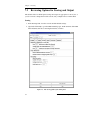
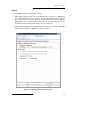
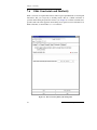
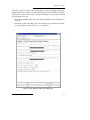
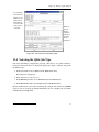
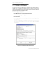
1
FirstDiscovery 3.0
Quick Start Guide
Copyright © 2004 Schrödinger, LLC. All rights reserved.
Schrödinger, FirstDiscovery, Glide, Impact, Jaguar, Liaison, LigPrep, Maestro, Prime, QSite, and
QikProp are trademarks of Schrödinger, LLC.
MacroModel is a registered trademark of Schrödinger, LLC.
To the maximum extent permitted by applicable law, this publication is provided “as is” without
warranty of any kind. This publication may contain trademarks of other companies.
Revision A, June 2004
Contents
Chapter 1: Document Overview..........................................................................1
Chapter 2: The FirstDiscovery Suite ..................................................................3
Chapter 3: Introduction to Maestro ...................................................................5
3.1 General Interface Behavior ..................................................................................5
3.2 Starting Maestro...................................................................................................5
3.3 The Maestro Main Window .................................................................................6
3.3.1 The Menu Bar ..........................................................................................7
3.3.2 The Toolbar ..............................................................................................8
3.3.3 Mouse Functions in the Workspace .......................................................11
3.3.4 Shortcut Key Combinations ...................................................................11
3.4 Maestro Projects ................................................................................................12
3.4.1 The Project Table Toolbar ......................................................................13
3.4.2 The Project Table Menus........................................................................15
3.4.3 Selecting Entries.....................................................................................15
3.4.4 Including Entries in the Workspace .......................................................16
3.4.5 Mouse Functions in the Project Table ....................................................16
3.4.6 Project Table Shortcut Keys ...................................................................17
3.5 Building a Structure ...........................................................................................18
3.6 Selecting Atoms .................................................................................................21
3.7 Maestro Command Scripts.................................................................................22
3.8 Specifying a Maestro Working Directory ..........................................................23
3.9 Undoing an Operation........................................................................................24
3.10 Running and Monitoring Jobs..........................................................................24
3.11 Getting Help.....................................................................................................26
3.12 Ending a Maestro Session................................................................................26
Chapter 4: Protein Preparation ........................................................................27
4.1 Preparing Proteins for FirstDiscovery ...............................................................27
4.2 Importing the Protein Complex Structure..........................................................27
4.3 Deleting Unwanted Waters ................................................................................28
4.4 Adjusting the Ligand .........................................................................................29
4.5 Running Protein Preparation on the Structure ...................................................32
4.6 Protein Preparation Output Structures ...............................................................34
FirstDiscovery 3.0 Quick Start Guide
iii
Contents
Chapter 5: Introduction to Glide ......................................................................35
Chapter 6: Creating Glide Grid Files ...............................................................37
6.1 Creating a Working Directory............................................................................37
6.2 Preparation .........................................................................................................38
6.3 Importing Maestro Files.....................................................................................38
6.4 Saving a Scratch Project ....................................................................................40
6.5 The Glide Panel: Choosing and Naming a Grid Generation Job .......................41
6.6 Designating the Ligand Molecule......................................................................43
6.7 Defining the Enclosing Box Center ...................................................................44
6.8 Starting and Monitoring the Grid Calculation ...................................................45
6.9 Exercise Summary .............................................................................................47
6.10 Running the Job With a Command Script .......................................................47
Chapter 7: Docking.............................................................................................49
7.1 Preparation .........................................................................................................49
7.2 Specifying a Pre-Existing Grid File for Docking ..............................................50
7.3 Selecting Ligands for Docking ..........................................................................50
7.4 Specifying a Reference Ligand..........................................................................53
7.5 Reviewing Options for Scoring and Output.......................................................54
7.6 Glide Constraints and Similarity........................................................................56
7.7 Starting the Docking Job....................................................................................58
7.8 Exercise Summary .............................................................................................58
7.9 Running the Job With a Command Script .........................................................59
Chapter 8: Examining Glide Data.....................................................................61
8.1 Preparation .........................................................................................................61
8.2 Displaying Pose Data.........................................................................................62
8.3 Viewing Poses ....................................................................................................62
8.4 Coloring and Labeling the Ligand .....................................................................64
8.5 Displaying Atoms by Proximity ........................................................................65
8.6 Coloring Carbons by Molecule Number............................................................66
8.7 Changing Molecular Representations ................................................................66
8.8 Visualizing Bad and Ugly Contacts ...................................................................66
8.9 Displaying Hydrogen Bonds..............................................................................68
8.10 Writing a File Containing a Single Ligand ......................................................69
iv
FirstDiscovery 3.0 Quick Start Guide
Contents
8.11 Saving Multiple Ligand Poses to a Single File................................................70
8.12 Exercise Summary ...........................................................................................70
Chapter 9: Introduction to Liaison...................................................................71
Chapter 10: Liaison Simulations.......................................................................73
10.1 Preparation .......................................................................................................73
10.2 Specifying Job Settings....................................................................................74
10.3 Loading a Receptor ..........................................................................................75
10.4 Creating a Ligand Source File .........................................................................76
10.5 Specifying a Ligand Source File and File Format ...........................................77
10.6 Setting Job Parameters.....................................................................................78
10.7 Specifying Atoms to Freeze.............................................................................79
10.8 Starting the Liaison Job ...................................................................................81
10.9 Exercise Summary ...........................................................................................82
10.10 Running the Job With a Command Script .....................................................84
Chapter 11: Analyzing Liaison Data ................................................................85
11.1 Preparation .......................................................................................................85
11.2 Creating a Binding Energy File .......................................................................86
11.3 Fitting Empirical Data Using the LRM Equation ............................................86
11.4 Predicting Binding Energies ............................................................................87
11.4.1 Performing the Predict Simulation.......................................................88
11.4.2 Predicting Binding Energy Using the LRM Model .............................89
11.5 Exercise Summary ...........................................................................................91
11.6 Running the Job With a Command Script .......................................................91
Chapter 12: Introduction to QSite....................................................................93
Chapter 13: Running a QSite DFT Job............................................................95
13.1 Preparation .......................................................................................................95
13.2 Importing a Structure .......................................................................................95
13.3 Preparing for QM Region Selection ................................................................96
13.4 Selecting the QSite Job Type ...........................................................................97
13.5 Defining a QM Region.....................................................................................98
13.6 Selecting a Basis Set ......................................................................................100
13.7 Including a Jaguar Keyword ..........................................................................100
13.8 Writing QSite Job Files..................................................................................100
FirstDiscovery 3.0 Quick Start Guide
v
Contents
Chapter 14: Getting Help.................................................................................103
Glossary .............................................................................................................105
Index...................................................................................................................109
vi
FirstDiscovery 3.0 Quick Start Guide
Chapter 1:
Document Overview
This manual contains tutorials designed to help you quickly become familiar with the
functionality of the FirstDiscovery™ software suite. In these tutorials, protein preparation,
Glide™, Liaison™, and QSite™ module tasks are performed using the Maestro interface.
For information about other FirstDiscovery modules and about performing tasks from the
command line, see the FirstDiscovery User Manual and the FirstDiscovery Command
Reference Manual.
Starting with FirstDiscovery 3.0, the FirstDiscovery Command Reference Manual is no
longer printed as hardcopy and bound with the other FirstDiscovery manuals. It is
provided on disk with the FirstDiscovery distribution, and is also available at
Schrödinger’s web site: http://www.schrodinger.com/Support/pdf.html.
If you need help on a topic, click the Help button in a Maestro panel, open Maestro’s help
facility from the Help menu on the main menu bar, or see the FirstDiscovery User Manual
or the FirstDiscovery Technical Notes. For more information, see Chapter 14.
In addition to the normal use of italics for names of documents, the font conventions used
in this manual are summarized in Table 1.1.
Table 1.1. Font conventions
Font
Example
Use
Sans serif
Project Table
Names of GUI features such as panels,
menus, menu items, buttons, labels
Monospace
$SCHRODINGER/maestro
File names, directory names, commands,
and environment variables
Italics
filename
Text that the user must replace with a
value
Sans serif
uppercase
ALT+H
Keyboard keys
In descriptions of command syntax, the usual UNIX conventions are used: square brackets
[ ] enclose optional items, and the pipe symbol | separates items in a list from which one
item must be chosen.
In this document, to type a command means to type the required text in the specified location, and to enter a command means to type the required text and then press the RETURN
key.
FirstDiscovery 3.0 Quick Start Guide
1
Chapter 1: Document Overview
2
FirstDiscovery 3.0 Quick Start Guide
Chapter 2:
The FirstDiscovery Suite
FirstDiscovery is a powerful protein modeling suite that consists of the program modules
Glide, Liaison, and QSite. Each module is designed to perform a specific drug discovery
or design task. To ready protein structures for use in FirstDiscovery, a protein preparation
facility is provided. In addition, the molecular mechanics program Impact™ provides
general-purpose modeling tools for FirstDiscovery. The FirstDiscovery programs are
operated from the Maestro graphical interface.
Protein Preparation for use in Glide, Liaison, and QSite can be performed for most
protein and protein-ligand complex PDB structures using the ProteinPrep panel in
Maestro. Command-line utilities complete the protein preparation facility.
Glide is designed to assist you in high-throughput screening of potential ligands based on
binding mode and affinity for a given receptor molecule. You can compare ligand scores
with those of other test ligands, or compare ligand geometries with those of a reference
ligand. Additionally, you can use Glide to generate one or more plausible binding modes
for a newly designed ligand. Once you locate favorable structures and/or bonding conformations with Glide, you can use Liaison to obtain binding energies for ligand-receptor
pairs.
Liaison is designed to predict ligand binding energies. Ligands for which binding energies
are known are used to calculate the Liaison SVD-fitted parameters—alpha, beta, and
gamma. These parameters are subsequently used to predict binding energies for other
ligands with the same receptor.
QSite is a mixed mode Quantum Mechanics/Molecular Mechanics (QM/MM) program
used to study geometries and energies of structures not parameterized for use with molecular mechanics, such as those that contain metals or represent transition states. QSite is
uniquely equipped to perform QM/MM calculations because it combines the superior
speed and power of Jaguar™ with the recognized accuracy of the OPLS-AA force field.
For information about Jaguar, see the Jaguar User Manual.
Maestro is Schrödinger’s powerful, unified, multi-platform graphical user interface
(GUI). It is designed to simplify modeling tasks, such as molecule building and data analysis, and also to facilitate the set up and submission of jobs to Schrödinger’s integrated
computational programs: Glide, Liaison, QSite, Impact, MacroModel, Jaguar, Prime™,
and QikProp. The main Maestro features include a project-based data management
facility, a scripting language for automating large or repetitive tasks, a wide range of
useful display options, a comprehensive molecular builder, and surfacing and entry plotting facilities. For more detailed information about the Maestro interface, see Chapter 3, of
this manual, the Maestro online help, or the Maestro User Manual.
FirstDiscovery 3.0 Quick Start Guide
3
Chapter 2: The FirstDiscovery Suite
The Impact computational engine can perform molecular mechanics calculations, either
through the Maestro interface or from the command line. For information on running basic
Impact jobs, see the Maestro online help, the FirstDiscovery User Manual, or the FirstDiscovery Command Reference Manual.
4
FirstDiscovery 3.0 Quick Start Guide
Chapter 3:
Introduction to Maestro
Maestro is the graphical user interface for all of Schrödinger’s products: FirstDiscovery
(Glide, Impact, Liaison, and QSite), Jaguar™, LigPrep™, MacroModel®, Prime, and
QikProp™. It contains tools for building, displaying, and manipulating chemical structures; for organizing, loading, and storing these structures and associated data; and for
setting up, monitoring, and visualizing the results of calculations on these structures. This
chapter provides a brief introduction to Maestro and some of its capabilities. For more
information, see the Maestro User Manual.
3.1
General Interface Behavior
Most Maestro panels are amodal: more than one panel can be open at a time, and a panel
need not be closed for an action to be carried out. Instead of a Close menu option or
button, each Maestro panel has a Hide button so that you can hide the panel from view.
Maestro supports the mouse functions common to many graphical user interfaces. The left
button is used for selecting: choosing menu items, clicking buttons, and selecting objects.
This button is also used for resizing and moving panels. The right button displays a
context-sensitive menu. Other common mouse functions are supported, such as using the
mouse in combination with the SHIFT or CTRL keys to select a range of items and select
or deselect a single item without affecting other items.
In addition, the mouse buttons are used for special functions described later in this chapter.
These functions assume that you have a three-button mouse. If you have a two-button
mouse, ensure that it is configured for three-button mouse simulation (the middle mouse
button is simulated by pressing or holding down both buttons simultaneously).
3.2
Starting Maestro
Before you start Maestro, you must first set the SCHRODINGER environment variable to
point to the installation directory. You can set this variable by entering the following
command at a shell prompt:
csh/tcsh:
setenv SCHRODINGER installation-directory
bash/ksh:
export SCHRODINGER=installation-directory
You might also need to set the DISPLAY environment variable if it is not set automatically
when you log in. To determine if you need to set this variable, enter the command
echo $DISPLAY
FirstDiscovery 3.0 Quick Start Guide
5
Chapter 3: Introduction to Maestro
If the response is a blank line, set the variable by entering the following command:
csh/tcsh:
setenv DISPLAY display-machine-name:0.0
bash/ksh:
export DISPLAY=display-machine-name:0.0
After you set the SCHRODINGER and DISPLAY environment variables, you can start
Maestro using the command
$SCHRODINGER/maestro options
If the $SCHRODINGER directory has been added to your path, you only need to enter the
command maestro. Options for this command are given in the Maestro User Manual.
The directory from which you started Maestro is Maestro’s current working directory, and
all data files are written to and read from this directory unless otherwise specified (see
Section 3.8 on page 23). You can change directories by entering the following command
in the command input area of the main window:
cd directory_name
where directory_name is either a full path or a relative path.
3.3
The Maestro Main Window
The Maestro main window is shown in Figure 3.1 on page 7. The main window components are as follows:
• Title bar—displays the project name and the current working directory
• Auto-Help—automatically displays context-sensitive help
• Menu bar—provides access to panels
• Workspace—displays molecular structures
• Clipping planes window—displays a small, top view of the Workspace and shows
the clipping planes and viewing volume indicators
• Toolbar—contains buttons for many common tasks, and also provides tools for displaying and manipulating structures and organizing the Workspace
• Status bar—displays the number of atoms, entries, residues, chains, and molecules
in the Workspace
• Sequence viewer—shows the sequences for proteins displayed in the Workspace
• Command input area—provides a place to enter Maestro commands
You can control the display of any of the last five components from the Display menu.
6
FirstDiscovery 3.0 Quick Start Guide
Chapter 3: Introduction to Maestro
Title bar
Auto-Help text area
Menu bar
Workspace
Toolbar
Viewing
volume
indicator
Sequence viewer
Status bar
Command input area
Clipping plane
Figure 3.1. The Maestro main window.
When a distinction between components in the main window and those in other panels is
needed, the term main is applied to the main window components (e.g., main toolbar).
3.3.1
The Menu Bar
The menus on the main menu bar provide access to panels, allow you to execute some
commands, and control the appearance of the Workspace. The main menus are as follows:
• Maestro menu—allows you to save or print images in the Workspace, execute system commands, save or load a panel layout, set preferences, set up Maestro command aliases, and quit Maestro.
FirstDiscovery 3.0 Quick Start Guide
7
Chapter 3: Introduction to Maestro
• Project menu—provides access to many project-related actions, such as opening
and closing a project and importing and exporting structures. These actions can also
be performed from the Project Table panel. For more information, see Section 3.4 on
page 12.
• Edit menu—allows you to undo actions, build and modify structures, define command scripts and macros, and find atoms in the Workspace.
• Display menu—provides access to panels that control the display of the contents of
the Workspace, to commands for the display of panels, and to options for the display
of main window components. Your choice of main window components displayed is
persistent between Maestro sessions.
• Tools menu—provides access to panels for grouping atoms, for measuring, for
aligning and superpositioning structures, and for viewing and visualizing data.
• Applications menu—provides access to panels for setting up, submitting, and monitoring jobs for all Schrödinger’s computational programs. Some products have a
submenu from which you can choose the task to be performed.
• Help menu—provides access to the Help panel and to a control for the display of
Balloon Help (tooltips).
3.3.2
The Toolbar
The main toolbar contains buttons for performing common tasks. There are three kinds of
buttons on the toolbar:
• Those that perform simple tasks, like clearing the Workspace
• Those that show and hide panels or open dialog boxes
• Those that display a menu when you click and hold
The third type of button is called a menu button and has a triangle in the lower right corner.
The menu is called a button menu. There are two kinds of items on button menus, and both
kinds can be on the same menu:
• Actions, which perform an action immediately
• States, which you set before an action is performed
When you select a state, it is stored and marked with a red diamond on the menu. Most
states on button menus are pick states (see Section 3.6 on page 21), which means you must
pick an atom in the Workspace before the action is performed. If you click a menu button
that has pick states, the button is indented to indicate that picking with the selected pick
state is in effect. If you double-click a menu button that has pick states, the action is
applied to all atoms. Some other menu buttons support double-clicking to apply an action:
this support is explicitly mentioned in the button description.
8
FirstDiscovery 3.0 Quick Start Guide
Chapter 3: Introduction to Maestro
You can show or hide the toolbar using the collapse button at the top or by selecting
Toolbar from the Display menu. You can hide it or move it to the right or left side of the
Workspace by right-clicking in the toolbar and selecting the appropriate option.
The buttons are described below. Some descriptions refer to features not described in this
chapter. See the Maestro User Manual for a fuller description of these features.
Open a project
Open the Open Project dialog box.
Import structures
Show the Import panel.
Show/Hide project table
Show the Project Table panel or hide it
if it is displayed.
Save as
Open the Save Project As dialog box,
to save the project with a new name.
Create entry from workspace
Create an entry in the current project
using the contents of the Workspace.
Delete
Choose an object to delete. Menu button
with a pick menu, a section to delete
hydrogens and waters and to open the
Atom Selection dialog box, and a section to delete other objects associated
with the structures in the Workspace.
Show/Hide Build panel
Show the Build panel or hide it if it is
displayed.
Add hydrogens
Pick atoms for hydrogen treatment.
Menu button with a pick menu and an
item to open the Atom Selection dialog
box.
Local transformation
Pick the object to transform. Menu button with a pick menu and an item to
open the Advanced Transformations
panel.
Undo/Redo
Undo or redo the last action. Performs
the same function as the Undo item on
the Edit menu, and changes to an arrow
pointing in the opposite direction when
an Undo has been performed, indicating
that its next action is Redo.
Fit to screen
Scale what is displayed to fit into the
Workspace, and reset the center of rotation.
Clear workspace
Clear all atoms from the Workspace
Set fog display state
Menu button. Automatic means on when
there are more than 40 atoms in the
Workspace, off when there are fewer.
Enhance depth cues
Optimize fogging and other depth cues
based on what is in the Workspace.
Rotate around X axis by 90 degrees
Rotate around Y axis by 90 degrees
FirstDiscovery 3.0 Quick Start Guide
9
Chapter 3: Introduction to Maestro
Tile entries
Arrange entries in a rectangular grid in
the Workspace.
Reset workspace
Reset the rotation, translation, and zoom
of the Workspace to the default state.
Save view
Save the current view of the Workspace:
orientation, location, and zoom.
Restore view
Restore the last saved view of the Workspace: orientation, location, and zoom.
Display only picked atoms
Pick atoms to display. Menu button with
a pick menu.
Display only
Display only the selected atoms. Menu
button with a list of predefined atom categories and an item to open the Atom
Selection dialog box.
Also display
Add the selected atoms to the display.
Menu button with a list of predefined
atom categories and an item to open the
Atom Selection dialog box.
Undisplay
Undisplay the selected atoms. Menu
button with a list of predefined atom categories and an item to open the Atom
Selection dialog box.
Display residues within N angstroms
of currently displayed atoms
Menu button with a list of values and an
item to open a dialog box to set a value.
Show, hide, or color ribbons
Menu button with items to control the
display of ribbons and atoms for proteins and to color ribbons by various
schemes.
Draw bonds in wire
Pick atoms for representation. Menu
button with a pick menu and an item to
open the Atom Selection dialog box.
Draw atoms in CPK
Pick atoms for representation. Menu
button with a pick menu and an item to
open the Atom Selection dialog box.
Draw atoms in ball and stick
Pick atoms for representation. Menu
button with a pick menu and an item to
open the Atom Selection dialog box.
Draw bonds in tube
Pick atoms for representation. Menu
button with a pick menu and an item to
open the Atom Selection dialog box.
Color all atoms by scheme
Menu button with a list of schemes.
Color residue by constant color
Pick residues to apply the selected color.
Double-click to color all atoms. Menu
button with a list of colors.
Label atoms
Label all atoms with the selected label.
Menu button with a list of label types
and an item to delete labels.
Label picked atoms
Menu button with a pick menu and
items to open the Atom Selection dialog
box, to open the Atom Labels panel at
the Composition folder, and to delete
labels.
10
FirstDiscovery 3.0 Quick Start Guide
Chapter 3: Introduction to Maestro
Display H-bonds
Pick molecules to display H-bonds.
Menu button with items to choose to
display H-bonds within the selected
molecule (intra) or between the selected
molecule and all other atoms in the
Workspace (inter), or to delete H-bonds.
3.3.3
Measure distances, angles or dihedrals
Pick atoms to define measurements.
Menu button with items to choose
between distance (default), angle, or
dihedral measurement, and to delete
measurements.
Mouse Functions in the Workspace
The middle and right mouse buttons have special uses in the Workspace. These can be
used on their own and in combination with the SHIFT and CTRL keys to perform common
operations, such as rotation, translation, centering, and zooming. Apart from centering a
molecule on an atom, all these operations involve dragging.
Table 3.1. Mapping of Workspace operations to mouse actions
Operation
Action
Rotate about the x- and y-axes
Drag with middle mouse button
Rotate about the x-axis only
Drag vertically with SHIFT and middle mouse button
Rotate about the y-axis only
Drag horizontally with SHIFT and middle mouse button
Rotate about the z-axis
Drag horizontally with CTRL and middle mouse button
Spot-center on an atom
Right-click
Translate in the x-y plane
Drag with right mouse button
Translate along the y-axis
Drag vertically with SHIFT and right mouse button
Translate along the x-axis
Drag horizontally with SHIFT and right mouse button
Translate about the z-axis
Drag horizontally with CTRL and right mouse button
Zoom
Drag horizontally with middle and right mouse buttons or with
SHIFT+CTRL and middle mouse button
3.3.4
Shortcut Key Combinations
Some frequently used operations that can be performed in the main window have been
assigned shortcut key combinations. The shortcuts, their functions, and their menu equivalents are listed in Table 3.2.
FirstDiscovery 3.0 Quick Start Guide
11
Chapter 3: Introduction to Maestro
Table 3.2. Shortcut keys in the Maestro main window
Keys
Action
Equivalent Menu Choices
ALT+B
Show Build panel
Edit > Build
ALT+C
Create entry
Project > Create Entry From Workspace
ALT+E
Show Command Script Editor panel
Edit > Command Script Editor
ALT+F
Open Find Atoms panel
Edit > Find
ALT+H
Show Help panel
Help > Help
ALT+I
Show Import panel
Project > Import Structures
ALT+M
Show Measurements panel
Tools > Measurements
ALT+N
New project
Project > New
ALT+O
Open project
Project > Open
ALT+P
Print
Maestro > Print
ALT+Q
Quit
Maestro > Quit
ALT+S
Show Sets panel
Tools > Sets
ALT+T
Show Project Table panel
Project > Show Table
ALT+W
Close project
Project > Close
ALT+Z
Undo/Redo last command
Edit > Undo/Redo
3.4
Maestro Projects
All the work you do in Maestro is done within a project. A project consists of a set of
entries, each of which contains one or more chemical structures and their associated data.
In any Maestro session, there can be only one Maestro project open. If you do not specify
a project when you start Maestro, a scratch project is created. You can work in a scratch
project without saving it, but you must save it in order to use it in future sessions. Maestro
also creates a scratch project when you close a project.
Likewise, if there is no entry displayed in the Workspace, Maestro creates a scratch entry.
Structures that you build in the Workspace constitute a scratch entry until you save the
structures as project entries. The scratch entry is not saved with the project unless you
explicitly incorporate it into the project. However, you can use a scratch entry as input for
some calculations.
The structures and their data are represented in the Project Table, which displays a list of
entries. Each entry is represented by a row in the Project Table. Each row contains the row
number, an icon indicating whether the entry is displayed in the Workspace (the In
12
FirstDiscovery 3.0 Quick Start Guide
Chapter 3: Introduction to Maestro
column), the entry title, a button to open the Surfaces panel if the entry has surfaces, the
entry name, and any entry properties. The row number is not a property of the entry.
You can open the Project Table panel by choosing Show Table from the Project menu, by
clicking the Show/Hide project table button on the toolbar, or by pressing ALT+T.
The Project Table panel contains a menu bar, a toolbar, and the table itself.
You can use entries as input for all of the computational programs—Glide, Impact, Jaguar,
Liaison, LigPrep, MacroModel, Prime, QikProp, and QSite. You can select entries as input
for the ePlayer, which displays the selected structures in sequence. You can also duplicate,
combine, rename, and sort entries, create properties, import structures as entries, and
export structures and properties from entries in various formats.
3.4.1
The Project Table Toolbar
The Project Table toolbar contains two groups of buttons and a status display. The first set
of buttons opens various panels that allow you to perform functions on the entries in the
Project Table. The second set of buttons controls the ePlayer, which “plays through” the
selected structures: each structure is displayed in the Workspace in sequence, at a given
time interval. See Section 3.3.2 on page 8 for a description of the types of toolbar buttons.
The buttons are described below.
Included
entry
Excluded
entry
Fixed or locked
entry
Selected
entries
Figure 3.2. The Project Table panel.
FirstDiscovery 3.0 Quick Start Guide
13
Chapter 3: Introduction to Maestro
Find
Open the Find panel for locating alphanumeric text in any column of the Project Table,
except for the row number.
Sort
Open the Sort panel for sorting entries by up to three properties.
Plot
Open the Plot panel for plotting entry properties.
Import structures
Open the Import panel for importing structures into the project.
Export structures
Open the Export panel for exporting structures to a file.
Columns menu
Display a menu for adjusting the column widths.
Entry selection
Open the Entry Selection dialog box for selecting entries based on criteria for entry
properties.
Go to start
Display the first selected structure.
Previous
Display the previous structure in the list of selected structures.
Play backward
Display the selected structures in sequence, moving toward the first.
Stop
Stop the ePlayer.
Play forward
Display the selected structures in sequence, moving toward the last.
Next
Display the next structure in the list of selected structures.
Go to end
Display the last selected structure.
ePlayer loop menu
Display a menu of options for repeating the display of the structures. Single direction
displays structures in a single direction, then repeats. Oscillate reverses direction each
time the beginning or end of the list is reached.
14
FirstDiscovery 3.0 Quick Start Guide
Chapter 3: Introduction to Maestro
The status display shows the number of selected entries. When you pause the cursor over
the display, the Balloon help shows the total number of entries, the number shown in the
table, the number selected, and the number included.
3.4.2
The Project Table Menus
• Table menu—provides tools for finding text, sorting entries, and plotting properties,
importing and exporting structures, and configuring the Project Table.
• Select menu—provides commands and access to the Entry Selection dialog box and
the Filter panel so that you can select entries.
• Entry menu—provides tools for including and excluding entries, controlling the
display of entries in the Project Table, and performing various operations on the
selected entries.
• Property menu—provides tools for displaying and manipulating properties.
• ePlayer menu—provides access to the play controls and the ePlayer options.
3.4.3
Selecting Entries
Many operations in Maestro are performed on the entries that are selected in the Project
Table. The Project Table functions much like any other table: you select rows by clicking,
shift-clicking, and control-clicking. However, because clicking in an editable cell of a
selected row enters edit mode, you should click in the Row column to select entries. See
Section 3.4.5 on page 16 for more information on mouse actions. There are shortcuts for
selecting classes of entries on the Select menu.
In addition to selecting entries manually, you can select entries that meet a combination of
conditions on their properties. Such combinations of conditions are called filters. Filters
are Entry Selection Language (ESL) expressions and are evaluated at the time they are
applied. For example, if you want to set up a Glide job that uses ligands with a low molecular weight (say, less than 300) and that has certain QikProp properties, you can set up a
filter and use it to select entries for the job. If you save it, you can use it again on a
different set of ligands that met the same selection criteria.
You can create filters in the Entry Selection dialog box, which you can open from the
Select menu (Only, Add, Deselect), from the Edit Filter dialog box, or by clicking the Entry
selection button on the toolbar.
FirstDiscovery 3.0 Quick Start Guide
15
Chapter 3: Introduction to Maestro
To create a filter, choose a property from the property list, choose a condition, and
combine it with the current filter by clicking Add, Subtract, or Intersect. These buttons
perform the Boolean operations OR, AND NOT, and AND on the corresponding ESL
expressions. Once you have created a filter, you can click OK to apply it immediately or
name and save it for later use.
3.4.4
Including Entries in the Workspace
In addition to selecting entries for various tasks, you also control which entries are
displayed in the Workspace from the Project Table. An entry that is displayed in the Workspace is said to be included in the Workspace; likewise, an entry that is not displayed is
excluded. Included entries are marked by an X in the diamond in the In column; excluded
entries are marked by an empty diamond. Entry inclusion is completely independent of
entry selection.
To include or exclude entries, you can click, shift-click, and control-click in the In column,
or select entries and then include or exclude them from the Entry menu. Inclusion with the
mouse works just like selection: when you include an entry by clicking, all other entries
are excluded.
It is sometimes useful to keep one entry in the Workspace and include others one by one:
for example, a receptor and a set of ligands. You can fix entries in the Workspace by
selecting the entries and choosing Fix from the Entry menu or by pressing ALT+F. A
padlock icon replaces the diamond in the In column to denote a fixed entry. To remove a
fixed entry from the Workspace, you must exclude it explicitly (ALT+X). It is not affected
by the inclusion or exclusion of other entries. Fixing affects only the inclusion of the
entry: you can still rotate, translate, or modify the structure.
3.4.5
Mouse Functions in the Project Table
The Project Table supports the standard use of shift-click and control-click to select
objects. This behavior applies to the selection of entries and the inclusion of entries in the
Workspace. Dragging to resize rows and columns and to move rows is also supported.
You can drag a set of non-contiguous entries to reposition them in the Project Table. When
you release the mouse button, the entries are placed after the first unselected entry that
precedes the entry on which the cursor is resting. For example, if you select entries 2, 4,
and 6, and release the mouse button on entry 3, these three entries are placed after entry 1,
because entry 1 is the first unselected entry that precedes entry 3. To move entries to the
top of the table, drag them above the top of the table; to move entries to the end of the
table, drag them below the end of the table.
A summary of project-based mouse functions is provided in Table 3.3.
16
FirstDiscovery 3.0 Quick Start Guide
Chapter 3: Introduction to Maestro
Table 3.3. Mouse operations in the Project Table
Task
Mouse Operation
Change a Boolean property value
Click repeatedly in a cell to cycle through the possible values (On, Off, Clear)
Display the Entry menu for an entry
Right-click anywhere in the entry. If the entry is not
selected, it becomes the selected entry. If the entry is
selected, the action is applied to all selected entries.
Display a version of the Property menu
for a property
Right-click in the column header
Edit the text or the value in a table cell
Click in the cell and edit the text or value
Include an entry, exclude all others
Click the In column of the entry
Move selected entries
Drag the entries
Paste text into a table cell
Middle-click
Resize rows or columns
Drag the boundary with the middle mouse button
Select an entry, deselect all others
For an unselected entry, click anywhere in the row
except the In column; for a selected entry, click the
row number.
Select or include multiple entries
Click the first entry then shift-click the last entry
Toggle the entry selection or inclusion
state
Control-click the entry or the In column
3.4.6
Project Table Shortcut Keys
Some frequently used project operations have been assigned shortcut key combinations.
The shortcuts, their functions, and their menu equivalents are listed in Table 3.4.
Table 3.4. Shortcut keys in the Project Table
Keys
Action
Equivalent Menu Choices
ALT+A
Select all entries
Select > All
ALT+F
Fix entry in Workspace
Entry > Fix
ALT+I
Show Import panel
Table > Import Structures
ALT+N
Include only selected entries
Entry > Include Only
ALT+U
Deselect all entries
Select > None
ALT+X
Exclude selected entries
Entry > Exclude
ALT+Z
Undo/Redo last command
Edit > Undo/Redo in main window
FirstDiscovery 3.0 Quick Start Guide
17
Chapter 3: Introduction to Maestro
3.5
Building a Structure
After you start Maestro, the first task is usually to create or import a structure. You can
open existing Maestro projects or import structures from other sources to obtain a structure. To build a structure, you use the Build panel, which you can open by choosing Fragments from the Edit menu, or by clicking the Show/Hide Build panel button in the toolbar.
The Build panel allows you to create structures by drawing or placing atoms or fragments in
the Workspace, and connecting them into a larger structure, to adjust atom positions and
bond orders, and to change atom properties. This panel contains a toolbar and three folders.
The Fragments folder offers a variety of molecular fragments from which to build a structure.
To place a fragment in the Workspace:
1. Select Place.
2. Choose a fragment library from the Fragments menu.
3. Click a fragment.
4. Click in the Workspace where you want the fragment to be placed.
There are several options for adding to a fragment that you have placed:
• Place another fragment and connect them using the Connect & Fuse panel, which
you open from the Edit menu on the main menu bar or with the Display Connect/Fuse
panel on the Build toolbar.
• Replace one or more atoms in the existing fragment with another fragment by selecting a fragment and clicking in the Workspace on the main atom to be replaced.
• Grow another fragment by selecting Grow and clicking the fragment you want to add
in the Fragments folder.
Grow mode uses predefined rules to connect a fragment to the grow bond. The grow
bond is marked by a green arrow. The new fragment replaces the atom at the head of
the arrow on the grow bond and all atoms attached to it. You can change the grow
bond by clicking on the desired grow bond in the Workspace. The arrow points to
the atom nearest to where you clicked.
18
FirstDiscovery 3.0 Quick Start Guide
Chapter 3: Introduction to Maestro
Figure 3.3. The Build panel.
You can also draw a structure freehand by choosing an element from the Draw button
menu on the Build panel toolbar and then drawing the structure.
In the Atom Properties folder you can change the properties of the atoms in the Workspace. For each item on the Property menu—Element, MacroModel Type, Partial Charge,
PDB Atom Name, Grow Name, and Atom Name—there is a set of tools you can use to
change the atom properties. For example, the Element tools consist of a periodic table
from which you can choose an element and pick an atom to change it to an atom of the
selected element.
Similarly, the Residue Properties folder provides tools for changing the properties of residues: the residue number, the residue name, and the chain name.
To adjust bond lengths, bond angles, dihedral angles, and chiralities during or after
building a structure, use the Adjust panel, which you open from the Edit menu on the main
menu bar or with the Display Adjust panel button on the Build panel toolbar.
FirstDiscovery 3.0 Quick Start Guide
19
Chapter 3: Introduction to Maestro
The toolbar of the Build panel provides quick access to tools for drawing and modifying
structures and labeling atoms. See Section 3.3.2 on page 8 for a description of the types of
toolbar buttons. The toolbar buttons and their use are described below.
Draw
Draw structures freehand in the Workspace. Menu button with a list of elements to draw
with (default C). Each click in the Workspace places an atom and connects it to the previous atom.
Delete
Choose an object to delete. Menu button with a pick menu and other items. Same as the
Delete button on the main toolbar.
Set element
Pick atoms to change to the selected element (default C). Menu button with a list of target
elements. Menu button with a limited list of target elements.
Increment bond order
Pick a bond to increase its bond order by one, to a maximum of 3.
Decrement bond order
Pick a bond to decrease its bond order by one, to a minimum of 0.
Increment formal charge
Pick an atom to increase its formal charge by one.
Decrement formal charge
Pick an atom to decrease its formal charge by one.
Move
Pick an atom to move in the xy plane or the z direction. Menu button with a list of drections. Moves in the xy plane are made by clicking the new location. Moves in the z direction are made in 0.5 Å increments.
Label
Apply heteroatom labels as you build a structure. The label consists of the element name
and formal charge, and is applied to atoms other than C and H.
Display Connect/Fuse panel
Open the Connect & Fuse panel so you can connect structures (create bonds between
structures) or fuse structures (replace atoms of one structure with those of another).
Display Adjust panel
Open the Adjust panel so you can change bond lengths, bond angles, dihedral angles, or
atom chiralities.
Add hydrogens
Pick to apply the current hydrogen treatment. Menu button with a pick menu and an item
to open the Atom Selection dialog box. Same as the Add hydrogens button on the main
toolbar.
20
FirstDiscovery 3.0 Quick Start Guide
Chapter 3: Introduction to Maestro
3.6
Selecting Atoms
Maestro has a powerful set of tools for selecting atoms in a structure that takes advantage
of chemical information about the structure. These tools are embedded in each panel in
which you might need to select atoms to apply some operation. Once you have chosen an
operation, you can use the tools to select, or pick, the atoms to apply the operation to.
To select all atoms in a molecule, a chain, a residue, or an entry, you can choose a pick
state using the Pick list. Once you have chosen the pick state, you can click on an atom in
the Workspace, and all the atoms that belong to the same structural unit, as defined by the
pick state, are selected. For example, if you choose Residue and click on any atom in a
glycine residue, all the atoms in that glycine residue are selected. To select individual
atoms, choose Atoms from the Pick list. The Pick list varies from panel to panel, because
not all pick states are appropriate for a given operation. For example, some panels have
only Atoms and Bonds in the Pick list.
To make atom selections based on more complex criteria, such as all carbon atoms in a
protein backbone, you can use the Atom Selection dialog box. To open this dialog box,
click the Select button. You can select an atom group from any of the folders in the dialog
box: Atom, Residue, Molecule, Chain, Entry, Substruct Notation, or Set. You can then
Figure 3.4. The Atom Selection dialog box.
FirstDiscovery 3.0 Quick Start Guide
21
Chapter 3: Introduction to Maestro
combine this group with the existing atom group using the buttons on the right: the Add
button (Boolean OR) includes all atoms in the new group or the existing group; the
Subtract button (Boolean AND NOT) excludes atoms in the new group from the existing
group; and the Intersect button (Boolean AND) includes only those atoms that are in both
the new group and the existing group. The existing group is expressed in Atom Specification Language (ASL) in the ASL text box, and is shown with light blue markers in the
Workspace. The current selection is shown with purple markers.
When you are satisfied with the selection, click OK to apply the operation you have chosen
with the selection you have made. The operation is described in a bar at the top of the
Atom Selection dialog box. Some operations take effect immediately, such as deleting
atoms. Others merely define a set of atoms to be used in a subsequent task, such as
selecting atoms for creation of a surface.
When the Atom Selection dialog box is open, you cannot perform other actions except for
rotation and translation of structures and picking. You can also open the help viewer.
3.7
Maestro Command Scripts
Although you can perform nearly all Maestro-supported operations through menus and
panels, you can also perform operations using Maestro commands, or compilations of
these commands, called scripts.
Command scripts can be used to automate lengthy procedures or repetitive tasks. Because
all Maestro commands are logged and displayed in the Command Script Editor panel, you
can create a command script by performing the operations with the GUI controls, copying
the logged commands from the Command History list into the Script area of the panel, then
saving the list of copied commands as a script. Short scripts can also be saved as macros,
which are run from the keys F1 through F12. See the Maestro User Manual for details.
To run an existing command script:
1. Open the Command Script Editor panel from the Edit menu in the main window.
2. Click Open Local and navigate to the directory containing the desired script.
3. Select a script in the Files list and click Open.
The command script is loaded into the Script window of the Command Script Editor
panel.
4. Click Run Script.
Command scripts cannot be used for Prime operations.
22
FirstDiscovery 3.0 Quick Start Guide
Chapter 3: Introduction to Maestro
The Command
History window
displays a log of
all commands
issued internally
within Maestro
when you interact
with a panel,
menu, or structure
Opens the Show/
Hide Command
panel, used to
determine which
commands are
logged in the
Command History
list
Figure 3.5. The Command Script Editor panel.
3.8
Specifying a Maestro Working Directory
When you use Maestro to start FirstDiscovery jobs, Maestro writes job output to the directory specified in the Directory folder of the Preferences panel. By default, the directory to
which Maestro writes files (the file i/o directory) is the directory from which you started
Maestro.
To change this directory:
1. Open the Preferences panel from the Maestro menu.
2. Click the Directory tab.
3. Select the option for the directory you want files to be read from and written to.
FirstDiscovery 3.0 Quick Start Guide
23
Chapter 3: Introduction to Maestro
Figure 3.6. The Directory folder of the Preferences panel.
3.9
Undoing an Operation
To undo a single operation, click the Undo button in the toolbar, choose Undo from the
Edit menu, or press ALT+Z. The word Undo in the menu is followed by text that describes
the operation or operations to undo. Not all operations can be undone: for example, global
rotations and translations are not undoable operations. For such operations you can use the
Save view and Restore view buttons in the toolbar, which save and restore a molecular
orientation.
If you think that you might want to undo a series of operations later, you can start an undo
block by selecting Begin Undo Block from the Edit menu. When you have completed the
group of operations you want to undo, end the block by selecting End Undo Block from the
Edit menu. Then, to undo the operations in the block, choose Undo from the Edit menu.
Undo is not supported for all Maestro operations. An undo block can be created only if at
least one undoable operation has been performed since the Begin Undo Block command
was issued.
3.10 Running and Monitoring Jobs
While FirstDiscovery jobs can be run from the command line, we suggest that you use the
Maestro GUI to set up and start these jobs, at least until you have some experience with
the programs and understand the directory structure and the input file requirements.
Maestro has dedicated panels for each product for preparing and submitting jobs. To use
these panels, make the appropriate choice for the product and task from the Applications
menu and its submenus.
24
FirstDiscovery 3.0 Quick Start Guide
Chapter 3: Introduction to Maestro
Figure 3.7. The Monitor panel.
Maestro also has a job control panel for monitoring the progress of jobs and for pausing,
resuming, or killing jobs—the Monitor panel. All jobs that belong to your user ID can be
displayed in the Monitor panel, whether or not they were started from Maestro. The text
pane shows some kinds of output from the job that is being monitored, such as the
contents of the log file. The Monitor panel opens automatically when you start a job. If it is
not open, you can open it by choosing Monitor from the Applications menu in the Maestro
main window.
While jobs are running, the Detach, Pause, Resume, Stop, Kill, and Update buttons are
active. When there are no jobs currently running, only the Monitor and Delete buttons are
active. These buttons act on the selected job. By default, only jobs started from the current
project are shown. To show other jobs, deselect Show jobs from current project only.
When a job that is being monitored ends, the results are automatically incorporated into
the project. If a job that is not currently being monitored ends, you can select it in the
Monitor panel and incorporate the results. Monitored jobs are incorporated only if they are
part of the project. You can monitor jobs that are not part of the project, but their results
are not incorporated. To add their results to the project, you must import them.
FirstDiscovery 3.0 Quick Start Guide
25
Chapter 3: Introduction to Maestro
3.11 Getting Help
Maestro comes with automatic, context-sensitive help (Auto-Help), Balloon help (tooltips), an online help facility, and a user manual. To get help, follow the steps below:
• Check the Auto-Help text box below the title bar of the main window. If help is available for the task you are performing, it is automatically displayed there. It describes
what actions are needed to perform the task.
• If your question concerns a GUI element, such as a button or option, there may be
Balloon help for the item. Pause the cursor over the element. If the Balloon help does
not appear, check that Show Balloon Help is selected in the Help menu of the main
window. If there is Balloon help for the element, it appears within a few seconds.
• If you do not find the help you need using either of the steps above, click the Help
button in the lower right corner of the appropriate panel. The Help panel is displayed
with a relevant help topic.
• For help with a concept or action not associated with a panel, open the Help panel
from the Help menu or press ALT+H.
If you do not find the information you need in the Maestro help system, check the
following sources:
• The Maestro User Manual
• The Maestro Release Notes
• The Frequently Asked Questions page, found at
http://www.schrodinger.com/Support/faq.html
3.12 Ending a Maestro Session
To end a Maestro session, choose Quit from the Maestro menu. To save a log file with a
record of all operations performed in the current session, click Quit, save log file in the Quit
panel. This information can be useful to Schrödinger support staff when responding to any
problem you report.
26
FirstDiscovery 3.0 Quick Start Guide
Chapter 4:
4.1
Protein Preparation
Preparing Proteins for FirstDiscovery
The quality of the results obtained from Glide, Liaison, and QSite depends on starting
structures that include all hydrogens, have correct charge states near the binding site, and
are reasonably free of major steric clashes. A typical PDB protein complex structure, as
downloaded from the Research Collaboratory for Structural Bioinformatics (RCSB) web
site (http://www.rcsb.org), has no hydrogens and may have residues in unusual charge
states. Schrödinger offers a Protein Preparation facility for use with FirstDiscovery that is
designed to ensure chemical correctness and to optimize protein structures.
The full Protein Preparation facility includes the ProteinPrep panel, the protprep
command-line application, and other utilities. See the FirstDiscovery User Manual for a
description of all the steps and options available. For most structures, however, including
the one used in this tutorial, Protein Preparation can be performed in a few steps with
Maestro and the ProteinPrep panel.
This tutorial carries out a Protein Preparation for 1ett, bovine thrombin with cocrystallized
ligand 4-TAPAP. Ligand bond orders are corrected using the Maestro Build panel. The
remaining preparation and refinement tasks run automatically as a job that is set up and
started from the ProteinPrep panel.
The 1ett structure is not a multimer and does not include cofactors or metal ions. See the
FirstDiscovery User Manual for information on preparing systems with these features.
To begin the tutorial:
1. If it is not already running, start Maestro.
2. In the Project menu, select New.
3. Name the new project 1ett.
4.2
Importing the Protein Complex Structure
Download the 1ett complex structure from the Protein Data Bank:
1. In your browser, go to http://www.rcsb.org/pdb.
2. Search the Archive by PDB ID for 1ETT.
3. Click Download/Display File and download the appropriate PDB file.
4. Uncompress the file if necessary.
FirstDiscovery 3.0 Quick Start Guide
27
Chapter 4: Protein Preparation
Import 1ETT.pdb into Maestro:
1. On the Maestro toolbar, click the Import structures button.
The Import panel is displayed.
2. From the Format options, select PDB.
3. Navigate to the directory in which you saved 1ETT.pdb.
4. Select 1ETT.pdb in the Files list and click Import.
The protein complex appears in the Workspace, colored according to the PDB-Maestro
structure conversion color scheme, which reports structural errors, missing atoms, and
nonstandard residues. The light gray that colors nearly all of the 1ETT structure indicates
standard residues. Orange indicates anything that is not a standard amino acid residue,
such as a ligand, cofactor, or metal ion. The 1ett structure consists of two protein chains
and a single ligand, 4-TAPAP, shown in orange.
In the terminal window where Maestro was started, you should see these messages:
WARNING check_residue: no template for residue 1 (TOS ), chain ’T’.
WARNING check_residue: no template for residue 2 (PAP ), chain ’T’.
WARNING check_residue: no template for residue 3 (PIP ), chain ’T’.
The ligand 4-TAPAP comprises three PDB HET groups: p-toluene sulfonate (TOS),
amidophenylalanine (PAP), and piperidine (PIP). None of these is a standard amino acid
residue, which means that there is no standard connection template to supply information
about bond order or formal charges. Without this information, Maestro creates a ligand
structure using only single bonds (and assigns no formal charges), which is far from
correct for 4-TAPAP. The ligand structure must be corrected before it can be used in Glide
and other FirstDiscovery applications. Bond order correction of the ligand is covered in
Section 4.4.
4.3
Deleting Unwanted Waters
There are hundreds of water oxygen atoms in this structure, as there are in most PDB
structures. Because water molecules vary in relevance to the binding mode of interest, the
Protein Preparation workflow allows you to decide in each case whether to keep all water
molecules, delete some, or delete all.
If cocrystallized water molecules are coordinated to metal ions or are forming hydrogenbond bridges between the ligand and protein, and you want to search for ligands that bind
in the same manner as the cocrystallized ligand, you should keep those waters. (After
28
FirstDiscovery 3.0 Quick Start Guide
Chapter 4: Protein Preparation
adding hydrogens to such waters, you should orient them appropriately to facilitate
receptor-ligand contacts. See the FirstDiscovery User Manual for more information.)
However, if you intend to search for ligands that might displace one or more waters, you
should delete some or all of the water molecules.
For 1ett, it is reasonable to delete all water molecules.
To delete all water molecules, choose one of the following:
• Choose Waters from the Delete button menu in the toolbar.
The water molecules are deleted.
• Enter this command in the Maestro command input area:
delete res HOH
4.4
Adjusting the Ligand
The ligand has been represented without bond order or formal charge information. This
information must be added. It is convenient to display only the ligand while doing this. For
most ligands and cofactors, you can do this by undisplaying the protein backbone and side
chains.
To undisplay protein components:
1. Choose Protein Backbone from the Undisplay button menu in the toolbar.
The protein backbone disappears.
2. Repeat Step 1 for Protein Side Chains.
The rest of the protein disappears.
3. Click the Fit to screen toolbar button to get a closer look at the ligand.
The ligand appears to consist of three disconnected fragments.
FirstDiscovery 3.0 Quick Start Guide
29
Chapter 4: Protein Preparation
This structure has no cofactors or metals, and waters have already been deleted, so
what remains should be the ligand. In this case, however, part of the ligand is missing too. Maestro recognizes amidophenylalanine (PAP) as an amino acid residue,
although a nonstandard one, and includes its “backbone” and side chain when it
undisplays the Protein Backbone and Protein Side Chains. To display the entire
ligand without the protein, you must use a different technique.
4. Choose All from the Also display button menu.
The entire structure is redisplayed.
To display only selected residues:
1. Choose Select from the Display only button menu in the toolbar.
2. The Atom Selection dialog box (ASD) appears, titled Select To Display Only.
3. Click the Residue tab and select Residue Type.
4. Scroll down the Residue Type list. PAP, PIP, and TOS are at the end of the list
because they are not standard residues.
5. In the list, click on PAP.
In the Workspace, the PAP residue is marked in magenta.
6. Click on TOS and drag over PIP and PAP to select all three.
The entire ligand is now marked in magenta.
7. Click the Add button.
The Atom Specification Language (ASL) expression for your selection appears in
the ASL text box, and the ligand is marked in cyan.
8. Click Create Set and type the set name 4-TAPAP, then click OK.
This makes future references to the ligand simpler.
9. Click OK again to exit the ASD.
Only the ligand appears in the Workspace.
30
FirstDiscovery 3.0 Quick Start Guide
Chapter 4: Protein Preparation
To adjust bond orders:
1. Choose Element from the Color all atoms by scheme button menu in the toolbar.
2. Click the Show/Hide Build panel button on the toolbar to open the Build panel.
3. In the Build panel toolbar, click Increment bond order.
4. In the Workspace, pick three bonds in each phenyl ring to increment them from single to double.
5. Pick the two S–O single bonds to make them double as well. (If dialog boxes appear
with warnings about atom valences, click OK to close them.)
6. Double the C-O single bond.
To adjust formal charge:
One of the amidophenyl nitrogens in the 4-TAPAP ligand should be protonated.
1. Double one of the two equivalent C-N bonds.
The double bond is displayed, but Maestro removes a hydrogen from the doublebonded nitrogen to maintain neutrality.
2. In the Build panel toolbar, click Increment formal charge.
3. Click the C=N nitrogen.
4. Choose Formal Charge from the Label atoms button menu in the toolbar.
The C=N nitrogen has formal charge +1.
The missing hydrogen will be added automatically in the preparation job.
5. Click Hide to close the Build panel.
FirstDiscovery 3.0 Quick Start Guide
31
Chapter 4: Protein Preparation
4.5
Running Protein Preparation on the Structure
1. Open the ProteinPrep panel from the Applications menu.
2. Type 1ett in the Job text box.
3. Choose a host for the job from the Host option menu.
If you use a different user name on the remote host you have selected, enter that
user name in the Login text box.
4. Pick ligand and Show markers are selected by default. Click an atom in the ligand.
The ligand is marked in blue-green.
Anything in the complex structure that was not selected as the ligand will be treated
as part of the receptor. This includes any cofactors, metals, or other ligands, if
present.
Figure 4.1. The Protein Preparation panel.
32
FirstDiscovery 3.0 Quick Start Guide
Chapter 4: Protein Preparation
5. To redisplay the receptor, choose All from the Also display button menu.
6. In the Procedure section of the ProteinPrep panel, ensure that Preparation and refinement, the default, is selected.
Each step can be run independently using the Preparation only or Refinement only
options.
7. Ensure that the default values of the following options are selected:
• Neutralization zone around the ligand: 10-20 Å
• Stop minimization when RMSD reaches: 0.30 Å
This default value allows the refinement portion of the job to halt when the
average RMSD of the heavy atoms reaches 0.30 Å.
• Incorporate results as: Separate entries.
This setting determines how the output structure is included in the Maestro
Project Table upon completion. Separate entries returns the protein and ligand
as separate entries, whereas Single entry does not. Single entry may be more
convenient if you want to run calculations on the complex (with the existing
ligand) immediately.
8. Click Start.
The Monitor panel is displayed, and the preparation stage begins.
During the preparation stage, hydrogen treatment is applied to the ligand and protein.
Residues within 10-20 Å of the ligand are neutralized, which may involve conformation
changes to some residues.
When preparation is finished, refinement begins. The refinement portion of the job
performs a series of restrained partial minimizations of the cocrystallized complex to optimize the positions of the newly added hydrogens and relieve any strain due to unphysically short distances in the X-ray structure.
Depending on the protein size, machine speed, and job settings, the 1ett preparation and
refinement job takes about 20 to 40 minutes.
Instead of starting the job immediately, you can click Write Job Files, then run the job
from the command line by entering $SCHRODINGER/protprep, This command has
options that allow fine control over the refinement section of the procedure. See the FirstDiscovery User Manual for details on the protprep command-line application.
FirstDiscovery 3.0 Quick Start Guide
33
Chapter 4: Protein Preparation
4.6
Protein Preparation Output Structures
Once the 1ett job is complete, examine the output structure files in Maestro. There will be
either one or two new entries in the Project Table, depending on whether you chose Single
entry or Separate entries as the incorporation mode. These files should exist after the job
is complete:
1ett_lig.mae
The input ligand structure file
1ett_lig_prep.mae
The post-preparation ligand structure file
1ett_lig_ref.mae
The post-refinement ligand structure file
1ett_prot.mae
The input receptor structure file
1ett_prot_prep.mae
The post-preparation receptor structure file
1ett_prot_ref.mae
Contains both the post-refinement receptor and ligand
structuresa
1ett.log
The log file for the complete preparation and refinement job
a. This file has the ligand structure appended so that Maestro can incorporate both structures.
Because the Separate entries option was chosen, there are now two new entries in the
Project Table. The first of the new entries, the refined receptor structure with all hydrogens, is the first structure in the 1ett_prot_ref.mae file and is automatically included
in the Workspace.
Exclude the receptor and include the second new entry to inspect the refined ligand structure. The extra hydrogen has been added to the charged nitrogen, and the guanidine group
is planar.
It is a good idea to examine prepared, refined protein and ligand structures in the Workspace, checking for obvious structural problems, making sure that the ligands and any
cofactors were properly hydrogen treated, that the correct formal charges, if any were
added, still exist, and that the structures look properly minimized. If any problems exist,
you can correct them in the input structure and then run the appropriate preparation and/or
refinement jobs again.
34
FirstDiscovery 3.0 Quick Start Guide
Chapter 5:
Introduction to Glide
Glide is a fast and accurate docking program that addresses a number of problems ranging
from database screening to highly accurate docking. The process has two main steps:
receptor grid generation followed by ligand docking and scoring. Each step is set up using
the Maestro graphical user interface.
In grid generation, the shape and properties of the receptor are represented on a grid by
several sets of fields that govern evaluation of the ligand poses. A ligand pose includes
both the internal conformation and the position and orientation relative to the receptor.
Grid generation setup can include defining Glide constraints: required hydrogen bond
donor/acceptor or metal/ligand interactions. This step also includes weighting calculations
if you want to do similarity scoring of ligands using a weighted algorithm.
During docking, Glide performs an efficient systematic search of conformational space.
The best binding mode for a ligand is then identified by thoroughly exploring the active
site using a series of hierarchical filters to select acceptable binding positions and orientations rapidly. Flexible minimization and Monte Carlo sampling then yield the final ligand
poses for accurate scoring. Optionally, ligand similarity scores can be used in docking
(even if weighting calculations were performed in grid generation).
There are two docking modes, standard precision and extra precision. Extra precision
docking is used to refine the results of a standard precision docking job.
To allow you to evaluate the scored ligands, Glide calculations can produce as output
either a library file (jobname_lib.mae), containing just the docked ligand structures, or a
pose viewer file (jobname_pv.mae), which also contains the receptor structure. You can
view either file in the Maestro Project Table, or you can view the pose viewer file in the
Glide Pose Viewer panel. You can also save the top poses to individual files for further
evaluation.
The exercises in the next three chapters demonstrate how to
• Generate Glide grid files
• Dock ligands from a multi-ligand file
• Select the top Glide poses from a pose viewer file
For the best performance in actual use, Protein Preparation should be run on both the
receptor and the candidate ligand structures before they are submitted to Glide. This
procedure is described in Chapter 4. The structure files used in Chapter 6, Chapter 7, and
Chapter 8 have already been prepared. For information on protein and ligand structure
preparation, see the FirstDiscovery User Manual and the chapter on optimizing performance in the FirstDiscovery Technical Notes.
FirstDiscovery 3.0 Quick Start Guide
35
Chapter 5: Introduction to Glide
36
FirstDiscovery 3.0 Quick Start Guide
Chapter 6:
Creating Glide Grid Files
This chapter contains exercises that demonstrate how to set up and start a grid file calculation job. Grid files reflect the area of the receptor, specifically the active site, that will be
searched when attempting to dock a ligand. You will use the grid files calculated in this
chapter to dock ligands in later Glide exercises.
6.1
Creating a Working Directory
The $SCHRODINGER/impact-vversion/tutorial/structures directory of your
FirstDiscovery distribution contains
• A Maestro-formatted receptor structure file
• A multi-structure file containing the receptor’s cocrystallized ligand and 19 structurally similar molecules
The tutorial directory also contains sample job files. These sample files are supplied
for comparison and for use as job input if you want to complete only some of the exercises
in this guide. As you perform the exercises you will create your own job files, so you must
first create a directory in which to write these files.
To create your working directory:
1. At a shell prompt, change to a directory in which you have write permission.
2. Create a new directory by entering the command:
mkdir workdir
In the text, this directory is referred to as the working directory.
3. In the working directory, create subdirectories named glide, grids, fit,
predict, lia_structures, and qsite.
The fit, predict, lia_structures, and qsite directories are used in the
Liaison and QSite tutorials.
4. In the working directory, create a soft link to the $SCHRODINGER/
impact-vversion/tutorial/structures directory by entering:
ln -s $SCHRODINGER/impact-vversion/tutorial/structures .
In the distribution, a directory called $SCHRODINGER/impact-vversion/tutorial/
maestro_cmd contains command scripts that automatically perform tasks described in
the exercises. The command scripts are provided so that you have the option of manually
FirstDiscovery 3.0 Quick Start Guide
37
Chapter 6: Creating Glide Grid Files
or automatically configuring the jobs in this guide and so that you will have examples for
creating your own command scripts. You do not need to copy these scripts; you can run
them from the distribution directory. Look for further instructions on using the scripts at
the conclusion of each chapter.
6.2
Preparation
Before you begin the exercises shown below, you must first have created a working directory as described in the previous section. If you have not yet set up your working directory,
do so now, then proceed with the instructions in the appropriate subsection below.
If you are starting with an active Maestro session:
Close any open project. If there are still atoms in the Workspace, remove them by clicking
the Clear Workspace button in the toolbar. In the command input area, enter the following
command to change into the correct directory:
cd workdir/grids
Proceed with the exercises below.
If you are starting with a new Maestro session:
Start Maestro from the workdir/grids subdirectory you have created, and proceed with
the exercises below.
6.3
Importing Maestro Files
Before you submit a Glide job, you must have at least the receptor displayed in the Workspace. In this exercise, you will import ligand and receptor structures into a Maestro
scratch project and then change the color of the ligand so that it is distinguishable from the
receptor. You will then use the imported structures to continue the exercises in this
chapter.
To import ligand and receptor structures and distinguish the ligand from the receptor by color:
1. Click the Import structures button on the toolbar.
The Import panel is displayed.
38
FirstDiscovery 3.0 Quick Start Guide
Chapter 6: Creating Glide Grid Files
To import only
some of the structures in a file,
deselect Import all
structures and type
the desired structure numbers in the
Start and Total
boxes
Selecting First
Imported
Structure from
this menu
causes only
the first structure in the
imported file to
be displayed
Figure 6.1. The Import panel.
2. Ensure that Maestro is selected from the Format menu.
3. Ensure that Import all structures is selected.
4. Ensure that First Imported Structure is selected from the Include in workspace menu.
5. Navigate
to
your
workdir/structures
directory
and
select
the
file
H01_H20_lig.mae.
6. Click Import.
Each ligand in the file H01_H20_lig.mae is placed in its own entry in the Project
Table, and the entry containing the first ligand is automatically included.
7. Choose aquamarine from the Color residue by constant color button menu.
8. Click an atom of the ligand.
The ligand is now colored aquamarine.
FirstDiscovery 3.0 Quick Start Guide
39
Chapter 6: Creating Glide Grid Files
Figure 6.2. The Project Table panel.
9. In the Import panel, deselect Replace workspace.
10. Import the structure in the file H01_rec.mae.
11. On the toolbar, click the Show/Hide project table button.
The Project Table panel is displayed, showing the entries for the 21 structures that
you have imported.
When you complete this exercise, you will have imported the H01 receptor, the cocrystallized ligand, and 19 structurally similar ligand structures into a scratch project. You will
also have displayed the receptor and the first ligand structure in the Workspace and colored
the ligand so that it is distinguishable from the receptor.
Generally, before you begin working on structures in a scratch project, you should save the
project. This ensures that Maestro saves all changes to the project without prompting you,
if your synchronization preference is set to Automatically. All data associated with a
scratch project is discarded when the Maestro session is ended or when you close the
project. Follow the instructions in the next exercise to save your project.
6.4
Saving a Scratch Project
This section describes how to save the project that you created in the preceding exercise.
1. From the Project menu in the main window, choose Save As.
The Save Project As project selector is displayed.
2. Navigate to your working directory (or click the Working Directory button).
40
FirstDiscovery 3.0 Quick Start Guide
Chapter 6: Creating Glide Grid Files
Double-click here
to move up a level
in the directory
structure
Figure 6.3. The Save Project As file selector.
3. In the Project text box, type docking at the end of the text. Maestro appends the
.prj extension to the project name you assign.
4. Click Save.
The title bar in the main window and the title text box in the Project Table panel
contain the new project name.
6.5
The Glide Panel: Choosing and Naming a Grid
Generation Job
To select the grid calculation function and assign a name to the job:
1. From the Applications menu in the main window, choose Glide.
The Glide panel is displayed with the Settings folder open.
2. In the Settings folder, choose Set up grids from the Choose Glide function option
menu.
3. In the Job text box, enter grids_H01. (Note that H01 contains a zero.)
When you assign a name to a grid generation job, Maestro copies the job name into the
Base name for grid files text box.
FirstDiscovery 3.0 Quick Start Guide
41
Chapter 6: Creating Glide Grid Files
When you choose Set up grids, Maestro sets the Directory for grid files to the current
working directory. If this is where you want to write the grid files, you do not need to
change the grid file directory setting. However, if you want to write the files to an alternative directory, you must specify the new directory in the Directory for grid files box.
For this exercise, if you did not start Maestro from your workdir/grids directory, enter
the path to this directory in the Directory for grid files text box.
Now that the new job has a name, you need to specify which molecule is the ligand. You
will do so in the next exercise.
By default,
the name
you enter in
this text box
becomes the
base name
for the job
output files
Figure 6.4. The Settings folder of the Glide panel.
42
FirstDiscovery 3.0 Quick Start Guide
Chapter 6: Creating Glide Grid Files
6.6
Designating the Ligand Molecule
To calculate a grid file, Glide must know the approximate conformational space that you
want to sample during the subsequent docking run. The simplest method of defining the
search space dimensions is by using the receptor’s cocrystallized ligand, if it is available.
Follow the instructions below to specify which Workspace molecule is the H01 ligand.
1. In the Settings folder of the Glide panel, choose Receptor plus a single ligand from
the Displayed structure is option menu.
2. If Choose an atom in the ligand molecule is not selected, select it.
3. In the Workspace, pick an atom in the ligand molecule.
The ligand molecule is colored aquamarine from the previous exercise.
Bounding
box
Figure 6.5. The marked ligand with bounding box.
FirstDiscovery 3.0 Quick Start Guide
43
Chapter 6: Creating Glide Grid Files
Once you pick an atom, the ligand molecule is marked with blue-green markers and a
bounding box with axes is displayed in green.
6.7
Defining the Enclosing Box Center
In this exercise, you will use the displayed ligand to create and size the bounding box and
enclosing box for a grid file calculation.
1. In the Glide panel, click the Site tab.
2. Under Specify center of enclosing box by, select Ligand centroid.
3. Click Specify Ligand.
The Ligand To Define Grid panel is displayed.
4. Select Use displayed ligand and click Hide.
5. Make sure that the Size of bounding box for placing ligand center option is set to
10 Å, the default range for the ligand center in FirstDiscovery 3.0.
The green bounding box defines the space through which the center of the defined
ligand is allowed to move during a subsequent docking calculation. You may change
the size of the box to allow the ligand to sample conformations over a larger space.
However, enlarging the box will increase the calculation time and may allow the
ligands being docked to explore a region of the protein site that is larger than the
region of interest.
6. In the Site folder, select Fit displayed ligand in the Size of enclosing box section.
The purple enclosing box that appears at the same time as the bounding box represents the volume of the protein for which grids will be calculated. Generally, you
should make the enclosing box as small as is consistent with the shape and character of the protein’s active site.
If you have a representative ligand in the active site, choosing Fit displayed ligand
generates an enclosing box that is large enough for most systems. However, if you
think that actives exist that are significantly larger than the cocrystallized ligand,
you should consider enlarging the enclosing box using the Fit ligands with length <=
option.
7. On the toolbar, click the Fit to screen button.
The ligand, the receptor, the bounding box, and the enclosing box are now visible in
the Workspace.
44
FirstDiscovery 3.0 Quick Start Guide
Chapter 6: Creating Glide Grid Files
Figure 6.6. The Site folder of the Glide panel.
6.8
Starting and Monitoring the Grid Calculation
The instructions below describe how to start a Glide job, how to interrupt a job, and how to
determine a job’s status.
1. Start the grids_H01 Glide job by clicking the Start button on the Glide panel.
The Monitor panel is displayed. While the job is in progress, the panel’s Status column displays the word “running.” When the job is complete, the status is changed to
“incorporated.”
FirstDiscovery 3.0 Quick Start Guide
45
Chapter 6: Creating Glide Grid Files
Figure 6.7. The Monitor panel.
2. Pause the Glide job by clicking on the job name in the list and then clicking Pause.
3. Resume the job by clicking Resume.
You can also start, monitor, and interrupt Glide jobs from the command line. For more
information, see the FirstDiscovery User Manual and the Maestro User Manual.
The job takes approximately 10 minutes, depending on your particular system configuration and workload. When the calculation is complete, these files should appear in your
grids directory:
grids_H01.inp
Command input for grids job
grids_H01.mae
Receptor structure input for grids job
grids_H01.log
Log summary file from grids job
grids_H01.out
Output summary file from grids job
as well as these output grid files for use in docking:
grids_H01.csc
grids_H01.save
grids_H01.greedy.save
grids_H01.grd
grids_H01.site
grids_H01.recep.mae
grids_H01.gsc
grids_H01.coul2.fld
grids_H01.vdw.fld
46
FirstDiscovery 3.0 Quick Start Guide
Chapter 6: Creating Glide Grid Files
When you run multiple calculations with the same job name, Glide overwrites some of the
created files and preserves others by appending incremented numbers to the existing file
names.
6.9
Exercise Summary
When you calculate grid files, the files are saved to disk, allowing you to use them in
subsequent docking jobs with additional ligands. In the next chapter, you will dock ligands
using the grid files you calculated in this chapter.
If you want to stop working on the tutorial now, choose Close Project from the Project
menu in the main menu bar.
6.10 Running the Job With a Command Script
A command script called grids_H01.cmd is included in the $SCHRODINGER/
impact-vversion/tutorial/maestro_cmd directory. This script uses the Maestro
command language in combination with Atom Specification Language (ASL) to accomplish the tasks described in this chapter. Note that the script does not start the job—it only
writes out the input files. To run the job, go to the Glide panel and click Start after the
script is finished. For more information about running a command script, see Section 3.7
on page 22.
Note that the command script will execute successfully only if you have set up your
working directory as specified in Section 6.1 on page 37 and run the command script from
your workdir/grids directory. Once you run the command script, save the project as
described in Section 6.4 on page 40.
The script-written input file, H01_grids.inp, is compatible with both the Linux x86
and the SGI IRIX platforms.
FirstDiscovery 3.0 Quick Start Guide
47
Chapter 6: Creating Glide Grid Files
48
FirstDiscovery 3.0 Quick Start Guide
Chapter 7:
Docking
The exercises in this chapter demonstrate how to use the grid files you calculated in the
previous chapter to dock ligands from a multi-ligand file.
7.1
Preparation
Before you start the exercises in this chapter, follow the appropriate instructions in this
section.
If you are continuing from the previous chapter and Maestro is running:
With the ligand and receptor structures displayed in the Workspace, enter the command
cd ../glide
in the command input area of the main window. This command puts you in the workdir/
glide directory, which you will use for the docking files you create in this chapter.
If you are continuing, but with a new Maestro session:
Enter the command
cd ../glide
in the command input area of the main window.
If Maestro is not running, start Maestro from the glide subdirectory in the working
directory you created.
If you are starting the tutorial with this chapter:
1. Create a working directory (see Section 6.1 on page 37).
2. Copy or create a soft link to the grid files that you will need to complete the docking
exercise in this chapter, or use the command script provided to set up the job files,
and then run the grid file calculation:
a. To begin by copying the provided grids, copy the grids_H01.* files from
$SCHRODINGER/impact-vversion/tutorial/grids to the grids subdirectory in the working directory.
b. To use the command script to set up the grid file calculation, use the instructions in Section 6.10 on page 47.
FirstDiscovery 3.0 Quick Start Guide
49
Chapter 7: Docking
7.2
Specifying a Pre-Existing Grid File for
Docking
In this section, you specify that the grid files you calculated in Chapter 6 be used for the
ligand docking job that will be run in this chapter.
1. Click the Clear workspace toolbar button.
2. Open the Glide panel and click the Settings tab. For help, see Section 6.5 on page 41.
3. Choose Dock one or more ligands from the Choose Glide function option menu.
Changing the Glide function changes the options and tabs that are available.
4. In the Job text box, delete glidetmp and type dock_confgen.
5. Make sure that Choose docking mode is set to Standard speed and precision. (For
information about the Extra precision option, see the FirstDiscovery User Manual, or
click the Help button and navigate to the Glide Settings folder topic.)
6. Click the Select button next to the Base name for grid files text box and choose
grids_H01.grd in the file selector. The name grids_H01 is displayed in the text
box.
7. The Directory for grid files text box displays the directory:
workdir/grids
The grid files are now specified. In the next exercise, you will start selecting ligands for
docking.
7.3
Selecting Ligands for Docking
You can select the ligand for docking in flexible docking mode by specifying a multiligand file or by selecting entries in the Project Table. Choose one of these methods:
To specify ligands from a multi-ligand file:
1. In the Glide panel, click the Ligand tab.
2. Make sure that Dock ligand(s) from files is selected.
50
FirstDiscovery 3.0 Quick Start Guide
Chapter 7: Docking
3. Make sure that Ligand structure file format is set to Maestro.
If a file already appears in the Specify one file in Maestro format list, select it and
then click Remove File.
4. Click Add File.
The Add Ligand Structure Files file selector is displayed.
5. Navigate to the workdir/structures directory and select the H01_H20_lig.mae
file in the Files list.
6. Click Add.
The file appears in the Specify one file in Maestro format list.
7. Under Docking/scoring mode, verify that Generate conformations for each input
structure (flexible docking) is selected.
To specify ligands from the Project Table:
1. In the Project Table, click the ligand entry H01, then shift-click the ligand H20.
All ligands from H01 to H20 are selected.
2. In the Ligand folder of the Glide panel, ensure that Dock selected entries from project
table is selected.
A file named dock_confgen.entries.mae, containing structures for the
entries, is created in the ../glide directory along with the input command file.
Depending on the number of entries you select, the file written to disk could be
large.
3. In the Docking/scoring mode section, verify that Generate conformations for each
input structure (flexible docking) is selected.
In this exercise, you chose one of two options for selecting ligands: either you specified
the name and format of the file that contains the ligands to be docked, or you selected
entries from the Project Table for docking. In the last step, you specified that Glide sample
various conformations for each ligand before docking the ligand with the receptor.
FirstDiscovery 3.0 Quick Start Guide
51
Chapter 7: Docking
Figure 7.1. The Ligand folder of the Glide panel.
If you already have a set of conformers, perhaps from a conformational search, docking
the ligands using the rigid docking mode is an alternate approach. Rigid docking uses the
ligand structures as they are and does not generate conformations or allow the ligand’s
torsional angles to vary, as flexible docking does.
52
FirstDiscovery 3.0 Quick Start Guide
Chapter 7: Docking
7.4
Specifying a Reference Ligand
You can specify a reference ligand while docking. Provided that the docked molecule (or
molecules) and the reference ligand are conformers, Glide computes and reports the RMS
deviation in atomic coordinates between the reference ligand and the poses generated for
the docked molecule(s). The RMS deviation is based on a comparison of heavy atoms.
The steps below describe how to designate a reference ligand.
1. In the bottom section of the Ligand folder, select Define a reference ligand.
2. Click Specify Ligand.
The Reference Ligand panel is displayed.
3. Select Use ligand from external file, and ensure that the Format menu option is Maestro.
4. Click Browse.
A file selector is displayed.
5. Locate and select the file
workdir/structures/H01_H20_lig.mae
6. Click Open.
In the Reference Ligand panel, you can leave the Structure number in ligand file
value set to 1 since the first structure in the multi-structure file is the cocrystallized
ligand for the H01 receptor.
7. Click Hide.
In this exercise, you specified a reference ligand for the docking of molecules in the structure file H01_H20_lig.mae. This completes the necessary adjustments to settings in the
Ligand folder. In the next exercise, you will view the Scoring folder settings.
Select to use a
ligand currently
included in the
Workspace as
the reference
ligand
Click to display a file
selector
Figure 7.2. The Reference Ligand panel.
FirstDiscovery 3.0 Quick Start Guide
53
Chapter 7: Docking
7.5
Reviewing Options for Scoring and Output
The default values for Glide ligand scoring and output are appropriate for most jobs, so
you do not need to change them for this exercise, but you might want to examine them.
Scoring
1. In the Scoring folder, view the controls and their default settings.
2. (Optional) Click Help to open the Glide Panel help topic. In the Contents, click Glide
Panel Features, then choose Scoring from the list of folders.
Figure 7.3. The Scoring folder of the Glide panel.
54
FirstDiscovery 3.0 Quick Start Guide
Chapter 7: Docking
Output
1. In the Output folder, view the default settings.
When Keep at most n poses is set to the default value of 1000, up to 1000 ligand
poses with the highest scores (i.e., the most favorable interactions with the receptor)
are saved in a pose viewer file. However, leaving the Keep at most n poses per
ligand value set to 1 for this exercise ensures that no more than 20 poses, one for
each ligand, will be collected and written to the pose viewer file.
2. (Optional) Click Help to open the Glide Panel help topic. In the Contents, click Glide
Panel Features, then choose Output from the list of folders.
Figure 7.4. The Output folder of the Glide panel.
FirstDiscovery 3.0 Quick Start Guide
55
Chapter 7: Docking
7.6
Glide Constraints and Similarity
Glide constraints are required interactions, either receptor-ligand H-bonds or metal-ligand
interactions, that you can specify as docking criteria. The use of Glide constraints is
optional. In the Glide grid generation exercise (see Chapter 6), no Glide constraints were
specified, and none will be applied to the docking job set up here. For more information on
Glide constraints, see the FirstDiscovery User Manual.
Figure 7.5. The Constraints folder of the Glide panel.
56
FirstDiscovery 3.0 Quick Start Guide
Chapter 7: Docking
Atom-pair similarity scoring can be used in docking to increase the likelihood that highranking ligands will be similar to (or different from) known actives. If similarity scoring is
selected, a file of known actives must be specified. Similarity scoring is optional and will
not be used in this exercise:
1. In the Glide Similarity folder, make sure that Use similarity score in docking is not
selected.
2. Optionally, read the online help topic for the folder. For more information on similarity scoring in Glide, see the FirstDiscovery User Manual.
Figure 7.6. The Similarity folder of the Glide panel.
FirstDiscovery 3.0 Quick Start Guide
57
Chapter 7: Docking
7.7
Starting the Docking Job
1. In the Glide panel, click Start.
The job starts and the Monitor panel is displayed.
2. Dismiss the Glide panel by clicking the Hide button.
The required computation time for all Glide docking jobs depends on the processor speed
and workload, the size and flexibility of the ligands to be docked, and the volume specified
by the enclosing box. As a rough estimate, docking a typical drug-like ligand takes about
one minute on a 1.2 to 1.5 GHz Pentium 4 Linux machine using FirstDiscovery 3.0 default
settings. On a similar machine, the 20-ligand docking job you started will usually finish in
less than 20 minutes. These files should exist after the job is complete:
dock_confgen.inp
Input file for docking job
dock_confgen.log
Log file from docking job
dock_confgen.out
Output file from docking job
dock_confgen_raw.mae
Unranked ligand poses
dock_confgen.rept
Table of ranked poses
dock_confgen_pv.mae
Receptor structure, followed by ranked poses
To confirm that these files have been written, open a terminal window and list the contents
of the current working directory, which was changed at the beginning of the chapter to
workdir/glide (see the title bar of the Maestro window). By default, the current working
directory is used for job startup and file i/o. (This default can be changed using options in
the Directory folder of the Preferences panel.) When you are finished checking the files,
close the terminal window and hide the Monitor panel.
7.8
Exercise Summary
The most meaningful result of this docking job is generating the pose file
dock_confgen_pv.mae. In pose viewer files such as this, which you can examine with
the Glide Pose Viewer panel, ligands are placed in a list and arranged so that poses with
the highest scores (i.e., most favorable interactions with the receptor) appear at the top.
This allows you to see at a glance which of the saved ligand poses should be studied
further.
In the next chapter, you will learn how to open and navigate in a pose viewer file, and how
to save the top scoring structures to separate files so that you can use them as input for
Liaison jobs.
58
FirstDiscovery 3.0 Quick Start Guide
Chapter 7: Docking
If you want to stop working on the tutorial now, choose Close from the Project menu in the
main menu bar.
7.9
Running the Job With a Command Script
A command script called dock_H01.cmd is provided in the $SCHRODINGER/
impact-vversion/tutorial/maestro_cmd directory. The script uses the Maestro
command language in combination with Atom Specification Language (ASL) to accomplish the tasks described in this chapter. Note that the script does not start the job; it only
writes out the input files. To start the job, you must click Start on the Glide panel after the
script has finished running. For more information on how to run a command script, see
Section 3.7 on page 22.
Note that the command script will execute successfully only if you have set up the
working directory as specified in Section 6.1 on page 37, and if you run the script from the
workdir/glide directory.
FirstDiscovery 3.0 Quick Start Guide
59
Chapter 7: Docking
60
FirstDiscovery 3.0 Quick Start Guide
Chapter 8:
Examining Glide Data
The exercises in this chapter describe how to use the Glide Pose Viewer panel to display
the results of a Glide docking job, and how to write pose files, some of which will be used
in the Liaison section. The emphasis in this chapter is on visual rather than numerical data.
For a more complete discussion of Glide output data, ligand poses, and scoring, see the
online help and the FirstDiscovery User Manual.
8.1
Preparation
Before you start the exercises in this chapter, follow the appropriate instructions in this
section.
If you are continuing from the previous chapter with Maestro running:
If you have done the exercises in the previous chapter and Maestro is still running, you
should already be in the workdir/glide directory. Proceed to “Clearing the Workspace,”
below.
If you are continuing, but with a new Maestro session:
If Maestro is not currently running, open a new shell, move to the workdir/glide subdirectory, and start Maestro according to the instructions in Section 3.2 on page 5.
If you are starting the tutorial with this chapter:
If you have not completed the exercises in Chapter 6 and Chapter 7, but want to work
through the exercises in this chapter, create a working directory and subdirectories as
described in Section 6.1 on page 37. Then, copy the file dock_confgen_pv.mae from
the directory $SCHRODINGER/impact-vversion/tutorial/glide/ to the workdir/
glide directory.
Clearing the Workspace:
If any structures are currently included in the Workspace, remove them by clicking the
Clear workspace toolbar button. (If there are no structures in the Workspace, the Clear
workspace button is not available.) Clearing the Workspace before opening a pose viewer
file is necessary because the structure is read into the Workspace and placed on top of any
currently included structures.
FirstDiscovery 3.0 Quick Start Guide
61
Chapter 8: Examining Glide Data
8.2
Displaying Pose Data
The following instructions describe how to use the Glide Pose Viewer panel to display the
ranked list of scored poses generated during a Glide docking job.
1. In the main window, choose Glide Pose Viewer from the Tools menu.
The Glide Pose Viewer panel is displayed.
2. In the Poses folder, click Open.
The Read Pose Files file selector is displayed.
3. Navigate to the workdir/glide directory.
4. Select the dock_confgen_pv.mae file and click Open.
The ligand poses in the file are listed in the Pose Viewer panel, as shown in
Figure 8.1 on page 63. Each ligand pose is identified by index number, title, ligand
number, conformation number, and pose number. For each pose, the table gives the
GlideScore (G-Score), E-Model, Energy, and various contact counts associated with
the pose-receptor combination. Some of these pose properties are described later in
this chapter.
5. Deselect the Display option.
The receptor structure is cleared from the Workspace. This is helpful if you want to
examine the structure of a selected ligand or if you want to center the display on a
ligand before redisplaying the receptor.
6. On the toolbar, click the Fit to screen button.
The ligand is resized and repositioned in the Workspace so that the structure is
entirely visible.
You have now opened the dock_confgen_pv.mae pose viewer file, viewed the first
pose, and optimized the pose’s position in the Workspace.
8.3
Viewing Poses
When you opened the Glide Pose Viewer panel, pose 1 was automatically selected and
displayed. Use the steps below to select ligand poses from the table and display the corresponding structures in the Workspace.
1. Add pose 2 to the selection by shift-clicking the second entry in the pose list.
2. Click Next to select and display only pose 3.
62
FirstDiscovery 3.0 Quick Start Guide
Figure 8.1. The Poses folder of the Glide Pose Viewer panel.
Chapter 8: Examining Glide Data
FirstDiscovery 3.0 Quick Start Guide
63
Chapter 8: Examining Glide Data
3. Reselect pose 1 by clicking twice on the Previous button.
Instead of using the Glide Pose Viewer to examine the docked ligand structures, you can
import the pose viewer file into the Project Table and use the ePlayer. However, the
ePlayer cannot show contacts and hydrogen bonds. For information on using the ePlayer,
see Section 3.4.1 on page 13 or the Maestro User Manual.
8.4
Coloring and Labeling the Ligand
This section describes how to redisplay the receptor molecule used in the grid file calculation, and to apply color and molecule number labels to the displayed ligand. The color
change will help distinguish the ligand molecule from the receptor, and the molecule
number labels will allow you to later manipulate the molecule using ASL.
1. On the toolbar, click and hold the Label atoms button, and choose Molecule Number
from the menu.
The ligand is labeled 1 (molecule 1).
2. On the toolbar, click and hold the Color by constant color button, and choose Purple
from the menu.
3. Click on an atom in the displayed structure.
The ligand is colored purple.
4. In the Poses folder of the Glide Pose Viewer panel, select Display.
The receptor is redisplayed in the Workspace.
The molecule number is useful when you are manipulating the molecule’s properties or
defining sets of atoms using ASL. Changing the color of the ligand can be helpful in visualizing the large-scale ligand-receptor interactions. In the next exercise, you will use the
molecule number of the ligand to selectively display only those receptor atoms that are
within a specified distance of the ligand. In subsequent exercises, you will examine interactions between the displayed ligand and receptor.
64
FirstDiscovery 3.0 Quick Start Guide
Chapter 8: Examining Glide Data
8.5
Displaying Atoms by Proximity
In this section you will display only part of the receptor molecule to better examine
contacts and hydrogen bonds between the displayed ligand and the binding pocket of the
receptor.
1. On the toolbar, click Display only and choose Select from the menu.
The Atom Selection dialog box (ASD) is opened with the heading Select to Display
Only.
2. Click the Molecule tab and select Molecule Number.
3. In the Workspace, click on an atom in the ligand.
The ligand molecule is marked in purple.
4. In the ASD, click Add (in the upper right portion of the panel).
The markers on the ligand molecule turn blue.
5. In the ASD, click Proximity (in the lower right portion of the panel).
The Proximity dialog box is displayed.
6. Make sure that Within is selected.
7. Type 5 into the text box, make sure that Angstroms is selected, and under Fill, select
Residues.
8. Click Update Markers.
The blue trace markers now include several nearby residues as well as the ligand.
9. Click OK to close the Proximity dialog box.
10. Examine the atom specification language (ASL) expression in the ASL box.
When you click OK in the ASD, all atoms that are more than 5 Å from the ligand are
undisplayed. Hiding the residues that do not come into contact with the ligand
allows you to better examine the ligand-receptor interactions.
The ASL expression uses the fillres option. This option causes all residues containing one or more atoms within 5 Å of the ligand to be displayed in full. If
fillres had not been used, only the atoms that met the proximity condition would
be displayed, and the other portions of these residues would be omitted.
11. Click OK.
In the Workspace, only the ligand and the nearby residues are displayed.
FirstDiscovery 3.0 Quick Start Guide
65
Chapter 8: Examining Glide Data
8.6
Coloring Carbons by Molecule Number
Assigning a distinctive color to the ligand molecule on screen is helpful for visualizing
large-scale ligand-receptor interactions. To view atom types, you must use a different
coloring scheme. In this exercise, you will color only the carbons in the displayed molecules by molecule number. This will leave non-carbon atoms colored by atom type so that
you can more thoroughly investigate contacts and hydrogen bonds.
• On the toolbar, click and hold the Color all atoms by scheme button and select Molecule Number (Carbons) from the menu.
In the Workspace, carbon atoms remain colored by molecule number, but non-carbon atoms are now colored by atom type.
8.7
Changing Molecular Representations
These instructions describe how to change the molecular representation of bonds in the
displayed ligand to “Tube.” Displaying some of the Workspace bonds in Tube representation can help you view intermolecular interactions more clearly.
1. On the toolbar, click the Draw bonds in tube button.
2. Pick an atom in the ligand molecule. The bonds in the ligand are displayed as tubes.
8.8
Visualizing Bad and Ugly Contacts
Since there are fewer disadvantageous than advantageous contacts in the structures
selected by Glide, visualizing only the former simplifies the interpretation of receptorligand interactions. Use the following instructions to visualize contacts that are Bad or
Ugly, according to default or user-defined criteria.
1. In the Poses folder of the Glide Pose Viewer panel, ensure that Display is selected.
2. In the Contacts folder, make sure Display contacts is selected.
The default behavior for this option is equivalent to selecting Bad contacts and Ugly
contacts, but not the more numerous Good contacts. Note that you can modify the
Contact cutoff Ratios for the displayed contacts.
66
FirstDiscovery 3.0 Quick Start Guide
Chapter 8: Examining Glide Data
Figure 8.2. The Contacts folder of the Glide Pose Viewer panel.
3. In the Poses folder, select a ligand pose in the list.
4. Click Visualize Contacts to Receptor.
The contacts are shown as dashed lines connecting Workspace atoms.
• Ugly contacts (red) are interactions with van der Waals radii closer than those
possible in real systems.
• Bad contacts (orange) are less close than Ugly ones, but are still unlikely in real
systems.
• Good contacts (green) are not currently displayed. Contacts are considered
Good if they are allowed according to empirical values for the particular atomtype interaction.
5. Return to the Contacts folder.
Note that you can select alternative atom sets for which to display contacts and Hbonds.
6. Click both of the Clear buttons to remove the atom set definitions.
In the following exercise, you will visualize any existing ligand-receptor hydrogen bonds.
FirstDiscovery 3.0 Quick Start Guide
67
Chapter 8: Examining Glide Data
8.9
Displaying Hydrogen Bonds
Use the following instructions to display hydrogen bonds between the ligand and the
receptor.
1. In the Poses folder, ensure that Display is selected.
2. In the H-Bonds folder, ensure that Display H-Bonds is selected.
3. In the Poses folder, select a ligand pose in the list.
4. Click Visualize H-Bonds to Receptor.
Hydrogen bonds are depicted in the Workspace as broken yellow lines.
5. Rotate the Workspace structures to better view the hydrogen bonds.
In this exercise, you displayed hydrogen bonds in the Workspace. As with contacts, you
can change the atom sets for which hydrogen bonds are displayed.
When you finish viewing the hydrogen bonds, click both Clear buttons in the H-Bonds
folder.
Figure 8.3. The H-Bonds folder of the Glide Pose Viewer panel.
68
FirstDiscovery 3.0 Quick Start Guide
Chapter 8: Examining Glide Data
8.10 Writing a File Containing a Single Ligand
In the previous exercise, you practiced using the Glide Pose Viewer’s analytical tools to
study ligand-receptor interactions. The instructions below describe how to create individual structure files for the top five poses in the pose viewer file. You will use these structure files later as input for a Liaison job.
1. In the Poses folder of the Glide Pose Viewer panel, deselect the receptor Display
option.
The receptor is removed from the Workspace.
2. Select the first pose in the pose list.
3. Click Write Displayed Poses.
The PoseWrite panel is displayed.
4. Ensure that Append is deselected, and then click Write To.
The Write Pose File file selector is displayed.
5. Navigate to the workdir/lia_structures directory.
6. After the text in the Selection text box, type H01_poses.mae.
7. Click Save.
8. Repeat the previous steps to create five more files, each containing one of the top five
ligand poses, starting again with pose 1. This time, use the following file names,
replacing lig# with the structure numbers of your five top poses, (e.g., H18, H06, and
so on).
pose1_lig#.mae
pose3_lig#.mae
pose5_lig#.mae
pose2_lig#.mae
pose4_lig#.mae
These numbers represent both the poses’ ranks in the list and the numbers of the
ligands within the multiple ligand structure file.
When you are finished, you will have written six files: five to use as input for Liaison jobs,
and one to use in the next exercise.
Figure 8.4. The PoseWrite panel.
FirstDiscovery 3.0 Quick Start Guide
69
Chapter 8: Examining Glide Data
When writing files for use with Liaison, you must place only one structure in each file.
Then you create a file, called a “ligand source file,” that lists the names of these structure
files. Instructions for creating this ligand source file are given in the exercise in
Section 10.4 on page 76.
8.11 Saving Multiple Ligand Poses to a Single File
There are two ways to save multiple ligand poses to a single file: select multiple ligands
from the list simultaneously or append structures to an existing file.
To save multiple structures to the same file simultaneously, use the steps for writing
displayed poses outlined in Section 8.10, except you select multiple poses simultaneously
in the list by holding down SHIFT while clicking on the first and last pose entries.
To append multiple structures to an existing file one at a time, follow the instructions
below. When you import either file type into Maestro, the structures are placed in separate
entries in a project.
1. In the Poses folder, select the second entry in the Pose List.
2. Click Write Displayed Poses.
3. In the PoseWrite panel, select Append.
4. Click Write To.
5. Select H01_poses.mae in the Files list.
6. Click Save.
7. Hide the PoseWrite and Glide Pose Viewer panels.
8.12 Exercise Summary
After you finish the exercises in this chapter, you will have completed the Glide portion of
the tutorial and will have written out the pose structure files that you will use in the
Liaison exercises that follow. If you want to continue with the Liaison exercises, proceed
to the next chapter.
If you want to stop working on the tutorial now, choose Close Project from the Project
menu in the main menu bar. If a dialog box appears and asks if you would like to save the
scratch project, click Discard. For more information about Quit panel options and log files,
see Section 3.12 on page 26.
70
FirstDiscovery 3.0 Quick Start Guide
Chapter 9:
Introduction to Liaison
Liaison uses the Linear Response Method (LRM) to calculate free energies of binding for
a protein and a group of ligands that are structurally similar to one another. The binding
free energies are calculated in three steps using the equation
∆G = α (<Ubvdw> – <Ufvdw >) + β (<Ubelec > – <Ufelec>) + γ (<Ubcav> – <Uf cav>)
Here, < > represents the ensemble average, b represents the bound form of the ligand, f
represents the free form of the ligand, and α, β, and γ are the coefficients. Uvdw, Uelec, and
Ucav are the van der Waals, electrostatic, and cavity energy terms, respectively, in the
continuum solvent model.
Liaison also calculates the GlideScore over the course of the LRM simulation. The
average GlideScore can then be used to predict binding energies using the alternate model
∆G = a(<GlideScore>) + b
where a is the GlideScore coefficient and b is a constant.
The exercises in Chapter 10 and Chapter 11 demonstrate:
• How to perform Liaison simulations on multiple ligands.
• How to perform a Liaison fitting calculation to determine the α, β, and γ coefficients
for the LRM equation.
• How to perform Liaison prediction tasks to calculate the binding energy for a new
ligand using the LRM method.
FirstDiscovery 3.0 Quick Start Guide
71
Chapter 9: Introduction to Liaison
72
FirstDiscovery 3.0 Quick Start Guide
Chapter 10: Liaison Simulations
In this chapter, you will set up and start a Liaison simulation job that will calculate the
ensemble average energy terms and GlideScores used in the equations on page 71.
10.1 Preparation
Before you start the exercises in this chapter, follow the appropriate instructions in this
section.
If you are continuing from the previous chapter and Maestro is open:
To perform the exercises in this chapter, you should make the fit directory your current
Maestro directory. Change to this directory by typing the following line in the command
input area of the main window.
cd ../fit
Proceed to Section 10.2 on page 74.
If you are continuing, but with a new Maestro session:
If you are not currently running Maestro, open a new terminal window, change to the
workdir/fit directory, and start Maestro according to the directions in Section 3.2 on
page 5. Then, proceed with Section 10.2 on page 74.
If you are starting the tutorial with this chapter:
If you have not completed the Glide tutorial but want to do the exercises in this chapter,
copy the following files from $SCHRODINGER/impact-vversion/tutorial/
lia_structures to the workdir/lia_structures subdirectory, replacing lig# with
the actual number in the files provided.
pose1_lig#.mae
pose2_lig#.mae
pose3_lig#.mae
FirstDiscovery 3.0 Quick Start Guide
pose4_lig#.mae
pose5_lig#.mae
liaison_ligands.txt
73
Chapter 10: Liaison Simulations
10.2 Specifying Job Settings
Before you can run a Liaison job, you must specify basic job settings like job name, job
type, and the number of processors you want to use. Follow the instructions below to
assign a job title and to specify that you want to run a new Liaison simulation on a single
processor.
1. In the main window, choose Liaison from the Applications menu.
The Liaison panel is displayed.
2. In the Settings folder, ensure that Simulate is selected.
3. Confirm that the value in the Number of processors to use text box is 1.
4. Type fit_sim in the Job text box.
5. In the System folder, verify that the Simulation type is set to Multiple ligands,
single receptor.
Figure 10.1. The Settings folder of the Liaison panel.
74
FirstDiscovery 3.0 Quick Start Guide
Chapter 10: Liaison Simulations
These options
are unavailable
because multiple ligands must
come from a
ligand source file
Figure 10.2. The System folder of the Liaison panel.
You have now established the general Liaison job settings. The next step in the job setup is
to load the receptor into the Workspace.
10.3 Loading a Receptor
Liaison simulations use the contents of the Workspace as the receptor structure. In this
exercise, you will import the receptor for the simulation and place it in the Workspace.
To load the receptor:
1. On the toolbar, click the Clear workspace button to exclude any structures that might
be in the Workspace.
FirstDiscovery 3.0 Quick Start Guide
75
Chapter 10: Liaison Simulations
2. On the toolbar, click the Import structures button.
The Import file selector is displayed.
3. Under Format, choose Maestro.
4. Navigate to the tutorial/structures directory.
5. Select H01_rec.mae in the Files list and click Import.
6. Click Hide to close the Import file selector.
In the multiple ligand, single receptor job that you will set up in the next section, the
ligands are specified using a ligand source file. If you were running a single ligand, single
receptor job, you could load the desired ligand into the Workspace along with the receptor,
or you could specify the ligand as a structure file, somewhat like in Glide.
10.4 Creating a Ligand Source File
To perform a multiple ligand Liaison calculation, you must create a ligand source file.
This is a text file that contains a name and a path to the ligand structure file for each ligand
to be evaluated.
To create a ligand source file for the five ligand poses that you wrote out in the previous chapter:
1. Open a text editor.
2. Open a terminal window and list the contents of your workdir/lia_structures
directory.
3. In the first line of the file, type pose1_lig#, replacing lig# with the number whose
ligand appears in your first pose file. Type one or more spaces, and on the same line
type the path name for the first ligand file as indicated below. Replace
tutorial_directory with the path to your tutorial/lia_structures directory.
On a new line, type the directory name and path for the next ligand, repeating this
for the final three ligands. Your file should have the same format as the text below.
pose1_lig#
pose2_lig#
pose3_lig#
pose4_lig#
pose5_lig#
76
tutorial_directory/lia_structures/pose1_lig#.mae
tutorial_directory/lia_structures/pose2_lig#.mae
tutorial_directory/lia_structures/pose3_lig#.mae
tutorial_directory/lia_structures/pose4_lig#.mae
tutorial_directory/lia_structures/pose5_lig#.mae
FirstDiscovery 3.0 Quick Start Guide
Chapter 10: Liaison Simulations
4. Save your ligand source file as:
workdir/lia_structures/liaison_ligands.txt
Note that the ligand source file is given a different name from the job because it
contains information about ligands only, and could be used for more than one
simulation.
Liaison creates a directory corresponding to each name entered in the left column of the
file, and looks for the corresponding structure files using the path names in the right
column. For example, if you enter pose1_H06 in the left column, Liaison creates a subdirectory called pose1_H06 in a directory named after your job name, fit_sim (workdir/
fit/fit_sim). The information in the right column of the ligand source file, workdir/
lia_structures/pose1_H06.mae is used to locate the input structure file. In the
next exercise, you will specify that Liaison use the ligand source file you have just created.
10.5 Specifying a Ligand Source File and File
Format
In the previous exercise, you created a ligand source file. Now you must specify the name
of the file and indicate the format of the referenced structure files.
To select the Liaison ligand source file and source file format:
1. In the main window, choose Liaison from the Applications menu and open the System folder.
2. Ensure that Maestro is selected in the Format of Ligand Files menu.
3. Click Browse.
The Open File file selector is displayed.
4. Locate and select the file:
workdir/lia_structures/liaison_ligands.txt
5. Click Open.
The liaison_ligands.txt path and filename appear in the Filename text box
of the System folder.
In the next exercise, you will view the default Liaison settings and change the number of
steps in the minimization.
FirstDiscovery 3.0 Quick Start Guide
77
Chapter 10: Liaison Simulations
10.6 Setting Job Parameters
The Minimization sampling method is the most desirable for quick fit and predict screenings. Hybrid Monte Carlo and Molecular Dynamics methods might produce better overall
results, but require more CPU time. At times you will want to change some of the simulation conditions for Liaison jobs.
To change the number of minimization steps:
1. In the Liaison Parameters folder, choose Minimization from the Sampling method
menu.
2. Ensure that Truncated Newton is selected in the Minimization algorithm menu.
3. In the Ligand Simulation folder, replace the default (500) in the Maximum minimization steps text box with 800.
Figure 10.3. The Parameters folder of the Liaison panel.
78
FirstDiscovery 3.0 Quick Start Guide
Chapter 10: Liaison Simulations
In this exercise, you changed the maximum number of steps in the ligand minimization
portion of the job to 800. Although the ligand minimizations in this job will probably not
take even 500 steps to converge, in future jobs you might want to change this setting, or
the analogous one in the Ligand/Receptor Simulation folder, which specifies the maximum
number of minimization steps for the bound ligand.
10.7 Specifying Atoms to Freeze
When you set up Liaison calculations, immobilizing (“freezing”) receptor atoms that do
not interact with the ligand is advantageous because it reduces the CPU time required for
simulations. Use the instructions below to freeze selected atoms.
1. In the Liaison panel, click the Constraints tab.
2. In the Constraints folder, click Frozen Atoms.
The Frozen Atoms panel is displayed.
Figure 10.4. The Constraints folder of the Liaison panel.
FirstDiscovery 3.0 Quick Start Guide
79
Chapter 10: Liaison Simulations
Figure 10.5. The Frozen Atoms panel.
3. In the Frozen Atoms panel, click Select.
The Atom Selection dialog box (ASD) is displayed.
4. Click the Residue tab and select Residue Number from the list on the left.
5. In the Residue Number field, type 120. Click Add.
Figure 10.6. The Residue folder of the Atom Selection dialog box.
80
FirstDiscovery 3.0 Quick Start Guide
Chapter 10: Liaison Simulations
Figure 10.7. The Proximity dialog box.
6. Click Proximity in the lower right of the ASD to open the Proximity dialog box.
The Proximity dialog box is displayed.
7. Ensure that Beyond and Angstroms are selected.
8. In the text field, type 18. Click OK to close the Proximity dialog box.
9. Note the ASL expression you have generated in the ASL field of the ASD. Click OK
to close the ASD.
In the Workspace, red padlock markers indicate frozen atoms.
10. Click Hide to close the Frozen Atoms panel.
In this exercise, you specified that all of the atoms of the receptor molecule farther than
18 Å from residue number 120 (located in the active site) be treated as a frozen shell.
Therefore, only the atoms closest to the receptor site will be able to move during the
Liaison calculations. This will reduce the CPU time required for the job.
10.8 Starting the Liaison Job
You are now ready to start the Liaison simulation job fit_sim.
1. Click Start on the Liaison panel.
The following files and directories are written:
• change_sgbparam_fit_sim
• fit_sim.mae, the receptor structure file used for each ligand’s bound state
simulation
FirstDiscovery 3.0 Quick Start Guide
81
Chapter 10: Liaison Simulations
• simulate_fit_sim, the script that starts the simulation
• fit_sim/
The fit_sim directory contains one subdirectory for each structure in the
ligand source file. Each subdirectory contains bound and free input files and
soft links to the structure files used as input. For example, pose1_lig#/
contains:
•
•
•
•
pose1_lig#.bound.inp
pose1_lig#.free.inp
pose1_lig#_rec.mae
pose1_lig#_lig.mae
2. Confirm that the Monitor panel is displayed as the job starts.
If the Monitor panel does not appear automatically, open it by selecting Monitor Jobs
from the Maestro Applications menu. For information on job monitor commands and
options, click Help in the Monitor panel.
3. When the job finishes, confirm that .stdout and .log files for each ligand have
been written to the fit_sim directory.
The bound and free simulations write multiple output files to each ligand’s subdirectory. In the pose1_lig#/ directory, confirm that the following files have been added:
•
•
•
•
•
•
•
•
pose1_lig#.bound.ave
pose1_lig#.bound.log
pose1_lig#.bound.out
pose1_lig#.free.ave
pose1_lig#.free.log
pose1_lig#.free.out
pose1_lig#_lig_min.mae
pose1_lig#_rec_min.mae
10.9 Exercise Summary
In this chapter, you set up and started Liaison simulation calculations. After the calculations are completed, the ligand.free.ave files and ligand.bound.ave files contain the
terms in the angular brackets used in the LRM equation (and the GlideScore equation) on
page 71. These job results are used in the next chapter for a Liaison fitting calculation. The
fitting calculation determines the alpha, beta, and gamma coefficients in the LRM equation, which can then be used to predict ligand binding energies.
Inside the fit_sim directory, a subdirectory for each ligand has been created. The
Liaison directory structure is schematically illustrated in Figure 10.8.
82
FirstDiscovery 3.0 Quick Start Guide
Chapter 10: Liaison Simulations
Liaison Directory Structure*
Maestro Working Directory
Master Liaison Run Directory (jobname)
ligand1
ligand2
ligand3
ligand4
analyze_jobname
simulate_jobname
jobname.dat
jobname.in
jobname.log
jobname.mae
jobname.out
change_sgbparam_jobname
ligand5
Input
Output
ligand#_structure
receptor_structure
ligand#.free.inp
ligand#.bound.inp
ligand#_lig_min.mae
ligand#_rec_min.mae
ligand#.free.out, .ave, & .log
ligand#.bound.out, .ave, & .log
[ligand#_lig_fin.mae]
[ligand#_rec_fin.mae]
[ligand#.free.trj]
[ligand#.bound.trj]
[cmpx.rst]
ligand1.stdout
ligand2.stdout
ligand3.stdout
ligand4.stdout
ligand5.stdout
jobname.log
Figure 10.8. The Liaison directory structure.
* Files in brackets [ ] are created only with Liaison Dynamics and HMC jobs.
In Figure 10.8, the top-level Maestro Working Directory contains the Master Liaison Run
Directory, the scripts used to run Liaison jobs, and the receptor structure file. In this tutorial, the Maestro Working Directory is /workdir/fit and the Master Liaison Run Directory is /workdir/fit/fit_sim. Subdirectories contain the input and output files for
jobs started by the simulate_jobname script.
If you want to stop working on the tutorial now, choose Close Project from the Project
menu in the main menu bar.
FirstDiscovery 3.0 Quick Start Guide
83
Chapter 10: Liaison Simulations
10.10 Running the Job With a Command Script
A command script called fit_lia.cmd has been provided in the $SCHRODINGER/
impact-vversion/tutorial/maestro_cmd directory. This script uses Maestro
command language and Atom Specification Language (ASL) to accomplish the tasks
described in this chapter.
When you use the provided command script to set up the job, you should note the
following. First, the script will call a file named liaison_ligands.txt. If you did not
create this file, you must copy it from $SCHRODINGER/impact-vversion/tutorial/
lia_structures into the /workdir/lia_structures directory. Then, you must edit
the file and replace tutorial_directory to reflect the path of your working tutorial directory, and replace the specific pose file names with the names of the new files that you
created in the previous chapter.
Finally, note that the script does not start the job; it only writes the input files. To start the
job, you must click Start on the Liaison panel after the script has finished running. For
information on how to run a command script, see Section 3.7 on page 22.
84
FirstDiscovery 3.0 Quick Start Guide
Chapter 11: Analyzing Liaison Data
In this chapter, you will run a Liaison Analysis job to fit the simulation results to experimental data using the LRM equation shown on page 71. (For information about using the
GlideScore equation instead, see the FirstDiscovery User Manual.) The Liaison simulation you completed in the previous chapter calculated the terms inside the angle brackets
in the LRM equation. The Fit job will determine the α, β, and γ coefficients based on the
terms from the previous chapter and the free energy values in the training set. These coefficients will then be used in a Predict job.
11.1 Preparation
Before you start the exercises, follow the appropriate instructions in this section.
If you are continuing from the previous chapter and Maestro is open:
To continue with the exercises in this chapter, make sure that you have set up a working
directory and performed a multiple ligand Liaison simulation. Then proceed to
Section 11.2 on page 86.
If you are continuing, but with a new Maestro session:
If Maestro is not currently running, open a terminal window, move to the workdir/fit
subdirectory, and start Maestro according to the instructions in Section 3.2 on page 5.
Then open the Liaison panel, delete the name impacttmp from the Job text box, and type
fit_sim in its place. Import the file H01_rec.mae from the workdir/structures
directory.
If you are starting the tutorial with this chapter:
1. If you have not yet done so, create a working directory using the instructions in
Section 6.1 on page 37.
2. Copy the items you will need to complete the exercises in this chapter or run the
Liaison Simulation job now, using a provided command script to set up the files.
a. If you choose to copy the necessary items, copy the file fit_sim.mae and the
directory fit_sim from $SCHRODINGER/impact-vversion/tutorial/
fit to workdir/fit.
b. If you want to run the Simulation job now using a command script to set up the
job, follow the instructions in Section 10.10 on page 84. Start the simulation
job and let it run to completion. This job takes approximately one hour.
3. Follow the instructions above for continuing with a new Maestro session.
FirstDiscovery 3.0 Quick Start Guide
85
Chapter 11: Analyzing Liaison Data
11.2 Creating a Binding Energy File
To run a Liaison Fit calculation, you must use as input a text file containing empirically
determined binding energies for the ligands in your training set. The Fit calculation will
determine the coefficients in the LRM equation. You can then use these coefficients with
Liaison to predict the free energy of binding for ligands that are structurally similar to the
ligands in the training set.
To create the file containing experimental binding energies for the structures to
which you are going to fit Liaison data:
1. In a text editor, open the file
$SCHRODINGER/impact-vversion/tutorial/fit/bindE.expt
2. Open another text editing session and create a new file.
3. In the first line of the new file, type pose1_lig# and replace lig# to match the name
you specified for your first pose in liaison_ligands.txt. Type one or more
spaces, then without pressing ENTER, copy the experimental binding energy (in
kcal/mol) from bindE.expt for the first ligand. Use a preceding minus sign if the
value is negative. On the next four lines, type the information for the other four
ligands. Your file should have the same format as the text below.
pose1_lig#
pose2_lig#
pose3_lig#
pose4_lig#
pose5_lig#
##.##
##.##
##.##
##.##
##.##
4. Name your new file bindE.expt and save it to the directory:
workdir/fit
In the next exercise, you will use controls on the Liaison panel to specify bindE.expt as
your ligand binding energy file.
11.3 Fitting Empirical Data Using the LRM
Equation
In this exercise, you will fit empirical data using the LRM equation.
1. In the Liaison panel, type fit_sim in the Job text box.
2. In the Settings folder, select Analyze results of earlier simulations.
3. In the Analysis folder, under Analysis type, select Fit.
86
FirstDiscovery 3.0 Quick Start Guide
Chapter 11: Analyzing Liaison Data
4. Make sure that Binding energy model is set to LIA equation.
5. Click Browse to the right of the Filename of ligand binding energies text box.
6. In the Open Ligand Binding Energy File dialog box, locate and select the file
workdir/fit/bindE.expt
7. Click Open.
You have now adjusted the settings needed to fit empirical data using the LRM
method.
8. To start the fitting job, click Start in the Liaison panel.
The Monitor panel appears, showing the results of the fitting job.
When the job has finished, these additional items appear in fit_sim:
analyze_fit_sim
fit_sim.dat
fit_sim.log
fit_sim.out
fit_sim.in
Included in fit_sim.out are the coefficients from the fit, Chi-square values, and RMSD
error.
In this exercise, you have performed a Liaison fitting analysis to determine the coefficients
used in the LRM equation. In the next exercise, you will learn how to use these calculated
coefficients to produce binding energies for ligands that are structurally similar to those in
the training set.
11.4 Predicting Binding Energies
These exercises describe how to use α, β, and γ coefficients calculated from the training
set to estimate the binding energy for a new, structurally similar, ligand. Before you can
predict the binding energy of a new ligand, you must run a Liaison simulation on the new
ligand. The simulation for the new ligand must be set up with the same parameters as in
the earlier simulation used to derive the coefficients for the LRM equation. Since simulations were covered in Chapter 10, simplified instructions will be provided in
Section 11.4.1.
FirstDiscovery 3.0 Quick Start Guide
87
Chapter 11: Analyzing Liaison Data
11.4.1 Performing the Predict Simulation
1. Make a directory called predict in the workdir.
2. Enter the following command in the command input area of the main window:
cd ../predict
If the H01 receptor with its frozen atoms is still displayed in the Workspace, go to
Step 4. Otherwise, continue with Step 3.
3. Click Clear workspace, then import the file:
tutorial/structures/H01_rec.mae
4. In the Liaison panel, type predict_sim in the Job text box.
5. In the Settings folder, select Simulate.
6. In the System folder, set the simulation type to Single ligand, single receptor.
7. In the Name to use for this ligand text box, type H06_altered.
8. In the Parameters folder:
a. Choose Minimization from the Sampling method menu.
b. In the Ligand Simulation folder, replace 500 with 800 in the Max minimization
steps text box.
9. Set up frozen atoms:
a. In the Liaison panel’s Constraints folder, click Frozen Atoms.
b. In the Frozen Atoms panel, click Select to open the Atom Selection dialog box
(ASD).
c. In the ASL field of the ASD, type
beyond 18 res. 120
and click OK.
10. Open the Import panel, deselect the Replace workspace option, and import the file:
tutorial/structures/H06_altered.mae
11. Use the Color by constant color toolbar button to color the ligand purple:
Choose purple from the Color by constant color button menu. Then click on the
ligand in the Workspace. The ligand molecule is now purple.
88
FirstDiscovery 3.0 Quick Start Guide
Chapter 11: Analyzing Liaison Data
12. In the System folder, select Select ligand molecule by picking an atom.
13. Pick an atom in the ligand.
A blue-green trace is superimposed onto the selected molecule.
14. Click Start.
The calculation is started and the Monitor panel is displayed.
This job should take about an hour to complete. After it finishes, the following items
should appear in the workdir/predict directory:
change_sgbparam_predict_sim
predict_sim/
predict_sim.mae
simulate_predict_sim
The predict_sim subdirectory should contain the following:
H06_altered/
H06_altered.stdout
predict_sim.log
The directory predict_sim/H06_altered contains data for the free and the bound
versions of the corresponding ligand:
H06_altered.bound.inp
H06_altered.free.inp
H06_altered.bound.ave
H06_altered.bound.log
H06_altered.bound.out
H06_altered.free.ave
H06_altered.free.log
H06_altered.free.out
H06_altered_lig.mae
H06_altered_lig_min.mae
H06_altered_rec.mae
H06_altered_rec_min.mae
Now you are ready to begin the Predict analysis task.
11.4.2 Predicting Binding Energy Using the LRM Model
1. In the Liaison panel, type predict_sim in the Job text box.
2. In the Settings folder, select Analyze results of earlier simulations.
3. In the Analysis folder, select Predict.
4. Under Binding energy model, select LIA equation.
5. From the Specify ligands by option menu, choose Enter list of ligand names.
6. Enter H06_altered in the Comma-separated list text box.
FirstDiscovery 3.0 Quick Start Guide
89
Chapter 11: Analyzing Liaison Data
7. Use a text editor to open the file:
workdir/fit/fit_sim.out
8. In the Analysis folder, under Prediction parameters, enter the alpha, beta, and gamma
values from the file in the corresponding text boxes.
9. Click Start.
The Monitor panel is displayed and logs the job’s progress.
When the job finishes, the following items are written to the workdir/predict directory:
analyze_predict_sim
predict_sim.dat
predict_sim.log
predict_sim.out
predict_sim.in
Figure 11.1. The Analysis folder of the Liaison panel.
90
FirstDiscovery 3.0 Quick Start Guide
Chapter 11: Analyzing Liaison Data
In predict_sim.out, you will find the binding energy of the H06_altered ligand.
The binding energy, reported in kcal/mol, can also be found in the upper window of the
Monitor panel.
The predicted binding energy is calculated from the LRM equation:
∆G = α (<Ubvdw> – <Ufvdw >) + β (<Ubelec > – <Ufelec>) + γ (<Ubcav> – <U f cav>)
The ensemble average <U> values were calculated during the simulation that you ran on
the H06_altered ligand. In the prediction job, ∆G is calculated using those values and
the values you supplied for the α, β, and γ coefficients.
11.5 Exercise Summary
If the calculated binding energy for the modified H06_altered ligand is more negative
than those of the training set ligands, then the modified molecule might be a good drug
candidate.
If you want to stop working on the tutorial now, choose Close from the Project menu in the
main menu bar. If a dialog box appears and asks if you would like to save the scratch
project, click Discard. For more information about Quit panel options and log files, see
Section 3.12 on page 26.
11.6 Running the Job With a Command Script
A command script, predict_lia.cmd, has been provided in the $SCHRODINGER/
impact-vversion/tutorial/maestro_cmd directory. The script uses the Maestro
command language in combination with Atom Specification Language (ASL) to accomplish the tasks described in Section 11.4.1 on page 88. Note that the script does not,
however, start the Predict Simulation job or prepare and start the Predict Analysis; it only
writes out the input files. To start the Predict Simulation job, you must click Start on the
Liaison panel after the predict_lia.cmd script has finished running. For more information on running a command script, see Section 3.7 on page 22. The script will run
successfully only if you have set up your tutorial directory as specified, and are running
from your workdir/fit directory. Before running the script, you must first create the
bindE.expt file as instructed in Section 11.2 on page 86.
FirstDiscovery 3.0 Quick Start Guide
91
Chapter 11: Analyzing Liaison Data
92
FirstDiscovery 3.0 Quick Start Guide
Chapter 12: Introduction to QSite
Like Liaison, QSite is a free energy calculation program. However, QSite uses a QM/MM
approach, and is powered by the Jaguar (QM) and Impact (MM) computational engines.
Mixed mode QM/MM free energy calculations will produce more accurate results, but
will require more CPU time.
To perform a QSite job, you must specify not only a receptor–ligand pair to be studied, but
you must define a QM region—a small number of atoms encompassing the ligand and
prominent atoms in the binding pocket of the receptor. The instructions in the next chapter
will lead you through setting up an example QSite job.
FirstDiscovery 3.0 Quick Start Guide
93
Chapter 12: Introduction to QSite
94
FirstDiscovery 3.0 Quick Start Guide
Chapter 13: Running a QSite DFT Job
For consistency and convenience, the protein/drug candidate structures used in the Glide
and Liaison sections of this guide will also be used to demonstrate QSite functionality.
However, keep in mind that QSite might be most valuable for modeling other types of
systems, particularly enzymatic systems involving transition states or metal atoms that are
poorly treated by empirical force fields such as OPLS-AA. The exercises in this chapter
demonstrate how to set up a QSite DFT job.
13.1 Preparation
Before you start the exercises in this chapter, follow the appropriate instructions in this
section.
If you are continuing from the previous chapter with Maestro running:
To prepare to write job files to your workdir/qsite directory, this needs to be your
current Maestro directory. Clear the Workspace and then change to the proper directory by
typing the following in the command input area of the main window:
cd ../qsite
Proceed to Section 13.2.
If you are starting with a new Maestro session:
Whether or not you have completed any other section in this guide, if you are not currently
running a Maestro session, open a terminal window, move to the workdir/qsite directory, and start Maestro according to the directions in Section 3.2 on page 5. Then proceed
with the exercises below.
13.2 Importing a Structure
To run a QSite job, you need to include in the Workspace the structure pair to be analyzed.
Use the following instruction set to import the combined structures of the H01 receptor
you have worked with in the other sections of this guide and the H06_altered structure,
for which you calculated the binding energy in the Liaison Predict task.
FirstDiscovery 3.0 Quick Start Guide
95
Chapter 13: Running a QSite DFT Job
1. On the toolbar, click the Import structures button.
The Import panel is displayed.
2. Select Maestro from the Format menu.
3. Navigate to workdir/structures and select the file H06alt_qsite.mae.
4. Ensure that Replace workspace is selected.
5. Click Import.
6. Click Hide to close the Import panel.
The H01 receptor and H06_altered ligand now appear in the Workspace and constitute
the scratch entry. In the next exercise, you will use these structures to define a QM region
for the QSite calculation.
13.3 Preparing for QM Region Selection
Before designating the QM region in a QSite job, you might need to manipulate the structure so that you can better view the residues that come into closest contact with the ligand.
This can include undisplaying parts of the structure, changing the molecular representation, and applying atom labels. The command script used in this exercise adjusts the color
and molecular representation of the H01 receptor active site and undisplays uninteresting
parts of the receptor structure, in order to simplify the designation of the QM region.
To execute the supplied preexisting command script:
1. In the main window, choose Command Script Editor from the Edit menu.
2. Click Open Local.
The Open Local Script Files file selector is displayed.
3. Navigate
to the directory $SCHRODINGER/impact-vversion/tutorial/
maestro_cmd and select the file qsiteprep.cmd.
4. Click Open.
5. In the Command Script Editor panel, click Run Script.
The script applies color to different residues, undisplays the residues that do not interact
with docked ligands, and orients the receptor in the Workspace so that you can easily
define the QM region of the receptor with backbone cuts.
96
FirstDiscovery 3.0 Quick Start Guide
Chapter 13: Running a QSite DFT Job
The Command
History text area
displays a log of
all Maestro commands issued
internally when
you interact with
a panel, menu,
or structure
When you
open an
existing
command
script file, it
is loaded
into the
Script area
Figure 13.1. The Command Script Editor panel.
13.4 Selecting the QSite Job Type
Like other Schrödinger computational programs, QSite has its own panel in Maestro.
Follow the instructions below to display the QSite panel, assign a jobname, and specify
the DFT job type.
1. In the main window, choose QSite from the Applications menu.
The QSite panel is displayed.
2. In the Job text box, enter H06_dft.
3. In the QM Settings folder, choose DFT-B3LYP from the Method menu.
4. In the Optimization folder, select Single Point from the Method menu.
Because minimizations can be time consuming, this example will calculate the QM/MM
energy at only one geometry. To include minimization in your own QSite jobs, select Minimization instead of Single Point.
FirstDiscovery 3.0 Quick Start Guide
97
Chapter 13: Running a QSite DFT Job
13.5 Defining a QM Region
You can select atoms for the QM region by selecting the ligand, making backbone or
sidechain cuts, or specifying ions. Typically, however, ion selection is used only for
isolated atoms and metallic cofactors. The following exercise demonstrates QM region
definition by ligand selection and backbone cutting.
To define the QM region by ligand:
1. In the QM Settings folder, click the Residues/Ligands button.
The QM Residue/Ligand panel is displayed.
2. Select Free ligands.
3. In the Workspace, pick an atom in the ligand, which is the molecule depicted in the
tube representation.
A red trace is superimposed on the ligand molecule that you select, and successfully selected residues appear in the list at the top of the QM Residue/Ligand
selection panel.
Figure 13.2. The QM Settings folder of the QSite panel.
98
FirstDiscovery 3.0 Quick Start Guide
Chapter 13: Running a QSite DFT Job
Figure 13.3. The QM Residue/Ligand selection panel.
To define the QM region by backbone:
1. In the QM Residue/Ligand selection panel, select Residue selection by backbone
picking.
2. In the Workspace, pick the carbonyl carbon of residue 15 and the amino nitrogen of
residue 18 to add residues 15 through 18 to the QM region.
The selected residues are added to the QM Residue/Ligand panel list.
QM region size is the most influential factor in QSite calculation speed. It is therefore not
advantageous to work with smaller model proteins. However, you might want to mark as
frozen atoms any portions of your system treated by the MM force field (see the
Constraints folder).
The undisplayed residues need to be redisplayed prior to starting the job.
1. On the toolbar, click and hold the Also display button, and select the option All.
All residues should be redisplayed.
2. If your preferences are not set to save Workspace changes automatically, click Create
Entry from Workspace in the Project menu to update the entry.
FirstDiscovery 3.0 Quick Start Guide
99
Chapter 13: Running a QSite DFT Job
13.6 Selecting a Basis Set
A variety of basis sets is available for use with QSite.
To change basis sets for the ligand molecule:
1. From the list at the top of the QM Residue/Ligand panel, select the ligand molecule
(listed as :8:1:).
2. From the Basis Set option menu, select lacvp*.
3. Click Hide to close the QM Residue/Ligand panel.
13.7 Including a Jaguar Keyword
Some Jaguar keywords can be used in QSite calculations. For example, to improve convergence in difficult cases, you can use the keyword for finer grids in the SCF calculations.
To use the keyword for level shifting:
• In the QM Settings folder, add the following to the default options in the QM Options
text box:
iacscf=2
For other Jaguar keywords, see the Jaguar User Manual.
This concludes the setup for the QSite DFT job. In the next exercise, you will write out job
files containing the settings you have specified.
13.8 Writing QSite Job Files
You may proceed with the QSite job by clicking Start in the QSite panel. However, the job
could take between one and five hours to complete. If you want to examine the job input
files without running the job, write them out by clicking Write Job Files. The following
files appear in your current working directory (workdir/qsite):
H06_dft.inp
H06_dft.jaguar.in
H06_dft.mae
Note that saved job files can be used to run QSite jobs only from the command line. See
the FirstDiscovery Command Reference Manual for more information and syntax for
running jobs from the command line.
100
FirstDiscovery 3.0 Quick Start Guide
Chapter 13: Running a QSite DFT Job
If you choose to run the QSite DFT job, the following additional files are written to your
qsite directory:
H06_dft.out
H06_dft_out.mae
H06_dft.jaguar.log
H06_dft.jaguar.out
H06_dft.jaguar.01.in
FirstDiscovery 3.0 Quick Start Guide
101
Chapter 13: Running a QSite DFT Job
102
FirstDiscovery 3.0 Quick Start Guide
Chapter 14: Getting Help
For help installing and setting up licenses for Schrödinger software, see the Schrödinger
Product Installation Guide.
The Maestro help facility consists of Auto-Help, Balloon Help (tooltips), and online help.
To get help, follow the steps below.
• Check the Auto-Help window below the title bar of the main window. If help is available for the task you are performing, it is automatically displayed there.
• If your question concerns an interface element, e.g., a button or option menu, there
may be Balloon Help for the item. Move the mouse pointer over the element. If there
is Balloon help for the element, it appears within a few seconds.
• If you do not find the help you need using the steps above, click the Help button in
the panel for whose settings you are seeking help. The Help panel is opened and a
relevant help topic is displayed.
• For help with a concept or action not associated with a panel, open the Help panel
from the Help menu on the main menu bar or by using the key combination ALT+H.
If you do not find the information you need in the Maestro help system, check the
following sources:
• The Maestro User Manual for questions about Maestro.
• The FirstDiscovery User Manual for questions about FirstDiscovery and FirstDiscovery panels in Maestro.
• The FirstDiscovery Command Reference Manual for information about commandline tasks and options. The Command Reference Manual is provided with the FirstDiscovery distribution but is not included in the printed FirstDiscovery Operating
Manual. and is also available with the other manuals and release notes at
Schrödinger’s web site (see below).
• The FirstDiscovery Technical Notes for information about technical or scientific
issues.
• The Maestro Release Notes.
• The FirstDiscovery Release Notes.
• The Frequently Asked Questions page, located at
http://www.schrodinger.com/Support/faq.html
FirstDiscovery 3.0 Quick Start Guide
103
Chapter 14: Getting Help
These manuals and release notes are available in PDF format from the Schrödinger web
site at http://www.schrodinger.com/Support/pdf.html. Information on additions and
corrections to the manuals is also available from this web page.
If you have questions that are not answered from any of the above sources, contact
Schrödinger using the information below.
Schrödinger
E-mail:
[email protected]
USPS:
1500 SW First Ave. Suite 1180, Portland, OR 97201
Phone:
(503) 299-1150
Fax:
(503) 299-4532
WWW:
http://www.schrodinger.com
FTP:
ftp://ftp.schrodinger.com
Generally, e-mail correspondence is best because you can send machine output, if necessary. When sending e-mail messages, please include the following information, most of
which can be obtained by entering $SCHRODINGER/machid at a command prompt:
•
•
•
•
•
•
•
•
104
All relevant user input and machine output
FirstDiscovery purchaser (company, research institution, or individual)
Primary FirstDiscovery user
Computer platform type
Operating system with version number
FirstDiscovery version number
Maestro version number
mmshare version number
FirstDiscovery 3.0 Quick Start Guide
Glossary
Auto-Help—Context-sensitive hints on how to perform operations associated with the
operation for which picking is currently taking place. The Auto-Help window is located in
the main window between the Maestro title bar and the main menu bar. The Auto-Help
window displays the version number of the program when no operation is being
performed.
Balloon Help—Automatic help that appears in a floating text box when the mouse pointer
is over an interface item.
Base Name—The name entered in the Base name for grid files text box that is used to
write grid files during a grid file calculation, or to find pre-existing grid files during a
docking job.
Binding Energy File—A text document specified during a Liaison Fit task that contains
the experimental binding energies for the ligands on which the job is being run. You must
create this file manually. The correct format for the document is two columns. The first
column contains the name of the directory in which Liaison placed the data for the ligand
of interest during the corresponding Simulate job. The second column contains the
ligand’s experimental binding energy in kcal/mole.
Bounding Box—The green, cube-shaped marker that appears in the Workspace during
Glide docking job setup after you select active site residues, coordinates, or a ligand to be
used as the box’s center. The box represents the space in which ligands are allowed to
move during docking. Increasing the size of the bounding box increases the space that can
be sampled by the docked ligands, and consequently increases the CPU time required for
the calculation.
Clipping Planes—Two horizontal lines in the Top View window. When moved onto the
Top View image of the Workspace structure, the clipping planes cause portions of the
Workspace structure to be hidden.
Command Input Area—The text box labeled Commands that appears by default along
the bottom of the main window. You can enter Maestro commands here. You can undisplay the command input area from the Display menu.
Contacts—Graphical representations of the van der Waals interactions between the atoms
of two or more molecules. Within Maestro, contacts are categorized as “Good,” “Bad,”
and “Ugly.” Good contacts are those that have van der Waals radii consistent with the
experimentally determined values for the involved atom types. Bad contacts depict those
interactions that are experimentally improbable. Ugly contacts represent van der Waals
interactions that are disallowed in experimental systems.
FirstDiscovery 3.0 Quick Start Guide
105
Glossary
Enclosing Box—The purple, cube-shaped marker that appears in the Workspace after you
specify active residue sites, coordinates, or a ligand to be used as a bounding box center
using the Glide panel. The enclosing box represents the space that any part of any specified
ligand can sample during a docking calculation. Compare this with the green bounding
box, which represents the space that the center of each specified ligand must be confined to
during a docking calculation.
Flexible Docking—In Glide, a job type in which alternate conformations for each ligand
are generated during the docking process, and then the interactions between the receptor
and the conformers are analyzed. After docking jobs are complete, the conformers, or
“poses,” are ranked according to their overall interaction with the receptor. The results can
be posted to a pose view file, which can be examined using the Glide Pose Viewer panel.
Glide Pose Viewer Panel—An analysis tool that displays the results of Glide docking
jobs. These results, which are recorded in a pose view file, include the ligand name, pose
number, overall score, number of contacts, and other data. The poses within the file are
arranged in the list according to score: ligands with the most energetically favorable interactions with the receptor appear at the beginning, and ligands with less favorable interactions appear near the end. The Glide Pose Viewer panel can also be used to visualize
contacts and hydrogen bonds between ligand and receptor molecules, or to write structure
files containing one or more ligand poses.
GlideScore—Glide’s scoring function (based on ChemScore). GlideScore is used in
ranking ligand poses found in docking. In Liaison, GlideScore is used in an alternative
binding energy model.
Global Transformation—Simultaneous translation or rotation of all Workspace atoms.
Grid Files—Files written by Glide during grid setup. These files contain data about the
properties of the associated receptor and are used during docking.
Ligand Centroid—Used to define the enclosing box center, a ligand centroid is the point
whose x, y, and z coordinates are the mean of the minimum and maximum x, y, and z
coordinates of all the atoms in the ligand.
Ligand Source File—A manually created text document, used in Liaison simulation
calculations, that contains the path and file names for each ligand, and also the names for
the directories in which Liaison will place ligand-specific job files. The directory names
should appear in the left column, and the path and file names on the right. It is acceptable
for the directory names to correspond with the file names.
Local Transformation—Translation or rotation of a subset of Workspace atoms.
Main Menu Bar—The menu bar at the top of the main window below the Auto-Help
window. The main menu bar contains menu titles (Maestro, Project, Edit, etc.) that, when
clicked, display menus from which selections can be made.
106
FirstDiscovery 3.0 Quick Start Guide
Glossary
Master Liaison Directory—The repository for the files and directories created during a
Liaison job. After a Liaison Simulate calculation, the master Liaison directory will contain
subdirectories corresponding to each analyzed ligand. The name of the master directory
corresponds to the name entered in the Liaison panel Job: text box.
Option Menu—A list of choices displayed when a button containing a raised square on
its right side is clicked.
Panel—The window that appears when an item is selected from a menu on the main menu
bar. Panels contain controls for performing various operations. Unlike dialog boxes,
panels can be left open while you perform other operations in other panels or in the main
window.
Picking—Clicking (right-clicking for left-handed mice) on an atom or other structural
element in a Workspace structure.
Pick—Options that control how a click on structural elements in the Workspace will be
interpreted. Available pick options are Atoms, Bonds, Residues, Chains, Molecules,
Entries, Sets, and Pick All Atoms.
Reference Ligand—In Glide, a user-specified structure whose ligand/receptor docking
score will be compared with all other docked ligands.
Rigid Docking—In Glide, a job type in which only supplied conformations of the specified ligands will be docked, scored, and displayed in a pose view file. This job type is
useful if you have already performed a conformational search on the ligands that you want
to dock.
Toolbar—The array of icon buttons, located by default along the left side of the main
window, which provides tools for common tasks, such as moving structures in the Workspace, changing what is displayed, opening a project, or undoing the most recent Maestro
operation. Move the mouse over the button for a tooltip describing the button’s function.
Buttons with triangles in the lower right-hand corner display an option menu when you
click them and hold down the left mouse button. Without releasing the mouse button,
move to the option you want to select.
Top View—The window located in the lower right corner of the Workspace that displays
an image of structures as viewed from above. The Top View window contains two clipping
planes. The window can be hidden or displayed by selecting Topview Window from the
Display menu.
Workspace—The large open area in the center of the main window. By default, it is
colored black. Molecular structures, whether built or imported, are displayed and manipulated here.
FirstDiscovery 3.0 Quick Start Guide
107
Glossary
108
FirstDiscovery 3.0 Quick Start Guide
Index
Symbols
D
$SCHRODINGER/protprep......................... 33
directory
current working................................ 6, 23
output ................................................... 23
for tutorial ............................................ 37
docking
reference ligands for ............................ 53
scoring preferences for......................... 54
selecting ligands for ............................. 50
specifying grid files for ........................ 50
starting jobs.......................................... 58
A
ASL, undisplaying atoms with..................... 65
atom labels, applying ................................... 64
Atom Selection dialog box (ASD)............... 21
atoms
coloring ................................................ 66
freezing ................................................ 79
numbering ............................................ 64
selecting ......................................... 21–22
undisplaying with ASL ........................ 65
Auto-Help .................................... 26, 103, 105
B
Balloon help ................................. 26, 103, 105
base name................................................... 105
basis set, selecting...................................... 100
binding energy file ............................... 86, 105
binding free energy, calculating ................... 71
bounding box ....................................... 44, 105
Build panel ................................................... 19
building structures.................................. 18–20
button menu ................................................... 8
C
clipping planes ........................................... 105
command input area................................... 105
command line, running Protein Preparation
from ......................................................... 33
Command Script Editor panel................ 23, 97
command scripts
for Glide docking ................................. 59
for Glide grid setup .............................. 47
for Liaison fit........................................ 84
for Liaison predict................................ 91
for QSite............................................... 96
Maestro ................................................ 22
command-line application
protprep ................................................ 27
constraints, Glide ......................................... 56
contacts ................................................ 66, 105
current working directory .............................. 6
FirstDiscovery 3.0 Quick Start Guide
E
enclosing box ....................................... 44, 106
entries, Project Table.................................... 12
including, excluding, and fixing........... 16
selecting ......................................... 15–16
sorting .................................................. 14
environment variables
DISPLAY........................................... 5–6
SCHRODINGER ................................. 5–6
ePlayer.................................................... 13, 14
excluded entries ........................................... 16
F
file i/o directory............................................ 23
files, importing ....................................... 38, 75
filters ...................................................... 15–16
fit task........................................................... 86
fixed entries.................................................. 16
flexible docking.......................................... 106
fonts................................................................ 1
fragments, building structures with.............. 18
Frozen Atoms panel ..................................... 80
G
Glide
analyzing data ...................................... 61
docking, output files............................. 58
enclosing box ....................................... 44
introduction to........................................ 3
output options ...................................... 55
pose viewer files................................... 62
Pose Viewer panel.............................. 106
reference ligands, specifying ............... 53
109
Index
scoring preferences, defining ............... 54
starting jobs.......................................... 58
Glide constraints .......................................... 56
Glide panel
Constraints folder................................. 56
Ligand folder........................................ 52
opening................................................. 41
Output folder............................ 55, 56, 57
Scoring folder....................................... 54
Similarity folder ................................... 56
Site folder............................................. 45
Glide Pose Viewer panel
Contacts folder ..................................... 67
H-Bonds folder..................................... 68
Poses folder.......................................... 63
GlideScore.................................................. 106
in Glide Pose Viewer............................ 62
in Liaison ............................................. 71
global transformations ............................... 106
grid calculations
creating................................................. 37
specifying files ..................................... 50
starting and monitoring ........................ 45
grid files ..................................................... 106
creating................................................. 37
specifying preexisting .......................... 50
grow bond .................................................... 18
G-Score (GlideScore)................................... 62
H
H-bonds, displaying ..................................... 68
help............................................................. 103
Help button................................................. 103
Help panel ............................................ 26, 103
Hide button..................................................... 5
hydrogen bonds, displaying ......................... 68
I
Impact, introduction to................................... 4
Import panel ................................................. 39
included entries ............................................ 16
interface behavior, of Maestro ....................... 5
J
Jaguar
basis sets............................................. 100
keywords ............................................ 100
job name, assigning...................................... 41
110
jobs
monitoring and stopping ...................... 45
running in Maestro......................... 24–25
K
Keep At Most n Pose(s) setting, in Glide .... 55
keywords, Jaguar........................................ 100
L
Liaison
binding energy file ............................... 86
directory structure ................................ 83
fit task....................................... 82, 86, 89
introduction to........................................ 3
job parameters...................................... 78
job type, specifying.............................. 74
master directory ................................. 107
predict task ..................................... 87, 89
simulation type, specifying .................. 74
starting jobs.......................................... 81
See also ligand source file
Liaison panel
Analysis folder ..................................... 90
Constraints folder................................. 79
Parameters folder ................................. 78
Settings folder ...................................... 74
System folder ....................................... 75
ligand centroid ........................................... 106
ligand pose files, writing .............................. 69
ligand poses, displaying ............................... 62
ligand source file ........................................ 106
creating................................................. 76
format................................................... 76
specifying............................................. 77
Linear Response Method ............................. 71
local transformations.................................. 106
log file, saving in Maestro............................ 26
LRM............................................................. 71
M
Maestro
help..................................................... 103
interface behavior................................... 5
introduction to........................................ 3
main window...................................... 6, 7
menus ................................................. 7–8
quitting ................................................. 26
running jobs from........................... 24–25
FirstDiscovery 3.0 Quick Start Guide
Index
scratch projects..................................... 12
starting.................................................... 6
undoing operations............................... 24
Maestro command input area....................... 29
Main Menu Bar .......................................... 106
main window.................................................. 7
menu button ................................................... 8
molecular representation, changing ............. 66
molecules
coloring ................................................ 64
coloring by number .............................. 66
numbering ............................................ 64
Monitor panel......................................... 25, 46
mouse functions ............................................. 5
Project Table panel......................... 16–17
Workspace............................................ 11
multiple ligand files, writing ........................ 70
O
online help.................................................... 26
option menu ............................................... 107
output
Glide docking....................................... 58
Liaison fit files ..................................... 89
Liaison simulation.......................... 82, 89
QSite files........................................... 100
output options, selecting .............................. 55
P
panel........................................................... 107
pick states......................................... 8, 21, 107
picking........................................................ 107
poses............................................................. 62
PoseWrite panel ........................................... 69
predict task ................................................... 87
Preferences panel ................................... 23, 24
processor number, specifying for Liaison
jobs .......................................................... 74
product installation..................................... 103
project entries............................................... 12
Project Facility, introduction........................ 12
Project Table panel................................. 13, 40
menus ................................................... 15
mouse functions ............................. 16–17
shortcut keys ........................................ 17
projects......................................................... 12
Protein Preparation
incorporate results as............................ 33
panel..................................................... 32
FirstDiscovery 3.0 Quick Start Guide
protein preparation ....................................... 27
Protein Preparation facility .......................... 27
ProteinPrep panel ......................................... 27
protprep (command-line application) .... 27, 33
protprep script .............................................. 33
Proximity dialog box ................................... 81
Q
QM region
defining by backbone ........................... 99
defining by ligand ................................ 98
selection ............................................... 96
QM Residue/Ligand panel ........................... 99
QM Settings folder, QSite panel .................. 98
QM/MM, defined ........................................... 3
QSite
basis sets............................................. 100
defined.................................................... 3
job files, writing ................................. 100
job type, selecting ................................ 97
output files.......................................... 100
QM region selection............................. 96
starting jobs........................................ 100
quitting Maestro ........................................... 26
R
reference ligand.................................... 53, 107
Reference Ligand panel ............................... 53
rigid docking ........................................ 52, 107
S
sample output
Glide docking....................................... 58
Liaison predict task files ...................... 89
Liaison simulation.......................... 82, 89
QSite files........................................... 100
Schrödinger contact information................ 104
scoring preferences, defining ....................... 54
scratch entries............................................... 12
scratch projects....................................... 12, 40
shortcut keys
main window.................................. 11–12
Project Table panel............................... 17
Similarity, in Glide....................................... 56
structures
building .......................................... 18–20
displaying in sequence ......................... 13
importing.............................................. 95
111
Index
T
U
technical support .................................. 26, 103
toolbar ........................................................ 107
Build panel ........................................... 20
main window.................................... 8–11
Project Table panel............................... 14
Top View window ...................................... 107
transformations
global.................................................. 106
local.................................................... 106
tutorial directory, creating............................ 37
type styles....................................................... 1
undoing Maestro operations......................... 24
112
W
working directory, creating .......................... 37
Workspace.................................................. 107
clearing................................................. 61
description.............................................. 6
including, excluding, and fixing entries 16
mouse functions ................................... 11
placing fragments................................. 18
scratch entries....................................... 12
FirstDiscovery 3.0 Quick Start Guide
120 West 45th Street
1500 SW First Avenue
3655 Nobel Drive
32nd Floor
Suite 1180
Suite 430
Dynamostraße 13
68165 Mannheim
New York, NY 10036
Portland, OR 97201
San Diego, CA 92122
Germany
..
SCHRODINGER