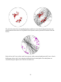
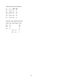
Download Orient Reference Manual 2.1.1

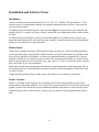
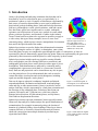
Orientation Data Analysis Software
Orient Reference Manual 2.1.1
© 1989-2012 Frederick W. Vollmer
Contents
ii
Legal Matters
iii
Installation and Software Notes
1
1
Introduction
2
Data and Coordinate Systems
2.1 Data Types
2.2 Coordinate Systems
2.3 Data Entry
3
3
4
Circular Plots
3.1 Scatter Plots
3.2 Circular Histograms
5
5
3
4
Spherical Projections
4.1 Geometry of Spherical Projections
4.2 Orthographic Spherical Projection
4.3 Stereographic Spherical Projections
4.4 Equal-area Spherical Projections
4.5 Projections in Orient
4.6 Data Symbols and Maxima
4.7 Contouring and Eigenvectors
4.8 Terminology of Spherical Projections
5
Graphs
5.1 PGR Graphs
6
Maps
6.1 Domain Analysis
7
Fault and Kinematic Analysis
6
7
8
9
9
10
Appendix A: Data File Format
Appendix B: Supported Image Formats
i
References
ii
Legal Matters
License
Orient software and accompanying documentation are copyright © Frederick W. Vollmer 1996, 2007,
2010, 2012. They come with no warrantees or guarantees whatsoever. The software is freeware and
may be downloaded and used without cost. It may not be redistributed or posted online. It is not free
software in the Free Software Foundation definition, as I, the author, retain all rights to the source code.
Referencing
In return for free use, I request that any significant use of the software in analyzing data or preparing
diagrams should be acknowledged and/or referenced. An acknowledgement could be, “I thank
Frederick W. Vollmer for the use of Orient 2.1.1 software.” A reference can be to one or more of the
following (see references): Vollmer, 1989; Vollmer, 1990; Vollmer, 1993; Vollmer, 1995; Vollmer, 2011;
Vollmer, 2012.
The Orient software may be referenced as:
Vollmer, F.W., 2011. Orient 2.1.1. www.frederickvollmer.com.
and the user manual (this document) as:
Vollmer, F.W., 2012. Orient Reference Manual 2.1.1. www.frederickvollmer.com.
Registration
Please consider registering the software, registration is free. This helps determine usage, and justify the
time spent in it's upkeep. To register, send an email to [email protected] with your user name,
affiliation, and usage. You will not be placed on any mailing list or contacted again. For example, send
me an email with something like:
User:
Affiliation:
Usage:
Frederick Vollmer
SUNY New Paltz, Geology Department
Undergraduate structural geology course and research
No Warrantees
This software and any related documentation is provided as is without warranty of any kind, either
express or implied, including, without limitation, the implied warranties or merchantability, fitness for
a particular purpose, or noninfringement. the entire risk arising out of use or performance of the
software remains with you.
iii
Installation and Software Notes
Installation
Orient is currently test run on Macintosh OS X 10.5, 10.6, 10.7, Windows XP, and Windows 7. This
includes classes of undergraduate students who regularly install and run the software. It has not been
tested on Linux systems.
To install on Apple Macintosh systems, either open the dmg file in your browser, or download it and
double click on it. A window will open, drag the contents into your Application folder or other suitable
location.
To install on Microsoft Windows systems, download the zip file to a suitable location, such as your
downloads folder. Right-click and extract the entire contents. A common mistake to only download the
Orient.exe file without the accompanying files.
Known Issues
When saving a graph as an image, different formats (jpg, png, bmp, etc.) will be available depending
on the operating system. On QuickTime enabled systems, several obscure formats are available which
may not be recognized by all software, it is best to use standard formats (see Appendix B). A known
problem is that the Save As dialog box does not add a file extension automatically, so you must insure
that an image file has the correct extension (.jpg, .png, .bmp, etc.). This is a bug in the current compiler
that is not fixable by me, the programmer.
When entering fault data, the spreadsheet should convert lineation pitches to trend and plunge. This is
not working correctly, so fault lineation data must be entered as trends and plunges. This will be fixed
in a future version.
I appreciate the reporting of bugs or other issues, and will try to correct them as time allows.
Future Versions
Orient 3 is currently in development. It is a complete rewrite of the program using an open source
multi-platform professional compiler, Free Pascal. This compiler produces faster code, has an advanced
graphics system, offers the ability to port to additional platforms, and removes certain licensing issues.
Significant bugs will be fixed in Orient 2, however any new features will be implemented in Orient 3
only.
iv
1. Introduction
Orient is for plotting and analyzing orientation data, data that can be
described by an axis or a direction in space or, equivalently, by a
position on a sphere or circle. Examples of data that are represented by
unit vectors (vectorial or directed data) or axes (axial or undirected
data) include geologic bedding planes, faults and fault slip directions,
fold axes, paleomagnetic vectors, glacial striations, wind and current
flow directions, optical axes in quartz and ice crystals, earthquake
epicenters, arrival directions of cosmic rays, normals to comet orbital
planes, positions of galaxies, and locations of whales in the Atlantic
Ocean. Orient has been written to be as general as possible, to apply to
a wide variety data types. Many examples, however, come from
structural geology, which requires extensive manipulation of orientation
data, and is the specialization of the author.
Figure 1. Lower hemisphere
equal-area projection of ice caxes from Kamb (1959).
Crystallographic axes such as
these are three-dimensional
undirected, or axial, data.
Spherical projections are used to display three-dimensional orientation
data by projecting the surface of a sphere, or hemisphere, onto a plane.
Lines and planes in space are considered to pass through the center of a unit sphere, so lines are
represented by the two diametrically opposed piercing points. Planes are represented by the great circle
generated by their intersection with the sphere or, more compactly, by their normal.
Spherical projections include equal-area (used for creating Schmidt
nets), stereographic (used for creating Wulff nets or stereonets), and
orthographic projections, these can be plotted on either upper or lower
hemispheres. Point distributions are analyzed by contouring and by
computing their eigenvectors (axial data) or vector means (vectorial
data). Data sets and projections can be rotated about any axis in space,
or to the principal axes. For two-dimensional data, such as wind or
current directions, circular plots and circular histograms, including
equal-area and kite diagrams, can be plotted.
Data can be input as spherical coordinates, longitude and latitude,
azimuth and altitude, declination and inclination, trend and plunge,
strike and dip, or other measurements. Orient is can also be used to
analyze fault data, which is represented by a fault plane orientation and
the direction of slip within that plane. From these data Orient can
generate P (Pressure) and T (Tension) axes, which are related to
principal stress directions, M (Movement) planes, and slip linears,
which indicate displacement directions.
Spherical projections represent orientations, but not spacial locations.
Orient uses map analysis to further analyze the spacial distributions of
orientation data. For example in structural geology the location of
domains of cylindrical folding, where bedding or other layers share a
common fold axis, is of interest. Orient's domain analysis features
subdivide a map region into multiple domains by maximizing an
eigenvalue-based index.
1
Figure 2. Circular histogram, or
rose diagram, of two-dimensional
undirected orientation data.
Figure 3. Fault data from Angilier
(1979). Fault slip data is directed,
or vectorial, data.
Figure 4. Subdomain orientation
axes from Vollmer (1990).
Figure 5. Earthquake epicenters
plotted with continent outlines.
2
2. Data and Coordinate Systems
2.1 Data Types
Orientation data are either unit vectors, referred to as vectorial or directed data, or unit axes, referred to
as axial or undirected data. Current flow directions, for example, are directed, while fold axes are
undirected. Plotting, contouring, and statistical analysis of these data types is different. Geometrically,
data represents either lines or planes, which can be directed or undirected. On spherical projections
planes and lines are considered to pass though the center of a unit sphere. Planes are represented by
either their great circle, the intersection of the plane with the unit sphere, or by their normal (often
referred to as the plane's pole).
Unit vectors or axes in three dimensions can be specified by their coordinates on the surface of the unit
sphere, these are the direction cosines. However, it is more common to specify just two independent
angles, a horizontal angle (such as strike, trend, or azimuth) and a vertical angle (such as dip, plunge or
inclination). Two dimensional data require a horizontal angle only. All available angular measures and
their definitions are listed in Appendix A. Orient has separate columns for lines and for planes,
primarily so fault data, which requires both, can be entered easily. Enter all plane data in the plane
columns, and line data in the line columns. Unused columns can be hidden if desired.
2.2 Coordinate Systems
Orient is designed to be used with all types of orientation measurements and coordinate systems, and
converts to and from user coordinate systems for data entry and output. This conversion is normally
transparent to the user, however, for rotations the user should be aware of the standard coordinate
system. Orient's standard coordinate system is a right-handed cartesian system defined by [X, Y, Z] =
[right, top, up]. Standard spherical coordinates are specified as longitude, θ, the counterclockwise angle
from X in the XY plane, and colatitude, ϕ, the angle from Z. Alternatively, coordinates are specified by
direction cosines in this coordinate system. Planes are represented by their upward normal.
Geographic data are generally given using longitude as the horizontal angle, the vertical angle is
commonly latitude or colatitude. Geologic data, however, are typically specified using azimuths for
horizontal angles, which are measured clockwise from Y (North), and typically [X, Y, Z] = [East,
North, Up]. User coordinates are typically strike and dip for planes, or trend and plunge for lines.
However, all common conventions are supported, including dip direction, declination, inclination,
zenith, and altitude (see Appendix A). Orient can convert among these conventions.
There are several conventions for strike and dip. By default Orient uses the common convention that
the dip is to the right looking along the strike (the right hand rule, e.g., Twiss and Moores, 2007). A
second convention, where the dip is to the left (the thumb of the right hand points down the dip), is
referred to as Strike left. This convention can be selected using the Data Format command. A third
convention, where a dip octant (N, NE, E, SE, etc.) is required is automatically converted as described
in the next section.
Angle units can be set as degrees, gradians (grads), or radians. The format applies to all angles and is
set using the Data Format command. The default is degrees.
Additional discussion of spherical coordinate systems is given in section 3.1.
3
2.3 Data Entry
Each data point must include a pair of angles specifying it's orientation in space. The first angle is
measured in a horizontal plane, and the second in a vertical plane. For typical geological data, these
would be strike and dip for planes, or trend and plunge for lines. However, all common conventions are
supported. Two dimensional data require horizontal angles only.
Before entering data, select the correct data format using the Data Format command. You may also
wish to hide or show appropriate columns using the Data View Options command. Note that separate
columns are used for planes and for lines, so make sure the required columns are visible. The Type
column can contain any alphanumeric identifier, and is optional. Specifying a type is required,
however, if multiple data types are entered in a single file. Also, settings, such as symbol sizes and
color, are saved for each type.
Additional fields include station identifiers, X, Y and
Z coordinates, domains, and comments, these are
listed in the Appendix. X and Y coordinates are
required for domain analysis as described later.
Orient does several automatic data conversions. An
older format used for compass readings of horizontal
angles is a bearing. These are given as degrees east
or west of north or south, for example, N30W. When
entering data in degrees in an azimuth format (such
as strike or trend) bearings are automatically
converted to azimuths, for example: N30W converts
to 330.
Figure 6. Data entry window.
A conversion is also done for plane data entered with a dip octant (N, NE, E, SE, S, SW, W, or NW).
Enter the strike first, and then the dip with dip octant. The strike will then be corrected to a strike (or
strike left, if that convention is being used). For example: [strike, dip] = [10, 30W] converts to [190,
30].
When entering fault data several conversions apply. First enter the fault plane orientation. Then, if the
slip trend is entered, the plunge is automatically calculated. If the slip plunge is entered instead, the
trend is automatically calculated. If the plunge is not a possible value (greater than the dip) it will be
highlighted in red. To enter the slip as a rake (pitch), enter the rake value in the plunge field followed
by the letter 'k', and the rake will be converted to a plunge. By convention, the rake is the clockwise
angle about the upward normal of the plane measured from the strike (with right hand thumb as upward
normal, rake is measured opposite from fingers).
Fault slip data is directed and must be entered as such. Normal faults have a positive plunge
(inclination), and reverse faults a negative plunge. To assist in entering slip data use 'n' and 'r' to convert
between the two. For example, [trend, plunge] = [10, 30] gives a normal slip, while [10, 30r] converts
to [190, -30] which is a reverse slip. [190, -30n] converts back to [10, 30]. This convention can be
combined with 'k' when entering a rake.
Data entry can be done using Orient's spreadsheet interface, or by importing a tab delimited file TSV
(Tab Separated Value) or TXT file from Excel, another spreadsheet, or a text editor. The File Import
Data command allows import of many additional text file formats. File format details are given in
Appendix A.
4
3. Circular Plots
Circular plots for two dimensional orientation data include scatter plots, vector mean display, and
circular histograms. Circular plots can also be used to display the horizontal angles of lines and planes,
such as lineation trends. Note that for planes the dip direction is plotted, the plot can be rotated 90° to
display them as strikes if desired. The data may be displayed as directed or undirected. Undirected data
plots two points at 180°. The settings for circular plots are located in the Circular Plot dialog box.
3.1 Circular Scatter Plots
A simple circular scatter plot shows the data distribution on the
perimeter of a unit circle. Lines may be drawn from the circle center if
desired. The vector mean, for directed or undirected data, can also be
displayed.
3.2 Circular Histograms
Two dimensional orientation data is commonly displayed as a circular
frequency histogram, where the data count is tallied for bins or sectors
of a set angular width. A commonly used graph is a rose diagram
Figure 7. Circular scatter plot.
constructed with sector radii proportional to class frequency (Figure 8).
Unfortunately, a rose diagram in this form is not a true histogram, and is
biased because the area displayed for a single count increases with the radius. An unbiased plot is an
equal-area circular histogram where each count has an equal area, and the sector area is proportional to
class frequency (Cheeney, 1983; Figure 9).
Figure 8. Rose diagram with
equidistant spacing. The
increasing area for larger bin
counts results in an area bias.
Figure 9. Equal-area circular
histogram, where each count has
an equal area.
Figure 10. Kite diagram.
A circular polygon histogram, or kite diagram, (Figure 10) is an alternative graph for displaying the
same information. In a kite diagram the bin sector centers are connected by straight lines.
5
4. Spherical Projections
A primary function of Orient is the creation and manipulation of spherical projections of orientation
data, in particular azimuthal spherical projections that project the surface of a sphere onto a plane. This
chapter discusses mathematical concepts related to spherical projections, in particular the geometry of
several common projections, and the spherical nets which are commonly used to display and work with
these projections. A section on nomenclature discuses terminology and common errors that occur in the
literature.
4.1 Geometry of Spherical Projections
A spherical projection is a mathematical transformation that maps points on the surface of a sphere to
points on another surface, commonly a plane. Astronomers, cartographers, geologists, and others have
devised numerous such projections over thousands of years, however two, the stereographic projection
and the equal-area projection, are particularly useful in for displaying the angular relationships among
lines and planes in three-dimensional space. A third projection, the orthographic projection, is less
commonly used, but it is described here as it's properties are easily visualized. These are azimuthal
spherical projections, projections of a sphere onto a plane that preserve the directions (azimuths) of
lines passing through the center of the projection. This is an important characteristic as azimuths, or
horizontal angles from north (strike, trend, etc.), are standard measurements in structural geology,
geophysics, and other scientific disciplines.
The orientations of lines and planes in space are fundamental
measurements in structural geology. Since planes can be uniquely
defined by the orientation of the plane's pole, or normal, it is sufficient
to describe the orientation of a line. If only the orientation of a line, and
not it's position, is being considered, it can be described in reference to
a unit sphere, of radius, R = 1. A right-handed cartesian coordinate
system is defined with zero at the center of the sphere. A standard
convention, used here, is to select X = east, Y = north, and Z = up
(ENU, a common alternative is X = north, Y = east, and Z = down,
NED). A line, L, passing through the center of the sphere, the origin,
will pierce the sphere at two diametrically opposed points (Figure 11).
Figure 11. Definition of the point,
P, on the unit sphere that defines
the orientation of the undirected
line L. The line is trending toward
X (east) and it's plunge is δ. The
Y coordinate axis (north) is into
the page.
If the line represents undirected axial data (as opposed to directed or
vectorial data), such as a fold axis or the pole to a joint plane, it is
allowable to choose either point. In structural geology the convention is
to choose the point on the lower hemisphere, P (the opposite convention
is used in mineralogy). The three coordinates of point P are known as
direction cosines, and uniquely define the orientation of the line. More
commonly, the trend (azimuth or declination) and plunge (inclination) of the line are given. In Figure 1,
the trend of the line is 090°, and it's plunge is δ. It is a helpful reminder to designate horizontal angles
using three digits, where 000° = north, 090° = east, 180° = south, etc., and to specify vertical angles
using two digits, from horizontal, 00°, to vertical, 90°. Note that directed data, such as fault slip
directions, may have negative, upward directed, inclinations.
An important tool for plotting line and plane data by hand, and for geometric problem solving, is a
spherical net. A spherical net is a grid formed by the projection of great and small circles, equivalent to
6
lines of longitude and latitude. Nets are commonly either meridianal or polar, that is, projected onto a
meridian (often the equator) or a pole. The terms equator and pole (or axis) will be used to refer to the
equivalent geometric features on the net, it is essential to remember that they do not have an absolute
reference frame, that is, the net axis is not equivalent to geographic north. When used to plot data by
hand, an overlay with an absolute geographic reference frame (north, east, south, etc.) is used.
The projections described here are spherical projections, so equal-area projection is assumed to mean
equal-area spherical projection. Other projections are possible, such as hyperboloidal projections,
which include equal-area and stereographic hyperboloidal projections (Yamaji, 2008; Vollmer, 2011).
In these projections the surface of a hyperboloid is projected onto a plane. These are used in the context
of strain analysis, and are unlikely to be confused with the more common spherical projections. All nets
and data projections illustrated were prepared using Orient.
4.2 Orthographic Spherical Projection
Orthographic projections are an important family of projections in which points are projected along
parallel rays, as if illuminated by an infinitely distant light source. Figure 12 gives the geometric
definition of the orthographic spherical projection. A corresponding orthographic polar net is shown in
Figure 13, and an orthographic meridianal net is shown in Figure 14. The projection of point P in the
Figure 12. Geometric definition of the
orthographic spherical projection. Point
P on the sphere is projected to point P'
on the plane.
Figure 13. Polar orthographic
net.
Figure 14. Meridianal
orthographic net.
sphere to point P' on the plane is parallel to the cartesian axis Z, effectively giving a projection
following a ray from Z equals positive infinity. This type of projection gives a realistic view of a distant
sphere, such as the moon viewed from Earth. It is azimuthal, but angles and area are not generally
preserved. When plotting geologic data it is important that area, and therefore data densities, are
preserved, so the orthographic projection unsuitable for such purposes. The net does, however, have
other uses, such as the construction of block diagrams (e.g., Ragan, 2009).
7
4.3 Stereographic Spherical Projection
The stereographic or equal-angle spherical projection is widely used in mineralogy and structural
geology. It is defined geometrically by a ray passing from a point on the sphere (here Z = 1) through a
point P on the sphere to the projected point P' on the plane (Figure 12). Note that all points on the
sphere can be projected except the point of projection itself, which plots at infinity. The corresponding
Figure 15. Geometric definition of the
stereographic projection. Point P on the
sphere is projected to point P' on the
plane.
Figure 16. Polar stereographic
net.
Figure 17. Meridianal
stereographic net, also known
as a stereonet or Wulff net.
stereographic nets (Figures 16 and 17), however, plot only one hemisphere. Both hemispheres can be
represented on the net, however the convention in structural geology is to use the lower hemisphere.
The meridinal stereographic net is known as a stereonet, or Wulff net, named after the crystallographer
G.V. Wulff who published the first stereographic net in 1902 (Whitten, 1966). The stereonet is
commonly used in mineralogy, however, the convention is to use the upper hemisphere. It is therefore
good practice to clearly label all projections, for example “lower-hemisphere stereographic projection.”
The projection is azimuthal, so lines passing through the center of the projection have true direction,
these represent great circles. Note that area in Figure 17 is clearly distorted, the projection preserves
angles (is conformal), but it does not preserve area. An important consequence is that great circles
(such as meridians) and small circles project as circular arcs. These
properties make it useful for numerous geometric constructions in
structural geology (Bucher, 1944; Phillips, 1954; Badgley, 1959; Lisle
and Leyshorn, 2004; Ragan, 2009).
The distortion of area, however, makes the stereographic projection
unsuitable for studying rock fabrics, such as multiple orientations of
bedding, joints, and crystallographic fabrics. Plotting such data is a
descriptive statistical procedure intended to identify significant clusters,
girdles, and other patterns. Figure 18 is a lower-hemisphere projection of
two data clusters which are identical except for rotation. They have
identical densities on the sphere, but this is distorted on the stereographic
projection. An equal-area projection should be used instead (Sander,
1948, 1950, 1970; Phillips, 1954; Badgley, 1959; Turner and Weiss,
1963; Whitten, 1966; Fisher et al., 1987; Ragan, 2009).
8
Figure 18. Lower-hemisphere
stereographic projection of two
data clusters showing density
distortion. See text for
discussion.
4.4 Equal-Area Spherical Projection
The Lambert azimuthal equal-area spherical projection is the correct
projection to use for displaying orientation data. It is not conformal, but
an important characteristic is that it preserves area, so densities are not
distorted (Figure 19). As discussed in the previous section, this makes it
useful for the examination of rock fabrics, including the orientations of
bedding, joints, and crystallographic fabrics (Billings, 1942; Sander,
1948, 1950, 1970; Phillips, 1954; Badgley, 1959; Turner and Weiss,
1963; Whitten, 1966; Fisher et al., 1987; Ragan, 2009). It appears widely
in the geologic literature, and is the most likely of these projections to be
encountered in scientific literature related to structural geology. Figures
20, 21 and 22 illustrate the geometric definition, polar net, and
meridianal net respectively.
Figure 19. Lower hemisphere
equal-area projection of two data
clusters showing lack of density
distortion.
The term azimuthal indicates that, like stereographic and orthographic
projections, lines passing through the center have true direction, and that
it is projected onto a plane. This distinguishes it from other equal-area projections, which include the
projection of a sphere onto conical and other surfaces, however, in structural geology, it can usually be
Figure 20. Geometric definition of
the equal-area projection.
Figure 21. Polar equal-area net.
Figure 22. Meridianal equalarea net, or Schmidt net.
referred to simply as an equal-area projection without ambiguity. The projection is also known as the
Schmidt projection, after W. Schmidt who first used it in structural geology in 1925 (Turner and Weiss,
1963), and the meridianal equal-area net, is known as a Schmidt net (Knopf and Ingerson, 1938;
Billings, 1942; Sander, 1948, 1950, 1970).
Stereonets are widely used in mineralogy, and their equal-angle property makes them useful for certain
graphical constructions, such as drill hole problems (Ragan, 2009), however they should not be used to
plot orientation data. The procedures for most geometric constructions commonly used in structural
geology are identical on stereonets and Schmidt nets. Schmidt nets are required for unbiased data
analysis, and can be used to solve most common geometric problems.
4.5 Projections in Orient
Orient plots three types of spherical projections as upper or lower hemisphere. To create a new plot,
open a data file and select New Spherical Projection. The settings for projections are set from the
9
Spherical Projections dialog box. Equal-area projections (below left) are useful for examining the
distribution of data points, since area is preserved. Clusters of points near the edge show a similar
density to clusters near the center. Stereographic projections (below right) distort area, but preserve
angular relationships. The data are bedding plane normals in folded Ordovician graywackes, New York
(from Vollmer, 1981).
Orthographic projections (below left) show data as projected from infinity, similar to a view of the
Moon from Earth. Lower hemisphere projections are normally used in structural geology, while upper
hemisphere projections are common in mineralogy. Orient can plot both upper and lower hemisphere
projections. Below right is an upper hemisphere equal-area projection.
Grid display and tick marks can be turned on or off, and polar grids (about Z) can be displayed. The
grids shown here are meridional grids, drawn about the Y axis. Projections can be rotated about
arbitrary axes if required. Below the projection has been rotated so the minimum eigenvector is parallel
to Z using the Graph Rotate command. The data here are poles to bedding planes, and a second set of
data representing minor fold axes has been added.
The equal-area projection is also known as a Lambert projection, and the associated meridional grid is
10
known as a Schmidt net. The meridional grid associated with a stereographic projection is known as a
Wulff net. All of the following plots, unless noted, are lower hemisphere equal-area projections.
4.6 Data Symbols and Maxima
Data symbols are selected from the Data tab panel of the Spherical Projection dialog box. Each data
type can have a different symbol, including fill and stroke colors. These settings are saved to simplify
the set up of additional plots. In the diagram below left, bedding plane orientations are displayed both
as poles to the beds, and as great circle arcs. Minor fold axes are displayed as red triangles. A plot of
just poles to planes, as shown on the right, is referred to as an S-pole or pi diagram, and is generally the
preferred method of displaying large amounts of data.
To calculate the best fit to a set of axial data the eigenvectors are calculated from an orientation matrix
formed by the summed products of the direction cosines. This gives three orthogonal vectors
corresponding to the maximum, intermediate, and minimum moments. In areas of cylindrical folding
the minumum eigenvector corresponds to the fold axis. Below left the minimum eigenvector and it's
great circle arc is plotted. This is the best-fit great circle for axial data. Select the Data Statistics
command to view the computed values. Here the fold axis trends 183° and plunges 03°. On the right all
three eigenvectors are displayed along with 95% confidence cones.
Vector mean directions, mean resultant lengths, and corresponding confidence cones can be calculated
for directed data. The confidence cone assumes a symmetric unimodal distribution, valid for n >= 25.
Note that these are not normally useful for undirected data.
11
4.6 Contouring and Eigenvectors
A simple scatter plot of data using an equal-area projection may suffice for the display of some data
sets, and Orient can be used to prepare such diagrams for publications. However Orient provides many
additional functions for manipulating and analyzing orientation data in more depth. Two important
statistical procedures are contouring and calculating data eigenvectors.
When analyzing orientation data a useful procedure is to contour the data to examine it for patterns
such as clusters and girdles (Fisher, et al., 1987; Vollmer, 1995). A critical point in this procedure is that
density calculations must be done on the sphere, prior to projection. Figure 23 is contoured plot of
poles to bedding from an outcrop of folded graywackes in Albany County, New York (from Vollmer,
Figure 23. Contoured lowerhemisphere equal-area
projection of 56 poles to
bedding.
Figure 24. Lower hemisphere
equal-area projection of 56 poles
to bedding with maximum and
minimum eigenvectors.
1981) which displays both cluster and girdle patterns. The relative strength of those can be computed,
and plotted, using the computed eigenvectors.
The concept of an average is familiar when dealing with scalar values like temperature. Determining
an “average” or “best” value for orientation data is more complex (averaging trends and plunges
separately does not work). If the data is vectorial, a vector mean can be computed, but axial data
requires the computation of eigenvectors. Eigenvectors are an important concept that allows the
determination of the “best” values for a tensor, such as principal stresses. In the context of orientation
data, imagine that each line plotted in Figure 24 is represented by a small mass at each of the two
points where it pieces the sphere (see Figure 11). If you were to spin the sphere, it would have a natural
tendency to spin about the axis of minimum density, this is the minimum eigenvector (the black point
in Figure 14). If you were to roll the sphere, it would have a natural tendency to stop with the
maximum density at the bottom, this is the maximum eigenvector (the white point in Figure 14). These
two vectors are exactly 90° apart, and 90° from the intermediate eigenvector (not shown).
Note that directed vectorial data, such as fault slip directions, is treated differently than axial data, and
it is important to distinguish between the two data types. A mean value for directed data is calculated as
a normalized vector mean, which may be directed upwards with a negative inclination, and not by
using eigenvectors. Contouring directed data requires calculating densities on both hemispheres.
Contouring of spherical projections is done by estimating a density function at points on the sphere
surface, and contouring that function. The density functions are calculated on the surface of a sphere,
back-projected onto a regular grid, and then contoured. Orient uses several contouring algorithms:
12
modified Kamb or Schmidt (Vollmer, 1993, 1995), and probability density (Diggle and Fisher, 1985).
Orient's contouring and gridding options are displayed in the Spherical Projection dialog box. Below
left is a plot calculated using a modified Kamb method.
The density function can be displayed as a gradient map, with or without overlying contours. A gradient
map is a bitmap where the color value of each pixel is mapped to the range of the density function. Two
or three color gradient maps can be created using user selected colors. Below right is a Red-Green-Blue
map.
Contours for directed data will be different in upper and lower hemispheres. Shown below are
combined gradient maps for upper (left) and lower hemispheres (right). The upper hemisphere plot is
also inverted, so the -X axis in each plot is adjacent. The gradient map here maps the probability
density function of magnetic remanence directions to the visible spectra. The data are 107
measurements of magnetic remanence from specimens of Precambrian volcanics (from Schmidt and
Embleton, 1985 in Fisher, et al., 1987).
13
4.7 Terminology of Spherical Projections
The equal-area projection is more correctly referred to as the Lambert azimuthal equal-area
projection, however in the context of structural geology, it is usually sufficiently clear to refer to it as
the equal-area projection, and, in most cases should be labeled as lower-hemisphere equal-area
projection in figure captions. Note that, although less common, hyperboloidal equal-area and
stereographic projections are useful in structural geology, as opposed to spherical projections.
The terminology of projections can be confusing, but it is important to use correct terms for effective
scientific communication. The terms stereographic projection and stereonet, in particular, are
frequently misused. Early references (Sander, 1948, 1950, translated 1970; Phillips, 1954; Badgley,
1959; Turner and Weiss, 1963; Whitten, 1966; Hobbs et al., 1976) are careful to use correct
terminology, as are most current structural geology texts (e.g., Marshak and Mitra, 1988; Van der
Pluijm and Marshak, 2004; Pollard and Fletcher, 2005; Twiss and Moores, 2007; Ragan, 2009) Note
that:
• The equal-area projection is not the stereographic projection
• The equal-area projection is not a type of stereographic projection
• A stereonet is a meridianal stereographic net, and is also known as a Wulff net
• A Schmidt net is a meridianal equal-area net
• An equal-area net is not a stereonet
• A Schmidt net is not a stereonet
• A projection of data is not a stereonet (or a net at all)
• The phrase equal-area stereographic projection is a contradiction (like square circle)
An additional term that is used in the context of spherical projections is stereogram, which is used to
refer to diagrams produced by stereographic projection, although it may include block diagrams
(Phillips, 1954). The phrase equal-area stereogram has been used to refer to a diagram produced by
equal-area projection (Lisle and Leyshorn, 2004), however as the term stereogram is used for a
diagram produced by stereographic projection, the term equal-area stereogram is a contradiction. The
phrase lower-hemisphere equal-area projection is clear and has a long history, and priority, of usage.
Finally, it is common to see projections (as Figures 8 and 9) labeled stereonets. This is incorrect, as a
projection is not a net (a net is a projection), and most likely it is an equal-area projection. Mislabeling
equal-area projections as stereographic projections is common. Some books discuss the equal-area
projection in a chapter titled Stereographic Projection. This is incorrect as the equal-area projection is
not a stereographic projection. An accurate chapter title would be Spherical Projections.
The equal-area projection and the Schmidt net have a long and rich history in structural geology.
Mislabeling them as stereonets is wrong, and disrespects that history. In the United States, for example,
the first edition of Billings (1942) discusses the use of the Schmidt equal-area net, including contouring
and fabric analysis. It is not until the second edition of Billings (1954) that stereographic projections
are discussed, citing Bucher (1944).
14
5 Graphs
5.1 PGR Graphs
The graph portion of Orient is used to plot data on a triangular Point-Girdle-Random (PGR) eigenvalue
plot. It is particularly useful in map domain analysis, where domains are defined in the Map portion of
the program, or input with the data file.
Given the orientation matrix eigenvectors e1, e2, and e3 for n data points, where e1 >= e2 >= e3, the
following are defined (Vollmer 1989):
Point
P = (e1 - e2)/n
Girdle
G = 2(e2 - e3)/n
Random
R = 3e3/n
Cylindricity
C=P+G
these have the property that:
P+G+R=1
and form the basis of a triangular plot. Cylindrical data sets plot near the top of the graph, along the PG join, point or cluster distributions plot near the upper left (P), girdle distributions plot near the upper
right (G), and random or uniformly distributed data will plot near the bottom of the graph (R). Figure
10 is a plot of bedding plane poles from a cylindrical fold in Ordovician graywackes (Vollmer, 1981),
and Figure 11 is the corresponding PGR graph. These indicate a well defined girdle with a distinct
maximum.
Figure 25. Lower hemisphere
equal-area projection of poles to
bedding from a fold in
Ordovician graywackes (Vollmer,
1981).
Figure 26. PGR graph of data
shown in Figure 10.
For comparison, a plot of ice fabric c-axes (digitized from Figure 7 in Kamb, 1959) is shown in Figure
27, which shows a much more scattered distribution, and plots nearer to the bottom of the PGR graph
(Figure 28).
15
16
Figure 27. Lower hemisphere
equal-area projection of ice caxes (Kamb, 1959).
Figure 28. PGR graph of data
shown in Figure 12.
17
6. Maps
Spherical projections aid in the analysis of the orientation data, such as rock foliations, but they do not
show their spacial distribution. To aid in spacial analysis, given map coordinates, Orient can plot the
spacial distributions of orientation data. This data can be spacially averaged and used for domain
analysis. For example, a common problem in mapping areas of complex geological structure is to
identify domains of cylindrical folding within the map area. Orient provides special capabilities to
search for such domains.
6.1 Domain Analysis
Spherical projections aid in the analysis of the orientations of geological structures such as foliations,
but they do not show their spacial distribution. A common problem in mapping areas of complex
geologic structure is to identify cylindrical domains within the map area.
18
Figure 29. Lower hemisphere equalarea projection of poles to 625
folliation planes from the Grovudalen
area of Norway (Vollmer, 1985).
Figure 30. Contour plot of data shown
in Figure 14.
Orient provides several indexes that may be maximized, including point, girdle, and cylindricity
indexes. To locate areas of cylindrical folding the cylindricity index should be maximized:
C = (E1 + E2 - 2(E3))/N
For a set of domains the sum of the products of the domain indexes (C1, C2, C3, ...) and the number of
data points within each domain (N1, N2, N3, ...):
Z = C1(N1) + C2(N2) + C3(N3) + ...
is maximized. Because:
N = N1 + N2 + N3 + ...
the maximum possible value for Z is equal to N. The normalized sum is:
C' = Z/N
Example
Figure 14 is an S-pole diagram of 625 foliation planes from the Grovudalen area of Norway (from
Vollmer, 1985), and a corresponding contour diagram. Although a maxima is present there is no well
defined girdle pattern to indicate a regional fold axis.
A map of poles to foliation (Figure 31) shows some areas of consistent orientation, but the location of
cylindrical domains is not obvious. This map is generated using the Map menu commands. The arrows
are horizontal projections of constant length vectors, so short arrows have steep plunges.
19
Figure 31. Map of poles to foliations of the
data shown in Figure 14.
Figure 32. Map of subdomain eigenvectors
generated from the data in Figure 16.
A plot of subdomain eigenvectors (Figure 32) brings out a clearer picture of average data trends.
However, visualizing which areas share a common axis is still not straightforward. This map is
generated using the Map > Domain command, and shows the maximum eigenvector orientations which
are equivalent to average poles to foliations.
To locate cylindrical domains, a subdomain search is done to maximize the cylindricity sum Z. This is
an interactive combination of manual and automatic searches. The automatic search proceeds by
identifying subdomains that can be moved into a new domain, while maintaining connectivity, and
increasing Z. A purely automatic search using three domains is shown (Figure 18). This has raised the
normalized cylindricity sum, C', from 0.297 to 0.784. Additional iterative manual editing and automatic
Figure 33. Initial automatic domain search
formed by grouping the subdomains of
Figure 17 into three domains maximizing
cylindricity.
Figure 34. Final domain configuration after
iterative manual editing and automatic
searching to find a stable configuration.
searching locates a stable solution with C' = 0.851 (Figure 19).
Plotting the data and on an equal area projection (below left) shows a clear segregation of the data into
20
three girdle distributions. The three minimum eigenvectors, corresponding to fold axes, show a
Figure 35. Lower hemisphere equalarea projection of data from Figure 29,
with foliation poles color-coded by
domain.
Figure 36. Synoptic plot of best fit
girdles and axes of data shown in
Figure 35.
consistent rotation across the map area, and suggest a refolding axis plunges gently northwest.
Figure 37. PGR graph of the three
domains compared to the total data set
(black).
Figure 38. Data from Figure XX colorcoded by domain.
A Point-Girdle-Random (PGR) plot (below left) shows the relative changes in cylindricity from the
whole area (black) to the three domains (color). Note that the green domain is closest to a point
distribution, and the blue is closest to a girdle. Below right is a map showing the domains applied to the
data set.
Finally, for comparison are contour plots of the three domains, left is the red domain, right is blue, and
bottom is green.
21
Figure 39. Contoured lower
hemisphere equal-area projection
of poles to foliation for domain 1.
Figure 41. Projection as Figure 39
for domain 2.
Figure 40. Projection as Figure 39
for domain 3 (green).
Detailed Procedure
The data must include X and Y coordinates for a domain search. Open a data set (such as the demo-2
data set used above), and a new map. The general procedure to set up a search is:
• Set the map boundary using the Map > Page Setup command.
• Set the number of subdomains with the Map > Domain command.
• Start the search by pressing the Search (S) button.
During a search use the following buttons:
•
•
•
•
•
Clear (C) - Set all subdomains to 0 (no domain).
Initialize (I) - Set all domains to current domain (1 to 9).
Auto Search (A) - Grow the current domain by increasing cylindricity.
Domain (1-9) - Select the current domain from the popup menu.
Best (B) - Restore the best domain configuration found in this session.
Initialize all subdomains to 1, set the current domain to 2, and do an automatic search. An automatic
search attempts to maximize cylindricity, C, while keeping the domains connected. For each subdomain
that can be moved into the current domain, it locates the one that will maximize C. The search proceeds
until no changes will increase C. The automatic search will not necessarily find the "best" solution
because it works stepwise from an initial state, and is constrained by boundary conditions, but it will
find a stable solution.
After an automatic search you can edit the subdomains with the mouse, but only if the domains remain
connected. An iterative process using manual editing and automatic searching is required to locate the
best possible solution.
22
7. Fault and Kinematic Analysis
Some data sets comprise planes that each contain a directed or undirected line. These data often
indicate movement directions, such as fault striae on slickenside surfaces. Other data, such as hinge
lines in fold axial planes or current directions in bedding planes, can also be plotted, however the
following focuses mainly on the kinematic analysis of faults. Note that there are numerous methods for
fault analysis, including diverse stress inversion techniques. Orient applies a kinematic analysis based
on M-plane, or movement plane, geometry as described below.
Fault data includes both fault plane orientations and directed slip line orientations. Because the slip line
lies within the fault plane, only three independent angles are required to specify this type of data.
Typically these angles are the strike and dip of the fault plane, and the pitch (rake) or trend of the slip
line. Note that the lines are directed and indicate the hanging wall movement, so a pitch greater than 0°
and less than 180° indicates a normal component, and a pitch greater than 180° indicates a reverse
component. Chapter 2 explains how to enter this type of data.
Once the data is entered Orient automatically generates several planes and axes from the fault data. Mplanes, or movement planes, are the planes containing the fault plane normal, n, and the slip line, s.
The M-axis, m, is normal to the M-plane. Additionally P-axes ("pressure" axes) and T-axes ("tension"
axes) are generated, these lie in the M-planes at 45° from the fault planes. The T-axis is at a 45° rotation
about m from s, and the P-axis is at a -45° rotation. These all show up as new data types in Orient and
may be plotted or contoured independently.
A tangent-line is defined here as the directed or undirected tangent to a point on a sphere in a specified
direction, where the point is the piercing point of a line passing through the center of the sphere. This
includes a tangent-lineation which is drawn through the piercing point of n, parallel to s. When
specifically used for fault data, this is also referred to as a slip-linear. A tangent-lineation may be drawn
indicating either hanging wall or footwall displacement sense. A hanging wall displacement sense uses
the standard footwall reference frame for faults, however a footwall displacement sense may allow
better visualization of motions on lower hemisphere projections. Below left is a tangent-lineation
diagram showing hanging wall displacement senses, to the right is the same using footwall
displacement senses. The data on these and following plots are 38 Neogene normal faults from central
Crete, Greece (Angelier, 1979).
23
If desired symbols for the fault plane normal may be plotted, as shown below.
A second type of tangent-line is a tangent-normal defined here as a tangent through the piercing point
of s parallel to n. This contains information identical to a tangent-lineation, and is an alternate form of
visualization. The tangent-normal sense may be defined by either hanging wall or footwall movement.
All four of these tangent-lines provide identical information, the choice is a matter of preference or
convention. Below left is a tangent-normal plot with tangent-normals directed towards the hanging
wall. On the right is the same, but with fault planes plotted. Although it is not necessary to plot the
planes, as they are perpendicular to the tangent-normals, it may help in visualizing the data.
24
The plot below shows the corresponding M-planes and M-axes. Note that the tangent-lineations and
tangent-normals shown above are all parallel to the M-planes, and are generated as rotations about the
M-axes.
Below left are the T-axes (yellow) and P-axes (green), with a contoured gradient on the P-axes. A beach
ball diagram, below right, can be plotted to display the best-fit nodal planes. The nodal planes are
calculated using the eigenvectors of the M-axes and P-axes.
25
Tangent-line and beach ball plots are only available for fault data with both plane and line data entered.
When setting the options for these plots note that the M-plane data set must be selected, these options
will be grayed out for the plane, line, P-axis, and T-axis sets. Tangent-lines are drawn as short arcs
starting at the piercing point and their length is specified in degrees. To plot a tangent-line centered on
the piercing point, select both hanging wall and footwall tangent-lines, and turn off one arrowhead by
setting it's length to zero.
26
Appendix A
Data File Format
Orient includes a spreadsheet interface for data entry, and reads and writes tab delimited files. These
files normally have an extension of TSV (Tab Separated Value) or TXT. This is a standard text readable
file format with each line of data separated by a CR (Carriage Return) character (or LF or CRLF), and
individual fields separated by a TAB character (ASCII control code 9). To import spreadsheet data from
Excel, your data must include identifying column headers. The following column headers may be used:
Station, X, Y, Z, Theta Plane, Phi Plane, Theta Line, Phi Line, Type, Domain, Comment
Station is an optional alphanumeric identifier (string) for a station location.
X, Y, and Z are optional numeric locations. X and Y are required for domain analysis. X should be a
numeric value increasing west to east, and Y should be a numeric value increasing from south to north.
Type is an optional alphanumeric identifier defining the type of data. Orient uses the Type value to
assign plot symbols and calculate statistics. Geological types could include, for example, S0, S1, and L
for foliations and lineations. Orient will remember settings assigned to the data type.
Domain is used by Orient to assign a structural domain from 0 to 9. Domain 0 is used to signify the
entire map area. This is optional.
Comment is an optional user entered string.
The angles theta plane and phi plane specify the orientations of planes, and theta line and phi line
specify the orientations of lines. Theta is a horizontal angle, and phi is a vertical angle. Allowable
column headers are shown in Table 1.
27
Theta Plane
Strike
Strike left
Dip direction
Phi Plane
Dip
Theta Line
Azimuth
Declination
Longitude
Trend
Phi Line
Altitude
Colatitude
Inclination
Latitude
Nadir
Plunge
Zenith
Notes
Right hand rule, dip is to right along strike
Dip is to left along strike
Azimuth of dip line
Angle from XY plane down toward -Z
Notes
Clockwise (negative) angle from Y (North)
Equal to azimuth
Counterclockwise (positive) angle from X
Equal to azimuth
Equal to latitude
Angle from Z down toward XY plane
Angle from XY plane down toward -Z
Angle from XY plane up toward Z
Angle from -Z up toward XY plane
Equal to inclination
Equal to colatitude
Table 1. Allowable column headers used to define horizontal angles (theta) and
vertical angles (phi) for planes and lines.
Angles may be in degrees, gradians (grads), or radians, however the angle format must be correctly set
in Orient before opening the file. Only one format for planes and one format for lines should be present
in a single file. Two dimensional data only require a theta value. Include a type value (such as "L", "S",
"S0", "F", etc.) to specify multiple data types in a single file.
In some cases, for data conversion, the phi column may contain letters. These special cases include
entering bearings, dip octants, rakes, and fault slip directions, and are described in Chapter 2.
Any additional columns are ignored by Orient. Orient will also read old format Orient DAT files. When
Orient saves a file it includes one line below the header that starts with "Orient". This is not required,
but may include additional settings in future releases, such as the angle format. Currently Orient does
not use the Z, Station, and Comment columns.
Example Data Files
A simple data file could be:
Strike
179
173
171
168
010
Dip
29
25
25
09
19
28
A data file with map coordinates:
X
34.5
45.7
123.3
58.2
66.7
Y
196.3
184.4
111.7
162.4
201.0
Strike
179
173
171
168
010
Dip
29
25
25
09
19
A data file with multiple data types:
Strike
230
018
141
Dip Trend Plunge Type
24
S0
54
S0
15
S1
138 02
L
140 09
L
29
Appendix B
Supported Image Formats
Bitmap Formats
Orient requires Quicktime or GDI+ for most bitmap export. Windows versions in particular will only
support BMP unless Quicktime is installed. Orient can save to the following bitmap (raster) graphics
file formats:
•
•
•
•
•
•
•
•
•
•
•
•
BMP
JPEG
JPEG 2000 Image
MacPaint
BMP
Photoshop
PICT
PNG
QuickTime Image
SGI Image
TGA
TIFF
When saving images it is important to make sure a correct file extension is included (e.g., .jpg), as it is
not added automatically.
Vector Image Formats
Vector-based image files can be imported into vector drawing programs such as Adobe Illustrator and
AutoCAD. Additionally, most web browsers can display SVG (Scaled Vector Graphics) files. Orient
does most drawing internally in vector format, with the exception of color gradient maps, which are
bitmaps and can not be exported in vector format. Therefore when exporting SVG or PDF files the
bitmap is saved separately, and the bitmap must be imported separately into any drawing program.
Adobe Illustrator allows placing a bitmap image in an open vector drawing, by sending the bitmap to
the back of the drawing, the vector image will overlay the bitmap.
Orient can save to the following vector image formats, with limitations noted below:
• DXF (AutoCAD Drawing Exchange Format)
• PDF (Adobe Portable Document Format)
• SVG (Scaled Vector Graphics)
DXF export does not support bitmaps, text, color, or clipping of symbols. PDF and SVG vector images
may contain some discrepancies, for example with fonts and font alignment. In general the most
compatible vector format is SVG, and this is the recommended vector format.
30
Acknowledgements
Portions of this document were prepared for Teaching Structural Geology, Geophysics, and Tectonics
in the 21st Century, On the Cutting Edge, held July 15-19 at the University of Tennessee, Knoxville. I
thank the conveners Barbara Tewksbury, Gregory Baker, William Dunne, Kip Hodges, Paul Karabinos,
and Michael Wysession. I thank Steven Wojtal, Haakon Fossen, and Josh Davis for discussions on
spherical projections.
31
References
Allmendinger, R.W., Gephart, J.W., and Marrett, R.A., 1989. Notes on Fault Slip Analysis. Prepared for
the Geological Society of America Short Course on “Quantitative Interpretation of Joints and
Faults”, November 4 & 5, 1989. 55 p.
Angelier, J., 1979. Determination of the mean principal directions of stresses for a given fault
population. Tectonophysics, v. 56, p. T17-T26.
Badgley, P.C., 1959. Structural methods for the exploration geologist. Harper and Brothers, New York,
280 pp.
Billings, M.P., 1942. Structural geology. Prentice-Hall, New York, 473 pp.
Billings, M.P., 1954. Structural geology, 2nd edition. Prentice-Hall, New York, 514 pp.
Bingham, C., 1974. An antipodally symmetric distribution on the sphere. Ann. Stats., v. 2, p. 12011225.
Bucher, W.H., 1944. The stereographic projection, a handy tool for the practical geologist. Journal of
Geology, v. 52, n.3, p. 191-212.
Davis, J.C., 1986, Statistics and data analysis in geology. Wiley, 646 pp.
Cheeny, R.F., 1983. Statistical methods in geology. Allen & Unwin, 169 pp.
Diggle, P.J., and Fisher, N.I., 1985, Sphere: a contouring program for spherical data. Computers &
Geoscience, v. 11, p. 725-766.
Fisher, N.I., Lewis, T., and Embleton, B.J., 1987. Statistical analysis of spherical data. Cambridge
University Press, Cambridge, 329 pp.
Hobbs, B.E., Means, W.D., and Williams, P.F., 1976. An outline of structural geology. Wiley, New
York, 571 pp.
Kamb, W.B., 1959, Ice petrofabric observations from Blue Glacier, Washington, in relation to theory
and experiment. Journal Geophysical Research, v. 64, p. 1891-1909.
Knopf, E.B., and Ingerson, E., 1938. Structural petrology. Geological Socity of America Memoir 6, 270
pp.
Lisle, R.J. and Leyshorn, P.R., 2004. Stereographic projection techniques for geologists and civil
engineers, 2nd edition. Cambridge University Press, Cambridge, 112 pp.
Mardia, K.V., 1972. Statistics of Directional Data. Academic Press.
Mardia, K.V., and Zemroch, P.J., 1977. Table of maximum likelihood estimates for the Bingham
distribution. Journal of Statistical Computation and Simulation, v. 6, p. 29-34.
Marshak, S., and Mitra, G., 1988. Basic methods of structural geology. Prentice Hall, 446 p.
Phillips, F.C., 1954. The use of stereographic projection in structural geology. Edward Arnold, London,
86 pp.
Pollard, D.D. and Fletcher, R.C., 2005. Fundamentals of structural geology. Cambridge University
Press, Cambridge, 463 500 pp.
Ragan, 2009. Structural geology: an introduction to geometrical techniques, 4th edition. Cambridge
University Press, Cambridge. 602 pp.
Ramsay, J.G., and Huber, M.I., 1987. The techniques of modern structural geology, volume 2: folds and
fractures. Academic Press, 700 pp.
Sander, B., 1970. An introduction to the study of fabrics of geological bodies, 1st English edition.
Pergamon Press, Oxford. 641 p. [Translated from Sander, 1948, 1950. German edition. SpringerVerlag].
Turner, F.J. and Weiss, L.E., 1963. Structural analysis of metamorphic tectonites. McGraw-Hill Book
Company, New York, 545 pp.
32
Twiss, R.J., 1990. Curved slickenfibers; a new brittle shear sense indicator with application to a sheared
serpentinite. Journal of Structural Geology, v. 11, p. 471-481.
Twiss, R.J. and Moores, 2007. Structural geology, 2nd edition. W.H. Freeman, New York, 736 pp.
Van der Pluijm, B.A. and Marshak, S., 2004. Earth structure, 2nd edition. W.W. Norton, New York, 656
p.
Vollmer, F.W., 1981. Structural studies of the Ordovician flysch and melange in Albany County, New
York: M.S. Thesis, State University of New York at Albany, Advisor W.D. Means, 151 p.
Vollmer, F.W., 1985. A structural study of the Grovudal fold-nappe, western Norway. Ph.D. Thesis,
University of Minnesota, Minneapolis, Advisor P.J. Hudleston, 233 p.
Vollmer, F.W., 1988. A computer model of sheath-nappes formed during crustal shear in the Western
Gneiss Region, central Norwegian Caledonides. Journal of Structural Geology, v. 10, p. 735-743.
Vollmer, F.W., 1989. A triangular fabric plot with applications for structural analysis (abstract). Eos, v.
70, p. 463.
Vollmer, F.W., 1990. An application of eigenvalue methods to structural domain analysis. Geological
Society of America Bulletin, v. 102, p. 786-791.
Vollmer, F.W., 1993. A modified Kamb method for contouring spherical orientation data. Geological
Society of America Abstracts with Programs, v. 25, p. 170.
Vollmer, F.W., 1995. C program for automatic contouring of spherical orientation data using a modified
Kamb method: Computers & Geosciences, v. 21, p. 31-49.
Vollmer, F.W., 2011. Orient 2.1.1: Spherical orientation data plotting program.
www.frederickvollmer.com.
Vollmer, F.W., 2011. Automatic contouring of two-dimensional finite strain data on the unit
hyperboloid and the use of hyperboloidal stereographic, equal-area and other projections for strain
analysis. Geological Society of America Abstracts with Programs, v. 43, n. 5, p. 605.
Vollmer, F.W., 2012. Orient User Manual 2.2. www.frederickvollmer.com. [this document]
Whitten, E.H.T., 1966. Structural geology of folded rocks. Rand McNally, Chicago, 663 pp.
Yamaji, A., 2008. Theories of strain analysis from shape fabrics: A perspective using hyperbolic
geometry. Journal of Structural Geology, v. 30, p. 1451-1465.
Additional Sources
Davis, G.H., Reynolds, S.J., and Kluth, C.F., 2012. Structural geology of rocks and regions, 3rd edition.
John Wiley, 839 pp.
Fosson, H., 2010. Structural geology. Cambridge University Press, Cambridge, 463 pp.
Phillips, F.C., 1971. The use of stereographic projection in structural geology, 3rd edition. Edward
Arnold, London, 83 pp.
Rowland, S.M., Duebendorfer, M., and Schiefelbein, I.M., 2007. Structural Analysis and Synthesis, 3rd
edition. Blackwell, 166 p.
33
34