1
Contents
Chapter 1
The Acquire Menu . . . . . . . . . . . . . . . . . . . . . . . . . . . . . . . . . . . . . . . . . . . . A-1
1.1
1.2
1.3
1.4
1.5
1.6
1.7
Chapter 2
The Windows Menu . . . . . . . . . . . . . . . . . . . . . . . . . . . . . . . . . . . . . . . . . . A-97
2.1
2.2
2.3
2.4
2.5
2.6
2.7
2.8
Chapter 3
Interactive plot editor [xwinplot] . . . . . . . . . . . . . . . . . . . . . . . . . . . . . . . . . . . A-98
Routine Spectrometer operation [iconnmr] . . . . . . . . . . . . . . . . . . . . . . . . . . . A-98
Lock [lockdisp]. . . . . . . . . . . . . . . . . . . . . . . . . . . . . . . . . . . . . . . . . . . . . . . . . A-98
Amplifier control [acbdisp] . . . . . . . . . . . . . . . . . . . . . . . . . . . . . . . . . . . . . . . A-99
Pulse program [pulsdisp] . . . . . . . . . . . . . . . . . . . . . . . . . . . . . . . . . . . . . . . . A-101
BSMS panel [bsmsdisp] . . . . . . . . . . . . . . . . . . . . . . . . . . . . . . . . . . . . . . . . . A-105
Temperature monitor [temon]. . . . . . . . . . . . . . . . . . . . . . . . . . . . . . . . . . . . . A-118
MAS rate monitor [masrmon] . . . . . . . . . . . . . . . . . . . . . . . . . . . . . . . . . . . . A-118
The Shape Tool . . . . . . . . . . . . . . . . . . . . . . . . . . . . . . . . . . . . . . . . . . . . . A-119
3.1
3.2
3.3
3.4
3.5
3.6
3.7
Chapter 4
General . . . . . . . . . . . . . . . . . . . . . . . . . . . . . . . . . . . . . . . . . . . . . . . . . . . . . . . . A-1
Preparing for data acquisition. . . . . . . . . . . . . . . . . . . . . . . . . . . . . . . . . . . . . . . A-2
The configuration suite [config] . . . . . . . . . . . . . . . . . . . . . . . . . . . . . . . . . . . . . A-2
Defining the acquisition data set [new, edc] . . . . . . . . . . . . . . . . . . . . . . . . . . . A-35
Setting up acquisition parameters. . . . . . . . . . . . . . . . . . . . . . . . . . . . . . . . . . . A-36
Interface control commands . . . . . . . . . . . . . . . . . . . . . . . . . . . . . . . . . . . . . . . A-79
Starting and stopping data acquisition . . . . . . . . . . . . . . . . . . . . . . . . . . . . . . . A-90
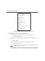
Introduction . . . . . . . . . . . . . . . . . . . . . . . . . . . . . . . . . . . . . . . . . . . . . . . . . .
Generate a new shape . . . . . . . . . . . . . . . . . . . . . . . . . . . . . . . . . . . . . . . . . . .
Manipulate existing Shape . . . . . . . . . . . . . . . . . . . . . . . . . . . . . . . . . . . . . . .
Analyze existing Shape . . . . . . . . . . . . . . . . . . . . . . . . . . . . . . . . . . . . . . . . .
Add 2 existing shapes to form a new shape . . . . . . . . . . . . . . . . . . . . . . . . . .
Merge 2 existing shapes to form a new shape . . . . . . . . . . . . . . . . . . . . . . . .
The Interactive Display Command stdisp. . . . . . . . . . . . . . . . . . . . . . . . . . . .
A-119
A-120
A-125
A-129
A-132
A-132
A-133
Writing Pulse Programs . . . . . . . . . . . . . . . . . . . . . . . . . . . . . . . . . . . . . A-139
4.1
4.2
4.3
4.4
4.5
4.6
4.7
4.8
4.9
4.10
4.11
4.12
4.13
4.14
Introduction . . . . . . . . . . . . . . . . . . . . . . . . . . . . . . . . . . . . . . . . . . . . . . . . . .
Pulse program library . . . . . . . . . . . . . . . . . . . . . . . . . . . . . . . . . . . . . . . . . . .
Pulse program display . . . . . . . . . . . . . . . . . . . . . . . . . . . . . . . . . . . . . . . . . .
Basic syntax rules . . . . . . . . . . . . . . . . . . . . . . . . . . . . . . . . . . . . . . . . . . . . . .
Pulse generation commands . . . . . . . . . . . . . . . . . . . . . . . . . . . . . . . . . . . . . .
Delay generation commands . . . . . . . . . . . . . . . . . . . . . . . . . . . . . . . . . . . . .
Simultaneous pulses and delays . . . . . . . . . . . . . . . . . . . . . . . . . . . . . . . . . . .
Decoupling . . . . . . . . . . . . . . . . . . . . . . . . . . . . . . . . . . . . . . . . . . . . . . . . . . .
Composite pulse decoupling (cpd) . . . . . . . . . . . . . . . . . . . . . . . . . . . . . . . . .
Loop commands . . . . . . . . . . . . . . . . . . . . . . . . . . . . . . . . . . . . . . . . . . . . . . .
Conditional pulse program execution. . . . . . . . . . . . . . . . . . . . . . . . . . . . . . .
Commands to suspend the pulse program execution . . . . . . . . . . . . . . . . . . .
Commands to start data acquisition . . . . . . . . . . . . . . . . . . . . . . . . . . . . . . . .
Working with acquisition memory buffers . . . . . . . . . . . . . . . . . . . . . . . . . . .
A-139
A-140
A-140
A-140
A-144
A-161
A-166
A-169
A-171
A-177
A-179
A-184
A-185
A-192
III
IV
4.15
4.16
4.17
4.18
4.19
Index
Writing memory buffers to disk . . . . . . . . . . . . . . . . . . . . . . . . . . . . . . . . . . .
Multiple receivers . . . . . . . . . . . . . . . . . . . . . . . . . . . . . . . . . . . . . . . . . . . . . .
Real time outputs . . . . . . . . . . . . . . . . . . . . . . . . . . . . . . . . . . . . . . . . . . . . . .
INDEX. . . . . . . . . . . . . . . . . . . . . . . . . . . . . . . . . . . . . . . . . . . . . . . . . . . .
Gradients.
Miscellaneous commands. . . . . . . . . . . . . . . . . . . . . . . . . . . . . . . . . . . . . . . .
INDEX
DONE
A-194
A-196
A-197
A-198
A-201
. . . . . . . . . . . . . . . . . . . . . . . . . . . . . . . . . . . . . . . . . . . . . . . . . . . . . .I-1
XWIN-NMR Comment Form
Chapter 1
The Acquire Menu
1.1 General
XWIN-NMR provides the following data acquisition commands:
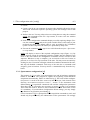
1. zg and go. Used to execute a NMR experiment based on acquisition parameters
set up with the command eda, The commands gs helps with the interactive
adjustment of the acquisition parameters by real-time displaying the fid or spectrum. zg and go may be invoked in AU programs to control several experiments.
2. iconnmr. You should use ICON-NMR for routine spectroscopy based on standard experiments, and for automation using a sample changer. ICON-NMR is
described in its own manual. The following two commands serve the same purpose, but are historically older. They are just maintained for compatibility reasons:
a) run. Used to execute a series of NMR experiments defined with the command set. A typical application of run is automated spectrometer operation
with a sample changer.
b) quicknmr. Execution of experiments based on standard parameter sets provided by Bruker or defined by the spectrometer administrator for routine
A-1
The Acquire Menu
A-2
applications. Requires only solvent and experiment to be specified before
execution can start.
INDEX
1.2 Preparing for data acquisition
DONE
INDEX
Before you can start with data acquisition, the following preparations are necessary:
1. Execute the configuration suite (command config). This is a sequence of commands which allows you to define your spectrometer environment. It is
required once after program installation, or if the environment changes.
2. Set up sample/experiment specific acquisition parameters (commands eda,
wobb, gs, rga, set, ased). Required for every experiment. Set up depends on
acquisition command to be used (zg/go, run, quicknmr).
Display the lock and fid windows. Required to observe fid signal and lock.
3. Start acquisition.
- zg: Starts an experiment based on free parameter set up with eda
-iconnmr: routine execution of standard experiments
Older commands:
- quicknmr: Executes experiments based on standard parameter sets
- run: Executes a series of experiments defined with the command set,
based on standard parameter sets (may use a sample changer).
1.3 The configuration suite [config]
Please execute the following sequence of commands to prepare XWIN-NMR for
data acquisition. Some of the commands will request the NMR superuser password. XWIN-NMR uses the concept of an NMR superuser. This is a normal system
user, who was defined to be the NMR superuser by the system administrator.
If an NMR superuser is defined, commands such as cf will prompt for the password of the NMR superuser, otherwise for the root password.
An NMR superuser may be set up or changed using the NMR user manager of
ICON-NMR. Please check the ICON-NMR manual. In addition, the NMR superuser
may also be entered at installation time of XWIN-NMR.
The command cfpp requires the root password since it modifies the system file /
1.3 The configuration suite [config]
A-3
etc/inittab.
1. Create a user id on your computer for anyone who should be allowed to start up
XWIN-NMR. INDEX
Invoke the respective operating system user manager tool for this
purpose.
INDEX
DONE
2. Define a data set. You may either select an existing data set using the command
search, the commands of the File->Open menu, or create a new one with the
File->New command.
3. Some of the configuration commands display a text file requiring changes. Execute the command setres and set the system variable Editor to the name of your
preferred text editor. The default editor is xedit, provided by the X Windows
system. On SGI computers, the editor jot is preferred by many users.
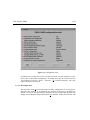
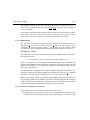
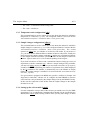
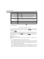
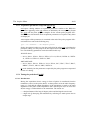
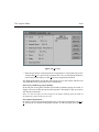
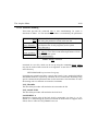
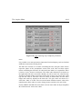
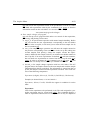
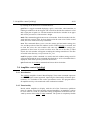
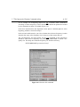
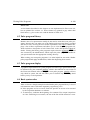
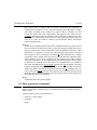
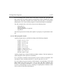
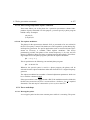
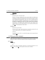
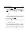
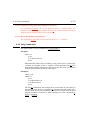
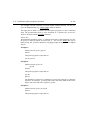
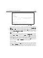
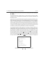
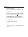
4. Execute the command config (type it in or call it from the Acquire->Spectrometer setup menu).
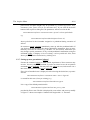
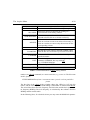
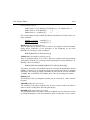
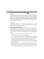
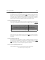
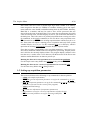
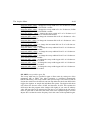
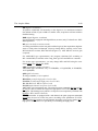
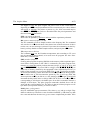
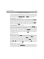
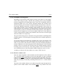
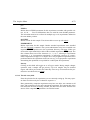
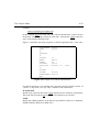
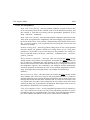
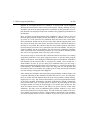
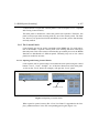
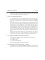
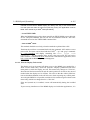
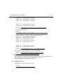
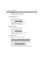
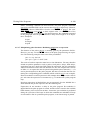
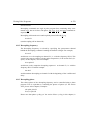
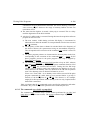
config will display a menu of the required configuration steps (Figure 1.1). By
default, all steps except for configuring a MAS or a BPSU unit are enabled. If you
click on the Start button, the configuration commands will be executed in this
sequence. Whenever a step is complete, you are invited to click on Continue to
proceed, or on Cancel to stop execution of the suite. You may restart execution by
clicking on Start. Execution will begin with the first enabled command of the suite,
and skip all disabled commands. Each step of the suite has a command name
assigned, given in brackets. You may invoke a command directly from the keyboard.
1.3.1 Spectrometer configuration [cf]
The purpose of cf is to make your spectrometer type and its hardware equipment
known to XWIN-NMR. The program is capable of recognizing certain hardware
components automatically, others are asked for by cf. The result of this configuration process is saved in the files uxnmr.conf and uxnmr.par, both located in the
directory XWINNMRHOME/conf/instr/<name>/. <name> is the instrument name
defined during cf. Acquisition commands will read the configuration parameters
from these files. It is therefore not necessary to invoke cf again if you terminate
XWIN-NMR and restart it. However, after installation of a new XWIN-NMR version
cf is mandatory. If your hardware configuration did not change, you may simply
type Return to any question posed during cf.
Correct execution of cf is a prerequisite for the acquisition commands to work, and
should only be performed by the administrator of the spectrometer. We strongly
The Acquire Menu
A-4
INDEX
DONE
INDEX
Figure 1.1 Configuration suite
recommend to save the files uxnmr.conf and uxnmr.par on tape, diskette, or elsewhere after a successful configuration. If needed, they may be restored into the
XWINNMRHOME/conf/instr/<name>/ directory. cf executed thereafter will only
require Returns to be entered.
1.3.1.1 Reconfiguration
If at any ealier time cf was executed successfully, configuration is an easy procedure since the answers to all questions are stored in a file and are prompted as
default. As long as the spectrometer hardware has not changed the operator may
simply answer Return to all questions until cf is finished. At the end a window will
1.3 The configuration suite [config]
A-5
appear giving an overview of the spectrometer configuration. You should now
check whether the configuration is correct and repeat cf if required.
INDEX
1.3.1.2 Configuration from scratch
INDEX
DONE
If there was no configuration directory on disk (e.g. on a replaced disk drive) cf
will start a configuration from scratch.
Please note: If the spectrometer requires a hardware_list file (to be described later
in this section) it is necessary to create the configuration directory manually and
put the hardware_list file there. Open a unix shell, retrieve the hardware_list from
the backup device and proceed as follows:
su
cd XWINNMRHOME/conf/instr
mkdir <instrument name>
cp <any-dir>/hardware_list <instrument name>
exit
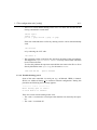
Now start XWIN-NMR and configure the spectrometer. Enter the name of the instrument (usually spect):
Enter new instrument name: spect
If you chose a name different from spect be sure to have this name set as alias in
the file /etc/hosts (see Troubleshooting page 10). Otherwise later cf is not able to
contact the spectrometer when it wants to check the spectrometer hardware.
cf offers a selection of spectrometer types:
What type of spectrometer?
(Datast AMX ARX ASX DMX DRX DPX DSX APEX-A APEX-D AMX3) DMX
cf needs the 1H frequency of the magnet:
Basic 1H frequency (with offset o1=0) in MHz: 500.13
Please wait for some seconds for cf to check the spectrometer hardware. On
Avance spectrometers it will examine the FCU‘s, the RCU and all its connected
digitizers, while on AMX/ARX systems it will detect the Aspect 3001 configuration and the digitizers.
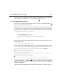
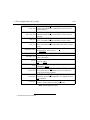
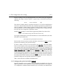
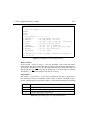
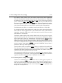
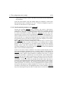
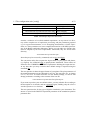
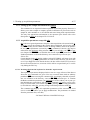
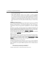
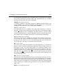
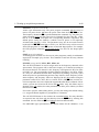
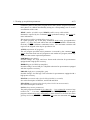
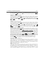
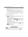
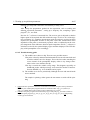
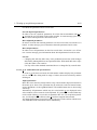
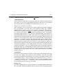
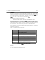
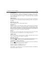
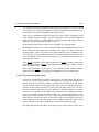
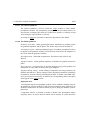
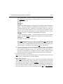
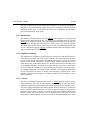
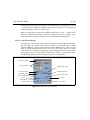
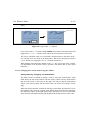
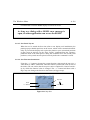
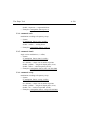
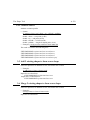
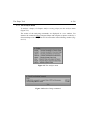
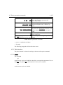
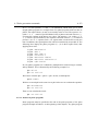
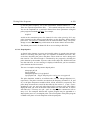
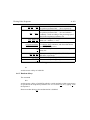
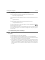
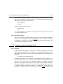
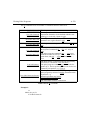
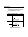
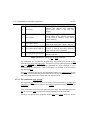
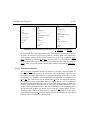
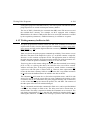
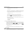
Afterwards all units controlled via serial port are configured. On Avance systems a
The Acquire Menu
A-6
window (see Figure 1.2) appears which contains all installed units and allows to
INDEX
DONE
INDEX
Figure 1.2 Configuration of RS 232 devices
set the device name of each unit. If an unit is not in use or has not been used
before, the device name shows no.
On non Avance spectrometers each unit is prompted for. Enter the name of the
device they are connected to. Usually a default device name is offered, e.g.
Which device is used for <unit>: tty03
You will be asked whether the spectrometer is equipped with a triple housing
1.3 The configuration suite [config]
A-7
preamplifier. If it is equipped with a HPPR instead, you must enter n, then you are
asked for the device used by the HPPR.
INDEX
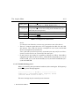
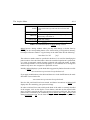
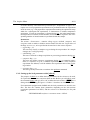
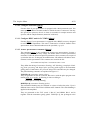
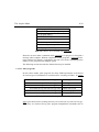
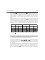
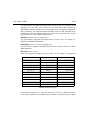
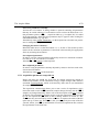
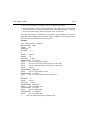
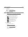
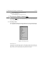
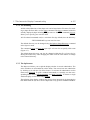
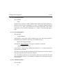
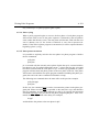
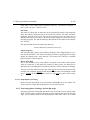
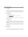
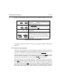
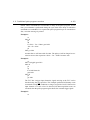
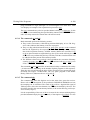
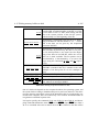
As soon as all configurator questions have been answered, the nucleus table stored
is displayed in a dialog winin the file XWINNMRHOME
INDEX /exp/stan/nmr/lists/nuclei.all
DONE
dow (see Table 1.1) . This table may now be modified according to your needs.
nuclei table
SAVE
1H
500.13
2H
76.77
3H
533.46
4He
380.55
ADD
RESTORE
QUIT
Table 1.1 Nuclei table
XWIN-NMR offers the following possibilities of editing the nucleus table:
Changing the frequency
Move the cursor onto a frequency value and depress the left mouse button. A new
number may be entered now.
Deleting a nucleus
Move the cursor onto the name of a nucleus and depress the left mouse button.
ADD (insert nucleus)
Move the cursor onto this command field and depress the left mouse button. The
file nuclei.all appears on the screen, and a nucleus can be selected. It is inserted
according
to
its
mass
number.
RESTORE
Activate this command field if something failed during the edit session. The
nucleus table is restored entirely from the file nuclei.all.
SAVE
All changes are saved, and the nuclei table disappears.
QUIT
All changes are discarded, and the nuclei table disappears.
The Acquire Menu
A-8
The result ist stored in the file XWINNMRHOME/conf/instr/<instrument name>/
nuclei, and is required by the commands edasp/edsp, where the table is displayed
to select a nucleus .
INDEX
At the end a window appears presenting
of the spectrometer configuDONEan overview
INDEX
ration. This overview is stored in the text file XWINNMRHOME/conf/instr/<instrument name>/uxnmr.info, and may be viewed or printed like any text file.
1.3.1.3 Related Files
The text file XWINNMRHOME/conf/instr/curinst contains the instrument name as
entered in cf. All files used and created by cf reside in the directory XWINNMRHOME/conf/instr/<instrument name>. A description may be found in Table
1.2. There are several subdirectories whose descriptions are shown in Table 1.3.
The hardware_list file
All AMX, ARX and ASX spectrometers and all non standard Avance spectrometers need the text file
XWINNMRHOME/conf/instr/<Instrument
Name>/hardware_list,
which is set up by the service engineer at installation time of the instrument, and
contains information about the hardware equipment of the spectrometer. The file
must not be modified. A safe copy should always be available on magnetic tape
and in form of a printout.
If a spectrometer is equipped with a 4-phase modulator, but not with a HPCU it is
possible to define this hardware equipment in the hardware list file. cf is required
afterwards. The unit may be connected to tty10 or tty20 on the CCU.
DMX spectrometers which are equipped with HRD16 and FADC digitizers can
use the analog filters on the HRD16 external box during measurements with the
FADC. For this kind of application, the RXC must not be defined in the hardware
list file, and the acquisition parameter SEOUT must be set to BB.
1.3.1.4 Layout of serial device connectors
All serial devices on the spectrometer are located at the CCU1:
• The RS-232 device tty00 is located on the CCU frontpanel and may be used by
a console terminal. During the boot procedure all messages are printed to this
1.3 The configuration suite [config]
A-9
text file created by cf containing information about the
acqu.conf Aspect 3001 hardware configuration (not for Avance
INDEX spectrometers).
created by cf containing an explanation of the
INDEX text fileDONE
acqu.conf_info
numbers found in acqu.conf (not for Avance spectrometers).
bbis_fcu
text file created by cf containing information about the
FCU‘s installed in the spectrometer (Avance only).
bbis_rcu
text file created by cf containing information about the
RCU and other boards connected to the RCU (Avance
only).
bsmsdisp.calibr
text file created as empty file by cf and filled in or used
by bsmsdisp (Avance only).
bsmsdisp.calibr.bak
hardware_list
nuclei
scon
backup file for bsmsdisp.calibr (Avance only).
text file in a special format containing a list of hardware components
text file containing the table of nuclei selected either in
cf or by ednuc.
parameter file containing spectrometer parameters; is
created by edscon.
uxnmr.conf
data file created by cf, and used by several commands;
its content may be examined by the XWINNMRHOME/
prog/bin/printconf program.
uxnmr.info
text file created by cf containing useful information
about the spectrometer hardware. It is displayed when
cf is finished.
uxnmr.par
standard parameter file created by cf containing the
answers of the operator to the cf questions
Table 1.2 Configuration files
1. Communication Control Unit
The Acquire Menu
A-10
rs232_device
Is created by cf and contains text files for the device configuration of several units (e.g. HPPR, BSMS, RX22 ...).
rs232_lock
Is created by cf and contains empty files used to lock devices
(to prevent thatDONE
a device from INDEX
being used simultaneously by
more than one unix process).
INDEX
cortab
Is created by the automatic spectrometer adjustment.
prosol
Is created by prosol.
users
Is created by eduser.
Table 1.3 Configuration subdirectories
device.
It is therefore not allowed to connect any spectrometer unit to this device!
• There is a connector panel above the CCU equipped with 9 RS-232 and 2 RS485 devices. The 9 RS-232 devices correspond to tty01-tty09, the RS-485
devices correspond to tty10 and tty20.
Note: tty08 and tty10 (and respectively tty09 and tty20) may only be used alternatively as these devices are connected to the same port!
• If more devices are needed it is possible to add up to 4 SIB‘s1. Each SIB is
equipped with 6 RS-232 devices (CH1 - CH6) which correspond to tty11-tty16
on the 1st SIB, tty21-tty26 on the 2nd SIB, tty31-tty36 on the 3rd SIB and tty41tty46 on the 4th SIB.
1.3.1.5 Trouble shooting: part 1
While cf is checking the spectrometer hardware (after entering the 1H frequency)
the following error message appears:
------------------ < iiconf > -----------------connection to <Instrument Name> (aqport0) failed
(‘startd‘ demon active on CCU ?)
This error message may be caused by several reasons:
1. Serial Interface Board
1.3 The configuration suite [config]
A-11
• There is no startd demon running on the CCU. To check this execute the following commands in a unix shell:
INDEX
telnet spect
INDEX
DONE
login: root
ps -ef | grep startd | grep -v grep
If the last commands does not list any running startd it can be started manually
with:
/etc/startd
or by rebooting the CCU with:
/etc/init 6
• The operating system on the host does not know the name of the spectrometer.
This happens if <Spectrometer Name> is a newly chosen name which has
never been used before.
To solve this problem the superuser must add the new name to the file /etc/hosts
directly behind the name spect, e.g. for the name drx300:
149.236.99.99
spect drx300
1.3.1.6 Trouble shooting: part 2
Some of the units controlled via serial port (e.g. ACB-board, HPPR, 3-channelSE451) are addressed during cf to read their internal configuration. During this
procedure the following error message appears:
--------- < cf > ----------Error during open of <unit>:
no such device or address
There are several reasons leading to this error:
• The <unit> is connected to a serial port other than the one entered by the operator.
• The <unit> is switched off.
The Acquire Menu
A-12
• The <unit> is connected with the wrong cable.
• The <unit> is defective.
INDEX
1.3.2 Temperature unit configuration
[cfte]
DONE
INDEX
This command must be used to inform XWIN-NMR about the channel to which the
temperature is connected, e.g. tty03. The configured channel is stored in the file
XWINNMRHOME/conf/instr/<instrument name>/rs232_device/temp.
1.3.3 Sample changer configuration [cfbacs]
This command must be used to inform XWIN-NMR about the channel to which the
sample changer is connected, e.g. tty12. The configured channel is stored in the file
XWINNMRHOME/conf/instr/<instrument name>/rs232_device/bacs. The second
question of cfbacs asks you whether to use the bar code reader. If your answer is
yes, you are invited to define the RS232 channel of the bar code printer. Finally, the
delay between the change sample command sx and the next command (frequently
ro, turn sample rotation on) must be specified to allow for the sample to settle in its
position. Typical values are 5 to 30 seconds, depending on the magnet.
If you want to make use of XWIN-NMR’s automation features (setting up a series of
experiments with the commands set ) without a sample changer being available,
you must call cfbacs anyway. In this case you are asked to enter the set up capacity,
a number from 1 to 120 defining the number of experiment entry fields displayed
by the set command. This number is automatically set to the number of sample
holders if a sample changer is installed. It is stored in the file XWINNMRHOME/conf/
instr/bacs_capacity.
For spectrometers equipped with BSMS the question “Airflow for Sample Lift
from BACS connected?“ allowes one to configure the BACS/BSMS so that the
LIFT function is not performed by the sample changer, but by the BSMS Lift only.
In this case the connection of the airflow from the sample changer to the Sample
lift must be cut off.
1.3.4 Setting up the solvent table [edsolv]
Use this command to set up a table of the solvents you intend to use for your NMR
experiments. It is a configuration command which should only be executed by the
administrator. edsolv opens a dialog window where you may add, change, or delete
1.3 The configuration suite [config]
A-13
lines by clicking on the corresponding button. New entries must get assigned an
arbitrary, but unique reference number. A typical entry in the table looks like the
following:
INDEX
Acetic
INDEX
- Acetic-Acid-D4
DONE
[02]
The reference number must be specified in brackets. It is used for identifying the
solvent on a barcode label when a barcode controlled experiment is performed, e.g.
using an automatic sample changer equipped with a barcode reader. In order for
such experiments to be executed properly, we recommend not to change the numbers any more once assigned to a particular solvent.
Initially, edsolv displays a solvent table suggested by Bruker from the text file
XWINNMRHOME/exp/stan/nmr/lists/solvents.all
.
If you apply modifications to the table and then exit via the SAVE button, the modified table is stored in the file
XWINNMRHOME/exp/stan/nmr/lists/solvents.
Now the file solvents has been created, and future invocations of edsolv will display this file containing your personal settings.
In order to define a solvent for an experiment, type eda (eda is described further
below in this chapter), and in the up-coming dialog window click on the downarrow button right of the SOLVENT parameter. The solvents file is displayed, and
you may select a solvent from the table. SOLVENT is evaluated by the commands
prosol, lock -acqu, sref and lopo, and during quicknmr and run. For the latter two
applications the acquisition parameters are obtained in the following way: They
are initialized with the parameters of the specified experiment. The probe head and
solvent dependent parameters (see command prosol) are then inserted according to
the setting of SOLVENT and the current probe head (see next section). Finally, any
parameter changes the user possibly requested are applied.
Table 1.4 describes the available command buttons.
1.3.5 Setting up the probe head table [edhead]
Use this command to set up a table of the probe heads you intend to use for your
NMR experiments, and to define the current probehead installed in the magnet. It
is a configuration command which should only be executed by the administrator.
The Acquire Menu
A-14
SAVE
Store modifications in the file
XWINNMRHOME/exp/stan/nmr/lists/solvents and
INDEX
quit.
ADD/CHANGE
Opens DONE
a new entry field
at the end of the table.
INDEX
DELETE
After enabling this button, clicking on a probehead entry will delete it.
CTRL/K key
ABORT
undo last change.
close edsolv window without storing changes.
Table 1.4 Command buttons in edsolv dialog window
edhead opens a dialog window where you may add, change, or delete lines by
clicking on the corresponding button. New entries must get assigned an arbitrary,
but unique reference number. A typical entry in the table looks like the following:
5 mm Dual 13C/1H
[03]
The reference number must be specified in brackets. It is used for identifying the
probe head on a barcode label when a barcode controlled experiment is performed,
e.g. using an automatic sample changer equipped with a barcode reader. In order
for such experiments to be executed properly, we recommend not to change the
numbers any more once assigned to a particular solvent.
Initially, edhead displays a probe head table suggested by Bruker from the text file
XWINNMRHOME/exp/stan/nmr/lists/probeheads.all
.
If you apply modifications to the table and then exit via the SAVE button, the modified table is stored in the file
XWINNMRHOME/exp/stan/nmr/lists/probeheads.
Now the file probeheads has been created, and future invocations of edhead will
display this file containing your personal settings.
In order to inform XWIN-NMR which probe head of the table is currently installed
in the magnet, click on the Define current button, and then on the desired table
entry. It will be stored in the file XWINNMRHOME/conf/instr/probehead. The current
probe head is evaluated by the commands prosol, edlock, lock -acqu, and lopo, and
during quicknmr and run. For the latter two applications the acquisition parameters
1.3 The configuration suite [config]
A-15
are obtained as described in the previous section (edsolv).
The XWIN-NMR acquisition commands (zg, go) store the current probe head in the
INDEX
acquisition parameter PROBHD of the acquired data set for future reference.
INDEX
Table 1.5 describes
the availableDONE
command buttons.
SAVE
Store modifications in the file
XWINNMRHOME/exp/stan/nmr/lists/probeheads
and quit.
ADD/CHANGE
Opens a new entry field at the end of the table.
DELETE
After enabling this button, clicking on a probehead entry will delete it.
CTRL/K key
ABORT
undo last change.
close edhead window without storing changes.
Table 1.5 Command buttons in edhead dialog window
1.3.6 Solvent/probehead dependent parameters [prosol, solvloop]
These parameters are required to run series of experiments using the commands
run or quicknmr, or by the PROSOL function of the command eda. If the values
are not known at this time, you may skip the command for now, and invoke it at a
later time.
The commands run and quicknmr are designed to run experiments based on standard parameter sets (provided by Bruker, or set up by your system administrator). If
one of these commands is active, the acquisition parameters for an experiment are
obtained in the following sequence:
1. They are initialized with the standard parameters of the selected experiment.
2. Parameters depending on the probe head and solvent are inserted according to
the setting of SOLVENT and the current probe head.
3. Finally, any parameter changes the user requested are applied.
The purpose of prosol and solvloop is to set up the parameters of step 2. prosol lets
you select a solvent and a probehead by displaying the tables you have defined earlier with edsolv and edhead. Then, for a selected solvent/nucleus combination,
The Acquire Menu
A-16
power levels and pulse lengths may be specified (e.g. Proton high power level,
transmitter pulse, power level for pre-saturation etc.). If you click on the SAVE
button of the respective dialog box, the parameters
will be saved in the file
INDEX
XWINNMRHOME/conf/instr/<instrument
DONE
name>/prosol/<solvent.probehead>
INDEX
e.g.
XWINNMRHOME/conf/instr/dmx300/prosol/acetic.01,
where probehead is the id number assigned to a probehead during execution of
edhead.
In contrast to prosol, solvloop immediately starts up with the probehead table. If
you click on the SAVE button after having defined the parameters, they are automatically stored for all solvents (e.g. the files *.01 are created). Afterwards you
may change special parameters of any solvent/probehead combination using the
command update. It displays a list of existing <solvent.probehead> files, from
where you can open the desired one by clicking on it.
1.3.7 Setting up user permissions [eduser]
Execute the command eduser to define which experiments a XWIN-NMR user may
execute. You may skip this command if you do not intend to use the acquisition
commands run or quicknmr. You may also skip eduser for now, and execute it at a
later time (but before invoking run or quicknmr).
First, a list of installed users is displayed. After selecting the desired one, a permission file
XWINNMRHOME/conf/instr/<instrument
name>/users/<login id>
is created for this user (if not yet existing), e.g.
XWINNMRHOME/conf/instr/dmx300/users/guest.
It is a copy of the default permission file
XWINNMRHOME/exp/stan/nmr/lists/sam_users_exam
provided by XWIN-NMR. The file is displayed by a text editor, and you may modify
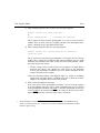
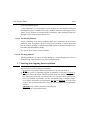
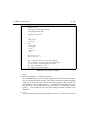
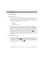
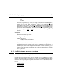
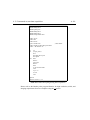
it. Figure 1.3 shows an example. Comment lines begin with a ’#’ character.
1.3 The configuration suite [config]
A-17
#Example user permission file
#
---Data set
names----------------INDEX
$DATE
INDEX
DONE
Name1
Name2
---Experiments:--------------0 PROTON128
- 1H experiment 128 scans
0 PROTON
- 1H experiment 16 scans
0 C13CPD
- C13 exp. comp. pulse dec. 1024 scans
0 N15IG
- 15N exp. inverse gated
1 INV4SW
- sw opt. inv. 4 pulse MC
1 INV4NDLRSW
- sw opt. inv. 4 pulse MC long range
2 HCCOSW
- sw opt. CH-correlation
2 HCCOLOCSW
- sw opt. COLOC
---Permissions (urgent editPAR composite exit(qnmr))--no yes no no
Figure 1.3 Example of a user permission file
Data set names
In the section ---Data set names--- you may predefine a list of data set names.
These will be the only names which may be given a data set during experiment set
up with the command set. The special name $DATE will be converted to the current date during set. Please note that the header text of a section may be arbitrary.
The leading ’---’ characters indicate the start of a section.
Experiments
The section ---Experiments--- is the list of experiments this user is permitted to
run. Each entry consists of a number, a name, and a comment. The number specifies the experiment type according to Table 1.6. The name must denote a parameter
0
normal experiment
1
experiment depending on 1 preparation experiment
2
experiment depending on 2 preparation experiments
T
variable temperature experiment
Table 1.6 Experiment types in a user permission file
The Acquire Menu
A-18
set in the directory XWINNMRHOME/exp/stan/nmr/par/. Experiments of type 1 or 2
require one or two preparation experiments to be performed before the experiment
itself can start (e.g. a 1D preparation experiment INDEX
determining the optimized sweep
width for a subsequent 2D experiment). T characterizes a variable temperature
DONE
INDEX
set, the initial temperature,
experiment. If such an experiment
is selected during
the temperature increment, and the number of increments are requested. The corresponding number of measurements are performed with this sample.
Permissions
The section ---Permissions--- contains 4 flags urgent, editPAR, composite, and
exit(qnmr) used to enable or disable certain features for this user. Legal values of
the flags are no or yes, to be specified in the next line in the correct sequence.
• urgent flag = yes
This user may classify a sample as urgent during the set procedure. In a sample
changer run, it will get priority.
• editPAR flag = yes
This user is allowed to change acquisition or processing parameters during set.
• composite flag = yes
This user may define composite experiments during set. A composite experiment is a sequence of up to 9 standard experiments. After a new composite
experiment was defined, it will be added to the experiment table of the set dialog window.
• exit(qnmr) flag = yes
This user gets the permission to terminate the quicknmr command.
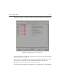
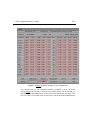
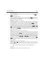
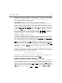
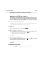
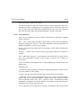
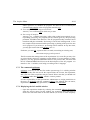
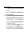
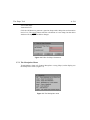
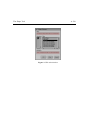
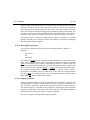
1.3.8 Setting up the lock parameter table [edlock]
The purpose of edlock is to define the lock parameters for the solvents to be used,
for a particular lock nucleus, and store them on disk. Before you call edlock, enter
the command locnuc and type 2H or 19F to define the lock nucleus. edlock opens a
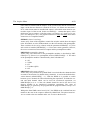
dialog window according to Figure 1.4. Table 1.7 describes its command buttons.
For instruments equipped with a BSMS unit, the lock parameters are stored in two
files. The first one contains those parameters depending on the lock nucleus
(acquisition parameter LOCNUC) and the solvent. For deuterium, its file path
name is
XWINNMRHOME/conf/instr/<instrument name>/2Hlock.
1.3 The configuration suite [config]
A-19
INDEX
INDEX
DONE
Figure 1.4 edlock parameter dialog box (for a BSMS unit)
For a fluorine lock (i.e. the acquisition parameter LOCNUC is set to 19F before
calling edlock), the file name is 19Flock in the same directory. The second file contains parameters depending on the solvent and on the probehead. The name of the
directory where it is located, is the solvent name, with the probe head identification
The Acquire Menu
A-20
SAVE
BSMS-FIELD
NUCLEUS
Store current setting in their files and quit.
Read current value from BSMS and update top line.
INDEX
Select new nucleus. Equivalent to clicking on a
INDEX
nucleusDONE
button in the dialog
window.
NEW SOLVENT
Insert new entry at table end. Initialize it with the last
selected solvent (click on a solvent to select it).
DELETE
Click on this button to activate delete mode. Then
click on a solvent to remove an entire solvent entry, or
click on a nucleus to remove only this nucleus for the
corresponding solvent.
ABORT
LOADSTAN
+/- POWER
LIST
COPY_VALUE
HELP
Discard any changes and quit.
Discard the current settings and load standard values
from the file XWINNMRHOME/exp/stan/nmr/list/2Hlock.
Increment the LPower values of all solvents by the
specified amount.
Print the lock parameters on the device given by the
parameter CURPRIN. Set it up with edo
(e.g. CURPRIN=$hplj4p).
automatically set the selected value for all solvents
Print help messages.
Table 1.7 Command buttons in edlock dialog window
number (see edhead command) as a name extension, e.g. Acetic.03. The file name
itself is param:
XWINNMRHOME/conf/instr/<instrument name>/prosol/<solvent.probeID>/
param.
The first line of the edlock dialog window shows the 2Hlock or 19F lock file
names, and the current probe head including is ID number as defined with edhead.
The second line shows the lock frequency, the field value and the basic spectrometer frequency BFREQ. The lock frequency is calculated by the software from the
BFREQ and the nucleus table.
In the following lines, for a desired solvent you may enter the BSMS lock parame-
1.3 The configuration suite [config]
A-21
ters LPower, LGain, LTime, LFilt, and LPhase valid for the current probehead.
These are the parameters stored in the param file. The parameters are loaded into
the hardware byINDEX
the commands lock, lopo. and lopoi. XWIN-NMR also provides the
special commands ltime, lgain, lfilter from which you may load the hardware
INDEX
directly, by ignoring
the values DONE
of the edlock table. These commands (also available in the Acquire->Interface control->BSMS unit submenu) request the numbers
to be entered on the keyboard, or they may be specified on the command line.
For SCM units, only LPower is available, stored in the 2Hlock or 19Flock file.
In the right half of the dialog window, for each solvent and a selected nucleus the
shift of the lock from 0 ppm (distance), the chemical shift value of the reference
signal (Ref., 0 ppm for TMS), and a width value may be specified. They are stored
in the 2Hlock or 19Flock file.
The Bruker standard 2Hlock file contains default values for lock power, loop gain,
loop time and loop filter for each solvent. If a spectrometer installation is started
from scratch, these values are automatically read when you do edlock the first
time. If the 2Hlock file already exists and the lock/loop parameters were already
defined, then these values are displayed and the values from the default file are not
used. The LOADSTAN button in edlock will read the default file and overwrite all
previous settings. Please make sure, before you use LOADSTAN, that you have a
print-out or disk copy of the original settings.
The table shown with the command edlock contains an additional column R.Shift.
The value (in ppm) entered here is added to the default calibration done by the sref
command. This allows chemical shift corrections where, for whatever reason, the
reference shift is not calculated accurately enough.
The parameters described last are used by the command sref for automatic calibration (referencing) of a spectrum. width (in ppm) defines the range that a reference
signal is searched for by sref in order to determine the exact origin.
1.3.9 Printer/plotter configuration [cfpp]
Execute the command cfpp to inform XWIN-NMR of which types of plotters or
printers are connected to your computer, and to which channels. During this procedure you will also assign names to these devices. They are used to define where a
spectrum plot or text printout is to be sent. All details of cfpp are explained in the
chapter The 1D Output Menu.
The Acquire Menu
A-22
1.3.10 Configure MAS unit [cfmas]
Execute cfmas if your spectrometer is equipped with a MAS pneumatic unit. You
INDEX
must specify the RS232 channel number to which the unit is connected. You may
also specify the pressure, the airDONE
on time (in seconds)
INDEXfor sample insertion and
ejection, and the sample diameter (normal or wide bore).
1.3.11 Configure BPSU unit for LC-NMR [cfbpsu]
Execute cfbpsu if your spectrometer is equipped with a BPSU accessory designed
to run LC-NMR experiments. This unit is connected to a RS232 channel of the
spectrometer whose channel number must be specified, e.g. tty13.
1.3.12 Avance spectrometer constants [edscon]
The command edscon is only available for Avance type spectrometers. It opens a
dialog window, where you may change the default value of certain spectrometer
constants. Unlike the normal acquisition parameters, these constants are not part of
a particular data set. If changed, the modifications will influence all further measurements on this spectrometer. The constants are stored in the file
XWINNMRHOME/conf/instr/<instrument
name>/scon.
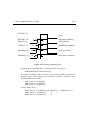
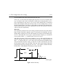
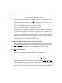
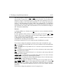
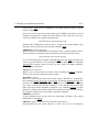
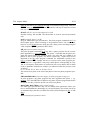
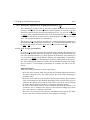
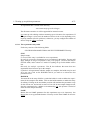
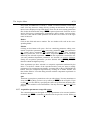
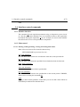
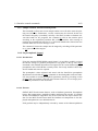
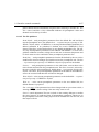
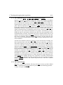
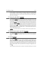
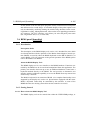
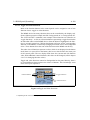
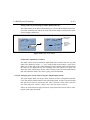
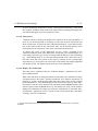
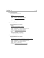
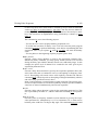
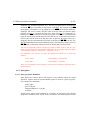
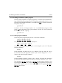
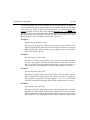
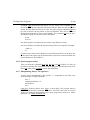
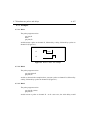
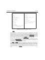
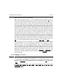
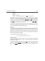
They define the timing of transmitter blanking, ASU blanking, preamplifier blanking, phase presetting, and shaped pulse presetting with respect to the transmitter
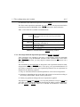
gating pulses. Furthermore, the pre-scan delays DE1 and DE2 may be changed.
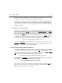
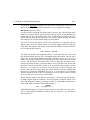
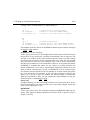
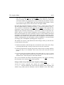
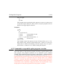
The pulse blanking constants are explained in Figure 1.5 .
TGPCH[1..8] (transmitter gating pulses)
They are generated on the TCU (word3, Bits 24-31) with the pulse program commands p1:f(1..8) or cw:f(1..8). Routing is done according to
TGPCH[FCUCHAN[channel]].
BLKTR[1..8] (transmitter blanking pulses)
The transmitter blanking may be switched on a time t1 before the pulse. Up to 8
different times can be used for the 8 different ASU channels. The same blanking is
applied to the amplifiers.
They are generated on the TCU (word 3, Bits 0-7 and NMR2, Bits 5 and 6)
together with the transmitter gating pulses TGPCH[1..8], but prolonged at the
1.3 The configuration suite [config]
A-23
INDEX
TGPCH[1..8]
INDEX
DONE
pulse
BLKTR[1..15]
BPCH[1..8]
t1
transmitter blanking
ASU blanking
TGPPA[1..5]
t2
preamplifier blanking
PHASPR[1..8]
t3
phase presetting
SHAPPR[1..8]
t4
shape pulse presetting
Figure 1.5 Presetting of blanking pulses
beginning by the times BLKTR[1..9]. Routing is done according to
BLKTR[RSEL[FCUCHAN[channel]]].
The routing according to RSEL is done by setting setting the RSEL parameters on
the digital routers. This routing can be switched at runtime by setting the corresponding NMR-control-words:
NMR1, Bits 0-3 for RSEL[1]
NMR1, Bits 4-7 for RSEL[2]
NMR1, Bits 8-11 for RSEL[3]
For more than 3 FCUs:
NMR1, Bits 12-15 for RSEL[3] and if RSEL[3] < 6
NMR7, Bits 0-3 for RSEL[4] "
" 4
"
NMR7, Bits 4-7 for RSEL[5] "
" 5
"
NMR1, Bits 8-11
The Acquire Menu
A-24
For more than 5 FCUs:
NMR7, Bits 8-11 for RSEL[5] and if RSEL[5] < 10 NMR7, Bits 4-7
INDEX
NMR7, Bits 12-15 for RSEL[6] "
" 6
"
NMR8, Bits 0-3 for RSEL[8]
"
"
7
"
DONE
INDEX
The corresponding routing of BLKTR, BLKPA and BPCH will follow these settings. Examples:
setnmr1 ^3 ^2 |1 |0 ; set RSEL[1] = 3
setnmr1 ^7 ^6 |5 ^4 ; set RSEL[2] = 2
BPCH[1..8] (ASU blanking pulses)
They are generated on the TCU (word 3, Bits 16-23) together with the transmitter
gating pulses TGPCH[1..8], but prolonged at the beginning by the times
BLKTR[1..5]. Routing is done according to
BLKTR[RSEL[FCUCHAN[channel]]].
TGPPA[1..5] (Preamplifier blanking pulses)
They are generated on the TCU (word 3, Bits 8-12) together with the transmitter
gating pulses TGPCH[1..8], prolonged at the beginning by the times BLKPA[1..5].
Routing is done according to
BLKPA[PRECHAN[SWIBOX[RSEL[FCUCHAN[channel]]]]]
The routing according to PRECHAN is done by selecting the preamplifier module
(HPPR) via RS232 at the beginning of the experiment and cannot be changed
afterwards. The routing according to SWIBOX is done with the switches SELH!H/
F (NMR2, Bit 2) and SELX!X/F (NMR2, Bit3). This can be changed at runtime.
BLKPA[1..5]
The blanking of the 5 preamplifier modules may be switched on a time t2 before
the pulse.
PHASPR[1..8] (phase presetting)
The switching of the phase programs may be done a time t3 before the pulse in
order to ensure a stable phase when the pulse begins.
SHAPPR[1..8] (shaped pulse presetting)
The propagation time of the phase versus the amplitude may be taken into account
by setting SHAPPR (t5). This value should be equal or larger than 1.4 µsec. Other-
1.3 The configuration suite [config]
A-25
wise the shaped pulse itself will be delayed by this time.
Please note: At the end of each shaped pulse the power is reset to its default value
INDEX
(e.g. for channel 1 pl1) and as consequence of this power setting the phase correction corresponding
to this power
is set as well. If the shaped pulse is terminated
INDEX
DONE
before this setting has taken place because there was not enough time to execute
the whole shaped pulse, the phase is still loaded as required for the shaped pulse,
namely with the phase cycle of the shaped pulse and not with the phase correction
value for the power pl[channel].
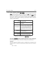
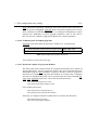
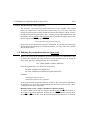
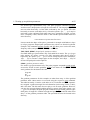
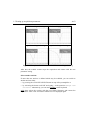
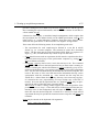
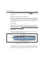
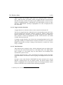
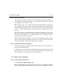
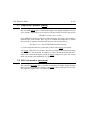
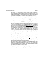
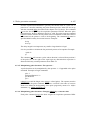
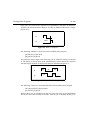
DE1, DE2
The acquisition parameter DE is the waiting period between the last pulse and the
begin of data acquisition (digitizer start) to avoid pulse feed through. You may
change DE by entering a new value. DE includes two sections, DE1 and DE2 (Figure 1.6). After DE1 the receiver gate is opened and the frequency is switched to
receive mode. If DE1 = -1, a default value of 4.0 µsec is used.
After DE2, the phase of the observe channel is set to 0. DE1 and DE2 both start
with DE and may range from 0 to DE. DE1 may be larger or smaller than DE2. If
DE2 = -1, a default value of 1.0 µsec will be used. The parameter PHASPR, which
will pull forward the phase setting, is taken into account automatically such that
the true phase setting occurs after DE2. This may lead to the situation where the
program prints the error message DE too small... even if DE2 is smaller than DE,
because DE2 + PHASPR[FCUCHAN[1]] is larger than DE..
DE
DE2
DE1
receiver gate
Figure 1.6 The DE delay
The Acquire Menu
A-26
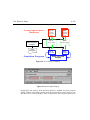
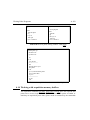
1.3.13 Avance frequency routing [edsp, edasp]
edasp is usually called from the NUCLEI button of the eda window, but may also
INDEX
be invoked as a keyboard command. In addition to nuclei setup, the edasp window
also shows the connections between
parts of the spectrometer,
DONEthe hardware
INDEX
namely FCUs, amplifiers, routers, high power modules and preamplifier modules.
This feature is only available for Avance type spectrometers. Table 1.8 shows the
available command buttons.
SAVE
SWITCH F1/F2
The aquisition parameters will be
saved on the disk
Exchanges the F1 nucleus with the
F2 nucleus
Exchanges the F1 nucleus with the
SWITCH F1/F3
F3 nucleus. With the SWITCH buttons you may easily swap between
observed and decoupled nuclei without having to reenter any frequencies
DEFAULT
sets the default routing for the selected set of nuclei
CANCEL
Exit without saving the parameters
PARAM
Shows the aquisition parameters as
they would be stored by SAVE
Table 1.8 Command buttons of edasp/edsp window
The Avance edasp/edsp display is logically divided into several vertical parts.
Some elements may be connected with the elements of the next part by clicking on
the corresponding two buttons. The rules to be obeyed are described below.
Frequency
The basic frequencies BF1-BF8 cannot be modified, they correspond to the
selected nucleus. For spectrum referencing the parameter SR is derived from SF
and BF1:
SR = SF - BF1
1.3 The configuration suite [config]
A-27
(SR is specified in Hertz ). Note that for spectrometers equipped with a BSMS unit
this number should be set to a value near 0, since the basic frequency of the
nucleus is chosen
such that the frequency reference standard (e.g. TMS) will have
INDEX
the frequency BF1 if the lock frequency has been set properly by the BSMS.
INDEX
DONE
Logical channels
There are two buttons for each logical channel. The buttons F1....F8 are used to
show and to alter the assignment of the physical FCU to the logical channel, e.g. if
F1 is connected to FCU2 this means that FCU number 2 will be used for the logical channel F1. If the nucleus for channel i is selected (not set to off) the button F
with the number i must be connected to one of FCU1...FCU8. The selected FCU
button must be connected to one of the amplifier buttons.
The lower button in NUC1...NUC8 in the logical channel group allows you to
select the nucleus. The displayed table is taken from the file
XWINNMRHOME/conf/instr/<instrument
name>/nuclei,
which is set up during the configuration command cf.
The parameters NUC1-NUC8, and the frequency offsets OFSxx are global parameters in XWIN-NMR: They are not only stored in the acqu file of the current data set
as acquisition parameters, but also in the file
XWINNMRHOME/conf
/instr/ < instrument name>/specpar
at the time the SAVE command is executed in edsp or edasp. They may be
imported from there into any dataset with the command edsp (this is actually the
difference between edasp and edsp).
Usage of edsp and edasp
Invoke edasp if the parameters of the current data set should be used as default.
edsp should be used, if the frequencies and nuclei of another experiment, previously defined with edasp or edsp, but in a different dataset, should be transferred to
the current data set. A typical example is the setup of a 1H experiment and a 13C
experiment with 1H-decoupling. For the first experiment a dataset 1 is created.
Within this dataset the nucleus 1H and the frequency SFO1 are chosen with the
command edasp. Then within a second data set the nucleus 13C for F1 and 1H for
F2 are chosen using the command edsp. Automatically the frequency SFO1 from
experiment 1 is transferred to SFO2 of experiment 2, because the same nucleus is
used for channel 2 as that one which was used in experiment 1 for channel F1. If
an inverse experiment would be done next, it is possible to interchange the nuclei
The Acquire Menu
A-28
for F1 and F2 from experiment 2 with the command edsp.
Amplifiers
INDEX
The frequency output of each FCU is hardwired to a router input and each router
output is hardwired to a specific amplifier.
display shows in the first colDONE The edsp
INDEX
umn the logical assignment of channels (F1-F8) to the FCUs, in the second column
the connections of the FCUs to the amplifiers which is done by the router. The
third column of connections shows the so-called switchbox, which can connect the
output of the first X-amplifier and of the 1H-amplifier to different preamplifiers by
means of relays or diode-switches.
Preamplifier
Up to 5 preamplifier modules can be installed in the HPPR. They are connected
directly to switch box outputs X, 19F , 1H or to optional High Power Transmitters
which may also be connected to these outputs.
Note and rules for manual routing
After each nucleus selection the default routing will be set. It can be accepted or,
may be changed by the user. This should be done only after the complete set of
nuclei has been selected. All changes in the routing are made by moving from the
left to the right through the display. Connections between two units may be created
or cut by two mouse clicks on the corresponding two buttons. The following rules
apply:
• Only one F1...F8 logical channel must be connected to each FCU.
• Several FCU’s may be connected to a single amplifier.
• Router restrictions: Router input 1 may be connected only to router output 1,2,
or 3, router input 2 only to 1, 2 ,3, and 4. Router inputs of the second or third
router may be connected to the output of the first router only if no other input
channel of this router goes to a different output channel of the first router.
• In the switch box each input button may be connected to any output button but
this connection must be one to one. Double connections from the same input
button are not allowed.
• Each preamplifier may only be connected to one amplifier, either through the
switch box or directly. Note however that the displayed connection to a preamplifier is of no physical influence as far as the connections between the amplifiers and the preamplifier modules are concerned. It is up to the operator to
1.3 The configuration suite [config]
A-29
ensure that the wiring is correct. The same is true for the correct connection to
the probehead.
INDEX
At the time the program creates the default routing, the amplifier is chosen such
that the nucleusINDEX
type is considered.
For 1H or 19F nuclei an amplifier of type H is
DONE
selected, for other nuclei an X type amplifier.
1.3.14 Install standard parameter sets [expinstall]
Execute the command expinstall (also available in the Acquire->Spectrometer
setup menu). XWIN-NMR is delivered with sets of acquisition, processing, and plot
parameters for many types of NMR experiments. They were compiled and tested
on various instruments in Bruker laboratories. expinstall lets you select your
instrument type, and stores the corresponding parameter sets, pulse programs, etc.
in their working directories XWINNMRHOME/exp/stan/nmr/par/, XWINNMRHOME/exp/
stan/nmr/lists/pp/, etc. respectively. During this process, it adapts certain acquisition parameters such as the observe frequency to the basic frequency of your spectrometer. cf must therefore have been executed before.
Since expinstall may overwrite existing files, it should only be invoked by the
administrator. In order to exclude such conflicts, we recommend not to modify
parameter sets, pulse programs, etc. provided by Bruker. Instead, before applying
changes, create a copy with a different name. expinstall needs only be executed
once after installation of a new XWIN-NMR version, or, if at a later time additonal
items are to be installed omitted initially.
On XWIN-NMR release media, in addition to the software modules Bruker provides
pulse program libraries, parameter sets etc. as listed in Table 1.9. The purpose of
expinstall is to install all desired items in their working directories for your type of
instrument, and to update certain parameters accordingly. Since this is a critical
configuration procedure, it should only be excuted by the system administrator.
expinstall starts up with a table of spectrometers. Select the correct one (the instrument specified during cf configuration is enabled by default) and click on the Proceed button. A new table comes up showing the possible actions that may be
performed. The highlighted buttons define the minimum required for data acquisition with Bruker pulse programs, and automated measurements based on Bruker
standard parameter sets. You may click on a highlighted button to disable installation, and on other buttons to enable installation. As soon as you click on the Proceed button of the dialog box, all highlighted features will be installed. expinstall
may be executed again at any later time to install items not selected earlier.
The Acquire Menu
A-30
Pulse program library
Composite pulse decoupling library
AU program library
Gradient file DONE
library
INDEX
INDEX
Shape file library
Standard experiments library
Standard composite experiments library
Scaling region files libary
Table 1.9 Libraries to be installed with expinstall
Please do not enter other commands while expinstall is in progress. It will print a
message when complete. Without compilation of AU programs , expinstall terminates within a few minutes. Compilation may take a few hours, depending on the
number of AU programs and computer speed.
The following sections describe the features that may be installed.
1.3.14.1 Pulse programs
On the release media, pulse programs for many NMR experiments are delivered
for various types of instruments in own directories according to Table 1.10. expinXWINNMRHOME/exp/stan/nmr/lists/pp.exam
AMX high resolution
XWINNMRHOME/exp/stan/nmr/lists/pp.rexam
ARX high resolution
XWINNMRHOME/exp/stan/nmr/lists/pp.dexam
AVANCE
XWINNMRHOME/exp/stan/nmr/lists/pp.solids
AMX/ASX solids
XWINNMRHOME/exp/stan/nmr/lists/pp.imag
micro-imaging
XWINNMRHOME/exp/stan/nmr/lists/pp.tomo
tomography
Table 1.10 Sample pulse program directories
stall copies them into the working directory XWINNMRHOME/exp/stan/nmr/lists/pp/,
where they are searched for by pulse program manipulation commands such as
1.3 The configuration suite [config]
A-31
edpul, and by the acquisition commands. If the item Enable Define Statements in
Pulse Programs is higlighted, expinstall opens each pulse program prior to installation, and removes
all double semicolons (;;) occurring at the beginning of a pulse
INDEX
program line. Definitions of pulse program parameters such as d11=30m or
INDEX
DONE by Bruker for certain experiments.
d12=20u are now
enabled as suggested
1.3.14.2 Composite pulse decoupling programs
expinstall copies them from the directories of Table 1.10. to the directory
XWINNMRHOME/exp/stan/nmr/lists/cpd.rexam
AMX/ARX/ASX
XWINNMRHOME/exp/stan/nmr/lists/cpd.dexam
AVANCE
Table 1.11 Sample cpd program directories
XWINNMRHOME/exp/stan/nmr/lists/cpd/.
1.3.14.3 Install and compile AU programs/modules
The XWIN-NMR release media include AU programs and modules for a number of
special applications. You may inspect the source code of AU programs after their
installation using the edau command. Usually the function of an AU program is
described in its header. AU programs and modules are written in the C language
and must be compiled before they can be executed with one of the command xau,
xaup, xaua. expinstall copies the C source files from the directories
XWINNMRHOME/prog/au/src.exam/
XWINNMRHOME/prog/au/modsrc.exam/
to the working directories
XWINNMRHOME/exp/stan/nmr/au/src/
XWINNMRHOME/exp/stan/nmr/au/modsrc/.
Then they are compiled, and the excutable files are stored in the directories
XWINNMRHOME/prog/au/bin/
XWINNMRHOME/prog/au/modbin/.
The Acquire Menu
A-32
1.3.14.4 Recompile all user AU programs
command are also stored in the
AU programs a user wrote himself using the edau
INDEX
directory XWINNMRHOME/exp/stan/nmr/au/src/. They are not deleted if a new
they happen
to have the name of a Bruker
XWIN-NMR version is installed (unless
DONE
INDEX
AU program; please avoid this). You must, however, recompile your own AU programs in order to make them compatible with the new program version.
1.3.14.5 Install library gradient files
On the release media, gradient files for a number of applications are delivered for
various types of instruments in own directories according to Table 1.10. expinstall
XWINNMRHOME/exp/stan/nmr/lists/gp.exam
XWINNMRHOME/exp/stan/nmr/lists/gp.dexam
XWINNMRHOME/exp/stan/nmr/lists/gp.solids
AMX high resolution
AVANCE
AMX/ASX solids
XWINNMRHOME/exp/stan/nmr/lists/gp.imag
micro-imaging
XWINNMRHOME/exp/stan/nmr/lists/gp.tomo
tomography
Table 1.12 Sample gradient file directories
copies them into the working directory XWINNMRHOME/exp/stan/nmr/lists/gp/,
where they are searched for by commands such as edgp, and by the acquisition
commands.
1.3.14.6 Install library shape files
On the release media, shape file for a number of NMR experiments are delivered
for various types of instruments in own directories according to Table 1.10. expinstall copies them into the working directory XWINNMRHOME/exp/stan/nmr/lists/
wave/, where they are searched for by the acquisition commands.
1.3.14.7 Convert standard parameters sets
After installation of XWIN-NMR from the release media, the directory
XWINNMRHOME/exp/stan/nmr/par.300/
1.3 The configuration suite [config]
XWINNMRHOME/exp/stan/nmr/lists/wave.exam
XWINNMRHOME/exp/stan/nmr/lists/wave.solids
INDEX
A-33
AMX high resolution
AMX/ASX solids
XWINNMRHOME/exp/stan/nmr/lists/wave.imag
micro-imaging
INDEX
DONE
XWINNMRHOME/exp/stan/nmr/lists/wave.tomo
tomography
Table 1.13 Sample shape files directories
contains a collection of so-called standard experiments. An experiment is a directory with a complete set of acquisition, processing, and plot parameters prepared
e.g. for a proton measurement, a 13C decoupling measurement, a COSY experiment, etc. These parameter sets were compiled and tested on a 300 MHz spectrometer in the Bruker application laboratory. Before you can make use of them, they
must be adapted to your local requirements. Afterwards, they are stored in the
directory
XWINNMRHOME/exp/stan/nmr/par/,
where they may be accessed by commands such as rpar and dirpar.
The conversion utility first requests the logical name of your printer and plotter,
e.g. $hplh4p. See command cfpp on printer/plotter installation. These names are
inserted in the CURPRIN and CURPLOT parameters defining the output devices.
At any later time you may overwrite these default settings if required using the
command edo.
The next question is about the paper format of your plotter. The plot parameters of
the standard parameter sets are adjusted for A3 size. You may leave A3, or change
it to A, A4, or B. A3 and B will take over the default settings, A4 and A will
change parameters according to the contents of the text file
XWINNMRHOME/exp/stan/nmr/lists/plotconvpar.
If you want to produce your own default values, you may edit this file according to
the description in its header, and run expinstall again, enabling only the Convert
standard parameter sets function.
The next question asks for the type of digitizer installed in your instrument. The
answer is stored in the DIGTYP acquisition parameter of the standard acquisition
parameter files.
The Acquire Menu
A-34
Finally, for AMX instruments you may initialize the parameters XL and YL with
the BSV10 attenuator setting 3 to prevent probe head damage.
INDEX
Parameter set conversion will now start and take a few minutes. During this process, frequencies are adapted to your
spectrometer,
the sweep width and 2D increDONE
INDEX
ments are corrected, and, for Avance type spectrometers, the default frequency
routing is initiated.
1.3.14.8 Update user permission files
Enable this item if you intend to use XWIN-NMR’s automated spectrometer operation features (commands set, run), or the commands quicknmr, setexp, and runexp.
For any XWIN-NMR user, a permission file may be created by the system administrator using the eduser command. Such a file contains the standard experiments
which may be carried out by this user, and other possibilies (see eduser command;
an example file is XWINNMRHOME/exp/stan/nmr/lists/sam_users_exam). Usually, a
new XWIN-NMR version includes new standard experiments stored in the file
XWINNMRHOME/exp/stan/nmr/par.300/.News
.
This part of expinstall displays a dialog box of all users. If you click on a user,
expinstall merges the new experiments into his (her) permission file. If you click
on the Select all button, all users will be updated.
1.3.14.9 Install standard composite experiments
A sequence of standard experiments may be composed to build a new standard
experiment, called a composite experiment (see also set command). Such experiments may be selected for execution in the dialog windows opened by set or quicknmr. These routines locate composite experiments in the file
XWINNMRHOME/conf/instr/<Instrument
Name>/users/.pool .
If you enable this expinstall item, this file is created by making a copy of the standard composite experiments provided by Bruker in the file
XWINNMRHOME/exp/stan/nmr/pp.300/.pool.
The .pool file of composite experiments is common to all users. With the set command, you may define own composite experiments, and define which user is
allowed to execute a particular experiment.
1.4 Defining the acquisition data set [new, edc]
A-35
1.3.14.10 Install standard scaling region files
XWINNMRHOME/exp/stan/nmr/lists/scl.exam/ includes files whose
The directory INDEX
names are composed of a nucleus and a solvent name, e.g. 13C.Acetic. The files
contain spectralINDEX
regions, usuallyDONE
around the solvent and reference, which are to be
excluded when the program scales a plot, or during sweep width optimization with
commands such as getlim. If this expinstall item is enabled, the sample region files
will be copied to their working directory
XWINNMRHOME/exp/stan/nmr/lists/scl/,
where they are accessed by the respective commands. If you need solvent/nucleus
combinations other than those provided by Bruker, you may create own suitable
files in this directory.
1.4 Defining the acquisition data set [new, edc]
Before you can set up the parameters for a data acquisition, you must define a data
set where the acquired data (fid), and later on the spectrum are to be stored. In
XWIN-NMR, data set a characterized by the 5 parameters
DU, USER, NAME, EXPNO, PROCNO.
From these parameters, two directories are derived:
/DU/data/USER/nmr/NAME/EXPNO/
/DU/data/USER/nmr/NAME/EXPNO/pdata/PROCNO/.
Examples:
/u/data/guest/nmr/sucrose/1/
/u/data/guest/nmr/sucrose/1/pdata/1/
In the first directory, acquisition data are stored by the acquisition commands in
the files fid or ser. A ser file contains multiple fids and is the result of a two-, three, or higher dimensional experiment.
Defining a data set for a single experiment acquisition with zg
In order to define a new data set, call the command New from the File menu, or
enter new or edc on the keyboard. A dialog box is displayed where you may enter
the data set parameters. DU is the disk partition where the data are to be located,
The Acquire Menu
A-36
and USER is the user’s own or another legal login name. NAME is an arbitrary
name assigned to the data set. EXPNO is a number, allowing you to run experiments under the same NAME, and differentiatingINDEX
them by the EXPNO. Similarly,
PROCNO is a number, and may be used to store several processed data sets
INDEX
derived from the same acquisitionDONE
data. If you enter
data set parameters for which
a data set already exists, it will be display as soon as you click on the OK button of
the dialog box. This is the same as if you had selected the data set using one of the
dir commands, or the search command (see The File Menu). Any acquisition command issued now would overwrite existing acquisition data with the new fid or ser
file. XWIN-NMR will output a warning prior to acquisition start only if the system
variable ZGsafety is set to yes. Use the command setres to set ZGsafety, which is
equivalent to invoking User interface from the Display->Options menu.
If no data set exists corresponding to the specified parameters, a new one is created, and is initialized with the same set of acquisition, processing, and plot parameters valid for the currently displayed data. The program display switches to the
new data set (i.e. makes it the current data set), but the data area of the XWIN-NMR
window remains blank since no data are present yet.
Defining the data set for an experiment to be executed from quicknmr
Use the sample name entry field in the quicknmr dialog window.
Defining the data sets for a series of experiment to be executed by run
Use the name entry field in the set dialog window.
1.5 Setting up acquisition parameters
This section will discuss the following set up commands for data acquisition:
• edinfo (edit sample information)
• eda, rpar (general acquisition parameter set up for the commands zg, go, gs)
• ased, as (acquisition parameter set up for the commands zg, go, gs restricted to
parameters referred to in the current pulse program)
• wobb (probehead tuning)
• gs (interactive adjustment of acquisition parameters)
• set (parameter set up for a series of experiments started with run)
• extset (external parameter set up for run using ASCII files)
1.5 Setting up acquisition parameters
A-37
1.5.1 Setting up the sample information file [edinfo]
This command is not required for data acquisition to perform properly. However, it
INDEX
allows you to store sample or company specific information of your choice such as
sample id, orderINDEX
number etc. toDONE
be entered and stored along with acquisition data.
You may also append this information to the spectrum plot. Please refer to the
description of edinfo in the chapter The File Menu.
1.5.2 Acquisition parameter setup with eda
eda is the most general parameter setup for a data acquisition to be started with zg.
With eda, you get the settings for the current data set displayed, and you may modify them. eda may also be called from the set dialog window, which is the parameter set up for experiments executed by the run command. Likewise, eda may be
called from the quicknmr dialog window. Before you call eda, you may use rpar
(see chapter The File Menu) to initialize the current acquisition parameters with a
standard parameter set from the directory XWINNMRHOME/exp/stan/nmr/par/.
Please note:
Certain buttons in the eda dialog window, such as PULPROG, will open a box with
a list of items, e.g. pulse program names. In order to select an item, you must click
on it. If you happen to click outside the box, the box will be disabled: If you move
the cursor back into the box, no mouse clicks will be accepted until you re-enable
it by hitting the ESC key.
1.5.2.1 Invoking eda from the keyboard or from the Acquire menu
The acquisition parameters displayed in this case are a copy of those of the data set
where the new command was given. You may overwrite them with an arbitrary
predefined parameter set using the command rpar. rpar displays the table of parameter sets available in the directory XWINNMRHOME/exp/stan/nmr/par/. It contains
the Bruker standard experiments (see expinstall) as well as others you or your system administrator copied there with the wpar command. rpar allows you to selectively overwrite either your current acquisition, plotting, or processing parameters
(or all of them). After rpar, you may change individual parameters with eda.
The command eda displays all acquisition parameters of the current data set at
once in a table, and allows you to apply modifications. The parameters are loaded
from the parameter file (a text file)
/DU/data/USER/nmr/NAME/EXPNO/acqu.
The Acquire Menu
A-38
Upon exit from eda via the SAVE button of the eda dialog window, all changes are
written into this file. Any parameter may also be entered from the keyboard: Type
in the parameter name, followed by Return. ThisINDEX
will print the current value and
waits for change or confirmation. As a second possibility, enter the parameter
DONE
name followed by a space character,
then typeINDEX
in the new value, followed by
Return.
If the current data set is a 2D or 3D data set, eda shows two or three columns
labelled F2 and F1, or F3, F2, and F1, respectively. The leftmost column (F2 for
2D, F3 for 3D) defines the acquisition dimension, whose parameters are stored in
the file acqu. Table 1.14 shows which parameter files correspond to the different
dimensions. You may access the parameters of any dimension also from the keyF3
F2
F1
Data
set type
Param.
Files
Command
Param.
Files
Command
Param.
Files
Command
1D
-
-
-
-
acqu
td
2D
-
-
acqu
td
acqu2
2 td
3D
acqu
td
acqu2
2 td
acqu3
1 td
Table 1.14 eda columns, corresponding parameter files and command example
board. Table 1.14 also shows the keyboard commands to access the time domain
size parameter TD, which exists for all dimensions of a 2D or 3D data set. Please
note that typing the parameter name (in lower case characters) always accesses the
acquisition dimension if not preceded by a dimension number.
Acquisition commands such as gs, zg, go, wobb, or rga read in the acquisition
parameters from the files acqu (acqu2, acqu3), compile them into a form suitable
for the spectrometer hardware, and load them into the hardware for execution of
the experiment.
The next section describes all the acquisition parameters in detail. Some of them
depend on the spectrometer type and are required e.g. for an AMX, but not for a
DMX. The contents of the eda dialog box may therefore differ accordingly. Actually, the parameters appearing in this window are taken from the so-called format
file
1.5 Setting up acquisition parameters
A-39
XWINNMRHOME/exp/stan/nmr/form/acqu.e,
which is linked (made identical) to a format file suitable for your instrument at the
INDEX
time of spectrometer configuration with cf. Format files are text files, which you
may adapt to your
requirements,
e.g. remove parameters you will never use or
INDEX
DONE
change, or change their output format. If you re-arrange the sequence of parameters in a format file, the eda display will change accordingly.
Please note: Before modifying a format file, make a copy!
Format files do not only define the arrangement of parameters in the eda window.
Some parameters, such as DW, AQ, FIDRES, SWH are defined in the format file
by means of an equation, expressing the relation to other parameters (e.g.
SWH=SW*SFO1). Parameters defined in a format file in this way are called temporary parameters, since they are not stored in an acquisition parameter file acqu,
which only contains parameters not depending on each other. You may insert own
temporary parameters into a format file by generating a corresponding new entry
in the format file similar to the entries of DW, AQ, etc.
1.5.2.2 Invoking eda from the keyboard or from set or quicknmr
Now, the parameters displayed are not those contained in the acqu* files of the currently displayed data set. Instead, they correspond to the experiment selected in the
set or quicknmr dialog window, and are valid only for the data set currently
selected in these dialog windows. See also command set for more details.
1.5.2.3 eda command buttons
Table 1.4 lists the command buttons available in the eda dialog box.
1.5.2.4 The acquisition parameters
The acquisition parameters are described in the standard eda order.
PULPROG (pulse program)
The pulse program to be executed by the acquisition commands gs, zg, go, and rga.
Type in a name, or click on the down arrow button right of the entry field to get a
list of available pulse programs. Click on the desired one to store it in PULPROG.
The first list entry is EDIT CURRENT, a command which displays the text of the
current pulse program. The pulse program list is generated according to the con-
The Acquire Menu
A-40
SAVE
Save modifications and quit.
1-COL
(only 1D)
Change eda display such that the parameters are arranINDEX
ged in a single column, including their description.
2-COL
(only 1D)
DONE
Change eda
display suchINDEX
that the parameters are arranged in two columns, omitting their description.
Parameter
Search. An entry field where you may specify the name
or some inital characters of a parameter. After typing
Return, the cursor is auto-positioned to the parameter.
NEXT
Continue search to next parameter matching the string.
ABORT
Discard any changes and quit.
Table 1.15 Command buttons in eda dialog window
tents of the directory
XWINNMRHOME/exp/stan/nmr/lists/pp/.
It contains the Bruker pulse programs according to the expinstall installation, and
the pulse programs created by yourself or your system administrator by means of
the command edpul.
A special chapter in this manual (Writing Pulse Programs) describes the pulse program language. The command pulsdisp displays a graphical representation of the
current pulse program. You will find a description of pulsdisp in the chapter The
Windows Menu.
AQ_mod (acquisition mode)
The acquisition mode with the possible settings qf, qseq, qsim (=standard setting),
DQD.
• qf = single channel detection. Only one detector is used.
• qseq = quadrature detection, sequential mode. Two detectors with a reference
phase shifted by 90 degrees are used. In the resulting fid, two successive data
points originate from different detectors. Their acquisition time difference is
given by the dwell time parameter DW.
• qsim = quadrature detection, simultaneous mode. Two detectors with a reference phase shifted by 90 degrees are used. In the resulting fid, two successive
data points originate from different detectors, but were sampled at the same
1.5 Setting up acquisition parameters
A-41
time. The acquisition time difference of two pairs of data points is two times the
dwell time parameter DW.
INDEX
• DQD= digital
quadrature detection (only available on suitably equpipped
Avance type spectrometers). Requires the acquisition parameter DIGMOD to
INDEX
DONE
be set to digital or homodecoupling digital. Digital quadrature detection has the
advantage over the previously described analog modes that the two receiver
channels are generated mathematically by the digital filters of such instruments,
and for this reason are not offset against each other, leading to a cleaner fid signal.
AQSEQ (acquisition sequence)
This parameter AQSEQ which take on one of the values 312 or 321. It is evaluated
by the 3D Fourier transform and describes the sequence of fids acquired in a ser
file during a 3D experiment (3 = the acquisition dimension, 1 and 2 = the orthogonal dimensions). The processing parameter AQORDER is not evaluated if AQSEQ
is set.
On Avance type systems, 3D pulse programs will set AQSEQ automatically if td
and td1 are used consistently within the pulse program. However, you may explicitly define AQSEQ in the pulse program. For this purpose, insert one of the following statements in the pulse program header: aqseq 321 or aqseq 312.
On both, AMX/ARX and Avance type systems, you can set or modify AQSEQ
using the command 3s AQSEQ before starting the transform.
TD (time domain size)
Defines the number of data points of the fid. For data set dimensions bigger than 1,
TD for F1 and F2 usually specifies the number of increments. It may be used in
pulse programs, e.g. by the pulse program commands lo to x times td1 or lo to x
times td2. Enlarging TD will give a better resolution of the fid (see parameter FIDRES) and hence the spectrum at the expense of a longer scan time AQ.
PARMODE (dimension of acquisition data)
1D, 2D, or 3D. Specifies the type of data to be acquired. If you change PARMODE
to a smaller dimension, unnecessary parameter files are deleted. If you switch to a
higher dimension, the required additional parameter files are fetched from the
directories
XWINNMRHOME/exp/stan/nmr/par/standard2D/, or
XWINNMRHOME/exp/stan/nmr/par/standard3D/ .
Existing acquisition data are deleted after approval by the user.
The Acquire Menu
A-42
NS (number of scans)
Defines the number of accumulation loops the pulse program commands go=n and
rcyc=n should perform.
INDEX
DS (number of dummy scans)
DONE
INDEX
Defines the number of loops the pulse program command go=n should perform
without digitizing and accumulating data, before continuing with NS true scans.
Used to get steady state conditions.
D0-D31 (delay parameters in seconds)
32 duration parameters, to be specified in seconds. They are executed as delays
without any further actions by the pulse program commands d0-d31. In Bruker
pulse programs, D1 is most often used as a relaxation delay, and D0 and D10 as
incrementable delays for 2D and 3D experiments, although any delay may be
incremented or decremented using the pulse program commands id0-id31 or dd0dd31, respectively. The changes are given by the parameters IN0-IN31. The pulse
program commands rd0-rd31 reset a respective delay to its original value. On
Avance systems, delays may also be changed by means of arithmetic expressions
during pulse program execution.
P0-P31 (pulse length parameters in microseconds)
32 duration parameters, to be specified in microseconds. They are executed by the
pulse program commands p0-p31, which execute a pulse on the specified channel
during the respective duration parameter. In Bruker pulse programs, P1 is most
often used as a 90 degree pulse. Pulses may be incremented or decremented by the
pulse program commands ipu0-ipu31 or dpu0-dpu31, respectively. The changes
are given by the parameters INP0-INP31. The pulse program commands rpu0rpu31 reset a respective pulse length to its original value. On Avance systems,
pulses may also be changed by means of arithmetic expressions during pulse program execution.
ND0, ND10 (number of delays D0 or D10)
Number of d0 and d10 commands in the increment loops of a pulse program for
2D or 3D experiments. Used to calculate the sweep width for the F1 and F2 dimensions according to
SW(F1)=1/(SFO1*ND0*IN0), SW(F2)=1/(SFO1*ND10*IN10),
respectively.
IN0, IN10 (increments for delays D0 and D10 in seconds)
1.5 Setting up acquisition parameters
A-43
The pulse program commands id0 and id10 increment the delays D0 and D10 by
IN0 and IN10, respectively. See also description of D0-D31. If you change IN0
during the setupINDEX
of a 2D experiment, the sweep width in the dimension F1 is recalculated according to SW=10e6/(SFO1*DR*IN0). If you change IN0 during the
INDEX the DONE
setup of a 3D experiment,
sweep width in the dimension F1 is recalculated
according to SW=10e6/(SFO1*DR*IN0). If you change IN10 during the setup of a
3D experiment, the sweep width in the dimension F2 is recalculated according to
SW=10e6/(SFO1*DR*IN10).
Features:
a) changing ND10 on a 3D data set in eda results in a correct calculation of IN10,
SW and SWH.
b) if the parameter IN0 or IN10 is changed by typing, for instance, in0 or in10
from the XWIN-NMR command line, then the sweep width in ppm is updated correctly, as well as the sweep width in Hz.
c) changing the sweep width by typing 1 SWH or 3 SWH from the XWIN-NMR
command line will change the increment.
d) Setting the parameters in an AU program with STOREPAR is possible.
If you want to change the parameters from the XWIN-NMR command line, type:
nd0 : to change the sweep width in F1 of a 2D or 3D data set (the increment IN0
is NOT changed)
nd10 : to change the sweep width in F2 of a 3D data set (the increment IN10 is
NOT changed)
in0 : to change the increment IN0 in F1 of a 2D or 3D data set (the sweep width
will be adjusted, but not ND0)
in10 : to change the increment IN10 in F2 of a 3D data set (the sweep width will
be adjusted, but not ND10)
1 SWH (1 SW) : to change the sweep width in Hz (ppm) in F1 of a 2D or 3D data
set (the increment IN0 will be adjusted, but not ND0)
2 SWH (1SW) : to change the sweep width in Hz (ppm) in F2 of a 3D data set (the
increment IN10 will be adjusted, but not ND10)
Note : 2 SWH (2 SW) on a 2D data set will change the sweep width in F2 and 3
SWH (3 SW) on a 3D data set will change the sweep width in F3! Therefore,
increments and ND0 or ND10 values will NOT be effected, because the changes
are made in the acquisition dimension and not in one of the indirect detected
dimension.
If you want to change the parameters in an AU program, use :
The Acquire Menu
A-44
storepar1("ND0", value) : changes the sweep width in F1 of a 2D data set, if ND0
is changed. value must be a INTEGER variable.
storepar3("ND0", value) : changes the sweep width
in F1 of a 3D data set, if ND0
INDEX
is changed. value must be a INTEGER variable.
DONE
storepar1("ND10", value) : changes
the sweep INDEX
width in F2 of a 3D data set, if
ND10 is changed. value must be a INTEGER variable.
storepar1("IN0", value) : to change the increment IN0 in F1 of a 2D data set. value
must be a FLOAT variable.
storepar3("IN0", value) : to change the increment IN0 in F1 of a 3D data set. value
must be a FLOAT variable.
storepar1("IN10", value) : to change the increment IN10 in F2 of a 3D data set.
value must be a FLOAT variable.
storepar1("SWH", value) : to change the sweep width in Hz in F1 of a 2D data set.
value must be a FLOAT variable.
storepar3("SWH", value) : to change the sweep width in Hz in F1 of a 3D data set.
value must be a FLOAT variable.
storepar1("SWH", value) : to change the sweep width in Hz in F2 of a 3D data set.
value must be a FLOAT variable.
storepar1("SW", value) : to change the sweep width in ppm in F1 of a 2D data set.
value must be a DOUBLE variable.
storepar3("SW", value) : to change the sweep width in ppm in F1 of a 3D data set.
value must be a DOUBLE variable.
storepar1("SW", value) : to change the sweep width in ppm in F2 of a 3D data set.
value must be a DOUBLE variable.
SW, SWH (sweep width in ppm, Hz)
The sweep width may be specified in ppm or Hertz units by setting one of the
parameters SW or SWH. The other parameter is calculated automatically
(SWH=SW*SFO1). The sweep width is the spectral range to be observed. SW in
conjunction with TD or the desired scan time AQ define the dwell time DW, which
triggers the digitizer to sample the individual data points. The digitizer hardware
only allows for discrete values of DW, and therefore for SW. This explains the
observation that the program often changes SW slightly if you enter an arbitrary
value. SW may also be set interactively from the sw-sfo1 button in the 1D utilities
menu. It ajusts SW so that it has the same value as the expanded region, and also
adjusts SFO1 so that the carrier frequency lies in the center of the expanded region.
1.5 Setting up acquisition parameters
A-45
For 2D and 3D experiments, SW as described above corresponds to the width in
the acquisition dimension, while the widths of the other dimensions are calculated
from the parameters
IN0, IN10, ND0, and ND10.
INDEX
FIDRES (fid resolution
INDEX in Hertz)
DONE
A temporary parameter calculated according to FIDRES=SW*SFO1/TD. If you
modify FIDRES to get a desired resolution, the time domain size is recalculated
according to TD=nextpower of 2 of ( (SW*SFO1)/FIDRES ).
FW (filter width in Hertz)
The analog filters are set according to this value when acquisition is started, or
with the ii command. If you change the sweep width, FW is recalculated according
to FW=1.25*SWH or FW=0.3125/DWOV. The latter equation is valid for Avance
systems, if digital filtering is enabled (DIGMOD=digital or homodecoupling digital). DWOV is the oversampling dwell time (see also parameter DIGMOD).
AQ (acquisition time in seconds)
The time to record one scan. Doubles if you increase TD or SW by a factor of two.
If you change AQ, TD is recalculated accordingly. It will not be rounded to the
next power of two, but be set to an even number giving the closest match to the
entered AQ value. Then AQ is recalculated from TD and SW.
RG (receiver gain)
The receiver gain controls the amplitude of the fid signal before it is fed into the
digitzer. It must be adjusted to maximum amplitude, without causing overflow of
the digitizer (in this case signal cutoff would occur, generating artefacts in the
transformed spectrum). The values depend on the receiver system of your spectrometer. You may use the command rga for automatic determination of the optimum RG value. rga performs some scans using the pulse program specified in
PULPROG and sets RG to the found value. You may then further adjust RG to fit
your special requirements.
DW (dwell time in microseconds)
The dwell time is the time difference between two data points of the fid. It is calculated from the sweep width according to DW=10e6/(2*SW*SFO1). If you change
DW, SW is recalculated according to SW=10e6/(2*(0.05+DW)*SFO1). The minimum dwell time (corresponding to the maximum possible sweep width) depends
on the digitizer type installed in the spectrometer (see also: DIGTYP parameter,
Table 1.16).
DWOV (oversampling dwell time)
The Acquire Menu
A-46
For spectrometers equipped with digital filters (Avance) only. It is displayed as an
information for the user, and is related to the dwell time DW according to
DW=DWOV*DECIM. DWOV is the actual sample
rate of the digitzer if digital filINDEX
tering is enabled. The decimation factor DECIM is chosen so that after the Fourier
transform the spectrum will have aDONE
spectral widthINDEX
as close as possible to the chosen
SW parameter. See also: DIGMOD parameter.
DECIM (decimation rate of digital filter)
For spectrometers equipped with digital filters (Avance) only. For details see:
DWOV and DIGMOD parameters.
DSPFIRM (firmware used for digital filtering)
For spectrometers equipped with digital filters (Avance) only. For details see: DIGMOD parameter.
DIGTYP (digitizer type)
XWIN-NMR supports the digitizer types of Table 1.16. The SADC is not prepared
DIGTYP
dynamic range
minimum DW
slow
12 bits
3 microsec
16bit
16 bits
4 microsec
fast
9 bits
0.1/0.05 microsec
BC132-12
12 bits
0.1 microsec
BC132-16
16 bits
2 microsec
FADC (=BC133)
12 bits
0.05 microsec
HADC (=HRD16)
16 bits
2.5 microsec
SADC
16 bits
3.325 microsec
HADC+
16 bits
3.325 microsec
SADC+
16 bits
3.325 microsec
IADC
16 bits
0.1/0.05 microsec
Table 1.16 Digitizer types
for sequential acquisition, i.e. AQ_mod must not be set to qseq. DIGTYP must be
set to a type installed in your spectrometer (more than one may be present). When
1.5 Setting up acquisition parameters
A-47
executing the expinstall command, you may enter a desired type. In this case, the
DIGTYP parameter of all standard parameters sets are updated accordingly.
INDEX
DIGMOD (digitization mode)
For spectrometers
equipped with
digital filters (Avance) only. The following three
INDEX
DONE
modes are available: analog, digital, homodecoupling-digital. Analog disables digital filtering and uses the analog filters in the conventional way. Digital turns on
digital filtering. Homodecoupling-digital also enables digital filtering, but limits
the sampling rate so that homodecoupling is still possible.
The receiver control unit (RCU) of all Avance instruments is equipped with two
digital signal processors (DSP) which can perform digital filtering during the
acquisition. The digitizer will sample with a dwell time DWOV which is related to
the conventional dwell time by
DW = DWOV * DECIM
The DSP will decimate the sampled points by a factor DECIM, and at the same
time perform digital filtering. The oversampling dwell time DWOV must be in the
range 2.5-5 µsec for HADC/HRD16 and FADC, and in the range 3.3-6.6 µsec for a
SADC. For homodecoupling the oversampling dwell time must be between 25 and
50 µsec. The decimation factor DECIM is chosen so that after the Fourier transform the spectrum will have a spectral width as close as possible to the chosen SW
parameter. The factor DECIM is stored as an acquisition status parameter (in the
file acqus). It is required to calculate a correct baseline correction of the fid, and
the first order phase correction during the Fourier transform (for the standard DSP
firmware; the parameter DSPFIRM may be set to used-defined if non-standard
firmware should be used. In this case the firmware file (in ASCII) must be located
in XWINNMRHOME/exp/stan/nmr/lists/DSPFIRM).
Digital filtering enhances the digitizer resolution by a factor given by the parameter DDR (digital digitizer resolution). The total digitizer resolution, which is the
sum of the hardware resolution according to Table 1.16 and DDR is still characterized by DR. DDR is related to DECIM according to(.
DDR =
2
log DECIM + 1
With DIGMOD=digital or homodecoupling digital it is possible to use AQ_mod =
qsim or DQD (digital quadrature detection), but not AQ_mod = qseq (sequential
data acquisition).
The Acquire Menu
A-48
DR (digitizer resolution)
Acquisition commands will normally set the digitzer to its maximum resolution
(the default of DR). If you set DR to a smaller value,
acquisition will start with the
INDEX
modified setting.
DONE
INDEX
DDR (digital digitizer resolution)
For spectrometers equipped with digital filters (Avance) only. For details see: DIGMOD parameter.
DE (pre-scan delay in microseconds)
A waiting period between the last pulse and the begin of data acquisition (digitizer
start) to avoid pulse feed through. You may change DE by entering a new value.
DE includes the sections, DE1 and DE2 (Figure 1.6). After DE1 the receiver gate
is opened.
For AMX/ARX type spectrometers, the program calculates DE according to
DE=1.4288*DW (or half this value if AQ_mod=qf). DE1 and DE2 are constants.
For Avance type spectrometers, you may change DE1 and DE2 using the command edscon. See edscon for details.
PHP (preamplifier module selection)
AMX/ARX type instruments only. 0=X-BB(HR), 2=X-QNP(HR), 8=X-BB(HP),
10=X-QNP(HP).
QNP (QNP selection)
An integer number (1-4) is required.
HL1-HL4, (ecoupler high power levels in db)
FL1-FL4 (F19 decoupler high power levels in db)
XL, YL (BSV!0-X, BSV!0-X power level)
ZL1-ZL4 (4th channel low power levels in db)
AMX/ARX type instruments only. The pulse program commands hl1-hl4 and fl1fl4 may be used to enable the respective high power level of the ecoupler or 19F
decoupler. The default power (which is set if power is not explicitely switched with
hl1-hl4) is HL1 (and FL1 for F19).
If the spectrometer is equipped with a 4th channel, the pulse program commands
zl1-zl4 may be used to set the low power according to the parameters ZL1-ZL4.
The command zlo switches the 4th channel decoupler to low power mode, zhi to
high power mode. There is no possibility of controlling the high power.
1.5 Setting up acquisition parameters
A-49
PL0-PL31 (32 power levels in db)
Avance type instruments only. The pulse program commands pl0-pl31 may be
used to set power
levels. pl0 takes the power value from the PL0 parameter, etc.
INDEX
The frequency channel must be specified behind the command. E.g., the pulse propl1:f2 sets the DONE
power level of channel f2 to the value PL1. Changram commandINDEX
nels f1 to f8 are legal, and require the corresponding hardware equipment. The
default power setting for channel n (which is used if power is not explicitely
switched with pl0-pl31) is PLn. The parameters may also be accessed from the
keyboard. Enter the command pl0 to set PL0, etc. PL0-PL31 may aslo be accessed
from CPD programs to control the power of hard and shaped pulses. For example,
the CPD program command p31:sp1:180 pl=pl1 uses PL1 for the shaped pulse
sp1.
CNST (array of constants)
32 floating point constants. For free use in pulse programs, usually in arithmentic
expressions. Example: p2=p1*cnst1. This statement would use the array element
CNST[1].
NUCLEI (set up nuclei), NUC1, BF1, SFO1, O1
The edit NUCLEI button is used to assign nuclei to the frequency channels of the
spectrometer. The program will set the basic frequeny of a channel according to
the selected nucleus. For channel 1, this frequency is designated as BF1, for channel 2 BF2, etc. The corresponding actual irradiation frequencies are SFO1, SFO2,
etc. They are calculated from the basic frequencies by adding a frequency offset
which may also be specfied during nucleus setup. Nucleus, basic frequency, irradiation frequency and frequency offset are displayed in the eda window using the
parameter names NUC1, BF1, SFO1, O1/O1P; NUC2, BF2, SFO2, O2/O2P, etc.
O1P corresponds to O1, but is displayed in ppm rather than Hertz (channels 5-8 for
Avance systems are located at the end of the eda table). Only the offsets may be
changed in the eda window, the other parameters are there just to inform you about
their current setting.
For Avance systems, while editing nuclei, you may also change the default routing
(i.e. assign a different amplifier or preamplifier to a channel).
The edit NUCLEI button in fact invokes the command edasp. You may therefore
set up nuclei not only from eda, but directly from the keyboard by entering this
command. See also the description of edasp to find out further details.
For AMX/ARX type spectrometers, the nucleus names for the channels 1-3 are
The Acquire Menu
A-50
designated NUCLEUS, DECNUC, and DECNUCB, respectively, rather than
NUC1-NUC3. Channel 4, which is a special hardware accessory for these instruments, has no nucleus parameter assigned.
INDEX
TL, DL, DBL (low power levels in
db for squareINDEX
pulse transmitters)
DONE
AMX/ARX type instruments with 3-channel interface (MCI) only. These are 3
parameter arrays of size 8, TL[0-7], DL[0-7], and DBL[0-7], one array for each
channel. The square pulse low power level may be set in a pulse program with the
commands tl0-tl7, dl0-dl7, dbl0-dbl7. For example, tl3 sets the power value TL[3]
in channel 1, dbl6 sets the value DBL[6] in channel 3. Low power mode for the 3
channels is activated with the pulse program commands tlo, dlo, dblo. Correspondingly, high power mode is activated with the commands thi, dhi, dbhi (channel 1 =
transmitter, channel 2 = decoupler, channel 3 = second decoupler).
CPDPRG1-CPDPRG8 (cpd programs)
Avance type instruments only. These parameters must contain the names of composite pulse decoupling (cpd) programs if a cpd experiment is to be carried out, i.e.
if the pulse program contains commands such as cpd1-cpd8 and cpds1-cpds8.
They execute the cpd program given by the parameters CPDPRG1-CPDPRG8 (the
cpds commands differ from the cpd commands in that they will execute the cpd
program synchronously with the pulse program). The channel where a cpd command is to execute its associated cpd program must be specified behind the cpd
command. For example, cpds5:f2 executes CPDPRG5 on channel f2 in synchronous mode.
If you click on the down-arrow button right of the CPDPRG parameters, a list of
available cpd programs is displayed, from which you may select one. The list is
created according to the contents of the directory
XWINNMRHOME/exp/stan/nmr/lists/cpd/.
Initially (after configuration of XWIN-NMR is complete) it contains Bruker’s cpd
programs. You may add own ones with the command edcpd.
CPDPRG, CPDPRGT, CPDPRGB, CPDPRG4 (cpd programs)
AMX/ARX type instruments with 3-channel interface (MCI) only. These parameters must contain the names of composite pulse decoupling (cpd) programs if a cpd
experiment is to be carried out, i.e. if the pulse program contains cpd type commands. The pulse program commands cpd and cpds execute the program CPDPRG
(cpds synchronously with the pulse program) on the decoupler. cpdt and cpdts execute CPDPRGT on the transmitter. cpdb and cpdbs execute CPDPRGB on the sec-
1.5 Setting up acquisition parameters
A-51
ond decoupler. cpd4 executes CPDPRG4 on the fourth channel (requires a special
hardware equipment).
INDEX
If you click on the down-arrow button right of the CPDPRG parameters, a list of
available cpd programs
INDEX is displayed,
DONEfrom which you may select one. The list is
created according to the contents of the directory
XWINNMRHOME/exp/stan/nmr/lists/cpd/.
Initially (after configuration of XWIN-NMR is complete) it contains Bruker’s cpd
programs. You may add own ones with the command edcpd.
GRDPROG (gradient program)
Requires Avance or AMX/ARX type instruments with 3-channel interface (MCI).
This is the name of a gradient program which must be located in the directory
XWINNMRHOME/exp/stan/nmr/lists/gp/.
It is executed by the pulse program command ngrad. See also edgp command. For
Avance type spectrometers, we recommend to use the pulse program commands
gron/groff for gradient control, and the :gp pulse option for shaped gradients,
which are more convenient.
LOCNUC (lock nucleus)
Must be set to the desired lock nucleus before invoking the edlock command,
which sets up the lock parameters for this nucleus.
SOLVENT (solvent)
Must be set to the solvent used in the current sample. SOLVENT is evaluated by
the commands prosol, lock -acqu, sref and lopo, and during quicknmr and run. For
the latter two applications the acquisition parameters are obtained in the following
way: They are initialized with the parameters of the specified experiment. The
probe head and solvent dependent parameters (see command prosol) are then
inserted according to the setting of SOLVENT and the current probe head. Finally,
any parameter changes the user possibly requested are applied.
PROBHD (probehead)
A status parameter stored at the end of an experiment according to the current
probehead set with edhead.
PROSOL (update probehead/solvent dependent parameters)
This parameter may take on the values true or false. If set to true, the following
The Acquire Menu
A-52
will happen in eda: The pulse lengths and power levels of the current data set
depending on the solvent and probehead will be overwritten by the values defined
P1, PL0) concerned may be
with prosol or solvloop. The pulses or powers (e.g.
INDEX
taken from the AU program pulsesort which describes the prosol parameters and
INDEX
their associated eda parameters. DONE
EXP (experiment performed)
Reserved to be updated by quicknmr and run with the experiment peformed.
RO (spinner rotation frequency in Hz)
The AU command ro will set sample rotation to the frequency RO. The command
will wait for 15 seconds and check if the desired rate could be achieved. If this is
not the case, an error message is printed. If you enter the command ro on the keyboard, you may disable or enable sample rotation, and specify the desired rate.
TE (temperature in Kelvin)
The command teset sets the Eurotherm temperature unit according to TE. teset
may be entered on the keyboard, or be used in an AU program. See also: Eurotherm unit, command edte.
NBL (number of buffers)
Used by pulse programs acquiring NBL fids in the memory of the acquisition processor before writing them to disk. NBL is evaluated by the pulse program commands lo to x times nbl (which performs this many loops), ze, zd, wr, if, df, st, and
st0. Normally, NBL is 1. If you set NBL to a bigger value, you may acquire up to
NBL fids in memory (limited by the equipment of the acquisition processor). A
buffer of the required size is reserved (NBL*TD). ze and zd will clear the buffer.
st0 will set the memory pointer where the next fid should be placed during acquisition to buffer start. st will increment the pointer by TD. wr will copy NBL fids
from acquisition memory to disk in a ser file, starting at buffer begin. if and df will
increment the file pointer in the ser file by NBL*TD. If TD is not a multiple of 256
(corresponding to 1024 bytes), the buffer space for an fid is extended to become a
multiple of 1024 bytes. The pulse program commands decribed above will all
work with the corrected buffer size. The effect is that an fid always begins at a 1K
byte block (in acquisition memory as well as on disk).
PAPS (phase cycling mode)
Only for AMX/ARX type spectrometers. The values cp, ap, and qp are legal. They
define in which way consecutive scans of an fid are handled. cp adds them, ap adds
two scans and subtracts the next two, qp uses a more complicated procedure. If the
1.5 Setting up acquisition parameters
A-53
transmitter pulses in the pulse program do not have phases assigned explicitely,
their phases are shifted automatically during the corresponding scan to ensure
accumulation ofINDEX
the scans.
WBST (numberINDEX
of wobble steps),
WBSW (wobble sweep width in Mhz)
DONE
Parameters required by the command wobb (probehead tuning). See wobb for
more information.
V9 (variation width of random delay in per cent)
In a pulse program, any of the delay commands d0-d31 may get appended the
option :r, e.g. d1:r. The result will be that each time this command is encountered,
the delay will get a different, randomized value . The maximum variation with
respect to the original value may be specified in V9.
AUNM (acquisition AU program)
The AU program specified in this parameter is executed by the command xaua.
xaua is most often used in an AU program to start another AU program, which may
depend on the current acquisition parameters.
POWMOD (power mode)
Possible settings: low, high, and linear. Power mode selection for spectrometers
equipped with a high power accessory.
HPPRGN (gain for HPPR preamplifier)
Possible settings: normal and plus. Amplifier selection for spectrometers equipped
with the respective accessory.
PRGAIN (high power preamplifier gain)
Possible settings: low and high. Gain selection for spectrometers equipped with a
high power accessory.
IN0-IN31 (increment values for the delays D0-D31 in seconds)
See earlier description of D0-D31, and of IN0 and IN10.
INP0-INP31 (increment values for the pulses P0-P31 in microseconds)
See earlier description of P0-P31.
L0-L31 (loop counter parameters)
The pulse program commands lo to x times l0, ... , lo to x times l31 execute a loop
to label x L0, ... , L31 times, respectively. Outside the loop, you may use the pulse
program commands iu0-iu31 and du0-du31, which increase or decrease the values
given by L0-L31 by 1. Assume the command iu0 is the next statement after lo to x
The Acquire Menu
A-54
times l0 and both, lo to x times l0 and iu0 are contained in larger loop. Then, the
first time the lo to x times l0 command is executed it will loop L0 times, the second
time L0+1 times, etc.
INDEX
SEOUT (SE 451 receiver unit output
to be used)INDEX
DONE
Possible settings: HR and BB. The BB channel is used for special experiments
only.
S0-S7 (ecoupler power 1 in db)
Only for AMX/ARX type spectrometers. The pulse program commands s0-s7 set
the Ecoupler power values according to the parameters S0-S7. We recommend,
however, to use hl1-hl4 instead, which provide a faster power switching using the
4 fast ecoupler registers (parameters HL1-HL4).
PH_ref (reference phase in degrees)
The pulse program command go=n may have a phase program for the receiver
phase appended, e.g. go=n ph1:r ph2. The option :r indicates that the phase program ph1 should control the reference phase. The value PH_ref is added to all
phases of such a phase program. For Avance systems the :r option may also be
appended to the adc pulse program command, for AMX/ARX systems to the
rcyc=n command. The example also has a second receiver phase program ph2.
Since it has not a :r appended, it may only contain phases corresponding to 0, 90,
180, or 270 degrees. Such phases are realized in such a way that the fids A and B
of the 2 quadrature channels are added to (or subtracted from) the previous scans
as follows:
0: +A, +B. 90: -B +A. 180: -A, -B. 270: +B -A.
The total receiver phase is the sum of the phases of the two phase programs specified.
PHCOR0-PHCOR31 (correction angles for phase programs in degrees)
In pulse programs, any phase program may have appended the option :r, e.g.
p1:ph2:r. The value PHCOR2 is added to any phase of phase program ph2 before
execution. See PH_ref for the special case of receiver phases.
ROUTWD1, ROUTWD2 (router control words)
For AMX type spectrometers only. Do not modify these parameters unless you
have a detailed hardware knowledge of your spectrometer. The control words are
set automatically at the time you define the nuclei (NUCLEI button in eda, or with
edsp).
SP07 (shaped pulse parameter table)
1.5 Setting up acquisition parameters
A-55
For Avance type spectrometers only. The pulse program command p1:sp2:f1
would execute a shaped pulse of length P1 on channel f1. The shaped pulse parameters are taken INDEX
from entry 2 of this table, indicated by the :sp2 option. The table
has totally 16 entries (with index 0-15), so that the options :sp0, ... , :sp15 may be
INDEX
DONE
used with a pulse
command. Each
table entry has 3 parameters assigned: a power
level, a frequency offset, and a file name. A file with the specified name must exist
in the directory
XWINNMRHOME/exp/stan/nmr/lists/wave/.
It must contain the shape of the pulse, generated for example with Bruker’s shape
or xshape programs. Shaped pulse parameters may also be set from the keyboard.
Example: The commands spnam2, spoffs2, and sp2 allow you to set the file name,
frequency offset, and power level for entry 2 of the table.
TP07, DP07, DBP07 (shaped pulse parameter tables)
For AMX/ARX type spectrometers only. Each table has 8 entries. The :spx:fy type
pulse options for Avance systems (see SP07 parameter table above) must be
replaced by the options :tp0, ... , tp7 to execute a shaped pulse on the transmitter,
:dp0, ... , dp7 to execute a shaped pulse on the decoupler, and :dbp0, ... , dbp7 to
execute a shaped pulse on decoupler B.
GP031 (gradient parameter table)
For Avance type spectrometers only. The pulse program commands gron0-gron31
are used to switch on static gradients, groff to turn them off. Example to enable
static gradients for the duration D1+D2:
d1 gron2
d2
d3 groff
The gradient parameters for this example are taken from entry 2 of the gradient
parameter table. Other entries are accessed using the respective gron command.
The table has totally 32 entries (with index 0-31). Each table entry has 4 parameters assigned: a gradient strength for each dimension (in the range -100%...100%),
and a file name. The file name does not play a role for static gradients. However,
you may also generate shaped gradient pulses by means of the pulse options :gp0,
..., :gp31. For example, the pulse program command p1:gp5 would generate a gradient pulse of length P1. Gradient strenght and pulse shape would be taken from
entry 5 of the gradient parameter table. The specified file must be located in the
directory
The Acquire Menu
A-56
XWINNMRHOME/exp/stan/nmr/lists/gp/.
It must contain the shape of the pulse, generated for example with Bruker’s shape
INDEX
or xshape programs. Gradient parameters may also be set from the keyboard.
gpz2, andINDEX
gpnam2 allow you to set the graExample: The commands gpx2, gpy2,
DONE
dient strength in the 3 dimensions and the file name for entry 2 of the table.
F1LIST-F3LIST ( frequency list files)
For AMX/ARX type spectrometers only. The pulse program commands o1-o3 set
the frequency of the transmitter, decoupler, or second decoupler, respectively, from
the current position of the respective frequency list file. The next time such a command is encountered, the next frequency is taken from the list. Example: d1 o1 (set
transmitter frequency during a delay of length D1 from the list defined by
F1LIST). See command edlist (in The File Menu) how to set up frequency lists.
FQ1LIST-FQ8LIST (frequency list files)
For Avance type spectrometers only. The pulse program commands fq1-fq8 set the
frequency of a spectrometer channel from the current position of the respective frequency list file. You must append one of the options :f1, ... , :f8 to these commands
to define the channel. For example, the command d1 fq2:f1 takes the frequency
value from the current entry of FQ2LIST, and loads it to channel f1. Execution is
performed during the delay D1. The next time the command is encountered, the
next frequency is taken from the list. See command edlist (in The File Menu) how
to set up frequency lists,.
DSLIST (data set list file)
The pulse program command wr #0 stores acquisition data in the files fid or ser of
the current data set. In contrast, the pulse program command wr #1 stores these
files in the first data set specified in the list file, wr #2 in the second data set, etc.
You may also access the data set list via a pointer (pointing to the first data set in
the list when the pulse program is started). The command wr ## stores the acquisition data in the data set corresponding to the current pointer position. The commands ifp and dfp increment or decrement the pointer by 1, rfp resets it to the
beginning of the list. See command edlist (in The File Menu) how to set up data set
lists.
VCLIST (variable loop counter list file)
The pulse program command lo to x times c executes a loop to the label x in the
pulse program. The number of times the loop is performed is taken from the current position in the loop counter list file. In order to proceed to the next list posi-
1.5 Setting up acquisition parameters
A-57
tion, the command ivc (for Avance, vc for AMX/ARX) must be used (e.g. d1 ivc).
See command edlist (in The File Menu) how to set up loop counter lists.
INDEX
VDLIST (variable delay list file)
executes a delay whose length is taken from the
The pulse program
command vd
INDEX
DONE
current position in the variable delay list file. In order to proceed to the next list
position, the command ivd (for Avance, vd for AMX/ARX) must be used (e.g. d1
ivd, or vd ivd). See command edlist (in The File Menu) how to set up variable
delay lists.
VPLIST (variable pulse list file)
The pulse program command vp executes a pulse whose length is taken from the
current position in the variable pulse list file. In order to proceed to the next list
position, the command ivp (for Avance, ip for AMX/ARX) must be used (e.g. d1
ivp). You may append the usual pulse and phase program options to vp, e.g. (vp
ph1):f2. See command edlist (in The File Menu) how to set up variable pulse lists.
VTLIST (variable temperature list file)
The AU program command rvtlist makes the specified list file available to the AU
program. The AU program command vt sets the Eurotherm temperature according
to the current position in the list. teready(<seconds>, <accuracy>) waits for the
temperature to settle: The AU program continues if the temperature is reached with
the specified accuracy (0.0-1.0), or the specified time has elapsed. In order to proceed to the next list position, the command ivtlist must be used (dvtlist goes to the
previous position). If you replace rvtlist by gvtlist, the temperature list file is not
taken from the VTLIST parameter, but the AU program will prompt for it. See
command edlist (in The File Menu) how to set up variable temperature lists.
The command edte is provided to control the Eurotherm parameter settings
FCUCHAN (FCU for channel fx)
Avance only. This is an array describing the usage of the 8 possible FCUs for the 8
logical channels (:f1 - :f8). FCUCHAN[1] = 2 means that FCU no. 2 is used for
channel f1. FCUCHAN[x] = 0 if the channel is not used. FCUCHAN[0] is always
unused. This routing is done completely by software.
RSEL (transmitter select)
Avance only. This is an array describing the connections of the 8 possible FCUs to
the amplifiers. The routing is done by the digital routers. RSEL[x] = 0 means no
connection. RSEL[1] = 2 means that FCU no. 1 is connected to amplifier no. 2 (1H
100 W standard). RSEL[0] is unused. If there are more than 3 FCUs, a second
The Acquire Menu
A-58
router must be installed and the output 1 of the second router must be connected to
input 3 of the first one. Router 2 is used for FCUs no. 3-5. If there are more than 5
FCUs a third router must be installed and output INDEX
1 of the third router must be connected to input 3 of the second. In this case RSEL[5] = 1 means that input 1 of the
INDEX
third router goes to output 1 of theDONE
first router (via
output 1 of 3, input 3 of 2, output 1 of 2 and input 3 of 1). The graphical interface in edsp and edasp shows these
connections in a simplified manner.
SWIBOX (channel switching)
Avance only. Some of the amplifiers contain fast switches which direct the output
to the 1H module, or to the X-BB module or to the 19F-module of the preamplifier.
These switches can be set by software with the parameter SWIBOX[1..15]. If no
such switch is installed, SWIBOX[n] = n. XWIN-NMR cannot guarantee, however,
the correct connections between these outputs and the preamplifier modules.
PRECHAN (preamplifier channel)
Avance only. The connection to the preamplifier modules is described by PRECHAN[1..15]. If there is no preamplifier involved, PRECHAN[n] = 5. The order
of the preamplifier modules is determined by their soft addresses:
0 = 2H
1 = X-BB
2 = 1H
3 = UserBox (QNP)
4 = 19F
OBSCHAN (observation channel)
Avance only. The parameter array OBSCHAN is used to define the channels which
are used for observation. By default always channel 1 is used as the default observation channel (OBSCHAN[1] = 1). With the HPPR it is possible to switch
between up to 3 channels for observation during the experiment. To define the second and third channel which can be used for interleaved acquisition, set
OBSCHAN[n] to 2 or 3 if the n-th channel should be used as the 2nd or 3rd
observe channel in an interleaved acquisition experiment. The value of
OBSCHAN[1] is ignored by the program and the program behaves always as if
OBSCHAN[1] = 1.
With pulses from NMR control word 2, bit 7, the HPPR can be switched from one
module to the next in the sequence defined by OBSCHAN. The pulses must be 1
µsec to switch to the next module and 4 µsec to reset to the first one:
1.5 Setting up acquisition parameters
A-59
Example: NBL=2, OBSCHAN[1]=1, OBSCHAN[2]=2
.....
INDEX
go = 2
1u setnmr2|7
INDEX
1u setnmr2^7 st
3 d1
p1
go = 3
4u setnmr2|7
1u setnmr2^7 st0
; acquisition on first nucleus
; switch to the next HPPR module
DONE
; switch to the next block in memory
; second acquisition
; switch back to the first HPPR module
; switch back to the first memory block
The modules which are chosen on the HPPR are defined by the complete routing in
the edasp or edsp window.
OVERFLW (overflow handling)
Avance type systems only. In certain applications small signals must be detected in
the presence of very strong ones, and many accumulating scans are required. This
can lead to an overflow of the 32 bit maximum dynamic range of an fid, resulting
in a distorted spectrum after Fourier transformation. XWIN-NMR does not normally
check for such an event since such situations only occur in special experiments,
and there are possiblities to work around those. However, an acquisition parameter
OVERFLW is available that allows for user control of overflow detection. By
default, OVERFLW is set to ignore, instructing the acquisition software not to care
about overflows. Alternatively, you may set OVERFLW to check, and the acquisition software will check before each scan whether an overflow would most probably occur during the next transient. In this case the experiment is halted. This
allows you to specify a large NS whithout the inherent danger of overflowing.
When the experiment is done, you can examine the actual number of scans performed using the command dpa or 2s ns.
Please note:
Overflow checking is a time consuming procedure carried out by the RCU. If enabled, the minimum recycle time between scans is noticeably enlarged, which may
cause certain experiments to fail.
DQDMODE
Avance type systems only. The acquisition parameter DQDMODE defines the frequency shift applied in Digital Quadrature Detection mode as positive (add) or
negative (subtract).
The Acquire Menu
A-60
1.5.3 Acquisition parameter setup with ased or as.
ased opens a dialog window of acquisition parameters similar to eda. While the
INDEX
parameters appearing in the eda window are defined by the corresponding format
compiler for INDEX
the current pulse program PULfile, ased calls the pulse programDONE
PROG and lets it determine which acquisition parameters are required. Only those
are displayed.
A description of the parameters is contained at the end of the pulse program delivered with XWIN-NMR in the following way:
;p1 : f1 channel - 90 degree pulse
Such a description is taken over into the text field of the editor ased to facilitate the
parameter editing. For this purpose the description must follow the above convention. The following parameters can be described in this way:
AVANCE-Series:
• P0-31, D0-31, PL0-31, IN0-31, INP0-31, L0-31, SP0-15, PCPD1-8, CNST031, GPX0-31, GPY0-31, GPZ0-31, NBL.
AMX/ARX/ASX:
• P0-31, D0-31, IN0-31, INP0-31, L0-31, HL1-4, S0-7, FS0-7, TP0-7, DP0-7,
DBP0-7, TL0-15, SP0-15, NBL, CNST0-31.
as works similarly, but the parameters required by the pulse program are requested
in form of a dialog.
1.5.4 Tuning the probehead [wobb]
1.5.4.1 Introduction
During the acquisition electric energy in form of pulses is transferred from the
transmitter (source) to the probe (drain). As these pulses are in the radio frequency
range it is vital that the output impedance of the transmitter is equal to the input
impedance of the probe. If the impedances don‘t match a part of (or in worst case
all) the energy is reflected back to the transmitter. The results are
• a bad performance like long 90 degree pulses and bad signal-to-noise and
• a high risk of destroying the transmitter by reflecting too much power into its
output stage1.
1.5 Setting up acquisition parameters
A-61
All probes used in spectrometers behave like a resonance circuit consisting of the
coil and one or more capacitors. The impedance of this circuit is frequency
dependent and the
nominal impedance is given for the resonance frequency only.
INDEX
Therefore it is necessary
INDEX
DONE
• to tune the probe with the tune knob to set the resonance frequency of the curcuit to the same value as the frequency of the transmitter pulses and
• to match the probe with the match knob to set the impedance of the probe to the
same value as the output impedance of the transmitter, which is generally 50 Ω.
Additionally, only special cables with 50 Ω impedance (as provided with the spectrometer) may be used for all radio frequency cables.
1.5.4.2 How to tune and match a probe
The wobb command allows you to tune and match a probe in an easy way even
when the coil is heavily mistuned and mismatched. Firstly, we should set the
parameters which define the wobble curve:
• SFO1..8: nuclei frequencies
These parameters are setup within edsp, edasp or eda. All nuclei specified in the
experiment whose rf signals pass through a HPPR1 preamplifier module can be
wobbled. If more than one nucleus is defined, wobb starts with the nucleus having the lowest frequency. The selected frequency (SFOx) specifies the center of
the wobble window.
• WBSW: wobble sweep width in MHz
This parameter sets the frequency range of the wobble sweep, which is from
SFOx-WBSW/2 to SFOx+WBSW/2. The lower limit for WBSW is at 0.001
MHz, the default value being 4 MHz. It can be set within eda or by typing
WBSW via the keyboard.
• WBST: number of wobble steps
This parameter determines the number of single frequencies measured by wobb
1. The acbdisp command (on Avance) or the router display (on AMX/ASX) allow you to watch
the reflected power as well as the forward power (the part of the energy which really is transferred to the probe).
1. High Performance PReamplifier with up to five preamplifier modules. The wobb command
is only available on spectrometers equipped with a HPPR preamplifier.
The Acquire Menu
A-62
and can be set within eda or by typing WBST via the keyboard. The allowed
range is between 256 and 4096, the default being 256. However, as the precision of the wobble curve displayed on screen is
limited by the number of pixels
INDEX
it is of no use to set WBST higher than the horizontal pixel number. On the
INDEX
other hand the display refresh DONE
rate decreases with
higher WBST.
Now enter the acquisition window by clicking Acquire -> Observe fid window and
start the wobble routine by clicking on Acquire -> Acquisition parameter setup ->
Tune probehead. Alternatively enter acqu and then wobb via the keyboard. The
acquisition is started and after a few seconds the wobble curve (see Figure 1.7) is
displayed and refreshed continuously. A vertical line is drawn at the center frequency (SFOx) to provide optical information on the frequency which is to be
tuned. The horizontal axis of the coordinate system is scaled in MHz and labeled
accordingly. Useful information like nucleus, tuning frequency, frequency of the
minimum of the wobble curve and wobble width, is displayed in the information
window. Simultaneously the LED display on the preamplifier is set and refreshed
accordingly (See “Preamplifier operating panel” on page 64.).
The wobble curve shows a dip downwards which changes while you turn the tune
or match knobs of the probe.
1. Turn the tune knob so that the dip moves towards the center of the screen. Keep
on turning until the dip is exactly in the center across the vertical line.
2. Turn the match knob so that the dip becomes deeper. Keep on turning until the
base of the dip is at a minimum. This occurs at the zero level line for most
probes.
3. On most probes the matching influences the tuning and vice versa, so repeat
steps 1 and 2 until the dip is exactly in the center of the screen and its base at
minimum level. Then the probe is tuned and matched.
Now you are finished with tuning and matching and may stop wobb by activating
the stop button or by entering stop via the keyboard.
Change wobble sweep width and center frequency during wobb
Activate the button wobb-SW and confirm the question Change
the
nucleus? with the ENTER key. Then enter the desired center frequency and
wobble sweep width (here the minimum value for WBSW is also 0.001 MHz).
1.5 Setting up acquisition parameters
A-63
bad matching and tuning:
bad matching, good tuning:
INDEX
INDEX
DONE
good matching, bad tuning:
good matching and tuning:
Figure 1.7 Examples of wobble curves with different matching and tuning
After that, the wobble routine stops the acquisition and restarts with the new
parameter setting.
Select another nucleus
If more than one nucleus is defined which may be wobbled, you can switch to
another nucleus either
• by pressing the CHANNEL SELECT button on top of the preamplifier or
• by activating the button wobb-SW and typing y to the question Change the
nucleus? Alternatively you can enter wbchan via the keyboard.
wobb then selects the nucleus with the next higher frequency and restarts the
acquisition. After a few seconds the wobble curve is displayed again.
The Acquire Menu
A-64
1.5.4.3 Preamplifier operating panel
Depending on the location of the magnet you may
not be able to see the display
INDEX
screen when tuning the probe. Therefore the operating panel of the preamplifier
has been equipped with an LED display
the case of wobbling, shows the
DONEwhich, inINDEX
interpreted wobble curve. The vertical component displays the deviation in the
direction matching, the horizontal component displays the deviation in the direction tuning. Matching represents a measure for the impedance value at the currently tuned frequency, one lit matching LED meaning zero and all LEDs lit
representing the curve maximum. The tuning display corresponds to the deviation
of the frequency of the curve minimum from the center frequency. If the difference
between the two frequencies is zero the two middle LEDs are lit, if the difference
is plus or minus half the wobble sweep width the entire left side or the entire right
side of the LEDs is lit, respectively.
The goal of the tuning process is therefore to keep the number of matching LEDs
minimal (optimal: 1) and to bring the lit tuning LEDs into the middle (optimal: the
middle two).
For accurate tuning, the deviations are weighted with a square root function. This
means that the sensitivity of the LEDs around zero becomes greater. However, in
order to get an idea for the direction of tuning for greatly mistuned impedances,
tendency LEDs have also been integrated into the operating panel. If the matching
tendency LED is lit upwards the deviation from the optimal matching setting is
becoming greater, and conversely. If the tuning tendency LED is lit leftwards, the
curve minimum moves to the left (towards smaller frequencies), and vice-versa.
A tendency of direction X in the wobble curve causes LED X to be lit.
1.5.4.4 How does wobble work?
Since the output impedance of the transmitter and the impedance of the cables is
50 Ω, the probe should, if possible, also have this impedance in order to eliminate
reflections. The wobb routine therefore compares the probe impedance with a 50 Ω
reference resistor which is built into each preamplifier module. The preamplifier
offers the possibility of internally switching between this 50 Ω resistor and the
probe.
The heart of the wobble software is an endless loop which steps through the frequencies in the wobble window. The command wobb is very similar to the com-
1.5 Setting up acquisition parameters
A-65
mand gs (go setup) and is therefore used similarly in many cases.
After startup the preparations needed for the acquisition, such as reading and
INDEX
defining acquisition parameters1, setting up a frequency list, compiling a pulse
are made.
program2, etc., INDEX
DONE
Now the 50 Ω reference is measured first. The receiver gain is adjusted so that the
highest point of the aquired data falls within the range of 18% to 45% of the digitizer resolution. If a complete measurement with the reference resistor has been
acquired, the preamplifier switches to the probe. After that, measurement of the
impedance of the probe is continuously repeated. After a completed scan the complex magnitude of the difference between probe impedance and 50 Ω reference is
calculated, scaled for the optimal display region and then displayed. The LED display of the preamplifier is set accordingly.
1.5.4.5 Trouble shooting guide
a) The wobble curve shows no dip. There are two possible reasons:
•The probe is heavily mistuned and mismatched. Just turn the tune knob and
check the wobble curve for changes. This works best when watching the
screen instead of the preamplifier display. Often a tiny change somewhere in the curve indicates the dip.
•The dip is outside the wobble sweep range. This happens especially on
broadband probes which previously were tuned for another X-nucleus.
Increase WBSW (e.g. 10 to 20 MHz) and try again.
b) The wobble curve moves periodically although the tune and match knobs
are not touched.
The sample is spinning: either ignore the movement or switch off the spinning.
1. wobb reads most parameters from the current data set with the exception of few parameters
needed by the wobble pulse program which are read from either acqu_go4 (Avance) or
acqu_go2 (AMX,ARX, ASX) located in XWINNMRHOME/prog/wobble.
2. wobb uses the pulse program XWINNMRHOME/prog/wobble/pulsprog_X, which is linked to
any of the pulse programs pp_amx_X, pp_arx_X, pp_dmx_X or pp_drx_X by cf depending
on the type of instrument.
The Acquire Menu
A-66
c) After starting acquisition one of these error messages appears:
wobble signal too weak with RG=...
INDEX
or
DONE
INDEX
Error changing RG ...
: maximum
RG reached
The rf signal received from the preamplifier is too low to be used for the
wobble curve. In most cases the rf signal path has been interrupted somewhere. Checking the rf signal path usually helps.
d) After starting acquisition the error message appears:
wobble signal too strong despite of smallest
receiver gain
The rf signal received from the preamplifier is too high to be used for the
wobble curve. Unplug the TUNE-IN cable at the preamplifier, put in a 10dB
attenuator and reconnect the cable. If this does not fix the problem a hardware fault may be the reason:
• The DC voltage of one or both of the receiver outputs is so high that the
acquired data always fall outside the valid range of the automatic
receiver gain adjustment. Get Bruker service to check and adjust the DC
voltages of both receiver outputs.
•There are unwanted signals at the digitizer input, e.g. spikes or oscillating
signals from the stages before. Get Bruker service to check the receiver
outputs or the digitizer inputs and fix the problem.
e) Errors in the preamplifier-controller:
If an error occurs in the preamplifier-controller1 an error message appears
on screen showing the type of error. After confirmation the error is cleared
in the preamplifier-controller and wobb is cancelled. Depending on the type
of error wobb can be restarted without errors. However, in most cases a thorough investigation and correction of the error is necessary.
1. The preamplifier-controller is a microcontroller located in the top of the HPPR housing
which is connected to the CCU via RS-232. It controls the different preamplifier modules
and their signal routing.
1.5 Setting up acquisition parameters
A-67
1.5.5 Interactive adjustment of acquisition parameters [gs]
The command gs executes, like zg, the pulse program defined by the acquisition
INDEX
parameter PULPROG in order to perform a data acquisition. In contrast to zg only
the first acquisition
loop in the pulse
program plays a role, e.g. up to the first go=n
INDEX
DONE
or rcyc=n pulse program command. Data is not accumulated by gs, but each new
scan replaces the data of the previous one. Phase programs are also not executed:
every scan uses the first phase of a referred list.
The purpose of gs is to observe the effect of a changed acquisition parameter on
the signal, thereby optimizing this parameter. gs is terminated immediately either
by stop or halt, and in contrast to go no data is saved on disc with halt.
1.5.5.1 gs on AVANCE spectrometers
As soon as gs has been activated, the acquisition starts and the fid is displayed in
the acquisition window, while the fid integral is displayed in the information window. The iconified XWinNmr-gs (gsdisp) appears on the desktop. After klicking on
it or activating modify gsdisp appears allowing the manipulation of parameters
with sliders (see Figure 1.8). On startup the frequency offset parameter group (O18) is active allowing all frequencies used by the current pulse program to be varied.
On 13C observe / 1H decoupling experiments for example, O1 and O2 are displayed.
Adjust parameter:
There are several possibilities to adjust a parameter:
• Move the cursor onto the slider, keep the left mouse button depressed and move
the mouse along the scale. The slider follows the cursor while changing the
parameter value.
• Move the cursor onto the scale and press the left mouse button. The parameter
value is incremented or decremented (depending on the position of the cursor in
relation to the slider position) and the slider moves closer to the cursor. Keeping
the mouse button depressed results in a continuous parameter change.
In order to increase the stepsize of the increment/decrement by a factor of 10
activate the sens *10 button. The stepsize is decreased accordingly by a factor
of 10 when the sens /10 button is activated.
• Move the cursor onto the scale and press the middle mouse button. The slider
moves to the cursor and the parameter value changes accordingly.
The Acquire Menu
A-68
INDEX
DONE
INDEX
Figure 1.8 gs display
• Enter the parameter via the keyboard. If a parameter is entered that may not be
varied within gs, it is saved in its parameter file. If it is an acquisition parameter,
it will only become effective after gs has been stopped and restarted.
All changed parameters except RG will become active at the earliest with the next
scan while RG itself will become active immediately.
Select new parameter group to modify:
In the left part of the gsdisp-window all selectable parameter groups are listed, so
simply select one of these groups by klicking onto it. Klicking on Stop acquisition
will stop the acquisition.
Note: it is not necessary to click exactly on the button, klicking onto the name of
the parameter group works just as well.
Save adjusted parameter:
In order to save the last touched parameter for a later data accumulation with go or
zg, activate the save button in the gsdisp-window. A status message gives informa-
1.5 Setting up acquisition parameters
A-69
tion about the parameter and its saved value.
Save all adjusted
parameters:
INDEX
In order to save all „touched“ parameters for a later data accumulation with go or
zg, activate the INDEX
save all button inDONE
the gsdisp-window. A status message gives information about which parameters have been saved.
Reset adjusted parameter:
In order to reset the last touched parameter to its last saved value, activate the reset
button. A status message gives information about the parameter and its value.
Reset all parameters:
In order to reset all parameters to their last saved value, activate the reset all button. A status message gives information about which parameters have been reset.
Caveats:
• Changing RG with the slider may cause problems because the slider changes
RG linearly although RG has an exponential effect. With small RG values especially the slider is too sensitive.
Use any of the other methods mentioned above to change RG by a small value.
1.5.5.2 gs on AMX/ARX/ASX spectrometers
As soon as gs has been activated, the information window displays the parameter
O1, its current value along with its range of values, the mouse sensitivity and the
fid integral.
Adjust parameter:
Move the cursor onto the modify button, keep a mouse button depressed and move
the mouse up or down. Fine ajustment may be achieved via the left mouse button,
coarse adjustment via the righthand button. The middle button has an intervening
sensitivity.
Alternatively all parameters which may be varied within gs (as displayed in the
select window) can be entered via the keyboard. If a parameter is entered that may
not be varied within gs, it is saved in its parameter file. If it is an acquisition parameter, it will only become effective after gs has been stopped and restarted.
All changed parameters except RG will become active at the earliest with the next
scan while RG itself will become active immediately.
The Acquire Menu
A-70
Select new parameter to modify:
Activate the select button. A dialog window is opened containing all parameters
to select the desired one. Certhat may be varied within gs. Use the mouse cursor
INDEX
tain parameters (pulses, delays, ...) require an index (e.g. 5 to adjust P5). It is asked
DONE
INDEX
for by the program. Alternately this
parameter may
be typed in after clicking the
PARAMETER field (e.g. type P5).
Alternatively enter gschan <Parameter> via the keyboard to select this new parameter for manipulation by mouse.
Changing the mouse sensitivity:
Below the label mouse: are the four buttons *2, /2, *8 and /8. The sensitivity of the
mouse for the variation of parameters is increased or decreased by the appropriate
factor by activating these buttons.
Save adjusted parameter:
In order to save the current parameter adjusted by mouse for a later data accumulation with go or zg, activate the save button.
Alternatively enter gsstore via the keyboard.
Reset adjusted parameter:
In order to reset the parameter currently adjusted by mouse to the last saved value,
activate the DEF button.
Alternatively enter gsres via the keyboard.
1.5.6 Acquisition parameter setup with set
Please note that you should use ICON-NMR for routine spectroscopy based on
standard experiments, and for automation using a sample changer rather than the
command set/run/quicknmr, which are historically older and are just maintained
for compatibility reasons.
The acquisition command run allows you to start a series of experiments. run is
most often used to work with an automatic sample changer, but may also be used if
samples are changed manually. Please refer to the description of the run command
for details. The command set must be used to set up the experiments to be executed
by run. All experiments you define in the set dialog window are stored in a file,
from where they are retrieved by run for execution. set requests the name of the file
upon start up, as does run. This feature, that you may specify the name of the file
yourself, allows you to set up and maintain several such experiment files, and run
the experiments at a desired time.
1.5 Setting up acquisition parameters
A-71
An experiment file is stored in the directory
XWINNMRHOME/prog/curdir/changer/.
INDEX
The file name extension .0 will be appended for internal reasons.
INDEX
DONE
set comes up with a dialog window containing up to 120 entries for experiments. If
a sample changer is to be used, the number of entries is 60 or 120, depending on its
capacity (number of holder positions). Otherwise, you my configure the number of
entries using the cfbacs command.
1.5.6.1 The experiment entry fields
Each entry consists of the following fields:
STAT HOLDER NAME EXPNO SOLVENT EXPERIMENT Priority
STAT
Sample status.
U=unused. This entry is available for a new experiment.
R=ready for acquisition. Parameter set up is complete for this holder. You may still
apply changes as long as acquisition is not yet in progess. Click on this field to
cancel R mode, and to return to U mode. Everything set up for this holder will be
lost.
nR=ready for multiple experiments. Like R, but indicates that more than one
experiments have been set up for this sample.
F=finished. All experiments with this sample are complete, the holedr may be used
for a new one. Click on the HOLDER field if you want to re-activate the last
parameters used.
HOLDER
You must fill in the entry field for a particular holder in order to define the experiment for the sample in this holder. Click on the holder number to anable this entry
for editing. Clicking on the next holder position will terminate the parameter set up
for the current one, and switch its status to R or nR. In non-sample changer mode,
after the experiments for a holder are terminated by run, the operator is invited to
insert the next sample manually.
NAME
Define data set NAME parameter for this experiment (up to 10 characters). See
eduser how to set up predefined names. You may use the same NAME for all sam-
The Acquire Menu
A-72
ples.
EXPNO
INDEX
Define data set EXPNO parameter for this experiment, a number with possible values, 10, 20, ... . Used to differentiate
data sets INDEX
with the same NAME parameter.
DONE
The increment must be 10 to allow for multiple (up to 10) experiments defined on
the same holder position.
SOLVENT
Define solvent for this sample. The solvent table was set up with edsolv.
EXPERIMENT
Define experiment for this sample. Bruker standard experiments were installed
with the expinstall command. The system administrator may have installed own
experiments and copied them to the experiment directory with wpar. When you
click on the experiment field, a table of the available experiments is displayed. The
first column shows one of the character 0, 1, 2, or, C, referring to experiments
requiring 0, 1, or 2 preparation experiments, or indicating composite (C) experiments. Experiments of type 1 or 2 require one or two preparation experiments to be
performed before the experiment itself can start (e.g. a 1D preparation experiment
determining the optimized sweep width for a subsequent 2D experiment).
Priority
Clicking on this field will toggle on or off urgent mode. During sample changer
operation, such a sample will get priority. Up to 10 samples may be declared
urgent, and will be processed in the order they were set up. You must have the permission to use this field (see eduser).
1.5.6.2 The title entry field
Enter the plot title for the experiment you are currently setting up. You may seperate lines in a title text by the 2-character sequence \n.
Plots generated by composite experiments may have two titles, one common to all
plots, and a particular one for each component experiment. The common title is the
one entered in the main set dialog window, the other titles are taken from the title
entries of the component experiments. See EditPar button.
1.5 Setting up acquisition parameters
A-73
1.5.6.3 Command buttons at the bottom of the set window
n EXPERIMENTS
INDEX
Opens a dialog window where you may specify up to 9 additional experiments for
this sample. If you
use the same
NAME parameter for the data sets, the program
INDEX
DONE
will automatically assign EXPNO data set parameters, e.g. 10, 11, 12, ... .
Defining a new composite experiment
If the experiment you have selected for a holder number has the name COMPOSITE (corresponding to the last entry of the experiment table), the n EXPERIMENTS button is used to create a new composite experiment. This requires a
permission to be granted with eduser. A composite experiment is a sequence of up
to 9 standard experiments (i.e. non-composite experiments), which, once defined,
will appear under the name it was given in the experiment table. After clicking on
the n EXPERIMENTS button, a table is show where you can define the sequence of
experiments that should constitute the composite experiment. With the define EXP
button you start a dialog which allows you to enter the name of the composite
experiment, a comment to appear in the experiment table together with the experiment name, and a list of users that should get the permission to execute the composite experiment (separate the list of users by a space character). Before you
define the new experiment in this way, you may modify selected parameters of the
component experiments via the EditPar button (see below). In order to delete a
composite experiment, click on a holder number. Select the desired composite
experiment. Click on n EXPERIMENTS. Click on define EXP. Answer Return to
all question until the list of allowed users is shown. Remove all users with the
backspace key and type Return. Now you will be asked whether the experiment
should be deleted.
n SAMPLES
Click on this button and enter a number n. The program will automatically set up
the next n free holder entries with the same parameters. The data set NAME
parameters are assigned in the following way. Assume the NAME parameter of the
current holder is June15. The next holders will get the names June15.1, June15.2,
... assigned. If NAME of the current holder is June15.1, the next holders will get
the names June15.2, June15.2, ... assigned. You may further modify the parameters
of a particular holder by clicking on its number.
Change User
The data set parameters for a XWIN-NMR data set are NAME, EXPNO, PROCNO,
DU, and USER. NAME and EXPNO may be specified in the corrsponding holder
The Acquire Menu
A-74
entry fields, and PROCNO is usually 1. USER is initilized with the current login
name. You may, however, change user by clicking on this button. You will get a
are the users owning permission
table of users displayed set up with eduser. TheseINDEX
files. Select the desired table entry enter the requested password. From now on, the
DONE
INDEX
entries of this user’s permission file
(experiments,
data set names, various permissions) are valid, and the USER parameter for the data sets will be set to the login
name of this user.
Holder
Click in this field and enter a number. The set window will scroll to the corresponding holder.
EditPar
Clicking on this button will open a list box containing parameter editing commands (acquisition parameters eda, processing parameters edp, plot parameters
edg, output device parameters edo, information file edinfo). Their execution
requires a permission, to be set with eduser. Acquisition parameters are normally
defined by the selected experiment. At the time the experiment is started, the solvent and probehead dependent parameters are inserted (see prosol, solvloop).
Finally, the acquisition parameters you have defined with eda are applied, and
therefore obtain the highest priority.
If the experiment you have selected is a composite experiment (indicated by the
letter C in the first column of the experiment table), and you want to modify
parameters of its component experiments, you must click on the n EXPERIMENTS
button, select the component experiment by clicking on its holder number, and
then invoke EditPar. Leave the dialog window with the component experiment via
the Return button.
Quit
Terminate set (requires a permission, to be set with eduser). You may terminate set
at any time. Everything you have set up will be preserved in the set up file. If you
re-enter set at a later time by specifying the same set up file name, the dialog box
will be filled in with the correct information. You may also leave set while run is in
progress.
1.5.7 Acquisition parameter setup with extset
The command extset was designed to set up experiments to be executed with the
command run, like the command set described in the previous section. While set
1.5 Setting up acquisition parameters
A-75
provides a dialog box to be filled in by the user, extset looks for ASCII type text
files containing the required information, and converts the contents of such files to
a form suitable INDEX
for run.
Laboratories often
employ a centralized
INDEX
DONE sample management, which requires that
the experiments are not defined locally on the NMR spectrometer with set, but
rather on PCs or a central laboratory computer, from where they must be transferred into the spectrometer via the network or via magnetic storage media.
XWIN-NMR offers the following means for accomplishing such tasks:
• The experiments for each sample may be defined in a text file in ASCII
format, e.g. on a remote computer. The structure of such a file is described
below. The file name must be of the form Name.NNN. NNN is a sequence of 3
digits, e.g. 001, and with Name may consist of up to 8 characters.
• If run should execute such an experiment, the file must be copied into the directory XWINNMRHOME/prog/tmp/ of the spectrometer computer (e.g. using rcp or
ftp in an Ethernet network).
• Start extset. run may also be active, but it does not have to be. The command
extset will remain active in the background as long as XWIN-NMR is running, or
until it is called again, which will terminate it. extset periodically (every 60 seconds) checks the directory XWINNMRHOME/prog/tmp/ for new ASCII experiment
files. Any new file will automatically be inserted into the desired setup file. The
result is the same as if the user had entered the information directly on the
spectrometer with the command set. Once entered into the setup file, the
ASCII file is deleted from the temporary directory XWINNMRHOME/prog/tmp/.
It is therefore the user's responsibility to keep a backup copy of this file, if
needed. If several ASCII experiment files are found by extset, they are processed in the order of their file name extensions NNN.
When extset is called, a dialog window appears first with the question Allow
permanent access to setup?. If the OK field is clicked extset will become permanently active in the background, and will enter all arriving ASCII experiment files into the desired setup file. If CANCEL is selected, a single ASCII
experiment file may be specified for insertion into the setup file, and extset will
terminate.
extset may be entered on the keyboard with arguments:
extset <path of an ASCII file>
The Acquire Menu
A-76
Example:
extset /usr/people/guest/expdat.234
INDEX
In this example extset will only insert the ASCII experiment file expdat.234 into
DONE
INDEX
the desired setup file, and performs
no other task.
In particular, extset will not be
active in the background afterwards.
Figure 1.9 illustrates the major properties of ASCII experiment files. Lines startSETUPNAME set20
USER
guest
#
SAMPLES
#
HOLDER
19
NAME
Feb25
EXPNO
50
SOLVENT
CDCl3
EXPTITLE created
#
HOLDER
7
SOVENT
Aceton
EXPERIMENT double
END
by
setd
Figure 1.9 Example of an ASCII experiment file
ing with the character # are comment lines, which are ignored. The file consists of
a series of keywords (one per line) combined with information.
SETUPNAME
Specifies the setup file into which extset should enter the following experiments.
This is the file from which run extracts the experiments to be executed.
USER
Defines the USER parameter of the data set specification (a data set is defined by
NAME, EXPNO, PROCNO, USER, DU).
1.5 Setting up acquisition parameters
A-77
SAMPLES
Between this keyword and the keyword END experiment names for the holder
positions may be
listed. The holder positions must be empty at the time extset tries
INDEX
to enter the experiments into the setup file. Otherwise an error situation occurs.
INDEX
DONE
extset logs errors
in the protocol
file generated by run.
An experiment is defined by the keywords
HOLDER, NAME, EXPNO, SOLVENT, EXPERIMENT, TITLE.
They correspond exactly to the fields of the set dialog window. NAME, EXPNO,
and TITLE are optional, i.e. they may be omitted. In that case XWIN-NMR uses
standard default values: EXPNO=10; no title; NAME is formed from the name of
the experiment file, the extension being replaced by the HOLDER number.
Only experiments of type 0 (no preparation experiments required) or C (composite
experiments) are allowed.
Table 1.17 summarizes all legal keywords.
#
SETUPNAME
USER
SAMPLES
HOLDER
comment line
name of destination setup file
data set USER parameter
start of holder definitions section
holder number
NAME
data set NAME parameter (optional)
EXPNO
data set EXPNO parameter (optional)
SOLVENT
EXPERIMENT
TITLE
END
solvent
experiment name (of type 0 or C)
rest of line is the plot title (optional)
end of holder definitions section
Table 1.17 extset ASCII file keywords
Features
1. Up to 9 different experiments per holder.
The Acquire Menu
A-78
2. The first experiment on a holder can be a composite experiment.
3. Each experiment can have an individual title. This applies also for the individINDEX
ual experiments of a composite experiment (see
the example below). Titles can
have more than one line. The line seperator is the \n sequence.
DONE
INDEX
If several experiments are defined for one holder, each experiment can have an
individual name (NAME) and experiment number (EXPNO). The following example ASCII text file summarizes the above points.
Example:
# in 1. column means : comment
SETUPNAME mike1
USER
eng
SAMPLES
HOLDER
8
#
NAME
June15
EXPNO
10
SOLVENT
CDCl3
EXPERIMENT sw_cosy45
TITLE
This is a title\nwith two lines
TITLE
This is a second title for the first exp. of the comp.
TITLE
This is a third title for the second exp. of the comp.
NAME
June16
EXPERIMENT PROTON
TITLE
This is a title\nwith two lines
EXPERIMENT C13CPD
TITLE
This is a title\nwith three lines\nThird line
#
HOLDER
9
NAME
June17
SOLVENT
CDCl3
EXPERIMENT PROTON
TITLE
This is a default title
EXPERIMENT C13CPD
TITLE
This is a default title
EXPERIMENT C13DEPT45
TITLE
This is a default title
#
Only one END statement per complete file !
1.6 Interface control commands
A-79
END
INDEXcommands
1.6 Interface control
INDEX
DONE
1.6.1 Initialize interface
The command ii loads acquisition parameters suhg as frequencies, power levels,
etc. into the spectrometer hardware just as it would do it before a data acquisition,
but without starting the acquisition. ii can, for example, be used to check whether
the software has access to all spectrometer components.
1.6.2 Shim control
1.6.2.1 Writing, reading, deleting, viewing and setting shim values
Shim values are stored in files located in the directory
XWINNMRHOME/exp/stan/nmr/lists/scm .
wsh, wsh <filename>
Save the shim values (which are read from the shim unit) in the specified file.
rsh, rsh <filename>
Read the shim values from the specified file and loads them into the shim unit.
delsh, delsh <filename>
Delete a shim file.
vish, vish <filename>
View the shim values stored in the specified file.
lish, lish <filename>
List the shim values stored in the specified file on the current printer CURPRIN,
which can be set using the command edo.
setsh
Display a table of shim gradients. In this table you can set shim values which are
immediately loaded into the shim hardware.
The Acquire Menu
A-80
1.6.2.2 Automatic shimming
autoshimming. Its syntax is
XWIN-NMR provides the command tune to start
INDEX
described in Table 1.18. The autoshim procedure is controlled by the parameters
DONE
INDEX
tune
Select tune file from a dialog box and start autoshim procedure using the parameters stored in the tune file.
tune <filename>
Start autoshim procedure using the parameters stored in the
specified tune file. In AU programs, use the syntax
tune(“filename“).
tune <gradient>
Start autoshim procedure for the specified gradient only
(e.g. tune z1). Uses XWIN-NMR-internal parameters. In AU
programs, use the syntax
tune(“gradientname“).
Table 1.18 tune command
contained in a tune file, which can be set up using the command edtune. edtune
may also be invoked with a tune file as an argument. A tune file is a text file stored
in the directory
XWINNMRHOME/exp/stan/nmr/lists/group .
It contains two example tune files, example and example_bsms, suitable for BSN18
and BSMS hardware, respectively, and show how to control auto-shimming using
special commands and parameters that are discussed now. Note that lines in a tune
file starting with a # character are treated as comments.
USE_FIDAREA
The auto-shim procedure will maximize the area under the fid.
USE_LOCKLEVEL
The auto-shim procedure will maximize the lock level.
LOCKDWELL n
Determines a mean value of the lock level by measuring it n times (3 <n <32,
default: n=5). Maximizing the lock level is based on mean values to suppress noise
effects. Has no effect if USE_FIDAREA was set.
1.6 Interface control commands
A-81
LOCKPHASE s i
The autoshim module is capable of optimizing the lock phase or shim gradient.
The shim optimization
INDEX commands are GRADIENT and SIMPLEX (see below),
while LOCKPHASE adjusts the lock phase. s=maximum step width, i=maximum
INDEX
DONE
number of iterations.
MAXLOCK m
Limits the maximum value of the lock level to the specified value. Avoids that the
lock signal move out of the display during the shimming procedure. Only required
for testing.
ROTATION ON (OFF)
Enables shimming with or without sample rotation.
GRADIENT s i
Example: z1 1000 3. All gradients that should be optimized during auto-shimming
must be specified in this way. s=maximum step width, i=maximum number of iterations. Each time a GRADIENT is encountered, this shim will be optimized. This
assumes that different gradients can be adjusted independently. See the SIMPLEX
command on how to adjust several shims simultaneously.
DELAY n
In order to give the lock enough time to settle when new shim values are loaded,
the program will wait n seconds before it starts reading the lock level.
TIMES n, END
This is a loop construct. Everything between TIMES n and END will be executed
n times. Nested looping up to a depth of 5 is possible.
RSH, RSH <filename>
The command rsh is executed. If no name is specified, the program will assume the
current solvent name as defined by the acquisition parameter SOLVENT.
AUTOSHIM ON (OFF) <gradient list>
When the tune command has terminated, the shim unit itself will continuously
auto-shim the gradients specified by this command.
Example for BSMS: AUTOSHIM ON Z1=2 Z2
Example for BSN18: AUTOSHIM ON Z1 Z2
For the BSMS, a step width may be set for each shim individually. For the BSN18,
the maximum number of shims is 4.
The Acquire Menu
A-82
AUTOSHIM OFF will disable auto-shimming by the shim unit.
The AUTOSHIM command may be written anywhere in a tune file. It will not
INDEX
become effective before tune has terminated.
DONE
INDEX
SIMPLEX <list of gradients>, SET
<gradient>
wc
The commands SET and SIMPLEX provide a simplex-based optimization procedure for several shims. SET sets the maximum step width w and the convergence
limit c for a gradient, e.g. SET Z1 20 3. SIMPLEX starts the simplex optimization
for the specified gradients, e.g. SIMPLEX Z1 Z2.
1.6.2.3 Gradient shimming (FOCUS) [gradshim]
Gradient shimming is described in its own manual. Please open the Help -> Other
topics -> Gradient shimming menu item to view or print it.
1.6.3 BSMS unit
Please refer to the description of the command edlock.
1.6.4 HPCU High power control unit
The HPCU handling (inlcuding commands such as edhpcu) is described in a separate manual, which can be viewed by selecting the
Help --> Other topics --> Solids manual
menu item.
1.6.5 MAS Magic angle spinning unit
The MAS handling (including commands such as mas) is described in a separate
manual, which can be viewed by selecting the
Help --> Other topics --> SB/MAS manual
menu item.
1.6.6 Amplifier protection limits
The command edacb opens a dialog windows where you can define the amplifier
hardware protection limits for pulse power, pulse width, and duty cycle.
1.6 Interface control commands
A-83
1.6.7 Sample rotation, insertion and injection
The command ro allows one to turn sample rotation on or off, and to enter the spinINDEX
ning rate (in Hertz). Furthermore, variable rotation may be selected. In this case
the rotation frequency
is randomly
varied by a few Hertz in order to eliminate solINDEX
DONE
vent side bands. In AU programs, the command ro will set the rotation speed
according to the acquisition parameter RO, without variation. After turning on
rotation, the command will wait for 15 sec and check whether the selected rate was
reached. Otherwise an error message is sent.
The command ij inserts the sample into the magnet by switching off the pneumatics, ej ejects it from the magnet.
1.6.8 Set preemphasis [setpre]
1.6.8.1 Introduction
Using this standard XWIN-NMR control feature it is possible to modify or reload
the current settings of gradient preemphasis in any plane on the fly. The setpre
command is the standard adjustment tool required for the various different types of
preemphasis units which Bruker currently offers. Previously installed values may
also be loaded and stored as required.
The preemphasis values adjusted and stored with the ParaVision preemphasis
adjustment tool and with the setpre command are interchangeable with each other.
It is also possible to read the preemphasis parameters stored by preceding version
of setpre and convert them to the new native format. However, it is no longer possible to write parameters in the old format.
1.6.8.2 Features
GREAT, BGU-II and Acustar features, such as Gradients generation, Preemphasis
bypass, B0 compensation, Amplifier modules and Protection switches, if available
for the actual hardware equipment, may be accessed from the setpre control window. For the BGU-II and Acustar units the Gradient coil temperature is also displayed and updated at a user defined interval.
Each gradient may be independently selected by means of the Channel pulldown
The Acquire Menu
A-84
INDEX
DONE
INDEX
Figure 1.10 setpre adjusting of pre-emphasis parameters
menu.
It is possible to set some parameters important for microimaging, such as Gradient
calibration constant and scaling factor.
The slider box consists of six sliders controlling the time and gain values for the
respective phase of the preemphasis action (slow, mid, fast) and three option
menus controlling the time base for which the time sliders are responsible; either
0.2 msec, 2 msec, 20 msec or 200 msec. The slider values themselves are shown on
the right hand side next to the slider. Should you wish to enter new values directly
from the keyboard simply click on the slider value to move text cursor into it and
type the new value in. The time values are shown in milliseconds, the time slider
ranges and sensitivity depend on the time base. The gain values are shown on a
scale from -100% to +100%. The two arrow buttons with the numeric value to the
right from the slider value are used to change mouse sensitivity for each slider.
For the GREAT and GREAT-3 units there exist one more slider to adjust Amplifier
DC offset between -100% and +100%.
1.6 Interface control commands
A-85
The amplifier matching parameters on the GREAT and GREAT-3, such as control
loop resistors, capacitors and impedance may also be adjusted by qualified personnel if enabled via
special commands in the setpre menu.
INDEX
There are five pushbuttons
the slider box: Store, Recall, Exchange, Undo,
INDEX under
DONE
Clear with the functions similar to a pocket calculator to store currently displayed
slider values in memory, recall them back, exchange memory and display, undo all
changes, and clear the gain preemphasis values.
At the bottom of the setpre window is the scrollable error message field.
On startup the currently set values contained within the preemphasis unit are read
by the program and displayed accordingly. The sliders are then on-line and
changes in their values are written directly and instantly to the preemphasis unit.
Also, the type of the preemphasis hardware is automatically detected, and the features unavailable for this particular hardware are excluded from the menus and
from the main window.
If the setpre command is given while an instance of setpre is already started, then
the preceding instance of setpre is deiconified if necessary and its window is raised
to the top of the screen.
If the user exits setpre via the Close or Exit command of the window manager
menu, then the module exits leaving the preemphasis unit in its current state.
1.6.8.3 The sliders and option menus
As with all X sliders there are three possible ways of employment. The first and
easiest way is by placing the mouse on the slider knob, pressing the middle mouse
button and moving the mouse sideways to achieve the desired result. The sliders
have the rolling feature. It means that if the slider reaches its rightmost (leftmost)
side but not the numerical limit of its value, then the slider rolls over to the other
side and continues moving to the given direction. Another possibility is to move
the mouse to the position on the slider where you want to be, and then by clicking
once on the middle button, the chosen value is set. The third possibility is is by
placing the mouse on either side of the slider button and holding down the left
mouse button. This has the effect of moving the slider in the desired direction in
steps according to the step value shown at the rightmost end of the slider, which
can be changed via the two arrow buttons on either side of the step value.
The input field between the slider itself and the step control field is used to enter
The Acquire Menu
A-86
directly the desired value of the slider.
The option menu to the left of the slider is used to set the time base for the correINDEX
sponding time silder. Changing time base changes also the time slider limits and
step size, but not the time slider value
in milliseconds,
except in the case where the
DONE
INDEX
time value becomes larger than the maximum limit - then it is truncated.
1.6.8.4 The pushbuttons
There are five pushbuttons under the sliders with functions equivalent to popular
pocket calculators.
Store - store current slider and option menu values for the current preemphasis
channel in memory for later use. The offset, impedance and loop parameters of
GREAT and GREAT-3 are also put in memory.
Recall - recall previously stored values from memory, set the sliders and hardware
accordingly.
Exchange - swap the values stored in memory and in the hardware to see which set
is better.
Undo - undo slider changes, i.e. reset back the values which were just after switching to this preemphasis channel or after startup of setpre if no channel was
switched yet.
Clear - set all three Gain sliders to zero to begin adjusting the channel from a well
defined state.
Important notes.
1. Neither Recall nor Exchange is possible if nothing has been Stored after switching to this channel or after startup.
2. Undo is possible only after something has been changed for this channel.
3. Important: One has to distinguish between the Store and Recall actions, which
operate only on the current preemphasis channel and in the computer memory
(NOT on the disk), and the File->Write... and File->Read... which influence all the
preemphasis parameters for all the channels and operate on the disk files also
clearing the Store/Recall and Undo states.
4. Very important: Note that these five buttons only influence the current preem-
1.6 Interface control commands
A-87
phasis channel and are immediately forgotten after switching to another one. The
File->Cancel and Edit->Clear commands influence all preemphasis values and
channels and areINDEX
always in effect.
INDEX
1.6.8.5 The File pulldown
DONE
Read default - read preemphasis parameters from the default file and load them
into the preemphasis unit. The default file is .../exp/stan/nmr/parx/preemp/<CURHEAD>/default, where <CURHEAD> is current probehead number defined by the
edhead command. If no probehead is defined, the word CURHEAD is used
instead. Therefore, each probehead has its own default preemphasis file. The offset, loop and impedance parameters of the GREAT and GREAT-3, as well as the
gradient calibration constant, scaling factors and rates to measure temperature and
to check status are also contained in these preemphasis parameter files.
Read from... - read preemphasis parameters from the file defined by the user via the
standard file selection dialogue and load them into the preemphasis unit. The file
.../exp/stan/nmr/parx/preemp/<CURHEAD>/default is proposed as the default.
Convert... - read preemphasis parameters in the old format, convert them to the
native format and load into the preemphasis unit. The file to convert is selected by
the user via the file selection dialogue, default being .../exp/stan/nmr/lists/preemp/
default. The offset, loop and impedance parameters of the GREAT and GREAT-3
can not be converted and therefore will not be changed.
Write default - write current preemphasis parameters to the default file .../exp/stan/
nmr/parx/preemp/<CURHEAD>/default.
Write to... - write current preemphasis parameters to the user defined file, the
default filename is proposed.
Exit - exit setpre. If the parameters have been changed and not yet written to disk, a
warning message is shown asking if the user really wants to exit.
Cancel - cancel adjustment. The user is asked via the warning dialogue to confirm
the cancel request. If confirmed, then all preemphasis parameters which were in
the preemphasis unit before starting setpre will be reloaded back into the unit, and
then setpre will exit.
The Acquire Menu
A-88
1.6.8.6 The Edit pulldown
Grad. calib. const. [Hz/cm] - enter the gradient calibration
INDEX constant in Hz/cm. Hz/
cm are the primary units for this constant, same as in the ParaVision package, and
this constant is read and saved DONE
along with theINDEX
preemphasis parameters by the
Read... and Write... commands.
Grad. calib. const. [G/mm] - enter the same gradient calibration constant in G/mm.
These units are supported for compatibility with microimaging AU programs written by Dr. Dieter Gross. This constant is automatically and instantly written to the
file .../conf/instr/gradient_calib, required by these AU programs, and it is also read
from there on startup.
Gradient scaling factor - enter the gradient scaling factor for the current gradient
direction. Ideally, all gradients should have scaling factors of 1.0. Using these
parameters it is possible to correct inaccuracies in the gradients. The scaling factors are read and saved by the Read... and Write... commands in the .../conf/instr/
gradient_calib file.
Rate to measure temperature - enter how often (in seconds) the setpre module
should measure the gradient coil temperature and update the setpre window title
bar. It cannot be guaranteed that rapid changes in the coil temperature will be
shown on the title bar earlier than in that time. However, if a dangerous increase of
the temperature appears, the preemphasis unit hardware should automatically
switch the gradients off. Entering the value of zero disables temperature measurement. The temperature measuring feature is unavailable for GREAT and
GREAT-3.
Rate to check error status - enter how often (in seconds) the setpre module should
check whether some error has occured in the preemphasis hardware. It cannot be
guaranteed that any error message from the preemphasis unit be shown in the error
message field earlier than that time. It follows that, if several error messages come
very rapidly after each other, some of them may be lost, while at least one of them
(namely the latter one) is guaranteed to be displayed. Entering the value of zero for
this parameter disables the error checking feature.
Clear all preemphasis values - set all preemphasis parameters for all channels to
zero. This could be used at the very start of the adjustment procedure to put the
preemphasis unit in a well defined state. The offset, loop and impedance parameters of the GREAT and GREAT-3 units are not cleared by this command.
1.6 Interface control commands
A-89
1.6.8.7 The Channel pulldown
The Channel pulldown
INDEX is used to switch the setpre module to adjust another
preemphasis channel. All preemphasis parameters of the preceding channel are
frosen before switching
be recalled from memory or undone (except
INDEX and cannot
DONE
from exiting the setpre module via Cancel).
On startup of setpre the Z channel is chosen for adjustment as the default.
1.6.8.8 The Enable pulldown
Gradients generation - enable gradient generation. If disabled, no gradient reaches
the gradients amplifiers and the probe. This feature only exists for the BGU-II.
Preemphasis bypass - enable preemphasis bypass. If enabled, preemphasis will not
be applied to the gradients, and they will be directly connected to the amplifiers as
they come from the gradient controller.
B0 compensation - enable B0 compensation. This feature only exists for the
BGU-II.
Amplifier modules - enable gradient amplifiers. If disabled, no gradient reaches the
probe.
Reset protection - reset protection circuit after dangerous rising of the gradient coil
temperature or some other erroneous state of preemphasis.
Impedance&loop editing - enable editing of impedance and loop parameters for
GREAT and GREAT-3. Wrong settings of these important parameters can damage
the hardware, therefore editing is disabled by default. To enable it the NMR superuser password must be known. If enabled, the corresponding sliders and option
menu appear in the setpre window.
Important notes
1. Preemphasis bypass and Amplifier modules can be enabled or disabled only for
all channels at once for the BGU-II and Acustar preemphasis units, while they are
enabled or disabled for the current channel if you are using the GREAT-3 preemphasis unit.
2. Important: while it is possible to enable or disable some preemphasis feature
explicitly, there is no way to detect in which state it currently is. (Check the LEDs
The Acquire Menu
A-90
on the preemphasis panel).
3. Very important: it is not possible to load anything into the hardware while the
INDEX
Preemphasis bypass is enabled. The setpre module memorizes all changes on the
sliders (if any) and tries to actualize
them in hardware.
DONE
INDEXAfter disabling bypass the
changed values will be written into the unit.
1.6.8.9 The Disable pulldown
All the commands of the Enable pulldown have their counterparts in the Disable
pulldown menu. Exceptions: the Reset protection command is simply duplicated
here to simplify reaching it, and knowing NMR superuser password is unnecessary
to disable Impedance&loop editing.
See also the notes for the Enable pulldown.
1.6.8.10 The Help pulldown
The Help pulldown, as well as the Help buttons in various dialogues are reserved
for online help feature but have not yet been implemented.
1.7 Starting and stopping data acquisition
This section covers the following commands:
• zg, go Start 1 experiment based on parameter set up with eda, ased, as.
4. run Start a series of experiments based on parameter set up with set, extset, or
by means of bar code labels. Must be used for automatic sample changer operation (Please be aware that you should use ICON-NMR for routine spectroscopy
based on standard experiments, and for automation using a sample changer.
ICON-NMR is described in its own manual. set, run and quicknmr serve the same
purpose, but are historically older. They are just maintained for compatibility
reasons).
• quicknmr Easy, routine execution of experiments.
• Displaying the lock and fid window
1.7 Starting and stopping data acquisition
A-91
1.7.1 The commands zg, go , tr, halt, stop, suspend and resume
Both the zg and the go command compile the current pulse program PULPROG
INDEX
and the acquisition parameters set up with eda (or ased, as, gs). The compiled output is loaded into
the acquisition
processor, and the pulse program is started. The
INDEX
DONE
acquired data are written to disk according to the wr statements in the pulse program. The most frequently used wr statement is wr #0. Each time it is encountered
in the pulse program, the acquisition data are stored on disk in the file fid or ser
(depending on the type of pulse program) of the data set from where zg or go was
started. Acquisition runs in background, and you may switch to another data set
and process or plot it while the experiment is in progress. Alternatively, you may
enable the Observe fid window, and look at the fid or (for 1D experiments) at the
transformed fid in real time. Acquisition may also be started from the Observe fid
window. In 1D pulse programs, the wr #0 statement is often placed at the end, after
NS scans are complete. Using the command tr (transfer) you may force the software to write the accumulated data on disk for processing or plotting before acquisition terminates.
And this is the difference between zg and go: If your current data set already contains acquisition data (a file fid or ser) from a previous acquisition, zg will overwrite them, and they are lost. This is done silently if the system variable ZGsafety
is set to no. Otherwise a warning is printed, and you may prevent acquisition start.
Enter the command setres (or call User interface from the Display->Options submenu) to set this variable accordingly. In contrast to zg, the command go will add
the acquired data to an already existing fid or ser file. It is dangerous, however, to
continue an experiment with go interrupted with stop or halt, which terminate
acquisition immediately or after the current scan, respectively. This could occur in
the middle of a phase cycle or a nD delay increment loop. In order to interrupt
acquisition at a well defined position of a pulse program, the pulse program command suspend (see Chapter Writing Pulse Programs) is provided. The keyboard
command suspend will halt the pulse program as soon as it encounters the pulse
program suspend statement, and resume acquisition there when the command
resume is typed in.
1.7.2 The command run
Run starts a series of experiments. You may enter run as soon as you have defined
at least 1 experiment in set. run will invite you to answer the following questions:
1. Enter set up file name:
The Acquire Menu
A-92
run will execute the experiments stored in the specified file. The file is created
and filled with experiments either by the commands set or extset, or from the
information read from bar code labels. It is stored
in the directory
INDEX
XWINNMRHOME
/prog/curdir/changer/.
DONE
INDEX
2. Enter sample changer AU program:
run will start up an AU program which takes over control of data acquisition,
processing, and plotting. Please enter:
a) single_sx for spectrometer operation with manual sample handling. Before
run will execute the next experiment(s) corresponding to the next holder
number in the set up file, it will invite you to insert the next sample. See b)
how to terminate run.
b) stan_sx for sample changer operation. run will move the sample carousel to
the position corresponding to the next holder in the set up file (taking into
account samples with priority), change the sample, execute the experiment(s) defined for this sample, and carry on with the next holder number in
the set up file. If no more experiments are defined, run will not terminate,
but wait until new experiments are inserted into the set up file with set or
extset. In order to terminate the run command, type in run again. run will
realize that it is already active, and ask you whether to terminate.
c) barcode_sx for sample changer operation with bar code reader. This AU
program moves the sample carousel to the next sample and reads the sample
information from the bar code label. The information is entered into the set
up file, the sample is inserted and the experiment executed. A bar code consists of the following components:
Experiment (2 digits), Solvent (2), UserID (3), LabelID (5), Checksum (1)
Example (in decimal form): 01 01 002 00001 9
Experiment, Solvent, UserID, LabelID also appear in readable for on the
label.
Experiment
Code for the experiment to be performed (0-99).The code assigned to a particular experiment may be viewed with edexp. This command displays a
table of experiments allowed for bar code operation. It may be adapted to
1.7 Starting and stopping data acquisition
A-93
your requirements. In order to restore the original table provided by Bruker
type edexp new. edexp displays its information from the file XWINNMRHOME/
conf/instr/barcode.exp.
INDEX
Solvent
INDEX
DONE
The solvent.
UserID
Defines the USER parameter of the data set. Remember that a the data set
path is /DU/data/USER/nmr/NAME/EXPNO/pdata/PROCNO/. NAME is
constructed from the first 5 characters of the name of the set up file, followed by the LabelID. EXPNO is set to 10 for the first experiment with a
sample, 11 for the next experiment, etc. (if any). PROCNO ist set to 1. DU is
defined in barcode_sx and may be changed there, if required.
LabelID
A label identification number, created automatically when printing labels
with the command prlabel (described in the chapter The 1D Output Menu).
Checksum
Provided to be able to detect read errors.
While run based on barcode_sx is active, you may invoke set at any time and
view which sample is in progress, and what has been measured so far. You
may even insert a sample without bar code label in an empty holder of the
sample changer, and define an experiment in set, also with priority.
d) An own AU program (which must be stored in the directory XWINNMRHOME/
exp/stan/nmr/au/modsrc/), e.g. to realize centralized sample management.
An example AU program remote_sx is part of the XWIN-NMR release. It
fetches the experiment file via Ethernet ftp from a remote computer. Please
note that such solutions depend on the particular laboratory environment.
3. First holder position (0=continue):
run will start with the specified holder position. It remembers the last one and
allows you to continue there if a run was aborted.
4. Enter name of list file:
While run proceeds, it builds up a list of data sets successfully acquired and
stores it in the specified file. At any a later time, you may process or re-process
the acquisition data using the command run proc. It will ask you to enter the list
file name (the whole path, or only the file name if located in your home directory), and the command to apply to all or to the selected data sets of the list.
You may specify any XWIN-NMR command such as efp, or xau <process>,
The Acquire Menu
A-94
where <process> is a suitable AU program. The data set list is created by the
command mkcurdatlist in the AU program started by run.
5. First sample already in magnet and locked: INDEX
Answer y or n to inform run in which way to start.
DONE
INDEX
6. Processing all samples:
Answer y or n. y enables processing. After a data set has been acquired, its corresponding processing AU program will be started (given by the processing
parameter AUNMP of this data set). The AU program usually contains Fourier
transform and plot commands. Processing is carried out in background, i.e. the
next sample will be measured while processing or plotting of the previous ones
are in progress. If you answer n, processing will be omitted. At any later time,
you may process the data with run proc (see 4.)
Each time you start run, a protocol file is created (overwriting an existing one):
XWINNMRHOME/prog/curdir/protocol.
The file contains the starting times of the experiments. It is a text file you may view
or print with the respective operating system utilities. For error tracking or other
purposes, you may generate additional entries in the protocol file. You must add
the AU command PROTOCOL(text) at the desired place of the AU program. text
must be a char * variable (a text string) according to the C language.
1.7.3 The command quicknmr
quicknmr is an easy to use tool for routine spectroscopy. It is a dialog window
where you define the data set for the acquired data, the solvent, the experiment,
and a plot title. Then acquisition may be started. Please note that you should now
use iconnmr rather than quicknmr, which is a newer product.
It is the responsibility of the spectrometer administrator to assign permissions to
the users of quicknmr with the command eduser: The allowed data set names,
experiments, right to modify parameters, and to exit from quicknmr.
1.7.4 Displaying the lock and fid window
• Open the acquisition window by selecting the command Observe fid window
from the Acquire menu. In this window, the acquisition data (fid) may be
observed in real time either in the time domain (as an fid) or in the frequency
1.7 Starting and stopping data acquisition
A-95
domain (as a spectrum). This window will also show the wobble curve during
the probehead tuning procedure.
• Execute the INDEX
command lockdisp (type it in or call it from the Windows menu).
The lock signal will be displayed for locking, shimming, or vising.
INDEX
DONE
The Acquire Menu
A-96
INDEX
DONE
INDEX
Chapter 2
The Windows Menu
The Windows menu contains XWIN-NMR commands which generate new windows
Figure 2.1 The Windows menu
independent of the main XWIN-NMR window. They may remain on screen simultaneously with other windows of this type, and with the main XWIN-NMR window.
Since XWIN-NMR is a multi-tasking program, the commands are executed in paral-
A-97
The Windows Menu
A-98
lel. For example, if a data acquisition is in progress, and the lock and the amplifier
control windows are open, the contents of all three windows are refreshed at the
same time, and the user may at any time move the
mouse into one of the windows
INDEX
and execute a command.
DONE
INDEX
2.1 Interactive plot editor [xwinplot]
The command xwinplot opens an interactive plot editor which allows you to set up
plots interactively on the screen and plot data on a variety of printers, or store data
in ecapsulated PostScript or other formats for inclusion in documents. The layouts
created with xwinplot may be used for plotting of other data sets. Particularly, the
XWIN-NMR command autoplot plots the current data set using the layout file whose
path name is defined by the parameter LAYOUT. This parameter must be set up
using the command edo. The following path name conventions are valid: If the
path name begins with a “~“ character, the specified path will be relative the the
login user’s home directory. If it begins with a “+“ sign, the path will be relative to
$WXINNMRHOME/plot/layouts/.
xwinplot is described in detail in its own manual, which is also accessible on line.
2.2 Routine Spectrometer operation [iconnmr]
The command iconnmr opens a special user interface designed for easy spectrometer operation in a routine environment. Please refer to the ICON-NMR manual for
details.
2.3 Lock [lockdisp]
The command lockdisp opens a new window and displays the spectrometer’s lock
signal. Parameters, such as shim values, influencing the lock signal may be
adjusted from the SCM or BSMS keyboards, or from the BSMS panel window
(see below). The lock signal enters an RS232 channel on the acquisition rack of the
spectrometer, and is transferred to the workstation over a network connection. The
RS232 channel number must be specified when executing the configuration command cf.
The lock display window provides a number of commands which may be activated
2.4 Amplifier control [acbdisp]
A-99
by clicking on the bottom row command buttons.
grid This is a toggle command displaying a grid, a vertical bar, a horizontal bar, or
INDEX
nothing in addition to the lock signal. The vertical bar divides the window in a left
and a right partINDEX
of equal size. The
horizontal bar divides the window in an upper
DONE
and a lower part at 85% of the window’s height.
mode This command toggles between two color modes. In the first mode, both forward and back sweeps of the lock are displayed in the same color. In the second
mode, the color of the back sweep is different.
store This command allows you to save the current grid and mode settings, the
size, and the position of the lock window in a file. When lockdisp is executed, and
no such file exists, the lock window will come up with default settings programmed in XWIN-NMR. If several save files exist, and one of the files is called
default, the lock window will appear according the settings stored there. The files
are stored in the directory /u/exp/stan/nmr/loc_win/.
read The purpose of this command is to read in the lock window settings saved in
a file generated with the store command described above. A list of available files is
displayed, from which you may select the desired one.
quit Terminates the lockdisp command and closes the lock window.
2.4 Amplifier control [acbdisp]
2.4.1 Introduction
The acbdisp (Amplifier Control Board Display) XWIN-NMR command represents
another new digital control approach, improving the functionality of Bruker Spectrometers. It is available for the Avance spectrometer series. The program allows
all amplifier activity to be monitored at the workstation terminal.
2.4.2 Functionality
Decide which amplifiers to display with the aid of the Transmitters pulldown
menu. It contains a list of all currently activated amplifiers. An amplifier is said to
be active when it is used in a particular routing arrangement which has been activated by means of the edasp or edsp command. The system is completely flexible
The Windows Menu
A-100
and able to monitor any of the 48 possible amplifiers in any given spectrometer.
Amplifier type and maximum output power is also displayed. Not only that but
depending on the type of experiment the correctINDEX
set of amplifiers will automatically be monitored by the program.
DONE
INDEX
2.4.3 Initialization
The aquisition startup routine informs acbdisp which amplifiers are being used
before the first pulse hits the probe. For those of you still fond of the Led System
acbdisp also configures the top part of the BSMS keyboard display where the chosen amplifiers forward and reflected power values, pulse type, observed channel
and mismatch leds may still be found. The set of leds on the BSMS keyboard may
also be configured using the acbbsms command which updates the display silently
without starting up the acb display.
2.4.4 Amplifier Sampling
The amplifiers are sampled at regular intervals, between five and fifteen times per
second (user selectable from the Controls window). This ensures that the workstation need only handle that amount of sampling necessary to achieve an accurate
picture of the current experiment. Should a fault condition develop the user is
notified by means of the status display line showing the first major fault plus a list
of all faulting amplifiers. The XWIN-NMR status line also gives notice of the fault.
In paused mode the amplifiers are still scanned once a second to check the respective amplifier status bits for a possible fault condition. If everything is functioning
correctly the Status line shows a standby status and may occasionly show blank
meaning that specified transmitter is currently blanked. The blank status is not a
failure condition.
2.4.5 Controls
The Controls pulldown menu provides access to acbdisp program itself as well as
the ACB directly. The scan rate push buttons control the rate at which the ACB is
sampled for transmission information. The push buttons may be activated by clicking on the appropriate button after having pulled down the window by clicking on
the Controls part of the menu bar. If you wish to pause the display at any time use
the pause display feature. ACB Reset resets the ACB and initializes all observed
channels afresh. This is necessary to free all amplifiers for action after the Transmission Power Down Button has been activated on the BSMS Keyboard, it takes
2.5 Pulse program [pulsdisp]
A-101
about 10 seconds. This also provides a useful way of testing all amplifiers currently connected to the system as the reset command searches for all amplifiers on
the system and INDEX
displays all of them (up to a total of 6).
INDEX
2.4.6 Motif Resources
DONE
Various colours and modes including the chosen font for the display may be
changed by editing the file /u/prog/version/app-defaults/AcbDisp. This file is
delivered with your release and sets up a default session's characteristics. It may be
changed at any time according to your personal preferences.
2.5 Pulse program [pulsdisp]
The command pulsdisp displays pulse programs written for Avance type spectrometers. It requires that the cf configuration command was executed for an Avance.
The spectrometer executes the timing of pulses on a processor called TCU (timing
control unit), while the frequencies, phases and power levels of pulses are handled
by the frequency control units (FCUs). For each frequency channel one FCU is
responsible. The pulse program display simulates the behaviour of the TCU and
the FCUs using a TCU simulator and a FCU simulator (Figure 2.2). The TCU simulator uses the same source code that is used by the embedded controller on the
TCU, and the FCU simulator uses that same memory image that is also used by the
FCU. That means that everything that comes out of this two simulation programs
reflect exactly what happens on the spectrometer hardware. You may specify the
duration of the simulation in terms of seconds or number of scans. The pulse program output is recorded during this time and visualized on the display. You will
find any fine detail of a timing sequence, even of implicite delays certain pulse program macro commands such as go=n apply.
The command pulsdisp uses the current pulse program defined by the parameter
PULPROG. In order to set or examine it, type in pulprog or eda. Figure 2.3 shows
the main window of the pulse program display routine. First click on the Observe
setup button. A table of possible channels will appear. Enable the channels you
want to observe by clicking on the checkbuttons. CH1 etc. denote the timing channels, FCU1 etc. the output of the frequency units, and GCU-X/Y/Z the outputs of
the gradient unit. FCU channels need only be enabled if phases or powers (shapes)
are to be displayed. Click on Apply or OK to make the current checkbutton settings
effective. OK will, in addition to Apply, close the table. Cancel will close it without
The Windows Menu
A-102
INDEX
Avance Spectrometer
TCU
Hardware
DONE TimingINDEX
Control
Unit
XWINNMR
Pulse Program
Compiler
Pulse
Program
Simulation Programs
FCU
Frequency
Control
Unit
TCU
FCU
Source Code
Memory Image
TCU
FCU
Simulator
Simulator
Pulse Program
Display
Figure 2.2 TCU and FCU simulator
Figure 2.3 Pulse Progam Display
changing the last settings. If the RCUGO channel is enabled, the pulse program
display window will contain a section with the RCUGO pulse, whose purpose is to
start the receiver control unit RCU. This is equivalent to the start pulse given to the
2.5 Pulse program [pulsdisp]
A-103
digitizer. If you enable the Receiver checkbox, a receiver field will be displayed
showing the on/off times of the receiver, and its phase. Finally, enabling the Prog
checkbox will cause
the pulse program line responsible for the generation of a cerINDEX
tain duration to be displayed in the same column as the graphical representation of
DONE
the duration. INDEX
Next, you must specify the duration of the simulation. Click on Time or Scans in
the main pulse program display window, depending on whether you want to specify a time or a scan interval to be simulated. Insert the time or the scan number
where simulation should start in the Start entry field, and the stopping time or the
last scan in the Stop entry field. Please note that if any FCU channel is enabled in
the Observe setup table, the contents of the Start entry will be ignored, and simulation will always start at time zero, equivalent to the first scan number. You may use
negative numbers for the scan number. This will cause the simulation of dummy
scans if specified in the acquisition parameter set. If you want to simulate just the
first scan of an experiment, enter 0 for Start, and 1 for Stop.
You are now ready to click on the Run simulation button. Note that if you change
acquisition parameters or the pulse program you have to quit the pulse program
display and restart it. Just running the simulation again is not sufficient. Simulation
time depends on the selected time or scan interval, usually a few seconds for a
small number of scans. If you are doing FCU simulation and if you are using a
pulse program that changes the phase very frequently (e.g. a pulse program with a
CPD sequence), the simulation time can be very long, and it is also possible that
the memory limit is exceeded or the graphic gets too large and will be truncated
(an error message will appear if this happens).
After running the simulation the actual pulse program display window (Figure 2.4)
is opened containing all the channels selected in the Observe setup. You may disable or re-enable selected channels from the Setup display button, without modifying the Observe setup. The Zoom in button allows you to investigate the fine details
of the pulse program. Particularly text labels indicating the length of durations,
power levels in db or per cent units, phases in degrees, or pulse program text will
not appear before you zoom in deep enough so as to create space for the text. The
Zoom out button reverses Zoom in and allows you get an overview of the entire
simulation. You may create an additional pulse program window (a copy of the
current one) from the New display button. You can use the one window as an overview, and the second one to zoom in. The procedure is not limited to two windows.
Use the Kill display button to close a window. If you want to get a print out of the
The Windows Menu
A-104
INDEX
DONE
INDEX
Figure 2.4 Display Window
current display, click on the Print button. The print dialog box allows you to start
printing, or to preview the output. The printer type, paper format, layout parameters, the preview command and the plot command must be specified in the print
setup dialog box. It is not always possible to output a long simulation on a single
sheet of paper with enough resolution. The print setup dialog therefore allows you
to expand the output in x and y direction across several pages. This is achieved by
filling the Split to X*Y pages entry with the desired numbers.
Finally, the Options menu of the main pulsdisp window contains the commands
Scale setup and FCU simulator setup. The Scale setup allows you to select logarithmic scaling of the time axis versus linear scaling. Linear scaling will cause a
duration to be drawn in dashed lines if it exceeds a certain limit, which may be
specified. The length of the drawing corresponds to the specified limit. The reason
2.6 BSMS panel [bsmsdisp]
A-105
for this feature is the fact that pulse programs usually contain microsecond pulses
and millisecond or second delays. A reasonable display of the pulse sequence can
only be obtained
by artificially limiting the width of long durations on the screen.
INDEX
Logarithmic scaling, although distorted, often results in an appealing presentation
INDEX
DONE
of a sequence. The
FCU simulator
setup allows you select the pulse power units
(db, a logarithmic unit, or %, a linear unit).
2.6 BSMS panel [bsmsdisp]
2.6.1 Introduction
Prerequisite Skills:
This description to the BSMS display tool version 1.0 is intended for users which
are already familiar with the operation of the Bruker Smart Magnet Control System (BSMS) accessed by either the BSMS keyboard version HR-20 (BOSS 1) or
version BOSS 2. For any questions to the general operation of the BSMS, please
refer to the BSMS User Manual.
About the BSMS Display Tool:
The BSMS display tool is a user interface to the BSMS hardware. Functions controlled by the BSMS can be accessed and manipulated from this application. The
primary user interface has been up to now an additional hardware control unit: a
keyboard attached directly to the BSMS. The tool provides an alternative user
interface with the additional capability to access the BSMS from any remote host
connected by a network.
The BOSS 2 keyboard is an extension of BOSS 1; its complete functionality is not
supported by the display tool version 1.0. Spectrometers equipped with the newer
BOSS 2 keyboard cannot fully be controlled by this software, as some of the
BSMS functions are missing (some shim currents cannot be accessed).
2.6.2 Getting Started
2.6.2.1 How to Start the BSMS Display Tool
The BSMS display tool can be started from either the XWIN-NMR-package, or
The Windows Menu
A-106
from a UNIX® command shell by entering the command bsmsdisp. An “&” typed
after the command in a UNIX® shell allows to continue operation with the shell
immediately.
INDEX
INDEX
Starting the Display Tool after aDONE
New Installation:
When the tool is started up the first time after a new installation, an automatic calibration process is invoked, checking the BSMS hardware for the limits of the functions supported by the display tool. The values displayed on the BSMS keyboard
(if connected) during this calibration process may be neglected. BSMS parameters
are left unchanged.
Start-up Options:
Start-up options are not recognized by the BSMS display tool directly; they are
passed to the X Window System®. To specify another font, add a font resource on
the command line as for example bsmsdisp -xrm “XBsmsDisp*fontList: *-helvetica-bold-r-normal-*-10-*-*-*-*-*-*-*”
2.6.2.2 The Main Panel
When starting the BSMS display tool, a first window, the so-called “main panel”
comes up, a window with the following layout:
Main Panel
Pulldown Menus
Menu Bar
Control Buttons
Figure 2.5 Layout of the Main Panel
In the upper part of the panel, a menu bar with pulldown menus labelled “Display”, “Options”, “Service”, as well as a “Help” menu provide commands controlling the general behaviour of the display tool. The lower part offers 5 so-called
2.6 BSMS panel [bsmsdisp]
A-107
“control buttons” to open the “control panels” (refer to Chapter 2.6.3.1: ”Opening
and Closing Control Panels”).
INDEX
The main panel is intended to control the general tool operation. Therefore, this
panel is alwaysINDEX
open when working
with any one of the control panels. The latter
DONE
can, however, be opened and closed individually to provide just the functionality
currently needed.
2.6.3 The Control Panels
Control panels are used to invoke commands on the BSMS unit. For each subsystem of the BSMS, a separate control panel exists offering functions referring to
that subsystem. Due to the extensive functionality provided by this tool, the BSMS
functions are distributed to 5 different panels. Normally, only one or two control
panels are needed at one time.
2.6.3.1 Opening and Closing Control Panels
Control panels can be opened (only) from within the main panel using the control
buttons “Level”, “Lock”, “Sample”, etc. of the lower button row in the main panel.
A click on the “Level” button for example, will open the “Level” panel:
Additional menu entry
Figure 2.6 Opening a Control Panel
When a panel is opened, an entry like “Close Level Panel” is appended to the “Display” pulldown menu to close the corresponding panel again (Figure 2.6).
The Windows Menu
A-108
A control panel currently not needed can be closed either by using the entry “Close
.... Panel” from the “Display” pulldown menu (refer to Figure 2.6) or by using the
window-managers “Close” or “Quit” entry.
INDEX
When a control panel is closed, the
additional menu
entry “Close ... Panel” in the
DONE
INDEX
“Display” pulldown menu of the main panel disappears again. The “Display” pulldown menu always contains the list of all currently opened control panels.
2.6.3.2 Control Panel Design
A closer look at the control panels reveals one design used throughout the display
tool. The upper area of the control panel contains a set of buttons, the so called
“Function Buttons”, which refer to functions on the BSMS device. They are used
either to switch functions on the device on or off, or are used to select a so-called
“value function”, a function representing a value displayed in the lower area of the
control panel, which can be changed with buttons, sliders or text/display fields.
The following figure describes the general layout of a control panel:
Control Panel Name
Function Buttons
Right Display Field
Current Function
Diff-Mode Button
Left Display Field
Function Minimum
Function Maximum
Slider
Step Size
Slider Button
-/+ Button
:2/*2 Button
Figure 2.7 Layout of a Control Panel
2.6 BSMS panel [bsmsdisp]
A-109
2.6.3.3 Toggle and Value Functions
Most of the function
buttons in the control panels can be assigned to one of two
INDEX
function classes: toggle or value functions.
INDEX
DONE
The BSMS device has many functions that can be controlled by the display tool.
Some of them represent a simple state like “being turned on” or “being turned off”.
The “LIFT ON-OFF” command is one example. These functions are referred to as
“toggle functions”. A click on a function button representing a toggle function has
an immediate effect on the BSMS device: when the button is highlighted, the function is currently turned on. Clicking that button will turn off the corresponding
function on the BSMS, visualized by changing the button color to the background
color1. These buttons show the state of the function on the BSMS unit directly.
The other class of functions represent a value, which is not displayed on the button
itself (there’s no space left on the button), but in two value fields in the lower part
of the control panel. The two display fields show the (current and old) function
value. With additional control elements, this value can be changed (refer to chapter
2.6.3.7 for changing function values).
Toggle and value functions cannot be distinguished on the panel directly; there’s
no visual difference between these two classes of buttons. This “knowledge” must
come out of your experience.
“Toggle Functions”
Function Buttons
“Value Functions”
Figure 2.8 Toggle and Value Functions
1. Depending on the current color setup
The Windows Menu
A-110
Figure 2.8 shows the “Sample” panel with its five function buttons. “LIFT ONOFF”, “SPIN ON-OFF” and “SPIN CALIB” are toggle functions, whereas the first
and third currently is turned off and the second (“SPIN
ON-OFF”) turned on (indiINDEX
cated by a highlighted button). “SPIN RATE” and “SPIN MEAS” in turn are value
DONE
INDEX
functions; “SPIN RATE” currently
is highlighted
as its value is displayed in the
two value fields.
2.6.3.4 Toggle (On/Off-) Functions
A toggle function is a function with two states: turned on and turned off.
The state of a toggle function is indicated on the corresponding button itself: a button with a bright color represents a function “turned on”, whereas a dark colored
button a function that is “turned off”1. For example in Figure 2.8, the “SPIN ONOFF” function is turned on (highlighted) and the “LIFT ON-OFF” and “SPIN
CALIB” functions turned off.
To change a toggle function, just click on the corresponding button and it’s state
will toggle; clicking on a button turned on will turn it off and vice versa, unless the
BSMS currently does not allow a change of that function, in which case a short
“beep” is emitted.
2.6.3.5 Value Functions
Value functions have assigned a value, which is displayed in the two display fields
in the lower part of the control panel (see “left display field” and “right display
field” in Figure 2.7). This means, only one value function can be displayed and
controlled in a panel at a time.
To change a functions value, “select” that function by clicking on the corresponding function button. The function values are going to be displayed in the two value
fields.
In Figure 2.8, the value function “SPIN RATE” has been selected as the “current
function” (indicated above the two display fields); the function button “SPIN
RATE” is highlighted. The current function values can be changed with the control
elements in the lower area, described in the following paragraphs.
1. Depending on the current color setup.
2.6 BSMS panel [bsmsdisp]
A-111
Each control panel can have a current function, once there is clicked on a value
function button. The current function name appears above the two display fields
and its corresponding
function button is highlighted.
INDEX
INDEX
DONE
2.6.3.6 The “Left / Right
Display Field”
The “left display field” contains as a reminder the initial value of the current function, e.g. the value at the time the current function was selected. The “right display
field” contains the actual value as currently set and confirmed by the BSMS
device.
Once a value function has been selected, their values are going to be displayed in
the “left display field” and “right display field”. Both value fields show the current
function value set on the BSMS device. When changing now that value (as
described below), the new (current) value is displayed in the right value field and
the left field remains unchanged. The actual value set on the BSMS device is
always displayed in the right value field, emphasized by the label “ACTUAL”
above. The left value field only changes when switching to another function; so
you can find there the “old” function value, indicated by the label “PREVIOUS”
above.
Changing a functions value is allowed only within the functions range, which is
displayed above the “slider”: The “function minimum” and “function maximum”
(Figure 2.7) show the functions smallest resp. largest value allowed to be set.
2.6.3.7 Methods to Change the Current Value of a Function
There are different methods provided to change the current function value:
7. Using the “-/+” button
8. Using the “slider”
9. Using the “right display field”
In the following paragraphs, each method is discussed.
2.6.3.8 Changing the Current Value Using the “-/+” Button
By clicking on the “-/+” button with the left mouse button, the current value displayed in the right value field is decreased (unless it has already reached its lower
The Windows Menu
A-112
limit):
INDEX
value decreased
DONE
INDEX
Click with left
mouse button
Figure 2.9 Usage of the “-/+” Button
If you click on the “-/+” button with the middle mouse button, the button label will
toggle from “-/+” to “+” and the value will be increased instead of decreased.
The size by which the value is in-/decreased is displayed next to the label “Step:”.
It is currently set to two units in the figure above, but can be changed by using the
“:2/*2” button (see paragraph 2.6.3.11: "Function Sensitivity").
When holding down the mouse button on the “-/+” key for a longer time, continuous adjustment of the function value is possible. This button has an auto repeat
behaviour.
2.6.3.9 Changing the Current Value Using the “Slider”
Setting Values by “Dragging” the Slider Button:
The slider provides a method to change a value by using the “slider button”. Push
(hold down) the left mouse button with the mouse pointer onto the slider button
and move the mouse to the left or to the right. You will see that the slider button
follows your mouse pointer and the actual value (ACTUAL) will change accordingly.
When the slider button has reached the left edge of the slider, the function is set to
the minimal value allowed (compare right display field with function minimum;
they should be equal). At the right sliders edge, the function is set to its maximum,
where function maximum and the right display field should show the same value.
2.6 BSMS panel [bsmsdisp]
A-113
Setting Values by Positioning the Slider Button Directly:
The slider button can be placed immediately by a click with the middle mouse butINDEX
ton on the estimated spot within the slider. The button jumps to that position without the draggingINDEX
behaviour:
DONE
Value changes
accordingly
Click with middle
mouse button
The slider
button “jumps”
to the new
position
Figure 2.10 Usage of the Slider
Continuous Adjustment of Values:
The slider can be used for continuous adjustment of the current value in a way that
maps to the behaviour of the “-/+” key: using the left mouse button, a click in the
slider area on the right of the slider button (not on the button itself) will increment
the value by the displayed step size. Holding down the button for a while will
adjust the value continuously. In turn, when clicking on the left of the slider button
(but still within the slider), the value is going to be decremented.
2.6.3.10 Changing the Current Value Using the “Right Display Field”
The right display field can accept values entered from the (computer-)keyboard.
Click with the left mouse button in the right display field. A frame is drawn around
that field and a cursor is placed after the value. Clear the current value, enter the
new value and press <return> (“Enter” key). The new value is set now.
Values out of the function range will not be accepted and the current value is redisplayed in the right value field.
The Windows Menu
A-114
2.6.3.11 Function Sensitivity
Two of the three methods to change the current function
INDEX value use an “offset” for
incrementation / decrementation (the “-/+” button and the slider method). This offset is displayed next to the label “Step:”.
DONE
INDEX
When clicked on the “:2/*2” button with the left mouse button, the current step
size is approximately halved; when clicked with the middle mouse button, approximately doubled. Change that step size and the current value, either with the slider
or the “-/+” button. Incrementation resp. decrementation will follow the new step
size now.
This size is useful for constant adjustment of function values and can be seen as
some kind of “function sensitivity”: a large step size will change the value faster
when using for example the “-/+” button held down for a certain time, while a
lower step size will be “less sensitive”.
Each value function has assigned an own step size! Switching to another function
will also switch to the other functions private step size. These function sensitivities
can be saved with the “Save Function Sensitivity” command.
2.6.3.12 The Differential Mode (Diff.Mode)
For normal operation, the panels display absolute numbers for value functions in
the left and right display fields.
In differential mode, the PREVIOUS field displays the change made the last time
the function was accessed. The ACTUAL field contains the total change made
since the function was selected to be the current function.
2.6.4 Display Tool Commands
2.6.4.1 Terminating the Display Tool
... from within the BSMS Display Tool:
Exit the BSMS display tool with the “Exit” command in the “Display” pulldown
menu, or by using the window-managers “Quit” or “Close” command. It is recom-
2.6 BSMS panel [bsmsdisp]
A-115
mended to terminate the BSMS display tool always this way. If this method does
not work (the tool does not react on inputs any more), the application must be
killed “from outside”
by a UNIX®shell (see below).
INDEX
INDEX
... from XWIN-NMR
DONE
When the BSMS display tool has been started from XWIN-NMR, next to the builtin exit- and quit-command, the tool can also be terminated with the “kill cmd”
command entered on the XWIN-NMR command line.
... from a UNIX® Shell
This method should be used only, when the methods explained above fail.
Terminate the tool from a command shell with the command “kill” and the correct
process-ID. The latter can be found with the UNIX® - “ps” and “grep” command:
ps | grep bsmsdisp will display something like “2010
ttyq6
0:00
bsmsdisp”. The first number (here: 2010) is the process-ID. The tool can be
killed with the command kill 2010. If that doesn’t terminate the application, enter
kill -9 2010 and the BSMS display tool disappears.
2.6.4.2 Turn the Display Tool On/Off
The display tool can be turned off when access to the BSMS is not needed for a
while. Use the menu entry “Turn Off” from the “Display” pulldown menu in the
main panel to switch the display tool off. This menu entry changes to “Turn On”,
when the tool has been turned off, and all control panels are closed (as they are not
needed when the display tool is off-line). You will see that the control panel buttons are disabled (dimmed) in the off-line state, when reopening any control panel.
Accessing the BSMS is not possible, until the tool is turned on again with the same
menu entry (which has changed now to) “Turn On”.
If the tool (turned on) is iconified, it turns off automatically during the iconified
state.
To prevent any interference of the BSMS display tool with other applications, it is
The Windows Menu
A-116
recommended to turn the BSMS display tool off if not in use.
INDEX
As long as a dialog with a BSMS error message is
DONE
INDEX
open, no other application can
access the
BSMS!
2.6.4.3 Save Panel Layout
When the tool is started the first time (after a new display tool installation), the
panels pop up at default positions on the screen, which can be customized individually. If you wish the display tool to place the panels at your customized positions
on the screen on start-up, use the “Save Layout” command from the “Options”
pulldown menu of the main panel. Calling this command saves the current panel
positions; so the panels must be placed correctly before the command is issued.
2.6.4.4 Save Function Sensitivities
Using the “-/+” button to change the current function value needs the step size, a
value which is added / subtracted, when this button is pushed (the same is true for
the slider). We saw earlier, that the step size can be compared to a kind of sensitivity, by which the function value is changed. The “-/+” button held down with a
larger step size changes the function value faster (in bigger steps).
Step Size
Slider
“-/+” Button
:2/*2 Button
Figure 2.11 Step-Size
2.6 BSMS panel [bsmsdisp]
A-117
To save all function sensitivities, use the “Save Function Sensitivity” entry from
the “Options” pulldown menu in the main panel. When restarting the display tool,
you should findINDEX
again your saved sensitivity values.
2.6.4.5 Setup Colors INDEX
DONE
5 different colors are used by the display tool, which can be set up individually: A
color for (1) the background of all panels, (2) the font used for the buttons and
labels of all panels, exclusive the font of the function buttons, (3) the function buttons in the control panel in the “turned off” state, (4) the function buttons in the
control panel in the “turned on” state, and (5) the function button font.
To change the colors of the application, use the “Color” command in the
“Options” pulldown menu of the main panel. Issuing the color command pops up a
color dialog. Select the type of color to change from the left box in the color dialog
(e.g. “Panel background” to set a new panel background color). Select now one of
the colors from the color palette on the right by clicking on the corresponding
color button (e.g. click on the red color on the color palette; the panel background
will change to red). The panels will show the new color immediately1.
2.6.4.6 Display Tool Calibration
The panel can be calibrated with the “Calibrate Display” command in the “Display” pulldown menu.
When value functions are changed with the control panels, the valid function range
is displayed above the slider (“function minimum” and “function maximum” in
Figure 2.7). A value can be set only within this range; other values are not accepted
by the BSMS device. The BSMS display tool does not know, however, these function ranges in advance; they depend on the currently installed BSMS hardware and
must be queried from the BSMS device by the display tool. This is done with the
display tool calibration; the ranges are saved into a defaults-file. If you think, function maxima / minima are not set correctly in the control panels due to hardware
exchange, just start a calibration.
1. Only the control panels show an immediate effect. The main panels colors change when you restart the
application.
The Windows Menu
A-118
2.7 Temperature monitor [temon]
INDEX
The command temon opens a window and displays
the sample temperature in Kelvin or Celsius, depending on yourDONE
selection. The INDEX
last setting is saved in the text file
$HOME/.xwinnmr-<host>/temon
where $HOME is the XWIN-NMR user’s home directory, and <host> the computer’s
network name. If the feature Write log file is enabled, the temperature is written
into a text file in regular, selectable time intervals. The log file name is
/DU/data/<user>/nmr/NAME/EXPNO/temperatureLog
i.e. in the acquisition directory of the data set from where temon was started.
The temon window has two modes. The first one displays the temperature along
with the time it was measured. In addition, it shows the minimum and the maximum value measured during the period the temon window was open. The second
mode only displays the temperature in a larger font.
2.8 MAS rate monitor [masrmon]
The command masrmon opens a window and displays the Magic Angle Spinning
Rate in Hertz. Its behaviour is similar to the temon window of the previous section.
The respective log file name is masRateLog.
Chapter 3
The Shape Tool
3.1 Introduction
XWIN-NMR 2.0 and later provides a number of utilities for the creation of pulse
shapes:
• The command stdisp opens a new display that allows you to view shapes, and
to interactively create and manipulate shapes using various parameters.
• The command st <parameters> allows you to generate or manipulate shapes
from the XWIN-NMR command line. The main purpose of this syntax is that the
command can easily be included in AU programs to produce shapes automatically.
• Once created or changed, a shape is stored in a text file in JCAMP-DX format
suitable to be displayed with stdisp, and to be executed by the Xwin-nmr
acquisition commands.
The st command is available in the following forms (stdisp provides the analogue
functions in its menus for display interactive work):
1. st generate <further parameters>
Generates new shapes
2. st manipulate <further parameters>
A-119
The Shape Tool
A-120
Manipulates existing shapes
3. st analyze <further parameters>
Analyze existing shapes
INDEX
4. st add <further parameters> DONE
Add 2 existing shapes to form a new shape
INDEX
5. st merge <further parameters>
Merge 2 existing shapes to form a new shape
3.2 Generate a new shape
• Syntax: st generate <shape type> <further parameters>
The result is stored the file
$XWINNMRHOME/exp/stan/nmr/lists/wave/<shape type>.
3.2.1 Burp Shapes
• Syntax:
st generate <shape type> <size>
or
st generate <shape type> <size> false
In the second case only amplitude data are generated.
int <size> = shape size in number of points
string <shape type> = one of:
EBurp1, EBurp2, IBurp1, IBurp2,
ReBurp, UBurp1, I2Burp, I3Burp.
• Example: st generate IBurp1 256
3.2.2 CosSinc Shapes
• Syntax:
st generate CosSinc <size> <cycles> <window size>
or
st generate CosSinc <size> false <cycles> <window size>
3.2 Generate a new shape
In the second case only amplitude data are generated.
int <size> = INDEX
shape size in number of points
int <cycles> = number of cycles to calculate
INDEX
DONE
double <window
size> = window
size in per cent
• Example: st generate CosSinc 128 4 50
3.2.3 Gauss Shapes
• Syntax:
st generate Gauss <size> <trunclevel>
or
st generate Gauss <size> false <trunclevel>
In the second case only amplitude data are generated.
int <size> = shape size in number of points
double <trunclevel> = truncation level in per cent
• Example: st generate Gauss 256 10
3.2.4 HalfGauss Shapes
• Syntax:
st generate HalfGauss <size> <trunclevel>
or
st generate HalfGauss <size> false <trunclevel>
In the second case only amplitude data are generated.
int <size> = shape size in number of points
double <trunclevel> = truncation level in per cent
• Example: st generate HalfGauss 256 10
3.2.5 GaussCascade Shapes
• Syntax:
st generate <shape type> <size>
or
A-121
The Shape Tool
st generate <shape type> <size> false
In the second case only amplitude data are generated.
INDEX
string <shape type> = one of:
DONE
INDEX
GaussCascadeG3 (Inversion),
GaussCascadeG4
(Exitation)
GaussCascadeQ3 (180 deg.), GaussCascadeQ5 (90 deg.)
int <size> = shape size in number of points
• Example: st generate GaussCascadeG4 256
3.2.6 Hermite Shapes
• Syntax:
st generate Hermite <size> <trunclevel> <quadcoeff>
or
st generate Hermite <size> false <trunclevel> <quadcoeff>
In the second case only amplitude data are generated.
int <size> = shape size in number of points
double <trunclevel> = truncation level in per cent
double <quadcoeff> = coefficient of quadratic term (-4.0 .... +6.0)
• Example: st generate Gauss 256 10 1.0
3.2.7 Hyperbolic Secant Shape
• Syntax:
st generate HypSec <size> <phase> <trunclevel> tru
or
st generate HypSec <size> <phase> <trunclevel> false
int <size> = shape size in number of points
double <phase> = phase (squareness) factor (0.0 <= p <= 16.0)
double <trunclevel> = truncation level in %
bolean <full / half > = full / half full or half passage (true / false)
• Example:st generate HypSec 256 1.0 .1 true
If only amplitude data are needed:
A-122
3.2 Generate a new shape
A-123
The call is:
st generate HypSec 256 false 1.0 .1 true
INDEX
3.2.8 Rectangle Shape
INDEX
DONE
• Syntax:
st generate Rectangle <size> <phase> <trunclevel>
int <size> = shape size in number of points
double <trunclevel> = truncation level in %
• Example: st generate Rectangle 256 10
If only amplitude data are needed:
The call is:
st generate Rectangle 256 false 10
3.2.9 Generate SinCos Shape
• Syntax:
st generate SinCos <size> <trunclevel> tru
or
st generate SinCos <size> <trunclevel> false
int <size> = shape size in number of points
double <factor> = factor phase amplitude factor (0.0 <= p <= 16.0)
bolean <full / half > = full / half full or half passage (true / false)
• Example: st generate SinCos 256 8 true
If only amplitude data are needed:
The call is:
st generate SinCos 256 false 8 true
3.2.10 Sinc Shape
• Syntax:
st generate Sinc <size> <cycnum>
int <size> = shape size in number of points
int <cycnum> = cycnum nunber of cycles to calculate
• Example: st generate Sinc 256 8
If only amplitude data are needed:
The Shape Tool
A-124
The call is:
st generate Sinc 256 false 8
INDEX
3.2.11 Sine * Sinc Shape
DONE
• Syntax:
st generate SineSinc <size> <cycnum>
INDEX
int <size> = shape size in number of points
int <cycnum> = cycnum nunber of cycles to calculate
• Example: st generate SineSinc 256 8
If only amplitude data are needed:
The call is:
st generate SineSinc 256 false 8
3.2.12 Sinus Shape
• Syntax:
st generate Sinus <size> <cycnum> <phase>
int <size> = shape size in number of points
int <cycnum> = cycnum nunber of cycles to calculate
double <phase> = phase phase angle (0.0 <= p <= 360.0)
• Example: st generate Sinus 256 8 180.0
If only amplitude data are needed:
The call is:
st generate Sinus 256 false 8 180.0
3.2.13 Sneeze Shape
• Syntax:
st generate Sneeze <size>
int <size> = shape size in number of points
• Example: st generate Sneeze 256
If only amplitude data are needed:
The call is:
st generate Sneeze 256 false
3.3 Manipulate existing Shape
A-125
3.2.14 Snob Shapes
• Syntax:
INDEX
st generate DSnob
<size>
INDEX
DONE
int <size> = shape size in number of points
The following Snob Shapes are implemented:
ESnob ISnob2 ISnob3 DSnob ESnob
• Example: st generate DSnob 256
If only amplitude data are needed:
The call is:
st generate IBurp1 256 false
3.2.15 Triangle Shape
• Syntax:
st generate Triangle <size>
int <size> = shape size in number of points
• Example: st generate Triangle 256
If only amplitude data are needed:
The call is:
st generate Triangle 256 false
3.3 Manipulate existing Shape
3.3.1 command cosm2
single cosine modulation (+/- offset)
• Syntax:
st manipulate Gauss cosm2 <size> <pulDur> <f>
int <size> = shape size in number of points
double <pulDur> = pulDur = length of shaped pulse (in us)
double <f> = offset frequency (in Hz)
• Example: st manipulate Gauss cosm2 128 100 3000
If only amplitude data are needed:
The Shape Tool
A-126
The call is:
st generate Triangle 256 false
INDEX
3.3.2 command offs
DONE
INDEX
phase modulation according to offset frequencies.
The manipulate command offs has following subcommands:
b - beginning at phase 0
m - phase of 0 at middle of shape
e - ending at phase 0
• Syntax:
st manipulate Gauss offs b <pulDur> <n> <f1> <f2>
double <pulDur> = pulDur = length of shaped pulse (in us)
double <f1> = offset frequency 1 (in Hz)
double <f2> = offset frequency 2 (in Hz)
...........
...........
double <fn> = offset frequency n (in Hz)
• Example: st manipulate Gauss offs b 100 2 2000 3000
Calculates phase modulation beginning at phase 0.
Optional commands are:
f - frequencies taken from frequency list.
• Syntax:
st manipulate Gauss offs b f <pulDur> <freqlist>
string <freqlist> = file with frequency-list
• Example: st manipulate Gauss offs b f 100 freqlist
p - additional phase setting.
• Syntax:
st manipulate Gauss offs m p <pulDur> <n> <f1> <p1> <f2> <p2>
double <pulDur> = pulDur = length of shaped pulse (in us)
int <num> = number of offset-frequencies
double <f1> = offset frequency 1 (in Hz)
3.3 Manipulate existing Shape
A-127
double <p1> = initial phase 1 (in degree)
double <f2> = offset frequency 2 (in Hz)
double <p2>INDEX
= initial phase 2 (in degree)
........
INDEX
DONE
........
double <fn> = offset frequency n (in Hz)
double <pn> = initial phase n (in degree)
• Example: st manipulate Gauss offs m p 100 2 2000 90 3000 3000
s - with additional scaling.
• Syntax:
st manipulate Gauss offs e s <pulDur> <n> <f1> <s1>> <f2> <s2>
double <pulDur> = pulDur = length of shaped pulse (in us)
int <num> = number of offset-frequencies
double <f1> = offset frequency 1 (in Hz)
double <s1> = scaling factor 1 (in %)
double <f2> = offset frequency 2 (in Hz)
double <s2> = scaling factor 2 (in %)
........
........
double <fn> = offset frequency n (in Hz)
double <sn> = scaling factor n (in %)
• Example: st manipulate Gauss offs e s 100 2 2000 50 3000 75
The options f, p, and s, respectively, may be combined:
• Example: st manipulate Gauss offs m f s 100 50 75 freqlist
• st manipulate Gauss offs e f p 100 90 180 freqlist
The manipulation command offs reads the shape file from XWINNMRHOME/exp/
stan/nmr/lists/wave and writes the manipulated file back to
XWINNMRHOME/exp/stan/nmr/lists/wave
3.3.3 command power
modulation according to frequency sweep
• Syntax:
st manipulate Gauss power <exponent>
The Shape Tool
A-128
double <exponent> = exponential factor
• Example: st manipulate Gauss power 2
3.3.4 command scale
DONE
INDEX
INDEX
modulation according to frequency sweep
• Syntax:
st manipulate Gauss scale <scalfac>
double <scalfac> = scaling factor
• Example: st manipulate Gauss scale 0.5
3.3.5 command sinm2
single cosine modulation (+/- offset)
• Syntax:
st manipulate Gauss sinm2 <scalfac>
int <nPoints> = shape size in number of points
double <pulDur> = length of shaped pulse (in us)
double <offset> = offset frequency (in Hz)
• Example: st manipulate Gauss sinm2 128 100 3000
3.3.6 command sweep
modulation according to frequency sweep
• Syntax:
st manipulate Gauss sweep <scalfac>
int <nPoints> = shape size in number of points
double <pulDur> = length of shaped pulse (in us)
double <sw> = total sweep-width (in Hz)
• Example: st manipulate Gauss sweep 128 100 5000
3.4 Analyze existing Shape
A-129
3.3.7 command trev
time reversal
INDEX
trev needs no additional parameters.
INDEX
DONE
• Example: st manipulate HalfGauss trev
3.4 Analyze existing Shape
• Syntax:
st analyze <shape type> <analyze command> <further parameter>
The shape is loaded from XWINNMRHOME/exp/stan/nmr/lists/wave
The following analyzing commands are implemented:
• integr integrate shape and compare to square.
• integr2 calculate power level compared to hard pulse.
• calcb1m calculate gammaB1max on resonance.
• calcb1mo calculate gammaB1max off resonance.
• calcpav calculate average power level.
• bandw2 calculate bandwidth for excitation.
• bandw2i calculate bandwidth for inversion.
• simProf simulate excitation Profile.
3.4.1 command bandw2
calculate bandwidth for excitation
• Syntax:
st analyze Gauss bandw2 <rotation>
double <rotation> = total rotation (in degree)
• Example: st analyze Gauss bandw2 90
• Result:
DeltaOmega-DeltaT factor.
The Shape Tool
A-130
3.4.2 command bandw2i
calculate bandwidth for inversion
• Syntax:
DONE
st analyze Gauss bandw2i <rotation>
INDEX
INDEX
double <rotation> = total rotation (in degree)
• Example: st analyze Gauss bandw2i 180
• Result:
DeltaOmega-DeltaT factor.
3.4.3 command calcb1m
calculate gammaB1max on resonance
• Syntax:
st analyze Gauss bandw2i <rotation>
double <pulDurShape> = length of shaped pulse (in us)
double <rotation> = total rotation (in degree)
• Example: st analyze Gauss calcb1m 100 180
• Result:
-maximum gammaB1 (on resonance).
-corresponding 90 degree square pulse.
3.4.4 command calcb1mo
calculate gammaB1max off resonance
• Syntax:
st analyze Gauss calcb1mo <pulDurShape> <rotation> <offset>
double <pulDurShape> = length of shaped pulse (in us)
double <rotation> = total rotation (in degree)
double <offset> = offset (in Hz
• Example: st analyze Gauss calcb1mo 100 90 3000
3.4 Analyze existing Shape
A-131
• Result:
-maximum gammaB1 (on resonance).
-corresponding
90 degree square pulse.
INDEX
INDEX
3.4.5 command calcpav
DONE
calculate average power
calcpav needs no additional parameters.
• Example: st analyze Gauss calcpav
• Result:
-mplitude relativ to a square pulse of 100%
-corresponding difference in dB.
-power relativ to a square pulse of 100%
3.4.6 command integr
integrate shape and compare to square.
integr needs no additional parameters.
• Example: st analyze Gauss integr
• Result:
-integral ratio compared to a square pulse of 100%
-corresponding difference in dB.
3.4.7 command integr2
calculate power level compared to hard pulse.
• Syntax:
st analyze Gauss integr2 <pulDurShape> <pulDurHard>
double <pulDurShape> = length of shaped pulse (in us)
double <pulDurHard> = length of reference hard pulse (in us)
• Example: st analyze Gauss integr2 100 50
• Result:
-integral ratio compared to a square pulse of 100%
-change of power level compared to level of hard pulse in dB.
The Shape Tool
A-132
3.4.8 command simProf
simulate excitation profile
INDEX
• Syntax:
DONE
INDEX
st analyze Gauss prof <from>
<to> <rfFielf>
<pulDur>
double <from> = start point (in Hz)
double <to> = end point (in Hz)
double <rfField> = rf-field (in Hz)
double <pulDur> = length of shaped pulse (in us)
• Example: st analyze Gauss simProf 0 5000 1000 250
The result is written in the following files:
XWINNMRHOME/exp/stan/nmr/lists/wave/Gauss.x
XWINNMRHOME/exp/stan/nmr/lists/wave/Gauss.y
XWINNMRHOME/exp/stan/nmr/lists/wave/Gauss.z
XWINNMRHOME/exp/stan/nmr/lists/wave/Gauss.prof
3.5 Add 2 existing shapes to form a new shape
If the two input files are different in size, the smaller one is taken.
• Example:
st add Gauss.1 Gauss.2 Gauss.result
Input files are taken from:
XWINNMRHOME/exp/stan/nmr/lists/wave
Output file is written back to:
XWINNMRHOME/exp/stan/nmr/lists/wave
3.6 Merge 2 existing shapes to form a new shape
If the two input files are different in size, the smaller one is taken.
• Example:
st merge Gauss.1 Gauss.2 Gauss.result
Input files are taken from:
3.7 The Interactive Display Command stdisp
A-133
XWINNMRHOME/exp/stan/nmr/lists/wave
Output file is written back to:
XWINNMRHOME/exp/stan/nmr/lists/wave
INDEX
INDEX
DONE
3.7 The Interactive Display Command stdisp
The command stdisp opens a new window that allows you to work work interactively with the shape tool.
3.7.1 The Shapes Menu
The commands described in the previous chapters may also be invoked from menues. To generate a new shape (cf. Chapter Generate a new shape) use the Shapes
Figure 3.1 The Shapes menu
menu (Figure 3.1):
To generate a new Gauss shape, click on in the Shapes menu. Now an editor window, (Figure 3.2) opens, which allows you to define parameters for your selected
shape. In the case of a Gaussian shape two parameters are required
The Shape Tool
A-134
-size of the shape
-truncation level
INDEX
Click the OK button to generate a gaussian shape with 1000 points and truncation
the calculation
of a new shape, but the editor
level of 1%. The Apply button starts
DONE
INDEX
window will stay open for further changes.
Figure 3.2 Editor for Shape Parameters
3.7.2 The Manipulate Menu
To manipulate a shape (cf. Chapter Manipulate existing Shape) on the display, use
the Maniplulate menu: (Figure 3.3)
Figure 3.3 The Manipulate menu
3.7 The Interactive Display Command stdisp
A-135
As an example for maniplating shapes the offs command (Phase Modulation
according to Offset frequency) will be described. To define the parameters needed
by the command,
an editor is available (Figure 3.4).
INDEX
In the first radiobuttonbox
alignment for the phase is defined (phase 0 at the
INDEX the DONE
beginning, middle or end of the shape).
In the second radiobuttonbox you select, whether the reference frequency is taken
from the first entry of the frequency list or from O1 of the current data set.
The checkbuttonbox provides options for the offs command. If the frequencies
should be taken from a frequency list, please use XWIN-NMR to define a frequency list. The shape tool reads the frequency list from the directory:
XWINNMRHOME/exp/stan/nmr/lists/f1
Figure 3.4 Editor for offs command
The Shape Tool
A-136
3.7.3 The Analyze menu
To analyze a shape (cf. Chapter Analyze existing shape) use the Analyze menu
INDEX
(Figure 3.5):
DONE
INDEX
The results of the analyzing commands are displayed in a text window. For
instance the command integr (Integrate Shape and compare to Square results for a
Gaussian shape with 1000 points and 1% truncation in the following window (Figure 3.6).
Figure 3.5 The Analyze menu
Figure 3.6 Result of integr command
3.7 The Interactive Display Command stdisp
A-137
3.7.4 File handling
All file related functions of the shape tool can be found in the File menu. For readINDEX
ing a shape file from disk, use the Open command. The Save command writes the
actually displayed
shape including
its type name to disk. The command Save As,
INDEX
DONE
allows you to specify your own file name.
All file related commands read, or write their files (by default) into the directory:
XWINNMRHOME/exp/stan/nmr/lists/wave
The default directory can be changed using Set Path to Shape Directory command
in the Options menu.
The commands Open and Save As open a file selection box to specify a file name
(Figure 3.7).
The default shape directory can also be changed within the file selection box by
editing the Filter entry. After changing the Filter click the Filter button to change
to the entered directory.
3.7.5 The Split menu
The shape tool allows you to split the display window in several subwindows. The
active windows are surrounded by a blue frame. You can activate one subwindow
by clicking on it with the left mouse button. To activate all subwindows use the
menu entry Select all. To split a window horizontally or vertically, use the corresponding menu entries Split horizontally and Split vertically. To return to single
window display use the menu entry Remove.
The splitting of the display window may also be done interactively by dragging the
blue frame with the left mouse button depressed to any position within the window.
The Shape Tool
A-138
INDEX
DONE
INDEX
Figure 3.7 File selection box
Chapter 4
Writing Pulse Programs
4.1 Introduction
A pulse program is an ASCII text consisting of a number of lines. Each line may
contain one or more pulse program commands which specify actions to be performed by the acquisition hardware and software. You set up a pulse program by
means of the XWIN-NMR commands edpul or edcpul. The chapter The File Menu
describes their syntax, and in which disk directories pulse programs are stored.
The XWIN-NMR acquisition commands gs, go, and zg execute the pulse program
defined by the acquisition parameter PULPROG (to be set up with eda or pulprog).
Pulse program execution is a two-step process: When typing gs, go, or zg, the
pulse program compiler is invoked and translates the pulse program text into an
internal binary form suitable to be executed. During this stage, syntax errors are
reported (acquisition will not be started if there are any). If compilation is successful, the compiled pulse program is loaded into the acquisition hardware, and the
measurement begins.
This chapter describes the pulse program language for AVANCE type instruments.
Many of the features are also valid for AMX/ARX/ASX type spectrometers, but we
recommend that you cross-check with the UXNMR User’s Guide 910901 for differences.
A-139
Writing Pulse Programs
A-140
Please note:
A few features described in this chapter are not implemented in XWIN-NMR 2.0,
INDEX
but are planned for revision 2.1. These features are printed in grey rather than
black letters, e.g. the section 4.9.4DONE
and the bottomINDEX
of Table 4.13.
4.2 Pulse program library
Routine users of a spectrometer usually do not need to write their own pulse programs. Instead, they can make use of the Bruker pulse program library provided
with XWIN-NMR, covering the most useful experiments. The edpul command displays a list of these experiments and allows you to view the pulse program text,
which includes a description of each. Please refer to the description of edpul for
details. Viewing the library pulse programs requires that the expinstall command
was executed by the administrator, which copies the pulse programs suitable for
your spectrometer into the appropriate working directory.
When writing your own pulse programs, it is often helpful to start with a Bruker
pulse program and apply modifications, rather than beginning from scratch.
4.3 Pulse program display
A graphical representation of a pulse program for Avance type spectrometers may
be obtained using the command pulsdisp, which is described in its own section of
the XWIN-NMR manual. After writing your own pulse program, pulsdisp will not
only check its syntax, but will also allow you to visualize any fine timing detail
before you try a real experiment.
4.4 Basic syntax rules
Table 4.1 shows a simple example from the Bruker pulse program library. It is used
to demonstrate some of the most important programming rules.
6. Pulse programs are line oriented. Each line specifies an action to be executed
by the acquisition hardware or software.
7. A semicolon (;) indicates the beginning of a comment. You can put it anywhere
in a line. Following its occurrence, the rest of the line will be treated as a com-
4.4 Basic syntax rules
A-141
;zgcw30
;avance-version
;1D sequence
INDEXwith CW decoupling
;using 30 degree flip angle
INDEX
DONE
#include <Avance.incl>
1 ze
d11 pl14:f2
d11 cw:f2
2 d1
p1*0.33 ph1
go=2 ph31
wr #0
d11 do:f2
exit
ph1=0 2 2 0 1 3 3 1
ph31=0 2 2 0 1 3 3 1
;pl1 : f1 channel - power level for pulse (default)
;pl14: f2 channel - power level for cw/hd decoupling
;p1 : f1 channel - 90 degree high power pulse
;d1 : relaxation delay; 1-5 * T1
;d11: delay for disk I/O [30 msec]
Table 4.1 Pulse program example
ment.
8. #include <filename> or #include “filename“
This command allows you to use pulse program text, which is stored in another
file, in your pulse program. It helps you to keep your pulse program reasonably
sized, and to re-use the same code in other pulse programs. By convention, if
the filename is given in angle brackets (< >), the file must be stored in the working directory $XWINNMRHOME/exp/stan/nmr/lists/pp/. Alternatively, double
quotes (“ “) are normally used to specify the entire path name of the file to be
included.
9. 1 ze
Any pulse program line may be preceded by a label (“1“ in this case). You need
Writing Pulse Programs
A-142
to label only those lines which must be reached by loop or branch commands
such as go=label, lo to label times n, goto label. You may also use labels for
numbering the lines of a pulse program. Labels
need not necessarily be numINDEX
bers. You can also use an alphanumeric string, followed by a comma, e.g. firstDONE
INDEX
label, ze.
The command ze serves the following purpose:
- To reset the scan counter (displayed during acquisition) to 0
- To enable the execution of dummy scans. This will cause the pulse program
command go=label to perform DS dummy scans before accumulating NS data
acquisition scans. If you replace ze with zd, go=label will omit the dummy
scans
- To reset phases to the beginning of phase programs (phase lists)
10.d11 pl14:f2
Execute a delay whose duration is given by the acquisition parameter D11.
Behind any delay command, you may specify further actions to be executed
during the delay (provided the duration chosen was sufficiently large). In this
example, the power level of channel f2 is switched to the value given by the
acquisition parameter PL14.
11.d11 cw:f2
Execute a delay whose duration is given by the acquisition parameter D11, and,
at the same time, turn on continuous wave (cw) decoupling on frequency channel f2. Decoupling will remain active until explicitly switched off with the
command do:f2. This delay and cw decoupling will begin immediately after the
end of the delay specified in item 5 above.
Items 5 and 6 illustrate a general feature of pulse programs: The actions specified in two adjacent lines are executed sequentially. Actions specified within the
same line are started simultaneously and execute in parallel.
12.2 d1
Execute a delay whose duration is given by the acquisition parameter D1. This
line is preceded by the label “2“, which is where the command go=2 loops back
to.
13.p1*0.33 ph1
Execute a pulse on frequency channel f1 whose duration is given by the acquisition parameter P1, multiplied by 0.33. For convenience, P1 is often used to
hold the pulse width for a 90 degree flip angle. The command p1*0.33 would
4.4 Basic syntax rules
A-143
then execute a 30 degree pulse. In general, you may specify the operator *
behind (not before!) a pulse or delay command, followed by a floating point
number. Please
note that the channel f1 does not occur explicitly: If no channel
INDEX
is given, f1 is assumed, and the command p1*0.33 is identical to p1*0.33:f1.
INDEX
DONE
The pulse is executed with a power (amplitude) defined by the acquisition
parameter PL1. PL1 is the default power level for channel f1, but you may also
use a different parameter. For example, the command pl7:f1 would set the channel f1 power from the parameter PL7. You would not specify, however, this
command in the same line as p1*0.33, but previously, along with a delay, in
order to give the transmitter time to settle before the pulse is executed.
The phase of this pulse is selected according to ph1 with ph1 being the name of
a phase program or phase list, to be specified behind the pulse. It is defined at
the end of the pulse program, in our example ph1=0 2 2 0 1 3 3 1. The phase of
the pulse varies according to the current data acquisition scan. For scan 1, p1
will get the phase 0*90 degrees, for scan 2 2*90, for scan 3 2*90, for scan 4
0*90, etc. After 8 scans, the list is exhausted. With scan 9 the pulse phase is
cycled, i.e. it restarts with the first phase in the list. Phase cycling is a method of
artefact suppression in the spectrum to be acquired. Cycling the pulse phase
requires the receiver phase to be cycled accordingly to ensure that coherent signals of subsequent scans will accumulate rather than cancel. This is achieved by
the receiver phase program ph31 in our example.
14.go=2 ph31
Execute 1 data acquisition scan, then loop to the pulse program line with label
“2“ until NS scans have been accumulated, NS being an acquisition parameter.
The NS scans are preceded by DS dummy scans (because the command ze is
used at the beginning of the pulse sequency rather than zd). A dummy scan does
not acquire any data, but requires the same time (given by the acquisition
parameter AQ) as a true scan. Dummy scans are used to put the spin system of
the sample into a steady state before acquisition starts.
The receiver phase is changed after each scan as described above for the pulse
phase. Phase cycling is based on the phase program ph31. Phase cycling is also
employed during the execution of dummy scans. DS and NS should therefore
be a multiple of the number of phases in the list.
The go=label command executes a delay, the so-called pre-scan delay to avoid
pulse feed through before it starts digitizing the NMR signal. During this time
Writing Pulse Programs
A-144
the receiver gate is opened, and for certain instruments the frequency is
switched from transmit to receive. You can read more about DE and its components DE1 and DE2 in the chapter The Acquire
Menu. Normally, you can
INDEX
accept the default DE value suggested by the program. The total time the
go=label command requires toDONE
execute a scanINDEX
is DE+AQ+3 milliseconds. The
last duration is required for internal reasons, namely the preparation of the next
scan. The 3 msec are valid for Avance type instruments. Older instruments
require 6 milliseconds.
15.wr #0
Writes the accumulated data as file fid into the EXPNO directory of the current
data set. Please note that the way the zgcw30 pulse program is built data are not
stored on disk before all NS scans have been accumulated. However, while
acquisition is in progress, you can force the program at any time to store the
data acquired so far, by entering the command tr on the keyboard (or by calling
it from the Acquire menu). You may process and plot this data while the acquisition continues. If you want to protect your data against power failures during
long term experiments, we recommend that you write the data on disk in regular intervals, for example every 1000 scans. To accomplish this, you would set
NS=1000, and add the line lo to 1 times 30 before the exit command. The pulse
program would then accumulate 30.000 scans totally, but store the result every
1000 scans. Please note that the loop must branch to the ze command. The reason for this is that wr #0 adds the last acquired data to the data already present
in the file. The real time fid display will only show the data currently present in
the acquisition processor’s memory.
16.exit
Signals the end of the pulse program.
4.5 Pulse generation commands
Table 4.2 shows the available types of commands for the generation of high frequency pulses.
A high frequency pulse is described by its
• duration (= pulse width)
• frequency
• phase
4.5 Pulse generation commands
A-145
p0, p1, ... , p31
INDEX
INDEX
Generate a pulse whose duration is taken
from the acquisition parameter P0, ...,
P31, respectively.
DONEGenerate a pulse of fixed length: up = a
3.5up, 10mp, 0.1sp
microsecond pulse (mp = millisec, sp =
sec).
P135, 30degree1Hpulse
Generate a pulse whose name is defined
by means of a define pulse statement, and
whose duration is defined by an expression.
vp
Generate a pulse whose duration is looked
up in a pulse list.
pulse(flipangle, auto, duration)
pulse(flipangle, power, auto)
Generate a pulse causing the specfied flip
angle.
Table 4.2 Pulse generation commands
• power (= amplitude) and shape
• flip angle
The following paragraphs will describe these items.
4.5.1 Pulse duration
The pulse duration is selected according to the name of the pulse command.
4.5.1.1 p0-p31
The command
p0
would execute a pulse of width P0, where P0 is an acquisition parameter. It is set
from eda, or by typing p0 on the keyboard. Likewise, the command
p1
would execute a pulse of width P1.
Writing Pulse Programs
A-146
4.5.1.2 Fixed length pulses
The command
10mp
INDEX
DONE
INDEX
would execute a pulse of width 10 milliseconds (called a fixed pulse because its
duration cannot be further manipulated, cf. below). The duration must be followed
by up, mp, or sp. These units indicate microseconds, milliseconds, and seconds,
respectively. If you omit the terminating “p“, a delay is executed rather than a
pulse.
4.5.1.3 User defined pulses
The command
30degree1Hpulse
would execute a pulse whose name is defined by the user, and whose duration is
determined by an arithmetic expression. For example, the line
define pulse 30degree1Hpulse
would define 30degree1Hpulse to be a pulse command, and the line
“30degree1Hpulse=p1*0.33“
(which must be quoted using double-quote characters (“)) would constitute the
expression for its duration.
The define line must be placed somewhere at the beginning of the pulse program
before the beginning of the actual pulse sequence.
Note: The defining expression of a user defined pulse must occur before the actual
start of the pulse sequence. It is evaluated at compile time of the pulse program,
not at run time.
4.5.1.4 Variable list pulses
The command
vp
4.5 Pulse generation commands
A-147
executes a pulse whose duration is given by the current value of a pulse list. A
pulse list is a text file containing one pulse duration per line. Pulse lists are set up
edlist (described in the chapter The File Menu). The command
with the command
INDEX
vp uses the list file given by the acquisition parameter VPLIST. When the pulse
DONE
program begins,INDEX
the first duration
in the list is valid. The pulse program command
ivp can be used to advance the list pointer to the next duration. If the end of the list
is encountered, the pointer is reset to the beginning. The command ivp must be
specified behind a delay for internal reasons. Examples:
d1 ivp
0.1u ivp.
The delay length is not important, any small or large duration is legal.
It is also possible to calculate the list position by means of an equation. Example:
“vpidx=5“
vp
The command vp will execute a pulse whose duration is selected from position 5
of the pulse list. At the right of the equal sign any dimensionless expression is
allowed which may contain parameters from Table 4.3.
4.5.1.5 Manipulating pulse durations: The operator *
A pulse duration can be manipulated by the operator “*“ if appended to the pulse
command. Examples of legal commands:
p1*1.5
30degree1Hpulse*3.33
p3*oneThird
vp*3
(10mp*0.33 would be illegal, since 10mp is a fixed pulse). The operator must be
placed behind the pulse command, not before. oneThird is the name of a macro
which was defined at the beginning of the pulse program by means of a #define
statement, e.g. #define oneThird 0.33.
4.5.1.6 Manipulating pulse durations: Changing p0-p31 by a constant value
Each pulse command p0-p31 has been assigned an acquisition parameter INP0-
Writing Pulse Programs
A-148
INP31, containing a duration (in microseconds). The pulse program commands
ipu0-ipu31 add INP0-INP31 to the current value of p0-p31, respectively. Likewise,
dpu0-dpu31 subtract INP0-INP31 from the current
value of p0-p31. The comINDEX
mands rpu0-rpu31 reset p0-p31 to their original value, i.e. to the values of the
DONE
For internal INDEX
reasons, the commands presented
parameters P0-P31 set up with eda.
in this paragraph must be specified behind a delay whose length is of no importance. Examples:
d1 ipu3
0.1u dpu0
d1 rpu0
4.5.1.7 Manipulating pulse durations: Redefining p0-p31 via an expression
The duration of the pulses p0-p31 is normally given by the parameters P0-P31.
However, you may overwrite these values in the pulse program using an expression. The following examples show some of the possibilities:
“p13=3s + aq - dw*10“
“p13=p13 + (p1*3.5 + d2/5.7)*td“
The result of such an expression must have a time dimension. You may therefore
include acquisition parameters such as pulses, fixed pulses, delays, fixed delays,
acquisition time AQ, dwell time DW within the expression, but also parameters
without a dimension such as the time domain size TD. The complete list is shown
in Table 4.3. An expression must be quoted using double quote characters (“ “). It
can be placed anywhere in the pulse program, but must occur before the line containing the corresponding pulse command (which would be p13 in our example).
Please note that the second expression in the example above assigns a new value to
p13 each time the expression is encountered, e.g. if contained in a pulse program
loop.
Note that expressions in labelled lines are not supported. Give the labelled line a
small duration and put the expression into the following line.
Expressions do not introduce a delay in the pulse program. Pre-evaluation is
applied before the pulse program is started, and the result is stored in the available
buffer memory to be accessed at run time. At run time, pre-evaluation is performed
during the cycle time of the loops in which the commands are embedded. If loops
are executed too fast in a particular pulse program, a run time message is printed.
4.5 Pulse generation commands
A-149
d0-d31 [sec]
p0-p31 [microsec]
INDEX
l0-l31 (loop counters)
INDEXin0-in31[sec]
DONE
inp0-inp31 [microsec]
aq [sec]
dw [microsec]
dwov [microsec]
de1, de2, de3 [microsec]
vd [sec]
vp [microsec]
nbl, ds, ns, nsdone, td, td1, td2
decim
cpdtim1-cpdtim8 [sec]
cnst0-cnst31
Table 4.3 Parameters which may be included in expressions
4.5.1.8 Manipulating the durations of user defined pulses
Users may define their own pulse commands using a statement such as
define pulse 30degree1Hpulse
at the beginning of the pulse program. The pulse would be executed by the command
30degree1Hpulse.
The duration of the pulse can be defined by a pulse program line such as
“30degree1Hpulse=p1*0.33“.
For such an expression the same rules apply, that are valid for the manipulation of
p0-p31, described in the previous section.
Note: The defining expression of a user defined pulse must occur before the actual
start of the pulse sequence. It is evaluated at compile time of the pulse program,
Writing Pulse Programs
A-150
not at run time.
4.5.2 Pulse frequency
4.5.2.1 Frequency channels
INDEX
DONE
INDEX
The RF frequency of a pulse is selected via the spectrometer channel number f1, ...
,f8 (the actual number of channels in your instrument depends on its type and
equipment). Executing a pulse on a particular channel means executing it with the
frequency defined for this channel. The commands
p1:f2
p2*0.33:f2
30degree1Hpulse*3.33:f2
vp:f2
would execute pulses with the duration P1 (P2*0.33, 30degree1Hpulse*3.33,
VPLIST, respectively) on channel f2. The pulse frequency is that assigned to f2,
namely SFO2, which is an acquisition parameter in MHz units. If the channel is
omitted, f1 is assumed as default. Generally, the frequencies of the channels f1-f8
are given by the parameters SFO1-SFO8 (cf. SFO1, NUCLEI, and edasp for more
information about defining frequencies for a particular channel). These parameters
are loaded into the synthesizer(s) before the pulse program starts, rather than at the
time a pulse is executed. This gives the hardware time to stabilize before the experiment begins.
4.5.2.2 Changing the frequency
It is possible to change the frequency of a channel within a pulse program. XWINNMR provides the commands fq1-fq8 for this purpose. They refer to frequency lists
from where the new frequency will be taken. A frequency list is a text file whose
lines are frequency values (cf. command edlist on the exact list format, and how to
set up a list). For example, the command
d1 fq2:f3
or
d1 fq=fq2:f3
uses the frequency list whose file name is given by the acquisition parameter
4.5 Pulse generation commands
A-151
FQ2LIST (fq1 would use FQ1LIST, etc.). You may set FQ1LIST etc. from the eda
command, and you can modify a selected list with edlist. The example would set
the frequency ofINDEX
channel 3 (:f3) by taking the current value from the list defined by
FQ2LIST. The current value is the first value in the list when you start the pulse
INDEX
is executed DONE
the first time. Next time fq2 is ecountered (e.g.
program and fq2
because it occurs several times in the pulse program, or because it is contained in a
loop) the current value will be the next one in the list, etc. At the end of the list, the
current value will be reset to the first list value. In general, fq1-fq8 not only set a
frequency, but also increment the list pointer to the next frequency in the list. The
fq1-fq8 commands must be written behind a delay. The frequency change occurs at
the beginning of this delay, which must not be shorter than 2 microseconds.
The list can optionally contain a frequency offset in MHz. If this is the case, the
frequency list values in Hz are added to this offset. If not, the list values are added
to the channel frequency (SFO1 for F1, SFO2 for F2, etc.).
The frequency can also be set from the parameters CNST0-31 or from any
number:
d1 fq=cnst20
; SFOn [MHz] + cnst20 [Hz]
d1 fq=3000
; SFOn [MHz] + 3000 Hz
These two commands set the frequency as specified in CNST20 or directly in the
pulse program.
4.5.3 Pulse phase
4.5.3.1 Phase programs: Definition
Pulse phases are relative phases with respect to the reference phase for signal
detection. A phase must be specified behind a pulse in form of a phase program.
For example, the commands
10mp:f1 ph3
p2*0.33:f2 ph4
30degree1Hpulse*3.33:f3 ph5
vp:f4 ph6
would execute pulses on the channels f1, f2, and f3, f4, repectively. The channel
frequencies would be SFO1, SFO2, SFO3, and SFO4. The channel phases would
Writing Pulse Programs
A-152
be set according to the current value of the phase programs ph3, ph4, ph5, and
ph6, respectively. If a phase program is omitted from a pulse command, the pulse
will have the last phase assigned to the channel INDEX
where the pulse is executed (the
default phase is zero when a pulse program is started and no phase was defined).
DONE
INDEX
The four examples above can also be written in the following form:
(10mp ph3):f1
(p2*0.33 ph4):f2
(30degree1Hpulse*3.33 ph5):f3
(vp ph6):f4
This form expresses more clearly that a phase is a property of a spectrometer channel.
4.5.3.2 Phase programs: Syntax
A phase program may be specified according to the following examples:
(1) ph1 = 0 0 1 1 2 2 3 3
(2) ph1 = (5) 0 3 2 4 1
(3) ph1 = {0}*4 {2}*4
(4) ph1 = {0 2}^1
(5) ph1 = {0 2}^1^2^3
(6) ph1 = {1 3}^1^2*2
(7) ph1 = {{0 2}*2}^1^2
(8) ph1 = {{{0}*2}^2^3^1}^2
(9) ph1 = (5) {1 2}*2^1
(10) ph1 = ph2*2 + ph3
A phase program may contain an arbitrary number of phases. The list of phases in
a phase program can be split over several lines.
In (1), the phases contained in the program are given in units of 90 degrees. The
actual phase values would therefore be 0, 0, 90, 90, 180, 180, 270, 270.
In (2), the phases are given in units of 360/5 degrees, corresponding to the actual
phase values 0*72, 3*72, 2*72, 4*72, 1*72 = 0, 216, 144, 288, 72 degrees. The
divisor, to be specified in parentheses ( ) in front of the phase list, may be as large
as 65536 (corresponding to 16 bits), resulting in a digital phase resolution of 360/
65536, which is better than 0.006 degrees.
4.5 Pulse generation commands
A-153
In (3) - (9), the operators “*“ and “^“ are introduced, which allow you to write
lengthy phase programs in a compact form. For phase programs with less than 16
phases, the explicit
forms (1) and (2) are usually easier to read. The operator “*n“
INDEX
(with n = 2, 3, ...) must be specified behind a list of phases enclosed in braces { }.
INDEX
DONE
It repeats the contents
of the braces
(n-1) times. The operator “^m“ (with n = 1, 2,
3, ...) must be specified behind a list of phases enclosed in braces { }, or behind a
previous “^m“ or “*“ operator. Each “^m“ repeats what is in the braces exactly one
time. In addition, the repeated phase list will be incremented by m (module 4). The
following lines display the phase programs (3) - (9) in their explicit form, after
applying these rules.
(3’) ph1 = 0 0 0 0 2 2 2 2
(4’) ph1 = 0 2 1 3
(5’) ph1 = 0 2 1 3 2 0 3 1
(6’) ph1 = 1 3 2 0 3 1 1 3
(7’) ph1 = 0 2 0 2 1 3 1 3 2 0 2 0
(8’) ph1 = 0 0 2 2 3 3 1 1 2 2 0 0 1 1 3 3
(9’) ph1 = (5) 1 2 1 2 2 0
In (10), phase programs are combined by multiplication with an integer constant,
and by addition. This is illustrated by the following example. Let
ph2 = 0 2 1 3
ph3 = 1 1 1 1 3 3 3 3
We want to calculate ph5 = ph2*2 + ph3. At first, we build ph2*2:
ph2*2 = 0 0 2 2
We have to extend ph2 to the same size as ph3 before we can evaluate the equation:
ph2 = 0 0 2 2 0 0 2 2
ph3 = 1 1 1 1 3 3 3 3
Then we can calculate the result:
ph1 = 1 1 3 3 3 3 1 1
4.5.3.3 Position of phase programs
Phase programs must be specified at the end of the pulse program (cf. the pulse
program example in Table 4.1 at the beginning of this chapter). Any pulse program
Writing Pulse Programs
A-154
may contain up to 32 phase programs (ph0 to ph31).
4.5.3.4 Phase cycling
INDEX
INDEX
When a pulse program begins toDONE
execute, the first
phase of each phase program
will become valid as soon as the pulse sequence is followed by data acquisition
scans (rather than dummy scans). The next phase will become valid with the next
scan or dummy scan (cf. the section Commands to start data acquisition for
details). If the end of a phase program is encountered, it will be repeated from the
beginning (phase cycling).
4.5.3.5 Phase pointer increment
It is possible to explicitly switch to the next phase in a phase program. Consider
the two commands
p1:f2 ph8^
p2:f2 ph8
p1 is executed with the currently active phase of ph8, then p2 is executed with the
next phase in p8. If you had omitted the carret (^) sign in the first line, p2 would
have been executed with the same phase as p1. A carret sign appended to a phase
program will increment the phase pointer to the next phase in the list. This phase
will become valid with the next pulse program command including this phase program (this can be the same command if included in a loop).
The following two commands have the same effect as the previous example:
p1:f2 ph8 ipp8
p2:f2 ph8
In this case, the command ipp8 is used to increment the pointer in the phase program ph8. Please note that ipp8 is specified on the same line as p1 and therefore
does not introduce an extra delay between p1 and p2. In general, the increment
commands ipp0-ipp31 are provided for the phase programs ph0-ph31. These commands can also be specified with a delay. For example,
d1 ipp7
would advance the pointer to the next phase in ph7.
4.5 Pulse generation commands
A-155
4.5.3.6 Adding a constant to a phase program
You may change
all phases in a phase program by a constant amount without havINDEX
ing to modify the phase program itself. Each phase program ph0-ph31 has a constant assigned, PHCOR0-PHCOR31
(accessable from eda, or from the keyboard).
INDEX
DONE
The phases of the pulse
(p1 ph8:r):f2
would be 2, 92, 182, 272 degrees if ph8 = 0 1 2 3 and PHCOR8=2 degrees. Without the :r option, the phase cycle of p1 would be 0, 90, 180, 270. The :r option can
be combined with the ^ sign, e.g.
(p1 ph8^:r):f2.
4.5.3.7 Phase program arithmetic
Each of the phase programs ph0-ph31 has 3 associated commands
ip0-ip31, dp0-dp31, rp0-rp31.
They can also be used with an integer multiplier n:
ip0*n - ip31*n, dp0*n - dp31*n.
Assume we had two phase programs ph3 = 0 2 2 0 and ph4 = (5) 0 1 2 3. The pulse
program command
20u ip3
would increment all phases of ph3 by 90 degrees. The next time that ph3 is
encountered in the pulse program, its phase cycle will be changed to “1 3 3 1“.
Likewise, the pulse program command
20u ip4
would increment all phases of ph4 by 360/ 5 degrees. The next time that ph4 is
encountered in the pulse program, its phase cycle will be changed to “(5) 1 2 3 4“.
The commands dp0-dp31 are inverse to ip0-ip31 and decrement all phases of the
associated phase program. The commands rp0-rp31 reset all phases of a phase program to their original values, i.e. to the values they had before applying ip0-ip31 or
dp0-dp31 the first time.
Writing Pulse Programs
A-156
The commands
6u ip3*2
7.5u dp4*2
INDEX
DONE
would increment ph3 by 2*90=180
degrees andINDEX
decrement ph4 by 2*360/5=144
degrees.
An increment/decrement phase program command must always be specified
behind a delay, which must be long enough for the increment/decrement to be
computed. The required time depends on the number of phases in the phase program, and amounts to 1.5 microseconds per phase and channel.
4.5.3.8 Phase presetting
A pulse program command such as
(p1 ph8):f2
suggests that phase switching to the current phase of the specified phase program
is executed at the same time as the pulse begins. Depending on the hardware, however, the phase may take a certain amount of time to become stable. For this reason, XWIN-NMR allows you to instruct the pulse program to set the new phase
somewhat earlier. Eight parameters PHASPR1-PHASPR8 are provided (to be set
from the edscon parameter editing command), one for each spectrometer channel.
Their default value is 3 microseconds. Therefore, the phase for any pulse will be
set 3 microseconds before the pulse begins. If you would change PHASPR3 to 4
microseconds, the phase of all pulses executed on channel 3 would be set 4 microseconds before the pulses begin.
Consider the following section of a pulse program, which executes two pulses in a
row (i.e. without a delay in between) on the same channel, but with different
phases:
(10up ph8):f2
(20up ph9):f2
Assume that PHASPR2 = 3 microseconds. Phase setting for the second pulse
would be initiated before the first pulse is finished, namely 7 microseconds after its
beginning.
4.5 Pulse generation commands
A-157
4.5.3.9 Phase setting independent of pulse commands
you set the phase for a particular spectrometer channel indeXWIN-NMR allows
INDEX
pendent of pulse commands. For this purpose, you must specify a phase program
behind a delay. INDEX
Examples:
DONE
(d1 ph1):f3
(0.1u ph3):f2
4.5.3.10 The 4-phase modulator
The phases for the spectrometer channels f1-f8, as presented so far, are realized in
the FCU (Frequency Control Unit) hardware of the acquisition system during digital frequency generation. For special applications such as certain solid state experiments an accessory is available called 4-phase modulator. This device
permanently provides four phases of the current frequency: 0, 90, 180, and 270
degrees. It therefore allows for faster switching between these phases. The following example shows the phase program syntax for the 4-phase modulator:
ph1 = +x +y -x -y
This is equivalent to the following conventional phase program:
ph1 = 0 90 180 270
Whenever the special syntax is used in a phase program, the phases will be
selected from the 4-phase modulator rather than from the FCU’s digital frequency
generator.
The 4-phase modulator has a number of internal adjustment parameters which can
be set with the command ed4ph.
If the spectrometer is not equipped with a HPCU the modulator must be defined in
the file $XWINNMRHOME/conf/instr/<intrumentName>/hardware_list. cf is required
afterwards. The unit may be connected to tty10 or tty20 on the CCU.
4.5.4 Power and shape
4.5.4.1 Rectangular pulses
A rectangular pulse has the same constant power while it is executing. The power
Writing Pulse Programs
A-158
is, like the pulse frequency, set via the spectrometer channel number f1, ... , f8.
There are acquisition parameters PL0, ... , PL31 which hold power values (in dB).
You set the amplitude for a particular channel INDEX
from these parameters using the
pulse program commands pl0-pl31. For example,
d1 pl5:f2
DONE
INDEX
would set the transmitter power for channel f2 to the value given by PL5. Any
pulse executed on this channel would therefore get the frequency SFO2 and the
power PL5. The pl0-pl31 commands must be written behind a delay. The power
change occurs within this delay, which must not be shorter than 2 microseconds.
The default power levels of channel f1-f8 are set according to PL0-PL8.
4.5.4.2 Shaped pulses
A shaped pulse changes its power (and possibly phase) in regular time intervals
while it is executing. The pulse shape is a sequence of numbers (stored in a file,
see below) describing the power and phase values which are active during each
time interval. The interval length is calculated by the program by dividing the
pulse duration by the number of power values in the shape file. Should it become
less than 200 nsec, an error message is displayed which tells you how much the
pulse duration must be increased.
The next 3 examples would generate shaped pulses.
(10mp:sp2 ph7):f1
(p1:sp1 ph8):f2
(30degree1Hpulse*3.33:sp3 ph9):f3
(vp:sp4 ph10):f4 Illegal! Shaped pulses with vp are not supported.
The pulse durations would be 10 milliseconds, P1, and 30degree1Hpulse*3.33,
respectively. The pulses would be executed on the frequency channels f1, f2, and
f3 (i.e. the pulse frequencies would be SFO1, SFO2, and SFO3), respectively. The
pulse shape characteristics would be described by the entries 2, 1, and 3 (corresponding to :sp2, :sp1, and :sp3) of the shaped pulse parameter table. This table is
displayed when you click on the SP07 label within eda. The table has 16 entries
with index 0-15. You may use :sp0 - :sp15 in a shaped pulse command to refer to
entry 0-15. The examples indicate that a phase program may be appended to a
shaped pulse just as to a rectangular pulse. The current phase of the phase program
is added to the phase of each component of the shaped pulse.
4.5 Pulse generation commands
A-159
Each entry of the shaped pulse parameter table has 3 parameters assigned: A
power value, an offset , and a file name.
INDEX
File name
The name of a shape
file. A shape
file can be generated by means of the programs
INDEX
DONE
shape and xshape, which are part of the XWIN-NMR release. You must start these
programs from the Unix level. You can also generate your own shape files in
ASCII format and convert them to the binary format required by XWIN-NMR using
the shape program. The ASCII and binary file formats are described in the Chapter
File Formats.
The specified file must be located in the directory
$XWINNMRHOME/exp/stan/nmr/lists/wave/.
Offset frequency
The offset frequency allows you to shift the frequency of the shaped pulse by a certain amount (in Hertz). This shift is internally realized by applying phase changes
during the shaped pulse’s time intervals. This method was chosen to maintain
phase coherency of the frequency.
Power value [dB]
This is the absolute power value which is assigned to the 100% relative power
value in a shape file. If the shape file contains a relative power less than 100, its
absolute power (including that of all others in the file) will be reduced accordingly.
You can access the table entries not only from eda, but also from the keyboard. For
example, the command spnam5 would display the file name corresponding to table
entry 5, spoffs2 the frequency offset of entry 2, and sp15 the power value of entry
15.
4.5.4.3 Shaped pulse presetting
Please read the description of the parameters SHAPPR[1-8] in the chapter The
Acquire Menu to ensure that shaped pulses are executed correctly.
4.5.5 Generating pulses causing a desired flip angle
The pulse generation commands described so far do not allow one to specify a flip
angle. The flip angle is implicitly defined via pulse duration and power. In fact, flip
angle, power, and duration are not independent of each other: Once two of them
Writing Pulse Programs
A-160
are known, the third one can be calculated. XWIN-NMR provides the possibility of
storing calibrated 90 degree pulses (using the pulse widths and the corresponding
power levels) for different probe heads and solvents
(cf. commands prosol and
INDEX
solvloop). Based on these values, the command pulse(flipangle, power, duration)
DONE
INDEX
generates a pulse of the desired flip
angle, provided
the user specifies the flip angle
and one of the two other arguments, and sets the unknown argument to auto. Note
that this feature is not yet available in XWIN-NMR 1.0 and 1.1.
Example 1:
pulse(90 deg, 0 dB, auto):f1 ph1
Generate a 90 degree pulse using a power level of 0 dB. The program calculates the required pulse width and executes the pulse on channel f1 using the
phase program ph1. Please note that a space character must be specified in
front of the deg and db units.
Example 2:
pulse(30 deg, pl2, auto):f2 ph1
Generate a 30 degree pulse using the power given by the acquisition parameter PL2. The program calculates the required pulse width and executes the
pulse on channel f2 using the phase program ph1. In general, you may use
pl0-pl31 for the second argument, referring to the parameters PL0-PL31.
Example 3:
pulse(45 deg, auto, 5u):f2 ph1
Generate a 45 degree pulse using a pulse width of 5 microseconds. The program calculates the required power and executes the pulse on channel f2
using the phase program ph1. You may append ’u’, ’m’, or ’s’ to the number
in the third argument to designate microseconds, milliseconds, or seconds.
Example 4:
pulse(45 deg, auto, p1):f2 ph1
Generate a 45 degree pulse using a pulse width defined by the acquisition
parameter P1. The program calculates the required power and executes the
pulse on channel f2 using the phase program ph1. Please note that you may
specify P0-P31 as the third argument, but no pulses defined by means of the
4.6 Delay generation commands
A-161
define pulse statement.
Example 5:
INDEX
pulse(90 deg, auto, 10m):sp1:f1 ph1
INDEX
DONE
Generate a 90 degree shaped pulse using a pulse width of 10 milliseconds.
The program calculates the required power and executes the pulse on channel f1 using the phase program ph1. Please note: Power calculation uses the
same formula for rectangular and shaped pulses. To account for the deviation from a rectangular pulse, a power correction value must be specified for
shaped pulses. The program expects this number (in db) in the corresponding SP entry of the shaped pulse parameter table. This example (:sp1),
would fetch the correction value from entry 1 (you could also enter the command sp1 on the keyboard to set the value).
Example 6:
pulse(auto, pl2, p2):f2 ph4
Generate a pulse using a width defined by the acquisition parameter P2, and
a power defined by PL2. This command is equivalent to
p2:f2 ph4
except that the power PL2 is set and the flip angle can be inspected by the
command ased.
4.6 Delay generation commands
Table 4.4 shows the available types of commands for the generation of delays. The
duration of a delay is selected according to the name of the delay command.
4.6.1 d0-d31
The command
d0
would execute a delay of width D0, where D0 is an acquisition parameter. It is set
from eda, or by typing d0 on the keyboard. Likewise, the command
Writing Pulse Programs
A-162
d0, d1, ... , d31
Generate a delay whose duration is taken from the
acquisition parameter D0, ..., D31, respectively.
INDEX
d0:r, ... d31:r
Generate a delay whose duration is taken from the
acquisition
D0, ..., D31 and which is
DONEparameter
INDEX
randomly varied according to the percentage specified in the acquisition parameter V9
3.5u, 10m, 0.1s
Generate a delay of fixed length: u = a microsecond
delay (m = millisec, s = sec).
compensationTime
Generate a delay whose name is defined by means
of a define delay statement, and whose duration is
defined by an expression.
vd
Generate a delay whose duration is looked up in a
delay list.
de1, de2, de3
dw, dwov
aq
Generate a delay of length DE1, DE2-DE1,
DE-DE2, respectively.
Generate a delay of length DW, DWOV.
Generate a delay of length AQ.
Table 4.4 Delay generation commands
d1
would execute a delay of width D1.
4.6.2 Random delays
The command
d0:r
would execute a delay of width D0 which is varied randomly within a percentage
as specified in the acquisition parameter V9. It is set from eda, or by typing v9 on
the keyboard.
Please note that during gs the randomization is disabled.
4.6 Delay generation commands
A-163
4.6.3 Fixed length delays
The command
10m
INDEX
INDEX
DONE
would execute a delay of 10 milliseconds (called a fixed delay because its duration
cannot be further manipulated, cf. below). The duration must be followed by u, m,
or s. These units indicate microseconds, milliseconds, and seconds, respectively.
4.6.4 User defined delays
For example, the line
define delay compensationTime
would define compensationTime to be a delay command, and the line
“compensationTime=d1*0.33“.
(which must be quoted using double-quote characters (“)) would constitute the
expression for its duration.
Then, the command
compensationTime
would execute a delay whose name is defined by the user, and whose duration is
determined by an arithmetic expression. The define line must be placed somewhere
at the beginning of the pulse program before the beginning of the actual pulse
sequence.
Note: The defining expression of a user defined delay must occur before the actual
start of the pulse sequence. It is evaluated at compile time of the pulse program,
not at run time.
4.6.5 Variable list delays
The command
vd
executes a delay whose duration is given by the current value of a delay list. A
delay list is a text file containing one delay per line. Delay lists are set up with the
Writing Pulse Programs
A-164
command edlist (described in the chapter The File Menu). The command vd uses
the list file given by the acquisition parameter VDLIST. When the pulse program is
started, the first duration in the list is valid. The pulse
program command ivd must
INDEX
be used to advance the list pointer to the next duration. If the end of the list is
encountered, the pointer is reset toDONE
the beginning.INDEX
The command ivd must be specified behind a delay for internal reasons. Examples:
d1 ivd
0.1u ivd
The delay length is not important, any small or large duration is legal.
It is also possible to calculate the list position by means of an equation. Example:
“vdidx=5“
vd
vd will execute a delay whose duration is selected from position 5 of the delay list.
At the right of the equal sign any dimensionless expression is allowed which may
contain parameters from Table 4.3.
4.6.6 Special purpose delays
These are the delay commands de1, de2, de3, dw, and aq of Table 4.4. They are
provided to facilitate the construction of pulse programs which must use the command adc (rather than go=label) to start data acquisition.
4.6.7 Manipulating delays: The operator *
A delay can be manipulated by the operator “*“ if appended to the delay command. Examples of legal commands:
d1*1.5
compensationTime*3.33
d3*oneThird
vd*3
(10m*0.33 would be illegal, since 10m is a fixed delay). The operator must be
placed behind the delay command, not before. oneThird is the name of a macro
which was defined at the beginning of the pulse program by means of a #define
statement, e.g. #define oneThird 0.33.
4.6 Delay generation commands
A-165
4.6.8 Manipulating delays: Changing d0-d31 by a constant value
Each delay command d0-d31 has assigned an acquisition parameter IN0-IN31,
INDEX
containing a duration (in seconds). The pulse program commands id0-id31 add
INP0-INP31 to INDEX
the current value
of d0-d31, respectively. Likewise, dd0-dd31 subDONE
tract INP0-INP31 from the current value of d0-d31. The commands rd0-rd31 reset
d0-d31 to their original value, i.e. to the values of the parameters D0-D31 set up
with eda. For internal reasons, the commands presented in this paragraph must be
specified behind a delay whose length is of no importance. Examples:
d1 id3
0.1u dd0
d1 rd0
In Bruker pulse programs, D0 and D10 are used as incrementable delays for 2D
and 3D experiments, IN0 and IN10 are the respective increments which are used to
calculate the sweep widths SW(F1) and SW(F2), respectively (cf. IN0, IN10 in the
chapter The Acquire Menu for more details).
4.6.9 Manipulating delays: Redefining d0-d31
The duration of the d0-d31 commands is normally given by the parameters D0D31. However, you may overwrite these values in the pulse program using an
expression in C language sysntax. The following examples show some of the possibilities:
“d13=3s + aq - dw*10“
“d13=d13 + (p1*3.5 + d2/5.7)*td“
The result of such an expression must have a time dimension. You may therefore
include acquisition parameters such as pulses, fixed pulses, delays, fixed delays,
acquisition time AQ, dwell time DW etc. within the expression, but also parameters without a dimension such as the time domain size TD. The complete list is
shown in Table 4.3. An expression must be double-quoted (“ “). It can be placed
anywhere in the pulse program, but must occur before the line containing the corresponding delay command (which would be d13 in our example). Please note that
the second expression in the example above assigns a new value to d13 each time
the expression is encountered, e.g. if contained in a pulse program loop.
Writing Pulse Programs
A-166
4.6.10 Manipulating the durations of user defined delays
Users may define their own delay commands using a statement such as
INDEX
define delay compensationTime
DONE
INDEX
at the beginning of the pulse program. The delay would be executed with the command
compensationTime.
The delay length would be defined by a pulse program line such as
“compensationTime=d1*0.33“.
For such an expression the same rules apply as for the manipulation of d0-d31,
described in the previous section.
Note: The defining expression of a user defined delay must occur before the actual
start of the pulse sequence. It is evaluated at compile time of the pulse program,
not at run time.
4.7 Simultaneous pulses and delays
4.7.1 Rules
The following rules are valid in pulse programs:
1. Pulses and delays specified on subsequent lines are executed sequentially.
2. Pulses and delays which are specified on the same line, and which are enclosed
in the same set of parentheses, are executed sequentially.
3. Pulses and delays which are specified on the same line, and which are enclosed
in different sets of parentheses, are executed simultaneously. The first item
within a set of parentheses is started at the same time as the first item in the
other parentheses. You may specify an arbitrary number of sets of parentheses
on a line.
4.7 Simultaneous pulses and delays
A-167
4.7.2 Examples
4.7.2.1 Rule 1
INDEX
INDEX
The pulse program
section
DONE
(p1 ph1):f1
100u
(p2 ph2):f2
would execute a pulse on channel f1, followed by a delay, followed by a pulse on
channel f2 (Figure 4.1).
f1
f2
p1 100u
p2
Figure 4.1 Rules 1 and 2: An example
4.7.2.2 Rule 2
The pulse program section
(p1 ph1 100u):f1
(p2 ph2):f2
would, as shown in the example above, execute a pulse on channel f1, followed by
a delay, followed by a pulse on channel f2 (Figure 4.1).
4.7.2.3 Rule 3
The pulse program section
(p1 ph1):f1 (100u)
(p2 ph2):f2
would execute a pulse on channel f1. At the same time, the 100u delay would
Writing Pulse Programs
A-168
begin, since it is enclosed in a separate set of parentheses. The pulse on channel f2
would not be executed before either p1 or 100u are finished, whichever is longer
(Figure 4.1)..
INDEX
DONE
INDEX
p1
f1
p2
100u
f2
Figure 4.2 Rule 3: example 1
The following example is a typical section of a DEPT pulse program.
(p4 ph2):f2 (p1 ph4 d2):f1
(p0 ph3):f2 (p2 ph5):f1
The pulses p4 and p1 begin at the same time, p4 on channel f2 and p1 on channel
f1. The pulses p0 and p2 start again simultaneously, but not before the sequence
with the longest duration of the previous line has terminated (Figure 4.3)..
f1
f2
p1
p4
d2
p2
p0
Figure 4.3 Rule 3: DEPT example
The following 2 lines were extracted from the COLOC Bruker pulse program.
(d6) (d0 p4 ph2):f2 (d0 p2 ph4):f1
(p3 ph3):f2 (p1 ph5):f1
We have three sets of parentheses in this case. The first items in each parenthesis
start at the same time, namely d6 and d0. After d0, p4 on channel f2 and p2 on
4.8 Decoupling
A-169
channel f1 start simultaneously. Assuming that d6 is larger than d0+p4 and d0+p2,
the second line would be executed after d6 has terminated.
INDEX
A final example for rule 3 is a line from the HNCO3D Bruker pulse program:
DONE
(p14:sp3 INDEX
ph1):f2 (p22 ph1):f3
The shaped pulse p14 is started simultaneously with the rectangular pulse p22.
4.8 Decoupling
4.8.1 Decoupling commands
Table 4.4 shows the available types of decoupling commands. Composite pulse
decoupling is discussed in more detail in the next section of this chapter in more
detail.
cw
continuous wave decoupling
hd
homodecoupling
cpds1, ... ,cpds8
composite pulse decoupling with cpd sequence 1, ..., 8,
synchronous mode
cpd1, ... ,cpd8
composite pulse decoupling with cpd sequence 1, ..., 8,
asynchronous mode
do
terminate decoupling
Table 4.5 Decoupling commands
Each pulse program line may contain one (and only one) decoupling command.
For example, the line
d1 cw:f1
would turn on cw-decoupling on channel f1 at the same time that d1 starts. The
line
go=2 cpds1:f2
would turn on composite pulse decoupling on channel f2 at the same time that fid
Writing Pulse Programs
A-170
detection starts.
Decoupling commands are legal in pulse program lines containing delay comINDEX
mands or go, but not in lines with pulses, adc, rcyc, lo, if, and goto commands or
expressions.
DONE
INDEX
Decoupling will remain active until explicitly turned off with do, e.g.
0.1u do:f1
(turn decoupling off on channel f1).
4.8.2 Decoupling frequency
The decoupling frequency is selected by specifying the spectrometer channel
behind the decoupling command. Omitting the channel is illegal. For example,
d1 cw:f2
would turn on cw decoupling on channel f2, i.e. with the frequency SFO2. This
syntax is the same as used for selecting pulse frequencies (cf. the section Pulse frequency in this chapter). The next example
0.1u cpds1:f3
would turn on the composite decoupling sequence 1 on channel f3, i.e. with the
frequency SFO3. The final example
3m do:f3
would terminate decoupling on channel f3 with the beginning of the 3 millisecond
delay.
4.8.3 Decoupling phase
The relative phase of the decoupling frequency can be controlled using a phase
program. This is equivalent to controlling the phases of pulses (cf. the section
Pulse phases in this chapter). Examples:
(d1 cpds1 ph2):f3
0.1u (cw ph1):f2
Please note that phase cycling (cf. the section Phase cycling in this chapter) is
4.9 Composite pulse decoupling (cpd)
A-171
applied to phase programs specified after decoupling commands in the same way
that phase programs are specified with pulses. A simple example demonstrating
this feature is the
pulse program section
INDEX
1m (cw ph1):f2
INDEX
d1 do:f2
DONE
which is equivalent to the section
(1mp ph1):f2
d1
A 1 millisecond pulse is executed on channel f2, followed by a delay d1. Its phase
is cycled according to ph1.
4.8.4 Decoupling power
The power of the spectrometer channel specified with the decoupling command is
valid. The power setting commands are pl0-pl31 (cf. the section Power and shape
in this chapter for details). For composite pulse decoupling, additional power setting features are provided (see below).
4.9 Composite pulse decoupling (cpd)
4.9.1 General
Composite pulse decoupling, as opposed to cw and hd decoupling, offers a large
degree of freedom for the users to set up their own decoupling pulse sequences. Up
to 8 different cpd sequences can be used in a pulse program. For example, the command line
d1 (cpds1 ph2):f3 (cpds2 ph4):f2
would start cpd sequence 1 on channel f3 and simultaneously cpd sequence 2 on
channel f2, while at the same time d1 begins. Sequence 1 is obtained from a text
file whose name is given by the acquisition parameter CPDPRG1. Likewise,
sequence 2 is obtained from a text file whose name is given by the acquisition
parameter CPDPRG2, etc. The text file contains the user defined cpd sequence, or
a standard sequence provided by Bruker (e.g. WALTZ16, GARP, BB). Cpd
sequences ( = cpd programs) are set up with the command edcpd (described in the
Writing Pulse Programs
A-172
chapter The File Menu). Table 4.6 shows the commands available to start a cpd
cpds1, ... ,cpds8
INDEX
Start decoupling using
the cpd program
CPDPRG1,
...
,
CPDPRG8.
DONE
INDEX The decoupling
sequence will start at line 1.
cpd1, ... ,cpd8
Like cpds1-cpds8, however, the decoupling
sequence will continue from the line where
it was stopped using do.
:f1, ..., :f8
Channel selector. To be appended to the cpd
commands.
cpdngs1, ... ,cpdngs8
cpdng1, ... ,cpdng8
Like the cpd commands above, however, the
transmitter gate for the specified channel
will not be opened. Gating is controlled by
the main pulse program, and can be tailored
by the user.
Table 4.6 Available cpd commands
decoupling sequence; and Table 4.7 shows the commands available to build a cpd
sequence.
4.9.2 Syntax of cpd sequences
The syntax of cpd sequences is demonstrated by examples. Table 4.8 shows the
realization of Broadband and Garp decoupling by means of cpd sequences. Each
sequence is an infinite loop, indicated by the last command jump to 1.
A pulse width may be specified in the form of a fixed pulse, (e.g. 850up) as indicated from pulse programs, or as a command p0-p31, also indicated from pulse
programs. The Garp sequence shows the usage of the lo loop command.
The Garp sequence, as well as the sequences in Table 4.9, make use of the command pcpd to generate pulses. This facilitates the executiion of the same sequence
for different nuclei on different channels. For example, if executed on channel f2
(f3), the pulse duration of pcpd is given by the parameter PCPD2 (PCPD3). This
allows you to specify the 90 degree pulse width for two different nuclei in PCPD2
and PCPD3, and decouple both nuclei within the same pulse program using the
4.9 Composite pulse decoupling (cpd)
p0, ... , p31
10up, 5mp, 2.5sp
INDEX
pcpd
INDEX
d0, ... , d31
10u, 5m, 2.5s
*3.5
:135.5
:sp0, ... , :sp15
pl=
pl=5
pl=sp13
pl=pl25
fq=
fq=2357
fq=cnst25
fq=fq2
;
lo to label times n
jump to label
#addphase, #setphase
A-173
Generate pulses with durations P0, ... , P31.
Generate pulses in micro-, milli-, and seconds
Generate a pulse with duration according to PCPD1,
... , PCPD8, depending on the channel where the
DONE
cpd sequence is executed (use eda to set PCPD).
Generate delays with durations D0, ... , D31.
Generate delays in micro-, milli-, and seconds.
Multiplier. Can be appended to p0-p31 or d0-d31.
Phase in degrees. Can be appended to pulses .
Shaped pulse selectors. Can be appended to pulses.
Power specifier (see example in Table 4.9):
in dB
according to shaped pulse parameters SP0-15
according to PL0-15
Frequency change
in Hz (relative to SFO1 for channel 1, SFO2 for 2...)
from the parameters CNST0-31
from the frequency list specified in FQ2LIST
Begin of a comment (until end of line)
Loop to label n times
Branch to label. Usually the last statement.
Special phase control commands
Table 4.7 Commands available to build cpd sequences
same cpd program.
Table 4.9 shows two cpd sequences based on shaped pulses. Shapes are selected in
the same way as described earlier in this chapter using the :sp0, ... , :sp15 pulse
selector options. The examples demonstrate the order in which duration multiplier,
shape selector and phase must be specified.
The sequences in Table 4.8 do not contain a power setting command. Therefore,
the current power setting of the main pulse program for the respective channel is
valid. In the right column of Table 4.9, the command pl=sp15 switches the power
of the channel where the sequence is executed to SP15, which is the power given in
Writing Pulse Programs
A-174
1 90up:0
160up:180
240up:0
........
570up:0
680up:180
810up:0
960up:180
1140up:0
1000up:180
850up:0
710up:180
.........
200up:0
110up:180
jump to 1
DONE
1 pcpd*0.339:0
pcpd*0.613:180
pcpd*2.864:0
INDEX
pcpd*2.981:180
INDEX
pcpd*0.770:0
.......
pcpd*0.593:0
lo to 1 times 2
2 pcpd*0.339:180
pcpd*0.613:0
.......
pcpd*2.843:180
pcpd*0.729:0
pcpd*0.593:180
lo to 2 times 2
jump to 1
Table 4.8 Broadband and GARP cpd sequences
1 pcpd*2:sp15:0
pcpd*2:sp15:0
pcpd*2:sp15:180
pcpd*2:sp15:180
pcpd*2:sp15:180
pcpd*2:sp15:0
pcpd*2:sp15:0
pcpd*2:sp15:180
pcpd*2:sp15:180
pcpd*2:sp15:180
pcpd*2:sp15:0
pcpd*2:sp15:0
pcpd*2:sp15:0
pcpd*2:sp15:180
pcpd*2:sp15:180
pcpd*2:sp15:0
jump to 1
1 pcpd*14.156:sp15:60 pl=sp15
pcpd*14.156:sp15:150
pcpd*14.156:sp15:0
pcpd*14.156:sp15:150
pcpd*14.156:sp15:60
2 pcpd*14.156:sp15:240
pcpd*14.156:sp15:330
pcpd*14.156:sp15:180
pcpd*14.156:sp15:330
pcpd*14.156:sp15:240
lo to 2 times 2
3 pcpd*14.156:sp15:60
pcpd*14.156:sp15:150
pcpd*14.156:sp15:0
pcpd*14.156:sp15:150
pcpd*14.156:sp15:60
jump to 1
Table 4.9 MLEVSP and MPF7 cpd sequences
entry 15 of the shaped pulse parameter table (which can be displayed in eda).
4.9 Composite pulse decoupling (cpd)
A-175
The following section of a pulse program starts a cpd program on channel f2, but
keeps the f2 transmitter output disabled (command cpdngs2) except for the periods
given by p2. The
p2 pulse actually serves as a gating pulse for cpd decoupling, and
INDEX
should not have a phase program assigned to prevent overwriting the cpd program
INDEX
DONE
phases.
1u cpdngs2:f2
(p1 ph1 d1):f1
1 (p2 d2):f2
lo to 1 times 10
lo to 2 times 10
4.9.3 Phase setting in cpd programs: #addphase, #setphase
In cpd programs, #addphase is the default mode, i.e. #addphase needs only be
specified to switch back to default mode in the case where #setphase mode was
previously used.
Example 1:
Commands in cpd program:
#addphase
pcpd:180
Pulse program command to start the cpd sequence:
d1 cpds2:f2 ph2
Resulting phase of the pcpd pulse: 180 plus the current phase in ph2.
Example 2:
Commands in cpd program:
#addphase
pcpd:sp15
Pulse program command to start the cpd sequence:
d1 cpd2:f2 ph2
Resulting phase of the pcpd shaped pulse: shaped pulse phase (according to
Writing Pulse Programs
A-176
the phases in the shape file) plus ph2.
Example 3:
INDEX
Commands in cpd program:
DONE
INDEX
#setphase
pcpd:sp15:180
Pulse program command to start the cpd sequence:
d1 cpd2:f2
Resulting phase of the pcpd shaped pulse: shaped pulse phase (according to
the phases in the shape file) plus 180.
Please note that in this example a phase program must not be used with cpd2
since the FCU does not support the real-time addition of more than two
phases.
4.9.4 Frequency Setting in CPD Programs
There are three ways to change the frequency of the channel where the CPD
sequence is applied. They are similar to the frequency setting commands in the
pulse program except that the channel specification after the command is not necessary in CPD programs.
4.9.4.1 Frequency Setting from Lists
The first method is to use a frequency list. The commands fq1-fq8 corresponding
to the frequency list parameters FQ1LIST-FQ8LIST set the frequency from the
next list item thereby advancing the list pointer to the next item. In contrast to the
pulse program the list assignment is done at compile time, not at run time. In the
following example the frequency setting at the first fq1 statement uses the first item
of the frequency list, the next command the second item. If the program loops back
to label 1 and the frequency list contains more than 2 items, nevertheless during
the next execution of the loop the frequency will be set from the first 2 list items.
Like in pulse programs the frequency offset can be specified in two ways: either
the offset is at the to of the list in MHz, or no offset is specified in the list. In this
latter case the measure frequency of the appropriate channel (SFO1 for F1, SFO2
for F2, etc.) is used as list offset.
4.10 Loop commands
A-177
4.9.4.2 Frequency setting using the parameters CNST0-31
fq=cnst25 will set the frequency SFO1 + CNST25 [Hz]. The
The command INDEX
parameter CNST25 can also be modified during gs. If used on channel F2 the basic
frequency SFO2INDEX
instead of SFO1
will be used etc.
DONE
4.9.4.3 Direct Specification of Frequencies
The command fq=3000 will set the frequency SFO1(2,3...) + 3000 Hz.
4.10 Loop commands
The general form of a loop command is lo to label times n
Example 1:
label1, d1
p1:f2
lo to label1 times 10
p2:f2
Remember that a label can be an arbitrary string, such as label1, followed by
a comma, or a number, such as 2, without a comma appended. The lo command in this example, although specified on an extra line, does not introduce
an extra delay between the last p1 pulse and p2.
Example 2:
label1, p1:f1
label2, d1
p1:f2
lo to label2 times 10
lo to label1 times 5
p2:f2
The first lo command in this example does not introduce an extra delay in
the pulse program. However, any further lo command will add a delay of 2.5
microseconds. XWIN-NMR will display a respective message when the pulse
program compiler is invoked, i.e. when entering one of the commands gs,
zg, go, or pulsdisp.
Writing Pulse Programs
A-178
The lo command exists in a number of variations shown in Table 4.10.
lo to label times 5
The loop counter isINDEX
a constant.
lo to label times td
TheDONE
loop counter is
TD, the time domain size in the
INDEX
acquisition dimension (to be defined with the command td, or in the left column in eda).
lo to label times td1
The loop counter is TD(F1) (command 1 td for 2D
parameter sets, right column in eda).
lo to label times nbl
The loop counter is the parameter NBL (cf. wr, st,
st0)
lo to label times l0
...........
lo to label times l31
The loop counter is L0, ..., L31 (to be defined with
the keyboard commands l0, ..., l31, or L array in
eda).
The pulse program commands iu0, ... , iu31 increment the counters l0-l31 by 1, du0, ... , du31 decrement them, and ru0, ... , ru31 reset them to L0, ...,
L31.
lo to label times c
The loop counter is taken from the list file given by
VCLIST (cf. commands vclist and edlist).
The pulse program command ivc advances the list
pointer by 1. The list pointer position can also be calculated by an equation, e.g. vcidx=5.
lo to label times myCounter
The loop counter is defined at the beginning of the
pulse program by means of a define statement and an
expression, e.g.
define loopcounter myCounter
“myCounter=aq/10m +1“
The result must not have a dimension.
Table 4.10 The lo commands
Example 3:
ze
label1, (d1 p1):f1
lo to label1 times l2
4.11 Conditional pulse program execution
A-179
1u iu2
p2:f2
go=label1
INDEX
Assume the
parameter L2DONE
is set to 1 using the keyboard command l2, or by
INDEX
setting L2=2 in eda. Then, before scan 1, (d1 p1):f1 would be executed
once, before scan 2 twice, etc. The lo command does not introduce an extra
delay in the sequence. The increment command iu2 is executed during the
specified 1 microsecond delay. You could replace the loop counter l2 with c
in this example, and iu2 with ivc to use the number of loops specified in a
list file.
Example 4:
define loopcounter myCounter
“myCounter=aq/10m +1“
ze
label1, (d1 p1):f1
lo to label1 times myCounter
go=label1
This example defines the variable myCounter to represent a loop counter. An
arithmetic expression assigns a value to it: the parameter AQ, divided by 10
milliseconds, plus 1. The compiler truncates the quotient aq/10m to give an
integer. The expression may include any of the parameters shown in Table
4.3 on page 149.
4.11 Conditional pulse program execution
4.11.1 Conditions evaluated at compile time
Consider the pulse program at the left part of Table 4.11. It combines two experiments in one pulse program, a simple Cosy and a Cosy with presaturation during
relaxation. The required pulse program statements to select or deselect presaturation are
#define aFlag
#ifdef aFlag
#ifndef aFlag
Writing Pulse Programs
A-180
#define PRESAT
#define PRESAT
1 ze
2 d11
DONE
3 0.1u
#ifdef PRESAT
d12 pl9:f1
d1 cw:f1
d13 do:f1
d12 pl1:f1
#endif
p1 ph1
d0
p0 ph2
go=2 ph31
d11 wr #0 if #0 id0 zd
lo to 3 times td1
exit
1 ze INDEX
2 d11
INDEX
3 0.1u
#include <Presat.incl>
p1 ph1
d0
p0 ph2
go=2 ph31
d11 wr #0 if #0 id0 zd
lo to 3 times td1
exit
Table 4.11 Using #define, #ifdef, #include
#endif
and correspond to C language pre-processor syntax. The name of aFlag can be
chosen by the user, in our example aFlag=PRESAT. The identifier aFlag is considered to be defined in the pulse program, if the statement #define aFlag is present,
otherwise it is considered to be undefined. The command #ifdef aFlag will ignore
all pulse program commands until the next #endif if aFlag is undefined, and accept
them if aFlag is defined. The command #ifndef aFlag works conversely.
In Table 4.11, #define PRESAT enables the presaturation command block. Inserting a semicolon (;#define PRESAT), would make the PRESAT flag undefined, and
the presaturation block would not be executed.
The #ifdef and #ifndef statements are evaluated by a pre-processor. The pulse program compiler will take over the pre-processed pulse program. For this reason
these statements do not introduce any timing changes. It is easy to view a pre-processed pulse program where all conditional statements beginning with a ’#’ have
been removed: Enter the pulsdisp command and click on the button Show program.
4.11 Conditional pulse program execution
A-181
The example could be extended to include double quantum filtering. For this purpose, an additional flag (e.g. #define DQF) could be defined.
INDEX
The right part of Table 4.11 shows the same pulse program in a more condensed
form. The presaturation
is now contained in a separate file, Presat.incl,
INDEX blockDONE
which is invoked with the #include statement.
Please note:
All statements beginning with a ’#’ character must start at the beginning of a line.
No spaces or tabs are placed in front of the ’#’. You can use #define not only to
define aFlag, but, as known from the C language preprocessor, to define complete
macros.
Example 1:
#define macro1 (p1 d1) (p2):f2
macro1
This pulse program is equivalent to:
(p1 d1) (p2):f2
Example 2:
#define macro2 (p1 d1) \n\
(p2):f2
macro2
This pulse program is equivalent to:
(p1 d1)
(p2):f2
The definition of macro2 is continued on a new line using the \n\ character
sequence. In example 1, p1 and p2 start at the same time, while in this example p2 start at the end of the sequence (p1 d1).
Example 3:
#define macro3 (p1 d1) \n (p2):f2
macro3
This pulse program is equivalent to:
Writing Pulse Programs
A-182
(p1 d1)
(p2):f2
INDEX
The definition of macro3 only requires one line. However, the \n character
sequence enforces a new line
when the macro
is invoked. For this reason,
DONE
INDEX
the pulse programs of the examples 2 and 3 are identical.
4.11.2 Conditions evaluated at run time
XWIN-NMR supports branching and evaluation of conditions within a pulse program while the pulse program execution is in progress. lists the available comgoto label
if expression goto label
Unconditional jump to label
Branch to label if the expression evaluates to true .
Branch to label if the trigger condition is true.
(not yet available in XWIN-NMR 1.0 and 1.1)
if (trigger) goto label
Positive level trigger specifiers:
trigpl1, trigpl2, trigpl3, trigpl4
Negative level trigger specifiers:
trignl1, trignl2, trignl3, trignl4
The same trigger specifiers as above are legal. The
next pulse program command will not be executed
until the trigger condition becomes true.
Example: 1u trigpl1
aDelay trigger
Positive edge trigger specifiers:
trigpe1, trigpe2, trigpe3, trigpe4
Negative edge trigger specifiers:
trigne1, trigne2, trigne3, trigne4
Table 4.12 Conditional pulse program execution
4.11 Conditional pulse program execution
A-183
mands. These commands do not introduce a delay in the pulse program. At run
time, pre-evaluation is performed during the cycle time of the loops in which the
commands are embedded.
INDEX If in a particular pulse program loops are executed too
fast, a run time message is printed.
Example 1:
INDEX
DONE
ze
lab1, d1
p1
d0
if “d0*2 + 7m > 500m“ goto lab2
“d0 = d0 + 10m“
p2
lab2, go=lab1
Assume that we will start with d0=10m. The pulse p2 will no longer be executed as soon as the expression “d0*2 + 7m > 500m“ becomes true.
Example 2:
ze
lab1, if (trigpl2) goto lab3
lab2, d1
p1
aq
lo to lab2 times ds
goto lab1
lab3, d1
p1
go=lab1
The TCU has 4 trigger input channels; signals arriving at the TCU can be
checked using the trig specifiers. This example performs DS dummy scans
to maintain steady state conditions as long as no positive level is detected on
input channel 2. If such a level is detected, NS data acquisition scans are
executed, then the pulse program again checks the external trigger signal.
Example 3:
ze
Writing Pulse Programs
lab1, d1 trigpl2
p1
go=lab1
A-184
INDEX
This example starts executing
the pulse sequence
DONE
INDEXas soon as a positive level
is detected on input channel 2. After each scan, the pulse program will wait
until the next trigger signal is detected.
Example 4:
ze
lab1, d1
p1
lo to lab1 times l2
0.1u iu1
;count number of scans
0.1u iu2
;increment l2
if “l1 <= 3“ goto lab2 ;if scancounter < 4
0.1u ru2
;reset l2 to L2
lab2, go=lab1
This example repeats the sequence (d1 p1) L2 times before scan 1, L2+1
times before scan 2, and L2+2 times before scan 3. Then, l2 is reset to its
initial value L2. Before all remaining scans the sequence (d1 p1) is generated L2 times. L1 must be set to 1 before starting the sequence.
4.12 Commands to suspend the pulse program execution
XWIN-NMR allows to stop the pulse program execution at specified points in the
pulse program. The program execution can be continued by the command
‚resume‘. The suspension can be done always (‚autosuspend‘, ‚calcautosuspend‘)
or conditionally, if the command ‚suspend‘ has been given by the user. Since the
program which is executed on the TCU is precalculated, the precalculated program
parts may be invalid, if a parameter has been changed before the command
‚resume‘ is executed. Therefore the possibility to prevent the precalculation has
been implemented (‚calcsuspend‘, ‚calcautosuspend‘). When program execution is
resumed after such a command, enough time must be left to precalculate a large
enough portion of the pulse program before the program is resumed.
4.13 Commands to start data acquisition
suspend
A-185
stop execution if command suspend has been given
autosuspend
stop execution always
calcsuspend
stop precalculation and stop execution on command
INDEX
INDEX stopDONE
calcautosuspend
precalculation and stop execution always
Table 4.13 Commands to suspend pulse program execution
4.13 Commands to start data acquisition
XWIN-NMR provides 5 basic pulse program commands to start data acquisition:
go=label, gonp=label, gosc, goscnp, adc.
The most commonly used command is go=label. It is a macro command, i.e. it
includes a number of different actions required for successful data acquisition. adc
allows you to control any fine detail of the acquisition process. All three acquisition commands place the digitized signal into a memory buffer, but do not store it
on disk. The wr command, described in a later section, is provided to write the
buffer contents to disk.
4.13.1 The commands go=label, gonp=label, gosc, goscnp
The left column of Table 4.16 shows a simple example of how to use go=label in a
pulse program. All go type commands perform the following actions (we assume
here that DE1 < DE2, otherwise DE1 and DE2 must be interchanged):
1. A delay DE1 is executed (cf. the description of DE1/DE2 in the chapter The
Acquire Menu). At the end of this delay, the receiver gate is opened and the
intermediate frequency (if required) is added to the frequency of the observe
channel. This corresponds to the execution of the command syrec.
2. A delay DE2-DE1 is executed. At the end of this delay, the phase of the
receiver channel is set to 0.
3. A delay DE-DE2 is executed. At the end of this delay, the digitizer is started.
Please refer to the description of the parameters DW/DWOV/DIGMOD on how
the sampling rate is selected. The result will be a digitized fid signal of TD data
points, where the time domain size TD is defined by the user (from eda, or by
typing td). The fid will be placed into the current memory buffer. The contents
of memory buffers can be transferred to disk by means of the wr pulse program
Writing Pulse Programs
A-186
command or the tr keyboard/menu command. The section Working with acquisition memory buffers discusses the usage of memory buffers and the size
restrictions of TD.
INDEX
4. The same time the digitizer is started, a delay AQ is executed. This is a delay
DONE
INDEX
until the digitization of the fid is finished.
5. A delay of 3 milliseconds is executed. During this time the acquisition software
prepares for the next scan:
a) The scan counter, visible during real time fid display, is incremented to
inform the user about the number of scans performed since the last executed
ze or zd statement.
b) The frequency of the observe channel is switched back to the frequency of
the observe nucleus (for spectrometers using an intermediate frequency).
This corresponds to the execution of the command sytra (which is inverse to
syrec).
c) The phase program pointers are incremented to the next phase in the lists,
corresponding to the execution of the commands ipp0, ... , ipp31 for the
phase programs present in the pulse program. This step is skipped by
gonp=label and goscnp.
d) The commands go=label and gonp=label perform a loop to label, whereas
gosc and goscnp do not loop. The pulse program commands between label
and go or gonp are executed DS+NS times. During the first DS loops
(dummy scans to achieve steady state conditions), the digitizer is not activated, otherwise the dummy scans are identical to the NS data acquisition
scans. If no dummy scans are desired, DS must be set to 0.
Please note: Even if DS > 0, no dummy scans will be executed if the pulse
program command zd (rather than ze) was executed before a go-loop is
entered (cf. the description of ze and zd). This feature is, for example,
employed in 2D experiments where dummy scans are only required before
the first fid is measured.
Table 4.14 shows that the go commands can be specified in conjunction with other
commands. PH_ref is an acquisition parameter to be defined by the user.
4.13.2 The commands rcyc=label, rcycnp=label
The command rcyc executes step 5 of the actions performed by go=label and
gonp=label (cf. the previous section). The rcycnp command skips step 5c.
4.13 Commands to start data acquisition
1
go=2 ph31
INDEX
INDEX
A-187
Receiver phase = ph31, realized via add/
subtract and channel A/B switching.
Legal phase values: 0, 90 180, 270
degrees.
DONE
2
go=2 ph30:r
Receiver phase = ph30 + PH_ref, realized
via the phase of the reference frequency
of the observe channel. Legal phase
values: arbitrary.
3
go=2 ph31 ph30:r
Combination of (1) and (2). The receiver
phase is the sum: ph31 + ph30 + PH_ref
4
go=2 ph31 ph30:r cpd1:f2
Decoupling starts at the same time the
receiver is opened, and stops automatically when the loop is executed.
5
go=2 ph31 ph30:r cpd1:f2 ph29
Like example 4, with a phase program for
the cpd sequence.
Table 4.14 Ways to specify a go or gonp command
The commands are provided for programming acquisition loops based on adc
rather than go=label and gonp=label. You must not specify phase programs behind
rcyc and rcycnp. However, decoupling commands are legal, although it is not
meaningful to use them here. Table 4.16 displays an example of an acquisition
loop based on rcyc.
The rcyc commands may also be specified behind a delay, e.g. 100u rcyc=2. In this
case, they are executed during the specified delay instead of the default 3 milliseconds. The delay must not be shorter than 100 microseconds.
4.13.3 The commands eosc, eoscnp
The command eosc executes steps 5a-5c of the actions performed by go=label and
gonp=label (cf. the previous section). The eoscnp command executes only steps 5a
and 5b.
These commands are provided for pulse programs with data acquisition based on
adc. In contrast to rcyc, the user must add the appropriate loop commands.
You must not specify phase programs behind eosc and eoscnp. However, decou-
Writing Pulse Programs
A-188
pling commands are legal, although it is not meaningful to use them here. Table
4.16 displays an example of an acquisition loop based on eosc.
INDEX
The eosc commands may also be specified behind a delay, e.g. 100u eosc. In this
case, they are executed during theDONE
specified delayINDEX
instead of the default 3 milliseconds. The delay must not be shorter than 100 microseconds.
4.13.4 The commands ze and zd
Both commands perform the following actions:
1. They set the scan counter, visible during real time fid display, to 0 or -DS. Negative values indicate that dummy scans are in progress.
2. They set a flag which informs the next go, gonp, gosc, goscnp, or adc command
that the fid, digitized by the respective command, should replace any existing
data in the acquisition memory. All NBL memory buffers are concerned. If ze
or zd are placed outside an acquisition loop, the replace mode will only be valid
for the first scan performed by the loop. The fids of all the scans that follow will
be added to the data present in the memory buffer.
3. The difference between ze and zd is that zd inhibits the execution of dummy
scans by go, gonp, gosc, goscnp, and by adc (combined with rcyc or eosc), even
if DS > 0.
The commands ze and zd should be written behind a delay command (with a delay
> 10 microseconds, depending on the number of phase programs in the sequence).
Then, they are executed during the delay. If they are placed on a separate line, their
execution will require 3 milliseconds. The cosy pulse program of the Bruker
library (Table 4.15) illustrates the use of ze and zd.
4.13.5 The command adc
The command adc starts the digitizer and, at the same time, opens the receiver.
Please refer to the description of the parameters DW/DWOV/DIGMOD on how
the sampling rate is calculated. The result of adc will be a digitized fid signal of
TD data points, where the time domain size TD must be defined by the user. The
fid will be placed in the current memory buffer (cf. the section Working with acquisition memory buffers).
It is the responsibility of the user of adc to account for the various switching delays
provided automatically by the go commands (cf. description of go=label). It is also
4.13 Commands to start data acquisition
A-189
1 ze
; enable dummy scans
2 d1
3 p1 ph1
INDEX
d0
INDEX
DONE
p0 ph2
go=2 ph31
d1 wr #0 if #0 id0 zd ; the next fid requires
; no dummy scans
lo to 3 times td1
exit
ph1=0 0 0 0 1 1 1 1 2 2 2 2 3 3 3 3
ph2=0 1 2 3
ph31=0 2 0 2 3 1 3 1 2 0 2 0 1 3 1 3
Table 4.15 Cosy pulse program: how to use ze and zd
the responsibility of the user to enable the intermediate frequency (command
syrec). XWIN-NMR provides the special delay generation commands de1, de2, de3,
dw, dwov, and aq to facilitate the handling of these items (de1=DE1, de2=DE2DE1, de3=DE-DE2). Any pulse program employing adc must contain one of the
commands eosc, eoscnp, rcyc, or rcycnp to ensure a correct end of scan handling.
You may use several adc commands in conjunction with, for example, a single
eosc command.
Table 4.16 shows the same pulse program realized via go=label, adc in conjunction with rcyc, and adc in conjunction with eosc. Table 4.17 shows how homodecoupling during data acquisition can be realized using adc. Homodecoupling
requires the receiver to be turned off at regular intervals. This can be achieved with
the option :e, appended to a pulse or delay command. It disables the receiver for
the duration of the respective pulse or delay. Please note: If :e does not occur
between the commands adc and rcyc/eosc but elsewhere in the pulse program, its
sense is reversed, i.e. the receiver is enabled rather than disabled.
The receiver phase
In pulse programs based on the adc command, the receiver phase must be specified
behind adc, e.g. adc ph31. This construction sends an interrupt signal to the RCU,
telling it to account for the receiver phase setting. Interrupt handling on the RCU is
a time consuming procedure which must be carried out during the recycle time of
Writing Pulse Programs
ze
2 d1
(p1 ph1):f1
;------------go=2 ph31
;------------wr #0
exit
A-190
ze
2 d1
(p1 ph1):f1
;-----------------DONE
de1
de2 adc ph31 syrec
de3 ph30
aq
rcyc=2
;-----------------wr #0
exit
ze
2 d1
(p1 ph1):f1
INDEX
;-----------------INDEX
de1
de2 adc ph31 syrec
de3 ph30
aq
eosc
lo to 2 times ns
;-----------------wr #0
exit
Table 4.16 The same pulse program based on go, adc/rcyc, and adc/eosc
an experiment. For certain applications (e.g. some imaging experiments) it may be
necessary to keep the recycle time as short as possible. Table 4.18 shows how
receiver phase setting can be moved outside the recycle loop (command recph
ph31), allowing for a shorter aq or rcyc. However, then it is not possible to set the
receiver phase differently for consecutive scans: Only after NS scans the command
ip31 in Table 4.18 (right column) will the phase, which is activated by recph ph31,
change.
4.13.6 External dwell pulses
The go and adc commands instruct the digitizer to acquire a desired number of
data points with a rate given by the dwell time. The dwell pulses, which activate
the digitizer in regular time intervals are generated internally (on the RCU) so that
the detection of a complete fid is automatically accomplished once initialized via
go or adc. This is the reason for the waiting time aq in the two rightmost columns
of Table 4.16. Certain experiments, however, require that the user can control the
detection of each individual data point of an fid. The pulse program in Table 4.19
displays an example of how this can be achieved. It performs identically to the
middle pulse program in Table 4.16, but now the dwell pulses are externally generated in the pulse program (i.e. by the TCU) using the :x pulse option. A corresponding cable connection between TCU and RCU is required. In this pulse
program the waiting time aq has been replaced by a loop generating as many dwell
pulses as required to measure TD data points.
4.13 Commands to start data acquisition
A-191
define delay dw1
define delay dw2
define
pulse pw3
INDEX
define delay dw4
INDEX
define
delay dw5 DONE
define loopcounter tdov
"dw1=0.1u"
"dw2=2u"
"dw4=2.5u"
"pw3=2*dwov/5"
"dw5=2*dwov-dw1-dw2-pw3-dw4"
"tdov = td *decim / 2"
1
2
10
; 20% dwell
ze
(d1 p1 ph31)
de1
de2 adc ph31 syrec
de3 ph0:r
dw1
dw2:e
pw3:f2:e
dw4:e
dw5
lo to 10 times tdov
50u
rcyc = 2
wr #0
exit
ph0=0
ph31=0 2 2 0 1 3 3 1
Table 4.17 Homodecoupling during data acquisition
Please refer to the Bruker pulse program libraries for high resolution, solids, and
imaging experiments for more examples using the :x option.
Writing Pulse Programs
1 ...
...
2 d1
10u adc ph31
aq
rcyc=2
10u ip31
lo to 1 times l1
...
A-192
DONE
1 ...
...
2u recph
ph31
INDEX
2 d1
INDEX
10u adc
aq
d2 rcyc=2
10u ip31
lo to 1 times l1
...
Table 4.18 Receiver phase setting without / with recph
define delay dx
define pulse px
“dx=dwov/2“
“px=dwov/2“
ze
2 d1
(p1 ph1):f1
;-----------------de1
de2 adc ph31 syrec
de3 ph30
3 dx
px:x ;external dwell pulse
lo to 3 times tdov
rcyc=2
;-----------------wr #0
exit
Table 4.19 Acquisition based on external dwell pulses
4.14 Working with acquisition memory buffers
The acquisition commands go=label, gonp=label, and adc place the acquired data
points into a memory buffer where they reside until new data points are added, or
until they are replaced by new data (replace mode is turned on by the commands
4.14 Working with acquisition memory buffers
A-193
ze and zd). A memory buffer provides space for TD data points, where TD must be
set by the user.
INDEX
All experiments having a single fid, and as a result, need just one memory buffer.
All digitized data
are accumulated
in this buffer by the acquisition commands, and
INDEX
DONE
then stored on disk.
Applications such as multi-dimensional experiments, imaging experiments, experiments varying parameters such as the decoupling frequency or recovery time generate several fids. The developer of a pulse program has the choice of utilizing a
single or several memory buffers to carry out such experiments. If a single buffer is
used, the buffer content must be transferred to disk before the next fid can be measured. If several buffers are used, several fids can be measured before a disk transfer
is required. The latter method is appropriate if the fids of the experiment succeed
one another so quickly that no disk transfer is possible in between them.
The acquisition parameter NBL determines the number of memory buffers provided (default: NBL=1). Each buffer has a size TD. The buffer size will be
rounded to the next multiple of 256 data points if the TD is not a multiple of 256.
The acquisition commands will put the fid into the current buffer. The current
buffer is buffer 1 by default. The pulse program command st makes the next buffer
the current buffer, and the command st0 makes the first buffer the current buffer.
The first buffer will also become the current buffer if st is executed more than NBL
times. The commands st and st0 must be specified behind a delay which must not
be shorter than 10 microseconds, e.g. 10u st. Table 4.20 shows an example, the
1 ze
d11 pl14:f2
d11 fq2:f2 st0
2 d1
3 d20 cw:f2
d13 do:f2
p1 ph1
go=2 ph31
d1 fq2:f2 st
lo to 3 times l4
d11 wr #0 if #0
exit
Table 4.20 Illustrating st and st0: noedif pulse program
Writing Pulse Programs
A-194
noedif pulse program of the Bruker library. The fids acquired with different decoupling frequencies are stored in subsequent memory buffers.
INDEX
The size of NBL is limited by the constraint that NBL times TD must not exceed
the available RCU memory. ForDONE
example, anINDEX
RCU equipped with 4 Mbytes
DRAM allows for about 3.8 Mbytes fid data to be stored (the remainder is needed
by the acquisition parameters). Additional memory is available as an option.
4.15 Writing memory buffers to disk
Any pulse program must contain at least one disk write command to transfer the
acquired data to disk, since the data acquisition commands go=label, gonp=label,
gosc, goscnp, and adc put the digitized data into a memory buffer, but do not store
them persistently.
Table 4.21 shows the pulse program commands provided by XWIN-NMR to access
disk files. The name of the output file is fid or ser. An fid file contains a single fid,
whereas a ser file contains a sequence of fids. The appropriate name is chosen by
the pulse program compiler: If a pulse program contains one of the increment, decrement, or reset file pointer commands, or st/st0, a ser file will result.
Tranferring data to disk means adding the data to the data contained in an existing
fid or ser file, or replacing this data (if no such file exists, one will be created).
Addition will take place if the pulse program is started with the command go,
replacement will take place if started with zg. However, data replacement only
occurs the first time a memory buffer is tranferred to disk. Any further invocation
of wr will cause the buffered data to be added to the data in the file.
The command zg will create the ser file before acquisition starts, and fill it with
zeroes if no ser file with the correct file size exists. Otherwise the existing ser file
is retained, and the wr command in the pulse program initially will overwrite the
ser file section defined by the current file pointer, TD, and NBL. The contents of
the other parts of the file will remain unchanged.
The wr commands (and all other commands in Table 4.21) can be specified behind
a delay (cf. the example in Table 4.20). The delay must not be shorter than 10
microseconds. The delay is required to initiate the command, not to execute it. The
only timing requirement for wr is that the disk transfer be complete before wr is
called again, otherwise, a run-time error message is printed. The actual execution
4.15 Writing memory buffers to disk
INDEX
wr #0
INDEX
A-195
Transfer the acquisition buffer to the file fid, or
transfer NBL acquisition buffers to the file ser of the
current data set. For ser files: Start writing into the
file at the current position of the disk file pointer,
DONE
which initially is at the beginning of the file.
wr #1, wr #2, wr #3, ...
Transferring is performed to the file fid or ser belonging to the data set with the number 1, 2, 3, ... contained in the data set list given by the acquisition
parameter DSLIST.
wr ##
Transferring is performed to the file fid or ser of the
data set which is pointed to by the data set list pointer. Its initial position is one item before the beginning of the data set list DSLIST, where the current
data set is made available. The list pointer can be
incremented by 1, decremented by 1, or reset to list
begin using the commands ifp, dfp, and rfp, respectively.
if #0, if #1, if #2, ...
Advance the disk file pointer for ser files by
TD*NBL (remember that TD is rounded to the next
multiple of 256 data points if it is not a multiple of
256).
df #0, df #1, df #2, ...
Decrement the file pointer (inverse of if).
rf #0, rf #1, rf #2, ...
Reset the file pointer to the beginning of the ser file.
rf #0 m, rf #1 m,
rf #2 m, ...
Set the file pointer to position m*TD*NBL of the ser
file, where m is an integer number.
Table 4.21 Writing acquisition buffers to disk
time of a disk write depends on the computer hardware, the operating system, and
the system load according to simultaneously active processes and users. This situation may become particularly critical if the destination disk is not physically connected to the computer, but is accessible only via a network: Networked disks do
not guarantee a defined response time.
It is legal to specifiy the commands if, zd, one of id0-31, one of ip0-31, and decoupling commands behind the same delay used for wr. It is important to use either a
zd or ze command after each wr before the next scan. Otherwise the data will be
Writing Pulse Programs
A-196
added to some previously acquired data.
When a pulse program writing to a ser file is started using the command zg, XWININDEX
NMR will at first simulate the program to determine the required file size. A ser file
of this size is then created, i.e. theDONE
ser file is not required
INDEXto grow during the experiment. This method avoids the danger of running out of disk space while acquisition is in progress. File size calculation takes into account the time domain size TD
of the acquisition dimension, NBL, and loop commands in the pulse program. The
simulation result should be equal to TD*TD(F1) for an nD experiment executed
from a 2D type data set, or to TD*TD(F1)*TD(F2) for an nD experiment executed
from a 3D type data set. Otherwise, a warning message will be printed even though
the experiment can still be executed. It is the responsibility of the user to set the
TD values of the respective dimensions to match the ser file size, since they are
used later for the Fourier transform and other processing routines. It is important to
set the correct values before the experiment starts, because XWIN-NMR will update
the status parameter files at the end of acquisition accordingly. If for any reason the
TD values in the status parameter files are incorrect after acquisition (check with
dpa!), you can still adjust them using the commands 1s td, 2s td, and 3s td.
When designing 3D pulse programs, the acquisition status parameter AQSEQ
describes the order 321 or 312, in which the 1D fids of a 3D acquisition are written
into the ser file (3 = the acquisition dimension, 1 and 2 = the orthogonal dimensions). AQSEQ will be set automatically and stored in the parameter file acqu if td
and td1 are used consistently within the 3D pulse program. However, you may
explicitly define AQSEQ in the pulse program. For this purpose, insert one of the
following statements in the pulse program header: aqseq 321 or aqseq 312. You
can also set or modify AQSEQ using the keyboard command 3s aqseq before starting the transform.
4.16 Multiple receivers
If a spectrometer is equipped with multiple receivers, the number of the receiver
(1-8) from where data should be acquired can be appended to the following commands, e.g. go5=label (if no number is present, 1 is assumed, e.g. go is equivalent
to go1):
go, gonp, gosc, goscnp, adc, rcyc, rcycnp, eosc, eoscnp, ze, zd, st, st0, aq, dw,
dwov, recph, wr, if.
4.17 Real time outputs
A-197
Parameters for the n’th RCU are taken from data set n of the data set list DSLIST.
The following parameters are relevant:
INDEX
AQ_mod, DECIM, DIGMOD, DIGTYP, DR, DSPFIRM, DSPFVS, FTLPGN,
NBL, OVERFLW,
SEOUT, SFO1,
SW, SW_h, TD.
INDEX
DONE
4.17 Real time outputs
The TCU provides a number of real time outputs which are used to control the various spectrometer components, such as gating and blanking the transmitters.
Please refer to your hardware documentation for information on which output is
connected to a particular device. The pulse program compiler will select the correct output automatically, e.g. for a command like p1:f2.
The file $XWINNMRHOME/exp/stan/nmr/lists/pp/Avance.incl contains a number of
macro definitions based on the outputs, which can be used in pulse programs.
The hardware documentation will also inform you which of the outputs are still
free for special purposes, e.g. for controlling a laser from a pulse program.
4.17.1 Type 1 outputs (“RCPs“)
These are 35 outputs which can be set with an accuracy of 12.5 nanoseconds and a
minimum of 50 nsec (also called RCP0, ... , RCP34). Two syntactically different
ways are provided to enable or disable the outputs.
1. The commands
p1:c0
5u:c25
vp:c15
would generate pulses of duration P1, 5 microseconds, and according to the
current pulse list pointer on the output channels 0, 25, and 15, respectively.
2. The command
1u setnmr0 | 15
would activate output channel 15 (using active=low logic) . It will remain active
Writing Pulse Programs
A-198
until explicitly deactivated, e.g. with the command
1u setnmr0 ^ 15
INDEX
DONE
INDEX
The characters “|“ (vertical bar) and “^“ (circumflex) can be used to set and
clear a bit in a register consisting of 35 bits. For this reason several outputs can
be disabled or enabled simultaneously. For example, the command
1u setnmr0 | 14 | 13 ^ 15
would enable the output channels 14 and 13, and disable channel 15.
The command setnmr0 must be specified behind a delay (in the previous examples it is 1 microsecond). The minimum delay is 200 nanoseconds.
Using the setnmr syntax, a pulse on a desired channel could be realized according to the following example:
; a 4 microsecond pulse on RCP7
4u setnmr0 | 7
1u setnmr0 ^ 7
4.17.2 Type 2 outputs (“NMR control words“)
These are 128 outputs which can be set with an accuracy of 25 nanoseconds and a
minimum of 50 nsec. They are organized in 8 registers of 16 bit size (called NMR
control words). The commands setnmr1, ... , setnmr8 are provided to enable or disable the channels 0-15 of each register. The syntax is identical to setnmr0
described in the previous section. For example, the command
1u setnmr3 | 0 | 13 ^ 15
would enable the output channels 0 and 13 and disable channel 15 of register 3.
4.18 Gradients
A gradient in a particular spacial dimension (x, y, z) is added to the homogenous
4.18 Gradients
A-199
magnetic field in the following way: The plane which is orthogonal to the gradient
direction and which contains the center of the receiver coil will see no gradient
field, while the two
most distant parts of the receiver coil in the respective direction
INDEX
will see the negative minimum and the positive maximum of the gradient field. The
INDEX
absolute value of
the maximumDONE
gradient field for either dimension is described by
a parameter, the gradient strength, which can be set by the operator (see below).
A gradient can have a constant strength during the time it is applied, or a variable
strength. Formally, this is treated by XWIN-NMR similarly to executing rectangular
and shaped high frequency pulses.
4.18.1 Rectangular gradients
A rectangular gradient has the same constant strength while it is turned on.
Example:
300u gron2
1m
100u groff
The command gron2 turns on a gradient with the beginning of a 300 microsecond
delay. The gradient remains active until explicitly disabled with the command
groff. In this example, the gradient is on during a period of 1.3 milliseconds. The
gradient strength in either dimension is given by the parameters GPX2, GPY2, and
GPZ2. In general, the commands gron0, ... , gron31 are provided to enable a gradient using the strength values GPX0, GPY0, GPZ0, ... , GPX31, GPY31, GPZ31,
respectively. The numbers must be in the range 0-100. You can set the parameters
by typing gpx0 etc. on the keyboard, or by opening the GPX/GPY/GPZ parameter
table: Enter eda, and select the GP031 button.
4.18.2 Shaped gradients
A shaped gradient changes its field in regular time intervals while it is applied. The
gradient shape is a sequence of real numbers (between -1.0 and 1.0 and stored in a
file, see below), namely the gradient strength values valid for each time interval.
The interval length is calculated by the program by dividing the desired gradient
duration by the number of strength values in the shape file. The gradient duration
must formally be specified by means of a pulse command.
The next 3 examples would generate shaped gradients.
Writing Pulse Programs
A-200
10mp:gp2
p1:gp1
gradPulse*3.33:gp3
INDEX
vp:gp4
Illegal! Shaped gradients with vp are not supported.
DONE
INDEX
The gradients would be applied for a duration of 10 milliseconds, P1, and gradPulse*3.33, respectively. The gradient shape characteristics would be described by
the entries 2, 1, and 3 (corresponding to :gp2, :gp1, and :gp3) of the gradient
parameter table. This table is displayed when you click on the GP031 button
within eda. The table has 32 entries with index 0-31. You may use :gp0 - :gp31 in a
shaped gradient command to refer to entry 0-31.
Each entry of the shaped gradient parameter table has 4 parameters assigned: GPX,
GPY, GPZ (the gradient strength multipliers for the 3 spacial dimensions), and a
file name (containing the gradient strength values).
File name
File name is the name of a gradient file. A gradient file can be generated by means
of the programs shape and xshape, which are part of the XWIN-NMR release. You
must start these programs from the Unix level. You can also generate your own
shape files in ASCII format and convert them to the binary format required by
XWIN-NMR using the shape program. The ASCII and binary file formats are
described in the Chapter File Formats.
The specified file must be located in the directory
$XWINNMRHOME/exp/stan/nmr/lists/wave/.
GPX, GPY, GPZ
These are multipliers with values from 0 to 100. They are applied to the gradient
strength values (which range from -1.0 to 1.0) in the shape file to obtain the final
gradient field strength.
You can access the table entries not only from eda, but also from the keyboard. For
example, the command gpnam5 would display the file name corresponding to table
entry 5, while gpx15 would display the strength value for the x dimension of entry
15.
4.19 Miscellaneous commands
A-201
4.19 Miscellaneous commands
INDEX
4.19.1 Switching on/off of Presetting of Blanking Pulses: preset
INDEX
DONE
The presetting of blanking pulses can be switched off by the command preset off at
the beginning of the pulse program. The generation of blanking pulses before the
pulse itself is then switched off, i.e. the program will behave as if all preset parameters (command edscon) would have been set to 0. The preset off command must
be written at the beginning of the pulse sequence and cannot be changed afterwards.
4.19.2 Generation of Blanking Pulses: gatepulse
Blanking pulses are usually generated automatically using the edscon preset
parameters. They can also be generated manually, which is useful if the command
preset off has been used. The gatepulse command will generate the transmitter
blanking pulses, the preamplifier blanking pulses and the ASU blanking pulses.
The syntax is: delay gatepulse 1 [ | 2...].
Examples:
3u gatepulse 1 ;generate blanking pulse for f1
p1:f1
d1
2u gatepulse 1|2 ;generate blanking pulses for f1 and f2
(p1):f1 (p2):f2
4.19.3 Printing messages
The command
print "Hello World"
prints the message Hello World during runtime of an experiment. The timing of the
printout is not necessarily correlated to the execution of the pulse program because
the TCU interprets the pulse program in advance of its execution. However, for
debugging complex pulse programs it could be helpful.
Writing Pulse Programs
A-202
INDEX
DONE
INDEX