Download 1 linear predictive coding - Penerbit UTM

First Edition 2008
© NORLAILI MAT SAFRI 2008
Hak cipta terpelihara. Tiada dibenarkan mengeluar ulang mana-mana bahagian artikel,
ilustrasi, dan isi kandungan buku ini dalam apa juga bentuk dan cara apa jua sama ada
dengan cara elektronik, fotokopi, mekanik, atau cara lain sebelum mendapat izin bertulis
daripada Timbalan Naib Canselor (Penyelidikan dan Inovasi), Universiti Teknologi
Malaysia, 81310 Skudai, Johor Darul Ta’zim, Malaysia. Perundingan tertakluk kepada
perkiraan royalti atau honorarium.
All rights reserved. No part of this publication may be reproduced or transmitted in any
form or by any means, electronic or mechanical including photocopy, recording, or any
information storage and retrieval system, without permission in writing from Universiti
Teknologi Malaysia, 81310 Skudai, Johor Darul Ta’zim, Malaysia.
Perpustakaan Negara Malaysia
Cataloguing-in-Publication Data
Speech : current features & extraction methods / editor Norlaili Mat Safri.
Includes index
ISBN 978-983-52-0650-4
1. Automatic speech recognition. 2. Signal processing. I. Norlaili Mat Safri.
621.384
Editor: Norlaili Mat Safri
Pereka Kulit: Mohd Nazir Md. Basri & Mohd Asmawidin Bidin
Diatur huruf oleh / Typeset by
Fakulti Kejuruteraan Elektrik
Diterbitkan di Malaysia oleh / Published in Malaysia by
PENERBIT
UNIVERSITI TEKNOLOGI MALAYSIA
34 – 38, Jln. Kebudayaan 1, Taman Universiti,
81300 Skudai,
Johor Darul Ta’zim, MALAYSIA.
(PENERBIT UTM anggota PERSATUAN PENERBIT BUKU MALAYSIA/
MALAYSIAN BOOK PUBLISHERS ASSOCIATION dengan no. keahlian 9101)
Dicetak di Malaysia oleh / Printed in Malaysia by
UNIVISION PRESS SDN. BHD.
Lot. 47 & 48, Jalan SR 1/9, Seksyen 9,
Jalan Serdang Raya, Taman Serdang Raya,
43300 Seri Kembangan,
Selangor Darul Ehsan, MALAYSIA.
CONTENTS
CHAPTER 1
LINEAR PREDICTIVE CODING
Rubita Sudirman, Ting Chee Ming
1
CHAPTER 2
HIDDEN MARKOV MODEL
13
Rubita Sudirman, Ting Chee Ming,
Hong Kai Sze
CHAPTER 3
DYNAMIC TIME WARPING
Rubita Sudirman,
Khairul Nadiah Khalid
31
CHAPTER 4
DYNAMIC TIME WARPING
FIXED FRAME
Rubita Sudirman, Sh-Hussain Salleh
43
CHAPTER 5
PITCH SCALE HARMONIC
FILTER
Rubita Sudirman,
Muhd Noorul Anam Mohd Norddin
59
CHAPTER 6
THE MODEL SYSTEM OF
ELECTROPALATOGRAPH
Rubita Sudirman, Chau Sheau Wei,
Muhd Noorul Anam Mohd Norddin
83
CHAPTER 7
THE ELECTROPALATOGRAPH
SOFTWARE
Rubita Sudirman, Chiang Yok Peng
109
CHAPTER 8
A MODEL OF
ELECTROGLOTTOGRAPH
SYSTEM
Rubita Sudirman, Ching Jian Haur,
Khairul Nadiah Khalid
129
CHAPTER 9
NASAL AIRFLOW SYSTEM
Chiang Yok Peng, Rubita Sudirman,
Khairul Nadiah Khalid
161
INDEX
187
PREFACE
Praise to Allah the Almighty who gave us guidance, opportunity
and strength to complete this book chapter.
This edition of Speech: Features & Extraction Methods contains 9
chapters where each chapter describes different methods in the
extraction of speech features. The methods presented are a
collection of speech extraction methods commonly used by
researchers in the field and 2 newly introduced methods obtained
from current research by the authors. This book is recommended
for the usage in speech related research as well as other
educational purposes. This compilation of research works is worth
to look into and further develop for improvements based on the
fundamental ideas illustrated throughout the chapters.
In the future we plan to compile our research works for speech
recognition applications using these different extracted features.
Norlaili Mat Safri
Universiti Teknologi Malaysia
2008
1
LINEAR PREDICTIVE CODING
Rubita Sudirman
Ting Chee Ming
INTRODUCTION
Today, speech recognition can be considered as a mature
technology, where current research and technologies have complex
combinations of methods and techniques to work well with each
other towards the refinement of the recognition. If for instance a
neural network wanted to be used as the recognizer, one would
intend to have a method that can reduce the network complexity
with less storage requirement which in return it will give faster
recognition.
LPC FEATURE EXTRACTION
The greatest importance of all recognition system is the signal
processing which converts the speech waveform to some type of
parametric representation (Rabiner and Shafer, 1978). This
parametric representation is then used for further analysis and
processing. In speech recognition, analysis can be done using
MFCC, cepstrum or LPC (Rabiner and Schafer, 1978; Rabiner and
Juang, 1993). However, in this research and chosen by many
others (Sakoe et al., 1989; Patil, 1998; Zbancioc and Costin, 2003),
LPC is used due to its ability to encode speech at low bit rate and
2
Speech: Current Feature and Extraction Methods
can provide the most accurate speech parameters, so that least
information is lost during the procedure. LPC also showed good
performances in speech recognition applications. Linear predictive
analysis of speech has become the predominant technique for
estimating the basic parameter of speech. It provides both an
accurate estimate of the speech parameters and also an efficient
computational model of speech.
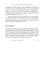
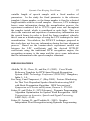
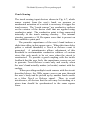
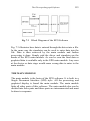
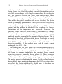
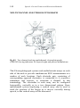
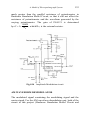
The modern day LP extractor consists of five major blocks:
pre-emphasis, frame blocking, windowing, autocorrelation analysis
and LPC computation. These are the procedures to calculate the
LPC coefficients and they are shown in Fig. 1.1. Each block in the
figure is described in the following sections.
PRE-EMPHASIS
Pre-emphasis is done to improve the signal-to-noise ratio (SNR), it
also increases the magnitude of the higher signal frequencies. The
front end process the speech signal using Linear Predictive Coding
(LPC) to obtain the coefficients, which represent its feature. The
first step to the process is to pre-emphasize the signal so that the
signal is spectrally flatten and make it less susceptible to finite
precision effects later in the signal processing. The pre-emphasis
is using the widely used first-order system as follows:
x ( n) = x ( n) − 0.95 x ( n − 1)
(1.1)
Linear Predictive Coding
SPEECH SIGNAL
PRE-EMPHASIS
x ( n) = x ( n) − 0.95 x ( n − 1)
FRAME BLOCKING
sˆ(n) = x( Li + N )
HAMMING WINDOWING
⎛ 2πn ⎞
⎟
⎝ N ⎠
w( n ) = 0.54 − 0.46 cos⎜
AUTO-CORRELATION ANALYSIS
N −1−m
R(m) =
∑ x(n) x(n + m)
n =0
LPC COMPUTATION
x ( n) ≅ a1 x ( n − 1) + a 2 x ( n − 2) + ... + a p x ( n − p )
LP
COEFFICIENTS
Fig. 1.1 Flow diagram of LPC process
3
4
Speech: Current Feature and Extraction Methods
FRAME BLOCKING
The result from the pre-emphasized signal is divided to equal
length frames of length N. The start of each frame is offset from
the start of the previous frame by L samples. The start of the
second frame begins at L and the third would begin at 2L and so
on. But, if L≤N, then adjoining frames will overlap and the LP
spectral estimates will show a high correlation. In this research, the
sampling frequency is 16 kHz, with average frame of 40 and
overlap of 10 ms. If we define xi as the ith segment of the sampled
speech s and I frames are required then the frame blocking process
can be described as
sˆ(n) = xi ( Li + N ), n = 0, 1, 2, ..., N - 1 , i = 0, 1, 2, ..., I - 1
(1.2)
WINDOWING
The purpose of windowing generally is to enhance the quality of
the spectral estimate of a signal and to divide the signal into frames
in time domain. Thus, after pre-emphasis, the signal is windowed
using the commonly used Hamming window function to fit the
purpose mentioned, where N is the length of the window. The
Hamming window used is written as
⎛ 2πn ⎞
w(n) = 0.54 − 0.46 cos⎜
⎟,
⎝ N −1⎠
for 0 ≤ n ≤ N-1
(1.3)
Linear Predictive Coding
5
LPC COEFFICIENTS COMPUTATION
Fundamental criteria of an LPC model for a sample speech at time
n, denoted as x(n) is an approximation of a linear combination of
previous samples, which is represented as
x(n) ≅ a1x(n − 1) + a2 x(n − 2) + ... + a p x(n − p)
(1.4)
where a1, a2,…,ap are coefficients which was assumed to be
constant for each speech frame.
To make an exact approximation to the speech signal x(n), an error
term which is the excitation of the signal is included as a filtering
term to Equation (1.4). G is the excitation gain and u(n) is the
normalized excitation.
p
x ( n) = ∑ a k x ( n − k ) + Gu ( n)
k =1
(1.5)
Using z-transform, Equation (1.5) becomes
p
−i
X ( z ) = ∑ a k z X ( z ) + GU ( z )
k =1
(1.6)
So the transfer function, H(z) is
H ( z) =
X ( z)
GU ( z )
=
1
p
−i
1 − ∑ ai z
k =1
=
1
A( z )
(1.7)
6
Speech: Current Feature and Extraction Methods
Then, the estimated x(n) which is also the linear combination of
previous samples, is define as
p
xˆ ( n ) = ∑ a x ( n − k )
k
k =1
(1.8)
The prediction error is the difference between the real signal and
the estimated signal:
p
e = x ( n) − xˆ ( n) = x ( n) − ∑ a k x ( n − k )
k =1
(1.9)
The error over a speech segment is defined as
p
⎡
⎤
E n = ∑ e n2 ( m ) = ⎢ ∑ x n ( m) − ∑ a k x n ( m − k ) ⎥
m
k =1
⎢⎣m
⎥⎦
2
(1.10)
The next step is to find ak by taking the derivative of En with
respect to ak and set them to zero.
∂E n
= 0 for k=1, 2, …, p.
∂a k
(1.11)
This brings Equation (1.10) to
p
∑ a k ∑ s n ( m − i )s n ( m − k ) = ∑ s n ( m )s n ( m − i )
k =1
m
m
(1.12)
7
Linear Predictive Coding
The calculation for ak which is a1, a2, .., ap will utilize autocorrelation through Durbin’s algorithm described next.
AUTOCORRELATION
The windowed signal then go through the autocorrelation process,
which is represented in Equation (1.13), p is the order of LPC
analysis. This is based on the estimated time average
autocorrelation.
N −1 − m
Rˆ ( m ) = ∑ x ( n ) x ( n + m ),
for m = 0 ,1, 2 ,.., p
n=0
(1.13)
xn(n) is the windowed signal, where xn(n)=x(n)w(n).
In matrix form, the set of linear equations can be expressed as:
Rm(1)
Rm(2)
⎡ Rm(0)
⎢ R (1)
Rm(0)
Rm(1)
⎢ m
⎢ Rm(2)
Rm(1)
Rm(0)
⎢
L
L
⎢ L
⎢ L
L
L
⎢
⎢⎣Rm( p−1) Rm( p−2) Rm( p−3)
L
L
L
L
L
L
Rm( p−1)⎤ ⎡â1 ⎤ ⎡Rm(1)⎤
⎢ ⎥
Rm( p−2)⎥⎥ ⎢â2 ⎥ ⎢⎢Rm(2)⎥⎥
Rm( p−3)⎥ ⎢â3 ⎥ ⎢Rm(3)⎥
⎥ ⎢ ⎥ =⎢
⎥
L ⎥ ⎢L⎥ ⎢ L ⎥
L ⎥ ⎢L⎥ ⎢ L ⎥
⎥⎢ ⎥ ⎢
⎥
Rm(0) ⎦⎥ ⎣⎢âp ⎦⎥ ⎣⎢Rm( p)⎦⎥
(1.14)
The common LPC analysis is using Durbin’s recursive algorithm,
which is based on Equations (1.15)-(1.20) and result of matrix
equation in (1.14):
8
Speech: Current Feature and Extraction Methods
E ( 0 ) = R(0)
(1.15)
i −1
ki =
R( i ) − ∑ a (j i −1 ) R( i − j )
j =1
,
E ( i −1 )
for
1≤i ≤ p
ai( i ) = k i
(1.16)
(1.17)
a (ji ) = a ij−1 + ki aii−−1j ,
for
Ei = (1 − k i2 ) Ei −1
1 ≤ j ≤ i −1
(1.18)
(1.19)
These equations are solved recursively for i = 0, 1,…, p, where p is
the order of the LPC analysis. Then, the final solution is when i =
p, which is
a j = a jp ,
for 1 ≤ j ≤ p
(1.20)
BURG’S METHOD
The Burg’s method for auto-regression spectral estimation is based
on minimizing the forward and backward prediction errors while
satisfying the Levinson-Durbin recursion. In contrast to other
auto-regression estimation methods like the Yule-Walker, the
Burg’s method avoids calculating the autocorrelation function, and
instead estimates the reflection coefficients directly.
9
Linear Predictive Coding
Let assume
f p (n) = e +p (n)
rp (n) = e −p (n) (backward
(forward prediction) and let
prediction).
kp
is
calculated
by
minimizing the sum of the squares of the forward and backward
prediction errors over the window, which is
E=
N −1 2
1
2
∑ f ( j ) + r ( j + 1)
p
p
2( N − P) j = p
(1.21)
and
E=
[
]
2
1 N−1
2
∑ f p−1(j)+ k prp−1(j) + ⎡⎢rp−1(j)+ kpf p−1(j)⎤⎥
⎣
⎦
2(N+ P) j=p
(1.22)
where kp is the desired partial correlation coefficient and fp 1 and rp1 are known from the previous pass. Error minimization can be
done by differentiating the error in Equation 1.22.
After simplification, the differentiation is:
1 N−1 ⎡ 2
∂E
2
=
∑ k p ⎢f p−1(j) + rp−1(j)⎤⎥ + 2fp−1(j)rp−1(j)
⎦
∂k p N − P j=p ⎣
(1.23)
Setting the derivative to zero gives the following recursive formula
for kp:
kp = −
2P
Q
(1.24)
10
where
Speech: Current Feature and Extraction Methods
P=
N −1
∑ f p −1 ( j )rp −1 ( j )
(1.25)
j= p
and
Q=
N −1
∑
j= p
f p2−1 ( j )rp2−1 ( j )
(1.26)
Once the reflection coefficient is determined, the predictor
coefficients can be calculated. If the autocorrelations are required,
Burg’s shows that Rp can be estimated by applying the new order-p
predictor to the previous estimates R0, R1, …, Rp-1 which is:
p
R p = − ∑ a p (i ) R p −1
(1.27)
i =1
The primary advantages of the Burg method are resolving closely
spaced sinusoids in signals with low noise levels, and estimating
short data records, in which case the AR power spectral density
estimates are very close to the true values (Parsons, 1986).
However, the accuracy of the Burg method is lower for high-order
models, long data records, and high signal-to-noise ratios. The
spectral density estimate computed by the Burg method is also
susceptible to frequency shifts (relative to the true frequency)
resulting from the initial phase of noisy sinusoidal.
Linear Predictive Coding
11
BIBLIOGRAPHIES
Bendat, J. S. and Piersol, A. G. (1984). Random Data: Analysis
and Measurement Procedures. New York: Wiley Intersciene.
Flanagan, J. L. and Ishizaka, K. (1976). Automatic Generation of
Voiceless Excitation in a Vocal Cord Vocal Tract Speech
Synthesizer. IEEE Transactions on Acoustics, Speech, and
Signal Processing. 24(2): 163-170.
Holmes, J. and Holmes, W. (2002). Speech Synthesis and
Recognition. 2nd Edition. London: Taylor and Francis.
Nong, T. H., Yunus, J., and Wong, L. C. (2002). SpeakerIndependent Malay Isolated Sounds Recognition. Proceedings
of the 9th International Conference on Neural Information
Processing. 5: 2405-2408.
Parsons, T. W. (1986). Voice and Speech Processing. New York :
McGraw-Hill.
Patil, P. B. (1998). Multilayered Network for LPC Based Speech
Recognition. IEEE Transactions on Consumer Electronics.
44(2): 435-438.
Rabiner, L. and Juang, B. H. (1993). Fundamentals of Speech
Recognition. Englewood Cliffs, New Jersey: Prentice Hall.
Rabiner, L. R. and Schafer, R. W. (1978). Digital Processing of
Speech Signals. Englewood Cliffs, New Jersey: Prentice Hall.
Sudirman, R., Salleh, Sh-H., and Ming, T. C. (2005). PreProcessing of Input Features using LPC and Warping Process.
Proceeding of International Conference on Computers,
Communications, and Signal Processing. 300-303.
Sze, H. K. (2004). The Design and Development of an
Educational Software on Automatic Speech Recognition.
Universiti Teknologi Malaysia: Master Thesis.
Tebelskis, J, Waibel, A, Petek, B., and Schmidbauer, O. (1991).
Continuous Speech Recognition using Linked Predictive
Neural Networks. International Conference on Acoustics,
Speech, and Signal Processing. 1: 61-64.
12
Speech: Current Feature and Extraction Methods
Zbancioc, M and Costin, M. (2003). Using Neural Networks and
LPCC to Improve Speech Recognition. International
Symposium on Signals, Circuits, and Systems. 2: 445-448.
2
HIDDEN MARKOV MODEL
Rubita Sudirman
Ting Chee Ming
Hong Kai Sze
INTRODUCTION
In this chapter, the Hidden Markov Model which is a well-known
and widely used statistical method for characterizing the spectral
properties of the frames of a pattern is presented. The basic theory
of Markov chain have been known to mathematicians and
engineers for more than 80 years ago, but it is only in the past few
decades that it has been applied to speech processing [Rabiner,
1989]. The basic theory of Hidden Markov Models was published
in a series of classic papers by Baum and his colleagues in the late
sixties and early seventies and was implemented for speech
processing applications by Baker at CMU and by Jelinek and his
colleagues at IBM in the 1970s (Rabiner and Juang, 1993).
Processes from the real world usually produce outputs that can
be observed and these outputs are characterized as signals. The
signal can be discrete, such as characters from an alphabet and
quantized vectors from a codebook. Alternatively, the signal can
be continuous, for example speech samples, temperature
measurements, music etc. Signal can be either stationary or nonstationary. It can be pure or contains noise or corrupted by
transmission of distortions and reverberation (Rabiner, 1989).
Chapter 1 has described that speech is a time-varying process
that has been modelled with linear systems, such as LPC analysis.
14
Speech: Current Feature and Extraction Methods
This is done by assuming that every short-time segment of
observation is a unit with a pre-chosen duration (Rabiner and
Juang, 1993). On most physical systems, the duration of short time
segment is determined empirically. The concatenation of these
short units of time makes no assumptions about the relationship
between adjacent units. Temporal variation can either be big or
small. The template approach is proven to be useful and becomes
the fundamental of many speech recognition systems.
The template method, albeit its usefulness, may not be the most
efficient technique. Many real world processes are observed to
have a sequential changing behaviour. The properties of the
process are commonly held steadily with minor fluctuations, for a
certain period, then at certain instances, change to another set of
properties. The opportunity for more efficient modelling can be
exploited if these periods of quasi steady behaviour are first
identified. Secondly, assumption has to be made that temporal
variations within each of these steady periods can be represented
statistically [Rabiner, 1989]. Hidden Markov model is a more
efficient representation that can be obtained using a common shorttime model for each of the steady part of the signal, along with
some characterizing of how one such period evolves to the next.
DEFINITION OF HMM
According to Rabiner and Juang (1993), hidden Markov model is a
doubly embedded stochastic process with an underlying stochastic
process that is not directly observable (it is hidden) but can be
observed only through another set of stochastic processes that
produce the sequence of observations.
An example from Rabiner (1989) is adapted and presented here
to illustrate the idea of HMM. Try to imagine the following
scenario. Let’s say you are in one room with a curtain that you
cannot see what is happening through the curtain.
On the other side is a person who is doing a coin-tossing
experiment with a few coins. The person does not let you know
Hidden Markov Model
15
which coin he selects at any time. Instead he tells you the result of
each coin flip. Thus a sequence of hidden coin-tossing experiments
is performed, with the observation sequence consists a series of
heads and tails. Here you observe the coin tossing result as follow:
O = (HTTHTHHHTTT…T), where H stands for heads and T
stands for tails.
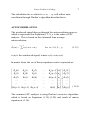
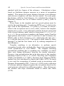
From the experiment above, the problem is how we want to build
an HMM to explain the observed sequence of results. One
possibility is by considering the experiment is performed using a ‘2
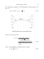
biased coins’, the possibilities are shown in Fig. 2.1.
Fig. 2.1 Two Biased Coin Model
In Fig. 2.1, there are 2 states, and each state represents a coin. In
state 1, the probability for the coin to produce a head is 0.75 while
the probability for it to produce a tail is 0.25. In state 2, the
probability to produce head is 0.25 while the probability to
produce tail is 0.75. The probability of leaving and re-entering both
states is 0.5. Here we associate every state with a biased coin. Now
we consider the HHT tossing experiment. We assume that the 1st
H is thrown using the 1st coin, the 2nd H with the 2nd coin and the
T is thrown using the 2nd coin. Now we calculate the probability
16
Speech: Current Feature and Extraction Methods
for it to happen with the assumption that this person starts with the
1st coin. The answer is (1 × 0.75) × (0.5 × 0.25) × (0.5 × 0.75) =
0.03516. For the second case, if the first 2 H are thrown using the
1st coin while T is thrown with the 2nd coin, the probability for it
to happen is (1 × 0.75) × (0.5 × 0.75) × (0.5 × 0.75) = 0.1055. Here
we notice that using a different model, the probability of getting
the same observations becomes different.
There are a few important points about the HMM. First, the
number of states of the model needs to be decided. However, the
decision is difficult to make without a priori information about the
system, thus sometimes trial and error is needed before the most
appropriate model size is known. Second, the model parameters
such as state transition probabilities and the probabilities of heads
and tails in each state) need to be optimized to best represent the
real situation. Finally, the size of sequence cannot be too small, if
this happens, the optimal model parameters cannot be estimated
[Rabiner and Juang, 1993].
ELEMENT OF AN HMM
The example from the previous section gives the idea of what
HMM is and how it can be applied in that simple scenario. The
elements of a HMM need to be defined as explained in Rabiner
and Juang (1993).
The discrete density HMM is characterized as follow:
(i) The number of states in the model, N. In the coin-tossing
experiments, each distinct biased coin represents one state.
Usually the states are interconnected in such a way that every
state can be reached by the others. This is called an ergodic
model. The individual states are labelled as {1, 2, …., N} and
the state at time t is denoted as qt.
(ii) The number of distinct observation symbols per state, M. The
observation symbols represent the physical output of the
Hidden Markov Model
17
modelled system. In the coin-tossing experiment, the
observation symbols are heads and tails. The individual
symbols are denoted as V = {v1, v2, …, vM}
(iii) The state transition probability distribution, A = {aij} which
can be expressed in the following form:
aij = P[qt +1 = j qt = i ]1 ≤ i, j ≤ N
(2.1)
(iv) The observation symbol probability distribution, B={bj(k)}
which can be expressed in the form below:
b j (k ) = P[ot = v k q t = j ],1 ≤ k ≤ M
(2.2)
(v) The initial state distribution π = {πi} in which
Π i = P[q1 = i ]1 ≤ i ≤ N
(2.3)
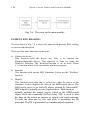
THREE PROBLEM OF HMM
There are three key problems of interest that must be solved in
order to apply HMM into the real applications. These problems are
described in [Rabiner and Juang, 1993], [Rabiner, 1989] and [3].
Problem 1: Given the observation sequence O=O1O2…Ot and
a model λ=(A,B,Π), how do we efficiently compute P(O, λ),
the probability of the observation sequence, given the model?
This is an evaluation problem. This can be viewed as getting a
score on how well a given model matches a given observation
sequence. This is useful but we need to choose among several
competing models.
18
Speech: Current Feature and Extraction Methods
Problem 2: Given the observation sequence O=O1O2…Ot and
a model λ, how do we choose a corresponding state sequence
Q=q1q2…qt which is optimal in some meaningful sense, for
example, it is most suitable to explain the observations?
The second problem is the one in which we attempt to uncover
the hidden part of the model to find the correct state sequence.
However there is usually none to be found. In practical
situations, the optimality criterion is usually used to best solve
the problem as good as possible. For continuous speech
recognition, the learning model structure is used to determine
the optimal state sequences and compute the average statistics
of the individual states.
Problem 3:
How to adjust the model parameters
λ=(A,B,Π) such that P(O, λ) is maximized?
The third problem is the problem of optimizing the model
parameters to best describe the given observation sequences and
this is known as the training problem.
SOLUTION TO THE PROBLEM
The solutions to the aforementioned three problems are the key
steps in applying HMM in speech recognition systems. Here the
formal mathematical solutions for each problem for HMM are
adapted from Rabiner (1989).
Problem 1
The probability of the observation sequence needs to be calculated,
given the model parameters. Thus the simplest solution is to
enumerating every possible state sequence of length T (the number
of observations). A fixed state sequence Q (Q=q1q2…qT) is
Hidden Markov Model
19
selected and the probability of the observation sequence O is given
by the following equation:
P (O Q, λ ) = bq2 (O1 ) • bq2 (O2 ) … bqT (Ot )
(2.4)
while the probability of such a state sequence Q happens is given
by the following:
P(Q, λ ) = Π q1 a q1q2 a q2 q3 … a qT −1qT
(2.5)
Then the product of both probabilities represented by that is
P(O,Q|λ), the probability of the observation sequence happening
with the state sequence Q. To calculate P(O|λ), calculations have to
be made for every possible state sequence Q, then summing up all
possibilities together. This calculation is computationally
unfeasible, even for small value of N and T. Thus a more efficient
procedure is required to solve Problem 1.
The method is called forward-backward procedure. Here the
forward variable αt(i) is defined as the probability of the partial
observation sequence O1,O2,...Ot (until time t) and state i, at time t,
given the model λ and can be calculated using the Forward
Procedure:
Initialization:
α 1 (i ) = Π i bi (Oi ),1 ≤ i ≤ N
(2.6a)
Induction:
⎡N
⎤
α t +1 ( j ) = ⎢∑ α t (i )aij ⎥b j (Ot +1 ),1 ≤ t ≤ T − 1,1 ≤ j ≤ N (2.6b)
⎣ i =1
⎦
Termination:
P(O λ ) = ∑ α T (i )
N
i =1
(2.6c)
20
Speech: Current Feature and Extraction Methods
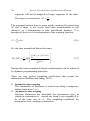
Step 1 actually initializes the forward probability of the initial
observation O1. The induction step is illustrated below, which
shows how the state sj is reached at time t+1 from the N possible
state qi, i=1,2,…,N at time t.
Fig. 2.2 Forward procedure
αt(i), the probability of O1,O2,...Ot, are observed and the state stops
at qi at time t, and the product αt(i)aij is the probability of the event
that O1,O2,...Ot, are observed and the state stops at qj at time t+1 via
state qi at time t. Adding up these products over all N possible
states, at time t result in the probability of qj at time t+1 with all the
accompanying previous partial observations. After this is done, the
summation is multiplied with bj(Ot+1), which means the probability
of Ot+1 happening at state qj at time t+1 with all accompanying
previous partial observations. The last termination step gives the
desired final result P(O|λ) as the sum of all terminal forward
variables.
The forward procedure needs fewer computations. It involves
only N(N+1)(T+1)+N multiplications and N(N-1)(T-1) additions
calculations.
Hidden Markov Model
21
Similarly, the backward variable β, which represents the
probability of the partial observation sequence from t+1 to the end,
given state i at time t and model λ, can be calculated as follows:
Initialization:
β T (i ) = 1
1≤ i ≤ N
(2.7a)
Induction:
β T (i ) = ∑ aij b j (Ot +1 )β t +1 ( j ),
t = T − 1, T − 2,......,1
1≤ i ≤ N
(2.7b)
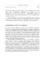
The first step defines all βT(i) to be 1. The induction step can be
illustrated as shown in Fig. 2.3. It shows that in order to have been
in state qi at time t, and to account for the rest of the observation
sequence, transition has to be made for every N possible states at
time t+1, accounted for the observation symbol Ot+1 in that state,
and this account for the rest of the observation sequence.
Fig. 2.3 Backward Procedure
22
Speech: Current Feature and Extraction Methods
Problem 2
There are several possible ways to solve this problem, since there
are a few possible optimally criteria. One possible optimality
criterion is by choosing the states, it, that are individually most
likely. By doing this the expected number of correct individual
states is maximized.
A new variable γ can be defined such that:
γ t (i ) = p(it = qi O, γ )
(2.8)
which represents the probability of being in state i at time t, given
the observation sequence O, and the model λ. In term of the
forward and backward variable, it can be expressed as:
λi (t ) =
α t (i )β t (i )
N
∑ α (i )β (i )
i =1
t
(2.9)
t
Because the α accounts for O1O2...Ot, and state qi at time t,
while β accounts for Ot+1Ot+2...OT given the state qi at time t. The
normalization factor P(O|λ) makes γi(t) a conditional probability.
Using γi(t), the individual most likely, it, at time t is:
qt = arg min [γ t (i )],1 ≤ t ≤ T
(2.10)
1<i < N
However, finding the optimal states might be a problem,
especially when there are disallowed transitions. The optimal state
obtained from this way may be an impossible state sequence since
it simply looks for the most likely state at every instance without
regarding to the global structure, neighbouring state and the length
of the observation sequence.
The disadvantage of the above methods is the need of global
constraint on the derived optimal state sequence. Another
23
Hidden Markov Model
optimality criteria may be used to determine the single best path
with the highest probability, by maximizing P(O,I|λ). A formal
method to find this single best state sequence is by using the
Viterbi Algorithm.
Initialization:
δ t (i ) = Π i bi (O1 )
ϕ1 (i ) = 0
1≤ i ≤ N
(2.11a)
Recursion:
δ t ( j ) = max [δ t −1 (i )aij ]b j (Ot )
1<i < N
ϕ t ( j ) = arg max [δ t −1 (i )aij ]
1< j < N
2≤t ≤T
1≤ j ≤ N
(2.11b)
2≤t ≤T
1≤ j ≤ N
Termination:
P = max [δ T (i )]
(2.11c)
1< j < N
Alternatively, the logarithms version can be used:
Initialization:
δ t (i ) = log(Π i ) + log(bi (Oi ))
ϕ1 (i ) = 0
1≤ i ≤ N
(2.12a)
24
Speech: Current Feature and Extraction Methods
Recursion:
δ t ( j ) = max [δ t −1 (i ) + log(aij )] + log(b j (Ot ))
(2.12b)
1< j < N
2 ≤ t ≤ T ,1 ≤ j ≤ N
ϕ t ( j ) = arg max [δ t −1 (i ) + log(aij )]
1< j < N
2 ≤ t ≤ T ,1 ≤ j ≤ N
Termination:
P = max [δ T (i )]
(2.12c)
1< j < N
The calculation required for this alternative implementation is N2T
additions. It does not need multiplications, thus making it more
computationally efficient. The logarithmic model parameters can
be calculated once and saved, thus the cost of finding the
logarithms is negligible.
Problem 3
The third problem is to readjust the model parameters {A,B,π} to
maximize the probability of the observation, when the model is
given. This is the most difficult problem and there is no known
way of solving the maximum likelihood model analytically. Hence,
an iterative procedure, such as the Baum-Welch method, or
gradient techniques must be used for optimization. Iterative BaumWelch method is discussed here.
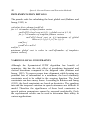
First, a new variable ξt(i,j) is defined which represents the
probability of being in state i at time t and state j at time t+1, given
25
Hidden Markov Model
the observation sequence O. The illustration of this process is in
Fig. 2.4.
ξ t (i, j ) = P(qt = i, qt +1 = j O, λ )
(2.13)
Fig. 2.4 Illustration of probability state
Thus we can write ζt(i,j) as:
ξ t (i, j ) =
=
α t (i )aij b j (Ot +1 )β t +1 ( j )
P(O λ )
α t (i )aij b j (Ot +1 )β t +1 ( j )
N
N
∑∑ α (i )a b (O )β ( j )
i =1 j =1
t
ij
j
t +1
(2.14)
t +1
and γ, is the probability of being in state i at time t:
N
γ t (i ) = ∑ ξ t (i, j )
j =1
(2.15)
26
Speech: Current Feature and Extraction Methods
Thus the re-estimation formulas of probability parameters are as
follow:
π j = γ 1 (i )
(2.16a)
T −1
aij =
∑ ξ (i, j )
t =1
T −1
t
∑ γ (i )
t =1
T −1
∑ α (i )a b (o )β ( j )
=
ij
t +1
j
t +1
∑∑ α (i )a b (o )β ( j )
t
T
t
t =1
T −1 N
t
t =1 j =1
ij
t +1
j
(2.16b)
t +1
N
∑ ∑ α (i )a b (o )β ( j )
b j (k ) =
t
t=
j =1
s ,t , ot = vk
T
ij
j
t +1
t +1
N
∑∑ α (i )a b (o )β ( j )
t =1 j =1
t
ij
j
t +1
(2.16c)
t +1
The re-estimation of π simply means the number of times in state i
at time t=1. The re-estimation of aij is the expected number of
transitions from state i to state j divide by expected number of
transitions from state i. The bj(k) is re-estimated using the expected
number of time in state j and observation symbol vk divided by the
expected number of times in state j.
If initial model is defined as λ and the re-estimation model as
λ’, then λ’ is the more likely model in the sense that
P(O|
λ’)>P(O| λ). This means another model that the observation
sequence is more likely to be produced have been found.
Iteratively using λ’ in place of λ and repeat the re-estimation
calculation, the probability of O being observed is improved, until
some limiting point is reached.
Hidden Markov Model
27
IMPLEMENTATION ISSUES WITH HMM
The discussion in the previous section has been around theory of
HMM. In this section, several practical implementation issues are
handled.
Scaling
For a sufficient long observation sequence, the dynamic range of
αt(i) computation can go beyond the precision range of any
existing computer. There exists a scaling procedure that can be
used to multiply the alpha values by a scaling coefficient which is
independent of i. A similar scaling can also be done to the βt(i).
Thus at the end the scaling coefficients are cancelled out.
Minimum Value for bjk
A second issue is the use of finite set of training data for training
the HMM model. If a symbol does not exist often in the
observation sequence, the probability for that symbol in some
states can become 0. This is not desirable because the probability
score can become 0 because of that bj(k). One way to solve this is
by setting a minimum value for bj(k).
Multiple Observation Sequence
The re-estimation formulas in the previous section consider only a
single training observation sequence. However in the real
applications, multiple observation sequences are usually available,
then model parameters can be re-estimated by a little
modifications.
28
Speech: Current Feature and Extraction Methods
1
∑ P ∑ α (I )a b (o )β ( j )
T −1
K
aij =
k =1
K
1
∑
k =1 Pk
k t =1
T −1 N
k
t
ij
k
t +1
j
k
t +1
∑∑ α (i )a b (o )β ( j )
t =1 j =1
t
ij
j
t +1
(2.17a)
t +1
1 T −1 k N
α t (i )aij b j (ot +1 )β t +1 ( j )
∑
∑ αt ∑
j =1
k =1 Pk t =1
K
b j (l ) =
s ,t ,ot = vt
1 T −1 N
∑
∑∑ α t (i )aij b j (ot +1 )β t +1 ( j )
k =1 Pk t =1 j =1
K
(2.17b)
From the above equations, observe that the modified re-estimation
formulas are actually a summation of the individual re-estimation
for each training observation sequence divided by the individual
probability for that particular sequence.
BRIEF REVIEW OF CONTINUOUS DENSITY HMM
The discussion in the previous section has considered only when
the observations are discrete symbols from a finite alphabet.
However, observations are often continuous signals. Although we
can convert continuous signal representations into sequence of
discrete symbols using vector quantization method, sometimes it is
an advantage to use HMMs with continuous observation densities.
Hidden Markov Model
29
REFERENCES
Rabiner, L.R. (1989). A tutorial on hidden Markov models and
selected applications in speech recognition. Proceedings of the
IEEE. 77(2):257 –286.
Rabiner, L. and Juang, B. H. (1993). Fundamentals of Speech
Recognition. Englewood Cliffs, N.J.: Prentice Hall. 69-481.
Mohaned, M. A. and Gader, P. (2000). Generalized Hidden Markov
Models – Part I-Theoretical Frameworks. IEEE Transactions on
Fuzzy Systems. 8(1): 67 –81.
Becchetti, C. and Ricotti, L. P. (2002). Speech Recognition Theory
and C++ Implementation. West Sussex: John Wiley & Sons Ltd.
122-301.
3
DYNAMIC TIME WARPING
Rubita Sudirman
Khairul Nadiah Khalid
INTRODUCTION
Template matching is an alternative to perform speech recognition.
However, the template matching encountered problems due to
speaking rate variability, in which there exist timing differences
between the two utterances. Speech has a constantly changing
signal, thus it is almost impossible to get the same signal for two
same utterances. The problem of time differences can be solved
through DTW algorithm: warping the template with the test
utterance based on their similarities. So, DTW algorithm actually
is a procedure, which combines both warping and distance
measurement. DTW is considered as one effective method in
speech pattern recognition, however the bad side of this method is
that it requires a long processing time plus large storage capacity,
especially for real time recognitions. Thus, it is only suitable for
application with isolated words, small vocabularies, and speaker
dependent with/without multi-speaker, which has yielded a good
recognition under these circumstances (Liu, et al., 1992).
Human speeches are never at the same uniform rate and there
is a need to align the features of the test utterance before
computing a match score. Dynamic Time Warping (DTW), which
is a Dynamic Programming technique, is widely used for solving
time-alignment problems.
32
Speech: Current Feature and Extraction Methods
DYNAMIC TIME WARPING
In order to understand Dynamic Time Warping, two procedures
need to be dealt with. The first one is the information in each
signal that has to be presented in some manner, called features.
(Rabiner and Juang, 1993). One of the features is the LPC-based
Cepstrum. The LPC-based Cepstrum procedure is the calculation
of the distances because some form of metric has to be used in the
DTW in order to obtain a match between the database and the test
templates. There are two types of distances, which are local
distances and global distances. Local distance is a computational
different between a feature of one signal and another feature.
Global distance is the overall computational difference between an
entire signal and another different length signal.
The ideal speech feature extractor might be the one that
produces the word that match the meaning of the speech. However,
the method to extract optimal feature from the speech signal is not
trivial. Thus separating the feature extraction process from the
pattern recognition process is a sensible thing to do, since it
enables the researchers to encapsulate the pattern recognition
process according to (Rabiner and Juang, 1993).
Feature extraction process outputs a feature vector at every
regular interval. For example, if an MFCC analysis is performed,
then the feature vector consists of the Mel-Frequency Cepstral
Coefficients over every fixed tempo. For a LPC analysis the
feature vector consists of prediction coefficients while the LPCbased Cepstrum analysis outputs Cepstrum coefficients.
Because the feature vectors could have multiple elements, a
method of calculating local distances is needed. The distance
measure between two feature vectors can be calculated using the
Euclidean distance metric. (Rabiner and Juang, 1993) Therefore,
the local distance between two feature vectors x and y is given by,
d ( x, y ) =
∑ (x
P
j =1
− yj)
2
j
(3.9)
Dynamic Time Warping
33
Although the Euclidean metric is computationally more expensive
than some other metrics, it gives more weight to large differences
in a single feature.
For example, let consider two feature vectors
A = a1 , a2 , a3 ,..., ai ,..., a I and B = b1 , b2 , b3 ,..., b j ,..., bJ , let A be the
template/reference speech pattern while B be the unknown/test
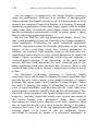
speech pattern. Translating sequences A and B into Fig. 3.1, the
warping function at each point is calculated. Calculation is done
based on Euclidean distance measure as a mean of recognition
mechanism. It takes the smallest distance between the test
utterance and the templates as the best match. For each point, the
distance called local distance, d is calculated by taking the
difference between two feature-vectors ai and bj:
d (i, j ) = b j − ai
(3.2)
Every frame in a template and test speech pattern must be used in
the matching path. If a point (i,j) is taken, in which i refers to the
template pattern axis (x-axis), while j refers to the test pattern axis
(y-axis), a new path must continue from previous point with a
lowest distance path, which is from point (i-1, j-1), (i-1, j), or (i, j1) of warping path shown in Fig. 3.2.
If D(i,j) is the global distance up to (i,j) with a local distance at
(i,j) given as d(i,j), then
D( i, j ) = min[D( i − 1, j − 1),D( i − 1, j ),D( i, j − 1)] + d( i, j )
(3.3)
34
Speech: Current Feature and Extraction Methods
j
Pm(I,J)
bJ
template pattern
Input pattern
adjustment
window
P(i,j)
bj
b2
b1
(1,1)
a1
a2
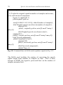
aI
ai
i
Template pattern
input pattern
Fig. 3.1 Fundamental of warping function
(i-1, j)
(i, j)
(i-1, j-1)
(i, j-1)
Fig. 3.2 DTW heuristic path type 1
Back to reference pattern A and B, if their feature vector B and an
input pattern with feature vector A, which each has NA and NB
frames, the DTW is able to find a function j=w(i), which maps the
Dynamic Time Warping
35
time axis i of A with the time axis j of B. The search is done frame
by frame through A to find the best frame in B, by making
comparison of their distances. After the warping function is
applied to A, distance d(i,j) becomes
d ( i , j( i )) = b j ' −a i
(3.4)
Then, distances of the vectors are summed on the warping
function. The weighted summation, E is:
I
E( F ) = ∑ d ( i , j( i ))* w( i )
i =1
(3.5)
where w(i) is a nonnegative weighting coefficient. The minimum
value of E will be reached when the warping function optimally
aligned the two pattern vectors.
A few restrictions have to be applied to the warping function to
ensure close approximation of properties of actual time axis
variations. This is to preserve essential features of the speech
pattern. Rabiner and Juang (1993) outlined the warping properties
as follows for DTW path Type I:
1.
2.
3.
4.
Monotonic conditions imposed: j (i − 1) ≤ j (i )
Continuity conditions imposed: j (i ) − j (i − 1) ≤ 1
Boundary conditions imposed: j (i ) = 1 and j ( J ) = I
Adjustment window implementation:
i − j (i ) ≤ r , r is a
positive integer
5. Slope condition: to hold this condition, say if b’j(i) moves
forward in one direction m times consecutively, then it must
also step n times diagonally in that direction. This is to make
sure a realistic relation between A and B, in which short
36
Speech: Current Feature and Extraction Methods
segments will not be mapped to longer segments of the other.
n
The slope is measured as: M = .
m
The warping function slope is more rigidly restricted by increasing
M, but if slope is too severe then time normalization is not
effective, so a denominator to time normalized distance, N is
introduced, however it is independent of the warping function.
I
N = ∑ w( i )
i =1
(3.6)
So, the time normalized distant becomes
⎡ ∑I d ( i , j( i ))* w( i ) ⎤
1
⎥
⎢
D( A, B ) = Min ⎢ i =1
⎥
I
N F
∑ w( i )
⎥
⎢
i =1
⎦
⎣
(3.7)
Having this time normalized distant, minimization can be achieved
by dynamic programming principles.
There are two typical weighting coefficients that permit the
minimization (Rabiner and Juang, 1993):
1. Symmetric time warping
The summation of distances is carried out along a temporary
defined time axis l=i+j.
2. Asymmetric time warping
Previous discussion has described the asymmetric type, in
which the summation is carried out along i axis warping B to
be of the same size as A. The weighting coefficient for
asymmetric time warping is defined as:
Dynamic Time Warping
w(i ) = j (i ) − j (i − 1)
37
(3.8)
When the warping function attempts to step in the direction of the j
axis,
the
weighting
coefficient
is
reduce
to
0
because j (i ) = j (i − 1) , thus w(i ) = 0 . Meanwhile, when the
warping function steps in the direction of i axis or diagonal, then
w(i ) = 1 , so N = I .
The asymmetric time warping algorithm only provides
compression of speech patterns. Therefore, in order to perform
speech pattern expansion, a linear algorithm has to be employed.
SYMMETRICAL DTW ALGORITHM
In speech signal, different speeches have different durations.
Ideally, when comparing different length of utterances of the same
word, the speaking rate and the utterance duration should not
contribute to the dissimilarity measurement. Several utterances of
the same word are possibly to have different durations while
utterances with the same duration differ in the middle because
different parts of the words have been spoken in different rates.
Thus a time alignment must be done in order to get the global
distance between two speech patterns.
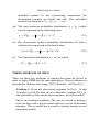
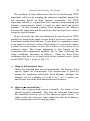
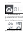
This problem is illustrated in Fig. 3.3, in which a “time to
time” matrix is used to visualize the alignment. The reference
pattern goes up the side and the input pattern goes along the
bottom. As shown in Fig. 3.3, “KOSsONGg” is the noisy version
of the template “KOSONG”. The idea is ‘s’ is closer match to “S”
compared with other alphabets in the template. The noisy input is
matched against all the templates. The best matching template is
the one that has the lowest distance path aligning the input pattern
to template. A simple global distance score for a path is simply the
sum of local distances that make up the path.
38
Speech: Current Feature and Extraction Methods
Fig. 3.3 Illustration of time alignment between pattern
“KOSONG” and a noisy input “KOSsONGg”
Now the lowest global distance path (or the best matching)
between an input and a template can be evaluated by all possible
paths. However, this is very inefficient as the possible number of
path increases exponentially as the input length increases. So some
constraints have to be considered on the matching process and
using these constraints as efficient algorithm.
There are many types of local constraints imposed, but they are
very straightforward and not restrictive. The constraints are:
1)
Matching path cannot go backwards in time.
2)
Every frame in the input must be used in a matching path.
3)
Local distance scores are combined and added to give a
global distance.
For now every frame in the template and input must be used in a
matching path. If a point (i,j) is taken in the time-time
Dynamic Time Warping
39
matrix(where i indexes the input pattern frame, j indexes the
template frame), then previous point must be (i-1,j-1), (i-1,j) or (i,j1). The key idea in this dynamic programming is that at point (i,j)
we can only continue from the lowest distance path that is from (i1,j-1),(i-1,j) or (i,j-1).
If D(i,j) is the global distance up to (i,j) and the local distance at
(i,j) is given by d(i,j), thus,
D(i, j ) = min[D(i −1, j −1), D(i −1, j ), D(i, j −1)] + d (i, j )
(3.10)
Given that D(1,1)=d(1,1), the efficient recursive formula for
computing D(i,j) can be found (Rabiner and Juang, 1993). The
final global distance D(n, N) is the overall score of the template
and the input. Thus, the input word can be recognized as the word
corresponding to the template with the lowest matching score. The
N value is normally different for every template.
The symmetrical DTW requires very small memory because
the only storage required is an array that holds every column of the
time-time matrix. The only direction that the match path can move
when at (i,j) in the time-time matrix are as shown in Fig. 3.4.
Fig. 3.4 The three possible directions the best matched may move
40
Speech: Current Feature and Extraction Methods
IMPLEMENTATION DETAILS
The pseudo code for calculating the least global cost (Rabiner and
Juang, 1993) is:
calculate first column (predCol)
for i=1 to number of input feature vector
curCol[0]=local cost at (i,0) + global cost at (i-1,0)
for j=1 to number of template feature vectors
curCol[j]=local cost at (i,j)+minimum of global
costs at (i-1,j),(i-1,j-1) or (i,j-1)
end for j
predCol=curCol
end for i
minimum global cost is value in curCol[number of templater
feature vectors]
VARIOUS LOCAL CONSTRAINTS
Although the Symmetrical DTW algorithm has benefit of
symmetry, this has the side effect of penalizing horizontal and
vertical transitions compared to the diagonal ones (Rabiner and
Juang, 1993). To ensure proper time alignment while keeping any
potential loss of information to a minimum, the local continuity
constraints need to be added to the warping function. The local
constraints can have many forms. According to Rabiner and Juang
(1993), the local constraints are based on heuristics. The speaking
rate and the temporal variation in speech utterances are difficult to
model. Therefore the significance of these local constraints in
speech pattern comparison cannot be assessed analytically. Only
the experimental results can be used to determine their utility in
various applications.
Dynamic Time Warping
41
BIBLIOGRAPHIES
Rabiner, L. and Juang, B. H. (1993). Fundamentals of Speech
Recognition. Englewood Cliffs, N.J.: Prentice Hall.
Liu, Y., Lee, Y. C., Chen, H. H., and Sun, G. Z. (1992). Speech
Recognition using Dynamic Time Warping with Neural
Network Trained Templates. International Joint Conference
in Neural Network. 2: 7-11.
4
DYNAMIC TIME WARPING
FRAME FIXING
Rubita Sudirman
Sh-Hussain Salleh
INTRODUCTION
Feature extraction is a vital part in speech recognition process
without good and appropriate feature extraction technique, a good
recognition cannot be expected. In this chapter, Dynamic Time
Warping Fixed Frame (DTW-FF) feature extraction technique is
presented. Further processing using DTW-FF algorithm to extract
another form of coefficients is also described in which these
coefficients will be used in the speech recognition stage. Also
included in this chapter is example of some results using the DTWFF method followed by the discussion.
DTW FRAME FIXING
In general, DTW frame fixing/alignment or DTW fix-frame
algorithm (DTW-FF) is done by matching the reference frames
against input frames with an emphasis on limiting the input frames
to the same number of reference frames. The algorithm is
composed based on compression and expansion technique. The
frame compression is done when several frames of unknown input
are matched to a single frame of reference template. On the other
hand, expansion is done when a single unknown input frame is
44
Speech: Current Feature and Extraction Methods
matched with few frames of the reference. Calculation is done
based on Euclidean distance measure as a mean of recognition
method. This means the lowest distance between a test utterance
and reference templates will have the best match. For each point,
the distance called as local distance, d is calculated by taking the
difference between two set of feature-vectors ai and bj (refer to
Chapter 3).
Every frame in the template and test speech pattern must be
used in the matching path. Considering DTW type 1 (which is the
type used in the experiment), if a point (i,j) is taken, in which i
refers to the test pattern axis (x-axis), while j refers to the template
pattern axis (y-axis), a new path must continue from previous point
with a lowest distance path, which is from point (i-1, j-1), (i-1, j),
or (i, j-1). Given a reference template with feature vector R and an
input pattern with feature vector T, each has NT and NR frames, the
DTW is able to find a function j=w(i), which maps the time axis i
of T with the time axis j of R. The search is done frame by frame
through T to find the best frame in R, by making comparison of
their distances.
Template matching is an alternative to perform speech
recognition beside other methods like linear time normalization,
vector quantization or even HMM. The template matching
encountered problems due to speaking rate variability, in which
there exist timing differences between the similar utterances.
However, time normalization has to be done prior to the template
matching found in Uma et al. (1992), Sae-Tang and Tanprasert
(2000), and Abdulla et al. (2003). Dynamic Time Warping (DTW)
method was first introduced by Sakoe and Chiba (1978), in which
it was used for recognition of isolated words in association with
Dynamic Programming (DP). Uma et al. (1992) used a collection
of reference pattern compared against the test pattern based on the
word patterns collected from different speakers. They did not use
the window and slope constraints found in Sakoe and Chiba
(1978).
Dynamic Time Warping Fixed Frame
45
The problem of time differences can be solved through DTW
algorithm, which is by warping the reference template against the
test utterance based on their features similarities. So, DTW
algorithm actually is a procedure that combines both warping and
distance measurement, which is based on their local and global
distance. In this research context, local distance is the distance
between the input data and the reference data for respective vectors
along the speech frames.
In this research, the time normalization is done based on DTW
method by warping the input vectors with a reference vector which
has almost similar local distance. It was done by expanding vectors
of an input to reference vectors which shows a vertical movement:
it shares the same feature vectors for a feature vector frame of an
unknown input. This frame alignment is also known as the
expansion and compression method, this is done following the
slope conditions described as follows. There are three slope
conditions that have to be dealt with in this research work, based
on the DTW Type 1 (refer to Fig. 3.1):
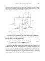
i- Slope is 0 (horizontal line)
When the warping path moves horizontally, the frames of the
speech signal are compressed. The compression is done by
taking the minimum calculated local distance amongst the
distance set, i.e. compare w(i) with w(i-1), w(i+1) and so on,
and choose the frame with minimum local distance.
ii- Slope is ∞ (vertical line)
When the warping path moves vertically, the frame of the
speech signal is expanded. This time the reference frame gets
the identical frame as w(i) of the unknown input source. In
other words, the reference frame duplicates the local distance
of that particular vertical warping frame.
46
Speech: Current Feature and Extraction Methods
iii- Slope is 1 (diagonal)
When the warping path moves diagonally, the frame is left as it
is because it already has the least local distance compared to
other movements.
Examples of the slope conditions are shown in Fig. 4.1.
template
a
compression
y
compression
a
s
expansion
s
s
a
a
y
a
a
Test input
Fig. 4.1 Compression and expansion rules
The F- and F+ is done by using our new so called DTW frame
fixing algorithm (DTW-FF). Consider the frame vectors of LPC
coefficients for input as i,…I, and reference as j…J, while F
denotes the frame.
Frame compression involves searching
minimum local distance out of distances in a frame set within a
threshold value represented as
F- = F(min{d(i,j)…(I,J)})
(4.1)
Dynamic Time Warping Fixed Frame
47
For example, if a horizontal warping path moved three frames in a
row, compression will take place. As stated in the Slope Condition
1, only one frame that has the least distance from it previous point
is selected to represent the DTW-FF coefficient.
Frame expansion involves duplicating a particular input frame to
multiple reference frames of w(i), represented as
F+ = F(w(i))
(4.2)
The duplicated frames are the expanded frames resulted from the
vertical warping path. The normalized data/sample has been tested
and compared to the typical DTW algorithm and results showed
the same global distance score.
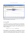
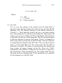
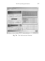
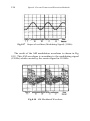
RESULTS OF DTW-FF ALGORITHM
The normalized data/sample has been tested and compared to the
typical DTW algorithm and results showed the same global
distance score. As a preliminary example to the DTW-FF
algorithm, Fig. 4.2 and Fig. 4.3 showed the comparison between
using the typical DTW and DTW-FF algorithm. It is clearly
shown that the input template has 39 frames (0-38) and the
reference template has 35 frames (0-34) and the warping path
showed the same score of 48.34.
48
Speech: Current Feature and Extraction Methods
Fig. 4.2 A warping path of word ‘dua’ generated from typical DTW
algorithm
However, it can be observed in Fig. 4.3 that expansion takes place
in frame 8 of the input template, being expanded to 6 frames (refer
to the y-axis which shows the frame expansion). Meanwhile,
compression occurs in frame 24 through 31 of the input template
whereby these frames are compressed to one frame only. This is
because the local distances between the frames are almost similar,
but it still considers the frame with least distance to represent those
frames in the warping path coordinates. Other compressions occur
in frame 0 and 1 as well as in frame 34 and 35 of the input signal,
both are compressed to one frame. Finally, the DTW-FF algorithm
was able to fix the test signal frame number equal to the reference
signal frame.
Dynamic Time Warping Fixed Frame
49
Fig. 4.3 A warping path generated from the DTW-FF algorithm showing
the expansion and compression of frames
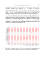
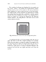
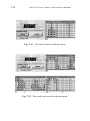
Fig. 4.4 shows an input with the frames that has been matched to a
reference template of the same utterance (word ‘kosong’). In this
example, initially the input template has 38 frames while the
reference template has 42 frames. By using the DTW-FF
algorithm the input frames have been expanded to 42, i.e. equals to
the number of frames of the reference template following the slope
conditions outlined earlier in this chapter. Let w(y) as the input
frame and r(x) as the reference frame.
50
Speech: Current Feature and Extraction Methods
Fig. 4.4 The DTW frame alignment between an input and a reference
template; the input which initially has 38 frames is fixed to 42 frames.
According to the slope condition (i), the local distances of the
unknown input frames of w(3),…, w(5)1 are compared and w(5)
appears to have the minimum local distance among these three
frames, so those 3 frames are compressed to one and occupies only
frame r(4). The same goes with frame w(6),…, w(8) in which
frame w(7) has the least local distance with respect to the reference
template, so they are compressed and occupies only frame r(5).
On the other hand, slope condition (ii) provides an expansion to the
input frame. For example, while frame w(15) of the input is
1
w represents the frame of the unknown input frames (in x-axis) while r represents the reference
template frame (in y-axis).
Dynamic Time Warping Fixed Frame
51
matched reference frame number
expanded to 4 frames, in which these 4 consecutive frames in the
reference template are identical; i.e. 4 frames of reference
template at frame r(10),…, r(13) have the same feature vectors as
frame w(15) of the input vectors, so frame w(15) occupies frame
r(10),…, r(13). These mean that frame w(15) of the input has
matched 4 feature vectors in a row of the reference template set.
Since the diagonal movement (slope condition (iii)) is the
fastest track (shortest path) towards achieving the global distance
point and giving the least local distance at all time compared to the
horizontal or vertical movements, no changes is made to the
frames involved, thus this slope considers a normal DTW
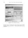
procedure. A closer view of the frame fixing between frame 4 and
16 in Fig. 4.4 can be viewed in Fig. 4.5.
Unknown input frame number
Fig. 4.5 A close-up view of Fig. 4.8 to show the compression and
expansion of template frames activities between frame 4 and frame 16
52
Speech: Current Feature and Extraction Methods
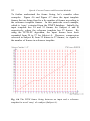
To further understand the frame fixing, let’s consider other
examples. Figure 4.6 and Figure 4.7 show the input template
frames that are being fixed to a fix number of frames according to
the reference template frames. In this particular word example,
which is ‘carry’ extracted from the TIMIT database. Initially the
input template has 24 and 32 frames for Subject A and B
respectively, where the reference template has 27 frames. By
using the DTW-FF algorithm, the input frames have been
expanded from 24 to 27 for Subject A. However, compression
occurred in Subject B, from 32 frames to 27 frames, i.e. equals to
the number of frames in reference template.
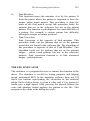
Fig. 4.6 The DTW frame fixing between an input and a reference
template for word ‘carry’ of a subject (Subject A).
Dynamic Time Warping Fixed Frame
53
Fig.4.7 The DTW frame fixing between an input and a reference
template for word ‘carry’ of another subject (Subject B)
In Fig. 4.7, frame compression is performed in frames r(7), r(8),
and r(9), and r(9) has the least local distance score (as indicated on
the reference template axis), thus loosing 2 frames here. On the
other hand, frame 19 is expanded to 6 frames, but considered as
gaining 5 frames, so the final number of frames after the fixing
process is equal to 24-2+5 = 27 frames.
Meanwhile in Fig. 4.8, frames r(1), r(2), r(3), and r(4) are
compressed to 1 (selecting r(4) which has the least local distance
score among the frames), thus loosing 3 frames. For frames r(5)
and r(6), the frames are compressed and frame 5 is selected
because of its lesser distance score than frame 6, thus losing by 1
frame, and the same goes to frame 20, 21, 22, and 23, they are
54
Speech: Current Feature and Extraction Methods
compressed and represented by frame 21, this time they are losing
3 frames. But frame 31 is expanded to 3 frames, means that it
gains 2 more frames in this expansion process. Therefore, after
frame fixing the total number of frames is equal to 32-3-1-3+2 =
27 frames.
DTW-FF features are obtained from the matching process in
the DTW-FF algorithm. The scores have been reduced from LPC
coefficient which is a 10-order feature vectors, into a coefficient
(which is called as DTW-FF coefficient) derived from each frame.
Besides fixing to equal number of frames between the unknown
input and the reference template, this activity has also
tremendously reduced the amount of inputs presented into the
back-propagation neural networks. As an example, calculation to
show the input size reduction for 250 samples of 49 frames with
LPC order-10 is as follows:
For input using the LPC coefficients,
InputLPC
= # of utterance × # of frames/utterance
× # of coefficient/frame
= 250 utterances × 49 frames/utterance
× 10 coefficient/frame
= 122,500 input coefficients
For input using the local distance score,
InputLD
= # of utterance × # of frames/utterance
× number of coefficient/frame
= 250 utterances × 49 frames/utterance
× 1 coefficient/frame
= 12,250 input coefficients
(4.1)
55
Dynamic Time Warping Fixed Frame
Therefore, the percentage of number coefficients reduced is
# of coefficients reduced (%) =
Input LPC − Input
Input LPC
LD
x100%
122500 − 12250
x100%
122500
= 90 %
=
Remember that the number of inputs to the back-propagation
neural networks has been reduced by 90% using the local distance
scores instead of the LPC coefficients, and still been able to yield
to a high recognition rate. The reduced coefficients percentage
will be higher if higher LPC order was used.
For example, if LPC of order 12 is used, then:
InputLPC = 250 utterances × 49 frames/utterance
× 12 coefficient/frame
= 147,000 input coefficients
Input using local distance score,
InputLD = 250 utterances × 49 frames/utterance
× 1 coefficient/frame
= 12250 input coefficients
Therefore, the percentage of number coefficients reduced is
Number of coefficients reduced (%) = 91.7%
56
Speech: Current Feature and Extraction Methods
These means a lot of network complexities and amount of
connection weights computations during the forward pass and
backward pass can be reduced. Thus a faster convergence is
achieved (also means less computation time) and this also allows
more parallel computing of the speech patterns being done at a
time (more patterns can be fed into the neural networks at the
same time).
From the observation of the experiment, the number of the frames
after being fixed, Nff is formulated as
N ff = N if − N cf + N ef
where Nif
(4.4)
number of input frame
Ncf
number of compressed frame
Nef
number of expanded frame
Having done the expansion and compression along the matching
path, the unknown input frame is matched to the reference
template frames. The frame fixing/ matching is a mean of solution
to speech frame variations whereby this technique still preserved
the global distance score as in the typical DTW method; the DTW
fixing frame (DTW-FF) algorithm only make adjustment on the
feature vectors of the horizontal and vertical local distance
movements, leaving the diagonal movements as it is with their
respective reference vectors. The frame fixing is done throughout
the samples, also taking considerations to the sample which has the
same number of frames as the averaged frames as the reference
template.
In comparison, the LTN technique (Salleh, 1997) used a
procedure of omitting and repeating the frames to normalize the
Dynamic Time Warping Fixed Frame
57
variable length of speech sample with a fixed number of
parameters. In the study the fixed parameter is the reference
template’s frame number, so the frame number is fixed to a desired
length suitable with the overall samples. However, LTN technique
looses some information during the normalization process: the
experiment conducted led to 13-22% equal error rate throughout
the samples tested, which is considered as quite high. This was
due to the omission and repetition of unnecessary information into
the speech frame (in order to fixed the frame numbers) whereby
this is seen as a disadvantage of using the LTN technique for time
normalization. Nevertheless, the DTW-FF technique proposed in
this study does not lose any information during the time alignment
process. Based on the counter-check experiment carried out
between the LPC coefficients and the derived DTW-FF
coefficients using the traditional DTW recognition engine, the
recognition accuracy is the same and this gives some indications
that the information in the speech samples remained.
BIBLIOGRAPHIES
Abdulla, W. H., Chow, D., and Sin, G. (2003). Cross-Words
Reference Template for DTW-based Speech Recognition
System. IEEE Technology Conference (TENCON). Bangalore,
India, 1: 1-4.
Sae-Tang, S and Tanprasert, C. (May 2000). Feature Windowing
for Thai Text-Dependent Speaker Identification using MLP
with Back-Propagation Algorithm. IEEE International
Symposium on Circuits and Systems, Geneva. 3: 579-582.
Sakoe, H. and Chiba, S. (1978 February). Dynamic Programming
Algorithm Optimization for Spoken Word Recognition. IEEE
Transactions on Acoustics, Speech and Signal Processing.
ASSP-26(1): 43-49.
Sakoe, H., Isotani, R., and Yoshida, K. (1989). SpeakerIndependent Word Recognition using Dynamic Programming
58
Speech: Current Feature and Extraction Methods
Neural Networks. Proceedings of International Conference in
Acoustics, Speech, and Signal Processing. 1: 29-32.
Salleh, S. H. (1997). An Evaluation of Preprocessors for Neural
Network Speaker Verification. University of Edinburgh, UK:
Ph.D. Thesis.
Soens, P. and Verhelst, W. (2005). Split Time Warping for
Improved Automatic Time Synchronization of Speech.
Proceeding of SPS DARTS, Antwerp, Belgium.
5
PITCH SCALE HARMONIC FILTER
Rubita Sudirman
Muhd Noorul Anam Mohd Norddin
INTRODUCTION
Pitch is defined as the property of sound that varies with variation
in the frequency of vibration. In speech processing aspect, pitch is
defined as the fundamental frequency (oscillation frequency) of the
glottal oscillation (vibration of the vocal folds). Pitch information
is one of speech acoustical features that not often taken into
consideration while doing speech recognition. In this research,
pitch is taken into consideration then it is optimized and was used
as another feature into NN along with DTW-FF feature. Pitch
contains spectral information of a particular speech, it is the feature
that was used to determine the fundamental frequency, F0 of a
speech at a particular time.
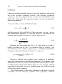
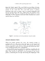
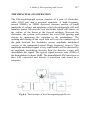
PITCH FEATURE EXTRACTION
The pitch feature considered in the study is extracted using a
method called pitch scaled harmonic filter (PSHF) (Jackson and
Mareno, 2003). In PSHF, pitch is optimized and these pitch
feature is retained and used as another input feature which is
combined with the DTW-FF feature for recognition using the NN.
These pitch features represent the formant frequencies of spoken
utterance. The optimization is needed in order to resolve glitches
60
Speech: Current Feature and Extraction Methods
due to octave error during the spectral activities, especially when
there is noise signal during the recording of the speech sample.
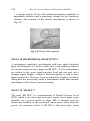
SFS
raw signal
(.wav file)
pitch
extraction
pitch
optimization
harmonic
decomposition
Fo
track
Fo r
Fo o
V(m)
U(m)
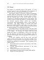
PSHF block
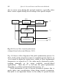
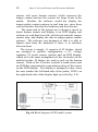
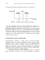
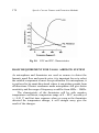
Fig. 5.4 Process flow of pitch optimization
(Adapted from Jackson and Mareno, 2003).
Fig. 5.4 shows a flow diagram of the pitch optimization process. In
short, firstly pitch extraction is done to sampled speech which is in
.wav format to obtain the initial (raw) values of their fundamental
frequencies, or referred as For; the value can be obtained by pitchtracking manually or by using available speech-related
applications. Then this For is fed into the pitch optimization
algorithm, to yield an optimized pitch frequency, Foo.
Pitch information is one of speech acoustical features that is
rarely taken into consideration when doing speech recognition.
But pitch is an important feature in the study of speech accents
61
Pitch Scale Harmonic Filter
(Chan et al., 1994; Wong and Siu, 2002). In this research, pitch is
optimized and been used as another feature into NN along with
LPC feature. Pitch contains spectral information of a particular
speech and this is the feature that is being used to determine the
fundamental frequency, F0. Pitch also affects the estimation of
spectral envelopes which the standard feature are sensitive to these
pitch changes (Stephenson et al., 2004). With that reason, in this
study pitch is optimized so that any pitch degradation could be
possibly minimized.
Pitch optimization is performed to resolve glitches in voice
activity and pitch discontinuities due to octave errors. The
algorithm of the pitch optimization is described in detail in Jackson
and Shadle (2001). The pitch tracking algorithm is to estimate the
pitch period τ by sharpening the spectrum at the first H harmonics,
h∈{1,2,3,..., H }. The lower and higher spectral spreads, S h+ and
S h− described the sharpness of the spectrum. Their spectral
equations are (Jackson and Shadle, 2001):
+
2
Sh (m, p) =| Sw(4h +1) | −
|S (4h)|2
(
)
1 2
∆
−
W
h
f
0 M
|W(h∆f )|2
w
(5.1)
0
Sh− (m, p) = | Sw (4h −1) |2 −
| Sw (4h) |2
1⎞
⎛
∆
+
W
h
f
⎜
⎟
0
M⎠
| W (h∆f0 ) |2 ⎝
2
(5.2)
4 fs
, M is the window length, fs is the sampling
∆τ ∆M
frequency, p is the increment time and m is the sample number.
The windowing function used is the Hanning window:
where ∆f 0 =
1
=
62
W(k) =
Speech: Current Feature and Extraction Methods
M⎛
sinc π(kM − 1 ) + sinc π (kM + 1 ) ⎞ -jπ∆f o M
⎜ sinc πkM +
⎟e
2
2 ⎝
⎠
(5.3)
The algorithm find the optimum pitch value for a particular time
by minimizing the difference between the calculated and the
measured smearing of the spectrum due to the window. The
difference is calculated by the minimum mean-squared error,
according to the cost function for window length, M:
H
J ( M , p ) = ∑ [ S h+ ( M , p ) 2 + S h− ( M , p ) 2 ]
h =1
(5.4)
This cost function is used to match the pitch of the decomposed
signals and optimization is done throughout the signal by repeating
the process with an increment time p. The optimized pitch is
compared to other pitch extractor method such as Speech Filing
System (SFS) (Huckvale, 2003) to ensure its reliability before they
are ready to be fed into NN. The sampling frequency used in this
processing is 16 kHz. The result of pitch optimization in Fig. 5.7
shows a very good estimation in which it differs only by ±1Hz
compared to using SFS. This result had been used for speech
synthesis and proven giving good result in Jackson and Shadle
(2001).
The optimized pitch is compared to other available method
such as Speech Filing System (SFS) to ensure its reliability before
they are ready to be fed into the NN. The sampling frequency used
in this processing is 16 kHz. The result of pitch optimization
shows a very good estimation; differ only by ±1Hz from SFS/raw
pitch (refer to Fig. 5.5). The non-optimized pitch has slightly
lower pitch value.
Pitch Scale Harmonic Filter
116
raw pitch
optimized pitch
114
112
pitch frequency (Hz)
110
108
106
104
102
100
98
96
# of pitch
Fig. 5.5 Plot of initial (raw) and optimized pitch of a word. A very
small pitch differences are spotted between the extracted pitches.
63
64
Speech: Current Feature and Extraction Methods
PITCH FEATURE EXTRACTION SOFTWARE
The extraction of pitch feature using pitch scaled harmonic filter is
described in details in this section. The process of selecting the
input and output filenames is also presented so that they are
organized and stored accordingly in order for easy access since
there are many files that will be generated from the PSHF
procedure. Some good and bad examples, error messages, level of
reporting during the execution, and graph plots from the results are
also included for reference while using the software.
The Pitch-Scaled Harmonic Filter (PSHF) is used to decompose
the sample speech into two components: (a) voiced and (b)
unvoiced components. PSHF V2.00 was the very first version
developed by Jackson and Shadle (Jackson and Shadle, 2000). It
has been revised several times by Jackson and Mareno (Jackson
and Mareno, 2001); the most recent version is V3.10. Currently
the PSHF software can be found in Linux and Window versions
(refer to web page in citation of Jackson and Mareno, 2001); there
has been no manual produced, but some FAQs are posted for
references. However, in this section only PSHF Linux version is
described.
Pitch Scale Harmonic Filter
65
PSHF Help Menu
Table 5.1 is the PSHF help menu on the default values used for
PSHF execution and their explanation.
Table 5.1: PSHF help menu: the default values used and their
explanation
Flag
Default
Explanation
-b
[4]
Number of periods used in algorithm
-d
[2]
Initial step size (as a power of 2).
-e
[10.0]
External pitch sampling period (ms).
-i
[10.0]
Internal pitch sampling period (ms).
-m
[40.0]
Minimum fundamental frequency
(Hz)
-t
False
Whether fast optimization pitch is
performed
-E
[20.0]
-H
[8]
-M
[500.0]
External pitch offset (ms).
Number of periodic in cost function.
Maximum fundamental frequency
(Hz).
Whether power-based pair are
-P
False
-T
[0]
-S
none
produced
Different levels of reporting
Script of pitch wave files, and output
path
66
Speech: Current Feature and Extraction Methods
The Flags and Options
-b
The number of periods used in PSHF algorithm, default
is 4. The reason of choosing four-pitch periods is that
the periodic part is concentrated into every fourth bin of
the spectrum
-d
The initial step size is used for setting the processing
step
-e
External pitch sampling period is the pitch period
extracted from the pitch-tracking activity
-i
The internal pitch sampling period is the optimized
pitch period
-m
The minimum fundamental frequency, F0 can be
specified at this option, unless the default value will
be used
-t
From Table 5.1, "-t" option is self explained
-E
This is the point where the external pitch offset can be
specified
-H
The number of periodic in the cost function
-M
Maximum F0 specification is done at this option. But
the default value is high enough for a normal spoken
speech, so no need to include this option in the
execution line if processing a normal spoken speech
signal
-P
In this PSHF version, the power-based pair is currently
not available. However, this routine will only provide
signal-based output
Pitch Scale Harmonic Filter
67
-T
Including this option will show the stage of PSHF
processing, how many samples has been processed
-S
This is a must option because without it nothing will be
processed.
HOW TO RUN PSHF
There are some ground rules that has to be followed to run PSHF.
The rules are explained in the following subsections.
Pitch-Tracking
The initial values of the fundamental frequency, F0 that is referred
to as the raw pitch, need to be provided before PSHF can be used.
The raw pitch estimates can be obtained by pitch-tracking the
signal manually, or can be extracted using the shareware software
called SFS, which is available from the internet. It can also be
extracted from many speech-related applications. The SFS
window in Fig. 5.6 show which toolbar is used to extract the raw
pitch estimates of the speech signal, while Fig. 5.7 is how the raw
pitch estimates being exported to a desired directory; it has to be
placed in the same directory as the input waveform. The extracted
pitch can be viewed with respect to the source speech as in Fig.
5.8.
68
Speech: Current Feature and Extraction Methods
Fig. 5.6 SFS window showing how fundamental frequency pitch track
been obtained from the original speech signal.
Fig. 5.7 SFS window showing how extracted fundamental frequency, Fx
is exported for PSHF usage.
Pitch Scale Harmonic Filter
69
Fig. 5.8 Pitch graphic from SFS; speech signal (top) with corresponding
extracted pitch (bottom) on SFS window.
Executing PSHF
To run PSHF, one has to type the following at the command line,
which is also already in the run.sh file, in which it is located, in the
\test directory (note that the external pitch estimate could vary
from one speech signal to another, so the run.sh file has to be
edited accordingly):
../pshf -E 8 -e 4 -i 1 -d 1 -S ./scriptfile.scp
The external (-e) and internal (-i) sampling rates for the
fundamental frequency tracks specify the time between each data
point in the raw and optimized pitch tracks, respectively. That is,
if there are 530 F0 values given for a file that is 5.3 seconds in
70
Speech: Current Feature and Extraction Methods
duration, then the external step size is 5.3sec/530 = 10
milliseconds, which would be represented as "-e 10", which
corresponds to the spacing between each sample point in the input
f0 file. One should know that when running multiple files at once,
the "-e" has to has same values, otherwise they have to be executed
separately. If the "-e" value is wrong, then a "segmentation fault"
message will come out and the process ended, so no output will be
generated.
Other flags can also be included in the command to view different
levels or results status, for example
../pshf -E 8 -e 4 -i 1 -d 1 -T 1 -S ./scriptfile.scp
to view every step of the reporting levels. Note that by keeping "-i
0" will generate the output pitch track (of the optimized F0 values)
for every sample. However, please notice that "-i" can only accept
the values 0, 1, and a value equal to the "-e" option. Be warned
that choosing "-i 0" will slow down the PSHF execution very much
because of a very small offset for each pitch track, yet it returns
essentially the same results as "-i 1".
The following is an example of command line, which includes the
different level of reporting, -T option. At the percent sign, write
../pshf -E 8 -e 5 -i 5 -d 2 -T 2 -S ./scriptfile.scp
and press ‘enter’. Then the following result will be generated.
71
Pitch Scale Harmonic Filter
-- PSHF v3.10 by Philip J.B. Jackson \& David M. Moreno, (c)
2003 -nT = 65501, nSeg = 34927
nT = 113963, nSeg = 47337
nT = 139189, nSeg = 24849
nT = 252459, nSeg = 73059
nT = 295903, nSeg = 37219
nT = 402229, nSeg = 69673
nT = 441843, nSeg = 40095
in/fetea1\fetea_0a.wav out/fetea\fetea_0a
--------------- PSHF process completed successfully --------------where nT is number of points in temporary signals and nSeg is
number of point in resultant output signals.
Input-Output Files Organization
The input and output filenames should be edited in the
scriptfile.scp file using any word editor. The line looks as follows
with corresponding raw pitch estimate, the waveform, and base
name to use for output files; voiced component(filename _v.wav)
and unvoiced component (filename _u.wav) result. The bold italic
parts are generated automatically indicating the periodic and
aperiodic component respectively.
in/raw\_pitch.f0
in/waveform.wav
out/filename
PSHF is capable of running several wave files at a time, but it
requires a set of raw pitch estimates (.f0 file) for each wave file
along with the input waveform. Nevertheless, one set of input and
output does not have to be in the same directory as the other sets.
A multiple-wave-files run should be written as follows in the
72
Speech: Current Feature and Extraction Methods
scriptfile.scp file. The scriptfile.scp can be edited using any word
editor, i.e.: wordpad, notepad, winedt.
in/raw_pitch1.f0
in1/raw_pitch2.f0
in2/raw_pitch3.f0
in/waveform1.wav out/filename1
in1/waveform2.wav out/filename2
in2/waveform3.wav out/filename3
Note that the raw pitch fundamental frequency has to be in the
same directory as the input waveform, and the output will
automatically be generated in the output directory, consisting of
two output files: filename_v.wav and filename_u.wav, and an
optimized pitch file, filename_opt.f0, is also generated into the
output directory. A simple block diagram in Fig. 5.9 summarizes
the files required as input for PSHF and the output files generated.
If the .f0 file is not in the same directory as the input .wav file, the
PSHF will pop a message "unsuccessful in reading input files".
On the other hand, if the .f0 file is not configured correctly, the
"PitchFile couldn't be opened!" message will come out.
Input files required
pitch.f0
speech_file.wav
PSHF
Output files generated
speech_file_v.wav
speech_file_u.wav
optimized_pitch.f0
Fig. 5.9 Block diagram to summarize the required input and
generated output files in PSHF process
The difference between the estimates of fundamental frequency
(raw_pitch.f0) and the optimized frequency (filename_opt.f0) can
be seen by plotting the curves from both files, see Fig. 5.10. From
the plot, it can be seen that the optimized pitch frequency has a
slightly higher value than the estimates.
Pitch Scale Harmonic Filter
73
Fig. 5.10 Example of the estimates and optimized fundamental frequency
plotted against time in milliseconds.
Example: 'before' and 'after' PSHF
The signals in Figure B.8 are signals before and after going
through PSHF algorithm, for a vowel-fricative combination of
nonsense word /avaivi/ spoken by an adult female subject. The
figure was produced using Matlab with command lines written in
M-file shown in Fig. 5.12. Be aware that the M-file and other files
used in the routine sit in the same directory, i.e. in this example,
the original signal is avaivi.wav while the output files are
avaivi_v.wav and avaivi_u.wav.
The command line for this example is:
74
Speech: Current Feature and Extraction Methods
../pshf -E 8 -e 5 -i 5 -d 2 -T 3 -S ./scriptfile.scp
and the result is generated as follows:
-- PSHF v3.10 by Philip J.B. Jackson \& David M. Moreno, (c)
2003 -offset = 17183
offset = 17423
nT = 17669, nSeg = 725
offset = 21023
offset = 21263
offset = 21503
nT = 50165, nSeg = 29599
offset = 80303
offset = 80543
offset = 80783
nT = 105383, nSeg = 25477
offset = 136703
offset = 136943
offset = 137183
nT = 163707, nSeg = 27371
offset = 166703
offset = 166943
offset = 167183
nT = 167391, nSeg = 895
in/fetea1/fetea0a.wav out/fetea1/fetea0a
--------------- PSHF process completed successfully --------------Note: offset is the number of current pitch frames.
Pitch Scale Harmonic Filter
75
% The following command is to call /'kosong'/ from the PSHF
output directory
original=wavread('kosong.wav');
voiced=wavread('kosong_v.wav');
unvoiced=wavread('kosong_u.wav');
var=0.5;
nfft=input('nfft = ');
Fs = 48000;
window = nfft;
noverlap = round(window*var);
[B1,F1,T1]=specgram(original, nfft, Fs, window,
noverlap);
[B2,F2,T2]=specgram(voiced, nfft, Fs, window, noverlap);
[B3,F3,T3]=specgram(unvoiced, nfft, Fs, window,
noverlap);
% Command to convert x-axis from number of samples to time
(sec).
maxT1 = max(T1);
a1= length(original);
t1 = 0:maxT1/a1:maxT1-(maxT1/a1);
miny1 = min(original);
maxy1 = max(original);
maxT2 = max(T2);
a2= length(voiced);
t2 = 0:maxT2/a2:maxT2-(maxT2/a2);
miny2 = min(voiced);
maxy2 = max(voiced);
maxT3 = max(T3);
a3= length(unvoiced);
t3 = 0:maxT3/a3:maxT3-(maxT3/a3);
miny3 = min(unvoiced);
76
Speech: Current Feature and Extraction Methods
maxy3 = max(unvoiced);
% To plot the original signal in number of samples and in time,
voice and unvoiced component.
figure(1); subplot(411)
plot(original); grid on
axis([0 180652 -0.15 0.15]); xlabel('number of samples');
title('Original speech waveform in number of samples');
subplot(412)
plot(t1, original); grid on; axis([0 maxT1 miny1
maxy1])
title('Original speech waveform in time');
subplot(413)
plot(t2, voiced); grid on; axis([0 maxT2 miny2 maxy2])
title('Voiced component');
ylabel('Amplitude (Unit)');
subplot(414)
plot(t3, unvoiced); grid on; axis([0 maxT3 miny3
maxy3])
title('Unvoiced component');
xlabel('Time, s');
Fig. 5.11 Command lines in M-file used to produce signals in Fig. 5.12
The M-file used includes the routine of converting the speech
signal length from number of samples to time. This is done
because in PSHF, the signal is processed base on the number of
samples presented in it.
Pitch Scale Harmonic Filter
77
Fig. 5.12 Example of signal before and after PSHF. The original signal
in number of samples (first), original signal in time before the PSHF
(second), the voiced component (third) and unvoiced component
(bottom) are signals after PSHF.
Note that the unvoiced component has relatively smaller amplitude
than the voiced component.
78
Speech: Current Feature and Extraction Methods
Bad Examples
The command line follows is an example of bad initialization of –e
option, and shows a two level of reporting (-T 2). The -e option
should has a value calculated as signal length/number of estimated
pitch periods, the final unit is in milliseconds. As a result of
smaller value of -e than the appropriate one, the aperiodic
component in third figure of Figure B.9 is missing between
duration of 3.7-4.2 seconds and completely silent after about 5.5
seconds. Another thing that pointed out the error is the amplitude
of the aperiodic component. Aperiodic component typically has
very small amplitude compared to the periodic component.
../pshf -E 8 -e 3 -i 7 -d 2 -T 2 –S ./scriptfile.scp
-- PSHF v3.10 by Philip J.B. Jackson \& David M. Moreno, (c)
2003 -nT = 39665, nSeg = 21289
nT = 68761, nSeg = 28825
nT = 83881, nSeg = 15317
nT = 151841, nSeg = 44153
nT = 177919, nSeg = 22739
nT = 241707, nSeg = 42195
nT = 265491, nSeg = 24447
in/CHS\_3\_sp\_azhaizhiuzhu.wav out/CHS\_3\_azhaizhiuzhu
Fig. 5.13 shows A bad example when inappropriate external pitch
sampling period (-e) was not calculated correctly. First - The
original signal in number of samples, second - Original signal in
time before the PSHF, third - the voiced component, fourth unvoiced component after PSHF. Note that in the aperiodic
component (third from top), part of the signal is missing between
3.7-4.2 seconds, and completely silent after about 5.5 seconds.
Pitch Scale Harmonic Filter
79
Also, the amplitude of the aperiodic component is not appropriate.
Typically, it has very small amplitude compared to the periodic
component.
Fig. 5.13 A bad example when inappropriate external pitch sampling
period (-e) was not calculated correctly.
80
Speech: Current Feature and Extraction Methods
BIBLIOGRAPHIES
Chan, M.V., Feng, X., Heinen, J.A., and Niederjohn, R.J. (1994).
Classification of Speech Accents with Neural Networks. IEEE
International Conference on Neural Networks. 7: 4483-4486.
Huckvale, M. A. (2003). Speech Filing System SFS, 2003.
Release 4. 4.
Department of Phonetic and Linguistic,
University College London, UK. http://www. phon. ucl. ac.
uk/resource/sfs/
Jackson, P. J. B. (2001). Acoustic Cues of Voiced and Voiceless
Plosives for Determining Place of Articulation, Proceeding of
Workshop on Consistent and Reliable Acoustic Cues for Sound
Analysis (CRAC). Aalborg, Denmark. 19-22.
Jackson, P. J. B. and Mareno, D. (2003). PSHF Beta Version 3.
10, CVSSP – University of Surrey, Guilford, UK.
http://www.ee.surrey.ac.uk/Personal/P.Jackson
Jackson, P. J. B. and Shadle, C. H. (2000). Frication Noise
Modulated by Voicing as Revealed by Pitch-Scaled
Decomposition. Journal of Acoustical Society of America.
108(4): 1421-1434.
Jackson, P. J. B. and Shadle, C. H. (2001). Pitch-Scaled
Estimation of Simultaneous Voiced and Turbulence Noise
Components in Speech. IEEE Transactions on Speech and
Audio Processing. 9(7): 713-726.
Mair, S. J. and Shadle, C. H. (1996). The Voiced/Voiceless
Distinction in Fricatives: EPG, Acoustic, and Aerodynamic
Data. Proceedings of the Institute of Acoustics, 18(9): 163169.
Mareno, D. M., Jackson, P. J. B., Hernando, J., and Russell, M. J.
(2003).
Improved ASR in Noise Using Harmonic
Decomposition. International Conference in Phonetic Science.
Barcelona, 1: 14.
Salleh, S. H. (1997). An Evaluation of Preprocessors for Neural
Network Speaker Verification. University of Edinburgh, UK:
Ph.D. Thesis.
Pitch Scale Harmonic Filter
81
Shadle, C. H. (1995). Modeling the Noise Source in Voiced
Fricatives. Proceedings of the National Congress on Acoustics.
Trodheim, Germany, 3: 145-148.
Shadle, C. H. and Mair, S. J. (1996). Quantifying Spectral
Characteristics of Fricatives. Proceeding of ICSLP.
Philadelphia, 1521-1524.
Wong, P-F. and Siu, M-H. (2002). Integration of Tone Related
Feature for Chinese Speech Recognition. 6th International
Conference on Signal Processing. 1: 476-479.
6
THE MODEL SYSTEM OF
ELECTROPALATOGRAPH
Rubita Sudirman
Chau Sheau Wei
Muhd Noorul Anam Mohd Norddin
INTRODUCTION
Speech station is used by the speech therapist in
rehabilitation of a range of communication disorders. It is
the combination of three types of speech therapy devices,
which are Laryngograph (Electroglottograph), Nasal
Airflow System and Electropalatograph (EPG). These
three types of devices used different concepts to detect and
analyzed the speech abnormalities of the patient.
Laryngograph detect the vibrations of the vocal fold as well
as simple movement of glottis, nasal air flow measures both
nasal and oral airflow, EPG detects the contact between the
tongue and palate, during speech. With the assistance of
the speech station, the effectiveness of speech therapy is
much more improved.
Electropalatograph is an electropalatography system. It
detects and displays the dynamic motion of the tongue by
using an artificial palate applied on the roof of the mouth.
The artificial palate is custom made. The tongue contacts
are displayed in tongue-palate contact patterns.
84
Speech: Current Feature and Extraction Methods
The Tongue
The tongue is a muscular organ in the mouth. It is the
primary organ of taste and important in the formation of
speech and in the chewing and swallowing of food.
The tongue, which is covered by a mucous membrane,
extends from the hyoid bone at the back of the mouth
upward and forward to the lips. Its upper surface, borders,
and the forward part of the lower surface are free;
elsewhere it is attached to adjacent parts of the mouth. The
extrinsic muscles attach the tongue to external points, and
the intrinsic muscles fibers, which run vertically,
transversely, and longitudinally, allow it great range of
movement. The upper surface is covered with small
projections called papillae, which give it a rough texture.
The color of the tongue, usually pinkish-red but discolored
by various diseases, is an indication of health.
The tongue serves as an organ of taste, with taste buds
scattered over its surface and concentrated towards the back
of the tongue. In chewing, the tongue holds the food
against the teeth; in swallowing, it moves the food back
into the pharynx, and then into the esophagus when the
pressure of the tongue closes the opening of the tranches, or
windpipe.
It also acts, together with the lips, teeth, and hard
palate, to form word sounds. It is the most versatile of the
articulators, being involved in the production of all vowels
and the vast majority of consonants. The versatility of the
tongue allows:
Horizontal anterior/posterior movement of the body,
i)
blade and tip.
ii) Vertical superior/inferior movement of the body
blade and tip.
iii) Transverse concave/convex movement.
iv) Spread/tapered contrast in the tongue blade and tip.
Degree of central grooving.
v)
The Model System of Electropalatograph
85
Different sounds required different tongue configurations.
By altering tongue position and shape, the size of the oral
cavity, and therefore its resonating characteristics, are
changed. Fig. 6.1 shows human oral cavity and speech
articulators.
nasal cavity
Hard palate
Oral cavity
Velum
Uvula
alveolar ridge
lips
teeth
pharynx
epiglottis
vocal cord
Fig. 6.1 Human vocal tract
The Palate
The palate is the roof of the mouth, separating the mouth
from the nasal cavities. The palate consists of two
portions: the hard palate in front and the soft palate behind.
The hard palate is formed of perioseum, a bony plate
covered by mucous membrane, and arches over to meet the
gums in front and on either side. The soft palate is a
movable fold of mucous membrane enclosing muscular
86
Speech: Current Feature and Extraction Methods
fibers. Its sides blend with the pharynx (throat), but its
lower border is free. It is suspended from the rear of the
hard palate so as to form a wall or division between the
mouth and the pharynx. During swallowing, this wall is
raised to close the entrance to the nasal passages. A small
cone-shaped structure, the uvula, hangs from the lower
border of the soft palate.
The condition called cleft palate is a birth defect the
results from incomplete development of the palate. It is
characterized by a hole or gap in the palate that may extend
from behind the teeth to the nasal cavity.
SPEECH PRODUCTION
The respiratory system is the source of power in nearly all
speech sounds. The air stream from the passes between the
vocal cords, which are two smalls muscular folds located in
the larynx at the top of the wind wipe. If the vocal cords
are apart, the air from the lung will have relatively free
passage into the pharynx and the mouth. If the vocal cords
are adjusted to have a narrow passage between them, the air
stream will cause them to be sucked together. There will
be no flow of air and the pressure underneath will be built
to until hey are blown apart again. This caused them to be
sucked together again and the vibrator cycle will continue.
Sound produced when the vocal cords are vibrating are said
to be voiced, and when they are apart are said to be
voiceless.
The air passes above the vocal cords are known as the
vocal tract. In the formation of consonants, the air stream
through the vocal tract is obstructed in the same way. The
arrow going from one the lower articulator to one of the
upper articulator as shown in the figure below indicates
some of the possible places of articulation. The required
principal terms in the description of English articulations
The Model System of Electropalatograph
87
and the structures of the vocal tract involved, are; bilabial
(the two lips), dental (tongue tip or blade and the upper
front teeth), alveolar (tongue tip or blade and the teeth
ridge), retroflex (tongue tip and the back part of the teeth
ridge), palato-alveolar (tongue blade and the back part of
the teeth ridge), palatal (front of tongue and hard palate)
and velar (back of tongue and soft palate).
The articulators
a)
The respiratory system
Speech sounds in the majority of cases, are powered
by the expiratory phase respiration. During speech, a
great deal of control is required.
b)
The larynx
Air passes from the lungs to the larynx. For many of
the speech sounds, the vocal folds are used to
interrupt the flow of air, causing periodic pulses of
air, or phonation. During speech, the frequency of
vibration changes as pitch is changed in intonation
c)
The pharynx
Its role in speech is that of a resonating cavity, the
dimensions of which can be altered, e.g. shortened or
lengthened, by raising or lowering the larynx
d)
The velum
During normal respiration and the production of nasal
consonant, the pharynx is coupled to the nasal cavity.
However, for the vast majority of the consonant of
English, the nasal cavity is closed while the velum is
relaxed.
The additional places of articulation shown in the figure are
required in the description of other languages. The 6 basic
manners of articulation, which is used in these places of
articulation are:
88
Speech: Current Feature and Extraction Methods
a)
Stops
Stops involve of the articulators so that the air stream
cannot go out of the mouth. There is said to be nasal
stops if the soft palate is raised so that the nasal tract
is blocked off, the air stream will be completely
obstructed. The pressure in the mouth will be built
up an oral stop will be formed.
Fricatives
A fricative sound involves the close approximation of
2 articulators. This cause the air stream is partially
obstructed and a turbulent airflow is produced.
Approximants
When one articulator approaches another but does not
make the vocal tract so narrow that the turbulent air
stream results, the approximants are produced.
Trills
A trill results when an articulator is held loosely
fairly close to another articulator, so that it is set into
vibration by the air stream.
Taps
If one articulator is thrown against another, as when
the loosely held tongue tip makes a single tap against
the upper teeth or the alveolar ridge. A tap is
produced if one articulator is thrown against another.
Laterals
When the air stream is obstructed in the midline of
the oral tract, and there is incomplete closure between
one or both sides of the tongue and the roof of the
mouth, the resulting sound is classified as a lateral.
b)
c)
d)
e)
f)
THE ELECTROPALATOGRAPH (EPG)
EPG is a device that uses an artificial palate applied to the
hard palate to detect and display the dynamic motions of
the tongue.
Electroplatography is an instrumental
The Model System of Electropalatograph
89
technique for determining tongue/palate contact pattern
during speech. EPG is an extremely useful additional tool,
when used in conjunction with conventional therapy
techniques.
Electropalatography
allows
objective
assessment, enabling appropriate targeting of therapy. It
provides visual feedback, which assists in therapy and can
be extremely motivating for therapist and patient. Besides,
it gives an objective measurement of outcome, which is an
increasingly important consideration for the therapist.
The main applications of EPG are:
Training a person in articulation handicaps
1.
• Due to auditory and other sensory deficit.
• Due to motor co-ordination problems
• Due to functional articulation difficulties.
• Structural abnormalities, e.g.: cleft palate
2.
Basic phonetic research into lingual articulatory
motions and configurations.
Both the therapist and patient can use the EPG. The
general strategy in using the technique for diagnosis is to
compare the patterns of tongue contact for a pathological
speaker with those of a normal speaker and to interpret the
differences in terms of lingual gestures.
The Artificial Palate
The artificial palate studded with 62 small electrodes, each
one 1-2 mm. The electrodes are arranged in 8 rows. Each
row has 8 electrodes apart from the first row, which has
only 6 electrodes because the mouth is narrower toward the
front teeth. The electrodes are divided into 3 zones
(alveolar-palatal-velar) as shown in Fig. 6.2.
90
Speech: Current Feature and Extraction Methods
Fig. 6.2 The artificial palate and the 3 zones
The palate is custom-made and simply clips to the upper
teeth. A plaster cast of the upper palate and the teeth is the
initial requirement from the end user. The palate are
supplied complete with insulated wires from each electrode
and connected to a signal conditioning circuit, which
collects contact data from the palate and pass it to a
computer. Fig. 6.3 shows different types of acrylic palates.
Fig. 6.3 Four different acrylic palates: a) is for a cleft palate
child, b) and c) are normal palates and d) is duplicate denture for
a 60-year old apraxic speaker.
The Model System of Electropalatograph
91
Tongue Dynamic
EPG contact patterns reveal stop/fricative/lateral
approximant articulations in the alveolar regions very
clearly, as well as palatal and velar articulations. General
advanced/retracted tongue settings can also be observed in
the contacts at the side of the mouth during vocalic
articulations.
When the tongue touches an electrode, it completes an
electrical circuit and a very low current flow. The grid of
electrodes records the position of the tongue 100 times per
second. This information is passed to a computer, which
displays it on a series of grids that match the arrangement
of the electrodes and shows how consonantal stop and
fricative articulations develop in time.
The tongue
dynamics is represented by the tongue-palate contact
patterns in real time. Fig. 6.4 shows contact patterns for
word ‘TACTICS’. Besides, the contact patterns can be also
shown by the number of the contact touched in a particular
area of the palate as a function of time (Fig. 6.6).
Fig. 6.4 Tongue-palate contact patterns
92
Speech: Current Feature and Extraction Methods
Fig. 6.5 The total contact that occurs in the alveolar area (A), the
palatal area (B) and the velar area (C) for the word ‘tractor’
The tongue contact also can be represented by the number
of times a given palatal electrode was touched during
production of speech as shown in Fig. 6.6.
Fig. 6.6 Contact frequency for two speaker A and B
The Model System of Electropalatograph
93
Touch Sensing
The touch sensing input devices shown in Fig. 6.7, which
senses contact from the user’s hand, no pressure or
mechanical actuation of a switch is necessary to trigger the
touch sensor. The “touch sensors” are conductive surfaces
on the exterior of the device shell that are applied using
conductive paint. The conductive paint is then connected
internally to the touch sensing circuitry. The internal
circuitry generates a 30 Hz square wave that is present on
the conductive paint pad.
The parasitic capacitance of the user’s hand induces a
slight time delay in this square wave. When this time delay
passes a critical threshold, a Touch or Release event is
generated. A potentiometer allows adjustment of this
threshold to accommodate conductive surfaces of various
sizes; this only needs to be set once when the circuit is
constructed. To provide a good coupling with the tactile
feedback that the user feels, the capacitance sensors are set
to generate Touch/Release events only and exactly when
the user’s hand actually makes (or breaks) contact with the
surface.
When providing multiple touch sensors with the circuit
described above, the 30Hz square waves can pass through
the user’s body and be picked up by another touch sensor
as a false Touch or Release signal. Thus, to avoid
interference, all devices that the user may be touching at a
given time should be synchronized to the same square
wave.
94
Speech: Current Feature and Extraction Methods
Fig. 6.7 Circuit diagram for a single touch sensor
The properties of touch-sensing devices are:
No moving parts for the touch sensors.
i)
ii) Touch sensors require no mechanical intermediary to
activate them.
iii) Operation by feel
Touch sensors can be arranged into regions that act
like a physical template on a touch tablet. The user
can feel the touch-sensing regions without looking at
the device or at the screen. This can reduce the time
that would be required to switch between devices or
widgets on the screen.
iv) Feedback
Touch sensors differ from traditional pushbuttons in
the amount and type of feedback provided. For cases
where a touch sensor is being used in an implicit role
and is not being used to simulate such devices,
The Model System of Electropalatograph
95
however, such feedback may not be needed or even
desired.
Accidental activation
v)
Because touch sensors require zero activation force,
they may be prone to accidental activation due to
inadvertent contact. In particular, when touch sensors
are used to trigger explicit actions, care needs to be
taken so that the user can rest his or her hand
comfortably on the device without triggering an
undesired action.
vi) Flexible form factor
Unlike a touch pad, which generally requires a planar
form factor, touch sensors can have an extremely
flexible shape; curved surfaces, uneven surfaces, or
even moving parts such as wheels and trackballs can
be touched sensitive. Touch sensors also have a near
zero vertical profile, which allows them to be used in
tight spaces that may not readily a traditional
pushbutton.
vii) Unobtrusive
Touch sensors can be added to a device without
necessarily making it look complex and cluttered
with buttons. The user may not even have to be
aware that the device incorporates a touch sensor.
viii) Low overhead to disengage
The proximity signals provided by a tablet and the
touch signals and a touch sensor support logically
distinct device states.
ix) Deactivation from software
Touch sensors lend themselves to deactivation from
software, because a touch sensor does not respond to
user input with a physical “click”. Thus, unlike a
pushbutton, a disabled touch sensor does not offer
any false physical feedback when it is touched, which
is useful if the user is in a context where the action is
96
x)
Speech: Current Feature and Extraction Methods
not valid or if the user does not want an added
feature.
Additional physical gestures
Some gestures that are not captured well by
pushbuttons can be captured by touch sensors. A
pushbutton that includes a touch sensor can capture
these gestures.
Touch Operated Switch
Operation methods of the touched operated switch:
a)
Hum
Mains wiring causes an electrical hum field. This is
picked up on the body and can be easily detected by
almost any high impedance input device.
b)
Leakage
Apply a DC voltage between earth and any touch
paint and a person touching it will allow the voltage
to a leakage current away to earth. Not as reliable as
mains hum since skin resistance varies wildly from
person and also depends on the person’s age and
emotional state, as well as on the atmospheric
humidity.
c)
Capacitance
This requires an oscillator as well as the detector but
can be more reliable because it doesn’t rely on hum
or leakage or any other variable effect.
d)
Heat
Most semiconductors are heat sensitive and can
detect skin temperature. Main problem is the time
delay as heat flows from a finger to the
The Model System of Electropalatograph
97
semiconductor, so more of an interesting idea than a
practical solution.
e)
Light reflection
A finger will reflect light.
f)
Light transmission
A finger will reduce light falling on a detector but
this will usually rely on ambient lighting so it is not
suitable for a lot of uses.
g)
Acoustic damping
It has an oscillator, which drive a piezo (crystal)
earpiece. Once started, a finger touch the earpiece
will stop the oscillator. A loud noise will start it
again.
h)
Motion
The movement of a finger close to the detector could
operate a switch.
METHODOLOGY
This section will focus on the explanation on the design of
each block in the block diagram and the implementation of
the software to read data and display it in tongue palate
contact patterns.
In the EPG system, the artificial palate is important to
detect the contacts between the tongue and the palate. The
detected contact signals are sent to a signal conditioning
circuit and an electronic unit to be processes and displayed
in tongue-palate contact patterns in real time. However, in
this project, due to some financial problems the artificial
palate was not used. It was replaced by 62 touch sensors,
which were made of metal or conductor. Therefore, the
98
Speech: Current Feature and Extraction Methods
sensors will sense human contact, which represent the
tongue contact because the sensors too large to put in the
mouth. Besides, the software would not display the
tongue-palate contact patterns in real time too, since there
was no interface between the hardware and the software.
The main task of the project are to design a circuit to
detect human contact and display it on LED display and
software to read data from file, which represents the tongue
contact data, and display the data in tongue-palate contact
patterns. The software was designed so that it is able to
capture data from the hardware if there is in interface
between them.
The circuit is simple. It consists of 62 latches, which
are arranged in parallel configuration, a 6V voltage
regulator, 62 touch sensors (palate) and an LED display,
which are in the same arrangement of the electrodes on the
artificial palate. D latches are used to pick up the human
contact. Each of the D latches controls a touch sensor and
an LED that represents the equivalent position of the sensor
on the LED display. The display is arranged so that, when
the user touches the left-hand-side of the palate, LED’s on
the right-hand-side of the display light up (refer Fig. 6.8).
Fig. 6.8 Block diagram of EPG model system
The Model System of Electropalatograph
99
RESULTS
The hardware is required to light up the LEDs on the Led
display when the touch sensors on the palate are touched at
the equivalent position. For example, when a user is
touching a row of the sensors at the bottom of the palate, a
row of LEDs at the bottom of the LED display are on the
same time as shown in Fig. 6.9. If the user removes his/her
hand, the LEDs would change to ‘off’ state. When the user
continues to touch the other sensors on the palate, the LEDs
at the equivalent position on the LED display light up
continuously to show the movement of the user’s hand.
The system would not delay the period of ‘on’ state of
the LED. It should show the dynamic motions of the
tongue movement (it is actually the hand movement)
because the movement of the tongue is continuous. The
time delay of the ‘on’ state of LED would not show the
actual movement of the tongue.
Fig. 6.9 The palate when it is touching and the condition
of the LED display
100
Speech: Current Feature and Extraction Methods
The results of software are displayed in two modes on
the screen. Mode 1 will display the tongue-palate contact
patterns one by one on the screen as the user pronounces
some alphabets or some words (however, at the movement,
the tongue-palate contact patterns are displayed by reading
the contact data from data file). In Mode 2, all the contact
patterns that were displayed in Mode 1 are displayed on a
group of palates in a group for displaying the different
contact patterns. By using Mode 2, the users can see each
contact patterns clearly.
Fig. 6.10 Enter the correct file name during blank palate
As indicated in Fig. 6.10, the program asks the user to
enter the name of the file, which is going to be opened.
When the user enters a wrong file name, the program tells
the user that the file cannot be opened then asks the user to
try again. However, the user is only given a chance to try.
If the user still enters a wrong or invalid filename, the
program will tell the user again and then exit from the
system.
The Model System of Electropalatograph
101
Fig. 6.11 The contact patterns when pronouncing ‘a’
Some data files that contain the contact data for the
tongue-palate contact patterns when pronouncing
alphabet/word were created. The program will read these
data and then display them on the screen as tongue-palate
contact patterns. Fig. 6.11 shows the tongue-palate contact
when pronouncing an alphabet ‘a’.
Fig. 6.12 The contact patterns when pronouncing ‘c’
102
Speech: Current Feature and Extraction Methods
Fig. 6.13 The contact pattern when pronouncing ‘t’
Fig. 6.14 The contact pattern when pronouncing ‘s’
Fig. 6.15 The contact pattern when pronouncing ‘i’
The Model System of Electropalatograph
103
Fig. 6.11-6.15 show the tongue-palate contact patterns
when a user pronounce the alphabet ‘a’, ‘c’, ‘t’, ‘s’ and ‘i’,
respectively. When the user pronounces these alphabets
continuously, the program will also display each contact
pattern continuously. This illustrates the dynamic motions
of the tongue movement.
As shown in the figures, there are three different keys
for the user to choose. The user presses <ESC> key to exit
the system, <SPACEBAR> key to repeat displaying the
contact patterns, <TAB> key to enter Mode 2.
104
Speech: Current Feature and Extraction Methods
Fig. 6.16 The tongue-palate contact patterns in Mode 2 (part I)
The Model System of Electropalatograph
105
Fig. 6.17 The tongue-palate contact patterns in Mode 2 (part II)
In Mode 2, all the tongue-palate contact patterns are
displayed on different palates, as indicated in Fig. 6.16 and
Fig. 6.17. Both figures showed the contact patterns for
pronouncing the alphabet ‘a’, ‘c’, ‘t’, ‘s’ and ‘i’, for two
times. Thus, there are ten contact patterns to be displayed.
Due to there are only eight patterns can be displayed at a
time, the last two contact patterns are displayed on the next
screen.
The program will wait for the instruction of the user to
continue displaying the following patterns on the next
screen after the first group of the contact patterns (eight
contact patterns in a group). When there are no more
patterns to be displayed, the program will tell the user by
displaying a word ‘END’ on the screen and ask the user to
press any key to exit the system.
However, when there are only eight contact patterns or
less, the program will display all the contact patterns at the
first time. For example, when a user pronounce four
106
Speech: Current Feature and Extraction Methods
alphabets ‘a’, ‘c’, ‘t’, ‘s’ and ‘i’ continuously, there are
only four patterns is less than eight patterns. The program
will display all these patterns on four of the eight palates on
the screen (Fig. 6.18).
Fig. 6.18 The tongue-palate contact patterns in Mode 2 (part III)
CONCLUSION
The EPG model system is divided into two parts, which are
hardware and software. The hardware part detects the
human contacts and displays it n an LED display. The
software part reads the contact data from data file and
displays it in tongue-palate contact patterns. This software
is actually designed for the use of real time displaying. If
there is an interface between the software and hardware and
the artificial palate is used, the tongue palate contact
patterns can be displayed in real time modifying some parts
of the program.
The Model System of Electropalatograph
107
BIBLIOGRAPHIES
Boylestad, R. and Nashelsky, L. (1996). “Electronic
Devices And Circuit Theory”, 6th. Ed. USA: Prentice
Hall International.
Bristow, G. (1986). “Electronic Speech Recognition”,
London, U.K.: Collins Professional and Technical
Books.
Carr, J.J. and Brown, J.M. (1998). “Introduction to
Biomedical Equipment Technology”, 3rd ed. USA:
Prentice Hall International.
Fallside, F. and Woods, W.A. (1985). “Computer Speech
Processing”, USA: Prentice Hall International.
Lafore, R (1991). “Object-Oriented Programming in Turbo
C++”, USA: Prentice Hall International.
Petuzzelis, T. (1994). “The Alarm, Sensor and Security
Circuit Cookbook”, USA: Tab Books.
Ronald J.Tocci (1995). “Digital System Principles And
Application”, 6th. Ed. Prentice Hall International
Rowden, C. (1992). “Speech Processing”, London, U.K.:
McGraw-Hill Book Company.
Schildt, H. (1998). “C++ From the Grow Up”, 2nd. Ed.
California, U.S.A.: Osborne McGraw-Hill.
Thomas L. Floyd (1996). “Electronic Devices”, 5th Ed.
USA: Prentice Hall International.
7
THE ELECTROPALATOGRAPH
SOFTWARE
Rubita Sudirman
Chiang Yok Peng
INTRODUCTION
The Electropalatograph Software is a Windows® based software
which is developed using Microsoft® Visual C++ 6.0. This
software will receive data from an electropalatograph device via
a parallel port. This software will then detect the tongue —
palate contact pattern. This pattern will be manipulated and
displayed on the screen. Subsequently, this pattern can be
compared with existing patterns in the library. The
Electropalatograph Software provides a few methods of
comparison. With these resources a patient having difficulty in
speech can be taught to improve their speech. This software also
provides a built in help file which be a great assistance to new user
and those who are not familiar with electropalatograph software.
A simulation software is used as a virtual device to test this
software. This simulation software has an artificial palate which
consists of 62 sensors on the artificial palate itself This simulation
software would make it easier for user to understand the
Electropalatograph software.
The driver software will read from the parallel port and write to a
file.The driver receives data in hexadecimal but writes it in binary
format. The driver will read the data every time the data available
signal is high, in this case it is the busy signal. The driver will stop
110
Speech: Current Feature and Extraction Methods
reading when there is a pause of around 10 seconds or if 12 patterns
have been read.
The Electropalatograph software also has reference and
diagnostic function in its main module. These functions are to
further analyze the tongue — palate patterns of the patient.
THE TOUNGE
The tongue is an important muscular organ in the mouth. Its serves
three major functions which are the formation speech , the organ of
taste and the chewing and swallowing of food.
The tongue extends from the hyoid bone at the rear of the mouth
until the lips. The tongue is covered by a mucous membrane. Most
parts of tongue are not in contact with any other parts in the mouth,
these would include the upper surface, its borders and the forward
part of the lower surface.
This would give the tongue a great freedom of movement. The
upper surface of the tongue is covered with papillae. The color of
the tongue can be a good indication of the health of a person. The
normal color of the tongue is pinkish — red.
There are taste buds scattered over the surface of the tongue, thus
making the tongue an organ of taste. The tongue also assists the
chewing process by holding the food between the teeth. The
tongues also moves the food back into the pharynx and then into
the esophagus. This process is commonly known as swallowing.
The tongue with the lips, teeth and the hard palate plays a major
role in speech formation. Being the most agile and versatile of all
the organs listed above, the tongue is involved in most of the
production of consonants and vowels. The tongue is free to move in
much direction. These would include transverse concave
movement, central grooving, horizontal/vertical anterior/posterior
movement of the body blade and tip, spread/tapered contrast in the
tongue blade and tip.
Various sounds would certainly require different tongue
position and configuration. The resonating characteristic would
The Electropalatograph Software
111
change when the tongue position and shape and when the size of
the oral cavity is changed.
THE PALATE
The palate is the upper part of the mouth. It is also known as the
roof of the mouth. The palate separates the mouth from the nasal
cavities. The palate is divided into two parts which are the hard
palate and the soft palate. The hard palate is in the front and the
latter is located at the rear. The soft palate is movable mucous
membrane which has muscular fibers in it. Where as the hard palate
is formed by a bony plate which is covered by mucous membrane.
The soft palate is suspended on the rear of the hard palate. The soft
palate forms a kind of wall between the pharynx and the mouth. In
the swallowing process this wall is raised up to allow food to enter.
The defect called cleft palate is the condition of incomplete
development of the palate. A person who has this defect would
have a hole or gap in the palate which could occur anywhere along
the hard and soft palate.
SPEECH PRODUCTION
The source of almost all speech sounds is produced by the
respiratory system. This occurs when the air stream passes the
vocal cords. Generally the vocal cords are two muscles located in
the larynx. When the vocal cords are apart air can flow freely
from the lungs to the mouth. But when the vocal cords are together
there would be a narrow passage for the air stream to flow. What
happens here is the pressure is built up until the vocal cords are
blown apart. Then the vocal cords are sucked together again and
this cause a vibration cycle. It is this vibration pattern which
produces sound. In short sound is produced when the vocal cords
are together.
Vocal tract is the air that travels above the vocal cords. Basically,
112
Speech: Current Feature and Extraction Methods
the same process occurs to the vocal tract in the formation of
constant In a normal human being there are four articulates that
make up the human speech and sound:
a) The respiratory is the power source of sound.
b) The pharynx plays the function of a resonating cavity.
c) The larynx. It is where the vocal cords are located. It is
responsible of the control of frequency and intonation. As
explained earlier it causes periodic pulses of air. This
periodic pulse is also known as phonation.
d) The velum is not used much in the production of the English
language. It is used in other language.
MANNERS OF ARTICULATION
a) Trills - It occurs when two articulates are quite close to each
other. It will vibrate when an air stream passes by.
b) Taps - This occurs when one articulator is thrown against
another. For example when the tongue is thrown against the
palate
c) Stops - A stops involves the closure of the articulates so that
the air stream cannot go out of the mouth. This means air
can only come out through the nose. An oral stop occurs
when air cannot come out from the mouth completely
d) Fricatives - Fricatives is produced when the air stream is
partially obstructed and a turbulent airflow is produced.
e) Approximants - This occurs when one articulate is
approaching another but no vocal tract is made. The turbulent
air stream causes the approximants to be produced.
f) Laterals - Laterals are produced when the air stream is
obstructed in the midline of the oral tract. There is incomplete
closure between the tongue and the palate.
The Electropalatograph Software
113
ELECTROPALATOGRAPH (EPG)
EPG is a device used to detect the dynamic movement of the tongue
by capturing its contact pattern against the palate. Thus this method
requires an artificial palate. EPG is basically used as an additional
tool of speech therapy. EPG is used to determine the exact problem
or problems and to determine the therapy that needs to be used. The
visual feedback is also useful to provide patients and therapist a
gauge of improvement and advancement. The area few condition
in which EPG would be necessary and useful. There are:
a)
b)
c)
d)
e)
motor coordination problems
dysfunctional articulation
structural abnormalities
sensory deficit
auditory deficit
THE ARTIFICIAL PLATE
The artificial palate is studded with 62 electrodes. These electrodes
are arranged in 8 rows with the upper most row having 6 electrodes
(Fig. 7.1). The artificial palate is clipped to the teeth. The wires
used are completely insulated to ensure the safety of the patients.
The data collected from the electrodes are then passed on to a
computer for further processing.
EPG contact patterns would show articulations very clearly. It
could reveal stops, fricatives and lateral approximations. Generally
it would reveal things that cannot be known by normal speech
therapy. When the tongue touched the electrodes the electrodes
generate a signal. This signal is then sent to the computer through
the two insulated wires. Each electrode will send separate signal
through the wires. Fig. 7.2 shows examples of EPG patterns.
114
Speech: Current Feature and Extraction Methods
Fig. 7.1
Fig. 7.2
The Artificial Palate
Examples of tongue – palate contact pattern
BLOCK DIAGRAM OF THE EPG SOFTWARE
This software has three major parts that contribute to the major
design. There is also a help program created for the benefit of the
users- They are:
1) The main module
2) The driver
3) The simulator
The Electropalatograph Software
Fig. 7.3
115
Block Diagram of the EPG Software
Fig. 7.3 illustrates how data is entered through the driver into a file.
In the same way the simulator can be used to enter data into the
file. Data is then retrieved by the main module and further
processing is done. Simply said the driver and simulator are the
hands of the EPG main module. As can be seen the final data or
graphical data is available only in the EPG main module. Any error
at the device or data stage would cause wrong data to enter to the
main module.
THE MAIN MODULE
The main module is the brain of the EPG software. It is built in a
Single Document Interface (SDI) style. All the processing and
graphical display is found the main module. The main module
links all other parts of this software. The main module also can be
divided into three parts and these parts are interconnected and must
be done in sequence.
116
Speech: Current Feature and Extraction Methods
Fig. 7.4
The parts in the main module
PATIENT EPG READING
The first block of Fig. 7.4 is where the input of the patients EPG reading
is collected and displa ed.
y
There are four main functions in this part :
a) Connect to device
This function calls the driver out. This is to connect the
Electropalatograph device. This function is done by using the
'WinExec' Function'. The `WinExec' function is an in built Visual
C++ function which calls out another windows program.
b) Simulate
This function calls out the EPG Simulator. It also use the `WinExec'
function
c) Display
This function reads data that is written by either the driver or the
simulator. It then displays the data in the MSFlexgrid object. The
MSFlexgrid object is an ActiveX object created by Microsoft®.
MSFlexgrid is actually an excel spread sheet. This function
actually updates the output screen which is the MSFlexgrid
object. Here the command 'SelTextArray (ID)' is used to plot
the data on the screen as squares or simply said touch patterns.
It reads the data one by one and plots it according the ID
provided. The ID is generated by a mathematical equation.
The Electropalatograph Software
117
J + 1, I + (K × 11)
Where
J = row
I = Column
K = Pattern number
d) Save file
It is to save the pattern of the patient into the hard disk or
anywhere else desired. Firstly this function uses the 'Do Modal'
function. The 'Do Modal' function is an inbuilt function in
Visual C++. This function would call out a save/open dialog
box. This dialog box is similar to the dialog box that comes out
when we try to save a Microsoft Word document. This function
is altered to fit the use of this program. The first alteration done
is that the function is turn to save mode. Then it is changed so
that it only allows saving files in EPG format. Next the function
is manipulated to display only EPG files. The next this function
does is writes data that is in the screen into the file that is
selected or created.. The data is extracted from the buffer and
then written in binary format in the file. Here the 'CFiIe'
command is used .Before writing the file we have to specific a
few parameters. These parameters are the length of the file, the
file name and the starting point. These parameters are supplied
in this program as a default value.
118
Speech: Current Feature and Extraction Methods
REFERENCE FILE
This part has only two functions:
a) Open File
This function opens files to be displayed in the
reference output. The reference output is also an
MSFlexgrid object. The function calls out the 'Do Modal'
function and then the user select the file to be opened.
The 'Do Modal' function is altered to open files this time. The
file type is set to EPF files. Then the CFile command is used to
read data from the reference file. To be noted the reference file
is in binary format. Then the data which is read is then
transferred to the MSFlexgrid object using the “SetTextArray
(ID)” function.
b) Save File
This function does the same thing the save file in the previous
section.
DIAGNOSTIC FUNCTION
There are three diagnostic functions
a)
Find Match
Find match is a procedure that finds the matching patterns
between the reference file and the patients contact pattern.
Then the data is displayed on the reference output which is
an MSFlexgrid object. The method of comparing is by
using the if - else statement. If both the data form the
patient and the reference are the same then a square is
plotted on the diagnostic pane. The process is repeated until
all data is processed- When no speech pattern is produced
the find match will not compared it with a speech. It will
not process the no speech sections.
The Electropalatograph Software
b)
c)
119
Find Mistakes
This function locates the mistakes done by the patient. It
finds the places where the patient is supposed to have the
tongue palate touch pattern. This procedure is done the
same as the find match except this procedure looks for
patterns that are in the reference but not in the patient
pattern. This function could diagnose the exact difficulty of
a patient. For example a certain patient has difficulty
placing the tongue in certain positions.
Find Correction
Find Correction is the opposite of find mistakes. This
procedure looks out for patterns that are in the patients
speech but not found in the reference file. The algorithm of
this procedure is opposite of that of 'Find Mistakes'. This
algorithm looks out for patterns that are in the patients
tongue – palate touch patterns but not in the reference
patterns. Find correction function is to find unwanted
tongue - palate patterns.
THE EPG SIMULATOR
The simulator is a program that tries to imitate the function of the
driver. The simulator is useful for testing purposes and helping
people understand EPG. In the simulator software there are 124
check box buttons representing the electrodes in the artificial
palate. Each of these boxes is given a value and if it is pressed it
would give a high signal. After pressing the desired buttons the
write and simulate button updates the pattern to the file. This
program is also done in the dialog box style.
120
Speech: Current Feature and Extraction Methods
Fig. 7.5 Flowchart of the EPG Simulator
THE HELP PROGRAM
A help program is created to aid a person to understand EPG, the
software and its capabilities. It is created in a dialog box style. It is
created with a dropdown menu to choose the help topic. Once the
display button is pressed the help topic is displayed on the screen.
Each of the topics is assign a variable, and when it is chosen this
variable activates the data. This data is then printed to the screen
using an MSFlexgrid Object.
The Electropalatograph Software
121
RESULT
The end product of this project is a single document type interface
with multiple functions. The main module of the EPG software
interface is as Fig. 7.1 and the EPG Simulator is as Fig. 7.7.
Fig. 7.6
The EPG main module window
Fig. 7.7 The EPG Simulator Interface
122
Speech: Current Feature and Extraction Methods
The Result of the EPG Simulator
Fig. 7.8 and 7.9 showed that the simulator software works as an
artificial palate. First the buttons are pressed, then the button
“simulate & write” is pressed.
Fig. 7.8 The simulator buttons are pressed
Fig. 7.9 The results after the display button is pressed
The Electropalatograph Software
123
The Results of the Driver
Fig. 7.10 shows the results obtained when the data available pin is
high and pin l and pin 2 is grounded. Testing with the device could
not be done because the device is fully functional.
Fig. 7.10 The results of the driver
From the diagram above we can see that the 7th and 8th columns
from the left are not marked. This shows that the pin 1 and pin 2
retrieves data to column 8 and column 7 respectively.
The Results of the Reference
The library file is opened using the open file function. For
example, the letter s (Fig. 7.11) and the next is the word "tactics".
In Fig. 7.12 the word "tactics is" displayed in the reference pane.
The slider can be moved to view the latter patterns.
124
Speech: Current Feature and Extraction Methods
Fig. 7.11
The letter S in the reference pane
Fig. 7.12 The word tactics in the reference pane
The Electropalatograph Software
125
The Results of the Diagnostic Functions
The diagnostic function requires both the input from the patient
and the reference file. Fig. 7.13 will display the results obtained
using the EPG Simulator and the reference file tactics. Then the
button “find mistakes” is pressed.
Fig. 7.13 The “find mistakes” function
Example in Fig. 7.14 will display the result obtained using the
driver with the pin 8, 3, 1 grounded and the reference file tactics.
Then the button find match is pressed.
126
Speech: Current Feature and Extraction Methods
Fig. 7.14
The ‘find match’ function
Example in Fig. 7.15 displays the results obtained using the EPG
Simulator and the reference file ‘I’. Then the button find correction
is pressed.
The Electropalatograph Software
Fig. 7.16
The ‘find correction’ function
127
128
Speech: Current Feature and Extraction Methods
BIBLIOGRAPHIES
Bristow, G (1986). Electronic Speech Recognition., London, UK.:
Collins Professional and Technical Books.
Carr, J.J and Brown J.M. (1998). Introduction to Biomedical
Equipment Technology. , 3rd ed. United States of America:
Prentice Hall International.
Chapman, D.(1998) SAMS Teach Yourself Visual C++ 6 in 21
Days. Indianapolis: Macmillan Computer Publishing.
Chapman, D (1997) SAMS Teach Yourself C++ 6 in 21 Days., 2nd
ed. Indianapolis: Macmillan Computer Publishing.
Fallside, F. and Woods, W.A (1985). Computer Speech Procesing,
United States of America : Prentice Hall International.
Rowden, C (1992). Speech Processing. , London. U.K.: McGrawHill Book Company.
8
A MODEL OF
ELECTROGLOTTOGRAPH SYSTEM
Rubita Sudirman
Ching Jian Haur
Khairul Nadiah Khalid
BACKGROUND
Speech has evolved over a period of tens of thousands of years as
the primary means of communication between human beings.
Since the evaluation of speech and of homo sapiens have proceed
hand-in-hand, it seems reasonable to assume that human speech
production mechanisms, and the resulting acoustic signal, are
optimally adapted to human speech perception mechanisms.
There a lot of method to measure and analyse the speech
production, there are Electropalatography (EPG), Accelerometer,
Rothenberg Mask, Optical Tracking (Strain gauge), X-ray
Microbeam (Magnetometer), Ultrasound, Electromyography
(EMG), X-ray cine, Magnetic Resonance Imaging (MRI), Pressure
Transducers, Respitrace, Photoglottography (PGG), Video,
Electroglottography (EGG), Velotrace and Photoglossometry.
The Electroglottography, sometime also known as Electrolaryngography or Laryngography (trademark of Laryngography
Limited) is a non-invasive method of measuring vocal fold contact
during voicing without affecting speech production. The
electroglottograph or known as EGG measures the variations in
impedances to a very small electrical current between the
electrodes pair placed across the neck as the area of vocal fold
130
Speech: Current Feature and Extraction Methods
contact changes during voicing. This method was first developed
by Fabre (1957) and influential contributions are credited to
Fourcin (1971 with Abbertion) and Frokjaer-Jensen (1968 with
Thorvaldsen). The computer unit will process the data and display
the electroglottograpgh (EGG waveform) in real time then analyse
by the pathologies or therapist. They can relate the waveform with
the actual movement of vocal fold. The movement here means the
closure and opening phase, maximum contact and maximum open
between the flap of tissue. Commercially available for this devices
are produced by Laryngography Ltd. (Since 1974), Synchrovoice,
F-J Electronics, Glottal Enterprise and Kay Elemetrics
Corporations.
Actually pathologies or speech therapist trained the patients to
perform the non-medical evaluation of a voice disorder and
execute a plan to improve voice. In additional the Ear, Nose and
Throat department, Phoniatrics, speech scientists, phoneticts and
linguistics department, foreign language teachers and so on. They
can interpret the EGG waveform and analyse the voice regularity,
voice quality, pitch, loudness control, fundamental frequency,
voice onset time, the effects of laryngeal co-articulation and phephonatory laryngeal.
ARTICULATORY
Speech is the result of a highly complex and versatile system of
coordinated muscular movements. The involved structures are
known as the articulators. Their movements are controlled
neurologically. The articulators are the respiratory system, larynx,
pharynx, velum, lips, tongue, teeth and hard palate.
The articulators discussed here will concentrate to larynx,
because the Electroglottograph directly related to larynx or vocal
fold. The larynx is located in the neck (trachea), it acts as a valve
between the lungs and mouth, and as such it plays an essential role
in eating and breathing. The “Adam apple”, seen most prominently
on men, forms the front of the larynx. The vocal folds extend back
A Model of Electropalatograph System
131
from the Adam’s apple. The vocal folds are two flaps of tissue.
Muscles can move the cartilages in order to adjust the position and
tension of the vocal fold. The vocal fold serves 2 primary
functions, there are to create voice or speech production and
prevent foreign object that have slipped post the epiglottis from
entering the lung. Here we will discuss the first function of vocal
folds only. So, the segments with vocal folds vibrations are voiced
and all others are voiceless.
Fig 8.1 Articulators used in the production of speech sounds
SPEECH PRODUCTION
When the people produce the voice, the acoustic energy is
produced; the air will passes from the lungs to the larynx and
exhales. For many of the speech sounds, the opening and closing
of vocal folds like a valve are use to interrupt and obstruct the flow
of air, causing periodic of air, or phonation.
In more detail, speech is produced by inhaling, expanding the rib
cage and lowering the diaphragm, so that air is drawn into the
lungs. The pressure in the lung is the increased by the reverse
process, contracting the rib cage and raising the diaphragm. This
132
Speech: Current Feature and Extraction Methods
increased pressure forces the air to flow up the trachea (wind pipe).
At the top of the trachea it encounters the larynx, a bony structure
covered by skin containing a silt-like orifice, the vocal fold or
glottis. The flow of air through the vocal fold causes a local drop in
pressure by the Bernoulli effect. This drop in pressure allows the
tension in the laryngeal muscles to close the vocal fold, thereby
interrupting the flow of air. The pressure then builds up again,
forcing the vocal fold apart, and enabling the air flow to continue.
This cycle then repeats itself. The rest of the vocal tract, the oral
and nasal passages, then acts as a filter, allowing the harmonics of
the electroglottograph waveform which lies near the natural
resonance of the tract to pass, whilst attenuating the others.
Some of the time the vocal fold are not vibrate there are when
the vocal fold are held together, because there are no airs escapes
from the lungs It also cause by when we open breathing, the vocal
fold pulled as far apart as possible, voiceless and whisper.
Fig 8.2 The sequence of vibration
When vibration, each repetition of this cycle causes a “glottal
pulse”. The number of times this occurs in a second is the
A Model of Electropalatograph System
133
fundamental frequency of voice which for the men is around
125Hz, for woman are around 200Hz and for the children are
around 300Hz. Normally the frequency of vibration will in the
ranges between 60Hz and 400Hz. Differing length and mass of
vocal folds lead to different fundamental frequencies of vibration.
Breathy voice (murmur) will cause the vocal folds vibrate, but
there is also a significant amount of air escaping through the
glottis, cause turbulence. In creak, only the front part of the vocal
folds is vibrating, giving a very low frequency (speaking at the
lowest pitch). The creak and creaky voice are often call
“laryngealization” or vocal fry”.
Fig 8.3 The speech cycle
Fig 8.4 vocal fold open (left) and close (right) by endoscopies
When we try to produce the sounds “sss…” and “zzz…” or
“fff…” and “vvv…” in alternation, the only change between each
pairs is in the position of the vocal folds (open versus closed) and
the voicing of the resultant sound (voiceless versus voiced).
134
Speech: Current Feature and Extraction Methods
According to the American Speech-Language-Hearing
Association (ASHA), the normal voice is judge according to
whether the pitch, loudness and quality are adequate for
communication and suit a particular person. A person may use a
pitch which is too high or too deep, too loud or too soft, too hoarse,
breathy or nasal. Sometimes a voice may seem inappropriate for an
individual, such as a high-pitched voice in an adult male.
The voice is in problem when the pitch, loudness or quality calls
attention to itself rather than to what the speaker is saying. It is also
a problem if the speaker experience pain or discomfort when
speaking or singing.
INTERPRETING AND DESCRIPTION OF EGG
WAVEFORM
This section will explain the EGG signal especially with respect to
the shape of the waveform and to the time domain characteristics
of the physiological features.
As mentioned before, the EGG signal is regarded as a correlate
of the glottal area or the glottal opening width or the airflow pass
the vocal folds. An experiment show an insulating strip was
inserted between the vocal folds of an adult male during phonation
to prevent electrical contact between them. There was no apparent
effect of the production of an acoustic wave, but after the removal
of the insulator the amplitude of the EGG signal increased.
Additionally, the results enable the researcher to establish a linear
relationship between the vocal folds contact area (VFCA) and the
output of the electroglottograph. However, proper placement of the
electrodes is very important since a slight shift might cause
spurious effects in the recorded signal.
In this study, the increased vocal fold contact is consistently
plotted upwards on the y-axis.
A Model of Electropalatograph System
135
Fig 8.5(a) [Left] Phase of the idealized EGG waveform related to the
vibration cycle
Fig 8.5(b) [Right] The model of the EGG waveform with annotated
vocal folds movements phases.
The following paragraphs will discuss about the phase of the vocal
fold contact. The six segments of the waveform above are denoted
with the letters a, b, c, d, e, f, while instances of the fold movement
are denoted with the number 1,2,3,4,5,6,7,8. When the vocal fold is
open and it is ensured that it is no lateral contact between the vocal
fold, the impedance is maximal and peak glottal flow occurs
(segment e). The waveform in this segment is flat, with small
fluctuations. Then the upper margins of the vocal fold make the
initial contact (segment f). In the next phase of the movement
(denoted as a) the lower margins come into contact and the vocal
fold as a whole continue to close-zipper like. If the vocal fold
closes very rapidly and along their whole length, the phase (f) and
(a) become indistinguishable and consequently the slope of the
closure phase (f) + (a) become steep (refer to Fig. 8.5(a)). The
presence of this knee is typical for low to normal voice intensities
and the slope of segment (f) is more gradual than the slope of (a).
136
Speech: Current Feature and Extraction Methods
Next phase is the glottal closure phase. Over large portion of the
closing phase, the vocal fold adduct towards their medial position
with little or no change in the length contact along the midsagittal
line. Just prior to closure, the vocal fold contact area almost
parallel with a narrow opening along their entire length. Closure
occurs almost simultaneously along the entire midsagittal line.
Thus, while the glottal area does not reflect this fact, the glottal
closure is an abrupt phenomenon. This type of closure is typically
seen as the pitch is raised.
During the next phase (indicate as b), the vocal fold remain in
contact and the airflow is blocked. Like in phase (e), limited
fluctuations of the impedance are observed. However, the
waveform is not flat, but rather forms a smooth hill (or hump).
During this phase contact increases until the maximum is reached
and then slowly decrease again. The maximum of the EGG
amplitude usually occurs after the instant of glottal closure. This is
the result of the elastic collision of the tissue. This leads to mainly
perpendicular vocal folds extension, which may cause the rounding
of the EGG waveform, whose typical shape during the full contact
phase is parabolic. If the contact area and its depth remain
unchanged, the EGG is flat.
The opening and the open phase are describes analogously. In
the process of vocal fold separation the contact between the fold
starts to diminish and subsequently the lower margins of the vocal
fold begin to separate, initializing the opening. Lower margin
separation proceeds gradually during phase (c). Then the upper
margins also begin to separate, resulting in acceleration in the
growth of impedance (phase (d)) until the full opening is reached.
The glottis grows in size during the phase. As the contact between
the vocal fold is not maintained anymore, the EGG waveform does
not reflect the glottal width or the glottal area. It also does not
contain any information about the glottal flow.
A Model of Electropalatograph System
137
THE PRINCIPAL OF OPERATION
The Electroglottograph system consists of a pair of electrodes,
cable, EGG unit and a personal computer. A high frequency
around 300kHz to 5MHz electrical constant current of small
amplitude of voltage and amperage which physiologically safe and
harmless passes between the two electrodes which will situate on
the surface of the throat at the thyroid cartilage. Between the
electrodes, the system will monitor the vocal fold opening and
closure by measuring the variation in the conductance. The
opening and closing of the vocal fold will vary the conductivity of
the path between the electrodes causes amplitude modulated
version of the transmitted signal (High frequency source). This
amplitude-modulated signal is very small and it will be detected by
an amplitude modulation detector then the detector circuit will
demodulate this signal. The typical signal-to-noise ratio (SNR) of
the demodulator is about 40dB. The demodulated AM waveform is
then A/D converted and derives a waveform and stored in a
computer.
Fig 8.6 The Principle of the Electroglottograph Device
138
Speech: Current Feature and Extraction Methods
Fig 8.7 The detected Parameter
Mainly the movement of the vocal fold causes the rapid
variation in the conductance, as they are separated; the transversal
electrical impedance is high due to the fact that air impedance is
much higher than tissue impedance. As they approximate and the
contact between them increases, the impedance decreases, which
result in a relatively higher current flow through the larynx
structures. At the maximum contact the decrease is about 1% (up
to 2%) of the total larynx conductance. According to Childers and
Krishnamurthy the reason for the current modulation effect is a
longer tissue passage for the radio frequency current when the
glottis is open, since the total impedance of the tissue is a function
of the length of the tissue passage. Generally the impedance is least
for full fold contact because under this condition there are, in
effect, many parallel equally conductive resistance paths between
the electrodes. The combined total parallel resistance is less than
the resistance of any one path. Therefore, it is reasonable to
postulate that the tissue impedance seen by the EGG device is
inversely proportional to lateral contacts area of the vocal fold.
The amplitude of the signal changes because of permanently
varying vocal fold contacts. It depends on:
A Model of Electropalatograph System
139
1. The configuration and placement of the electrodes
2. The electrical contact between the electrodes and the skin
3. The position of the larynx and the vocal fold within the
throat
4. The structure of the thyroid cartilage
5. The amount and proportion of muscular, glandular and
fatty tissue around the larynx
6. The distance between the electrodes.
It may happen that the impedance fluctuation caused by the
vocal folds’ movements is too weak to be registered. It also has to
be noted that EGG signals of acceptable quality are harder to
obtain from women and children than from men. This is related to
the smaller mass of the vocal folds, the wider angle of the thyroid
cartilage and different proportions between different types of
tissues.
SINGLE-CHANNEL ELECTROGLOTTOGRAPH
The previous single channel Electroglottograph system are being
used at many research laboratories, but except for rudimentary
applications such as the measurements of vocal period, the
technique has not been accepted for general clinical use. Basically
there have 3 main reasons why the EGG is not use more
commonly. According to Dr. Martin Rothenberg with his
publication in Journal of Voice, the first is that there are many
subjects for whom the previously available commercial units either
year no output or one that is very noisy and/or very different from
vocal fold contact area. The noisy or distorted waveform will
disturb the user to indicate that waveform. Second, to obtain
waveform that represent primarily the vocal fold contact area,
previous unit require accurate placement of the electrodes with
respect to the vocal fold. The practice of using extra guard-ring or
reference electrode for reducing noise makes accurate placement
140
Speech: Current Feature and Extraction Methods
more important, since if the glottis is mistakenly placed in the
electrical field going to the guard or reference electrode, the
closing of the vocal folds cam actually at to draw current away
from the primary electrode and cause a partial signal inversion, or
at least a distortion of the waveform. This cam easily tested
experimentally be purposely shifting the contractor locations
during the held vowel and looking fore changes in the waveform.
Third, the electroglottography is not used more commonly because
the various waveform features of interest to clinician have not yet
been clearly charted. This is undoubtedly due in part to the first to
problems, since it would be a waste of effort to document in detail
the characteristics of a device that cannot be trusted.
Fig 8.8 Various sources of noise or artifactual signal components that
can be degrade electroglottograph performance as an indicator of vocal
fold contact area
Fig 8.8 shows some of more significant noise with the schematic
representations of a basic two electrode (signal channel) EGG, and
below are the explanations about these noises.
A Model of Electropalatograph System
141
LOW FREQUENCY ARTIFACT
A low frequency artifact can result from such factors as electrode
movement of the muscularly controlled (nonvibratory) movement
of the larynx and the articulators during continues speech. Since
these movements vary little during each glottal cycle, their effect
on the EGG waveform are theoretically removable by means of a
high pass filter with a cut off frequency slightly below the voice
fundamental frequency. If the filter is of the “linear phase shift” or
“constant delay” variety (this description are mathematically
equivalent), little distortion of the vocal fold contact area
waveform will be introduced by the filter aside from a small
known, fixed delay. Since low-frequency artifacts can be removed
by filtering, this component has not been included in the
illustrative EGG Waveforms in the figure above. However, some
of the commercial EGG units make available an output containing
lower-frequency components. The user, though, should keep in
mind that these low-frequency outputs would always contain, to
some degree, artifacts from other movements in or near the larynxartifacts that are inherently not separable from the desired
components.
RANDOM NOISE
The random noise such as a small amount of broad-band random
noise, analogous to the “hiss” in a weak AM radio broadcast
transmission and the “snow” in a weak television signal, is always
introduced by the electronics in the transmitter and receiver
circuitry and by RF energy from the environment that is picked up
by the receiver circuit of the EGG unit. In the Fig 8.8, these
random signal represented by R .Random noise can be difficult to
identify in an EGG signal from a very hoarse or aperiodic voice,
since the noise causes cycle-to-cycle variations in the signal that
maybe similar in some respects to aperiodicities caused by
irregular vocal fold movements. However, in most cases random
142
Speech: Current Feature and Extraction Methods
noise is easy to identify in EGG waveform by it variability
between glottal cycles. In addition if the EGG unit employs in
automatic gain or label control circuit, the label in random noise in
an EGG waveform is easy to measure by merely stopping the
voice, as by holding the vocal folds closed against a positive lung
pressure, and measuring the resulting broad-band noise, since the
random noise components tend not to depend on the presence or
absence of vocal fold vibrations.
VOICE-SYNCHRONOUS NOISE
The most inherently troublesome noise sources are those that are
caused by the voice itself and therefore tend to produce EGG
components that are synchronous week the desired vocal fold
contact area signal, that are the same or similar in every glottal
cycle. In the figure, these voice-synchronous noise components
represented as S. This such noise can caused by any voicegenerated physiological vibration that can affect the electrical
impedance between the EGG electrode likes tissue vibrations at the
skin-electrode interface, vibrations of the pharyngeal walls or
tongue, vibratory movements of the false vocal fold or adjacent
structures. Because of the mass of the tissue involved, the tissue
vibrations causing the synchronous noise will tend to be smoothly
varying at the vocal fundamental frequency, and as a result, voicesynchronous noise components will tend to be smoothly varying
(have changes in the waveform that are less abrupt and much
weaker high frequency harmonics) than the vocal fold contact area
waveform. The voice-synchronous noise is the most difficult to
separate from the true waveform.
Referring to Fig 8.8, A+R+S represent that EGG output with all
the noise in small amplitude A and large amplitude A. Normally,
the vocal fold contact area component maybe too small amplitude
for some application when the modulation of the RF transmitter
current caused by the variations in vocal fold contact falls much
below about 0.1%, though the precise boundaries for various
A Model of Electropalatograph System
143
voices and application are not well determined at this time. On the
other hand, with a well-design EGG unit, properly placed electrode
and good electrode-skin contact, modulation percentages greater
than about 0.2% generally produce an EGG output in which the
vocal fold contact area component A tends clearly to dominate, as
illustrated in the lowermost A+R+S trace. There have others
possible distortion factors, like power line interference (easily
identified by its synchronism to the power line frequency and
generally removable by better electrical shielding and grounding or
by moving to another test locations) or a non-uniform electrical
field over the area of the vocal folds.
As a conclusion for signal channel EGG system, if the vocal fold
contact area signal is too weak, it can result in an EGG waveform
that is dominated by either low-frequency artifact, random noise or
voice-synchronous noise in Fig 8.8. Because of the some neck
physiologies, a weak signal component can be present even when
the electrodes are not placed optimally. It is quite difficult to locate
it, because the movement of the larynx or neck during the test
procedure can disturb this propose. As the result, is difficult to
place the electrodes in the best position, and the resulting the EGG
signal will not sufficiently strong to trust as an adequate
representation of the vocal fold contact area. At last, the new
multichannel electroglottograph system is developed.
144
Speech: Current Feature and Extraction Methods
MULTICHANNEL ELECTROGLOTTOGRAPH
Fig 8.9 Two-channel tracking multichannel electroglottograph
(TMEGG) having indicators for larynx height and percent modulations.
This Electroglottograph system used multielectrode arrays on each
side of the neck to provide simultaneous EGG measurements at a
number of neck locations. Each electrode pair, consisting of
corresponding opposed electrodes, is connected to it respective
transmitter and receiver, to constitute a channel, in this
terminology. The electrodes in each array can be configured
horizontally, vertically or in a two dimensional pattern. Since
multichannel system employing a vertical array can be used to
track the position of the larynx as it moves vertically during
speech, so the vertical array will be discussed.
A Model of Electropalatograph System
145
There have a major problem in implementing a multichannel
EGG, it is the noise and distortion that can be generated by
interference between the RF the electrical currents in the various
channels. Though there are a number of methods that can be used
to reduce such interference. One of the methods is technique of
time-synchronizing the RF signal sources. In the two-channel
vertical array prototype constructed using this principle, careful
electrical design has resulted in a noise level in each channel that is
no more than that of any pre-existing commercial design, even
though somewhat smaller electrodes are used than is commonly
the practice.
Thus, good performance is attained with electrodes small
enough to be used in an array, this high level of performance has
also been attained without the use of field-forming or reference
electrode techniques that would distort the output from electrode
pairs not at the level of the glottis. In addition, since the design
provides separate electric fields for each electrode pair, more
electrodes could be added without signal degradation. The
frequency of the electrical current used, 2MHz, and the maximum
voltage and current, to which the subject is exposed, about 1V and
10mA, respectively, are similar to that in other commercial units.
The important feature of the electrical design is that it does not
employ the “feedback” or automatic level-adjusting techniques of
some previous designs, so that the DC component of the
demodulated receiver voltage can be calibrated in terms of the
transverse impedance of the neck, and the ratio of the amplitude of
the AC component of the TMEGG output in each channel to the
DC output for the channel can be readily calibrated in terms of
percent modulation of the electrode voltage. Thus, the percent
modulation for each channel could be displayed for the operator as
a measure of the efficiency of operation and signal reliability. To
simplify the display, it should be sufficient to show only the
percent modulation of the strongest channel (the greatest percent
modulation). This indication of percent modulation could be
compared with a range of percent modulation sufficient for proper
operation, when such a range is developed by future research.
146
Speech: Current Feature and Extraction Methods
For the purpose of comparison, the output display separately
using an oscilloscope. However, it is possible to automatically
either combine the channel outputs or select between them, so as to
produce one optimized signal for display or recording. If desired,
amplitude normalization of this final output signal could be added,
using some form of automatic gain control circuit. Naturally, the
percent modulation measurement would be made using a signal
that preceded any such normalization.
For use the TMEGG with the mutichannel display device, the
user would normally position the electrode array for approximately
equal amplitudes. Positioning for equal waveform amplitudes
would be expected to place the electrode differences in the contact
pattern of the vocal folds along their vertical dimension, in
addition, the electrical field intensity from an electrode pair was
significantly non-uniform over the vertical dimension of vocal fold
contact. Equal waveform amplitude would also not indicate a
centered glottal position if the physiology of the neck caused
grossly different field intensities for each electrode pair at the
plane aquidistant from each electrode pair. However, there is not
evidence that either of these factors is significant in subjects tested
to date.
An alternative positioning procedure, a relatively simple
electronic circuit can be used to compare the output amplitudes and
provide the user with a meter or bar graph indication of correct
position. The meter in the Fig 8.9 labeled “Larynx Height”. When
the meter is showing the center, it means that the trace A and B
were of equal amplitude, and therefore that the vocal folds were
approximately centered vertically between the electrode pairs. The
electrical voltage applied to the larynx height meter could also be
output as “tracking” signal that would trace vertical movement of
the larynx during voice production. Since these vertical
movements are much lower than the vocal folds vibrations, they
can be recorded directly on a chart recorder having a frequency
response flat to only 5 or 10 Hz. An approximate calibration of the
tracking signal, as in terms of volts per millimeter larynx
movement, is possible by means of a reciprocal techniques in
A Model of Electropalatograph System
147
which the larynx is held still during a constant vowel while the
electrode are move vertically by some convenient increment, say
5mm, and the resulting variation in the tracking voltage is
recorded. So as conclusion here, the multichannel EGG can be
develop further, since it is better than normal or single EGG.
POWER SUPPLIES
For this project, the linear voltage regulators are used. Since most
of the ICs used in this project need positive and negative supplies.
The fixed positive and fixed negative voltage regulators start with
78XX and 79XX are used.
The capacitors are not always necessary, but to maintain the
output in constant DC value, an input capacitor is used to
prevent unwanted oscillations when the regulator is some
distance from the power supply filter such that the line has a
significant inductance whereas the output capacitor acts
basically as a line filter to improve transient response.
The input voltage must be at least 2V above the output voltage
in order to maintain regulation. These integrated circuits have
internal thermal overload protection and short circuit current
limiting features. Thermal overload occurs when the internal
power dissipation becomes excessive and the temperature of the
device exceeds a certain value. The heat sinks are functioning to
reduce the heat from the power dissipation.
148
Speech: Current Feature and Extraction Methods
Fig 8.10 Power supplies unit
OSCILLATOR
Oscillator is an electronic circuit that operates with positive
feedback and produces a time-varying output signal without an
external input signal. The Wien-bridge oscillators are applied to
generate the high frequency source. The Wien-bridge oscillator is
one of the RC oscillators which can produce the sinusoidal output
up to 1 MHz. It is by far the most widely used type of RC
oscillator for this range of frequencies.
Fig 8.11 is the Oscillator in Hardware Simulation Model
Circuit and Simulation System Circuit to generate high frequency
source. The wide band op-amp LF351 used here can be viewed as
a noninverting amplifier configuration with the input signal fed
back from the output through the lead-lag circuit. From the
principle of Wein-bridge oscillator, when the output voltage peaks
at a frequency or called resonant frequency, at that point the
attenuation of the circuit is one third if the same value of
A Model of Electropalatograph System
149
resistors and capacitors are used in lead-lag circuit. Since
the closed feedback loop gain of oscillator must equal to 1, this
mean the gain of amplifier should be equal to 3.
Fig 8.11 Wein-Bridge Oscillator for the Carrier Signal
To start up the oscillation, the close loop gain of amplifier
must be more than three until the output signal builds up to a
desired level. From the calculations:
Acl =
R 1 + R 2 + R 3 20 k Ω + 10 kΩ + 10 k Ω
=
=4
R2
10 k Ω
(8.1)
The use of the back-to-back zener diodes here are to modify the
voltage-divider circuit. The amplitude of output waveform will
increase until the signal reaches the zener breakdown voltage, the
zeners conduct and effectively short out R3 this will lower the
amplifier's closed-loop gain to 3. So the total loop gain is 1 and the
output signal levels off and the oscillation is sustained.
150
Speech: Current Feature and Extraction Methods
The resonant frequency for the high frequency source is:
fr =
1
1
=
= 338 .6 kHz
2Π RC 2Π( 4 .7 k Ω )( 100 pF )
(8.2)
Fig 8.12 is another circuit for the oscillator used in
simulation system circuit, the IC used is UA741. All the parts are
maintain the same except the resonant frequency, because this
frequency need between the range 100Hz to 300Hz, since the vocal
fold vibration (open and close) is around this range and depends on
individual.
Fig 8.12 Wein-Bridge Oscillator for Modulating Signal
The resonant frequency by calculation from the Equation 8.1 for
the Modulating Signal is:
fr =
1
1
=
= 159.2 Hz
2ΠRC 2Π (100kΩ)(10nF )
(8.3)
A Model of Electropalatograph System
151
AMPLITUDE MODULATION (AM)
A primary use of the radio frequency signals are to transfer the
communication information or signal from one point to another.
When a constant current source is injected into the larynx, the
vibration of vocal fold will modulate the amplitude, and cause
the amplitude modulation of the high frequency source.
The output of the oscillator will be amplified by the preamplifier until a certain value. The value of resistor R in Fig
8.12 is relatively higher than the 500 Ω potentiometer, so that
the current flow across the potentiometer is almost constant
although varying the resistance of potentiometer. The constant
current flow to the variable potentiometer will generate the
amplitude modulation waveform.
From the principle of communication, since both
waveforms for Simulation System Circuit are in sine wave, so
that the equation for carrier signal is
Vc = E c cos ω c t = E c cos 2Π (339 x10 3 )t
(8.4)
and the modulating signal's equation in Simulation System Circuit
is
Vs = E s cos ω s t = E s cos 2Π (159)t
(8.5)
so that the modulated signal in Simulation System Circuit will be
Vm = ( Ec + Es cos ωs t ) cos ω s t
= Ec (1 + m cos ω s t ) cos ωc t
(8.6)
(8.7)
which m is ratio of Es and Ee. The percentage of modulation is
given as:
⎛E ⎞
(8.8)
%m = ⎜⎜ s ⎟⎟100%
⎝ Ec ⎠
152
Speech: Current Feature and Extraction Methods
in frequency domain, the spectrum can be view as Fig 8.13:
Fig 8.13 AM Spectrum in frequency domain
In the Simulation System Circuit, MC1496 is used as an
amplitude modulator with a minor modification. The MC1496 is a
monolithic balanced modulator which consists of an upper quad
differential amplifier driven by a standard differential amplifier
with dual current sources. The output correctors are cross-coupled
so that the full-wave balanced multiplication of the two input
voltages occurs. The output signal is a constant times the product
of the two input signals.
INSTRUMENTATION AMPLIFIER
Instrumentation amplifier is widely used in medical electronic
equipment such as in data acquisition systems where remote
sensing of input variable required. The use of instrumentation
amplifier in this model is to amplify small signals that riding on
large common-mode voltages. The characteristics are high input
impedance, high common-mode rejection, and low input noise.
Low output offset and low output impedance.
The input impedance either differential mode or common
mode of INA121 is up to 1012 Ω . This impedance is relatively
A Model of Electropalatograph System
153
much greater than the parallel resistance of potentiometer in
Hardware Simulation Model Circuit, so that it will not affect the
resistance of potentiometer and the waveform generated by the
varying potentiometer. The gain of INA121 is determined
50kΩ
by: G = 1 +
, which RG, is the external resistor.
RG
Fig 8.14 Amplitude Modulation circuit
AM WAVEFORM DEMODULATOR
The modulated signal containing the modulating signal and the
carrier signal, For the AM waveform demodulator part, both of the
circuit in this project (Hardware Simulation Model Circuit and
154
Speech: Current Feature and Extraction Methods
Simulation System Circuit) need to separate these two signals and
the modulating signal is the signal which contains information of
vocal fold contact area signal.
In the AM waveform demodulation circuit, the diode acts as a
rectifier, which it can rectify only the positive side AM waveform.
This positive side waveform is containing the DC value. To get the
positive envelope from the positive side AM waveform, a pair of
parallel resistor and capacitor is added after the diode. The value of
1
R and C in parallel are determined by fs <<
<< fc where
RC
RC = τ or time constant. From the Fig 8.15, C discharges only
slightly between carrier peaks and voltage v approximates the
envelope of Vin. Finally C1 acts as a DC block to remove the bias of
the unmodulated carrier component. Since the DC block distorts
low frequency components, conventional envelope detectors are
inadequate for signals with important low frequency content.
Fig 8.15 AM Envelope Detector
Theoretical calculation for frequency is 1 = 1 = 1000rads
τ
RC
So this 1000 rad s-1 is in the range of fs and fc.
−1
A Model of Electropalatograph System
155
RESULT AND DISCUSSION
The result of the high frequency oscillator (carrier signal) for
Hardware Simulation Model Circuit and Simulation System is
showed in the Fig 8.16. Calculated value of frequency is 338.6kHz,
but the frequency which obtained from the result is 110kHz. The
practical frequency is different from the calculation because the
project is using protoboard with the high frequency; the stray
capacitance exists between the conductors of the board. Besides,
the resistors in used also have their own tolerance within certain
percentage, so all of this will cause the resonant frequency to differ
from the calculated value frequency.
Fig 8.16 Output of High Frequency Oscillator (Carrier Signal) (110
kHz)
To generate the modulating signal in the Simulation System
Circuit, another Weirs-bridge oscillator is built, the resonant
frequency of this oscillator by calculation which represents the
vibration frequency of vocal fold is 159.2Hz. In practical, the
output of the oscillator is 130Hz. The frequency is not much
different from the calculation because the frequency is low. Fig
8.17 shown the output of the oscillator.
156
Speech: Current Feature and Extraction Methods
Fig 8.17 Output of oscillator (Modulating Signal) (130Hz)
The result of the AM modulation waveform is shown in Fig
8.18. This AM waveform is according to the modulating signal
(130Hz) which carried by the carrier signal in 110 kHz.
Fig 8.18 AM Modulated Waveform
A Model of Electropalatograph System
157
The output of the project is the signal which represents the vocal
fold contact area, so by simulating this model, supposedly the
output here will get exactly same signal as the modulating signal
which the signal before the AM circuit. But for this project, the
shape of the output is not exactly same because of the capacitors
discharge in the AM demodulator circuit. The time constant must
be really effective to perform the original waveform. Besides that,
after the demodulator, the output signal envelope with high
frequency component, so the low pass filter is to reduce the high
frequency component, then the waveform is shown in Fig 8.19.
The output frequency is still maintained at 130Hz.
Fig 8.19 Output of the Simulation System (130Hz)
This output which captured from the oscilloscope is same as the
output which displayed in the computer using PCL-816 with the
written software. This means that the signal sent to the PC via
ADC can display the graph using this software and software
performs the conversion correctly. The output from the monitor is
shown in Fig 8.22. This output is captured on the screen in DOS
mode with the color inverted and this is the final output of the
project.
158
Speech: Current Feature and Extraction Methods
Fig 8.22 The Output From the Computer Screen
BIBLIOGRAPHIES
Ainsworth W.A.(1988), Speech Recognition By Machine, United
Kingdom: Peter Peregrines Ltd.
Baken R.J. (1992),Electroglottography, Journal of Voice,Vol. 6,
New York: Raven Press
Bowden C. (1992), Speech Processing, U.K.: McGraw-Hill.
Boylestad R. and Nashelsky L. (1996), Electronic Devices And
Circuit Theory, Sixth Edition, U.S.A.: Prentice Hall.
Carlson A.B. (1986), Communication Systems, An Introduction to
Signals and Noise in Electrical Communication, Third Edition,
Singapore: McGraw-Hill.
Carr J.J. and Brown J.M. (1998), Introduction to Biomedical
Equipment Technology, New Jersey: Prentice Hall.
A Model of Electropalatograph System
159
Carr. J.J. (1994), Mastering Oscillator Circuits Through Projects
& Experiments, U.S.A.: McGraw-Hill.
Childers D.G. and Keun S. B., (1992). Detection of Laryngeal
Function Using Speech and Electroglottographic Data, IEEE
Transactions On Biomedical Engineering. Vol. 39, No.1.
Childers, D.G, Krishnamurthy A.K.. (1985), A Critical Review of
Electroglottography, CRC Critical Reviews in Biomedical
Engineering. U.S.A.:CRC Press.
Daugherty K.M. (1995), Analog-To-Digital Conversion, A
Practical Approach, U.S.A.: McGraw-Hill.
Fallside F. And Woods W.A. (1985), Computer Speech Processing,
U.K.: Prentice Hall.
Floyd T.L.(1999) ,Electronic Devices, Fifth Edition, U.S.A.:
Prentice Hall.
Glottal Enterprises, Two-Channel Electroglottograph Model EG2
Manual, New York.
Kamen M.P. (1989), Synchronized Videostroscopy and
Electroglottography, in Journal of Voice, Vol. 3, New York:
Raven Press.
Lafore R. (1991), Object-Oriented Programming In Turbo C++,
U.S.A.: Waite Group Press.
Medical Electronic Research Group (1998), SNOR+ Installation
Guide Version 2, United Kingdom: University of Kent at
Canterbury.
Medical Electronic Research Group (1998), SNOR+ Quick Start
Version 2, United Kingdom : University of Kent at Canterbury.
Medical Electronic Research Group (1998), SNOR+ User Manual
Version 2, United Kingdom: University of Kent at Canterbury.
Perry G. (1994), C by Example, Academic Edition, U.S.A. Prentice
Hall.
Rothenberg M. (1992). A Multichannel Electroglottograph,
Journal of Voice, Vol. 6, No I. New York: Raven Press.
Syrdal A.K., Bennett B. and Greenspan S. (1995) ,Applied Speech
Technology, U.S.A.: CRC Press.
9
NASAL AIRFLOW SYSTEM
Chiang Yok Peng
Rubita Sudirman
Khairul Nadiah Khalid
INTRODUCTION
Voice is a very important element throughout our life. Everyday
we communicate with other people by talking, express our feelings
by singing, laughing and shouting. However, with an inaccurate
speech production, miscommunications or even misunderstanding
can happened. Speech production requires a complex coordination
of the articulators, which included the larynx, pharynx, velum, lips,
teeth and hard palate, and also the tongue. Patients of inaccurate
speech production normally were caused by accidents or since
born or under other special reasons.
It was long ago since the scientists started to show their interest
in speech rehabilitation. Researches have been done and finally
they came out with the equipment called the nasal airflow system.
This nasal airflow system works by comparing the patient's nasal
airflow and voice reading with the normal sample provided by a
normal speech person and displaying the results in a personal
computer. Normally this system is helpful in speech therapy and
also in singing teachers' studios.
An example of the nasal airflow system that is on the market now
is shown in Fig. 9.1. Nasal Airflow System does not stand-alone.
Typically, it is combined with Linguagraph (a clinical
electropalatography system), Laryngograph (measures function of
larynx) and also Videofluoroscopy (detects the movement of the
velum and tongue).
162
Speech: Current Feature and Extraction Methods
Fig. 9.1 Nasal Airflow System
NASAL AIRFLOW SYSTEM + LINGUAGRAPH
Fig. 9.2
Data from a normal speaker
Fig. 9.2 is a result for the word "smoke" produced by a normal
speaker. The top trace is the envelope of the speech sound and the
next two traces represent the nasal and oral airflow. The bottom
three traces show the total lingua-palatal contact in each of the
alveolar, palatal and velar regions. To the right, is a snapshot of the
Nasal Airflow System
163
tongue contacts at the point indicated by the cursor and panel of
patient data. Observe the speech waveform, we see low-level
sound at the beginning, representing the voiceless fricative /s/,
followed by a higher level region during the voiced, nasal constant,
/m/. There is then an even higher region, during the voiced
diphthong, ending in a smaller peak representing the final voiceless
plosive, /k/. The nasal and oral airflow waveforms show oral flow
during the /s/, nasal flow during the /m/, and oral flow during the
remainder of the word, as expected.
The tongue contact waveforms show a build up of contact in all
regions (but especially the alveolar region) for the /s/, a release for
the /m/, and a build up of velar contact, during the vowel, in
preparation for the final plosive /k/. Fine detail, such as the groove
for the /s/, can only be seen in a complete contact pattern snapshot.
This is provided at the cursor position (maximum contact for the
/s/).
In contrast, Fig. 9.3 is the data for a dysarthric subject.
Fig. 9.3
Data from a Dysarthric
Although the "Speech" waveform has a similar overall shape to
the normal trace, the airflow and tongue waveforms are completely
different. While the oral airflow stops during the nasal /m/, the
nasal airflow persists throughout the word, except for a brief
164
Speech: Current Feature and Extraction Methods
closure just prior to the final plosive /k/. Tongue contact, in the
alveolar region, is virtually 100% at all times. In the palatal and
velar regions, it is also high, falling slightly for the fricative /s/ and
the final part of the diphthong. These results reflect this subject's
impaired velar and lingual function.
NASAL AIRFLOW SYSTEM + LARYNGOGRAPH
The Fig. 9.4 illustrates Nasal Airflow System combined with the
envelope of the output from a portable Laryngograph system.
Fig. 9.4
Nasal Airflow System + Laryngograph
Here, the top trace shows the envelope of the resulting speech
sound, the second and third traces are the nasal and oral airflow,
and the bottom trace is the envelope of the voicing signal. Look at
the sound trace (top), we initially see a pulse of sound energy,
corresponding to the plosive /b/, falling off, during the first vowel.
Nasal Airflow System
165
This is followed by a short silence, during the closure for the /g/,
after which there is another pulse for the plosive /g/, reducing
slightly in level for the second vowel and reducing further for the
final nasal consonant /n/.
The nasal airflow is virtually zero until the final, nasalised /n/,
while the oral airflow peaks, during the two plosives and persists, at
a lower level, during the vowels. The voicing (bottom trace) is
present at all times, except during the brief silence, during the
closure for the /g/. This is as would be expected.
THEORY OF RESPIRATORY SYSTEM AND SENSORS
Speech is the result of a highly complex and versatile system of
coordinated muscular movements. The involved structures are
known as the articulators. Their movement is controlled neurologically. Fig. 9.5 shows the respiratory system of human being.
Fig. 9.5 Respiratory System
166
Speech: Current Feature and Extraction Methods
SPEECH PRODUCTION
Speech sounds are air pressure waves, which in the majority of
cases, are powered by the expiratory phase respiration. During
speech, a great deal of control is required.
i)
i)
ii)
iii)
iv)
The Larynx
Air passes from the lungs to the larynx. For many of the
speech sounds, the vocal folds are used to interrupt the flow
of air, causing pulses of air, or phonation. Differing length
and mass of vocal folds lead to different fundamental
frequencies of vibration: around 125Hz in men, 200Hz in
women, and 300Hz in children. During speech, the
frequency of vibration changes as pitch is changed in
intonation.
The Pharynx
The air pressure waves then pass through the pharynx. Its
role in speech is that of a resonating cavity, the dimensions
of which can be altered, e.g. shortened or lengthened, by
raising or lowering the larynx.
The Velum
During normal respiration, the pharynx is coupled to the
nasal cavity; this is also the case during the production of
nasal consonants. However, for the vast majority of the
consonants of English, the nasal cavity is closed. The
velum, which is relaxed during normal respiration, is
elevated. The degree of closure necessary is dependent on
the sound, and its phonetic context.
The Lips
The lips have three functions: a place of closure, further
altering the size and shape of the resonation cavity by
altering lip shape, e.g. /‫ں‬/, and a sound source, e.g. during /f/
- upper incisors
lower lip. Air passes through the gap
under pressure, causing friction.
The Teeth and Hard Palate
These are not active articulators, but essential contributors.
Nasal Airflow System
v)
167
The Tongue
The most versatile of the articulators, being involved in the
production of all vowels and the vast majority of
consonants. The versatility of the tongue allows:
ƒ Horizontal anterior/posterior movement of the body,
blade, and tip
ƒ Vertical superior/inferior movement of the body blade
and tip
ƒ Transverse concave/convex movement
ƒ Spread/tapered contrast in the tongue blade and tip
ƒ Degree of central grooving.
Different sounds require different tongue configurations. By
altering tongue position and shape, the size of the oral cavity, and
therefore its resonating characteristics, are changed.
If we take one example of a class of speech sounds – the plosive
– these require vela-pharyngeal closure and stopping of the oral
cavity. Air pressure builds up in the oral cavity and the rapid
release of the closure, + or – voicing, causes the sound. For
example, the voiceless alveolar /t/: the superior longitudinal muscle
enables the tongue to form a seal around the alveolar ridge and
edges of the hard palate. The velum rises as the levator palatini
contracts, and closes against the pharyngeal wall. Expiratory air
builds up pressure in the oral cavity and this is released as the
tongue rapidly comes away from the alveolar ridge.
That's just one sound. When we consider that the average rate of
speech is up to 4 syllable per second, each of which can contain
anything up to seven consonants and a vowel sound, the complexity
of articulator movement becomes apparent. It has been estimated
that over 100 muscles are involved in the speech process and
that their controlled co-ordination requires around 140,000 neuromuscular events every second.
168
Speech: Current Feature and Extraction Methods
MICROPHONE
Sound is generated when we displace the normal random motion of
air molecules. Sound travels as a wave, where it can travel through
liquid and solid bodies, and other substances, but not vacuum.
There are three kinds of sound:
i. Ultrasound: Where sound exists above the threshold of
hearing.
ii. Infrasound: Where sound exists below the hearing range.
iii. Normal sound: Where sound exists in the hearing range.
Sounds have three fundamental characteristics: pitch, timbre and
loudness. Pitch is the fundamental or basic type of a sound and is
determined by the frequency of the tone. Frequency of a wave is a
measure of the number of complete waves per second; unit is hertz
(Hz). Pitch is also classified to bass, midrange and treble. Timbre is
the character of a sound, which enables us to distinguish between
different musical instruments, including the voice while loudness
overcomes the hearing characteristics by boosting the extremes
sound ranges at low volume settings. Loudness is not the same
with volume. In volume, we just increased all the tones in level.
Audio spectrum has a range of 20Hz to 20 kHz. Consequently,
useful frequency range for microphones seems to be from about
50Hz to l5kHz. Although there are different models of
microphones, they all do the same job. They are basically a
collector of sound that transforms acoustical movements (the
vibrations of air created by the sound waves) into electrical
vibrations. This conversion is relatively direct and the electrical
vibration can then be amplified, recorded or transmitted.
TYPES OF MICROPHONES
i) Carbon Microphone
The disadvantages of this microphone are it is noisy and will not
respond to other than a limited range of sound frequencies and
Nasal Airflow System
169
small compared to the wavelength of sound that reach it.
ii) Crystal Microphone
It is adequate for output sound without first considering its
function. It has an unusual electrical property known as
piezoelectric effect. Advantages are it supplies a moderately high
output-signal voltage for a given sound input and the size is quite
small, hence suitable for applications such as hearing aids.
However, high temperatures and high humidity level can easily
damage it. Its frequency response is too poor.
iii) Ceramic Microphone
The element used in this microphone is barium titanate. It is
better than the crystal counterpart in heat, humidity and has high
signal output.
iv) Dynamic Microphone
It consists of ribbon microphone and moving coil microphone.
Ribbon microphone also known as velocity microphone. It is
sensitive only to sounds coming at it from the front or back, not
from the sides, supplies a bidirectional or figure-8 pickup pattern.
For moving coil microphone, it develops a much greater output
signal for a given sound pressure input. Bass-reflex speaker
technique is sometimes included in dynamic microphones to
extend and improve low-frequency response. Advantages of
these microphones are: good transient response, a fair to good
output signal level, smooth and wide frequency response, high
reliability, and moderate cost.
v) Condenser Microphone
The output impedance of condenser microphones is extremely
high. In order to avoid the use of connecting cables, the amplifier
is built right into the microphone. The amplifier is more likely an
impedance-changing device.
vi)Electret Microphone
It is just like condenser microphones, which require two voltages
170
Speech: Current Feature and Extraction Methods
– a voltage supply for the self-contained transistor amplifier or
impedance converter and a polarising voltage for the condenser
element. The example of the electret microphone is shown in
Fig. 9.6.
Fig. 9.6 Electret Microphone
WHAT IS MICROPHONE SENSITIVITY?
A microphone sensitivity specification tells how much electrical
input (in thousands of a volt or 'millivolts') a microphone produces
for certain sound pressure input (in dB SPL). If two microphones
are subject to the same sound pressure level and one puts out a
stronger signal (higher voltages), that microphone is said to have
higher sensitivity. However, keep in mind that a higher sensitivity
rating does not necessarily make a microphone better than another
microphone with a lower sensitivity rating.
WHAT IS “Db SPL”?
The term "dB SPL" is a measurement of Sound Pressure Level
(SPL) which is the force that acoustical sound waves apply to air
particles. As a person speaks or sings, SPL is stronger near the
mouth and weakens as the acoustical waves move away from the
person. As reference levels, 0 dB SPL is the most quiet sound
Nasal Airflow System
171
human can normally hear and 1 dB is the smallest change in level
that the human ear can detect. For comparison, at 3 feet, speech
conversation level is about 60 dB SPL and a jackhammer's level is
about 120 dB SPL. 74 dB SPL is typical of the sound intensity 12
inches away from a talker. 94 dB SPL is typical of the sound
intensity 1 inch away from a talker.
THERMISTOR
The word thermistor is actually a contraction of the words "thermal
resistor". It is an electronic component that exhibits a large change
in resistance with only a small change in temperature. It is
constructed of Ge, Si, or a mixture of oxides of cobalt, nickel,
strontium, or manganese. This predictable change in resistance as
temperature changes is the basis for all applications of thermistors.
The thermistor sensors are fabricated by forming a powdered
semiconductor material, compressed between two conductive
surfaces, which support the 2 terminals. It is usually monitored with
a bridge circuit and then the variation are amplified by a known
factor and expanded into a standard range, so to cover the entire
useful temperature excursion.
Thermistors can be ranged in size from 3-mm to 22-mm in
diameter. The advantages of thermistors over other forms of
thermal sensor are for the following reasons:
i. Supply an alternative, relatively low cost to typical
thermometer
ii. Enable faster measurement with highly superior accuracy.
iii. Large coefficient and large range of resistance values available.
iv. Able to operate over a wide temperature range in a solid, liquid
or gaseous environment.
v. Adaptable size and shape for a wide variety of mechanical
environments ability to withstand electrical and mechanical
stresses.
Thermistors are widely used in the following application: fan
control, Temperature sensing, circuit protection, temperature control
and indication and compensation
172
Speech: Current Feature and Extraction Methods
The compound employed will determined whether the device
has a positive or negative temperature coefficient. If a resistance
value of the thermistor increases with the temperature, the
thermistor is of the PTC type (Positive Temperature Coefficient)
and if a resistance value of the thermistor decreases with the
temperature, the thermistor is of the NTC type (Negative
Temperature Coefficient).
There are, fundamentally, two ways to change the temperature
of the device: internally and externally. A simple change in current
through the device will result in an internal change in temperature.
A small applied voltage will result in a current too small to raise the
body temperature above that of the surroundings. In this region, the
thermistor will act like a resistor and have a positive temperature
coefficient. However, as the current increases, the temperature will
raise to the point where the negative temperature coefficient will
appear.
An external change would require changing the temperature of
the surrounding medium or immersing the device in a hot or cold
solution. The variation law connecting the resistance to the
temperature value is not linear but approximated to an exponential
law, which can be presented on a logarithmic range:
R t = R o − e B( 1 / T−1 / To )
where
(9.1)
Rt = Resistance of thermistor
Ro = Nominal Resistance of thermistor
B = Material Constant
T = Thermistor Body Temperature
To = Nominal Temperature of Thermistor
The examples of the different kind of thermistor are shown in Fig.
9.7.
Nasal Airflow System
173
Fig. 9.7 Thermistors
NTC THERMISTOR
Commercial NTC thermistors can be classified into two major
groups, depending upon the method by which electrodes are
attached to the ceramic body. The first group consists of bead type
thermistor, where they have platinum alloy lead wires, which are
directly sintered into the ceramic body.
Bead type thermistors includes the following: Bare Beads, Glass
Coated Beads, Ruggedised Beads, Miniature Glass Probes, Glass
Probes, Glass Rods and Bead-In-Glass Enclosure.
The second group of thermistors has metalled surface contacts.
All of these types are available with radial or axial leads as well as
without leads for surface mounting or mounting by means of spring
contacts.
Metalled surface contact thermistor include the following: Disks,
Chips (Wafers), Surface Mount, Flakes, Rods and Washers.
PTC THERMISTOR
As NTC thermistor is more popular-use than PTC thermistor, thus
discussions on PTC thermistor is not included in this literature
review. The characteristics of a representative thermistor with a
negative and positive temperature coefficient are provided in Fig.
9.8.
174
Speech: Current Feature and Extraction Methods
Fig. 9.8 NTC and PTC Characteristics
BASIC REQUIREMENT FOR NASAL AIRFLOW SYSTEM
As microphone and thermistor are used as sensors to detect the
human's nasal flow and speech voice, it is important for us to select
the suitable component to meet the specification. For microphone, it
is preferred to be omni-directional where it can pickup sounds from
all directions. Electret condenser made microphone will give better
sensitivity and the range of frequency would be from 60Hz – 10kHz.
The characteristic of the thermistor will be with negative
temperature coefficient, temperature range of 0 – 80°C, accuracy of
+/- 0.01 'C and fast time response where as soon as the thermistor
detected the temperature change, it will straight away give the
result of the changes.
Nasal Airflow System
175
HARDWARE DESIGN
The design of each circuit in block diagram of nasal airflow system
is shown in Fig. 9.9. The thermistor's circuit begins with a
thermistor situated in a Wheatstone Bridge, the signal generated
will then go to the differential amplifier. The signal generated from
the microphone will go to a two-stage pre-amplifier, afterwards the
signal will be amplified again and lastly is the filtering process.
Both signals obtained from the sensors will then be connected to
A/Dl converter where waves will be displayed on the computer.
Fig. 9.9 Hardware Block Diagram
THERMISTOR CIRCUIT
Wheatstone Bridge
The function of Wheatstone Bridge in voltage mode is to produce a
voltage output that varies linearly with the temperature, utilize the
NTC thermistor as the active leg in the Wheatstone Bridge. The
circuit in Fig. 9.10 produces an output voltage that is linear within
+/- 0.06°C from 25°C to 45°C. It is designed to produce 1V at 25°C
and 200mV at 45°C by selecting the value of R2 and R3. The value
of Ri is selected to best provide linearization of the 10kQ thermistor
over the 25°C to 45°C temperature range.
176
Speech: Current Feature and Extraction Methods
Fig. 9.10
Wheatstone Bridge
At temperature below 25°C, the thermistor will have the
characteristics of a PTC thermistor; as temperature rise, the
resistance will drop thus the voltage value will rise at the same
time. It will reach its maximum voltage at 25°C and afterwards, as
the temperature increase, the voltage value will drop
proportionally. The difference of resistance in the bridge circuit is
determined using equation (9.2).
T1 R 3
=
R1 R2
Differential Amplifier
Fig. 9.11
Differential Amplifier
(9.2)
Nasal Airflow System
177
The differential amplifier is an extremely popular amplifier that is
used nowadays. Note that the amplifier has two separate inputs and
one output. The inputs get the signal supply from the differential
voltages that generated due to resistance changes at the Wheatstone
bridge circuit.
When opposite signals are applied to the inputs, the process of
amplifying with the gain of 10 will be done. Let's say if the input
signal has the value of 500mV, then the output voltage will be 5V.
The gain, A is obtained by:
A=
RF 10kΩ
=
= 10
RA 1kΩ
(9.3)
MICROPHONE CIRCUIT
Pre-Amplifier
Fig. 9.12 Pre-Amplifier
This circuit in Fig. 9.12 is used to give out a microphone pre-amp
stage to an amplifier, which will power the signal. The NPN
transistors used are ECG123A. The collector feedback network
employs a feedback path from collector to base to increase the
178
Speech: Current Feature and Extraction Methods
stability of the system. It operates in much the same way as the
emitter-bias configuration. To obtain the gain of amplification of
each stage, one must step by step do the following calculation.
First, the base current value of the first stage, IB must be find.
IB =
Vcc − VBE
RF + β RC
(9.4)
P has the same value as hF'E which is the small signal current
gain. 0 is obtained from the data sheet that is provided from the
manufacturer. After IB is obtained, then IE, the emitter current can
be calculated.
I E = ( β + 1) I B
(9.5)
The next step is to calculate the re of the circuit.
re =
26mV
IE
(9.6)
− 4.7kΩ
re
(9.7)
And finally the gain desired:
A=
As for the second stage, same step is followed. The difference is
that for Equation (9.7), the 4.7kΩ resistor is replaced by 1 kΩ.
Nasal Airflow System
179
Inverting Amplifier
Fig. 9.13
Inverting Amplifier
The most widely used constant gain amplifier circuit is the
inverting amplifier, shown in Fig. 9.13. The output is obtained by
multiplying the input by a fixed or constant gain, set by the input
resistor and feedback resistor – this output is also being inverted
from the input. The input signal generated from the pre-amplifier is
applied to the inverting (-) input while the non-inverting (+) input is
grounded.
Referring to the circuit in Fig. 9.13, gain, A is calculated as:
A=−
RF
10kΩ
=−
= −10
RA
1kΩ
(9.8)
The negative value of A indicates that the output signal is inverted
(phase shift by 180o).
180
Speech: Current Feature and Extraction Methods
High-Pass Filter
Fig. 9.14 High-Pass Filter
A high pass filter is one that significantly attenuates or rejects all
frequencies below fc and passes all frequencies above fc. The critical
frequency is the frequency at which the output voltage is 70.7
percent of the passband voltage, as shown in Fig. 9.15.
Fig. 9.15 High-Pass Filter Response
The circuit shown in Fig. 9.14 is a second order high pass filter.
The critical frequency, fc is calculated by the formula
fc = 1 / 2πRC assuming the two capacitors have the same value, as
well as the resistors. The circuit designed has the critical frequency
of:
fc = 1 / 2 π( 20 k Ω)( 10 µF)
= 76 Hz ≈ 80 Hz
Nasal Airflow System
181
RESULTS AND DISCUSSION
The waveform results from the hardware unit, which displayed on
the personal computer, are discussed in this section. One thing that
has to be mentioned is the signal supposed to be generated from
microphone and thermistor is being replaced by signal generated
from the function generator. This is because by the time I received
those sensors, the time left for me before the actual presentation is
just left not more than two weeks. As the microphone and
thermistor being examined together with the rest of the circuit
design, no signal is obtained at all from these sensors. Due to time
limitation, further troubleshooting cannot be carried out and thus
finally, signal from function generator as replacement has been
made.
Another is about the pre-amplifier of the microphone. Firstly,
this preamplifier was not constructed at all because the ICs:
SSM2017 and OP275G was not received from the manufacturer
even though orders have been made due to stock shortage.
SSM2017 is a low noise pre-amplifier specially made for audio
amplification where noises from the environment are being reduced
to the very minimum effect. More information on this chip can be
referred to Appendix 7. OP275G is just a JFET/bipolar amplifier.
The circuit of pre-amplifier shown at Fig. 9.4 is provided by Dr.
Jasmy two days before the presentation. The circuit has been
constructed and tested. It seems that the circuit can worked but the
output waveform obtained is different from the expected result.
Further troubleshooting could not be carried out and thus, at the
end, the waveform results displayed on the personal computer are
not discussed here.
182
Speech: Current Feature and Extraction Methods
MICROPHONE’S RESULT
The input wave is a sinus wave with the amplitude of 0.6V.
Figure 9.16
Microphone’s Input
After the stage of amplification with the gain of 10, the
amplitude of signal became 5.75V, approximate value of the theory.
The theory value of the signal is 6V.
Figure 9.17
Microphone’s Result after Amplification
At the last stage, the signal wave under 80Hz has been filtered
and the amplitude of the signal is amplified again by the gain of 2.
Nasal Airflow System
183
Finally, the peak to peak voltage value became approximately 12V.
Figure 9.18 Microphone’s Result after Filtration
Regarding the filtering process, this 12V voltage can only be
obtained after 80Hz as steady-state characteristics has been
achieved. For frequency below 80Hz, waveform can still be
obtained but with the voltage value less than 12V. For frequency
that is less than 20Hz, the waveform is totally been cut off. This
incident happened because the filters that were build are only a
two-stage filter, where the slope after the critical frequency exists.
If we truly want the frequency below 80Hz been cut-off
immediately, where the frequency response has the characteristics
of a step function, then multistage filter must be built to improve
the accuracy.
184
Speech: Current Feature and Extraction Methods
THERMISTOR’S RESULT
The input waveform is a sinus wave with the peak to peak
amplitude of 2V.
Figure 9.19 Sine Wave Input
After the amplification with the gain of 10, the value obtained is
17.81V, approximately the theory's value, 20V.
Figure 9.20 Sine Wave’s Result after Amplification
Nasal Airflow System
185
If the input signal is the square wave signal with the peak to peak
voltage of 2, then the output voltage shown below will be
generated.
Figure 9.21 Square Wave’s Result after Amplification
And finally, if triangle wave is given, then the display below is
obtained.
Figure 9.22 Triangle Wave’s Result after Amplification
186
Speech: Current Feature and Extraction Methods
BIBLIOGRAPHIES
Barwick, J. (1990). Microphones — Technology & Technique.Focal
Press.
Clifford, M. (1977). Microphones. W.Foulsharn & Co. Ltd.
Gayford, M. (1994). Microphones Engineering Handbook. Focal
Press.
Hyde, F.J. (1971). Thermistors. London Iliffe Books.
Lafore, R. (1991). Object Oriented Programming in Turbo C++.
Waite Group Press.
Nisbett, A. (1993). The Use of Microphones. Focal Press.
Perry, G. (1993). C by Example. Prentice Hall, New Jersey.
Robertson, A.E. (1963). Microphones. London Iliffe Books Ltd.
INDEX
A
aperiodic, 71, 78, 141
articulators, 84, 85, 87, 88, 130,
141, 161, 165, 166, 167
asymmetric, 36, 37
autocorrelation, 2, 7, 8
auto-regression, 8
B
back-propagation, 54, 55
backward
procedure, 19
variable, 20, 22
Baum-Welch, 24
C
cepstrum, 1
compression, 37, 43, 45, 46, 47, 48,
49, 51, 52, 53, 56
connection weights, 56
contact pattern, 83, 89, 91, 97, 98,
100, 101, 102, 103, 104, 105,
106, 109, 113, 114, 118, 146,
163
continuity, 40
D
decompose, 64
demodulated AM, 137
demodulator, 137, 153, 157
DTW, 31, 32, 34, 35, 37, 39, 40,
43, 44, 45, 46, 47, 48, 49, 50, 51,
52, 53, 54, 56, 57, 59
fix-frame, 43
DTW-FF coefficient, 47, 54, 57
dynamic programming, 36, 39
E
EGG, 129, 130, 134, 135, 136, 137,
138, 139, 140, 141, 142, 143,
144, 145, 147
electroglottograph, 129, 132, 134,
140, 143, 144
electropalatograph, see also EPG
EPG, 80, 83, 88, 89, 91, 97, 98,
106, 113, 114, 115, 116, 117,
119, 120, 121, 122, 125, 126,
129
ergodic, 16
Euclidean distance, 32, 33, 44
excitation, 5
expansion, 37, 43, 45, 46, 47, 48,
49, 51, 54, 56
F
feature
extraction, 32, 43
vectors, 33, 44
finite, 2, 27, 28
precision, 2
first-order, 2
forward procedure, 20
frame blocking, 2, 4
fundamental frequency, 59, 61, 65,
66, 67, 68, 69, 72, 73, 130, 133,
141, 142
188
Speech: Current Feature and Extraction Methods
G
global distance, 32, 33, 37, 38, 39,
45, 47, 51, 56
H
Hanning window, 61
hard palate, 84, 85, 87, 88, 110,
111, 130, 161, 167
harmonics, 61, 132, 142
Hidden Markov Model, 13, 29
high-order, 10
horizontal, 40, 45, 47, 51, 56, 110
I
Induction, 19, 21
Initialization, 19, 21, 23
input pattern, 34, 37, 39, 44
isolated word, 31, 44
L
Laryngograph, 83, 161, 164
levator palatini, 167
Levinson-Durbin, 8
linear, 5, 6, 7, 13, 37, 44, 134, 141,
147, 172, 175
local distance, 32, 33, 37, 39, 44,
45, 46, 48, 50, 51, 53, 54, 55, 56
low bit rate, 1
LPC, 1, 2, 3, 5, 7, 8, 11, 13, 32, 46,
54, 55, 57, 61
M
match score, 31
matching template, 37
maximum likelihood, 24
MFCC, 1, 32
midsagittal, 136
N
nasal airflow, 161, 163, 165, 175
neural networks, 54, 55, 56
O
observation, 14, 15, 16, 17, 18, 19,
20, 21, 22, 24, 25, 26, 27, 28, 56
observation sequence, 15, 17, 18,
19, 20, 21, 22, 25, 26, 27, 28
octave error, 60, 61
omission, 57
optimal state, 18, 22
optimization, 24, 59, 60, 61, 62, 65
oral cavity, 85, 111, 167
oscillation frequency, 59
P
palate, 83, 85, 86, 87, 88, 89, 90,
91, 97, 98, 99, 100, 101, 106,
109, 110, 111, 112, 113, 114,
119, 122
parameters, 1, 16, 18, 24, 26, 27,
57, 117
partial correlation, 9
periodic, 65, 66, 71, 78, 79, 87,
112, 131
pharynx, 84, 86, 87, 110, 111, 112,
130, 161, 166
pitch, 59, 60, 61, 62, 63, 64, 65, 66,
67, 68, 69, 70, 71, 72, 74, 78, 79,
87, 130, 133, 134, 136, 166, 168
pitch
optimization, 60, 61, 62
tracking, 60, 66, 67
prediction error, 6, 8, 9
predictor, 10
pre-emphasis, 2, 4
probability distribution, 17
PSHF, 59, 64, 65, 66, 67, 68, 69,
70, 71, 72, 73, 74, 75, 76, 77, 78,
80
R
raw pitch, 62, 67, 71, 72
189
Index
recursion, 8
formula, 9, 39
re-estimation, 26, 27, 28
reference pattern, 34, 37, 44, 119
reflection coefficients, 8
repetition, 57, 132
tongue-palate, 83, 91, 97, 98, 100,
101, 103, 104, 105, 106
touch sensor, 93, 94, 95, 96, 97, 98,
99
training data, 27
transfer function, 5
turbulent airflow, 88, 112
S
sampling frequency, 4, 61, 62
scaling, 27
segmentation fault, 70
sequence, 14, 15, 16, 17, 18, 19,
21, 22, 28, 115, 132
short-time segment, 14
slope constraints, 44
SNR, 2, 137
speaking rate, 31, 37, 40, 44
spectral, 4, 8, 10, 13, 59, 60, 61
density, 10
envelope, 61
spread, 61
speech
feature, 32
processing, 13, 59
recognition, 1, 14, 18, 29, 31, 43,
44, 59, 60
stochastic process, 14
T
template matching, 31, 44
temporal variation, 14, 40
termination, 20
test utterance, 31, 33, 44, 45
threshold, 46, 93, 168
time normalization, 36, 44, 45, 57
timing difference, 31, 44
TIMIT, 52
Tongue, 84, 91
U
unvoiced, 64, 71, 75, 76, 77, 78
utterance duration, 37
V
variable, 19, 22, 24, 57, 96, 120,
151, 152
vector quantization, 28, 44
velar, 87, 89, 91, 92, 162, 163, 164
vertical, 40, 45, 47, 51, 56, 95, 110,
144, 145, 146
Viterbi, 23
vocal tract, 85, 86, 88, 112, 132
voiced, 64, 71, 75, 76, 77, 78, 86,
131, 133, 163
W
warping
function, 33, 34, 35, 36, 37, 40
path, 33, 45, 46, 47, 48, 49
properties, 35
window, 4, 9, 35, 44, 61, 62, 67,
68, 69, 75, 121
windowing, 2, 4, 61
Y
Yule-Walker, 8
Z
z-transform, 5