Download User manual

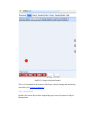
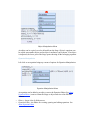
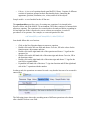
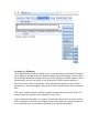
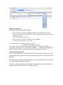
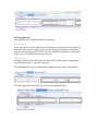
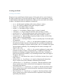
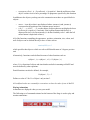
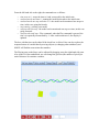
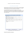
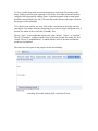
MoPiX 2.0 Manual Tabbed environment of MoPiX 2.0
MoPiX 2.0 Environment consists of several different parts:
•
•
Resources - offer different information and a possibility of exploring models and
equations.
Stage - the construction and play area. Models are built and run in this part.
It is divided into two adjustable panes, left hand side for construction and running
and the right hand side one for bringing/keeping and manipulating the equations.
Set of buttons on the top of the Stage controls the addition of new objects,
changing an object's size, orientation and colour (in addition to the way of doing it
by adding the equations onto an object) as well as loading/saving models (See
Saving, Retrieving Models and Equations ) and MathML manipulation (See
Viewing, Editing and Saving MathML ).
MoPiX 2.0 Stage with loaded model
The set of commands at the bottom of the Stage controls playing and monitoring
of models (See Playing Animations )
Object Manipulation
Double-click on an object on the Stage brings up a menu of options for Object
Manipulation.
Object Manipulation Menu
An object can be copied, saved or deleted from the Stage. Object's equations can
be copied onto another object and an object's attributes can be shown. If an object
is inspected, the lower part of the Stage opens showing all the belonging equation.
Equation Manipulation
Left click on an equation brings up a menu of options for Equation Manipulation.
Equation Manipulation Menu
An equation can be added to an object, sent to the Equation Editor (See about
Equation Editor ) removed from the Stage or object and viewed in different
formats.
•
•
History - keeps a list of all the moves.
Equation Editor - the Editor for creating, opening and editing equations. See
about Equation Editor
•
Library - it is a set of equations based upon MoPiX 1 library. Consists of different
sections of equations grouped on their functionality basis: controlling the
appearance, position, orientation, size, colour, and trail of the objects.
Sample models - a set of models for the off line use.
The equation editor provides a way of creating new equations. It is situated in the
Equation Editor tab of the MoPiX 2.0 environment. The Editor consists of a button which
starts new equation. The equation to be created needs to be analyzed before expanding its
left and right text fields: it needs to be seen as a binary tree structure, in order of
precedence of its operators. For example, to create an equation like this:
redColour(ME,t)=redColour(ME,t-1)-delta47(ME,t)×2
One should follow this set of actions:
•
•
•
•
•
•
Click on the New Equation button to start new equation
Double-click on the left text field and choose Function, fill in the values for the
function name, object name and time
Double-click on the right hand side of the equation and choose '-' sign from the
operators list
Double-click on the left hand side of the minus sign and choose Function, fill in
the functions values
Double-click on the right hand side of the minus sign and choose '*' sign for the
text field to expand further
Expand the left hand side of the times '*' sign into function and fill the right hand
side of the '*' operation with the number
In other words, the operations are entered in such a way that the last one to be executed is
entered first.
The following picture shows the cascading menu of different operations to be chosen
after a double-click on a text field.
Creating New Equations
The Equation Editor supports creation of user’s own equations by opening of a template
for an equation clicking on the New Equation button. By positioning the cursor on one of
the text fields and double-clicking, a menu of all the operations available appears. When
an operation is chosen, a new pair of text fields opens with the desired operator in
between (in case of binary operations), a text field with the operator (in case of unary
operation) or a function template with text fields for the function name, object name and
time.
This can be continued further, until the complete equation has been created. While it is
being created, the equation is also displayed on the screen.
Once completed by the editor, it is ready to be sent to the Stage where it can be used do
define a property or behaviour of an object. Being on the Stage, the created equation can
be reused many times or sent back to the Editor to be opened and changed.
Supported Operations
The Equation Editor supports the following:
•
•
•
•
•
Basic arithmetic operations: addition, subtraction, multiplication, division;
Relational operations: less than, greater than, less then or equal to, greater than or
equal to, not equal;
Logical operations: and, or, not;
Other arithmetic operations: absolute value, remainder.
Trigonometric operations: sin, cos, tan;
User Defined Functions are supported in the form of:
functionName (Object name, time)
where Object name refers to the object on the Stage currently dealt with (ME) or any
other object in relation with the it (OTEHR1, OTHER2, …, OTHER9). The functions are
functions of time and the second argument specifies particular time instance.
Opening Existing Equations
Library , Stage and Resources tabs of the MoPiX 2.0 environment are all sources of 'live'
equations that can be opened by left-clicking and choosing Send To Equation Editor from
the menu.
The equation can be further edited in the same ways as explained in the previous sections
i.e. using expanding and deleting features.
In this way, existing equations can be changed by replacing their parts with the desired
elements. The following picture shows an open equation.
Deleting Equations
The equations can be deleted partially or completely.
Partial deletion
Parts of an equation can be deleted by left-clicking on an operator and choosing Delete.
In this way, the operator together with the two belonging operands are removed and
replaced with an empty text field. The rest of the equation can further be edited in the
same ways as described in the previous sections.
Complete deletion
Complete deletion can be done either by clicking the CLOSE button or applying the
partial deletion on the '=' sign of the equation.
The following picture shows partial deletion applied to an operator of an equation.
The following picture shows the effect of the above partial deletion.
Creating your Model
Creating a new Model
Elements of your model begin as black squares. Click on the Add new object button on
the Stage as many times as you need to get the objects. They have no behaviour, colour,
or other attributes other than the initial position. When you run your model each element
or object i is displayed where its attributes are defined as:
•
•
•
•
•
•
•
•
•
•
•
•
•
•
•
•
•
x(i , t) – the horizontal coordinate of the centre of object i at time t
y(i , t) – the vertical coordinate of the centre of object i at time t
width(i , t) – the width of object i at time t
height(i , t) – the height of object i at time t
rotation(i , t) – the number of degrees object i at time t is rotated
redColour(i , t) – the percentage of red in the colour of object i at time t
greenColour(i , t) – the percentage of green in the colour of object i at time t
blueColour(i , t) – the percentage of blue in the colour of object i at time t
transparency(i , t) – the percentage of opacity of object i at time t (100 is fully
opaque, while 0 is fully transparent)
appearance(i , t) – the shape of object i at time t (currently only Circle and Square
are supported).
x0(i , t), x1(i , t), x2(i , t), … x359(i , t) – the horizontal coordinate of a point on
the perimeter of object i at time t (x0 represents the x coordinate of point on the
perimeter at a heading of 0 degrees from the entre, x90 is x coordinate of the point
on the perimeter reached by a ray emanating from the centre at an angle of 90
degrees, and so on)
y0(i , t), y1(i , t), y2(i , t), … y359(i , t) – the vertical coordinate of a point on the
perimeter of object i at time t (y0 represents the y coordinate of point on the
perimeter at a heading of 0 degrees from the centre, x90 is the y coordinate of
point on the perimeter reached by a ray emanating from the centre at an angle of
90 degrees, and so on)
penDown(i , t) – only when it has a value of 1 will object i at time t leave a trail
when it moves
thicknessPen(i , t) – if penDown(i , t) is equal to 1 then the trail drawn when
object i at time t moves has a thickness controlled by this function
redColourPen(i , t) – if penDown(i , t) is equal to 1 then the trail drawn when
object i at time t moves has a colour whose red component is the percentage
specified by this function
greenColourPen(i , t) – if penDown(i , t) is equal to 1 then the trail drawn when
object i at time t moves has a colour whose green component is the percentage
specified by this function
blueColourPen(i , t) – if penDown(i , t) is equal to 1 then the trail drawn when
object i at time t moves has a colour whose blue component is the percentage
specified by this function
•
transparencyPen(i , t) – if penDown(i , t) is equal to 1 then the trail drawn when
object i at time t moves has a percentage of opaqueness specified by this function
In addition to the objects you drag out to the construction area there are special built-in
objects:
•
•
mouse – is an object that is not displayed whose x(mouse,t) and y(mouse,t)
correspond to the position of the computer mouse at time t
a, b, c, … z, A, B, C, … Z– are the names of objects that are not displayed whose
keyDown(,t) is equal to 1 if and only if the keyboard button labelled key is
depressed at time t (keyDown(mouse,t) is defined similarly to be 1 when the left
mouse button is depressed at time t)
All of the functions controlling the appearance, position, orientation, size, colour, and
trail of objects can be defined directly to have a value such as:
rotation(ME,t)=t×2
which specifies that object to which we refer as ME should rotate at 2 degrees per time
unit.
Alternatively, functions can be defined in terms of other functions such as:
x(object i , t) = x(object i , t-1) + Vx(object i , t)
where Vx is a function of objects and time that has no built-in meaning to MoPiX and
must be defined by other equations.
Partial functions can also be defined, for example,
Vx(object i , 3) = 5
Defines a value of 5 for Vx of object i only at time 3.
All undefined values are assumed for convenience to have the value of zero in MoPiX.
Playing Animations
Animations are displayed when you run your model.
The following set of commands situated on the bottom of the Stage is used to play and
monitor animations:
From the left hand side to the right, the commands are as follows:
•
•
•
•
•
•
time reset to 0 - resets the time to 0 and your model to the initial state
run backwards until time 0 - running the model backwards to the initial state
run backwards one step until time is 0 - the model can be monitored one step at a
time, in this case going backwards
stop running - pausing your model
run forwards one step - the model can be monitored one step at a time, in this case
going forwards
run forwards until stop - Play command: when the Play command is pressed, the
time t is repeatedly incremented by 1. After each increment of t, the display is
updated.
The box with the time can be edited if the check box is clicked. One can also explore the
temporal nature of a model then by moving objects (or changing other attributes) and
MoPiX will find the nearest time that matches.
The Playing area on the Stage can be adjusted by dragging away the right-hand side pane.
Also in the Grid box underneath, one can change the grid size (the number of pixels per
unit of distance) by entering a number.
Playing the Two Animated Objects with Graphs model
Viewing, Editing and Saving MathML
The button MathML on the Stage opens a window pane with the current model's MathML
XML (all the objects on the stage). The options are offered underneath. The usual rightclick menu options: select, cut, copy, paste and delete are all allowed.
You can edit the XML and when you close the window the model is updated
appropriately. (Please be careful since the error handling is weak.) Alternatively, you can
copy and paste the contents into a file or email message. To restore the model at another
time or on another computer you can copy the saved XML to the clipboard and paste it
into the XML window.
Showing MathML of the Growing Rectangle model
Saving, Retrieving Models and Equations
To Save a model along with its associated equations click on the Save button on the
Stage. Dialog text boxes open requiring a User Name. Press Enter when this has been
completed and a description window opens. A short description of the created model
should be entered followed by OK. The status line at the bottom of the stage will show
the progress of the uploading.
To Load the saved work by any user, click on the Load button on the Stage and after
entering the User Name, enter the description (key word or a longer description) and, if
desired, the author of the work in the CreatedBy: line.
The tag "Type:" is also added that can have the value "model", "object", or "equation".
The tag "CreatedOn:" is added with the value of the time and date the model was first
created. The tag "LastModifiedOn:" is added with the value of the time and date the
model was last updated.
The status line will report on the progress on the downloading.
Searching for models with tag 'ball' created by all users.