Download SigmaPlot® 8.0 Programming Guide

SigmaPlot 8.0
Programming Guide
®
For more information about SPSS® Science software products, please visit our WWW
site at http://www.spss.com or contact
SPSS Science Marketing Department
SPSS Inc.
233 South Wacker Drive, 11th Floor
Chicago, IL 60606-6307
Tel: (312) 651-3000
Fax: (312) 651-3668
SPSS and SigmaPlot are registered trademarks and the other product names are the
trademarks of SPSS Inc. for its proprietary computer software. No material describing
such software may be produced or distributed without the written permission of the
owners of the trademark and license rights in the software and the copyrights in the
published materials.
The SOFTWARE and documentation are provided with RESTRICTED RIGHTS. Use,
duplication, or disclosure by the Government is subject to restrictions as set forth in
subdivision (c)(1)(ii) of The Rights in Technical Data and Computer Software clause at
52.227-7013. Contractor/manufacturer is SPSS Inc., 233 South Wacker Drive, 11 th
Floor, Chicago, IL 60606-6307.
General notice: Other product names mentioned herein are used for identification
purposes only and may be trademarks of their respective companies.
Windows is a registered trademark of Microsoft Corporation.
ImageStream® Graphics & Presentation Filters, copyright © 1991-1997 by INSO Corporation.
All Rights Reserved.
ImageStream Graphics Filters is a registered trademark and ImageStream is a trademark of
INSO Corporation.
SigmaPlot® 8.0 Programming Guide
Copyright © 2002 by SPSS Inc.
All rights reserved.
Printed in the United States of America.
No part of this publication may be reproduced, stored in a retrieval system, or
transmitted, in any form or by any means, electronic, mechanical, photocopying,
recording, or otherwise, without the prior written permission of the publisher.
1234567890
05 04 03 02 01 00
ISBN 1-56827-233-2
Contents
Introduction ................................................................................ 1
Transforms .................................................................................................................. 1
Regressions ................................................................................................................. 1
Automation .................................................................................................................. 2
Using Transforms ......................................................................... 3
Using the Transform Dialog Box .................................................................................. 3
Transform Syntax and Structure .................................................................................. 4
Transform Components ............................................................................................... 6
Transform Tutorial ....................................................................... 11
Starting a Transform .................................................................................................. 11
Saving and Executing Transforms .............................................................................. 14
Graphing the Transform Results ................................................................................ 14
Recoding Example ..................................................................................................... 15
Transform Operators ..................................................................... 17
Order of Operation ..................................................................................................... 17
Operations on Ranges ................................................................................................ 18
Arithmetic Operators .................................................................................................. 19
Relational Operators ................................................................................................... 19
Logical Operators ....................................................................................................... 20
Transform Function Reference ......................................................... 21
Function Arguments ................................................................................................... 21
Transform Function Descriptions ............................................................................... 22
User-defined Functions .............................................................................................. 69
Example Transforms ..................................................................... 71
Data Transform Examples .......................................................................................... 71
Graphing Transform Examples ................................................................................... 84
Introduction To The Regression Wizard ............................................ 141
Regression Overview ............................................................................................... 141
The Regression Wizard ............................................................................................ 142
Opening .FIT Files ..................................................................................................... 143
About the Curve Fitter .............................................................................................. 144
References for the Marquardt-Levenberg
iii
Contents
Algorithm .......................................................................................................................................145
Regression Wizard ..................................................................... 147
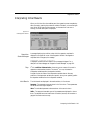
Using the Regression Wizard ....................................................................................147
Running a Regression From a Notebook ..................................................................151
Creating New Regression Equations .........................................................................152
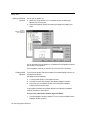
Viewing and Editing Code .........................................................................................153
Variable Options .......................................................................................................154
Equation Options ......................................................................................................155
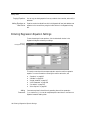
Saving Regression Equation Changes .......................................................................162
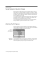
Watching The Fit Progress ........................................................................................162
Interpreting Initial Results ........................................................................................163
Saving Regression Results .......................................................................................165
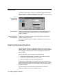
Graphing Regression Equations ................................................................................166
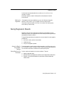
Interpreting Regression Reports ...............................................................................167
Regression Equation Libraries and Notebooks .........................................................175
Curve Fitting Date And Time Data .............................................................................177
Regression Results Messages ..................................................................................181
Editing Code ............................................................................. 185
About Regression Equations .....................................................................................185
Entering Regression Equation Settings ....................................................................188
Saving Equations ......................................................................................................192
Equations ..................................................................................................................193
Variables ...................................................................................................................194
Weight Variables .......................................................................................................197
Initial Parameters ......................................................................................................198
Constraints ...............................................................................................................199
Other Options ...........................................................................................................200
Automatic Determination of Initial Parameters .........................................................202
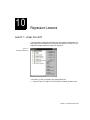
Regression Lessons .................................................................... 205
Lesson 1: Linear Curve Fit ........................................................................................205
Lesson 2: Sigmoidal Function Fit ..............................................................................212
Advanced Regression Examples ..................................................... 219
Curve Fitting Pitfalls ..................................................................................................219
Example 2: Weighted Regression ............................................................................225
Example 3: Piecewise Continuous Function .............................................................227
Example 4: Using Dependencies ..............................................................................229
Example 5: Solving Nonlinear Equations ..................................................................232
Example 6: Multiple Function Nonlinear Regression ................................................234
iv
Contents
Example 7: Advanced Nonlinear Regression ............................................................ 237
Automating Routine Tasks ............................................................ 241
Creating Macros ....................................................................................................... 241
Running Your Macro ................................................................................................ 244
Editing Macros ......................................................................................................... 245
About user-defined functions ................................................................................... 251
Using the Dialog Box Editor ..................................................................................... 251
Using the Object Browser ......................................................................................... 252
Using the Add Procedure Dialog Box ....................................................................... 253
Using the Debug Window ......................................................................................... 253
SigmaPlot Automation Reference ................................................... 255
Opening SigmaPlot from Microsoft Word or Excel .................................................. 255
SigmaPlot Objects and Collections ........................................................................... 256
SigmaPlot Properties ............................................................................................... 266
SigmaPlot Methods .................................................................................................. 275
Regression Equation Library ......................................................... 285
Index ..................................................................................... 301
v
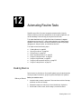
1
Introduction
The Programming Guide provides you with complete descriptions of SigmaPlot’s
powerful math, data manipulation, regression, and curve fitting features. It also
describes how to use SigmaPlot’s Interactive Development Environment (IDE) and
Macro Recorder to automate and customize SigmaPlot tasks.
Transforms
0
Transforms are sets of equations that manipulate and calculate data. Math transforms
apply math functions to existing data and also generate serial and random data. To
perform a transform, you enter variables and standard arithmetic and logic operators
into a transform dialog. Your equations can specify that a transform access data from a
worksheet as well as save equation results to a worksheet.
Transforms can be saved as independent .XFM files for later opening or
modification. Because transforms are saved as plain text (ASCII) files, they can be
created and edited using any word processor that can edit and save text files.
The transform chapters describe the use and structure of transforms, followed by a
brief tutorial, reference sections on transform operators and functions, and finally a
list and description of the sample transform files and graphs included with
SigmaPlot.
Regressions
0
The SigmaPlot Regression Wizard replaces the older curve fitter with a new interface
and over one hundred new equations. The major new features of this interface
include:
➤
a graphical interface rather than text code
a library of over 100 built-in equations in twelve different categories
➤ graphical examples of the curves and equations for built-in equations
➤
Transforms 1
Introduction
➤
➤
➤
➤
➤
➤
automatic initial parameter determination—no coding is required in most cases
selection of variables directly from either worksheet columns or graph curves
full statistical report generation
automatic curve plotting to existing or new graphs
new regression equation documents for the notebook
new text report documents for the notebook
The Regression Wizard chapters describe how to use these features.
The Curve Fitter
The Regression Wizard uses the curve fitter to fit user-defined linear equations to
data. The curve fitter modifies the parameters (coefficients) of your equation, and
finds the parameters which cause the equation to most closely fit your data.
You can specify up to 25 equation parameters and ten independent equation
variables. When you enter your equation, you can specify up to 25 parameter
constraints, which limit the search area when the curve fitter checks for parameter
values.
The curve fitter can also use weighted least squares for greater accuracy.
User-defined equations can be saved to notebooks or regression libraries and selected
for later use or modification.
Automation
0
SigmaPlot OLE Automation technology provides you with a wide range of
possibilities for automating frequently-performed tasks, using macros and userdefined features.
SigmaPlot’s Macro Recorder lets you record is a set of procedures and then run them
automatically with a single command. Most of the operations that you perform in
SigmaPlot can be recorded.
The Macro Window provides a fully-featured programming environment that uses
SigmaPlot Basic as the core programming language. If you are familiar with Microsoft
Visual Basic, most of what you know will apply as you use SigmaPlot’s macro
language.
2 Automation
2
Using Transforms
Transforms are math functions and equations that generate and are applied to
worksheet data. Transforms provide extremely flexible data manipulation, allowing
powerful mathematical calculations to be performed on specific sets of your data.
Using the Transform Dialog Box
0
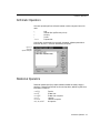
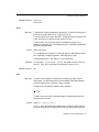
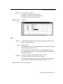
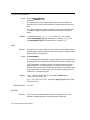
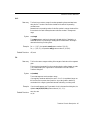
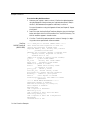
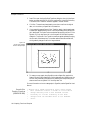
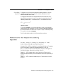
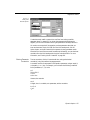
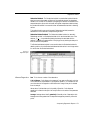
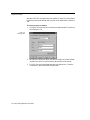
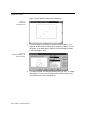
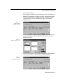
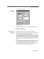
To begin a transform, choose the Transforms menu User-Defined Transform
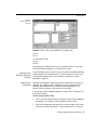
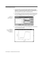
command or press F10. The User-Defined Transform dialog box appears.
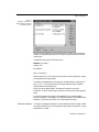
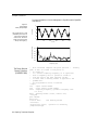
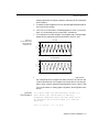
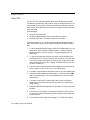
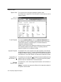
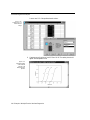
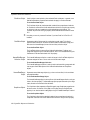
Figure 2–1
The User-Defined
Transform Dialog Box
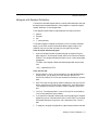
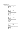
Creating a Transform
The first step to transform worksheet data is to enter the desired equations in the edit
box. If no previously entered transform equations exist, the edit box is empty:
otherwise, the last transform entered appears.
Select the edit box to begin entering transform instructions. As you enter text into
the transform edit box, the box scrolls down to accommodate additional lines.
Up to 100 lines of equations can be entered. Equations can be entered on separate
lines or on the same line.
Using the Transform Dialog Box 3
Using Transforms
Once you have completed the transform, you can run it by clicking Run.
Transform Files
Transforms can be saved as independent transform files. The default extension is
.XFM. Transform files are plain text files that can also be edited with any word
processing program.
Use the New, Open, Save, and Save As options in the User-Defined Transform dialog
box to begin new transforms, open existing transforms, save the contents of the
current edit box to a transform file, and save an existing transform file to a different
file name.
The last transform you entered, opened, or imported always appears in the edit
window when you open the User-Defined Transform dialog box. To permanently
save a transform, you must use the Save, or Save As options.
Transform Syntax and Structure
0
Use standard syntax and equations when defining user-defined transforms in
SigmaPlot or SigmaStat. This section discusses the basics and the details for entering
transform equations.
Transform Syntax
Transforms are entered as equations with the results placed to the left of the equal
sign (=) and the calculation placed to the right of the equal sign. Results can be
defined as either variables (which can be used in other equations), or as the worksheet
column or cells where results are to be placed.
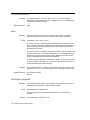
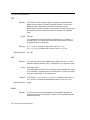
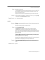
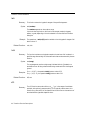
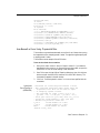
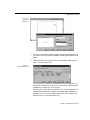
Entering Transforms
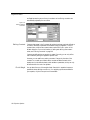
To type an equation in the transform edit box, click in the edit box and begin typing.
When you complete a line, press Enter to move the cursor to the first position on the
next line.
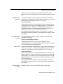
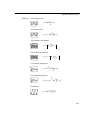
Figure 2–2
Typing Equations
into the Edit Window
4 Transform Syntax and Structure
Using Transforms
You can leave spaces between equation elements: x = a+b is the same as
x = a + b. However, you may find it necessary to conserve space by omitting spaces.
Blank lines are ignored so that you can use them to separate or group equations for
easier reading.
If the equation requires more than one line, you may want to begin the second and
any subsequent lines indented a couple of spaces (press the space bar before typing
the line). Although this is not necessary, indenting helps distinguish a continuing
equation from a new one.
Σ
You can resize the transform dialog box to enlarge the edit box. You can press Ctrl+X,
Ctrl+C, and Ctrl+V to cut, copy, and paste text in the edit window.
Transforms are limited to a maximum of 100 lines. Note that you can enter more
than one transform statement on a line; however, this is only recommended if space
is a premium.
Σ
Use only parentheses to enclose expressions. Curly brackets and square brackets are
reserved for other uses.
Commenting
on Equations
To enter a comment, type an apostrophe (’) or a semicolon (;), then type the
comment to the right of the apostrophe or semicolon. If the comment requires more
than one line, repeat the apostrophe or semicolon on each line before continuing the
comment.
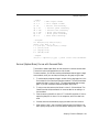
Sequence
of Expression
SigmaPlot and SigmaStat generally solve equations regardless of their sequence in the
transform edit box. However, the col function (which returns the values in a
worksheet column) depends on the sequence of the equations, as shown in the
following example.
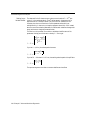
Example:
The sequence of the equations:
col(1)=col(4)^alpha
col(2)=col(1)*theta
must occur as shown. The second equation depends on the data produced by the
first. Reversing the order produces different results. To avoid this sequence problem,
assign variables to the results of the computation, then equate the variables to
columns:
x=col(4)
y=x^alpha
z=y∗theta
col(1)=y
col(2)=z
The sequence of the equations is now unimportant.
Transform Syntax and Structure 5
Using Transforms
Transform Components
0
Transform equations consist of variables and functions. Operators are used to define
variables or apply functions to scalars and ranges. A scalar is a single worksheet cell,
number, missing value, or text string. A range is a worksheet column or group of
scalars.
Variables
You can define variables for use in other equations within a transform. Variable
definition uses the following form
variable = expression
Variable names must begin with a letter: after that, they can include any letter or
number, or the underscore character (_). Variable names are case sensitive—an “A” is
not the equivalent of an “a.” Once a variable has been defined by means of an
expression, that variable cannot be redefined within the same transform.
Functions
A function is similar to a variable, except that it refers to a general expression, not a
specific one, and thus requires arguments. The syntax for a function declaration is
function(argument 1,argument 2,...) = expression
where function is the name of the function, and one or more argument names are
enclosed in parentheses. Function and argument names must follow the same rules as
variable names.
User-Defined Functions Frequently used functions can be copied to the Clipboard
and pasted into the transform window.
Constructs
Transform constructs are special structures that allow more complex procedures than
functions. Constructs begin with an opening condition statement, followed by one
or more transform equations, and end with a closing statement. The available
constructs are for loops and if...then...else statements.
Operators
A complete set of arithmetic, relational, and logic operators are provided. Arithmetic
operators perform simple math between numbers. Relational operators define limits
and conditions between numbers, variables, and equations. Logic operators set
simple conditions for if statements. For a list of the operators and their functions, see
Chapter “Transform Operators”, on page 17.
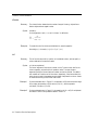
Numbers
Numbers can be entered as integers, in floating point style, or in scientific notation.
All numbers are stored with 15 figures of significance. Use a minus sign in front of
the number to signify a negative value.
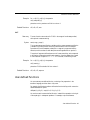
6 Transform Components
Using Transforms
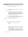
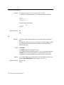
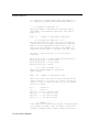
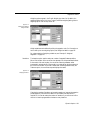
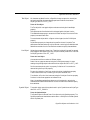
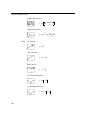
Figure 2–3
Examples of the Transform
Equation Elements Typed into
the Transform Window
Missing values, represented in the worksheet as a pair of dashes, are considered nonnumeric. All arithmetic operations which include a missing value result in another
missing value.
To generate a missing value, divide zero by zero
Example: If you define:
missing = 0/0
the operation:
size({1,2,3,missing})
returns a value of 4.0. (The size function returns the number of elements in a range,
including labels and missing values.)
The transform language does not recognize two successive dashes; for example, the
string {1,2,3,--} is not recognized as a valid range. Dashes are used to represent
missing values in the worksheet only.
Strings, such as text labels placed in worksheet cells, are also non-numeric
information. To define a text string in a transform, enclose it with double quotation
marks.
As with missing values, strings may not be operated upon, but are propagated
through an operation. The exception is for relational operators, which make a lexical
comparison of the strings, and return true or false results accordingly.
Scalars and Ranges
The transform language recognizes two kinds of elements: scalars and ranges. A scalar
is any single number, string, or missing value. Anything that can be placed in a single
worksheet cell is a scalar.
Transform Components 7
Using Transforms
A range (sometimes called a vector or list) is a one-dimensional array of one or more
scalars. Columns in the worksheet are considered ranges.
Ranges can also be defined using curly bracket ({}) notation. The range elements are
listed in sequence inside the brackets, separated by commas. Most functions which
accept scalars also accept ranges, unless specifically restricted. Typically, whatever a
function does with a scalar, it does repeatedly for each entry in a range. A single
function can operate on either a cell or an entire column.
Example 1: The entry:
{1,2,3,4,5}
produces a range of five values, from 1 through 5.
Example 2: The operation:
{col(1), col(2)}
concatenates columns 1 and 2 into a single range. Note that elements constituting a
range need not be of the same type, i.e., numbers, labels and missing values.
Example 3: The entry:
{x,col(4)∗3,1,sin(col(3))}
also produces a range.
Array References
Individual scalars can be accessed within a range by means of the square bracket ([])
constructor notation. If the bracket notation encloses a range, each entry in the
enclosed range is used to access a scalar, resulting in a new range with the elements
rearranged.
Example: For the range:
x = {1.4,3.7,3.3,4.8}
the notation:
x[3]
returns 3.3, the third element in the range. The notation:
x[{4,1,2}]
produces the range {4.8,1.4,3.7}. The constructor notation is not restricted to
variables: any expression that produces a range can use this notation.
8 Transform Components
Using Transforms
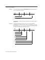
Example: The operation:
col(3)[2]
produces the same result as col(3,2,2), or cell(3,2). The notation:
{2,4,6,8}[3]
produces 6. If the value enclosed in the square brackets is also a range, a range
consisting of the specified values is produced.
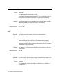
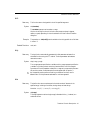
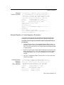
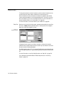
Example: The operation:
col(1)[{1,3,5}]
produces the first, third, and fifth elements of column 1.
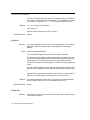
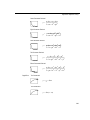
Figure 2–4
Range and Array Reference
Operations Typed into
the User Defined
Transform Window
Transform Components 9
Notes
0
3
Transform Tutorial
The following tutorial is designed to familiarize you with some basic transform
equation principles. You will enter transform data into a worksheet and generate a
2D graph.
Starting a Transform
0
To begin a transform:
1.
Click the New Notebook
button, or choose the File menu New command
and select Notebook. An empty worksheet appears.
2.
Choose the Data menu User-Defined Transform command. The User-Defined
Transform dialog box appears. If necessary, click New to clear the edit window
and begin a new session.
3.
Defining a Variable
Click the upper left corner of the edit window and type:
t=data(−10,11,1.5)
4.
Add a few spaces, then type the comment:
'generates serial data
The data function is used to generate serial data from a specified start and stop,
using an optional increment.
5.
Press Enter to move to the next line, then type:
col(1)=t 'put t into column 1
This places the variable t into column 1 of the data worksheet.
Starting a Transform 11
Transform Tutorial
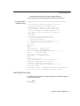
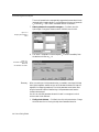
6.
Press Enter, then type:
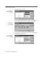
cell(2,1) = "Results:" 'enclose strings in quotes
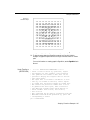
Figure 3–1
The Edit Window with
All the Transform
Equations Entered
This places the label “Results:” in row one of column 2. Text strings must be
enclosed in quotation marks.
7.
Defining a Function
Press Enter, then type:
f(x)=2∗x^3−7∗x^2
Press Enter, add a couple of spaces, then type:
+9∗x−5
If you want an equation to use more than one line, start each additional line
with a blank space or two to distinguish it from a new equation.
12 Starting a Transform
Transform Tutorial
8.
Press Enter, then type:
y=f(t)
This variable declaration uses the function f and variable t declared in the
previous equations.
9.
Add a few spaces, then type:
put y into col(3)
This places the results of the preceding equation (which defines y) in column 3
of the worksheet.
Note that you can also collapse the last two lines into one equation:
col(3)=f(t)
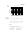
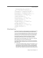
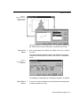
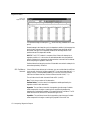
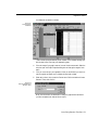
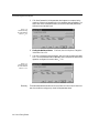
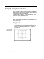
Click Run. If you have entered all the transform equations correctly, the data
will appear as shown in Figure 3–2.
Figure 3–2
The Data Generated by
the Transform Tutorial
Starting a Transform 13
Transform Tutorial
Saving and Executing Transforms
0
After entering the transform equations, save the transform to a file, then run the
transform.
1.
Click Save, and specify a file name and destination for the file. The default
extension for transform files is .XFM.
Saved transforms can be opened with the Transform dialog box Open button.
2.
Click Run. If you have entered all the transform equations correctly, you should
generate the data shown in Figure 3–2.
Graphing the Transform Results
0
Once the transform is executed and the results are placed in the worksheet, you then
treat the results like any other worksheet data.
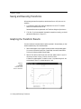
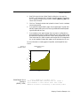
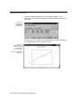
1.
Select a scatter graph from the graph toolbar and select a simple scatter graph.
You can also choose the Graph menu Create Graph command, select Scatter
Plot then click Next and select Simple Scatter.
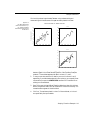
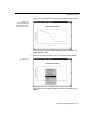
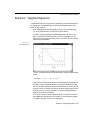
2.
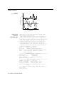
Select XY Pair as the Data Format, then click Next. Select column 1 as your X
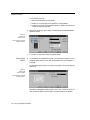
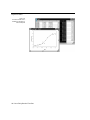
column and column 3 as your Y column, then click Finish.
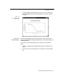
A Scatter Plot graph appears. The data in column 1 is plotted along the X axis
and the data in column 3 is plotted along the Y axis.
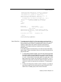
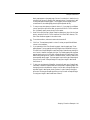
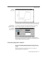
Figure 3–3
A Graph
of Plotting the
Transform Tutorial
Data as a Scatter Plot
14 Saving and Executing Transforms
Transform Tutorial
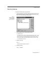
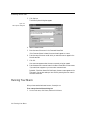
Recoding Example
0
This example illustrates a simple recoding transform.
1.
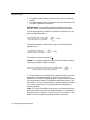
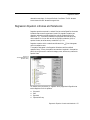
Choose the Data menu User-Defined Transforms command to open the UserDefined Transform dialog box. If desired, click Save to save the existing transform to a file. Click New to begin a new transform.
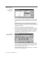
2.
Click the upper left corner of the edit window and type:
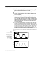
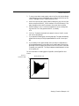
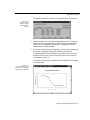
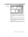
Figure 3–4
Entering the Recoding
Transform Example
into the User-Defined
Transform Edit Window
x = random(15,2,0,7)
This creates uniformly random numbers distributed between 0 and 7, using 2
as a seed. However, the numbers generated have fifteen significant digits. To
round off the numbers to two decimal places, modify this function to read:
x = round(random,15,2,0,7),2)
3.
Press Enter, then type:
col(1) = x
to place the random numbers in column 1.
4.
Press Enter and type:
col(2,1) = "Recoded "
Recoding Example 15
Transform Tutorial
Note the space between the d and the quotation mark ("). All characters,
including space characters, within quotes are entered into cells as part of the
label.
Press Enter, then type:
col(2,2) = "Variable:"
5.
To create the code data, press Enter, then type:
col(3) = if(x<2,"small",
Press Enter, add a couple of spaces, then type:
if(x >=2 and x<5, "medium","large"))
If you want an equation to use more than one line, start each additional line
with a blank space or two to distinguish it from a new equation.
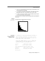
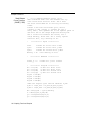
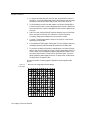
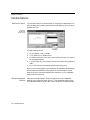
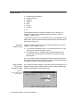
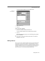
6.
Click Run. If you have entered all the transform equations correctly, the data
will appear as shown in Figure 3–5.
7.
You can save your new data with the Save command from the File menu.
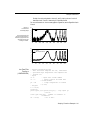
Figure 3–5
Results of the Recoding
Example Transform
16 Recoding Example
4
Transform Operators
Transforms use operators to define variables and apply functions. A complete set of
arithmetic, relational, and logical operators are provided.
Order of Operation
0
The order of precedence is consistent with P.E.M.A. (Parentheses, Exponentiation,
Multiplication, and Addition) and proceeds as follows, except that parentheses
override any other rule:
➤
➤
➤
➤
➤
➤
➤
➤
Exponentiation, associating from right to left
Unary minus
Multiplication and division, associating from left to right
Addition and subtraction, associating from left to right
Relational operators
Logical negation
Logical and, associating from left to right
Logical or, associating from left to right
This list permits complicated expressions to be written without requiring too many
parentheses.
Example: The statement:
a<10 and b<5
groups to (a<10) and (b<5), not to (a<(10 and b))<5.
Order of Operation 17
Transform Operators
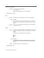
Σ
Note that only parentheses can group terms for processing. Curly and square brackets
are reserved for other uses.
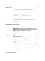
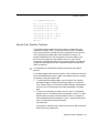
Figure 4–1
Examples of Transform
Operators
Operations on Ranges
0
The standard arithmetic operators—addition, subtraction, multiplication, division,
and exponentiation—follow basic rules when used with scalars. For operations
involving two ranges corresponding entries are added, subtracted, etc., resulting in a
range representing the sums, differences, etc., of the two ranges.
If one range is shorter than the other, the operation continues to the length of the
longer range, and missing value symbols are used where the shorter range ends.
For operations involving a range and a scalar, the scalar is used against each entry in
the range.
Example: The operation:
col(4)∗2
produces a range of values, with each entry twice the value of the corresponding value
in column 4.
18 Operations on Ranges
Transform Operators
Arithmetic Operators
0
Arithmetic operators perform arithmetic between a scalar or range and return the
result.
+
−
∗
/
^ or ∗∗
Add
Subtract (also signifies unary minus)
Multiply
Divide
Exponentiate
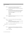
Multiplication must be explicitly noted with the asterisk. Adjacent parenthetical
terms such as (a+b) (c−4) are not automatically multiplied.
Figure 4–2
Arithmetic
Operator Examples
Relational Operators
0
Relational operators specify the relation between variables and scalars, ranges or
equations, or between user-defined functions and equations, establishing definitions,
limits and/or conditions.
= or .EQ.
> or .GT.
>= or .GE.
< or .LT.
<= or .LE.
<>,!=, #, or .NE.
Equal to
Greater than
Greater than or equal to
Less than
Less than or equal to
Not equal to
Arithmetic Operators 19
Transform Operators
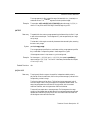
The alphabetic characters can be entered in upper or lower case.
Figure 4–3
Relational and Logical
Operator Examples
Logical Operators
0
Logical operators are used to set the conditions for if function statements.
and, &
or, |
not, ∼
20 Logical Operators
Intersection
Union
Negation
5
Transform Function Reference
SigmaPlot provides many predefined functions, including arithmetic, statistical,
trigonometric, and number-generating functions. In addition, you can define
functions of your own.
Function Arguments
0
Function arguments are placed in parentheses following the function name,
separated by commas. Arguments must be typed in the sequence shown for each
function.
You must provide the required arguments for each function first, followed by any
optional arguments desired. Any omitted optional arguments are set to the default
value. Optional arguments are always omitted from right to left. If only one
argument is omitted, it will be the last argument. If two are omitted, the last two
arguments are set to the default value.
You can use a missing value (i.e., 0/0) as a placeholder to omit an argument.
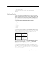
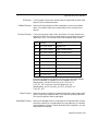
Example: The col function has three arguments: column, top, and bottom. Therefore,
the syntax for the col function is:
col(column,top,bottom)
The column number argument is required, but the first (top) and last (bottom) rows
are optional, defaulting to row 1 as the first row and the last row with data for the last
row.
col(2) returns the entirety of column 2.
col(2,5) returns column 2 from row 5 to the end of the column.
col(2,5,100) returns column 2 from row 5 to row 100.
col(2,0/0,50) returns column 2 from row 1 to the 50th row in the column.
Function Arguments 21
Transform Function Reference
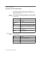
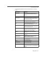
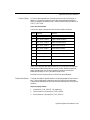
Transform Function Descriptions
0
The following list groups transforms by function type. It is followed by an
alphabetical reference containing complete descriptions of all transform functions
and their syntax, with examples.
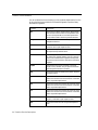
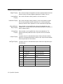
Worksheet
Functions
Data Manipulation
Functions
These worksheet functions are used to specify cells and columns from the worksheet,
either to read data from the worksheet for transformation, or to specify a destination
for transform results.
Function
Description
block
The block function returns a specified block of cells from
the worksheet.
blockheight, blockwidth
The blockheight and blockwidth functions return a specified block of cells or block dimension from the worksheet.
cell
The cell function returns a specific cell from the worksheet.
col
The col function returns a worksheet column or portion of
a column.
put into
The put into function places variable or equation results in
a worksheet column.
subblock
The subblock function returns a specified block of cells
from within another block.
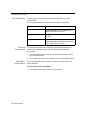
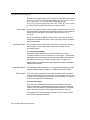
The data manipulation functions are used to generate non-random data, and to
sample, select, and sort data.
Function
Description
data
The data function generates serial data.
if
The if function conditionally selects between two data sets.
nth
The nth function returns an incremental sampling of data.
sort
The sort function rearranges data in ascending order.
22 Transform Function Descriptions
Transform Function Reference
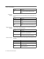
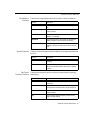
Trigonometric
Functions
Numeric Functions
Range Functions
SigmaPlot and SigmaStat provide a complete set of trigonometric functions.
Function
Description
arccos, arcsin, arctan
These functions return the arccosine, arcsine, and arctangent of the specified argument.
cos, sin, tan
These functions return the cosine, sine, and tangent of the
specified argument.
cosh, sinh, tanh
These functions return the hyperbolic cosine, sine, and tangent of the specified argument.
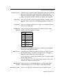
The numeric functions perform a specific type of calculation on a number or range
of numbers and returns the appropriate results.
Function
Description
abs
The abs function returns the absolute value.
exp
The exp function returns the values for e raised to the specified numbers.
factorial
The factorial function returns the factorial for each specified
number.
mod
The mod function returns the modulus, or remainder of
division, for specified numerators and divisors.
ln
The ln function returns the natural logarithm for the
specified numbers.
log
The log function returns the base 10 logarithm for
the specified numbers.
sqrt
The sqrt function returns the square root for the specified
numbers.
The following functions give information on ranges.
Function
Description
count
The count function returns the number of numeric values
in a range.
missing
The missing function returns the number of missing values
and text strings in a range.
Transform Function Descriptions 23
Transform Function Reference
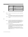
Accumulation
Functions
Random Generation
Functions
Precision Functions
Function
Description
size
The size function returns the number of data points in a
range, including all numbers, missing values, and text
strings.
The accumulation functions return values equal to the accumulated operation of the
function.
Function
Description
diff
The diff function returns the differences of the numbers in
a range.
sum
The sum function returns the cumulative sum of a range of
numbers.
total
The total function returns the value of the total sum of a
range.
The two “random” number generating functions can be used to create a series of
normally or uniformly distributed numbers.
Function
Description
gaussian
The gaussian function is used to generate a series of normally (Gaussian or “bell” shaped) distributed numbers with
a specified mean and standard deviation.
random
The random function is used to generate a series of uniformly distributed numbers within a specified range.
The precision functions are used to convert numbers to whole numbers or to round
off numbers.
Function
Description
int
The int function converts numbers to integers.
prec
The prec function rounds numbers off to a specified number of significant digits.
round
The round function rounds numbers off to a specified
number of decimal places.
24 Transform Function Descriptions
Transform Function Reference
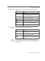
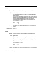
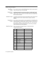
Statistical Functions
Area and Distance
Functions
Curve Fitting
Functions
The statistical functions perform statistical calculations on a range or ranges of
numbers.
Function
Description
avg
The avg function calculates the averages of corresponding
numbers across ranges. It can be used to calculate the average across rows for worksheet columns.
max, min
The max function returns the largest value in a range; the
min function returns the smallest value.
mean
The mean function calculates the mean of a range.
runavg
The runavg function produces a range of running averages.
stddev
The stddev function returns the standard deviation of a
range.
stderr
The stderr function calculates the standard error of a range.
These functions can be used to calculate the areas and distances specified by X,Y
coordinates. Units are based on the units used for X and Y.
Function
Description
area
The area function finds the area of a polygon described in
X,Y coordinates.
distance
The distance function calculates the distance of a line whose
segments are described in X,Y coordinates.
partdist
The partdist function calculates the distances from an initial
X,Y coordinate to successive X,Y coordinates in a cumulative fashion.
These functions are designed to be used in conjunction with SigmaPlot’s nonlinear
curve fitter, to allow automatic determination of initial equation parameter estimates
from the source data.
Transform Function Descriptions 25
Transform Function Reference
You can use these functions to develop your own parameter determination function
by using the functions provided with the Standard Regression Equations library
provided with SigmaPlot.
Function
Description
ape
This function is used for the polynomials, rational polynomials and other functions which can be expressed as linear
functions of the parameters. A linear least squares estimation procedure is used to obtain the parameter estimates.
dsinp
This function returns an estimate of the phase in radians of
damped sine functions.
fwhm
This function returns the x width of a peak at half the peak’s
maximum value for peak shaped functions.
inv
The inv function generates the inverse matrix of an invertible square matrix provided as a block.
lowess
The lowess algorithm is used to smooth noisy data. “Lowess” means locally weighted regression. Each point along the
smooth curve is obtained from a regression of data points
close to the curve point with the closest points more heavily
weighted.
lowpass
The lowpass function returns smoothed y values from
ranges of x and y variables, using an optional user-defined
smoothing factor that uses FFT and IFFT.
sinp
This function returns an estimate of the phase in radians of
sinusoidal functions.
x25
This function returns the x value for the y value 25% of the
distance from the minimum to the maximum of smoothed
data for sigmoidal shaped functions.
x50
This function returns the x value for the y value 50% of the
distance from the minimum to the maximum of smoothed
data for sigmoidal shaped functions.
x75
This function returns the x value for the y value 75% of the
distance from the minimum to the maximum of smoothed
data for sigmoidal shaped functions.
xatymax
This function returns the x value for the maximum y in the
range of y coordinates for peak shaped functions.
xwtr
This function returns x75-x25 for sigmoidal shaped functions.
26 Transform Function Descriptions
Transform Function Reference
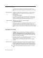
Miscellaneous
Functions
Special Constructs
Fast Fourier
Transform Functions
These functions are specialized functions which perform a variety of operations.
Function
Description
choose
The choose function is the mathematical “n choose r” function.
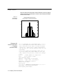
histogram
The histogram function generates a histogram from a range
or column of data.
interpolate
The interpolate function performs linear interpolation
between X,Y coordinates.
polynomial
The polynomial function returns results for specified independent variables for a specified polynomial equation.
rgbcolor
The rgbcolor(r,g,b) color function takes arguments r,g, and
b between 0 and 255 and returns color to cells in the worksheet.
Transform constructs are special structures that allow more complex procedures than
functions.
Function
Description
for
The for statement is a looping construct used for iterative
processing.
if...then...else
The if...then...else construct proceeds along one of two possible series of procedures based on the results of a specified
condition.
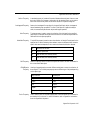
These functions are used to remove noise from and smooth data using frequencybased filtering.
Function
Description
fft
The fft function finds the frequency domain representation
of your data.
invfft
The invfft function takes the inverse fft of the data produced by the fft to restore the data to its new filtered form.
real
The real function strips the real numbers out of a range of
complex numbers.
img
The img function strips the imaginary numbers out of a
range of complex numbers.
Transform Function Descriptions 27
Transform Function Reference
Function
Description
complex
The complex function converts a block of real and/or imaginary numbers into a range of complex numbers.
mulcpx
The mulcpx function multiplies two ranges of complex
numbers together.
invcpx
The invcpx takes the reciprocal of a range of complex numbers.
abs
Summary
Syntax
The abs function returns the absolute value for each number in the specified range.
abs(numbers)
The numbers argument can be a scalar or range of numbers. Any missing value or text
string contained within a range is ignored and returned as the string or missing value.
Example
The operation col(2) = abs(col(1)) places the absolute values of the data in column 1
in column 2.
Summary
The ape function is used for the polynomials, rational polynomials and other
functions which can be expressed as linear functions of the parameters. A linear least
squares estimation procedure is used to obtain the parameter estimates. The ape
function is used to automatically generate the initial parameter estimates for
SigmaPlot’s nonlinear curve fitter from the equation provided.
ape
Syntax
ape(x range,y range,n,m,s,f)
The x range and y range arguments specify the independent and dependent variables,
or functions of them (e.g., ln(x)). Any missing value or text string contained within
one of the ranges is ignored and will not be treated as a data point. x range and y range
must be the same size
The n argument specifies the order of the numerator of the equation. The m
argument specifies the order of the denominator of the equation. n and m must be
greater than or equal to 0 ( n, m ≥ 0 ). If m is greater than 0 then n must be less than
or equal to m (if m > 0 , n ≤ m ).
28 Transform Function Descriptions
Transform Function Reference
The s argument specifies whether or not a constant is used. s=0 specifies no constant
term y0 in the numerator, s=1 specifies a constant term y0 in the numerator. s must be
either 0 or 1. If n = 0, s cannot be 0 (there must be a constant).
The number of valid data points must be greater than or equal to n + m + s .
The optional f argument defines the amount of Lowess smoothing, and corresponds
to the fraction of data points used for each regression. f must be greater than or equal
to 0 and less than or equal to 1. 0 ≤ f ≤ 1 . If f is omitted, no smoothing is used.
Example
For x = {0,1,2}, y={0,1,4}, the operation col(1)=ape(x,y,1,1,1,0.5] ) places the 3
parameter estimates for the equation
a + bx
f ( x ) = -------------1 + cx
as the values {5.32907052e-15, 0.66666667, -0.33333333} in column 1.
arccos
Summary
Syntax
This function returns the inverse of the corresponding trigonometric function.
arccos(numbers)
The numbers argument can be a scalar or range. You can also use the abbreviated
function name acos.
The values for the numbers argument must be within -1 and 1, inclusive. Results are
returned in degrees, radians, or grads, depending on the Trigonometric Units selected
in the User-Defined Transform dialog box. Any missing value or text string
contained within a range is ignored and returned as the string or missing value.
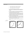
The function domain (in radians) is
arccos
Example
Related Functions
0toπ
The operation col(2) = acos(col(1)) places the arccosine of all column 1 data points
in column 2.
cos, sin, tan
arcsin, arctan
Transform Function Descriptions 29
Transform Function Reference
arcsin
Summary
Syntax
This function returns the inverse of the corresponding trigonometric function.
arcsin(numbers)
The numbers argument can be a scalar or range. You can also use the abbreviated
function name asin.
The values for the numbers argument must be within -1 and 1, inclusive. Results are
returned in degrees, radians, or grads, depending on the Trigonometric Units selected
in the User-Defined Transform dialog box. Any missing value or text string
contained within a range is ignored and returned as the string or missing value.
The function domain (in radians) is:
arcsin
Example
Related Functions
–π
--- to π
--2 2
The operation col(2) = asin(col(1)) places the arcsine of all column 1 data points in
column 2.
cos, sin, tan
arccos, arctan
arctan
Summary
Syntax
This function returns the inverse of the corresponding trigonometric function.
arctan(numbers)
The numbers argument can be a scalar or range. You can also use the abbreviated
function name atan.
The numbers argument can be any value. Results are returned in degrees, radians, or
grads, depending on the Trigonometric Units selected in the User-Defined
Transform dialog box.
The function domain (in radians) is:
arctan
Example
π π
– --- to --2 2
The operation col(2) = atan(col(1)) places the arctangent of all column 1 data points
in column 2.
30 Transform Function Descriptions
Transform Function Reference
Related Functions
cos, sin, tan
arccos, arcsin
area
Summary
The area function returns the area of a simple polygon. The outline of the polygon is
formed by the xy pairs specified in an x range and a y range.
The list of points does not need to be closed. If the last xy pair does not equal the first
xy pair, the polygon is closed from the last xy pair to the first.
The area function only works with simple non-overlapping polygons. If line
segments in the polygon cross, the overlapping portion is considered a negative area,
and results are unpredictable.
Syntax
area(x range,y range)
The x range argument contains the x coordinates, and the y range argument contains
the x coordinates. Corresponding values in these ranges form xy pairs.
If the ranges are uneven in size, excess x or y points are ignored.
Example
Related Functions
For the ranges x = {0,1,1,0} and y = {0,0,1,1}, the operation area (x,y) returns a
value of 1. The X and Y coordinates provided describe a square of 1 unit.
dist
avg
Summary
The avg function averages the numbers across corresponding ranges, instead of
within ranges. The resulting range is the row-wise average of the range arguments.
Unlike the mean function, avg returns a range, not a scalar.
The avg function calculates the arithmetic mean, defined as:
n
x = 1--n
∑ xi
i=1
The avg function can be used to calculate averages of worksheet data across rows
rather than within columns.
Syntax
avg({x1,x 2...},{y1,y2...},{z1,z2...})
The x1, y1, and z1 are corresponding numbers within ranges. Any missing value or
text string contained within a range returns the string or missing value as the result.
Transform Function Descriptions 31
Transform Function Reference
Example
Related Functions
The operation avg({1,2,3},{3,4,5}) returns {2,3,4}. 1 from the first range is
averaged with 3 from the second range, 2 is averaged with 4, and 3 is averaged with
5. The result is returned as a range.
mean
block
Summary
Syntax
The block function returns a block of cells from the worksheet, using a range
specified by the upper left and lower right cell row and column coordinates.
block(column 1,row 1,column 2,row 2)
The column 1 and row 1 arguments are the coordinates for the upper left cell of the
block; the column 2 and row 2 arguments are the coordinates for the lower right cell
of the block. All values within this range are returned. Operations performed on a
block always return a block.
If column 2 and row 2 are omitted, then the last row and/or column is assumed to be
the last row and column of the data in the worksheet. If you are equating a block to
another block, then the last row and/or column is assumed to be the last row and
column of the equated block (see the following example).
All column and row arguments must be scalar (not ranges). To use a column title for
the column argument, enclose the column title in quotes; block uses the column in
the worksheet whose title matches the string.
Example
Related Functions
The command block(5,1) = −block(1,1,3,24) reverses the sign for the values in the
range from cell (1,1) to cell (3,24) and places them in a block beginning in cell (5,1).
blockheight, blockwidth
subblock
blockheight, blockwidth
Summary
Syntax
The blockheight and blockwidth functions return the number of rows or columns,
respectively, of a defined block of cells from the worksheet.
blockheight(block) blockwidth(block)
The block argument can be a variable defined as a block, or a block function
statement.
Example
For the statement x = block(2,1,12,10)
32 Transform Function Descriptions
Transform Function Reference
The operation cell(1,1) = blockheight(x) places the number 10 in column 1, row 1 of
the worksheet
The operation cell(1,2) = blockwidth(x) places the number 11 in column 1, row 2 of
the worksheet.
Related Functions
block
subblock
cell
Summary
Syntax
The cell function returns the contents of a cell in the worksheet, and can specify a cell
destination for transform results.
cell (column,row)
Both column and row arguments must be scalar (not ranges). To use a column title
for the column argument, enclose the column title in quotes; cell uses the column in
the worksheet whose title matches the string.
Data placed in a cell inserts or overwrites according to the current insert mode.
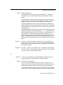
Example 1
For the worksheet shown in Figure 5–1, both the operations cell(2,3) and
cell("EXP2",3) return a value of 0.5.
Example 2
For the worksheet shown in Figure 5–1, the operation
cell(3,3) = 64^cell(2,3)
raises 64 to the power of the number in cell (2,3), and places the result in
cell (3,3).
Related Functions
col
Figure 5–1
Transform Function Descriptions 33
Transform Function Reference
choose
Summary
Syntax
The choose function determines the number of ways of choosing r objects from n
distinct objects without regard to order.
choose(n,r)
For the arguments n and r, r < n and “n choose r” is defined as:
n!
 n = -------------------- r
r! ( n – r)!
Examples
To create a function for the binomial distribution, enter the equation:
binomial(p,n,r) = choose(n,r) ∗ (p^r) ∗ (1−p) ^ (n−r)
col
Summary
Syntax
The col function returns all or a portion of a worksheet column, and can specify a
column destination for transform results.
col (column,top,bottom)
The column argument is the column number or title. To use a column title for the
column argument, enclose the title in quotation marks. The top and bottom
arguments specify the first and last row numbers, and can be omitted. The default
row numbers are 1 and the end of the column, respectively; if both are omitted, the
entire column is used. All parameters must be scalar. Data placed in a column inserts
or overwrites according to the current insert mode.
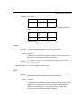
Example 1
For the worksheet shown in Figure 5–1, the operation col(3) returns the entire range
of five values, the operation col(3,4) returns {8.9, 9.1}, and the operation
col("data2",2,3) returns {7.9,8.4}.
Example 2
For the worksheet shown in Figure 5–1, the operation col(4) = col(3)∗2 multiples all
the values in column 3 and places the results in column 4.
34 Transform Function Descriptions
Transform Function Reference
Related Functions
cell
Figure 5–2
complex
Summary
Syntax
Converts a block of real and imaginary numbers into a range of complex numbers.
complex (range,range)
The first range contains the real values, the second range contains the imaginary
values and is optional. If you do not specify the second range, the complex transform
returns zeros for the imaginary numbers. If you do specify an imaginary range, it
must contain the same number of values as the real value range.
Example
If x = {1,2,3,4,5,6,7,8,9,10}, the operation complex(x) returns {{1,2,3,4,....,9,10},
{0,0,0,0,....,0,0}}.
If x = {1.0,-0.75,3.1} and y = {1.2,2.1,-1.1}, the operation complex(x,y) returns
{{1.0,-0.75,3.1}, {1.2,2.1,-1.1}}.
Related Functions
fft, invfft, real, imaginary, mulcpx, invcpx
cos
Summary
This function returns ranges consisting of the cosine of each value in the argument
given.
This and other trigonometric functions can take values in radians, degrees, or grads.
This is determined by the Trigonometric Units selected in the User-Defined
Transform dialog box.
Transform Function Descriptions 35
Transform Function Reference
Syntax
cos(numbers)
The numbers argument can be a scalar or range.
If you regularly use values outside of the usual −2π to 2π (or equivalent) range, use
the mod function to prevent loss of precision. Any missing value or text string
contained within a range is ignored and returned as the string or missing value.
Example
Related Functions
If you choose Degrees as your Trigonometric Units in the User-Defined Transform
dialog box, the operation cos({0,60,90,120,180}) returns values of
{1,0.5,0,−0.5,−1}.
acos, asin, atan
sin, tan
cosh
Summary
Syntax
This function returns the hyperbolic cosine of the specified argument.
cosh(numbers)
The numbers argument can be a scalar or range.
Like the circular trig functions, this function also accepts numbers in degrees,
radians, or grads, depending on the units selected in the User-Defined Transform
dialog box. Any missing value or text string contained within a range is ignored and
returned as the string or missing value.
Example
Related Functions
The operation x = cosh(col(2)) sets the variable x to be the hyperbolic cosine of all
data in column 2.
sinh, tanh
count
Summary
Syntax
The count function returns the value or range of values equal to the number of nonmissing numeric values in a range. Missing values and text strings are not counted.
count(range)
The range argument must be a single range (indicated with the {} brackets) or a
worksheet column.
36 Transform Function Descriptions
Transform Function Reference
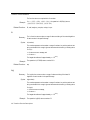
Examples
For the worksheet in Figure 5–1:
the operation count(col(1)) returns a value of 5,
the operation count(col(2)) returns a value of 6, and
the operation count(col(3)) returns a value of 0.
Related Functions
missing, size
Figure 5–3
data
Summary
Syntax
The data function generates a range of numbers from a starting number to an end
number, in specified increments.
data(start,stop,step)
All arguments must be scalar. The start argument specifies the beginning number and
the end argument sets the last number.
If the step parameter is omitted, it defaults to 1. The start parameter can be more
than or less than the stop parameter. In either case, data steps in the correct direction.
Remainders are ignored.
Examples
The operation data(1,5) returns the range of values {1,2,3,4,5}.
The operation data(10,1,2) returns the values {10,8,6,4,2}.
Note that if start and stop are equal, this function produces a number of copies of
start equal to step. For example, the operation data(1,1,4) returns {1,1,1,1}.
Related Functions
size, [ ] array reference
Transform Function Descriptions 37
Transform Function Reference
diff
Summary
The diff function returns a range or ranges of numbers which are the differences
between a given number in a range and the preceding number. The value of the
preceding number is subtracted from the value of the following number.
Because there is no preceding number for the first number in a range, the value of the
first number in the result is always the same as the first number in the argument
range.
Syntax
diff(range)
The range argument must be a single range (indicated with the {} brackets) or a
worksheet column. Any missing value or text string contained within the range is
returned as the string or missing value.
Examples
Related Functions
For x = {9,16,7}, the operation diff(x) returns a value of {9,7,−9}.
For y = {4,−6,12}, the operation diff(y) returns a value of {4,−10,18}.
sum, total
dist
Summary
Syntax
The dist function returns a scalar representing the distance along a line. The line is
described in segments defined by the X,Y pairs specified in an x range and a y range.
dist(x range,y range)
The x range argument contains the X coordinates, and the y range argument contains
the Y coordinates. Corresponding values in these ranges form X,Y pairs. If the ranges
are uneven in size, excess X or Y points are ignored.
Example
Related Functions
For the ranges x ={0,1,1,0,0} and y = {0,0,1,1,0}, the operation dist(x,y) returns
4.0. The X and Y coordinates provided describe a square of 1 unit x by 1 unit y.
partdist
dsinp
Summary
The dsinp function automatically generates the initial parameter estimates for a
damped sinusoidal functions using the FFT method. The four parameter estimates
are returned as a vector.
38 Transform Function Descriptions
Transform Function Reference
Syntax
Σ
Related Functions
dsinp(x range, y range)
The x range argument specifies the x variable, and the y range argument specifies the
y variable. Any missing value or text string contained within one of the ranges is
ignored and will not be treated as a data point. x range and y range must be the same
size, and the number of valid data points must be greater than or equal to 3.
dsinp is especially used to estimate parameters on waveform functions. This is only
useful when this function is used in conjunction with nonlinear regression.
sinp
exp
Summary
Syntax
The exp function returns a range of values consisting of the number e raised to each
number in the specified range. This is numerically identical to the expression
e^(numbers), but uses a faster algorithm.
exp(numbers)
The numbers argument can be a scalar or range of numbers. Any missing value or text
string contained within a range is ignored and returned as the string or missing value.
Example
Related Functions
The operation exp(1) returns a value of 2.718281828459045.
ln
factorial
Summary
Syntax
The factorial function returns the factorial of a specified range.
factorial({range})
The range argument must be a single range (indicated with the {} brackets) or a
worksheet column. Any missing value or text string contained within a range is
ignored and returned as the string or missing value. Non-integers are rounded down
to the nearest integer or 1, whichever is larger.
For factorial(x):
x < 0 returns a missing value,
0 ≤ x < 180 returns x!, and
x ≥ 180 returns +∞
Example 1
The operation factorial({1,2,3,4,5}) returns {1,2,6,24,120}.
Transform Function Descriptions 39
Transform Function Reference
Example 2
To create a transform equation function for the Poisson distribution, you can type:
Poisson(m,x)=(m^x)∗exp(−m)/factorial(x)
fft
Summary
Syntax
The fft function finds the frequency domain representation of your data using the
Fast Fourier Transform.
fft(range)
The parameter can be a range of real values or a block of complex values. For
complex values there are two columns of data. The first column contains the real
values and the second column represents the imaginary values. This function works
on data sizes of size 2n numbers. If your data set is not 2n in length, the fft function
pads 0 at the beginning and end of the data range to make the length 2n.
The fft function returns a range of complex numbers.
Example
Related Functions
For x = {1,2,3,4,5,6,7,8,9,10}, the operation fft(x) takes the Fourier transform of
the ramp function with real data from 1 to 10 with 3 zeros padded on the front and
back and returns a 2 by 16 block of complex numbers.
invfft, real, imaginary, complex, mulcpx, invcpx
for
Summary
Syntax
The for statement is a looping construct used for iterative processing.
for loop variable = initial value to end value step increment do
equation
equation
.
.
.
end for
Transform equation statements are evaluated iteratively within the for loop. When a
for statement is encountered, all functions within the loop are evaluated separately
from the rest of the transform.
The loop variable can be any previously undeclared variable name. The initial value
for the loop is the beginning value to be used in the loop statements. The end value
for the loop variable specifies the last value to be processed by the for statement. After
the end value is processed, the loop is terminated. In addition, you can specify a loop
40 Transform Function Descriptions
Transform Function Reference
variable step increment, which is used to “skip” values when proceeding from the
initial value to end value. If no increment is specified, an increment of 1 is assumed.
Σ
You must separate for, to, step, do, end for, and all condition statement operators,
variables and values with spaces.
The for loop statement is followed by a series of one or more transform equations
which process the loop variable values.
Inside for loops, you can:
➤
➤
indent equations
nest for loops
Note that these conditions are allowed only within for loops. You cannot redefine
variable names within for loops.
Example 1
The operation:
for i = 1 to size(col(1)) do
cell(2,i) = cell(1,i)*i
end for
multiplies all the values in column 1 by their row number and places them in column
2.
Example 2
The operation:
for j = cell(1,1) to cell (1,64) step 2 do
col(10) = col(9)^j
end for
Takes the value from cell (1,1) and increments by 2 until the value in cell (1,64) is
reached, raises the data in column 9 to that power, and places the results in column
10.
fwhm
Summary
Syntax
The fwhm function returns value of the x width at half-maxima in the ranges of
coordinates provided, with optional Lowess smoothing.
fwhm(x range, y range,f)
The x range argument specifies the x variable, and the y range argument specifies the
y variable. Any missing value or text string contained within one of the ranges is
ignored and will not be treated as a data point. x range and y range must have the
same size, and the number of valid data points must be greater than or equal to 3.
Transform Function Descriptions 41
Transform Function Reference
The optional f argument defines the amount of Lowess smoothing, and corresponds
to the fraction of data points used for each regression. f must be greater than or equal
to 0 and less than or equal to 1. 0 ≤ f ≤ 1 . If f is omitted, no smoothing is used.
Example
For x = {0,1,2}, y={0,1,4}, the operation
col(1)=fwhm(x,y)
places the x width at half-maxima 1.00 into column 1.
Related Functions
xatymax
gaussian
Summary
Syntax
This function generates a specified number of normally (Gaussian or “bell” shaped)
distributed numbers from a seed number, using a supplied mean and standard
deviation.
gaussian(number,seed,mean,stddev)
The number argument specifies how many random numbers to generate.
The seed argument is the random number generation seed to be used by the function.
If you want to generate a different random number sequence each time the function
is used, enter 0/0 for the seed. Enter the same number to generate an identical
random number sequence. If the seed argument is omitted, a randomly selected seed
is used.
The mean and stddev arguments are the mean and standard deviation of the normal
distribution curve, respectively. If mean and stddev are omitted, they default to 0 and
1.
Note that function arguments are omitted from right to left. If you want to specify a
stddev, you must either specify the mean argument or omit it by using 0/0.
Example
Related Functions
The operation gaussian(100) uses a seed of 0 to produce 100 normally distributed
random numbers, with a mean of 0.0 and a standard deviation of 1.0.
random
histogram
Summary
The histogram function produces a histogram of the values range in a specified range,
using a defined interval set.
42 Transform Function Descriptions
Transform Function Reference
Syntax
histogram(range,buckets)
The range argument must be a single range (indicated with the {} brackets) or a
worksheet column. Any missing value or text string contained within a range is
ignored.
The buckets argument is used to specify either the number of evenly incremented
histogram intervals, or both the number and ranges of the intervals. This value can
be scalar or a range. In both versions, missing values and strings are ignored.
If the buckets parameter is a scalar, it must be a positive integer. A scalar buckets
argument generates a number of intervals equal to the buckets value. The histogram
intervals are evenly sized; the range is the minimum value to the maximum value of
the specified range.
If the buckets argument is specified as a range, each number in the range becomes the
upper bound (inclusive) of an interval. Values from −∞ to ≤ the first bucket fall in
the first histogram interval, values from > first bucket to ≤ second bucket fall in the
second interval, etc. The buckets range must be strictly increasing in value. An
additional interval is defined to catch any value which does not fall into the defined
ranges. The number of values occurring in this extra interval (including 0, or no
values outside the range) becomes the last entry of the range produced by histogram
function.
Example 1
For col(1) = {1,20,30,35,40,50,60}, the operation col(2) = histogram(col(1),3)
places the range {2,3,2} in column 2. The bucket intervals are automatically set to
20, 40, and 60, so that two of the values in column 1 fall under 20, three fall under
40, and two fall under 60.
Example 2
For buckets = {25,50,75}, the operation col(3) = histogram(col(1),buckets) places
{2,4,1,0} in col(3). Two of the values in column 1 fall under 25, four fall under 50,
one under 75, and no values fall outside the range.
Summary
The if function either selects one of two values based on a specified condition, or
proceeds along a series of calculations bases on a specified condition.
if
Syntax
if(condition,true value,false value)
The true value and false value arguments can be any scalar or range. For a true
condition, the true value is returned; for a false condition, the false value is returned.
If the false value argument is omitted, a false condition returns a missing value.
If the condition argument is scalar, then the entire true value or false value argument
is returned. If the condition argument contains a range, the result is a new range. For
Transform Function Descriptions 43
Transform Function Reference
each true entry in the condition range, the corresponding entry in the true value
argument is returned. For a false entry in the condition range, the corresponding
entry in false value is returned.
If the false value is omitted and the condition entry is false, the corresponding entry
in the true value range is omitted. This can be used to conditionally extract data from
a range.
Example 1
The operation col(2) = if(col(1)< 75,”FAIL","PASS") reads in the values from
column 1, and places the word “FAIL” in column 2 if the column 1 value is less than
75, and the word “PASS” if the value is 75 or greater.
Example 2
For the operation y = if(x < 2 or x > 4,99,x), an x value less than 2 or greater than 4
returns a y value of 99, and all other x values return a y value equal to the
corresponding x value.
If you set x = {1,2,3,4,5}, then y is returned as {99,2,3,4,99}. The condition was
true for the first and last x range entries, so 99 was returned. The condition was false
for x = 2, 3, and 4, so the x value was returned for the second, third, and fourth x
values.
if...then...else
Summary
Syntax
The if...then...else function proceeds along one of two possible series of calculations
based on a specified condition.
if condition then
statement
statement...
else
statement
statement...
end if
To use the if...then...else construct, follow the if condition then statement by one or
more transform equation statements, then specify the else statement(s). When an
if...then...else statement is encountered, all functions within the statement are
evaluated separately from the rest of the transform.
Σ
You must separate if, then, and all condition statement operators, variables, and
values with spaces.
Inside if...then...else constructs, you can:
➤
type more than one equation on a line
44 Transform Function Descriptions
Transform Function Reference
➤
indent equations
➤ nest additional if constructs
Note that these conditions are allowed only within if...else statements. You cannot
redefine variable names within an if...then...else construct.
Example
The operations:
i = cell(1,1)
j = cell(1,2)
If i < 1 and j > 1 then x = col(3)
else x = col(4)
end if
sets x equal to column 3 if i is less than 1 and j is greater than 1; otherwise,
x is equal to column 4.
imaginary (img)
Summary
Syntax
The imaginary function strips the imaginary values out of a range of complex
numbers.
img(block)
The range is made up of complex numbers.
Example
If x = {{1,2,3,4,5,6,7,8,9,10}, {0,0,0,....0,0}}, the operation img(x) returns
{0,0,0,0,0,0,0,0,0,0}.
If x = {{1.0,-0.75, 3.1}, {1.2,2.1,-1.1}}, the operation img(x) returns {1.2,2.1,1.1}.
Related Functions
real, fft, invfft, complex, mulcpx, invcpx
int
Summary
Syntax
The int function returns a number or range of numbers equal to the largest integer
less than or equal to each corresponding number in the specified range. All numbers
are rounded down to the nearest integer.
int(numbers)
The numbers argument can be a scalar or range of numbers. Any missing value or
text string contained within a range is ignored and returned as the string or missing
value.
Transform Function Descriptions 45
Transform Function Reference
Example
Related Functions
The operation int({.9,1.2,2.2,−3.8}) returns a range of {0.0,1.0,2.0,−4.0}.
prec, round
interpolate
Summary
Syntax
The interpolate function performs linear interpolation on a set of X,Y pairs defined
by an x range and a y range. The function returns a range of interpolated y values
from a range of values between the minimum and maximum of the x range.
interpolate(x range,y range,range)
Values in the x range argument must be strictly increasing or strictly decreasing.
The range argument must be a single range (indicated with the {} brackets) or a
worksheet column. Missing values and text strings are not allowed in the x range and
y range. Text strings in range are replaced by missing values.
Extrapolation is not possible; missing value symbols are returned for range argument
values less than the lowest x range value or greater than the highest x range value.
Examples
For x = {0,1,2}, y = {0,1,4}, and range = data(0,2,.5) (this data operation returns
numbers from 0 to 2 at increments of 0.5), the operation
col(1) = interpolate(x,y,range) places the range {0.0,0.5,1.0,2.5,4.0}
into column 1.
If range had included values outside the range for x, missing values would have been
returned for those out-of-range values.
inv
Summary
Syntax
The inv function generates the inverse matrix of an invertible square matrix provided
as a block.
inv(block)
The block argument is a block of numbers with real values in the form of a square
matrix. The number of rows must equal the number of columns.
The function returns a block of numbers with real values in the form of the inverse of
the square matrix provided.
46 Transform Function Descriptions
Transform Function Reference
Example
For the matrix:
1.00
3.00
4.00
2.00
1.00
3.00
3.00
4.00
2.00
in block(2,3,4,5) the operation block(2,7)=inv(block(2,3,4,5)) generates the inverse
matrix:
-0.40
0.40
0.20
0.20
-0.40
0.20
0.20
0.20
-0.20
in block (2,7,4,9).
invcpx
Summary
Syntax
This function takes the reciprocal of a range of complex numbers.
invcp(block)
The input and output are blocks of complex numbers. The invcpx function returns
the range 1/c for each complex number in the input block.
Example
Related Functions
If x = complex ({3,0,1}, {0,1,1}), the operation invcpx(x) returns {{0.33333, 0.0,
0.5}, {0.0,−1.0,−0.5}}.
fft, invfft, real, imaginary, complex, mulcpx
invfft
Summary
Syntax
The inverse fft function (invfft) takes the inverse Fast Fourier Transform (fft) of the
data produced by the fft to restore the data to its new filtered form.
invfft(block)
The parameter is a complex block of spectral numbers with the real values in the first
column and the imaginary values in the second column. This data is usually
generated from the fft function. The invfft function works on data sizes of size 2n
numbers. If your data set is not 2n in length, the invfft function pads 0 at the
beginning and end of the data range to make the length 2n.
Transform Function Descriptions 47
Transform Function Reference
The function returns a complex block of numbers.
Example
Related Functions
If x = {{1,2,3,...,9,10}, {0,0,0,...,0,0}}, the operation invfft(fft(x)) returns
{{0,0,0,1,2,3,...,9,10,0,0,0}, {0,0,0,...0,0}.
fft, real, imaginary, complex, mulcpx, invcpx
ln
Summary
Syntax
The ln function returns a value or range of values consisting of the natural logarithm
of each number in the specified range.
ln(numbers)
The numbers argument can be a scalar or range of numbers. Any missing value or text
string contained within a range is ignored and returned as the string or missing value.
For ln(x):
x < 0 returns an error message, and
x = 0 returns −∞
The largest value allowed is approximately x < 104933.
Example
Related Functions
The operation ln(2.71828) returns a value ≈ 1.0.
exp
log
Summary
Syntax
The log function returns a value or range of values consisting of the base 10
logarithm of each number in the specified range.
log(numbers)
The numbers argument can be a scalar or range of numbers. Any missing value or text
string contained within a range is ignored and returned as the string or missing value.
For log(x):
x < 0 returns an error message,
x = 0 returns −∞
The largest value allowed is approximately x < 104933.
Example
The operation log(100) returns a value of 2.
48 Transform Function Descriptions
Transform Function Reference
lookup
Summary
Syntax
The lookup function compares values with a specified table of boundaries and
returns either a corresponding index from a one-dimensional table, or a
corresponding value from a two-dimensional table.
lookup(numbers,x table,y table)
The numbers argument is the range of values looked up in the specified x table. The x
table argument consists of the upper bounds (inclusive) of the x intervals within the
table and must be ascending in value. The lower bounds are the values of the
previous numbers in the table (−∞ for the first interval).
You must specify numbers and an x table. If only the numbers and x table arguments
are specified, the lookup function returns an index number corresponding to the x
table interval; the interval from -∞ to the first boundary corresponds to an index of
1, the second to 2, etc.
If a number value is larger than the last entry in x table, lookup will return a missing
value as the index. You can avoid missing value results by specifying 1/0 (infinity) as
the last value in x table.
The optional y table argument is used to assign y values to the x index numbers. The
y table argument must be the same size as the x table argument, but the elements do
not need to be in any particular order. If y table is specified, lookup returns the y
table value corresponding to the x table index value, i.e., the first y table value for an
index of 1, the second y table value for an index of 2, etc.
Σ
Note that the x table and y table ranges correspond to what is normally called a
“lookup table.”
Transform Function Descriptions 49
Transform Function Reference
Example 1
For n={-4,11,31} and x={1,10,30}, col(1)=lookup(n,x) places the index values of 1,
3, and -- (missing value) in column1.
index #
1
2
3
x table
1
10
30
-4
11
31 —— (missing value)
-4 falls beneath 1, or the first x boundary; 11 falls beyond 10 but below 30, and 31
lies beyond 30.
Example 2
To generate triplet values for the range {9,6,5}, you can use the expression
lookup(data( 1/3 ,3, 1/3 ),data(1,3),{9,6,5}) to return {9,9,9,6,6,6,5,5,5}. This looks
up the numbers 1/3 , 2/3 , 1, 1 1/3 , 1 2/3 , 2, 2 1/3 , 2 2/3 , and 3 using x table boundaries
1, 2, and 3 and corresponding y table values 9, 6, and 5.
y table
9
6
5
x table
1
2
3
1/3
2/3
1
1 1/3
1 2/3
2
2 1/3
2 2/3
3
50 Transform Function Descriptions
Transform Function Reference
lowess
Summary
Syntax
The lowess function returns smoothed y values as a range from the ranges of x and y
variables provided, using a user-defined smoothing factor. “Lowess” means locally
weighted regression. Each point along the smooth curve is obtained from a regression
of data points close to the curve point with the closest points more heavily weighted.
lowess(x range, y range, f )
The x range argument specifies the x variable, and the y range argument specifies the y
variable. Any missing value or text string contained within one of the ranges is
ignored and will not be treated as a data point. x range and y range must be the same
size, and the number of valid data points must be greater than or equal to 3.
The f argument defines the amount of Lowess smoothing, and corresponds to the
fraction of data points used for each regression. f must be greater than or equal to 0
and less than or equal to 1. 0 ≤ f ≤ 1 . Note that unlike lowpass, lowess requires an f
argument.
Example
For x = {1,2,3,4}, y={0.13, 0.17, 0.50, 0.60}, the operation
col(1)=lowess(x,y,1)
places the smoothed y data 0.10, 0.25, 0.43, 0.63 into column 1.
Related Functions
lowpass
lowpass
Summary
Syntax
The lowpass function returns smoothed y values from ranges of x and y variables,
using an optional user-defined smoothing factor that uses FFT and IFFT.
lowpass(x range, y range, f )
The x range argument specifies the x variable, and the y range argument specifies the y
variable. Any missing value or text string contained within one of the ranges is
ignored and will not be treated as a data point. x range and y range must be the same
size, and the number of valid data points must be greater than or equal to 3.
The optional f argument defines whether FFT and IFFT are used. f must be greater
than or equal to 0 and less than or equal to 100 ( 0 ≤ f ≤ 100 ). If f is omitted, no
Fourier transformation is used.
Σ
lowpass is especially designed to perform smoothing on waveform functions as a part
of nonlinear regression.
Transform Function Descriptions 51
Transform Function Reference
Example
For x = {0,1,2}, y={0,1,4}, the operation
col(1)=lowpass(x,y,88)
places the newly smoothed data 0.25, 1.50, 2.25 into column 1.
Related Functions
lowess
max
Summary
Syntax
The max function returns the largest number found in the range specified.
max(range)
The range argument must be a single range (indicated with the {} brackets) or a
worksheet column. Any missing value or text string contained within a range is
ignored.
Example
For x = {7,4,−4,5}, the operation max(x) returns a value of 7, and the operation
min(x) returns a value of −4.
Summary
The mean function returns the average of the range specified. Use this function to
calculate column averages (as opposed to using the avg function to calculate row
averages).
mean
The mean function calculates the arithmetic mean, defined as:
n
x = --1- ∑ x i
n
i=1
Syntax
mean(range)
The range argument must be a single range (indicated with the {} brackets) or a
worksheet column. Any missing value or text string contained within a range is
ignored.
Example
Related Functions
The operation mean({1,2,3,4}) returns a value of 2.5.
avg
52 Transform Function Descriptions
Transform Function Reference
min
Summary
Syntax
The min function returns the smallest number in the range specified.
min(range)
The range argument must be a single range (indicated with the {} brackets) or a
worksheet column. Any missing value or text string contained within a range is
ignored.
Example
For x = {7,4,−4,5}, the operation max(x) returns a value of 7, and the operation
min(x) returns a value of −4.
missing
Summary
Syntax
The missing function returns a value or range of values equal to the number of
missing values and text strings in the specified range.
missing(range)
The range argument must be a single range (indicated with the {} brackets) or a
worksheet column.
Example
Related Functions
For Figure 5–1, the operation missing(col(1)) returns a value of 1, the operation
missing(col(2)) returns a value of 0, and the operation missing(col(3)) returns a value
of 4.
count, size
Figure 5–4
Transform Function Descriptions 53
Transform Function Reference
mod
Summary
The mod function returns the modulus (the remainder from division) for
corresponding numbers in numerator and divisor arguments.
This is the real (not integral) modulus, so both ranges may be nonintegral values.
Syntax
mod(numerator,divisor)
The numerator and divisor arguments can be scalars or ranges. Any missing value or
text string contained within a range is returned as the string or missing value.
For any divisor ≠ 0, the mod function returns the remainder of
For mod(x,0), that is, for divisor = 0,
numerator
-------------------------------divisor
.
x > 0 returns +∞
x = 0 returns +∞
x < 0 returns −∞
Example
The operation mod({4,5,4,5},{2,2,3,3}) returns the range {0,1,1,2}. These are the
remainders for 4÷2, 5÷2, 4÷3, and 5÷3.
mulcpx
Summary
Syntax
The mulcpx function multiplies two blocks of complex numbers together.
mulcpx(block, block)
Both input blocks should be the same length. The mulcpx function returns a block
that contains the complex multiplication of the two ranges.
Example
Related Functions
If u = {{1,1,0},{0,1,1}}, the operation mulcpx(u,u) returns {{1,0,−1}, {0,2,0}}.
fft, invfft, real, imaginary, complex, invcpx
nth
Summary
Syntax
The nth function returns a sampling of a provided range, with the frequency
indicated by a scalar number. The result always begins with the first entry in the
specified range.
nth(range,increment)
54 Transform Function Descriptions
Transform Function Reference
The range argument is either a specified range (indicated with the {} brackets) or a
worksheet column. The increment argument must be a positive integer.
Example
The operation col(1)=nth({1,2,3,4,5,6,7,8,9,10},3) places the range {1,4,7,10} in
column 1. Every third value of the range is returned, beginning with 1.
Summary
The partdist function returns a range representing the distance from the first X,Y pair
to each other successive pair. The line segment X,Y pairs are specified by an x range
and a y range.
partdist
The last value in this range is numerically the same as that returned by dist, assuming
the same x and y ranges.
Syntax
partdist(x range,y range)
The x range argument specifies the x coordinates, and the y range argument specifies
the y coordinates. Corresponding values in these ranges form xy pairs.
If the ranges are uneven in size, excess x or y points are ignored.
Example
Related Functions
For the ranges x = {0,1,1,0,0} and y = {0,0,1,1,0}, the operation partdist(x,y)
returns a range of {0,1,2,3,4}. The X and Y coordinates provided describe a square
of 1 unit x by 1 unit y.
dist
polynomial
Summary
The polynomial function returns the results for independent variable values in
polynomials. Given the coefficients, this function produces a range of y values for the
corresponding x values in range.
The function takes one of two forms. The first form has two arguments, both of
which are ranges. Values in the first range are the independent variable values. The
second range represents the coefficients of the polynomial, with the constant
coefficient listed first, and the highest order coefficient listed last.
The second form accepts two or more arguments. The first argument is a range
consisting of the independent variable values. All successive arguments are scalar and
represent the coefficients of a polynomial, with the constant coefficient listed first
and the highest order coefficient listed last.
Transform Function Descriptions 55
Transform Function Reference
Syntax
polynomial(range,coefficents) or
polynomial(range,a0,a1,...,an)
The range argument must be a single range (indicated with the {} brackets) or a
worksheet column. Text strings contained within a range are returned as a missing
value.
The coefficients argument is a range consisting of the polynomial coefficient values,
from lowest to highest. Alternately, the coefficients can be listed individually as
scalars.
Example
To solve the polynomial y = x 2 + x + 1 for x values of 0, 1, and 2, type the
equation polynomial({0,1,2},1,1,1). Alternately, you could set x ={1,1,1}, then
enter polynomial({0,1,2},x). Both operations return a range of {1,3,7}.
prec
Summary
Syntax
The prec function rounds a number or range of numbers to the specified number of
significant digits, or places of significance. Values are rounded to the nearest integer;
values of exactly 0.5 are rounded up.
prec(numbers,digits)
The numbers argument can be a scalar or range of numbers. Any missing value or text
string contained within a range is ignored and returned as the string or missing value.
If the digits argument is a scalar, all numbers in the range have the same number of
places of significance. If the digits argument is a range, the number of places of
significance vary according to the corresponding range values. If the size of the digits
range is smaller than the numbers range, the function returns missing values for all
numbers with no corresponding digits.
Example
For x = {13570,3.141,.0155,999,1.92}, the operation prec(x,2) returns
{14000,3.100,.0160,1000,1.90}.
For y = {123.5,123.5,123.5,123.5}, the operation prec(y,{1,2,3,4}) returns {100.0,
120.0,124.0,123.5}.
Related Functions
int, round
put into
Summary
The put into function places calculation results in a designated column on the
worksheet. It operates faster than the equivalent equality relationship.
56 Transform Function Descriptions
Transform Function Reference
Syntax
put results into col(column)
The results argument can be either the result of an equation, function or variable. The
column argument is either the column number of the destination column, or the
column title, enclosed in quotes.
Data put into columns inserts or overwrites according to the current insert mode.
Example
Related Functions
To place the results of the equation y = data(1,100) in column 1, you can type col(1)
= y. However, entering put y into col(1) runs faster.
col = (arithmetic) operator
random
Summary
This function generates a specified number of uniformly distributed numbers within
the range.
Rand and rnd are synonyms for the random function.
Syntax
random(number,seed,low,high)
The number argument specifies how many random numbers to generate.
The seed argument is the random number generation seed to be used by the
function. If you want to generate a different random number sequence each time the
function is used, enter 0/0 for the seed. If the seed argument is omitted, a randomly
selected seed is used.
The low and high arguments specify the beginning and end of the random number
distribution range. The low boundary is included in the range. If low and high are
omitted, they default to 0 and 1, respectively.
Note that function arguments are omitted from right to left. If you want to specify a
high boundary, you must specify the low boundary argument first.
Example
Related Functions
The operation random(50,0/0,1,7) produces 50 uniformly distributed random
numbers between 1 and 7. The sequence is different each time this random function
is used.
gaussian
Transform Function Descriptions 57
Transform Function Reference
real
Summary
Syntax
The real function strips the real values from a complex block of numbers.
real (range)
The range argument consists of complex numbers.
Example
Related Functions
If x = complex ({1,2,3,...,9,10}, {0,0,...,0}), the operation real(x) returns
{1,2,3,4,5,6,7,8,9,10}, leaving the imaginary values out.
fft, invfft, imaginary, complex, mulcpx, invcpx
rgbcolor
Summary
Syntax
The transform function rgbcolor takes arguments r, g, and b between 0 and 255 and
returns the corresponding color to cells in the worksheet. This function can be used
to apply custom colors to any element of a graph or plot that can use colors chosen
from a worksheet column.
rgbcolor(r,g,b)
The r,g,b arguments define the red, green, and blue intensity portions of the color.
These values must be scalars between 0 and 255. Numbers for the arguments less
than 0 or greater than 255 are truncated to these values.
Examples
The operation rgbcolor(255,0,0) returns red.
The operation rgbcolor(0,255,0) returns green.
The operation rgbcolor(0,0,255) returns blue.
The following statements place the secondary colors yellow, magenta, and cyan into
rows 1, 2, and 3 into column 1:
cell(1,1)=rgbcolor(255,255,0)
cell(1,2)=rgbcolor(255,0,255)
cell(1,3)=rgbcolor(0,255,255)
Shades of gray are generated using equal arguments. To place black, gray, and white
in the first three rows of column 1:
cell(1,1)=rgbcolor(0,0,0)
cell(1,2)=rgbcolor(127,127,127)
cell(1,3)=rgbcolor(255,255,255)
58 Transform Function Descriptions
Transform Function Reference
round
Summary
Syntax
The round function rounds a number or range of numbers to the specified decimal
places of accuracy. Values are rounded up or down to the nearest integer; values of
exactly 0.5 are rounded up.
round(numbers,places)
The numbers argument can be a scalar or range of numbers. Any missing value or
text string contained within a range is ignored and returned as the string or missing
value.
If the places argument is negative, rounding occurs to the left of the decimal point.
To round to the nearest whole number, use a places argument of 0.
Examples
Related Functions
The operation round(92.1541,2) returns a value of 92.15.
The operation round(0.19112,1) returns a value of 0.2.
The operation round(92.1541,−2) returns a value of 100.0.
int, prec
runavg
Summary
Syntax
The runavg function produces a range of running averages, using a window of a
specified size as the size of the range to be averaged. The resulting range is the same
length as the argument range.
runavg(range,window)
The range argument must be a single range (indicated with the {} brackets) or a
worksheet column. Any missing value or text string contained within a range is
replaced with 0.
If the window argument is even, the next highest odd number is used. The tails of
the running average are computed by appending
w i nd ow – 1 )
(----------------------- additional initial and final values to their respective ends of range.
2
Transform Function Descriptions 59
Transform Function Reference
Example
The operation runavg({1,2,3,4,5},3) returns {1.33,2,3,4,4.67}.
The value of the window argument is 3, so the first result value is calculated as:
(---------------3 – 1) + 1 + 2
2
----------------------------------3
The second value is calculated as:
1+2+3
--------------------3
Related Functions
, etc.
avg
mean
sin
Summary
This function returns ranges consisting of the sine of each value in the argument
given.
This and other trigonometric functions can take values in radians, degrees, or grads.
This is determined by the Trigonometric Units selected in the User-Defined
Transform dialog box.
Syntax
sin(numbers)
The numbers argument can be a scalar or range.
If you regularly use values outside of the usual −2π to 2π (or equivalent) range, use
the mod function to prevent loss of precision. Any missing value or text string
contained within a range is ignored and returned as the string or missing value.
Example
Related Functions
If you choose Degrees as your Trigonometric Units in the transform dialog box, the
operation sin({0,30,90,180,270}) returns values of {0,0.5,1,0,−1}.
acos, asin, atan
cos, tan
60 Transform Function Descriptions
Transform Function Reference
sinh
Summary
Syntax
This function returns the hyperbolic sine of the specified argument.
sinh(numbers)
The numbers argument can be a scalar or range.
Like the circular trig functions, this function also accepts numbers in degrees,
radians, or grads, depending on the units selected in the User-Defined Transform
dialog box.
Example
Related Functions
The operation x = sinh(col(3)) sets the variable x to be the hyperbolic sine of all data
in column 3.
cosh, tanh
sinp
Summary
Syntax
The sinp function automatically generates the initial parameter estimates for a
sinusoidal functions using the FFT method. The three parameter estimates are
returned as a vector.
sinp(x range, y range)
The x range argument specifies the x variable, and the y range argument specifies the
y variable. Any missing value or text string contained within one of the ranges is
ignored and will not be treated as a data point. x range and y range must be the same
size, and the number of valid data points must be greater than or equal to 3.
Σ
sinp is especially used to perform smoothing on waveform functions, used in
determination of initial parameter estimates for nonlinear regression.
size
Summary
The size function returns a value equal to the total number of elements in the
specified range, including all numbers, missing values, and text strings.
Note that siz e ( X ) ½ count ( X ) + missing ( X ) .
Syntax
size(range)
The range argument must be a single range (indicated with the {} brackets) or a
worksheet column.
Transform Function Descriptions 61
Transform Function Reference
Example
For Figure 5–1:
the operation size(col(1)) returns a value of 6,
the operation size(col(2)) returns a value of 6, and
the operation size(col(3)) returns a value of 4.
Related Functions
count, missing
Figure 5–5
sort
Summary
Syntax
This function can be used to sort a range of numbers in ascending order, or a range of
numbers in ascending order together with a block of data.
sort(block,range)
The range argument can be either a specified range (indicated with the {} brackets)
or a worksheet column. If the block argument is omitted, the data in range is sorted
in ascending order.
Example
The operation col(2) = sort(col(1)) returns the contents of column 1 arranged in
ascending order and places it in column 2.
To reverse the order of the sort, you can create a custom function:
reverse(x) = x[data(size(x),1)]
then apply it to the results of the sort. For example, reverse(sort(x)) sorts range x in
descending order.
62 Transform Function Descriptions
Transform Function Reference
Example
The operation:
block(3,1) = sort(block(1,1,2,size(col(2)),col(2))
sorts data in columns 1 and 2 using column 2 as the key column and places the
sorted data in columns 3 and 4.
Related Functions
size, data
sqrt
Summary
Syntax
The sqrt function returns a value or range of values consisting of the square root of
each value in the specified range. Numerically, this is the same as {numbers}^0.5, but
uses a faster algorithm.
sqrt(numbers)
The numbers argument can be a scalar or range of numbers. Any missing value or text
string contained within a range is ignored and returned as the string or missing value.
For numbers < 0, sqrt generates a missing value.
Example
The operation sqrt({−1,0,1,2}) returns the range {--,0,1,1.414}.
stddev
Summary
The stddev function returns the standard deviation of the specified range, as defined
by:
n
1
s = ---------n–1
∑ (x i – x )
1--2 2
i=1
Syntax
stddev(range)
The range argument must be a single range (indicated with the {} brackets) or a
worksheet column. Any missing value or text string contained within a range is
ignored.
Example
Related Functions
For the range x = {1,2}, the operation stddev(x) returns a value of .70711.
stderr
Transform Function Descriptions 63
Transform Function Reference
stderr
Summary
The stderr function returns the standard error of the mean of the specified range, as
defined by
s
------n
where s is the standard deviation.
Syntax
stderr(range)
The range argument must be a single range (indicated with the {} brackets) or a
worksheet column. Any missing value or text string contained within a range is
ignored.
Example
Related Functions
For the range x = {1,2}, the operation stderr(x) returns a value of 0.5.
stddev
subblock
Summary
Syntax
The subblock function returns a block of cells from within another previously
defined block of cells from the worksheet. The subblock is defined using the upper
left and lower right cells of the subblock, relative to the range defined by the source
block.
subblock (block, column 1, row 1, column 2, row 2)
The block argument can be a variable defined as a block, or a block function
statement.
The column 1 and row 1 arguments are the relative coordinates for the upper left cell
of the subblock with respect to the source block. The column 2 and row 2 arguments
are the relative coordinates for the lower right cell of the subblock. All values within
this range are returned. Operations performed on a block always return a block. If
column 2 and row 2 are omitted, then the last row and/or column is assumed to be
the last row and column of the source block.
All column and row arguments must be scalar (not ranges).
Example
Related Functions
For x = block (3,1,20,42) the operation subblock (x,1,1,1,1) returns cell (3,1) and
the operation subblock (x,5,5) returns the block from cell (7, 5) to cell (20, 42).
block, blockheight, blockwidth
64 Transform Function Descriptions
Transform Function Reference
sum
Summary
The function sum returns a range of numbers representing the accumulated sums
along the list. The value of the number is added to the value of the preceding
cumulative sum.
Because there is no preceding number for the first number in a range, the value of the
first number in the result is always the same as the first number in the argument
range.
Syntax
sum(range)
The range argument must be a single range (indicated with the {} brackets) or a
worksheet column. Any text string or missing value contained within the range is
returned as the string or missing value.
Example
Related Functions
For x = {2,6,7}, the operation sum(x) returns a value of {2,8,15}.
For y = {4,12,−6}, the operation sum(y) returns a value of {4,16,10}.
diff, total
tan
Summary
This function returns ranges consisting of the tangent of each value in the argument
given.
This and other trigonometric functions can take values in radians, degrees, or grads.
This is determined by the Trigonometric Units selected in the User-Defined
Transform dialog box.
Syntax
tan(numbers)
The numbers argument can be a scalar or range.
If you regularly use values outside of the usual −2π to 2π (or equivalent) range, use
the mod function to prevent loss of precision. Any missing value or text string
contained within a range is ignored and returned as the string or missing value.
Example
Related Functions
If you choose Degrees as your Trigonometric Units in the transform dialog box, the
operation tan({0,45,135,180}) returns values of {0,1,−1,0}.
acos, asin, atan
cos, sin
Transform Function Descriptions 65
Transform Function Reference
tanh
Summary
Syntax
This function returns the hyperbolic tangent of the specified argument.
tanh(numbers)
The numbers argument can be a scalar or range.
Like the circular trig functions, this function also accepts numbers in degrees,
radians, or grads, depending on the units selected in the User-Defined Transform
dialog box.
Example
Related Functions
The operation x = tanh(col(3)) sets the variable x to be the hyperbolic tangent of all
data in column 3.
cosh, sinh
total
Summary
Syntax
The function total returns a single value equal to the total sum of all numbers in a
specified range. Numerically, this is the same as the last number returned by the sum
function.
total(range)
The range argument must be a single range (indicated with the {} brackets) or a
worksheet column. Missing values and text strings contained within the range are
ignored.
Examples
Related Functions
For x = {9,16,7}, the operation total(x) returns a value of 32.
For y = {4,12,−6}, the operation total(y) returns a value of 10.
diff, sum
x25
Summary
r
rangeThe x25 function returns value of the x at ymin + --------------in the ranges of coordinates
4
provided, with optional Lowess smoothing. This is typically used to return the x
value for the y value at 25% of the distance from the minimum to the maximum of
smoothed data for sigmoidal shaped functions.
66 Transform Function Descriptions
Transform Function Reference
Syntax
x25(x range, y range, f )
The x range argument specifies the x variable, and the y range argument specifies the
y variable. Any missing value or text string contained within one of the ranges is
ignored and will not be treated as a data point. x range and y range must have the
same size, and the number of valid data points must be greater than or equal to 3.
The optional f argument defines the amount of Lowess smoothing, and corresponds
to the fraction of data points used for each regression. f must be greater than or equal
to 0 and less than or equal to 1. 0 ≤ f ≤ 1 . If f is omitted, no smoothing is used.
Example
For x = {0,1,2}, y={0,1,4}, the operation
col(1)=x25(x,y)
r
rangeplaces the x at ymin + --------------as 1.00 into column 1.
4
Related Functions
x50, x75, xatymax, xwtr
x50
Summary
Syntax
r
rangeThe x50 function returns value of the x at ymin + --------------in the ranges of coordinates
2
provided, with optional Lowess smoothing. This is typically used to return the x
value for the y value at 50% of the distance from the minimum to the maximum of
smoothed data for sigmoidal shaped functions.
x50(x range, y range, f )
The x range argument specifies the x variable, and the y range argument specifies the
y variable. Any missing value or text string contained within one of the ranges is
ignored and will not be treated as a data point. x range and y range must have the
same size, and the number of valid data points must be greater than or equal to 3.
The optional f argument defines the amount of Lowess smoothing, and corresponds
to the fraction of data points used for each regression. f must be greater than or equal
to 0 and less than or equal to 1. 0 ≤ f ≤ 1 . If f is omitted, no smoothing is used.
Example
For x = {0,1,2}, y={0,1,4}, the operation
col(1)=x50(x,y)
r
rangeplaces the x at ymin + --------------as 1.00 into column 1.
2
Related Functions
x25, x75, xatymax, xwtr
Transform Function Descriptions 67
Transform Function Reference
x75
Summary
Syntax
3r
range- in the ranges of coordinates
The x75 function returns value of the x at ymin + -----------------4
provided, with optional Lowess smoothing. This is typically used to return the x
value for the y value at 75% of the distance from the minimum to the maximum of
smoothed data for sigmoidal shaped functions.
x75(x range, y range, f )
The x range argument specifies the x variable, and the y range argument specifies the
y variable. Any missing value or text string contained within one of the ranges is
ignored and will not be treated as a data point. x range and y range must have the
same size, and the number of valid data points must be greater than or equal to 3.
The optional f argument defines the amount of Lowess smoothing, and corresponds
to the fraction of data points used for each regression. f must be greater than or equal
to 0 and less than or equal to 1. 0 ≤ f ≤ 1 . If f is omitted, no smoothing is used.
Example
For x = {0,1,2}, y={0,1,4}, the operation
col(1)=x75(x,y)
3r
range- as 2.00 into column 1.
places the x at ymin + -----------------4
Related Functions
x25, x50, xatymax, xwtr
xatymax
Summary
Syntax
The xatymax function returns the x value at the maximum y value found, with
optional Lowess smoothing.
xatymax(x range, y range, f )
The x range argument specifies the x variable, and the y range argument specifies the
y variable. Any missing value or text string contained within one of the ranges is
ignored and will not be treated as a data point. x range and y range must have the
same size, and the number of valid data points must be greater than or equal to 3.
Σ
The optional f argument defines the amount of Lowess smoothing, and corresponds
to the fraction of data points used for each regression. f must be greater than or equal
to 0 and less than or equal to 1. 0 ≤ f ≤ 1 . If f is not defined, no smoothing is used.
If duplicate y maximums are found xatymax will return the average value of all the x
at y maximums.
68 Transform Function Descriptions
Transform Function Reference
Example
For x = {0,1,2}, y={0,1,4}, the operation
col(1)=xatymax(x,y)
places the x at the y maximum as 2.00 into column 1.
Related Functions
x25, x50, x75, xwtr
xwtr
Summary
Syntax
The xwtr function returns value of x75-x25 in the ranges of coordinates provided,
with optional Lowess smoothing.
xwtr(x range, y range, f )
The x range argument specifies the x variable, and the y range argument specifies the
y variable. Any missing value or text string contained within one of the ranges is
ignored and will not be treated as a data point. x range and y range must have the
same size, and the number of valid data points must be greater than or equal to 3.
The optional f argument defines the amount of Lowess smoothing, and corresponds
to the fraction of data points used for each regression. f must be greater than or equal
to 0 and less than or equal to 1. 0 ≤ f ≤ 1 . If f is omitted, no smoothing is used.
Example
For x = {0,1,2}, y={0,1,4}, the operation
col(1)=xwtr(x,y)
places the x75-x25 as double 1.00 into column 1.
Related Functions
x25, x50, x75, xatymax
User-defined Functions
0
You can create any user-defined function, consisting of any expression in the
transform language, and then refer to it by name.
For example, the following transform defines the function dist2pts, which returns the
distance between two points
dist2pts(x1,y1,x2,y2) = sqrt((x2−x1)^2+(y2−y1)^2)
You can then use this custom-defined function, instead of the expression to the right
of the equal sign, in subsequent equations. For example, to plot the distances
User-defined Functions 69
Transform Function Reference
between two sets of XY coordinates, with the first points stored in columns 1 and 2,
and the second in columns 3 and 4, enter:
col(5) = dist2pts(col(1),col(2),col(3),col(4))
The resulting distances are placed in column 5.
Saving
User-Defined
Functions
Frequently used variable values and custom transforms can be saved to a transform
file, then copied and pasted into the desired transform.
To save user-defined functions to a file, then apply them to a transform:
1.
Define the variables and functions in the Transform window, then click the Save
button.
2.
When the Save dialog box appears, name the file something like “User-Defined
Functions.”
3.
Select the function you want to use in the transform, then press Ctrl+C or
Ctrl+Ins.
4.
Open the transform file you want to copy the function to, click the point in the
text where you want to enter the function, then press Ctrl+V or Shift+Ins.
70 User-defined Functions
6
Example Transforms
Many mathematical transform examples, along with appropriate graphs and
worksheets are included with SigmaPlot. This chapter is describes the data transform
examples and the graphing transform examples provided. Each description contains
the text of the transform and, where applicable, a graph displaying the possible
results of the transform.
The sample transforms and the XFMS.JNB notebook can be found in the XFMS
folder.
Data Transform Examples
0
The data transform examples are provided to show you how transform equations can
manipulate and calculate data.
One Way Analysis of Variance (ANOVA)
0
A One Way Analysis of Variance (ANOVA) table can be created from the results of a
regression or nonlinear regression. The original Y values, the Y data from the fitted
curve, and the parameters are used to generate the table.
The transform assumes you have placed the original Y data in column 2, the fitted Y
data in column 3, and the regression coefficients or function parameters in column 4.
You can either place this data in these columns, or change the column numbers used
by the transform.
The One Way ANOVA transform contains examples of the following transform
functions:
➤
➤
➤
➤
➤
count
if
total
mean
{...} (constructor notation)
Data Transform Examples 71
Example Transforms
To use the One Way ANOVA transform:
1.
Make sure your original Y data is in column 2. Perform the desired regression
using the Regression Wizard, and save your Predicted values (fitted Y data) in
column 3, and Parameters (the regression coefficients) in column 4.
For more information on using the Regression Wizard, see Chapter 8, “Regression Wizard.”
One Way
ANOVA Transform
(ANOVA.XFM)
2.
Press F10 to open the User-Defined Transform dialog box, then click the Open
button and open the ANOVA.XFM transform file in the XFMS directory. The
ANOVA transform appears in the edit window.
3.
Click Run. The ANOVA results are placed in columns 5 through 9, or beginning at the column specified with the anova variable.
‘****** Analysis of Variance (ANOVA) Table ******
‘This transform takes regression or curve fit
‘results and constructs an ANOVA table
‘Required INPUT: y data, fitted y data, function
‘
parameters/coefficients
‘RESULTS: sum of squares, degrees of freedom, mean
‘
squared, F-value, R-squared & R values,
‘
standard error of fit;
‘INPUT to be placed in (specify source columns):
y_col=2
‘y data column number
fit_col=3
‘fitted y data column number
param_col=4
‘parameter column number
‘ANOVA to be placed in column:
anova=5
‘ANOVA table starting column
‘(5 columns x 10 rows)
y=col(y_col)
‘define y values
f=col(fit_col) ‘define fitted y values
p=col(param_col) ‘define function parameters
n=count(y)
‘number of y data points
tdof=n-1
‘total degrees of freedom
r=count(if(p<>0,p,"--")) ‘the number of nonzero
‘parameters
‘******* ANOVA TABLE CALCULATION *******
‘Regression Degrees of Freedom:
rdof=tdof-if(r<count(p),r-2,count(p)-1)
‘Error Degrees of Freedom:
edof=tdof-rdof
‘Sum of Squares of Residuals:
SSE=total((y-f)^2)
‘Sum of Squares of Error about the Mean:
SSM=total((y-mean(y))^2)
‘Sum of Squares of Error due to Regression:
SSR=SSM-SSE
‘Standard Error of Fit:
72 Data Transform Examples
Example Transforms
se=sqrt(SSE/rdof)
‘F value:
f1=((SSM-SSE)/(edof))/(SSE/rdof)
F=if(n<2,"n < 2 !",f1)
‘R squared:
R2=(1-SSE/SSM)
‘****** PLACE ANOVA TABLE IN WORKSHEET *******
col(anova)={0/0,"REGRESSION","ERROR","TOTAL"}
col(anova+1)={"SUM OF SQUARES",SSR,SSE,SSM}
col(anova+2)={"DEG FREEDOM",edof,rdof,tdof}
col(anova+3)={"MEAN SQUARE",(SSR/edof),(SSE/rdof)}
col(anova+4)={"F",F}
col(anova,7)={"#POINTS","R SQUARED","R","STD ERR"}
col(anova+1,7)={n,R2,sqrt(R2),se}
Area Beneath a Curve Using Trapezoidal Rule
0
This transform computes the area beneath a curve from X and Y data columns using
the trapezoidal rule for unequally spaced X values. The algorithm applies equally well
to equally spaced X values.
This transform uses an example of the diff function.
To use the Area Under Curve transform:
Area Under
Curve Transform
(AREA.XFM)
1.
Place your X data in column 1 and your Y data in column 2. If your data has
been placed in other columns, you can specify these columns after you open the
AREA.XFM file. You can use an existing or new worksheet.
2.
Press F10 to open the User-Defined Transform dialog box, then click the Open
button and open the AREA.XFM transform file in the XFMS directory. The
Area transform appears in the edit window.
3.
Click Run. The area is placed in column 3 or in the column specified with the
res variable.
‘*Transform for Calculating Area Beneath a Curve*
‘ This transform integrates under curves using the
‘ trapezoidal rule. This can be used for equal
‘ or unequally spaced x values.
‘ The algorithm is: sigma i from 0 to n-1, or
‘ {yi(xi+1 - xi) + (1/2)(yi+1 - yi)(xi+1 - xi)}
‘ Place your x data in x_col and y data in y_col or
‘ change the column numbers to suit your data.
‘ Results are placed in column res.
x_col=1
‘column number for x data
y_col=2
‘column number for y data
res=3
‘column number for result
‘Define x and y data
Data Transform Examples 73
Example Transforms
x=col(x_col)
y=col(y_col)
‘**************** CALCULATE AREA ****************
‘Compute the range of differences between
‘ x[i] & x[i-1]
xdif1=diff(x)
n=count(x)
‘Delete first valuexdif=xdif1[data(2,n)]
‘not a difference
‘Compute the range of differences between
‘ y[i] & y[i-1]
ydif1=diff(y)
‘Delete first valueydif=ydif1[data(2,n)]
‘not a difference
‘Use only y values from y[1] to y[n-1]
y1=y[data(1,n-1)]
‘Calculate trapezoidal integration
intgrl=y1*xdif+0.5*ydif*xdif
a=total(intgrl)
‘******** PLACE RESULTS IN WORKSHEET *********
col(res)=a
‘Put area in column res
Bivariate Statistics
0
This transform takes two data columns of equal length and computes their means,
standard deviations, covariance, and correlation coefficient. The columns must be of
equal length.
The Bivariate transform uses examples of these transform functions
➤
mean
➤ stddev
➤ total
74 Data Transform Examples
Example Transforms
To use the Bivariate transform:
Bivariate Statistics
Transform
(BIVARIAT.XFM)
1.
Place your X data in column 1 and your Y data in column 2. If your data has
been placed in other columns, you can specify these columns after you open the
BIVARIAT.XFM transform file. You can enter data into an existing worksheet or
a new worksheet.
2.
Press F10 to open the User-Defined Transform dialog box, then click the Open
button, and open the BIVARIAT.XFM transform file in the XFMS directory.
The Bivariate Statistics transform appears in the edit window.
3.
Click Run. The results are placed in columns 3 and 4, or beginning in the column specified with the res variable.
‘ This transform integrates under curves using the
‘ trapezoidal rule
‘*** Transform to Compute Bivariate Statistics ***
‘ This transform takes x and y data and returns
‘ the means, standard deviations, covariance, and
‘ correlation coefficient (rxy)
‘ Place your x data in x_col and y data in y_col
‘ or change the column numbers to suit your data.
‘ Results are placed in columns res and res+1
x_col=1
‘column number for x data
y_col=2
‘column number for y data
res=3
‘first results column
‘Define x and y data
x=col(x_col)
y=col(y_col)
‘************* CALCULATE STATISTICS *************
n=size(col(x_col)) ‘number of x values
‘n must be > 1
mx=mean(x)
‘mean of x data
my=mean(y)
‘mean of y data
sx=stddev(x)
‘standard deviation of x data
sy=stddev(y)
‘standard deviation of y data
‘covariance of x and y
sxy=if(n>1,(total(x*y)-n*mx*my)/(n-1),0)
‘correlation coefficient of x and y
rxy=sxy/(sx*sy)
‘********* PLACE STATISTICS IN WORKSHEET *********
col(res)={"N","MEAN X","MEAN Y","STD DEV X",
"STD DEV Y","COVARIANCE","CORR COEFF"}
col(res+1)= if(n>1,{n,mx,my,sx,sy,sxy,rxy},"n<=1")
Data Transform Examples 75
Example Transforms
Differential Equation Solving
0
This transform can be used to solve user-defined differential equations. You can
define up to four first order equations, named fp1(x1,y1,y2,y3,y4) through
fp4(x1,y1,y2,y3,y4). Set any unused equations = 0.
To solve a first order differential equation:
1.
Begin a new worksheet by choosing the File menu New command, then choosing Worksheet; this transform requires a clean worksheet to work correctly.
2.
Open the User-Defined Transforms dialog box by selecting the Transforms
menu User Defined command, then clicking the Open button, and opening the
DIFFEQN.XFM transform file in the XFMS directory. The Differential Equation Solving transform appears in the edit window.
3.
Scroll to the Number of Equations section and enter a value for the neqn variable. This is the number of equations you want to solve, up to four.
4.
Scroll down to the Differential Equations section, and set the fp1 through fp4
functions to the desired functions. Set any unused equations = 0. If only one
first order differential equation is used, then only the fp1 transform equation is
used and fp2, fp3, and fp4 are set to 0. For example, if you only wanted to solve
the differential equation:
dy
-------1- = – ay 1
dt
you would enter:
fp1(x,y1,y2,y3,y4) = −a*y1
fp2(x,y1,y2,y3,y4) = 0
fp3(x,y1,y2,y3,y4) = 0
fp4(x,y1,y2,y3,y4) = 0
5.
Scroll down to the Initial Values heading and set the nstep variable to the number of integration (X variable) steps you want to use. The more steps you set, the
longer the transform takes.
6.
Set the initial X value x0, final X value x1, and the Y1 through Y4 values (placed
in cells (2,1) through (5,1)). If you are not using a y1 value, set that value to
zero (0). For example, for the single equation example above, you could enter:
x0 = 0
;initial x
x1 = 1
;final x
cell(2,1) = 1
;y1 initial value
cell(3,1) = 0
;y2 initial value
76 Data Transform Examples
Example Transforms
cell(4,1) = 0
cell(5,1) = 0
;y3 initial value
;y4 initial value
7.
Click Run. The results output is placed in columns 1 through neqn+1.
8.
To graph your results, create a Line Plot graphing column 1 as your X data and
columns 2 through 5 as your Y data.
Plasma Iron Kinetics - IV Bolus 55Fe
Figure 6–1
Differential Equation Graph
10
y1
y2
55
Fe Concentration (% of total dose)
100
y3
y4
1
0.0
0.1
0.2
0.3
0.4
0.5
0.6
0.7
0.8
0.9
1.0
Time (days)
For information on creating a graph plotting one X data column against many Y
data columns see the SigmaPlot’s User’s Manual.
Differential Equation
Solving Transform
(DIFFEQN.XFM)
The transform example solves the equations:
dy
-------1 = – ( r 65 + r 75 + r 85 )y 1 + r 56 y 2 + r 57 y 3
dt
dy
-------2 = r 65 y 1 – r 56 y 2
dt
dy
-------3 = r 75 y 1 – r 57 y 3
dt
dy
-------4 = r 85 y 1
dt
Data Transform Examples 77
Example Transforms
‘*** Solution of Coupled First Order Differential ***
‘*** Equations by Fourth Order Runge-Kutta Method ***
‘
***** Number of Equations *****
‘Enter the number of differential equations "neqn"
‘the number of differential equations, less than or
‘equal to 4
neqn = 4
‘number of differential equations
‘
***** Differential Equations ******
‘Set the functions fp1, fp2, fp3, fp4 to be equal to
‘coupled first order ordinary differential equations
‘where x is the independent variable and y1, y2, y3,
‘and y4 are the dependent variables. The number of
‘equations must be equal to the neqn value set above.
‘If neqn < 4 then use zeros (0) for the unused
‘equations
fp1(x,y1,y2,y3,y4)
fp2(x,y1,y2,y3,y4)
fp3(x,y1,y2,y3,y4)
fp4(x,y1,y2,y3,y4)
=
=
=
=
-(r65+r75+r85)*y1+r56*y2+r57*y3
r65*y1-r56*y2
r75*y1-r57*y3
r85*y1
‘
****** Initial Values ******
‘Enter the maximum number of integration
‘steps "nstep".
nstep = 25
;number of integration steps
‘Enter the initial and final x values followed by the
‘initial values of y1 (and y2, y3 and y4, if they are
‘used). If neqn < 4 then use zeros (0) for the unused
‘initial yi values.
x0 = 0
x1 = 1
cell(2,1)
cell(3,1)
cell(4,1)
cell(5,1)
=
=
=
=
‘initial x
‘final x
100 ‘y1 initial value
0 ‘y2 initial value
0 ‘y3 initial value
0 ‘y4 initial value
‘
**** RESULTS ****
‘ The output will be placed in columns 1 through neqn+1.
‘x is placed in column 1. The yi values are placed in
‘columns 2 through neqn+1. Other columns are used for
78 Data Transform Examples
Example Transforms
‘program working space.
‘
***** Parameter Values *****
‘Enter all necessary parameter values below
r65
r75
r85
r56
r57
‘
=
=
=
=
=
2.2
2.3
8.4
4.2
0.32
********** PROGRAM **********
fp(x,y1,y2,y3,y4,m) = if(m=1, fp1(x,y1,y2,y3,y4),
if(m=2, fp2(x,y1,y2,y3,y4),
if(m=3, fp3(x,y1,y2,y3,y4),
if(m=4, fp4(x,y1,y2,y3,y4)))))
h = (x1-x0)/nstep
hh = 0.5*h
h6 = h/6
cell(1,1) = x0
n2 = neqn+2
‘yt
n3 = neqn+3
‘dydx
n4 = neqn+4
‘dyt
n5 = neqn+5
‘dym
‘ Fixed Step Size Fourth Order Runge-Kutta
for k = 1 to nstep do
xk = x0 + (k-1)*h
xh = xk + hh
for i = 1 to neqn do
cell(n3,i) = fp(xk,cell(2,k),cell(3,k),
cell(4,k),cell(5,k),i)
‘dydx
cell(n2,i) = cell(i+1,k) +
hh*cell(n3,i)
‘yt
end for
for i1 = 1 to neqn do
cell(n4,i1) = fp(xh,cell(n2,1),cell(n2,2),
cell(n2,3),cell(n2,4),i1)
‘dyt
cell(n2,i1) = cell(i1+1,k) +
hh*cell(n4,i1)
‘yt
end for
for i2 = 1 to neqn do
cell(n5,i2) = fp(xh,cell(n2,1),cell(n2,2),
cell(n2,3),cell(n2,4),i2)
‘dym
cell(n2,i2) = cell(i2+1,k) +
Data Transform Examples 79
Example Transforms
h*cell(n5,i2)
‘yt
cell(n5,i2) = cell(n5,i2) +
cell(n4,i2)
‘dym = dym + dyt
end for
for i3 = 1 to neqn do
cell(n4,i3) = fp(xk+h,cell(n2,1),cell(n2,2),
cell(n2,3),cell(n2,4),i3)
‘dyt
cell(i3+1,k+1) = cell(i3+1,k) + h6*(cell(n3,i3)
+ cell(n4,i3) + 2*cell(n5,i3))
end for
cell(1,k+1) = cell(1,k) + h
end for
F-test to Determine Statistical Improvement in Regressions
0
This transform compares two equations from the same family to determine if the
higher order provides a statistical improvement in fit.
Often it is unclear whether a higher order model fits the data better than a lower
order. Equations where higher orders may produce better fits include: simple
polynomials of different order, the sums of exponentials for transient response data,
and the sums of hyperbolic functions for saturation ligand binding data.
F-TEST.XFM uses the residuals from two regressions to compute the sums of squares
of the residuals, then creates the F statistic and computes an approximate P value for
the significance level.
You can try this transform out on the provided sample graph, or run it on the
residuals produced by your own regression sessions. Residuals are saved to the
worksheet by the Regression Wizard.
1.
80 Data Transform Examples
To use the provided sample data and graph, open the F-test worksheet and
graph in the XFMS.JNB notebook. The worksheet contains raw data in columns 1 and 2, and curve fit results for the two competitive binding models in
columns 3-5 and 6-8. The graph plots the raw data and the two curve fits.
Example Transforms
Figure 6–2
Comparing Two Curve
Fits
Use of the F Test
0.20
0.18
Log (Drug) vs Bound
Log (Drug) vs y fit 1
Log (Drug) vs y fit 2
0.16
0.14
Bound
0.12
0.10
0.08
0.06
0.04
0.02
0.00
-12
-11
-10
-9
-8
-7
-6
-5
-4
Log [Competitor]
2.
To use your own data, enter the XY data to be curve fit in columns 1 and 2,
respectively. Select the first curve fit equation and use it to fit the data, place the
parameters, fit results and residuals in the first empty columns (3-5). Run the
second curve fit and place the results in columns 6-8 (the default). If desired,
create graphs of these results using the wizard.
3.
Press F10 to open the User-Defined Transform dialog box, then open the FTEST.XFM transform file. Specify n1 and n2, the number of parameters in the
lower and higher order functions. In the example provided, these are 3 and 5,
respectively.
If necessary, specify cs1 and cs2, the column locations for the residuals of each
curve fit, and cres, the first column for the two column output.
4.
F-test Transform
(F-TEST.XFM)
Click Run. The F-test value and corresponding P value are placed into the worksheet. If P < 0.05, you can predict that the higher order equation provides a statistically better fit.
'***** Compare Two Nonlinear Curve Fits *****
'*****
with the F test
*****
'This transform uses the residuals from two
'curve fits of functions from the same family
'to determine if there is a significant
'improvement in the fit provided by the higher
'order fitting function.
'The F statistic is computed and used to obtain
'an approximate P value.
'****** Input ******
n1=3 'number parameters for 1st function
'(fewest parameters)
Data Transform Examples 81
Example Transforms
n2=5 ' number parameters for 2nd function
cs1 = 6 ' residual column for function 1
cs2 = 9 ' residual column for function 2
cres =10 ' first column of two results columns
'****** Program ******
N=size(col(cs1))
ss1=total(col(cs1)^2)
ss2=total(col(cs2)^2)
F = ((ss1-ss2)/ss2)*((N-n2)/(n2-n1))
'Approximate P value for F distribution
N1=n2-n1
' A&S, Eq. 26.6.15, p. 947
N2=N-n2
x=(F^(1/3)*(1-2/(9*N2))-(1-2/(9*N1)))/
sqrt(2/(9*N1)+F^(2/3)*2/(9*N2))
'Normal distribution approximation for P value
pi=3.1415926 ' A&S, Eq. 26.2.17, p 932
z=exp(-x^2/2)/sqrt(2*pi)
t=1/(1+.2316419*x)
p=z*(.31938153*t-.356563782*t^2+1.781477937
*t^3-1.821255978*t^4+1.330274429*t^5)
'****** Output ******
col(cres)={" F = ", " p = "}
col(cres+1)={F,p}
R2 for Nonlinear Regressions
0
You can use this transform to compute the coefficient of determination (R2) for the
results of a nonlinear regression. The original Y values and the Y data from the fitted
curve are used to calculate R2.
To save the fitted Y values of the nonlinear regression to the worksheet, use the
Regression Wizard to save the Function results to the appropriate column (for this
transform, column 3).
1.
Place your original Y data in column 2 of the worksheet and the fitted Y data in
column 3. If your data has been placed in other columns, you can specify these
columns after you open the R2.XFM transform file. You can enter data into an
existing or a new worksheet.
2.
Press F10 to open the User-Defined Transform dialog box, then click the Open
button and open the R2.XFM transform file in the XFMS directory. The R2
transform appears in the edit window.
3.
Click Run. The R2 value is placed in column 4 of the worksheet, or in the column specified with the res variable.
82 Data Transform Examples
Example Transforms
R Squared
Transform (R2.XFM)
‘***Transform to Compute R Square (Coefficient ***
‘** of Determination) for Nonlinear Curve Fits **
‘ Place your y data in y_col and the fitted y data
‘ in fit_col or change the column numbers to suit
‘ your data. Results are placed in column res.
y_col=2
‘column number for y data
fit_col=3
‘column number for fit results
res=4
‘column number for R2 result
‘Define y and fitted y values
y=col(y_col)
yfit=col(fit_col)
‘************** CALCULATE R SQUARE **************
n=yfit-y
d=y-mean(y)
r2=1.0-total(n^2)/total(d^2)
‘****** PLACE R SQUARE VALUE IN WORKSHEET *******
col(res)={"R SQUARE",r2}
Standard Deviation of Linear Regression Parameters
0
This transform computes linear 1st-order regression parameter values (slope and
intercept) and their standard deviations using X and Y data sets of equal length.
To calculate 1st-order regression parameters and their standard deviations for
XY data points:
Standard Deviation
Regression
Transform
(STDV_REG.XFM)
1.
Place the X data in column 1 of the worksheet and the Y data in column 2. If
your data is in other columns, you can specify these columns after you open the
STDV_REG.XFM transform file. You can enter data into an existing worksheet
or a new worksheet.
2.
Press F10 to open the User-Defined Transform dialog box, then click the Open
button, and open the STDV_REG.XFM transform file in the XFMS directory.
If necessary, change the x_col, y_col, and res variables to the correct column
numbers.
3.
Click Run. The results are placed in columns 3 and 4, or in the columns specified by the res variable.
‘** Transform to Compute Standard Deviations of **
‘******** Linear Regression Coefficients *********’
‘Place your x data in x_col and y data in y_col or
‘ change the column numbers to suit your data.
‘ Results are placed in columns res and res+1.
x_col=1
‘column number for x data
y_col=2
‘column number for y data
res=3
‘first results column
x=col(x_col)
‘Define x values
y=col(y_col)
‘Define y values
Data Transform Examples 83
Example Transforms
‘********** CALCULATE PARAMETER VALUES **********
n=size(col(x_col)) ‘n must be > 2
mx=mean(x)
my=mean(y)
sumxx=total(x*x)
sumyy=total(y*y)
sumxy=total(x*y)
a1=(sumxy-n*mx*my)/(sumxx-n*mx*mx) ‘slope
a0=my-a1*mx
‘intercept
‘**** CALCULATE PARAMETER STANDARD DEVIATIONS ****
sregxy=if(n>2,sqrt((sumyy-n*a0*my-a1*sumxy)/(n-2)) ,0)
s0=sregxy*sqrt(sumxx/(n*(sumxx-n*mx*mx))) ‘SD a0
s1=sregxy/sqrt(sumxx-n*mx*mx)
‘SD a1
‘********** PLACE RESULTS IN WORKSHEET **********
col(res)={"n","INTERCEPT","SLOPE","STD DEV INT ",
"STD DEV SLOPE"}
col(res+1)=if(n>2,{n,a0,a1,s0,s1},{"n <= 2"})
Graphing Transform Examples
0
The graph transform examples are provided to show you how transform equations
can manipulate and calculate data to create complex graphs.
Each of the following descriptions provide instructions on how to use SigmaPlot to
create graphs. Most of these graphs, however, are already set up as sample graphs. If
you use the provided worksheet and graphs with the corresponding transform files,
SigmaPlot will automatically create the graphs after you run the transform.
Control Chart for Fractional Defectives with Unequal Sample Sizes
0
This example computes the fraction of defectives p for a set of unequally sized
samples using their corresponding numbers of defects, the control limits for p, and
data for the upper and lower control lines.
This transform contains examples of the following transform functions:
➤
➤
stddev
sqrt
To calculate and graph the fraction of defectives and control lines for given sample
sizes and number of defects per sample, you can either use the provided sample data
and graph or begin a new notebook, enter your own data and create your own graph
using the data.
84 Graphing Transform Examples
Example Transforms
1.
To use the provided sample data and graph, open the Control Chart worksheet
and graph in the Control Chart section of the Transform Examples notebook.
The worksheet appears with data in columns 1, 2, and 3. The graph page
appears with an empty graph.
2.
To use your own data, place the sample sizes in column 1 and the corresponding
number of defects data in column 2 of a new worksheet. If your data is in other
columns, you can specify these columns after you open the CONTCHRT.XFM
transform file. You can enter your data in an existing or a new worksheet.
3.
Press F10 to open the User-Defined Transform dialog box, then click the Open
button and open the CONTCHRT.XFM transform file in the XFMS directory.
The Control Chart transform appears in the edit window.
4.
Click Run. The results are placed in columns 4 through 5 of the worksheet.
5.
If you opened the Control Chart graph, view the graph page. The graph plots
the fraction of defectives using a Line and Scatter plot with a Simple Straight
Line style graphing column 3 as Y data versus the row numbers. The control
lines are plotted as a Simple Horizontal Step Plot using columns 4 and 5 versus
their row numbers. The mean line for the fractional defectives is drawn with a
reference line.
6.
To create your own graph, create a Line and Scatter Plot, with a Simple Line
style, then plot column 3 as Y data against the row numbers. Add an additional
Line Plot using the Multiple Horizontal Step Plot style, plotting columns 4 and
5 versus their two numbers, then add a reference line to plot the mean line for
the fractional device.
For more information on creating graphs in SigmaPlot, refer to the SigmaPlot
User’s Manual.
Graphing Transform Examples 85
Example Transforms
Figure 6–3
Control Chart Graph
Fractional Device, p
0.04
0.03
0.02
0.01
0.00
0
5
10
15
20
25
30
35
Lot Number
Control Chart
Transform
(CONTROL.XFM)
;Transform for Fraction Defective Control Chart
;with Unequal Sample Sizes
; This transform takes sample size and number of
; defectives returns the fraction of defectives
; and data for upper and lower control limit lines
; Place the sample size data in n_col and the
; number of defects in def_col, or change the
; column numbers to suit your data. Fraction
; defective results are placed in the percent_col
; column, and the data for the control lines is
; placed in columns cl and cl+1.
n_col=1
‘sample size column
def_col=2
‘number of defectives column
percent_col=3 ‘fraction defective results column
cl=4
‘first results column for control
‘limit line data
‘********* CALCULATE FRACTION DEFECTIVE **********
n=col(n_col)
‘sample sizes
def=col(def_col)
‘defectives
col(p_col)=def/n
‘fraction defective
pbar=total(def)/total(n)
‘*********** CALCULATE CONTROL LIMITS ************
stddev = sqrt(pbar*(1 - pbar)/n)
ucl=pbar+3*stddev
‘upper control limit
lcl=pbar-3*stddev
‘lower control limit
lclt=if(lcl>=0,lcl,0) ‘truncated lower control
‘limit
‘**** DATA FOR CONTROL LIMIT LINE STEP CHART ****
col(cl)=ucl
col(cl+1)=lclt
86 Graphing Transform Examples
Example Transforms
Cubic Spline Interpolation and Computation of First and Second Derivatives
0
This example takes data with irregularly spaced X values and generates a cubic spline
interpolant. The CBESPLN1.XFM transform takes X data which may be irregularly
spaced and generates the coefficients for a cubic spline interpolant. The
CBESPLN2.XFM transform takes the coefficients and generates the spline
interpolant and its two derivatives.
The values for the interpolant start at a specified minimum X which may be less
than, equal to, or greater than the X value of the original first data point. The
interpolant has equally spaced X values that end at a specified maximum which may
be less than, equal to, or greater than the largest X value of the original data.
Note that this is not the same algorithm that SigmaPlot uses; this algorithm does not
handle multiple valued functions, whereas SigmaPlot does.
To use the transform to generate and graph a cubic spline interpolant, you can either
use the provided sample data and graph, or begin a new notebook, enter your own
data and create your own graph using the data.
1.
To use the provided sample data and graph, open the Cubic Spline worksheet
and graph by double-clicking the graph page icon in the Cubic Spline section of
the Transform Examples notebook. The worksheet appears with data in columns
1 and 2 and the graph page appears with two graphs. The first graph plots the
original XY data as a scatter plot. The second graph appears empty.
2.
To use your own data, enter the irregularly spaced XY data into the worksheet.
The X values must be sorted in strictly increasing values. The default X and Y
data columns used by the transform are columns 1 and 2, respectively.
3.
Press F10 to open the User-Defined Transform dialog box, then click the Open
button, and open the CBESPLN1.XFM transform file in the XFMS directory.
The first Cubic Spline transform appears in the edit window.
4.
Move to the Input Variables heading. Set the X data column variable cx, the Y
data column cy, the beginning interpolated X value xbegin, the ending interpolated X value xend, and the X increments for the interpolated points xstep. A
larger X step results in a smoother curve but takes longer to compute.
5.
Enter the end condition setting iend for the interpolation.
6.
You can use first, second, or third order conditions.
If you have only a few data points, you should try different orders to see which
one you like the most. See the example for the effect of too low an order on the
first and second derivatives.
Graphing Transform Examples 87
Example Transforms
1
end spline segments approach straight lines asymptotically
2
end spline segments approach parabolas asymptotically
3
end spline segments approach cubics asymptotically
7.
Move to the RESULTS heading and enter the first column number for the
results cr. This column for the beginning of the results block is specified in both
transforms.
8.
Click Run to run the transform. When it finishes, press F10 then open the
CBESPLN2.XFM transform file in the XFMS directory. Make sure that the cr
variable is identical to the previous value, then click Run.
9.
If you opened the Cubic Spline graph, view the page. The first graph plots the
original XY data as a scatter plot and the interpolated data as a second line plot
by picking the cr column as the X column and cr+1 as the Y column. The second graph plots the derivatives as line plots using the cr column versus the cr+2
column and the cr column versus the cr+3 column.
10. To create your own graphs using SigmaPlot, create a Scatter Plot using a Simple
Scatter style which plots the original data in columns 1 and 2 as XY pairs. Add
an additional Line Plot using a Simple Spline Curve, then plot the cr column as
the X column against the cr+1 column as the Y column.
For more information on creating graphs in SigmaPlot, see the SigmaPlot User’s
Manual.
Figure 6–4
Cubic Spline Graph
Cubic Spline Interpolation
First and Second Derivatives
100
50
x data v y data
interp x v interp y
80
interp x v 1st deriv
interp x v 2nd deriv
40
30
60
Y
20
40
10
0
20
-10
0
-20
-20
-30
-1
0
1
2
3
X
88 Graphing Transform Examples
4
5
6
-1
0
1
2
3
X
4
5
6
Example Transforms
Cubic Spline
1 Transform
(CBESPLN1.XFM)
‘**** Cubic Spline Interpolation and Computation ****
‘
**** of Derivatives ****
‘This transform takes an x,y data set with increasing
‘ordered x values and computes a cubic spline
‘interpolation. The first and second derivatives of
‘the spline are also computed.
‘Two transform files are run in sequence. This
‘transform computes the spline coefficients. The
‘CBESPLN2.XFM transform computes the spline and two
‘derivatives.
‘
********** Input Variables **********
cx=1
‘x data column number
cy=2
‘y data column number
xbegin=-.5
‘first x value for interpolation
xend=5
‘last x value for interpolation
xstep=.025
‘x interval for interpolation
‘There are 3
‘ iend = 1:
‘ iend = 2:
‘ iend = 3:
iend=1
spline end conditions allowed:
linear end conditions
quadratic end conditions
cubic end conditions
‘end condition = 1, 2, or 3
‘
************ RESULTS ************
‘The results are placed into a block of 9 columns
‘starting at column cr. Column cr MUST be
‘specified identically in both transforms. Columns
‘cr to cr+3 contain the x mesh the spline and the
‘first two derivatives. Columns cr+4 to cr+7
‘contain the a, b, c and d spline coefficients.
‘Column cr+8 is for working variables.
cr=3
‘1st column of results block
‘
************ PROGRAM ************
cr4=cr+4
‘column for "a" spline coefficients
cr5=cr+5
‘column for "b" spline coefficients
cr6=cr+6
‘column for "c" spline coefficients
cr7=cr+7
‘column for "d" spline coefficients
cr8=cr+8
‘working column
n=size(col(cx))
cell(cr8,1)=cx
cell(cr8,2)=cy
cell(cr8,3)=cr
cell(cr8,4)=xbegin
Graphing Transform Examples 89
Example Transforms
cell(cr8,5)=xend
cell(cr8,6)=xstep
‘compute S for n-2 rows
nm1=n-1
nm2=n-2
cell(cr8,7)=cell(cx,2)-cell(cx,1)
‘dx1
cell(cr8,8)=(cell(cy,2)-cell(cy,1))
/cell(cr8,7)*6
‘dy1
for i=1 to nm2 do
dx2=cell(cx,i+2)-cell(cx,i+1)
‘dx2
dy2=(cell(cy,i+2)-cell(cy,i+1))/dx2*6 ‘dy2
cell(cr4,i)=cell(cr8,7)
‘dx1
cell(cr5,i)=2*(cell(cr8,7)+dx2)
‘2(dx1+dx2)
cell(cr6,i)=dx2
‘dx2
cell(cr7,i)=dy2-cell(cr8,8)
‘dy2-dy1
cell(cr8,7)=dx2
‘dx1=dx2
cell(cr8,8)=dy2
‘dy1=dy2
end for
‘adjust first and last rows for end condition
dx11=cell(cx,2)-cell(cx,1)
dx1n=cell(cx,n)-cell(cx,nm1)
if iend=2 then
cell(cr5,1)=cell(cr5,1)+dx11
cell(cr5,nm2)=cell(cr5,nm2)+dx1n
else if iend = 3 then
dx12=cell(cx,3)-cell(cx,2)
cell(cr5,1)=(dx11+dx12)*(dx11+2*dx12)/dx12
cell(cr6,1)=(dx12*dx12-dx11*dx11)/dx12
dx2n=cell(cx,nm1)-cell(cx,nm2)
cell(cr4,nm2)=(dx2n*dx2n-dx1n*dx1n)/dx2n
cell(cr5,nm2)=(dx1n+dx2n)*(dx1n+2*dx2n)/dx2n
end if
end if
‘solve the tridiagonal system
‘first reduce
for j = 2 to nm2 do
jm1=j-1
cell(cr4,j)=cell(cr4,j)/cell(cr5,jm1)
cell(cr5,j)=cell(cr5,j)-cell(cr4,j)*cell(cr6,jm1)
cell(cr7,j)=cell(cr7,j)-cell(cr4,j)*cell(cr7,jm1)
end for
‘ next back substitute
cell(cr7,nm1)=cell(cr7,nm2)/cell(cr5,nm2)
for k =nm2-1 to 1 step -1 do
cell(cr7,k+1)=(cell(cr7,k)-cell(cr6,k)*
90 Graphing Transform Examples
Example Transforms
cell(cr7,k+2))/cell(cr5,k)
end for
‘ specify the end conditions
if iend = 1 then
‘linear ends
cell(cr7,1)=0.0
cell(cr7,n)=0.0
else if iend = 2 then
‘quadratic ends
cell(cr7,1)=cell(cr7,2)
cell(cr7,n)=cell(cr7,nm1)
else if iend = 3 then
‘cubic ends
cell(cr7,1)=((dx11+dx12)*cell(cr7,2)dx11*cell(cr7,3))/dx12
cell(cr7,n)=((dx2n+dx1n)*cell(cr7,nm1)dx1n*cell(cr7,nm2))/dx2n
end if
end if
end if
‘ compute coefficients of cubic polynomial
for m = 1 to nm1 do
mp1=m+1
h=cell(cx,mp1)-cell(cx,m)
cell(cr4,m)=(cell(cr7,mp1)-cell(cr7,m))/(6*h) ‘a(i)
cell(cr5,m)=cell(cr7,m)/2
‘b(i)
cell(cr6,m)=((cell(cy,mp1)-cell(cy,m))/h)((2*h*cell(cr7,m)+h*cell(cr7,mp1))/6) ‘c(i)
end for
Cubic Spline 2
Transform
(CBESPLN2.XFM)
‘********** Spline Generation **********
‘Run this transform after you run CBESPLN1.XFM.
‘Make sure to enter the same results column
‘number value cr as in CBESPLN1.XFM.
‘
********** Input Variables **********
cr=3 ‘1st column of results block, contains
‘spline x mesh. This must be the same
‘value as in CBESPLN1.XFM.
‘
************ PROGRAM ************
cr1=cr+1 ‘column for spline values
cr2=cr+2 ‘column for 1st derivative of spline
cr3=cr+3 ‘column for 2nd derivative of spline
cr4=cr+4 ‘column for "a" spline coefficients
cr5=cr+5 ‘column for "b" spline coefficients
cr6=cr+6 ‘column for "c" spline coefficients
cr8=cr+8 ‘working column
xbegin=cell(cr8,4)
Graphing Transform Examples 91
Example Transforms
xend=cell(cr8,5)
xstep=cell(cr8,6)
cx=cell(cr8,1)
cy=cell(cr8,2)
n=size(col(cx))
x1end=int((xend-xbegin)/xstep)+1
cell(cr8,9)=1
‘index of x value
x=col(cx)
f(a,b,c,y,dxx)=y+dxx*(c+dxx*(b+dxx*a))
f1(a,b,c,dxx)=c+dxx*(2*b+dxx*(3*a))
f2(a,b,dxx)=2*b+6*a*dxx
for u1 = 1 to x1end do
u=xbegin+(u1-1)*xstep
cell(cr,u1)=u
‘put u value in col cr
xj=cell(cr8,9)
if u <= x[n] then
if u <= x[xj+1] then ‘test u <= x(i+1)
dx=u-x[xj]
‘dx
cell(cr1,u1)=f(cell(cr4,xj),cell(cr5,xj),
cell(cr6,xj),cell(cy,xj),dx)
cell(cr2,u1)=f1(cell(cr4,xj),
cell(cr5,xj),cell(cr6,xj),dx)
cell(cr3,u1)=f2(cell(cr4,xj),cell(cr5,xj),dx)
else
for j1 = 1 to n do ‘start search loop
if j1>1 then
if u <= x[j1] then
if u > x[j1-1] then
xj1=j1-1
dx1=u-x[xj1]
‘dx
cell(cr1,u1)=f(cell(cr4,xj1),cell(cr5,xj1),
cell(cr6,xj1),cell(cy,xj1),dx1)
cell(cr2,u1)=f1(cell(cr4,xj1),cell(cr5,xj1),
cell(cr6,xj1),dx1)
cell(cr3,u1)=f2(cell(cr4,xj1),
cell(cr5,xj1),dx1)
cell(cr8,9)=j1-1
end if
end if
end if
end for
‘end search loop
end if
else
xj2=xj
dx2=u-x[xj2]
cell(cr1,u1)=f(cell(cr4,xj2),cell(cr5,xj2),
cell(cr6,xj2),cell(cy,xj2),dx2)
92 Graphing Transform Examples
Example Transforms
cell(cr2,u1)=f1(cell(cr4,xj2),cell(cr5,xj2),
cell(cr6,xj2),dx2)
cell(cr3,u1)=f2(cell(cr4,xj2),cell(cr5,xj2),dx2)
end if
end for
Fast Fourier Transform
0
The Fast Fourier Transform converts data from the time domain to the frequency
domain. It can be used to remove noise from, or smooth data using frequency-based
filtering. Use the fft function to find the frequency domain representation of your
data, then edit the results to remove any frequency which may adversely affect the
original data.
The Fast Fourier Transform uses the following transform functions:
➤
➤
➤
➤
➤
➤
➤
fft
invfft
real
img
complex
mulcpx
invcpx
The Fast Fourier Transform operates on a range of real values or a block of complex
values. For complex values there are two columns of data. The first column contains
the real values and the second column represents the imaginary values. The
worksheet format of a block of complex numbers is:
r1
i1
r2
i2
....
....
rn
in
where r values are real elements, and i values are imaginary elements. In transform
language syntax, the two columns {{r1, r2, ... rn},{i1, i2, ... in}} are written as:
block({r1, r2, ... rn},{i1, i2, ... in})
This function works on data sizes of size 2 n numbers. If your data set is not 2n in
length, the fft function pads 0 at the beginning and end of the data range to make the
length 2n. A procedure for unpadding the results is given in the example Smoothing
with a Low Pass Filter on page 99.
Graphing Transform Examples 93
Example Transforms
The fft function returns a range of complex numbers. The Fast Fourier Transform is
usually graphed with respect to frequency. To produce a frequency scale, use the
relationship:
f=fs*(data(0,n/2)-1)/n
where fs is the sampling frequency. The example transform POWSPEC.XFM.
includes the automatic generation of a frequency scale (see page 94).
The Fast Fourier Transform operates on data which is assumed to be periodic over
the interval being analyzed. If the data is not periodic, then unwanted high frequency
components are introduced. To prevent these high frequency components from
occurring, windows can be applied to the data before using the fft transform. The
Hanning window is a cosine function that drops to zero at each end of the data. The
example transform POWSPEC.XFM includes the option to implement the Hanning
window (see page 94).
Using the
Block Function
To return the full fft data to the worksheet:
1.
First assign the data you want to filter to column 1 of the worksheet. You can
generate the data using a transform, or use your own measurements.
2.
Press F10 to open the User-Defined Transforms dialog box, then click the New
button to start a new transform.
3.
Type the following transform in the edit window:
x=col(1)
’real data
tx=fft(x)
’compute the fft
block(2)=tx ’place real fft data back in col(2)
’place imaginary fft data in col(3)
4.
Computing Power
Spectral Density
Click Run. The results are placed starting one column over from the original
data.
The example transform POWSPEC.XFM uses the Fast Fourier Transform function,
then computes the power spectral density, a frequency axis, and makes optional use
of a Hanning window.
To calculate and graph the power spectral density of a set of data, you can either use
the provided sample data and graph, or begin a new notebook, enter your own data
and create your own graph using the data.
1.
To use the sample worksheet and graph, open the Power Spectral Density worksheet and graph by double-clicking the graph page icon in the Power Spectral
Density section of the Transform Examples notebook. Data appears in column 1
of the worksheet, and two graphs appear on the graph page. The top graph
shows data generated by the sum of two sine waves plus Gaussian random noise.
94 Graphing Transform Examples
Example Transforms
The data is represented by:
f(t)=sin(2*pi*f1*t)+0.3*sin(2*pi*f2*t)+g(t)
where f1=10 cycles/sec (cps), f2=100cps, and the Gaussian random noise has
mean 0 and standard deviation of 0.2. The lower graph is empty.
2.
To use your own data, place your data in column 1. If your data is in a different
column, specify the new column after you open the POWSPEC.XFM transform
file.
3.
Press F10 to open the User-Defined Transform dialog box, then click the Open
button, and open POWSPEC.XFM transform file in the XFMS directory. The
Power Spectral Density transform appears in the edit window.
Σ
To use this transform, the Trigonometric Units must be set to Radians.
4.
Click Run. Since the frequency sampling value (fs) is nonzero, a frequency axis is
generated in column 2 and the power spectral density data in column 3.
5.
If you opened the Power Spectral Density graph, view the graph page. Two
graphs appear on the page. The top graph plots the data generated by the sum of
two sine waves plus Gaussian random noise using a Line Plot with Simple
Straight Line style graphing column 1 versus row numbers. The lower graph
plots the power spectral density using a Line Plot with a Simple Straight Line
style, graphing column 2 as the X data (frequency), and column 3 as the Y data.
6.
To plot your own data using SigmaPlot, choose the Graph menu Create Graph
command, or select the Graph Wizard from the toolbar. Create a Line Plot with
a Simple Straight Line style plotting your original data versus row numbers by
choosing Single Y data format. If you set the frequency sampling value (fs) to
nonzero, create a Line Plot with a Simple Straight Line style, graphing columns
2 and 3 using XY Pair data format. Otherwise, create a Line Plot with a Simple
Straight Line style plotting column 3 (power spectral density) versus row numbers by choosing Single Y data format.
The power spectral density plot of the signal f(t) shows two major peaks at the
two frequencies of the sine waves (10cps and 100cps), and a more or less constant noise level in between.
Graphing Transform Examples 95
Example Transforms
For more information on how to create graphs in SigmaPlot, see the SigmaPlot
User’s Manual.
Figure 6–5
Power Spectral
Density Example Graph
1
Amplitude
The top graph shows f(t) data
generated by the sum of two
sine waves plus Gaussian
random noise. The bottom
graph is the power spectral
density of the signal f(t).
2
0
-1
-2
0
100
200
300
400
500
150
200
250
Power Spectral Density
X Axis
1e+6
1e+5
1e+4
1e+3
1e+2
1e+1
1e+0
0
50
100
Frequency (cps)
The Power Spectral
Density Transform
(POWSPEC.XFM)
‘
This transform computes the power spectral ‘
density
(psd) of data in column ci and places it
‘
in column co.
‘
If a nonzero sampling frequency fs is specified
‘
then a frequency axis is placed in column co
‘
with the psd in the next adjacent column.
‘
If han=1 then a Hanning window is applied to the
‘
padded data.
‘
Set Trigonometric Units to Radians
‘ Input
ci=1
‘input column number
co=2
‘first output column number
fs=10 ‘sampling frequency (produces frequency axis
‘ if fs>0)
han=1 ‘Hanning window (1=use, 0=don’t use)
‘ Program
pi=3.1415926
x1=col(ci)
if han=1 then
‘use Hanning window
n=size(x1)
nlog2=log(n)/log(2) ‘pad data if necessary
powup=int(nlog2)
96 Graphing Transform Examples
Example Transforms
intup1=if(nlog2-powup<1e-14, 2^powup, 2^(powup+1))
rl=if(mod(n,2)>0, (intup1-n+1)/2, (intup1-n+2)/2
ru=if(mod(n,2)>0, intup1-rl, intup1-r1+1)
x=if(rl-1>0, if(intup1-ru>0, {data(0,0,rl-1), x1,
data(0,0,intup1-ru)},{data(0,0,rl),x1}),
if(intup1-ru>0, {x1,data,(0,0,intup1-ru)}, {x1}))
w=.5*(1-cos(2*pi*data(0,intup1-1)/(intup1-1)))
xf=w*x
‘multiply padded data by window
else
xf=x1
end if
tx=fft(xf)
nf=size(tx)/4
‘fft of data
‘half the zero padded
‘data length
spec=real(tx)^2+img(tx)^2 ‘power spectral density
spechalf=spec[data(1,nf+1)] ‘half the symmetric psd
‘data
f=fs*data(0,nf)/(2*nf)
‘frequency axis
‘ Output
col(co)=if(fs>0,f,spechalf)
col(co+1)=if(fs>0,spechalf)
Kernel Smoothing
The example transform SMOOTH.XFM smooths data by convolving the Fast
Fourier Transform of a triangular smoothing kernel together with the fft of the data.
Smoothing data using this transform is computationally very fast; the number of
operations is greatly reduced over traditional methods, and the results are
comparable. To increase the smoothing, increase the width of the triangular
smoothing kernel.
To calculate and graph the smoothed data, you can either use the provided sample
data and graph, or begin a new notebook, enter your own data, and create your own
graph using the data.
1.
To use the sample worksheet and graph, open the Kernel Smoothing worksheet
and graph by double-clicking the graph page icon in the Kernel Smoothing section of the Transform Examples notebook. Data appears in columns 1 through
4, 6, and 7 of the worksheet, and two graphs appear on the graph page. The first
graph has two plots, the signal, and the signal with noise distortion. Column 1
contains the X data, column 2 contains the Y data for the signal, and column 3
contains the Y data for the signal and the noise distortion. The lower graph is
empty.
2.
To use your own data, place your data in columns 1 through 2. If your data is in
other columns, specify the new columns after you open the SMOOTH.XFM
transform file. If necessary, specify a new column for the results.
Graphing Transform Examples 97
Example Transforms
3.
Press F10 to open the User-Defined Transform dialog box, then click the Open
button, and open SMOOTH.XFM transform file in the XFMS directory. The
Kernel Smoothing transform appears in the edit window.
Σ
To use this transform, make sure the Insert mode is turned off.
4.
Click Run. The results are placed in column 5 unless you specified a different
column in the transform.
5.
If you opened the Kernel Smoothing graph, view the graph page. Two graphs
appear on the page. The first graph has two plots, the signal, and the signal with
noise distortion. The Line Plot with a Multiple Straight Line style graphs column 1 as the X data, column 2 as the Y data for the signal, and column 3 as the
Y data for the signal and the noise distortion. The lower Line Plot with a Simple
Straight Line style plots column 1 as the X data, and column 5 as the Y data
using XY Pairs data format.
6.
To plot your own data using SigmaPlot, choose the Graph menu Create Graph
command, or select the Graph Wizard from the toolbar. Create a Line Plot with
a Multiple Straight Line style using X Many Y data format, plotting column 1 as
the X data, column 2 as the Y data for the signal, and column 3 as the Y data for
the signal and the noise distortion. Create a second Line Plot graph with a Simple Straight Line style using the data in columns 1 and 5, graphing column 1 as
the X data and column 5 as the Y data using XY Pairs data format.
For more information on how to create graphs in SigmaPlot, see the SigmaPlot User’s
Manual.
Figure 6–6
Kernel Smoothing Graph
Signal
Signal + Noise
1.5
1.0
The top graph shows two
plots: the signal, and the
signal plus noise distortion.
The bottom graph is the
kernel smoothing of the
signal with smoothing
set at 10%.
0.5
0.0
0
1.5
50
100
150
200
250
100
150
200
250
10% Smoothing
1.0
0.5
0.0
0
98 Graphing Transform Examples
50
Example Transforms
The Kernel
Smoothing
Transform
(SMOOTH.XFM)
' Kernel Smoothing
' This transform smooths data using kernel smoothing
' Input
ci=3
' input column number
co=5
' output column number
r=10
' percentage smoothing
' Program
x=col(ci)
' data
n1=size(x)
tx=fft(x)
' fft of data
nx=size(tx)/2
n=if(int(r*nx/200)>0, int(r*nx/200), 1)
' generate triangular smoothing kernel
lt={data(n,0,-1), data(0,0,nx-2*n-2), data(0,n)}
lt1=lt/total(lt)
tk=fft(lt1)
' fft of kernel
td=mulcpx(tk,tx)
' convolve kernel and data
sd=invfft(td)
' transform back to time domain
tsd=real(sd)
' normalize data
' Output
ru=if(mod(n1,2)>0, (nx-n1+1)/2, (nx-n1+2)/2)
' strip out padded channels
rl=if(mod(n1,2)>0, nx-ru, nx-ru+1)
tsd1=tsd[data(ru,rl)]
col(co)=tsd1 ' save smoothed data to worksheet
Smoothing with a
Low Pass Filter
The Low Pass Filter transform smooths data by eliminating high frequencies. Use
this transform in contrast to the Kernel Smoothing transform which smooths data by
augmenting some frequencies while minimizing others. The transform statements
describing how the low pass filter works are:
x=col(1)
f=5
‘the data to smooth
‘number of channels to eliminate
tx=fft(x)
‘fft of data
r=data(1,size(tx)/2) ‘total number of channels
mp=size(tx)/4
‘get the midpoint
‘remove the frequencies
td=if( r<mp-f or r>mp+1+f,tx,0)
sd=invfft( td )
‘convert back to time domain
col(2)=real(sd)
‘save smoothed data to worksheet
The LOWPASS.XFM transform expresses f as a percentage for ease of use. As the
value of f increases, more high frequency channels are removed. Note that this is a
Graphing Transform Examples 99
Example Transforms
digital transform which cuts data at a discrete boundary. In addition, this transform
does not alter the phase of the data, which makes it more accurate than analog
filtering. A high pass or band pass filter can be constructed in the same manner.
To calculate and graph the smoothing of a set of data using a low pass filter, you can
either use the provided sample data and graph, or begin a new notebook, enter your
own data, and create your own graph using the data.
1.
To use the sample worksheet and graph, open the Low Pass Smoothing worksheet and graph by double-clicking the graph page icon in the Low Pass
Smoothing section of the Transform Examples notebook. Data appears in columns 1 through 4 of the worksheet, and two graphs showing plots appear on the
graph page. Column 1 contains the X data, column 2 contains the Y data for the
signal and the noise distortion, column 3 contains the X data, and column 4
contains the Y data for the original signal. The top graph plots the signal plus
the noise distortion; the bottom graph plots the signal.
2.
To use your own data, place your data in columns 1 through 2. If your data is in
other columns, specify the new columns after you open the LOWPASS.XFM
transform file. If necessary, specify a new column for the results.
3.
Press F10 to open the User-Defined Transform dialog box, then click the Open
button, and open LOWPASS.XFM transform file in the XFMS directory. The
Low Pass Filter transform appears in the edit window.
Σ
To use this transform, make sure Insert mode is turned off.
4.
Click Run. The results are placed starting in column 5, unless you specified a
different column in the transform.
5.
If you opened the Low Pass Smoothing graph, view the graph page. Two graphs
appear. The top graph plots the signal plus the noise distortion, using a Line
Plot with a Simple Straight Line style and XY Pairs data format graphing column 1 as the X data, column 2 as the Y data for the signal and the noise distortion. The bottom graph displays two plots. A Scatter Plot with a Simple Scatter
Style and XY Pairs data format, plots column 3 as the X data, and column 4 as
the Y data for the original signal. A second Line Plot with a Simple Straight Line
style using data in columns 1 and 5, plots column 1 as the X data and column 5
as the Y data using XY Pairs data format.
6.
To plot your own data using SigmaPlot, choose the Graph menu Create Graph
command, or select the Graph Wizard from the toolbar. Create two graphs.
Graph the signal plus the noise distortion, using a Line Plot with a Simple
Straight Line style and XY Pairs data format graphing column 1 as the X data,
column 2 as the Y data for the signal and the noise distortion. Create a second
graph with two plots. Plot the original signal using a Scatter Plot with a Simple
Scatter Style and XY Pairs data format, plotting column 3 as the X data, and column 4 as the Y data for the original signal. Add a second Line Plot with a Simple
100 Graphing Transform Examples
Example Transforms
Straight Line style using data in columns 1 and 5, plotting column 1 as the X
data and column 5 as the Y data using XY Pairs data format.
For more information on how to create graphs in SigmaPlot, see the SigmaPlot User’s
Manual.
Figure 6–7
Low Pass Filter
Smoothing Graph
10
Signal plus noise
8
6
The top graph shows the
signal plus noise distortion.
The bottom graph shows the
signal and the low pass
filtering set at 88%.
4
2
0
-2
0
100
200
300
400
500
600
700
800
900
400
500
600
700
800
900
10
Signal
88% lowpass filtered
8
6
4
2
0
-2
0
Low Pass Filter
Transform
(LOWPASS.XFM)
100
200
300
‘ Lowpass Smoothing Filter
‘ This transform computes the fft, eliminates
‘ specified high frequencies and computes the
‘ inverse fft
‘ Input
ci =2
‘ input data column number
co = 5
‘ output lowpass filtered data
‘ column number
pr = 88
‘ % high frequencies to remove
‘ (0-100)
‘ Program
x = col(ci)
n=size(x)
pr1=if(pr<0,0,if(pr>100,100,pr)) ‘ trap input pr
‘ errors
f=int((pr1/100)*mp)
‘number of channels to
‘ eliminate
tx = fft(x)
‘ fft of data
Graphing Transform Examples 101
Example Transforms
r = data(1,size(tx)/2) ‘ number of data + padded
‘ channels
mp = size(tx)/4
‘ mid point of symmetric
‘ channels
fc = if( r<mp-f+1 or r>mp+f ,1,0 ) ‘ eliminate high
‘ frequencies
td = mulcpx(complex(fc),tx)
sd = invfft( td )
‘ convert back to time domain
‘ Output
ru=if(mod(n,2)>0, (2*mp-n+1)/2, (2*mp-n+2)/2)
‘ remove padded channels
rl=if(mod(n,2)>0, 2*mp-ru, 2*mp-ru+1)
col(co) = real(sd)[data(ru,rl)]
‘ place results in worksheet
block(6,1)=tx
cell(8,1)= mp
cell(8,2)=f
cell(8,3)=pr1
cell(8,4)=n
col(9)=fc
col(10)=r
col(11)=real(tx)^2+img(tx)^2
‘ PSD
Gain Filter Smoothing
The GAINFILT.XFM transform example demonstrates gain filter smoothing. This
method eliminates all frequencies with power spectral density levels below a specified
threshold. The transform statements describing how gain filter smoothing works are:
P=4000
x=col(1)
‘psd threshold
‘data
tx=fft(x)
‘compute fft of data
md=real(tx)^2+img(tx)^2 ‘compute sd
kc=if(md>P,1,0)
‘remove frequencies with
‘psd<P
sd=mulcpx(complex(kc),tx) ‘remove frequency
‘components from x
td=real( invfft(sd) )
‘convert back to time domain
col(2)=td
‘place results in worksheet
To calculate and graph the smoothing of a set of data using a gain filter, you can
either use the provided sample data and graph, or begin a new notebook, enter your
own data, and create your own graph using the data.
1.
To use the sample worksheet and graph, open the Gain Filter Smoothing worksheet and graph by double-clicking the graph page icon in the Gain Filter
Smoothing section of the Transform Examples notebook. Data appears in columns 1 through 3 of the worksheet, and two graphs showing plots, and one
102 Graphing Transform Examples
Example Transforms
blank graph appear on the graph page. Column 1 contains the Y data for the signal plus noise, column 2 contains the X data and column 3 contains the Y data
for the power spectral density graph. The top graph plots the signal plus the
noise distortion; the middle graph plots the power spectral density.
2.
To use your own data, place your data in column 1. If your data is in a different
column, specify the new column after you open the GAINFILT.XFM transform
file. If necessary, specify a new column for the results.
3.
Press F10 to open the User-Defined Transform dialog box, then click the Open
button, and open GAINFILT.XFM transform file in the XFMS directory. The
Gain Filter transform appears in the edit window.
Σ
To use this transform, make sure Insert mode is turned off.
4.
Click Run. The results are placed in column 5 unless you specified a different
column in the transform.
5.
If you opened the Gain Filter Smoothing graph, view the graph page. Three
graphs appear. The top graph plots the signal plus the noise distortion using a
Line Plot with a Simple Straight line style and Single Y data format, plotting column 1 as the Y data for the signal plus noise. The middle graph plots the power
spectral density using a Line Plot with a Simple Straight Line style and XY Pairs
data format, plotting column 2 as the X data and column 3 as the Y data for the
power spectral density graph. The lower graph is a plot of the gain filtered signal,
using a Line Plot with a Simple Straight Line style, and single Y data format
from column 5.
6.
To plot your own data using SigmaPlot, choose the Graph menu Create Graph
command, or select the Graph Wizard from the toolbar. Create two graphs. Plot
the signal plus the noise distortion using a Line Plot with a Simple Straight line
style and Single Y data format, plotting column 1 as the Y data for the signal
plus noise. Plot the gain filtered signal using a Line Plot with a Simple Straight
Line style, and single Y data format from column 5.
Graphing Transform Examples 103
Example Transforms
For more information on how to create graphs in SigmaPlot, see the SigmaPlot User’s
Manual.
Figure 6–8
Gain Filter
Smoothing Graph
5
Signal plus noise
4
3
2
The top graph shows the
signal plus noise distortion.
The middle graph shows the
power spectral density of the
signal plus noise distortion.
The lower graph shows the
gain filter smoothed data.
1
0
-1
-2
-3
0
50
100
150
200
Time
50000
Power Spectral Density
40000
30000
20000
10000
0
0
10
20
30
40
50
Frequency
5
4
Gain filtered signal
P = 4000
3
2
1
0
-1
-2
-3
0
Gain Filter Transform
(GAINFILT.XFM)
50
100
Time
150
200
‘ Gain Filtering
‘
This transform filters data by removing
‘
frequency components with power spectral density
‘
magnitude less than a specified value
‘ Input
104 Graphing Transform Examples
Example Transforms
ci = 1
co = 5
P = 4000
‘ input data column number
‘ output column number
‘ psd threshold
‘ Program
x=col(ci)
n=size(x)
tx = fft(x)
‘ compute fft
md = real(tx)^2 + img(tx)^2 ‘ compute psd
kc = if(md > P,1,0) ‘ find frequencies with psd < P
sd = mulcpx(complex(kc),tx) ‘ remove frequency
‘ components from x
td = real( invfft(sd) ) ‘convert back to the time
‘ domain
nx=size(tx)/2
‘ remove padded channels
ru=if(mod(n,2)>0, (nx-n+1)/2, (nx-n+2)/2)
rl=if(mod(n,2)>0, nx-ru, nx-ru+1)
‘ Output
col(co) = td[data(ru,rl)] ‘ place results in worksheet
Frequency Plot
0
This transform example creates a frequency plot showing the frequency of the
occurrence of data in the Y direction. Data is grouped in specified intervals, then
horizontally plotted for a specific Y value. Parameters can be set to display symbols
that are displaced a specific distance from each other or that touch or overlap. You
can also plot the mean value of each data interval. This transform example shows
overlapping symbols which give the impression of data mass.
To calculate and graph the frequency of the occurrence of a set of data, you can either
use the provided sample data and graph, or begin a new notebook, enter your own
data and create your own graph using the data.
1.
To use the sample worksheet and graph, open the Frequency Plot worksheet and
graph by double-clicking the graph page icon in the Frequency Plot section of
the Transform Examples notebook. Data appears in columns 1 through 3 of the
worksheet, and an empty graph appears on the graph page.
2.
To use your own data, place your data in columns 1 through 3. You can put data
in as many or as few columns as desired, but if you use the sample transform you
must change the X locations of the Y values in the second line under the Input
heading in the transform file to reflect the number of data columns you are
using. If your data is in other columns or more than three columns, specify the
new columns after you open the FREQPLOT.XFM transform file.
Enter the tick labels for the X axis in a separate column, and specify tick labels
Graphing Transform Examples 105
Example Transforms
from a column using the Tick Labels Type drop-down list in the Tick Labels
panel in Graph Properties Axis tab.
3.
Press F10 to open the User-Defined Transform dialog box, then click the Open
button, and open the FREQPLOT.XFM transform file in the XFMS directory.
The Frequency Plot transform appears in the edit window.
4.
Click Run. The results are placed starting one column over from the original
data.
5.
If you opened the sample Frequency Plot graph, view the graph page. A Scatter
Plot appears plotting columns 5 and 6, 7 and 8, and 9 and 10 as three separate
XY Pair plots. The lines passing through each data interval is a fourth Line Plot
with a Simple Straight Line style plotting columns 11 and 12 as an XY pair, representing the mean value of each data interval. The X axis tick marks are generated by the transform. The axis labels are taken from column 13.
Figure 6–9
Frequency Plot Graph
Frequency Plot
100
90
80
Percentage
70
60
50
40
30
20
10
0
Control
6.
Drug A
Drug B
To create your own graph using SigmaPlot, make a graph with three Scatter
Plots with Simple Scatter styles. Plot each consecutive result column pair as XY
pair scatter plots. If the mean line option is active in the transform, plot the last
consecutive result column pair as a XY pair Line Plot with Simple Straight Line
style. Use labels typed into a worksheet column as the X axis tick labels.
For more information on how to create graphs in SigmaPlot, see the SigmaPlot
User’s Manual.
106 Graphing Transform Examples
Example Transforms
Frequency
Plot Transform
(FREQPLOT.XFM)
‘
‘
‘
*********Frequency Plot********
*********FREQPLOT.XFM*********
**7-26-95**
‘This transform creates frequency plots and mean bars ‘of
multiple y data columns
‘It uses data in the first columns of the worksheet and
‘creates column pairs for graphing
‘
********Procedure - Data Entry*******
‘1. TURN INSERT OFF
‘2. Enter y data groups into columns in the worksheet
‘starting with column 1
‘3. Select a symbol diameter d (try 0.05 to 0.10 in)
‘4. Specify the x locations for the groups (1,2,3,...
‘are typically used since ticks are usually labeled)
‘Important! Make sure that the number of numbers in
‘x={1,2,...} equals the number of y data columns
‘5. Enter the width of your graph wg in inches (double
‘click on graph to determine its width)
‘6. Enter the x range of your graph (usually 1 + number
‘of groups)
‘7. Enter the vertical data interval w into which data
‘points will be grouped
‘8. Enter the first vertical data interval start value
‘(e.g., 0 if the vertical range is 0 to 100)
‘9. Enter the horizontal distance fx between symbols
‘(try 0.05, use negative value for overlap effect)
‘10. Specify ml=1 if you want mean lines computed and
‘ specify mean line width eml
‘11. Specify intvl=1, 2 or 3 to place the y data at the
‘bottom, center or top of the vertical data interval
‘ ********Procedure - Graph********
‘1. Create x,y scatter plots for the column pairs
‘2. If mean lines are computed create an x,y line plot
‘ with no symbols from the last two columns generated
‘
********Input*******
d =.08‘size (diameter) of symbol (in)
x={1,2,3}‘x locations for groups of y
‘values(typically 1,2,3, etc.)
wg=5‘width of graph (in)
wd=4‘x range of graph (x maximum minus ‘x mininum)
fx=0.05‘horizontal distance between
‘symbols (fraction of symbol
Graphing Transform Examples 107
Example Transforms
‘diameter)
w=1‘vertical data interval (y axis
‘units)
ys=0‘first vertical data interval
‘start value (y axis units)
intvl=3‘specifies y display position in w
‘interval(1=bottom,2=center,3=top)
ml=1‘include mean lines (0=no, 1=yes)
eml=.6‘width of mean line (x axis units)
‘
*********Program**********
cy=1‘first y group column number
colfi=size(x)
e=1e-18
wx=(1+fx)*d*wd/wg‘horizontal distance between
‘symbol centers (user units)
ypos=if(intvl=1,w,if(intvl=2,w/2,0)) ‘y display
‘position
for j = 1 to colfi do
‘multiple column loop
coly=col(cy+j-1)-e
buckets=data(ys,max(coly)+w+e,w)
h=histogram(coly,buckets) ‘histogram of data
h0=if(h>0,h)
‘histogram with zero values
‘excluded
buckets0=if(h>0,buckets) ‘corresponding bucket values
hs0=sum(h0)
col(colfi+2*j+1)=lookup(data(1,total(h0)),sum(h0),buckets0)ypos
‘y values
tem=lookup(data(1,total(h0)),sum(h0),h0)
col(colfi+2*j)=x[j]+ wx*(mod(data(1,size(tem)),tem)-(tem-1)/
2)‘x values
col(3*colfi+2,3*j-2,3*j)=if(ml>0,{x[j]-eml/2,x[j]+eml/2,0/
0})‘x values for mean lines
col(3*colfi+3,3*j-2,3*j)=if(ml>0,{1,1,0/0} *mean(col(j))‘y
values for mean lines
end for
Gaussian Cumulative Distribution from the Error Function
Rational approximations can be used to compute many special functions. This
transform demonstrates a polynomial approximation for the error function. The
error function is then used to generate the Gaussian cumulative distribution
function. The absolute maximum error for the error function approximation is less
than 2.5 x 10-5 (M. Abramowitz and L.A. Stegun, Handbook of Mathematical
Functions, p. 299).
108 Graphing Transform Examples
0
Example Transforms
To calculate and graph the Gaussian cumulative distribution for given X values, you
can either use the provided sample data and graph or begin a new notebook, enter
your own data and create your own graph using the data.
1.
To use the sample worksheet and graph, open the Gaussian worksheet and graph
by double-clicking the graph page icon in the Gaussian section of the Transform
Examples notebook. Data appears in column 1 of the worksheet and two empty
graphs appear on the graph page.
2.
To use your own data, place the X data in column 1. If your data has been placed
in another column, you can specify the column after you open the
GAUSDIST.XFM transform file.
3.
Press F10 to open the User-Defined Transform dialog box, then click the Open
button, and open the GAUSDIST.XFM transform file in the XFMS directory.
The Gaussian Cumulative transform appears in the edit window.
4.
Click Run. The results are placed in column 2, or in the column specified by the
res variable.
5.
If you opened the sample Gaussian graph, view the graph page. A Line Plot
appears with a spline curve in the first graph with column 1 as the X data versus
column 2 as the distribution (Y) data (see Figure 6–10 on page 110).
6.
To create your own graph using SigmaPlot, make a Line Plot graph with a Simple Spline Curve. The spline curve plots column 1 as the X data versus column 2
as the distribution (Y) data (see Figure 6–10 on page 110).
For more information on how to create graphs in SigmaPlot, see the SigmaPlot
User’s Manual.
Gaussian Cumulative
Distribution on a
Probability Scale
The probability scale is the inverse of the Gaussian cumulative distribution function.
When a Gaussian cumulative distribution function is graphed using the probability
scale, the result is a straight line.
1.
If you opened the sample Gaussian graph, view the graph page. A straight line
plot appears in the second graph plotting the distribution data in column 3
along a probability scale.
2.
To create your own graph using SigmaPlot, create a Line Plot with a Simple
Straight Line using column 1 as your X data and column 3 as your Y data, and
set the Y axis scale to Probability.
For information on how to create graphs in SigmaPlot, see the SigmaPlot User’s
Manual.
Graphing Transform Examples 109
Example Transforms
Figure 6–10
Gaussian Cumulative
Distribution Graphs
Gaussian Cumulative Distribution Function
Probability Scale
Linear Scale
1.2
99.999
99.99
1.0
99.9
99
0.8
90
0.6
70
50
30
0.4
10
0.2
1
0.0
0.1
-0.2
0.01
0.001
-5
Gaussian Distribution
(GAUSDIST.XFM)
-4
-3
-2
-1
0
1
2
3
4
5
-5
-4
-3
-2
-1
0
1
2
3
‘*** Gaussian Cumulative Distribution Function ***
‘************** (C.D.F.) Transform ***************
‘ This transform takes x data and returns the
‘ results of a Gaussian Cumulative Distribution
‘ function
‘ Place your x data in x_col or change the column
‘ number to suit your data. Results are placed in
‘ column res
x_col=1
‘column for x data
res=2
‘column for Gaussian Cumulative
‘Distribution values
x=col(x_col) ‘define x values
‘*** CALCULATE POLYNOMIAL APPROXIMATION TO THE ***
‘**************** ERROR FUNCTION *****************
‘ You can place the functions erf(x) and terf(x)
‘ in the Transform Library to create user-defined
‘ functions for the error function.
erf(x)=1-(.3480242*terf(x)-.0958798*terf(x)^2
+.7478556*terf(x)^3)*exp(-x^2)
terf(x)=1/(1+.47047*x)
erf1(x)=if(x<0,-erf(-x),erf(x))
‘** CALCULATE GAUSSIAN CUMULATIVE DISTRIBUTION **
‘******** AND PLACE RESULTS IN WORKSHEET ********
P(x)=(erf1(x/sqrt(2))+1)/2 ‘Gaussian C.D.F.
col(res)=P(x)
col(res+1)=col(res)*100
110 Graphing Transform Examples
4
5
Example Transforms
Histogram with Gaussian Distribution
0
This transform calculates histogram data for a normally distributed sample, then uses
the sample mean and standard deviation of the histogram to compute and graph a
Gaussian distribution for the histogram data.
The Histogram Gaussian transform uses examples of the following functions:
➤
gaussian
➤ histogram
➤ size
➤ [...] (array reference)
To calculate and graph a histogram and Gaussian curve for a normally distributed
sample, you can either use the provided sample data and graph or begin a new
notebook, enter your own data, and create your own graph using the data.
To use the sample worksheet and graph:
1.
Open the Histogram Gaussian worksheet and graph by double-clicking the
graph page icon in the Histogram Gaussian section of the Transform Examples
notebook. The Histogram worksheet with data in column 1 and an empty graph
page appears.
The data in the Histogram Gaussian worksheet was generated using the transform:
col(1) = gaussian(100,0,325,2)
To use your own data:
1.
Place the sample in column 1 of the worksheet. If your data has been placed in
another column, you can specify this column after you open the HISTGAUS.XFM transform file. You can enter the data into an existing or new worksheet.
2.
Press F10 to open the User-Defined Transform dialog box, then click the Open
button, and open the HISTGAUS.XFM transform file in the XFMS directory.
The Histogram with Gaussian Distribution transform appears in the edit window.
3.
Click Run. The results are placed in columns 2 through 5 of the worksheet, or
in the columns specified by the res variable.
4.
If you opened the Histogram Gaussian graph, view the graph page. A histogram
appears using column 2 as X data versus column 3 as the Y data. The curve plots
the Gaussian distribution using column 4 as X data versus column 5 as the Y
data.
5.
To create your own graph using SigmaPlot, create a simple vertical bar chart and
Graphing Transform Examples 111
Example Transforms
set the bar widths as wide as possible. Add the Gaussian curve to the graph by
creating another plot using the data in column 4 as the X data and the data in
column 5 as the Y data.
Figure 6–11
The Histogram
Gaussian Graph
Gaussian Distribution Using the
Sample Mean and Standard Deviation
25
20
15
10
5
0
316 318 320 322 324 326 328 330 332 334
Histogram with
Gaussian Distribution
Transform
(HISTGAUS.XFM)
‘******* Transform for a Histogram with a *******
‘****** Superimposed Gaussian Distribution ******
‘ This transform can be used to create histogram
‘ values for a sample with a normal distribution
‘ and the data for a smooth Gaussian curve for the
‘ histogram
‘ Place your normally distributed sample data in
‘ x_col or change the column number to suit your
‘ data. Results are placed in columns res through
‘ rc+3.
x_col=1
‘column number for sample data
res=2
‘first results column
‘Set histogram range:
min=318
‘left limit of histogram
max=334
‘right limit of histogram
interval=1 ‘histogram interval
‘define source data:
x=col(x_col)
‘*********** GENERATE HISTOGRAM DATA ************
historange = data(min,max,interval)
h=histogram(x,historange)
112 Graphing Transform Examples
Example Transforms
int2=interval/2
y=h[data(2,size(h)-1)]
‘***** PLACE HISTOGRAM XY DATA IN WORKSHEET *****
‘bar positions (x values):
col(res)=historange[data(1,size(historange)-1)]
+int2
‘bar heights (y values):
col(res+1)= y
‘*** GENERATE GAUSSIAN DISTRIBUTION CURVE DATA ***
pi=3.1415926
m=mean(x)
s=stddev(x)
x1=data(m-3*s,m+3*s,6*s/20)
y1=exp(-((x1-m)/s)^2/2)/(sqrt(2*pi)*s)
‘**** PLACE GAUSSIAN CURVE DATA IN WORKSHEET *****
col(res+2)= x1
col(res+3)= y1*interval*total(y)
Linear Regression with Confidence and Prediction Intervals
0
This transform computes the linear regression and upper and lower confidence and
prediction limits for X and Y columns of equal length. A rational polynomial
approximation is used to compute the t values used for these confidence limits.
Figure 6–12 displays the sample Linear Regression graph with the results of the
LINREGR.XFM transform plotted.
The LINREGR.XFM transform contains examples of these two functions:
➤
➤
min
max
To calculate and graph a linear regression and confidence and prediction limits for
XY data points, you can either use the provided sample data and graph or begin a
new notebook, enter your own data, and create your own graph using the data.
1.
To use the provided sample data and graph, open the Linear Regression worksheet and graph by double-clicking the graph page icon in the Linear Regression
section of the Transform Examples notebook. The worksheet appears with data
in columns 1 and 2. The graph page appears with a scatter graph plotting the
original data in columns 1 and 2.
2.
To use your own data, place the X data in column 1 and the Y data in column 2.
If your data has been placed in other columns, you can specify these columns
after you open the LINREGR.XFM transform file. You can enter data into an
existing or a new worksheet.
3.
Press F10 to open the User-Defined Transform dialog box, then click the Open
button, and open the LINREGR.XFM transform in the XFMS directory. The
Graphing Transform Examples 113
Example Transforms
Linear Regression transform appears in the edit window. If necessary, change the
x_col, y_col, and res variables to the correct column numbers (this is not necessary for the example Linear Regression worksheet data).
4.
Change the Z variable to reflect the desired confidence level (this is not necessary for the example Linear Regression worksheet data).
5.
Click Run. The results are placed in columns 3 through 8, or in the columns
specified by the res variable.
6.
If you opened the Linear Regression graph, view the graph page. The original
data in columns 1 and 2 is plotted as a scatter plot. The regression is plotted as a
solid line plot using column 3 as the X data versus column 4 as the Y data, the
confidence limits are plotted as dashed lines using column 3 as a single X column versus columns 7 and 8 as many Y columns, and the prediction limits are
plotted as dotted lines using column 3 as a single X column versus columns 7
and 8 as many Y columns.
7.
To create your own graph in SigmaPlot, create a Scatter Plot with a Simple
Regression, plotting column 1 against column 2 as the symbols and using column 3 plotted against column 4 as the regression. Add confidence and prediction intervals using column 3 as the X column and columns 7 and 8 as the Y
columns.
For more information on creating graphs in SigmaPlot, see the SigmaPlot User’s
Manual.
Figure 6–12
Linear Regression Graph
95% Confidence and Prediction Intervals
1500
Confidence
Prediction
1000
500
0
0
114 Graphing Transform Examples
50
100
150
200
250
300
Example Transforms
Linear Regression
Transform
(LINREGR.XFM)
‘*** Transform to Compute a Linear Regression ***
‘**** with Confidence & Prediction Intervals ****
‘ Place your x data in x_col and y data in y_col or
‘ change the column numbers to suit your data.
‘ Results are placed in columns res through res+5.
x_col=1
y_col=2
res=3
x=col(x_col)
y=col(y_col)
‘column number for x data
‘column number for y data
‘first results column
‘Define x values
‘Define y values
‘Define z value for 95% confidence interval
‘for 99% confidence interval, use z=2.576
z=1.96
‘z for 95% confidence
‘z=2.576
‘z for 99% confidence
;********* DEFINE REGRESSION PARAMETERS **********
n=size(x)
‘number of data points
v=n-2
‘n must be > 2
xbar=mean(x)
‘mean of x
denom=total((x-xbar)^2) ‘sum of sqs about mean
alpha=total(x^2)/(n*denom) ‘1,1 coeff of (X'X)^-1
beta=-xbar/denom
‘1,2 coeff of (X'X)^-1
delta=1/denom
‘2,2 coeff of (X'X)^-1
r1=total(y)
‘1st row of X'Y
r2=total(x*y)
‘2nd row of X'Y
b0=alpha*r1+beta*r2
‘intercept parameter
b1=beta*r1+delta*r2
‘slope parameter
‘*** CALCULATE REGRESSION AND CONFIDENCE DATA ***
‘Regression data
xreg=data(min(x),max(x),(max(x)-min(x))/20)
yreg=b0+b1*xreg
‘Compute t value
t123=z+(z^3+z)/(4*v)+(5*z^5+16*z^3+3*z)/(96*v^2)
t4=(3*z^7+19*z^5+17*z^3-15*z)/(384*v^3)
t5=79*z^9+776*z^7+1482*z^5-1920*z^3-945*z
t=t123+t4+t5/(92160*v^4)
‘Estimate of sigma
s=sqrt(total(((y-(b0+b1*x))^2))/v)
‘Confidence Limit data
term=alpha+2*beta*xreg+delta*xreg^2
conf_lim=sqrt(term)
Graphing Transform Examples 115
Example Transforms
up_conf=yreg+t*s*conf_lim
low_conf=yreg-t*s*conf_lim
‘upper limit
‘lower limit
‘Prediction Intervals data
pred_lim=sqrt(1+term)
up_pred=yreg+t*s*pred_lim ‘upper prediction limit
low_pred=yreg-t*s*pred_lim ‘lower prediction limit
‘******* PLACE REGRESSION AND CONFIDENCE *********
‘************** DATA IN WORKSHEET ****************
‘Regression
col(res)=xreg
col(res+1)=yreg
‘x values of regression line
‘y values of regression line
‘Confidence Interval
col(res+2)=up_conf ‘upper confidence limit
col(res+3)=low_conf ‘lower confidence limit
‘Prediction
col(res+4)=up_pred ‘upper prediction limit
col(res+5)=low_pred ‘lower prediction limit
Low Pass Filter
0
This transform is a smoothing filter which produces a data sequence with reduced
high frequency components. The resulting data can be graphed using the original X
data.
To calculate and graph a data sequence with reduced high frequency components,
you can either use the provided sample data and graph or begin a new notebook,
enter your own data, and create your own graph using the data.
1.
To use the provided sample data and graph, double-click the Low Pass Filter
graph page icon in the Low Pass Filter section of the Transform Examples notebook. The worksheet appears with data in columns 1 and 2. The graph page
appears with two graphs. The first is a line graph plotting the raw data in columns 1 and 2 (see Figure 6–11 on page 112). The second graph is empty.
2.
To use your own data, place your Y data (amplitude) in column 2 of the worksheet, and the X data (time) in column 1. If your data is in other columns, you
can specify these columns after you open the LOWPFILT.XFM file. You can
enter your data in an existing or new worksheet.
3.
Press F10 to open the User-Defined Transform dialog box, then click the Open
button, and open the LOWPFILT.XFM transform file in the XFMS directory.
The Low Pass Filter transform appears in the edit window.
4.
Set the sampling interval dt (the time interval between data points) and the half
power point fc values. The half power point is the frequency at which the
116 Graphing Transform Examples
Example Transforms
squared magnitude of the frequency response is reduced by half of its magnitude
at zero frequency.
5.
If necessary, change the cy1 source column value and cy2 filtered data results to
the correct column numbers.
6.
Click Run to run the transform. Filtered data appears in column 3 in the worksheet, or in the worksheet column you specified in the transform.
7.
If you opened the Low Pass Filter graph, view the graph page. The second graph
appears as a line graph plotting the smoothed data in columns 1 and 3.
Figure 6–13
Low Pass Filter Graph
Plotting Raw Data
and Filtered Data
Raw Data
2
Y Axis
1
0
-1
-2
0
2
4
6
8
10
8
10
Low Pass Filtered
2
Y Axis
1
0
-1
-2
0
8.
2
4
Time (sec)
6
To create your own graphs in SigmaPlot, create the first graph as a Line Plot
with a Simple Spline Curve using the raw data in columns 1 and 2 as the X and
Y data. Make the second Line Plot graph with a Simple Spline Curve using the
data in column1 as the X data and the smoothed data in column 3 as the Y data.
For more information on creating graphs in SigmaPlot, see the SigmaPlot User’s
Manual.
Low Pass
Filter Transform
‘**** First Order Low Pass Recursive Filter ****
‘This filter will smooth data by reducing
‘frequency components above the half power point.
‘It generates the filtered output y(i) from the
‘data x(i).
‘y(i) = a y(i-1) + (1 - a) x(i)
Graphing Transform Examples 117
Example Transforms
‘where a is computed from the specified half power
‘point fc.
‘
********** Input **********
dt = .01 ‘sampling interval (sec)
fc = 5
‘half power point of filter (Hz)
cy1 = 2 ‘column number for input data
‘
********** RESULTS **********
cy2 = 3
‘
‘column number for filtered output
********** Program **********
pi=arccos(-1)
cos2pft = cos(2*pi*fc*dt)
a = 2-cos2pft - sqrt(cos2pft^2-4*cos2pft+3)
‘filter coefficient
cell(cy,1)=cell(cx,1)
‘recursive filter
for i=2 to size(col(cx)) do
cell(cy,i)=a*cell(cy,i-1)+(1-a)*cell(cx,i)
end for
Lowess Smoothing
0
Smoothing is used to elicit trends from noisy data. Lowess smoothing produces
smooth curves under a variety of conditions1. "Lowess" means locally weighted
regression. Each point along the smooth curve is obtained from a regression of data
points close to the curve point with the closest points more heavily weighted.
The y value of the data point is replaced by the y value on the regression line. The
amount of smoothing, which affects the number of points in the regression, is
specified by the user with the parameter f. This parameter is the fraction of the total
number of points that is used in each regression. If there are 50 points along the
smooth curve with f = 0.2 then 50 weighted regressions are performed and each
regression is performed using 10 points.
An example of the use of lowess smoothing for the U.S. wheat production from 1872
to 1958 is shown in the figures below. The smoothing parameter f was chosen to be
1. Visualizing Data, William S. Cleveland
118 Graphing Transform Examples
Example Transforms
0.2 since this produced a good tradeoff between noisy undersmoothing and
oversmoothing which misses some of the peak-and-valley details in the data.
Figure 6–14
U.S. Wheat data and the
lowess smoothed curve (f =
0.2). Notice the definite
decreased production during
World War II.
Lowess Smoothed U.S. Wheat Production
f = 0.2
1400
1200
1000
6
Production (bushels x 10 )
1200
1000
800
800
600
600
400
400
200
1860
1880
1900
1920
1940
1960
1980
200
1860
1880
1900
1920
1940
1960
1980
1940
1960
1980
f = 0.2
1400
1200
1000
800
600
400
200
1860
1880
1900
1920
1.
To use the provided sample data and graph, open the Lowess Smoothing worksheet and graph in the Lowess Smoothing section of the Transform Examples
notebook. The worksheet appears with data in columns 1, 2, and 3.
2.
To use your own data, enter the XY data for your curve in columns 1 and 2,
respectively. If your data has been placed in other columns, you can specify these
columns after you open the LOWESS.XFM transform file. Enter data into an
existing or a new worksheet.
3.
Press F10 to open the User-Defined Transform dialog box, then click the Open
button, and open the LOWESS.XFM transform file in the XFMS directory. The
Lowess transform appears in the edit window.
4.
Click Run. The results are placed in column 3 of the worksheet, or in the column specified by the ouput variable.
Graphing Transform Examples 119
Example Transforms
5.
If you opened the Lowess Smoothing graph, view the graph page. The smoothed
curve is plotted on the second graph and both the orginal and smoothed data are
plotted on the third.
If you want to plot your own results, create a line plot of column 1 versus column 3.
For more information of creating graphs, see the SigmaPlot User’s Manual.
LOWESS.XFM
'******Lowess Smoothing Example******
x=col(1)
y=col(2)
f=0.2
'******Results******
col(3)=output
'******Program******
output=lowess(x,y,f)
Normalized Histogram
0
This simple transform creates a histogram normalized to unit area. The resulting data
can be graphed as a bar chart. Histogram bar locations are shifted to be placed over
the histogram box locations. The resulting bar chart is an approximation to a
probability density function (see Figure 6–16 on page 123).
To calculate and graph a normalized histogram sample, you can either use the
provided sample data and graph or begin a new notebook, enter your own data, and
create your own graph using the data.
1.
To use the provided sample data and graph, open the Normalized Histogram
worksheet and graph in the Normalized Histogram and Graph section of the
Transform Examples notebook. The worksheet appears with data in column 1.
The data is made up of exponentially distributed random numbers generated
with the transform:
x = random(200,1,1.e−10,1)col(1) = −ln(x)
The graph page appears with an empty graph.
2.
To use your own data, place your data in column 1 of the worksheet. If your
data has been placed in another column, you can specify this column after you
open the NORMHIST.XFM transform file. You can enter data into an existing
or new worksheet.
3.
Press F10 to open the User-Defined Transform dialog box, then click the Open
button, and open the NORMHIST.XFM transform file in the XFMS directory.
The Normalized Histogram transform appears in the edit window.
120 Graphing Transform Examples
Example Transforms
4.
Click Run. The results are placed in columns 2 and 3 of the worksheet, or in the
columns specified by the res variable.
5.
If you opened the Normalized Histogram graph, view the graph page. A histogram appears using column 2 as X data versus column 3 as the Y data.
6.
To create your own graph in SigmaPlot, create a Vertical Bar chart with simple
bars, then set the bar widths as wide as possible.
For more information of creating bar charts and setting bar widths, see the SigmaPlot
User’s Manual.
Figure 6–15
Normalized
Histogram Graph
Normalized Histogram of Exponential Random Numbers
n=200
0.8
0.6
0.4
0.2
0.0
0
Normalized
Histogram Transform
(NORMHIST.XFM)
1
2
3
4
5
‘** Transform to Generate Normalized Histogram **
‘ This transform normalizes a bar chart to unit
‘ area. Box locations are shifted since bars are
‘ drawn about their center points
‘ Place your sample data in x_col or change the
‘ column number to suit your data. Results are
‘ placed in columns res through res+1.
x_col=1
res=2
‘ sample data column
‘first results column
‘Set histogram box width and upper limit
limit=5.5
‘upper limit of last box
delta=0.5
‘histogram box width
x=col(x_col)
Graphing Transform Examples 121
Example Transforms
‘**** CALCULATE AND NORMALIZE HISTOGRAM DATA ****
r=data(delta,limit,delta) ‘histogram boxes
h=histogram(x,r)
‘create histogram
h1=h[data(1,size(h)-1)] ‘remove last box
‘shift bar center locations
x1=r-delta/2
‘histogram x values
‘normalize histogram
y1=h1/(total(h1)*delta)
‘histogram Y values
‘* PLACE NORMALIZED HISTOGRAM DATA IN WORKSHEET *
col(res)=x1
col(res+1)=y1
Shading Beneath Line Plot Curves
0
These are a pair of transforms that use two different methods to draw colors or
hatches below a curve.
SHADE_1.XFM uses bar chart fills or colors to fill the area below a curve. This
method must be used if you want to fill with a color; however, you can only shade to
an axis, and you can only use the default Windows fill patterns.
SHADE_2.XFM uses line plots to fill below curves. This transform can also be used
to draw fill lines between two curves.
Shading Below a
Curve with Color
To use this transform to create a shade under a curve, you can either use the provided
sample data and graph or begin a new notebook, enter your own data, and create
your own graph using the data.
1.
To use the provided sample data and graph, open the Shade 1 worksheet and
graph by double-clicking the graph page icon in the Shade 1 section of the
Transform Examples notebook. The worksheet appears with data in columns 1
and 2. The graph page appears with a line graph plotting column 1 against column 2.
2.
To use your own data, enter the XY data for your curve in columns 1 and 2,
respectively. If your data has been placed in other columns, you can specify these
columns after you open the SHADE_1.XFM transform file. Enter data into an
existing or a new worksheet.
3.
Create a line graph with two curves using your own data by creating a Line Plot
with a Simple Straight Line curve plotting the column 1 data against the column
2 data.
122 Graphing Transform Examples
Example Transforms
4.
Press F10 to open the User-Defined Transform dialog box, then open the
SHADE_1.XFM transform file. The Shade 1 transform appears in the edit window. If necessary, change the source column numbers x_data and y_data to the
correct column numbers.
5.
Click Run. The data for the bar chart is placed in columns 3 and 4, or whatever
columns were specified.
6.
If you opened the sample Shade 1 graph, view the graph page. The graph automatically appears plotting the curve of the original data and the data representing the shade under the curve.
7.
If you created your own graph (see step 3) and you want to use SigmaPlot to
plot the shade under the curve, add the shade under the curve by creating a Simple Vertical Bar Chart that plots columns 3 and 4, setting the bar width to maximum and the bar fill to either no pattern and the same color fill and edge as the
line, or with a default Windows hatch pattern and fill and edge colors of none.
For more information on creating graphs in SigmaPlot, see the SigmaPlot User’s
Manual.
Figure 6–16
The Shade 1 Graph
Shading Below a Curve
with Color
14
12
Y Axis
10
8
6
4
2
0
5
10
15
20
25
X Axis
Shade Beneath Curve
Transform
(SHADE_1.XFM)
‘
****** Shading to an Axis ******
‘This transform uses vertical bars to create a
‘fill between a curve and an axis. The x data
‘MUST be sorted in increasing or decreasing order.
Graphing Transform Examples 123
Example Transforms
‘Apply this transform to your x,y data column pair.
‘
************ Input ************
x_data = col(1) ‘column for x data
y_data = col(2) ‘column for y data
density = 200
‘ The density determines how many bars are used
‘to create the fill under the curve. The larger
‘the density, the more bars are used, and the
‘longer the graph takes to draw or print. For
‘relatively "flat" curves, try using a smaller
‘value for the density (like about 150). For
‘sharply peaked curves, it may be necessary to
‘increase the value of the density (to about 350).
‘
********** Output **********
x_result = 3 ‘ column for x patterned bar fill
y_result = 4 ‘ column for y patterned bar fill
‘
************ Program ************
dmax = max(x_data)
dmin = min(x_data)
dx = (dmax-dmin)/density
x = data(dmin,dmax,dx)
y = interpolate(x_data,y_data,x)
col(x_result) = x
col(y_result) = y
Shading
Between Curves
To use this transform to create a shade pattern between two curves, you can either use
the provided sample data and graph, or begin a new notebook, enter your own data,
and create your own graph using the data.
1.
To use the provided sample data and graph, open the Shade 2 worksheet and
graph by double-clicking the graph page icon in the Shade 2 section of the
Transform Examples notebook. The worksheet appears with data in columns 1
through 4. The graph page appears with a line and scatter graph with two curves
plotting column 1 against column 2 and column 3 against column 4.
2.
To use your own data, enter the XY data for the first curve in columns one and
two, and the XY data for the second curve in columns three and four, respectively. The X data for both curves must be in strictly increasing order. If your
data has been placed in other columns, you can specify these columns after you
open the SHADE_2.XFM transform file. You can enter data into an existing or
a new worksheet.
124 Graphing Transform Examples
Example Transforms
3.
To use your own data to create a graph, make a Line Plot with Multiple Straight
Lines plotting the column 1 data against column 2 data for the first curve, and
column 3 data against column 4 data as the second curve.
4.
Press F10 to open the User-Defined Transform dialog box, then click the Open
button, and open the SHADE_2.XFM transform in the XFMS directory. If necessary, change the source column numbers to the correct column numbers.
5.
Set the fill density to use. For a solid color between the curves, use a large density, about 500. For a nicely spaced vertical fill, try a density
of 50.
6.
Click Run. The data for the shade lines is placed in columns 5 and 6, or whatever columns were selected.
7.
If you opened the Shade 2 graph, view the graph page. The graph automatically
appears with the new plot filling the space between the curves in the original
plot
8.
If you created your own graph (see step 3) and you want to use SigmaPlot to
plot the shade between the curves, add a new Line and Scatter Plot with Multiple Straight Lines to the graph using columns 5 and 6 for the X and Y data, and
if necessary, turn symbols off. The new plot appears as shade between the curves
of the original plot.
For more information on creating graphs in SigmaPlot, see the SigmaPlot User’s
Manual.
Figure 6–17
The Shade 2 Graph
Shading Between Lines
10
9
8
Y Axis
7
6
5
4
3
2
1
0
1
2
3
4
5
6
7
8
9
X Axis
Graphing Transform Examples 125
Example Transforms
Shade Between
Curves Transform
(SHADE_2.XFM)
‘
****** Shading Between Curves ******
‘This transform fills the area between two x-y
‘line curves with vertical lines. The x data
‘for both curves MUST be in strictly increasing
‘order.
‘Create a new line and scatter plot, select
‘'result_x' and 'result_y' columns for the x
‘and y axes.; Turn symbols off in the Symbols panel of
‘the Plot tab in the Graph Properties dialog box.
‘For a solid color between the curves, use a
‘large density, about 500. For a nicely spaced
‘vertical fill, try a density of 50.
‘
************ Input ************
cx1=1
cy1=2
cx2=3
cy2=4
density =
‘
‘column for first curve x data
‘column for first curve y data
‘column for second curve x data
‘column for second curve y data
50 ‘line density of fill
*********** RESULTS ************
result_x = 5
result_y = 6
‘column for x fill results
‘column for y fill results
‘
*********** Program ************
X1 = col(cx1) ‘x data for first curve
Y1 = col(cy1) ‘y data for first curve
X2 = col(cx2) ‘x data for second curve
Y2 = col(cy2) ‘y data for second curve
x1_min = min(X1)
x2_min = min(X2)
x1_max = max(X1)
x2_max = max(X2)
‘Take the largest x_min and the smallest x_max
x_min = if(x1_min < x2_min,x2_min,x1_min)
x_max = if(x1_max > x2_max,x2_max,x1_max)
dx = abs(x_max - x_min)/density
x = data(x_min,x_max,dx)
y1 = interpolate(X1,Y1,x)
y2 = interpolate(X2,Y2,x)
126 Graphing Transform Examples
Example Transforms
a = interpolate(x,x,x)
for i = 1 to size(a)
cell(result_x,3*i-2)
cell(result_x,3*i-1)
cell(result_x,3*i) =
do
=a[i]
=a[i]
0/0
cell(result_y,3*i-2) = y1[i]
cell(result_y,3*i-1) = y2[i]
cell(result_y,3*i) = 0/0
end for
Smooth Color Transition Transform
0
This transform example creates a smooth color transition corresponding to the
changes across a range of values. The transform places color cells in a worksheet
column that change from a specified start color to a specified end color, each color
cell incrementing an equivalent shade for each data value in the range. This
transform example shows how the color transform can be set to display a “cool”
(blue) color that corresponds to small residuals, and a “hot” (red) color that
corresponds to large residuals resulting from a nonlinear regression. Since residuals
vary positively and negatively about zero, the absolute values for the residuals are
used in the transform.
Σ
It is unnecessary to sort the data before executing the smooth color transition
transform.
To calculate and graph the smooth color transition of a set of data, you can either use
the provided sample data and graph, or begin a new notebook, enter your own data,
and create your own graph using the data.
1.
To use the sample worksheet and graph, open the Smooth Color Transition
worksheet and graph by double-clicking the graph page icon in the Smooth
Color Transition section of the Transform Examples notebook. Data appears in
columns 1 and 2 of the worksheet, and a scatter graph appears on the graph
page.
2.
To use your own data, place your data in columns 1 and 2. For the residuals
example, column 2 is the absolute value of the residuals in column 1. To obtain
absolute values of your data, use the abs transform function. For example, to
obtain the absolute values of the data set in column 1, type the following transform in the User-Defined Transform dialog box:
col(2)=abs(col(1))
If your data is in a different column, specify the new column after you open the
RGBCOLOR.XFM transform file.
Graphing Transform Examples 127
Example Transforms
3.
Press F10 to open the User-Defined Transform dialog box, then click the Open
button, and open the RGBCOLOR.XFM transform file in the XFMS directory.
The Smooth Color Transition transform appears in the edit window.
4.
Click Run. The results are placed starting one column over from the original
data, or in the column you specified in the transform.
5.
If you opened the sample Smooth Color Transition graph, view the graph page.
A Scatter Plot appears plotting column 2 as a Simple Scatter plot style using Single Y data format. The symbol colors are obtained by specifying column 3 in the
Symbols, Fill Color drop-down list in the Plots panel of the Graph Properties
dialog box. The Smooth Color Transition transform applies gradually changing
colors to each of the data points. The smaller residual values are colored blue,
which gradually changes to red for the larger residuals.
Figure 6–18
Smooth Color Transition
Transform Example Graph
3
2
1
0
0
6.
10
20
30
40
50
60
To create your own graph using SigmaPlot, make a Scatter Plot graph with a
Scatter Plot with Simple Scatter style. Plot the data as Single Y data format. Use
the color cells produced by the transform by selecting the corresponding worksheet column from the Symbol Fill Color drop-down list.
For more information on how to create graphs in SigmaPlot, see the SigmaPlot User’s
Manual.
Smooth Color
Transition Transform
(RGBCOLOR.XFM)
‘ Smooth Color Shade Transition from a Data Column
‘
This transform creates a column of colors which
‘
change smoothly from a user defined initial
‘
intensity to a final intensity as the data
‘
changes from its minimum value to its maximum
‘
value.
128 Graphing Transform Examples
Example Transforms
‘ Input
ci = 2
co = 3
sr =0
sg = 50
sb = 255
fr = 255
fg = 50
fb = 0
‘ data input column
‘ color output column
‘ initial red intensity
‘ initial green intensity
‘ initial blue intensity
‘ final red intensity
‘ final green intensity
‘ final blue intensity
‘ Program
d = max(col(ci))-min(col(ci))
range = if( d=0, 1, d)
t = (col(ci) - min(col(ci)))/range
r = (fr-sr)*t+sr
g = (fg-sg)*t+sg
b = (fb-sb)*t+sb
‘ Output
col(co) = rgbcolor(r,g,b) ‘ place colors into worksheet
Survival (Kaplan-Meier) Curves with Censored Data
0
This transform creates Kaplan-Meier survival curves with or without censored data.
The survival curve may be graphed alone or with the data.
To use the transform, you can either use the provided sample data and graph or begin
a new notebook, enter your own data, and create your own graph using the data.
1.
To use the sample worksheet and graph, double-click the graph page icon in the
Survival section of the Transforms Examples notebook. The Survival worksheet
appears with data in columns 1 and 2. The graph page appears with an empty
graph. If you open the sample worksheet and graph, skip to step 7.
2.
To use your own data, enter survival times in column 1 of the worksheet. Ties
(identical survival times) are allowed. You can enter data into an existing or a
new worksheet.
3.
Enter the censoring identifier in column 2. This identifier should be 1 if the corresponding data point in column 1 is a true response, and 0 if the data is censored.
4.
If desired, save the unsorted data by copying the data to two other columns.
5.
Select columns 1 and 2, then choose the Transforms menu Sort Selection command. Specify the key column in the Sort Selection dialog box as column 1, and
Graphing Transform Examples 129
Example Transforms
Figure 6–19
The Survival Graph
Survival Curve Example with Censored Data
1.2
1.0
3 tied uncensored values
}
3 untied censored values
Survival
}
0.8
2 tied uncensored &
2 tied censored values
}
0.6
0.4
incorrectly placed,
tied censored data
should follow
uncensored data
0.2
0.0
0
5
10
15
20
Time (months)
the sort order option as Ascending.
6.
Check for any ties between true response and censored data. If any exist, make
sure that within the tied data, the censored data follows the true response data.
7.
From the worksheet, press F10 to open the User-Defined Transform dialog box,
then click the Open button, and open the SURVIVAL.XFM transform in the
XFMS directory.
8.
Click Run to run the file. The sorted time, cumulative survival probability, and
the standard error are placed in columns res, res+1, and res+2, respectively. For
graphical purposes a zero, one, and zero have been placed in the first rows of the
sorted time, cumulative survival curve probability and standard error columns.
9.
If you opened the sample Survival graph, view the page. The Simple Horizontal
Step Plot graphs the survival curve data from columns res as the X data versus
column res+1 as the Y data and a Scatter Plot graphs the data from the same columns. The first data point of the Scatter Plot at (0,1) is not displayed by selecting rows 2 to end in the Portions of Columns Plotted area of the Data section in
the Plots tab of the Graph Properties dialog box. As shown in Figure 6–19, a tied
censored data point has been incorrectly placed; it should follow uncensored
data.
10. To graph a survival curve using SigmaPlot, create a Line graph with a Simple
Horizontal Step Plot graphing column res as the X data versus column res+1 as
the Y data. If desired, create an additional Scatter plot, superimposing the survival data using the same columns for X data and Y data. To turn off the symbol
drawn at x = 0 and y = 1, select Plot 2 and set Only rows = 2 to end by 1 in the
130 Graphing Transform Examples
Example Transforms
Plots tab and Data sections of the Graph Properties dialog box.
For more information on creating graphs, see the SigmaPlot User’s Manual.
Survival Transform
(SURVIVAL.XFM)
'*Kaplan-Meier Survival Curves with Censored Data*
' This transform calculates cumulative survival
' probabilities and their standard errors
' Enter survival times in column sur_col and a
' censor index in column cen_col (0=censored,
' 1=not), or change the column numbers to suit
' your data. Results are placed in columns res
' and res+1.
' Procedure:
' 1) sort by increasing survival time
' 2) place censored data last if ties
' 3) run this transform
' 4) plot survival data as columns 3 vs 4, as
'
a stepped line shape with symbols
sur_col=1
cen_col=2
res=3
sur=col(sur_col) 'survival data
cen=col(cen_col) 'censored data
'********* CALCULATE CUMULATIVE SURVIVAL *********
mv=0/0
'missing value
i=data(1,size(sur)) 'integers
N=size(sur)
'number of cases
n=N+1
pi=(N-i+1-cen)/(N-i+1)
cs=10^(sum(log(pi))) 'cumulative survival
'Calculate standard error of survival
se=cs*sqrt(sum(cen/((N-i)*(N-i+1))))
'********** PLACE RESULTS IN WORKSHEET **********
col(res)={0,sur}
col(res+1)={1,cs}
col(res+2)={0,se}
'cumulative survival probability
'standard error of survival
User-Defined Axis Scale
0
The USERAXIS.XFM transform is a specific example how to transform data to fit
the user-defined axis scale.
100
log  log  --------- 
  y 
Graphing Transform Examples 131
Example Transforms
This transform:
➤
transforms the data using the new axis scale
creates Y interval data for the new scale
100
log  log  --------- 
  y   Y axis, you can either
To use this transform to graph data along a
use the provided sample data and graph, or begin a new notebook, enter your own
data, and create your own graph using the data.
➤
1.
To use the sample worksheet and graph, double-click the graph page icon in the
User Defined Axis Scale section of the Transforms Examples notebook. The
User Defined Axis Scale worksheet appears with data in columns 1 through 3.
The graph page appears with an empty graph with gridlines.
2.
To use your own data, place your original X data in column 1, Y data in column
2, and the Y axis tick interval values in column 3. If your data has been placed in
other columns, you can specify these columns after you open the USERAXIS.XFM file.
3.
Press F10 to open the User-Defined Transform dialog box, then open the
USERAXIS.XFM transform. If necessary, change the y_col, tick_col, and res
variables to the correct column numbers.
4.
Click Run. The results are placed in columns 4 and 5, or the columns specified
by the res variable.
5.
If you opened the User Defined Axis Scale graph, view the page. The graph is
already set up to plot the data and grid lines.
6.
To plot the transformed Y data using SigmaPlot, plot column 1 as the X values
versus column 4 as the Y values.
To plot the Y axis tick marks, open the Ticks panel under the Axes tab of the
Graph Properties dialog box. Select Column 5 from the Major Tick Intervals
drop-down list.
To draw the tick labels, use the Y tick interval data as the tick label source by
selecting Column 3 from the Tick Label Type drop-down list in the Tick Labels
panel under the Axes tab of the Graph Properties dialog box.
For more information on creating graphs and modifying tick marks and tick
labels, see the SigmaPlot User’s Manual.
132 Graphing Transform Examples
Example Transforms
Figure 6–20
User-Defined Axis
Scale Graph
PLATELET DEPOSITION - 5 µ TEFLON
DEPOSITION (% MAXIMUM)
1.0
5.0
10.0
20.0
30.0
40.0
50.0
60.0
70.0
80.0
90.0
95.0
96.0
97.0
98.0
99.0
99.5
99.9
.1
1.0
10.0
100.0
1000.0
SHEAR STRESS
User-Defined Axis
Scale Transform
(USERAXIS.XFM)
‘** Transform for the User Defined Y Axis Scale **
‘************* f(y)=log(log(100/y)) **************
‘ This transform is an example of how to transform
‘ your data to fit a custom axis scale, and to
‘ compute the grid line intervals for that scale
‘
‘
‘
‘
Place your y data in y_col and the y tick mark
locations in tick_col or change the column
number to suit your data. Results are placed
beginning in column res
y_col=2
tick_col=3
res=4
y_data=col(y_col) ‘Original y data
‘*********** FUNCTION FOR Y AXIS SCALE ***********
f(y)=log(log(100/y))
‘Transform for axis scale
‘*********** COMPUTE Y TICK INTERVAL DATA ************
y1=f(col(tick_col))
‘y tick intervals
‘*** PLACE Y DATA AND Y AXIS GRID IN WORKSHEET ***
col(res)=f(y_data)
‘transformed y data
col(res+1)=y1
‘y values for y grid
Graphing Transform Examples 133
Example Transforms
Vector Plot
0
The VECTOR.XFM transform creates a field of vectors (lines with arrow heads)
from data which specifies the X and Y position, length, and angle of each vector. The
data is entered into four columns. Executing the transform produces six columns of
three XY pairs, which describe the arrow body and the upper and lower components
of the arrow head.
Other settings are:
➤
the length of the arrow head
➤ the angle in degrees between the arrow head and the arrow body
➤ the length of the vector (if you want to specify it as a constant)
To generate a vector plot, you can either use the provided sample data and graph or
begin a new notebook, enter your own data, and create your own graph using the
data.
1.
To use the sample worksheet and graph, double-click the graph page icon in the
Vector section of the Transform Examples notebook. The Vector worksheet
appears with data in columns 1 through 4. The graph page appears with an
empty graph.
2.
To use your own data, enter the vector information into the worksheet. Data
must be entered in four column format, with the XY position of the vector starting in the first column, the length of the vectors (which correspond to the axis
units), and the angle of the vector, in degrees. The default starting column for
this block is column one.
3.
Press F10 to open the User-Defined Transforms dialog box, then click the Open
button to open the VECTOR.XFM file in the XFMS directory.
4.
If necessary, change the starting worksheet column for your vector data block xc.
5.
If desired, change the default arrowhead length L (in axis units) and the Angle
used by the arrowhead lines. This is the angle between the main line and each
arrowhead line.
6.
If you want to use vectors of constant length, set the l value to the desired
length, then uncomment the remaining two lines under the Constant Vector
Length heading.
7.
Make sure that Radians are selected as the Trigonometric Units (they should be
by default.
8.
Click Run to run the transform. The transform produces six columns of three
XY pairs, which describe the arrow body and the upper and lower components
of the arrow head.
9.
If you opened the Vector graph, view the page. The Line Plot with Multiple
134 Graphing Transform Examples
Example Transforms
Figure 6–21
The Vector Graph
Straight Line appears plotting columns 5 through 10 as XY pairs.
10. To plot the vector data using SigmaPlot, create a Line Plot with Multiple
Straight Line graph that plots columns 5 through 10 as three vector XY column
pairs.
For more information on creating graphs in SigmaPlot, see the SigmaPlot User’s
Manual.
Vector Transform
(VECTOR.XFM)
' ******** VECTOR PLOT TRANSFORM ********
' Given a field of vector x,y positions, angles
' and lengths (in four columns), this transform
' will generate six columns of data that can be
' plotted to display the original data as vectors
' with arrow heads.
' The input data is located in columns xc to xc+3
' with x,y in columns xc and xc+1, vector angles
' in column xc+2 and vector lengths in column xc+3.
' The results are placed in columns xc+4 to xc+9
' To generate the vector plot, make a Line Plot
' with Multiple Straight Lines using XYpairs of
' these columns: xc+4 vs xc+5, xc+6 vs xc+7,
' xc+8 vs xc+9.
' This transform may be used in conjunction with the
' MESH.XFM transform which generates x,y pairs and
' corresponding z values.
pi= 3.14159265359
Graphing Transform Examples 135
Example Transforms
'
************ Input ************
xc=1
' column for start of data block
L =.1
' length of arrow head
Angle = pi/6
' angle of arrow head (radians).
' ********** Constant Vector Length **********
' To specify a constant vector length uncomment the
' two lines below and specify the vector length.
l=.5 ' length of vector (used only for constant
' length vectors). Uncomment the two
' statements below to use this value to specify
' vectors with constant length l.
' This will overwrite any data in column xc+3.
'nm=size(col(xc))
'col(xc+3)=data(l,l,nm)
'
************ Results ************
' Column numbers for the vector output. These
' two columns will contain the data that displays
' the body of each vector.
body_x = xc+4
body_y = xc+5
' Columns containing the coordinates of the
' "left-hand" branch of the arrow head.
left_branch_x = xc+6
left_branch_y = xc+7
' Columns containing the coordinates of the
' "right-hand" branch of the arrow head.
right_branch_x = xc+8
right_branch_y = xc+9
'
************ Program ************
x=col(xc)
'x positions of the vector field
y=col(xc+1)
'y positions of the vector field
theta=col(xc+2)
'angles of the vectors
m=abs(col(xc+3))
'lengths of the vectors
start_x=x-(m/2)*cos(theta)
start_y=y-(m/2)*sin(theta)
end_x=x+(m/2)*cos(theta)
end_y=y+(m/2)*sin(theta)
' Calculate the coordinates of the bodies of
' the vectors.
sx = data(1,size(end_x)*3)
col(body_x) = if(mod(sx,3)=1,start_x[int(sx/3)+1],
if(mod(sx,3)=2,end_x[int(sx/3)+1],0/0))
col(body_y) = if(mod(sx,3)=1,start_y[int(sx/3)+1],
if(mod(sx,3)=2,end_y[int(sx/3)+1],0/0))
' Calculate the coordinates of the arrow heads for
' the vectors.
vec_col_size = size(col(body_x))
for i = 1 to vec_col_size step 3 do
temp = if(cell(body_x,i)=cell(body_x,i+1),pi/2,
136 Graphing Transform Examples
Example Transforms
arctan((cell(body_y,i+1) - cell(body_y,i))/
(cell(body_x,i+1)-cell(body_x,i))))
Theta = if(cell(body_y,i)-cell(body_y,i+1)<0,
if(cell(body_x,i) <= cell(body_x,i+1),temp,
if(cell(body_x,i) > cell(body_x,i+1),pi+temp,0/0)),
if(cell(body_x,i) < cell(body_x,i+1),temp,
if(cell(body_x,i) >= cell(body_x,i+1),pi+temp,0/0)))
cell(left_branch_x,i) = cell(body_x,i+1)
cell(left_branch_x,i+1) = L * cos(pi + Theta
- Angle) + cell(body_x,i+1)
cell(left_branch_x,i+2) = 0/0
cell(left_branch_y,i) = cell(body_y,i+1)
cell(left_branch_y,i+1) = L * sin(pi + Theta
- Angle) + cell(body_y,i+1)
cell(left_branch_y,i+2) = 0/0
cell(right_branch_x,i) = cell(body_x,i+1)
cell(right_branch_x,i+1) = L * cos(pi + Theta
+ Angle) + cell(body_x,i+1)
cell(right_branch_x,i+2) = 0/0
cell(right_branch_y,i) = cell(body_y,i+1)
cell(right_branch_y,i+1) = L * sin(pi + Theta
+ Angle) + cell(body_y,i+1)
cell(right_branch_y,i+2) = 0/0
end for
Z Plane Design Curves
0
The ZPLANE.XFM transform is a specific example of the use of transforms to generate
data for a unit circle and curves of constant damping ratio and natural frequency.
The root locus technique analyzes performance of a digital controller in the z plane
using the unit circle as the stability boundary and the curves of constant damping
ratio and frequency for a second order system to evaluate controller performance.
Root locus data is loaded from an external source and plotted in Cartesian
coordinates along with the design curves in order to determine performance.
Refer to Digital Control of Dynamic Systems, Gene. F. Franklin and J. David Powell,
Addison-Wesley, pp. 32 and 104 for the equations and graph.
To calculate the data for the design curves, you can either use the provided sample
data and graph, or begin a new notebook, enter your own data, and create your own
graph using the data.
1.
To use the sample worksheet and graph, double-click the graph page icon in the
Z Plane section of the Transform Examples notebook. The Z Plane worksheet
appears with data in columns 1 through 10. The Z Plane graph page appears
with the design curve data plotted over some sample root locus data. This plot
uses columns 1 and 2 as the first curve and columns 3 and 4 as the second curve.
Graphing Transform Examples 137
Example Transforms
2.
To use your own data, place your root locus, zero, and pole data in columns 1
through 10. If your locus data has been placed in other columns, you can change
the location of the results columns after you open the ZPLANE.XFM file.
3.
To plot the design curves of your data, create a Line Plot with Multiple Spline
Curves, then plot column 1 as the X data against column 2 as the Y data for the
first curve and column 3 as the X data against column 4 as the Y data as the second curve.
4.
Press F10 to open the User-Defined Transform dialog box, then click the Open
button, and open the ZPLANE.XFM transform in the XFMS directory.
If necessary, change the res variable to the correct column number.
5.
Click Run. The results are placed in columns 11 through 20, or the columns
specified by the res variable.
6.
If you opened the Z Plane graph, view the page. The circle, frequency trajectory,
and damping trajectory data is automatically plotted with the design data.
7.
To plot the circle data using SigmaPlot, create Multiple Line Plots with Simple
Spline Curves. For the first plot use column 11 as the X values versus column 12
as the Y values. To plot the frequency trajectory data (zeta) plot column 13 versus column 14 and column 15 versus column 16 as the XY pairs. To plot the
damping trajectory data (omega) plot column 17 versus column 18 and column
19 versus column 20 as the XY pairs.
For more information on creating graphs in SigmaPlot, see the SigmaPlot User’s
Manual.
Figure 6–22
Z Plane Graph
Root Locus for Compensated Antenna Design
1.2
ω n=.5¶/T
ζ = 0
1.0
.8
0 . 3 Κ =1
v
.6
0 . 7
.4
. 1 π / Τ
.2
0.0
o
o
-.2
-.4
-.6
-.8
-1.0
-1.2
-1.2
-1.0
138 Graphing Transform Examples
-.8
-.6
-.4
-.2
0.0
.2
.4
.6
.8
1.0
1.2
Example Transforms
Z Plane Transform
(ZPLANE.XFM)
‘****** Transform for Z Plane Design Curves ******
‘ This transform generates the data for a unit
‘ circle and curves of constant damping ratio and
‘ natural frequency
‘ See Digital Control of Dynamic Systems,
‘ G.F. Franklin, J.D. Powell, pp. 32, 104.
‘ Root locus, zero, and pole data is loaded from an
‘ external source
res=11
‘********* CALCULATE DATA FOR UNIT CIRCLE ********
pi=3.1415926
n=50
theta=data(0,2*pi*(1+1/n),pi/n)
circ_x=cos(theta)
‘circle x coordinates
circ_y=sin(theta)
‘circle y coordinates
‘**** CALCULATE CONSTANT DAMPING TRAJECTORIES ****t
th=data(0,pi*(1+1/n),pi/n)
‘Data for zeta 1:
z1=.3
‘zeta 1 constant
r1=exp(-th*z1/(sqrt(1-z1^2)))
z1_x={r1*cos(th),"--",r1*cos(th)} ‘zeta 1 x coord
z1_y={r1*sin(th),"--",-r1*sin(th)} ‘zeta 1 y coord
‘Data for zeta 2:
z2=.7
‘zeta 2 constant
r2=exp(-th*z2/(sqrt(1-z2^2)))
z2_x={r2*cos(th),"--",r2*cos(th)} ‘zeta 2 x coord
z2_y={r2*sin(th),"--",-r2*sin(th)} ‘zeta 2 y coord
‘*** CALCULATE CONSTANT FREQUENCY TRAJECTORIES ***
‘Data for omega 1:
wnT1=0.1*pi
‘omega 1 constant
z={data(0,.99,.05),.9999}
th1=wnT1*sqrt(1-z^2)
r3=exp(-th1*z/(sqrt(1-z^2)))
w1_x={r3*cos(th1),"--",r3*cos(th1)}
‘omega 1 x
w1_y={r3*sin(th1),"--",-r3*sin(th1)} ‘omega 1 y
‘Data for omega 2:
wnT2=.5*pi
‘omega 1 constant
th2=wnT2*sqrt(1-z^2)
r4=exp(-th2*z/(sqrt(1-z^2)))
w2_x={r4*cos(th2),"--",r4*cos(th2)}
‘omega 2 x
w2_y={r4*sin(th2),"--",-r4*sin(th2)} ‘omega 2 y
‘* PLACE CIRCLE AND TRAJECTORY DATA IN WORKSHEET *
col(res)=circ_x
‘circle x coordinates
col(res+1)=circ_y
‘circle y coordinates
col(res+2)=z1_x
‘zeta 1 x coordinates
col(res+3)=z1_y
‘zeta 1 y coordinates
col(res+4)=z2_x
‘zeta 2 x coordinates
col(res+5)=z2_y
‘zeta 2 y coordinates
col(res+6)=w1_x
‘omega 1 x coordinates
Graphing Transform Examples 139
Example Transforms
col(res+7)=w1_y
col(res+8)=w2_x
col(res+9)=w2_y
140 Graphing Transform Examples
‘omega 1 y coordinates
‘omega 2 x coordinates
‘omega 2 y coordinates
7
Introduction To The Regression
Wizard
This chapter describes:
➤
An overview of regression.
➤ The Regression Wizard (see page 142).
➤ Opening .FIT files (see page 143).
➤ The Marquardt-Levenberg curve fitting algorithm (see page 145).
Regression Overview
What is Regression?
0
Regression is most often used by scientists and engineers to visualize and plot the
curve that best describes the shape and behavior of their data.
Regression procedures find an association between independent and dependent
variables that, when graphed on a Cartesian coordinate system, produces a straight
line, plane or curve. This is also commonly known as curve fitting.
The independent variables are the known, or predictor, variables. These are most
often your X axis values. When the independent variables are varied, they result in
corresponding values for the dependent, or response, variables, most often assigned to
the Y axis.
Regression finds the equation that most closely describes, or fits, the actual data,
using the values of one or more independent variables to predict the value of a
dependent variable. The resulting equation can then be plotted over the original data
to produce a curve that fits the data.
Regression Overview 141
Introduction To The Regression Wizard
The Regression Wizard
0
SigmaPlot uses the Regression Wizard to perform regression and curve fitting. The
Regression Wizard provides a step-by step guide through the procedures that let you
fit the curve of a known function to your data, and then automatically plot the curve
and produce statistical results.
The Regression Wizard greatly simplifies curve fitting. There is no need to be
familiar with programming or higher mathematics. The large library of built-in
equations are graphically presented and organized by different categories, making
selection of your models very straight-forward. Built-in shortcuts let you bypass all
but the simplest procedures; fitting a curve to your data can be as simple as picking
the equation to use, then clicking a button.
The Regression Wizard can be used to
➤
Select the function describing the shape of your data. SigmaPlot provides over
100 built-in equations. You can also create your own custom regression
equations.
➤ Select the variables to fit to the function. You can select your variables from
either a graph or a worksheet.
➤ Evaluate and save your results. Resulting curves can be plotted automatically on
a graph, and statistical results saved to the worksheet and text reports.
These procedures are described in further detail in the next chapter.
Figure 7–1
Selecting an Equation from
the Regression Wizard
142 The Regression Wizard
Introduction To The Regression Wizard
Feature Highlights
The Regression Wizard offers notable improvements over the previous SigmaPlot
curve fitters. These include:
➤
➤
➤
➤
➤
➤
➤
A built-in Equation Library that can be extended limitlessly with your own userdefined functions and libraries.
Graphical display of built-in equations.
Graphical selection of variables from worksheets or graphs.
Automatic parameter estimation for widely varied datasets.
Automatic plotting of results.
Automatic generation of textual reports.
Inclusion of fit equations into notebooks.
The Regression Wizard is also one-hundred percent compatible with older .FIT files,
as described below.
Opening .FIT Files
0
Use the File menu Open command to open old curve fit (.FIT) files, selecting
SigmaPlot Curve Fit as the file type. .FIT files are opened as a single equation in a
notebook.
.FIT files can also be opened from the library panel of the Regression Wizard.
Adding .FIT Files to a
Library or Notebook
You can add these equations to other notebooks by copying and pasting. To add
them to your regression library, open the library notebook (STANDARD.JFL for
SigmaPlot’s built-in library), then copy the equation and paste it into the desired
section of the library notebook.
You can also create your own library by simply combining all your old .FIT files into
a single notebook, then setting this notebook to be your default equation library (see
“Using a Different Library for the Regression Wizard” on page 176).
Opening .FIT Files 143
Introduction To The Regression Wizard
Remember, sections appear as categories in the library, so create a new section to
create a new equation category.
Figure 7–2
Opening a .FIT file as a
notebook using the File menu
Open... command
.FIT files as well as new equations do not have graphic previews of the equation.
About the Curve Fitter
0
The curve fitter works by varying the parameters (coefficients) of an equation, and
finds the parameters which cause the equation to most closely fit your data. Both the
equation and initial parameter values must be provided. All built-in equations have
the curve equation and initial parameters predefined.
The curve fitter accepts up to 25 equation parameters and ten independent equation
variables. You can also specify up to 25 parameter constraints, which limit the search
area of the curve fitter when checking for parameter values.
The regression curve fitter can also use weighted least squares for greater accuracy.
144 About the Curve Fitter
Introduction To The Regression Wizard
Curve-fitting
Algorithm
The SigmaPlot curve fitter uses the Marquardt-Levenberg algorithm to find the
coefficients (parameters) of the independent variable(s) that give the “best fit”
between the equation and the data.
This algorithm seeks the values of the parameters that minimize the sum of the
squared differences between the values of the observed and predicted values of the
dependent variable where yi is the observed and ŷi is the predicted value of the
n
SS =
∑ w i ( y i – yi )
2
i=1
dependent variable.
This process is iterative—the curve fitter begins with a “guess” at the parameters,
checks to see how well the equation fits, then continues to make better guesses until
the differences between the residual sum of squares no longer decreases significantly.
This condition is known as convergence.
For informative references about curve-fitting algorithms, see below.
References for the Marquardt-Levenberg
Algorithm
0
Press, W. H., Flannery, B. P., Teukolsky, S. A., and Vetterling, W. T. (1986).
Numerical Recipes. Cambridge: Cambridge University Press.
Marquardt, D.W. (1963). An Algorithm for Least Squares Estimation of Parameters.
Journal of the Society of Industrial and Applied Mathematics, 11, 431-441.
Nash, J.C. (1979). Compact Numerical Methods for Computers: Linear Algebra and
Function Minimization. New York: John Wiley & Sons, Inc.
Shrager, R.I. (1970). Regression with Linear Constraints: An Extension of the
Magnified Diagonal Method. Journal of the Association for Computing Machinery, 17,
446-452.
Shrager, R.I. (1972). Quadratic Programming for N. Communications of the ACM,
15, 41-45.
References for the Marquardt-Levenberg Algorithm 145
Notes
0
8
Regression Wizard
The Regression Wizard is designed to help you select an equation and other
components necessary to run a regression on your data. The Regression Wizard
guides you through:
➤
Selecting your equation, variables, and other options.
➤ Saving the results and generating a report.
➤ Plotting the predicted variables.
Using the Regression Wizard
0
To run the Regression Wizard:
Selecting the
Data Source
1.
Open or view the page or worksheet with the data you want to fit.
If you select a graph, right-click the curve you want fitted, and choose Fit Curve.
If you are using a worksheet, highlight the variables you want to fit, then press
F5 or choose the Statistics menu Regression Wizard command. The Regression
Wizard opens.
Selecting the
Equation to Use
2.
Select an equation using the Equation Category and Equation Name drop-down
lists. You can view different equations by selecting different categories and
names. The equation’s mathematical expression and shape appear to the left.
Using the Regression Wizard 147
Regression Wizard
Figure 8–1
Selecting an Equation
Category and
Equation Name
For a complete list of the built-in equations, see “Regression Equation Library”
on page 285.
If the equation you want to use isn’t on this list, you can create a new equation.
See “Editing Code” on page 185 for more information. You can also browse
other notebooks and regression equation libraries for other equations; see
“Regression Equation Libraries and Notebooks” on page 175 for more information on using equation libraries.
Σ
Note that the equation you select is remembered the next time you open the
wizard.
If the Finish button is available, you can click it to complete your regression. If it
is not available, or if you want to further specify your results, click Next.
Selecting the
Variables to Fit
3.
Clicking Next opens the variables panel. You can select or reselect your variables
from this panel. To select a variable, click a curve on a graph, or click a column
in a worksheet. The equation picture to the left prompts you for which variable
to select.
You can also modify other equation settings and options from this panel using
the Options button. These options include changing initial parameter estimates,
parameter constraints, weighting, and other related settings.
For more information on setting options, see “Equation Options” on page 155.
148 Using the Regression Wizard
Regression Wizard
Figure 8–2
Selecting a Plot as the
Data Source for the
Regression Wizard
If you pick variables from a worksheet column, you can also set the data format.
See “Variable Options” below for descriptions of the different data formats.
Viewing Initial
Results
4.
When you have selected your variables, you can either click Finish, or click Next
to continue.
Clicking Next executes the regression equation and displays the initial results.
These results are also displayed if you receive a warning or error message about
your fit.
Figure 8–3
The Initial Results for
a Regression
For interpretation of these results, see “Interpreting Initial Results” on page 163.
Setting Results
Options
5.
If you wish to modify the remainder of the results that are automatically saved,
click Next. Otherwise, click Finish.
Using the Regression Wizard 149
Regression Wizard
The first results panel lists
➤ which results are saved to the worksheet
➤ whether or not a text report of the regression is to be generated
➤ whether or not a copy of the regression equation is saved to the section that
contains the data that was fitted
6.
Select which results you want to keep. These settings are remembered between
regression sessions.
7.
Click Finish or click Next to select the graphed results.
8.
If you selected your variables from a graph, you can add your equation curve to
that graph automatically. You can also plot the equation on any other graph on
that page.
Figure 8–4
Selecting the
Results to Save
These settings are retained
between sessions.
Setting Graph
Options
You also always have the option of creating a new graph of the original data and
fitted curve.
Figure 8–5
Selecting the
Results to Graph
These settings are retained
between sessions.
After selecting the graphed results you want, click Finish. Click Next only if you
want to select the specific columns used to contain the data for the equation.
150 Using the Regression Wizard
Regression Wizard
9.
To select the columns to use for the plotted results, click the columns in the
worksheet where you want the results to always appear. Remember, these settings are re-used each time you perform a regression.
Figure 8–6
Selecting the Graph
Results Columns
These settings are retained
between sessions.
Finishing the
Regression
When you click Finish, all your results are displayed in the worksheet, report, and
graph. The initial defaults are to save parameter and computed dependent variable
values to the worksheet, to create a statistical report, and to graph the results.
To change the results that are saved, use the Next button to go through the entire
wizard, changing your settings as desired.
Running a Regression From a Notebook
0
Because regression equations can be treated like any other notebook item, you can
select and open regression equations directly from a notebook. This is particularly
convenient if you have created or stored equations along with the rest of your graphs
and data.
1.
View the notebook with the equation you want to use, and double-click the
equation. You can also click the equation, then click the Open button. The
Regression Wizard opens with the equation selected.
2.
Select the variables as prompted by clicking a curve or worksheet columns. Note
that at this point you can open and view any notebook, worksheet or page you
would like, and pick your variables from that source.
Running a Regression From a Notebook 151
Regression Wizard
Figure 8–7
Selecting a Regression
Equation from a Notebook
to Start the Regression
Wizard
3.
Click Finish to complete the regression, or click Next if you want to view initial
results or change your results options.
Creating New Regression Equations
0
You can create new regression equations two different ways: by using the New button
in the Regression Wizard, or by creating a new item for a notebook.
When you create a new equation, the Regression editing dialog box appears with
blank headings. For information on how to fill in these headings, see “Editing Code”
on page 185.
152 Creating New Regression Equations
Regression Wizard
Viewing and Editing Code
Viewing Code
0
To view the code for the current equation document, click the Edit Code button. For
more information, see “Editing Code” on page 185.
You can click the Edit Code button from the equation or variables panels. The Edit
Code button opens the Regression dialog box. All settings for the equation are
displayed.
Figure 8–8
Viewing the code for a
built-in equation in the
Regression dialog box.
Σ
Note that the Equations, Parameters, and Variables are non-editable for built-in
SigmaPlot equations. However, you can edit and save our built-in equations as new
equations. Simply click Add As, add the equation to the desired section, and then edit
the Equations, Variables and Parameters as desired.
You can also copy and paste equations from notebook to notebook like any other
notebook item. Pasted built-in equations also become completely editable.
Entering the code for new equations is described in detail in “Editing Code” on page
185.
Viewing and Editing Code 153
Regression Wizard
Variable Options
Data Format Options
0
If you use data columns from the worksheet, you can specify the data format to use
in the variables panel. By default, the data format when assigning columns from the
worksheet is XY Pair.
Figure 8–9
Variable Data
Format Options
The data format options are:
➤
XY pair: Select an x and a y variable.
Y only: Select only a y variable column.
➤ XY column means: pick one x column, then multiple y columns; the y columns
will be graphed as means.
➤ Y column means only: pick multiple y columns; the columns will be graphed as
means.
➤ From Code: uses the current settings as shown when editing code.
➤
When you use an existing graph as your data source, the Regression Wizard displays
a format reflecting the data format of the graph. You cannot change this format
unless you switch to using the worksheet as your data source, or run the regression
directly from editing the code.
Multiple Independent
Variables
154 Variable Options
Although the standard regression library only supports up to two independent
variables, the curve fitter can accept up to ten. To use models that have more than
two independent variables, simply create or open a model with the desired equation
Regression Wizard
and variables. The Regression Wizard will prompt you to select columns for each
defined variable.
Figure 8–10
Variable Data Format Options
for a 3D Function
Equation Options
0
If the curve fitter fails to find a good fit for the curve, you can try changing the
regression options to see if you can improve the fit. To set options for a regression,
click the Options button in the Variables panel of the Regression Wizard. The
Regression Options dialog box of the Regression Wizard appears.
Figure 8–11
Regression Option
Dialog Box
Σ
If you want to edit the settings in the equation document manually, click the Edit
Code button. For more information on editing equation documents manually, see
“Editing Code” on page 185.
Use the Regression Options dialog box to
➤
change initial parameter values
➤ add or change constraints
➤ change constant values
Equation Options 155
Regression Wizard
➤
use weighted fitting, if it is available
➤ change convergence options
Parameters
The default setting for the equation is shown. The Automatic setting available with
the built-in SigmaPlot equations uses algorithms that analyze your data to predict
initial parameter estimates. These do not work in all cases, so you may need to enter
a different value. Just click the parameter you want to change, and make the change
in the edit box.
The values that appear in the Initial Parameters drop-down list were previously
entered as parameter values. Any parameter values you enter will also be retained
between sessions.
Figure 8–12
Setting Initial
Parameter Options
Parameters can be either a numeric value or a function. The value of the parameter
should approximate the final result, in order to help the curve fitter reach a valid
result, but this depends on the complexity and number of parameters of the
equation. Often an initial parameter nowhere near the final result will still work.
However, a good initial estimate helps guarantee better and faster results.
For more information on how parameters work, see “Initial Parameters” on page
198. For an example on the effect of different initial parameter values, see “Curve
Fitting Pitfalls” on page 219. For more information on the use of automatic
parameter estimation, see “Automatic Determination of Initial Parameters” on page
202.
Constraints
156 Equation Options
Constraints are used to set limits and conditions for parameter values, restricting the
regression search range and improving curve fitter speed and accuracy. Constraints
are often unnecessary, but should always be used whenever appropriate for your
model.
Regression Wizard
Figure 8–13
Setting Initial
Parameter Options
Constraints are also useful to prevent the curve fitter from testing unrealistic
parameter values. For example, if you know that a parameter should always be
negative, you can enter a constraint defining the parameter to be always less than 0.
You can also use constraints if the regression produces parameter values that you
know are inaccurate. Simply click Back from the initial results panel, click the
Options button, and enter constraint(s) that prevent the wrong parameter results.
Note that if the curve fitter encounters constraints while iterating, you can view these
constraints from the initial results panel using the Constraints button. For more
information, see “Checking Use of Constraints” on page 164.
Entering Parameter
Constraints
To enter constraints, click the Constraints edit box, and type the desired
constraint(s), using the transform language operators.
A constraint must be a linear equation of the equation parameters, using an equal (=)
or inequality (< or >) sign. For example, you could enter the following constraints
for the parameters a, b, c, d, and e:
a <1
10∗b+c/20>2
d−e=15
a>b+c+d+e
However, the constraint
a∗x<1
is illegal, since x is a variable, not a parameter, and the constraints
b+c^2>4
d∗e=1
Equation Options 157
Regression Wizard
are illegal because they are nonlinear. Inconsistent and conflicting constraints are
automatically rejected by the curve fitter.
Figure 8–14
Entering Parameter
Constraints
Defining Constants
Constants that appear in the Constants edit window have been previously defined as
a constant, rather than a parameter to be determined by the regression. To edit a
constant value, or define new constant values, use the Edit Code... option of the
Wizard dialog box. For more information on editing and defining new constant
values, see “Defining Constants” on page 190.
Constants are defined when an equation is created. Currently, you can only define
new constants by editing the regression equation code.
However, you can redefine any existing constants. Change only the value of the
constant. Do not add new constant values; constant variables must exist in the
equation and not be defined already under variables or parameters, so they can only
be defined within the code of an equation.
Fit with Weight
158 Equation Options
You can select from any of the weights listed. Some built-in equations have some
predefined values, although most do not. If no weighting options are available for
your equation, only the None option will be available.
Regression Wizard
Weighting options appear in the Fit with Weight drop-down list. By default, the
weighting applied to the fit is None. To apply a different weighting setting, select a
weighting option from the drop-down list.
Figure 8–15
Selecting a Predefined
Weight Variable
Weight variables must be defined by editing the regression code. For information on
how to define your own weighting options, see “Weight Variables” on page 197.
For a demonstration of weighting variable use, see “Example 2: Weighted
Regression” on page 225.
Iterations
The Iterations option sets the maximum number of repeated fit attempts before
failure. Each iteration of the curve fitter is an attempt to find the parameters that best
fit the model. With each iteration, the curve fitter varies the parameter values
incrementally, and tests the fit of that model to your data. When the improvement in
the fit from one iteration to the next is smaller than the setting determined by the
Tolerance option, the curve fitter stops and displays the results.
Figure 8–16
Changing Iterations
Changing the number of iterations can be used to speed up or improve the regression
process, especially if more than the default of 100 iterations are required for a
complex fit. You can also reduce the number of iterations if you want to end a fit to
check on its interim progress before it takes too many iterations.
Equation Options 159
Regression Wizard
To change the maximum number of iterations, enter the number of iterations to use,
or select a previously used number of iterations from the drop down list.
When the maximum number of iterations is reached, the regression stops and the
current results are displayed in the initial parameters panel. If you want to continue
with more iterations, you can click the Iterations button. For more information on
using the Iterations button, see “More Iterations” on page 164.
For more information on the use of iterations, see “Iterations” on page 201.
Step Size
Step size, or the limit of the initial change in parameter values used by the curve fitter
as it tries, or iterates, different parameter values, is a setting that can be changed to
speed up or improve the regression process.
Figure 8–17
Changing Step Size
A large step size can cause the curve fitter to wander too far away from the best
parameter values, whereas a step size that is too small may never allow the curve fitter
to reach the value of the best parameters.
The default step size value is 100. To change the Step Size value, type the desired step
size in the Step Size edit box, or select a previously defined value from the drop-down
list.
For more information on use of the Step Size option, see “Step Size” on page 201.
For an example of the possible effects of different step sizes, see “Curve Fitting
Pitfalls” on page 219.
160 Equation Options
Regression Wizard
Tolerance
The Tolerance option controls the condition that must be met in order to end the
regression process. When the absolute value of the difference between the norm of the
residuals (square root of the sum of squares of the residuals), from one iteration to the
next, is less than the tolerance value, the iteration stops. The norm for each iteration
is displayed in the progress dialog box, and the final norm is displayed in the initial
results panel.
Figure 8–18
Changing Tolerance
When the tolerance condition has been met, a minimum of the sum of squares has
usually been found, which indicates a correct solution. However, local minimums in
the sum of squares can also cause the curve fitter to find an incorrect solution. For an
example of the possible effects of different tolerance values, see “Curve Fitting
Pitfalls” on page 219.
Decreasing the value of the tolerance makes the requirement for finding an
acceptable solution more strict; increasing the tolerance relaxes this requirement.
The default tolerance setting is 0.0001. To change the tolerance value, type the
desired value in the Tolerance edit box, or select a previously defined value from the
drop-down list. For more details on the use of changing tolerance, see “Tolerance” on
page 201.
Equation Options 161
Regression Wizard
Saving Regression Equation Changes
0
When an equation is edited using the Options or Regression dialogs, or when you
add an equation, all changes are updated to the equation in the library or notebook.
However, just like other notebook items, these changes are not saved to the file until
the notebook is saved. Changes made to regression libraries are automatically saved
when the Regression Wizard is closed.
You can also save changes to regression libraries using the Save or Save As buttons in
the Regression Wizard. This saves the current regression library notebook to disk.
Save As allows you to save the regression library to a new file.
If you have a regression library open as a notebook, you can also save changes by
saving the notebook using the File menu Save or Save As... command.
Watching The Fit Progress
0
During the regression process, the Regression fit progress dialog box displays the
number of iterations completed, the norm value for each iteration, and a progress bar
indicating the percent complete of the maximum iterations.
Figure 8–19
The Regression Fit
Progress Dialog Box
Cancelling a
Regression
To stop a regression while it is running, click the Cancel button. The initial results
appear, displaying the most recent parameter values, and the norm value. You can
continue the regression process by clicking the More Iterations button.
162 Saving Regression Equation Changes
Regression Wizard
Interpreting Initial Results
0
When you click Next from the variables panel, the regression process completes by
either converging, reaching the maximum number of iterations, or encountering an
error. When any of these conditions are met, or whenever there is an error or
warning, the initial results panel is displayed.
Figure 8–20
Initial Regression Results
Completion
Status Messages
A message displaying the condition under which the regression completed is
displayed in the upper left corner of the Regression Wizard. If the regression
completed with convergence, the message:
Converged, tolerance satisfied
is displayed. Otherwise, another status or error message is displayed. For a
description of these messages, see “Regression Results Messages” on page 181.
Rsqr
R2 is the coefficient of determination, the most common measure of how well a
regression model describes the data. The closer R2 is to one, the better the
independent variables predict the dependent variable.
R2 equals 0 when the values of the independent variable does not allow any
prediction of the dependent variables, and equals 1 when you can perfectly predict
the dependent variables from the independent variables.
Initial Results
The initial results are displayed in the results window, in five columns.
Parameter The parameter names are shown in the first column. These parameters
are derived from the original equation.
Value The calculated parameter values are shown in the second column.
StdErr The asymptotic standard errors of the parameters are displayed in column
three. The standard errors and coefficients of variation (see next) can be used as a
gauge of the fitted curve's accuracy.
Interpreting Initial Results 163
Regression Wizard
CV(%) The parameter coefficients of variation, expressed as a percentage, are
displayed in column four. This is the normalized version of the standard errors:
CV % = standard error × 100 § parameter value
The coefficient of variation values and standard errors (see above) can be used as a
gauge of the accuracy of the fitted curve.
Dependency The last column shows the parameter dependencies. The dependence
of a parameter is defined to be
( variance of the parameter, other parameters constant )
dependence = 1 – -----------------------------------------------------------------------------------------------------------------------------------( variance of the parameter, other parameters changing )
Parameters with dependencies near 1 are strongly dependent on one another. This
may indicate that the equation(s) used are too complicated and “overparameterized”—too many parameters are being used, and using a model with fewer
parameters may be better.
Changing the
Regression Equation
or Variables
More Iterations
Checking Use of
Constraints
To go back to any of the previous panels, just click Back. This is especially useful if
you need to change the model (equation) used, or if you need to modify any of the
equation options and try the curve fit again.
If the maximum number of iterations was reached before convergence, or if you
canceled the regression, the More Iterations button is available. Click More Iterations
to continue for as many iterations as specified by the Iterations equation option, or
until completion of the regression.
If you used parameter constraints, you can determine if the regression results
involved any constraints by clicking the View Constraints button. This button is
dimmed if no constraints were entered.
Figure 8–21
The Constraints Dialog Box
The Constraints dialog box displays all constraints, and flags the ones encountered
with the word “(active)”. A constraint is flagged as active when the parameter values
lie on the constraint boundary. For example, the constraint:
a +b <1
164 Interpreting Initial Results
Regression Wizard
is active when the parameters satisfy the condition a+b=1, but if a+b<1, the
constraint is inactive.
Note that an equality constraint is always active (unless there are constraint
inconsistencies).
Quitting the
Regression
If the regression results are unsatisfactory, you can click Back and change the
equation or other options, or you can select Cancel to close the wizard.
If you want to keep your results, click Finish. You can also click Next to specify
which results you want to keep.
Saving Regression Results
0
Regression reports and other data results are saved using the Regression Wizard
results options panel, which appears after the initial results panel. Settings made here
are retained from session to session.
The type of data results that can be saved to the current notebook for each regression
procedure are:
➤
the function results, saved to the worksheet
➤ a statistical report
➤ a copy of the regression equation
Saving the Results
using Default
Settings
Saving Results to the
Worksheet
To save the regression results using the default save setting, click Finish at any point
the Finish button is active. If you want to see or modify the results that are produced,
you can use the Next button to advance to the results options panel.
Function results can be saved to the current worksheet. These are
➤
equation parameter values
predicted values of the dependent variable for each independent variable value
➤ residuals, or the difference between the predicted and observed dependent
variable values
➤
Saving Regression Results 165
Regression Wizard
To place any of these values in a column in the worksheet, simply check the results
you want to keep. If you want to set a specific column in which to always place these
values, you can click a column on a worksheet for each result.
Figure 8–22
Generating and Saving
a Report from the
Regression Wizard
Saving a Report
Adding the Equation
to the Notebook
Regression reports are saved to the current section by checking the Report option.
For more information about interpreting reports, see “Interpreting Regression
Reports” on page 167.
To add the current regression equation to the current notebook, check the Add
Equation to Notebook check box.
If this option is selected, a copy of the equation is added to the current section of
your notebook.
Graphing Regression Equations
0
SigmaPlot can graph the results of a regression as a fitted curve. A curve or graph is
created by default. If you want to disable graphed results, you can change the options
in the Regression Wizard graph panel. Note that these settings are retained from
session to session.
From the graph panel, you can choose to plot the results either by
➤
adding a plot to an existing graph. This option is only available if the fitted
variables were assigned by selecting them from a graph.
➤ creating a new graph of the original data and fitted curve
To add a plot to an existing graph, click the Add Curve to check box option, then
select the graph to which you want to add a plot from the drop-down list. The dropdown list includes all the graphs on the current page. If there is no existing graph,
this option is dimmed.
If you want to specify the columns used to plot the fitted curve, click Next.
Otherwise, the data is placed in the first available columns.
166 Graphing Regression Equations
Regression Wizard
Figure 8–23
A Fitted Curve
Added to a Graph
To create a new graph, click the Create New Graph check box. Click Finish to create
a new notebook section containing a worksheet of the plotted data and graph page.
Data Plotted for
Regression Curves
You can specify the worksheet columns used to add a fitted curve to an existing
graph, or to create a new graph, by clicking Next from the graph panel.
Figure 8–24
The Regression Wizard
Pick Output Dialog Box
From this panel you can select worksheet columns for X, Y, (and Z data for 3D
graphs) by clicking worksheet columns. The default of First Empty places the results
in the first available column after the last filled cell.
Interpreting Regression Reports
0
Reports can be automatically generated by the Regression Wizard for each curve
fitting session. The statistical results are displayed to four decimal places of precision
by default.
Reports are displayed using the SigmaPlot report editor. For information on
modifying reports, refer to the User’s Manual.
Interpreting Regression Reports 167
Regression Wizard
Equation Code
This is a printout of the code used to generate the regression results.
See “Editing Code” on page 185, for more information on how to read the code for a
regression equation.
Figure 8–25
Regression Report
R and R Squared
The multiple correlation coefficient, and R2, the coefficient of determination, are
both measures of how well the regression model describes the data. R values near 1
indicate that the equation is a good description of the relation between the
independent and dependent variables.
R equals 0 when the values of the independent variable does not allow any prediction
of the dependent variables, and equals 1 when you can perfectly predict the
dependent variables from the independent variables.
Adjusted R Squared
The adjusted R2, R2adj, is also a measure of how well the regression model describes
the data, but takes into account the number of independent variables, which reflects
the degrees of freedom. Larger R2adj values (nearer to 1) indicate that the equation is
a good description of the relation between the independent and dependent variables.
Standard Error of
the Estimate ( S y x )
The standard error of the estimate S y x is a measure of the actual variability about the
regression plane of the underlying population. The underlying population generally
falls within about two standard errors of the observed sample.
Statistical
Summary Table
The standard error, t and P values are approximations based on the final iteration of
the regression.
Estimate The value for the constant and coefficients of the independent variables for
the regression model are listed.
168 Interpreting Regression Reports
Regression Wizard
Standard Error The standard errors are estimates of the uncertainties in the
estimates of the regression coefficients (analogous to the standard error of the mean).
The true regression coefficients of the underlying population are generally within
about two standard errors of the observed sample coefficients. Large standard errors
may indicate multicollinearity.
The default procedure for computing standard errors is based on whether or not the
regression problem is weighted. In an unweighted problem, the standard error for
each parameter includes a factor that estimates the standard deviation of the observed
data. In this case, it is assumed that the errors for all data points have the same
variance. In a weighted problem, this factor is ignored because the weights themselves
provide the error information for the data.
t statistic The t statistic tests the null hypothesis that the coefficient of the
independent variable is zero, that is, the independent variable does not contribute to
predicting the dependent variable. t is the ratio of the regression coefficient to its
standard error, or
regression coefficient
t = --------------------------------------------------------------------------------------------standard error of regression coefficient
You can conclude from “large” t values that the independent variable can be used to
predict the dependent variable (i.e., that the coefficient is not zero).
P value P is the P value calculated for t. The P value is the probability of being
wrong in concluding that the coefficient is not zero (i.e., the probability of falsely
rejecting the null hypothesis, or committing a Type I error, based on t). The smaller
the P value, the greater the probability that the coefficient is not zero.
Traditionally, you can conclude that the independent variable can be used to predict
the dependent variable when P < 0.05.
Analysis of Variance
(ANOVA) Table
The ANOVA (analysis of variance) table lists the ANOVA statistics for the regression
and the corresponding F value for each step.
SS (Sum of Squares) The sum of squares are measures of variability of the
dependent variable.
➤
The sum of squares due to regression measures the difference of the regression
plane from the mean of the dependent variable
➤ The residual sum of squares is a measure of the size of the residuals, which are
the differences between the observed values of the dependent variable and the
values predicted by the regression model
DF (Degrees of Freedom) Degrees of freedom represent the number of observations
and variables in the regression equation.
Interpreting Regression Reports 169
Regression Wizard
➤
The regression degrees of freedom is a measure of the number of independent
variables
➤ The residual degrees of freedom is a measure of the number of observations less
the number of parameters in the equation
MS (Mean Square) The mean square provides two estimates of the population
variances. Comparing these variance estimates is the basis of analysis of variance.
The mean square regression is a measure of the variation of the regression from the
mean of the dependent variable, or
SS reg
sum of squares due to regression
= MS reg
------------------------------------------------------------------------------ = -----------regression degrees of freedom
DF reg
The residual mean square is a measure of the variation of the residuals about the
regression plane, or
SS res
residual sum of squares
------------------------------------------------------------------ = ----------- = MS res
residual degrees of freedom
DF res
2
The residual mean square is also equal to S y x .
F statistic The F test statistic gauges the contribution of the independent variables
in predicting the dependent variable. It is the ratio
MS reg
regression variation from the dependent variable mean
- = F
----------------------------------------------------------------------------------------------------------------------------------- = -----------residual variation about the regression
MS res
If F is a large number, you can conclude that the independent variables contribute to
the prediction of the dependent variable (i.e., at least one of the coefficients is
different from zero, and the “unexplained variability” is smaller than what is expected
from random sampling variability of the dependent variable about its mean). If the F
ratio is around 1, you can conclude that there is no association between the variables
(i.e., the data is consistent with the null hypothesis that all the samples are just
randomly distributed).
P value The P value is the probability of being wrong in concluding that there is an
association between the dependent and independent variables (i.e., the probability of
falsely rejecting the null hypothesis, or committing a Type I error, based on F). The
smaller the P value, the greater the probability that there is an association.
170 Interpreting Regression Reports
Regression Wizard
Figure 8–26
Regression Report
Traditionally, you can conclude that the independent variable can be used to predict
the dependent variable when P < 0.05.
PRESS Statistic
PRESS, the Predicted Residual Error Sum of Squares, is a gauge of how well a
regression model predicts new data. The smaller the PRESS statistic, the better the
predictive ability of the model.
The PRESS statistic is computed by summing the squares of the prediction errors
(the differences between predicted and observed values) for each observation, with
that point deleted from the computation of the regression equation.
Durbin-Watson
Statistic
The Durbin-Watson statistic is a measure of correlation between the residuals. If the
residuals are not correlated, the Durbin-Watson statistic will be 2; the more this value
differs from 2, the greater the likelihood that the residuals are correlated.
Regression assumes that the residuals are independent of each other; the DurbinWatson test is used to check this assumption. If the Durbin-Watson value deviates
from 2 by more than 0.50, a warning appears in the report, i.e., if the DurbinWatson statistic is below 1.50 or above 2.50.
Normality Test
The normality test results display whether the data passed or failed the test of the
assumption that the source population is normally distributed around the regression,
and the P value calculated by the test. All regressions assume a source population to
be normally distributed about the regression line. If the normality test fails, a
warning appears in the report.
Failure of the normality test can indicate the presence of outlying influential points
or an incorrect regression model.
Interpreting Regression Reports 171
Regression Wizard
Constant
Variance Test
The constant variance test results displays whether or not the data passed or failed the
test of the assumption that the variance of the dependent variable in the source
population is constant regardless of the value of the independent variable, and the P
value calculated by the test. When the constant variance test fails, a warning appears
in the report.
If the constant variance test fails, you should consider trying a different model (i.e.,
one that more closely follows the pattern of the data) using a weighted regression, or
transforming the independent variable to stabilize the variance and obtain more
accurate estimates of the parameters in the regression equation.
If you perform a weighted regression, the normality and equal variance tests use the
weighted residuals w i ( y i – ŷ i ) instead of the raw residuals y i – ŷ i .
Power
The power, or sensitivity, of a regression is the probability that the model correctly
describes the relationship of the variables, if there is a relationship.
Regression power is affected by the number of observations, the chance of
erroneously reporting a difference α (alpha), and the slope of the regression.
Alpha (a) Alpha (α) is the acceptable probability of incorrectly concluding that the
model is correct. An α error is also called a Type I error (a Type I error is when you
reject the hypothesis of no association when this hypothesis is true).
Smaller values of α result in stricter requirements before concluding the model is
correct, but a greater possibility of concluding the model is incorrect when it is really
correct (a Type II error). Larger values of α make it easier to conclude that the model
is correct, but also increase the risk of accepting an incorrect model (a Type I error).
Regression
Diagnostics
The regression diagnostic results display the values for the predicted values, residuals,
and other diagnostic results.
Row This is the row number of the observation.
Predicted Values This is the value for the dependent variable predicted by the
regression model for each observation.
Residuals These are the unweighted raw residuals, the difference between the
predicted and observed values for the dependent variables.
Standardized Residuals The standardized residual is the raw residual divided by the
standard error of the estimate S y x .
If the residuals are normally distributed about the regression, about 66% of the
standardized residuals have values between −1 and +1, and about 95% of the
standardized residuals have values between −2 and +2. A larger standardized residual
indicates that the point is far from the regression. Values less than -2.5 or larger than
2.5 may indicate outlying cases.
172 Interpreting Regression Reports
Regression Wizard
Studentized Residuals The Studentized residual is a standardized residual that also
takes into account the greater confidence of the predicted values of the dependent
variable in the “middle” of the data set. By weighting the values of the residuals of the
extreme data points (those with the lowest and highest independent variable values),
the Studentized residual is more sensitive than the standardized residual in detecting
outliers.
This residual is also known as the internally Studentized residual, because the
standard error of the estimate is computed using all data.
Studentized Deleted Residuals The Studentized deleted residual, or externally
Studentized residual, is a Studentized residual which uses the standard error of the
estimate S y x ( – i ) , computed after deleting the data point associated with the
residual. This reflects the greater effect of outlying points by deleting the data point
from the variance computation.
The Studentized deleted residual is more sensitive than the Studentized residual in
detecting outliers, since the Studentized deleted residual results in much larger values
for outliers than the Studentized residual.
Figure 8–27
Regression Report
Influence Diagnostics
Row This is the row number of the observation.
Cook's Distance Cook's distance is a measure of how great an effect each point has
on the estimates of the parameters in the regression equation. It is a measure of how
much the values of the regression coefficients would change if that point is deleted
from the analysis.
Values above 1 indicate that a point is possibly influential. Cook's distances
exceeding 4 indicate that the point has a major effect on the values of the parameter
estimates.
Leverage Leverage values identify potentially influential points. Observations with
leverages a two times greater than the expected leverages are potentially influential
points.
Interpreting Regression Reports 173
Regression Wizard
Figure 8–28
Regression Report
p
The expected leverage of a data point is --- , where there are p parameters and n data
n
points.
Because leverage is calculated using only the dependent variable, high leverage points
tend to be at the extremes of the independent variables (large and small values),
where small changes in the independent variables can have large effects on the
predicted values of the dependent variable.
DFFITS The DFFITSi statistic is a measure of the influence of a data point on
regression prediction. It is the number of estimated standard errors the predicted
value for a data point changes when the observed value is removed from the data set
before computing the regression coefficients.
Predicted values that change by more than 2.0 standard errors when the data point is
removed are potentially influential.
95% Confidence
Intervals
If the confidence interval does not include zero, you can conclude that the coefficient
is not zero with the level of confidence specified. This can also be described as P < α
(alpha), where α is the acceptable probability of incorrectly concluding that the
coefficient is different than zero, and the confidence interval is 100(1 − α).
The confidence level for both intervals is fixed at 95% (α=0.05).
Row This is the row number of the observation.
Predicted Values This is the value for the dependent variable predicted by the
regression model for each observation.
Regression The confidence interval for the regression gives the range of variable
values computed for the region containing the true relationship between the
dependent and independent variables, for the specified level of confidence. The 5%
values are lower limits and the 95% values are the upper limits.
Population The confidence interval for the population gives the range of variable
values computed for the region containing the population from which the
174 Interpreting Regression Reports
Regression Wizard
observations were drawn, for the specified level of confidence. The 5% values are
lower limits and the 95% values are the upper limits.
Regression Equation Libraries and Notebooks
0
Regression equations are stored in notebook files just as other SigmaPlot documents.
Notebooks that are used to organize and contain only regression equations are
referred to as libraries, and distinguished from ordinary notebooks with a file
extension of .JFL. These library notebooks can be opened and modified like any
other notebook file. You can also use ordinary SigmaPlot notebooks (.JNB) as
equation libraries, as well as save any notebook as a .JFL file.
Regression equations within notebooks are indicated with a
next to the equation name.
icon that appears
The equations that appear in the Regression Wizard are read from a default
regression library. The way the equations are named and organized in the equations
panel is by using the section name as the category name, and the entry name as the
equation name.
Figure 8–29
The Standard Regression
Equation Library
For example, the STANDARD.JFL regression library supplied with SigmaPlot has
twelve categories of built-in equations:
➤
Polynomial
Peak
➤ Sigmoidal
➤ Exponential Decay
➤
Regression Equation Libraries and Notebooks 175
Regression Wizard
➤
➤
➤
➤
➤
➤
➤
➤
Exponential Rise to Maximum
Exponential Growth
Hyperbola
Waveform
Power
Rational
Logarithm
3D
These categories correspond to the section names within the STANDARD.JFL
notebook. The equations for these different categories are listed in Appendix ,
“Regression Equation Library”.
To see the library currently in use, click the Back button from the Regression Wizard
equation panel. Previously selected libraries and open notebooks can be selected from
the Library Drop Down list.
Opening an
Equation Library
A regression equation library can be opened, viewed and modified as any ordinary
notebook. To open a regression library:
➤
Click the Open toolbar button, select *.JFL as the file type from the File Type
drop-down list, then select the library to open, or
➤ Click the Open button in the Regression Wizard library panel to open the
current library. The library panel can be reached by clicking Back from the
Equations panel.
You can copy, paste, rename and delete regression equations as any other notebook
item. Opening a regression equation directly from a notebook automatically launches
the Regression Wizard with the variables panel selected.
Using a Different
Library for the
Regression Wizard
You can also select another notebook or library as the source for the equations in the
Regression Wizard. Selecting a different equation library changes the categories and
equations listed Regression Wizard equations panel.
Figure 8–30
Selecting the Regression
Equation Library
176 Regression Equation Libraries and Notebooks
Regression Wizard
To change the library:
Σ
1.
Start the Regression Wizard by pressing F5 or choosing the Statistics menu
Regression Wizard command.
2.
Click Back to view the library panel. To change the library used, enter the new
library path and name, or click Browse...
3.
The File Open dialog box appears. Change the path and select the file to use as
your regression library. When you start the Regression Wizard next, it will continue to use the equation library selected in the library panel.
Note that opening a regression equation directly from a notebook does not reset the
equation library.
Curve Fitting Date And Time Data
0
You can run the Regression wizard on data plotted versus calendar times and dates.
Dates within and near the twentieth century are stored internally as very large
numbers. However, you can convert these dates to relatively small numbers by setting
Day Zero to the first date of your date, then converting the date data to numbers.
After curve fitting the data, you can switch the numbers back to dates.
Figure 8–31
You can curve fit
dates, but you
must convert the
dates to
numbers first.
Time only data
(as shown in
column 1) does
not require a
conversion.
Σ
If you have entered clock times only, then you can directly curve fit those time
without having to convert these to numbers. Time only entries assume the internal
Curve Fitting Date And Time Data 177
Regression Wizard
start date of 4713 B.C. (the start of the Julian calendar). However, if you have entered
times using a more recent calendar date, you must convert these times to numbers as
well.
To convert your dates to numbers:
1.
Choose the Tools menu Options command, then select Date and Time from the
Show Settings For list.
2.
Set Day Zero to be the first date of your data, or to begin very close to the starting date of your data. You must include the year as well as month and day.
3.
Click OK, then view the worksheet and select your data column. Choose the
Format menu Cells command and choose Numeric.
Figure 8–32
Setting Day Zero
178 Curve Fitting Date And Time Data
Regression Wizard
Your dates are converted to numbers.
Figure 8–33
Converting Dates
to Numbers
These numbers should be relatively small numbers. If the numbers are large, you
did not select a Day Zero near your data starting date.
4.
If the axis range of you graph is manual, convert it back to automatic. Select the
axis, then open the Graph Properties dialog box and change the range to Automatic.
5.
Click you curve and run your regression. When you are finished, you must convert the original and fitted curve x variable columns back to dates.
6.
Select each column, then choose the Format menu Cells command and choose
Date and Time, then click OK.
Figure 8–34
Selecting the Regression
Equation Library
When the columns are converted back to dates, the graph should rescale and
you have completed your date and time curve fit.
Curve Fitting Date And Time Data 179
Regression Wizard
Figure 8–35
The Data and Fitted Curve X
Variables Converted Back to
Dates and Graphed
180 Curve Fitting Date And Time Data
Regression Wizard
Regression Results Messages
0
When the initial results of a regression are displayed, a message about the completion
status appears. Explanations of the different messages are found below.
Completion
Status Messages
Converged, tolerance satisfied. This message appears when the convergence
criterion, which compares the relative change in the norm to the specified tolerance,
is satisfied. Note that this result may still be false, caused by a local minimum in the
sum of squares.
Converged, zero parameter changes. The changes in all parameters between the
last two iterations are less than the computer's precision.
Did not converge, exceeded maximum number of iterations. More iterations were
required to satisfy the convergence criteria. Select More Iterations to continue for the
same number of iterations or increase the number of iterations specified in the
Options dialog box and rerun the regression.
Did not converge, inner loop failure. There are two nested iterative loops in the
Marquardt algorithm. This diagnostic occurs after 50 sequential iterations in the
inner loop. The use of constraints may cause this to happen due to a lack of
convergence. In some cases, the parameter values obtained with constraints are still
valid, in the sense that they result in good estimates of the regression parameters.
Terminated by user. You pressed Esc, or selected the Cancel button and terminated
the regression process.
Function overflow using initial parameter values. The regression iteration process
could not get started since the first function evaluation resulted in a math error. For
example, if you used f = sqrt(−a*x), and the initial a value and all x values are
positive, a math error occurs. Examine your equation, parameter values and
independent variable values, and make the appropriate changes.
Parameters may not be valid. Array ill conditioned on final iteration. During the
regression iteration process the inverse of an array (the product of the transpose of the
Jacobian matrix with itself) is required. Sometimes this array is nearly singular (has a
nearly zero determinant) for which very poor parameter estimates would be obtained.
SigmaPlot uses an estimate of the “condition” of the array (ill conditioned means
nearly singular) to generate this message (see Dongarra, J.J., Bunch, J.R., Moler,
C.B., and Stewart, G.W., Linpack User's Guide, SIAM, Philadelphia, 1979 for the
computation of condition numbers).
Usually this message should be taken seriously, as something is usually very wrong.
For example, if an exponential underflow has occurred for all x values, part of the
equation is essentially eliminated. SigmaPlot still tries to estimate the parameters
associated with this phantom part of the equation, which can result in invalid
parameter estimates.
Regression Results Messages 181
Regression Wizard
A minority of the time the “correct,” though poorly conditioned, parameters are
obtained. This situation may occur, for example, when fitting polynomial or other
linear equations.
Parameters may not be valid. Array numerically singular on final iteration. This is a
variant of the above condition. Instead of using the condition number the inverted
array is multiplied by the original array and the resulting array elements are tested
(the off diagonal elements are compared to 0.0 and the diagonal elements compared
to 1.0).
If the absolute value of any off diagonal element or difference of the diagonal element
from 1.0 is greater than a specified tolerance, then the original array is considered to
be singular.
Parameters may not be valid. Overflow in partial derivatives. The partial
derivatives of the function to be fit, with respect to the parameters, are computed
numerically using first order differences.
Math errors from various sources can cause errors in this computation. For example if
your model contains exponentials and the parameters and independent variable
values cause exponential underflows, then the numerical computation of the partial
derivative will be independent of the parameter(s). SigmaPlot checks for this
independence.
Check the parameter values in the results screen, the range of the independent
variable(s) and your equation to determine the problem.
Error Status
Messages
Bad constraint. The regression cannot proceed because a constraint you defined
either was not linear or contained syntax errors.
Invalid or missing ‘fit to’ statement. The regression lacks a fit to statement, or the fit
to statement contains one or more syntax errors.
No observations to fit. The regression cannot proceed unless at least one x,y data
pair (observation) is included. Check to be sure that the data columns referenced in
the regression specifications contain data.
No parameters to fit. The regression specifications do not include any parameter
definitions. To add parameter definitions, return to the Edit Regression dialog box
and type the parameter definitions, in the Parameters edit window.
No weight statement. The regression specifications include a fit to statement with an
unknown weight variable. Check the Variables edit window to see if a weight variable
has been defined and that this corresponds to the variable in the regression statement.
Not enough or bad number of observations. In regression, the x and y data sets must
be of the same size. The data sets (x and y columns) you specified contain unequal
numbers of values.
182 Regression Results Messages
Regression Wizard
Problem loading the file [Filename]. File too long; truncated. The fit file you tried
to load is too long. Regression files can be up to 50 characters wide and 80 lines long.
Any additional characters or lines were truncated when the file was loaded into the
Edit Window.
Section has already been submitted. This regression section has already been
defined.
Symbol [Variable or Function] has not been defined. The fit to statement in the
regression definition contains an observed variable which is undefined, or the fit to
statement in the regression definition contains an undefined function. Examine the
regression specifications you have defined and be sure that the dependent variable
listed in the regression statement exists and corresponds to the variable defined in the
Variables edit window and that the function listed in the regression statement exists
and corresponds to the function you defined in the Equations edit window.
Unreferenced variable. The regression specifications define a parameter that is not
referenced in any other statements. Either delete the parameter definition, or
reference it in another statement.
Regression Results Messages 183
Regression Wizard
184 Regression Results Messages
9
Editing Code
You can edit a regression equation by clicking the Edit Code button from the
Regression Wizard. Regression equations can be selected from within the wizard, or
opened from a notebook directly.
You can also create new regression equations. Creating a new equation requires entry
of all the code necessary to perform a regression. This chapter covers:
➤
➤
➤
➤
➤
➤
Selecting an equation for editing (see page 186)
Entering equation code (see page 188)
Defining constants (see page 190)
Entering variables code (see page 194)
Entering parameters code (see page 198)
Entering code for parameter constraints and other options (see page 199)
About Regression Equations
0
Equations contain not only the regression model function, but other information
needed by SigmaPlot to run a regression. All regression equations contain code
defining the equations, parameter settings, variables, constraints, and other options
used.
To edit the code for an equation, you need to either open and edit an existing
equation, or create a new equation.
Protected Code for
Built-in Equations
Using .FIT Files
All built-in equations provided in STANDARD.JFL have protected portions of code
which can be viewed and copied but not edited. However, you may use Add As to
create a duplicate entry that can be edited, and you can also copy a built-in equation
from the library to another notebook or section and edit it.
For information on opening and editing SigmaPlot 3.0 and earlier .FIT files, see
“Opening .FIT Files” on page 143.
About Regression Equations 185
Editing Code
Opening an Existing
Equation
You can open an equation by:
➤
double-clicking an equation icon in a notebook window, or selecting the
equation then clicking Open
➤ starting the Regression Wizard, then selecting the equation by category and
name
Figure 9–1
Opening an Equation
from a Notebook
You can also double-click and equation in a notebook while the Regression Wizard is
open to switch to that equation.
Once an equation is opened, you can edit it by clicking the Edit Code button.
Creating a New
Equation
If you require an equation that does not appear in the standard equation library, you
can create a new equation.
New equations can be created by:
➤
Clicking the New button in the Regression Wizard
Choosing File menu New command, and selecting Regression Equation
➤ Right-clicking in the notebook window, and choosing New, Regression
Equation from the shortcut menu
➤
A new equation document has no default settings for the equations, parameters,
variables, constraints, or other options.
To create a new equation from within the Regression Wizard:
1.
Open the Regression Wizard by pressing F5 or by choosing the Statistics menu
Regression Wizard command.
186 About Regression Equations
Editing Code
2.
Click New to create a new equation document. The Regression dialog box
appears.
Figure 9–2
Selecting Regression
Equation from
the New dialog box
To use the File Menu New Command:
1.
Select the notebook section where you want to add the equation. If you want the
equation to be created in a new section, click the notebook icon.
2.
Choose the File menu New command, and select Regression Equation from the
New drop-down list.
3.
Click OK to create the new equation. The Regression dialog box opens.
To create an Equation from the Notebook View:
1.
Right-click the section where you want the equation to go. If you want the equation to be created in a new section, right-click the notebook icon.
2.
Choose New from the shortcut menu, and choose Regression Equation. The
Regression dialog box opens.
Figure 9–3
Creating a New Equation
from the Notebook
About Regression Equations 187
Editing Code
Copying Equations
Adding Equations as
New Entries
You can copy an existing equation from any notebook view to another, and modify it
as desired.
Equations can also be edited from within the Regression Wizard, and added as new
equations to the current library using the Add As button in the Regression dialog
box.
Entering Regression Equation Settings
To enter the settings for new equations, click the desired edit window in the
Regression dialog box and enter your settings.
Figure 9–4
The Regression Dialog
This section covers the minimum steps required to enter the code for a regression
equation. For more information on entering the code for each section, see:
➤
➤
➤
➤
➤
➤
Adding
Comments
“Equations” on page 193
“Variables” on page 194
“Weight Variables” on page 197
“Initial Parameters” on page 198
“Constraints” on page 199
“Other Options” on page 200
Comments are placed in the edit box by preceding them with an apostrophe
(’), or a semicolon (;). You can also use apostrophes or semicolons to comment out
equations instead of deleting them.
188 Entering Regression Equation Settings
0
Editing Code
Entering Equations
To enter the code for the Equation section:
1.
Click in the Equation window and type the regression equation model, using
the transform language operators and functions.
The equation should contain all of the variables you plan to use as independent
variables, as well as the name for the predicted dependent variable (which is not
your y variable). You can use any valid variable name for your equation variables
and parameters, but short, single letter names are recommended for the sake of
simplicity.
Omit the observed dependent variable name from the regression model. The
observed dependent variable (typically your y variable) is used in the fit statement.
2.
Press the Enter key when finished with the regression equation model, then type
the fit statement. The simplest form of the fit statement is:
fit f to y
Where f is the predicted dependent variable from the regression model, and y is
the variable that will be defined as the observed dependent variable (typically the
variable plotted as y in the worksheet).
3.
You can also define whether or not weighting is used. For more information on
how to perform weighted regressions, see “Weight Variables” on page 197.
Figure 9–5
Entering the Regression
Equation
and the
Regression Statement
Entering Regression Equation Settings 189
Editing Code
Example The code
f=m*x+b
fit f to y
can be used as the model for the function f ( x ) = mx + b , and also defines y as the
observed dependent variable. In this example, x is the independent variable, and m
and b the equation parameters.
Defining Constants
Constants that appear in the equations can also be defined under the equations
heading. If you decide that an equation parameter should be a constant rather than a
parameter to be determined by the regression, define the value for that constant here,
then make sure you don’t enter this value in the parameters section.
Constants defined here appear under the Constants option in the Regression
Options dialog box.
Entering Variables
Independent, dependent, and weighting variables are defined in the Variables
section. One of the variables defined must be the observed values of the dependent
variable: that is, the “unknown” variable to be solved for. The rest are the
independent variables (predictor, or known variables) and an optional weighting
variable.
To define your variables:
1.
Click in the Variables section and type the character or string you used for the
first variable in your regression equation.
2.
Type an equal sign (=), then enter a range for the variable. Ranges can be any
transform language function that produces a range, but typically is simply a
worksheet column.
Note that the variable values used by the Regression Wizard depend entirely on
what are selected from the graph or worksheet; the values entered here are only
used if the From Code data format is selected, or if the regression is run directly
from the Regression dialog box.
3.
Repeat these steps for each variable in your equation. Up to ten independent
variables can be defined, but you must define at least one variable for a regression equation to function. The curve fitter checks the variable definitions for
errors and for consistency with the regression equation.
190 Entering Regression Equation Settings
Editing Code
Figure 9–6
Entering the Variable
Definitions
Example: To define x and y as the variables for the equation code
f=m*x+b
fit f to y
you could enter the code
x=col(1)
y=col(2)
which defines an x variable as column 1 and a y variable as column 2, using these
columns whenever the regression is run directly from the code.
Automatic Initial
Parameter Estimation
Functions
Entering Initial
Parameters
Any user-defined functions you plan on using to compute initial parameter estimates
must be entered into the Variables section. For more information on how to code
initial parameter estimate function, see “Automatic Determination of Initial
Parameters” on page 202.
Parameters are the equation coefficients and offset constants that you are trying to
estimate in your equation model. The definitions or functions entered into the
Parameters sections determine which variables are used as parameters in your
equation model, and also their initial values for the curve fitter.
The curve fitter checks the parameter equations for errors and for consistency with
the regression equations.
To enter initial parameter values:
1.
Click in the Initial Parameters section and type the name of the first parameter
as it appears in your equation model, followed by an equals (=) sign.
2.
Enter the initial parameter value used by the curve fitter. Ideally, this should be
as close to the real value as possible. This value can be numeric, or a function
Entering Regression Equation Settings 191
Editing Code
that computes a “good guess” for the parameter. Using a function for the initial
parameter value is called automatic parameter estimation. For more information
on parameter estimation, see “Automatic Determination of Initial Parameters”
on page 202.
Example If your data for the equation code
f=m*x+b
fit f to y
appear to rise to the right and run through the origin, you could define your initial
parameter as
m=0.5
b=0
These are good initial guesses, since the m coefficient is the slope and the b constant
is the y-intercept of a straight line.
Constraints
Options
Parameter Constraints are completely optional, and should only be entered if you
suspect they will improve the performance of the curve fitter. See “Constraints” on
page 199 for when and how to enter constraints.
The Iterations, Step Size and Tolerance options sometimes can be used to improve or
limit your curve fit. The default settings work for the large majority of cases, so you
do not need to change these setting unless truly required. For conditions that may
call for the use of these options, see “Curve Fitting Pitfalls” on page 219. For more
information on the effect of these options, see “Other Options” on page 200.
Saving Equations
0
Once you are satisfied with the settings you have entered into the Regression dialog
box, you can save the equation. Clicking OK automatically updates the equation
entry in the current notebook or regression library. If you created a new equation,
you are prompted to name it before it is added to your notebook.
If you are editing an existing equation, you can click Add As to add the code as a new
equation to the current library or notebook.
In order to save your changes to disk, you must also save the notebook or library.
Changes to your current regression library are automatically saved when you close the
wizard. You can also save changes before you close the wizard by clicking the Save
button. Click Save As to save the regression library to a new file.
If your equation is part of a visible notebook, you can save changes by saving the
notebook using the Save button or the File menu Save or Save As commands.
192 Saving Equations
Editing Code
Note that when an equation is edited using the Regression Options dialog box, all
the changes are also automatically updated and saved.
Saving Equation
Copies with Results
You can save equations along with the targeted page or worksheet while saving your
regression results. Just check the Add Equation to Notebook option in the results
panel, and a copy of the equation used is added to the same section as reports and
other results.
Equations
0
The Equation section of the Regression dialog box defines the model used to perform
the regression as well as the names of the variables and parameters used.
The regression equation code is defined using the transform language operators and
functions. The equation must contain all of the variables you wish to use. These
include all independent variables, the predicted dependent variable, and observed
dependent variable. All parameters and constants used are also defined here.
The Equation code consists of two required components:
➤
➤
The equation model describing the function(s) to be fit to the data
The fit statement, which defines the predicted dependent variable and,
optionally, the name of a weighting variable
The independent variable and parameters are defined within the equation function.
Also, any constants that are used must also be defined under the Equations section.
Defining the Equation
Model
The equation model sets the predicted variable (called f in all built-in functions) to
be a function of one or more independent variables (called x in the built-in twodimensional Cartesian functions) and various unknown coefficients, called
parameters.
The model may be described by more than one function. For example, the following
three equations define a dependent variable f, which is a constant for x < 1 and a
straight line for x ≥ 1 .
f = if (x < 1, constant (x), line (x))
constant (x) = c
line (x) = a + b * x
Number of
Parameters
You can enter and define up to 25 parameters, but a large number of parameters will
slow down the regression process. You can determine if you are using too many
parameters by examining the parameter dependencies of your regression results.
Dependencies near 1.0 (0.999 for example) indicate that the equation is
overparameterized, and that you can probably remove one or more dependent
Equations 193
Editing Code
parameters. For more information on parameter dependencies, see “Interpreting
Initial Results” on page 163.
Defining the Fit
Statement
The most general form of the fit statement is:
fit f to y with weight w
f identifies the predicted dependent variable to be fit to the data in the set of
equations, as defined by the model.
y is the observed dependent variable, later defined in the Variables section, whose
value is generally determined from a worksheet column.
w is the optional weight variable, also defined in the Variables section. Any valid
variable name can be used in place of f, y, and w.
If the optional weighting variable is not used, the fit statement has the form:
fit f to y
Defining Constants
Constants are simply defined by setting one of the parameters of the equation model
to a value, using the form
constant=value
For example, one commonly used constant is pi, defined as
pi=3.14159265359
Defining Alternate Fit
Statements
You can create alternate fit statements that call different weight variables. These
statements appear as fit statements preceeded by two single quotes ('', not a double
quote).
For each weight variable you define, you can create a weighting option by adding
commented fit statements to the equation window.
For example, an Equation window that reads
f=a*exp(-b*x)+c*exp(-d*x)+g*exp(-h*x)
fit f to y
''fit f to y with weight Reciprocal
would display the option Reciprocal in the Regressions Options dialog box Fit With
Weight list.
Variables
0
Independent, dependent, and weighting variables are defined in the Variables edit
window. One of the variables defined must be the observed values of the dependent
194 Variables
Editing Code
Figure 9–7
An Equations Window with
Alternate Fit Statements
variable: that is, the “unknown” variable to be solved for. The rest are the
independent variables (predictor, or known variables) and any optional weighting
variables. Up to ten independent variables can be defined.
To define your variables, select the Variables edit window, then type the variable
definitions. You generally need to define at least two variables—one for the
dependent variable data, and at least one for the independent variable data.
Variable Definitions
Variable definitions use the form:
variable = range
You can use any valid variable name, but short, single letter names are recommended
for the sake of simplicity (for example, x and y). The range can either be the column
number for the data associated with each variable, or a manually entered range.
Most typically, the range is data read from a worksheet. The curve fitter uses
SigmaPlot’s transform language, so the notation for a column number is:
col(column,top,bottom)
The column argument determines the column number or title. To use a column title
for the column argument, enclose the column title in quotation marks. The top and
bottom arguments specify the first and last row numbers and can be omitted. The
default row numbers are 1 and the end of the column, respectively. If both are
omitted, the entire column is used. For example, to define the variable x to be
column 1, enter:
x = col(1)
Data may also be entered directly in the variables section. For example, you can
define y and z variables by entering:
Variables 195
Editing Code
y = {1,2,4,8,16,32,64}
z = data(1,100)
Σ
Transform
Language Operations
This method can have some advantages. For example, in the example above the data
function was used to automatically generate Z values of 1 through 100, which is
simpler than typing the numbers into the worksheet.
Note that the Regression Wizard generally ignores the default variable settings,
although it requires valid variable definitions in order to evaluate an equation.
Variables are redefined when the variables are selected from within the wizard.
However, you can force the use of the hard-coded variable definitions, either by
selecting From Code as the data source, or running the regression directly from the
Regression dialog box.
You can use any transform language operator or function when defining a variable.
For example:
x = 10^data(−2, log(10.8),0.5)
y = ((col(2)−col(2)*(.277*col(1))^0.8))*1.0e−12
z = 1/sqrt(abs(col(3)))
are all valid variable names.
User-Defined
Functions
Any user-defined functions that are used later in the regression code must be defined
in the Variables section.
Concatenating
Columns
Constructor notation can be used to concatenate data sets. For example, you may
want to fit an equation simultaneously to multiple y columns paired with one x
column. If the x data is in column 1 and the y data is in columns 2 through 6, you
can enter the following variable statements
x = {col (1), col (1), col (1), col (1), col (1)}
y = {col (2), col (3), col (4), col (5), col (6)}
The variable x is then column 1 concatenated with itself four times, and variable y is
the concatenation of columns 2 through 6.
If the function to be fit is f, then the fit statement
fit f to y
fits f to the dependent variable values in columns 2 through 6 for the independent
variable values in column 1.
196 Variables
Editing Code
Weight Variables
0
Variables used to perform weighted regressions are known as weight variables. All
weight variables must be defined along with other variables in the Variables window.
Specifying the
Weight Variable
to Use
The use of weighting is specified by the Equation section code, which can call weight
variables defined under Variables. Weight variables are selected from the fit
statement, using the syntax
fit f to y with weight w
where w is the weight variable defined under Variables. See “Equations” on page 193
for additional details on how to define the fit statement.
Generally, a weight variable is defined as the reciprocal of either the observed
dependent variable or its square. For example, if y=col(2) is the observed dependent
variable, the weighting variable can defined as 1/col(2) or as
1/col(2)^2.
For a demonstration of weighting variable use, see “Example 2: Weighted
Regression” on page 225.
Defining Optional
Weight Variables
You can define more than one possible weight variable, and select the one to use from
the Regression Options dialog box. Simply create multiple weight variables, then
create alternate fit statement entries selecting the different weight variables in the
Equations window. For more information on creating alternate fit statements, see
“Defining Alternate Fit Statements” on page 194.
When to Use
Weighting
Least squares regressions assumes that the errors at all data points are equal. When
the error variance is not homogeneous, weighting should be used. If variability
increases with the dependent variable value, larger dependent variable values will
have larger residuals. Large residuals will cause the squared residuals for large
dependent variable values to overwhelm the small dependent variable value residuals.
The total sum of squares will be sensitive only to the large dependent variable values,
leading to an incorrect regression.
You may also need to weight the regression when there is a requirement for the curve
to pass through some point. For example, the (0,0) data point can be heavily
weighted to force the curve through the origin.
Σ
The Weighting
Process: Norm and
Residuals Changes
Note that if you use weighted least squares, the regression values are valid, but the
statistical values produced for the curve are not.
The weight values are proportional to the reciprocals of the variances of the
dependent variable. Weighting multiplies the corresponding squared term in the sum
of squares, dividing the absolute value of the residual by its standard error. This
Weight Variables 197
Editing Code
causes all terms of the sum of squares to have a similar contribution, resulting in an
improved regression.
For weighted least squares, the weights w are included in the sum of squares to be
minimized.
n
SS =
∑ w i ( y i – yi )
2
i=1
When weighting is used, the norm that is computed and displayed in the Progress
dialog box and initial results is S S , and includes the effect of weighting. The
residuals computed are the weighted residuals w i ( y i – yi ).
Initial Parameters
0
The code under the Initial Parameters section specify which equation coefficients and
constants to vary and also set the initial parameter values for the regression.
To enter parameters, select the Initial Parameters window, then type the parameters
definitions using the form:
parameter=initial value
All parameters must appear in the equation model. All equation unknowns not
defined as variables or constants must be defined in Initial Parameters.
Initial Parameter
Values
Automatic Parameter
Estimation
For the initial values, a “best guess” may speed up the regression process. If your
equation is relatively simple (only two or three parameters), the initial parameter
values may not be important. For more complex equations, however, good initial
parameter values can be critical for a successful convergence to a solution.
All built-in equations use a technique called automatic parameter estimation, which
computes an approximation of the function parameters by analyzing the raw data.
You can indicate the parameter value you wish to appear as the Automatic setting by
typing two single quotes followed by the string Auto after the parameter setting. For
example, entering the parameter line
a=max(y) ''Auto
tells the Regression Options dialog box to use max(y) as the Automatic parameter
value for a.
This technique is further described under “Automatic Determination of Initial
Parameters” on page 202.
198 Initial Parameters
Editing Code
Alternate Parameter
Values
You can insert alternate parameter values that appear in the Regression Options
dialog box Initial Parameter Values drop-down lists. To add an alternate, insert a new
line after the default value, then type two single quotes, followed by the alternate
parameter setting. For example, the line
d=-F(0)[2] ''Auto
''d=0.01
causes an alternate value of 0.01 to appear in the Regression Options dialog box
Initial Parameter Values drop-down list for d.
Alternate parameter values are automatically inserted when different parameter
values are entered into the Regression Options dialog box.
Constraints
0
Linear parameter constraints are defined under the Constraints section. A maximum
of 25 constraints can be entered. Use of constraints is optional.
Constraints are used to set limits and conditions for parameter values, restricting the
regression search range and improving regression speed and accuracy. Liberal use of
constraints in problems which have a relatively large number of parameters is a
convenient way to guide the regression and avoid searching in unrealistic regions of
parameter space.
Valid Constraints
A constraint must be a linear equation of the parameters using an equality (=) or
inequality (< or >). For example, the following constraints for the parameters a, b, c,
d, and e are valid:
a <1
10∗b+c/20 > 2
d−e = 15
a>b+c+d+e
whereas
a∗x<1
is illegal since x is not a constant, and
b+c^2>4
d∗e=1
are illegal because they are nonlinear.
Σ
Although the curve fitter checks the constraints for consistency, you should still
examine your constraint definitions before executing the regression. For example, the
two constraints:
Constraints 199
Editing Code
Figure 9–8
Entering Iteration, Step Size,
and Tolerance Options
a <1
a >2
are inconsistent. The parameter a cannot be both less than 1 and greater than 2. If
you execute a regression with inconsistent constraints, a message appears in the
Results dialog box warning you to check your constraint equations.
Other Options
0
You can use several special options to influence regression operation. The different
options can be used to speed up or improve the regression process, but their use is
optional. The three options are:
➤
Iterations, the maximum number of repeated regression attempts.
➤ Step Size, the limit of the initial change in parameter values used by the
regression as it tries different parameter values.
➤ Tolerance, one of the conditions that must be met to end the regression process.
When the absolute value of the difference between the norm of the residuals
from one iteration to the next is less than the tolerance, this condition is satisfied
and the regression considered to be complete.
Options are entered in the Options section edit boxes. The default values are
displayed for new equations. These settings will work for most cases, but can be
changed to overcome any problems encountered with the regression, or to perform
other tasks, such as evaluating parameter estimation.
200 Other Options
Editing Code
Iterations
Setting the number of iterations, or the maximum number of repeated regression
attempts, is useful if you do not want to regression to proceed beyond a certain
number of iterations, or if the regression exceeds the default number of iterations.
The default iteration value is 100. To change the number of iterations, simply enter
the maximum number of iterations in the Iterations edit box.
Evaluating Parameter
Values Using 0
Iterations
Iterations must be non-negative. However, the setting Iterations to 0 causes no
iterations occur; instead, the regression evaluates the function at all values of the
independent variables using the parameter values entered under the Initial
Parameters section and returns the results.
If you are trying to evaluate the effectiveness of automatic parameter estimation
function, setting Iterations to 0 allows you to view what initial parameter values were
computed by your algorithms.
Using zero iterations can be very useful for evaluating the effect of changes in
parameter values. For example, once you have determined the parameters using the
regression, you can enter these values plus or minus a percentage, run the regression
with zero iterations, then graph the function results to view the effect of the
parameter changes.
Step Size
The initial step size used by the Marquardt-Levenberg algorithm is controlled by the
Step Size option. The value of the Step Size option is only indirectly related to
changes in the parameters, so only relative changes to the step size value are
important.
The default step size value is 100. To change the step size value, type a new value into
the edit box. The step size number equals the largest step size allowed when changing
parameter values. Changing the step size to a much smaller number can be used to
prevent the curve fitter from taking large initial steps when searching around
suspected minima.
For an example of the possible effects of step size, see “Curve Fitting Pitfalls” on page
219.
If you are familiar with this algorithm, step size is the inverse of the Marquardt
parameter.
Tolerance
The Tolerance option controls the conditions that must be met in order to end the
regression process. When the absolute value of the difference between the norm of
the residuals from one iteration to the next is less than the tolerance, the regression is
considered to be complete.
Other Options 201
Editing Code
The curve fitter uses two stopping criteria:
➤
When the absolute value of the difference between the norm of the residuals
(square root of the sum of squares of the residuals), from one iteration to the
next, is less than the tolerance value, the iteration stops.
➤ When all parameter values stop changing in all significant places, the regression
stops.
When the tolerance condition has been met, a minimum has usually been found.
The default value for tolerance is 0.0001. To change the tolerance value, type the
required value in the Tolerance edit box. The tolerance number sets the value that
must be met to end the iterations.
More precise parameter values can be obtained by decreasing the tolerance value. If
there is a sharp sum of squares response surface near the minimum, then decreasing
the tolerance from the default value will have little effect.
However, if the response surface is shallow about the minimum (indicating a large
variability for one or more of the parameters), then decreasing tolerance can result in
large changes to parameter values.
For an example of the possible effects of tolerance, see “Curve Fitting Pitfalls” on
page 219.
Automatic Determination of Initial Parameters
0
SigmaPlot automatically obtains estimates of the initial parameter values for all builtin equations found in STANDARD.JFL. When automatic parameter estimation is
used, you no longer have to enter static values for parameters yourself—the
parameters determine their own values by analyzing the data.
Σ
Note that it is only important that the initial parameter values are robust among
varying data sets, i.e., that in most cases the curve fitter converges to the correct
solution. The estimated parameters only have to be a “best guess” (somewhere in the
same ballpark as the real values, but not right next to them).
You can create your own methods of parameter determination using the new
transform function provided just for this purpose.
The general procedure is to smooth the data, if required, and then use functions
specific to each equation to obtain the initial parameter estimates.
Consider the logistic function as an example. This function has the stretched “s”
shape that changes gradually from a low value to a high value or vice versa.
202 Automatic Determination of Initial Parameters
Editing Code
The three parameters for this function determine the high value (a), the x value at
which the function is 50% of the function’s amplitude (x0) and the width of the
transition (b). As expressed in the transform language, the function is entered into
the Equation window as
f=a/(1+exp(-(x-x0)/b))
fit f to y
Noise in the data can lead to significant errors in the estimates of x0 and b.
Therefore, a smoothing algorithm is used to reduce the noise in the data and three
functions are then used on the smoothed data to obtain the parameter estimates.
To estimate the parameter a the maximum y value is used. The x value at 50% of the
amplitude is used to estimate x0, and the difference between the x values at 75% and
25% of the amplitude is used to estimate b. As entered into the Initial Parameters
window, these are
a=max(y) ''Auto
b=xwtr(x,y,.5)/4 ''Auto
x0=x50(x,y,.5) ''Auto
Both the fwhm and xwtr transform functions have been specifically designed to aid
the estimation of function parameters. For more details on these specialized
transform functions, see “Curve Fitting Functions” on page 25.
The ''Auto comment that follows each parameter is used to identify that parameter
value as the Automatic setting from within the Regression Options dialog box.
Note that these values may not at all reflect the final values, but they are approximate
enough to prevent the curve fitter from finding false or invalid results.
Automatic Determination of Initial Parameters 203
Notes
0
10
Regression Lessons
Lesson 1: Linear Curve Fit
0
This tutorial lesson is designed to familiarize you with regression fundamentals. The
sample graph and worksheet files for the tutorials are located in the NONLIN.JNB
Regression Examples notebook provided with SigmaPlot.
Figure 10–1
The NONLIN.JNB Notebook
In this lesson, you will fit a straight line to existing data points.
1.
Open the Tutorial 1 Graph in the NONLIN.JNB notebook and examine the
Lesson 1: Linear Curve Fit 205
Regression Lessons
graph. The points appear to nearly follow a straight line.
Figure 10–2
The Graph with
Unfitted Data Points
2.
Choose the Statistics menu Regression Wizard command or press F5. The
Regression Wizard dialog box displays lists of equations by category. If the Linear equation is not already selected, select the Polynomial category and select
Linear as the equation name.
3.
Click Next to proceed. The next panel prompts you to pick your x, or independent variable. Click the curve on the page to select it. Note that clicking the
curve selects both the x and y variables for you.
Figure 10–3
Selecting an Equation in the
Regression Wizard
206 Lesson 1: Linear Curve Fit
Regression Lessons
Figure 10–4
Selecting the
Variables to Fit
4.
Click Next. The Iterations dialog box appears, displaying the progress of the fitting process. When the process is completed, the initial regression results are displayed.
5.
Examine the results. The first result column is the parameter values; the intercept is −.94 and the slope is 1.24.
Figure 10–5
Examining Initial Results
The next column is an estimate of the standard error for each parameter. The
intercept has a standard error of about 0.36—not that good—and the slope has
a standard error of about 0.10, which isn't bad.
The third column is the coefficient of variation (CV%) for each parameter. This
is defined as the standard error divided by the parameter value, expressed as a
percentage. The CV% for the intercept is about 38.2%, which is large in comparison to the CV% for the slope (about 8.7%).
Lesson 1: Linear Curve Fit 207
Regression Lessons
The dependencies are shown in the last column. If these numbers are very close
to 1.0, they indicate a dependency between two or more parameters, and you
can probably remove one of them from your model.
Adding a Parameter
Constraint
To make y always positive when x is positive, you cannot have a negative y intercept.
You can recalculate the regression with this condition by constraining the parameter
y0 to be positive. That way y will never be negative when x>0.
1.
From the initial results panel, click Back. The variables panel is displayed.
2.
Click the Options button. The Options dialog box is displayed. Enter a value of
y0>0
into the Constraints edit box. This defines the constraint y0>0, which forces the
y intercept to be positive.
Figure 10–6
Adding a Parameter
Constraint Option to the
Regression Options
dialog box
3.
Click OK, then click Next to refit the data with a straight line, this time subject
to the constraint y0>0. When the initial results are displayed, the value for y0 is
now about 9.3 × 10 -9, very close to zero, and the slope has slightly decreased to
a value of approximately 0.98.
Figure 10–7
The Results
of the Second Fit
4.
208 Lesson 1: Linear Curve Fit
Select Constraints; the Constraints dialog box appears with the constraint y0>0
flagged with the label “(active)” indicating that it was used in the nonlinear
regression.
Regression Lessons
Figure 10–8
The Constraints dialog box
Note that nonlinear regressions may find parameters that satisfy the constraints
without having to activate some or all of the constraints. Constraints that are not
used are not flagged as (active).
Saving Results
5.
Click OK to return to the Nonlinear Regression Results dialog box, then click
Next to proceed.
6.
You can select the results to save for a regression. These results are destroyed by
default each time you run another regression equation.
You can save some of your results to a worksheet, and other results to a text
report. To save worksheet results, make sure the results you want saved are
checked in the results list. You have the option to save parameter values, predicted dependent (y) variable values for the original independent (x) variable,
and the residuals about the regression for each original dependent variable.
Figure 10–9
Saving the Nonlinear
Regression Results
Using the Keep Regression
Results dialog box
7.
To save a text report, make sure the Report option is checked. The report for a
nonlinear regression lists all the settings entered into the nonlinear regression
dialog box, a table of the values and statistics for the regression parameters, and
some regression diagnostics.
You can also save a copy of the regression equation you used to the same section
as the page or worksheet on which you ran the regression. Check the Add Equation to Notebook option to save a copy of your equation.
Click Next to proceed.
Lesson 1: Linear Curve Fit 209
Regression Lessons
Graphing Results
8.
To plot the regression function on the existing graph, make sure the Add curve
to Graph #1 option is checked.
9.
Click Finish display your report and graphed results.
Figure 10–10
The Graph Results
Panel
Figure 10–11
Regression
Results for a
Linear
Regression
210 Lesson 1: Linear Curve Fit
Regression Lessons
Comparing
Regression Wizard
Results with Linear
Regression Results
The original data for this graph could have been fitted automatically in SigmaPlot
with a linear regression using the Statistics menu Linear Regression command.
However, because you cannot specify constraints for the regression coefficients, a first
order regression gives different results.
To add a linear regression to your original data plot:
1.
Select the plot of your original data by clicking it on the graph, then choose the
Statistics menu Linear Regression command.
2.
Select to draw a 1st order regression and pick a dotted line type for the regression line.
3.
Click OK to accept the regression settings, then view the graph. Note the difference between the regression and the fitted line (use the View menu to zoom in
on the graph if necessary).
Figure 10–12
Selecting a Linear
Regression
Figure 10–13
Comparing the Fitted
Curve with a First
Order Regression
Note that if you had not used a parameter constraint, the result of the nonlinear
regression would have been identical to the linear regression.
If desired, you can now save the graph and worksheet to a file using the File menu
Save As command.
Lesson 1: Linear Curve Fit 211
Regression Lessons
Lesson 2: Sigmoidal Function Fit
0
This tutorial leads you through the steps involved in solving a typical nonlinear
function for a “real world” scenario.
Examining and
Analyzing the Data
The data used for this tutorial represents blood pressure measurements made in the
neck (carotid sinus pressure), and near the outlet of the heart (the mean arterial
pressure).
These pressures are inversely related. If the blood pressure in your neck goes down,
your heart needs to pump harder to provide blood flow to your brain. Without this
immediate compensation, you could pass out every time you stood up.
Sensors in your neck detect changes in blood pressure, sending feedback signals to
the heart. For example, when you first get out of bed in the morning, your blood
tends to drain down toward your legs. This decreases the blood pressure in your
neck, so the sensors tell the heart to pump harder, preventing a decrease in blood flow
to the brain.
You can do an interesting experiment to demonstrate this effect. Stand up and relax
for a minute, then take your pulse rate. Count the number of pulses in 30 seconds,
then lie down and immediately take your pulse rate again. Your pulse rate will
decrease as much as 25%. (Your heart doesn't have to pump as hard to get blood to
the brain when you are lying down.)
1.
Open the Tutorial 2 graph file by double-clicking the graph page icon in the
Tutorial 2 section in the NONLIN.JNB notebook. Examine the graph. The two
pressures are clearly inversely related. As one rises, the other decreases. The shape
appears to be a reverse sigmoid, suggesting the use of a sigmoidal equation.
A sigmoid shaped curve looks like an S that has had its upper right and lower left
corners stretched. In this case, the S is backwards, since it starts at a large value,
then decreases to a smaller value.
212 Lesson 2: Sigmoidal Function Fit
Regression Lessons
Various forms of the sigmoid function are commonly used to describe sigmoids.
Figure 10–14
Inverse Sigmoidal Curve
Showing the Relationship
Between Arterial Pressure
and Carotid Sinus Pressure
In this case, you will use the four parameter sigmoid function provided in the
standard regression library.
2.
Right-click the curve and choose Fit Curve. The Regression Wizard appears.
Figure 10–15
Choosing Fit Curve
Select Sigmoidal as your equation category, and Sigmoid, 4 Parameter as your
equation.
Lesson 2: Sigmoidal Function Fit 213
Regression Lessons
Figure 10–16
Selecting the Sigmoid, 4
Parameter Equation
3.
Click Next twice. If you have correctly selected the curve, the Iterations dialog
box appears, displaying the value for each parameter and the norm for each iteration.
Note that the iterations proceed more slowly than those for the linear fit. This is
because the equation is much more complex and there are more parameters.
Watch the norm value decrease—this number is an index of the fit closeness, and
decreases as the fit improves.
When the fit condition is satisfied, the initial results are displayed.
4.
Examine the results. The first column displays the parameter value, and the next
column displays the estimated standard error. The third column is the coefficient of variation (CV%) for each parameter. (Note that these CV% values are
unrealistically good—the largest is about 3.9%. Generally, CV% values for
physiological measurements are greater than 5%.)
Figure 10–17
The Fit Results for the Four
Parameter Sigmoid Function
True nonlinear regression problems (like this sigmoidal fit, but unlike a linear
fit) have CV% values that are not absolutely correct. However, they still can be
used to compare the relative variability of parameters. For example, b (3.9) is
more than eight times as variable as c (0.45).
None of the dependencies shown in the last column are close to 1.0, suggesting
that the model is not over-parameterized.
214 Lesson 2: Sigmoidal Function Fit
Regression Lessons
5.
To save the regression results and graph the curve, click Finish. A report along
with worksheet data and a fitted curve are added to your notebook, worksheet
and graph.
Figure 10–18
The Fitted Curve for the
Sigmoidal Data
Fitting with A
Different Equation
More than a single regression can be run and plotted on a graph. Typically, this is
done to gauge the effects of changes to parameter values, or to compare the effect of a
different fit equation.
In this case, try a five parameter logistic function instead of the four parameter
version.
1.
Press F5. The Regression Wizard appears. Select Sigmoid, 5 Parameter as your
equation.
2.
Click Next, then click the Options button. Enter a value of 5 into the Iterations
box.
Lesson 2: Sigmoidal Function Fit 215
Regression Lessons
The iterations option specifies the maximum number of iterations to perform
before displaying the current results. You can see if a long regression is working
correctly by limiting the number of iterations to perform. If the regression does
not complete within the number of iterations specified, you can continue by
clicking the More Iterations option in the initial results panel. Click OK.
Figure 10–19
The Regression
Options dialog box
3.
Click Next to calculate the new fit. Note that the Iteration dialog box now says
“Iteration n of 5.” Each iteration also requires much more time to calculate, and
more iterations are required to produce a result.
After five iterations, the initial results panel is displayed. Note that the More
Iterations option is no longer dimmed. Click More Iterations for five more iterations.
Figure 10–20
Results of the Five Parameter
Logistic Equation Fit After
Five Iterations
216 Lesson 2: Sigmoidal Function Fit
Regression Lessons
The regression continues to completion, converging after four more iterations.
Figure 10–21
Results of the Five
Parameter Logistic
Equation Fit More
Iterations
4.
Examine the results. The norm value, standard deviations and CV% values are
smaller than for the four parameter fit, indicating that this may be a better fit.
However, two of the dependencies are close to 1.0, suggesting that the fifth
parameter may not have been needed.
5.
Click Finish to save the results of this regression. Another report, more data, and
the curve for this regression equation are all added to your notebook.
To distinguish between the two regression lines, double-click one of them and
change the line color to blue, then use the Plot drop-down list to change the
other regression curve to red.
Compare the curve fits visually. As expected, the five parameter function appears
to fit slightly better.
Figure 10–22
The SigmaPlot Graph with
both Four and Five Parameter
Logistic Equation Fit Results
Lesson 2: Sigmoidal Function Fit 217
Notes
0
11
Advanced Regression Examples
Curve Fitting Pitfalls
0
This example demonstrates some of the problems that can be encountered during
nonlinear regression fits.
Peaks in chromatograph data are sometimes fit with sums of Gaussian or Lorentzian
distributions. A simplified form of the Lorentzian distribution is:
1
y = -----------------------------2
1 + ( x – x0 )
–∞ < x < ∞
where x0 is the location of the peak value.
A graph of the distribution for x0 = 0 is shown in Figure 11–1.
1.
Open the Pitfalls worksheet and graph by double-clicking the Pitfalls Graph in
the NONLIN.JNB notebook. Note the positions of data points on the curve.
2.
Open the Simplified Lorentzian regression equation by double-clicking it in the
Regression Examples notebook. The Regression Wizard opens and displays the
variables panel (see Figure 11–7 on page 222).
3.
Click one of the symbols on the graph so that the Variables selected are Columns
1 and 2.
The object is to determine the peak location x0 for the data. Since this data was
generated from the Lorentzian function above using x0 = 0, the regression
should always find the parameter value x0 = 0.
Curve Fitting Pitfalls 219
Advanced Regression Examples
How the Curve Fitter
Finds x0
To find x0, the curve fitter computes the sum of squares function:
3
∑
f (xi) – yi
2
i=1
as a function of the parameter x0. The graph of this result using the x and y data
is provided in Figure 11–1. The curve fitter then searches this parameter space
for any x0 value where a relative minimum exists.
The sum of squares for x0 has two minima—an absolute minimum at x0 = 0 and
a relative minimum at x0 = 4.03—and a maximum at 2.5. As the curve fitter
searches for a minimum, it may stumble upon the local minimum and return an
incorrect result. If you start exactly at a maximum, the curve fitter may also
remain there.
Figure 11–1
The Plot of the Sum of
Squares for x0 = 0 of a
Simplified Lorentzian
Distribution
1.2
1.0
Sum of Squares
0.8
0.6
0.4
0.2
0.0
-10
-8
-6
-4
-2
0
2
4
6
8
10
x0
4.
Figure 11–2
The Regression Options
dialog box Showing
Step Size Set to 0.00001
220 Curve Fitting Pitfalls
False convergence caused by a small step size Click the Options button. Note
that the value of x0 is set to 1000, and the Step Size option is set to 0.000001.
Advanced Regression Examples
Click OK, then click Next.
Using the large initial value of x0 and a small step size, the curve fitter takes one
small step, finds that there is no change in the sum of squares using the default
value for tolerance (0.0001), and declares the tolerance condition is satisfied.
The very low slope in the sum of squares at this large x0 value causes the
regression to stop.
Figure 11–3
The Results Using
a Step Size of 0.00001
5.
False convergence caused by a large step size and tolerance Click Back, then
click the Options button. Open the Step Size list and select 100; this is the
default step size value.
6.
Click OK, then click Next. The curve fitter takes a large step, reaches negative x0
values, and finds a value x0 = -546 for which the tolerance is satisfied.
Figure 11–4
Selecting a Step Size of 100
Figure 11–5
The Results
Using a Step Size of 100
Curve Fitting Pitfalls 221
Advanced Regression Examples
The sum of squares function asymptotically approaches the same value for both
large positive and negative values of x, so the difference of the sum of squares for
x0 = 1000 and x0 = -546 is within the default value for the tolerance.
7.
Reducing tolerance for a successful convergence Click Back, then click
Options again. Change the Tolerance value to 0.000001, then click OK.
8.
Click Next. The regression continues beyond x0 = -546 and successfully finds
the absolute minimum at x0 = 0.
Figure 11–6
Changing the Tolerance to
0.0001
Figure 11–7
The Results of Using a Step
Size of 100
and Tolerance of 0.000001
Summary
When you used a poor initial parameter value, you needed to use a large initial step
size to get the regression started, and you had to decrease the tolerance to keep the
regression from stopping prematurely. Poor initial parameters can arise also when
using the Automatic method of determining initial parameters as well as when
constant values are used.
You will now use initial parameter values which result in convergence to a local
minimum and a local maximum.
1.
222 Curve Fitting Pitfalls
Finding a local minimum Click Back, then click the Options button. Change
the initial value of x0 to 10 using the drop down Parameter Values list.
Advanced Regression Examples
Figure 11–8
Changing the Initial
Parameter Value of x0 to 10
and the Tolerance to 0.0001
2.
Select the Tolerance option and change the tolerance back to the default value of
0.0001, then click OK.
3.
Click Next. The regression converges to x0 = 4.03, which corresponds to the
local minimum.
Figure 11–9
The Nonlinear Regression
Results Using an Initial
Parameter Value of x0 = 10
In this example, you know that a local minimum was found by viewing the sum
of squares function for the single parameter x0. However, when there are many
parameters, it is usually not obvious whether an absolute minimum or a local
minimum has been found.
4.
Finding a local maximum Click Back, then click the Options button. Change
the initial parameter value of x0 to 2.5, then click OK.
Curve Fitting Pitfalls 223
Advanced Regression Examples
5.
Click Next. Because this initial parameter value happens to correspond to the
maximum of the sum of squares function, the regression stops immediately. The
slope is zero within the default tolerance, so the curve fitter falsely determines
that a minimum has been found.
6.
Finding the absolute minimum
initial value of x0 to 2.0.
7.
Click OK to close the Options dialog box, then click Next to execute the regression. The initial parameter value is reasonably close to the optimum value, so the
regression converges to the correct value x0 = 0.0.
Figure 11–10
The Results Using
an Initial Parameter
Value of x0 = 2.5
Click Back, then click Options. Change the
Figure 11–11
The Results Using
an Initial Parameter
Value of x0 = 2.0
Summary
224 Curve Fitting Pitfalls
These last examples demonstrate how the curve fitter can find a local minimum and
even a local maximum using poorly chosen initial parameter values.
Advanced Regression Examples
Example 2: Weighted Regression
0
The data obtained from the lung washout of intravenously injected dissolved Xenon
133 is graphed in the Weighted Graph in the Weighted Regression section of the
NONLIN.JNB notebook.
1.
Open the Weighted worksheet and graph by double-clicking the graph page
icon in the Weighted section of the NONLIN.JNB notebook.
The data in the graph displays the compartmental behavior of Xenon in the
body. Three behaviors are seen: the wash-in from the blood (rapid rise), the
washout from the lung (rapid decrease), and the recirculation of Xenon shunted
past the lung (slow decrease).
Figure 11–12
The Weighted Graph
The sum of three exponentials (a triple exponential) is used as a compartmental
model:
CountRate = a1 e – 1 1 t + a2 e – 1 2 t + a3 e –1 3 t
Least squares curve fitting assumes that the standard deviations of all data points
are equal. However, the standard deviation for radioactive decay data increases
with the count rate. Radioactive decay data is characterized by a Poisson random
process, for which the mean and the variance are equal. Weighting must be used
to account for the non-uniform variability in the data. These weights are the
reciprocal of the variance of the data.
For a Poisson process, the variance equals the mean. You can use the inverse of
the measurements as an estimate of the weights. The initial weighting variable
only needs to be proportional to the inverse variance.
Example 2: Weighted Regression 225
Advanced Regression Examples
2.
Double-click the Weighted Triple Exponential equation in the Weighted
Regression section.
Figure 11–13
The Weighted Triple
Exponential Equation
Click the Edit Code button, and examine the Variable value
w = 1/(col)2
This sets w to equal the reciprocal of the data in column 2. Click Cancel to close
the dialog box.
3.
Click the datapoints to select your variables. To use the w variable as the weighting variable, click Options, and select w as the Fit With Weight value.
Figure 11–14
Selecting a Weight Variable
Click OK to close the dialog box.
4.
Click Next to run the regression. The curve fitter finds a solution quickly. Click
Finish to complete the regression.
5.
What would be the result without weighting? Press F5, then click Next and click
Options. Change the weighting to (none), then click OK.
6.
Click Finish. The curve fitter goes through many more iterations. When it is
completed, view the Weighted graph page.
The graph shows the nonlinear regression results with and without weighting.
The weighted results fit the very small recirculation data (represented by the
226 Example 2: Weighted Regression
Advanced Regression Examples
third exponential) quite well. However, when weighting is not used, the curve
fitter ignored the relatively small values in the recirculation portion of the data,
resulting in a poor fit.
Figure 11–15
Comparing the Function
Results of Weighted
and Unweighted
Nonlinear Regression Fits
Example 3: Piecewise Continuous Function
0
The data obtained from the wash-in of a volatile liquid into a mixing chamber is
modeled by three separate equations, representing three line segments joined at their
endpoints:
x 2 ( t – t1 )
f 1 ( t ) = x 1 ( T 1 – t ) + --------------------( T 1 – t1 )
x 3(t – T 1)
f 2 ( t ) = x 2 ( T 2 – t ) + ----------------------(T2 – T1)
x 4(t – T 4)
f 3 ( t ) = x 3 ( t 4 – t ) + ----------------------( t4 – T 2 )
where:
 f 1 ( t ) if t1 < t < T 1

f =  f 2 ( t ) if T 1 < t < T 2

 f 3 ( t ) if T 2 < t < t4
Example 3: Piecewise Continuous Function 227
Advanced Regression Examples
1.
Open the Piecewise Continuous worksheet and graph by double-clicking the
graph page icon in the Piecewise Continuous section of the NONLIN.JNB
notebook. The data appears to be described by three lines, representing the three
regions: before wash-in, during wash-in, and following wash-in.
2.
View the notebook, and double-click the Piecewise Continuous Regression Equation. Click the datapoints to select the data, then click Next to run the regression.
The model, with parameters x1, x2, x3, x4, T1, and T2, is fit to the data.
3.
Click Finish. When the fit is complete, view the graph page. A continuous curve
fits the three segments of the data.
Figure 11–16
The Weighted Triple
Exponential Equation
Figure 11–17
The Data in the Piecewise
Continuous Graph Fitted
with the Equations
for Three Lines
228 Example 3: Piecewise Continuous Function
Advanced Regression Examples
Example 4: Using Dependencies
0
This example demonstrates the use of dependencies to determine when the data has
been “over-parameterized.” Too many parameters result in dependencies very near
1.0. If a mathematical model contains too many parameters, a less complex model
may be found that adequately describes the data.
Sums of exponentials are commonly used to characterize the dynamic behavior of
compartmental models. In this example you model data generated from the sum of
two exponentials with one, two, and three exponential models, and you examine the
parameter dependencies in each case.
Dependencies Over a
Restricted Range
The first fit is made to data over a restricted range, which does not reveal the true
nature of the data.
1.
Open the Dependencies worksheet and graph by double-clicking the graph page
icon in the Dependencies section of the Regression Examples notebook. The
data generated from the sum of two exponentials:
f ( t ) = 0.9e – t + 0.1e –0.2t
is graphed on a semi-logarithmic scale over the range 0 to 3.
Figure 11–18
The Dependencies
Graph Showing the Data
for the Sum of Two
Exponentials
Although the data is slightly curved, the “break” associated with the two distinct
exponentials is not obvious.
2.
Right-click the curve and choose Fit Curve to open the Regression Wizard.
3.
Select the Exponential Decay category and the Single, 2 Parameter exponential
Example 4: Using Dependencies 229
Advanced Regression Examples
decay equation, then click Next twice.
Figure 11–19
Selecting the 2 Parameter
Single Exponential Decay
Equation
The results show that the dependencies are not near 1.0, indicating that the single exponential parameters, a1 and b1, are not dependent on one another.
Figure 11–20
The Results of Fitting
the Data
to a Single Exponential
4.
Click Back twice, and change the equation to the Double, 4 parameter exponential decay equation. Click Next twice.
Figure 11–21
Selecting the 4 Parameter
Double Exponential Decay
Equation
230 Example 4: Using Dependencies
Advanced Regression Examples
The results show that the parameter dependencies for the double exponential are
acceptable, indicating that they are unlikely to be dependent, and that using a
double exponential produces a better fit (the curve fitter in fact finds the exact
parameter values used to generate the data, producing a perfect fit with an R2 of 1).
Figure 11–22
The Results of Fitting the
Data to the
Sum of Two Exponentials
Dependencies Over
an Extended Range
5.
Click Back twice, and change the equation to a Triple, 6 Parameter exponential
decay equation. Click Next twice.
Figure 11–23
Selecting the 6 Parameter
Triple Exponential Decay
Equation
The results show that the parameter dependencies for a, b, c, and d are 1.00,
suggesting that the three exponential model is too complex and that one exponential may be eliminated. Click Cancel when finished.
Figure 11–24
The Results of Fitting the
Data to the
Sum of Three Exponentials
Example 4: Using Dependencies 231
Advanced Regression Examples
Example 5: Solving Nonlinear Equations
0
You can use the nonlinear regression to solve nonlinear equations. For example, given
a y value in a nonlinear equation, you can use the nonlinear regression to solve for the
x value by making the x value an unknown parameter.
Consider the problem of finding the LD50 of a dose response experiment. The LD50
is the function of the four parameter logistic equation:
a1 - + d
f ( x ) = ---------------------b (x – c )
1+e
where x is the dose and f(x) is the response, then using nonlinear regression, you can
find the value for x where:
a1
+d
50 = ----------------------b (x – c )
1+e
1.
Open the Solving Nonlinear Equations worksheet and graph file by doubleclicking the graph page icon in the Solving Nonlinear Equations section of the
NONLIN.JNB notebook. Note that the value for x at y = 50 appears to be
approximately 150.
Figure 11–25
The Solving Nonlinear
Equations Graph, a Four
Parameter Logistic Curve
232 Example 5: Solving Nonlinear Equations
Advanced Regression Examples
2.
Double-click the Solving Nonlinear Equation and click the Edit Code button.
3.
Examine the regression statements. Note that x is a parameter, y = 0, and the fit
equation is modified:
Figure 11–26
The Solving Nonlinear
Equations Statements Used
to Solve Four Parameter
Logistic Equation with Known
Parameters
f = p1/(1 + exp(p2∗(x−p3))) + p4 − 50
Since you are fitting f to y = 0, these statements effectively solve the original
problem for x when y = 50. The values for parameters a, b, c, and d were
obtained by fitting the four parameter logistic equation to a given set of dose
response data.
4.
Click Run to execute the regression. The parameter solution is the unknown x.
For this example, x is approximately 149.5.
Figure 11–27
The Results the Solving
Nonlinear Equations Example
Example 5: Solving Nonlinear Equations 233
Advanced Regression Examples
Example 6: Multiple Function Nonlinear Regression
0
You can use the Regression Wizard to fit more than one function at a time. This
process involves combining your data into additional columns, then creating a third
column which identifies the original data sets.
This example fits three separate equations to three data sets.
x-
x-
x-
T  ----T  ----T  ----E 
E 
E 
1
2
1
- , f 2 ( x ) = ---------------------- , f 3 ( x ) = ---------------------f 1 ( x ) = ---------------------n
n
n






x
x
x
1 + -----1 + -----1 + -----E 
E 
E 
1
2
3
n
1.
n
n
Open the Multiple Function worksheet and graph by double-clicking the graph
page icon in the Multiple Function section of the NONLIN.JNB notebook.
The data points are for three dose responses.
Columns 1 and 2 hold the combined data for the three curves. Column 3 is used
to identify the three different data sets. A 0 corresponds to the first dataset, 1 to
the second, and 2 to the third.
Figure 11–28
The Multiple Function
Graph with Three
Curves
2.
Double-click the Multiple Functions Equation. The Regression Wizard opens
with the variables panel displayed. Click Edit Code.
234 Example 6: Multiple Function Nonlinear Regression
Advanced Regression Examples
Figure 11–29
The Multiple
Function Statements
3.
Examine the fit statements. The fit equation is an if statement which uses different equations depending on the value of d, which is the data set identifier variable. If d = 0, the data is fit to f1: if d = 1, the data is fit to f2; and if d = 2, the
data is fit to f3.
The functions share the T and n parameters, but have individual E parameters of
E1, E2, and E3.
4.
Click Run to execute the regression. The fit proceeds slowly but fits each data set
to the separate equation. Click Next to ensure that the Predicted function results
are saved to the worksheet, then Next again and make sure no graph is being created. Click Finish to end the fit.
5.
To graph the results, you need to create a plot of the predicted results. View the
page and select the graph, then create a straight line plot of rows 1-12 of column
Example 6: Multiple Function Nonlinear Regression 235
Advanced Regression Examples
1 versus rows 1-12 of the predicted results column.
Figure 11–30
Creating a Plot of a
Restricted Data
Range
6.
Create two more line plots of rows 13-23 and 24-34. The results plots should
appear as three separate curves.
Figure 11–31
A SigmaPlot Graph
of the Predicted
Results of the
Multiple Function
Equation
236 Example 6: Multiple Function Nonlinear Regression
Advanced Regression Examples
Example 7: Advanced Nonlinear Regression
0
Consider the function:
( b + cx )-dx
----------------------------x+a
f = 1–e
When fitted to the data in columns 1 and 2 in the Advanced Techniques worksheet,
this equation presents several problems:
➤
Parameter identifiability
Very large x values
➤ Very large y error value range
➤
These problems are outlined and solved below.
If you want to view the regression functions for this equation, open the Advanced
Techniques worksheet and graph in the Advanced Techniques section of the
NONLIN.JNB notebook. Double-click the Advanced Techniques Equation to open
the Regression Wizard. If you want to run the equation, use the graph of the
transformed data.
Overparameterized
Equations
The equation has four parameters, a, b, c, and d. The numerator in the exponential:
– dx ( b + cx )
can have identical values for an infinite number of possible parameter combinations.
For example, the parameter values:
b = c = 1 and d = 2
and the values:
b = c = 2 and d = 1
result in identical numerator terms.
The curve fitter cannot find a unique set of parameters. The parameters are not
uniquely identifiable, as indicated by the large values for variance inflation factor
(VIF), and dependency values near 1.0.
The solution to this problem is to multiply the d parameter with the other terms to
create the equation:
f = 1–e
– x ( db + dcx )
------------------------------x+a
then treat the db and dc terms as single parameters. This reduces the number of
parameters to three.
Example 7: Advanced Nonlinear Regression 237
Advanced Regression Examples
Scaling Large
Variable Values
The data used for the fit has enormous x values, around a value of 1 × 1024 (see
column 1 in the worksheet above). These x values appear in the argument of an
exponential which is limited to about ±700, which is much smaller than 1024.
However, when the curve fitter tries to find the parameter values which are
multiplied with x, it does not try to keep the argument value within ±700. Instead,
when the curve fitter varies the parameters, it overflows and underflows the argument
range, and does not change the parameter values.
The solution to this problem is to scale the x variable and redefine some of the
parameters. Multiply and divide each x value by 1 × 1024 to get:
– 24
x db + dc10
--------------------x 
– 10
-------------– 24 
10 – 24
10
-------------------------------------------------------– 24
x
10
-------------- + a
– 24
10
– 24
f = 1–e
If you let X = x(10-24), then the equation becomes:
– X ( db + dc10 X )
------------------------------------------– 24
X + 10 a
24
f = 1–e
If you let CD = 1024dc and A = 10−24a, the resulting scaled equation is simplified to:
f = 1–e
– X ( db + CDX )
------------------------------------X+A
The exponent argument now does not cause underflows and overflows.
238 Example 7: Advanced Nonlinear Regression
Advanced Regression Examples
The graph of the transformed x data is displayed below the original data.
Figure 11–32
The Graph Page
for the Advanced
Techniques Example
Small Independent
Variable Values:
Weighting for NonUniform Errors
The y values for the data range from very small values to very large values. However,
for this problem, we know that the y values do not have the same errors—smaller y
values have smaller errors.
The curve fitter fits the data by minimizing the sum of the squares of the residuals.
Because the squares of the residuals extend over an even larger range than the data,
small residual squared numbers are essentially ignored.
The solution to this non-uniform error problem is to use weighting, so that all
residual squared terms are approximately the same size.
Example 7: Advanced Nonlinear Regression 239
Advanced Regression Examples
Fitting with a weighting variable of 1/y2 (the inverse of y squared), which is
proportional to the inverse of the variance of the y data, produces a better fit for low
y value data.
Figure 11–33
The Results of the
ADVANCED.FIT
with Weighting
To see the results of the regression without weighting, open the Options dialog box
and change the weighting to (none) before finishing.
Figure 11–34
The Graph Showing the
Results of Weighted
and Unweighted
Nonlinear Regressions
The dotted line indicates the
unweighted fit.
240 Example 7: Advanced Nonlinear Regression
12
Automating Routine Tasks
SigmaPlot uses a VBA®-like macro language to access automation internally.
However, whether you have never programmed, or are an expert programmer, you
can take advantage of this technology by using the Macro Recorder.
This chapter describes how to use SigmaPlot’s Macro Recorder and integrated
development environment (IDE). It also contains descriptions of related features
accessible in the Macro window, including the Sax Basic programming language,
debugging tool, dialog box editor, and user-defined functions.
This chapter contains the following topics:
➤
➤
➤
➤
➤
➤
➤
➤
“Creating Macros” on page 241
“Running Your Macro” on page 244
“Editing Macros” on page 245
“About user-defined functions” on page 251
“Using the Dialog Box Editor” on page 251
“Using the Object Browser” on page 252
“Using the Add Procedure Dialog Box” on page 253
“Using the Debug Window” on page 253
Creating Macros
0
Record a macro any time that you find yourself regularly typing the same keystrokes,
choosing the same commands, or going through the same sequence of operations.
Before you Record
Before you record the macro:
1.
Analyze the task you want to automate. If the macro has more than a few steps,
write down an outline of the steps.
2.
Rehearse the sequence to make sure you have included every single action.
3.
Decide what to call the macro, where to assign it, and where to save it.
Creating Macros 241
Automating Routine Tasks
Recording a Macro
To learn how to place macros on the menu, see “Creating Macros as Menu
Commands” on page 243.
To record a macro:
1.
On the Tools menu, click Macro, and then click Record New Macro.
The REC appears in the status area of SigmaPlot’s main window, indicating that
the macro is recording your menu selections and keystrokes.
Figure 12–1
The Status Bar
2.
Complete the activity you want to include in this macro.
Note that the Macro Recorder does not record cursor movements.
3.
When you are finished recording the macro., on the Tools menu, click Macro,
and then click Stop Recording.
The Macro Recorder stops recording and the Macro Options dialog box
appears.
Figure 12–2
Macros Options
Dialog Box
4.
Type a name for the macro in the Name text box.
Give the macro a descriptive name. You can use a combination of upper- and
lowercase letters, numbers, and underscores. For example a macro that formats
all of your graph legends to match a certain report might be called
“Report1AddFormatToLegend”.
5.
Enter a more detailed description in the Description text box.
6.
Click OK.
After you have finished recording the macro, save it globally (for use in all of SigmaPlot) or locally (for use in a particular notebook file).
242 Creating Macros
Automating Routine Tasks
When you return to the Notebook window, your macro appears in the
Notebook.
Figure 12–3
Macros associated with
notebooks appear in the
notebook. Double-click a
macro icon to open the
Macros dialog box.
Creating Macros as
Menu Commands
You can place your macro as a menu command on the main menu that you specify.
For example, your new macro could appear on the main menu under the macro
command “My Macros.”
To create a new menu command:
1.
On the Tools menu, click Macro, and then click Macros.
The Macros dialog box appears.
Figure 12–4
Macros Dialog Box
2.
Select a macro from the Macro Name scroll-down list.
Creating Macros 243
Automating Routine Tasks
3.
Click Options.
The Macro Options dialog box appears.
Figure 12–5
Macros Options Dialog Box
4.
Select Command Name.
5.
Enter the name of the macro in the Command Name field.
If the Command Name is cleared, the macro doesn’t appear on a menu.
6.
Enter the name of the menu under which you want the macro to appear in the
Menu Name field.
7.
Click OK.
Your new macro appears under the menu command you’ve just created.
8.
Enter the same menu command name in the Menu Name field of future macros
if you want them to appear on your new macro command menu.
By default, if the Menu Name field is left empty, the macro name appears on the
Tools menu. You can also create your own menu by entering the menu name in
the Menu Name field.
Running Your Macro
After you have recorded and saved a macro, it’s ready to run.
To run a macro from the Macros dialog box:
1.
244 Running Your Macro
On the Tools menu, click Macro, and then click Macros.
0
Automating Routine Tasks
The Macros dialog box appears with a list of available macros.
Figure 12–6
Macros Dialog Box
2.
Select the macro to run.
3.
Click Run.
To run a macro from a notebook:
1.
From within a notebook, double-click the macro icon.
The Macro dialog box appears with the corresponding macro selected.
2.
Σ
Editing Macros
Click Run.
If the macro does not have any errors or run into difficulties with your data, it
will run to completion.
You can also run a macro from the Macro script window. This is useful for
debugging the macro script.
0
When you record a macro, SigmaPlot generates a series of program statements that
are equivalent to the actions that you perform. These statements are in a form of
SigmaPlot language that has custom extensions specifically for SigmaPlot automation
and appear in the Macro Window. You can edit these statements to modify the
actions of the macro. You can also add comments to describe code.
Editing Macros 245
Automating Routine Tasks
To edit a macro:
1.
On the Tools menu, click Macro, and then click Macros.
The Macros dialog box appears.
2.
Select a macro from the Macro list.
3.
Click Edit.
4.
The Macro Window appears.
Object Browser
Programming Editor
Figure 12–7
The Macro Window
The Macro Toolbar
Color-coded Text
Using the Macro
Window Toolbar
The Macro Window toolbar appears at the top of the Macro Window. It contains
buttons grouped by function.
Figure 12–8
The Macro Window Toolbar
Start
New
Procedure
246 Editing Macros
Stop
Pause/
Continue
Step In
Find
Step Out
Step Over
Toggle
Breakpoint
Step to
Cursor
Quick
View
Macros
Object
Browser
Dialog
Box Editor
Reference
Automating Routine Tasks
The following table describes the functions of the toolbar buttons in the Macro
Window.
Toolbar button
Description
New Procedure
Opens the Add Procedure dialog box that lets you
name the procedure and paste procedure code into your
macro file.
Start
Runs the active macro and opens the Debug Window.
Pause/Continue
Pauses and restarts a running macro. This button also
pauses and restarts recording of SigmaPlot commands
while using the Macro Recorder.
Stop
Terminates recording of SigmaPlot commands in the
Macro Recorder. Also, stops a running macro.
Find
Opens the Find dialog where you can define a search
for text strings in the Macro Window.
Step In
Executes the current line. If the current line is a
subroutine or function call, execution will stop on the
first line of that subroutine or call.
Step Over
Executes to the next line. If the current line is a
subroutine or a function call, execution of that
subroutine or function call will complete.
Step Out
Steps execution out of the current subroutine or
function call.
Step to Cursor
Steps execution out to the current subroutine or
function call.
Toggle Breakpoint
Toggles the breakpoint on the current line. The
breakpoint stops program execution.
Quick View
Shows the value of the expression under the cursor in
the Immediate Window.
Macros
Opens the Macros dialog box.
Dialog Box Editor
Opens the Dialog Box Editor.
Object Browser
Opens the Object Browser.
Reference
Opens the Reference dialog box which contains a list of
all programs that are extensions of the SigmaPlot Basic
language.
Editing Macros 247
Automating Routine Tasks
Color-Coded Display
The color-coding of text in the Macro Window indicates what type of code
you are viewing.
The following table describes the default text colors used in the script text:
Object and
Procedure Lists
Text Color
Description
Blue
Identifies reserved words in Visual Basic (for
example, Sub End Sub, and Dim).
Magenta
Identifies SigmaPlot macro commands and
functions.
Green
Identifies comments in your macro code.
Separates program documentation from the code
as you read through your macros.
The Object and Procedure lists show SigmaPlot objects and procedures for the
current macro. These lists are useful when your macros become longer and
more complex.
➤
The object identified as “(General)” groups all of the procedures that are not
part of any specific object.
➤ The Procedure list shows all of the procedures for the currently selected object.
Setting Macro
Window Options
You can set appearance options for the Macro window in the Macros tab of the
Options dialog box.
To set the options of the Macro Window:
1.
248 Editing Macros
With a macro window open, on the Tools, click Options.
Automating Routine Tasks
The Options dialog box appears.
Figure 12–9
The Options Dialog Box
Macro Tab
Parts of the Macro
Programming
Language
2.
Click the Macros tab.
3.
Set text colors for different types of macro code and Debug Window output.
4.
Change font characteristics.
5.
Set the location for the macro library.
The following topics list the parts of the macro programming language:
➤
Statements are instructions to SigmaPlot to perform an action(s). Statements can
consist of keywords, operators, variables, and procedure calls.
Keywords are terms that have special meaning in SigmaPlot. For example, the
Sub and End Sub keywords mark the beginning and end of a macro. By default,
keywords appears as blue text on color monitors. To find out more about a specific keyword in a macro, select the keyword and press F1. When you do this, a
topic in the SigmaPlot on-line reference appears and presents information about
the term.
➤
You can add optional comments to describe a macro command or function, and
how it interacts in the script. When the macro is running, comment lines are
ignored. Indicate a comment by beginning a line with an apostrophe.
Comments always must end the line they’re on. The next program line must go
on a new line. By default, comment lines appear as green text.
Editing Macros 249
Automating Routine Tasks
Scrolling and Moving When you use the scroll bars the insertion point does not change. To edit the macro
the Insertion Point code that you are viewing in the macro window, you must move the insertion point
manually.
To edit macro code manually:
Editing Macro Code
1.
In the Macro window, click where you want to edit.
2.
You can also use arrows and key combinations to move the insertion point;
when you do this the window scrolls automatically.
You can edit macro code in the same way you edit text in most word-processing and
text editing programs. You add select and delete text, type over code, or insert text by
moving the insertion point and then typing in new text. As with other programming
languages, you can also add comments to code.
To edit macro code:
➤
Open the macro code window and select the text to edit.
Adding Comments to
Code
Adding comments to code is an excellent way to identify the purpose of the various
parts of a macro and to map locations as you edit a complex macro. Comments can
be inserted that fully document how to use and how to understand the macro code.
Deleting
Unnecessary Code
The Macro Recorder creates code corresponding exactly to the actions that you make
in SigmaPlot while the recorder was turned on. You may need to edit out
unwanted steps.
Moving and Copying Code You can cut, copy, and paste selected text.
Finding and Replacing Code When you need to find and change text in a macro
that you have written, use the Find commands. For example, if you change the name
of a file that is referenced in your macro, you need to change every instance of the file
name in your macro. Use Find to locate the instances of the filename in the macro
and replace using cut and paste edit commands.
Adding Existing
Macros to a Macro
If you have another macro that already does what you want, you can just paste it into
your new macro. Copy and paste the macro into your new macro, test it in the new
code and run it.
What Macro The Macro Recorder does not record the following types of activity:
Recorder Records ➤ Cursor movement
If you want to include this type of activity in your macro, you can use the IDE
features.
250 Editing Macros
Automating Routine Tasks
About User-Defined Functions
0
A user-defined function is a combination of math expressions and Basic code. The
function always requires input data values and always returns a value. You supply the
function with a value; it performs calculations on the values and returns a new value
as the answer. Functions can work with text, dates, and codes, not just numbers.
A user-defined function is similar to a macro but there are differences. Some of the
differences are listed in the following table.
For More Information
Recorded macros
User-defined functions
Performs a SigmaPlot action,
such as creating a new chart.
Macros change the state of the
program.
Returns a value; cannot perform
actions. Functions return answers
based on input values.
Can be recorded.
Must be created in Macro code.
Are enclosed in the Sub and
End Sub keywords.
Are enclosed in the keywords
Function and End Function.
The on-line help has an extensive section on user-defined functions. From anywhere
in the Macro window, press F1, or choose Help Topics from the Help menu.
Creating User-Defined A user-defined function is like any of the built-in SigmaPlot function. Because you
Functions create the user-defined function, however, you have control over exactly what it does.
A single user-defined function can replace database and spreadsheet data
manipulation with a single program that you call from inside SigmaPlot. It is a lot
easier to remember a single program than it is to remember several
spreadsheet macros.
For a full explanation of User Defined Functions, see the Automation on-line
reference Help file.
Using the Dialog Box Editor
0
The Dialog Box Editor lets you design and customize your own dialog boxes. When
you are designing and creating SigmaPlot macros, you can automatically create the
necessary dialog box code and dialog monitor function code with the Dialog Box
About user-defined functions 251
Automating Routine Tasks
Editor. Like the other automated coding features in SigmaPlot, the code may require
further customization.
To create a custom dialog box:
1.
In the Macro Window, place the insertion point where you want to put the code
for the dialog box.
2.
On the Macro Window toolbar click the Dialog Box Editor button. A blank
dialog grid appears.
3.
Now you can select a tool, such as a button or check boxes, from the Toolbox.
The cursor changes to a cross when you move it over the grid.
4.
To place a tool on the dialog box, click a position on the grid. A default tool will
be added to the dialog grid.
5.
Resize the dialog box by dragging the handles on the sides and the corners.
6.
Right-click any of the controls that you have placed on the dialog surface (after
selecting the control) and enter a name for the control.
7.
Right-click the dialog form (with no control selected) and enter a name for the
dialog monitor function in the DialogFunc field.
8.
To finish, click OK. The code for the dialog box with controls will be written to
the Macro Window.
9.
Finally, and in most cases, you must edit the code for dialog box monitor function to define the specific behavior of the elements in your dialog box.
For more information, see the Automation on-line help reference.
Using the Object Browser
0
The Object Browser displays all SigmaPlot object classes. The methods and
properties associated with each SigmaPlot macro object class are listed. A short
description of each object appears in the dialog box as you select them from the list.
By clicking F1, you can access extensive Help that includes example code for the
individual properties and methods. The Paste feature lets you insert generic code
based on your selection into a macro.
The Object Browser will be familiar and useful if you are comfortable with object
oriented programming. If you are not, consult one of the excellent introductory texts
on Visual Basic.
For full details on using the Object Browser, press F1 from anywhere in
the Macro window.
252 Using the Object Browser
Automating Routine Tasks
Using the Add Procedure Dialog Box
0
Organizing your code in procedures makes it easier to manage and reuse. SigmaPlot
macros, like Visual Basic programs, must have at least one procedure (the main
subroutine) and often they have several. The main procedure may contain only a few
statements, aside from calling subroutines that do the work.
SigmaPlot provides a dialog box that generates procedure code for your macros.
Using the Add
Procedure Dialog Box
By using the Add Procedure dialog box, you can define a sub, function, or property
using the Name, Type, and Scope boxes. Clicking OK pastes the code for a new
procedure into your macro at the insertion point.
For full details on using the Add Procedure, press F1 from anywhere in the
Macro window.
Using the Debug Window
0
The Debug Window contains a group of features that are helpful when you are
trying to locate and resolve errors in your macro code. The debugging tools in
SigmaPlot will be familiar if you have used one of the modern visual programming
languages or Microsoft Visual Basic for Applications. Essentially, the Debug Window
gives you incremental control over the execution of your program so that you can
sleuth errors in your programs. The Debug Window also gives you a precise way to
determine the contents of your variables. Again, a series of buttons is used to select
the operation mode of the Debug Window.
Debug Toolbar
Buttons
The debugging features of the Debug Window are controlled by buttons on the
Macro Window toolbar. To review:
➤
The four Step buttons provide methods for controlling the execution of
commands. They offer various ways of responding to subroutines and functions.
➤ The Breakpoint button lets you set a point and execute the program until it
reaches that point.
➤ The Quick View button displays the value of the expression in the immediate
window.
The inclusion of these features for controlling program execution are a standard but
powerful combination of tools for writing and editing macros.
Debug Window Tabs
The output from the Debug Window is organized in four tabs that allow you to type
in statements, observe program execution responses, and iteratively modify your code
using this feedback. If you have never used a debugging tool and are new to
Using the Add Procedure Dialog Box 253
Automating Routine Tasks
programming, it would be a good idea to supplement the following description with
further study.
Immediate Tab
The Immediate Tab lets you evaluate an expression, assign a specific value to a
variable or call a subroutine and evaluate the results. Trace mode prints the code in
the tab when the macro is running.
➤
Type "?expr" and press Enter to show the value of "expr".
Type "var = expr" and press Enter to change the value of "var".
➤ Type "set var = expr" and press Enter to change the reference of "var".
➤ Type "subname args" and press Enter to call a subroutine or built-in expression
“subname” with arguments “args”.
➤ Type "trace" and press Enter to toggle trace mode. Trace mode prints each
statement in the Immediate Tab when a macro is running.
➤
Watch Tab
The Watch Tab lists variables, functions, and expressions that are calculated during
execution of the program.
➤
Each time program execution pauses, the value of each line in the window is
updated.
➤ The expression to the left of the "->" may be edited.
➤ Pressing Enter updates all the values immediately.
➤ Pressing Ctrl+Y deletes the line.
Stack Tab
The output from the Stack Tab lists the program lines that called the current
statement. This is a macro command audit and is helpful to determine the order of
statements in you program.
➤
The first line is the current statement. The second line is the one that called the
first, and so on.
➤ Clicking a line brings that macro into a sheet and highlights the line in the edit
window.
254 Using the Debug Window
13
SigmaPlot Automation Reference
OLE Automation is a technology that lets other applications, development tools, and
macro languages use a program. SigmaPlot Automation allows you to integrate
SigmaPlot with the applications you have developed. It also provides an effective tool
to customize or automate frequent tasks you want to perform.
Automation uses objects to manipulate a program. Objects are the fundamental
building block of macros; nearly all macro programs involve modifying objects.
Every item in SigmaPlot-graphs, worksheets, axes, tick marks, reports, notebooks,
etc.-can be represented by an object.
SigmaPlot uses a VBAÆ-like macro language to access automation internally. For
more information on recording and editing SigmaPlot macros, see About Macros.
This chapter contains the following topics:
➤
“Opening SigmaPlot from Microsoft Word or Excel” on page 255
“SigmaPlot Objects and Collections” on page 256
➤ “SigmaPlot Properties” on page 266
➤ “SigmaPlot Methods” on page 275
➤
Opening SigmaPlot from Microsoft Word or Excel
0
To open SigmaPlot from Microsoft Word or Excel, you must first create a macro
from within either application.
To create the macro:
1.
In Excel or Word, choose Tools/Macro/Visual Basic Editor.
Visual Basic appears.
2.
Choose Insert/Module.
3.
Type:
Sub SigmaPlot()
'
Opening SigmaPlot from Microsoft Word or Excel 255
SigmaPlot Automation Reference
' SigmaPlot Macro
'
'
Dim SPApp as Object
Set SPApp = CreateObject("SigmaPlot.Application.1")
SPApp.Visible = True
SPApp.Application.Notebooks.Add
End Sub
4.
Choose Run/Run Sub/User Form to run the macro.
SigmaPlot appears with an empty worksheet and notebook window.
To open SigmaPlot from Word or Excel in the future:
1.
Choose Tools/Macro/Macros to open the Macros dialog box.
2.
Select SigmaPlot.
3.
Click Run.
SigmaPlot Objects and Collections
0
An object represents any type of identifiable item in SigmaPlot. Graphs, axes,
notebooks, worksheets, and worksheet columns are all objects.
A collection is an object that contains several other objects, usually of the same type;
for example, all the items in a notebook are contained in a single collection object.
Collections can have methods and properties that affect the all objects in the
collection.
Properties and methods are used to modify objects and collections of objects. To
specify the properties and methods for an object that is part of a collection, you need
to return that individual object from the collection first.
For more information, refer to SigmaPlot Automation Help from the SigmaPlot
Help menu.
Application Object
An Application object represents the SigmaPlot application, within which all other
objects are found. (Most other objects must exist inside higher-level objects. You
access objects by applying properties and methods on these higher-level objects.) It is
a "user-creatable" object, that is, outside programs can run SigmaPlot and access its
properties directly, and will be registered in registry as SPW32.Application.
The Application object properties and methods return or manipulate attributes of
the SigmaPlot application and main window, and access the list of notebooks and
from there all other objects.
256 SigmaPlot Objects and Collections
SigmaPlot Automation Reference
To use the Application Object
Use Application properties to return attributes of the SigmaPlot application. Note
that when using the SigmaPlot macro window, all Application methods and
properties are global, that is, you do not need to specify the Application object.
Notebooks Collection
Object
The Notebooks collection represents the list of open notebooks in SigmaPlot. Use
this collection to create new documents and open existing documents, as well as to
specify and return individual notebooks as objects.
To use the NotebooksCollection
A Notebooks collection is returned using the Application object Notebooks property.
Use the Add method to add a new notebook to the collection. You can return a
specific Notebook object using either the Item property or the collection index
Notebook Object
Represents a SigmaPlot notebook file (including template and equation library files).
Notebook properties and methods are used to set individual notebook file attributes
and specify individual notebook items, e.g., worksheets, graph pages, reports, etc.
Also used to return a collection of notebook items as objects.
To use the Notebook Object
Notebook objects are returned using the Notebooks or ActiveDocument Application
object properties. Access individual notebook items using the NotebookItems
property, which returns the NotebookItems collection.
NotebookItems
Collection Object
This collection represents all the items in a notebook, and is used to create new items
and open existing items. Also used to specify and return the different notebook items
as objects. Worksheets, pages, equations, reports, macros, and section and notebook
folders are all notebook items and can be returned as objects.
To use the NotebookItems Collection
The NotebookItems collection is returned using the NotebookItems property of a
Notebook object. You can return individual notebook item objects using either the
Item method or collection index, and add new notebook item objects, such as
worksheets and graph pages, using the Add method.
NativeWorksheetItem
Object
This object represents the SigmaPlot data worksheet. Use this object to perform
worksheet edit operations, and to access the data using the DataTable property.
To use the NativeWorksheetItem Object
The NativeWorksheetItem object has the standard notebook item properties and
methods. A NativeWorksheetItem is returned from the NotebookItems collection
using the Item property or collection index, and created using the NotebookItems
Add method. The NativeWorksheetItem object has an ItemType property and
NotebookItems.Add method value of 1.
SigmaPlot Objects and Collections 257
SigmaPlot Automation Reference
ExcelItem Object
Use this object to manipulate in-place activated Excel worksheets. In general, most
NativeWorksheetItem properties and methods also apply to Excel worksheets.
To use the ExcelItem Object
Σ
DataTable Object
The ExcelItem object also has the standard notebook item properties and methods.
An ExcelItem is returned from the NotebookItems collection using the Item property
or collection index, and created using the NotebookItems Add method. The
ExcelItem object has an ItemType property and NotebookItems.Add method value
of 8.
Note that you can only create an ExcelItem if you have Excel for Office 95 or 97
installed.
Represents a table of data as used by a worksheet or graph page. This object's
properties and methods can be used to access the data in a worksheet or page, and
also return the NamedRanges (row and column titles) collection object.
To use the DataTable Object
The DataTable objects is returned from NativeWorksheetItem, ExcelItem, and
GraphItem objects using the DataTable method, and in turn accesses data using the
GetData and PutData methods and the Cell property.
NamedDataRanges
Collection Object
The NamedDataRanges collection contains all ranges in the DataTable object that
have been assigned a name. Column and row titles are name ranges.
To use the NamedDataRanges Collection
The NamedDataRanges collection is mainly used to retrieve existing ranges and add
new ranges to DataTable objects within NativeWorksheetItem and GraphItem
objects.
NamedDataRange
Object
Represents named data range objects (e.g. column and row titles) in the worksheet
and page data tables.
To use the NamedDataRange Object
The NamedDataRange object is returned from the NamedRanges collection using an
index or the Item property. The NamedRange object properties are mainly the range
name, dimensions and other similar attributes.
GraphItem Object
The GraphItem object represents a SigmaPlot graph page. GraphItem properties can
be used to return a collection of the graphs on the page using the GraphObjects
property. It can also be used to create graphs using the CreateWizardGraph method.
To use the GraphItem Object
The GraphItem object has the standard notebook item properties and methods. A
GraphItem is returned from the NotebookItems collection using the Item property
258 SigmaPlot Objects and Collections
SigmaPlot Automation Reference
or collection index, and created using the NotebookItems Add method. The
GraphItem object has an ItemType property and NotebookItems Add method value
of 2.
Pages Collection/
Page Object
The Page object represents a SigmaPlot graph page. Graph pages can be different
sizes and colors, and a page object can be used to return the collections of objects on
that page. Pages have an ObjectType value of 1 or GPT_PAGE.
To use the Page Object
A graph page is returned from a GraphItem object using the GraphPages property.
Note that since there is currently only one page per graph item, you can always use
.GraphPages(0) to return a page. Use the ChildObjects property to return the
GraphObjects collection, or the Graphs property. Note that if a graph is part of a
Group object, it can only be returned using the Graph property.
Many Page attributes and attribute values can only be returned or set using the
GetAttribute and SetAttribute methods. Use the Page Attribute constants to specify
these attributes.
Page GraphObjects
Collection
The Page GraphObjects Collection represents a collection of the child objects
returned from a Page object.
To use the Page GraphObjects Collection
A Page GraphObjects collection is returned from a Page object using the
ChildObjects property. You can also return Page GraphObjects collections composed
only of Graph objects using the Graphs property.
Graph Object
The Graph object represents a SigmaPlot graph. A graph is used to access the parts of
a graph, e.g., plots, axes, etc., as well as to change graph attributes such as title, size,
and position. Graph objects have an ObjectType value of 2 or GPT_GRAPH.
To use the Graph Object
A Graph object is returned from a Page GraphObjects collection. Note that you can
create a GraphObjects collection composed only of the graphs using the Page object
Graphs property. The ChildObjects or Plots properties are used to return the graph
object's Plots collection. Other properties, such as Axes and AutoLegend, are used to
return other graph objects.
Many Graph attributes and attribute values can only be returned or set using the
GetAttribute and SetAttribute methods. Use the Graph Attribute constants to specify
these attributes.
Plot GraphObjects
Collection
Represents a collection of the child objects returned from a Graph object.
SigmaPlot Objects and Collections 259
SigmaPlot Automation Reference
To use the Plot GraphObjects Collection
A Plot GraphObjects collection is returned from a Graph object using either the
ChildObjects or Plots property. Use the Plots collection to return specific Plot
objects.
Plot Object
The Plot object represents a data plot and all its attributes and child objects. Plots
have an ObjectType value of 3 or GPT_PLOT.
To use the Plot Object
Plot properties and methods are mainly used to return the Plot child objects. Return
specific Plot child objects using different Plot properties:
➤
➤
➤
➤
➤
Line returns the Line plot object
Symbols returns the Symbol plot object
Fill returns the Solid plot object (e.g. bars)
DropLines returns a collection of the drop line Line objects
Functions returns collection of the Function objects (e.g. regression and
reference lines)
Use .ChildObjects(0) to return the Tuple GraphObjects collection. Tuples represent
the individual plot curves.
Many Plot attributes and attribute values can only be returned or set using the
GetAttribute and SetAttribute methods. Use the Plot Attribute constants to specify
these attributes.
Axes GraphObjects
Collection
The Axes collection corresponds to all the sets of axes available for a graph.
To use the Axes Collection
Use the index to return specific x, y or z axes from an Axes collection.
Axis Object
The Axis objects represents a SigmaPlot axis. Axes have an ObjectType value of 4 or
GPT_AXIS.
To use the Axis Object
An axis has several Line and Text objects associated with it, including the axis line
itself, grid lines, tick marks and labels, and the axis title. Use the LineAttributes
property to return the collection of axis lines, and the AxisTitles and
TickLabelAttributes property to return collection of axis text objects.
Most other Axis attributes, such as range, scale, breaks, etc., can only be returned or
set using the GetAttribute and SetAttribute methods. Use the Axis Attribute
constants to specify these attributes.
260 SigmaPlot Objects and Collections
SigmaPlot Automation Reference
Text Object
All characters and labels found on a SigmaPlot change correspond to a text object
and can be modified using text object properties and methods. Axes have an
ObjectType value of 5 or GPT_TEXT.
To use the Text Object
The Text object for most graph objects can be returned using the NameObject
property.
Text objects are also found below both AutoLegend and Axis objects. Use the
TickLabelAttributes property to access the tick label Text object. Use the AxisTitles
property to access the axis titles.
To access the text objects within a Page or an AutoLegend, use the ChildObjects
property.
Use the Name property to change the string used for the text. Most other Text
attributes and attribute values can only be returned or set using the GetAttribute and
SetAttribute methods. Use the Text Attribute constants to specify these attributes.
Line Object
Objects that correspond to drawn lines. These lines include all lines used for axes and
plots, regression and reference lines, drop lines, and manually drawn lines. Lines have
an ObjectType value of 6 or GPT_LINE.
To use the Lines Object
Lines are returned from a number of different objects:
Drawn lines on a page are returned using the ChildObjects property. Lines are
creating using the Page object Add method with an object value of 6 or GPT_LINE.
Plot lines are returned using the Line property. Collections of Lines can also be
returned using the DropLines property.
To return the collection of axis lines, use the Axis object LineAttributes property.
These include the axis lines, tick marks, grid lines, and axis break lines.
The collection of function lines is returned using the Plot object Functions property.
Functions include linear regression and reference lines.
Many Line attributes and attribute values can only be returned or set using the
GetAttribute and SetAttribute methods. Use the Line Attribute constants to specify
these attributes.
Symbol Object
The symbol object controls the symbols used in a plot. Symbols have an ObjectType
value of & or GPT_SYMBOL.
To use the Symbols Object
The Symbols object is returned from a Plot object using the Symbols property. The
Symbols properties and methods are used to return or modify the individual symbols
within the parent plot.
SigmaPlot Objects and Collections 261
SigmaPlot Automation Reference
Many Symbol attributes and attribute values can only be returned or set using the
GetAttribute and SetAttribute methods. Use the Symbol Attribute constants to
specify these attributes.
Solid Object
A solid object can represent many different graph and page objects. All drawn shapesellipses and rectangles, as well as graph bars and boxes, pie slices, meshes, and any
other "filled" object. Solids have an ObjectType value of 8 or GPT_SOLID.
To use the Solid Object
Solid objects can be returned from a number of other groups or collections using
different properties:
To access the solid object(s) for a Plot, use the Fill property.
To access the solid object(s) within a Page or an AutoLegend, use the ChildObjects
property.
Many Solid attributes and attribute values can only be returned or set using the
GetAttribute and SetAttribute methods. Use the Solid Attribute constants to specify
these attributes.
Tuple GraphObjects
Collection
Represents the collection of tuples for a Plot object. A tuple is an individual curve or
series representing a plotted column or column set. For example, an XY pair plotted
as a scatter plot, a single column plotted as a bar series, or a column plotted as a mean
are all tuples.
To use the Tuples GraphObjects Collection
The Tuples collection is returned from a Plot using the ChildObjects property. Use
the Tuple collection return specific tuples or add new tuples.
Tuple Object
A tuple is an object that represents a plotted column or column pair, displayed as a
curve, datapoint, or bar series. A plot always consists of a collection of one or more
tuples. Tuples have an ObjectType value of 9 or GPT_TUPLE.
To use the Tuple Object
Tuples are returned from the Tuples GraphObjects collection. Most generic
GraphObject properties are not retained by tuples; instead, use the SetAttribute and
GetAttribute methods to return or change the tuple properties. Use the Tuple
Attribute constants to specify these attributes.
Function
GraphObjects
Collection
The Functions collection consists of all regression, confidence, prediction, and
reference lines for a plot.
To use the Functions Collection
The functions collection is basically used to return individual function objects.
Return the Functions Collection from a Plot object using the Functions property.
262 SigmaPlot Objects and Collections
SigmaPlot Automation Reference
Function Object
A Function object represents one of the various function lines of a Plot object. In
addition to Line object properties, functions also have properties and attributes
specific to regression and reference lines. Functions have an ObjectType value of 10
or GPT_FUNCTION.
To use the Function Object
The Function object is returned from the Functions collection as follows:
Index
Constant
Function
1
SLA_FUNC_REGR
Regression Line
2
SLA_FUNC_CONF1
Upper Confidence Intervals
3
SLA_FUNC_CONF2
Lower Confidence Interval
4
SLA_FUNC_PRED1
Upper Prediction Interval
5
SLA_FUNC_PRED2
Lower Prediction Interval
6
SLA_FUNC_QC1
1st Reference Line (Upper Specification)
7
SLA_FUNC_QC2
2nd Reference Line (Upper Control Line)
8
SLA_FUNC_QC3
3rd Reference Line (Mean)
9
SLA_FUNC_QC4
4th Reference Line (Lower Control Line)
10
SLA_FUNC_QC5
5th Reference Line (Lower Specification)
Most Function attributes and attribute values can only be returned or set using the
GetAttribute and SetAttribute methods. Use the Function Attribute constants to
specify these attributes. You can return the label for reference lines using the
NameObject property, but only if the label is turned on first.
Note that Function lines are turned on or off with Plot object attributes.
DropLines Collection
The DropLines object is a special collection of lines that represent the drop lines for a
plot. The DropLines object is returned using the Plot object DropLines property.
There are three different sets of drop lines that can be retrieved from the DropLines
collection:
DropLine property indexes:
1.
xy plane (SLA_FLAG_DROPZ , 3D graphs only)
2.
Y axis/x direction or yz plane (SLA_FLAG_DROPX)
3.
X axis/y direction or zx plane (SLA_FLAG_DROPY)
SigmaPlot Objects and Collections 263
SigmaPlot Automation Reference
Note that drop lines are turned on and off using the Plot object SetAttribute method,
using the SLA_PLOTOPTIONS property coupled with the SLA_FLAG_DROPX,
SLA_FLAG_DROPY, or SLA_FLAG_DROPZ value, and using the
FLAG_SET_BIT to turn on drop lines, or the FLAG_CLEAR_BIT to turn off drop
lines. Other drop line properties are set using Line object attributes.
Group Object
A group is any grouped collection of objects, generally created with the Format menu
Group command. Grouped objects can be treated as a single object. AutoLegends are
a special class of Group object. Groups have an ObjectType value of 12 or
GPT_BAG.
Many Group attributes and attribute values can only be returned or set using the
GetAttribute and SetAttribute methods. Use the Group (Bag) Attribute constants to
specify these attributes.
AutoLegend Object
The AutoLegend object is really a specific Group object consisting of a solid object
and text objects. The AutoLegend object is returned from a graph using the
AutoLegend property.
To use the AutoLegend Object
Manipulate the AutoLegend object as you would a Group object. Use the
ChildObjects property to return the members of the AutoLegend. .ChildObjects(0)
always returns the Solid rectangle object used as the AutoLegend border/background,
and indexes >0 to return the individual Text objects used for the legend keys.
Legends can also be manipulated with many Text attributes using the GetAttribute
and SetAttribute methods.
GraphObject Object
FitItem Object
The GraphObject object corresponds to non-SigmaPlot objects residing on a graph
page, such as pasted bitmaps or metafiles, or embedded or linked OLE objects.
The FitIItem object corresponds to the a SigmaPlot equation and all the equation
code parameters and settings. FitItems are used not only for regressions, but for other
nonlinear curve fitting applications, and function plotting and solving. The results of
a FitItem are accessed from a FitResults object.
To use the FitItem Object
The FitItem object has the standard notebook item properties and methods. A
FitItem is returned from the NotebookItems collection using the Item property or
collection index, and created using the NotebookItems Add method. The FittItem
object has an ItemType property and NotebookItems.Add method value of 6.
The complete list of FitItem properties and methods also can be found in FitItem
and FitResults Properties and Methods.
264 SigmaPlot Objects and Collections
SigmaPlot Automation Reference
FitResults Object
The FitResults object is used to return the different values computed by the
nonlinear regression. These statistics and other results are specifically useful for
computing additional statistics that can be derived from these results.
The complete list of FitResult properties can also be found in FitItem and FitResults
Properties and Methods.
TransformItem
Object
Represents either an open transform or opened transform file as an object. You can
load transforms, specify the transform code, and replace variables before executing a
transform.
To use the TransformItem Object
The TransformItem object has the standard notebook item properties and methods;
however transforms cannot be currently saved as notebook objects, only created and
opened. If you want to save a transform to a .xfm file, use the Name property to
specify a file name and path before using the Save method.
When using a TransfomItem object, you must first declare a variable as an object and
then define it as a newly added transform item. Create a new TransformItem
collection using the NotebookItems Add method, using a value of 9. After defining
the transform object, open it using the Open method.
Specify the transform code using the Text property. To change the value of a
transform variable, use the AddVariableExpression method. Run transforms using
the Execute method.
Note: After executing a transform, it is a good idea to close it, as you are limited to
four concurrent transforms that can be open simultaneously.
ReportItem Object
A ReportItem represents the RTF (Rich Text Format) documents used for text and
regression reports in SigmaPlot. You can use the ReportItem properties to add and
remove block of text from a report.
To use the ReportItem Object
The ReportItem object has the standard notebook item properties and methods. A
ReportItem is returned from the NotebookItems collection using the Item property
or collection index and created using the NotebookItems Add method. SigmaPlot
reports have an ItemType property and NotebookItems.Add method value of value
of 5, and SigmaStat reports have a value of 4.
MacroItem Object
Represents a SigmaPlot macro. You can use this command to edit and run macros
from within macros, or to run macros from outside applications.
To use the MacroItem Object
The MacroItem object has the standard notebook item properties and methods. A
MacroItem is returned from the NotebookItems collection using the Item property
SigmaPlot Objects and Collections 265
SigmaPlot Automation Reference
or collection index, and created using the NotebookItems Add method. The
MacroItem object has an ItemType property and NotebookItems.Add method value
of 0.
NotebookItem Object
Represents the notebook item in the notebook window. You can use this object to
rename the notebook item. The notebook item can always be reference with
NotebookItems(0).
To use the NotebookItem Object
The NotebookItem object has most of the standard notebook item properties and
methods, and created using the NotebookItems Add method. The NotebookItem
object has an ItemType property and NotebookItems.Add method value of 7.
SectionItem Object
Represents the section folders within a SigmaPlot notebook.
To use the SectionItem Object
The SectionItem object most of the standard notebook item properties and methods.
A SectionItem is returned from the NotebookItems collection using the Item
property or collection index, and created using the NotebookItems Add method. The
SectionItem object has an ItemType property and NotebookItems.Add method value
of 3.
SigmaPlot Properties
0
A property is a setting or other attribute of an objectóthink of a property as an
"adjective." For example, properties of a graph include the size, location, type and
style of plot, and the data that is plotted. To change the settings of an object, you
change the properties settings. Properties are also used to access the objects that are
below the current object in the hierarchy.
To change a property setting, type the object reference followed with a period, then
type the property name, an equal sign (=), and the property value.
For more information, refer to SigmaPlot Automation Help from the SigmaPlot
Help menu.
Application Property
Σ
266 SigmaPlot Properties
Used without an object qualifier, this property returns an Application object that
represents the SigmaPlot application. Used with an object qualifier, this property
returns an Application object that represents the creator of the specified object (you
can use this property with an Automation object to return that object's application).
Use the CreateObject and GetObject functions give you access to an Automation
object.
SigmaPlot Automation Reference
Author Property
Autolegend Property
Axis Property
Axistitles Property
A standard property of notebook files and all NotebookItems objects. Returns or sets
the Author field in the Summary Information for all notebook items, or the Author
field under the Summary tab of the Windows 95/98 file Properties dialog box.
Returns the Autolegend Group object for the specified Graph object. Autolegends
have all standard group properties. The first ChildObject of a legends is always a
solid; the successive objects are text objects with legend symbols.
The Axes property is used to return the collection of Axis objects for the specified
graph object. Individual axis objects have a number of line and text objects that are
returned with Axis object properties.
The AxisTitle property is used to return the collection of axis title Text objects for the
specified Axis. Use the following index values to return the different titles. Note the
specific title returned depends on the current axis dimension/direction selected.
0
Bottom/Left axis title
1
Right/Top axis title
2
Sub axis title (not currently shown)
3
Sub axis title (not currently shown)
Cell Property
Returns or sets the value of a cell with the specified column and row coordinates for
the current DataTable object.
ChildObjects
Property
Used by all page objects that contain different sub-objects to return the collection of
those objects. The ChildObjects property returns different type of objects depending
on the object type:
Color Property
Object Returns
ChildObjects
Page
Page GraphObjects
Graph
Plots
Plot
Tuples
Tuples
Tuple
Group (including Autolegends)
all group objects
Gets or sets the color for all drawn page objects. Use the different color constants for
the standard VGA color set. For more information, refer to SigmaPlot Automation
from the SigmaPlot Help menu.
SigmaPlot Properties 267
SigmaPlot Automation Reference
Comments Property
Syntax: Notebook/NotebookItems object.Comments
A standard property of notebook files and all NotebookItems objects. Returns or sets
the Description field in the Summary Information for all notebook items, or the
Comments section under the Summary tab of the Windows 95/98 file Properties
dialog box for notebook files.
Count Property
CurrentDataItem
Property
A property available to all collection objects that returns the number of objects
within that collection.
The CurrentDataItem property returns the worksheet window in focus as an object.
You must still use the ActiveDocument property to specify the currently active
notebook.
Note that if a worksheet is not in focus an error is returned.
CurrentItem Property
This property returns whatever notebook item currently has focus as an object. You
must still use the ActiveDocument property to specify the currently active notebook.
CurrentPageItem
Property
Returns the current graph page window as a GraphItem object. You must still use the
ActiveDocument property to specify the currently active notebook.
If the current item in focus is not a page, an error is returned.
DataTable Property
DefaultPath Property
DropLines Property
Returns the DataTable object for the specified worksheet object.
Sets or returns the default path used by the Application object to save and retrieve
files. Files are opened using the Notebooks collection Open method and saved using
the Notebook object Save or SaveAs methods.
Returns the DropLines line collection for a Plot object. Line objects within the
DropLines collection have standard line properties.
Use an index to return a specific set of drop lines from the DropLines collection:
1.
XYplane (SLA_FLAG_DROPZ , 3D graphs only)
2.
Y axis/X direction or YZ plane (SLA_FLAG_DROPX)
3.
X axis/Y direction or ZX plane (SLA_FLAG_DROPY)
Some drop line properties are controlled from the Plot object; for example, use the
SetAttribute(SLA_PLOTOPTIONS,SLA_FLAG_DROPX Or FLAG_SET_BIT)
plot object method to turn on y axis drop lines. Other drop line properties are set
using Line object attributes.
Expanded Property
268 SigmaPlot Properties
A property of notebook window notebooks and sections, which opens or closes the
tree for that notebook section, or returns a true or false value for the current view.
SigmaPlot Automation Reference
Fill Property
The Fill property is used to return the Solid object for the specified Plot object. Solid
objects for plots include bars and boxes.
FullName Property
Returns the filename and path for either the application or the current notebook
object. If the notebook object has not yet been saved to a file, an empty string is
returned.
Functions Property
The Functions property is used to return the collection of Function objects for the
specified Plot object. Plot functions include regression and confidence lines, and all
reference (QC) lines. The individual function lines are specified using an index:
Index
Constant
Function
1
SLA_FUNC_REGR
Regression Line
2
SLA_FUNC_CONF1
Upper Confidence Intervals
3
SLA_FUNC_CONF2
Lower Confidence Interval
4
SLA_FUNC_PRED1
Upper Prediction Interval
5
SLA_FUNC_PRED2
Lower Prediction Interval
6
SLA_FUNC_QC1
1st Reference Line (Upper Specification)
7
SLA_FUNC_QC2
2nd Reference Line (Upper Control Line)
8
SLA_FUNC_QC3
3rd Reference Line (Mean)
9
SLA_FUNC_QC4
4th Reference Line (Lower Control Line)
10
SLA_FUNC_QC5
5th Reference Line (Lower Specification)
Note that most regression and reference lines options are controlled with different
plot and line attributes. For example, to turn on a regression line, use
SetAttribute(SLA_REGROPTIONS,SLA_REGR_FORPLOT Or
FLAG_SET_BIT), and to turn on the third reference line, use
SetAttribute(SLA_QCOPTIONS,SLA_QCOPTS_SHOWQC3 Or
FLAG_SET_BIT)
Graphs Property
Returns the collection of graphs for the specified Page object. Use the index to select
a specific Graph object. Graphs are used in turn to return the different graph items:
Plots, Axes, the graph title, and the graph legend.
GraphPages Property
Returns the GraphPages collection of Page objects for a GraphItem object. However,
since there is currently only one graph page for any given graph item, you can always
use GraphPages(0). However, in order to access items within a GraphItem, you must
always specify the GraphPage.
SigmaPlot Properties 269
SigmaPlot Automation Reference
Height Property
InsertionMode
Property
Interactive Property
IsCurrentBrowser
Entry Property
IsCurrentItem
Property
IsOpen Property
ItemType Property
Sets or returns the height of the application window or specified notebook document
window in pixels, or the size of pages and page objects in 1000ths of an inch.
Sets or returns a Boolean indicating whether or not Insert mode is on.
Sets or returns a Boolean indicating whether or not the user is allowed to interact
with the running notebook window or application. Do not set the Application
property to False from within SigmaPlot or you will lose access to the application.
Returns whether or not the specified item is the currently selected item in the
notebook tree. This is particularly useful when adding new objects to a notebook in s
specific notebook location.
Returns whether or not the specified item is the currently selected item. This
property is particularly useful when used in conjunction with the CurrentItem
property.
A property common to all NotebookItems objects. Returns a Boolean indicating
whether or not the specified document or section is open. Open and close notebook
items using the Open and Close methods.
A property common to all NotebookItems objects. Returns an integer denoting the
item/object type.
1
CT_WORKSHEET
NativeWorksheetItem
2
CT_GRAPHICPAGE
GraphItem
3
CT_FOLDER
SectionItem
4
CT_STATTEST
ReportItem (SigmaStat)
5
CT_REPORT
ReportItem (SigmaPlot)
6
CT_FIT
FitItem
7
CT_NOTEBOOK
NotebookItem
8
CT_EXCELWORKSHEET
ExcelItem
9
CT_TRANSFORM
TransformItem
10
270 SigmaPlot Properties
MacroItem
SigmaPlot Automation Reference
Keywords Property
A standard property of notebook files and all NotebookItems objects. Sets the Keywords
field under the Summary tab of the Windows 95/98 file Properties dialog box.
Note that the keywords for notebook items are not currently displayed or used. The
default keywords used by SigmaPlot notebooks are "SigmaPlot" and "SigmaStat."
Left Property
Sets or returns the left coordinate of the application window or specified notebook
document window in pixels, or the size of pages and page objects in 1000ths of an
inch.
Line Property
Returns the Line object for the specified Plot object. Lines are available in both line
plots and line and scatter plots.
LineAttributes
Property
Returns the collection of axis Line objects for the specified Axis object. Use the
collection index to return a specific line object:
Index
Line
1
Axis Lines
2
Major Ticks
3
Minor Ticks
4
Major Grid
5
Minor Grid
6
Axis Break
Note that many axis line attributes are set with the different Axis object attributes,
using the Axis object SetAttribute method.
Name Property
A standard property of almost all SigmaPlot objects. Returns or sets the Title name
and field in the Summary Information for all notebook items, the filename for a
notebook file, and the object name or title for page objects.
To set the title used for a notebook, use the Notebook object Title property, or set the
name for NotebookItems(0).
Note: If you attempt to set the name of a document to the existing name, you will
receive an error message and the macro will halt.
NamedRanges
Property
NameObject Property
Returns the collection of NamedDataRanges from a DataTable object. Use the
NamedDataRanges collection to return a specific NamedDataRange object.
Returns the Text object that corresponds to the name of the specified object.
SigmaPlot Properties 271
SigmaPlot Automation Reference
NameOfRange
Property
Sets or returns the name for a NamedDataRange object. Useful for returning lists of
column and row titles, which are named ranges.
NotebookItems
Property
A Notebook object property that returns the collection of notebook items. Use the
NotebookItems collection to access individual notebook items. Worksheets, pages,
equations, reports, macros, and section and notebook folders are all notebook items
and can be returned as objects.
Notebooks Property
An Application object property that returns the Notebooks collection object. Use the
Notebooks collection to return individual Notebook objects and create new
notebooks.
NumberFormat
Property
Sets or returns the format used by the currently selected cells in the DataTable of the
NativeWorksheetItem or ExcelItem object. If there is no selection, the format for the
entire worksheet is assumed. If there are mixed formats, a NULL value is returned.
Both Number and Date and Time formats are set or returned using the standard
number and date and time format designations.
ObjectType Property
272 SigmaPlot Properties
Returns the type value for the specified object. The values returned and
corresponding object types are:
Value
Constant
Object
1
GPT_PAGE
Page
2
GPT_GRAPH
Graph
3
GPT_PLOT
Plot
4
GPT_AXIS
Axis
5
GPT_TEXT
Text
6
GPT_LINE
Line
7
GPT_SYMBOL
Symbol
8
GPT_SOLID
Solid
9
GPT_TUPLE
Tuple
10
GPT_FUNCTION
Function
11
GPT_EXTERNAL
External
12
GPT_BAG
Group
13
GPT_DATATABLE
DataTable
SigmaPlot Automation Reference
OwnerGraphObject
Property
Returns the object that the current object is contained within. This applies to the
different graph page object hierarchies, where the Parent property is not supported.
Parent Property
Returns the object or collection immediately "above" the current object. For graph
page items, use the OwnerGraphObject property instead.
Path Property
Returns the default path in which SigmaPlot looks for documents, or the path of the
specified notebook file.
For notebooks, you can use the Name property to return the file name without the
path, or use the FullName property to return the file name and the path together.
Plots Property
Returns the collection of plots for the specified Graph object. Use an index to return
the individual Plot objects for the graph.
Saved Property
Returns a True or False value for whether of not the document has been saved since
the last changes. Note that notebook items that are closed from within SigmaPlot are
automatically saved to the notebook, but that the notebook file is only saved using a
Save or Save As command or method.
SelectedText
Property
Returns the text of the current selection from a ReportItem. You can set or return a
text selection using the SelectionExtent property.
SelectionExtent
Property
Returns the array of current selection extents from a ReportItem or ExcelItem. The
start and stop indices for each selection are listed as individual members of the array,
e.g., .SelectionExtent(0) is the start of the first selection, and SelectionExtent(1) is
the end of the first selection.
ShowStatsWorksheet
Property
If this Boolean property is set to “True,” SigmaPlot opens up a statistics window that
displays statistics about the specified NativeWorksheetItem. Statistics include: mean,
standard deviation, standard error, half-widths for 95% and 99% confidence
intervals, sample size, total, minimum, maximum, smallest positive value, and
number of missing values. If this property is set to “False,” the statistics window is
closed if open.
This property returns “True” if the statistics worksheet window is open or “False” if
the worksheet window is not open or the specified NativeWorksheet is not open.
If the specified NativeWorksheet object is not open, setting this property has no
effect.
StatsWorksheetData
Table Property
Returns the Column Statistics worksheet as a DataTable object.
Returns an object expression representing the read-only data table belonging to the
NativeWorksheetItemís statistics worksheet. If the worksheet has not been opened
using the ShowStatsWorksheet property, this property returns nothing.
SigmaPlot Properties 273
SigmaPlot Automation Reference
StatusBar Property
StockScheme
Property
Subject Property
Sets or returns the SigmaPlot application window status bar text. Note that when a
macro is running within SigmaPlot, it will also issue status messages that will
overwrite messages set with the StatusBar property. A macro running in VB or VBA
outside SigmaPlot will not create its own status bar messages other than those set
with StatusBar.
Returns the property scheme value for a variable, which can then be assigned to a
graph object.
STOCKSCHEME_COLOR_BW
&H00010001
STOCKSCHEME_COLOR_GRAYS
&H00020001
STOCKSCHEME_COLOR_EARTH
&H00030001
STOCKSCHEME_COLOR_FOREST
&H00040001
STOCKSCHEME_COLOR_OCEAN
&H00050001
STOCKSCHEME_COLOR_RAINBOW
&H00060001
STOCKSCHEME_COLOR_OLDINCREMENT
&H00070001
STOCKSCHEME_SYMBOL_DOUBLE
&H00010002
STOCKSCHEME_SYMBOL_MONOCHROME
&H00020002
STOCKSCHEME_SYMBOL_DOTTEDDOUBLE
&H00030002
STOCKSCHEME_SYMBOL_OLDINCREMENT
&H00040002
STOCKSCHEME_LINE_MONOCHROME
&H00010003
STOCKSCHEME_LINE_OLDINCREMENT
&H00020003
STOCKSCHEME_PATTERN_MONOCHROME
&H00010004
STOCKSCHEME_PATTERN_OLDINCREMENT
&H00020004
A standard property of notebook files and all NotebookItems objects. Sets the Subject
field under the Summary tab of the Windows 95/98 file Properties dialog box.
Note that the Subject for notebook items is not currently displayed or used.
Symbols Property
274 SigmaPlot Properties
Returns the Symbol object for the specified Plot object.
SigmaPlot Automation Reference
Template Property
Returns the Notebook object used as the template source file. The template is used
for new page creation. To create a graph page using a template file, use the
ApplyPageTemplate method.
Text Property
Specifies the text for the report, transform or macro code. The text is unformatted,
plain text.
Σ
Use the vbCrLf string data constant to insert a carriage-return and linefeed string.
Transforms: To change the value of a transform variable, use the
AddVariableExpression method. Run transforms using the Execute method.
TickLabelAttributes
Property
Returns the tick label Text objects for the specified Axis object.
Title Property
A Notebook object property. Sets the Name of the NotebookItem object of the
Notebook file, and the Title field under the Summary tab of the Windows 95/98 file
Properties dialog box. Does not affect the file name; to change the file name, use
either the Name or FullName property.
Top Property
Sets or returns the top coordinate of the application window or specified notebook
document window.
Visible Property
A property common to the Application, Notebook, and NotebookItems document
objects. Sets or returns a Boolean indicating whether or not the application or
specified document window is visible. Do not set the Application property to False
from within SigmaPlot or you will lose access to the application.
Note that hidden document windows will still appear in the notebook window tree.
Setting Visible=False for a notebook object hides all document windows for the
notebook as well.
Width Property
Sets or returns the width of the application window or specified notebook document
window.
SigmaPlot Methods
0
Methods are an action that can be performed on or by an object-think of methods as
"verbs." For example, the WorksheetEditItem object has Copy and Clear methods.
Methods can have parameters that specify the action ("adverbs").
For more information, refer to SigmaPlot Automation Help from the SigmaPlot
Help menu.
SigmaPlot Methods 275
SigmaPlot Automation Reference
Activate Method
Add Method
Makes the specified notebook the object specified by the ActiveDocument property.
The Add method is used in collections to add a new item to the collection. The
parameters depend on the collection type:
Collection
Value
Notebooks
NotebookItems
Parameters
None
1
CT_WORKSHEET
2
CT_GRAPHICPAGE
2
CT_FOLDER
4
CT_STATTEST
5
CT_REPORT
6
CT_FIT
7
CT_NOTEBOOK
8
CT_EXCELWORKSHEET
9
CT_TRANSFORMTransformItem
10
Graph Objects
NamedRanges
276 SigmaPlot Methods
2
GPT_GRAPH, more...
3
GPT_PLOT, more...
4
GPT_AXIS, more...
5
GPT_TEXT, more...
6
GPT_LINE, more...
7
GPT_SYMBOL, more...
8
GPT_SOLID, more...
9
GPT_TUPLE, more...
10
GPT_FUNCTION, more...
11
GPT_EXTERNAL, more...
12
GPT_BAG, more...
Name string, Left long, Top long, Width
long, Height long, NamedRange
SigmaPlot Automation Reference
The GraphObjects collection uses the CreateGraphFromTemplate and
CreateWizardGraph methods to create new GraphObject objects.
AddVariable
Expression Method
Allows the substitution of any transform variable with a value.
ApplyPageTemplate
Method
Overwrites the current GraphItem using a new page template specified by the
template name. Optionally, you can specify the notebook file to use as the source of
the template page. If no template file is specified, the default template notebook is
used, as returned by the Template property.
AddWizardAxis
Method
Adds an additional axis to the current graph and plot on the specified GraphItem
object, using the AddWizardAxis options. If there is only one plot for the current
graph, SigmaPlot will return an error. Use the following parameters to specify the
type of scale, the dimension, and the position for the new axis:
Scale TYPE
SAA_TYPE_LINEAR
SAA_TYPE_COMMON (Base 10)
SAA_TYPE_LOG (Base e)
SAA_TYPE_PROBABILITY
SAA_TYPE_PROBIT
SAA_TYPE_LOGIT
Dimension
DIM_X
1
The X dimension
DIM_Y
2
The Y dimension
DIM_Z
3
The Z dimension (if applicable)
Position
AxisPosRightNormal
0
AxisPosRightOffset
1
AxisPosTopNormal
2
AxisPosTopOffset
3
SigmaPlot Methods 277
SigmaPlot Automation Reference
Position
AddWizardPlot
Method
AxisPosLeftNormal
4
AxisPosLeftOffset
5
AxisPosBottomNormal
6
AxisPosBottomOffset
7
Adds another plot to the current graph on the specified GraphItem object using the
following parameters to define the plot:
Parameter
Values
Optional
graph type
any valid type name
no
graph style
any valid style name
no
data format
any valid data format name
no
column array
any column number/title array
no
columns per plot array
array of columns in each plot
yes
error bar source
any valid source name
error bar plots only
error bar computation
any valid computation name
error bar plots only
angular axis units
any valid angle unit name
polar plots only
lower range bound
any valid degree value
polar plots only
upper range bound
any valid degree value
polar plots only
ternary units
upper range of ternary axis scale
ternary plots only
Clear Method
Clears the selection in items that support this.
Close Method
The Close method is used to close notebooks and notebook items. The parameters
for each object type depend on the object:
Notebook Save before closing Boolean, filename string
NotebookItems Save before closing Boolean
Specifying a Save before closing value of "False" closes the notebook or notebook
item without saving changes made to the object.
Note that for NotebookItems and SectionItems, a Close corresponds to an Expanded
= False.
278 SigmaPlot Methods
SigmaPlot Automation Reference
Copy Method
CreateGraphFrom
Template Method
CreateWizardGraph
Method
Cut Method
Delete Method
DeleteCells Method
Copies the currently selected item within the specified notebook item. If no item is
selected, then an error is returned.
Creates a graph for a GraphItem from the Graph Style Gallery.
Creates a graph in the specified GraphItem object using the Graph Wizard options.
These options are expressed using the following parameters:
Parameter
Values
Optional
graph type
any valid type name
no
graph style
any valid style name
no
data format
any valid data format name
no
columns plotted
any column number/title array
no
columns per plot
array of columns in each plot
yes
error bar source
any valid source name
error bar plots only
error bar computation
any valid computation name
error bar plots only
angular axis units
any valid angle unit name
polar plots only
lower range bound
any valid degree value
polar plots only
upper range bound
any valid degree value
polar plots only
ternary units
upper range of ternary axis scale
ternary plots only
Removes the current selection from the specified object, placing the contents on the
clipboard. This method is equivalent to using the Copy method, followed by the
Clear method. However, whereas Copy places OLE link formats on the clipboard for
GraphItem objects, Cut does not.
Deletes a notebook item from a NotebookItems collection, as specified using an
index number or name. If the item does not exist, an error is returned.
Deletes the specified cells from the worksheet. The remaining cells can be moved in
two different directions to fill in the deleted region:
1.
Shift Cells Up
2.
Shift Cells Left
SigmaPlot Methods 279
SigmaPlot Automation Reference
To delete an entire column or row, simply set the column bottom or row right value
to the system maximum:
Rows: 32,000,000
Columns: 32,000
Execute Method
Export Method
Used to execute the specified TransformItem.
SigmaPlot Automation supports export of NativeWorksheetItem objects, GraphItem
objects, and NotebookItem objects of type CT_NOTEBOOK.
➤
If applied to a NativeWorksheetItem object, this method exports either the data
in the worksheet to the specified data format or the entire notebook to a
previous SPW file format.
➤ If applied to a GraphItem object, this method exports either the graphic data on
the page to the specified graphic format or the entire notebook to a previous
SPW file format.
➤ If applied to the first NotebookItem in the NotebookItemList, this method
exports the entire notebook to a previous SPW file format.
GetAttribute Method
The GetAttribute method is used by all graph page objects to retrieve current
attribute settings. Attributes are numeric values that also have constants assigned to
them. For a list of all these attributes and constants, see SigmaPlot Constants.
Message Forwarding: If you use the GetAttribute method to retrieve an attribute that
does not exist for the current object, the message is automatically routed to an object
that has this attribute using the message forwarding table.
To use the Object Browser to view Constants You can view alternate values for
attributes and constants by selecting the current attribute value, then clicking the
Object Browser button. All valid alternate values will be listedóto use a different
value, select the value and click Paste.
GetData Method
Returns the data within the specified range from a DataTable object as a variant. This
variant is always returned as a one dimensional array. If a 2D array is specified, the
data is stacked as a linear array. To ensure that GetData retrieves all data in a row or
column, specify the worksheet maximum as the right of bottom parameter.
GetMaxLegalSize
Method
Initializes the values of the maximum worksheet column and row values, so that they
can be returned as a variables.
GetMaxUsedSize
Method
Initializes the values of the maximum used worksheet column and row values, so that
they can be returned as a variables.
280 SigmaPlot Methods
SigmaPlot Automation Reference
Goto Method
Moves worksheet cursor position to the specified cell coordinate for the current
NativeWorksheetItem or ExcelItem object.
Help Method
Opens an on-line Windows help file to a specific topic context map ID number (as a
long) or search index keyword (K-word). You can use either the ID number or an
index keyword. If any of the parameters are left empty, the SigmaPlot help file
defaults are used.
Import Method
InsertCells Method
Imports a data file with the specified file name into an existing
NativeWorksheetItem. You can specify both the import starting location in the
SigmaPlot worksheet, as well as the range of data imported.
Inserts the specified block of cells into the worksheet. The existing cells can be moved
in two different directions to accommodate the inserted region:
1.
Shift Cells Down
2.
Shift Cells Right
To insert an entire column or row, simply set the column bottom or row right value
to the system maximum:
Rows: 32,000,000
Columns: 32,000
Mesh Method
Converts unsorted xyz triplet data to evenly incremented mesh data, as required by
mesh and contour plots. The optional parameters control the results columns, mesh
range and increment, and original datapoint weighting. Note that the output
columns must be specified if the data is to be returned to the worksheet.
Item Method
Returns an object from the collection as specified by the object index number or
name. Note that the index begins with 0 by default. The Item method is equivalent
to specifying an object from the collection object using an index. If the item does not
exist, an error is returned.
ModifyWizardPlot
Method
Modifies the current plot on the specified GraphItem object using the following
parameters:
Parameter
Values
Optional
graph type
any valid type name
no
graph style
any valid style name
no
data format
any valid data format name
no
column array
any column number/title array
no
SigmaPlot Methods 281
SigmaPlot Automation Reference
NormalizeTernary
Data Method
Open Method
Parameter
Values
Optional
columns per plot array
array of columns in each plot
yes
error bar source
any valid source name
error bar plots only
error bar computation
any valid computation name
error bar plots only
angular axis units
any valid angle unit name
polar plots only
lower range bound
any valid degree value
polar plots only
upper range bound
any valid degree value
polar plots only
ternary units
upper range of ternary axis scale
ternary plots only
Normalize three columns of raw data to 100 or 1 for a ternary plot.
Opens the notebook specified within the Notebooks collection, or the specified
notebook item. The parameter depends upon whether you are opening a notebook
or a notebook item.
Note that for NotebookItems and SectionItems, an Open corresponds to an
Expanded = True.
Paste Method
Print Method
Place the contents of the Windows Clipboard into the selected notebook item
document, at the current position, if applicable. The format specified is an available
clipboard format, as displayed by the Edit menu Paste Special command.
Prints the selected item, including any items within specified NotebookItems and
SectionItems. Specifying the Notebook prints all items in the notebook.
PrintStatsWorksheet
Method
Prints the NativeWorksheetItemís statistics worksheet. If the worksheet has not been
opened using the ShowStatsWorksheet property, this method fails.
PutData Method
Places the specified variant into the worksheet starting at the specified location. The
data can be a 2D array.
Quit Method
Ends SigmaPlot. If SigmaPlot is in use, then this method is ignored.
Redo Method
Redoes the last undone action for the specified object. If redo has been disabled in
SigmaPlot for either the worksheet or page, this method has no effect.
Remove Method
Deletes the specified object. The index can be a number or a name. If the specified
index does not exist, an error is returned.
282 SigmaPlot Methods
SigmaPlot Automation Reference
Run Method
Runs a FitItem or Macro without closing the object.
SaveAs Method
Save a notebook file for the first time, or to a new file name and path. Note that you
need to provide the file extension. Recognized SigmaPlot notebook file extensions are
.JNB, .JNT, and .JFL
Save Method
Saves a Notebook object to disk using the current FullName , or a notebook item to
the notebook (without saving the notebook file to disk). If no FullName exists for a
notebook, an error occurs. To save a notebook that has not yet been saved, you must
use the SaveAs method.
Note: Transform text can be saved to an .xfm file by naming the transform first with
the full file name, extension, and path.
Select Method
Selects all of the items within the specified selection region. In addition, if “Top”
equals “Bottom” and “Right” equals “Left,” the resulting selection includes the
object that the specified point lies within.
If “AddToSelection” is “False” then the previous selection list is replaced by the new
list. If “True,” then the newly selected items are added to the existing selection list.
SelectAll Method
Selects the entire contents of the item.
SelectObject Method
Clears the current GraphItem selection list and selects the specified graph object so
that it can be altered using the SetSelectedObjectsAttribute method. Line and Solid
objects can only be selected if they are top level drawing objects (not child objects of
other objects).
SetAttribute Method
The SetAttribute method is used by all graph page objects to change current attribute
settings. Attributes are numeric values that also have constants assigned to them. For
a list of all these attributes and constants, see SigmaPlot Constants.
Message Forwarding: If you use the SetAttribute method to change an attribute that
does not exist for the current object, the message is automatically routed to an object
that has this attribute using the message forwarding table.
Using the Object Browser to view Constants You can view alternate values for
attributes and constants by selecting the current attribute value, then clicking the
Object Browser button. All valid alternate values will be listedóto use a different
value, select the value and click Paste.
SetCurrentObject
Attribute Method
Changes the attribute specified by “Attribute,” of the “current object” on the graphics
page. Use one of the following three techniques to set the “current object” on the
graphics page:
➤
Click the object using the mouse.
SigmaPlot Methods 283
SigmaPlot Automation Reference
➤
Use the SigmaPlot menus (e.g. “Select Graph”).
➤ Use the SetObjectCurrent method.
If the specified GraphItem is not open or there is no current object of the appropriate
type on the page, the method will fail.
SetObjectCurrent
Method
Sets the specified object to the “current” object for the purpose of the
“SetCurrentObjectAttribute” command.
It the specified GraphItem is not open, the method will fail.
SetSelectedObjects
Attribute Method
Changes the attribute specified by “Attribute” for all the selected objects on the
graphics page. Select graphics page objects using one of the following two techniques:
➤
Click the object with the mouse.
➤ Use the SelectObject method.
TransposePaste
Method
Pastes the data in the clipboard into the worksheet, transposing the row and column
indices of the data such that rows and columns are swapped. If there is nothing in the
clipboard or the data is not of the right type, nothing will happen.
Undo Method
Undoes the last performed action for the specified object. If undo has been disabled
in SigmaPlot for either the worksheet or page, this method has no effect.
284 SigmaPlot Methods
A
Regression Equation Library
This appendix lists the equations found in the Regression Equation Library.
Polynomial
Linear
y = y 0 + ax
Quadratic
y = y 0 + ax + bx
2
Cubic
2
y = y 0 + ax + bx + cx
3
Inverse First Order
y = y 0 + a-x
Inverse Second Order
by = y 0 + a-- + ---x x2
285
Regression Equation Library
Inverse Third Order
cb- + ---y = y 0 + a-- + ---x x2 x3
Peak
Three Parameter Gaussian
y = ae
– x 0
– 0.5  x------------
b
2
Four Parameter Gaussian
y = y 0 + ae
– x 0
– 0.5  x-----------b 
2
Three Parameter Modified Gaussian
y = ae
x – x0 
– 0.5  --------------- b 
c
Four Parameter Modified Gaussian
y = y 0 + ae
x – x0 
– 0.5  ---------------b 
Three Parameter Lorentzian
a
y = ------------------------------x–x 2
1 +  -------------0- 
b
Four Parameter Lorentzian
a
y = y 0 + ------------------------------x–x 2
1 + -------------0- 
b
286
c
Regression Equation Library
Four Parameter Pseudo-Voigt


x–x 2
1
– 0.5  -------------0
 -------------------------------2-
b
y = a c
– x 0  + ( 1 – c )e
 x------------+
1

 b  


Five Parameter Pseudo-Voigt


x–x 2
1
– 0.5  -------------0
 b 
 -------------------------------2-
y = y0 + a c 
 x – x 0-  + ( 1 – c )e
 1 +  ------------b  

Three Parameter Log Normal
y = ae


x 
 ln ---– 0.5   x 0 
 ----------------
 b 
2
Four Parameter Log Normal
y = y 0 + ae


x 
 ln  ---– 0.5   x 0 
 ----------------
 b 
2
Four Parameter Weibull
1- c
--
1--- c – 1 x – x 0  c – 1 c
1 – c---------– ------------- +  -----------
c
x–x
c---------b
– 1- c
c---------– 1- c

0

-------------- + 
y = a
e

c
c 
b
– 1+ c---------c
Five Parameter Weibull
--1- c
1--- c – 1 x – x0  c – 1 c
1---------– c– ------------- + ---------- c 
x–x
c–1 c
b
c–1 c
--------------0 +  -----------
y = y + a  -----------
e
c
0
 c 
b
c – 1+ ---------c
287
Regression Equation Library
Sigmoidal
Three Parameter Sigmoid
a
y = --------------------------1+e
x–x
–  ------------0-
 b 
Four Parameter Sigmoid
a
y = y 0 + --------------------------1+e
x–x
–  -------------0
b
Five Parameter Sigmoid
a
y = y 0 + ----------------------------------1+e
x–x
–  -------------0
 b 
c
Three Parameter Logistic
a
y = ---------------------x-  b
1 +  ---x 0
Four Parameter Logistic
a
y = y 0 + ---------------------x-  b
1 +  ---x 0
Four Parameter Weibull
1 c
y = a 1–e
--
c
x – x 0 + b ln 2 -
–  ---------------------------------

b


Five Parameter Weibull
1 c
y = y0 + a 1 – e
288
--
c
x – x 0 + b ln 2 -
–  ---------------------------------

b


Regression Equation Library
Three Parameter Gompertz Growth Model
y = ae
–e
x–x 
0
–  ------------- b 
Four Parameter Gompertz Growth Model
y = y 0 + ae
–e
x–x 
0
–  ------------- b 
Three Parameter Hill Function
ax b y = -------------cb + xb
Four Parameter Hill Function
ax b y = y 0 + -------------cb + xb
Three Parameter Chapman Model
y = a (1 – e
– bx c
)
Four Parameter Chapman Model
y = y 0 + a (1 – e
– bx c
)
289
Regression Equation Library
Exponential Decay
Two Parameter Single Exponential Decay
y = ae
– bx
Three Parameter Single Exponential Decay
y = y 0 + ae
– bx
Four Parameter Double Exponential Decay
y = ae
– bx
+ ce
– dx
Five Parameter Double Exponential Decay
y = y 0 + ae
– bx
+ ce
– dx
Six Parameter Triple Exponential Decay
y = ae
– bx
+ ce
– dx
+ ge
– hx
Seven Parameter Triple Exponential Decay
y = y 0 + ae
– bx
+ ce
– dx
+ ge
– hx
Modified Three Parameter Single Exponential Decay
y = ae
290
b 
 --------- x + c-
Regression Equation Library
Exponential Linear Combination
y = y 0 + ae
Exponential Rise to
Maximum
– bx
+ cx
Two Parameter Single Exponential Rise to Maximum
y = a ( 1 –e–b x )
Three Parameter Single Exponential Rise to Maximum
y = y0 + a ( 1 –e–b x )
Four Parameter Double Exponential Rise to Maximum
y = a ( 1 –e
–b x
) + c ( 1 –e
–d x
)
Five Parameter Double Exponential Rise to Maximum
y = y0 + a ( 1 –e
–b x
) + c( 1–e
–d x
)
Two Parameter Simple Exponent Rise to Maximum
x
y = a (1 –b )
Three Parameter Simple Exponent Rise to Maximum
x
y = y0 + a ( 1 –b )
291
Regression Equation Library
Exponential Growth
One Parameter Single Exponential Growth
y = e
ax
Two Parameter Single Exponential Growth
y = ae
bx
Three Parameter Single Exponential Growth
y = y 0 + ae
bx
Four Parameter Double Exponential Growth
bx
y = ae + ce
dx
Five Parameter Double Exponential Growth
bx
y = y 0 + ae + ce
dx
Modified One Parameter Single Exponential Growth
y = ae
ax
Modified Two Parameter Single Exponential Growth
y = e
292
a ( x – x 0)
Regression Equation Library
Stirling Model
( e bx – 1 )
y = y 0 + a----------------------b
Two Parameter Simple Exponent
y = ab
x
Three Parameter Simple Exponent
y = y 0 + ab
x
Modified Two Parameter Simple Exponent
y = y 0 + ( log a )a
Hyperbola
x
Two Parameter Rectangular Hyperbola
ax
y = ----------b+x
Three Parameter Rectangular Hyperbola I
ax
y = y 0 + ----------b+x
Three Parameter Rectangular Hyperbola II
ax + cx
y = ----------b+x
293
Regression Equation Library
Four Parameter Double Rectangular Hyperbola
cx
ax + ----------y = ----------b+x d+x
Five Parameter Double Rectangular Hyperbola
cx + ex
ax + ----------y = ----------b+x d+x
Two Parameter Hyperbolic Decay
ab
y = ----------b+x
Three Parameter Hyperbolic Decay
ab
y = y 0 + ----------b+x
Modified Hyperbola I
ax
y = --------------1 + bx
Modified Hyperbola II
x
y = -------------a + bx
Modified Hyperbola III
b
y = a – ---------------------1---
( 1 + cx ) d
294
Regression Equation Library
Waveform
Three Parameter Sine
2πx + c
y = a sin  --------
b
Four Parameter Sine
--------- + c
y = y 0 + a sin  2πx

b
Three Parameter Sine Squared
--------- + c
y = a sin  2πx
 b

2
Four Parameter Sine Squared
y = y 0 + a sin  2πx
--------- 
 b + c
2
Four Parameter Damped Sine
y = ae
x
–  --
d
--------- + c
sin  2πx

b
Five Parameter Damped Sine
y = y 0 + ae
x
–  --
d
--------- + c
sin  2πx

b
Modified Sine
π ( x – x 0 )
y = a sin  ---------------------
b
295
Regression Equation Library
Modified Sine Squared
π ( x – x 0 )
y = a sin  ---------------------
b
2
Modified Damped Sine
y = ae
Power
– x-- 
c
( x – x 0 )
---------------------sin  π

b
Two Parameter
y = ax b
Three Parameter
y = y 0 + ax b
Pareto Function
1
y = 1 – ---xa
Three Parameter Symmetric
y = a x – x0
b
Four Parameter Symmetric
y = y 0 + a x – x0
296
b
Regression Equation Library
Modified Two Parameter I
y = a (1 – x –b )
Modified Two Parameter II
y = a (1 + x ) b
Modified Pareto
1 y = 1 – ---------------------( 1 + ax ) b
Rational
One Parameter Rational I
1 y = ----------x+a
One Parameter Rational II
1 y = -------------1 + ax
Two Parameter Rational I
1 y = -------------a + bx
Two Parameter Rational II
a y = -------------1 + bx
297
Regression Equation Library
Three Parameter Rational I
+ bxy = a-------------1 + cx
Three Parameter Rational II
+ axy = 1-------------b + cx
Three Parameter Rational III
+ bxy = a-------------c+x
Three Parameter Rational IV
a + xy = ------------b + cx
Four Parameter Rational
a + bx
y = ----------------------------2
1 + cx + dx
Five Parameter Rational
2
a + bx + cx y = ----------------------------2
1 + dx + ex
Six Parameter Rational
2
a + bx + cx
y = ------------------------------------------2
3
1 + dx + ex + fx
298
Regression Equation Library
Seven Parameter Rational
2
3
+ bx + cx + dx y = a------------------------------------------2
3
1 + ex + fx + gx
Eight Parameter Rational
2
3
a + bx + cx + dx y = --------------------------------------------------------2
3
4
1 + ex + fx + gx + hx
Nine Parameter Rational
2
3
4
a + bx + cx + dx + ex y = ---------------------------------------------------------2
3
4
1 + fx + gx + hx + ix
Ten Parameter Rational
2
3
4
a + bx + cx + dx + ex
y = ----------------------------------------------------------------------2
3
4
5
1 + fx + gx + hx + ix + jx
Eleven Parameter Rational
2
3
4
5
a + bx + cx + dx + ex + fx
y = -----------------------------------------------------------------------2
3
4
5
1 + gx + hx + ix + jx + kx
Logarithm
Two Parameter I
y = y 0 + a ln x
Two Parameter II
y = a ln ( x – x 0 )
299
Regression Equation Library
Two Parameter III
y = ln ( a + bx )
Second Order
y = y 0 + a ln x + b ( ln x )
2
Third Order
2
y = y 0 + a ln x + b ( ln x ) + c ( ln x )
3 Dimensional
3
Plane
z = z 0 + ax + by
Paraboloid
2
z = z 0 + ax + by + cx + dy
2
Gaussian
z = ae
x – x  2 y – y  2
– 0.5  -------------0 +  -------------0
b
c
Lorentzian
a
z = -------------------------------------------------------------------------2
y–y 2
x–x
1 + -------------0-  1 + ------------0- 
c
b
300
I
ndex
.FIT files 143
.XFM files 1, 4
A
ABS function 28
Absolute minimum
sum of squares 223, 224
Accumulation functions 24
Add Procedure Dialog Box 253
Adjusted R2
regression results 168
Algorithm
Marquardt-Levenberg 145, 160, 201
Alpha value
power 172
ANOVA
one way ANOVA transform 71–73
ANOVA table
regression results 169
APE function 28
ARCCOS function 29
ARCSIN function 30
ARCTAN function 30
Area and distance
functions 25
Area beneath a curve
transform 73–74
AREA function 31
Arguments, transform 21
see also function arguments
Arithmetic operators
transforms 19
Array reference
example of use 111
Automation 241–254
introduction 2
methods 275
objects 256
properties 266
AVG function 31
Axis scale
user-defined 131–133
user-defined transform 131–133
B
Bar chart histogram with Gaussian distribution 111–113
Bivariate statistics transform 74–75
BLOCK function 32
Fast Fourier transform 94
BLOCKHEIGHT function 32
BLOCKWIDTH function 32
C
Cancelling a regession 162
CELL function 33
CHOOSE function 34
Coefficient of determination
stepwise regression results 163, 168
Coefficient of determination (R2) transform 82–83
Coefficient of variation
parameters 164, 207, 214–217
Coefficients
regression results 168
COL function 21, 34
Color
smooth color transition transform 127–129
Comments
entering regression 188
Completion status messages
regression results 181–182
COMPLEX function 35
Components
see transform components 6–9
Computing
derivatives 87–93
Confidence interval
linear regressions 113–116
regression results 174
301
Index
Constant variance test
regression results 172
Constraints, parameter
badly formed 182
defining 158
entering 156–158, 199–200, 208–209
viewing 164
Constructor notation
example of use 71
regression example 196
square bracket 8
Convergence 145
Cook’s Distance test
results 173
Correlation coefficient
regression results 163, 168
COS function 35
COSH function 36
COUNT function 36, 71
Curly brackets 5
Curve fitter
functions 25
introduction 144
Curve fitting pitfalls 219–240
Curves
coefficient of determination 82–83
curves of constant damping and natural frequency
137–140
Kaplan-Meier survival curve transform 129–131
transform for integrating under a curve 73–74
transform for shading pattern under line plot curves
122–124
z-plane design curve transform 137–140
D
Data format options
Regression Wizard 154
DATA function 11, 37, 84
Data manipulation functions 22
Data menu
user-defined 15–16
Debug Window 253
Defining
variables 11
Degrees of freedom
regression results 169
Dependencies
exponential equation 229
parameter 164, 208, 214, 229–231
Dependent variables
entering 190–198
see also variables
Derivatives
302
computation 87–93
Descriptions
of transform functions 22–66
DFFITS test
regression results 174
Diagnostics
influence 173
regression results 172
Dialog Box Editor 251
DIFF function 38, 73
Differential equation
solving 76–80
DIST function 38
Distance
functions 25
DSNIP function 38
Durbin-Watson test
regression results 171
E
Editing
equations 153
macro code 250
macros 245–250
Editing Code 185–203
Entering
constraints, parameter 156–158, 199–200, 208–209
equations, regression 189–190
iterations 159–160, 201
options 200–202
parameters 198–199
regression comments 188
regression equation settings 188–192
regression statements 189–190, 205–209
step size 160, 201
tolerance 161, 201
transforms 3–4, 11–13
variables 190–198
Equation solving 232–233
Equations
editing 153
overparameterized 237
saving 192
Equations, regression
entering 189–190
entering settings 188–192
examples 285–300
executing 214
fit statements 220
iterations 159–160, 201
logistic 232
parameters 198–199
regression statements 182, 189–190
Index
results 163–166, 214
results messages 181–183
running again 164
saving results 165–166
solving 232–233
step size 160, 201
tolerance 161, 201
variables 190–198
weight variables 194
Equations, transform
creating 3
entering 3–4
syntax and structure 4–5
variables 19–20
Error function
Gaussian cumulative distribution 108–110
Error status messages
regression results 182–183
Examples
regression 219–240
regression equations 285–300
transforms 71–140
see also transform examples and regression examples
Executing
transforms 14
Exiting
regression dialog 165
EXP function 39
Exponential equations
dependency example 229
F
F statistic
regression results 170
FACTORIAL function 39
Fast Fourier functions 27
Fast Fourier transform 93–105
BLOCK function 94
gain filter smoothing 102
Hanning window 94
kernel smoothing 97
low pass smoothing filter 99
power spectral density 94
FFT function 40
Files
.XFM 1
transform 4
Filtering
Fast Fourier transforms 93–105
gain filter transform 102
low pass 99
Filters
smoothing 116–118
Fit f to y with weight w 194
Fit statements
modifying 220
Fit with weight 158
FOR function 40
Fractional defective control chart transform 84–86
Frequency plot 105–108
Functions
ABS 28
accumulation 24
APE 28
ARCCOS 29
ARCSIN 30
ARCTAN 30
AREA 31
area and distance 25
AVG 31
BLOCK 32, 94
BLOCKHEIGHT 32
BLOCKWIDTH 32
CELL 33
CHOOSE 34
COL 21, 34
COMPLEX 35
COS 35
COSH 36
COUNT 36, 71
curve fitting 25
DATA 37, 84
data manipulation 22
defining 12
descriptions 22
DIFF 38, 73
DIST 38
distance 25
DSINP 38
error 108–110
EXP 39
FACTORIAL 39
Fast Fourier 27
FFT 40
FOR 40
FWHM 41
GAUSSIAN 42, 108–110, 111
HISTOGRAM 42, 111, 120
IF 20, 43, 71
IF, THEN, ELSE 44
IMAGINARY (IMG) 45
INT 45
INTERPOLATE 46
INV 46
INVCPX 47
INVFFT 47
LN 48
303
Index
LOG 48
logistic 232, 233
LOOKUP 49, 84
LOWESS 51
LOWPASS 51
MAX 52, 113
MEAN 52, 71, 74
MIN 53, 113
miscellaneous 27
MISSING 53
MOD 54
MULCPX 54
NTH 54
numeric 23
PARTDIST 55
Poisson distribution 40
POLYNOMIAL 55
PREC 56
precision 24
PUT INTO 56
RANDOM 57
random number 24
range 23
REAL 58
regression 234–237
RGBCOLOR 58
ROUND 59
RUNAVG 59
SIN 60
SINH 61
SINP 61
SIZE 61, 111
SORT 62
special constructs 27
SQRT 63
statistical 25
STDDEV 63, 74
STDERR 64
SUBBLOCK 64
SUM 65
TAN 65
TANH 66
TOTAL 66, 71, 74
trigonometric 23
user-defined 6, 69–70
worksheet 22
X25 66
X50 67
X75 68
XATYMAX 68
XWTR 69
see also transforms and transform functions
FWHM function 41
304
G
GAUSSIAN function 42, 108–110, 111
Gaussian transform
cumulative distribution histogram 111–113
GAUSSIAN function 108–110, 111
Gaussian transforms
GAUSSIAN function 42
Graphs
transform results 14
H
Hanning window 94
HISTOGRAM function 42, 111, 120
Histogram transforms
HISTOGRAM function 42, 111, 120
histogram with Gaussian distribution 111–113
normalized histogram transform 120–122
Homoscedasticity
see also constant variance test 172
I
IF function 43, 71
logical operators 20
IF, THEN, ELSE function 44
IMAGINARY function 45
IMG function 45
Independent variables
entering 190–198
see also variables
Influence diagnostics
regression results 173
Influential point tests 173
INT function 45
Integrating under curve transform 73–74
see also trapezoidal rule transform
INTERPOLATE function 46
Interpreting results
regression 163–166, 214
Introduction
Automation 2
transforms and regression 1–2
INV function 46
INVCPX function 47
INVFFT function 47
Iterations 145
entering 159–160, 201
exceed maximum numbers 181
more iterations 181
K
Kaplan-Meier survival curve transform 129–131
Index
Kernel smoothing
Fast Fourier transform 97
L
Least squares
regression 225
Leverage test
regression results 173
Line plot curve
shading pattern transform 122–124
Linear regression
comparing with linear regression results 211
comparing with nonlinear regression results 211
Linear regression dialog 205–211
parameter values transform 83–84
standard deviation 83–84
with confidence and prediction intervals transform
113–116
LN function 48
Local maximum
sum of squares 223
Local minimum
finding 222
LOG function 48
Logical operators
transforms 20
Logistic function
4 parameter 212–217
5 parameter 217
four parameter 232, 233
LOOKUP function 49, 84
Lorentzian distribution
regression example 219–224
Low pass filter 116–118
Low pass smoothing filter 99
LOWESS function 51
LOWPASS function 51
M
Macro Recorder
introduction 2
Macro Window
color-coded display 248
Object and Procedure lists 248
setting options 248
Macros
Add Procedure Dialog Box 253
adding comments to code 250
Debug Window 253
Dialog Box Editor 251
editing 245–250
editing code 250
modifying 245–250
Object Browser 252
programming language 249
recording 241–242
running 244–245
user-defined functions 251
viewing 245–250
Marquardt-Levenberg algorithm 145, 160, 201
Math menu
transform 3
MAX function 52, 113
MEAN function 52, 71, 74
Mean squares
regression results 170
Messages
completion status 181–182
error status 182–183
regression results 181–183
regression status 163
Methods 275
Activate method 276
Add method 276
AddVariableExpression method 277
AddWizardAxis method 277
AddWizardPlot method 278
ApplyPageTemplate method 277
Clear method 278
Close method 278
Copy method 279
CreateGraphFromTemplate method 279
CreateWizardGraph method 279
Cut method 279
Delete method 279
DeleteCells method 279
Execute method 280
Export method 280
GetAttribute method 280
GetData method 280
GetMaxLegalSize method 280
GetMaxUsedSize method 280
Goto method 281
Help method 281
Import method 281
InsertCells method 281
Interpolate3DMesh method 281
Item method 281
ModifyWizardPlot method 281
NormalizeTernaryData method 282
Open method 282
Paste method 282
Print method 282
PrintStatsWorksheet method 282
PutData method 282
Quit method 282
305
Index
Redo method 282
Remove method 282
Run method 283
Save method 283
SaveAs method 283
Select method 283
SelectAll method 283
SelectObject method 283
SetAttribute method 283
SetCurrentObjectAttribute method 283
SetObjectCurrent method 284
SetSelectedObjectsAttribute method 284
TransposePaste method 284
Undo method 284
MIN function 53, 113
MISSING function 53
Missing values
in transforms 7
MOD function 54
Modifying
recorded macros 245–250
MULCPX function 54
Multiple independent variables 154
N
Nonlinear regression
see regression
Norm
effect of weighting 197
in iterations dialog 214
Normality test
regression 171
Normalized histogram
see histogram transforms
NTH function 54
Numbers
functions 23
precision functions 24
random generation functions 24
Numeric functions 23
O
Object Browser 252
Objects 256
Application object 256
AutoLegend object 264
Axes graph/objects collection 260
Axis object 260
Cell property 267
DataTable object 258
DropLines collection 263
ExcelItem object 258
306
FitItem object 264
FitResults object 265
Function graphobjects collection 262
Function object 263
Graph object 259
GraphItem object 258
GraphObject object 264
Group object 264
Line object 261
MacroItem object 265
NamedDataRange object 258
NamedDataRanges collection object 258
NativeWorksheetItem object 257
Notebook object 257
NotebookItem object 266
NotebookItems collection object 257
Notebooks collection object 257
Page graph/objects collection 259
Pages collection/Page object 259
Plot graph/objects collection 259
Plot object 260
ReportItem object 265
SectionItem object 266
Solid object 262
Symbol object 261
Text object 261
TransformItem object 265
Tuple graph/objects collection 262
Tuple object 262
OLE Automation
introduction 2
One way analysis of variance (ANOVA) transform 71–73
Operators
see transform operators
Options button
Regression Wizard 153
Options, regression
entering 200–202
iterations 159–160, 201
regression equations 188–192
step size 160, 201
tolerance 161, 201, 222
P
P value
regression results 169, 170
Parameters
coefficient of variation 164, 207, 214–217
constraints 156–158, 199–200, 208–209
convergence message 181
default settings in Regression Wizard 156
defined but not referenced 183
dependencies 164, 208, 214, 229–231
Index
entering 198–199
identifiability 237
initial values 198
initial values, determining 202
invalid 181–182
logistic functions 212–217
missing 182
regression results 163, 207, 214–217
standard error 163, 207, 214–217
viewing constraints 164
see also function arguments
PARTDIST function 55
Piecewise continuous model
regression example 227–228
Plotting
frequencies 105–108
regression results 209–211
transform results 14
Poisson distribution 225
Polynomial
approximation for error function 108
POLYNOMIAL function 55
Population
confidence interval results 175
Power
alpha value 172
regression results 172
Power spectral density
Fast Fourier transform 94
PREC function 56
Precision functions 24
Predicted values
regression diagnostic results 172
regression results 174
Prediction intervals
linear regressions 113–116
PRESS statistic
regression results 171
Probability scale 109
Properties 266
Application property 266
Author property 267
Autolegend property 267
Axis property 267
Axistitles property 267
Cell property 267
ChildObjects property 267
Color property 267
Comments property 268
Count property 268
CurrentDataItem property 268
CurrentItem property 268
CurrentPageItem property 268
DataTable property 268
DefaultPath property 268
DropLines property 268
Expanded property 268
Fill property 269
FullName property 269
Functions property 269
GraphPages property 269
Graphs property 269
Height property 270
InsertionMode property 270
Interactive property 270
IsCurrentBrowser entry property 270
IsCurrentItem property 270
IsOpen property 270
ItemType property 270
Keywords property 271
Left property 271
Line property 271
LineAttributes property 271
Name property 271
NamedObject property 271
NamedOfRange property 272
NamedRanges property 271
Notebooks property 272
NumberFormat property 272
ObjectType property 272
OwnerGraphObject property 273
Parent property 273
Path property 273
Plots property 273
Saved property 273
SelectedText property 273
ShowStatsWorksheet property 273
StatsWorksheetDataTable property 273
StatusBar property 274
StockScheme property 274
Subject property 274
Symbols property 274
Template property 275
Text property 275
TickLabelAttributes property 275
Title property 275
Top priority 275
Visible property 275
Width property 275
PUT INTO function 56
Q
Quitting
regression dialog 165
307
Index
R
R (correlation coefficient) 163
R (correlation coefficient) regression 168
R2 (coefficient of determination)
regression 163, 168
RANDOM function 57
Random generation functions 24
Random number generation
exponentially distributed 122
Ranges
functions 23
operators 18–20
REAL function 58
Recording
macros 241–242
References for Marquardt-Levenberg Algorithm 145
Regression
absolute minimum 222
advanced techniques 237–240
comparing results with linear regression 211
completion status messages 163
constraints, parameter 156–158, 199–200
entering equation settings 188–192
Equation Library 148
error status messages 182–183
examples 205, 219–240
executing 205–208, 214
fit statements 220
generating a regression equation 189–190
influencing operation 200–202
introduction 1–2
iterations 145, 159–160, 201
linear regression 205–211
local maximum 222
local minimum 222
logistic function regression 212–217
Marquardt-Levenberg algorithm 145
multiple function 234–237
options 200–202
overview 1–2
parameters 198–199, 229–231
plotting results 209–211
quitting 165
report 167–175
results 163–166, 205–208, 211, 214
results messages 181–183
running a regression again 164
saving results 165–166, 209–211
scaling x variable 238
solving equations 232–233
step size 160, 201
straight line 205–211
tips 219–240
308
tolerance 161, 201, 222
transform functions 196
tutorial 205–217
variables 190–198, 225
weight variables 194, 197–198, 225
weighted regression 225–227
see also linear regression and regression examples
Regression Equation library 148, 285
3 Dimensional 300
Gaussian 300
Lorentzian 300
Paraboloid 300
Plane 300
Exponential Decay 290
1 Parameter Single 292
2 Parameter Simple Exponent 291, 293
2 Parameter Single 291, 292
2 Parameter Single Exponential Decay 290
3 Parameter Simple Exponent 291, 293
3 Parameter Single 291, 292
3 Parameter Single Exponential Decay 290
4 Parameter Double 291, 292
4 Parameter Double Exponential Decay 290
5 Parameter Double 291, 292
5 Parameter Double Exponential Decay 290
6 Parameter Triple Exponential Decay 290
7 Parameter Triple Exponential Decay 290
Exponential Linear Combination 291
Modified 1 Parameter Single 292
Modified 2 Parameter Simple Exponent 293
Modified 2 Parameter Single 292
Modified 3 Parameter Single Exponential Decay
290
Stirling Model 293
Exponential Growth 292
Exponential Rise to Maximum 291
Hyperbola 293
2 Parameter Hyperbolic Decay 294
2 Parameter Rectangular Hyperbola 293
3 Parameter Hyperbola II 293
3 Parameter Hyperbolic Decay 294
3 Parameter Rectangular Hyperbola I 293
4 Parameter Double Rectangular Hyperbola 294
5 Parameter Double Rectangular Hyperbola 294
Modified Hyperbola I 294
Modified Hyperbola II 294
Modified Hyperbola III 294
Logarithm 299
2 Parameter I 299
2 Parameter II 299
Index
2 Parameter III 300
2nd Order 300
3rd Order 300
Peak 286
3 Parameter Gaussian 286
3 Parameter Log Normal 287
3 Parameter Lorentzian 286
3 Parameter Modified Gaussian 286
4 Parameter Gaussian 286
4 Parameter Log Normal 287
4 Parameter Lorentzian 286
4 Parameter Modified Gaussian 286
4 Parameter Pseudo-Voigt 287
4 Parameter Weibul 287
5 Parameter Pseudo-Voigt 287
5 Parameter Weibul 287
Polynomials 285
Cubic 285
Inverse 2nd Order 285
Inverse 3rd Order 286
Inverse First Order 285
Linear 285
Quadratic 285
Power 296
2 Parameter 296
3 Parameter 296
3 Parameter Symmetric 296
4 Parameter Symmetric 296
Modified 2 Parameter I 297
Modified 2 Parameter II 297
Modified Pareto 297
Pareto Function 296
Rational 297
1 Parameter Rational I 297
1 Parameter Rational II 297
10 Parameter Rational 299
11 Parameter Rational 299
2 Parameter Rational I 297
2 Parameter Rational II 297
3 Parameter Rational I 298
3 Parameter Rational II 298
3 Parameter Rational III 298
3 Parameter Rational IV 298
4 Parameter Rational 298
5 Parameter Rational 298
6 Parameter Rational 298
7 Parameter Rational 299
8 Parameter Rational 299
9 Parameter Rational 299
Sigmoidal 288
3 Parameter Chapman Model 289
3 Parameter Gompertz Growth Model 289
3 Parameter Hill Function 289
3 Parameter Logistic 288
3 Parameter Sigmoid 288
4 Parameter Chapman Model 289
4 Parameter Gompertz Growth Model 289
4 Parameter Hill Function 289
4 Parameter Logistic 288
4 Parameter Sigmoidal 288
4 Parameter Weibul 288
5 Parameter Sigmoidal 288
5 Parameter Weibul 288
Waveform 295
3 Parameter Sine 295
3 Parameter Sine Squared 295
4 Parameter Damped Sine 295
4 Parameter Sine 295
4 Parameter Sine Squared 295
5 Parameter Damped Sine 295
Modified Damped Sine 296
Modified Sine 295
Modified Sine Squared 296
Regression examples
advanced techniques 237–240
constructor notation 196
dependencies 229–231
Lorentzian distribution 219–224
multiple function 234–237
piecewise continuous model 227–228
solving equations 232–233
weighted regression 225–227
Regression functions
multiple function regression 234–237
Regression results
ANOVA table 169
coefficients 168
confidence interval 174
confidence interval for the regression 174
constant variance test 172
constants 168
Cook’s Distance test 173
DFFITS 174
diagnostics 172
Durbin-Watson statistic 171
F statistic 170
influence diagnostics 173
leverage 173
normality test 171
P value 169, 170
309
Index
power 172
predicted values 174
PRESS statistic 171
standard error 169
standard error of the estimate 168
statistics 168
sum of squares 169
t statistic 169
Regression statements
bad or missing 182
containing unknown function 183
editing 222
entering 205–209
unknown variable 183
Regression Wizard 142–143, 147
cancelling a regression 162
constraints 156–158
creating new equations 152
default results 151
equation options 155
finish button 151
fit with weight 158
interpreting initial results 163
introduction 141–145
iterations 159
multiple independent variables 154
opening .FIT files 143
parameters 156
running regression from a notebook 151
saving equation changes 162
selecting data 147
selecting equations 147
selecting variables 148
setting graph options 150
setting results options 149
step size 160
tolerance 161
using 147–175
variable options 154
viewing and editing code 153
viewing initial results 149
watching the progress 162
Relational operators
transforms 19–20
Reports
regression 167–175
Residual tests
Durbin-Watson statistic 171
PRESS statistic 171
Residuals
effect of weighting 197
regression diagnostic results 172
standardized 172
studentized 173
310
studentized deleted 173
Results
completion status messages 181–182
error status messages 182–183
regression 163–166, 205–208, 214
regression messages 163, 181–183
saving regression 165–166
viewing constraints 164
RGBCOLOR function 58
ROUND function 59
RUNAVG function 59
S
Sample transforms 71–140
Satisfying
tolerance 181–182
Saving
regression equation changes 162
regression results 165–166, 209–211
transforms 4, 14
user-defined transforms 70
Scalars
operators 18–20
Scale
probability 109
Scale, axis
user-defined axis 131–133
Settings
regression equations 188
Shading
between curves 124
Shading pattern transform
for line plot curve 122–127
SigmaPlot Basic
introduction 2
SIN function 60
SINH function 61
SINP function 61
SIZE function 61, 111
Smooth color transition transform 127–129
Smoothing
Fast Fourier transforms 93–105
gain filter 102
kernel 97
low pass filter 99, 116–118
Solving
differential equations 76–80
SORT function 62
Special construct functions 27
SQRT function 63
Square brackets
in transforms 9
Standard deviation of linear regression coefficients trans-
Index
form 83–84
Standard error
parameter 163, 207, 214–217
regression results 169
Standard error of the estimate
regression results 168
Standardized residuals
regression diagnostic results 172
Statements
IF function 20
Statistical functions 25
Statistical summary table
results 168
Statistics
bivariate 74–75
Durbin-Watson 171
F statistic 170
PRESS 171
t statistic 169
STDDEV function 63, 74
STDERR function 64
Step graph transform 84–86
Step size 160
default value 160
entering 160, 201
Stepwise regression results
adjusted R2 168
Strings 12
in transforms 7
Studentized deleted residuals
regression results 173
Studentized residuals
regression diagnostic results 173
SUBBLOCK function 64
SUM function 65
Sum of squares
absolute minimum 223
local maximum 223
regression results 169
Survival Curve transform
see Kaplan-Meier survival curve transform
T
t statistic regression results 169
TAN function 65
TANH function 66
Tolerance 161
default setting 161
entering 161, 201
reducing 222
satisfying 181–182
TOTAL function 66, 71, 74
Transform components 6–9
scalars & ranges 18–20
user-defined functions 6
variables 19–20
Transform components, scalars and ranges
see also transform operators 18
Transform components, variables
see also transform operators, relational operators 19
Transform examples 11–14, 71–140
analysis of variance table 71–73
anova table 71–73
bivariate statistics 74–75
coefficient of determination for nonlinear regressions
82–83
control chart 84–86
cubic spline 87–93
cubic spline interpolation 87–93
differential equation solving 76–80
F -test
to determine statistical improvement in regression
80–82
Fast Fourier transforms 93–105
fractional defective control chart 84–86
Frequency plot 105–108
Gaussian cumulative distribution 108–110
histogram with Gaussian distribution 111–113
Kaplan-Meier survival curves 129–131
linear regression parameters 83–84
linear regression standard deviations 83–84
linear regressions 113–116
low pass filter 116–118
normalized histogram 120–122
polynomial approximation for error functions 108
shading pattern for line plot curves 122–127
smooth color transition 127–129
trapezoidal rule beneath a curve 73–74
user-defined axis scale 131–133
vector plot 134–135
z-plane design curves 137–140
see also transforms
Transform functions 21–70
arguments 21
DATA 11
defining 12
defining variables 196
descriptions 22–66
multiple regression 234–237
user-defined 6, 69–70, 131–133
see also transforms and functions
Transform operators 17–20
arithmetic 19
defining variables 196
logical 20
order of operation 17–18
311
Index
ranges & scalars 18–20
relational 19–20
Transforms
ANOVA.XFM 72
AREA.XFM 73–74
arguments 21
BIVARIAT.XFM 75
CBESPLN1.XFM 87, 89–91
CBESPLN2.XFM 87, 91–93
components 6–9
CONTROL.XFM 85–86
creating 3
curly brackets 5
dialog 3–4
DIFFEQN.XFM 76, 77–80
entering 3–4, 11–13
examples 11–14, 71–140
executing 14
files 4
FREQPLOT.XFM 105–108
F-TEST.XFM 80, 81–82
function descriptions 22–66
GAINFILT.XFM 102–105
GAUSDIST.XFM 109–110
HISTGAUS.XFM 111–113
introduction 1–2
LINREGR.XFM 113–116
LOWPASS.XFM 99–102
LOWPFILT.XFM 116
maximum size 3
missing values 7
NORMHIST.XFM 120, 121
operators 17–20
order of precedence 17–18
overview 1
parentheses 6
plotting results 14
POWSPEC.XFM 94, 96–97
R2.XFM 82–83
ranges & scalars 18–20
RGBCOLOR.XFM 127–129
saving 4, 14
SHADE_1.XFM 122–124
SHADE_2.XFM 122, 126–127
SMOOTH.XFM 97–99
square brackets 9
STDV_REG.XFM 83–84
strings 7
SURVIVAL.XFM 130–131
syntax and structure 4–5
tutorial 11–14
user-defined 15–16, 108–110, 131–133
user-defined functions 6
using 3–9
312
variables 19–20
VECTOR.XFM 134–137
ZPLANE.XFM 137–140
see also transform functions and examples 21
Trapezoidal rule transform 73–74
Trigonometric functions 23
Tutorial
user-defined transforms 15–16
Tutorials
regression 205–217
transform 11–14
U
User-defined
differential equations 76–80
F -test 80–82
User-defined functions 6, 69–70
axis scale 131–133
error functions 108–110
saving 70
User-defined transforms
for loops 40
function descriptions 22
tutorial 15–16
vector plots 134–135
V
Values
missing 7
Variables
defining 11, 195–198
dependent 190–198
entering 190–198
independent 190–198
relational operators 19–20
scaling large values 238
unknown 183
weight variable 194, 197–198, 225
Vector
plot 134–135
Viewing
constraints, parameter 164
recorded macros 245–250
W
Weight variables
defining 197
entering 190–198
non-uniform errors 239
norm and residual changes 197
regression 225
when to use 194, 197
Index
Weighted regression
regression examples 225–227
weight variables 197
Worksheet functions
overview 22
X
X25 function 66
X50 function 67
X75 function 68
XATYMAX function 68
XFM files 4
XWTR function 69
Z
z-plane design curves transform 137–140
313