Download SigmaPlot® 8.0 Programming Guide

11
Advanced Regression Examples
Curve Fitting Pitfalls
0
This example demonstrates some of the problems that can be encountered during
nonlinear regression fits.
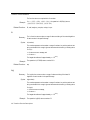
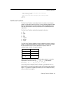
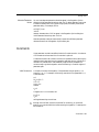
Peaks in chromatograph data are sometimes fit with sums of Gaussian or Lorentzian
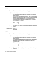
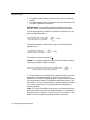
distributions. A simplified form of the Lorentzian distribution is:
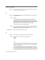
1
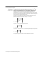
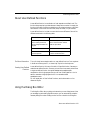
y = -----------------------------2
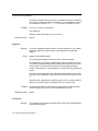
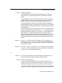
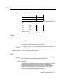
1 + ( x – x0 )
–∞ < x < ∞
where x0 is the location of the peak value.
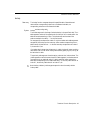
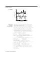
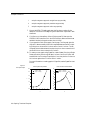
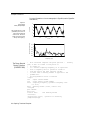
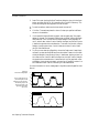
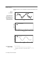
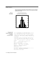
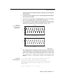
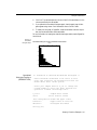
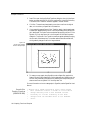
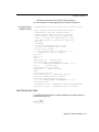
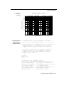
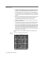
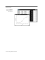
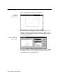
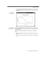
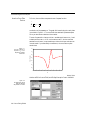
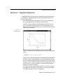
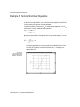
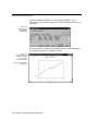
A graph of the distribution for x0 = 0 is shown in Figure 11–1.
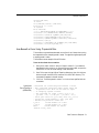
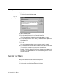
1.
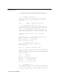
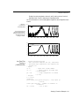
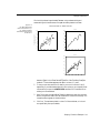
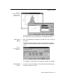
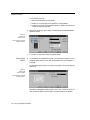
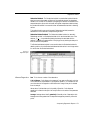
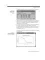
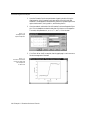
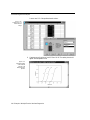
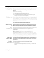
Open the Pitfalls worksheet and graph by double-clicking the Pitfalls Graph in
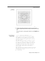
the NONLIN.JNB notebook. Note the positions of data points on the curve.
2.
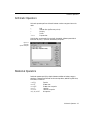
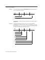
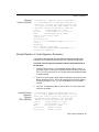
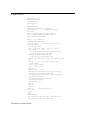
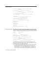
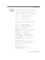
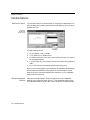
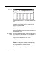
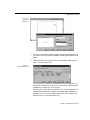
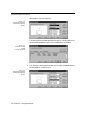
Open the Simplified Lorentzian regression equation by double-clicking it in the
Regression Examples notebook. The Regression Wizard opens and displays the
variables panel (see Figure 11–7 on page 222).
3.
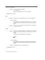
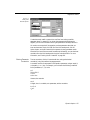
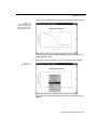
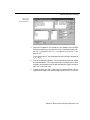
Click one of the symbols on the graph so that the Variables selected are Columns
1 and 2.
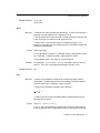
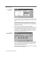
The object is to determine the peak location x0 for the data. Since this data was
generated from the Lorentzian function above using x0 = 0, the regression
should always find the parameter value x0 = 0.
Curve Fitting Pitfalls 219