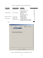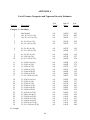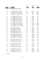
1
ROADSIDE SAFETY ANALYSIS PROGRAM (RSAP)
USER’S MANUAL
NCHRP Project 22-9
Improved Procedures for Cost-Effectiveness Analysis
Of Roadside Safety Features
Prepared for
National Cooperative Highway Research Program
Transportation Research Board
National Research Council
By
King K. Mak
Consultant
and
Dean L. Sicking
University of Nebraska
June 2002
TABLE OF CONTENTS
Page
List of Figures ………………………………………………………………………………… iii
List of Tables .………………………………………………………………………………… vi
1.
INTRODUCTION ……………………………………………………………..……..
1.1
BACKGROUND …………………..………………………………………….
1.2
STUDY OBJECTIVE .………………………………..………………………
1.3
OVERVIEW OF RSAP PROGRAM …………………………………………
1.4
CONTENTS OF USER’S MANUAL ………………………………….…….
2.
INSTALLATION OF RSAP PROGRAM ……………..…………………….………. 3
2.1
SYSTEM REQUIREMENTS ………………………………………...………. 3
2.2
INSTALLATION PROCEDURES ………………………………………….... 3
3.
GENERAL INSTRUCTIONS ……………………………………………….……….
3.1
SCREENS ……………………………………………………...…….……….
3.1.1 Parts of a Screen .………………………………………..…….……….
3.1.2 Parts of a Dialog Box …..…………………………………….……….
3.2
MENUS …………………………..………….……………………….……….
3.2.1 FILE Menu ………………..………………………………….……….
3.2.2 VIEW Menu ………………..………………………………………….
3.2.3 PROJECT Menu ..………………………………..…………….………
3.2.4 ALTERNATIVE Menu ………………..…………..……….………...
3.2.5 HELP Menu ……………………………….………………………….
3.3
BUTTONS ………………………….………………………………….……..
3.4
COMMAND BUTTONS ………………………………….…………………..
3.5
DATA ENTRY ……………………..……………………………………….…
4.
DATA INPUT ………………………………….……………………………………... 17
4.1
DATA ENTRY SCREENS ………………………………………..….………. 17
4.1.1 OPENING FILE Screen .……………………………………….………. …… 18
4.1.2 PROJECT SETTINGS Screen………………………………………………… 20
4.1.3 MAIN INPUT Screen………………………………….………………………. 20
4.1.4 COST Screen ………………………………………………………….………. 22
4.1.5 HIGHWAY Screen ……………….………………………………….………. 23
4.1.6 SEGMENTS Screen ………………………………………………….………. 25
4.1.7 FEATURES Screen.………………………………….………………………… 27
4.1.8 USER DEFINED FEATURE Screen ………………………………….……… 31
4.1.9 Alternatives …………………………..………………………………………... 32
4.2
1
1
1
1
2
4
4
6
7
8
8
10
11
12
13
14
15
15
OPTIONS SCREENS ………………………………….…………………….. 33
i
4.2.1
4.2.2
4.2.3
4.2.4
4.2.5
UNITS Screen ………………………………………………..……….
REPORTS Screen ……………..…………………………….……….
CRASH COST Screen ..……………………………………..……….
VEHICLE MIX Screen ..…………………………………………….
EDIT FEATURE Screen ..……………………………………..……..
34
34
35
39
42
5.
DATA CHECKING AND PROCESSING ..………………………………..……….
5.1
DATA CHECKING ..………………………………………………………..
5.1.1 PRE-CALC CHECK Screen ..………………………………..……….
5.1.2 MESSAGES Screen ..……………………………………………..….
5.2
DATA PROCESSING ..……………………………………..……………….
5.3
SAVING THE DATA ..……………………………………………..……….
45
45
45
46
47
49
6.
REPORTS ..…………………………………………………………………..……….
6.1
REPORTS ..…………………………………………………..……..……….
6.1.1 BENEFIT COST RATIO Report ..…………………………..……….
6.1.2 ALTERNATIVE COST Report ..……………………………..…….
6.1.3 FEATURE COST Report ..………………..………………..……….
6.1.4 INPUT DATA Report ..……………………………………..……….
6.1.5 Clearing of Reports ..……………………………………..……….
6.2
PRINTING THE REPORT ..………………………………………..……….
51
51
52
53
54
56
58
59
APPENDIX A. LIST OF FEATURE CATEGORIES AND TYPES AND SEVERITY
ESTIMATES ………………………………………………………..………. 60
APPENDIX B. LIST OF PRE-CALCULATION CHECKS ………………………..………. 70
APPENDIX C. SAMPLE APPLICATIONS ..…………….………………………..………. 73
APPENDIX D. FREQUENTLY ASKED QUESTIONS …………………………..………. 97
ii
LIST OF FIGURES
Page
Figure No.
1
Typical Screen ..……………………………………………………………..……….
6
2
Typical Dialog Box ..………………………………………………………..……….
7
3
FILE Menu for OPEN FILE Screen ………………………………………..……….
9
4
FILE Menu for MAIN INPUT Screen ..……………………………………………..
10
5
VIEW Menu for OPEN FILE Screen ..……………………………………………… 11
6
VIEW Menu for MAIN INPUT Screen ..……………………………………….…… 11
7
PROJECT Menu for MAIN INPUT Screen ..………………………………..………. 12
8
ALTERNATIVE Menu for MAIN INPUT Screen ..………………………………… 13
9
HELP Menu for OPEN FILE Screen ..……………………..………………..………. 13
10
HELP Menu for MAIN INPUT Screen ..……………..……………………..………. 13
11
Multiple-choice Data Entry ..………………………………………………..………. 16
12
OPEN FILE Screen ..………………………………………………………………….. 19
13
OPEN Dialog Box ..………………………………………………………………….. 19
14
PROJECT SETTINGS Screen ..……………………………………………………… 20
15
MAIN INPUT Screen ..………………………………………………………………. 21
16
HIGHWAY Screen ..……………………………………………………..…..………. 23
17
SEGMENTS Screen ..…………………………………………………………..……. 25
18
FEATURES Screen ..…………………………………………….…………..………. 29
19
USER DEFINED FEATURE Screen ..……………………………………….……… 31
20
OPTIONS Screen ..…………………………………………………………..………. 33
iii
Page
Figure No.
21
REPORTS Screen ..………………………………………………………………….
22
CRASH COST Screen for Roadside Design Guide Crash Cost Figures ……..………. 36
23
CRASH COST Screen for FHWA Comprehensive Crash Cost Figures ..…………… 37
24
User-Defined CRASH COST Screen ..………………………………………………. 38
25
User-Defined CRASH COST Screen ..………………………………………………. 39
26
VEHICLE MIX Screen for Nominal Percent Truck ..………………………………… 40
27
VEHICLE MIX Screen for Vehicle Type ..………………………………………….. 41
28
VEHICLE MIX Screen for Vehicle Category ..……………………………………… 42
29
EDIT FEATURE Screen ..…………………………………………………………… 43
30
CONFIRM Dialog Box ..…………………………………………………………….. 44
31
PRE-CALC CHECK Screen ..……………………………………………………….. 46
32
MESSAGES Window ..……………………………………………………………… 47
33
DATA PROCESSING Screen ..……………………………………………………… 48
34
PROCESSING COMPLETED Dialog Box ..………………………………………… 48
35
ERROR MESSAGE Dialog Box ..…………………………………………………… 49
36
CONFIRM SAVE Dialog Box ..……………………………………………………… 49
37
SAVE AS Dialog Box ..……………………………………………………..………. 50
38
REPLACE Dialog Box ..……………………………………………………..………. 50
39
BENEFIT COST RATIO Report ..…………………………………………..………. 53
40
ALTERNATIVE COST Report ..…………………………………………..……….
41
FEATURE COST Report ..…………………………………………………………… 55
42
Page 1 of INPUT DATA Report ..……………………………………………………. 56
iv
35
54
Figure No.
Page
43
Page 2 of INPUT DATA Report ..…………………………………………..……….
57
44
Page 3 of INPUT DATA Report ..…………………………………………………… 58
45
PRINT Dialog Box ..…………………………………………………………………. 59
A-1
Culvert End Types ..…………………………………………………………………… 69
C-1.
Highway Plan and Profile – Sample Project 1 ………………………………………… 82
C-2(a) Alternative 1 (Baseline Condition) – Sample Project 1 …..…………………………… 83
C-2(b) Alternative 2 (Install Guardrail) – Sample Project 1 …………………………………. 84
C-2(c) Alternative 3 (Extend Culvert) – Sample Project 1 ……...……………………………. 85
C-3
Benefit Cost Ratio Report - Sample Project 1 .……………….………………………. 86
C-4
Alternative Cost Report - Sample Project 1...………….……………………………… 86
C-5(a) Feature Cost Report – Sample Project 1 - Alternative 1 ..……………………………. 87
C-5(b) Feature Cost Report – Sample Project 1 - Alternative 2 ..……………………………. 87
C-5(c) Feature Cost Report – Sample Project 1 - Alternative 3 ..……………………………. 88
C-6(a) Alternative 1 (Baseline Condition) – Sample Project 2 …..…………………………… 91
C-6(b) Alternative 2 (Install Guardrail) – Sample Project 2 …………………………………. 92
C-6(c) Alternative 3 (Install Crash Cushion) – Sample Project 2 .……………………………. 93
C-7
Benefit Cost Ratio Report - Sample Project 2...……………….………………………. 94
C-8
Alternative Cost Report - Sample Project 2 ………….………………………………. 94
C-9(a) Feature Cost Report – Sample Project 2 - Alternative 1 ..……………………………. 95
C-9(b) Feature Cost Report – Sample Project 2 - Alternative 2 ..……………………………. 95
C-9(c) Feature Cost Report – Sample Project 2 - Alternative 3 ..……………………………. 96
v
LIST OF TABLES
Table
Page
1
Built-in Crash Cost Figures ..……………………………………….………………
36
2
Vehicle Mix Calculations and Default Values ..…………………………………….
40
C-1
Input Data for Sample Project 1 ……………....…………………………………….
80
C-2
Input Data for Sample Project 2..…………………………………………………….
89
vi
I. INTRODUCTION
1.1
BACKGROUND
The 1988 and 1996 American Association of State Highway and Transportation Officials
(AASHTO) Roadside Design Guide includes general warrants for the use of traffic barriers and
other roadside safety features. However, these warrants do not address the cost-effectiveness of
such installations. The Roadside Design Guide also includes information on a computer
program, ROADSIDE, which was developed for cost-effectiveness analysis. However, agencies
using the ROADSIDE program have experienced difficulties, and some have found the results
questionable.
The Federal Highway Administration (FHWA) has adopted National Cooperative
Highway Research Program (NCHRP) Report 350, Recommended Procedures for the Safety
Performance Evaluation of Highway Features, as the official guidelines for safety performance
evaluation of highway features. The guidelines incorporate the multiple performance level
concept for roadside safety features. The intent of the multiple performance level concept is to
provide roadside safety features that are better tailored to the specific conditions of a site. The
current version of the ROADSIDE program does not readily allow for the analysis of different
performance levels. Research is needed to develop improved software for cost-effectiveness
analysis of roadside features and to formulate procedures for using the software to apply the
multiple performance level concept.
1.2
STUDY OBJECTIVE
The objective of this study was, therefore, to develop an improved micro-computer based
cost-effectiveness analysis procedure for use in: (1) assessing alternative roadside safety
treatments at both point locations and sections of roadway, and (2) developing warrants and
guidelines including those which consider performance levels of safety features.
1.3
OVERVIEW OF RSAP PROGRAM
The Roadside Safety Analysis Program (RSAP) was developed as a result of this study.
The RSAP program is comprised of two separate, but integrated programs: the User Interface
Program and the Main Analysis Program.
The Main Analysis Program contains the cost-effectiveness procedure itself and performs
all the necessary calculations. The Main Analysis Program is written in the FORTRAN
language due to its efficiency in performing scientific calculations. However, the FORTRAN
language is very poor in terms of user interface. Thus, user interface is handled through the User
Interface Program so that the Main Analysis Program is transparent to the users, i.e., the users do
not work directly with the Main Analysis Program. The User Interface Program is written in the
Microsoft C++ language, which is more adept at providing a user-friendly environment through
the use of windows, screens, and menus.
1
The User Interface Program provides the users with a simple and structured means to
input the data into the RSAP program. The program generates input data files that, together with
the default data files, serve as inputs to the Main Analysis Program. After processing by the
Main Analysis Program, the User Interface Program then takes the outputs from the Main
Analysis Program and presents the results to the users. The transfer of data files between the
User Interface Program and the Main Analysis Program is in ASCII format for simplicity and
ease of file transfer.
1.4
CONTENTS OF USER’S MANUAL
This User’s Manual is one of two reports prepared under this study. The other report is
the Engineer’s Manual. The User’s Manual provides reference for users on the operations of the
RSAP program. The Engineer’s Manual is intended as a reference document for users who are
interested in the details of the procedure, including descriptions of algorithms, source materials,
validation and calibration results, discussions of limitations, sample applications, and research
needs.
There are five additional chapters in this User’s Manual:
•
•
•
•
•
Chapter II - Installation. This chapter outlines instructions for installing the
RSAP program onto the computer.
Chapter III - General Instructions. This chapter provides general instructions on
the use of the RSAP program.
Chapter IV - Data Input. This chapter provides instructions on how to input the
data into the program.
Chapter V - Data Processing. This chapter describes how to process the input
data.
Chapter VI - Reports. This chapter describes the reports available from the
program.
In addition, there are four appendices. Appendix A shows a list of feature categories and
types and the associated severity estimates. Appendix B lists the edit, range, and consistency
checks built into the program. Appendix C provides details on the two sample problems
included with the RSAP installation program. Appendix D provides answers to some frequently
asked questions.
2
II. INSTALLING THE RSAP PROGRAM
This chapter outlines the steps to install the RSAP program onto your computer,
including the system requirements and installation procedures.
2.1
SYSTEM REQUIREMENTS
To run the RSAP program, your computer must be a PC, and have the following:
•
•
•
•
•
2.2
A Pentium III or better platform. The program will work on older platforms, but
the computation time will be excessively long and is, therefore, not
recommended. The computer should have a hard drive and a CD-ROM drive.
Memory. A minimum of 128 Mb RAM memory is recommended.
Disk space. A minimum of 10 MB disk space on the hard drive is required for the
program. The two manuals would require another 15MB if you wish to install
them onto the hard drive.
Mouse. The use of a mouse is recommended.
Operating system. The program will work with WINDOWS 95, 98, Me, NT,
2000 and XP operating systems.
INSTALLATION PROCEDURES
The RSAP installation program is provided on one CD-ROM, which also contains the
two manuals. Before running the installation program, you should have a good understanding of
the WINDOWS operating environment and general mouse and keyboard techniques. When you
are ready to run the installation program:
1.
2.
3.
Insert the CD-ROM into the CD-ROM drive.
The installation wizard should come up automatically. If not, click on START,
then RUN, and type in D (or whatever the CD-ROM drive is):
INSTALLRSAP,EXE and click on OK or press ENTER.
Follow the on-screen instructions to install the RSAP program.
The program will automatically complete the installation of the RSAP program to your
computer, including:
•
•
•
•
•
Unzip all the files.
Create a subdirectory C:\PROGRAM FILES\NCHRP\RSAP or another directory
that you specify.
Copy all executable and default data files onto the subdirectory.
Copy WINDOWS system related files (i.e., *.DLL, *.INI, *.GID and *.HLP files)
into the appropriate WINDOWS system directories.
Install an icon on the desktop and a menu item under PROGRAMS for the RSAP
program.
3
III. GENERAL INSTRUCTIONS
This chapter provides general instructions on the basics of using the RSAP program. The
RSAP program is designed to work in a WINDOWS environment with screens, menus, icons,
command buttons, and dialog boxes.
3.1
SCREENS
The term “screen,” as used in the context of this report, is a general term to denote any
window or dialog box that pertain specifically to the input, processing, and output of the RSAP
program. Windows and dialog boxes common to all WINDOWS applications, such as OPEN
FILE, CLOSE FILE, PRINT SETUP, etc., are not included in this list of screens and will not be
discussed in this report. It is assumed that users are already familiar with the WINDOWS
operating environment.
The RSAP program utilizes the following screens:
Screen
Function
OPEN FILE
Create a new project or to open an existing project.
PROJECT SETTING
Provide entry for project description and selection of the manner
the seed number will be generated: random or specified.
MAIN INPUT
Main screen for data entry. Provides entries on alternative
description and access to the COST, HIGHWAY, SEGMENTS,
and FEATURES data entry screens.
COST
Provide entries on data regarding direct cost computations,
including: project life, discount rate, total installation cost and
annual maintenance cost.
HIGHWAY
Provide entries on general highway data, including: area type,
functional class, highway type, number of lanes, lane width,
shoulder width, speed limit, average daily traffic (ADT), nominal
percent truck, traffic growth factor, and user-defined encroachment
rate adjustment factor.
SEGMENTS
Provide entries on data regarding individual homogeneous
segment(s), including: length of segment, median type and width,
percent grade, and horizontal curvature.
FEATURES
Provide entries on data regarding roadside feature(s), including:
category and type, length, width, location, flare rate, offset from
edge of travelway, distance from beginning of first segment, and,
4
Screen
Function
for features of a repetitive nature (e.g., line of utility poles), the
number of repetitions and spacing between features.
OPTIONS
Provide access to the UNITS, REPORTS, CRASH COST,
VEHICLE MIX, and EDIT FEATURE data entry screens.
UNITS
Select unit of measurement: English or SI.
REPORTS
Select reports to be displayed: INPUT DATA, BENEFIT COST
RATIO, ALTERNATIVE COST, and FEATURE COST.
CRASH COST
Allow selection of default crash cost figures and revisions to the
default values.
VEHICLE MIX
Allow selection of default vehicle mix data and revisions to the
default values.
EDIT FEATURE
Allow user to add, delete or edit user-defined features
USER DEFINED
FEATURE
Provide entries to data regarding a user defined feature,
including: feature description, severity indices (SI) at zero (0) and
100 km/h (62.2 mph), and average cost per impact.
PRE-CALC CHECK
Show results of pre-calculation checks.
MESSAGES
Show error and warning messages from the pre-calculation edit
and consistency checks.
PROCESSING
Provide information on the status of project analysis.
BENEFIT/COST RATIO
REPORT
Present the incremental benefit/cost (B/C) ratios associated with
the alternatives.
ALTERNATIVE COST
REPORT
Present the predicted impact frequencies and the annualized
crash, installation, maintenance and repair costs associated with the
alternatives.
FEATURE COST
REPORT
Present the predicted impact frequencies, average severity,
and the annualized crash costs associated with individual features
of each alternative.
INPUT DATA REPORT
Present the input data for each alternative of the project.
More detailed descriptions of these screens are presented in the following chapters.
5
3.1.1
Parts of a Screen
Figure 1 shows the key elements of a typical screen. Note that a particular screen may
have some or all of these elements.
Figure 1. Typical Screen
The key elements of a typical screen are:
•
•
•
Title bar. The title bar at the top of the screen shows the title of the project being
analyzed.
Menu bar. The menu bar below the title bar at the top of the screen shows the
available menus for that screen.
Tool bar. The tool bar below the menu bar at the top of the screen shows buttons
of available functions that may be accessed directly for that screen.
6
•
•
•
3.1.2
Work space. The work space is where you enter, edit, or view the data.
Status bar. The status bar at the bottom of the screen provides brief descriptions
of the buttons displayed in the button bar. The three boxes to the right of the
status bar show the status of the CAPS LOCK, NUM LOCK, and SCROLL
LOCK keys.
Command buttons. The command buttons located near the bottom of the
workspace allow you to execute the available commands shown in the buttons.
Parts of a Dialog Box
Note that some of the screens listed above are actually dialog boxes without the typical
elements of a screen. Figure 2 shows an example of a dialog box.
Figure 2. Typical Dialog Box
7
The key elements of a dialog box are:
•
•
•
3.2
Title bar. The title bar at the top of the screen shows the title of the dialog box.
Work space. The work space is where you enter, edit, or view the data.
Command buttons. The command buttons located near the bottom of the work
space allow you to execute the available commands shown in the buttons.
MENUS
The following is a list of menus used with the User Interface Program. Some or all these
menus may appear on the menu bar depending on the screen. The functions of these menus are
as follows:
Menu
Function
FILE
Create, open, save, close, or print a project input data file.
VIEW
View options for default settings and values, reports, and error and
warning messages, and to toggle the display of the tool bar and
status bar.
PROJECT
Analyze the project, change the level of convergence, conduct edit
consistency checks on the input data, or view/change the project
settings.
ALTERNATIVE
Add, duplicate, or remove an alternative, or go to the previous or
next alternative.
HELP
Access help information.
Each menu provides a list of commands or access to another screen of information. More
details on the menus are presented in the following sections.
3.2.1 FILE Menu
The FILE menu, when opened, contains various commands for working with an input
data file. The available commands and their functions or actions are shown as follows. Note
that some or all of these commands may be shown in the menu.
Command
Function/Action
NEW PROJECT
Create a new project file. The PROJECT SETTINGS screen will
be displayed
8
Command
Function/Action
OPEN PROJECT
Open an existing project file. The MAIN INPUT screen will be
displayed.
CLOSE
Close current project file. You will be offered the option of saving
or not saving the current file if the file has been modified.
SAVE PROJECT
Save current project file under the existing file name.
SAVE AS
Save current project file under a different file name. The SAVE
AS dialog box will be displayed
PRINT
Print reports of the current project. The PRINT dialog box will be
displayed
PRINT PREVIEW
Preview reports of the current project prior to printing. The
BENEFIT COST RATIO REPORT screen will be displayed.
PRINT SETUP
Set up the printer. The PRINT SETUP dialog box will be
displayed.
EXIT
Exit the RSAP program. You will be offered the option of saving
or not saving the current project file prior to exiting from the
program if the file has been modified.
The FILE menu with the OPEN FILE screen is shown in Figure 3 and the FILE menu
with the MAIN INPUT screen is shown in Figure 4.
Figure 3. FILE Menu for OPEN FILE Screen
9
Figure 4. FILE Menu for MAIN INPUT Screen
3.2.2 VIEW Menu
The VIEW menu allows the user to view options for default settings and values, reports,
and error and warning messages, and to toggle display of the tool bar and status bar.
The available commands and their functions or actions are shown as follows:
Command
Function/Action
CRASH COST
View/change current default option on crash cost figures and heir
values. The CRASH COST screen will be displayed.
VEHICLE MIX
View/change current default option on vehicle mix and their
values. The VEHICLE MIX screen will be displayed
REPORTS
View/change list of reports to be displayed and printed. The
BENEFIT COST RATIO REPORT screen will be displayed.
OPTIONS
Provide access to default settings on: units, reports, crash cost,
vehicle mix, and user-defined feature. The OPTIONS screen will
be displayed.
MESSAGES
View error and warning messages. The MESSAGES screen will
be displayed.
TOOL BAR
Toggle display of tool bar.
STATUS BAR
Toggle display of status bar.
10
The VIEW menu with the OPEN FILE screen is shown in Figure 5 and the VIEW menu
with the MAIN INPUT screen is shown in Figure 6.
Figure 5. VIEW Menu for OPEN FILE Screen
Figure 6. VIEW Menu for MAIN INPUT Screen
3.2.3 PROJECT Menu
The PROJECT menu allows the user to analyze the current project, change the level of
convergence, conduct edit and consistency checks on the input data, and review/change the
project settings. The available commands and their functions or actions are shown as follows:
Command
Function/Action
ANALYZE
Analyze the current project. The program will automatically
conduct the pre-calculation checks. If there are any errors or
warnings, the ERROR MESSAGE screen will be displayed. If
there are no errors or warnings, analysis of the project will
commence and the PROCESSING screen will be displayed.
LEVEL OF
CONVERGENCE
Select level of convergence for the analysis. Three levels of
convergence are available: high, medium and low, which
correspond to 1.0, 5.0 and 10.0 percent of convergence.
11
Command
Function/Action
SETTINGS
Enter/view/change project title and manner by which the seed
number is selected. The PROJECT SETTINGS screen will be
displayed.
PRE-CALC CHECK
Perform edit and consistency checks on the input data. The PRECALC CHECK screen will be displayed.
The PROJECT menu with the MAIN INPUT screen is shown in Figure 7.
Figure 7. PROJECT Menu for MAIN INPUT Screen
3.2.4
ALTERNATIVE Menu
The ALTERNATIVE menu allows the user to add, duplicate, or remove an alternative, or
to go to the previous or next alternative. The available commands and their functions or actions
are shown as follows:
Command
Function/Action
ADD
Add a new alternative. The MAIN INPUT screen for the new
alternative will be displayed
DUPLICATE
Duplicate the current alternative as a new alternative. The MAIN
INPUT screen for the new alternative will be displayed
PREVIOUS
Display previous alternative. The MAIN INPUT screen for the
previous alternative will be displayed
NEXT
Display next alternative. The MAIN INPUT screen for the next
alternative will be displayed
REMOVE
Delete current alternative. The MAIN INPUT screen for the
previous alternative will be displayed
The ALTERNATIVE menu with the MAIN INPUT screen is shown in Figure 8.
12
Figure 8. ALTERNATIVE Menu for MAIN INPUT Screen
3.2.5 HELP Menu
The HELP menu provides access to the on-screen HELP file. Alternatively, you can
press F1 to access the on-screen HELP file. The HELP menu is available for all screens. The
available commands and their functions or actions are shown as follows:
Command
Function/Action
HELP TOPICS
List contents of help topics.
ABOUT RSAP
View RSAP version and general information.
The HELP menus for the OPEN FILE screen and the MAIN INPUT screen are shown in
Figures 9 and 10, respectively.
Figure 9 HELP Menu for OPEN FILE Screen
Figure 10. FILE Menu for MAIN INPUT Screen
13
3.3
BUTTONS
A series of buttons is provided on the tool bar to facilitate access to some of the more
commonly used functions. The available buttons for the various screens are as follows:
Button
Function
Description
OPENING SCREEN
NEW FILE
Create a new project data file.
OPEN FILE
Open an existing project data file.
HELP
Help.
DATA INPUT SCREENS
NEW FILE
Create a new project data file.
OPEN FILE
Open an existing project data file.
SAVE FILE
Save current project data file.
PRINT
Print current project data file.
HELP
Help.
PREVIOUS ALTERNATIVE
Display previous alternative.
NEXT ALTERNATIVE
Display next alternative.
ADD ALTERNATIVE
Add a new alternative.
DUPLICATE ALTERNATIVE
Duplicate alternative as a new alternative.
DELETE ALTERNATIVE
Delete this alternative.
PRE-CALC CHECK
Check project data for inconsistency.
ANALYSIS
Perform analysis on this project.
CONVERGENCE
Change level of convergence.
REPORT SCREENS
PRINT
NEXT PAGE
PREV PAGE
TWO PAGE/ONE PAGE
Print report.
Go to next page of report.
Go back to previous page of report.
Toggle between showing the reports in either
a two-page or one-page format.
Zoom in on the display.
Zoom out on the display.
Close REPORT screen and return to MAIN
INPUT screen.
ZOOM IN
ZOOM OUT
CLOSE
14
3.4
COMMAND BUTTONS
The command buttons shown near the bottom of some screens allow you to execute the
specific commands shown in the buttons. Some or all these command buttons may appear on the
screen depending on the screen.
Command buttons specific to the RSAP program and their functions or actions for the
various screens are shown as follows:
Button
Function/Action
SEGMENTS SCREEN
÷
≠
ADD SEGMENT
INSERT SEGMENT
REMOVE SEGMENT
Go to next segment..
Go back to previous segment.
Add new segment.
Insert new segment after current segment.
Delete current segment.
FEATURES SCREEN
÷
≠
ADD FEATURE
INSERT FEATURE
REMOVE FEATURE
Go to next feature.
Go back to previous feature.
Add new feature.
Insert new feature after the current feature.
Delete the current feature.
There are other command buttons used with various dialog boxes and windows, such as
OK, OPEN, SELECT, CANCEL, etc. These command buttons are commonly used with
WINDOWS applications and are self-explanatory. Descriptions of these command buttons and
their functions or actions are provided in the discussions of the dialog boxes and windows and
will not be repeated here.
3.5
DATA ENTRY
When a data entry screen is first selected, the cursor will be at the first data entry, which
is highlighted and the default value for the data entry will be shown. If you want to keep the
default value, press ENTER or TAB and the cursor will automatically move to the next data
entry. If you want to enter a value different from that of the default value, enter the data and then
press ENTER or TAB to move to the next data entry.
You can move forward to the next data entry by pressing the TAB key or backward to the
previous data entry by pressing the SHIFT and TAB keys together and the current data entry will
not be changed. You can also move to any data entry on the screen and any part of the data entry
by clicking on the desired location of that data entry with the mouse. Note that when you access
15
a data entry with the mouse, the data entry will not be highlighted and it will be in an “insert”
mode instead of a “replace” mode.
There are three basic forms of data entries:
1.
Descriptive. For a descriptive entry, such as the title of the project or description of an
alternative, enter the description in the space provided. The length of the entry is limited
by the space available. Abbreviations are necessary if the length of the entry is more than
the available space.
2.
Multiple Choice. A DOWN ARROW shown on the right of the data entry identifies a
multiple choice data entry. Click on the DOWN ARROW and the list of choices will
appear in a window. An example of a multiple choice data entry is shown in Figure 3.
Figure 11. Multiple Choice Data Entry
You can scroll through the choices using the UP and DOWN or LEFT and RIGHT
ARROW keys or use the mouse to drag on the choices. To select an entry, double click
on your choice. Alternatively, you can click on your choice or use the ARROW keys to
get to your choice and press ENTER. The multiple choice window will then close and
the selected item will appear in the data entry.
To exit from the multiple choice window without making a choice or changing the
current choice, use the TAB key to go to the next data entry or use the mouse to click on
the data entry of your choice.
3.
Numeric. For a numeric data entry, enter the data in the space provided. The unit of the
data entry, e.g., meter (m), percent (%), etc., is shown on the right of the data entry.
16
IV. DATA INPUT
This chapter provides instructions on how to enter project input data into the RSAP
program. To start the RSAP program under the WINDOWS operating environment, click on
START, PROGRAMS, and then RSAP. When the RSAP program is first started, the OPEN
FILE screen will be displayed.
4.1
DATA ENTRY SCREENS
The following screens are used with the data input process:
Screen
Function
OPEN FILE
Create a new project or to open an existing project.
PROJECT SETTING
Provide entry for project description and selection of the manner
the seed number will be generated: random or specified.
MAIN INPUT
Main screen for data entry. Provides entries on alternative
description and access to the COST, HIGHWAY, SEGMENTS,
and FEATURES data entry screens.
COST
Provide entries on data regarding direct cost computations,
including: project life, discount rate, total installation cost and
annual maintenance cost.
HIGHWAY
Provide entries on general highway data, including: area type,
functional class, highway type, number of lanes, lane width,
shoulder width, speed limit, average daily traffic (ADT), nominal
percent truck, traffic growth factor, and user-defined encroachment
rate adjustment factor.
SEGMENTS
Provide entries on data regarding individual homogeneous
segment(s), including: length of segment, median type and width,
percent grade, and horizontal curvature.
FEATURES
Provide entries on data regarding roadside feature(s), including:
category and type, length, width, location, flare rate, offset from
edge of travelway, distance from beginning of first segment, and,
for features of a repetitive nature (e.g., line of utility poles), the
number of repetitions and spacing between features.
OPTIONS
Provide access to the UNITS, REPORTS, CRASH COST,
VEHICLE MIX, and EDIT FEATURE data entry screens.
17
Screen
Function
UNITS
Select unit of measurement: English or SI.
REPORTS
Select reports to be displayed: INPUT DATA, BENEFIT COST
RATIO, ALTERNATIVE COST, and FEATURE COST.
CRASH COST
Allow selection of default crash cost figures and revisions to the
default values.
VEHICLE MIX
Allow selection of default vehicle mix data and revisions to the
default values.
EDIT FEATURE
Allow user to add, delete or edit user-defined features
USER DEFINED
FEATURE
Provide entries to data regarding a user defined feature,
including: feature description, severity indices (SI) at zero (0) and
100 km/h (62.2 mph), and average cost per impact.
Detailed descriptions of these screens are provided in the following sections.
4.1.1
OPEN FILE Screen
When the RSAP program is first initiated, the OPEN FILE screen, as shown in Figure 12,
will appear. The OPEN FILE screen allows the user to create a new project file or to open an
existing project file.
To create a new project file, click on the NEW FILE button, or click on the FILE menu
and then the NEW PROJECT command. The PROJECT SETTINGS screen will then appear
(see section 4.1.2 for details on the MAIN INPUT screen).
To open an existing project file, click on the OPEN FILE button, or click on the FILE
menu, then the OPEN PROJECT command, and the OPEN FILE dialog box will appear, as
shown in Figure 13. A list of available input data files with the extension of .RPD in the current
directory or subdirectory will be displayed. Enter the name of the project file you wish to open
in the space provided under FILE NAME and click on the OPEN button or press ENTER.
Alternately, select the file you wish to open from the list of available input data files and double
click on the file name, or single click on the file name (which will then be highlighted) and then
click on the OPEN button or press ENTER. The MAIN INPUT screen showing data for the
selected project input data file will appear for editing or processing (see Section 4.1.3 for details
on the MAIN INPUT screen).
18
Figure 12. OPEN FILE screen
Figure 13. OPEN FILE Dialog Box
19
4.1.2 PROJECT SETTINGS Screen
Upon selecting the command to create a new input data file, the PROJECT SETTINGS
screen, as shown in Figure 14, will appear. You can also call up this screen by clicking on the
PROJECT menu, and then the SETTINGS command.
Figure 14. PROJECT SETTINGS Screen
The PROJECT SETTINGS screen provides for entry of the project title and selection of
the manner in which the seed number is to be determined: random or specified. The default is
random seed number, in which case the computer will generate at random a different seed
number for each run. For a new project, the random seed number option is recommended.
Due to the randomness of the seed number and the nature of the Monte Carlo simulation,
the results for an identical project will vary from run to run. For an existing project, it may be
desirable to keep the same seed number to eliminate the randomness so that the results can be
better compared among runs. The seed number used with each run is shown as part of the
INPUT DATA REPORT. To select the specified seed number option, select the SPECIFIED
SEED NUMBER option and enter the seed number in the space provided, then click on the OK
button or press ENTER. As with all WINDOWS applications, you may cancel any action and
exit the screen by clicking on the CANCEL button.
4.1.3
MAIN INPUT Screen
Upon creating a new input data file or opening an existing input data file, the MAIN
INPUT screen, as shown in Figure 15, would appear.
20
Figure 15. MAIN INPUT Screen
If you are creating a new project input data file, all the entries will show the default
values. If you are opening an existing project input data file, the data entries for the existing
project will be shown.
From the MAIN INPUT screen, you can take the following data entry actions:
•
Enter description of current alternative in the space provided. Note that the first
alternative is typically the baseline or existing condition.
•
Access the COST, HIGHWAY, SEGMENTS, or FEATURES screens for data entry or
editing for the current alternative by clicking on the name of the corresponding folder.
•
Switch to another alternative, add a new alternative, duplicate the current alternative as a
new alternative, or delete the current alternative. The MAIN INPUT screen will start with
the first alternative, which is the baseline or existing condition. You can then add other
alternatives as appropriate. The data entered or shown on the COST, HIGHWAY,
SEGMENT, and FEATURE screens will pertain to the alternative currently shown.
When you switch to another alternative, the data on these screens will change to the new
alternative automatically. When an alternative is deleted, all data on the COST,
21
HIGHWAY, SEGMENT, and FEATURE screens corresponding to that alternative will
be deleted automatically.
•
Review entered data for the project. You can review the entered data by going through
the individual COST, HIGHWAY, SEGMENT, and FEATURE screens for each of the
alternatives, or by using the INPUT DATA REPORT for each of the alternatives. To
access the reports, click on the VIEW menu and then the REPORTS command.
4.1.4
COST Screen
The COST screen is also shown as part of the MAIN INPUT screen in Figure 15,
providing entries on direct cost figures pertaining to the specific alternative. A listing of the data
entries under the COST screen is as follows:
Data Entry
Type
Description
LIFE (YEARS)
(Default is 25 years)
Numeric
Life of project in years.
DISCOUNT RATE
(Default is 4.0 percent)
Numeric
Discount rate in percent.
TOTAL INSTALLATION
COST ($)
Numeric
Total installation cost for alternative.
ANNUAL MAINTENANCE
COST ($)
Numeric
Annual maintenance cost for alternative.
Note that the total installation cost for the alternative will be converted automatically by
the program to an annualized cost based on the project life and the discount rate for use in the
benefit/cost ratio calculations. This allows for the use of different project life and discount rate
for different alternatives.
It should be emphasized that alternative 1 (baseline conditions) must have the lowest
installation cost or an error message, “Installation cost must be greater than that of alternative 1,”
will be displayed during the pre-calculation checks and the program will not perform the
analysis. The rationale for this error message is that the baseline alternative is the “do nothing”
option and should not have any installation cost. The installation costs for the other alternatives
do not have to be in any specific order. The program will automatically reorder the alternatives
in ascending order of direct costs.
Also note that there is no entry for the salvage value. The rationale is that most of the
roadside features will have little or no salvage value. The inclusion of salvage values would
have minimal effect on the benefit cost ratio calculations and is, therefore, not included to reduce
the number of input data elements.
22
4.1.5
HIGHWAY Screen
The HIGHWAY screen, as shown in Figure 16, provides entries on general highway data,
including area type, functional class, highway type, number of lanes, lane width, shoulder width,
speed limit, average daily traffic (ADT), nominal percent truck, traffic growth factor, and
encroachment rate adjustment factor.
Figure 16. HIGHWAY Screen
A listing of the data entries under the HIGHWAY screen is as follows:
Data Entry
Type
Description
AREA TYPE
(Default is RURAL)
Multiple Choice
RURAL
URBAN
23
Data Entry
Type
Description
FUNCTIONAL CLASS
(Default is FREEWAY)
Multiple Choice
FREEWAY
PRINCIPAL (MAJOR) ARTERIAL
MINOR ARTERIAL
COLLECTOR
LOCAL
HIGHWAY TYPE
(Default is TWO-WAY,
DIVIDED)
Multiple Choice
TWO-WAY, DIVIDED
TWO-WAY, UNDIVIDED
ONE-WAY
NUMBER OF LANES
Numeric
Enter total number of lanes.
LANE WIDTH
Numeric
Enter lane width.
SHOULDER WIDTH
Numeric
Enter shoulder width.
SPEED LIMIT
Numeric
Enter speed limit.
ADT
Numeric
Enter current average daily traffic (ADT).
PERCENT TRUCK
(Default is 10.0 percent)
Numeric
Enter nominal percentage of trucks.
TRAFFIC GROWTH
FACTOR
Numeric
Enter annual traffic growth rate in
percent.
ENCROACHMENT RATE Numeric
ADJUSTMENT FACTOR
(Default is 1.0)
Enter user-defined adjustment factor for
encroachment rate.
The area type and functional class are in accordance with AASHTO designations. The
number of lanes refers to the total number of lanes. For example, for a two-lane or four-lane
undivided highway, the number of lanes entered is 2 or 4, respectively. For a six-lane divided
highway with three lanes in each direction, the number of lanes entered should be 6 (and not 3).
The shoulder width is assumed to be the same for both directions of travel. For undivided
highways, only a single entry is provided for shoulder width. For divided highways, two
separate entries are provided for left and right shoulders.
The speed limit is the posted speed limit. During beta testing, some agencies have
expressed the preference of using the design speed instead of the speed limit, which is acceptable
from a computational standpoint. However, since the design speed is typically higher than the
speed limit, it would affect the impact speed and angle distribution and the resulting severity
estimates and crash costs.
24
The average daily traffic (ADT) refers to the total ADT for both directions of traffic. The
encroachment rate adjustment factor is intended for use in special situations where the
encroachment rate is expected to differ significantly from the average. The default value is 1.0,
i.e., no adjustment. A value of greater than 1.0 is used when the encroachment rate is expected
to be higher than average, e.g., at locations where there have been a higher than average crash
experience. A value of less than 1.0 is used when the encroachment rate is expected to be lower
than average, e.g., at locations where safety countermeasures such as rumble strips on shoulders
are implemented.
4.1.6
SEGMENTS Screen
The SEGMENTS screen, as shown in Figure 17, provides entries on data regarding
individual homogeneous segments, including length of segment, median type and width, percent
grade, and horizontal curvature (direction and radius).
Figure 17. SEGMENTS Screen
25
A listing of the data entries under the SEGMENTS screen is shown as follows:
Data Entry
Type
Description
LENGTH
Numeric
Enter length of segment.
MEDIAN TYPE
Multiple Choice
(Default is MEDIAN OF
DIVIDED HIGHWAY)
MEDIAN OF DIVIDED HIGHWAY
NO MEDIAN, UNDIVIDED HIGHWAY
PAINTED MEDIAN, UNDIVIDED
HIGHWAY
TWO-WAY, LEFT-TURN LANE,
UNDIVIDED HIGHWAY
NOT APPLICABLE
MEDIAN WIDTH
Numeric
Enter width of median. Enter 0.0 for no median.
GRADE (%)
(Default is 0.0)
Numeric
Enter vertical grade in percent. 0.0 for no grade;
(+ or blank) for upgrade; and (-) for downgrade in
the direction of vehicle travel.
HORIZONTAL CURVE (Two associated data entries)
DIRECTION
Multiple Choice
OF CURVE
(Default is NONE)
NONE
LEFT
RIGHT
RADIUS OF
CURVE
Enter radius of curve. This entry will appear only if
the entry for DIRECTION OF CURVE is LEFT or
RIGHT.
Numeric
The entire section of highway covered in the project is broken down into a number of
homogeneous segments as defined by the following geometric characteristics, median type and
width, vertical grade and horizontal curvature. In other words, within each segment, the median
type and width, vertical grade and horizontal curvature should be the same.
For a divided highway, there should always be a median. The median width is defined as
the distance from edge of travelway to edge of travelway. For undivided highways, three
different scenarios are provided: no median, painted median, or two-way, left-turn lane. The
median width should be 0.0 for no median, the width of the painted median, or the width of the
two-way, left-turn lane, respectively. For one-way roadways, enter not applicable for median
type and 0.0 for median width.
The vertical grade can be upgrade (+ or blank) or downgrade (-) in reference to the
direction of travel and is expressed as a percentage. There is no provision for vertical curves,
i.e., crest of hill or bottom of sag. Thus, vertical curves will have to be approximated as the
26
approach grade or level, i.e., as a V-shape or a trapezoidal shape, depending on the length and
curvature of the vertical curve.
For horizontal curvature, there are two associated entries: DIRECTION OF CURVE and
RADIUS OF CURVE. Only the entry for DIRECTION OF CURVE is shown initially. For a
tangent section, enter NONE. For a curved segment, indicate if the direction of curve is LEFT or
RIGHT in the direction of travel and the entry for RADIUS OF CURVE will appear. Enter the
radius of the curve in the space provided.
You can switch to the next or the previous SEGMENTS screen using the ÷ or ≠
command button, respectively. Note that you can switch only among existing SEGMENTS
screens. You can add or insert a new segment using the ADD SEGMENT or INSERT
SEGMENT command button. The ADD SEGMENT command will add a new segment to the
end of the list, e.g., if there are 3 existing segments, a new segment 4 will be added regardless of
the current segment shown. The INSERT SEGMENT command will add a segment before the
current segment, e.g., if there are 3 existing segments and the current segment shown is 2, a new
segment 2 will be added and the old segments 2 and 3 will be renumbered to new segments 3 and
4. Finally, you can delete the current segment using the REMOVE SEGMENT command
button. Note that the segments will renumber automatically upon removal of a segment.
4.1.7
FEATURES Screen
The FEATURES screen, as shown in Figure 18, provides entries on data regarding
roadside features, including feature category and type, length, width, location, offset, flare rate,
offset, distance from beginning of first segment, and, for features of a repetitive nature (e.g., line
of utility poles), the number of repetitions and spacing.
A listing of the data entries under the FEATURES screen is shown as follows:
Data Entry
Type
Description
CATEGORY
Multiple Choice
(Default is 1. FORESLOPES)
1.
2.
3.
4.
5.
6.
7.
8.
FORESLOPES
BACKSLOPES
PARALLEL DITCHES
INTERSECTING SLOPES
FIXED OBJECTS
CULVERT END
LONGITUDINAL BARRIERS
TERMINALS AND CRASH
CUSHIONS
9. MISCELLEANEOUS
USER-DEFINED FEATURE
TYPE
Multiple Choice
(Default is 1. FLAT GROUND)
Feature type within category. (See
Appendix A for list of feature types.)
Data Entry
Description
Type
27
LENGTH
Numeric
Enter length of feature.
WIDTH
Numeric
Enter width of feature.
LOCATION
(Default is RIGHT)
Multiple Choice
RIGHT
MEDIAN
LEFT
OFFSET FROM EDGE
OF TRAVELWAY.
Numeric
Enter lateral offset to from edge of
travelway to front face of feature.
FLARE RATE (Two associated data items)
LOCATION
(Default is N/A)
Multiple Choice
N/A
DOWNSTREAM
UPSTREAM
FLARE RATE
Multiple Choice
(Default is 10:1 and 0.1)
This entry will appear only if the entry
for LOCATION is not N/A.
DISTANCE FROM
BEGINNING OF
FIRST SEGMENT
10:1
15:1
25:1
50:1
OTHER (Enter actual flare rate.)
Numeric
Enter distance of feature from
beginning of the first segment in
meters.
REPETITIONS (Two associated data items)
NUMBER
(Default is 0)
Numeric
Enter number of repetitions.
SPACING
. (Default is 0)
Numeric
Enter spacing between repetitious features.
This entry will appear only if the entry for
NUMBER is greater than 0.
Select the feature category that best describes the feature for which the data is being
entered. For each feature category, there is a corresponding list of feature types, as shown in
Appendix A. Select the feature type that best describes the feature for which the data is being
entered. This list of feature categories and corresponding features types is similar to that for the
ROADSIDE program. If the feature in question is not represented by any of the features in the
standard list, use the USER DEFINED FEATURE to define the feature and its attributes. More
details on the use of USER DEFINED FEATURE are provided in the next section.
28
Figure 18. FEATURES Screen
Enter the length and width of the feature. The location of the feature is in reference to the
direction of travel. For undivided and one-way highways, the feature may be located on the right
or left side of the highway. For divided highways, the feature may be located on the right side of
the highway, the median, or on the far left side of the highway beyond the travel lanes in the
opposing direction of traffic.
The lateral offset of the feature is measured from the edge of the travelway (i.e., edge line
or edge of pavement if there is no edge line) to the face of the feature. For undivided and oneway highways and the right and left entries for divided highways, the lateral offset is measured
to the nearest edge of the travelway. For the median of a divided highway, the lateral offset is
measured only from the edge of the travelway in the direction of travel. Consider the example of
two guardrails shielding a bridge pier in the center of the median. The width of the median is 60
ft and each guardrail is located 20 ft from the respective edge of the travelway. The location for
both guardrails would be entered as MEDIAN. The lateral offset of the guardrail in the direction
29
of travel would be entered as 20 ft while the lateral offset of the guardrail for the opposing
direction of travel would be entered as 40 ft.
For a feature that flares away from the roadway, such as a flared guardrail or end
terminal, enter the FLARE RATE, otherwise skip this entry (the default entry is N/A for no
flare). There are two associated entries for flare rate: LOCATION and FLARE RATE. Only the
entry for LOCATION is shown initially. The first data item, LOCATION, identifies if there is
no flare (N/A) and, if there is a flare, the location of the flare (DOWNSTREAM or
UPSTREAM). The DOWNSTREAM location refers to the trailing end of a guardrail or
terminal where the upstream end is closer to the roadway edge than the downstream end. The
UPSTREAM location refers to the leading end of a guardrail or terminal where the upstream end
is further off the roadway edge than the downstream end.
If there is a flare, i.e., LOCATION is not N/A, the entry for FLARE RATE will appear.
The flare rate is defined as the ratio of lateral distance over longitudinal distance. For example,
if the guardrail tapers laterally 1 ft for every 15 ft of longitudinal distance, the flare rate is 15:1 or
0.067. A list of the more common flare rates is provided in the multiple-choice entry. If the
actual flare rate is different from one of the listed flare rates, select OTHER and enter the actual
flare rate in the space provided.
The longitudinal location of a feature is always taken from the beginning of the first
segment, which serves as the reference point for all features, regardless of the segment the
feature is located in.
For repetitious features, such as a line of utility poles, it is not necessary to enter data on
each feature. Instead, enter the number of repetitions (i.e., total number for that feature) and the
spacing between the features and the program will automatically enter the data for all these
features. ). There are two associated entries for flare rate: REPETITIONS and SPACING. Only
the entry for REPETITIONS is shown initially. Once a number other than zero (0) is entered for
REPETITIONS, the entry for SPACING will appear. Enter the spacing in the space provided.
For example, if there are a total of 10 utility poles in a line spaced at 300 ft apart, enter 10 for the
REPETITIONS and 300 ft for SPACING. Note that any feature beyond the end of the last
segment will not be included in the analysis. An edit check is built into the program such that, if
any feature extends beyond the end of the last segment, the analysis will not be conducted and an
error message will be displayed.
You can switch to another FEATURES screen using the ÷ or ≠ command button. Note
that you can switch only among existing FEATURES screens. You can add or insert a new
feature using the ADD FEATURE or INSERT FEATURE command button. The ADD
FEATURE command will add a new feature to the end of the list, e.g., if there are 3 existing
features, a new feature 4 will be added regardless of the current feature shown. The INSERT
FEATURE command will add a feature before the current feature, e.g., if there are 3 existing
features and the current feature shown is 2, a new feature 2 will be added and the old features 2
and 3 will be renumbered to new features 3 and 4. Finally, you can delete the current feature
using the REMOVE FEATURE command button.
30
4.1.8 USER DEFINED FEATURE Screen
While the standard list of features is quite extensive, it cannot cover all potential features
and there may be situations in which the feature in question is not represented by any of the
features in the standard list. To allow for such situations, the program provides the users with
the option to define their own features and its attributes.
To create a new user defined feature, select USER DEFINED FEATURE from the
FEATURE CATEGORY list and NEW from the FEATURE TYPE list. The USER DEFINED
FEATURE screen, as shown in Figure 19 will appear for defining the new feature and its
attributes.
Figure 19. USER DEFINED FEATURE Screen
A listing of the data entries under the USER DEFINED FEATURE screen is as follows:
Data Entry
Type
Description
DESCRIPTION
Descriptive
Enter name of feature
SI AT ZERO (0)
IMPACT SPEED
Numeric
Enter severity estimate (SI) of feature
when impacted at a speed of zero (0) km/h
(mph)
SI AT 100 KM/H
(62.2 MPH) IMPACT
SPEED
Numeric
Enter severity estimate (SI) of feature
when impacted at a speed of 100 km/h
(62.2 mph)
AVERAGE REPAIR
COST PER IMPACT
Numeric
Enter estimated average repair cost per
impact.
31
A descriptive, but concise, name should be provided for the feature so that it can be easily
identified in the future. Note that, once a user-defined feature is created, it will be available for
all future RSAP runs. There are three attributes for a user-defined feature:
•
SI at zero (0) impact speed. Provide the severity estimate, expressed in terms of
the Severity Index (SI), for the feature when impacted at a speed of zero (0). This
value is typically zero (0) unless there is an inherent severity associated with the
feature, such as a vertical drop in elevation.
•
SI at 100 km/h (62.2 mph) impact speed. Provide the severity estimate, expressed
in terms of the Severity Index (SI), for the feature when impacted at a speed of
100 km/h (62.2 mph). A linear relationship is assumed, i.e., the SI increases
linearly with increase in impact speed. The rate of increase in SI per unit speed is
calculated by dividing the difference in SI at 100 km/h (62.2 mph) and at zero (0)
by 100 or 62.2, depending on the unit of speed used:
Rate of Increase in SI = (SI100 - SI0)/100 (or 62.2)
•
Average repair cost per impact.
Once a user defined feature is created, the name of the feature will appear in the list for
feature types whenever the USER DEFINED FEATURE category is selected and you can select
the feature for use in current and future projects. You can edit the attributes of any user-defined
features from the EDIT FEATURE screen, more details of which will be presented in a later
section.
4.1.9 Alternatives
After completing all data entries for the first or baseline alternative, proceed to data entry
for the second alternative by clicking on the ADD ALTERNATIVE button, or click on the
ALTERNATIVE menu and then the ADD command. Note that, when a new alternative is
added, data entries from the first alternative will automatically be copied to the new alternative
since many of the entries will remain unchanged among the alternatives. The user will only have
to edit those entries that are different in the new alternative without re-entering data entries that
remain unchanged. This reduces the amount of data entry for subsequent alternatives. This
process will be repeated until data entries are completed for all the alternatives.
There is also the option of duplicating the current alternative as a new alternative by
clicking on the DUPLICATE ALTERNATIVE button, or click on the ALTERNATIVE menu
and then the DUPLICATE command. This option is used in situations where the user wishes to
duplicate data entries from the current alternative instead of data entries from the first or baseline
alternative.
Upon completion of the data entries for all alternatives, the user may then proceed with
the pre-calculation checks and analysis, details of which will be presented in the next Chapter.
32
4.2
OPTIONS SCREEN
The program provides users with the option to change and edit the following default
values used in the display or calculations of the program: unit of measurement, reports to be
displayed, crash cost figures, vehicle mix data, and edit user defined features. The OPTIONS
screen, as shown in Figure 20, can be accessed by clicking on the VIEW menu and then the
OPTIONS command.
Figure 20. OPTIONS Screen
From the OPTIONS screen, you may access the following default data entry screens:
Screen
Function
UNITS
Select unit of measurement: English or SI.
33
Screen
Function
REPORTS
Select reports to be displayed: INPUT DATA, BENEFIT COST
RATIO, ALTERNATIVE COST, and FEATURE COST.
CRASH COST
Allow selection of default crash cost figures and revisions to the
default values.
VEHICLE MIX
Allow selection of default vehicle mix data and revisions to the
default values.
EDIT FEATURE
Allow user to add, delete or edit user-defined features
To access a specific screen, click on the title of that folder. After completing all the
changes to the various default data screen, click OK to exit the OPTIONS screen. You can also
exit the OPTIONS screen anytime without making any changes by clicking on the CANCEL
button.
4.2.1
UNITS Screen
The UNITS screen is also shown in Figure 20 with the OPTIONS screen and allows the
user to select the unit of measurement to be used with the program: English or SI. To select the
unit of measurement, click in the circle next to the desired unit of measurement. The default is
SI units. Once the unit of measurement is selected, all data input and report screens for the
current and future projects will be displayed in that unit until changed by the user.
4.2.2 REPORTS Screen
The REPORTS screen, as shown in Figure 21, allows the user to select the reports to be
displayed and printed. There are four available reports:
•
•
•
•
BENEFIT COST RATIO REPORT,
ALTERNATIVE COST REPORT,
FEATURE COST REPORT, and
INPUT DATA REPORT.
To select a specific report, check the box next to the desired report. The default condition
is to select all four reports.
34
Figure 21. REPORTS Screen
4.2.3 CRASH COST Screen
There is a choice of four different sets of crash cost figures for use with the analysis:
1.
2.
3.
4.
Crash cost figures from the 2002 AASHTO Roadside Design Guide;
Federal Highway Administration (FHWA) comprehensive crash cost figures;
User-defined crash cost figures categorized by: fatal, severe injury, moderate
injury, minor injury, and property-damage-only (PDO); or
User-defined crash cost figures categorized by: fatal, injury, and propertydamage-only (PDO).
The AASHTO Roadside Design Guide and the FHWA comprehensive crash cost figures
are already built into the program, as shown in Table 1.
35
Table 1. Built-in Crash Cost Figures
Crash Severity
Fatal Crash
Severe Injury Crash
Moderate Injury Crash
Slight Injury Crash
PDO Crash Level 2
PDO Crash Level 1
Roadside Design Guide
$1,000,000
200,000
12,500
3,750
3,125
625
FHWA Comprehensive Cost
$2,600,000
180,000
36,000
19,000
2,000
2,000
The default crash cost figures are those from the AASHTO Roadside Design Guide. The
CRASH COST screen for the AASHTO Roadside Design Guide crash cost figures is shown in
Figure 22.
Figure 22. CRASH COST Screen for Roadside Design Guide Crash Cost Figures
36
The CRASH COST screen for the FHWA Comprehensive crash cost figures is shown in
Figure 23.
.
Figure 23. CRASH COST Screen for FHWA Comprehensive Crash Cost Figures
Note that, while both the Roadside Design Guide and FHWA comprehensive cost figures
are built into the program, they are not hard coded and may be changed and updated from their
respective screens as new figures become available.
If you prefer to use your own crash cost figures, you can define the crash costs using one
of two categorization schemes:
1.
Fatal, severe injury, moderate injury, minor injury, and property-damage-only
(PDO), or
2.
Fatal, injury, and property-damage-only (PDO).
37
If you select to use the categories of: fatal, severe injury, moderate injury, minor injury,
and property-damage-only (PDO), the CRASH COST screen shown in Figure 24 will appear.
Figure 24. User-Defined CRASH COST Screen
Enter the costs for fatal, severe injury, moderate injury, minor injury, and propertydamage-only (PDO) crashes in the spaces provided.
If you select to use the simpler categories of: fatal, injury, and property-damage-only
(PDO), the CRASH COST screen shown in Figure 25 will appear. Enter the costs for fatal,
injury and property-damage-only (PDO) crashes in the spaces provided.
38
Figure 25. User-Defined CRASH COST Screen
4.2.4 VEHICLE MIX Screen
The RSAP program defines 12 categories of vehicles for use in the cost-effectiveness
analysis. The vehicle mix, or the percentage of the vehicle population within each of the 12
vehicle categories, is calculated from the nominal percent truck data entry (see Section 4.1.5,
HIGHWAY Screen). There is a choice of three different approaches for calculating the vehicle
mix:
1.
2.
3.
Built-in or default vehicle mix distributions,
User defined vehicle mix distributions by vehicle type, and
User defined vehicle mix distributions by vehicle category.
The built-in or default equations for the calculations are shown in Table 2. T is the
nominal percent of truck traffic and the default value is 10 percent. The corresponding default
percentages for the 12 vehicle categories are also shown in Table 2 and the VEHICLE MIX
screen with the default nominal percent truck calculations is shown in Figure 26.
39
Table 2. Vehicle Mix Calculations and Default Values
Vehicle Type
Percent of Traffic
Description
Passenger Car
[0.6*(100-T)]%
Pickup and Van
[0.4*(100-T)]%
Single Unit Truck
T%, if T<4%
4%, if T>=4%
0%, if T<4%
(T-4)%, if T>=4%
820-kg (Small)
1410-kg (Intermediate)
2000-kg (Large)
Small Pickup Truck
Mini-Van
Full-Size Pickup Truck
Specialty Vehicle
8000-kg (Empty)
13500-kg (Loaded)
13500-kg (Empty)
36000-kg Van-Trailer (Loaded)
36000-kg Tank-Trailer (Loaded)
Tractor Trailer
Percent in Vehicle Mix
Total
Figure 26. VEHICLE MIX Screen for Nominal Percent Truck
40
8.1
33.6
11.9
9.4
12.6
10.5
3.6
2.9
1.2
1.3
3.6
1.3
100.0
If you prefer to use a different vehicle mix distribution than that built into the program,
select the option of entering user-defined vehicle mix distribution using either vehicle types or
vehicle categories. Under vehicle types, you can define the vehicle mix percentages for all 12
vehicle types. Under vehicle categories, you only need to define the vehicle mix percentages of
the 4 vehicle categories, i.e., passenger cars, pickup trucks and vans, single unit trucks, and
tractor-trailer.
The VEHICLE MIX screen for user-defined vehicle mix distribution by vehicle type is
shown in Figure 27.
Figure 27. VEHICLE MIX Screen for Vehicle Type
Enter the percentage of the vehicle population for each of the 12 vehicle types in the
spaces provided, except for the small car (820-kg passenger car). Note that the box for this data
entry is shaded and not available for data input. This is to assure that the percentages will add up
to 100 percent.
41
The VEHICLE MIX screen for user-defined vehicle mix distribution by vehicle category
is shown in Figure 28.
Figure 28. VEHICLE MIX Screen for Vehicle Category
Enter the percentage of the vehicle population for each of the 4 vehicle categories in the
spaces provided, except for passenger cars. Again, the box for this data entry is shaded and not
available for data input to assure that the percentages will add up to 100 percent.
.
4.2.5
EDIT FEATURE Screen
The EDIT FEATURE screen, as shown in Figure 29, allows the user to add, delete, or
edit the user-defined features and their attributes.
42
Figure 29. EDIT FEATURE screen
To add a new feature, click on the ADD button and the USER DEFINED FEATURE
screen, shown previously in Figure 19, will appear. Details on how to enter data for this screen
were discussed previously in Section 4.1.9, USER DEFINED FEATURE Screen, and will not be
repeated herein. Upon completion of data entry, click on the OK button to return to the EDIT
FEATURE screen. Note that the name of the newly added feature will be added to the existing
list of user-defined features in the window. You may click on the CANCEL button any time to
return to the EDIT FEATURE screen without adding a new feature.
To delete an existing feature, click on the feature that you wish to delete from the list of
features shown in the window. The selected feature will be highlighted, then click on the
DELETE button to delete the feature. A CONFIRM dialog box, as shown in Figure 30, will
appear to confirm that you wish to delete the feature. Click on the OK button to complete the
deletion or the CANCEL button to return to the EDIT FEATURE screen without deleting the
feature.
43
Figure 30. CONFIRM Dialog Box
To edit an existing feature, click on the feature that you wish to edit from the list of
features shown in the window. The selected feature will be highlighted, then click on the EDIT
button to edit the feature. The USER DEFINED FEATURE screen, shown previously in Figure
19, will appear with the current data on the attributes of the feature. Upon completion of the
editing, click on the OK button to return to the EDIT FEATURE screen. You may click on the
CANCEL button any time to return to the EDIT FEATURE screen without editing the selected
feature.
44
V. DATA CHECKING AND PROCESSING
5.1
DATA CHECKING
A series of pre-calculation checks are built into the program to check the data entries, a
list of which is shown as Appendix B. There are three types of checks:
1.
2.
3.
Edit checks;
Range checks; and
Consistency checks.
Edit checks include checking for alphanumeric entries in numeric fields and the
maximum number of alternatives, sections and hazards. All errors from edit checks are hard
checks, i.e., the program will not analyze the project until errors from the edit checks are
corrected.
Range checks compare a data entry to some predetermined range for that particular data
entry. The range is shown in the status bar on the bottom of the screen for the current data entry.
For example, the range for the number of lanes is selected to be between 1 and 16 lanes. If a
number outside of the range, e.g., 18, is entered, a message will be displayed to warn the user
that the data entry is outside of the predetermined range. Most range checks are soft checks with
warning messages only, i.e., the user can ignore the message and keep the data entry if so
desired.
A consistency check compares the entry for two or more interrelated data elements to
ensure that the entered data are consistent among these data elements. For example, if the
HIGHWAY TYPE is one-way, then the MEDIAN WIDTH should be 0.0. If an inconsistency is
detected, a message will be displayed to warn the user that the data entry is not consistent. Most
consistency checks are soft checks with warning messages only, i.e., the user can ignore the
message and keep the data entry if so desired.
5.1.1
PRE-CALC CHECK Screen
The Main Analysis Program automatically performs the edit, range and consistency
checks prior to analysis of the project. If no errors (hard checks) or warnings (soft checks) are
detected, the program will proceed with the analysis. If there are any errors or warnings, the
PRE-CALC CHECK screen, as shown in Figure 31, will be displayed, showing the number of
errors and warnings and the messages.
If there are any errors, the program will not proceed with the analysis. Click on the OK
button and return to the MAIN INPUT screen to correct the errors prior to submitting the project
again for analysis. If there are only warning messages, but no errors, the program will ask if you
wish to continue with the analysis despite the warnings. If you want to proceed with the
analysis, click the OK button and the program will proceed with the analysis. If you wish to
check and correct the warnings first prior to analysis, click on the CANCEL button and the
program will return you to the MAIN INPUT screen for correction of the warnings.
45
Figure 31. PRE-CALC CHECK Screen
You can also run the edit, range and consistency checks at any time during the data entry
process without analyzing the project. Click on the PRE-CALC CHECK button on the tool bar,
or click on the PROJECT menu and then the PRE-CALC CHECK command to run the checks.
Upon completion of the checks, the results will be displayed in the PRE-CALC CHECK dialog
box, showing the number of errors (hard checks) and warnings (soft checks) and the error or
warning messages. Regardless of whether there are errors or messages, click on the OK button
to return to the MAIN INPUT screen.
5.1.2
MESSAGES Screen
It may be convenient to view the error and warning messages while making the
corrections. Click on the VIEW menu and then the MESSAGES command, the MESSAGES
window will appear below the data entry screens, as shown in Figure 32. Note that the
MESSAGES window may obscure part of the MAIN INPUT screen, rendering some the data
entries and command buttons at the bottom not accessible. If that poses a problem, move the
message window lower or adjust the size of the window to eliminate this problem. To remove
the MESSAGES window from the screen, again click on the VIEW menu and then the
MESSAGES command.
46
Figure 32. MESSAGES Window
5.2
DATA PROCESSING
Data processing refers to the execution of the Main Analysis Program for the current
project input data file. Data processing is initiated by either clicking on ANALYSIS button on
the tool bar, or the PROJECT menu and then the ANALYZE command.
As mentioned previously, the program will automatically conduct edit, range and
consistency checks on the project input data prior to initiating the analysis. The program will not
proceed with the analysis if there are errors in the input data from the hard checks, but will
proceed when there are only warnings from the soft checks.
The DATA PROCESSING screen, as shown in Figure 33, is displayed when the project
is being processed.
47
Figure 33. DATA PROCESSING Screen
The DATA PROCESSING screen indicates the status of the processing, i.e., which
alternative the program is analyzing and a count of the number of iterations. Upon completion of
the processing, the PROCESSING COMPLETED dialog box, as shown in Figure 34, will
appear. Click on the OK button and the program will display the reports (see Chapter VI,
REPORTS, for details of the reports.)
Figure 34. PROCESSING COMPLETED Dialog Box
If a problem is encountered in running the Main Analysis Program and the analysis is
terminated unexpected, an ERROR MESSAGE dialog box, as shown in Figure 35, will be
displayed informing the user that a problem has occurred and the analysis was not completed.
48
Figure 35. ERROR MESSAGE Dialog Box
5.3
SAVING THE DATA
The entered data can be saved by clicking on the SAVE FILE button on the tool bar, or
the FILE menu and then the CLOSE, SAVE PROJECT, or SAVE AS command.
With the CLOSE command, if a file name is already established and no modifications
have been made, the program will close the project and return to the OPEN FILE screen. If a file
name is already established and there are modifications to the data, a CONFIRM SAVE dialog
box, as shown in Figure 36, will appear. Click on the YES button if you want to overwrite the
existing file with the current data and close the project. Click on the NO button if you want to
close the project, but do not want to want to overwrite the existing file with the current data.
Click on the CANCEL button if you do not wish to close the project.
Figure 36. CONFIRM SAVE Dialog Box
With the SAVE command, the program will overwrite the existing file with the current
data and then return to the project. There is no confirmation request and regardless of whether
there are any modifications to the data.
If a file name is not previously established under the CLOSE or SAVE PROJECT
command, or if you use the SAVE AS command, the SAVE AS dialog box, as shown in Figure
37, will appear.
49
Figure 37. SAVE AS Dialog Box
Go to the directory or subdirectory you wish to save the project file in and enter the name
of the file in the space provided under FILE NAME and click on the SAVE button or press
ENTER. The extension of *.RPD will be automatically added to the file name. It is
recommended that the extension .RPD be used with the file name for consistency and ease of
retrieval in the future. However, you may use any extension or no extension if you so choose.
If you wish to save the file under an existing file name, click on the name of the file you
wish to use from the list of input data files in the directory or subdirectory. The file name will be
highlighted. Then click on the SAVE button or press ENTER. The REPLACE dialog box, as
shown in Figure 38, will appear asking if you want to replace the existing file. Click on the YES
button to confirm replacing the existing file. Click on the NO button if you want to cancel the
command and the program will return you to the SAVE AS dialog box, previously shown in
Figure 37.
Figure 38. REPLACE Dialog Box
50
VI. REPORTS
6.1
REPORTS
Upon completion of data processing by the Main Analysis Program, the PROCESSING
COMPLETED dialog box, shown previously in Figure 34, will appear indicating that the
processing has been completed. Click on the OK button and the program will automatically
switch to display of the reports. You may also access the reports at any time by clicking on the
VIEW menu and then the REPORTS command; or the FILE menu and the PRINT PREVIEW
command.
Four separate reports summarizing the analysis results from the Main Analysis Program
and input data are available. These four reports, in order of appearance, are as follows:
Report
Description
B/C RATIO
Presents the incremental benefit/cost (B/C) ratios associated with
the alternatives in a tabular format for all pairwise combinations of
alternatives, e.g., alternative 1 to alternative 2, alternative 2 to
alternative 3, and alternative 2 to alternative 3, etc. Note that the
alternatives are re-arranged in ascending order of direct cost, i.e.,
the direct cost of each alternative is higher than that of the previous
alternative, so that the denominator of the b/c ratio will not be
negative..
ALTERNATIVE COST
Presents the predicted crash frequencies, and the annual
installation, maintenance, and repair costs associated with each of
the alternatives in a tabular format.
FEATURE COST
Presents the predicted impact frequencies, average severity, and
crash costs associated with individual features of each alternative
in a tabular format.
INPUT DATA
Presents the input data for each alternative in a summary form.
Descriptions of these reports are presented in the following sections. You can select
which report(s) to display and print by clicking on the boxes to the left of the reports in the
REPORTS screen (see Section 4.2.2). The selected reports are identified by “Τ” marks in the
boxes. It is generally recommended that all four reports be included for display, but select only
the reports you want to print to avoid printing unnecessary pages.
The B/C RATIO report is typically the first page to be displayed if it is selected. As
explained previously in Section 3.3, BUTTONS, there are a number of buttons in the tool bar for
the users to review of the reports.
51
Button
Function/Action
PRINT
NEXT PAGE
PREV PAGE
TWO PAGE/ONE PAGE
Print report.
Go to next page of report.
Go back to previous page of report.
Toggle between showing the reports in either a two-page or
one-page format.
Zoom in on the display.
Zoom out on the display.
Close REPORT screen and return to MAIN INPUT screen.
ZOOM IN
ZOOM OUT
CLOSE
6.1.1 BENEFIT/COST RATIO REPORT
The B/C RATIO report, an example of which is shown in Figure 39, is a one-page report,
presenting the incremental benefit/cost (B/C) ratios associated with the alternatives in a tabular
format. The following information is provided in B/C RATIO report:
•
•
•
•
Date and time of the report.
Project identification, including the file name and project description.
Alternatives and descriptions
Table showing the pairwise B/C ratios among the alternatives.
The number at row 1 and column 2 is the B/C ratio of Alternative 2 to Alternative 1.
Similarly, the B/C ratio of Alternative 3 to Alternative 1 is the number at row 1 and column 3
and the B/C ratio of Alternative 3 to Alternative 2 is the number at row 2 and column 3. Note
that the numbering of the rows and columns may not always be sequential, i.e., 1, 2, 3, etc., but
can be out of order, e.g., 1, 3 and 2. The reason is that, other than Alternative 1, which must
have the lowest direct cost, the other alternatives are automatically arranged in ascending order
of direct costs. This assures that the denominator of the B/C ratio will always be positive.
Also, note that the B/C ratio may be positive or negative. The B/C ratio is the ratio of
benefits, measured in terms of reduction in crash costs, over costs, which are the direct costs
associated with the safety improvement. The denominator, direct costs, is purposely kept
positive by arranging the alternatives in an ascending order of direct costs. The sign of the B/C
ratio is, therefore, a function of the benefits. If the benefits are positive, i.e., a reduction in crash
costs, the B/C ratio is positive. If the benefits are negative, i.e., an increase in crash costs, the
B/C ratio is negative. Needless to say, a safety improvement with a negative B/C ratio is not a
prime candidate for implementation.
It should be emphasized that the B/C ratios by themselves could be misleading. For
example, if the difference in direct costs between two alternatives is very small, any change in
the benefits could result in a huge swing in the B/C ratio. Users should also examine the crash
and direct costs for the individual alternatives and features to make sure that the B/C ratio is not
an artifact of some other factors.
52
Figure 39. BENEFIT COST RATIO Report
6.1.2 ALTERNATIVE COST REPORT
The ALTERNATIVE COST report, an example of which is shown in Figure 40, is a onepage report, summarizing the crash and direct costs of each alternative in a tabular format. The
following information is provided in ALTERNATIVE COST report:
•
•
•
•
Date and time of the report.
Project identification, including the file name and project description.
Alternatives and descriptions
Table showing, for each alternative, the expected crash frequency, crash cost,
installation cost, maintenance cost and repair cost associated with the alternative.
Note that all figures are on an annual basis.
53
Figure 40. ALTERNATIVE COST Report
The ALTERNATIVE COST report provides the breakdown on the crash and direct costs
associated with each alternative. Note that the direct cost for an alternative is the sum of the
installation, maintenance, and repair costs.
6.1.3 FEATURE COST REPORT
The FEATURE COST report, an example of which is shown in Figure 41, is a one-page
report for each alternative, summarizing the crash and direct costs of each alternative in a tabular
format. The following information is provided in ALTERNATIVE COST report:
54
•
•
•
•
Date and time of the report.
Project identification, including the file name and project description.
Alternative description
Table showing, for each feature of the alternative, its distance from the beginning
of the first segment, the expected annual crash frequency, average severity,
annualized crash cost, and the feature category and type.
Figure 41. FEATURE COST Report
The FEATURE COST report provides the users with information on the individual
features and how the safety improvements in the alternatives affect the crash frequency, severity
and cost associated of these features.
55
6.1.4 INPUT DATA Report
The INPUT DATA report summarizes the input data and has three pages for each
alternative. Examples of pages 1, 2 and 3 are shown in Figures 42, 43, and 44, respectively.
Each report page has the following general information:
•
•
•
Date and time of the report.
Project identification, including the file name and project description.
Alternative description.
Figure 42. Page 1 of INPUT DATA Report
56
Page 1 of the INPUT DATA report, shown in Figure 42, summarized the input data from
the COST, HIGHWAY, and SEGMENTS screens for each alternative. Note that one of the
items reported is the Random Seed Number used with the run. As explained previously under
Section 4.1.2, PROJECT SETTINGS Screen, the results for an identical project will vary from
run to run due the randomness of the seed number and the nature of the Monte Carlo simulation.
For an existing project, it may sometimes be desirable to keep the same seed number to eliminate
the randomness so that the results can be better compared among runs.
Figure 43. Page 2 of INPUT DATA Report
57
Figure 44. Page 3 of INPUT DATA Report
Pages 2 and 3 of the INPUT DATA report summarize the input data from the
FEATURES screen for each alternative. Page 2 of the report, as shown in Figure 43, tabulates
the features with information on the category and type for each feature. For repetitive features,
each feature is listed and identified as *.1, *.2, *.3, etc. where * represents the number of the
feature.
6.1.5
Clearing of Reports
It should be noted that any change to the project settings or inputs would automatically
cause all the reports to be cleared. This purpose of this re-initiation of the reports is to ensure
that the reports would always correspond to the project settings and input data. Once a change is
58
made to the project settings or input data, the input data report will be updated and may no
longer correspond to the previous reports.
6.2
PRINTING THE REPORT
To print the selected reports, click on the PRINT button on the report display screens, or
the PRINT button on the tool bar, or click on the FILE menu and then the PRINT command. The
PRINT dialog box, as shown in Figure 45, will appear.
Figure 45. PRINT Dialog Box
You can specify the printer and its properties, the print range, and number of copies from
the dialog box, then click on the OK button or press ENTER to start printing. You can also
change the setup for the printer from this dialog box or by selecting the PRINTER SETUP
command under the FILE menu.
59
APPENDIX A
List of Feature Categories and Types and Severity Estimates
Type No.
Description
SI at
0 mph
Rate of
Slope
SI at
60 mph
Category 1 = Foreslopes
1
2
3
Flat Ground
10:1, H <0.3 m (1 ft)
10:1, H >=0.3 m (1 ft)
0.0
0.0
0.0
0.0078
0.0138
0.0186
0.47
0.83
1.11
4
5
8:1, H <0.3 m (1 ft)
8:1, H >=0.3 m (1 ft)
0.0
0.0
0.0158
0.0222
0.95
1.33
6
7
6:1, H <0.3 m (1 ft)
6:1, H >=0.3 m (1 ft)
0.0
0.0
0.0270
0.0286
1.62
1.72
8
9
10
4:1, H <0.3 m (1 ft)
4:1, H 0.3 m (1 ft)
4:1, H >=2.0 m (7 ft)
0.0
0.0
0.0
0.0242
0.0378
0.0430
1.45
2.27
2.58
11
12
13
14
15
16
17
3:1, H 0.15 m (6 in.)
3:1, H 0.3 m (1 ft)
3:1, H 2.0 m (7 ft)
3:1, H 4.0 m (13 ft)
3:1, H 6.0 m (20 ft)
3:1, H 8.0 m (26 ft)
3:1, H >=10.0 m (33 ft)
0.0
0.0
0.0
0.0
0.0
0.0
0.0
0.0290
0.0458
0.0578
0.0597
0.0605
0.0609
0.0615
1.74
2.75
3.47
3.58
3.63
3.65
3.69
18
19
20
21
22
23
24
25
26
27
28
29
30
2:1, H 0.15 m (6 in.)
2:1, H 0.3 m (1 ft)
2:1, H 2.0 m (7 ft)
2:1, H 4.0 m (13 ft)
2:1, H 6.0 m (20 ft)
2:1, H 8.0 m (26 ft)
2:1, H 10.0 m (33 ft)
2:1, H14.0 m (46 ft)
2:1, H 18.0 m (59 ft)
2:1, H 22.0 m (72 ft)
2:1, H 26.0 m (85 ft)
2:1, H 30.0 m (112 ft)
2:1, H >=34.0 m (125 ft)
0.0
0.0
0.0
0.0
0.0
0.0
0.0
0.0
0.0
0.0
0.0
0.0
0.0
0.0382
0.0562
0.0778
0.0841
0.0865
0.0893
0.0965
0.1041
0.1101
0.1121
0.1137
0.1145
0.1149
2.29
3.37
4.67
5.05
5.19
5.36
5.79
6.25
6.61
6.73
6.82
6.87
6.89
H = Height
60
Type No.
Description
SI at
0 mph
Rate of
Slope
SI at
60 mph
0.0
0.0
0.0
0.0
0.0
0.0
0.0
0.0
0.0
0.0
0.0
0.0
0.0
0.0
0.0446
0.0629
0.0865
0.0957
0.1005
0.1057
0.1173
0.1281
0.1377
0.1449
0.1469
0.1513
0.1545
0.1565
2.68
3.77
5.19
5.74
6.03
6.34
7.04
7.69
8.26
8.69
8.81
9.08
9.27
9.39
0.0
0.0
2.5
4.9
5.85
6.7
8.1
9.4
9.8
10.0
0.0078
0.0701
0.0442
0.0234
0.0232
0.0230
0.0200
0.0060
0.0024
0.0000
0.47
4.21
5.15
6.30
7.24
8.08
9.30
9.76
9.94
10.00
Category 1 = Foreslopes (Cont’d)
31
32
33
34
35
36
37
38
39
40
41
42
43
44
1.5:1, H = 0.15 m (6 in.)
1.5:1, H 0.3 m (1 ft)
1.5:1, H 2.0 m (7 ft)
1.5:1, H 4.0 m (13 ft)
1.5:1, H 6.0 m (20 ft)
1.5:1, H 8.0 m (26 ft)
1.5:1, H 10.0 m (33 ft)
1.5:1, H 14.0 m (46 ft)
1.5:1, H 18.0 m (59 ft)
1.5:1, H 22.0 m (72 ft)
1.5:1, H 26.0 m (85 ft)
1.5:1, H 30.0 m (98 ft)
1.5:1, H 34.0 m (112 ft)
1.5:1, H >=38.0 m (125 ft)
45
46
47
48
49
50
51
52
53
54
Vertical, H 0 m (0 ft)
Vertical, H 0.3 m (1 ft)
Vertical, H 2.0 m (7 ft)
Vertical, H 4.0 m (13 ft)
Vertical, H 6.0 m (20 ft)
Vertical, H 8.0 m (26 ft)
Vertical, H 10.0 m (33 ft)
Vertical, H 14.0 m (46 ft)
Vertical, H 18.0 m (59 ft)
Vertical, H >=22.0 m (72 ft)
Category 2 = Backslopes
1
2
10:1, H <0.3 m (1 ft)
10:1, H >=0.3 m (1 ft)
0.0
0.0
0.0062
0.0054
0.37
0.32
3
4
8:1, H <0.3 m (1 ft)
8:1, H >=0.3 m (1 ft)
0.0
0.0
0.0070
0.0054
0.42
0.32
5
6
6:1, H <0.3 m (1 ft)
6:1, H >=0.3 m (1 ft)
0.0
0.0
0.0086
0.0054
0.52
0.32
7
4:1, H >=0.15 m (6 in.)
0.0
0.0094
0.56
8
9
3:1, H <1.0 m (3 ft)
3:1, H >=1.0 m (3 ft)
0.0
0.0
0.0122
0.0170
0.73
1.02
H = Height
61
Type No.
Description
SI at
0 mph
Rate of
Slope
SI at
60 mph
Category 2 = Backslopes (Cont’d)
10
11
12
13
2:1, H 0.15 m (6 in.)
2:1, H 0.3 m (1 ft)
2:1, H 0.6 m (2 ft)
2:1, H >=1.2 m (4 ft)
0.0
0.0
0.0
0.0
0.0190
0.0214
0.0254
0.0290
1.14
1.28
1.52
1.74
14
15
16
17
1.5:1, H 0.15 m (6 in.)
1.5:1, H 0.3 m (1 ft)
1.5:1, H 0.6 m (2 ft)
1.5:1, H >=1.2 m (4 ft)
0.0
0.0
0.0
0.0
0.0268
0.0318
0.0362
0.0384
1.61
1.91
2.17
2.30
18
19
20
21
1:1, H 0.15 m (6 in.)
1:1, H 0.3 m (1 ft)
1:1, H 0.6 m (2 ft)
1:1, H >1.2 m (4 ft)
0.0
0.0
0.0
0.0
0.0290
0.0390
0.0434
0.0454
1.74
2.34
2.60
2.72
22
23
24
25
Vertical, H 0.15 m (6 in.)
Vertical, H 0.3 m (1 ft)
Vertical, H 0.6 m (2 ft)
Vertical, H >=1.0 m (3 ft)
0.0
0.0
0.0
0.0
0.0362
0.0398
0.0386
0.0366
2.17
2.39
2.32
2.20
Category 3 = Parallel Ditches
1
2
2:1 Foreslope, 2:1 Backslope
2:1 Foreslope, 3:1 Backslope
0.0
0.0
0.0538
0.0510
3.23
3.06
3
4
5
3:1 Foreslope, 2:1 Backslope
3:1 Foreslope, 3:1 Backslope
3:1 Foreslope, 4:1 Backslope
0.0
0.0
0.0
0.0506
0.0476
0.0440
3.04
2.86
2.64
6
7
8
4:1 Foreslope, 2:1 Backslope
4:1 Foreslope, 3:1 Backslope
4:1 Foreslope, 4:1 Backslope
0.0
0.0
0.0
0.0454
0.0392
0.0366
2.72
2.35
2.20
9
10
11
12
6:1 Foreslope, 2:1 Backslope
6:1 Foreslope, 3:1 Backslope
6:1 Foreslope, 4:1 Backslope
6:1 Foreslope, 6:1 Backslope
0.0
0.0
0.0
0.0
0.0356
0.0302
0.0270
0.0238
2.14
1.81
1.62
1.43
H = Height
62
Type No.
Description
SI at
0 mph
Rate of
Slope
SI at
60 mph
Category 4 = Intersecting Slopes
1
2
3
4
5
6
10:1 (Negative), H <1.0 m (3 ft)
10:1 (Negative), H >=1.0 m (3 ft)
8:1 (Negative), H 0.3 m (1 ft)
8:1 (Negative), H 1.0 m (3 ft)
8:1 (Negative), H 2.0 m (7ft)
8:1 (Negative), H >=4.0 m (13 ft)
0.0
0.0
0.0
0.0
0.0
0.0
0.0270
0.0296
0.0374
0.0446
0.0462
0.0466
1.62
1.78
2.24
2.68
2.77
2.80
7
8
9
10
11
12
6:1 (Negative), H 0.3 m (1 ft)
6:1 (Negative), H 1.0 m (3 ft)
6:1 (Negative), H 2.0 m (7 ft)
6:1 (Negative), H 4.0 m (13 ft)
6:1 (Negative), H 6.0 m (20 ft)
6:1 (Negative), H >=8.0 m (26 ft)
0.0
0.0
0.0
0.0
0.0
0.0
0.0450
0.0587
0.0689
0.0721
0.0727
0.0729
2.70
3.52
4.13
4.33
4.36
4.37
13
14
15
16
17
18
19
20
4:1 (Negative), H 0.3 m (1 ft)
4:1 (Negative), H 1.0 m (3 ft)
4:1 (Negative), H 2.0 m (7 ft)
4:1 (Negative), H 4.0 m (13 ft)
4:1 (Negative), H 6.0 m (20 ft)
4:1 (Negative), H 8.0 m (26 ft)
4:1 (Negative), H 10.0 m (33 ft)
4:1 (Negative), H >=14.0 m (46 ft)
0.0
0.0
0.0
0.0
0.0
0.0
0.0
0.0
0.0490
0.0671
0.0859
0.1011
0.1067
0.1115
0.1141
0.1145
2.94
4.03
5.15
6.07
6.40
6.69
6.85
6.87
21
22
23
24
25
26
27
28
29
3:1 (Negative), H 0.3 m (1 ft)
3:1 (Negative), H 1.0 m (3 ft)
3:1 (Negative), H 2.0 m (7 ft)
3:1 (Negative), H 4.0 m (13 ft)
3:1 (Negative), H 6.0 m (20 ft)
3:1 (Negative), H 8.0 m (26 ft)
3:1 (Negative), H 10.0 m (33 ft)
3:1 (Negative), H 14.0 m (46 ft)
3:1 (Negative), H >=18.0 m (59 ft)
0.0
0.0
0.0
0.0
0.0
0.0
0.0
0.0
0.0
0.0490
0.0685
0.0905
0.1117
0.1233
0.1333
0.1403
0.1411
0.1419
2.94
4.11
5.43
6.70
7.40
8.00
8.42
8.47
8.51
30
31
32
33
34
35
2:1 (Negative), H 0.3 m (1 ft)
2:1 (Negative), H 1.0 m (3 ft)
2:1 (Negative), H 2.0 m (7 ft)
2:1 (Negative), H 4.0 m (13 ft)
2:1 (Negative), H 6.0 m (20 ft)
2:1 (Negative), H 8.0 m (26 ft)
0.0
0.0
0.0
0.0
0.0
0.0
0.0490
0.0693
0.0929
0.1181
0.1345
0.1493
2.94
4.16
5.57
7.09
8.07
8.96
H = Height
63
Type No.
Description
SI at
0 mph
Rate of
Slope
SI at
60 mph
Category 4 = Intersecting Slopes (Cont’d)
36
37
38
39
2:1 (Negative), H 10.0 m (33 ft)
2:1 (Negative), H 14.0 m (46 ft)
2:1 (Negative), H 18.0 m (59 ft)
2:1 (Negative), H >=22.0 m (72 ft)
0.0
0.0
0.0
0.0
0.1649
0.1697
0.1717
0.1721
9.89
10.00
10.00
10.00
40
41
42
43
44
45
46
47
48
49
1.5:1 (Negative), H 0.3 m (1 ft)
1.5:1 (Negative), H 1.0 m (3 ft)
1.5:1 (Negative), H 2.0 m (7 ft)
1.5:1 (Negative), H 4.0 m (13 ft)
1.5:1 (Negative), H 6.0 m (20 ft)
1.5:1 (Negative), H 8.0 m (26 ft)
1.5:1 (Negative), H 10.0 m (33 ft)
1.5:1 (Negative), H 14.0 m (46 ft)
1.5:1 (Negative), H 18.0 m (59 ft)
1.5:1 (Negative), H >=22.0 m (72 ft)
0.0
0.0
0.0
0.0
0.0
0.0
0.0
0.0
0.0
0.0
0.0490
0.0693
0.0929
0.1193
0.1367
0.1537
0.1741
0.1812
0.1842
0.1858
2.94
4.16
5.57
7.16
8.20
9.22
10.00
10.00
10.00
10.00
50
51
52
53
54
55
56
57
58
59
Vertical Drop, H 0 m (0 ft)
Vertical Drop, H 0.3 m (1 ft)
Vertical Drop, H 1.0 m (3 ft)
Vertical Drop, H 2.0 m (7 ft)
Vertical Drop, H 4.0 m (13 ft)
Vertical Drop, H 8.0 m (26 ft)
Vertical Drop, H 10.0 m (33 ft)
Vertical Drop, H 14.0 m (46 ft)
Vertical Drop, H 18.0 m (59 ft)
Vertical Drop, H >=22.0 m (72 ft)
0.0
0.0
2.5
4.9
5.85
6.7
8.1
9.4
9.8
10.0
0.0078
0.0701
0.0442
0.0234
0.0232
0.0230
0.0200
0.0060
0.0024
0.0000
0.17
4.21
5.15
6.30
7.24
8.08
9.30
9.76
9.94
10.00
60
61
62
10:1 (Positive), H 0.15 m (6 in.)
10:1 (Positive), H 0.3 m (1 ft)
10:1 (Positive), H >=0.6 m (2 ft)
0.0
0.0
0.0
0.0170
0.0224
0.0231
1.02
1.34
1.39
63
64
65
66
8:1 (Positive), H 0.15 m (6 in.)
8:1 (Positive), H 0.3 m (1 ft)
8:1 (Positive), H 0.6 m (2 ft)
8:1 (Positive), H >=1.0 m (3 ft)
0.0
0.0
0.0
0.0
0.0170
0.0270
0.0286
0.0290
1.02
1.62
1.72
1.74
67
68
69
70
6:1 (Positive), H 0.15 m (6 in.)
6:1 (Positive), H 0.3 m (1 ft)
6:1 (Positive), H 0.6 m (2 ft)
6:1 (Positive), H >=1.0 m (3 ft)
0.0
0.0
0.0
0.0
0.0170
0.0350
0.0374
0.0386
1.02
2.10
2.24
2.32
H = Height
64
Type No.
Description
SI at
0 mph
Rate of
Slope
SI at
60 mph
Category 4 = Intersecting Slopes (Cont’d)
71
72
73
74
4:1 (Positive), H 0.15 m (6 in.)
4:1 (Positive), H 0.3 m (1 ft)
4:1 (Positive), H 0.6 m (2 ft)
4:1 (Positive), H >=1.0 m (3 ft)
0.0
0.0
0.0
0.0
0.0182
0.0486
0.0530
0.0536
1.09
2.92
3.18
3.22
75
76
77
78
3:1 (Positive), H 0.15 m (6 in.)
3:1 (Positive), H 0.3 m (1 ft)
3:1 (Positive), H 0.6 m (2 ft)
3:1 (Positive), H >=1.0 m (3 ft)
0.0
0.0
0.0
0.0
0.0182
0.0591
0.0623
0.0643
1.09
3.55
3.74
3.86
79
80
81
82
2:1 (Positive), H 0.15 m (6 in.)
2:1 (Positive), H 0.3 m (1 ft)
2:1 (Positive), H 0.6 m (2 ft)
2:1 (Positive), H >=1.0 m (3 ft)
0.0
0.0
0.0
0.0
0.0190
0.0731
0.0779
0.0799
1.14
4.39
4.67
4.79
83
84
85
86
1.5:1 (Positive), H 0.15 m (6 in.)
1.5:1 (Positive), H 0.3 m (1 ft)
1.5:1 (Positive), H 0.6 m (2 ft)
1.5:1 (Positive), H >=1.0 m (3 ft)
0.0
0.0
0.0
0.0
0.0198
0.0821
0.0871
0.0891
1.19
4.93
5.23
5.35
87
88
89
90
1:1 (Positive), H 0.15 m (6 in.)
1:1 (Positive), H 0.3 m (1 ft)
1:1 (Positive), H 0.6 m (2 ft)
1:1 (Positive), H >=1.0 m (3 ft)
0.0
0.0
0.0
0.0
0.0198
0.0905
0.0961
0.0981
1.19
5.43
5.77
5.89
Category 5 = Fixed Objects
1
2
3
Round, 0.5 m (1.5 ft) Dia.
Round, 1.0 m (3 ft) Dia.
Round, >=2.0 m (7 ft) Dia.
0.0
0.0
0.0
0.0929
0.0913
0.0901
5.57
5.48
5.41
4
5
6
7
8
Rect., W 0.5 m (1.5 ft), H 0.15 m (6 in.)
Rect., W 0.5 m (1.5 ft), H 0.3 m (1 ft)
Rect., W 0.5 m (1.5 ft), H 0.5 m (1.5 ft)
Rect., W 0.5 m (1.5 ft), H 0.6 m (2 ft)
Rect., W 0.5 m (1.5 ft), H >1.0 m (3 ft)
0.0
0.0
0.0
0.0
0.0
0.0124
0.0917
0.0977
0.1017
0.1049
0.74
5.50
5.86
6.10
6.29
H = Height, W= Width, Dia. = Diameter, Rect. = Rectangular
65
Type No.
Description
SI at
0 mph
Rate of
Slope
SI at
60 mph
Category 5 = Fixed Objects (Cont’d)
9
10
11
12
13
Rect., W 1.25 m (4 ft), H 0.15 m (6 in.)
Rect., W 1.25 m (4 ft), H 0.3 m (1 ft)
Rect., W 1.25 m (4 ft), H 0.5 m (1.5 ft)
Rect., W 1.25 m (4 ft), H 0.6 m (2 ft)
Rect., W 1.25 m (4 ft), H >1.0 m (3 ft)
0.0
0.0
0.0
0.0
0.0
0.0210
0.0901
0.0961
0.0989
0.1029
1.26
5.41
5.77
5.93
6.17
14
15
16
Rect., W >=2.0 m (7 ft), H 0.15 m (6 in.)
Rect., W >=2.0 m (7 ft), H 0.3 m (1 ft)
Rect., W >=2.0 m (7 ft), H 0.5 m (1.5 ft)
0.0
0.0
0.0
0.0254
0.0889
0.0941
1.52
5.33
5.65
17
18
Rect., W >=2.0 m (7 ft), H 0.6 m (2 ft)
Rect., W >=2.0 m (7 ft), H >1.0 m (3 ft)
0.0
0.0
0.0977
0.1009
5.86
6.05
19
20
21
22
23
24
25
Tree, 50 mm (2 in.) Dia.
Tree, 100 mm (4 in.)Dia.
Tree, 150 mm (6 in.) Dia.
Tree, 200 mm (8 in.) Dia.
Tree, 250 mm (10 in.) Dia.
Tree, 300 mm (12 in.) Dia.
Tree, >300 mm (12 in.) Dia.
0.0
0.0
0.0
0.0
0.0
0.0
0.0
0.0090
0.0270
0.0566
0.0839
0.0969
0.0997
0.1017
0.54
1.62
3.40
5.03
5.81
5.98
6.10
26
27
28
29
Wooden Utility Pole, 200 mm (8 in.) Dia. 0.0
Wooden Utility Pole, 250 mm (10 in.) Dia. 0.0
Wooden Utility Pole, 300 mm (12 in.) Dia. 0.0
Wooden Utility Pole, >300 mm (12 in.) Dia. 0.0
0.0819
0.0949
0.0989
0.1017
4.91
5.69
5.93
6.10
30
31
32
33
34
Brk. Support, Delta V = 1.5 m/s (5 fps)
Brk. Support, Delta V = 3.0 m/s (10 fps)
Brk. Support, Delta V = 4.5 m/s (15 fps)
Brk. Support, Delta V = 6.1 m/s (20 fps)
Brk. Support, Delta V = 7.6 m/s (25 fps)
0.0278
0.0382
0.0494
0.0601
0.0721
1.67
2.29
2.96
3.61
4.33
0.0
0.0
0.0
0.0
0.0
H = Height, Dia. = Diameter, Rect. = Rectangular, Brk. = Breakaway,
Delta V = Velocity Change
Category 6 = Culvert End (see Figure A.1 for illustrations of culvert end types)
1
2
3
4
5
Type A, H 0.3 m (1 ft)
Type A, H 0.5 m (1.5 ft)
Type A, H 0.6 m (2 ft)
Type A, H 1.0 m (3 ft)
Type A, H 1.2 m (4 ft)
0.0
0.0
0.0
0.0
0.0
66
0.0448
0.0506
0.0663
0.0727
0.0767
2.69
3.04
3.98
4.36
4.60
Type No.
SI at
0 mph
Description
Rate of
Slope
SI at
60 mph
Category 6 = Culvert End (see Figure A.1 for illustrations of culvert end types)
6
7
Type A, H 1.8 m (6 ft)
Type A, H 2.4 m (8 ft)
0.0
0.0
0.0747
0.0718
4.48
4.31
8
9
10
11
12
13
14
Type B, H 0.3 m (1 ft)
Type B, H 0.5 m (1.5 ft)
Type B, H 0.6 m (2 ft)
Type B, H 1.0 m (3 ft)
Type B, H 1.2 m (4 ft)
Type B, H 1.8 m (6 ft)
Type B, H 2.4 m (8 ft)
0.0
0.0
0.0
0.0
0.0
0.0
0.0
0.0154
0.0232
0.0296
0.0436
0.0532
0.0683
0.0817
0.92
1.39
1.78
2.62
3.19
4.10
4.90
18
19
20
21
Type C, H 1.0 m (3 ft)
Type C, H 1.2 m (4 ft)
Type C, H 1.8 m (6 ft)
Type C, H 2.4 m (8 ft)
0.0
0.0
0.0
0.0
0.0917
0.0963
0.1052
0.1141
5.50
5.78
6.31
6.85
22
23
24
25
26
27
28
Type D, H 0.3 m (1 ft)
Type D, H 0.5 m (1.5 ft)
Type D, H 0.6 m (2 ft)
Type D, H 1.0 m (3 ft)
Type D, H 1.2 m (4 ft)
Type D, H 1.8 m (6 ft)
Type D, H 2.4 m (8 ft)
0.0
0.0
0.0
0.0
0.0
0.0
0.0
0.0394
0.0494
0.0518
0.0633
0.0689
0.0817
0.0915
2.36
2.96
3.11
3.80
4.13
4.90
5.49
29
30
31
32
33
34
35
Type E, H 0.3 m (1 ft)
Type E, H 0.5 m (1.5 ft)
Type E, H 0.6 m (2 ft)
Type E, H 1.0 m (3 ft)
Type E, H 1.2 m (4 ft)
Type E, H 1.8 m (6 ft)
Type E, H 2.4 m (8 ft)
0.0
0.0
0.0
0.0
0.0
0.0
0.0
0.0566
0.0663
0.0699
0.0788
0.0834
0.0932
0.0995
3.40
3.98
4.19
4.73
5.00
5.59
5.97
0.0
0.0
0.0
0.0
0.1944
0.1944
0.1944
0.1944
4.93
4.93
4.93
4.93
H = Height
Category 7 = Traffic Barriers*
1
2
3
4
TL-1 Guardrail
TL-2 Guardrail
TL-3 Guardrail
TL-4 Guardrail
67
SI at
0 mph
Rate of
Slope
SI at
60 mph
TL-3 Median Barrier
TL-4 Median Barrier
TL-5 Median Barrier
0.0
0.0
0.0
0.1944
0.1944
0.1944
4.93
4.93
4.93
8
9
10
11
TL-2 Portable Barrier
TL-3 Portable Barrier
Other TL-2 Portable Barrier
Other TL-3 Portable Barrier
0.0
0.0
0.0
0.0
0.1944
0.1944
0.1944
0.1944
4.93
4.93
4.93
4.93
12
13
14
15
16
17
TL-1 Bridge Rail
TL-2 Bridge Rail
TL-3 Bridge Rail
TL-4 Bridge Rail
TL-5 Bridge Rail
TL-6 Bridge Rail
0.0
0.0
0.0
0.0
0.0
0.0
0.1944
0.1944
0.1944
0.1944
0.1944
0.1944
4.93
4.93
4.93
4.93
4.93
4.93
Type No.
Description
Category 7 = Traffic Barriers* (Cont’d)
5
6
7
* Note. Rate of slope is based on lateral velocity, Vlat = V*sinθ, where V is the impact velocity
and θ the impact angle. The values provided under heading “SI at 60 mph” are for impact speed
of 60 mph and 25 degrees.
Category 8 = Terminals and Crash Cushions
1
2
3
4
5
6
7
8
9
10
11
Blunt End
Cable Guardrail Terminal
Turned down Terminal
Sloped End PCB Terminal
BCT/MELT
TL-2 Guardrail Terminal
TL-3 Guardrail Terminal
0.0
0.0
0.0
0.0
0.0
0.0
0.0
0.0862
0.0500
0.0715
0.0568
0.0695
0.0550
0.0524
5.17
3.00
4.29
3.41
4.17
3.30
3.14
Redirecting TL-2 Crash Cushion
Redirecting TL-3 Crash Cushion
Non-redirecting TL-2 Crash Cushion
Non-redirecting TL-3 Crash Cushion
0.0
0.0
0.0
0.0
0.0568
0.0568
0.0637
0.0637
3.41
3.41
3.82
3.82
0.0
0.0
0.0
0.2100
0.2300
0.2300
5.32
5.83
5.83
Category 9 = Miscellaneous*
1
2
3
Barrier Penetration
Rollover Top of Barrier
Rollover in Front of Barrier
68
Figure A.1. Culvert End Types
69
APPENDIX B
Pre-Calculation Checks
Crash Cost Figures
•
All values of crash cost figures must be greater than 0.0, otherwise post an error.
Vehicle Mix Figures
•
All values of vehicle mix must be between 0.0 and 100.0, otherwise post an error.
COST Screen
•
Total Installation Cost for all alternatives other than Alternative 1 must not be 0,
otherwise post an error.
•
Total Installation Cost for all alternatives must be greater than that of Alternative 1,
otherwise post an error.
•
Project Life must be greater than 0, otherwise post an error. Project Life should range
from 1 to 25, otherwise post a warning.
•
Discount Rate must be greater than 0, otherwise post an error. Discount Rate should
range from 2.0 to 10.0 percent, otherwise post a warning.
•
Annual Maintenance Cost must not be less than 0, otherwise post an error.
HIGHWAY Page
•
Number of Lanes must be greater than 0, otherwise post an error. Number of Lanes
should range from 1 to 16, otherwise post a warning.
•
For divided highways, the Number of Lanes should be 4 or greater, otherwise post a
warning.
•
Lane Width must be greater than 0, otherwise post an error. Lane Width should range
from 2.4 to 5.5 m (8 to 18 ft), otherwise post a warning.
•
Shoulder Width must be greater than 0, otherwise post an error. Shoulder Width should
range from 0 to 4.5 m (0 to 15 ft), otherwise post a warning.
70
•
Speed Limit must be greater than 0, otherwise post an error. Speed Limit should be 70
km/h (45 mph) or greater, otherwise post a warning.
•
Percent Truck must be in the range of 0 to 100, otherwise post an error. If Percent Truck
is greater than 25 percent, then post a warning.
•
ADT must be greater than 0, otherwise post an error. If ADT is greater than 200,000, post
a warning.
•
Traffic Growth Factor should range from negative 10 percent to positive 10 percent,
otherwise post a warning.
•
Encroachment Rate Adjustment Factor must be greater than 0, otherwise post an error.
SEGMENT Screen
•
Segment Length must be greater than zero, otherwise post an error.
•
If Median Type is “No Median, Undivided Highway” or “Not Applicable”, then Median
Width must be zero, otherwise post an error.
•
If Median Type is “Median of Divided Highway”, “Painted Median, Undivided
Highway”, or “Two-Way, Left-Turn Lane, Undivided Highway”, then Median Width
must be greater than zero, otherwise post an error. Median Width should be between 1.2
and 35 m (4 to 115 ft), otherwise post a warning.
•
Percent Grade must be within the range of -25% to 25%, otherwise, post an error. If the
Percent Grade is less than –15% or greater than 15%, post a warning.
•
Radius of Curve must be greater than 25 m (80 ft), otherwise post an error. If the curve
radius is greater than 25 m (80 ft), but less than 60 m (200 ft), then post a warning.
FEATURES Screen
•
Length must be greater than 0, if not then an error will be posted.
•
Width must be greater than 0, otherwise post an error. If Width is greater than 50 m (165
ft), then post a warning.
•
Flare Rate must be in the range of 0.000 and 1.000, otherwise post an error.
•
Offset must be greater than 0, otherwise post an error. If Offset is 0, enter an arbitrary
value of 0.01 (ft or m). If Offset is greater than 15 m (50 ft), then post a warning.
71
•
Distance from Beginning of First Segment must be greater than or equal to 0, otherwise
post an error.
•
Distance from Beginning of First Segment plus length of feature must be less than the
total length (sum of lengths) of all segments, otherwise post an error.
•
Number of Repetitions must be greater than or equal to 0, otherwise post an error.
•
Spacing must be greater than Length of feature, otherwise post an error.
•
Features located beyond the end of the last segment will be ignored and an error posted if
the total segment length is greater than Distance from Beginning of First Segment +
Number Repetitions * Spacing.
72
APPENDIX C
SAMPLE PROJECTS
A general discussion of steps to be taken in setting up a project and two hypothetical
sample projects to illustrate how to set up and run a RSAP project, and to read and interpret the
reports are presented in this Appendix.
C.1
GENERAL STEPS IN SETTING UP A PROJECT
The general steps to set up and analyze the project are outlined as follows. These steps
are shown for illustration purposes and may vary among users.
•
Select project setting and default values, including: random v. specific seed number, unit
of measurement, reports to be included, default crash cost figures and default vehicle
mix.
•
Gather applicable information on baseline conditions. Select length of highway section
for analysis. Keep length of highway section to a minimum. Longer highway section will
increase processing time with no apparent advantage. Recall that the program
automatically adds a 500-m long virtual segment before the beginning of the first
segment and after the end of the last segment. This ensures that all encroachments will
be accounted for, regardless of the location of the feature within the segments. Thus, you
may locate a feature as close to the beginning of the first segment or the end of the last
segment as long as the feature is totally within the segments.
•
Break down the highway section into homogeneous segments. Each homogeneous
segment will have the same median type and width, vertical grade and horizontal
curvature.
•
Identify features to be included in the analysis. Keep the number of features as small as
possible and include only those features that change among the alternatives. In situations
where the features are the same on both sides of two-way highway, it will simplify the
project by entering data for only one side of the highway since the other side should yield
the same results.
The main reason for keeping the number of features small is that it becomes more and
more difficult to keep track of the features and their incremental effects as the number of
features increase. Also, if a feature remains unchanged among the alternatives, e.g., a
roadside slope, it is not contributing to either the benefits or costs of the alternatives and
all it does is increasing processing time.
•
Arrange the features in order of ascending distance from the beginning of the first
segment. This makes checking of the features easier. Make sure that the features do not
overlap each other, i.e., occupying the same space. Sometimes a feature may have to be
73
broken into multiple features due to differences in the impact severity, e.g., guardrail and
guardrail terminals. Make sure that these features are arranged such that the end of one
feature is the beginning of the next feature. For example, the end of the upstream
guardrail terminal should coincide with the beginning of the guardrail length-of-need
section, and the end of the guardrail length-of-need section should coincide with the
beginning of the downstream terminal.
•
Gather applicable information on alternatives. Note that highway and segment data
elements seldom change from alternative to alternative. Most of the changes are in the
cost and feature items. Keep in mind that Alternative 1 (baseline conditions) must have
the lowest installation cost, i.e., the installation costs for other alternatives cannot be
lower or equal to that of Alternative 1.
•
Features from the baseline conditions should be kept in the other alternatives unless they
are removed, replaced, or modified. For example, a fixed object under the baseline
conditions should be included in the alternative where guardrails are installed to shield
the fixed object since an impacting vehicle could penetrate the guardrail and strike the
fixed object.
•
Arrange the new features in order of ascending distance from the beginning of the first
segment. It is probably easier from the data entry standpoint to add the new features to
the end of list after the existing features from the baseline conditions.
•
Enter the project data. Some users have found it helpful to develop a data entry form to
record the data before entering the data into the program.
•
Select the level of convergence and analyze the project. It is advisable to use the high
level of convergence only for the final runs. Use a low or medium level of convergence
in the initial runs to cut down on the processing time.
The program will run the pre-calculation checks before continuing with the analysis.
Keep in mind that there are two different types of checks and messages: error and
warning. Errors must be corrected before the program would proceed with the analysis.
Warnings are intended to bring to the attention of the users data entries that are outside of
the normal ranges just in case the data is entered incorrectly. However, users can ignore
the warnings and proceed with the analysis.
C.2
SAMPLE PROJECT 1
The first hypothetical sample project pertains to the treatment of a culvert headwall on a
resurfacing project. This sample project is similar to the one shown in Appendix A of the 2002
Roadside Design Guide. Note that the sample project is greatly simplified with roadside features
entered only for the right side of the roadway.
74
C.2.1 Project Data
Table C-1 summarizes the input data for this sample project. The highway is a two-lane
undivided highway with a functional classification of rural minor arterial. Lane width is 3.7 m
(12 ft) and the shoulder width is 2.0 m (6.5 ft). The highway has a speed limit of 100 km/h (60
mph) with an ADT of 5,000 vehicles per day, 10.0 percent truck, and an annual traffic growth of
2.0 percent.
As discussed previously, the highway section is broken down into segments with
homogeneous geometrics, including: horizontal curvature, vertical grade, and median type and
width. For the sample project, only the vertical grade comes into play for selecting the segments
since this is an undivided highway with a straight horizontal alignment. The highway section has
a 3.0 percent downgrade, followed by a 150 m (492 ft) long vertical curve, and then a 3.0 percent
upgrade. Thus, the highway section is broken down into three segments. The first segment is
100 m (329 ft) long with a downgrade of 3.0 percent. The second segment is 150 m (492 ft) long
and level (representing the vertical curve). The third segment is 100 m (329 ft) long with an
upgrade of 3.0 percent. The lengths of the first and third segments were selected arbitrarily. A
schematic of the plan and profile of the highway section is shown in Figure C-1.
The baseline conditions consist of a 13 m (43 ft) long, 2 m (6.5 ft) high Type C concrete
culvert headwall located in segment 2, as shown in Figure C-2(a). The culvert headwalls have a
lateral offset of 2.5 m (8 ft) from the edge of the travelway. The ditch for the culvert is 2 m (6.5
ft) deep with a 1 m (3 ft) wide flat bottom and 3:1 slopes on either side. The baseline conditions
are modeled with three features:
1.
Type C concrete culvert headwall. Feature category is “Culvert End” and feature
type is “Type C, 2.4 m (8 ft) Height.”
2.
Front slope of ditch. Feature category is “Intersecting Slopes” and feature type is
“3:1 (Negative), 2.0 m (7 ft).”
3.
Back slope of ditch. Feature category is “Intersecting Slopes” and feature type is
“3:1 (Positive), >=1.0 m (3 ft).”
The first candidate improvement (Alternative 2), as illustrated in Figure C-2(b), is to
install a W-beam, strong-post guardrail to shield the culvert headwall and the intersecting slopes.
The guardrail is offset 2 m (6.5 ft) from the edge of the travelway, or 0.5 m (1.5 ft) in front of the
culvert headwall, with a length of 70 m (230 ft) plus crashworthy end terminals at both the
upstream and downstream ends of the guardrails with no flare. A length of 3.8 m (12.5 ft) is
used with the terminals assuming that post 3 is the beginning of length-of-need. A width of 0.5
m (1.5 ft) is used for both the guardrails and the terminals. The installation cost for the approach
guardrail is $5,000. Note that the installation cost is half of the total cost since only the right side
of the highway is modeled.
In addition to the three features from the baseline conditions, three additional features are
added to model the guardrail and the two terminals, as follows:
75
4.
Upstream guardrail terminal. Feature category is “Terminals and Crash
Cushions” and feature type is “TL-3 Guardrail Terminal.”
5.
Guardrail. Feature category is “Longitudinal Barriers” and feature type is “TL-3
Guardrail.”
6.
Downstream guardrail terminal. Feature category is “Terminals and Crash
Cushions” and feature type is “TL-3 Guardrail Terminal.”
The second candidate improvement (Alternative 3) is to extend the length of the culvert
by 7.5 m (25 ft), from 2.5 m (8 ft) to 10 m (33 ft), beyond the edge of the travelway, as shown in
Figure C-2(c). The installation cost for extending the culvert is $50,000. Again, note that the
installation cost is half of the total cost since only the right side of the highway is modeled. The
same three features are used to model Alternative 3 as the baseline conditions under Alternative
1, with the exception of increasing the lateral offsets by 7.5 m (25 ft).
C.2.2 Reports
Figure C-3 shows the Benefit Cost (B/C) Ratio report analysis results for this sample
project. The B/C ratio for installing a guardrail over existing conditions (i.e., Alternative 2 v.
Alternative 1) is 4.33, indicating that this safety treatment is cost-beneficial. The B/C ratio for
extending the culvert over existing conditions (Alternative 3 v. Alternative 1) is 4.09, indicating
that this safety treatment is also cost-beneficial. However, the B/C ratio for extending the culvert
over installing a guardrail (Alternative 3 v. Alternative 2) is 3.96, suggesting that extending the
culvert may be the more cost-beneficial treatment. Thus, based on the benefit/cost analysis
results, a designer would select extending the culvert as the safety treatment for this sample
project.
The Alternative Cost report, shown in Figure C-4, shows the predicted annual crash
frequency, the annualized crash cost, and the annualized direct cost items: installation,
maintenance, and repair. For the baseline conditions (Alternative 1), the predicted crash
frequency is 0.0226 per year with an associated crash cost of $4,347. For the improvement with
guardrail installation (Alternative 2), the predicted crash frequency is increased to 0.0416 per
year, but the associated crash cost is decreased to $2,860 with annualized installation and repair
costs of $343. For the improvement extending the culvert (Alternative 3), the predicted crash
frequency is reduced to 0.0015 per year and the associated crash cost is further decreased to $417
with an annualized installation cost of $960.
Figure C-5(a) shows the Feature Cost report for Alternative 1. Information is provided
on each feature of Alternative 1, including: predicted annual crash frequency, average severity,
and annualized crash cost. Feature 1, culvert headwall, accounts for most of the crash frequency
and associated crash cost for the baseline conditions with a predicted crash frequency of 0.0113
per year, an average severity index (SI) of 6.48, and an associated annual crash cost of $2,984.
For Feature 2, front slope of ditch, the predicted crash frequency is 0.0107 per year with an
average severity index (SI) of 6.50 and an associated annual crash cost of $1,363. Feature 3,
back slope of ditch, has a predicted crash frequency of 0.0007 per year, with an average severity
index (SI) of 2.26 and an associated annual crash cost of $0.21.
76
Note that the extremely low predicted crash frequency and cost for Feature 3 does not
necessarily mean that the feature is not struck, but rather it is an artifact of the algorithm used in
the program. When a vehicle impacts two or more features, only the impact with the highest
severity is counted. Since the front slope of the ditch and the culvert headwall essentially shields
the back slope of the ditch and it has the lowest severity, only a fraction of the impacts with the
back slope of the ditch is counted.
The Feature Cost report for Alternative 2 is shown in Figure C-5(b). The predicted
annual crash frequency and cost for Feature 1, culvert end, are reduced to 0.0016 and $85,
respectively. Similarly, the predicted annual crash frequency and cost for Feature 2, front slope
of ditch, are also reduced to 0.0034 and $529, respectively. The crash frequency and cost for
Feature 3, back slope of ditch, remain very small. However, the installed guardrail (length-ofneed section and terminals combined) has a higher predicted annual crash frequency of 0.0364,
but with a lower associated annual crash cost of $2,246.
The Feature Cost report for Alternative 3, as shown in Figure C-5(c), is similar to that for
Alternative 1 with the same features, but at a greater lateral offset. The predicted annual crash
frequency and cost for Feature 1, culvert end, are reduced to 0.0012 and $333, respectively.
Similarly, the predicted annual crash frequency and cost for Feature 2, front slope of ditch, are
also reduced to 0.00026 and $83, respectively. The crash frequency and cost for Feature 3, back
slope of ditch, remain insignificant.
C.3
SAMPLE PROJECT 2
The second hypothetical sample project pertains to the treatment of bridge piers. Note
that the sample application is again simplified with roadside features entered only for the median
of the divided.
C.3.1 Project Data
Table C-2 summarizes the input data for this sample project. The highway is a four-lane
divided highway with a functional classification of rural freeway. Lane width is 3.7 m (12 ft)
and the shoulder width is 3.0 m (10 ft) on the right and 2.0 m (6.5 ft) on the left (median side).
The highway has a speed limit of 112 km/h (70 mph) with an ADT of 12,000 vehicles per day,
30.0 percent truck, and an annual traffic growth of 2.0 percent.
The highway section is 305 m (1,000 ft) long, level, curved to the right with a radius of
610 m (2,000 ft), and has a median width of 18.3 m (60 ft). Since the highway section is
homogeneous with respect to vertical grade, horizontal curve, and median type and width, only a
single segment is needed. Note that the length of the segment was selected arbitrarily.
The baseline conditions consist of a single feature: four 0.9-m (3-ft) diameter bridge
piers, spaced 3.6 m (12 ft) apart, as shown in Figure C-6(a). The bridge piers are represented by
a user-defined feature with severity indices (SI) of 0.0 and 9.0 at impact speeds of zero (0) and
100 km/h (62.2 mph), respectively. There are four repetitions, i.e., four bridge piers, and the
77
spacing is 3.6 m (12 ft). The bridge piers are offset 8.7 m (28.5 ft) from the edge of the
travelway.
The first candidate improvement (Alternative 2), as shown in Figure C-6(b), is to install
W-beam, strong-post guardrails to shield the bridge piers, one for each direction of travel. Each
guardrail is represented by three features: (1) a 76.2 m (250 ft) long length-of-need section, (2) a
crashworthy TL-3 terminal on the leading end, and (3) a turndown terminal on the trailing end (a
crashworthy terminal is not needed for the trailing end since the traffic is one-way in the
direction of travel.) The guardrails are offset 6.1 m (20 ft) from the edge of the travelway.
However, since the guardrails are located in the median and the data entries are in accordance
with the principal direction of travel, the offsets are, therefore, 6.1 m (20 ft) for the near side
guardrail and 12.2 m (40 ft) for the far side guardrail. A width of 0.5 m (1.5 ft) is used for both
the guardrails and the terminals. The installation cost for the approach guardrails is $6,000.
The second candidate improvement (Alternative 3), as shown in Figure C-6(c), is to fill in
the spaces between the bridge piers with concrete so that the bridge piers essentially become a
concrete barrier and place non-redirective crash cushions on both ends of the bridge piers. Thus,
Feature 1 for Alternative 3 is no longer bridge piers, but replaced by a TL-3 median barrier with
a length of 11.9 m (39 ft) and a width of 0.9 m (3 ft). The lateral offset for the concrete barrier is
the same as the bridge piers at 8.7 m (28.5 ft). The other two features are the two non-redirective
crash cushions, i.e., arrays of sand barrels, with a length of 8.5 m (28 ft) and a width of 1.8 m (6
ft). The installation cost is $12,000.
Note that a warning is posted for the 30 percent truck traffic in the vehicle mix from the
pre-calculation checks. Any percentage of trucks over 25 percent will receive such a warning to
make the entry is correct, but it will not affect the analysis of the project.
C.3.2 Reports
Figure C-7 shows the Benefit-Cost Ratio report for this sample application. The B/C
ratio for installing a guardrail over existing conditions is –13.61. The negative B/C ratio
indicates that this safety treatment actually increases the crash cost and is not cost-beneficial.
The B/C ratio for installing crash cushions and filling in between the bridge piers over existing
conditions is 0.24, indicating that this safety treatment is also not cost-beneficial. Based on the
benefit/cost analysis results, one may conclude that no safety treatment is needed at the site.
However, it should be noted that the results of the benefit/cost analysis is only an approximation.
The crash costs for the two alternatives are very close and slight variations in the simulation
results could produce different conclusions. More importantly, there may be other
considerations beyond the cost-benefit analysis. Thus, a designer may still select the safety
treatment of installing crash cushions and filling in between the bridge piers for this sample
project even with a B/C ratio of less than 1.0.
The Alternative Cost report is shown in Figure C-8. The predicted annual frequency for
the baseline condition (Alternative 1) is 0.0332 with an associated crash cost of $2,648. For the
improvement with guardrail installation (Alternative 2), the predicted crash frequency is
increased to 0.5304 crashes per year and the associated crash cost is also increased to $8,271,
with an annualized installation cost of $384 and annual repair cost of $31 for a total annual direct
78
cost of $415. For the improvement of installing crash cushions and filling in with concrete
between the bridge piers (Alternative 3), the predicted annual crash frequency is increased to
0.1306, but the associated crash cost is decreased to $2,461 with an annualized installation cost
of $768 and annual repair cost of $21 for a total annual direct cost of $789.
Again, information is provided on the individual features under the Feature Cost reports
for each of the three Alternatives, including: predicted annual crash frequency, average severity,
and annualized crash cost. Figure C-9(a) shows the Feature Cost report for the baseline
conditions (Alternative 1). There is only one feature, bridge piers, for this alternative, but there
are four items for this feature, denoted as Features 1.1, 1.2, 1.3, and 1.4. As may be expected,
the bridge piers on the two ends have higher crash frequency and cost than the two bridge piers
in the middle, while the average severity is similar among the bridge piers from 6.08 to 6.14.
The predicted annual frequency for the four bridge piers combined is 0.0332 with an associated
annual crash cost of $2,648.
The Feature Cost report for Alternative 2 is shown in Figure C-9(b). The predicted
annual crash frequency and cost for Feature 1, bridge piers, are reduced to 0.0072 and $383,
respectively. However, the two installed guardrails (length-of-need sections and terminals
combined) have a predicted annual crash frequency of 0.5232 with an associated annual crash
cost of $7,888. It is apparent from this report that this is not a viable alternative.
The Feature Cost report for Alternative 3 is shown in Figure C-9(c). The longitudinal
barrier (Feature 2), which replaces the bridge piers by filling in the spaces between the bridge
piers, increases the predicted annual crash frequency to 0.0467, but reduces the annual crash cost
to $819. The two non-redirective crash cushions, Features 1 and 3 also have higher predicted
annual crash frequency of 0.0839, but the associated annual crash cost is only $1,642. Overall,
this safety improvement greatly increases the crash frequency, but reduces the average crash
severity (SI), thus resulting in a lower overall annual crash cost.
79
Table C-1. Input Data for Sample Project 1
Data Element
Cost Data
Project Life
Discount Rate
Installation Cost
Annual Maintenance Cost
Baseline Conditions
(Alternative 1)
Install Guardrail
(Alternative 2)
Extend Culvert
(Alternative 3)
25 Years
4.0%
$0
$0
25 Years
4.0%
$5,000
$0
25 Years
4.0%
$15,000
$0
Same
Same
Same
Same
Same
Same
Same
Same
Same
Same
Same
Same
Same
Same
Same
Same
Same
Same
100 m (329 ft)
- 3.0%
Straight
Same
Same
Same
Same
Same
Same
150 m (492 ft)
Level
Straight
Same
Same
Same
Same
Same
Same
100 m (329 ft)
+ 3.0%
Straight
Same
Same
Same
Same
Same
Same
Same
Same
Same
Same
Same
Same
10.0 m
Same
Highway Data
Functional Class
Rural Minor Arterial
Highway Type
2-Lane Undivided
Lane Width
3.7 m (12 ft)
Shoulder Width
2.0 m (6.5 ft)
Speed Limit
100 km/h (60 mph)
ADT
5,000
Percent Truck
10.0%
Traffic Growth Factor
1.0%/Year
User-Defined Adjustment
1.0
Factor
Segment Data
Segment 1
Segment Length
Vertical Grade
Horizontal Alignment
Segment 2
Segment Length
Vertical Grade
Horizontal Alignment
Segment 3
Segment Length
Vertical Grade
Horizontal Alignment
Feature Data
Culvert Headwall, Type C, 2 m (6.5 ft) High
Length
13 m (43 ft)
Width
0.3 m (1.0 ft)
Lateral Offset
2.5 m (8 ft)
Distance from Beginning
150 m (492 ft)
of First Segment
80
Table C-1. Input Data for Sample Project 1 (Cont’d)
Data Element
Baseline Conditions
(Alternative 1)
Install Guardrail
(Alternative 2)
Extend Culvert
(Alternative 3)
Same
Same
Same
Same
Same
12.5 m (41 ft)
10.3 m (34 ft)
Same
Same
Same
Same
Same
Same
12.5 m (41 ft)
10.3 m (34 ft)
Same
N/A
N/A
N/A
N/A
70 m (230 ft)
0.5 m (1.5 ft)
2 m (6.5 ft)
120 m (393 ft) - Upstream
N/A
N/A
N/A
N/A
N/A
N/A
N/A
N/A
N/A
3.8 m (12.5 ft)
0.5 m (1.5 ft)
2 m (6.5 ft)
116.2 m (381 ft) - Upstream
190 m (623 ft) - Downstream
N/A
N/A
N/A
N/A
N/A
Feature Data (Cont’d)
Intersecting Slopes, 3:1 (Negative), 2 m (6.5 ft) High
Length
6.0 m (20 ft)
Width
20 m (66 ft)
Lateral Offset
2.8 m (8 ft)
Distance from Beginning
150 m (492 ft)
of First Segment
Intersecting Slopes, 3:1 (Positive), 2 m (6.5 ft) High
Length
6.0 m (20 ft)
Width
20 m (66 ft)
Lateral Offset
2.8 m (8 ft)
Distance from Beginning
157 m (515 ft)
of First Segment
W-Beam Strong Post Guardrail
Length
Width
Lateral Offset
Distance from Beginning
of First Segment
Crashworthy End Terminals
Length
Width
Lateral Offset
Distance from Beginning
of First Segment
81
Figure C-1. Highway Plan and Profile – Sample Project 1
82
Figure C-2(a). Alternative 1 (Baseline Condition) – Sample Project 1
83
Figure C-2(b). Alternative 2 (Install Guardrail) – Sample Project 1
84
Figure C-2(c). Alternative 3 (Extent Culvert) – Sample Project 1
85
Figure C-3. Benefit Cost Ratio Report - Sample Project 1
Figure C-4. Alternative Cost Report - Sample Project 1
86
Figure C-5(a). Feature Cost Report – Sample Project 1 - Alternative 1
Figure C-5(b). Feature Cost Report – Sample Project 1 - Alternative 2
87
Figure C-5(c). Feature Cost Report – Sample Project 1 - Alternative 3
88
Table C-2. Input Data for Sample Project 2
Data Element
Cost Data
Project Life
Discount Rate
Installation Cost
Annual Maintenance Cost
Highway Data
Functional Class
Highway Type
Lane Width
Shoulder Width - Right
- Left
Speed Limit
ADT
Percent Truck
Traffic Growth Factor
User-Defined Adjustment
Factor
Segment Data
Segment 1
Segment Length
Median Width
Vertical Grade
Horizontal Alignment
Baseline Conditions
(Alternative 1)
Install Guardrail
(Alternative 2)
Install Crash Cushion
(Alternative 3)
25 Years
4.0%
$0
$0
25 Years
4.0%
$6,000
$0
25 Years
4.0%
$12,000
$0
Rural Freeway
4-Lane Divided
3.7 m (12 ft)
3.0 m (10 ft)
1.8 m (6 ft)
112 km/h (70 mph)
15,000
30%
2.0%/Year
1.0
Same
Same
Same
Same
Same
Same
Same
Same
Same
Same
Same
Same
Same
Same
Same
Same
Same
Same
Same
Same
305 m (1000 ft)
18.3 m (60 ft)
Level
Curve to Right
Radius 610 m (2000 ft)
Same
Same
Same
Same
Same
Same
Same
Same
Feature Data
Bridge Piers, four 0.9-m (3-ft) diameter columns spaced 3.6 m (12 ft) apart
Length
0.9 m (3 ft)
Same
Width
0.9 m (3 ft)
Same
Lateral Offset
8.7 m (28.5 ft)
Same
Distance from Beginning
152 m (500 ft)
Same
of First Segment
Repetitions
4
Same
Spacing
3.6 m (12 ft)
Same
89
N/A
N/A
N/A
N/A
N/A
N/A
Table C-2. Input Data for Sample Project 2 (Cont’d)
Data Element
Baseline Conditions
(Alternative 1)
Feature Data (Cont’d)
W-Beam Strong Post Guardrail
Length
Width
Lateral Offset
Distance from Beginning
of First Segment
N/A
N/A
N/A
N/A
Crashworthy End Terminals (Upstream)
Length
N/A
Width
N/A
Lateral Offset
N/A
Distance from Beginning
of First Segment
N/A
Extend Culvert
(Alternative 3)
76.2 m (250 ft)
0.5 m (1.5 ft)
6.1 m (20 ft) – Near Side
12.2 m (40 ft) – Far Side
98.8 m (325 ft) – Near Side
141.6 m (464 ft) – Far Side
N/A
N/A
N/A
3.8 m (12.5 ft)
0.5 m (1.5 ft)
6.1 m (20 ft) – Near Side
12.2 m (40 ft) – Far Side
95 m (312.5 ft) – Near Side
217 m (714 ft) – Far Side
N/A
N/A
N/A
7.6 m (25 ft)
0.5 m (1.5 ft)
6.1 m (20 ft) – Near Side
12.2 m (40 ft) – Far Side
175 m (575 ft) – Near Side
134 m (439 ft) – Far Side
N/A
N/A
N/A
Turned Down End Terminals (Downstream)
Length
N/A
Width
N/A
Lateral Offset
N/A
Distance from Beginning
of First Segment
Install Guardrail
(Alternative 2)
N/A
Vertical Concrete Wall (Concrete Fill-In between Piers)
Length
N/A
Width
N/A
Lateral Offset
N/A
Distance from Beginning
N/A
of First Segment
N/A
N/A
N/A
N/A
Non-Redirective Crash Cushion
Length
Width
Lateral Offset
Distance from Beginning
of First Segment
N/A
N/A
N/A
N/A
N/A
N/A
N/A
N/A
90
N/A
N/A
N/A
11.9 m (39 ft)
0.9 m (3 ft)
8.7 m (28.5 ft)
152 m (500 ft)
8.5 m (28 ft)
1.8 m (6 ft)
8.2 m (27 ft)
143.5 m (472 ft) - Upstream
163.7 m (539 ft) – Downstream
Figure C-6(a). Alternative 1 (Baseline Condition) – Sample Project 2
91
Figure C-6(b). Alternative 2 (Install Guardrail) – Sample Project 2
92
Figure C-6(c). Alternative 3 (Install Crash Cushion) – Sample Project 2
93
Figure C-7. Benefit Cost Ratio Report – Sample Project 2
Figure C-8. Alternative Cost Report – Sample Project 2
94
Figure C-9(a). Feature Cost Report – Sample Project 2 - Alternative 1
Figure C-9(b). Feature Cost Report – Sample Project 2 - Alternative 2
95
Figure C-9(c). Feature Cost Report – Sample Project 2 - Alternative 3
96
APPENDIX D
Frequently Asked Questions
GENERAL
•
I ran the same project several times and the results are different. Why?
Response: With the Monte Carlo simulation approach, the results will vary from run to
run if the random seed number option is selected under Project Settings. If you wish to
keep the results consistent among runs on the same project for comparison purposes,
select the specified seed number option in the “Project Settings” dialog box and enter the
seed number used for the initial run, which is provided in the INPUT DATA report.
For typical applications, it is recommended to use the random seed number option for
new projects and the specified seed number option for all runs under the same project to
keep the results consistent among the runs.
•
Can I use the RSAP program to evaluate the need for a median barrier?
Response: The RSAP program is intended for ran-off-road crashes and cannot handle
cross-median, vehicle-to-vehicle type crashes. Thus, you cannot evaluate the need for a
median barrier directly. However, you may model the situation to approximate crossmedian crashes for the evaluation. The model will consist of:
1. A one-way highway representing half of the divided highway with half of the ADT.
The left side of the one-way highway would represent the median of the divided
highway.
2. A phantom user-defined feature placed on the left side of the one-way highway at the
location where the edge of the travelway for the opposing direction of travel would
have been.
3. This phantom feature will have severity estimates approximating that of a cross
median crash based on historical accident experience and adjusted for the probability
that a crossover vehicle may not impact with a vehicle in the opposing direction of
travel.
4. Keep in mind that the estimated accident costs are only one-half of the total for a
divided highway. Thus, all direct costs should also be halved.
•
I have been running a constant sample (highway, segment, and feature remains constant)
with different values of accident costs. The outputs reflect something that is counterintuitive. When I increase the accident cost figures, the accident costs increase as
expected, but the accident frequencies also increases. I expect that the accident
frequency should stay the same, regardless of the accident cost figures.
Response: This is an artifact of how accident frequency is estimated in the RSAP
program. To simplify the tracking process (and thus the processing time), accident
frequency is determined by dividing total accident cost with average impact severity.
Since you are changing accident costs, but not the impact severity, you would
97
proportionally increase the accident frequency. This is usually not a problem since an
agency would use only one set of accident cost figures for all their analyses.
Unfortunately, the RSAP program is the wrong tool for what you are trying to evaluate.
•
I analyzed the project previously and reviewed the project reports. But now all the
project reports are showing blanks. What happened?
Response: It is likely that you have made some changes to the project settings or data
inputs that would automatically cause all the reports to be cleared.
COST SCREEN
•
Can I have different project life and discount rate for different alternatives?
Response: You may have different project life for different alternatives, but there is only
one discount rate. Since all costs are expressed on an annualized basis, different project
life is not a problem.
•
What should I do when Alternative 1, the baseline conditions, does not have the lowest
Total Installation Cost? I received an error message and I could not proceed with the
analysis.
Response: For a typical project, the Total Installation Cost for Alternative 1 is zero since
it represents the “do-nothing” option. However, if for whatever reason, the Total
Installation Cost for Alternative 1 is not the lowest among the alternatives, take the
lowest-cost alternative and make it Alternative 1 regardless whether it represents the
baseline conditions.
•
Do I have to arrange all the alternatives in ascending order of Total Installation Cost?
Response: No, as long as Alternative 1 has the lowest Total Installation Cost. The
program will automatically reorder the remaining alternatives in ascending order of the
Total Installation Cost.
•
What about salvage values?
Response: For a typical project, the salvage value is usually insignificant when compared
to the other cost items. Thus, it was decided to assume a zero (0) salvage value for all
projects.
HIGHWAY SCREEN
•
Can I use the design speed in place of speed limit?
Response: Yes, you may use design speed in place of speed limit. The rationale for using
speed limit is that it is more closely related to the operating speed. However, if you
98
prefer to use design speed, keep in mind that this change could affect the impact speed
distribution and the subsequent severity estimates.
SEGMENTS SCREEN
•
How do I enter the width of the median shoulder?
Response: For divided highways, there is an entry for left shoulder width, which would
correspond to the median shoulder. It is assumed that the shoulder widths are the same
for both directions of travel. For undivided highways, there is only a single entry for the
right shoulder width, which again is assumed to be the same for both directions of travel.
•
Under the location pull down menu for the features, there is right, median, or left. How
do I tell the program if the feature is on the left or right median side?
Response: There is no separate entry for the left or right median side. However, since
the placement of the feature is in relation to the principal direction of travel, the lateral
offset of the feature would place it in the proper place on the median. For example, if
you have a 30-ft median and the features, e.g., pipe openings, are 8 feet from the edge of
the travelway on both sides, enter the location as median with lateral offsets of 8 feet and
22 feet, respectively.
FEATURES SCREEN
•
How do I handle features that are not on the standard list in the program?
Response: You will have to enter the feature that is not on the standard list as a "User
Defined Feature." Under Feature Category, select "User Defined Feature,” then select
“New” under “Feature Type.” The program will then prompt you for the needed data,
which include: feature description, SI at zero (0) and 100 km/h (62.2 mph), and repair
cost.
•
What should I enter for the length of a guardrail terminal?
Response: The length of the terminal should be the non-directive portion of the terminal.
For example, the total length of the FLEAT terminal is 37.5 ft and the beginning of
length-of-need is at 12.5 ft from the nose of the terminal. The length of the terminal
should be 12.5 ft and not 37.5 ft. However, remember to add the 25 ft from the terminal
to the length-of-need section of the guardrail.
•
Is there any difference in severity estimates between an end-on impact and a side impact
for a guardrail terminal?
Under the current program, each feature has only one severity estimate (SI) regardless of
the direction of travel or the area of impact. Thus, there is no difference in the severity
estimates between an end-on impact and a side impact for a guardrail terminal. If you
99
think the distinction is critical, you can enter the nose and the side of the terminal as
separate features with different severity estimates using “User-Defined Features.”
•
How close can I place a feature to the beginning of the first highway segment or the end
of the last highway segment?
Response: You may locate a feature as close to the beginning of the first segment or the
end of the last segment as long as the feature is totally within the segments. The program
automatically adds a 500-m long virtual segment before the beginning of the first
segment and after the end of the last segment. This ensures that all encroachments will
be accounted for, regardless of the location of the feature within the segments.
•
Can I use my own repair cost for a feature?
Yes, you can create a new feature under “user defined features” and enter your own
severity estimates and repair costs.
REPORTS
•
What does it mean when I have a negative benefit/cost ratio?
A negative benefit/cost (B/C) ratio indicates that the safety improvement under
consideration has a negative benefit, i.e., it increases crash costs instead decreasing them.
Note that the denominator on direct costs is always positive. Negative B/C ratios occur
mostly frequently for safety improvements, such as shielding of a fixed hazard with
guardrails, which reduce the frequency and severity of impacts with the fixed hazard, but
create additional impacts with the guardrails.
•
What are the ALTERNATIVE COST and FEATURE COST reports for?
The ALTERNATIVE COST report provides more detailed information on the benefits
and costs associated with each alternative. The B/C ratios could sometimes be
misleading and should not be used without checking on the benefits and costs of
individual alternatives. For example, for alternatives that have small differences in direct
costs, i.e., installation plus maintenance and repair costs, the value of the denominator for
the B/C ratio would be very small and random fluctuations in the benefits or accident
costs could result in significant changes in the B/C ratio.
The FEATURE COST report provides detailed information on the accident frequency,
severity, and cost for each feature. These figures provide users with information on how
the alternatives affect each of the features and where the benefit, i.e., reduction in
accident costs, are coming from.
100