Download Carlson Agstar 2013

Carlson Agstar
Carlson Software Inc.
User’s manual
July 23, 2012
Contents
Chapter 1.
Product Overview
1
Product Overview . . . . . . . . . . . . . . . . . . . . . . . . . . . . . . . . . . . . . . . . . . . .
2
Quickstart Guide . . . . . . . . . . . . . . . . . . . . . . . . . . . . . . . . . . . . . . . . . . . .
2
System Requirements . . . . . . . . . . . . . . . . . . . . . . . . . . . . . . . . . . . . . . . . . .
3
Installing Agstar . . . . . . . . . . . . . . . . . . . . . . . . . . . . . . . . . . . . . . . . . . . . .
4
Command Entry . . . . . . . . . . . . . . . . . . . . . . . . . . . . . . . . . . . . . . . . . . . . .
9
Startup Wizard . . . . . . . . . . . . . . . . . . . . . . . . . . . . . . . . . . . . . . . . . . . . .
10
AuthorizingAgstar . . . . . . . . . . . . . . . . . . . . . . . . . . . . . . . . . . . . . . . . . . .
12
License Agreement . . . . . . . . . . . . . . . . . . . . . . . . . . . . . . . . . . . . . . . . . . .
14
Technical Support . . . . . . . . . . . . . . . . . . . . . . . . . . . . . . . . . . . . . . . . . . . .
17
Chapter 2.
File Commands
19
New . . . . . . . . . . . . . . . . . . . . . . . . . . . . . . . . . . . . . . . . . . . . . . . . . . .
20
Open . . . . . . . . . . . . . . . . . . . . . . . . . . . . . . . . . . . . . . . . . . . . . . . . . . .
21
Close . . . . . . . . . . . . . . . . . . . . . . . . . . . . . . . . . . . . . . . . . . . . . . . . . .
21
Save . . . . . . . . . . . . . . . . . . . . . . . . . . . . . . . . . . . . . . . . . . . . . . . . . . .
21
Save As . . . . . . . . . . . . . . . . . . . . . . . . . . . . . . . . . . . . . . . . . . . . . . . . .
21
Plot . . . . . . . . . . . . . . . . . . . . . . . . . . . . . . . . . . . . . . . . . . . . . . . . . . .
22
Import LandXML File . . . . . . . . . . . . . . . . . . . . . . . . . . . . . . . . . . . . . . . . .
26
Import Google Earth File . . . . . . . . . . . . . . . . . . . . . . . . . . . . . . . . . . . . . . . .
28
Import/Export Topcon TIN File . . . . . . . . . . . . . . . . . . . . . . . . . . . . . . . . . . . . .
29
Import/Export Trimble TTM File . . . . . . . . . . . . . . . . . . . . . . . . . . . . . . . . . . . .
29
Write Polyline File . . . . . . . . . . . . . . . . . . . . . . . . . . . . . . . . . . . . . . . . . . .
29
Export LandXML File . . . . . . . . . . . . . . . . . . . . . . . . . . . . . . . . . . . . . . . . .
31
Export Google Earth File . . . . . . . . . . . . . . . . . . . . . . . . . . . . . . . . . . . . . . . .
33
Exit . . . . . . . . . . . . . . . . . . . . . . . . . . . . . . . . . . . . . . . . . . . . . . . . . . .
34
Chapter 3.
Edit Commands
35
Undo . . . . . . . . . . . . . . . . . . . . . . . . . . . . . . . . . . . . . . . . . . . . . . . . . .
36
Erase . . . . . . . . . . . . . . . . . . . . . . . . . . . . . . . . . . . . . . . . . . . . . . . . . .
36
Delete Layer . . . . . . . . . . . . . . . . . . . . . . . . . . . . . . . . . . . . . . . . . . . . . . .
36
Move . . . . . . . . . . . . . . . . . . . . . . . . . . . . . . . . . . . . . . . . . . . . . . . . . .
36
Copy . . . . . . . . . . . . . . . . . . . . . . . . . . . . . . . . . . . . . . . . . . . . . . . . . . .
37
Explode . . . . . . . . . . . . . . . . . . . . . . . . . . . . . . . . . . . . . . . . . . . . . . . . .
37
Offset . . . . . . . . . . . . . . . . . . . . . . . . . . . . . . . . . . . . . . . . . . . . . . . . . .
38
i
Trim . . . . . . . . . . . . . . . . . . . . . . . . . . . . . . . . . . . . . . . . . . . . . . . . . . .
38
Scale . . . . . . . . . . . . . . . . . . . . . . . . . . . . . . . . . . . . . . . . . . . . . . . . . . .
38
Extend To Edge . . . . . . . . . . . . . . . . . . . . . . . . . . . . . . . . . . . . . . . . . . . . .
39
Extend by Distance . . . . . . . . . . . . . . . . . . . . . . . . . . . . . . . . . . . . . . . . . . .
39
Break by Closed Polyline . . . . . . . . . . . . . . . . . . . . . . . . . . . . . . . . . . . . . . . .
40
Break at Intersection . . . . . . . . . . . . . . . . . . . . . . . . . . . . . . . . . . . . . . . . . .
41
Change Properties . . . . . . . . . . . . . . . . . . . . . . . . . . . . . . . . . . . . . . . . . . . .
41
Change Elevations . . . . . . . . . . . . . . . . . . . . . . . . . . . . . . . . . . . . . . . . . . .
42
Rotate . . . . . . . . . . . . . . . . . . . . . . . . . . . . . . . . . . . . . . . . . . . . . . . . . .
42
Edit Text . . . . . . . . . . . . . . . . . . . . . . . . . . . . . . . . . . . . . . . . . . . . . . . . .
44
Text Style . . . . . . . . . . . . . . . . . . . . . . . . . . . . . . . . . . . . . . . . . . . . . . . .
44
Text EnlargeReduce . . . . . . . . . . . . . . . . . . . . . . . . . . . . . . . . . . . . . . . . . . .
44
Join Nearest . . . . . . . . . . . . . . . . . . . . . . . . . . . . . . . . . . . . . . . . . . . . . . .
44
Offset 3D Polyline . . . . . . . . . . . . . . . . . . . . . . . . . . . . . . . . . . . . . . . . . . .
45
Entities to Polylines . . . . . . . . . . . . . . . . . . . . . . . . . . . . . . . . . . . . . . . . . . .
46
Reverse Polyline . . . . . . . . . . . . . . . . . . . . . . . . . . . . . . . . . . . . . . . . . . . .
47
Reduce Polyline Vertices . . . . . . . . . . . . . . . . . . . . . . . . . . . . . . . . . . . . . . . .
47
Smooth Polyline . . . . . . . . . . . . . . . . . . . . . . . . . . . . . . . . . . . . . . . . . . . . .
47
Add Polyline Vertex . . . . . . . . . . . . . . . . . . . . . . . . . . . . . . . . . . . . . . . . . . .
48
Close Polylines . . . . . . . . . . . . . . . . . . . . . . . . . . . . . . . . . . . . . . . . . . . . .
48
Edit Polyline Vertex . . . . . . . . . . . . . . . . . . . . . . . . . . . . . . . . . . . . . . . . . . .
48
Open Polylines . . . . . . . . . . . . . . . . . . . . . . . . . . . . . . . . . . . . . . . . . . . . .
49
Remove Polyline Arcs . . . . . . . . . . . . . . . . . . . . . . . . . . . . . . . . . . . . . . . . .
49
Remove Polyline Segment . . . . . . . . . . . . . . . . . . . . . . . . . . . . . . . . . . . . . . .
49
Remove Polyline Vertex . . . . . . . . . . . . . . . . . . . . . . . . . . . . . . . . . . . . . . . .
50
Image Clip . . . . . . . . . . . . . . . . . . . . . . . . . . . . . . . . . . . . . . . . . . . . . . .
50
Image Frame . . . . . . . . . . . . . . . . . . . . . . . . . . . . . . . . . . . . . . . . . . . . . .
51
Image Adjust . . . . . . . . . . . . . . . . . . . . . . . . . . . . . . . . . . . . . . . . . . . . . .
51
Chapter 4.
Contents
View Commands
53
Zoom - Window . . . . . . . . . . . . . . . . . . . . . . . . . . . . . . . . . . . . . . . . . . . . .
54
Zoom Previous . . . . . . . . . . . . . . . . . . . . . . . . . . . . . . . . . . . . . . . . . . . . .
54
Zoom Center . . . . . . . . . . . . . . . . . . . . . . . . . . . . . . . . . . . . . . . . . . . . . .
54
Zoom Extents . . . . . . . . . . . . . . . . . . . . . . . . . . . . . . . . . . . . . . . . . . . . . .
54
Zoom IN . . . . . . . . . . . . . . . . . . . . . . . . . . . . . . . . . . . . . . . . . . . . . . . . .
54
Zoom OUT . . . . . . . . . . . . . . . . . . . . . . . . . . . . . . . . . . . . . . . . . . . . . . .
54
Pan . . . . . . . . . . . . . . . . . . . . . . . . . . . . . . . . . . . . . . . . . . . . . . . . . . .
55
3D Viewer Window . . . . . . . . . . . . . . . . . . . . . . . . . . . . . . . . . . . . . . . . . . .
55
Regen . . . . . . . . . . . . . . . . . . . . . . . . . . . . . . . . . . . . . . . . . . . . . . . . . .
56
ii
Twist Screen Standard . . . . . . . . . . . . . . . . . . . . . . . . . . . . . . . . . . . . . . . . .
56
Twist Screen Line . . . . . . . . . . . . . . . . . . . . . . . . . . . . . . . . . . . . . . . . . . . .
57
Twist Screen Surveyor . . . . . . . . . . . . . . . . . . . . . . . . . . . . . . . . . . . . . . . . .
57
Restore Due North . . . . . . . . . . . . . . . . . . . . . . . . . . . . . . . . . . . . . . . . . . .
57
Layer ID . . . . . . . . . . . . . . . . . . . . . . . . . . . . . . . . . . . . . . . . . . . . . . . . .
57
Change Layer . . . . . . . . . . . . . . . . . . . . . . . . . . . . . . . . . . . . . . . . . . . . . .
57
Freeze Layer . . . . . . . . . . . . . . . . . . . . . . . . . . . . . . . . . . . . . . . . . . . . . .
58
Isolate Layer . . . . . . . . . . . . . . . . . . . . . . . . . . . . . . . . . . . . . . . . . . . . . .
58
Restore Layer . . . . . . . . . . . . . . . . . . . . . . . . . . . . . . . . . . . . . . . . . . . . . .
58
Thaw Layer . . . . . . . . . . . . . . . . . . . . . . . . . . . . . . . . . . . . . . . . . . . . . . .
58
List . . . . . . . . . . . . . . . . . . . . . . . . . . . . . . . . . . . . . . . . . . . . . . . . . . .
58
Polyline Info . . . . . . . . . . . . . . . . . . . . . . . . . . . . . . . . . . . . . . . . . . . . . .
59
Drawing Inspector . . . . . . . . . . . . . . . . . . . . . . . . . . . . . . . . . . . . . . . . . . .
59
Chapter 5.
61
Line . . . . . . . . . . . . . . . . . . . . . . . . . . . . . . . . . . . . . . . . . . . . . . . . . . .
62
2D Polyline . . . . . . . . . . . . . . . . . . . . . . . . . . . . . . . . . . . . . . . . . . . . . . .
62
3D Polyline . . . . . . . . . . . . . . . . . . . . . . . . . . . . . . . . . . . . . . . . . . . . . . .
63
Circle . . . . . . . . . . . . . . . . . . . . . . . . . . . . . . . . . . . . . . . . . . . . . . . . . .
64
Insert . . . . . . . . . . . . . . . . . . . . . . . . . . . . . . . . . . . . . . . . . . . . . . . . . .
64
Text . . . . . . . . . . . . . . . . . . . . . . . . . . . . . . . . . . . . . . . . . . . . . . . . . . .
65
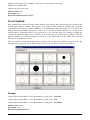
Insert Symbols . . . . . . . . . . . . . . . . . . . . . . . . . . . . . . . . . . . . . . . . . . . . .
66
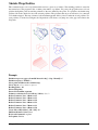
Shrink-Wrap Entities . . . . . . . . . . . . . . . . . . . . . . . . . . . . . . . . . . . . . . . . . .
67
3 Point Curve . . . . . . . . . . . . . . . . . . . . . . . . . . . . . . . . . . . . . . . . . . . . . .
68
PC PT Radius Point . . . . . . . . . . . . . . . . . . . . . . . . . . . . . . . . . . . . . . . . . . .
68
PC Radius Chord . . . . . . . . . . . . . . . . . . . . . . . . . . . . . . . . . . . . . . . . . . . .
68
Raster Image . . . . . . . . . . . . . . . . . . . . . . . . . . . . . . . . . . . . . . . . . . . . . .
69
Place Image by World File . . . . . . . . . . . . . . . . . . . . . . . . . . . . . . . . . . . . . . .
71
Place Google Earth Image . . . . . . . . . . . . . . . . . . . . . . . . . . . . . . . . . . . . . . .
71
Custom Linework Label Formatter . . . . . . . . . . . . . . . . . . . . . . . . . . . . . . . . . . .
73
Draw Barscale . . . . . . . . . . . . . . . . . . . . . . . . . . . . . . . . . . . . . . . . . . . . . .
75
Draw North Arrow . . . . . . . . . . . . . . . . . . . . . . . . . . . . . . . . . . . . . . . . . . .
75
Chapter 6.
Contents
Draw Commands
Settings Commands
77
Drawing Setup . . . . . . . . . . . . . . . . . . . . . . . . . . . . . . . . . . . . . . . . . . . . .
78
Units Control . . . . . . . . . . . . . . . . . . . . . . . . . . . . . . . . . . . . . . . . . . . . . .
79
Object Snap . . . . . . . . . . . . . . . . . . . . . . . . . . . . . . . . . . . . . . . . . . . . . . .
81
Set Environment Variables . . . . . . . . . . . . . . . . . . . . . . . . . . . . . . . . . . . . . . .
84
Toolbars . . . . . . . . . . . . . . . . . . . . . . . . . . . . . . . . . . . . . . . . . . . . . . . . .
86
iii
Options . . . . . . . . . . . . . . . . . . . . . . . . . . . . . . . . . . . . . . . . . . . . . . . . .
87
Edit Symbol Library . . . . . . . . . . . . . . . . . . . . . . . . . . . . . . . . . . . . . . . . . . 100
Configure . . . . . . . . . . . . . . . . . . . . . . . . . . . . . . . . . . . . . . . . . . . . . . . . 101
Chapter 7.
Survey Commands
109
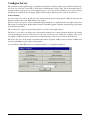
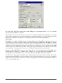
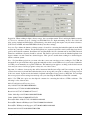
Configure Survey . . . . . . . . . . . . . . . . . . . . . . . . . . . . . . . . . . . . . . . . . . . . 110
Equipment Commands . . . . . . . . . . . . . . . . . . . . . . . . . . . . . . . . . . . . . . . . . 118
CSI GBX Pro . . . . . . . . . . . . . . . . . . . . . . . . . . . . . . . . . . . . . . . . . . 118
Geodimeter . . . . . . . . . . . . . . . . . . . . . . . . . . . . . . . . . . . . . . . . . . . 118
Impulse Laser . . . . . . . . . . . . . . . . . . . . . . . . . . . . . . . . . . . . . . . . . . 120
Leica GPS System 500 . . . . . . . . . . . . . . . . . . . . . . . . . . . . . . . . . . . . . 120
Leica TC Series . . . . . . . . . . . . . . . . . . . . . . . . . . . . . . . . . . . . . . . . . 122
Manual Total Station . . . . . . . . . . . . . . . . . . . . . . . . . . . . . . . . . . . . . . 123
Navcom Configuration Guide . . . . . . . . . . . . . . . . . . . . . . . . . . . . . . . . . 123
Navcom GPS Setup . . . . . . . . . . . . . . . . . . . . . . . . . . . . . . . . . . . . . . . 125
Nikon Total Stations . . . . . . . . . . . . . . . . . . . . . . . . . . . . . . . . . . . . . . 129
Simulation GPS . . . . . . . . . . . . . . . . . . . . . . . . . . . . . . . . . . . . . . . . . 130
Sokkia . . . . . . . . . . . . . . . . . . . . . . . . . . . . . . . . . . . . . . . . . . . . . 130
Topcon Total Stations . . . . . . . . . . . . . . . . . . . . . . . . . . . . . . . . . . . . . . 132
Trimble . . . . . . . . . . . . . . . . . . . . . . . . . . . . . . . . . . . . . . . . . . . . . 134
Align GPS To Local Coordinates . . . . . . . . . . . . . . . . . . . . . . . . . . . . . . . . . . . . 137
Align to Benchmark . . . . . . . . . . . . . . . . . . . . . . . . . . . . . . . . . . . . . . . . . . . 140
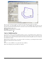
Typical Alignment Scenarios . . . . . . . . . . . . . . . . . . . . . . . . . . . . . . . . . . . . . . 140
Survey Benchmark . . . . . . . . . . . . . . . . . . . . . . . . . . . . . . . . . . . . . . . . . . . 141
Survey Perimeter . . . . . . . . . . . . . . . . . . . . . . . . . . . . . . . . . . . . . . . . . . . . 142
Survey Interior Surface . . . . . . . . . . . . . . . . . . . . . . . . . . . . . . . . . . . . . . . . . 143
Survey Subdivision line . . . . . . . . . . . . . . . . . . . . . . . . . . . . . . . . . . . . . . . . . 144
Survey Master Benchmark . . . . . . . . . . . . . . . . . . . . . . . . . . . . . . . . . . . . . . . 145
Monitor GPS Position . . . . . . . . . . . . . . . . . . . . . . . . . . . . . . . . . . . . . . . . . . 146
Stakeout Design Surface . . . . . . . . . . . . . . . . . . . . . . . . . . . . . . . . . . . . . . . . 147
Chapter 8.
Design Commands
148
Set Perimeter . . . . . . . . . . . . . . . . . . . . . . . . . . . . . . . . . . . . . . . . . . . . . . 149
Create Existing Ground Grid . . . . . . . . . . . . . . . . . . . . . . . . . . . . . . . . . . . . . . 149
Design Field . . . . . . . . . . . . . . . . . . . . . . . . . . . . . . . . . . . . . . . . . . . . . . . 149
Adjust Field Elevation . . . . . . . . . . . . . . . . . . . . . . . . . . . . . . . . . . . . . . . . . 151
Draw Subdivision Line . . . . . . . . . . . . . . . . . . . . . . . . . . . . . . . . . . . . . . . . . 151
Assign Subdivision Area Name . . . . . . . . . . . . . . . . . . . . . . . . . . . . . . . . . . . . . 152
Area Name Inspector . . . . . . . . . . . . . . . . . . . . . . . . . . . . . . . . . . . . . . . . . . 153
Contents
iv
Label Area Names . . . . . . . . . . . . . . . . . . . . . . . . . . . . . . . . . . . . . . . . . . . 154
Surface Inspector . . . . . . . . . . . . . . . . . . . . . . . . . . . . . . . . . . . . . . . . . . . . 154
Chapter 9.
Tools Commands
156
Follow Elevation . . . . . . . . . . . . . . . . . . . . . . . . . . . . . . . . . . . . . . . . . . . . 157
Distance MeasureSwathing . . . . . . . . . . . . . . . . . . . . . . . . . . . . . . . . . . . . . . . 158
Distance Measure with Pen . . . . . . . . . . . . . . . . . . . . . . . . . . . . . . . . . . . . . . . 160
Stakeout Design Surface . . . . . . . . . . . . . . . . . . . . . . . . . . . . . . . . . . . . . . . . 160
Watershed Analysis . . . . . . . . . . . . . . . . . . . . . . . . . . . . . . . . . . . . . . . . . . . 161
Run Off Tracking . . . . . . . . . . . . . . . . . . . . . . . . . . . . . . . . . . . . . . . . . . . . 167
Point Defaults . . . . . . . . . . . . . . . . . . . . . . . . . . . . . . . . . . . . . . . . . . . . . . 167
DrawLocate Points . . . . . . . . . . . . . . . . . . . . . . . . . . . . . . . . . . . . . . . . . . . 169
Draw Field to Finish . . . . . . . . . . . . . . . . . . . . . . . . . . . . . . . . . . . . . . . . . . 172
List Points . . . . . . . . . . . . . . . . . . . . . . . . . . . . . . . . . . . . . . . . . . . . . . . . 208
Edit Points . . . . . . . . . . . . . . . . . . . . . . . . . . . . . . . . . . . . . . . . . . . . . . . . 208
Erase Points . . . . . . . . . . . . . . . . . . . . . . . . . . . . . . . . . . . . . . . . . . . . . . . 209
Import TextASCII File . . . . . . . . . . . . . . . . . . . . . . . . . . . . . . . . . . . . . . . . . 209
Export TextASCII File . . . . . . . . . . . . . . . . . . . . . . . . . . . . . . . . . . . . . . . . . 210
Set Coordinate File . . . . . . . . . . . . . . . . . . . . . . . . . . . . . . . . . . . . . . . . . . . 212
CooRDinate File Utilities . . . . . . . . . . . . . . . . . . . . . . . . . . . . . . . . . . . . . . . . 212
Create Design Surface Points . . . . . . . . . . . . . . . . . . . . . . . . . . . . . . . . . . . . . . 217
Edit Point Attributes . . . . . . . . . . . . . . . . . . . . . . . . . . . . . . . . . . . . . . . . . . 218
Move Point Attributes . . . . . . . . . . . . . . . . . . . . . . . . . . . . . . . . . . . . . . . . . . 219
Resize Point Attributes . . . . . . . . . . . . . . . . . . . . . . . . . . . . . . . . . . . . . . . . . 219
Erase Point Attributes . . . . . . . . . . . . . . . . . . . . . . . . . . . . . . . . . . . . . . . . . . 219
Inverse . . . . . . . . . . . . . . . . . . . . . . . . . . . . . . . . . . . . . . . . . . . . . . . . . . 220
Occupy Point . . . . . . . . . . . . . . . . . . . . . . . . . . . . . . . . . . . . . . . . . . . . . . 220
Traverse . . . . . . . . . . . . . . . . . . . . . . . . . . . . . . . . . . . . . . . . . . . . . . . . . 221
Side Shots . . . . . . . . . . . . . . . . . . . . . . . . . . . . . . . . . . . . . . . . . . . . . . . . 222
EnterAssign Point . . . . . . . . . . . . . . . . . . . . . . . . . . . . . . . . . . . . . . . . . . . . 223
Area Defaults . . . . . . . . . . . . . . . . . . . . . . . . . . . . . . . . . . . . . . . . . . . . . . 223
Inverse with Area . . . . . . . . . . . . . . . . . . . . . . . . . . . . . . . . . . . . . . . . . . . . 227
Area by Interior Point . . . . . . . . . . . . . . . . . . . . . . . . . . . . . . . . . . . . . . . . . . 229
Area by Closed Polylines . . . . . . . . . . . . . . . . . . . . . . . . . . . . . . . . . . . . . . . . 229
BearingBearing Intersect . . . . . . . . . . . . . . . . . . . . . . . . . . . . . . . . . . . . . . . . 231
BearingDistance Intersect . . . . . . . . . . . . . . . . . . . . . . . . . . . . . . . . . . . . . . . . 231
DistanceDistance Intersect . . . . . . . . . . . . . . . . . . . . . . . . . . . . . . . . . . . . . . . 232
EditProcess Raw File . . . . . . . . . . . . . . . . . . . . . . . . . . . . . . . . . . . . . . . . . . 232
Contents
v
Chapter 10.
Display Commands
243
Display . . . . . . . . . . . . . . . . . . . . . . . . . . . . . . . . . . . . . . . . . . . . . . . . . 244
CutFill Spreadsheet . . . . . . . . . . . . . . . . . . . . . . . . . . . . . . . . . . . . . . . . . . . 244
Pad Design Report . . . . . . . . . . . . . . . . . . . . . . . . . . . . . . . . . . . . . . . . . . . 246
Display Options . . . . . . . . . . . . . . . . . . . . . . . . . . . . . . . . . . . . . . . . . . . . . 247
Chapter 11.
GIS Commands
249
GIS Database Settings . . . . . . . . . . . . . . . . . . . . . . . . . . . . . . . . . . . . . . . . . 250
Define GIS Features . . . . . . . . . . . . . . . . . . . . . . . . . . . . . . . . . . . . . . . . . . . 250
Input-Edit GIS Data . . . . . . . . . . . . . . . . . . . . . . . . . . . . . . . . . . . . . . . . . . . 252
GIS Inspector . . . . . . . . . . . . . . . . . . . . . . . . . . . . . . . . . . . . . . . . . . . . . . 253
GIS Inspector Settings . . . . . . . . . . . . . . . . . . . . . . . . . . . . . . . . . . . . . . . . . 254
GIS Query/Report . . . . . . . . . . . . . . . . . . . . . . . . . . . . . . . . . . . . . . . . . . . . 255
Import SHP File . . . . . . . . . . . . . . . . . . . . . . . . . . . . . . . . . . . . . . . . . . . . . 257
Export SHP File . . . . . . . . . . . . . . . . . . . . . . . . . . . . . . . . . . . . . . . . . . . . . 259
Chapter 12.
Help Commands
261
OnLine Help . . . . . . . . . . . . . . . . . . . . . . . . . . . . . . . . . . . . . . . . . . . . . . 262
Training Movies . . . . . . . . . . . . . . . . . . . . . . . . . . . . . . . . . . . . . . . . . . . . . 262
Contents
vi
Product Overview
1
This chapter describes the product overview, and system requirements for operating Agstar. It also contains
instructions for installing and authorizing Agstar, setting up your first project, and a description of non-menu
specific commands.
Product Overview
Quickstart Guide
Startup Wizard
Command Entry
System Requirements
Installing Agstar
Authorizing Agstar
Technical Support
1
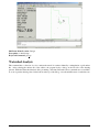
Product Overview
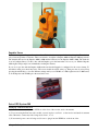
Agstar offers a complete package of land-levelling tools for agricultural and irrigation purposes. It carries a versatile
suite of commands designed to simplify and speed up the professional surveyor's work, as well as reduce costs by
minimizing the amount of dirt to move.
For data collection, Agstar supports a wide range of GPS RTK receivers, including such popular brands as Navcom,
Ashtech, Leica, Sokkiam, and Trimble; if you have it, Agstar probably supports it, which means you may not even
need to upgrade your hardware.
Agstar handles both the survey and the design sides of land-levelling, allowing you to survey large fields with GPS,
and then determine the optimal field design requiring the least amount of dirt moved. Agstar enables you to set the
cut/fill ratio, the amount of dirt to import or export, and a host of other design parameters. It also allows you to
subdivide the field and assign different designs to each subdivision, which is useful if you want crowns in your field.
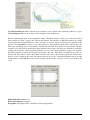
After field design, Agstar can display design information in a variety of ways:
1) A pad report detailing the total cubic cut/fill yardage, the field area, the field grade, and other useful information.
2) A color-coded cut/fill spreadsheet (cutsheet) showing the amount of cut/fill for each field segment.
3) A color-coded contour map depicting the existing or cut/fill contour lines.
4) An option to ''Stakeout Design Surface'', which tells the user the cut or fill with an on-screen lightbar, while
navigating the field.
Agstar is the latest in a long line of powerful software survey tools produced by Carlson Software, including Carlson
SurvCE and Carlson Survey. In addition to it's basic land survey and design commands, it contains many of the useful
features of it's predecessors, allowing you to view and manipulate your survey data in a wide variety of ways.
Carlson Software also provides some of the best technical support in the industry. If you ever need help with it, don't
hesitate to contact us for free technical support.
Quickstart Guide
You will find all of the most commonly used Agstar command under the Survey, Design, and Display menus.
To survey and design your first field, it is recommended that you consult the following sections of the manual (in
order):
1) Survey/Configure Survey - In this section, you must set your Equipment type to the GPS equipment you are using.
Then in the GPS Settings menu, set your Project Type to State Plane 83, and set your Zone to correspond to the local
region in which you are working.
2) Survey/Equipment Setup - In this section, you must set up your equipment specific setting. This usual requires
configuring your stationary GPS unit to base, and your mobile GPS unit to rover.
3) Survey/Survey Master Benchmark - In this section, you will survey a reference point, defining the origin of the
coordinate system.
4) Survey/Survey Perimeter - In this section, you will survey the border of your field.
5) Survey/Survey Interior Surface - In this section, you will survey the interior of your field.
6) Design/Create Existing Ground Grid - In this section, you will define a grid interval, a necessary step when your
survey is complete, and you want to begin designing the field.
7) Design/Design Field - In this section, you will generate a design for you field.
8) Now use any of the command under the Display menu to generate design information. To inspect the field
design with your mouse, run Design/Surface Inspector. To view the cuts and fills at your vehicle's position using an
onscreen lightbar, go to Tools/Stakeout Design Surface.
To create field subdivisions, consult the following commands (in order):
Chapter 1. Product Overview
2
1) Survey/Survey Subdivision Line or Design/Draw Subdivision Line - The first of these allows you to create a
subdivision line with your vehicle. The second allows you to create a subdivision line by drawing it with the mouse.
2) Design/Assign Subdivision Area Names - Use this command to name or rename a subdivision area.
3) Design/Area Name Inspector - Use this command to view existing field area names.
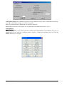
System Requirements
Operating System
Microsoft® Windows® 98, Windows Millennium Edition (ME), Windows XP Professional, Windows 2000 Professional, or Windows® NT 4.0 with SP 6.0 or later.
Notes: It is recommended that you install and run Agstar on an English version of the operating system. Users
of Windows NT 4.0 or Windows 2000 Professional must have Administrator permissions to install Agstar. Not
assigning these permissions can cause Agstar to perform incorrectly. See Windows Help for information about
assigning user permissions.
Processor
Intel® Pentium® III, IV or AMD-K6® III PC, 450MHz or higher
RAM
128 MB
Video
VGA display 1024 x 768
Hard disk
500MB free disk space
Pointing device
Mouse
CD-ROM
Any speed (for installation only)
GPS Equipment
RTK base and rover
Optional hardware
Printer or plotter
Digitizer
Modem or access to an Internet connection
Open GL-compatible 3D video card
The OpenGL driver that comes with the 3D graphics card must have the following: Full support of OpenGL or later.
An OpenGL Installable Client Driver (ICD). The graphics card must have an ICD in its OpenGL driver software.
The ''miniGL'' driver provided with some cards is not sufficient for use with this Autodesk CAD engine.
Chapter 1. Product Overview
3
Web browser
Microsoft Internet Explorer 5.0
Netscape Navigator 4.5 or later
Installing Agstar
If you're installing Agstar on Microsoft® Windows NT® 4.0 and Windows 2000, you must have permission to write
to the necessary system registry sections. To do this, make sure that you have administrative permissions on the
computer on which you're installing.
Before you install Agstar, close all running applications. Make sure you disable any virus-checking software. Please
refer to your virus software documentation for instructions.
Note: If you are upgrading from an older version of Agstar, you must uninstall the older version before installing
Agstar. This is required for successful software installation and to meet the guidelines of the EULA (End User
License Agreement).
1 Insert the CD into the CD-ROM drive.
If Autorun is enabled, it begins the setup process when you insert the CD.
To stop Autorun from starting the installation process automatically, hold down the SHIFT key when you insert the
CD.
To start the installation process without using Autorun, from the Start menu (Windows), choose Run. Enter the
CD-ROM drive letter, and setup. For example, enter d:\setup.
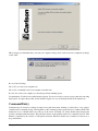
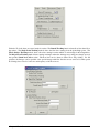
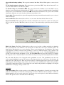
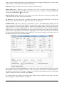
2 The Windows Installer dialog box is displayed.
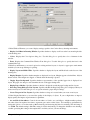
3 After reading the initial Agstar dialog box, press Next. If this is the initial installation, you will see the dialog
shown below.
Chapter 1. Product Overview
4
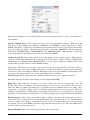
If this version of Agstar has already been installed, you will see the slightly different dialog shown below.
In this case, it is recommended that you remove the current installation. After the current installation is removed,
you may start the install process once more to continue.
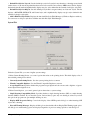
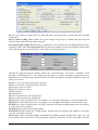
4 On the Serial Number dialog box, you must enter the serial number provided with your copy of Agstar.
Chapter 1. Product Overview
5
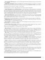
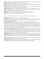
5 On the Select Installation Type dialog box, select the type of installation you want: Typical, Compact, or Custom.
Choose Next.
Typical installs the following features:
• Program files: Executables, menus, toolbars, Help templates, TrueType® fonts, and additional support files
• Internet tools: Support files
• Fonts: SHX fonts
• Samples: Sample drawings
• Help files: Online documentation
Chapter 1. Product Overview
6
Compact installs only the program files and fonts.
Custom installs only the files you select. By default, the Custom installation option installs all Agstar features. To
install only the features you want, choose a feature, and then select one of the following options from the list:
• Will be installed on local hard drive: Installs a feature or component of a feature on your hard drive.
• Entire feature will be installed on local hard drive: Installs a feature and its components on your hard drive.
• Feature will be installed when required only: Installs a feature on demand.
• Entire feature will be unavailable: Makes the feature unavailable.
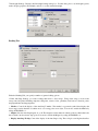
6 On the Destination Folder dialog box, do one of the following:
Choose Next to accept the default destination folder/directory.
Choose Browse to specify a different drive and folder where you want Agstar to be installed. Choose any directory
that is mapped to your computer (including network directories) or enter a new path. Choose OK and then Next.
Setup installs some files required by Agstar in your system folder (for example, c:\Windows\System, or
c:\Winnt\System32). This folder may be on a different drive than the folder you specify as the installation folder
(for example, d:\Program Files\ Agstar). You may need up to 60 MB of space in your system folder, depending
on the components you select to install. Setup alerts you if there is insufficient free space on the drive that contains
your system folder.
7 On the Start Installation page, choose Next to start the installation.
Chapter 1. Product Overview
7
8 The Updating System dialog box is displayed while Agstar is installed.
9 When the installation is complete, the Setup Complete dialog box is displayed. Choose Finish to exit the installation program.
Chapter 1. Product Overview
8
10It is strongly recommended that you restart your computer at this point in order for the new configuration settings
to take effect.
Do one of the following:
Choose Yes to restart your computer now.
Choose No to manually restart your computer at another time.
If you do not restart your computer, you may have problems running Agstar.
Congratulations! You have successfully installed Agstar. You are now ready to register your product and start using
the program. To register the product, double-click the Agstar icon on your desktop and follow the instructions.
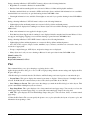
Command Entry
Commands may be issued by selecting an entry from a pull-down menu, clicking a toolbar button, or by typing a
command at the command prompt. Pressing Enter at the command prompt repeats that last command. Pull-down
menus have a row of header names across the top of the screen. Selecting one of these header names displays the
possible commands under that name. The pull-down menus are the primary method for command selection. This
manual is organized by the contents of each pull-down menu. Pull-down menus may sometimes be referred to as
drop-down menus.
Chapter 1. Product Overview
9
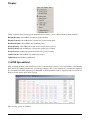
Startup Wizard
For creating a new drawing in Agstar, the Startup Wizard can guide you through starting and setting up the drawing.
This wizard is optional and can be turned on or off in the Configure Survey — General Settings command. You can
also exit out of the Startup Wizard at any time.
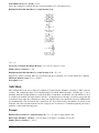
When the New drawing command is executed, you first get the standard AutoCAD choice of ''Start from Scratch'',
''Use a Template'' or ''Use a Wizard''. Typically, you want to the ''Use a Template'' option and choose the drawing
template (SURVEY.DWT). The drawing template will set of some basic drawing parameters such as default layer
names.
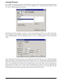
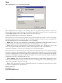
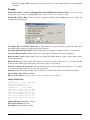
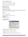
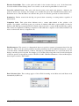
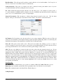
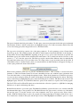
After selecting the AutoCAD new drawing option, the New Drawing Wizard dialog box opens. The Startup Wizard
begins with a dialog to set the drawing name and scale. The first step to do is set the drawing (.dwg) name by picking
the Set button. This brings up the file selection dialog. Change to the directory/folder (''Save in'' field) where you
want to store the drawing. You can either select an existing folder or create a new folder. To select an existing folder,
pull down the Save in field to select a folder or drive, click the Move Up icon next to the Save in field and/or the
pick the folder name from the list. To create a new folder, pick the Create New Folder icon to the right of the Save
in field. Then type in the drawing name in the File name field and click the Save button.
Chapter 1. Product Overview
10
After setting the drawing name, you can set the drawing horizontal scale, symbol size, text size and unit mode
(English or Metric). Then click the Next button.
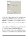
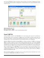
The next startup dialog sets the Data Path and CRD File. The Data Path is the folder where Agstar will store the
data files such as raw (.RW5) files and profile (.PRO) files. The Set button for the Data Path allows you to select an
existing folder or create a new folder. See the Set Data Directory command for more information. The coordinate
(.CRD) File is the coordinate file for storing the point data. There is an option to create a new or existing coordinate
(.CRD) file. The new option will erase any point data that is found in the specified CRD file. The existing option
will retain any point data in the specified coordinate (.CRD) file. If the specified coordinate (.CRD) file does not
exist, the wizard will create a new file.
The next wizard step depends on the Import Points option. The Data Collector option will start the data collection
routines to download data from a collector. The Text/ASCII option will import point data from a text/ASCII file.
See the Data Collection and Import Text/ASCII File commands for more information on running these routines. If
the None option is set, then the Startup Wizard is finished.
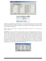
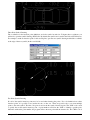
Once point data has been imported from the data collector or text/ASCII file, the wizard guides you through drawing
the points. There are options to run Draw/Locate Points, Field To Finish or None. If None is selected, then the
Startup Wizard is finished. Draw/Locate Points will import the points into the drawing using the same symbol and
layer for all the points. From the Draw/Locate Points dialog, set the symbol, layer and point attributes to draw
(description, elevation) and then pick the Draw All button. The Field To Finish command will import the points
into the drawing using different layers and symbols depending on the point descriptions that refer to the code table
defined in Field to Finish. Also Field to Finish can draw linework. See the Draw/Locate Point and Field To Finish
commands for more information on running these routines. After drawing the points, the wizard will zoom the
display around the points. Then the wizard is finished.
Chapter 1. Product Overview
11
AuthorizingAgstar
The first time you start Agstar, the Registration Wizard is displayed.
1 Carlson Software has installed an automated procedure for registering your software license. Change keys are no
longer given over the telephone. Please choose one of the following registration methods.
• Form: This method allows you to fill out a form that you can print out and fax or mail to Carlson Software for
registration.
• Internet: If your computer is online, you may register automatically over the Internet. Your information is sent
to a Carlson Software server , validated and returned in just a few seconds. If you are using a dial-up connection,
please establish this connection before attempting to register.
• Enter change key: Choose this method after you have received your change key from Carlson Software (if you
previously used the Form method above).
• Register Later: Choose this method if your want to register later. You may run Agstar for 30 days before you
are required to register.
2 After you choose the registration method, press Next
3 Choose the reason for installation. The very first time you install Agstar is the only time you will choose the first
reason. All subsequent installations require a choice from the remaining options.
Chapter 1. Product Overview
12
• New install or maintenance upgrade of Carlson Software: If you are installing Agstar for the first time, choose
this reason.
• Home use. See License Agreement: Choose this reason if you are installing on your home computer. See your
license agreement for more details!
• Re-Installation of Carlson Software: Choose this reason if you are reinstalling on the same computer with no
modifications.
• Windows or AutoCAD upgrade: Choose this reason if you have reinstalled Agstar after installing a new version
of Microsoft Windows.
• New Hardware: Choose this reason if you are installing Agstar on a new computer or if your existing computer
has had some of its hardware replaced such as the hard disk, network adapter, etc.
4 After you choose the reason for installation, press Next
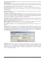
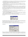
5 Next, enter the required information into the dialog.
If you are using the Form method, press the Print Fax Form button to print out the form. You may fax this form
to the number printed on the form or mail it to Carlson Software, 102 W. Second St., Suite 200 Maysville, KY
41056-1003.
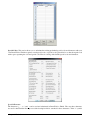
If you are using the Internet method, press Next. After a few seconds, your registration will complete. If your
registration is successful, you will receive a message such as the one below. If your registration is unsuccessful,
please note the reason why and try again. Keep in mind that each serial number may be registered to a single
computer only.
If you do not have access to the internet and do not have a printer, you must write down the information from the
User Info tab (shown above) and fax it to 606-564-9525 or mail it to Carlson Software, 102 W. Second St., Suite
200 Maysville, KY 41056-1003.
Chapter 1. Product Overview
13
License Agreement
Copyright 1992-2012 Carlson Software All Rights Reserved
CAUTION! READ THIS NOTICE BEFORE USING SOFTWARE
Please read the following Software License Agreement before using the SOFTWARE. Using this SOFTWARE indicates that you have accepted its terms and conditions.
Carlson AgStar 2013
END-USER LICENSE AGREEMENT FOR CARLSON SOFTWARE
IMPORTANT-READ CAREFULLY: This Carlson Software End-User License Agreement (''EULA'')
is a legal agreement between you (either an individual or a single entity) and Carlson Software, Inc for
the software accompanying this EULA, which includes computer software and may include associated
media, printed materials, and ''online'' or electronic documentation (''SOFTWARE PRODUCT'' or ''SOFTWARE''). By exercising your rights to use the SOFTWARE, you agree to be bound by the terms of this
EULA. If you do not agree to the terms and conditions of this EULA, you may not use the SOFTWARE. IF
YOU DO NOT AGREE TO THE TERMS AND CONDITIONS OF THIS EULA, DO NOT INSTALL OR
USE ANY PART OF THE SOFTWARE.
Carlson Software, Inc., referred to as ''LICENSOR'', develops and/or licenses proprietary computer programs
and sells use licenses for such proprietary computer programs together with or apart from accompanying copyrighted material and documentation and;
End User desires to obtain the benefits thereof and, in return for which, is willing to abide by the obligations and fee agreements applicable to LICENSOR's use licenses in LICENSOR's proprietary computer programs.
For good and valuable consideration, including but not limited to license grant in accordance with this Agreement
by LICENSOR to End User's covenant regarding LICENSOR's proprietary rights, LICENSOR agrees to permit
End User to utilize materials representing LICENSOR's product or products subject to the following terms and
conditions:
1. License Grant: Subject to the terms, conditions and limitations of this EULA, LICENSOR hereby grants
End User a personal, limited, non-exclusive, non-transferable, license to utilize the Software Product you have purchased. The license granted in this EULA creates no license, express or implied, to any other intellectual property
of Licensor, except for the specific Software Product which they have lawfully purchased from LICENSOR.
This EULA grants you the following rights: You may install and use one copy of the SOFTWARE PRODUCT,
or any prior version for the same operating system, on a single computer. The primary user of the computer on
which the SOFTWARE PRODUCT is installed may make a second copy for his or her exclusive use on a portable
computer.
Storage/Network Use. You may also store or install a copy of the SOFTWARE PRODUCT on a storage device,
such as a network server, used only to install or run the SOFTWARE PRODUCT on your other computers over
an internal network; however, you must acquire and dedicate a license for each separate computer on which the
SOFTWARE PRODUCT is installed or run from the storage device. A license for the SOFTWARE PRODUCT
may not be shared or used concurrently on different computers.
2. Exclusive Source. End User shall obtain all LICENSOR authorized product materials through LICENSOR or LICENSOR'S authorized representative and no other source. LICENSOR authorized product materials
include, but are not limited to, manuals, license agreements and media upon which LICENSOR's proprietary
computer programs are recorded. End User shall make no copies of any kind of any of the materials furnished by
LICENSOR or LICENSOR's authorized representative, except as specifically authorized to do so in this EULA.
End User is not entitled to make archival copies of those portions of LICENSOR's product(s) that are provided on a
machine readable media.
Chapter 1. Product Overview
14
3. Proprietary Rights of Licensor. End User agrees that LICENSOR retains exclusive ownership of the
trademarks and service marks represented by its company name and logo and all of the documentation and
computer recorded data related thereto. End User also agrees that all techniques, algorithms, and processes
contained in LICENSOR's computer program products or any modification or extraction thereof constitute TRADE
SECRETS OF LICENSOR and will be safeguarded by End User, but in no event shall End User exercise less than
due diligence and care in accordance with the laws of the country of purchase and International Law, whichever
operates to best protect the interests of LICENSOR. End User shall not copy, reproduce, re-manufacture or in
any way duplicate all or any part of LICENSOR products WHETHER MODIFIED OR TRANSLATED INTO
ANOTHER LANGUAGE OR NOT, or in any documentation, or in any other material provided by LICENSOR
in association with LICENSOR's computer program products regardless of what manner of storage and retrieval
the product exists, except as specified in this Agreement and in accordance with the terms and conditions of this
Agreement which remain in force. End User agrees that in the event End User breaches this EULA, End User will
be liable for damages as may be determined by a court of competent jurisdiction.
4. Restrictions. End User's rights and obligations under this EULA are nonexclusive and personal in nature,
and the intellectual property Licensor grants to End User is subject to applicable law other than bankruptcy law. End
User may not transfer or assign the SOFTWARE, rights under this EULA or accompanying user documentation,
or any updates of the SOFTWARE which may be provided under this EULA, to a third party unless End User
receives written consent from Licensor at least 30 days prior to the completion of transfer. Licensor reserves the
right to deny transfer or assignment if, in its sole discretion, Licensor determines the transfer not to be a necessity.
Whether or not a transfer or assignment is allowed shall be determined in Licensor's sole discretion after taking
into consideration certain factors to find the existence of a necessity including, but not limited to, merger or
acquisition of an entity, complete asset acquisition, change of control, severe economic hardship, severe loss of
human resources or significant loss in business divisions, or winding down of entity affairs.
If Carlson consents to a transfer, such transfer shall be allowed only as a one-time permanent transfer of this
EULA and Software to another end user, provided the initial End User retains no copies or previous versions of
the Software. The transfer must include all of the Software, including all component parts, any media and printed
materials, any upgrades, this EULA, and any associated license key. The transfer may not be an indirect transfer,
such as a consignment, rental or lease. No corresponding Maintenance Agreement rights shall transfer with the
SOFTWARE transfer to the subsequent end user. Prior to the transfer, the subsequent end user receiving the
Software from the initial End User must agree to all terms of this EULA, with the added condition that no further
transfers to third parties are permitted for any reason whatsoever, and shall agree to the terms and conditions of a
new Maintenance Agreement with Licensor.
You may not reverse engineer, decompile, or disassemble the SOFTWARE or alter the images utilized in the
SOFTWARE and user documentation. The SOFTWARE PRODUCT is licensed as a single product. Its component
parts may not be separated for use on more than one computer. You shall communicate to any individual user in
your facility that they are bound by the restrictions of this license agreement may not copy or alter the SOFTWARE
for use outside End User's facilities.
Upgrades. If you purchase an upgrade of a SOFTWARE PRODUCT and you use it on different machine from one
where upgraded SOFTWARE PRODUCT was used, use of original SOFTWARE PRODUCT must be discontinued
and confirmed within 30 days. If such use is not discontinued, it is a material breach of this EULA and LICENSOR
shall be entitled to all remedies available to it under this EULA, and under the laws of Kentucky, USA.
5. Security Mechanisms. Licensor and its affiliated companies take all legal steps to eliminate piracy of
their software products. In this context, the Software Product may include a security mechanism that can detect the
installation or use of illegal copies of the Software Product, and collect and transmit data about those illegal copies.
Data collected will not include any customer data created with the Software. By using the Software Product, you
consent to such detection and collection of data, as well as its transmission and use if an illegal copy is detected.
Licensor also reserves the right to use a hardware lock device, license administration software, and/or a license
authorization key to control access to the Software. You may not take any steps to avoid or defeat the purpose of any
such measures. Use of any Software without any required lock device or authorization key provided by Licensor is
Chapter 1. Product Overview
15
prohibited.
6. Audit Rights. End User agrees that LICENSOR has the right to require an audit (electronic or otherwise)
of the LICENSOR Materials and the Installation thereof and access thereto. As part of any such audit, LICENSOR
or its authorized representative will have the right, on fifteen (15) days' prior notice to End User, to inspect End
User's records, systems and facilities, including machine IDs, serial numbers and related information, to verify
that the use of any and all LICENSOR Materials is in conformance with this Agreement. End User will provide
full cooperation to enable any such audit. If LICENSOR determines that End User's use is not in conformity with
this EULA, End User will obtain immediately and pay for a valid license to bring End User's use into compliance
with this EULA and other applicable terms and pay the reasonable costs of the audit. In addition to such payment
rights, LICENSOR reserves the right to seek any other remedies available at law or in equity, whether under this
Agreement or otherwise.
7. Warranty. THE PRODUCT IS PROVIDED ''AS IS'' WITH ALL FAULTS. TO THE MAXIMUM EXTENT
PERMITTED BY LAW, LICENSOR HEREBY DISCLAIMS ALL WARRANTIES, WHETHER EXPRESS
OR IMPLIED, INCLUDING WITHOUT LIMITATION IMPLIED WARRANTIES OF MERCHANITIBILITY,
FITNESS FOR A PARTICULAR PURPOSE, AND WARRANTIES THAT THE PRODUCT IS FREE OF
DEFECTS AND NON-INFRINGING, WITH REGARD TO THE SOFTWARE, AND THE ACCOMPANYING
WRITTEN MATERIALS. YOU BEAR ENTIRE RISK AS TO SELECTING THE PRODUCT FOR YOUR
PURPOSES AND AS TO THE QUALITY AND PERFORMANCE OF THE PRODUCT. THIS LIMITATION
WILL APPLY NOTWITHSTANDING THE FAILURE OF ESSENTIAL PURPOSE OF ANY REMEDY. In any
event, LICENSOR will not honor any warranty shown to exist for hich inaccurate or incorrect identifying data has
been provided to LICENSOR. The product(s) provided are intended for commercial use only and should not be
utilized as the sole data source in clinical decisions as to levels of care.
8. LIMITATION OF LIABILITY. EXCEPT AS REQUIRED BY LAW, LICENSOR AND ITS DISTRIBUTORS, DIRECTORS, LICENSORS, CONTRIBUTORS AND AGENTS (COLLECTIVELY, THE ''LICENSOR
GROUP'') WILL NOT BE LIABLE FOR ANY INDIRECT, SPECIAL, INCIDENTAL, CONSEQUENTIAL OR
EXEMPLARY DAMAGES ARISING OUT OF OR IN ANY WAY RELATING TO THIS EULA OR THE USE
OF OR INABILITY TO USE THE PRODUCT, INCLUDING WITHOUT LIMITATION DAMAGES FOR LOSS
OF GOODWILL, WORK STOPPAGE, LOST PROFITS, LOSS OF DATA, AND COMPUTER FAILURE OR
MALFUNCTION, EVEN IF ADVISED OF THE POSSIBILITY OF SUCH DAMAGES AND REGARDLESS
OF THE THEORY (CONTRACT, TORT OR OTHERWISE) UPON WHICH SUCH CLAIM IS BASED. THE
LICENSOR GROUP'S COLLECTIVE LIABILITY UNDER THIS AGREEMENT WILL NOT EXCEED THE
GREATER OF $500 (FIVE HUNDRED DOLLARS) AND THE FEES PAID BY YOU UNDER THIS LICENSE
(IF ANY).
9. Update Policy. LICENSOR may, from time to time, revise the performance of its product(s) and in doing so, incur NO obligation to furnish such revisions to any End User nor shall it warrant or guarantee that any
revision to the SOFTWARE will perform as expected by the End User on End User's equipment. At LICENSOR's
option, LICENSOR may provide such revisions to the End User.
10. Customer Service. Although it is the LICENSOR's customary practice to provide reasonable assistance
and support in the use of its products to its customers, LICENSOR shall not be obligated to any End User to provide
technical assistance or support through this Agreement and may at LICENSOR's sole election charge a fee for
customer support.
11. Termination of End User License. If any one or more of the provisions of this Agreement is breached,
the license granted by this Agreement is hereby terminated. In the event of such termination, all rights of the
LICENSOR shall remain in force and effect. Any protected health information data of End User maintained on
LICENSOR'S data base shall upon reasonable notice to End User and at the discretion of LICENSOR may be
destroyed.
Chapter 1. Product Overview
16
12. Copyright. The SOFTWARE (including, but not limited to, any images, photographs, animations, video, audio,
music and or text incorporated into the SOFTWARE), and all intellectual property rights associated with it, whether
exists in a tangible media or in an electronic image media is owned by LICENSOR and is protected by United
States copyright laws and international treaty provisions and all other commonwealth or national laws. LICENSOR
reserves all intellectual property rights in the Products, except for the rights expressly granted in this Agreement.
You may not remove or alter any trademark, logo, copyright or other proprietary notice in or on the Product. This
license does not grant you any right to use the trademarks, service marks or logos of LICENSOR or its licensors.
You may not copy any user documentation accompanying the SOFTWARE.
13. Injunctive Relief. It is understood and agreed that, notwithstanding any other provision of this Agreement, LICENSOR has the unequivocal right to obtain timely injunctive relief to protect the proprietary rights of LICENSOR.
14. Entire Agreement. This EULA constitutes the entire agreement between the parties and supersedes any
prior agreements. This EULA may only be changed by mutual written consent.
15. End User Agreement Acknowledgment. The End User hereby accepts all the terms and conditions of
this Agreement without exception, deletion, alteration. End User acknowledges they are authorized to enter this
agreement on behalf of any organization for which the license is sought. Any unauthorized use of LICENSOR
products will be considered a breach of this Agreement, subject to liquidated damages and otherwise unlawful and
willful infringement of LICENSOR's trade secrets and/or proprietary products.
16. Payment and Refund Policy. The use of the SOFTWARE herein is deemed a commercial use and under
the terms of this license agreement End User shall not be entitled to any refund of purchase price. End User agrees
to pay all user fees promptly. LICENSOR is authorized by End User to suspend any further access to SOFTWARE
in the event fees are not fully paid. End user entity shall promptly pay any and all access and use charges incurred
regardless of the end user. End user is responsible for protecting any pass word and user identity supplied to End
User.
17. Loss/Theft/Misuse. End user shall promptly report to LICENSOR the theft or other loss of any password and/or user identity required to access SOFTWARE. LICENSOR shall not be responsible for maintaining the
integrity of End User data in the event that end user's data base is accessed and/or altered by an unauthorized end
user due to the failure of licensed End User to protect its password or user identity. End User shall be responsible
for any costs incurred by LICENSOR due to the negligence or reckless disregard of End User's failure to protect its
password or user identity.
18. Civil/Criminal Investigation. End user shall fully cooperate with LICENSOR and or any person authorized by LICENSOR (including local, state, or federal law enforcement officials) to investigate any alleged theft,
misuse or unauthorized use of SOFTWARE or data related thereto.
19. U.S. Government Restricted Rights. The SOFTWARE PRODUCT and documentation are provided
with RESTRICTED RIGHTS. Use, duplication, or disclosure by the Government is subject to restrictions as set
forth in subparagraph (b)(1)(ii) and (c) of the Rights in Technical Data and Computer Software clause at DFARS
252.227-7013 or subparagraphs (c)(1) and (2) of the Commercial Computer Software-Restricted Rights at 48 CFR
52.227-19, as applicable.
20. Governing Law. This EULA shall be governed and construed in accordance with the laws of the Commonwealth of Kentucky, USA.
Technical Support
Discussion Groups
Chapter 1. Product Overview
17
Carlson Software operates user discussion groups. The NNTP address is news.carlsonsw.com. Visit our website for
complete details on how to connect to these discussion groups.
Electronic Mail
The technical support email address is [email protected]
Internet
The Knowledge base is available at update.carlsonsw.com/kbase
Program updates and patches are available at update.carlsonsw.com
Technical support documents are available at www.carlsonsw.com
Phone or Facsimile
Phone: 606-564-5028
Fax: 606-564-6422
Fax for registrations only: 606-564-9525
Please submit your company name, product version, and serial number with all support inquiries
Chapter 1. Product Overview
18
File Commands
2
19
New
This command allows you to create a new drawing file.
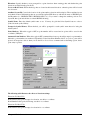
This command defines the settings for a new drawing. There are two methods that you can use to create a new
drawing. (The first option, Open a Drawing, is not available from the NEW command. To open an existing drawing,
use the OPEN command.) Choose one of the icons at the top of the dialog box.
1 Under Start from Scratch, you can start a new drawing file.
This command starts a new drawing using default settings defined in either the surv.dwt or surviso.dwt template,
depending on the measurement system you've chosen. You cannot modify the surv.dwt or surviso.dwt templates. To
start a new drawing based on a customized template, see Use a Template.
• English: This option starts a new drawing based on the Imperial measurement system. The drawing is based on
the surv.dwt template, and the default drawing boundary (the drawing limits) is 12 × 9 inches.
• Metric: This option starts a new drawing based on the metric measurement system. The drawing is based on the
surviso.dwt template, and the default drawing boundary (the drawing limits) is 429 × 297 millimeters.
2 Under Use a Template, you can start a new drawing based on a customized template.
This command creates a new drawing using the settings defined in a template drawing you select. Template drawings
store all the settings for a drawing and may also include predefined layers, dimension styles, and views. Template
drawings are distinguished from other drawing files by the .dwt file extension. They are normally kept in the template
directory. Several template drawings are included with AgStar. You can make additional template drawings by
changing the extensions of drawing file names to .dwt.
• Select a Template: This option lists all template files that currently exist in the drawing template file location,
which is specified in the Options dialog box. Choose a file to use as a starting point for your new drawing. A preview
image of the selected file is displayed to the right.
• Browse: This option displays the Select a Template File dialog box (a standard file selection dialog box) where
you can access template files in other directions.
Menu Location: File
Prerequisite: None
Keyboard Command: NEW
Chapter 2. File Commands
20
Open
This command allows you to open an existing drawing file. AgStar displays the Select File dialog box (a standard
file selection dialog box). Select a file and click Open.
Menu Location: File
Prerequisite: None
Keyboard Command: OPEN
Close
Function
This command allows you to close the current drawing. AgStar closes the current drawing if there have been no
changes since the drawing was last saved. If you have modified the drawing, the program prompts you to save or
discard the changes. You can close a file that has been opened in Read-only mode if you have made no changes or
if you are willing to discard changes. To save changes to a read-only file, you must use the SAVEAS command.
Menu Location: File
Prerequisite: None
Keyboard Command: CLOSE
Save
If the drawing is named, Carlson Survey saves the drawing without requesting a file name. If the drawing is unnamed,
the program displays the Save Drawing As dialog box (see SAVEAS) and saves the drawing with the file name you
specify. If the drawing is read-only, use the SAVEAS command to save the changed file under a different name.
This command allows you to save the drawing under the current file name or a specified name
Menu Location: File
Prerequisite: None
Keyboard Command: SAVE or QSAVE
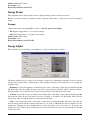
Save As
This command allows you to save an unnamed drawing with a file name or renames the current drawing.
AgStar displays the Save Drawing As standard file selection dialog box. Enter a file name and type. You can select
any of the following file types:
• AutoCAD 2000 (*.dwg)
• AutoCAD R14/LT 98/LT 97 Drawing (*.dwg)
• AutoCAD R13/LT 95 Drawing (*.dwg)
• Drawing Template File (*.dwt)
• Carlson Software 2002 DXF (*.dxf)
• AutoCAD R14/LT 98/LT 97 DXF (*.dxf)
• AutoCAD R13/LT 95 DXF (*.dxf)
• AutoCAD R12/LT2 DXF (*.dxf)
AgStar saves the file under the specified file name. If the drawing is already named, the program saves the drawing
to the new file name. If you save the file as a drawing template, the program displays the Template Description
dialog box, where you can provide a description for the template and set the units of measurement.
Chapter 2. File Commands
21
Saving a drawing in Release 14/LT 98/LT 97 format is subject to the following limitations:
• Hyperlinks are converted to Release 14 attached URLs.
• Database links and freestanding labels are converted to Release 14 links and displayable attributes.
• Database attached labels are converted to MText and leader objects, and their link information is not available.
Attached labels are restored if you open the drawing in AutoCAD 2000 or later.
• Lineweight information is not available. Lineweights are restored if you open the drawing in AutoCAD 2000 or
later.
Saving a drawing in Release 13/LT 95 format is subject to the following limitations:
• Lightweight polyline and hatch patterns are converted to R13 polylines and hatch patterns.
• Raster objects are displayed as bounding boxes. Raster objects are restored if the drawing is opened in AutoCAD
2000 or later.
• Draw order information is not applied for display or print.
• Xrefs that have been clipped with a boundary box are displayed in full as attached xrefs because Release 13 does
not support xref clipping. Clipping is restored if the drawing is opened in AutoCAD 2000 or later.
Saving a drawing in Release 12/LT 2 DXF format is subject to the following limitations:
• Lightweight polylines and hatch patterns are converted to R12 polylines and hatch patterns.
• All solids, bodies, regions, ellipses, leaders, multilines, rays, tolerances, and xlines are converted to lines, arcs,
and circles as appropriate.
• Groups, complex linetypes, OLE objects, and preview images are not displayed.
• Many objects are lost if you save a drawing as Release 12 and open it later in AutoCAD 2000 or later.
Menu Location: File
Prerequisite: None
Keyboard Command: SAVEAS
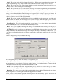
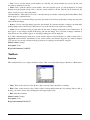
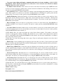
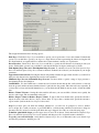
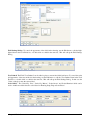
Plot
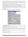
This command allows you to plot a drawing to a plotting device or file.
AgStar displays the Plot dialog box. Choose OK to begin plotting with the current settings and display the Plot
Progress dialog box.
1 The Plot dialog box includes the tabs, Plot Device and Plot Settings, and several options to customize the plot.
• Layout Name: This option displays the current layout name or displays ''Selected layouts'' if multiple tabs are
selected. If the Model tab is current when you choose Plot, the Layout Name shows ''Model.''
• Save Changes to Layout: This option saves the changes you make in the Plot dialog box in the layout. This
option is unavailable if multiple layouts are selected.
• Page Setup Name: This option displays a list of any named and saved page setups. You can choose to base the
current page setup on a named page setup, or you can add a new named page setup by choosing Add.
• Add: This option displays the User Defined Page Setups dialog box. You can create, delete, or rename named
page setups.
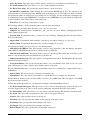
2 Under the Plot Device Tab you can specify the plotter to use, a plot style table, the layout or layouts to plot, and
information about plotting to a file.
Chapter 2. File Commands
22
• Plotter Configuration: This field displays the currently configured plotting device, the port to which it's connected or its network location, and any additional user-defined comments about the plotter. A list of the available
system printers and PC3 file names is displayed in the Name list. An icon is displayed in front of the plotting device
name to identify it as a PC3 file name or a system printer.
• Properties: The option displays the Plotter Configuration Editor (PC3 Editor), where you can modify or view
the current plotter configuration, ports, device, and media settings.
• Hints: This option displays information about the specific plotting device.
• Plot Style Table (Pen Assignments): This option sets the plot style table, edits the plot style table, or creates a
new plot style table.
• Name: This option displays the plot style table assigned to the current Model tab or layout tab and a list of the
currently available plot style tables. If more than one layout tab is selected and the selected layout tabs have different
plot style tables assigned, the list displays ''Varies.''
• Edit: This option displays the Plot Style Table Editor, where you can edit the selected plot style table.
• New: This option displays the Add-a-Plot-Style-Table wizard, which you can use to create a new plot style table.
• Plot Stamp: This option places a plot stamp on a specified corner of each drawing and/or logs it to a file.
• On: This options turns on plot stamping.
• Settings: This option displays the Plot Stamp dialog box, where you can specify the information you want
applied to the plot stamp, such as drawing name, date and time, and plot scale.
• What to Plot: This field defines the tabs to be plotted.
• Current Tab: This option plots the current Model or layout tab. If multiple tabs are selected, the tab that shows
its viewing area is plotted.
• Selected Tabs: This option plots multiple preselected Model or layout tabs. To select multiple tabs, hold down
CTRL while selecting the tabs. If only one tab is selected, this option is unavailable.
• All Layout Tabs: This option plots all layout tabs, regardless of which tab is selected.
Chapter 2. File Commands
23
• Number of Copies: This option denotes the number of copies that are plotted. If multiple layouts and copies are
selected, any layouts that are set to plot to a file or AutoSpool produce a single plot.
• Plot to File: This option plots output to a file rather than to the plotter.
• File Name: This option specifies the plot file name. The default plot file name is the drawing name and the tab
name, separated by a hyphen, with a .plt file extension.
• Location: This option displays the directory location where the plot file is stored. The default location is the
directory where the drawing file resides.
• [...]: This option displays a standard Browse for Folder dialog box, where you can choose the directory location
to store a plot file.
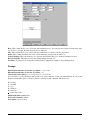
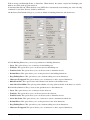
3 Under the Plot Settings Tab you specify paper size, orientation, plot area and scale, offset, and other options.
• Paper Size and Paper Units: This field displays standard paper sizes available for the selected plotting device.
Actual paper sizes are indicated by the width (X axis direction) and height (Y axis direction). If no plotter is selected,
the full standard paper size list is displayed and available for selection. A default paper size is set for the plotting
device when you create a PC3 file with the Add-a-Plotter wizard. The paper size you select is saved with a layout
and overrides the PC3 file settings. If you are plotting a raster image, such as a BMP or TIFF file, the size of the plot
is specified in pixels, not in inches or millimeters.
• Plot Device: This field displays the name of the currently selected plot device.
• Paper Size: This field displays a list of the available paper sizes.
• Printable Area: This field displays the actual area on the paper that is used for the plot based on the current
paper size.
• Inches: This option allows you to specify inches for the plotting units.
• MM: This option allows you to specify millimeters for the plotting units.
• Drawing Orientation: This option specifies the orientation of the drawing on the paper for plotters that support
landscape or portrait orientation. You can change the drawing orientation to achieve a 0-, 90-, 180-, or 270-degree
Chapter 2. File Commands
24
plot rotation by selecting Portrait, Landscape, or Plot Upside-Down. The paper icon represents the media orientation
of the selected paper. The letter icon represents the orientation of the drawing on the page.
• Portrait: This option orients and plots the drawing so that the short edge of the paper represents the top of the
page.
• Landscape: This option orients and plots the drawing so that the long edge of the paper represents the top of the
page.
• Plot Upside-Down: This option orients and plots the drawing upside down.
• Plot Area: This option specifies the portion of the drawing to be plotted.
• Layout: This option plots everything within the margins of the specified paper size, with the origin calculated
from 0,0 in the layout. Available only when a layout is selected. If you choose to turn off the paper image and layout
background on the Display tab of the Options dialog box, the Layouts selection becomes Limits.
• Limits: This option plots the entire drawing area defined by the drawing limits. If the current viewport does not
display a plan view, this option has the same effect as the Extents option. Available only when the Model tab is
selected.
• Extents: This option plots the portion of the current space of the drawing that contains objects. All geometry in
the current space is plotted. AgStar may regenerate the drawing to recalculate the extents before plotting.
• Display: This option plots the view in the current viewport in the selected Model tab or the current paper space
view in the layout.
• View: This option plots a previously saved view. You can select a named view from the list provided. If there are
no saved views in the drawing, this option is unavailable.
• Window: This option plots any portion of the drawing you specify. If you select Window, the Window button
becomes available. Choose the Window button to use the pointing device to specify the two corners of the area to
be plotted or enter coordinate values.
• Plot Scale: This option controls the plot area. The default scale setting is 1:1 when plotting a layout. The
default setting is Scaled to Fit when plotting a Model tab. When you select a standard scale, the scale is displayed
in Custom.
• Scale: This option defines the exact scale for the plot. The four most recently used standard scales are displayed
at the top of the list.
• Custom: This option creates a custom scale. You can create a custom scale by entering the number of inches or
millimeters equal to the number of drawing units.
• Scale Lineweights: This option scales lineweights in proportion to the plot scale. Lineweights normally specify
the linewidth of printed objects and are plotted with the linewidth size regardless of the plot scale.
• Plot Offset: This field specifies an offset of the plotting area from the lower-left corner of the paper. In a layout,
the lower-left corner of a specified plot area is positioned at the lower-left margin of the paper. You can offset the
origin by entering a positive or negative value. The plotter unit values are in inches or millimeters on the paper.
• Center the Plot: This option automatically calculates the X and Y offset values to center the plot on the paper.
• X: This field specifies the plot origin in the X direction.
• Y: This field specifies the plot origin in the Y direction.
• Plot Options: This field specifies options for lineweights, plot styles, and the current plot style table. You can
select whether lineweights are plotted. By selecting Plot with Plot Styles, you plot using the object plot styles that
are assigned to the geometry, as defined by the plot style table.
• Plot object lineweights: This option plots lineweights.
• Plot with Plot Styles: This option plots using the plot styles applied to objects and defined in the plot style
table. All style definitions with different property characteristics are stored in the plot style tables and can be easily
attached to the geometry. This setting can replace pen mapping in earlier versions of AutoCAD.
Chapter 2. File Commands
25
• Plot Paperspace Last: This option plots model space geometry first. Paper space geometry is usually plotted
before model space geometry.
• Hide Objects: This option plots layouts with hidden lines removed for objects in the layout environment (paper
space). Hidden line removal for model space objects in viewports is controlled by the Viewports Hide property in
the Object Property Manager. This is displayed in the plot preview, but not in the layout.
• Full Preview: This option displays the drawing as it will appear when plotted on paper. To exit the print preview,
right-click and choose Exit.
• Partial Preview: This option quickly shows an accurate representation of the effective plot area relative to the
paper size and printable area. Partial preview also gives advance notice of any warnings that you might encounter
when plotting. The final location of the plot depends on the plotter. Changes that modify the effective plot area
include those made to the plot origin, which you define under Plot Offset on the Plot Settings tab. If you offset the
origin so much that the effective area extends outside the preview area, the program displays a warning.
Menu Location: File
Prerequisite: None
Keyboard Command: PLOT
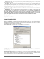
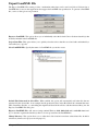
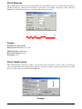
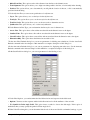
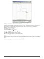
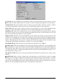
Import LandXML File
The Import LandXML File routine provides a mechanism where land-based data from other software applications
(including Carlson Software) can be brought into a project and used for analysis and/or design purposes. To import
a LandXML file, a series of dialog boxes are presented:
Select LandXML File: Specify the name of a LandXML file you wish to import.
LandXML Units: Indicates the Units of Measure associated with the incoming LandXML file (see the Unit Differences item below).
Point Protection: When enabled, you are prompted for a course of action if an existing LandXML file you've
selected contains COGO points that have the same number(s) as those that already exist in the drawing. When
disabled, existing point data in the project is updated with the values from the LandXML file.
Chapter 2. File Commands
26
Destination File Method: This option allows you to indicate how the incoming data file(s) are named as they are
imported.
Load Surfaces into Surface Manager: When enabled, this option will automatically add surface model (TIN) data
into the Surface Manager and graphically represents (draws) the surface model/contours according to the current
settings found in the Triangulate & Contour command.
Use Old FLT Triangulation File Format to Import Surface Data: When enabled, the older ASCII-based Carlson
*.FLT file format will be used in place of the newer and more efficient *.TIN file format.
Save All Existing Ground Profiles from One Centerline to the Same File: When enabled, collections of existing
ground profiles associated with a particular centerline are combined into a single *.PRO file.
Change Directory: This option allows you to adjust the folder location where the new data files will be written.
Import from LandXML: Enable or disable various entries that should used to produce the data files found within
the LandXML file.
Unit Differences: If the Units of Measure specified in the LandXML file are different than those found in Drawing
Setup, you will be prompted for a course of action.
Manning's ''n'': If you are importing sewer data from a LandXML file and if the LandXML file does not carry
Manning's ''n'' values, you will be prompted to specify a default Manning's ''n'' value for all incoming sewer entities
that don't already have a Mannings ''n'' value.
Import Structures: If you are importing sewer data from a LandXML file and structure values specified in the
LandXML file do not exist in the Structure Library, you will be prompted to indicate the structure(s) that should
be imported into the Structure Library. Use standard Windows click, shift+click and/or ctrl+click functionality to
Chapter 2. File Commands
27
select multiple structures at the same time.
Skip Invisible Triangles: This option applies to importing TIN surfaces from Civil 3D. When this option is active,
triangles marked by Civil 3D as invisible or excluded are not imported.
Note:
• The LandXML initiative is being driven by the land development industry as an acceptable means to share and
transfer land data rather than the traditional graphical representation of that data. It also provides an effective
means for transferring a variety data (points, centerlines, profiles, surface models, sewer data, etc). Another
advantage of LandXML is that the LandXML data structure is CAD and software vendor neutral (meaning
you don't have to own or use the CAD or software product used by your data provider).
• Visit http://www.landxml.org for additional information on the uses and acceptance of the LandXML initiative.
Pulldown Menu Location(s): File > Import
Keyboard Command: landxml import
Prerequisite: A LandXML file to import
Import Google Earth File
The Import Google Earth File command allows you to insert a KML (Keyhole Markup Language or alternatively
a KMZ) file of points (KML Placemark), polylines (KML Path) and closed polylines (KML Polygon) into your
drawing. Throughout this discussion, KML will be used to also describe KMZ files unless explicitly noted.
Import Lines and Polygons: When this option is selected, KML Path and Polygon entries will be placed into the
drawing as open or closed polylines, respectively.
Import Points: When this option is selected, KML Placemark entries will be placed into the drawing and active
coordinate file.
Point Protect: When enabled, existing points in the active coordinate file will not be over-written.
Use Folders as Layers: When enabled, KML Folder entries will be used to create layer names in CAD and the
supported KML options described above will be placed onto the layer that conforms the the Folder to which they
belong.
Default Layer: The supported KML options described above that are not contained in a KML folder will be placed
into the specified layer.
Note:
• Placemarks, paths or polygon entries that have an altitude value specified will be imported at the proper ''Z''
elevation in the CAD drawing.
• KML or KMZ files can be specified for the import process.
Prompts
Chapter 2. File Commands
28
Google Earth File to Read: Select a previously saved KML or KMZ file.
• To import a Google Earth image into your drawing, use the Place Google Earth Image command.
• To import a Google Earth terrain data into a Carlson TIN (surface model), use the Place Google Earth Image
command.
• To export content from your drawing to a KML file, use the Export Google Earth File command.
Pulldown Menu Location: File > Import
Keyboard Command: kmlread
Prerequisite: A KML or KMZ file with Placemark, Path and/or Polygon information, an active coordinate file with
an established projection zone through Drawing Setup.
Import/Export Topcon TIN File
The Export Topcon TIN File command writes a Topcon TIN file (.TN3) from a Carlson triangulation file (.TIN,
.FLT). The routine first prompts for the Carlson file and then the Topcon file.
The Import Topcon TIN File command creates a Carlson Tin file (.TIN, .FLT) from a Topcon triangulation file
(.TN3). The routine first prompts for the Topcon file and then the Carlson file.
The units (Feet or Meters) for the triangulation file are the current units set in Drawing Setup.
Pulldown Menu Location: File > Import/Export
Keyboard Command: topcon tin, tn3 to tin
Prerequisite: A triangulation file
Import/Export Trimble TTM File
These commands convert between Trimble TTM format triangulation files and Carlson format. First you select the
source file to read and then the destination file to write.
Pulldown Menu Location: File->Import/Export
Keyboard Command: ttm2tin, tin2ttm
Prerequisite: File to convert
Write Polyline File
This command creates a polyline file that contains the point data of the select polylines. The objects supported by
this tool include polylines, arcs and lines. Several different output formats are supported.
The Carlson format (.PLN) is a text file format that is used by some Carlson commands and by machine control
(Carlson Grade, Dozer 2000, GradeStar) for the plan view. Each polyline begins with a line of ''POLYLINE, Color
number, etc''. Then the points for the polyline are listed on separate lines in X,Y,Z format.
The DTM and Idan formats create linework files for the DTM and Idan programs.
The MicroStation format (.txt) can be imported into MicroStation. This format has the coordinates as space delimited
for each polyline point. There is an extra column with a 1 or 0 where 1 specifies the start of a new polyline.
The Moss format creates a INP file for the MX/MOSS Genio program.
The Peabody format is a company specific format for Peabody Energy.
The Topcon format creates a Topcon LN3 file.
The 12D format creates a file format compatible with the 12d modeling program.
Note:
Chapter 2. File Commands
29
• The former Google (KML) output option has been been moved to the dedicated Export Google Earth File
command.
Prompts
Polyline file format [<Carlson>/DTM/Idan/MicroStation/MOSS/Peabody/Topcon/12D]? Specify the desired
output option by specifying the CAPITALIZED option or press Enter for the <default> option.
Polyline File to Write dialog: Create a new file or Append to Existing. If the Carlson option was selected, the
following dialog then appears:
Use Polyline File for Grid File Utilities macro: When enabled, the option will write a polyline file that can be
used with Grid File Utilities for inclusion/exclusion perimeters.
Specify Exclusion/Warning Polylines: When enabled, this option applies to machine control for warning areas.
Specify WorkZone Polylines: When enabled, this option applies to machine control for working areas.
Reduce Polyline Vertices: When enabled, this option applies the Reduce Polyline Vertices to the polyline vertices
before writing the file..
Offset Cutoff: Indicate the allowable offset distance (essentially the middle ordinate distance of a 3-point arc) that
would allow the middle vertex between two other vertex locations to be removed.
Include Z coordinate in polyline file: When enabled, this option controls whether the elevation(s) (or ''Z'' value)
of the selected polyline vertices are written to the polyline file.
Decimals: Indicate the desired amount of precision for the coordinate values that should be written to the file.
Select polylines, lines and arcs to write.
FILter/<Select entities>: Pick the entities to process press Enter when complete.
Sample Polyline File:
POLYLINE,51,0,0.0,CONT|V-STRM-PIPE
5375168.9320,3932304.7050,0.0000
5375193.3310,3932211.6150,0.0000
POLYLINE,150,0,0.0,CONT|V-BRKL
5375026.8800,3932090.0480,962.8334
5375062.3960,3932105.7540,961.5399
5375075.5640,3932115.7940,961.1595
5375079.0150,3932128.0920,961.1532
5375081.6860,3932159.7840,961.6147
5375086.6920,3932195.6480,962.6206
etc.
Pulldown Menu Location: File > Export
Keyboard Command: polywrite
Prerequisite: Polylines in the drawing
Chapter 2. File Commands
30
Export LandXML File
The Export LandXML File routine provides a mechanism where data can be sent from Carlson Software into a
LandXML file for use in other applications that support the LandXML data specification. To generate a LandXML
file, a series of dialog boxes are presented:
Export to LandXML: This option allows you to individually select the desired Carlson Software data file(s) that
should be included in the LandXML file.
Project Data Files: This option allows you to quickly select the various data files associated with, and defined by a
Carlson Project (*.prj) file.
Select LandXML File: Specify the name of a LandXML file you wish to create.
Include Files Referenced in Select Files: When enabled, this option will automatically add other files that are
referenced by the selected file. As an example, the file produced by the Carlson Road Network command references
TINs, Centerlines, Profiles, etc, and adding the single Road Network file will also add the referenced file(s) into the
Export to LandXML File dialog box.
Export to LandXML File: Add, remove (using standard Windows click, shift+click and/or ctrl+click functionality) or otherwise organize the data file(s) that is to be incorporated into the LandXML file.
Change Directory: This option allows you to adjust the folder location from where selected data files should be
referenced (often used for project revision purposes).
Chapter 2. File Commands
31
Report: Create a report (suitable for file transmission or archival purposes) of the file(s) selected to be incorporated
into the LandXML file.
LandXML Units: Specify the desired Units of Measure that reflect the outgoing data.
Point Protection: When enabled, you are prompted for a course of action if an existing LandXML file you've
selected contains COGO points that have the same number(s) as those being selected for the LandXML file. When
disabled, point data you've selected for the LandXML file are automatically written to (or updated into) the existing
LandXML file.
Exported Element Protection: When enabled, you are prompted if existing data (such as a centerline) in a
LandXML file should be updated with data of the same name that you have selected for the LandXML file.
Precision: Set the desired level of precision for each of the various measurement categories.
Profiles:
There are two major different types of profiles in LandXML: ProfSurf and ProfAlign. ProfSurf is typically an
existing surface that is usually created using existing surface data. The data for this type of profile it is stored in
a series of station-elevation values as a representation of a PntList2D list. ProfAlign is for a design profile. The
data for this type of profile is stored in LandXML elements starting from the simplest one: PVI element, CircCurve
element, ParaCurve element, etc.
Carlson differentiates the two types mentioned above by using the profile type in the Carlson .pro file: Generic =
ProSurf, Road = ProAlign.
Note:
• The LandXML initiative is being driven by the land development industry as an acceptable means to share and
transfer land data rather than the traditional graphical representation of that data. It also provides an effective
means for transferring a variety data (points, centerlines, profiles, surface models, sewer data, etc). Another
Chapter 2. File Commands
32
advantage of LandXML is that the LandXML data structure is CAD and software vendor neutral (meaning
you don't have to own or use the CAD or software product used by your data provider).
• Visit http://www.landxml.org for additional information on the uses and acceptance of the LandXML initiative.
Pulldown Menu Location(s): File > Export
Keyboard Command: landxml export
Prerequisite: Carlson project data files to convert
Export Google Earth File
The Export Google Earth File allows you to produce a KML (Keyhole Markup Language or alternatively a KMZ)
file of Carlson points, lines, arcs and polylines for rendering in other mapping and GIS applications such as Google
Earth. Throughout this discussion, KML will be used to also describe KMZ files unless explicitly noted.
Drape on Google Terrain (2D): When this option is selected, entities written to the KML file will have an Altitude
setting of ''Clamped to ground.''
Use Elevations from the Drawing (3D): When this option is selected, entities written to the KML file will have an
Altitude setting of ''Absolute.''
Include Selected Points: When enabled, this option exports selected Carlson point information to the KML <Placemark><Point>...</Point></Placemark> tag structure.
Include Layer Information: When enabled, this option organizes exported information based on the layer of each
entity, with each CAD layer becoming a KML <Folder>...</Folder> entry with the color of the group taking the
general color of the CAD layer.
Shade Closed Regions: When enabled, all closed polyline regions (e.g. building pads, ponds, etc) will be fillshaded.
Export to KMZ Format: When enabled, the KML file is written to the more compact (zipped) KMZ version of the
standard KML file format.
Display Results in Google Earth: When enabled, the results of the KML are passed to and automatically opened
with Google Earth.
Note:
• When the Use Elevations from the Drawing (3D) option is selected, be aware that elevation values lower than
the Google Earth terrain may be obstructed in the Google Earth display.
• Attribute information (e.g. Number, Elevation, Description) of selected Carlson points are also written to the
KML and will display in the ''balloon'' when a point is picked in the Google Earth display or data hierarchy.
Chapter 2. File Commands
33
• When the Shade Closed Regions toggle is enabled, note that all closed polyline regions will become fill shaded
and may lead to undesired results for items such as closed contours.
• When prompted for the name of the KML/KMZ file to write, the appropriate KML or KMZ file extension
based on the Export to KMZ Format toggle will be added to the file if the file extension is not specified.
• Arcs and polylines with arcs are converted into chord segments that closely approximate the arc(s).
• Other entities not supported for direct export to a KML file (e.g. circles, 3DFaces, ellipses, splines, multilines,
regions and solids), can be first turned into polylines with the Entities to Polylines command. Text entities can
be converted to polylines through the use of the Text Explode To Polylines command.
• The graphical symbology of any/all items sent to the KML file can be manually modified via the Google Earth
interface.
Prompts
Select points, polylines, lines and arcs to write.
FILter/<Select entities>: Select the desired entities and press Enter when complete.
• To import a Google Earth image into your drawing, use the Place Google Earth Image command.
• To import a Google Earth terrain data into a Carlson TIN (surface model), use the Place Google Earth Image
command.
• To import KML content into your drawing, use the Import Google Earth File command.
Pulldown Menu Location: File > Export
Keyboard Command: kmlwrite
Prerequisite: Points, lines or polylines in the drawing with an established projection zone through Drawing Setup.
Exit
This command allows you to exit AgStar.
This option allows you to quit the program if there have been no changes since the drawing was last saved. If the
drawing has been modified, the program displays the Drawing Modification dialog box to prompt you to save or
discard the changes before quitting.
You can close a file that has been opened in read-only mode if you have made no modifications or if you are willing
to discard them. To save modifications to a read-only drawing, use the SAVEAS command under the File menu.
Menu Location: File
Prerequisite: None
Keyboard Command: QUIT
Chapter 2. File Commands
34
Edit Commands
3
35
Undo
This command allows you to reverse the effect of previously issued commands.
Menu Location: Edit
Prerequisite: None
Keyboard Command: U
Erase
This command allows you to remove objects from a drawing.
Menu Location: Edit
Prerequisite: None
Keyboard Command: ERASE, E
Delete Layer
This command erases all the entities on the specified layers and deletes the layers from the drawing.
1 In the Erase by Layer/Type dialog box, you can enter the name of the layer to be deleted, or you can specify a
layer to delete by picking an entity on that layer.
• Layers of entities to erase: This field displays the layer names to be erased. You also have the option of typing
layer names in this field.
• Select Layers from Screen: This option allows you to select entities on the layers you want deleted.
• Select Layers by Name: This option allows you to choose a layer name from the list of layers in the drawing.
2 Under Types of entities on matching layers to erase, you specify which types of entities to erase.
You can clear All and specify which entity types to include in the selection set. For instance, if you have both
linework and points on the same layer, and you want to erase only the linework, you can clear All and select Line
and Polyline.
Menu Location: Edit
Prerequisite: None
Keyboard Command: LDEL
Move
This command allows you to displace objects a specified distance in a specified direction.
Chapter 3. Edit Commands
36
Menu Location: Edit
Prerequisite: None
Keyboard Command: MOVE, M
Copy
This command copies all objects you select to the Clipboard. You can paste the contents of the Clipboard into a
document or drawing as an OLE object.
You can also use CTRL+C to run this command. If the cursor is in the drawing area, Carlson Survey copies the
selected objects to the Clipboard. If the cursor is on the command line or in the text window, the program copies the
selected text to the Clipboard.
Menu Location: Edit, Clipboard >
Prerequisite: None
Keyboard Command: COPYCLIP
Explode
This command allows you to break a compound object into its component objects.
Results differ depending on the type of compound object you're exploding. The following is a list of objects that can
be exploded and the results for each.
• All Explodable Objects: Produces object geometry that may look the same, but the color, linetype, and
lineweight of the object may change.
• Block: Removes one grouping level at a time. If a block contains a polyline or a nested block, exploding the
block exposes the polyline or nested block object, which must then be exploded to expose its individual objects.
Blocks with equal X, Y, and Z scales explode into their component objects. Blocks with unequal X, Y, and Z scales
(nonuniformly scaled blocks) might explode into unexpected objects.
When nonuniformly scaled blocks contain objects that cannot be exploded, they are collected into an anonymous
block (named with a ''*E'' prefix) and referenced with the nonuniform scaling. If all the objects in such a block
cannot be exploded, the selected block reference will not be exploded. Body, 3D Solid, and Region entities in a
nonuniformly scaled block cannot be exploded.
Exploding a block that contains attributes deletes the attribute values and redisplays the attribute definitions.
• 2D and Lightweight Polyline: Discards any associated width or tangent information.
• Wide Polyline: Places the resulting lines and arcs along the center of the polyline. Carlson Survey discards any
associated width or tangent information.
• 3D Polyline: Explodes into line segments. Any linetype assigned to the 3D polyline is applied to each resulting
line segment.
• Leaders: Explodes into lines, splines, solids (arrow heads), block inserts (arrow heads, annotation blocks),
Mtext, or tolerance objects, depending on the leader.
• Mtext: Explodes into text entities
• Multiline: Explodes into lines and arcs.
• 3D Solid: Explodes planar surfaces into regions. Nonplanar surfaces explode into bodies.
• Region: Explodes into lines, arcs, or splines.
• Body: Explodes into a single-surface body (nonplanar surfaces), regions, or curves.
• Polyface Mesh: Explodes one-vertex meshes into a point object. Two-vertex meshes explode into a line. Threevertex meshes explode into 3D faces.
Chapter 3. Edit Commands
37
• Circle Within a Nonuniformly Scaled Block: Explodes a circle within a nonuniformly scaled block into ellipses.
• Arc Within a Nonuniformly Scaled Block: Explodes an arc within a nonuniformly scaled block into elliptical
arcs.
Menu Location: Edit
Prerequisite: None
Keyboard Command: EXPLODE, X
Offset
This command creates a new object at a specified distance from an existing object or through a specified point.
Offset does not support 3D polylines. Use Offset 3D Polyline to offset these entities.
Prompts
1 Specify offset distance or [Through] <Through>: Press Enter
The Through option allows you to screen pick the location of the offset. You can also enter a value for the interval
of the offset.
2 Select object to offset or <exit>: select entity
3 Specify through point: pick point
Menu Location: Edit
Prerequisite: None
Keyboard Command: OFFSET
Trim
This command allows you to trim objects at a cutting edge defined by other objects.
Prompts
1 Select cutting edges ...
Select objects: pick entity
2 Select object to trim or shift-select to extend or [Project/Edge/Undo]: select entity to be trimmed
• Project: You can project the object to be trimmed in order to trim objects that do not intersect.
• Edge: You can project the trimming edge in order to trim objects that do not intersect.
• Undo: This option allows you to undo the above projections.
Menu Location: Edit
Prerequisite: None
Keyboard Command: TRIM, TR
Scale
This command allows you to enlarge or reduce selected objects equally in the X, Y, and Z directions.
Prompts
1 Select objects: pick entities
2 Specify base point: pick point on screen as reference
Chapter 3. Edit Commands
38
3 Specify scale factor or [Reference]: scale to desired size
Menu Location: Edit
Prerequisite: None
Keyboard Command: SC
Extend To Edge
This command allows you to extend an object to meet another object.
Prompts
1 Select boundary edges ...
Select objects: pick entity
2 Select object to extend or shift-select to trim or [Project/Edge/Undo]: pick entity
You have the option of trimming or projecting objects and edges.
Menu Location: Edit, Extend >
Prerequisite: None
Keyboard Command: EXTEND
Extend by Distance
This command extends a line or polyline, or creates a new line or polyline from an existing one, using a specified
distance. The new segment of the line or polyline is drawn from the current position in the direction indicated by
the current position arrowhead.
You start by selecting an existing line or polyline. Initially, the current position is the closest vertex to the location
where the line or polyline was selected. Extending from the endpoint of a polyline will add a new point to that
polyline, while extending from any other point will create a new polyline.
There are two modes of operation: draw mode (D) and move mode (M). When you are in draw mode, extending
will draw line or polyline segments. When you are in move mode, the current position arrowhead can be moved
without drawing segments. The orientation of the current position arrowhead can be changed with the Right, Left,
and Angle commands.
Here is a list of the Extend by Distance options:
Key Name Action
D
M
#
Draw mode
Move mode
Number
R
L
E
Right rotate
Left rotate
T#
Total distance
A#
Angle change
A
Chapter 3. Edit Commands
Extend to edge
Align
Actions draw or extend the line or
polyline
Actions only move the pointer
Distance to draw or extend
Rotates clockwise 90 degrees
Rotates counterclockwise 90 degrees
Extends to intersection with a selected
line or polyline
Sets current segment to specified distance
Rotates pointer by specified number
of degrees
Rotates pointer to align with segment
39
B
Bearing
S
Switch
N
Next
P
Previous
U
C
O
Help
Undo
Sets pointer direction by bearing in
format: Qdd.mmss with Q-quadrant,
d-degrees, m-minutes, s-seconds (e.g.
130.1005 is NE 30 degrees, 10 minutes, and 5 seconds)
Reverses pointer direction
Moves pointer to next point
Moves pointer to previous point
Undo the last Extend by Distance
command
Close
Closes the polyline
Open
Help
Opens the polyline
Displays this list
Prompts
1 Select line or pline to extend: select line or polyline
Pick the polyline near the place to extend
2 Enter or pick distance to draw (A,B,C,E,L,M,N,O,P,R,S,T,U,Help): T50
The line is extended to a total length of 50 units.
3 Enter or pick distance to draw (A,B,C,E,L,M,N,O,P,R,S,T,U,Help): R
The pointer is turned to the right.
4 Enter or pick distance to draw (A,B,C,E,L,M,N,O,P,R,S,T,U,Help): 75
A polyline is drawn to 75 units.
5 Enter or pick distance to draw (A,B,C,E,L,M,N,O,P,R,S,T,U,Help): B145.0000
The pointer is turned toward NE at a bearing of 45 degrees.
6 Enter or pick distance to draw (A,B,C,E,L,M,N,O,P,R,S,T,U,Help): 50
A polyline is drawn to 50 units.
7 Enter or pick distance to draw (A,B,C,E,L,M,N,O,P,R,S,T,U,Help): Press Enter
Press Enter to end the command.
Menu Location: Edit, Extend >
Prerequisite: An existing line or polyline with at least one segment from which to start.
Keyboard Command: EXTENDER
Break by Closed Polyline
This command will force a break where all lines and polylines cross the ''break'' polyline. In addition to breaking
lines and polylines, you can also put the segments to new layers based on whether the segments are inside or outside
the break polyline. Polylines with arc segments are not handled. To reconnect the broken lines and polylines, use
the Join Nearest command.
Prompts
1 Select the clip edge polyline: pick a closed polyline
Chapter 3. Edit Commands
40
2 Select the polylines and lines to be clipped.
Select Objects: pick the entities to break
3 Specify layer names for Inside segments (Yes/<No>)? Yes
4 Enter a layer name for the Inside segments <0>: Press Enter
5 Specify layer names for Outside segments (Yes/<No>)? Yes
6 Enter a layer name for the Outside segments <0>: Final
Menu Location: Edit, Break >
Prerequisite: A closed polyline
Keyboard Command: CLIPLINE
Break at Intersection
This command allows you to break a line, arc, or polyline at the intersection of another line, arc, or polyline. This
command is often used in conjunction with the Area by Lines & Arcs command because many times, to get the
correct area of a figure, you must break it from adjoining lines.
Prompts
1 Select Line, Arc, or Polyline to Break
Select object: select entity to break
2 [int on] Pick Intersection to break at: pick intersection point
Menu Location: Edit, Break >
Prerequisite: None
Keyboard Command: BREAKAT
Change Properties
This command allows you to change certain properties of existing objects.
1 In the Change Properties dialog box, you must choose the properties to modify.
• Color: This option allows you to change the color of the object.
• Layer: This option allows you to change the layer of the object.
• Linetype: This option allows you to change the linetype of the object.
• Linetype Scale: This option specifies the linetype scale factor for the new linetype.
• Thickness: This option specifies the distance to extrude the object above or below its elevation.
Chapter 3. Edit Commands
41
Note: The Properties command allows you to modify entity specific properties such as the radius of a circle or the
height of a text entity.
Menu Location: Edit, Change >
Prerequisite: None
Keyboard Command: DDCHPROP
Change Elevations
This command allows you to change the elevation of selected entities. You can move the entity to a specified
elevation from its current elevation (absolute) or you can specify a differential change to be added to or subtracted
from an entity's current elevation. If AgStar points are selected, their attribute text and Z axis (Elevation) coordinate
are changed. Elevation values are not changed in the current coordinate file. You must choose the command Update
CRD File from Drawing under Coordinate File Utilities on the Points menu to update the elevation values in the
current coordinate file.
Prompts
1 Ignore zero elevations (<Yes>/No)? Press Enter
If you answer No, then entities with elevation 0 will be changed.
2 [A]bsolute or [D]ifferential Change <A>: A
3 Elevation to change to <0.0>: 125
4 Select Entities for elevation change.
Select objects: pick entities from screen
5 Select objects: Press Enter
Menu Location: Edit, Change >
Prerequisite: an entity with elevation
Keyboard Command: CHGELEV
Rotate
This command changes the display angle of objects by rotating them. This command has a sub-menu consisting of
two items, as described below :
By Bearing
Function
This command allows the user to rotate the coordinate database of all or part of the drawing. To translate the
coordinate database, use the MOVE command.
Prompts
Select entities to rotate. Select objects: W
First corner: (pick point)
Other corner: (pick point)
Select objects: [Enter]
Base pivot point ?
Number/<Pick point>: N
By responding with N the program switches to point number input.
Pick point/<point number>: 2
Chapter 3. Edit Commands
42
The program then reads the coordinate value from the current CooRDinate file.
Reference Bearing point ?
Pick point/<point number>: P
By responding with P the program then switches back to screen picking mode.
Number/<Pick point:>: (pick point)
Reference Bearing N 44d31'1'' E
The program then displays the reference bearing defined by the two points selected.
Azimuth/<Bearing (Qdd.mmss)>: 245.3030
Enter an A to input an Azimuth or enter the bearing. The above response defines a bearing of South 45 degrees, 30
minutes, and 30 seconds East.
The program then changes the database to the new bearing.
If point objects are selected the program warns:
This command DOES NOT change the coordinates in the CooRDinate file!
Use CooRDinate File Utilities menu option F to update the file.
Standard Rotate
Function
This command allows the user to choose objects and then prompts for a base point. It then prompts the user to
choose whether to rotate by rotation angle (default) or by reference angle. As the mouse is moved around, the
rotated position of the object keeps changing, giving an idea
of its final position. The user can then click on a point to select the angle of rotation and thereby, the final
position of the object. The angle of rotation can be also be entered from the keyboard. The object is rotated
through that angle, relative to its current inclination to the coordinate axes. Whether the rotation is clockwise or
counter-clockwise can be set using the ''Units Control'' command under the ''Inq-Set'' pulldown menu. Alternatively,
the rotation can be achieved by reference angle. This is done by first choosing the ''Reference'' option after entering
the base point. The user then has to select the reference angle, whose orientation needs to be changed. The user
can either enter this at the keyboard or choose a line on the object by selecting two points on it. The user is then
prompted to choose the new angle, which can again be entered at the keyboard or selected by choosing two points
on an exisiting object. This option of rotating by reference is particularly useful when objects need to be aligned by
rotation.
Prompts
Select objects: pick an objects to be rotated (press <ENTER> after selecting required objects, to end selection)
Base point : pick base point
<Rotation Angle>/Reference : 40 (objects will be rotated by 40 units about the base point, the units and direction
depending on the settings in the Units Control dialog box.)
<Rotation Angle>/Reference : type ‘ref' to choose rotation by reference angle
Reference angle <E> : Choose the direction which is meant to be the reference angle. For example, if a line at
45o to the horizontal needs to be at 120o in the resultant figure, then, the reference angle needs to be chosen as 45o
. This can be done in two ways : typing 45o at the keyboard or choosing two points on the reference line which is
oriented in the required angle ( 45o in this case.)
New angle : Choose the direction that the reference angle previously chosen needs to be oriented. In the example
under consideration, the new angle will be 120o . Once again, it can be specified in two ways : from the keyboard
or by specifying two points on the drawing.
Chapter 3. Edit Commands
43
Edit Text
This command allows you to edit text and attribute labels.
1 Select Text to Edit: select the text
You can modify text in provided text field.
Menu Location: Edit, Text>
Prerequisite: Text
Keyboard Command: EDITXT
Text Style
This command allows the user to change the current text style to one of the available text styles. The font style can
be given any name by the user, following which the user is prompted to select the specific font file to be used and
the text orientation, inclination, height, width etc. If the ''?'' option is entered, the current text style and its details
are listed.
Pull-Down Menu Location: Edit
Prerequisite: None.
Text EnlargeReduce
This command allows you to scale text entities up or down in size. The command prompts for a scale multiplier and
a selection set of text objects. If you want to enlarge the text, enter a value greater than one. If you want to reduce
the text, enter a decimal fraction such as .5, which would reduce the text size by 50%. Use this command if you
set up your drawing for one plotting scale and then decide to change to a new plotting scale. The Change Text Size
command can alternatively be used to set the text size to a specific value.
Prompts
1 Scaling Multiplier: enter value
Select Text for Scaling.
2 Select objects: select the text
Menu Location: Edit, Text >
Prerequisite: Text
Keyboard Command: TXTENL
Join Nearest
This command joins lines or polylines together, and allows you to join lines that do not exactly meet. You specify
the maximum distance to join, along with other options, in the dialog box shown below. You can join many entities
at once.
Chapter 3. Edit Commands
44
1 You must specify the maximum separation distance parameter. Entities beyond this distance will not join.
2 Under Connection Method you must determine how entities are connected.
• Average Endpoints Together: This option averages together the endpoints of the two entities when joined.
• Directly Connect Endpoints: This option directly connects the endpoints of the two entities with a polyline.
• Fillet With Radius Zero: This option will perform a tight fillet on the two entities.
3 In the Join Nearest Options dialog box you can choose to join only lines with common elevations or layers.
• Convert lines into polylines: The option will automatically convert any lines in the selection set into polylines.
• Join only identical layers: This option will join entities on the same layer.
• Join only common elevations: This option will join entities with identical elevations.
Menu Location: Edit
Prerequisite: Lines or Polylines to be joined.
Keyboard Command: NEARJOIN
Offset 3D Polyline
This command allows you to offset a 3D polyline entity in both the horizontal and vertical directions. There are
five offset methods. The Interval method applies one horizontal and one vertical offset to all the vertices of the
polyline. The Constant method has a horizontal offset and sets the elevation of the polyline to one constant elevation. The Variable method allows you to specify each horizontal and vertical offset individually either by polyline
segment or for each point. The vertical offset can be specified by actual vertical distance, percent slope or slope ratio.
The surface method allows to offset/project a 3D polyline entity on to a surface (tin;flt;grd) based on cut and fill
outslope ratio.
The multiple method allows multiple offsets of a 3D polyline with separate layers. User can add, insert and delete
offsets rows and set individual layers. The option Progressive Offsets draws offsets progressively, i.e. successive
offsets uses last drawn offset as base.
Chapter 3. Edit Commands
45
Prompts
Enter the offset method [<Interval>/Constant/Variable/Surface/Multiple]: press Enter
Vertical/<Horizontal offset amount>: 15
Percent/Ratio/Vertical offset amount <0>: 10
Select a polyline to offset (Enter for none): select a 3D poly
Select side to offset: pick a point
Select a point on the graphics screen that is in the direction of the side of line to offset.
Select a polyline to offset (Enter for none): press Enter
Pulldown Menu Location: Edit > Polyline Utilities
Keyboard Command: offset3d
Prerequisite: polyline
Entities to Polylines
This command converts selected lines, arcs, circles, 3Dfaces, and solids into individual polylines. You may use Join
Nearest to convert adjoining lines and arcs into continuous polylines.
Prompts
1 Select lines, arcs, circles, 3Dfaces and solids to convert.
Select objects: pick entities
Menu Location: Edit, Polyline Utilities>
Prerequisite: Lines, arcs or other entities to convert.
Chapter 3. Edit Commands
46
Keyboard Command: TOPLINE
Reverse Polyline
This command reverses the order of the line and/or arc segments of a polyline. This can be used in conjunction
with the commands such as Station Polyline/Centerline or Profile from Surface Entities, since the polyline must be
plotted in the direction of increasing stations. If it is more convenient to draft a polyline in one direction you may
do so and then use the Reverse Polyline command to change its order. This command can also be used to reverse a
3D Polyline Breakline or a 3D Pad Template. Temporary arrows are drawn along the polyline to graphically show
the new polyline direction.
Prompts
1 Select the Polyline to Reverse: pick point on polyline
Menu Location: Edit, Polyline Utilities>
Prerequisite: A polyline
Keyboard Command: REVPLINE
Reduce Polyline Vertices
This command removes points from a polyline without significantly changing the polyline. The offset cutoff is the
maximum distance that the polyline can move when you remove a point. For example, in a polyline with three points
in a straight line, the middle point can be removed without changing the polyline.
Prompts
1 Enter the offset cutoff <0.1>: .5
2 Select polylines to reduce.
Select objects: pick polylines
Menu Location: Edit, Polyline Utilities>
Prerequisite: A polyline
Keyboard Command: REDUCE
Smooth Polyline
This command allows you to smooth selected polylines using a modified Bezier method. The resulting polyline
passes through all the original points, and only the segments between the original points are smoothed. The looping
factor controls the smoothing amount. A higher factor gives more looping.
Prompts
1 Enter the looping factor (1-10) <5>: 7
2 Enter the offset cutoff <0.05>: Press Enter
3 Select polylines to smooth.
Select objects: pick polylines
Menu Location: Edit, Polyline Utilities>
Prerequisite: A polyline
Keyboard Command: SMOOTHPL
Chapter 3. Edit Commands
47
Add Polyline Vertex
This command allows you to add points to a polyline. Select the polyline to modify, then pick or enter the coordinates
for the new point. The new point is inserted into the polyline at the nearest polyline segment. On a 3D polyline, the
elevation of the new vertex is calculated for you.
Prompts
1 Select polyline to add to: pick a polyline
2 Pick or enter point to add: pick a point
Menu Location: Edit, Polyline Utilities>
Prerequisite: A polyline
Keyboard Command: ADDPL
Close Polylines
This command allows you to close a selection set of open polylines.
Menu Location: Edit, Polyline Utilities>
Prerequisite: Open polyline(s).
Keyboard Command: CLOSEPL
Edit Polyline Vertex
This tool allows you to make changes in the coordinates of vertices on all polyline types. Upon execution you will
be asked to select a polyline to edit. Upon selection a temporary marker will be placed at all of the vertices of the
polyline, making them easy to distinguish. Then pick near the vertex you wish to edit, and the following dialog
appears.
At the top of the dialog it identifies the type of polyline, being 2D or 3D. In the case of 2D polylines it allows you
convert the polyine. You have the ability to type in new northing, easting or elevation values. You can also determine
the 3D coordinate position by using distances and slope to/from adjacent points. As you change the values in the
dialog, new values for derivatives are being calculated. For example if you change the horizontal distances, the
coordinates will change.
Prompts
Chapter 3. Edit Commands
48
1 Select polyline to edit: pick a 2D or 3D polyline
After you pick a polyline, the vertices are marked with a temporary X symbol
2 Pick point on polyline to edit: pick the vertex to edit
3 Dialog box is shown
4 Select polyline vertex to edit: press enter to quit or select another polyline
Menu Location: Edit, Polyline Utilities>
Prerequisite: A polyline
Keyboard Command: EDITPL
Open Polylines
This command allows you to open a selection set of closed polylines.
Menu Location: Edit, Polyline Utilities>
Prerequisite: Closed polyline(s).
Keyboard Command: OPENPL
Remove Polyline Arcs
This command allows you to replace arc segments in polylines with chords. Removing arcs is a prerequisite to some
commands that don't handle arcs, such as Break by Closed Polyline and Make 3D Grid file. This command can add
many vertices to the polyline.
Prompts
1 Select polylines to remove arcs from.
Select objects: pick polylines
2 Offset cutoff <0.5>: Press Enter
This specifies the maximum distance that any point on the arc will be allowed to shift.
Menu Location: Edit, Polyline Utilities>
Prerequisite: A polyline
Keyboard Command: RMARC
Remove Polyline Segment
This command allows you to remove a specified segment from a polyline. (A polyline segment is the section between
two vertices of the polyline.) There are two options for removing the segment. When you specify the Continuous
option, the two vertices of the removed segments are averaged together to keep the polyline continuous. When you
specify the Break option, the segment is left missing in the polyline, resulting in two separate polylines.
Prompts
1 Break polyline at removal or keep continuous [<Break>/Continuous]? C
2 Select polyline segment to remove: pick point on polyline segment
Menu Location: Edit, Polyline Utilities>
Prerequisite: A polyline
Keyboard Command: REMOVEPL
Chapter 3. Edit Commands
49
Remove Polyline Vertex
This command allows you to remove the selected vertex from a polyline.
Prompts
1 Select polyline vertex to remove: pick point on polyline
Select the vertex to remove
Menu Location: Edit, Polyline Utilities>
Prerequisite: A polyline
Keyboard Command: RMVERTEX
Image Clip
This command allows you to create new clipping boundaries for an image object.
Prompts
1 Select image to clip: select the edge of an image
2 Enter image clipping option [ON/OFF/Delete/New boundary] <New>: enter an option or Press Enter
The boundary you specify must be in a plane parallel to the image object.
• On: Turns on clipping and displays the image clipped to the previously defined boundary.
• Off: Turns off clipping and displays the entire image and frame. If you reclip the image while clipping is turned
off, the program automatically turns clipping back on. The program prompts you to delete the old boundary even
when clipping is turned off and the clipping boundary is not visible.
• Delete: Removes a predefined clipping boundary and redisplays the full original image.
• New Boundary: Specifies a new clipping boundary. The boundary can be rectangular or polygonal, and consists
only of straight line segments. When defining a clipping boundary, specify vertices within the image boundary.
Self-intersecting vertices are valid. Rectangular is the default option. If you use the pointing device to specify a
point at the Enter Clipping Type prompt, the program interprets the point as the first corner of a rectangle.
3 Enter clipping type [Polygonal/Rectangular] <Rectangular>: enter P or Press Enter
• Polygonal: Uses specified points to define a polygonal boundary.
Specify first point: Specify a point
Specify next point or [Undo]: specify a point or enter u
Specify next point or [Undo]: specify a point or enter u
Specify next point or [Close/Undo]: specify a point, or enter c or u
You must specify at least three points to define a polygon.
If the image already has a clipping boundary defined, AgStar displays the following prompt:
Delete old boundary? [No/Yes] <Yes>: enter N or Press Enter
If you choose Yes, the program redraws the entire image and the command continues; if you choose No, the command ends.
• Rectangular: Specifies a rectangular boundary by its opposite corners. AgStar always draws the rectangle
parallel to the edges of the image.
Specify first corner point: specify a point
Specify opposite corner point: specify a point
Chapter 3. Edit Commands
50
Menu Location: Edit, Image>
Prerequisite: None
Keyboard Command: IMAGECLIP
Image Frame
This command controls whether Carlson Survey displays the image frame or hides it from view.
Because you select an image by clicking its frame, setting the image frame to off prevents you from selecting an
image.
Prompts
1 Enter image frame setting [ON/OFF] <current>: enter an option or Press Enter
• On: Displays image frames so you can select images.
• Off: Hides image frames so you cannot select images.
Menu Location: Edit, Image>
Prerequisite: None
Keyboard Command: IMAGEFRAME
Image Adjust
This command controls the display of the brightness, contrast, and fade values of images.
The Image Adjust dialog box controls how the image is displayed by adjusting the brightness, contrast, and fade
settings of the selected image. Adjusting these values changes the display of the image but does not change the
image file itself.
• Brightness: Controls the brightness, and indirectly the contrast, of the image. Values range from 0 through 100.
The greater the value, the brighter the image and the more pixels that become white when you increase contrast.
Moving the slider to the left decreases the value; moving the slider to the right increases the value.
• Contrast: Controls the contrast, and indirectly the fading effect, of the image. Values range from 0 through 100.
The greater the value, the more each pixel is forced to its primary or secondary color. Moving the slider to the left
decreases the value; moving the slider to the right increases the value.
• Fade: Controls the fading effect of the image. Values range from 0 through 100. The greater the value, the
more the image blends with the current background color. A value of 100 blends the image completely into the
background. Changing the screen background color causes the image to fade to the new color. In plotting, the
background color for fade is white. Moving the slider to the left decreases the value; moving the slider to the right
increases the value.
Chapter 3. Edit Commands
51
• Image Preview: Displays a preview of the selected image. The preview image updates dynamically to reflect
changes to the brightness, contrast, and fade settings.
• Reset: Resets values for brightness, contrast, and fade to default settings (50, 50, and 0, respectively).
Menu Location: Edit, Image>
Prerequisite: None
Keyboard Command: IMAGEADJUST
Chapter 3. Edit Commands
52
View Commands
4
53
Zoom - Window
This commands zooms to display an area you specify by two opposite corners of a rectangular window.
Menu Location: View, Zoom>
Prerequisite: None
Keyboard Command: ZOOM, W
Zoom Previous
This command zooms to display a previous view. You can restore up to 10 previous views.
Menu Location: View, Zoom>
Prerequisite: None
Keyboard Command: ZOOM, P
Zoom Center
This command zooms to display a window you define by picking a center point and a magnification value or height.
A smaller value for the height increases the magnification. A larger value decreases the magnification.
Prompts
1 Specify center point: pick a point
2 Enter magnification or height <226.66>: enter a value
Menu Location: View, Zoom>
Prerequisite: None
Keyboard Command: ZOOM, C
Zoom Extents
This command zooms to display the drawing extents. You can use Zoom Extents transparently, but it always regenerates the drawing.
Menu Location: View, Zoom>
Prerequisite: None
Keyboard Command: ZOOM, E
Zoom IN
This command increases the zoom factor of the current viewport by a factor of 2.0.
Menu Location: View, Zoom>
Prerequisite: None
Keyboard Command: ZOOM, 2.0x
Zoom OUT
This command decreases the zoom factor of the current viewport by a factor of 0.5.
Menu Location: View, Zoom>
Prerequisite: None
Keyboard Command: ZOOM, 0.5x
Chapter 4. View Commands
54
Pan
This command moves the drawing display in the current viewport. The cursor changes to a hand cursor. By holding
down the pick button on the pointing device, you lock the cursor to its current location relative to the viewport
coordinate system. The drawing display is moved in the same direction as the cursor.
When you reach a logical extent (the edge of the drawing space), a bar is displayed on the hand cursor on the side
where the extent has been reached. Depending on whether the logical extent is at the top, bottom, or side of the
drawing, the bar is either horizontal (top or bottom) or vertical (left or right side).
When you release the pick button, panning stops. You can release the pick button, move the cursor to another
location in the drawing, and then press the pick button again to pan the display from that location.
To stop panning at any time, press Enter or ESC.
Menu Location: View
Prerequisite: None
Keyboard Command: P
3D Viewer Window
This command allows you to view the selected 3D faces, polylines, lines, and points in 3D using the OpenGL
graphics library for rendering, which gives it superior performance. This command gives you the ability to zoom in
and out, pan, rotate around the X, Y, or Z axis, and shade in user-positioned lighting. You also have the option to
export the view to a windows bitmap (.BMP) file. The window below is displayed after you select the entities to be
shown. To pan the display, click on the image and drag the pointer.
Chapter 4. View Commands
55
• Ignore Zero Elv: This option excludes entities on zero elevation from the display.
• Vert. Scale: Controls the vertical exaggeration of the 3D display.
• Light Position: This control represents the position of the sun in the sky looking from above. The position of
the sun in the center of the control means the sun is in a zenith, and a position near the edge of the circle means the
sun is near the horizon. To move the sun, simply drag it to new location or click there.
• Dynamic Zoom Mode: Allows you to zoom in and out by holding the left mouse button down and moving the
mouse up and down.
• Zoom In: This option incrementally zooms in to the view.
• Zoom Out: This option incrementally zooms out to the view.
• Pan Mode: Allows you to pan the display
• Shade Model: This option allows you to shade the surfaces of your view. The color of the shade depends on the
lighting of the surface, which you adjust using the Light Position control in the middle of the controls window. See
Light Position below.
• Export to BMP: This option creates a .BMP bitmap file from your current view.
• Rotation Mode: Allows you to rotate the view in the X or Y axis while the cursor is in the middle of the display.
Rotates on the Z axis when the cursor is near any edge of the display. The cursor will indicate the axis.
• Plan View: This option restores the X, Y, and Z axes back to zero.
• Set Acad View: This option allows you to send the current 3D view back to the AgStar screen when you exit the
3D Viewer window. You update the current CAD view to match the view that is displayed in the 3D viewer window.
• Z-Axis: This slider rotates the view on the Z axis. The range of these sliders is -180 to +180 degrees with middle
being 0, which is the default position when the viewer starts.
• Y-Axis: This slider rotates the view on the Y axis.
• X-Axis: This slider rotates the view on the X axis.
Menu Location: View
Prerequisite: Entities to display.
Keyboard Command: CUBE
Regen
This command regenerates the drawing and refreshes the current viewport.
Menu Location: View
Prerequisite: None
Keyboard Command: REGEN
Twist Screen Standard
This command allows you to ''twist'' the screen's orientation so that a direction other than North is toward the top of
the screen and the drawing. It does not do a coordinate rotation, and it leaves the database unchanged. The ROTATE
and MOVE commands in the Edit menu can be used to do a coordinate rotation and translation.
This command prompts you for the twist angle, then adjusts the screen and crosshairs to that angle. The twist angle
is always measured counterclockwise, with 0 degrees at the east/right.
Menu Location: View, Twist Screen>
Prerequisite: None
Keyboard Command: TWIST1
Chapter 4. View Commands
56
Twist Screen Line
This command is a variation of Twist Screen Standard. The command aligns a selected line to be parallel to the
east-west direction of your graphics screen.
Think of the line you select as a pointer or arrow that will be moved to point in the east direction of the screen.
Select the line closest to the line endpoint that you want to point in the horizontal or east direction of the screen.
Menu Location: View, Twist Screen>
Prerequisite: None
Keyboard Command: TWIST2
Twist Screen Surveyor
This command is another variation of Twist Screen Standard. You enter the angle/azimuth that you want to be
aligned parallel to the east-west direction of the graphics screen.
Menu Location: View, Twist Screen>
Prerequisite: None
Keyboard Command: TWIST3
Restore Due North
This command twists the screen to make due north vertical.
Menu Location: View, Twist Screen>
Prerequisite: None
Keyboard Command: TWIST4
Layer ID
This command reports the layer name of the selected entity.
Prompts
Pick entity to read layer: pick an entity
Layer: FINAL
Pick entity to read layer: Press Enter to end
Pull-Down Menu Location: View
Prerequisite: None.
Keyboard Command: layerid
Change Layer
This command allows you to change the layer of a group of entities you select. The layer name can be either typed
or read from an existing entity you select.
Prompts
1 Select entities to be changed.
Select objects: pick entities
2 Pick entity with new layer or press Enter to type name: pick another entity
The first selection is now assigned to the layer of the second selection.
Chapter 4. View Commands
57
Menu Location: View
Prerequisite: Entities to change.
Keyboard Command: LCHG
Freeze Layer
This command allows you to freeze layers assigned to the entities you select.
Menu Location: View
Prerequisite: None
Keyboard Command: LOFF
Isolate Layer
This command allows you to freeze all layers except the layers assigned to the entities you select. The program
prompts to see if you would like to retain the PNT layers, which keeps the point layers from freezing. These layers
include PNT, PNTMARK, PNTELEV, PNTDESC, and PNTELEV.
Prompts
1 Select objects on layers to isolate.
Select objects: pick entities
2 Retain POINT layers [Yes/<No>]? Press Enter
Menu Location: View
Prerequisite: None
Keyboard Command: ISOLATE
Restore Layer
This command thaws the layers frozen by the Isolate Layer command.
Menu Location: View
Prerequisite: You must have previously run the Isolate Layer command
Keyboard Command: RESTORE
Thaw Layer
This command allows you to thaw the layers frozen by the Freeze Layer command.
Menu Location: View
Prerequisite: None
Keyboard Command: LON
List
Displays database information for selected objects.
Carlson Survey lists the object type, object layer, and X,Y,Z position relative to the current user coordinate system
(UCS) and whether the object is in model space or paper space.
LIST reports color, linetype, and lineweight information if these items are not set to BYLAYER. The thickness of
an object is displayed if it is nonzero. Z coordinate information defines the elevation. If the extrusion direction
of the entry differs from the Z axis (0,0,1) of the current UCS, LIST also reports the extrusion direction in UCS
coordinates.
Chapter 4. View Commands
58
LIST reports additional information related to the specific object selected.
Menu Location: View
Prerequisite: None
Keyboard Command: LIST
Polyline Info
This command reports the length and elevation of the selected line or polyline.
Prompts
Pick Polyline or Line: pick a polyline
Polyline length: 145.43 Elevation: 100.0
Pull-Down Menu Location: View
Keyboard Command: polylen
Prerequisite: A polyline
Drawing Inspector
This command reports object properties to you as you move the cursor over an entity. You can simply move the
pointer over an entity and the selected property will be displayed either in a pop-up window next to the pointer
and/or on the status bar, depending on the selected option. Drawing Inspector is a transparent command that can
run while other commands are running. Once Drawing Inspector is started, it will stay active even while running
other commands until you turn it off. To turn off Drawing Inspector, run the command again to toggle it off by
pick Drawing Inspector from the Inquiry pull-down menu or from the toolbar or by typing the command name, or
right-click and choose Turn off Drawing Inspector. The options for this command are set in the menu that pops
up by clicking the right mouse button. The available properties are: Layer Name, Elevation, Azimuth-Distance,
Bearing-Distance, Point Data, Text Data, Curve Data, 3D Face Data, Polyline Data and Polyline Blips.
In the Drawing Inspector menu, you can choose one or more properties to display.
Display Layer Name: Allows you to display the layer name of the entity.
Display Entity Type: Allows you to display the type of the entity (ie. TEXT or POLYLINE).
Display Elevation: Allows you to display the elevation of the entity.
Chapter 4. View Commands
59
Display Azimuth-Distance: Allows you to display the azimuth and distance of a line.
Display Bearing-Distance: Allows you to display the bearing and distance of a line.
Display Point Data: Allows you to display the coordinate data of point.
Display Text Data: Allows you to display the attributes of text.
Display Curve Data: Allows you to display the radius, arc length, chord length and delta angle of a curve.
Display Polyline Data: Allows you to display the end point elevations, horizontal distance, slope distance and slope
ratios.
Display 3D Face Data: Allows you to display the Z elevations at the face corners.
Display Polyline Blips: Allows you to displays temporary blip plus marks at the vertice locations of polylines.
Display Polyline Direction: Allows you to displays temporary arrows to show the direction of polylines.
In the Drawing Inspector menu, you can also choose how the property information is reported.
Enable Highlighting: Allows you to highlight the object that the Drawing Inspector is reporting.
Enable Tag Display: Enables you to view the information next to the cursor on the screen.
Show Data On Status Bar: Enables you to view the information on the status bar, in the lower corner of the screen.
Use Default Cursor: When enabled, only the drawing cursor shows. When disabled, the mouse pointer is also
shown.
Report In High Precision: When enabled, displays 8 decimals on distance and 4 decimal seconds on angles.
Example of Drawing Inspector reporting
Bearing-Distance using the Tag Display
Pulldown Menu Location: View
Keyboard Command: inspector
Prerequisite: None
Chapter 4. View Commands
60
Draw Commands
5
61
Line
This command allows you to draw a line entity by picking points on the screen or by supplying the coordinate values
using the point number and associated coordinates stored in the current coordinate file. The Line command links the
line with the points when the line is drawn using point numbers if the Link Linework with Points option is turned
on. This option is set under General Settings in the Configure command in the Settings menu. With links active,
changing a point with a command like Move Points automatically updates the line. This command always draws 2D
lines with a zero elevation.
Prompts
1 Pick point or point numbers: 1-3
You may enter a single point number or a range of point numbers
2 Undo/Distance/<Pick point or point numbers>: 16
3 Undo/+/-/Close/Distance/<Pick point or point numbers>: 35
4 Undo/+/-/Close/Distance/<Pick point or point numbers>: +
The + or - activates an additional prompt option that allows you to plot line segments at a 90 degree deflection angle
from the last line.
5 Perpendicular Distance Right: 80
6 Undo/+/-/Close/Distance/<Pick point or point numbers>: The + or - activates an additional prompt option that allows you to plot line segments at a 90 degree deflection angle
from the last line.
7 Perpendicular Distance Left: 105.12
8 Undo/+/-/Close/Distance/<Pick point or point numbers>: D
The distance option allows you to input a distance for the next line segment. The position of the cursor determines
the angle.
9 Enter distance: 174.32
10Undo/+/-/Close/Distance/<Pick point or point numbers>: C
The close option draws a line segment back to the original starting point
Menu Location: Draw
Prerequisite: None
Keyboard Command: 2DLINE
2D Polyline
Function
This command draws a polyline entity. You can either provide point numbers from the current coordinate file or
pick points on the screen to define coordinates. A Polyline is a series of line and/or arc segments joined together in
one entity or object.
Prompts
1 Pick point or point numbers: pick point
2 Undo/Arc/Length/<Pick point or point numbers>: 3
3 Undo/+/-/Arc/Close/Length/<Pick point or point numbers>: +
The + or - activates an additional prompt option that allows you to plot line segments at a 90 degree deflection angle
from the last line. This is useful for plotting buildings. See also the Extend by Distance command on the Edit menu.
Chapter 5. Draw Commands
62
4 Perpendicular Distance Right: 50
5 Arc/Length/+/-/Close/Undo/<Pick To point or point number>: C
This closes the polyline and ends the command.
Menu Location: Draw
Prerequisite: None
Keyboard Command: 2DP
3D Polyline
Function
This command allows you to set a specified layer and plot a 3D polyline which can be used to define breaklines and
features to better define surface models. You can pick points from the graphics screen or use point numbers from
the current coordinate file. You can also specify a range of point numbers. For example, entering ''3-1,5,10'' would
draw 3D Line segments from point number 3 to 2 to 1 to 5 to 10.
You can choose to pick points from a surface model that is stored in a file, which can be either a grid (.GRD) file
or triangulation (.FLT) file. When a point is picked or a point number is entered, the program uses the northing and
easting of this point and calculates the elevation from the surface model.
When you create a 3D polyline by picking points from the screen, be careful not to miss a point resulting in a zero
elevation. This creates a 3D polyline that drops to zero at one point. As points are picked, Draw 3D Polyline reports
the coordinate so you can check that the correct elevation was used. If you miss a point and see a zero elevation,
you can type Undo at the next prompt.
Prompts
1 Layer Name for 3DPoly <BREAKLINE>: Press Enter
2 Prompt for elevations (.XY filter) (Yes/<No>)? Y
Using the .XY filter allows you to pick the X and Y coordinate from the screen and type in the elevation. If you
enter N, then the Z coordinate of the point picked will be applied.
3 Use surface model from file (Yes/<No>)? No
If you choose Yes, then when a point is picked the elevation of the picked point is calculated using a surface model.
The surface model can be either a grid (.GRD) file or triangulation (.FLT) file.
4 Undo/<Pick point or point numbers>: pick point
5 Elevation <0.0>: 99.5
6 Undo/<Pick point or point numbers>: 15
This is a point number from the current coordinate file.
7 Undo/<Pick point or point numbers>: pick point
8 Percent slope/Ratio slope/Elevation <99.5>: P for Percent slope.
9 Ratio slope/Elevation/Percent slope <-2.53>: -2
Sets the elevation of this point to make a 2 percent slope from the previous point.
10Undo/Close/<Pick point or point numbers>: Press Enter
Pressing Enter ends the command.
11Draw another 3D polyline [Yes/<No>]? N
Menu Location: Draw
Chapter 5. Draw Commands
63
Prerequisite: None
Keyboard Command: 3DPLINE
Circle
This command allows you to draw a circle.
Prompts
1 Pick center point or point number or [3P/2P/TTR]: pick point or specify option
• 3P: This option draws a circle based on three points on the circumference.
• 2P: This option draws a circle based on two endpoints of the diameter.
• TTR-Tangent, Tangent, Radius: This option draws a circle with a specified radius tangent to two objects.
2 Specify radius of circle or [Diameter]: enter a value
Sometimes more than one circle matches the criteria specified in the command. The circle whose tangent points are
closest to the selected points is drawn.
Menu Location: Draw
Prerequisite: None
Keyboard Command: SCIRCLE
Insert
This command allows you to place a named block or drawing into the current drawing.
1 In the Insert dialog box, you specify the block to insert and define the position for the inserted block. The last
block you insert during the current editing session becomes the default block for subsequent uses of this command.
• Name: This field specifies the name of a block to insert or the name of a file to insert as a block.
• Browse: This button opens the Select Drawing File dialog box (a standard file selection dialog box) where you
can select a block or a file to insert.
2 Under Insertion Point, you specify the insertion point for the block.
• Specify On-Screen: This option specifies the insertion point of the block using the pointing device.
• X: This field sets the X coordinate value.
• Y: This field sets the Y coordinate value.
Chapter 5. Draw Commands
64
• Z: This field sets the Z coordinate value.
3 Under Scale, you specify the scale for the inserted block. Specifying negative values for the X, Y, and Z scale
factors inserts a mirror image of a block.
• Specify On-Screen: This option specifies the insertion point of the block using the pointing device.
• X: This field sets the X coordinate value.
• Y: This field sets the Y coordinate value.
• Z: This field sets the Z coordinate value.
• Uniform Scale: This option specifies a single scale value for X, Y, and Z coordinates. A value specified for X is
also reflected in the Y and Z values.
4 Under Rotation, you specify the rotation angle for the inserted block.
• Specify On-Screen: This option specifies the rotation angle of the block using the pointing device.
• Angle: This field sets a rotation angle for the inserted block.
5 You can explode the block and inserts to the individual parts of the block. When you select Explode, you specify
only an X scale factor.
Menu Location: Draw
Prerequisite: None
Keyboard Command: DDINSERT
Text
Creates a single-line text object.
You can use the TEXT to enter several lines of text that you can rotate, justify, and resize. As you type at the Enter
Text prompt, the text you are typing is displayed on the screen. Each line of text is a separate object. To end a line
and begin another, press Enter after entering characters at the Enter Text prompt. To end the TEXT command, press
Enter without entering any characters at the Enter Text prompt.
By applying a style to the text, you can use a variety of character patterns or fonts that you can stretch, compress,
make oblique, mirror, or align in a vertical column.
If TEXT was the last command entered, pressing ENTER at the Specify Start Point of Text prompt skips the prompts
for height and rotation angle and immediately displays the Enter Text prompt. The text is placed directly beneath
the previous line of text. The point specified at the prompt is also stored as the Insertion Point object snap.
Prompts
1 Current text style: ''MONO'' Text height: 4.00
2 Specify start point of text or [Justify/Style]: S
The style option lets you change the textstyle on the fly
3 Enter style name or [?] <MONO>: STANDARD
4 Current text style: ''STANDARD'' Text height: 4.00
5 Specify start point of text or [Justify/Style]: J
The justify option lets you specify the justification for the text.
6 Enter an option [Align/Fit/Center/Middle/Right/TL/TC/TR/ML/MC/MR/BL/BC/BR]: BC
In this case BC = Bottom Center
7 Specify bottom-center point of text: pick point or enter coordinates
8 Specify height <4.00>: press enter to select default or enter text height
Chapter 5. Draw Commands
65
9 Specify rotation angle of text <0d0'0''>: press enter to select default or enter angle
10Enter text: Found Iron Pin
11Enter text: press enter to end
Menu Location: Draw
Prerequisite: None
Keyboard Command: DTEXT, TEXT
Insert Symbols
This command inserts symbols from the symbol library into the drawing. The symbol library may be edited using
the Edit Symbol Library command. The locations for the symbols can be specified by picking points, specifying
point numbers in the current coordinate (.CRD) file or by entering the northing and easting. If you specify a point
number and that point number already has a symbol on it, you will be prompted whether or not to replace the
existing symbol. Selecting the Enter coords option allows you to insert the symbol by entering a northing and
easting. Using the Select entities option, symbols can also be placed on arcs, points, lines or polylines. Under the
Options command, you can turn prompting for rotation on or off. With rotation off, the symbol will be inserted
horizontal to the current twist screen.
Choose a symbol from the Select Symbol dialog by clicking on it. You may select a different category by choosing
the Symbol Category drop down list. Within each category, use the scroll bar to view all of the symbols.
Prompts
1 Options/Select entities/Enter coords/<Point numbers or pick point>: pick point
2 Options/Select entities/Enter coords/<Point numbers or pick point>: 5-10
3 Options/Select entities/Enter coords/<Point numbers or pick point>: Press Enter
Menu Location: Draw
Prerequisite: None
Keyboard Command: PTSYM
Chapter 5. Draw Commands
66
Shrink-Wrap Entities
This command creates a closed polyline which encloses a given set of entities. The resulting polyline is created in
the current layer. The program works on either point entities or polylines. For points, the program creates a closed
polyline through the points around the perimeter of the area defined by the points. For polylines, the shrink-wrap
polyline follows the outside border of the selected polylines. The polylines that are processed have to be connected
to be shrink-wrapped. The snap tolerance is the maximum gap that will be joined to make the closed polyline. For
open polylines, as in the bottom figure, the Gap method works better, as it jumps across the gaps and connects the
end points.
Prompts
Shrink-wrap across gaps or bounded linework only [<Gap>/Bound]? G
Shrink-wrap layer <FINAL>:
Select points and linework to shrink-wrap.
Select objects: select entities to process
Reading points... 46
Inserted 46 points.
Inserted 23 breakline segments
Perimeter reduction level 0-3 (0-None, 3-Most) <2>: 2
Reduce Perimeter Pass: 1 Removed: 5
Reduce Perimeter Pass: 2 Removed: 3
Reduce Perimeter Pass: 3 Removed: 4
Reduce Perimeter Pass: 4 Removed: 2
Reduce Perimeter Pass: 5 Removed: 1
Reduce Perimeter Pass: 6 Removed: 0
Create 2D or 3D Polyline [<2D>/3D]? 2D
Pulldown Menu Location: Draw
Keyboard Command: swplines
Prerequisite: Entities
Chapter 5. Draw Commands
67
3 Point Curve
This command draws an arc between three points. The first point is the PC, the second is a point on the arc, and the
third is the PT. The points can either be picked on-screen or specified by point number.
Prompts
1 Pick PC point or point numbers: 101
2 Pick Second point or point number: 102
3 Pick PT point or point number: 103
Menu Location: Draw, Curves >
Prerequisite: None
Keyboard Command: 3PA
PC PT Radius Point
This command draws an arc between the PC point, radius point, and PT point. The points can either be picked
on-screen or specified by point number. Given these points, the arc can be drawn clockwise or counterclockwise.
The program shows one direction and asks if it is correct. If you want the arc to go in the other direction, enter No.
Prompts
1 Pick PC point or point number: 101
2 Pick Radius point or point number: 102
3 Pick PT point or point number: 103
4 Is the direction of this arc correct ? No/<Yes>: N
The arc draws in the other direction.
Menu Location: Draw, Curves >
Prerequisite: None
Keyboard Command: PCA
PC Radius Chord
This command draws an arc given the PC point, radius length, chord length, and chord bearing. The PC point can
either be picked on-screen or specified by point number. Given these points, the arc can be drawn clockwise or
counterclockwise. The program shows one direction and asks if it is correct. If you want the arc to go in the other
direction, enter No.
Prompts
1 Radius of Arc <-40.00>: 500
2 PC Start Point ?
Pick point or point number: pick a point
3 Chord bearing or chord endpoint (<Bearing>/Point)? Press Enter
4 Enter Bearing (Qdd.mmss) <90.0000>: 145.1041 (for NE 45°10'41'')
5 Chord Length <200.46>: 200
Chapter 5. Draw Commands
68
6 Is this arc in the correct direction (<Yes>/No)? Press Enter
Menu Location: Draw, Curves >
Prerequisite: None
Keyboard Command: SRCB
Raster Image
This command allows you to manage raster images.
1 The Image Manager dialog box lists all the image files attached to the current drawing. You can view the parameters and details for selected images. You can attach new image files and detach, locate, reload, and unload existing
images.
• List View: This button lists the image definitions attached to the drawing. Each image name appears only once
regardless of how many times you attach (insert) the image. You can sort the list of images by name, status (loaded,
unloaded, or not found), size, type (TIFF, for example), date, or the saved path and file name. By default, Carlson
Survey displays the list alphabetically by image name.
To select multiple images, hold down SHIFT or CTRL while selecting items.
To sort the list alphabetically or numerically by a specific column, click that column's heading.
To change the width of the column, drag the line between the column headings to the right or left. The program
saves and restores the settings when you reopen the dialog box.
To change an image name, select it and then click it again, or select it and then press F2. You cannot edit names
of images that reside in external references (xrefs). Image names can include up to 255 characters and can contain
letters, digits, spaces, and any special characters not used by Microsoft® Windows® or Carlson Survey. The image
name can be identical to the file name, but changing the image name does not change the file name.
• Tree View: This button displays all the image definitions and the levels of nesting of images within xrefs. The top
level of the tree view shows images that you attached directly to the drawing, images nested in block references, and
the names of externally referenced drawings containing images. The names of the images attached to the externally
referenced drawings appear nested within the drawing at the next tree level. To insert a copy of an already attached
image, select it, and then choose Attach.
Tree view lists the image names only (not file names) and lists the image name just once, regardless of how many
times you attach (insert) the image.
You can edit an image name by selecting it and then clicking it again, or by selecting it and then pressing F2.
However, you cannot select more than one image at a time.
Chapter 5. Draw Commands
69
• Attach: This option displays the Select Image File dialog box. When you unload and then reload an image, the
program draws that image on top. Images remain loaded or unloaded from one drawing session to the next.
• Detach: This option removes the selected image definitions from the drawing database and erases all the associated image objects from the drawing and from the display.
• Reload: This option loads the most recent version of an image or reloads an image that was previously unloaded.
Reloading does not control whether the image is displayed, but it ensures display of the most current image.
• Unload: This option unloads image data from working memory without erasing the image objects from the
drawing. It is recommended that you unload images no longer needed for editing to improve performance. An
unloaded image cannot be displayed or plotted. You can selectively load and unload individual images from a
working list of images associated with the drawing file.
• Details: This option opens the Image File Details dialog box, which displays the image name, saved path, active
path, file creation date and time, file size and type, color system, color depth, width and height in pixels, resolution,
default size in units, and a preview image.
• Image Found At: This field shows the path of the selected image. If you select multiple images, this field
remains blank. The path shown is the actual path where the image resides.
• Browse: This option opens the Select Image File dialog box (a standard file selection dialog box). The path you
select appears under Image Found At.
• Save Path: This option stores the new path information. Press ESC while editing the path to restore the old path.
If the program cannot find the referenced image in the new path, the image's status changes to Not Found. If you
do not choose Save Path after editing the path, the program uses the original image path the next time you load the
drawing.
2 Under the Image dialog box, you can attach an image.
3 In the Image dialog box, you must first identify the image and the path.
• Name: This field identifies the image you have selected to attach, either from the Select Image File dialog box
(an unattached image) or from the list of previously attached images. To add another instance of an image file that
is already attached, select the image name from the list and choose OK.
• Browse: This option opens the Select Image File dialog box (a standard file selection dialog box). If Show
Preview is selected, the program displays a preview of the selected file.
• Retain Path: This option saves the path of the image file with the image definition. If Retain Path is not selected,
only the image name is saved and AgStar searches the Support File Search Path.
4 Under Insertion Point, you must specify the insertion point for the selected image. Specify On-Screen is the
default. The default insertion point is 0,0.
Chapter 5. Draw Commands
70
• Specify On-Screen: This option directs input to the command line or the pointing device. If Specify On-Screen
is cleared, enter the insertion point in X, Y, and Z.
• X: This field sets the X coordinate value.
• Y: This field sets the Y coordinate value.
• Z: This field sets the Z coordinate value.
5 Under Scale, you must specify the scale factor of the selected image. Specify On-Screen directs input to the
command line or the pointing device. If Specify On-Screen is cleared, enter a value for the scale factor. The default
scale factor is 1.
6 Under Rotation, you must specify the rotation angle of the selected image. If Specify On-Screen is selected, you
may wait until you exit the dialog box to rotate the object with your pointing device or enter a rotation angle value
on the command line. If Specify On-Screen is cleared, enter the rotation angle value in the dialog box. The default
rotation angle is 0.
Menu Location: Draw
Prerequisite: Raster image
Keyboard Command: IMAGE
Place Image by World File
This function allows you to insert Geo-Referenced image files into AutoCAD drawings. This process requires the
presence of an accompanying World file. The TFW file contains information about the location and scaling of the
actual raster image TIF file. This eliminates the guesswork in inserting, moving, and rotating raster images to the
project area. You begin by selecting the TFW or JGW file to process. If the related TIF file is present in the same
directory, the image will be inserted into the proper coordinates.
Prompts
Select World File: choose existing .TFW or .JGW file
Pulldown Menu Location: Draw > Images
Keyboard Command: geotiff
Prerequisite: A georeferenced image file
Place Google Earth Image
In addition to providing a graphical method for displaying feature-rich data located anywhere on the globe, Google
Earth also provides the ability for software applications to extract its aerial imagery. While the positional accuracy
of the Google Earth surface should be considered ''approximate,'' it might be suitable for preliminary land-planning
studies or ''proof-of-concept'' preliminary designs.
Consider the following example. Based on the physical screen size of the Google Earth application and the ''zoom''
(or ''view'') resolution of a project site, the following values (summarized at the bottom of the dialog box) were
returned:
Chapter 5. Draw Commands
71
Unit
Feet
Pixels
Feet/Pixel
1637
1366
1.19
Horizontal
966
809
1.19
Vertical
Google Earth View Area
In the sample above, the total area is calculated and displayed (0.1 mi2 ) along with the desired ''spatial reference''
coordinate system for our project site.
Spatial Reference: Displays the spatial reference coordinate projection system of the current drawing. The projection can be set using the Drawing Setup command.
Extent - Current Google Earth View: Gets the overall dimensions of the Google Earth session and displays the
results in both pixels and the appropriate units of measure.
Extent - Current Drawing View: Gets the overall dimensions of the current CAD view and displays the results in
both pixels and the appropriate units of measure.
Extent - Select from Drawing: Sets the overall dimensions of the Google Earth session to conform with a drawing
window from CAD and displays the results in both pixels and the appropriate units of measure.
Image Type: Allows the ability to indicate the type of image to be placed into the drawing. Gray-scale images
can be inserted into the drawing automatically, color drawings must be manually saved from Google Earth and then
selected for insertion in the CAD drawing (see the Prompts section below).
Image Layer: Allows the ability to indicate the layer upon which the image should be inserted.
Note:
• Once an image has been inserted into the CAD drawing, it may be helpful to create an associated ''world'' file
for the image in case it needs to be re-inserted into the active drawing (or an alternate drawing). Creating a
''world'' file assists with this task. To generate a world file, please reference the Create by Image in Drawing
command.
• Once the image has been inserted into the CAD drawing, it may be helpful to control its ''display order'' by
using the View > Display Order > Order by Layer command or View > Display Order > Send to Back
command.
• The Place Google Earth Image routine fetches aerial imagery in real-time from the Google servers and requires
an Internet connection to proceed. In the event that an Internet connection is not available, the following error
message may be displayed: ''Failed to initialize Google Earth. Please ensure Google Earth client software is
functional and online''
Chapter 5. Draw Commands
72
• It bears repeating that the aerial imagery returned by Google Earth should only be used for illustrative or
proof-of-concept purposes only!
Prompts
First corner/Identify Entity <Current view>: Identify one corner of a drawing window that should be used to
set the Google Earth display or pick an existing entity with discreet upper and lower bounds to define a region or
press Enter to use the current view (this is the same as the ''Extent - Current Drawing View'' option above).
Specify opposite corner: Identify the opposite corner of a drawing window that should be used to set the Google
Earth display.
For Color images: Use Windows functionality (Alt+Tab) to switch focus to the Google Earth application and use
the Google Earth > File > Save > Save Image command (Ctrl+Alt+S) to save the current Google Earth image.
Once saved,
Click OK on the Carlson alert dialog box shown above and locate/select the image just saved. Click Open when the
file has been located
Pulldown Menu Location: Draw > Images
Keyboard Command: google image
Prerequisite: Coordinate projection system, Functioning version of Google Earth, Internet connection
Custom Linework Label Formatter
This command allows you to customize the labeling for lines and polylines. You are first prompted to select a line
or polyline to label, given the existing defaults currently set. The linework is shown as labeled on the screen. The
command line, shown below, also offers you an important choice called Options. When you type 'O' for options the
below dialog box appears. In this dialog, there are three columns at the top of the dialog, along with other features.
On the command line, there is also a choice called Format (F), which allows you to enter quick-key style keywords
for quickly changing the label format. See below for these
Chapter 5. Draw Commands
73
Row: This column allows you to stack the data in different ways. You can place more than one item in the same
row. If None is selected, then that item will not be displayed.
Side: This column allows you to place each item either inside or outside of the line or polyline.
Order: This column determines the order of items when they are placed in the same row.
General Settings: This button brings you to the Annotate Defaults dialog, see 'Annotate Defaults' for more.
Reset To Defaults: This button restores the default settings shown above.
Load/Save: You may also Load and Save different label configurations with the corresponding buttons.
Prompts
Options/Format/Points/<Select line or polyline>: select entity
Options/Format/Points/<Select line or polyline>: O
Custom Line Label dialog choose your preferences and click OK
You can decide to go into the Option dialog at the start of the command, or after your initial labeling. If you use the
Format command line option, you will be asked to enter the Format command. The choices are:
B = bearing
A = azimuth
G = gon
D = distance
R = next row
= switch side of line
Pulldown Menu Location: Draw
Keyboard Command: annline
Prerequisite: An arc to label
Chapter 5. Draw Commands
74
Draw Barscale
This command draws a barscale at the user-specified scale. The command options are set in the dialog shown here.
The Horizontal Scale controls the size and labels for the barscale. For example, enter 50 for 1 inch = 50 feet in
English mode. The Barscale Style chooses between different barscale formats.
Prompts
Draw Barscale options dialog
Pick location for barscale: pick a point
Pulldown Menu Location: Draw
Keyboard Command: barscale
Prerequisite: None
Draw North Arrow
This command inserts a north arrow symbol. You can select from several styles of arrows, and you can add your
own by using the Edit Library button which is similar to the Symbols Library command. The north arrow symbol
library is stored in the narrow.dta file in the USER folder.
Prompts
Chapter 5. Draw Commands
75
Draw North Arrow Dialog choose an arrow symbol, layer and other variables
Specify insertion point: pick a point
X scale factor <1> / Corner / XYZ: press Enter
Y scale factor (default=X): press Enter
Rotation angle <0d0'0''>: press Enter
Pulldown Menu Location: Draw
Keyboard Command: narrow
Prerequisite: None
Chapter 5. Draw Commands
76
Settings Commands
6
77
Drawing Setup
Function
This command displays a dialog box for setting drawing parameters, including the plotting scale, size of symbols,
label annotation size, and the drawing mode.
1 Under Scale and Size Settings you can determine scale and size of drawing entities.
• English 1in=?ft: This option tells Carlson Survey which unit mode to use. This affects the prompting and
reports. When you are working on a drawing in English units, one unit equals one foot. In metric, one unit equals
one meter.
• Metric 1m=?m: This option sets the metric scale to meters only.
• Horizontal Scale: This option allows you to set the horizontal scale of the drawing. For example, if the horizontal
scale is set to 50, then 1'' = 50' in your drawing.
• Symbol Plot Size: This value is a scaler that represents the size on the plot. The Drawing Units are determined
by multiplying the scaler by the horizontal scale. In English mode the scaler represents the plotted size in inches. In
Metric mode, this value is the plotted size in centimeters. The Symbol Plot Size is not entered in Drawing Units.
• Drawing Units: This field shows the result of the Symbol Plot Size value (the scaler) multiplied by the horizontal
scale.
• Text Plot Size: This value is a scaler that represents the size on the plot. The Drawing Units are determined by
multiplying the scaler by the horizontal scale. In English mode the scaler represents the plotted size in inches. In
Metric mode, this value is the plotted size in centimeters. The Text Plot Size is not entered in Drawing Units.
• Drawing Units: This field shows the result of the Text Plot Size value (the scaler) multiplied by the horizontal
scale.
• Line Type Scaler: This option sets the linetype scale by multiplying this scaler by the horizontal scale.
2 Under Angle Mode you determine how angles are entered and displayed.
• Bearing: This option sets reporting to bearing mode for any of the inquiry commands.
• Azimuth: This option sets reporting to north based azimuth mode for any of the inquiry commands.
• Gon: This option sets reporting to gon mode for any of the inquiry commands.
3 The Set Paper button allows you to draw a rectangle on the screen that represents the edge of your paper. After
you have set the horizontal scale, press the Set Paper button and the following dialog box appears
Chapter 6. Settings Commands
78
.
• Layout: This option lets you specify landscape or portrait paper orientation. Landscape layout is where the width
of the page is greater than the height of the page. Portrait layout is the opposite.
• Paper Size: This option allows you to specify the paper size. The numbers in parenthesis represent drawing units
and will be multiplied by the horizontal scale to determine the rectangle to be drawn. If you select the Other option,
you will be prompted on the command line for the horizontal and vertical sizes of the paper.
Prompts
1 Pick or Type lower left corner point for border <(5000.00 5000.00 0.0)>: pick point
2 Erase existing Set Paper boundary [<Yes>/No]? Y
This prompt only appears if there is an existing paper boundary in this drawing
3 Set Limits [Yes/<No>]? Y
If you answer Yes to Set Limits, drawing limits are enabled, and AgStar restricts the coordinates you can enter to
within the paper boundary. Drawing limits also determines the area of the drawing that can display grid dots, and the
minimum area displayed by the Zoom All command on the View menu. To turn drawing limits off, type in LIMITS
on the command line and set to Off.
Menu Location: Settings
Prerequisite: None
Keyboard Command: SETUP
Units Control
Function
The Drawing Units dialog box controls coordinate and angle display formats and determines precision.
Chapter 6. Settings Commands
79
1 Under Length, you specify the current unit of measurement and the precision for the current units.
• Type: This field sets the current format for units of measure. The values include Architectural, Decimal, Engineering, Fractional, and Scientific. The Engineering and Architectural formats produce feet-and-inches displays and
assume that each drawing unit represents one inch. The other formats can represent any real-world unit.
• Precision: This field sets the number of decimal places for the current units display.
2 Under Angle you specify the current angle format and the precision for the current angle display.
• Type: This field sets the current angle format.
• Precision: This field sets the precision for the current angle display.
Carlson Survey uses the following conventions for the various angle measures: decimal degrees appear as decimal numbers, grads appear with a lowercase g suffix, and radians appear with a lowercase r suffix. The degrees/minutes/seconds format uses d for degrees, ' for minutes, and '' for seconds, for example:
123d45'56.7''
Surveyor's units show angles as bearings, using N or S for north or south, degrees/minutes/seconds for how far east
or west the angle is from direct north or south, and E or W for east or west, for example:
N 45d0'0'' E
The angle is always less than 90 degrees and is displayed in the degrees/minutes/seconds format. If the angle is
precisely north, south, east, or west, only the single letter representing the compass point is displayed.
• Clockwise: This option calculates positive angles in the clockwise direction. The default direction for positive
angles is counterclockwise.
When the program prompts for an angle, you can point in the desired direction or enter an angle regardless of the
setting specified for Clockwise.
3 Under Drawing Units for AgStar DesignCenter blocks, you can control the unit of measurement used for block
insertions. A block created in units that differ from the units specified in this option is scaled and inserted in the
specified units. Select Unitless to insert the block as is and not scale the block to match the specified units. Source
content units and Target drawing units settings in the User Preferences tab of the Options dialog box under the
Settings menu are used when Insert Units are not defined.
4 Sample Output displays an example of the current settings for units and angles.
Direction displays the Direction Control dialog box described below.
Chapter 6. Settings Commands
80
A The Base Angle determines where 0 degrees is located when the program calculates angles. The base angle sets
the direction of the base angle. These options affect the entry of angles, object rotation angles, the display format,
and the entry of polar, cylindrical, and spherical coordinates. Choose East, North, West, or South, or choose Other
to indicate an alternative direction. The default direction for the zero angle is East. In AgStar, the base angle is
relative to the orientation of the user coordinate system.
• East: Sets the base angle to east (default is zero degrees).
• North: Sets the base angle to 90 degrees north.
• West: Sets the base angle to 180 degrees west.
• South: Sets the base angle to 270 degrees south.
• Other: Sets a direction different from the points of the compass.
• Angle: Sets the angle. Available only when Other is selected.
• Pick an Angle: Uses the pointing device to define the angle based on the angle of an imaginary line connecting
any two points you specify. Available only when Other is selected.
Menu Location: Settings
Prerequisite: None
Keyboard Command: UNITS
Object Snap
Function
The Drafting Settings dialog box sets object snap modes.
Chapter 6. Settings Commands
81
1 Under Object Snap, you set object snaps.
• Object Snap On: This option turns running object snaps on and off. The object snaps selected under Object
Snap Modes are active while object snap is on. This setting is also controlled by the OSMODE system variable.
• Object Snap Tracking On: This option turns object snap tracking on and off. With object snap tracking the
cursor can track along alignment paths based on other object snap points when specifying points in a command. To
use object snap tracking, you must turn on one or more object snaps.
2 Under Object Snap Modes, you turn on running object snaps.
• Endpoint: Snaps to the closest endpoint of an arc, elliptical arc, line, multiline, polyline segment, spline, region,
or ray or to the closest corner of a trace, solid, or 3D face.
• Midpoint: Snaps to the midpoint of an arc, ellipse, elliptical arc, line, multiline, polyline segment, solid, spline,
or xline.
• Center: Snaps to the center of an arc, circle, ellipse, or elliptical arc.
• Node: Snaps to a point object.
• Quadrant: Snaps to a quadrant point of an arc, circle, ellipse, or elliptical arc.
Chapter 6. Settings Commands
82
• Intersection: Snaps to the intersection of an arc, circle, ellipse, elliptical arc, line, multiline, polyline, ray, spline,
or xline. Intersection snaps to the edges of regions and curves, but does not snap to the edges or corners of 3D solids.
Extended Intersection snaps to the imaginary intersection of two objects that would intersect if the objects were
extended along their natural paths. Carlson Survey automatically turns on Extended Intersection when you select
the Intersection object snap mode. You might get varying results if you have both the Intersection and Apparent
Intersection running object snaps turned on at the same time. Intersection and Extended Intersection work with
edges of regions and curves, but not with edges or corners of 3D solids.
• Extension: Causes a temporary extension line to display when you pass the cursor over the endpoint of objects,
so you can draw objects to and from points on the extension line.
• Insertion: Snaps to the insertion point of an attribute, a block, a shape, or text.
• Perpendicular: Snaps to a point perpendicular to an arc, circle, ellipse, elliptical arc, line, multiline, polyline,
ray, solid, spline, or xline. AgStar automatically turns on Deferred Perpendicular snap mode when the object you
are drawing requires you to complete more than one perpendicular snap. You can use a line, arc, circle, polyline,
ray, xline, multiline, or 3D solid edge as an object from which to draw a perpendicular line. You can use Deferred
Perpendicular to draw perpendicular lines between such objects. When the aperture box passes over a Deferred
Perpendicular snap point, the program displays a Snaptip and marker.
• Tangent: Snaps to the tangent of an arc, circle, ellipse, or elliptical arc. AgStar automatically turns on Deferred
Tangent snap mode when the object you are drawing requires you to complete more than one tangent snap. For
example, you can use Deferred Tangent to draw a line that is tangent to two arcs, polyline arcs, or circles. When the
aperture box passes over a Deferred Tangent snap point, the program displays a marker and Snaptip. If you use the
From option in conjunction with the Tangent snap mode to draw objects other than lines from arcs or circles, the
first point drawn is tangent to the arc or circle in relation to the last point selected in the drawing area.
• Nearest: Snaps to the nearest point on an arc, circle, ellipse, elliptical arc, line, multiline, point, polyline, spline,
or xline.
• Apparent Intersection: Apparent Intersection includes two separate snap modes: Apparent Intersection and
Extended Apparent Intersection. You can also locate Intersection and Extended Intersection snap points while
running Apparent Intersection object snap mode is on. Apparent Intersection snaps to the apparent intersection of
two objects (arc, circle, ellipse, elliptical arc, line, multiline, polyline, ray, spline, or xline) that do not intersect in
3D space but may appear to intersect in the drawing display. Extended Apparent Intersection snaps to the imaginary
intersection of two objects that would appear to intersect if the objects were extended along their natural paths. You
might get varying results if you have both the Intersection and Apparent Intersection running object snaps turned on
at the same time. Apparent and Extended Apparent Intersection work with edges of regions and curves but not with
edges or corners of 3D solids.
• Parallel: Draws a vector parallel to another object whenever AgStar prompts you for the second point of a vector.
After specifying the first point of a vector, if you move the cursor over a straight line segment of another object,
Chapter 6. Settings Commands
83
the program acquires the point. When the path of the object you create is parallel to the line segment, the program
displays an alignment path, which you can use to create the parallel object.
• Clear All: This option turns off all object snap modes.
• Select All: This option turns on all object snap modes.
Menu Location: Settings
Prerequisite: None
Keyboard Command: OSNAP
Set Environment Variables
Function
The AutoCAD engine stores the values for its operating environment and some of its commands in system variables.
Each system variable has an associated type: integer, real, point, switch, or text string. This command allows you to
list or change the values of system variables.
1 Dialog Fields
• List Box: Contains a list of the variables associated with the currently running version of AutoCAD. There are
more items than will display on the list box, use the scroll bar to move up and down through the list. Picking on
an item in the list box makes it the current item, causing the information about the item to be displayed, and can be
affected by most of the edit commands explained below.
• Edit Field: When an item on the list box is picked, its current setting is displayed in the edit field. If you intend to
make changes in an item, use standard editing procedures including the use of arrow keys and/or pointer movements
to make changes. Once changes have been made, you must use the CHANGE options explained below to effect
changes. Pressing enter at the edit field will have no effect on the item in the list. If the item selected is a read-only
variable, the edit field will be grayed-out and will not allow input.
• Description: When an item on the list box is picked, its definition is referenced and displayed in this field. This
can be a benefit in learning the uses of the assorted system variables. This is a display only field, so you can't change
the description given.
Chapter 6. Settings Commands
84
2 Under Type Group, the type of variable will be displayed indicated by one of the radio buttons. Each of these
types are explained below for your benefit. For additional information on variable types used by AutoCAD, obtain
and consult a source of AutoCAD documentation.
• Integer: Defined as a whole number in the range from -32767 to +32768, no decimal value accepted.
• Real: Defined as a real number in the range from -1.797E+308 to +1.797E+308, with extreme decimal accuracy
maintained.. Some real variables have a smaller range than previously stated.
• String: Defined as a sequential array of characters in the range from 0 to 65535 characters, with a range of ASCII
(0-255). Numbers can be included in strings, even though they have no mathematical significance.
• 2D Point: Defined as a list of two real numbers in the range from -1.797E+308 to +1.797E+308 separated by a
comma, having extreme decimal accuracy maintained. Always maintain the X,Y format, one (and only one) comma
must be used, separating the X and Y.
• 3D Point: Defined as a list of three real numbers in the range from -1.797E+308 to +1.797E+308 separated by
commas. While editing a 3D point, you must always maintain the X,Y,Z format, two (no less or no more), commas
must used, separating the X and Y and Z values.
3 Under Range Group, the variable displayed will usually have a range displayed. The FROM value indicating the
minimum, and the TO value being the maximum value accepted.
4 Under the Store Group, depending on the type of variable, AutoCAD may store the value in the drawing or the
configuration file, or it may not be stored. Each of these types are explained below for your benefit.
• Not Stored: Some variables, such as PLATFORM and CDATE, are not stored because they are system interdependent.
• In Drawing: Most variables are stored in the drawing, making the drawing format more personal than just a
database of objects. This allows you to open a drawing and have it behave just as though you had never left it.
• In Config: These are variables that remain the same regardless of the drawing opened. APERTURE and PICKBOX are just two examples of variables stored in the configuration file.
5 Under Access Group, depending on the type of variable, AutoCAD may not allow you to make changes to it. Each
of these types are explained below.
• Read Only: Some variables, such as PLATFORM and CDATE, are read-only and therefore cannot be changed.
Read-Only variables are marked and the edit field will be grayed indicating that you can't change the variable.
• Read/Write: Most variables are read/write and can be changed. These variables are marked and the edit field
will be active so you can change the variable.
6 Under Binary Group, depending on the type of variable, the value may be off or on, yes or no. If the variable type
is not binary, this group will be grayed out entirely.
• Off (0): Indicate an off condition. Some variables, such as ATTREQ, are simply on or off toggles. You may
change a binary item by clicking in this group to change the variable, or changing the value in the edit field.
• On (1): Indicate an on condition. Binary variables are simply on or off toggles. Their range is from 0 to 1. You
may change a binary item by clicking to change the variable, or changing the value in the edit field.
7 Control Buttons - These buttons are the main controls in the use of the Variable Editor. Each buttons purpose is
explained below.
• OK: Used to accept the changes made during the variable editing process, returning you to the command prompt
with changes in effect.
• Cancel: Used to cancel the changes made during the variable editing process, returning you to the command
prompt without the changes in effect.
• Load: Used to load a saved set of system variables. This allows you to create a drawing, save the system
variables, open a second drawing, and load those variables into that drawing. Read-only variables are skipped.
Chapter 6. Settings Commands
85
• Save: Used to save the current system variables to a disk file. All system variables are stored to the file, even
those that are marked as read-only.
• Print: Used to print the current system variables. After choosing this option, you will prompted for an output
filename, then the program will proceed to write the system variables to the file. This file can be loaded into any
editor or word processor, edited and printed.
8 Variable Buttons - These buttons are used to control the changes in variables, while using the Variable Editor. Each
buttons purpose is explained below.
• Change: Used to execute the changes typed into the edit field. You must use this button, simply pressing enter
will not make the change.
• Restore: Used to cancel the changes typed into the edit field. If you make a mistake or change your mind while
making changes in the edit field, press this button to restore the edit field to the value before editing.
• Status: Used to determine if the program will echo the status of changes being made to the command area. If
this toggle is on, any changes made from the dialog will echo the change. Also if a stream of change commands is
being read from a file, and the toggle is on, the changes taking place will be displayed.
Note: This command displays many more system variables than are found in Chapter 18, which contains a list of
supported system variables. Modification of any system variable other than the supported ones found in Chapter
18 is done at your own risk, and may result in program errors requiring a re-installation of AgStar.
Menu Location: Settings
Prerequisite: None
Keyboard Command: VAREDIT
Toolbars
Function
This command allows you to display and hide toolbars. Click on a toolbar name and press the Show or Hide button.
• Show: Turns on the selected toolbar. If the toolbar is already visible, then this does nothing.
• Hide: Turns off the selected toolbar. If the toolbars is already hidden, then this does nothing. If the toolbar is
floating, you can also turn it off by clicking the x in the upper right corner.
• Exit: Exits this command
Menu Location: Settings
Prerequisite: None
Keyboard Command: TBARCFG
Chapter 6. Settings Commands
86
Options
Function
This command allows you to customize the AgStar settings.
Files Tab
Under the Files Tab, you specify the directories in which the program searches for support, driver, menu, and other
files. You can also specify optional, settings such as which dictionary to use for checking spelling. Each option
under the Files Tab displays a list of the directories and files used by Carlson Survey. To specify a location for a
directory or file, double-click the directory or file from the list. Choose Browse and use the Browse for Folder dialog
box (a standard file selection dialog box) to locate the directory or file you want to use.
1 Support File Search Path: Specifies the directories in which Carlson Survey searches for support files. In addition
to the files required to run the program, you can include files for fonts, menus, drawings to insert, linetypes, and
hatch patterns in the support file search path.
2 Device Driver File Search Path: Specifies where the program looks for device drivers for the video display,
pointing devices, printers, and plotters.
3 Miscellaneous File Names: Specifies the names and locations of various types of files.
• Menu File: Specifies the location of the menu file.
• Default Internet Location: Specifies the default Internet location used by both the Connect to Internet option
on the Help menu, and the Launch Browser button on the Standard toolbar.
4 Text Editor, Dictionary, and Font File Names: Specifies a number of optional settings.
• Text Editor Application: Specifies the text editor application to use for editing mtext objects.
• Custom Dictionary File: Specifies a custom dictionary to use (if you have one).
• Alternate Font File: Specifies the location of the font file to use if Carlson Survey cannot locate the original
font and an alternate font is not specified in the font mapping file. If you choose Browse, the program displays the
Chapter 6. Settings Commands
87
Alternate Font dialog box, from which you can choose an available font.
• Font Mapping File: Specifies the location of the file that defines how Carlson Survey should convert fonts it
cannot locate.
5 Print File, Spooler, and Prolog Section Names: Specifies settings related to plotting.
• Plot File Name For Legacy Plotting Scripts: Specifies a default name for the temporary plot files used with
plotting scripts created with earlier versions of Autodesk products. The default name is the drawing name plus .plt
file name. The default name used with Carlson Survey drawings is the drawing name-layout name plus the .plt file
name extension. Some plotting device drivers, however, use a different plot file extension name. This option only
affects the default plot file name used for plotting scripts created with earlier versions of Autodesk products.
• Print Spool Executable: Specifies the application to use for print spooling. You can enter the executable file
name as well as any command line arguments you want to use. For example, you can enter myspool.bat %s to spool
plot files to myspool.bat and have a unique plot file name automatically generated.
6 Printer Support File Path: Specifies search path settings for printer support files.
• Print Spooler File Location: Specifies the path for print spool files. AgStar writes the plot to this location.
• Printer Configuration Search Path: Specifies the path for printer configuration files (PC3 files).
• Printer Description File Search Path: Specifies the path for files with a .pmp file extension, or printer description files.
• Plot Style Table Search Path: Specifies the path for files with an .stb or .ctb extension, or plot style table files
(both named plot style tables and color-dependent plot style tables).
7 Search Path for ObjectDBX Applications: Specifies the path for ObjectDBX™ application files. You can enter
multiple URL addresses under this option. (Multiple URLs should be separated by a semi-colon.) AgStar searches
the specified URLs when an associated ObjectDBX application cannot be located. Only URL addresses can be
entered in this option.
8 Automatic Save File Location: Specifies the path for the file created when you select Automatic Save on the
Open and Save tab.
9 Drawing Template File Location: Specifies the path for the template files used by the setup wizards.
10Log File Location: Specifies the path for the log file created when you select Maintain a Log File on the Open
and Save tab.
11Temporary Drawing File Location: Specifies the location AgStar uses to store temporary files. The program
creates temporary files on disk and then deletes them when you exit the program. If you plan to run the program
from a write-protected directory (for example, if you are working on a network or opening files from a CD), specify
an alternate location for your temporary files. The directory you specify must not be write-protected.
12Buttons: You use the following buttons to manipulate the files and paths.
• Browse: Displays the Browse for Folder or Select a File dialog box, depending on what you selected in the List
of Folders and Files.
• Add: Adds a search path for the selected directory.
• Remove: Removes the selected search path or file.
• Move Up: Moves the selected search path above the preceding search path.
• Move Down: Moves the selected search path below the following search path.
• Set Current: Makes the selected project or spelling dictionary current.
Display Tab
Chapter 6. Settings Commands
88
1 Under Window Elements, you control display settings specific to the Carlson Survey drawing environment.
• Display Scroll Bars in Drawing Window: Specifies whether to display scroll bars at the bottom and right sides
of the drawing area.
• Colors: Displays the Color Options dialog box. Use this dialog box to specify the colors of elements in the
window.
• Fonts: Displays the Command Line Window Font dialog box. Use this dialog box to specify the font for the
command line text.
2 Under Layout Elements, you control options for existing and new layouts. A layout is a paper space environment
in which you can set up drawings for plotting.
• Display Layout and Model Tabs: Specifies whether to display the layout and Model tabs at the bottom of the
drawing area.
• Display Margins: Specifies whether margins are displayed in a layout. Margins appear as dashed lines. Objects
drawn outside of the margins are clipped or omitted when the drawing is plotted.
• Display Paper Background: Specifies whether a representation of the specified paper size is displayed in a
layout. The paper size and plot scale determine the size of the paper background.
• Display Paper Shadow: Specifies whether a shadow is displayed around the paper background in a layout.
• Show Page Setup Dialog for New Layouts: Specifies whether the Page Setup dialog box is displayed when you
create a new layout. Use this dialog box to set options related to paper and plot settings.
• Create Viewport in New Layouts: Specifies whether a viewport is created when you create a new layout.
3 Under Display Resolution, you control the quality of the display of objects. If you set high values to improve
display quality, the impact on performance is significant.
• Arc and Circle Smoothness: Controls the smoothness of circles, arcs, and ellipses. A higher number produces
smoother objects, but requires more time to regenerate, pan, and zoom the objects. You can improve performance by
setting this option to a low value such as 100 for drawing, and increasing the value for rendering. The valid range is
1 to 20,000. The default setting is 100. This setting is saved in the drawing. To change the default for new drawings,
consider specifying this setting in the template files on which you base your new drawings.
Chapter 6. Settings Commands
89
• Segments in a Polyline Curve: Sets the number of line segments to be generated for each polyline curve.
The higher the number, the greater the performance impact. Set this option to a low value such as 4 to optimize
performance for drawing. Values range from -32767 to 32767. The default setting is 8. This setting is saved in the
drawing.
4 Under Display Performance, you control display settings that affect Carlson Survey performance.
• Apply Solid Fill: Controls whether solid fills in objects are displayed. Objects with solid fill include multilines,
traces, solids, all hatches (including solid-fill), and wide polylines. You must regenerate the drawing by using
REGEN for this setting to take effect. This setting is saved in the drawing. Clear this option to optimize performance.
• Show Text Boundary Frame Only: Displays the frames for text objects instead of displaying the text objects.
After you select or clear this option, you must use REGEN to update the display. This setting is saved in the drawing.
Select this option to optimize performance.
5 Under Crosshair Size, you control the size of the crosshairs. The valid range is from 1 to 100 percent of the total
screen. At 100 percent, the ends of the crosshairs are never visible. When the size is decreased to 99 percent or
below, the crosshairs have a finite size, and the ends of the crosshairs are visible at the edge of the drawing area. The
default size is 5 percent.
Open and Save Tab
Under the Open and Save Tab, you control options that relate to opening and saving files.
1 Under File Save, you control settings related to saving a file in Carlson Survey.
• Save As: Displays the valid file formats used when saving a file with SAVE and SAVEAS. The file format
selected for this option is the default format that all drawings are saved as when you use SAVE or SAVEAS. Saving
an AgStar file to any DXF format affects performance. Set the Save As option to AgStar 2000 Drawing to optimize
performance while saving.
• Save a Thumbnail Preview Image: Specifies whether an image of the drawing should be displayed in the
Preview area of the Select File dialog box.
•
Incremental Save Percentage: Sets the percentage of potential wasted space in a drawing file. When the
Chapter 6. Settings Commands
90
specified percentage is reached, the program performs a full save instead of an incremental save. Full saves eliminate
wasted space. If you set Incremental Save Percentage to 0, every save is a full save. Although incremental saves
increase the size of your drawing, avoid setting a very low value. Low values degrade performance because the
program performs time-consuming full saves more often. For optimum performance, set the value to 50. If hard
disk space is scarce, set the value to 25. If you set the value to 20 or less, performance of the SAVE and SAVEAS
commands slows significantly.
2 File Safety Precautions settings help you avoid data loss and detect errors.
• Automatic Save: Saves your drawing automatically at the interval you specify. You can specify the location
of all Autosave files by using the SAVEFILEPATH system variable. SAVEFILE (read-only) stores the name of the
Autosave file.
• Minutes Between Saves: Specifies how often the drawing is saved when using Automatic Save. The value is
stored in SAVETIME.
• Create Backup Copy with Each Save: Specifies whether a backup copy of a drawing is created when you save
the drawing. The backup copy is created in the same location as the drawing. The ISAVEBAK system variable
controls whether a backup copy of the drawing is created.
• Maintain a Log File: Specifies whether the contents of the text window are written to a log file. To specify the
location and name of the log file, use the Files tab in the Options dialog box.
• File Extension for Temporary Files: Specifies a unique extension that allows you to identify your temporary
files in a network environment. The default extension is .ac$.
3 Under File Open, you control settings that relate to recently used files and open files.
• Number of Recently Used Files to List: Controls the number of recently used files that are listed in the File
menu for quick access. Valid values are 0 to 9.
• Display Full Path In Title: Displays the full path of the active drawing in the drawing's title bar, or in the Carlson
Survey title bar if the drawing is maximized.
4 Under External References (Xrefs), you control the settings that relate to editing and loading external references.
• Demand Load Xrefs: Controls demand loading of xrefs. Demand loading improves performance by loading
only the parts of the referenced drawing needed to regenerate the current drawing. External Reference File Demand
Load is also controlled by the XLOADCTL system variable.
• Disabled: Turns off demand loading.
• Enabled: Turns on demand loading and improves performance. Select the Enabled setting to enhance the loading
process when you are working with clipped xrefs that contain a spatial or layer index. When this option is selected,
other users cannot edit the file while it is being referenced.
• Enabled with Copy: Turns on demand loading but uses a copy of the referenced drawing. Other users can edit
the original drawing.
• Retain Changes to Xref Layers: Saves changes to layer properties and states for xref-dependent layers. When
the drawing is reloaded, the properties currently assigned to xref-dependent layers are retained. This setting is saved
in the drawing.
Plotting Tab
Chapter 6. Settings Commands
91
Under the Plotting Tab, you control options related to plotting.
1 Under Default Plot Settings For New Drawings, you control default plotting settings for new drawings or drawings
created in AutoCAD Release 14 or earlier that have never been saved in Carlson Survey 2000 format.
• Use As Default Output Device: Sets the default output device for new drawings and for drawings created
in AutoCAD Release 14 or earlier that have never been saved in Carlson Survey 2000 format. The list displays
any plotter configuration files (PC3) found in the plotter configuration search path and any system printers that are
configured in the system.
• Use Last Successful Plot Settings: Sets the plotting settings according to the settings of the last successful plot.
• Add or Configure Plotters: Displays the Autodesk Plotter Manager (a Windows system window). You can add
or configure a plotter with the Autodesk Plotter Manager.
2 Under General Plot Options, you control options that relate to the general plotting environment including paper
size settings, system printer alert behavior, and OLE objects in an AgStar drawing.
• Keep the Layout Paper Size If Possible: Uses the paper size specified on the Layout Settings tab in the Page
Setup dialog box under the File menu as long as the selected output device can plot to this paper size. If the selected
output device cannot plot to this paper size, the program displays a warning message and uses the paper size specified
either in the plotter configuration file (PC3) or in the default system settings if the output device is a system printer.
You can also set Keep the Layout Paper Size If Possible by setting PAPERUPDATE to 0.
• Use the Plot Device Paper Size: Uses the paper size specified either in the plotter configuration file (PC3) or in
the default system settings if the output device is a system printer. You can also set Use the Plot Device Paper Size
by setting PAPERUPDATE to 1.
• System Printer Spool Alert: Determines whether to alert you if the plotted drawing is spooled through a system
printer because of an input or output port conflict.
• Always Alert (And Log Errors): Alerts you and always logs an error when the plotted drawing spools through
a system printer.
• Alert First Time Only (And Log Errors): Alerts you once and always logs an error when the plotted drawing
spools through a system printer.
Chapter 6. Settings Commands
92
• Never Alert (And Log First Error): Never alerts you and logs only the first error when the plotted drawing
spools through a system printer.
• Never Alert (Do Not Log Errors): Never alerts you or logs an error when the plotted drawing spools through a
system printer.
• OLE Plot Quality: Determines the quality of plotted OLE objects. The values are Line Art, Text, Graphics,
Photograph, and High Quality Photograph.
• Use OLE Application When Plotting OLE Objects: Launches the application used to create the OLE object
when plotting a drawing with OLE objects. You can use this option if you want to optimize the quality of plotted
OLE objects. This setting is saved in the drawing. You can also control this option by using the OLESTARTUP
system variable.
• Hide System Printer: Controls whether Windows system printers are displayed in the Plot and Page Setup
dialog boxes under the File menu. This option hides standard Windows system printers only. You can control the
size of the list of devices in the Plot and Page Setup dialog boxes by moving a device's PC3 file out of the Plotters
directory and its subdirectories.
3 Under Default Plot Style Behavior, you control options related to plot style behavior in all drawings. Changing
the default plot style behavior using the Options dialog box does not affect the current drawing. A plot style is a
collection of property settings defined in a plot style table and applied when the drawing is plotted. The default
setting is Use Color Dependent Plot Styles. The plot style list on the Object Properties toolbar is disabled by default.
You enable the list after you select the Use Named Plot Styles option and open a new drawing. You can also control
Default Plot Style Behavior by using the PSTYLEPOLICY system variable.
• Use Color Dependent Plot Styles: Uses color-dependent plot styles in both new drawings and drawings created
in earlier versions of Autodesk products. Color-dependent plot styles use the numbers from the color index to create
a plot style table with a .ctb file extension. Each color is defined by a name or number ranging from 1 to 255. You
can assign each color number to a different pen on a pen plotter to achieve different property settings in the plotted
drawing. If this option is selected, a plot style is created for each color setting. You can also control Use Color
Dependent Plot Styles by setting the PSTYLEPOLICY system variable to 1.
If you want to change the default plot style behavior for a drawing, select this option or Use Named Plot Styles
before opening or creating a drawing. Changing the default plot style behavior using the Options dialog box affects
only new drawings or drawings created in an earlier release of an Autodesk product that have never been saved in
AgStar 2000 format. This setting is saved with the drawing. Once a drawing is saved with Use Color Dependent Plot
Styles as the default, you can change the default to Use Named Plot Styles with a migration utility with a migration
utility. However, once a drawing is saved with Use Named Plot Styles as the default, you cannot change it to Use
Color Dependent Plot Styles.
• Use Named Plot Styles: Uses named plot styles in both new drawings and drawings created in earlier versions
of Autodesk products. AgStar plots the drawing according to the property settings you specify in the plot style
definition. The plot style is defined in the plot style table attached to the layout or viewport. Named plot style tables
are files with the file extension .stb. You can also control Use Named Plot Styles by setting the PSTYLEPOLICY
system variable to 0.
If you want to change the default plot style behavior for a drawing, select this option or Use Color Dependent Plot
Styles before opening or creating a drawing. Changing the default plot style behavior using the Options dialog box
affects only new drawings or drawings created in an earlier release of an Autodesk product that have never been
saved in AgStar 2000 format. This setting is saved with the drawing. Once a drawing is saved with Use Color
Dependent Plot Styles as the default, you can change the default to Use Named Plot Styles with a migration utility.
However, once a drawing is saved with Use Named Plot Styles as the default, you cannot change it to Use Color
Dependent Plot Styles.
• Default Plot Style Table: Specifies the default plot style table to attach to new drawings. A plot style table is a
file with a .ctb or an .stb extension that includes and defines plot styles. If you are using color-dependent plot styles,
this option lists all color dependent plot style tables found in the search path as well as the value of None. If you are
using named plot styles, this option lists all named plot styles tables.
Chapter 6. Settings Commands
93
• Default Plot Style for Layer 0: Sets the default plot style for Layer 0 for new drawings or drawings created with
earlier releases of an Autodesk product that have never been saved in Carlson Survey 2000 format. The list displays
the default value Normal and alphabetically displays any plot styles defined in the currently loaded plot style table.
• Default Plot Style for Objects: Sets the default plot style that is assigned when you create new objects. The list
displays a BYLAYER, BYBLOCK, and Normal style, and it alphabetically displays any plot styles defined in the
currently loaded plot style table.
• Add or Edit Plot Style Tables: Displays the Autodesk Plot Style Table Manager (a Windows Explorer window).
You can create or edit plot style tables with the Autodesk Plot Style Table Manager.
System Tab
Under the System Tab, you control AgStar system settings.
1 Under Current Pointing Device, you control options that relate to the pointing device. This field displays a list of
the available pointing device drivers.
• Current System Pointing Device: Sets the system pointing device as current.
• Wintab Compatible Digitizer: Sets the Wintab Compatible Digitizer as current.
• Accept Input From: Specifies whether the program accepts input from both a mouse and a digitizer or ignores
mouse input when a digitizer is set.
2 Under General Options, you control general options that relate to system settings.
• Single-Drawing Compatibility Mode: Specifies whether a single-drawing interface (SDI) or a multi-drawing
interface (MDI) is enabled. If you select this option, Carlson Survey opens only one drawing at a time. If you clear
this option, the program can open multiple drawings at once.
• Display OLE Properties Dialog: Controls the display of the OLE Properties dialog box when inserting OLE
objects into a drawing.
• Show All Warning Messages: Displays all dialog boxes that include a Don't Display This Warning Again option.
All dialog boxes with warning options are displayed regardless of previous settings specific to each dialog box.
Chapter 6. Settings Commands
94
• Beep on Error in User Input: Specifies whether the program should sound an alarm beep when it detects an
invalid entry.
• Allow Long Symbol Names: Determines whether long symbol names are enabled. Named objects can include
up to 255 characters. Names can include letters, numbers, blank spaces, and any special character not used by
Windows and Carlson Survey for other purposes. When this option is enabled, long names can be used for layers,
dimension styles, blocks, linetypes, text styles, layouts, UCS names, views, and viewport configurations. This option
is saved in the drawing.
3 Under Live Enabler Options, you specify how Carlson Survey checks for Object Enablers. Using Object Enablers,
you can display and use custom objects in Carlson Survey drawings even when the ObjectARX application that
created them is unavailable.
• Never: Prevents the program from checking for Object Enablers regardless of your settings in the Today window.
• When Autodesk Point A is Available in Today: Carlson Survey checks for Object Enablers only if Autodesk
Point A is open in the Today window. It is not necessary for the Today window to be open. However, the program
checks for Object Enablers only if a live Internet connection is present.
• Always: Carlson Survey always checks for Object Enablers regardless of your settings in the Today window.
• Maximum Number of Unsuccessful Checks: Specifies the number of times AgStar will continue to check for
Object Enablers after unsuccessful attempts.
User Preferences Tab
Under the User Preferences Tab, you control options that optimize the way you work in Carlson Survey.
1 Under Windows Standard Behavior you specify whether Windows behavior is applied when working in AgStar.
• Windows Standard Accelerator Keys: Follows Windows standards in interpreting keyboard accelerators (for
example, CTRL+C equals COPYCLIP). If this option is cleared, the program interprets keyboard accelerators by
using AgStar standards rather than Windows standards (for example, CTRL+C equals Cancel, CTRL+V toggles
among the viewports).
Chapter 6. Settings Commands
95
• Shortcut Menus in Drawing Area: Controls whether right-clicking in the drawing area displays a shortcut menu
or issues ENTER.
• Right-Click Customization: Displays the Right-Click Customization dialog box. You can also set Shortcut
Menus in Drawing Area and the right-click customization settings by using the SHORTCUTMENU system variable.
2 DesignCenter - this section does not apply to Carlson Survey.
3 Under Hyperlink, you control settings that relate to the display properties of hyperlinks.
• Display Hyperlink Cursor and Shortcut Menu: Controls the display of the hyperlink cursor and shortcut
menu. The hyperlink cursor appears alongside the crosshairs whenever the pointing device moves over an object
that contains a hyperlink. The hyperlink shortcut menu provides additional options when you select an object that
contains a hyperlink and then right-click in the drawing area. If this option is cleared, the hyperlink cursor is never
displayed and the Hyperlink option on shortcut menus is not available (if shortcut menus are enabled).
• Display Hyperlink Tooltip: Controls the display of the Hyperlink tooltip. If this option is selected, a hyperlink
tooltip is displayed when the pointing device moves over an object that contains a hyperlink. Display Hyperlink
Cursor and Shortcut Menu must be selected to enable this option
4 Under Priority for Coordinate Data Entry, you control how Carlson Survey responds to input of coordinate data.
• Running Object Snap: Specifies that running object snaps override coordinate entry at all times. You can also
set OSNAPCOORD to 0 to enable Running Object Snap.
• Keyboard Entry: Specifies that coordinate entry overrides running object snaps at all times. You can also set
OSNAPCOORD to 1 to enable Keyboard Entry.
• Keyboard Entry Except Scripts: Specifies that coordinate entry overrides running object snaps, except in
scripts. You can also set OSNAPCOORD to 2 to enable Keyboard Entry Except Scripts.
5 Under Object Sorting Methods, you determine the sort order of objects.
• Object Selection: Controls how objects are sorted during selection. If this option is selected, Carlson Survey
sorts objects available for selection from those created first to those created last. If two overlapping objects are
chosen during object selection, the program recognizes the newest object as the selected object. If this option is
cleared, object selection is determined by a random sort order. This setting is saved in the drawing.
• Object Snap: Controls how objects are sorted when using Object Snap. If this option is selected, Carlson Survey
sorts objects available for selection from those created first to those created last. If two overlapping objects are
chosen when using Object Snap, the program recognizes the newest object as the object to snap to. If this option is
cleared, Object Snap is determined by a random sort order. This setting is saved in the drawing.
• Redraws: Controls how objects are sorted when using the REDRAW command. If this option is selected, the
program sorts and redraws objects in the drawing from those created first to those created last. If this option is
cleared, the redrawing of objects is determined by a random sort order. This setting is saved in the drawing.
• Regens: Controls how objects are sorted when using the REGEN command. If this option is selected, the
program sorts and regenerates objects in the drawing from those created first to those created last. If this option is
cleared, the regeneration of objects is determined by a random sort order. This setting is saved in the drawing.
• Plotting: Controls how objects are sorted during plotting. If this option is selected, the program sorts and plots
objects in the drawing from those created first to those created last. If this option is cleared, the plotting of objects
is determined by a random sort order. This setting is saved in the drawing.
• PostScript Output: Controls how objects are sorted in PostScript output. If this option is selected, the program
sorts and exports objects in the drawing from those created first to those created last. If this option is cleared, the
exporting of objects is determined by a random sort order. This setting is saved in the drawing.
• Lineweight Settings: Displays the Lineweight Settings dialog box. Use this dialog box to set lineweight options,
such as display properties and defaults, and also to set the current lineweight.
6 Associative Dimensioning - this section does not apply to Carlson Survey.
Chapter 6. Settings Commands
96
7 Lineweight Settings - Displays the Lineweight Settings dialog box. Use this dialog box to set lineweight options,
such as display properties and defaults, and also to set the current lineweight.
Drafting Tab
Under the Drafting Tab, you specify a number of general editing options.
1 Under AutoSnap Settings, you control settings that relate to object snaps. Using object snaps, you can locate
exact points and planes including endpoints, midpoints, centers, nodes, quadrants, intersections, insertion points,
and perpendicular and tangent planes.
• Marker: Controls the display of the AutoSnap™ marker. The marker is a geometric symbol that displays the
object snap location when the crosshairs move over a snap point on an object. You can also enable the Marker by
setting AUTOSNAP to 1.
• Magnet: Sets the AutoSnap magnet on or off. The magnet is an automatic movement of the crosshairs that locks
the crosshairs onto the nearest snap point. You can also enable the Magnet by setting AUTOSNAP to 4.
• Display AutoSnap Tooltip: Controls the display of the AutoSnap tooltip. The tooltip is a text flag that describes
Chapter 6. Settings Commands
97
which part of the object you are snapping to. You can turn object snaps on and off from the Object Snap tab in the
Drafting Settings dialog box. You can also enable the Display AutoSnap tooltip option by setting AUTOSNAP to 2.
• Display AutoSnap Aperture Box: Controls the display of the AutoSnap aperture box. The aperture box is a box
that appears inside the crosshairs when you snap to an object. You can also set the Display AutoSnap Aperture Box
by using the APBOX system variable.
• AutoSnap Marker Color: Specifies the color of the AutoSnap marker.
2 Under AutoSnap Marker Size, you set the display size for the AutoSnap marker. Values range from 1 to 20 pixels.
3 Under Tracking Settings, you control the settings that relate to tracking behavior.
• Display Polar Tracking Vector: Sets polar tracking behavior on or off. With polar tracking, you can draw lines
along angles relative to a drawing command From or To point. Polar angles are 90-degree divisors, such as 45, 30,
and 15 degrees.
• Display AutoTrack Tooltip: Controls the display of the AutoTrack tooltip. The tooltip is a text flag that displays
the tracking coordinates. You can turn Object Snap Tracking on and off on the Object Snap tab in the Drafting
Settings dialog box. You can also enable the AutoTrack tooltip by setting AUTOSNAP to 32.
4 Under Aperture Size, you set the display size for the Autosnap aperture. When Display AutoSnap Aperture Box
is selected (or when APBOX is set to 1), the aperture box is displayed in the center of the crosshairs when you snap
to an object. The size of the aperture determines how close to a snap point you can be before the magnet locks the
aperture box to the snap point. The smaller the aperture, the closer you must be to the snap point to activate the
magnet. Values range from 1 to 50 pixels. You can also set Aperture Size by using the APERTURE system variable.
Selection Tab
Under the Selection Tab, you control settings that relate to object selection methods.
1 Under Selection Modes, you determine the methods of selecting objects.
• Noun/Verb Selection: Allows you to select an object before starting a command. The command affects the
previously selected object or objects. You can also set this option by using the PICKFIRST system variable.
Chapter 6. Settings Commands
98
• You can use many editing and inquiry commands with noun/verb selection, including: ALIGN, DVIEW,
PROPERTIES, ARRAY, ERASE, ROTATE, BLOCK, EXPLODE, SCALE, CHANGE, LIST, STRETCH, CHPROP,
MIRROR, WBLOCK, COPY, and MOVE.
• Use Shift to Add to Selection: Adds or removes an object to the selection set when you press SHIFT and select
an object. To clear a selection set quickly, draw a selection window in a blank area of the drawing. You can also set
this option by using the PICKADD system variable.
• Press and Drag: Draws a selection window by selecting a point and dragging the pointing device to a second
point. If this option is not selected, you can draw a selection window by selecting two separate points with the
pointing device. You can also set this option by using the PICKDRAG system variable.
• Implied Windowing: Initiates the drawing of a selection window when you select a point outside an object.
Drawing the selection window from left to right selects objects inside the window's boundaries. Drawing from
right to left selects objects within and crossing the window's boundaries. You can also set this option by using the
PICKAUTO system variable.
• Object Grouping: Selects all objects in a group when you select one object in that group. With GROUP you
can create and name a set of objects for selection. You can also set this option by setting the PICKSTYLE system
variable to 1.
• Associative Hatch: Determines which objects are selected when you select an associative hatch. If this option
is selected, boundary objects are also selected when you select an associative hatch. You can also set this option by
setting the PICKSTYLE system variable to 2.
2 Under Pickbox Size, you control the display size of the Carlson Survey pickbox. The pickbox is the object
selection tool that appears in editing commands. The default size is set to 3 pixels; values range from 0 to 20. You
can also set the Pickbox Size by using the PICKBOX system variable. If you use the command line to set Pickbox
Size, values range from 0 to 32767.
3 Under Grips, you control the settings that relate to grips. Grips are small squares displayed on an object after it
has been selected.
• Enable Grips: Controls whether grips are displayed on an object after you select it. You can edit an object with
grips by selecting a grip and using the shortcut menu. Enabling grips in a drawing significantly affects performance.
Clear this option to optimize performance.
• Enable Grips within Blocks: Controls how grips are displayed on a block after you select it. If this option is
selected, AgStar displays all grips for each object in the block. If this option is cleared, the program displays one
grip located at the insertion point of the block. You can edit an object with grips by selecting a grip and using the
shortcut menu.
• Unselected Grip Color: Determines the color of an unselected grip. If you choose Other from the color list,
Carlson Survey displays the Select Color dialog box. the program displays an unselected grip as the outline of a
small square. You can also set Unselected Grip Color by using the GRIPCOLOR system variable.
• Selected Grip Color: Determines the color of a selected grip. If you choose Other from the color list, Carlson
Survey displays the Select Color dialog box. The program displays a selected grip as a filled small square. You can
also set Selected Grip Color by using the GRIPHOT system variable.
4 Under Grip Size, you control the display size of grips. The default size is set to 3 pixels; values range from 1 to
20. You can also set the Grip Size by using the GRIPSIZE system variable. If you use the command line to set Grip
Size, values range from 1 to 255.
Menu Location: Settings
Prerequisite: None
Keyboard Command: PREFERENCES
Chapter 6. Settings Commands
99
Edit Symbol Library
This command allows you to customize the symbol library. The symbols are sorted alphabetically within each
category, while categories are remaining in the order placed to allow the more frequently accessed categories be on
top.
• Add Category: Categories are a way for grouping symbols by type for your own convenience in symbol selection. A new category is added by selecting this button. An edit field then appears in the tree view on the left and
waits for you to enter the category name. Pressing the Enter key finishes the input.
• Rename: Select the category or symbol that you want to rename and press this button. By default, the symbol
description is the same as file name.
• Remove: Select the category or symbol that you want to remove and press this button
• Up: If a symbol is selected, this moves the symbol up into the next category. If a category is selected, this moves
the category up in the list.
• Down: If a symbol is selected, this moves the symbol down into the next category. If a category is selected, this
moves the category down in the list.
• Create Symbol: Allows you to select drawing entities to create a new symbol. The symbol should be drawn at
unit size (scale 1:1) because Carlson Survey will scale the symbol by the current drawing scale when the symbol is
used.
• Import Symbols: Allows you to select existing drawing (.DWG) files to populate the selected category. If the
files you select are not in the Carlson Survey SUP directory, the program will offer an option of copying them there.
• Save: Saves the symbol library list.
• Exit: Exit the dialog. If there are unsaved changes, you will be prompted to save.
Notes: The symbol library is stored in an ASCII file named symbols.dta in the Carlson Survey \USER directory.
Menu Location: Settings
Prerequisite: None
Keyboard Command: EDITPTSYM
Chapter 6. Settings Commands
100
Configure
Function
This command allows you to set the default settings that are used each time you start a new drawing or load an
existing drawing. These settings are stored in *.ini files in the Carlson Survey directory. Configure restores the
current drawing settings to these default settings.
1 In the Configure dialog box you choose between General Settings, Survey Settings, and Drawing Setup.
2 In the General Settings dialog box you can set options for Carlson Survey.
A Under General, you can choose options relevant to points, angles, and start up.
• Use Startup Wizard: This option controls whether the wizard appears when you create a new drawing.
• Generate Report Log: This option allows output from several commands to be accumulated in a report buffer.
Any report that is displayed in the standard report viewer is also added to the report log. While activated, the report
log resides in the lower left corner of the desktop as a minimized title bar displaying the number of lines in the report
buffer. To view the report log, pick the maximize icon on this title bar. You can edit the report log, save it to a file,
or print it. To quickly turn the report log on and off, you can type REPORT at the command prompt, which toggles
the report log on/off.
• Save Drawing INI Files: This option creates an .ini file with the same name as the .dwg file to store the project
data files for the drawing.
• Put Data Files in DWG Directory: This option sets the Data Path to the directory of the drawing. The Data
Path is the default directory for data files such as the coordinate file (.crd).
• Auto Zoom Center for New Points: This option will zoom center on new points.
Chapter 6. Settings Commands
101
• Ignore Zero Elevs: This option causes entities with zero elevations to be excluded from calculations, etc.
• Use South Azimuth: This option allows you to use a south azimuth for calculations.
• Use Dview Twist Angle: This option keeps text horizontal to a twist screen view.
• Set PDSIZE to Symbol Size: When checked, the system variable PDSIZE will be set to the same size as the
symbol size that you set in Drawing Setup. PDSIZE controls the display size of AutoCAD point entities. Normally
AutoCAD point entities are displayed as a dot, and the size does not apply. You may modify the point display type
by changing the system variable PDMODE. For example, if you set PDMODE to 64, point entities are displayed as
a square regardless of the Carlson Survey symbol type used.
• Point Layer: You can assign a layer name for points.
B Under Support Paths, you must determine paths for file allocation and retrieval.
• Data Path: You determine where data files (*.crd, *.grd, etc.) are stored.
• LSP Path: You determine where command files (*.dcl, *.arx, etc.) are stored. Warning: Changing this path can
render AgStar non-functional
• Program Path: You determine where *.exe files are located. Warning: Changing this path can render Carlson
Survey non-functional
• Support Path: You determine where auxiliary *.dwg files (point symbols, linetypes, etc.) are stored
• MS Excel Path: You determine the path for the *.exe file for MS Excel is located.
C Under Object Linking, you can set reactors to the drawing entities.
• Link Points with CRD File: This option attaches a reactor to the point entities so that any change to the entities
such as MOVE or ROTATE will update the coordinates in the coordinate file.
• Link Linework with Points: This option attaches reactors to line and polyline entities that are drawn by point
number so that moving the points automatically moves the linework.
• Link Labels with Linework: This option applies to bearing/distance annotation. This link updates the annotation
when the linework is modified.
• Group Point Entities: This option joins the three entities of a point (attribute block, symbol, node). For each
point, selecting any one of these entities selects all three entities for the point.
D Under CRD File Pt# Format, you can set the point number format for coordinate files as either numeric only or
alphanumeric.
• Numeric Only: This options allows for numeric point numbers only.
• Alphanumeric: This option allows point numbers to contain characters, for example 5A, 5B, and 5C.
E Under Database Format you choose between Microsoft Access 97 or 2000 format. This only applies to new .MDB
files created by Carlson Survey
F Under Report Print Specifications, you determine formatting for the Standard Report Viewer.
• Use Degree Symbol in Reports: This option lets you choose between using the degree circle symbol and a ''d''
for degree angles in the report. The ''d'' can be used for printers that don't handle the degree circle symbol.
• Use Print Settings: This option allows you to use settings on the Plot Settings Tab under Plot in the File menu.
• Use Page#: This option adds a page number to the bottom of each page in the report.
• Text Size: This option specifies text size for the reports.
• Lines/Page: This option specifies the number of lines per page of the report viewer.
• Left Margin: This option specifies the left margin of the report.
• Top Margin: This option specifies the top margin of the report.
• Bottom Margin: This option specifies the bottom margin of the report.
Chapter 6. Settings Commands
102
G Under Title Block, you set the height and width of the title block.
H Under Contour Options, you set the smoothing and offset parameters.
• Smooth Contours: This option automatically applies a smoothing factor to the calculated contour line.
• Low/High slider: This slider bar determines the amount of smoothing to be applied.
• Reduce Vertices: This option automatically applies a reduction to the number of vertices created in the calculating the contour lines.
• Offset Distance: This option determines offset distance of the contour lines.
3 In the Drawing Setup dialog box you have options for setting drawing parameters, including the plotting scale,
size of symbols, label annotation size, and the drawing mode.
A Under Scale and Size Settings, you can determine scale and size of drawing entities.
• English 1in=?ft: This option tells the program which unit mode to use. This affects the prompting and reports.
When you are working on a drawing in English units, one unit equals one foot.
• Metric 1m=?m: This option sets the metric scale to meters only.
• Horizontal Scale: This option allows you to set the horizontal scale of the drawing. For example, if the horizontal
scale is set to 50, then 1'' = 50' in your drawing.
• Vertical Scale: This option allows you to set the vertical scale of the drawing.
• Symbol Size: . This value is a scaler that represents the size on the plot. The Drawing Units are determined by
multiplying the scaler by the horizontal scale. In English mode the scaler represents the plotted size in inches. In
Metric mode, this value is the plotted size in centimeters. The Symbol Plot Size is not entered in Drawing Units
• Text Size: This value is a scaler that represents the size on the plot. The Drawing Units are determined by
multiplying the scaler by the horizontal scale. In English mode the scaler represents the plotted size in inches. In
Metric mode, this value is the plotted size in centimeters. The Text Plot Size is not entered in Drawing Units.
• Line Type Scaler: This option sets the linetype scale by multiplying this scaler by the horizontal scale.
• Symbol Name: This option allows you to set the default symbol name for points.
Chapter 6. Settings Commands
103
• Select Symbol: Click this button to graphically select the default symbol.
B Under Point Prompt-Label Settings, select the options that determine how the points are to be labeled and how
you will be prompted for point entry.
• Descriptions: Determines whether you are prompted for a point description when creating points and whether
the point descriptions are labeled in the point block.
• Elevations: Sets prompting and labeling for point elevations.
• Locate on Real Z Axis: Switches between locating points at zero elevation and at the actual stored elevations.
• Instrument & Rod Height: Turns on prompting for instrument and rod heights when creating points.
• Prompt for Symbol Name: When checked, the program will prompt for a symbol name as each point is drawn.
Otherwise, the default symbol name set in this dialog box will be used.
• Attribute Layout ID: Controls the location of the point number, elevation, and description. These attribute
layouts are defined in drawings that are stored in the AgStar Support directory with the file name of SRVPNO plus
the ID number (i.e. SRVPNO1.DWG, SRVPNO2.DWG, etc.). If you want to change the attribute positions for a
layout ID, then edit the associated SRVPNO drawing.
C Under Angle Mode, you determine how angles are entered and displayed.
• Bearing: This option sets reporting to bearing mode for any of the Inquiry commands.
• Azimuth: This option sets reporting to north based azimuth mode for any of the Inquiry commands.
• Gon: This option sets reporting to gon mode for any of the Inquiry commands.
• Other: Allows you to set a custom angle mode by using the Units Control command (described later in this
chapter).
D Under Vertical Angle Mode select an option to determine how the vertical angle is calculated. Vertical Angle
Prompt applies to creating points with commands such as Traverse.
• None: The vertical angle will not be used to calculate point elevations.
• 0 Degrees Level: The vertical angle is used to calculate elevation and horizontal distance.
• 90 Degrees Level: The zenith angle is used to calculate elevation and horizontal distance.
• Elevation Difference: Use the elevation difference to calculate the elevation.
E Under Point Number Settings, select the options that determine whether you will be prompted for point numbers
by the commands that locate points.
• Point Numbers: When this toggle is checked on, points that are inserted by AgStar commands are shown with
a point number, and a coordinate is stored in the current coordinate (.crd) file. When this toggle is off, points are
shown with no point number plotted and no coordinate is stored in the current coordinate (.CRD) file.
• Automatic Point Numbering: If this toggle is checked on, commands that locate a point will automatically
insert a point number for each point drawn on the screen. If Automatic Point Numbering toggle is off, commands
that locate a point will prompt for a point number.
4 In the Configure survey Settings dialog box, you set defaults for coordinate geometry calculations and design
work.
Chapter 6. Settings Commands
104
5 In the General Settings dialog box under COGO-Design, you can set defaults for offsets and stakeout.
A Under Options for Calculate Offsets, you must set defaults for offsets.
• Maximum Offset to Calc: This option allows you to set the maximum distance an offset will be calculated from
an origin.
• Display Offsets Ahead/Behind Centerline: This option allows you to display the calculated offsets apart from
the centerline.
• Store Station Text to CRD File: This option allows you to save station text in the coordinate file with the points.
• Label Station and Offsets: This option allows you to label the generated stations and offsets.
• Sort Report by Stations: This option allows you to sort the output report by generated stations.
• Report Point Coordinates: This option allows you to report coordinates for all points generated.
B Under Define Centerline by, you must determine if centerlines are picked as polylines or as points.
C Under Options for Radial Stakeout, you must set defaults for the report, including angle format.
• Maximum Horiz Distance: This option allows you to define the maximum horizontal distance.
• Report Slope Distance: This option allows you to include the slope distance in the report.
• Use Cut Sheet Format: This option allows you to use the cut sheet format in the report.
• Azimuth: This option reports azimuth for radial stakeout.
• Angle Right: This option reports angle right for radial stakeout.
• Both: This option reports both azimuth and angle right for radial stakeout.
D Under Number of Decimal Places for List Points, you can set the precision for both Northing/Easting and elevation. You also set scale factors for line and curve tables.
E Under Initial Traverse/Sideshot Angle Mode you can determine if angles are represented as azimuth or angle right.
Alternatively, you can set the default to prompt you each time.
Chapter 6. Settings Commands
105
F Show Occupy and Backsight Points on Status Bar: When checked, the current occupied and backsight point
numbers are visible in the program status bar.
G Automatic Raw File On: When checked, a raw (.RW5) file is automatically created during any of the following
commands: Locate Point, Traverse, Sideshot, and Inverse.
8 In the Survey Text Defaults dialog box, you can set defaults for building, dimension, and adjoiner text.
A Under Building Dimensions, you set text specification for building dimensions.
• Layer: This option allows you to set the layer for the building text.
• Text Style: This option allows you to set the text style for the building text.
• Text Size Scaler: This option allows you to set the text scaler to determine text size.
• Decimal Places: This option allows you to set the precision for the building dimensions.
• Drop Trailing Zeroes: This option allows you to truncate trailing zeroes from dimensions.
• Characters To Append: This options allows you to set characters to add to reported dimensions.
• Offset From Line: This option sets the offset distance from the line to the dimension text.
• Auto Label Closed Pline: This option specifies whether a closed polyline is labeled on the interior or exterior.
B Under Offset Dimension Text, you can set text specifications for offset dimensions.
• Layer: This option allows you to set the layer for the offset text.
• Text Style: This option allows you to set the text style for the offset text.
• Text Size Scaler: This option allows you to set the text scaler to determine text size.
• Arrow Size Scaler: This option allows you to set the arrow scaler to determine arrowhead size.
• Decimal Places: This option allows you to set the precision for the offset dimensions.
• Drop Trailing Zeroes: This option allows you to truncate trailing zeroes from dimensions.
• Characters To Append: This options allows you to set characters to add to reported dimensions.
Chapter 6. Settings Commands
106
• Offset From Line: This option sets the offset distance from the line to the dimension text.
• Text Alignment: This options allows you to align text either parallel to the line, or horizontally in the drawing.
• Position: This options allows you to determine if you will pick the location of the text, or if it is automatically
positioned in the drawing.
C Under Adjoiner Text you can set text specifications for adjoiner text.
• Layer: This option allows you to set the layer for the adjoiner text.
• Text Style: This option allows you to set the text style for the adjoiner text.
• Text Size Scaler: This option allows you to set the text scaler to determine text size.
• Justification: This option allows you to set the text justification.
D Under Dimension Line Type, you can determine the line style to use for dimensions.
• Arrow Line: This option draws a line with an arrowhead from the dimension text to the figure.
• Standard Line: This option draws a line with no arrowhead from the dimension text to the figure.
• Curved Leaders: This option draws a curved line with an arrowhead from the dimension text to the figure.
• Dimension Only: This option draws the dimension text with no line.
7 In the Area Label Defaults dialog box you can set parameters for labeling area calculations. See the Area Label
Defaults command in the Area chapter of this manual for a complete description of this dialog box.
8 In the Annotation Defaults dialog box you can set parameters for displaying annotation text. See the Annotate
Defaults command in the Annotate chapter of this manual for a complete description of this dialog box.
9 In the Stack Label Arc dialog box, you can set parameters for the labeling of arcs.
A Under Label Options, you can determine the label abbreviations and sequence in the label stack.
• Options: You must set the sequence and the label abbreviations for all the attributes of the arc label.
• Use Symbol for Delta Angle Label: This option inserts a symbol to denote the delta angle. If this option is
unchecked, then you may specify the prefix for Delta Angle above.
B Under Label Chord Angle in, you can determine if the chords of the arc are labeled as azimuths, bearings, or gons.
Chapter 6. Settings Commands
107
C Under Type of Curve, you can specify if the arc is a roadway or railway curve.
10In the Line/Curve Table defaults dialog box, you can set parameters for producing line and curve tables.
A In the Line/Curve Table dialog box, you must assign text size and layers.
• Label Text Layer: This option sets the layer for the label text.
• Label Text Style: This option sets the text style for label text.
• Label Text Size: This option sets the text size for label text.
• Line Label Prefix: This option sets the label prefix for lines.
• Table Text Layer: This option sets the layer for the table text.
• Table Text Style: This option sets the text style for table text.
• Table Text Size: This option sets the text size for table text.
• Curve Label Prefix: This option sets the label prefix for curves.
• Prompt for Label Location: This option prompts you for label position.
B Under Line Table Distance, you can choose between slope or horizontal distance.
C Under Curve Options, you can determine sequence of the curve table.
D Under Label Angles in, you determine if angles are labeled in azimuths, bearings, or gons.
E Under Automatic Table Update, you determine if the table is automatically updated when lines or curves are
modified.
F Under Label Alignment, you set the label as horizontal or parallel.
Menu Location: Settings
Prerequisites: None
Keyboard Command: CONFIG SCAD
Chapter 6. Settings Commands
108
Survey Commands
7
109
Configure Survey
This command sets the equipment type, communication parameters and other AgStar options. Make sure the Equipment Type box shows the correct GPS or Total Station equipment that you'll be using. The down triangle button to
the right of this box brings up a list of the equipment types to choose from. The eight buttons in Configure bring up
the dialog boxes which are used to change AgStar's default settings. Explanations for each are shown below.
General Settings
If you are using a total station, Rod Height is the distance from the prism to the ground. For GPS, Rod Height is the
distance from the center of the GPS antenna to the ground.
The Show AgStar Startup Icon controls whether the AgStar Startup Icon is displayed in the lower right of the screen.
This startup icon brings up the AgStar function menu for launching AgStar commands without having to pick them
from the pull-down menu.
The Use Bold Font toggles between using standard or bold font for the AgStar dialogs.
The Twist Screen In Direction Of Movement will rotate the drawing view so that your current direction of movement
is facing straight up in the view. This rotate is for the view only and does not change the coordinates. This option
only applies to GPS and robotic total stations in commands that show the arrow icon such as Track Position.
The Station Type chooses the format of centerline station labels. Typically 1+00 is used for feet units, 1+000 is used
for metric and 100 has no plus symbol in the number.
Serial COM Port - The GPS receiver or total station attaches to your AgStar computer us
Chapter 7. Survey Commands
110
ing a serial cable. This cable is plugged into a serial COM port on your computer called 1, 2, 3 or 4 . Check the
circle denoting the COM Port to be used.
The Baud Rate, Parity, Char Length and Stop Bits are the serial port communication parameters for the AgStar
computer. These parameters need to match the parameters on the instrument that you are using. The Defaults button
will set these communication parameters to the standard parameters for the current equipment type.
GPS Settings
The RMS Tolerance checks the RMS values when reading GPS positions. The RMS is the accuracy value reported
by the GPS receiver. There are separate settings for the horizontal and vertical RMS values. The RMS (root meaned
squared) value means that the reported coordinate is within +/- the RMS value of the true coordinate to a certain
confidence level. The confidence level depends on the GPS receiver. Typically it is a 98% confidence. If either RMS
value exceeds the user-defined tolerance while storing points, AgStar will default to ''No'' when it asks if you want
to store the point. You are required to choose yes to override the tolerance check and store the point.
Suggestion: When GPS RTK systems loose lock and go ''Float'', both the horizontal and vertical RMS values
typically jump up to sub-meter (1' or higher) values. In AgStar, one foot is the default for the GPS RMS Tolerance .
Some operators set the GPS RMS Tolerance low to 0.2 to check for high RMS values while still ''Fixed''.
Store Fixed Only - The position of the GPS rover is considered either ''Autonomous'', ''Float'' or ''Fixed'' based on the
solution status from the GPS base corrections. When you are storing points and the Store Fixed Only box is checked,
AgStar will only store points if your position is ''Fixed''. We suggest you leave this box checked. It ensures that you
do not record inaccurate points.
Chapter 7. Survey Commands
111
Suggestion: When walking in light to heavy canopy, the rover might remain ''Float'' and display RMS accuracies
of over a foot, sub-meter or more. Setting your GPS RMS Tolerance high and turning off Store Fixed Only will
allow storing wetland and LOD (limits of disturbance) points under canopy that require only sub-meter tolerances.
(USCG beacon DGPS sub-meter RTK GPS will always use these settings.)
Projection Type defines the datum coordinate system to be used for converting the latitude/longitude from the GPS
receiver into cartesian coordinates. For the United States two separate horizontal control systems have been developed by the Federal Government: State Plane 1927 and State Plane 1983. For international use the UTM (Universal
Transverse and Mecator System) should be selected. The Lat/Lon option will convert the latitude/longitude from
degrees minutes seconds format into decimal degrees. This option is useful when working in a decimal degrees
lat/lon coordinate system.
Zone - For State Plane projections, you must select the correct state zone that you are working in. For UTM, the
Automatic Zone option will have the program automatically use the correct UTM zone for your location. Otherwise
for UTM, you can manually set a specific UTM zone. This manual option applies to working on the border between
zones and you want to force the program to always use one of those zones.
Important: Coordinates of surveyed points will be inaccurate if the Projection Type and Zone settings are wrong. If
you have done survey work and then realize that they are set wrong, then your point coordinates are wrong, but your
work is not wasted. AgStar records the latitude, longitude and height of every point in a *.RW5 file. You can input
the correct projection zone settings later and reprocess your data using the Edit-Process Raw File command.
Model - For UTM, this option sets the ellipsoid constants for converting the lat/lon to UTM coordinates. The
following is a list of the models:
Model Earth Radius(m) Flattening factor
Airy 1830 6377563.396 0.00334085064038
Modified Airy 6377340.189 0.00334085064038
Bessel 1841 6377397.155 0.00334277318217
Clarke 1866 ellipsoid 6378206.4 0.00339007530409
Clarke 1880 6378249.145 0.00340756137870
Everest(EA-India 1830) 6377276.345 0.00332444929666
Everest(EB - Brunei & E.Malaysia) 6377298.556 0.00332444929666
Everest(ED - W.Malaysia & Singapore) 6377304.063 0.00332444929666
International 1924 6378388.0 0.00336700336700
Chapter 7. Survey Commands
112
Helmert 1906 6378200.0 0.00335232986926
Hough 1960 6378270.0 0.00336700336700
Geodetic Reference System 1980 6378137.0 0.00335281068118
South American 1969 and Australian National 6378160.0 0.00335289186924
World Geodetic System 1972 6378135.0 0.00335277945417
World Geodetic System 1984 6378137.0 0.00335281066475
Transformation - The transformation in the Align Local Coordinates command can either be by plane similarity or
rigid body methods. Both methods use a best-fit least squares transformation. The difference is that the rigid body
method does a transformation with a translation and rotation and without a scale. The plane similarity does a rotation,
translation and scale. This option only applies when two or more points are used in Align Local Coordinates.
One Pt Align Azimuth - This option applies to the rotation when using one point in Align Local Coordinates. For this
alignment method, the state plane coordinate is translated to the local coordinate. Then the rotation can use either
the state plane grid or the geodetic as north. No scale is applied in this transformation. The state plane and geodetic
true north diverge slightly in the east and west edges of the state plane zone. This option allows you to choose which
north to use.
Geoid To Apply - This option will account for the geoid undulation in determining the orthometric elevation of
the measurement. The definition of the geoid model as currently adopted by the National Geodetic Survey is the
equipotential surface of the Earth's gravity field which best fits, in a least squares sense, global mean sea level.
Orthometric elevation measurements are used in survey calculations. In order to convert ellipsoid heights (He) as
measured by GPS into orthometric elvations (Eo), you must provide for a correction between the GPS-measured
ellipsoid (reference ellipsoid) and a constant leval gravitational surface, the geoid. This correction is the geoid
undulation (Ug). The formula is He=Eo + Ug.
The Geoid models are essentially large elevation difference models in grid format. AgStar has two geoid models
available. Geoid99 covers the United States at 1 minute grid intervals. EGM96 covers the entire globe at 15 minute
intervals. These Geoid models are huge and take a lot of disk space and memory. The Geoid model files are not
installed automatically and instead need to be installed by going to the Geoid folder on the AgStar installation CD.
Once installed onto AgStar, you then need to specify your location by lat/lon so that the program only needs to load
a local portion of the Geoid model. To set your local Geoid area, pick the Set Geoid Area button. Setting the Geoid
area will carve out a Geoid model around the specified lat/lon covering a square area of 2 degrees by 2 degrees
which is about 100 miles by 100 miles.
AgStar applies the Geoid model by subtracting the Geoid undulation from the GPS elevation. The resulting elevation
is then used and displayed. In the Monitor function, the Geoid undulation is displayed.
In practice, the Geoid model is most applicable to two types of alignment scenarios. One of these types is when
setting up the base over a known point and having no alignment control points. The other is when there is one
alignment control point. When using multiple alignment control points, the Geoid model is not as important
because AgStar can model the elevation
difference which can generally pick up the local Geoid undulation.
Project Scale Factor - After converting the LAT/LONG from the GPS to the state plane coordinates and applying
the Align Local Coordinates, the Project Scale Factor is applied as the final adjustment to the coordinates. This
adjustment is used on the X,Y and not the Z. The Project Scale Factor is applied by dividing the distance between
the coordinate and a base point by the Project Scale Factor. The coordinate is then set by starting from the base point
and moving in the direction to the coordinate for the adjusted distance. The base point is the first point in Align
Local Coordinates. If there are no points specified in Align Local Coordinates, then 0,0 is used as base point. The
Project Scale Factor can be entered directly or calculated using the grid factor and elevation for the current position.
When using the current position, the program will read the LAT/LONG from the GPS receiver. The scale factor is
then calculated as: (State Plane Grid Factor - (Elevation/Earth Radius)).
Laser Offset Settings - There is an option to use a laser for reading the distance andr angle for offset points. When
this option is enabled, you can choose the laser equipment type and communication parameters. The serial port for
Chapter 7. Survey Commands
113
the laser must be different than the GPS which requires at least two serial ports on the computer. When using a laser
for offsets, the program will read the current position from the GPS and then read the laser for the distance and angle
to the point. This combination allows you to calculate points that cannot be directly reached by the GPS. There are
two methods in the Point Store command to use the laser when this option is enabled. The Point Store dialog will
have a new Laser button which will bring up another dialog that allows you to take multiple shots from the laser.
The other method is to click on the Offset toggle in the Point Store dialog. Then when you do the Read function, the
program will read the GPS position and then pop-up a dialog for taking one offset shot.
Point Settings
Beep for Store Point - This option will make a triple beep to indicate when a point is stored in the coordinate file.
User-Entered Point Notes - Point Notes are additional descriptions that can be stored with a point. A regular point
consists of a point number, northing, easting, elevation and 32 character description. These points are stored in a
.CRD file. Point Notes are a way to add an unlimited number of lines of text to a point number. With Point Notes
ON in the Store Point command, the program will prompt for notes after collecting a point. The notes are stored in a
file that uses the name of the coordinate file with a .NOT extension. For example, a coordinate file called JOB5.CRD
would have a note file called JOB5.NOT.
Coordinates in Point Notes - When storing a point, this option will store the point number, northing, easting, elevation and description in the point notes as well. This may be used as a backup or reference to coordinate data as it
was originally stored.
GPS RMS in Point Notes - When storing a point, this option will store the horizontal and vertical RMS values in the
note field for the point. This offers a good check on the quality of the shot.
GPS DOPs in Point Notes - When storing a point, this option will store the DOP (dilution of precision) values as
reported from the GPS receiver.
Rod Height in Point Notes - When storing a point, this option will store the rod height value in the note field for the
point.
Project Scaler in Point Notes - When storing a point, this option will store the project scale factor in the note field
for the point.
Chapter 7. Survey Commands
114
Time/Date in Point Notes - This option will store the time and date that the point was stored in the note file. AgStar
will read the time from the computer.
Drawing Options control how points are drawn by default. It controls the layer, symbol number and whether points
will be drawn with descriptions and elevations. AgStar's Field to Finish code table can override these defaults.
The symbol used for default points is displayed. You can choose another symbol by changing the Symbol name or
by selecting one from the table that the Select Symbol button brings up. Default point settings are used for points
whose descriptions don't correspond to any category
on the Field to Finish code table.
Label Descriptions and Label Elevations Control whether these two items of information appear on your drawing
next to each point.
Locate on Real Z Axis will record points with their true elevations. If this setting is off, all points recorded will have
an elevation of zero.
Layer for Points indicates the layer where all default points will be drawn. For points using a code on the code table,
the code table will determine their layer.
Number of Readings specifies how many times AgStar will read from the instrument in the Read function of the
Point Store command. This applies to both GPS and total stations. The readings will be averaged to find a more
accurate position.
Direct-Reverse Tolerances are used with total stations to check the pairs of direct and reverse horizontal angles,
vertical angles and distances. When these values are off by more than the tolerance, the program will display a
warning.
Field to Finish is explained fully in the Field to Finish command definition. Basically it uses a code table which
holds information on types of points (ie. Man Hole or Edge of Pavement). When the settings Use Code Table...For
Symbols, For Layers and For Descriptions are selected, AgStar will look to the code table for how to draw points of
a particular code description.
The file containing the active code table appears after Code File: You can change this with the button Select File.
The Split Multiple Codes option will draw multiple points from the same point when that point description has
multiple codes. For example, a point with description ''EP DR'' will draw the point twice: once with the properties
of code EP and a second time using code DR. When this option is off, the program will use the first code and draw
the point once.
The Check Descriptions With Code Table option will display a warning beforing storing a point if that point description is not found in the code table. With this option off, the program will go ahead and store the point and the point
will be drawn using the default point properties.
Stakeout Settings
Display GPS RMS in Stakeout causes AgStar to report the constantly updating horizontal RMS accuracy values
while staking a point. The only disadvantage to having this option active is that it slows down a little the stakeout
position update.
Draw Trail displays a line in the stakeout screen showing where you've been as you move towards the stakeout point.
This option only applies to GPS.
Auto Zoom will zoom the drawing display in or out so that both your current position and stakeout target are visable
on the screen.
Zero Horizontal Angle To Target will set the horizontal angle of the total station to zero in the direction towards the
stakeout point. When stakeout is completed, the horizontal angle is set back to the original value. This option only
applies to total stations.
Store Cutsheet/Stakeout Data in Note File will store stakeout data in the note file (.NOT) for the current coordinate
file. At the end of staking out a point, there is an option to store the staked coordinates in the current coordinate
file. This stakeout note file option allows you to store more stakeout data in addition to the staked coordinates. This
Chapter 7. Survey Commands
115
additional data includes the target coordinates and horizontal and vertical difference between the staked and target
points. This stakeout note data can be used in reports with the List Points or CutSheet Report commands.
Store Cutsheet/Stakeout Data in Excel Spreadsheet will display a cutsheet report in an Excel spreadsheet. The
spreadsheet will pop-up at the end of each point stakeout. The report can be saved in Excel format and processed by
Excel.
Store Stakeout Points To Separate Coordinate File will store the staked points to a different coordinate file besides
the current coordinate file. This allows you to use the same point number for the target and staked points. The staked
point coordinate file can be specified by picking the Select Coordinate File button.
Check Total Station Turn Angle will compare the angle from the instrument and the angle to the target point. If this
difference is greater than the specified tolerance, then AgStar will display a warning message.
Stakeout Tolerance controls the maximum difference between the target location and actual staked point. When the
staked point is beyond the tolerance, AgStar displays a warning dialog.
GPS Number of Reads for Final Avg specifies how many times AgStar will read the GPS receiver position for the
final staked point. These reading are averaged. Averaging several readings while occupying one point yields a more
accurate result, but inevitably takes longer.
Total Station Scale Settings
These settings apply only to total stations.
The Project Scale Factor is multiplied by the measured distance from the total station when calculating the foresight
point coordinates. A typical project scale factor for working in state plane coordinates is slightly less than one.
Factors greater than 2.0 or less than 0.5 are not allowed. The Project Scale Factor can be entered directly or choose
the Calculate button. The Calculate function takes a state plane coordinate and calculates the project scale factor as
the state plane grid factor minus the elevation factor (Grid Factor - elevation/earth radius). The state plane coordinate
is specified by a point number from the current coordinate file.
The Calculate State Plane Scale Factor At Each Setup option will calculate the scale factor for each shot as the
combined grid and elevation factors (see above equation). The scale factor is calculated at both the occupied and
Chapter 7. Survey Commands
116
foresight points and then averaged. To use this option, you must be working in state plane coordinates and set the
state plane zone in this dialog.
The Correct For Earth Curvature option adjusts the horizontal distance and vertical differece to the foresight point
to account for the earth curvature.
Depth Sounder Settings
AgStar can use depth sounders in combination with GPS to collect points of underwater surfaces. AgStar supports
depth sounders that output standard NMEA data, the Odom Digitrace model and the Hydrotrac model. For the
Odom Digitrace, you also need to specify the depth unit mode that the instrument is set to.
The depth sounder must be connected to a separate serial port than the GPS. The Baud Rate between the computer
serial port and the depth sounder is also specified here. The Store Depth In Notes option will record the water depth
in the current note file (.NOT) when a point is stored to the coordinate file. The Debug number can be used when
contacting technical support if the depth sounder is not communicating to AgStar
Elevation Difference Settings
These setting apply to the Elevation Difference command.
Grading Tolerance is the target difference between the actual elevation and the design surface.
AgStar can use an external Light Bar to indicate whether your current position is in cut, fill or on-grade. Currently
AgStar supports light bars made by Apache and Mikrofyn. The Light Bar must be connected to a separate serial
port than the GPS.
GIS Settings
A standard point is stored in the coordinate file with a maximum 32 character description. The GIS Settings allow
you to store more data with each point.
The Store Data In Note File option will record additional fields for each point in the note file. The note file has
the same name as the current coordinate file except with a .NOT instead of .CRD file extension. The fields that
are recorded are defined by the GIS File (.GIS). This file defines a sequence of field names and prompts. For
example, a GIS file for manholes could contain Location, Depth and Condition fields. Choose the Select File button
to choose the GIS file to use. Or use the Select GIS File Automatically by Point Description to use different GIS files
depending on the point description. With this option, the program will look for a GIS file with the same name as
the point description. For example, if the point description is MH, then the GIS file will be MH.GIS. See the Define
Note File Prompts command for more information.
The Store Data Direct To Database option will store additional fields for each point in a Microsoft Access database.
The database to store the data is set in the Output File line. The Template File is a database that defines the fields to
record. See the Define Template Database command for more information.
Chapter 7. Survey Commands
117
Equipment Commands
CSI GBX Pro
Geodimeter
Impulse Laser
Leica GPS System 500
Leica TC Series
Manual Total Station
Nikon Total Stations
Simulation (GPS)
Sokkia
Topcon Total Stations
Trimble
Navcom GPS Setup
Navcom Configuration Guide
CSI GBX Pro
Hardware Setup
1) Connect the receiver to the antenna by coaxial antenna cable if it is not already connected, and ensure that that
the receiver has ample power.
2) Ensure that the antenna is tracking corrections from an MSK Radio Beacon. The easiest way to do this is to use
the antenna's automatic frequency scanning when first powering on the receiver
a) To do this, enter the [SETUP] menu, and select the option [AUTO BX SEARCH]
-Note that the beacon automatically selected by this scan will be saved to the receiver's memory and used automatically in the future, until either the scan is executed again, or until a new beacon is specified manually. Thus, it is not
necessary to scan each time the bacon is used, provided it is still operating in the same general area.
b) A scan can be performed again in the event that the beacon is lost to scan for the next nearest beacon.
3) Enter the [Setup] menu, then select [Options] then [NMEA ON/OFF]. This menu allows the enabling or disabling
of various NMEA messages. The only ones which are necessary are the GGA, GSV and GSA messages. All others
should be disabled.
Software Setup
4) In AgStar, no further setup is necessary to make use of the CSI GBX Pro. Simply use the other AgStar functions
as normal. Note however, that the elevations reported by the CSI GBX Pro are MSL(Mean Sea Level).
Geodimeter
Geodimeter 600 For Remote Mode
Note: Firmware version 696-03.xx or higher is required on the instrument.
SET-UP
1. Connect the instrument to the battery pack. There is no need to connect the keyboard to the battery if it is going
to be turned off, or attached to the unit. 2. Connect the prism to the top port of GeoRadio.
3. Connect the bottom port of the GeoRadio to AgStar. Then turn on the radio.
4. Turn on the Geodimeter. The Geodimeter starts with the screen for leveling the instrument. When the instrument
is leveled press [ENT] key to continue to the next step. Now the instrument starts compensator calibration. You can
Chapter 7. Survey Commands
118
wait for calibration to finish or turn it off. To turn calibration off press on [F] 22, enter 0 for comp. This needs to be
done when the instrument is turned on and before [ENT] is pressed.
5. Next Geodimeter will ask for different values for pressure, offset, etc. They can either be left like they are by
pressing on [ENT] or they can be changed.
6. Press [F] 79, it is the End of Transfer character, which should be set to 4. 7. To set radio, and station channels,
press [MNU], and enter 1 for ''Set''. After set press 5, which will give the user opportunity to change channel, station,
and remote address.
NOTE: The channel, station and remote address on the Geodimeter should match the channel, station and remote
address in AgStar.
8. To set the Geodimeter for remote mode, press on RPU, then 3 for remote and 1 for ok, you can answer [NO] to
''Define Window?'' If [ENT] is pressed, the instrument will ask ''Aim to A Press Ent'', for which the user have aim
to upper/lower left boundary and press [ENT], for ''Aim to B Press Ent'', aim to the upper/lower right boundary and
press [ENT]. For ''Measure ref obj?'' press [ENT] if you want a reference object, otherwise press [NO]. Than the
instrument is going to say remove keyboard however the keyboard can stay on.
9. After Geodimeter display screen turns itself off, it's ready for AgStar.
AGSTAR 1. In Configure Survey, under equipment type there should be Geodimeter. In General Settings Baud Rate
should be set to 9600.
2. After Configure Survey go to Total Station Setup and make sure GeoRadio is checked, and the channel, station
and remote address is the same as it is in the total station.
NOTE: We recommend using channel 3.
3. If calibration box is checked the instrument will calibrate, to turn of calibration the box should be unmarked.
4. In setup there is also an option to turn on/off-tracking lights.
Geodimeter 600 For Direct Connection
1. Connect the instrument to the battery pack, and the control unit to AgStar.
2. Under AgStar go to Configure Survey and place Geodimeter in Equipment type.
3. Click on General Settings make sure that the baud rate is set to 9600.
4. Exit Configure Survey.
5. Go to Total Station Setup and check Connect to Station and click OK.
Now you are ready.
Chapter 7. Survey Commands
119
Impulse Laser
There are two types of Impulse Lasers from Laser Tech. One has a compass for horizontal angles. The other has
only a laser range finder for distance. These are refered to in AgStar as Impulse 9600 and Impulse 4800 respectively.
The default baud rate for the Impulse 9600 is 9600 and the baud rate for the Impulse 4800 is 4800. The baud rate
is set in Configure Survey. To take a shot with the Impulse, press the button that is closest to you. With the Impulse
4800, AgStar will prompt for an azimuth after reading the distance.
If you do not get data with the Impulse 4800, make sure that the Impulse is configured for the correct format. To
check the format, press the far key twice. The screen should show SYS at the top. Then press the close key. Keep
pressing the middle key to view the different settings until you see IP 200 or Cr 400. AgStar needs Cr 400 format.
So if the Impulse reads IP 200, press the near button once.
Leica GPS System 500
Setting Up a 500 Series Receiver
1.) Connect the antenna cable to the ANT Port on the front of the receiver, and to the antenna.
2.) If you are using the PacCrest radio module, screw it in place over Port 1 on the receiver and attach its antenna
cable. Otherwise, connect any radio being used to Port 1, 2 or 3.
3.) If an external power source is being used, be sure to plug it into the PWR Port on the front of the
Chapter 7. Survey Commands
120
receiver.
4.) If external power is not being used, ensure that there are batteries in one or both of the batter slots on the bottom
of the receiver.
5.) Plug the 9 pin serial connection cable into the serial port of the computer running AgStar and into the Terminal
Port on the front of the receiver.
Configuring AgStar for Use With a 500 Series Receiver
1.) Select ''Configure Survey'' from the AgStar pull-down menu. This will open a new window with several buttons
on it, as well as a pull down list labelled ''Equipment Type.'' Select ''Leica 500 Series'' in the Equipment Type menu,
then select ''General Settings.''
2.) Ensure that the COM port is set to the one that the serial cable is plugged into, and that the Baud Rate is 9600,
the Char Length 8, the Stop Bits 1, and the Parity None. Close this menu and the Configure Survey menu.
3.) In the Survey pull-down menu, select ''Equipment Setup.'' This will open another menu with several
selectable options and several buttons.
4.) Use the radio buttons on the top right to select whether the receiver will be a rover or a base station. Also be sure
to select the antenna types being used from the pulldown menu at left.
5.) Enter the desired Satellite Elevation Cutoff in the text box above the column of buttons. All satellites with
elevations less than this number will not be used in position calculation(receiver default is 15).
6.) Select the ''Radio Settings'' button. This will open another window with several selectable settings. Select the
Port number the radio is attached to on the front of the receiver, the baud rate of the radio, number of radio stop bits
and radio parity. These last three settings should be listed in the documentation for the radio being used. Also, select
the desired format to use for sending and receiving messages from the bottomost option. Exit this menu.
7.) If the GPS receiver is being configured as a base station, select the ''Configure Base Station'' button from the
Equipment Setup menu, and proceed with step 8. Otherwise, the receiver is ready for use.
8.) There will now be a menu with a few buttons to select a method of determining the base station's present location.
The options are:
> Read From GPS- R ead one or more position readings from the GPS and use this position or the average of several
poss itions for the base station corrections.
> Enter Lat/Lon- this option will bring up a menu to enter the exact Latitude, Longitude, and elevation of the
receiver's position by hand.
> Enter State Plane Coord- This option will bring up a menu to enter the coordinates of the position of the base
station according to the state plane coordinate system.
> Read from File- this option will read a coordinate set from a file already saved to the computer.
Select whichever method will be used, and enter any necessary data. The receiver is now configured and ready for
use.
Other Buttons In the Setup Menu:
1.) Power Cycle Receiver- This will shut the receiver down and then power it up again. Used to clear the receiver's
memory.
2.) Power off Receiver- Shuts the receiver down. Note that if this button is pressed, any settings changes made while
in this menu will not be saved to the receiver.
3.) Send command to receiver- this will allow for sending messages to the receiver. The user must enter the message
by hand. This feature is only intended for use in conjunction with the technical support provided with AgStar.
Troubleshooting the Leica 500 Series in AgStar
Several possible errors can occur in the course of using a 500 Series Leica receiver with AgStar. AgStar will use
all its standard error messages to report usual types of error messages, such as an inabilty to communicate with
Chapter 7. Survey Commands
121
the satellites that are being tracked. In addition, the Leica 500 Series of receivers will have their own set of error
messages unique to themselves. This type of error message is reported if there is an error during the transmission of
various configuration messages to the receiver to set up the base station settings. Such messages will say ''Set Port
Message Rejected'', or ''Set Base Antenna Message Rejected'' or ''Set Antenna Height Message Rejected'' or ''Set
RTK Message Rejected.'' Each indicates which particular facet of the configuration failed. If one of these messages
is rejected, it is likely a momentary transmission error. If, on the other hand, several (or all) are rejected, it is possible
there is a problem in the communication line between the computer and the receiver, which should be checked.
Leica TC Series
Remote Mode
1. Turn on Leica 2. Connect Leica to rover radio, and connect the radio to the larger battery.
3. Connect the base radio to AgStar, and the smaller battery.
4. Under Survey go to Configure Survey, and under equipment type put Leica TC
5. To make sure the baud rate matches, under Configure Survey menu click on General Settings and check if the baud
rate is 19200. When Leica is turned on under Main Menu enter 5 for ''Configuration'', and 2 for ''Communication
Mode'', then enter 1 for ''Gsi parameters'', and check if the baud rate is also set 19200.
6. Line Terminator in ''Gsi paramiters'' should be set to CR/LF
7. Press [F1] for ''cont'' when done.
8. When back in Communication Mode screen enter 5 for ''RCS (Remote) ON/OFF'' and make sure it's NOT set for
remote mode.
9. In Main Menu press [F6] for ''meas'' when ready to measure.
10. In AgStar go to Total Station Setup and for Connection Mode check remote.
11. When done click on OK.
To put Leica in Tracking: On Gun press ''FNC'' then ATR+ and LOCk+
TCA 1800
1. Turn on Leica
2. Connect Leica to AgStar
3. In AgStar go to Configure Survey, and under equipment type put Leica TC
4. To make sure the baud rate matches, under Configure Survey menu click on General Settings and check the baud
rate. When Leica is turned on press [F3] for ''conf'', then enter 3. The baud rate can be changed by pressing [F6] for
''list'', when done enter [CONT]. In addtion to baud rate parity, char length, and stop bits should also match.
NOTE: Default in AgStar is not the same as default in Leica.
Chapter 7. Survey Commands
122
Manual Total Station
This method allows you to run AgStar in total station mode without being connected to equipment. The program will
prompt you to enter the horizontal angle, zenith angle and slope distance. This method can be used for demonstration
purposes or to work with total stations that cannot connect to AgStar. For these total stations, instead of the automatic
connection, you can take a shot, read the instrument and then manually enter the data into AgStar.
As with other total stations, the first step is to run Total Station Setup to establish the occupied point, backsight and
instrument/rod heights before running AgStar functions. Then in AgStar functions, when you pick the Read button,
the program will bring up a dialog for entering the angles and distance. The angles should be entered in dd.mmss
format (degrees.minutes seconds).
Navcom Configuration Guide
This guide will walk you through the setup process for your Navcom units. It covers individual unit setup as well as
base/rover setup under the simplest possible configuration. If you want to customize the configuration, consult the
reference manual
A) Preliminary setup steps
Perform the following preliminary steps to initialize your computer for communication with your Navcom units:
1) Startup the Carlson product you intend to use.
2) Select Configure Survey, from the Survey Menu.
3) Select Navcom from the Equipment Type dropdown
4) Click the General Settings button. Verify that the Serial COM Port is set to the port you intend to use to communicate with your Navcom unit. (usually COM1).
5) In the COM Port Settings box, click Default, and verify that baud rate=19200, parity=NONE, char length=8, and
stop bits=1.
6) Click OK, and then click the GPS Settings button.
Chapter 7. Survey Commands
123
7) Under General Settings, set your HRMS and VRMS tolerance. For single-unit setup, these numbers should be at
least 10. For base/rover configuration, they should be around 0.01.
8) Under Projection Type, select the coordinate plane you wish to use. For state plane, make sure you choose the
proper zone.
9) Click Ok and then click Exit.
B) Single-unit setup (no corrections)
Before attempting a multi-unit setup, it is recommended that you first try setting up your Navcom unit to output an
uncorrected position. The steps to do so are explained here:
1) Mount your GPS Antenna on a tripod in a place where its view of the sky is not obstructed.
2) If your antenna is separate from your receiver, connect your antenna to your receiver's antenna port. (This step
can be skipped for the RT-3010S, and other all-in-one models)
3) Plug your receiver into a power supply, or insert fully charged batteries into the battery ports. (Not all units have
battery ports).
4) Turn your receiver on by holding down the power button for a few seconds, or until the status lights flash on.
5) Use the serial port cable to connect your computer to port A of your Navcom unit. Make sure the port on your
computer that you use corresponds to the one you chose during preliminary setup.
6) Under the Survey menu, choose Equipment Setup.
7) If a Port Setup window pops up, set Control Port to Port A, and RTK Data Port to Radio Port.
8) Setup is now complete. Steps that follow are optional.
9) Click the Navigation Status button. From here you can monitor the progress of your Navcom unit as it calculates
its position.
10) It may take a few minutes for the unit to calculate its position, if the unit was reset, or newly turned on. When
the calculation is complete, Valid Navigation will read Yes. When this occurs, the Navcom unit is ready for use.
Click Close, then click Cancel Without Saving.
11) To monitor your position, choose Monitor GPS Position from the Survey menu, and you will see your current
position. All AgStar GPS functions should now work.
C) Multi-unit setup (using corrections from a base)
1) Base Setup
a) Perform the preliminary and single-unit setup steps described above.
b) Attach the radio antenna to the radio port of your base unit.
c) Select Equipment Setup from the Survey menu.
d) Select a Correction Type. We recommend NCT RTK.
e) Click the Configure Base button.
f) When prompted to enter a position, enter the exact position of the base unit. Note that the accuracy of your rover's
calculation depends on this position being completely accurate.
g) Enter a Station ID of 0. The Station ID is only used in RTCM mode.
h) Verify that Station Type now reads Base.
i) Base station setup is complete. Click Save Settings and Exit.
2) Switch the device you're plugged in to:
After configuring the base, unplug your serial cable from your base's port A, and plug it into your rover's port A.
Note: Whenever you switch the device you're plugged into be sure to close the GPS Setup window first.
Chapter 7. Survey Commands
124
3) Rover Setup
a) Perform the preliminary and single-unit setup steps described above.
b) Attach the radio antenna to the radio port of your rover unit.
c) Select Equipment Setup from the Survey menu.
d) Select a Correction Type. We recommend NCT RTK. Note that this selection must match the selection made
during base setup.
e) Click the Configure Rover button.
f) Verify that Station Type now reads Rover.
g) Rover setup is complete. Steps that follow are optional.
h) You can verify that the rover is receiving correction by clicking the Monitor Incoming Corrections. The open
window shows the time since each correction type was last received (delta time). In NCT RTK mode, the delta time
of 5b, should stay around 1 second, and the delta time of message 5c should not go above 30 seconds. If these
numbers are high, or if they read NEVER, try repeating the setup process or calling Carlson Software technical
support.
i) Click Save Settings and Exit, and then choose Monitor GPS Position from the Survey menu. The Status display
should eventually go to Lock.
Troubleshooting Base/Rover Configuration:
If you've configured a base to output corrections, and you're rover does not appear to be receiving the corrections,
try each of the following in order:
1) Verify that your base and rover are both set to the same correction type.
2) Under Configure Radio, check that your rover is set to slave, and that your base is set to master.
3) Under Configure Ports, check that both your base and your rover's RTK Data Ports are set to the proper value
(Usually Radio Port).
4) Under the Edit Base Position, check that your base is set to a valid position. Note that if the given position is too
far away from the position the base is reading, the base will not send corrections.
5) If you're trying to use RTCM, make sure the base and rover have the same station ID's.
6) Try increase the RTK Max Age constraint.
7) Under Navigation Status, verify that the Navigation is valid on both units. If either unit does not have a valid
position solution, correction wills not work.
8) Under Monitor Corrections, verify that the corrections you're using are arriving regularly. If they aren't you may
need to reset both units.
9) Try configuring the base and rover again.
10) If all else fails, Soft Reset both units through the Reset Unit menu. After doing so, you will have to reconfigure the
port settings of each device through the Configure Ports menu, and wait a few minutes for the devices to recalculate
their position.
11) If none of these steps work, contact Carlson Software Technical Support.
Navcom GPS Setup
AgStar supports Navcom's NCT-2000D GPS message protocol, firmware versions 2.6 and later. If your Navcom
unit has an earlier firmware version, contact Navcom for a free upgrade. AgStar has been tested extensively with
Navcom models RT-3010S and RT-3020M.
From the Navcom GPS setup menu, or any of its submenus, the current device settings can be obtained by clicking
the Retrieve Settings button. New settings can be saved by clicking the Save Settings or the Save Settings and Exit
button. To cancel your changes, click Cancel without Saving.
Chapter 7. Survey Commands
125
By changing the SV Elevation Mask, you can prevent the Navcom Unit from using any satellite below a specified
elevation angle (Range: 0-90). By changing the PDOP Mask, you can prevent the Navcom Unit from using any
GPS solution with a PDOP above a specified value (Range:1-25).
By changing the RTK Max Age, you can prevent the Navcom Unit from using any RTK corrections older than a
specified number of seconds. (Range: 0-1275, Multiple of 5).
By changing the Base Station ID on a base, you can provide your base with a unique identifying number so that
rovers can specify which base they want to use for corrections. By changing this settingson a rover, you can specify
which base unit you want to use. If 0 is specified, the rover will use any base station it can find. The base station ID
only applies when using the RTCM correction format. (Range: 1-1023)
You can choose between 4 different Correction Types: NCT (Navcom Proprietary), CMR (Trimble's format), RTCM
RTK (Messages 18-22), or RTCM DGPS (Message 1 and 9). When configured to BASE, changing the correction
type changes the type being sent. When configured to ROVER, changing the correction type changes the type the
unit is listening for. A ROVER will ignore all incoming correction messages except those of the type specified.
Configure Ports Submenu:
The Control Port should be configured to Port A or Port B, depending on which of the Navcom units' ports you are
plugged into. (Note that the Control Port refers to the number of the port on the Navcom unit, NOT the number of
the COM port on your computer) If the Control Port is configured improperly, you will not be able to communicate
with your Navcom unit.
The RTK Data Port refers to the device port out of which RTK corrections will be sent. This value should be set
to Radio Port, unless you want to set up a non-wireless Base/Rover connection through Port A or Port B. The RTK
Data Port cannot be the same as the Control Port.
Configure Radio Submenu:
The Radio ID is the value used to identify a unit on a wireless network of Navcom units. Make sure that no other
Navcom unit in your vicinity shares the same Radio ID. By default, the Radio ID is the same as your Navcom unit's
serial number. This value can be changed, although there isn't usually any need to do so.
The Local Radio Type can be set to either Master or Slave. Radio communication will only work between Masters
and Slaves. Only one unit on your network should be set to Master. It makes sense to make the base unit a Master,
and all rovers Slaves. These settings will be handled automatically by the Configure Base and Configure Rover
routines. So there generally isn't any reason to set the Local Radio Type manually.
The Local Antenna Power Level allows you to configure your radio to use more or less power. The less power the
radio has, the less it will be able to communicate over longer distances. It may be useful to change the power level
if you're rover is not travelling far from your base, and you're trying to conserve battery power.
Within the Navcom Radio Setup menu, you will be able to access the following status information for all visible
Navcom units on the network:
External Power: Indicates whether the unit is plugged into an external power source(On or Off).
Battery A: Indicates whether a well charged battery is plugged into Battery Port A (On/Good or Off/Low)
Battery B: Indicates whether a well charged battery is plugged into Battery Port B (On/Good or Off/Low)
Status: Indicates whether the unit is sending out corrections. (BASE or ROVER)
If more than two units are present, you can access this information for the additional units by selecting the desired
unit's radio ID from the Remote Radio ID dropdown menu.
Configure RTCM Submenu:
(Note: To access this menu, first configure the unit as a BASE and set the Correction Type to either RTCM RTK or
RTCM DGPS.)
Choose message 18/19 to make your RTCM RTK base broadcast RTCM message types 18/19.
Choose message 20/21 to make your RTCM RTK base broadcast RTCM message types 20/21.
Chapter 7. Survey Commands
126
Choose message 1 to make your RTCM DGPS base broadcast RTCM message type 1.
Choose message 9 to make your RTCM DGPS base broadcast RTCM message type 9
Edit Base Position Submenu:
(Note: To access this menu, first configure the unit as a BASE)
If your BASE already has a GPS position set, it will be shown here. (If you don't see it, trying pressing Retrieve).
To edit this value, change the displayed number and press the Lock button.
Click Survey to read a new GPS position from the Navcom unit.
Click Empty, to clear the GPS position from the unit.
Reset Unit Submenu:
Click Soft Reset to send a reset command to the Navcom unit. If the command is successful, all three status lights
on the unit should go solid temporarily. After performing a soft reset, you will have to go to the Configure Port
Submenu to reconfigure the control port.
Click Factory Reset to send an emergency reset command to the Navcom unit. However, in nearly all cases, it is
only necessary to use the Soft Reset button. After performing a factory reset, you will have to go to the Configure
Port Submenu to reconfigure the control port. View Firmware Submenu:
This submenu displays the Navcom firmware version your unit is using, along with the hardware serial numbers and
the hardware model name.
Navigation Status Submenu:
If Valid Navigation reads Yes, your unit has successfully solved its position. If it reads No, the unit's position has
not yet been calculated, and an error message explaining why will be displayed in the Error field. A rover will not
try to use RTK corrections unless its navigation is valid. Similarly, a base will not broadcast correction unless its
navigation is valid.
Navigation Status will read AUTONOMOUS if it is not receiving the type of corrections it has been configured to
use. It will read FLOAT if it is receiving the right kind of corrections, but hasn't finished using them to calculate its
position. It will read LOCK when it is receiving corrections and has successfully used them to calculate its position.
Navigation Mode displays the specific type of correction that is currently being used.
# of Satellites Used shows the number of satellites the unit is able to use in its solution.
All DOP values are also shown here (GDOP, PDOP, HDOP, VDOP, and TDOP).
Click Refresh to load the latest values from the device.
Monitor Incoming Corrections Submenu:
(Note: To access this menu, the local unit must be configured as a ROVER.)
This menu displays the number of seconds since the arrival of each RTK correction type. At the top, the correction
type currently being used is displayed.
In NCT Correction Mode, the relevant messages are 5B (correction), which should be arriving every second, and 5C
(base position), which should be arriving every 16 seconds.
In CMR Correction Mode, the relevant messages are cmr0 (correction), which should be arriving every second, and
cmr1(base position), which should be arriving every 30 seconds.
In RTCM RTK Correction Mode, the relevant messages are RTCM message 22, and either messages 18 and 19,
or messages 20 and 21, depending on your base's RTCM setup. Messages 18-21 should be arriving every second.
Message 22 should be arriving every 6 seconds.
In RTCM DGPS Correction Mode, the age of correction messages (1 and 9) cannot be monitored here.
Click Refresh to load the latest values from the device. Configure Base Submenu:
Chapter 7. Survey Commands
127
Before clicking Configure Base, first choose the type of corrections you want to use. When you click Configure
Base, all steps necessary to configuring a base will be performed. You will be prompted for a Base Position and
a Radio ID. Upon completion, the unit status should read BASE. If it does not, or if an error occurs during base
configuration, try again, or consult the Base/Rover configuration troubleshooting section below.
Configure Rover Submenu:
Before clicking Configure Rover, first choose the type of corrections you want to use. When you click Configure Rover, all steps necessary to configuring a base will be performed. Upon completion, the unit status should
read ROVER. If it does not, or if an error occurs during rover configuration, try again, or consult the Base/Rover
configuration troubleshooting section below.
Switching the device you're plugged in to:
Whenever you switch the device you're plugged into be sure to either close the GPS Setup window, or click Retrieve
Settings from the top level GPS setup menu.
Troubleshooting Invalid Navigations:
If the Navigation Status menu reports an invalid navigation, you're unit has not yet been able to calculate it's position.
The unit may need more time, if less than 4 satellites are visible, or an error is reported. If you can't get a valid
solution for a few minutes, try raising the PDOP mask, or lowering the Satellite elevation mask.
Troubleshooting Base/Rover Configuration:
If you've configured a base to output corrections, and you're rover does not appear to be receiving the corrections,
try each of the following in order:
1) Verify that your BASE and ROVER are both set to the same correction type.
2) Under Configure Radio, check that your ROVER is set to slave, and that your BASE is set to master.
3) Under Configure Ports, check that both your base and your rover's RTK Data Ports are set to the proper value
(Usually Radio Port).
4) Under the Edit Base Position, check that your BASE is set to a valid position. Note that if the given position is
too far away from the position the BASE is reading, the BASE will not send corrections.
5) If you're trying to use RTCM, make sure the BASE and ROVER have the same station ID's.
6) Try increase the RTK Max Age constraint.
7) Under Navigation Status, verify that the Navigation is valid on both units. If either unit does not have a valid
position solution, correction wills not work.
8) Under Monitor Corrections, verify that the corrections you're using are arriving regularly. If they aren't you may
need to reset both units.
9) Try configuring the base and rover again.
10) If all else fails, Soft Reset both units through the Reset Unit menu. After doing so, you will have to reconfigure the
port settings of each device through the Configure Ports menu, and wait a few minutes for the devices to recalculate
their position.
11) If none of these steps work, contact Carlson Software Technical Support.
Troubleshooting when you can't establish communication with the unit:
If all of your commands in the GPS setup menu are failing, try opening the Configure Ports submenu, selecting the
proper Control Port, and saving the new settings. Make sure that you're plugged into the port you have chosen to be
the control port.
If this does not work, issue a soft reset command. If this fails, try a factory reset command. If even this fails, call
Carlson Software Technical Support.
Chapter 7. Survey Commands
128
Nikon Total Stations
Nikon A-Series includes the A5LG/A5, A10LG/A10 and A20LG/A20. Also the C-100 and D-50 have the same
communication as the A-Series and should be used in the SET mode.
Nikon 500 Setup
1. Turn on Nikon
2. Turn it Horizontally and Vertically to set it.
3. Connect Nikon to AgStar
NOTE: 9-pin serial cable from Nikon to AgStar should be NGT type and not SOKTOP.
4. In AgStar go to Configure Survey, and under equipment type put Nikon 300,400,500 series.
5. To make sure the baud rate matches, under the Configure Survey menu click on General Settings and check the
baud rate. On Nikon press [MENU], then 3 for ''sett'', and 6 for ''comm''. The baud rate can be changed using the
arrow keys.
6. Exit the Configure Survey menu.
7. To check if units (Ft /M) matches for correct results, in AgStar under Inq-Set go to Drawing Setup and select the
appropriate button. On Nikon, press [MENU] and 3 for ''sett'' again, but now press 5 for ''unit''.
Chapter 7. Survey Commands
129
Simulation GPS
Simulation GPS mode is for demonstration purposes to show or pratice AgStar functions. This mode allows you to
run AgStar without being hooked up to any equipment. The program will automatically generate a position. This
position is the first point in the alignment. If there is no alignment, then the starting point is 5000,5000,1000. There
are keyboard commands to control the simulation position during continuous read commands such as Stakeout and
Track Position. Here are the keyboard commands:
L - Turn Left
R - Turn Right
F - Go Faster
S - Slow Down
U - Up
D - Down
W - Switch Direction
Sokkia
Sokkia Radian IS
Hardware Setup 1) Make sure that the Radian IS has fully charged batteries installed, as described in the receiver
documentation.
2) Connect the Radian IS serial cable to ''COM1'' on the Radian IS, plugging the other end into the controlling
computer's serial port.
3) If the Radian IS is to be used as a base, connect a PDL base radio to the ''COM2'' port of the receiver. If the IS is
to be used as a rover, connect a PDL rover radio to the ''COM2'' port if the receiver.
4) Power the Radian IS on with its external power switch.
5) Once the receiver finishes its self-initialization (when all the lights on the side panel go out and then the battery
light lights in just one position), it is ready for use with AgStar. However, positions will not be able to be logged
until the receiver has acquired a few satellites. The receiver has enough satellites when the center light is at the
second or higher level (when it is orange instead of red).
Software Setup
6) To configure the IS for use, select ''Equipment Setup'' from the Survey pull-down menu. This will open a menu
with several options:
a) Radio Baud Rate- This radio button sets the baud rate for COM2, the radio COM port. Make
sure this number and the number the PDL's are set for is the same.
b) Station Type-This sets whether the Radian IS is to be configured as a base station or a rover.
c) Elevation Type-This allows selection of Geoid (MSL) or Ellipsoidal measures for height/altitude.
d) RTK Dynamics- This sets the dynamics mode of the receiver. In general, this setting should be set to ''Dynamic/Kinematic''
e) Message Type-sets what format of corrections this receiver will send/receive for RTK.
f) Motion Dynamics-Used to set the receiver's calculations appropriate to the motion of the receiver. g) Elevation
Mask-This is the satellite elevation cutoff. No satellites with elevation less than this number will be used in corrections. This allows filtering out of satellites close to the horizon, which provide less accurate calculations for
positions.
h) Send Command to Receiver- Allows a specific user-entered command to be sent to the receiver. Mostly used for
troubleshooting with Technical support.
i) Configure Base- Configures the parameters of a base station for the receiver (Ex: Current position, etc.)
Chapter 7. Survey Commands
130
j) Power Cycle Receiver- powers the receiver down and then turns it back on, clearing the main memory.
k) Save and Exit-save all settings changes and exit this menu.
l) Cancel-Restore original settings and exit this menu.
To set the Radian IS up as a Rover:
7) Select ''Rover'' for Station Type, and set the Radio Baud to match the PDL's which are being used. Also, set ''RTK
Dynamics'' to ''Dynamic/Kinematic'', and set Motion Dynamics to the appropriate option.
8) Select ''Exit and Save''. The receiver is now ready for use as a rover.
To set the Radian IS up as a Base:
7) Select ''Base'' for station type, and set the Radio Baud to math the PDL's which are being used.
For most jobs, set RTK Dynamics to ''Dynamic/Kinematic'' (unless you are sure that static is more appropriate-even
small fluctuations from wind on the pole can cause problems in Static mode). Set motion dynamics to Foot/Walking,
and then select ''Configure Base Station''
9) In the menu dialog that opens, there are a few buttons:
a) Read from GPS-Read a position from the GPS and fix to that position
b) Enter Lat/Lon-Fix to a manually entered Lat/Lon position
c) Enter State Plane Coord- Fix to a manually entered State Plane Northing/Easting position
d) Read From File- Fix to a position read from a *.ref file.
e) Cancel-Cancel base setup
If Read From GPS is selected, the software will read once from the GPS receiver, and then fix to that position. If
Enter Lat/Lon is selected, a dialog box will open and a Latitude and Longitude must be input manually. If Enter
State Plane Coord is selected, a dialog box will open allowing the input of a set of Northing/Easting coordinates by
hand. Read from File will open a File->Open dialog and ask for the file name of the file to open.
Regardless of which option is selected, after the position is determined, this position will be displayed, and dialog
boxes will open to enter a station id and the measured base antenna height. Once these values are entered, base setup
is complete and the ''Exit and Save'' button can be selected to exit the GPS Setup menu.
Sokkia 500 Series
1) Turn on Sokkia
2) Turn it Horizontally and Vertically to set it.
3) Connect Sokkia to AgStar
4) In AgStar go to Configure Survey, and under equipment type put Sokkia
Chapter 7. Survey Commands
131
5) To make sure the baud rate matches, under the Configure Survey menu click on General Settings and check the
baud rate. On Sokkia press [ESC], then [CNFG]. Scroll down or enter 4 for ''Comms setup.'' The baud rate can be
changed using the arrow keys, when done press [ESC].
6) Exit the Configure Survey menu.
7) To check if units (Ft /M) matches for correct results, in AgStar under Inq-Set go to Drawing Setup and select the
appropriate button. On Sokkia, in [CNFG] scroll to or enter 5 for ''unit'' and select appropriate unit using the arrow
keys.
Topcon Total Stations
The Topcon instrument must have CR/LF (carriage return/linefeed) turned on for communication with AgStar.
To set this with 200 series:
1. Turn instrument off
2. Turn instrument on while holding F2 key
3. Choose F3 (Others set)
4. Press F4 (Page down)
5. Choose F3 (CR/LF) and set it on
To set this with 700 series:
1. Choose Parameter from the main screen
2. Scroll down until you find CR/LF and set it on
Topcon GTS-700
To set the instrument to work with AgStar, press [F2] for ''std'' on the instrument.
Topcon 800-A Remote Setup
Topcon Setup:
1. Turn on the Topcon
Chapter 7. Survey Commands
132
2. Connect the Topcon to one of the radios, and the other radio connect to AgStar
3. Under the Survey menu go to Configure Survey, and under equipment type select Topcon800A-Remote.
4. To set Topcon for external mode Press [F1] for ''prog'', then [F6] for ''more''. This will lead to more programs.
Enter [F2] for ''Ext.Link.''
5. To select the radio channel, in External Link enter 2 for ''settings'' and 4 for ''parameter (radio modem)'', then 3
for ''set channel''. Using the arrow keys change the channel. When done press for [F1] for set, then press [ESC] until
get back to External Link Menu.
NOTE: Channel on the Topcon should match the channel set in AgStar.
6. After channel is set press 1 for ''Execute''
7. Topcon is ready.
NOTE: If the batteries are low either in Topcon or the radios, communication problems will arise.
AgStar Setup:
Chapter 7. Survey Commands
133
1. In Configure Survey, under equipment type there should be Topcon800A-remote. In General Settings Baud Rate
should be set to 9600.
2. After Configure Survey go to Total Station Setup and make sure the radio channel or radio frequency matches the
channel and frequency in AgStar. Press Ok when done.
Topcon 800A Quick Lock
1. Dismount the handle from the Topcon, and mount RC-2H. Secure it with the fixing screw.
2. Attach RC-2R to the prism, and turn it on.
3. Using the Y cable attach the RC-2H to the radio and AgStar.
4. In Joystick click on Quick Lock and Topcon will do angle turn until it finds a prism in which it will lock to, and
will start tracking.
5. If RC-2H is not attached to the radio with Y cable, when Quick Lock is pressed the big yellow button on RC-2H
needs to be pressed in order for the Topcon to search for the prism.
Trimble
Trimble NT300D 1) In order to properly configure the NT300D to work with AgStar, it must first be powered up in
Setup mode (by holding down the [Setup] button on the front panel of the receiver while powering it on) so that the
advanced setup options are available. Once the NT300D is powered up in this mode, bring up the Setup menu via
the [Setup] button. Page down using the More menu option until the I/O menu item is available, and select it.
a. In the I/O menu, select whichever port is to be used to interface the receiver with the computer running AgStar
(Port 1 by default). Next, set both the input and the output to transmit/receive in NMEA, at 9600 baud rate. The final
option, Remote Select, should be set to Primary.
b. Now the NMEA sentences must be configured. From the I/O menu, enter the NMEA Sentences submenu. Disable
all sentences, save for the GGA sentences and the GSA sentences. Ensure the Talker ID is GP. From here, Return to
the I/O menu.
c. The NMEA Control menu item, reachable from the I/O menu, has three options. The Output Rate here should be
set to 1 second, the Position Output Rate set to Output Rate, and the NMEA Output Version to 2.1.
Next, the GPS settings must be configured, and can be found in the GPS menu under the main Setup menu.
Chapter 7. Survey Commands
134
The GPS Mode should be set to 3D, and the DGPS mode set to Auto. The DGPS source should be toggled to
Internal, and the Pos/Vel Filter should be Off. Mask Values should be left at Default, and the SNR at M.
Finally, the Beacon Receiver configuration (under Beacon Receiver on the Setup Menu) needs to have its Search
Mode set to Auto-Dist Mode. All other values in all menus ought to either be left at their default settings, or
configured as necessary to the local conditions (in the case of antenna height, etc.).
2) The RMS value reported in AgStar is the RMS value of the standard deviation of the range inputs to the navigation
process including pseudoranges and DGPS corrections.
The NT300D is now properly configured, and if connected to a computer running AgStar, will transmit position fix
data to the computer automatically. Before using it, however, it is best to power it down and then turn it back on
normally, as running it in Setup Mode is not recommended.
Trimble 4000 Series
Hardware Setup:
1. Setup the antenna and GPS receiver as normal. The radio should be on I/O Port 2.
2. Connect the Computer that AgStar is running on to I/O Port 1 by the appropriate cable.
Front-Panel Configuration:
Base Station:
1. After powering on the receiver, press the [Control] Button. From the selections available, select MORE. This
will bring up a second page of options. Select MORE again. The front panel screen should now be on RECEIVER
CONTROL ''3 of 7''.
2. Select BAUD RATE/FORMAT, and from the menu that this creates, select SERIAL PORT 1 SETTINGS.
3. Ensure that the port is set to 38400 baud, 8-Odd-1 Format, with no flow control.
4. Similarly, make sure that the settings for I/O Port 2 agree with those of the type of radio being used (typically
9600 8-None-1).
5. Return to the RECEIVER CONTROL menu, and go to page 4 o 7. Select REFERENCE POSITION.
6. Enter the Lat/Lon of the position the base is located at. Alternately, select HERE to have the GPS unit read the
current position and use that as the base reference point.
7. On page 1 of the RECEIVER CONTROL menu, select RTK OUTPUT CONTROL.
8. Set the RTK OUTPUTS to Port 2, and the ANTENNA HEIGHT to the measured height of the antenna.
9. Ensure that all other forms of output (Cycled Output, 1PPS output, Event Markers, etc.) are disable. These
options may all be accessed with the submenus accessible through the [Control] button.
10. Ensure that the Synch time of the Rover and Base are the same. This setting may be accessed by first pressing
[Control] and then cycling through the menus until the MASKS/SYNCH TIME option is available
Rover Station:
1. After powering on the receiver, press the [Control] Button. From the selections available, select MORE. This
will bring up a second page of options. Select MORE again. The front panel screen should now be on RECEIVER
CONTROL ''3 of 7''.
2. Select BAUD RATE/FORMAT, and from the menu that this creates, select SERIAL PORT 1 SETTINGS.
3. Ensure that the port is set to 38400 baud, 8-Odd-1 Format, with no flow control.
4. Similarly, make sure that the settings for I/O Port 2 agree with those of the type of radio being used (typically
9600 8-None-1). 5. Return to the RECEIVER CONTROL menus, and go to page 2.
6. Select RTK ROVER CONTROL.
7. Toggle the ENABLE setting to L1/L2.
Chapter 7. Survey Commands
135
8. Push the [Status] button, and select POSITION. There should now be an RTK option. Select it. This will bring
up a screen displaying delta Northing/Easting, correction status, etc.
9. Ensure that the STATIC option appears at the right. This means you are in kinematic/rover mode. If instead the
ROVE option is available, select it.
10. Ensure that all other forms of output (Cycled Output, 1PPS output, Event Markers, etc.) are disable. These
options may all be accessed with the submenus accessible through the [Control] button.
11. Ensure that the Synch time of the Rover and Base are the same. This setting may be accessed by first pressing
[Control] and then cycling through the menus until the MASKS/SYNCH TIME option is available.
Trimble 4700/4800
Hardware and Equipment:
1. Make sure that the computer's serial port is connected to the 4700/4800 in it's COM1 port (typically the port that
a data collector is normally plugged into). Power should be supplied on COM2, and any radio used for RTK should
be plugged into COM3.
2. All other equipment (antenna, wires, etc.) should be set up as normally directed by the manuals.
Software Configuration:
1. After selecting the Trimble 4700 equipment type from the ''configure survey'' menu, open up ''Equipment Setup.''
This should bring up a new window/dialog box with the following options:
a. Receiver Type- Select whether you are using a 4700 or 4800 receiver.
b. Station Type- Choose what type of RTK station you are setting this receiver up as- a base or rover.
c. RTK Correction type- Select the type of Corrections you would like a base station to transmit. Note that CMR
messages should be used for most precision applications, as RTCM is only capable of producing less-accurate
floating precision positions
d. Radio Baud Rate- The baud rate of the radio port. This should be left at the default setting of 9600 in general
e. Satellite Elevation Cutoff- All satellites with elevation from the horizon of less than this numeber will not be used
in calculating a position. This allows less accurate low elevation satellite to be factored out of a position.
f. Configure Base Station- Will configure the receiver to act as a base. See ''Configuring the Base Station'' below.
g. Cancel without saving- will exit this menu without saving any changes that have been made.
h. Save and Exit- Will save these settings to the reciever and to AgStar's setup and exit out of this menu.
Configuring Rover: No real configuration is necessary, aside from setting up the equipment and setting the appropriate Receiver Type, Station Type, and Satellite Elevation Cutoff.
Configuring Base Station: 1. After selecting all the appropriate settings in ''Configure GPS,'' click on the ''Configure
Base Station'' button.
2. In the menu dialog that opens, there are a few buttons:
a. Read from GPS-Read a position from the GPS and fix to that position
b. Enter Lat/Lon-Fix to a manually entered Lat/Lon position
c. Enter State Plane Coord- Fix to a manually entered State Plane Northing/Easting position
d. Read From File- Fix to a position read from a *.ref file.
e. Cancel-Cancel base setup
If Read From GPS is selected, the software will read once from the GPS receiver, and then fix to that position. If
Enter Lat/Lon is selected, a dialog box will open and a Latitude and Longitude must be input manually. If Enter
State Plane Coord is selected, a dialog box will open allowing the input of a set of Northing/Easting coordinates by
hand. Read from File will open a File->Open dialog and ask for a file name of a reference file (*.REF) to open for
use in corrections.
Chapter 7. Survey Commands
136
Regardless of which option is selected, after the position is determined, this position will be displayed, and dialog
boxes will open to enter a station id(used by the base to identify iteself to the rover(s)) and the measured base antenna
height. Once these values are entered, base setup is complete and the ''Exit and Save'' button can be selected to exit
the GPS Setup menu. At this point, whenever looking at a menu that displays the connection status, ''REFERENCE''
will be displayed, instead of Float, Fixed, or Autonomous.
Align GPS To Local Coordinates
AgStar reads a latitude, longitude and height position from the GPS rover receiver and converts these values to
State Plane or UTM coordinates for the current zone as set in Configure Survey. Using local coordinates and their
corresponding GPS position, Align Local Coordinates applies a transformation to convert the state plane or UTM
coordinate to the local. AgStar can operate in three different modes depending on the Align Local Coordinate
settings:
1) No points - No Adjustment
2) One point - Translation Only
3) Two or more points - Translate, Rotate and Scale
Without any alignment points set, AgStar will operate with no alignment which directly uses the state plane or UTM
coordinates. In order for the coordinates to be the true state plane coordinates in this alignment mode, the GPS base
receiver must be set up over a known point and the true Lat/Long for the point must be entered in the base as the
base position. Otherwise, if the base is set over an arbitrary point, then the coordinates will not be true state plane.
Chapter 7. Survey Commands
137
In one point alignment mode, one pair of GPS and local coordinates is specified. The differences between the GPS
and local northing, easting and elevation for these points are used as the translation distances in the transformation.
The rotation will use either the state plane grid or the geodetic as north. No scale is applied in this transformation.
A two or more point alignment is used to align to an existing local coordinate system. At least two pairs of local and
GPS coordinates must be entered.
In addition to the northing and easting transformation, SurvStar will also translate the elevation from the GPS system
to the local. The elevation difference between the two systems is modeled by a best-fit plane.
An alignment is only valid if the base receiver setup has not changed since the alignment points were recorded. In
order to use an alignment when returning to a site, you must set up the base receiver in the same position and enter
the same LAT/LONG coordinates for the base.
The Align GPS to Local Crds menu item brings up the alignment dialog box. There is more information than to fit
in one window, so use the View button to switch between viewing the local coordinates and the GPS Lat/Lon.
Each line in the box represents one alignment point. Each point in an alignment file relates a specific Lat/Lon/Elv
to a specific Northing/Easting/Elevation for your local coordinate system. AgStar will use the current alignment
file every time that the GPS is read. It provides the necessary adjustment to properly convert that position to your
coordinate system.
In the local points view, the HRes column shows the horizontal residual and the VRes column shows the vertical
residual. The residual is the difference between the actual point and the point calculated using the alignment transformation. In GPS points view, the HRMS and VRMS columns show the horizontal and vertical RMS values when
that point was recorded.
The On/Off buttons allow you to switch whether the highlighted point is used for the horizontal and/or vertical
alignment. The HV column shows a ‘Y' if this point is used in the calculations. Otherwise it shows an ‘N'. The H
column represents horizontal control and the V column vertical control. For example, you may wish to use 2 points
for horizontal alignment and one for vertical.
The Optimize button will find the combination of turning alignment points on/off for horizontal and vertical such
that the horizontal and vertical residuals are minimized.
The Desc field shows an optional description of the alignment points.
The scale factor and average horizontal and vertical residuals appear at the top of the window. These values serve
as a check that the alignment is valid. The scale factor factor should be closed to 1.0 (in range of 0.9 to 1.1). The
average residuals should be less than 0.2.
XY On/Off toggles the highlighted alignment point horizontal component off or on. Alignment points with the
horizontal component toggled off will not use the northing and easting of that point for adjustment calculations.
Z On/Off toggles the highlighted alignment point vertical component off or on. Alignment points with the vertical
component toggled off will not use the elevation of that point for adjustment calculations.
Note: When you toggle either the XY or Z component off or on for any alignment point the scale factor and
Horiz/Vert residuals are recalculated automatically. Breifly toggling XY or Z components off or on and reviewing
the scale factor and residuals changes is a quick approach to finding the best alignment points. AgStar can handle
an unlimited number of alignment points.
Highlight an existing alignment point entry and pick Delete to delete that alignment point.
Pick the Add button to create an alignment point. The Add Alignment Point dialog box appears. There are two ways
to enter the local coordinate points: by entering the N, E, Z, or by using an existing point number stored in the current
coordinate CRD file. The GPS values can also be specified by two methods: by entering in the Latitude, Longitude
and Height or by occupying the control point with the rover and taking a GPS reading at this location. Manually
entering the Lat/Lon can only be done when the base is setup on a known location using a true lat/lon position.
Otherwise AgStar needs to use the Read GPS method. For this method, the base can be setup with a lat/lon that
only needs to be close (within 100 feet) of the actual lat/lon. This type of position can be read from an autonomous
GPS posiiton. With the base setup on this approximate lat/lon, go with the rover to the control points and use the
Read GPS option in the Add function. The rover GPS solution must be in ''fixed'' status when the alignment point
Chapter 7. Survey Commands
138
is added. By reading the rover GPS position for the alignment points, the alignment will transform the coordinates
from the GPS system of the current base setup to your local coordinate system.
Load allows you to open an existing alignment file. Only one alignment file can be open at a time. Alignment files
have a DAT extension and stored in the Data directory by default.
Save stores alignment files (DAT extensions) to a file. Files are by default stored to the Data subdirectory.
The OK button will set the current alignment to the settings in the dialog.
Alignment Methods
AgStar can operate by the following Alignment methods:
Alignment Method 1) - No alignment points
Alignment Method 2) - One point alignment
Alignment Method 3) - Two or more alignment points
Alignment Method 1
With no alignment of the rover, AgStar will report Northing and Easting as State Plane or UTM coordinates. In
order for this method to give accurate State Plane or UTM coordinate values, the GPS base receiver must be set up
over a known point and configured using the true Lat/Long/Hgt or true State Plane coordinates. If the base is set
over an arbitrary point, configured by reading the GPS, the RTK GPS stored coordinates will be translated up to a
200 feet but accurate in relation to each other.
When using this method, you can skip Align GPS to Local Crds and start surveying immediately once the base is
configured and transmitting its position and the rover is fixed.
In most cases, you cannot use Method 1 because you will not have setup the base on a point whose exact true position
you know. Therefore the base corrections are going to be off a certain distance north/south and a certain distance
east/west. This is why you want to do an alignment. You are showing AgStar how to correct for the north/south and
east/west offsets. Any points surveyed with the alignment file active will be translated to their proper position.
To gather alignment points, you put the GPS antenna over a point with known coordinates and AgStar records the
GPS Lat/Lon/Elv and the Northing/Easting/Elevation you give it. This point can be a local coordinate, for example
a stake you are calling 5000,5000. It can also be a true State Plane point. Using one or more State Plane points will
give you an alignment to true State Plane (even if your base is not using its own true position.)
Alignment Mehtod 2
This method uses one alignment point to translate the GPS coordinates to local or true State Plane coordinates.
Remember that if the base is set up over an arbitrary point, the GPS coordinates can be off from true state plane by
up to 200 feet. This alignment method can be used to correct for this by translating the system onto true state plane
coordinates.
You can choose if you want the coordinate system North to be Geodetic North or State Plane Grid North under
Configure Survey>GPS Settings. If you specify a scale factor in that dialog box, it will be applied to all points
recorded.
One point alignment is useful for data collection on a new site. In this case you can set up the GPS base receiver
anywhere convenient. Then position the rover over a point (preferably one you can find again) and add this point as
your one alignment point by reading the GPS point and
entering a local coordinate like 5000,5000,100.
point at 5000,5000,100.
Now the local coordinate system is set around this first
This method is commonly used for small topo or stockpile RTK GPS surveys. When collecting or staking data at
distances greater than 2 miles from the base, both the horizontal and vertical errors will begin to increase gradually.
Therefore, you should use a multiple point alignment for large projects.
Alignment Method 3
Chapter 7. Survey Commands
139
This method is useful if you are arriving on a job which has already been surveyed. It assures that your survey is in
the same coordinate system as the original survey.
Using control points, this method transforms the GPS coordinates to an existing local coordinate system. This
method takes pairs of GPS coordinates and the corresponding local coordinates to define the translation, rotation
and scale of the alignment.
In Configure Survey>GPS Settings, there is a choice for the transformation as Plane Similarity or Rigid Body. Plane
Similarity will apply a scale factor to the transformation. The scale factor will be based on the alignment points and
should always be very near 1.0 to be correct. The Rigid Body option will align by translate and rotate but no scale.
Any difference in scale between the GPS and local coordinate systems will be distributed equally between the two
alignment points. These differences will appear as horizontal residuals in the Alignment dialog.
Two pairs of points are sufficient to define the translation, rotation and scale for the transformation. But adding
more alignment points yields the most accurate results for aligning to existing coordinate systems. Since two pairs
of coordinates are sufficient to define the transformation, there is extra data when there are three or more pairs. The
program uses a least-squares best-fit routine to find the transformation that minimizes the residuals. This one best-fit
transformation is used to convert from the GPS to the local coordinate system for all the points. The residuals are
the differences between the transformed GPS coordinates and the actual local coordinates.
A multiple point alignment is especially helpful on a survey which covers a large area. The error in raw GPS
coordinates increases as you get farther from the base. Taking alignment points around the perimeter of your job
site as alignment points will give you the best geometry for the alignment.
Align to Benchmark
If the base is moved for any reason, or if significant time has passed since the Master Benchmark was surveyed, it
may be necessary to align to (or ''tie-in to'') a benchmark. Be sure your vehicle is positioned in exactly the same
place in the field it was when you initially surveyed the benchmark.
Steps
1 You will be prompted to select a benchmark from the drawing. Click on the benchmark you want to align to.
2
With your vehicle positioned over the benchmark point, press the Read button. When the readings complete, click
Ok on the Read Average GPS window.
3
You will be asked to select a number of GPS readings to be taken (10 is enough). Click Ok to begin readings. The
coordinate system is now aligned to the chosen benchmark.
Pull-Down Menu Location: Survey
Prerequisite: A master benchmark, and preferably, fixed RTK
Keyboard Command: align bmark
Typical Alignment Scenarios
Scenario: New site. In this case, there are no established coordinates on the site.
Alignment: Choose a point on site and do a one point alignment. For the local alignment point, enter the coordinates
that you would like to use (ie 5000,5000,100). Under Configure AgStar->GPS Settings, The One Pt Align Azimuth
option chooses between using true north (geodetic) or state plane north (grid). To use real world ground distances,
set the Project Scale
Factor under Configure Survey->GPS Settings. Otherwise the default scale factor of 1.0 will collect points
on state plane distances.
Scenario: One known state plane coordinate and you want to work in the state plane coordinate system.
Chapter 7. Survey Commands
140
Alignment: Either setup the base over the known state plane coordinate or do a one point alignment on this known
state plane point. In Configure Survey->GPS Settings, set the One Point Align Azimuth to Grid and set the scale
factor to 1.0.
Scenario: Multiple known control points.
Alignment: Choose two or more control points to align to. It is best to use control points around the perimeter of
the site. Use as many control points as are available or enough to envelope the site. In Configure Survey->GPS
Settings, set the Transformation to Plane Similarity to fit the GPS points onto the control points and set the Project
Scale Factor to 1.0. After making the alignment, stake out another control point (ideally one the is not used in the
alignment) to make sure the alignment is good.
Survey Benchmark
It is common practice to put intersperse five or more benchmark points across your field. Benchmark point surveys
are more accurate then interior or perimeter surveys, because they are taken while motionless, and because they
average over many GPS readings. After surveying a benchmark, you may want to mark it with a flag, in case you
return to the field later, and need to realign to a benchmark (see Align to Benchmark).
Steps
1 Set the Number of Readings field to the number of readings to be taken and averaged (10 is enough).
2
With your vehicle positioned over the benchmark point, press the Read button. When the readings complete, click
Ok on the Read Average GPS window.
3 Press the Store button, then press Exit. You'll probably want to mark this point with a flag.
Pull-Down Menu Location: Survey
Prerequisite: A master benchmark, and fixed RTK
Keyboard Command: store pt
Chapter 7. Survey Commands
141
Survey Perimeter
Before surveying the interior of the field, you must first survey the perimeter (border). Any surveyed points outside
of the perimeter will not be factored into the field design.
Steps
1 To survey a point every time a specified horizontal distance is travel, select Distance as the interval type, and type
the desired interval in the Interval(x/y) field. Alternatively, you can specify an amount of time between surveyed
points by selecting the Time interval type.
2 Now, with your vehicle positioned at the edge of the field, press Start and begin piloting your vehicle around the
field.
Chapter 7. Survey Commands
142
3 If you need to stop in the middle, press Stop, and when prompted to close the perimeter, press No.
4 When the survey is complete, press Stop, and choose Yes to close the perimeter. Then click Exit.
Pull-Down Menu Location: Survey
Prerequisite: A master benchmark, and preferably, fixed RTK
Keyboard Command: survey perim
Survey Interior Surface
To get an accurate model of the field, a larger number of points within the interior of your field must be surveyed.
Normally, it is sufficient to have ten to twenty feet separating your survey points; however, if there is a lot of variation
in the slope of the field, you may need the points to be closer together.
Steps
1 To survey a point every time a specified horizontal distance is travel, select Distance as the interval type, and type
the desired interval in the Interval(x/y) cell. Alternatively, you can specify an amount of time between surveyed
points by selecting the Time interval type.
2 Press Start and begin piloting your vehicle back and forth across the field.
Chapter 7. Survey Commands
143
Try not to leave any unsurveyed patches, especially in areas where the terrain's natural slope changes.
3 If you need to stop in the middle, press Stop. If you need to add a benchmark, press Stop, then press Add
Benchmark, and follow the instructions in the Survey Benchmark section of this manual. When complete, click Exit.
Pull-Down Menu Location: Survey
Prerequisite: A closed perimeter, and fixed RTK
Keyboard Command: auto pts
Survey Subdivision line
You may wish to divide your field into multiple sub-fields, in order to assign different designs to different areas.
There are two ways to divide up your field: To draw the subdivision line with your mouse, see instructions on the
Draw Subdivision Line feature. To draw the subdivision line with your vehicle, using GPS, select Survey Subdivision
Line from the Survey menu.
When surveying a subdivision line, no new points are added to the drawing, so performing this function without
RTK will not compromise the accuracy of the data.
Steps
1 If you do not have an RTK base set up, uncheck the Require RTK box.
2 Press start, and begin to pilot your vehicle across the field.
Chapter 7. Survey Commands
144
3 When you've reached the other side of the field, press Stop. Then press Exit. Note that after pressing stop, the
subdivision is complete, and that you can't continue it later, as you can with during perimeter and interior surveys.
4 You will now be prompted to assign names to the two new areas. See instructions on Assign Subdivision Area
Name for what to do next. Note that you must assign a name to any new section before you can design it.
Pull-Down Menu Location: Survey
Prerequisite: A closed perimeter, and preferably, fixed RTK
Keyboard Command: survey subdivide
Survey Master Benchmark
A master benchmark point must be surveyed before any other points. Its purpose is to define the origin of your local
coordinate system. When you survey a master benchmark, a mapping from GPS coordinates to your local coordinate system is created. For more complex coordinate mapping functionality, see the Align to Local Coordinates
command.
Steps
1 Set the Number of Readings field to the number of readings to be taken and averaged (10 is enough).
2 With your vehicle positioned over the benchmark point, press the Read button.
Chapter 7. Survey Commands
145
3 When the readings complete, click Ok on the Read Average GPS window. Press the Store button. You will be
prompted for the desired coordinates of your master benchmark.
4 Enter the coordinates, click Ok, and then Exit. You may also want to mark the benchmark with a flag, in case you
return to the field later, and need to realign to a benchmark (see Align to Benchmark).
Pull-Down Menu Location: Survey
Prerequisite: A drawing name, and fixed RTK
Keyboard Command: store pt2
Monitor GPS Position
This command reports the current GPS Lat/Lon, local coordinates and GPS solution status. The latitude and longitude are reported in the DD.MMSSSSSS format. In this example, the latitude is 42 degrees, 21minutes, 46.4414
seconds north. The longitude is 71 degrees, 8 minutes and 31.5699 seconds west. Negative longitudes indicate
longitudes west.
The next three items are state plane or local coordinates depending on the transformation in the Align Local Coordinates command. The HRMS and VRMS are measures of the reliability of the position that the receiver has calculated.
They correspond to the position horizontally and vertically, respectively. If the receiver is autonomous, not receiving
Chapter 7. Survey Commands
146
corrections from a base, the RMS can be up to a few hundred feet. If this rover is computing a ''Fixed'' position,
the RMS values should be less than one foot, probably close to a tenth of a foot. If the receiver looses the fix and
becomes ''Float'', the RMS values will jump to between one and ten feet.
Depending on the type of GPS receiver, the Monitor screen will also show more values like radio link status and
receiver battery status.
The Skyplot button will jump you to that window so you can see the satellites the receiver is using.
Stakeout Design Surface
This feature reports the cut/fill at each point in the field over which you drive.
Steps
1 Select Stakeout Design Surface from the Tools menu, and begin to pilot your vehicle. When complete, press Exit
Pull-Down Menu Location:Survey
Prerequisite: A field design
Keyboard Command: grd gps
Chapter 7. Survey Commands
147
Design Commands
8
148
Set Perimeter
Use this command to select the ''CLOSED'' polyline that defines the outer most limit of the disturbed area. Volume
calculation will take place inside this boundary.
Prerequisite: a closed polyline
Keyboard Command: tag inclu
Create Existing Ground Grid
AgStar uses a grid to model the field. The area for the grid is automatically set to cover all the 3D entities in the
drawing. Before designing a field, you must set the grid density. For fields with a lot of natural slope variation,
the dimensions of the grid cell should be made smaller to ensure high accuracy. However, 50X50 should be dense
enough for most fields. Note that the higher the density, the more time it will take to calculate the optimal field
design.
Steps
1 Set the toggle to Dimensions of a Cell, and specify the desire cell size. 50X50 is recommended. (higher density
corresponds to lower cell dimensions)
2 Press Ok.
Pull-Down Menu Location: Design
Prerequisite: A closed perimeter
Keyboard Command: mk exgrd
Design Field
This routine allows you either to specify a desired field design, or have Agstar calculate the optimal field design
through an iterative process. If the field has been divided into multiple sections, field design can either be performed
on a specific section, or on the entire field as a whole.
Chapter 8. Design Commands
149
The design field menu has the following options:
Dual Slope: Check Dual Slope, if you would like to specify your slope in terms of rows and columns. Uncheck this
option if you would like to specify your slope as a single direction value representing the direction along the fall
line. Both methods are equally effective, and the choice between them is merely one of preference.
Draw Direction: Check Draw Direction if you would like to specify the fall direction by drawing it with your
mouse. Uncheck this option if you would like to enter the fall direction in degrees with respect to North.
Find Optimal Slope Direction / Find Optimal Slope Percent: To calculate a best fit, both Find Optimal Slope
Direction and Find Optimal Slope Percent must be checked. Uncheck both of these if you already know your design
parameters.
Approximate Natural Grade: Pressing this button will quickly calculate an approximate best fit for you field. You
must press this button before beginning the exact best fit calculation.
Minimum Slope Percent & Maximum Slope Percent: Use these fields to specify a range of slope percents to
check during the best fit calculation.
Cut/Fill Ratio: Use the Cut/Fill ratio to define the ratio between the amount the dirt swells when it is removed
from the ground, and the amount it shrinks when it is put back into the ground. This value will vary regionally. If
you have the local cut swell and fill shrink factors, you can divide the fill shrink by the cut swell to obtain the cut/fill
ratio.
Balance Volume Tolerance: Setting this value smaller will cause your cuts and fills to balance more equally, but
may also take longer. The recommended value is 0.1.
Balance Import Volume & Balance Export Volume: To import dirt from another field, specify the amount to
import in cubic yards in the Balance Import Volume field. To export dirt to another field, specify the amount to
export in cubic yards in the Balance Export Volume field.
Steps If you have split your field into multiple subdivisions, you will now be prompted to select a subdivision to design. Do so with your mouse, or press ESCAPE to override existing subdivisions and create a design for
the entire field. If you have not divide up the field, this step is skipped. Now take one of the following steps:
To find the optimal field design, press the Approximate Natural Grade button. Verify that both Find Optimal Slope
Direction and Find Optimal Slope Percent are checked, and then press Ok to begin the iterative calculation
To specify your own field design, verify that Find Optimal Slope Percent is unchecked, enter your desired slope
and direction parameters, and then press Ok.
Chapter 8. Design Commands
150
Pull-Down Menu Location: Design
Prerequisite: An existing ground grid. Also, a named subdivision, if applicable.
Keyboard Command: slope pad
Adjust Field Elevation
This command raises or lowers an entire field by a specified amount. Before running this command, a field design
must be completed since this command adjusts an existing design. At the first prompt, you can pick inside a design
subdivision to adjust, or choose to adjust the entire field. To raise the field, enter a positive elevation difference and
to lower the field, enter a negative elevation difference. After the adjustment, the program reports the new quantities.
Prompts
Pick inside subdivision area to select, or press <Enter> to select entire field: pick point
Elevation difference: 1
Pull-Down Menu Location: Design
Prerequisite: A design field
Keyboard Command: dz pad agstar
Draw Subdivision Line
You may wish to divide your field into multiple sub-fields, in order to assign different designs to each area. There
are two ways to divide up your field: To draw the subdivision line with your vehicle using GPS, see instructions on
the Survey Subdivision Line feature. To draw the subdivision line with your mouse, select Draw Subdivision Line
from the Design menu.
Steps
1 Move your mouse to the edge of your field. When two arrows appear, click on the desired start location for the
subdivision line.
2 Point and click to draw any number of intermediate points on the subdivision.
3 When you are ready to draw the endpoint, move the mouse to the edge of the field.
Chapter 8. Design Commands
151
4 When two arrows appear, click on the desired endpoint.
5 You will now be prompted to assign names to the two new areas. See instructions on Assign Subdivision Area
Name for what to do next. Note that you must assign a name to any new section before you can design it.
Pull-Down Menu Location: Design
Prerequisite: A closed perimeter
Keyboard Command: draw subdivide
Assign Subdivision Area Name
Before you can design a subdivision, it must first be named.
Steps
1 When prompted to select a subdivision area, click on the subdivision area you wish to name. It should change
color.
2 When prompted, type the desired area name and press ENTER.
Chapter 8. Design Commands
152
Pull-Down Menu Location: Design
Prerequisite: Draw or survey subdivision.
Keyboard Command: set subperim
Area Name Inspector
This feature allows you to view the names of each field subarea by dragging the mouse over it.
Steps
1 Drag the mouse over each existing area to view its name.
2 When finished, press ESCAPE.
Chapter 8. Design Commands
153
Pull-Down Menu Location: Design
Prerequisite: The naming of all subdivision areas.
Keyboard Command: view subperim
Label Area Names
This command draws text labels inside each field subarea. Besides labeling the area name, there is an option to
label the area of each subarea. The labels are automatically drawn in the center of each subarea.
Prompts
Text size <10.0>: press Enter
Label area size [Yes/<No>]? press Enter
Pull-Down Menu Location: Design
Prerequisite: Named subdivision areas
Keyboard Command: label subperim
Surface Inspector
Select Surface Inspector from the Design menu. Drag the mouse to a point to view its existing elevation, design
elevation, and cut/fill value. When finished, press ESCAPE. Note that this feature cannot be used until you've run
Design Field.
Steps
1 Drag the mouse over the field to view the existing elevation, design elevation, and cut/fill values at each point.
2 When finished, press ESCAPE.
Chapter 8. Design Commands
154
Pull-Down Menu Location: Design
Prerequisite: A field design
Keyboard Command: grdvals2
Chapter 8. Design Commands
155
Tools Commands
9
156
Follow Elevation
This routine will direct you along a chosen elevation using GPS readings. You will need to provide a target elevation
and whether the uphill direction is on your left or your right. When you stray out of your chosen elevation tolerance,
arrows will appear on the screen, or on an external lightbar, telling you which way to turn to find the target elevation.
This feature is useful for designing a field with steps, for example, in planting rice levies.
The following options are available:
Keep Polyline: Select this options if you would like the path you drive to remain in the drawing.
Elevation tolerance: Set this value to the amount of deviation in elevation you are willing to tolerate.
Elevation: Set this value to the desired elevation you will drive along, or click Read to read this value from GPS.
Steps
1 Fill in the desired values for the parameters described above.
2 Click on Start to begin.
3 Pilot your vehicle along the desired elevation with the guidance of the left and right arrows on the screen, or using
a lightbar. When within tolerance, the arrows become target symbols.
Chapter 9. Tools Commands
157
4 Set the direction of inclination as you go (select Uphill on Left or Uphill on Right). Without knowing which way
uphill is, the software will not be able to guide you along the proper course.
5 When complete, click Exit.
Pull-Down Menu Location: Tools
Prerequisite: Locked RTK
Keyboard Command: follow elev
Distance MeasureSwathing
This routine has two uses: To measure a driven distance, and to create or follow a swath of a desired width.
Chapter 9. Tools Commands
158
Distance Measure: To measure a distance, set the toggle to Create Swath/Measure Distance and press Start. The
distance will be reported as you go. To restart the measurement, press Restart. To exit, press Exit. You will then be
asked whether or not you would like to save the trail you have driven in the drawing.
Create Swath: Set the toggle to Create Swath/Measure Distance. Set the swathing width to the desired width of the
swath in feet. If you would like to be guided with arrows in such a way that each swath row is a specified distance
from the adjacent swath row, set the swathing tolerance to the desire value. Press Start to begin.
If you want your swaths to be adjacent, on-screen arrows or a connected lightbar will begin to direct you once you
have completed a row. Press exit to finish.
Chapter 9. Tools Commands
159
Follow Swath: Set the toggle to Follow Swath. Set the swathing tolerance to the amount of variation in feet you are
willing to tolerate from the swath you will follow. If you would like to draw a trail of the path you drive, leave Draw
Swath checked. Press Start. You will be prompted to select the swath you want to follow. Then you will be directed
along the chosen swath by on-screen arrows or a connected lightbar. Click Exit to stop.
Pull-Down Menu Location: Tools
Prerequisite: None
Keyboard Command: swathing
Distance Measure with Pen
Click on any two locations in the field, and the distance between them will be reported at the command line.
Pull-Down Menu Location: Tools
Prerequisite: None
Keyboard Command: dist
Stakeout Design Surface
This feature reports the cut/fill at each point in the field over which you drive.
Steps
1 Select Stakeout Design Surface from the Tools menu, and begin to pilot your vehicle. When complete, press Exit
Chapter 9. Tools Commands
160
Pull-Down Menu Location: Design
Prerequisite: A field design
Keyboard Command: grd gps
Watershed Analysis
This command has a collection of tools to analyze the runoff of a surface defined by a triangulation or grid surface
file. After selecting the surface file of the surface, the program docks a dialog on the left side of the drawing
window. While the Watershed Analysis dialog is running, other AutoCAD and Carlson commands are not available.
To zoom or pan the drawing view, use the buttons at the top of the dialog, or use the middle button of a wheel-mouse.
Chapter 9. Tools Commands
161
Watershed Analysis calculates the flow connections between the triangles and along the edges of the triangulation.
The Rainfall amount is used in the processing for figuring the runoff volume to determine when the volume is
enough to spillover a local depression in the surface. Besides the Rainfall amount, the runoff coefficients as defined
in Define Runoff Layers are also used to calculate the runoff volumes. When the local depression is small enough
the runoff will continue through. Otherwise this spot is called a sink for where the runoff stops. The Round to dZ
is a process option that rounds the elevations of the surface model to simplify the processing. Set this value to zero
for no rounding. The Allow Overflow Along Boundary option applies to watersheds that have runoff that hits the
surface border. This option will check whether this border runoff can spillover and merge with the neighboring
watersheds along the border.
Chapter 9. Tools Commands
162
The Draw Watersheds function draws the watershed areas using the settings under the Draw tab. The back
arrow next to the Draw Watersheds button will erase any previous Draw Watershed entities. The Watershed
Perimeters option will draw closed polyline perimeters for each watershed area. The Fill Watershed Areas
option will solid fill hatch each area using different colors. The Buffer Hatch option will hatch the perimeters
of the watershed areas with the specified width instead of hatching in the entire watershed area. The Hatch
Structure Areas option will hatch the drainage areas covered by structure inlets defined in the Structures tab.
The Sink Locations setting draws a symbol at the low point for each drainage area. The High Point Locations
option draws a triangle symbol at the highest point within each watershed. Typically, this high point will be
along the watershed boundary polylines that follow the high points along the ridges between the watersheds.
The Pond Areas option draws a solid fill hatch in blue for the area covered by the runoff volume of low points.
In the example shown, the Fill Watershed Areas and Sink Locations options are active. The Max Flow Lines
option draws polylines for the longest flow line within each watershed. These longest flow polylines can be used
to calculate the time of concentration. The Spillover Location option draws symbols at low points within the
watershed area that fill up with runoff and spillover on the way to the lowest (sink) location of the watershed.
The Setup button allows you to specify criteria for identifying spillover points. These settings include the
minimum drainage area, storage volume, drainage volume and ponding depth. These settings allow you to filter
out small spillover points (ie a pothole) and only draw the significant ones. The Group Watershed Entities
option will make AutoCAD groups for the set of entities drawn for each watershed. The Symbol Options and
Layer Options buttons allow you to set the symbols and layers to use for the entities created by Watershed Analysis.
The Above Point function reports the watershed data of the current pointer position in real-time as the pointer is
moved around. The watershed data is shown in a tooltip next to the pointer position. This data has values for the
overall watershed that the position is in including the sink elevation, sink name, drainage area and average slope
percent. This data also has values for the watershed above the current point including the drainage area and runoff
volume. Plus this data shows the elevation and runoff coefficient at the current point. If the position is picked with
the mouse, then the program draws a polyline perimeter for the drainage area above the current point.
The Above Line function is similar to Above Point except that you pick two points and the program draws the
watershed for all flow that crosses the line between these two points. For example, you can pick points at the left
and right banks of a stream to get the drainage area for that stream above these points.
Chapter 9. Tools Commands
163
Under the Tools tab there are several analysis routines. The Runoff Tracking function draws flow lines that follow
the surface. The Single Point Tracking method draws the flow lines starting from the picked high points. The
Whole Surface Tracking method draws a flow line starting from the middle of each triangle in the triangulation.
The Major Flow Tracking method draws starting in triangles where the drainage area coming into triangle exceeds
the specified Cutoff Area Above value. The flow lines can be drawn as either 2D or 3D polylines. For 2D
polylines, the linetype can be specified or the special linetype with flow direction arrows can be used. This special
flow linetype has controls for the size and frequency of the flow arrows.
Chapter 9. Tools Commands
164
The Draw Connections function draws lines with arrows between the triangles for how the program has determined
their flow connections.
When a triangulation file is processed by Watershed Analysis, some of the flow connection data is stored into the
triangulation file to speed up reprocessing. The Re-Process function resets this flow connection data to start the
flow calculations from scratch.
The Detail Inspect function reports flow connection data at the pointer position in real-time as the pointer is
moved. This data includes the current position triangle number, connecting flow triangle number, sink node number,
watershed name, border elevation, ridge elevation, low elevation, downstream sink number, number of source
triangles, number of source nodes, current elevation and spillover elevation.
The Watershed Inspect function reports runoff flow data at the pointer position in real-time as the pointer is moved.
The runoff data is shown in a tooltip next to the pointer and in the Data tab. This data has values for the overall
watershed that the position is in including the sink elevation, sink name, drainage area and average slope percent.
This data also has values for the watershed above the current point including the drainage area and runoff volume.
Plus this data shows the elevation and runoff coefficient at the current point. When the Hatch Area Being Inspected
option is active, the watershed area for the current position is hatched during inspection.
Chapter 9. Tools Commands
165
The Watersheds Report function runs the report formatter to choose which of the watershed parameters to report.
The Ponds Report function reports the position and depth of each ponding area.
Besides calculating the runoff of the triangulation surface, Watershed Analysis can also process the runoff effects
from structures for inlets, storage ponds, culverts and channels. The structures in Watershed Analysis are simply
for placement and watershed delineation. These structures do not have design considerations for parameters like
pipe size. In the Structure tab, there is a list of the structures to apply with the current surface. The list shows the
name, type and drainage area for each structure. The Draw function will draw symbols for each structure. The Inlet
structures act as sinks in the watershed and capture all the flow that comes to the inlet point. Each inlet is defined by
a single point and a name. The Storage Tank structures also act as sinks and are defined by a single point and name.
The Culvert structures route the flow from the culvert inlet to the outlet. The culverts are defined by two points for
the inlet and outlet and by a name. The Channel structure is the same as the Culvert except that it can have more
than two points to define the flow path. The structure data can be stored to a Watershed Structure File (wst) using
the Save button. The Load button can read the structure data from either a wst file or from a sewer network file
(.sew).
Pulldown Menu Location: Tools
Keyboard Command: watershed
Prerequisite: Triangulation File or Grid File created by Design Field
Chapter 9. Tools Commands
166
Run Off Tracking
This command draws 3D polylines starting at user picked points downhill until they reach a local minimum or the
end of the grid or TIN. In effect it simulates the path of a rain drop. The program also reports the horizontal and
slope distances, average slope, maximum slope, and vertical drop. These values can be used for time of concentration
calculations. Runoff tracking is a convenient way to identify distinct watershed areas and is an alternative to the
automated Watershed Analysis command.
Prompts
Enter the run off path layer <RUNOFF>: press Enter
Select Surface Model dialog box
Choose the grid file or triangulation file that models the surface. If a grid is selected, it will prompt:
Extrapolate grid to full grid size (Yes/<No>)? Yes If the limits of the surface data doesn't cover the entire grid
area, then the values for the grid cells beyond the data limit must be extrapolated in order to compute slopes in that
area. This prompt only appears if there are grid cells without values.
Local pond spillover depth <4.80>: press Enter This allows the runoff line to continue past flat or low points in
the grid or TIN, by allowing these area to fill up with water, in essence, up to the specified depth, thus letting the
runoff polyline continue on.
Draw tracking for all grid cells or pick individuals [All/<Pick>]: press Enter Pressing Enter leads to individual
picking of runoff tracking lines, while A for All would fill draw runoff polylines starting from each grid cell or each
triangulation triangle.
Pick origin of rain drop: pick a point at the top of the run off polyline
Pick origin of rain drop (Enter to end): press Enter
Pulldown Menu Location: Tools
Keyboard Command: runoff
Prerequisite: A .grd file created by Design Field
Point Defaults
This command sets AgStar point options.
Descriptions: Specify whether you are prompted for a point description when creating points and whether the point
descriptions are labeled in the point block.
Chapter 9. Tools Commands
167
Elevations: Specify whether you are prompted for a point elevations when creating points and whether the point
elevations are labeled in the point block.
Locate on Real Z Axis: When checked, points are located at their actual elevation, otherwise points will be located
zero elevation.
Attribute Layout ID: Controls the location of the point number, elevation and description. These attribute layouts
are defined in AutoCAD drawings that are stored in the AgStar SUP directory with the file name of SRVPNO plus
the ID number (i.e. SRVPNO1.DWG, SRVPNO2.DWG, etc.). If you want to change the attribute positions for a
layout ID, then open and edit the associated SRVPNO drawing.
Symbol Name: Enter the default symbol name to use. You may also pick the Select Symbol button to select a
symbol from the symbol library.
Prompt for Symbol Names: When checked, you will be prompted for each symbol name instead of using the
default symbol.
Point Numbers: When this toggle is OFF, no point number will be created and no points will be stored in the
coordinate (.CRD) file.
Automatic Point Numbers: When this toggle is OFF, commands that locate a point will prompt for a point number.
Otherwise, point numbers are numbered sequentially. If the Start Point Number field is set to 0, no point will be
plotted. An exception to this is when you use the Draw-Locate Points command and use the Range option, then a
point entity is plotted.
The following table illustrates the effects of elevation settings:
Elevations Yes Real Z No
Picked Point Labels point, Prompts for elevation, uses 0 for z coordinate
Point Number Labels point, No Prompt, uses 0 for z coordinate
Elevations Yes Real Z Yes
Picked Point Labels point, Prompts for elevation for z coordinate
Chapter 9. Tools Commands
168
Point Number Labels point, No Prompt, uses z coordinate from file
Elevations No Real Z No
Picked Point No Label, No Prompt, uses 0 for z coordinate
Point Number No Label, No Prompt, uses 0 for z coordinate
Elevations No Real Z Yes
Picked Point Labels point, No Prompt, uses z coordinate of picked point
Point Number Labels point, No Prompt, uses z coordinate from file
Start Point Number: Specify the next point number to use.
Vertical Angle Mode: Specify how AgStar should prompt you for vertical angles. None means no prompt. Applies
to creating points with commands such as Traverse. The vertical angle is used to calculate the point elevation.
Separate Attribute Layers: Specify settings for point attribute layers.
None: The point symbol, point number, elevation and description use the layer names PNTMARK, PNTNO, PNTELEV and PNTDESC.
Points: The point number, elevation and description layers are composed by concatenating the point layer and the
string NO, ELEV, and DESC respectively. For example, if the point layer is UTIL then the attribute layers will be
UTILNO, UTILELEV and UTILDESC.
Symbols: The point symbol layer is composed by concatenating the point layer and the string MARK. For example,
if the point layer is UTIL then the symbol layer will be UTILMARK.
Both: The point symbol, point number, elevation and description layers are composed by concatenating the point
layer and the string MARK, NO, ELEV, and DESC respectively. For example, if the point layer is UTIL then the
symbol/attribute layers will be UTILMARK, UTILNO, UTILELEV and UTILDESC.
Layer for Points: Specify the layer name for AgStar points.
Auto Zoom: When checked, AutoCAD will perform a Zoom—Center around new points to keep the display centered around current working area. This only applies during commands such as Traverse. This setting is also
available in Configure Survey under General Settings where it is called Auto Zoom Center for New Points.
Use Field to Finish For: Allows you to use the code definitions from Field to Finish for the point symbols and/or
layers when creating new points. For example, when creating a point with description ''EP'', AgStar would look up
''EP'' in the Field to Finish table and will use the symbol and layer defined in this code table instead of the symbol
and layer set in Point Defaults.
GIS File: This option lets you specify a GIS file to be used when creating new points. The GIS file contains a list
of fields to prompt for. For each point that is created, the program will prompt for these fields and store the results
to the note file (.not) associated with the current CRD file.
Pull-Down Menu Location: Tools > Points
Prerequisite: None
Keyboard Command: ptsetup
DrawLocate Points
This command inserts either new or existing points into the drawing. New points are created by picking points
or by entering northing and easting coordinates. Existing points are placed by entering the points numbers which
reference the current coordinate file. You will be prompted to choose a coordinate file if no coordinate file is set
current.
Symbol Name: Enter the symbol name to use. You may also pick the Select button to select a symbol from the
symbol library.
Symbol Rotation Azimuth: Specifies the rotation angle that will be used for the point symbols. This angle is used
in a counterclockwise direction relative to the current twist screen .
Chapter 9. Tools Commands
169
Layer by Desc: When checked, points are inserted in the layer named by the point description. Using Layer by
Desc. organizes the points by description and allows for layer management such as using Isolate Layers to show
only points on a certain layer. If a character is detected that cannot be used in a layer name, the layer name will be
truncated at the invalid character. For example, a point description of ''UP=105'' would use layer ''UP''. The Field to
Finish command is a more powerful method to insert points by description.
Layer Prefix: This string is added to the beginning of the layer name when using Layer by Dec. For example, a
Layer Prefix of ''PNT '' and a point with the description ''EP'' would use the layer ''PNT EP''. Layer Prefix is optional.
It allows all the point layers to be grouped so that you can select all the point layers by PNT*.
Draw Nodes Only: When checked, only the AutoCAD POINT entities are inserted and not the point block and
symbol. This option is most useful when there are a lot of points to insert because inserting the nodes only is much
faster. AgStar routines like Triangulate & Contour and Make 3D Grid File can use these points and do not need the
point block and symbol.
Elev Text Only: When checked, the text of the point elevation is drawn without the point block, symbol or node.
The decimal place of elevation text is placed at the northing and easting point location.
Locate Within Polyline: When checked, you will be prompted to select a closed polyline. Only the points that are
inside this closed polyline will be drawn.
Locate Within Distance: When checked, you will be prompted for a reference point and a distance. Only the points
that are within the search distance from the reference point will be drawn.
Locate Within Coordinate Range: When checked, only the points that are within the specified range of northing,
easting and elevation will be drawn. The program prompts for the minimum and maximum northing, easting and
elevations. These values default to the actual min and max in the CRD file. Then the program prompts for the point
number range of points to check.
Descriptions: Specify whether you are prompted for a point description when creating points and whether the point
descriptions are labeled in the point block.
Elevations: Specify whether you are prompted for a point elevations when creating points and whether the point
elevations are labeled in the point block.
Chapter 9. Tools Commands
170
Locate on Real Z Axis: When checked, points are located at their actual elevation, otherwise points will be located
zero elevation.
Notes: Works with the note file (.not) associated with the current CRD file. The note file contains unlimited point
descriptions in addition to the fixed 32 character point descriptions in the CRD file. When creating points with Notes
on, the program will prompt for point notes to be stored with the point. When drawing existing point with Notes on,
any notes for the points are drawn as text entities below the point description.
Use '+': When checked, labels the positive elevations with a leading '+'. Only applies when drawing points from a
coordinate file.
Use '-': When checked, labels the negative elevations with a leading '-'. Only applies when drawing points from a
coordinate file.
Label Zeros: When checked, points with zero elevation will be labeled when the Elevations option is on. Otherwise
only points with nonzero elevation will be labeled.
Decimals: Specify the display precision for the elevation labels.
Point Numbers: When this toggle is OFF, no point number will be created and no points will be stored in the
coordinate (.CRD) file.
Automatic Point Numbers: When this toggle is OFF, commands that locate a point will prompt for a point number.
Otherwise, point numbers are numbered sequentially.
Start Point Number: Specify the next point number to use.
Wildcard Match of pt description: Can be used to filter the points to be drawn. For example, entering ''EP'' for the
wildcard would drawn only points with a description of ''EP''. An asterisk (*) is the default setting, it matches any
character sequence, meaning no filtering occurs.
Erase Duplicates: When this option is checked, Draw-Locate Points will detect and erase duplicate points on the
screen. For example, if you are drawing points 1-10 and point 6 is already in the drawing, point 6 will be erased
before points 1-10 are drawn.
Layer Name: Specify the layer name for AgStar points. You may pick the Select Layer button to select from the
list of existing layers.
Draw Range: This command will draw a user specified range of points from the current CRD file.
Draw All: This command will draw all the points in the CRD file and then the program will perform a zoom extents
the display to show the points.
Enter and Assign: This command can be used to create new points by typing in the point northing and easting.
Screen Pick Point: This command allows you to create points by picking the point coordinate on the screen. For
example, you could set the Object Snap to EndPoint and pick the end point of a building polyline to create a point
at the building corner.
Prompts
To create a new point.
Locate Point dialog Choose Screen Pick Point.
Pick point to create: (pick point)
Enter Point Elevation <500>: 498.43 This prompt only appears if elevation prompting is turned on.
Enter point description: HUB This prompt only appears if description prompting is turned on.
To locate a point in the coordinate file (point number 3 in this example).
Locate Point dialog Choose Draw Range.
Point numbers to draw: 3
PtNo. North(y) East(x) Elev(z) Description
Chapter 9. Tools Commands
171
3 4154.28 4147.35 0.00
Point numbers to draw: 1-2. Locates a range of points. From 1 to 2.
PtNo. North(y) East(x) Elev(z) Description
1 4252.76 4158.32 0.00 RADPT
2 4258.11 4059.38 0.00
Point numbers to draw: Press Enter. This ends the routine.
Pull-Down Menu Location: Tools
Keyboard Command: LP
Prerequisite: You may want to execute Drawing Setup to set the scale and size
Draw Field to Finish
This command turns data collector field notes into a final drawing by matching the descriptions of the field points
with user-defined codes. The points are brought into the drawing with attributes defined by the code, including the
layer, symbol, size and linetype. Draw Field to Finish also uses an improved coding method.
Example drawing results using the example points and example code definitions
Two files are used in Draw Field to Finish - a coordinate file and a field code definition file. The coordinate file
consists of point#, x,y,z points with text description fields. The description fields contain codes for the Draw Field
to Finish processing. An ASCII data file can be converted into a coordinate file using the Import Text/ASCII File
command. The field code definition file defines the layer, symbol, size and other actions to apply with each code.
These file names are displayed at the top line of the Draw Field to Finish dialog box.
Draw Field to Finish can translate the field points into Carlson points (also called coordinate geometry points
or cogo points) with a symbol, layer, and size defined by the code. The point settings of whether to label the
description, point number, and elevation and whether to locate the point at zero or at the real Z can be found in
the Additional Draw Options of the Draw Field to Finish dialog box. The Draw-Locate Points command has these
point settings stored separately in the Point Defaults menu. Draw-Locate Points provides a simpler method for
Chapter 9. Tools Commands
172
drawing points compared with Draw Field to Finish.
Field-to-Finish will layerize the points and linework according to the code definitions. If the layers to use are not
already defined, Field-to-Finish will create the necessary layers and assign different colors. To have the same colors
for these layers in all your drawings, define the layers in the prototype drawing. The prototype drawing is the
default drawing that is loaded whenever a new drawing is created. To define layers in the prototype drawing, save
your current drawing and then start a new drawing with the New command. Don't give the new drawing a name,
just click OK. Then define the layers as desired with the Layer command. When you are done creating layers, use
the Save As command and change to Drawing Template (.DWT) under Save as Type. The default drawing template
that is used is named Carlson12.DWT. This template name will correspond to the version of AutoCAD that is being
used. You can overwrite this default template or make a new drawing template. If you make a new one, you may
want to edit the Carlson icon to use the new one. To edit the icon, highlight the icon with one click and then click
the right mouse button. Choose Properties and then Shortcut and change the drawing template name.
There are two different methods for connecting linework. One method creates line work by connecting points with
the same code. The linetype is defined by the code as either points only (no line work), lines, 2D polylines, both
2D and 3D polylines, or 3D polylines (breaklines). Distinct lines with the same code are defined by adding a group
number to the end of the code name in the data file. With this method, all points with the description CODE1 will
be one line while points with CODE2 will be another line. Both CODE1 and CODE2 use the definition for CODE.
For example, the code EP could be a code for edge of pavement that is to be connected as 3D polylines. If there are
two separate edge of pavement lines on the left and right sides of a road, all the points for the left side could have
the description EP1 and the points on the right side could be EP2.
The second method is the PointCAD format. This method also connects points with the same code. The difference
is that instead of using a number after the code for distinct lines, you use the same code with an additional code for
starting and ending the line. For example, +0 is used to start a line and -0 to end. So the coding for a segment of edge
of pavement could be EP+0, EP, EP, EP-0. Another special code that has been added to Field to Finish is +7, -7.
This 7 code will use the linetype definition of line, 2D polyline or 3D polyline defined by the Draw Field to Finish
code. For example, if EP is defined as a 3D polyline, then the coding EP+7, EP, EP, EP-7 will create a 3D polyline.
Otherwise codes like +0, -0, which is defined as start and end line, will draw EP as a line. Other PointCAD special
codes are: +4 starts a curved 2D polyline, *4 starts a closed curved 2D polyline, +1 begins a 3-point arc, +5 starts a
3D polyline, *5 starts a closed 3D polyline, +6 starts a 2D polyline, *6 starts a closed 2D polyline, +7 starts a line
whose type is specified by the field code definition, -05 starts a curved 3D polyline section, -50 ends that section,
+8 starts a 2D and 3D polyline combination, *8 starts a closed 2D and 3D polyline combination, -08 starts a 2D and
3D polyline combination curved section, -80 ends that section. //, followed by a field code, concatenates that field
code's description on to the point's description. For example, OAK//04 might become LIVE OAK TREE 4'' if the
field code OAK translates to LIVE OAK TREE and the field code 04 translates to 4''.
The advantage to the PointCAD method is that you don't have to keep track of line numbers. For example, if you
are surveying 50 curb lines, the first method would require you to use 50 distinct curb numbers. The advantage to
the first method is that you don't have to use the start and end codes. Also the Nearest Found connection option
applies to the first method.
Draw
Chapter 9. Tools Commands
173
Range of Points: Specify the range of points to draw.
Point Group: Specify the point group(s) to process.
Entities To Draw: The Points option draws only the points and point attributes. The Lines option draws only the
linework and the Symbols draws only the symbols. Any combination of these options can be processed as well as
individual processing of each entity.
Draw Within: These options are methods to filter the points to draw. The Polyline method prompts for a closed
polyline and only draws points inside this polyline. The Distance method uses a specified center point and distance
to only draw points within this circle. The Window/Coordinate Range prompts for lower left and upper right points
Chapter 9. Tools Commands
174
to define the rectangular area to draw points.
Point Label Settings: Specify whether you want Draw Field to Finish to label the Point Numbers, Descriptions,
and/or Points Notes which are contained in the note (.NOT) file that is associated with the coordinate (.CRD) file.
Elevation Label Settings: Specify the elevation labeling options. The Label Zeros option will label the elevations
of points with z=0. Use Parentheses will place parenthesis around the elevation text. Use '+' and Use '-' will place
the appropriate symbol in front of the elevation.
Locate Points on Real Z Axis: Choose between locating all the points at real Z elevation, all at zero elevation or to
use the real Z setting as defined in the individual codes.
PC-PT Curve Type: Sets the method for drawing curves with more than 3 points. The Bezier option draws a
smooth polyline through all the curve points. The Sequential Arcs method draws multiple arcs with arc end points at
each of the curve points. These arcs are tangent to the preceding line segment. The Best Fit method creates a single
best-fit curve for all the curve points between the PC and PT.
Layer Prefix: Optional layer prefix added to all entities drawn with Draw Field to Finish.
Erase Existing Draw Field to Finish Entities: When checked, this option will erase from the drawing any old
entities created by previous Field-To-Finish runs before drawing the new entities.
In Range: This option only erases and redraws those Draw Field to Finish entities that are within the specified range
of points to process.
Creating Point Groups: Point Groups can be created in one or two different ways. Each field code definition
can specify Point Group(s) that all point numbers that use that code will be added to. Multiple field codes can use
the same Point Group name. Check the By Code Definition checkbox for that option. The second method is to
automatically create Point Groups for each code that is processed. Check the Automatically By Code checkbox for
that option. Ignore Code Suffix, if checked, will cause the codes to be considered after removing the numeric suffix.
For example, points with the EP10 and EP11 codes will both be automatically added to the Point Group named EP.
No matter how the Point Group is created, the Group Name Prefix can be used to add a prefix to the group name.
Note: if the Point Group already exists, it will be erased first before being created again by either of these two
methods.
Creating Point Notes: These options append point notes to the coordinate file data for some of the data fields
processed by Field-to-Finish. These notes can then be used by other commands like List Points to report these
fields. For example, this enables List Points to report both the point coordinate file description as well as the point
drawing description as generated by Field-to-Finish.
Flip Text for Twist Screen: This option will rotate the point labels and symbol by 180 degrees when needed to make
them right-side up readable relative to the current twist screen drawing view. This option applies to the Rotate To
Line and Rotate special code (ROT).
Pause on Undefined Codes: When checked, Draw Field to Finish will pause if it encounters a description that is
not defined in the code table.
Chapter 9. Tools Commands
175
Abort without drawing anything: This stops the command. Run Draw Field to Finish again to correct the code
table.
Use the default settings for this point: This option draws a point in the ''MISC'' layer with no linework. To set
your own default, define a code called ''SC DFLT''.
Use default settings for all undefined codes: This option will draw all undefined codes in the ''MISC'' layer by
default or a user specified layer as defined in the ''SC DFLT'' code. A good way to check the data file for unmatched
descriptions is to use the Print Table command and choose the Data Points and Distinct Code options. This command
will print the different codes in the data file and identify any undefined codes.
Preview Only: When checked, this option will temporarily draw the points and linework and allow you to review it
with zoom and pan.
Auto Zoom Extents: When checked, this will force a zoom extents after Draw Field to Finish is done.
Report Codes/Points: This routine prints the code table or the data file to the screen, file, or printer. A useful option
here is to print the data file (CRD Points) and choose Sort by Codes which will group the data points by distinct
codes.
Edit Codes / Points: The Field to Finish dialog box allows you to load the coordinate and field code definition
files, view and edit the code definitions, view and edit the coordinate file, view reports, and then return to the
Draw Field to Finish dialog box to process the files. The top section displays the code definitions. The bottom
section has three columns of functions each pertaining to controls for different elements of the command. The
Code Table section provides controls for settings, sorting and reporting of codes. The Code Definitions section
provides tools for the creation and editing of codes. The Coordinate File section provides controls for coordinate
files and points. It also contains the Draw controls which starts the processing of the data using Draw Field to Finish.
The code table editor has a list of categories and a spreadsheet of codes. The spreadsheet shows the codes
for the currently highlighted category. The category toolbar buttons allow you to add, remove, edit the names and
change the order of the categories. There are two fixed categories. The Unassigned category shows any codes with
blank categories. The All category shows all the codes. You can control which fields are visible in the spreadsheet
by using the Column Options button. You can make edits to the fields in the spreadsheet or highlight a row and pick
the Edit button to bring up a dialog to edit the code.
Code Table
Code Table Settings: These options provide tools for defining the coding method to be used for processing of the
point data. Various import tools allow for the importing of codes from different software packages. Controls for
handling multiple codes are located on this dialog. All special codes can be replaced to other characters defined by
the user. The special codes are listed and edited on this dialog.
Chapter 9. Tools Commands
176
Set: Choose this button to specify a new code table. The name of the current table is shown in the field to the right
of this button.
Process Carlson Coding: When checked, this option interprets and processes coordinate files based upon the
Carlson Coding method and data collection method.
Process Eagle Point Coding: When checked, coordinate files are processed based on the Eagle Point Data Collection method. When selected the Eagle Point Codes button becomes available for selection and displays the following
dialog. This dialog allows for customization of the eagle point special designators.
Currently the supported designators include, ''Field Code'', ''Point-On-Curve'', ''Close Line'', ''Line End'', ''Insert
Description'' and ''Bearing Close''. Also supported is the ability to recognize overwriting of descriptions just as
Eagle Point does by using the space separator instead of the ''Insert Description'' designator. Examples of supported
coding are as follows:
.TC Places a node and or line per the field code library.
TC Places a node and or line per the field code library.
-TC Specifies a point on a curve.
TC- Specifies a point on a curve.
..TC Stops the line.
TC! Stops the line.
.TC+ Closes the line back to the starting point.
TC+ Closes the line back to the starting point.
.TC# Typically coded on the third corner of a rectangle to close the figure with having to locate the fourth corner.
TC# Typically coded on the third corner of a rectangle to close the figure with having to locate the fourth corner.
WV.W1 Places a node as specified by the code ''WV'' in the field code library and then begins a line as specified by
code ''W'' in the field code library.
.TC.EP.FL Results in three lines coming together.
TC1.TC2.TC3 Results in three lines coming together. All three lines are specified by the definition of the single
code ''TC'' in the field code library.
TC.TC1 When used in conjunction with the ''Draw Field Codes Without a Suffix as Points Only'' toggle, ''TC'' will
be recognized as the node and ''TC1'' will be recognized as the line so that if the code ''TC'' in the field code library
Chapter 9. Tools Commands
177
is defined as a polyline, line or 3D polyline, duplicate lines will not be unintentionally placed when this shot only
pertains to a single element. Keep in mind that all line work must have a numeric suffix when using this toggle.
TREE * OAK Result on screen would be: TREE OAK
TREE OAK * Result on screen would be: OAK TREE
TREE OAK Result on screen would be: OAK
TC1!.TC2-.VLT6# Stops ''TC1'', continues ''TC2'' as a point on a curve and closes VLT6 as a rectangle using the
''Bearing Close'' code.
Note: The use of the ''Use Multiple Codes for Linework Only'' toggle is recommended when using Eagle Point
Coding.
Process CAiCE Coding: When checked, coordinate files are processed based on the CAiCE Data Collection
method. Examples of supported coding are as follows:
169 is just the code 169.
145C10 is the code 145 and line #10.
169C25C is the code 169, line #25, and the point is on a curve.
172C12B is the code 172, line #12, and this point closes the line.
Process SDMS Coding: This option processes coordinate files based upon SDMS coding method. When active,
the program will prompt for an SDMS .PRJ file to process.
Split Multiple Codes:
Multiple codes are defined by including each code in the point description field separated by a space. A single data
point can be used in different lines by assigning it multiple codes. For instance, a point might be part of both a
curb line and a driveway line with a description of ''CURB DRW''. Field-to-Finish uses spaces as the delimiter for
multiple codes. You should avoid spaces in the descriptions except for where multiple codes are intended or after
the ''/'' character. For example, a code for light post should not be ''LGT POST'' but instead should be ''LGTPOST''.
There are three options for the handling of multiple codes when encountered. The All option will split all multiple
codes and process each code based upon their code definition. When None is select both codes will be processed
based upon their code definition. If the Prompt option is checked on, when Field-to-Finish detects multiple codes
on a point the following dialog will be displayed with options for handling the codes.
Import Land Desktop Desc Key: This option imports and converts a Land Desktop Description Key into a Carlson
Draw Field to Finish (fld) code definition file. The Land Desktop Description Key file is a mdb file and is found in
the Land Desktop Project file path. It is located in the under the COGO/DescKey directory.
Import TDS Codes: This option imports TDS codes into the Carlson Field to Finish (fld) code definition file.
Import Trimble Codes: This option imports Trimble .FXL file codes into the Carlson Field to Finish (fld) code
definition file.
Import Eagle Point Codes: This option imports Eagle Point codes into the Carlson Field to Finish (fld) code
definition file.
Chapter 9. Tools Commands
178
Import C&G Description Table: This option imports C&G code tables (tbl) into the Carlson Field to Finish (fld)
code definition file.
Import Text/ASCII Codes: This option imports code definitions from a user-defined format. Each row in the text
file should represent one code. The program will prompt for the delimiter (ie. comma separated) that is used in the
text file and then for the field type for each of the columns (ie. ''Layer'' or ''Description'').
Import GIS Feature Codes: This option imports features in a .GIS file from Define GIS Features into F2F codes.
Import SurvCE Codes: This option imports a SurvCE Feature Code List (fcl) into a Carlson Field to Finish (fld)
code definition file.
Export SurvCE Codes: This option creates a SurvCE Feature Code List (fcl) from the current a Carlson Field to
Finish (fld) code definition file.
Draw Field Codes Without a Suffix as Points Only: This option is useful for when wanting to use a field code
sometimes for linework and sometimes for just points but it is preferred to number the lines rather than using start
and stop codes. For example, if the field code EP is defined to use the Line Entity type, then EP25 will be drawn as
a Line, however if just EP is used, no linework will connect to that COGO point.
Use Multiple Codes for Linework Only: When checked, and multiple codes are detected, only linework will be
drawn for the secondary codes. Points are only created based on the primary code. If you want symbols for all
multiple codes, then this setting should not be checked.
Max Delta-Height for Linework: Use this option to specify the maximum elevation difference that Draw Field to
Finish should draw any section of linework. This option is for use with 3d polylines and lines.
Max Length for Linework: Specify the maximum length that Draw Field to Finish should draw any section of
linework.
GIS Special Codes: This option allows you to use GIS attribute for Field-to-Finish special coding. For a select
group of special codes, a GIS attribute can be assigned. When processing the points, if a point has GIS data for the
specified attribute, then that attribute value is used for the special coding. For example, you can have a GIS attribute
of COMMENT set to the Append Description special code. Then if a point has a GIS attribute for COMMENT, the
value of that COMMENT will be added to the description label for that point.
Substitution Codes: This option defines a lookup table for translations of the raw point descriptions. This
translation is done as a pre-processing step before the regular Field-to-Finish processing. For example, if you had
a substitution setup for ''25'' = ''EOP'', then a point description of ''25'' would get translated to ''EOP'' and then this
''EOP'' would be processed with Field-to-Finish. Use the Import and Export functions to load and save substition
codes to a comma separated text file.
Chapter 9. Tools Commands
179
Special Codes: This section allows you to substitute the existing predefined special codes and characters with your
own. Draw Field to Finish recognizes several special codes. A special code is placed before or after the regular code
with a space separating the code and special code. Here is a listing of the default special codes and characters.
Special Characters
The characters (*, -, +, /, and ) can be used and substituted in Draw Field to Finish. The way these characters
are used is that when the file is processed the description field is searched for these characters. If the ''+'' symbol
Chapter 9. Tools Commands
180
was changed to ''-'' then the program would look for ''-'' and change it to ''+''. This is useful when a particular data
collector may not have all the symbols available. With these substitutions you can make a character that is provided
on the data collector generate the symbol needed. Multiple characters can also be used. For example ''–'' can be used
to in order to produce a ''/'' character or any of the characters listed above.
Special Codes
''/''
Carlson points in the drawing have point attributes including a description. When Field-to-Finish draws the points,
the point description from the coordinate file is processed to match a code. The code then defines the description
that is drawn with the point. For example, consider a code of ''UP'' with a description of ''POLE'' and a data point
with the description ''UP''. The data point description ''UP'' would be matched with the code ''UP'' and the point
would end up being drawn with the description ''POLE''. A special character ''/'' (the forward slash or divide key) can
be used for an unprocessed description to append. Everything after the ''/'' is added directly to the point description
and is not considered a code and no further substitution is done on it. For example, a data point with the description
''UP / 150'' with the same code ''UP'' definition above would be drawn with the description ''POLE 150''.
''\''
This special code takes the part of the description after the ''\'' and puts it as the prefix before the point description.
For example, a data point with the description ''TR \ 24ft'' and a ''TR'' code definition with a description of ''Tree''
would be drawn with a description of ''24ft Tree''.
''//''
This special code causes text after the ''//'' to be interpreted as a field code. That field code's description is then
appended to the first field code's description. For example, if the field code 02 has the description 2'' and the field
code OAK has the description oak tree, then 02//OAK will result in the point having the description of 2'' oak tree.
If the ''/'' character has been replaced with a different character, for example with a & character, then the ''//'' code
would become ''&&''.
''\\''
This special code is the same as ''//'' except that field code's description is then prefixed instead of appended to the
first field code's description.
MULT
This code applies when the Split Multiple Codes under Code Table Settings is set to None and you want to override
this setting and explicitly spilt selected codes. Multiple codes apply to points with dual code definitions for drawing
two different style points or for connecting different linework to the same point. For example, if a point is both a
sidewalk and driveway corner, then the point description could be ''SW MULTDR''.
PC
This code begins a three point arc or a curved line when used with the ''PT'' code (see below). The point with this
special code is the first point on the arc. The next point with the code is considered a point on the arc, and third point
with the code is the arc endpoint. For example (in point number, X, Y, Z, description format),
10, 500, 500, 0, EP PC - start curve
11, 525, 527, 0, EP - second point on curve
12, 531, 533, 0, EP - end point of curve
PT
Chapter 9. Tools Commands
181
This is a special code that can be used with ''PC'' to define a curve with more than three points or a tangent two-point
curve. Starting at the point with the ''PC'', the program will look for a ''PT''. If the ''PT'' is found, all the points
between the ''PC'' and ''PT'' are used for the curve which is drawn as a smoothed polyline that passes through all
points and only curves the polyline between points. If no ''PT'' is found, then the regular three point arc is applied
as explained above. If no points are found between the ''PC'' and ''PT'', then the point prior to the ''PC'' and the point
after the ''PT'' are used to create tangents for the resulting curve.
CTOG
This special code toggles curve mode on and off. Instead of using PC to start a curve, you can use CTOG. Likewise,
instead of using PT to end a curve, you can use CTOG.
CLO
This code forces the lines drawn between a series of points with the same code to close back to the first point with
the same code. For example, shots 1-4 all have the BLD description with the exception of point 4. Its description
is BLD CLO. This will force the linework drawn for the BLD code to close back to point 1 which is the first point
with the description of BLD.
GAP
This special code makes a single segment break in the current linework. For example, if you have a curb polyline
that you want to break to skip over a driveway, then you could add the GAP code at the start of the driveway and
continue the curb as normal on the other side.
NE
This code represents no elevation. A point with this special code is located at zero elevation.
NOS
This code indicates that the point should be ''non-surface''; that is, that it should be ignored when contouring or
creating surfaces. This can also be controlled per-field code by turning on the Non-Surface toggle in the Edit Field
Code Definition dialog box.
Offsets: OH, OV, OFL, OFB
The codes ''OH'' and ''OV'' stand for offset horizontal and offset vertical. These offset codes apply to 2D and 3D
polylines. A single set of offset codes can be used to offset the polyline a set amount. For example,
10, 500, 500, 100, EP OH2.5 OV-.5
11, 525, 527, 101, EP
12, 531, 533, 103, EP
This would create a polyline connecting points 10,11 and 12 and an offset polyline with a 2.5 horizontal and -0.5
vertical offset. The direction of the horizontal offset is determined by the direction of the polyline. A positive
horizontal offset goes right from the polyline direction and a negative goes left. The horizontal and vertical offset
amounts apply starting at the point with the offset codes until a new offset code or the end of the polyline. Only one
horizontal and vertical offset can be applied to 2D polylines. For 3D polylines, multiple offset codes can be used to
make a variable offset. For example,
10, 500, 500, 100, EP OH2.5 OV-.5
11, 525, 527, 101, EP OH5.5 OV-.75
12, 531, 533, 103, EP OH7.5
Chapter 9. Tools Commands
182
This would offset the first point horizontal 2.5 and vertical -0.5, the second point horizontal 5.5 and vertical -0.75
and the third point horizontal 7.5 and vertical -0.75.
When there are multiple ''OH'' codes for the same point, the polyline is offset multiple times.
The ''OFL'' code stands for offset left horizontal. The only difference with the ''OH'' code is that you don't have to
enter the ''-'' to go left.
The ''OFB'' code stands for offset both left and right horizontal. For example, if the points follow the center of a
ROW, the OFB code can be use to create the left and right edges of the ROW.
SZ
This code is used to set a different symbol size. There are several ways to use this code. It can take multiple scale
factors for different dimensions by putting an ID character after the factor.
SZ: If nothing follows the SZ code, then the next point with the same field code as the current point will be used to
determine the size.
SZ#: The value of the new symbol size is specified after the SZ. This value is the actual size in drawing units. For
example, SZ2.
SZ#X: The value after the SZ is used to scale the symbol in the X dimension. For example, SZ2X.
SZ#Y: The value after the SZ is used to scale the symbol in the Y dimension. For example, SZ2Y.
SZ#Z or SZ#V: The value after the SZ is used to scale the symbol in the Z (Vertical) dimension. For example, SZ2Z.
SZ#H: The value after the SZ is used to scale the symbol in the X,Y (Horizontal) dimensions. For example, SZ2H.
SZ#S: The value after the SZ is a symbol size scaler that get multiplied by the drawing horizontal scale to determine
the actual drawing units. For example, SZ0.2S.
The X, Y, Z, V and H can be combined. For example, to scale a symbol by 10 horizontally and 25 vertically, use
SZ10H25Z. Or to scale a symbol by 2 in the X direction and 4 in the Y direction, use SZ2X4Y.
When multiple SZ codes are used in the same point description, the symbol is drawn multiple times at the different
sizes. For example, a point description of ''TREE SZ5 SZ10'' will draw the tree symbol twice. One symbol will be
size 5 and the other size 10.
ROT
This code is used to set the rotation of the point symbol. If a point number follows the ROT code, then angle from the
current point to this point number is used for the rotation. For example, ''ROT45'' would rotate the symbol towards
point number 45. If there is no point number after the ROT code, then the rotation point is the next point number
with the same code as the current point or a companion code for the current code. ROT can also be used to rotate
towards an angle clockwise from north by using ‘+' or ‘-' in front of the number. For example ROT+45 rotates the
point symbol to the northeast and ROT-90 rotates the point symbol to the west.
SMO
This code is used to smooth the polyline.
AZI & DIST
The AZI and DIST codes are used together to locate an offset point. The AZI sets the offset azimuth and DIST sets
Chapter 9. Tools Commands
183
the distance. The values should directly follow the code. For example, AZI25 DIST4.2 would draw the point offset
4.2 at an azimuth of 25 degrees.
JOG
The ''JOG'' special code allows for additional points to be inserted into the line work at perpendicular or straight
offsets. Only offsets should follow the JOG code. Positive numbers indicate a jog to the right and negative numbers
indicate a jog to the left. Alternatively, ''R#'' and ''L#'' can be used where # is the distance to either the right or the
left. Finally, ''S#'' can be used to make an offset straight ahead by using a positive # or behind by using a negative #.
For example, ''BLDG JOG S10.1 R5 L12.2 L5 L12.2'' or equivalently ''BLDG JOG S10.1 5 -12.2 -5 -12.2'' advances
10.1 units and then draws a closed rectangle on the right hand side of an existing line. The offsets are always done
in the X-Y plane. If the current line is vertical, an offset to the right is along the positive X-axis.
JPN
The ''JPN'' (Join to Point Name) special code joins to the point named immediately after the code. For example,
''JPN205'' causes a line to be drawn from the current point to the point ''205''. JPN is designed to work for adding a
segment at the start of linework. So the point with the JPN code should be at first segment of the linework.
NEAR
This special code sets the current polyline to Nearest Found connection order. This applies to codes that have the
Connection Order set to Sequential and you want to override this setting to Nearest Found for the current polyline.
RECT
The ''RECT'' special code causes a rectangle to be formed on a 2D or 3D polyline using one of two different methods.
If a number follows ''RECT'' (e.g., ''RECT10''), a rectangle will be drawn 10 units to the right of the last two points
ending on the point with the ''RECT'' code. Use a negative offset to place the rectangle on the left side (e.g., ''RECT2.5''). For example if locating the left side of a 10' rectangular concrete pad using the code conc for concrete, the
description of the two left points would be (conc) for the first point and (conc rect10) for the second. If no number
follows ''RECT'', then the polyline will be closed by shooting right angles from the first point of the polyline and the
current point and creating a new point where those two lines cross. This method requires three points be established
on the pad.
LTF
The ''LTF'' (LineType Flip) special code switches the side for the linetype. This option applies to non-symmetrical
linetypes like the treeline or guard rail for when you want the linetype to face the other way.
CIR
The ''CIR'' special code stops the linework on the previous point and causes this point to create a circle in one of
three different ways. The first way uses just the current point as the center with the CIR special code followed
immediately by the radius. For example ''CIR5.0'' will create a circle centered on this point with radius 5 and at
the elevation of the current point. The second method uses two points, the first point specifying the center and the
elevation, and the second point specifying the radius. Only the first point has the ''CIR'' code. The third method uses
3 or more points that specify the perimeter of the circle in 2D with the first point specifying the elevation. For this
method, the ''CIR'' special code is only on the first point.
The ''CIR'' code can be used with all of the linetypes including ''points only''. The circles are always parallel to the
X-Y plane.
For Multi-Point 2ND Code
Chapter 9. Tools Commands
184
When used on the first point of a multi-point symbol, the ''2ND'' code indicates that the second point of the sequence
(i.e., the next point after the current one) should be used as the second symbol insertion point for a multi-point
symbol. Please refer to Symbol Pts in the Edit Field Code Definition section below.
For Multi-Point 3RD Code
When used on the first point of a multi-point symbol, the ''3RD'' code indicates that the third point of the sequence
should be used as the third symbol insertion point. The ''3RD'' code should be used with the ''2ND'' code. Please
refer to Symbol Pts in the Edit Field Code Definition section below.
3D Special Codes
Below are the special codes that can be used for the easy creation of 3D surfaces. The resulting 3D face entities can
be viewed in the Carlson 3D viewer by entering ''cube'' on the command line.
FACE3D
Makes a triangle mesh of 3D face entities by triangulating points starting with the current point and continuing until
the line ends or another 3D special code is found. The points must be ordered along the perimeter. Although the
mesh will be built if the points are clockwise or counterclockwise along the perimeter, the visible side in the Carlson
3D viewer, ''cube'', is the clockwise side by default. On the Advanced tab, the shading mode may be set to Shade
both or Shade back if you would prefer to see both sides or just the counter-clockwise side.
HOLE3D
Makes an exclusion area within the triangle mesh identified by the point number following this code (e.g.,
''HOLE3D101'' will start a hole in point # 101). If no point number is given (''HOLE3D''), the exclusion area is
applied to the last mesh or if there is a mesh in the process of being constructed by the current sequence of points, it
is ended and the hole is applied to it. Note that a hole can only be applied to a mesh that was created by FACE3D
(not BLOCK3D or WALL3D). Note also that it can be difficult to predict what the ''last mesh'' was if it used a
different field code since the points of the coordinate file are processed by order of field code first and then point
number. There is no limit to how many holes can be applied to a FACE3D mesh. The points of the hole itself are
Chapter 9. Tools Commands
185
not added to the FACE3D mesh; they are projected on to the best plane that contains the FACE3D mesh and then
the hole is cut-out.
Example 1:
2500 HOUSE1 FACE3D /front of house
2501 HOUSE1
2502 HOUSE1
2503 HOUSE1
2504 HOUSE1
2505 VENT1 HOLE3D2500 /applies 2505-2508 as a hole to last mesh that uses point #2500. So any point in the
range 2500-2504 would have the same effect.
2506 VENT1
2507 VENT1
2508 VENT1
Example 2:
2500 HOUSE1 FACE3D /front of house
2501 HOUSE1
2502 HOUSE1
2503 HOUSE1
2504 HOUSE1
2505 HOUSE1 HOLE3D /stops the above mesh and applies 2505-2508 as a hole
2506 HOUSE1
2507 HOUSE1
2508 HOUSE1
Example 3:
2500 HOUSE1 FACE3D /front of house
2501 HOUSE1
2502 HOUSE1
2503 HOUSE1
2504 HOUSE1
2505 WINDOW1 FACE3D HOLE3D2503 /applies 2505-2508 as a hole to above mesh 2500-2504 and starts a new
mesh using the WINDOW field code.
2506 WINDOW1
2507 WINDOW1
2508 WINDOW1
Example 4 (same result as Example 3):
2500 HOUSE1 FACE3D /front of house
2501 HOUSE1
2502 HOUSE1
2503 HOUSE1
2504 HOUSE1
2505 WINDOW1 FACE3D /starts a new mesh using the WINDOW field code.
2506 WINDOW1
2507 WINDOW1
2508 WINDOW1 HOLE3D2504 /makes the mesh 2505-2508 also be a hole in the mesh 2500-2504.
BLOCK3D
Makes a set of 3D faces to make a 3d block using the height value entered after the code (e.g., ''BLOCK3D2.3'' with
height 2.3). Heights can be positive or negative. With 3 points, makes a parallelogram base that is extruded up (or
down if height is negative) to form a 6-sided block, including top and bottom. With 4 or more points, makes a closed
Chapter 9. Tools Commands
186
polygon for the base that is then extruded by the height. The points can be laid out in clockwise or counterclockwise
order around the perimeter. The perimeter or base does not have to be a convex polygon.
WALL3D
Makes a set of 3D faces above the polyline using a height value entered after the code (e.g., ''WALL3D2.3'' with
height 2.3). The height can be negative if the points on the top of the wall have been shot. If no parameter exists,
then the height is determined by the distance from the current point to the next point. This is a signed distance so
the surveyor can shoot either the top of the wall or the bottom of the wall. Both sides of the wall will have triangles
and so both sides will always be visible in the Carlson 3D viewer ''cube''.
Example 5 – 6' high wall shot along the bottom:
2000 1000.000 1060.000 100.000 WALL1 WALL3D6.0 /wall 6'
2001 1100.000 1060.000 100.000 WALL1
2002 1100.000 1160.000 100.000 WALL1
Example 6 – 6' high wall, height specified by 1st to 2nd point, shot along the top:
2020 1100.000 1160.000 100.000 WALL2 WALL3D /height by 2nd pt
2021 1100.000 1160.000 106.000 WALL2
2022 1000.000 1160.000 106.000 WALL2
Load Default
This button sets the special codes to Carlson, Eagle Point, Geopak, InRoads or TMOSS defaults.
Code Table (continued)
Sort Table - This sorts the code table by either code name or layer.
Report Codes/Points - This routine prints the code table or the data file to the screen, file, or printer. A useful option
here is to print the data file (CRD Points) and choose Sort by Codes which will group the data points by distinct
codes.
Chapter 9. Tools Commands
187
Code Table by CRD - This command will create code table definitions based on the coordinate file field descriptions. This is useful when creating a code table from scratch.
Save: Saves the Draw Field to Finish field code definition (.FLD) file.
Save As: Reacts the same as Save but allows for specification of file name and location to save to.
Code Definitions
Edit: If only one field code is selected, then this command opens the Edit Field Code Definition dialog box. If
multiple field codes are selected (by holding down the control key or shift key and clicking on the rows), then the
Multiple Set dialog box will open.
Chapter 9. Tools Commands
188
The code definition dialog has three tabs: General, Symbol and Linetype. Here are the settings under General:
Processing ON: This toggle controls whether this code will be processed.
Code: This is the key name that identities the code and is matched with the field data descriptions. It is
important to note that the * character, used in this field, is regarded as a wildcard or ''match anything'' code. For
example, a field code definition with the code defined as TREE* will be used for any raw description of TREE.
Raw descriptions of TREEA, TREE12, TREE, etc. will match the TREE code definition. This will always be the
case unless there is a more specific code is found. For example is there was a code TREEA in the code definition
file, then that code would be used instead of the TREE code.
Use Code Sequence: This specifies a sequence type code. Sequences are a way to simplify field entry of a
sequence of codes. For example, a road cross-section could be SHD1 EP1 CL EP2 SHD2. Instead of entering these
different descriptions, one sequence definition can store these descriptions in order. Then just the sequence code
(such as RD) is used in the field. The cross-section can be shot in left to right then left right order, right to left then
right to left order, or alternating left to right then right to left order. The alternating method is known as the Zorro
style. The one restriction is that the shots always start from a right or left edge.
To set up a sequence, choose the Sequence toggle in the Edit Code dialog. Then pick the Define Code Sequence button. This brings up a dialog for entering the sequence codes in order. These sequence codes should be
defined as normal codes somewhere else in the Draw Field to Finish code table (ie SHD as a 3D polyline). In the
field, the one template code is used for all the cross-sections shots (ie RD for all the points). Then Draw Field to
Finish will substitute this template code with the sequence codes (ie substitute RD with SHD).
Chapter 9. Tools Commands
189
Resulting points and linework showing Zorro style template Define Code Sequence: This sets the code names that
make up the sequence.
Full Name: This is an optional field that describes the code for viewing.
Description: This value is assigned to the point description attribute when the point is drawn. This description can be different than the field description. An additional description can be added to a point by entering it after
a forward slash in the data description field.
Use Raw Description: This option turns off the Description field described above. Instead the points will
be drawn with their original unprocessed descriptions. The Attribute Block option applies to the point block with
Chapter 9. Tools Commands
190
point #, elevation and description fields. The Text Attribute applies to drawing the description as text. The format
of the description is controlled by the Attribute Format setting.
Main Layer: The point and line work for the code will be created in this layer.
Distinct Point Layer: When this toggle is selected, the line work is created in the layer defined in the
Layer field and the points are created in the specified distinct point layer. For example, you could have DRIVEWAY
for linework and DRIVEWAY PNT for the points.
Dual 3D Polyline Layer: Displays the layer that the 3d polyline will drawn on when using an Entity Type
of 3D and 2D. The layer name can be typed in this field.
Set 3D Layer: Sets the layer that the 3d polyline will drawn on when using an Entity Type of 3D and 2D.
The layer can be selected from the list or typed in at the bottom of the dialog box.
Attribute Format: This chooses the type of point entities to create. The Attribute Block format creates the
Carlson point entity which is block with attributes for point#, elevation and description. The Text Attribute format
creates text entities for each of the point attributes. When the Text Attribute format is selected, the Set button is
available where you can control which attributes to draw as text and the position, rotation, decimals, style, prefix,
suffix and layer for each attribute. The Offset Scalers control the distance for the text from the point for the different
positions. These offset distances are calculated by multiplying the scaler by the horizontal scale for the drawing.
The Avoid Overlap With Block Attributes option expands the offset distance starting point from the point to the
bounding box that encloses the point block attributes.
Also, for points notes and SurvCE GIS attributes, you can choose to all or selected fields. For selected, use the Add,
Edit and Remove buttons to build the list of fields to label. To specify the field to label, the Sequence# method sets
the field by its order position. For example, a sequence of 3 would use the third attribute for the point. The Name
method sets the field to label by field name such as HRMS.
For each field, there are settings for the rotation, prefix, suffix, position, decimals, layer and style. The decimals setting applies to GIS fields that are real numbers.
Chapter 9. Tools Commands
191
Besides labeling attributes as text with this method, the Custom Attributes feature is a way to label attributes as
block attributes.
Separate Attribute Layers: This controls the layers of the point and symbol attributes. With ''None'' the
point layers are the standard layers, ''PNTNO'', ''PNTELEV'' and ''PNTDESC'', and the symbol layer is ''PNTMARK''. With ''Points'' or ''Both'' the point attribute layers begin with the layer for the code followed by the attribute
type. For example, the ''DWL'' code shown in this dialog has a layer name ''DRIVEWAY''. The point attributes
would then be ''DRIVEWAYNO'', ''DRIVEWAYELEV'' and ''DRIVEWAYDESC''. With ''Symbols'' or ''Both'' the
symbol attribute layer begins with the layer for the code followed by ''MARK''.
Attribute Layout ID: Controls the location of the point number, elevation and description. These attribute
layouts are defined in the drawings that are stored in the Carlson SUP directory with the file name of SRVPNO plus
the ID number (i.e. SRVPNO1.DWG, SRVPNO2.DWG, etc.). If you want to change the attribute positions for a
layout ID, then open and edit the associated SRVPNO drawing.
Point Groups: This field is for the name of the point group that all points with this code will be added to.
If the points for this code belong to multiple point groups, you can specify multiple point group names in this field
separated by commas. Under Draw in Additional Draw Options, there is an option whether to automatically use the
code name as the point group name or to use the name defined in the code definition.
Text Size Scaler: This is a scaler value that is multiplied by the horizontal scale to obtain the actual size.
Set Color: The line work will be drawn in this color. The default is BYLAYER.
Entity Type: This defines the line entity to be created. Points only does not create any line work. 3D
Polyline can be used for breaklines. 3D and 2D entity type selection creates a 3d polyline in the layer specified in the Dual 3d polyline layer setting and a 2d polyline in the layer identified in the Layer setting. Since
3d polylines do not display linetypes, this is useful when needing linework in 3d for design work while also
needing to display linetypes for final plotting of the drawing. This provides an easy and quick way to turn off all
2d polylines or all 3d polylines by using the layer control dialog or the appropriate toggles in the Draw Points dialog.
Elevation Integers: This controls the number of digits to display to the left of the decimal point for the elevation label. The All setting will show the full elevation digits. The other settings allow you to limit the number
of digits to display for the purpose of reducing the amount of space the elevation labels take up in the drawing.
For example, if a site is in the 4000 foot elevation range, then this setting could be set to three digits (000) and an
elevation of 4321 would be labeled as 321.
Elevation Decimals: This controls the display precision for the elevation label.
Chapter 9. Tools Commands
192
Elevation Prefix/Suffix: These set the prefix and suffix for the elevation label per code. In the Draw function under Additional Draw Settings, there is an override to set the elevation prefix/suffix for all the codes.
Locate Pts on Real Z Axis: This option will draw the points at the actual point elevation. Otherwise the
points are drawn at zero elevation. For example, you could turn this option off for the FH for fire hydrant code to
drawn them at zero. Then the GND code could have this option on to draw the ground shots at their elevations.
Non-Surface: Entities created with this flag are ignored when contouring or creating surfaces regardless of
their elevation.
Companion Codes: This option allows different codes to connect when defined as line, polyline or 3d
polyline. For example, a main line power pole code may be defined as PP while a service utility pole may be
defined as UP. When processing Draw Field to Finish, it may be desired to connect all PP and UP codes together.
This could be accomplished by defining a companion for UP as PP and a companion code for PP as UP. Each code
needs to reference the other as a companion code.
Fixed Parameters: This option is a coding method where you specify a sequence of parameters that follow the
main code. There can be up to three parameters and these parameters can be an additional description or special
codes Size, Rotate, Azimuth, Distance or Offsets. The purpose for Fixed Parameters is to save keystrokes by not
having to enter the special code prefix. For example, for a code TR for Tree along with a size 12 feet and description
of Oak, the special code description would be ''TR SZ12 // OAK''. With Fixed Parameters of Size and Description,
the description would be ''TR 12 OAK''.
Data Collection Codes: These settings apply to Carlson Field for turning on the Offset mode and Rotate mode
automatically by F2F code.
Chapter 9. Tools Commands
193
Here are the settings on the Symbol tab:
Set Symbol: This is the point symbol for the code. The dialog allows you to select from the symbols defined in the Symbol Library which is setup with the Settings->Symbol Library command. Besides the symbols
from the symbol library, you can also use any symbols that are defined as blocks in the current drawing by entering
the block name in the symbol edit box. To have a point without a symbol, use the Carlson symbol named SPT0
which represents ''no symbol''. Unit Symbol: This option will draw the point symbol at unit (1:1) scale. For
example, this option could be used for a symbol that is already drawn to actual dimensions such as a car symbol.
Random Rotate: This option will randomly rotate the symbol. For example, this option could be used for
tree symbols to have the trees drawn in various orientations.
Rotate To Line: This option applies to points that are part of Field-to-Finish linework.
align the point attributes and symbol to the associated linework.
This option will
Symbol Size Scaler: This is a scaler value that is multiplied by the horizontal scale to obtain the actual
size in the drawing. The horizontal scale can be set in Drawing Setup.
Custom Attributes: This feature allows you to use customized blocks that have customized attributes (the
tag/value pairs). This feature works for both point attribute blocks and symbols. For attribute blocks, Field-toFinish looks for attributes with the tags ''PT#'', ''ELEV2'', and ''DESC2''. The custom attributes feature allows you
to define additional attributes in their custom blocks on a per-field code basis. The dialog shows five attributes at a
time. The number of attributes is unlimited. Use the Next and Back buttons to show more attributes.
For an example, the custom block could have an attribute with the tag ''TREE SPECIES'' and there is a separate field code for each species of tree. Each of those field codes can specify the value that should be assigned to
the attribute that has the TREE SPECIES tag. Then when the points are drawn, the tree species is shown. Note that
the custom attributes must have their Constant and Preset properties set to ''no''. The custom attributes settings in F2F
should not use those tags that the software already handles (PT#, ELEV2, and DESC2), or the setting will be ignored.
Chapter 9. Tools Commands
194
The Values for the attributes can be fixed strings that you enter in the dialog shown here. Or they can be dynamic
parameters including point#, northing, easting, elevation or description for the current point as well as a point note
or GIS attribute. To setup a parameter value, pick the Set button and then select the attribute. The Decimals setting
applies to fields that are real values.
Besides labeling as block attributes, the Attribute Format method of Text mode is a way to label the attributes as text entities.
Symbol Points: For each code definition, the symbol insertion points can be defined with up to three points. To
define the symbol insertion points, choose the Symbol Pts button in the Edit Code Definition dialog box. By default,
the symbol insertion is defined by one point at the symbol center (0,0). A one point insertion definition can be used
to insert a symbol offset from the center. With a two insertion point definitions, the program will rotate and scale
the symbol. For example, two insertion points can be used to insert a tree symbol to size the tree, where the first
point is for the tree center and the second is for the drip line. With three insertion point definitions, the program
will rotate and scale the symbol in both X and Y. For example, three points can be used to insert a car symbol with
the first point being the front drivers side, the second point as the back driver side (to rotate and scale the length)
and the third as the back passenger side (to scale the width). Besides the insertion point coordinates, you can define
a description for each point which is used for the drawn point description and is used for prompting in the Insert
Multi-Point Symbol command and in Carlson Field data collection.
Chapter 9. Tools Commands
195
Three Point Symbol Drawing
The coordinates for the insertion point definitions are for the symbol at unit size. To figure these coordinates, you
will need to open the symbol drawing (.DWG) file. By default, the symbols are located in the Carlson SUP directory.
For example to make an insertion point for the tree drip line, open the tree symbol drawing and find the coordinate
at the edge of the tree symbol (in this case 0.5,0.0).
Two Point Symbol Drawing
Not all of the symbol insertion points need to be used when drawing the points. If a code definition has a three
insertion points, it is possible to use just the first two or first one. There are special codes to associate multiple
points to the same symbol. The first code point is used as the first symbol insertion point. The ''2ND'' code is used
to specify the second symbol insertion point. A point number can follow the ''2ND'' to identify a specific point.
Otherwise without the point number, the program will use the next point with the current code. The ''3RD'' code is
Chapter 9. Tools Commands
196
used to specify the third symbol insertion point and similar to the ''2ND'' code, a point number after the ''3RD'' is
optional. The ''2ND'' and ''3RD'' codes should be assigned to the first point. For example, consider a code of ''CAR''
with a three point symbol insertion definition. If point #1 has a description of ''CAR 2ND 3RD'', then point #1 will
be used as the first symbol insertion point and the next two points with the ''CAR'' description will be used as the
second and third symbol insertion points.
Multi Point Symbol DrawingDraw 2nd Symbol: This option creates a second symbol on each point. This
additional symbol can be used to add a 3D symbol to a 2D symbol used as the first symbol. Besides selecting the
symbol name, there are settings for the symbol size and layer.
Chapter 9. Tools Commands
197
Here are the settings on the Linetype tab:
Set Linetype: Line work can be drawn in any of the special linetypes or with the linetype for the layer
(''BYLAYER''). There are three types of pre-defined linetypes: CAD, Entity and Continuous. The type is shown
as part of the linetype names in the list. The CAD linetypes are the default linetypes available in AutoCAD and
IntelliCAD. The Entity linetypes insert text or symbol entities at the linetype interval. These linetypes are the
same as used with the Annotate->Polyline To Special Line command. The Continuous linetypes define a special
linetype in CAD and create continuous polylines with that special linetype. These linetypes are the same as with
the Annotate->Change Polyline Linetype command. Besides these pre-defined linetypes within Field-to-Finish,
you can also use any linetype that is defined in the drawing by entering that linetype name in the linetype edit box
or by picking the Select From Drawing button within the Set Linetype dialog. The spacing and size of the special
linetypes is determined by the CAD LTSCALE system variable and by the field code settings Line Type Spacing
Scaler and Line Type Text Scaler. The special linetype ''hedge'' is drawn with a user specified width. You will be
prompted for this information when you select that linetype. The special linetype ''userdash'' is drawn with user
specified distances for the length of the dash and the length of the gap between dashes.
Line Width: This controls the width for the linework. Only applies to 2D polylines.
Linetype Text: This is the text that is used for the user-defined linetype. First use Set Linetype to either
Other E or UserDef C. Then this text will be used for the linetype. For example, if you have a code for a 8'' PVC
pipeline, then you could set this text to 8'' PVC.
Linetype Spacing Scaler: This is a scaler value that is multiplied by the CAD LTSCALE system variable
to give the distance between symbols in the line.
Linetype Text Scaler: This is a scaler value that is multiplied by the CAD LTSCALE system variable to
give the size of the text in a line.
Flip Linetype: This option switches the side for the linetype which applies to non-symmetrical linetypes like
the treeline or guard rail.
Smooth Polyline: This applies a modified Bezier smoothing to the polyline.
pass through all the original points.
Chapter 9. Tools Commands
The smoothed polyline will
198
Hard Breakline: This will tag the 3D polylines created with this code as hard breaklines. In Triangulate &
Contour, contours are not smoothed as they cross hard barriers.
Connection Order: The points of a distinct code can be connected in their point number order or by nearest found which makes the line by adding the next closest point.
Tie: When checked the linework drawn with this code will always close. For example if you have points 1,
2, 3, and 4 with the code BLDG and Tie is checked on for the code BLDG, then the linework will be drawn from
point 1 to 2 to 3 to 4 and then back to point 1, closing the figure.
Linework Description: This description is labeled along linework created by this code. The Set button
displays a dialog to control the layer, style and size for these labels. You can also set the label interval.
Set Template: For 3D polyline codes, this option allows you to assign a template (.TPL) file to the code. The code
points act as the centerline for the template and the program will drawn parallel 3D polylines for each break point
(grade ID) in the template. The template file is defined in the Civil Design module.
Select All: This option selects all the codes. This can be used when only wanting to process a couple of
codes. For example, use the select all option to select all the codes and then turn them off. Now select the codes for
processing and turn them on. Also it can be used to make a global change to all the codes.
Add: The new code definition is inserted in the list in the position after the currently selected one. If none
are selected for positioning, the new code is placed at the top. Only one code definition may be highlighted before
running this routine. Copy: This option copies the definition of a selected code. It opens the Edit Field Code
Definition dialog and copies the definition of the selected code to the appropriate settings. It does not copy the name
of the code. It is a time saving tool to use when creating codes that are similar with only a couple of differences.
Cut: This command will remove the highlighted code definitions from the list and puts them in a buffer for retrieval
with Paste. Paste: This command will insert the code definitions put in the buffer by the Cut command. These
codes will be inserted after the row of the currently highlighted code or at the top. Search: Allows you to search
for a specific code in the list.
Coordinate File
Set CRD File: This command allows you to specify a coordinate (.CRD,.CGC,.MDB,.ZAK) file to process.
Edit Points: This command opens the Edit Points spreadsheet editor. See Edit Points for more details.
Draw: This command returns to the Draw Field to Finish dialog box.
Coding Examples
Chapter 9. Tools Commands
199
Under the Carlson Projects folder, there is an example that shows the different ways for linework coding along
with examples for many of the special codes. The examples are in f2f example.crd and f2f example.fld. Here is a
breakdown of the features that the points illustrate.
Point 1: Point Entity by itself
Points 2-3: Using Begin code to start a line; end line using Begin code for next line
Points 4-5: Using Begin and End to start and stop linework
Point 6: Point Entity by itself after End code
Points 7-11: Linework by code defined as Polyline entity type; using End as break between linework
Points 12-15: Linework by code defined as Polyline entity type; using Begin as break between linework
Points 16-19: Linework by code defined as Polyline entity type; using # after code instead of Begin/End to separate
linework
Points 20-22: Linework by code defined as Polyline entity type without using Begin/End to start/stop linework
Points 24-26: 3 point curve using on PC code
Points 27-30: 3+ point curve using PC/Point codes
Points 32-33: 2 point tangent curve using PC/Point codes
Points 35-39: reverse curve using PC/Point codes
Point 40: Regular point without extra descriPointion
Point 41: Using // to use a code descriPointion as a suffix
Point 42: Using \\ to use a code descriPointion as a prefix
Point 43: Using / to append a descriPointion
Point 44: Using \ to add a descriPointion as a prefix
Point 45: Using ROT and a Point# to rotate to that Point#
Point 46: Using ROT and a value to set the rotation
Point 47: Using ROT by itself to rotate to the next Point#
Point 48: Regular point without rotation
Point 49: Using AZI and DIST codes to offset the point
Point 50: Using SZ with value to set size of symbol
Points 51-52: Using SZ by itself to size symbol by the distance to the next point
Point 53: Using SZ with 2 values to draw multiple symbols at those sizes
Points 54-55: Using 2ND code to size the symbol
Points 56-58: Using 2ND and 3RD codes to size the symbol in 2 dimensions
Points 59-62: Using CLO to close the linework
Points 63-64: Using RECT with two points and a value to create a rectangle
Points 65-67: Using RECT with three points to create a rectangle
Points 68-69: Using OH to offset right a fixed amount
Points 70-73: Using OH on multiple points to offset various amounts
Points 74-75: Using multiple OH on the same point to offset polyline multiple times
Points 76-77: Using OH with negative value for offset to left
Points 78-79: Using OFL with value for offset left a fixed amount
Points 80-81: Using OFB with value to offset both left and right a fixed amount
Point 82: Using CIR to draw circle at specified radius
Points 83-84: Using CIR to draw circle using two points for center and perimeter
Points 85-89: Using CIR to draw best-fit circle through points on perimeter
Points 90-91: Using JPN to join linework to another Point#
Points 92-95: Using SMO to create smoothed linework
Points 96-97: Using JOG to create additional linework segment extensions
Points 98-102: Using GAP to create a break in the linework
Points 103-106: Using LFT to switch linetype to left side
Points 107-109: Using WALL3D with specified height value
Points 110-112: Using WALL3D with height from 2nd point
Points 113-115: Using BLOCK3D with height and three points to define parallelogram
Points 116-123: Using BLOCK3D with height and multiple points to define perimeter
Points 124-128: Using FACE3D with multiple points to make a surface
Chapter 9. Tools Commands
200
Points 129-132: Using HOLE3D with multiple points to define the perimeter of a hole in the FACE3D surface
Point 133: Using code definition with Attribute Format set to Text and only Elevation turned on with Label Decimal
On Point
PointCAD Coding
Field-to-Finish supports an early Carlson style of linework coding called PointCAD. The PointCAD codes use
numbers with +,-,* symbols as follows:
+0 Starts a regular 2D line (not a polyline) that is open.
*0 Starts a regular 2D line that is closed.
+4 Starts a curved 2D polyline that is open.
*4 Starts a curved 2D polyline that is closed.
+1 Begins a 3-point arc.
-0 or -1 or -3 or -4 or -5 or -6 or -7 Ends a line.
+5 Starts a 3D polyline that is open.
*5 Starts a 3D polyline that is closed.
+6 Starts a 2D polyline that is open.
*6 Starts a 2D polyline that is closed.
+7 starts line whose type (2D line, 2D polyline, 3D polyline) is specified by the point's field code definition. If the
field code definition is to use points, then a 2D line is started.
+2 Middle point of 3 point arc
-05 starts a curved 3D polyline section.
-50 ends a curved 3D polyline section.
+8 starts a 2D and 3D polyline combination that is open.
*8 starts a 2D and 3D polyline combination that is closed.
-8 ends a 2D and 3D polyline combination.
-08 starts a 2D and 3D polyline combination curve that is open.
-80 reverts back to a straight 2D and 3D polyline combination.
Chapter 9. Tools Commands
201
PointCAD linework coding examples
GIS Processing
With GIS processing activated, the entities created by Field-to-Finish are linked to a GIS feature name and
attributes. These GIS links can be used by the routines in the GIS module such as Input-Edit GIS Data.
GIS processing in Field-to-Finish starts with the GIS Table setting in the initial Draw Field To Finish dialog. The GIS Table is the .GIS file created by the Define GIS Features command which defines the GIS feature
names and attributes. Setting the GIS Table is optional but useful. The GIS Table is used as the reference in the Set
functions for selecting a GIS feature name to assign to Field-to-Finish codes. Additionally, when processing the
Field-to-Finish codes, any associated attributes from the GIS Table will be attached to the entities. Also, attributes
generated from Field-to-Finish are added to the GIS Table. So using the GIS Table links the GIS module commands
with Field-to-Finish.
Each Field-to-Finish code has settings to assign GIS feature names. In the Edit Field Code Definition dialog, the GIS Setup button brings up a dialog for setting the GIS feature names and attribute options for the current
code. Since Field-to-Finish codes are capable of drawing both points and linework and GIS can have different
features for points and linework, there are separate settings for the GIS feature names for points and linework. For
example, a Field-to-Finish code UP for utility pole could be setup to draw both points with symbols at the poles and
polylines between these points. Then you could have different GIS feature names for the pole points and linework
with separate GIS attributes for each.
For Attributes to Create, these options create GIS attribute data which is stored in the database setup by the
GIS Settings command and linked to the entities created by Field-to-Finish.
SurvCE GIS Fields: This option uses the attribute data generated by SurvCE which is stored in a .vtt file with the
same file name as the current coordinate file except with the .vtt extension.
Field-to-Finish Code: This option creates an attribute named CODE with a value of the Field-to-Finish code name
(ie. UP).
Field-to-Finish Full Name: This option creates an attribute named FULL NAME with a value of the Field-to-Finish
Full Name (ie. Utility Pole).
Special Codes: This option creates attributes for Field-to-Finish special codes including OH (Offset Horizontal),
OV (Offset Vertical), SZ (Size), ROT (Rotation), AZI (Azimuth) and DIST (Distance).
Chapter 9. Tools Commands
202
Point Number: This option creates an attribute named POINT NAME with a value of the point number from the
coordinate file.
Drawing Description: This option creates an attribute named POINT DWG DESC with a value of the point
description for the point block created in the drawing.
Coordinate File Description: This option creates an attribute named POINT RAW DESC with a value of the point
description from the coordinate file.
Default Code Tables
Default code tables are installed under Carlson Projects\Settings including Carlson.fld and the following DOT's:
CA, CO, FL, IA, IL, IN, LA, MA, MD, MN, MO, MS, NC, ND, NE, NY, OH, SD, TX, WA and WI.
Tree Surveys
Tree surveys can be coded simply by using general Field-to-Finish coding methods such as defining a code for
a tree (''OAK'') with a tree symbol and using the SZ special code for sizing the symbol. For tree survey specific
features, go to the Tree Survey button on the first Field-to-Finish dialog. This function brings up a dialog with tree
survey settings. The tree survey works with three attributes for each tree: trunk, drip and tag. Trunk is the diameter
of the tree trunk. Drip is the radius of the tree canopy. Tag is an id for the tree for reporting.
Important: The Tree Survey Settings apply to codes that are set to a Feature Type of Tree. To set the Feature Type, go to Edit Codes and then the General tab of the Edit Field Code Definition dialog.
Chapter 9. Tools Commands
203
On the Tree Entry Options dialog tab:
Begin Tree ID From: This is the number to start incrementing tree tags from in case the tree coding is missing tags
and you want to assign tags for reporting.
Draw Point Attribute Block: controls whether to draw the point block with the point #, elevation and description
attributes.
Draw Circle for Trunk Diameter: creates a circle with the trunk diameter.
Draw Treeline by Drip Radius in Scale: shrinkwraps the tree driplines to get the overall treeline perimeter.
Draw Tree Symbol for Drip Radius in Scale: draws individual symbols for each tree using the symbols defined in
the code table and scaled by the drip size attribute.
Draw Tree Symbol by Factor of Trunk Size: draws individual symbols for each tree using the symbols defined in
the code table and scaled by the trunk size attribute multiplied by 12. For example, a 10'' trunk size is drawn as a
10ft symbol.
Draw Same Size Tree Symbol: draws individual symbols for each tree using the symbols defined in the code table
and at size of 6.
Chapter 9. Tools Commands
204
On the Layer dialog tab, there are optional layer names for different types of tree entities to append either as a prefix
or suffix to the layer from the code table.
On the Description Codes tab, there are setting to help identify the tree attributes in the point description. The
program looks for the trunk size, drip size and tag ID in the point description after the tree code. By default, the
program expects the attributes to by in the order of trunk size, drip size and tag ID. Here's an example default order:
OAK 16 12 100
where OAK is the tree code from the code table, 16 is the trunk diameter, 12 is the drip radius and 100 is the tag ID.
If the attributes are in a different order, then the suffix/prefix settings can be used to identify the attributes.
When the program finds a specified prefix or suffix, that tells the program which attribute to use. For example, if the
Trunk Suffix is ''in'' and the Drip Suffix is ''ft'' and the Tag Prefix is ''T'', then
OAK T100 16in 12ft
means tag ID of 100, trunk diameter 16 and drip radius 12 feet.
Chapter 9. Tools Commands
205
In addition to looking for the tree attributes in the point description, the program can also read these attributes from
GIS fields. On the GIS Attributes dialog tab, you can set the GIS field names for the tree attributes.
On the Label tab, there are settings for the tree text labels for the size, offset from trunk center, style and location.
When creating a tree table, only the tag text is labeled. Otherwise, the label is drawn. The Label Description Setup
dialog sets which fields to include the the label, the field order, prefix and suffix.
When Field-to-Finish draws entities, the program checks for codes set as tree features and applies the settings from
the Tree Survey dialog. When tree features are found, the number of trees are reported along with a prompt for
whether to draw a tree table. The tree table has the tag ID, code description and trunk diameter.
Here is an example with the following three points:
Point# Northing Easting Description
1 4994.73 4923.15 OAK 24 38 301
2 5034.59 4881.40 PINE 18 24 302
3 4987.32 4975.79 PINE 12 20 303
Chapter 9. Tools Commands
206
Dripline drawn as Treeline method along with a tree table.
Another feature of Tree Survey is the Tree Report under the Report Codes/Points function. The Report
Formatter option can be used to make a custom report and output to Excel or create a custom table in the drawing.
Tree ID Botanic Name Trunk
T301 Oak 24''
T302 Pine 18''
T303 Pine 12''
Pulldown Menu Location: Tools > Points
Keyboard Command: fld2fin
Prerequisite: A data file of points with descriptions
Chapter 9. Tools Commands
207
List Points
This command generates a report of point numbers, northings, eastings, elevations and descriptions.
Selection Method-Range: Allows you to specify the points to list by point number range
Selection Method-Area: Allows you to select a closed polyline to list all of the points inside of that polyline.
Selection Method-Selection Set: Allows you to specify the points to list by selecting them from the drawing.
Range of Points: If you are using the Range method, specify the range of points to list here. To quickly specify all
points, click the All button.
Description Match: Can be used to filter the point list. For example, entering ''EP'' for the Description Match
would only list those points with a description of ''EP''. An asterisk (*) is the default setting, it matches any character
sequence, meaning no filtering occurs.
Report Coordinate Range: When checked, the point list will include the minimum and maximum northing, easting
and elevation.
List Point Notes: When checked, any additional point notes assigned to the points will be included in the point list.
Point notes can be entered using the Input-Edit Point command found in Coordinate File Utilities.
Use Report Formatter: When checked, you may customize the fields and layout of the point report using the
Report Formatter. The Report Formatter can also be used to export the point report to Excel or Access.
Double Space Between Points: When checked, the report will be double spaced.
The point list report is displayed in the Standard Report Viewer which can print, draw and save the report file. This
report viewer cannot be used to edit the coordinate file. Instead use the Edit Points command in the *Points* menu.
Pull-Down Menu Location: Points
Prerequisite: points in a coordinate file or on the screen
Keyboard Command: listpt
Edit Points
This command edits point data in the current coordinate file. The current coordinate file can be set with the Set
Coordinate File command. Edit Points shows all the points in the coordinate file. New points can be added and
points can be deleted by using the Insert and Delete keys.
Chapter 9. Tools Commands
208
This tool also lets you edit notes associated with each point. While the standard point description is limited to 32
characters, the drawing notes are not. When you click on a given point, you can add numerous lines of notes about
that point in the bottom of the dialog. Keep in mind that these notes are stored in a separate file with the extension
''.not'' having the same name as the CRD and residing in the same folder.
Pull-Down Menu Location: Points
Keyboard Command: EDITPT
Prerequisite: None
Erase Points
This command erases AgStar points inserts from the drawing. The points to erase can either be selected from the
screen or specified by point number. Erasing a AgStar point will erase the point symbol, point attributes, and point
node. The points may optionally be erased from the coordinate file. As long as the points are not deleted from the
coordinate file, they can be redrawn with Draw-Locate Points.
Prompts
Select points from screen or by point number (Screen/<Number>)? Press Enter
Point numbers to erase: 1-5
Delete points from coordinate file (Yes/<No>)? Press Enter
Erasing AgStar Points ....
Number of points erased> 5
Pull-Down Menu Location: Points
Keyboard Command: DELPT
Prerequisite: AgStar points to be erased
Import TextASCII File
This command converts point data from an ASCII text file into the current AgStar coordinate (.CRD) file. Each line
of the text file can contain any combination of point number, northing, easting, elevation and description. All point
information should be on one line with the values separated by a comma, space or other delimiter. Under the Source
File Format setting you can choose from some specific formats or User-Defined. For User-Defined, the format of
the text file is specified in the Coordinate Order field where the value identifiers are listed with the appropriate
delimiters. For example:
For a text file with northing, easting, elevation and comma delimiters:
5100.0,5150.5,485.1
5127.1,5190.3,487.3
The Coordinate Order would be:
Y,X,Z
For a text file with point number, easting, northing, elevation, description and space delimiters:
1 5000.0 5000.0 490.3 TRAV
2 5030.4 4930.5 495.5 TRAV
The Coordinate Order would be:
PXYZD
Chapter 9. Tools Commands
209
Common formats can be selected from the Common Format List. All the lines in the text file should contain only
point data and any header lines should be removed. To read the text file, pick the Select Text/ASCII File button
and choose the file to read. Then the selected file is displayed in the Preview Window to help with filling out the
Coordinate Order. When the Coordinate Order is set, click OK to read the text file. The Wild Card Descriptions
Match allows for only point with matching
descriptions to be imported. With Point Protect active, the program will check if a point number already exists in the CRD before importing the point. If a point conflict is found, you can either assign a new point number or
overwrite the old point. The Value to Add to Point Numbers allows you to renumber the points as they are imported.
The Header Lines to Skip value is the number of lines not to be processed at the start of the text file.
Multiple files can be imported at once. In the Select Text/ASCII Files routine, you can select multiple files by using
the Shift or Ctrl keys while picking files. You can also run Select Text/ASCII Files multiple times. The files to
import are listed in the top scroll display window. The point data from all the import files can be stored to the
current CRD file or to separate files for each import file. The separate file option will name the CRD files by the
import file with a .CRD file extension. For example, the import file job125.txt would create job125.crd.
The special formats of Leica *.gsi files, TDS *.cr5 files, Geodimeter *.obs/*.raw files, Laser Atlanta *.txt files,
Trimble *.pos files, Zeiss *.txt files, Traverse PC *.trv files, Maptech and Benchmark *.dat files can be directly
imported by choosing that File Format at the top of the dialog.
Pull-Down Menu Location: Tools > Points
Prerequisite: A text file to read
Keyboard Command: readpt
Export TextASCII File
This command outputs point data from the current AgStar coordinate file to an ASCII text file. Specify the type of
file to write with the Coordinate Order radio buttons. There are several variations on point number, northing, easting,
elevation and descriptions as well as specific formats for Leica, Geodimeter, Zeiss, Maptech and D45 formats.
Chapter 9. Tools Commands
210
In addition there is an option, User-Defined Format, to define the order of the fields output. When using the UserDefined format, after selecting OK, the User-Define Export Format dialog will appear.
On this dialog, specify the order of the fields by defining a number sequence in each field. You can skip fields and
omit data in the output file by leaving None in the sequence field for this data.
The point data to export can be specified by selecting a range of points, or by a selection set of points from the
screen. The desired option is specified by selecting the option under the Selection Method on the Export Text/ASCII
File dialog. A description filter is also available for exporting only points from the range or selection set with certain
descriptions. After selecting the OK button, another dialog appears that allows you to specify a new text?ASCII file
or to append data into an existing file. The standard file selection dialog allows you to specify the export file name.
Pull-Down Menu Location: Tools > Points
Prerequisite: A Coordinate File (.CRD)
Keyboard Command: writept
Chapter 9. Tools Commands
211
Set Coordinate File
This command allows the user to set the name of the current coordinate file. This file is used by different commands
that compute, store and recall the coordinates. The file has an extension of .CRD and by default is stored in the
configured data subdirectory. When prompted for the name, if you type in a path name the file will be stored in the
specified path. If you don't specify a path then the default path that is configured in the Configure Survey command
will be used.
The Existing button is the default and can be selected by pressing [Enter] (note the thicker highlighting around the
button) or select either button by clicking on it with your pointing device. The underlined characters are the short
cut keys that can be selected by the character and pressing [Enter].
Pull-Down Menu Location: Tools > Points
Prerequisite: None
Keyboard Command: setcrd
CooRDinate File Utilities
This command allows you to manipulate the coordinates stored in a coordinate (.CRD) file. One of the most important commands is the Update CRD File from Drawing which allows you to update the file after editing the drawing
with commands such as Erase, Move, Rotate or Change Elevations. Another handy option is the Draw Entities by
Point Number which allows the user to input point number ranges and plot Lines, Arcs, Polylines or 3D polylines.
Coordinate files have either numeric or alphanumeric point numbers. Alphanumeric point numbers consist of nine
or less digits and letters (i.e. point number 7A). The type of point number format is displayed at the top title bar of
the dialog shown on the next page.
Coordinate File Utilities Options
Open CRD File: Allows the user to switch to another file. When you exit Coordinate File Utilities this will be the
current file that you work with in AgStar.
Copy CRD File: Copies a coordinate file to another file name. This can be used to make a backup of your coordinate
file.
Switch Point Number Format: Allows you to convert the current CRD file from numeric format to alphanumeric
format.
Import Text/ASCII File: This routine converts point data from a text file into the current coordinate (.CRD) file.
See the Import Text/ASCII File command in this chapter for more information.
Export Text/ASCII Text File: This routine outputs point data from the current coordinate (.CRD) file to a ASCII
Text file. See the Export Text/ASCII File command in this chapter for more information.
Edit Header: Enter or edit the job information associated with the coordinate file. Fields include Job Description,
Job Number and Job Date.
Chapter 9. Tools Commands
212
Compress CRD File: Removes unused point numbers by renumbering high point numbers into the unused spaces.
For example, for an original file with points 1,2,105,107,108,109 would be compressed to 1,2,3,4,5,6.
Coordinate Transformation: Transforms coordinates between local, state plane 27, state plane 83, latitude/longitude, and Universal Transverse Mercator (UTM). Works on individually entered coordinates, by range
of point numbers and with on-screen entities. For converting between state plane 27 and 83, AgStar calls upon
NADCON from the National Geodetic Survey to apply the latitude/longitude adjustment. The NADCON program,
ndcon210.exe, is stored in the AgStar EXEC directory.
The Enter Coordinates input option transforms one coordinate at a time. The coordinates can be typed in or use the
Input Point Number option. Output Point Number is an option to store the results in the coordinate file.
When transforming a local coordinate system, there are three methods as shown in this dialog. The Align by Two
Pairs of Points option uses two pairs of source and destination coordinates. The first pair defines the translation as
the difference between the source and destination northing and easting. This destination point is also the pivot point
for rotation. Rotation can be entered directly or defined by a second pair of points where the bearing between the
first and second source points is rotated to align with the bearing from the first and second destination points. There
is an option to also apply scaling. The scaling holds the angle between points and adjusts the distances by the scale
factor. The scale factor is calculated for each point as the elevation factor at the first source point times the grid
factor at the first destination point averaged with the elevation factor at the transform point times the grid factor at
the transform point.
The other local transformation options are used when there are more than two pairs for translation points. Since two
pairs of points are sufficient to define the translation and rotation, more than two pairs of points provides more than
enough information. Over Determination by Plane Similarity is used to find the least squares best fit transformation
for all the given source and destination points. Besides doing a translation and rotation, this option will also scales
the points during the transformation. The Rigid Body Transformation also does a best fit least squares transformation
but applies only translation and rotation with no scale.
Chapter 9. Tools Commands
213
When running AgStar with AutoCAD Map, the Coordinate Transformation dialog has an option called ''Other''
which activates all the AutoCAD Map transformations.
Draw Entities by Point#'s: Draw Lines, Arcs, 3DLines, Polylines or 3DPolys by defining a range of point numbers.
Example Prompts:
Enter Menu Option? <L>: P
Plot Entities by Point Number
Type of entity, Arc/Polyline/3dpoly/2dline/Exit/<Line>: P
This response causes the program to plot polylines.
Example: ‘1*4-7-10*12-5-8' would draw lines from point number's 1 through 4 then to 7, to 10 through 12,
then to 5 to 8. (limit 132 characters)
Undo/<Enter point numbers or ranges>: 1*10-20*30
The program draws a polyline from point number 1 through 10 to point number 20 through 30.
New Last Point Number: This option sets the highest point number in the CRD file. All points above this number
are erased.
Update Drawing from CRD File: This function updates the position of AgStar points in the drawing to match the
position stored in the coordinate file. This command also has options to erase and draw points. For the erase option,
point are erased from the drawing if the point number does not exist in the coordinate file. For the draw option, if
a point number in the CRD file does not exist in the drawing, then this point is drawn using the settings from the
dialog. The number of points modified, erased and drawn is reported at the end of the command.
Chapter 9. Tools Commands
214
Update CRD File from Drawing: This function allows you to select all or some of the points in the drawing and
add or update them to the .CRD file. The points can be filtered with AutoCAD's Select Objects: selection mechanism
and/or wild card matching of the point descriptions. The Update Point Descriptions option determines whether the
point descriptions from the drawing will be stored to the CRD file. Use this command to update the file after a
global edit such as Move, Rotate, Renumber Points, Change Elevations, Erase, etc. This routine directly reads Leica
(Wildsoft), Softdesk, Geodimeter, InRoads, Land Development Desktop, and Eagle Point point blocks.
Compare Points: This function compares the coordinates in the .CRD file with either the coordinates for the
matching point numbers in the drawing file, with matching point numbers from another CRD file or with different
point numbers from the same CRD file. A report is created for any differences that shows the point numbers and the
differences. The difference can be reported as a bearing and distance between the two points, as distance North/South
and East/West or as the delta-X and delta-Y. There is an option whether to include the point coordinates in the report.
List Points: List the points stored in the .CRD file. See the List Points command in this chapter for more information.
Delete Points: Deletes points in the file by defining a range of point numbers to delete or by picking a polyline that
defines a perimeter from which points inside or outside the perimeter are deleted.
Screen Pick Point: Pick a point on the graphics screen and add or update it's coordinate values to the .CRD file. This
command does not plot a point, point attributes or point symbol. Use the command Draw-Locate Points command
to do this.
Chapter 9. Tools Commands
215
Scale Points: This option multiplies the point northing, easting, and elevation by the scale conversion factor. You can
use this routine for metric-english conversion. See the Scale Points command in this chapter for more information.
Translate Points: This option translates a range of points based on entered delta x and delta y, entered coordinates
or translation point numbers. See the Translate Points command in this chapter for more information.
Rotate Points: This option rotates a range of points based on entered degrees or rotation, entered azimuths, entered
bearings or rotation point numbers. See the Rotate Points command in this chapter for more information.
Align Points: This option does a translate based on a source point and destination point and then rotates to align the
first source point and a second source point with the first destination point and a second destination point. See the
Align Points command in this chapter for more information.
Duplicate Points: This function searches the CRD file for points with the same northing, easting and elevation. The
tolerances for considering points to have the same coordinate are set in the dialog separately for northing/easting and
elevation. To be counted the same coordinate, both the northing/easting and elevation must be within the tolerance
distance. The duplicate points can be erased or only reported. For the erase option, the first point number is kept
and any higher point numbers with duplicate coordinates are erased from the CRD file.
Point Number Report: This routine list the used and unused point numbers in the .CRD file.
Renumber Points: This option renumbers points in the user-specified range starting from a new point number. The
old point numbers are erased. The condense points will renumber such that there are no unused point numbers in
the renumbered range. Otherwise the spaces between the points is maintained. In the example shown, renumbering
1-25 with points 1,2,24,25 to starting point number 101 will result in points 101,102,103,104 if condense is on or
101,102,124,125 if condense is off.
Description for Points: This option sets the point description field with the user-specified text for a range of point
numbers.
Input-Edit Point: Enter or edit the coordinate values or the description of a point. The Notes section is for adding
optional point notes which are additional point descriptions. The standard description field is limited to 32 characters. Under notes, any number of lines of text can be assigned to the point. A list box shows the lines of notes. To
add a note line, pick a blank line in the list box and then type in the note in the edit box belong the list box and press
Enter. To edit a note, highlight the line in the list box and edit the text in the edit box.
Chapter 9. Tools Commands
216
Map Points from 2nd File: This routine adds point to the current CRD file from points stored in a second CRD
file. The points to copy are specified by numbers one at a time.
Destination Point Number: 55 This is the point number to create in the current CRD file.
Source Point Number: 25 This is the point number to copy from the second CRD file.
Point# Northing Easting Elevation
25 52.516 13.328 0.000
Destination Point Number: Press Enter to end
Point Protect Toggle: Toggles point protection on and off.
Pull-Down Menu Location: Tools
Keyboard Command: CFU
Prerequisite: None
Create Design Surface Points
This command creates points on the design surface grid. The points are drawn in the drawing and stored in the
current coordinate file. At the first prompt, you can pick inside a design subdivision to process, or choose to process
the entire field.
These design points can be used for stakeout or reporting.
Prompts
Pick inside subdivision area to select, or press <Enter> to select entire field: pick point
Highest Point Number: 3949
Starting Point Number <3950>: press Enter
Pull-Down Menu Location: Tools > Points
Prerequisite: A design field
Chapter 9. Tools Commands
217
Keyboard Command: autopnt agstar
Edit Point Attributes
This command will edit the attributes of a Carlson point, such as the symbol type, point number, elevation and
description. When this command is invoked, the command line will prompt the user: Select point to edit (Enter
to end). At this point, you can select any part of the point including the symbol, elevation, point number or the
description. Next, a dialog will appear as shown.
To change the symbol, either type in a new symbol name in the edit box, or choose the ''Select Symbol'' button
where you can choose from a list of symbols. To change any of the other properties of the point, simply change or
replace the contents of the edit box with the new information. Both Drawing Description and CRD File Descriptions
are displayed. When a change to the Drawing description is made, this change will not be reflected in the coordinate
file. This allows the change of a description that is defined in the Field to Finish (fld) table for a particular code.
If a change is made in the CRD File description, it will be reflected in the coordinate file. Take note that if the
CRD file description is changed, running Field to Finish will change the definitions for the point(s) changed. If you
change the point number to a number that already exists in the current CRD file, and point protect is ON, you will
be prompted [O]verwrite w/new coordinates, overwrite [A]ll, or use number <1000>:. You can choose to use
the next available point number in the CRD file (this is the default), or overwrite the point number. The properties
that you modify, with the exception of Drawing Description, will update the current CRD file. All modifications
will update screen entities. Selecting the History button will bring up another dialog box that displays the point
history of the point chosen. A history of the point will be listed, but only if, under General Setting, the Maintain
CRD History File had been set to ON (selected) for the coordinate file that you are working with. With the CRD
History feature of Carlson, all point changes can be rolled back.
You may also choose to use the AutoCAD DDATTE command to change the attributes of a point. If you do this,
then the CRD file will not be updated and if you change the elevation attribute, the point will not change its current
Z location.
Chapter 9. Tools Commands
218
Pulldown Menu Location: Tools > Points
Keyboard Command: editpnt
Prerequisite: Carlson points
Move Point Attributes
This command allows the user to move Carlson point attributes (including the point number, elevation or description)
one at a time.
Prompts
Select Point Number, Elevation, or Description to Move: select point attribute
Pick new location: pick point
Pick new angle: pick new angle or press Enter
Pulldown Menu Location: Tools > Points
Keyboard Command: movepnt
Prerequisite: Carlson points
Resize Point Attributes
This command sets the size of the selected point attributes (point number, elevation, description) and point symbols.
This command is similar to Scale Point Attributes, but instead of scaling the size by a factor, all the select points are
set to the same specified size. Points can also be chosen based upon Point Groups.
Prompts
Enter point attribute and symbol size <4.0>: press Enter
Scale symbols only, point labels only or both [Symbols/Labels/<Both>]? press Enter
Select points from screen, group or by point number [<Screen>/Group/Number]? press Enter
Select Carlson Software points.
Select objects: pick the point entities
Finding Carlson Software Point Attributes ....
Number of entities changed> 10
Pulldown Menu Location: Tools > Points
Keyboard Command: sizepnt
Prerequisite: Carlson points
Erase Point Attributes
This command allows you to erase point attributes like the number, elevation or description individually by picking
on the attribute to erase.
Prompts
Select Point No., Elev, or Desc to Erase: select point attribute
Pulldown Menu Location: Tools > Points
Keyboard Command: erasepnt
Chapter 9. Tools Commands
219
Prerequisite: Carlson points
Inverse
This command returns/inverses the bearing/azimuth and horizontal distance between two points. The command
prompts for series of points. Use the appropriate object snap mode to select the points from the screen or use the
point numbers to reference coordinates stored in the current coordinate file. The results are then displayed. This
command is also used in conjunction with the Traverse and Sideshot commands to occupy and backsight two points.
The last two points you Inverse to are the Backsight and the Occupied point for the Traverse and Sideshot commands.
Press [Enter] at the point prompt to end the command.
You can also inverse around an arc by inversing to the PC and then entering A for Arc option. The program will ask
for the radius point, the curve direction left or right and the PT point. The curve data is then reported. There is an
unequal PC-Radius and PT-Radius distance check. The tolerance for this is set in the Area Label Defaults command.
There are several input options for Inverse that are set by entering O for Options. Sideshot inverse holds the current occupied point and calculates the bearing/distance to each entered point. The Pairs option reports the bearing/distance between pairs of points and not for every entered point. For example, if points 1,2,11,12 were entered,
the bearing/distance would be reported for 1,2 and 11,12 but not 2,11. The Auto Increment option uses the next
point number by just pressing Enter. To exit the routine with Auto Increment active, End must be entered.
There are also several angle output options that are set at the second prompt in the Options. The angle can be
reported as either Bearing, Azimuth or Angle Right.
Prompts
Calculate Bearing & Distance from starting point?
Traverse/Sideshot/Options/Arc/Point number or pick point: (pick point)
Traverse/Sideshot/Options/Arc/Point number or pick point: 9 Use point number 9.
PtNo. North(y) East(x) Elev(z) Description
9 4909.25 4648.37 0.00
Bearing: N 81d8'54'' E Azimuth: 81d8'54''
Horizontal Distance: 261.17407461
Pull-Down Menu Location: Tools > COGO
Prerequisite: None
Occupy Point
This command sets the occupied point and backsight angle for other COGO commands such as Traverse. For setting
the occupied point, you have the option of picking a point on the screen, entering coordinates at the command line or
typing in a point number that will be read from the current coordinate file. Four options are available for determining
the backsight direction: Azimuth, Bearing, Point and None. For the ''Point'' option, you may pick a point on the
screen, input coordinates, or type a point number that will be read from the current coordinate file. For the ''Azimuth''
and ''Bearing'' option, you enter the backsight angle in the selected format. The ''None'' option sets the backsight to
an azimuth of 0 (north).
You can also set the occupied point by using the Inverse command. If you inverse from point 3 to point 1, you have
set point 1 as the occupied point and point 3 as the backsight. For more information, see the Inverse command.
The current occupied point and backsight are shown in the lower right hand corner of the AutoCAD status bar just
below the command line.
Chapter 9. Tools Commands
220
Prompts
Set Occupied Point
Pick point or point number: pick a point (5000 5000 0.0)
Set backsight method [Azimuth/Bearing/None/<Point>]? Press Enter to accept the ''Point'' default value. To
select a different option, enter the first letter of the desired option and press enter.
Set Backsight Point
Pick point or point number: pick a point (5184.76 5381.3 0.0)
Pull-Down Menu Location: Tools > Cogo
Prerequisite: None
Traverse
This command allows the user to input any combination of turned angles, azimuths or bearings to define a traverse
or figure. The command prompts for an Angle-Bearing Code which defines the angle or bearing type. Codes 1
through 4 define the bearing quadrants; 1 being North-East, 2 South-East, 3 South-West, and 4 North-West. Code 5
is a north based azimuth, 6 an angle turned to the left, 7 an angle turned to the right, 8 a deflection angle left and 9 a
deflection angle right. The command draws lines between located points (if the Line On/Off is set to on) and plots
the points calculated and stores them in the current CooRDinate File if point numbering is On. If Point Protect is
turned On, Traverse checks if the point numbers are already stored in the file. This command always occupies the
last point it calculated and backsights the point before that.
There are Angle-Bearing code input options for Traverse that are set by entering O for Options. The Angle Right
option prompts for the angle right and skips the angle-bearing code prompt. The Azimuth option prompts for the
azimuth and skips the angle-bearing code prompt.
Prompts
Occupied Point ?
Pick point or point number: (pick point)
You will only be prompted for the occupied point the first time you use the command.
Use the Inverse command to set the occupied and backsight points.
Exit/Options/Line/Side Shot/Inverse/<Angle-Bearing Code <7>: [Enter]
Pressing [Enter] uses the default angle right code.
Enter Angle (dd.mmss) <90.0000>: 88.1324
You can also enter L or R to define an angle 90 degrees Left or Right.
Backsight Point ?
Pick point or point number: (pick point)
Number inverse/<Distance>: 100
*.CRD File to process <c:/sc/data/LOT.crd>: [Enter]
This prompt comes up only if you have not set a current CooRDinate file with another command.
Exit/Options/Line/Side Shot/Inverse/<Angle-Bearing Code <7>>: 14*9-45.2045
Uses the bearing defined by point numbers 14 & 9 and subtracts the angle 45 degrees, 20 minutes, and 45 seconds.
You can use a + or - in this type of entry.
Number inverse/<Distance>: N
Chapter 9. Tools Commands
221
Point number inverse (i.e. 10*20): 14*9/2
Causes the command to recall the distance from point number 14 to 9 and divide it by 2.
Exit/Options/Line/Side Shot/Inverse/<Angle-Bearing Code
<7>>: L
Select Line or Polyline that defines Bearing: (select line that defines bearing)
Number inverse/<Distance>: 100
Exit/Options/Line/Side Shot/Inverse/<Angle-Bearing Code <7>>: E
Input an E to end the command. Enter S to execute the Side Shots command or I to execute the Inverse command.
Pull-Down Menu Location: Tools > COGO
Prerequisite: None
Side Shots
This command allows the user to input any combination of turned angles, azimuths or bearings to define a traverse
or figure. The command prompts for an Angle-Bearing Code which defines the angle or bearing type. Codes 1
through 4 define the bearing quadrants; 1 being North-East, 2 South-East, 3 South-West, and 4 North-West. Code 5
is a north based azimuth, 6 an angle turned to the left, 7 an angled turned to the right, 8 a deflection angle left and
9 a deflection angle right. The command plots the points calculated and stores them in the current CooRDinate File
if point numbering is On. If Point Protect is turned On, Side Shots checks if the point numbers are already stored
in the file. All points calculated radiate from the occupied point. Use the Inverse command explained previously to
define the occupied and backsight points.
Prompts
Exit/Line/Traverse/Inverse/<Angle-Bearing Code <7>: 6 Code 6 for angle turned to left.
Enter Angle (dd.mmss) <45.5413>: 22.3524 Angle of 22 degrees, 35 minutes, 24 seconds.
Number inverse/<Distance>: 120.91
Chapter 9. Tools Commands
222
Enter Vertical Angle (dd.mmss) <90.0000>: 88.2548
This prompt only comes up if you have Vertical angle prompting set to 1 or 2.
Instrument Height <5.0>: 5.12
Rod-Target Height <5.0>: 5.12
These prompts only come up if you have Instrument and Rod height prompting turned on.
Hz Distance> 120.86
Enter Point Elevation <1033.31>: [Enter] Press [Enter] to use this elevation calculated by the command.
Enter point description: Topo Shot
Exit/Line/Traverse/Inverse/<Angle-Bearing Code <6>>: E
Pull-Down Menu Location: Tools > COGO
Prerequisite: None
EnterAssign Point
This command creates a point at the user-entered coordinates. The point is both stored to the current CRD file and
drawn on the screen. The program will prompt for the northing and easting. Whether the program prompts for point
number, elevation and description depends on the settings in the Point Defaults command. Point Defaults also sets
the point symbol and layer.
Prompts
Enter North(y): 5000
Enter East(x): 5000
Enter Point Elevation <>: 100
Enter point description <>: START
Enter North(y): Press Enter to end the routine
Pull-Down Menu Location: Tools > Cogo
Prerequisite: None
Area Defaults
This command allows you to specify default settings for area labeling. The Area Defaults dialog is divided into 3
tabs. The first is the Label Fields and Settings tab. The top portion of the Label Fields and Settings tab contains
two listboxes which are used to control which of the possible ten area fields will be used for area labeling. You use
the Add and Remove buttons to control which fields will be included in area labels. You can also add to the Used
Fields list by double-clicking on items in the Available Fields list. The area label will include the values in the order
as specified in the Used Fields listbox. To change the order you use the Move Up and Move Down buttons.
When a grid projection is defined in Drawing Setup, the Available Fields with include geodetic areas where the
areas are adjusted by the projection. The Base Z from Drawing Setup is used for the elevation factor for this
adjustment.
Chapter 9. Tools Commands
223
Field Settings Dialog: To control the appearance of the fields in the drawing, use the Edit button to edit the highlighted item in the Used Fields list, or double click on a field in the same list. This will call up the Field Settings
Dialog.
User Defined: The Field ''User Defined'' can be added to place a custom fixed label in all areas. To control the value
and appearance of the custom label in the drawing, use the Edit button to edit the ''User Defined'' item in the Used
Fields list, or double click on a field in the same list. This will call up the Field Settings Dialog. In this case the
''Value'' setting becomes the custom label.
Scaled labels: The ''Scaled Sq. Feet'', ''Scaled Sq. Meters'', ''Scaled Acres'' and ''Scaled Permiter'' fields can be
used to include area labels that are scaled based on Drawing Setup ''Report Scale Factor''.
Chapter 9. Tools Commands
224
Text Style: This allows you to set a text style for the area labels. You can enter the name manually or use the Select
Style button to call up a dialog which presents a list of known text styles.
Text Size: This value is multiplied by the horizontal scale to obtain the actual text size.
Text Layer: This allows you to assign a layer for the area text. You can enter the name manually or use the Select
Layer button to call up a dialog which presents a list of known layers.
Text Color: This allows you to to assign a color for the area text. Use the Select Color button to call up the standard
color picker dialog. To use the default for the Text Layer, select ByLayer.
Prefix and Suffix: Although most area labeling uses the suffix, as in 1.25 Acres or 3.515 Hectares. But for those
who prefer a prefix, as in Ac: 1.25, this routine can create that area labeling style automatically (see below for
example of results of using a prefix with square feet and acres).
Justification: Use this to control whether the label field is left, centered or right justified.
+/-: This allows you to display + or - in the Prefix or Suffix of the area labels, or choose None.
Precision: Choose precision level for the currently selected field.
Below the Available and Used Fields lists the following items for further controlling area label generation:
Use Commas in Labels: This allows you to use commas in the area labels.
Use MText: Check this box to turn on the use of MText for area labels. If this is checked all area labels will be
grouped into as few MText entities as possible. Area labels with different text styles, justification or layers will not
be combined into the same MText entity.
Erase Previous Labels: When checked, previous area labels for the area being relabeled will be erased.
Label Placement: When auto placement of area labels is used, the labels can be placed either at the centroid of
area or at the rear side. This is accomplished by selecting either the Center or Rear Side radio button, respectively.
When Center is selected the user can choose to have the labels oriented according to the side lines of the area
by checking the Align By Sides checkbox. When either Align By Sides or Rear Side is selected, the checkbox
Flip Text for Twist Screen can be selected to have the label rotated 180 degrees to present it in the best reading
orientation relative to the current Twist Screen rotation setting.
Draw Symbol Around Lot Description: When the Lot Description field is included in the Used Fields list, the
user can check this checkbox to have a symbol drawn around the Lot Description field. When this box is checked,
you specify the symbol name in the Symbol Name field or click on the current symbol (drawn to the right) to
graphically choose the desired symbol. You specify the layer by entering the name in the Layer box or by clicking
on the Select button to choose from a dialog that presents all known layers.
Symbol Buffer Offset: By default, the symbol will be automatically scaled according to the text length and size of
the Lot Description value for the area. For additional control of symbol scaling, the user can enter a number in text
size units in the Symbol Buffer Offset box. This value will be added to the automatically generated default scaling
value.
Avoid Label Overlap: If this box is checked the area labels will be checked for overlaps after they are generated.
Please see the Overlap Manager documentation for more information.
Overlap Settings: Click this button to go to the Avoid Label Overlaps dialog where you can review or modify the
Overlap Manager settings. Please see the Overlap Manager documentation for more information.
Chapter 9. Tools Commands
225
Table Process Settings Tab:
Use Area Tables: Use this control to determine whether area labels are sent to a table or not. Options are ''Never'',
''Always'' or ''By Scaler''.
To Table Area: When the user has selected ''By Scaler'' in the ''Use Area Tables'' list this item is enabled. When
''By Scaler'' is selected and the area is less than this minimum, the area label is sent to a table.
Area Reference Numbering: There are three different methods for setting the reference number: Next Available
will automatically use the lowest available number. Specified With Prompt will prompt you for a number for
each area. Specified with Auto Numbering will automatically use the lowest available number starting with the
specified number.
Auto Place Table References: When checked, will automatically place the area reference label according to the
settings for the area labels as specified in the Label Field and Settings tab (see above). Otherwise you will be
prompted to pick each label location manually.
Chapter 9. Tools Commands
226
Area Commands Tab:
Max gap to join: You use this option during Area by Lines & Arcs command. When connecting lines and arcs that
define the perimeter, the program will join endpoints if the distance between the two points is less than the specified
gap. Otherwise the program will report an error and will not report an area.
Prompt whether to retain polylines created by Area by Interior Point: When checked the user will be asked
whether to retain the polylines created by the ''Area by Interior Point'' command.
Polyline Layer: Will be enabled when ''Prompt whether to retain polylines created by Area by Interior Point'' is
checked to allow the user to select the layer that any such created polylines will be placed in.
Load/Save: These buttons save and recall all the Area Default settings to a .ARS settings file.
Tip: Keep in mind that changes in Area Defaults, if changed from the Area/Layout pulldown menu, only
apply to that work session. If changed within the Configure command, the changes apply to all new work sessions
as well.
Pulldown Menu Location: Tools > Areas
Keyboard Command: defarea
Prerequisite: None
Inverse with Area
This command generates a report of the angle and horizontal distance between a series of points, and calculates
the area of the closed figure defined by the points. Curve data can also be entered and reported. The points can be
either picked on the screen, or entered by point number. You can also enter a range of point numbers (i.e. 1-9). The
closure is reported using the total distance inversed, and the difference between the starting and ending points, as
the closure error.
At the first command prompt, you can enter O for Options to bring up the command options. The Different Radius
Tolerance checks that the distance between the PC and radius point and the PT and radius point match for curves.
There is an option to report the distances in both feet and meters. The Use Report Formatter chooses between the
Chapter 9. Tools Commands
227
standard report or customizing the report. You can also set the decimal precisions for the report and whether to
report stations for the distances along the perimeter.
The area can be labeled in the drawing using the settings from the Area Defaults command. If you don't want to
label the area, press Enter at the pick label point prompt. This command creates a polyline of the figure which can
be erased or kept in the drawing.
Prompts
Options/<Pick Starting point or point number>: pick a point
Pick point or point numbers (R-RadiusPt,U-Undo,Enter to end): pick a point
Pick point or point numbers (R-RadiusPt,U-Undo,Enter to end): R for radius
Radius point number or pick point: pick a point
Curve direction [Left/<Right>]? press Enter
Pick End of Arc or point number (U-Undo,Enter to end): pick a point
Pick point or point numbers (R-RadiusPt,U-Undo,Enter to end): pick a point
Point number (R-RadiusPt,U-Undo,Enter to end): pick a point
Point number (R-RadiusPt,U-Undo,Enter to end): pick a point
Point number (R-RadiusPt,U-Undo,Enter to end): press Enter
SQ. FEET: 27247.4 SQ. YARDS: 3027.5 SQ. MILES: 0.0
ACRES: 0.63 PERIMETER: 668.35
Pick area label centering point: pick a point
Erase Polyline Yes/No <Yes>: press Enter The command plots a polyline that represents the figure you defined if
you want to keep the polyline respond with No.
Inverse with Area
CRD File> c:\data\newplat.crd
PNTNO BEARING
DISTANCE NORTHING
903
4940.73
Closure Error Distance> 0.0000
Chapter 9. Tools Commands
EASTING
2490.40
STATION
0.00
DESC
StartPt
S 48°43'58'' W 136.21
228
904
Total Distance Inversed> 1008.07
AREA: 74664.6 SQ METERS
Pulldown Menu Location: Tools > Areas
Keyboard Command: ia
Prerequisite: None
Area by Interior Point
This command calculates and labels the area of the perimeter surrounding a picked interior point. The Boundary
Polyline command is used to find the perimeter. Generally, this command will only work on closed or overlapping
objects. Use Area by Lines & Arcs for other applications. The settings for the area label and for whether to prompt
to create a closed polyline for the area are under the Area Defaults command.
Prompts
Pick point inside area perimeter: pick a point
Pick area label centering point (Enter for none): pick a point
The area is then plotted at the point selected.
Pulldown Menu Location: Tools > Area
Keyboard Command: ptarea
Prerequisite: Set Area Defaults
Area by Closed Polylines
This command will calculate and report the area of single area and multiple area closed polylines. In the case
of multiple areas, the user can choose to have the areas totaled (Total Multiple Areas) into a single result or
to generate data for each area separately. Area by Closed Polyline will also automatically find special Carlson
attributes attached to the polyline, in addition to capturing the area itself. These attributes will appear in the report,
which can be the standard report or which can be presented in the Report Formatter, which itself links to Excel
and Access. For example, property names and owner names, as applied to a polyline using the Mine modules,
will report out automatically using Area by Closed Polyline. The command ''Draw Lots from File...'' will apply
''extended entity data'' to the lot polylines, which includes the lot name, and this will also report out when using
Area by Closed Polyline. In addition, lot names, or any interior text whatsoever, can be captured and included in
the report. The plot of the area on-screen can be canceled if only the report is desired.
Chapter 9. Tools Commands
229
Prompts
Select Area Polyline: select the area polyline
SQ. FEET: 64862.9 SQ. YARDS: 7207.0 SQ. MILES: 0.0
ACRES: 1.5 PERIMETER: 1018.7
Pick area label centering point (Enter for none): pick a location
When auto-placing labels at the rear of lots or when aligning labels by the sides of the lot the user will also be
prompted to pick one or more centerlines (Select the Centerline Polylines). The routine will find the closest
centerline and use this to determine the location of the front and back corners of the area.
When additional interior text is selected, the standard report will include that text:
Polyline Area 11/17/2004 12:49
Polyline Area: 43560.0 sq ft, 1.00 acres
Polyline Perimeter: 838.35 ft
Text: 16 Sf: 43560.0; Ac: 1.00
In this case, the ''16'' refers to Lot 16, and appears in the report because the lot number and existing area labeling
were selected along with the polyline for the lot.
Chapter 9. Tools Commands
230
Pulldown Menu Location: Tools > Area
Keyboard Command: plarea
Prerequisite: Set Area Label Defaults
BearingBearing Intersect
This command locates a point at the intersection of two lines. The lines can be defined by picking two points,
selecting a line or typing in a bearing. After the lines are defined a point symbol is located at the point of intersection.
The figure below shows a graphical example of this command.
Prompts
[Enter] to use preview point/or select 1st Base point ?
Point number or pick point>: [Enter]
Pressing [Enter] causes the program to use the point coordinates highlighted by the preview arrow.
Define 1st angle by (Line/Points?Right/Azimuth/Bearing) <Bearing>: L
Select Line or Polyline that Defines 1st Bearing: (select line)
2nd Base point ?
Point number or pick point: (pick point)
Define 2nd bearing by (Line/Points/Right/Azimuth/Bearing) <Line>:
[Enter] to use preview point/or pick 1st point that defines 2nd bearing.
Pick point or Point number: (pick point)
2nd point that defines 2nd bearing ?
Pick point or Point number: (pick point)
The point is then located at the computed point of intersection.
Bearing-Bearing Intersect
Bearing-Distance Intersect
Pull-Down Menu Location: Tools, Locate at Intersect >
Prerequisite: Execute Drawing Setup to set Defaults.
BearingDistance Intersect
The Bearing-Distance Intersection command prompts the user for a base point from which the known bearing
intersects. Then define the bearing by one of three methods. The bearing can be defined by picking two points,
selecting a line with the same bearing or by typing in the bearing in the form of Qdd.mmss (similar to the Locate
by Bearing command). Next the user is prompted for a base point from which the known distance radiates. After
entering the known distance a circle is drawn radiating from the selected base point and a line defined by the bearing
is extended to intersect the circle. The user then picks the correct point for the solution desired and a point symbol
is located at the selected intersection. The command then erases the temporary circle and line.
NOTE: Except where noted, most of the Carlson routines leave the selection of the appropriate osnap mode up to
the user. If a command turns on an osnap the prompt line of a command will notate which osnap is on by enclosing
it in brackets. For example if the MIDpoint Osnap is on: [mid on] will appear in the point prompt line. Each of the
predefined point symbols have a POINT entity at the center of the symbol, therefore the NODE ObjectSNAP mode
should be used when snapping lines or other drawing entities to point symbols.
Chapter 9. Tools Commands
231
Prompts
[Enter] to use preview point/or select known Bearing base point ?
Pick point or Point number: (pick point)
Define bearing by (Line/Points/Bearing <P>: L
Select Line that defines Bearing: (select line)
Known distance base point ?
Pick point or Point number: (pick point)
Enter/Pick Distance: 40.41
[int on] Pick Intersection point ([Enter] to cancel): (pick point)
Enter Point Number <55>: [Enter]
This prompt appears only if Automatic Point Numbering is set to No.
Enter Point Symbol Number <4>: [Enter]
This prompt appears only if point symbol prompting is set to Yes. Symbol number four is located at the computed
coordinate and labeled point number 55.
Pull-Down Menu Location: Tools, Locate at Intersect >
Prerequisite: Run Drawing Setup to set defaults.
DistanceDistance Intersect
This command creates a point at the distance-distance intersection from two base points. The program prompts for
two distances and two base points. The two possible intersections (A,B) are shown on the screen. You can either
pick near the desired intersection or type in the letter A or B. The A intersection is clockwise from the first point.
Prompts
Select 1st base point
Pick point or point number: 1
Points/<1st distance>: 46.72
Select 2nd base point
Pick point or point number: 2
Points/<2nd distance>: 38.96
Pick near solution or Enter [A] or [B]: pick a point
Pull-Down Menu Location: Tools, Locate at Intersect>
Prerequisite: None
EditProcess Raw File
This program reads or creates a raw data (.RW5) file that contains various lines of data (records) that could be likened
to a surveyor's field book. You can specify point coordinates, job information, notes, and the angles and distances
that make up traverse or sideshots records. Once the raw data is created or read it can be processed/reduced to
coordinates that are stored in the current coordinate (.CRD) file.
Chapter 9. Tools Commands
232
The raw file can also be created or appended using the Locate Point, Traverse, Sideshot, and Inverse commands on
the Cogo menu. To store the data inputs from these commands into a raw file, first toggle on the Raw File ON/OFF
command on the Cogo menu. It is possible to always have the raw data file open to store data inputs. To enable this
option, choose Configure from the Settings menu, then choose Survey Settings, then choose General Settings. Turn
on the Automatic Raw File toggle in this dialog.
The raw files created by TDS data collector programs are also compatible without conversion. The command Data
Collectors on the Tools menu has options for reading other data collectors native file formats and converting them
to raw data (.RW5) format. Within the raw data editor, the File menu includes an import menu for converting raw
data from other formats.
When you select the Edit-Process Raw Data File command you are prompted to specify the name of the raw data
(.RW5) file. The current coordinate file is used automatically. To change the current coordinate file, use the Set
Coordinate File command in the Points menu before starting this command. If no coordinate file is current, the
program will prompt you to set the current coordinate (.CRD) file.
Edit-Process Raw Data File uses an optional graphics window to display the points and traverse lines in real time.
As data is entered or edited, the graphics window will be updated to show the configuration or new configuration of
the traverse. The graphics window is toggled on or off from the Display — Graphics Window menu inside the raw
file editor. Within the graphics window, real time zoom and pan are available. You may select whether to zoom or
pan from the Display — Graphics Window menu also. To zoom in press and hold the left mouse button and drag in
the direction of the + symbol. To zoom out, press and hold the left button and drag in the direction of the - symbol.
To pan, set the graphics window to pan mode, then press and hold the left mouse button and then drag to desired
position. With the Resize Text option on the text becomes smaller/larger in the view when you zoom in/out.
Edit-Process Raw Data File uses a spreadsheet for editing the raw data as shown. Each row of the spreadsheet
represents one record of data. There are 14 types of data records. The type of data record is shown in the first
column. Different record types use different numbers of columns. Whenever the data record type changes between
rows, a record header is added to the spreadsheet that describes each column of data in the following row.
To edit the raw data, simply highlight the cell and type in the new value. To change the type of record, pick on the
down arrow in the first column and choose a new data type from the list. To delete a row, highlight any cell in the
row and hit the Delete key or choose Delete Row from the Edit menu. Records can be added pressing the Insert key,
Chapter 9. Tools Commands
233
pressing the down arrow key from the last line in the spreadsheet, or by choosing one of the add records from the
Add menu.
Record Types
TR (Traverse)
The traverse record contains the occupied point number, foresight point number, angle mode, horizontal angle,
distance, vertical angle and description. When processed, this record will calculate and store the coordinates for
the foresight point. Traversing also moves the setup by making the traverse foresight point the next occupied point
and the traverse occupied point becomes the next backsight point. The different angle modes are NE for northeast
bearing, SE for southeast, SW for southwest, NW for northwest, AZ for azimuth, AL for angle left, AR for angle
right, DL for deflection angle left and DR for deflection angle right. To set the angle code, pick on the Code down
arrow and choose from the list. The horizontal and vertical angles should be entered as dd.mmss. For example,
45.2305 is 45 degrees, 23 minutes and 5 seconds. The vertical angle can be shown as vertical angle (0 degrees
level), zenith angle (90 degrees level) or elevation difference. The vertical angle mode is set in the Display menu.
The distance mode is also set in the Display menu as either slope or horizontal distance. The description field is
used as the foresight point description.
SS (SideShot)
The sideshot record is the same as the traverse record except that sideshot does not move the setup.
HI (Instrument and Rod Height)
This record sets the instrument and rod heights used in elevation calculations. This record should precede any
traverse and sideshot records that you want the heights applied to.
BK (BackSight)
The backsight record contains the occupied point number, backsight point number, backsight azimuth and the set
azimuth. This record should precede any traverse and sideshot records that use this setup. If no backsight point is
entered, the program uses the backsight azimuth to turn angles from. The Set Azimuth is the circle reading of the
instrument when sighting the backsight. A Set Azimuth of zero is the default.
PT (Store Point)
The store point record consists of a point number, northing, easting, elevation and description. When processing,
this data will be stored as a point in the coordinate file.
DS (Description)
The description record is an additional note appears in the spreadsheet editor and printouts. This record is not used
in processing.
CL (Closing Shot)
The closing shot record is the traverse record where the foresight point is the closing point for the traverse. This
record is used by the adjustment commands in the Process menu. There should be only one CL record in each
Traverse loop (Name Record) in the raw file. If there is no CL record, the process adjustment routines will prompt
for which shot is the closing shot.
AB (Angle Balance)
The Angle Balance is the traverse record that the Angle Balance routine in the Process menu uses to compare the
angle between the occupied point and foresight point of this record with a user-specified reference angle. There
Chapter 9. Tools Commands
234
should be only one AB record in the raw file. If there is no AB record, then the Angle Balance routine will prompt
for which shot to use as the angle balance.
CL + AB (Closing Shot and Angle Balance)
This record is used as both the closing shot and angle balance records.
FD (Foresight Direct)
The foresight direct is a traverse record used in a direct and reverse set. When the program finds one the of directreverse measurement records, it will look for the other three records to complete the set.
FR (Foresight Reverse)
The foresight reverse is a traverse record used in a direct and reverse set.
BD (Backsight Direct)
The backsight direct is a traverse record used in a direct and reverse set.
BR (Backsight Reverse)
The backsight reverse is a traverse record used in a direct and reverse set.
NAME (Traverse Name)
This record acts as an identifier for the group of records that make up a traverse. All the records after the NAME
record belong to that traverse up to the next NAME record or the end of the file. This record allows you to have
multiple traverses in one raw file. When running one of the Process commands, the program will bring up a list of
all the traverse names. Simply choose which traverse to process. If you have only one traverse in the raw file, then
you don't need the NAME record.
Menus
File
The File menu of the Raw Editor dialog box contains commands for printing, importing, exporting, and saving files.
• Print: This command displays the raw file data using the standard report viewer. You can print the report, draw
it in the drawing, or save it to a file.
• Import: These routines convert raw data from other formats into the current Carlson Survey RW5 format. The
converted raw data will be added to the end of any existing data in the editor. In many cases, the raw data file to
import can be downloaded directly from the data collector or instrument using the Data Collectors command. The
following supported formats (along with their standard file extension) are listed here.
• Sokkia/Leitz (.RAW): Several data collectors generate this format including the SDR series collectors.
• Wild/Leica (.GSI or .RAW): This reads the Leica raw file in Wildsoft, Liscad or 10-20-30-40 format. There is
an option to specify for direct-reverse shot order if any.
• SMI: (.RAW)
• Geodimeter: (.OBS or .RAW)
• Nikon: (.RAW)
• MDL Laser: (.CDS)
• Fieldbook (.FBK): From Softdesk or Land Development Desktop.
• SurvCOGO: (.RAW or .TXT)
Chapter 9. Tools Commands
235
• PC Cogo: (.BAT)
• Survis: (.RAW)
• C&G: (RAW)
• Caice: (.DMP)
• Carlson: (.RW5)
• Maptech: (.FLD)
• Sokkia SDR: (.SDR or .RAW)
• TDS: (.RW5)
• 3TA5: (.TXT)
• Export: These routines convert the AgStar raw data (.RW5) file to other formats. The following file formats are
supported.
• Caice: (.DMP)
• Fieldbook: (.FBK)
• Sokkia: (.SDR)
• Save/Save As: These commands save the raw data as a *.RW5 file.
• Exit: This command exits the raw file editor.
Edit
Under the Edit menu of the Raw Editor are basic cut, copy, and paste commands for editing. To edit the raw data,
simply highlight the cell and type in the new value. To change the type of record, pick on the down arrow in the first
column and choose a new data type from the list. To delete a row, highlight any cell in the row and press the Delete
key, or choose Delete Row from the Edit menu. Data can be hidden from view with the Hide and Show commands.
Search
Under the Search menu of the Raw Editor are basic Find and Replace commands. You enter in a string you want to
find and, optionally, what you want to replace it with.
Display
The Display menu of the Raw Editor contains settings to control how the information is displayed.
• Vertical: Vertical can be shown as Vertical Angle, Zenith Angle, Elevation Difference, or None. You pick the
item off the menu list, and a check mark is placed in front of the selection.
• Distance: There are two choices for showing distance in the Raw Editor, slope and horizontal. You pick the item
off the menu list, and a check mark is placed in front of the selection.
• Graphics: There are three toggles in this menu.
• On/Off: Toggle whether the graphics mode is available.
• Zoom/Pan: Toggles whether the cursor will zoom or pan
• Text Resize: Toggles whether text in the graphics screen should resize when zoom factor changes.
Add
You can add records by pressing the Insert key, pressing the down arrow key from the last line in the spreadsheet,
or by choosing one of the add records from the Add menu of the Raw Editor. Record types are shown above in this
section.
Chapter 9. Tools Commands
236
CRD
The CRD menu of the Raw Editor contains commands for manipulating points in a coordinate file.
• Edit Point: This command creates new points in the coordinate file, or edits existing points.
• List Points: This command generates a list of points from the coordinate file. The dialog box gives the total
number of points, and allows for listing a certain range of points. The list is displayed in the report viewer. See List
Points in the Points chapter for more details.
• Set Coordinate File: Allows you to change the current coordinate (.CRD) file
Process (Compute Points)
The commands under the Process (Compute Points) menu of the Raw File Editor provide various methods for
processing the raw file and for storing the calculated points in the coordinate file. The different types are described
separately for each adjustment.
No Adjust
This command processes the raw file and stores the calculated coordinates to the coordinate file. The name No
Adjust means that no angle balance or traverse adjustment will be applied.
The dialog box prompts for the following options.
• Direct-Reverse Vertical Angles: For any direct-reverse raw data, you can choose to process the direct-reverse
shots using only the foresight direct shot, or to balance all shots.
• Report Angle Format: This setting specifies the angle format for the report. The By File option specifies that
the report should use the angle format in the RW5 file.
• Calculate Elevations: The Calculate Elevations option controls for which points elevations will be calculated.
For example, if the traverse point elevations have already been adjusted and you need to recalculate the sideshot
elevations, then use the SideShots Only option.
• Report SideShots: This option specifies whether to include the sideshot data in the process results report.
• Point Protect: This option will check the coordinate file for existing point data before processing. If the foresight
point number for any traverse or sideshot record is already a stored coordinate in the coordinate file, then the program
shows a list of conflicting point numbers. You can either continue processing and overwrite the coordinate file
coordinates with the calculated raw file coordinates, or you can cancel the processing to go back to the editor to
change foresight numbers.
Chapter 9. Tools Commands
237
• Create Point Notes: This option will generate a note file (.NOT) named after the coordinate file. The note file
contains additional descriptions for points. With this option active, the text from all note records (DS records) will
be stored to the note file for the foresight point number preceding the note records.
• Decimal Places for Report: Controls the number of decimals used in the report, ranging from zero to four.
• Use Report Formatter: Allows you to customize the process results report by selecting the layout of the fields to
display. The report formatter can also output the report to Microsoft Excel and Access. Without the report formatter,
the program generates a standard results report.
• Calculate State Plane Scale Factor at Each Setup: This will calculate a scale factor for each TR and SS
record. This scale factor is calculated as the average of the scale factors at the occupied and foresights points. At
these points, the scale factor is calculated as the state plane grid factor minus the elevation divided by the earth radius
[SF = Grid Factor - (Elev/Earth Radius)]. In order to calculate the state plane scale factors, the traverse coordinates
must be in state plane coordinates. When this option is selected, the program will prompt for the state plane zone to
use. Select either Zone 27 or 83.
• Scale Factor: This factor is multiplied by the slope distance for the traverse and sideshot records.
• Correct for Earth Curvature: This adjusts the calculated points for the effect of the Earth's curvature. Typically
this adjustment is small and adjusts the elevation more than the horizontal.
• Reference Closing Point (OPTIONAL): This is an optional field for entering the coordinates to compare the
ending traverse point with. This reference closing point is used to calculate the closure. If you do not specify this
option the command will use the starting coordinate as the reference closing point.
After you select OK for the first dialog box, the Traverse Points dialog box appears. Enter the starting and ending
point numbers.
The command reads the raw file to set the defaults for these point numbers, which are used to calculate the closure.
The difference between the ending point and the reference closing point is the closure error. The sum of the traverse
distances from the starting to the ending point is used as the total distance traversed.
After you pick OK for the second dialog box, the program starts processing the raw file from the top record down.
The result is displayed in the standard report viewer, which you can use to save, print, or draw the report.
Angle Balance
This process command applies an angle balance to the traverse lines when calculating the coordinates. This command displays the same dialog box as No Adjust. The angle balance takes the angular error divided by the number of
traverse lines and adjusts the angle of each traverse line by that amount. The angular error is the difference between
Chapter 9. Tools Commands
238
the angle balance shot and a reference angle. The angle balance shot is specified as a type AB or CL+AB record
in the raw file. If no AB record is found in the raw file, then the command prompts for which traverse shot to use
as the angle balance shot. The angle from the angle balance shot is calculated as the angle from the occupied point
to the foresight point. The reference angle can be specified as a bearing, as an azimuth, or by two point numbers
in the dialog box shown. The angle balance report shows the unadjusted points, the unadjusted closure, the angular
error, the adjusted points, and the adjusted closure. Typically, but not always, applying the angle balance correction
improves the traverse closure.
Compass, Crandall, Transit
These process commands apply the selected rule of Compass, Crandall, or Transit, to the traverse lines when calculating the coordinates. The dialog box is the same for all three methods.
• Reference Closing Point: This is the field for entering the point number and coordinates to compare the ending
traverse point with. The reference closing point is used to calculate the closure.
• Direct-Reverse Vertical Angles: For any direct-reverse raw data, you can choose to process the direct-reverse
shots using only the foresight direct shot, or to balance all shots.
• Report Angle Format: This setting specifies the angle format for the report. The By File option specifies that
the report should use the angle format in the RW5 file.
• Calculate Elevations: The Calculate Elevations option controls for which points elevations will be calculated.
For example, if the traverse point elevations have already been adjusted and you need to recalculate the sideshot
elevations, then use the SideShots Only option.
• Create Point Notes: This option will generate a note file (.NOT) named after the coordinate file. The note file
contains additional descriptions for points. With this option active, the text from all note records (DS records) will
be stored to the note file for the foresight point number preceding the note records.
• Report Unadjusted Points: Includes the unadjusted points in the report.
• Vertical Error Adjustment: Adjusts the vertical error for elevation difference.
• Report Point Adjustments: Reports the adjustment of each point.
• Apply Angle Balance: Applies the Angle Balance method to the traverse lines for calculating coordinates.
Chapter 9. Tools Commands
239
• Point Protect: This option will check the coordinate file for existing point data before processing. If the foresight
point number for any traverse or sideshot record is already a stored coordinate in the coordinate file, then the program
shows a list of conflicting point numbers. You can either continue processing and overwrite the coordinate file
coordinates with the calculated raw file coordinates, or you can cancel the processing to go back to the editor to
change foresight numbers.
• Report SideShots: This option specifies whether to include the sideshot data in the process results report.
• Decimal Places for Report: Controls the number of decimals used in the report, ranging from zero to four.
• Use Report Formatter: Allows you to customize the process results report by selecting the layout of the fields to
display. The report formatter can also output the report to Microsoft Excel and Access. Without the report formatter,
the program generates a standard results report.
• Calculate State Plane Scale Factor at Each Setup: This will calculate a scale factor for each TR and SS
record. This scale factor is calculated as the average of the scale factors at the occupied and foresights points. At
these points, the scale factor is calculated as the state plane grid factor minus the elevation divided by the earth radius
[SF = Grid Factor - (Elev/Earth Radius)]. In order to calculate the state plane scale factors, the traverse coordinates
must be in state plane coordinates. When this option is selected, the program will prompt for the state plane zone to
use. Select either Zone 27 or 83.
• Scale Factor: This factor is multiplied by the slope distance for the traverse and sideshot records.
• Correct for Earth Curvature: This adjusts the calculated points for the effect of the Earth's curvature. Typically
this adjustment is small and adjusts the elevation more than the horizontal.
After the command adjusts the traverse, it also recalculates the sideshots. The closure error is calculated as the
difference between the closing shot and a reference point. The closing shot is specified as a type CL or CL+AB
record in the raw file. If no CL record is found in the raw file, then the command prompts for which traverse shot to
use as the closing shot. The foresight point is used as the closing coordinate. The reference point can be specified
by point number or by entering the northing, easting, and elevation. The process results report shows the unadjusted
points, closure error, adjustments to each traverse point, and adjusted points.
Tools
The Tools menu of the Raw Editor contains commands to help you manage points and angles in the raw file.
• Direct-Reverse Report: This command creates a report of direct and reverse shots along with the resulting
averaged shots. The residuals are the difference between the measurement and the final average. A sample report is
shown below.
Chapter 9. Tools Commands
240
• Reduce Direct-Reverse: This command processes the direct and reverse shots and simplifies the raw file by
replacing the sets of direct and reverse shots with the resulting average traverse record.
• Update Raw from Points: This command updates the horizontal angle, distance, and vertical angle data in
the raw file using the coordinates from the coordinate file. This command can be used to generate a raw file from
point numbers only. To create raw data from points, first create rows of Traverse and/or SideShot records in the
spreadsheet containing only the occupied and foresight point numbers. Set the angle code to the desired format,
then run Update Raw from Points. All the angles and distances will be filled in.
• Find Bad Angle: This command applies the angular error to each traverse record one at a time. The adjusted
traverse record that improves the closure the most is reported as the Bad Angle. The angular error is the difference
between the angle balance shot and a reference angle.
• Append Another Raw File: This command prompts for a raw file (.RW5). The file is read and its data is added
to the end of the existing raw file. For example, if you are editing the raw file from a first day's work, and you have a
separate raw file containing a second day's work, you can use this routine to add the second raw data file to the first.
• Draw Traverse-Sideshot Lines: This command draws lines for all the traverse and sideshot records. Sideshot
Traverses are traverses that do not lead to the closing or ending point. You can specify different layers so that you
can draw different lines with different colors. This command does not process the raw file. Instead it reads the raw
file, and, for each traverse and sideshot record, it looks up the coordinates for the occupied and foresight points in
the CRD file. You may need to run the No Adjust command under Process (Compute Points) menu of the Raw
Editor before you run this command.
• Renumber Points: This command renumbers points in the raw file. This applies to all point numbers including:
TR, SS, and PT records. You specify the range of point numbers to change and the amount to change in the dialog
box.
Format of the Raw File (.RW5 extension)
The following are supported record header codes with their field headers.
BK Backsight
OP Occupy Point Number
BP Backsight Point Number (if 0 the next field's azimuth will be used for)
BS Back Azimuth
BC Back Circle
DS Description
LS Line of Sight
Chapter 9. Tools Commands
241
HI Height of Instrument
HR Height of Rod/Target
SP Store Point
PN Point Number
N North Coordinate
E East Coordinate
EL Elevation
- Point Description/Note
TR Traverse
SS Side Shot
CL Closure Record
AB Angle Balance Record
OP Occupy Point Number
FP Foresight Point Number
(one of the following 6)
AZ Azimuth (angle code 5)
BR Bearing (angle code 1 = NE, 2 = SE, 3 = SW, 4 = NW)
AR Angle Right (angle code 7)
AL Angle Left (angle code 6)
DR Deflection Angle Right (angle code 9)
DL Deflection Angle Left (angle code 8)
(one of the following 3)
ZE Zenith Angle (90 degrees level)
VA Vertical Angle (0 degrees level)
CE Change/Difference in Elevation from Instrument Point
SD Slope Distance (if ZE or VA above)
HD Horizontal Distance (if CE above)
Menu Location: Tools
Prerequisite: None
Keyboard Command: RAWEDIT
Chapter 9. Tools Commands
242
Display Commands
10
243
Display
Check or uncheck the following options under the Display menu to show or hide elements from the drawing:
Existing Drawing: Shows/Hides all surveyed points and lines.
Existing Contours: Shows/Hides the contours lines for the existing field.
Benchmark Points: Shows/Hides the benchmark points.
Design Drawing: Shows/Hides the design arrows created in Design Field.
Design Contours: Shows/Hides the contours lines for the proposed field.
Design Grid: Shows/hides the grid created in the Design Field routine.
Cutfill Contours: Shows/Hides the cut/fill contour lines.
Cutfill Labels: Shows/hides cut/fill labels.
CutFill Spreadsheet
After designing the field, select Cut/Fill Spreadsheet from the Display menu to view a spreadsheet of the resulting
field. If there are multiple subdivisions, you will be prompted to choose the subdivision you would like displayed.
If you want the entire field displayed, press ESCAPE. A cut/fill spreadsheet will be displayed, with cut areas in red,
fill areas in blue, and no-grade areas in green.
The following options are available:
Chapter 10. Display Commands
244
Print: If you only wish to print part of the cutsheet, drag your mouse over the desired region while left-clicking the
mouse. The desired region should now be highlighted. Select Print from the File menu.
To print the selected region, check the Print Selection toggle. Other select the Print All toggle. You can also choose
between Portrait and Landscape printing orientations. Click Ok to print.
Summarize: You may increase the grid cell size by going to Summarize under the View menu, and choosing a
desired scale factor. Cutsheet grid sizes must be a multiple of the grid size chosen during the Make Existing Ground
Grid routine.
Options: By default, only cuts and fills are displayed in the spreadsheet. However, the existing and design elevations
of each cell can also be displayed by going to Options under the View menu.
Chapter 10. Display Commands
245
Font Size: You may increase the font size by going to Font Size under the View menu, and select the desired font
size. This feature is useful if you need to fit more data onto a printout.
Import/Export: You can export/import the cutsheet to/from Excel or any other database program, through standard
cut & paste procedures.
Quit: To quit, choose Quit from the File menu.
Pull-Down Menu Location: Display
Prerequisite: A field design
Keyboard Command: show cutsheet
Pad Design Report
Select Pad Design Report from the Display menu to show the design and benchmark information for each field.
Chapter 10. Display Commands
246
Pull-Down Menu Location: Display
Prerequisite: A field design
Keyboard Command: bmark cf report
Display Options
These settings apply to various AgStar commands.
Point Size: Sets the size of surveyed points in the drawing.
Benchmark Size: Sets the size of benchmark points in the drawing.
Surface Inspector Label Size: Sets the text size of labels created by Surface Inspector.
Cut/Fill Label Interval: Sets how many grid cells to skip between labels. Set this value lower to increase the
density of the cut/fill labels.
Label Existing Surface Elevation: Controls whether to label the existing elevation along with the cut/fill labels.
Label Design Surface Elevation: Controls whether to label the design elevation along with the cut/fill labels.
Contour Interval: The elevation difference between each contour line.
Color Contouring: Check this option to show the contour lines with a color gradient.
Label Interval: Controls how many elevation labels per contour.
Contour Interval: The elevation difference between each contour line.
Chapter 10. Display Commands
247
Contour Label Size: Sets the text size for the contour labels.
Break Contours at Label: Controls whether to create a gap in the contours under the labels.
Pull-Down Menu Location: Display
Prerequisite: None
Keyboard Command: ag display options
Chapter 10. Display Commands
248
GIS Commands
11
249
GIS Database Settings
This command sets the current GIS Features and GIS Data Format. The GIS Features file (.GIS) defines the GIS
features and the attributes for each feature. This file is set by the Define GIS Features command.
The Data Format defines where the GIS data will be stored. For Single File Type Database, the data is stored in an
external database in either SQLite format (.DB) or MicroSoft® Access (.MDB). The Esri MSC Data stores the GIS
data within the drawing file in a format that both Carlson and Esri use. Starting with ArcGIS 9.3, Esri added support
for MSC which makes the DWG file a type of geodatabase with the feature definitions, GIS data and geometry all
stored in the file.
Prompts
GIS Setting dialog Click both file buttons and select new or existing files.
Pulldown Menu Location: GIS
Keyboard Command: gis config
Prerequisite: None
Define GIS Features
This command creates the Feature/Attribute data structure, or schema, for GIS functionality. The structure is stored
in a special Carlson file with a (.GIS) file extension. A feature, such as a manhole, can have multiple attributes, such
as Number of rungs, Type of material, Number of inlets, etc. Features can be organized into Categories: Utilities,
Roads, Properties. The Category designation is an arbitrary way of organizing the features. Features and attributes
can be imported from Field to Finish, Esri MSC data within the drawing, or from older Carlson Template Database
Chapter 11. GIS Commands
250
MDB files.
Features and attributes can of course also be defined ''from scratch'' in the Define GIS Features dialog box.
1) The first field to set is the GIS file you are working with. Use the File menu to create a new (.GIS) file or open an
existing one for editing.
2) Next, set up one or more Category Names, using the Category menu. GIS feature codes can be categorized (e.g.
STRUCTURES, UTILITIES, ROAD FEATURES, etc.). At least one category must be created.
3) Next, define Features, using the Feature menu. e.g. A category such as UTILITIES might have features such as
manholes, light poles, fire hydrants, water valves, etc.
4) Lastly, define the attributes for the Feature. Each attribute has:
a) a Name
b) a Full Name, or Prompt
c) a Type - Integer, Character or Real
d) a Default Value - these can be preset, or read from a list of automatically generated values using the Default
button
e) optionally, a List of values to pick from. Use the List Values button to build a list
f) whether the attribute is required
g) whether the attribute Value can be field Edited, appears as Read Only, or is Hidden
h) whether the value used is restricted to the list
Chapter 11. GIS Commands
251
Geometry Settings
At the bottom of the dialog box the user can specify the geometry settings for each feature, whether it is a
line or point feature, what layer it is to be drawn on, what block to use to represent it, what text style to use, and
what linetype to use.
Pulldown Menu Location: GIS
Keyboard Command: def template
Prerequisite: None
Input-Edit GIS Data
This routine creates, reviews and appends GIS data linked to entities stored in the drawing.
The GIS Smart Prompting dialog has a spreadsheet format for editing the data fields. The GIS table to process
is selected in the pull-down list in the upper right of the dialog. The GIS tables that are available depend on
the tables that are defined in the current template database. Use the GIS Database Settings and Define Template
Database commands to setup the tables. Once you select a table to process, the fields for that table are displayed in
a spreadsheet format. If a field is related to a field in another table in the database, a ''+'' character is shown next to
the field name. Picking the ''+'' will open another dialog box with the related data in the other table. The data in this
related table is not editable, only the data in the initial linked table.
The bottom portion of the dialog has features for attaching images to the entity. Existing image files (BMP, JPG or
GIF) can be linked by choosing the New option. The Update option will replace the current image with a newly
selected image. The Delete option will remove the current, attached image. The Capture button will take a shot in
the field using a configured camera and then attach the image to the entity. Different digital cameras can be used by
picking Pick or Set Camera.
The Input-Edit GIS Data command is an excellent way to simply review the data associated with an entity. If the
entity has GIS data, the banner line at the top of the dialog will display ''Entity has GIS Data''. If not, the banner
Chapter 11. GIS Commands
252
line will display ''Entity has no GIS Data''. Even when the entity has no data, the default values for the prompts will
appear. Pressing OK will assign this data to the entity. To avoid assigning data to the entity (if it has none), press
Cancel. Alternately, you can use the commands GIS Inspector Settings, followed by GIS Data Inspector, to review
the data with no possibility of editing or inputting data in the process.
There are three methods for selecting the drawing entities to process: S for Select, P for Pick and N for Number:
Select Object method: With this method, you pick the drawing entity to process the data attached to that entity.
When selecting a Carlson point, the point number is used to link to the database.
Pick method: For this method, you pick inside a closed polyline to process the data attached to that polyline.
Number method: Here you simply input the point number from the current CRD file to process.
Prompts
Select object (Number/Pick/<Select>): P
Pick a point inside polygon (Select/Number/<Pick>): pick a point
GIS Smart Prompting dialog make selections
Pulldown Menu Location: GIS
Keyboard Command: gisdata
Prerequisite: MDB GIS prompting must be created in Define Template Database and points or entities must exist
to link GIS information to.
GIS Inspector
This command displays all or portions of the data attached to drawing entities in real-time. How much of the attached
data is displayed is set by the command GIS Inspector Settings. When you move the cursor over an entity with GIS
data, selected fields are displayed in a tooltip box next to the cursor. For data attached to closed polylines, you can
move the cursor anywhere inside the polyline to show the data. Polylines that are closed will highlight with a solid
fill as you inspect each one. Open polylines, such as road centerlines, will highlight with a solid fill generated along
the length of the polyline. The solid fill color for all highlighting is set in GIS Inspector Settings.
The routine starts by prompting you to select entities. The entities that you select will be used by GIS Inspector.
In the case of a large drawing, this selection allows you to limit the entities for inspector to a local area instead of
having to process the whole drawing. Then after reading the entities, you can move the cursor around the drawing to
inspect the GIS data. You can also use the arrow, page up and page down keys to pan and zoom the display. Pressing
enter ends the routine.
Prompts
Chapter 11. GIS Commands
253
Select objects: select entities with attached data
Arrow keys=Pan; PageUp/Down=ZoomOut/In;
Zoom=Pick left-lower and right-upper corner;
Move pointer over entity with Gis Data (Enter to End): move cursor over entities with data; press Enter to end
Pulldown Menu Location: GIS
Keyboard Command: gis inspector
Prerequisite: MDB GIS Prompting must be created in Define Template Database and entities must have linked
GIS information.
GIS Inspector Settings
This command sets up the fields to be displayed when using GIS Data Inspector. Each GIS table code can have
different display options stored in the GIS Inspector Settings command.
GIS Inspector Settings reads all the points and entities with GIS information currently linked in the drawing and
displays a list of the linked data tables under the Available GIS Table column. When a GIS Table code is highlighted
(i.e. 0001 or Road), the fields for this GIS table are displayed to the right in the Select Fields column. Up to 6
fields or lines of GIS data can be defined for display for each GIS code table, including one picture. To add a field
to the display list, double-click on the field name. To remove a field from the display list, highlight the GIS table to
remove from and then use the Clear Settings buttons. The Last Option button will remove the last field to display
from the current GIS table. The Picture Name will remove the image from the display list. The Entire Line button
removes all the fields from display for the current GIS table.
Chapter 11. GIS Commands
254
Pulldown Menu Location: GIS
Keyboard Command: set inspector
Prerequisite: MDB GIS Prompting must be created in Define Template Database and points or entities must have
linked GIS information.
GIS Query/Report
This command applies a user-defined query on a data table or related tables with the database. Records in the table
that pass the query can be reported or the associated entities can be highlighted in the drawing. The Query Using
option in the main dialog box sets the source of the data table to process as either GIS data attached to selected
drawing entities or from the current Output MDB file.
Chapter 11. GIS Commands
255
The query is defined in the dialog shown here. To add a query, enter a new query name in the in the space underneath
Current Query. If there is already a name there, just highlight and type over it with a new name, then hit Clear All
to clear out existing query lines and get full access to all Feature Names.
The top portion of the dialog contains a list of the query parameters. To add a parameter, select a Feature Name
from the pop-up list. The available features will either be all the features found in the GIS links of the drawing or
all the features from the Output MDB file depending on the Query Using option. Once the feature is specified, the
Field Name pop-up list contains all the available fields in the feature. Choose a field from this list. Next choose the
operator (=, >, etc.) from the operator list. The Value pop-up list contains all the different values for that field that
are found in the current data set. You can either select one of these values or type in another value into this field. If
a Field Name relates to another Feature, when you select that Field, an additional button will appear allowing you
to add a query parameter from the related feature.
When all the parameter values are set, pick the Add Parameter button. Once a feature is selected and add a
parameter is added, the Feature Names list becomes unavailable because any additional query parameters must
come from that feature, or relate through that primary feature. When all the parameters are defined for the query,
you can save these settings by filling out a name Current Query field and then picking the Save button. This query
can be recalled later by highlighting the query name and clicking the Load button. The Delete button removes the
highlighted query. The Save, Load and Delete functions operate on the current set of queries active in the program.
The Save To File and Load From File functions read and write the collection of queries to a .QRY file for managing
different sets of queries and sharing with others.
Pick the Execute button to process the query. The Mark Screen Entities option will set the color of entities with GIS
data that match the query to the specified color. The Build Selection Set option creates a selection set of the entities
that pass the query. To use this selection set in other commands, enter ''P'' for previous at the ''Select objects:''
prompt. With the Generate Report option, the program will bring up the Report Formatter which allows you to
choose the fields to include in the report and the report format. If the Highlight Screen Entities option is on, then
Chapter 11. GIS Commands
256
the program will highlight the entities with GIS data that pass the query. Point entities are highlighted by drawing
a box around the point and polylines are highlighted by solid fill. Shown here is the report for all manholes with a
Condition of Good.
Pulldown Menu Location: GIS
Keyboard Command: gis query
Prerequisite: MDB file with data or entities with linked GIS information
Import SHP File
The Import SHP File command converts ESRI SHP files into Carlson drawing entities and can also optionally write
the available attribute data to an external Access MDB file and create GIS links between the drawing entities and
the records in the database. Use the Geometry with GIS Data Import Option to accomplish this. Use the Geometry
Only Import Option to just draw the linework. If you don't need the data, this option is much faster.
The Import SHP File dialog displays the Output MDB file to add data to and the source SHP file to be imported.
SHP files are similar to entities in one layer in CAD. You must specify the table name to store the data in the MDB
database and the layer name for the entities to be created. Typically these names are the same or near equivalent as
the SHP file name. Once these names are entered, the Import Polylines from SHP button becomes available. Pick
this button to import the SHP files entities and database. You can also assign elevations by a specified data attribute.
There are primarily three types of ESRI SHP files: Points, Arcs and Polygons. Each will provide different options
on Import. Once the SHP file is selected, Carlson detects the data contents of the file and sets the dialog options
for importing either polygons, arcs or points. Carlson GIS also supports the use of three other types of SHP files:
PointM, PolylineM and PolylgonM.
Both Arc and Polygon SHP files are brought into Carlson as polylines in the drawing, with attribute data stored in
an external Access .MDB database file if that option is selected.
Chapter 11. GIS Commands
257
Point SHP files are imported in a three step process. The first step uses the Import SHP File command to create a
coordinate file (.crd) for the points in the SHP file and a corresponding table in the output MDB file for the points
database. The second is to use Draw Locate Points to draw the points from the CRD file into the drawing. The third
step uses Create Links to select the points in the drawing and link the database to these plotted points.
Note: If the SHP file you are Importing is in a different Projection or Units than that specified in the Drawing Setup,
then a transformation will occur during Import, as long as the (.PRJ) Projection file is present with the SHP set of
files. If there is no (.PRJ) file with the SHP, then no transformations will occur.
Chapter 11. GIS Commands
258
Pulldown Menu Location: GIS
Keyboard Command: import shp
Export SHP File
This command creates a SHP file from the selected entities in the drawing. After selecting entities to be converted, a
dialog shows the number of Points, Polylines (Arcs) and Closed Polylines (Polygons) found in the drawing selection
set. Those Points, Arcs and Polygons with database information linked are displayed with their database table names.
Any Points, Arcs and Polygons without linked database information display as unknown.
Highlight the Point, Arc and Polygon tables to output or selects Export All to select all entities including the UNKOWN entities to export into SHP files. The Export SHP File commands outputs all entities selected into SHP files
with the same name as their table name into a subdirectory selected. Also Points can be stored in the ESRI Arcview
database as 3D X, Y and Z coordinates when Include Z Coordinates is toggled on. SHP files do not have arc entities.
So the export routine will convert arcs and polyline arcs into a series of small chords segments. The Offset Cutoff
field sets the maximum horizontal shift allowed between the original arc and the chord segments.
These SHP files can be imported into ESRI's Arcview product. Database GIS links in Carlson are converted to SHP
files by storing the GIS database information into DBF files for ESRI's Arcview product to read and link to.
Prompts
Specify Name for SHP File dialog select .SHP file name
Select objects select entities
Export Carlson Entities to SHP File dialog choose settings, click OK
Chapter 11. GIS Commands
259
Pulldown Menu Location: GIS
Keyboard Command: export shp
Prerequisite: None
Chapter 11. GIS Commands
260
Help Commands
12
261
OnLine Help
This command opens the AgStar on-line Help File.
Menu Location: Help
Prerequisite: None
Keyboard Command: [F1] or HELP
Training Movies
This command opens an application that lets you choose from several training movies. The movies provide instruction for all aspects of AgStar.
Menu Location: Help
Prerequisite: None
Keyboard Command: RUN MOVIES
Chapter 12. Help Commands
262
Index
plus-0.5in
.PRO, 27
2D Polyline, 62
3 Point Curve, 68
3D Polyline, 63, 67, 191, 192
3D Viewer Window, 55
Add, 22, 31, 88, 99, 100, 138, 199, 202, 234, 236, 256
Add Polyline Vertex, 48
Adjust Field Elevation, 151
Align, 32, 39, 65, 113, 137–141, 145, 146, 213, 225
Align GPS To Local Coordinates, 137
Align to Benchmark, 140, 141, 146
Alphanumeric, 102, 212
Angle Balance, 234, 235, 238, 239, 242
Angle Mode, 78, 104, 105
Append Another Raw File, 241
Arc, 34, 68, 175, 220, 250, 257, 259
Area, 24, 113, 145, 152, 163–165, 208, 226, 227, 229,
231
Area by Closed Polylines, 229
Area by Interior Point, 229
Area Defaults, 223, 227–229
Area Name Inspector, 153
ASE, 36, 126–128
Assign Subdivision Area Name, 152
Attributes, 191, 206, 219
AuthorizingAgstar, 12
Automatic Point Numbers, 168, 171
Azimuth, 43, 78, 102, 104, 105, 113, 140, 169, 221,
234, 241, 242
Barscale, 75
Bearing, 40, 42, 43, 68, 78, 104, 220–222, 231, 232,
242
BearingBearing Intersect, 231
BearingDistance Intersect, 231
Benchmark, 2, 140, 141, 144, 247
Boundary, 162, 229
Break, 41, 49
Break at Intersection, 41
Break by Closed Polyline, 40, 49
Breakline, 199
Centerline, 31
Change, 12, 26, 42, 86
Change Elevations, 42, 212, 215
Change Layer, 57
Change Properties, 41
Circle, 64, 89, 204, 241
Close, 21, 33, 34, 40, 49, 106, 124, 177, 178, 229, 259
Close Polylines, 48
Closure, 242
Command Entry, 1, 9
Configuration, 88, 118, 125, 128, 136
Configure, 101, 104, 110, 121, 124–128, 130, 131,
136, 139–141, 227, 233
Configure Survey, 110, 119–123, 129, 132–134, 137,
140, 141, 169, 212
Contours, 244
Convert, 45
Coordinate File, 116, 176, 199, 208
CooRDinate File Utilities, 212
Coordinate File Utilities, 212
Coordinate Transformation, 213
Copy, 37, 91, 199
Create, 30, 32, 65, 100, 159, 202
Create Design Surface Points, 217
Create Existing Ground Grid, 149
CSI GBX Pro, 118
Custom, 6, 7, 16, 25, 96, 192, 194
Custom Linework Label Formatter, 73
Cut/Fill, 150, 244
CutFill Spreadsheet, 244
Cut Sheet, 105
Cutsheet, 245
D, 2–4, 7, 9–11, 13–17, 21, 22, 25–34, 36–40, 42–52,
55–60, 62–67, 70–72, 74, 80–102, 104–108,
112–117, 123–128, 130, 131, 134, 135, 138–
147, 149–155, 158–161, 163–165, 167–174,
176, 178, 179, 181–218, 220–225, 227, 228,
230–239, 241, 242, 246–248, 250–259
Database, 22, 102, 117, 250, 259
Data Collecto, 235
Data Files in DWG Directory, 101
Decimal Places, 106
Defaults, 74, 107, 111, 231
Define GIS Features, 250, 251
Definition, 175, 176, 188
Delete Layer, 36
Delta Angle, 107
density, 149, 247
Design, 2, 3, 80, 96, 105, 149, 151–155, 161, 199, 244
Design Commands, 148
Design Field, 149, 154, 166, 167, 244
Discussion Groups, 17
Display, 244, 246–248
263
Display Commands, 243
Display Options, 247
DistanceDistance Intersect, 232
Distance MeasureSwathing, 158
Distance Measure with Pen, 160
Dozer, 29
Draw, 11, 20–22, 24, 34, 39, 62–69, 71–76, 78–80,
83, 85, 88, 89, 94, 96, 99, 103, 115, 150,
153, 160, 163, 165–167, 171–174, 176, 179,
193, 196, 197, 199, 202–204, 212, 215, 218,
225, 244
Draw Barscale, 75
Draw Commands, 61
Draw Field to Finish, 172, 173, 175, 176, 178–180,
188, 189, 193, 199
Drawing Inspector, 59, 60
Drawing Setup, 27, 29, 34, 72, 78, 101–103, 129, 132,
172, 194, 223, 224, 231, 232, 258
DrawLocate Points, 169
Draw North Arrow, 75, 76
Draw Subdivision Line, 151
Eagle Point, 177, 178
Earth Curvature, 117, 238, 240
Edit, 3, 23, 36–39, 41, 42, 44, 45, 51, 52, 56, 62, 75,
84–86, 125, 127, 128, 176, 185, 188, 189,
195, 199, 202, 203, 224, 235–237, 240, 241,
251
Edit Commands, 35
Edit Point, 216, 237
Edit Point Attributes, 218
Edit Points, 208
Edit Polyline Vertex, 48
EditProcess Raw File, 232
Edit Symbol Library, 100
Edit Text, 44
Elevation, 33, 42, 59, 63, 104, 121, 126, 130, 136,
138, 139, 151, 157, 167–171, 192, 193, 217,
223, 237, 239, 242
Elevation Difference, 104, 117
Enter and Assign, 171
EnterAssign Point, 223
Entities to Polylines, 46
Equipment, 2, 3, 110, 121, 123–125, 130, 136
Equipment Commands, 118
Erase, 36, 79, 171, 212, 215, 219, 225, 228
Erase Point Attributes, 219
Erase Points, 209
Exit, 34, 86, 100, 121, 124, 125, 131, 136, 137, 141,
143–147, 158–160, 236
Explode, 37, 38, 65
Export Google Earth File, 33
Export LandXML File, 31
Export SHP File, 259
Index
Export TextASCII File, 210
Extend, 39, 40, 83
Extend by Distance, 39, 40, 62
Extend To Edge, 39
Extrapolate, 167
Factor, 127, 204
Field to Finish, 11, 115, 169, 170, 173, 176, 178, 218
File Commands, 19
Fillet, 45
Find Bad Angle, 241
Follow Elevation, 157
Freeze Layer, 58
Geodimeter, 118, 119, 210, 215, 235
GIS Commands, 249
GIS Database Settings, 250, 252
GIS File, 117, 169
GIS Inspector, 253
GIS Inspector Settings, 253, 254
GIS Query/Report, 255
Grid, 2, 116, 238, 240, 244
Grid File Utilities, 30
Header, 212
Help Commands, 261
Image Adjust, 51
Image Clip, 50
Image Frame, 51
Import/Export Topcon TIN File, 29
Import/Export Trimble TTM File, 29
Import Google Earth File, 28
Import LandXML File, 26
Import SHP File, 257, 258
Import TextASCII File, 209
Impulse Laser, 120
Info, 13
Input-Edit GIS Data, 202, 252
Input-Edit Point, 208
Inquiry, 104
InRoads, 187
Insert, 64, 65, 67, 70, 80, 83, 177, 195, 208, 233, 236
Insert Symbols, 66
Installing Agstar, 4
Interior Point, 227
Inverse, 220–222, 229
Inverse with Area, 227, 228
Isolate Layer, 58, 170
Join, 45, 184
Join Nearest, 44–46
Label, 104, 107, 108, 115, 154, 168, 169, 175, 206,
220, 223, 225, 226, 231, 244, 247, 248
264
Label Angle, 108
Label Area Names, 154
Label Elevations, 115
Label Zeros, 171, 175
Layer, 28, 33, 41, 57, 59, 63, 72, 94, 106, 107, 163,
169–171, 173, 175, 179, 191, 192, 205, 225
Layer ID, 57
Layers, 28, 36, 91, 115, 169, 192
least squares, 113, 213
Leica, 118, 121, 122
Leica GPS System 500, 120
Leica TC Series, 122
Length, 68, 80, 111
License Agreement, 4, 13, 14
Line, 3, 22, 25, 28, 36, 41, 46, 62, 63, 74, 78, 89, 96,
97, 102, 103, 106–108, 122, 144, 151, 163,
174, 175, 178, 179, 184, 189, 194, 198–200,
210, 212, 214, 221, 222, 227, 229, 231, 232,
241, 254
List, 58, 69, 84, 88, 91, 105, 116, 175, 179, 208, 210,
215, 251
List Points, 208, 215, 237
Locate on Real Z Axis, 104, 115, 168, 170
Locate Point, 11, 171
Locate Within Coordinate Range, 170
Make, 4, 7, 88, 110, 124, 126, 128, 130, 136, 170,
185–187, 245
Manual Total Station, 123
Maptech, 236
MicroStation, 29, 30
Monitor GPS Position, 146
Move, 36, 39, 40, 62, 88, 110, 151, 212, 215, 219,
223, 254
Move Point Attributes, 219
NADCON, 213
National Geodetic Survey, 113
Navcom Configuration Guide, 123
Navcom GPS Setup, 125
Nearest Found, 173, 184
New, 20, 23, 43, 50, 89, 92, 101, 125, 140, 169, 173,
252
Nikon, 118, 129, 235
Nikon Total Stations, 129
Nodes, 170
Note File, 115, 117
Numeric, 102
Object Linking, 102
Object Snap, 81, 82, 96, 98, 171
Occupy Point, 220, 241, 242
Offset, 38, 45, 49, 103, 105, 106, 113, 114, 182, 202,
225, 259
Offset 3D Polyline, 45
Index
Offset Cutoff, 30
OLE objects, 22, 92–94
OnLine Help, 262
Open, 21, 40, 48, 55, 73, 91, 131, 136, 253
Open Polylines, 49
Options, 20, 25, 66, 73, 87, 89, 91–95, 103, 105, 107,
108, 115, 118, 163, 172, 176, 192, 204, 212,
220, 221, 226–228, 245
Pad Design Report, 246
Pan, 55, 56, 135, 236, 254
Parameters, 193
PC PT Radius Point, 68
PC Radius Chord, 68
PDMODE, 102
PDSIZE, 102
Place Google Earth Image, 71, 72
Place Image by World File, 71
Plot, 22–26, 78, 88, 91–94, 96, 102, 103, 214
Point Defaults, 167, 169, 172, 223
Point Description, 117, 242
Point Entity, 200
Point Layer, 102, 191
Point Notes, 114, 115, 175, 238, 239
Point Number Format, 212
Point Protect, 26, 28, 32, 210, 217, 221, 222, 237, 240
Points, 11, 28, 33, 34, 42, 74, 102, 106, 115, 116, 168,
169, 171, 172, 174–177, 179, 187, 192, 195,
199–201, 207–213, 215–217, 219, 232, 233,
241, 244, 257–259
Polyline, 30, 36, 37, 41, 46–50, 59, 60, 62, 90, 157,
170, 174, 227, 229, 230, 257
Polyline File, 30
Polyline Info, 59
Polylines, 30, 34, 40, 45, 230, 253, 257
Pond, 163
Precision, 32, 80, 225
Process, 3, 112, 165, 177, 178, 189, 202, 226, 233–
235, 237, 241
Product Overview, 1, 2
Profile, 31, 32
Projects, 200, 203
Quickstart Guide, 2
Raster Image, 69
Reduce Polyline Vertices, 30, 47
Reduce Vertices, 103
Regen, 56, 96
Registration, 12
Remove, 37, 50, 67, 88, 100, 191, 213, 223
Remove Polyline Arcs, 49
Remove Polyline Segment, 49
Remove Polyline Vertex, 50
Removing, 49
265
Renumber Points, 215, 241
repackaged, vi
Report, 31, 60, 102, 105, 166, 176, 187, 207, 208,
216, 227, 229, 237–240, 256
Report Log, 101
Resize Point Attributes, 219
Restore, 86, 131
Restore Due North, 57
Restore Layer, 58
Reverse, 40, 47, 115, 235, 240, 241
Reverse Polyline, 47
Rotate, 42, 43, 56, 137, 193, 194, 212, 215, 216
Runoff, 162, 164, 167
Run Off Tracking, 167
RW, 11, 106, 112, 178, 232, 233, 235–237, 239, 241
Save, 10, 21, 22, 27, 70, 73, 74, 86, 88, 90, 91, 100,
101, 125, 139, 166, 173, 188, 227, 256
Save As, 21, 90, 173, 188, 236
Scale, 25, 38, 41, 56, 65, 71, 75, 78, 103, 106, 113,
114, 116, 140, 141, 191, 194, 204, 216, 219,
224, 226, 238, 240
Screen Pick Point, 171
Section Name, 88
Set Coordinate File, 212, 237
Set Data Directory, 11
Set Environment Variables, 84
Set Perimeter, 149
Settings Commands, 77
Shade, 56, 185
SHP File, 259
Shrink-Wrap Entities, 67
Side Shots, 222
Simulation GPS, 130
Slope, 150
Slope Distance, 105, 242
Smart Prompting, 252, 253
SMI, 235
Smooth Contours, 103
Smooth Polyline, 47, 198
Softdesk, 235
Sokkia, 130–132, 235, 236
Special, 179–181, 185
SQL, 250
SRVPNO, 104, 168, 192
Stack Label Arc, 107
Stakeout Design Surface, 147, 160
Standard, 87, 95
standard deviation, 135
Start Point Number, 168, 169, 171
Startup Wizard, 1, 10, 11, 101
State Plane, 2, 112, 113, 121, 131, 136, 137, 139
Step, 124, 125, 140–145, 147, 149–154, 157, 160
Surface, 2, 27, 46, 164, 182, 193, 247
Index
Surface Entities, 47
Surface Inspector, 2, 154, 247
Surface Model, 167
SurvCE, 2, 179, 191, 202
SurvCOGO, 235
Survey Benchmark, 141, 144
Survey Commands, 109
Survey Interior Surface, 143
Survey Master Benchmark, 145
Surveyor, 80
Survey Perimeter, 142
Survey Subdivision line, 144
SurvStar, 138
Symbol Library, 66, 194
Symbol Size, 102, 103
System Requirements, 1, 3
TDS, 178, 233, 236
Technical Support, 1, 17, 125, 128
Template, 10, 20, 21, 47, 88, 117, 199
Template Database, 117, 250, 252–255
Text, 11, 22, 34, 44, 59, 60, 65, 78, 87, 90, 93, 102,
103, 105–108, 154, 170, 172, 175, 179, 191,
192, 195, 198, 201, 210–212, 224, 225, 230,
233, 236
Text EnlargeReduce, 44
Text Size, 44
Text Style, 44
TFW file, 71
Thaw Layer, 58
TIF file, 71
Title Block, 103
TO, 14–16, 47, 58, 85, 97–99, 118, 127, 129, 182
Toolbars, 86
Tools Commands, 156
Topcon Total Stations, 132
TR-, 64
Training Movies, 262
Transit, 239
Translate Points, 216
Traverse, 221–223, 233–235, 238, 241, 242
Triangulation, 27
Trim, 38, 118, 126
Trimble, 2, 29, 134–136, 178, 210
TS, 15–17, 66, 81, 100, 132, 135, 198
Twist, 102, 225
Twist Screen Line, 57
Twist Screen Standard, 56, 57
Twist Screen Surveyor, 57
Typical Alignment Scenarios, 140
Undo, 36, 38–40, 50, 62, 63, 214, 228
Units Control, 79, 104
Universal Transverse Mercator, 213
266
Update, 16, 42, 108, 212, 215, 241
Update Drawing from CRD File, 214
Vertical Angle, 104, 223, 236, 237, 239, 242
Vertical Angle Mode, 104, 169
View, 25, 26, 54–60, 69, 72, 73, 79, 102, 127, 138,
208, 245, 246
View Commands, 53
Volume, 149, 150
Watershed Analysis, 161–163, 165–167
Wild, 171, 210, 235
Wildsoft, 235
Write Polyline File, 29
Zeiss, 210
Zone Polylines, 30
Zoom Center, 54
Zoom Extents, 54
Zoom Previous, 54
Zoom - Window, 54
Zoom IN, 54
Zoom OUT, 54
Index
267