1
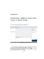
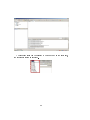
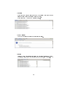
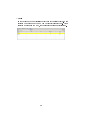
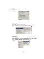
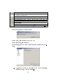
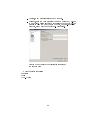
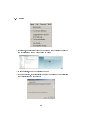
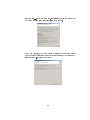
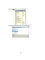
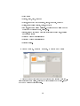
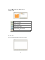
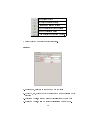
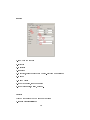
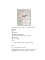
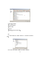
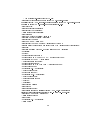
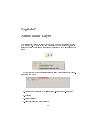
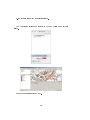
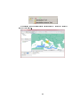
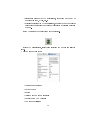
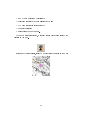
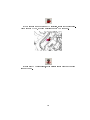
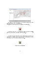
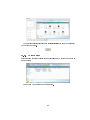
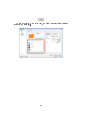
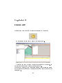
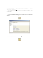
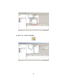
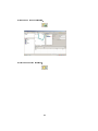
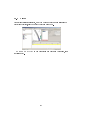
ALCOTRA European Project RISKNAT
B2/C2 - Hydrogeological and landslides risk
BEEGIS
Software for digital survey mapping
USER MANUAL
May 2012
Indice
1 Introduction
1.1 Short history of BeeGIS and credits . . . . . . . . . . . . . . .
1.2 Some hints to the tutorial employ . . . . . . . . . . . . . . . .
4
4
5
2 INSTALLING BeeGIS FROM OSGEO
2.1 Program Installation . . . . . . . . . . . . . . . . . . . . . . .
2.2 Software Conguration . . . . . . . . . . . . . . . . . . . . . .
6
6
9
3 STARTING BeeGIS FOR THE VERY FIRST TIME
10
4 Menu
4.1 File . .
4.2 Edit . .
4.3 Pan . .
4.4 Layer . .
4.5 Map . .
4.6 Data . .
4.7 Window
4.8 Help . .
14
14
17
18
18
23
25
26
29
.
.
.
.
.
.
.
.
.
.
.
.
.
.
.
.
.
.
.
.
.
.
.
.
.
.
.
.
.
.
.
.
.
.
.
.
.
.
.
.
.
.
.
.
.
.
.
.
.
.
.
.
.
.
.
.
.
.
.
.
.
.
.
.
.
.
.
.
.
.
.
.
.
.
.
.
.
.
.
.
.
.
.
.
.
.
.
.
.
.
.
.
.
.
.
.
.
.
.
.
.
.
.
.
.
.
.
.
.
.
.
.
.
.
.
.
.
.
.
.
.
.
.
.
.
.
.
.
.
.
.
.
.
.
.
.
.
.
.
.
.
.
.
.
.
.
.
.
.
.
.
.
.
.
.
.
.
.
.
.
.
.
.
.
.
.
.
.
.
.
.
.
.
.
.
.
.
.
.
.
.
.
.
.
.
.
.
.
.
.
.
.
.
.
.
.
.
.
.
.
.
.
.
.
.
.
.
.
.
.
.
.
.
.
.
.
.
.
.
.
.
.
.
.
.
.
.
.
.
.
.
.
.
.
.
.
.
.
.
.
5 Tool bars
32
5.1 Create map . . . . . . . . . . . . . . . . . . . . . . . . . . . . 35
6 Create a New Project
6.1 Coordinate Reference System(CRS) .
6.1.1 .prj File . . . . . . . . . . . .
6.2 Importing a Raster File . . . . . . .
6.3 Importing a SHP les . . . . . . . .
6.4 Create a New Layer . . . . . . . . .
6.5 Stile Editor . . . . . . . . . . . . . .
7 Annotation Layer
.
.
.
.
.
.
.
.
.
.
.
.
.
.
.
.
.
.
.
.
.
.
.
.
.
.
.
.
.
.
.
.
.
.
.
.
.
.
.
.
.
.
.
.
.
.
.
.
.
.
.
.
.
.
.
.
.
.
.
.
.
.
.
.
.
.
.
.
.
.
.
.
.
.
.
.
.
.
.
.
.
.
.
.
36
36
37
38
39
40
45
58
2
8 Geonote
8.1 Structure of a geonote
8.1.1 Drawing . . . .
8.1.2 Text . . . . . .
8.1.3 Media . . . . .
8.2 Fieldbook . . . . . . .
8.2.1 Search . . . . .
.
.
.
.
.
.
.
.
.
.
.
.
.
.
.
.
.
.
.
.
.
.
.
.
.
.
.
.
.
.
.
.
.
.
.
.
.
.
.
.
.
.
.
.
.
.
.
.
.
.
.
.
.
.
.
.
.
.
.
.
.
.
.
.
.
.
.
.
.
.
.
.
.
.
.
.
.
.
.
.
.
.
.
.
.
.
.
.
.
.
.
.
.
.
.
.
.
.
.
.
.
.
.
.
.
.
.
.
.
.
.
.
.
.
.
.
.
.
.
.
.
.
.
.
.
.
.
.
.
.
.
.
61
62
62
63
64
66
66
9 GPS Tolls
72
9.1 GPS Toolbar . . . . . . . . . . . . . . . . . . . . . . . . . . . 72
10 Form Editor
10.1 Label . . .
10.2 Texteld .
10.3 Textarea .
10.4 Combobox
10.5 Checkbox
10.6 Radio . .
10.7 Separator
.
.
.
.
.
.
.
.
.
.
.
.
.
.
.
.
.
.
.
.
.
.
.
.
.
.
.
.
.
.
.
.
.
.
.
.
.
.
.
.
.
.
.
.
.
.
.
.
.
.
.
.
.
.
.
.
.
.
.
.
.
.
.
.
.
.
.
.
.
.
.
.
.
.
.
.
.
11 Form View
.
.
.
.
.
.
.
.
.
.
.
.
.
.
.
.
.
.
.
.
.
.
.
.
.
.
.
.
.
.
.
.
.
.
.
.
.
.
.
.
.
.
.
.
.
.
.
.
.
.
.
.
.
.
.
.
.
.
.
.
.
.
.
.
.
.
.
.
.
.
.
.
.
.
.
.
.
.
.
.
.
.
.
.
.
.
.
.
.
.
.
.
.
.
.
.
.
.
.
.
.
.
.
.
.
.
.
.
.
.
.
.
.
.
.
.
.
.
.
.
.
.
.
.
.
.
79
80
81
82
82
83
83
85
86
12 Style Editor
88
12.0.1 Line library . . . . . . . . . . . . . . . . . . . . . . . . 88
12.0.2 Point library . . . . . . . . . . . . . . . . . . . . . . . 89
12.0.3 Polygon layer . . . . . . . . . . . . . . . . . . . . . . . 90
13 Database
92
13.1 Filter . . . . . . . . . . . . . . . . . . . . . . . . . . . . . . . . 97
14 Altri Strumenti
98
14.1 GPS data Export . . . . . . . . . . . . . . . . . . . . . . . . . 98
14.2 Photo Import (adapted from Antonello's Manual) . . . . . . . . 100
14.3 Import data from Geopaparazzi . . . . . . . . . . . . . . . . . 104
3
Capitolo 1
Introduction
BeeGIS is a development project of a mobile GIS for digital eld survey. A
simple and easy to use tool is request when working on `hard' environment,
where lab facilities are not available. This need pushes to research solutions for collecting georoferenced data and informations with expeditious
and stand-alone methods.
The choice of the open source environment has been mainly due to the needs
of collaborative work among developers and users.
Taking in account `to not reinvent the wheel', a multiplatforms (Win, Mac,
Linux) and opens source GIS as uDig (see udig.refraction.net) is used as
an engine on which new tools have been built. Those plug-in are the main
objects of description in this manual.
1.1 Short history of BeeGIS and credits
In the 1999, some researcher of LINEE (Laboratory of INformation-technology
for Earth and Environment) of Urbino Univesity (www.uniurb.it/ISDA/Linee
/linee.html) started to operate some test of digital geological eld mapping
using a Pen Computer Fujitsu (operative system: Windows 98) and Microstation Geographic by Bentley. First experiences were unsatisfying for many
reasons: screen readability, refresh and rendering of maps, software designed
for CAD drawing, etc.
Some years later, the development of Windows XP operative system allowed the use of more ecient Tablet PC, with tools (like ink-technology)
more suitable for managing data input by a stylus on the screen. Therefore the idea of a development of an adequate software took place again.
Thanks to a collaborative work with a software house, MapIT was born in
2004. This eld collector software was commercialised for a short period,
until the software house with commercial rights decided not keeping on with the collaboration. The success of this rst realise among international
and national agencies and researcher institutes, suggest to develop this ex4
perience and the acquired knowledges were redirected in the open source
environment. The open source project of uDig (udig.refraction.net) was chosen as the engine of the system mainly for the available documentation and
its development environment (Eclipse). Thanks to a doctorate work, a rst
version of plug-ins for GPS, Geonotes and Annotations management were
built. This new-sprung project was almost immediately supported by some
smart researchers of ARPA Piemonte (Environmental Agency of Piemonte
Region Italy). Because of their appreciation of MapIT, they decided to
nancially support the BeeGIS development contributing also with suggestions and customising requests. Nowadays, Hydrologis (an environmental
engineering company www.hydrologis.com) manages the main development
of this software.
The BeeGIS version illustrated in this manual has been supported by ARPA
Piemonte thanks to RISKNAT European Project.
BeeGIS continues to be mainly a working method open to new directions
and collaboration.
1.2 Some hints to the tutorial employ
This manual intend to help beginners approaching BeeGIS (version 2011).
In the rst chapter, the best way of installing the software in Windows environment. The user should take in account that BeeGIS can be transferred
from a PC to another just copying the OSGEO folder. Then menu' and
toolbars are described. When suited, some tool utilisation are developed.
The main tools like GPS acquisition, geonotes, annotations, style editor and
form editor were the main object of detailed description. Other functions, as
photo and geopaparazzi import were largely inspired by the previous manual
of BeeGIS written by Dr. Andrea Antonello for his PhD dissertation (download from http://www.cyberax.eu/book/1524142/beegis-manual) of Environmental Sciences Doctorate at Urbino University. According to the licence
agreements some written parts and gures are used. However this work is not
exhaustive and therefore we strongly recommend the documentation available uDig website and its manuals (e.g. indianocean.coaps.fsu.edu/FOSS GIS
/Introduction to uDig 1 1 0 RC8.pdf).
Like the whole project of BeeGIS, also this manual (Latex format) is open
to the contribution of everybody wants to participate to its development and
improvement inside the philosophy of open-source approach.
5
Capitolo 2
INSTALLING BeeGIS FROM
OSGEO
One of the best way for installing the Windows version of BeeGIS is OSGEO4W
package which allows the user to install and update a number of open source
GIS. More information can be found at http://trac.osgeo.org/osgeo4w/
2.1 Program Installation
1. Download the le from http://download.osgeo.org/osgeo4w/osgeo4wsetup.exe and start to setup from the installation wizard;
6
2. Select Advanced Install ;
3. Chose a destination folder (Root directory) and the users (All Users
recommended, if any user could run the program);
4. Select a folder where the installation les will be stored;
7
5. Select the connection type. If necessary, insert data of the Proxy Host ;
6. Now a window with all the OSGEO4W software options will appears.
Choose the software you intend to install; if you want install BeeGIS
only you can nd it listed under Desktop;
7. After a short process, BeeGIS will be installed and ready to use.
8
2.2 Software Conguration
The default conguration run with 340 Mb of memory for Java virtual machine.
If you got a PC with more then 1Gb of RAM, the amount of runtime memory
should be augmented.
From Window Preferences, select General the sub-menu Runtime Preferences and modify the amount of memory. A good option is 1024 Mb or
more.
At the end, clik on the button `Restart with the above settings '.
9
Capitolo 3
STARTING BeeGIS FOR THE
VERY FIRST TIME
At the very rst time, BeeGIS shows this window:
As you can see, the toolbars are very few. In the right side, the `welcome
window' address to the online tutorial of uDig by Refraction.
The extant of the screen, the other windows are empty. In the middle, the
grey space will be taken by map window.
10
A customised scale can be inserted by keyboard and in the right side,
the coordinate system is reported.
11
• Catalog
Every layer we create will be saved in the catalog were every le is
listed showing also the address where they are.
Every line with + can show a sublist of les.
• Web Catalog
The Web Catalog show links to cartographic sites.
• Search
Allows a query for researching inside the catalog: inserting a string,
the result will be shown in the right area wit name, and address.
12
• Table
In the table window are visualized every eld of the selected layer. Data
referred to a feature on the map can be directly inserted here. When
selected a feature in the map, the corresponding line is highlighted.
13
Capitolo 4
Menu
4.1 File
•
`New', open ...:
New Project, creates a new project;
14
New Map, adds a new layer in the map;
New Layer, from the window `other ' it's possible to select from
a database
Other, open a wizard:
•
`Close', close the project;
•
`Close all', close the program;
•
`Open File'..., open many format:
15
•
`Open Project', open an existing project;
•
`Save Project as', save project with a new name;
•
`Open Map', open an existing map;
•
`Rename', give a new name to an existing project;
•
`Redraw', redraw the map;
•
`Print', print the map of the project;
•
`Import', import many le type. From a list select the format, click on
`next ` a wizard will be opend.
•
`Export', export dierent data types from a list;
•
`Properties', change the properties of the project;
•
`Exit', close the program.
16
4.2 Edit
•
`Cut', cut selected data;
•
`Copy', copy selected data;
•
`Paste', paste selected data;
•
`Delete', delete selected data;
•
`Select', allow two dierent kinds of selection:
Select all features, select all features of the current layer;
Conta, open a window that provides the number of features of the
current layer;
•
`Deselect', deselect all features;
•
`Operations...', list of operations available within Tools;
•
`Save', save the last operation done;
•
`Delete all', deletes all operations.
17
4.3 Pan
•
`Show all', show all data in the map, zooming the map;
•
`Zoom-in', zoom to increase the scale;
•
`Zoom-out', zoom to decrease the scale;
4.4 Layer
18
•
`Add'..., add new data from the list
•
`Create', create a new layer (see `Create a new layers ').
19
•
`Legend' : insert a new legend in the map with the layers and styles
added;
•
`Grid' : insert a new layer in the list and a grid on the map;
20
•
`Scale' : insert the scale bar on the map;
•
`Other...' : add symbols in the layer that can be chosen from a list; e.g.
selecting `North Arrow ' the symbol of the True North appears on the
map.
21
•
`Layer' :
Set map Projection From Layer, reimposes map features according
to the selected layer;
Layer summary, open a window with the summary of features of the
current layer;
•
`Modify the style'...: window from which is possible to modify some
features of the layer: colour, features ... (see Style editor );
•
`Layer Properties' : window which allows to change the coordinate
reference system, customizing them.
22
4.5 Map
•
`Mylar', highlight selected layer, making it more clear to others;
•
`Count Map features',
•
`Rendering Tools',
•
`Map Properties', show the map properties: the coordinate system
allows to customize the reference data of map and to create le .prj
(see prj File ).
23
Palette: allow to change the standard colours and other features related to the map display;
Summary: list of info of the map.
24
4.6 Data
•
Resource, summary of resources.
Set Projection, allow the editing of projections (see denition of the
coordinates and projections );
Add Feature Type, open a window to add new layer (see Create new
plans/layers ).
25
4.7 Window
•
`Open View' :
Map View, show the classic screen,
Style View: show the styles and their characteristics.
Other: idem.
•
`Show view' : list a number of tools: catalog, web, catalog, search,
plans, favourites, projects, style, table and more...;
26
Open `catalog ' window (see above);
Open the `web catalog ' in a browser that allows to link
to a network (see above);
`Find ' windows (see above);
Open the list of planes (see Create new layers);
`Favourites', list of the most commonly used les, as the le map;
List of projects open until that moment;
`Style editor';
List of records and elds of the database, for the current layer;
Open many tools of BeeGis: database, catalog and eldbook...
•
`Reset View', restore the origin setting;
•
`Close View', close all views except the map;
•
`Close all Views', close all views;
•
`Preferences'
ted.
, windows where the general program settings can be edi-
GPS, allow to modify the properties of the GPS: Corrections,
Graphics property, Advanced settings...;
27
General, many general settings can be changed.
Geonotes, sets the data necessary to send a geonota by e-mail
to an address. Fields are lled with reference data of the e-mail
address to who you want to send the data, the user-name and
password, along with the complete e-mail address.
Window where to place the coordinates for sending
the geonota data
Edit the project properties
Rendering
Tools
WMS-C Tiles
28
4.8 Help
•
`Welcome', is an introduction to the program that contains the link to
the tutorial of uDig and his ocial web page;
•
`Help contents', open the tutorial of uDig;
•
`Tips and tricks', tips will display for every opening of the application
(if the selection box is checked);
29
•
`Sending Log...', send the error log. Is possible to copy the entire text
under the heading `log le content ' and then send it.
•
`Find and install', If the rst option is selected the program starts
an automatic updates; if the second option is selected the programme
researches web-sites for the update;
30
•
`Key Assist...', list of the keyboard commands;
•
`About uDig', general information about software uDig.
31
Capitolo 5
Tool bars
Undo-Redo, undo the last changes and cancels the undo command;
Redraw Map, delete the changes done on the map;
End features drawing, stop the refresh of the map;
Show all data, show all data on the map;
Zoom in - Zoom out, increases and decreases the scale view of the map;
Show selected data, highlight selected data only;
Save, save all changes;
Delete changes, delete last changes done.
32
Zoom, with the left click of the mouse a rectangular fence
allows to zoom in;
Pan, with the left button it change the view on the map;
Select feature with fence, the fence allows to select the vectorial
features on the layer, highlighting their characteristic on the table;
Map Point info, display info about a selected point;
Length, ruler estimating the length of a line on the map;
length can be read on the bottom-left corner of uDig frame.
Load an image on the map, load image on the map layer. Next
command allows to change the image leaded:
- Select Image, select the image;
- Move Image, move the selected image;
- Resize Image, resize the image;
- Delete Image, delete loaded image;
- Place Markers,insert numbered markers on the image;
- Move Markers, move the markers on the image;
- Warp Image, modify the image with markers
`Edit features', edit all features: point, line and polygon:
- Edit features, edit selected features dragging nodes;
- Add node, add a node to a line or a polygon;
- Remove node,
33
`Create feature', create points, lines and polygons.
In the case of polygon, this tool allow to:
- Fill area, ll the polygon;
- Create rectangle, insert a rectangular area;
- Create ellipse, insert an elliptical area;
Delete feature, delete the selected features: points,
lines or polygons;
Draw freehand on the annotation layer, tool for writing
freehand on a map, the characteristics of the line can be modied;
- Annotation remove tool, removes the stored annotations;
Geonote Tool : create a sheet similar to a post-it where is possible to take
geo-referenced note and insert any kind of les (e.g. pictures).
- Geonote selection : select geonote with a bounding box;
- Move Geonote : move geonote;
Active Region Tool, with a bounding box is dened the area under analysis
(useful for high resolution map):
`Move Mapgraphic', change the property or style, where the resolution or
coordinates can be dened with the keyboard.
34
5.1 Create map
`New Layer', add new layer by choosing the type from a list
select it and press Forward ;
`New Map', open a new map within the current project.
The main purpose of BeeGIS is to collect geo-referenced data and information right in the eld. That's why placing them on a base-map such as
technical papers, orthophotos or topographic map is so important.
To load a topographic base the easiest and faster way is to drag it; once
chosen the le (e.g. a geo-referenced .ti le) with a drag-and-drop within
the area of the map the le is imported. At the same time a new layer is
created for this raster and it appears in the list.
Example of raster CTR (geo-referenced ti) loaded onto the map.
35
Capitolo 6
Create a New Project
6.1 Coordinate Reference System(CRS)
uDig exploit the CRS dened by EPSG (European Petroleum Survey Group)
and it allows to customize them in order to improve the accuracy of positioning and georeferencing and to better correct projection errors (see also
uDig manual at http://indianocean.coaps.fsu.edu/FOSS GIS/Introduction
to uDig 1 1 0 RC8.pdf (pag.38).
Example.
In Italy, apart the WGS84 used for GPS positioning, the main projection
systems are Gaus-Boaga and UTM-ED50. Gaus-Boaga projection system
is dened in EPSG standard as Monte Mario/Italy zone 1 (for the West
sector) with a code number 3003 and Monte Mario/Italy zone 2 (for the
Est sector) with a code number 3004. In BeeGIS version has been added
36
other customized CRS found as: Peninsular Part/Accuracy 3-4m (30031000
and 30041000), Sardinia /Accuracy 3-4m (30031001 and 30041001), Sicily/Accuracy 3-4m (30031002 and 30041002).
6.1.1
.prj File
These les keep information on coordinate system of another georeferenced
le raster (ex. TIFF) or vectorial (ex. SHAPE) and are written in WellKnown Text (WTK). A simple way to create a .prj le can be found in the
CRS denition window (see above). The script can be copied-and-pasted in
a text editor (ex. Notepad). Once the new le has been saved with the same
name of the georeferencing le (ti, shp, ), the format extension of .txt must
be changed in .prj. The .prj le must be placed in the same folder of the
georeferencing le.
When a rst .prj le has been created, you just can make a copy of the
rst one and change the name with that of the new georeferencing le.
37
In the gure above every ti les use the same CRS, therefore the .prj
les keep the same text. The only dierence is the name of the le, that
must be related to the single ti le.
6.2 Importing a Raster File
The more common raster les to add in a GIS project are maps or aerial
photos. The simplest way of importing those les is a `drag-and-drop'.
At the end of loading and rendering, the raster image will be posted and
georeferenced (with a corresponding .prj le).
38
6.3 Importing a SHP les
Th SHAPE le can be considered a standard for GIS projects.
Every SHP le corresponds to a feature layer like points, lines and polygons.
It consists of three dierent les at least.
•
.shp, for geometry description;
•
.dbf, for database attributes;
•
.shx, for geometry index.
To this minimum number of les, other les like .prj (for example) can
be added.
39
Also in this case, when operating on the eld, the easiest way to insert a
shape in the project is the one of drag-and-drop inside the map or the layer
window.
6.4 Create a New Layer
From menu' `Layer', select `Create' and `Create New Layer' window will be
opened.
The attributes of the features of this layer can be added or selected in
this window:
1. name of layer;
2. add new attributes to the list;
40
3. name and type of the attribute;
4. delete attributes.
At the end, click on `OK' and the new layer can be inserted in in the list
of layers.
In the `Layer' window, layer properties can be modied.
Arrows move the position of the layer in the list;
`Mylar' is a sort of highlighter of the layer;
`Zoom to layer' shows the sector of the map where is the selected layer.
Changes to the layer properties can be performed also by clicking on it
with the right button of the mouse.
• Copy;
41
• Paste;
• delete;
• Style editor;
• Zoom to layer;
• Rename;
• Operations:
Make Hole ;
Select all Features, automatically select and highlight all the feature of that layer;
Count, the number of the selected feature is shown in a new
window;
42
View lines orientation, show the drawing orientation of lines with
arrow;
Invert geometry orientation, invert the drawing orientation of
lines;
Move features one layer up, move the selected feature to the layer
above;
Move features one layer down, move the selected feature to the
layer below;
Reshape, create a new layer with the same feature if Added to
Map ;
Resource Resume, open a window showing information of the
features in the layer such CRS, Lat & Long, etc.
43
Set Map Projection From Layer ;
Layer Resume, open a window showing information of the layer
such Lat & Long, le address, etc.
•
Export, export of the layer opening the following windows from which
the user can choose the way.
44
•
Properties, open a window that gives information on CRS and the
resume as seen before.
6.5 Stile Editor
Style Editor
Clicking on the icon, the user open the `Style Editor' window. On the
left side the styling method can be chosen.
Simple
This way allows to modify the general style properties of the features of
the selected layer
45
•
`Geometry' ;
•
`Mode', Point, Line, Polygon;
•
`Linea', style of the border (visible, colour, thickness, opacity);
•
`Fill', style of lling (visible, colour, opacity);
•
`Symbol', only for point feature - choosing among a little number
of simple symbols like square, circle, etc.;
•
`Label', insert a label from database attributes dening font, position
and rotation angle;
•
`Minimum scale of visualization' ;
•
`Maximum scale of visualization' ;
•
`Replace Styles'.
Simple Lines, Simple Points, Simple Polygons
This part of the Style Editor has been designed for managing more complex cartographic symbolism, allowing import of library of symbols (.svg ad
SLD) and managing their properties.
46
In the top-left sector, the `Rules' list is showed
la `Rules List'
`Add a new group' ;
`Add a new rule' ;
`Delete selected rule' ;
`Delete all rule', cancella tutto;
Move up or down the selected rule in the list.
Style list
in the down left sector a list of Style can be created
47
Save selected style;
Save all the selected styles;
Delete all the selected styles;
Load the selected style in the list;
Export the selected style;
Open a library of style from a folder.
The right window manages the style properties.
General
1. `Rule name', attribute or change a name to the rule;
2. `Oset (x, y)', oset of the symbol respect to the real position of the
feature;
3. `Maximum Scale', maximum scale of visualisation of the symbol;
4. `Minimum Scale', minimum scale of visualisation of the symbol.
48
Border
1. show/hide the border;
2. `Width' ;
3. `Opacity' ;
4. `Colour' ;
5. `Graphics', insert a graphic symbol (ex. gif) from a user folder;
6. `Dash' ;
7. `Dash Oset' ;
8. `Line Cap' : butt, round or square ;
9. `Line Join' : bevel, milter, or round.
Labels
Window that allows you to manage any labels :
1. `Enable/disable labelling' ;
49
2. `Label' : can be inserted manually or by attribute of database;
3. `Opacity' ;
4. `Font' ;
5. `Font colour' ;
6. `Halo', improves visualization;
7. `Perpendicular Oset', of the label to the centroid;
8. `Initial Gap' ;
9. `Vendor Options'.
Filter
A script can be inserted in the form to manage symbolism.
Tema
Back to the original uDig style editor:
1. `Attributes', style can be dened by an attribute of the database;
2. `Classes', number of class of the features (only 12 classes);
50
3. `Interval', statistics;
4. `Normalizzazione' ;
5. `Altrimenti' ;
6. `Show' ;
7. `Palette', predened colour table.
XML
An advancer user can be insert a script in XML language for dening a
style.
See the example for bedding attitude (for geology operators)
51
<?xml version='1.0' encoding='UTF-8'?>
<sld:StyledLayerDescriptor xmlns='http://www.opengis.net/sld'
xmlns:sld='http://www.opengis.net/sld' xmlns:ogc='http://www.opengis.net/ogc'
xmlns:gml='http://www.opengis.net/gml' version='1.0.0'>
<sld:UserLayer>
<sld:LayerFeatureConstraints>
<sld:FeatureTypeConstraint/>
</sld:LayerFeatureConstraints>
<sld:UserStyle>
<sld:Name>pointSymbolizer</sld:Name>
<sld:Title>pointSymbolizer</sld:Title>
<sld:FeatureTypeStyle>
<sld:Name>name</sld:Name>
<sld:FeatureTypeName>Feature</sld:FeatureTypeName>
<sld:SemanticTypeIdentier>SemanticType[ANY]</sld:SemanticTypeIdentier>
<sld:Rule>
<sld:Title>Inclined bedding - Showing strike and dip</sld:Title>
<ogc:Filter>
<ogc:And>
<ogc:PropertyIsNotEqualTo>
<ogc:PropertyName>ORIENTAMEN</ogc:PropertyName>
<ogc:Literal>INVERSA</ogc:Literal>
</ogc:PropertyIsNotEqualTo>
<ogc:PropertyIsBetween>
<ogc:PropertyName>INCLINAZIO</ogc:PropertyName>
<ogc:LowerBoundary>
<ogc:Literal>5.0</ogc:Literal>
</ogc:LowerBoundary>
<ogc:UpperBoundary>
<ogc:Literal>84.0</ogc:Literal>
</ogc:UpperBoundary>
</ogc:PropertyIsBetween>
</ogc:And>
</ogc:Filter>
<sld:PointSymbolizer>
<sld:Graphic>
<sld:ExternalGraphic>
<sld:OnlineResource xmlns:xlink='http://www.w3.org/1999/xlink'
xlink:type='simple' xlink:href='le:/C:/sld_images/dip_norm.gif'/>
<sld:Format>image/gif</sld:Format>
</sld:ExternalGraphic>
<sld:Opacity>
<ogc:Literal>1.0</ogc:Literal>
</sld:Opacity>
52
<sld:Size>
<ogc:Literal>25.0</ogc:Literal>
</sld:Size>
<sld:Rotation>
<ogc:PropertyName>IMMERSIONE</ogc:PropertyName>
</sld:Rotation>
</sld:Graphic>
</sld:PointSymbolizer>
</sld:Rule>
<sld:Rule>
<sld:Title>Overturned bedding - Showing strike and dip</sld:Title>
<ogc:Filter>
<ogc:And>
<ogc:PropertyIsEqualTo>
<ogc:PropertyName>ORIENTAMEN</ogc:PropertyName>
<ogc:Literal>INVERSA</ogc:Literal>
</ogc:PropertyIsEqualTo>
<ogc:PropertyIsBetween>
<ogc:PropertyName>INCLINAZIO</ogc:PropertyName>
<ogc:LowerBoundary>
<ogc:Literal>5.0</ogc:Literal>
</ogc:LowerBoundary>
<ogc:UpperBoundary>
<ogc:Literal>84.0</ogc:Literal>
</ogc:UpperBoundary>
</ogc:PropertyIsBetween>
</ogc:And>
</ogc:Filter>
<sld:PointSymbolizer>
<sld:Graphic>
<sld:ExternalGraphic>
<sld:OnlineResource xmlns:xlink='http://www.w3.org/1999/xlink' xlink:type='simple'
xlink:href='le:/C:/sld_images/dip_overt.gif'/>
<sld:Format>image/gif</sld:Format>
</sld:ExternalGraphic>
<sld:Opacity>
<ogc:Literal>1.0</ogc:Literal>
</sld:Opacity>
<sld:Size>
<ogc:Literal>25.0</ogc:Literal>
</sld:Size>
<sld:Rotation>
<ogc:PropertyName>IMMERSIONE</ogc:PropertyName>
</sld:Rotation>
53
</sld:Graphic>
</sld:PointSymbolizer>
</sld:Rule>
<sld:Rule>
<sld:Title>Vertical bedding - Showing strike</sld:Title>
<ogc:Filter>
<ogc:And>
<ogc:PropertyIsNotEqualTo>
<ogc:PropertyName>ORIENTAMEN</ogc:PropertyName>
<ogc:Literal>INVERSA</ogc:Literal>
</ogc:PropertyIsNotEqualTo>
<ogc:PropertyIsGreaterThan>
<ogc:PropertyName>INCLINAZIO</ogc:PropertyName>
<ogc:Literal>84.0</ogc:Literal>
</ogc:PropertyIsGreaterThan>
</ogc:And>
</ogc:Filter>
<sld:PointSymbolizer>
<sld:Graphic>
<sld:ExternalGraphic>
<sld:OnlineResource xmlns:xlink='http://www.w3.org/1999/xlink'
xlink:type='simple' xlink:href='le:/C:/sld_images/dip'vert.gif'/>
<sld:Format>image/gif</sld:Format>
</sld:ExternalGraphic>
<sld:Opacity>
<ogc:Literal>1.0</ogc:Literal>
</sld:Opacity>
<sld:Size>
<ogc:Literal>25.0</ogc:Literal>
</sld:Size>
<sld:Rotation>
<ogc:PropertyName>IMMERSIONE</ogc:PropertyName>
</sld:Rotation>
</sld:Graphic>
</sld:PointSymbolizer>
</sld:Rule>
<sld:Rule>
<sld:Title>Horizontal bedding</sld:Title>
<ogc:Filter>
<ogc:And>
<ogc:PropertyIsNotEqualTo>
<ogc:PropertyName>ORIENTAMEN</ogc:PropertyName>
<ogc:Literal>INVERSA</ogc:Literal>
</ogc:PropertyIsNotEqualTo>
54
<ogc:PropertyIsLessThan>
<ogc:PropertyName>INCLINAZIO</ogc:PropertyName>
<ogc:Literal>5.0</ogc:Literal>
</ogc:PropertyIsLessThan>
</ogc:And>
</ogc:Filter>
<sld:PointSymbolizer>
<sld:Graphic>
<sld:ExternalGraphic>
<sld:OnlineResource xmlns:xlink='http://www.w3.org/1999/xlink'
xlink:type='simple' xlink:href='le:/C:/sld_images/dip_horiz.gif'/>
<sld:Format>image/gif</sld:Format>
</sld:ExternalGraphic>
<sld:Opacity>
<ogc:Literal>1.0</ogc:Literal>
</sld:Opacity>
<sld:Size>
<ogc:Literal>25.0</ogc:Literal>
</sld:Size>
<sld:Rotation>
<ogc:PropertyName>IMMERSIONE</ogc:PropertyName>
</sld:Rotation>
</sld:Graphic>
</sld:PointSymbolizer>
</sld:Rule>
</sld:FeatureTypeStyle>
<sld:FeatureTypeStyle>
<sld:Name>TEXT_LABEL</sld:Name>
<sld:FeatureTypeName>Feature</sld:FeatureTypeName>
<sld:SemanticTypeIdentier>SemanticType[ANY]</sld:SemanticTypeIdentier>
<sld:Rule>
<sld:Name>Default/all others</sld:Name>
<ogc:Filter>
<ogc:PropertyIsEqualTo>
<ogc:Literal>1</ogc:Literal>
<ogc:Literal>1</ogc:Literal>
</ogc:PropertyIsEqualTo>
</ogc:Filter>
<sld:MinScaleDenominator>1.0</sld:MinScaleDenominator>
<sld:MaxScaleDenominator>1.7976931348623157E308</sld:MaxScaleDenominator>
<sld:TextSymbolizer>
<sld:Label>
<ogc:PropertyName>INCLINAZIO</ogc:PropertyName>
</sld:Label>
55
<sld:Font>
<sld:CssParameter name='font-family'>
<ogc:Literal>Arial</ogc:Literal>
</sld:CssParameter>
<sld:CssParameter name='font-size'>
<ogc:Literal>12.0</ogc:Literal>
</sld:CssParameter>
<sld:CssParameter name='font-style'>
<ogc:Literal>normal</ogc:Literal>
</sld:CssParameter>
<sld:CssParameter name='font-weight'>
<ogc:Literal>bold</ogc:Literal>
</sld:CssParameter>
</sld:Font>
<sld:LabelPlacement>
<sld:PointPlacement>
<sld:AnchorPoint>
<sld:AnchorPointX>
<ogc:Literal>0.00</ogc:Literal>
</sld:AnchorPointX>
<sld:AnchorPointY>
<ogc:Literal>-0.20</ogc:Literal>
</sld:AnchorPointY>
</sld:AnchorPoint>
<sld:Displacement>
<sld:DisplacementX>
<ogc:Literal>5.0</ogc:Literal>
</sld:DisplacementX>
<sld:DisplacementY>
<ogc:Literal>0</ogc:Literal>
</sld:DisplacementY>
</sld:Displacement>
<sld:Rotation>
<ogc:PropertyName>IMMERSIONE</ogc:PropertyName>
</sld:Rotation>
</sld:PointPlacement>
</sld:LabelPlacement>
<sld:Halo>
<sld:Radius>
<ogc:Literal>1.0</ogc:Literal>
</sld:Radius>
<sld:Fill>
<sld:CssParameter name='ll'> <ogc:Literal>#FFFF00</ogc:Literal>
</sld:CssParameter>
56
<sld:CssParameter name='ll-opacity'>
<ogc:Literal>0.10000000149011612</ogc:Literal>
</sld:CssParameter>
</sld:Fill>
</sld:Halo>
<sld:Fill>
<sld:CssParameter name='ll'>
<ogc:Literal>#000000</ogc:Literal>
</sld:CssParameter>
<sld:CssParameter name='ll-opacity'>
<ogc:Literal>1.0</ogc:Literal>
</sld:CssParameter>
</sld:Fill>
</sld:TextSymbolizer>
</sld:Rule>
</sld:FeatureTypeStyle>
</sld:UserStyle>
</sld:UserLayer>
</sld:StyledLayerDescriptor>
Questo script puo' essere utilizzato con un copia e incolla nella nestra
dello Style Editor XML utilizzando i simboli di giacitura opportunamente
nominati.
57
Capitolo 7
Annotation Layer
The traditional method of eld mapping need pen and pencils for drawing
on a paper map. Thanks to the Ink Technology of the Tablet Pcs, BeeGIS
includes the use of a stylus on the screen by clicking on the Annotation Tool
icon:
`Draw freehand on the annotation layer' : allow drawing lines and colouring areas in a map:
1. thickness of the line in ve classes (from 1-thinnest to 5-thickest);
2. opacity ;
3. colour palette ;
4. clear the area from all drawings ;
58
5. remove last stroke from annotations layer.
The Annotation stylus draw directly on the map whilst a new layer is
listed.
Example of annotations on a map.
59
`Annotation remove tool' : deletes previous lines by tracking a straight
line on these strokes.
60
Capitolo 8
Geonote
The Geonote Too l allows the user to insert georeferenced Post-it-like notes
on the map during survey.
After clicking for the very rst time on the Geonote toolbar, a geonote layer
will be listed. Every geonote will be stored in this layer.
The icon of a geonote is similar to a red drawing Pin
If inserted by GPS tool, the icon will be
When created by Photo import (see later):
The user can open an already inserted geonote by clicking on the tip of
the pin. Because it cab be dicult, we suggest to drag a fence around the
61
pin (wit the stylus or with a mouse pushing the left button). The geonote
pin will become green and a post-it will appear.
Another way to open a geonote is the tool `Open the Fieldbook ' (see
later): a new Fieldbook window will be opened.
8.1 Structure of a geonote
The geonote comprises three main eld:
• Drowing;
• Text;
• Media.
Other default data are also captured (see later).
8.1.1
Drawing
In this area, drawing, sketch, hand-writing can be inserted with the aid of
drawing tools for: thickness, opacity, colour table, delete all, delete, shrink
the view, magnier.
62
8.1.2
Text
Just use the keyboard for inserting a note in this area.
63
8.1.3
Media
By drag-and-drop you can insert any le. For example, if you insert a
spreadsheet with measurements that le will be associated to that geonote
and therefore georeferenced.
A special tool is available for pictures (see later).
At the end of the work on the geonote, just click on the `diskette' icon
to save.
For reading the default information or change something on them, just
click on the 'Geonote Properties' icon.
1. date, time and Lat/Long position;
2. name of the geonote: it can be modied;
3. table of background colour;
4. save all the properties;
64
5. cancel;
6. save the geonote content and properties in a external folder:
this tool allows to save geonote data and informations in a folder or
make a new folder.
As result:
65
• two text les: `geonote_info.txt ' with general properties (date,
time, position) and `geonote_textbox.txt ' with the text note;
• a raster le with the drawing note;
• a folder storing all the les inserted in the Media eld.
7. delete the geonote;
8. default colour: useful during eldwork.
8.2 Fieldbook
The Fieldbook allows to manage all the geonotes. To open it, just click on
the icon in the toolbar
A new windows will appear and can be located in any sector of the
BeeGIS main window.
8.2.1
Search
When a geonote is selected in the Fieldbook list, this one will be highlighted
in the map with a change pin colour.
The search selections can be performed by:
66
• name of geonote;
• default colours;
• date;
• way of geonote creation;
67
1. This combobox show the research method:
• Name,
• Colour,
• Date,
• Type.
2. This bar that changes depending on the choice of the type of research
done over;
Search by the name of the genote;
Search by colour of the genote;
Search by date;
RSearch by type: normal, GPS, photo import...
3. list of all selected geonotes;
4. display geonote area.
Clicking with the right mouse button on the name of a geonote in the
list, open this menu:
•
`Zoom to geonotes', center the map on the geonote selected (green);
•
`Remove geonotes', delete the geonote;
•
`Export to feature layer', create a new point layer for the selected geonote and a related table with FID, title (with the name of the geonote),
text (with the inserted text note), time stamp (with date ant time);
68
•
`Dump geonotes', see above;
•
`Dump geonotes binary', this tool saves the geonote data in an external
fold with .zip format;
•
`Import geonotes archive', import dumped geonotes;
•
`Send geonotes', send a selected geonote by e-mail.
By clicking on this tool, BeeGIS automatically send an e-mail with a
dumped geonote folder in attachment to a predened e-mail address.
Set the e-mail address from the menu' Window Options
69
in the `Preference' window, clicking on `Geonotes' in the list, a form
has to be lled with e-mail address and settings.
Back to the `Send geonotes' tool, when on-line connection is ready, a
window message show the status of mailing.
70
The mail recipient will get a message with an attached .zip le.
•
`Sort notes by title', alphabetically sort the geonotes by names;
•
`Sort notes by time', temporally sort from newer to older.
71
Capitolo 9
GPS Tolls
BeeGIS is able to manage NMEA string of data from GPS receivers.
One of the less complicated way of working in the eld is the usage of a
bluetooth connected device, because of no wire. Attention: check from time
to time if bluetooth connection is working!
9.1 GPS Toolbar
`Open GPS settings ', connect the GPS receiver opening this window
72
by `search port' the user must look for the COM port of the bluetooth
GPS device in the list that will appear.
When found and selected, click on `OK' and then on radio button `Start
GPS'.
When NMEA signals allow to dene the GPS location this sting and message
will appear.
In this window, the user can set also:
73
•
`Interval in seconds for GPS acquisition', depending on the way of
workings (on foot, by car, etc.);
•
`Distance threshold for GPS acquisition', important when the operator
is stopping for avoiding to acquire a typical cloud of position points in
the map.
`Stop GPS' stops the connection with the receiver.
`Start GPS data logging ', start the log recording of GPS data in a selected
layer.
A window shows these data:
• Northing and Easting;
• Lat and Long;
• Speed;
• Altitude above medium sea level;
• Quality of the NMEA signal;
• Number of Satellites;
74
• HDOP (High Dilution Of Precision);
• Dierence of altitude between ellipsoid and msl;
• UTC time (useful for pictures sync);
• Magnetic variation;
• angle (azimuth of movement).
When GPS signal is received, a squared cursor with cross will show the
position in the map.
`Manual GPS points tools ', insert GPS point using the stylus on the map;
75
`Add a geonote from the current GPS position ', this is the tool for inserting a geonote by GPS, showing a special pin with GPS icon on it.
`Automatic GPS points tools ', automatically insert point and drawing
line on the map.
76
The frequency of capture is related to the chosen time elapse at the start
(Interval in second for GPS acquisition ).
Points, lines or polygons are drawn depending the chosen layer.
`Center the map on the GPS position ', when selected, center the visualization of the area of the map around the GPS cursor.
The following tool buttons allow to automatically create new layers where
collecting GPS positions when the user has no time or opportunity to create
a new layer with the uDig procedures (see before).
`Create a new point layer ';
77
`Create a new lines layer to work on ';
`Create a new polygon layer to work on ', crea in automatico un nuovo
piano con geometria poligoni per inserire in maniera speditiva dei poligoni
con il GPS.
78
Capitolo 10
Form Editor
Form Editor is a BeeGIS tool to create and edit customised forms to insert
data.
Open the Form Editor
Open the Form View
The Form Editor botton open a grid window in the Map area.
The `Properties' window show the properties (geometry, name, etc.) of
the inserted widgets
79
It is possible to insert each selected widgets within the lattice by dragging
it with the left mouse button on the `Form Editor'.
10.1 Label
After selection of the Label widget on the right side, just put the cursor
on the grid and drag a rectangle in the position where the user want to insert
a label. This rectangle will be snapped in the sector of the grid selected.
Those Properties will appear in the lower window:
80
• `layout
height e layout width ', dimensions of the label ; they can be
modied by inserting dierent value in the properties or dragging a
node of the rectangle;
• `layout
X e layout Y ', coordinates of the label position in the grid;
• `name ', name of the
label ;
• `tab ', to name a tab visible in the lower part of the form view;
• `text ', to name or insert a text that will displayed on the
• `widget
label ;
type '.
10.2 Texteld
As seen before, after selection of the Texteld widget on the right side,
just put the cursor on the grid and drag a rectangle in the position where
the user want to insert a space for text. This rectangle will be snapped in
the sector of the grid selected.
In the Properties:
• `default
time;
value ', is shown when the user open the form view for the rst
• `eldname ', to choose an attribute of the database related to the layer
selected by a combobox that appears when click on it;
81
• `layout
height e layout width ', the same as for the label;
• `layout
X e layout Y ', the same as for the label;
• `name ', the same as for the label;
• `tab ', the same as for the label;
• `text
type ', by a combobox the user can choose among string, integer
and double ;
• `widget
type '.
10.3 Textarea
Similar to texteld, but with a larger area where writing a text.
The properties are the same as the texteld.
10.4 Combobox
In this eld can be inserted a predened list of values, names, qualities,
etc., to be chosen when data input.
The original property that can be listed and modied is:
82
• `items ', to attribute a value/text from a list saved in a text (.txt) le
as shown in the following example or a list separate by semicolons as
shown in the gure above.
10.5 Checkbox
For Boolean eld where yes/no, true/false, etc. is request.
Properties, the only dierence with the previous ones is the:
• `default
selection ', where the user can choose among true or false.
10.6 Radio
Insert a list in the form view with radio button close to the items.
83
84
Properties: similar to the Combobox, apart of `orientation' that allow to
insert an horizontal or vertical list.
10.7 Separator
This widget allows to create a fence to keep separate some eld.
Properties: `orientation', for vertical or horizontal line orientation.
85
Capitolo 11
Form View
Once a form for collecting data has been designed with the Form Editor for
features in a layer, or a new geometry is inserted in that layer, the Form
View will be open. If the user wants to insert or modify data of a previous
saved feature, he/she needs to click on the icon in the toolbar.
By inserting data in the eld or checking by Radio or Checkbox, the user
can ll the database table.
86
ATTENTION: Make sure to click on diskette icon to save the data.
Exemple of how a Combobox appears in the Form View
87
Capitolo 12
Style Editor
The Style Editor allows to use dierent symbols for the mapped features.
The user can manage customized symbol libraries.
12.0.1
Line library
Every symbol can be created or imported and saved in the Style List (see
in Point library)
To use a symbol of the Style List, the user must select `Load selected style
into the rules list '.
88
12.0.2
Point library
The user can load graphic symbols (as .svg) into the Style List by `Import
supported les to style '.
Symbols can be renamed in the `Rule name ' and/or combined to dene
new styles and saved in the Style list.
When in the list the symbols are saved as SLD in a uDig folder that the
user can open by `Open the style library folder '.
89
When `Load selected style into the rules list 'is selected the symbol is ready
to be edited and used.
12.0.3
Polygon layer
Polygons with dierent colours or graphic stiles can be created and saved in
a uDig folder
then it can be imported in the Style List.
90
To use a polygon of the Style List, the user must select `Load selected
style into the rules list '.
91
Capitolo 13
Database
Database view open a window to create a connection to a database
In the left side of this window a list of database is shown.
Database view open a window to create a connection to a database. In
the left side of this window a list of database is shown.
For every new project, a new database is created, but the user can create
new database or can connect to previous ones or to a remote database (as
PostgreSQL).
92
The database selected among the list is highlighted in green: in this one
attribute and data are saved.
The icons in the top right part of the window allows the user to manage
the database:
`Open in database browser view ', show the structure of the database for
editing;
`Open an existing embedded database ', open an embedded database in
which data can be loaded;
93
`Create a new embedded database ',
94
`Create a new remote database ',
`Export an embedded database ',
95
`Import an embedded database ',
`Delete a database denition ',
`View some statistics of the active database ',
96
13.1 Filter
When `lter active ' is selected, only the working database are visualized;
with `lter project ', all the project database are shown.
EMBEDDED DATABASE for denitions and hints see Antonello, 2009
(bibliography).
97
Capitolo 14
Altri Strumenti
14.1 GPS data Export
BeeGIS allows the export of GPS log data.
98
Click on Export from File menu.
Then select Export GPS Log to open the wizard.
In the white eld, insert timestamps of : - Start and End
Choose the option for lines or points and insert the destination folder.
Push on Finish and the a new layer will be created showing point or lines in
the map.
99
In the Database view, the data from GPS log can be QUERYED.
14.2 Photo Import
(adapted from Antonello's Manual)
BeeGIS provides a tool dedicated to the alignment of pictures taken with a
digital camera with the internal GPS log.
BeeGIS provides a tool dedicated to the alignment of pictures taken with
a digital camera with the internal GPS log.
The following example will assume that a survey has been done and that the
user took several GPS drawn lines and geonotes, as well as several pictures
100
with a digital camera. Once the user starts his post-processing, he will be in
the situation shown in gure below, i.e. visualizing the taken geonotes, GPS
paths drawn and annotations.
`List of photos in the camera'
What is not visible in Figure above is the background GPS log that was
taken during the survey. It is possible to visualize the data in the GPS log
by using the embedded database view (see section of Embedded database.
For example to have an idea of how many GPS points were taken in the
log, it is possible to execute the query SELECT count(*) FROM GPSLOG
inside the database view as is shown in gure below
The user will have to connect the digital camera he used for the surveying
to the computer and will then be able to visualize the folder with the taken
pictures, in the path where the operating system mounted the camera's storage media. In this case the camera was mounted on the folder /media/disk and
the pictures taken are inside the sub-folder /media/disk/DCIM/100CANON.
After these preparation parts, it is possible to start the import wizard from
the main le menu under import.
101
The generic import wizard will show up as in gure above and propose
an Import Photos entry.
Once selected the Import Photo, the panel to import the pictures is
visualized. The panel need just two informations, that are:
1. The folder that contains the pictures to be imported. It is very important to note that BeeGIS is not able to read the creation time of a
picture, but only the last modication time.
Therefore it is necessary to execute the import directly on the camera
mounted on a local folder. If the imaged are instead copied to disk,
this will change the the last modication time and therefore make the
import tool useless.
2. The time shift between the GPS time (UTC) and the camera time at
the time of shooting the pictures. This value dense the accuracy of
the import and obviously needs to be checked when starting to take
pictures during the survey. At that point it is simple to compare the
GPS time visible in the GPS view of BeeGIS and the camera time.
102
Once nish is pushed, BeeGIS starts the importing process. During the
process the pictures timestamps are compared with the internal gps log points and in the position of the nearest gps point by timestamps a new geonote
is created, containing the picture in the geonote's mediabox. Pictures that
have no GPS point taken at the time of shooting, are ignored and at the end
of the import a list of not imported pictures is proposed to the user to be
able to understand if the import has been successful.
The gure shows the situation after a successful import of pictures. BeeGIS in that case shows a geonote, named after the imported picture, for
103
every imported picture. in the urge it can be noted that in the mediabox
the picture is available for further processing.
14.3 Import data from Geopaparazzi
Geopaparazzi is an apps for tablet and smartphone with Android operative
system and it can be downloaded from Android Market.
https://market.android.com/details?id=eu.hydrologis.geopaparazzi&hl=it
After connect the smartphone or insert the media card in your PC, select
Import from File menu'.
Then select the option Import Geopaparazzi Data Folder to open a wizard, wher you must selct the geopaparazzi root folder and an output folder
where shape les will be stored, as shown in the following gures.
Import from menu' le
104
Wizard to import from Geopaparazzi ...
Click on Finish to import all Geopaparazzi data in BeeGIS.
Pins with photo icon will be visualized on the map. The black arrow shows
the direction (azimuth) of the photoshot.
New layers will be created:
•
`Notes', .shp created by Note folder of Geopaparazzi;
•
`GPSlines' and `GPSpoints' : layers from Geopaparazzi GPS log.
105
• The geonotes with all those data will be stored in the eldbook.
Import data from Geopaparazzi: GPS linee, GPS punti, note e geonote
106
Table of the Notes: see description (text) and timestamps.
Table of GPSlines: see the timestamps of rst and last GPS points.
107
A geonote is created for each imported picture, stored in Mediabox of the
Geonote.
108
-
Tutorial - February 2012
109