Download user manual - EIA-FR

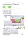
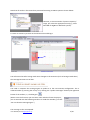
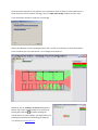
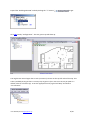
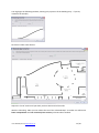
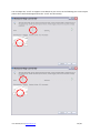
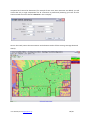
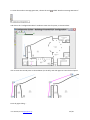
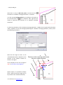
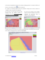
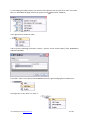
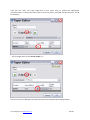
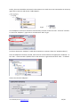
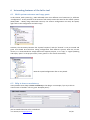
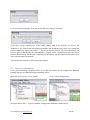
 Getting started InCov is a radio network planning tool for indoor coverage. InCov is developed at the EIA‐FR in collaboration with Ericsson. InCov handles both indoor and outdoor‐to‐indoor coverage. Indoor coverage is shown first. Outdoor‐
to‐indoor coverage is shown in Section 4. If you intend to use InCov it is strongly recommended that you go through this manual in sequence using a color copy. This manual will explain the steps to use the software with screen shots so you might want to read it just to learn the features InCov provides, namely: ‐ Coverage based on scanned floor plan (no AutoCAD, even hand drawn plan might be sufficient). ‐ Easy adjustment of cell power; for all antennas covering the cell. ‐ Single computation for all antennas in a cell/on the same channel. ‐ Optional power setting via a feeding network. As InCov is still under development, please do not hesitate to let us know your need using the contacts at the end of this document. To install the InCov demo just extract the InCovDemo folder from the received ZIP file. Open the InCovDemo folder. 1 Start InCov Double click on InCov.exe You should get (note that it may take a few seconds to start) : InCov ©2008, EIA‐FR ([email protected]) 1/34 Then, you are warned that you are using a version of InCov which is still under development. This version is for testing purpose only. You should have received this version to help us serve your needs. Thus, we are eager to receive your feedback at: jean‐[email protected] or [email protected]. After having clicked anywhere on the black window you should obtain this: Notice the scale (in meters) , the two antennas and the legend for the received power. InCov ©2008, EIA‐FR ([email protected]) 2/34 You can adjust the power of an entire cell by right‐clicking on any antenna in that cell and choosing “Adjust Cell Power …”. A cell is defined by its radio channel. In our example, there are only two antennas, each defining a different cell, i.e., each with a different channel. The following slider pops up. You can adjust the cell power. Observe the coverage map! For example, subtracting 100dB from the left antenna leaves only the coverage of the right antenna. You can also edit the EIRP power, by right‐clicking on one antenna and choosing “Edit” … … to get the following window: InCov ©2008, EIA‐FR ([email protected]) 3/34 By default, the “Coverage [dBm]” is shown But you can also view the best server map (the two antennas here are on two different channels). Notice the change in the “Legend” (the color and the name “Coverage …” are chosen automatically. Please let us know if manual choices should be included in future releases). Note the legend and the threshold are easy to change to your taste using the “Configure Color Blender” button in the Configuration Editor window: InCov ©2008, EIA‐FR ([email protected]) 4/34 Note that all results in this manual are presented assuming an UMTS system as shown below: However, to choose another “System Frequency” range, just select the appropriate one (e.g., select WiFi ISM for ZigBee or Bluetooth system). To move an antenna: just click on the antenna icon and drag it. You will notice that after having made some changes to the antennas (such as having moved them) the coverage becomes out of date. You need to compute the coverage again to update it to the new antenna configuration. This is achieved either by pressing the F5 key or by clicking the “Update Coverages” button (the rightmost button of the toolbar, i.e., the blue gear ). (Minor note: the first time you use some action which will save the project; you are warned with the following window. To avoid this reminder, just click “Do not show this message again”.) The coverage is then recomputed. InCov ©2008, EIA‐FR ([email protected]) 5/34 Recall that each channel (or cell) requires one computation (even if there are many antennas on a same channel as usual in indoor coverage). This is a major time saving compare to other tools. If you moved the antenna in each cells you will get: Notice the indication of the total elapsed time. Click “Cancel” (or tab‐enter) to close this window. Once computed, the new “Best Server” (or coverage) map shows up. Note that you can zoom (or un‐zoom) the display to best fit you screen or better position an antenna by clicking the hand tool and then scrolling the mouse wheel. On some laptops, you might want to try pressing the two buttons and moving you finger on InCov ©2008, EIA‐FR ([email protected]) 6/34 the right side of the pad. The scale is, of course, changed accordingly. Now you are going to learn how to input and use your own floor plan. 2 Add Your Indoor Map Now we are going to add another building floorplan and we will give it a scale (in meters). Right click on the Demo_InCov and choose “Add Region …” (we use the term Region instead of Floorplan to be more generic, in case of femto cell planning for example): Type in "BuildingA Floor00" You see now a new folder for your floor plan in the project window. Right‐click on “BuildingA Floor00” and choose “Add Map …” Pick the following file (a00.jpg) in the folder …\InCovDemo\IndoorProjects: Note that you can add any graphic file (scanned, hand‐drawn, screen copy, … InCov ©2008, EIA‐FR ([email protected]) 7/34 in all most‐used format like *.jpg, *.bmp, etc.) InCov ©2008, EIA‐FR ([email protected]) 8/34 Expand the “BuildingA Floor00” node by clicking the “+” button ( ) to get: Click edit nearby “Configuration”. This way your map will show up. You might have noticed again that a scale (in meters) is shown at the top left side of the map. This scale is probably wrong as there is no easy way to guess it (so it was set to 25 cm per pixel as a default value for all new map). To set the appropriate scale, right click “Map” and choose “Co‐reference”. InCov ©2008, EIA‐FR ([email protected]) 9/34 to get Maximize the window (as you might not see the whole building as you would like to) … … and then click and drag the mouse in the map to get the scale at some appropriate location of your choice. You must now enter the coordinates (or one set of x & y coordinates and a distance) : InCov ©2008, EIA‐FR ([email protected]) 10/34 Note that you can still modify the scale and d=15m, in this example). after having entered the values (x=0, y=0 Once you are satisfied, click “OK” at the bottom right of the “Coreference Map” window. You will now get the correct scale in the “Configuration Editor” window as show below: Now, you need to create a wall map so that the program knows on your floor plan what is a wall and what is not (we call it the “Obstacle Map”). Right click “Configuration” > “Add Obstacle Map” > “From Map…”. InCov ©2008, EIA‐FR ([email protected]) 11/34 You might get the following window, showing only a portion of the building map … if you do, maximize the window, Such that it looks more like this: Adjust the “Level” slider until you think you have almost all of the walls. With the “Shrinking” slider you can reduce the size of the “Obstacle Map”. A smaller size will lead to faster computations and not necessarily less accuracy. Click OK when satisfied. InCov ©2008, EIA‐FR ([email protected]) 12/34 You can then obtain something like this (here ~52’000 pixels): or like this by adjusting the “Shrinking” factor (~19’000 pixels): InCov ©2008, EIA‐FR ([email protected]) 13/34 You can adjust the “Level” to suppress some details as you can see in the following two screen copies (notice that a wall also disappeared as the “Level” was decreased): InCov ©2008, EIA‐FR ([email protected]) 14/34 You can then edit the “Obstacle Map” image to further modify the map. In order to do this, double click your “Obstacle Map” in the project window (or right‐click and “edit”). The conventional Microsoft Windows application “Paint” will open as follows. In the following example, we added a wall that was erased in the “Level‐Shrinking” process. Usually, it is recommended that you remove things that are not walls, typically texts. However, you will see that our prediction algorithm is rather robust with respect to these kinds of artefacts. Once you have finished, simply save and close MS‐Paint (or close and save but do not use “Save As”). In future releases we might introduce colored walls to let the user choose various wall types (and wall attenuation if deemed necessary). Since usually InCov predictions are rather robust with respect with inaccurate wall descriptions, metallic shelves locations, special walls, etc., please let us know what are your needs and send us your project with an indication of where a poor accuracy is observed. In InCov, you can toggle “Show/Hide Map” (the original floor plan) as shown below: InCov ©2008, EIA‐FR ([email protected]) 15/34 and turn on/off obstacles view using the following toggle button: Now you are ready to place an antenna: click on the “Omni Antenna” tool. and click to place the antenna where you want. For example: Right click the antenna > Edit InCov ©2008, EIA‐FR ([email protected]) 16/34 Fill the properties like this for example. Note that the “Location X” and “Y” might differ from above since your co‐reference might not be exactly as shown in this manual. Then compute the coverage as already described (clicking the blue gear ). Note that only a single computation per cell needs to be performed so if you add several antennas with the same channel, all these antennas will belong to the same cell. The total coverage will be InCov ©2008, EIA‐FR ([email protected]) 17/34 computed and cannot be dissociated, for example if two more omni antennas are added, you will notice that only a single computation for all 3 antennas is performed (assuming you have set all 3 antennas with the same channel: channel 2 in this example): Here is the result (notice the two antennas at the bottom used to fill the missing coverage detected above): InCov ©2008, EIA‐FR ([email protected]) 18/34 3 Patch antennas We will now add a patch antenna. Select the patch antenna tool: To better see the introduction of the patch antenna, it is suggested that you toggle off the “obstacle map” and “coverage” display by clicking on the following icons: Now you can move the “patch antenna” icon on the map as shown below: InCov ©2008, EIA‐FR ([email protected]) 19/34 You will notice that if you drag the “patch antenna” near a wall and click, the antenna will snap on the wall and the patch direction is set automatically (but you can change it of course as you will see). To stop adding patch antennas or to change the orientation, right‐click (to get the arrow pointer … and click on the patch antenna to select it: Now you can choose the direction by clicking on the square tip of the patch antenna. You can also edit manually the direction angle by editing the patch antenna (right‐click, choose “edit”): … to get any desired direction (here 32°) : InCov ©2008, EIA‐FR ([email protected]) 20/34 ) Note that in an open space, the effect of a patch antenna is better seen. The steps necessary to obtain the following screen copy is left as an exercise for the reader: (The patch antenna is not yet fully calibrated in this release of InCov so the user might prefer to use an omni antenna instead). As for all antennas, you can also adjust the power on the patch antenna by right‐clicking on this kind of antenna and choosing “Adjust Cell Power …”. In fact, as the name suggests, it is the cell power which is adjusted by right‐clicking on any antenna in a cell and choosing “Adjust Cell Power …”. It is recalled that a cell is defined by a channel and that all the antennas on that channel contributes to the coverage of this cell. You are encouraged to “play” with both the “Adjust Cell Power …” which is very fast and “Edit …” on any particular antenna to get the desired coverage. You will easily discover that the computation takes a non negligible time, only if you change the power setting of one antenna with respect to the others in the same cell (on the same channel). Note: To rename a “Configuration”: by right‐click on the “Configuration” folder or its name and choose “Rename”. To save your project (Ctrl‐S) or File > Save. InCov ©2008, EIA‐FR ([email protected]) 21/34 Now, you will learn how to take into account the coverage (or interference) from outdoor antennas placed far away from the building under investigation. 4 Coverage from outdoor antennas InCov allows you to compute the indoor coverage from outdoor antennas. The example below guides you to add the coverage from a single outdoor antenna. You should only have measurements (or predictions) of the received power at a number of outdoor locations and know the approximate direction of the outdoor antenna. For example, consider the following situation: The indoor coverage from the outdoor antenna will be computed after entering an outdoor coverage with the appropriate parameters (next page). generator as a broken line ‐79 dBm
‐81 dBm ‐85 dBm InCov ©2008, EIA‐FR ([email protected]) 22/34 To enter the outdoor coverage generator, choose the tool called “Outdoor Coverage Generator” and click in the “Configuration Editor” window to enter the first point, as shown below: click to enter the second point as shown below (on the left), and click again to enter the third point: Finish by right‐cliking … InCov ©2008, EIA‐FR ([email protected]) 23/34 … and you will get: Note that it is easy to add extra points. Just click with the tool when an “Outdoor Coverage Generator” is selected. It is also easy to remove a point by just clicking on the point to be removed when the tool is selected. Then, right‐click (as usual) to terminate the insertion of an “Outdoor Coverage Generator”. To edit the parameters of the “Outdoor Coverage generator”, double click (or right click and choose “Edit”) anywhere in the red rectangle (delimiting the “Outdoor Coverage generator” points). Enter the following parameters: Note that the angle to enter in the “DistantAntennaForm” depends on the location of the outdoor antenna as shown in the figure. Direction of the incoming radio waves
from the outdoor antenna
In our example, we can use an angle of 300° or ‐60° (minus sixty degrees). 300°
-60°
(Upon request, it is possible to change the 0° reference and the angle sign to be positive in the clockwise direction) InCov ©2008, EIA‐FR ([email protected]) 24/34 You have then completed the insertion of an outdoor coverage generator. To compute its effect, just press F5 or click the blue wheel (like for an antenna). For example, the following figures present the predicted coverage with all other antennas at ‐100 dBm (so their coverage can be neglected). On the right, the result shows that the radio coverage from the outdoor antenna is attenuated by the wall. The prediction outside the building should not be considered. On the left, the power for the outdoor antenna has been increased by 20 dB to exaggerate the penetration effect of outdoor to indoor propagation. To further demonstrate the effect of an outdoor coverage generator, the following result shows the same outdoor coverage generator as above but in free space: InCov ©2008, EIA‐FR ([email protected]) 25/34 5 Add a feeding network InCov allows you to a feeding network: from the UMTS Node B (or GSM BTS) to each antenna. This feature has not yet been fully tested. We welcome any comment. The idea is to help you verify the feeding network and the power settings once the antenna layout has been chosen. A feeding network may look like this (as an example): A3
738 450
+2.0dBi
Sous-sol Bellerive 32
A4
738 450
+2.0dBi
1er extension
Bellerive 32
D + 19dBm/cr
E + 16dBm/cr
G + 15dBm/cr
A9
738 450
+2.0dBi
Attique Bellerive 23
D + 19dBm/cr
E + 15dBm/cr
G + 14dBm/cr
K18
22m LCF1/2
D -1.6dB
E -2.3dB
G -2.5dB
A8
738 450
+2.0dBi
2ème Bellerive 23
D + 16dBm/cr
E + 13dBm/cr
G + 12dBm/cr
K17
30m LCF1/2
D -2.0dB
E -3.0dB
G -3.2dB
D + 18dBm/cr
E + 15dBm/cr
G + 14dBm/cr
K12
42m LCF1/2
D -3.0dB
E -4.3dB
G -4.6dB
K11
20m LCF1/2
D -1.4dB
E -2.0dB
G -2.2dB
A14
738 450
+2.0dBi
3ème sous-sol
Bignami
A13
738 450
+2.0dBi
2ème sous-sol
Bignami
D + 20dBm/cr
E + 17dBm/cr
G + 16dBm/cr
A12
738 450
+2.0dBi
1er sous-sol
Bignami
A11
738 450
+2.0dBi
Résidence
D + 22dBm/cr
E + 18dBm/cr
G + 16dBm/cr
D + 21dBm/cr
E + 19dBm/cr
G + 18dBm/cr
D + 24dBm/cr
E + 22dBm/cr
G + 21dBm/cr
-3.5 dB
ZAPD-21
K6
20m LCF1/2
D -1.4dB
E -2.0dB
G -2.2dB
-3.5 dB
C5
-3.5 dB
ZAPD-21
C8
-3.5 dB
A2
738 450
+2.0dBi
1er Bellerive 32
K7
36m LCF1/2
D -2.4dB
E -3.5dB
G -3.8dB
K5
65m LCF1/2
D -4.4dB
E -6.4dB
G -7.0dB
K10
10m LCF1/2
A7
D -0.7dB
738 450
E -1.0dB
+2.0dBi
G -1.1dB
1er étage Bellerive 23
D + 23dBm/cr
E + 20dBm/cr
G + 19dBm/cr
K16
22m LCF1/2
D -1.6dB
E -2.3dB
G -2.5dB
K15
40m LCF1/2
D -2.7dB
E -4.0dB
G -4.3dB
A15
800 10137
+2.0dBi
Rez Bâtiment B
K21
6m LCF1/2
D -0.3dB
E -0.5dB
G -0.5dB
-3.5 dB
C11
D + 23dBm/cr
E + 22dBm/cr
G + 21dBm/cr
-3.5 dB
ZAPD-21
-3.5 dB
-3.5 dB
-6.5dB
C7
-3.5 dB
C10
C4
-3.5 dB
ZAPD-21
C13
D + 27dBm/cr
E + 26dBm/cr
G + 26dBm/cr
A1
738 450
+2.0dBi
Rez Ecuries
-6.5dB
-0.5 dB
-1.0 dB 86010023
C12
K2
70m LCF7/8
D -2.7dB
E -4.0dB
G -4.4dB
ZAPD-21
C3
C6
K13
40m LCF7/8
D -1.7dB
E -2.5dB
G -2.8dB
K8
43m LCF1/2
D -3.0dB
E -4.3dB
G -4.6dB
K3
76m LCF1/2
D -5.1dB
E -7.4dB
G -8.1dB
A5
738 450
+2.0dBi
Parking Bellerive 23
-3.5 dB
K63236101
-10 dB
-6.5dB
A6
800 10137
+2.0dBi
Rez inf Bellerive 23
K9
10m LCF1/2
D -0.7dB
E -1.0dB
G -1.1dB
K14
72m LCF7/8
D -2.8dB
E -4.2dB
G -4.6dB
-3.5 dB
K20
35m LCF1/2
D -2.4dB
E -3.5dB
G -3.8dB
-6.5dB
ZB4PDI 2000N
ZAPD-21
D + 16dBm/cr
E + 14dBm/cr
G + 13dBm/cr
A10
738 450
+2.0dBi
Rez Corthésy
K4
25m LCF1/2
D -1.7dB
E -2.5dB
G -2.7dB
-3.5 dB
ZAPD-21
-3.5 dB
-7.0 dB
D + 26dBm/cr
E + 25dBm/cr
G + 25dBm/cr
K19
13m LCF1/2
D -0.9dB
E -1.3dB
G -1.4dB
D + 14dBm/cr
E + 13dBm/cr
G + 13dBm/cr
-0.5 dB
K63236101
C9
-10 dB
-3.5dB
HH800HF
C2
-3.5dB
-3.5dB
K1
40m LCF7/8
D -1.7dB
E -2.5dB
G -2.8dB
HH800HF
C1
+43 dBm
H1
-3.5dB
(théorique)
H2
BTS
GSM 900
RBS 2202
In InCov, it will look like this (note that a simpler feeding network for 5 antennas is shown here): InCov ©2008, EIA‐FR ([email protected]) 26/34 To start adding a feeding network, you will first add a BTS (we use the same term “BTS” for a GSM BTS or a UMTS Node B). Right click on the project name and choose “Add BTS”. Then right‐click on the BTS to “Edit”: and to input the following parameters: “Name”, “System” and its “Power [dBm]” (here: NodeBdemo, UMTS and 30 dBm): Then add a “Wire” to the BTS (name NodeBdemo here) by right‐clicking again on the BTS icon: And right‐click on the “Wire” to “Edit” it: InCov ©2008, EIA‐FR ([email protected]) 27/34 And insert the appropriate parameters (“Length [m]” and “Loss [dB]”, the “Name” of the wire is optional): Now you can add a taper after the wire (right‐click on the wire): And add as many “Wire” as there are output connectors to the taper: So adding 2 “Wires” (for a tapper with two output ports for example) gives: At this point it is recommended to edit each wire, enter the appropriate loss and length and perhaps choose a different name for each wire: InCov ©2008, EIA‐FR ([email protected]) 28/34 Then you can “Edit” the Taper (right‐click on the Taper icon) to choose the appropriate “Connected wire” in the list box and to type in the correct taper “Loss [dB]” parameters (here ‐3.5 dB for example): … do not forget same for the second output, i.e., You can continue to add tapers and wires to each line to complete the feeding network. InCov ©2008, EIA‐FR ([email protected]) 29/34 Finally, the wires should be connected to the antennas. For each wire to be connected to an antenna, right‐click on the wire and choose “Add Endpoint” to get This “Endpoint” can then be named so it will be easy to select it from the “Edit … Antenna” window. To name the “Endpoint”, right‐click on it and choose “Edit” to get: (In future release this “Endpoint” could also be linked to an antenna from the “Endpoint Editor”.) Once all endpoints have been created, each antenna can be linked to the appropriate “Endpoint”. In the “Edit … Antenna Editor” (double‐click on the antenna or right‐click and chose “Edit…” as follows ) Choose the desired “Endpoint”: InCov ©2008, EIA‐FR ([email protected]) 30/34 Note that the BTS and the entire feeding network can support multi‐system (e.g., UMTS and GSM): The parameters of each wire and taper can be adjusted Thus, the correct “Endpoint” powers are computed: And the appropriate “Endpoint” can be chosen for each antenna: InCov ©2008, EIA‐FR ([email protected]) 31/34 6 Interesting features of the InCov tool 6.1 Multi­system antennas and copy­paste In this release, each system (e.g., UMT and GSM) must use a different set of antennas (i.e., different “Configuration”. As the position of the antennas will usually remain the same for the cellular systems (GSM, GPRS … UMTS) using multi‐band antennas, the antenna configuration can easily be copied; right‐click on the configuration and select copy: However, the consistency between the “System frequency” and the “channel” is not yet insured and great care should be used when mixing configuration with different systems. With the current version, it is recommended to simply define two separate projects, or to “copy” a “region”/building and simply “paste” in the project menu (“InCov_Demo” in the screen shot below). Note the copied configuration after it was pasted. 6.2 Help to insure consistency InCov provides some help to insure consistency in the design. For example, if you try to link an antenna with a “Default” cell to a given “BTS (End point)”: you are notified that the cell is not defined: InCov ©2008, EIA‐FR ([email protected]) 32/34 To let you verify your design, InCov will provide the at the antenna connector If you then change manually the “Power (EIRP) [dBm]” field of the antenna, the link to the “Endpoint” is lost; N/C for Not Connected is displayed in the “BTS (End point)” field. If you change the antenna EIRP using “Adjust Cell Power …”, you will be not warned but the power adjustment will have no effect (a warning will be implemented in a future release. The warning will let you choose between disconnecting the antenna or adjusting the BTS power and thus adjusting the power on all other antennas linked to this BTS). If you wish other consistency check, please let us know. 6.3 Obstacle attenuation In very special building, the default value of the wall attenuation can be changed and additional building wall type can defined using the following menus: Right‐click on the project “InCov_Demo” or on a chosen configuration: And then choose “Edit…” to get the window “Configuration Obstacles” shown below. InCov ©2008, EIA‐FR ([email protected]) 33/34 The configuration (1 dB/cm for the black wall) is shown. Configuring the color and the other parameters for a new type of wall is very easy: 7 To conclude You can now experiment with InCov and let us know how we can improve it, for you or with you, by contacting: Jean‐Frédéric Wagen jean‐[email protected] +41 26 429 6553 (voice) +41 78 737 4273 (mobile) wagenjf (SKYPE) Enjoy ! … and let us know. InCov ©2008, EIA‐FR ([email protected]) 34/34