Download Quality Assurance Handbook for Air Pollution Measurement Systems

United States
Environmental Protection
Agency
Air
Office of Air Quality
Planning and Standards
Research Triangle Park, NC 27711
EPA-454/R-98-004
August 1998
Quality Assurance Handbook for
Air Pollution Measurement
Systems
Volume II: Part 1
Ambient Air Quality Monitoring Program
Quality System Development
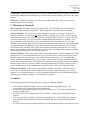
Foreword
This document represents Volume II of a 5-volume quality assurance (QA) handbook series dedicated to air
pollution measurement systems. Volume I provides general QA guidance that is pertinent to the remaining
volumes. Volume II is dedicated to the Ambient Air Quality Surveillance Program and the data collection
activities of that program.
The intent of the document is twofold. The first is to provide additional information and guidance on the
material covered in the Code of Federal Regulations pertaining to the Ambient Air Quality Surveillance
Program. The second is to establish a set of consistent QA practices that will improve the quality of the
nation’s ambient air data and ensure data comparability among sites across the nation. Therefore, the
document is written for technical personnel at State and local monitoring agencies and is intended to provide
enough information to develop a quality system for ambient air quality monitoring.
The information in this document was revised/developed by many of the organizations implementing the
Ambient Air Quality Surveillance Program. Therefore, the guidance has been peer reviewed and accepted by
these organizations and should serve to provide consistency among the organizations collecting and reporting
ambient air data.
This document has been written in a style similar to a QA project plan, as specified in the document “EPA
Requirements for Quality Assurance Project Plans for Environmental Data Operations” (EPA QA/R5).
Earlier versions of the Handbook contained many of the sections required in EPA QA/R5 and since many
State and local agencies, as well as the EPA, are familiar with these elements, it was felt that the document
would be more readable in this format.
This document is available on hardcopy as well as accessible as a PDF file on the Internet under the Ambient
Monitoring Technical Information Center (AMTIC) Homepage (http://www.epa.gov/ttn/amtic). The
document can be read and printed using Adobe Acrobat Reader software, which is freeware that is available
from many Internet sites (including the EPA web site). The Internet version is write-protected and will be
updated every three years. It is recommended that the Handbook be accessed through the Internet. AMTIC
will provide information on updates to the Handbook. Hardcopy versions are available by writing or calling:
OAQPS Library
MD-16
RTP, NC 27711
(919)541-5514
Recommendations for modifications or revisions are always welcome. Comments should be sent to the
appropriate Regional Office points of contact identified on AMTIC bulletin board. The Handbook Steering
Committee plans on meeting quarterly to discuss any pertinent issues or proposed changes.
ii
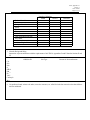
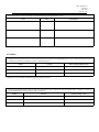
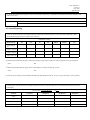
Contents
Section
Page
Revision
Date
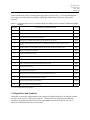
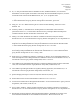
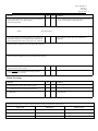
Foreword . . . . . . . . . . . . . . . . . . . . . . . . . . . . . . . . . . . . . . . . . . . . . . . . . . . ii
0
8/98
Contents . . . . . . . . . . . . . . . . . . . . . . . . . . . . . . . . . . . . . . . . . . . . . . . . . . . . iii
0
8/98
Acknowledgments . . . . . . . . . . . . . . . . . . . . . . . . . . . . . . . . . . . . . . . . . . . vi
0
8/98
Figures and Tables . . . . . . . . . . . . . . . . . . . . . . . . . . . . . . . . . . . . . . . . . . . vii
0
8/98
Acronyms and Abbreviations . . . . . . . . . . . . . . . . . . . . . . . . . . . . . . . . . . ix
0
8/98
0
8/98
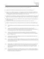
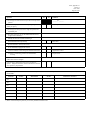
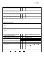
1. Program Organization
1.1 Organization Responsibilities . . . . . . . . . . . . . . . . . . . . . . . . . . 1/5
1.2 Lines of Communication . . . . . . . . . . . . . . . . . . . . . . . . . . . . . . . 4/5
1.3 The Handbook Steering Committee . . . . . . . . . . . . . . . . . . . . . 5/5
0
8/98
2. Program Background
2.1 Ambient Air Quality Monitoring Network . . . . . . . . . . . . . . . 1/5
2.2 Ambient Air Monitoring QA Program . . . . . . . . . . . . . . . . . . 3/5
0
8/98
3. Data Quality Objectives
3.1 The DQO Process . . . . . . . . . . . . . . . . . . . . . . . . . . . . . . . . . . . . 3/6
3.2 Ambient Air Quality DQOs . . . . . . . . . . . . . . . . . . . . . . . . . . . . 3/6
3.3 Measurement Quality Objectives . . . . . . . . . . . . . . . . . . . . . . . 4/6
0
8/98
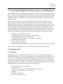
4. Personnel Qualification, Training and Guidance
4.1 Personnel Qualifications . . . . . . . . . . . . . . . . . . . . . . . . . . . . . . . 1/4
4.2 Training . . . . . . . . . . . . . . . . . . . . . . . . . . . . . . . . . . . . . . . . . . . . . 1/4
4.3 Regulations and Guidance . . . . . . . . . . . . . . . . . . . . . . . . . . . . . 2/4
0
8/98
5. Documentation and Records . . . . . . . . . . . . . . . . . . . . . . . . . . . . . . 1/5
0
8/98
0
8/98
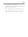
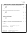
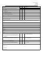
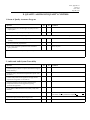
PROJECT MANAGEMENT
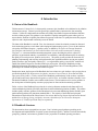
0. Introduction
0.1 Intent of Handbook . . . . . . . . . . . . . . . . . . . . . . . . . . . . . . . . . . .
0.2 Handbook Structure . . . . . . . . . . . . . . . . . . . . . . . . . . . . . . . . . . .
0.3 Shall, Must, Should, May . . . . . . . . . . . . . . . . . . . . . . . . . . . . . .
0.4 Handbook Review and Distribution . . . . . . . . . . . . . . . . . . . . .
1/2
1/2
2/2
2/2
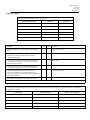
MEASUREMENT ACQUISITION
6. Sampling Process Design
6.1 Monitoring Objectives and Spatial Scales . . . . . . . . . . . . . . .
6.2 Site Location . . . . . . . . . . . . . . . . . . . . . . . . . . . . . . . . . . . . . . . . .
6.3 Monitor Placement . . . . . . . . . . . . . . . . . . . . . . . . . . . . . . . . . . . .
6.4 Minimum Network Requirements . . . . . . . . . . . . . . . . . . . . . .
6.5 Sampling Schedules . . . . . . . . . . . . . . . . . . . . . . . . . . . . . . . . . .
iii
3/15
6/15
10/15
12/15
13/15
Section
Page
Revision
Date
7. Sampling Methods
7.1 Environmental Control . . . . . . . . . . . . . . . . . . . . . . . . . . . . . . . . 1/14
7.2 Sampling Probes and Manifolds . . . . . . . . . . . . . . . . . . . . . . . . 4/14
7.3 Reference and Equivalent Methods . . . . . . . . . . . . . . . . . . . . . 11/14
0
8/98
8. Sample Handling and Custody
8.1 Sample Handling . . . . . . . . . . . . . . . . . . . . . . . . . . . . . . . . . . . . . 1/4
8.2 Chain-of-Custody . . . . . . . . . . . . . . . . . . . . . . . . . . . . . . . . . . . . . 3/4
0
8/98
9. Analytical Methods
9.1 Standard Operating Procedures . . . . . . . . . . . . . . . . . . . . . . . . . 1/3
9.2 Good Laboratory Practices . . . . . . . . . . . . . . . . . . . . . . . . . . . . . 2/3
9.3 Laboratory Activities . . . . . . . . . . . . . . . . . . . . . . . . . . . . . . . . . . 2/3
0
8/98
10. Quality Control
10.1 Use of Computers in Quality Control . . . . . . . . . . . . . . . . . . 5/5
0
8/98
11. Instrument/Equipment Testing, Inspection, and
Maintenance
11.1 Instrumentation . . . . . . . . . . . . . . . . . . . . . . . . . . . . . . . . . . . . . 1/5
11.2 Preventive Maintenance . . . . . . . . . . . . . . . . . . . . . . . . . . . . . . 3/5
0
8/98
12. Instrument Calibration and Frequency
12.1 Calibration Standards . . . . . . . . . . . . . . . . . . . . . . . . . . . . . . . .
12.2 Multi-point Calibrations . . . . . . . . . . . . . . . . . . . . . . . . . . . . . .
12.3 Level 1 Zero and Span Calibration . . . . . . . . . . . . . . . . . . . . .
12.4 Level 2 Zero and Span Check . . . . . . . . . . . . . . . . . . . . . . . . .
12.5 Physical Zero and Span Adjustments . . . . . . . . . . . . . . . . . . .
12.6 Frequency of Calibration and Analyzer Adjustment . . . . . .
12.7 Automatic Self-Adjusting Analyzers . . . . . . . . . . . . . . . . . . .
12.8 Data Reduction using Calibration Information . . . . . . . . . .
12.9 Validation of Ambient Data Based on Calibration . . . . . . .
Information
0
8/98
0
8/98
0
8/98
13 Inspection/Acceptance for Supplies and Consumables
13.1 Supplies Management . . . . . . . . . . . . . . . . . . . . . . . . . . . . . . . .
13.2 Standards and Reagents . . . . . . . . . . . . . . . . . . . . . . . . . . . . . .
13.3 Volumetric Glassware . . . . . . . . . . . . . . . . . . . . . . . . . . . . . . .
13.4 Filters . . . . . . . . . . . . . . . . . . . . . . . . . . . . . . . . . . . . . . . . . . . . . .
2/13
3/13
4/13
6/13
6/13
7/13
10/13
11/13
13/13
1/4
1/4
3/4
3/4
14. Data Acquisition and Information Management
14.1 General . . . . . . . . . . . . . . . . . . . . . . . . . . . . . . . . . . . . . . . . . . . . 1/13
14.2 Data Acquisition . . . . . . . . . . . . . . . . . . . . . . . . . . . . . . . . . . . . 6/13
14.3 The Information Management System . . . . . . . . . . . . . . . . . . 11/13
iv
Section
Page
Revision
Date
0
8/98
0
8/98
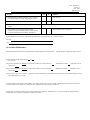
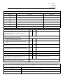
17. Data Review, Verification, Validation
17.1 Data Review Methods . . . . . . . . . . . . . . . . . . . . . . . . . . . . . . 3/5
17.2 Data Verification Methods . . . . . . . . . . . . . . . . . . . . . . . . . . 3/5
17.3 Data Validation Methods . . . . . . . . . . . . . . . . . . . . . . . . . . . . 4/5
0
8/98
18. Reconciliation with Data Quality Objectives
18.1 Five Steps of the DQA Process . . . . . . . . . . . . . . . . . . . . . . 2/9
0
8/98
0
8/98
0
8/98
6-A Characteristics of Spatial Scales Related to Each Pollutant
0
8/98
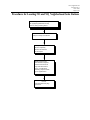
6-B Procedures for Locating Open Path Instruments
0
8/98
7
0
8/98
ASSESSMENT/OVERSIGHT
15. Assessment and Corrective Action
15.1 Network Reviews . . . . . . . . . . . . . . . . . . . . . . . . . . . . . . . . . .
15.2 Performance Evaluations . . . . . . . . . . . . . . . . . . . . . . . . . . . .
15.3 Technical Systems Audits . . . . . . . . . . . . . . . . . . . . . . . . . . .
15.4 Data Quality Assessments . . . . . . . . . . . . . . . . . . . . . . . . . . .
1/15
4/15
9/15
14/15
16. Reports to Management
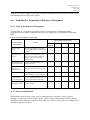
16.1 Guidelines for the preparation of reports to
Management . . . . . . . . . . . . . . . . . . . . . . . . . . . . . . . . . . . . . . 2/4
DATA VALIDATION AND USABILITY
References
Appendices
2.
QA Related Guidance Documents for Ambient Air
Monitoring Activities
3
Measurement Quality Objectives
Summary of Probe Siting Criteria
12
Calibration of Primary and Secondary Standards for Flow
Measurements
0
8/98
14
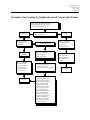
Example Procedure for Calibrating a Data Acquisition
System
0
8/98
15
Audit Information
0
8/98
16
Examples of Reports to Management
0
8/98
v
Acknowledgments
This QA Hand Book is the product of the combined efforts of the EPA Office of Air Quality Planning and
Standards, the EPA National Exposure Research Laboratory, the EPA Regional Offices, and the State and
local organizations. The development and review of the material found in this document was accomplished
through the activities of the Red Book Steering Committee. The following individuals are acknowledged for
their contributions.
State and Local Organizations
Douglas Tubbs, Ventura County APCD, Ventura, CA
Michael Warren, California Office of Emergency Services, Sacramento, CA
Alice Westerinen, California Air Resources Board, Sacramento, CA
Charles Pieteranin, New Jersey Department of Environmental Protection, Trenton, NJ
EPA Regions
Region
1 Norman Beloin, Mary Jane Cuzzupe
2 Clinton Cusick, Marcus Kantz
3 Victor Guide, Theodore Erdman
4 Dennis Mikel, Jerry Burger, Chuck Padgett
5 Gordon Jones
6 Kuenja Chung
7 Doug Brune
8 Richard Edmonds, Ron Heavner, Gordan MacRae, Joe Delwiche
9 Manny Aquitania, Bob Pallarino
10 Laura Castrilli
National Exposure Research Laboratory
William Mitchell, Frank McElroy, David Gemmill
Research Triangle Institute
Jim Flanagan, Cynthia Salmons
Office of Air Quality Planning and Standards
Joseph Elkins, David Musick , Joann Rice, Shelly Eberly
A special thanks to Monica Nees who provided an overall edit on the document.
vi
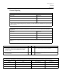
Figures
Number
Title
Section/Page
1.1
Ambient air program organization
................................................
1/1
1.2
Lines of communication
.......................................................
1/4
2.1
Ambient air quality monitoring process
2.2
Ambient Air Quality Monitoring QA Program
3.1
Effect of positive bias on the annual average estimate, resulting in a false positive decision error
3/1
3.2
Effect of negative bias on the annual average estimate, resulting in a false negative decision error
3/1
4.1
Hierarchy of regulations and guidance
............................................
4/3
4.2
EPA QA Division Guidance Documents
..........................................
4/4
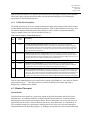
6.1
Wind rose pattern
.............................................................
6/8
7.1
Example design for shelter
7.2
............................................
......................................
2/1
2/3
.....................................................
7/2
Vertical laminar flow manifold
..................................................
7/4
7.3
Conventional manifold system
..................................................
7/5
7.4
Alternate manifold system
......................................................
7/5
7.5
Positions of calibration line in sampling manifold
7.6
Acceptable areas for PM10 and PM2.5 micro, middle, neighborhood, and urban samplers except
for microscale street canyon sites. . . . . . . . . . . . . . . . . . . . . . . . . . . . . . . . . . . . . . . . . . . . . . . . .
7/8
7.7
Optical mounting platform
.....................................................
7/9
8.1
Example sample label
.........................................................
8/2
8.2
Example field chain of custody form
8.3
Example laboratory chain of custody form
10.1
Flow diagram of the acceptance of routine data values
10.2
Types of quality control and quality assessment activities
12.1
Examples of simple zero and span control charts
12.2
Suggested zero and span drift limits when calibration is used to calculate measurements is
updated each zero/span calibration and when fixed calibration is used to calculate measurements
12/11
14.1
DAS flow diagram
14/8
14.2
Data input flow diagram
15.1
Definition of independent assessment
15.2
....................................
..............................................
.........................................
7/6
8/3
8/4
................................
10/1
.............................
10/2
....................................
12/9
............................................................
.......................................................
14/12
.............................................
15/8
Pre-audit activities
............................................................
15/9
15.3
On site activities
.............................................................
15/11
15.4
Audit finding form
............................................................
15/12
15.5
Post-audit activities
...........................................................
15/13
15.6
Audit response form
...........................................................
15/14
18.1
DQA in the context of the data life cycle
..........................................
vii
18/1
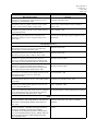
Tables
Number
Section/Page
Title
3-1
Measurement Quality Objectives-Parameter CO
. . . . . . . . . . . . . . . . . . . . . . . . . . . . . . . . . . 3/5
4-1
Suggested Sequence of Core QA-related Ambient Air Training Courses for Ambient Air
Monitoring and QA Personnel . . . . . . . . . . . . . . . . . . . . . . . . . . . . . . . . . . . . . . . . . . . . . . . .
4/2
5-1
Types of Information That Should be Retained Through Document Control
. . . . . . . . . . . . 5/1
6-1
Relationship Among Monitoring Objectives and Scales of Representativeness
. . . . . . . . . . . 6/4
6-2
Summary of Spatial Scales for SLAMS, NAMS, PAMS and Open Path Sites
. . . . . . . . . . . 6/5
6-3
Relationships of Topography, AIR Flow, and Monitoring Site Selection
6-4
Site Descriptions of PAMS Monitoring Sites
6-5
Relationships of Topography, Air Flow, and Monitoring Site Selection
6-6
NAMS Station Number Criteria
6-7
PM2.5 Core SLAMS Sites related to MSA
6-8
Goals for the Number of PM2.5 NAMS by Region
6-9
PAMS Minimum Network Requirements
6-10
Ozone Monitoring Seasons PAMS Affected States
6-11
PM2.5 Sampling Schedule
7-1
Environment Control Parameters
7-2
Summary of Probe and Monitoring Path Siting Criteria
7-3
Minimum Separation Distance Between Sampling Probes and Roadways
7-4
Techniques for Quality Control of Support Services
. . . . . . . . . . . . . . . . . . . . . . . . . . . . . . . 7/11
7-5
Performance Specifications for Automated Methods
. . . . . . . . . . . . . . . . . . . . . . . . . . . . . . . 7/14
10-1
PM2.5 Field QC Checks
10-2
PM2.5 laboratory QC Checks
11-1
Routine Operations
14-1
Data Reporting Requirements
15-1
NPAP Acceptance Criteria
15-2
Suggested Elements of an Audit Plan
. . . . . . . . . . . . . . . . . . . . . . . . . . . . . . . . . . . . . . . . . . . 15/10
16-1
Types of QA Reports to Management
. . . . . . . . . . . . . . . . . . . . . . . . . . . . . . . . . . . . . . . . . . . 16/2
16-2
Sources of Information for Preparing Reports to Management
16-3
Presentation Methods for Use in Reports to Management
18-1
Summary of Violations of DQO Assumptions
18-2
Weights for Estimating Three-Year Bias and Precision
18-3
Summary of Bias and Precision
. . . . . . . . . . . . . . . . 6/9
. . . . . . . . . . . . . . . . . . . . . . . . . . . . . . . . . . . . . 6/10
. . . . . . . . . . . . . . . . 6/11
. . . . . . . . . . . . . . . . . . . . . . . . . . . . . . . . . . . . . . . . . . . . . . . 6/13
. . . . . . . . . . . . . . . . . . . . . . . . . . . . . . . . . . . . . . . . 6/13
. . . . . . . . . . . . . . . . . . . . . . . . . . . . . . . . . 6/12
. . . . . . . . . . . . . . . . . . . . . . . . . . . . . . . . . . . . . . . 6/13
. . . . . . . . . . . . . . . . . . . . . . . . . . . . . . . . 6/15
. . . . . . . . . . . . . . . . . . . . . . . . . . . . . . . . . . . . . . . . . . . . . . . . . . . 6/15
. . . . . . . . . . . . . . . . . . . . . . . . . . . . . . . . . . . . . . . . . . . . . . 7/3
. . . . . . . . . . . . . . . . . . . . . . . . . . . . . 7/7
. . . . . . . . . . . . . . 7/8
. . . . . . . . . . . . . . . . . . . . . . . . . . . . . . . . . . . . . . . . . . . . . . . . . . . . . . 10/3
. . . . . . . . . . . . . . . . . . . . . . . . . . . . . . . . . . . . . . . . . . . . . . . . . . 10/4
. . . . . . . . . . . . . . . . . . . . . . . . . . . . . . . . . . . . . . . . . . . . . . . . . . . . . . . . . 11/5
. . . . . . . . . . . . . . . . . . . . . . . . . . . . . . . . . . . . . . . . . . . . . . . . . 14/6
. . . . . . . . . . . . . . . . . . . . . . . . . . . . . . . . . . . . . . . . . . . . . . . . . . . 15/6
. . . . . . . . . . . . . . . . . . . . . . . 16/3
. . . . . . . . . . . . . . . . . . . . . . . . . . . 16/3
. . . . . . . . . . . . . . . . . . . . . . . . . . . . . . . . . . . . 18/5
. . . . . . . . . . . . . . . . . . . . . . . . . . . . . 18/6
. . . . . . . . . . . . . . . . . . . . . . . . . . . . . . . . . . . . . . . . . . . . . . . 18/9
viii
Acronyms and Abbreviations
AIRS
ADBA
AMTIC
APTI
AQSSD
AWMA
CAA
CBI
CFR
CMD
CO
CSA
DCO
DD
DQA
DQAO
DQOs
EDO
EMAD
EPA
EPAAR
ESD
ETSD
FAR
FEM
FIPS
FRM
GIS
GLP
HAP
IAG
IDP
IT
ITPID
LAN
MACT
MQAG
MQOs
MPA
MSA
MSR
NAAQS
NAMS
NECMSA
NESHAP
NIST
NPAP
NSPS
OAQPS
OARM
OIRM
Aerometric Information Retrieval System
AIRS data base administrator
Ambient Monitoring Technical Information Center
Air Pollution Training Institute
Air Quality Strategies and Standards Division
Air and Waste Management Association
Clean Air Act
confidential business information
Code of Federal Regulations
Contracts Management Division
Contracting Officer
consolidated statistical area
Document Control Officer
Division Director
data quality assessment
Deputy QA Officers
data quality objectives
environmental data operation
Emissions, Monitoring, and Analysis Division
Environmental Protection Agency
EPA Acquisition Regulations
Emission Standards Division
Enterprise Technology Services Division
Federal Acquisition Regulations
Federal Equivalent Method
Federal Information Processing Standards
Federal Reference Method
geographical information systems
good laboratory practice
hazardous air pollutants
interagency agreement
Individual Development Plans
information technology
Information Transfer and Program Integration Division
local area network
Maximum Achievable Control Technology
Monitoring and Quality Assurance Group
measurement quality objectives
monitoring planning area
metropolitan statistical area
management system review
National Ambient Air Quality Standards
national air monitoring station
New England county metropolitan statistical area
National Emission Standards for Hazardous Air Pollutants
National Institute of Standards and Technology
National Performance Audit Program
New Source Performance Standard
Office of Air Quality Planning and Standards
Office of Administration and Resources Management
Office of Information Resources Management
ix
OMB
ORD
PAMS
P&A
PC
PE
PR
PMSA
PSD
PDW
QA
QA/QC
QAARWP
QAD
QAM
QAO
QAPP
QMP
RCRA
SAMWG
SCG
SIPS
SIRMO
SLAMS
SOP
SOW
SPMS
SYSOP
TSA
TSP
VOC
WAM
Office of Management and Budget
Office of Research and Development
Photochemical Assessment Monitoring Stations
precision and accuracy
personal computer
performance evaluation
procurement request
primary metropolitan statistical area
Prevention of Significant Deterioration
primary wind direction
quality assurance
quality assurance/quality control
quality assurance annual report and work plan
EPA Quality Assurance Division
quality assurance manager
quality assurance officer
quality assurance project plan
quality management plan
Resource Conservation and Recovery Act
Standing Air Monitoring Workgroup
Source Characterization Group
State Implementation Plans
servicing information resources management officer
state and local monitoring stations
standard operating procedure
statement or scope of work
special purpose monitoring stations
system operator
technical system audit
total suspended solids
volatile organic compound
Work Assignment Manager
x
Part I, Introduction
Revision No: 0
Date: 8/98
Page 1 of 2
0. Introduction
0.1 Intent of the Handbook
This document is Volume II of a 5-volume quality assurance (QA) handbook series dedicated to air pollution
measurement systems. Volume I provides general QA guidance that is pertinent to the four remaining
volumes. Volume II is dedicated to the Ambient Air Quality Surveillance Program and the data collection
activities of that program. This guidance is one element of a quality management system whose goal is to
ensure that the Ambient Air Quality Surveillance Program provides data of a quality that meets the program
objectives and is implemented consistently across the Nation.
The intent of the Handbook is twofold. First, the document is written for technical personnel at State and
local monitoring agencies to assist them in developing and implementing a quality system for the Ambient
Air Quality Surveillance Program. A quality system, as defined by The American National StandardSpecifications and Guidelines for Environmental Data Collection and Environmental Technology
Programs9, is “a structured and documented management system describing the policies, objectives,
principles, organizational authority, responsibilities, accountability, and implementation plan for ensuring
the quality in its work processes, products, and services. The quality system provides the framework for
planning, implementing, and assessing work performed by the organization and for carrying out required
quality assurance (QA) and quality control (QC)”. An organizations quality system for the Ambient Air
Quality Surveillance Program is described in their QA project plan. Second, the Handbook provides
additional information and guidance on the material covered in the Code of Federal Regulations (CFR)
pertaining to the Ambient Air Quality Surveillance Program.
Based on the intent, the first part of the Handbook has been written in a style similar to a QA project plan as
specified in the draft EPA Requirements for Quality Assurance Project Plans for Environmental Data
Operations (EPA QA/R5)34. Earlier versions of the Handbook contained many of the sections required in
QA/R5 and because many State and local agencies, as well as EPA, are familiar with these elements, it was
felt that the Handbook would be more readable in this format. The information can be used as guidance in
the development of detailed quality assurance project plans for State and local monitoring operations.
Earlier versions of the Handbook focused on the six criteria pollutants monitored at the State and Local
Ambient Monitoring Stations (SLAMS) and National Ambient Monitoring Stations (NAMS). This edition
includes quality assurance guidance for the Photochemical Assessment Monitoring Stations (PAMS), open
path monitoring and the fine particulate standard (PM2.5). The majority of the PAMS and open path
information are derived from the Photochemical Assessment Monitoring Stations Implementation Manual
and the Network Design, Siting, and Quality Assurance Guidelines for the Ultraviolet Absorption
Spectrometer (UV-DOS) Open Path Analyzer respectively.
0.2 Handbook Structure
The document has been segregated into two parts. Part 1 includes general guidance pertaining to the
development and implementation of a quality system (based upon QA/R5), and Part 2 includes the methods,
grouped by pollutant, and written as guidance for the preparation of standard operating procedures.
Part I, Introduction
Revision No: 0
Date: 8/98
Page 2 of 2
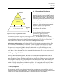
0.3 Shall, Must, Should and May
This Handbook uses the accepted definitions of shall, must, should and may, as defined in ANSI/ASQC E419949:
<
<
<
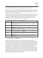
shall, must When the element and deviation from specification will constitute non-conformance with
should
may
40 CFR and the Clean Air Act
when the element is recommended
when the element is optional or discretionary
0.4 Handbook Review and Distribution
The information in this Handbook was revised and/or developed by many of the organizations implementing
the Ambient Air Quality Surveillance Program (see Acknowledgments). It has been peer-reviewed and
accepted by these organizations and serves to provide consistency among the organizations collecting and
reporting ambient air data.
This Handbook is accessible as a PDF file on the Internet under the AMTIC Homepage:
[http://www.epa.gov/ttn/amtic]
The document can be read and printed using Adobe Acrobat Reader software, which is freeware available
from many Internet sites including the EPA web site. The Internet version is write-protected and will be
updated every three years. It is recommended that the Handbook be accessed through the Internet. AMTIC
will provide information on updates to the Handbook.
Hardcopy versions are available by writing or calling:
OAQPS Library
MD-16
RTP, NC 27711
(919)541-5514
Recommendations for modifications or revisions are always welcome. Comments should be sent to the
appropriate Regional Office Ambient Air Monitoring contact or posted on AMTIC. The Handbook Steering
Committee will meet quarterly to discuss any pertinent issues and proposed changes.
Part I, Section: 1
Revision No: 0
Date: 8/98
Page 1 of 5
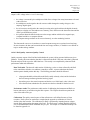
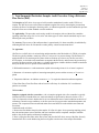
1. Program Organization
NERL
OAQPS
Clean Air
NAMS, SLAMS
PAMS, PSD
Regions
State &
locals
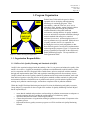
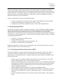
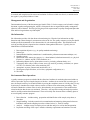
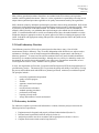
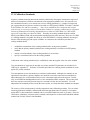
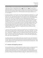
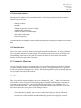
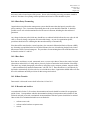
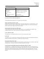
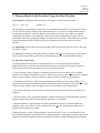
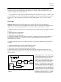
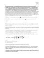
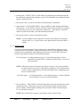
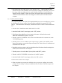
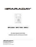
Figure 1.1 Ambient Air Program Organization
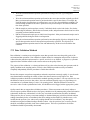
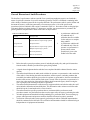
Federal, State, Tribal and local agencies all have
important roles in developing and implementing
satisfactory air monitoring programs. EPA's
responsibility, under the Clean Air Act (CAA) as
amended in 1990, includes: setting National Ambient
Air Quality Standards (NAAQS) for pollutants
considered harmful to the public health and
environment; ensuring that these air quality standards
are met or attained (in cooperation with States) through
national standards and strategies to control air
emissions from sources; and ensuring that sources of
toxic air pollutants are well controlled. Within the area
of quality assurance, the EPA is responsible for
developing the necessary tools and guidance so that
State and local agencies can effectively implement their
monitoring and QA programs. Figure 1.1 represents the
primary organizations responsible for the Ambient Air
Quality Monitoring Program. The responsibilities of
each organization follow.
1.1 Organization Responsibilities
1.1.1 Office of Air Quality Planning and Standards (OAQPS)
OAQPS is the organization charged under the authority of the CAA to protect and enhance the quality of the
nation’s air resources. OAQPS sets standards for pollutants considered harmful to public health or welfare
and, in cooperation with EPA’s Regional Offices and the States, enforces compliance with the standards
through state implementation plans (SIPs) and regulations controlling emissions from stationary sources.
OAQPS evaluates the need to regulate potential air pollutants and develops national standards; works with
State and local agencies to develop plans for meeting these standards; monitors national air quality trends
and maintains a database of information on air pollution and controls; provides technical guidance and
training on air pollution control strategies; and monitors compliance with air pollution standards.
Within the OAQPS Emissions Monitoring and Analysis Division, the Monitoring and Quality Assurance
Group (MQAG) is responsible for the oversight of the Ambient Air Quality Monitoring Network. MQAG
has the responsibility to:
<
<
<
<
ensure that the methods and procedures used in making air pollution measurements are adequate to
meet the programs objectives and that the resulting data are of satisfactory quality
operate the National Performance Audit Program (NPAP)
evaluate the performance of organizations making air pollution measurements of importance to the
regulatory process
implement satisfactory quality assurance programs over EPA's Ambient Air Quality Monitoring
Network
Part I, Section: 1
Revision No: 0
Date: 8/98
Page 2 of 5
<
<
ensure that guidance pertaining to the quality assurance aspects of the Ambient Air Program are
written and revised as necessary
render technical assistance to the EPA Regional Offices and air pollution monitoring community
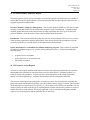
In particular to this Handbook, OAQPS will be responsible for:
<
<
<
<
coordinating the Steering Committee responsible for continued improvement of the Handbook
seeking resolution on Handbook issues
incorporating agreed upon revisions into the Handbook
reviewing and revising (if necessary) the Handbook (Vol II) every three years
Specific MQAG leads for the various QA activities (e.g, precision and accuracy, training, etc.) can be found
within the OAQPS Homepage on the Internet (http://www.epa.gov/oar/oaqps/qa/) and on the AMTIC
Bulletin Board under “Points of Contact (QA/QC contacts)”
1.1.2 EPA Regional Offices
EPA Regional Offices have been developed to address environmental issues related to the states within their
jurisdiction and to administer and oversee regulatory and congressionally mandated programs.
The major quality assurance responsibilities of EPA's Regional Offices in regards to the Ambient Air
Quality Program are the coordination of quality assurance matters between the various EPA offices and the
State and local agencies. This role requires that the Regional Offices make available to the State and local
agencies the technical and quality assurance information developed by EPA Headquarters and make known
to EPA Headquarters the unmet quality assurance needs of the State and local agencies. Another very
important function of the Regional Office is the evaluation of the capabilities of State and local agency
laboratories to measure the criteria air pollutants. These reviews are accomplished through network reviews
and technical systems audits whose frequency is addressed in the Code of Federal Regulations. To be
effective in these roles, the Regional Offices must maintain their technical capabilities with respect to air
pollution monitoring.
Specific responsibilities as it relates to the Handbook include:
<
<
<
<
<
serving as a liaison to the State and local reporting agencies for their particular Region
serving on the Handbook Steering Committee
fielding questions related to the Handbook
reporting issues that would require Steering Committee attention
serving as a reviewer of the Handbook and participating in its revision
1.1.3 State and Local Agencies
40 CFR Part 58 defines a State Agency as “the air pollution control agency primarily responsible for the
development and implementation of a plan (SIP) under the Act (CAA)”. Section 302 of the CAA provides
a more detailed description of the air pollution control agency.
40 CFR Part 58 defines the Local Agency as “any local government agency, other than the state agency,
which is charged with the responsibility for carrying out a portion of the plan (SIP).
Part I, Section: 1
Revision No: 0
Date: 8/98
Page 3 of 5
The major responsibility of State and local agencies is the implementation of a satisfactory monitoring
program, which would naturally include the implementation of an appropriate quality assurance program. It
is the responsibility of State and local agencies to implement quality assurance programs in all phases of the
data collection process, including the field, their own laboratories, and in any consulting and contractor
laboratories which they may use to obtain data.
Specific responsibilities as it relates to the Handbook include:
<
<
<
serving as a representative for the State and local agencies on the Handbook Steering Committee
assisting in the development of QA guidance for various sections
reporting issues and comments to Regional Contacts or on the AMTIC Bulletin Board
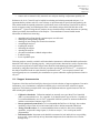
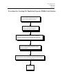
1.1.4 Reporting Organizations
40 CFR Part 58 Appendix A defines a reporting organization as “a State, subordinate organization within a
State, or other organization that is responsible for a set of stations that monitor the same pollutant and for
which precision or accuracy assessments can be pooled. States must define one or more reporting
organization for each pollutant such that each monitoring station in the State SLAMS network is included in
one, and only one, reporting organization.” Common factors that should be considered by States in defining
a reporting organization include:
1.
2.
3.
4.
operation by a common team of field operators,
common calibration facilities,
oversight by a common quality assurance organization, and
support by a common laboratory or headquarters.
Reporting organizations are used as one level of aggregation in the evaluation of quarterly and yearly data
quality assessments of precision, bias and accuracy.
1.1.5 National Exposure Research Laboratory (NERL)
The mission of NERL is to develop scientific information and assessment tools to improve the Agency’s
exposure/risk assessments, identify sources of environmental stressors, understand the transfer and
transformation of environmental stressors, and develop multi-media exposure models. The NERL provides
the following activities:
<
<
<
<
<
develops, improves, and validates methods and instruments for measuring gaseous, semi-volatile,
and non-volatile pollutants in source emissions and in ambient air
supports multi-media approaches to assessing human exposure to toxic contaminated media through
development and evaluation of analytical methods and reference materials, and provides analytical
and method support for special monitoring projects for trace elements and other inorganic and
organic constituents and pollutants
develops standards and systems needed for assuring and controlling data quality
assesses whether emerging methods for monitoring criteria pollutants are “equivalent” to accepted
Federal Reference Methods and are capable of addressing the Agency’s research and regulatory
objectives
provides an independent audit and review function on data collected by NERL or other appropriate
clients
Part I, Section: 1
Revision No: 0
Date: 8/98
Page 4 of 5
Historically, NERL was responsible for the development and maintenance of all five volumes of the
Handbook and will continue to assist in the following activities for Handbook Volume II:
<
<
<
<
serving on the Steering Committee
providing overall guidance
participating in the Handbook review process
developing and submitting new methods including the appropriate QA/QC
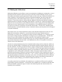
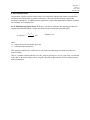
1.2 Lines of Communication
NERL
Technical
Expertise
OAQPS
National Oversight
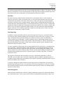
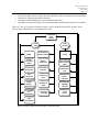
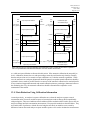
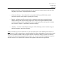
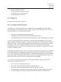
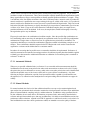
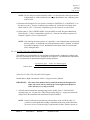
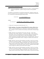
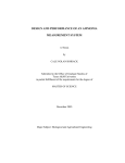
In order to maintain a successful Ambient Air
Quality Monitoring Program, effective
communication is essential. Figure 1.2
illustrates the lines of communication between
EPA Regions 1-10
the different organizations responsible for this
Regional Oversight
program. The figure represents a general
model. Specific lines of communication
within an EPA Region may be different as
long as it is understood and maintained among
State Air Pollution
State Air Pollution
all air monitoring organizations. Lines of
Control Agency
Control Agency
communication will ensure that decisions can
Local Agency Oversight
Local Agency Oversight
be made at the most appropriate levels in a
more time-efficient manner. It also means
that each organization in this structure must
Reporting
Reporting
Organizations
Organizations
be aware of the regulations governing the
QA Oversight
QA Oversight
Ambient Air Quality Monitoring Program.
Any issues that require a decision, especially
in relation to the quality of data, or the quality
Local Agency
Local Agency
system, should follow this line. At times, it is
appropriate to obtain information from a level
Figure 1.2 Lines of communication
higher than the normal lines of
communication, as shown by the dashed line
from a local agency to the EPA Regional Office. This is appropriate as long as decisions are not made
during these information seeking communications. If important decisions are made at various locations
along the line, it is important that the information is disseminated in all directions in order that
improvements to the quality system can reach all organizations in the Program. Nationwide communication
will be accomplished through AMTIC and the subsequent revisions to this Handbook.
Part I, Section: 1
Revision No: 0
Date: 8/98
Page 5 of 5
1.3 The Handbook Steering Committee
The Handbook Steering Committee is made up of representatives from following four entities in order to
provide representation at the Federal, State and local level:
<
<
<
<
OAQPS-
OAQPS is represented by the coordinator for the Handbook and other representatives
of the Ambient Air Quality Monitoring QA Team.
Regions- A minimum of 1 representative from each EPA Regional Office.
NERL A minimum of one representative. NERL represents historical knowledge of the
Handbook series as well as the expertise in the reference and equivalent methods
program and QA activities.
SAMWG - A minimum of three members from SAMWG who represent State and local air
monitoring organizations.
The mission of the committee is to provide a mechanism to meet the goals of the Handbook; which are to
provide guidance on quality assurance techniques that can help to ensure that data meet the Ambient Air
Quality Monitoring Program objectives and to ensure data comparability across the Nation.
The Steering Committee will meet quarterly to discuss emerging ambient air monitoring issues that have the
potential to effect the Handbook. Issues may surface from comments made by State and local agencies to
Regional liaisons, AMTIC bulletin board comments, or the development/revision of regulations. The
committee will also attempt to meet on an annual basis at a relevant national air meeting. This will provide
another forum to elicit comments and suggestions from agencies implementing ambient air monitoring
networks.
Part I, Section: 2
Revision No: 0
Date: 8/98
Page 1 of 5
2. Program Background
2.1 Ambient Air Quality Monitoring Network.
The purpose of this section is to describe the general concepts for establishing the Ambient Air Quality
Monitoring Network. The majority of this material as well as additional details can be found in the CAA,
40 CFR Part 5824 and their references.
Between the years 1900 and 1970, the emission of six principal pollutants increased significantly. The
principal pollutants, also called criteria pollutants are: particulate matter (PM10 and PM2.5), sulfur dioxide,
carbon monoxide, nitrogen dioxide, ozone, and lead. In 1970 the CAA was signed into law. The CAA and
its amendments provides the framework for all pertinent organizations to protect air quality.
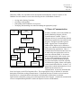
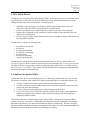
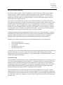
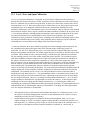
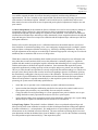
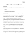
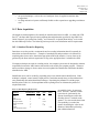
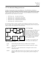
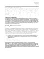
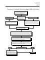
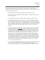
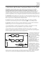
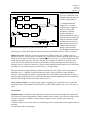
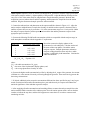
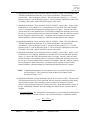
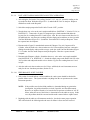
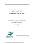
As illustrated in Figure 2.1, air quality samples are generally collected for one or more of the following
objectives:
Ambient Air Quality Monitoring Process
EPA Responsibility
Air Quality
Standard
State/Local
Responsibility
<
<
<
Ambient
Air Data
<
Emergency
Control
Attainment of
Air Quality
Standards
Trends
Analysis
Control
Strategy
Adjust
Classification
State
Implementation
Plan
Research
With the end use of the air quality samples as a
prime consideration, the network should be
designed to:
1.
2.
Continue
Air Quality
Measurement
to judge compliance with and/or progress
made towards meeting ambient air quality
standards
to activate emergency control procedures
that prevent or alleviate air pollution
episodes as well as develop long term
control strategies
to observe pollution trends throughout the
region, including non-urban areas
to provide a data base for research and
evaluation of effects: urban, land-use, and
transportation planning; development and
evaluation of abatement/control strategies;
and development and validation of
diffusion models
3.
Figure 2.1 Ambient air quality monitoring process
4.
determine the highest concentrations
expected to occur in the area covered by the
network;
determine representative concentrations in
areas of high population density;
determine the impact on ambient pollution
levels of significant sources or source
categories;
determine the general background
concentration levels;
Part I, Section: 2
Revision No: 0
Date: 8/98
Page 2 of 5
5. determine the extent of regional pollutant transport among populated areas, and in support of
secondary standards; and
6. determine the welfare-related impacts in more rural and remote areas (such as visibility impairment
and effects on vegetation)
These six objectives indicate the nature of the samples that the monitoring network will collect and will be
used during the development of data quality objectives (Section 3). As one reviews the objectives, it
becomes apparent that it will be rare that sites can be located to meet more than two or three objectives.
Therefore, each organization needs to prioritize their objectives in order to choose the sites that are most
representative of that objective and will provide data of adequate quality.
Through the process of implementing the CAA, a number of ambient air quality monitoring networks have
been developed. The EPA's Ambient Air Quality Monitoring Program is carried out by State and local
agencies and consists of four major categories of monitoring stations or networks that measure the criteria
pollutants. These stations are described below.
State and Local Air Monitoring Stations (SLAMS)
The SLAMS consist of a network of ~ 4,000 monitoring stations whose size and distribution is largely
determined by the needs of State and local air pollution control agencies to meet their respective state
implementation plan (SIP) requirements. The SIPs provide for the implementation, maintenance, and
enforcement of the national ambient air quality standards (NAAQS) in each air quality control region within
a state.
National Air Monitoring Stations (NAMS)
The NAMS (~1,000 stations) are a subset of the SLAMS network with emphasis being given to urban and
multi-source areas. In effect, they are key sites under SLAMS, with emphasis on areas of expected
maximum concentrations (category A) and stations which combine poor air quality with high population
density (category B). Generally, category B monitors would represent larger spatial scales than category A
monitors.
Special Purpose Monitoring Stations (SPMS)
Special Purpose Monitoring Stations provide for special studies needed by the State and local agencies to
support SIPs and other air program activities. The SPMS are not permanently established and can be
adjusted to accommodate changing needs and priorities. The SPMS are used to supplement the fixed
monitoring network as circumstances require and resources permit. If the data from SPMS are used for SIP
purposes, they must meet all QA and methodology requirements for SLAMS monitoring.
Photochemical Assessment Monitoring Stations (PAMS)
A PAMS network is required in each ozone non-attainment area that is designated serious, severe, or
extreme. The required networks will have from two to five sites, depending on the population of the area.
There is a phase-in period of one site per year which started in 1994. The ultimate PAMS network could
exceed 90 sites at the end of the 5-year phase-in period.
Part I, Section: 2
Revision No: 0
Date: 8/98
Page 3 of 5
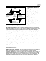
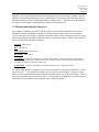
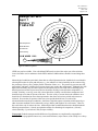
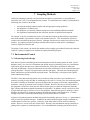
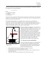
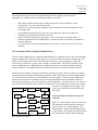
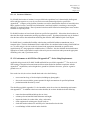
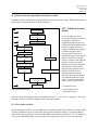
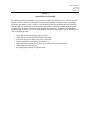
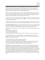
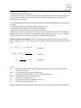
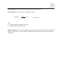
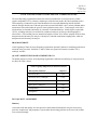
2.2 Ambient Air Monitoring
QA Program
Planning
NAAMP
Methods
Guidance
Reports
Data Quality Assessments
P & A Reports
QA Reports
Audit Reports
DQOs
Training
Ambient Air
QA
Life Cycle
Implementation
QAPP development
Internal QC Activities
P&A
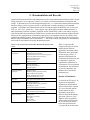
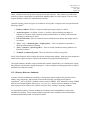
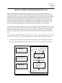
Figure 2.2 represents the stages of the
Ambient Air Quality Monitoring QA
Program. The planning, implementation,
assessment and reporting tools will be
briefly discussed below.
2.2.1 Planning
Planning activities include:
Assessments
Systems Audits (State/EPA)
Network Reviews
FRM Performance Evaluation
The National Ambient Air Management
Plan (NAAMP) - This is a document that
describes how the QA activities that are the
responsibility of the EPA Regions and
Headquarters will be implemented.
Figure 2.2 Ambient Air Quality Monitoring QA Program
Data Quality Objectives (DQOs) - DQOs are qualitative and quantitative statements derived from the
outputs of the DQO Process that: 1) clarify the study objective; 2) define the most appropriate type of data
to collect; 3) determine the most appropriate conditions from which to collect the data; and 4) specify
tolerable limits on decision errors which will be used as the basis for establishing the quantity and quality of
data needed to support the decision. This process is discussed in Section 3.
Methods- Reference methods and measurement principles have been written for each criteria pollutant.
Since these methods can not be applied to the actual instruments acquired by each State and local
organization, they should be considered as guidance for detailed standard operating procedures that would
be developed as part of an acceptable QA project plan.
Training - Training is a part of any good monitoring program. Training activities are discussed in Section
4.
Guidance - This QA Handbook as well as many other guidance documents have been developed for the
Ambient Air Quality Monitoring Program. A list of these documents is included in Appendix 2.
2.2.2 Implementation
Implementation activities include:
QA Project Plan (QAPP) Development - Each State and local organization must develop a QAPP. The
primary purpose of the QAPP is to provide an overview of the project, describe the need for the
measurements, and define QA/QC activities to be applied to the project, all within a single document. The
QAPP should be detailed enough to provide a clear description of every aspect of the project and include
information for every member of the project staff, including samplers, lab staff, and data reviewers. The
QAPP facilitates communication among clients, data users, project staff, management, and external
Part I, Section: 2
Revision No: 0
Date: 8/98
Page 4 of 5
reviewers. Effective implementation of the QAPP assists project managers in keeping projects on schedule
and within the resource budget.
Internal QC Activities - Quality Control (QC) is the overall system of technical activities that measures the
attributes and performance of a process, item, or service against defined standards to verify that they meet
the stated requirements established by the customer; that are used to fulfill requirements for quality9. In the
case of the Ambient Air Quality Monitoring Network, QC activities are used to ensure that measurement
uncertainty is maintained within established acceptance criteria for the attainment of the DQOs.
Federal regulation provides for the implementation of a number of qualitative and quantitative checks to
ensure that the data will meet the DQOs. Each of the checks attempts to evaluate phases of measurement
uncertainty. Some of these checks are discussed below and in Section 10.
Precision and Accuracy (P & A) Checks - These checks are described in the Code of Federal
Regulations14, as well as a number of sections in this document, in particular, Section 10. These checks
can be used to provide an overall assessment of measurement uncertainty.
Zero/Span Checks - These checks provide an internal quality control check of proper operation of the
measurement system. These checks are discussed in Section 10 and 12.
Annual Certifications - A certification is the process which ensures the traceability and viability of
various QC standards. Standard traceability is the process of transferring the accuracy or authority of
a primary standard to a field-usable standard. Traceability protocols are available for certifying a
working standard by direct comparison to an NIST-SRM 66 91,. Certification requirements are included
in Section 10 as well as the individual methods in Part 2.
Calibrations - Calibrations should be carried out at the field monitoring site by allowing the analyzer
to sample test atmospheres containing known pollutant concentrations. Calibrations are discussed in
Section 12.
2.2.3 Assessments
Assessment, as defined in E49, are evaluation processes used to measure the performance or effectiveness of
a system and its elements. It is an all inclusive term used to denote any of the following: audit, performance
evaluation, management systems review, peer review, inspection, or surveillance. Assessments for the
Ambient Air Quality Monitoring Program, as discussed in Section 15, include:
Technical Systems Audits (TSA) -A TSA is an on-site review and inspection of a State or local agency's
ambient air monitoring program to assess its compliance with established regulations governing the
collection, analysis, validation, and reporting of ambient air quality data. Both EPA and State organizations
perform TSAs. Procedures for this audit are included in Appendix 15 and discussed in general terms in
Section 16
Network Reviews - The network review is used to determine how well a particular air monitoring network
is achieving its required air monitoring objective(s), and how it should be modified to continue to meet its
objective(s). Network reviews are discussed in Section 16.
Part I, Section: 2
Revision No: 0
Date: 8/98
Page 5 of 5
Performance Evaluations- Performance evaluations are a type of audit in which the quantitative data
generated in a measurement system are obtained independently and compared with routinely obtained data to
evaluate the proficiency of an analyst , laboratory, or measurement system. The following performance
evaluations are included in the Ambient Air Quality Monitoring Program:
State Performance Evaluations (Audits) - These performance evaluation audits are used to
provide an independent assessment on the measurement operations of each instrument by
comparing performance samples or devices of “known” concentrations or values to the values
measured by the instrument. This audit is discussed in Section 16.
NPAP - The goal of the NPAP is to provide audit material and devices that will enable EPA to
assess the proficiency of agencies who are operating monitors in the SLAMS, NAMS, PAMS and
PSD networks. NPAP samples or devices of “known” concentration or values, but unknown to the
audited organization, are compared to the values measured by the audited instrument. This audit is
discussed in Section 16.
PM2.5 Federal Reference Method (FRM) Performance Evaluation -The FRM Performance
Evaluation is a quality assurance activity which will be used to evaluate measurement system bias
of the PM2.5 monitoring network. The pertinent regulations for this performance evaluation are
found in 40 CFR Part 58, Appendix A14. The strategy is to collocate a portable FRM PM2.5 air
sampling instrument with an established routine air monitoring instrument, operate both monitors in
exactly the same manner and then compare the results of this instrument against the routine sampler
at the site. This evaluation is discussed in Section 16.
2.2.4 Reports
All concentration data will require data assessments to evaluate the attainment of the DQOs, and reports of
these assessments or reviews. The following types of reports, as discussed in Section 16, should include:
Data quality assessment (DQA) -is the scientific and statistical evaluation to determine if data are of the
right type, quality and quantity to support their intended use (DQOs). QA/QC data can be statistically
assessed at various levels of aggregation to determine whether the DQOs have been attained. Data quality
assessments of precision, bias and accuracy can be aggregated at the following three levels.
<
<
<
Monitor- monitor/method designation
Reporting Organization- monitors in a method designation, all monitors
National - monitors in a method designation, all monitors
P & A Reports - These reports are generated annually and evaluate the precision and accuracy data against
the acceptance criteria discussed in Section 3.
QA Reports - A QA report provides an evaluation of QA/QC data for a given time period to determine
whether the data quality objectives were met. Discussions of QA reports can be found in sections 16 and
18.
Meetings and Calls - Various national meetings and conference calls can be used as assessment tools for
improving the network. It is important that information derived from the avenues of communication are
appropriately documented (annual QA Reports) .
Part I, Section: 3
Revision No: 0
Date: 8/98
Page 1 of 6
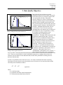
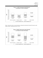
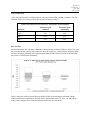
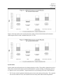
3. Data Quality Objectives
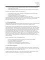
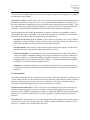
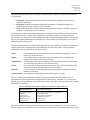
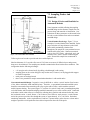
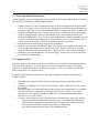
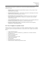
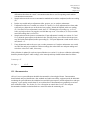
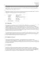
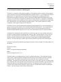
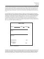
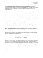
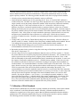
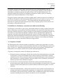
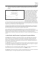
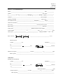
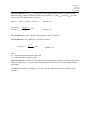
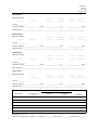
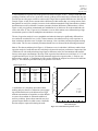
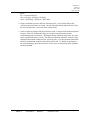
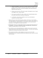
Data collected for the Ambient Air Quality
Monitoring Program are used to make very specific
0.07
Unbiased, mean = 14
decisions that can have an economic impact on the
Biased (+15%), mean = 16.6
0.06
area represented by the data. Data quality
0.05
objectives (DQOs) are a full set of performance
0.04
constraints needed to design an environmental data
0.03
operation (EDO), including a specification of the
0.02
level of uncertainty that a decision maker (data user)
0.01
is willing to accept in the data to which the decision
0
will apply. Throughout this document, the term
0
5
10
15
20
25
30
35
40
45
-0.01
decision maker is used. This term represents
Concentration
individuals that are the ultimate users of ambient air
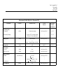
Figure 3.1. Effect of positive bias on the annual average
data and therefore may be responsible for: setting
estimate, resulting in a false positive decision error
the NAAQS, developing a quality system,
evaluating the data, or declaring an area
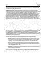
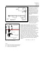
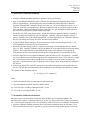
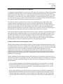
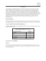
0.07
nonattainment. The DQO will be based on the data
Unbiased, mean = 16
0.06
requirements of the decision maker. Decision
Biased (-15%), mean = 13.6
0.05
makers need to feel confident that the data used to
make environmental decisions are of adequate
0.04
quality. The data used in these decisions are never
0.03
error free and always contain some level of
0.02
uncertainty. Because of these uncertainties or
0.01
errors, there is a possibility that decision makers
may declare an area “nonattainment” when the area
0
0
5
10
15
20
25
30
35
40
45
is actually in “attainment” (false positive error) or
Concentration
“attainment” when actually the area is in
Figure 3.2. Effect of negative bias on the annual average
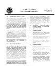
“nonattainment” (false negative error). Figures 3.1
resulting in a false negative decision error
and 3.2 illustrate how false positive and negative
errors can affect a NAAQS attainment/nonattainment decision based on an annual mean concentration value
of 15. There are serious political, economic and health consequences of making such decision errors.
Therefore, decision makers need to understand and set limits on the probabilities of making incorrect
decisions with these data.
Probability Density
Probability Density
0.08
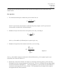
In order to set probability limits on decision errors, one needs to understand and control uncertainty.
Uncertainty is used as a generic term to describe the sum of all sources of error associated with an EDO.
Uncertainty can be illustrated as follows:
2
2
2
So ' Sp % Sm
(equation 1)
Where:
So= overall uncertainty
Sp= population uncertainty (spatial and temporal)
Sm= measurement uncertainty (data collection)
Part I, Section: 3
Revision No: 0
Date: 8/98
Page 2 of 6
The estimate of overall uncertainty is an important component in the DQO process. Both population and
measurement uncertainties must be understood.
Population uncertainties - The most important data quality attribute of any ambient air monitoring
network is representativeness. This term refers to the degree in which data accurately and precisely represent
a characteristic of a population, parameter variation at a sampling point, a process condition, or an
environmental condition9. Population uncertainty, the spatial and temporal components of error, can effect
representativeness. These uncertainties can be controlled through the selection of appropriate boundary
conditions (the area and the time period) to which the decision will apply, and the development of a proper
statistical sampling design (see Section 6). Appendix H of the QAD document titled EPA Guidance for
Quality Assurance Project Plans32 provides a very good dissertation on representativeness. It does not
matter how precise or unbiased the measurement values are if a site is unrepresentative of the population it
is presumed to represent. Assuring the collection of a representative air quality sample depends on the
following factors:
< selecting a network size that is consistent with the monitoring objectives and locating representative
sampling sites
< determining restraints on the sampling sites that are imposed by meteorology, local topography,
emission sources, and the physical constraints and documenting these
< planning sampling schedules that are consistent with the monitoring objectives
Measurement uncertainties are the errors associated with the EDO, including errors associated with the
field, preparation and laboratory measurement phases. At each measurement phase, errors can occur, that in
most cases, are additive. The goal of a QA program is to control measurement uncertainty to an acceptable
level through the use of various quality control and evaluation techniques. In a resource constrained
environment, it is most important to be able to calculate/evaluate the total measurement system uncertainty
(Sm) and compare this to the DQO. If resources are available, it may be possible to evaluate various phases
(field, laboratory) of the measurement system.
Three data quality indicators are most important in determining total measurement uncertainty:
<
Precision - a measure of mutual agreement among individual measurements of the same property
usually under prescribed similar conditions. This is the random component of error. Precision is
estimated by various statistical techniques using some derivation of the standard deviation.
<
Bias - the systematic or persistent distortion of a measurement process which causes error in one
direction. Bias will be determined by estimating the positive and negative deviation from the true
value as a percentage of the true value.
<
Detectability - The determination of the low range critical value of a characteristic that a method
specific procedure can reliably discern.
Accuracy has been a term frequently used to represent closeness to “truth” and includes a combination of
precision and bias error components. This term has been used throughout the CFR and in some of the
sections of this document. If possible, it is recommended that an attempt be made to distinguish
measurement uncertainties into precision and bias components.
Part I, Section: 3
Revision No: 0
Date: 8/98
Page 3 of 6
3.1 The DQOs Process
The DQO process is used to facilitate the planning of EDOs. It asks the data user to focus their EDO efforts
by specifying the use of the data (the decision), the decision criteria, and the probability they can accept
making an incorrect decision based on the data. The DQO process:
<
<
<
<
establishes a common language to be shared by decision makers, technical personnel, and
statisticians in their discussion of program objectives and data quality
provides a mechanism to pare down a multitude of objectives into major critical questions
facilitates the development of clear statements of program objectives and constraints which will
optimize data collection plans
provides a logical structure within which an iterative process of guidance, design, and feedback may
be accomplished efficiently
The DQO process contains the following steps:
<
<
<
<
<
<
<
the problem to be resolved
the decision
the inputs to the decision
the boundaries of the study
the decision rule
the limits on uncertainty
study design optimization
The DQO Process is fully discussed in the document titled Guidance for the Data Quality Objectives
Process EPA QA/G439, and is available on the EPA QA Division Homepage (http://es.epa.gov/ncerqa/qa/).
The EPA QA Division also provides a software program titled Data Quality Objectives (DQO) Decision
Error Feasibility Trials (DEFT). This software can help individuals develop appropriate sampling designs
based upon the outputs of the DQO Process.
3.2 Ambient Air Quality DQOs
As indicated above, the first step in the DQO process is to identify the problems that need to be resolved.
The objectives (problems) of the Ambient Air Quality Monitoring Program as mentioned in Section 2 are:
1. To judge compliance with and/or progress made towards meeting the NAAQS.
2. To activate emergency control procedures that prevent or alleviate air pollution episodes as well as
develop long term control strategies.
3. To observe pollution trends throughout the region, including non-urban areas.
4. To provide a data base for research and evaluation of effects: urban, land-use, and transportation
planning; development and evaluation of abatement/control strategies; and development and
validation of diffusion models.
These different objectives could potentially require different DQOs, making the development of DQOs
complex. However, if one were to establish DQOs based upon the objective requiring the most stringent
data quality requirements, one could assume that the other objectives could be met. Therefore, the DQOs
have been initially established based upon ensuring that decision makers can make attainment/nonattainment
decisions in relation to the NAAQS within a specified degree of certainty.
Part I, Section: 3
Revision No: 0
Date: 8/98
Page 4 of 6
Appendix 3 will eventually contain information on the DQO process for each criteria pollutant. Since the
Ambient Air Quality Monitoring Network was established prior to the development of the DQO Process, a
different technique was used to establish data quality acceptance levels27. Therefore, all criteria pollutants
are being reviewed in order to establish DQOs using the current DQO process.
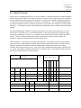
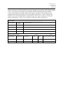
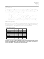
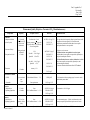
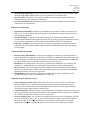
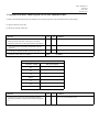
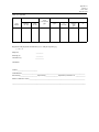
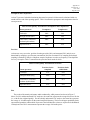
3.3 Measurement Quality Objectives
Once a DQO is established, the quality of the data must be evaluated and controlled to ensure that it is
maintained within the established acceptance criteria. Measurement quality objectives are designed to
evaluate and control various phases (sampling, preparation, analysis) of the measurement process to ensure
that total measurement uncertainty is within the range prescribed by the DQOs. MQOs can be defined in
terms of the following data quality indicators:
Precision - defined above
Bias - defined above.
Representativeness - defined above
Detectability- defined above
Completeness - a measure of the amount of valid data obtained from a measurement system compared to the
amount that was expected to be obtained under correct, normal conditions. Data completeness requirements are
included in the reference methods (40 CFR Pt. 50).
Comparability - a measure of confidence with which one data set can be compared to another.
For each of these attributes, acceptance criteria can be developed for various phases of the EDO. Various
parts of 40 CFR 21- 24 have identified acceptance criteria for some of these attributes. In theory, if these
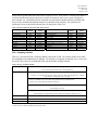
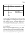
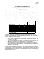
MQOs are met, measurement uncertainty should be controlled to the levels required by the DQO. Tables of
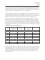
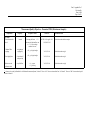
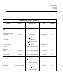
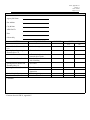
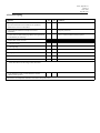
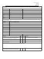
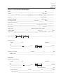
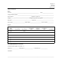
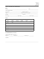
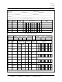
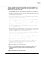
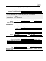
the most critical MQOs can be developed. Table 3-1 is an example of an MQO table for carbon monoxide.
MQO tables for the remaining criteria pollutants can be found in Appendix 3.
Section No: 3
Revision No: 0
Date: 8/98
Page 5 of 6
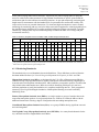
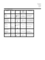
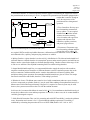
Table 3-1 Measurement Quality Objectives - Parameter CO
Measurement Quality Objectives - Parameter CO (Nondispersive Infrared Photometry)
Requirement
Standard Reporting Units
Shelter Temperature
Temperature range
Temperature control
Equipment
CO analyzer
Flow controllers
Flowmeters
Detection Limit
Noise
Lower detectable level
Completeness
8-hour average
Compressed Gases
Dilution gas (zero air)
Gaseous standards
Frequency
Acceptance Criteria
Reference
All data
ppm
40 CFR, Pt 50.8
Daily
Daily
20 to 30E C.
< ± 2E C
Purchase
specification
Reference or equivalent method
Flow rate regulated to ± 1%
Accuracy ± 2%
40 CFR, Pt 50, App C
"
“
Purchase
specification
0.5 ppm
1.0 ppm
40 CFR, Pt 53.20 & 23
“
hourly
$75 % of hourly averages for the 8hour period
40 CFR, Pt 50.8
Purchase
specification
Purchase
specification
< 0.1 ppm CO
40 CFR, Pt 50, App C
"
EPA-600/R97/12
NIST Traceable
(e.g., EPA Protocol Gas)
40 CFR, Pt. 53.20
Vol II, S 7.1 1/
Information/Action
Instruments designated as reference or equivalent have been
tested over this temperature range. Maintain shelter
temperature above sample dewpoint. Shelter should have a
24- hour temperature recorder. Flag all data for which
temperature range or fluctuations are outside acceptance
criteria.
Instruments designated as reference or equivalent have been
determined to meet these acceptance criteria.
Return cylinder to supplier.
Carbon monoxide in nitrogen or air EPA Protocol Gases have
a 36-month certification period and must be recertified to
extend the certification.
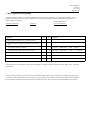
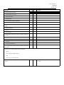
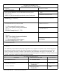
Section No: 3
Revision No: 0
Date: 8/98
Page 6 of 6
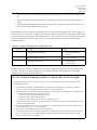
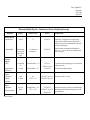
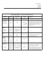
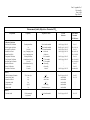
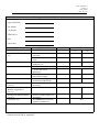
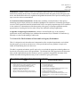
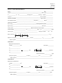
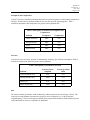
Measurement Quality Objectives - Parameter CO (Nondispersive Infrared Photometry)
Requirement
Calibration
Multipoint calibration
(at least 5 points)
Zero/span check-level 1
Flowmeters
Performance Evaluation
(NPAP)
Frequency
Acceptance Criteria
Reference
Upon receipt,
adjustment, or
1/ 6 months
All points within ± 2% of full scale
of best-fit straight line
Vol II, S 12.6
Vol II, MS.2.6.1
1/ 2 weeks
Zero drift # ± 2 to 3 ppm
Span drift # ± 20 to 25 %
Vol II, S 12.6
"
Zero drift # ± 1 to 1.5 ppm
Span drift # ± 15%
Vol II, S 12.6
"
1/3 months
Accuracy ± 2 %
Vol II, App 12
1/year at selected
sites
Mean absolute difference # 15%
Vol II, S 16.3
State requirements
Vol II, pp 15, S 3
State audits
Information/Action
Zero gas and at least four upscale calibration points. Points
outside acceptance criterion are repeated. If still outside
criterion, consult manufacturers manual and invalidate data to
last acceptable calibration.
If calibration updated at each zero/span, invalidate data to
last acceptable check, adjust analyzer, perform multipoint
calibration.
If fixed calibration used to calculate data, invalidate data to
last acceptable check, adjust analyzer, perform multipoint
calibration.
Flowmeter calibration should be traceable to NIST standards.
Use information to inform reporting agency for corrective
action and technical systems audits
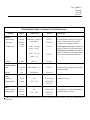
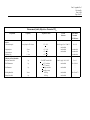
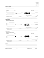
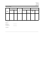
1 /year
Precision
Single analyzer
Reporting organization
Accuracy
Single analyzer
Reporting organization
1/
½ weeks
1/3 months
25 % of sites
quarterly (all sites
yearly)
None
95% CI # ± 15%
None
95% CI # ± 20%
40 CFR, Pt 58, App A
EPA-600/4-83-023
Vol II, App 15, S 5
40 CFR, Pt 58, App A
Concentration = 8 to 10 ppm. Aggregation of a quarters
measured precision values.
Four concentration ranges. If failure, recalibrate and
reanalyze. Repeated failure requires corrective action.
- reference refers to the QA Handbook for Air Pollution Measurement Systems Volume II . The use of “S” refers to sections within the handbook. The use of “MS” refers to sections
of the method for the particular pollutant.
Part I, Section: 4
Revision No: 0
Date: 8/98
Page 1 of 4
4. Personnel Qualifications, Training and Guidance
4.1 Personnel Qualifications
Personnel assigned to ambient air monitoring activities are expected to have met the educational, work
experience, responsibility, personal attributes and training requirements for their positions. In some cases,
certain positions may require certification and or recertification. These requirements should be outlined in
the position advertisement and in personal position descriptions. Records on personnel qualifications and
training should be maintained and should be accessible for review during audit activities. These records
should be retained as described in Section 5.
4.2 Training
Adequate education and training are integral to any monitoring program that strives for reliable and
comparable data. Training is aimed at increasing the effectiveness of employees and their organization. As
part of a quality assurance program, 40 CFR Part 58 App A14 requires the development of operational
procedures for training. These procedures should include information on:
<
<
<
personnel qualifications- general and position specific
training requirements - by position
frequency of training
Appropriate training should be available to employees supporting the Ambient Air Quality Monitoring
Program, commensurate with their duties. Such training may consist of classroom lectures, workshops,
teleconferences and on-the-job training.
4.2.1 Suggested Training
Over the years, a number of courses have been developed for personnel involved with ambient air
monitoring and quality assurance aspects. Formal QA/QC training is offered through the following
organizations:
<
<
<
<
<
<
Air Pollution Training Institute (APTI) http://www.epa.gov/oar/oaq.apti.html
Air & Waste Management Association (AWMA) http://www2.awma.org
American Society for Quality Control (ASQC) http://www.asqc.org/products/educat.html
EPA Institute
EPA Quality Assurance Division (QAD) http://es.epa.gov/ncerqa/qa/
EPA Regional Offices
In addition, OAQPS uses contractors and academic institutions to develop and provide training for data
collection activities that support regulatory efforts throughout OAQPS, as well as the States and Regions.
The OAQPS QA Program maintains a list of available courses.
Table 4-1 provides a suggested sequence of core QA-related ambient air monitoring courses for ambient air
monitoring staff, and QA managers (marked by asterisk). The suggested course sequences assume little or
no experience in QA/QC or air monitoring. Persons having experience in the subject matter described in the
Part I, Section: 4
Revision No: 0
Date: 8/98
Page 2 of 4
courses would select courses according to their appropriate experience level. Courses not included in the
core sequence would be selected according to individual responsibilities, preferences, and available
resources.
Table 4-1. Suggested Sequence of Core QA-related Ambient Air Training Courses for Ambient Air Monitoring and QA
Personnel
Sequence
Course Title (SI = self instructional)
Source
1*
Air Pollution Control Orientation Course (Revised), SI:422
APTI
2*
Principles and Practices of Air Pollution Control, 452
APTI
3*
Orientation to Quality Assurance Management
QAD
4*
Introduction to Ambient Air Monitoring (Under Revision 7/98), SI:434
APTI
5*
General Quality Assurance Considerations for Ambient Air Monitoring (Under Revision 9/98),
SI:471
APTI
6*
Quality Assurance for Air Pollution Measurement Systems (Under Revision 8/98), 470
APTI
7*
Data Quality Objectives Workshop
QAD
8*
Quality Assurance Project Plan
QAD
9
Atmospheric Sampling (Under Revision 7/98), 435
APTI
10
Analytical Methods for Air Quality Standards, 464
APTI
11
Chain Of Custody Procedures for Samples and Data, SI:443
APTI
*
Data Quality Assessment
QAD
*
Management Systems Review
QAD
*
Beginning Environmental Statistical Techniques (Revised), SI:473A
APTI
*
Introduction to Environmental Statistics, SI:473B
APTI
*
Quality Audits for Improved Performance
AWMA
*
Statistics for Effective Decision Making
ASQC
* Courses recommended for QA Managers
4.3 Regulations and Guidance
Information on the proper implementation of the Ambient Air Quality Monitoring QA Program has been
developed at three levels, as indicated in Figure 4.1. The top two levels (shaded) provide standards,
regulations and guidance that form the basis for implementation documents for specific projects. A
discussion of the information in these levels follow.
Part I, Section: 4
Revision No: 0
Date: 8/98
Page 3 of 4
4.3.1 Standards and Regulations
CFR
Standards &
Regulations
At the highest level, standards and regulations
determine what QA is required for the monitoring
program and therefore sets the stage for program
and project specific guidance. The standards and
regulations pertinent to the Ambient Air Quality
Monitoring Program include:
E4
QAD R&G
NAAMP
Program
Specific
QA Handbook
Ambient Monitoring Guidance
Project
Specific
SIPs, QA Project Plans, SOPs
CFR - The CFR series provides the mandate for
monitoring and the minimum requirements for
the quality system. It also requires the
development of QA Project Plans for any
environmental data operations.
E4 - E4 refers to the document American
National Standard-Specifications and
Guidelines for Quality Systems for
Figure 4.1 Hierarchy of regulations and guidance
Environmental Data Collection and
Environmental Technology Programs (ANSI/ASQC E4-1994)9. This document describes a basic set of
mandatory specifications and non-mandatory guidelines by which a quality system for programs involving
environmental data collection can be planned, implemented, and assessed. The EPA QA Order (5360.1
CHG 1) adheres to E4 under the authority of the Office of Management and Budget.
QAD guidance and regulations- QAD refers to the EPA QA Division, the organization within the EPA
that is responsible for the “Mandatory QA Program”. QAD is responsible for developing QA and QC
requirements and for overseeing Agency-wide implementation of the EPA Quality System. QAD has
developed a series of regulation/guidance documents that describe how to plan implement and assess
environmental data operations. Figure 4.2 describes the documents and the stages in the EDO in which they
apply. Many of these documents and can be downloaded from the Internet (http://es.epa.gov/ncerqa/qa/).
4.3.2 Program Specific Guidance
Based upon the standards and regulations, the Office of Air Quality Planning and Standards, ORD, and
other organizations implementing air monitoring have developed guidance specific to the Ambient Air
Quality Monitoring Program. This Handbook provides the majority of the guidance necessary for the State
and local agencies to develop QA project plans specific to their data collection needs. Other guidance has
been developed specific to a part of the measurement system (i.e., calibration techniques) or to specific
methods. A listing of this guidance is included in Appendix 2. It is anticipated that the majority of these
documents will be available through the Internet, most likely on the AMTIC bulletin board
4.3.3 Project Specific
The term “project specific” refers to the environmental data operations that occur at each State and local
organization operating a monitoring network. An environmental data operation refers to the work performed
to obtain, use, or report information pertaining to environmental processes and conditions9..
G-5S
Guidance on
Sampling Plans
Intended use,
Study boundaries,
Quality goals,
Resource constraints
Limits on
decision errors
Decision rule
Decision rule,
Limits on
decision error
Design
Figure 4.2 EPA QA Division Guidance Documents
G-4R
DQOs for
Research
G-4S
DQO Process
for Superfund
G-4
Guidance on the
DQO Process
(decision making)
Initial
Planning
Sampling
plan,
analytical
methods
G-5
Guidance on QA
Project Plans
Implementation
Planning
P
G-6
Guidance for
Preparing Standard
Operating Procedures
SOP documentation
P ce
SO man
r
o
f
er
Protocols
specifications
G-8
Guidance on
Technical
Assessments
As
s
pro essm
toc ent
ols
Data
Collection
G-9
Guidance for Data
Quality Assessment
Assessment
Routine data
Ancillary data,
QC data
Implementation
TSAs, PEs,
surveillance
Planning
Part I, Section: 4
Revision No: 0
Date: 8/98
Page 4 of 4
Part I, Section: 5
Revision No: 0
Date: 8/98
Page: 1 of 5
5. Documentation and Records
Organizations that perform EDOs and management activities must establish and maintain procedures for the
timely preparation, review, approval, issuance, use, control, revision and maintenance of documents and
records. A document, from a records management perspective, is a volume that contains information which
describes, defines, specifies, reports, certifies, or provides data or results pertaining to environmental
programs. As defined in the Federal Records Act of 1950 and the Paperwork Reduction Act of 1995 (now
44 U.S.C. 3101-3107), records are: "...books, papers, maps, photographs, machine readable materials, or
other documentary materials, regardless of physical form or characteristics, made or received by an agency
of the United States Government under Federal Law or in connection with the transaction of public business
and preserved or appropriate for preservation by that agency or its legitimate successor as evidence of the
organization, functions, policies, decisions, procedures, operations, or other activities of the Government or
because of the informational value of data in them.... " This section will provide guidance of documentation
and records for the Ambient Air Quality Monitoring Program.
Table 5-1 Types of Information that Should be Retained Through Document
Control
Categories
Record/Document Types
Management and
Organization
State Implementation Plan
Reporting agency information
Organizational structure of monitoring program
Personnel qualifications and training
Quality management plan
Document control plan
Support contracts
Site Information
Network description
Site characterization file
Site maps/pictures
Environmental Data
Operations
QA Project Plans
Standard operating procedures (SOPs)
Field and laboratory notebooks
Sample handling/custody records
Inspection/maintenance records
Raw Data
Any original data (routine and QC)
Data Reporting
Air quality index report
Annual SLAMS air quality information
Data/summary reports
Journal articles/papers/presentations
Data Management
Data algorithms
Data management plans/flowcharts
Quality Assurance
Control charts
Data quality assessments
QA reports
System audits
Network reviews
Table 5-1 represents the
categories and types of records
and documents which are
applicable to document control.
Information on key documents
in each category follow. It
should be noted that the list
contains documents that may not
be applicable to particular
organizations and therefore is
not meant to be a list of required
documentation. This list should
also not be construed as the
definitive list of record and
document types.
Statute of Limitations As stated in 40 CFR part 31.42,
in general, all information
considered as documentation
and records should be retained
for 3 years from the date the
grantee submits its final
expenditure report unless
otherwise noted in the funding
agreement. However, if any
litigation, claim, negotiation,
audit or other action involving
the records has been started
before the expiration of the
3-year period, the records must
Part I, Section: 5
Revision No: 0
Date: 8/98
Page: 2 of 5
be retained until completion of the action and resolution of all issues which arise from it, or until the end of
the regular 3-year period, whichever is later.
Management and Organization
Documentation for many of the document types listed in Table 5-1 for this category can be found in a single
document, a quality management plan, which is a blueprint for how an organizations quality management
objectives will be attained. The EPA QA Division provides requirements for quality management plans that
State and local organizations may find helpful33.
Site Information
Site information provides vital data about each monitoring site. Historical site information can help
determine and evaluate changes in measurement values at the site. The quality assurance project plan should
include specific documentation of site characteristics for each monitoring station. This information will
assist in providing objective inputs into the evaluation of data gathered at that site. Typically, the site
identification record should include:
1.
2.
3.
4.
5.
6.
7.
8.
9.
10.
Data acquisition objective (e.g., air quality standards monitoring).
Station type.
Instrumentation checklist (manufacturer’s model number, pollutant measurement technique, etc.).
Sampling system.
Spatial scale of the station (site category--i.e., urban/industrial, suburban/commercial, etc.; physical
location--i.e., address, AQCR, UTM coordinates, etc.).
Influential pollutant sources (point and area sources, proximity, pollutant density, etc.).
Topography (hills, valleys, bodies of water, trees; type and size, proximity, orientation, etc. picture
of a 360o view from the probe of the monitoring site).
Atmospheric exposure (unrestricted, interferences, etc.).
Site diagram (sample flowsheet, service lines, equipment configuration, etc.).
Site audits.
Environmental Data Operations
A quality assurance program associated with the collection of ambient air monitoring data must include an
effective procedure for preserving the integrity of the data. Ambient air test results and, in certain types of
tests, the sample itself may be essential elements in proving the compliance status of a facility; that is, it may
be necessary to introduce the sample or the test results as evidence in an enforcement proceeding. These
will not be admitted as evidence unless it can be shown that they are representative of the conditions that
existed at the time that the test was conducted. Therefore, each step in the testing and analysis procedure
must be carefully monitored and documented. There are basically four elements in the evidentiary phase of
an overall quality assurance program:
1. Data collection - includes testing, preparation and identification of the sample, strip charts, or
other data.
2. Sample handling - includes protection from contamination and tampering during transfer between
individuals and from the sampling site to the evidence locker (i.e., chain of custody).
3. Analysis - includes storage of samples prior to and after analysis as well as data interpretation.
4. Preparation and filing of test report - includes evidentiary requirements and retention of records.
Part I, Section: 5
Revision No: 0
Date: 8/98
Page: 3 of 5
Failure to include any one of these elements in the collection and analysis of ambient air monitoring data
may render the results of the program inadmissible as evidence, or may seriously undermine the credibility
of any report based on these data.
Environmental data operations include all the operations required to successfully measure and report a value
within the data quality objectives. Documentation for environmental data operations would include:
<
<
<
<
QA Project Plans - Documents how environmental data operations are planned, implemented, and
assessed during the life cycle of a program, project, or task32,34. See below.
Standard operating procedures (SOPs)-Written documents that detail the method for an
operation, analysis, or action with thoroughly prescribed techniques and steps42. See Section 9 and
below.
Field and laboratory notebooks- Any documentation that may provide additional information
about the environmental data operation (e.g., calibration notebooks, temperature records, site notes,
maintenance records etc.). See below
Sample handling/custody records- Records tracing sample handling from the site through
analysis, including transportation to facilities, sample storage, and handling between individuals
within facilities. Section 12 provides more information on this activity.
Quality Assurance Project Plans-As mentioned in the assistance agreement sections of 40 CFR parts 30.54 (Non-State an Local Gov.) and
31.45 (State and Local Gov.) quality assurance programs must be established. In addition to the grant
requirements, 40 CFR Part 58 Appendix A14 states that each quality assurance program must be described
in detail in accordance with the EPA Requirements for Quality Assurance Project Plans for Environmental
Data Operations 34.
Standard operating procedures-Standard operating procedures are written documents that detail the method for an operation, analysis, or
action with thoroughly prescribed techniques and steps. It is officially approved as the method for all
routine activities, especially those that are involved in the environmental data operations, which generally
involve repetitious operations performed in a consistent manner. SOPs should be written by individuals
performing the procedures that are being standardized. Individuals with appropriate training and experience
with the process need to review the SOPs, and the SOPs should be approved by the supervisor of the
personnel responsible for writing the document. For documentation purposes, the approving official should
sign and date the title page of the SOP. More details of SOPs are discussed in Section 9
Field and Laboratory Notebooks-Manual recording of data are sometimes required for ambient air tests. Standardized forms should be
utilized to ensure that all necessary information is obtained. These forms should be designed to clearly
identify the process tested, the date and time, location of the test station, and operating personnel. This
information may determine the credibility of the data and should not be erased or altered. Any errors should
be crossed out with a single line, and the correct value recorded above the crossed-out number.
Part I, Section: 5
Revision No: 0
Date: 8/98
Page: 4 of 5
Do not discard original field records; copies are not normally admissible as evidence. For neatness, the field
data may be transcribed or copied for incorporation in a final report, but the originals should be kept on file.
Since these records may be subpoenaed, it is important that all field notes be legible.
Raw Data
Raw data includes any original factual information from a measurement activity or study recorded in
laboratory work sheets, records, memoranda, notes, or exact copies thereof and that are necessary for the
reconstruction and evaluation of the report of the activity or study. Raw data may include photographs,
microfilm or microfiche copies, computer printouts, magnetic media, including dictated observations, and
recorded data from automated instruments. For automated information systems, raw data is considered the
original observations recorded by the information system that are needed to verify, calculate, or derive data
that are or may be reported. Organizations should critically review the Ambient Air Quality Monitoring
Program and create a list of what the organization considers raw data and provide a means to store this
information in a manner that is readily accessible.
Data Reporting
In addition to samples and field records, the report of the analysis itself may serve as material evidence.
Just as the procedures and data leading up to the final report are subject to the rules of evidence, so is the
report. Written documents, generally speaking, are considered as hearsay, and are not admissible as
evidence without a proper foundation. A proper foundation consists of introducing testimony from all
persons having anything to do with the major portions of the test and analysis. Thus the field operator, all
persons having custody of the samples, and the analyst would be required to lay the foundation for the
introduction of the test report as evidence.
To ensure compliance with legal rules, all test reports should be filed in a safe place by a custodian having
this responsibility. Although the field notes and calculations are not generally included in the summary
report, these materials may be required at a future date to bolster the acceptability and credibility of the
report as evidence in an enforcement proceeding. Therefore, the full report including all original notes and
calculation sheets should be kept in the file. Signed receipts for all samples, strip charts, or other data,
should also be filed.
The original of a document is the best evidence, and a copy is not normally admissible as evidence.
Microfilm, snap-out carbon copies, and similar contemporary business methods of producing copies are
acceptable in many jurisdictions if unavailability of the original is adequately explained and if the copy was
made in the ordinary course of business.
In summary, although all original calculations and test data need not be included in the final report, they
should be kept in the agency's files. It is a good rule to file all reports together in a secure place. Keeping
these documents under lock and key will ensure that the author can testify at future court hearings that the
report has not been altered.
Data Management
Much of the data collected for the Ambient Air Quality Monitoring Program will be collected through the
use of automated systems. These systems must be effectively managed and documented by using a set of
Part I, Section: 5
Revision No: 0
Date: 8/98
Page: 5 of 5
guidelines and principles by which adherence will ensure data integrity. Discussions of data management
activities and the requirements for documentation can be found in section 15.
Quality Assurance
Quality assurance information is necessary to document the quality of data. This information should be
retained in a manner that it can be associated with the routine data that it represents. QA Information
include:
<
<
<
<
Control charts - Use of control charts is explained in section 12.
Data quality assessments (DQAs)- These assessments are a statistical and scientific evaluation of
the data set to determine the validity and performance of the data collection design and to determine
the adequacy of the data set for its intended use. Further discussion on DQAs can be found in
section 16.
QA Reports - Reports pertaining to the quality of data, usually related to some aggregate
(quarterly, yearly etc.) focusing on measurement quality attributes and data quality objectives, are
discussed in Sections 3 and 18.
Evaluation/Audits- Assessments of various phases of the environmental data operation are
discussed in section 16.
Part I, Section: 6
Revision No. 0
Date: 8/98
Page 1 of 15
6. Sampling Process Design
The selection of a specific monitoring site includes four major activities :
1.
2.
3.
4.
Developing and understanding the monitoring objective and appropriate data quality objectives.
Identifying the spatial scale most appropriate for the monitoring objective of the site.
Identifying the general locations where the monitoring site should be placed.
Identifying specific monitoring sites.
This section describes the general concepts for establishing the State and Local Air Monitoring Stations
(SLAMS), National Air Monitoring Stations (NAMS), Photochemical Assessment Monitoring Stations
(PAMS), and open path monitoring. Additional details can be found in 40 CFR Part 58 23 and the PAMS
Implementation Manual 77.
Air quality samples are generally collected for one or more of the following purposes:
<
<
<
<
to judge compliance with and/or progress made towards meeting ambient air quality standards
to activate emergency control procedures that prevent or alleviate air pollution episodes
to observe pollution trends throughout the region, including nonurban areas
to provide a data base for research evaluation of effects: urban, land-use, and transportation
planning; development and evaluation of abatement strategies; and development and validation of
diffusion models
Compliance Monitoring
The information required for selecting the number of samplers and the sampler locations include isopleth
maps, population density maps, and source locations. The following are suggested guidelines:
<
<
<
<
<
<
the priority area is the zone of highest pollution concentration within the region; one or more
stations are to be located in this area
close attention should be given to densely populated areas within the region, especially when they
are in the vicinity of heavy pollution
the quality of air entering the region is to be assessed by stations situated on the periphery of the
region; meteorological factors (e.g., frequencies of wind directions) are of primary importance in
locating these stations
sampling should be undertaken in areas of projected growth to determine the effects of future
development on the environment
a major objective of surveillance is evaluation of progress made in attaining the desired air quality;
for this purpose, sampling stations should be strategically situated to facilitate evaluation of the
implemented control tactics
some information of air quality should be available to represent all portions of the regions
Some stations will be capable of fulfilling more than one of the functions indicated; for example, a station
located in a densely populated area can indicate population exposures and can also document the changes in
pollutant concentrations resulting from mitigation strategies used in the area.
Part I, Section: 6
Revision No. 0
Date: 8/98
Page 2 of 15
Emergency Episode Monitoring
For episode avoidance purposes, data are needed quickly--in no less than a few hours after the pollutant
contacts the sensor. While it is possible to obtain data rapidly by on-site manual data reduction and
telephone reporting, there is a trend towards using automated monitoring networks. The severity of the
problem, the size of the receptor area, and the availability of resources all influence both the scope and
sophistication of the monitoring system.
It is necessary to use continuous air samplers because of the short durations of episodes and the control
actions taken must be based on real-time measurements that are correlated with the decision criteria. Based
on episode alert criteria and mechanisms now in use, 1-h averaging times are adequate for surveillance of
episode conditions. Shorter averaging times provide information on data collecting excursions, but they
increase the need for automation because of the bulk of data obtained. Longer averaging times (>6 hours)
are not desirable because of the delay in response that these impose. After an alert is announced, data are
needed quickly so that requests for information on the event can be provided.
Collection and analysis must be accomplished rapidly if the data are to be useful immediately. Collection
instruments must be fully operable at the onset of an episode. For the instrument to be maintained in peak
operating condition, either personnel must be stationed at the sites during an episode or automated
equipment must be operated that can provide automatic data transmission to a central location.
Monitoring sites should be located in areas where human health and welfare are most threatened:
<
<
<
<
<
in densely populated areas
near large stationary sources of pollution
near hospitals
near high density traffic areas
near homes for the aged
A network of sites is useful in determining the range of pollutant concentrations within the area, but the most
desirable monitoring sites are not necessarily the most convenient. Public buildings such as schools,
firehouses, police stations, hospitals, and water or sewage plants should be considered for reasons of access,
security and existing communications.
Trends Monitoring
Trends monitoring is characterized by locating a minimal number of monitoring sites across as large an area
as possible while still meeting the monitoring objectives. The program objective is to determine the extent
and nature of the air pollution and to determine the variations in the measured levels of the atmospheric
contaminants in respect to the geographical, socio-economic, climatological and other factors. The data are
useful in planning epidemiological investigations and in providing the background against which more
intensive community and statewide studies of air pollution can be conducted.
Urban sampling stations are usually located in the most densely populated areas of the region. In most
regions, there are several urban sites. Non-urban stations encompass various topographical categories such
as farmland, desert, forest, mountain and coast. Non-urban stations are not selected specifically to be “clean
air” control sites for urban areas, but they do provide a relative comparison between some urban and nearby
non-urban areas.
Part I, Section: 6
Revision No. 0
Date: 8/98
Page 3 of 15
In interpreting trends data, limitations imposed by the network design must be considered. Even though
precautions are taken to ensure that each sampling site is as representative as possible of the designated
area, it is impossible to be certain that measurements obtained at a specific site are not unduly influenced by
local factors. Such factors can include topography, structures, sources of pollution in the immediate vicinity
of the site, and other variables; the effects which cannot always be accurately anticipated, but nevertheless,
should be considered in network design. Comparisons among pollution levels for various areas are valid
only if the sites are representative of the conditions for which the study is designed.
Research Monitoring
Air monitoring networks related to health effects are composed of integrating samplers both for determining
pollutant concentrations for < 24 hours and for developing long term (> 24 hour) ambient air quality
standards. The research requires that monitoring points be located so that the resulting data will represent
the population group under evaluation. Therefore, the monitoring stations are established in the centers of
small well-defined residential areas within a community. Data correlations are made between observed
health effects and observed air quality exposures.
Requirements for aerometric monitoring in support of health studies are as follows:
<
<
<
<
the station must be located in or near the population under study
pollutant sampling averaging times must be sufficiently short to allow for use in acute health effect
studies that form the scientific basis for short-term standards
sampling frequency, usually daily, should be sufficient to characterize air quality as a function of
time
the monitoring system should be flexible and responsive to emergency conditions with data
available on short notice
6.1. Monitoring Objectives and Spatial Scales
With the end use of the air quality samples as a prime consideration, the SLAMS/NAMS networks should
be designed to determine one of six basic monitoring objectives listed below:
1.
2.
3.
4.
5.
Highest concentrations expected to occur in the area covered by the network.
Representative concentrations in areas of high population density.
Impact on ambient pollution levels of significant sources or source categories.
General background concentration levels.
Extent of regional pollutant transport among populated areas, and in support of secondary
standards.
6. Welfare-related impacts in more rural and remote areas.
These six objectives indicate the nature of the samples that the monitoring network will collect which must
be representative of the spatial area being studied. In the case of PAMS, the design criteria are site specific,
and therefore, there are specific monitoring objectives associated with each location for which PAMS
stations are required (see Table 6-4).
Part I, Section: 6
Revision No. 0
Date: 8/98
Page 4 of 15
Sampling equipment requirements are generally divided into three categories, consistent with the desired
averaging times:
1. Continuous- Pollutant concentrations determined with automated methods, and recorded or
displayed continuously.
2. Integrated- Pollutant concentrations determined with manual or automated methods from
integrated hourly or daily samples on a fixed schedule.
3. Static- Pollutant estimates or effects determined from long-term (weekly or monthly) exposure to
qualitative measurement devices or materials.
Air monitoring sites that use automated equipment to continually sample and analyze pollutant levels may
be classified as primary. Primary monitoring stations are generally located in areas where pollutant
concentrations are expected to be among the highest and in areas with the highest population densities; thus,
they are often used in health effects research networks. These stations are also designed as part of the air
pollution episode warning system.
The goal in siting stations is to correctly match the spatial scale represented by the sample of monitored air
with the spatial scale most appropriate for the monitoring objective of the station. The representative
measurement scales of greatest interest are shown below:
Micro
Concentrations in air volumes associated with area dimensions ranging from several
meters up to about 100 meters
Middle
Concentrations typical of areas up to several city blocks in size with dimensions
ranging from about 100 meters to 0.5 kilometer
Neighborhood
Concentrations within some extended area of the city that has relatively uniform land
use with dimensions in the 0.5 to 4.0 kilometers range
Urban
Overall, citywide conditions with dimensions on the order of 4 to 50 kilometers. This
scale would usually require more than one site for definition
Regional
Usually a rural area of reasonably homogeneous geography and extends from tens to
hundreds of kilometers
National/Global Concentrations characterizing the nation and the globe as a whole
Table 6-1 illustrates the relationships among the four basic monitoring objectives and the scales of
representativeness that are generally most appropriate for that objective. Appendix 6-A provides more
detailed spatial characteristics for each pollutant while Table 6-2 provides a summary for SLAMS, NAMS,
PAMS and open path sites.
Table 6-1 Relationship Among Monitoring Objectives and Scales of Representativeness
Monitoring Objective
Appropriate Siting Scale
Highest Concentration
Population
Source impact
General/background
Regional Transport
Welfare-related
Micro, middle, neighborhood, sometimes urban
Neighborhood, urban
Micro, middle, neighborhood
Neighborhood, regional
Urban./regional
Urban/regional
There is the potential for using open path monitoring for microscale spatial scales. For microscale areas,
however, siting of open path analyzers must reflect proper regard for the specific monitoring objectives and
Part I, Section: 6
Revision No. 0
Date: 8/98
Page 5 of 15
for the path-averaging nature of these analyzers. Specifically, the path-averaging nature of open path
analyzers could result in underestimations of high pollutant concentrations at specific points within the
measurement path for other ambient air monitoring situations. In open path monitoring, monitoring path
lengths must be commensurate with the intended scale of representativeness and located carefully with
respect to local sources or potential obstructions. For short-term/high-concentration or source-oriented
monitoring, the monitoring path may need to be further restricted in length and be oriented perpendicular to
the wind direction(s) determined by air quality modeling leading to the highest concentration, if possible.
Alternatively, multiple paths may be used advantageously to obtain both wider area coverage and peak
concentration sensitivity.
Table 6-2 Summary of Spatial Scales for SLAMS, NAMS, PAMS and Open Path (OP) Sites
Spatial Scale
Scale Applicable for SLAMS
SO2
Micro
Middle
CO
O3
NO2
*
Scales Required for NAMS
Pb
PM10
PM2.5 SO2
*
*
*
*
*
*
*
*
*
*
*
*
*
*
*
*
*
*
*
*
*
*
*
*
CO
O3
NO2
*
*
*
*
*
*
*
PAMS
OP
Pb
PM10
PM2.5
*
*
*1
*
*
*1
*
*
*
*
*
*2
*
*
*
Neighborhood
Urban
*
*
Regional
*
*
*2
*
1
- Only permitted if representative of many such microscale environments in a residential district (for middle scale, at least two)
-Either urban or regional scale for regional transport sites.
2
6.1.1 Monitoring Boundaries
The standards refer to several boundaries that are defined below. These definitions are derived from the
document entitled Guidance for Network Design and Optimum Site Exposure for PM2.5 and PM10.
Metropolitan Statistical Area (MSA)- are designated by the U.S. Office of Management and Budget
(OMB) as having a large population nucleus, together with adjacent communities having a high degree of
economic and social integration with that nucleus. MSA boundaries correspond to portions of counties that
often include urban and nonurban areas. MSAs are useful for identifying which parts of a state have
sufficient populations to justify the installation of a compliance monitoring network. Their geographical
extent may be too big for defining the boundaries of Metropolitan Planning Areas and Community
Monitoring Zones.
Primary Metropolitan Statistical Area (PMSA)- are single counties or groups of counties that are the
component metropolitan portions of a mega-metropolitan area. PMSAs are similar the MSAs with the
additional characteristic of having a degree of integration with surrounding metropolitan areas.
Consolidated Metropolitan Statistical Area (CSA)- are a group of PMSAs having significant economic
and social integration.
New England County Metropolitan Statistical Area (NECMSA)- is a county-based alternative for the
city- and town-based New England MSAs and CMSAs.
Part I, Section: 6
Revision No. 0
Date: 8/98
Page 6 of 15
Monitoring Planning Area (MPA)- are defined by SIPs as the basic planning unit for PM2.5 monitoring. A
MPA is a contiguous geographic area with established, well defined boundaries. MPAs may cross state
lines and can be further subdivided into Community Monitoring Zones. A MPA does not necessarily
correspond to the boundaries within which pollution control strategies will be applied. MPAs will normally
contain at least 200,000 people, though portions of a state not associated with MSAs can be considered as a
single MSA. Optional MPAs may be designated for other areas of a state. MPAs in MSAs are completely
covered by one or more Community Monitoring Zones.
Community Monitoring Zone (CMZ)- When spatial averaging is utilized for making comparisons to the
annual PM2.5 NAAQS, CMZs must be defined in the monitoring network description. This averaging
approach is specified in 40 CFR part 50 Appendix N. A CMZ should characterize an area of relatively
similar annual average air quality (i.e., the average concentrations at individual sites should not exceed the
spatial average by more than 20%). CMZs have dimensions of 4-50 km with boundaries defined by political
demarcations with population attributes. They could be smaller in densely populated areas with large
pollutant gradients. Each CMZ would ideally equal the collective zone of representation of one or more
community-oriented monitors within that zone. The CMZ, applicable only to PM2.5, is intended to represent
the spatial uniformity of PM2.5 concentrations. In practice, more than one monitor may be needed with each
CMZ to evaluate the spatial uniformity of PM2.5 concentrations and to accurately calculate the spatial
average for comparison with the annual PM2.5 NAAQS. When spatial averaging is used, each MPA would
be completely covered by one or more contiguous CMZs.
6.2 Site Location
Four criteria should be considered, either singly or in combination when locating sites, depending on the
sampling objective. Orient the monitoring sites to measure the following:
1.
2.
3.
4.
Impacts of known pollutant emission categories on air quality.
Population density relative to receptor-dose levels, both short and long term.
Impacts of known pollutant emission sources (area and point) on air quality.
Representative area-wide air quality.
To select locations according to these criteria, it is necessary to have detailed information on the location of
sources of emissions, geographical variability of ambient pollutant concentrations, meteorological conditions
and population density. Therefore, selection of the number, locations and types of sampling stations is a
complex process. The variability of sources and their intensities of emissions, terrains, meteorological
conditions and demographic features requires that each network be developed individually. Thus, selection
of the network will be based upon the best available evidence and on the experience of the decision team.
The sampling site selection process involves considerations of the following factors:
Economics - The amount of resources required for the entire data collection activity, including
instrumentation, installation, maintenance, data retrieval, data analysis, quality assurance and data
interpretation.
Security - Experience has shown that in some cases, a particular site may not be appropriate for the
establishment of an ambient monitoring station simply due to problems with the security of the equipment in
a certain area. If the problems cannot be remedied via the use of standard security measures such as
lighting, fences, etc., then attempts should be made to locate the site as near to the identified sector as
possible while maintaining adequate security.
Part I, Section: 6
Revision No. 0
Date: 8/98
Page 7 of 15
Logistics - Logistics is the process of dealing with the procurement, maintenance and transportation of
material and personnel for a monitoring operation. This process requires the full knowledge of all aspects of
the data collection operation including:
Planning
Reconnaissance
Training
Scheduling
Safety
Staffing
Procurement of goods and services
Communications
Inventory
Atmospheric considerations - Atmospheric considerations may include spatial and temporal variabilities
of the pollutants and their transport. Effects of buildings, terrain, and heat sources or sinks on the air
trajectories can produce local anomalies of excessive pollutant concentrations. Meteorology must be
considered in determining not only the geographical location of a monitoring site but also such factors as
height, direction, and extension of sampling probes. The following meteorological factors can greatly
influence the dispersal of pollutants:
Wind speed affects the travel time from the pollutant source to the receptor and the dilution of polluted
air in the downwind direction. The concentrations of air pollutants are inversely proportional to the wind
speed.
Wind direction influences the general movements of pollutants in the atmosphere. Review of available
data can indicate mean wind direction in the vicinity of the major sources of emissions.
Wind variability refers to the random motions in both horizontal and vertical velocity components of
the wind. These random motions can be considered atmospheric turbulence, which is either mechanical
(caused by structures and changes in terrain) or thermal (caused by heating and cooling of land masses or
bodies of water). If the scale of turbulent motion is larger than the size of the pollutant plume, the
turbulence will move the entire plume and cause looping and fanning; if smaller, it will cause the plume to
diffuse and spread out.
If the meteorological phenomena impact with some regularity, data may need to be interpreted in light of
these atmospheric conditions. Other meteorological condition to consider are atmospheric stability and
lapse rate.
A useful way of displaying wind data is a wind rose diagram constructed to show the distribution of wind
speeds and directions. The wind rose diagram shown in Figure 6.1 represents conditions as they converge
on the center from each direction of the compass. More detailed guidance for meteorological considerations
is available49. Relevant weather information such as stability-wind roses are usually available from local
National Weather Service stations. For PAMS monitoring, in many areas, there are three types of high
ozone days: overwhelming transport, weak transport (or mixed transport and stagnation) and stagnation.
The wind rose concept to site monitors is only applicable to the transport types, but not applicable to the
stagnation type. In general, transport types dominate north of 40oN, stagnation types dominate the Ohio
River Valley and northern Gulf Coast, and a mixture of the two is observed in the rest of the eastern United
States. In areas where stagnation dominates the high ozone days, a well-defined primary wind direction
Part I, Section: 6
Revision No. 0
Date: 8/98
Page 8 of 15
Raleigh, NC 84-9
April 1
October 31
7 AM-6 PM
N
12%
10%
8%
6%
4%
2%
W
E
NOTE: Frequencies
indicate direction
from which the
wind is blowing.
CALM WINDS 1.38%
S
CALMS
1-3
4-6
7-10
11-16
17-21
+21
Figure 6.1 Wind rose pattern
(PWD) may not be available. If no well-defined PWD can be resolved, the major axes of the emissions
sources should be used as substitutes for the PWDs and the PAMS monitors should be located along these
axes.
Meteorological conditions, particularly those that can affect light transmission, should also be considered in
selecting the location for open path analyzers (e.g., the influence of relative humidity on the creation of fog,
the percentage of heavy snow, and the possible formation of haze, etc.). The percent fog, percent snow fall,
percent haze, and hourly visibility (from nearest airport) may impact data completeness. Although sites with
high relative humidity may have data capture rates around 90 percent, sites with relative humidity greater
than 80 percent more than 20 percent of the time should be carefully assessed for data completeness, or
avoided. Similarly, severe fog, snow fall, or haze that affects visibility can affect data completeness and
should be kept to less than 20 percent of the time. The time of day or season when such conditions occur
should also be determined to ensure that representative data from various time periods and seasons are
collected. No more than 20 percent of data in any time period should be lost as a result of the
aforementioned meteorological conditions. Sometimes, high data capture at locations with frequent fog or
other obscurant conditions can be enhanced by using a shorter path length of 50 to 100 meters. However,
this can be done only for microscale sites. Meteorological data considerations therefore should include the
following measurements: (1) hourly precipitation amounts for climatological comparisons, (2) hourly
relative humidity, (3) percent haze, and (4) airport visibility.
Topography Both the transport and the diffusion of air pollutants are complicated by topographical
features. Minor topographical features may exert small influences; major features, such as deep river valleys
Part I, Section: 6
Revision No. 0
Date: 8/98
Page 9 of 15
or mountain ranges, may affect large areas. Before final site selection, review the topography of the area to
ensure that the purpose of monitoring at that site will not be adversely affected. Table 6-3 summarizes
important topographical features, their effects on air flow, and some examples of influences on monitoring
site selection. Land use and topographical characterization of specific areas can be determined from U.S.
Geological Survey (USGS) maps as well as from land use maps.
Table 6-3 Relationships of Topography, Air Flow, and Monitoring Site Selection
Topographical
feature
Influence on air flow
Influence on monitoring site selection
Slope/Valley
Downward air currents at night and on cold
days; up slope winds on clear days when
valley heating occurs. Slope winds and
valley channeled winds; tendency toward
down-slope and down-valley winds;
tendency toward inversions
Slopes and valleys as special sites for air monitors because
pollutants generally are well dispersed; concentration
levels not representative of other geographic areas;
possible placement of monitor to determine concentration
levels in a population or industrial center in valley
Water
Sea or lake breezes inland or parallel to
shoreline during the day or in cold weather;
land breezes at night.
Monitors on shorelines generally for background readings
or for obtaining pollution data on water traffic
Hill
Sharp ridges causing turbulence; air flow
around obstructions during stable
conditions, but over obstructions during
unstable conditions
Depends on source orientation; upwind source emissions
generally mixed down the slope, and siting at foot of hill
not generally advantageous; downwind source emissions
generally down washed near the source; monitoring close
to a source generally desirable if population centers
adjacent or if monitoring protects workers
Natural or manmade
obstruction
Eddy effects
Placement near obstructions not generally representative
in readings
Pollutant Considerations A sampling site or an array of sites for one pollutant may be appropriate for
another pollutant species because of the configuration of sources, the local meteorology, or the terrain.
Pollutants undergo changes in their compositions between their emission and their detection; therefore, the
impact of that change on the measuring system should be considered. Atmospheric chemical reactions such
as the production of O3 in the presence of NOx and hydrocarbons (HCs) and the time delay between the
emission of NOx and HCs and the detection peak of O3 values may require either a sampling network for
the precursors of O3 and/or a different network for the actual O3 measurement.
The success of the PAMS monitoring program is predicated on the fact that no site is unduly influenced by
any one stationary emissions source or small group of emissions sources. Any significant influences would
cause the ambient levels measured by that particular site to mimic the emissions rates of this source or
sources rather than following the changes in nonattainment area-wide emissions as intended by the Rule.
For purposes of this screening procedure, if more than 10% of the typical "lower end" concentration
measured in an urban area is due to a nearby source of precursor emissions, then the PAMS site must be
relocated or a more refined analysis conducted than is presented here. Detailed procedures can be found in
the PAMS Implementation Manual77.
None of the factors mentioned above stand alone. Each is dependent in part on the others. However, the
objective of the sampling program must be clearly defined before the selection process can be initiated, and
the initial definition of priorities may have to be reevaluated after consideration of the remaining factors and
before the final site selection. While the interactions of the factors are complex, the site selection problems
can be resolved. Experience in the operation of air quality measurement systems; estimates of air quality,
Part I, Section: 6
Revision No. 0
Date: 8/98
Page 10 of 15
field and theoretical studies of air diffusion; and considerations of atmospheric chemistry and air pollution
effects make up the required expertise needed to select the optimum sampling site for obtaining data
representative of the monitoring objectives.
6.2.1 PAMS Site descriptions
The PAMS network array for an area should be fashioned to supply measurements which will assist States
in understanding and solving ozone nonattainment problems. EPA has determined that for the larger areas,
the minimum network which will provide data sufficient to satisfy a number of important monitoring
objectives should consist of five sites as described in Table 6-4
Table 6-4 Site Descriptions of PAMS Monitoring Sites
Meas.
Scale
Description
1
Urban
Upwind and background characterization to identify those areas which are subjected to
overwhelming incoming transport of ozone. The #1 Sites are located in the predominant morning
upwind direction from the local area of maximum precursor emissions and at a distance sufficient to
obtain urban scale measurements. Typically, these sites will be located near the upwind edge of the
photochemical grid model domain.
2
Neighborhood
Maximum ozone precursor emissions impacts located immediately downwind (using the same
morning wind direction as for locating Site #1) of the area of maximum precursor emissions and are
typically placed near the downwind boundary of the central business district (CBD) or primary area of
precursor emissions mix to obtain neighborhood scale measurements.
2a
Neighborhood
Maximum ozone precursor emissions impacts -second-most predominant morning wind direction
3
Urban
Maximum ozone concentrations occurring downwind from the area of maximum precursor
emissions. Locations for #3 Sites should be chosen so that urban scale measurements are obtained.
Typically, these sites are located 10 to 30 miles from the fringe of the urban area
4
Urban
Extreme downwind monitoring of transported ozone and its precursor concentrations exiting the area
and will identify those areas which are potentially contributing to overwhelming ozone transport into
other areas. The #4 Sites are located in the predominant afternoon downwind direction from the local
area of maximum precursor emissions at a distance sufficient to obtain urban scale measurements.
Typically, these sites will be located near the downwind edge of the photochemical grid model domain.
Site
#
There are three fundamental criteria to consider when locating a final PAMS site: sector analysis, distance,
and proximate sources 77. These three criteria are considered carefully by EPA when approving or
disapproving a candidate site for PAMS
6.3 Monitor Placement
SLAMS/NAMS
Final placement of the monitor at a selected site depends on physical obstructions and activities in the
immediate area, accessibility/availability of utilities and other support facilities in correlation with the
defined purpose of the specific monitor and its design. Because obstructions such as trees and fences can
significantly alter the air flow, monitors should be placed away from obstructions. It is important for air
flow around the monitor to be representative of the general air flow in the area to prevent sampling bias.
Detailed information on urban physiography (e.g., buildings, street dimensions) can be determined through
Part I, Section: 6
Revision No. 0
Date: 8/98
Page 11 of 15
visual observations, aerial photography and surveys. Such information can be important in determining the
exact locations of pollutant sources in and around the prospective monitoring site areas.
Network designers should avoid sampling locations that are unduly influenced by down wash or ground dust
(e.g., a rooftop air inlet near a stack or a ground- level inlet near an unpaved road); in these cases, the sample
intake should either be elevated above the level of the maximum ground turbulence effect or placed at a
reasonable distance from the source of ground dust.
Depending on the defined monitoring objective, the monitors are placed according to exposure to pollution.
Due to the various physical and meteorological constraints discussed above, tradeoffs will be made to locate
a site in order to optimize representativeness of sample collection. The consideration should include
categorization of sites relative to their local placements. Suggested categories relating to sample site
placement for measuring a corresponding pollution impact are identified in Table 6-5.
Table 6-5 Relationships of Topography, Air Flow, and Monitoring Site Selection
Station Category
Characterization
A (ground level)
Heavy pollutant concentrations, high potential for pollutant buildup. A site 3 to 5 m (10-16 ft) from
major traffic artery and that has local terrain features restricting ventilation. A sampler probe that is 3
to 6 m (10-20 ft) above ground.
B (ground level)
Heavy pollutant concentrations, minimal potential for a pollutant buildup. A site 3 to 15 m (15-50 ft)
from a major traffic artery, with good natural ventilation. A sampler probe that is 3 to 6 m (10-20 ft)
above ground.
C (ground level)
Moderate pollutant concentrations. A site 15 to 60 m (5-200 ft) from a major traffic artery. A sampler
probe that is 3 to 6 m ( 10-20 ft ) above ground.
D (ground level)
Low pollutant concentrations. A site 60 > m (> 200 ft) for a traffic artery. A sampler probe that is 3
to 6 m (10-20 ft) above ground.
E (air mass)
Sampler probe that is between 6 and 45 m (20-150 ft) above ground. Two subclasses: (1) good
exposure from all sides (e.g., on top of building) or (2) directionally biased exposure (probe extended
from window).
F (source-oriented)
A sampler that is adjacent to a point source. Monitoring that yields data directly relatable to the
emission source.
6.3.1 Concurrent Open Path Monitoring
In addition to requirements for establishing a new site, 40 CFR Part 58, Appendix D17 addresses
requirements for changing to an open path monitor at an existing SLAMS site. Changes must be made with
careful consideration given to the impact of the change on the network/site's ability to meet the intended
goals. Appendix D17 requires that the effects of the change on the monitoring data be quantified, if possible,
or at least characterized. Appendix D17 requires concurrent, nominally collocated monitoring in all cases
where an open path analyzer is intended to replace a criteria pollutant point monitor which meets either of
the following: (1) data collected at the site represent the maximum concentration for a particular
nonattainment area, or (2) data collected at the site are currently used to characterize the development of a
nonattainment area State implementation plan (SIP). The recommended period of concurrent monitoring is
one year (or one season of maximum pollutant concentration) with a maximum term indexed to the subject
pollutant NAAQS compliance interval (e.g., three calendar years for O3). These requirements are intended
to provide a bridge between point and open path air monitoring data to evaluate and promote continuity in
understanding of the historical representation of the database.
Part I, Section: 6
Revision No. 0
Date: 8/98
Page 12 of 15
Sites at which open path analyzers are likely to be used to measure NO2 and O3 are generally going to be
neighborhood scales of representativeness or larger. Since NO2 and O3 concentration levels at such sites are
likely to be homogeneous, concurrent monitoring is not likely to be useful. However, concurrent monitoring
would be required if data from the site were used for attainment designations. In the future, monitoring
efforts for SO2 are likely to concentrate on assessing potential short-term (5-minute average) SO2 sourcerelated impacts and be conducted at source-oriented micro- to middle-scale sites. For such situations,
concurrent monitoring of SO2 may be useful. Additional information on procedures for locating open path
sites can be found in Appendix 6-B
6.4 Minimum Network Requirements
Table 6-6 lists the appropriate numbers of stations for each NAMS, as determined by population and
concentrations categories, for SO2 and PM10 as specified in 40 CFR part 58 Appendix D17. Tables 6-7 and
6-8 identify the numbers of core SLAMs and NAMS goals for the PM2.5 Network.
Table 6-6 NAMS Station Number Criteria
Approximate number of Stations per
area
Pollutant
Population Category
High
Conc.
Medium
Conc.
Low
Conc.
CO
>500,000
>2
NA
NA
NA
Pb
>500,000
>2
NA
NA
NA
>1,000,000
>2
NA
NA
NA
>200,000
>2
NA
NA
NA
> 1,000,000
--
6-10
4-8
2-4
500,000-1,000,000
--
4-8
2-4
1-2
650,000-500,000
--
3-4
1-2
0-1
100,000-650,000
--
1-2
0-1
0
NO2
O3
PM10 and SO2
In addition to requiring reasonably consistent methodologies for sampling ozone precursors and
meteorological parameters, 40 CFR 5824 (and subsequently 40 CFR 58, Appendix D), specifies minimum
network requirements and sampling frequencies. For clarity, Table 2 of Appendix D17 of the codified Rule
has been reformatted and follows as Table 6-9. More detailed explanations can be found in the PAMS
Implementation Manual 77.
Part I, Section: 6
Revision No. 0
Date: 8/98
Page 13 of 15
Table 6-7 PM2.5 Core SLAMS Sites
Related to MSA
MSA
Population
Min Required
No. of Core Sites1
>1 Million
3
>2 Million
4
>4 Million
6
>6 Million
8
>8 Million
10
Table 6-8 Goals for the Number of PM2.5 NAMS by Region
EPA
Region
Number
of NAMS
EPA
Region
Number
of NAMS
1
15 - 20
6
25 - 35
2
20 - 30
7
10 - 15
3
20 - 25
8
10 - 15
4
35 - 50
9
25 - 40
5
35 - 50
10
10 - 15
1
Core SLAMS at PAMS are in addition
to this number
Table 6-9 PAMS Minimum Network Requirements
VOC SAMPLING FREQUENCY REQUIREMENTS
MINIMUM NETWORK REQUIREMENTS
Type
POPULATION OF MSA/CMSA
LESS THAN 500,000
500,000
TO
1,000,000
1,000,000
TO
2,000,000
GREATER
THAN
2,000,000
FREQ
TYPE
SITE LOCATION
A
A or C
(1)
B
A/D or
C/F
(2)
C
A or C
(1)
B/E
(2)
A or C
(3)
A or C
(1)
B/E
(2)
B/E
(2)
A or C
(3)
A or C
(1)
B/E
(2)
B/E
(2)
A or C
(3)
A or C
(4)
Requirement
8 3-Hour Samples Every Third Day
1 24-Hour Sample Every Sixth Day
8 3-Hour Samples Everyday
1 24-Hour Sample Every Sixth Day (year-round)
8 3-Hr Samples 5 Hi-Event/Previous Days & Every 6th Day
1 24-Hour Sample Every Sixth Day
CARBONYL SAMPLING FREQUENCY REQUIREMENTS
Type
D
E
F
Requirement
8 3-Hour Samples Every Third Day
8 3-Hour Samples Everyday
8 3-Hr Samples 5 Hi-Event/Previous Days & Every 6th Day
MINIMUM PHASE-IN
OPERATING
SITE LOCATION
RECOMMENDATION
YEARS AFTER
PROMULGATION
NUMBER OF
SITES OPERATING
1
1
2
2
2
2,3
3
3
1,2,3
4
4
1,2,3,4
5
5
1,2,2,3,4
Part I, Section: 6
Revision No. 0
Date: 8/98
Page 14 of 15
6.5 Sampling Schedules
Current Federal regulations specify the frequency of sampling for criteria pollutants to meet minimum State
implementation plan (SIP) surveillance requirements. Continuous sampling is specified except for 24-hour
measurements of PM10, PM2.5 (see below) Pb, and TSP and 24-hour integrated values of SO2 and NO2.
The 24-hour samples PM10, Pb, and TSP should be taken from midnight (local standard time) to midnight
and thus represent calendar days to permit the direct use of sampling data in standard daily meteorological
summaries. The frequency of sampling is minimally every six days and the specific day of the week is
idendtified based upon the national sampling schedule.
The following are recommended frequencies for noncontinuous hi-vol and impinger sampling to adequately
define SO2, and NO2 levels:
1.
2.
3.
4.
5.
6.
The most polluted sites in an urban area should be sampled at frequencies greater than the minimum
requirements.
Sites where the highest 24-hour and annual averages are expected should yield the most frequent particulate
samples.
Areas of maximum SO2 and NO2 concentrations should be sampled using continuous monitors in place of
SO2/ NO2 impingers if possible.
Noncritical sites (sites with other than maximum concentration) can be sampled intermittently. Intermittent
sampling calls for adopting a systematic sampling schedule that considers statistical relationships for
characterizing an air pollutant for a given time period and area (see items 6 and 7 below). Any schedule
which provides 61 samples/yr and 5/quarter (in accordance with item 6 below) is satisfactory, but not as
convenient as the systematic schedule of every 6th day, for example.
Downwind sites monitoring SO2, NO2, and particulate matter from isolated point sources should use
continuous instruments for gaseous pollutants, and should sample at least once every 6 days for particulate
matter.
The minimum numbers of samples required for appropriate summary statistics should be taken. At least 75%
of the total possible observations must be present before summary statistics are calculated. The exact
requirements follow:
Time Interval
Minimum number of observations/averages
3-h running average
8-h running average
64 h
Monthly
Quarterly
Yearly
3 consecutive hourly observations
6 hourly observations
18 hourly observations
61 daily averages
3 consecutive monthly averages
9 monthly averages with at least 6 monthly averages/quarter
For intermittent sampling data, there must be at least five observations/quarter; if one month has no
observations, the remaining two months must have at least two.
7. If validation procedures indicate that the criteria in item 6 are not fulfilled (the minimum numbers
must be valid observations), the sampling frequency should be increased during the period in which
corrective measures are being pursued.
More extensive treatments of sampling frequencies, as related to data analysis, are in references 7, 50 and
55. Section 4.3 of 40 CFR 58, Appendix D17, stipulates that the PAMS monitoring should be conducted
annually throughout the months of June, July and August as a minimum. In most States, these months
Part I, Section: 6
Revision No. 0
Date: 8/98
Page 15 of 15
incorporate the periods when peak ozone values are likely to occur. EPA, however, encourages the States to
extend the PAMS monitoring period whenever feasible to include the entire ozone season or perhaps the
entire calendar year. Monitoring which is conducted on an intermittent schedule should be coincident with
the previously-established intermittent schedule for particulate matter sampling. The codified ozone
monitoring seasons for the PAMS-affected States are displayed in Table 6-10
Table 6-10 Ozone Monitoring Seasons PAMS Affected States
State
Begin
End
State
Month
Month
California
January
December
Massachusetts
Connecticut
April
October
New Hampshire
Delaware
April
October
New Jersey
District of Columbia
April
October
New York
Georgia
April
October
Pennsylvania
Illinois
April
October
Rhode Island
Indiana
April
September
Texas AQCR 4, 5, 7, 10, 11
Louisiana
January
December
Texas AQCR 1, 2, 3, 6, 8, 9, 12
Maine
April
September
Virginia
Maryland
April
October
Wisconsin
.
Begin
Month
April
April
April
April
April
April
January
March
April
April 15
End
Month
September
September
October
October
October
September
December
October
October
October 15
PM2.5 Sampling Schedule
Table 6-11 represents the PM2.5 sampling schedule as discussed in CFR. The 24-hour sample will be taken
from midnight (local standard time) to midnight The frequency of sampling is minimally every six days and
the specific day of the week is idendtified based upon the national sampling schedule.
Table 6-11 PM2.5 Sampling Schedule
Sampling Frequency
Types of Sites Subject to Sampling Frequency
(As per 40 CFR part 58 Section 58.13 and Appendix D)
Daily
At least 2 core PM2.5 sites in each MSA with population > 1M
( At least 1 in 3 if collocated with continuous analyzer in priority 2 areas, which are MSAs with > 1 Million
people and PM2.5 concentrations > 80% of NAAQS)
At least 2 core PM2.5 sites in each MSA with population between 500K and 1M
(At least 1 in 3 if collocated with continuous analyzer)
1 core PM2.5 site in each PAMS area
(daily sampling year round)
1 site in areas suspected to have conc > 24-hr PM2.5 NAAQS
(daily sampling encouraged during seasons of high concentrations, otherwise 1 in 3)
1 in 3
all other SLAMS
1 in 6
SLAMS with Regional Office waiver*
Any
SPMs**
* In accordance with future EPA guidance
** Status of sites is examined during annual network review
Part I, Section: 7
Revision No: 0
Date: 8/98
Page 1 of 14
7. Sampling Methods
Ambient air sampling is primarily concerned with the atmospheric concentrations of such pollutants as
particulates, SO2, NOX, CO, and photochemical oxidants. To establish the basic validity of such ambient air
monitoring data, it must be shown that:
<
<
<
<
the proposed sampling method complies with the appropriate testing regulations
the equipment is accurately sited
the equipment was accurately calibrated using correct and established calibration methods
the organization implementing the data collection operation are qualified and competent
For example, if the only reasonable test site has a less than ideal location, the data collection organization
must decide whether a representative sample can be obtained at the site. This determination should be
recorded and included in the program's protocol. Although after-the-fact site analysis may suffice in some
instances, good quality assurance techniques dictate that this analysis be made prior to expending the
resources required to collect the data.
The purpose of this section is to describe the attributes of the sampling system that will ensure the collection
of data of a quality acceptable for the Ambient Air Quality Monitoring Program.
7.1 Environmental Control
7.1.1 Monitoring Station Design
State and local agencies should design their monitoring stations with the station operator in mind. Careful
thought to safety, ease of access to instruments and optimal work space should be given every consideration.
If the station operator has these issues addressed, then he/she will be able to perform their duties more
efficiently and diligently. Having the instruments in an area that is difficult to work in creates frustration and
prolongs downtime. The goal is to optimize data collection and quality. This must start with designing the
shelter and laboratory around staff needs and requirements. The following is a description of the optimal
station and laboratory design.
The EPA is aware that monitoring stations may be located in urban areas where space and land are at a
premium, especially in large cities that are monitoring for NOx and CO. In many cases, the monitoring station
is located in a building or school that is gracious enough to allow an agency to locate their equipment there.
Sometimes, a storage or janitorial closet is all that is available. However, this can pose serious problems. If
the equipment is located in a closet, then it is difficult for the agency to control the temperature, humidity,
light, vibration and chemicals that the instruments are subjected to. In addition, security can also be an issue
if people other than agency staff have access to the equipment. State and local agencies should give serious
thought to locating their air monitoring equipment in stand-alone shelters with limited access, or modify
existing rooms to the recommended station design if funds and staff time are available.
In general, air monitoring stations should be designed for functionality and ease of access, i.e., instrumentation
easily accessed for operation and repair. In addition, the shelter should be rugged enough to withstand any
weather that the local area may generate. In the past, small utility trailers were the norm in monitoring
shelters. However, in some areas, this will not suffice. Recently, steel and aluminum storage containers are
gaining wide acceptance as monitoring shelters. It is recommended that monitoring stations be housed in
Part I, Section: 7
Revision No: 0
Date: 8/98
Page 2 of 14
shelters that are fairly secure from intrusion or vandalism. All sites should be located in fenced or secure
areas with access only through locked gates or secure pathways. The shelter’s design dictates that they be
insulated (R-19 minimum) to prevent temperature extremes within the shelter. All foundations should be
earthquake secured. All monitoring shelters should be designed to control excessive vibrations and external
light falling on the instruments, and provide 110/220 VAC voltage throughout the year. When designing a
monitoring shelter, make sure that enough electrical circuits are secured for the current load of equipment plus
other instruments that may be added later. Figure 7.1 represents one shelter design that has proven adequate.
The first feature of the shelter is that there are two rooms separated by a door. The reasons for this are twofold. The entry and access should be into the computer/data review area. This allows access to the site
without having to open the room that
houses the equipment. It also isolates
the equipment from cold/hot air that
can come into the shelter when
someone enters. Also, the Data
Acquisition System (DAS)/data review
area is isolated from the noise and
vibration of the equipment. This area
can be a place where the operator can
print data, and prepare samples for the
laboratory. This also gives the
operator an area where cursory data
review can take place. If something is
observed during this initial review then
possible problems can be corrected or
Figure 7.1 Example design for shelter
investigated at that time. The DAS
can be linked through cables that travel
through conduit into the equipment area. The conduit is attached to the ceiling or walls and then dropped
down to the instrument rack.
The air conditioning/heating unit should be mounted to heat and cool the equipment room. When specifying
the unit, make sure it will cool the room on the warmest and heat on the coldest days of the year. Also, make
sure the electrical circuits are able to carry the load. If necessary, keep the door closed between the computer
and equipment room to lessen the load on the heating or cooling equipment.
All air quality instrumentation should be located in an instrument rack or equivalent. The instruments and
their support equipment are placed on sliding trays or rails. By placing the racks away from the wall, the rear
of the instruments are accessible. The trays or rails allows the site operators access to the instruments without
removing them from the racks. Most instrument vendors offer sliding rails as an optional purchase.
7.1.2 Sampling Environment
A proper sampling environment demands control of all physical parameters external to the samples that might
affect sample stability, chemical reactions within the sampler, or the function of sampler components. The
important parameters to be controlled are summarized in Table 7-1.
Part I, Section: 7
Revision No: 0
Date: 8/98
Page 3 of 14
Table 7-1 Environment Control Parameters
Parameter
Source of specification
Method of Control
Instrument vibration
Manufacturer’s specifications
Design of instrument housings, benches, etc., per
manufacturer’s specifications.
Light
Method description or
manufacturer’s specifications
Shield chemicals or instruments that can be affected by
natural or artificial light
Electrical voltage
Method description or
manufacturer’s specifications
Constant voltage transformers or regulators; separate
power lines; isolated high current drain equipment such
as hi-vols, heating baths, pumps from regulated circuits
Temperature
Method description or
manufacturer’s specifications
Regulated air conditioning system 24-hour temperature
recorder; use electric heating and cooling only
Humidity
Method description or
manufacturer’s specifications
Regulated air conditioning system; 24-hour temperature
recorder
With respect to environmental temperature for designated analyzers, most such analyzers have been tested
and qualified over a temperature range of 20oC to 30oC; few are qualified over a wider range. This
temperature range specifies both the range of acceptable operating temperatures and the range of
temperature change which the analyzer can accommodate without excessive drift. The latter, the range of
temperature change that may occur between zero and span adjustments, is the most important. When one is
outfitting a shelter with monitoring equipment, it is important to recognize and accommodate the instrument
with the most sensitive temperature requirement.
To accommodate energy conservation regulations or guidelines specifying lower thermostat settings,
designated analyzers located in facilities subject to these restrictions may be operated at temperatures down
to 18oC, provided the analyzer temperature does not fluctuate by more than 10oC between zero and span
adjustments. Operators should be alert to situations where environmental temperatures might fall below
18oC, such as during night hours or weekends. Temperatures below 18oC may necessitate additional
temperature control equipment or rejection of the area as a sampling site.
Shelter temperatures above 30oC also occur, due to temperature control equipment that is malfunctioning,
lack of adequate power capacity, or shelters of inadequate design for the environmental conditions.
Occasional fluctuations above 30oC may require additional assurances that data quality is maintained. Sites
that continually have problems maintaining adequate temperatures may necessitate additional temperature
control equipment or rejection of the area as a sampling site. If this is not an option, a waiver to operate
beyond the required temperature range should be sought with the EPA Regional Office, if it can be shown
that the site can meet established data quality requirements.
In order to detect and correct temperature fluctuations, a 24-hour temperature recorder at the analyzer site is
suggested. These recorders can be connected to data loggers and should be considered official
documentation that should be filed (see Section 5). Many vendors offer these type of devices. Usually they
are thermocouple/thermistor devices of simple design and are generally very sturdy. Reasons for using
electronic shelter temperature devices are two-fold: 1) through remote interrogation of the DAS, the agency
can tell if values collected by air quality instruments are valid, and 2) that the shelter temperature is within a
safe operating range if the air conditioning/heating system fails.
Part I, Section: 7
Revision No: 0
Date: 8/98
Page 4 of 14
7.2 Sampling Probes And
Manifolds
7.2.1 Design of Probes and Manifolds for
Automated Methods
Some important variables affecting the sampling
manifold design are the diameter, length, flow rate,
pressure drop, and materials of construction. Considerations for these parameters are discussed below
for both a vertical laminar flow and a conventional
manifold design.
Vertical laminar flow design - Figure 7.2 is an
example of a vertical laminar flow manifold. By the
proper selection of a large diameter vertical inlet
probe and by maintaining a laminar flow
throughout, the sample air is not permitted to react
with the walls of the probe. Numerous materials
such as glass, PVC plastic, galvanized steel, and
Figure 7.2 Vertical laminar flow manifold
stainless steel, can be used for constructing the
probe. Removable sample lines constructed of
Teflon or glass can be used to provide each device with sample air.
Inlet line diameters of 15 cm with a flow rate of 150 L/min are necessary if diffusion losses and pressure
drops are to be minimized. The sampling rate should be maintained to insure laminar flow conditions. This
configuration has the following advantages:
<
<
<
<
a 15-cm pipe can be cleaned easily by pulling a cloth through it with a string
sampling ports can be cut into the pipe at any location and, if unused, can be plugged with stoppers
of similar composition
metal poses no breakage hazard
there is less potential for sample contamination than there is with smaller tubes
Conventional manifold design - In practice, it may be difficult to achieve vertical laminar flow because
of the elbows within the intake manifold system. Therefore, a conventional horizontal manifold system
should be constructed of inert materials such as Pyrex glass and/or Teflon, and in modular sections to
enable frequent cleaning. The system (Figure 7.3) consists of a vertical "candy cane" protruding through the
roof of the shelter with a horizontal sampling manifold connected by a tee to the vertical section. Connected
to the other vertical outlet of the tee is a bottle for collecting heavy particles and moisture before they enter
the horizontal section. A small blower, 1700 L/min at 0 cm of water at static pressure, is at the exhaust
end of the system to provide a flow through the system of approximately 85 to 140 L/min. Particulate
monitoring instruments, such as nephelometers, each have separate intake probes that are as short and as
straight as possible to avoid particulate losses due to impaction on the walls of the probe.
Part I, Section: 7
Revision No: 0
Date: 8/98
Page 5 of 14
Another type of manifold that is
being widely used is known as
the “ARB” style manifold
illustrated in Figure 7.4. This
manifold has a reduced profile,
i.e., there is less volume in the
cane and manifold, therefore,
there is less of a need for bypass flow.
Figure 7.3 Conventional manifold system
Teflon
Tubing
Borosilicate Glass
Sample Cane
1 m
2 m
Roof (Insulated R-19)
PVC Pipe
Teflon Ferrule
FEP Teflon Tubing
to Analyzers
Borosilcate Glass
Manifold
Figure 7.4 Alternate manifold design
Where:
Cv = Volume of the sample cane and extensions
Mv = Volume of the sample manifold and trap
Lv = Volume of the instrument lines
These manifolds allow the user
more options than the other
conventional manifolds. If the
combined flow rates are high
enough with the instruments at
the monitoring location, by-pass
flow devices such as blower
motors are not required.
Residence time Determination: The residence time of
pollutants within the sampling manifold is critical.
Residence time is defined as the amount of time that it
takes for a sample of air to travel from the opening of the
cane to the inlet of the instrument and is required to be less
than 20 seconds for reactive gas monitors18. It is
recommended that the residence time within the manifold
and sample lines to the instruments be less than 10
seconds. If the volume of the manifold does not allow this
to occur, then a blower motor or other device (vacuum
pump) can be used to decrease the residence time. The
residence time for a manifold system is determined in the
following way. First the volume of the cane, manifold and
sample lines must be determined using the following
equation:
Total Volume = Cv +Mv + Lv
Part I, Section: 7
Revision No: 0
Date: 8/98
Page 6 of 14
Each of the components of the sampling system must be measured individually. To measure the volume of
the components, use the following calculation:
V = pi * (d/2)2 * L
Where:
V = volume of the component
pi = 3.14159
L = Length of the component
d = inside diameter
Once the total volume is determined, divide the volume by the flow rate of all instruments. This will give the
residence time. If the residence time is greater than 10 seconds, attach a blower or vacuum pump to increase
the flow rate and decrease the residence time.
It has been demonstrated that there are no significant losses of reactive gas (O3) concentrations in
conventional 13 mm inside diameter sampling lines of glass or Teflon if the sample residence time is 10
seconds or less. This is true even in sample lines up to 38 m in length, which collect substantial amounts of
visible contamination due to ambient aerosols. However, when the sample residence time exceeds 20
seconds, loss is detectable, and at 60 seconds the loss is nearly complete.
Excess Cal. Gas
Calibrator
Gas
Analyzer
Analyzer
Pump
7.2.2 Placement of Probes and Manifolds
Analyzer
Figure 7.5 Positions of calibration line in
sampling manifold
<
<
<
<
Placement of tubing on the Manifold: If the manifold that is
employed at the station has multiple ports (See Figures 7.3 and
7.4) then placement of the instrument lines can be crucial. If a
manifold similar to Figure 7.5 is used, it is suggested that
instruments requiring lower flows be placed towards the
bottom of the manifold. The general rule of thumb states that
the calibration line (if used) placement should be in a location
so that the calibration gases flow past the instruments before
the gas is evacuated out of the manifold. Figure 7.5 illustrates
two potential introduction ports for the calibration gas. The
port at the elbow of the sampling cane provides more
information about the cleanliness of the sampling system.
Probes and manifolds must be placed to avoid introducing bias
to the sample. Important considerations are probe height
above the ground, probe length (for horizontal probes), and
physical influences near the probe. Some general guidelines
for probe and manifold placement are:
probes should not be placed next to air outlets such as exhaust fan openings
horizontal probes must extend beyond building overhangs
probes should not be near physical obstructions such as chimneys which can affect the air flow in
the vicinity of the probe
height of the probe above the ground depends on the pollutant being measured
Part I, Section: 7
Revision No: 0
Date: 8/98
Page 7 of 14
In addition, Table 7-2 summarizes the probe and monitoring path siting criteria while Table 7-3 summarizes
the spacing of probes from roadways. This information can be found in 40 CFR part 58, Appendix E18
For PM10 and PM2.5, Figure 7.6 provides the acceptable areas for micro, middle, neighborhood and urban
samplers, with the exception of microscale street canyon sites.
Table 7-2 Summary of Probe and Monitoring Path Siting Criteria
Pollutant
Scale (maximum
monitoring path length,
meters)
Height from ground
to probe or 80% of
monitoring pathA
(meters)
Horizontal and vertical
distance from supporting
structuresB to probe or 90%
monitoring path A
(meters)
Distance from trees to
probe of monitoring
path A
(meters)
SO2 C, D, E, F
Middle (300m)
Neighborhood, Urban,
and Regional (1 km)
3 - 15
>1
>10
CO D, E, G
Micro, Middle (300m)
Neighborhood (I km)
3 + 0.5; 3 - 15
>1
>10
O3C, D, E
Middle (300m)
Neighborhood, Urban,
and Regional (1 km)
3 - 15
>1
>10
Ozone precursors
for (PAMS) C, D, E
Neighborhood, and
Urban (1km)
3 - 15
>1
>10
NO2 C, D, E
Middle (300m)
Neighborhood, and
Urban (1 km)
3 - 15
>1
>10
Pb C, D, E, F, H
Micro, Middle
Neighborhood, Urban,
and Regional (1 km)
2-7 (micro); 2-15
(all other scales)
>2 (all scales, horizontal
distance only)
>10 (all scales)
PM 10 C, D, E, F, H
Micro, Middle
Neighborhood, Urban,
and Regional
2-7 (micro); 2-15
(all other scales)
>2 (all scales, horizontal
distance only)
>10 (all scales)
PM 2.5 C, D, E, F, H, I
Micro, Middle
Neighborhood, Urban,
and Regional
2-7 (micro); 2-15
(all other scales)
>2 (all scales, horizontal
distance only)
>10 (all scales)
N/A - Not applicable
A
- Monitoring Path for open path analyzers is applicable only to middle or neighborhood scale CO monitoring and all applicable
scales for monitoring SO2, O3, O3 precursors, and NO2
B
- When probe is located on a rooftop, this separation distance is in reference to walls, parapets, or penthouses located on roof
C
Should be > 20 meters from the dripline of tree(s) and must be 10 meters from the dripline when the trees (s) act as an
obstruction
D
- Distance from sampler, probe, or 90% of monitoring path to obstacle, such as a building, must be at least twice the height the
obstacle protrudes above the sampler, probe or monitoring path. Sites not meeting this criterion may be classified as middle scale.
E
Must have unrestricted air flow 270o around probe or sampler; 180o if the probe is on the side f a building
F
- The Probe, sampler, or monitoring path should be away from minor sources, such as a furnace or incineration flues. The
separation distance is dependent on the height of the minor sources’s emission point (such as a flue), the type of fuel or waste bed,
and the quality of fuel (sulfur, ash, or lead content). This criterion is designed to avoid undue influences from minor sources.
G
- For microscale CO monitoring sites, he probe must be >10 meters from a street intersection and preferably at a midblock
location
H
- For collocated Pb an PM-10 samplers, a 2-4 meter separation distance between collocated samplers must be met
I
- For collocated PM-.5 samplers, a 1-4 meter separation distance between collocated samplers must be met.
Part I, Section: 7
Revision No: 0
Date: 8/98
Page 8 of 14
Table 7-3 Minimum Separation Distance Between Sampling Probes and Roadways
Roadway ave. daily
Minimum separation distance in meters between roadways and probes or monitoring paths at
traffic vehicles per
various scales
day
O3
Neighbor.
& Urban
NO2
Neighbor.
& Urban
CO
Neighbor.
Micro
Pb
Middle
< 10,000
10
10
10
5-15
>15-50
15,000
20
20
25
20,000
30
30
45
30,000
PAMS
Neighbor.,
Urban, Reg.
>50
> 10
20
5-15
>15-75
>75
5-15
>15-100
>100
30
80
> 40,000
40,000
50
50
115
50,000
135
> 60,000
150
50
70,000
100
100
100
>110,000
250
250
250
40
Unacceptable at all traffic levels
60
20
Preferred area for category (a) site microscale if
monitor is 2 - 7 meters high, middle scale otherwise
80
Middle Scale Suitable for
Category (a) site but not preferred
Neighborhood Scale Suitable
for category (b) Site
Urban Scale
No
Category
(a) Sites
ADT of Affecting Roads x 103
100
0
0
20
40
60
80
100
120
140
160
Distance of PM10 and PM2.5 Samplers from Nearest Traffic Lane, (meters)
Figure 7.6 Acceptable areas for PM10 and PM2.5 micro, middle, neighborhood, and urban samplers except for microscale
street canyon sites
Part I, Section: 7
Revision No: 0
Date: 8/98
Page 9 of 14
Open Path Monitoring
To ensure that open path monitoring data are representative of the intended monitoring objective(s), specific
path siting criteria are needed. 40 CFR part 58, Appendix E18, contains specific location criteria applicable
to monitoring paths after the general station siting has been selected based on the monitoring objectives,
spatial scales of representativeness, and other considerations presented in Appendix D17. The new open path
siting requirements largely parallel the existing requirements for point analyzers, with the revised provisions
applicable to either a "probe" (for point analyzers), a "monitoring path" (for open path analyzers), or both,
as appropriate. Criteria for the monitoring path of an open path analyzer are given for horizontal and
vertical placement, spacing from minor sources, spacing from obstructions, spacing from trees, and spacing
from roadways. These criteria are summarized in Table 7-2.
Cumulative Interferences on a Monitoring Path: To control the sum effect on a path measurement from
all the possible interferences which exist around the path, the cumulative length or portion of a monitoring
path that is affected by obstructions, trees, or roadways must not exceed 10 percent of the total monitoring
path length. This limit for cumulative interferences on the monitoring path controls the total amount of
interference from minor sources, obstructions, roadways, and other factors that might unduly influence the
open path monitoring data.
Monitoring Path Length: For NO2, O3, and SO2, the monitoring path length must not exceed 1 kilometer
for analyzers in neighborhood, urban, or regional scales, or 300 meters for middle scale monitoring sites.
These path limitations are necessary in order to produce a path concentration representative of the
measurement scale and to limit the averaging of peak
concentration values. In addition, the selected path
emitter bolted to cap
length should be long enough to encompass plume
meander and expected plume width during periods
when high concentrations are expected. In areas
subject to frequent periods of rain, snow, fog, or dust, a
cap
shortened monitoring path length should be considered
to minimize the loss of monitoring data due to these
concrete pipe
~ 2-3' diameter
temporary optical obstructions.
sand
10'
ground
5'
Figure 7.7 Optical mounting platform
Mounting of Components and Optical Path
Alignment: Since movements or instability can
misalign the optical path, causing a loss of light and
less accurate measurements or poor readings, highly
stable optical platforms are critical. Steel buildings and
wooden platforms should be avoided as they tend to
move more than brick buildings when wind and
temperature conditions vary. Metal roofing will, for
example, expand when heated by the sun in the
summer. A concrete pillar with a wide base, placed
upon a stable base material, has been found to work
well in field studies. A sketch of an optical platform is
included in Figure 7.7
Part I, Section: 7
Revision No: 0
Date: 8/98
Page 10 of 14
7.2.3 Probe and Manifold Maintenance
After an adequately designed sampling probe and/or manifold has been selected and installed, the following
steps will help in maintaining constant sampling conditions:
1. Conduct a leak test. For the conventional manifold, seal all ports and pump down to approximately
1.25 cm water gauge vacuum, as indicated by a vacuum gauge or manometer connected to one port.
Isolate the system. The vacuum measurement should show no change at the end of a 15-min period.
2. Establish cleaning techniques and a schedule. A large diameter manifold may be cleaned by pulling
a cloth on a string through it. Otherwise the manifold must be disassembled periodically and
cleaned with distilled water. Soap, alcohol, or other products that may contain hydrocarbons should
be avoided when cleaning the sampling train. These products may leave a residue that may affect
volatile organic measurements. Visible dirt should not be allowed to accumulate.
3. Plug the ports on the manifold when sampling lines are detached.
4. Maintain a flow rate in the manifold that is either 3 to 5 times the total sampling requirements or at
a rate equal the total sampling requirement plus 140 L/min . Either rate will help to reduce the
sample residence time in the manifold and ensure adequate gas flow to the monitoring instruments.
5. Maintain the vacuum in the manifold <0.64 cm water gauge. Keeping the vacuum low will help to
prevent the development of leaks.
7.2.4 Support Services
Most of the support services necessary for the successful operation of ambient air monitoring networks can
be provided by the laboratory. The major support services are the generation of reagent water and the
preparation of standard atmospheres for calibration of equipment. Table 7-4 summarizes guidelines for
quality control of these two support services.
In addition to the information presented above, the following should be considered when designing a
sampling manifold:
<
<
<
<
suspending strips of paper in front of the blower's exhaust to permit a visual check of blower
operation
positioning air conditioner vents away from the manifold to reduce condensation of water vapor in
the manifold
positioning sample ports of the manifold toward the ceiling to reduce the potential for accumulation
of moisture in analyzer sampling lines, and using borosilicate glass, stainless steel, or their
equivalent for VOC sampling manifolds at PAMS sites is to avoid adsorption and desorption
reactions of VOC's on FEP Teflon
if moisture in the sample train poses a problem (moisture can absorb gases, namely NOx and SO2) :
C wrap the manifold and instrument lines with “heat wrap”, a product that has heating coils
within a cloth covering that allows the manifold to be maintained at a constant temperature.
C make sure the manifold has a moisture trap and that it is emptied often.
C use of water resistant particulate filters in-line with the instrument
Part I, Section: 7
Revision No: 0
Date: 8/98
Page 11 of 14
Table 7-4 Techniques for Quality Control of Support Services
Support Service
Laboratory and
calibration gases
Reagents and water
Parameters affecting
quality
Control techniques
Purity specifications vary among
manufacturers
Develop purchasing guides
Variation among lots
Overlap use of old and new cylinders
Atmospheric interferences
Adopt filtering and drying procedures
Composition
Ensure traceability to primary standard
Commercial source variation
Develop purchasing guides.
Batch test for conductivity
Purity requirements
Redistillation, heating, deionization with
ion exchange columns
Atmospheric interferences
Filtration of exchange air
Generation and storage
equipment
Maintenance schedules from manufacturers
7.3 Reference And Equivalent Methods
For monitoring in a SLAMS or NAMS network, either reference or equivalent methods are usually required.
This requirement, and any exceptions, are specified in 40 CFR part 58, Appendix C16. In addition,
reference or equivalent methods may be required for other monitoring applications, such as those associated
with prevention of significant deterioration (PSD). Requiring the use of reference or equivalent methods
helps to assure the reliability of air quality measurements including: ease of specification, guarantee of
minimum performance, better instruction manuals, flexibility of application, comparability with other data
and increased credibility of measurements. However, designation as a reference or equivalent method
provides no guarantee that a particular analyzer will always operate properly. Appendices A14 and B15
require the monitoring organization to establish an internal QC program. Specific guidance for a minimum
QC program is described in Section 10 of this Handbook.
The definitions and specifications of reference and equivalent methods are given in 40 CFR part 5323. For
most monitoring applications, the distinction between reference and equivalent methods is unimportant and
either may be used interchangeably.
Reference and equivalent methods may be either manual or automated (analyzers). For SO2, particulates,
and Pb, the reference method for each is a unique manual method that is completely specified in 40 CFR
part 5021 ( appendices A, B, and G respectively); all other approved methods for SO2 and Pb qualify as
equivalent methods. As yet, there is no provision in the regulations for designating equivalent methods for
particulates. For CO, NO2, and O3, Part 5021 provides only a measurement principle and calibration
procedure applicable to reference methods for those pollutants. Automated methods (analyzers) for these
pollutants may be designated as either reference methods or equivalent methods, depending on whether the
methods utilize the same measurement principle and calibration procedure specified in Part 5021 for
reference methods. Because any analyzer that meets the requirements of the specified measurement
principle and calibration procedure may be designated as a reference method, there are numerous reference
Part I, Section: 7
Revision No: 0
Date: 8/98
Page 12 of 14
methods for CO, NO2, and O3. Further information on this subject is in the preamble to 40 CFR part 5323.
Part II of this Handbook provides details on many of the current reference or equivalent methods.
Except for the unique reference methods for SO2, particulates, and Pb specified in 40 CFR Part 5021, all
reference and equivalent methods must be officially designated as such by EPA under the provisions of 40
CFR part 5323. Notice of each designated method is published in the Federal Register at the time of
designation. In addition, a current list of all designated reference and equivalent methods is maintained and
updated by EPA whenever a new method is designated. This list can be found on the AMTIC Bulletin
Board (http://www.epa.gov/ttn/amtic), obtained from the Quality Assurance Coordinator at any EPA
Regional Office, or from the National Environmental Research Laboratory (MD-77, RTP NC 27711).
Moreover, any analyzer offered for sale as a reference or equivalent method after April 16, 1976, must bear
a label or sticker indicating that the analyzer has been designated as a reference or equivalent method by
EPA.
Sellers of designated automated methods must comply with the conditions summarized below:
1. A copy of the approved operation or instruction manual must accompany the analyzer when it is
delivered to the ultimate purchaser.
2. The analyzer must not generate any unreasonable hazard to operators or to the environment.
3. The analyzer must function within the limits of the performance specifications in Table 7-5 for at
least 1 year after delivery when maintained and operated in accordance with the operation manual.
4. Any analyzer offered or sale as a reference or equivalent method must bear a label or sticker
indicating that it has been designated as a reference or equivalent method in accordance with 40
CFR Part 5323.
5. If such an analyzer has one or more selectable ranges, the label or sticker must be placed in close
proximity to the range selector and must indicate which range or ranges have been designated as
reference or equivalent methods.
6. An applicant who offers analyzers for sale as reference or equivalent methods is required to
maintain a list of purchasers of such analyzers and to notify them within 30 days if a reference or
equivalent method designation applicable to the analyzers has been canceled or if adjustment of the
analyzers is necessary under 40 CFR part 53.11(b) to avoid a cancellation.
Aside from occasional malfunctions, consistent or repeated noncompliance with any of these conditions
should be reported to EPA at the address given previously. In selecting designated methods, remember that
designation of a method indicates only that it meets certain minimum standards. Competitive differences
still exist among designated analyzers. Some analyzers or methods may have performance, operational,
economic or other advantages over others. A careful selection process based on the individual air
monitoring application and circumstances is very important.
Some of the performance tests and other criteria used to qualify a method for designation as a reference or
equivalent method are intended only as pass/fail tests to determine compliance with the minimum standards.
Test data may not allow quantitative comparison of one method with another.
PM2.5 Reference and Equivalent Methods
All formal sampler design and performance requirements and the operational requirements applicable to
reference methods for PM2.5 are specified in Appendix L of 40 CFR Part 5021 (EPA 1997a). These
requirements are quite specific and include explicit design specifications for the type of sampler, the type of
Part I, Section: 7
Revision No: 0
Date: 8/98
Page 13 of 14
filter, the sample flow rate, and the construction of the sample collecting components. However, various
designs for the flow-rate control system, the filter holder, the operator interface controls, and the exterior
housing are possible. Hence, various reference method samplers from different manufacturers may vary
considerably in appearance and operation. Also, a reference method may have a single filter capability
(single sample sampler) or a multiple filter capability (sequential sample sampler), provided no deviations
are necessary in the design and construction of the sample collection components specified in the reference
method regulation. A PM2.5 method is not a reference method until it has been demonstrated to meet all the
reference method regulatory requirements and has been officially designated by EPA as a reference method
for PM2.5.
Equivalent methods for PM2.5 have a much wider latitude in their design, configuration, and operating
principle than reference methods. These methods are not required to be based on filter collection of PM2.5;
therefore, continuous or semi-continuous analyzers and new types of PM2.5 measurement technologies are
not precluded as possible equivalent methods. Equivalent methods are not necessarily required to meet all
the requirements specified for reference methods, but they must demonstrate both comparability to
reference method measurements and similar PM2.5 measurement precision.
The requirements that some (but not all) candidate methods must meet to be designated by EPA as
equivalent methods are specified in 40 CFR Part 5323. To minimize the difficulty of meeting equivalent
method designation requirements, three classes of equivalent methods have been established in the 40 CFR
Part 5323 regulations, based on a candidate method’s extent of deviation from the reference method
requirements. All three classes of equivalent methods are acceptable for SLAMS or SLAMS-related PM2.5
monitoring. But not all types of equivalent methods may be equally suited to various PM2.5 monitoring
requirements or applications.
Class I equivalent methods are very similar to reference methods, with only minor deviations, and must
meet nearly all of the reference method specifications and requirements. The requirements for designation as
Class I equivalent methods are only slightly more extensive than the designation requirements for reference
methods. Also, because of their substantial similarity to reference methods, Class I equivalent methods
operate very much the same as reference methods.
Class II equivalent methods are filter-collection-based methods that differ more substantially from the
reference method requirements. The requirements for designation as Class II methods may be considerably
more extensive than for reference or Class I equivalent methods, depending on the specific nature of the
variance from the reference method requirements.
Class III equivalent methods cover any PM2.5 methods that cannot qualify as reference or Class I or II
equivalent methods because of more profound differences from the reference method requirements. This
class encompasses PM2.5 methods such as continuous or semi-continuous PM2.5 analyzers and potential new
PM2.5 measurement technologies. The requirements for designation as Class III methods are the most
extensive, and, because of the wide variety of PM2.5 measurement principles that could be employed for
candidate Class III equivalent methods, the designation requirements are not explicitly provided in 40 CFR
Part 53.
Part I, Section: 7
Revision No: 0
Date: 8/98
Page 14 of 14
Table 7-5. Performance Specifications for Automated Methods
Performance Parameter
Units
SO2
O3
CO
NO2
Def and test
procedureSec.
1) Range
ppm
0-0.5
0-0.5
0-50
0-0.5
53.23(a)
2) Noise
ppm
0.005
0.005
0.50
0.005
53.23(b)
3) Lower detectable limit
ppm
0.01
0.01
1.0
0.01
53.23©
4) Interference equivalent
Each Interferant
Total Interferant
ppm
+.02
0.06
+.02
0.06
+.1.0
1.5
+.02
0.04
5) Zero drift, 14 and 24 hour
ppm
+.02
+.02
+1.0
+.02
6) Span drift, 24 hour
20% of upper range limit
80% of upper range limit
percent
+20.0
+5.0
+20
+5.0
+ 10
+2.5
+20
+5.0
7) Lag time
minutes
20
20
10
20
53.23(e)
8) Rise Time
minutes
15
15
5
15
53.23(e)
9) Fall Time
minutes
15
15
5
15
53.23(e)
0.01
0.015
0.01
0.01
0.5
0.5
0.02
0.03
10) Precision
20% of upper range limit
80% of upper range limit
53.23(d)
53.23(e)
53.23(e)
ppm
53.23(e)
Part I, Section: 8
Revision No: 0
Date: 8/98
Page 1 of 4
8. Sample Handling and Custody
A critical activity within any data collection phase is the process of handling samples in the field, through
the transit stages, through storage and through the analytical phases. Documentation ensuring that proper
handling has occurred is part of the custody record.
8.1 Sample Handling
In the Ambient Air Quality Monitoring Program, only the manual methods of lead, particulates (PM10 and
PM2.5), and PAMS samples are handled. In particular, one must pay particular attention to the handling of
filters for PM2.5. It has been suggested that the process of filter handling may be where the largest portion of
measurement error occurs. Due to the manner in which concentrations are determined, it is critical that
samples are handled as specified in SOPs. The various phases of sample handling include:
<
<
<
labeling,
sample collection, and
transportation.
8.1.1 Sample Labeling and Identification
Care must be taken to properly mark all samples and monitoring device readings to ensure positive identification throughout the test and analysis procedures. The rules of evidence used in legal proceedings require
that procedures for identification of samples used in analyses form the basis for future evidence. An
admission by the laboratory analyst that he/she cannot be positive whether he/she analyzed sample No. 6 or
sample No. 9, for example, could destroy the validity of the entire test report.
Positive identification also must be provided for any filters used in the program. If ink is used for marking, it
must be indelible and unaffected by the gases and temperatures to which it will be subjected. Other methods
of identification can be used (bar coding), if they provide a positive means of identification and do not impair
the capacity of the filter to function.
Each sampling transport container should have a unique identification to preclude the possibility of
interchange. The number of the container should be subsequently recorded on the analysis data form. Figure
8.1 shows a standardized identification sticker which may be used. Additional information may be added as
required, depending on the particular monitoring program.
Samples must be properly handled to ensure that there is no contamination and that the sample analyzed is
actually the sample taken under the conditions reported. For this reason, samples should be kept in a secure
place between the time they are collected and the time they are analyzed. It is highly recommended that all
samples be secured until discarded. These security measures should be documented by a written record signed
by the handlers of the sample.
Strip charts from automated analyzers must also be clearly and unambiguously identified. The information
must be placed upon each strip chart so as not to interfere with any of the data on the chart. If the strip chart
is very long, the information should be placed at periodic intervals on the chart. The markings should be
indelible and permanently affixed to each strip chart.
Part I, Section: 8
Revision No: 0
Date: 8/98
Page 2 of 4
(Name of Sampling Organization)
Sample ID No: _________________________
Sample Type:___________________________
Date Collected: _________________________
Site Name:_____________________________
Site Address:___________________________
Sampler:_______________________________
Figure 8.1 Example sample label
8.1.2 Sample Collection
To reduce the possibility of invalidating the results, all collected samples must be carefully removed from
the monitoring device and placed in sealed, nonreactive containers. The best method of sealing depends on
the container; in general, the best way is to simply use a piece of tape to preclude accidental opening of the
container and to act as a sufficient safeguard where all other aspects of the chain-of-custody procedure are
observed. However, when there is any possibility of temporary access to the samples by unauthorized
personnel, the sample containers or envelopes should be sealed with a self-adhesive sticker which has been
signed and numbered by the operating technician. This sticker must adhere firmly to ensure that it cannot
be removed without destruction. The samples should then be delivered to the laboratory for analysis. It is
recommended that this be done on the same day that the sample is taken from the monitor. If this is
impractical, all the samples should be placed in a carrying case (preferably locked) for protection from
breakage, contamination, and loss.
8.1.3 Transportation
In transporting samples and other monitoring data, it is important that precautions be taken to eliminate the
possibility of tampering, accidental destruction, and/or physical and chemical action on the sample.
Attributes that can effect the integrity of samples include temperature extremes, air pressure (air
transportation) and the physical handling of samples (packing, jostling, etc. ). These practical
considerations must be dealt with on a site-by-site basis and should be documented in the organizations
QAPP and site specific SOPs .
The person who has custody of the samples, strip charts, or other data must be able to testify that no
tampering occurred. Security must be continuous. If the samples are put in a vehicle, lock the vehicle.
After delivery to the laboratory, the samples must be kept in a secured place.
To ensure that none of the sample is lost in transport, mark all liquid levels on the side of the container with
a grease pencil. Thus, any major losses which occur will be readily ascertainable.
When using passivated stainless steel canisters for PAMS, the canister pressure, upon receipt, should be
recorded and compared to the final sample collection pressure to indicate canister leakage and sample loss.
Part I, Section: 8
Revision No: 0
Date: 8/98
Page 3 of 4
8.2 Chain Of Custody
If the results of a sampling program are to be used as evidence, a written record must be available listing the
location of the data at all times. This chain-of custody record is necessary to make a prima facie showing of
the representativeness of the sampling data. Without it, one cannot be sure that the sampling data analyzed
was the same as the data reported to have been taken at a particular time. The data should be handled only
by persons associated in some way with the test program. A good general rule to follow is "the fewer hands
the better," even though a properly sealed sample may pass through a number of hands without affecting its
integrity.
Each person handling the samples or strip charts must be able to state from whom the item was received
and to whom it was delivered. It is recommended practice to have each recipient sign a chain-of-custody
form for the sampling data. Figure 8.2 is an example of a form which may be used to establish the chain of
custody. This form should accompany the samples or strip charts at all times from the field to the
laboratory. All persons who handle the data should sign the form.
When using the U.S. Postal Service to transport sampling data, only certified or registered mail should be
used, and a return receipt should be requested. When using the United Parcel Service, or similar means of
shipment, information describing the enclosed sampling data should be placed on the bill of lading.
Similarly, when using next-day services, a copy of the receipt, including the air bill number, should be kept
as a record. The package should be marked "Deliver to Addressee Only," and it should be addressed to the
specific person authorized to receive the package.
W.O. No
Project Name
Sample
Type
Remarks
Number & Type of Container
Samplers: (Signature)
Sta.
No.
Date
Time
Relinquished By: (signature)
Station Description
Date
Time
Figure 8.2 Example field chain of custody form
Received By: (signature)
(Print)
Comments
Part I, Section: 8
Revision No: 0
Date: 8/98
Page 4 of 4
Once the samples arrive at their destination, the samples should first be checked to ensure that their integrity
is intact. Any samples whose integrity are questionable should be flagged and these flags should be
“carried” along with the data until the validity of the samples can be proven. This information can be
included in the remark section of Figure 8.2 or documented on another form. A chain of custody form
should be used to track the handling of the samples through various stages of storage, processing and
analysis at the laboratory. Figure 8.3 is an example of a laboratory chain of custody form.
Laboratory/Plant: _________________________________________________
Sample Number
Number of
Container
Sample Description
Person responsible for samples
Sample Number
Relinquished
By:
Time:
Received By:
Figure 8.3 Example laboratory chain of custody form
Time:
Date:
Date:
Reason for change in custody
Part I, Section: 9
Revision No: 0
Date: 8/98
Page 1 of 3
9. Analytical Methods
The choice of methods used for any EDO should be influenced by the DQO. From the DQO and an
understanding of the potential population uncertainty, one can then determine what measurement uncertainty
is tolerable and select the method most appropriate in meeting that tolerance. Methods are usually selected
based upon their performance characteristics (precision, bias, limits of detection), ease of use, and their
reliability in field and laboratory conditions.
Since both field and analytical procedures have been developed for the criteria pollutants in the Ambient Air
Quality Monitoring Program, and can be found in Part II of this document, this section will discuss the
general concepts of standard operating procedures and good laboratory practices as they relate to the
reference and equivalent methods.
9.1 Standard Operating Procedures
In order to perform sampling and analysis operations consistently, standard operating procedure (SOPs)
must be written as part of the QAPP. Standard operating procedures (SOPs) are written documents that
detail the method for an operation, analysis, or action with thoroughly prescribed techniques and steps and is
officially approved as the method for performing certain routine or repetitive tasks9.
SOPs should ensure consistent conformance with organizational practices, serve as training aids, provide
ready reference and documentation of proper procedures, reduce work effort, reduce error occurrences in
data, and improve data comparability, credibility, and defensibility. They should be sufficiently clear and
written in a step-by-step format to be readily understood by a person knowledgeable in the general concept
of the procedure. Elements to include in SOPs are:
1.
2.
3.
4.
5.
6.
7.
8.
9.
10.
11.
12.
13.
14.
15.
Scope and Applicability
Summary of Method
Definitions
Health and Safety Warnings
Cautions
Interferences
Personnel Qualifications
Apparatus and Materials
Instrument or Method Calibration
Sample Collection
Handling and Preservation Sample Preparation and Analysis
Troubleshooting
Data Acquisition, Calculations & Data Reduction
Computer Hardware & Software (used to manipulate analytical results and report data)
Data Management and Records Management
SOPs should follow the guidance document Guidance for the Preparation of Standard Operating
Procedures EPA QA/G-642. Copies of this document are available through the QAD office as well as the
QAD Homepage (http://es.epa.gov/ncerqa).
Part I, Section: 9
Revision No: 0
Date: 8/98
Page 2 of 3
Many of these operational procedures listed above are included in the EPA reference and equivalent
methods, and EPA guidance documents. However, it is the organization's responsibility to develop its own
unique written operational procedures applicable to air quality measurements made by the organization.
SOPs should be written by individuals performing the procedures that are being standardized. SOPs for the
Ambient Air Quality Monitoring Program environmental data operations must be included in QAPPs, either
by reference or by inclusion of the actual method. If a method is referenced, it must be stated that the
method is followed exactly or an addendum that explains changes to the method must be included in the
QAPP. If a modified method will be used for an extended period of time, the method should be revised to
include the changes to appropriate sections. In general, approval of SOPs occur during the approval of the
QAPP. Individuals with appropriate training and experience with the particular SOPs in the QAPP need to
review the SOPs.
9.2 Good Laboratory Practices
Good laboratory practices (GLPs) refer to general practices that relate to many, if not all of the
measurements made in a laboratory. They are usually independent of the SOP and cover subjects such as
maintenance of facilities, records, sample management and handling, reagent control, and cleaning of
laboratory glassware99. In many cases the activities mentioned above may not be formally documented
because they are considered common knowledge. Although not every activity in a laboratory needs to be
documented, the activities that could potentially cause unnecessary measurement uncertainties, or have
caused significant variance or bias, should be cause to generate a method.
In 1982, the Organization for Economic Co-operation and Development (OECD) developed principles of
good laboratory practice. The intent of GLP is to promote the quality and validity of test data by covering
the process and conditions under which EDOs are planned, performed, monitored, recorded and reported.
The principles include97 :
<
<
<
<
<
<
<
<
<
<
test facility organization and personnel
quality assurance program
facilities
apparatus, material and reagents
test systems
test and reference substances
standard operating procedures
performance of the study
reporting of study results
storage and retention of records and material
9.3 Laboratory Activities
For ambient air samples to provide useful information or evidence, laboratory analyses must meet the
following four basic requirements:
1.
2.
3.
4.
Equipment must be frequently and properly calibrated and maintained (Section 12).
Personnel must be qualified to make the analysis (Section 4).
Analytical procedures must be in accordance with accepted practice (Section 9.1 above).
Complete and accurate records must be kept (Section 5).
Part I, Section: 9
Revision No: 0
Date: 8/98
Page 3 of 3
As indicated, these subjects are discussed in other sections of this document. For the Ambient Air Quality
Monitoring Program, laboratory activities are mainly focused on the pollutants associated with manual
measurements; basically lead, particulate matter, and PAMS (VOCs). However, many laboratories also
prepare reference material, test or certify instruments, and perform other activities necessary to collect and
report measurement data. Each laboratory should define these critical activities and ensure there are
consistent methods for their implementation.
Part I, Section No: 10
Revision No: 0
Date: 8/98
Page 1 of 5
10. Quality Control
Quality Control (QC) is the overall system of technical activities that measures the attributes and
performance of a process, item, or service against defined standards to verify that they meet the stated
requirements established by the customer9. QC is both corrective and proactive in establishing techniques to
prevent the generation of unacceptable data, and so the policy for corrective action should be outlined. In
the case of the Ambient Air Quality Monitoring Program, QC activities are used to ensure that measurement
uncertainty, as discussed in Section 4, is maintained within acceptance criteria for the attainment of the
DQO. Figure 10.1 describes the process of accepting routine data, which includes implementing and
evaluating QC activities. The QAD document titled EPA Guidance for Quality Assurance Project Plans31
provides additional guidance on this subject. This document is available on the EPA QA Division
Homepage (http://es.epa.gov/ncerqa/qa/).
Reference
Material
Quality Control
Sample
Measurement
Process
QC
sample
Reference
Material
Data
Sample
Data
Quality
Assessment
Accept
QC Data
Specification
Figure 10.1 Flow diagram of the acceptance of routine data values
There is a wide variety of techniques that fall under the category of QC. Figure 10.2 lists a number of these
activities. Figures 10.1 and 10.2 illustrate the types QC and quality assessment activities used to assess data
quality. For the Ambient Air Quality Monitoring Program, 40 CFR Part 58 Appendix A14, and the federal
reference and equivalent methods in Part II of this document discuss a number of QC checks that are to be
used. The MQO tables included in Appendix 3 also identify the most critical QC samples. However, it is
the responsibility of the State and local organizations through the development of their QAPP and quality
system to develop and document the:
<
<
<
<
<
QC techniques
frequency of the check and the point in the measurement process in which the check is introduced
traceability of standards
matrix of the check sample
level of concentration of analyte of interest
Part I, Section No: 10
Revision No: 0
Date: 8/98
Page 2 of 5
<
<
<
<
actions to be taken in the event that a QC check identifies a failed or changed measurement system
formulae for estimating data quality indicators
procedures for documenting QC results, including control charts
description of how the data will be used to determine that measurement performance is acceptable
Tables 10-1 and 10-2 provide an example of the QC criteria established for the PM2.5 network. Some
of the elements identified above are included in this table.
Environmental
Quality
Assurance
Quality
Control
Training
Quality
Assessments
Internal Standard
Reference Material
Technical
Competence of
Analysis
Replicate
Measurements
Good Laboratory
Practices (GLP)
Internal On-going
Inspections
Good
Measurement
Practices (GMP)
Quality Control
Charts
Standarrd
Operating
Procedures (SOPs)
Interchange of
Analysis
Proper Facilities
and
Instrumentation
External
External Standard
Reference Material
(NPAP)
Technical Systems
Audit
Interchange of
Instruments
Proper
Documentation
Figure 10.2 Types of quality control and quality assessment activities
Interlab
Comparisons
DQO/MQO
Assessment
Network
Reviews
Part I, Section 10
Revision No: 0
Date: 8/98
Page 3 of 5
Table 10-1 PM2.5 Field QC Checks
Requirement
Frequency
Acceptance Criteria
CFR Reference
2.12 Reference
Information Provided
Calibration Standards
Flow Rate Transfer Std.
Field Thermometer
1/yr
1/yr
1/yr
Part 50, App.L Sec 9.1, 9.2
not described
not described
not described
not described
Sec. 6.3
Sec 4.2 and 8.3
“
“
“
Certification of Traceability
Certification of Traceability
Field Barometer
+2% of NIST-traceable Std.
+ 0.1o C resolution
+ 0.5o C accuracy
+ 1 mm Hg resolution
+ 5 mm Hg accuracy
If multi-point failure
1/yr
1/4 weeks
every 5 sampling events
every 5 sampling events
If multi-point failure
on installation, then 1/yr
1/4 weeks
on installation, then 1/yr
1/4 weeks
1/ 4 weeks
+ 2% of transfer standard
+ 2% of transfer standard
+ 4% of transfer standard
80 mL/min
80 mL/min
+ 2% of standard
+ 2EC of standard
+ 4EC of standard
±10 mm Hg
±10 mm Hg
1 min/mo
Part 50, App.L, Sec 9.2
Part 50, App.L, Sec 9.2.5
Part 50, App.L, Sec 7.4
"
Part 50, App.L, Sec 9.3
Part 50, App.L, Sec 9.3
"
“
"
Part 50, App.L, Sec 7.4
Sec 6.3 and 6.6
Sec 8.3
Sec 8.3
Sec. 8.3
Sec. 8.3
Sec. 6.4
Sec. 6.4 and 8.2
Sec. 6.4 and 8.2
Sec. 6.5
Sec. 8.2
not described
Calibration drift and memory effects
Calibration drift and memory effects
Calibration drift and memory effects
Sampler function
Sampler function
Calibration drift and memory effects
Calibration drift and memory effects
Calibration drift and memory effects
Calibration drift and memory effects
Calibration drift and memory effects
Verification of to assure proper function
See 2.12 reference
+30 ug
Part 50, App.L Sec 8.2
Sec. 7.10
Measurement system contamination
every 6 days
CV < 10%
Part 58, App.A, Sec 3.5, 5.5
Sec. 10.3
Measurement system precision
1/2wk (automated)
1/3mo (manual)
4/yr
4/yr
4/yr
4/yr (?)
+ 4% of transfer standard
Part 58, App A, Sec 3.5.1
Sec. 8.1
Instrument bias/accuracy
< 80 mL/min
< 80 mL/min
+ 2EC
±10 mm Hg
not described
not described
not described
"
"
"
"
Sampler function
Sampler function
Calibration drift and memory effects
Calibration drift and memory effects
25% of sites 4/yr
1/yr
1/yr
1/yr
1/yr
1/yr
+ 10%
+ 4% of audit standard
< 80 mL/min
< 80 mL/min
+ 2EC
±10 mm Hg
Part 58, App A, Sec 3.5.3
not described
not described
not described
not described
not described
Sec 10.3
Sec 10.2
Measurement system bias
External verification bias/accuracy
Sampler function
Sampler function
Calibration drift and memory effects
Calibration drift and memory effects
Calibration/Verification
Flow Rate (FR) Calibration
FR multi-point verification
One point FR verification
External Leak Check
Internal Leak Check
Temperature Calibration
Temp multi-point verification
One- point temp Verification
Pressure Calibration
Pressure Verification
Clock/timer Verification
Blanks
Field Blanks
Precision Checks
Collocated samples
Accuracy
Flow rate audit
External Leak Check
Internal Leak Check
Temperature Check
Pressure Check
Audits (external assessments)
FRM Performance audit
Flow rate audit
External Leak Check
Internal Leak Check
Temperature Audit
Pressure Audit
Certification of Traceability
Part I, Section 10
Revision No: 0
Date: 8/98
Page 4 of 5
Table 10-2 PM2.5 Laboratory QC Checks
Requirement
Frequency
Acceptance Criteria
QA Guidance
Document
2.12 Reference
3-lot
3 per batch
+15 ug difference
+15 ug difference
2.12 Sec. 7
Part 50, App.L Sec 8.2
2.12 Sec. 7.10
1/yr
3 mo
3 mo
Manufacturers spec.
+ 2EC
±2%
2.12 sec 7.2
QAPP Sec. 13/16
QAPP Sec. 13/16
Balance Audit
1/year
+15 Fg for unexposed
filters
2.12 Sec 10.2
Laboratory technician operation
Balance Check
beginning, every
10th samples, end
2.12 Sec. 7.8
Balance accuracy/stability
< 3 ug
3-6 mo.
1/yr
25 ug
25 ug
2.12 Sec 4.3 and 7.3
"
1 per weighing
session
+15 ug difference
2.12 Tab 7-1
QAPP Sec. 13/16
Blanks
Lot Blanks
Lab Blanks
Calibration/Verification
Balance Calibration
Lab Temp. Calibration
Lab Humidity Calibration
Information Provided
Filter stabilization/equilibrium
Laboratory contamination
Verification of equipment operation
Verification of equipment operation
Verification of equipment operation
Accuracy
Calibration standards
Working Mass Stds.
Primary Mass Stds.
Precision
Duplicate filter weighings
Standards verification
Primary standards verification
Weighing repeatability/filter stability
Part I, Section No: 10
Revision No: 0
Date: 8/98
Page 5 of 5
Other elements of an organization’s QAPP that may contain related sampling and analytical QC
requirements include:
<
Sampling Design, which identifies the planned field QC samples as well as procedures for QC
sample preparation and handling;
<
Sampling Methods Requirements, which includes requirements for determining if the collected
samples accurately represent the population of interest;
<
Sample Handling and Custody Requirements, which discusses any QC devices employed to
ensure samples are not tampered with (e.g., custody seals) or subjected to other unacceptable
conditions during transport;
<
Analytical Methods Requirements, which includes information on the subsampling methods and
information on the preparation of QC samples (e.g., blanks and replicates); and
<
Instrument Calibration and Frequency, which defines prescribed criteria for triggering
recalibration (e.g., failed calibration checks).
10.1 Use of Computers for Quality Control
With the wide range of economical computers now available, consideration should be given to a computer
system that can process and output the information in a timely fashion. Such a computer system should be
able to:
<
<
<
<
<
<
<
<
<
<
compute calibration equations
compute measures of linearity of calibrations (e.g., standard error or correlation coefficient)
plot calibration curves
compute zero/span drift results
plot zero/span drift data
compute precision and accuracy results
compute control chart limits
plot control charts
automatically flag out-of-control results
maintain and retrieve calibration and performance records
Part I, Section: 11
Revision No: 0
Date: 8/98
Page 1 of 5
11. Instrument Equipment Testing, Inspection, and Maintenance
Implementing an ambient air monitoring network, with the various types of equipment needed, is no easy
task. It is important that all equipment used to produce data are tested, inspected, and maintained in sound
condition. Every piece of equipment has an expected life span. Through proper testing, inspection and
maintenance programs, organizations can be assured that equipment is capable of operating at acceptable
performance levels.
Some procedures for equipment testing, inspection and maintenance are explained below or in other
sections. Due to the enormous amount of equipment that potentially could be used in the Ambient Air
Monitoring Program, this section can not provide guidance on each type of equipment. In most cases, the
manufacturers of the equipment provide inspection and maintenance information in the operating manuals.
What is important is that State and local organizations, in the development of the QAPP and a quality
system, should address the scheduling and documentation of routine testing, inspection and maintenance.
Many organizations develop detailed maintenance documents for ambient air monitoring; some for each
monitoring site. Elements to include in testing, inspection and maintenance documents would include:
<
<
<
<
<
<
<
<
equipment lists - by organization or station
spare equipment/parts lists - by equipment, including suppliers
inspection/maintenance frequency - by equipment
testing frequency and source of the test concentrations or equipment
equipment replacement schedules
sources of repair- by equipment
service agreements that are in place
monthly check sheets and entry forms for documenting testing, inspection, maintenance performed
Testing, inspection and maintenance procedures should be available at each monitoring station.
11.1 Instrumentation
11.1.1 Analyzers
Except for the specific exceptions described in Appendix C of Part 5816, monitoring methods used for
SLAMS monitoring must be a reference or equivalent method, designated as such by the 40 CFR Part 5323
(see Section 7.3). Among reference and equivalent methods, a variety of analyzer designs and features are
available. For some pollutants, analyzers employing different measurement principles are available, and
some analyzer models provide a higher level of performance than others that may only meet the minimum
performance specifications (see Table 7-5). Accordingly, in selecting a designated method for a particular
monitoring application, consideration should be given to such aspects as:
<
<
<
<
<
<
<
the suitability of the measurement principle
analyzer sensitivity
susceptibility to interferences that may be present at the monitoring site
requirements for support gases or other equipment
reliability
maintenance requirements
initial as well as operating costs
Part I, Section: 11
Revision No: 0
Date: 8/98
Page 2 of 5
<
features such as internal or fully automatic zero and span checking or adjustment capability, etc.
References 60, 68 69, 70 and 95 may be helpful in evaluating and selecting automated analyzers. It is
important that the purchase order for a new reference or equivalent analyzer specify the designation by the
EPA and document the required performance specifications, terms of the warranty, time limits for delivery
and for acceptance testing, and what happens in the event that the analyzer delivered falls short of the
requirements60. Upon receiving the new analyzer, the user should carefully read the instruction or operating
manual provided by the manufacturer of the analyzer. The manufacturer's manual should contain
information or instructions concerning:
<
<
<
<
<
<
<
<
<
<
unpacking and verifying that all component parts were delivered
checking for damage during shipment
checking for loose fittings and electrical connections
assembling the analyzer
installing the analyzer
calibrating the analyzer
operating the analyzer
preventive maintenance schedule and procedures
trouble shooting
list of expendable parts
Following analyzer assembly, an initial verification that the instrument is calibrated should be performed to
determine if the analyzer is operating properly. Analyzer performance characteristics such as response time,
noise, short-term span and zero drift, and precision should be checked during the initial calibration or
measured by using abbreviated forms of the test procedures provided in 40 CFR Part 5323. Acceptance of
the analyzer should be based on results from these performance tests60. Once accepted, reference and
equivalent analyzers are warranted by the manufacturer to operate within the required performance limit for
one year23.
11.1.2 Support Instrumentation
Experience of the State and local staff plays the major role in the selection of support equipment. Preventive
maintenance, ease of maintenance, and general reliability play a crucial role in the selection of support
equipment. The following examples show some support equipment and some typical features to look for
when selecting this equipment.
<
<
<
<
Calibration Standards: Calibration standards are normally two types: Mass Flow Controlled
(MFC) or permeation devices. See Appendix 12 for details on these type of devices. Normally, it
is recommended that they are 110 VAC, compatible with DAS systems for automated calibrations
and have true transistor-transistor logic (TTL).
Data Acquisition Systems (DAS): It is recommended that DAS have 16 bit logic, have modem
capabilities, allow remote access and control and be able to initiate automated calibrations.
Analog Chart Recorders: It is recommended that chart recorders be able to have multi-pen
capablities, accept multi-voltage inputs (i.e, be able to accept 1, 5 or 10 volt inputs) and be
programmable.
Instrument Racks: Instrument racks should be constructed of steel and be able to accept sliding
trays or rails. Open racks help to keep instrument temperature down and allow air to circulate
through easily.
Part I, Section: 11
Revision No: 0
Date: 8/98
Page 3 of 5
<
Zero Air Systems: Zero air systems should be able to deliver 10 liters/min of air that is free of
contaminants, be free of ozone, NO, NO2, SO2 to 0.001 ppm and CO and Hydrocarbons to 0.1 ppm.
There are many commercially available systems. However, simple designs can be obtained by using
a series of canisters. See Section 12 for more guidance on zero air.
11.1 3 Laboratory Support
State and local agencies should employ full laboratory facilities. These facilities should be equipped with all
equipment to test, repair, troubleshoot and calibrate all analyzers and support equipment necessary to
operate the Ambient Air Monitoring Networks. In some cases, a State or local agency may have a central
laboratory.
The laboratory should be designed to accommodate the air quality lab/shop and PM10 and PM2.5 filter rooms,
and enforcement instrumentation support activities. The air quality portion consists of several benches
flanked by instrument racks. One bench and rack are dedicated to ozone traceability. The other instrument
racks are designated for calibration and repair. A room should be set aside to house spare parts and extra
analyzers.
A manifold/sample cane should be mounted behind the bench. If possible, mount a sample cane through the
roof to allow any analyzers that are being tested to sample outside air. Any excess calibration gas can be
exhausted to the atmosphere. It is recommended that the pump room be external to the building to eliminate
noise.
Each bench area should have an instrument rack that is attached to the bench. The instrument rack should be
equipped with sliding trays or rails that allow easy installation of instruments. If instrumentation needs to be
repaired and then calibrated, this can be performed on the bench top or within the rack. Analyzers then can
be allowed to warm up and be calibrated by a calibration unit. Instruments that are to be tested are
connected to the sample manifold and allowed to sample air in the same manner as if the analyzer is being
operated within a monitoring station. The analyzer's analog voltage is connected to a DAS and chart
recorder and allowed to operate. If intermittent problems occur, then they can be observed on the chart
recorder. The analyzer can be allowed to operate over several days to see if the anomaly or problem
reappears. If it does, there is a chart record of the problem. If the instrument rack has a DAS and calibrator,
nightly auto calibrations can be performed to see how the analyzer reacts to known gas concentrations. In
addition, the ozone recertification bench and rack are attached to a work bench. The rack should house the
ozone primary standard, and the ozone transfer standards that are being checked for recertification. Zero air
is plumbed into this rack for the calibration and testing of ozone analyzers and transfer standards.
11.2 Preventive Maintenance
Every State and local agency should develop a preventive maintenance program. Preventive maintenance is
what its name implies; maintaining the equipment within a network to prevent downtime and costly repairs.
Preventive maintenance is an ongoing portion of quality control. Since this is an ongoing process, it
normally is enveloped into the daily routines. In addition to the daily routines, there are monthly, quarterly,
semi-annually, and annually scheduled activities that must be performed.
Preventive maintenance is the responsibility of the station operators and the supervisory staff. It is
important that the supervisor reviews the preventive maintenance work, and continually checks the schedule.
The supervisor is responsible for making sure that the preventive maintenance is being accomplished in a
Part I, Section: 11
Revision No: 0
Date: 8/98
Page 4 of 5
timely manner. Preventive maintenance is not a static process. Procedures must be updated for many
reasons, including but not limited to new models or types of instruments and new or updated methods. Each
piece of equipment (analyzers and support equipment) should have a bound notebook that contains all
preventive maintenance and repair data for that particular instrument. This notebook should stay with the
instrument wherever it travels.
The preventive maintenance schedule is changed whenever an activity is moved or is completed. For
instance, if a multipoint calibration is performed in February instead of the March date, then the six month
due date moves from August to September. The schedule is constantly in flux because repairs must be
followed by calibrations or verifications. On a regular basis, the supervisor should review the preventive
maintenance schedule with the station operators.
11.2.1 Instrumentation Log
Each instrument and support equipment (with the exception of the instrument racks) should have a
Instrumentation Repair Log. The log can be a folder or bound notebook that contains the repair and
calibration history of that particular instrument. Whenever multipoint calibrations, instrument maintenance,
repair, or relocation occur, detailed notes are written in the instrumentation log. The log contains the most
recent multipoint calibration report, a preventive maintenance sheet, and the acceptance testing information.
If an instrument is malfunctioning and a decision is made to relocate that instrument, the log travels with that
device. The log can be reviewed by staff for possible clues to the reasons behind the instrument
malfunction. In addition, if the instrument is shipped to the manufacturer for repairs, the log always travels
with the instrument. This helps the non-agency repair personnel with troubleshooting instrument problems.
11.2.2 Station Maintenance
Station maintenance is a portion of preventive maintenance that does not occur on a routine basis. These
tasks usually occur on an “as needed” basis. The station maintenance items are checked monthly or
whenever an agency knows that the maintenance needs to be performed. Examples of some station
maintenance items include:
<
<
<
<
<
<
<
floor cleaning
shelter inspection
air conditioner repair
AC filter replacement
weed abatement
roof repair
general cleaning
Part I, Section: 11
Revision No: 0
Date: 8/98
Page 5 of 5
11.2.3 Station Log
The station log is a chronology of the events that occur at the monitoring station. The log is an important
part of the equation because it contains the narrative of problems and solutions to problems. The site log
notes should be written in a narrative rather than technical details. The technical details belong in the
instrumentation log. The items that belong in the station log are:
<
<
<
<
<
<
the date, time, and initials of the person(s) who have arrived at the site
brief description of the weather (i.e., clear, breezy, sunny, raining)
brief description of exterior of the site. Any changes that might affect the data, for instance, if
someone is parking a truck or tractor near the site, this may explain high NOx values, etc.
any unusual noises, vibrations or anything out of the ordinary
description of the work accomplished at the site (i.e., calibrated instruments, repaired analyzer)
detailed information about the instruments that may be needed for repairs or troubleshooting
11.2.4 Routine Operations
Routine operations are the checks that occur at specified periods of time during a monitoring station visit.
The duties are the routine day-to-day operations that must be performed in order to operate a monitoring
network at optimal levels. Some typical routine operations are detailed in Table 11-1.
Table 11-1 Routine Operations
Item
Print Data
Mark Charts
Check Exterior
Change Filters.
Drain Compressor
Leak Test
Check Desiccant
Inspect tubing
Inspect manifold and cane
Check electrical
connections
Each
Visit
X
X
Weekly
Monthly
X
X
X
X
X
X
X
X
In addition to these items, the exterior of the building, sample cane, meteorological instruments and tower,
entry door, electrical cables and any other items deemed necessary to check should be inspected for wear,
corrosion and weathering. Costly repairs can be avoided in this manner.
Part I, Section:12
Revision No: 0
Date: 8/98
Page 1 of 13
12. Instrument Calibration and Frequency
Prior to the implementation of a sampling and analysis program, a variety of sampling and analysis equipment must be calibrated. All data and calculations involved in these calibration activities should be recorded
in a calibration log book. It is suggested that this log be arranged so that a separate section is designated for
each apparatus and sampler used in the program.
In some cases, reagents are prepared prior to sampling. Some of these reagents will be used to calibrate the
equipment, while others will become an integral part of the sample itself. In any case, their integrity must
be carefully maintained from preparation through analysis. If there are any doubts about the method by
which the reagents for a particular test were prepared or about the competence of the laboratory technician
preparing these items, the credibility of the ambient air samples and the test results will be diminished. It is
essential that a careful record be kept listing the dates the reagents were prepared, by whom, and their
locations at all times from preparation until actual use. Prior to the test, one individual should be given the
responsibility of monitoring the handling and the use of the reagents. Each use of the reagents should be
recorded in a field or lab notebook.
Calibration of an analyzer establishes the quantitative relationship between actual pollutant concentration
input (in ppm, ppb, ug/m3, etc.) and the analyzer's response (chart recorder reading, output volts, digital
output, etc.). This relationship is used to convert subsequent analyzer response values to corresponding
pollutant concentrations. Since the response of most analyzers has a tendency to change somewhat with
time (drift), the calibration must be updated (or the analyzer's response must be adjusted) periodically to
maintain a high degree of accuracy. Each analyzer should be calibrated as directed by the analyzer's operation or instruction manual and in accordance with the general guidance provided here. For reference methods for CO, NO2, and O3, detailed calibration procedures may also be found in the appropriate appendix to
40 CFR Part 5021. Additional calibration information is contained in References 29, 30, 76, 77, 100 and
111 and in Part II.
Calibrations should be carried out at the field monitoring site by allowing the analyzer to sample test
atmospheres containing known pollutant concentrations. The analyzer to be calibrated should be in
operation for at least several hours (preferably overnight) prior to the calibration so that it is fully warmed
up and its operation has stabilized. During the calibration, the analyzer should be operating in its normal
sampling mode, and it should sample the test atmosphere through all filters, scrubbers, conditioners, and
other components used during normal ambient sampling and through as much of the ambient air inlet
system as is practicable. All operational adjustments to the analyzer should be completed prior to the
calibration (see section 12.7). Analyzers that will be used on more than one range or that have autoranging capability should be calibrated separately on each applicable range.
Calibration documentation should be maintained with each analyzer and also in a central backup file. Documentation should be readily available for review and should include calibration data, calibration
equation(s) (and curve, if prepared), analyzer identification, calibration date, analyzer location, calibration
standards used and their traceabilities, identification of calibration equipment used, and the person
conducting the calibration.
Part I, Section:12
Revision No: 0
Date: 8/98
Page 2 of 13
12.1 Calibration Standards
In general, ambient monitoring instruments should be calibrated by allowing the instrument to sample and
analyze test atmospheres of known concentrations of the appropriate pollutant in air. All such (non-zero)
test concentrations must be, or be derived from, local or working standards (e.g., cylinders of compressed
gas or permeation devices) that are certified as traceable to a NIST primary standard. "Traceable" is defined
in 40 CFR Parts 5021 and 5824 as meaning “ ... that a local standard has been compared and certified,
either directly or via not more than one intermediate standard, to a primary standard such as a National
Institute of Standards and Technology Standard Reference Material (NIST SRM) or a USEPA/NISTapproved Certified Reference Material (CRM)”. Normally, the working standard should be certified
directly to the SRM or CRM, with an intermediate standard used only when necessary. Direct use of a CRM
as a working standard is acceptable, but direct use of an NIST SRM as a working standard is discouraged
because of the limited supply and expense of SRM's. At a minimum, the certification procedure for a
working standard should:
<
<
<
<
establish the concentration of the working standard relative to the primary standard
certify that the primary standard (and hence the working standard) is traceable to an NIST primary
standard
include a test of the stability of the working standard over several days
specify a recertification interval for the working standard
Certification of the working standard may be established by either the supplier or the user of the standard.
Test concentrations of ozone must be traceable to a primary standard UV photometer as described in 40
CFR Part 50 Appendix D17. Reference 67 describes procedures for certifying transfer standards for ozone
against UV primary standards.
Test concentrations at zero concentration are considered valid standards. Although zero standards are not
required to be traceable to a primary standard, care should be exercised to ensure that zero standards are
indeed adequately free of all substances likely to cause a detectable response from the analyzer. Periodically, several different and independent sources of zero standards should be compared. The one that yields
the lowest response can usually (but not always) be assumed to be the “best zero standard”. If several
independent zero standards produce exactly the same response, it is likely that all the standards are adequate.
The accuracy of flow measurements is critically important in many calibration procedures. Flow or volume
measuring instruments should be calibrated and certified at appropriate intervals (usually 3 to 6 months)
against NIST or other authoritative standards such as a traceable bubble flow meter or gas meter. Flow rate
verifications, calibrations, acceptance criteria, methods, and frequencies are discussed in individual methods
found in Part II of this Volume of the Handbook.
Part I, Section:12
Revision No: 0
Date: 8/98
Page 3 of 13
12.2 Multi-point Calibrations
Multi-point calibrations consist of three or more test concentrations, including zero concentration, a concentration between 80% and 90% of the full scale range of the analyzer under calibration, and one or more
intermediate concentrations spaced approximately equally over the scale range. Multi-point calibrations are
used to establish or verify the linearity of analyzers upon initial installation, after major repairs and at
specified frequencies. Most modern analyzers have a linear or very nearly linear response with concentration. If a non-linear analyzer is being calibrated, additional calibration points should be included to
adequately define the calibration relationship, which should be a smooth curve. Multi-point calibrations are
likely to be more accurate than two-point calibrations because of the averaging effect of the multiple points
and because an error in the generation of a test concentration (or in recording the analyzer's response) is
more likely to be noticed as a point that is inconsistent with the others. For this reason, calibration points
should be plotted or evaluated statistically as they are obtained so that any deviant points can be investigated
or repeated immediately.
Most analyzers have zero and span adjustment controls, which should be adjusted based on the zero and
highest test concentrations, respectively, to provide the desired scale range within the analyzer's
specifications (see section 12.5). For analyzers in routine operation, unadjusted (''as is") analyzer zero and
span response readings should be obtained prior to making any zero or span adjustments . NO/NO2/NOx
analyzers may not have individual zero and span controls for each channel; the analyzer's operation/instruction manual should be consulted for the proper zero and span adjustment procedure. Zero and
span controls often interact with each other, so the adjustments may have to be repeated several times to
obtain the desired final adjustments.
After the zero and span adjustments have been completed and the analyzer has been allowed to stabilize on
the new zero and span settings, all calibration test concentrations should be introduced into the analyzer for
the final calibration. The final, post-adjusted analyzer response readings should be obtained from the same
device (chart recorder, data acquisition system, etc.) that will be used for subsequent ambient measurements.
The analyzer readings are plotted against the respective test concentrations, and the best linear (or nonlinear
if appropriate) curve to fit the points is determined. Ideally, least squares regression analysis (with an
appropriate transformation of the data for non-linear analyzers) should be used to determine the slope and
intercept for the best fit calibration line of the form, y = mx + a, where y represents the analyzer response, x
represents the pollutant concentration, m is the slope, and a is the x-axis intercept of the best fit calibration
line. When this calibration relationship is subsequently used to compute concentration measurements (x)
from analyzer response readings (y), the formula is transposed to the form, x = (y - a)/m.
As a quality control check on calibrations, the standard error or correlation coefficient can be calculated
along with the regression calculations. A control chart of the standard error or correlation coefficient could
then be maintained to monitor the degree of scatter in the calibration points and, if desired, limits of acceptability can be established.
Part I, Section:12
Revision No: 0
Date: 8/98
Page 4 of 13
12.3 Level 1 Zero and Span Calibration
A level 1 zero and span calibration is a simplified, two-point analyzer calibration used when analyzer
linearity does not need to be checked or verified. Sometimes when no adjustments are made to the analyzer,
the level 1 calibration may be called a zero/span check, in which case it must not be confused with a level 2
zero/span check (see 12.4). Since most analyzers have a reliably linear or near-linear output response with
concentration, they can be adequately calibrated with only two concentration standards (two-point
calibration). Furthermore, one of the standards may be zero concentration, which is relatively easily obtained
and need not be certified. Hence, only one certified concentration standard is needed for the two-point (level
1 ) zero and span calibration. Although lacking the advantages of the multi-point calibration, the two-point
zero and span calibration can be (and should be) carried out much more frequently. Also, two-point
calibrations are easily automated. Frequent checks or updating of the calibration relationship with a 2-point
zero and span calibration improves the quality of the monitoring data by helping to keep the calibration
relationship more closely matched to any changes (drift) in the analyzer response.
As with any calibration, the analyzer should be operating in its normal sampling mode, and generally the
test concentrations should pass through as much of the inlet and sample conditioning system as is
practicable. For NO2, SO2, and particularly for O3, wet or dirty inlet lines and particulate filters can cause
changes in the pollutant concentration. For PAMS, sample inlet lines to the analyzer should be kept as short
as possible. Efforts should be made, at least periodically, to introduce the span calibration concentration
into the sampling system as close to the outdoor sample inlet point as possible. The calibration response
under these conditions can then be compared to the response when the span concentration is introduced at
the analyzer, downstream of the sample inlet components, as a check of the entire sample inlet system.
Some CO analyzers may be temporarily operated at reduced vent or purge flows, or the test atmosphere may
enter the analyzer at a point other than the normal sample inlet provided that such a deviation from the
normal sample mode is permitted by the analyzer's operation or instruction manual and the analyzer's
response is not likely to be altered by the deviation. Any such operational modifications should be used with
caution, and the lack of effect should be verified by comparing test calibrations made before and after the
modification. The standards used for a level 1 zero and span calibration must be certified traceable as
described previously under Section 12.1. The span standard should be a concentration between about 70%
and 90% of the analyzer's full scale measurement range. Adjustments to the analyzer may be made during
the zero and span calibration. However, it is strongly recommended that unadjusted (i.e., "as is") analyzer
response readings be obtained before any adjustments are made to the analyzer. As described later, these
unadjusted zero and span readings provide valuable information for: (1) confirming the validity of (or
invalidating) the measurements obtained immediately preceding the calibration, (2) monitoring the analyzer's
calibration drift, and (3) determining the frequency of recalibration. Accordingly, the following procedure
for a zero and span calibration is recommended:
1.
2.
Disconnect the analyzer's inlet from the ambient intake and connect it to a calibration system. Leave
the analyzer in its normal sampling mode, and make no other adjustments to the analyzer (except as
mentioned previously for some CO analyzers).
Sample and measure the span test concentration and record the unadjusted, stable ("as is") span
response reading (S'). NOTE: All analyzer response readings should be recorded in the analyzer's normal output units, e.g., millivolts, percent of scale, etc. (the same units used for the calibration curve). If
these units are concentration units they should be identified as “indicated" or “uncorrected” to
Part I, Section:12
Revision No: 0
Date: 8/98
Page 5 of 13
3.
4.
5.
6.
7.
differentiate them from the “actual” concentration units that are used for reporting actual ambient
concentration measurements.
Sample and measure the zero test concentration standard and record the unadjusted, stable zero reading
(Z').
Perform any needed analyzer adjustments (flow, pressure, etc.) or analyzer maintenance.
If adjustment of the zero is needed (see sections 12.5 and 12.6) or if any adjustments have been made
to the analyzer, adjust the zero to the desired zero reading. Record the adjusted, stable zero reading
(Z). Note that if no zero adjustment is made, the Z=Z’. Offsetting the zero reading (e.g., to 5% of
scale) may help to observe any negative zero drift that may occur. If an offset (A) is used, record the
non-offset reading, that is, record Z-A.
Sample and measure the span test concentration. If span adjustment is needed (see sections 12.5 and
12.6), adjust the span response to the desired value, allowing for any zero offset used in the previous
step. Record the final adjusted, stable span reading (S). If no span adjustment is made and no offset is
used, then S = S’.
If any adjustments made to the zero, span, or other parameters or if analyzer maintenance was carried
out, allow the analyzer to restabilize at the new settings, then recheck the zero and span readings and
record new values for Z and S, if necessary.
If the calibration is updated for each zero/span calibration (see section 12.9), the new calibration relationship
should be plotted using the Z and S readings, or the intercept and slope should be determined as follows:
I=intercept = Z
M= slope =
S-Z
span concentration
12.3.1 Documentation
All level 1 zero or span calibrations should be documented in a chronological format. Documentation
should include analyzer identification, date, standard used and its traceability, equipment used, the individual
conducting the span calibration, the unadjusted zero and drift span responses, and the adjusted zero and span
responses. Again, quality control charts are an excellent form of documentation to graphically record and
track calibration results. See Section 12.6 for a discussion on control chats. Level 1 zero and span
documentation should be maintained both in a central file and at the monitoring site.
Part I, Section:12
Revision No: 0
Date: 8/98
Page 6 of 13
12.4 Level 2 Zero and Span Check
A level 2 zero and span check is an ''unofficial" check of an analyzer's response. It may include dynamic
checks made with uncertified test concentrations, artificial stimulation of the analyzer's detector, electronic
or other types of checks of a portion of the analyzer, etc. Level 2 zero and span checks are not to be used as
a basis for analyzer zero or span adjustments, calibration updates, or adjustment of ambient data. They are
intended as quick, convenient checks to be used between zero and span calibrations to check for possible
analyzer malfunction or calibration drift. Whenever a level 2 zero and span check indicates a possible
calibration problem, a level 1 zero and span (or multipoint) calibration should be carried out before any
corrective action is taken.
If a level 2 zero and span check is to be used in the quality control program, a “reference response” for the
check should be obtained immediately following a zero and span (or multipoint) calibration while the
analyzer's calibration is accurately known. Subsequent level 2 check responses should then be compared to
the most recent reference response to determine if a change in response has occurred. For automatic level 2
zero and span checks, the first scheduled check following the calibration should be used for the reference response. It should be kept in mind that any level 2 check that involves only part of the analyzer's system
cannot provide information about the portions of the system not checked and therefore cannot be used as a
verification of the overall analyzer calibration.
12.5 Physical Zero and Span Adjustments
Almost all ambient monitoring instruments have physical means by which to make zero and span adjustments. These adjustments are used to obtain the desired nominal scale range (within the instruments'
specifications), to provide convenient (nominal) scale units, and to periodically adjust the instruments' response to correct for calibration drift. Note: NO/NO2/NOX analyzers may not have individual zero and span
controls for each channel. If that is the case, the zero and span controls must be adjusted only under the conditions specified in the calibration procedure provided in the analyzer's operation/instruction manual.
Precise adjustment of the zero and span controls may not be possible because of: (1) limited resolution of
the controls, (2) interaction between the zero and span controls, and (3) possible delayed reaction to adjustment or a substantial stabilization period after adjustments are made. Precise adjustments may not be
necessary because calibration of the analyzer following zero and span adjustments will define the precise
response characteristic (calibration curve). Accordingly, zero and span adjustments must always be
followed by a calibration. Allow sufficient time between the adjustments and the calibration for the analyzer
to fully stabilize. This stabilization time may be substantial for some analyzers. Also, obtain unadjusted response readings before adjustments are made, as described in the previous section on level 1 zero and span
calibration.
Zero and span adjustments do not necessarily need to be made at each calibration. In fact, where only relatively small adjustments would be made, it is probably more accurate not to make the adjustments because
of the difficulty of making precise adjustments mentioned earlier. An appropriate question, then, is how
much zero or span drift can be allowed before a physical zero or span adjustment should be made to an analyzer?
Part I, Section:12
Revision No: 0
Date: 8/98
Page 7 of 13
Ideally, all ambient measurements obtained from an analyzer should be calculated or adjusted on the basis of
the most recent (zero and span or multipoint) calibration or on the basis of both the previous and subsequent
calibrations (see section 12.9). In this case, considerable drift (i.e., deviation from an original or nominal response curve) can be allowed before physical adjustments must be made because the calibration curve used
to calculate the ambient measurements is kept in close agreement with the actual analyzer response. The
chief limitations are the amount of change in the effective scale range of the analyzer that can be tolerated
and possible loss of linearity in the analyzer's response due to excessive deviation from the design range.
Cumulative drifts of up to 20% or 25% of full scale from the original or nominal zero and span values may
not be unreasonable, subject to the limitations mentioned above.
In situations where it is not possible to update the calibration curve used to calculate the ambient readings
after each zero and span calibration, then the ambient readings must be calculated from the most recent
multipoint calibration curve or from a fixed nominal or "universal" calibration curve (section 12.9). In this
case the zero and span calibrations serve only to measure or monitor the deviation (drift error) between the
actual analyzer response curve and the calibration curve used to calculate the ambient measurements. Since
this error must be kept small, physical zero and span adjustments are much more critical and should be made
before the error becomes large. More information on drift limits and determining when physical zero and
span adjustments are needed is contained in the next section on frequency of calibration.
12.6 Frequency of Calibration and Analyzer Adjustment
As previously indicated, a multipoint calibration should be carried out on new analyzer(s), or after major
repairs, to establish analyzer linearity. It is also appropriate to carry out a multipoint calibration on each
analyzer in routine operation at least twice per year to reverify linearity, although an annual multipoint audit
may serve in lieu of one of these. Nonlinear analyzers may require more frequent multipoint calibration if
they cannot be calibrated adequately with 2-point calibrations. Specific requirements for calibration can be
found in the guidance methods (Part II) and summarized in Appendix 3.
The calibrations referred to below would normally be 2-point zero and span (level 1) calibrations. However,
a multi-point calibration can always substitute for a 2-point calibration. An analyzer should be calibrated (or
recalibrated):
<
<
<
<
<
<
upon initial installation
following physical relocation
after any repairs or service that might affect its calibration
following an interruption in operation of more than a few days
upon any indication of analyzer malfunction or change in calibration
at some routine interval (see below)
Analyzers in routine operation should be recalibrated periodically to maintain close agreement between the
calibration relationship used to convert analyzer responses to concentration measurements and the actual
response of the analyzer. The frequency of this routine periodic recalibration is a matter of judgment and is
a tradeoff among several considerations, including: the inherent stability of the analyzer under the prevailing
conditions of temperature, pressure, line voltage, etc. at the monitoring site; the cost and inconvenience of
Part I, Section:12
Revision No: 0
Date: 8/98
Page 8 of 13
carrying out the calibrations; the quality of the ambient measurements needed; the number of ambient
measurements lost during the calibrations; and the risk of collecting invalid data because of a malfunction
or response problem with the analyzer that wouldn't be discovered until a calibration is carried out.
When a new monitoring instrument is first installed, level 1 zero and span calibrations should be very
frequent, perhaps daily or 3 times per week, because little or no information is available on the drift performance of the analyzer. Information on another unit of the same model analyzer may be useful; however,
individual units of the same model may perform quite differently. After enough information on the drift
performance of the analyzer has been accumulated, the calibration frequency can be adjusted to provide a
suitable compromise among the various considerations mentioned above. However, prudence suggests that
the calibration frequency should not be less than every two weeks. If a biweekly frequency is selected and
the level 1 zero/span calibration is carried out on the same day as the one-point precision check required in
Subsection 3 of Appendices A and B of Part 5824, the precision check must be done first.
To facilitate the process of determining calibration frequency, it is strongly recommended that control charts
be used to monitor the zero and span drift performance of each analyzer. Control charts can be constructed
in different ways, but the important points are to visually represent and statistically monitor zero and span
drift, and to be alerted if the drift becomes excessive so that corrective action can be taken. Examples of
simple zero and span control charts are shown in Figure 12.1. Such control charts make important use of the
unadjusted zero and span response readings mentioned in Section 12.3.
In the zero drift chart of Figure 12.1, cumulative zero drift is shown by plotting the zero deviation in ppb for
each zero/span calibration relative to a nominal calibration curve (intercept = 0 scale percent, slope = 200
scale percent per ppm for a nominal scale range of 0.5 ppm). This zero deviation may be calculated as
follows:
DZ'
Z )&I o
mo
X 1000 ppb/ppm
where:
DZ = zero deviation from the reference calibration (e.g., nominal or original calibration), ppb;
Z' = unadjusted zero reading, e.g., scale percent;
Io = intercept of reference calibration, e.g., scale percent;
mo = slope of reference calibration, e.g., scale percent/ppm.
Similarly, cumulative span drift may be shown by plotting the percent deviation in the slope of the
calibration curve relative to the reference calibration. This percent deviation in the span slope may be
calculated as follows:
D s'
m c&mo
mo
X 100 percent
Part I, Section:12
Revision No: 0
Date: 8/98
Page 9 of 13
where:
Ds = span deviation from reference calibration, percent;
mo= slope of reference calibration, e.g., scale percent/ppm;
mc= slope of current analyzer calibration
slope '
S )&Z )
C
, e.g., scale percent/ppm;
S' = unadjusted span reading, e.g., scale percent;
Z' = unadjusted zero reading, e.g., scale percent;
C = span concentration.
Where physical zero or span adjustments have been made to the analyzer (marked by diamonds along the
horizontal axes in Figure 12.1), both the unadjusted (Z', S') and the adjusted readings (Z, S) are plotted
(substitute Z for Z' and S for S' in the formulas). The connecting line stops at the unadjusted reading, makes
a vertical transition representative of the physical adjustment, then continues from the adjusted reading.
Tot. Net Zero Drift, ppb
-1.77
Number of Drift Periods:
60
Avg. Drift Period, days:
2.48
Avg. Zero Drift/Period,ppb:
-0.03
Std Dev. Zero Drift, ppb:
2.53
Avg Abs zero Drift/Period, days: 0.80
30
Zero Drift, ppb
20
10
0
-10
-20
-30
30
60
90
120
150
180
Day of Year
Tot. Net Span Drift, ppb
15.45
Number of Drift Periods:
60
Avg. Drift Period, days:
2.48
Avg. Zero Drift/Period,ppb:
0.26
Std Dev. Span Drift, ppb:
2.12
Avg Abs zero Drift/Period, days:
2.95
15
10
0
percent
Span Drift,
5
-5
-10
-15
30
60
90
120
Day of Year
Figure 12.1 Examples of simple zero and span charts
150
180
Part I, Section:12
Revision No: 0
Date: 8/98
Page 10 of 13
The charts in Figure 12.1 cover a period of 180 days, with zero/span calibration every 2 or 3 days (2.5 days
on the average). Practical adjustment limits were set at +15 ppb for zero and + 7% for span, (shown as
broken lines in Figure 12.1), although most of the span adjustments and all of the zero adjustments were
made before these limits were reached. These limits could have been set wider because the calibration slope
and intercept used to calculate the ambient readings were updated at each zero/span calibration. Narrower
limits may be needed if the calibration curve used to calculate the ambient data is not updated at each
zero/span calibration.
The total net cumulative zero drift over the entire 180 day period (ignoring zero adjustments) was -1.77 ppb,
indicating that the analyzer's zero stability was good. Total net cumulative span drift (ignoring span adjustments) was +15.45%, indicating that the analyzer should be watched closely for continued positive span
drift. Most of the individual zero and span drifts (i.e., the net change from one zero/span calibration to the
next) were small. The average of the absolute values of these individual zero drifts (ignoring zero
adjustments) was 0.80 ppb, and the average of the absolute values of the individual span drifts (ignoring
span adjustments) was 2.95 percent. In view of these relatively low values, the frequency of zero/span
calibrations could be reduced, say to twice a week or every 4 days, particularly if level 2 zero/span checks
were used between the level 1 zero/span calibrations. However, such reduced calibration frequency would
tend to increase the average error between the actual analyzer response and the calibration curve used to
calculate the ambient measurements. Reduced calibration frequency would also increase the risk of
collecting invalid data because of potentially increased delay in discovering a malfunction or serious
response change. If either of the average zero or average span drift is large, more frequent zero/span
calibration should be considered.
A final pair of statistics that should be calculated is the standard deviations of the individual zero and span
drifts, respectively (again, ignoring zero and span adjustments). These values (2.53 ppb and 2.12%, respectively, for the charts shown in Figure 12.1) provide a measure of the typical drift performance of the analyzer. A band equal to +3 standard deviations can be established to represent “normal” performance of the
analyzer. Such a band is represented on the charts of Figure 12.1 by the I-bands at the right edge of the
charts. Any excursion outside of these bands is an indication of a possible performance problem that may
need corrective action or additional scrutiny.
In continuous monitoring, the total cumulative drift, average of the absolute values of the individual drifts,
and the standard deviation of the individual drifts should be calculated on a running basis over the last 100
or so days. Figure 12.2 summarizes some of the ranges and control chart limits discussed previously. These
limits are suggested, but they could be modified somewhat at the discretion of the monitoring agency. There
are also other ways to control chart.
12.7 Automatic Self-Adjusting Analyzers
Some air monitoring analyzers are capable of periodically carrying out automatic zero and span calibrations
and making their own zero and span self adjustments to predetermined readings. How should such
automatic zero/span calibrations be treated? If the automatic zero/span calibration meets all the
requirements discussed previously for level 1 zero and span calibrations (i.e., traceable standards that pass
through the sample inlet and sample conditioning system) and both the adjusted and unadjusted zero and
span response readings can be obtained from the data recording device, then the calibration may be treated
Part I, Section:12
Revision No: 0
Date: 8/98
Page 11 of 13
Calibration updated at each zero/span
Zero
Drift
Adjust analyzer and recalibrate
+ 20 to 30 ppb
(2 to 3 ppm CO)
Span
Drift
+20% to 25%
Fixed calibration used to calculate data
Zero
Drift
+ 10 to 15 ppb
(1 to 1.5 ppm CO)
+3 std dev
+15%
Normal analyzer
range
Normal analyzer range
+1 std dev
Adjustment
optional
+1 std dev
Analyzer adjustment
0
-1 std dev
Span
Drift
Adjust and recalibrate analyzer
Analyzer adjustment optional
+3 std dev
Invalidate data, adjust
and recalibrate analyzer
not recommended
Analyzer adjustment
0
-1 std dev
not recommended
Adjustment
optional
-3 std dev
-3 std dev
adjust and recalibrate analyzer
Analyzer adjustment optional
-10 to -15 ppb
-20 % to -25%
(-1 to -1.5 ppm CO)
- 20 to -30 ppb
(-2 to -3 ppm CO)
Adjust analyzer and recalibrate
-15%
Invalidate data, adjust
and recalibrate analyzer
Figure 12.2 Suggested zero and span drift limits when calibration is used to calculate measurements is updated at
each zero/span calibration and when fixed calibration is used to calculate measurements.
as a valid zero/span calibration as discussed in this section. If the automatic calibrations do not qualify as
level 1 calibrations (because the zero and span readings cannot be read from the strip chart for example),
then the analyzer must receive manual zero/span calibrations as if it had no automatic capabilities. In this
case, the automatic zero and span adjustments should be ignored, except that manual calibrations should be
separated in time as much as possible from the occurrence of the automatic calibrations for maximal benefit.
It may sometimes happen that automatic and manual calibrations interact, producing a detrimental effect on
the monitoring data. If so, the automatic calibrations should be discontinued or adjusted to avoid
continuation of the conflict.
12. 8 Data Reduction Using Calibration Information
As noted previously, an analyzer's response calibration curve relates the analyzer response to actual
concentration units of measure, and the response of most analyzers tends to change (drift) unpredictably
with passing time. These two conditions must be addressed in the mechanism that is used to process the raw
analyzer readings into final concentration measurements. Four practical methods are described below. They
are listed in order of preference, with the first one being the most likely to minimize errors caused by
differences between the actual analyzer response and the response curve used to calculate the measurements.
Part I, Section:12
Revision No: 0
Date: 8/98
Page 12 of 13
As would be expected, the order also reflects decreasing complexity and decreasing difficulty of
implementation. The first 3 methods are best implemented with automatic data processing systems because
of the number of calculations required. Methods 3 and 4 could be used on a manual basis and are more
labor intensive because of the need for more frequent and precise physical adjustment of analyzer zero and
span controls
1) Linear Interpolation--In this method, the (linear) calibration curve used to convert analyzer readings to
concentration values is defined by a slope and intercept, which are updated at each calibration. Both
unadjusted and adjusted response readings are required for each calibration. Each ambient concentration is
calculated from individual slope and intercept values determined by linear interpolation between the adjusted
slope and intercept of the most recent previous calibration and the unadjusted slope and intercept of the first
subsequent calibration.
Because of the need for subsequent (level 1) calibration information, this method cannot be used for real
time calculation of concentration readings. Also, some contingency arrangement (such as method 2) must be
employed when a subsequent calibration is missing (e.g., following a disabling malfunction). Physical zero
and span adjustments to the analyzer are needed only to maintain an appropriate scale range or to avoid scale
nonlinearity due to cumulative drift in excess of design values.
Within these constraints, data invalidation limits should be based on net change from one calibration to the
next, rather than on total cumulative drift, because the calibration is continually updated. A significant
problem with this method is acquiring the requisite calibration data and making sure it is merged correctly
with the ambient data to facilitate the required calculations. Some automated data acquisition systems
support this application by making special provisions to acquire and process periodic zero and span data.
One way to ensure that the zero/span data are correctly merged with the ambient readings is to code the zero
and span values directly into the data set at the location corresponding to the time of calibration, replacing
the normal hourly reading that is lost anyway because of the calibration. This data can be marked (such as
with a negative sign) to differentiate it from ambient data and later deleted from the final report printout.
When zero and span data is acquired automatically by a data acquisition system for direct computer
processing, the system must be sufficiently sophisticated to:
<
<
<
<
ensure that zero or span data is never inadvertently reported as ambient measurements
ignore transient data during the stabilization period before the analyzer has reached a stable zero or
span response (this period may vary considerably from one analyzer to another)
average the stable zero and span readings over some appropriate time period so that the zero or span
reading obtained accurately represents the analyzers true zero or span response
ignore ambient readings for an appropriate period of time immediately following a zero or span reading
until the analyzer response has restabilized to the ambient-level concentration
2) Step-Change Update--This method is similar to Method 1 above except that the adjusted slope and
intercept of the most recent calibration are used to calculate all subsequent ambient readings until updated
by another calibration (i.e., no interpolation). No unadjusted zero or span readings are used, and ambient
measurements can be calculated in real time if desired. The same comments concerning physical zero and
span adjustments and data invalidation limits given for Method 1 apply, as well as the comments concerning
zero and span data acquired automatically by a data acquisition system.
Part I, Section:12
Revision No: 0
Date: 8/98
Page 13 of 13
3) Major Calibration Update--In this method, the calibration slope and intercept used to calculate ambient
measurements are updated only for "major" calibration--i.e., monthly or quarterly multi-point calibrations.
All ambient measurements are calculated from the most recent major calibration. Between major
calibrations, periodic zero and span calibrations are used to measure the difference between the most recent
major calibration and the current instrument response. Whenever this difference exceeds the established
zero/span adjustment limits (see sections 12.5 and 12.6), physical zero and/or span adjustments are made to
the analyzer to restore a match between the current analyzer response and the most recent major calibration.
Neither adjusted nor unadjusted zero or span readings are used in the calculation of the ambient concentrations.
4) "Universal" Calibration--A fixed, "universal" calibration is established for the analyzer and used to
calculate all ambient readings. All calibrations are used to measure the deviation of the current analyzer
response from the universal calibration. Whenever this deviation exceeds the established zero and span
adjustment limits, physical zero and/or span adjustments are made to the analyzer to match the current
analyzer response to the universal calibration.
12.9 Validation of Ambient Data Based on Calibration Information
When zero or span drift validation limits (see section 12.6) are exceeded, ambient measurements should be
invalidated back to the most recent point in time where such measurements are known to be valid. Usually
this point is the previous calibration (or accuracy audit), unless some other point in time can be identified
and related to the probable cause of the excessive drift (such as a power failure or malfunction). Also, data
following an analyzer malfunction or period of non-operation should be regarded as invalid until the next
subsequent (level 1 ) calibration unless unadjusted zero and span readings at that calibration can support its
validity.
Part I, Section: 13
Revision No: 0
Date: 8/98
Page 1 of 4
13. Inspection/Acceptance for Supplies and Consumables
Pollutant parameters are measured using either wet chemical techniques or physical methods. Chemical
analysis always involves the use of consumable supplies that must be replaced on a schedule consistent with
their stability and with the rate at which samples are taken. Currently used instruments require adequate
supplies of chemicals for operation for 3 months so that the supplier can comply with the delivery schedules.
In some cases, analytical reagents for specific air contaminants deteriorate rapidly and need protective
storage. The following information may be helpful when considering the use of these consumable items.
Much of the information presented below is derived from the document Quality Assurance Principles for
Analytical Laboratories36 .
13.1 Supplies Management
Control of supplies and consumables is important to the success of the quality assurance program. It is
important that specifications for each item are prepared and adhered to during the procurement process.
When specifications are prepared, the following points should be considered: identity, purity, potency,
source, tests to be conducted for quality and purity, need for further purification, storage and handling
procedures, and replacement dates.
As part of supplies management, the following actions are recommended:
<
<
<
<
<
<
<
establish criteria and specifications for the important supplies and consumables
check and test the supplies and consumables against specifications, before placing them in use
design and maintain a supplies management program to ensure the quality of reagents used in dayto-day operations, paying particular attention to primary reference standards, working standards,
and standard solutions
decide on the kinds of purified water that are necessary, and develop suitable tests and testing
intervals to ensure the quality of water used in analytical work and for cleaning glassware
purchase only Class A volumetric glassware and perform calibrations and recalibrations that are
necessary to achieve reliable results
establish procedures for cleaning and storing glassware with due consideration for the need for
special treatment of glassware used in trace analysis
discard chipped and etched glassware
13.2 Standards and Reagents
In some cases, reagents are prepared prior to sampling. Some of these reagents will be used to calibrate
the equipment, while others will become an integral part of the sample itself. In any case, their integrity
must be carefully maintained from preparation through analysis. If there are any doubts about the method
by which the reagents for a particular test were prepared or about the competence of the laboratory
technician preparing these items, the credibility of the ambient air samples and the test results will be
diminished. It is essential that a careful record be kept listing the dates the reagents were prepared, by
Part I, Section: 13
Revision No: 0
Date: 8/98
Page 2 of 4
whom, and their locations at all times from preparation until actual use. Prior to the test, one individual
should be given the responsibility of monitoring the handling and the use of the reagents. Each use of the
reagents should be recorded in a field/laboratory notebook.
Chemical reagents, solvents and gases are available in various grades. Reagents can be categorized into the
following 6 grades36:
1. Primary standard - Each lot is analyzed, and the percentage of purity is certified.
2. Analyzed reagents- Can fall into 2 classes: a) each lot is analyzed and the percentages of
impurities are reported; and b) conformity with specified tolerances is claimed, or the maximum
percentages of impurities are listed.
3. USP and NF Grade- These are chemical reference standards where identity and strength analysis
are ensured.
4. “Pure,” “c.p.,” “chemically pure,” “highest purity” - These are qualitative statements for
chemicals without numerical meaning
5. “Pure,” “purified,” “practical grades” - These are usually intended as starting substances for
laboratory syntheses.
6. Technical or commercial grades - These are chemicals of widely varying purity.
Part II of this document, which contains the reference and equivalent methods, define the grades and purities
needed for the reagents and gases required in the Ambient Air Quality Monitoring Program.
All reagent containers should be properly labeled either with the original label or at a minimum, the reagent,
date prepared, expiration date, strength and preparer. Leftover reagents used during preparation or analysis
should never be returned to bottles.
13.2.1 Primary Reference Standards
A primary reference standard can be defined as a homogenous material with specific properties such as
identity, unity, and potency, that has been measured and certified by a qualified and recognized
organization36, such as the NIST ) standard reference materials (SRMs). NIST maintains a catalog of SRMs
that can be accessed through the Internet (http://www.nist.gov). Primary reference standards are usually
quite expensive and are often used to calibrate, develop or assay working or secondary standards.
It is important that primary reference standards are maintained, stored and handled in a manner that
maintains their integrity. These samples should be kept under secure conditions and records should be
maintained that document chain of custody information.
Part I, Section: 13
Revision No: 0
Date: 8/98
Page 3 of 4
13.2.2 Standard Solutions
Most laboratories maintain a stock of standard solutions. The following information on these solutions
should be kept in a log book:
<
<
<
<
<
<
<
identity of solution
strength
method of preparation (reference to SOP)
standardization calculations
recheck of solution for initial strength
date made/expiration date
initials of the analyst
As mentioned above, all standard solutions should contain appropriate labeling as to contents and expiration
dates.
13.2.3 Purified Water
Water is one of the most critical but most often forgotten reagent in the laboratory. The water purification
process should be documented, from the quality of the starting raw water to the systems used to purify the
water including, how the water is delivered, the containers in which it is stored, and the tests and the
frequency used to ensure the quality of the water.
13.3 Volumetric Glassware
Use of the appropriate glassware is important since many preparation and analysis require the development
of reagents, standards, dilutions and controlled delivery systems. It is suggested that “Class A” glassware
be used in all operations requiring precise volumes. SOPs requiring volumetric glassware should specify the
size/type required for each specific operation.
13.4 Filters
Filters are used for the manual methods for the criteria pollutants PM10 , PM 2.5, and Pb. No commercially
available filter is ideal in all respects. The sampling program should determine the relative importance of
certain filter evaluation criteria (e.g., physical and chemical characteristics, ease of handling, cost). The
reference methods for the PM10 , PM 2.5, and Pb present detailed acceptance criteria for filters; some of the
basic criteria that must be met regardless of the filter type follows:
<
Visual inspection for pinholes, tears, creases, or other flaws which may affect the collection
efficiency of the filter which may be consistent through a batch. This visual inspection would also
be made prior to filter installation and during laboratory pre- and post-weighings to assure the
Part I, Section: 13
Revision No: 0
Date: 8/98
Page 4 of 4
integrity of the filter is maintained and therefore, the ambient air sample obtained with each filter
adequately represents the sampled pollutant conditions.
<
Collection efficiency - Greater than 99% as measured by DOP test (ASTM 2988) with 0.3
micrometer particles at the sampler's operating face velocity.
<
Integrity - (pollutant specific) measured as the concentration equivalent corresponding to the
difference between the initial and final weights of the filter when weighed and handled under
simulated sampling conditions (equilibration, initial weighing, placement on inoperative sampler,
removal from a sampler, re-equilibration, and final weighing).
<
Alkalinity - Less than 0.005 milliequivalent/gram of filter following at least 2 months storage at
ambient temperature and relative humidity.
Note: Some filters may not be suitable for use with all samplers. Due to filter handling characteristics or
rapid increases in flow resistance due to episodic loading, some filters, although they meet the above criteria,
may not be compatible with the model of sampler chosen. It would be prudent to evaluate more than one
filter type before purchasing large quantities for network use. In some cases EPA Headquarters may have
national contracts for acceptable filters which will be supplied to State and local organizations.
Part I, Section: 14
Revision No: 0
Date: 8/98
Page 1 of 13
14. Data Acquisition and Information Management
14.1 General
Success of the Ambient Air Quality Program objectives rely on data and their interpretation. It is critical
that data be available to users and that these data are:
<
<
<
<
reliable
of known quality
easily accessible to a variety of users
aggregated in a manner consistent with it prime use
In order to accomplish this activity, information must be collected and managed in a manner that protects
and ensures its integrity.
Most of the data collected from the Ambient Air Monitoring Program will be collected through automated
systems at various facilities. These systems must be effectively managed by using a set of guidelines and
principles by which adherence will ensure data integrity. The EPA has a document entitled Good
Automated Laboratory Practices (GALP)38. The GALP defines six data management principles:
1. DATA: The system must provide a method of assuring the integrity of all entered data.
Communication, transfer, manipulation, and the storage/recall process all offer potential for data
corruption. The demonstration of control necessitates the collection of evidence to prove that the system
provides reasonable protection against data corruption.
2. FORMULAE: The formulas and decision algorithms employed by the system must be accurate and
appropriate. Users cannot assume that the test or decision criteria are correct; those formulas must be
inspected and verified.
3. AUDIT: An audit trail that tracks data entry and modification to the responsible individual is a
critical element in the control process. The trail generally utilizes a password system or equivalent to
identify the person or persons entering a data point, and generates a protected file logging all unusual
events.
4. CHANGE: A consistent and appropriate change control procedure capable of tracking the system
operation and application software is a critical element in the control process. All software changes
should follow carefully planned procedures, including a pre-install test protocol and appropriate
documentation update.
5. STANDARD OPERATING PROCEDURES (SOPs): Control of even the most carefully designed and
implemented systems will be thwarted if appropriate procedures are not followed. The principles implies
the development of clear directions and Standard Operating Procedures (SOPs); the training of all
users; and the availability of appropriate user support documentation.
Part I, Section: 14
Revision No: 0
Date: 8/98
Page 2 of 13
6. DISASTER: Consistent control of a system requires the development of alternative plans for system
failure, disaster recovery, and unauthorized access. The control principle must extend to planning for
reasonable unusual events and system stresses.
The principles listed above apply to both the local and central information management systems. In order to
address these principles the following elements will be discussed:
Personnel
Facilities
Security
Software
Raw Data
Records/Archive
Quality Assurance
Equipment
Standard Operating Procedures
Data Entry
Data transfer
Reporting
14.1.1 Personnel
Each organization responsible for data on automated systems should identify a person within the
organization responsible for this information management system. This person should have adequate
education, training, and experience to enable him/her to perform the assigned system functions. This person
should be identified in the organizational structure in the QAPP. To assist or assure user competence, users
should be provided with clear standard operating procedures (SOPs) to enable them to perform the assigned
functions and sufficient training to clarify these SOPs.
Once an information management system is in place, data should be made available to the system in a timely
manner. Personnel responsible for local and central systems should be of sufficient number for the timely
and proper implementation of the information management system.
14.1.2 Quality Assurance
As part of the quality assurance responsibility, a group/individual needs to be identified whose
responsibilities would be primarily those of system and data inspection, audit and review. The objective of
QA is to provide proof that the information management system operates in a correct manner consistent with
its recommended functions.
14.1.3 Facilities
The facility used to house the information management system should have provisions to regulate the
environmental conditions (temperature, humidity, electricity) adequately to protect the systems against data
loss. The facility should also have adequate storage capability for the automated information management
system and provide for retention of raw data, including archives of computer resident data.
Part I, Section: 14
Revision No: 0
Date: 8/98
Page 3 of 13
14.1.4 Equipment
Information management system equipment should be of appropriate design and capacity to function
according to the specifications. Guidelines for the minimum hardware specifications of the system should be
developed. Hardware should be on a maintenance schedule. Backup and recovery procedures should be
accomplished on a routine basis and should be incorporated into SOPs.
14.1.5 Security
Information management systems need to be safeguarded against accidental or deliberate:
<
Modification or destruction of data- This relates to maintaining the integrity of the data which
would include developing policy/procedures for computer use (password protection and
authorization) data entry (i.e., double entry, verification checks etc.) editing, and transfer.
<
Unavailability of data or services - Ensuring that data does not get lost (i.e. data backup policies
and storage on more than one media or system) or that services are not interrupted (maintenance of
hardware, surge protection, backup systems)
Unwanted disclosure of data- This relates to confidentiality and ensuring that secured or
confidential data can not accidentally or deliberately be disclosed.
<
14.1.6 Standard Operating Procedures
Standard operating procedures (SOPs) are protocols for routine activities involved in a data collection
activity which generally involve repetitious operations performed in a consistent manner. SOPs should be
established for:
<
<
<
<
<
<
<
<
<
maintaining system security
defining raw data (distinction between raw and processed data)
entry of data
verification of manually or electronically input data
interpretation of error codes/flags and corrective action
changing data
data analysis, processing, transfer, storage, and retrieval
backup and recovery
electronic reporting (if applicable)
14.1.7 Software
Software, either developed internally or “off -the-shelf” must accurately perform its intended function. Tests
of the software prior to implementation should occur and be documented. Algorithms should be checked
Part I, Section: 14
Revision No: 0
Date: 8/98
Page 4 of 13
and source code reviewed as part of the process. Source code, including processing comments, should be
archived. Procedures for reporting software problems and corrective action should be in place.
14.1.8 Data Entry/Formatting
Organizations using information management systems should ensure that data input is traceable to the
person entering it. Also, instruments transmitting data to the system should be identified. It should be
possible to trace each record transmitted back to the source instrument, including the date and time of
generation.
Any change in data entry after initial entry should have an audit trail which indicates the new value, the old
value, a reason for change, and person who entered the change. As part of a organizations QAPP,
procedures should exist for validating the data entered manually or automatically.
Since data will be transferred to a central repository, the Aerometric Information Retrieval System (AIRS),
any formatting accomplished at the local level that enhances the ease of transferring the data to the central
data structure will be most advantageous. The procedures for transmitting data to the AIRS data base can
be found in section 14.2 and 14.3.
14.1.9 Raw Data
Raw data are worksheets, records, memoranda, notes, or exact copies thereof, that are the result of original
observations and activities of a study and are necessary for the reconstruction and evaluation of that study....
"Raw data" may include photographs, microfilm or microfiche copies, computer printouts, magnetic media,
... and recorded data from automated instruments" (40 CFR 792.3). Data entered into a system directly by
keyboard or automatically by lab test devices are considered raw data. Organizations should define raw data
above this minimum and make provisions for their storage and retrieval.
14.1.10 Data Transfer
Data transfer is discussed in more detail in Sections 14.2 and 14.3
14.1.11 Records and Archive
As mentioned in Section 5, all raw data, documentation and records should be retained for an appropriate
period of time. Correspondence and other documentation relating to interpretation and evaluation of data
collected, analyzed, processed or maintained on automated data collection systems should also be retained.
Other records to be maintained include but are not limited to:
<
<
<
software source code
software and/or hardware acceptance tests
records
Part I, Section: 14
Revision No: 0
Date: 8/98
Page 5 of 13
<
<
<
<
hardware maintenance records
records of problems and corrective actions
records of qa activities (inspections etc.)
records of backups and recoveries
14.1.12 Reporting
Reporting will be discussed in Section 14.2
14.1.13 Systematic Data Management
An orderly process of data management, based on the analysis of all data handling procedures and their
interrelationships, is sometimes referred to as a “systems” approach. This kind of systematic overview of
the total data function is accomplished in three phases:
<
<
<
surveying current and future reporting requirements
outlining the present routine flow of data within and outside the agency
redesigning the current system to allow maximum functional overlap of filing and retrieval routines
A survey of current reporting requirements involves summarizing and categorizing the reports currently
required and their important data elements. The purpose of this analysis is to identify report elements that
require similar input, to allow optimum scheduling, and to differentiate between required reports and those
provided as a service. Future reporting requirements will be based on projected legal requirements,
projected developments of systems for communicating with various data banks, and projected growth of the
air quality surveillance network.
Outlining present data flow requires a review of the origin of each data form, the editing procedures applied,
the calculations performed, the application of quality control procedures, and the reports for which each
form is used. The purpose of outlining the data flow is to identify data elements that are subjected to similar
checks and to similar calculating procedures and to classify them according to their points of origin. Once
again, this procedure provides a means of preventing unnecessary duplication.
As a final step in systematic data management, the data system should be continually updated. The
following items are suggested for review:
<
<
<
<
<
what operations are duplicated in the system?
how can the system be changed to eliminate needless duplications?
how do the manual systems and computerized systems augment each other?
are the data formats, identification codes, and other elements compatible throughout the system?
can reporting schedules be changed to minimize the filing and retrieval of each data record?
Part I, Section: 14
Revision No: 0
Date: 8/98
Page 6 of 13
<
<
can special techniques, such as the use of multi-part forms, be applied to minimize data
transposition?
are filing and retrieval systems sufficiently flexible to allow expansion or upgrading at minimum
cost?
14.2 Data Acquisition
All ambient air monitoring data will eventually be transferred and stored in AIRS. As stated in 40 CFR
Part 5824, the State shall report all criteria pollutant data and information specified by the AIRS Users
Guide (Volume II, Air Quality Data Coding 3, and Volume III, Air Quality Data Storage4) to be coded
into the AIRS-AQS Format. The following sections provides some information on these requirements.
14.2.1 Standard Forms for Reporting
Data forms are used to provide a consistent format for recording information that will eventually be
entered into an electronic data base. Examples of standard forms and procedures to be followed in
completing these forms can be found in the appropriate AIRS AQS manuals3,4, but any form can be
generated by the State and local organization as long as the appropriate data, is submitted to AIRS.
If computer techniques are used for recording results, the computer system must be designed to maintain
compatibility between the AIRS station codes and the codes used by the computer program. Whenever
station parameters change or when a station is moved, updated site identification information should be
submitted to the AIRS.
Identification errors can be avoided by preprinting entry forms with the station identification. If this
technique is adopted, control must be employed to be certain that unused forms are discarded and new
ones printed when the station identification changes. Preprinting the pollutant I.D. and the proper
decimal points (Table 14-1) for that pollutant on the reporting forms can eliminate the problem of
misplaced decimals.
Table 14-1 Data Reporting Requirements
Pollutant
Decimal Places
PM2.5
-PM10
-Lead
1
Sulfur dioxide
2
Nitrogen dioxide
3
Carbon monoxide
0
Ozone
2
PAMS
2
* part per billion-carbon
3
uq/m
15
50
1.5
ppm
ppbC*
0.03
0.053
9
0.12
6.23
Acceptability limits for start-stop
times, flow rate, and other routine
system checks performed by the
operator should appear on the data
recording form as a reminder to the
operator. If a value outside these limits
of acceptability is recorded, the
operator should flag the value for the
attention of individuals performing
data validation functions.
Part I, Section: 14
Revision No: 0
Date: 8/98
Page 7 of 13
14.2.2 Data Errors in Intermittent Sampling
The most common errors in recording data in the field are transposition of digits and incorrect placement
of decimal points. These errors are almost impossible to detect. The decimal error can be avoided to
some extent by providing an operator with the guidelines in Table 14-1 that are listed by the
concentrations reported in the AIRS data base.
14.2.3 Data Errors in Continuous Sampling
Data errors in continuous sampling primarily include errors in recording device functioning, errors in
strip chart reading for manual techniques or in data transmission for automated techniques of data
recording.
Strip chart errors - Errors due to recording device malfunctions of strip charts can occur. General
guidelines to avoid errors or loss of data caused by mechanical problems follow:
<
<
<
<
<
<
perform a daily check to assure an adequate supply of strip chart paper
check the ink level in the recorder pen to verify that the level is adequate for the next sampling
period and that the pen tip is not blocked
perform a daily check to verify that the pen on the recorder aligns with the baseline of the strip
chart during the instrument zero check.
verify the timing of the strip chart drive against a standard timepiece immediately after
installation of the recorder and at intervals dictated by experience with the recorder
replace recorder pens, and soak in cleaning solution occasionally
examine the strip chart for apparent evidence of chart drag or malfunction, and mark suspected
intervals
When reviewing a strip chart, typical signs of system malfunction are:
<
<
<
<
<
a straight trace for several hours (other than minimum detectable)
excessive noise as indicated by a wide solid trace, or erratic behavior such as spikes that are
sharper than possible with the normal instrument response time (noisy outputs usually result
when analyzers are exposed to vibrations)
a long steady increase or decrease in deflection
a cyclic pattern of the trace with a definite time period indicating a sensitivity to changes in
temperature or parameters other than the pollutant concentration
periods where the trace drops below the zero baseline (this may result from a larger-than-normal
drop in the ambient room temperature or power line voltage)
Part I, Section: 14
Revision No: 0
Date: 8/98
Page 8 of 13
Void any data for any time interval for which malfunction of the sampling system is detected.
Suggestions for minimizing errors in reading strip charts are as follows:
<
<
<
<
<
chart readers should be trained with a standard strip of chart, whose readings have been
determined by one or more experienced readers
when the new reader can perform adequately on the standard strip, then permit him/her to read
new sample charts
an individual should spend only a portion of a day reading strip charts since productivity
reliability are expected to decrease after a few hours
a senior technician should verify a percentage (5-10%) of the reduced strip chart values. If
minimum performance criteria established for a particular network are not being met, additional
training is indicated
use a chart reader to reduce technician fatigue and to achieve accuracy and consistency in data
reduction
14.2.4 Automated Data Acquisition Requirements
The use of a data logging device to automate data handling from a continuous sensor is not a strict guarantee
against recording errors. Internal validity checks are necessary to avoid serious data recording errors. This
section provides information on Data Acquisition Systems (DAS), a term signifying any system that
collects, stores, summarizes, reports, prints, calculates or transfers data. The transfer is usually from an
analog or digital format to a digital medium. In addition, this section will discuss limitations with data
collected with DAS. Uncertainty of data will be discussed and how to ascertain the quality of the data.
DAS have been available to air quality professionals since the early 1980s. The first systems were single
and multi-channel systems that collected data on magnetic media. This media was usually hand transferred
to a central location or laboratory for downloading to a central computer. With the advent of digital data
transfer from the stations to a central location, the need to hand transfer data has diminished. However,
errors in data reporting can occur with strip chart as well as digital data. For DAS, there are two sources of
error between the instrument (sensor) and the recording device: 1) the output signal from the sensor, and 2)
the errors in recording by the data logger. This
section will relate how to ascertain quality data
A/D
Mutiplexer
Ambient Instrument
Converter
from DAS.
Storage
Medium
RAM
Memory
CPU
On Site
Printer
Hardcopy
Report
Modem
Central
Computer
Data Storage
Medium
Figure 14.1 DAS flow diagram
14.2.4.1 DAS Data Acquisition Layout and
Collection
Figure 14.1 shows the basic transfer of data from
the instrument to the final product, a hard copy
report or transfer to a central computer. The
instrument has a voltage potential that generally
is a DC voltage. This voltage varies directly with
the concentration collected. Most instruments’
Part I, Section: 14
Revision No: 0
Date: 8/98
Page 9 of 13
output is a DC voltage in the 0-1 or 0-5 volts range.
<
<
<
<
<
the voltage is measured by the multiplexer which allows voltages from many instruments to be read
at the same time.
the multiplexer sends a signal to the a/d converter which changes the analog voltage to a low
amperage digital signal.
the a/d converter send signals to the central processing unit (cpu) that directs the digital electronic
signals to a display or to the random access memory (ram) which stores the short-term data until the
end of a pre-defined time period.
the cpu then shunts the data from the ram to the storage medium which can be magnetic tape,
computer hard-drive or computer diskette.
the computer storage medium can be accessed remotely, or at the monitoring location.
The data transfer can occur via modem to a central computer storage area or printed out as hard copy.
In some instances, the data can be transferred from one storage medium (i.e. hard drive to a diskette or
tape) to another storage medium.
14.2.4.2 DAS Quality Assurance/Quality Control
Quality assurance aspects of the DAS deal with whether the system is being operated within some given
guidance. Usually, this means that the data that is collected on the DAS is the same value that is generated
from the analyzer all the way to the AIRS data base. This usually is accomplished by a data trail audit
performance audits and calibrations.
Data Trail Audit- The data trail audit consists of following a value or values collected by the DAS
to the central data collection site and then eventually to AIRS. A person other than the normal
station operator should perform this duty. The following procedure should be followed:
<
<
<
a data point should be collected from the DAS (usually an hourly value) and be checked on
the DAS storage medium against the hard copy report
the auditor goes to the central computer and checks to see if this hourly value is the same
if the data has been submitted to airs, then the airs data base should be checked as well
Performance Audit- The performance audit consists of challenging the instrument and DAS to a
known audit source gas and observing the final response. The response should correspond to the
value of the audit source gas.
Calibrations-The quality control aspects of data collection are well defined in terms of chart
recorders. DAS systems are much more complex but the approach to calibration of a DAS is
similar to the chart recorder. The calibration of a DAS is performed by inputting known voltages
into the DAS and measuring the output of the DAS. The DAS owner’s manual should be followed.
It is recommended that DAS be calibrated once per year. An example of a calibration technique can
be found in Appendix 14.
Part I, Section: 14
Revision No: 0
Date: 8/98
Page 10 of 13
14.2.4.3 DAS Data Transfer
Data transfer is usually accomplished in three ways: hard copy printout, downloading data from internal
storage medium to external storage medium, or digital transfer via the telephone lines.
Hard copy report- Most DAS have the ability to create a hard copy report. Usually, this report is
in tabular format showing 1 minute, 5 minute or hourly averages vs. hours in the day. Agencies are
encouraged to keep hard copy printouts for several reasons:
<
<
<
<
the hard copy report can be reviewed by the station operators during site visits to ascertain the
quality of the data
the hard copy reports can be compared against the strip charts at the site for validation
notes can be made on the hard copy reports for later review by data review staff
this creates a “back-up” to the electronically based data
External Storage- This term refers to storing and transferring the data on diskettes or tape. Many
DAS have the ability to download data to diskette or cassette tape. The data can then be hand
transferred to a central office for downloading and data review.
Digital Transfer- There are many commercially available DAS which allow access to the computer
via the telephone and modem. These systems allow fast and effective ways to download data to a
central location. The EPA recommends using these systems for the following reasons:
<
<
<
In case of malfunction of an ambient instrument, the senior staff at the central location can try
to diagnose any problems and decide a course of action.
Downloading the data allows the data processing team to get a head start on reviewing the data.
When pollution levels are high or forecasted to be high, this allows the pollution forecaster the
ability to check trends.
As stated previously, the measurement instruments produce an analog voltage that is collected by a
DAS and averaged for a particular time period (e.g., one hour). The data is stored by the DAS and
may be retrieved via phone line and modem by a central computer. The data should be stored on a
central computer until the end of the month as preliminary data. The station operators/lab technician
should print out the data at the monitoring station and submit a report outlining any corrections or
changes to the preliminary data that is stored. In addition to the electronic collected data, the analog
output of the analyzers should be recorded on chart recorders. This serves as a back-up system in
case of DAS failure.
14.2.4.4 DAS Data Review
The data review is an ongoing process that is performed by the station operators (SO) and the data processing
team (DP). It would be extremely difficult for the data processing team to review the raw data without the
Part I, Section: 14
Revision No: 0
Date: 8/98
Page 11 of 13
notations, notes and calibration information that the station operators provide for the group. The review
process for the station operator could include:
<
<
<
<
(SO) reviewing calibration information, the hourly data, and any flags that could effect data and
recording any information on the daily summaries that might be vital to proper review of the data
(SO)at regular intervals, bringing strip charts, daily summaries, monthly maintenance sheets and site
log notes to the laboratory for secondary review
(SO) at the laboratory, reviewing the data and marking any notations, or invalidations that occurred,
providing strip charts, daily summaries, site notes, and monthly maintenance sheets for ready access
by the data processing staff
(DP) reviewing all hand reduced data, calibrations, precision data, station notes, and monthly
maintenance sheets for the month; checking a percentage of all calibrations and strip chart data for
comparison against the DAS, and if significant differences are observed, determining what
corrective action steps are required
14.2.4.5 DAS Data Handling and Reporting
This section presents standard data handling and reporting techniques that should be used by reporting
agencies.
Initialization Errors -All data acquisition systems must be initialized. The initialization consists of an operator “setting up” the
parameters so that the voltages produced by the instruments can be read, scaled correctly and reported in the
correct units. Errors in initializations can create problems when the data is collected and reported. Read the
manufacturer’s literature before parameters are collected. If the manufacturer does state how these
parameters are collected, request this information The following should be performed when setting up the
initializations:
<
<
<
<
<
<
<
check the full scale outputs of each parameter.
calibrations should be followed after each initialization (each channel of a DAS should be calibrated
independently) Appendix 14 provides an example of a DAS calibration technique.
review the instantaneous data stream if possible to see if the DAS is collecting the data correctly
save the initializations to a storage medium; if the DAS does not have this capability, print out the
initialization and store it at the central computer location and at the monitoring location
check to see if the flagging routines are performed correctly; data that is collected during calibrations
and down time should be flagged correctly
check the DAS for excessive noise. Noisy data that is outside of the normal background is a concern.
Noisy data can be caused by improperly connected leads to the multiplexer, noisy AC power, or a
bad multiplexer. Refer to the owner’s manual for help on noisy data
check to see that the average times are correct. Some DAS consider 45 minutes to be a valid hour,
while others consider 48 minutes. Agency guidelines should be referred to before setting up
averaging times
Part I, Section: 14
Revision No: 0
Date: 8/98
Page 12 of 13
14.3 The Information Management System
Eventually, all required data will reside in the AIRS data base. The AIRS database is divided into 4
subsystems, two of which are important to the ambient air monitoring: 1) the air quality subsystem (AQS)
including air quality data and monitoring site descriptions, and 2) the geographic/common subsystem, which
contains geographic and other codes common to the other 3 subsystems and database control information.
Information on the AQS is described in 5 users manual:
1.
2.
3.
4.
5.
AIRS Volume AQ1. - Air Quality Data Dictionary
AIRS Volume AQ2 - Air Quality Data Coding Manual
AIRS Volume AQ3 - Air Quality Data Storage Manual
AIRS Volume AQ4 - Air Quality Data Retrieval Manual
AIRS Volume AQ5 - Ad-hoc Retrieval Manual
Recommended procedures for coding, key punching, and data editing are described in various sections of
these users manuals These documents should be available to data management personnel. The AQS system
contains a number of files in which data are entered and stored.
14.3.1 Data Input
User
LOAD Data
in
Screening File
User
EDIT Data
User
CORRECT
Errors
Corrected Screening File
EPA
Screeing file
released to
user
EPA
EPA Validates data
using SCAN. After
validation, data is
UPDATEd
Figure 14.2 Data input flow diagram
User
NOTIFY EPA
that data is ready
for UPDATE
One of the functions of the AIRS is to read
transactions coded by State, local and
regional users of AIRS, validate these
transactions, and use them to update the
AIRS database as illustrated in Figure 14.2.
To accomplish this, there are two primary
players, AIRS users and the AIRS data
base administrator (ADBA).
The AIRS users are responsible for the
following steps in the update process:
LOAD
transfers transactions (either from tape or a database) into a screening file.
EDIT
checks the validity of the transactions in the screening file and produces a report to
identify errors.
CORRECT
alters, removes, or creates transactions in the screening file in order to fix errors
identified in the EDIT.
NOTIFY
informs the ADBA that transactions in the screening file are ready to be updated. This
function can also be used to cancel a request to update a particular screening file for
updating.
Part I, Section: 14
Revision No: 0
Date: 8/98
Page 13 of 13
MESSAGE
allows the user and the ADBA to track the above mentioned functions performed to a
screening file when they were performed, and who performed them.
DELETE
removes any transactions that exist in a screening file.
The ADBA primarily performs the following functions in the updating process:
SCAN
produces a report used by the ADBA to coordinate the update processing across
several screening files. This function also “locks” the screening file to prevent the user
access to the screening file during the updating activity.
UPDATE
changes values and files on the AIRS database identified during the SCAN process.
This process also removes any transactions from the screening file that have been
updated and releases the screening file back to the user.
14.3.2 Processing of Quality Assurance Information
It is of the utmost importance that all precision and accuracy assessment readings from an analyzer be
processed exactly as ambient readings recorded at that time would be processed. Many automated data
acquisition and processing systems do not include provision for handling such extra readings, and this
capability may be difficult to incorporate into such systems unless it is done in the early planning stage.
External or hand processing of such readings should be discouraged unless it is done with extreme care and
assurance that processing is identical to the way ambient readings are processed by the automated system.
Perhaps the best way to handle such readings is to enter them into the automatic processing system in such a
way that the system thinks they are actual ambient readings and processes them accordingly. After
processing, the readings can be removed from the final ambient data listing and used in the data quality
assessment calculations.
14.3.3 Non-Programmed Adjustments to Ambient Data
Adjustments to ambient data, made routinely according to a documented, pre-established procedure (programmed adjustments), would be a normal part of an overall scheme to maintain high levels of data quality.
In contrast, after-the-fact adjustments or "corrections" are occasionally proposed to ambient data based on
unanticipated events or discoveries. This latter type of adjustment should be scrutinized completely before
any changes are made to ambient data. These changes should be discussed with the appropriate EPA
Regional Office prior to enacting these changes. In general, such adjustments are discouraged as there is a
substantial risk that they may cause more harm than good. There is also a risk that such proposed
adjustments might be used or might appear to be used for ulterior purposes.
If, after scrutiny, a special, unprogrammed adjustment is determined to be appropriate and is made to a block
of ambient data, it is very important to ensure that the exact same adjustment is also made to any QA data
(precision and accuracy measurements) obtained during the affected time period. Any data quality
calculations affected by the change should also be recomputed. All such adjustments should be completely
documented, including the rationale and justification for the adjustment.
Part I, Section: 15
Revision No: 0
Date: 8/98
Page 1 of 15
15. Assessment and Corrective Action
An assessment is an evaluation process used to measure the performance or effectiveness of a system and its
elements. It is an all-inclusive term used to denote any of the following: audit, performance evaluation,
management systems review, peer review, inspection and surveillance9. For the Ambient Air Quality
Monitoring Program, the following assessments will be discussed: network reviews, performance evaluations,
technical systems audits and data quality assessments.
15.1 Network Reviews
Conformance with network requirements of the Ambient Air Monitoring Network set forth in 40 CFR
Appendices D17 and E18 are determined through annual network reviews of the ambient air quality monitoring
system. The annual review of the network is used to determine how well the network is achieving its
required monitoring objectives and how it should be modified to continue to meet its objectives. Most
network reviews are accomplished by the EPA Regional Office, however, the following information can be
useful to State and local organizations to prepare for reviews or assess their networks.
In order to maintain consistency in implementing and collecting information from a network review, EPA has
developed SLAMS/NAMS/PAMS Network Review Guidance. The information presented in this section
provides some excerpts from this guidance document.
15.1.1 Network Selection
Due to the resource-intensive nature of network reviews, it may be necessary to prioritize agencies and/or
pollutants to be reviewed. The following criteria may be used to select networks:
<
<
<
<
date of last review
areas where attainment/nonattainment redesignations are taking place or are likely to take place
results of special studies, saturation sampling, point source oriented ambient monitoring, etc.
agencies which have proposed network modifications since the last network review
In addition, pollutant-specific priorities may be considered (e.g., newly designated ozone nonattainment areas,
PM10 "problem areas", etc.).
Once the agencies have been selected for review, significant data and information pertaining to the review
should be compiled and evaluated. Such information might include the following:
<
<
<
<
network files for the selected agency (including updated site information and site photographs)
AIRS reports (AMP220, 225, 380, 390, 450)
air quality summaries for the past five years for the monitors in the network
emissions trends reports for major metropolitan areas
Part I, Section: 15
Revision No: 0
Date: 8/98
Page 2 of 15
<
<
emission information, such as emission density maps for the region in which the monitor is located
and emission maps showing the major sources of emissions
National Weather Service summaries for monitoring network area
Upon receiving the information, it should be checked to ensure it was the latest revision and for consistency.
Discrepancies should be noted on the checklist (Appendix 15) and resolved with the agency during the
review. Files and/or photographs that need to be updated should also be identified.
15.1.2 Conformance to 40 CFR Part 58 Appendix D- Network Design Requirements
With regard to 40 CFR Part 58 Appendix D17 requirements, the network reviewer must determine the
adequacy of the network in terms of number and location of monitors: specifically, (1) is the agency meeting
the number of monitors required by the design criteria requirements?; and (2) are the monitors properly
located, based on the monitoring objectives and spatial scales of representativeness?
15.1.2.1 Number of Monitors
For SLAMS, the number of monitors required is not specified in the regulations, with the exception of PM2.5
stations, but rather is determined by the Regional Office and State agencies on a case-by-case basis to meet
the monitoring objectives specified in Appendix D17. Adequacy of the network may be determined by using a
variety of tools, including the following:
<
<
<
<
<
<
<
maps of historical monitoring data
maps of emission densities
dispersion modeling
special studies/saturation sampling
best professional judgement
SIP requirements
revised monitoring strategies (e.g., lead strategy, reengineering air monitoring network)
For NAMS, areas to be monitored must be selected based on urbanized population and pollutant
concentration levels. To determine whether the number of NAMS are adequate, the number of NAMS
operating is compared to the number of NAMS specified in Appendix D17 and summarized in Table 6-6 in
this Handbook. The number of NAMS operating can be determined from the AMP220 report in AIRS. The
number of monitors required based on concentration levels and population can be determined from the
AMP450 report and the latest census population data.
For PAMS, the required number and type of monitoring sites and sampling requirements are based on the
population of the affected MSA/CMSA or ozone nonattainment area (whichever is larger). PAMS minimum
monitoring network requirements are summarized in Table 6-9.
Part I, Section: 15
Revision No: 0
Date: 8/98
Page 3 of 15
15.1.2.2 Location of Monitors
For SLAMS, the location of monitors is not specified in the regulations, but is determined by the Regional
Office and State agencies on a case-by-case basis to meet the monitoring objectives specified in
Appendix D17. Adequacy of the location of monitors can only be determined on the basis of stated objectives.
Maps, graphical overlays, and GIS-based information is extremely helpful in visualizing or assessing the
adequacy of monitor locations. Plots of potential emissions and/or historical monitoring data versus monitor
locations are especially useful.
For NAMS, locations are based on the objectives specified in Appendix D17. Most often, these locations are
those that have high concentrations and large population exposure. Population information may be obtained
from the latest census data and ambient monitoring data from the AIRS AMP450 Quick Look Report.
For PAMS, there is considerable flexibility when locating each PAMS within a nonattainment area or
transport region. The three fundamental criteria which need to be considered when locating a final PAMS site
are: (1) sector analysis - the site needs to be located in the appropriate downwind (or upwind) sector
(approximately 45o) using appropriate wind directions; (2) distance - the sites should be located at distances
appropriate to obtain a representative sample of the areas precursor emissions and represent the appropriate
monitoring scale; and (3) proximate sources.
15.1.3 Conformance to 40 CFR Part 58 Appendix E18 - Probe Siting Requirements
Applicable siting criteria for SLAMS, NAMS and PAMS are specified in Appendix E18. The on-site visit
itself consists of the physical measurements and observations needed to determine compliance with the
Appendix E18 requirements, such as height above ground level, distance from trees, paved or vegetative
ground cover, etc.
Prior to the site visit, the reviewer should obtain and review the following:
<
<
<
most recent hard copy of site description (including any photographs)
data on the seasons with the greatest potential for high concentrations for specified pollutants
predominant wind direction by season
The checklist provided in Appendix 15 is also intended to assist the reviewer in determining conformance
with Appendix E18. In addition to the items on the checklist, the reviewer should also do the following:
<
<
<
<
<
<
ensure that the manifold and inlet probes are clean
estimate probe and manifold inside diameters and lengths
inspect the shelter for weather leaks, safety, and security
check equipment for missing parts, frayed cords, etc.
check that monitor exhausts are not likely to be introduced back to the inlet
record findings in field notebook and/or checklist
Part I, Section: 15
Revision No: 0
Date: 8/98
Page 4 of 15
<
<
take photographs/videotape in the 8 directions
document site conditions, with additional photographs/videotape
15.1.4 Checklists and Other Discussion Topics
Checklists are provided in Appendix 15 to assist network reviewers (SLAMS, NAMS, and PAMS) in
conducting the review. In addition to the items included in the checklists, other subjects for possible
discussion as part of the network review and overall adequacy of the monitoring program include:
<
<
<
<
<
<
<
<
installation of new monitors
relocation of existing monitors
siting criteria problems and suggested solutions
problems with data submittals and data completeness
maintenance and replacement of existing monitors and related equipment
quality assurance problems
air quality studies and special monitoring programs
other issues
-proposed regulations
-funding
15.1.5 Summary of Findings
Upon completion of the network review, a written network evaluation should be prepared. The evaluation
should include any deficiencies identified in the review, corrective actions needed to address the deficiencies,
and a schedule for implementing the corrective actions. The kinds of discrepancies/deficiencies to be
identified in the evaluation include discrepancies between the agency network description and the AIRS
network description; and deficiencies in the number, location, and/or type of monitors. Regions are
encouraged to send copies of the SLAMS, NAMS and PAMS network reviews to OAQPS's Monitoring and
Quality Assurance Group. Also, the AIRS has an area for the entry of these reviews.
15.2 Performance Evaluations
Performance evaluations (PEs) are a means of independently verifying and evaluating the quality of data from
a measurement phase, or the overall measurement system. This is accomplished through the use of samples
of known composition and concentration or devices that produce a known effect. These samples can be
introduced into the measurement system as single blind (identity is known but concentration is not) or double
blind (concentration and identity unknown). These samples can be used to control and evaluate bias,
accuracy and precision and to determine whether DQOs or MQOs have been satisfied. PEs can also be used
to determine inter- and intra-laboratory variability and temporal variability over long projects.
Part I, Section: 15
Revision No: 0
Date: 8/98
Page 5 of 15
15.2.1 National Performance Audit Program
The NPAP is a cooperative effort among OAQPS, the 10 EPA Regional Offices, and the 170 state and local
agencies that operate the SLAMS/NAMS/PAMS/PSD air pollution monitors. Also included in the NPAP are
approximately 135 organizations (governmental and private) that operate air monitors at PSD sites.
Participation in the NPAP is required for agencies operating SLAMS/NAMS/PAMS/PSD monitors as per
Section 2.4 of 40 CFR Part 58, Appendix A and Section 2.4 of 40 CFR Part 58, Appendix B. Participation
in the NPAP program is also mandatory for the 22 agencies which monitor for photochemical oxidants under
EPA’s Photochemical Assessment Monitoring (PAMS) program. These agencies monitor for carbonyl
compounds, volatile organic compounds, NOx and ozone.
The NPAP’s goal is to provide audit materials and devices that will enable EPA to assess the proficiency of
agencies that are operating monitors in the SLAMS/NAMS/PAMS/PSD networks. To accomplish this, the
NPAP has established acceptable limits or performance criteria, based on the data quality needs of the
SLAMS/NAMS/PAMS/PSD requirements, for each of the audit materials and devices used in the NPAP.
All audit devices and materials used in the NPAP are certified as to their true value, and that certification is
traceable to a National Institute of Standards and Technology (NIST) standard material or device wherever
possible. The audit materials used in the NPAP are as representative and comparable as possible to the
calibration materials and actual air samples used and/or collected in the SLAMS/NAMS/PAMS/PSD
networks. The audit material/gas cylinder ranges used in the NPAP are specified in the Federal Register.
The NPAP is managed by the Monitoring and Quality Assurance Group of OAQPS. The mailing address for
the NPAP is:
NPAP Project Officer
US EPA
Office of Air Quality Planning and Standards
MD-14
Research Triangle Park, NC 27711
The NPAP audits are accomplished using a variety of mailable audit systems. The participants use these
audit systems to generate pollutant concentrations and flowing air streams which are introduced into their
sampling system. The pollutant concentrations and air stream flow rate are unknown to the audit
participants. The outputs from the sampler that result from the use of the audit system are recorded on a data
form, returned to EPA, and compared to the concentration or flow rate that should have been generated by the
audit system under the environmental conditions at the site. The differences between the EPA expected
(certified) values and the NPAP participants’ reported values are calculated and returned to the participant.
Table 15-1 lists the acceptance criteria for the audit material.
Part I, Section: 15
Revision No: 0
Date: 8/98
Page 6 of 15
Table 15-1 NPAP Acceptance Criteria
Audit
High volume/PM-10 (SSI)
Dichot (PM-10)
Pb (analytical)
SO2, NO2, O3 and CO
PAMS
Volatile Organic Compounds
Carbonyls
EPA determined limits
% difference > ± 15% for 1 or more flows
% difference > ±15% for 1 or more flows
% difference > ± 15% for 1 or more levels
Mean absolute % difference > 15%
Compound Specific
Compound and level specific
Description of NPAP Audit Materials/Devices
The following materials and devices are currently being used in NPAP:
High-Volume/PM-10 (SSI) Flow Audits
The reference flow (ReF) device used for the high volume flow audit consists of a modified orifice, a wind
deflector, a manometer, and five resistance plates. The ReF for the PM-10 size selective inlet (SSI) flow
audit is similar except a filter is used as the only resistance.
Sulfur Dioxide/Carbon Monoxide (GDS) Audits
The gas dilution system (GDS) consists of a dilution device, a zero air generator and a cylinder of gas
containing approximately 30 ppm sulfur dioxide and 3000 ppm carbon monoxide.
Ozone (TECO 165) Audit
The audit device is self-contained with its own zero air and ozone generation system.
Lead Audit
The samples are 1.9 cm wide and 20 cm long glass fiber filter strips that have been spiked with an aqueous
solution of lead nitrate and oven-dried. Two filter strips comprise a sample.
Dichotomous (PM-10) Flow Audit
The audit device consists of a laminar flow element (LFE), an inclined manometer, an altimeter, and a small
dial thermometer. It measures fine flow (15.00 lpm) and total flow (16.7 lpm).
Ozone/Nitrogen Dioxide/Sulfur Dioxide/Carbon Monoxide (TECO 175) Audit
The audit device is a combination of the TECO 165 and the GDS audit systems. It uses the same zero air
generation system as the GDS, the ozone generation system of the TECO 165, and a gas cylinder containing
approximately 3000 ppm carbon monoxide, 30 ppm sulfur dioxide and 30 ppm nitric oxide. The ozone
generation system is used with the pollutant gas to convert nitric oxide to nitrogen dioxide via a gas phase
titration.
Part I, Section: 15
Revision No: 0
Date: 8/98
Page 7 of 15
PAMS Volatile Organic Compound (VOC) Audit
This audit uses a gas transfer system (GTS), stock (concentrated) compressed gas mixtures containing PAMS
compounds and 1.5L compressed gas (audit) cylinders. The stock mixtures are mixed and diluted using the
GTS and the resulting mixture is placed in the 1.5L audit cylinders. These audit cylinders are pressurized to
800-1000 psi to yield recoverable gas volumes of 60 to 80 L. Three audits are scheduled for each year.
Each of the 22 PAMS agencies receives one cylinder for each audit. The cylinders contain between 15 and 35
PAMS analytes at concentrations from 10 to 60 ppbv as carbon. The PAMS VOC audit was added to the
NPAP in 1995. There are plans to phase out the treated aluminum cylinders for replacement with humidified
SUMMA ® or Silcosteel ® stainless steel canisters.
PAMS Carbonyl Compound Audit
This audit uses three glass tubes containing dinitrophenylhydrazene (DNPH) coated silica gel which have
been spiked with solutions containing acetone, formaldehyde and acetaldehyde. Each tube contains from 0.2
to 10 micrograms of each dirivatized carbonyl compound. A blank cartridge is typically included with each
audit sample set. The audit is conducted on the same schedule as the PAMS VOC audit. Each PAMS agency
recovers the carbonyl compounds from the three DNPH-tubes and reports the results to EPA. The PAMS
carbonyl audit was added to the NPAP in 1995.
15.2.2 PM2.5 FRM Performance Evaluation
The Federal Reference Method (FRM) Performance Evaluation is a quality assurance activity which will be
used to evaluate measurement system bias of the PM2.5 monitoring network. The pertinent regulations for
this performance audit are found in 40 CFR Part 58, Appendix A, section 3.5.3. The strategy is to collocate a
portable FRM PM2.5 air sampling instrument with an established routine air monitoring site, operate both
monitors in exactly the same manner and then compare the results of this instrument against the routine
sampler at the site. For allocation of FRM evaluations, every method designation must:
<
<
<
allocate 25% of sites, including collocated sites (even those collocated with FRM instruments), to
FRM performance evaluations (values of .5 and greater round up) each year. All sites would be
audited within 4 years
have at least 1 monitor evaluated
be evaluated at a frequency of 4 per year
Since performance evaluations are independent assessments, Figure 15.1 was developed to define
independence for the FRM performance evaluation to allow State and local organizations to implement this
activity. Since the regulations define the performance evaluations as an NPAP like activity, EPA has made
arrangements to implement this audit. State/locals can determine, on a yearly basis, to utilize federal
implementation by directing their appropriate percentage of grant resources back to the OAQPS or implement
the audit themselves.
Part I, Section: 15
Revision No: 0
Date: 8/98
Page 8 of 15
Independent assessment - an assessment performed by a qualified individual, group, or organization that is not part of the
organization directly performing and accountable for the work being assessed. This auditing organization must not be involved
with the generation of the routine ambient air monitoring data. An organization can conduct the FRM Performance Audit if it can
meet the above definition and has a management structure that, at a minimum, will allow for the separation of its routine sampling
personnel from its auditing personnel by two levels of management, as illustrated in Figure 1. In addition, the pre and post
weighing of audit filters must be performed by separate laboratory facility using separate laboratory equipment. Field and
laboratory personnel would be required to meet the FRM Performance Audit field and laboratory training and certification
requirements. The State and local organizations are also asked to consider participating in the centralized field and laboratory
standards certification process.
Organization
3rd Level
Supervision
Organization
2nd Level
Supervision
Organization
2nd Level
Supervision
Organization
1st Level
Supervision
Organization
1st Level
Supervision
Organization
1st Level
Supervision
Organization
1st Level
Supervision
Organization
Personnel
QA Lab Analysis
Organization
Personnel
QA Field Sampling
Organization
Personnel
Routine Lab Analysis
Organization
Personnel
Routine Field Sampling
Figure 1
Organizations planning to implement the FRM Performance Audit must submit a plan demonstrating independence to the EPA
Regional Office responsible for overseeing quality assurance related activities for the ambient air monitoring network.
Figure 15.1 Definition of independent assessment
The following activities will be established for federal implementation:
<
<
field personnel assigned to each EPA Region, the hours based upon the number of required audits in the
Region
2 National laboratories, one in Region 4 and one in Region 10 to serve as weighing labs
Information on the FRM performance evaluation can be found in the FRM Performance Evaluation
Implementation Plan found on the AMTIC Bulletin Board.
Part I, Section: 15
Revision No: 0
Date: 8/98
Page 9 of 15
15.2.3 State and Local Organization Performance Audits
In addition to NPAP, State and local organizations also conduct performance audits. Detailed information on
the procedures for this audit can be found in Appendix 15.
15.3 Technical Systems
Audits
Month
Develop Audit Schedule
6
5
Contact Reporting Organization
to Set Tentative Dates
4
Revise Schedule as Necessary
3
Contact Reporting Organization
to Discuss Audit Procedures
Firm Dates for On-Site Visits
2
Send Questionnaire and Request
Preliminary Support Material
Initiate Travel Plans
Review Material Discuss with
Reporting Organization QA Officer
Develop Checklist of Points
for Discussion
Finalize Travel Plans with Information
Provided by Reporting Organization
1
Contact Agency to Set Specific
Interview and Site Inspection Times
0
Figure 15.2 Pre-audit activities
Travel On-Site
A systems audit is an on-site
review and inspection of a State or
local agency's ambient air
monitoring program to assess its
compliance with established regulations governing the collection,
analysis, validation, and reporting
of ambient air quality data. A
systems audit of each state or
autonomous agency within an EPA
Region is performed every three
years by a member of the Regional
Quality Assurance (QA) staff.
Detailed discussions of the audits
performed by the EPA and the
State and local organizations are
found in Appendix 15; the
information presented in this
section provides general guidance
for conducting technical systems
audits. A systems audit should
consist of three separate phases:
< pre-audit activities
< on-site audit activities
< post-audit activities
Summary activity flow diagrams have been included as Figures 15.2, 15.3 and 15.5, respectively. The reader
may find it useful to refer to these diagrams while reading this guidance.
15.3.1 Pre-Audit ActivitiesAt the beginning of each fiscal year, the audit lead or a designated member of the audit team, should establish
a tentative schedule for on-site systems audits of the agencies within their Region. It is suggested that the
audit lead develop an audit plan. This plan should address the elements listed in Table 15-2. The audit plan
is not a major undertaking and in most cases will be a one page table or report. However, the document
Part I, Section: 15
Revision No: 0
Date: 8/98
Page 10 of 15
represents thoughtful and conscious planning for an efficient and successful audit. The audit plan should be
made available to the organization audited, with adequate lead time to ensure that appropriate personnel and
documents are available for the audit. Three months prior to the audit, the audit lead should contact the
quality assurance officer (QAO) of the organization to be audited to coordinate specific dates and schedules
for the on-site audit visit. During this initial contact, the audit lead should arrange a tentative schedule for
meetings with key personnel as well as for inspection of selected ambient air quality monitoring and measurement operations. At the same time, a schedule should be set for the exit interview used to debrief the agency
director or his/her designee, on the systems audit outcome. As part of this scheduling, the audit lead should
indicate any special requirements such as access to specific areas or activities. The audit lead should inform
the agency QAO that the QAO will receive a questionnaire, which is to be reviewed and completed.
Table 15-2 Suggested Elements of an Audit Plan
Audit Title -
Official title of audit that will be used on checksheets and reports
Audit Number-
Year and number of audit can be combined; 91-1, 91-2Date of audit
Scope -
Establishes the boundary of the audit and identifies the groups and activities to be evaluated. The scope can
vary from general overview, total system, to part of system, which will effect the length of the audit.
Purpose -
What the audit should achieve
Standards -
Standards are criteria against which performance is evaluated. These standards must be clear and concise and
should be used consistently when auditing similar facilities or procedures. The use of audit checklists is
suggested to assure that the full scope of an audit is covered. An example checklist for the Regional RSA is
found in Appendix 15-A.
Audit team -
Team lead and members.
Auditees -
People that should be available for the audit from the audited organization. This should include the Program
Manager, Principal Investigator, organizations QA Representative, and other management, and technicians as
necessary.
Documents -
Documents that should be available in order for the audit to proceed efficiently. Too often documents are
asked for during an audit, when auditors do not have the time to wait for these documents to be found.
Documents could include QMPs, QAPjPs, SOPs, GLPs, control charts, raw data, QA/QC data, previous audit
reports etc.
Timeline -
A timeline of when organizations (auditors/auditees) will be notified of the audit in order for efficient
scheduling and full participation of all parties.
The audit lead should emphasize that the completed questionnaire is to be returned within one (1) month of
receipt. The information within the questionnaire is considered a minimum, and both the Region and the
agency under audit should feel free to include additional information. Once the completed questionnaire has
been received, it should be reviewed and compared with the pertinent criteria and regulations. The PARS and
completeness data as well as any other information on data quality can augment the documentation received
from the reporting organization under audit. This preliminary evaluation will be instrumental in selecting the
sites to be evaluated and in the decision on the extent of the monitoring site data audit. The audit lteam
should then prepare a checklist detailing specific points for discussion with agency personnel.
The audit team should be made of several members to offer a wide variety of backgrounds and expertise. This
team may then divide into groups once on-site, so that both audit coverage and time utilization can be
Part I, Section: 15
Revision No: 0
Date: 8/98
Page 11 of 15
Audit Team Interview of Reporting Organization Director
Interview with Key Personnel
Audit Group 1
Interview Planning Manager
Audit Group 2
Interview Field Operations Manager
Visit Sites (Agency Selected)
Interview Laboratory Director
Visit Laboratory, Witness Operations
optimized. A possible division may
be that one group assesses the
support laboratory and headquarters
operations while another evaluates
sites, and subsequently assesses audit
and calibration information. The
audit lead should confirm the
proposed audit schedule with the
audited organization immediately
prior to traveling to the site.
Visit Sites (Region Selected)
15.3.2. On-Site Activities
Visit Audit and Calibration Facility
Review Sample Receiving and Custody
Select Portion of Data, Initiate Audit Trail
Select Portion of Data, Initiate Audit Trail
Establish Data Audit Trail Through
Laboratory Operations to Data
Management Function
Meet to
Discuss
Findings
Establish Trail Through Field
Operations to Data Management
Finalize Audit Trails and Complete Data Audit
Prepare Audit Result Summary of:
(a) Overall operations (b) data audit findings
(c) laboratory operations (d) field operations
Complete audit finding forms and debreifing report
Discuss Findings with Key Personnel QA Officer
Exit Interview with Reporting Organization Director
to Obtain Signatures on audit finding forms
On-Site Audit Complete
The audit team should meet initially
with the audited agency's director or
his/her designee to discuss the scope,
duration, and activities involved with
the audit. This should be followed by
a meeting with key personnel identified from the completed questionnaire, or indicated by the agency
QAO. Key personnel to be interviewed during the audit are those individuals with responsibilities for:
planning, field operations, laboratory
operations, QA/QC, data management and reporting. At the conclusion of these introductory meetings,
the audit team may begin work as two
or more independent groups, as
illustrated in Figure 15.3. To
increase uniformity of site inspections, it is suggested that a site
checklist be developed and used. The
format for Regional TSAs are found
in Appendix 15.
Figure 15.3 On-site activities
The importance of the audit of data
quality (ADQ) cannot be overstated. Thus, sufficient time and effort should be devoted to this activity so that
the audit team has a clear understanding and complete documentation of data flow. Its importance stems
from the need to have documentation on the quality of ambient air monitoring data for all the criteria
pollutants for which the agency has monitoring requirements. The ADQ will serve as an effective framework
for organizing the extensive amount of information gathered during the audit of laboratory, field monitoring
and support functions within the agency.
Part I, Section: 15
Revision No: 0
Date: 8/98
Page 12 of 15
The entire audit team should prepare a brief written summary of findings, organized into the following areas:
planning, field operations, laboratory operations, quality assurance/quality control, data management, and
reporting. Problems with specific areas should be discussed and an attempt made to rank them in order of
their potential impact on data quality. For the more serious problems, audit findings should be drafted (Fig.
15.4) .
The audit finding form has been designed such that one is filled out for each major deficiency that requires
formal corrective action. They inform the agency being audited about a serious finding that may compromise
the quality of the data and therefore require specific corrective actions. They are initiated by the audit team,
and discussed at the debriefing. During the debriefing discussion, evidence may be presented that reduces
the significance of the finding; in which case the finding may be removed. If the audited agency is in
agreement with the finding, the form is signed by the agency's director or his/her designee during the exit
interview. If a disagreement occurs, the QA Team should record the opinions of the agency audited and set a
time at some later date to address the finding at issue.
Audit Finding
Audit Title:
Audit #:
Finding #:
Finding:
Discussion:
QA Lead Signature:
Date:
Audited Agencies
Signature:
Date:
Figure 15.4. Audit finding form
The audit is now completed by having the audit team members meet once again with key personnel, the QAO
and finally with the agency's director to present their findings. This is also the opportunity for the agency to
present their disagreements. The audit team should simply state the audit results, including an indication of
the potential data quality impact. During these meetings, the audit team should also discuss the systems
Part I, Section: 15
Revision No: 0
Date: 8/98
Page 13 of 15
audit reporting schedule and notify agency personnel that they will be given a chance to comment in writing,
within a certain time period, on the prepared audit report in advance of any formal distribution.
Travel Back to Regional Headquarters
Audit Team Works Together to Prepare Report
15.3.3 Post-Audit ActivitiesThe major post-audit activity is the preparation of the
systems audit report. The report will include:
In t e r n a l R e v i e w a t R e g i o n a l H e a d q u a r t e r s
<
Incorporate Comments and Revise Documents
<
Issue Copies to Reporting Organization Director
for Distribution and Written Comment
<
Incorporate Written Comments Received
from Reporting Organization
Submit Final Draft Report for
Internal Regional Review
Revise Report and Incorporate Comments
as Necessary
Prepare Final Copies
Distribute to Reporting Organization
Director, OAQPS and Region
Figure 15.5. Post-audit activities
<
<
audit title and number and any other identifying
information
audit team leaders, audit team participants and
audited participants
background information about the project, purpose of
the audit, dates of the audit, particular measurement
phase or parameters that were audited, and a brief
description of the audit process
summary and conclusions of the audit and corrective
action requirements
attachments or appendices that include all audit
evaluations and audit finding forms
To prepare the report, the audit team should meet and
compare observations with collected documents and
results of interviews and discussions with key personnel.
Expected QA project plan implementation is compared
with observed accomplishments and deficiencies and the
audit findings are reviewed in detail. Within thirty (30)
calendar days of the completion of the audit, the audit
report should be prepared and submitted.
The technical systems audit report is submitted to the audited agency. It is suggested that a cover letter be
used to reiterate the fact that the audit report is being provided for review and written comment. The letter
should also indicate that, should no written comments be received by the audit lead within thirty (30) calendar
days from the report date, it will be assumed acceptable to the agency in its current form, and will be formally
distributed without further changes.
If the agency has written comments or questions concerning the audit report, the audit team should review and
incorporate them as appropriate, and subsequently prepare and resubmit a report in final form within thirty
(30) days of receipt of the written comments. Copies of this report should be sent to the agency director or
his/her designee for internal distribution. The transmittal letter for the amended report should indicate official
distribution and again draw attention to the agreed-upon schedule for corrective action implementation.
Part I, Section: 15
Revision No: 0
Date: 8/98
Page 14 of 15
15.3.4 Follow-up and Corrective Action Requirements
As part of corrective action and follow-up, an audit finding response form (Fig 15.6) is generated by the
audited organization for each finding form submitted by the audit team. The audit finding response form is
signed by the audited organizations director and sent to the organization responsible for oversight who
reviews and accepts the corrective action. The audit response form should be completed by the audited
organization within 30 days of acceptance of the audit report.
Audit Finding Response Form
Audit Title:
Audit #:
Finding:
Cause of the problem:
Actions taken or planned for correction:
Responsibilities and timetable for the above actions:
Prepared by:
Reviewed by:
Date:
Date:
Remarks:
Is this audit finding closed?
When?
File with official audit records. Send copy to auditee
Figure 15.6. Audit response form
Finding #:
Part I, Section: 15
Revision No: 0
Date: 8/98
Page 15 of 15
15.4 Data Quality Assessments
A data quality assessment (DQA) is the statistical analysis of environmental data, to determine whether the
quality of data is adequate to support the decision which are based on the DQOs. Data are appropriate if the
level of uncertainty in a decision, based on the data, is acceptable. The DQA process is described in detail in
Guidance for the Data Quality Assessment Process, EPA QA/G-9 41, in Section 18 and is summarized
below.
1.
Review the data quality objectives (DQOs) and sampling design of the program: review the DQO
and develop one, if it has not already been done. Define statistical hypothesis, tolerance limits,
and/or confidence intervals.
2.
Conduct preliminary data review. Review QA data and other available QA reports, calculate
summary statistics, plots and graphs. Look for patterns, relationships, or anomalies.
3.
Select the statistical test: select the best test for analysis based on the preliminary review, and
identify underlying assumptions about the data for that test.
4.
Verify test assumptions: decide whether the underlying assumptions made by the selected test hold
true for the data and the consequences.
5.
Perform the statistical test: perform test and document inferences. Evaluate the performance for
future use.
The G-941 document provides many appropriate statistical tests. QAD is also developing statistical software
to complement the document. Both can be found on the QAD Homepage (http://es.epa.gov/ncerqa).
OAQPS plans on performing data quality assessments for the pollutants of the Ambient Air Quality
Monitoring Network at a yearly frequency for data reports and at a 3-year frequency for more interpretative
reports. Reporting organizations and State and local agencies are encouraged to implement data quality
assessments at their levels. Attaining the DQOs at a local level will ensure that the DQOs will be met when
data is aggregated at higher levels.
Part I, Section No: 16
Revision No: 0
Date: 8/98
Page 1 of 4
16. Reports to Management
This section provides guidance and suggestions to air monitoring organizations on how to report the quality
of the aerometric data and how to convey personnel information and requests for assistance concerning
quality control and quality assurance problems. The guidance offered here is primarily intended for reporting
organizations that provide data to one or more of these national networks:
<
<
<
<
<
SLAMS (State and Local Air Monitoring Stations)
NAMS (National Air Monitoring Stations, a subset of SLAMS)
PAMS (Photochemical Air Monitoring Stations)
PSD (Prevention of Significant Deterioration stations)
Air Toxics
This guidance may also be useful in preparing reports that summarize data quality of other pollutant
measurements such as those made at Special Purpose Monitoring Stations and state-specific programs.
Several kinds of reports can be prepared; the size and frequency of the reports will depend on the information
requested or to be conveyed. A brief, corrective action form or letter-style report might ask for attention to an
urgent problem. On the other hand, an annual quality assurance report to management would be a much
larger report containing sections such as:
<
<
<
<
<
<
executive summary
network background and present status
quality objectives for measurement data
quality assurance procedures
results of quality assurance activities
recommendations for further quality assurance work, with suggestions for improving performance
and fixing problems with equipment, personnel training, infrastructure needs, etc.
A report to management should not solely consist of tabulations of analyzer-by-analyzer precision and
accuracy check results for criteria pollutants. This information is required to be submitted with the data each
quarter and is thus already available to management through AIRS. Instead, the annual quality assurance
report to management should summarize and discuss the results of such checks. These summaries from
individual reporting organizations can be incorporated into additional reports issued by the State and/or the
EPA Regional Office.
This section provides general information for the preparation of reports to management and includes:
<
<
<
the types of reports that might be prepared, the general content of each type of report, and a
suggested frequency for their preparation
sources of information that can be tapped to retrieve information for the reports
techniques and methods for concise and effective presentation of information
Part I, Section No: 16
Revision No: 0
Date: 8/98
Page 2 of 4
Appendix 16 presents examples of two types of reports to management; the annual quality assurance report
to management and a corrective action request.
16.1 Guidelines for Preparation of Reports to Management
16.1.1 Types of QA Reports to Management
Listed in Table 16-1 are examples of typical QA reports to management. An individual reporting
organization may have others to add to the list or may create reports that are combinations of those listed
below.
Table 16-1 Types of QA Reports to Management
Suggested Reporting Frequency
Type of QA Report
to Management
Contents
As
required
Week
Month
Quarter
Year
Corrective action
request
Description of problem; recommended
action required; feedback on resolution of
problem
x
Control chart with
summary
Repetitive field or lab activity; control
limits versus time. Prepare monthly or
whenever new check or calibration
samples are used.
x
National Performance
Audit Program results
Summary of SLAMS, NAMS, and
NPAP audit results
x
State and local
organization
performance audits
Summary of audit results;
recommendations for action, as needed.
x
x
System audits
Summary of system audit results;
recommendations for action, as needed.
x
x
Quality assurance
report to management
Executive summary. Precision, bias, and
system and performance audit results.
Network reviews (by
EPA Regional Office)
Review results and suggestions for
actions, as needed.
x
x
x
x
x
x
16.1.2 Sources of Information
Information for inclusion in the various reports to management may come from a variety of sources,
including: records of precision and accuracy checks, results of systems and performance audits, laboratory
and field instrument maintenance logbooks, NPAP audits, etc. Table 16-2 lists useful sources and the type of
information expected to be found.
Part I, Section No: 16
Revision No: 0
Date: 8/98
Page 3 of 4
Table 16-2 Sources of Information for Preparing Reports to Management
Information Source
Expected Information and Usefulness
State implementation plan
Types of monitors, locations, and sampling schedule
Quality assurance program and project plans
Data quality indicators and goals for precision, accuracy,
completeness, timeliness
Quality objectives for measurement data document
Quality objectives for measurement data. Audit procedures and
frequency.
Laboratory and field instrument maintenance logbooks
Record of maintenance activity, synopsis of failures,
recommendations for equipment overhaul or replacement
Laboratory weighing room records of temperature, humidity
A record of whether or not environmental control in the
weighing room is adequate to meet goals
Audit results (NPAP, local, etc.)
Results of audit tests on ambient air pollutant measurement
devices
16.1.3 Methods of Presenting Information
Reports to Management are most effective when the information is given in a succinct, well-summarized
fashion. Methods useful for distilling and presenting information in ways that are easy to comprehend are
listed in Table 16-3. Several of these methods will be available on-line in the revised AIRS database; others
are available in commercially available statistical and spreadsheet computer programs.
Table 16-3. Presentation Methods for Use in Reports to Management
Presentation Method
Typical Use
Examples
Written text
Description of results and responses to
problems
Appendix 16
Control chart
Shows whether a repetitive process stays
within QC limits.
Figure 12.3 of this Handbook
Black box report
Shows if project goals were met.
Executive Summary of Appendix 16
Bar charts
Shows relationships between numerical
values.
Included in most graphic and spreadsheet
programs
X Y (scatter) charts
Shows relationships between two
variables.
Included in most graphic and spreadsheet
programs
Probability limit charts
Show a numerical value with its
associated precision range.
Figure 1 of Appendix 16
Part I, Section No: 16
Revision No: 0
Date: 8/98
Page 4 of 4
16.1.4 Annual Quality Assurance Report
The annual quality assurance report (an example is provided in Appendix 16) should consist of a number of
sections that describe the quality objectives for measurement data and how those objectives have been met. A
suggested organization might include:
Executive Summary of Report to Management - The executive summary should be a short (no more than
two page) section that summarizes the annual quality assurance report to management. It should contain a
checklist graphic that lets the reader know how the reporting organization has met its goals for the report
period. In addition, a short discussion of future needs and plans should be included.
Introduction - This section describes the quality objectives for measurement data and serves as an overview
of the reporting organization's structure and functions. It also briefly describes the procedures used by the
reporting organization to assess the quality of field and laboratory measurements.
Quality information for each ambient air pollutant monitoring program - These sections are organized
by ambient air pollutant category (e.g., gaseous criteria pollutants, air toxics). Each section includes the
following topics:
<
<
<
program overview and update
quality objectives for measurement data
data quality assessment
16.1.5 Corrective Active Request
A corrective action request should be made whenever anyone in the reporting organization notes a problem
that demands either immediate or long-term action to correct a safety defect, a operational problem, or a
failure to comply with procedures. A typical corrective action request form, with example information
entered, is shown in Appendix 16. A separate form should be used for each problem identified.
The corrective action report form is designed as a closed-loop system. First it identifies the originator, that
person who reports and identifies the problem, states the problem, and may suggest a solution. The form then
directs the request to a specific person (or persons), i.e., the recipient, who would be best qualified to "fix" the
problem. Finally, the form closes the loop by requiring that the recipient state how the problem was resolved
and the effectiveness of the solution. The form is signed and a copy is returned to the originator and other
copies are sent to the supervisor and the applicable files for the record.
Section 17
Revision No: 0
Date: 8/98
Page 1 of 5
17. Data Review, Verification and Validation
Data review, verification and validation are techniques used to accept, reject or qualify data in an objective
and consistent manner. Verification can be defined as confirmation by examination and provision of objective
evidence that specified requirements have been fulfilled. Validation can be defined as confirmation by
examination and provision of objective evidence that the particular requirements for a specific intended use
are fulfilled. It is important to describe the criteria for deciding the degree to which each data item has met
its quality specifications as described in an organization’s QAPP. This section will describe the techniques
used to make these assessments.
In general, these assessment activities are performed by persons implementing the environmental data
operations as well as by personnel “independent” of the operation, such as the organization’s QA personnel
and at some specified frequency. The procedures, personnel and frequency of the assessments should be
included in an organization’s QAPP. These activities should occur prior to submitting data to AIRS and prior
to final data quality assessments that will be discussed in Section 18.
Each of the following areas of discussion should be considered during the data review/verification/validation
processes. Some of the discussion applies to situations in which a sample is separated from its native
environment and transported to a laboratory for analysis and data generation; others are applicable to
automated instruments. The following information is an excerpt from EPA G-532:
Sampling Design - How closely a measurement represents the actual environment at a given time and
location is a complex issue that is considered during development of the sampling design. Each sample
should be checked for conformity to the specifications, including type and location (spatial and temporal). By
noting the deviations in sufficient detail, subsequent data users will be able to determine the data’s usability
under scenarios different from those included in project planning.
Sample Collection Procedures- Details of how a sample is separated from its native time/space location are
important for properly interpreting the measurement results. Sampling methods and field SOPs provide these
details, which include sampling and ancillary equipment and procedures (including equipment
decontamination). Acceptable departures (for example, alternate equipment) from the QAPP, and the action
to be taken if the requirements cannot be satisfied, should be specified for each critical aspect. Validation
activities should note potentially unacceptable departures from the QAPP. Comments from field surveillance
on deviations from written sampling plans also should be noted.
Sample Handling- Details of how a sample is physically treated and handled during relocation from its
original site to the actual measurement site are extremely important. Correct interpretation of the subsequent
measurement results requires that deviations from the sample handling section of the QAPP and the actions
taken to minimize or control the changes, be detailed. Data collection activities should indicate events that
occur during sample handling that may affect the integrity of the samples. At a minimum, investigators
should evaluate the sample containers and the preservation methods used and ensure that they are appropriate
to the nature of the sample and the type of data generated from the sample. Checks on the identity of the
sample (e.g., proper labeling and chain of custody records) as well as proper physical/chemical storage
Section 17
Revision No: 0
Date: 8/98
Page 2 of 5
conditions (e.g., chain of custody and storage records) should be made to ensure that the sample continues to
be representative of its native environment as it moves through the analytical process.
Analytical Procedures- Each sample should be verified to ensure that the procedures used to generate the
data were implemented as specified. Acceptance criteria should be developed for important components of
the procedures, along with suitable codes for characterizing each sample's deviation from the procedure. Data
validation activities should determine how seriously a sample deviated beyond the acceptable limit so that the
potential effects of the deviation can be evaluated during DQA.
Quality Control- The quality control section of the QAPP specifies the QC checks that are to be performed
during sample collection, handling and analysis. These include analyses of check standards, blanks and
replicates, which provide indications of the quality of data being produced by specified components of the
measurement process. For each specified QC check, the procedure, acceptance criteria, and corrective action
(and changes) should be specified. Data validation should document the corrective actions that were taken,
which samples were affected, and the potential effect of the actions on the validity of the data.
Calibration- Calibration of instruments and equipment and the information that should be presented to
ensure that the calibrations:
<
<
<
<
were performed within an acceptable time prior to generation of measurement data
were performed in the proper sequence
included the proper number of calibration points
were performed using standards that “bracketed” the range of reported measurement results
otherwise, results falling outside the calibration range should be flagged as such
< had acceptable linearity checks and other checks to ensure that the measurement system was stable
when the calibration was performed
When calibration problems are identified, any data produced between the suspect calibration event and any
subsequent recalibration should be flagged to alert data users.
Data Reduction and Processing- Checks on data integrity evaluate the accuracy of “raw” data and include
the comparison of important events and the duplicate keying of data to identify data entry errors.
Data reduction is an irreversible process that involves a loss of detail in the data and may involve averaging
across time (for example, hourly or daily averages) or space (for example, compositing results from samples
thought to be physically equivalent) such as the PM2.5 spatial averaging techniques. Since this summarizing
process produces few values to represent a group of many data points, its validity should be well-documented
in the QAPP. Potential data anomalies can be investigated by simple statistical analyses41.
The information generation step involves the synthesis of the results of previous operations and the
construction of tables and charts suitable for use in reports. How information generation is checked, the
requirements for the outcome, and how deviations from the requirements will be treated, should be addressed.
Section 17
Revision No: 0
Date: 8/98
Page 3 of 5
17.1 Data Review Methods
The flow of data from the field environmental data operations to the storage in the database requires several
distinct and separate steps:
<
<
<
<
<
initial selection of hardware and software for the acquisition, storage, retrieval and transmittal of data
organization and the control of the data flow from the field sites and the analytical laboratory
input and validation of the data
manipulation, analysis and archival of the data
submittal of the data into the EPA’s AIRS database.
Both manual and computer-oriented systems require individual reviews of all data tabulations. As an
individual scans tabulations, there is no way to determine that all values are valid. The purpose of manual
inspection is to spot unusually high (or low) values (outliers) that might indicate a gross error in the data
collection system. In order to recognize that the reported concentration of a given pollutant is extreme, the
individual must have basic knowledge of the major pollutants and of air quality conditions prevalent at the
reporting station. Data values considered questionable should be flagged for verification. This scanning for
high/low values is sensitive to spurious extreme values but not to intermediate values that could also be
grossly in error.
Manual review of data tabulations also allows detection of uncorrected drift in the zero baseline of a
continuous sensor. Zero drift may be indicated when the daily minimum concentration tends to increase or
decrease from the norm over a period of several days. For example, at most sampling stations, the early
morning (3:00 a.m. to 4:00 a.m.) concentrations of carbon monoxide tend to reach a minimum (e.g., 2 to
4 ppm). If the minimum concentration differs significantly from this, a zero drift may be suspected. Zero
drift could be confirmed by review of the original strip chart.
In an automated data processing system, procedures for data validation can easily be incorporated into the
basic software. The computer can be programmed to scan data values for extreme values, outliers or ranges.
These checks can be further refined to account for time of day, time of week, and other cyclic conditions.
Questionable data values are then flagged on the data tabulation to indicate a possible error. Other types of
data review can consist of preliminary evaluations of a set of data, calculating some basic statistical quantiles
and examining the data using graphical representations.
17.2 Data Verification Methods
Data verification is defined as the confirmation by examination and provision of objective evidence that
specified requirements have been fulfilled32. These requirements for each data operation is included in the
organizations QAPP and in SOPs. The data verification process involves the inspection, analysis, and
acceptance of the field data or samples. These inspections can take the form of technical systems audits
(internal or external) or frequent inspections by field operators and lab technicians. Questions that might be
asked during the verification process include:
Section 17
Revision No: 0
Date: 8/98
Page 4 of 5
<
<
<
<
<
Were the environmental data operations performed according to the SOP’s governing those
operations?
Were the environmental data operations performed on the correct time and date originally specified?
Many environmental operations must be performed within a specific time frame; for example, the
NAAQS samples for particulates are collected once every six days from midnight to midnight. The
monitor timing mechanisms must have operated correctly for the sample to be collected within the
time frame specified.
Did the sampler or monitor perform correctly? Individual checks such as leak checks, flow checks,
meteorological influences, and all other assessments, audits, and performance checks must have been
acceptably performed and documented.
Did the environmental sample pass an initial visual inspection? Many environmental samples can be
flagged (qualified) during the initial visual inspection.
Were the environmental data operations performed to meet data quality objectives designed for those
specific data operations and were the operations performed as specified? The objectives for
environmental data operations must be clear and understood by all those involved with the data
collection.
17.3 Data Validation Methods
Data validation is a routine process designed to ensure that reported values meet the quality goals of the
environmental data operations. Data validation is further defined as examination and provision of objective
evidence that the particular requirements for a specific intended use are fulfilled. A progressive, systematic
approach to data validation must be used to ensure and assess the quality of data.
The purpose of data validation is to detect and then verify any data values that may not represent actual air
quality conditions at the sampling station. Effective data validation procedures usually are handled
completely independently from the procedures of initial data collection.
Because the computer can perform computations and make comparisons extremely rapidly; it can also make
some determination concerning the validity of data values that are not necessarily high or low. Data
validation procedures should be recommended as standard operating procedures. One way to do this is to test
the difference between successive data values, since one would not normally expect very rapid changes in
concentrations of a pollutant during a 5-min or 1-h reporting period. When the difference between two
successive values exceeds a predetermined value, the tabulation can be flagged, with an appropriate symbol.
Quality control data can support data validation procedures. If data assessment results clearly indicate a
serious response problem with the analyzer, the agency should review all pertinent quality control information
to determine whether any ambient data, as well as any associated assessment data, should be invalidated.
When precision, bias or accuracy assessment readings are obtained during any period for which the ambient
readings immediately before or immediately after these readings are determined, by suitable reason, to be
invalid, then the precision, bias and accuracy readings should also be invalidated. Any data quality
calculations using the invalidated readings should be redone. Also, the precision, bias or accuracy checks
should be rescheduled, preferably in the same calendar quarter. The basis or justification for all data
invalidations should be permanently documented.
Section 17
Revision No: 0
Date: 8/98
Page 5 of 5
Certain criteria, based upon CFR and field operator and laboratory technician judgement, may be used to
invalidate a sample or measurement. These criteria should be explicitly identified in the organizations QAPP.
Many organizations use flags or result qualifiers to identify potential problems with data or a sample. A flag
is an indicator of the fact and the reason that a data value (a) did not produce a numeric result, (b) produced a
numeric result but it is qualified in some respect relating to the type or validity of the result, or (c) produced a
numeric result but for administrative reasons is not to be reported outside the organization. Flags can be used
both in the field and in the laboratory to signify data that may be suspect due to contamination, special events
or failure of QC limits. Flags can be used to determine if individuals samples (data), or samples from a
particular instrument, will be invalidated. In all cases, the sample (data) should be thoroughly reviewed by
the organization prior to any invalidation.
Flags may be used alone or in combination to invalidate samples. Since the possible flag combinations can
be overwhelming and can not always be anticipated, an organization needs to review these flag combinations
and determine if single values or values from a site for a particular time period will be invalidated. The
organization should keep a record of the combination of flags that resulted in invalidating a sample or set of
samples. These combinations should be reported to the EPA Region and can be used to ensure that the
organization evaluates and invalidates data in a consistent manner.
Procedures for screening data for possible errors or anomalies should also be implemented. References 41
and 90 recommend several statistical screening procedures for ambient air quality data that should be applied
to identify gross data anomalies. Additional information on validation of air monitoring data is contained in
references 89 and 110.
17.3.1 Automated Methods
When zero or span drift validation limits (see Section 12) are exceeded, ambient measurements should be
invalidated back to the most recent point in time where such measurements are known to be valid. Usually
this point is the previous calibration (or accuracy audit), unless some other point in time can be identified and
related to the probable cause of the excessive drift (such as a power failure or malfunction). Also, data
following an analyzer malfunction or period of non-operation should be regarded as invalid until the next
subsequent (level 1) calibration unless unadjusted zero and span readings at that calibration can support its
validity.
17.3.2 Manual Methods
For manual methods, the first level of data validation should be to accept or reject monitoring data based
upon results from operational checks selected to monitor the critical parameters in all three major and distinct
phases of manual methods--sampling, analysis, and data reduction. In addition to using operational checks
for data validation, the user must observe all limitations, acceptance limits, and warnings described in the
reference and equivalent methods per se that may invalidate data. It is further recommended that results from
performance audits/evaluations required in 40 CFR 58 Appendices A and B not be used as a sole criteria for
data invalidation because these checks (performance audits) are intended to assess the quality of the data.
Part 1, Section: 18
Revision No: 0
Date: 8/98
Page 1 of 9
18.0 Reconciliation with Data Quality Objectives
Section 3 described the data quality objective (DQO) process, which is an important planning tool to
determine the objectives of an environmental data operation, to understand and agree upon the allowable
uncertainty in the data, and with that, optimize the sampling design. This information, along with sampling
and analytical methods and appropriate QA/QC should be documented in an organization’s QAPP. The
QAPP is then implemented by the State or local organization under the premise that if it is followed, the
DQOs should be met. Reconciliation with the DQO involves reviewing both routine and QA/QC data to
determine whether the DQOs have been attained and that the data is adequate for its intended use. This
process of evaluating the data against the DQOs has been termed data quality assessment (DQA).
The DQA process has been developed for cases where formal DQOs have been established. However, these
procedures can also be used for data that do not formally have DQOs. Guidance on the DQA process can be
found in the document titled Guidance for Data Quality Assessment (EPA QA/G-9)41. This document
focuses on evaluating data for fitness in decision- making and also provides many graphical and statistical
tools.
DQA is built on a fundamental premise: “ Data quality, as a concept, is meaningful only when it relates to
the intended use of the data41". By using the DQA Process, one can answer two fundamental questions:
1. Can the decision (or estimate) be made with the desired confidence, given the quality of the data set?
2. How well can the sampling design be expected to perform over a wide range of possible outcomes?
Quality Assurance Assessment
Planning
Data Quality Objectives Process
Quality Assurance Project Plan Development
Implementation
QC/Performance
Evaluation Data
Routine Data
Inputs
Data Validation/Verification
-Verify measurement performance
-Verify measurement procedures
and reporting requirements
Output
Field data collection and associated
Quality Assurance/Quality Control Activities
Validated/Verified Data
Inputs
Data Quality Assessment
- Review DQOs and design
Assessment
Data Validation/Verification
Data Quality Assessment
- Conduct preliminary data review
- Select statistical test
- Verify assumptions
- Draw conclusions
Output
Conclusions Drawn From Data
Figure 18.1 DQA in the context of the data life cycle.
Part 1, Section: 18
Revision No: 0
Date: 8/98
Page 2 of 9
DQA is a key part of the assessment phase of the data life cycle (Fig. 18.1), which is very similar to the
ambient air QA life cycle described in Section 2 (Fig. 2.2) . As the part of the assessment phase that follows
data validation and verification, DQA determines how well the validated data can support their intended use.
18.1 Five Steps of the DQA Process
As described in EPA QA/G-941, the DQA process is comprised of five steps. The steps are detailed below.
Since DQOs are available for the PM2.5 program, they will be used as an example for the type of information
that might be considered in each step. The PM2.5 information is italicized and comes from a Model PM2.5
QAPP for a fictitious reporting organization called Palookaville. The Model QAPP was developed to help
States and local organizations develop QAPPs based upon the new R-5 34 QAPP requirements.
Step 1. Review DQOs and Sampling Design. Review the DQO outputs to assure that they are still
applicable. If DQOs have not been developed, specify DQOs before evaluating the data (e.g., for
environmental decisions, define the statistical hypothesis and specify tolerable limits on decision errors; for
estimation problems, define an acceptable confidence probability interval width). Review the sampling
design and data collection documentation for consistency with the DQOs.
The PM2.5 DQOs define the primary objective of the PM2.5 ambient air monitoring network (PM2.5 NAAQS
comparison), translate the objective into a statistical hypothesis (3-year average of annual mean PM2.5
concentrations less than or equal to 15 µg/m3 and 3-year average of annual 98th percentiles of the PM2.5
concentrations less than or equal to 65 µg/m3), and identify limits on the decision errors (incorrectly
conclude area in non-attainment when it truly is in attainment no more than 5% of the time, and
incorrectly conclude area in attainment when it truly is in non-attainment no more than 5% of the time).
The CFR contains the details for the sampling design, including the rationale for the design, the design
assumptions, and the sampling locations and frequency. If any deviations from the sampling design have
occurred, these will be indicated and their potential effect carefully considered throughout the entire
DQA.
Step 2. Conduct Preliminary Data Review. Review QA reports, calculate basic statistics, and generate
graphs of data. Use this information to learn about the structure of the data and identify patterns,
relationships, or potential anomalies.
A preliminary data review will be performed to uncover potential limitations to using the data, to reveal
outliers, and generally to explore the basic structure of the data. The first step is to review the quality
assurance reports. The second step is to calculate basic summary statistics, generate graphical
presentations of the data, and review these summary statistics and graphs.
Review Quality Assurance Reports. Palookaville will review all relevant quality assurance reports that
describe the data collection and reporting process. Particular attention will be directed to looking for
anomalies in recorded data, missing values, and any deviations from standard operating procedures.
This is a qualitative review. However, any concerns will be further investigated in the next two steps.
Part 1, Section: 18
Revision No: 0
Date: 8/98
Page 3 of 9
Calculation of Summary Statistics and Generation of Graphical Presentations. Palookaville will
generate some summary statistics for each of its primary and QA samplers. The summary statistics will be
calculated at the quarterly, annual, and three-year levels and will include only valid samples. The
summary statistics are:
Number of samples, mean concentration, median concentration, standard deviation, coefficient of
variation, maximum concentration, minimum concentration, interquartile range, skewness and
kurtosis.
These statistics will also be calculated for the percent differences at the collocated sites. The results will
be summarized in a table. Particular attention will be given to the impact on the statistics caused by the
observations noted in the quality assurance review. In fact, Palookaville may evaluate the influence of a
potential outlier by evaluating the change in the summary statistics resulting from exclusion of the outlier.
Palookaville will generate some graphics to present the results from the summary statistics and to show
the spatial continuity over Palookaville. Maps will be created for the annual and three-year means,
maxima, and interquartile ranges for a total of 6 maps. The maps will help uncover potential outliers and
will help in the network design review. Additionally, basic histograms will be generated for each of the
primary and QA samplers and for the percent difference at the collocated sites. The histograms will be
useful in identifying anomalies and evaluating the normality assumption in the measurement errors.
Step 3. Select the Statistical Test. Select the most appropriate procedure for summarizing and analyzing
the data, based upon the reviews of the DQOs, the sampling design, and the preliminary data review. Identify
the key underlying assumptions that must hold for the statistical procedures to be valid.
The primary objective for the PM2.5 mass monitoring is determining compliance with the PM2.5 NAAQS.
As a result, the null and alternative hypotheses are:
H0: X # 15 µg/m 3 and Y #65 µg/m 3
H A: X > 15 µg/m 3 or Y> 65 µg/m 3
where X is the three-year average PM2.5 concentration and Y is the three-year average of the annual 98th
percentiles of the PM2.5 concentrations recorded for an individual monitor. The exact calculations for X
and Y are specified in 40 CFR Part 50 Appendix N. The null hypothesis is rejected, that is, it is concluded
that the area is not in compliance with the PM2.5 NAAQS when the observed three-year average of the
annual arithmetic mean concentration exceeds 15.05 µg/m3 or when the observed three-year average of
the annual 98th percentiles exceeds 65.5 µg/m3. If the bias of the sampler is greater than -10% and less
than +10% and the precision is within 10%, then the error rates (Type I and Type II) associated with this
statistical test are less than or equal to 5%. The definitions of bias and precision will be outlined in the
following step.
Part 1, Section: 18
Revision No: 0
Date: 8/98
Page 4 of 9
Step 4. Verify Assumptions of Statistical Test. Evaluate whether the underlying assumptions hold, or
whether departures are acceptable, given the actual data and other information about the study.
The assumptions behind the statistical test include those associated with the development of the DQOs in
addition to the bias and precision assumptions. Their method of verification will be addressed in this
step. Note that when less than three years of data are available, this verification will be based on as much
data as are available.
The DQO is based on the annual arithmetic mean NAAQS. For each primary sampler, Palookaville will
determine which, if either, of the PM2.5 NAAQS is violated. In the DQO development, it was assumed that
the annual standard is more restrictive than the 24-hour standard. If there are any samplers that violate
ONLY the 24-hour NAAQS, then this assumption is not correct. The seriousness of violating this
assumption is not clear. Conceptually, the DQOs can be developed based on the 24-hour NAAQS and the
more restrictive bias and precision limits selected. However, Palookaville will assume the annual
standard is more restrictive, until proven otherwise.
Normal distribution for measurement error. Assuming that measurement errors are normally distributed
is common in environmental monitoring. Palookaville has not investigated the sensitivity of the statistical
test to violate this assumption; although, small departures from normality generally do not create serious
problems. Palookaville will evaluate the reasonableness of the normality assumption by reviewing a
normal probability plot, calculating the Shapiro-Wilk W test statistic (if sample size less than 50), and
calculating the Kolmogorov-Smirnoff test statistic (if sampler size greater than 50). All three techniques
are provided by standard statistical packages and by the statistical tools provided in EPA QA/G-9D: Data
Quality Evaluation Statistical Tools (DataQUEST). If the plot or statistics indicate possible violations of
normality, Palookaville may need to determine the sensitivity of the DQOs to departures in normality.
Decision error can occur when the estimated 3-year average differs from the actual, or true, 3-year
average. This is not really an assumption as much as a statement that the data collected by an ambient
air monitor is stochastic, meaning that there are errors in the measurement process, as mentioned in the
previous assumption.
The limits on precision and bias are based on the smallest number of required sample values in a 3-year
period. In the development of the DQOs, the smallest number of required samples was used. The reason
for this was to ensure that the confidence was sufficient in the minimal case; if more samples are
collected, then the confidence in the resulting decision will be even higher. For each of the samplers,
Palookaville will determine how many samples were collected in each quarter. If this number meets or
exceeds 12, then the data completeness requirements for the DQO are met.
The decision error limits were set at 5%. Again, this is more of a statement. If the other assumptions are
met, then the decision error limits are less than or equal to 5%.
Measurement imprecision was established at 10% coefficient of variation (CV). For each sampler,
Palookaville will review the coefficient of variation calculated in Step 2. If any exceed 10%, Palookaville
may need to determine the sensitivity of the DQOs to larger levels of measurement imprecision.
Part 1, Section: 18
Revision No: 0
Date: 8/98
Page 5 of 9
Table 18-1 will be completed during each DQA. The table summarizes which, if any, assumptions have
been violated. A check will be placed in each of the row/column combinations that apply. Ideally, there
will be no checks. However, if there are checks in the table, the implication is that the decision error rates
are unknown even if the bias and precision limits are achieved. As mentioned above, if any of the DQO
assumptions are violated, then Palookaville will need to reevaluate its DQOs.
Achievement of bias and precision limits. Lastly, Palookaville will check the assumption that at the threeyear level of aggregation the sampler bias is within + 10% and precision is less than 10%. The data
from the collocated samplers will be used to estimate quarterly, annual, and three-year bias and precision
estimates even though it is only the three-year estimates that are critical for the statistical test.
Since all the initial samplers being deployed by Palookaville will be FRMs, the samplers at each of the
collocated sites will be identical method designations. As such, it is difficult to determine which of the
collocated samplers is closer to the true PM2.5 concentration. Palookaville will calculate an estimate of
precision. A bias measure will also be calculated but it can only describe the relative difference of one
sampler to the other, not definitively indicate which sampler is more “true.” Following are the algorithms
for calculating precision and bias. This are similar, but differ slightly, from the equations in 40 CFR Part
58 Appendix A14.
Table 18-1. Summary of Violations of DQO Assumptions
Site
Violate
24-Hour Standard
ONLY?
Measurement Errors
Non-Normal?
Data Complete?
($ 12 samples per
quarter)
Measurement CV
> 10%?
Primary Samplers
A1
A2
A3
A4
B1
QA Samplers
A1
B1
Before describing the algorithm, first some ground work. When less than three years of collocated data
are available, then the three-year bias and precision estimates must be predicted. Palookaville’s strategy
for accomplishing this will be to use all available quarters of data as the basis for projecting where the
bias and precision estimates will be at the end of the three-year monitoring period. Three-year point
estimates will be computed by weighting the quarterly components, using the most applicable of the
following assumptions:
Part 1, Section: 18
Revision No: 0
Date: 8/98
Page 6 of 9
1. Most recent quarters precision and bias are most representative of what the future quarters will
be.
2. All previous quarters precision and bias are equally representative of what the future quarters
will be.
3. Something unusual happened in the most recent quarter, so the most representative quarters are
all the previous ones, minus the most recent.
Each of these scenarios results in weights that will be used in the following algorithms. The weights are
shown in Table 18-2 where the variable Q represents the number of quarters for which observed bias and
precision estimates are available. Note that when Q=12, that is, when there are bias and precision values
for all of the quarters in the three-year period, then all of the following scenarios result in the same
weighting scheme.
Table 18-2. Weights for Estimating Three-Year Bias and Precision
Scenario
1
Assumption
Weights
Latest quarter most representative
wq = 12-(Q-1) for latest quarter,
wq = 1 otherwise
2
All quarters equally representative
wq = 12/Q for each quarter
3
Latest quarter unrepresentative
wq = 1 for latest quarter,
wq = 11/(Q-1) otherwise
In addition to point estimates, Palookaville will develop confidence intervals for the bias and precision
estimates. This will be accomplished using a re-sampling technique. The protocol for creating the
confidence intervals are outlined in Box 18-1.
Box 18-1. Method for Estimating Confidence in Achieving Bias and Precision DQOs
Let Z be the statistic of interest (bias or precision). For a given weighting scenario, the re-sampling will be
implemented as follows:
1.
2.
3.
4.
5.
Determine M, the number of collocated pairs per quarter for the remaining 12-Q quarters (default is
M=15 or can use M=average number observed for the previous Q quarters.
Randomly select with replacement M collocated pairs per quarter for each of the future 12-Q quarters in a
manner consistent with the given weighting scenario.
Scenario 1: Select pairs from latest quarter only.
Scenario 2: Select pairs from any quarter.
Scenario 3: Select pairs from any quarter except the latest one.
Result from this step is “complete” collocated data for a three-year period, from which bias and precision
estimates can be determined.
Based on the “filled-out” three-year period from step 2, calculate three-year bias and precision estimate,
using Equation 1 where wq = 1 for each quarter.
Repeat steps 2 and 3 numerous times, such as 1000 times.
Determine P, the fraction of the 1000 simulations for which the three-year bias and precision criteria are
met. P is interpreted as the probability that the sampler is generating observations consistent with the
three-year bias and precision DQOs.
Part 1, Section: 18
Revision No: 0
Date: 8/98
Page 7 of 9
The algorithms for determining whether the bias and precision DQOs have been achieved for each
sampler follow
Bias Algorithm
1. For each measurement pair, estimate the percent relative bias, di .
di'
Yi&Xi
(Yi%Xi)/2
x100
where Xi represents the concentration recorded by the primary sampler, and Yi represents the
concentration recorded by the collocated sampler.
2. Summarize the percent relative bias to the quarterly level, Dj,q, according to
n
1 j,q
Dj,q'
jd
nj,q i'1 i
where nj,q is the number of collocated pairs in quarter q for site j.
3. Summarize the quarterly bias estimates to the three-year level using
nq
j wq Dj,q
D̂ j '
q'1
nq
j wq
Equation 1
q'1
where nq is the number of quarters with actual collocated data and wq is the weight for quarter q as
specified by the scenario in Table 18-2.
4. Examine Dj,q to determine whether one sampler is consistently measuring above or below the other.
To formally test this, an non-parametric test will be used. The test is called the Wilcoxon Signed Rank
Test and is described in EPA QA/G-941. If the null hypothesis is rejected, then one of the samplers is
consistently measuring above or below the other. This information may be helpful in directing the
investigation into the cause of the bias.
Part 1, Section: 18
Revision No: 0
Date: 8/98
Page 8 of 9
Precision Algorithm
1. For each measurement pair, calculate the coefficient of variation according to Equation 20 from
Section 14 and repeated below:
CVi '
*di*
2
2. Summarize the coefficient of variation to the quarterly level, CVj,q, according to
nj
j CVi
2
CVj,q '
i'1
nj,q
where nj,q is the number of collocated pairs in quarter q for site j.
3. Summarize the quarterly precision estimates to the three-year level using
nq
ˆ '
CV
j
2
j (wqCVj,q )
q'1
Equation 2
nq
j wq
q'1
where nq is the number of quarters with actual collocated data and wq is the weight for quarter q as
specified by the scenario is Table 24-2.
4. If the null hypothesis in the Wilcoxon signed rank test was not rejected, then the coefficient of
variation can be interpreted as a measure of precision. If the null hypothesis in the Wilcoxon signed
rank test was rejected, the coefficient of variation has both a component representing precision and a
component representing the (squared) bias.
Confidence in Bias and Precision Estimates
1. Follow the method described in Box 18-1 to estimate the probability that the sampler is generating
observations consistent with the three-year bias and precision DQOs. The re-sampling must be done
for each collocated site.
Part 1, Section: 18
Revision No: 0
Date: 8/98
Page 9 of 9
Summary of Bias and Precision Estimation
The results from the calculations and re-sampling will be summarized in Table 18-3. There will be one
line for each site operating a collocated sampler.
Table 18-3. Summary of Bias and Precision
Collocated
Three-year Bias Estimate
(Equation. 1)
Three-year Precision Estimate Null Hypothesis of Wilcoxon
Test Rejected?
(Equation. 2)
P
(Box 18-1)
A1
B1
Step 5. Draw Conclusions from the Data.- Perform the calculations required for the statistical test and
document the inferences drawn as a result of these calculations. If the design is to be used again, evaluate the
performance of the sampling design.
Before determining whether the monitored data indicate compliance with the PM2.5 NAAQS, Palookaville
must first determine if any of the assumptions upon which the statistical test is based are violated. This
can be easily checked in Step 5 because of all the work done in Step 4. In particular, as long as
<
<
in Table 18-1, there are no checks, and
in Table 18-3,
C the three year bias estimate is in the interval [-10%,10%], and
C the three year precision estimate is less than or equal to 10%
then the assumptions underlying the test appear to be valid. As a result, if the observed three-year
average PM2.5 concentration is less than 15 µg/m3 and the observed three-year average 98th percentile is
less than 65 µg/m3, the conclusion is that the area seems to be in compliance with the PM2.5 NAAQS, with
an error rate of 5%.
If any of the assumptions have been violated, then the level of confidence associated with the test is
suspect and will have to be further investigate.
DQA without DQOs
Even though DQOs, based upon the EPA G-4 guidance has not been developed for all criteria pollutants, a
process very similar to this approach was originally used27. In addition, State and local organizations collect
enough types of QA/QC data to estimate the quality of there data and should be able to express the
confidence in that information.
Part 1, References
Revision No: 0
Date: 8/98
Page 1 of 8
References
1. Air Quality Monitoring Site description Guideline, U.S. Environmental Protection Agency, Research Triangle Park,
N.C. OAQPS No. 1.2-019, 1974. Draft
2.
Air Quality Monitoring Site description Guideline, U.S. Environmental Protection Agency, research Triangle Park,
N.C. OAQPS No. 1.2-019, 1974. Draft
3.
AIRS Users Guide, Volume AQ2, "Air Quality Data Coding," U.S. Environmental Protection Agency, Research
Triangle Park, North Carolina, 1993.
4.
AIRS Users Guide, Volume AQ3, "Air Quality Data Storage," U.S. Environmental Protection Agency, Research
Triangle Park, North Carolina, 1993.
5.
AIRS Users Guide, Volume AQ4, "Air Quality Data Retrieval," U.S. Environmental Protection Agency, Research
Triangle Park, North Carolina, 1993.
6.
AIRS Users Guide, Volume AQ5, "AIRS Ad Hoc Retrieval," U.S. Environmental Protection Agency, Research
Triangle Park, North Carolina, 1993.
7.
Akland, G. Design of Sampling Schedule. JAPCA 22. April 1972
8.
Ambient Monitoring Guidelines for Prevention of Significant Deterioration (PSD), EPA-450/4-87-007, U.S.
Environmental Protection Agency, Research Triangle Park, May 1987.
9.
American National Standard, Specifications and Guidelines for Quality Systems for Environmental Data Collection
and Environmental Technology Programs, ANSI/ASQC E4-1994, American Society for Quality Control, 1994
10. Berg, Neil J., et al., Enhanced Ozone Monitoring Network Design and Siting Criteria Guidance Document, EPA450/4-91-033, U.S. Environmental Protection Agency, Research Triangle Park, North Carolina, November 1991.
11. Catalog of NBS Standard Reference Materials. NBS Special Publication 260, U.S. Department of Commerce,
National Bureau of Standards, Washington, DC. 1984-85 Edition.
12. Clean Air Act
13. Clean Air Act Ozone Design Value Study, Preliminary Draft, U.S. Environmental Protection Agency, Research
Triangle Park, North Carolina, April 1993.
14. Code of Federal Regulations, Title 40, Part 58, Appendix A, U.S. Government Printing Office, 1996
15. Code of Federal Regulations, Title 40, Part 58, Appendix B, U.S. Government Printing Office, 1996
16. Code of Federal Regulations, Title 40, Part 58, Appendix C, U.S. Government Printing Office, 1996
Part 1, References
Revision No: 0
Date: 8/98
Page 2 of 8
17. Code of Federal Regulations, Title 40, Part 58, Appendix D, U.S. Government Printing Office, 1996
18. Code of Federal Regulations, Title 40, Part 58, Appendix E, U.S. Government Printing Office, 1996
19. Code of Federal Regulations, Title 40, Part 58, Appendix F, U.S. Government Printing Office, 1996
20. Code of Federal Regulations, Title 40, Part 58, Appendix G, U.S. Government Printing Office, 1996
21. Code of Federal Regulations, Title 40, Part 50, U.S. Government Printing Office, 1996
22. Code of Federal Regulations, Title 40, Part 51, U.S. Government Printing Office, 1996
23. Code of Federal Regulations, Title 40, Part 53, U.S. Government Printing Office, 1996
24. Code of Federal Regulations, Title 40, Part 58, U.S. Government Printing Office, 1996
25. Cox, William M. and Shao-Hang Chu, "Meteorologically Adjusted Ozone Trends in Urban Areas: A Probabilistic
Approach," Tropospheric Ozone and the Environment II, Air and Waste Management Association, Pittsburgh,
Pennsylvania, 1992.
26. Criteria For Assessing The Role of Transported Ozone/Precursors in Ozone Nonattainment Areas, EPA-450/4-91015, U.S. Environmental Protection Agency, Research Triangle Park, North Carolina, May 1991.
27. Curran, Thomas C. et.al., “Establishing Data Quality Acceptance Criteria for Air Pollution Data” Transactions of
the 35 Annual Conference of the American Society for Quality Control (May 27-29,1981)
28. Dorosz-Stargardt, Geri, "Initial Implementation of the Photochemical Assessment Monitoring Stations (PAMS)
Network," U.S. Environmental Protection Agency, Research Triangle Park, North Carolina, 1993.
29. Easton, W.C., "Use of the Flame Photometric Detector Method for Measurement of Sulfur Dioxide in Ambient Air:
A Technical Assistance Document." EPA-600/4-78-024. U.S. Environmental Protection Agency. Research
Triangle Park, NC 27711. May 1978.
30. Ellis, E.C., "Technical Assistance Document for the Chemiluminescence Measurement of Nitrogen Dioxide."
EPA-600/4-75-003. U.S. Environmental Protection Agency, Research Triangle Park, NC 27711. December 1975.
31. Enhanced Ozone Monitoring Network Design and Siting Criteria Guidance Document, EPA-450/4-91-033,
November 1991.
32. “EPA Guidance for Quality Assurance Project Plans,” EPA QA/G-5 U.S. Environmental Protection Agency, QAD,
External Working Draft, November 1996.
33. “EPA Requirements for Quality Management Plans," EPA QA/R-2 U.S. Environmental Protection Agency, QAD,
August 1994.
Part 1, References
Revision No: 0
Date: 8/98
Page 3 of 8
34. “EPA Requirements for Quality Assurance Project Plans for Environmental Data Operations,” EPA QA/R-5 U.S.
Environmental Protection Agency, QAD, Interim Draft Final, August 1994.
35. “EPA Traceability Protocol for Assay and Certification of Gaseous Calibration Standards (Revised September
1993)” EPA 600/R93/224, September 1993
36. Garfield, Frederick M. , “Quality Assurance Principles for Analytical Laboratories” Association of Official
Analytical Chemists, Arlington VA, 1984
37. Gerald, Nash O., William F. Hunt, Jr., Geri Dorosz-Stargardt, and Neil H. Frank, "Requirements for the
Establishment of Enhanced Ozone Monitoring Networks," presented at the Air and Waste Management/EPA
Symposium "Measurement of Toxic and Related Air Pollutants," Durham, North Carolina, May 4-7, 1993.
38. “Good Automated Laboratory Practices” EPA 2185. U.S. Environmental Protection Agency, QAD, August 10,
1995.
39. Guidance for the Data Quality Objectives Process, U.S. Environmental Protection Agency, Quality Assurance
Management Staff, EPA QA/G-4, March 14, 1994.
40. Guidance for the Development and Approval of Photochemical Assessment Monitoring Stations Network Plans,
Preliminary Draft, U.S. Environmental Protection Agency, Research Triangle Park, North Carolina, June 1993.
41. Guidance for the Data Quality Assessment Process EPA QA/G-9 U.S. Environmental Protection Agency, QAD
EPA/600/R-96/084, July 1996.
42. Guidance for the Preparation of Standard Operating Procedures (SOPs) EPA QA/G-6 U.S. Environmental
Protection Agency, QAD, November 1995.
43. Guideline on the Meaning and Use of Precision and Accuracy Data Required by 40 CFR Part 58, Appendices A
and B, U.S. Environmental Protection Agency, EPA-600/4-83-023, June 1983.
44. Guideline on Modification to Monitoring Seasons for Ozone," U.S. Environmental Protection Agency, Research
Triangle Park, North Carolina, March 1990.
45. Guideline for the Interpretation of Ozone Air Quality Standards, EPA-450/4-79-003, U.S. Environmental
Protection Agency, Research Triangle Park, North Carolina, January 1979.
46. Guideline for the Implementation of the Ambient Air Monitoring Regulations 40 CFR Part 58, EPA-450/4-79-038,
U.S. Environmental Protection Agency, Research Triangle Park, North Carolina, November 1979.
47. Guideline for PM-10 Episode Monitoring Methods, EPA-450/4-83-005, February 1983.
48. Guidelines for Development of a Quality Assurance Program--Reference Method for the Continuous Measurement
of Carbon Monoxide in the Atmosphere. EPA-R4-73-028a, Office of Research and Monitoring, U.S. Environmental Protection Agency, Washington, DC. June 1973.
Part 1, References
Revision No: 0
Date: 8/98
Page 4 of 8
49. Guidelines for Evaluation of Air Quality Data. U.S. Environmental Protection Agency, Office of Air Quality
Planning and Standards. OAQPS No. 1.2-015. January 1974. P. 21
50. Guidelines of Air Quality Monitoring Network Design and Instrument Siting.U.S. Environmental Protection
Agency, Office of Air Quality Planning and Standards. OAQPS No. 1.2 -012. Revised September 1975. Draft
51. Guidelines for Evaluation of Air Quality Trends. U.S. Environmental Protection Agency, Office of Air Quality
Planning and Standards. OAQPS No. 1.2-014. December 1974.
52. Guidelines for Development of a Quality Assurance Program--Reference Method for the Continuous Measurement
of Carbon Monoxide in the Atmosphere. EPA-R4-73-028a, Office of Research and Monitoring, U.S. Environmental Protection Agency, Washington, DC. June 1973.
53. Hughes, E.E., “A Procedure for Establishing Traceability of Gas Mixtures to Certain National Bureau of Standards
SRM’s”, EPA 600/7-81-010, May 1981, U.S. EPA
54. Hunike, Elizabeth T., "Standard Operating Procedure for Performing the Routine Activities of the AREAL
Coordinator of the National Performance Audit Program," U.S. Environmental Protection Agency, AREAL, Office
of Research and Development, AREAL/RTP-SOP-QAD-553, September 1993.
55. Hunt, William F., Jr. and Nash O. Gerald, "The Enhanced Ozone Monitoring Network Required by the New Clean
Air Act Amendments," 91-160.3, Air and Waste Management Association, Vancouver, 1991.
56. Hunt, W. F. The Precision Associated with the Sampling Frequency of Log Normally Distributed Air Pollutant
Measurements. JAPCA 22. September 1972
57. Interim Guidelines and Specifications for Preparing Quality Assurance Project Plans, QAMS-005/80, U.S.
Environmental Protection Agency, EPA-600/4-83-004, 1983.
58. Interim Guidelines and Specifications for Preparing Quality Assurance Program Plans, QAMS-004/80, U.S.
Environmental Protection Agency, Office of Monitoring Systems and Quality Assurance, Office of Research and
Development, EPA-600/8-83-024, June 1983.
59. Investigation of Flow Rate Calibration Procedures Associated with the High Volume Method for Determination of
Suspended Particulates. EPA-600/4-78-047, Environmental Monitoring Systems Laboratory, U.S. Environmental
Protection Agency, Research Triangle Park, NC. August 1978.
60. Kopecky, M.J. and B. Roger, “Quality Assurance for Procurement of Air Analyzers," 33rd Annual Technical
Conference Transactions, American Society for Quality Control, Houston, TX, May 1979.
61. List of Designated Reference and Equivalent Methods," U.S. Environmental Protection Agency, Atmospheric
Research and Exposure Assessment Laboratory, Research Triangle Park, North Carolina, November 12, 1993.
62. List of Designated Reference and Equivalent Methods. Available from the U.S. Environmental Protection Agency,
Office of Research and Development, Environmental Monitoring Systems Laboratory, Research Triangle Park, NC.
Part 1, References
Revision No: 0
Date: 8/98
Page 5 of 8
63. Liu, L.-J. Sally, Petros Koutrakis, Helen H. Suh, James D. Mulik, and Robert M. Burton, "Use of Personal
Measurements for Ozone Exposure Assessment: A Pilot Study," "Environmental Health Perspectives," Journal of
the National Institute of Environmental Health Sciences, Vol. 101, No. 4, September 1993.
64. Ludwig, F.L. and E. Shelar, Site Selection for the Monitoring of Photochemical Air Pollutants, EPA-450/3-78-013,
U.S. Environmental Protection Agency, Research Triangle Park, North Carolina, April 1978.
65. Ludwig, F.L. and J. H. S. Kealoha. Selecting Sites for Carbon Monoxide monitoring. EPA-450/3-75-077.
September 1975.
66. McClenney, William A., "Instrumentation to Meet Requirements for Measurement of Ozone Precursor
Hydrocarbons in the U.S.A.," U.S. Environmental Protection Agency, Atmospheric Research and Exposure
Assessment Laboratory, Research Triangle Park, North Carolina, 1993.
67. McElroy, F.F. Transfer Standards for the Calibration of Ambient Air Monitoring Analyzers for Ozone.
EPA-600/4-79-056. U.S. Environmental Protection Agency, Research Triangle Park, NC 27711. September 1979.
68. Michie, R.M., Jr., F.F. McElroy, J.A. Sokash, V.L. Thompson and B.P. Fritschel. Performance Test Results and
Comparative Data for Designated Reference and Equivalent Methods for Nitrogen Dioxide. EPA-600/4-83019,
U.S. Environmental Protection Agency, Research Triangle Park, NC 27711. June 1983.
69. Michie, R.M., Jr., F.F. McElroy, F.W. Sexton, and V.L. Thompson. Performance Test Results and Comparative
Data for Designated Equivalent Methods for Sulfur Dioxide. EPA600/4-84-015, U.S. Environmental Protection
Agency, Research Triangle Park, NC 27711. January, 1984.
70. Michie, R.M., Jr., F.F. McElroy, J.A. Sokash, V.L. Thompson, D.P. Dayton, and C.R. Sutcliffe. Performance Test
Results and Comparative Data for Designated Reference Methods for Carbon Monoxide. EPA-600/ 4-83-013, U.S.
Environmental Protection Agency, Research Triangle Park, NC 27711. June 1983.
71. On-Site Meteorological Instrumentation Requirements to Characterize Diffusion from Point Sources, EPA-600/981-020, U.S. Environmental Protection Agency, Research Triangle Park, North Carolina, 1981.
72. On-Site Meteorological Program Guidance for Regulatory Modeling Applications, EPA-450/4-87-013, U.S.
Environmental Protection Agency, Research Triangle Park, North Carolina, 1987.
73. Optimum Sampling Site Exposure Criteria for Lead, EPA-450/4-84-012, February 1984.
74. Optimum Site Exposure Criteria for SO2 Monitoring, EPA-450/3-77-013, April 1977.
75. Ozone and Carbon Monoxide Areas Designated Nonattainment," U.S. Environmental Protection Agency, Research
Triangle Park, North Carolina, October 26, 1991.
76. Paur, R.J. and F.F. McElroy. Technical Assistance Document for the Calibration of Ambient Ozone Monitors.
EPA-600/4-79-057. U.S. Environmental Protection Agency, Research Triangle Park, NC 27711. September 1979.
77. Photochemical Assessment Monitoring Stations Implementation Manual. EPA-454/B-93-051, Office of Air
Quality Planning and Standards, U.S. Environmental Protection Agency, Research Triangle Park, NC.
Part 1, References
Revision No: 0
Date: 8/98
Page 6 of 8
78. Protocol for Establishing Traceability of Calibration Gases Used With Continuous Source Emission Monitors.
August 25, 1977. Available from the U.S. Environmental Protection Agency, Environmental Monitoring Systems
Laboratory, Quality Assurance Branch, (MD-77), Research Triangle Park, NC.
79. Purdue, Larry J., "Continuous Monitoring of VOC Precursors," presented at the VOC Workshop Assessment and
Evaluation, Amersfoort, The Netherlands, January 26-27, 1993.
80. Purdue, Larry J., Dave-Paul Dayton, Joann Rice and Joan Bursey, Technical Assistance Document for Sampling
and Analysis of Ozone Precursors, EPA-600/8-91-215, U.S. Environmental Protection Agency, Atmospheric
Research and Exposure Assessment Laboratory, Research Triangle Park, North Carolina, October 1991.
81. Quality Control Practice in Processing Air Pollution Samples. U.S. Environmental Protection Agency. APTD1132. March 1973
82. Quality Assurance Handbook for Air Pollution Measurement System. Volume 1-Principles. EPA-600/9-76-005,
March 1976.
83. Quality Assurance Handbook for Air Pollution Measurement Systems, Volume ll--Ambient Air Specific Methods.
EPA-600t4-77/027a Environmental Monitoring Systems Laboratory, U.S. Environmental Protection Agency,
Research Triangle Park, NC.
84. Quality Assurance Handbook for Air Pollution Measurement Systems. Volume II-Ambient Air Specific Methods.
EPA-600/4-77/027a, May 1977.
85. Quality Assurance Handbook for Air Pollution Measurement Systems, Volume ll--Ambient Air Specific Methods.
EPA-600t4-77027a5 Environmental Monitoring Systems Laboratory, U.S. Environmental Protection Agency,
Research Triangle Park, NC.
86. Quality Control Practice in Processing Air Pollution Samples. U.S. Environmental Protection Agency. APTD1132. March 1973
87. Quality Assurance Handbook for Air Pollution Measurement Systems, Volume IV: Meteorological Measurements,
EPA-600/4-82-060, U.S. Environmental Protection Agency, Research Triangle Park, North Carolina, 1989.
88. Rethinking The Ozone Problem In Urban And Regional Air Pollution, National Research Council, National
Academy Press, Washington, D.C., 1991.
89. Rhodes, R.C. "Guideline on the Meaning and Use of Precision and Accuracy Data Required by 40 CFR Part 58,
Appendices A and B." EPA60014-83-023. U.S. Environmental Protection Agency, Research Triangle Park, NC
27711. June 1983.
90. Screening Procedures for Ambient Air Quality Data. EPA-450/2-78037 (OAQPS 1.2-092). July 1978.
91. Selecting Sites for Carbon Monoxide Monitoring, EPA-450/3-75-077, September 1975.
92. Selecting Sites for Monitoring Total Suspended Particulates, EPA-450/3-77-018, December 1977.
Part 1, References
Revision No: 0
Date: 8/98
Page 7 of 8
93. Selecting Sites for Carbon Monoxide Monitoring, EPA-450/3-75-077, September 1975.
94. Selecting Sites for Monitoring Total Suspended Particulates, EPA-450/3-77-018, December 1977.
95. Sexton, F.W., F.F. McElroy, R.M. Mickie, Jr., V.L. Thompson, and J.A. Bowen. Performance Test Results and
Comparative Data~for Designated Reference and Equivalent Methods for Ozone. EPA-600/4-83-003, U.S. Environmental Protection Agency, Research Triangle Park, NC 27711. April 1983.
96. Shao-Hang Chu, "Meteorological Considerations in Siting Monitors of Photochemical Pollutants," presented at the
Regional Photochemical Measurement and Modeling Study Conference, San Diego, California, November 1993.
97. Singer, Donald C and Ronald P. Upton, “Guidlines for Laboratory Quality Auditing” 1993, ASQC Quality Press,
Milwaukee, WI 411 pp.
98. Site Selection for the Monitoring of Photochemical Air Pollutants, EPA-450/3-78-013, April 1978.
99. Taylor, J.K. 1987. Quality Assurance of Chemical Measurements. Lewis Publishers, Chelsea, Michigan. 328pp
100.
Technical Assistance Document for Sampling and Analysis of Ozone Precursors, EPA-600/8-91-215, October
1991.
101.
Technical Assistance Document for the Chemiluminescence Measurement of Nitrogen Dioxide.
EPA-600/4-75-003, Office of Research and Development, Environmental Monitoring Systems Laboratory,
U.S. Environmental Protection Agency, Research Triangle Park, NC. December 1975.
102.
Technical Assistance Document for the Calibration of Ambient Ozone Monitors. EPA-600/479057,
Environmental Monitoring Systems Laboratory, U.S. Environmental Protection Agency, Research Triangle
Park, NC. September 1979.
103.
Technical Assistance Document for Sampling and Analysis of Toxic Organic Compounds in Ambient Air,
EPA-600/8-90-005, March 1990.
104.
Technical Support for Enhanced Air Quality Modeling Analysis for the Purpose of Development of the 1994
Ozone State Implementation Plan Guidance, U.S. Environmental Protection Agency, Research Triangle Park,
North Carolina, Draft, April 1993.
105.
Traceability Protocol for Establishing True Concentrations of Gases Used for Calibration and Audits of Air
Pollution Analyzers, (Protocol No. 2). June 15, 1978. Available from the U.S. Environmental Protection
Agency, Environmental Monitoring Systems Laboratory, Quality Assurance Branch (MD-77), Research
Triangle Park, NC.
106.
Transfer Standards for Calibration of Air Monitoring Analyzers for Ozone. Technical Assistance Document.
EPA-600/4-79-056, Environmental Monitoring Systems Laboratory, U.S. Environmental Protection Agency,
Research Triangle Park, NC. September 1979.
Part 1, References
Revision No: 0
Date: 8/98
Page 8 of 8
107.
U.S. Environmental Protection Agency, ~Ambient Monitoring Guidelines for Prevention of Significant Deterioration (PSD).~ EPA-450/2-78-019 ~OAQPS 1.2-0.96). May 1978.
108.
Use of the Flame Photometric Detector Method for Measurement of Sulfur Dioxide in Ambient Air. Technical
Assistance Document. EPA-600/4-78-024, U.S. Environmental Protection Agency, Environmental Monitoring
Systems Laboratory, Research Triangle Park, NC. May 1978.
109.
Validation of Air Monitoring Data EPA-600/4-80-030. U.S. Environmental Protection Agency. June 1980.
110.
Validation of Air Monitoring Data, U.S. Environmental Protection Agency, EPA-600/4-80-030, June 1980.
111.
Von Lehmden, D.J., "Suppression Effect of CO2 on FPD Total Sulfur Air Analyzers and Recommended
Corrective Action." Proceedings, 4th Joint Conference on Sensing Society, pp. 360-365, 1978.
Part I, Appendix 2
Revision No: 1
Date: 8/98
Page 1 of 7
Appendix 2
QA-Related Guidance Documents for Ambient Air Monitoring
Activities
The following documents provide guidance on various aspects of the Ambient Air Quality Monitoring Program. It is
anticipated that many of these documents will be available on the Internet and the AMTIC Bulletin Board.
Part I, Appendix 2
Revision No: 1
Date: 8/98
Page 2 of 7
QA-RELATED AMBIENT MONITORING DOCUMENTS
DOCUMENT TITLE
STATUS
General
Quality Assurance Handbook for Air Pollution
Measurement Systems, Volume I: A Field Guide to
Environmental Quality Assurance, U.S. Environmental
Protection Agency, EPA-600/R-94-038a, April 1994.
Current
Quality Assurance Handbook for Air Pollution
Measurement Systems, Volume II: Ambient Air Specific
Methods, U.S. Environmental Protection Agency, EPA600/R-94-038b, April 1994.
Interim edition [replaces EPA-600/4-77-027a (revised
1990)]; final updated edition expected early 1998.
Quality Assurance Handbook for Air Pollution
Measurement Systems, Volume III: Stationary Source
Specific Methods, U.S. Environmental Protection Agency,
EPA-600/R-94-038c, September 1994.
Interim edition [replaces EPA-600/4-77-027b (revised
1992); final updated edition expected late 1995.
Quality Assurance Handbook for Air Pollution
Measurement Systems, Volume IV: Meteorological
Measurements, U.S. Environmental Protection Agency,
EPA-600/R-94/038d, Revised April 1994.
Quality Assurance Handbook for Air Pollution
Measurement Systems, Volume V: Precipitation
Measurement Systems (Interim Edition), EPA-600/R-94038e, April 1994.
Interim edition (replaces EPA-600/4-82-042a-b); final
updated edition expected early 1996.
Air Monitoring Strategy for State Implementation Plans,
EPA-450/2-77-010, June 1977.
Historical interest only
Guideline on the Implementation of the Ambient Air
Monitoring Regulations 40 CFR Part 58, EPA-450/4-79038, November 1979.
Historical interest only
Model Quality Assurance Project Plan for the PM2.5
Ambient Air Monitoring Program, March 1998
Presently on AMTIC
www.epa.gov/ttn/amtic/pmqa.html
Quality Management
EPA Quality Systems Requirements for Environmental
Programs, EPA QA/R-1
Available in Summer, 1998
Guidance for Developing Quality Systems for
Environmental Data Operations EPA QA/G-1
Fall, 1998.
EPA Requirements for Quality Management Plans," EPA
QA/R-2 U.S. Environmental Protection Agency, QAD,
August 1994.
Final version of this document is expected to be
available in Summer, 1998.
Guidance for Preparing Quality Management Plans EPA
QA/G-2:
Unsure when available.
Part I, Appendix 2
Revision No: 1
Date: 8/98
Page 3 of 7
DOCUMENT TITLE
STATUS
Guidance for the Management Systems Review Process
EPA QA/G-3: Draft January, 1994
Available in Summer, 1998.
EPA Requirements for Quality Assurance Project Plans,
QA/R-5, Current Version: Draft - August 1994
Final version of this document will be available in
Spring, 1997.
“Guidance on Quality Assurance Project Plans" EPA/G5, EPA/600/R-98/018.
Final - February 1998
Policy and Program Requirements to Implement the
Mandatory Quality Assurance Program, Order 5360.1,
April 1984.
Current, basis for EPA QA program (updated in 1995
draft Order)
Data Quality Objectives
Data Quality Objectives for the Toxic Air Monitoring
System (Stages I and II), December 1987.
Historical interest only.
Data Quality Objectives for the Urban Air Toxic
Monitoring Program (Stages I and II), June 6, 1988.
Historical interest only.
Guidance on Applying the Data Quality Objectives
Process for Ambient Air Monitoring Around Superfund
Sites (Stages I and II), EPA-450/4-89-015, August 1989.
Basically current guidance
Guidance on Applying the Data Quality Objectives
Process for Ambient Air Monitoring Around Superfund
Sites (Stage III), EPA-450/4-90-005, March 1990.
Basically current guidance
Decision Error Feasibility Trials (DEFT) Software for the
Data Quality Objectives Process, QA/G-4D:
EPA/600/R-96/056,
Final: September, 1994
The Data Quality Objectives Process: Case Studies, EPA
QA/G-4CS:
Expected to be available in Fall, 1998.
Guidance for the Data Quality Objectives Process, U.S.
QA/G-4, EPA/600/R-96/055,
Final: September, 1994
Ambient Air Monitoring Data Quality Objectives (DQOs)
for the Photochemical Assessment Monitoring Stations
Program preliminary draft report, July 9, 1992.
Incorporated DQOs in PAMS Implementation Manual
NPAP
Hunike, Elizabeth T. and Joseph B. Elkins, "The National
Performance Audit Program (NPAP)," EPA-600/A-93143, 1993.
Historical interest only; not a policy or guidance
document
Hunike, Elizabeth T., "Standard Operating Procedure for
Performing the Routine Activities of the AREAL
Coordinator of the National Performance Audit Program,"
U.S. Environmental Protection Agency, AREAL, Office of
Research and Development, AREAL/RTP-SOP-QAD553, September 1993.
Current
Part I, Appendix 2
Revision No: 1
Date: 8/98
Page 4 of 7
DOCUMENT TITLE
STATUS
Quality Assurance Project Plan for the National
Performance Audit Program (NPAP), U.S. Environmental
Protection Agency, September 15, 1993.
Includes the following Standard Operating Procedures:
-
Revision of the NPAP QAPP
SOP-QAD-004: Audit Systems Verification Center
Operational Procedures
SOP-QAD-508: Calibration of ReF Devices for
Surveying Performance of Hi-Vol Sampler Flow Rates
SOP-QAD-510: Conducting the Lead NPAP Audit
SOP-QAD-512: Calibration of a Pulsed Fluorescent
SO2 Analyzer
SOP-QAD-520: SO2 Audit Device Calibration
SOP-QAD-521: Conducting the Sulfate-Nitrate
NPAP Audit
SOP-QAD-523: Analysis of NO/NO2/NOx in Gas
Cylinders
SOP-QAD-542: NO2 Audit Device Quality
Assurance Operation Checks
SOP-QAD-543: Quality Assurance Checks of Dichot
(PM-10) Audit Devices
SOP-QAD-544: Conducting an Ozone National
Performance Audit
SOP-QAD-546: Computer Data Entry, Report
Printing and Maintenance for the NPAP
SOP-QAD-547: Conducting Performance Audits for
Carbon Monoxide
SOP-QAD-548: Data Validation for Data Bases of the
NPAP
SOP-QAD-549: Analysis of CO in Gas Cylinders with
GFC Analysis
SOP-QAD-551: Editing NPAP Data Bases
SOP-QAD-553: Performing the Routine Activities of
the AREAL Coordinator of the NPAP
P&A
Analysis of Protocol Gases: An Ongoing Quality
Assurance Audit, U.S. Environmental Protection Agency,
EPA-600/A-93-168, May 1993.
Historical interest only
Guideline on the Meaning and Use of Precision and
Accuracy Data Required by 40 CFR Part 58, Appendices
A and B, U.S. Environmental Protection Agency, EPA600/4-83-023, June 1983.
Some items out of date (e.g., SAROAD versus AIRS,
no PM-10, etc.)
Issues Concerning the Use of Precision and Accuracy
Data, Special Report, U.S. Environmental Protection
Agency, EPA-450/4-84-006, February 1984.
Historical interest only
Part I, Appendix 2
Revision No: 1
Date: 8/98
Page 5 of 7
DOCUMENT TITLE
STATUS
Guidance for the Data Quality Assessment: Practical
Methods for Data Analysis EPA QA/G-9
EPA/600/R-96/084,
Final: January, 1998
System Audits
National Air Audit System Guidance Manual for FY
1988-FY 1989, U.S. Environmental Protection Agency,
EPA-450/2-88-002, February 1988.
National audit report discontinued in FY89
Network Design and Siting
Enhanced Ozone Monitoring Network Design and Siting
Criteria Guidance Document, EPA-450/4-91-033,
November 1991.
PAMS Implementation Manual, EPA-454/B-93-051,
March 1994
Guidance for Conducting Ambient Air Monitoring for
Lead Around Lead Point Sources, January 1992.
Designed to supersede EPA-450/4-81-006, assuming
change in lead NAAQS and revised EPA lead policy;
policy has been changed but not NAAQS
Guidance for Network Design and Optimum Site
Exposure for PM2.5 and PM10, December, 1997
Draft published 12/15/97. Presently on AMTIC
www.epa.gov/ttn/amtic
Guideline for PM-10 Monitoring and Data Reporting,
May 1985.
Partially out of date
Guideline for Short-Term Lead Monitoring in the Vicinity
of Point Sources, OAQPS Number 1.2-122, March 26,
1979.
Superseded by Guidance for Conducting Ambient Air
Monitoring for Lead Around Point Sources, January
1992
Network Design and Optimum Site Exposure Criteria for
Particulate Matter, EPA-450/4-87-009, May 1987.
Basically current; could be revised when new PM
standard is proposed
Guidance for Network Design and Optimum Exposure for
PM2.5 and PM10. Draft December 1997
Currently draft on AMTIC
Network Design and Site Exposure Criteria for Selected
Noncriteria Air Pollutants, EPA-450/4-84-022,
September 1984.
Partially out of date
Appendix E and F to Network Design and Site Exposure
Criteria for Selected Noncriteria Air Pollutants, EPA450/4-84-022a, October 1987.
Partially out of date
Optimum Sampling Site Exposure Criteria for Lead,
EPA-450/4-84-012, February 1984.
Historical interest only
Optimum Site Exposure Criteria for SO2 Monitoring,
EPA-450/3-77-013, April 1977.
Should be revised when EPA promulgates final SO2
regulation
Part I, Appendix 2
Revision No: 1
Date: 8/98
Page 6 of 7
DOCUMENT TITLE
STATUS
Selecting Sites for Carbon Monoxide Monitoring, EPA450/3-75-077, September 1975.
Current guidance but out of date
Selecting Sites for Monitoring Total Suspended
Particulates, EPA-450/3-77-018, December 1977.
Historical interest only
Site Selection for the Monitoring of Photochemical Air
Pollutants, EPA-450/3-78-013, April 1978.
Need for revision partially met through PAMS
Implementation Manual (EPA-454/8-98-051)
Ambient Air Monitoring Methods
Photochemical Assessment Monitoring Stations
Implementation Manual, EPA-454/B-93-051, October
1994
Currently being revised; sections being included in
PAMS Implementation Manual
Technical Assistance Document for Sampling and
Analysis of Toxic Organic Compounds in Ambient Air,
EPA-600/8-90-005, March 1990.
EPA QA/G-6: Guidance for the Preparation of Standard
Operating Procedures for Quality-Related Operations Final
- EPA/600/R-96/027, November, 1995
Ambient Air Monitoring Costs
Guidance for Estimating Ambient Air Monitoring Costs
for Criteria Pollutants and Selected Air Toxic Pollutants,
EPA-454/R-93-042, October 1993.
Partially out of date; need longer amortization
schedule
Other
Ambient Monitoring Guidelines for Prevention of
Significant Deterioration (PSD), EPA-450/4-87-007, May
1987.
Partially out of date
EPA Traceability Protocol for Assay and Certification of
Gaseous Calibration Standards, EPA-600/R-93-224,
Revised September 1993.
Current guidance
Guidebook: Preparation and Review of Emission Test
Reports, January 10, 1992.
Current guidance
Guidebook: Preparation and Review of Site Specific Test
Plans, OAQPS, December 1991.
Current guidance
Guideline on the Identification and Use of Air Quality
Data Affected by Exceptional Events, EPA-450/4-86-007,
July 1986.
Currently being updated by MQAG
Part I, Appendix 2
Revision No: 1
Date: 8/98
Page 7 of 7
DOCUMENT TITLE
STATUS
IntraAgency Task Force Report on Air Quality Indicators,
EPA-450/4-81-015, February 1981.
Not a policy or guidance document; could be updated
to include more modern analysis and presentation
techniques
Screening Procedures for Ambient Air Quality Data,
EPA-450/2-78-037, July 1978.
Could be updated to include more modern computer
programs and newer screening procedures
Third Generation Air Quality Modeling System, Vol. 4:
Project Verification and Validation, EPA-600/R-94-220d,
June 1994 (draft, in review).
Being updated
Validation of Air Monitoring Data, U.S. Environmental
Protection Agency, EPA-600/4-80-030, June 1980.
Partially out of date;
Part I, Appendix: 3
Revision No:
Date: 8/98
Page: 1 of 20
Appendix 3
Measurement Quality Objectives
Part I, Appendix No: 3
Revision No:
Date: 9/4/98
Page 2 of 20
Measurement Quality Objectives - Parameter NO2 (Chemiluminescence)
Requirement
Frequency
Acceptance Criteria
Reference
Standard Reporting Units
All data
ppm
40 CFR, Pt 50.11
Daily
Daily
20 to 30E C
# ± 2E C
40 CFR, Pt. 53.20
Vol II, S 7.1 1/
Vol II, MS 2.3.2
Purchase
specification
Reference or equivalent method
Flow rate regulated to ± 2 %
Accuracy ± 2 %
40 CFR, Pt 53.9
40 CFR, Pt 50, App F, S 2.2
EPA-600/4-75-003
Purchase
specification
0.005 ppm
0.01 ppm
40 CFR, Pt 53.20 & 23
“
Quarterly
75 %
40 CFR, Pt 50.11
Purchase
specification
Purchase
specification
Free of contaminants
EPA-600/4-75-003
NIST Traceable
(e.g., EPA Protocol Gas)
40 CFR, Pt 50, App F, S 1.3
EPA-600/R-97/121
Shelter Temperature
Temperature range
Temperature control
Equipment
NO2 analyzer
Air flow controllers
Flowmeters
Detection
Noise
Lower detectable level
Completeness
Hourly Data
Compressed Gases
Dilution gas (zero air)
Gaseous standards
Information/Action
Instruments designated as reference or equivalent have been tested
over this temperature range. Maintain shelter temperature above
sample dewpoint. Shelter should have a 24- hour temperature
recorder. Flag all data for which temperature range or fluctuations
are outside acceptance criteria.
Instruments designated as reference or equivalent have been
determined to meet these acceptance criteria
Return cylinder to supplier.
Nitric oxide in nitrogen EPA Protocol Gases have a 24-month
certification period and must be recertified to extend the
certification.
Part I, Appendix No: 3
Revision No:
Date: 9/4/98
Page 3 of 20
Measurement Quality Objectives - Parameter NO2 (Chemiluminescence)
Requirement
Calibration
Multipoint calibration
(at least 5 points)
Convertor efficiency
Zero/span check- level 1
Frequency
Acceptance Criteria
Reference
> 1/6 months.,
after failure of QC
check or after
maintenance
Residence time < 2 min
Dynam. parameter > 2.75 ppm-min
All points within ± 2 % of full scale
of best-fit straight line
40 CFR, Pt 50, App F, S 1
Vol II, S 12.6
Vol II, MS 2.3.2
During multipoint
calibrations
1/ 2 weeks
$ 96 %
Zero drift # ± 20 to 30 ppb
Span drift # ± 20 to 25 %
40 CFR, Pt. 50, App F
Vol II, MS.2.3.2
Vol II, S 12.6
Vol II, MS 2.3.2
Zero drift # ± 10 to 15 ppb
Span drift # ± 15 %
Flowmeters
1/3 months
Vol II, S 12.6
Vol II, MS 2.3.2
Information/Action
Zero gas and at least four upscale calibration points. Points outside
acceptance criterion are repeated. If still outside consult
manufacturers manual and invalidate data to last acceptable
multipoint calibration or zero/span check .
Replace or service converter.
If calibration factors are updated after each zero/span,
invalidate data to last acceptable zero/span check, adjust analyzer,
and perform multipoint calibration.
If fixed calibration factors are used to calculate data, invalidate
data to last acceptable zero/span check, adjust analyzer, and
perform multipoint calibration.
Flowmeter calibration should be traceable to NIST standards.
Accuracy ± 2 %
Vol II, App 12
Performance Evaluation
(NPAP)
State audits
Precision
Single analyzer
Reporting organization
Accuracy
Single analyzer
Reporting organization
1/
1/year at selected
sites
1/year
Mean absolute difference # 15 %
NPAP QAPP
State requirements
Vol II, App 15, S 3
1/ 2 weeks
1/3 months
None
95 % Confidence Interval # ± 15 %
40 CFR, Pt 58, App A
EPA-600/4-83-023
Vol II, App 15, S 6
Concentration. = 0.08-0.10 ppm.
25 % of sites
quarterly (all sites
yearly)
None
95% Confidence Interval # ± 20%
40 CFR, Pt 58, App A
EPA-600/4-83-023
Vol II, App 15, S 3
Four concentration ranges. If failure, recalibrate analyzer and
reanalyze samples. Repeated failure requires corrective action.
Use information to inform reporting agency for corrective action
and technical systems audits.
- reference refers to the QA Handbook for Air Pollution Measurement Systems, Volume II . The use of “S” refers to sections within Part 1 of Volume II. The use of “MS” refers to method-specific
sections in Volume II.
Part I, Appendix No: 3
Revision No:
Date: 9/4/98
Page 4 of 20
Measurement Quality Objectives - Parameter O3 (Ultraviolet Photometric)
Requirement
Standard Reporting Units
Shelter Temperature
Temperature range
Temperature control
Equipment
O3 analyzer
Detection
Noise
Lower detectable level
Completeness (seasonal)
Maximum 1-hour
concentration
Transfer standard
Qualification and
certification
Recertification to local
primary standard
Frequency
Acceptance Criteria
Reference
All data
ppm
40 CFR, Pt 50.9
Daily
Daily
20 to 30E C.
# ± 2E C
40 CFR, Pt. 53.20
Vol II, S 7.1 1/
Determination of Ozone by
Ultraviolet Analysis (draft)
Purchase
specification
Reference or equivalent method
40 CFR, Pt 53.9
EPA-600/4-79-057
Purchase
specification
0.005 ppm
0.01 ppm
40 CFR, Pt. 53.20 & 23
“
Daily
75% values from 9:01 AM to 9:00
PM (LST)
40 CFR, Pt 50, App H, S 3
Upon receipt of
transfer standard
1/3 months
(if at a fixed site)
±4% or ±4 ppb (whichever greater)
RSD of six slopes # 3.7%
Std. dev. of six intercepts #1.5%
New slope = ±0.05 of previous
EPA-600/4-79-056
EPA-600/4-79-057
“
“
Information/Action
Instruments designated as reference or equivalent have been tested
over this temperature range. Maintain shelter temperature above
sample dewpoint. Shelter should have a 24- hour temperature
recorder. Flag all data for which temperature range or fluctuations
are outside acceptance criteria.
Air flow controllers must be capable of regulating air flows as
necessary to meet the output stability and photometer precision
requirements. The photometric measurement of absorption is not
directly related to flow rate, but may be indirectly related due to
thermal or other effects.
Instruments designated as reference or equivalent have been
determined to meet these acceptance criteria.
A missing daily maximum ozone value may be assumed to be less
than the standard if valid daily maxima on the preceding and
following days do not exceed 75 percent of the standard.
6 comparison runs that include, at minimum, 6 concentrations per
comparison run including 0 and 90 + 5% of upper range.
A single six-point comparison run.
Part I, Appendix No: 3
Revision No:
Date: 9/4/98
Page 5 of 20
Measurement Quality Objectives - Parameter O3 (Ultraviolet Photometric)
Requirement
Local primary standard
Certification/recertification
to Standard Photometer
(if recertified via a transfer
standard)
EPA Standard Reference
Photometer recertification
Zero air
Ozone analyzer calibration
Zero/span check -level 1
Multipoint calibration
(at least 5 points)
Performance Evaluation
(NPAP)
State audits
Frequency
Acceptance Criteria
Reference
1/year
Difference # ±5 %
(preferably ± 3%)
Regression slopes = 1.00 ± 0.03 and
two intercepts are 0 ± 3 ppb
Determination of Ozone by
Ultraviolet Analysis (draft)
"
1/year
Regression slope = 1.00 + 0.01
and intercept < 3 ppb
Protocol for Recertification of
Standard Reference
Photometers... (TRC
Environmental Document)
Purchase
specification
Free of O3 or any substance that
might react with O3 (e.g., NO, NO2,
hydrocarbons, and particulates)
EPA-600/4-79-057
1/ 2 weeks
Zero drift # ± 20 to 30 ppb
Span drift # ± 20 to 25 %
Vol II, S 12.6
“
Zero drift # ± 10 to 15 ppb
Span drift # ± 15%
Vol II, S 12.6
“
Upon receipt,
adjustment, or
1/ 6 months
Linearity error <5%
40 CFR, Pt 50, App D, S 5.2.3
EPA-600/4-79-057 S.5
Vol II, S 12.2
1/year at selected
sites
1/year
Mean absolute difference # 15%
Vol II, S 16.3
State requirements
Vol II, App 15, S 3
"
Information/Action
The local primary standard is a standard in its own right, but it must
be repaired and recertified if the acceptance criterion is exceeded.
9 replicate analysis over 12 conc. ranges. Disagreement must be
resolved. EPA Standard Reference Photometer rechecked with
NIST. If OK Network STANDARD REFERENCE
PHOTOMETER must be repaired.
Return cylinder to supplier
If calibration updated at each zero/span, Invalidate data to last
acceptable check, adjust analyzer, perform multipoint calibration.
If fixed calibration used to calculate data, Invalidate data to last
acceptable check, adjust analyzer, perform multipoint calibration.
Zero gas and at least four upscale calibration points. Check verify
accuracy of flow dilution. Redo analysis. If failure persists
corrective action required.
Use information to inform reporting agency for corrective action
and technical systems audits.
Part I, Appendix No: 3
Revision No:
Date: 9/4/98
Page 6 of 20
Measurement Quality Objectives - Parameter O3 (Ultraviolet Photometric)
Requirement
Precision
Single analyzer
Reporting organization
Accuracy
Single analyzer
Annual accuracy
1/
Frequency
Acceptance Criteria
Reference
Information/Action
1/ 2 weeks
1/3 months
None
95% CI < ± 15%
40 CFR, Pt 58, App A
EPA-600/4-83-023
Vol II, App 15, S 6
Concentration = 0.08-0.10 ppm.
25 % of sites
quarterly (all sites
yearly)
None
95% CI # ± 20%
40 CFR, Pt 58, App A
EPA-600/4-83-023
Vol II, App 15, S 6
Four concentration ranges. If failure, recalibrate and reanalyze.
Repeated failure requires corrective action.
- reference refers to the QA Handbook for Air Pollution Measurement Systems, Volume II . The use of “S” refers to sections within Part 1 of Volume II. The use of “MS” refers to method-specific
sections in Volume II.
Part I, Appendix No: 3
Revision No:
Date: 9/4/98
Page 7 of 20
Measurement Quality Objectives - Parameter Lead (Atomic Absorption Spectroscopy)
Requirement
Reporting Units
Filter Checks
Visual defect check
Filter Integrity
Collection efficiency
Integrity
pH
Equipment
Sampler
Flow rate transfer
standard
Detection Limit
LDL
Completeness
Sampler calibration
Orifice calibration unit
(flow rate transfer
standard)
Elapsed time meter
On/Off Timer
Sampler flow rate
Frequency
Acceptance Criteria
3
Reference
Information/Action
All data
µg/m
40 CFR, Pt 50.12
All filters
See reference
Vol II, MS 2.2.4
Purchase
specification
99%
2.4 mg max weight loss
6 to 10
40 CFR, Pt 50, App B, S 7.1
“
“
Purchase
specification
Purchase
specification
Reference or equivalent method
0.02 std. m3/min
40 CFR, Pt 53.9
40 CFR, Pt 50, App B, S 7
"
Not applicable
0.07 Fg/m3
40 CFR, Pt 50, App G, S 2
This value is based on a collaborative test of the method. Assumed air
volume of 2,400 m3.
Quarterly
75%
On receipt and
yearly
Indicated flow rate within ± 2 %
of actual flow rate
Vol II, MS 2.8.1
Vol II, MS 2.2.2
Adopt a new calibration curve. A rotary-type, gas displacement meter
is the recommended NIST-traceable reference standard.
Adjust or replace meter
On receipt and 1/6
months
On receipt and 1/3
months
On receipt, if audit
deviation > 7 %,
after maintenance
± 2 min/24 hours
“
± 30 min/24 hour
Vol II, MS 2.2.2
All points within ± 5 % of full
scale of best-fit straight line
"
Discard any defective filters
Measure using DOP test (ASTM-2988). Reject shipment
Checked against elapsed time meter. Adjust or repair.
Rerun points outside limits until acceptable.
Part I, Appendix No: 3
Revision No:
Date: 9/4/98
Page 8 of 20
Measurement Quality Objectives - Parameter Lead (Atomic Absorption Spectroscopy)
Requirement
Analytical calibration
Reproducibility test
Calibration stability
Performance
Evaluation
(NPAP)
Sampler performance
Audit (flow rate)
Precision
Single analyzer
Reporting
organization
Accuracy
Single analyzer
Reporting organization
Frequency
Acceptance Criteria
Reference
Information/Action
On receipt
# 5%
Vol II, MS 2.8.1
Before first sample,
after every tenth
sample, after last
sample
# ± 5 % deviation from
calibration curve.
Vol II, MS 2.8.5
1/year at selected
sites
1/3 months
Mean absolute difference # 15%
Percentage difference # ±7%
Vol II, S 16.3
40 CFR, Pt 58, App A
Vol II, MS 2.2.8
1/6 days
1/ 3 months
None
95% CI < ± 15%
40 CFR, Pt 58, App A, S 5.3
40 CFR, Pt 58, App A, S 5.3
Both lead values must be > 0.15 µg/m 3
25 % of sites
quarterly
Percentage difference # ± 16%
95% CI # ± 20%
Vol II, MS 2.8.8
40 CFR, Pt 58, App A, S 3.4
EPA-600/4-83-023
Analyze three audit samples in each of the two concentration ranges.
The audit samples shall be distributed as much as possible over the
entire calendar quarter.
Reproducibility = 100 ([high response-low response]/average
response). Responses should be corrected for the blank level. If
acceptance criterion is exceeded, instrument should be checked by a
service rep or qualified operator.
Alternate between two control standards with concentrations# 1
µg/mL or 1 to # 10 µg/mL. Take corrective action and repeat the
previous ten analyses.
Use information to inform reporting agency for corrective action and
technical systems audits
Recalibrate before any additional sampling
1/
- reference refers to the QA Handbook for Air Pollution Measurement Systems, Volume II . The use of “S” refers to sections within Part 1 of Volume II. The use of “MS” refers to method-specific
sections in Volume II.
Part I, Appendix No: 3
Revision No:
Date: 9/4/98
Page 9 of 20
Measurement Quality Objectives - Parameter PM10 (Dichotomous Sampler)
Requirement
Reporting Units
Filter Checks
Visual defect check
Filter Integrity
Collection efficiency
Integrity
Alkalinity
Filter Conditioning
Equilibration time
Temperature range
Temperature control
Humidity range
Humidity control
Equipment
Sampler
Flow rate transfer
standard
Analytical balance
Frequency
Acceptance Criteria
Reference
All data
µg/m 3
40 CFR, Pt 50.7
All filters
See reference
Vol II, MS 2.10.4
Purchase
specification
99 %
± 5 µg/m 3
< 25.0 microequivalents/gram
40 CFR, Pt 50, App M, S 7.2
“
“
All Filters
“
“
“
“
at least 24 hours
15 to 30E C
± 3E C
20 to 45 % relative humidity
± 5 % relative humidity
40 CFR, Pt 50, App M, S 9.3
40 CFR, Pt 50, App M, S 7.4
“
“
“
Purchase
specification
Purchase
specification
Purchase
specification
Reference or equivalent method
40 CFR, Pt 53.9
± 2 % accuracy
(NIST traceable)
Sensitivity = 0.1 mg
40 CFR, Pt 50, App M, S7.3
Mass reference
standards
Purchase
specification
Detection Limit
LDL
Not applicable
Completeness
quarterly
NIST traceable
(e.g., ANSI/ASTM Class 2)
Not applicable
75%
40 CFR, Pt 50, App M, S 7.5
Vol II, MS 2.10.4
Information/Action
Discard any defective filters
As measure by DOP test (ASTM-2988). Reject shipment.
Following 2 months storage at ambient temp and relative humidity.
Reject filters
Repeat equilibration
Keep thermometer in balance room and record temperature daily.
Keep hygrometer in the balance room and record humidity daily.
This acceptance criterion is inconsistent with other acceptance criteria
for balance that are in the quality assurance handbook.
Vol II, MS 2.10.4
40 CFR, Pt 50, App M, S 3.1
40 CFR, Pt 50, App K, S 2.3
The lower limit of the mass concentration is determined by the
repeatability of filter tare weights, assuming the nominal air sample
volume for the sampler.
Part I, Appendix No: 3
Revision No:
Date: 9/4/98
Page 10 of 20
Measurement Quality Objectives - Parameter PM10 (Dichotomous Sampler)
Requirement
Frequency
Acceptance Criteria
Reference
On installation, after
repairs, after out-oflimits flow check
<4% difference from
manufacturers spec and actual
40 CFR, Pt 50, App M, S 7.1
Vol II, MS 2.10.2
Adopt new calibration curve if no evidence of damage, otherwise
replace.
Elapsed time meter
On receipt and 1/6
months
± 15 min
Adjust or replace.
Flow-rate transfer
Standard
Periodically
±2% over the expected range of
ambient conditions
40 CFR, Pt 50, App M, S 7.1
Vol II, MS 2.10.1
40 CFR, Pt 50, App M, S 8.2
Vol II, MS 2.10.1
Sampler Calibration
Flow control device
Balance Calibration
Performance
Evaluation
(NPAP)
Precision
Single analyzer
Reporting
organization
Accuracy
Single analyzer
Annual accuracy
1/year
Vol II, MS 2.10.4
1/year at selected
sites
Mean absolute difference # 15%
Vol II, S 16.3
1/6 days
# 5 Fg/m3 for conc. #80 µg/m 3
40 CFR, Pt 50, App M, S 4.1
1/ 3 months
7% for conc. >80 µg/m 3
95% CI < ± 15%
40 CFR, Pt 58, App A, S 5.3
EPA-600/4-83-023
25 % of sites
quarterly (all sites
yearly)
None
95% CI # ± 20%
40 CFR, Pt 58, App A
EPA-600/4-83-023
Vol II, App 15, S 6
Information/Action
Checked against NIST-traceable primary standard.
Calibrate and maintain according to the manufacturer's
recommendations.
Use information to inform reporting agency for corrective action and
technical systems audits
Both PM10 values must be > 20 µg/m 3.
Transfer standards different then those used in calibration. Recalibrate
before any additional sampling. Invalidate data to last acceptable flow
check if difference > 10%.
Part I, Appendix No: 3
Revision No:
Date: 9/4/98
Page 11 of 20
Measurement Quality Objectives - Parameter PM10 (Dichotomous Sampler)
Requirement
QC Checks
Field calibration flow
check
"Standard" filter
weighing
Reweighing filters
Balance zero and
calibration check
Frequency
Acceptance Criteria
Reference
1/month
Percentage difference # ±7 %
from sampler's indicated flow rate
or # ± 10 % from design
condition flow rate
40 CFR, Pt 50, App M, S 8.2
Vol II, MS 2.10.3
at beginning of
weighing day
Information/Action
Trouble shoot and recalibrate sampler.
± 20 Fg of original weight
Vol II, S 2.10.4
Trouble shoot and reweigh.
5 exposed and 5
unexposed/day
± 20 Fg of original weight
Vol II, S 2.10.4
Trouble shoot and reweigh.
every fifth filter
± 4 Fg at zero
± 2 Fg at 10 mg
Vol II, S 2.10.4
Trouble shoot and reweigh.
1/
- reference refers to the QA Handbook for Air Pollution Measurement Systems, Volume II . The use of “S” refers to sections within Part 1 of Volume II. The use of “MS” refers to method-specific
sections in Volume II.
Part I, Appendix No: 3
Revision No:
Date: 9/4/98
Page 12 of 20
Measurement Quality Objectives - Parameter SO2 (Ultraviolet Fluorescence)
Requirement
Standard Reporting Units
Shelter Temperature
Temperature range
Temperature control
Equipment
SO2 analyzer
Air flow controllers
Flowmeters
Detection
Noise
Lower detectable level
Completeness
Annual standard
24-hour standard
3-hour standard
Compressed Gases
Dilution gas (zero air)
Gaseous standards
Frequency
Acceptance Criteria
Reference
All data
ppm
40 CFR, Pt 50.4
Daily
Daily
20 to 30E C
# ± 2E C
40 CFR Pt. 53.20
Vol II, S 7.1 1/
Vol II, MS 2.9
Purchase
specification
Reference or equivalent method
Flow rate regulated to ± 2 %
Accuracy ± 2 %
Vol II, MS 2.9
"
"
Purchase
specification
.005 ppm
.01 ppm
40 CFR, Pt 53.20 & 23
“
Quarterly
24 hours
3 hours
75%
75%
75%
40 CFR, Pt 50.43
“
“
Purchase
specification
Purchase
specification
SO2 free, 21 % O2/78 % N2, 300 to
400 ppm CO2, # 0.1 ppm aromatics
NIST Traceable (e.g., permeation
tube or EPA Protocol Gas
Vol II, MS 2.9.2
EPA-600/R97/121
Information/Action
Instruments designated as reference or equivalent have been tested
over this temperature range. Maintain temperature above sample
dewpoint. Shelter should have a 24- hour temperature recorder.
Flag all data for which temperature range or fluctuations are
outside acceptance criteria.
Instruments designated as reference or equivalent have been
determined to meet these acceptance criteria.
Return cylinder to supplier. It is recommended that a clean air
system be used instead of compressed air cylinders.
Sulfur dioxide in nitrogen EPA Protocol Gases have a 24-month
certification period for concentrations between 40 and 499 ppm
and a 36-month certification period for higher concentrations.
Part I, Appendix No: 3
Revision No:
Date: 9/4/98
Page 13 of 20
Measurement Quality Objectives - Parameter SO2 (Ultraviolet Fluorescence)
Requirement
Calibration
Multipoint calibration
(at least 4 points)
Zero/span check -level 1
Flowmeters
Performance Evaluation
(NPAP)
State audits
Precision
Single analyzer
Reporting organization
Accuracy
Annual accuracy checkReporting organization
Frequency
Acceptance Criteria
Reference
Upon receipt,
adjustment, or
1/ 6 months
1/ 2 weeks
All points within + 2% of full scale of
best-fit straight line
Vol II, S 12.6
Vol II, MS 2.9.2
Zero drift # ± 20 to 30 ppb
Span drift # ± 20 to 25 %
Vol II, S 12.6
“
Zero drift # ± 10 to 15 ppb
Span drift # ± 15%
Vol II, S 12.6
“
1/3 months
Accuracy ± 2 %
Vol II, App 12
1/year at selected
sites
1/year
Mean absolute difference # 15%
Vol II, S 16.3
State requirements
Vol II, App 15, S 3
1/2 weeks
1/3 months
None
95% CI < ± 15%
40 CFR, Pt 58, App
EPA-600/4-83-023
Vol II, S 16, S2
25 % of sites
quarterly (all
sites yearly)
None
95% CI # ± 20%
40 CFR, Pt 58, App A
EPA-600/4-83-023
Vol II, S 16
Information/Action
Zero gas and at least three upscale points. Note: two pages from
Section 2.4 (Calibration Procedures) of Vol II, MS 2.9.2 are
missing from the 1994 reprinting of the QA Handbook.
If calibration updated at each zero/span- Invalidate data to last
acceptable check, adjust analyzer, perform multipoint calibration
If fixed calibration used to calculate data. Invalidate data to last
acceptable check, adjust analyzer, perform multipoint calibration
Flowmeter calibration should be traceable to NIST standards
Use information to inform reporting agency for corrective action
and technical systems audits.
Concentration = 0.08-0.10 ppm.
Four concentration ranges. If failure, recalibrate and reanalyze.
Repeated failure requires corrective action.
1/
- reference refers to the QA Handbook for Air Pollution Measurement Systems, Volume II . The use of “S” refers to sections within Part 1 of Volume II. The use of “MS” refers to method-specific
sections in Volume II.
Part I, Appendix No: 3
Revision No:
Date: 9/4/98
Page 14 of 20
Measurement Quality Objectives - Parameter CO (Nondispersive Infrared Photometry)
Requirement
Standard Reporting Units
Shelter Temperature
Temperature range
Temperature control
Equipment
CO analyzer
Flow controllers
Flowmeters
Detection Limit
Noise
Lower detectable level
Completeness
8-hour average
Compressed Gases
Dilution gas (zero air)
Gaseous standards
Frequency
Acceptance Criteria
Reference
All data
ppm
40 CFR, Pt 50.8
Daily
Daily
20 to 30E C.
< ± 2E C
Purchase
specification
Reference or equivalent method
Flow rate regulated to ± 1%
Accuracy ± 2%
40 CFR, Pt 50, App C
"
“
Purchase
specification
0.5 ppm
1.0 ppm
40 CFR, Pt 53.20 & 23
“
hourly
$75 % of hourly averages for the 8hour period
40 CFR, Pt 50.8
Purchase
specification
Purchase
specification
< 0.1 ppm CO
40 CFR, Pt 50, App C
"
EPA-600/R97/12
NIST Traceable
(e.g., EPA Protocol Gas)
40 CFR, Pt. 53.20
Vol II, S 7.1 1/
Information/Action
Instruments designated as reference or equivalent have been
tested over this temperature range. Maintain shelter
temperature above sample dewpoint. Shelter should have a 24hour temperature recorder. Flag all data for which temperature
range or fluctuations are outside acceptance criteria.
Instruments designated as reference or equivalent have been
determined to meet these acceptance criteria.
Return cylinder to supplier.
Carbon monoxide in nitrogen or air EPA Protocol Gases have a
36-month certification period and must be recertified to extend
the certification.
Part I, Appendix No: 3
Revision No:
Date: 9/4/98
Page 15 of 20
Measurement Quality Objectives - Parameter CO (Nondispersive Infrared Photometry)
Requirement
Calibration
Multipoint calibration
(at least 5 points)
Zero/span check-level 1
Flowmeters
Performance Evaluation
(NPAP)
Frequency
Acceptance Criteria
Reference
Upon receipt,
adjustment, or
1/ 6 months
All points within ± 2% of full scale of
best-fit straight line
Vol II, S 12.6
Vol II, MS.2.6.1
1/ 2 weeks
Zero drift # ± 2 to 3 ppm
Span drift # ± 20 to 25 %
Vol II, S 12.6
"
Zero drift # ± 1 to 1.5 ppm
Span drift # ± 15%
Vol II, S 12.6
"
1/3 months
Accuracy ± 2 %
Vol II, App 12
1/year at selected
sites
Mean absolute difference # 15%
Vol II, S 16.3
State requirements
Vol II, pp 15, S 3
State audits
Information/Action
Zero gas and at least four upscale calibration points. Points
outside acceptance criterion are repeated. If still outside
criterion, consult manufacturers manual and invalidate data to
last acceptable calibration.
If calibration updated at each zero/span, invalidate data to
last acceptable check, adjust analyzer, perform multipoint
calibration.
If fixed calibration used to calculate data, invalidate data to
last acceptable check, adjust analyzer, perform multipoint
calibration.
Flowmeter calibration should be traceable to NIST standards.
Use information to inform reporting agency for corrective
action and technical systems audits
1 /year
Precision
Single analyzer
Reporting organization
Accuracy
Single analyzer
Reporting organization
1/
1/2 weeks
1/3 months
25 % of sites
quarterly (all sites
yearly)
None
95% CI # ± 15%
None
95% CI # ± 20%
40 CFR, Pt 58, App A
EPA-600/4-83-023
Vol II, App 15, S 5
40 CFR, Pt 58, App A
Concentration = 8 to 10 ppm. Aggregation of a quarters
measured precision values.
Four concentration ranges. If failure, recalibrate and reanalyze.
Repeated failure requires corrective action.
- reference refers to the QA Handbook for Air Pollution Measurement Systems, Volume II . The use of “S” refers to sections within Part 1 of Volume II. The use of “MS” refers to method-specific
sections in Volume II.
Part I, Appendix No: 3
Revision No:
Date: 9/4/98
Page 16 of 20
Measurement Quality Objectives- Parameter PM2.5
Requirement
Frequency
Acceptance Criteria
40 CFR
Reference
QA Guidance
Document
2.12 Reference
all filters
< 30 days before sampling
Part 50, App.L Sec 8.3
Sec. 7.9
“
< 10 days at 25O C from sample end date
< 30 days at 4OC from sample end date
“
“
Sec. 7.11
“
Sampling Period
All data
1380-1500 minutes
or
value if < 1380 and exceedance of NAAQS
Part 50, App.L Sec 3.3
Reporting Units
All data
Fg/m3
Part 50.3
Detection Limit
Lower DL
Upper Conc. Limit
All data
All data
2 Fg/m3
200 Fg/m
< 5% of 16.67
< 2% CV
measured < 5% average for < 5 min.
< 5o C of ambient for <30min
Part 50, App.L Sec 7.4
“
“
Filter Temp Sensor
every 24 hours of op
“
“
“
Data Completeness
quarterly
75%
Part 50, App. N, Sec. 2.1
Filter Holding Times
Pre-sampling
Post-sampling Weighing
Sampling Instrument
Flow Rate
3
Part 50, App.L Sec 3.1
Part 50, App.L Sec 3.2
Sec. 11.1
Part I, Appendix No: 3
Revision No:
Date: 9/4/98
Page 17 of 20
Measurement Quality Objectives- Parameter PM2.5
Requirement
Frequency
Acceptance Criteria
40 CFR
Reference
QA Guidance
Document
2.12 Reference
All Filters
See reference
Part 50, App.L Sec 6.0
Sec 7.5
All filters
“
“
“
Part 50, App.L Sec 8.2
“
“
“
“
Sec. 7.6
"
"
"
"
“
“
“
24 hours minimum
20-23o C
o
+2 C SD over 24 hr
30% - 40% RH or
_+ 5% sampling RH but >20%RH
+ 5% SD over 24 hr.
+ 5% RH
located in filter conditioning environment
Part 50, App.L Sec 8.3.3
“8.3.2
Filter Checks
Lot Blanks
3 filters per lot
less than 15 Fg change between weighings
not described
Sec. 7.7
Exposure Lot Blanks
3 filters per lot
less than 15 Fg change between weighings
not described
Sec. 7.7
Lab QC Checks
Field Filter Blank
10% or 1 per weighing session
+30 Fg change between weighings
Part 50, App.L Sec 8.3
Sec. 7.7
Lab Filter Blank
10% or 1 per weighing session
+15 Fg change between weighings
Part 50, App.L Sec 8.3
“
Balance Check
beginning, every 10th sample,
end
1 per weighing session
< 3 Fg
not described
Sec. 7.9
+15 Fg change between weighings
not described
Sec 7.11
Filter
Visual Defect Check
Filter Conditioning Environment
Equilibration
Temp. Range
Temp. Control
Humidity Range
Humidity Control
Pre/post sampling RH
Balance
Duplicate Filter Weighing
Part I, Appendix No: 3
Revision No:
Date: 9/4/98
Page 18 of 20
Measurement Quality Objectives- Parameter PM2.5
Requirement
Calibration/Verification
Flow Rate (FR) Calibration
FR multi-point verification
One point FR verification
External Leak Check
Internal Leak Check
Temperature Calibration
Temp M-point Verification
One-point temp Verification
Pressure Calibration
Pressure Verification
Clock/timer Verification
Accuracy
FRM Performance Evaluation
External Leak Check
Internal Leak Check
Temperature Audit
Pressure Audit
Balance Audit
Accuracy
Flow Rate Audit
Frequency
Acceptance Criteria
40 CFR
Reference
QA Guidance
Document
2.12 Reference
If multi-point failure
1/yr
1/4 weeks
every 5 sampling events
every 5 sampling events
If multi-point failure
on installation, then 1/yr
1/4 weeks
on installation, then 1/yr
1/4 weeks
1/ 4 weeks
+ 2% of transfer standard
+ 2% of transfer standard
+ 4% of transfer standard
80 mL/min
80 mL/min
+ 2% of standard
+ 2EC of standard
+ 4EC of standard
±10 mm Hg
±10 mm Hg
1 min/mo
Part 50, App.L, Sec 9.2
Part 50, App.L, Sec 9.2.5
Part 50, App.L, Sec 9.2
Part 50, App.L, Sec 7.4
"
Part 50, App.L, Sec 9.3
Part 50, App.L, Sec 9.3
"
“
“
Part 50, App.L, Sec 7.4
Sec 6.3
Sec 6.3 & 8.4
Sec 8.4
Sec. 6.6 & 8.4
Sec. 6.6 & 8.4
Sec. 6.4
Sec. 6.4 and 8.4
Sec. 6.4 and 8.4
Sec. 6.5
Sec. 8.2
not described
25% of sites 4/yr
4/yr
4/yr
4/yr
4/yr (?)
1/yr
+ 10%
< 80 mL/min
< 80 mL/min
+ 2EC
±10 mm Hg
Manufacturers specs
Part 58, App A, Sec 3.5
not described
not described
not described
not described
not described
Sec 10.2
Sec. 10.2
"
"
"
"
1/2wk (automated)
4/yr (manual)
+ 4% of audit standard
Part 58, App A, Sec 3.5
Sec. 10.2
Part I, Appendix No: 3
Revision No:
Date: 9/4/98
Page 19 of 20
Measurement Quality Objectives- Parameter PM2.5
Requirement
Precision
Collocated samples
Single analyzer
Single Analyzer
Reporting Org.
Calibration & Check Standards
Flow Rate Transfer Std.
Field Thermometer
Field Barometer
Working Mass Stds.
Primary Mass Stds.
Frequency
Acceptance Criteria
40 CFR
Reference
QA Guidance
Document
2.12 Reference
every 6 days for 25% of sites
CV < 10%
Sec. 10.2
1/3 mo.
1/ yr
1/ 3 mo.
CV < 10%
CV < 10%
CV < 10%
Part 58, App.A, Sec 3.5 and 5.5
not described
not described
not described
1/yr
1/yr
+2% of NIST-traceable Std.
+ 0.1o C resolution
+ 0.5o C accuracy
+ 1 mm Hg resolution
+ 5 mm Hg accuracy
0.025 mg
0.025 mg
1/yr
3-6 mo.
1/yr
Part 50, App.L Sec 9.1 & 9.2
not described
not described
not described
not described
not described
not described
not described
Sec. 6.3
Sec 4.2 & 6.4
“
“
“
Sec 4.3 and 7.3
"
Part I, Appendix No: 3
Revision No:
Date: 9/4/98
Page 20 of 20
Measurement Quality Objectives - Parameter PAMS Volatile Organic Compounds (VOC)
Requirement
Standard Reporting Units
Shelter Temperature
Temperature range
Frequency
Acceptance Criteria
Reference
All data
ppbC
TAD, July 1997
Daily
Detection Limit
System detection limit
Completeness (sesonal)
Calibration
Multipoint retention time
calibration standard
Performance Evaluation
NPAP
Precision
Duplicate samples
QC Checks
Retention time (RT)
calibration check
Vol II, S 7.1
1 ppbC
TAD Sect 2.8 2.3
annually
85 %
TAD 2.8.1
Start of analytical season
correlation coefficient > 0.995
TAD 2.8.2.3
prior to start of sampling
season and twice during
monitoring season
In absence of specified objectives
within 25%
TAD 2.8.2.3
once/2weeks automated
10% -manual
± 25% RSD or RPD
TAD 2.8.2.1.1
Weekly
Response Factor within 10% RPD of
calibration curve
TAD 2.8.2.3
< 10 ppbC total
Canister cleaning
Background/carryover
20 to 30E C.
1/
weekly and after
calibration & RT
< 20 ppbC for both columns or
<10 ppbC per column
Information/Action
Instruments designated as reference or equivalent have been
tested over this temperature range. Maintain shelter
temperature above sample dewpoint. Shelter should have a 24hour temperature recorder. Flag all data for which temperature
range or fluctuations are outside acceptance criteria.
Calculation based on multiple manual or automated analysis
and 40 CFR recommendations
Triplicate analysis of multiple level propane standards over the
expected sample concentration range (a minimum of three
levels)
Useful for informing reporting agency for corrective actions
and technical systems audits.
Comparison of duplicate field samples, or replicate sample
analysis using manual or automated field devices.
Retention time checked versus annual PAMS retention time
cylinder provided to each site in the program.
Canister cleaning per approved methodology
TAD 2.8.2.3
Background testing according to TAD
Part I, Appendix 6-A
Revision No. 1
Date: 8/98
Page 1 of 4
Appendix 6-A
Characteristics of Spatial Scales Related to Each Pollutant
The following tables provides information in order to match the spatial scale represented by the monitor with
the monitoring objectives. This information can also be found in 40 CFR Part 58, Appendix D.
Appendix 6-A
Revision No. 0
Date:9/4/98
Page 2 of 4
Pollutant
Spatial Scale
Characteristics
PM10
Micro
Areas such as downtown street canyons and traffic corridors; generally not extending more than 15 meters from the roadway but could continue the
length of the roadway. Sites should be located near inhabited buildings or locations where the general public can be expected to be exposed to the
concentration measured.
Middle
Measurements of this type would be appropriate for the evaluation of possible short-term public health effects
of particulate matter pollution. This scale also includes the characteristic concentrations for other areas with dimensions of a few hundred meters such
as the parking lot and feeder streets associated with shopping centers, stadia, and office buildings. In the case of PM10, unpaved or seldom swept
parking lots associated with these sources could be an important source in addition to the vehicular emissions themselves.
Neighborhood
Measurements in this category would represent conditions throughout some reasonably homogeneous urban subregion
with dimensions of a few kilometers. This category also includes industrial and commercial neighborhoods, as well as residential.
Urban
This class of measurement would be made to characterize the particulate matter concentration over an entire metropolitan or rural area. Such
measurements would be useful for assessing trends in area-wide air quality, and hence, the effectiveness of large scale air pollution control strategies.
Regional
PM2.5
These measurements would characterize conditions over areas with dimensions of as much as hundreds of kilometers. Using representative conditions
for an area implies some degree of homogeneity in that area. For this reason, regional scale measurements would be most applicable to sparsely
populated areas with reasonably uniform ground cover. Data characteristics of this scale would provide information about larger scale processes of
particulate matter emissions, losses and transport.
Micro
Areas such as downtown street canyons and traffic corridors where the general public can be expected to be exposed to maximum concentrations from
mobile sources. In some circumstances, the microscale is appropriate for particulate stations; core SLAMS on the microscale should however, be limited
to urban sites that are representative of long term human exposure and of many such microenvironments in the area.
Middle
Measurements of this type would be appropriate for the evaluation of possible short-term exposure public health effects of particulate matter pollution.
This scale also includes the characteristic concentrations for other areas with dimensions of a few hundred meters such as the parking lot and feeder
streets associated with shopping centers, stadia, and office buildings.
Neighborhood
Urban
Regional
Measurements in this category would represent conditions throughout some reasonably homogeneous urban subregion
with dimensions of a few kilometers and of generally more regular shape than middle scale. Much of the PM2.5 exposures are expected to be
associated with this scale of measurement. This category also include industrial and commercial neighborhoods, as well as residential.
This class of measurement would be made to characterize the particulate matter concentration over an entire metropolitan or rural area. Such
measurements would be useful for assessing trends in area-wide air quality, and hence, the effectiveness of large scale air pollution control strategies.
These measurements would characterize conditions over areas with dimensions of as much as hundreds of kilometers. Using representative conditions
for an area implies some degree of homogeneity in that area. For this reason, regional scale measurements would be most applicable to sparsely
populated areas with reasonably uniform ground cover. Data characteristics of this scale would provide information about larger scale processes of
particulate matter emissions, losses and transport.
Appendix 6-A
Revision No. 0
Date:9/4/98
Page 3 of 4
Pollutant
Spatial Scale
Characteristics
SO2
Middle
Assessing the effects of control strategies to reduce urban concentrations (especially for the 3-hour and 24-hour averaging times) and monitoring air
pollution episodes.
Neighborhood
This scale applies in areas where the SO2 concentration gradient is relatively flat (mainly suburban areas surrounding the urban center) or in large
sections of small cities and towns. May be associated with baseline concentrations in areas of projected growth.
Urban
Data from this scale could be used for the assessment of air quality trends and the effect of control strategies on urban scale air quality.
Regional
Provide information on background air quality and interregional pollutant transport.
Micro
Measurements on this scale would represent distributions within street canyons, over sidewalks, and near major roadways.
Middle
This category covers dimensions from 100 meters to 0.5 kilometer. In certain cases, it may apply to regions that have a total length of several
kilometers. If an attempt is made to characterize street-side conditions throughout the downtown area or along an extended stretch of freeway, the
dimensions may be tens of meters by kilometers. Also include the parking lots and feeder streets associated with indirect sources (shopping centers,
stadia, and office buildings) which attract significant numbers of pollutant emitters.
CO
Neighborhood
O3
NO2
Homogeneous urban subregions, with dimensions of a few kilometers
Middle
Represents conditions close to sources of NOx such as roads where it would be expected that suppression of O3 concentrations would occur.
Neighborhood
Represents conditions throughout some reasonably homogeneous urban subregion, with dimensions of a few kilometers. Useful for developing,
testing, and revising concepts and models that describe urban/regional concentration patterns.
Urban
Used to estimate concentrations over large portions of an urban area with dimensions of several kilometers to 50 or more kilometers. Such
measurements will be used for determining trends, and designing area-wide control strategies. The urban scale stations would also be used to measure
high concentrations downwind of the area having the highest precursor emissions.
Regional
Used to typify concentrations over large portions of a metropolitan area and even larger areas with dimensions of as much as hundreds of kilometers.
Such measurements will be useful for assessing the ozone that is transported into an urban area.
Middle
Dimensions from about 100 meters to 0.5 kilometer. These measurements would characterize the public exposure to NO2 in populated areas.
Neighborhood
Same as for O3
Urban
Same as for O3
Appendix 6-A
Revision No. 0
Date:9/4/98
Page 4 of 4
Pollutant
Spatial Scale
Characteristics
Pb
Micro
Would typify areas such as downtown street canyons and traffic corridors where the general public would be exposed to maximum concentrations from
mobile sources. Because of the very steep ambient Pb gradients resulting from Pb emissions from mobile sources, the dimensions of the Micro scale
for Pb generally would not extend beyond 15 meters from the roadway.
Middle
Represents Pb air quality levels in areas up to several city blocks in size with dimensions on the order of approximately 100 meters to 500 meters.
However, the dimensions for middle scale roadway type stations would probably be on the order of 50-150 meters because of the exponential decrease
in lead concentration with increasing distances from roadways. The middle scale may for example, include schools and playgrounds in center city areas
which are close to major roadways.
Neighborhood
Would characterize air quality conditions throughout some relatively uniform land use areas with dimensions in the 0.5 to 4.0 kilometer range. Stations
of this scale would provide monitoring data in areas representing conditions where children live and play.
Would be used to present ambient Pb concentrations over an entire metropolitan area with dimensions in the 4 to 50 kilometer range.
Urban
PAMs
Neighborhood
Urban
Would define conditions within some extended areas of the city that have a relatively uniform land use and range from 0.5 to 4 km. Measurements on
a neighborhood scale represent conditions throughout a homogeneous urban subregion. Precursor concentrations, on this scale of a few kilometers,
will become well mixed and can be used to assess exposure impacts and track emissions. Neighborhood data will provide information on pollutants
relative to residential and local business districts. VOC sampling at Site #2 is characteristic of a neighborhood scale. Measurements of these reactants
are ideally located just downwind of the edge of the urban core emission areas. Further definition of neighborhood and urban scales is provided in
Appendix D of 40 CFR 58 and Reference 9.
Would represent concentration distributions over a metropolitan area. Monitoring on this scale relates to precursor emission distributions and control
strategy plans for an MSA/CMSA. PAMS Sites #1, #3, and #4 are characteristic of the urban scale.
Part I, Appendix 6-B
Revision No: 0
Date: 8/98
Page 1 of 6
Appendix 6-B
Procedures for locating Open Path Instruments
The following figures represent procedures for locating open path instruments for various pollutants based
upon different sampling scales.
Part I, Appendix 6-B
Revision No: 0
Date: 8/98
Page 2 of 6
Procedures for Locating NO Source-Impact Stations.
2
Assemble background material: emissions
inventories, meteorological data, topographic/
population/land use maps, wind roses, existing
monitoring data, stack parameters, etc.
Annual impacts
Use emissions data,
annual meteorology,
and appropriate models
to identify areas of
highest annual impacts.
Is the objective to determine annual or
short-term impacts?
Select potential monitoring
sites as close to peak
concentrations as possible.
From emission inventory data
and maps, identify all major
source points in the upwind
directions from each potential
monitoring site up to 200 to
250 meters away from the site.
Final site.
Choose sites with the least
impacts from other sources.
Short-term
impacts
Use appropriate meteorological and source
emissions data to
determine areas of
highest short-term
impacts.
Part I, Appendix 6-B
Revision No: 0
Date: 8/98
Page 3 of 6
Procedures for Locating NO and NO2 Neighborhood Scale Stations.
Assemble background material: meteorological
data, topographic/population/land use maps,
wind roses, existing monitoring data, etc.
Identify areas of major NOxemissions.
Identify most frequent wind
directions emphasizing
directions associated with
low wind speeds.
Identify prospective siting
areas downwind of major NO
emissions areas and near the
edge of the urban emissions
region. For health-related
monitoring, emphasis would be
given to populated areas.
Final site.
Avoid areas influenced by large
point sources.
Part I, Appendix 6-B
Revision No: 0
Date: 8/98
Page 4 of 6
Procedures for Locating O 3 Neighborhood and Urban Scale Stations.
Assemble background material: meteorological
data, topographic/population/land use maps,
wind roses, existing monitoring data, etc.
Neighborhood
Is the purpose to define
typical or highest
concentrations?
Typical city
concentrations
Select reasonably typical
homogeneous neighborhood near geographical
center of region, but
removed from influence
of major NOx sources.
Final site
Is the monitor to characterize neighborhood or urban conditions?
High concentration areas
Determine most frequent
wind speed and direction for
periods of important
photochemical activity.
Urban
Determine most frequent
wind direction associated
with important
photochemical activity.
Select prospective monitoring area upwind for
most frequent direction
and outside area of city
influence.
Use emissions inventories to
define extent of area of
important VOC and NO emissions.
x
Select prospective monitoring
area in direction from city that
is most frequently downwind
during periods of photochemical
activity. Distance to upwind
edge of city should be about
equal to the distance travelled
by air moving for 5 to 7 hours
at wind speeds prevailing
during periods of photochemical
activity. For health-related
purposes, a monitor out of the
major NO emissions area, but in
a populated neighborhood is
desirable. Prospective areas
should always be outside area
of major NOx emissions.
Final site
Part I, Appendix 6-B
Revision No: 0
Date: 8/98
Page 5 of 6
Procedures for Locating SO2 Population Exposure Middle-Scale Stations
Assemble background material: meteorological
data, topographic/population/landuse maps,
wind roses, existing monitoring data, etc.
Determine the prevailing winter wind
direction and the direction toward the
maximum emission zone of the city
From emissions inventory data, maps or survey, identify all
SO2 source points in the general upwind directions from each
prospective monitoring site up to 200 meters out from the site
Construct 10 degree plume sectors from each source
point in downwind direction for all source points
previously identified
Eliminate specific sites located within 10 degrees plume sectors and
buildings with stack s from consideration. Choose sites such that impacts
from SO2 sources in other directions are minimized
Final site
Part I, Appendix 6-B
Revision No: 0
Date: 8/98
Page 6 of 6
Procedures for Locating SO2 Point Source-Impact Middle-Scale Stations
Assemble background material: meteorological
data, topographic/population/landuse maps,
wind roses, existing monitoring data, etc.
Establish sites for
monitoring peak impacts
of subject point source
Annual impact point
Using point source data, annual meteorology
simulate an annual SO2 pattern around the
source
Short-term impact points
Using procedures for isolated point source monitoring,
appropriate meteorological data, and emission rates,
determine the locations of peak 3- and 24 - hour impact
points
Select siting areas close to peak
concentration points as possible
From inventory, maps, or survey, identify all source points in the upwind
directions from each prospective monitoring site up to 200 meters out from the
site. The upwind directions are toward the subject point source locations from
each monitoring site, plus other directions for the annual impact point station
Construct 10 degree plume sectors from each source in the downwind
direction for all source points previously identified
Eliminate specific sites located within 10 degrees plume sectors and
buildings with stacks from consideration. Choose sites such that impacts
from SO2 sources in other directions are minimized
NO
From wind statistics, determine
frequency of downwind conditions.
Do mobile sampling either as routine
or to adjust permanent site location.
Annual impact point site ?
YES
Final Site
Part I, Appendix 12
Revision No: 0
Date: 8/98
Page 1 of 7
Appendix 12
Calibration of Primary and Secondary Standards for Flow
Measurements
Part I, Appendix 12
Revision No: 0
Date: 8/98
Page 2 of 7
Calibration of Primary and Secondary Standards for Flow Measurements
1. Introduction
Air pollution monitoring quality control procedures call for flow calibrations to be performed on field
calibration devices. These “field standard” calibration units require a mass flow or volumetric flow
calibration to ascertain the final concentration of the gas. This appendix will examine the how to obtain a
flow device that is traceable to the National Institute of Standards and Technology (NIST). This discussion
will also discuss secondary and primary standards and the establishment of their traceability.
2. Definitions
Traceability: This term is defined in 40 CFR Parts 50 and 58 as meaning, “that a local standard has been
compared and certified, either directly or via not more than one intermediate standard, to a primary standard
such as a National Institute of Standards and Technology Standard Reference Material (NIST-SRM).1
Primary Standard: This is a flow device that is certified to be directly traceable to the NIST-SRM. These
devices usually provide paperwork that proves that the device is traceable. Bubblemeters, volumetric burettes
and some piston devices can be considered to be primary standards. Check with the vendor for certification
of a primary standard. The primary standard should remain in the central laboratory and not be moved.
Transfer Standard: A transfer standard is a device that is certified against a primary standard. These
standards usually travel to monitoring stations. Transfer standards can be volumetric, electronic flow meters,
wet test meters, pressure gauges or pressure/flow transducers. These devices usually have a certain amount
of error involved in their operation and can drift with time. Therefore they must be verified against a primary
standard on a known set schedule.
Calibration Standards: Calibration standards are devices that are specifically designed to be placed in a
monitoring location and can be used to calibrate air monitoring instruments. See Section 12 for definitions
and cautions concerning calibrations of air quality instruments. These devices are commercially available
from a number of vendors. These units usually are permeation devices or mass flow calibrators (MFC). The
flow rates of these devices are verified by the transfer standard on a set schedule.
Permeation devices: Permeation devices are calibration units that pass a known volume of air over a
permeation tube. The permeation tube is a small cylinder (usually steel) that has a permeable membrane at
one end. Usually the tube is filled with a liquid that permeate out through the membrane at a given rate at a
very narrow temperature range. By knowing the permeation rate and the air flow rate, a NIST traceable
concentration in parts per million can be calculated2.
Mass Flow Controller: MFC are a device that works on the principle of heat loss. The mass flow meter
within the MFC has a small thermister that is sensitive to heat loss. A potential voltage is applied to the
thermister. As the air flow increases across the thermister, the resistance of the thermister changes. This
change in resistance can be measured very accurately by electronic circuitry. The mass flow circuitry can then
be integrated with controlling loop circuit that can control/monitor the flow instantaneously. Usually, MFC
have two channels, gas and diluant or air flow. The gas portion of the unit allows for gases from compressed
cylinders to be allowed in and metered. The air flow side of the unit blends down the high concentration from
the compressed cylinders to the desired working concentration. The flow rate of both portions of the unit
must be measured accurately. It is important when purchasing a MFC calibrator that it meet the 40 CFR 50
requirements of have +/- 2% accuracy3.
Verification: A verification is the process of checking one primary authority against another primary
authority. This can be done by inter-comparing two primary standards against each other or an agency
primary standard against another agencies primary standard or NIST standard.
Part I, Appendix 12
Revision No: 0
Date: 8/98
Page 3 of 7
Certification: A certification is the process of checking a transfer standard against a primary standard and
establishing a mathematical relationship that is used to adjust the transfer standard values back to the primary
standard.
Calibration: A calibration is the process of checking and adjusting the flow rate of a field calibration
standard against a transfer standard.
3. Hierarchy of Standards
NIST Standards: The highest authority lies with the NIST. The NIST keeps a set of standards that is
referenced by all manufacturers of glassware, standard equipment and electronic primary standards.
Primary Standards: The next level is a primary standard. Every state or local agency, contractor or
laboratory should have, at a minimum, one primary standard. Normally, once you have received a primary
standard from the manufacturer, it will not need to be re-verified by NIST. However, if a shift is observed,
contact the manufacturer to reverify your primary standard against the manufacturer’s standards. If two
primary standards exist for flow devices, then one should be considered the alpha unit, etc. It is good
laboratory practice that the alpha unit always remain in the laboratory and should not be used outside, unless
you suspect the unit is not operating correctly, then it should be sent to the manufacturer for repair and recertification to NIST standards. If the agency has two primary standards, the beta unit can be a traveling
instrument but should be crossed referenced once per year to verify that neither unit has shifted its standards.
Primary standards should agree with one another within 2%.
Transfer Standards: The next level of traceability is the transfer standard. Transfer standards can be many
different devices. It is recommended that if one type of device be used as a transfer standard for an agency.
This will eliminate any error that may occur from different types of standards. It is recommended that
transfer standards be calibrated at least every six months. Electronic type of transfer standards sometimes
have problems with baseline drift. If this appears to be a problem, then verification of the transfer standard
should occur more often. If an agency is small, one transfer standard may be sufficient. However, most
agencies will have many transfer standards and will probably need to reverify on a staggered schedule.
Calibration Standards: As discussed earlier, calibration standards can be MFC or permeation devices.
These units are calibrated by the transfer standards. These should be calibrated quarterly, or if a shift in
response occurs with the instruments. It is also recommended that the flow rates of calibration standards be
calibrated when a cylinder is changed or a permeation tube is replaced.
4. Cautions
The following precautions should be taken before verifying or calibrating standards:
< When checking calibration standards, always ventilate the monitoring shelter properly. Gas
concentrations may be generated that can be health hazards.
< Always transport the transfer standards in its protective carrying case. The internal hardware can be
damaged by sudden jolts.
< Do not leave the transfer standards in the sun or a closed car. Extreme heat can damage the internal
computer.
< Zero air systems and gas cylinders are operated under high pressure. Always bleed of pressure to the
connecting lines before and after operation of the standard. This will assure that the unit will not be
damaged.
< Use caution whenever using electronic equipment. Read the directions carefully to avoid electrical shock.
Part I, Appendix 12
Revision No: 0
Date: 8/98
Page 4 of 7
5. Primary Standard Verification
Generally, primary standards do not need to be re-verified to NIST standards. However, if the primary
standard is a bubble, piston or electronic type of instrument, it is recommended that it be re-verified against
another primary standard. If the agency suspects that the primary standard is not operating correctly, it is
recommended that it be sent to the manufacturer for repair and re-calibration. The following procedure
should be used when verifying a primary standard:
<
<
<
<
<
<
Allow the primary standards to warm up sufficiently.
Attach the alpha primary standard to an air flow generating device. Note: it is useful if MFC calibrator
is available for this test. The MFC can meter air/gas flows and allow the user to change the flow rate in
the ranges normally used by the primary standard. Attach tubing to the primary standard from the output
of the air supply. With most primary standards, the gas flow range is 0 - 200 cc/min, while the air flow
is 0 - 10 liters/min. Since this is a large difference, the primary standard usually are purchased with two
or three sets of volumes. Attach the air flow measuring device to the primary standard. Making sure
that the ports are open, allow air to pass through the primary standard. Record the barometric pressure
and the shelter temperature.
If using a MFC, set the flow rate Thumb Wheel Settings (TWS) to the desired setting. Allow the
calibrator to stabilize, usually 2-3 minutes. Read the value of the alpha primary standard. Record 5-10
readings and average. Without changing the TWS, attach the beta primary standard. Record the
response of this unit and average. Record these on to a sheet.
Adjust the Thumb Wheel Settings to the next level that you wish to measure and repeat step 3. It is
recommended that a minimum of 5 levels be measured.
Repeat this procedure for the gas device using flows in the range of the primary standard flow device.
Repeat steps 3-4.
After the values have been averaged and tabulated, adjust the values to Standard Temperature and
Pressure (STP). For air monitoring, standard temperature is 298o Kelvin, 29.92 inches of Mercury.
Calculate the percent difference for each point (using the alpha primary standard as the known). Also,
calculate the least squares regression of the air and gas flows, using the alpha as the abscissa.
Calculations
Since primary standards are volumetric measuring devices, the flows must be corrected to standard
temperature and pressure, i.e., 298o Kelvin and 29.92 in Hg (inches of mercury). The following equation
illustrates how to calculate the standard temperature and pressure correction factor:
Fc = Fr * (Pm/29.92 in Hg) * (298o K/Tm) (equation 1)
Where:
Fc = Corrected flow rate to standard conditions
Fr = Uncorrected flow rate readings
Pm = Atmospheric barometric pressure at the site; in Hg
Tm = Shelter temperature in degrees. Kelvin (i.e., 273o Kelvin + temperature in degrees C)
6. Transfer Standard Certification
After the Primary Standard has been certified to NIST standards or verified against another primary
standard, the traceability of the primary standard can be “transferred” to the field transfer standard.
Part I, Appendix 12
Revision No: 0
Date: 8/98
Page 5 of 7
Generally, transfer standards should be re-verified on a regular basis or if the agency suspects that the
transfer standard baseline has drifted or malfunctioned. The transfer standard must always be verified
against a primary standard. The following procedure should be used when verifying a transfer standard:
< Allow the primary standard and transfer standard to warm up sufficiently.
< Attach the primary standard to an air flow generating device. Note: it is useful if MFC calibrator is
available for this test. The MFC can meter air/gas flows and allow the user to change the flow rate in the
ranges normally used by the primary and transfer standard. With most primary and transfer standards,
the gas flow range is 0 - 200 cc/min, while the air flow is 0 - 10 liters/min. Since this is a large
difference, the primary and transfer standard usually are purchased with two or three sets of volumes.
Making sure that the ports are open, allow air to pass through the primary standard. Attach the output of
the primary standard to the input of the transfer standard. Record the barometric pressure and the shelter
temperature. Note: if the primary or transfer standard are piston type of instrument, this can cause the
non-piston type of standard flow rates to fluctuate over a wide range. If this is the case, then the
procedure as outlined in section .5 should be used, substituting the transfer standard for the beta primary
standard.
< If using a MFC, set the flow rate Thumb Wheel Settings to the desired setting. Allow the calibrator to
stabilize, usually 2-3 minutes. Read the value of the primary standard and the transfer standard. Record
5-10 readings and average the values from the primary standard and the transfer standard.
< Adjust the Thumb Wheel Settings to the next level that you wish to measure and repeat step 3. It is
recommended that a minimum of 5 levels be measured.
< Repeat this procedure for the gas device using flows in the range of the primary and transfer standard
flow devices. Repeat steps 3-4.
< After the values have been averaged and tabulated, adjust the values to STP. See equation 1. Calculate
the percent difference for each point (using the primary standard as the known). Also, calculate the least
squares regression of the air and gas flows, using the primary standard as the abscissa. Note: at this
time, the relationship of the transfer standard and the primary standard must be examined. In some cases,
the response of the transfer standard may not be 1:1 with the primary standard. If this is the case, then
the correlation coefficient must the factor examined in accepting or rejecting the transfer standard as a
useable standard. It is recommended that the correlation coefficient be no less than 0.9990. Also, if the
agency deems it necessary, the slope, intercept and correlation coefficient may be averaged over a period
of time to ascertain the relative drift of the transfer standard in relationship to the primary. It is
recommended that a new transfer standard be tested at least twice to ascertain the drift of the instrument.
If the slope and intercept or the transfer standard relative to a primary is not exactly 1:1, then a slope and
intercept factor must be applied to the output of the transfer standard whenever it is used in a field
situation. By using the equation y = mx+b, where y = raw reading from transfer standard, m = slope
factor of the linear regression, x = adjusted reading of the transfer standard and b = the intercept of the
linear regression, then the adjusted value for every reading on the transfer standard is; x = (y-b)/m.
Every value read on the transfer standard should be adjusted using this equation. By performing this
derivation, all transfer standard values are adjusted back to the primary standard.
7. Calibration of Field Standard
After the transfer standard has been certified to a primary standard, the traceability of the transfer standard
can be “transferred” to the field calibration standard. Generally, calibration standards should be recalibrated on a regular basis or if the agency suspects that the calibration standard baseline has drifted or
malfunctioned. The calibration standard must always be verified against a transfer or primary standard.
The following procedure should be used when verifying a transfer standard:
Part I, Appendix 12
Revision No: 0
Date: 8/98
Page 6 of 7
7.1 Mass Flow Calibration Standards
< Allow the calibration standard and transfer standard to warm up sufficiently.
< Note: if the calibration standard is a MFC calibrator, then the calibration standard response will be a
TWS or a digital display. Attach tubing to the transfer standard from the output of the calibration
standard. With most MFC calibrators, the gas flow range is 0 - 200 cc/min, while the air flow is 0 - 10
liters/min. Since this is a large difference, the transfer standard usually are purchased with two or three
sets of volumes. Making sure that the ports are open, allow air to pass through the transfer standard.
Record the barometric pressure and the shelter temperature.
< Set the flow rate TWS to the desired setting. Actuate the calibration standard (calibrator) manually or
remotely using the data acquisition system if applicable. Allow the calibrator to stabilize, usually 2-3
minutes. Read the value of the transfer standard and record the digital display or TWS on the calibrator.
Record 5-10 readings and average the values from the transfer standard.
< Adjust the Thumb Wheel Settings to the next level that you wish to measure and repeat steps 3. It is
recommended that a minimum of 5 levels be measured.
< Repeat this procedure for the gas device using flows in the range of field calibration devices. Repeat
steps 3-4. Note: with MFC calibrators, the gas and diluant air are brought together in an internal mixing
chamber. The combined mixture is then shunted to the output of the calibrator. It is important to
disconnect the air flow source from the unit and cap the air input port before measuring the gas flow.
< After the values have been averaged and tabulated, adjust the values to STP. See equation 1. Calculate
the percent difference for each point (using the transfer standard as the known). Note: make sure to apply
the correction factor for the transfer standard to the raw outputs if necessary before calculating the
regression. Calculate the least squares regression of the air and gas flows, using the primary standard as
the abscissa.
< Once the gas and air flows mass flow meters have been calibrated using the transfer standard, the next
step is to calculate the concentration that will be blended down from the high concentration gas cylinder.
The equation for this calculation follows:
C = (G *Fg)/(Fg +Fa) (equation 2)
where:
C = Final concentration of gas from the output of calibrator in ppm
G = Gas concentration from NIST traceable cylinder in ppm
Fg = Flow rate of the cylinder gas through the MFC, cc/min
Fa = Flow rate of air through the MFC, cc/min
7.2 Permeation Calibration Standards
Permeation devices work on a different principle from the MFC type of calibration standard. The
permeation device allows a calibrated volume of air to pass over a permeation tube of a known permeation
rate. It is the measurement of the flow rate to STP that is critical to the success of calibration of instruments.
< Allow the calibration standard permeation device and transfer standard to warm up sufficiently. Note:
Most permeation devices must be operated at a specific temperature range for the operator to know the
Part I, Appendix 12
Revision No: 0
Date: 8/98
Page 7 of 7
permeation rate. Allow sufficient time for the permeation device to warm up to this temperature. See the
manufacturer’s manual for guidance.
< Attach the output of the permeation device to the input of the transfer standard. Set the flow rate TWS or
rotometer to the desired setting. Actuate the calibration standard (calibrator) manually or remotely using
the data acquisition system if applicable. Allow the calibrator to stabilize. Read the value of the transfer
standard and record the TWS or rotometers on the calibrator. Record 5-10 readings and average the
values from the transfer standard.
< Adjust the Thumb Wheel Settings or rotometer to the next level that you wish to measure and repeat
steps 2. It is recommended that a minimum of 5 levels be measured.
Once the flow rates have been measured the calculation for permeation devices concentrations is as follows:
C = (Pr * Mv)/(Ft*Mw) (equation 3)
where:
C = Concentration in ppm
Pr = permeation rate of permeation tube at a known temperature, usually as ug/min
Mv= Molar gas constant at standard pressure, 24.45 liters/mole
Mw = Molecular weight of the permeation gas, grams/mole
Ft = STP flow rate of diluant air across the permeation tube, liters/min
REFERENCES
1. Code of Federal Regulations, Title40, Part 50, “definitions"
2. Code of Federal Regulations, Title40, Part 50, Appendix A, section 10.
3. Code of Federal Regulations, Title40, Part 50, Appendix C, section 2.2
Part I, Appendix 14
Revison No: 1
Date:8/98
Page 1 of 2
Appendix 14
Example Procedure for Calibrating a Data Aquisition System
Part I, Appendix 14
Revison No: 1
Date:8/98
Page 2 of 2
The following is an example of a DAS calibration. The DAS owner’s manual should be
followed. The calibration of a DAS is performed by inputting known voltages into the DAS and
measuring the output of the DAS.
1. The calibration begins by obtaining a voltage source and an ohm/voltmeter.
2. Place a wire lead across the input of the DAS multiplexer. With this "shorted" out, the
DAS should read zero.
3. If the output does not read zero, adjust the output according to the owners manual.
4. After the background zero has been determined, it is time to adjust the full scale of the
system. Most DAS system work on a 1, 5 or 10 volt range, i.e., the full scale equals an
output of voltage. In the case of a 0 - 1000 ppb range instrument, 1.00 volts equals 1000
ppb. Accordingly, 500 ppb equals 0.5 volts (500 milivolts). To get the DAS to be linear
throughout the range of the instrument being measured, the DAS must be tested for
linearity.
5. Attach the voltage source to a voltmeter. Adjust the voltage source to 1.000 volts (this
is critical that the output be 1.000 volts). Attach the output of the voltage source the
DAS multiplexer. The DAS should read 1000 ppb. Adjust the DAS voltage A/D card
accordingly. Adjust the output of the voltage source to 0.250 volts. The DAS output
should read 250 ppb. Adjust the A/D card in the DAS accordingly. Once you have
adjusted in the lower range of the DAS, check the full scale point. With the voltage
source at 1.000 volts, the output should be 1000 ppb. If it isn't, then adjust the DAS to
allow the high and low points to be as close to the source voltage as possible. In some
cases, the linearity of the DAS may be in question. If this occurs, the data collected may
need to be adjusted using a linear regression equation. See Section 2.0.9 for details on
data adjustment. The critical range for many instruments is in the lower 10 % of the
scale. It is critical that this be linear.
6. Every channel on a DAS should be calibrated. In some newer DAS systems, there is only
one A/D card voltage adjustment which is carried throughout the multiplexer. This
usually will adjust all channels. It is recommended that DAS be calibrated once per year.
Part I, Appendix 15
Revision No: 1
Date: 8/98
Page
Appendix 15
Audit Information
The following sections are included in the Appendix:
Section
1
2
3
4
Description
Network Audit Checklist
EPA Regional Technical System Audit Information and Questionnaire
State and Local Audit Procedures
California Air Resources Board Thru-The-Probe Criteria Audits
Part I, Appendix 15
Section 1
Date: 9/4/98
Page 1 of 11
Section 1
Network Review Checklist
The following checklist is intended to assist reviewers in conducting a network review. The checklist will
help the reviewer to determine if the network conforms with the network design and siting requirements
specified in Appendices D and E. Section I of the checklist includes general information on the network.
Section II addresses conformance with Appendix D requirements. Section III includes pollutant-specific
evaluation forms to address conformance with Appendix E requirements. In addition to completing the
checklist during the network review, the following list of action items is provided as a guide during an onsite
visit of a monitoring station.
!
!
!
!
!
!
!
ensure that the manifold and inlet probe are clean
estimate probe and manifold inside diameter and length
inspect the shelter for weather leads, safety, and security
check equipment for missing parts, frayed cords, etc.
check that monitor exhausts are not likely to be reentrained by the sampling inlet
record findings in field notebook
take photographs/videotape in eight directions
Part I, Appendix 15
Section 1
Date: 9/4/98
Page 2 of 11
NETWORK REVIEW CHECKLIST
SECTION I - GENERAL INFORMATION
Reviewer:
1. State or Local Agency:
Review Date:
Address
Contact
Telephone Number
2. Type of network review (check all that apply)
9SLAMS
9NAMS
9PAMS
9SPM/Other
3. Network Summary Description
Number of sites currently operating or temporarily inoperative (#30 days), not including collocated or index sites.
SLAMS
NAMS
PAMS
SPM/Other
(excluding
NAMS/PAMS)
CO
--SO2
--NO2
O3
PM10
--Pb
--PM2.5
VOC
----Carbonyls
----Met
----4. Network Description
Date of most current official network description?
Copy available for review?
For each site, are the following items included:
AIRS Site ID
Sampling and Analysis Method
Operative Schedule
Monitoring Objective
Scale of Representativeness
Zip Code
Any Proposed Changes
5. Date of last network review?
Yes
9
No
9
9
9
9
9
9
9
9
9
9
9
9
9
9
9
Part I, Appendix 15
Section 1
Date: 9/4/98
Page 3 of 11
Modifications made since last network review
Number of Monitors
Added
Deleted
Relocated
Carbon Monoxide
Lead
Nitrogen Dioxide
Ozone
PM-10
PM2.5
Sulfur Dioxide
Total Suspended Particulate
For PAMS:
Carbonyls
Meteorological Measurements
VOCs
7. Network Design and Siting
Summarize any nonconformance with the requirements of 40 CFR 58, Appendices D and E found in Sections II and
III
AIRS Site ID
Site Type
Reason for Nonconformance
CO
SO2
NO2
O3
PM10
PM2.5
Pb
VOC
Carbonyls
Met
8. List problems found, actions to be taken, corrective measures, etc. called for in the last network review that still have
not been addressed.
Part I, Appendix 15
Section 1
Date: 9/4/98
Page 4 of 11
SECTION II - EVALUATION OF CONFORMANCE WITH APPENDIX D REQUIREMENTS
1. Is the Agency meeting the number of monitors required based on 40 CFR Part 58 requirements?
SLAMS
NAMS
PAMS
If no, explain:
2. Is the Agency operating existing monitors according to 40 CFR Part 58 requirements?
SLAMS
NAMS
PAMS
If no, explain:
3. Are monitors properly located based on monitoring objectives and spatial scales of
representativeness specified in Appendix D?
SLAMS
NAMS
PAMS
If no, explain:
4. For PAMS, when C or F sampling frequency is used, has an ozone event forecasting scheme been
submitted and reviewed?
Yes
No
9
9
9
9
9
9
Yes
No
9
9
9
9
9
9
Yes
No
9
9
9
9
9
9
Yes
9
No
9
If no, explain:
Network Design/Review Determined by (check all that apply)
9 Dispersion modeling
9 Special studies (including saturation sampling)
9 Best professional judgement
9 Other (specify
)
Comment (for example, SO2 dispersion modeling for urbanized area A; PM-10 saturation study for urbanized area B, etc.)
Evaluation was based on the following information (check all that apply):
9 emission inventory data
9 meteorological data
9 climatological data
9 traffic data
9 AIRS site reports
9 topographic data9 site photographs, videotape, etc.
9 historical data 9 other (specify
)
Part I, Appendix 15
Section 1
Date: 9/4/98
Page 5 of 11
SECTION III - EVALUATION OF CONFORMANCE WITH APPENDIX E REQUIREMENTS
IIIA - CARBON MONOXIDE NAMS/SLAMS SITE EVALUATION
Agency Site Name
:
Site Address
:
City & State
:
AIRS Site ID
:
Date
:
Observed by
:
CRITERIA
Horizontal and Vertical Probe
Placement (Par. 4.1)
Spacing from Obstructions
(Par. 4.2)
Spacing from Roads (Par. 4.3)
Spacing from Trees (Par 4.4)
REQUIREMENTS
OBSERVED
CRITERIA MET?
Yes
No
3 ±½ m for microscale
3-15 m for middle and
neighborhood scale
$270E or 180E if on side of
building
2-10 m from edge of nearest
traffic lane for microscale;
$10 m from intersection,
preferably at midblock
See Table 1 for middle and
neighborhood scale
Should be $10 m from dripline
of trees
Comments
*Citations from 40 CFR 58, Appendix E.
N/A
Part I, Appendix 15
Section 1
Date: 9/4/98
Page 6 of 11
IIIB - LEAD NAMS/SLAMS SITE EVALUATION
Agency Site Name
:
Site Address
:
City & State
:
AIRS Site ID
:
Date
:
Observed by
:
CRITERIA
REQUIREMENTS
Vertical Probe Placement (Par.
7.1)
2-7 m above ground for
microscale
2-15 m above ground for other
scales
$ 2 m from walls, parapets,
penthouses, etc.
2 x height differential
At least 270E (except for street
canyon sites)
Recommended that none are in
the vicinity
5-15 m for microscale
Obstructions on Roof (Par. 7.2)
Obstacle Distance (Par. 7.2)
Unrestricted Airflow (Par. 7.2)
Furnace or Incinerator Flues
(Par. 7.2)
Spacing from Station to Road
(Par. 7.3)
Spacing from Trees (Par. 7.4)
See Table 4 for other scales
Should be $ 20 m from trees
$10 m if trees are an
obstruction
Comments
*Citations from 40 CFR 58, Appendix E.
OBSERVED
CRITERIA MET?
Yes
No
N/A
N/A
Part I, Appendix 15
Section 1
Date: 9/4/98
Page 7 of 11
IIIC - NITROGEN DIOXIDE NAMS/SLAMS SITE EVALUATION
Agency Site Name
:
Site Address
:
City & State
:
AIRS Site ID
:
Date
:
Observed by
:
CRITERIA
Vertical Probe Placement (Par.
6.1)
Spacing from Supporting
Structure (Par. 6.1)
Obstacle Distance (Par. 6.2)
Unrestricted Airflow (Par. 6.2)
Spacing between Station and
Roadway (Par. 6.3)
Spacing from Trees (Par. 6.4)
Probe Material (Par. 9)
Residence Time (Par. 9)
Comments
REQUIREMENTS
OBSERVED
CRITERIA MET?
Yes
No
3-15 m above ground
Greater than 1 m
$ Twice the height the obstacle
protrudes above probe
Must be 270E or 180E if on
side of building
See Table 3
Should be $ 20 m
$10 m if trees are an
obstruction
Teflon or pyrex glass
Less than 20 seconds
*Citations from 40 CFR 58, Appendix E.
N/A
Part I, Appendix 15
Section 1
Date: 9/4/98
Page 8 of 11
IIID - OZONE NAMS/SLAMS SITE EVALUATION
Agency Site Name
:
Site Address
:
City & State
:
AIRS Site ID
:
Date
:
Observed by
:
CRITERIA
Vertical Probe Placement (Par.
5.1)
Spacing from Supporting
Structure (Par. 5.1)
Obstacle Distance (Par. 5.2)
Unrestricted Airflow (Par. 5.2)
Spacing between Station and
Roadway (Par. 5.3)
Spacing from Trees (Par. 5.4)
Probe Material (Par. 9)
Residence Time (Par. 9)
Comments
REQUIREMENTS
OBSERVED
CRITERIA MET?
Yes
No
3-15 m above ground
Greater than 1 m
$ Twice the height the obstacle
protrudes above probe
Must include predominant
wind. 180E if on side of
building. Otherwise 270E
See Table 2
Should be $ 20 m
$10 m if blocking daytime wind
Teflon or pyrex glass
Less than 20 seconds
*Citations from 40 CFR 58, Appendix E.
N/A
Part I, Appendix 15
Section 1
Date: 9/4/98
Page 9 of 11
IIIE - PM2.5 NAMS/SLAMS SITE EVALUATION
Agency Site Name
:
Make and Model #
of Instrument
:
Site Address
:
City & State
:
AIRS Site ID
:
Date
:
Observed by
:
CRITERIA*
REQUIREMENTS*
Vertical Probe Placement (Par.
8.1)
2-7 m above ground for microscale
Obstructions on Roof
Spacing from Trees (Par. 8.2)
Obstacle Distance (Par. 8.2)
Unrestricted Airflow (Par. 8.2)
Furnace or Incinerator Flues
(Par. 8.2)
Distance between Co-located
Monitors (Appendix A,
Par. 3.5.2)
Spacing from Station to Road
(Par. 8.3)
Paving (Par. 8.4)
2-15 m above ground for other
scales
$ 2 m from walls, parapets,
penthouses, etc.
Should be $ 20 m from dripline of
trees
Must be $ 10 m from dripline if
trees are an obstruction**
2 x height differential (street
canyon sites exempt)
At least 270E including the
predominant wind direction
Recommended that none are in
the vicinity
1 to 4 m
See Par. 8.3 and/or Figure 2 of
Appendix E
Area should be paved or have
vegetative ground cover
OBSERVED
CRITERIA MET?
Yes
No
N/A
N/A
N/A
Comments
*Citations from 40 CFR 58, Appendix E.
**A tree is considered an obstruction if the distance between the tree(s) and the sampler is less than the height
that the tree protrudes above the sampler.
Part I, Appendix 15
Section 1
Date: 9/4/98
Page 10 of 11
IIIF - PM10 NAMS/SLAMS SITE EVALUATION
Agency Site Name
:
Site Address
:
City & State
:
AIRS Site ID
:
Date
:
Observed by
:
CRITERIA
REQUIREMENTS
Vertical Probe Placement (Par.
8.1)
2-7 m above ground for
microscale
2-15 m above ground for other
scales
$ 2 m from walls, parapets,
penthouses, etc.
Should be $ 20 m from trees
$ 10 m if trees are an
obstruction
2 x height differential (street
canyon sites exempt)
At least 270E including the
predominant wind direction
Recommended that none are in
the vicinity
2 to 4 m
Obstructions on Roof
Spacing from Trees (Par. 8.2)
Obstacle Distance (Par. 8.2)
Unrestricted Airflow (Par. 8.2)
Furnace or Incinerator Flues
(Par. 8.2)
Distance between Co-located
Monitors (Appendix A,
Par. 3.3)
Spacing from Station to Road
(Par. 8.3)
Paving (Par. 8.4)
See Par. 8.3 and/or Figure 2 of
Appendix E
Area should be paved or have
vegetative ground cover
Comments
*Citations from 40 CFR 58, Appendix E.
OBSERVED
CRITERIA MET?
Yes
No
N/A
N/A
N/A
Part I, Appendix 15
Section 1
Date: 9/4/98
Page 11 of 11
IIIG - SULFUR DIOXIDE NAMS/SLAMS SITE EVALUATION
Agency Site Name
:
Site Address
:
City & State
:
AIRS Site ID
:
Date
:
Observed by
:
CRITERIA
Horizontal and Vertical Probe
Placement (Par. 3.1)
Spacing from Obstructions
(Par. 3.2)
Spacing from Trees (Par. 3.3)
REQUIREMENTS
OBSERVED
CRITERIA MET?
Yes
No
3-15 m above ground
> 1 m from supporting structure
Away from dirty, dusty areas
If on side of building, should be
on side of prevailing winter
wind
$ 1 m from walls, parapets,
penthouses, etc.
If neighborhood scale, probe
must be at a distance $ twice
the height the obstacle
protrudes above probe
$270E arc of unrestricted
airflow around vertical probes
and wind during peak season
must be included in arc
180E if on side of building
No furnace or incineration flues
or other minor sources of SO2
should be nearby
Should be $ 20 m from dripline
of trees
$ 10 m when trees act as an
obstruction
*Citations from 40 CFR 58, Appendix E.
N/A
N/A
N/A
Part I, Appendix 15
Section 2
Date: 8/98
Page 1 of 50
Section 2
EPA Regional Technical Systems Audits Information and Questionnaire
1.0 Scope
The purpose of the guidance included here is to provide the background and appropriate technical criteria
which form the basis for the air program evaluation by the Regional audit team. To promote national
uniformity in the evaluation of state and local agency monitoring programs and agencies' performance, all
EPA Regional Offices are required to use the questionnaire that follows, the audit finding and response
forms (Figures 15.4 and 15.5 in Section 15 ), and the systems audit reporting format that follows in Section
6 of this appendix, upon implementing an audit.
The scope of a systems audit is of major concern to both EPA Regions and the agency to be evaluated. A
systems audit, as defined in the context of this document, is seen to include an appraisal of the following
program areas: network management, field operations, laboratory operations, data management, quality
assurance and reporting. The guidance provided concerning topics for discussion during an on-site interview
have been organized around these key program areas. Besides the on-site interviews, the evaluation should
include the review of some representative ambient air monitoring sites and the monitoring data processing
procedure from field acquisition through reporting into the AIRS computer system. The systems audit
results should present a clear, complete and accurate picture of the agency's acquisition of ambient air
monitoring data.
The following topics are covered in the subsections below:
<
<
<
<
<
a discussion of:
1. the requirements on the agency operating the SLAMS network;
2. program facets to be evaluated by the audit; and
3. additional criteria to assist in determining the required extent of the forthcoming audit;
a recommended audit protocol for use by the Regional audit team, followed by a detailed discussion
of audit results reporting,
criteria for the evaluation of State and local agency performance including suggested topics for discussion during the on-site interviews,
a questionnaire, organized around the six key program areas to be evaluated, and
a bibliography of APA guideline documents, which provides additional technical background for the
different program areas under audit.
Section 15 of this Handbook provides a general description of the audit process which includes planning,
implementation, and reporting and complements the material in this appendix. It is suggested that Section
15 should be read and understood. The guidance provided in this section is addressed primarily to EPA
Regional audit leads and members of the Regional audit teams to guide them in developing and implementing an effective and nationally uniform audit program. However, the criteria presented can also prove
useful to agencies under audit to provide them with descriptions of the program areas to be evaluated.
Clarification of certain sections, special agency circumstances, and regulation or guideline changes may
require additional discussion or information. For these reasons, a list of contact names and telephone numbers are provided on the AMTIC Bulletin Board (http://www.epa.gov/ttn/amtic).
Part I, Appendix 15
Section 2
Date: 8/98
Page 2 of 50
The authority to perform systems audits is derived from the Code of Federal Regulation (Title 40);
specifically: 40 CFR Part 35, which discusses agency grants and grant conditions, and 40 CFR Part 58,
which addresses installation, operation and quality assurance of the SLAMS/NAMS networks. The
regulations contained in 40 CFR Part 35 mandate the performance of audits of agency air monitoring
programs by the Regional Administrators or their designees.
The specific regulatory requirements of an EPA-acceptable quality assurance program are to be found in to
40 CFR Part 58 Appendix A and in the document titled EPA Requirements for Quality Assurance Project
Plans for Environmental Data Operations32 The elements described in the document provide the
framework for organizing the required operational procedures, integrating quality assurance activities and
documenting overall program operations.
2.0 Guidelines for Preliminary Assessment and Audit Systems Planning
In performing a systems audit of a given agency, the Regional audit lead is seeking a complete and accurate
picture of that agency's current ambient air monitoring operations. Past experience has shown that four (4)
person-days should be allowed for an agency operating 10-20 sites within close geographical proximity. The
exact number of people and the time allotted to conduct the audit are dependent on the magnitude and
complexity of the agency and on the EPA Regional Office resources. During the allotted time frame, the
Regional QA audit team should perform those inspections and interviews recommended in the questionnaire.
This includes on-site interviews with key program personnel, evaluations of some ambient air monitoring
sites operated by the agency, and scrutiny of data processing procedures.
3.0 Frequency of Audits
The EPA Regional Office retains the regulatory responsibility to evaluate agency performance every three
years. Regional Offices are urged to use the questionnaire that follows, the audit finding and response forms
(Figs. 15.4 and 15.5 ), and the audit reporting format in Section 6.0 of this appendix. Utilizing the forms
mentioned above will establish a uniform basis for audit reporting throughout the country.
The primary screening tools to aid the EPA Regional QA audit team are:
A. National Performance Audit Program (NPAP) Data--which provide detailed information on the ability
of participants to certify transfer standards and/or calibrate monitoring instrumentation. Audit data
summaries provide a relative performance ranking for each participating agency when compared to the
other participants for a particular pollutant. These data could be used as a preliminary assessment of
laboratory operations at the different local agencies.
B. Precision and Accuracy Reporting System (PARS) Data--which provide detailed information on
precision and accuracy checks for each local agency and each pollutant, on a quarterly basis. These data
summaries could be used to identify out-of-control conditions at different local agencies, for certain
pollutants.
C. AIRS AP430 Data Summaries-- which provide a numerical count of monitors meeting and those not
meeting specifications on monitoring data completeness on a quarterly basis, together with an associated summary of precision and accuracy probability limits. In addition the program will provide data
summaries indicating the percent of data by site and/or by state for each pollutant.
Part I, Appendix 15
Section 2
Date: 8/98
Page 3 of 50
4.0 Selection of Monitoring Sites for Evaluation
It is suggested that approximately five percent (5%) of the sites of each local agency included in the reporting
organization be inspected during a systems audit. Many reporting organizations contain a large number of
monitoring agencies, while in other cases, a monitoring agency is its own reporting organization. For smaller
local agencies, no fewer than two (2) sites should be inspected. To insure that the selected sites represent a
fair cross-section of agency operations, one half of the sites to be evaluated should be selected by the agency
itself, while the other half should be selected by the Regional QA audit team.
The audit team should use both the Precision and Accuracy Reporting System (PARS) and the AIRS
computer databases in deciding on specific sites to be evaluated. High flexibility exists in the outputs
obtainable from the AIRS AP430 computer program; data completeness can be assessed by pollutant, site,
agency, time period and season. These data summaries will assist the audit team in spotting potentially
persistent operational problems in need of more complete on-site evaluation. At least one site showing poor
data completeness, as defined by AIRS must be included in those selected to be evaluated.
If the reporting organization under audit operates many sites and/or its structure is complicated and perhaps
inhomogeneous, then an additional number of sites above the initial 5% level should be inspected so that a
fair and accurate picture of the state and local agency's ability to conduct field monitoring activities can be
obtained. At the completion of the site evaluations, the audit team is expected to have established the
adequacy of the operating procedures, the flow of data from the sites, and be able to provide conclusions
about the adequacy of the environmental data operations of the reporting organization.
5.0 Data and Information Management Audits
With the implementation of automated data acquisition systems, the data management function has become
increasingly complex. Therefore, a complete systems audit must include a review of the data processing and
reporting procedures starting at the acquisition stage and terminating at the point of data entry into the AIRS
computer system. The process of auditing the data processing trail will be dependent on size and
organizational characteristics of the reporting organization, the volume of data processed, and the data
acquisition system's characteristics. The details of performing a data processing audit are left, therefore, to
Regional and reporting organization personnel working together to establish a data processing audit trail
appropriate for a given agency.
Besides establishing and documenting processing trails, the data processing audits procedure must involve a
certain amount of manual recomputation of raw data. The preliminary guidance provided here, for the number
of data to be manually recalculated, should be considered a minimum, enabling only the detection of gross
data mishandling:
(a) For continuous monitoring of criteria pollutants, the Regional audit lead should choose two 24-hour
periods from the high and low seasons for that particular pollutant per local agency per year. In most
cases the seasons of choice will be winter and summer. The pollutant and time interval choices are left
to the discretion of the Regional audit lead.
(b) For manual monitoring, four 24-hour periods per local agency per year should be recomputed. The
Regional audit lead should choose the periods for the data processing audit while planning the systems
audit and inspecting the completeness records provided by the AIRS AP430 data. The recommended
acceptance limits for the differences between the data input into AIRS and that recalculated during the
Part I, Appendix 15
Section 2
Date: 8/98
Page 4 of 50
on-site phase of the systems audit, are given in Table 1. Systems audits conducted on large reporting
organizations (e.g. four local agencies) require recomputation of eight 24-hour periods for each of the
criteria pollutants monitored continuously. This results from two 24-hour periods being recomputed for
each local agency, for each pollutant monitored, during a given year. For manual methods, sixteen
24-hour periods are recomputed, consisting of four periods per local agency, per year.
Table 1. Acceptance Criteria for Data Audits
Data Acquisition Mode
Pollutants
Measurement Range
(ppm)(a)
Tolerance Limits
Automatic Data Retrieval
SO2,, O3, NO2
CO
0-0.5, or 0-1.0
0-20, or 0-50
+ 3ppb
+ 0.3ppm
Strip chart Records
SO2,, O3, NO2
CO
0-0.5, or 0-1.0
0-20, or 0-50
+ 20 ppb
+ 1ppm
Manual Reduction
TSP
Pb
__________
__________
+ 2 ug/m3 (b)
+ 0.1 ug/m3
(a) Appropriate scaling should be used for higher measurement ranges.
(b) Specified at 760 mm Hg and 25O C.
6.0 Audit Reporting
The Systems Audit Report format discussed in this section has been prepared to be consistent with guidance
offered by the STAPPA/ALAPCO Ad Hoc Air Monitoring Audit Committee. The format is considered as
acceptable for annual systems audit reports submitted to the OAQPS. audit team members shall use this
framework as a starting point and include additional material, comments, and information provided by the
agency during the audit to present an accurate and complete picture of its operations and performance
evaluation.
At a minimum, the systems audit report should include the following six sections:
1) Executive Summary--summarizes the overall performance of the agency's monitoring program. It should
highlight problem areas needing additional attention and should describe any significant conclusions and/or
broad recommendations.
2) Introduction--describes the purpose and scope of the audit and identifies the audit team members, key
agency personnel, and other section or area leaders who were interviewed. It should also indicate the agency's
facilities and monitoring sites which were visited and inspected, together with the dates and times of the
on-site audit visit. Acknowledgment of the cooperation and assistance of the Director and the QAO should
also be considered for inclusion.
3) Audit Results--presents sufficient technical detail to allow a complete understanding of the agency operations. The information obtained during the audit should be organized using the recommended subjects and
the specific instructions given below.
A. Network Design and Siting
1. Network Size--Provide an overview of the network size and the number of local agencies responsible
to the state for network operation.
Part I, Appendix 15
Section 2
Date: 8/98
Page 5 of 50
2. Network Design and Siting--Describe any deficiencies in network design or probe siting discovered
during the audit. Indicate what corrective actions are planned to correct deficiencies.
3. Network Audit--briefly discuss the conclusions of the last network annual audit and outline any
planned network revision resulting from that audit.
4. Non-criteria Pollutants--Briefly discuss the agency's monitoring and quality assurance activities
related to non-criteria pollutants.
B. Resources and Facilities
1. Instruments and Methods--Describe any instrument nonconformance with the requirements of 40
CFR 50, 51, 53, and 58. Briefly summarize agency needs for instrument replacement over and above
nonconforming instruments.
2. Staff and Facilities--Comment on staff training, adequacy of facilities and availability of NISTtraceable standard materials and equipment necessary for the agency to properly conduct the bi-weekly
precision checks and quarterly accuracy audits required under 40 CFR Part 58, Appendix A.
3. Laboratory Facilities--Discuss any deficiencies of laboratory procedures, staffing and facilities to
conduct the tests and analyses needed to implement the SLAMS/NAMS monitoring and the quality
assurance plans.
C. Data and Data Management
1. Data Processing and Submittal-- Comment on the adequacy of the agency's staff and facilities to
process and submit air quality data as specified in 40 CFR 58.35 and the reporting requirements of 40
CFR 58, Appendices A and F. Include an indication of the timeliness of data submission by indicating
the fraction of data which are submitted more than forty-five (45) days late.
2. Data Review--A brief discussion of the agency's performance in meeting the 75% criteria for data
completeness. Additionally, discuss any remedial actions necessary to improve data reporting.
3. Data Correction--Discuss the adequacy and documentation of corrections and/or deletions made to
preliminary ambient air data, and their consistency with both the agency's QA Manual and Standard
Operating Procedures, and any revised protocols.
4. Annual Report--Comment on the completeness, adequacy and timeliness of submission of the
SLAMS Annual Report which is required under 40 CFR 58.26.
D. Quality Assurance/Quality Control
1. Status of Quality Assurance Plan--Discuss the status of the Agency's Quality Assurance Plan.
Include an indication of its approval status, the approval status of recent changes and a general
discussion of the consistency, determined during the systems audit, between the Agency Standard
Operating Procedures and the Quality Assurance Plan.
2. Audit Participation--Indicate frequency of participation in an audit program. Include as necessary, the
agency's participation in the National Performance Audit Program (NPAP) as required by 40 CFR Part
58. Comment on audit results and any corrective actions taken.
3. Accuracy and Precision--As a goal, the 95% probability limits for precision (all pollutants) and TSP
accuracy should be less than + 15%. At 95% probability limits, the accuracy for all other pollutants
should be less than +20%. Using a short narrative and a summary table, compare the reporting
organization's performance against these goals over the last two years. Explain any deviations.
Part I, Appendix 15
Section 2
Date: 8/98
Page 6 of 50
4) Discussion--includes a narrative of the way in which the audit results above are being interpreted. It
should clearly identify the derivation of audit results which affect both data quality and overall agency operations, and should outline the basis in regulations and guideline documents for the specific, mutually agreed
upon, corrective action recommendations.
5) Conclusions and Recommendations--should center around the overall performance of the agency's
monitoring program. Major problem areas should be highlighted. The salient facts of mutually agreed upon
corrective action agreements should be included in this section. An equally important aspect to be considered
in the conclusion is a determination of the homogeneity of the agency's reporting organizations and the
appropriateness of pooling the Precision and Accuracy data within the reporting organizations.
6) Appendix of Supporting Documentation--contains a clean and legible copy of the completed
questionnaire and any audit finding forms. Additional documentation may be included if it contributes significantly to a clearer understanding of audit results
7.0 Criteria For The Evaluation of State and Local Agency Performance
Table 2 is designed to assist the audit team in interpretation of the completed questionnaire received back
from the agency prior to the on-site interviews. It also provides the necessary guidance for topics to be
further developed during the on-site interviews.
The table is organized such that the specific topics to be covered and the appropriate technical guidance are
keyed to the major subject areas of the questionnaire. The left-hand side of the page itemizes the discussion
topics and the right-hand side provides citations to specific regulations and guideline documents which
establish the technical background necessary for the evaluation of agency performance.
Table 2 Criteria For The Evaluation of State and Local Agency Performance
Topic
Planning
<
General information on reporting organization and status
of Air Program, QA Plan and availability of SOPs
<
Conformance of network design with regulation, and
completeness of network documentation
<
Organization staffing and adequacy of
educational background and training of key personnel
<
Adequacy of current facilities and proposed modifications
Background Documents
<
<
<
<
State Implementation Plan
U.S. EPA QAMS 005/80
Previous Systems Audit report
QA Handbook for Air Pollution Measurement Systems, Vol. ll-Ambient Air Specific Methods, Section 2.0.1.
< 40 CFR 58 Appendices D and E
< OAQPS Siting Documents (available by pollutant)
< QA Handbook for Air Pollution Measurement Systems, Vol. l-Principles, Section 1.4 Vol. ll--Ambient Air Specific Methods,
Section 2.0.5
Part I, Appendix 15
Section 2
Date: 8/98
Page 7 of 50
Topic
Field Operations
<
Routine operational practices for SLAMS network, and
conformance with regulations
<
<
Types of analyzers and samplers used for SLAMS network
Adequacy of field procedures, standards used and
field documentation employed for SLAMS network
<
Frequency of zero/span checks, calibrations and
credibility of calibration equipment used
<
Traceability of monitoring and calibration standards
<
Preventive maintenance system including spare parts,
tools and service contracts for major equipment
Record keeping to include inspection of some site log
books and chain-of-custody procedures
Data acquisition and handling system establishing
a data audit trail from the site to the central data
processing facility
<
<
Laboratory Operations
<
Routine operational practices for manual methods used
in SLAMS network to include quality of chemical and
storage times
<
List of analytical methods used for criteria pollutants
and adherence to reference method protocols
<
Additional analyses performed to satisfy regional, state
or local requirements
<
Laboratory quality control including the regular usage
of duplicates, blanks, spikes and multi-point calibrations
<
Participation in EPA NPAP and method for inclusion
of audit materials in analytical run
<
Documentation and traceability of laboratory
measurements such as weighing, humidity and
temperature determinations
Preventive maintenance in the laboratory to include
service contracts on major pieces of instrumentation
Laboratory record keeping and chain-of-custody
procedures to include inspection of logbooks used
Adequacy of Laboratory facilities, Health and
Safety practices and disposal of wastes
Data acquisition, handling and manipulations
system establishing data flow in the laboratory, data
back-up system and data reduction steps
Data validation procedures, establishing an audit trail for
the laboratory to the central data processing facility
<
<
<
<
<
Background Documents
< QA Handbook for Air Pollution Measurement Systems, Vol. ll,
Section 2.0.9
< QA Handbook for Air Pollution Measurement Systems, Vol. ll
< 40 CFR 50 plus Appendices A through G (potentially K for PM 1
O)
< 40 CFR 58 Appendix C--Requirements for SLAMS analyzers
< QA Handbook for Air Pollution Measurement Systems, Vol. ll
< Instruction Manuals for Designated Analyzers
< QA Handbook for Air Pollution Measurement Systems, Vol. ll-Ambient Air Specific Methods Section 2.0.9
< QA Handbook for Air Pollution Measurement Systems, Vol. ll-Ambient Air Specific Methods Section 2.0.7
< 40 CFR 58 Appendix A Section 2.3
< QA Handbook for Air Pollution Measurement Systems, Vol. Il,
Section 2.0.6
< QA Handbook for Air Pollution Measurement Systems, Vol. Il-Ambient Air Specific Methods Sections 2.0.3 and 2.0.9
< 40 CFR 50 Appendices A and B, and QA Handbook, Vol. ll
< 40 CFR 58 Appendix C; "List of Designated Reference and
Equivalent Methods"
< Refer to locally available protocols for analysis of aldehydes,
sulfate, nitrate, pollens, hydrocarbons, or other toxic air
contaminants.
< U.S. EPA APTD-1132 “Quality Control Practices in Processing
Air Pollution Samples"
< 40 CFR 58 Appendix C; “'List of Designated Reference and
Equivalent Methods"
< 40 CFR 58 Appendix A Section 2.4
< QA Handbook for Air Pollution Measurement Systems, Vol. ll,
Section 2.0.10
< 40 CFR 58 Appendix C; "List of Designated Reference and
Equivalent Methods"
< 40 CFR 58 Appendix C; “List of Designated Reference and
Equivalent Methods”
< QA Handbook for Air Pollution Measurement Systems, Vol. ll,
Section 2.0.6
< Handbook for Analytical Quality Control in Water and Wastewater
Laboratories
< QA Handbook for Air Pollution Measurement Systems. Vol. ll.
Sections 2.0.3 and 2.0.9
< Annual Book of ASTM Standards, Part 41, 1 978.
Standard Recommended Practice for Dealing with Outlying
Observations (E 178-75)
Part I, Appendix 15
Section 2
Date: 8/98
Page 8 of 50
Topic
Data Management
<
Data flow from field and laboratory activities to a
central data processing facility
<
Extent of computerization of data management system
and verification of media changes, transcriptions
and manual data entry
<
Software used for processing and its documentation;
to include functional description of software, test cases
and configuration control for subsequent revisions
<
System back-up and recovery capabilities
<
Data screening, flagging and validation
<
<
<
Data correction procedures and key personnel
allowed to correct ambient air data
Reports generated for in-house distribution and
for submittal to EPA
Responsibility for preparing data for entry into
the SAROAD and PARS systems and for responsibility
for its final validation prior to submission
QA/QC Program
<
Status of QA Program and its implementation
<
Documentation of audit procedures, integrity of audit
devices and acceptance criteria for audit results
<
Participation in the National Performance Audit
Program for what pollutants and ranking of results
<
<
<
Additional internal audits such as document reviews or
data processing audits
Procedure and implementation of corrective action
Frequency of performance and concentration levels for
precision checks for each criteria pollutant
Reporting
<
Preparation of precision and accuracy summaries
for the PARS system
<
Other internal reports used to track performance
and corrective action implementation
<
Summary air data reports required by regulations
<
Completeness, legibility and validity of P & A
data on Form 1
Background Documents
< QA Handbook for Air Pollution Measurement Systems, Vol. Il,
Section 2.0.3
< QA Handbook for Air Pollution Measurement Systems, Vol. ll,
Section 2.0.9
< QA Handbook for Air Pollution Measurement Systems, Vol. Il,
Sections 2.0.3 and 2.0.9
< Validation of Air Monitoring Data, EPA-600/4-80-030
< Screening Procedures for Ambient Air Quality Data,
EPA450/2-78-037
< QA Handbook for Air Pollution Measurement Systems, Vol. ll,
Section 2.0.9
< AQS Manual Series, Vol. ll, AIRS User's Manual, EPA
< 40 CFR 58 Appendix A and QAMS 005/80
< QA Handbook for Air Pollution Measurement Systems, Vol. ll,
Sections 2.0.16 and 2.0.12
< 40 CFR 58 Appendix A
< QA Handbook for Air Pollution Measurement Systems, Vol. ll,
Section 2.0.10
< 40 CFR 58 Appendix A
< PARS User's Manual (in preparation)
< 40 CFR 58 Appendix A
< 40 CFR 58 Appendices F and G
< 40 CFR 58 Appendix A
Part I, Appendix 15
Section 2
Date: 8/98
Page 9 of 50
Systems Audit Long Form Questionnaire
A. Network Management
1. General
2. Network Design and Siting
3. Organization, Staffing and Training
4. Facilities
B. Field Operations
1. Routine Operations
2. Quality Control
3. Preventative Maintenance
4 Record Keeping
5. Data Acquisition and Handling
C. Laboratory Operations
1. Routine Operations
2. Quality Control
3. Preventative Maintenance
4 Record Keeping
5. Data Acquisition and Handling
6. Specific Pollutants
PM-10 and PM 2.5
Lead
D. Data and Data Management
1. Data handling
2. Software Documentation
3. Data Validation and Correction
4. Data Processing
5. Internal Reporting
6. External reporting
E. Quality Assurance/Quality Control
1. Status of Quality Assurance Program
2. Audits and Audits System Traceability
3. National Performance Audit Program (NPAP) and Additional Audits
4. Documentation and data Processing Review
5. Corrective Action System
7. Audit Result Acceptance Criteria
Part I, Appendix 15
Section 2
Date: 8/98
Page 10 of 50
A. NETWORK MANAGEMENT
1. General
Questions
Yes
No
Comments
a) Is there an organization chart showing the agency’s structure
and its reporting organization (attach charts)?
b) Basis for the current structure of the agency’s reporting
organization?
Field operations for all local agencies, conducted by a
common team of field operators?
Common calibration facilities are used for all local agencies?
Precision checks performed by common staff for all local
agencies?
Accuracy checks performed by common staff for all local
agencies?
Data handling follows uniform procedure for all local
agencies?
Traceability of all standards by one central support
laboratory?
One central analytical laboratory handles all analyses for
manual methods?
c) Does the agency feel that the data for the reporting
organizations it contains can be pooled?
d) Describe any changes which will be made within the agency’s monitoring program the next calendar year
e) Complete the table below for each of the pollutants monitored as part of your air monitoring network
SO2
NAMS
SLAMS
SPM
PAMS
Total
NO2
CO
O3
PM-10
PM-2.5
Pb
Part I, Appendix 15
Section 2
Date: 8/98
Page 11 of 50
Question
Yes
No
Comment
f) What is the most current official SLAMS Network
Description?
I. Is it available for public inspection
II Does it include the following for each site
Monitor ID Code (AIRS Site ID#)
Sampling and Analysis Method
Operative Schedule
Monitoring Objective and Scale of Representativeness
Any Proposed Changes
g) Modification since last audit
Date of last audit: ________________
Number of Monitors
Pollutant
Added
Deleted
Relocated
SO2
NO2
CO
O3
PM-10
PM-2.5
Pb
H) What changes to the Air Monitoring Network are planned for the next period (discuss equipment needs in section B.3.g)
Question
I) Does an overall SLAM/NAMS Monitoring Plan exist?
j) Has the agency prepared and implemented standard operating
procedures (SOPs) for all facets of agency operation?
k) Do the SOPs adequately address ANSI/ASQC E-4.quality
system required by 40 CFR App A
Yes
No
Comment
Part I, Appendix 15
Section 2
Date: 8/98
Page 12 of 50
l) Clearly identify by section number and /or document title, major changes made to documents since the last on-site review
Title/Section #
Question
Pollutant(s) Affected
Yes
m) Does the agency have an implemented plan for operations
during emergency episodes?
Indicate latest revision, approval date and current location of
this plan
No
Comment
Document Title
Revision Date:
Approved:
n) During episodes, are communications sufficient so that
regulatory actions are based on real time data?
o) Identify the section of the emergency episode plan where
quality control procedures can be found.
2. Network Design and Siting
a) Indicate by Site ID # any non-conformance with the requirements of 40 CFR 58, Appendices D and E
Monitor
Site ID
Reason for Non-Conformance
SO2
O3
CO
NO2
PM-10
PM-2.5
Pb
b) Please provide the following information on your previous Network Review required by 40 CFR 58.20d.
Review performed on: Date
Performed by:
Location and title of review document:
Briefly discuss all problems uncovered by this review
Part I, Appendix 15
Section 2
Date: 8/98
Page 13 of 50
Question
Yes
No
Comment
c) Have NAMS hard copy information reports been prepared and
submitted for all monitoring sites within the network?
d) Does each site have the required information including:
AIRS Site ID Number?
Photographs/slides to the four cardinal compass points?
Startup and shutdown dates?
Documentation of instrumentation?
Reasons for periods of missing data?
e) Who has custody of the current network documents
Name:
Title:
f) Does the current level of monitoring effort, site placement,
instrumentation, etc., meet requirements imposed by
current grant conditions?
g) How often is the network design and siting reviewed?
Frequency:
Date of last review:
h) Provide a summary of the monitoring activities conducted as the SLAMS/NAMS network by the agency
I. Monitoring is seasonal for (indicate pollutant and month of high and low concentrations).
Pollutant
High Concentrations
Low Concentrations
II Monitoring is year-round for (indicate
pollutant)
Pollutant
Collocated (Y/N)
Collocated (Y/N)
Part I, Appendix 15
Section 2
Date: 8/98
Page 14 of 50
Question
Yes
No
Comment
I) Does the number of collocated monitoring sites meet the
requirements of 40 CFR 58 Appendix A?
j) Does the agency monitor and/or analyze for non-criteria air
and /or toxic air pollutants?
If j is yes complete forms below
Pollutant
Monitoring Method/Instrument
3. Organization, Staffing and Training
a) Key Individuals
Agency Director:
Slams Network Manager:
Quality Assurance Officer:
Field Operations Supervisor:
Laboratory Supervisor:
Data Management Supervisor:
SLAMS Reporting Supervisor:
b) Number of personnel available to each of the following program areas
Program Area
Number
Comment on need for additional personnel
Network Design and
Siting
Resources and
Facilities
Data and Data
Management
QA/QC
Question
c) Does the agency have an established training program?
I Where is it documented
II Does it make use seminars, courses, EPA sponsored
college level courses?
Yes
No
Comment
SOP Available (Y/N)
Part I, Appendix 15
Section 2
Date: 8/98
Page 15 of 50
III Indicate below the 3 most recent training events and identify the personnel participating in them.
Event
Dates
Participant(s)
4. Facilities
a) Identify the principal facilities where the work is performed which is related to the SLAMS/NAMS network. Do not include monitoring sites but do
include any work which is performed by contract or other arrangements
Facility
Location
Main SLAMS/NAMS Function
b) Indicate any areas of facilities that should be upgraded. Identify by location
c) Are there any significant changes which are likely to be implemented to agency facilities before the next systems audit? Comment on your agency’s
needs for additional physical space (laboratory, office, storage, etc.)
Facility
Function
Proposed Change - Date
Part I, Appendix 15
Section 2
Date: 8/98
Page 16 of 50
B: FIELD OPERATIONS
1. Routine Operations
Complete the table
Pollutant Monitored
Date of Last SOP
Revision
SO2
NO2
CO
O3
PM-10
PM-2.5
Pb
Question
Yes
No
Comment
a) Is the documentation of monitoring SOPs complete
b) Are such procedures available to all field operations personnel
c) Are SOPs prepared and available to field personnel which
detail operations during episode monitoring?
d) For what does each reporting organization within the agency monitor
Reporting Organization
# of Sites
Pollutants
Part I, Appendix 15
Section 2
Date: 8/98
Page 17 of 50
Question
Yes
No
Comment
e) On average, how often are most of your sites visited by a field
operator?
______ per _______
f)Is this visit frequency consistent for all reporting organizations
within your agency.
If no, why:
g) On average, how many sites does a single site operator have
responsibility for?
h) How many of the sites of your SLAMS/NAMS network are
equipped with manifolds(s)
I Briefly describe most common manifold type
II Are Manifolds cleaned periodically
How often?
III If the manifold is cleaned, what is used
IV Are manifold(s) equipped with a blower
V Is there sufficient air flow through the manifold at all times?
Approximate air flow:
VI Is there a conditioning period for the manifold after
cleaning?
Length of time:
I)What material is used for instrument lines?
2) How often are lines changed?
j) Has the agency obtained necessary waiver provisions to
operate equipment which does not meet the effective reference
and equivalency requirements?
k) Please complete the table below to indicate which analyzers do not conform with the requirements of 40 CFR 53 for NAMS, SLAMS, or SIP
related SPM’s
Pollutant
Number
Make/Model
Site ID
SO2
NO2
CO
O3
PM-10
PM-2.5
Pb
l) Please comment briefly and prioritize your currently identified instrument needs
Comments on Variances
Part I, Appendix 15
Section 2
Date: 8/98
Page 18 of 50
2 Quality Control
a) Please indicate the frequency of multi point calibrations
Reporting Organization
Question
Pollutant
Yes
No
Frequency
Comment
b) Are field calibration procedures included in the document
SOPs
Location (site, lab etc.):
c) Are calibrations performed in keeping with the guidance in
section Vol II of the QA Handbook for Air Pollution
Measurement Systems?
If no, why?
d) Are calibration procedures consistent with the operational;
requirements of Appendices to 40 CFR 50 or to analyzer
operation/instruction manuals.
If no, why?
e) Have changes been made to calibration methods based on
manufacturer’s suggestions for a particular instrument
f) Do standard materials used for calibrations meet the
requirements of appendices to 40 CFR 50 (EPA reference
methods) and Appendix A tp 40 CFR (traceability of materialsto
NIST-SRMs or CRMs)?
Comment on deviations
g) Are all flow-measurement devices checked and certified ?
h) Please list the authoritative standards used for each type of flow measurement, indicate the frequency of calibration standards to maintain field
material/device credibility
Flow Device
Primary Standard
Frequency of Calibration
Part I, Appendix 15
Section 2
Date: 8/98
Page 19 of 50
Question
Yes
No
Comment
I) Where do filed operations personnel obtain gaseous standards?
Are those standards certified by:
The agency laboratory
EPA/NERL standards laboratory
A laboratory separate from this agency’s but part of the
same reporting organization?
The vendor?
NIST
j) Does the documentation include expiration data of
certification?
Reference to primary standard used
What traceability is used?
Please attach an example of recent documentation of
traceability
k) Is calibration equipment maintained at each site?
For what pollutants
l) How is the functional integrity of this equipment documented
m) Please complete the table below for your agency’s site standards (up to 7% of the sites, not to exceed 20 sites)
Parameter
CO
NO2
SO2
O3
Primary Standard
Secondary Standard
Recertification Date
Part I, Appendix 15
Section 2
Date: 8/98
Page 20 of 50
Please complete the table below for Continuous Analyzers
Pollutant
Span Conc.
Frequency
PM 10 Analyzers
Flow Rate
Frequency
PM2.5 Analyzers
Question
Yes
No
Comment
n) Are level 1 zero and span (z/s) calibrations (or calibration
checks made for all continuous monitoring equipment and
flow checks made for PM 10 and PM2.5 samplers
o) Does the agency have acceptance criteria for zero/span
checks
I. Are these criteria known to the field operations
personnel?
II. Are they documented in standard operating procedures?
If not indicate document and section where they can be
found?
III. Do the documents discussed in (II) above indicate when
zero/span adjustments should and should not be made?
Indicate an example
IV. Are zero and span check control charts maintained?
Part I, Appendix 15
Section 2
Date: 8/98
Page 21 of 50
Question
Yes
No
p) In keeping with 40 CFR 58 regulations, are any necessary
zero and span adjustments made after precision checks?
Comment
If no, why not?
(q) Are precision check control charts maintained?
(r) Who has the responsibility for performing zero/span
checks?
(s) Are precision checks routinely performed within
concentration ranges and with a frequency which meets or
exceeds the requirements of 40 CFR 58, Appendix A?
Please comment on any discrepancies
(t) Please identify person(s) with the responsibility for performance of precision checks on continuous analyzers.
Person(s)
Title
3. Preventive Maintenance
a) Has the field operator been given any special training in performing preventive maintenance?
b) Is this training routinely reinforced? Yes
If no, why not?
Briefly comment on background and/or courses
No
c) If preventive maintenance is MINOR, it is performed at (check one or more): field site
manufacturer
,
Headquarters facilities
, equipment is sent to
d) If preventive maintenance is MAJOR, it is performed at (check one or more): field site
manufacturer
,
Headquarters facilities
,equipment is sent to
e) Does the agency have service contracts or agreements in place with instrument manufacturers? Indicate below or attach additional pages to show
which instrumentation is covered.
f) Comment briefly on the adequacy and availability of the supply of spare parts, tools and manuals available to the field operator to perform any
necessary maintenance activities. Do you feel that this is adequate to prevent any significant data loss?
g) Is the agency currently experiencing any recurring problem with equipment or manufacturer(s)? If so, please identify the equipment and/or
manufacturer, and comment on steps taken to remedy the problem.
Part I, Appendix 15
Section 2
Date: 8/98
Page 22 of 50
4. Record Keeping
Question
Yes
No
Comment
a) Is a log book(s) maintained at each site to document site visits,
preventive maintenance and resolution of site operational
problems and corrective actions taken?
Other uses?
b) Is the logbook maintained currently and reviewed
periodically?
Frequency of Review
(c) Once entries are made and all pages filled, is the logbook sent
to the laboratory for archiving?
If no, is it stored at other location(s) (specify)
(d) What other records are used?
Zero/span record?
Gas usage log?
Maintenance log?
Log of precision checks?
Control charts?
A record of audits?
Please describe the use and storage of these documents.
(e) Are calibration records or at least calibration constants
available to field operators?
Please attach an example field calibration record sheet to this questionnaire
Part I, Appendix 15
Section 2
Date: 8/98
Page 23 of 50
5. Data Acquisition and Handling
(a) With the exception of PM 10, are instrument outputs (that is data) recorded to (a) stripcharts, (b) magnetic tape acquisition system, (c)
digitized and telemetered directly to agency headquarters? Please complete the table below for each of the reporting organizations, or
agencies within the overall R.O.
Data Acquisition Media
Reporting Organization
Pollutants
(a, b, c or combination)
Question
Yes
No
Comment
b) Is there stripchart backup for all continuous analyzers?
(c) Where is the flow of high-volume samplers recorded at the
site?
For samplers with flow controllers?
Log sheet
, Dixon chart
, Other
On High-volume samplers without flow controllers?
Log sheet
, Dixon chart
, Other
(specify)
(specify)
d) What kind of recovery capabilities for data acquisition equipment are available to the field operator after power outages, storms, etc? Briefly
describe below.
(e) Using a summary flow diagram, indicate below all data handling steps performed at the air monitoring site. Identify the format, frequency
and contents of data submittals to the data processing section. Clearly indicate points at which flow path differs for different criteria pollutants.
Be sure to include all calibration, zero/span and precision check data flow paths. How is the integrity of the data handling system verified?
Part I, Appendix 15
Section 2
Date: 8/98
Page 24 of 50
C. LABORATORY OPERATIONS
1. Routine Operations
(a) What analytical methods are employed in support of your air monitoring network?
Analysis
Methods
PM-10
Pb
PM 2.5
SO4
NO3
Others (list by pollutant)
Question
Yes
b) Are bubblers used for any criteria pollutants in any
agencies?
No
Comment
If yes, attach a table which indicates the number of sites
where bubblers are used, the agency and
pollutant(s).
(c) Do any laboratory procedures deviate from the
reference, equivalent, or approved methods?
If yes, are the deviations for lead analysis
, PM-10
filter conditioning
or other
(specify below)?
(d) Have the procedures and/or any changes been approved
by EPA?
Date of Approval
(e) Is the documentation of Laboratory SOP complete?
Complete the table below.
Analysis
Method
PM-10
Pb
SO4
NO3
PM 2.5
Others (list by
pollutant)
Part I, Appendix 15
Section 2
Date: 8/98
Page 25 of 50
(f) Is sufficient instrumentation available to conduct your laboratory analyses? Yes
Instrument Needed
Analysis
No
If no, please indicate instrumentation needs
New or Replacement
Year of Acquisition
2. Quality Control
a) Please complete the table for your agency’s laboratory standards.
Parameter
Primary Standard
Secondary Standard
CO
NO2
SO2
O3
Weights
Temperature
Moisture
Barometric Pressure
Flow
Lead
Sulfate
Nitrate
Question
b) Are all chemicals and solutions clearly marked with an
indication of shelf life?
c) Are chemicals removed and properly disposed of when shelf
life expires?
d) Are only ACS chemicals used by the laboratory?
Yes
No
Comment
Recertification Date
Part I, Appendix 15
Section 2
Date: 8/98
Page 26 of 50
e) Comment on the traceability of chemicals used in the preparation of calibration standards.
Question
Yes
No
Comment
f) Does the laboratory Purchase standard solutions such as
those for use with lead or other AA analysis?
Make the solutions themselves?
If the laboratory staff routinely make their own standard
solutions, are procedures for such available?
Attach an example.
g) Are all calibration procedures documented?
Where?
(title)
(revision)
Unless fully documented, attach a brief description of a calibration procedure.
(h) Are at least one duplicate, one blank, and one standard or
spike included with a given analytical batch?
Identify analyses for which this is routine operation
Ii) Briefly describe the laboratory’s use of data derived from blank analyses.
Question
Yes
No
Comment
Do criteria exist which determine acceptable/non-acceptable
blank data?
Please complete the table below.
Pollutant
SO2
NO2
SO4
NO3
Pb
PM2.5
Blank Acceptance Criteria
Part I, Appendix 15
Section 2
Date: 8/98
Page 27 of 50
j) How frequently and at what concentration ranges does the lab perform duplicate analysis? What constitutes acceptable agreement? Please complete
the table below
Pollutant
Frequency
Acceptance Criteria
SO2
NO2
SO4
NO3
Pb
PM-10
(k) How does the lab use data from spiked samples? Please indicate what may be considered acceptable percentage recovery by analysis? Please
complete the table below
Pollutant
% Recovery Acceptance Criteria
Question
Yes
No
(I) Does the laboratory routinely include samples of reference
material obtained from EPA within an analytical batch
(m) Are mid-range standards included in analytical batches?
If yes, are such standards included as a QC check (span check)
on analytical stability?
Please indicate the frequency, level and compound used in the space provided below
(n) Do criteria exist for “real time quality control based on the
results obtained for the mid-range standards discussed above?
Comment
If yes, indicate frequency, level, and material used.
Part I, Appendix 15
Section 2
Date: 8/98
Page 28 of 50
Question
Yes
No
Comment
If yes, briefly discuss them below or indicate the document in which they can be found.
(o) Are appropriate acceptance criteria documented for each type
of analysis conducted?
Are they known to at least the analysts working with
respective instruments?
3. Preventive Maintenance
Question
Yes
No
Comment
(a) For laboratory equipment, who has responsibility for major and/or minor preventive maintenance?
Person
Title
(b) Is most maintenance performed: in the lab?
in the instrument repair facility?
at the manufacturer’s facility?
(c) Is a maintenance log maintained for each major laboratory
instrument?
Comment
(d) Are service contracts in place for the following analytical
instruments
Analytical Balance
Atomic Absorption Spectrometer
Ion Chromatograph
Automated Colorimeter
4. Record Keeping
Question
Yes
No
Comment
(a) Are all samples that are received by the laboratory logged in?
assigned a unique laboratory sample number?
routed to the appropriate analytical section?
Discuss sample routing and special needs for analysis (or attach a copy of the latest SOP which covers this). Attach a flow chart if possible
(b) Are logbooks kept for all analytical laboratory instruments?
Part I, Appendix 15
Section 2
Date: 8/98
Page 29 of 50
Question
Yes
No
Comment
(c) Do these logbooks indicate:
analytical batches processed?
quality control data?
calibration data?
results of blanks, spikes and duplicates?
initials of analyst?
(d) Is there a logbook which indicates the checks made on:
weights
humidity indicators?
balances?
thermometer(s)?
(e) Are logbooks maintained to track the preparation of filters for
the field?
Are they current?
Do they indicate proper use of conditioning?
Weighings?
Stamping and numbering?
(f) Are logbooks kept which track filters returning from the field
for analysis?
(g) How are data records from the laboratory archived?
Where?
Who has the responsibility? Person
Title
How long are records kept? Years
(h) Does a chain-of-custody procedure exist for laboratory
samples?
If yes, indicate date, title and revision number where it can
be found.
Part I, Appendix 15
Section 2
Date: 8/98
Page 30 of 50
5. Data Acquisition and Handling
Question
Yes
No
Comment
(a) Identify those laboratory instruments which make use of computer interfaces directly to record data. Which ones use stripcharts? integrators?
(b) Are QC data readily available to the analyst during a given
analytical run?
(c) For those instruments which are computer interfaced, indicate which are backed up by stripcharts?
(d) What is the laboratory’s capability with regard to data recovery? In case of problems, can they recapture data or are they dependent on computer
operations? Discuss briefly.
(e) Has a users manual been prepared for the automated data
acquisition instrumentation?
Comment
Is it in the analyst’s or user’s possession?
Is it current?
(f) Please provide below a data flow diagram which establishes, by a short summary flow chart: transcriptions, validations, and reporting format
changes the data goes through before being released to the data management group. Attach additional pages as necessary.
Part I, Appendix 15
Section 2
Date: 8/98
Page 31 of 50
6. Specific Pollutants: PM-10 and PM 2.5 and Lead
Question
Yes
No
Comment
PM10 and PM 2.5
(a) Are filters supplied by EPA used at SLAMS sites?
(b) Do filters meet the specifications in the Federal Register 40
CFR 50?
(c) Are filters visually inspected via strong light from a view box
for pinholes and other imperfections?
If no, comment on way imperfections are determined?
(d) Are filters permanently marked with a serial number?
Indicate when and how this is accomplished
(e) Are unexposed filters equilibrated in controlled conditioning
environment which meets or exceeds the requirements of 40
CFR 50?
If no, why not?
(f) Is the conditioning environment monitored?
Indicate frequency
Are the monitors properly calibrated
Indicate frequency
(g) Is the balance checked with Class “S” weights each day it is
used?
If no, indicate frequency of such checks
(h) Is the balance check information placed in QC logbook?
If no, where is it recorded?
(i) Is the filter weighed to the nearest milligram?
If not, what mass increment
(j) Are filter serial numbers and tare weights permanently
recorded in a bound notebook?
If no, indicate where
(k) Are filters packaged for protection while transporting to and
from the monitoring sites?
(l) How often are filter samples collected? (Indicate average lapse time (hrs.) between end of sampling and laboratory receipt.)
(m) Are field measurements recorded in logbook or on filter
folder?
(n) Are exposed filters reconditioned for at least 24 hrs in the
same conditioning environment as for unexposed filters?
If no, why not?
(o) Are exposed filters removed from folders, etc., before
conditioning?
(p) Is the exposed filter weighed to the nearest milligram?
(q) Are exposed filters archived
When?
Where?
Indicate retention period
Part I, Appendix 15
Section 2
Date: 8/98
Page 32 of 50
Question
(r) Are blank filters reweighed?
Yes
No
Comment
If no, explain why not.
If yes, how frequently?
(s) Are analyses performed on filters?
Indicate analyses other than Pb and mass which are
routinely performed.
(t) Are sample weights and collection data recorded in a bound
laboratory logbook?
On data forms?
(u) Are measured air volumes corrected to reference conditions
as given in CFR regulations (Qstd of 760 mm Hg and 25EC)
prior to calculating the Pb concentration?
If not, indicate conditions routinely employed for both
internal and external reporting
LEAD
(a) Is analysis for lead being conducted using atomic absorption
spectrometry with air acetylene flame?
If not, has the agency received an equivalency designation of
their procedure?
(b) Is either the hot acid or ultrasonic extraction procedure being
followed precisely?
Which?
(c) Is Class A borosilicate glassware used throughout the
analysis?
(d) Is all glassware scrupulously cleaned with detergent, soaked
and rinsed three times with distilled-deionized water?
If not, briefly describe or attach procedure.
(e) If extracted samples are stored, are linear polyethylene bottles
used?
(f) Are all batches of glass fiber filters tested for background lead
content?
At a rate of 20 to 30 random filters per batch of 500 or
greater?
(g) Are ACS reagent grade HNO3 and HCI used in the analysis
Indicate rate
If not, indicate grade used
(h) Is a calibration curve available having concentrations that
cover the linear absorption range of the atomic absorption
instrumentation?
(I) Is the stability of the calibration curve checked by alternately
remeasuring every 10th sample a concentration # 1Fg Pb/ml; #
10 Fg Pb/ml?
If not, indicate frequency.
(j) Are measured air volumes corrected to reference conditions as
given in CFR regulations (Qstd of 760 mm Hg and 25EC) prior
to calculating the Pb concentration?
If not, indicate conditions routinely employed for both
internal and external reporting.
(k) In either the hot or ultrasonic extraction procedure, is there
always a 30-min H2O soaking period to allow HNO3 trapped in
the filter to diffuse into the rinse water?
Part I, Appendix 15
Section 2
Date: 8/98
Page 33 of 50
Question
Yes
No
Comment
(I) Is a quality control program in effect that includes periodic
quantification of (1) lead in 3/4" x 8" glass fiber filter strips
containing 100-300 Fg Pb/strip, and/or (2) a similar strip with
600-1000Fg strip, and (3) blank filter strips with zero Pb
content to determine if the method, as being used, has any bias?
Comment on lead QC program or attach applicable SOP
(m) Are blank Pb values subtracted from Pb samples assayed?
If not, explain why
Part I, Appendix 15
Section 2
Date: 8/98
Page 34 of 50
D: DATA AND DATA MANAGEMENT
1. Data Handling
Question
Yes
No
Comment
(a) Is there a procedure, description, or a chart which shows a
complete data sequence from point of acquisition to point of
submission of data to EPA?
Please provide below a data flow diagram indicating both the data flow within the reporting organization and the data received from the various local
agencies.
(b) Are data handling and data reduction procedures
documented?
For data from continuous analyzers?
For data from non-continuous methods?
(c) In what format and medium are data submitted to data processing section? Please provide separate entry for each reporting organization.
Reporting Organization
Data
Medium
Format
Part I, Appendix 15
Section 2
Date: 8/98
Page 35 of 50
Question
Yes
No
Comment
(d) How often are data received at the processing center from the field sites and laboratory? at least once a week?
once a month?
every 1- 2 weeks?
(e) Is there documentation accompanying the data regarding any media changes, transcriptions, and/or flags which have been placed into the data
before data are released to agency internal data processing? Describe.
(f) How are the data actually entered to the computer system? Digitization of stripcharts? Manual or computerized transcriptions? Other?
(g) Is a double-key entry system used for data at the processing
center?
duplicate card decks prepared
If no, why not?
If yes, provide brief description
(h) Have special data handling procedures been adopted for air
pollution episodes?
2. Software Documentation
Question
Yes
No
Comment
(a) Does the agency have available a copy of the AIRS Manual?
(b) Does the agency have the PARS user’s guide available?
c) Does the Data Management Section have complete software
documentation?
If yes, indicate the implementation date and latest revision
dates for such documentation.
(d) Do the documentation standards follow the guidance offered
by the EPA Software Documentation Protocols?
If no, what protocols are they based on?
e) What is the origin of the software used to process air monitoring data prior to its release into the SAROAD/NADB database?
I. Purchased?
Supplier
Date of latest version
Il. Written in-house?
Latest version
Date
lll. Purchased with modifications in-house?
Latest version
Date
(f) Is a user s manual available to data management personnel for
all software currently in use at the agency for processing
SLAMS/NAMS data?
Part I, Appendix 15
Section 2
Date: 8/98
Page 36 of 50
Question
Yes
No
Comment
(g) Is there a functional description either: included in the user’ s
manual?
separate from it and available to the users?
(h) Are the computer system contents, including ambient air
monitoring data backed up regularly?
Briefly describe, indicating at least the media, frequency, and
backup-media storage location
(I) What is the recovery capability (how much time and data would be lost) in the event of a significant computer problem?
(j) Are test data available to evaluate the integrity of the
software?
Is it properly documented?
3. Data Validation and Correction
Question
(a) Have validation criteria, applicable to all pollutant data
processed by the reporting organization been established and
documented?
Yes
No
Comment
If yes, indicate document where such criteria can be found
(title, revision date).
(b) Does documentation exist on the identification and
applicability of flags (i.e., identification of suspect values)
within the data as recorded with the data in the computer
files?
(c) Do documented data validation criteria employ address limits
on and for the following:
I. Operational parameters, such as flow rate
measurements or flow rate changes
II. Calibration raw data, calibration validation and
calibration equipment tests.
III. All special checks unique to a measurement system
IV. Tests for outliers in routine data as part of screening
process
V. Manual checks such as hand calculation of
concentrations and their comparison with
computer-calculated data
(d) Are changes to data submitted to NADB documented in a
permanent file?
If no, why not?
Part I, Appendix 15
Section 2
Date: 8/98
Page 37 of 50
Question
Yes
No
(e) Are changes performed according to a documented Standard
Operating Procedure or your Agency Quality
Assurance Project Plan?
Comment
If not according to the QA Project Plan, please attach a copy
of your current Standard Operating Procedure
(f) Who has signature authority for approving corrections?
(Name)
(Program Function)
(g) Are data validation summaries prepared at each critical point
in the measurement process or information flow and forwarded
with the applicable block of data to the next level of validation?
Please indicate the points where such summaries are
performed.
(h) What criteria are applied for data to be deleted? Discuss briefly.
(I) What criteria are applied to cause data to be reprocessed ? Discuss.
(j) Is the group supplying data provided an opportunity to review
data and correct erroneous entries?
If yes, how?
(k) Are corrected data resubmitted to the issuing group for
cross-checking prior to release?
4. Data Processing
Question
Yes
No
Comment
(a) Does the agency generate data summary reports?
Are the data used for in-house distribution and use?
Publication ?
Other (specify)
(b) Please list at least three (3) reports routinely generated, providing the information requested below
Report Title
Distribution
Period Covered
Part I, Appendix 15
Section 2
Date: 8/98
Page 38 of 50
Question
Yes
No
(c) Have special procedures been instituted for pollution index
reporting?
Comment
If yes, provide brief description.
(d) Who at the agency has the responsibility for submitting data to AIRS?
Name
Title
Is the data reviewed and approved by an officer of the agency
prior to submittal?
(e) Are those persons different from the individuals who submit
data to PARS?
If yes, provide name and title of individual responsible for PARS data submittal.
Name
Title
PARS data review and approval (name)
(f) How often are data submitted to:
-
AIRS ?
PARS?
(g) How and/or in what form are data submitted?
TO AIRS?
TO PARS?
(h) Are the recommendations and requirements for data coding
and submittal, in the AIRS User’s Manual?
Comment on any routine deviations in coding procedures.
(f) Are the recommendations and requirements for data coding
and submittal, in the PARS User’s Guide, followed closely?
Comment on any routine deviations in coding and/or
computational procedures.
(j) Does the agency routinely request a hard copy printout on
submitted data:
from AIRS?
from PARS?
(k) Are records kept for at least 3 years by the agency in an
orderly, accessible form?
If yes, does this include raw data , calculation
data , and reports ? If no, please comment.
(l) In what format are data received at the data processing center? (Specify appropriate pollutant.)
(a) concentration units
(b) % chart
(c) voltages
(d) other
, QC
Part I, Appendix 15
Section 2
Date: 8/98
Page 39 of 50
Question
Yes
No
Comment
(m) Do field data include the following documentation?
Site ID?
Pollutant type?
Date received at the center?
Collection data (flow, time date)?
Date of Laboratory Analysis /if applicable)
Operator/Analyst?
(n) Are the appropriate calibration equations submitted with the
data to the processing center?
If not, explain.
(o) Provide a brief description of the procedures and appropriate formulae used to convert field data to concentrations prior to input into the data
bank.
SO2
NO2
CO
O3
PM 2.5
CH4THC
Pb
PM 10
If no, specify conditions used
(p) Are all concentrations corrected to EPA standard (298EK,
760 mm Hg) temperature and pressure condition before input to
the AIRS?
(q) Are data reduction audits performed on a routine basis?
If yes, at what frequency?
are they done by an independent group?
(r) Are there special procedures available for handling and
processing precision, accuracy, calibrations and span checks?
If yes, provide a brief description: Span checks
Calibration data
Precision data
Accuracy data
If no, comment
Part I, Appendix 15
Section 2
Date: 8/98
Page 40 of 50
Question
(s) Are precision and accuracy data checked each time they are
recorded, calculated or transcribed to ensure that incorrect
values are not submitted to EPA?
(t) Is a final data processing check performed prior to submission
of any data?
Yes
No
Comment
Please comment and/or provide a brief description of
checks performed
If yes, document procedure briefly
If no, explain
Part I, Appendix 15
Section 2
Date: 8/98
Page 41 of 50
5. Internal Reporting
(a) What reports are prepared and submitted as a result of the audits required under 40 CFR Appendix A?
Report Title
Frequency
(Please include an example audit report and, by attaching a coversheet, identify the distribution such reports are given
within the agency.)
b) What internal reports are prepared and submitted as a result of precision checks also required under 40 CFR 58
Appendix A?
Report Title
Frequency
(Please include an example of a precision check report and, identify the distribution such reports receive within the
agency.)
Question
Yes
No
Comment
(c) Do either the audit or precision reports indicated include a
discussion of corrective actions initiated based on audit or
precision results?
If yes, identify report(s) and section numbers
(d) Does the agency prepare Precision and Accuracy summaries
other than Form 1?
If no, please attach examples of recent summaries including
a recent Form 1.
(e) Who has the responsibility for the calculation and preparation of data summaries? To whom are such P and A summaries delivered?
Name
Title
Type of Report
Recipient
Part I, Appendix 15
Section 2
Date: 8/98
Page 42 of 50
(f) Identify the individual within the agency who receives the results of the agency’s participation in the NPAP and the internal distribution of the
results once received.
Principal Contact for NPAP is (name, title)
Distribution
6. External Reporting
(a) For the current calendar year or portion thereof which ended at least 90 calendar days prior to the receipt of this questionnaire, please
provide the following percentages for required data submitted
%Submitted on Time*
Monitoring Qtr.
SO2
CO
O3
NO2
PM2.5
PM-10
Pb
1 (Jan 1-March
31)
2 (Apr 1- June 30)
3 (July 1-Sept. 30)
4 (Oct.1-Dec. 31)
*"On-Time" = within 90 calendar days after the end of the quarter in which the data were collected.
(b) Identify the individual within the agency with the responsibility for preparing the required 40 CFR 58 Appendix F and G reporting inputs.
Name
Title
(c) Identify the individual within the agency with the responsibility for reviewing and releasing the data.
Name
Title
(d) Does the agency regularly report the Pollutant Standard Index (PSI)? Briefly describe the media, coverage, and frequency of such reporting.
(e) What fraction of the SLAMS sites (by pollutant) reported less than 75% of the data (adjusted for seasonal monitoring and site start-ups and
terminations)?
Percent of Sites <75% Data Recovery
Pollutant
Ozone
Nitrogen Dioxide
Sulfur Dioxide
Carbon Monoxide
1st Quarter
2nd Quarter
FY
3rd Quarter
4th Quarter
Part I, Appendix 15
Section 2
Date: 8/98
Page 43 of 50
PM-10
PM2.5
Lead
Question
Yes
No
Comment
(f) Does the agency’s annual report (as required in 40 CFR
58.26) include the following?
Data summary required in Appendix F
Annual precision and accuracy information described in
Section 5.2 of Appendix A.
Location, date, pollution source and duration of all
episodes reaching the significant harm levels.
Certification by a senior officer in the State or his designee.
(g) Please provide the dates at which the annual reports have been submitted for the last 2 years.
Part I, Appendix 15
Section 2
Date: 8/98
Page 44 of 50
E. QUALITY ASSURANCE/QUALITY CONTROL
1. Status of Quality Assurance Program
Question
Yes
No
Comment
(a) Does the agency have an EPA-approved quality assurance
program plan?
If yes, have changes to the plan been approved by the EPA?
Please provide: Date of Original Approval
Date of Last Revision
Date of Latest Approval
b) Do you have any revisions to your QA Program Plan still
pending?
(c) Is the QA Plan fully implemented?
(d) Are copies of QA Plan or pertinent sections available to
agency personnel?
If no, why not?
(e) Which individuals routinely receive updates to QA Plan?
2. Audits and Audit System Traceability
Question
Yes
No
Comment
(a) Does the agency maintain a separate audit/calibration support
facility laboratory?
(b) Has the agency documented and implemented specific audit
procedures?
(c) Have audit procedures been prepared in keeping with the
requirements of Appendix A to 40 CFR 58?
(d) Do the procedures meet the specific requirements for
independent standards and the suggestions regarding
personnel and equipment?
(e) Are SRM or CRM materials used to routinely certify audit
materials?
(f) Does the agency routinely use NIST-SRM or CPM materials?
(g) Does the agency audit the Meteorological sites?
For audits only?
For calibrations only?
For both?
For neither, secondary standards are employed
Part I, Appendix 15
Section 2
Date: 8/98
Page 45 of 50
(g) Please list below areas routinely covered by this review, the date of the last review, and changes made as a direct result of the review.
Pollutants
Audit Method
Audit Standard
CO
O3
NO2
S02
PM-10
PM 2.5
Question
Yes
No
Comment
(h) Are SRM or CRM materials used to establish traceability of
calibration and zero/span check materials provided to field
operations personnel?
(I) Specifically for gaseous standards, how is the traceability of
audit system standard materials established?
Are they: purchased certified by the vendor?
certified by the QA support laboratory which is part of this
agency?
(j) Are all agency traceability and standardization methods used
documented?
Indicate document where such methods can be found.
(k) Do the traceability and standardization methods conform
with the guidance of VOL. Il of the Handbook for Air Pollution
Measurement Systems?
For permeation devices?
For cylinder gases?
(l) Does the agency have identifiable auditing equipment
(specifically intended for sole use) for audits?
If yes, provide specific identification
(m) How often is auditing equipment certified for accuracy
against standards and equipment of higher authority?
(n) As a result of the audit equipment checks performed, have pass/fail (acceptance criteria) been decided for this equipment? Indicate what these
criteria are with respect to each pollutant. Where are such criteria documented?
Pollutant
Criteria
Part I, Appendix 15
Section 2
Date: 8/98
Page 46 of 50
3. National Performance Audit Program (NPAP) And Additional Audits
(a) Identify the individual with primary responsibility for the required participation in the National Performance Audit Program.
For gaseous materials? (name, title)
For laboratory materials? (name, title)
Question
Yes
No
Comment
(b) Does the agency currently have in place any contracts or
similar agreements either with another agency or outside
contractor to perform any of the audits required by 40 CFR 58?
If yes, has the agency included QA requirements with this
agreement?
Is the agency adequately familiar with their QA program?
(c) Date last systems audit was conducted
Date:
By Whom:
(d) Please complete the table below
Parameter Audited
Date of Last NPAP
SO2
CO
Pb
PM-10
O3
NO2
Question
(e) Does the agency participate in the National Performance
Audit Program (NPAP) as required under 40 CFR 58 Appendix
A?
Yes
No
Comment
If no, why not? Summarize below.
Part I, Appendix 15
Section 2
Date: 8/98
Page 47 of 50
4. Documentation and Data Processing Review
Question
Yes
No
Comment
(a) Does the agency periodically review its record-keeping
activities?
Please list below areas routinely covered by this review, the date of the last review, and changes made as a direct result of the review.
Area/Function
Date of Review
Changes?
(Y/N)
Question
Discuss Changes
Yes
No
(b) Are data audits (specific re-reductions of strip charts or
similar activities routinely performed for criteria pollutants data
reported by the agency?
Comment
If no, please explain.
(c) Are procedures for such data audits documented?
(d) Are they consistent with the recommendations of Sections
16.4.2.3 of Vol. II of the QA Handbook for Air Pollution
Measurement Systems?
If no, why not?
(e) What is the frequency and level (as a percentage of data processed of these audits?
Pollutant
Audit Frequency
Period of Data Audited
% of Data Rechecked
(f) Identify the criteria for acceptable/non-acceptable result from a data processing audit for each pollutant, as appropriate
Pollutant
Acceptance Criteria
Data Concentration Level
Part I, Appendix 15
Section 2
Date: 8/98
Page 48 of 50
Question
Yes
No
(g) Are procedures documented and implemented for corrective
actions based on results of data audits which fall outside the
established limits?
Comment
If yes, where are such corrective action procedures
documented?
5. Corrective Action System
Question
Yes
No
Comment
(a) Does the agency have a comprehensive Corrective Action
program in place and operational?
b) Have the procedures been documented?
As a part of the agency QA Plan?
As a separate Standard Operating Procedure?
Briefly describe it or attach a copy
(c) How is responsibility for implementing corrective actions on the basis of audits, calibration problems, zero/span checks, etc assigned? Briefly
discuss.
(d) How does the agency follow up on implemented corrective actions?
(e) Briefly describe two (2) recent examples of the ways ;n which the above corrective action system was employed to remove a problem area with
I. Audit Results:
Il. Data Management:
Part I, Appendix 15
Section 2
Date: 8/98
Page 49 of 50
6. Audit Result Acceptance Criteria
Question
Yes
No
Comment
(a) Has the agency established and has it documented criteria to
define agency-acceptable audit results?
Please complete the table below with the pollutant, monitor and acceptance criteria.
Pollutant
Audit Result Acceptance Criteria
CO
O3
NO2
SO2
PM-10.
PM2.5
Question
(b) Were these audit criteria based on, or derived from, the
guidance found in Vol./. Il of the QA Handbook for Air Pollution
Measurement System, Section 2.0.12?
Yes
No
Comment
If no, please explain.
If yes, please explain any changes or assumptions made in
the derivation.
(c) What corrective action may be taken if criteria are exceeded? If possible, indicate two examples of corrective actions taken within the period since
the previous systems audit which are based directly on the criteria discussed above.
Corrective Action # 1
Corrective Action #2
(d) As a goal, the 95 percent probability limits for precision (all pollutants) and PM-10 accuracy should be less than + 15 percent. At 95 percent probability
limits, the accuracy for all other pollutants should be less than +20 percent. Using a short narrative and a summary table, compare the reporting
organizations performance against these goals over the last year. Explain any deviations.
Part I, Appendix 15
Section 2
Date: 8/98
Page 50 of 50
NOTE: Precision and accuracy are based on reporting organizations; therefore this question concerns the reporting organizations that are the responsibility
of the agency. Complete the tables below indicating the number of reporting organizations meeting the goal stated above for each pollutant by quarter
I. Precision Goals
(Report level 2 checks unless otherwise directed by Regional Office.)
Pollutant
# of
Reporting
Organization
Qtr/Yr
Qtr/Yr
Qtr/Yr
Qtr/Yr
CO
O3
NO2
SO2
PM-10.
PM2.5
Pb
I. Accuracy Goals
(Report level 2 checks unless otherwise directed by Regional Office.)
Pollutant
# of
Reporting
Organization
Qtr/Yr
Qtr/Yr
CO
O3
NO2
SO2
PM-10.
PM2.5
Pb
(e) To the extent possible, describe problems preventing the meeting of precision and accuracy goals.
Qtr/Yr
Qtr/Yr
Appendix 15
Section 3
Date: 8/98
Page 1 of 58
Section 3
State and Local Audit Procedures
40 CFR 58, Appendix A1 outlines the minimum quality assurance requirements for state and local air
monitoring stations (SLAMS). All subsequent revisions to Appendix A have been included in the
preparation of this document2. Quality assurance guidelines for PSD monitoring are found in 40 CFR 58,
Appendix B3.
This section describes performance audit procedures for each automated and manual monitoring method
referenced in Appendix A1. In addition, quality assurance and quality control are defined, standard
traceability procedures are discussed, and data interpretation procedures are specified relative to the
requirements of Appendix A1.
Quality Assurance and Control
Emphasis on quality assurance is increasing in the environmental community. Since its introduction in the
manufacturing industry 30 years ago, quality assurance has expanded in scope to include all phases of
environmental monitoring.
Quality assurance consists of two distinct and equally important functions. One function is the assessment of
the quality of the monitoring data by estimating their precision and accuracy. The other function is the control and improvement of data quality by implementing quality control policies and procedures and by taking
corrective actions. These two functions form a control loop where the assessment indicates when data
quality is inadequate and where the control effort must be increased until the data quality is acceptable. Each
agency should develop and implement a quality control program consisting of policies, procedures,
specifications, standards, corrective measures, and documentation necessary to : 1) provide data of adequate
quality to meet monitoring objectives and, 2) minimize loss of air quality data because of malfunctions and
out- of-control conditions.
The selection and degree of specific control measures and corrective actions depend on a number of factors
such as the monitoring methods and equipment, field and laboratory conditions, monitoring objectives, level
of data quality required, expertise of assigned personnel, cost of control procedures, and pollutant concentration levels.
Standard Traceability
Traceability is the process of transferring the accuracy or authority of a primary standard to a field-usable
standard. Gaseous standards (permeation tubes and devices and cylinders of compressed gas) used to obtain
audit concentrations of CO, SO2, and NO2 must be working standards certified by comparison to NIST-SRM's. Traceability protocols are available for certifying a working standard by direct comparison to an
NIST-SRM4,5. Direct use of an NIST-SRM is discouraged because of the limited supply and expense.
NIST-SRM availability and ordering procedures are given in Reference 6.
Test concentrations for O3 must be obtained by means of a UV photometric calibration procedure
(Subsection A.10.4) or by a certified transfer standard7. Flow measurements must be made by an instrument
that is traceable to an authoritative volume or other standard8,9.
Appendix 15
Section 3
Date: 8/98
Page 2 of 58
General Discussion of Audit Procedures
The benefits of a performance audit are twofold. From a participant standpoint, agencies are furnished a
means of rapid self-evaluation of a specific monitoring operation. The EPA is furnished a continuing index
of the validity of the data reported to the air quality data bank. The performance audit is used to validate and
document the accuracy of the data generated by a measurement system. A list of the specific audit
procedures which are outlined in this section is contained in Table A-1. Procedures which use the principles
of dynamic dilution, gas phase titration, UV photometry, and flow rate measurement are presented. The
general guidelines for performance audits are the same for all procedures.
Table A-1 Audit Procedures
1.
Pollutant
Audit procedure
Sulfur dioxide
Dynamic dilution--permeation tube
Dynamic dilution--compressed gas cylinder
Nitrogen dioxide
Gas phase titration
Carbon monoxide
Dynamic dilution--compressed gas cylinder
Multiple compressed gas cylinders
Ozone
Ultraviolet photometry
Total suspended particulate
Flow rate measurement
2.
A performance audit should
be conducted only if
calibration data are available
for the analyzers or samplers
being audited.
A performance audit should
be conducted only if the site
operator or representative is
present, unless written
permission is given to the
auditor before the audit.
3.
Before the audit, a general procedures protocol, including the audit policy and special instructions
from the auditor, should be provided to the agency being audited.
4.
A signed acknowledgment that the audit has been completed should be obtained from the station
operator.
The auditor should discuss the audit results with the site operator or representative at the conclusion
of the audit. A form showing the audit concentrations, station responses, and other pertinent data
recorded by the auditor should be given to the site operator or representative; the form must indicate
that the results are not official until the final report is issued. If the site operator or representative is
not on-site at the conclusion of the audit, the auditor should contact the agency before leaving the
area or promptly when returning to the base of operations.
The auditor should document the verification of his equipment before and after the audit; this verification includes calibration and traceability data. This information and a written record of the audit
should be kept in a bound notebook in a secure location.
The auditor should use specific procedures that are consistent with the performance audit
procedures manual. Any deviation from these must be approved by the agency performing the audit.
All audit equipment and standards including standard gases, permeation tubes, flow measuring apparatus, and temperature and pressure monitors should be referenced to primary standards.
Verification of the total audit system output by performing an audit on calibrated instrumentation
should be conducted before the audit. The verification instrumentation should be calibrated using an
independent set of equipment and standards.
5.
6.
7.
8.
9.
Appendix 15
Section 3
Date: 8/98
Page 3 of 58
10.
Upon arrival at the audit site, all equipment should be inspected for transit damage. Each auditor
should have a quality control checklist or a specified procedure that can be used to verify system
integrity.
Before starting the audit, the auditor should
record the following data: the site address,
operating agency, type of analyzer being
PEDCo Environmental, Inc.
audited, zero and span settings, type of
11499 Chester Road
in-station calibration used, and general
Cincinnati, Ohio 45246-0100
operating procedures. These data may be
Date ________________________ Auditor
used later to determine the cause of dis____________________
crepancies between the audit concentrations
and station responses. The auditor should
Start ________________________ Parameter
also mark the data record with a stamp
Figure A.1 Audit identification stamp
similar to the one shown in Figure A.1 to
verify that the audit was performed and to
prevent the audit data from being transcribed and mistaken for ambient monitoring data. Before disconnecting a monitor or sampler from its ambient sampling mode, have the station operator make a note on the data
acquisition system to indicate that an audit is being performed.
Performance Audit by
All station responses should be converted by the station operator to engineering units (e.g., ppm or ug/m3)
by using the same procedures used to convert the actual ambient data. This procedure allows evaluation of
the total monitoring system--the station operator, equipment, and procedures.
Upon completion of the audit, all monitoring equipment must be reconnected and returned to the configuration recorded before initiating the audit. Before the auditor leaves the station, audit calculations should
be performed to ensure that no extraneous or inconsistent differences exist in the data. Sometimes a
recording mistake is found after leaving the station, and the error cannot be rectified without returning to the
test site.
1. Sulfur Dioxide Audit Procedure Using Dynamic Permeation Dilution
1.1 Principle-Audit concentrations are generated by a dynamic system which dilutes an SO2 permeation
source with clean, dry air. This method can be used to audit all commercially available SO2/total sulfur
analyzers. Several variations in clean, dry air must be made to accommodate operating characteristics of
certain analyzers. The procedure, its applicability, precision and accuracy, and apparatus requirements are
discussed in the following subsections.
1.2 Applicability-The dynamic dilution method can be used to supply SO2 audit concentrations in the range
of 0 to 0.5 ppm. Concentrations for challenging other operating ranges such as 0 to 50 ppb, 0 to 0.2 ppm, 0
to 1.0 ppm, and 0 to 5 ppm can also be generated by using this procedure.
1.3 Accuracy-The accuracy of the audit procedure should be within +2.5% if the SO2 permeation source is
referenced and if gas flow rates are determined using EPA recommended procedures.
1.4 Apparatus-An audit system which uses a dynamic permeation dilution device to generate concentrations
is illustrated in Figure A.2. The eight components of the system are discussed below.
Appendix 15
Section 3
Date: 8/98
Page 4 of 58
1. Permeation Chamber--A constant-temperature chamber capable of maintaining the temperature around
the permeation tube to an accuracy of +0.10EC is required. The permeation oven should be equipped with a
readout that is sensitive enough to
verify the temperature of the
permeation device during normal
Mixing
Flow
operation.
Flowmeter
Chamber
Controller
Clean
Dry
Air
Flow
Controller
Flowmeter
Permeation
Tube and Oven
Output Manifold
FT
Vent
Extra Outlets Capped
When Not in Use
2. Flow Controllers--Devices capable of maintaining constant flow
rates to within + 2% are required.
Suitable flow controllers include
stainless steel micro metering
valves in tandem with a precision
regulator and with mass flow
controllers, capillary restrictors,
and porous plug restrictors.
To Inlet of Analyzer
Being Audited
3. Flowmeters--Flowmeters capable of measuring pollutant and diluent gas flow rates to within +2%
are required. NIST-traceable soap bubble flowmeters, calibrated mass flow controllers or mass flowmeters,
and calibrated orifice, capillary, and porous plug restrictors are suitable.
Figure A.2 Schematic diagram of a permeation audit system
4. Mixing Chamber--A glass chamber is used to mix SO2 with dilution air. The inlet and outlet should be of
sufficient diameter so that the chamber is at atmospheric pressure under normal operation, and sufficient turbulence must be created in the chamber to facilitate thorough mixing. Chamber volumes in the range of 100
to 500 cm3 are sufficient. Glass Kjeldahl connecting flasks are suitable mixing chambers.
5. Output Manifold and Sample Line--An output manifold used to supply the analyzer with an audit atmosphere at ambient pressure should be of sufficient diameter to ensure a minimum pressure drop at the
analyzer connection, and the manifold must be vented so that ambient air will not mix with the audit
atmosphere during system operations. Recommended manifold materials are glass or Teflon. The sample
line must be nonreactive and flexible; therefore, Teflon tubing is preferred.
6. Dilution Air Source--The diluent source must be free of sulfur contaminants and water vapor; clean dry
air from a compressed gas cylinder (Grade 0.1) may be used. When auditing a flame photometric analyzer, a
diluent source which contains approximately 350 ppm CO2 is required. A clean air system may be used;
however, the system must not remove the CO2 from the ambient airstream.
In all cases, the O2 content of the diluent air must be 20.9 +0.2%. Gas manufacturers that blend clean dry air
do not always adhere to the exact ambient proportions of O2 and N2; in these cases, the O2 content should be
verified by paramagnetic response.
7. Sulfur Dioxide Permeation Tube--An SO2 permeation tube with NIST traceability is used as the pollutant
source. Permeation rates between 0.5 to 1.5 ug/min fulfill the auditing requirements. Traceability is
established by referencing the permeation device to an NIST-SRM (number 1625. 1626. or 1627)
Appendix 15
Section 3
Date: 8/98
Page 5 of 58
8. Permeation Tube Storage--A storage device capable of keeping the permeation tube encased in dry air is
required; small cases containing Drierite or silica gel will serve this purpose. The useful life of a permeation
tube will vary among vendor types (a 9-mo life can be used for estimating purposes); low temperature (2E to
5 EC) will prolong the tube life. Do not freeze the permeation tube.
1.5 Procedure
Equipment Setup --Remove the permeation tube from the storage case, insert it into the permeation
chamber, and start the carrier flow (approximately 50 cm3/min ) across the tube. Set the permeation
temperature at the desired setting and allow the permeation source to equilibrate. For changes of 1E or 2EC,
an equilibrium period of 3 h should suffice. For changes of 10EC or when the source is removed from low
temperature storage, an equilibrium period of 24 h is advisable. Several commercially available permeation
calibrators use a carrier flow to maintain a constant temperature around the tube during transport. In this
instance, equilibration is not necessary because the oven temperature is continuously maintained within
0.10EC of the desired permeation temperature.
Audit sequence--After all the equipment has been assembled and set up, have the station operator mark the
strip chart recorder to indicate that an audit is beginning. The auditor's name, start time, date, and auditing
agency should be entered; if it is not possible to record written comments on the chart, record the start and
stop times to preclude the use of audit
data as monitoring data. After
Station Manifold
recording these data, disconnect the
analyzer sample line from the station
manifold and connect it to the audit
To Analyzers
Teletype
manifold, as shown in Figure A.3.
Data
Station
Printout
Aquisition
Analyzers
Cap the sample port on the station
in
System
Volts
manifold. The audit atmosphere must
be introduced through any associated
Test
filters or sample pretreatment
Atmosphere
Audit Manifold
Exhaust
apparatus to duplicate the path taken
by an ambient sample. Record the
analyzer type and other identification
Figure A.3 Schematic configuration utilized in auditing the gas analyzers
data on the data form (Table A-2).
Conduct the audit as shown in steps
1-5 below.
1. Introduce into the audit manifold a clean dry air gas at a flow rate
in excess of 10% to 50% of the analyzer sample demand. Allow the
analyzer to sample the clean dry air until a stable response is
obtained; that is, until the response does not vary more than 12% of
the measurement range over a 5-min period. Obtain the station
response and concentration from the station operator, and record the
data in the appropriate blanks on the data form.
Audit Point
1
2
3
4
Concentration
Range (ppm)
0.03 - 0.08
0.15 - 0.20
0.35 - 0.45
0.80 - 0.90
2. Generate SLAMS audit concentrations (which are compatible with the analyzer range) as audit atmospheres consistent with the requirements in Appendix A1.
Appendix 15
Section 3
Date: 8/98
Page 6 of 58
Generate the concentrations by adjusting the dilution air flow rate (FD) and the permeation device air flow
rate (FC) to provide the necessary dilution factor. Calculate the concentrations as follows.
[SO2]'
PR x 103
FC % FD
x 3.82 x 10&4
Equation 1-1
where:
[SO2] = SO2 audit concentration, ppm,
PR = permeation flow rate at the specified temperature, ug SO2/min,
FC = carrier flow rate over the permeation tube, standard liters/min, and
FD = diluent air flow rate, standard liters/min.
103 converts liters to m3, and the 3.82 x 10-4 converts ug SO2/cm 3 to ppm SO2 at 25EC and 760 mm Hg
3. Generate the highest audit concentration first, and consecutively generate audit points of decreasing
concentration. Allow the analyzer to sample the audit atmosphere until a stable response is obtained. Obtain
the station response and concentration from the station operator, and record the data in the appropriate
spaces in Table A-2.
4. If desired, additional points at upscale concentrations different from those specified in step 2 may be
generated. Generation of these audit concentrations plus a post audit clean dry air response will enhance the
statistical significance of the audit data regression analysis.
5. After supplying all audit concentrations and recording all data, reconnect the analyzer sample line to the
station manifold. Make a notation of the audit stop time and have the station operator make a note on the
data recorder to indicate the stop time. Have the station operator check all equipment to ensure that it is in
order to resume normal monitoring activities.
1.6 Calculations-Tabulate the data in Table A-2 in the appropriate blank spaces.
% difference--The % difference is calculated as follows.
% Difference '
CM & CA
CA
x 100
Equation 1-2
where:
CM = the station measured concentration, ppm
CA = the calculated audit concentration, ppm.
Regression analysis-- Calculate by the method of least squares the slope, intercept, and correlation coefficient of the station analyzer response data (y) versus the audit concentration data (x). These data can be
used to interpret the analyzer performance.
1.7 Reference- References 4 through 6 and 10 and 11 provide additional information on this SO2 audit
procedure.
Appendix 15
Section 3
Date: 8/98
Page 7 of 58
Table A-2 Sulfur Dioxide Data Report
Station ________________________________________________________________ Date: _____________
Address ____________________________________________________________ Start Time:_____________
TA _____________ oC;
PA _______________ mm Hg; PH2O ___________ mm Hg Auditor:_____________
Analyzer ________________________________________________________ Serial Number _____________
Calibration standard _______________________________________________ Span source ______________
Last calibration date ___________________________________ Frequency __________ Range ____________
Calibration Comments _______________________________________________________________________
Zero setting_______________________________________________ Data acquisition system _____________
Span setting _________________________________________________________ Recorder ______________
Audit system ___________________________________ Bubble flowmeter serial number __________________
Audit standard _______________________; P ___________________ psig; [ ] = __________________ ppm
Clean, dry air ________________________________________________
Flow correction
PA & PH O
2
760 mm
x
298 K
TA % 273
Catalytic oxidizer
Yes
No
= _____________________________________ = (CF)
Dilution air response __________________________ % Chart; ________________ VDC; ______________ ppm
Other response __________________________________________________________________________
Audit Point I
Dilution flow measurement
Volume _______________ cm3
Flowmeter ___________
T1____________________
T2____________________ T ____________ min
T3____________________
CF
Volume
T
= ________cm3/min
Audit concentration ______________ ppm
Analyzer response ___________________ % Chart; ________________ VDC; __________________ ppm
Other response_______________________________________________________________________
Audit Point II
Dilution flow measurement
Volume _______________ cm3
Flowmeter ___________
T1____________________
T2____________________
T
____________ min
CF
Volume
T
= __________cm3/min
T3____________________
Audit concentration ______________ ppm
Analyzer response ___________________ % Chart; ________________ VDC; __________________ ppm
Other response_______________________________________________________________________
Appendix 15
Section 3
Date: 8/98
Page 8 of 58
Table A-2 continued
Audit Point III
Dilution flow measurement
Volume _______________ cm3
Flowmeter ___________
T1____________________
T
T2____________________
____________ min
CF
Volume
T
= __________cm3/min
T3____________________
Audit concentration ______________ ppm
Analyzer response ___________________ % Chart; ________________ VDC; __________________ ppm
Other response_______________________________________________________________________
Audit Point IV
Dilution flow measurement
Volume _______________ cm3
Flowmeter ___________
T1____________________
T2____________________
T
____________ min
CF
Volume
T
= __________cm3/min
T3____________________
Audit concentration ______________ ppm
Analyzer response ___________________ % Chart; ________________ VDC; __________________ ppm
Other response_______________________________________________________________________
Audit Point V
Dilution flow measurement
Volume _______________ cm3
Flowmeter ___________
T1____________________
T2____________________
T ____________ min
CF
Volume
T
= __________cm3/min
T3____________________
Audit concentration ______________ ppm
Analyzer response ___________________ % Chart; ________________ VDC; __________________ ppm
Other response_______________________________________________________________________
Method
______________________________________________________________________________________
_____________________________________________________________________________________
_____________________________________________________________________________________
Permeation temperature ___________ OC
Permeation rate _________ ug/min
Appendix 15
Section 3
Date: 8/98
Page 9 of 58
Table A-2 continued
Gas flow rates
std cm3/min
Point
Number
QC
QD
Analyzer response
Audit
Concentration
,
ppm
ppm
%
MV/chart
Difference
Analyzeraudit
ppm
%
Regression analysis [audit concentration (x) vs. Analyzer response (y)]
y = mx + b
Slope (m)
_________
Intercept (b)
_________
Correlation (r)
__________
Comments:
___________________________________________________________________________________________
Appendix 15
Section 3
Date: 8/98
Page 10 of 58
2. Sulfur Dioxide Audit Procedure Using Dynamic Dilution of a Gas Cylinder
2.1 Principle- A dynamic dilution system is used to generate SO2 concentrations in air for auditing
continuous ambient analyzers. The audit procedure consists of diluting a gas cylinder of low SO2
concentration with clean dry dilution air. Traceability is established by referencing the gas cylinder to an
NIST-SRM. This procedure can be used to audit all commercially available SO2/total sulfur analyzers.
Variations in clean dry air must be made to accommodate operating characteristics of certain analyzers. The
procedure, its applicability, accuracy, and apparatus requirements are discussed in the following subsections.
2.2 Applicability-Dynamic dilution can be used to supply SO2 audit concentrations in the range of 0 to 0.5
ppm. Concentrations for challenging other operating ranges such as 0 to 50 ppb, 0 to 0.2 ppm, 0 to 1.0 ppm,
and 0 to 5 ppm can also be readily generated by using this procedure.
2.3 Accuracy-The accuracy of the audit procedure should be within +2.5% if the SO2 gas cylinder
concentration is referenced and if gas flow rates are determined using EPA recommended procedures.
2.4 Apparatus-An audit system which uses a dynamic dilution device to generate audit concentrations is
illustrated in Figure A.4. The seven components of the device are discussed below.
1. Gas Cylinder Regulator--A stainless steel gas regulator is acceptable. A low dead space, two stage
regulator should be used to achieve rapid equilibration. A purge assembly is helpful.
2. Flow Controllers--Devices capable of maintaining constant flow rates to within +2% are required.
Suitable flow controllers include stainless steel micro metering valves in tandem with a precision regulator,
mass flow controllers, capillary restrictors, and porous plug restrictors.
FD
Flow
Controller
Flowmeter
3. Flowmeters--Flowmeters capa
ble of measuring pollutant and
diluent gas flow rates to within
+2% are required. NIST-traceable
soap bubble flowmeters,
calibrated mass flow controllers
or mass flowmeters, and
calibrated orifice, capillary, and
porous plug restrictors are
suitable for flow determination.
Mixing
Chamber
Clean Dry
Air
Flow
Controller
Flowmeter
SO2
STD
(50 ppm)
Permeation
Tube and Oven
FP
4. Mixing Chamber--A glass or
Teflon chamber is used to mix the
SO2 with dilution air. The inlet
Extra Outlets Capped
To Inlet of Analyzer
When Not in Use
and outlet should be of sufficient
Being Audited
diameter so that the chamber is at
Figure A.4 Schematic diagram of a dilution audit system
atmospheric pressure under
normal operation, and sufficient
turbulence must be created in the chamber to facilitate thorough mixing. Chamber volumes in the range of
100 to 500 cm3 are sufficient. Glass Kjeldahl connecting flasks are suitable mixing chambers.
Output Manifold
Vent
FT
Appendix 15
Section 3
Date: 8/98
Page 11 of 58
5. Output Manifold and Sample Line--An output manifold used to supply the analyzer with an audit
atmosphere at ambient pressure should be of sufficient diameter to ensure a minimum pressure drop at the
analyzer connection, and the manifold must be vented so that ambient air will not mix with the audit
atmosphere during system operations. Recommended manifold materials are glass or Teflon. The sample
line must be nonreactive and flexible; therefore, Teflon tubing is preferred.
6. Dilution Air Source--The diluent source must be free of sulfur contaminants and water vapor; clean dry
air from a compressed gas cylinder (Grade 0.1) may be used. When auditing a flame photometric analyzer, a
diluent source which contains approximately 350 ppm CO2 is required. A clean air system may be used;
however, the system must not remove the CO2 from the ambient airstream.
In all cases, the O2 content of the diluent air must be 20.9 +0.2%. Gas manufacturers that blend clean dry air
do not always adhere to the exact ambient proportions of O2 and N2; in these cases, the O2 content should be
verified by paramagnetic response.
7. Sulfur Dioxide Gas Cylinder--A compressed gas cylinder containing 50 to 100 ppm SO2 in air is used as
the dilution source. This cylinder must be traceable to an NIST-SRM (number 1661, 1662, 1663, or 1664).
2.5 Procedure--Equipment setup--Assemble the audit equipment as required, and verify that all equipment
is operational. If a dilution air system equipped with a catalytic oxidizer is used, allow the oxidizer to warm
up for 30 min. Connect the gas regulator to the SO2 cylinder, and evacuate the regulator as follows:
1. With the cylinder valve closed, connect a vacuum pump to the evacuation outlet on the regulator and start
the pump.
2. Open and close the evacuation port.
3. Open and close the cylinder valve.
4. Open and close the evacuation port.
5. Repeat steps 2 through 4 five more times to be sure all O2 impurities are removed from the regulator.
If the regulator does not have an evacuation port but has a supported diaphragm, the procedure can be
conducted at the gas exit port. For regulators that do not have an evacuation port but have an unsupported
diaphragm, use the following procedure:
1. Connect the regulator to the cylinder, and close the gas exit port.
2. Open and close the cylinder valve to pressurize the regulator.
3. Open the gas exit port, and allow the gas to purge the regulator. Repeat steps 2 and 3 five more times;
then close the gas exit port, and open the cylinder valve. The regulator should remain under pressure.
Connect the gas cylinder to the audit device. Repeat the procedure for each cylinder.
Audit sequence--Before disconnecting the analyzer from the station manifold, mark the data recorder to
indicate that an audit is beginning. The auditor's name, start time, date, and auditing organization should be
recorded. If it is not possible to record written comments, the start and stop times should be recorded to
preclude the use of audit data as monitoring data. After recording these data, disconnect the analyzer sample
line from the station manifold, and connect it to the audit manifold, as shown in Figure A.5. Cap the sample
port on the station manifold. The audit atmosphere must be introduced through any associated filters or
sample pretreatment apparatus to duplicate the path taken by an ambient sample. Record the analyzer type
and other identification data on the data form (Table A-3). Conduct the audit by following steps 1 through 5
below.
Appendix 15
Section 3
Date: 8/98
Page 12 of 58
Station Manifold
To Analyzers
Station
Analyzers
Test
Atmosphere
Audit Manifold
Data
Aquisition
System
Teletype
Printout
in
Volts
Exhaust
Figure A.5 Schematic configuration utilized in auditing the gas analyzers
Audit point
Concentration range (ppm)
1
2
3
4
0.03-0.08
0.15-0.20
0.35-0.45
0.80-0.90
1. Introduce into the audit manifold a
clean dry air-gas at a flow rate in
excess of 10% to 50% of the
analyzer sample demand. Allow the
analyzer to sample the clean dry air
until a stable response is obtained;
that is, until the response does not
vary more than +2% of the
measurement range over a 5-min
period. Obtain the station response
and concentration from the station
operator and record the data in the
appropriate blanks on the data form.
2. Generate the SLAMS audit concentrations (which
are compatible with the analyzer range) as audit
atmospheres consistent with the requirements in
Appendix A1.
Generate the audit concentrations by adjusting the
pollutant flow rate (Fp) and the total flow rate (Ft) to
provide the necessary dilution factor.
Calculate the audit concentration as follows:
[SO2] '
FP
FT
x [SO2]STD
Equation 1-3
where:
[SO2] = audit concentration of SO2, ppm,
FP
= pollutant flow rate, cm3/min
FT
=total flow rate, cm3/ min [equal to the sum of the pollutant flow rate (FP) and the dilution flow rate
(FD)
[SO2]STD=concentration of the standard cylinder, ppm.
3. Generate the highest audit concentration first, and consecutively generate audit points of decreasing
concentration. Allow the analyzer to sample the audit atmosphere until a stable response is obtained. Obtain
the station response and concentration from the station operator, and record the data in the appropriate
spaces in Table A-3.
4. If desired, additional points at upscale concentrations different from those specified in step 2 may be
generated. Generation of these audit concentrations plus a post audit lean dry air response will enhance the
statistical significance of the audit data regression analysis.
Appendix 15
Section 3
Date: 8/98
Page 13 of 58
5. After supplying all audit sample concentrations and recording all data, reconnect the analyzer sample line
to the station manifold. Make a notation of the audit stop time. Have the station operator make a note on the
data recorder to indicate the stop time, and check all equipment to ensure that it is in order to resume normal
monitoring activities.
2.6 Calculations- Record the data in Table A-3 in the appropriate spaces.
% difference--The % difference is calculated as follows.
% Difference '
CM & CA
CA
x 100
Equation 1-4
where:
CM = the station measured concentration, ppm
CA = the calculated audit concentration, ppm.
Regression analysis--Calculate by the method of least squares the slope, intercept, and correlation coefficient of the station analyzer response data (y) versus the audit concentration data (x). These data can be
used to interpret the analyzer performance.
2.7 References
References 4 through 6 and 10 and 11 provide additional information on this SO2 audit procedure.
Appendix 15
Section 3
Date: 8/98
Page 14 of 58
Table A-3 SO2 Audit Data Report
Station ________________________________________________________________ Date: _____________
Address ____________________________________________________________ Start Time:_____________
TA _____________ oC;
PA _______________ mm Hg; PH2O ___________ mm Hg Auditor:_____________
Analyzer ________________________________________________________ Serial Number _____________
Calibration standard _______________________________________________ Span source ______________
Last calibration date ___________________________________ Frequency __________ Range ____________
Calibration Comments _______________________________________________________________________
Zero setting_______________________________________________ Data acquisition system _____________
Span setting _________________________________________________________ Recorder ______________
Audit system ___________________________________ Bubble flowmeter serial number _________________
Audit standard _______________________; P ___________________ psig; [ ] = __________________ ppm
Clean, dry air ________________________________________________
Flow correction
PA & PH O
2
760 mm
298 K
TA % 273
x
Catalytic oxidizer
Yes
No
= _____________________________________ = (CF)
Dilution air flow
Volume _______________ cm3
Flowmeter ___________
T1____________________
T2____________________ T ____________ min
T3____________________
CF
Volume
T
= __________cm3/min
Dilution air response __________________________ % Chart; ________________ VDC; ______________ ppm
Other response __________________________________________________________________________
Audit Point I
Pollutant flow measurement
Volume _______________ cm3
Flowmeter ___________
T1____________________
T2____________________
T ____________ min
CF
Volume
T
= __________cm3/min
T3____________________
Audit concentration ______________ ppm
Analyzer response ___________________ % Chart; ________________ VDC; __________________ ppm
Other response_______________________________________________________________________
Appendix 15
Section 3
Date: 8/98
Page 15 of 58
Audit Point II
Pollutant flow measurement
Volume _______________ cm3
Flowmeter ___________
T1____________________
T2____________________
T
____________ min
CF
T3____________________
Volume
T
= __________cm3/min
Audit concentration ______________ ppm
Analyzer response ___________________ % Chart; ________________ VDC; __________________ ppm
Other response_______________________________________________________________________
Audit Point III
Pollutant flow measurement
Volume _______________ cm3
Flowmeter ___________
T1____________________
T2____________________
T
____________ min
CF
Volume
T
= __________cm3/min
T3____________________
Audit concentration ______________ ppm
Analyzer response ___________________ % Chart; ________________ VDC; __________________ ppm
Other response_______________________________________________________________________
Audit Point IV
Pollutant flow measurement
Volume _______________ cm3
Flowmeter ___________
T1____________________
T2____________________
T ____________ min
CF
Volume
T
= __________cm3/min
T3____________________
Audit concentration ______________ ppm
Analyzer response ___________________ % Chart; ________________ VDC; __________________ ppm
Other response_______________________________________________________________________
Audit Point V
Pollutant flow measurement
Volume _______________ cm3
Flowmeter ___________
T1____________________
T2____________________ T ____________ min
T3____________________
CF
Volume
T
= __________cm3/min
Audit concentration ______________ ppm
Analyzer response ___________________ % Chart; ________________ VDC; __________________ ppm
Other response_______________________________________________________________________
Appendix 15
Section 3
Date: 8/98
Page 16 of 58
Table A-3 continued
flow rates
Point
Number
Pollutant
cm3/min
Total
cm3/min
Audit
Concentration
,
ppm
Analyzer response
ppm
%
MV/chart
Difference
Analyzeraudit
ppm
%
Regression analysis [audit concentration (x) vs. Analyzer response (y)]
y = mx + b
Slope (m)
_________
Intercept (b)
_________
Correlation (r)
__________
Comments:
Auditor_________________________
Audit Method ______________________________________________________________________________
Zero Setting _____________________ Span setting _______________ Equivalency reference no. ____________
Station Calibration source_____________________________________________________________________
__________________________________________________________________________________________
Appendix 15
Section 3
Date: 8/98
Page 17 of 58
3. Nitrogen Dioxide Audit Procedure Using Gas Phase Titration
3.1 Principle-The auditing procedure is based on the gas phase reaction between NO and O3
NO + O3
÷ NO2 +O2 -
Equation 1-5
The generated NO2 concentration is equal to the NO concentration consumed by the reaction of 03 with excess NO. The NO and NOX channels of the chemiluminescence NOX analyzer are audited with known NO
concentrations produced by a dynamic dilution system which uses clean dry air to dilute a gas cylinder
containing NO in nitrogen. After completion of the NO-NOX audits, stoichiometric mixtures of NO2 in
combination with NO are generated by adding 03 to known NO concentrations. These audit data are used to
evaluate the calibration of the NO-NOX-NO2 analyzer channels and to calculate analyzer converter
efficiency.
3.2 Applicability-The procedure can be used to supply audit concentrations of NO-NO2-NOX in the range
of 0.010 to 2.0 ppm.
3.3 Accuracy-The accuracy of the audit procedure should be within +2.5% if the NO gas cylinder concentration is referenced and if the gas flow rates are determined by using EPA-recommended procedures.
3.4 Apparatus--Audit system
A typical gas phase titration system is illustrated in Figure A.6. All connections and components
downstream from the 03 generator and the pollutant source must be constructed of nonreactive (glass or
Teflon) material. The seven components of the system are discussed below.
1. Flow Controllers--Devices capable of maintaining constant flow rates to within +2% are required.
Suitable flow controllers include brass (for air) or stainless steel (for NOX) micro metering valves in tandem
with a precision regulator, mass flow controllers, capillary restrictors, and porous plug restrictors.
2. Flowmeters--Flowmeters capable of measuring pollutant and diluent gas flow rates to within +2% are
required. NIST-traceable soap bubble flowmeters, calibrated mass flow controllers or mass flowmeters, and
calibrated orifice, capillary, and porous plug restrictors are all suitable for flow determination.
3. Gas Cylinder Regulator--A noncorrosive two-stage stainless steel regulator with an evacuation port is
suggested.
4. Ozone Generator--An 03 generator that produces a stable concentration is required during the gas phase
titration sequence of the audit. An ultraviolet lamp generator is recommended.
5. Reaction Chamber--A glass chamber used for the quantitative reaction of 03 with NO should have
sufficient volume, 100 to 500 cm3, for the residence time to be < 2 min. Elongated glass bulbs such as
Kjeldahl connecting flasks are suitable.
6. Mixing Chamber--A glass or Teflon chamber is used to mix the NO, NO2, or 03 with dilution air. The
inlet and outlet should be of sufficient diameter so that the chamber is at atmospheric pressure under normal
operation, and sufficient turbulence must be created in the chamber to facilitate thorough mixing. Chamber
Appendix 15
Section 3
Date: 8/98
Page 18 of 58
Flow
Controller
volumes in the range of 150 to
250 cm3 are sufficient. Glass
Kjeldahl connecting flasks are
suitable mixing chambers.
Flowmeter
Clean Dry
Air
FD
7. Output Manifold and
Sample Line--An output
Reaction
manifold used to supply the
Chamber
F
analyzer with an audit
atmosphere at ambient
Flow
pressure should be of
Flowmeter
Controller
sufficient diameter to ensure a
minimum pressure drop at the
NO
Output Manifold
F
analyzer connection, and the
STD
Vent
manifold must be vented so
that ambient air will not mix
Extra Outlets Capped
To Inlet of Analyzer
When Not in Use
Being Audited
with the audit atmosphere
during system operations.
Figure A.6 Schematic diagram of a gas phase titration audit system
Recommended manifold materials are glass or Teflon. The sample line must be nonreactive and flexible; therefore, Teflon is preferred.
FO
Flow
Controller
Flowmeter
O3
Generator
VRC
Mixing
Chamber
NO
T
Dilution air system--Clean dry air from a compressed gas cylinder (Grade 0.1) is a suitable source for
dilution air; however, if large volumes of clean dry air (>5 liters/min) are required, purified compressed air is
preferred. The clean dry air must be free of contaminants such as NO, N02, 03 or reactive hydrocarbons that
would cause detectable responses on the NOX analyzer or that might react with NO or NO2 in the audit
system. The air can be purified to meet these specifications by passing it through silica gel for drying, by
treating it with 03 to convert any NO to NO2, and by passing it through activated charcoal (6-14 mesh) and a
molecular sieve (6-16 mesh, type 4A) to remove NO2, O3, or hydrocarbons.
Silica gel maintains its drying efficiency until it has absorbed 20% of its weight; it can be regenerated indefinitely at 120EC. Addition of cobalt chloride to the surface of the gel provides a water absorption
indicator. A transparent drying column is recommended. The activated charcoal and molecular sieve have a
finite absorption capability; because it is difficult to determine when the capability has been exceeded, both
should be replaced either before each audit or after 8 hrs of use.
Nitric oxide gas cylinder--A compressed gas cylinder containing 50 to 100 ppm NO in N2 is used as the
NO dilution source. This cylinder must be traceable to an NIST-SRM (number 1683, 1684, 1685, 1686, or
1687).
3.5 Procedure
Equipment setup--Assemble the audit equipment as required, and verify that all equipment is operational.
If a clean, dry air system equipped with a catalytic oxidizer and/or O3 lamp is used, allow the oxidizer and/or
O3 lamp to warm up for 30 minutes. Connect the gas regulator to the NO cylinder, and evacuate the
regulator as follows:
1. With the cylinder valve closed, connect a vacuum pump to the evacuation outlet on the regulator, and start
the pump.
2. Open and close the evacuation port.
Appendix 15
Section 3
Date: 8/98
Page 19 of 58
3. Open and close the cylinder
4. Open and close the evacuation port.
5. Repeat steps 2 through 4 five more times to be sure all O2 impurities are removed from the regulator. If
the regulator does not have an evacuation port but has a supported diaphragm, the procedure can be
conducted at the gas exit port.
For regulators that do not have an evacuation port but have an unsupported diaphragm, use the following
procedure:
1. Connect the regulator to the cylinder, and close the gas exit port.
2. Open and close the cylinder valve to pressurize the regulator.
3. Open the gas exit port, and allow the gas to purge the regulator.
4. Repeat steps 2 and 3 five more times, close the gas exit port, and open the cylinder valve. Connect the
dilution air source and NO cylinder to the audit device as shown in Figure A.6. Use 1/8-in. o.d. tubing of
minimum length for the connection between the NO cylinder and the audit device.
Dynamic parameter specifications--The flow conditions used in the GPT audit system are selected to
assure a complete NO-O3 reaction. The gas flow rates must be adjusted according to the following relationships:
PR ' [NO]RC x tR $ 2.75 ppm&min
[NO]RC ' [NO]STD x
tR '
VRC
FO % FNO
Equation 1-6
FNO
FO % FNO
Equation 1-7
# 2 min
Equation 1-8
where:
PR
=dynamic parameter specification, determined empirically, to ensure complete reaction of the
available 03, ppm-min,
[NO]RC = NO concentration in the reaction chamber, ppm,
tR
= residence time of the reactant gases in the reaction chamber, min,
[NO]STD = concentration of the NO gas cylinder, ppm.
FNO
= NO flow rate, standard cm3/min,
FO
= O3 generator air flow rate, standard cm3/min, and
VRC
=volume of the reaction chamber, cm3.
The flow conditions to be used in the GPT audit system are selected according to the following sequence:
Appendix 15
Section 3
Date: 8/98
Page 20 of 58
1. Determine FT, the total flow
rate required at the output
manifold (FT = analyzer(s)
demand plus 10% to 50% excess).
Station Manifold
To Analyzers
Data
Aquisition
System
Station
Analyzers
Test
Atmosphere
Audit Manifold
Teletype
Printout
in
Volts
Exhaust
2. Determine FNO. the flow rate of
NO required to generate the
lowest NO concentration required
at the output manifold during the
GPT (approximately 0.15 ppm).
Figure A.7 Schematic of configuration utilized in auditing the gas analyzers
FNO '
0.15 x FT
Equation 1-9
[NO]STD
3. Measure the system's reaction chamber volume; must be in the range of approximately 100 to 500 cm3.
4. Compute FO.
FO'
[NO]STD x FNO x VRC
2.75
&FNO
Equation 1-10
5. Compute tR, using Equation 1-8; verify that tR < 2 min.
6. Compute FD
FD = FT - FO - FNO
Equation 1-11
where:
FD = diluent air flow, standard cm3/min.
Adjust FO to the value determined above. FO should not be further adjusted during the NO-NOX or NO2 audit
procedures; only FNO (or FD) and the O3 generator settings are adjusted during the course of the audit.
Audit sequence--After all the equipment has been assembled and set up, have the station operator mark the
strip chart recorder to indicate that the audit is beginning. Information such as the auditors' name, start time,
date, and auditing organization should be entered. If it is not possible to enter written comments, the start
and stop times should be recorded to preclude the use of audit data as monitoring data. After recording the
data, disconnect the analyzer sample line from the station manifold, and connect it to the audit manifold, as
shown in Figure A.7. Cap the sample port on the station manifold. The audit atmosphere must be introduced
Appendix 15
Section 3
Date: 8/98
Page 21 of 58
through any associated filters or sample pretreatment apparatus to duplicate the path taken by an ambient
sample. Record the analyzer type and other identification data on the data form (Table A-4).
Conduct the NO-NOX and NO2 audits as follows:
NO-NOX Audit--The NO-NOX audit involves generating concentrations to challenge the calibration of the
NO and NOX channels of the analyzer. Data collected during this audit are used to construct a calibration
curve that will be used later for calculating the NO2 audit concentrations.
NO-NOX Audit Procedure-1. Introduce clean dry air into the audit manifold at a flow rate in excess of 10% to 50% of the analyzer
sample demand. Allow the analyzer to sample the clean dry air until a stable response is obtained; that is,
until the response does not vary more than + 2% of the measurement range over a 5-min period. Record the
readings for the NO, NOX, and NO2 channels, and have the station operator report the audit responses in
concentration units. Record these data and the responses of all three channels in Table A-4.
2. Generate upscale NO audit concentrations corresponding to 10%, 20%, 40%, 60%, and 90% of the fullscale range of the analyzer by adjusting the flow rate of the NO standard. For each audit concentration level
generated, calculate the NO concentration
[NO] '
FP
FT
x [NO]STD
Equation 1-12
where
[NO] = NO-NOX audit concentration, ppm (the NO2 impurity in the stock standard should be negligible),
FP
= pollutant flow rate, cm3/min,
FT
= total flow rate, cm3/min, and
[NO]STD = concentration of the standard cylinder, ppm.
NOTE: Alternatively, the upscale NO audit concentrations may be generated by maintaining a constant
pollutant flow rate (FP) and varying the dilution air flow rate (FD). In this case, the entries for dilution air
flow and pollutant flow in Table A-4 should be reversed and clearly indicated.
3. Generate the lowest audit concentration level first and consecutively generate audit points of increasing
concentration. Allow the analyzer to sample the audit atmosphere until a stable response is obtained. Record
the audit concentration. Obtain the station response and concentration from the station operator for the NO,
NOX, and NO2 channels, and record the data in the appropriate spaces in Table A-4.
4. Prepare audit calibration curves for the NO and NOX channels by using least squares. Include the zero air
points. (The audit concentration is the x variable; the analyzer response in % chart is the y variable.) The
NO audit calibration curve will be used to determine the actual audit concentrations during the generation of
the NO2 atmospheres.
The NOX audit calibration curve will be used to determine NO2 converter efficiency.
Appendix 15
Section 3
Date: 8/98
Page 22 of 58
NO2 Audit--The NO2 audit involves generating NO2 concentrations in combination with approximately
0.10 ppm of NO to challenge the calibration of the NO2 channel of the analyzer. The NO2 audit concentrations are calculated from the responses of the NO channel of the analyzer using the NO audit calibration
equation obtained during the NO/NOX audit.
NO2 Audit Procedure-1. Verify that the O3 generator air flow rate (FO) is adjusted to the value determined earlier (Dynamic
parameter specifications).
2.Generate the SLAMS audit concentrations (which are compatible with the analyzer range) consistent with
the Appendix A' requirements.
3. Generate an NO concentration which is
approximately 0.08 to 0.12 ppm higher than the NO2
audit concentration level required. Allow the analyzer
1
0.03-0.08
to sample this concentration until a stable response is
2
0.15-0.45
obtained; that is, until the response does not vary more
3
0.35-0.45
than +2 % of the measurement range over a 5-minute
4
0.80-0.90
period. Record the NO and NOX responses on the data
form. Calculate and record [NO]ORlG and [NOX]ORIG
using the NO and NOX audit calibration equations derived during the NO-NOX audit.
Audit point
Concentration range (ppm)
4. Adjust the 03 generator to generate sufficient 03 to produce a decrease in the NO concentration equivalent
to the NO2 audit concentration level required. After the analyzer response stabilizes, record the NO and
NOX responses on the data form. Calculate and record [NO]REM and [NOX]REM using the NO and NOX audit
calibration equations derived during the NO-NOX audit. (Note: [NO]REM should be approximately 0.08 to
0.12 ppm for each audit point).
5. Calculate and record the NO2 audit concentration [NO2]A.
[NO2]A = [NO]ORIG - [NO]REM
Equation 1-13
6. Obtain the NO2 station response and concentration from the station operator and record on the data form.
7. Generate the highest audit concentration level first, and consecutively generate audit points of decreasing
NO2 concentration. Allow the analyzer to sample the audit atmospheres until stable responses are obtained.
Obtain the necessary data and record in the appropriate spaces in Table A-4.
8. If desired, additional points at upscale concentrations different from those specified in step 2, may be
generated. These additional audit points plus the zero air point (obtained at the start of the audit) will
enhance the statistical significance of the audit data regression analysis.
9. After supplying all audit sample concentrations and recording all data, reconnect the analyzer sample line
to the station manifold. Make a notation of the audit stop time. Have the station operator make a note on the
data recorder to indicate the stop time, and check all equipment to ensure that it is in order to resume normal
monitoring activities.
Appendix 15
Section 3
Date: 8/98
Page 23 of 58
Converter efficiency--[NO2]CONV is calculated for each audit point using Equation 1-14 and is used to
determine the NOX analyzer converter efficiency using Equation 1-15. [NOX]ORIG and [NOX]REM are calculated from the NOX audit calibration equation.
[NO2]CONV = [NO2]A - [NOX]ORlG - [NOX]REM
% converter
efficiency
'
[NO2]CONV
[NO2]A
x 100
Equation 1-14
Equation 1-15
3.6 Calculations-Record the audit data in the appropriate spaces of Table A-4.
Percent difference--The % difference is calculated as follows:
% difference '
CM&CA
CA
x 100
Equation 1-16
where:
CM = station-measured concentration, ppm, and
CA = calculated audit concentration, ppm
Regression analysis--Calculate by least squares the slope, intercept and correlation coefficient of the station
analyzer response data (y) versus the audit concentration data These data can be used to interpret analyzer
performance.
3.7 Reference- References 4 through 6, 8, 10, and 12 provide additional information on the NO2 audit
procedure.
Appendix 15
Section 3
Date: 8/98
Page 24 of 58
Table A-4 Gas Phase Audit Data Report
Station ________________________________________________________________ Date: _____________
Address ____________________________________________________________ Start Time:_____________
TA _____________ oC;
PA _______________ mm Hg; PH2O ___________ mm Hg Auditor:_____________
Analyzer ________________________________________________________ Serial Number _____________
Calibration standard _______________________________________________ Span source ______________
Last calibration date ___________________________________ Frequency __________ Range ____________
Calibration Comments _______________________________________________________________________
Flow settings ______________________________________________________________________________
Zero setting
NO__________________ NOX_________________ NO2______________
Span setting
NO__________________ NOX_________________ NO2______________
Other settings ______________________________________________________________________________
Audit system ___________________________________ Bubble flowmeter serial number _________________
Audit standard _______________________; P ___________________ psig; [ ] = __________________ ppm
Clean, dry air ________________________________________________
Flow correction
PA & PH O
2
760 mm
x
298 K
TA % 273
= _____________________________________ =
F
(C)
Dilution air flow
Volume _______________ cm3
Flowmeter ___________
T1____________________
T2____________________
T
____________ min
CF
T3____________________
Volume
T
= __________cm3/min
Ozone generator flow
Volume _______________ cm3
Flowmeter ___________
T1____________________
T2____________________
T
____________ min
CF
Volume
T
Vdc
(
T3____________________
= __________cm3/min
Analyzer response clean dry air
% Chart
)
ppm
NO
________
________
________
________
NOX
________
________
________
________
NO2
________
________
________
________
Appendix 15
Section 3
Date: 8/98
Page 25 of 58
Table A-4 continued
Part 1 NO-NOX AUDIT
NO-NOX Audit point I (10%)
Pollutant flow measurement
Volume _______________ cm3
Flowmeter ___________
T1____________________
T2____________________
T
____________ min
Volume
T
CF
= __________cm3/min
T3____________________
NO, NOX audit concentration ______________ ppm
Analyzer response
% Chart
NO-NOX Audit point II (20%)
Vdc
(
)
ppm
NO
________
________
________
________
NOX
________
________
________
________
NO2
________
________
________
________
Pollutant flow measurement
Volume _______________ cm3
Flowmeter ___________
T1____________________
T2____________________
T
____________ min
CF
Volume
T
= __________cm3/min
T3____________________
NO, NOX audit concentration ______________ ppm
Analyzer response
% Chart
NO-NOX Audit point I (40%)
Vdc
(
)
ppm
NO
________
________
________
________
NOX
________
________
________
________
NO2
________
________
________
________
Pollutant flow measurement
Volume _______________ cm3
Flowmeter ___________
T1____________________
T2____________________
T
____________ min
CF
Volume
T
= __________cm3/min
T3____________________
NO, NOX audit concentration ______________ ppm
Analyzer response
% Chart
Vdc
(
)
ppm
NO
________
________
________
________
NOX
________
________
________
________
NO2
________
________
________
________
Appendix 15
Section 3
Date: 8/98
Page 26 of 58
Table A-4 continued
NO-NOX Audit point II (60%)
Pollutant flow measurement
Volume _______________ cm3
Flowmeter ___________
T1____________________
T2____________________
____________ min
T
CF
Volume
T
= __________cm3/min
T3____________________
NO, NOX audit concentration ______________ ppm
Analyzer response
% Chart
NO-NOX Audit point II (90%)
Vdc
(
)
ppm
NO
________
________
________
________
NOX
________
________
________
________
NO2
________
________
________
________
Pollutant flow measurement
Volume _______________ cm3
Flowmeter ___________
T1____________________
T2____________________
____________ min
T
CF
Volume
T
= __________cm3/min
T3____________________
NO, NOX audit concentration ______________ ppm
Analyzer response
% Chart
Vdc
(
)
NO
________
________
________
________
NOX
________
________
________
________
NO2
________
________
________
________
NO-NOX audit calibration equation (y = mx + b)
NO audit concentration (x)
vs. Analyzer response in
% chart (y)
Slope (m) = _________
Intercept (b) = _________
Correlation (r) =__________
ppm
NO audit concentration (x)
vs. Analyzer response in
% chart (y)
Slope (m) = _________
Intercept (b) = _________
Correlation (r) =__________
Appendix 15
Section 3
Date: 8/98
Page 27 of 58
Table A-4 continued
Part II NO2 Audit
NO2 Audit Point I
Analyzer response
% Chart
VDC
(
)
[
]*
ORIG
NO
________
________
________
________
ppm
NOX
________
________
________
________
ppm
O3 generator setting = ____________________
% Chart
VDC
(
)
[
]*
NO
________
________
________
________
ppm
NOX
________
________
________
________
ppm
[NO2]A = [NO]*ORIG - [NO]* REM = ________
% Chart
NO2
________
% Chart
NO2 Audit Point II
Analyzer response
ORIG
VDC
(
________
VDC
)
ppm
________
(
)
ppm
________
[
]*
ppm
ORIG
NO
________
________
________
________
ppm
NOX
________
________
________
________
ppm
O3 generator setting = ____________________
% Chart
VDC
(
)
[
]*
NO
________
________
________
________
ppm
NOX
________
________
________
________
ppm
[NO2]A = [NO]*ORIG - [NO]* REM = ________
% Chart
NO2
NO2 Audit Point III
Analyzer response
ORIG
________
% Chart
VDC
________
VDC
(
)
________
(
)
ppm
ppm
________
[
]*
ppm
ORIG
NO
________
________
________
________
ppm
NOX
________
________
________
________
ppm
O3 generator setting = ____________________
% Chart
VDC
(
)
[
]*
ORIG
NO
________
________
________
________
ppm
NOX
________
________
________
________
ppm
[NO2]A = [NO]*ORIG - [NO]* REM = ________
% Chart
NO2
________
VDC
________
(
)
________
ppm
ppm
________
ppm
Appendix 15
Section 3
Date: 8/98
Page 28 of 58
Table A-4 continued
NO2 Audit Point IV
Analyzer response
% Chart
VDC
(
)
[
]*
ORIG
NO
________
________
________
________
ppm
NOX
________
________
________
________
ppm
O3 generator setting = ____________________
% Chart
VDC
(
)
[
]*
NO
________
________
________
________
ppm
NOX
________
________
________
________
ppm
[NO2]A = [NO]*ORIG - [NO]* REM = ________
% Chart
NO2
VDC
________
% Chart
NO2 Audit Point V
Analyzer response
ORIG
(
________
VDC
)
ppm
________
(
ppm
)
________
[
]*
ppm
ORIG
NO
________
________
________
________
ppm
NOX
________
________
________
________
ppm
O3 generator setting = ____________________
% Chart
VDC
(
)
[
]*
NO
________
________
________
________
ppm
NOX
________
________
________
________
ppm
[NO2]A = [NO]*ORIG - [NO]* REM = ________
% Chart
NO2
VDC
________
(
________
)
ppm
ppm
________
________
* Calculated concentration from NO or NOX audit calibration equation (y = mx + b)
Part III Data Tabulation
NO Channel
Analyzer-NO
Point
Audit Conc. ppm
ORIG
Concentration
ppm
Response
Difference
Analyzer-audit
ppm
Zero
10%
20%
40%
60%
90%
Analyzer response (ppm) = m (audit) + b
Slope (m)= ____________; Intercept (b) = ___________; Correlation (r) = ___________
%
ppm
Appendix 15
Section 3
Date: 8/98
Page 29 of 58
Table A-4 continued
NOX Channel
Analyzer-NOX
Difference
Audit Conc. ppm
Point
NO
NO2
Concentration
ppm
NOXTotal
Response
Analyzer-audit
ppm
%
Zero
10%
20%
40%
60%
90%
Analyzer response (ppm) = m (audit) + b
Slope (m)= ____________; Intercept (b) = ___________; Correlation (r) = ___________
NO2 Channel
Analyzer-NO2
Audit Conc. ppm
Point
Concentration
ppm
Response
Difference
Analyzer-audit
ppm
%
Zero
1
2
3
4
5
Analyzer response (ppm) = m (audit) + b
Slope (m)= ____________; Intercept (b) = ___________; Correlation (r) = ___________
Converter efficiency
Point Number
1
2
3
4
5
[NO2]A, ppm
[NO2]CONV, ppm
Percent converter efficiency
Appendix 15
Section 3
Date: 8/98
Page 30 of 58
4. Carbon Monoxide Audit Procedure Using Dynamic Dilution of a Gas Cylinder
4.1 Principle--A dynamic calibration system used to generate CO concentrations for auditing continuous
ambient analyzers, consists of diluting a CO gas cylinder with clean dry air.
4.2 Applicability-Dynamic dilution can be used to audit all types of CO analyzers; CO concentrations in the
range of 0 to 100 ppm can be generated.
4.3 Accuracy-The accuracy of the audit procedure should be within +2.5% if the CO gas cylinder concentration is referenced and if gas flow rates are determined using recommended procedures.
FD
Flow
Controller
Flowmeter
4.4 Apparatus-An audit
system which uses a
dynamic dilution device to
generate audit
concentrations is
illustrated in Figure A.8.
The seven components of
the system are discussed
below.
Mixing
Chamber
Clean Dry
Air
Flow
Controller
Permeation
Tube and Oven
Flowmeter
CO
STD
FP
Output Manifold
FT
Vent
Extra Outlets Capped
When Not in Use
Figure A.8 Schematic diagram of a dilution audit system
To Inlet of Analyzer
Being Audited
1. Gas cylinder regulator.
A brass regulator is
acceptable. A low dead
space, two-stage regulator
should be used to achieve
rapid equilibration.
2. Flow controllers. Devices capable of maintaining constant flow rates to within +2% are required. Suitable
flow controllers include brass micro metering valves in tandem with a precision regulator, mass flow
controllers, capillary restrictors, and porous plug restrictors.
3. Flowmeters. Flowmeters capable of measuring pollutant and diluent gas flow rates to within +2% are
required. NIST-traceable soap bubble flowmeters, calibrated mass flow controllers mass flowmeters, and
calibrated orifice, capillary, and porous plug restrictors are suitable.
4. Mixing chamber. A glass or Teflon chamber is used to mix the CO with dilution air. The inlet and outlet
should be of sufficient diameter so that the chamber is at atmospheric pressure under normal operation, and
sufficient turbulence must be created in the chamber to facilitate thorough mixing. Chamber volumes in the
range of 100 to 250 cm3 are sufficient. Glass Kjeldahl connecting flasks are suitable mixing chambers.
5. Output manifold and sample line. An output manifold used to supply the analyzer with an audit
atmosphere at ambient pressure should be of sufficient diameter to ensure a minimum pressure drop at the
analyzer connection, and the manifold must be vented so that ambient air will not mix with the audit
atmosphere during system operations. Recommended manifold materials are glass or Teflon. The sample
line must be nonreactive and flexible; therefore, Teflon tubing is preferred .
Appendix 15
Section 3
Date: 8/98
Page 31 of 58
6. Dilution air source. The diluent source must be free of CO and water vapor. Clean dry air from a
compressed gas cylinder is suitable choices for dilution air. A catalytic oxidizer connected in line is one
method of scrubbing CO from the dilution air.
7. CO gas cylinder. A compressed gas cylinder containing 100 to 200 ppm CO in an air or N2 matrix is used
as the CO dilution source. If the CO standard is contained in a N2 matrix the zero air dilution ratio cannot be
less than 100:1. This cylinder must be traceable to an NIST-SRM (number 1677, 1678 1679, 1680, or
1681).
4.5 Procedure
Equipment setup- Assemble the audit equipment as required, and verify that all the equipment is
operational. If a clean dry air system equipped with a catalytic oxidizer is used, allow the oxidizer to warm
up for 30 min. Connect the gas regulator to the CO cylinder, and evacuate the regulator as follows:
1. With the cylinder valve closed connect a vacuum pump to the evacuation outlet on the regulator, and start
the pump.
2. Open and close the evacuation port.
3. Open and close the cylinder valve.
4. Open and close the evacuation port.
5. Repeat steps 2 through 4 five more times to be sure all E2 impurities are removed from the regulator. If
the regulator does not have an evacuation port but has a supported diaphragm, the procedure can be
conducted at the gas exit port..
For regulators that do not have an evacuation port but have an unsupported diaphragm, use the following
procedure:
1. Connect the regulator to the cylinder, and close the gas exit port.
2. Open and close the cylinder valve to pressurize the regulator.
3. Open the gas exit port, and allow the gas to purge the regulator.
4. Repeat steps 2 and 3 five more times; then close the gas exit port, and open the cylinder valve. The
regulator should remain under pressure. Connect the gas cylinder to the audit device. Repeat the procedure
for each cylinder.
Station Manifold
To Analyzers
Station
Analyzers
Test
Atmosphere
Audit Manifold
Data
Aquisition
System
Teletype
Printout
in
Volts
Exhaust
Figure A.9 Schematic of configuration utilized in auditing the gas
analyzers
Audit sequence-After all the equipment has
been assembled and set up, have the station
operator mark the strip chart recorder to
indicate that an audit is beginning. Information such as the auditor's name start time,
date, and auditing organization should be
entered. If it is not possible to enter written
comments, the start and stop times should
be recorded to preclude the use of audit data
as monitoring data. After recording the data,
disconnect the analyzer sample line from the
station manifold, and connect it to the audit
manifold, as shown in Figure A.9. Cap the
sample port on the station manifold. The
Appendix 15
Section 3
Date: 8/98
Page 32 of 58
audit atmosphere must be introduced through any associated filters or sample pretreatment apparatus to
duplicate the path taken by an ambient sample. Record the analyzer type and other identification data on the
data form (Table A-5). Conduct the audit as follows:
1. Introduce into the audit manifold a clean dry air at a flow rate in excess of 10% to 50% of the analyzer
sample demand. Allow the analyzer to sample the clean dry air until a stable response is obtained; that is,
until the response does not vary more than + 2% of the measurement range over a 5-min period. Obtain the
station response and concentration from the station operator, and record the data in the appropriate spaces
on the data form.
2. Generate the SLAMS audit concentrations
Audit point
Concentration Range (ppm)
(which are compatible with the analyzer range) as
audit atmospheres consistent with the Appendix A1
1
3-8
requirements.
2
15-20
3
35-45
Generate the audit concentrations by adjusting the
4
80-90
pollutant flow rate (FP) and the total flow rate (FT) to
provide the necessary dilution factor. Calculate the
audit concentration as follows:
[CO] '
FP
FT
x [CO]STD
Equation 1-17
where:
[CO] = audit concentration of CO, ppm
FP = pollutant flow rate, cm3/ min
FT = total flow rate, cm3/min [equal to the sum of the pollutant flow rate (FP) and the dilution flow
rate (FD)], and
[CO]STD = concentration of the standard cylinder, ppm.
3. Generate the highest audit concentration level first. and consecutively generate audit points of decreasing
concentrations. Allow the analyzer to sample the audit atmosphere until a stable response is obtained.
Obtain the station response and concentration from the station operator, and record the data in appropriate
spaces in Table A-5.
4. If desired, additional points at upscale concentrations different from those specified in step 2 may be
generated. Generation of these audit concentrations plus a post audit clean dry air response will enhance the
statistical significance of the audit data regression analysis
5. After supplying all audit sample concentrations and recording all data, reconnect the analyzer sample line
to the station manifold. Make a notation of the audit stop time. Have the station operator make a note on the
data recorder to indicate the stop time, and check all equipment to ensure that it is in order to resume normal
monitoring activities.
Appendix 15
Section 3
Date: 8/98
Page 33 of 58
4.6 Calculations-Record the audit data in the appropriate spaces of Table A-4.
Percent difference--The % difference is calculated as follows
% difference '
CM&CA
CA
x 100
Equation 1-18
where
CM = station-measured concentration, ppm, and
CA = calculated audit concentration, ppm
Regression analysis--Calculate by least squares the slope, intercept and correlation coefficient of the station
analyzer response data (y) versus the audit concentration data These data can be used to interpret analyzer
performance.
4.7 Reference- References 4 through , 10, and 13 provide additional information on the CO audit procedure.
Appendix 15
Section 3
Date: 8/98
Page 34 of 58
Table A-5 Carbon Monoxide Audit Data Report
Station ________________________________________________________________ Date: _____________
Address ____________________________________________________________ Start Time:_____________
TA _____________ oC;
PA _______________ mm Hg; PH2O ___________ mm Hg Auditor:_____________
Analyzer ________________________________________________________ Serial Number _____________
Calibration standard _______________________________________________ Span source ______________
Last calibration date ___________________________________ Frequency __________ Range ____________
Calibration Comments _______________________________________________________________________
Zero setting_______________________________________________ Data acquisition system _____________
Span setting _________________________________________________________ Recorder ______________
Audit system ___________________________________ Bubble flowmeter serial number _________________
Audit standard _______________________; P ___________________ psig; [ ] = __________________ ppm
Clean, dry air ________________________________________________
Flow correction
PA & PH O
2
760 mm
298 K
TA % 273
x
Catalytic oxidizer
Yes
No
= _____________________________________ = (CF)
Dilution air flow
Volume _______________ cm3
Flowmeter ___________
T1____________________
T2____________________
T ____________ min
CF
Volume
T
= __________cm3/min
T3____________________
Clean dry air response __________________________ % Chart; ________________ VDC; ______________ ppm
Other response __________________________________________________________________________
Audit Point I
Pollutant flow measurement
Volume _______________ cm3
Flowmeter ___________
T1____________________
T2____________________
T ____________ min
CF
Volume
T
= __________cm3/min
T3____________________
Audit concentration ______________ ppm
Analyzer response ___________________ % Chart; __________________ VDC; __________________ ppm
Other response_______________________________________________________________________
Appendix 15
Section 3
Date: 8/98
Page 35 of 58
Table A-5 continued
Audit Point II
Pollutant flow measurement
Volume _______________ cm3
Flowmeter ___________
T1____________________
T
T2____________________
____________ min
Volume
T
CF
= __________cm3/min
T3____________________
Audit concentration ______________ ppm
Analyzer response ___________________ % Chart; __________________ VDC; __________________ ppm
Other response_______________________________________________________________________
Audit Point III
Pollutant flow measurement
Volume _______________ cm3
Flowmeter ___________
T1____________________
T2____________________
T ____________ min
T3____________________
CF
Volume
T
= __________cm3/min
Audit concentration ______________ ppm
Analyzer response ___________________ % Chart; __________________ VDC; __________________ ppm
Other response_______________________________________________________________________
Audit Point VI
Pollutant flow measurement
Volume _______________ cm3
Flowmeter ___________
T1____________________
T2____________________
T ____________ min
CF
Volume
T
= __________cm3/min
T3____________________
Audit concentration ______________ ppm
Analyzer response ___________________ % Chart; __________________ VDC; __________________ ppm
Other response_______________________________________________________________________
Audit Point V
Pollutant flow measurement
Volume _______________ cm3
Flowmeter ___________
T1____________________
T2____________________
T ____________ min
CF
Volume
T
= __________cm3/min
T3____________________
Audit concentration ______________ ppm
Analyzer response ___________________ % Chart; ________________ VDC; __________________ ppm
Other response_______________________________________________________________________
Appendix 15
Section 3
Date: 8/98
Page 36 of 58
TableA-5 continued
Part 1
Location ______________________________________________________
Date _____________________
Analyzer/model number _______________________________________________________________________
Serial number ___________________________________ Pollutant cylinder no. __________________________
Auditor _____________________________________ Pollutant cylinder concentration ____________________
Start time ______________________________________ Stop time ___________________________________
Zero setting ________________________ Span setting ______________________ Time constant ____________
Part II
Point
Number
3
FP, cm /min
3
Fr, cm /min
Zero
Audit
Concentratio
n ppm
Analyzer
response
Analyzer
concentration,
ppm
% difference
Zero
1
2
3
4
5
Part III REGRESSION ANALYSIS
Analyzer response (ppm) = m (audit) + b
Slope (m) =____________ ; Intercept (b) _________________; Correlation (r) = _____________
Comments:
___________________________________________________________________________________________
Appendix 15
Section 3
Date: 8/98
Page 37 of 58
5. Carbon Monoxide Audit Procedure Using Multiple Concentration Gas Cylinders
5.1 Principle-Separate compressed gas cylinders which contain various CO concentrations are supplied in
excess to a vented manifold; the analyzer which is being audited samples each concentration until a stable
response results.
5.2 Applicability- The procedure can be used to audit all types of CO analyzers. Concentrations of CO in
the range of 0 to 100 ppm can be generated.
5.3 Accuracy-The accuracy of the audit procedure should be within +2.5% if the CO gas cylinder concentration is referenced and if gas flow rates are determined using recommended procedures.
5.4 Apparatus-A system used to generate audit concentrations is illustrated in Figure A.10. The six
components of the system are discussed below.
1. Gas cylinder regulator. A brass regulator is acceptable. A low dead space, two-stage regulator should be
used to achieve rapid equilibration.
Flow
Controller
2. Flow controllers. Devices capable of
maintaining constant flow rates to within
+2% are required. Suitable flow
controllers include brass micro metering
valves in tandem with a precision
regulator, mass flow controllers, capillary
restrictors, and porous plug restrictors.
Flowmeter
Cylinder
Regulator
CO
STD
Output Manifold
FT
Vent
Extra Outlets Capped
When Not in Use
To Inlet of Analyzer
Being Audited
Figure A.10 Schematic diagram of a dynamic audit system
3. Flowmeters. Flowmeters capable of
measuring pollutant and diluent gas flow
rates to within +2% are required.
NIST-traceable soap bubble flowmeters,
calibrated mass flow controllers mass
flowmeters, and calibrated orifice,
capillary, and porous plug restrictors are suitable.
4. Output manifold and sample line. An output manifold used to supply the analyzer with an audit
atmosphere at ambient pressure should be of sufficient diameter to ensure a minimum pressure drop at the
analyzer connection, and the manifold must be vented so that ambient air will not mix with the audit
atmosphere during system operations. Recommended manifold materials are glass or Teflon. The sample
line must be nonreactive and flexible; therefore, Teflon tubing is preferred .
5. CO gas cylinder. A compressed gas cylinder containing CO in an air matrix is used as the audit gas.
These cylinders must be traceable to an NIST-SRM (number 1677, 1678 1679, 1680, or 1681), and must be
within the following concentration ranges: 3 to 8 ppm, 15 to 20 ppm, 35 to 45 ppm, and 80 to 90 ppm.
6. Dilution air source. The diluent source must be free of CO and water vapor. Clean dry air from a
compressed gas cylinder is suitable choices for dilution air. A catalytic oxidizer connected in line is one
method of scrubbing CO from the dilution air.
Appendix 15
Section 3
Date: 8/98
Page 38 of 58
5.5 Procedure
Equipment setup- Assemble the audit equipment as required and verify that all the equipment is
operational. If a clean dry air system equipped with a catalytic oxidizer is used for a zero air source, allow
the oxidizer to warm up for 30 min. Connect the gas regulator to a CO cylinder, and evacuate the regulator
as follows:
1. With the cylinder valve closed, connect a vacuum pump to the evacuation outlet on the regulator and start
the pump.
2. Open and close the evacuation port.
3. Open and close the cylinder valve.
4. Open and close the evacuation port.
5. Repeat steps 2 through 4 five more times to be sure all O2 impurities are removed from the regulator. If
the regulator does not have an evacuation port but has a supported diaphragm, the procedure can be
conducted at the gas exit port.
For regulators that do not have an evacuation port but have an unsupported diaphragm, use the following
procedure:
1. Connect the regulator to the cylinder, and close the gas exit port.
2. Open and close the cylinder valve to pressurize the regulator.
3. Open the gas exit port, and -allow the gas to purge the regulator.
4. Repeat steps 2 and 3 five more times; then close the gas exit port, and open the cylinder valve. (The
regulator should remain under pressure.) Connect the gas cylinder to the audit device.
Repeat the procedure for each cylinder.
Audit sequence--After all the equipment has
been assembled and set up, have the station
operator mark the strip chart recorder to indicate
To Analyzers
that an audit is beginning. Information such as the
Teletype
Data
Station
Printout
auditor's name, start time, date, and auditing
Aquisition
Analyzers
in
System
organization should be entered. If it is not
Volts
possible to enter written comments, the Start and
Test
stop times should be recorded to preclude the use
Atmosphere
Audit Manifold
Exhaust
of audit data as monitoring data. After recording
the data, disconnect the analyzer sample line from
the station manifold, and connect it to the audit
Figure A.11 Schematic of configuration in auditing the gas
manifold, as shown in Figure A.11. Cap the
analyzers
sample port on the station manifold. The audit
atmosphere must be introduced through any associated filters or sample pretreatment apparatus to duplicate the path taken by an ambient sample. Record
the analyzer type and other identification data on the data form (Table A-6).
Station Manifold
Conduct the audit as follows:
1. Introduce into the audit manifold a zero air gas at a flow rate in excess of 10% to 50% of the analyzer
sample demand. Allow the analyzer to sample the zero air until a stable response is obtained; that is, until
Appendix 15
Section 3
Date: 8/98
Page 39 of 58
the response does not vary more than +2% of the measurement range over a 5-min period. Obtain the station
response and concentration from the station operator, and record the data in the appropriate spaces on the
data form.
2. Generate the SLAMS audit concentrations (which are compatible with the analyzer range) as audit
atmospheres consistent with the Appendix Al requirements.
Audit point
Concentration range, (ppm)
1
2
3
4
3-8
15-20
35-45
80-90
3. Generate the highest audit concentration level first,
and consecutively generate decreasing concentrations.
The audit concentration equals the CO gas cylinder
concentration.
4. If desired, additional points at upscale
concentrations different from those specified in step 2
may be
generated. Generation of these audit concentrations
plus a post audit clean dry air response will enhance the statistical significance of the audit data regression
analysis.
5. After supplying all audit concentrations and recording all data, reconnect the analyzer sample line to the
station manifold. Make a notation of the audit stop time. Have the station operator make a note on the data
recorder to indicate the stop time, and check all equipment to ensure that it is in order to resume normal
monitoring activities.
5.6 Calculations-Record the audit data in the appropriate spaces of Table A-4.
Percent difference--The % difference is calculated as follows:
% difference '
CM&CA
CA
x 100
Equation 1-19
where:
CM = station-measured concentration, ppm, and
CA = calculated audit concentration, ppm
Regression analysis--Calculate by least squares the slope, intercept and correlation coefficient of the station
analyzer response data (y) versus the audit concentration data These data can be used to interpret analyzer
performance.
5.7 References-References 4 through 6, 10, and 13 provide additional information on the CO audit
procedure.
Appendix 15
Section 3
Date: 8/98
Page 40 of 58
Table A-6 Carbon Monoxide Audit Data Report
Part 1
Location ____________________________________________________
Date ______________________
Analyzer/model number _______________________________________________________________________
Serial number ___________________________________ Pollutant cylinder no. __________________________
Auditor _____________________________________ Pollutant cylinder concentration ____________________
Start time ______________________________________ Stop time ___________________________________
Zero setting ________________________ Span setting ______________________ Time constant ____________
Part II
Point
Number
Audit
cylinder
number
Zero
Zero
NIST
reference
conc. ppm
Analyzer
response
Analyzer
concentration
, ppm
% difference
1
2
3
4
5
Part III REGRESSION ANALYSIS
Analyzer response (ppm) = m (audit) + b
Slope (m) =____________ ; Intercept (b) _________________; Correlation (r) = _____________
Comments:
___________________________________________________________________________________________
Appendix 15
Section 3
Date: 8/98
Page 41 of 58
6. Ozone Audit Procedure Using Ultraviolet Photometry
6.1 Principle- O3 concentrations are generated by using a UV generator (transfer standard), and each
atmosphere is verified by using UV photometry. The UV photometry procedure for O3 audits is based on
the Lambert-Beer absorption law:
Transmittance '
l
' e &ac1
lO
Equation 1-20
where:
a= the absorption coefficient of O3 at 254 nm = 308 + 4atm-1 cm-1 at 0O C and 760 torr,
c= the O3 concentration, atm and
l= the optical path length, cm.
6.2 Applicability- The procedure can be used to audit all types of commercially available O3 analyzers
which operate in a range of 0 to 1ppm
6.3 Accuracy- The accuracy of the audit procedure should be within + 2.5% if the O3 source is a photometer
or transfer standard, and flow rates are determined to using EPA-recommended procedures.
6.4 Apparatus- An UV photometric system which is used for auditing O3 analyzers is illustrated in Figure
A.12. The system consists of an O3 source and a standard UV photometer. Components of the system are
discussed below.
1. Ozone generator. An O3 generator that produces a stable O3 concentration is required. An UV lamp
generator is recommended.
2. Flow controllers. Devices capable of maintaining constant flow rates to within +2% are required. Suitable
flow controllers include brass micro metering valves in tandem with a precision regulator, mass flow
controllers, capillary restrictors, and porous plug restrictors.
3. Flowmeters. Flowmeters capable of measuring pollutant and diluent gas flow rates to within +2% are
required. NIST-traceable soap bubble flowmeters, calibrated mass flow controllers mass flowmeters, and
calibrated orifice, capillary, and porous plug restrictors are suitable
4. Mixing chamber. A glass or Teflon chamber is used to mix the O3 with dilution air. The inlet and outlet
should be of sufficient diameter so that the chamber is at atmospheric pressure under normal operation, and
sufficient turbulence must be created in the chamber to facilitate thorough mixing. Chamber volumes in the
range of 100 to 500 cm3 are sufficient. Glass Kjeldahl connecting flasks are suitable mixing chambers.
Appendix 15
Section 3
Date: 8/98
Page 42 of 58
FO
Flow
Controller
Flowmeter
FO
Flow
Controller
Flowmeter
O3
Generator
Mixing
Chamber
Output Manifold
Clean
Dry Air
Extra Outlets Capped
When Not in Use
FZ
To Inlet of Analyzer
Being Audited
Two-way
Valve
Flow
Controller
Vent
UV Photometeter
Optics
Source
Absorption Cell
Detector
Special Processing
Electronicss
Flowmeter
Flow
Controller
Pump
Exhaust
Figure A.12 Schematic diagram of an ultraviolet photometric audit system
5. Output manifold. An output manifold used to supply the analyzer with an audit atmosphere at ambient
pressure. The manifold should be of sufficient diameter to ensure minimum pressure drop at the output
ports, and the manifold must be vented so that ambient air will not mix with the audit atmosphere during
system operations. Recommended manifold materials are glass or Teflon.
6. Sample line and connecting lines. The sample lines and connecting lines downstream of the O3 generator
must be made of non-reactive material such as Teflon.
7. Dilution air system. Clean dry air from a compressed gas cylinder (Grade 0.1) is a suitable source of
dilution air; however, if large volumes of air (5 liters/min or greater) are required, purified compressed air is
preferred. The clean dry air must be free of contaminants, such as such as NO, N02, 03 or reactive
hydrocarbons that would cause detectable responses on the NOX analyzer or that might react with NO or
NO2 in the audit system. The air can be purified to meet these specifications by passing it through silica gel
for drying, by treating it with 03 to convert any NO to NO2, and by passing it through activated charcoal
(6-14 mesh) and a molecular sieve (6-16 mesh, type 4A) to remove NO2, O3, or hydrocarbons.
Silica gel maintains its drying efficiency until it has absorbed 20% of its weight; it can be regenerated indefinitely at 120EC. Addition of cobalt chloride to the surface of the gel provides a water absorption
indicator. A transparent drying column is recommended. The activated charcoal and molecular sieve have a
finite absorption capability; because it is difficult to determine when the capability has been exceeded, both
should be replaced either before each audit or after 8 hrs of use.
Appendix 15
Section 3
Date: 8/98
Page 43 of 58
8. Ultraviolet photometer- The UV photometer consists of a low-pressure mercury discharge lamp,
collimator optics, an absorption cell, a detector, and signal-processing electronics. as illustrated in Figure
A.12. The photometer must be capable of measuring the transmittance, l/lO , at a wavelength of 254 NM
with sufficient precision for the standard deviation of concentration measurements not to exceed the greater
of 0.005ppm or 3% of the concentration. Because the low pressure mercury lamp radiates at several
wavelengths, the photometer must incorporate suitable means to be sure that no O3 is generated in the cell by
the lamp and at least 99.5% of the radiation sensed by the detector is 254-nm radiation. This goal can be
achieved by prudent selection of the optical filter and detector response characteristics. The length of the
light path through the absorption cell must be known with an accuracy of at least 99.5% In addition, the cell
and associated plumbing O3 from contact with cell walls and gas handling components.
9. Barometer. A barometer with an accuracy of + torr is required to determine the absolute cell pressure.
10. Temperature indicator. A temperature indicator accurate to + 1o C is required to determine cell
temperature.
6.5 Procedure
Equipment setup- Assemble the audit equipment according to figure A.12. Allow the photometer and O3
generator to warm up for approximately 1 h or until the normal operating cell temperature, 6o to 8o C above
ambient, is attained.
Photometer adjustment (Dasibi)- Several checks are made after the photometer has reached normal operating
temperature.
1. Switch the photometer to sampling frequency. Using Table A-7, record and calculate the mean of five
consecutive readouts. The mean sample frequency should be between 45.0 and 49.0.
2. Switch the photometer to control frequency. Using table A-7, record and calculate the mean of five
consecutive readouts. the mean control frequency should be between 23.0 and 28.0
3. Switch the photometer to span. Record this span number and calculate the new span number as follows.
Span number ' 45.684 x
760
Pb
x
Tc % 273.16
Equation 1-21
273.16
where:
Pb = barometric pressure, mm Hg, and
Tc= cell temperature ,o C.
Dial in the new span number on the photometer, and display the correct entry.
4. Switch the selector to the operate position, and adjust the flowmeter to 2 l/min. Using the offset adjust
control on the front panel of the photometer, set the instrument to read between 0.005 and 0,010 while
sampling clean dry air.
5. Determine the true zero display reading by recording 10 consecutive display updates from the panel meter.
Calculate the mean of these 10 readings.
Appendix 15
Section 3
Date: 8/98
Page 44 of 58
Audit sequence-Adjust the clean dry airflow rate through the O3 generator to meet the range specifications.
of the station analyzer and the O3 output capability of the generator. Adjust the dilution clean dry air flow
rate pf 10 to 50% of the station analyzer and photometer sample demand is generated. Mark the data
acquisition system to indicate that an audit is beginning, and disconnect the sample line from the station
manifold. Plug the disconnected sample port to the station manifold.
2. Connect the audit analyzer and photometer to the output manifold as shown in Figure A.12. Allow the
station analyzer and photometer to sample the clean dry air until the station response is obtained; That is,
until the response does not vary by more then + 2% of the measurement range over a 5-min period. Obtain
the analyzer response from the station operator, and record the data and the photometer response in the
appropriate spaces in table A-7.
3. Generate the following SLAMS audit concentrations (which are compatible with the analyzer range) as
audit atmospheres consistent with the Appendix A1 requirements.
Audit point
Concentration range, (ppm)
1
2
3
4
0.03 - 0.08
0.15 - 0.20
0.35 - 0.45
0.80 - 0.90
[O3] = RD - RZ.
Record ten consecutive display updates of the
photometer for each audit point. Calculate and record
the mean of these ten updates. Record the station
analyzer response. Both the photometer and station
analyzer readings should be taken only after a stable
response is exhibited by both instruments. Calculate the
audit concentrations:
Equation 1-22
where:
[O3] = the audit concentration of O3, ppm,
RD = the mean of the 10 photometer display updates, and
RZ = the average photometer clean dry air offset
4. Generate the highest audit concentration level first by adjusting the O3 output of the generator, the amount
of dilution air, or the amount of clean dry air flowing through the generator. Then consecutively generate the
decreasing concentrations.
5. If desired, additional points at upscale concentrations different from those specified in step 3 may be generated. Generation of these audit concentrations plus a post audit clean dry air response will enhance the
statistical significance of the audit data regression analysis.
6. After supplying all audit concentrations and recording all data, reconnect the analyzer sample line to the
station manifold. Make a notation of the audit stop time. Have the station operator make a note on the data
recorder to indicate the stop time, and check all equipment to ensure that it is in order to resume normal
monitoring activities.
Appendix 15
Section 3
Date: 8/98
Page 45 of 58
6.6 Calculations-Record the audit data in the appropriate spaces of Table A-4.
Percent difference--The % difference is calculated as follows:
% difference '
CM&CA
CA
x 100
Equation 1-23
where:
CM = station-measured concentration, ppm, and
CA = calculated audit concentration, ppm
Regression analysis--Calculate by least squares the slope, intercept and correlation coefficient of the station
analyzer response data (y) versus the audit concentration data These data can be used to interpret analyzer
performance.
Appendix 15
Section 3
Date: 8/98
Page 46 of 58
Table A-7 Ozone Audit Data Report
Station ________________________________________________________________ Date: _____________
Address ____________________________________________________________ Start Time:_____________
TA _____________ oC;
PA _______________ mm Hg; PH2O ___________ mm Hg Auditor:_____________
Analyzer ________________________________________________________ Serial Number _____________
Calibration standard _______________________________________________ Span source ______________
Last calibration date ___________________________________ Frequency __________ Range ____________
Calibration Comments _______________________________________________________________________
Zero setting_______________________________________________ Data acquisition system _____________
Span setting _________________________________________________________ Recorder ______________
Audit system ____________________________________________ Serial number ______________________
Clean, dry air _______________________________________________________________________________
Sample frequency _____________________________________
Cell temperature (TC) _______________o C
Control frequency ____________________________________
Span number calculation:
45.684 x
760 mm
PA
x
TC % 273
273
= _______________________________
Observed span number __________________________________________________
Dilution air
Photometer display
_______
_________
________
________
________
________
________
________
________
________
Average __________
Analyzer response ___________________ Chart;
__________________VDC;
___________________ppm
Other Response _____________________________________________________________________________
Audit Point I
Photometer display
_______
_________
________
________
________
________
________
________
________
________
Average __________
Analyzer response ___________________ Chart;
__________________VDC;
___________________ppm
Other Response _____________________________________________________________________________
Appendix 15
Section 3
Date: 8/98
Page 47 of 58
Audit Point II
Photometer display
_______
_________
________
________
________
________
________
________
________
________
Average __________
Analyzer response ___________________ Chart;
__________________VDC;
___________________ppm
Other Response _____________________________________________________________________________
Audit Point III
Photometer display
_______
_________
________
________
________
________
________
________
________
________
Average __________
Analyzer response ___________________ Chart;
__________________VDC;
___________________ppm
Other Response _____________________________________________________________________________
Audit Point IV
Photometer display
_______
_________
________
________
________
________
________
________
________
________
Average __________
Analyzer response ___________________ Chart;
__________________VDC;
___________________ppm
Other Response _____________________________________________________________________________
Audit Point V
Photometer display
_______
_________
________
________
________
________
________
________
________
________
Average __________
Analyzer response ___________________ Chart;
__________________VDC;
___________________ppm
Other Response _____________________________________________________________________________
Analyzer
Point Number
Audit concentration,
ppm
Response
Concentration
ppm
%
difference
1
2
3
4
5
6
Regression (y = mx + b)
Analyzer response (ppm) = m(audit) + b Slope(m) = _________ Intercept (b) = ________ Correlation (r)=_______
Appendix 15
Section 3
Date: 8/98
Page 48 of 58
7. Total Suspended Particulate Sampler Audit Procedure Using a Reference
Flow Device (ReF)
7.1 Principle-An ReF device is one type of orifice transfer standard and is used to audit a TSP hi-vol
sampler. The ReF device uses orifice plates to audit the sampler flow rate by measuring the pressure drop
caused by the flow of air through a restricting orifice. A calibration equation is used to translate this pressure
drop into a flow rate at either standard or actual conditions.
7.2 Applicability- The procedure can be used to audit hi-vol samplers with or without flow controllers
operating in the flow range of 0.5 to 2.4 std m3/min. Other types of orifice transfer standards may be used
following the same procedures.
7.3 Accuracy-The accuracy of the audit procedure is approximately 2% when traceability is established by
calibrating the ReF device to a Rootsmeter or other primary volume measurement device.
7.4 Apparatus1.ReF device- An ReF device is an interfacing unit that attaches to the filter holder of a TSP hi-vol sampler.
The device typically exhibits a sensitivity of 0.01 m3/ min per 0.1-in. pressure change. The ReF device is
equipped with five air-restricting orifice plates which are used one at a time to vary the flow rate of the
hi-vol sampler. A slack tube water manometer accompanies the ReF device and measures the pressure drop
caused by the flow restriction of the plates. A cylindrical plexiglass windflow deflector should be attached to
the top of the ReF device to protect it from ambient air flow.
2. Differential manometer--A tube manometer capable of measuring at least 16 in. of water is required.
3. Barometer--A barometer capable of measuring atmospheric pressure with an accuracy of +2 torr is required.
4. Temperature indicator--An indicator accurate to +1EC is required to determine ambient temperature.
5 Glass fiber filter--Glass fiber filters with at least 99% efficiency for collection of 0.3-um diameter
particles are suitable.
7.5 ProcedureSamplers equipped with flow controllers--A hi-vol sampler equipped with a flow controller is typically
calibrated in terms of standard flow rate. Audit calculations are performed as shown in Section 12.11.6.
Note: It is imperative to know whether the hi-vol was calibrated in terms of actual conditions at the time of
calibration, seasonal average conditions, or the flow rates have been corrected to standard temperature and
pressure. The comparison between audit and station flow rates MUST be made with the same units and
corrections.
Conduct the audit as follows:
1. Remove the filter holder clamp from the sampler. If a filter is in place for an upcoming sampling period,
have the station operator remove the filter and store it until the audit is completed. Attempt to schedule
audits so they do not interfere with normal sampling runs.
2. Place a clean glass fiber filter on the filter screen, and place the ReF device on top of the filter. Securely
fasten the ReF device to the holder using the four wingnuts at each corner of the sampler filter holder.
Appendix 15
Section 3
Date: 8/98
Page 49 of 58
3. With no resistance plate in the ReF device, close the lid and fasten it using the two wingnuts. Place the
wind deflector in position, and then connect and zero the water manometer.
4. Start the sampler motor and allow it to stabilize. A warm-up time of 25 min should be allowed. Record
the pressure drop shown on the manometer (in. H2O), ambient temperature lEC), barometric pressure (mm
Hg), and station flow rate (obtained from the station operator) on the data form in Table A-8. If the
barometric pressure cannot be determined by an audit barometer (because of high elevations that exceed the
limits of the barometer), determine the barometric pressure (PA) as follows:
PA = 760 - (elevation in meters x 0.076). Equation 1-24
5. At the conclusion of the audit, have the station operator replace the filter and reset the sampler timer as it
was before the audit.
Samplers without flow controllers --A hi-vol sampler not equipped with a constant flow controller is
typically calibrated in terms of actual flow rates. Audit calculations are performed as shown in Subsection
7.6.
Note: It is imperative to know whether the hi-vol was calibrated in terms of actual conditions at the time of
calibration, seasonal average conditions, or the flow rates have been corrected to standard temperature and
pressure. The comparison between audit and station flow rates MUST be made with the same units and
corrections.
Conduct the audit as follows.:
1. Remove the filter holder clamp from the sampler. If a filter is in place for an upcoming sampling period,
have the station operator remove the filter and store it until the audit is completed. Attempt to schedule
audits so they do not interfere with normal sampling runs.
2. Place the ReF device on the filter holder, and secure the device to the holder by tightening the four
wingnuts at each corner of the sample filter holder.
3. Place the 18-hole resistance plate in the ReF device, close the lid, and fasten the lid using the two
wingnuts. Place the wind deflector in position, and then connect and zero the water manometer.
4. Start the sampler motor and allow it to stabilize. A warm-up time of ~5 min should be allowed. Record
the pressure drop shown on the manometer (in. H2O), ambient temperature (EC), barometric pressure (mm
Hg), and station flow rate (obtained from the station operator) on the data form in Table A-8. If the
barometric pressure cannot be determined by an audit barometer (because of high elevations that exceed the
limits of the barometer), determine the barometric pressure by using Equation A-24.
5. Repeat steps 3 and 4 using the remaining resistance plates.
6. At the conclusion of the audit, have the station operator replace the filter and reset the sampler timer as it
was before the audit.
7.6 Calculations
Calculate the audit flow rate at standard conditions for those hi-vols with flow rates corrected to standard
temperature and pressure.
QSTD '
1
m
)H
Pb
760
298
Ta
&b
Equation 1-25
Appendix 15
Section 3
Date: 8/98
Page 50 of 58
where:
QSTD =standard flow rate, m3/min
m and b =calibration coefficients determined during calibration of the ReF device, using flow rates corrected
to standard conditions
)H
= pressure drop shown on the manometer, in. H2O
Pb
= barometric pressure, mm Hg, and
Ta
= ambient temperature in degrees Kelvin (273.16 + EC)
Perform this calculation for each flow rate comparison and calculate the % difference for each audit point as
follows:
% difference '
FS & FA
FA
x 100
Equation 1-26
where:
FS = the station-measured flow rate, std m3/min, and
FA = the audit flow rate, std m3/min.
For samplers calibrated in terms of actual or seasonal average conditions, calculate the audit flow rate in
terms of actual conditions:
QACT ' QSTD
760
Pb
Ta
298.16
Equation 1-29
where:
QACT = the actual flow rate, m3/min
QSTD = the standard flow rate, m3/min
Pb = the barometric pressure, mm Hg, and
Ta = the ambient temperature in degrees Kelvin (273.16 + EC).
Note: If seasonal temperature and barometric pressure were used in the calibration of the hi-vol sampler,
then:
Pb = seasonal barometric pressure, mm Hg, and
Ta = seasonal ambient temperature in degrees Kelvin (273.16 + EC)
convert from m3/min to ft3/min by multiplying by 35.31.
7.7 References- References 8 and 9 provide additional information on the TSP audit procedure.
Appendix 15
Section 3
Date: 8/98
Page 51 of 58
Table A-8 Hi-vol Sampler Audit Data Report
Station location _______________________________________________________________________________
Date _______________________________________________
Barometric pressure ______________________
Time _________________________________________________ Temperature ___________________________
Sampler serial number __________________________________ Serial number ____________________________
Flow controller number __________________________________
Analyzer
Plate
Number
Audit
manometer
reading in. H2O
Audit
Flow
Response
Difference
Flow
m3/min
%
No plate
18
13
10
7
5
Audit device ID number _____________________________________________________ Regression coefficient
Qstd; Slope (m) = _________ Intercept (b) = ___________
Qact; Slope (m) = _________ Intercept (b) = ___________
Other information:
Audited by:______________________________________
Authorized by :______________________________
___________________________________________________________________________________________
Appendix 15
Section 3
Date: 8/98
Page 52 of 58
8 Data Interpretation
Interpretation of quality assurance audit results is not well defined, and audit data must be assembled and
presented so that interpretation is possible. Subsection 8.1 discusses the data reporting requirements
specified in Appendix A1. In addition to these requirements, optional data interpretation methods, including
case examples, are in Subsection 8.2.
8.1 SLAMS Reporting Requirements- Reference 1 specifies the minimum data reporting procedures for
automated and manual methods. Compare the station responses obtained for each audit point.
% difference '
CM&CA
CA
x 100
Equation 1-29
where:
CM = station-measured concentration, ppm, and
CA = calculated audit concentration,
This comparison indicates the % difference for each audit concentration generated and each analyzer response recorded.
Table A-9 contains example audit data for an SO2 analyzer operating on a 0- to 0.5-ppm range. As indicated
by the data set, the station analyzer shows a negative deviation of approximately 4% when compared to the
audit concentrations.
Appendix 15
Section 3
Date: 8/98
Page 53 of 58
Table A-9. Example Audit Data for an SO2 Analyzer
SLAMS
concentration
range ppm
Audit
concentration
ppm
Station
analyzer
response, ppm
%
difference
0.03 to 0.08
0.15 to 0.20
0.35 to 0.45
0.044
0.165
0.412
0.042
0.159
0.394
-4.6
-3.6
-4.4
A % difference calculation is used to evaluate manual method audit data. For example, a hi-vol sampler
with a flow controller is audited using an ReF device. A one-point audit is performed at the normal operating
flow rate with a glass fiber filter on the device. The audit and station flow rates are compared on the basis of
% difference using Equation 1-29 and are designated as CA and CM, respectively.
Table A-10 Least Squares Calculations
3x
x ' average x value '
N
3y
y ' average y value '
N
3x 3y
3xy&
N
slope ' m '
(3x)2
3x 2 &
N
intercept ' b ' y & mx
ms x
correlation coefficient ' r '
Sy
S 2y
S 2x
3y 2 2
&y
N
' variance of the y values '
(N&1)
3x 2 2
&x
N
' variance of the x values '
(N&1)
8.2 Least Squares
The data analysis described in Appendix A1 calculates
the % accuracy of the audit data at specific operating
levels within an analyzer's range. Because this method
compares the operating differences at a maximum of
four points, its use in determining overall analyzer
performance is limited.
With an increase in the number and range of audit
points generated, linear regression analysis can be used
to aid in evaluating analyzer performance data. This
method involves supplying a zero concentration and
five upscale concentrations corresponding to
approximately 10%, 20%, 40%, 60%. and 90% of the
analytical range. The regression coefficients are
calculated by designating the audit concentration
(ppm) as the abscissa (x variable) and the station
analyzer response (ppm) as the ordinate (y variable).
The resultant straight line (y = mx + b) minimizes the
sum of the squares of the deviations of the data points
from the line.
Table A.11 Linear Regression Criteria
Slope
Excellent
< + 5%
Satisfactory + 6%- + 15%
Unsatisfactory
> + 15%
between analyzer response and audit conc.
between analyzer response and audit conc.
between analyzer response and audit conc.
Intercept
Satisfactory
Unsatisfactory
of analyzer range
of analyzer range
< + 3%
> + 3%
Correlation coefficient
Satisfactory
0.9950 to (1.0000)
Unsatisfactory <0.9950
linear analyzer response to audit conc.
nonlinear analyzer response to audit conc.
Table A-10 summarizes the
calculations by the method of
least squares, and Table A-11
lists criteria which may be used
to evaluate the regression data in
terms of analyzer performance.
The slope and intercept describe
the data set when fitted to a line;
the correlation coefficient describes how well the straight line
fits the data points. Presently
Appendix 15
Section 3
Date: 8/98
Page 54 of 58
0.5
Audit
Conc.
(ppm)
Station
Conc.
(ppm)
%
Difference
1
2
3
4
5
6
.000
.044
.103
.165
.294
.412
.000
.042
.098
.159
.283
.394
-4.6
-4.9
-3.6
-3.7
-4.4
Station Measured Concentration (ppm)
Point
No
0.4
0.3
0.2
r = 0.9999
m = 0.958
b = 0.000
0.1
Analyzer Concentration
Analyzer Concentration
there are no published criteria for
judging analyzer performance. Criteria are normally
0
specified by the operating agency. Figure A.13
0
0.1
0.2
0.3
0.4
0.5
Audit Concentration (ppm)
shows an example audit data set that is analyzed
both by the % difference and least squares technique. Figure A.13 Example of audit data regression analysis
45
Audit Concentration
Audit Concentration
(a) Audit data from an ideal station
Analyzer Concentration
45
(b) Systematic differences between
station values and audit values
45
Audit Concentration
Analyzer Concentration
Analyzer Concentration
(c) Linear and systematic differences
between station values and audit values
45
Audit Concentration
45
Audit Concentration
(d), (e) Differences resulting from inaccurate calibration standard
Figure A.15 Multiple audit data variations
The slope shows an average difference of
-4.2% which agrees with the % difference
data. The zero intercept of 0.000 agrees
with the analyzer response during the audit;
this indicates a nonbias response. The
correlation coefficient of 0.9999 indicates a
linear response to the audit points. It can be
deduced that the % difference of the slope
index is caused by the calibration source
(i.e., the standard pollutant source, flow
measurement apparatus, and the dilution air
source). Figure A.14 illustrates data variations which may be encountered when
auditing a monitored network.
Figure A.14(a) represents audit results in
which the analyzer response agrees
perfectly with the generated audit
concentrations. Figure A.14(b) represents
data from a group of stations showing
constant systematic differences, (i.e.,
differences independent of concentration
levels between stations and between
stations and the audit system).
A network of stations showing linear
systematic differences that may or may not
be independent of concentration is shown in
Figure A.14 (c). This example is more
representative of audit data resulting from a
network of stations. Figure A.14(d) and
Appendix 15
Section 3
Date: 8/98
Page 55 of 58
A.14(e) illustrates two special cases of the general case shown in Figure A.14(c). Analysis of the data for a
grouping of stations, such as for a given State, not only yields precision and accuracy estimates but may also
provide clues as to the proper corrective action to take if larger than acceptable differences are observed. For
example, Figure A.14(d) shows constant relative differences within stations that vary among stations. Such
data patterns can result, for example, from errors in the calibration standards if high concentration cylinders
and dilution are used for calibration. Constant systematic (absolute) differences (within stations), such as
Figure A.14(b), may indicate contaminated zero and dilution air, in which case all results would tend to be
on one side of the 45o line. Figure A.14(e) illustrates a case in which stations were calibrated using a high
concentration span level, but not multipoint concentrations or zero point.
The use of regression analysis is not as straightforward when the intercept is significantly different from
zero and/or the correlation is low (<0.995). In these instances, the auditor must rely on his experience to
draw conclusions about the cause of a high or low intercept, a low correlation, and the subsequent meaning
of the results. The five most commonly encountered audit cases are discussed in the following subsections.
Case 1--The data set and data plot in Figure A.15 illustrates a case in which the % difference and the linear
regression analysis of audit data must be used jointly to characterize analyzer performance. Inspection of the
% difference for each audit point shows large negative differences at the low concentrations and small differences at the upper concentrations. The slope of the regression line indicates an overall slope of +2.2% and
a significant intercept of -0.014. The following statements apply to the regression data: 1. Analyzer zero
drift may have occurred. 2. The dilution air source used to calibrate the analyzer has a bias (not of sufficient
purity). 3. The calibration procedure used by the operator is not correct.
Data for figure A.15
1
2
3
4
5
6
Audit
Concentration
(ppm)
.000
.053
.119
.222
.269
.396
Station
Concentration
(ppm)
-.013
.043
.103
.208
.263
.392
0.5
%
Difference
-18.9
-13.5
- 6.3
- 2.2
- 1.0
A similar data set is frequently encountered when
auditing analyzers that use a calibration system supplying scrubbed ambient air as the diluent source. High
ambient concentrations of impurities are often difficult
to remove from ambient air without the addition of
auxiliary scrubbers. Spent sorbent materials may also
generate impure dilution air which causes a detectable
absolute analyzer response bias during the audit.
0.4
Station Measured Concentration (ppm)
Point
No.
0.3
0.2
r = 0.9997
m = 1.022
b = -0.014
0.1
0
-0.1
0
0.1
0.2
0.3
0.4
Audit Concentration (ppm)
Figure A.15. Audit data interpretation- Case 1.
0.5
Appendix 15
Section 3
Date: 8/98
Page 56 of 58
Case 2--Figure A.16 shows that Case 2 is similar to Case 1, but the zero response is accurate. The percent
data range from large negative differences at low concentration levels to negligible differences at high
concentration levels. However, the regression slope indicates a difference of 0.2% between the audit concentrations and analyzer responses and a zero intercept of -0.009. Inspection of the individual differences
Station Measured Concentration (ppm)
0.5
Data for Figure A.16
Point
No.
0.4
With Zero Intercept
r = 0.9996
m = 1.026
b = 0.016
0.3
0.2
1
2
3
4
5
6
Without Zero
Intercept
r = 0.9991
m = 1.001
b = 0.009
0.1
0
0
0.1
0.2
0.3
0.4
0.5
Audit
Concentration
(ppm)
.000
.053
.119
.222
.269
.396
Station
Concentration
(ppm)
.000
.043
.103
.208
.263
.392
%
Difference
-18.9
-13.5
- 6.3
- 2.2
- 1.0
indicates either a nonlinear response or a true negative
zero response. Recalculation of the regression coefficients, excluding the zero audit data, indicates the true
zero lies at approximately -0.016 ppm.
Audit Concentration (ppm)
Figure A.16 Audit data interpretation- Case 2
This situation is most commonly encountered when
auditing analyzers that use log amplifiers, logic counter
circuitry, or data loggers that are incapable of recording a negative response. Flame photometric and UV
photometric analyzers may exhibit audit data of this kind.
Case 3--Figure A.17 illustrates a data set which indicates a positive response to the audit zero air concentration. An inspection of the % difference data shows a large positive difference at the lower audit concentrations and negligible differences at the higher audit
0.5
Station Measured Concentration (ppm)
Data for Figure A.17
Point
No.
0.4
1
2
3
4
5
6
0.3
0.2
r = 0.9997
m = 0.980
b = 0.014
0.1
0
0
0.1
0.2
0.3
0.4
Audit Concentration (ppm)
Figure A.17 Audit data interpretation- Case 3
0.5
Audit
Concentration
(ppm)
.000
.053
.119
.222
.269
.396
Station
Concentration
(ppm)
.013
.064
.132
.235
.282
.409
%
Difference
14.3
13.8
6.3
2.2
1.0
concentrations. The slope of the regression line indicates
a difference between the audit concentrations and
analyzer responses of -2.0% with an intercept that is not
significantly different from the zero-air response. The
data indicate that the audit zero-air source has a positive
bias or the problem may be caused by analyzer positive
zero drift.
Appendix 15
Section 3
Date: 8/98
Page 57 of 58
Case 4--The data in Figure A.18 illustrate a nonlinear analyzer response. An operating organization may not
detect a nonlinear response if an analyzer is calibrated using only a zero and one upscale span concentration.
When an analyzer responds in a nonlinear fashion, the audit data will show varying percent differences and
the regression data will normally show a low correlation coefficient and possibly a significant zero intercept.
A graphic plot will verify suspected analyzer nonlinearity.
Data for Figure A.18
0.5
Station Measured Concentration (ppm)
Point
No.
0.4
Audit
Concentration
(ppm)
%
Difference
-25.0
-29.8
-26.8
-10.8
6.2
.000
.064
.080
.134
.296
.503
.000
.072
.114
.183
.332
.474
1
2
3
4
5
6
0.3
Station
Concentration
(ppm)
0.2
r = 0.9899
m = 1.056
b = 0.029
Case 5--The data illustrated in Figure A.19
show the results of an audit performed on a
NOX analyzer. The regression coefficients show
an overall difference between the audit
0
0
0.1
0.2
0.3
0.4
0.5
concentrations and analyzer responses of
Audit Concentration (ppm)
-20.0% and an intercept of 0.011 ppm. The
Figure A.18 Audit data interpretation- Case 4
analyzer response for the zero concentration and
first four audit concentrations shows a constant bias which would be expected for the entire range. Percent
differences for the three remaining audit levels become increasingly large. A graphic plot of the audit data
indicates the analyzer converter efficiency is decreasing with increasing audit concentration.
0.1
Data for Figure A.19
Station Measured Concentration (ppm)
1
Point
No.
0.8
1
2
3
4
5
6
7
8
0.6
0.4
r = 0.9991
m = 0.800
b = 0.011
0.2
0
0
0.2
0.4
0.6
0.8
Audit Concentration (ppm)
Figure A.19 Audit data interpretation-Case 5
1
Audit
Concentration
(ppm)
.000
.056
.106
.206
.313
.417
.651
.885
Station
Concentration
(ppm)
.000
.049
.094
.180
.273
.355
.540
.703
%
Difference
-12.5
-11.3
-12.6
-12.8
-14.9
-17.1
-19.7
Appendix 15
Section 3
Date: 8/98
Page 58 of 58
References
1. 40 CFR 58, Appendix A--Quality Assurance Requirements for State and Local Air Monitoring Stations
(SLAMS), Ambient Air Quality Surveillance.
2. Ref. 1. July 1, 1984.
3. 40 CFR 58, Appendix B--Qauality Assurance Requirements for Prevention of Significant Deterioration
(PSD) Air Monitoring,
4. Traceability Protocol for Establishing True Concentrations of Gases Used for Calibration and Audits of
Air Pollution Analyzers, (Protocol No. 2). June 15, 1978. Available from the U.S. EnvironmentalProtection
Agency, Environmental Monitoring Systems Laboratory, Quality Assurance Branch (MD-77), Research
Triangle Park, NC.
5 Protocol for Establishing Traceability of Calibration Gases Used With Continuous Source Ernission
Monitors. August 25, 1977. Available from the U.S. Environmental Protection Agency, Environmental
Monitoring Systems Laboratory, Quality Assurance Branch, (MD-77), Research Triangle Park, NC.
6. Catalog of NIST Standard Reference Materials. NIST Special Publication 260, U.S. Department of
Commerce, National Bureau of Standards, Washington, DC. 1984-85 Edition.
7. Transfer Standards for Calibration of Air Monitoring Analyzers for Ozone. Technical Assistance Document. EPA-600/4-79-056, Environmental Monitoring Systems Laboratory, U.S. Environmental Protection
Agency, Research Triangle Park, NC. September 1979.
8. Quality Assurance Handbook for Air Pollution Measurement Systems, Volume ll--Ambient Air Specific
Methods. EPA-600t4-77027a5 Environmental Monitoring Systems Laboratory, U.S. Environmental
Protection Agency, Research Triangle Park, NC.
9. Investigation of Flow Rate Calibration Procedures Associated with the High Volume Method for Determination of Suspended Particulates. EPA-600/4-78-047, Environmental Monitoring Systems Laboratory,
U.S. Environmental Protection Agency, Research Triangle Park, NC. August 1978.
10. List of Designated Reference and Equivalent Methods. Available from the U.S. Environmental Protection Agency, Office of Research and Development, Environmental Monitoring Systems Laboratory,
Research Triangle Park, NC.
11. Use of the Flame Photometric Detector Method for Measurement of Sulfur Dioxide in Ambient Air.
Technical Assistance Document. EPA-600/4-78-024, U.S. Environmental Protection Agency,
Environmental Monitoring Systems Laboratory, Research Triangle Park, NC. May 1978.
12. Technical Assistance Document for the Chemiluminescence Measurement of Nitrogen
Dioxide.EPA-600/4-75-003, Office of Research and Development, Environmental Monitoring Systems
Laboratory, U.S. Environmental Protection Agency, Research Triangle Park, NC. December 1975.
13. Guidelines for Development of a Quality Assurance Program--Reference Method for the Continuous
Measurement of Carbon Monoxide in the Atmosphere. EPA-R4-73-028a, Office of Research and
Monitoring, U.S. Environmental Protection Agency, Washington, DC. June 1973.
14. Technical Assistance Document for the Calibration of Ambient Ozone Monitors. EPA-600/479057,
Environmental Monitoring Systems Laboratory, U.S. Environmental Protection Agency, Research Triangle
Park, NC. September 1979.
Appendix 15
Section 4
Date: 8/98
Page 1 of 35
STATE OF CALIFORNIA AIR RESOURCES BOARD
MONITORING AND LABORATORY DIVISION
QUALITY ASSURANCE SECTION
VOLUME V
AUDIT PROCEDURES MANUAL
FOR
AIR QUALITY MONITORING
APPENDIX E
PERFORMANCE AUDIT PROCEDURES
FOR
THRU-THE-PROBE CRITERIA AUDITS
Appendix 15
Section 4
Date: 8/98
Page 2 of 35
NOVEMBER 1995
TABLE OF CONTENTS
APPENDIX E
PERFORMANCE AUDIT PROCEDURES
FOR
THRU-THE-PROBE CRITERIA AUDITS
PAGES REVISION
DATE
E.1 - PERFORMANCE AUDIT PROCEDURES
E.1.0 INTRODUCTION
E.1.0.1
E.1.0.2
4
11-01-95
16
4
11-01-95
1
4
11-01-95
1
4
11-01-95
5
5
11-01-95
Printing Audit Results
Air Quality Data Action (AQDA)
E.1.4 SHUT DOWN PROCEDURES -- VAN
E.1.4.1
E.1.4.2
5
Station Data Retrieval
Audit Program Initiation
Ozone Audit
Carbon Monoxide Analyzer Calibration
CO, THC, CH4, NO2, And SO2 Audit
H2S Audit
Meta-Xylene Check
Non-Methane Hydrocarbon Audit
Post-Audit Carbon Monoxide Analyzer Calibration
Performance Audit Failures
E.1.3 POST-AUDIT PROCEDURES
E.1.3.1
E.1.3.2
11-01-95
Generator
Van Interior
Site Set-Up
Van O3 Instrument Operational Check
E.1.2 THRU-THE-PROBE AUDIT
E.1.2.1
E.1.2.2
E.1.2.3
E.1.2.4
E.1.2.5
E.1.2.6
E.1.2.7
E.1.2.8
E.1.2.9
E.1.2.10
4
General Information
Equipment
E.1.1 START-UP PROCEDURES
E.1.1.1
E.1.1.2
E.1.1.3
E.1.1.4
2
Interior
Exterior
E.1.5 CALIBRATION CHECKS AND PROCEDURES
Appendix 15
Section 4
Date: 8/98
Page 3 of 35
E.1.5.1
E.1.5.2
E.1.5.3
E.1.5.4
E.1.5.5
Quarterly "LINE LOSS" Start-Up Procedure
Quarterly Audit Presentation "LINE LOSS" Test
Quarterly Instrument And Gas Recertification
Quarterly Audit Gas Comparison With Standards Laboratory
Annual Recertification Procedures
Appendix 15
Section 4
Date: 8/98
Page 4 of 35
FIGURES
Page
Figure E.1.1.1...QA Audit Station Data Worksheet................................................................... 10
Figure E.1.1.2...QA Audit Van Data Worksheet....................................................................... 12
Figure E.1.2.1...Audit Gas Flow Chart ................................................................................... 25
Figure E.1.5.1...Quarterly Line Loss Test Form........................................................................ 35
TABLES
Page
Table E.1.2.1...Levels of Pollutant Concentrations (ppm) ........................................................ 26
T10N1BBK/LMG
Appendix 15
Section 4
Date: 8/98
Page 5 of 35
STATE OF CALIFORNIA AIR RESOURCES BOARD
MONITORING AND LABORATORY DIVISION
QUALITY ASSURANCE SECTION
VOLUME V
AUDIT PROCEDURES MANUAL
FOR
AIR QUALITY MONITORING
APPENDIX E.1
PERFORMANCE AUDIT PROCEDURES
FOR
THRU-THE-PROBE CRITERIA AUDITS
NOVEMBER 1995
Appendix 15
Section 4
Date: 8/98
Page 6 of 35
E.1.0
INTRODUCTION
E.1.0.1 GENERAL INFORMATION
The California Air Resources Board, Air Monitoring Quality Assurance Procedures address the
requirements for the set-up and operation of the audit equipment used while conducting
performance audits as specified by 40 CFR Part 58, Appendix A. Read the entire procedures
before beginning the audit.
The Quality Assurance Section (QAS) conducts thru-the-probe audit by diluting known quantities
of National Institute of Standards and Technology (NIST) traceable gases with 25 liters of pure air
to achieve ambient levels, then challenging the analyzers through the site's inlet probe. This audit
method tests the integrity of the ambient monitoring site's entire ambient air sampling system,
from the probe inlet to the air monitoring equipment.
In this method, a gas calibrator is used to control the dilution of high concentration gases from
compressed gas cylinders containing CO, NO, S02, CH4; CO, H2S; CO, CH4, and C6H14. The
gas calibrator is also used as an ozone source. The API 400 ozone analyzer is used as a transfer
standard for auditing the site's ozone analyzer. A TECO 48 CO analyzer is calibrated at two
known ambient level concentrations, plus zero, and is used to trace the amount of CO present in
the diluted sample. The amount of CO present in the diluted sample is then used to calculate the
true concentrations of the other gases in the compressed gas cylinder at each audit level.
The gases and transfer standards used in the audits are certified on a quarterly basis by the
Standards Laboratory of the Program Evaluation and Standards Section.
E.1.0.2 EQUIPMENT
The current thru-the-probe audit system utilizes the following equipment:
1.
Mobile audit van with auxiliary 12.5 KW AC generator.
2.
Elgar 1001SL - II Voltage stabilized line conditioner.
3.
Elgar 401SD-001 Selectable frequency oscillator.
4.
Compressed gas cylinder traceable to the National Institute of Standards and Technology
(NIST).
a. Carbon Monoxide, 40-45 ppm (High CO).
b. Carbon Monoxide, 6 - 8 ppm (Low CO).
Volume V
Section E.1.0
Revision 4
November 1, 1995
Appendix 15
Section 4
Date: 8/98
Page 7 of 35
c. Ultrapure Zero Air.
d. Superblend 1: Carbon Monoxide (CO), Methane (CH4), Sulfur Dioxide
(SO2), and Nitric Oxide (NO).
e. Superblend 2: Carbon Monoxide (CO) and Hydrogen Sulfide (H2S).
f. Superblend 3: Carbon Monoxide (CO), Methane (CH4), and Hexane
(C6H14).
g. Meta-Xylene.
5.
Aadco 737R pure air system with CH4 burner and compressor capable of delivering a
constant 20 lpm air supply measured at the output of the audit gas presentation line.
6.
Dasibi 1009 CP Gas Calibrator with ozone generator and ozone analyzer or Dasibi 1009 CP
Gas Calibrator with ozone generator and an API 400 ozone analyzer.
7.
TECO 48 Carbon Monoxide (CO) analyzer.
8.
150 foot 1/2" teflon line with stainless steel braiding.
9.
10 lpm by-pass rotameter and glass mixing tee.
10. PX961 Electronic Barometer.
11. 30 lpm Vol-o-Flo.
12. Portable or rack-mounted computer, printer, and related audit software.
Volume V
Section E.1.0
Revision 4
November 1, 1995
Appendix 15
Section 4
Date: 8/98
Page 8 of 35
E.1.1
START-UP PROCEDURES
E.1.1.1 GENERATOR
1. Open the generator compartment cover.
2. Check to ensure that the generator oil level is in the safe operating zone.
E.1.1.2 VAN INTERIOR
1. Ensure that the power source selector switch is in the neutral (unloaded) position.
2. Ensure that all circuit breakers are on.
3. Start the generator. After the generator speed is stable (3 - 5 minutes), place the power
source selector switch in the generator position.
4. Remove the end cap from the 150 foot audit gas presentation line ("LINE").
5. Turn on the power to the compressor.
6. Turn on the power to the Aadco.
7. Turn on the power to the line conditioner.
8. Turn on the power to the barometric pressure transducer.
9. Turn on the power to the gas calibrator, API 400 ozone analyzer and the CO analyzer.
Press the air switch on the Dasibi 1009 CP to the "ON" position.
10. Turn on the power to chart recorder and press "START/STOP". The chart recorder will log in
with the current time and the channels that are in use. Ensure that the yellow "POWER" light
is lit to indicate the logging mode; if not, press "START/STOP" again.
11. Drain all water from the two (2) compressed air water traps located on the back of the Aadco.
12. Allow a one hour warm-up time for the Dasibi 1009 CP.
13. Allow a 2 1/2 hour warm-up time for the TECO 48.
Volume V
Section E.1.1
Revision 4
November 1, 1995
Appendix 15
Section 4
Date: 8/98
Page 9 of 35
E.1.1.3 SITE SET-UP
1. Attach approximately 2 to 5 feet of 1/4" teflon tubing to the open end of the 150 foot
audit gas presentation line if necessary. This will depend on the site's inlet probe
configuration.
2. Check the Aadco compressor and all cooling fans for normal operation. Recheck and
purge any residual water from the water traps.
3. Ensure that the air switch on the Dasibi 1009 CP is in the "ON" position and the air flow
thumbwheel is set to obtain a flow of 25.0 liters per minute (lpm).
4. Record the site name, site number, date, air monitoring personnel present, and the
auditors' names on the van and site charts.
5. Before taking the line up to the site's inlet probe, measure the van's output flow using a
Vol-o-Flo or other suitable flow measurement device. The site's inlet flow is determined by
totaling the flow of all the instruments in use. Record the flows on the QA Audit
Van Data Worksheet (Figure E.1.1.2).
NOTE: The audit van's line output flow must be a minimum of 1 lpm greater than the
station's probe inlet flow.
6. If the audit van's line output flow exceeds the station's inlet flow by more than 10 liters, a
by-pass must be used at the end of the line to vent excess flow.
NOTE: A glass tee of equal interior diameter may be used as a by- pass by inserting the
teflon tubing attached to the line into the side port, securing one end of the tee to
the station's inlet probe and allowing the excess flow to be vented out the third
port. Some stations may contain only a single ozone analyzer, in which case a 10
lpm by-pass rotameter is attached to the end of the line with a 2 foot teflon tubing
attached to the rotameter, and the glass tee connected in the same fashion as above.
7. Check for an internal by-pass flow between 0.3 and 0.4 lpm on the by-pass rotameter.
8. Record the station information on the QA Audit Station Data Worksheet (Figure E.1.1.1).
Volume V
Section E.1.1
Revision 4
November 1, 1995
Appendix 15
Section 4
Date: 8/98
Page 10 of 35
QA AUDIT STATION DATA WORKSHEET
SITE NAME:______________________________________________ DATE:__________________________________
SITE NUMBER: _____________________________ CONTACT PERSON/PHONE: _____________________________
SITE ADDRESS: ____________________________________________________________________________________
CORRECTION FOR ZEROES: YES[ ] NO [ ] DATA READ BY: AUDITOR [ ]
DATA READ FROM: CHART [ ] DAS [ ]
OPERATOR [ ]
OTHER [ ] TYPE: __________________________________________
INSTRUMENT RANGE AND RESPONSE:
OZONE OFF
INSTRUMENT
O3
CO
THC
CH4
SO2
H2S
NO
NOX
OZONE ON
NO
NOX
RANGE:
(PPM)
XXXX
XXXX
XXXXX
XXXXX
RESPONSE:
PRE-ZERO
XXXX
XXXX
XXXXX
XXXXX
HIGH - 1ST PT
XXXX
XXXX
XXXXX
XXXXX
XXXX
XXXX
XXXXX
XXXXX
XXXX
XXXX
XXXXX
XXXXX
XXXX
XXXX
XXXXX
XXXXX
NOX - 1ST PT
MED. - 2ND PT
NOX - 2ND PT
XXXX
XXXX
XXXXX
XXXXX
XXXX
XXXX
XXXXX
XXXXX
XXXX
XXXX
LOW - 3RD PT
M-XYLENE
NOX - OPT PT
POST-ZERO
STATION INSTRUMENT INFORMATION:
INSTRUMENTS
OZONE
CO
THC/CH4
SO2
H2S
MANUFACTURER
MODEL NUMBER
PROPERTY NUMBER
EPA EQUIV. NUM.
NAMS/SLAMS/SPM
ZERO SETTING
SPAN SETTING
PRESS/VAC (+/-)
INDICATED FLOW
CALIBRATION DATE
CONVERTER
TEMP.
MLD-98 REVSED 02/94
Figure E.1.1.1 QA Audit Station Data Worksheet
Volume V
Section E.1.1
Revision 4
November 1, 1995
NO/NOX
Appendix 15
Section 4
Date: 8/98
Page 11 of 35
E.1.1.4 VAN O3 INSTRUMENT OPERATIONAL CHECK
NOTE:The following section applies only to the Dasibi 1009 CP. If the API 400 ozone
analyzer is being used to measure the ozone output, the following section does not
apply.
1. Turn the selector switch on the Dasibi 1009 CP to "SAMP. FREQ.". Record the sample
frequency response on the QA Audit Van Data Worksheet (Figure E.1.1.2).
2. Turn the selector switch to "CONT. FREQ.". Record the control frequency on the QA Audit
Van Data Worksheet (Figure E.1.1.2).
NOTE: Make certain that both the sample frequency and the control frequency are within
correct tolerance limits. The sample frequency should be between 40.000 and
48.000 megahertz, while the control frequency should be between 21.000 and
28.000 megahertz. If the sample and control frequency are not within these ranges,
adjustment is not needed before the audit, but needs to be corrected prior to the
next audit. (See Volume II Air Monitoring Quality Assurance Manual, Appendix
A, Section. A.1.2.3.)
3. Locate the TP/GAS switch on the Dasibi 1009 CP, if so equipped, and switch it to the
"TP" (temperature) position. The display for the "TP" is the gas mass flow controller.
Record the temperature on the QA Audit Van Data Worksheet (Figure E.1.1.2). The
display should read 60 + 5. If the calibrator is not equipped with a TP/GAS selector
switch, the temperature is read from the digital volt meter in the upper right hand corner.
Record the temperature on the QA Audit Van Data Worksheet (Figure E.1.1.2). The
temperature should be 35 + 3. If either temperature is not within the acceptable range,
the audit may not be performed.
4. Turn the selector switch to the "SPAN" position and adjust the span to 5200, 5210, 5220, 5230,
and 5240, respectively. There are a total of four selector switches. The span selector switch is
the third switch from the left on the front of the Dasibi 1009 CP under "SPAN SET". Allow
sufficient time at each span position for the chart recorder to mark the chart (5 minutes). These
points should be within 0.2% of full scale at 0, 10, 20, 30, and 40% on the chart. Adjust the
analog zero or span pots as necessary.
5. Set the span setting to 5250 and confirm the correct setting when the display is updated. The
span setting is to remain at 5250 throughout the performance audit. Ensure that the span
setting has marked correctly on the chart.
6. Turn the selector switch back to the "OPERATE" position.
7. Adjust the sample flow rate for 2.8 lpm and record the flow rate on the QA Audit Van Data
Worksheet (Figure E.1.1.2).
Volume V
Section E.1.1
Revision 4
November 1, 1995
Appendix 15
Section 4
Date: 8/98
Page 12 of 35
SITE NAME: ___________________________________________ AUDIT DATE: ____________________________
SITE NUM. _____________________ TECO 48 ID#: _______________________ API 400 ID#: _________________
VAN: A [ ] B [ ] VAN FLOW: __________________________ STAION FLOW: __________________________
AUDITORS: _________________________________________ / ___________________________________________
QUARTER 1 [ ] 2 [ ] 3 [ ] 4 [ ] STANDARDS VERSION: ____________________ YEAR: _____________
AUDIT
POINT
OZONE
SETTING
DISPLAY
AIR
OZONE DISPLAY
OZONE
AVE.
VAN CO ANALYZER RESPONSES
CYLINDER
CONTENT
AUDIT
POINT
AAADCO
MODE
PRE-AUDIT
HI CO
LOW CO
THUMBWHEEL
OZONE
GAS
ZERO
XXXXX
XXXXX
HIGH
XXXXX
XXXXX
MIDDLE
XXXXX
XXXXX
ULTRAPURE
DISPLAY
AIR
GAS
DISPLAY
READINGS
XXXXXXX
XXXXXXX
XXXXX
XXXXX
NO2
LOW
DISPLAY
AVERAGE
POST-AUDIT
HI CO
ULTRAPURE
XXXX
XXXX
NO2
OPTION
AADCO
XXXXXXX
XXXXXXX
XXXXX
XXXXX
NO2
XXXXXXX
XXXXXXX
M-XYLENE
OPT NO
XXXXX
XXXXX
ZERO
XXXXX
XXXXX
XXXX
Figure E.1.1.2 QA Audit Van Data Worksheet
Volume V
Section E.1.1
Revision 4
November 1, 1995
Appendix 15
Section 4
Date: 8/98
Page 13 of 35
E.1.2
THRU-THE-PROBE AUDIT
E.1.2.1 STATION DATA RETRIEVAL
The data responses for each pollutant at each level of testing are taken from the data aquisition
system used for record. The data aquisition system varies from strip chart recorders to data logger
systems to telemetry systems. The data are read or interpreted by the station operator (in most
locations) and reported to the auditor who records this data on a station data worksheet for later
transfer to the computer in the audit van for computing the final results.
The strip chart data retrieval is done by taking pre and post zero response in parts per million along
with a response at each of the three levels of the audit. The zero is not used in calculating the
percent deviation if the technician does not normally use zero correction in reducing the strip chart
data.
Many of the districts are using electronic data loggers which store data at the site until collected on
a weekly or monthly basis. The data are handled like the chart recorder data, except they are read
off a display at each level of test, then recorded by the auditor on the worksheet for later transfer to
the computer.
Several of the districts have strip charts and telemetry systems which send data to the home office.
The telemetry data are considered the primary data reduction method and the strip charts are the
back-up. The telemetry is updated every few minutes on dedicated telephone lines and the data are
averaged and stored in the home office computer. The station results are obtained by the station
operator calling the office at each level of audit for analyzer results or dialing the office computer
through telephone modem and directly receiving the data going into the office computer. These
results are recorded on the station data worksheet for later entry into the audit van computer.
When data are taken from data loggers or telemetry systems, zero responses are usually not part of
the computation for percent difference. This is because any offset is normally programmed into
the calculation the office computer performs before its data output.
E.1.2.2 AUDIT PROGRAM INITIATION
1. Turn on the computer.
2. Select Option 2 "FOX VAN AUDIT PROGRAM" from the Quality Assurance Menu.
3. Press the "ENTER" key to start the program.
Volume V
Section E.1.2
Revision 4
November 1, 1995
Appendix 15
Section 4
Date: 8/98
Page 14 of 35
4. Select Option 1, "SELECT SITE", from the ARB Van Audit Program's Main Menu and enter
the information requested by the computer prompt. This information can be obtained from the
Quality Assurance Site List.
5. Press Escape ("ESC") to return to the ARB Van Audit Program's Main Menu.
6. Select Option 2, "DATA ENTRY MENU", from the ARB Van Audit Program's Main Menu.
Select Option 1, "VAN OZONE", from the Data Entry Menu to enter the audit van's responses
for barometric pressure, pre-zero, audit points, and post-zero. Select Option 3 to enter the
station's responses for the audit levels and instrument information.
7. Press Escape ("ESC") to return to the Data Entry Menu.
NOTE:
You may continue to access either the Van Ozone or the Station O3 by using the
Escape ("ESC") key. This will allow you to update the files as the actual data are
entered.
E.1.2.3 OZONE AUDIT
True ozone (ozone concentration at the site's inlet probe) is determined by applying an ozone
correction factor to the net display reading from the Dasibi 1009 CP, then applying the altitude
correction factor (if applicable), and multiplying by the line loss correction factor (one minus
the line loss percentage) as indicated by the following formula.
True Ozone (ppm) = (O3 Display Response [ppm] - O3 Zero Response [ppm] x (Ozone
Calibration Correction Factor) x (Altitude Correction Factor) x (Line Loss
Correction Factor).
NOTE: If the audit van uses the API 400 ozone analyzer to measure the ozone generated by
the Dasibi 1009-CP, true ozone is determined by applying an ozone correction factor
to the net display reading from the API 400 ozone analyzer, then multiplying by the
line loss correction factor.
True Ozone (ppm) = (O3 Display Response - O3 Zero Response [ppm] x (Ozone Calibration
Correction Factor) x (Line Loss Correction Factor).
1. If not in Option 1, "VAN OZONE", of the Data Entry Menu, return there and enter the current
barometric pressure. The barometric pressure is taken from the reading of the barometric
pressure display. Enter the display reading on the QA Audit Van Data Worksheet (Figure
E.1.1.2) and into the computer.
NOTE: If the API 400 Ozone Analyzer is being used to measure the true ozone
Volume V
Section E.1.2
Revision 4
November 1, 1995
Appendix 15
Section 4
Date: 8/98
Page 15 of 35
concentration,enter "A" when prompted to do so. The API 400 ozone analyzer is
corrected internally fortemperature and pressure, so the computer does not correct it
further.
2. O3 Audit Point 1 - Make certain that switches on the Dasibi 1009 CP are in the correct audit
positions before continuing. These positions are as follows:
a. The Air Switch is "ON".
b. The Ozone switch is "OFF".
c. The Auto/Man switch is in the "MAN" position.
d. The Latch/Load switch is in the "LOAD" position.
When the zero has stabilized, take 10 consecutive readings from the Dasibi 1009 CP or the API
400 display and record them on the QA Audit Van Data Worksheet (Figure E.1.1.2). Record
the average of the ten readings on the worksheet and enter this average into the computer for the
Audit Van "PRE-ZERO" response. Record the site's zero response on the QA Audit Station
Data Worksheet (Figure E.1.1.1) and enter it into the computer under the Station O3
"PRE-ZERO" response.
NOTE: The 10 consecutive readings taken from the van ozone analyzer displays are to be
taken at 30 second intervals (5 minute averages).
NOTE: Normal zero response for the Dasibi 1009 CP or the API 400 is between +.002 ppm,
while the station response is usually between +.01 ppm.
3. O3 Audit Point 2 - Set the thumbwheel on the Dasibi 1009 CP for a number sufficient to reach
the Level 1 ozone response of 0.35 to 0.45 ppm. Press the "OZONE" switch to the "ON"
position. When the readings have stabilized, take ten consecutive readings from the appropriate
display (Step 2 above). Record these readings on the QA Audit Van Data Worksheet and enter
the average of the ten readings into the computer. Record the site's Level 1 ozone response on
the QA Audit Station Data Worksheet (Figure E.1.1.1) and into the computer under the Station
O3 "HIGH" response.
NOTE: Stabilization time will vary from site to site, depending on the instrument response, but
verify a stable trace/reading for at least 10 minutes. Normal Level 1 ozone is a setting
between 35 and 60 on the "MAN O3" thumbwheel on the Dasibi 1009-CP.
4. O3 Audit Point 3 - Set the thumbwheel on the Dasibi 1009 CP for a number sufficient to reach
the Level 2 ozone response of 0.15 to 0.20 ppm. When the readings have stabilized, take ten
consecutive readings from the appropriate display (Step 2 above). Record these readings on the
QA Audit Van Data Worksheet and enter the average of the ten readings into the computer.
Volume V
Section E.1.2
Revision 4
November 1, 1995
Appendix 15
Section 4
Date: 8/98
Page 16 of 35
Record the site's Level 2 ozone response on the QA Audit Station Data Worksheet (Figure
E.1.1.1) and into the computer under the Station O3 "MEDIUM" response.
NOTE: Normal Level 2 ozone is a setting between 20 and 40 on the "MAN O3" thumbwheel
on the Dasibi 1009-CP.
5. O3 Audit Point 4 - Set the thumbwheel on the Dasibi 1009 CP for a number sufficient to reach
the Level 3 ozone response of 0.03 to 0.08 ppm. When the readings have stabilized, take ten
consecutive readings from the appropriate display (Step 2 above). Record these readings on the
QA Audit Van Data Worksheet and enter the average of the ten readings into the computer.
Record the site's Level 2 ozone response on the QA Audit Station Data Worksheet (Figure
E.1.1.1) and into the computer under the Station O3 "MEDIUM" response.
NOTE: Normal Level 3 ozone is a setting between 10 and 20 on the "MAN O3" thumbwheel
on the Dasibi 1009-CP.
6. O3 Audit Point 5 - Press the ozone switch to the "OFF" position. When the zero has stabilized,
take 10 consecutive readings from the the appropriate display (Step 2 above) and record them on
the QA Audit Van Data Worksheet (Figure E.1.1.2). Record the average of the ten readings on
the worksheet and enter this average into the computer for the Audit Van "POST-ZERO"
response. Record the site's zero response on the QA Audit Station Data Worksheet (Figure
E.1.1.1) and enter it into the computer under the Station O3 "POST-ZERO" response.
7. If the site contains only an ozone analyzer, the preliminary ozone audit report may be printed out
at this time. Refer to Section E.1.3.1.
E.1.2.4 CARBON MONOXIDE ANALYZER CALIBRATION
The concentrations of CO, NO, CH4, and SO2 present in the diluted gas is determined by
certifying the TECO 48 CO analyzer using Ultrapure air, Aadco zero air, and NIST traceable span
gases in the 45ppm and 7ppm CO ranges, then tracing the amount of CO present in the diluted
sample as indicated by the following formula:
CO Analyzer Slope and Intercept:
Readings From CO Analyzer Display (Y) Vs. Zero and Span Cylinders of Known CO
Concentration (X) in ppm
The final pollutant concentrations are based on pre- and post- certification results of the audit van's
CO calibration gases.
NOTE: All responses are to be entered into the computer and on the QA Audit Van Data
Worksheet under the Van CO Analyzer response.
Volume V
Section E.1.2
Revision 4
November 1, 1995
Appendix 15
Section 4
Date: 8/98
Page 17 of 35
The three-way valve, located next to the sample manifold, has two positions that are used during
the CO Analyzer Calibration Procedure. These will be referred to as POSITION "1" and
POSITION "2".
POSITION "1" - 1/4" teflon line from the Instrument Port of the rear manifold through the
needle valve to the Calibration Port of the front manifold.
POSITION "2" - 1/8" teflon line from the CO span cylinders/Ultrapure Air to the pressure
regulator. 1/4" teflon line from the pressure regulator to the Calibration
Port of the front manifold.
1. Ensure that the CO analyzer has swarmed up for a minimum of 2 1/2 hours (can be warming up
during ozone audit or while driving to the site).
2. Check the sample flow to the TECO 48 CO Analyzer. It should be set for approximately 1 lpm.
3. Readjust the needle valve on the by-pass rotameter (if necessary) in POSITION "1" to obtain a
by-pass flow between 0.3 and 0.4 lpm.
4. Set the zero thumbwheels on the TECO 48 CO Analyzer so the display reads zero (0.0), + 0.1.
5. When the zero display has stabilized, mark it on the chart and record the reading on the QA
Audit Van Data Worksheet under pre-audit Aadco Zero (Figure E.1.1.2).
6. Turn off the valve/pump on the Dasibi 1009 CP.
7. Switch from POSITION "1" to POSITION "2" on the three-way valve. Connect the 45* ppm
CO compressed gas cylinder standard and adjust the cylinder's pressure regulator for a by-pass
flow between 0.3 and 0.4 lpm.
8. Adjust the span thumbwheels on the TECO 48 CO analyzer until the display matches the actual
span value. When the chart recorder indicates a stable trace for CO, record the cylinder number
on the chart next to the trace. Record the CO analyzer's response on the QA Audit Van Data
Worksheet under pre-audit High CO (Figure E.1.1.2).
9. Disconnect the 45 ppm CO standard and connect the 7** ppm CO standard. Adjust the
cylinder's pressure regulator to obtain a by-pass flow between 0.3 and 0.4 lpm. When the chart
recorder indicates a stable trace for CO, record the cylinder number on the chart next to the
trace. Record the CO analyzer's response on the QA Audit Van Data Worksheet (Figure
E.1.1.2).
10.Disconnect the 7 ppm standard and connect the Ultrapure Zero Air Cylinder. Adjust the
cylinder's pressure regulator to obtain a by-pass flow between 0.3 and 0.4 lpm. When the chart
recorder indicates a stable trace for CO, record the cylinder number on the chart next to the
trace. Record the CO analyzer's response on the QA Audit Van Data Worksheet (Figure
E.1.1.2).
Volume V
Section E.1.2
Revision 4
November 1, 1995
Appendix 15
Section 4
Date: 8/98
Page 18 of 35
NOTE: The CO analyzer response should be within + 0.2 chart divisions of the expected value.
If adjustments are made to either the zero or span thumbwheels, the calibration points
must be rerun.
11.Disconnect the Ultrapure Zero Air cylinder. Switch from POSITION "2" to POSITION "1" on
the three-way valve. Turn the compressed gas cylinders off. Switch the Valve/Pump on the
Dasibi 1009 CP "ON". If necessary, readjust the by-pass flow between 0.3 and 0.4 lpm.
12.Select option 2, "DATA ENTRY MENU" from the ARB Van Audit Program's Main Menu.
Select Option 2, "VAN CO (Superblend cylinder #1)". Enter the CO analyzer responses for
Ultrapure, High CO, Low CO, and AADCO.
NOTE: After entering the chart responses, it is possible to enter estimated chart responses until
the best response for each audit level of the performance audit is obtained. It will then
be possible to adjust the "GAS" thumbwheel on the Dasibi 1009 CP to obtain these
levels during the audit.
E.1.2.5 CO, THC, CH4, NO2, AND SO2 AUDIT
The ambient level concentrations for each pollutant are determined by multiplying a dilution ratio
times the concentration value for each pollutant at each audit level. The dilution ratio and ambient
level concentrations are determined using the following formulae:
CO Response (ppm) & Aadco Zero Response(ppm)
CO Analyzer Slope
Dilution Ratio '
High CO Standard (ppm)
Values for CO, THC, CH4, NO, NOX, SO2 (in ppm) =
Dilution Ratio x High Concentration Value*** (in ppm) for that pollutant
IMPORTANT: The status of the methane burner should be monitored throughout the
audit. This can be done by checking the heater lights on the monitor to
insure that they are cycling on and off.
1. Check the station instruments operating ranges before starting Point 1. If the NO/NOX
operating range is 0 - 0.5 ppm or the THC/CH4 operating range is 0 - 10 ppm, disconnect the
sample line to the instrument at the manifold and cap the manifold.
NOTE: In the event that an Ozone audit was performed prior to the NO/NOX audit, it is
possible to use the thumbwheel settings obtained from the ozone audit to determine
the correct levels of ozone necessary to perform the Gas Phase Titration portion of
Volume V
Section E.1.2
Revision 4
November 1, 1995
Appendix 15
Section 4
Date: 8/98
Page 19 of 35
the NO/NOX audit.
2. Open the valve on the Superblend compressed gas cylinder and adjust the regulator to 15 psi.
3. Superblend Audit Point 1: Record all zero instrument responses on the QA Audit Station Data
Worksheet (Figure E.1.1.1) and the QA Audit Van Data Worksheet (Figure E.1.1.2). These
responses will also be entered into the computer.
4. Superblend Audit Point 2: Press the Dasibi 1009 CP "GAS" switch "ON", "OZONE" switch is
"OFF". Set the "GAS" thumbwheels on the Dasibi 1009 CP to 650 to obtain Level 1
concentrations of CO, SO2, THC/CH4 and NO, provided the NO/NOX instrument operating
range is 0-1 ppm and the THC/CH4 operating range is 0-20 ppm. After the audit van's chart
recorder trace for CO has stabilized, take ten consecutive readings from the display and record
the average of the ten readings on the QA Audit Van Worksheet. Enter the analyzer's response
into the computer to obtain the actual values. Record the station's responses when the readings
have stabilized, and enter them into the computer.
NOTE: All thumbwheel settings are approximate. Thumbwheel adjustment will be necessary to
obtain values in the correct audit ranges.
5. Superblend Audit Point 3: Reset the "GAS" thumbwheel on the Dasibi 1009 CP to 300. At this
point, Level 1 concentrations of NO/NOX, and Level 2 concentrations of CO, SO2 and
THC/CH4 (if the operating range is 0-20 ppm) are obtained. After the audit van's chart
recorder trace for CO has stabilized, take ten consecutive readings from the display and record
the average of the readings on the QA Audit Van Worksheet. Enter the analyzer's response into
the computer to obtain actual values. Record the station's responses when the readings have
stabilized, and enter them into the computer.
6. Superblend Audit Point 4: Press the Dasibi 1009 CP "OZONE" switch "ON", and readjust the
"OZONE" thumbwheels to obtain the Level 1 NO2 concentration. The nominal NO2
concentration = [Site NO Response (point 3) - Site NO Response (point 4)] x [1 + True NO
(point 3) - Site Net NO Response (point 3)]. Do not make any adjustments to other Dasibi
1009 CP settings. Record the station's NO/NOX responses when stable.
NOTE: If an ozone audit was performed prior to the NO2 audit, it is possible to use the
thumbwheel settings obtained during that audit to determine the correct levels of ozone
necessary to perform the Gas Phase Titration portion of the NO2 audit. The amount
of NO titrated should not exceed 90% of the original NO concentration if possible.
7. Superblend Audit Point 5: Press the "OZONE" switch "OFF". Set the "GAS" thumbwheels to
230 to obtain Level 2 concentrations of NO/NOX only. After the audit van's chart recorder
trace for CO has stabilized, take ten consecutive readings from the display and record the
average of the readings on the QA Audit Van Worksheet. Enter the analyzer's response into the
computer to obtain the actual values. Record the station's response when the readings have
stabilized, and enter them into the computer.
Volume V
Section E.1.2
Revision 4
November 1, 1995
Appendix 15
Section 4
Date: 8/98
Page 20 of 35
8. Superblend Audit Point 6: Press the Dasibi 1009 CP "OZONE" switch "ON" and readjust the
"OZONE" thumbwheels to obtain the Level 2 NO2 concentration. The nominal NO2
concentration = [Site No Response (Point 5) - Site NO Response (point 6)] x [1 + True NO
Response (point 5) - Site NO Response (point 5). Do not make any adjustments to other 1009
CP settings. Record the station's NO/NOX responses when stable.
9. Superblend Audit Point 7: Press the Dasibi 1009 CP "OZONE" switch "OFF". Set the "GAS"
thumbwheels to 130 to obtain Level 3 concentrations of CO, NO/NOX, SO2, and CH4/THC
(Level 1 concentration if the instrument operating range is 0-10 ppm). After the van's chart
recorder trace for CO has stabilized, take ten consecutive readings from the display and record
the average of the ten readings on the QA Audit Van Worksheet. Enter the analyzer's response
into the computer to obtain actual values. Record the station's response on the QA Audit
Station Worksheet when the readings have stabilized, and enter them into the computer.
10.Superblend Audit Point 8: Press the Dasibi 1009 CP "OZONE" switch "ON" and readjust the
"OZONE" thumbwheels to obtain the Level 3 NO2 concentration. The nominal NO2
concentration = [Site NO Response (point 7) - Site NO response (point 8)] x [1 + True NO
Response (point 7) - Site NO Response (point 7). Do not make any adjustments to other 1009
CP settings. Record the station's NO/NOX responses when stable.
11.Superblend Audit Point 9: Press the Dasibi 1009 CP "OZONE" switch "OFF". Set the "GAS"
thumbwheels to 50 to obtain an additional NO and THC/CH4 level if the NO/NOX operating
range is 0-.5 ppm or the THC/CH4 operating range is 0-10 ppm. After the audit van's chart
recorder trace for CO has stabilized, take ten consecutive readings from the display and record
the average of the ten readings on the QA Audit Van Worksheet. Enter the analyzer's response
into the computer to obtain actual values. Record the station's response on the QA Audit
Station Worksheet when the readings have stabilized, and enter them into the computer.
NOTE: If Superblend Audit Point 9 is not needed for a lower NO and/or THC/CH4 level,
proceed to Step 12. This point may be used for Meta-Xylene (Meta-Xylene
Procedure, Section E.1.2.7).
12.Superblend Audit Point 10: Press the Dasibi 1009 CP "GAS" switch to "OFF". After the audit
van's chart recorder trace for CO has stabilized, take ten consecutive readings from the display
and record the average of the ten readings on the QA Audit Van Worksheet. Enter the
analyzer's response into the computer to obtain actual values. Record the station's response on
the QA Audit Station Worksheet when the readings have stabilized, and enter them into the
computer.
a. Converter Efficiency: The converted NO2 concentration is used at each point to determine the
NO/NOX analyzer converter efficiency. The converter efficiency is calculated as follows:
% CE '
Volume V
Section E.1.2
NO & NOX
x 100
NO
Revision 4
November 1, 1995
Appendix 15
Section 4
Date: 8/98
Page 21 of 35
Where:
CE = Converter Efficiency
NO = ([NO]orig - [NO]rem) / NO Slope
NOX = ([NOX]orig - [NOX]rem) / NOX Slope
b. In the event that the converter efficiency falls below 96%, an Air Quality Data Action
(AQDA) request will need to be issued. All data will be deleted for the period of time that
the converter efficiency is out of the correct control limits.
c. In the event that an analyzer fails the performance audit, a diagram of the audit setup should
be drawn. This will facilitate the issuing of an AQDA request and make possible
troubleshooting easier in the future. The diagram should include the setup of the site's inlet
probe, manifold and delivery system. The diagram should also include the analyzers being
audited and the method of hook-up to the site's inlet probe. Any other pertinent information
should be included that could have affected the audit results. In addition to the diagram, a
list of troubleshooting procedures that were used to correct or determine possible problems
should be included.
Volume V
Section E.1.2
Revision 4
November 1, 1995
Appendix 15
Section 4
Date: 8/98
Page 22 of 35
E.1.2.6 H2S AUDIT
NOTE: Turn the three-way valve in the back of the audit van from Superblend cylinder 1
(Super1) to Superblend cylinder 2 (Super 2). Open the valve on Super 2 and adjust the
regulator for 15 psi. Close the valve on Super 1.
The ambient level concentrations for each pollutant are determined by multiplying a dilution ratio
times the concentration value for each pollutant at each audit level. The dilution ratio and ambient
level concentrations are determined using the following formulae:
CO Chart Value (ppm) & Aadco Zero Response (ppm)
(CO Analyzer Slope)
Dilution Ratio '
H2S CO Concentration (ppm)
Values for H2S (in ppm) = Dilution Ratio x High Concentration Value*
1. Calibrate the CO instrument as described in Section E.1.2.4.
2. H2S Audit Point 1: Select option 2, "DATA ENTRY MENU", from the ARB Van Audit
Program's Main Menu. Select option F, "H2S MENU", from the Data Entry Menu. Select
Option 1, "VAN CO (Superblend cyl #2)", and enter the CO analyzer responses for Ultrapure
Zero Air, High CO, Low CO, and Aadco from the QA Audit Van Data Worksheet (Figure
E.1.1.2).
3. H2S Audit Point 2: Press the Dasibi 1009 CP "GAS" switch "ON". Set the "GAS" thumbwheels
to 460 to obtain Audit Point 1 concentration for H2S. After the audit van's chart recorder trace
for CO has stabilized, take ten consecutive readings from the display and record the average of
the ten readings on the QA Audit Van Data Worksheet. Enter the analyzer's response into the
computer to obtain actual values. Record the station's response on the QA Audit Station Data
Worksheet, and enter them into the computer.
4. H2S Audit Point 3: Set the "GAS" thumbwheels on the Dasibi 1009 CP to 230, to obtain Audit
Point 2 concentration for H2S. After the audit van's chart recorder trace for CO has stabilized,
take ten consecutive readings from the display and record the average of the ten readings on the
QA Audit Van Data Worksheet. Enter the analyzer's response into the computer to obtain
actual values. Record the station's response on the QA Audit Station Data Worksheet when the
readings have stabilized, and enter them into the computer.
5. H2S Audit Point 4: Set the "GAS" thumbwheels on the Dasibi 1009 CP to 130, to obtain Audit
Level 3 concentration for H2S. After the audit van's chart recorder trace for CO has stabilized,
take ten consecutive readings from the display and record the average of the ten readings on the
QA Audit Van Data Worksheet. Enter the analyzer's response into the computer to obtain
actual values. Record the station's response on the QA Audit Station Data Worksheet when the
readings have stabilized, and enter them into the computer.
Volume V
Section E.1.2
Revision 4
November 1, 1995
Appendix 15
Section 4
Date: 8/98
Page 23 of 35
6. H2S Audit Point 5: Press the 1009 CP "GAS" switch to "OFF". After the audit van's chart
recorder trace for CO has stabilized, take ten consecutive readings from the display and record
the average of the ten readings on the QA Audit Van Data Worksheet. Enter the analyzer's
response into the computer to obtain actual values. Record the station's response on the QA
Audit Station Data Worksheet when the readings have stabilized, then enter them into the
computer.
E.1.2.7 META-XYLENE CHECK
After completing the last audit point of the Superblend dilution, but prior to the final zero, perform
the following steps for meta- xylene if the station being audited has an operating THC/CH4
analyzer. If the station has an SO2 analyzer, interference for SO2 can also be checked at the same
time.
1. Press the "GAS" thumbwheel on the Dasibi 1009 CP to "OFF".
2. Switch the Dasibi 1009 CP internal pump to the "OFF" position.
3. If the Station being audited has a Ozone Analyzer, disconnect the line from the sample
distribution manifold and cap off the open port.
4. Turn the "AADCO/CYLINDER" Valve, on the front of the audit van's instrument rack, to the
"CYLINDER" position.
5. Turn the pressure valve on the Meta-xylene compressed gas cylinder to the "OPEN" position.
Increase the regulator pressure until the pressure gauge on the front of the van's instrument rack
reads between 15 and 20 psi.
6. Record the station's response on the QA Audit Station Data Worksheet when the readings have
stabilized, and enter them into the computer.
7. Turn the pressure valve on the Meta-Xylene cylinder to the "OFF" position.
8. Turn the "AADCO/CYLINDER" valve back to the "AADCO" position.
9. Switch the Dasibi 1009 CP internal pump back to the "ON" position.
10.Reconnect the station Ozone analyzer.
11.When the station's zero response has stabilized, take ten consecutive readings and record the
average of the ten readings on the QA Audit Station Data Worksheet. Enter the response into
the computer.
Volume V
Section E.1.2
Revision 4
November 1, 1995
Appendix 15
Section 4
Date: 8/98
Page 24 of 35
E.1.2.8 NON-METHANE HYDROCARBON AUDIT
NOTE: Disconnect the Superblend 1 cylinder in the back of the audit van. Connect Superblend 3
cylinder to the Superblend 1 cylinder line using the connector on the Superblend 3
cylinder.
The ambient level concentrations for each pollutant are determined by multiplying a dilution ratio
times the concentration value for each pollutant at each audit level. The dilution ratio and ambient
level concentrations are determined using the following formula:
Diution Ratio '
True CO Response
Superblend Bottle Co Concentration
WHERE:
True CO Response '
CO Display Value & (Aadco Ultrapure) & CO Intercept
CO Slope
1. Calibrate the CO instrument as described in Section E.1.2.4.
2. NMHC Audit Point 1: Select Option 2, "DATA ENTRY MENU", from the ARB Van Audit
Program's Main Menu. Select Option M, "NMHC MENU" from the Data Entry Menu. Select
Option 1, "VAN CO (Superblend cyl #2)", and enter the CO analyzer responses for Ultrapure
Zero Air, High CO, Low CO, and Aadco Zero from the QA Audit Van Data Worksheet (Figure
E.1.1.2).
3. NMHC Audit Point 2: Press the Dasibi 1009 CP "GAS" switch "ON". Set the "GAS"
thumbwheels to 460 to obtain Audit Point 1 concentration for NMHC. After the audit van's
chart recorder trace for CO has stabilized, take ten consecutive readings from the display and
record the average of the ten readings on the QA Audit Van Data Worksheet. Enter the
analyzer's response into the computer to obtain actual values. Record the station's response on
the QA Audit Station Data Worksheet when the readings have stabilized, then enter them into
the computer.
4. NMHC Audit Point 3: Reset the "GAS" thumbwheels on the Dasibi 1009 CP to 230 to obtain
Audit Point 2 concentrations for NMHC. After the audit van's chart recorder indicates a stable
trace for CO, take ten consecutive readings from the display and record the average of the ten
readings on the QA Audit Van Data Worksheet. Enter the analyzer's response into the computer
to obtain actual values. Record the station's response on the QA Audit Station Data Worksheet
when the readings have stabilized, then enter them into the computer.
5. NMHC Audit Point 4: Reset the "GAS" thumbwheels on the Dasibi 1009 CP to 130 to obtain
Audit Point 3 concentrations for NMHC. After the audit van's chart recorder indicates a stable
trace for CO, take ten consecutive readings from the display and record the average of the ten
readings on the QA Audit Van Data Worksheet. Enter the analyzer's response into the computer
Volume V
Section E.1.2
Revision 4
November 1, 1995
Appendix 15
Section 4
Date: 8/98
Page 25 of 35
to obtain actual values. Record the station's response on the QA Audit Station Data Worksheet
when the readings have stabilized, then enter them into the computer.
6. NMHC Audit Point 5: Press the Dasibi 1009 CP "GAS" switch to "OFF". After the audit van's
chart recorder indicates a stable trace for CO, take ten consecutive readings from the analyzer
display and record the average of the ten readings on the QA Audit Van Data Worksheet. Enter
the analyzer's response into the computer to obtain actual values. Record the station's response
on the QA Audit Station Data Worksheet when the readings have stabilized, then enter them
into the computer.
AUDIT STANDARDS DATA SHEET
HIGH CONCENTRATION BLEND
CO
NO
CH4
SO2
=
=
=
=
HIGH CONCENTRATION BLEND
14,500 ppm
330 ppm
6,600 ppm
150 ppm
AMBIENT LEVEL GASES
CO = 14,800 ppm
H2S =
320 ppm
7 ppm and 45 ppm CO
Ultra-Pure Air
Nist Traceable
Calibration Standard
HIGH CONCENTRATION BLEND
CO
C6H14
CH4
= 15,350 ppm
=
557 ppm
= 6,680 ppm
ALL CYLINDER CONCENTRATIONS ARE APPROXIMATE
DASIBI 1009 CP Calibrator
with Ozone Source and
Ozone Photometer
API 400 Ozone Analyzer
TECO 48 CO
Analyzer
(0-50 ppm Range)
AIR FLOW = 25 LITERS PER MINUTE
DILUTED CONCENTRATION
CO, NO, CH4, SO2, H2S, C6H14
AUDIT VAN DELIVERY SYSTEM
DILUTION RATIO '
True CO response (ppm)
Superblend Cylinder CO Concentration (ppm)
AUDIT MONITORING STATION INLET
TRUE CONCENTRATION = Superblend Concentrations x Dilution Ratio
Figure E.1.2.1 Audit Gas Flow Chart
Volume V
Section E.1.2
Revision 4
November 1, 1995
Appendix 15
Section 4
Date: 8/98
Page 26 of 35
Table E.1.2.1 - LEVELS OF POLLUTANT CONCENTRATIONS (PPM)
STEP #
1
2
3
4
5
O3 (PPM)
ZERO
0.35 - 0.45
0.15 - 0.20
0.03 - 0.08
ZERO
O3 OFF
Point
#
O3 ON
NO
NOX
NO
NOX
NO2
CO
THC/CH4
SO2
H2S
HEXANE
METHANE
1
ZERO
ZERO
XXX
XXX
XXX
ZERO
ZERO
ZERO
ZERO
ZERO
ZERO
2
*
.900
.35-.45
.35-.45
0-10
15-20
.15-.20
.15-.20
0-10
0-10
0-10
0-10
0-10
0-10
0-10
0-10
3
**
.440
35-45
.440
4
15-20
.O65
5
.275
9
.175
.170
03-08
ZERO
XXX
XXX
.03-.08
.O70
OPTIONAL
M-XYLENE
.070
*
**
.03-.08
03-08
.100
ZERO
.275
.170
8
10
.375
ZERO
.100
.170
.440
.275
6
7
15-20
03-08
XXX
ZERO
ZERO
ZERO
ZERO
ZERO
Indicates Point 1 for NO/NOX analyzers operating on a 0-1.0 ppm range.
Indicates Point 1 for NO/NOX analyzers operating on a 0-0.5 ppm range.
LEVEL #
NO/NOX
O3
SO2
THC/CH4
CO
H2S
HEXANE
METHANE
1
0.35-0.45
0.35-0.45
0.35-0.45
*
15-20
35-45
.35-.45
0-10
15-20
2
0.15-0.20
0.15-0.20
0.15-0.20
**
03-08
15-20
.15-.20
0-10
0-10
3
0.03-0.08
0.03-0.08
0.03-0.08
03-08
03-08
.03-.08
0-10
0-10
*
**
Indicates Level 1 for THC/CH4 analyzers operating on a 0-20 ppm range.
Indicates Level 1 for THC/CH4 analyzers operating on a 0-10 ppm range.
Volume V
Section E.1.2
Revision 4
November 1, 1995
Appendix 15
Section 4
Date: 8/98
Page 27 of 35
E.1.2.9
POST-AUDIT CARBON MONOXIDE ANALYZER CALIBRATION
1. After taking the final Aadco Zero reading (Section E.1.2.5, step 12), record this reading on the
QA Audit Van Data Worksheet (Figure E.1.1.2) under both the Van CO Analyzer Response
and the Post-Audit Aadco Response.
2. Switch the sample pump on the Dasibi 1009 CP to the "OFF" position.
3. Turn the three-way valve on the van's sample manifold from POSITION "1" (Section E.1.2.4) to
POSITION "2". Connect the 45 ppm CO compressed gas cylinder standard and adjust the
by-pass flow for a reading between 0.3 and 0.4 lpm. After the van's chart recorder trace for CO
has stabilized, take ten consecutive readings from the display and record them on the QA Audit
Van Data Worksheet (Figure E.1.1.2) under the Post-Audit Hi-CO Analyzer Response. Enter
the response into the computer.
4. Disconnect the 45 ppm CO standard and connect the Ultrapure Zero Air Compressed Gas
Cylinder. After the audit van's chart recorder trace for CO has stabilized, take ten consecutive
readings from the display and record the average on the QA Audit Van Data Worksheet (Figure
E.1.1.2) under the Post-Audit Ultrapure Analyzer Response. Enter the response into the
computer.
5. Disconnect the Ultrapure cylinder. Switch the three-way valve on the van's sample manifold
from POSITION "2" to POSITION "1". Switch the sample pump on the Dasibi 1009 CP to the
"ON" position and readjust the needle valve to obtain a by-pass flow reading between 0.3 and
0.4 lpm.
6. After the audit van's chart recorder trace for CO has stabilized, the van's instruments are now
ready for the van shut-down procedure (Section E.1.4).
E.1.2.10
PERFORMANCE AUDIT FAILURES
1. If the results of an audit indicate a failed condition, the entire system should be checked for
possible failure causes. The System includes everything from the van operation to the station
instrument operation.
NOTE:
If the possible cause for the failed condition is determined during any point in the
investigation, the problem should be resolved, if possible, and the audit resumed.
However, an AQDA will need to be issued to the site operator to indicate an "AS IS"
failure, unless the cause of the failure is determined to be the audit van set-up. In this
case, the problem should be corrected and the audit restarted with no AQDA issued.
2. Beginning with the audit van, all instruments need to be checked to ensure proper operation.
This will include all the following unless the cause for failure is discovered and resolved.
Volume V
Section E.1.2
Revision 4
November 1, 1995
Appendix 15
Section 4
Date: 8/98
Page 28 of 35
a. Check the van calibrator. Is the air flow set correctly? What values do the mass flow
controllers indicate? If doing an ozone audit, are the switches set correctly? Are the
thumbwheels set to the correct values? Does the display on the API ozone analyzer
indicate the correct ozone level?
b. If doing a gaseous audit, is the TECO 48 CO analyzer indicating the correct CO range?
Is the methane reactor cycling on and off?
c. Is the compressor running? Is the Aadco cycling? Are the input and output pressures
set correctly? Is the by-pass set between 0.3 and 0.4 lpm?
d. Are all the lines connected to the manifolds? Are the lines to the instruments
connected? Are any leaks detected?
3. When all of these have been checked for proper operation, the next step is to ensure that the
station being audited is receiving enough flow to the inlet probe. The flow can be checked with
a Vol-O-Flo to determine whether the station is receiving too much flow (pressurizing the
instruments), or not enough flow (starving the instruments).
4. Following this (if necessary), check the path of the audit gas from the probe inlet to the back of
the instruments. This can be accomplished by visually examining the probe inlet, probe line,
manifold, all related teflon lines, and any in-line filters.
5. If no possible cause can be determined during this examination, the next step is to remove the
audit presentation line from the station's inlet probe and connect it to the back of the instrument
manifold, then rechecking the instruments for proper response.
6. If the instruments still indicate a failed condition, the last step is to remove the audit
presentation line from the instrument manifold and checking for the proper response at the back
of the instruments.
Volume V
Section E.1.2
Revision 4
November 1, 1995
Appendix 15
Section 4
Date: 8/98
Page 29 of 35
E.1.3
POST-AUDIT PROCEDURES
E.1.3.1 PRINTING AUDIT RESULTS
1. After final CO calibration, verify that all the audit van's and station's responses have been
correctly entered.
2. Select Option 3, "PRINT MENU", from the ARB Van Audit Program's Main Menu.
3. Select Option 1, "AUDIT RESULTS", from the Print Menu.
4. Verify that the correct site information is being displayed. If not, type in the correct site
number. Enter "P" for Preliminary results and then 3 for number of copies to be printed. Enter
"Y" if the information is correct, and the computer will recalculate the data and print out the
number of copies requested. If the information is not correct, enter "N", and enter the correct
information.
5. Give the station operator one copy of the audit report, and retain the other two copies for ARB
use.
E.1.3.2 AIR QUALITY DATA ACTION (AQDA)
NOTE: AQDA'S are issued when the audit reveals that the station's instruments are not
operating within the prescribed limits. These limits are defined in EPA's Volume II.
If the station being audited has failed the audit or a portion of the audit, it will be necessary to issue
an Air Quality Data Action (AQDA).
Volume V
Section E.1.3
Revision 4
November 1, 1996
Appendix 15
Section 4
Date: 8/98
Page 30 of 35
E.1.4 SHUT DOWN PROCEDURES -- VAN
E.1.4.1 INTERIOR
1. After printing the preliminary audit report, exit the audit program by pressing escape (ESC)
until the display on the computer screen reads "ARE YOU SURE YOU WANT TO
EXIT?(Y/N) [ ]. Enter "Y" to exit the program, and type "PARK" at the prompt. This parks
the heads on the computer and avoids damage to the hard disk. Shut the computer off.
2. Turn off the power to the printer.
3. Turn off the power to the Dasibi 1009 CP.
4. Turn off the power to the TECO 48.
5. Turn off the power to the Elgar.
6. Close all compressed gas cylinders' valves.
7. Turn off the power to the Aadco compressor.
8. Turn off the power to the Methane Reactor.
9. Turn off the air conditioning units, if they were used.
10.After placing the generator power switch in the "UNLOADED" position, shut off the generator.
11.Secure all loose articles or equipment in preparation for transportation to another location.
E.1.4.2 EXTERIOR
1. Remove the audit presentation "LINE" from the site's inlet probe.
2. Reel in the audit presentation "LINE" and cap the end. Tighten the securing bolt on the "LINE"
reel to prevent the "LINE" from unrolling while in transit.
3. Secure the ladder and safety cones, if used, in the the audit van.
4. Verify that the van steps are up. If the steps are electric, turn the power off.
Volume V
Section E.1.4
Revision 4
November 1, 1995
Appendix 15
Section 4
Date: 9/4/98
Page 31 of 35
E.1.5
CALIBRATIONS CHECKS AND PROCEDURES
E.1.5.1 QUARTERLY "LINE LOSS" START-UP PROCEDURE
The purpose of the line loss test is to determine the actual ozone concentration that is being
delivered to the end of the audit presentation line. The line is 150 feet long and there is an
expected ozone loss due to the length of the line. By analyzing the ozone concentration before and
after the line, it is possible to determine the amount of ozone loss due to the line. This percentage
loss is then used to correct for true ozone.
1. Plug in the audit van land line.
2. Place the Generator/Land Line switch in the "LAND LINE" position.
3. Turn on the Aadco.
4. Turn on the compressor.
5. Turn on the Elgar line conditioner power.
6. Turn on the power to the Dasibi 1009 CP and press the air switch to the "ON" position.
7. Turn on the Omega chart recorder power.
8. Press "START" to begin the recorder logging. It will log in with the correct time and the
channels in use. Record the date, vehicle, type of test performed, and the name of the person
performing the test.
9. Drain the moisture from the compressed air water traps located on the back of the Aadco.
E.1.5.2 QUARTERLY AUDIT PRESENTATION "LINE LOSS" TEST
Two (2) lines are used during the quarterly "LINE LOSS" test, referred to as the "INSIDE" line and
the "OUTSIDE" line.
INSIDE - 1/4 Inch teflon line from the Instrument Port of the rear manifold through the
needle valve to the Calibration Port of the front manifold.
OUTSIDE- 1/2 Inch by 150 foot stainless steel braided line with 10 lpm by-pass
rotameter, glass tee, and two feet of teflon line to connect to the front manifold.
NOTE:
Two manifolds are used in the audit vans.
The "FRONT" manifold is used to deliver the diluted sample or the zero and span gases to the van
ozone and CO instruments, and utilizes a 0.3 to 0.4 lpm by-pass to keep a slight (one inch of water)
positive pressure in the manifold to prevent any dilution with outside air.
Volume V
Section E.1.5
Revision 5
November 1, 1995
Appendix 15
Section 4
Date: 9/4/98
Page 32 of 35
The "REAR" manifold is used to deliver the diluted pollutant concentrations of audit gases to the
inlet probe of the station being audited. This manifold works under a positive pressure of 30 psi
and delivers a flow rate between 15 and 30 lpm.
1. Warm up the Dasibi 1009 CP for a least one hour prior to performing the "LINE LOSS" check.
2. Uncap the OUTSIDE line and connect a 10 lpm by-pass rotameter and a glass tee to it by use of
a 1/4 inch teflon line (5 feet is sufficient).
3. Press the air switch on the Dasibi 1009 CP to the "ON" position and adjust the air thumbwheel
setting to achieve an output flow of 15 lpm or greater.
4. Connect the INSIDE line to the front manifold on the instrument rack and adjust the by-pass
flow for 0.3 to 0.4 lpm using the in-line needle valve(s).
5. Disconnect the INSIDE line from the front manifold and connect the OUTSIDE line. Adjust the
by-pass flow rate to 0.3 to 0.4 lpm by partially blocking the open end of the glass tee using
masking tape or other suitable material.
6. Disconnect the OUTSIDE line and reconnect the INSIDE line. Readjust the by-pass flow
between 0.3 and 0.4 lpm, if needed.
7. Allow the ozone response to establish a stable trace on the chart recorder for at least 10 minutes.
When the trace has stabilized, take 10 consecutive readings from the Dasibi 1009 CP display
and record them on Quarterly Line Loss Test Form, (Figure E.1.5.1).
8. Disconnect the INSIDE from the front manifold and reconnect the OUTSIDE LINE. Readjust
the by-pass flow between 0.3 and 0.4 lpm, if needed.
9. Allow the ozone response to establish a stable trace on the chart recorder for at least 10 minutes.
When the trace has stabilized, take ten (10) consecutive readings from the Dasibi 1009 CP
display and record them on the Quarterly Line Loss Test Form (Figure E.1.5.1).
10. Repeat steps 6 through 9 for a total of three readings.
11. Adjust the ozone thumbwheel on the Dasibi 1009 CP to achieve Level 1 (Table E.1.2.1)
concentrations of ozone. This setting is usually between 30 and 60 on the "MAN"
thumbwheel. Press the ozone switch "ON".
12. Repeat steps 6 through 9 for a total of three readings.
13. Adjust the ozone thumbwheel on the Dasibi 1009 CP to achieve Level 2 (Table E.1.2.1)
concentrations of ozone. This setting is usually between 20 and 40 on the "MAN"
thumbwheel.
14. Repeat steps 6 through 9 for a total of three readings.
Volume V
Section E.1.5
Revision 5
November 1, 1995
Appendix 15
Section 4
Date: 9/4/98
Page 33 of 35
15. Adjust the ozone thumbwheel on the Dasibi 1009 CP to achieve Level 3 (Table E.1.2.1)
concentrations of ozone. This setting is usually between 10 and 20 on the "MAN"
thumbwheel.
16. Repeat steps 6 through 9 for a total of three readings.
17. To figure the quarterly line loss, total the readings for the INSIDE line for each level, and
divide this total by the number of readings. Record the results under the average for that level.
Repeat this process for the OUTSIDE line. Add the zero correction to each level to arrive at
the corrected response. Compare the INSIDE line response to the OUTSIDE line response to
arrive at a percent difference for each level. Total all three levels and divide the total by three
to arrive at the average percent difference. Add this average percent difference to the previous
line loss percent difference (has to be within + 1%). Divide this by two to arrive at the current
quarter line loss.
NOTE: "QUARTERLY LINE LOSS TEST FORM" ozone response should be within +
2.5% of the manifold ozone response.
18. Press the ozone on the Dasibi 1009 CP "OFF".
19. Repeat steps 6 through 9 for a total of three readings.
20. Drain the moisture from the Aadco water traps.
21. Turn the compressor off.
22. Turn the Aadco off.
23. Turn the Dasibi 1009 CP off.
24. Turn the Elgar 1001-SL off.
25. Turn the chart recorder off.
26.Disconnect the OUTSIDE line from the front manifold and reconnect the INSIDE line.
27.Remove the 10 lpm by-pass rotameter and glass tee from the OUTSIDE line and recap the line.
28. Rewind the OUTSIDE line back onto the reel.
E.1.5.3 QUARTERLY INSTRUMENT AND GAS RECERTIFICATION
1. Dasibi 1009 CP - The Standards Laboratory recertifies the UV Photometer against a Primary
Photometer and checks the mass flow controllers. The slope and intercept derived from the
ozone certification are entered into the van standards file and used to calculate true van ozone
concentrations.
Volume V
Section E.1.5
Revision 5
November 1, 1995
Appendix 15
Section 4
Date: 9/4/98
Page 34 of 35
2. Dasibi 1008 PC - The Standards Laboratory recertifies the UV Photometer against a Primary
Photometer. The slope and intercept derived from this certification are used to calculate true
ozone concentrations. The Dasibi 1008 PC is used in areas inaccessible to the audit van.
3. Gases - The High and Low Carbon Monoxide Standards, H2S, and Superblend Gas Standards
(NO, CH4, SO2, CO and C6H14, CH4, CO) are recertified by the Standards Laboratory. The
concentrations obtained from certification are entered into the van standard's file and are used to
determine the true values during a performance audit.
E.1.5.4 QUARTERLY AUDIT GAS COMPARISON WITH STANDARDS LABORATORY
At the beginning of each quarter, an in-house audit will be performed with the Program Evaluation
and Standards Section. The purpose of this audit is to verify the actual concentration of the gases
at the end of the audit presentation line. This audit is to be performed following the standard
Performance Audit format outlined in Sections E.1.2.3, E.1.2.4, E.1.3, and E.1.4 of this procedure.
The results obtained from this audit can be used to correct the computer generated audit gas
concentrations to actual audit gas concentrations in the event that there is a greater than + 3.6
percent difference between the calculated and actual values.
E.1.5.5 ANNUAL RECERTIFICATION PROCEDURES
1. Annual certifications are performed on the TECO 48 Carbon Monoxide Analyzer, Barometric
Pressure Transducer, Thermometers, and Ultrapure Air.
2. TECO 48 CO Analyzer - Certified by the Standards Laboratory against NIST traceable primary
CO standards for the 0-50 ppm range only. A linearity check is also performed at the same
time to verify that the instrument is linear throughout the entire operating range.
3. Barometric Pressure Transducer - Certified by the Standards Laboratory against a mercury
manometer and a Wallace & Tiernan pressure gauge. A slope and intercept are derived from
this certification, and entered into the van standards file to be used in the correction of ozone and
PM10 data to the standard barometric pressure of 760 mm Hg.
4. Hi-Vol Orifice - Certified by the Standards Laboratory against a Primary Roots Meter. The
slope and intercept derived from the certification are entered into the van standards file, and are
used to calculate Hi-Vol sampler flow rates.
Volume V
Section E.1.5
Revision 5
November 1, 1995
Appendix 15
Section 4
Date: 9/4/98
Page 35 of 35
INSTRUMENT: ________________________________ ID#: _____________________ DATE:_________________
QUARTER 1[ ]
2[ ]
3[ ]
4[ ]
VEHICLE: VAN “A” [ ]
TRUE OZONE = _____________________
VAN “B” [ ]
PREVIOUS QUARTER LINE LOSS = _________________
INSIDE
OUTSIDE
ZERO
AIR
SET
ZERO
AVERAGE
% DIFFERENCE
HIGH
O3
SET
HIGH
O3
SET
AVERAGE
% DIFFERENCE
MED
O3
SET
MED
O3
SET
AVERAGE
% DIFFERENCE
LOW
O3
SET
LOW
O3
SET
AVERAGE
% DIFFERENCE
ZERO
AIR
SET
ZERO
AIR
SET
AVERAGE
% DIFFERENCE
Quarterly line loss = Current Quarter Line Loss/Previous Quarter Line Loss
2
QA FORM LL1
QUARTERLY LINE LOSS %
Figure E.1.5.1 Quarterly Line Loss Test Form
Volume V
Section E.1.5
Revision 5
November 1, 1995
Appendix 16
Revision No: 1
Date: 8/98
Page 1 of 24
Appendix 16
Examples of Reports to Management
The following example of an annual quality assurance report consist of a number of sections that
describe the quality objectives for selected sets of measurement data and how those objectives
have been met. Sections include:
<
<
<
Executive Summary,
Introduction, and
Quality information for each ambient air pollutant monitoring program..
The report is titled "Acme Reporting Organization, Annual Quality Assurance Report for 2000".
Appendix 16
Revision No: 1
Date: 8/98
Page 2 of 24
ACME REPORTING ORGANIZATION
ANNUAL QUALITY ASSURANCE REPORT FOR 2000
Prepared by
Quality Assurance Department
Acme Reporting Organization
110 Generic Office Building
Townone XX, 00001
April 2001
Appendix 16
Revision No: 1
Date: 8/98
Page 3 of 24
ACME REPORTING ORGANIZATION
ANNUAL QUALITY ASSURANCE REPORT FOR 2000
TABLE OF CONTENTS
EXECUTIVE SUMMARY
INTRODUCTION
< Data quality
< Quality assurance procedures
GASEOUS CRITERIA POLLUTANTS
< Program update
< Quality objectives for measurement data
< Data quality assessment
PARTICULATE CRITERIA POLLUTANTS
< Program update
< Quality objectives for measurement data
< Data quality assessment
TOTAL AND SPECIATED VOLATILE ORGANIC COMPOUNDS
< Program update
< Quality objectives for measurement data
< Data quality assessment
AIR TOXIC COMPOUNDS
< Program update
< Quality objectives for measurement data
< Data quality assessment
Appendix 16
Revision No: 1
Date: 8/98
Page 4 of 24
ACME REPORTING ORGANIZATION
ANNUAL QUALITY ASSURANCE REPORT FOR 2000
EXECUTIVE SUMMARY
This summary describes the Acme Reporting Organization's (ARO's) success in meeting its quality
objectives for ambient air pollution monitoring data. ARO's attainment of quantitative objectives, such as
promptness, completeness, precision, and bias, are shown in Table 1, below. ARO met these objectives for
all pollutants, with the exception of nitrogen dioxide. The failure to meet completeness and timeliness goals
for nitrogen dioxide was due to the breakdown of several older analyzers. Replacement parts were installed
and the analyzers are now providing data that meet ARO's quality objectives.
Table 1. Attainment of Quantitative Quality Objectives for Ambient Air Monitoring Data
Program met objectives for
Measurement
Promptness
Completeness
Precision
Bias
Air Toxics
Yes
Yes
Yes
Yes
Carbon Monoxide
Yes
Yes
Yes
Yes
Lead
Yes
Yes
Yes
Yes
Nitrogen Dioxide
No
No
Yes
Yes
Ozone
Yes
Yes
Yes
Yes
Sulfur Dioxide
Yes
Yes
Yes
Yes
PM10
Yes
Yes
Yes
Yes
PM2.5
Yes
Yes
Yes
Yes
Volatile Organic
Compounds (VOCs)
Yes
Yes
Yes
Yes
Other quality objectives (for example those concerning siting, recordkeeping, etc.) were assessed via
laboratory and field system audits. The results of these audits indicate compliance with ARO's standard
operating procedures except for the following:
< The Towntwo site was shadowed by a 20 story office building which was recently completed. This
site was closed in July 2000.
< The Townfour site had problems with vandalism. A new, more secure, fence was installed in April
and the sheriff's department increased patrols in the area to prevent reoccurrences.
< Newly acquired laboratory analytical instruments did not have maintenance logs. New logs were
obtained and personnel were instructed on their use. A spot check, approximately one month later,
indicated the new logs were in use.
A review of equipment inventories identified three older sulfur dioxide ambient air monitors that, based on
our past experience, are likely to experience problems. Cost information and a schedule for replacement has
been prepared and submitted to management for funding. Based on this schedule, the new monitors will be
installed before the end of 2001.
Appendix 16
Revision No: 1
Date: 8/98
Page 5 of 24
INTRODUCTION
The Acme Reporting Organization (ARO) conducts ambient air monitoring programs for the State Bureau
of Environmental Quality and local air quality management districts. These programs involve:
< monitoring of criteria pollutants to determine the National Ambient Air Quality Standards (NAAQS)
attainment status of state and local air quality. This monitoring is conducted as part of the State and
Local Air Monitoring Stations (SLAMS) and National Air Monitoring Stations (NAMS) networks.
< monitoring compounds (volatile organic compounds and nitrogen oxides), referred to as ozone
precursors, that can produce the criteria pollutant ozone. This monitoring is conducted as part of the
Photochemical Assessment Monitoring Stations (PAMS) network.
< monitoring toxic air pollutants.
The purpose of this report is to summarize the results of quality assurance activities performed by ARO to
ensure that the data meets its quality objectives. This report is organized by ambient air pollutant category
(e.g., gaseous criteria pollutants, air toxics). The following are discussed for each pollutant category:
< program overview and update
< quality objectives for measurement data
< data quality assessment
DATA QUALITY
Data quality is related to the need of users for data of sufficient quality for decision making. Each user
specifies their needed data quality in the form of their data quality objectives (DQOs). Quality objectives
for measurement data are designed to ensure that the end user's DQOs are met. Measurement quality
objectives are concerned with both with quantitative objectives (such as representativeness, completeness,
promptness, accuracy, precision and detection level) and qualitative objectives (such as site placement,
operator training, and sample handling techniques).
QUALITY ASSURANCE PROCEDURES
Quality assurance is a general term for the procedures used to ensure that a particular measurement meets
the quality requirements for its intended use. In addition to performing tests to determine bias and precision,
additional quality indicators (such as sensitivity, representativeness, completeness, timeliness,
documentation quality, and sample custody control) are also evaluated. Quality assurance procedures fall
under two categories:
< quality control - procedures built into the daily sampling and analysis methodologies to ensure data
quality, and
< quality assessment - which refers to periodic outside evaluations of data quality.
Some ambient air monitoring is performed by automated equipment located at field sites, while other
measurements are made by taking samples in the field which are transported to the laboratory for analysis.
For this reason, it is useful to divide quality assurance procedures into two parts – field quality assurance
and laboratory quality assurance.
Appendix 16
Revision No: 1
Date: 8/98
Page 6 of 24
Field Quality Assurance
Quality control of automated analyzers and samplers consists of calibration and precision checks. The
overall precision of sampling methods is measured using collocated samplers. Quality assurance is evaluated
by periodic performance and system audits.
Calibration - Automated analyzers (except ozone) are calibrated by comparing the instrument's response
when sampling a cylinder gas standard mixture to the cylinder's known concentration level. The analyzer is
then adjusted to produce the correct response. Ozone analyzers are calibrated by on-site generation of ozone
whose concentration is determined by a separate analyzer which has its calibration traceable to the U.S.
Environmental Protection Agency. The site's analyzer is then adjusted to produce the same measured
concentration as the traceable analyzer. Manual samplers are calibrated by comparing their volumetric flow
rate at one or more flow rates to the flow measured by a flow rate transfer standard. Calibrations are
performed when an instrument is first installed and at semi-annual intervals thereafter. Calibrations are also
performed after instrument repairs or when quality control charts indicate a drift in response to quality
control check standards.
Precision - Precision is a measure of the variability of an instrument. The precision of automated analyzers
is evaluated by comparing the sample's known concentration against the instrument's response. The
precision of manual samplers is determined by collocated sampling – the simultaneous operation of two
identical samplers placed side by side. The difference in the results of the two samplers is used to estimate
the precision of the entire measurement process (i.e., both field and laboratory precision).
Performance Audits - The bias of automated methods is assessed through field performance audits.
Performance audits are conducted by sampling a blind sample (i.e., a sample whose concentration is known,
but not to the operator). Bias is evaluated by comparing the measured response to the known value.
Typically, performance audits are performed annually using blind samples of several different
concentrations.
System Audits - System audits indicate how well a sampling site conforms to the standard operating
procedures as well as how well the site is located with respect to its mission (e.g., urban or rural sampling,
special purpose sampling site, etc.). System audits involve sending a trained observer (QA Auditor) to the
site to review the site compliance with standard operating procedures. Some areas reviewed include: site
location (possible obstruction, presence of nearby pollutant sources), site security, site characteristics (urban
versus suburban or rural), site maintenance, physical facilities (maintenance, type and operational quality of
equipment, buildings, etc.), recordkeeping, sample handling, storage and transport.
Laboratory Quality Assurance
Laboratory quality control includes calibration of analytical instrumentation, analysis of blank samples to
check for contamination, and analysis of duplicate samples to evaluate precision. Quality assurance is
accomplished through laboratory performance and system audits.
Calibration - Laboratory analytical instruments are calibrated by comparing the instrument's response when
sampling standards of known concentration level. The difference between the measured and known
concentrations is then used to adjust the instrument to produce the correct response.
Blank Analysis - A blank sample is one that has intentionally not been exposed to the pollutant of interest.
Analysis of blank samples reveals possible contamination in the laboratory or during field handling or
transportation.
Appendix 16
Revision No: 1
Date: 8/98
Page 7 of 24
Duplicate Analysis - Duplicate analyses of the same sample are performed to monitor the precision of the
analytical method.
Performance Audits - Regular performance audits are conducted by having the laboratory analyze samples
whose physical or chemical properties have been certified by an external laboratory or standards
organization. The difference between the laboratory's reported value and the certified values is used to
evaluate the analytical method's accuracy.
System Audits - System audits indicate how well the laboratory conforms to its standard operating
procedures. System audits involve sending a trained observer (QA Auditor) to the laboratory to review
compliance with standard operating conditions. Areas examined include: record keeping, sample custody,
equipment maintenance, personnel training and qualifications, and a general review of facilities and
equipment.
Appendix 16
Revision No: 1
Date: 8/98
Page 8 of 24
GASEOUS CRITERIA POLLUTANTS
The Acme Reporting Organization monitors the ambient concentrations of the gaseous criteria pollutants
carbon monoxide (CO), nitrogen dioxide (NO2), ozone (O3), and sulfur dioxide (SO2) to determine
attainment of Federal (NAAQS) and State ambient air quality standards. Monitoring of these pollutants is
conducted continuously by a network of automated stations.
PROGRAM UPDATE
At the beginning of 2000, the Acme Reporting Organization operated 38 ambient air monitoring stations
that measured gaseous criteria pollutants. On March 1, 2000, a station was opened at Townone to monitor
CO, NO2, O3, and SO2 . The station at Towntwo, which monitored NO2, O3, and SO2, was closed in April
2000.
QUALITY OBJECTIVES FOR MEASUREMENT DATA
The Quality Objectives for the Acme Reporting Organization's ambient air monitoring of gaseous criteria
pollutants are shown in Table 2, below.
Table 2. Quality Objectives for Gaseous Criteria Pollutants
Data Quality Indicator
Objective
Precision
±10%
Bias
±15%
Completeness
75%
Promptness
100%
DATA QUALITY ASSESSMENT
Summary
Assessment of the data quality for ARO gaseous criteria pollutants showed that all instruments met goals
for accuracy, precision, completeness, and promptness. System audits showed siting problems at three sites,
two of these were corrected promptly, while the third site had to be closed due to the construction of a
nearby large office building.
Appendix 16
Revision No: 1
Date: 8/98
Page 9 of 24
Promptness and Completeness
At least 75 percent of scheduled monitoring data must be reported for purposes of determining attainment of
NAAQS. All data must be submitted within 90 days after the end of the reporting quarter. Table 3
summarizes promptness and completeness for gaseous criteria pollutant data.
Table 3. Data Quality Assessment for Promptness and
Completeness
Pollutant
Promptness
Completeness
Carbon monoxide
100%
95%
Nitrogen dioxide
100%
97%
Ozone
100%
94%
Sulfur dioxide
100%
96%
Precision
At least once every two weeks, precision is determined by sampling a gas of known concentration. Table 4
summarizes the precision checks for gaseous criteria pollutants.
Table 4. Data Quality Assessment for Precision
Precision checks
completed
Percentage within
limits
Carbon monoxide (CO)
98%
98%
Nitrogen dioxide (NO2)
100%
97%
Ozone (O3)
97%
98%
Sulfur dioxide (SO2)
100%
98%
Pollutant
Bias
The results of annual performance audits conducted by ARO personnel are shown in Figure 1, below. The
center line for each pollutant represents the average bias across all analyzers (i.e., with all analyzers
weighted equally). The lower and upper probability limits represent the boundaries within which 95 percent
of the individual bias values are expected to be distributed.
Appendix 16
Revision No: 1
Date: 8/98
Page 10 of 24
Figure 2 shows the results of external performance audits performed with the National Performance Audit
Program (NPAP), administered by the U.S. EPA.
Appendix 16
Revision No: 1
Date: 8/98
Page 11 of 24
System Audits
Systems audits were performed at approximately 25 percent of the sites during the calendar year 2000.
These audits evaluated areas such as siting criteria, analyzer operation and maintenance, operator training,
recordkeeping, and serve as a general review of site operations. No significant problems were observed,
except for the following:
<
The Towntwo site was shadowed by a 20 story office building which was recently completed. This
site was closed in July 2000.
<
The Townfour site had problems with repeated vandalism. A new, more secure, fence was installed
in April and the sheriff's department increased patrols in the area to prevent reoccurrences.
<
The Townsix site had vegetation which had grown too close to the analyzer inlet probes. The
vegetation was removed within one week after the problem was reported. Personnel from the County
Parks and Recreation Department provided assistance removing the vegitation.
Appendix 16
Revision No: 1
Date: 8/98
Page 12 of 24
PARTICULATE CRITERIA POLLUTANTS
The Acme Reporting Organization monitors the ambient concentrations of three particulate criteria
pollutants:
<
<
<
lead,
PM10 (particles with an aerodynamic diameter less than or equal to a nominal 10 micrometers, and
PM2.5 (particles with an aerodynamic diameter less than or equal to a nominal 2.5 micrometers)
This monitoring is used to determine attainment of Federal (NAAQS) and State ambient air quality
standards. Monitoring of these pollutants is conducted by sampling for 24 hours every six days by a
network of manually operated samplers.
PROGRAM UPDATE
At the beginning of 2000, the Acme Reporting Organization operated 22 ambient air monitoring stations
that measured particulate criteria pollutants. On March 1, 2000, a station was opened at Townone to
monitor PM10, PM2.5, and lead. The station at Towntwo, which monitored PM10, PM2.5, and lead, was closed
in April 2000.
QUALITY OBJECTIVES FOR MEASUREMENT DATA
The Quality Objectives for the Acme Reporting Organization's ambient air monitoring of particulate criteria
pollutants are shown in Table 5, below.
Table 5. Quality Objectives for Particulate Criteria Pollutants
Data Quality Indicator
Objective
Precision
±7%
Bias
±10%
Completeness
75%
Promptness
100%
DATA QUALITY ASSESSMENT
Summary
Assessment of the data quality for ARO particulate criteria pollutants showed that all samplers met goals for
accuracy, precision, completeness, and promptness. System audits showed siting problems at three sites.
Two of these were corrected promptly, while the third site had to be closed due to the construction of a large
office building, nearby.
Appendix 16
Revision No: 1
Date: 8/98
Page 13 of 24
Promptness and Completeness
At least 75 percent of scheduled monitoring data must be reported for purposes of determining attainment of
NAAQS. All data must be submitted within 90 days after the end of the reporting quarter. Table 6
summarizes promptness and completeness data for particulate criteria pollutants.
Table 6. Data Quality Assessment for Promptness and Completeness
Pollutant
Promptness
Completeness
Lead
100%
93%
PM10
100%
95%
PM2.5
100%
92%
Precision
Precision is determined by operating collocated samplers (i.e., two identical samplers operated in the
identical manner). Due to the anticipated poor precision for very low levels of pollutants, only collocated
measurements above a minimum level (0.15 Fg/m3 for lead, 20 Fg/m3 for PM10, and 6 Fg/m3 for PM2.5) are
used to evaluate precision. Table 7 summarizes the results of collocated measurements made during the
calendar year 2000.
Table 7. Data Quality Assessment for Precision
Collocated precision
measurements completed
Collocated
measurements within
limits
Lead
98%
98%
PM10
100%
97%
PM2.5
97%
98%
Pollutant
Appendix 16
Revision No: 1
Date: 8/98
Page 14 of 24
Flow rate precision
A flow rate precision check is conducted at least every two weeks for PM10 and PM2.5 samplers. The flow
should be within ±10% of the specified value. Results are shown in Table 8.
Table 8. Flow Rate Precision Checks for Particulate Criteria Pollutants
Precision Checks
completed
Precision Checks
within limits
Lead
98%
98%
PM10
100%
97%
PM2.5
97%
98%
Pollutant
Flow rate bias
Results of the annual flow rate audits conducted by ARO personnel are shown in Figure 3, below. The center
line for each pollutant represents the average bias across all sampler (i.e., with all sampler weighted equally).
The lower and upper probability limits represent the boundaries within which 95 percent of the individual
bias values are expected to be distributed.
Figure 4 shows the results of external flow rate audits for PM10 and lead samplers performed with the
National Performance Audit Program (NPAP) which is administered by the U.S. EPA. Currently NPAP
audits of PM2.5 samplers involve sampler collocation rather than flow rate checks.
Appendix 16
Revision No: 1
Date: 8/98
Page 15 of 24
Measurement Bias
Measurement bias is evaluated for PM2.5 analyzers by collocated sampling using a audit sampler. For
internal audits, the collocated measurements provide an estimate of bias resulting from sampler operations.
For external NPAP audits, the collocated measurements provide an estimate of bias resulting from both
sampler and laboratory operations. Measurement bias for lead is evaluated by use of standard lead test
samples. This provides an estimate of the bias resulting from laboratory operations. The results of the
annual performance audits of PM2.5 and lead conducted by ARO personnel are shown in Figure 5, below.
Appendix 16
Revision No: 1
Date: 8/98
Page 16 of 24
Figure 6 shows the results of external performance audits for PM10 and lead performed with the National
Performance Audit Program (NPAP) which is administered by the U.S. EPA.
System Audits
Systems audits were performed at approximately one fourth of the sites and at the central analytical
laboratory during calendar year 2000. These audits evaluated areas such as siting criteria, equipment
operation and maintenance, operator training, recordkeeping, and served as a general review of site
operations. No significant problems were observed, except for the following:
<
<
The Towntwo site was shadowed by a 20 story office building which was recently completed. This site
was closed in July 2000.
The Townfour site had problems with repeated vandalism. A new, more secure, fence was installed in
April and the sheriff's department increased patrols in the area to prevent reoccurrences.
No significant problems were found in the laboratory audits, except for failure to keep maintenance logs on
several newly acquired analytical instruments. New logs were obtained and personnel instructed on their use.
A spot check, approximately one month later, indicated the logs were in use.
Appendix 16
Revision No: 1
Date: 8/98
Page 17 of 24
TOTAL AND SPECIATED VOLATILE ORGANIC COMPOUNDS (PAMS)
The Acme Reporting Organization monitors the ambient concentrations of ozone precursors (volatile
organic compounds [VOCs], carbonyls, and nitrogen oxides that can produce the criteria pollutant ozone).
This monitoring is conducted as part of the Photochemical Assessment Monitoring Stations (PAMS)
network. Nitrogen dioxide (one of the nitrogen oxides measured in PAMS) is also a criteria pollutant and its
measurement is described under the gaseous criteria pollutant section, above. Total nitrogen oxides (NOx)
measurements are obtained continuously by a network of automated stations. Volatile organic compounds
(VOCs), excluding carbonyls, are measured by continuous analyzers (on-line gas chromatographs) at
selected sites. The remaining sites use automated samplers to collect VOC canister samplers which are then
transported to the laboratory for analysis. Carbonyls are collected in adsorbent sampling tubes, which are
transported to the laboratory for analysis.
PROGRAM UPDATE
At the beginning of 2000, the Acme Reporting Organization operated 5 ambient air monitoring stations that
measured ozone precursors. On March 1, 2000, a station was opened at Townone to monitor VOCs,
carbonyls, and NOx.
QUALITY OBJECTIVES FOR MEASUREMENT DATA
The Quality Objectives for the Acme Reporting Organization's ambient air monitoring of ozone precursors
are shown in Table 9, below.
Table 9. Quality Objectives for Ozone Precursors
Data Quality Indicator
Objective
Precision (NOx)
±10%
Precision (VOC, Carbonyls)
±25%
Bias (NOx)
±15%
Bias (VOC, Carbonyls)
±20%
Completeness
75%
Promptness
100%
DATA QUALITY ASSESSMENT
Summary
Assessment of the data quality for ozone precursors showed that all instruments met goals for accuracy,
precision, completeness, and promptness. System audits showed siting problems at two sites, both of these
were corrected promptly.
Appendix 16
Revision No: 1
Date: 8/98
Page 18 of 24
Promptness and Completeness
At least 75 percent of scheduled monitoring data must be reported. All data must be submitted within six
months after the end of the reporting quarter. Table 10 summarizes promptness and completeness data for
ozone precursors.
Table 10. Data Quality Assessment for Promptness and Completeness
Ozone precursor
Promptness
Completeness
Carbonyls
100%
80%
Nitrogen Oxides (NOx)
100%
96%
Total VOCs (Total nonmethane hydrocarbons)
100%
87%
Speciated VOCs
100%
83%
Precision
At least once every two weeks, precision for nitrogen oxides (NOx) and automated VOC analysis were
determined by sampling a gas of known concentration. Precision for manual VOC sampling and carbonyl
sampling is obtained by analysis of duplicate samples. Duplicates are taken at a frequency of one duplicate
for every 10 samples. Table 11 summarizes the precision check results for 2000.
Table 11. Data Quality Assessment for Precision
Precision checks
completed
Precision checks
within limits
Carbonyls
91%
90%
Nitrogen Oxides (NOx)
98%
97%
Total VOCs (Total nonmethane hydrocarbons)
90%
91%
Speciated VOCs
95%
80%
Ozone precursor
Bias
The results of the annual performance audits conducted by ARO personnel are shown in Figure 7,
below. For NOx and the automated VOC analyzers, the center line represents the average bias across all sites
(i.e., with all sites weighted equally). For the carbonyl and manual VOC analyses, the center line represents
the average of all audit samples for the central analytical laboratory. The lower and upper probability limits
represent the boundaries within which 95 percent of the individual bias values are expected to be distributed.
Carbonyl and Total VOC measurements represent the average of all audit species.
Appendix 16
Revision No: 1
Date: 8/98
Page 19 of 24
Figure 8 shows the results of the external performance audits performed with the National Performance
Audit Program (NPAP) which is administered by the U.S. EPA.
System Audits
Systems audits were performed at two sites during calendar year 2000. These audits evaluated areas such as
siting criteria, analyzer and sampler operation and maintenance, operator training, recordkeeping, and serve
as a general review of site operations. In general both sites were performing well except for the following:
<
The Townsix site had vegetation which had grown too close to the analyzer inlet probes. The vegetation
was removed within one week, with assistance from the County Parks and Recreation Department.
Appendix 16
Revision No: 1
Date: 8/98
Page 20 of 24
A systems audit was also performed at the central analytical laboratory. Results were good with only minor
items noted for improvements.
Appendix 16
Revision No: 1
Date: 8/98
Page 21 of 24
AIR TOXICS
The Acme Reporting Organization monitors the ambient concentrations of air toxic compounds. Three
different methods are used, depending on the class of air toxic compound. Volatile organic compounds
(VOCs), excluding carbonyls, are measured by continuous analyzers (on-line gas chromatographs) at
selected sites. The remaining sites use automated samplers to collect VOC cannister samplers which are
then transported to the laboratory for analysis. Carbonyls are collected with adsorbent sampling tubes, which
are transported to the laboratory for analysis. Inorganic compounds are collected on PM2.5 filters (as part of
particulate criteria pollutant monitoring) and analyzed (after weighing for PM2.5 mass) by inductively
coupled plasma mass spectrometry (ICP MS). This monitoring is conducted as part of the Air Toxics
monitoring network.
PROGRAM UPDATE
At the beginning of 2000, the Acme Reporting Organization operated five ambient air monitoring stations
that measured ambient air toxics. On March 1, 2000, a station was opened at Townone to monitor air toxics.
QUALITY OBJECTIVES FOR MEASUREMENT DATA
The Quality Objectives for the Acme Reporting Organization's ambient air monitoring of ambient air toxics
are shown in Table 12, below.
Table 12. Quality Objectives for Air Toxics
Data Quality Indicator
Objective
Precision
±25%
Bias
±25%
Completeness
75%
Promptness
100%
DATA QUALITY ASSESSMENT
Summary
Assessment of the data quality for ambient air toxics showed that all instruments met goals for accuracy,
precision, completeness, and promptness. System audits showed siting problems at two sites, both of these
were corrected promptly.
Appendix 16
Revision No: 1
Date: 8/98
Page 22 of 24
Promptness and Completeness
At least 75 percent of scheduled monitoring data must be reported. All data must be submitted within six
months after the end of the reporting quarter. Table 13 summarizes promptness and completeness for
ambient air toxics monitoring data.
Table 13. Data Quality Assessment for Promptness and Completeness
Pollutant
Promptness
Completeness
Carbonyls
100%
78%
Volatile organic compounds
100%
84%
Inorganic compounds
100%
87%
Precision
At least once every two weeks, precision for automated VOC analysis is determined by sampling a gas of
known concentration. Precision for manual VOC sampling, carbonyl sampling, and inorganic sampling is
obtained by analysis of duplicate samples. Duplicates are taken at a frequency of one duplicate for every 10
samples. Table 14 summarizes the precision check results for 2000.
Table 14. Data Quality Assessment for Precision
Pollutant
Precision checks
completed
Precision checks
within limits
Carbonyls
91%
90%
Volatile organic compounds
98%
97%
Inorganic compounds
90%
91%
Bias
The results of the annual performance audits conducted by ARO personnel are shown in Figure 9,
below. For the automated VOC analyzers, the center line represents the average bias across all sites (i.e.,
with all sites weighted equally). For the carbonyl, manual VOC, and inorganic analyses, the center line
represents the average of all audit samples for the central analytical laboratory. The lower and upper
probability limits represent the boundaries within which 95 percent of the individual bias values are
expected to be distributed. All measurements represent the average of all audit species.
Appendix 16
Revision No: 1
Date: 8/98
Page 23 of 24
Figure 10 shows the results of the external performance audits performed with the National Performance
Audit Program (NPAP) which is administered by the U.S. EPA.
Appendix 16
Revision No: 1
Date: 8/98
Page 24 of 24
System Audits
Systems audits were performed at two sites during the calendar year 2000. These audits evaluated areas
such as siting criteria, analyzer and sampler operation and maintenance, operator training, recordkeeping,
and serve as a general review of site operations. No significant problems were found, except for the
following:
<
The Townsix site had vegetation which had grown too close to the analyzer inlet probes. The vegetation
was removed within one week, with assistance from the County Parks and Recreation Department.
A systems audit was also performed at the central analytical laboratory. No significant problems were
found.
Example of Corrective Action Form
A corrective action request should be made whenever anyone in the reporting organization notes a problem
that demands either immediate or long-term action to correct a safety defect, a operational problem, or a
failure to comply with procedures. A typical corrective action request form, with example information
entered, is shown below. A separate form should be used for each problem identified.
The corrective action report form is designed as a closed-loop system. First it identifies the originator, that
person who reports and identifies the problem, states the problem, and may suggest a solution. The form
then directs the request to a specific person (or persons), i.e., the recipient, who would be best qualified to
"fix" the problem. Finally, the form closes the loop by requiring that the recipient state how the problem was
resolved and the effectiveness of the solution. The form is signed and a copy is returned to the originator and
other copies are sent to the supervisor and the applicable files for the record.
Appendix 16
Revision No: 1
Date: 8/98
Page 25 of 24
ARO - Corrective Action Request
Part A - To be completed by requestor
To:
Organization Responsible for Action
John S. Visor
ARO Ambient Air Monitoring Section
Urgency:
9 Emergency (failure to take action immediately may result in injury or property damage)
9 Immediate (4 hours)
9 As resources allow
From:
: Urgent
9 Routine (7 days)
(24
hours)
9 For Information only
William Operator
phone:
fax:
(000) 555 - 1001
(000) 555 - 1000
e-mail: billo@localhost
Copies to:
(Always send a copy to the ARO Site Coordinator at 115 Generic Office Building, Townone XX, 00001)
Problem Identification
Site(Location): Townsix site
System: sample inlet
Date problem identified: Aug. 1, 2000
Nature of problem: Glass sample inlet and dropout trap broken during removal
of weeds from site
Recommended Action:
Signature:
Replace broken parts
William Operator
Date:
Aug. 1, 2000
Part B - to be completed by responsible organization
Problem Resolution
Date corrective action taken: August 4, 2000
Summary of Corrective Action: Replacement parts were ordered and received. The new
parts were installed within three days of the request. Data from the days with a cracked sample inlet will
be flagged as questionable.
Effectiveness of corrective action:
Sample inlet restored to new condition.
Signature: John Visor
Date: Aug. 4, 2000
Phone: (000) 555 - 2000
Fax: (000) 555 - 2001
e-mail: jsv@localhost
Send copies of the completed form to the requestor and the ARO Site Coordinator at 115 Generic Office Building,
Townone XX, 00001)
ARO form CAR-1 , May 1, 1999
TECHNICAL REPORT DATA
(Please read Instructions on reverse before completing)
1. REPORT NO.
2.
3. RECIPIENT'S ACCESSION NO.
EPA-454/R-98-004
4. TITLE AND SUBTITLE
5. REPORT DATE
Quality ssurance Handbook for Air Pollution Measurement Systems
Volume II: Part 1
Ambient Air Qualiy Monitoring Program Quality System Development
7. AUTHOR(S)
1998
6. PERFORMING ORGANIZATION CODE
8. PERFORMING ORGANIZATION REPORT NO.
Michael Papp (Coordinator)
9. PERFORMING ORGANIZATION NAME AND ADDRESS
10. PROGRAM ELEMENT NO.
U.S. Environmental Protection Agency
Office of Air Quality Planning and Standards
MD-14
Research Triangle Park, NC 27711
11. CONTRACT/GRANT NO.
12. SPONSORING AGENCY NAME AND ADDRESS
13. TYPE OF REPORT AND PERIOD COVERED
Director
Office of Air Quality Planning and Standards
Office of Air and Radiation
U.S. Environmental Protection Agency
Research Triangle Park, NC 27711
14. SPONSORING AGENCY CODE
EPA/200/04
15. SUPPLEMENTARY NOTES
16. ABSTRACT
-
The Handbook provides additional information and guidance on the material covered in the Code of Federal Regulations
pertaining to the Ambient Air Quality Surveillance Program and establishes a set of consistent QA practices that will
improve the quality of the nation’s ambient air data and ensure data comparability among sites across the nation. The
document is written for technical personnel at State and local monitoring agencies to assist them to develop and implement
a quality system for the Ambient Air Quality Surveillance Program.
17.
KEY WORDS AND DOCUMENT ANALYSIS
a.
DESCRIPTORS
b. IDENTIFIERS/OPEN ENDED TERMS
QA Handbook Vol II
Air Pollution control
18. DISTRIBUTION STATEMENT
19. SECURITY CLASS (Report)
c. COSATI Field/Group
21. NO. OF PAGES
Unclassified
Release Unlimited
20. SECURITY CLASS (Page)
Unclassified
EPA Form 2220-1 (Rev. 4-77)
PREVIOUS EDITION IS OBSOLETE
22. PRICE