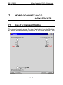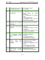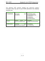
1
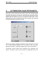
Cookbook PACE 2008 Simulation Engineering GmbH 2008 © Copyright by IBE GmbH 1994-2008 IBE Simulation Engineering GmbH Postfach 1142 D-85623 Glonn Germany Tel.: +49-(0)8093-5000 Fax: +49-(0)8093-902687 E-mail: [email protected] Home: www.ibepace.com This reference manual is valid for PACE 2008. PACE and the accompanied documentation is furnished under a licence and may not be used, copied, disclosed and/or distributed exept in accordance with the terms of said license. No part of this manual may be copied, reproduced, translated or published in any form without prior written permission from IBE. This document is subject to change without notice. All features described in this manual represent no obligations of the manufacturer of this software. All brand and product names are trademarks or registered trademarks of the respective companies. II Contents 1 Introduction . . . . . . . . . . . . . . . . . . . . . . . . . . . . . . 1-1 1.1 The Software-Tool PACE . . . . . . . . . . . . . . . . . . . . . 1 - 1 1.2 Bibliography . . . . . . . . . . . . . . . . . . . . . . . . . . . . . . . 1 - 3 .................................................. 2 Attributed PACE-Petri-Nets . . . . . . . . . . . . . 2 - 1 .................................................. 3 Introduction into PACE . . . . . . . . . . . . . . . . . . 3 - 1 .................................................. 4 Use of Smalltalk in PACE . . . . . . . . . . . . . . . . 4 - 1 4.1 Working with Objects . . . . . . . . . . . . . . . . . . . . . . . . 4 - 1 4.2 Extra Codes . . . . . . . . . . . . . . . . . . . . . . . . . . . . . . . 4 - 10 .................................................. 5 Simple PACE-Constructs . . . . . . . . . . . . . . . . 5 - 1 5.1 Counter . . . . . . . . . . . . . . . . . . . . . . . . . . . . . . . . . . . 5 - 1 5.2 Random Number Generator . . . . . . . . . . . . . . . . . . 5 - 1 5.3 Branching . . . . . . . . . . . . . . . . . . . . . . . . . . . . . . . . . 5 - 2 5.4 Loop . . . . . . . . . . . . . . . . . . . . . . . . . . . . . . . . . . . . . . 5 - 5 5.5 Timeout . . . . . . . . . . . . . . . . . . . . . . . . . . . . . . . . . . . 5 - 6 5.6 Firing of tokens at a special time . . . . . . . . . . . . . . 5 - 7 5.7 Rotating Table . . . . . . . . . . . . . . . . . . . . . . . . . . . . . . 5 - 8 5.8 Processing . . . . . . . . . . . . . . . . . . . . . . . . . . . . . . . . 5 - 13 5.9 Overflow . . . . . . . . . . . . . . . . . . . . . . . . . . . . . . . . . . 5 - 16 5.10 Queues . . . . . . . . . . . . . . . . . . . . . . . . . . . . . . . . . . 5 - 18 5.11 Packing and Unpacking of Objects . . . . . . . . . . 5 - 20 .................................................. 6 Statistics and Distributions . . . . . . . . . . . . . 6 - 1 6.1 Statistics . . . . . . . . . . . . . . . . . . . . . . . . . . . . . . . . . . 6 - 1 6.1.1 Bar-Diagrams and Line-Diagrams . . . . . . . . . . . . . . 6 - 1 6.1.2 Resetting Diagrams . . . . . . . . . . . . . . . . . . . . . . . . . 6 - 6 6.2 Distributions . . . . . . . . . . . . . . . . . . . . . . . . . . . . . . . 6 - 7 6.2.1 Exponential . . . . . . . . . . . . . . . . . . . . . . . . . . . . . . . 6 - 7 III 6.2.2 Normal . . . . . . . . . . . . . . . . . . . . . . . . . . . . . . . . . . . 6 - 8 6.2.3 Uniform . . . . . . . . . . . . . . . . . . . . . . . . . . . . . . . . . . . 6 - 9 .................................................. 7 More complex PACE-Constructs . 7-1 7.1 Use of a Standard Module . . . . . . . . . . . . . . . . . . . . 7 - 1 7.2 Switch . . . . . . . . . . . . . . . . . . . . . . . . . . . . . . . . . . . . . 7 - 7 7.3 PACE Modules . . . . . . . . . . . . . . . . . . . . . . . . . . . . 7 - 10 7.3.1 Implementation of a simple language element . . . . . . . . 7.3.2 Use of language elements during the development of a net . . . . . . . . . . . . . . . 7.4 Netfunctions . . . . . . . . . . . . . . . . . . . . . . . . . . . . . . 7.5 Improvement and Optimization . . . . . . . . . . . . . . . 7.6 Connecting a DLL written in C to PACE . . . . . . . 7 - 10 7 - 12 7 - 18 7 - 24 7 - 32 .................................................. Appendix: List of the PACE Training Nets IV ....... A-1 IBE / PACE 1 Introduction INTRODUCTION While the PACE-manual is describing all features of PACE completely with only a few examples, the present "cookbook" introduces into the basics of PACE in more application oriented manner. Basically this cookbook contains the topics, that are treated during an introduction, usually in PACE courses. It therefore contains a great number of typical examples which can be used as templates during modeling. The handling of PACE is dealt with here only sporadically. One finds information about that in the manual or in the online-manual. The PACE starter that is added to every PACE delivery provides a good entrance into the handling of PACE and into the feed in of inscriptions into a PACE model. For the preparation of inscriptions, for the direct carrying out of Smalltalk code in a so-called Workspace and for the loading and executing of the examples basic knowledge is necessary about Smalltalk. This is provided by the Smalltalk Primer added to the delivery by PACE which contains also numerous examples and practices. 1.1 The Software-Tool PACE PACE is a SoftwareTool for the modeling and simulation of event oriented systems. It employs attributed hierarchical stochastic Petri nets with time and Fuzzy modeling and is therefore particularly well suited for the description of real systems with parallel activities. The theory, underlying Petri nets, was developed by C. A. Petri in the year 1962, within the framework of his dissertation "Communication with Automats" at the TH Darmstadt in Germany. The target of the work consisted in creating a tool which can be used for the 1-1 IBE / PACE Introduction description and the simulation of parallel processes. The tool proposed by Petri achieved, particularly due to the graphical approach, within short time wide scientific interest, but could not achieve because of his initial unwieldiness spread use in the industrial area. With the appearance of powerful and cheap computers on the market at the end of the eighties computer supported Petri net simulators which virtually are usable at every workplace became possible. One of the best known Petri net simulators with very many advanced features is PACE who has found a broad acceptance within the last years. The spectrum of the applications reaches from the processing of abstract mathematical models over the simulation of concrete systems as manufacturing plants or business processes to the programming of complex operations as for example they can be found in the publications of Konrad Zuse. The basis of the modern Petri net theory was developed 1970 by J. L. Peterson. Since then Petri nets with today's common symbols for places and transitions are in use. In order to cover more and more new fields with Petri nets, the initial concept was expanded by many people and adapted to the respective needs. Also PACE implements a modern form of attributed Petri nets with numerous enlargements. Some of the essential enlargements are: · · · · · · · · · Possibility to build hierarchical nets. Net attributation und data processing with the object-oriented programming language Smalltalk. Use of individual and problem--related icons instead of the standard icons of the net elements. Restriction of the capacity of places. Time modelling. Modelling of random behaviour with mathematical and empirical probability distributions. Inhibitors Global variables and net variables. Fuzzy-Logic 1-2 IBE / PACE · · · · Introduction Call of external procedures (e.g. drivers, I/O-Handler) and von programming systems during the simulation resp. the execution of a net. Net functions. Procedures to optimize net functions. etc. The many extensions of Petri nets and of the Smalltalk library are incorporated in IBE's modelling and simulation language MSL, which is described completely in the PACE user manual. 1.2 Bibliography Bibliographical references to Petri nets, Fuzzy technics and Smalltalk are found at the end of the PACE User Manual. References for Smalltalk are also found at the end of the Smalltalk Primer. 1-3 IBE / PACE 2 PACE Petri Nets ATTRIBUTED PACE-PETRI-NETS Petri nets in their initial form are built up from four element types. The static elements are the places, transitions and connectors which determine the topology of the net. The dynamic elements are the tokens that can move in the net according to certain rules. In the attributed Petri nets of PACE there are also modules and channels for the hierarchical construction of nets. Places are passive elements, transitions active elements of a Petri net. A token always "wanders" from one place to the next place passing a transition. Transitions always vary in the net with places. Connectors connect places with transitions and transitions with places. The place in front of the transition is designated also as an 2-1 IBE / PACE PACE Petri Nets entry or input place, that after the transition as an outgoing or output place. The current state of a net is defined by the tokens on the places. State changes of the net are defined by the "movement" of the tokens from place to place. The token alternation in the net is induced by so-called "firing" of transitions. A transition in this case takes over tokens from its input-places and stores new tokens in its output-places. For the hierarchical structuring of nets PACE offers two further net elements, namely modules and channels. Modules are also active elements and are employed for the reusable organization of partial networks. During their construction all network elements may be used. On the other hand channels are passive network elements which consist only of places and further channels. While the meaning of modules during the development of nets is obvious, the meaning of channels which are useful during the development of complex nets is not as easy to understand. By means of a simple analogy the channel concept can be clarified, however: Places can be compared with single cable-connections beween hardware modules. Channels can be compared with tupes in which bundles of cable-connections are put together to connect modules. The active elements of a Petri net are called T-elements whereas the passive elements are called S-elements. To simplify the understanding of specialized literatur and the present text the usual keywords in use with Petri nets are listed in the following table: 2-2 IBE / PACE PACE Petri Nets Process Model System, Process German Englisch Stelle, Platz, Bedingung place, condition Situation, storage, Buffer Transition, Ereignis transiton, event Transition, Process (-step) Konnektor, Kante, Bogen connector , arc Connection Situation, crossing (point) Marke, Kern token Information, Material Modul module Module, partial net Kanal channel Combination of passive net elements 2-3 IBE / PACE 3 Introduction into PACE INTRODUCTION INTO PACE The state of a Petri net is determined by the token contents of its places. Modifications of the network status are induced by the firing (switching) of transitions. Under 'firing' one understands the consumption of the entry tokens and/or the generation of output tokens. The firing od a transition consists of 2 steps, namely the activation of the transition and the following token-alternation. A transition can fire if at least one token is available in every input place. the capacity of every output place is not exceeded. 3-1 IBE / PACE Introduction into PACE Considering these rules the following statements hold for the illustrations net002a and net002b: The transition in net002a can fire exactly once. In this case the net represented in net002b is produced. As described above the entry tokens are consumed and a new token is generated. Example: In a production two parts are put together and represent a new third part. The transition in figure net003 cannot fire because the capacity of the output place shown in square brackets would be exceeded. 3-2 IBE / PACE Introduction into PACE The conditions for the firing of transitions (input conditions) are expanded by adding of connector attributes to the entry connectors. Tokens and connectors can be provided for this purpose with 3-3 IBE / PACE Introduction into PACE attributes which are to be seen during the network view as legends of the corresponding network elements. The transition can only fire if a token that contains the same constant factor as the connector is on the place. The entry tokens are consumed and output tokens are generated in accordance with the attributes of the output connectors (that are connector variables or connector constants). If now instead of a constant a variable name is the attribute of a an input connector, the value of the token attribute is assigned to the variable during the activation of the transition. These variabels are known in the "vicinity" of a transition (that is up to the bordering places) and are called "transition local" variables. 3-4 IBE / PACE Introduction into PACE Connector attributes at the output connectors are employed for the generation of output tokens (these are made always while firing). During the generation of the output tokens at the output connectors with variable attributes, the value of the transition-local variables are taken over. In case of variables the values of the transition-local variabels are assigned to the token attributes; for constant connector attributes tokens with constant attributes are produced. In general to tokens and connectors as many attributes as desired can be assigned. About a connector with connector attribute n only flags with flag attribute n can flow. The variable assignment is independent of the tokens on the place. The token attributes are assigned in turn to the variables as these are defined with the attributation of the connectors. Investigate the behaviour of the following net: 3-5 IBE / PACE Introduction into PACE A transition with input connectors with the same variable names can only fire if the values which are assigned to the variables are equal(matching). A connector variable is known only in the environment of the transition to which the connector is coupled. Connector variables are local variables. One can recognize them by their beginning letter which is a small alphabetic character unlike the global variables which are known to net as a whole and must begin with a capital letter (Smalltalk-conventions). The attributes of tokens on places are independent of the assignment to the variables of connectors. 3-6 IBE / PACE Introduction into PACE What happens in the following net? 3-7 IBE / PACE Introduction into PACE Summary: Conditions for firing (activation): 1. At least one token must be on all input places. 2. The number of attributes of the connector and the token must be equal. 3. The contents of the token attributes must be the same if several input connector attributes are the same. 4. If a connector attribute is a constant the corresponding token atttribute must be equal. 5. The maximum capacity of the output places may no be reached 6. If an attribute of an input connector is a variable, then the value of the corresponding token attribute is assigned to it. The transition fires: 1. The input tokens are destroyed. 2. The output tokens are generated in accordance with the markings of the output connectors; to token variables are assigned the values of the transition local variables. In case of constant connector attributes the constants are assiged to the token attributes. 3-8 IBE / PACE Use of Smalltalk in PACE 4 USE OF SMALLTALK IN PACE 4.1 Working with Objects The processing of objects occurs in the transitions of a net. The code, necessary for that, is formulated with the object-oriented programming language Smalltalk-80. In every transition during firing Smalltalk-code for the processing of objects is executed. In every transition three types of code can be established: a) Condition Code: This code must deliver one of the boolean values true oder false and is executed at first during the activation of a transition. Default is true. If false is returned the transition is not activated and cannot fire. b) Delay Code: This code must deliver a positive number which defines the delay betrween the activation and the firing of the transition. The firing is delayed by so many simulator time units as this number indicates. c) Action Code: This code is executed when firing a transition and contains the actuall instructions for the object processing. The following example shows Condition Code by which branching is realized. The Smalltalk expression m > 5 resp. m <= 5 respond dependent of the actual values of the variables either true or false. 4-1 IBE / PACE Use of Smalltalk in PACE How does the net progess in case of n > 5? 4-2 IBE / PACE Use of Smalltalk in PACE During programming unwanted side-effects can appear. The following net shows an example: In case of transitions that manipulate objects of the classes Array, Association, Dictionary, OrderedCollection and Set Smalltalk does after an assigment to a variable not work with a copy of these objects, but directly with the original instance. Therefore sometimes unwanted effects arise, that can be avoided through suitable programming (normally copying of the object). 4-3 IBE / PACE Use of Smalltalk in PACE By the Delay code the firing of the transition is delayed by the assigned time units. Examine this with the following net. You can find 'time window' under the menu point 'view' in the Pace main board (The Visual Petri-Net Developer): If several transitions can fire at the same time the order of firing is not defined resp. accidential. By this unwanted effects can occur. For instance the parallel incoming workpieces in a material flow system are sorted timeless. A "waiting" at the sorting place has to be forced (e.g. with very small delays). 4-4 IBE / PACE Use of Smalltalk in PACE Investigate the following net: A token in the left net runs five rounds until the first transition in the right net fires. What happens in the left and in the right net of the following figure? 4-5 IBE / PACE Use of Smalltalk in PACE In the left case all 3 tokens are planed be the scheduler together, that means for execution at the same time; they are processed in parallel. In the right case the three events are scheduled and executed one after the other. This is the reason why in the left case 3 time units are necessary until all three tokens have been processed. In the right case 6 time unit are necessary to process the tokens. To this difference in working modes one has to pay attention when modelling the working of workpieces with machines which are represented by transitions. An inhibitor is the negation of a connector through which never a token can flow. He is used like a normal input connector with the following difference: · · If a token fullfils the condition the transition cannot fire. If no token fullfils the condition the transition can fire. The transition in the following net can fire until the token with the number 2 has been transfered to the right place. 4-6 IBE / PACE Use of Smalltalk in PACE The next example shows how the state in the right place can be changed without consuming an input token. 4-7 IBE / PACE Use of Smalltalk in PACE 4-8 IBE / PACE Use of Smalltalk in PACE Summary: Conditions for firing (activation): 1. All input places store at least one token. 2. The number of attributes of the connector and the tokens have to be equal. 3. All places which are connected with the inverted input of a transition must not have tokens with the same connecotr legends. 4. If several connectors have the same connector legends the contents of the tokens must be equal. 5. If the connector attribute is a constant the token attribute must be the same constant. 6. The maximal capacity of the output places must not be exceeded. 7. The condition code true is requested. 8. If the input connector attribute is a variable the value of the corresponding token attribute is assigned to the ltransition ocal variable. The transition is activated: 9. After activation the firing is delayed be the time units which result from the execution of the delay code. The transition fires: 10. The action code is executed. 11. The input tokens are destroyed. 12. The output tokens are generated according to the attributes of the output connectors. Variables are assigned the value of the transition local variable, in case of constants the constants are used. 4-9 IBE / PACE 4.2 Use of Smalltalk in PACE Extra Codes Extra Codes are necessary for the organizational embedding of PACE nets. Each model can have four extra codes which can be defined in the Net-Editor-Menu of the Visual Petri-Net Developer, menu function: extra codes. They are used for the following tasks: · Initialization Code It serves as the name says for the initialization of the net before its execution. This includes the initialization of global variables and data fields, the opening of files etc. · Break Code It is executed when a simulation run is interrupted by the user or with a break message. In the break code there could be e.g. intermediate evaluations and reports which inform the user about the progress of the simulation. · Continuation Code If a simulation run is interrupted the user can change parameter adjustments according to the actual situation of the simulation to influence the further execution of the simulation model. With the continuation code these adjustments can be read in and are available for the further execution of the model. · Termination Code The termination code is used for finishing tasks like evaluation, output and if necessary graphical representation of the simulation results, the closing of files, etc. Initialization code and termination code is actually used in each larger model; see the examples in the directory 'samples'. Break code and especially continuation code is necessary for interactive simulation models in which the user has to influence the 4 - 10 IBE / PACE Use of Smalltalk in PACE execution of the model. Examples of interactive simulation models are: y Training Models With interactive simulation models schedulers (freight traffic, running control etc.) can economically be prepared for their later work. · Evaluation Models It often isn't clear from the start of complex system models how the model behaves under different initial parameters. Although it is possible to determine with the optimization possibilities provided by PACE parameter sets which lead to a good or even optimal flowing of the model. If however the number of parameters and the variation area is too extensive, the calculations frequently cannot be carried out in sensible time. With evaluation models the value ranges of parameters and if necessary also the algorithms to change them can be changed by trying out by the user during the models execution. By that the following optimization runs then can be carried out in adequate time. 4 - 11 IBE / PACE Simple PACE-Constructs 5 SIMPLE PACE-CONSTRUCTS 5.1 Counter The following figure shows a counter. If a transition fires the contents of the input token is incremented resp. decremented by 1 and then inserted in the output token. 5.2 Random Number Generator A random number generator is made, if a flag is attributed with a distribution (for example Exponential, Normal, Weibull). The message 'next' is sent to this distribution by the connected transition. By this one receives the next random value from the distribution 5-1 IBE / PACE Simple PACE-Constructs which for example can be assigned to a variable z for the further use or can be used directly in the delay-code of a transition. 5.3 Branching There are essentially two methods to model branching. The first method consists in labelling the connectors with constants in order to let flow through only specific objects. This possibility only works however for simple objects like Boolean, integers, strings, symbols. 5-2 IBE / PACE Simple PACE-Constructs 5-3 IBE / PACE Simple PACE-Constructs The second possibility uses Condition Codes: Branching which starts from a place is a fundamental conflict in Petri nets. This is the reason why one should allways force the direction when modelling branching, if possible. If nothing is specified the strategy implemented in PACE, that is either deterministic or accidental, is used. The respectively desired strategy can be changed with the following message in a Workspace: UserPreferences randomScheduling: aBoolean where aBoolean is either true (accidential) or false (deterministic). 5-4 IBE / PACE 5.4 Simple PACE-Constructs Loop The following net shows a loop. The token with the constant array flows into the loop. Each number in the array is then incremented by 1. If all numbers have been incremented the token leaves the loop. This is done with a branch where one of the methods described in section 5.3 is used. 5-5 IBE / PACE 5.5 Simple PACE-Constructs Timeout The following example shows how a timeout is modelled in PACE. If the transition 'Interrupting Timeout' does not fire inbetween 30 time units the transition with the delay fires. 5-6 IBE / PACE 5.6 Simple PACE-Constructs Firing of tokens at a special time In the following example all tokens which have been collected until 3 p.m. are fired at 3 p.m. The transition with the delay 9 adds the 9 missing hours until midnight to simulate a 24 hours cycle. 5-7 IBE / PACE 5.7 Simple PACE-Constructs Rotating Table Let's examine the simple transport problem shown in the following figure. It consists of two operating robots and a turntable with three positions. If the container in Position1 is empty, then Robot1 can put a part in it. If the container in Position3 is full, Robot2 can remove the part from it. The turntable requires a time unit for turning the containers from one position to the next. The numbering of the containers (represented by tokens where the first attribute is the number of the container and the second attribute is its filling level) are not relevant during the simulation. They only have to show that the containers are allways stored in the same order on the rotating table. The following net modified insignificantly can als be used for the simulation of a conveyor belt. 5-8 IBE / PACE Simple PACE-Constructs To conserve space, we won't discuss the source of the parts to be moved (module "PartsSource") and their further processing (module "PartsTreatment") here. We'll simply assume that the parts will arrive and will be processed statistically. The two next figures show the two modules, "PartsSource " and "PartsTreatment." Here we clearly assume a random distribution of the points in time when a part is delivered or used. Delivery of parts is as follows (module "PartsSource"): the token located at a given place is delayed by the random value of the time delay. Then the transition fires, and delivers a token to each of the places connected to it. One is used to plan the next part delivery. The token which runs to the place "PartsArrival" represents the part delivered from outside the system. 5-9 IBE / PACE Simple PACE-Constructs The following two figures model the work of the processing robots. Here again we're looking only at the delivery of parts. In the container at "Position1" there is a token whose attributes indicate which of the three containers on the turntable is in position, and that this container is empty. The transition "HandlingRobot1" can fire only if, along with this token, there is also a token (a part) in the place "PartsArrival." If the transition fires, it collects both tokens and places a token with the attribute value "full" (a part) in the container at "Position1." 5 - 10 IBE / PACE Simple PACE-Constructs The model of the turntable shown in the next figure is only a little more complicated. Here we see, a bit more subtly, the input/output interfaces "Position1" and "Position3" from the next-higher level with its initial values and the container "Position2" which is not accessible to either handling robot. The partial net shown here rotates the current attributes regarding the three stated positions. 5 - 11 IBE / PACE Simple PACE-Constructs Since the turntable switches the positions according to a time unit, the transition "tr4" fires once in each time unit and places a token in each of the places, pl1 to pl4. The token inserted in pl1 plans firing up to the next time unit. Until that point, transitions tr1 through tr3 fire, since there is a token in each of the input places of all these transitions, and they transport the tokens lying in the three positions on to the next position in each case. 5 - 12 IBE / PACE 5.8 Simple PACE-Constructs Processing If a token has to stay in a certain module during the execution this can be realized as follows: The token stays as long in the module till the working time is over. 5 - 13 IBE / PACE Simple PACE-Constructs By the number of the tokens with which the place 'Waiting for work' is initialized the maximal number of the simultaneous working processes in the module can be set (for example maximal number of batch processes). If the Modul is supposed to carry out only one task at a time, also the following 'WorkingModul' with an inhibitor can be used: 5 - 14 IBE / PACE Simple PACE-Constructs 5 - 15 IBE / PACE 5.9 Simple PACE-Constructs Overflow Usually tokens would accumulate before a module if it can not include any more tokens. In following example the tokens which would accumulate in case of a busy module are drawed off into the place designated with 'overflow'. If one would leave out the overflow place, so the "superfluous" tokens would be destroyed. 5 - 16 IBE / PACE Simple PACE-Constructs 5 - 17 IBE / PACE 5.10 Simple PACE-Constructs Queues A typical queue problem could read approximately as follows: "In a production enterprise the material edition is serviced by only one employee which is according to his opinion overloaded. The other employees complain about too high delays. Judge the situation!" Dates: y 12 employee/hour arrive in the average y The middle serving-time is 3.33 minute/employee. y Arrival-times and serving-times are distributed exponential Pure solution : y middle utilization 66 %. y Middle Number employee in the queue can be determined in theory Task: Make a histogram for the following queue-example for the distribution of the delays onto different waiting room reservations. (see also PACE manual, section 10.3.2). 5 - 18 IBE / PACE Simple PACE-Constructs 5 - 19 IBE / PACE 5.11 Simple PACE-Constructs Packing and Unpacking of Objects During modelling the case occurs frequently that objects (tokens) have to be gathered and to be distributed later again. For example one can think on products which are brought to their workmanship place in baskets or parcels. Such cases can be modelled simply when the attributes of the tokens are buffered as the elements of an OrderedCollection representing the entire container content, and the tokens are destroyed after that (packing). The OrderedCollection then flows as the attribute of a token representing the whole container through the net to the point at which the packed tokens have to be processed. There one can, if this is requested, generate the tokens again and attribute tem correspondingly with the elements of the OrderedCollection (unpacking). We consider here only the simplest case in which the tokens have no attributes and in which the number of packed objects alone is sufficient to describe the container. Since we want to formulate the packing and unpacking in each case as modules, we first have to introduce two module variables1, a 1 For simplicity we assume that all container store the same maximum number of objects. 5 - 20 IBE / PACE Simple PACE-Constructs module variable that indicates how many objects in the container can be stored and a module variable that indicates the current filling level of the actual container. The window shown in the preceeding figure for the definition and initialization of module variables can be opended in the 'net editor'menu of the Visual Petri-Net Developer, menu item 'local variables'. The module variable #NumberOfObjects defines the maximum 5 - 21 IBE / PACE Simple PACE-Constructs number of objects in a container, the module variable #Count indicates the actual filling level. #Count is initialized with 0. #NumberOfObjects can be set by the user. In the following net the packaging of objects is shown. We eliminate all tokens except for the last one and attribute this one with 'count'. The value of 'count' agrees when leaving the module with the predefined maximum number in a container # NumberOfObjects. 5 - 22 IBE / PACE Simple PACE-Constructs The next net shows the unpacking of objects, that is the generation of the tokens representing the original objects at another point of the net. Exercise: Extend the modules 'Packing' and 'Unpacking' for container, which store a different maximum number of objects and for attributed tokens. 5 - 23 IBE / PACE Statistics and Distributions 6 STATISTICS AND DISTRIBUTIONS 6.1 Statistics 6.1.1 Bar-Diagrams and Line-Diagrams PACE offers the possibility to represent data items which results during the simulation in time-controlled bar or line diagrams. You find the handling of these statistical windows in the PACE user manual, section 8.8: 'Time Dependent Diagrams'. In all diagrams standard functions are defaulted in the in each case assigned block (cf. PACE user manual). It is however possible to change the default diagram-function in order to display the behavior of own objects. In this case one has to be aware that the functions always return a Smalltalk point x@y. In the following example a histogram was assigned to a place: 6-1 IBE / PACE Statistics and Distributions 6-2 IBE / PACE Statistics and Distributions Line Diagram for a Place: Load the image net018.im from the directory 'tutorial' in the PACE installation directory: The line diagram shows for each time point (x axis) the number of tokens (y axis) which lie on the place with legend: 'line diagram on this place', which results in a sinus curve. 6-3 IBE / PACE Statistics and Distributions 6-4 IBE / PACE Statistics and Distributions Histogram for a Collector: You can load this net net019 from the net directory of the tutorial directory in the PACE installation directory. The histogram is connected to the connector with attribute '(n)': 6-5 IBE / PACE 6.1.2 Statistics and Distributions Resetting Diagrams For special applications which evaluate an optimum in several simulation runs the opened diagrams must be cleared before the next run in part or in total. For this purpose there are the following methods: The function resetPlaceStatistics: which takes as an argument the name of a place which is connected to the transition that contains the function call, resets the graphics of all statistics windows of the indicated place. Example: self resetPlaceStatistics: 'place1'. With the function resetAllStatistics all opened statistics windows of a net can be reset. Example: self resetAllStatistics. 6-6 IBE / PACE 6.2 Statistics and Distributions Distributions In PACE the most important continuous mathematical distributions are available. The distributions can be displayed for user defined parameters with the menu items 'probability densities' and 'probability distributions' in the evaluator menu of the PACE main board (Visual Petri-Net Developer). The distributions are completely described in chapters 10 of the PACE user manual. There also an example is shown how one can make empirical distributions and use them in simulation models. Here we show examples with three important standard distributions, namely the exponential distribution, the normal distribution and the uniform distribution. 6.2.1 Exponential Description: The class Exponential is an implementation of the exponential function. Methods: mean: x generates a new exponential distribution with mean value x. next delivers the next value of the distribution. = is the argument an exponential distribution with the same mean value then true is returned, otherwise false. == are receiver and argument the same instance of an exponential distribution then true is returned, otherwise false. 6-7 IBE / PACE 6.2.2 Statistics and Distributions Normal Description: The class Normal implements a normal or Gaussian distribution. Methods: mean: x deviation: y Generates a normal distribution with mean value x and standartd deviation y. next Attention: returns the next value of the distribution. With a normal distribution also negative values can appear. For only positive values of the are meaningful one has to pay attention that the values of a nomal distribution are not directly assigned to a delay. 6-8 IBE / PACE 6.2.3 Statistics and Distributions Uniform Description: The class Uniform implements the distribution where the probability for all arguments is the same. Methods: from: x to: y Generates a uniform distribution with the lower limit x and the upper limit y. next returns the next value of the distribution. printOn: x Writes an ASCII representation of the receiver in the stream x. = If the argument also represents a uniform distribution for the same intervall, then true is returned, otherwise false. 6-9 IBE / PACE == Statistics and Distributions If the receiver and the argument represent the same instance of the distribution true is returned, otherwise false. 6 - 10 IBE / PACE More Complex PACE-Constructs 7 MORE COMPLEX PACECONSTRUCTS 7.1 Use of a Standard Module The present example shows the use of a standard module. Modules are stored in the subdirectory ‘modules’ of the PACE directory. The 7-1 IBE / PACE More Complex PACE-Constructs example models a production with two kinds of objects which arrive exponentially distributed with a mean value of 20 and 30 minutes. For the processing of the objects a mean time of 13 minutes is required. The processing of the more seldom arriving objects shall be preferred. At first the generation of the two product streams and its processing is modelled. A new model is opened for this and the entries shown in the foregoing illustration are carried out in the edit window. The next step is to insert and connect the module ‘priority.sub’ of the module library (this is the directory ‘modules’ in the PACE directory). 7-2 IBE / PACE More Complex PACE-Constructs The attributes of the connectors (prio n) have also been inserted. As identification of an object the object number n the used, which as shown in the next illustration is assigned after an object arrived. The priority of the object type arriving more frequently is lower than the priority of the object which arrives more seldom. This means that the priority number of the object type arriving more frequently is higher than the priority number of the other object type. To start the processing of an object an initial token must be inserted in the place 'Next token'. To start the processing of the next object the lower transition must be connected with the place 'Next token'. 7-3 IBE / PACE More Complex PACE-Constructs By this one gets the following net which is represented in edit and in simulation mode (immediately of initialization). 7-4 IBE / PACE More Complex PACE-Constructs If one finally connects a consumer to the lower transition who documents the order of the tokens in a Transcript window (done in the three point code), then the net and a Transcript window looks as follows: 7-5 IBE / PACE More Complex PACE-Constructs One recognizes the change in the processing order of objects in accordance with the object priorities(e.g. object 3 is processed before object 2). 7-6 IBE / PACE 7.2 More Complex PACE-Constructs Switch When modelling working processes very often the case occurs that the working process has to be switched off and on by the operator, from case to case. In the following figure 'Switch' a module representing the switch is contained. The actual switch is contained in the module 'switch.switch'. The variable 'SwitchAdjustment' used therein has to be initialized when initializing the module (Initializationcode) according to: 7-7 IBE / PACE More Complex PACE-Constructs SwitchAdjustment := #ein SwitchAdjustment is a module variable but could also be delared as a global variable. 7-8 IBE / PACE More Complex PACE-Constructs If during the execution of the model the shift key is pressed a query window opens and asks if the actual position of the switch has to be changed. The delay code 2 for the right transition in the module Switch is necessary to guaranty that all tokens have left the Switch and therefore for the next generated token the new switch position is already effective. The proposed method is only usefull if the switch is often passed by tokens. If this is not the case and if one wants not to press the shift key until the next token passes the switch one should implement the query as a separat partial net with enough token traffic. 7-9 IBE / PACE 7.3 More Complex PACE-Constructs PACE Modules In PACE hierarchical Petri nets can be built up in a modular way. The network components constructed with the PACE module technique can be employed after their preparation in the entire net or in other nets. With this procedure amongst other things also Workflow description languages can be implemented in a simple manner. The procedure to be adopted when implementing language elements of such languages is demonstrated in the following with at a simple example. 7.3.1 Implementation of a simple language element To make the procedure transparent, a very simple language element will be implemented in the following. We choose a simple counter 'Counter', which merely increments numbers. Starting point is the following simple Petri net: 7 - 10 IBE / PACE More Complex PACE-Constructs It consists of three simple net elements: the places 'input' and 'output', which contain the tokens before the entry and after the exit of the module 'Counter'. The module 'Counter' is very simpleand shown in the following figure: It shows the places 'input' and 'output' (drawn more weakly) as the interface to the environment and consists only of one transition which increments incomming numbers by 1. To bring the module ‘Counter' in a reusable form we have to store it using the function 'store module' in the 'file'-menu of the PACE main board. After that 'Counter' can be used as a "language element" during the further development of the net. The use of modules resp. language elements can be improved by the use of meaningful icons which give an intuitive impression of the semantics behind the language elements. In the present example the icon of an abacus is used. By this we get the following representation of the module 'Counter': 7 - 11 IBE / PACE More Complex PACE-Constructs The development of more complex modules can be done in a similar manner. Amongst others the following PACE properties can be used advantageously: · · · Modules can be developed hierarchically. Moudles can have module variables which are instantiated with every use of the module. During the development of a module all language elements of Smalltalk-80 and the full Smalltalk library can be used. 7.3.2 Use of language elements during the development of a net With the preceeding steps the new language element 'Counter' is available generally. We now show how predefined language elements are put together to "net programs". 7 - 12 IBE / PACE More Complex PACE-Constructs In the next figure the module 'Counter' has been inserted 4 times with the function 'restore module' of the No-Selection-Menu of the window in edit-mode: To do something more or less meaningful with the module 'use of module counter' we could connect the four instances of 'Counter': To do this several changes and extensions have to be done with the graphical PACE editor. These consist in: · Exchange of the places 'input' and 'output' of the instances of 'Counter' on the right side. 7 - 13 IBE / PACE · · More Complex PACE-Constructs Insertion of transitions beween the output and input places of the 4 instances of 'Counter'. Insertion and Attributation of the connectors. In real applications the names of the input and output places should also be changed, so that they are named unambiguously (what we do without here). To run a simulation we need tokens attributed with a number. We insert three tokens in the upper left place using the following input 7 - 14 IBE / PACE More Complex PACE-Constructs window which opens after the selection of the menu item 'initial tokens' in the selection menu of this place: We assign to the three tokens the initial values 1, 100 and 1000. Our window 'use of module counter' now looks as follows: 7 - 15 IBE / PACE More Complex PACE-Constructs Up to now we have worked in the 'edit'-Mode. For we have finshed the development of our simple net we now press the 'simulate'-button on the left lower corner of the window and start the simulation. The next figure shows a snapshot of the net window during the simulation. Two tokens lie on the upper left and right place, the third tokens with the attribute '832' just moves from the upper right to the upper left place. 7 - 16 IBE / PACE More Complex PACE-Constructs This examples also shows that the implementation of standardized semigraphical language elements leads to the same disadvantages as they also occur with the implementation of high level programming languages. Here as there the standardization of language elements makes a certain overhead that would be presumably in part recoverable by an optimizing net editor, however, because of the increasing computer technology (faster and faster processors, more and more storage) this doesn't make any difference. 7 - 17 IBE / PACE 7.4 More Complex PACE-Constructs Netfunctions The multiple insertion of a module shown in the previous example would easily lead in case of bigger modules to inflated nets in which big parts of the net would be identical. This would only be questionable with respect to today's computers if the nets are very large. The multiple insertion of a module has, however, a further disadvantage. If changes or corrections of a module are made, the changes have to be made at all places where the Modul was inserted. Because the net in this case must be edited at different places this can be an extensive and error-prone job. There was the same problem during the programming in higher programming languages which led to the introduction of blocks (Smalltalk), of subprograms (Fortran) or of procedures (Algol, pascal, C). The repeatedly needed code is integrated in this case only once into a program and can be called from different program places. In PACE there is also the possibility to call blocks from different inscriptions (see section 3.4 of the PACE Smalltalk Primer). In addition it is also possible to call "netfunctions" which are executed as subprocesses in parallel to each other and to the main process. The process with which the simulation model starts is designated as the main process in this case. For the starting of a netfunction there are five methods: addTokenTo: addTokenTo:with: addTokenTo:with:with: addTokenTo:with:with:with: addTokenTo:attributes: which are also used when reacting on external events (see PACE User Manual, chapter 3). 7 - 18 IBE / PACE More Complex PACE-Constructs To support netfunctions independent partial networks must be provided by the main net, first of all. A partial network must have entryplaces and exit-transitions. We restrict in the following to one entryplace and one exit-transition, since this case most frequently occurs and since it can be generalized easily. A netfunction is started when a token is placed into the entry-place by execution of one of the above listed addToken methods. As a last step of the netfunction one of the above methods returns a token into the initial net. This token can be used for example in order to synchronize the continuation of the calling net with the end of the netfunction and to deliver results to the calling environment. An end signal of the netfunction is always necessary (either in form of data and/or as a token) in order to prevent that the non reentrant netfunctions are called simultaneously repeatedly. In order to keep an eye on a concrete example, we consider the net "netA" shown in the following illustration which consists of 3 uses of the module "PartialNet" which were combined with each other by two transitions. We choose this net in order to demonstrate how the task of the modules 'PartialNet' can be transfered to a subprocess. 7 - 19 IBE / PACE More Complex PACE-Constructs In the present case of course one could avoid the multiple use of "PartialNet" also by the modeling a loop. In more general cases when the modules to be inserted are used on different hierarchical levels of a net there is however no simple alternative to a netfunctions apart from inserting the module repeatedly. 7 - 20 IBE / PACE More Complex PACE-Constructs The net equivalent to net 'netA' in which the module "PartialNet" was put only once is shown in the following figure, 'netB': As an alternative to it the net represented in the next illustration can also be used. 7 - 21 IBE / PACE More Complex PACE-Constructs The right partial network is called by inserting a token into the place "Entry". The place in which the result is supposed to be delivered is to be indicated in this case as an argument; the return places are "Return1" and "Return2". The respective return place is brought to the return-transition as value of the connector variable "return". With the places "Return1" and "Return2" in the main net the subprocess are synchronized with the main process. It is guaranteed that the partial network is not executed simultaneously repeatedly. If the value nil is indicated instead of the return place, the main process does not expect any end message of the subprocess progressing simultaneously If the PartialNet is used independently in several parallel branches of a net, it can be guaranteed easily, that at one time only one subprocess progresses (see the following figure). A token is placed into the 7 - 22 IBE / PACE More Complex PACE-Constructs right place; this and the entry token are used to start the subprocess. Further tokens which are placed into the place 'Entry' can only run if the exit transition fires and inserts a flag into the right place again. 7 - 23 IBE / PACE 7.5 More Complex PACE-Constructs Improvement and Optimization One can distinguish basically between two kinds of model improvement: 1. Procedural Improvement This kind of improvements are carried out by a suitable design of a net and/or with improvements of the inscription code. These improvements depend usually very strongly on the problem and are therefore part of the modeling. 2. Parameter Optimization Models normally can be supplied with different parameter sets and then show a different behavior for each set. Frequently the optimal parameter set is searched with respect to specific defaulted criteria (e.g. as few as possible resources for the processing of a specific work load in a specific time). PACE offers support for both kinds of improvements. The graphics editor allows to change a net very rapidly to implement and investigate changes of a net and different solutions. To optimize parameter sets PACE offers supporting methods and exact mathematical procedures. It allows the program-controlled repetition of simulation runs with different code to be assigned to each repetition. This can for instance be used to change the values of the model's parameters during the restart of the model (mostly in the initialization code). In the PACE optimization manual the graphical and mathematical optimization procedures and methods available in PACE are described. To the extensive examples in this chapter there are corresponding models in the samples directory of the PACE installation directory. 7 - 24 IBE / PACE More Complex PACE-Constructs As a tutorial we here demonstrate the most important procedures with a simple transparent example. We investigate an „unknown“ test module which we have to provide with a number as input value and which delivers a number as the corresponding result. We want to know for which input value the module delivers the maximal output value. The search for the optimum is carried out in the following as well graphically as algorithmicly. To paint the dependence between the input value and the output value the net in the foregoing figure is extended as follows: 7 - 25 IBE / PACE More Complex PACE-Constructs 7 - 26 IBE / PACE More Complex PACE-Constructs The global variable ModuleCurve is defined in the initialization code with the statement: (ModuleCurve := Curve named: ‘ModuleCurve’) clear The Curve ‘ModuleCurve’ has to be installed from the PACE Views menu. For repeated execution of the model the curve is cleared before each simulation run. The scaling of the curve the parameter menu of the curve is used. To open it postition the cursor on the scale of the curve and press the right mouse button. After adjusting the values they are overtaken in the curve window by pressing the return button of the keyboard. After this the parameter menu is deleted by selecting with the left mouse button the cross in the right upper corner. In the place at top an initial token with value 0 is inserted which starts the evaluation of the curve. We investigate the result curve in the interval between 0 and 4. If no description of the module is available this interval has to be determined „experimentally“. For instance one can first investigate a larger interval. In this case one has to switch on the parameter option „automatic scaling“ in the window of the output curve „ModuleCurve“. To start the simulation switch at least in one of the net windows into simulation mode, execute with the right mouse button (cursor in a net window in simulation mode) first the menu function „initialize“ and the one of the menu functions „run“ or „background run“. The result of the execution is shown in the next figure. Using the scaling of the window one can roughly read the input value with the greatest result value. If one wants to know this value more precisely it is recommended to switch on the option „cursor position display“ in the parameter menu of the curve. Then under the curve in the curve window the position of the mouse cursor is shown. If one positions the mouse cursor on the maximum one can read off the position of the maximum. The curve window shows that the maximum value occurs for the input value 0.795. 7 - 27 IBE / PACE More Complex PACE-Constructs To evaluate the demanded input value with one of the optimizers implemented in PACE the „TestModule“ is incorporated into a netfunction „Func“. 7 - 28 IBE / PACE More Complex PACE-Constructs 7 - 29 IBE / PACE More Complex PACE-Constructs For the input values from the optimizer are delivered in form of a vector but the „TestModule“ expects the input value directly the value is calculated at the begin of the netfunction with the assignment: val := vec. at: 1. The result is delivered to the optimizer with the statement: self netResult: res. The two small nets to the left serve for the call of the optimizer and for the output of the result into a Transcript window. One receives as in the case of the graphical evaluation the result 0.79. To make it possible to duplicate the example we finally announce the module „TestExample“ which is merely the sum of sinus and cosinus. 7 - 30 IBE / PACE More Complex PACE-Constructs In more complicated possibly multi-dimensional cases in which a pre-developed module whose behaviour is not so easy to predict (e.g. a production line) has to be incorporated in a model similar algorithmic procedures have to be applied to evaluate the optimal parametrization. 7 - 31 IBE / PACE 7.6 More Complex PACE-Constructs Connecting a DLL written in C to PACE We look at the example represented in the following figure in which a circulating token increments a counter up to a certain value and then resets it. To show the interface between PACE and C we replace in the following the Smalltalk inscriptions by messages which call C-procedures of the dynamic link library ‘userdll.dll’ to be developed. After making these changes our net looks e.g. as follows: 7 - 32 IBE / PACE More Complex PACE-Constructs In the left transition we call with the message ‘procedure0:’ a C-procedure ‘incrementValue’ which increments the parameter n and returns the incremented value back to the net. The right transition calls with the message ‘procedure1:’ the C-procedure ‘checkValue’ which resets the value of n in case that the value 11 is reached. To implement the interface between Smalltalk and C we have to extend the C-module ‘userdllvm.c’ (see the directory 'makedll' in the PACE installation directory) to implement the mentioned two procedures. The link list „UserProcs“ has to be extended for this and the two mentioned procedures have to be added. /* PACE 2008 * Development of uderdllvm.dll: File userdllvm.c * * Procedures to be connected by the user: * For different numbers of parameters there a designated in * each case 6 procedures. These are connected to Smalltalk using the * primitive numbers 110xy . * * The first digit x (x = 0,..,5) defines the number of the procedure. 7 - 33 IBE / PACE More Complex PACE-Constructs * The second digit y (y = 0,.. 4) defines the number of parameters. * * If the number of designated procedures with a special number of * parameters is to small in an application, the user has to define * instead only one procedure and has to branch from this procedure * to the other procedures * * If there are more than 4 parameters the user has to store these in a * collection and has to transfer the collection to C. */ #include "userprim.h" #include "userdll.h" static upInt value; extern void UserProcs(); void incrementValue(); void checkValue(); extern void UserProcs() { UPaddPrimitive(11001, incrementValue, 1); UPaddPrimitive(11011, checkValue, 1); } void incrementValue(upHandle receiver, upHandle n) { value = UPSTtoCint(n) + 1; UPreturnHandle(UPCtoSTint(value)); } void checkValue(upHandle receiver, upHandle n) { if (UPSTtoCint(n) > 10) { value = 0;}; UPreturnHandle(UPCtoSTint(value)); } Then we have to translate userdllvm.c, e.g. with Visual C/C++, Version 6.0. In the directory: 7 - 34 IBE / PACE More Complex PACE-Constructs pace-directory\Makedll\Example we have prepared all files for this purpose. After loading the workspace the above C-module is displayed and ‘userdllvm.dll’ can be generated automatically. In the example directory we move the file name ‘pace2008.imm’, which contains the example ‘Cexample2’, with pressed left mouse button over the file name ‘pacevm.exe’. If we release the mouse button PACE is started from the example directory and our newly generated file ‘userdllvm.dll’ is loaded. If we would have started PACE by double clicking on the image ‘pacevm.imm’, our new userdllvm.dll would not have been used. Instead the default- or dummy-file ‘userdlvm.dll’ in the Windows system directory would have been invoked. Recommendation: If a project team uses an extended interface it is recommended to replace the default-file userdllvm.dll of the team with the new ‘userdllvm.dll’ which implements the extended interface. 7 - 35 IBE / PACE Apppendix: List of PACE training nets Appendix: List of the PACE Training Nets File Description Use 000 Token with String Transfer to a connector variable 001 3 initial tokens with 1 constant. 1 Token mit 2 constants. Constant input and output connectors To show the element types of an extended Petri net 002 3 initial tokens with conditions Conditions for firing with input setting 003 4 initial tokens with condition and capacity Condition capacity for firing with 004 2 initial tokens with constants Condition constants for firing with 005 2 initial tokens with constant number and constant input and output connector Conditon for firing with coinstants and taking over of input attributes 006 2 initial tokens with constant number and Condition for firing with constant token attribute and A-1 IBE / PACE variable input output connector 007 Apppendix: List of PACE training nets and 3 initial tokens with constants. A token with 2 constants. Constant input and output connectors. taking over of input and output attributes in variables a) Firing conditions with constant token attribute and handling over the constants of the output connector. b) Problem with the number of arguments for tokens resp. connectors. 008 Generating transitions with 4 numbers connector and following branching with variable connectors. a) "Infinite" token generation b) Mode of branching (random/ deterministic) 009 4 initial tokens with 2 equal constants, 2 diffenrent numbers, 2 equal variable input connectors and 1 output connector. Activation if two input tokens are identical 010 transition code Incrementing and decrementing 011 "Controlled" branching with token generation a) Sorting b) Firing conditions true/false c) Generation of tokens with incremented attribut 012 Counter with delay a) Delay b) Comment! c) Incrementation A-2 IBE / PACE Apppendix: List of PACE training nets 013 2 independent counters with different delays a) "Concept of time" b) Firing list 014 3 nets with array and increments a) Transition code is executed during firing not when activating. b) 2 possibilities for transition code. c) Clean separation e) Smalltalk code (read from and write to an array) 015 Inhibitor with constant connector Number as connector attribute 016 Generator and inverter module a) Module b) Alternating values of a token in 2 places c) Delay (not relevant for the working of the example). 017 2 connected delays with histogram at the place a) Uniform distribution b) Delays c) Connected Delays d) Histogramm at a place 018 Sinus curve positive offset, diagram. a)Trigonometrical functions b) Statistics window c) Show the refinement of the curve d) Counting up and down e) Line diagram at a place 019 with line Histogram of a connecotr with normal distribution a) Normal distribution b) Histogram of a connector A-3 IBE / PACE Apppendix: List of PACE training nets 020 Line diagram of a connector with exponential course Line diagram of a connector 021 Exponential distribution with connector histogram Exponential distribution 022 Normal distribution with connector histogram Normal distribution 023 Uniform with histogram Uniform distribution 024 Counter Incrementing by 1 025 Random generator with uniform distribution Random generator 026 Branching: Variant with constant connector attribute Branching variant #x 027 Branching: Variant with firing conditions Branching variant fire 028 Loop a) 4 times loop b) then branch off 029 Timeout a) Timeout "consequences" distribution connector A-4 without IBE / PACE Apppendix: List of PACE training nets 030 Clock units with 24 032 Processing in predefined time. Only one task at a time. a) Semaphores for controlling b) Duration of the process c) Variation mit capacity 033 Variation of net032: Processing in predefined time. Only one task at a time. a) Semaphores for controlling b) Duration of the process c) Variation mit capacity 034 Variation von net032: Processing in predefined time. With overflow Overflow 035 Creation of an Array 036 Variation of net035: Creation of an Array 037 Creation Association 038 Variation Association 039 Dictionary of time timetable a) Array b) Output of different elements of the array. a) Array b) Output of different elements of the array. an a) Association b) Output of different elements of the association. with a) Association b) Output of different elements of the association and incrementation a) Dictionary b) Output of different elements of the dictionary A-5 IBE / PACE 040 Apppendix: List of PACE training nets a) Dictionary b) Manipulation dictionary Dictionary of the 041 Ordered Collection a) Ordered Collection b) Output of different elements 042 Ordered Collection a) Ordered Collection b) Manipulation 043 Set a) Set b) Output of different elements 044 Set a) Set b) Generation numbers of prime 045 Copying of number and dictionary Shallow copy 046 Copying of dictionary and OrderedCollection a) Deep copy of dictionaries b) Copy to another token with an OrderedCollection 047 Dictionary Variations of the generation 048 File a) Creating of a file which contains an OrderedCollection b) Writes only the last of two collections 049 FIFO first in first out A-6 IBE / PACE Apppendix: List of PACE training nets 050 LIFO last in first out with sort for an OrderedCollection 051 Sort out by priorities Output with respect to priorities 052 Output Message to an output window 053 Input of a BarGauge use of a global variable 054 Module variables a) Modul globale Variable b) Modulvariable 055 Input "Yes/No" with Dialog (true/false) 056 Input string mit Dialog (string) 057 Changing icons 057 Changing icons of a module 060 Queue a) Behaviour of queues b) Testing of statistics 061 Working off an order a) Simultaneous scheduling of events b) Sequential scheduling 100 Handling over of arguments to connector 4 a Order of transfers Further nets: A-7 IBE / PACE Apppendix: List of PACE training nets The directory nets contains besides the netxxx.net training examples, which are part of each PACE distribution the following example nets: FOERDMOD Switch PackUnpack conveyor /turntable belt a) Rotating table b) Part processing c) Roboter1 d) Roboter2 e) Parts source Switch on/off by choice of partial nets a) switch b) Manual intervention Packing and Unpacking of objects a) Packing b) Unpacking A-8