Download Dataflow Design Tool - ODU Computer Science

NASA Technical Memorandum 4672
Dataflow Design Tool
User’s Manual
Robert L. Jones III
Langley Research Center • Hampton, Virginia
National Aeronautics and Space Administration
Langley Research Center • Hampton, Virginia 23681-0001
February 1996
The use of trademarks or names of manufacturers in this report is for
accurate reporting and does not constitute an official endorsement,
either expressed or implied, of such products or manufacturers by the
National Aeronautics and Space Administration.
Available electronically at the following URL address: http://techreports.larc.nasa.gov/ltrs/ltrs.html
Printed copies available from the following:
NASA Center for AeroSpace Information
800 Elkridge Landing Road
Linthicum Heights, MD 21090-2934
(301) 621-0390
National Technical Information Service (NTIS)
5285 Port Royal Road
Springfield, VA 22161-2171
(703) 487-4650
Contents
Nomenclature . . . . . . . . . . . . . . . . . . . . . . . . . . . . . . . . . . . . . . . . . . . . . . . . . . . . . . . . . . . . . . . . . . . . . ix
1. Introduction . . . . . . . . . . . . . . . . . . . . . . . . . . . . . . . . . . . . . . . . . . . . . . . . . . . . . . . . . . . . . . . . . . . . . 1
2. Dataflow Graphs. . . . . . . . . . . . . . . . . . . . . . . . . . . . . . . . . . . . . . . . . . . . . . . . . . . . . . . . . . . . . . . . . . 2
2.1. Measuring and Constraining Parallelism . . . . . . . . . . . . . . . . . . . . . . . . . . . . . . . . . . . . . . . . . . . . 3
2.2. Run-Time Memory Requirements . . . . . . . . . . . . . . . . . . . . . . . . . . . . . . . . . . . . . . . . . . . . . . . . . 4
2.3. Control Edges. . . . . . . . . . . . . . . . . . . . . . . . . . . . . . . . . . . . . . . . . . . . . . . . . . . . . . . . . . . . . . . . . 4
3. Dataflow Design Tool . . . . . . . . . . . . . . . . . . . . . . . . . . . . . . . . . . . . . . . . . . . . . . . . . . . . . . . . . . . . . 5
3.1. File Input/Output . . . . . . . . . . . . . . . . . . . . . . . . . . . . . . . . . . . . . . . . . . . . . . . . . . . . . . . . . . . . . . 6
3.1.1. Graph Text File . . . . . . . . . . . . . . . . . . . . . . . . . . . . . . . . . . . . . . . . . . . . . . . . . . . . . . . . . . . . 6
3.1.2. Notes File . . . . . . . . . . . . . . . . . . . . . . . . . . . . . . . . . . . . . . . . . . . . . . . . . . . . . . . . . . . . . . . . . 7
3.2. Main Program Overview . . . . . . . . . . . . . . . . . . . . . . . . . . . . . . . . . . . . . . . . . . . . . . . . . . . . . . . . 7
3.2.1. File Menu. . . . . . . . . . . . . . . . . . . . . . . . . . . . . . . . . . . . . . . . . . . . . . . . . . . . . . . . . . . . . . . . . 7
3.2.2. Setup Menu . . . . . . . . . . . . . . . . . . . . . . . . . . . . . . . . . . . . . . . . . . . . . . . . . . . . . . . . . . . . . . . 8
3.2.3. Window Menu. . . . . . . . . . . . . . . . . . . . . . . . . . . . . . . . . . . . . . . . . . . . . . . . . . . . . . . . . . . . . 9
3.2.4. Help Menu . . . . . . . . . . . . . . . . . . . . . . . . . . . . . . . . . . . . . . . . . . . . . . . . . . . . . . . . . . . . . . . . 9
4. Metrics Window . . . . . . . . . . . . . . . . . . . . . . . . . . . . . . . . . . . . . . . . . . . . . . . . . . . . . . . . . . . . . . . . . . 9
4.1. Metrics Window Menus . . . . . . . . . . . . . . . . . . . . . . . . . . . . . . . . . . . . . . . . . . . . . . . . . . . . . . . . 12
4.1.1. Display Menu . . . . . . . . . . . . . . . . . . . . . . . . . . . . . . . . . . . . . . . . . . . . . . . . . . . . . . . . . . . . 12
4.1.2. Set Menu . . . . . . . . . . . . . . . . . . . . . . . . . . . . . . . . . . . . . . . . . . . . . . . . . . . . . . . . . . . . . . . . 12
4.2. Total Computing Effort . . . . . . . . . . . . . . . . . . . . . . . . . . . . . . . . . . . . . . . . . . . . . . . . . . . . . . . . 12
5. Graph Play . . . . . . . . . . . . . . . . . . . . . . . . . . . . . . . . . . . . . . . . . . . . . . . . . . . . . . . . . . . . . . . . . . . . . 13
5.1. Single Graph Play Window . . . . . . . . . . . . . . . . . . . . . . . . . . . . . . . . . . . . . . . . . . . . . . . . . . . . . 13
5.1.1. Display Menu . . . . . . . . . . . . . . . . . . . . . . . . . . . . . . . . . . . . . . . . . . . . . . . . . . . . . . . . . . . . 13
5.1.2. Select Menu . . . . . . . . . . . . . . . . . . . . . . . . . . . . . . . . . . . . . . . . . . . . . . . . . . . . . . . . . . . . . . 16
5.2. Total Graph Play Window . . . . . . . . . . . . . . . . . . . . . . . . . . . . . . . . . . . . . . . . . . . . . . . . . . . . . . 18
5.2.1. Display Menu . . . . . . . . . . . . . . . . . . . . . . . . . . . . . . . . . . . . . . . . . . . . . . . . . . . . . . . . . . . . 21
5.2.2. Select Menu . . . . . . . . . . . . . . . . . . . . . . . . . . . . . . . . . . . . . . . . . . . . . . . . . . . . . . . . . . . . . . 21
6. Measuring Concurrency and Processor Utilization . . . . . . . . . . . . . . . . . . . . . . . . . . . . . . . . . . . . . . 21
6.1. Display Menu. . . . . . . . . . . . . . . . . . . . . . . . . . . . . . . . . . . . . . . . . . . . . . . . . . . . . . . . . . . . . . . . 21
6.2. Select Menu . . . . . . . . . . . . . . . . . . . . . . . . . . . . . . . . . . . . . . . . . . . . . . . . . . . . . . . . . . . . . . . . . 22
6.3. Utilization Window Overview . . . . . . . . . . . . . . . . . . . . . . . . . . . . . . . . . . . . . . . . . . . . . . . . . . . 22
6.4. Portraying Processor Utilization of Multiple Graphs. . . . . . . . . . . . . . . . . . . . . . . . . . . . . . . . . . 23
6.4.1. Parallel Execution Model Window . . . . . . . . . . . . . . . . . . . . . . . . . . . . . . . . . . . . . . . . . . . . 24
6.4.1.1. Overview . . . . . . . . . . . . . . . . . . . . . . . . . . . . . . . . . . . . . . . . . . . . . . . . . . . . . . . . . . . . . 24
6.4.1.2. Display menu. . . . . . . . . . . . . . . . . . . . . . . . . . . . . . . . . . . . . . . . . . . . . . . . . . . . . . . . . . 25
6.4.2. Time Multiplex Model Window . . . . . . . . . . . . . . . . . . . . . . . . . . . . . . . . . . . . . . . . . . . . . . 25
6.4.2.1. Display menu. . . . . . . . . . . . . . . . . . . . . . . . . . . . . . . . . . . . . . . . . . . . . . . . . . . . . . . . . . 25
6.4.2.2. Select menu . . . . . . . . . . . . . . . . . . . . . . . . . . . . . . . . . . . . . . . . . . . . . . . . . . . . . . . . . . . 27
6.4.3. Phasing Window Overview . . . . . . . . . . . . . . . . . . . . . . . . . . . . . . . . . . . . . . . . . . . . . . . . . . 28
7. Measuring Graph-Theoretic Speedup Performance . . . . . . . . . . . . . . . . . . . . . . . . . . . . . . . . . . . . . . 28
7.1. Overview . . . . . . . . . . . . . . . . . . . . . . . . . . . . . . . . . . . . . . . . . . . . . . . . . . . . . . . . . . . . . . . . . . . 28
7.2. Display Menu. . . . . . . . . . . . . . . . . . . . . . . . . . . . . . . . . . . . . . . . . . . . . . . . . . . . . . . . . . . . . . . . 28
iii
8. Summarizing Dataflow Graph Attributes. . . . . . . . . . . . . . . . . . . . . . . . . . . . . . . . . . . . . . . . . . . . . . 29
8.1. Overview . . . . . . . . . . . . . . . . . . . . . . . . . . . . . . . . . . . . . . . . . . . . . . . . . . . . . . . . . . . . . . . . . . . 29
8.2. Display Menu. . . . . . . . . . . . . . . . . . . . . . . . . . . . . . . . . . . . . . . . . . . . . . . . . . . . . . . . . . . . . . . . 29
9. Operating Points . . . . . . . . . . . . . . . . . . . . . . . . . . . . . . . . . . . . . . . . . . . . . . . . . . . . . . . . . . . . . . . . . 31
9.1. Overview . . . . . . . . . . . . . . . . . . . . . . . . . . . . . . . . . . . . . . . . . . . . . . . . . . . . . . . . . . . . . . . . . . . 31
9.2. Display Menu. . . . . . . . . . . . . . . . . . . . . . . . . . . . . . . . . . . . . . . . . . . . . . . . . . . . . . . . . . . . . . . . 32
10. Case Studies . . . . . . . . . . . . . . . . . . . . . . . . . . . . . . . . . . . . . . . . . . . . . . . . . . . . . . . . . . . . . . . . . . . 33
10.1. Optimization of Dataflow-Derived Schedule. . . . . . . . . . . . . . . . . . . . . . . . . . . . . . . . . . . . . . . 33
10.1.1. Initialization of Control Edges. . . . . . . . . . . . . . . . . . . . . . . . . . . . . . . . . . . . . . . . . . . . . . . 36
10.1.2. Updating Dataflow Graph . . . . . . . . . . . . . . . . . . . . . . . . . . . . . . . . . . . . . . . . . . . . . . . . . . 38
10.2. Modeling Communication Delays . . . . . . . . . . . . . . . . . . . . . . . . . . . . . . . . . . . . . . . . . . . . . . . 40
10.2.1. Network with Communication Controller . . . . . . . . . . . . . . . . . . . . . . . . . . . . . . . . . . . . . . 41
10.2.2. Network without Communication Controller . . . . . . . . . . . . . . . . . . . . . . . . . . . . . . . . . . . 42
10.3. Multiple Graph Models . . . . . . . . . . . . . . . . . . . . . . . . . . . . . . . . . . . . . . . . . . . . . . . . . . . . . . . 43
10.3.1. Parallel Execution of Multiple Graphs . . . . . . . . . . . . . . . . . . . . . . . . . . . . . . . . . . . . . . . . 43
10.3.2. Time Multiplex Execution of Multiple Graphs . . . . . . . . . . . . . . . . . . . . . . . . . . . . . . . . . . 44
11. Future Enhancements . . . . . . . . . . . . . . . . . . . . . . . . . . . . . . . . . . . . . . . . . . . . . . . . . . . . . . . . . . . . 48
12. Concluding Remarks . . . . . . . . . . . . . . . . . . . . . . . . . . . . . . . . . . . . . . . . . . . . . . . . . . . . . . . . . . . . 54
Appendix—Graph Text Description . . . . . . . . . . . . . . . . . . . . . . . . . . . . . . . . . . . . . . . . . . . . . . . . . . . 55
References . . . . . . . . . . . . . . . . . . . . . . . . . . . . . . . . . . . . . . . . . . . . . . . . . . . . . . . . . . . . . . . . . . . . . . . 58
iv
Figures
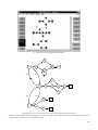
Figure 1. Dataflow graph example. . . . . . . . . . . . . . . . . . . . . . . . . . . . . . . . . . . . . . . . . . . . . . . . . . . . . 2
Figure 2. Dataflow Design Tool information flow. . . . . . . . . . . . . . . . . . . . . . . . . . . . . . . . . . . . . . . . . 5
Figure 3. Example of DESIGN.INI file. . . . . . . . . . . . . . . . . . . . . . . . . . . . . . . . . . . . . . . . . . . . . . . . . . 6
Figure 4. Design Tool main window. . . . . . . . . . . . . . . . . . . . . . . . . . . . . . . . . . . . . . . . . . . . . . . . . . . . 7
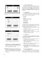
Figure 5. Dialogue box for opening graph file. . . . . . . . . . . . . . . . . . . . . . . . . . . . . . . . . . . . . . . . . . . . 8
Figure 6. Dialogue box for exiting Design Tool program. . . . . . . . . . . . . . . . . . . . . . . . . . . . . . . . . . . . 8
Figure 7. Dialogue box for selection of architecture model. . . . . . . . . . . . . . . . . . . . . . . . . . . . . . . . . . 8
Figure 8. Dialogue box for selection of multiple graph strategy. . . . . . . . . . . . . . . . . . . . . . . . . . . . . . . 9
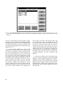
Figure 9. Choose Help menu in main window (or press F1) to invoke on-screen Help window. . . . . 10
Figure 10. About box. . . . . . . . . . . . . . . . . . . . . . . . . . . . . . . . . . . . . . . . . . . . . . . . . . . . . . . . . . . . . . . 10
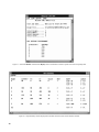
Figure 11. Metrics window. . . . . . . . . . . . . . . . . . . . . . . . . . . . . . . . . . . . . . . . . . . . . . . . . . . . . . . . . . . 10
Figure 12. TCE dialogue box for each architecture model. . . . . . . . . . . . . . . . . . . . . . . . . . . . . . . . . . 11
Figure 13. Dialogue box to select desired sink for TBIO calculations. . . . . . . . . . . . . . . . . . . . . . . . . 12
Figure 14. Dialogue box to set TBO value. . . . . . . . . . . . . . . . . . . . . . . . . . . . . . . . . . . . . . . . . . . . . . . 12
Figure 15. Dialogue box to set processor limit. . . . . . . . . . . . . . . . . . . . . . . . . . . . . . . . . . . . . . . . . . . . 12
Figure 16. Dialogue box to change graph name. . . . . . . . . . . . . . . . . . . . . . . . . . . . . . . . . . . . . . . . . . . 13
Figure 17. Single graph play window. Shaded bars indicate task execution duration;
unshaded bars indicate slack time. . . . . . . . . . . . . . . . . . . . . . . . . . . . . . . . . . . . . . . . . . . . . . . . . . . . 14
Figure 18. Two ways to display information about a node. . . . . . . . . . . . . . . . . . . . . . . . . . . . . . . . . . . 15
Figure 19. Single graph play window showing internal transitions associated with reading,
processing, and writing data.. . . . . . . . . . . . . . . . . . . . . . . . . . . . . . . . . . . . . . . . . . . . . . . . . . . . . . . . 16
Figure 20. Select Display:Paths... menu command to display all paths or just critical
paths, or Display:Circuits... menu command to display same for circuits. Paths and
circuits are denoted with gray-shaded bars. . . . . . . . . . . . . . . . . . . . . . . . . . . . . . . . . . . . . . . . . . . . . 17
Figure 21. Choose Display... command from Select menu to customize display of
nodes within Graph Play windows.. . . . . . . . . . . . . . . . . . . . . . . . . . . . . . . . . . . . . . . . . . . . . . . . . . . 18
Figure 22. Choose Jump by... command from Select menu to choose nodes or events
to jump to when moving time cursors with arrow keys. . . . . . . . . . . . . . . . . . . . . . . . . . . . . . . . . . . . 18
Figure 23. Choose Scroll Step command from Select menu to set amount to increment
when using horizontal scroll bar with a zoomed interval.. . . . . . . . . . . . . . . . . . . . . . . . . . . . . . . . . . 18
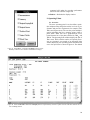
Figure 24. Total Graph Play window for DFG of figure 1 at TBO = 314 time units.
Numbers over bars indicate relative data packet numbers.. . . . . . . . . . . . . . . . . . . . . . . . . . . . . . . . . 19
Figure 25. Single Graph Play window view can be customized with Slice and
Display... menu commands. Left and right time cursors (vertical lines) are shown
measuring processing time of task C, which begins at time 100 time units and has a
duration of 70 time units. . . . . . . . . . . . . . . . . . . . . . . . . . . . . . . . . . . . . . . . . . . . . . . . . . . . . . . . . . . 19
Figure 26. Lower bound on TBO (TBOlb) is limited inherently by recurrence loop of
algorithm, composed of nodes D and E. . . . . . . . . . . . . . . . . . . . . . . . . . . . . . . . . . . . . . . . . . . . . . . . 20
Figure 27. Single Resource Envelope window displays processor utilization associated
with Single Graph Play window.. . . . . . . . . . . . . . . . . . . . . . . . . . . . . . . . . . . . . . . . . . . . . . . . . . . . . 21
v
Figure 28. Total Resource Envelope window displays processor utilization associated
with Total Graph Play window. . . . . . . . . . . . . . . . . . . . . . . . . . . . . . . . . . . . . . . . . . . . . . . . . . . . . . 22
Figure 29. Select Utilization command from Display menu in Total Resource Envelope
window to measure utilization of processors. Utilization depicted is associated with one
TBO interval of 314 time units as shown in figure 28. . . . . . . . . . . . . . . . . . . . . . . . . . . . . . . . . . . . . 22
Figure 30. TRE window time cursors define time interval for utilization measurements. . . . . . . . . . . 23
Figure 31. Parallel Execution model assumes no control over graph phasing, which requires
worst-case processor design. In Time Multiplex Execution model, phasing between graphs
is fixed to particular values by user. This deterministic phasing, and hence overlap,
between graph reduces processor requirements based on amount of graph overlap. . . . . . . . . . . . . . 24
Figure 32. Parallel Graph Execution window displays processor requirements and
utilization under Parallel Execution model. . . . . . . . . . . . . . . . . . . . . . . . . . . . . . . . . . . . . . . . . . . . . 25
Figure 33. Time Multiplex window portrays processor requirements and utilization for
algorithm graphs analyzed with Time Multiplex model. . . . . . . . . . . . . . . . . . . . . . . . . . . . . . . . . . . 26
Figure 34. Select save Results command from Display menu of Time Multiplex
window to save contents of Utilization window. Utilization window must be opened
to save Results. . . . . . . . . . . . . . . . . . . . . . . . . . . . . . . . . . . . . . . . . . . . . . . . . . . . . . . . . . . . . . . . . . . 27
Figure 35. Select Edit Graph Sequence from Select menu to define order in which
graphs should execute within scheduling cycle. Replicating graph n times allows
multiple sampling rates within graph system. That is, a given graph will execute n
times more often within scheduling cycle than other graphs. . . . . . . . . . . . . . . . . . . . . . . . . . . . . . . . 28
Figure 36. Performance window displays theoretical speedup performance of DFG.
Shown is speedup limit associated with DFG of figure 1. . . . . . . . . . . . . . . . . . . . . . . . . . . . . . . . . . 29
Figure 37. Select save Results command from Display menu in Performance window
to update Notes file with speedup data.. . . . . . . . . . . . . . . . . . . . . . . . . . . . . . . . . . . . . . . . . . . . . . . . 30
Figure 38. Graph Summary window displays DFG attributes associated with current
dataflow schedule.. . . . . . . . . . . . . . . . . . . . . . . . . . . . . . . . . . . . . . . . . . . . . . . . . . . . . . . . . . . . . . . . 30
Figure 39. Select Show... command from Display menu in Graph Summary window
to select amount of information to display.. . . . . . . . . . . . . . . . . . . . . . . . . . . . . . . . . . . . . . . . . . . . . 31
Figure 40. Select save Results command from Display menu in Graph Summary window
to update Notes file with DFG attributes for current scheduling solution. . . . . . . . . . . . . . . . . . . . . . 31
Figure 41. Operating Point window plots TBO versus TBIO. Number above each
point represents number of processors required to achieve that level of performance.
Subscript alb denotes absolute lower bound. . . . . . . . . . . . . . . . . . . . . . . . . . . . . . . . . . . . . . . . . . . . 32
Figure 42. Select Show... command from Display menu in Operating Point window to
select graph and option (index) to view. . . . . . . . . . . . . . . . . . . . . . . . . . . . . . . . . . . . . . . . . . . . . . . . 33
Figure 43. Dataflow schedule for desired number of processors (three for example) and
TBO (314 time units) may in fact require more processors (four in this case). User may
wish to eliminate needless parallelism and fill in underutilized processor time. Figure
shows intent to delay node C behind nodes B, D, or E. . . . . . . . . . . . . . . . . . . . . . . . . . . . . . . . . . . . 34
Figure 44. Imposing intra-iteration control edge E
C delays node C within its slack time
so that TBIO is not increased. Rescheduling node C eliminates needless parallelism so
same TBIO can be obtained with two processors, rather than three. . . . . . . . . . . . . . . . . . . . . . . . . . 35
Figure 45. The Design Tool prevents insertion of artificial precedence relationships not
permissible as steady-state schedules.. . . . . . . . . . . . . . . . . . . . . . . . . . . . . . . . . . . . . . . . . . . . . . . . . 35
vi
Figure 46. Imposing control edge B
D delays node D behind node B. Since nodes
B and D belong to different iterations, control edge imposes inter-iteration dependency
requiring initial tokens (one, in this example). Design Tool automatically calculates
appropriate number of initial tokens. . . . . . . . . . . . . . . . . . . . . . . . . . . . . . . . . . . . . . . . . . . . . . . . . . 36
Figure 47. Dataflow graph attributes and timing are displayed in Graph Summary window.
Edge added between nodes B and D requires initial token (OF = 1). . . . . . . . . . . . . . . . . . . . . . . . . . 37
Figure 48. Algorithm function example. . . . . . . . . . . . . . . . . . . . . . . . . . . . . . . . . . . . . . . . . . . . . . . . . 37
Figure 49. Inter-iteration control edges may be initialized with tokens, depending on iteration
number separation. . . . . . . . . . . . . . . . . . . . . . . . . . . . . . . . . . . . . . . . . . . . . . . . . . . . . . . . . . . . . . . . 38
Figure 50. Operating Point plane for three-processor design. . . . . . . . . . . . . . . . . . . . . . . . . . . . . . . . . 39
Figure 51. Updating dataflow graph with design attributes. . . . . . . . . . . . . . . . . . . . . . . . . . . . . . . . . . 39
Figure 52. Select View command from File menu in main window to view graph file.
Updated graph for three-processor design is shown. Note added control edges in
middle window.. . . . . . . . . . . . . . . . . . . . . . . . . . . . . . . . . . . . . . . . . . . . . . . . . . . . . . . . . . . . . . . . . . 40
Figure 53. After dataflow graph has been updated, current design may be overwritten.
Alternate design is shown with same number of processors: TBO increases to 350 time
units and TBIO decreases to 590 time units. Subscript alb denotes absolute lower bound.. . . . . . . . 41
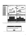
Figure 54. Design Tool warns user when updating a dataflow graph for same number of
processors will overwrite a previous design. . . . . . . . . . . . . . . . . . . . . . . . . . . . . . . . . . . . . . . . . . . . 41
Figure 55. Dataflow graph with communication delays modeled by edge delays. . . . . . . . . . . . . . . . . 42
Figure 56. Dataflow analysis of DFG of figure 55 with communication delays and
Network with Com Controller model.. . . . . . . . . . . . . . . . . . . . . . . . . . . . . . . . . . . . . . . . . . . . . . . . . 42
Figure 57. Effect of edge delays on node slack time. Intra-iteration slack of node C is
reduced by C
F edge delay of 20 time units. Inter-iteration slack of node E is reduced
by E
D edge delay of 10 time units. . . . . . . . . . . . . . . . . . . . . . . . . . . . . . . . . . . . . . . . . . . . . . . . . 43
Figure 58. Dataflow analysis of DFG of figure 55 with communication delays and
Network without Com Controller model. . . . . . . . . . . . . . . . . . . . . . . . . . . . . . . . . . . . . . . . . . . . . . . 44
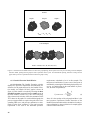
Figure 59. Three graph examples used in demonstrating multiple graph analysis and design. . . . . . . . 45
Figure 60. Capture of multiple graphs with ATAMM graph-entry tool. . . . . . . . . . . . . . . . . . . . . . . . . 46
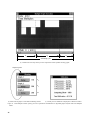
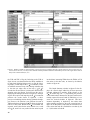
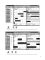
Figure 61. When more than one graph is in graph file, each is given its own Metrics
window and associated displays windows. Minimizing Metrics windows (Graphs 2
and 3 in this figure) hides all opened window displays pertaining to the graphs.
Dataflow analysis of Graph 1 shows four processors are required for an iteration period
of 200 time units.. . . . . . . . . . . . . . . . . . . . . . . . . . . . . . . . . . . . . . . . . . . . . . . . . . . . . . . . . . . . . . . . . 46
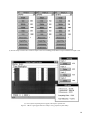
Figure 62. Dataflow analysis of Graph 2 shows eight processors are required for
iteration period of 108 time units. . . . . . . . . . . . . . . . . . . . . . . . . . . . . . . . . . . . . . . . . . . . . . . . . . . . . 47
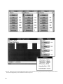
Figure 63. Dataflow analysis of Graph 3 shows four processors are required for
iteration period of 134 time units. . . . . . . . . . . . . . . . . . . . . . . . . . . . . . . . . . . . . . . . . . . . . . . . . . . . . 47
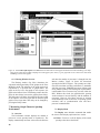
Figure 64. Parallel Graph Execution window summarizes processor requirements for
all graphs intended to execute in parallel. Since it is assumed that phasing between graphs
cannot be controlled in parallel graph strategy, total processor requirement is worst case, or
sum of individual processor requirements. . . . . . . . . . . . . . . . . . . . . . . . . . . . . . . . . . . . . . . . . . . . . . 48
Figure 65. Time multiplex strategy assumes phasing between graphs can be controlled by
defining a finite delay between inputs to graphs. . . . . . . . . . . . . . . . . . . . . . . . . . . . . . . . . . . . . . . . . 49
vii
Figure 66. Select Edit Graph Sequence command from Select menu in Multiple Graph
window to edit periodic graph sequence. User can also replicate graphs so that they
execute n-times as often as other graphs within scheduling cycle. Figure shows Graph 2
has been replicated twice. . . . . . . . . . . . . . . . . . . . . . . . . . . . . . . . . . . . . . . . . . . . . . . . . . . . . . . . . . . 50
Figure 67. TBO for a given graph under time multiplex strategy depends on phase delays. . . . . . . . . . 51
Figure 68. Phase delays can be altered with Phasing window to fill in idle time between
graph transitions. Phase delays have been reduced to increase throughput and processor
utilization in relation to figure 67.. . . . . . . . . . . . . . . . . . . . . . . . . . . . . . . . . . . . . . . . . . . . . . . . . . . . 52
Figure 69. In time multiplex mode, updating graph file not only sets graph attributes such
as queue sizes but imposes control edges (with delay attributes) around sources to control
phase of graphs.. . . . . . . . . . . . . . . . . . . . . . . . . . . . . . . . . . . . . . . . . . . . . . . . . . . . . . . . . . . . . . . . . . 53
viii
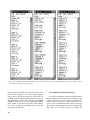
Nomenclature
AMOS
ATAMM multicomputer operating system
ATAMM
algorithm to architecture mapping model
control edge
artificial data dependency added to dataflow graph to alter schedule
data packet (data set)
input, output, and intermediate computations for given iteration
D
set of edge latencies representing communication delay between dependent
tasks
Dcritical path
total number of initial tokens in longest path
Dloop
total number of initial tokens within graph recurrence loop
DFG
dataflow graph
DSP
digital signal processing
di j
edge
communication delay between task i and task j
EF
earliest finish time of node
ES
earliest start time of node
FIFO
first in first out
graph
graphical and mathematical model of algorithm decomposition where tasks
are represented by nodes or vertices and data or control dependencies are
represented by directed edges or arcs
GVSC
generic VHSIC spaceborne computer
index
operating point option for same number of active processors
instantiations
same task simultaneously executing in multiple processors for different data
sets
L
set of task latencies
latency
execution time of task represented by node
Ledge
latency of edge representing communication delay
LF
latest finish time of node
Li
ith element in L; latency of ith task
Lloop
sum of node and edge latencies in graph recurrence loop
Lnode
latency of node representing executable task
Mo
initial marking of graph
Ni
ith node in graph
Network with
Com Controller
architecture model which assumes processors are fully connected via
communication paths; each processing element is paired with communication (com) controller which handles transfer of information after processor
sets up for transfer
Network without
Com Controller
architecture model which assumes processors are fully connected via
communication paths; model does not assume each processing unit is paired
with communication (com) controller which handles transfer of information
node
graph vertex represents algorithm instructions or task to be executed
represents data dependency (real or artificial) within directed graph; edge is
implemented with FIFO queue or buffer
ix
operating point
predicted performance and resource requirement characterized by TBO,
TBIO, and R
ω
schedule length
OE
output empty; number of initially empty output queue slots
OF
output full; number of initially full output queue slots
parallel execution
execution of multiple graphs in parallel without controlling graph phasing
phase
time delay between input injection of two or more graphs
partial ordering of tasks
PI
parallel-interface bus
R
available processors
Rc
calculated processor requirement; corresponds to theoretic lower limit
S
speedup
schedule length
minimum time to execute all tasks for given computation
SGP
single graph play
Shared Memory/
No Contention
architecture model which assumes processors are fully connected to shared
memory with enough paths to avoid contention
sink
graph output data stream
slack (float)
maximum time token can be delayed at node without increasing delay in
longest path
source
graph input data stream
SRE
single resource envelope
T
set of tasks
task
set of instructions as basic unit of scheduling
TBI
time between inputs
TBIO
time between input and output
TBIOlb
lower bound time between input and output
TBO
time between outputs
TBOlb
lower bound time between outputs
TCE
total computing effort
TGP
total graph play
Ti
ith task in T
time multiplex execution execution of multiple graphs in parallel by controlling graph phasing
To
maximum time per token ratio for all graph recurrence loops
token
initial conditions and data values within graph
token bound
maximum number of tokens on edge
TRE
total resource envelope
U
utilization
VHSIC
very-high-speed integrated circuit
x
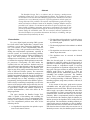
Abstract
The Dataflow Design Tool is a software tool for selecting a multiprocessor
scheduling solution for a class of computational problems. The problems of interest
are those that can be described with a dataflow graph and are intended to be executed
repetitively on a set of identical processors. Typical applications include signal processing and control law problems. The software tool implements graph-search algorithms and analysis techniques based on the dataflow paradigm. Dataflow analyses
provided by the software are introduced and shown to effectively determine performance bounds, scheduling constraints, and resource requirements. The software tool
provides performance optimization through the inclusion of artificial precedence constraints among the schedulable tasks. The user interface and tool capabilities are
described. Examples are provided to demonstrate the analysis, scheduling, and optimization functions facilitated by the tool.
1. Introduction
For years, digital signal processing (DSP) systems
have been used to realize digital filters, compute Fourier
transforms, execute data compression algorithms, and
run a vast amount of other computationally intensive
algorithms. Today, both government and industry are
finding that computational requirements, especially in
real-time systems, are becoming increasingly challenging. As a result, many users are relying on multiprocessing to solve these problems. To take advantage of
multiprocessor architectures, novel methods are needed
to facilitate the mapping of DSP applications onto multiple processors. Consequently, the DSP market has
exploded with new and innovative hardware and software architectures that efficiently exploit the parallelism
inherent in many DSP applications. The dataflow paradigm has also been getting considerable attention in the
areas of DSP and real-time systems. The commercial
products offered today utilize the dataflow paradigm as a
graphical programming language but do not incorporate
dataflow analyses in designing a multiprocessing solution. Although there are many advantages to graphical
programming, the full potential of the dataflow representation is lost by not utilizing it analytically as well. In the
absence of the analysis and/or design offered by the software tool described in this paper, programmers must rely
on approximate compile time solutions (heuristics) or
run-time implementations, which often utilize ad hoc
design approaches.
This paper describes the Dataflow Design Tool,
which is capable of determining and evaluating the
steady-state behavior of a class of computational problems for iterative parallel execution on multiple processors. The computational problems must meet all the
following criteria:
1. An algorithm decomposition into primitive operations or tasks must be known.
2. The algorithm task dependencies, preferably due to
the inherent data dependencies, must be modeled
by a directed graph.
3. The directed graph must be deterministic as defined
below.
4. The algorithm execution must be repetitive for an
infinite input data stream.
5. The algorithm must be executed on identical
processors.
When the directed graph is a result of inherent data
dependencies within the problem, the directed graph is
equivalent to a dataflow graph. Dataflow graphs are generalized models of computation capable of exposing
inherent parallelism in algorithms ranging from fine to
large grain. This paper assumes an understanding of both
dataflow graph theory as described by a Petri net
(marked graph) and the fundamental problem of task
scheduling onto multiple processors. The Dataflow
Design Tool is a Microsoft Windows application, and
thus a working knowledge of Microsoft Windows (i.e.,
launching programs, using menus, window scroll bars) is
also assumed.
In the context of this paper, graph nodes represent
schedulable tasks, and graph edges represent the data
dependencies between the tasks. Because the data dependencies imply a precedence relationship, the tasks make
up a partial-order set. That is, some tasks must execute in
a particular order, whereas other tasks may execute independently. When a computational problem or algorithm
can be described with a dataflow graph, the inherent parallelism present in the algorithm can be readily observed
and exploited. The deterministic modeling methods presented in this paper are applicable to a class of dataflow
graphs where the time to execute tasks are assumed constant from iteration to iteration when executed on a set of
identical processors. Also, the dataflow graph is assumed
data independent; that is, any decisions present within
the computational problem are contained within the
graph nodes rather than described at the graph level. The
dataflow graph provides both a graphical model and a
mathematical model capable of determining run-time
behavior and resource requirements at compile time. In
particular, dataflow graph analysis can determine the
exploitable parallelism, theoretical performance bounds,
speedup, and resource requirements of the system.
Because the graph edges imply data storage, the resource
requirement specifies the minimum amount of memory
needed for data buffers as well as the processor requirements. This information allows the user to match the
resource requirements with resource availability. In addition, the nonpreemptive scheduling and synchronization
of the tasks that are sufficient to obtain the theoretical
performance are specified by the dataflow graph. This
property allows the user to direct the run-time execution
according to the dataflow firing rules (i.e., when tasks are
enabled for execution) so that the run-time effort is simply reduced to allocating an idle processor to an enabled
task (refs. 1 and 2). When resource availability is not sufficient to achieve optimum performance, a technique of
optimizing the dataflow graph with artificial data dependencies called “control edges” is utilized.
An efficient software tool that applies the mathematical models presented is desirable for solving problems in
a timely manner. A software tool developed for design
and analysis is introduced. The software program,
referred to hereafter as the “Dataflow Design Tool” or
“Design Tool,” provides automatic and interactive analysis capabilities applicable to the design of a multiprocessing solution. The development of the Design Tool was
motivated by a need to adapt multiprocessing computations to emerging very-high-speed integrated circuit
(VHSIC) space-qualified hardware for aerospace applications. In addition to the Design Tool, a multiprocessing
operating system based on a directed-graph approach
called the “ATAMM multicomputer operating system”
(AMOS) was developed. AMOS executes the rules of the
algorithm to architecture mapping model (ATAMM) and
has been successfully demonstrated on a generic VHSIC
spaceborne computer (GVSC) consisting of four processors loosely coupled on a parallel-interface (PI) bus
(refs. 1 and 2). The Design Tool was developed not only
for the AMOS and GVSC application development environment presented in references 1 and 3 but also for
other potential dataflow applications. For example, information provided by the Design Tool could be used for
scheduling constraints to aid heuristic scheduling
algorithms.
A formal discussion of dataflow graph modeling is
presented in section 2 along with definitions of graphtheoretic performance metrics. Sections 3 through 9 pro2
vide an overview of the user interface and the capabilities
of the Dataflow Design Tool version 3.0. Further discussions of the models implemented by the Design Tool are
provided in section 10 for a few case studies. Enhancements planned for the tool are discussed in section 11.
2. Dataflow Graphs
A generalized description of a multiprocessing problem and how it can be modeled by a directed graph is
presented. Such formalism is useful in defining the models and graph analysis procedures supported by the
Design Tool. A computational problem can often be
decomposed into a set of tasks to be scheduled for execution (ref. 4). If the tasks are not independent of one
another, a precedence relationship will be imposed on the
tasks in order to obtain correct computational results.
A task system can be represented formally as a
5-tuple (T , , L, D, Mo). The set T = {T1, T2, T3,..., Tn}
is a nonempty set of n tasks to be executed, and
is the
precedence relationship on T such that Ti Tj signifies
that Tj cannot execute until the completion of Ti. The set
L = {L1, L2, L3,..., Ln} is a nonempty, strictly positive
set of run-time latencies such that task Ti takes Li amount
of time to execute. The set D = {di j, dk l, dm n,...,
dx y} is a strictly positive set of latencies associated
with each precedence relationship. A latency di j in D
that is associated with the precedence Ti Tj represents
the time required to communicate the data from Ti to Tj.
Finally, Mo is the initial state of the system as indicated
by the presence of initial data.
Such task systems can be described by a directed
graph where nodes (vertices) represent the tasks and
edges (arcs) describe the precedence relationship
between the tasks. When the precedence constraints
given by
are a result of the dataflow between the
tasks, the directed graph is equivalent to a dataflow graph
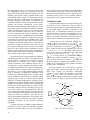
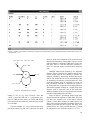
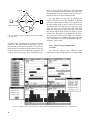
(DFG) as shown in figure 1. Special transitions called
Latency
390
B
Source
Node
90
90
90
A
C
F
Edge
190
D
E
90
Token
Figure 1. Dataflow graph example.
Sink
sources and sinks are also provided to model the input
and output data streams of the task system. The presence
of data is indicated within the DFG by the placement of
tokens. The DFG is initially in the state indicated by the
marking Mo. The graph transitions through other markings as a result of a sequence of node firings. That is,
when a token is available on every input edge of a node
and sufficient resources are available for the execution of
the task represented by the node, the node fires. When
the node associated with task Ti fires, it consumes one
token from each of its input edges, delays an amount of
time equal to Li, and then deposits one token on each of
its output edges. Sources and sinks have special firing
rules in that sources are unconditionally enabled for firing and sinks consume tokens but do not produce any. By
analyzing the DFG in terms of its critical path, critical
circuit, dataflow schedule, and the token bounds within
the graph, the performance characteristics and resource
requirements can be determined a priori. The Design
Tool uses this dataflow representation of a task system
and the graph-theoretic performance metrics presented
herein. The Design Tool relies heavily on the dataflow
graph for its functionality and interface. However, when
the abstraction of representing the task dependencies
Tj) by an edge is used so often, one may adopt the
(Ti
terminology of saying a “node executes” on a processor
even though a node only represents task instructions that
get executed. Nevertheless, depending on the context of
the discussion, the terms “node” and “task” are used
interchangeably in this paper.
2.1. Measuring and Constraining Parallelism
The two types of concurrency that can be exploited
in dataflow algorithms can be classified as parallel and
pipeline. Two graph-theoretic metrics are measured by
the Design Tool as indicators of the degree of concurrency that may be exploited. The metrics are referred to
as TBIO (time between input and output) and TBO (time
between outputs) and reflect the degree of parallel and
pipeline concurrency, respectively.
Parallel concurrency is associated with the execution
of tasks that are independent (no precedence relationship
imposed by ). The extent to which parallel concurrency can be exploited depends on the number of parallel
paths within the DFG and the number of resources available to exploit the parallelism. The elapsed time between
the production of an input token by the source and the
consumption of the corresponding output token by the
sink is defined as the time between input and output, or
TBIO. TBIO is frequently equivalent to the scheduling
length ω, defined as the minimum time to execute all
tasks for a given data set. However, when initial tokens
are present, the scheduling length may be greater than
TBIO. The TBIO metric in relation to the time it would
take to execute all tasks sequentially can be a good measure of the parallel concurrency inherent within a DFG.
If there are no initial tokens present in the DFG, TBIO
can be determined by using the traditional critical path
analysis, where TBIO is given as the sum of node latencies in L and data communication delays in D (modeled
by edge latency) contained in the critical path. When Mo
defines initial tokens in the forward direction, the graph
takes on a different behavior (ref. 5). This occurs in
many signal processing and control algorithms where initial tokens are expected to provide previous state information (history) or to provide delays within the
algorithm. A general equation is used by the Design Tool
to calculate the critical path, and thus TBIO, as a function
of TBO when initial tokens are present along forward
paths:
TBIO =
∑
L node
∀ n ode ∈ critical path
+
∑
L node
∀ e dge ∈ critical path
– ( D critical path ) ( TBO )
(1)
where Lnode are the node latencies, Ledge are the edge
latencies, and Dcritical path is the total delay along the critical path (ref. 5). The critical path, defined as the path
without slack, is the path that maximizes equation (1).
Including edge latency as a model parameter provides a
simple, but effective, means of modeling the cost of communicating data between nodes. This communication
model assumes that nodes with multiple output edges can
communicate the data for each edge simultaneously.
Of particular interest are the cases when the algorithm modeled by the DFG is executed repetitively for
different data sets (data samples in DSP terminology).
Pipeline concurrency is associated with the repetitive
execution of the algorithm for successive data sets without waiting for the completion of earlier data sets. The
iteration period and thus throughput (inverse of the iteration period) is characterized by the metric TBO (time
between outputs), defined as the time between consecutive consumptions of output tokens by a sink. Because of
the consistency property of deterministic dataflow
graphs, all tasks execute with period TBO (refs. 6 and 7).
This implies that if input data are injected into the graph
with period TBI (time between inputs) then output data
will be generated at the graph sink with period
TBO = TBI. The minimum graph-theoretic iteration
period To due to recurrence loops is given by the largest
ratio of loop time Lloop to the initial tokens within the
loop Dloop for all recurrence loops within the DFG
(refs. 7–9):
∑
To
∑

L node +
L edge


L
loop
∈ loop
edge ∈ loop 
= max  ------------  = max  node
--------------------------------------------------------- D loop 


D loop


(2)
3
Given a finite number of processors, the actual lower
bound on the iteration period (or TBOlb) is given by
TCE
TBO lb = max T o, ----------- 
R
(3)
where TCE is the total computing effort and R is the
available number of processors. If communication effort
modeled by edge delays is ignored, TCE can be calculated from the latencies in L as
TCE =
∑ Li
(4)
i∈L
and the theoretically optimum value of Rc for a given
TBO period, referred to as the calculated R, can be computed as
Rc =
TCE
-----------TBO
(5)
is applied to the ratio of
where the ceiling function1
TCE to TBO. Since every task executes once within an
iteration period of TBO with R processors and takes TCE
amount of time with one processor, speedup S can be
defined by Amdahl’s Law as
TCE
S = -----------TBO
(6)
and processor utilization U ranging from 0 to 1 can be
defined as
S
U = --R
(7)
for a processor requirement R.
By definition, the critical path does not contain
slack; thus, critical path tokens will not wait on edges for
noncritical path tokens, ideally. The inherent nature of
dataflow graphs is to accept data tokens as quickly as the
graph and available resources (processors and memory)
will allow. When this occurs, the graph becomes congested with tokens waiting on the edges for processing
because of the finite resources available, without resulting in throughput above the graph-imposed upper bound
(refs. 10 and 11). However, when tokens wait on the critical path for execution because of token congestion
within the graph, an increase in TBIO above the lower
bound occurs. This increase in TBIO can be undesirable
for many real-time applications. Therefore, to prevent
saturation, constraining the parallelism that can be
exploited becomes necessary. The parallelism in dataflow graphs can be constrained by limiting the input
1The
ceiling of a real number x, denoted as
smallest integer greater than or equal to x.
4
x , is equal to the
injection rate to the graph. Adding a delay loop around
the source makes the source no longer unconditionally
enabled (ref. 1). It is important to determine the appropriate lower bound on TBO for a given graph and number
of resources.
2.2. Run-Time Memory Requirements
The scheduling techniques offered in this paper are
intended for modeling the periodic execution of algorithms. In many instances, the algorithms may execute
indefinitely on an unlimited stream of input data; this is
typically true for DSP algorithms. To achieve a high
degree of pipeline concurrency, a task may be required to
begin processing the next data sets before completing the
execution of the current data set, resulting in multiple
instantiations of a task. Multiple instantiations of a task
require that a task execute on different processors simultaneously for different, sequential data sets. System
memory requirements increase with the instantiation
requirements of tasks, since multiply instantiated tasks
must be redundantly allocated on multiple processors.
For deterministic algorithms executing at constant iteration periods, the bound on the number of task instantiations can be calculated as
Instantiations of T i =
Li
-----------TBO
(8)
Even though the multiprocessor schedules determined by the Design Tool are periodic, it is important to
determine whether the memory requirement for the data
is bounded. However, just knowing that the memory
requirement is bounded may not be enough. One may
also wish to calculate the maximum memory requirements a priori. By knowing the upper bound on memory,
the memory can be allocated statically at compile time to
avoid the run-time overhead of dynamic memory management. Dataflow graph edges model a FIFO management of tokens migrating through a graph and thus imply
physical storage of the data shared among tasks. Using
graph-theoretic rules, the Design Tool is capable of
determining the bound on memory required for the
shared data as a function of the dataflow schedule.
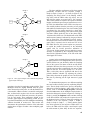
2.3. Control Edges
When resource requirements for a given dataflow
graph schedule are greater than resource availability,
imposing additional precedence constraints or artificial
data dependencies onto T (thereby changing the schedule) is a viable way to improve performance (refs. 1, 5,
and 12). These artificial data dependencies are referred to
as “control edges.” The Design Tool allows the user to
alter the dataflow schedule by choosing that a given task
be delayed until the execution of another task. The
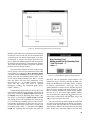
Task system (T, L, , Mo):
T Set of tasks
L Fixed-task latencies
Partial order on T
Mo Initial state
DFG
Dataflow
graph (DFG)
Performance bounds:
Schedule length ω
Time between input and output TBIOlb
Minimum iteration period To
Time between outputs TBOlb
Slack
Processor utilization
Run-time requirements:
Task instantiations
Processor requirement
Data buffers
Artificial , control edges
Graph
Analysis
Dataflow graph:
Nodes represent T
Edges describe
Tokens indicate presence of data
Initial marking = Mo
Graphical displays:
Gantt chart task execution
Single iteration (SGP)
Periodic execution (TGP)
Resource envelopes
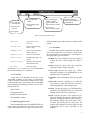
Figure 2. Dataflow Design Tool information flow.
Design Tool automatically models this additional precedence constraint as a control edge and initializes the edge
with tokens (positive or negative), as needed, to provide
proper synchronization. That is, as a function of the new
schedule, the precedence constraint may impose intraiteration dependencies for the same data set, which do
not require an initial token. On the other hand, the precedence relationship may impose inter-iteration dependency for different data sets, which requires initial tokens
to occur.
3. Dataflow Design Tool
The dataflow paradigm presented in the previous
section is useful for exposing inherent parallelism constrained only by the data precedences. Such a hardwareindependent analysis can indicate whether a given
algorithm decomposition has too little or too much parallelism early on in the development stage before the user
attempts to map the algorithm onto hardware. The Dataflow Design Tool version 3.0, described in the remaining
sections, analyzes dataflow graphs and applies the design
principles discussed herein to multiprocessor applications. The software was written in C++2 and executes in
Microsoft Windows3 or Windows NT. The software can
2Version
3Version
3.1 by Borland International, Inc.
3.1 by Microsoft Corporation.
be hosted on an i386/486 personal computer or a compatible type. The various displays and features are presented
in this section. As a convention, menu commands are
denoted with the ☛ symbol.
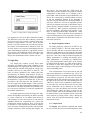
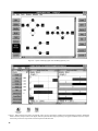
Figure 2 provides an overview of the input and output process flow of the Design Tool. After a DFG is
loaded, the Design Tool will search the DFG for recurrence loops (circuits) and determine the minimum iteration period To by using equation (2), where To is zero if
no circuits are present. TBO will initially be set to the
largest task latency or To, whichever is larger. The calculated processor requirement Rc is initially given by equation (5). TBIO is determined from equation (1). Any
changes to R will result in an update of the optimum
value for TBO (TBOlb) from equation (3). For a given
value of R, TBO may be changed to a value greater than
or equal to TBOlb. When the schedule is altered (resulting in added control edges), the analysis is repeated to
determine the new critical path, critical circuits, and
modifications to the performance bounds.
The dataflow graph example shown in figure 1 is
used to present the displays and capabilities of the tool.
The format for the graph description file is described in
section 3.1.1, and the complete graph text description
used for figure 1 is provided in the appendix. The node
latencies shown in figure 1 are interpreted generally as
time units so that “real time” can be user interpreted.
5
That is, if the clock used to measure or derive the task
durations has a resolution of 100 µsec, the latency of
node A can be interpreted to be 9 µsec. To maintain the
resolution of time when applying the equations of section 2, the Design Tool always rounds (applies the ceiling function) to the next highest clock tick.
3.1. File Input/Output
The Design Tool takes input from a graph text file
that specifies the topology and attributes of the DFG. The
graph text file format is given in this section. Updates to
the graph text file (e.g., GRAPHFILE.GTF) with design
attributes and artificial dependencies are made directly
by the Design Tool, with the original version saved as a
backup (graphfile.bak). In addition to this graph text file,
the Design Tool can accept input from the ATAMM
graph-entry tool4 developed for the AMOS system at the
Langley Research Center. Updates to the graph file are
made via dynamic data exchange (DDE) messages to the
graph-entry tool for a given design point (R, TBO, and
TBIO). Changes to the graph topology due to added control edges appear in real time. The graph-entry tool is
responsible for writing the graph updates to the graph
file.
The Design Tool also makes use of other files. An
.RTT file is created automatically for each graph file
(GRAPHFILE.RTT) and contains performance information needed for follow-up design sessions of previously
updated graphs. Two .TMP files are also created for processing paths (PATHS.TMP) and circuits (CIRCS.TMP)
within the graph. An .INI file (DESIGN.INI) stores
(1) the graph file used in the last session; (2) the default
graph file extension to search for when opening a file;
(3) the location of the ATAMM graph-entry tool, if used;
and (4) the editor to be used to display the notes file (discussed in section 3.1.2). An example of the .INI file is
shown in figure 3.
[DesignTool]
Extension = *.GTF
Model = 0
3.1.1. Graph Text File
The Design Tool allows the user to describe a dataflow graph with a text file. The file may only describe a
single graph. Updates to the file (node instantiations,
queue sizes, input injection rate, and added control
edges) for a given analysis or design are done automatically by the tool by using the update Graph menu command within the Operating Point window (defined in
section 9). The format of the file is given below. Keywords are not case sensitive, items shown in brackets [ ]
are optional, name specifies a character string with a
maximum of 20 characters and no spaces, and integer
specifies a number from 0 to 32767. Optional parameters
that are omitted have a default value of zero. Blank lines
separating statements are allowed. See appendix for
examples.
The first line in the file must be
GRAPH name
Following the GRAPH statement (in any order) are
To specify a node transition:
NODE name
Editor = C:\WINNT\NOTEPAD.EXE
Figure 3. Example of DESIGN.INI file.
4Written
6
by Asa M. Andrews, CTA, Inc.
specifies a node with a
unique name
[PRIORITY integer] task priority for information
only
[READ integer]
time to read input data
PROCESS integer
time to process data
[WRITE integer]
time to write output data or
set up for communication
INST integer
task instantiations
END NODE
end of node object
Note that the statements between NODE and END NODE
may be in any order.
To specify a source transition:
SOURCE name
specifies a source with a
unique name
TBI integer
time between inputs, i.e., the
input injection period
END SOURCE
end of source object
Graph = D:\WIN16\ATAMM\DEMO\DFG.GRF
GraphTool = D:\WIN16\ATAMM\GRAPH\GRAPHGEN.EXE
specifies the name of the
graph
To specify a sink transition:
SINK name
specifies a sink with a unique
name
END SINK
end of sink object
To specify an edge (edges must be specified following
the NODE, SOURCE, and SINK statements):
Open, close, and
view DFG file
Name and view
notes file
Select architecture
model
Select multiple graph
strategy
View operating point
window, multiple
graph windows, and
desired metrics window
Invokes on-line help
and provides information
on DesignTool.
Select color or
black and white display
Exit program
Figure 4. Design Tool main window.
EDGE type
type can be DATA or
CONTROL
INITIAL name
name of node producing
tokens to edge
TERMINAL name
name of node consuming
tokens from edge
TOKENS integer
number of initial tokens
QUEUE integer
minimum FIFO queue size
of edge
[DELAY integer]
edge delay used to model
communication time
END EDGE
end of edge object
Note that the INITIAL and TERMINAL statements must
precede the remaining EDGE statements.
3.1.2. Notes File
A notes file is a file designated by the user via the
save Notes command for the saving of performance
results or personal notes during the design session. After
creation, the file can be viewed at any time via the Notes
menu command. The following windows can save information to this file:
Graph window
Performance window
Parallel Execution window
Time Multiplex window
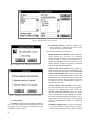
3.2. Main Program Overview
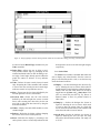
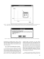
Upon invoking the Design Tool (DESIGN.EXE), the
main window will appear at the top of the screen with a
caption and menus as shown in figure 4. The menu com-
mands provided by the main window are defined in this
section.
3.2.1. File Menu
The File menu includes commands that enable the
user to open a graph file, create and view a notes file for
the current session, or exit the program. A description of
each command is given as follows:
☛ Open—Invokes the dialogue box shown in figure 5
to allow the user to select a graph file to open as
input.
☛ Close—Ends the current session for a particular
graph file without exiting the program.
☛ View File—Invokes the editor (e.g., NOTEPAD.EXE) specified in the DESIGN.INI file for
displaying the current graph file.
☛ Get Info—Shows information on the current graph
file.
☛ Save Info—Invokes a dialogue box to allow the
user to specify a notes file in which to save information regarding the current design session.
☛ Notes—Invokes the editor (e.g., NOTEPAD.EXE)
specified in the DESIGN.INI file for viewing and
updating the notes file with personal notes.
☛ Exit—Exits the program. Upon exiting the program, the dialogue box shown in figure 6 will be
displayed. Clicking the OK button will exit the program whereas clicking Cancel will return to previous state. By checking the Save Setup box, the
program will remember the current graph file and
automatically load it upon reexecution of the
program.
7
Figure 5. Dialogue box for opening graph file.
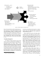
☛ Architecture Model—Invokes the dialogue box
shown in figure 7 to allow the user to select a general model of the target architecture.
The architectural models are defined as
Figure 6. Dialogue box for exiting Design Tool program.
Shared Memory/No Contention—This architecture
model assumes the processors are completely
connected to shared memory with enough paths to
avoid contention. In effect, this model provides an
architecture-independent model that exposes the parallelism inherent within the algorithm, constrained
only by the algorithm decomposition.
Network with Com Controller—This architecture
model assumes the processors are completely connected via communication paths. Unlike the Network
without Com Controller option, each processing unit
is paired with a communication (com) controller that
handles the transfer of information after the processor
sets up for the transfer. Thus, the processors will not
be burdened with the communication transfers to
neighboring processors.
Figure 7. Dialogue box for selection of architecture model.
3.2.2. Setup Menu
The Setup menu includes commands that enable the
user to select the architecture model and the type of multiple graph execution strategy. A description of each
command is given as follows.
8
Network without Com Controller—This architecture model assumes the processors are completely
connected via communication paths. Unlike the
Network with Com Controller option, this model
does not assume that each processing unit is paired
with a communication (com) controller that handles
the transfer of information after the processor sets up
for the transfer. Thus, each processor will be burdened
with the communication transfers to neighboring
processors.
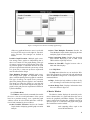
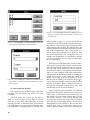
☛ Multiple Graph Strategy—Invokes the dialogue
box shown in figure 8 to allow the user to choose
multiple graph execution strategy. The user simply
Figure 8. Dialogue box for selection of multiple graph strategy.
clicks on a graph and chooses to move it to the left
for Parallel Execution or to the right for Time Multiplex Execution. The strategies are defined as
follows.
Parallel Graph Execution—Multiple graph execution strategy where graphs are independent; that is,
there is no control over the graph phasing. This type
of strategy requires more processors than if the phasing between graphs is controlled. Because the peak
processor requirements within the system may overlap
at a given time, a worst-case processor requirement
must be utilized in the design.
Time Multiplex Execution—Multiple graph execution strategy where graphs are dependent on each
other, in that the phasing between graphs is controlled.
This type of strategy can require fewer processors
than if the phasing between graphs is not controlled.
The intent is to phase the graphs in a way that idle
time is filled in as processors migrate from graph to
graph, but the peak processor requirement is limited to
system availability.
3.2.3. Window Menu
The Window menu includes commands that enable
the user to view the overall performance of the system
based on a particular strategy, view a particular graph
window, or draw in color or black and white. A description of each command is given as follows.
☛ show Parallel Execution—Invokes the Parallel
Graph window displaying parallel graph execution
analysis.
☛ show Time Multiplex Execution—Invokes the
Time Multiplex Graph window displaying the time
multiplex graph execution analysis.
☛ show Operating Points—Invokes the Operating
Point window displaying a plot of TBO versus
TBIO with the required processors.
☛ Draw in Color/BW—Toggles between color or
black and white displays.
3.2.4. Help Menu
The Help menu allows the user to invoke the Windows Help program for on-screen help and information
about the Dataflow Design Tool. A description of each
command follows.
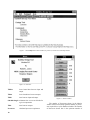
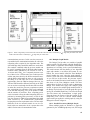
☛ Help—Invokes the help window as shown in figure 9. (Pressing F1 also invokes the help window.)
☛ About Design Tool—Displays information about
the tool as shown in figure 10.
4. Metrics Window
The Metrics window displays the numerical performance characteristics of a graph and allows the user to
invoke the graphical performance displays. The graph
name is shown in the window title. A Metrics window as
shown in figure 11 is created for each graph in the graph
file. Performance metrics include
TCE
total computing effort; equal to the
sum of all task latencies
9
Figure 9. Choose Help menu in main window (or press F1) to invoke on-screen Help window.
Figure 10. About box.
TBIOlb
lower bound time between input and
output
TBOlb
lower bound time between outputs
TBIO
time between input and output
Schedule length minimum time to execute all tasks for
a given computation
TBO
time between outputs
Processors
calculated processor requirement
10
Figure 11. Metrics window.
The number of Processors shown in the Metrics
window will not necessarily equal the number of processors required for a cyclic dataflow schedule. The number
of Processors shown here is the optimum number of
Shared Memory
No Contention
Network with
Com Controller
Network without
Com Controller
Figure 12. TCE dialogue box for each architecture model.
processors for the current TBO setting from equation (5)
and is referred to as the calculated processor requirement. The actual processor requirement may be greater
than the calculated requirement because of the partial
ordering of tasks. The job of scheduling partially ordered
tasks to processors is known to be NP-complete (ref. 4).
This implies that an exhaustive search (rescheduling
tasks with start times greater than the earliest start times
given by the dataflow analysis) is required to find an
optimum solution that achieves the timing criteria (e.g.,
minimum TBO and/or schedule length) with only the calculated processor requirement. However, one cannot
guarantee that a solution even exists when both TBO and
R are held constant (ref. 9). In such cases, one must
choose a heuristic that relaxes the criteria, fixing one
parameter (e.g., processors) and allowing the other (e.g.,
TBO) to vary until a solution is found.
The graphical windows provided by the Design Tool
are briefly described below. A more detailed description
of each is provided in later sections. The windows can be
invoked from the Metrics window by clicking on the buttons defined below.
☛ Single Graph Play (SGP)—A Gantt chart displaying the steady-state task schedule for a single computation. The chart is constructed by allowing tasks
to start at the earliest possible time (referred to as
the earliest start (ES) time) with infinite resources
assumed. The chart is plotted with tasks names
shown vertically, task execution duration given by
bars, and a horizontal time axis equal to the schedule length.
☛ Total Graph Play (TGP)—A Gantt chart displaying the steady-state task schedule for multiple computations executed simultaneously over one
scheduling period (which repeats indefinitely). The
chart is constructed by allowing tasks to start at an
earliest time equal to the ES times (given by the
SGP) modulo TBO with infinite resources
assumed. The chart is plotted similar to the SGP
except only over a TBO time interval. Multiple
instantiations of a task are shown by creating multiple rows per task; this allows the bars to overlap.
☛ Single Resource Envelope (SRE)—A plot of the
processor requirement for the SGP.
☛ Total Resource Envelope (TRE)—A plot of the
processor requirement for the TGP.
☛ Performance—Plots speedup versus processors
given by equation (6).
The following buttons, when clicked on, provide
numerical data on DFG attributes, computing effort, and
allow the user to select a sink (for graphs with multiple
sinks) to measure TBIO.
☛ Graph Summary—Displays a window summarizing the DFG attributes: node names, latencies, earliest start, latest finish, instantiations, and FIFO
queue sizes.
☛ TCE—Invokes the dialogue box shown in figure 12, which shows a breakdown of computing
effort. The TCE dialogue box is discussed in more
detail in section 4.2.
☛ TBIOlb—Invokes the dialogue box shown in figure 13 to select the desired sink in which to measure TBIO.
☛ TBIO/Schedule Length—Toggles between displaying TBIOlb or the schedule length, ω.
☛ TBO—Allows the user to increment (+) or decrement (−) TBO or set it (=) to a desired value.
11
4.1. Metrics Window Menus
The previous section presented the buttons used to
invoke displays and set parameters. The Metrics window
also provides two menus, Display and Set, as shown in
figure 11, that can be used instead of the buttons. The
commands for the Display and Set menus are described
as follows.
4.1.1. Display Menu
Figure 13. Dialogue box to select desired sink for TBIO
calculations.
The Display menu includes commands that enable
the user to view and arrange the previously described
window displays. The first six commands
☛ Graph
☛ TCE
☛ Schedule length / TBIO
☛ Graph Play
☛ Concurrency
☛ Performance
are equivalent to the button definitions given previously.
The following three commands allow the user to refresh
and arrange the displays currently on the screen.
Figure 14. Dialogue box to set TBO value.
☛ Tile—Tiles the currently active windows invoked
by the Metrics window.
☛ Cascade—Cascades the currently active windows
invoked by the Metrics window.
☛ Reset—Refreshes the currently active windows
invoked by the Metrics window.
4.1.2. Set Menu
The Set menu includes commands that enable the
user to define the calculated processor value, set TBO,
and change the graph name.
☛ Processors—Invokes the dialogue box in figure 15
to set the calculated processor limit.
Figure 15. Dialogue box to set processor limit.
Clicking on the = button invokes the dialogue box
shown in figure 14. The minimum TBO value permissible is determined from equation (3) for the
current calculated processor setting.
☛ Processors—Allows the user to increment (+) or
decrement (−) the calculated processor limit. Each
time the calculated processors count is changed,
TBO is set to the optimum value determined from
equation (3).
12
☛ TBO—Invokes the dialogue box in figure 14 to set
the desired TBO period.
☛ Sink —Invokes the dialogue box in figure 13 to set
the desired sink for TBIO calculations.
☛ Graph Name—Invokes the dialogue box in figure 16 to allow the user to rename the graph for display purposes.
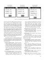
4.2. Total Computing Effort
The total computing effort (TCE) value given by the
Metrics window depends on the chosen architecture
model defined in section 3. Figure 12 shows the dialogue
Figure 16. Dialogue box to change graph name.
box displayed for each of the three architecture models.
The difference between the Shared Memory model and
the Network with Com Controller model is in the interpretation of graph attribute write time. For the network
models, write time is assumed to represent setup time for
the transfer of information and is denoted as such. The
Network without Com Controller model displays the time
spent communicating (defined by edge delays) because
the processor will be burdened with the effort. Since the
graph described by DFG.GTF does not define edge
delays, the communication effort is shown to be zero.
5. Graph Play
The Graph Play windows provide Gantt charts
describing the dataflow-derived task schedules of the
algorithm graph. The single graph play (SGP) shows the
steady-state time schedule of the graph for a single computation, referred to as “data packet” or “data set.” The
tasks are shown scheduled at the earliest start times
determined by the dataflow graph analysis. If tasks are
scheduled this way and infinite resources are assumed,
all the inherent parallelism present within the algorithm
decomposition is exposed and limited only by the data
precedences. The SGP shows the task schedule over a
time axis equal to the schedule length ω. Task executions
are represented by bars with lengths proportional to the
task latencies. The SGP determines the minimum number of processors sufficient to execute the algorithm for
the schedule length shown.
For digital signal processing and control law algorithms, the algorithm represented by the DFG is assumed
to execute repetitively on an infinite input stream. In
such instances, the user does not have to wait until the
algorithm finishes the computations for a given data
packet before starting on the next. Thus, it is of interest
to determine a cyclic schedule that permits the simultaneous execution of multiple data packets which exploits
pipeline concurrency while assuring data integrity. For
this purpose, the total graph play (TGP) shows the
steady-state, periodic schedule of the graph for multiple
computations or data packets over a schedule cycle of
period TBO, which is assumed to repeat indefinitely. The
TGP is also constructed by assuming infinite resources
so that the parallelism inherent in the algorithm is
exposed. The TGP determines the maximum number of
processors sufficient to execute the algorithm periodically and, as mentioned in section 4, that number may be
greater than the calculated number of processors given
by equation (5). When processor requirements exceed
processor availability, the Design Tool provides a technique of inserting artificial data dependencies, called
“control edges,” to alter the dataflow-derived schedule in
hopes of reducing the processor requirement. Insertion of
control edges is explained in more detail later in this section and in section 10.1.
5.1. Single Graph Play Window
The single graph play window for the DFG of figure 1 is shown in figure 17. The task (node) names are
shown vertically, and time is represented along the horizontal axis. Node latencies are represented by the length
of the red (shaded) bars. Slack time, defined as the maximum time a task can be delayed without degrading the
TBIOlb performance or violating inter-iteration precedence relationships, is represented by unshaded bars
(fig. 17(a)). Intra-iteration control edges can be inserted
by utilizing the SGP window. It is often useful to observe
the location of slack time displayed by the SGP and
insert control edges to take advantage of the slack time
while rescheduling nodes.
Time measurements can be taken with the left and
right cursors displayed as vertical lines (fig. 17(b)). The
left and right cursors are controlled with the left and right
mouse buttons, respectively. The left cursor can also be
controlled with the left and right arrows keys alone, and
the right cursor in the same way while holding down the
<Shift> key. There are also commands to enable the user
to zoom into time intervals between the left and right
cursors. Information can be obtained on any node by
pointing to a node and clicking the left mouse button
while holding the <Shift> key down, as shown in figure 18(a). Figure 18(b) shows information that can also
be obtained on the event associated with the current left
cursor position by pressing <Shift + Enter>. Moving the
cursors with the keyboard automatically updates the
information window.
5.1.1. Display Menu
The Display menu includes commands that enable
the user to zoom into and view internal transitions, slack
13
Graph name
Inter-iteration
slack time
Node name
Intra-iteration
slack time
TBO-width
segment line
Left cursor:
controlled by left
mouse button or
left and right arrow keys.
Left cursor
time, TL
Right cursor:
controlled by right
mouse button or
left and right arrow keys
+ <Shift> key.
TR – TL
Figure 17. Single graph play window. Shaded bars indicate task execution duration; unshaded bars indicate slack time.
14
(a) Click on a node bar while holding down <Shift> key.
(b) Move left time cursor with left and right arrow keys.
Figure 18. Two ways to display information about a node.
time, paths, circuits, and legends. A description of each
command is given as follows.
the information box for the node, as shown in
figure 18.
☛ Show Transitions—Turns on and off the display
of internal transitions: read, process, and write
(setup) time as shown in figure 19.
☛ Legend—Displays the legend for the given display
mode.
☛ show Segments—Turns on and off the display of
TBO-width segments (separated by dotted lines)
that indicate the multiple computations for
successive data packets shown by the TGP window. In fact, the TGP window can be constructed
by superimposing the TBO-width segments.
☛ Show Slack—Turns on and off the display of slack
time by using unshaded bars.
☛ Paths...—Shows none of the paths, all of the paths,
or just the critical paths within the graph by denoting member nodes with gray bars (fig. 20(a)).
☛ Circuits...—Shows none of the circuits, all of the
circuits, or just the critical circuits within the graph
by denoting member nodes with gray bars
(fig. 20(b)).
☛ Select Node—Allows the user to highlight selected
nodes (bars) in gray by clicking on a bar or using
the up and down arrow keys to obtain information
on the selected node. Given a selected (grayshaded) node, all nodes independent of it will be
highlighted in yellow. Pressing the <Enter> key
while holding down the <Shift> key will display
☛ Add Edge—Allows the user to insert an intraiteration control edge between two nodes, for
Nt. Selecting this command will
example, Ni
display at the bottom of the window the following
prompt for the terminal side of the edge:
Initial Node --> Terminal Node?
The terminal node (Nt, node receiving data from
edge) is prompted for first, since the intent is to
delay a particular node behind another. Point and
click the left mouse button on the terminal node.
The display will be updated and show all nodes
independent of the terminal node highlighted in
yellow—these highlighted nodes are the only
options for the terminal node to create an intraiteration control edge. At this point the text display
will prompt the user for the initial node (Ni):
Initial Node? --> Nt
Upon clicking the left mouse button on the initial
node Ni, all displays will be automatically updated
and show the new performance based on this newly
inserted edge. This procedure can be canceled
before selecting the initial node by pressing the
<Esc> key. After the edge has been inserted, it can
15
Figure 19. Single graph play window showing internal transitions associated with reading, processing, and writing data.
be removed by the Delete Edge command or by the
Undo command.
☛ Delete Edge—Allows the user to delete a previously inserted control edge by prompting for the
terminal and initial nodes as done in adding a control edge. Control edges already present within the
graph file cannot be deleted. A beep indicates
success.
☛ Undo—Deletes the most recently inserted control
edge. Repeating the Undo command will continue
to remove the most recently inserted control edges
until none remain. A beep indicates success.
☛ Slice—Zooms into the time interval defined by the
left and right time cursors (vertical lines).
☛ Previous Slice—Zooms into the time interval
defined by the left and right time cursors (vertical
lines). After zooming into a time slice, the user can
move left or right of the time interval by using the
horizontal scroll bar.
☛ Whole—Displays the entire SGP schedule over the
schedule length.
☛ Redraw—Refreshes the display without changing
the current zoom or time cursor positions.
☛ Reset—Refreshes the display by returning to the
entire picture (removes zoom) and positions the left
16
and right time cursors to the left and right margins,
respectively.
5.1.2. Select Menu
The Select menu includes commands that enable the
user to display only selected nodes, force the cursors to
jump to selected nodes and/or events, or set the time step
for the horizontal scroll bar.
☛ Display...—Invokes the dialogue box shown in figure 21, allowing the user to choose which nodes to
include and the vertical ordering within the display.
Double click the node name shown in the list to
toggle between [x] show and [_] don't show. Click
once on a node and press the Top, Up, Down, or
Bottom buttons to move its position relative to
other nodes.
☛ Jump by...—Invokes the dialogue box shown in
figure 22, allowing the user to choose which node
or event to have the cursors jump by. Check the
box for the desired node and/or event condition and
select the node and/or event of interest.
☛ Scroll Step—Invokes the dialogue box shown in
figure 23, allowing the user to select the jump
interval for the horizontal scroll bar. The range is 0
to 32767.
(a) Display:Paths menu.
(b) Display:Circuits menu.
Figure 20. Select Display:Paths... menu command to display all paths or just critical paths, or Display:Circuits... menu command to display same for circuits. Paths and circuits are denoted with gray-shaded bars.
17
Figure 23. Choose Scroll Step command from Select menu to set
amount to increment when using horizontal scroll bar with a
zoomed interval.
Figure 21. Choose Display... command from Select menu to customize display of nodes within Graph Play windows.
Figure 22. Choose Jump by... command from Select menu to
choose nodes or events to jump to when moving time cursors
with arrow keys.
width segments in figure 17, one can observe that the
construction of the TGP from the ES module TBO mapping function is equivalent to superimposing the TBOwidth segments onto the SGP. The numbers above the
node bars indicate the relative data packet (data set) numbers of the scheduled task. That is, data packet n + 1
denotes a data packet injected into the graph one TBO
interval after data packet n. The overlapped execution of
multiple node instantiations is represented by multiple
rows for the same node, as is the case for node B requiring two instantiations.
Referring to the scheduled effort of nodes D and E,
which form a recurrence loop (circuit), one can observe
some idle time from the completion time of E to the earliest start of D, which shows up as slack in figure 25.
Since this slack time is a result of inter-iteration dependencies, it is also a function of TBO; this can be demonstrated by reducing the TBO of the DFG by changing the
number of processors to four. Doing this causes the
Design Tool to apply an R of 4 in equation (3), and to
find that TBO is limited by the recurrence loop D E,
having a time per token ratio of 280 time units, as shown
in figure 26. At TBO = TBOlb = 280 time units, there is
no longer idle (slack) time in the recurrence loop, since
node D begins as soon as node E completes.
5.2. Total Graph Play Window
This section discusses the TGP window, offers some
comments and observations, and defines the menu
commands.
The Total Graph Play window for the DFG of
figure 1 is shown in figure 24 for a TBO of 314 time
units. Just as in the SGP, task (node) names are shown
vertically and time is represented along the horizontal
axis. Node latencies are represented by the length of the
red (shaded) bars. Comparing figure 24 with the TBO18
Before we discuss menu commands, one difference
between the SGP and TGP windows involves insertion of
control edges. As mentioned in the previous section, one
can impose only intra-iteration control edges with the
SGP window. However, with the TGP window, both
intra- and inter-iteration control edges may be imposed.
Intra- and inter-iteration edges (data or control) can be
distinguished from one another by the fact that intraiteration edges have no initial tokens whereas interiteration edges do. Whether an imposed control edge has
Figure 24. Total Graph Play window for DFG of figure 1 at TBO = 314 time units. Numbers over bars indicate relative data packet
numbers.
Figure 25. Single Graph Play window view can be customized with Slice and Display... menu commands. Left and right time cursors (vertical lines) are shown measuring processing time of task C, which begins at time 100 time units and has a duration of 70 time units.
19
Figure 26. Lower bound on TBO (TBOlb) is limited inherently by recurrence loop of algorithm, composed of nodes D and E.
one or more initial tokens is schedule dependent. The
Design Tool automatically calculates the proper number
of initial tokens (if any) needed on a control edge (at the
time of insertion) to model the proper synchronization
between the nodes. Once a control edge is inserted with a
determined number of initial tokens, the initial token
count will not change as the schedule is altered by adding
more control edges or changing TBO. Thus, the favored
schedule resulting from the initialized control edges at
one TBO period may not be favorable at a different TBO
period.
Most of the features offered by the SGP window are
also offered by the Total Graph Play window. Rather
than redefining the shared functionality, only the added
or missing features are discussed in this section. Refer to
section 5.1.1. for detailed descriptions of the common
menu commands.
20
5.2.1. Display Menu
The commands offered by the Display menu are
equivalent to that of the SGP window except for the following omissions:
There is no Show Segments command, since the
TGP displays the superimposed TBO-width segments shown by the SGP window.
There is no Show Slack command, since the display would become messy because of the overlapped task schedules shown within the TGP.
The TGP window includes a command not offered by the
SGP window, which is
☛ Show Packets—Shows the relative data packet
(data set) numbers above the associated node execution bars.
Figure 27. Single Resource Envelope window displays processor utilization associated with Single Graph Play window.
5.2.2. Select Menu
The Select menu includes commands that enable the
user to display only selected nodes, force the cursors to
jump to selected nodes and/or events, or set the time step
for the horizontal scroll. Since the commands are functionally equivalent to the Select menu commands provided by the SGP window, see section 5.1.2. for a
description of each command.
6. Measuring Concurrency and Processor
Utilization
The Concurrency windows plot processor requirements and utilization over time for the DFG schedules.
The plots are referred to as resource envelopes, and the
area under the curve is equal to the computing effort
required of the processors. The single resource envelope
(SRE) shows the steady-state processor requirements of
the DFG for the execution of a single computation or
data packet. The SRE for the dataflow schedule of figure 17 is shown in figure 27. For the Shared Memory/No
Contention and the Network with Com Controller models, the SRE is equivalent to counting the number of
overlapped execution bars within the SGP over the
schedule length time interval. The SRE determines the
minimum number of processors sufficient to execute the
algorithm for a desired schedule length and TBIO. For
the Network without Com Controller model, the SRE
includes the effort required for communication as modeled by the edge delays. The total resource envelope
(TRE) shows the steady-state, periodic processor
requirements for multiple computations of data packets
over a schedule cycle of period TBO, which is assumed
to repeat indefinitely. The TRE for the dataflow schedule
of figure 24 is shown in figure 28. The TRE determines
the maximum number of processors sufficient to execute
the algorithm periodically with period TBO. Like the
SRE, the TRE is equivalent to counting the number of
overlapped execution bars in the TGP when not using the
Network without Com Controller model. Processor utilization measurements can be taken from the TRE
window.
6.1. Display Menu
The Display menu includes the commands:
☛ Slice
☛ Previous Slice
☛ Whole
☛ Redraw
☛ Reset
that enable the user to zoom in, zoom out, or refresh the
picture. These are functionally equivalent to the same
commands provided in the graph play windows, so an
explanation of each will not be given here. Refer instead
to section 5.1.1 for detailed explanations of each
command.
21
Figure 28. Total Resource Envelope window displays processor utilization associated with Total Graph Play window.
6.2. Select Menu
The Select menu includes the commands
☛ Jump by...
☛ Scroll Step
that enable the user to force the cursors to jump to
selected nodes and/or events and set the time step for the
horizontal scroll just as in the graph play windows. Refer
to section 5.1.2 for detailed explanation of each
command.
Figure 29. Select Utilization command from Display menu in
Total Resource Envelope window to measure utilization of processors. Utilization depicted is associated with one TBO interval
of 314 time units as shown in figure 28.
The Total Resource Envelope window provides an
additional command that enables the user to measure
processor utilization within a scheduling period:
☛ Utilization—Invokes the window shown in figure 29, which displays processor utilization measurements. The measurements are based on the
time interval defined by the current left and right
time cursor positions.
22
6.3. Utilization Window Overview
The Utilization window displays the utilization of
the processors and the computing effort (area under the
envelope) for the interval defined by the left and right
time cursors. Note that the computing effort shown in
figure 29 for an entire TBO interval is equal to the TCE
measurement (sum of all node latencies) given by the
Metrics window in figure 11. The Utilization window is
automatically updated based on current cursor positions
each time the Utilization command is selected from the
Display menu in the TRE window. An example is shown
in figure 30. Not only is the total processor utilization
measured, but the incremental processor utilization as
well, that is, the utilization of 1 processor, 2 processors,
3 processors, etc.
(a) Time interval starting at 90 time units (within a given TBO period) of width 166 time units is defined.
(b) Utilization within time interval is measured to be 88.6 percent. Area under curve within interval is 588 time units.
Figure 30. TRE window time cursors define time interval for utilization measurements.
6.4. Portraying Processor Utilization of Multiple
Graphs
This section describes the Concurrency window,
provided to analyze multiple graph execution under the
multiple graph execution strategies. As discussed in
section 3.2.2, the Design Tool provides two models for
multiple graph analysis: Parallel Execution and Time
Multiplex Execution. In the Parallel model, the phasing
between the graphs is nondeterministic, whereas in the
Time Multiplex model, the phasing between the graphs is
known a priori. Figure 31 portrays the differences
between the two models and the effect on the total processor requirements. Since the Parallel Execution model
assumes that the phasing of the graphs (and hence the
overlap of the individual TRE’s) cannot be controlled,
the system must provide for the worst-case processor
requirements, that is, summation of the processor
requirements of the individual graphs. In the Time Multiplex model, the overall processor requirement is a function of the overlap between graphs (determined by the
user). Thus, the determinism provided by the Time Multiplex model can result in fewer processors.
There are two window displays for the multiple
graph models, one for each model. The window displays
and user-interface to each are discussed in this section.
23
Parallel
Graph 1
Graph 2
Graph 3
R2
R1
R3
Rtotal = R1 + R2 + R3
Time Multiplex
R2
R1
R3
R2
R1
Rtotal = max(R1, R12, R2, R23, R3, R31)
Figure 31. Parallel Execution model assumes no control over graph phasing, which requires worst-case processor design. In Time Multiplex
Execution model, phasing between graphs is fixed to particular values by user. This deterministic phasing, and hence overlap, between
graph reduces processor requirements based on amount of graph overlap.
6.4.1. Parallel Execution Model Window
6.4.1.1. Overview. The Parallel Execution window
displays the processor requirements and utilization performance for all graphs analyzed by the Parallel Execution model. An example for three graphs is shown in
figure 32. This window is invoked by selecting the show
Parallel Execution command from the window menu in
the main window (section 3.2.3). The Total Computing
Effort shown in the window will be the summation of the
TCE values for all graphs. For each individual graph, the
processor requirements are equal to the peak of the corresponding TRE curve, and processor utilization is calculated as before from equation (7). The total processor
requirement is the sum of the individual processor
24
requirements, calculated to be 16 in this example. The
total processor utilization (Uparallel model) of the system is
calculated by summing the individual graph speedup values (eq. (6)) and dividing by the total number of processors, as shown in equation (9):
∑
∀ i graphs
Si
U parallel model = -------------------------R total
(9)
where Si is the speedup of the ith graph and Rtotal is the
total processor requirement. Further discussion of the
Parallel Execution model and the calculation of total processor utilization by using a collection of example graphs
is deferred until section 10.3.
exact delays are portrayed in the Phasing window shown
in figure 33(b).
Figure 32. Parallel Graph Execution window displays processor
requirements and utilization under Parallel Execution model.
6.4.1.2. Display menu. The Display menu includes
commands that enable the user to change display options
and save results. The commands are defined below.
☛ Show...—Allows the user to change viewing
options.
☛ Save Results—Saves the utilization measurements
shown in the window to the notes file. The name of
the notes file can be defined with the Save Info
command from the File menu in the main window.
(See section 3.2.1.)
☛ Redraw—Refreshes the display.
6.4.2. Time Multiplex Model Window
The Time Multiplex window portrays the processor
requirements and utilization for the algorithm graphs
analyzed with the Time Multiplex model. A sample display is shown in figure 33(a) for three graphs. The window displays the overall resource envelope due to the
overlap of the resource envelopes of the individual
graphs. The display portrays the processor utilization,
which is dependent on the phase delays between graphs
for a single periodic scheduling cycle. The graph
sequence and phasing determines the amount of overlap
and thus the peak processor requirements for all time
multiplex graphs. The dotted lines in figure 33(a) indicate the graph phase delays. The sequence order and
The Phasing window is used to define the phase
between the graphs. The phase between two graphs (G1
and G2) is determined by the amount of delay between
injecting input data into G1 and G2. A given graph may
be required to receive input data more than once in a single scheduling cycle, and hence execute more often than
others within a given sequence. Such a graph is said to be
multiply instantiated or replicated. In effect, this is equivalent to having multiple sampling rates within the multiple graph system. The resulting TBO for a given graph is
the total amount of delay in a sequence cycle divided by
the number of instantiations for the graph. In the example
of figure 33, all graphs have the same TBO, which is
d1 + d2 + d3 = 600 time units. Since TBO is a function of
the phase delays and the total processor requirement
depends on the resulting overlaps of graphs, the TBO and
Processors button and menu commands are disabled.
These two parameters cannot be changed independently
by the user. Instead, these parameters reflect the resulting
time multiplex characteristics. As in measuring utilization for individual graphs, the overall processor utilization is displayed via the Utilization window shown in
figure 33(c). The computing effort (area under the curve)
is equal to the sum of all computing efforts for the individual graphs.
6.4.2.1. Display menu. The Display menu includes
commands that enable the user to view processor utilization, show input injection intervals, and zoom into a time
interval. For more information, select the Display menu
command name.
☛ Utilization—Displays the Utilization window of
figure 33(c), which shows the overall processor utilization. See section 6.3 for further discussion of
the Utilization window.
☛ Show Segments—Displays dotted lines indicating
the graph phase delays.
☛ save Results—Saves the information shown in the
Utilization window in the notes file (section 3.1.2),
as shown in figure 34. In addition to naming the
notes file from the Design Tool main window, the
Utilization window must be opened (the Utilization
window does the actual calculation of processor
utilization when opened).
The following commands:
☛ Slice
☛ Previous Slice
☛ Whole
25
d1
d2
d3
Scheduling cycle
(a) Total Resource Envelope shows processor requirement of three parallel executing graphs.
Graph sequence
d3
d1
d2
(b) Phase between graphs is controlled with Phasing window.
(c) Overall processor utilization is displayed via Utilization window.
Figure 33. Time Multiplex window portrays processor requirements and utilization for algorithm graphs analyzed with Time Multiplex
model.
26
Figure 34. Select save Results command from Display menu of Time Multiplex window to save contents of Utilization window. Utilization
window must be opened to save results.
☛ Redraw
☛ Reset
are identical to the commands provided by the graph play
windows. See section 5.1.1 for definitions.
6.4.2.2. Select menu. The Select menu includes
commands that enable the user to force the cursors to
jump to selected events and to set the time step for the
horizontal scroll bar.
☛ Edit Graph Sequence—Invokes the dialogue box
shown in figure 35 that allows the user to change
the sequential ordering of graphs. Graphs can be
replicated for multiple sampling rates by clicking
on a graph name and pressing the Replicate button.
The edited sequence and graph replications will be
depicted in the Phasing window upon selecting the
OK button.
☛ Reset Graph Delays—Resets the phase delays
between graphs such that graphs are separated by
the respective scheduling length times of the individual graphs.
☛ Reset Graph Sequence—Resets the graph
sequence such that each graph appears only once in
the sequence cycle. The resulting sequence will
reflect the order in which the graphs were saved in
the graph file created by the ATAMM graph-entry
tool. The order of the sequence is depicted in the
Phasing window.
The remaining Select menu commands
☛ Jump by...
☛ Scroll Step
are identical to the commands provided by the graph play
windows. See section 5.1.2. for definitions.
27
Figure 35. Select Edit Graph Sequence from Select menu to define order in which graphs should execute within scheduling cycle. Replicating graph n times allows multiple sampling rates within graph system. That is, a given graph will execute n times more often within
scheduling cycle than other graphs.
6.4.3. Phasing Window Overview
The Phasing window (fig. 33(b)) determines the
sequential ordering and delays of the graphs for the Time
Multiplex model. The ordering of the graph sequence is
represented by a top-down list of graph names. The
graph at the top is the first graph in the sequence; the
graph at the bottom is last. The Phasing window also displays the time delays between the graphs (phase delay).
The delay time is the delay from when the previous graph
in the sequence receives its input data to when the given
graph receives input data. This delay can be changed by
pressing the Delay button.
7. Measuring Graph-Theoretic Speedup
Performance
7.1. Overview
The Performance window displays the number of
processors versus speedup based on equation (6). The
display automatically increases or decreases the abscissa
28
each time the number of processors is changed from the
Metrics window. Figure 36 shows the theoretical
speedup for the DFG of figure 1. The speedup curve indicates that maximum speedup performance is attainable
with four processors; additional processors will not result
in any further speedup. This leveling-off of performance
is attributable to the recurrence loop (circuit) within the
DFG. Without this circuit, the graph-theoretic speedup
would continue to increase linearly with the addition of
processors. However, this linear increase in speedup
would ultimately break off because of operating system
overhead, such as synchronization costs and interprocessor communication.
7.2. Display Menu
The Display menu includes commands that enable
the user to select display options and save results.
☛ Values—Turns on or off the display of the actual
speedup values above the blocks.
Figure 36. Performance window displays theoretical speedup performance of DFG. Shown is speedup limit associated with DFG of
figure 1.
☛ Lines—Turns on or off major grid lines on the diagram for ordinate (speedup) values.
OE
output empty—number of initially empty
queue slots (memory buffers)
☛ save Results—Saves the speedup performance
information to the notes file. The name of the notes
file can be defined by using the Save Info command from the File display in the main window
(see section 3.1.2). Selecting this command will
update the speedup performance data in the file as
shown in figure 37.
OF
output full—number of initially full queue
slots (memory buffers) due to initial
tokens. Initial tokens are a result of either
initial conditions (data values) represented
by data edges or initial tokens on control
edges required to impose inter-iteration
dependencies.
☛ Redraw—Refreshes the display window.
QUEUE
output queue size = OE + OF
8. Summarizing Dataflow Graph Attributes
8.1. Overview
The Graph Summary window shown in figure 38
displays the DFG attributes and scheduling criteria for
the current design or operating point (processors, TBO,
and TBIO). The characteristics include
NAME
node names
LATENCY
node latencies
ES
earliest start times
LF
latest finish times
SLACK
slack times
INST
maximum node instantiations
Control edges are distinguished from data edges by using
blue text in the window display and an asterisk in the
notes file. The display is updated automatically as the
modeling parameters or characteristics change during the
design session.
8.2. Display Menu
The Display menu includes commands that enable
the user to select display options and save results.
☛ Show...—Invokes the dialogue box shown in figure 39 to allow the user to change the viewing
options. Simply check or uncheck the boxes to
show or hide the graph attributes, respectively.
☛ save Results—Saves the graph information to the
notes file. The name of the notes file can be defined
with the Save Info command from the File menu in
the main window (see section 3.1.2). Selecting this
29
Figure 37. Select save Results command from Display menu in Performance window to update notes file with speedup data.
Figure 38. Graph Summary window displays DFG attributes associated with current dataflow schedule.
30
command will update the speedup performance
data in the file as shown in figure 40.
☛ Redraw—Refreshes the display window.
9. Operating Points
9.1. Overview
The term “operating point” is used to define a particular multiprocessing design that results in a level of performance and processor requirement, for example, TBO,
TBIO, and R (processors). The user may select multiprocessing schedules that have operating points within a
plane TBO × TBIO that has a graph-theoretic lower
bound (bottom left of the plane) defined by TBOlb and
TBIOlb. The Operating Point window displays the plot of
TBO versus TBIO, with the number of required processors as a parameter. An example of an Operating Point
window displaying four operating points associated with
one to four processors is shown in figure 41. The dashed
Figure 39. Select Show... command from Display menu in Graph
Summary window to select amount of information to display.
Figure 40. Select save Results command from Display menu in Graph Summary window to update notes file with DFG attributes for current scheduling solution.
31
Figure 41. Operating Point window plots TBO versus TBIO. Number above each point represents number of processors required to achieve
that level of performance. Subscript alb denotes absolute lower bound.
lines indicate the absolute lower bound of the performance plane. The displayed plot is associated with only
one graph and index at a time. The term “index” is used
to distinguish different options for the same number of
processors. The Design Tool can utilize multiple graph
and index options when using graph files generated by
the ATAMM Graph-Entry Tool. The user can select the
graph and option (index) to view by using the Show...
command from the Display menu. If the graph has multiple sinks, the TBIO metric is equal to the maximum
TBIO for all paths within the graph.
The current undefined (user has not updated the
graph file for an operating point) design point is colored
red, operating points already defined (updated graph file)
are colored green, and a coincident undefined and
defined point is colored magenta. When the user is
searching the TBO/TBIO/R information box for a particular operating point (see next Point command), the
selected point is colored blue. The Display menu
commands
☛ Show...
☛ get Point
☛ Redraw
32
☛ update Graph
are defined next.
9.2. Display Menu
The Display menu includes commands that enable
the user to select the graph and the index to view, get
information (TBO, TBIO, and R) for an operating point,
refresh the display, and update the graph file with the
necessary modifications and characteristics to model (or
achieve) the desired operating point:
☛ Show...—Invokes the dialogue box shown in figure 42, which allows the user to choose the desired
graph and index for viewing.
☛ get Point—Displays the TBO, TBIO, and processor requirement for the operating point colored in
blue. After the command is selected and before the
dialogue box is closed, the command name changes
to next Point.
☛ next Point—This command is created in the menu
after the get Point command is selected. TBO,
TBIO, and processor requirement information for a
different operating point is displayed each time this
command is selected.
☛ Redraw—Refreshes the display.
by the dataflow may not lend themselves to this theoretical solution in terms of requiring three processors at a
TBO of 314 time units. The dataflow analysis provided
by the tool only guarantees the scheduling solution with
sufficient resources (processors). When resource requirements extend beyond resource availability, trade-offs
may be necessary between R, TBO, and TBIO, in addition to optimization of the dataflow schedule with artificial precedence constraints.
Figure 42. Select Show... command from Display menu in Operating Point window to select graph and option (index) to view.
☛ update Graph—Allows the user to update the
dataflow graph file for the current operating point.
A dialogue box will appear, reminding the user of
the total processor requirement for the operating
point and allowing the user to cancel the update. A
detailed discussion of updating the graph file is
given in the next section 10.1. Since the graph files
do not store performance information (only dataflow graph topology and attributes), TBO, TBIO,
and R values are saved in a separate file (same filename as graph file but with the extension .rtt) created by the Design Tool. When the graph file is
reopened, the information in this file is read so that
the Operating Point window can be redrawn to
show operating points defined in previous sessions.
10. Case Studies
For the purposes of presenting and demonstrating the
remaining Design Tool features, a few case examples
will be discussed. First, optimization of the DFG example in figure 1 will be demonstrated by inserting control
edges. Second, the effect of communication delays, modeled as edge delays, on the performance and displays previously presented will be demonstrated. And third, the
capability of the Design Tool in modeling multiple graph
execution scenarios will be demonstrated.
10.1. Optimization of Dataflow-Derived Schedule
The DFG example in figure 1 has the potential of
having a speedup performance of 3 with three processors
as indicated by equations (5) and (6) and portrayed in
figure 36. However, the precedence relationships given
The inclusion of additional precedence constraints in
the form of control edges may reduce the processor
requirements of a DFG for a desired level of performance. Since the problem of finding this optimum solution is NP-complete and requires an exhaustive search,
the Design Tool was developed to help the user find
appropriate control edges when needed and to make
trade-offs when the optimum solution cannot be found or
does not exist (ref. 9). The solution for a particular TBO,
TBIO, and R is ultimately application dependent. That is,
one application may dictate that suboptimal graph
latency (TBIO > TBIOlb) may be traded for maximum
throughput (1/TBOlb) while another application may dictate just the opposite. An application may also specify a
control or signal-processing sampling period (TBO) and
the time lag between graph input g(t) and graph output
g(t − TBIO) that is greater than the lower bounds determined from graph analysis, possibly making it easier to
find a scheduling solution. The use of the Design Tool
for solving the optimum three-processor solution is presented in this section.
With reference to figure 43, node C has intraiteration slack time that may be utilized (by delaying
node C) without degradation in TBIO performance.
Selecting the Add Edge command from the Display
menu in the SGP window and clicking on the execution
bar of node C immediately highlights the nodes independent of node C. These highlighted nodes are the only
options for an intra-iteration control edge. By using the
time cursors, one can easily determined that node C can
be delayed behind node E without extending beyond its
slack time. Clicking on node E results in the inclusion of
the E
C constraint, thereby eliminating the needless
parallelism for a single iteration, as shown in figure 44.
Even though the computing effort is smaller than before
adding the E
C constraint, there is still some computing effort requiring four processors. Additional precedence constraints may exist that could effectively
reallocate the computing effort requiring four processors
to fill in the underutilized idle time requiring only two
processors.
By using the time cursors, the user can locate the
four-processor effort in the TGP (note cursor position in
33
Figure 43. Dataflow schedule for desired number of processors (three for example) and TBO (314 time units) may in fact require more processors (four in this case). User may wish to eliminate needless parallelism and fill in underutilized processor time. Figure shows intent to
delay node C behind nodes B, D, or E.
the TGP and TRE of fig. 44). Referring to the TGP of
figure 44, one can determine that the likely candidate is
to delay node D behind either node C or node B. Selecting node C, which imposes the C
D constraint, creates
an artificial recurrence loop with a timing violation; that
is, the time per token ratio of the loop C D
E
exceeds the current TBO of 314 time units. When such a
situation arises, the Design Tool will warn the user by
displaying the dialogue box shown in figure 45. Attempting the other option and imposing the B D constraint
produces the results shown in figure 46, a threeprocessor scheduling solution having optimum throughput. However, the solution is not optimum in terms of
TBIO performance. Imposing B D effectively delayed
node D 76 time units. Before the B
D constraint was
imposed, node D had 20 time units of slack. As a result
of B
D, node D is now pushed 56 time units beyond
34
its slack time, increasing TBIO above the TBIOlb of 570
time units to 626 time units, as shown by the Metrics
window of figure 46.
The Graph Summary window in figure 47 also displays the control edges added for the three-processor
schedule, indicated by asterisks. With reference to the
B
D control edge, OF = 1 (representing the presence
of one initial token) characterizes the inter-iteration relationship required between B and D (TBO delay of 1) to
assure the desired schedule in figure 46. This interiteration dependency is implied by the relative data
packet numbers assigned to the node execution bars in
figure 46. If data packet 2 represents the nth iteration of a
node, notice that node D is enabled for execution by the
(n − 1)th iteration of node B.
Figure 44. Imposing intra-iteration control edge E
C delays node C within its slack time so that TBIO is not increased. Rescheduling
node C eliminates needless parallelism so same TBIO can be obtained with two processors, rather than three.
Figure 45. The Design Tool prevents insertion of artificial precedence relationships not permissible as steady-state schedules.
35
Figure 46. Imposing control edge B
D delays node D behind node B. Since nodes B and D belong to different iterations, control edge
imposes inter-iteration dependency requiring initial tokens (one, in this example). Design Tool automatically calculates appropriate number of initial tokens.
10.1.1. Initialization of Control Edges
The three-processor scheduling solution in the previous section required an inter-iteration control edge with
an initial token. Even though this initial token is determined automatically by the Design Tool, a brief explanation of inter-iteration dependency is provided in this
section.
As discussed in section 2, many signal processing
and control algorithms require previous state information
(history) or delays within the algorithm. These delays
can be modeled by initial tokens on edges. With reference to figure 48, the node output z(n) associated with
the nth iteration is dependent on the current input x(n),
input y(n − d1) provided by the (n − d1)th iteration, and
input w(n − d2) produced by the (n − d2)th iteration. But,
the initial tokens necessary to obtain a desired algorithm
function affect the permissible schedule of tasks for a
36
desired iteration period. Implementation of this function
would require d1 initial tokens on the y(n − d1) edge and
d2 initial tokens on the w(n − d2) edge in order to create
the desired delays. In such cases, the critical path, and
thus TBIO, is also dependent on the iteration period TBO
(ref. 5).
For example, given that a node fires when all input
tokens are available, if sufficient resources are present,
the earliest time at which the node shown in figure 48
could fire would depend on the longest path latency leading to the x(n) or y(n − d1) edges. Assuming that the d1
and d2 tokens are the only initial tokens within the graph,
the time for a token associated with the nth iteration to
reach the x(n) edge would equal the path latency leading
to the x(n) edge. Likewise, the minimum time at which
the “token” firing the nth iteration on the y(n − d1) edge
could arrive from the source equals the path latency
Figure 47. Dataflow graph attributes and timing are displayed in Graph Summary window. Edge added between nodes B and D requires initial token (OF = 1).
tokens is equal to the summation of the associated node
latencies less the product of d and TBO. Thus, the critical
path (and TBIO) is a function of TBO and is given as the
path from source to sink that maximizes equation (1),
where d is the total number of initial tokens along the
path.
z(n) = x(n) * y(n – d1) * w(n – d2)
d1
y(n – d1)
x(n)
*
z(n)
w(n – d2)
d2
Figure 48. Algorithm function example.
leading to the y(n − d1) edge. However, since this
“token” is associated with the (n − d1)th iteration (produced d1 TBO intervals earlier), the actual path latency
referenced to the same iteration is reduced by the product
of d1 and TBO.
From this example, it is easy to infer that the actual
path latency along any path with a collection of d initial
Although initial tokens defined by the algorithm
functions tend to complicate the dataflow analysis, they
become useful when the user attempts to optimize the
dataflow schedule by introducing artificial data dependencies. The options the user has for rescheduling a task
are bounded by the number of task end times in a Total
Graph Play diagram when the reschedule is a result of a
new precedence constraint. As mentioned in section 5,
the Total Graph Play is equivalent to the superposition of
TBO-width segments dividing up a Single Graph Play
diagram. Such an equivalent view of the steady-state
dataflow schedule will be used to generalize the potential
precedence relationships between nodes.
Figure 49 shows a generalized Single Graph Play
diagram divided into segments of TBO width. The numbers above the segments refer to the relative iteration
numbers or data packet numbers for each segment. The
figure shows that the bounded rescheduling options can
actually be divided into three regions. The three cases
assume that the user wishes to reschedule node Tn behind
the completion of one of the three nodes: T1, T2, or T3.
37
Time
Figure 49. Inter-iteration control edges may be initialized with tokens, depending on iteration number separation.
Tn,
If the user decided to impose the constraint T2
the two nodes would belong to the same iteration i (intraiteration dependency). Thus, the control edge imposing
Tn would not require an initial token.
T2
If the user decided to impose the constraint T3
Tn,
the two nodes would not belong to the same iteration i,
but would instead be separated by three iterations. That
is, the ith iteration of node Tn would be triggered by the
(i − 3)th iteration of node T3. This implies that during the
transient state of execution, node Tn would fire three
times on three consecutive data sets before node T3 fired
even once. The only way this could happen is if the edge
Tn had three initial tokens.
T3
The last case may seem strange at first. If the user
imposed the constraint T1
Tn, the two nodes would
again not belong to the same iteration i, but would
38
instead be separated by a single iteration. What is strange
about this is that the ith iteration of node Tn would be
triggered by the (i + 1)th iteration of node T1, a data set
injected into the graph in the future. This implies that
during the transient state of execution, node Tn would
have to throw away the first token received from T1 and
not fire until receiving the second (and subsequent)
tokens. This type of synchronization can be modeled
with “negative” token counts. These “negative” token
counts are referred to as antitokens. By permitting initial
token counts to be negative as well as positive, more
rescheduling options (corresponding to segments to the
left of the node to reschedule) are available to the user.
10.1.2. Updating Dataflow Graph
A multiprocessor solution of the dataflow graph in
figure 1 was designed in the previous section. The
Figure 50. Operating Point plane for three-processor design.
dataflow graph characterizes not only the partial ordering
of tasks for correct results, but also the communication,
synchronization, and memory requirements at run time.
As discussed in section 9, the Design Tool allows the
user to update the dataflow graph file with the appropriate attributes that characterize a multiprocessor solution.
This section presents the update procedures required for
the three-processor design example.
Once the design is finalized as shown in the previous
section, the user can review the performance plane (TBO
versus TBIO) by selecting the show Operating Points
command from the Window menu in the main window.
Having done this, the Operating Point window in figure 50 will be displayed showing the TBO = 314 time
units and TBIO = 626 time units performance of the
three-processor (R = 3) scheduling solution. Figure 50
shows that this design will result in optimum
throughput (1/TBOlb) but suboptimal graph latency
(TBIO > TBIOlb).
The dataflow graph described by the file DFG.GTF
can be updated with the design attributes summarized in
figure 47 by selecting the update Graph command from
the Display menu in the Operating Point window. (See
also section 9.) Invoking the update Graph command
will prompt the user with the dialogue box shown in figure 51. In addition to reminding the user of the processor
requirements, the dialogue box allows the user to accept
or cancel the update to the graph. Refer to section 9 for
the meaning of the “Index = 1” statement in the update
Graph box. Selecting Yes will update the graph file
Figure 51. Updating dataflow graph with design attributes.
DFG.GTF with the appropriate graph attributes. The
updated file can be viewed by selecting the View command from the File menu in the main window, as shown
in figure 52 (approximately a three-page view). The
updated attributes (referenced to the appendix) shown in
figure 52 can be compared with those of figure 47. Note
that the required instantiations of node B (left window)
has been set to 2, two control edges (middle window)
have been added, the control edge B D has been initialized with a single token, and data edges A
C and
B
F require two queue slots each.
The user may alter an updated graph as many times
as required, overwriting the current design. For example,
one may decide later that TBO may be sacrificed for an
improvement in TBIO for the same number of processors
(three in this case). Increasing TBO to 350 time units
39
Figure 52. Select View command from File menu in main window to view graph file. Updated graph for three-processor design is shown.
Note added control edges in middle window.
happens to decrease TBIO to 590 time units in this example, as shown in figure 53. The current “updated graph”
design point is still shown (in green), whereas the new
(possibly alternative) design point is shown (in red) with
the information “Point” box. Selecting the update
Graph command for a previously updated graph for the
same number of processors will result in the dialogue
box shown in figure 54, reminding the user that this
design point already exists.
40
10.2. Modeling Communication Delays
Up to now, the dataflow model has assumed a shared
memory architecture without processor contention. This
section will briefly discuss the effect of communication
delays on the two network models discussed in section 3.2.2. The communication delays that are not negligible between synchronized nodes can be modeled with
edge delays in the dataflow graph. To simplify the
Figure 53. After dataflow graph has been updated, current design may be overwritten. Alternate design is shown with same number of processors: TBO increases to 350 time units and TBIO decreases to 590 time units. Subscript alb denotes absolute lower bound.
Figure 54. Design Tool warns user when updating a dataflow graph for same number of processors will overwrite a previous design.
demonstration, the dataflow graph of figure 1 will be
used except that the edge delays shown in figure 55 are
added. The dataflow analysis via the Design Tool network model with and without communication processors
will be demonstrated.
10.2.1. Network with Communication Controller
The Network with Com Controller model assumes
that each processing element is paired with a communications processor, controller, or state machine. In this
way, the burden of transferring information between processors is removed from the processing elements. The
effect of edge delays on the dataflow analysis conducted
before can be seen by examining figure 56. With the
computed number of processors set to three, TBOlb
remains 314 time units. This is only because the total
communication delay of 20 time units added to the recurrence loop results in a time/token ratio of 300 time units,
still less than TCE/3 = 940/3 ≈ 314 time units. Note, that
TCE remains 940 time units, since the communication
effort does not consume processor time. The significant
difference between this dataflow analysis and the previous one (Shared Memory/No Contention) is the finite
gaps between the dependent node execution bars and the
corresponding processor idle time.
It should be mentioned here that this model assumes
that the communications required of all edges can occur
41
Latency
cessor to do in this graph during this time, but maybe
there is something for it to do elsewhere, especially in the
multiple graph execution scenarios. Note that the overhead is the same as the shared memory model.
390
B
10
90
A
Edge Delay
25
90
50
C
30
190
90
20
F
15
10
D
E
90
10
Figure 55. Dataflow graph with communication delays modeled
by edge delays.
in parallel. Thus, the minimum time required to transfer
results of a node with multiple output edges is equal to
the maximum of all output edge delays. The processor
idle time that occurs during communications (which may
result in 0-percent processor utilization at times) is necessary to assure data integrity. There is nothing for a pro-
The edge delays not only affect the calculation of
earliest start times but also the calculation of inherent
slack time. With reference to figure 57, it is apparent that
the intra-iteration slack of node C (which was 300 time
units before) has been reduced to 265 time units. Edge
delay also affects the inter-iteration slack. The slack
within the recurrence loop was 24 time units without the
edge delays, and the slack of node E in figure 57 is now
14 time units. This slack can be calculated as the difference between the iteration period, TBO = 314 time units,
and the total loop time including edge delay, 300 time
units. The difference is equal to the slack within the loop,
in this case 14 time units.
10.2.2. Network without Communication
Controller
The Network without Com Controller model
assumes that each processing element is not paired with a
Figure 56. Dataflow analysis of DFG of figure 55 with communication delays and Network with Com Controller model.
42
20
Figure 57. Effect of edge delays on node slack time. Intra-iteration slack of node C is reduced by C
iteration slack of node E is reduced by E
D edge delay of 10 time units.
communications processor. In this case the processor is
responsible for the communications burden as well as the
computing effort required by the algorithm tasks. The
effect that edge delays under this model have on the dataflow analysis conducted under the previous models can
be seen by examining figure 58. With the added communications effort, indicated by the increase in TCE to
1110 time units, TBOlb for a computed processor number of three is now 370 time units. One would expect the
earliest start times shown by the SGP to remain the same,
and the SRE would remain the same as well except for
the filling in of idle time due to the communication
requirements. Since the TBO has changed, however, the
TGP and TRE should be different. Referring to the TRE,
one can see that even though the idle time has been filled
in under this model, the processor requirement remains
four with slightly less utilization. This can be attributed
to the fact that computing power is the product of TBO
and the number of processors. Thus, computing power
can be increased to meet the added computing effort of a
problem by increasing TBO, processors, or both. In this
case, the increase in TBO has accommodated the added
effort incurred by the communication requirements,
keeping the processor requirement at four. The one major
difference in the two network models is seen in overhead, in this case measured to be 26.1 percent due to the
added 170 time units of communication effort.
F edge delay of 20 time units. Inter-
10.3. Multiple Graph Models
The Design Tool provides two models of parallel
graph execution. The first model, called the Parallel Execution model, is applicable when multiple, independent
algorithms are executing in the system simultaneously.
The model assumes that the phasing of one algorithm
graph with another is not known and cannot be controlled. The second model, called the Time Multiplex
model, handles the cases where the graph phasing is
known a priori and can be controlled deterministically.
As you will see in this section, the processor requirements of the Parallel Execution model tend to be greater
than those of the Time Multiplex model. The three
graphs shown in figure 59 will be used to demonstrate
Design Tool features that apply both multiple graph
models. At present, the multiple graph model features of
the Design Tool can only be used with graph files generated by the ATAMM Graph-Entry Tool, since the Graph
Text File format only accommodates a single graph.
Figure 60 shows the capture of the three graphs by the
Graph-Entry Tool. The user chooses which multiple
graph model gets applied to which graphs by using the
dialogue box shown in figure 8.
10.3.1. Parallel Execution of Multiple Graphs
When multiple graphs are defined in a graph file
generated by the ATAMM graph-entry tool, the Design
43
Figure 58. Dataflow analysis of DFG of figure 55 with communication delays and Network without Com Controller model.
Tool creates a Metrics window for each graph. The first
graph found in the file will be opened along with the
SGP window. All other Metrics windows will be minimized to icons, as shown beside the Parallel Execution
window icon at the bottom of figure 61.
Figure 61 also indicates that Graph 1 requires a fourprocessor schedule for an iteration period of 200 time
units. This is an optimum four-processor solution for
both TBIO and TBO, since there is no idle time in the
periodic schedule. At this level of throughput (1/TBO),
three data sets would execute simultaneously in the
graph. Figure 62 shows the Metrics window, SGP window, and TGP window of Graph 2; eight processors are
required at an iteration period of 108 time units. The
TGP shows that five data sets would be processed in the
graph simultaneously at this level of throughput. The
dataflow analysis of Graph 3, portrayed in figure 63,
indicates that four processors would suffice for an iteration period of 134 time units. Since the dataflow schedules of Graph 2 and Graph 3 have idle time, the solutions
are not optimal. Nonetheless, a search for a better solution will not be shown here, since the intent of this discussion is to demonstrate the multiple graph analysis
features.
44
Given the individual scheduling solutions portrayed
in figures 61 to 63, the overall processor requirements
and utilization are displayed by the Parallel Graph Execution window in figure 64. The total computing effort is
computed as 1950 time units by summing the TCE values for all graphs. For each individual graph, the processor requirement is equal to the peak of the corresponding
TRE curve and processor utilization is calculated from
equation (7). To provide for the worst-case overlap of the
individual TRE’s, the total processor requirement is the
sum of the individual processor requirements, calculated
to be 16 in this example. As defined in section 6.4, the
total processor utilization of the system is calculated
from equation (9), where the individual graph speedup
values are summed together and divided by the total
number of processors. In this example, utilization of all
processors is computed to be (800/200 + 750/108 + 400/
134)/16 = 87.1 percent.
10.3.2. Time Multiplex Execution of Multiple
Graphs
This section demonstrates the idea of deterministically controlling the phasing between graphs, which can
produce scheduling solutions with fewer processors. The
Graph 1
400
B
100
G1
100
A
Sink
D
200
C
Graph 2
200
N2
50
G2
N1
N3
100
100
N4
N6
Sink
100
N5
200
Graph 3
200
T2
Out1
T3
Out2
100
G3
T1
100
Figure 59. Three graph examples used in demonstrating multiple
graph analysis and design.
procedures involved in analyzing graphs with the Time
Multiplex model are slightly different from the procedures discussed up to this point. As with the Parallel Execution model, a Metric window is created for each graph.
But, as discussed in section 6.4.2, the user cannot independently control the TBO and processors (R) parameters for each graph. These parameters depend on the
periodic graph sequence and phasing, which are portrayed and controlled by the Time Multiplex and Phasing
windows described in section 6.4.2. This section will
demonstrate the performance behavior of the individual
graphs shown in figure 59 under a time multiplex graph
scenario.
The time multiplex performance of the three graphs
periodically executed with the sequence {Graph 1,
Graph 2, Graph 3, Graph 1,...} is shown in figure 65. By
comparing the delays shown in the Phasing window
(fig. 65(b)) with the TBIO values (fig. 65(a)), one can
infer that the graphs are spaced out by the respective
TBIO values (which are equal to the respective schedule
lengths) such that the processing of graphs does not overlap. Thus, the dashed lines in the resource envelope window actually indicate when the processing of one graph
ends and that of another begins. Also, since neither graph
is replicated (i.e., the system operates by a single sampling rate in DSP terminology), the time between graph
executions (TBO) equals the sum of the phase delays,
1350 time units in this case. The disablement of the TBO
and Processors buttons is indicated by the grayed button
text in figure 65(a). The calculated processor requirement shown next to the Processors button is one for each
graph. This is expected, since in each case TCE is less
than TBO. However, the system requires two processors
to exploit the parallel concurrency in the individual
graphs with an overall processors utilization of
72.2 percent. In this example, the area under the resource
envelope, as indicated by the Computing Effort value
shown in the Utilization window, is the sum of the individual graph TCE values.
Assume in the remaining discussions that this multiple graph problem is to be mapped onto a three-processor
system and that one can arbitrarily define the sampling
rates of the system. The intent would be to fully utilize
(minimize idle time) the three processors in a way that
overall system speedup is maximized. One can see from
figure 65 that for an overall speedup of 1.44 (TCE/
TBO = 1950/1350), there is significant idle time in the
periodic dataflow schedule. By adjusting the relative
phase delays between the graphs, the user can fill in this
idle time by allowing just the right amount of graph
overlap.
For demonstration purposes, two different sampling
rates can be allowed in the system by replicating Graph 2
twice. That is, Graph 2 will receive, process, and produce
data twice as often as Graphs 1 and 3 within a cycle. To
do this, click on the Edit Graph Sequence command
from the Select menu in the Multiple Graph window to
invoke the dialogue box shown in figure 66. Clicking on
Graph 2, pressing the Replicate button, and then clicking
on the Down button will produce the sequence shown in
the dialogue list box. Figure 67 shows the resulting performance of the new sequence {Graph 1, Graph 2,
Graph 3, Graph 2, Graph 1, ...}. Notice that the graphs
have been separated by the respective TBIO values. As
before, the TBO values for Graph 1 and Graph 3 equal
the total amount of phase delay in this new sequence,
45
Figure 60. Capture of multiple graphs with ATAMM graph-entry tool.
Figure 61. When more than one graph is in graph file, each is given its own Metrics window and associated displays windows. Minimizing
Metrics windows (Graphs 2 and 3 in this figure) hides all opened window displays pertaining to the graphs. Dataflow analysis of Graph 1
shows four processors are required for an iteration period of 200 time units.
46
Figure 62. Dataflow analysis of Graph 2 shows eight processors are required for iteration period of 108 time units.
Figure 63. Dataflow analysis of Graph 3 shows four processors are required for iteration period of 134 time units.
47
(500 time units) along both paths converging onto
Graph 2. Hence, Graph 2 will always produce output
every 500 time units in this solution. Noting the results in
the Utilization window, the processor utilization has
increased to 90 percent with an overall speedup of 2.7
(2700/1000).
Figure 64. Parallel Graph Execution window summarizes processor requirements for all graphs intended to execute in parallel.
Since it is assumed that phasing between graphs cannot be controlled in parallel graph strategy, total processor requirement is
worst case, or sum of individual processor requirements.
1800 time units. However, since Graph 2 produces output twice in this period, it has twice the throughput as the
other graphs. Consequently, its TBO value is 900 time
units. Whether a replicated graph produces output with a
fixed period depends on the total phase delay that converges on the graph in a given sequence. With reference
to the Phasing window of figure 67, notice that Graph 2
will receive input (and produce output) after 1050 time
units (Graph 1 to Graph 2), and then after 750 time units
(Graph 3 to Graph 2), and then after 1050 time units, and
so on. This means that within a cycle of 1800 time units,
Graph 2 actually has two TBO intervals. However, over
the 1800 time unit cycle, the average TBO interval for
Graph 2 is 900 time units, the value always displayed in
the Metrics window.
A three-processor, dual-sampling-rate solution that
fills in as much idle time as possible (any further overlap
of graphs will require four or more processors) is shown
in figure 68. The phase delays have been reduced such
that the overall scheduling cycle is now 1000 time units.
Unlike the two-processor example where Graph 2 produced output in an oscillating fashion due to the unbalanced phase delay, this solution has equal phase delay
48
The dataflow analysis shown by this example predicts the performance and resource requirements of a
multiple graph execution scenario, assuming that the
graphs are phased as shown in figure 68. In the same way
that graph edges describe the communication and synchronization required of partially ordered tasks, the
graph edges can also be used to describe a multiple graph
execution sequence. Just as edge delays can be used to
model communication delays between synchronized
tasks, edge delays can model the phase delays between
synchronized graphs. To do this, the Design Tool
imposes control edges (with edge delay) onto sources
normally unconditionally enabled. The control edges are
added to the sources along with the usual graph attributes
as a result of updating the graph, as discussed in section 10.1.2. For the Parallel Execution model (which is
the model of choice for a single graph), sources are
updated with a self-loop control edge with a delay equal
to the desired TBO of the graph. This prevents the source
from being unconditionally enabled and instead injects
input periodically with period TBO when desired. For
the Time Multiplex model, the sources are updated with
a network of edges that describe the desired graph
sequence and phase. Figure 69(a) shows the resulting
ATAMM Graph-Entry Tool display after the graphs have
been updated. Not apparent in the picture, because the
edges overlap one another, are two edges forming a loop
between Graph 1 and Graph 2 and between Graph 2 and
Graph 3, as portrayed in figure 69(b). An initial token
marks the edge incident on Graph 1 to indicate that it
fires first. The firing of Graph 1 will encumber the token
and deposit output tokens for node A and the source G2.
However, the token destined for G2 will not appear for
250 time units, which imposes the desired phase delay
between Graph 1 and Graph 2. After 250 time units,
source G2 will encumber the token and deposit a token
for source G3 (and node N1), which takes 350 time units
to arrive. The sequence of firings continues delaying
Graph 2 after G3 by 150 time units and Graph 1 after
Graph 2 by 250 time units, returning the token back to
the initial marking and allowing the sequence to repeat
indefinitely.
11. Future Enhancements
Extensions to the Design Tool planned in the near
future include incorporating heuristics to automate the
(a) TBIOlb values.
(b) Here delays are set to TBIOlb of each graph (shown in Phasing window), placing graphs back-to-back without processing overlap.
Dashed lines in resource envelope denote phase delay between graphs.
Figure 65. Time multiplex strategy assumes phasing between graphs can be controlled by defining a finite delay between inputs to graphs.
49
Figure 66. Select Edit Graph Sequence command from Select menu in Multiple Graph window to edit periodic graph sequence. User can
also replicate graphs so that they execute n-times as often as other graphs within scheduling cycle. Figure shows Graph 2 has been replicated twice.
selection of control edges and static processor assignments for optimal or near-optimal scheduling solutions.
Also planned are enhancements to the underlying model
and control edge heuristics to permit the design of realtime multiprocessing applications for both hard and soft
deadlines (ref. 13).
For hard real-time modeling, the design would
assume worst-case task latencies. It has been observed
that under such assumptions, run-time dataflow behavior
may result in anomalous behavior such as requiring more
processors than indicated from the worst-case scenario
(ref. 14). This is a result of the nondeterministic overlap
of computing effort required of independent tasks (both
intra-iteration and inter-iteration dependencies). That is,
when tasks finish earlier than the worst-case execution
times (and they frequently will), predecessor tasks have
the potential of starting earlier, altering the resource
envelope predicted by the worst-case analysis, and consuming processing power away from other tasks, which
may result in missed deadlines. Static assignment of
50
tasks (nodes) to processors with fixed start times will
prevent this behavior, since the independent nodes will
be prevented from moving and altering the resource
envelope in a way that exceeds the worst-case processors
requirements. However, such anomalies can also be
avoided by inserting additional control edges that impose
stability criteria (ref. 14). Incorporating a stability criteria algorithm similar to that of reference 14 would allow
the Design Tool to not only determine control edges for
increased performance, but also to guarantee hard
deadlines.
In the context of DSP systems, the Design Tool can
support only a single sampling rate per graph. Many DSP
algorithms require multiple sampling rates, which is
equivalent to graph nodes encumbering and depositing
multiple tokens per firing, as opposed to only one token.
Enhancements are planned to the graph analysis techniques that will support multiple sampling rates within a
DSP algorithm.
(a) Because Graph 2 executes twice as often as Graphs 1 and 3 in a scheduling period, TBO for Graph 2 is half that of Graphs 1 and 3.
(b) New sequence and phasing between graphs, with Graph 2 repeated twice.
Figure 67. TBO for a given graph under time multiplex strategy depends on phase delays.
51
Figure 68. Phase delays can be altered with Phasing window to fill in idle time between graph transitions. Phase delays have been reduced
to increase throughput and processor utilization in relation to figure 67.
52
(a) Graph-entry tool after graphs have been updated.
B
In
A
D
Out
C
250
250
A
A
In
A
A
A
Out
A
150
350
In
A
Out1
A
Out2
A
(b) Edge delays on source control edges impose sequence and phasing portrayed in figure 68.
Figure 69. In time multiplex mode, updating graph file not only sets graph attributes such as queue sizes but imposes control edges (with
delay attributes) around sources to control phase of graphs.
53
12. Concluding Remarks
The Dataflow Design Tool, a software tool that provides automatic graph analysis of algorithm decompositions, was presented. The graph analysis is based on the
dataflow paradigm, which is very good at exposing
inherent parallelism within algorithms. The functionality
of the Design Tool was defined and shown to facilitate
the selection of graph-theoretic multiprocessing solutions. The addition of artificial data dependencies (control edges) was shown to be a viable technique for
improving scheduling performance by reducing the processor requirements. The selection of an optimum solution is based on user-selected criteria: time between
outputs, time between input and output, and number of
processors (or trade-offs among these parameters when a
solution optimizing all three cannot be found or may not
exist). Case studies demonstrated the ability of the tool to
optimize a dataflow-derived scheduling solution by using
control edges, to model communication delays between
synchronized tasks, and accommodate multiple graph
modeling. The dataflow graph actually describes all the
pertinent run-time criteria such as task instantiations,
54
synchronization, communication, shared memory
requirements, and iteration period. The dataflow graph
used as input is updated by the Design Tool so that the
run-time scheduling solution is represented by the dataflow graph. However, the dataflow model used and
updated by the Design Tool at compile time does not
imply that a dataflow graph implementation must be used
at run time. If the user has a dataflow machine (hardware
and/or software implementation), the dataflow graph can
be executed as is to achieve the solution predicted by the
tool. Alternatively, the user may wish to implement a
static scheduling solution with a heuristically chosen
schedule. In this case, the static scheduling algorithms
could be tailored to use the dataflow analysis (e.g., earliest start and slack times of nodes) as criteria to obtain a
static solution that also assures for data integrity that precedence constraints are not violated.
NASA Langley Research Center
Hampton, VA 23681-0001
September 21, 1995
Appendix
Graph Text Description
Graph text file of figure 1
Graph DFG
Node A
Read 10
Process 70
Write 10
Inst 1
End Node
Node B
Read 10
Process 370
Write 10
Inst 1
End Node
Node C
Read 10
Process 70
Write 10
Inst 1
End Node
Node D
Read 10
Process 170
Write 10
Inst 1
End Node
Node E
Read 10
Process 70
Write 10
Inst 1
End Node
Edge Data
Initial A
Terminal B
Tokens 0
Queue 1
End Edge
Edge Data
Initial A
Terminal D
Tokens 0
Queue 1
End Edge
Node F
Read 10
Process 70
Write 10
Inst 1
End Node
Edge Data
Initial B
Terminal F
Tokens 0
Queue 1
End Edge
Edge Data
Initial D
Terminal E
Tokens 0
Queue 1
End Edge
Source Src
TBI 0
End Source
Sink Snk
End Sink
Edge Data
Initial F
Terminal Snk
Tokens 0
Queue 1
End Edge
Edge Data
Initial E
Terminal D
Tokens 1
Queue 1
End Edge
Edge Data
Initial Src
Terminal A
Tokens 0
Queue 1
End Edge
Edge Data
Initial A
Terminal C
Tokens 0
Queue 1
End Edge
Edge Data
Initial E
Terminal F
Tokens 0
Queue 1
End Edge
Edge Data
Initial C
Terminal F
Tokens 0
Queue 1
End Edge
55
Graph text file of figure 1 updated for three-processor schedule
Graph DFG
Node A
Read 10
Process 70
Write 10
Inst 1
End Node
Node B
Read 10
Process 370
Write 10
Inst 2
End Node
Node C
Read 10
Process 70
Write 10
Inst 1
End Node
Node D
Read 10
Process 170
Write 10
Inst 1
End Node
Node E
Read 10
Process 70
Write 10
Inst 1
End Node
56
Node F
Read 10
Process 70
Write 10
Inst 1
End Node
Edge Data
Initial A
Terminal B
Tokens 0
Queue 1
End Edge
Edge Data
Initial C
Terminal F
Tokens 0
Queue 1
End Edge
Source Src
TBI 314
End Source
Sink Snk
End Sink
Edge Data
Initial B
Terminal F
Tokens 0
Queue 2
End Edge
Edge Data
Initial A
Terminal D
Tokens 0
Queue 1
End Edge
Edge Data
Initial Src
Terminal A
Tokens 0
Queue 1
End Edge
Edge Data
Initial F
Terminal Snk
Tokens 0
Queue 1
End Edge
Edge Data
Initial D
Terminal E
Tokens 0
Queue 1
End Edge
EDGE
CONTROL
INITIAL E
TERMINAL C
TOKENS 0
QUEUE 1
END EDGE
Edge Data
Initial A
Terminal C
Tokens 0
Queue 2
End Edge
Edge Data
Initial E
Terminal D
Tokens 1
Queue 1
End Edge
EDGE
CONTROL
INITIAL B
TERMINAL D
TOKENS 1
QUEUE 2
END EDGE
Edge Data
Initial E
Terminal F
Tokens 0
Queue 1
End Edge
Graph text file of figure 55 with communication delays modeled by edge delays
Graph DFG
Node A
Read 10
Process 70
Write 10
Inst 1
End Node
Node B
Read 10
Process 370
Write 10
Inst 1
End Node
Node C
Read 10
Process 70
Write 10
Inst 1
End Node
Node D
Read 10
Process 170
Write 10
Inst 1
End Node
Node E
Read 10
Process 70
Write 10
Inst 1
End Node
Node F
Read 10
Process 70
Write 10
Inst 1
End Node
Source Src
TBI 400
End Source
Sink Snk
End Sink
Edge Data
Initial Src
Terminal A
Tokens 0
Queue 1
End Edge
Edge Data
Initial A
Terminal B
Tokens 0
Queue 1
DELAY 10
End Edge
Edge Data
Initial B
Terminal F
Tokens 0
Queue 1
DELAY 25
End Edge
Edge Data
Initial A
Terminal D
Tokens 0
Queue 1
DELAY 30
End Edge
Edge Data
Initial F
Terminal Snk
Tokens 0
Queue 1
End Edge
Edge Data
Initial D
Terminal E
Tokens 0
Queue 1
DELAY 10
End Edge
Edge Data
Initial A
Terminal C
Tokens 0
Queue 1
DELAY 50
End Edge
Edge Data
Initial C
Terminal F
Tokens 0
Queue 1
DELAY 20
End Edge
Edge Data
Initial E
Terminal D
Tokens 1
Queue 2
DELAY 10
End Edge
Edge Data
Initial E
Terminal F
Tokens 0
Queue 1
DELAY 15
End Edge
57
References
1. Mielke, R.; Stoughton, J.; Som, S.; Obando, R.; Malekpour,
M.; and Mandala, B.: Algorithm to Architecture Mapping
Model (ATAMM) Multicomputer Operating System Functional
Specification. NASA CR-4339, 1990.
2. Hayes, P. J.; Jones, R. L.; Benz, H. F.; Andrews, A. M.; and
Malekpour, M. R.: Enhanced ATAMM Implementation on a
GVSC Multiprocessor. GOMAC/1992 Digest of Papers, 181,
Nov. 1992.
3. Jones, Robert L.; Stoughton, John W.; and Mielke, Roland R.:
Analysis Tool for Concurrent Processing Computer Systems.
IEEE Proceedings of the Southeastcon ‘91, Volume 2, 1991.
4. Coffman, E. G., ed.: Computer and Job-Shop Scheduling Theory. John Wiley & Sons, Inc., 1976.
8. Parhi, Keshab K.; and Messerschmitt, David G.: Static RateOptimal Scheduling of Iterative Data-Flow Programs Via
Optimum Unfolding. IEEE Trans. Computers, vol. 40, no. 2,
Feb. 1991, pp. 178–195.
9. Heemstra de Groot, Sonia M.; Gerez, Sabih H.; and Herrmann,
Otto E.: Range-Chart-Guided Iterative Data-Flow Graph
Scheduling. IEEE Trans. Circuits & Syst., vol. 39, no. 5, May
1992, pp. 351–364.
10. Culler, David E.: Resource Requirements of Dataflow Programs. Proceedings of the 15th Annual International Symposium on Computer Architecture, IEEE, 1988, pp. 141–150.
11. Som, S.; Mielke, R. R.; and Stoughton, J. W.: Effects of
Resource Saturation in Real-Time Computing on Data Flow
Architectures. Twenty-Fifth Asilomer Conference on Signals,
Systems & Computers, Volume 1, IEEE, 1991.
5. Jones, Robert L., III: Design Tool for Multiprocessor Scheduling and Evaluation of Iterative Dataflow Algorithms. NASA
TP-3491, 1995.
12. Som, S.; Obando, R.; Mielke, R. R.; and Stoughton, J. W.:
ATAMM: A Computational Model for Real-Time Data Flow
Architectures. Int. J. Mini & Microcomput., vol. 15, no. 1,
1993, pp. 11–22.
6. Som, Sukhamoy; Stoughton, John W.; and Mielke, Roland:
Strategies for Concurrent Processing of Complex Algorithms
in Data Driven Architectures. NASA CR-187450, 1990.
13. Stankovic, John A.; and Ramamritham, Krithi: What is Predictability for Real-Time Systems? Real-Time Syst., vol. 2,
1990, pp. 247–254.
7. Lee, Edward Ashford: Consistency in Dataflow Graphs. IEEE
Trans. Parallel & Distrib. Syst., vol. 2, no. 2, Apr. 1991,
pp. 223–235.
14. Manacher, G. K.: Production and Stabilization of Real-Time
Task Schedules. J. Assoc. Comput. Mach., vol. 14, no. 3,
July 1967, pp. 439–465.
58
Form Approved
OMB No. 0704-0188
REPORT DOCUMENTATION PAGE
Public reporting burden for this collection of information is estimated to average 1 hour per response, including the time for reviewing instructions, searching existing data sources,
gathering and maintaining the data needed, and completing and reviewing the collection of information. Send comments regarding this burden estimate or any other aspect of this
collection of information, including suggestions for reducing this burden, to Washington Headquarters Services, Directorate for Information Operations and Reports, 1215 Jefferson
Davis Highway, Suite 1204, Arlington, VA 22202-4302, and to the Office of Management and Budget, Paperwork Reduction Project (0704-0188), Washington, DC 20503.
1. AGENCY USE ONLY (Leave blank)
2. REPORT DATE
February 1996
3. REPORT TYPE AND DATES COVERED
Technical Memorandum
4. TITLE AND SUBTITLE
5. FUNDING NUMBERS
Dataflow Design Tool
User’s Manual
WU 233-01-03-13
6. AUTHOR(S)
Robert L. Jones III
7. PERFORMING ORGANIZATION NAME(S) AND ADDRESS(ES)
8. PERFORMING ORGANIZATION
REPORT NUMBER
NASA Langley Research Center
Hampton, VA 23681-0001
L-17451
9. SPONSORING/MONITORING AGENCY NAME(S) AND ADDRESS(ES)
10. SPONSORING/MONITORING
AGENCY REPORT NUMBER
National Aeronautics and Space Administration
Washington, DC 20546-0001
NASA TM-4672
11. SUPPLEMENTARY NOTES
12a. DISTRIBUTION/AVAILABILITY STATEMENT
12b. DISTRIBUTION CODE
Unclassified–Unlimited
Subject Category 61
Availability: NASA CASI (301) 621-0390
13. ABSTRACT (Maximum 200 words)
The Dataflow Design Tool is a software tool for selecting a multiprocessor scheduling solution for a class of computational problems. The problems of interest are those that can be described with a dataflow graph and are
intended to be executed repetitively on a set of identical processors. Typical applications include signal processing
and control law problems. The software tool implements graph-search algorithms and analysis techniques based on
the dataflow paradigm. Dataflow analyses provided by the software are introduced and shown to effectively determine performance bounds, scheduling constraints, and resource requirements. The software tool provides performance optimization through the inclusion of artificial precedence constraints among the schedulable tasks. The
user interface and tool capabilities are described. Examples are provided to demonstrate the analysis, scheduling,
and optimization functions facilitated by the tool.
14. SUBJECT TERMS
Multiprocessing; Real-time processing; Scheduling theory; Graph-theoretic model;
Graph-search algorithms; Dataflow paradigm; Petri net; Performance metrics;
Computer-aided design; Digital signal processing; Control law; Windows environment
17. SECURITY CLASSIFICATION
OF REPORT
Unclassified
NSN 7540-01-280-5500
18. SECURITY CLASSIFICATION
OF THIS PAGE
Unclassified
19. SECURITY CLASSIFICATION
OF ABSTRACT
15. NUMBER OF PAGES
67
16. PRICE CODE
A04
20. LIMITATION
OF ABSTRACT
Unclassified
Standard Form 298 (Rev. 2-89)
Prescribed by ANSI Std. Z39-18
298-102