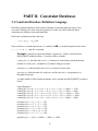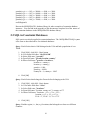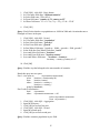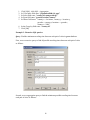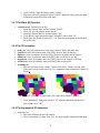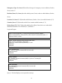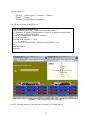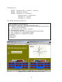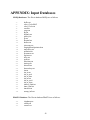
1
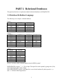
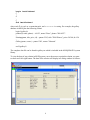
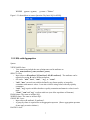
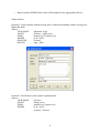
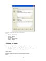
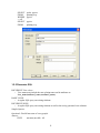
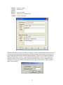
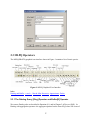
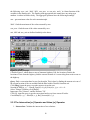
MLPQ/PReSTO Users' Manual
Peter Revesz
Department of Computer Science & Engineering
University of Nebraska - Lincoln
[email protected]
November 18, 2004
The MLPQ/PReSTO system is a constraint database system developed at the University of
Nebraska-Lincoln. MLPQ stands for Management of Linear Programming Queries and PReSTO
stands for Parametric Rectangles Spatio-Temporal Objects. These were formerly two separate
systems that were combined into one system.
The executable file of the MLPQ/PReSTO system, running Microsoft 2000, and all the sample text
files listed in the appendix of this document are available free as down-loadable files from the
webpage: http://www.cse.unl.edu/~revesz. The webpage also contains a list of publications
related to the MLPQ/PReSTO system.
The MLPQ/PReSTO system is a complex system that enables you to do a range of applications
from basic relational databases, to constraint databases, GIS databases, and web applications. The
Users' Manual is organized according to the following table of contents.
Acknowlegements: Partial funding for developing the MLPQ/PReSTO system was provided by
the United States National Science Foundation under grants IRI-9625055, IRI-9632871, and EIA0091530. The following students made major contributions to this project: Scot Anderson, Brian
Boon, Mengchu Cai, Rui Chen, Pradip Kanjamala, Yiming Li, Yugou Liu, Syed Mohiuddin, Tim
Perrin, Yonghui Wang, and Shasha Wu. Many other students in the database systems classes at
the University of Nebraska-Lincoln made additional contributions by noticing and/or debugging
particular features.
1
CONTENTS
PART I. RELATIONAL DATABASES.......................................................................................................................3
1.1 DATABASE DEFINITION LANGUAGE ........................................................................................................................3
1.2 SQL SYNTAX ..........................................................................................................................................................5
1.2.1 Basic SQL .......................................................................................................................................................6
1.2.2 SQL with Aggregation ....................................................................................................................................7
1.2.3 SQL with Set Operations ................................................................................................................................9
1.2.4 Nested SQL Queries ....................................................................................................................................10
1.2.5 Recursive SQL ..............................................................................................................................................11
PART II. CONSTRAINT DATABASES ...................................................................................................................13
2.1 CONSTRAINT DATABASE DEFINITION LANGUAGE .................................................................................................13
2.2 SQL IN CONSTRAINT DATABASES .........................................................................................................................14
2.3 MLPQ OPERATORS ...............................................................................................................................................17
2.3.1 The Datalog Query [Dlog] Operator and Buffer[B] Operator ....................................................................17
2.3.2 The Intersection [∩ ] Operator and Union [∪ ] Operator ..........................................................................18
2.3.3 The [Max] Operator and [Min] Operator....................................................................................................19
2.3.4 Recursive Queries.........................................................................................................................................20
2.3.5 Approximate Operator [Apx] ......................................................................................................................20
2.3.6 Delete Relations [Del]..................................................................................................................................20
PART III. GIS/PRESTO ..............................................................................................................................................21
3.1 GIS .......................................................................................................................................................................21
3.1.1 Drawing........................................................................................................................................................21
3.1.2 Zoom.............................................................................................................................................................22
3.1.3 Area ..............................................................................................................................................................22
3.1.4 Set and Color Relation Operators for Color Bands Display ........................................................................22
3.1.5 The 2D Animation.........................................................................................................................................23
3.1.6 The Transformation from the TIN to Constraint Database ..........................................................................25
3.1.7 The Transformation from Polygon File to Constraint Database..................................................................26
3.1.8 The Similarity [S] Operator for Similarity Queries......................................................................................26
3.1.9 Querying Maps .............................................................................................................................................26
3.1.10 The Complement [C] Operator ..................................................................................................................27
3.2 PRESTO................................................................................................................................................................27
3.2.1 The Intersection [ ∩] Operator and Union [∪] Operator ...........................................................................29
3.2.2 The [Area] Operator ....................................................................................................................................30
3.2.3 The Difference [−] Operator........................................................................................................................30
3.2.4 The Complement [C] Operator ....................................................................................................................30
3.2.5 The Datalog Query [Dlog] Operator ...........................................................................................................30
3.2.6 The Collide [X] Operator .............................................................................................................................30
3.2.7 The Block [B] Operator................................................................................................................................31
3.2.8 The 2D Animation.........................................................................................................................................31
3.2.9 The Exponential 2D Animation ....................................................................................................................31
3.2.10 The Regression Animation..........................................................................................................................32
PART IV. WEB APPLICATION ...............................................................................................................................33
4.1 SYSTEM INFRASTRUCTURE ....................................................................................................................................33
4.2 COMMUNICATION PROTOCOL ................................................................................................................................33
4.3 SAMPLE APPLICATION ...........................................................................................................................................36
APPENDIX: INPUT DATABASES ............................................................................................................................42
2
PART I. Relational Databases
This part describes how to implement standard relational databases in MLPQ/PReSTO.
1.1 Database Definition Language
The following is an example relational database.
Painter
ID
123
126
234
335
456
NAME
Ross
Itero
Picasso
OKeefe
Miro
PHONE
888-4567
345-1122
456-3345
567-8999
777-7777
Painting
PNUM
2345
4536
6666
7878
6789
7896
9889
TITLE
Wild Waters
Sea Storm
Wild Waters
High Tide
Paradise
Faded Rose
Sunset
PRICE
245.00
8359.00
6799.00
98000.00
590000.00
145.00
975000.00
Gallery
PNUM
2345
6666
4536
7878
6789
7896
9889
OWNER
Johnson
Johnson
McCloud
McCloud
Palmer
Palmer
Palmer
ID
126
335
234
456
234
123
234
How we can enter such a relational database into the MLPQ system?
MLPQ/PReSTO accepts a ".txt" file as input. The input file can be opened by going to the {File}
menu, and selecting the {Open} dialog.
In the MLPQ/PReSTO system, each input file is a set of rules bracketed by the keywords begin
and end. It has the following structure:
3
begin %moduleName%
l1
l2
.
ln
end %moduleName%
where each li is a rule or a constraint tuple, and moduleName is a string. For example, the gallery
database in MLPQ has the following format:
begin %gallery%
painter(id, name, phone) :- id=123, name="Rose", phone="888-4567".
...
Painting(pnum, title, price, id) :- pnum=2345, title="Wild Waters", price=245.00, id=126.
...
Gallery(pnum, owner) :- pnum=2345, owner="Johnson".
...
end %gallery%
The complete data file can be found in gallery.txt which is included in the MLPQ/PReSTO system
library.
To view the data of any relation in MLPQ system, move the mouse to point the relation you want
to check and click right button. The data of the relation will display in a dialog window as follows:
4
To change the color of each relation, move your mouse to either of the two color rectangles to the
left of the relation name and right click your mouse. A color window will appear for color
selection. The first and second color rectangles represent start color and end color respectively, if
the relation has a time variable.
1.2 SQL Syntax
The syntax of MLPQ SQL follows the standard of SQL with some restrictions that are explained in
the subsections below.
(Those who are already familiar with SQL in another system should read these restrictions
especially carefully.)
The SQL syntax will be illustrated using the gallery.txt database. Do the following:
1. Load the gallery.txt database
2. Click [SQL] to query the database in SQL.
3. Dialog box will appear which looks like this:
5
4. Select the type of query by clicking the appropriate button. Another dialog box will appear
accordingly.
5. Enter the query and click [OK].
6. The result will be displayed in the property window.
1.2.1 Basic SQL
Syntax:
SELECT clause
o Input values by the format as relation_name.attribute_name. (This dot notation is always
required in MLPQ SQL)
FROM clause
o Input values as relation names.
o Must use the "as" keyword in declaring tuple variables.
WHERE clause
o Only supports conjunctive multiple conditions, and those must be separated by "," instead
of "and".
o Does not support disjunctive conditions. (Note: Disjunctions can be realized by the
"UNION" in Set Operation.)
o String constant is marked by double quotation.
o Supports only the relational operators: "=", ">", "<", ">=", "<=".
Sample Queries:
Question 1: Find the name and phone number of the painter with id 123.
Answer:
SELECT painter.name, painter.phone
FROM
painter
WHERE painter.id = 123
Question 2: Find the title of the paintings in Palmer's Gallery.
Answer:
SELECT p.title
FROM
gallery as g, painting as p
6
WHERE
g.pnum = p.pnum,
g.owner = "Palmer"
Figure 1.2.1 showed how to answer Question 2 by basic SQL in MLPQ.
1.2.2 SQL with Aggregation
Syntax:
VIEW NAME clause
o View name must include the new relation name and its attributes as
view_name(attribute1_name, attribute2_name)
SELECT clause
o Input values as R1.attribute1, R2.attribute2, OP (R1.attribute3). The attributes can be
numerical or string, R can be different relations.
o OP can be " min", "max", "sum", " avg", or "count".
o "min", "max" can work on variables defined by any linear equality or inequality
constraints with numeric values. It can also work for string values with only equality
constraints.
o "sum", "avg" require variables that have equality constraints and numeric values in each
tuple.
o "count", "sum" and "avg" work on multi-sets (sets allow repetitions of elements).
FROM clause: The same as in Basic SQL
WHERE clause: The same as in Basic SQL
GROUP BY clause
o Input value as R.attribute1, R.attribute2 .
o A group by clause is required for each aggregation operator. (Hence aggregation operators
do not apply to entire relations.)
HAVING clause
7
o
Input as another WHERE clause which will be applied on the aggregation result set.
Sample Queries:
Question 5: List the painters with the average price of their listed paintings with the average price
higher than 8000.
Answer:
VIEW NAME
Q6(pname, avgp)
SELECT
p2.name, avg(p1.price)
FROM
painting as p1, painter as p2
WHERE
p1.id = p2.id
GROUP BY
p2.name
HAVING
avgp > 8000
Question 7: Find Picasso's most expensive painting listed.
Answer:
VIEW NAME
Q7(price)
SELECT
max(p1.price)
FROM
painting as p1, painter as p2
WHERE
p1.id = p2.id,
p2.name = "Picasso"
8
1.2.3 SQL with Set Operations
MLPQ allows only the UNION and the INTERSECTION set operations.
These are illustrated below.
Sample Queries:
Question 3: Find all paintings that were painted by either Itero or Picasso.
Answer:
SELECT painting.title
FROM
painting, painter
WHERE painter.id = painting.id,
painter.name = "OKeefe"
UNION
SELECT painting.title
FROM
painting, painter
WHERE painter.id = painting.id,
painter.name = "Picasso"
Figure 1.2.2 showed how to answer Question 3 by Set SQL in MLPQ.
9
Question 4: Find all the owners who are also painters.
Answer:
SELECT painter.name
FROM
painter
INTERSECT
SELECT gallery.owner
FROM
gallery
1.2.4 Nested SQL Queries
Syntax:
o Nesting can be done only through ONE attribute.
o Keywords used: "in", "not in", ">= all", "<= all", ">= some", "<= some".
o ">= all", "<= all" can not be used for string comparison.
Sample Queries:
Question 8: Find the title and price of the most expensive painting.
Answer:
10
SELECT
FROM
WHERE
>= all
SELECT
FROM
p.title, p.price
painting as p
p.price
p.price
painting as p
1.2.5 Recursive SQL
RECURSIVE View clause
o View name must include the new relation name and its attributes as
view_name(attribute1_name, attribute2_name)
BASIC RULE:
o A regular SQL query on existing relations
RECURSIVE RULE:
o A regular SQL query on existing relations as well as the newly generated view relations.
Sample Queries:
Question 9: Find all ancestors of every people.
Answer:
VIEW
ancestor(anc,chd) AS
11
(SELECT
FROM
UNION
(SELECT
FROM
WHERE
r.parent, r.child
relation as r)
a1.anc, a2.child
ancestor as a1, relation as a2
a1.chd = a2.parent)
When the OK button is clicked, a dialog will appear to ask for approximation control. If you are
not sure about the termination of your query, the approximation setup window can be used to
approximate the solution of the problems that do not have a finite least fixed point solution by
placing a bound on the solution. Approximation helps guarantee a result will be obtained in
situations where recursive queries may otherwise be unsafe. But if you are confident on the
termination of your query and want to return all results, please uncheck the “Approximation”
choice and click OK.
12
PART II. Constraint Databases
2.1 Constraint Database Definition Language
In MLPQ constraint databases can be entered similarly to relational databases using linear
constraint Datalog rules in the form of Equation (4.1) in Revesz (2002) with only linear
constraints (no relations) on the right hand side.
Each linear constraint must have the form:
a 1 x1 + a2 x2 + . + an xn θ b
where each ai is a constant and each xi is a variable, and θ i is a relational operator of the form
=, <, >, <=, or >= and b is a constant.
Example: Consider the constraint database "regions.txt", which is included in the
MLPQ/PReSTO database library. It consists of three relations.
country(id,x,y,t) describes the set of (x, y) locations of each country with identification
number id at each year t, (boundaries of countries change over time.)
location(c,x,y) which describes the set of (x,y) location of cities, and
growth(t,c,p) which describes for each year t and for each city c, its population p in
thousands of persons.
A sample instance of this constraint database can be entered into MLPQ/PReSTO as shown
below:
begin%Regions%
country(id,x,y,t):- id = 1, x >= 0, x <= 4, y >=5, y <= 15, t >= 1800, t <= 1950.
country(id,x,y,t):- id = 1, x >= 0, x <= 8, y >=5, y <= 15, t >= 1950, t <= 2000.
country(id,x,y,t):- id = 2, x > = 4, x <= 12, y >=5, y <= 15, t >= 1800, t <= 1950.
country(id,x,y,t):- id = 2, x > = 8, x <= 12, y >=5, y <= 15, t >= 1950, t <= 2000.
country(id,x,y,t):- id = 3, x >= 0, x <= 12, y >=0, y <= 5, t >= 1800, t <= 2000.
location(c,x,y):- x = 3, y = 2, c = 101.
location(c,x,y):- x = 7, y = 3, c = 102.
location(c,x,y):- x = 5, y = 6, c = 103.
location(c,x,y):- x = 7, y = 10, c = 104.
location(c,x,y):- x = 10, y = 8, c = 105.
location(c,x,y):- x = 1, y = 7, c = 106.
growth(t,c,p):- c = 101, p = 10000, t >=1800, t <= 2000.
13
growth(t,c,p):- c = 102, p = 20000, t >=1800, t <= 2000.
growth(t,c,p):- c = 103, p = 10000, t >=1800, t <= 2000.
growth(t,c,p):- c = 104, p = 30000, t >=1800, t <= 2000.
growth(t,c,p):- c = 105, p = 40000, t >=1800, t <= 2000.
growth(t,c,p):- c = 106, p = 35000, t >=1800, t <= 2000.
end%Regions%
Browse the MLPQ/PReSTO database library for other examples of constraint database
instances. You can find in the appendix of this document a complete list of the names of
the constraint databases in the MLPQ/PReSTO database library.
2.2 SQL in Constraint Databases
SQL queries can also be applied in constraint databases. The MLPQ/PReSTO SQL syntax
is the same as described above for relational databases.
Query: Find all cities that in 1900 belonged to the USA and had a population of over
10000.
1.
2.
3.
4.
5.
Click [SQL], click SQL - Basic button
In View name field enter: "cityUSA1900"
In Select field enter: "growth.c"
In From field enter: "growth, location, country"
In Where field enter: "growth.c = location.c,
location.x = country.x,
location.y = country.y,
growth.t = 1900,
growth.p > 10000,
country.id = 1, country.t = 1900"
6. Click [OK]
Query: Find all cities that belonged to France before belonging to the USA.
1.
2.
3.
4.
5.
Click [SQL], click SQL - Basic button
In View name field enter: "cities"
In Select field enter: "location.c"
In From field enter: "location, country as C1, country as C2"
In Where field enter: "location.x = C1.x , C1.x = C2.x ,
location.y = C1.y , C1.y = C2.y ,
C1.id = 2 , C2.id = 1, C1.t < C2.t"
6. Click [OK]
Query: Find the region, i.e., the (x,y) locations, that belonged to at least two different
countries.
14
1.
2.
3.
4.
5.
Click [SQL], click SQL - Basic button
In View name field enter: "differentcountries"
In Select field enter: "C1.x, C1.y"
In From field enter: "country as C1, country as C2"
In Where field enter: "C1.x = C2.x, C1.y = C2.y, C1.id < C2.id"
6. Click [OK]
Query: Find all cities that have a population over 10000 in 2000 and a location that never
belonged to France in the past.
1.
2.
3.
4.
5.
6.
7.
8.
9.
Click [SQL], click SQL - Nested
In View name field enter: "population"
In first Select field enter: "growth.c"
In first From field enter: "growth"
In first Where field enter: "growth.p > 10000, growth.t = 2000, growth.c"
In the field after first Where filed enter: "not in"
In second Select field enter: "location.c"
In second From field enter: "location, country"
In second Where field enter: "location.x = country.x,
location.y = country.y,country.id = 2"
10. Click [OK]
Query: Find the city that belonged to the most number of countries.
Break this query into two parts
Part 1: view name as
citycountries(c,namecount)
select
location.c, count(country.id)
from
location, country
where location.x = country.x,
location.y = country.y
group by location.c ;
Part 2:select citycountries.c
from
citycountries
where citycountries.namecount >= all
(select citycountries.namecount
from citycountries )
1. Click [SQL], click SQL - Aggregation
2. Input the first query
3. Click [OK] to execute first part.
4. Click [SQL], click SQL - Nested
5. Input the second query
6. Click [OK] to execute second part.
Query: Find the countries population in year 2000.
15
Click [SQL], click SQL - Aggregation
In View name field enter: "population2000( id, pop)"
In Select field enter: "country.id, sum(growth.p)"
In From field enter: "growth, location, country"
In Where field enter: "country.x = location.x, country.y = location.y,
growth.t = country.t, location.c = growth.c,
country.t = 2000"
6. In the Group by field enter: "country.id"
7. Click [OK]
1.
2.
3.
4.
5.
Example 2: Recursive SQL queries
Query: Find the minimum traveling time between each pair of cities in go.txt database.
First, we use recursive query to find all possible traveling times between each pair of cities
as follows:
Second, we use aggregation query to find the minimum possible traveling time bewteen
each pair of cities as follows:
16
2.3 MLPQ Operators
The MLPQ/PReSTO graphical user interface shown in Figure 1 contains a list of iconic queries.
Figure 1: MLPQ Graphical User Interface
Index:
Datalog and Buffer, ∩ and ∪ , Max & Min, Recursive, Approximate, Delete.
2.3.1 The Datalog Query [Dlog] Operator and Buffer[B] Operator
We can use Datalog rules as described in Equation (4.1) and in Chapter 5 of Revesz (2002). In
Datalog with aggregation operators the aggregate operator has the form OP(f) where OP is one of
17
the following: max, min, MAX, MIN, sum_max, or sum_min, and f is a linear function of the
variables in the Datalog rule. The Datalog with aggregation rule cannot have any string-type
attribute in either its head or body. The aggregate operators have the following meanings:
max - gets maximum value for each constraint tuple.
MAX - finds the maximum of the values returned by max.
sum_max - finds the sum of the values returned by max.
min, MIN and sum_min are defined similarly to the above.
Figure 2: Buffer Example
Consider Figure 2 which shows a map of interstate highway I-80, the location of hotels, the
locations of exits form the highway, and the current location of a car traveling from west to east on
the highway.
Query: Find a convenient hotel to stay for the night. This is done by finding the nearest exit east of
the current location of the car and then find the hotel within 50 miles from that exit.
Click [Dlog], input the query to get the nearest exit on the east.
Nearest(id, MIN(x), y) : - Current_Pos(id2, x0, y0), Exit(id, x, y), x - x0 >= 0.
Select "Nearest" Relation, click [Buffer].
Input name "Buf_Nearest", and the Distance "50".
Click [Q], input the query to get the convenient hotel away from at most 50 miles.
Convenient(id, x, y) : - Hotel(id, x, y), Buf_Nearest(id1, x, y).
2.3.2 The Intersection [∩
∩ ] Operator and Union [∪
∪ ] Operator
1. Intersection: Calculate the intersection of two relations.
18
1. Select two relations from the left window which have the same attributes.
2. Click [∩
∩ ].
3. Input relation name "Intersect" which is the intersection of these two relations.
Note: For intersection, the system also matches the ids of the objects. So if two objects
have the different ids, then the intersection would be empty.
Hint: To make two relations R1(id, x, y) and R2(id, x, y) have the same id, insert the
following Datalog query ("New_R1" and "New_R2" will have the same id "1"):
New_R1(1, x, y) : - R1(id, x, y).
New_R2(1, x, y) : - R2(id, x, y).
2. Union: Calculate the union of two relations.
1. Select two relations from the left window.
2. Click [∪ ].
3. Input the relation name "Union" which is the union of these two relations.
Note: for union, these two relations need not to have the same id since they are still in the
output even they have different ids.
2.3.3 The [Max] Operator and [Min] Operator
1. Max: Calculate the maximum value for a given evaluation function.
crops.txt: Calculate the maximum profit for the evaluation function: 300corn + 250rye +
100sunflower + 150wheat.
1. Select the relation "crops" from the left window.
2. Click [Max].
3. Input new relation name "max_profit", the evaluation function
"300corn+250rye+100sunflower+150wheat", and the constant value for the
evaluation function is "0".
4. Right click the relation "max_profit" to show the maximum profit.
2. Min: Calculate the minimum value for a given evaluation function.
1. Select one relation from the left window.
2. Click [Min].
3. Input new relation name "min_rel", the evaluation function, and the constant value
for the evaluation function.
4. Right click the relation "min_rel" to show the minimum value.
Note: The [Max] and [Min] operators only work for the evaluation function which will
return the positive maximum/minimum value.
19
2.3.4 Recursive Queries
1. houses.txt: the relation "can_build" is created by recursive Datalog query. See the
constraint tuples of the relation.
2. pollution.txt: the relation "oktobuy" is created by recursive Datalog query. See the
constraint tuples of the relation, not the display result.
3. powernew.txt: the relation "can_build" is created by recursive Datalog query. See the
constraint tuples of the relation, not the display result.
Note: For [Dlog] Operator, the recursive query only can be inserted into recursive database,
that is, the new recursive query could be inserted only when the current database is
recursive.
2.3.5 Approximate Operator [Apx]
Approximation can be used to achieve an approximate solution to problems that do not have a
finite least fixed point solution by placing a bound on the solution. Approximation helps guarantee
a result will be obtained in situations where recursive queries may otherwise be unsafe. Detailed
discussion can be found in Chapter 9 of the textbook. By default the system automatically enables
approximation as true and uses a bound of 30. You can change this bound by clicking [Apx]
button. To disable approximation enter 0 for the bound or uncheck the "Use Approximation" box.
This is a global setting; however, it will only apply to databases that have been opened or queries
executed after the bound has been set.
Consider the following example of a recursive Datalog query used to calculate the difference
relation:
D(x,y,z) :- x-y>=0, -x+y>=0, z>=0, -z>=0.
D(x,y,z) :- D(x1,y,z1), x-x1>=1, -x+x1>=-1, z-z1>=1, -z+z1>=-1.
This query will never terminate and is hence not safe without using appoximation. Refer to the
table on page 100 of the textbook. By setting approximate boundry, we can achieve an
approximate result in feasible time.
2.3.6 Delete Relations [Del]
Delete relation [Del ] operator can delete any existing relations. It can be used to remove some
temporary results.
1. Select the relations you want to remove in the list box. You can select multiple relations
and delete them at the same time.
2. Click the [Del ] button.
3. Check the relation list again in the popup message box and click OK to execute the
operation if everything is correct.
20
PART III. GIS/PReSTO
3.1 GIS
Syntax
1. We sometimes restrict the head of the rules to be one of the following: r(id,x,y), or
r(id,x,y,t) or r(id,x,y,z) where id is the identification number of an object, and x,y are two
spatial variables, which could be augmented by a temporal variable t or a third spatial
variable z. These cases of linear constraint databases allow us to do some extra operations
that are special to GIS objects.
2. GIS Database: The GIS database must use "GIS" as the module name; that is, the input
file must have the structure:
begin %GIS%
l1
l2
.
ln
end %GIS%
Operators
Drawing, Zoom, Area, Color Bands, 2D Animation, TIN to Constraint, Polygon File to Constraint,
Similarity, Querying Maps, Complement.
3.1.1 Drawing
1. Drawing Line:
1. Open a non-empty database (i.e., a database that already contains at least one
relation);
2. Left click the right window;
3. Left click [Line];
4. Left click the mouse to get one point, move mouse, then left click the mouse to get
another point;
5. Input the relation name "Line1" (any string) to get the line relation "Line1".
2. Drawing Rectangle:
1. Open a non-empty database (i.e., a database that already contains at least one
relation);
2. Left click the right window;
3. Left click [Rectangle];
4. Left click the mouse to get one point, move mouse, then left click the mouse to get
another point;
5. Input the relation name "Rectangle1" (any string) to get the rectangle relation
"Rectangle1".
21
3. Drawing Polygon:
1. Open a non-empty database (i.e., a database that already contain at least one
relation);
2. Left click the right window;
3. Left click [Polygon];
4. Left click the mouse to get one point, continue to left click the mouse to get other
points;
5. Double click to finish the drawing.
6. Input the relation name "Polygon1" (any string), and the Object ID "1" (any integer
number) to get the polygon relation "Polygon1".
4. Show Constraints: After operation 2, left click the relation "New_relation" in the left
window, to get the dialog which shows the constraints of this relation.
3.1.2 Zoom
1. To shrink the displayed object, click [Zoom Out].
2. To enlarge the displayed object, click [Zoom In], left push down the mouse, drag a
rectangle to include the area you want to enlarge, then release the button. The selected area
will be enlarged.
3.1.3 Area
1. Area: Calculate the area of relation "Buf_Nearest".
1. Select the Generated relation "Buf_Nearest" in the left window.
2. Click [Area].
3. Input the MinX, MaxX, and Step Size of the area to be calculated. By referring the
coordinates of the window, input the number for MinX "0", and MaxX "400", and
the Step Size "400", then get the total area of the relation since it is in the region
totally.
4. Input the area relation name "Buf_Nearest_Area", left click it to show the area in
constraints.
Note: The step size is to get various aggregate information for different bands of the object.
2. Bands Area: Calculate the area of relation "Buf_Nearest" with bands.
1. Select the Generated relation "Buf_Nearest" in the left window.
2. Click [Area].
3. Input the MinX "0", the MaxX "400", the Step Size "200".
4. Input the relation name "Buf_Nearest_Area", left click it to show the areas of these
two bands from 0 to 200 and 200 to 400 in constraints.
3.1.4 Set and Color Relation Operators for Color Bands Display
1. Color_Circle.txt:
1. Select "Circle" relation, see the monochromatic circle.
2. Select "NEW_Circle" relation, then click [Color Relation].
22
2.
3.
4.
5.
3. Select the new Generated "Color_NEW_Circle" relation, see the color circle (if not,
click the {View} Menu, uncheck {Same Relation Color} Option).
tin.txt:
1. Select "tin" relation, click [Color Relation].
2. Select the Generated "Color_tin" relation, then see the color Nebraska (different
colors stand for different heights of those places).
tiniowa_final.txt:
1. Select "tiniowa_final" relation, then click [Set], then click add button in the dialog,
then input "1000", "5000" and select "red" color. Then click the ok button.
2. Then click [Color Relation], then select the new Generated "Color_tiniowa_final"
relation, then see the red partial Iowa state (only the heights between 1000 and 5000
are displayed). (If it's not red, then select {View} menu, then uncheck {Same
Relation Color}.)
tinne_final.txt:
1. Select "tinne_final" relation, then click [Set], then click add button, then input
"1000", "3000" and select "blue" color. Then click ok button.
2. Then click [Color Relation], then select "Color_tinne_final" relation, then see the
blue partial Nebraska state (only the heights between 1000 and 3000 are displayed).
(If it's not blue, then select {View} menu, then uncheck {Same Relation Color}.)
tinresult.txt: Monochromatic map display. Select "tin" relation, then see the Nebraska
state map, also shown in Figure 4.
Figure 4: Mean Annual Air Temperature
3.1.5 The 2D Animation
1. sface.txt: select relations one by one, then click [Play], then see the face becomes smiling.
23
Figure 3: Two Snapshots of a Video on California Gull Ranges
2. Consider Figure 3 which shows two snapshots of the habitat range of the California Gull
birds. The data is available in file sgull.txt. Select all except Gull, then select "Gull"
relation, then click [Play], then see the gull changing.
Query 1: How much did the area of the California Gull change from 1970 to 1990?
1. Click [Dlog] to insert the query to get the Gull snapshot at 1970:
Gull0(i, x, y) : - Gull(i, x, y, 0).
2. Click [Dlog] to insert the query to get the Gull snapshot at 1990:
Gull60(i, x, y) : - Gull(i, x, y, 60).
3. Click the relation "Gull0", then click [Area] to get the area of the Gull at 1970.
Input the MinX=0, MaxX=500 and Step=500. Give the name of the area of the
relation "Gull0" as "Gull0_Area".
4. Click the relation "Gull60", then click [Area] to get the area of the Gull at 1990.
Input the MinX=0, MaxX=500 and Step=500. Give the name of the area of the
relation "Gull60" as "Gull60_Area".
5. Click [Dlog] to insert the query to get the area difference of the California Gull t
between 1970 and 1990:
Gull_Area_Diff(a) : - Gull0_Area( x, y, a1), Gull60_Area( x, y, a2),
a1 - a2 + a = 0.
6. Right Click the relation "CA_Gull_Area_Diff" to show the constraints and the area
difference.
24
Query 2: How much did the area of the California Gull change from 1970 to 1990 in the
state of California?
7. Click [Dlog] to insert the query to get the Gull snapshot at 1970:
Gull70(1, x, y) : - Gull(i, x, y, 0).
8. Click [Dlog] to insert the query to get the Gull snapshot at 1990:
Gull90(1, x, y) : - Gull(i, x, y, 60).
9. Select the relation "Gull70" and "CA", then click [∩ ] to get the area of the Gull at
1970 in the state of California. Input the relation name "CA_Gull70".
10. Click the relation "Gull90" and "CA", then click [∩ ] to get the area of the Gull at
1990 in the state of California. Input the relation name "CA_Gull90".
11. Click the relation "CA_Gull70", then click [Area] to get the area of the Gull at 1970
in the state of California. Input the MinX=0, MaxX=500 and Step=500. Give the
name of the area of the relation "CA_Gull70" as "Gull70_Area".
12. Click the relation "CA_Gull90", then click [Area] to get the area of the Gull at 1990
in the state of California. Input the MinX=0, MaxX=500 and Step=500. Give the
name of the area of the relation "CA_Gull90" as "Gull90_Area".
13. Click [Dlog] to insert the query to get the area difference of the California Gull t
between 1970 and 1990 in the state of California:
CA_Gull_Area_Diff(a) : -
Gull70_Area( x, y, a1), Gull90_Area( x, y, a2),
a1 - a2 + a = 0.
14. Right Click the relation "CA_Gull_Area_Diff" to show the constraints and the area
difference.
3. Consider the file slincoln.txt. Select "City" relation, then click [Play], then see the Lincoln,
Nebraska city area changing.
3.1.6 The Transformation from the TIN to Constraint Database
1. tin_ia.net: Transform the TIN of Iowa to constraint database.
1. Click menu {New}, then click submenu {File}, click {Import File}, then click
{Elevation File}.
2. Choose the file "tin_ia.net".
3. Input the relation name "tin_ia", then input "tin_ia_ascii" in the third filed, click ok
button to Generate the constraint file "tin_ia.txt".
4. Use Notepad to open the file "tin_ia.txt" to see the transformed constraints.
Note: The file "tin_ia.net" is the TIN structure of Iowa State with the longitude, latitude
and elevation for each point. The file "tin_ia_ascii" includes the slope and aspect of each
point.
25
2. tin_ne.net: Transform the TIN of Nebraska to constraint database.
1. Click menu {New}, then click submenu {File}, click {Import File}, then click
{Elevation File}.
2. Choose the file "tin_ne.net".
3. Input the relation name "tin_ne", then input "tin_ne_ascii" in the third filed, click ok
button to generate the constraint file "tin_ne.txt".
4. Use Notepad to open the file "tin_ne.txt" to see the transformed constraints.
3.1.7 The Transformation from Polygon File to Constraint Database
1. veg90.pol: Transform polygon file to constraint database.
1. Click menu {New}, then click submenu {File}, click {Import File}, then click
{Elevation File}.
2. Choose the file "veg90.pol".
3. Input the relation name "vege".
4. Click the "vege" relation in the left window, you will see the constraint tuples of
these polygons.
3.1.8 The Similarity [S] Operator for Similarity Queries
1. db.lin: Query similarities among the lines.
1. Click menu {New}, then click submenu {File}, then click {Import File}, then click
{Import Line}.
2. Select the file "db.lin".
3. Input the relation name "lines".
4. Then select any one relation, then click [S], then the relations are ordered as the
similarity order from the specified one.
3.1.9 Querying Maps
1. usmap_info.txt:
1. Select all of the relations, then see the U.S. map with 50 states.
2. The scale of this map is shown by clicking the constraints of the relation "Scale",
the unit is kilometer.
3. The "Capital" relation is the capital cities of the states.
Query 1: Find the capital city of Nebraska:
4. Click [Q], then input
NE_Capital(name) : - NE(id, x, y), Capital(id, name).
5. Right click the relation "NE_capital" to see the capital city of Nebraska State.
Query 2: Find the area of the state of Nebraska in MST zone.
26
6. Click [Q], then input
NE_MST(i, x, y) : - NE(i, x, y), MST(j, x, y).
7. Select the relation "NE_MST", then click [Area].
8. Input MinX=0, MaxX=500 and Step=500.
9. Input the name of the area relation as "NE_MST_Area".
10. Then right click the relation "NE_MST_Area" to see the area of the state of
Nebraska in MST zone.
3.1.10 The Complement [C] Operator
1. usmap_info.txt:
1. Select the relation "AK" from the left window.
2. Click [C].
3. Input the relation time "comp" and click [OK]..
4. Click the relation "comp" which shows the complement of the "AK".
3.2 PReSTO
Syntax
1. PReSTO Relation: A relation R in PReSTO is defined as follows:
where
R:
the name of the relation,
Ai: the relational attributes,
ai,j, bi , ci and di: constraints (c1 <= c2 , c3 >= c2 – c1 ).
x1, x2:
x interval endpoints,
y1, y2:
y interval endpoints,
t:
time,
p:
period,
e:
end time.
27
Note: For non-periodic relations, c3 = -1, c4 = -1. The attributes id, x1, y1, x2, y2, t, p, s are
default attributes.
2. PReSTO Database: The PReSTO database must use "STDB" as the module name; that is,
the input file must have the structure:
begin %STDB%
r1
r2
.
rn
end %STDB%
3. PReSTO Query:
1. Define a relation with non-default attributes.
Example: Define the cloud relation with the attribute humidity.
clouds(h) :- i=1,
x1 - t = 105,
y1 - 0.5t = 200,
x2 - t = 111,
y2 - 0.6t = 205,
t >=0, t<=300,
p = -1, s = 0,
h = 0.
2. Selection:
$(condition1, condition2, . , conditionk) Relation(A1, . , An)
Example: Find the cool area in Nebraska.
begin %STDB%
Nebraska(temp) :- i=1, x1=4, y1=4.5, x2=19.5, y2=14.5,
t>=1,t<= 15,p=-1,temp=30.
Nebraska(temp) :- i=2, x1=20, y1=4.5, x2=35, y2=14.5,
t>=1,t<= 15,p=-1,temp=90.
Nebraska(temp) :- i=3, x1=35.5, y1=5, x2=46, y2=14.5,
t>=1,t<= 15,p=-1,temp=60.
cool_area(temp):-$(temp>=50,temp<=80)nebraska(temp).
end %STDB%
3. Projection:
ResultRelation(Ai, . , Aj) : - Relation(A1, . , Am)
28
4. Intersection: Relation1 * Relation2.
Example: Find if the ship and the torpedo will meet with each other.
begin %STDB%
ship() :- i=1,
x1-t=20,y1=20,
x2-t=30,y2=25,
t>=0,t<=25,
p=-1,s=-1.
torpedo() :- i=1,
x1=45,y1+t=45,
x2=48,y2+t=51,
t>=0,t<=25,
p=-1,s=-1.
hit() :- ship() * torpedo().
end %STDB%
Operators
Index: ∩ and ∪ , Area, Difference, Complement, Datalog Query (Dlog), Collide, Block, 2D
Animation, Exponential 2D Animation, Regression Animation.
3.2.1 The Intersection [ ∩] Operator and Union [∪
∪] Operator
1. weather.txt:
Query 1: Find which region is likely to get rain.
1. Select the relation "cool_area" and "wet_cloud" from the left window.
2. Click [∩
∩ ].
3. Input a relation name "get_rain" which is the intersection of these two relations.
Query 2: Find which region is likely to get snow.
4. Select the relation "cold_area" and "wet_cloud" from the left window.
5. Click [∩
∩ ].
6. Input a relation name "get_snow" which is the intersection of these two relations.
Query 3: Find which region is likely to get rain or get snow.
7. Select the relation "get_rain" and "get_snow" from the left window.
8. Click [∪
∪ ].
9. Input a relation name "get_rain_snow" which is the union of these two relations.
2. flight.txt:
Query: Will the plane hit the fleet?
29
1. Select the relation "plane" and "fleet" from the left window.
2. Click [∩
∩ ].
3. Input a relation name "hit_fleet" which is the intersection of these two relations.
3.2.2 The [Area] Operator
1. cloudmap.txt:
Query: Find the area of the clouds at time 10.
1.
2.
3.
4.
Select the relation "clouds" from the left window.
Click [Area].
Input the time of the clouds "10".
A dialog box pop up to give the area of the clouds at time "10".
3.2.3 The Difference [−] Operator
1. cloudmap.txt:
1. Select the relation "california" and "clouds" from the left window.
2. Click [-].
3. Input the relation time "diff".
4. Click the relation "diff" which shows the difference between California and the
clouds at time "0".
3.2.4 The Complement [C] Operator
2. cloudmap.txt:
1. Select the relation "clouds" from the left window.
2. Click [C].
3. Input the relation time "comp".
4. Click the relation "comp" which shows the complement of clouds at time "0".
3.2.5 The Datalog Query [Dlog] Operator
1. weather.txt:
1. Click [Dlog].
2. To get the area where the temperature between 50 and 80, input the query:
cool(temp) : - $(temp >= 50, temp <= 80)nebraska (temp).
3. Click the relation "cool" which shows the interested area.
3.2.6 The Collide [X] Operator
1. collide.txt:
1. Select all relations, then click [Play], then see both are moving.
30
2. Click [Collide], input the relation name "collide".
3. Then select the new generated relation "collide", then click [Play], then see them
collide then bounce back from each other.
3.2.7 The Block [B] Operator
1. yellowstone.txt: Foam blocks the fire.
1. Select the relation "lake" and the relation "foam1".
2. Click [ B], give the relation name "blocks".
3. Select the relation "blocks" and the relation "fire".
4. Click [Block], input the relation name "blockfire" and set time "10".
5. Click [Forward] button 10 times till t = 10. Then see the snapshot of the blocked
fire at that time.
3.2.8 The 2D Animation
1.
2.
3.
4.
5.
6.
7.
halley.txt: select all relations, then click [Play], then see Halley hit some stars.
comet3.txt: select all relations, then click [Play], then see they are moving.
flight.txt: select all relations, then click [Play], then see the planes hit the targets.
shuttle.txt: select all relations, then click [Play], then see the bus is moving.
torpedo.txt: select all relations, then click [Play], then see the torpedo is moving.
weather.txt: select all relations, then click [Play], then see the result.
cloudmap.txt:
1. Select all relations except "clouds" relation, then select "clouds" relation, click
[Play], then see the cloud is moving. Two snapshots of the animation are shown in
Figure 5.
Figure 5: Cloud at t=25 (left) and t=182 (right) in the PReSTO system
2. Click [Animation], change the speed to "95", then the animation speed will be
slower than it was "100".
3.2.9 The Exponential 2D Animation
1. mulcolony.txt:
1. Select the relation from the left window.
2. Click [(Animation (A)] then click "Yes" for observing the exponential animation.
31
Note: If click [A] then click "No", then execute the linear animation.
2. sincolony.txt: Click [(Animation (A)] then click "Yes" for observing the exponential
animation.
3. sinirreg.txt: Click [(Animation (A)] then click "Yes" for observing the exponential
animation.
4. threecolony.txt: Click [(Animation (A)] then click "Yes" for observing the exponential
animation.
3.2.10 The Regression Animation
1. irrigationcountry.txt:
1. Select the relation "NeCounty" from the left window.
2. Click [AR] then enter start and end time instances.
2. Relation will be displayed on the left window.
3. Select all the relation created below relation "NeCounty".
4. Click [play R ] to view the regression animation.
32
PART IV. Web Application
4.1 System Infrastructure
The MLPQ web accessible server and the dependent applications are collaborative systems. A
three-tier Browser/Server architecture can be described as shown in Figure 6.
Figure 6: MLPQ Web Access System (B/S) Infrastructures
Each tier has its own responsibilities that are listed in Table 1.
Browser
(User Interface)
User interfaces
Send user's requests
to Web Server
Accept results from
middle tier
Display the results
Middle tier
(Business Logic)
Accept requests from the
browser
Parse the request to CDB
acceptable command and
arguments
Send commands to CDB
Accept result from CDB
Explain the result
Return result to Browser
CDB Server
Accept commands and
arguments from Web
Server
Activate related
operations according to
the command and
arguments
Return the results to
middle tier
Table 1: Responsibilities for each layer in MLPQ Web Access B/S System
4.2 Communication protocol
33
The MLPQ Web Accessible server uses socket to communicate with other programs. Figure 7 is
the main window of MLPQ web accessible server. To make it work for web access, the "listen"
menu should be selected first. Then the server will listen to a predefined socket port and ready to
act according to the messages received from the port.
Figure 7: Main window of the MLPQ web accessible server with listen menu item
The default environment settings are saved in mlpq_nt.cfg file and the values of the settings are
displayed in Table 2. The system administrator can modify these three settings to configure the
server.
Name and Value
Description
WorkDir = "c:\inetpub\wwwroot\dbs\".
Define the directory to load constraint
database files by the server.
OutPut = "c:\inetpub\wwwroot\dbs\".
Define the directory for the server to
output its result file.
Port = "2222".
Define the socket port value
Table 2: Settings in mlpq_nt.cfg
Table 3 lists all commands and their arguments recognized by the MLPQ web accessible server.
<user> records the login user name. <filename> is the name of constraint database opened in the
server. <relation name> provides the name of the new relation that will be created on the MLPQ
web accessible server. <color> is used to assign a color for the selected relation. The execution of
each command may return 0, 1, or a file name. "1" means there are some errors within the
execution. "0" result tells people that the command is executed successfully. If a file name was
returned, it also means the command is successfully executed.
Command
Open
Arguments
Actions on CDB
<user> <filename>$
Result
Create a view for
0 (success)
the user and open a
1 (fail)
CDB data file.
Close
<user> <filename>$
Close the view of
34
0 (success)
SQLBasic
SQLAggregate
the user.
1 (fail)
<user> <filename>
Execute a SQL
File.txt#
<relation name>
query on the user's
1 (fail)
#<select>#<from>#<where>$
view.
<user> <filename>
Execute a SQL
File.txt#
<relation name>
query on the user's
1 (fail)
#<select>#<from>#<where>
view.
#<group>#<having>$
SQLSet
<user> <filename>
Execute a SQL
File.txt#
< relation name>
query on the user's
1 (fail)
#<select1>#<from1>#<where1>
view.
#<set_op>
#<select2>#<from2>#<where2>$
SQLNested
<user> <filename>
Execute a SQL
File.txt#
<relation name>
query on the user's
1 (fail)
#<select1>#<from1>#<where1>
view.
#<nest_op>
#<select2>#<from2>#<where2>$
Datalog
<user> <filename>
Execute a Datalog
file.txt#
<datalog string>$
query on the user's
1 (fail)
view.
Include
<user> <filename>
Highlight the
0 (success)
<relation name> <color>$
relation by its
1 (fail)
name and assign a
color for it in the
view.
Clear
<user> <filename>$
Deselect all
0 (success)
relations in the
1 (fail)
view
GetImage
<user> <filename>$
Copy the image of
35
File.bmp#
the view in screen
1: fail
and save to disk.
ColorRelation
Zoom
GetAnimation
<user> <filename>
Do color relation
0 (success)
<relation_name>$
on given relation.
1 (fail)
<user> <filename> <x> <y> <w> Zoom the image.
0 (success)
<h>$
1 (fail)
<user> <filename> <Start Time>
Generate serious
0 (success)
<End Time> <Interval Time>$
animation images
1 (fail)
to the output
directory
Table 3: Command list to MLPQ Web Access Program
Table 4 maps the value of <color> to the actual color assigned to the relation.
Value of <color>
Color of the relation
0
Black
1
Red
2
Green
3
Blue
4 - 16777216
RGB(Value)
Table 4: Map from the value of <color> to actual color of the relation
4.3 Sample application
Police Emergency Constraint database
The Police Emergency application is a sample implementation that applies the functions provided
by the MLPQ web accessible server in a three-tier architecture. Suppose we know about a town
represented by constraint database as follows.
36
Emergency (Type, No, Street, T) describes what type of emergency occurs at address (Number,
Street) at time T.
Resident (Name, No, Street) describes which person (Name) resides at which address (Number,
Street).
Location (No, Street, X, Y) describes which house (Number, Street) is at which location (X, Y).
Contains (Street, X, Y) describes which Street contains which locations (X, Y).
Police (Name, VIN, X, Y, T) describes which police officer (Name) drives car with vehicle
identification number VIN at location (X, Y) and time T.
Login and Logout:
Login
Session.Contents("SERVER") = Request.ServerVariables("SERVER_NAME")
Session.Contents("USR") = Request("STR_USR") Session.Contents("VIEW_NM") = 0
Response.Redirect "a1.htm"
Create a Socket.TCP object and connect to the server:
asObj = Server.CreateObject( "Socket.TCP" )
asObj.Host = Session.Contents("SERVER") & ":2222"
asObj.Open
asObj.Wait
Open a database file:
str = "Open " & Session.Contents("USR") &" police.txt$"
asObj.SendText str
asObj.Wait
Select a relation:
str = "Include " & Session.Contents("USR") &" police.txt Townmap 0$"
asObj.SendText str
asObj.Wait
Return the image:
str = "GetImage " & Session.Contents("USR") &" police.txt$"
asObj.SendText str
asObj.Wait
Query 1: Find and display a street upon the town map.
37
The SQL query is:
SELECT Contains.Street, Contains.x, Contains.y
FROM
Contains
WHERE Contains.Street = inputStreet
The VB and ASP code in middle tier is
Code in middle tier to find the street:
Session.Contents("VIEW_NM") = Session.Contents("VIEW_NM") + 1
str = "SQLBasic " & Session.Contents("USR") & " police.txt " & Session.Contents("USR")
& Session.Contents("VIEW_NM")
str = str & "# Contains.Street, Contains.x, Contains.y"
str = str & "# Contains"
if Request("STR_STREET") = "" Then
str = str & "$"
Else str = str & "# Contains.Street= '" & Request("STR_STREET") & "'$"
End if
asObj.SendText str
asObj.Wait
Figure 7: Town map query and its result page
Query 2: Find the location of the emergencies during a given time interval.
38
The SQL query is:
SELECT Emergency.Type, Location.x, Location.y
FROM
Emergency, Location
WHERE Emergency.No = Location.No,
Emergency.Street = Location.Street,
Emergency.T >= starttime,
Emergency.T <= endtime
The VB and ASP code in middle tier is
Code in middle tier to find emergencies:
Session.Contents("VIEW_NM") = Session.Contents("VIEW_NM") + 1
str = "SQLBasic " & Session.Contents("USR") & " police.txt " & Session.Contents("USR") &
Session.Contents("VIEW_NM")
str = str & "# Emergency.Type, Location.x, Location.y"
str = str & "# Emergency, Location"
str = str & "# Emergency.No=Location.No, Emergency.Street=Location.Street"
str = str & ", Emergency.T>= " & Request("STR_TIME1")
str = str & ", Emergency.T<="& Request("STR_TIME2")
str = str & "$"
asObj.SendText
str asObj.Wait
Figure 8: Page to find the Emergencies and its result
39
Query 3: Find the places where the given police officer pname is reachable at time.
The Datalog is
Reach(n) :- Contains(n, x, y), Police(Name, VIN, x, y, T),
Name = pname, T = time.
Reach(n) :- Reach(m), Contains(m, x, y), Contains(n, x, y).
Reachable(n, x, y) :- Reach(n), Contains(n, x, y).
The VB and ASP code in middle tier is
Code in middle tier to find the reachable street for the officer:
Session.Contents("VIEW_NM") = Session.Contents("VIEW_NM") + 1
prefix = Session.Contents("USR") & Session.Contents("VIEW_NM")
str = "Datalog " & Session.Contents("USR") & " police.txt " & prefix
str = str & "Reach(n) :- Contains2(n,x,y), Police(Name, VIN, x, y, T), Name=" & Chr(34) &
Request("STR_NAME") & Chr(34) & ", T=" & Request("STR_TIME") & ".$"
asObj.SendText str
asObj.Wait
str = "Datalog " & Session.Contents("USR") & " police.txt " & prefix
str = str & "Reach(n) :- "& prefix &"Reach(m), Contains2(m, x, y), Contains2(n, x, y).$"
asObj.SendText str
asObj.Wait
str = "Datalog " & Session.Contents("USR") & " police.txt " & prefix
str = str & "Rable(n, x, y) :- "& prefix &"Reach(n), Contains2(n, x, y).$"
asObj.SendText
str asObj.Wait
40
Figure 9: Page to find the reachable street for a given Police officer and its result
41
APPENDIX: Input Databases
MLPQ Databases: The files in database/MLPQ are as follows:
1.
2.
3.
4.
5.
6.
7.
8.
9.
10.
11.
12.
13.
14.
15.
16.
17.
18.
19.
20.
21.
22.
23.
24.
25.
26.
27.
28.
29.
30.
31.
32.
33.
34.
buffer.txt
color_Circle.RNG
color_Circle.txt
cost.dat
crops.txt
db.lin
diffonly.txt
gallery.txt
go.txt
hospital.txt
houses.txt
irricounty.txt
StepingStoneOptimized.txt
mulcolony.txt
pollution.txt
powernew.txt
regions.txt
sface.txt
sgull.txt
sincolony.txt
sinirreg.txt
slincoln.txt
threecolony.txt
tin.txt
tin_ia.net
tin_ia_ascii
tin_ia_data
tin_ne.net
tin_ne_ascii
tin_ne_data
tiniowa_final.txt
tinne_final.txt
tinresult.txt
usmap_info.txt
PReSTO Database: The files in database/PReSTO are as follows:
35.
36.
37.
cloudmap.txt
collide.txt
comet3.txt
42
38.
39.
40.
41.
42.
fight.txt
halley.txt
torpedo.txt
weather.txt
yellowstone.txt
43