
1
Version 3 Modeling System User’s Guide July 2010 Mesoscale & Microscale Meteorology Division • National Center for Atmospheric Research Foreword This User’s Guide describes the Advanced Research WRF (ARW) Version 3.2 modeling system, released in April 2010. As the ARW is developed further, this document will be continuously enhanced and updated. Please send feedback to [email protected]. This document is complementary to the ARW Tech Note (http://www.mmm.ucar.edu/wrf/users/docs/arw_v3.pdf), which describes the equations, numerics, boundary conditions, and nesting etc. in greater detail. Highlights of updates to WRFV3.2 include: New physics options: o Milbrandt-Yau double moment microphysics o Building Energy Model (BEM) – a new urban physics option o Vegetation-height dependent thermal roughness length for MM5 and MYJ surface layer physics options o Sea-ice consideration in RUC and PX LSMs o Slope/shading effects extend to all shortwave radiation options o Use of semi-Lagrangian fall-term calculation in WSM and WDM schemes o Shallow convection option with G3 scheme o Garratt enthalpy flux formulation for tropical storm application o Single-column ocean mixed layer model extends to all surface physics options Nonlinear Backscatter Anisotropic (NBA) sub-grid turbulence stress for LES Wildland fire module ndown vertical nesting using constant refinement factor WRF-Chem updates WRF-DA updates: o Improvement on multiple outer loop minimization o Adjoint sensitivity tools o Improved efficiency for WRF adjoint code o PrepBufr data for 4D-Var o Software improvement (compile time, memory usage, etc.) Software framework enhancements: o Run-time input/output field specification and increased number of auxiliary I/O streams o Improved domain decomposition for MPI and OpenMP to increase the maximum number of processors/threads allowed o Added support for GPU acceleration of microphysics (WSM3 and WSM5) using PGI 10.3 accelerator directives o WRF and WPS ported to 64-bit Windows o Improved performance and scaling to 10^5 cores on high-end systems including Blue Gene/P and Cray XT5 o ESMF 4 support For the latest version of this document, please visit the ARW Users’ Web site at http://www.mmm.ucar.edu/wrf/users/. Contributors to this guide: Wei Wang, Cindy Bruyère, Michael Duda, Jimy Dudhia, Dave Gill, Hui-Chuan Lin, John Michalakes, Syed Rizvi, and Xin Zhang. Contributors to WRF-Fire chapter: Jonathan D. Beezley, Janice L. Coen, and Jan Mandel CONTENTS 1. Overview Introduction ................................................................................. 1-1 The WRF Modeling System Program Components ..................... 1-2 2. Software Installation Introduction .................................................................................. 2-1 Required Compilers and Scripting Languages ............................. 2-2 Required/Optional Libraries to Download..................................... 2-2 Post-Processing Utilities............................................................... 2-3 Unix Environment Settings ........................................................... 2-4 Building the WRF Code................................................................ 2-5 Building the WPS Code................................................................ 2-6 Building the WRFDA Code........................................................... 2-7 3. The WRF Preprocessing System (WPS) Introduction ................................................................................. 3-1 Function of Each WPS Program ................................................. 3-2 Installing the WPS....................................................................... 3-4 Running the WPS........................................................................ 3-7 Creating Nested Domains with the WPS................................... 3-18 Selecting Between USGS and MODIS-based Land Use Classifications........................................................... 3-20 Selecting Static Data for the Gravity Wave Drag Scheme ........ 3-21 Using Multiple Meteorological Data Sources............................. 3-22 Parallelism in the WPS.............................................................. 3-25 Checking WPS Output .............................................................. 3-26 WPS Utility Programs................................................................ 3-27 Writing Meteorological Data to the Intermediate Format ........... 3-30 Creating and Editing Vtables..................................................... 3-32 Writing Static Data to the Geogrid Binary Format ..................... 3-34 Description of Namelist Variables ............................................. 3-37 Description of GEOGRID.TBL Options ..................................... 3-43 Description of index Options ..................................................... 3-46 Description of METGRID.TBL Options...................................... 3-48 Available Interpolation Options in Geogrid and Metgrid ............ 3-51 Land Use and Soil Categories in the Static Data ...................... 3-54 WPS Output Fields.................................................................... 3-56 4. WRF Initialization Introduction ................................................................................. 4-1 Initialization for Ideal Data Cases................................................ 4-3 Initialization for Real Data Cases ................................................ 4-5 WRF-ARW V3: User’s Guide i CONTENTS 5. WRF Model Introduction ................................................................................ 5-1 Installing WRF ............................................................................ 5-2 Running WRF ............................................................................. 5-7 Examples of namelist for various applications .......................... 5-23 Check Output ........................................................................... 5-25 Trouble Shooting....................................................................... 5-26 Physics and Dynamics Options................................................. 5-27 Description of Namelist Variables ............................................. 5-37 WRF Output Fields.................................................................... 5-62 6. WRF Data Assimilation Introduction ................................................................................. 6-1 Installing WRFDA …. .................................................................. 6-3 Installing WRFNL and WRFPLUS............................................... 6-7 Running Observation Preprocessor (OBSPROC) ...................... 6-9 Running WRFDA....................................................................... 6-14 Radiance Data Assimilations in WRFDA................................... 6-22 WRFDA Diagnostics ................................................................. 6-31 Updating WRF boundary conditions.......................................... 6-34 Running gen_be........................................................................ 6-35 Additional WRFDA Exercises.................................................... 6-38 Hybrid Data Assimilation .......................................................... 6-41 Description of Namelist Variables ............................................. 6-44 7. Objective Analysis (OBSGRID) Introduction ................................................................................. 7-1 Program Flow.............................................................................. 7-2 Source of Observations............................................................... 7-3 Objective Analysis techniques in OBSGRID ............................... 7-3 Quality Control for Observations ................................................. 7-5 Additional Observations .............................................................. 7-6 Surface FDDA option .................................................................. 7-6 Objective Analysis on Model Nests ............................................. 7-7 How to run OBSGRID ................................................................. 7-7 Output Files................................................................................. 7-9 Plot Utilities ............................................................................... 7-11 Observations Format................................................................. 7-12 OBSGRID Namelist................................................................... 7-15 WRF-ARW V3: User’s Guide ii CONTENTS 8. WRF Software Introduction ................................................................................. 8-1 WRF Build Mechanism................................................................ 8-1 Registry....................................................................................... 8-4 I/O Applications Program Interface (I/O API) ............................ 8-14 Timekeeping ............................................................................. 8-14 Software Documentation........................................................... 8-15 Performance ............................................................................. 8-15 Run-Time IO ............................................................................. 8-15 9. Post-Processing Programs Introduction ................................................................................. 9-1 NCL.. .......................................................................................... 9-2 RIP4 . ........................................................................................ 9-19 ARWpost ................................................................................... 9-28 WPP ........................................................................................ 9-35 VAPOR ..................................................................................... 9-50 10. Utilities and Tools Introduction ............................................................................... 10-1 read_wrf_nc .............................................................................. 10-1 iowrf . ........................................................................................ 10-5 p_interp ..................................................................................... 10-6 TC Bogus Scheme .................................................................... 10-8 v_interp ................................................................................... 10-10 proc_oml ................................................................................. 10-12 Tools ...................................................................................... 10-13 Appendix A: WRF-Fire Introduction .................................................................................A-1 WRF_Fire in idealized cases ......................................................A-3 Fire variables in namelist.input ...................................................A-3 namelist.input ..............................................................................A-5 Running WRF_Fire on real data..................................................A-6 Fire state variables....................................................................A-11 WRF-Fire software ...................................................................A-12 WRF-ARW V3: User’s Guide iii CONTENTS WRF-ARW V3: User’s Guide iv OVERVIEW Chapter 1: Overview Table of Contents Introduction The WRF ARW Modeling System Program Components Introduction The Advanced Research WRF (ARW) modeling system has been in development for the past few years. The current release is Version 3, available since April 2008. The ARW is designed to be a flexible, state-of-the-art atmospheric simulation system that is portable and efficient on available parallel computing platforms. The ARW is suitable for use in a broad range of applications across scales ranging from meters to thousands of kilometers, including: Idealized simulations (e.g. LES, convection, baroclinic waves) Parameterization research Data assimilation research Forecast research Real-time NWP Hurricane research Regional climate research Coupled-model applications Teaching The Mesoscale and Microscale Meteorology Division of NCAR is currently maintaining and supporting a subset of the overall WRF code (Version 3) that includes: WRF Software Framework (WSF) Advanced Research WRF (ARW) dynamic solver, including one-way, two-way nesting and moving nest. The WRF Preprocessing System (WPS) WRF Data Assimilation (WRF-DA) system which currently supports 3DVAR 4DVAR, and hybrid data assimilation capabilities Numerous physics packages contributed by WRF partners and the research community Several graphics programs and conversion programs for other graphics tools And these are the subjects of this document. WRF-ARW V3: User’s Guide 1-1 OVERVIEW The WRF modeling system software is in the public domain and is freely available for community use. The WRF Modeling System Program Components The following figure shows the flowchart for the WRF Modeling System Version 3. As shown in the diagram, the WRF Modeling System consists of these major programs: The WRF Preprocessing System (WPS) WRF-Var ARW solver Post-processing & Visualization tools WPS This program is used primarily for real-data simulations. Its functions include 1) defining simulation domains; 2) interpolating terrestrial data (such as terrain, landuse, and soil WRF-ARW V3: User’s Guide 1-2 OVERVIEW types) to the simulation domain; and 3) degribbing and interpolating meteorological data from another model to this simulation domain. Its main features include: GRIB 1/2 meteorological data from various centers around the world USGS 24 category and MODIS 20 category land datasets Map projections for 1) polar stereographic, 2) Lambert-Conformal, 3) Mercator and 4) latitude-longitude Nesting User-interfaces to input other static data as well as met data WRFDA This program is optional, but can be used to ingest observations into the interpolated analyses created by WPS. It can also be used to update WRF model's initial condition when WRF model is run in cycling mode. Its main features are as follows. It is based on incremental variational data assimilation technique, and has both 3DVar and 4D-Var capabilities It also include the capability of hybrid data assimilation (Variational + Ensemble) Conjugate gradient method is utilized to minimized the cost function in analysis control variable space Analysis is performed on un-staggered Arakawa A-grid Analysis increments are interpolated to staggered Arakawa C-grid and it gets added to the background (first guess) to get final analysis at WRF-model grid Conventional observation data input may be supplied both in ASCII or “PREPBUFR” format via “obsproc” utility Multiple satellite observation data input may be supplied BUFR format Multiple radar data (reflectivity & radial velocity) input is supplied through ASCII format Multiple outer loop to address the nonlinearity Capability to compute adjoint sensitivity Horizontal component of the background (first guess) error is represented via recursive filter (for regional) or power spectrum (for global). The vertical component is applied through projections on climatologically generated averaged eigenvectors and its corresponding eigenvalues Horizontal and vertical background errors are non-separable. Each eigenvector has its own horizontal climatologically determined length scale Preconditioning of background part of the cost function is done via control variable transform U defined as B= UUT It includes “gen_be” utility to generate the climatological background error covariance estimate via the NMC-method or ensemble perturbations A utility program to update WRF boundary condition file after WRF-DA WRF-ARW V3: User’s Guide 1-3 OVERVIEW ARW Solver This is the key component of the modeling system, which is composed of several initialization programs for idealized, and real-data simulations, and the numerical integration program. The key features of the WRF model include: Fully compressible nonhydrostatic equations with hydrostatic option Regional and global applications Complete Coriolis and curvature terms Two-way nesting with multiple nests and nest levels Concurrent one-way nesting with multiple nests and nest levels Offline one-way nesting with vertical nesting Moving nests (prescribed moves and vortex tracking) Mass-based terrain following coordinate Vertical grid-spacing can vary with height Map-scale factors for these projections: o polar stereographic (conformal) o Lambert-conformal o Mercator (conformal) o Latitude and longitude which can be rotated Arakawa C-grid staggering Runge-Kutta 2nd and 3rd order time integration options Scalar-conserving flux form for prognostic variables 2nd to 6th order advection options (horizontal and vertical) Monotonic transport and positive-definite advection option for moisture, scalar, tracer, and TKE Time-split small step for acoustic and gravity-wave modes: o small step horizontally explicit, vertically implicit o divergence damping option and vertical time off-centering o external-mode filtering option Upper boundary absorption and Rayleigh damping Lateral boundary conditions o idealized cases: periodic, symmetric, and open radiative o real cases: specified with relaxation zone Full physics options for land-surface, planetary boundary layer, atmospheric and surface radiation, microphysics and cumulus convection A single column ocean mixed layer model Grid analysis nudging using separate upper-air and surface data, and observation nudging Spectral nudging Digital filter initialization Adaptive time stepping Gravity wave drag A number of idealized examples WRF-ARW V3: User’s Guide 1-4 OVERVIEW Graphics and Verification Tools Several programs are supported, including RIP4 (based on NCAR Graphics), NCAR Graphics Command Language (NCL), and conversion programs for other readily available graphics packages like GrADS. Program VAPOR, Visualization and Analysis Platform for Ocean, Atmosphere, and Solar Researchers (http://www.vapor.ucar.edu/), is a 3-dimensional data visualization tool, and it is developed and supported by the VAPOR team at NCAR ([email protected]). Program MET, Model Evaluation Tools (http://www.dtcenter.org/met/users/), is developed and supported by the Developmental Testbed Center at NCAR ([email protected]). The details of these programs are described more in the chapters in this user's guide. WRF-ARW V3: User’s Guide 1-5 OVERVIEW WRF-ARW V3: User’s Guide 1-6 SOFTWARE INSTALLATION Chapter 2: Software Installation Table of Contents Introduction Required Compilers and Scripting Languages Required/Optional Libraries to Download Post-Processing Utilities UNIX Environment Settings Building the WRF Code Building the WPS Code Building the WRFDA Code Introduction The WRF modeling system software installation is fairly straightforward on the ported platforms listed below. The model-component portion of the package is mostly selfcontained. The WRF model does contain the source code to a Fortran interface to ESMF and the source to FFTPACK . Contained within the WRF system is the WRFDA component, which has several external libraries that the user must install (for various observation types and linear algebra solvers). Similarly, the WPS package, separate from the WRF source code, has additional external libraries that must be built (in support of Grib2 processing). The one external package that all of the systems require is the netCDF library, which is one of the supported I/O API packages. The netCDF libraries or source code are available from the Unidata homepage at http://www.unidata.ucar.edu (select DOWNLOADS, registration required). There are three tar files for the WRF code. The first is the WRF model (including the real and ideal pre-processors). The second is the WRFDA code. The third tar file is for WRF chemistry. In order to run the WRF chemistry code, both the WRF model and the chemistry tar file must be combined. The WRF model has been successfully ported to a number of Unix-based machines. We do not have access to all of them and must rely on outside users and vendors to supply the required configuration information for the compiler and loader options. Below is a list of the supported combinations of hardware and software for WRF. Vendor Hardware OS Compiler Cray X1 UniCOS vendor Cray AMD Linux PGI WRF-ARW V3: User’s Guide 2-1 SOFTWARE INSTALLATION IBM Power Series AIX vendor SGI IA64 / Opteron Linux Intel COTS* IA32 Linux Intel / PGI / gfortran / g95 / PathScale COTS IA64 / Opteron Linux Intel / PGI / gfortran / PathScale Mac Power Series Darwin xlf / g95 / PGI / Intel Mac Intel Darwin g95 / PGI / Intel * Commercial Off The Shelf systems The WRF model may be built to run on a single processor machine, a shared-memory machine (that use the OpenMP API), a distributed memory machine (with the appropriate MPI libraries), or on a distributed cluster (utilizing both OpenMP and MPI). The WRFDA and WPS packages run on the above listed systems. Required Compilers and Scripting Languages The majority of the WRF model, WPS, and WRFDA codes are written in Fortran (what many refer to as Fortran 90). The software layer, RSL, which sits between WRF and WRFDA, and the MPI interface is written in C. WPS makes direct calls to the MPI libraries for distributed memory message passing. There are also ancillary programs that are written in C to perform file parsing and file construction, which are required for default building of the WRF modeling code. Additionally, the WRF build mechanism uses several scripting languages: including perl, Cshell and Bourne shell. The traditional UNIX text/file processing utilities are used: make, m4, sed, and awk. See Chapter 8: WRF Software (Required Software) for a more detailed listing of the necessary pieces for the WRF build. Required/Optional Libraries to Download The only library that is almost always required is the netCDF package from Unidata (login > Downloads > NetCDF). Most of the WRF post-processing packages assume that the data from the WRF model, the WPS package, or the WRFDA program is using the netCDF libraries. One may also need to add /path-to-netcdf/netcdf/bin to your path so that one may execute netCDF utility commands, such as ncdump. WRF-ARW V3: User’s Guide 2-2 SOFTWARE INSTALLATION Note 1: If one wants to compile WRF system components on a Linux system that has access to multiple compilers, link the correct external libraries. For example, do not link the libraries built with PathScale when compiling the WRF components with gfortran. Even more, the same options when building the netCDF libraries must be used when building the WRF code (32 vs 64 bit, assumptions about underscores in the symbol names, etc.). Note 2: If netCDF-4 is used, be sure that it is installed without activating the new capabilities (such as parallel I/O based on HDF5). The WRF modeling system currently only uses its classic data model supported in netCDF-4. If you are going to be running distributed memory WRF jobs, you need a version of MPI. You can pick up a version of mpich, but you might want your system group to install the code. A working installation of MPI is required prior to a build of WRF using distributed memory. Either MPI-1 or MPI-2 are acceptable. Do you already have an MPI lying around? Try which mpif90 which mpicc which mpirun If these are all defined executables in your path, you are probably OK. Make sure your paths are set up to point to the MPI lib, include, and bin directories. As with the netCDF libraries, you must build MPI consistently with the WRF source code. Note that to output WRF model data in Grib1 format, Todd Hutchinson (WSI) has provided a complete source library that is included with the software release. However, when trying to link the WPS, the WRF model, and the WRFDA data streams together, always use the netCDF format. Post-Processing Utilities The more widely used (and therefore supported) WRF post-processing utilities are: NCL (homepage and WRF download) o NCAR Command Language written by NCAR’s Computer Information Systems Laboratory (formerly the Scientific Computing Division) o NCL scripts written and maintained by WRF support o many template scripts are provided that are tailored for specific real-data and ideal-data cases o raw WRF output can be input with the NCL scripts o interactive or command-file driven WRF-ARW V3: User’s Guide 2-3 SOFTWARE INSTALLATION GrADS (homepage and WRF download) o download GrADS executable, build format converter o programs are available to convert the WRF output into an input format suitable for GrADS o interpolates to regular lat/lon grid o simple to generate publication quality RIP (homepage and WRF download) o RIP4 written and maintained by Mark Stoelinga, UW o interpolation to various surfaces, trajectories, hundreds of diagnostic calculations o Fortran source provided o based on the NCAR Graphics package o pre-processor converts WRF, WPS, and WRFDA data to RIP input format o table driven UNIX Environment Settings There are only a few environmental settings that are WRF system related. Most of these are not required, but when things start acting badly, test some out. In Cshell syntax: setenv WRF_EM_CORE 1 o explicitly defines which model core to build setenv WRF_NMM_CORE 0 o explicitly defines which model core NOT to build setenv WRF_DA_CORE 0 o explicitly defines no data assimilation setenv NETCDF /usr/local/netcdf (or where ever you have it stuck) o all of the WRF components want both the lib and the include directories setenv OMP_NUM_THREADS n (where n is the number of procs to use) o if you have OpenMP on your system, this is how to specify the number of threads setenv MP_STACK_SIZE 64000000 o OpenMP blows through the stack size, set it large. o However, if the model still crashes, it may be a problem of over specifying stack size. Set stack size sufficiently large, but not unlimited. o On some system, the equivalent parameter could be KMP_STACKSIZE, or OMP_STACKSIZE. unlimit o especially if you are on a small system WRF-ARW V3: User’s Guide 2-4 SOFTWARE INSTALLATION Building the WRF Code The WRF code has a fairly complicated build mechanism. It tries to determine the architecture that you are on, and then presents you with options to allow you to select the preferred build method. For example, if you are on a Linux machine, it determines whether this is a 32 or 64 bit machine, and then prompts you for the desired usage of processors (such as serial, shared memory, or distributed memory). You select from among the available compiling options in the build mechanism. For example, do not choose a PGI build if you do not have PGI compilers installed on your system. Get the WRF zipped tar file from WRFV3 from o o http://www.mmm.ucar.edu/wrf/users/download/get_source.html always get the latest version if you are not trying to continue a long project unzip and untar the file o gzip -cd WRFV3.TAR.gz | tar -xf – o alternatively tar –xzf WRFV3.TAR.gz on some systems cd WRFV3 ./configure o serial means single processor o smpar means Symmetric Multi-Processing/Shared Memory Parallel (OpenMP) – this does not reliably work on most non-IBM machines o dmpar means Distributed Memory Parallel (MPI) o dm+sm means Distributed Memory with Shared Memory (for example, MPI across nodes with OpenMP within a node) – usually better performance is through dmpar only o the second option is for nesting: 0 = no nesting, 1 = standard static nesting, 2 = nesting with a prescribed set of moves, 3 = nesting that allows a domain to follow a vortex (typhoon tracking) ./compile em_real (or any of the directory names in ./WRFV3/test directory) ls -ls main/*.exe o if you built a real-data case, you should see ndown.exe, real.exe, and wrf.exe o if you built an ideal-data case, you should see ideal.exe and wrf.exe Users wishing to run the WRF chemistry code must first download the WRF model tar file, and untar it. Then the chemistry code is untar’ed in the WRFV3 directory (this is the chem directory structure). Once the source code from the tar files is combined, then users may proceed with the WRF chemistry build. WRF-ARW V3: User’s Guide 2-5 SOFTWARE INSTALLATION Building the WPS Code Building WPS requires that WRFV3 is already built. Get the WPS zipped tar file WPSV3.TAR.gz from o http://www.mmm.ucar.edu/wrf/users/download/get_source.html Also download the geographical dataset from the same page, there are two choices based on the dataset size unzip and untar the source code file o gzip -cd WPSV3.TAR.gz | tar -xf cd WPS ./configure o choose one of the options o usually, option "1" and option “2” are for serial builds, that is the best for an initial test, most large domains work with a single processor for WPS o WPS requires that you build for the appropriate Grib decoding, select an option that is suitable for the data you will use with the ungrib program (the Grib2 option will work for either Grib1 or Grib2 data) o If you select a Grib2 option, you must have those libraries prepared and built in advance (see the chapter on WPS for the location of these compression libraries) ./compile ls -ls *.exe o you should see geogrid.exe, ungrib.exe, and metgrid.exe (if you are missing both geogrid.exe and metgrid.exe, you probably need to fix where the path to WRF is pointing in the configure.wps file; if you are missing ungrib.exe, try a Grib1-only build to further isolate the problem) ls -ls util/*.exe o you should see a number of utility executables: avg_tsfc.exe, calc_ecmwf_p.exe, g1print.exe, g2print.exe, height_ukmo.exe, mod_levs.exe, plotfmt.exe, plotgrids.exe, and rd_intermediate.exe (files requiring NCAR Graphics are plotfmt.exe and plotgrids.exe) if geogrid.exe and metgrid.exe executables are missing, probably the path to the WRFV3 directory structure is incorrect (found inside the configure.wps file) if the ungrib.exe is missing, probably the Grib2 libraries are not linked or built correctly if the plotfmt.exe or the plotgrids.exe programs are missing, probably the NCAR Graphics path is set incorrectly WRF-ARW V3: User’s Guide 2-6 SOFTWARE INSTALLATION Building the WRFDA Code WRFDA uses the same build mechanism as WRF, and as a consequence, this mechanism must be instructed to configure and build the code for WRFDA rather than WRF. Additionally, the paths to libraries needed by WRFDA code must be set, as described in the steps below. Get the WRFDA zipped tar file, WRFDAV3.TAR.gz, from http://www.mmm.ucar.edu/wrf/users/download/get_source.html Unzip and untar the WRFDA code o gzip -cd WRFDAV3.TAR.gz | tar -xf – o This will create a directory, WRFDA cd WRFDA o In addition to NETCDF, set up environment variables pointing to additional libraries required by WRFDA. o Please note: only NETCDF library is mandatory to compile basic WRFDA system, all other libraries are optional. o Only if you intend to use PREPBUFR observation data from NCEP, environment variable BUFR has to be set with setenv BUFR 1 o Only if you intend to use satellite radiance data, either CRTM or RTTOV (V8.7) has to be installed. The latest available CRTM version 2.0.2 is included in this release version and it will be compiled automatically when appropriate environmental variable is set. Users do not need to download the CRTM and install it. However, RTTOV still need to be downloaded (http://www.metoffice.gov.uk/science/creating/wor king_together/nwpsaf_public.html) and installed using the same compiler as will be used to build WRFDA, since the library produced by one compiler may not be compatible with code compiled with another. Assuming, CRTM will be used to assimilate radiance data, the necessary environment variable should be set with o setenv CRTM 1 (CRTM will be compiled and installed under var/external/crtm directory automatically) OR/AND for example, that RTTOV have been installed in subdirectories of /usr/local, the necessary environment variable should be set with o setenv RTTOV /usr/local/rttov87 (make sure librttov.a is in $RTTOV directory) WRF-ARW V3: User’s Guide 2-7 SOFTWARE INSTALLATION ./configure wrfda o serial means single processor o smpar means Symmetric Multi-Processing/Shared Memory Parallel (OpenMP) o dmpar means Distributed Memory Parallel (MPI) o dm+sm means Distributed Memory with Shared Memory (for example, MPI across nodes with OpenMP within a node) ./compile all_wrfvar ls -ls var/build/*.exe o If the compilation was successful, da_wrfvar.exe, da_update_bc.exe, and other executables should be found in the var/build directory and their links are in var/da directory; obsproc.exe should be found in the var/obsproc/src directory WRF-ARW V3: User’s Guide 2-8 WPS Chapter 3: WRF Preprocessing System (WPS) Table of Contents Introduction Function of Each WPS Program Installing the WPS Running the WPS Creating Nested Domains with the WPS Selecting Between USGS and MODIS-based Land Use Data Selecting Static Data for the Gravity Wave Drag Scheme Using Multiple Meteorological Data Sources Parallelism in the WPS Checking WPS Output WPS Utility Programs Writing Meteorological Data to the Intermediate Format Creating and Editing Vtables Writing Static Data to the Geogrid Binary Format Description of Namelist Variables Description of GEOGRID.TBL Options Description of index Options Description of METGRID.TBL Options Available Interpolation Options in Geogrid and Metgrid Land Use and Soil Categories in the Static Data WPS Output Fields Introduction The WRF Preprocessing System (WPS) is a set of three programs whose collective role is to prepare input to the real program for real-data simulations. Each of the programs performs one stage of the preparation: geogrid defines model domains and interpolates static geographical data to the grids; ungrib extracts meteorological fields from GRIBformatted files; and metgrid horizontally interpolates the meteorological fields extracted by ungrib to the model grids defined by geogrid. The work of vertically interpolating meteorological fields to WRF eta levels is performed within the real program. WRF-ARW V3: User’s Guide 3-1 WPS The data flow between the programs of the WPS is shown in the figure above. Each of the WPS programs reads parameters from a common namelist file, as shown in the figure. This namelist file has separate namelist records for each of the programs and a shared namelist record, which defines parameters that are used by more than one WPS program. Not shown in the figure are additional table files that are used by individual programs. These tables provide additional control over the programs’ operation, though they generally do not need to be changed by the user. The GEOGRID.TBL, METGRID.TBL, and Vtable files are explained later in this document, though for now, the user need not be concerned with them. The build mechanism for the WPS, which is very similar to the build mechanism used by the WRF model, provides options for compiling the WPS on a variety of platforms. When MPICH libraries and suitable compilers are available, the metgrid and geogrid programs may be compiled for distributed memory execution, which allows large model domains to be processed in less time. The work performed by the ungrib program is not amenable to parallelization, so ungrib may only be run on a single processor. Function of Each WPS Program The WPS consists of three independent programs: geogrid, ungrib, and metgrid. Also included in the WPS are several utility programs, which are described in the section on utility programs. A brief description of each of the three main programs is given below, with further details presented in subsequent sections. Program geogrid The purpose of geogrid is to define the simulation domains, and interpolate various terrestrial data sets to the model grids. The simulation domains are defined using WRF-ARW V3: User’s Guide 3-2 WPS information specified by the user in the “geogrid” namelist record of the WPS namelist file, namelist.wps. In addition to computing the latitude, longitude, and map scale factors at every grid point, geogrid will interpolate soil categories, land use category, terrain height, annual mean deep soil temperature, monthly vegetation fraction, monthly albedo, maximum snow albedo, and slope category to the model grids by default. Global data sets for each of these fields are provided through the WRF download page, and, because these data are time-invariant, they only need to be downloaded once. Several of the data sets are available in only one resolution, but others are made available in resolutions of 30", 2', 5', and 10'; here, " denotes arc seconds and ' denotes arc minutes. The user need not download all available resolutions for a data set, although the interpolated fields will generally be more representative if a resolution of data near to that of the simulation domain is used. However, users who expect to work with domains having grid spacings that cover a large range may wish to eventually download all available resolutions of the static terrestrial data. Besides interpolating the default terrestrial fields, the geogrid program is general enough to be able to interpolate most continuous and categorical fields to the simulation domains. New or additional data sets may be interpolated to the simulation domain through the use of the table file, GEOGRID.TBL. The GEOGRID.TBL file defines each of the fields that will be produced by geogrid; it describes the interpolation methods to be used for a field, as well as the location on the file system where the data set for that field is located. Output from geogrid is written in the WRF I/O API format, and thus, by selecting the NetCDF I/O format, geogrid can be made to write its output in NetCDF for easy visualization using external software packages, including ncview, NCL, and the new release of RIP4. Program ungrib The ungrib program reads GRIB files, "degribs" the data, and writes the data in a simple format, called the intermediate format (see the section on writing data to the intermediate format for details of the format). The GRIB files contain time-varying meteorological fields and are typically from another regional or global model, such as NCEP's NAM or GFS models. The ungrib program can read GRIB Edition 1 and, if compiled with a "GRIB2" option, GRIB Edition 2 files. GRIB files typically contain more fields than are needed to initialize WRF. Both versions of the GRIB format use various codes to identify the variables and levels in the GRIB file. Ungrib uses tables of these codes – called Vtables, for "variable tables" – to define which fields to extract from the GRIB file and write to the intermediate format. Details about the codes can be found in the WMO GRIB documentation and in documentation from the originating center. Vtables for common GRIB model output files are provided with the ungrib software. Vtables are provided for NAM 104 and 212 grids, the NAM AWIP format, GFS, the NCEP/NCAR Reanalysis archived at NCAR, RUC (pressure level data and hybrid WRF-ARW V3: User’s Guide 3-3 WPS coordinate data), AFWA's AGRMET land surface model output, ECMWF, and other data sets. Users can create their own Vtable for other model output using any of the Vtables as a template; further details on the meaning of fields in a Vtable are provided in the section on creating and editing Vtables. Ungrib can write intermediate data files in any one of three user-selectable formats: WPS – a new format containing additional information useful for the downstream programs; SI – the previous intermediate format of the WRF system; and MM5 format, which is included here so that ungrib can be used to provide GRIB2 input to the MM5 modeling system. Any of these formats may be used by WPS to initialize WRF, although the WPS format is recommended. Program metgrid The metgrid program horizontally interpolates the intermediate-format meteorological data that are extracted by the ungrib program onto the simulation domains defined by the geogrid program. The interpolated metgrid output can then be ingested by the WRF real program. The range of dates that will be interpolated by metgrid are defined in the “share” namelist record of the WPS namelist file, and date ranges must be specified individually in the namelist for each simulation domain. Since the work of the metgrid program, like that of the ungrib program, is time-dependent, metgrid is run every time a new simulation is initialized. Control over how each meteorological field is interpolated is provided by the METGRID.TBL file. The METGRID.TBL file provides one section for each field, and within a section, it is possible to specify options such as the interpolation methods to be used for the field, the field that acts as the mask for masked interpolations, and the grid staggering (e.g., U, V in ARW; H, V in NMM) to which a field is interpolated. Output from metgrid is written in the WRF I/O API format, and thus, by selecting the NetCDF I/O format, metgrid can be made to write its output in NetCDF for easy visualization using external software packages, including the new version of RIP4. Installing the WPS The WRF Preprocessing System uses a build mechanism similar to that used by the WRF model. External libraries for geogrid and metgrid are limited to those required by the WRF model, since the WPS uses the WRF model's implementations of the WRF I/O API; consequently, WRF must be compiled prior to installation of the WPS so that the I/O API libraries in the WRF external directory will be available to WPS programs. Additionally, the ungrib program requires three compression libraries for GRIB Edition 2 support; however, if support for GRIB2 data is not needed, ungrib can be compiled without these compression libraries. WRF-ARW V3: User’s Guide 3-4 WPS Required Libraries The only library that is required to build the WRF model is NetCDF. The user can find the source code, precompiled binaries, and documentation at the UNIDATA home page (http://www.unidata.ucar.edu/software/netcdf/). Most users will select the NetCDF I/O option for WPS due to the easy access to utility programs that support the NetCDF data format, and before configuring the WPS, users should ensure that the environment variable NETCDF is set to the path of the NetCDF installation. Where WRF adds a software layer between the model and the communications package, the WPS programs geogrid and metgrid make MPI calls directly. Most multi-processor machines come preconfigured with a version of MPI, so it is unlikely that users will need to install this package by themselves. Three libraries are required by the ungrib program for GRIB Edition 2 compression support. Users are encouraged to engage their system administrators for the installation of these packages so that traditional library paths and include paths are maintained. Paths to user-installed compression libraries are handled in the configure.wps file by the COMPRESSION_LIBS and COMPRESSION_INC variables. 1) JasPer (an implementation of the JPEG2000 standard for "lossy" compression) http://www.ece.uvic.ca/~mdadams/jasper/ Go down to “JasPer software”, one of the "click here" parts is the source. > ./configure > make > make install Note: The GRIB2 libraries expect to find include files in "jasper/jasper.h", so it may be necessary to manually create a "jasper" subdirectory in the "include" directory created by the JasPer installation, and manually link header files there. 2) PNG (compression library for "lossless" compression) http://www.libpng.org/pub/png/libpng.html Scroll down to "Source code" and choose a mirror site. > ./configure > make check > make install 3) zlib (a compression library used by the PNG library) http://www.zlib.net/ Go to "The current release is publicly available here" section and download. > ./configure > make > make install WRF-ARW V3: User’s Guide 3-5 WPS To get around portability issues, the NCEP GRIB libraries, w3 and g2, have been included in the WPS distribution. The original versions of these libraries are available for download from NCEP at http://www.nco.ncep.noaa.gov/pmb/codes/GRIB2/. The specific tar files to download are g2lib and w3lib. Because the ungrib program requires modules from these files, they are not suitable for usage with a traditional library option during the link stage of the build. Required Compilers and Scripting Languages The WPS requires the same Fortran and C compilers as were used to build the WRF model, since the WPS executables link to WRF's I/O API libraries. After executing the ./configure command in the WPS directory, a list of supported compilers on the current system architecture are presented. WPS Installation Steps Download the WPSV3.TAR.gz file and unpack it at the same directory level as WRFV3, as shown below. > ls -rw-r--r-- 1 drwxr-xr-x 18 563863 WPS.TAR.gz 4096 WRFV3 > gzip -d WPSV3.TAR.gz > tar xf WPSV3.TAR > ls drwxr-xr-x 7 -rw-r--r-- 1 drwxr-xr-x 18 4096 WPS 3491840 WPSV3.TAR 4096 WRFV3 At this point, a listing of the current working directory should at least include the directories WRFV3 and WPS. First, compile WRF (see the instructions for installing WRF). Then, after the WRF executables are generated, change to the WPS directory and issue the configure command followed by the compile command as below. > cd WPS > ./configure o Choose one of the configure options > ./compile >& compile.output After issuing the compile command, a listing of the current working directory should reveal symbolic links to executables for each of the three WPS programs: geogrid.exe, ungrib.exe, and metgrid.exe. If any of these links do not exist, check the compilation output in compile.output to see what went wrong. WRF-ARW V3: User’s Guide 3-6 WPS > ls drwxr-xr-x -rwxr-xr-x -rwxr-xr-x -rw-r--r--rwxr-xr-x -rw-r--r-drwxr-xr-x lrwxrwxrwx -rwxr-xr-x drwxr-xr-x lrwxrwxrwx -rw-r--r--rw-r--r--rw-r--r--rw-r--r--rw-r--r-drwxr-xr-x lrwxrwxrwx drwxr-xr-x 2 1 1 1 1 1 4 1 1 3 1 1 1 1 1 1 4 1 3 4096 1672 3510 85973 4257 2486 4096 23 1328 4096 23 1101 1987 1075 652 4786 4096 21 4096 arch clean compile compile.output configure configure.wps geogrid geogrid.exe -> geogrid/src/geogrid.exe link_grib.csh metgrid metgrid.exe -> metgrid/src/metgrid.exe namelist.wps namelist.wps.all_options namelist.wps.global namelist.wps.nmm README ungrib ungrib.exe -> ungrib/src/ungrib.exe util Running the WPS There are essentially three main steps to running the WRF Preprocessing System: 1. Define a model coarse domain and any nested domains with geogrid. 2. Extract meteorological fields from GRIB data sets for the simulation period with ungrib. 3. Horizontally interpolate meteorological fields to the model domains with metgrid. When multiple simulations are to be run for the same model domains, it is only necessary to perform the first step once; thereafter, only time-varying data need to be processed for each simulation using steps two and three. Similarly, if several model domains are being run for the same time period using the same meteorological data source, it is not necessary to run ungrib separately for each simulation. Below, the details of each of the three steps are explained. Step 1: Define model domains with geogrid In the root of the WPS directory structure, symbolic links to the programs geogrid.exe, ungrib.exe, and metgrid.exe should exist if the WPS software was successfully installed. In addition to these three links, a namelist.wps file should exist. Thus, a listing in the WPS root directory should look something like: > ls drwxr-xr-x -rwxr-xr-x -rwxr-xr-x -rw-r--r--rwxr-xr-x -rw-r--r-- 2 1 1 1 1 1 4096 1672 3510 85973 4257 2486 WRF-ARW V3: User’s Guide arch clean compile compile.output configure configure.wps 3-7 WPS drwxr-xr-x lrwxrwxrwx -rwxr-xr-x drwxr-xr-x lrwxrwxrwx -rw-r--r--rw-r--r--rw-r--r--rw-r--r--rw-r--r-drwxr-xr-x lrwxrwxrwx drwxr-xr-x 4 1 1 3 1 1 1 1 1 1 4 1 3 4096 23 1328 4096 23 1101 1987 1075 652 4786 4096 21 4096 geogrid geogrid.exe -> geogrid/src/geogrid.exe link_grib.csh metgrid metgrid.exe -> metgrid/src/metgrid.exe namelist.wps namelist.wps.all_options namelist.wps.global namelist.wps.nmm README ungrib ungrib.exe -> ungrib/src/ungrib.exe util The model coarse domain and any nested domains are defined in the “geogrid” namelist record of the namelist.wps file, and, additionally, parameters in the “share” namelist record need to be set. An example of these two namelist records is given below, and the user is referred to the description of namelist variables for more information on the purpose and possible values of each variable. &share wrf_core = 'ARW', max_dom = 2, start_date = '2008-03-24_12:00:00','2008-03-24_12:00:00', end_date = '2008-03-24_18:00:00','2008-03-24_12:00:00', interval_seconds = 21600, io_form_geogrid = 2 / &geogrid parent_id = 1, 1, parent_grid_ratio = 1, 3, i_parent_start = 1, 31, j_parent_start = 1, 17, s_we = 1, 1, e_we = 74, 112, s_sn = 1, 1, e_sn = 61, 97, geog_data_res = '10m','2m', dx = 30000, dy = 30000, map_proj = 'lambert', ref_lat = 34.83, ref_lon = -81.03, truelat1 = 30.0, truelat2 = 60.0, stand_lon = -98., geog_data_path = '/mmm/users/wrfhelp/WPS_GEOG/' / To summarize a set of typical changes to the “share” namelist record relevant to geogrid, the WRF dynamical core must first be selected with wrf_core. If WPS is being run for an ARW simulation, wrf_core should be set to 'ARW', and if running for an NMM simulation, it should be set to 'NMM'. After selecting the dynamical core, the total number of domains (in the case of ARW) or nesting levels (in the case of NMM) must be chosen with max_dom. Since geogrid produces only time-independent data, the start_date, end_date, and interval_seconds variables are ignored by geogrid. Optionally, a location (if not the default, which is the current working directory) where domain files WRF-ARW V3: User’s Guide 3-8 WPS should be written to may be indicated with the opt_output_from_geogrid_path variable, and the format of these domain files may be changed with io_form_geogrid. In the “geogrid” namelist record, the projection of the simulation domain is defined, as are the size and location of all model grids. The map projection to be used for the model domains is specified with the map_proj variable. Each of the four possible map projections in the ARW are shown graphically in the full-page figure below, and the namelist variables used to set the parameters of the projection are summarized in the following table. Map projection / value of map_proj Projection parameters Lambert Conformal / 'lambert' truelat1 truelat2 (optional) stand_lon Mercator / 'mercator' Polar stereographic / 'polar' truelat1 Regular latitude-longitude, or cylindrical equidistant / 'lat-lon' pole_lat pole_lon stand_lon truelat1 stand_lon In the illustrations of the Lambert conformal, polar stereographic, and Mercator projections, it may be seen that the so-called true latitude (or true latitudes, in the case of the Lambert conformal), is the latitude at which the surface of projection intersects or is tangent to the surface of the earth. At this latitude, there is no distortion in the distances in the map projection, while at other latitudes, the distance on the surface of the earth is related to the distance on the surface of projection by a map scale factor. Ideally, the map projection and its accompanying parameters should be chosen to minimize the maximum distortion within the area covered by the model grids, since a high amount of distortion, evidenced by map scale factors significantly different from unity, can restrict the model time step more than necessary. As a general guideline, the polar stereographic projection is best suited for high-latitude WRF domains, the Lambert conformal projection is wellsuited for mid-latitude domains, and the Mercator projection is good for low-latitude domains or domains with predominantly west-east extent. The cylindrical equidistant projection is required for global ARW simulations, although in its rotated aspect (i.e., when pole_lat, pole_lon, and stand_lon are changed from their default values) it can also be well-suited for regional domains anywhere on the earth’s surface. WRF-ARW V3: User’s Guide 3-9 WPS WRF-ARW V3: User’s Guide 3-10 WPS When configuring a rotated latitude-longitude grid, the namelist parameters pole_lat, pole_lon, and stand_lon are changed from their default values. The parameters pole_lat and pole_lon specify the latitude and longitude of the geographic north pole within the model’s computational grid, and stand_lon gives the rotation about the earth’s axis. In the context of the ARW, the computational grid refers to the regular latitude-longitude grid on which model computation is done, and on whose latitude circles Fourier filters are applied at high latitudes; users interested in the details of this filtering are referred to the WRF Version 3 Technical Note, and here, it suffices to note that the computational latitude-longitude grid is always represented with computational latitude lines running parallel to the x-axis of the model grid and computational longitude lines running parallel to the y-axis of the grid. If the earth’s geographic latitude-longitude grid coincides with the computational grid, a global ARW domain shows the earth’s surface as it is normally visualized on a regular latitude-longitude grid. If instead the geographic grid does not coincide with the model computational grid, geographical meridians and parallels appear as complex curves. The difference is most easily illustrated by way of example. In top half of the figure below, the earth is shown with the geographical latitude-longitude grid coinciding with the computational latitude-longitude grid. In the bottom half, the geographic grid (not shown) has been rotated so that the geographic poles of the earth are no longer located at the poles of the computational grid. WRF-ARW V3: User’s Guide 3-11 WPS When WRF is to be run for a regional domain configuration, the location of the coarse domain is determined using the ref_lat and ref_lon variables, which specify the latitude and longitude, respectively, of the center of the coarse domain. If nested domains are to be processed, their locations with respect to the parent domain are specified with the i_parent_start and j_parent_start variables; further details of setting up nested domains are provided in the section on nested domains. Next, the dimensions of the coarse domain are determined by the variables dx and dy, which specify the nominal grid distance in the x-direction and y-direction, and e_we and e_sn, which give the number of velocity points (i.e., u-staggered or v-staggered points) in the x- and y-directions; for the 'lambert', 'mercator', and 'polar' projections, dx and dy are given in meters, and for the 'lat-lon' projection, dx and dy are given in degrees. For nested domains, only the variables e_we and e_sn are used to determine the dimensions of the grid, and dx and dy should not be specified for nests, since their values are determined recursively based on the values of the parent_grid_ratio and parent_id variables, which specify the ratio of a nest's parent grid distance to the nest's grid distance and the grid number of the nest's parent, respectively. If the regular latitude-longitude projection will be used for a regional domain, care must be taken to ensure that the map scale factors in the region covered by the domain do not deviate significantly from unity. This can be accomplished by rotating the projection such that the area covered by the domain is located near the equator of the projection, since, for the regular latitude-longitude projection, the map scale factors in the x-direction are given by the cosine of the computational latitude. For example, in the figure above showing the unrotated and rotated earth, it can be seen that, in the rotated aspect, New Zealand is located along the computational equator, and thus, the rotation used there would be suitable for a domain covering New Zealand. As a general guideline for rotating the latitude-longitude projection for regional domains, the namelist parameters pole_lat, pole_lon, and stand_lon may be chosen according to the formulas in the following table. pole_lat pole_lon stand_lon (ref_lat, ref_lon) in N.H. 90.0 - ref_lat 180.0 (ref_lat, ref_lon) in S.H. 90.0 + ref_lat 0.0 -ref_lon 180.0 - ref_lon For global WRF simulations, the coverage of the coarse domain is, of course, global, so ref_lat and ref_lon do not apply, and dx and dy should not be specified, since the nominal grid distance is computed automatically based on the number of grid points. Also, it should be noted that the latitude-longitude, or cylindrical equidistant, projection (map_proj = 'lat-lon') is the only projection in WRF that can support a global domain. Nested domains within a global domain must not cover any area north of computational latitude +45 or south of computational latitude -45, since polar filters are applied poleward of these latitudes (although the cutoff latitude can be changed in the WRF namelist). Besides setting variables related to the projection, location, and coverage of model domains, the path to the static geographical data sets must be correctly specified with the WRF-ARW V3: User’s Guide 3-12 WPS geog_data_path variable. Also, the user may select which resolution of static data geogrid will interpolate from using the geog_data_res variable, whose value should match one of the resolutions of data in the GEOGRID.TBL. If the full set of static data are downloaded from the WRF download page, possible resolutions include '30s', '2m', '5m', and '10m', corresponding to 30-arc-second data, 2-, 5-, and 10-arc-minute data. Depending on the value of the wrf_core namelist variable, the appropriate GEOGRID.TBL file must be used with geogrid, since the grid staggerings that WPS interpolates to differ between dynamical cores. For the ARW, the GEOGRID.TBL.ARW file should be used, and for the NMM, the GEOGRID.TBL.NMM file should be used. Selection of the appropriate GEOGRID.TBL is accomplished by linking the correct file to GEOGRID.TBL in the geogrid directory (or in the directory specified by opt_geogrid_tbl_path, if this variable is set in the namelist). > ls geogrid/GEOGRID.TBL lrwxrwxrwx 1 15 GEOGRID.TBL -> GEOGRID.TBL.ARW For more details on the meaning and possible values for each variable, the user is referred to a description of the namelist variables. Having suitably defined the simulation coarse domain and nested domains in the namelist.wps file, the geogrid.exe executable may be run to produce domain files. In the case of ARW domains, the domain files are named geo_em.d0N.nc, where N is the number of the nest defined in each file. When run for NMM domains, geogrid produces the file geo_nmm.d01.nc for the coarse domain, and geo_nmm_nest.l0N.nc files for each nesting level N. Also, note that the file suffix will vary depending on the io_form_geogrid that is selected. To run geogrid, issue the following command: > ./geogrid.exe When geogrid.exe has finished running, the message !!!!!!!!!!!!!!!!!!!!!!!!!!!!!!!!!!!!!!!!!!!!! ! Successful completion of geogrid. ! !!!!!!!!!!!!!!!!!!!!!!!!!!!!!!!!!!!!!!!!!!!!! should be printed, and a listing of the WPS root directory (or the directory specified by opt_output_from_geogrid_path, if this variable was set) should show the domain files. If not, the geogrid.log file may be consulted in an attempt to determine the possible cause of failure. For more information on checking the output of geogrid, the user is referred to the section on checking WPS output. > ls drwxr-xr-x -rwxr-xr-x -rwxr-xr-x -rw-r--r--rwxr-xr-x -rw-r--r--rw-r--r-- 2 1 1 1 1 1 1 4096 1672 3510 85973 4257 2486 1957004 WRF-ARW V3: User’s Guide arch clean compile compile.output configure configure.wps geo_em.d01.nc 3-13 WPS -rw-r--r-drwxr-xr-x lrwxrwxrwx -rw-r--r--rwxr-xr-x drwxr-xr-x lrwxrwxrwx -rw-r--r--rw-r--r--rw-r--r--rw-r--r--rw-r--r-drwxr-xr-x lrwxrwxrwx drwxr-xr-x 1 4 1 1 1 3 1 1 1 1 1 1 4 1 3 4745324 4096 23 11169 1328 4096 23 1094 1987 1075 652 4786 4096 21 4096 geo_em.d02.nc geogrid geogrid.exe -> geogrid/src/geogrid.exe geogrid.log link_grib.csh metgrid metgrid.exe -> metgrid/src/metgrid.exe namelist.wps namelist.wps.all_options namelist.wps.global namelist.wps.nmm README ungrib ungrib.exe -> ungrib/src/ungrib.exe util Step 2: Extracting meteorological fields from GRIB files with ungrib Having already downloaded meteorological data in GRIB format, the first step in extracting fields to the intermediate format involves editing the “share” and “ungrib” namelist records of the namelist.wps file – the same file that was edited to define the simulation domains. An example of the two namelist records is given below. &share wrf_core = 'ARW', max_dom = 2, start_date = '2008-03-24_12:00:00','2008-03-24_12:00:00', end_date = '2008-03-24_18:00:00','2008-03-24_12:00:00', interval_seconds = 21600, io_form_geogrid = 2 / &ungrib out_format = 'WPS', prefix = 'FILE' / In the “share” namelist record, the variables that are of relevance to ungrib are the starting and ending times of the coarse domain (start_date and end_date; alternatively, start_year, start_month, start_day, start_hour, end_year, end_month, end_day, and end_hour) and the interval between meteorological data files (interval_seconds). In the “ungrib” namelist record, the variable out_format is used to select the format of the intermediate data to be written by ungrib; the metgrid program can read any of the formats supported by ungrib, and thus, any of 'WPS', 'SI', and 'MM5' may be specified for out_format, although 'WPS' is recommended. Also in the "ungrib" namelist, the user may specify a path and prefix for the intermediate files with the prefix variable. For example, if prefix were set to 'ARGRMET', then the intermediate files created by ungrib would be named according to AGRMET:YYYY-MM-DD_HH, where YYYY-MM-DD_HH is the valid time of the data in the file. After suitably modifying the namelist.wps file, a Vtable must be supplied, and the GRIB files must be linked (or copied) to the filenames that are expected by ungrib. The WPS is WRF-ARW V3: User’s Guide 3-14 WPS supplied with Vtable files for many sources of meteorological data, and the appropriate Vtable may simply be symbolically linked to the file Vtable, which is the Vtable name expected by ungrib. For example, if the GRIB data are from the GFS model, this could be accomplished with > ln -s ungrib/Variable_Tables/Vtable.GFS Vtable The ungrib program will try to read GRIB files named GRIBFILE.AAA, GRIBFILE.AAB, …, GRIBFILE.ZZZ. In order to simplify the work of linking the GRIB files to these filenames, a shell script, link_grib.csh, is provided. The link_grib.csh script takes as a command-line argument a list of the GRIB files to be linked. For example, if the GRIB data were downloaded to the directory /data/gfs, the files could be linked with link_grib.csh as follows: > ls /data/gfs -rw-r--r-- 1 42728372 gfs_080324_12_00 -rw-r--r-- 1 48218303 gfs_080324_12_06 > ./link_grib.csh /data/gfs/gfs* After linking the GRIB files and Vtable, a listing of the WPS directory should look something like the following: > ls drwxr-xr-x -rwxr-xr-x -rwxr-xr-x -rw-r--r--rwxr-xr-x -rw-r--r--rw-r--r--rw-r--r-drwxr-xr-x lrwxrwxrwx -rw-r--r-lrwxrwxrwx lrwxrwxrwx -rwxr-xr-x drwxr-xr-x lrwxrwxrwx -rw-r--r--rw-r--r--rw-r--r--rw-r--r--rw-r--r-drwxr-xr-x lrwxrwxrwx drwxr-xr-x lrwxrwxrwx 2 1 1 1 1 1 1 1 4 1 1 1 1 1 3 1 1 1 1 1 1 4 1 3 1 4096 1672 3510 85973 4257 2486 1957004 4745324 4096 23 11169 38 38 1328 4096 23 1094 1987 1075 652 4786 4096 21 4096 33 arch clean compile compile.output configure configure.wps geo_em.d01.nc geo_em.d02.nc geogrid geogrid.exe -> geogrid/src/geogrid.exe geogrid.log GRIBFILE.AAA -> /data/gfs/gfs_080324_12_00 GRIBFILE.AAB -> /data/gfs/gfs_080324_12_06 link_grib.csh metgrid metgrid.exe -> metgrid/src/metgrid.exe namelist.wps namelist.wps.all_options namelist.wps.global namelist.wps.nmm README ungrib ungrib.exe -> ungrib/src/ungrib.exe util Vtable -> ungrib/Variable_Tables/Vtable.GFS After editing the namelist.wps file and linking the appropriate Vtable and GRIB files, the ungrib.exe executable may be run to produce files of meteorological data in the intermediate format. Ungrib may be run by simply typing the following: > ./ungrib.exe >& ungrib.output WRF-ARW V3: User’s Guide 3-15 WPS Since the ungrib program may produce a significant volume of output, it is recommended that ungrib output be redirected to a file, as in the command above. If ungrib.exe runs successfully, the message !!!!!!!!!!!!!!!!!!!!!!!!!!!!!!!!!!!!!!!!!!!!! ! Successful completion of ungrib. ! !!!!!!!!!!!!!!!!!!!!!!!!!!!!!!!!!!!!!!!!!!!!! will be written to the end of the ungrib.output file, and the intermediate files should appear in the current working directory. The intermediate files written by ungrib will have names of the form FILE:YYYY-MM-DD_HH (unless, of course, the prefix variable was set to a prefix other than 'FILE'). > ls drwxr-xr-x 2 4096 arch -rwxr-xr-x 1 1672 clean -rwxr-xr-x 1 3510 compile -rw-r--r-- 1 85973 compile.output -rwxr-xr-x 1 4257 configure -rw-r--r-- 1 2486 configure.wps -rw-r--r-- 1 154946888 FILE:2008-03-24_12 -rw-r--r-- 1 154946888 FILE:2008-03-24_18 -rw-r--r-- 1 1957004 geo_em.d01.nc -rw-r--r-- 1 4745324 geo_em.d02.nc drwxr-xr-x 4 4096 geogrid lrwxrwxrwx 1 23 geogrid.exe -> geogrid/src/geogrid.exe -rw-r--r-- 1 11169 geogrid.log lrwxrwxrwx 1 38 GRIBFILE.AAA -> /data/gfs/gfs_080324_12_00 lrwxrwxrwx 1 38 GRIBFILE.AAB -> /data/gfs/gfs_080324_12_06 -rwxr-xr-x 1 1328 link_grib.csh drwxr-xr-x 3 4096 metgrid lrwxrwxrwx 1 23 metgrid.exe -> metgrid/src/metgrid.exe -rw-r--r-- 1 1094 namelist.wps -rw-r--r-- 1 1987 namelist.wps.all_options -rw-r--r-- 1 1075 namelist.wps.global -rw-r--r-- 1 652 namelist.wps.nmm -rw-r--r-- 1 4786 README drwxr-xr-x 4 4096 ungrib lrwxrwxrwx 1 21 ungrib.exe -> ungrib/src/ungrib.exe -rw-r--r-- 1 1418 ungrib.log -rw-r--r-- 1 27787 ungrib.output drwxr-xr-x 3 4096 util lrwxrwxrwx 1 33 Vtable -> ungrib/Variable_Tables/Vtable.GFS Step 3: Horizontally interpolating meteorological data with metgrid In the final step of running the WPS, meteorological data extracted by ungrib are horizontally interpolated to the simulation grids defined by geogrid. In order to run metgrid, the namelist.wps file must be edited. In particular, the “share” and “metgrid” namelist records are of relevance to the metgrid program. Examples of these records are shown below. WRF-ARW V3: User’s Guide 3-16 WPS &share wrf_core = 'ARW', max_dom = 2, start_date = '2008-03-24_12:00:00','2008-03-24_12:00:00', end_date = '2008-03-24_18:00:00','2008-03-24_12:00:00', interval_seconds = 21600, io_form_geogrid = 2 / &metgrid fg_name io_form_metgrid / = 'FILE', = 2, By this point, there is generally no need to change any of the variables in the “share” namelist record, since those variables should have been suitably set in previous steps. If the "share" namelist was not edited while running geogrid and ungrib, however, the WRF dynamical core, number of domains, starting and ending times, interval between meteorological data, and path to the static domain files must be set in the “share” namelist record, as described in the steps to run geogrid and ungrib. In the “metgrid” namelist record, the path and prefix of the intermediate meteorological data files must be given with fg_name, the full path and file names of any intermediate files containing constant fields may be specified with the constants_name variable, and the output format for the horizontally interpolated files may be specified with the io_form_metgrid variable. Other variables in the “metgrid” namelist record, namely, opt_output_from_metgrid_path and opt_metgrid_tbl_path, allow the user to specify where interpolated data files should be written by metgrid and where the METGRID.TBL file may be found. As with geogrid and the GEOGRID.TBL file, a METGRID.TBL file appropriate for the WRF core must be linked in the metgrid directory (or in the directory specified by opt_metgrid_tbl_path, if this variable is set). > ls metgrid/METGRID.TBL lrwxrwxrwx 1 15 METGRID.TBL -> METGRID.TBL.ARW After suitably editing the namelist.wps file and verifying that the correct METGRID.TBL will be used, metgrid may be run by issuing the command > ./metgrid.exe If metgrid successfully ran, the message !!!!!!!!!!!!!!!!!!!!!!!!!!!!!!!!!!!!!!!!!!!!! ! Successful completion of metgrid. ! !!!!!!!!!!!!!!!!!!!!!!!!!!!!!!!!!!!!!!!!!!!!! will be printed. After successfully running, metgrid output files should appear in the WPS root directory (or in the directory specified by opt_output_from_metgrid_path, if this variable was set). These files will be named met_em.d0N.YYYY-MM-DD_HH:mm:ss.nc in WRF-ARW V3: User’s Guide 3-17 WPS the case of ARW domains, where N is the number of the nest whose data reside in the file, or met_nmm.d01.YYYY-MM-DD_HH:mm:ss.nc in the case of NMM domains. Here, YYYYMM-DD_HH:mm:ss refers to the date of the interpolated data in each file. If these files do not exist for each of the times in the range given in the “share” namelist record, the metgrid.log file may be consulted to help in determining the problem in running metgrid. > ls drwxr-xr-x 2 4096 arch -rwxr-xr-x 1 1672 clean -rwxr-xr-x 1 3510 compile -rw-r--r-- 1 85973 compile.output -rwxr-xr-x 1 4257 configure -rw-r--r-- 1 2486 configure.wps -rw-r--r-- 1 154946888 FILE:2008-03-24_12 -rw-r--r-- 1 154946888 FILE:2008-03-24_18 -rw-r--r-- 1 1957004 geo_em.d01.nc -rw-r--r-- 1 4745324 geo_em.d02.nc drwxr-xr-x 4 4096 geogrid lrwxrwxrwx 1 23 geogrid.exe -> geogrid/src/geogrid.exe -rw-r--r-- 1 11169 geogrid.log lrwxrwxrwx 1 38 GRIBFILE.AAA -> /data/gfs/gfs_080324_12_00 lrwxrwxrwx 1 38 GRIBFILE.AAB -> /data/gfs/gfs_080324_12_06 -rwxr-xr-x 1 1328 link_grib.csh -rw-r--r-- 1 5217648 met_em.d01.2008-03-24_12:00:00.nc -rw-r--r-- 1 5217648 met_em.d01.2008-03-24_18:00:00.nc -rw-r--r-- 1 12658200 met_em.d02.2008-03-24_12:00:00.nc drwxr-xr-x 3 4096 metgrid lrwxrwxrwx 1 23 metgrid.exe -> metgrid/src/metgrid.exe -rw-r--r-- 1 65970 metgrid.log -rw-r--r-- 1 1094 namelist.wps -rw-r--r-- 1 1987 namelist.wps.all_options -rw-r--r-- 1 1075 namelist.wps.global -rw-r--r-- 1 652 namelist.wps.nmm -rw-r--r-- 1 4786 README drwxr-xr-x 4 4096 ungrib lrwxrwxrwx 1 21 ungrib.exe -> ungrib/src/ungrib.exe -rw-r--r-- 1 1418 ungrib.log -rw-r--r-- 1 27787 ungrib.output drwxr-xr-x 3 4096 util lrwxrwxrwx 1 33 Vtable -> ungrib/Variable_Tables/Vtable.GFS Creating Nested Domains with the WPS To run the WPS for nested-domain simulations is essentially no more difficult than running for a single-domain case; the difference with nested-domain simulations is that the geogrid and metgrid programs process more than one grid when they are run, rather than a single grid for the simulation. In order to specify the size and location of nests, a number of variables in the namelist.wps file must be given lists of values, one value per nest. WRF-ARW V3: User’s Guide 3-18 WPS &share wrf_core = 'ARW', max_dom = 2, start_date = '2008-03-24_12:00:00','2008-03-24_12:00:00', end_date = '2008-03-24_18:00:00','2008-03-24_12:00:00', interval_seconds = 21600, io_form_geogrid = 2 / &geogrid parent_id = 1, 1, parent_grid_ratio = 1, 3, i_parent_start = 1, 31, j_parent_start = 1, 17, s_we = 1, 1, e_we = 74, 112, s_sn = 1, 1, e_sn = 61, 97, geog_data_res = '10m','2m', dx = 30000, dy = 30000, map_proj = 'lambert', ref_lat = 34.83, ref_lon = -81.03, truelat1 = 30.0, truelat2 = 60.0, stand_lon = -98. geog_data_path = '/mmm/users/wrfhelp/WPS_GEOG/' / The namelist variables that are affected by nests are shown in the (partial) namelist records above. The example shows namelist variables for a two-domain run (the coarse domain plus a single nest), and the effect on the namelist variables generalize to multiple nests in the obvious way: rather than specifying lists of two values, lists of N values must be specified, where N is the total number of model grids. In the above example, the first change to the “share” namelist record is to the max_dom variable, which must be set to the total number of nests in the simulation, including the coarse domain. Having determined the number of nests, all of the other affected namelist variables must be given a list of N values, one for each grid. The only other change to the “share” namelist record is to the starting and ending times. Here, a starting and ending time must be given for each nest, with the restriction that a nest cannot begin before its parent domain or end after its parent domain; also, it is suggested that nests be given starting and ending times that are identical to the desired starting times of the nest when running WPS. This is because the nests get their lateral boundary conditions from their parent domain, and thus, only the initial time for a nest needs to be processed by WPS, except when grid nudging, also called analysis nudging, is used in WRF. It is important to note that, when running WRF, the actual starting and ending times for all nests must be given in the WRF namelist.input file. The remaining changes are to the “geogrid” namelist record. In this record, the parent of each nest must be specified with the parent_id variable. Every nest must be a child of exactly one other nest, with the coarse domain being its own parent. Related to the identity of a nest's parent is the nest refinement ratio with respect to its parent, which is WRF-ARW V3: User’s Guide 3-19 WPS given by the parent_grid_ratio variable; this ratio determines the nominal grid spacing for a nest in relation to the grid spacing of the its parent. Next, the lower-left corner of a nest is specified as an (i, j) location in the nest’s parent domain; this is done through the i_parent_start and j_parent_start variables, and the specified location is given with respect to the unstaggered grid. Finally, the dimensions of each nest, in grid points, are given for each nest using the s_we, e_we, s_sn, and e_sn variables. The nesting setup in our example namelist is illustrated in the figure above, where it may be seen how each of the above-mentioned variables is determined. Currently, the starting grid point values in the south-north (s_sn) and westeast (s_we) directions must be specified as 1, and the ending grid point values (e_sn and e_we) determine, essentially, the full dimensions of the nest; to ensure that the upperright corner of the nest's grid is coincident with an unstaggered grid point in the parent domain, both e_we and e_sn must be one greater than some integer multiple of the nesting ratio. Also, for each nest, the resolution (or list or resolutions; see the description of namelist variables) of source data to interpolate from is specified with the geog_data_res variable. For a complete description of these namelist variables, the user is referred to the description of namelist variables. Selecting Between USGS and MODIS-based Land Use Classifications By default, the geogrid program will interpolate land use categories from USGS 24category data. However, the user may select an alternative set of land use categories based on the MODIS land-cover classification of the International Geosphere-Biosphere Programme and modified for the Noah land surface model. Although the MODIS-based data contain 20 categories of land use, these categories are not a subset of the 24 USGS categories; users interested in the specific categories in either data set can find a listing of the land use classes in the section on land use and soil categories. It must be emphasized WRF-ARW V3: User’s Guide 3-20 WPS that the MODIS-based categories should only be used with the Noah land surface model in WRF. The 20-category MODIS-based land use data may be selected instead of the USGS data at run-time through the geog_data_res variable in the “geogrid” namelist record. This is accomplished by prefixing each resolution of static data with the string “modis_30s+”. For example, in a three-domain configuration, where the geog_data_res variable would ordinarily be specified as geog_data_res = ‘10m’, ‘2m’, ‘30s’ the user should instead specify geog_data_res = ‘modis_30s+10m’, ‘modis_30s+2m’, ‘modis_30s+30s’ The effect of this change is to instruct the geogrid program to look, in each entry of the GEOGRID.TBL file, for a resolution of static data with a resolution denoted by ‘modis_30s’, and if such a resolution is not available, to instead look for a resolution denoted by the string following the ‘+’. Thus, for the GEOGRID.TBL entry for the LANDUSEF field, the MODIS-based land use data, which is identified with the string ‘modis_30s’, would be used instead of the ‘10m’, ‘2m’, and ‘30s’ resolutions of USGS data in the example above; for all other fields, the ‘10m’, ‘2m’, and ‘30s’ resolutions would be used for the first, second, and third domains, respectively. As an aside, when none of the resolutions specified for a domain in geog_data_res are found in a GEOGRID.TBL entry, the resolution denoted by ‘default’ will be used. Selecting Static Data for the Gravity Wave Drag Scheme The gravity wave drag by orography (GWDO) scheme in the ARW requires ten static fields from the WPS. In fact, these fields will be interpolated by the geogrid program regardless of whether the GWDO scheme will be used in the model. When the GWDO scheme will not be used, the fields will simply be ignored in WRF, and the user need not be concerned with the resolution of data from which the fields are interpolated. However, it is recommended that these fields be interpolated from a resolution of source data that is slightly lower (i.e., coarser) in resolution than the model grid; consequently, if the GWDO scheme will be used, care should be taken to select an appropriate resolution of GWDO static data. Currently, five resolutions of GWDO static data are available: 2degree, 1-degree, 30-minute, 20-minute, and 10-minute, denoted by the strings ‘2deg’, ‘1deg’, ‘30m’, ‘20m’, and ‘10m’, respectively. To select the resolution to interpolate from, the user should prefix the resolution specified for the geog_data_res variable in the “geogrid” namelist record by the string “XXX+”, where XXX is one of the five available resolutions of GWDO static data. For example, in a model configuration with a 48-km grid spacing, the geog_data_res variable might typically be specified as geog_data_res = ‘10m’, WRF-ARW V3: User’s Guide 3-21 WPS However, if the GWDO scheme were employed, the finest resolution of GWDO static data that is still lower in resolution than the model grid would be the 30-minute data, in which case the user should specify geog_data_res = ‘30m+10m’, If none of ‘2deg’, ‘1deg’, ‘30m’, or ‘20m’ are specified in combination with other resolutions of static data in the geog_data_res variable, the ‘10m’ GWDO static data will be used, since it is also designated as the ‘default’ resolution in the GEOGRID.TBL file. It is worth noting that, if 10-minute resolution GWDO data are to be used, but a different resolution is desired for other static fields (e.g., topography height), the user should simply omit ‘10m’ from the value given to the geog_data_res variable, since specifying geog_data_res = ‘10m+30s’, for example, would cause geogrid to use the 10-mintute data in preference to the 30second data for the non-GWDO fields, such as topography height and land use category, as well as for the GWDO fields. Using Multiple Meteorological Data Sources The metgrid program is capable of interpolating time-invariant fields, and it can also interpolate from multiple sources of meteorological data. The first of these capabilities uses the constants_name variable in the &metgrid namelist record. This variable may be set to a list of filenames – including path information where necessary – of intermediate-formatted files which contains time-invariant fields, and which should be used in the output for every time period processed by metgrid. For example, short simulations may use a constant SST field; this field need only be available at a single time, and may be used by setting the constants_name variable to the path and filename of the SST intermediate file. Typical uses of constants_name might look like &metgrid constants_name = '/data/ungribbed/constants/SST_FILE:2006-08-16_12' / or &metgrid constants_name = 'LANDSEA', 'SOILHGT' / The second metgrid capability – that of interpolating data from multiple sources – may be useful in situations where two or more complementary data sets need to be combined to produce the full input data needed by real.exe. To interpolate from multiple sources of time-varying, meteorological data, the fg_name variable in the &metgrid namelist record WRF-ARW V3: User’s Guide 3-22 WPS should be set to a list of prefixes of intermediate files, including path information when necessary. When multiple path-prefixes are given, and the same meteorological field is available from more than one of the sources, data from the last-specified source will take priority over all preceding sources. Thus, data sources may be prioritized by the order in which the sources are given. As an example of this capability, if surface fields are given in one data source and upperair data are given in another, the values assigned to the fg_name variable may look something like: &metgrid fg_name = '/data/ungribbed/SFC', '/data/ungribbed/UPPER_AIR' / To simplify the process of extracting fields from GRIB files, the prefix namelist variable in the &ungrib record may be employed. This variable allows the user to control the names of (and paths to) the intermediate files that are created by ungrib. The utility of this namelist variable is most easily illustrated by way of an example. Suppose we wish to work with the North American Regional Reanalysis (NARR) data set, which is split into separate GRIB files for 3-dimensional atmospheric data, surface data, and fixed-field data. We may begin by linking all of the "3D" GRIB files using the link_grib.csh script, and by linking the NARR Vtable to the filename Vtable. Then, we may suitably edit the &ungrib namelist record before running ungrib.exe so that the resulting intermediate files have an appropriate prefix: &ungrib out_format = 'WPS', prefix = 'NARR_3D', / After running ungrib.exe, the following files should exist (with a suitable substitution for the appropriate dates): NARR_3D:2008-08-16_12 NARR_3D:2008-08-16_15 NARR_3D:2008-08-16_18 ... Given intermediate files for the 3-dimensional fields, we may process the surface fields by linking the surface GRIB files and changing the prefix variable in the namelist: &ungrib out_format = 'WPS', prefix = 'NARR_SFC', / Again running ungrib.exe, the following should exist in addition to the NARR_3D files: NARR_SFC:2008-08-16_12 NARR_SFC:2008-08-16_15 NARR_SFC:2008-08-16_18 ... WRF-ARW V3: User’s Guide 3-23 WPS Finally, the fixed file is linked with the link_grib.csh script, and the prefix variable in the namelist is again set: &ungrib out_format = 'WPS', prefix = 'NARR_FIXED', / Having run ungrib.exe for the third time, the fixed fields should be available in addition to the surface and "3D" fields: NARR_FIXED:1979-11-08_00 For the sake of clarity, the fixed file may be renamed to remove any date information, for example, by renaming it to simply NARR_FIXED, since the fields in the file are static. In this example, we note that the NARR fixed data are only available at a specific time, 1979 November 08 at 0000 UTC, and thus, the user would need to set the correct starting and ending time for the data in the &share namelist record before running ungrib on the NARR fixed file; of course, the times should be re-set before metgrid is run. Given intermediate files for all three parts of the NARR data set, metgrid.exe may be run after the constants_name and fg_name variables in the &metgrid namelist record are set: &metgrid constants_name = 'NARR_FIXED', fg_name = 'NARR_3D', 'NARR_SFC' / Although less common, another situation where multiple data sources would be required is when a source of meteorological data from a regional model is insufficient to cover the entire simulation domain, and data from a larger regional model, or a global model, must be used when interpolating to the remaining points of the simulation grid. For example, to use NAM data wherever possible, and GFS data elsewhere, the following values might be assigned in the namelist: &metgrid fg_name = '/data/ungribbed/GFS', '/data/ungribbed/NAM' / Then the resulting model domain would use data as shown in the figure below. WRF-ARW V3: User’s Guide 3-24 WPS If no field is found in more than one source, then no prioritization need be applied by metgrid, and each field will simply be interpolated as usual; of course, each source should cover the entire simulation domain to avoid areas of missing data. Parallelism in the WPS If the dimensions of the domains to be processed by the WPS become too large to fit in the memory of a single CPU, it is possible to run the geogrid and metgrid programs in a distributed memory configuration. In order to compile geogrid and metgrid for distributed memory execution, the user must have MPI libraries installed on the target machine, and must have compiled WPS using one of the "DM parallel" configuration options. Upon successful compilation, the geogrid and metgrid programs may be run with the mpirun or mpiexec commands, or through a batch queuing system, depending on the machine. As mentioned earlier, the work of the ungrib program is not amenable to parallelization, and, further, the memory requirements for ungrib's processing are independent of the memory requirements of geogrid and metgrid; thus, ungrib is always compiled for a single processor and run on a single CPU, regardless of whether a "DM parallel" configuration option was selected during configuration. Each of the standard WRF I/O API formats (NetCDF, GRIB1, binary) has a corresponding parallel format, whose number is given by adding 100 to the io_form value (i.e., the value of io_form_geogrid and io_form_metgrid) for the standard format. It is not necessary to use a parallel io_form, but when one is used, each CPU will read/write its input/output to a separate file, whose name is simply the name that would be used during serial execution, but with a four-digit processor ID appended to the name. For example, running geogrid on four processors with io_form_geogrid=102 would create output files named geo_em.d01.nc.0000, geo_em.d01.nc.0001, geo_em.d01.nc.0002, and geo_em.d01.nc.0003 for the coarse domain. During distributed-memory execution, model domains are decomposed into rectangular patches, with each processor working on a single patch. When reading/writing from/to WRF-ARW V3: User’s Guide 3-25 WPS the WRF I/O API format, each processor reads/writes only its patch. Consequently, if a parallel io_form is chosen for the output of geogrid, metgrid must be run using the same number of processors as were used to run geogrid. Similarly, if a parallel io_form is chosen for the metgrid output files, the real program must be run using the same number of processors. Of course, it is still possible to use a standard io_form when running on multiple processors, in which case all data for the model domain will be distributed/collected upon input/output. As a final note, when geogrid or metgrid are run on multiple processors, each processor will write its own log file, with the log file names being appended with the same four-digit processor ID numbers that are used for the I/O API files. Checking WPS Output When running the WPS, it may be helpful to examine the output produced by the programs. For example, when determining the location of nests, it may be helpful to see the interpolated static geographical data and latitude/longitude fields. As another example, when importing a new source of data into WPS – either static data or meteorological data – it can often be helpful to check the resulting interpolated fields in order to make adjustments the interpolation methods used by geogrid or metgrid. By using the NetCDF format for the geogrid and metgrid I/O forms, a variety of visualization tools that read NetCDF data may be used to check the domain files processed by geogrid or the horizontally interpolated meteorological fields produced by metgrid. In order to set the file format for geogrid and metgrid to NetCDF, the user should specify 2 as the io_form_geogrid and io_form_metgrid in the WPS namelist file (Note: 2 is the default setting for these options): &share io_form_geogrid = 2, / &metgrid io_form_metgrid = 2, / Among the available tools, the ncdump, ncview, and new RIP4 programs may be of interest. The ncdump program is a compact utility distributed with the NetCDF libraries that lists the variables and attributes in a NetCDF file. This can be useful, in particular, for checking the domain parameters (e.g., west-east dimension, south-north dimension, or domain center point) in geogrid domain files, or for listing the fields in a file. The ncview program provides an interactive way to view fields in NetCDF files. Also, for users wishing to produce plots of fields suitable for use in publications, the new release of the RIP4 program may be of interest. The new RIP4 is capable of plotting horizontal contours, map backgrounds, and overlaying multiple fields within the same plot. WRF-ARW V3: User’s Guide 3-26 WPS Output from the ungrib program is always written in a simple binary format (either ‘WPS’, ‘SI’, or ‘MM5’), so software for viewing NetCDF files will almost certainly be of no use. However, an NCAR Graphics-based utility, plotfmt, is supplied with the WPS source code. This utility produces contour plots of the fields found in an intermediateformat file. If the NCAR Graphics libraries are properly installed, the plotfmt program is automatically compiled, along with other utility programs, when WPS is built. WPS Utility Programs Besides the three main WPS programs – geogrid, ungrib, and metgrid – there are a number of utility programs that come with the WPS, and which are compiled in the util directory. These utilities may be used to examine data files, visualize the location of nested domains, compute pressure fields, and compute average surface temperature fields. A. avg_tsfc.exe The avg_tsfc.exe program computes a daily mean surface temperature given input files in the intermediate format. Based on the range of dates specified in the "share" namelist section of the namelist.wps file, and also considering the interval between intermediate files, avg_tsfc.exe will use as many complete days' worth of data as possible in computing the average, beginning at the starting date specified in the namelist. If a complete day's worth of data is not available, no output file will be written, and the program will halt as soon as this can be determined. Similarly, any intermediate files for dates that cannot be used as part of a complete 24-hour period are ignored; for example, if there are five intermediate files available at a six-hour interval, the last file would be ignored. The computed average field is written to a new file named TAVGSFC using the same intermediate format version as the input files. This daily mean surface temperature field can then be ingested by metgrid by specifying 'TAVGSFC' for the constants_name variable in the "metgrid" namelist section. B. mod_levs.exe The mod_levs.exe program is used to remove levels of data from intermediate format files. The levels which are to be kept are specified in new namelist record in the namelist.wps file: &mod_levs press_pa = 201300 95000 85000 75000 65000 55000 45000 35000 25000 , 200100 , 100000 , , 90000 , , 80000 , , 70000 , , 60000 , , 50000 , , 40000 , , 30000 , , 20000 , WRF-ARW V3: User’s Guide 3-27 WPS 15000 , 5000 , 10000 , 1000 / Within the &mod_levs namelist record, the variable press_pa is used to specify a list of levels to keep; the specified levels should match values of xlvl in the intermediate format files (see the discussion of the WPS intermediate format for more information on the fields of the intermediate files). The mod_levs program takes two command-line arguments as its input. The first argument is the name of the intermediate file to operate on, and the second argument is the name of the output file to be written. Removing all but a specified subset of levels from meteorological data sets is particularly useful, for example, when one data set is to be used for the model initial conditions and a second data set is to be used for the lateral boundary conditions. This can be done by providing the initial conditions data set at the first time period to be interpolated by metgrid, and the boundary conditions data set for all other times. If the both data sets have the same number of vertical levels, then no work needs to be done; however, when these two data sets have a different number of levels, it will be necessary, at a minimum, to remove (m – n) levels, where m > n and m and n are the number of levels in each of the two data sets, from the data set with m levels. The necessity of having the same number of vertical levels in all files is due to a limitation in real.exe, which requires a constant number of vertical levels to interpolate from. The mod_levs utility is something of a temporary solution to the problem of accommodating two or more data sets with differing numbers of vertical levels. Should a user choose to use mod_levs, it should be noted that, although the vertical locations of the levels need not match between data sets, all data sets should have a surface level of data, and, when running real.exe and wrf.exe, the value of p_top must be chosen to be below the lowest top among the data sets. C. calc_ecmwf_p.exe In the course of vertically interpolating meteorological fields, the real program requires 3-d pressure and geopotential height fields on the same levels as the other atmospheric fields. The calc_ecmwf_p.exe utility may be used to create such these fields for use with ECMWF sigma-level data sets. Given a surface pressure field (or log of surface pressure field) and a list of coefficients A and B, calc_ecmwf_p.exe computes the pressure at an ECMWF sigma level k at grid point (i,j) as P ijk = A k + B k *Psfc ij . The list of coefficients used in the pressure computation can be copied from a table appropriate to the number of sigma levels in the data set from http://www.ecmwf.int/products/data/technical/model_levels/index.html. This table should be written in plain text to a file, ecmwf_coeffs, in the current working directory; for example, with 16 sigma levels, the file emcwf_coeffs would contain something like: 0 1 2 3 4 0.000000 5000.000000 9890.519531 14166.304688 17346.066406 WRF-ARW V3: User’s Guide 0.000000000 0.000000000 0.001720764 0.013197623 0.042217135 3-28 WPS 5 6 7 8 9 10 11 12 13 14 15 16 19121.152344 19371.250000 18164.472656 15742.183594 12488.050781 8881.824219 5437.539063 2626.257813 783.296631 0.000000 0.000000 0.000000 0.093761623 0.169571340 0.268015683 0.384274483 0.510830879 0.638268471 0.756384850 0.855612755 0.928746223 0.972985268 0.992281914 1.000000000 Additionally, if soil height (or soil geopotential), 3-d temperature, and 3-d specific humidity fields are available, calc_ecmwf_p.exe computes a 3-d geopotential height field, which is required to obtain an accurate vertical interpolation in the real program. Given a set of intermediate files produced by ungrib and the file ecmwf_coeffs, calc_ecmwf_p loops over all time periods in namelist.wps, and produces an additional intermediate file, PRES:YYYY-MM-DD_HH, for each time, which contains pressure and geopotential height data for each full sigma level, as well as a 3-d relative humidity field. This intermediate file should be specified to metgrid, along with the intermediate data produced by ungrib, by adding 'PRES' to the list of prefixes in the fg_name namelist variable. D. height_ukmo.exe The real program requires 3-d pressure and geopotential height fields to vertically interpolate the output of the metgrid program; however, data sets from the UKMO Unified Model contain a 3-d pressure field, but do not contain a geopotential height field. Accordingly, the height_ukmo.exe program may be used to compute a geopotential height field for data sets from the UKMO Unified Model. The height_ukmo.exe program requires no command-line arguments, but reads the &metgrid namelist record to get the prefix of the intermediate files created by ungrib.exe; the intermediate files indicated by the first prefix in the fg_name variable of the &metgrid namelist record are expected to contain a SOILHGT field, from which the height_ukmo.exe program computes, with the aid of an auxiliary table, the 3-d geopotential height field. The computed height field is written to a new intermediate file with the prefix HGT, and the prefix ‘HGT’ should then be added to the fg_name namelist variable in the &metgrid namelist record before running metgrid.exe. The name of the file containing the auxiliary table is currently hardwired in the source code of the height_ukmo.exe program, and it is the responsibility of the user to change this file name in WPS/util/src/height_ukmo.F to the name of the table with the same number of levels as the GRIB data processed by ungrib.exe; tables for data with 38, 50, and 70 levels are provided in the WPS/util directory with file names vertical_grid_38_20m_G3.txt, vertical_grid_50_20m_63km.txt , and vertical_grid_70_20m_80km.txt, respectively. WRF-ARW V3: User’s Guide 3-29 WPS E. plotgrids.exe The plotgrids.exe program is an NCAR Graphics-based utility whose purpose is to plot the locations of all nests defined in the namelist.wps file. The program operates on the namelist.wps file, and thus, may be run without having run any of the three main WPS programs. Upon successful completion, plotgrids produces an NCAR Graphics metafile, gmeta, which may be viewed using the idt command. The coarse domain is drawn to fill the plot frame, a map outline with political boundaries is drawn over the coarse domain, and any nested domains are drawn as rectangles outlining the extent of each nest. This utility may be useful particularly during initial placement of domains, at which time the user can iteratively adjust the locations of nests by editing the namelist.wps file, running plotgrids.exe, and determining a set of adjustments to the nest locations. Currently, this utility does not work for ARW domains that use the latitude-longitude projection (i.e., when map_proj = 'lat-lon'). F. g1print.exe The g1print.exe program takes as its only command-line argument the name of a GRIB Edition 1 file. The program prints a listing of the fields, levels, and dates of the data in the file. G. g2print.exe Similar to g1print.exe, the g2print.exe program takes as its only command-line argument the name of a GRIB Edition 2 file. The program prints a listing of the fields, levels, and dates of the data in the file. H. plotfmt.exe The plotfmt.exe is an NCAR Graphics program that plots the contents of an intermediate format file. The program takes as its only command-line argument the name of the file to plot, and produces an NCAR Graphics metafile, which contains contour plots of each field in input file. The graphics metafile output, gmeta, may be viewed with the idt command, or converted to another format using utilities such as ctrans. I. rd_intermediate.exe Given the name of a singe intermediate format file on the command line, the rd_intermediate.exe program prints information about the fields contained in the file. Writing Meteorological Data to the Intermediate Format The role of the ungrib program is to decode GRIB data sets into a simple intermediate format that is understood by metgrid. If meteorological data are not available in GRIB WRF-ARW V3: User’s Guide 3-30 WPS Edition 1 or GRIB Edition 2 formats, the user is responsible for writing such data into the intermediate file format. Fortunately, the intermediate format is relatively simple, consisting of a sequence of unformatted Fortran writes. It is important to note that these unformatted writes use big-endian byte order, which can typically be specified with compiler flags. Below, we describe the WPS intermediate format; users interested in the SI or MM5 intermediate formats can first gain familiarity with the WPS format, which is very similar, and later examine the Fortran subroutines that read and write all three intermediate formats (metgrid/src/read_met_module.F90 and metgrid/src/write_met_module.F90, respectively). When writing data to the WPS intermediate format, 2-dimensional fields are written as a rectangular array of real values. 3-dimensional arrays must be split across the vertical dimension into 2-dimensional arrays, which are written independently. It should also be noted that, for global data sets, either a Gaussian or cylindrical equidistant projection must be used, and for regional data sets, either a Mercator, Lambert conformal, polar stereographic, or cylindrical equidistant may be used. The sequence of writes used to write a single 2-dimensional array in the WPS intermediate format is as follows (note that not all of the variables declared below are used for a given projection of the data). integer :: version integer :: nx, ny integer :: iproj ! ! ! ! ! ! ! ! real :: nlats ! ! real :: xfcst ! real :: xlvl ! real :: startlat, startlon ! ! real :: deltalat, deltalon ! real :: dx, dy ! real :: xlonc ! real :: truelat1, truelat2 ! real :: earth_radius ! real, dimension(nx,ny) :: slab ! logical :: is_wind_grid_rel ! ! ! character (len=8) :: startloc ! ! ! character (len=9) :: field ! character (len=24) :: hdate ! character (len=25) :: units ! character (len=32) :: map_source character (len=46) :: desc ! Format version (must =5 for WPS format) x- and y-dimensions of 2-d array Code for projection of data in array: 0 = cylindrical equidistant 1 = Mercator 3 = Lambert conformal conic 4 = Gaussian (global only!) 5 = Polar stereographic Number of latitudes north of equator (for Gaussian grids) Forecast hour of data Vertical level of data in 2-d array Lat/lon of point in array indicated by startloc string Grid spacing, degrees Grid spacing, km Standard longitude of projection True latitudes of projection Earth radius, km The 2-d array holding the data Flag indicating whether winds are relative to source grid (TRUE) or relative to earth (FALSE) Which point in array is given by startlat/startlon; set either to 'SWCORNER' or 'CENTER ' Name of the field Valid date for data YYYY:MM:DD_HH:00:00 Units of data ! Source model / originating center Short description of data ! 1) WRITE FORMAT VERSION write(unit=ounit) version ! 2) WRITE METADATA ! Cylindrical equidistant WRF-ARW V3: User’s Guide 3-31 WPS if (iproj == 0) then write(unit=ounit) hdate, xfcst, map_source, field, & units, desc, xlvl, nx, ny, iproj write(unit=ounit) startloc, startlat, startlon, & deltalat, deltalon, earth_radius ! Mercator else if (iproj == 1) then write(unit=ounit) hdate, xfcst, map_source, field, & units, desc, xlvl, nx, ny, iproj write(unit=ounit) startloc, startlat, startlon, dx, dy, & truelat1, earth_radius ! Lambert conformal else if (iproj == 3) then write(unit=ounit) hdate, xfcst, map_source, field, & units, desc, xlvl, nx, ny, iproj write(unit=ounit) startloc, startlat, startlon, dx, dy, & xlonc, truelat1, truelat2, earth_radius ! Gaussian else if (iproj == 4) then write(unit=ounit) hdate, xfcst, map_source, field, & units, desc, xlvl, nx, ny, iproj write(unit=ounit) startloc, startlat, startlon, & nlats, deltalon, earth_radius ! Polar stereographic else if (iproj == 5) then write(unit=ounit) hdate, xfcst, map_source, field, & units, desc, xlvl, nx, ny, iproj write(unit=ounit) startloc, startlat, startlon, dx, dy, & xlonc, truelat1, earth_radius end if ! 3) WRITE WIND ROTATION FLAG write(unit=ounit) is_wind_grid_rel ! 4) WRITE 2-D ARRAY OF DATA write(unit=ounit) slab Creating and Editing Vtables Although Vtables are provided for many common data sets, it would be impossible for ungrib to anticipate every possible source of meteorological data in GRIB format. When a new source of data is to be processed by ungrib.exe, the user may create a new Vtable either from scratch, or by using an existing Vtable as an example. In either case, a basic knowledge of the meaning and use of the various fields of the Vtable will be helpful. Each Vtable contains either seven or eleven fields, depending on whether the Vtable is for a GRIB Edition 1 data source or a GRIB Edition 2 data source, respectively. The fields of a Vtable fall into one of three categories: fields that describe how the data are identified within the GRIB file, fields that describe how the data are identified by the ungrib and metgrid programs, and fields specific to GRIB Edition 2. Each variable to be extracted by ungrib.exe will have one or more lines in the Vtable, with multiple lines for WRF-ARW V3: User’s Guide 3-32 WPS data that are split among different level types – for example, a surface level and upper-air levels. The fields that must be specified for a line, or entry, in the Vtable depends on the specifics of the field and level. The first group of fields – those that describe how the data are identified within the GRIB file – are given under the column headings of the Vtable shown below. GRIB1| Level| From | To | Param| Type |Level1|Level2| -----+------+------+------+ The "GRIB1 Param" field specifies the GRIB code for the meteorological field, which is a number unique to that field within the data set. However, different data sets may use different GRIB codes for the same field – for example, temperature at upper-air levels has GRIB code 11 in GFS data, but GRIB code 130 in ECMWF data. To find the GRIB code for a field, the g1print.exe and g2print.exe utility program may be used. Given a GRIB code, the "Level Type", "From Level1", and "From Level2" fields are used to specify which levels a field may be found at. As with the "GRIB1 Param" field, the g1print.exe and g2print.exe programs may be used to find values for the level fields. The meanings of the level fields are dependent on the "Level Type" field, and are summarized in the following table. Level Upper-air Surface Sea-level Levels at a specified height AGL Fields given as layers Level Type 100 1 102 105 112 From Level1 * 0 0 Height, in meters, of the level above ground Starting level for the layer To Level2 (blank) (blank) (blank) (blank) Ending level for the layer When layer fields (Level Type 112) are specified, the starting and ending points for the layer have units that are dependent on the field itself; appropriate values may be found with the g1print.exe and g2print.exe utility programs. The second group of fields in a Vtable, those that describe how the data are identified within the metgrid and real programs, fall under the column headings shown below. | metgrid | metgrid | metgrid | | Name | Units | Description | +----------+---------+-----------------------------------------+ WRF-ARW V3: User’s Guide 3-33 WPS The most important of these three fields is the "metgrid Name" field, which determines the variable name that will be assigned to a meteorological field when it is written to the intermediate files by ungrib. This name should also match an entry in the METGRID.TBL file, so that the metgrid program can determine how the field is to be horizontally interpolated. The "metgrid Units" and "metgrid Description" fields specify the units and a short description for the field, respectively; here, it is important to note that if no description is given for a field, then ungrib will not write that field out to the intermediate files. The final group of fields, which provide GRIB2-specific information, are found under the column headings below. |GRIB2|GRIB2|GRIB2|GRIB2| |Discp|Catgy|Param|Level| +-----------------------+ The GRIB2 fields are only needed in a Vtable that is to be used for GRIB Edition 2 data sets, although having these fields in a Vtable does not prevent that Vtable from also being used for GRIB Edition 1 data. For example, the Vtable.GFS file contains GRIB2 Vtable fields, but is used for both 1-degree (GRIB1) GFS and 0.5-degree (GRIB2) GFS data sets. Since Vtables are provided for most known GRIB Edition 2 data sets, the corresponding Vtable fields are not described here at present. Writing Static Data to the Geogrid Binary Format The static geographical data sets that are interpolated by the geogrid program are stored as regular 2-d and 3-d arrays written in a simple binary raster format. Users with a new source for a given static field can ingest their data with WPS by writing the data set into this binary format. The geogrid format is capable of supporting single-level and multilevel continuous fields, categorical fields represented as dominant categories, and categorical fields given as fractional fields for each category. The most simple of these field types in terms of representation in the binary format is a categorical field given as a dominant category at each source grid point, an example of which is the 30-second USGS land use data set. WRF-ARW V3: User’s Guide 3-34 WPS For a categorical field given as dominant categories, the data must first be stored in a regular 2-d array of integers, with each integer giving the dominant category at the corresponding source grid point. Given this array, the data are written to a file, row-byrow, beginning at the bottom, or southern-most, row. For example, in the figure above, the elements of the n m array would be written in the order x 11 , x 12 , ..., x 1m , x 21 , ..., x 2m , ..., x n1 , ..., x nm . When written to the file, every element is stored as a 1-, 2-, 3-, or 4-byte integer in big-endian byte order (i.e., for the 4-byte integer ABCD, byte A is stored at the lowest address and byte D at the highest), although little-endian files may be used by setting endian=little in the "index" file for the data set. Every element in a file must use the same number of bytes for its storage, and, of course, it is advantageous to use the fewest number of bytes needed to represent the complete range of values in the array. When writing the binary data to a file, no header, record marker, or additional bytes should be written. For example, a 2-byte 1000 1000 array should result in a file whose size is exactly 2,000,000 bytes. Since Fortran unformatted writes add record markers, it is not possible to write a geogrid binary-formatted file directly from Fortran; instead, it is recommended that the C routines in read_geogrid.c and write_geogrid.c (in the geogrid/src directory) be called when writing data, either from C or Fortran code. Similar in format to a field of dominant categories is the case of a field of continuous, or real, values. Like dominant-category fields, single-level continuous fields are first organized as a regular 2-d array, then written, row-by-row, to a binary file. However, because a continuous field may contain non-integral or negative values, the storage representation of each element within the file is slightly more complex. All elements in the array must first be converted to integral values. This is done by first scaling all elements by a constant, chosen to maintain the required precision, and then removing any remaining fractional part through rounding. For example, if three decimal places of precision are required, the value -2.71828 would need to be divided by 0.001 and rounded to -2718. Following conversion of all array elements to integral values, if any negative values are found in the array, a second conversion must be applied: if elements are stored using 1 byte each, then 28 is added to each negative element; for storage using 2 bytes, 216 is added to each negative element; for storage using 3 bytes, 224 is added to each negative element; and for storage using 4 bytes, a value of 232 is added to each WRF-ARW V3: User’s Guide 3-35 WPS negative element. It is important to note that no conversion is applied to positive elements. Finally, the resulting positive, integral array is written as in the case of a dominant-category field. Multi-level continuous fields are handled much the same as single-level continuous fields. For an n m r array, conversion to a positive, integral field is first performed as described above. Then, each n m sub-array is written contiguously to the binary file as before, beginning with the smallest r-index. Categorical fields that are given as fractional fields for each possible category can be thought of as multi-level continuous fields, where each level k, 1 ≤ k ≤ r, is the fractional field for category k. When writing a field to a file in the geogrid binary format, the user should adhere to the naming convention used by the geogrid program, which expects data files to have names of the form xstart-xend.ystart-yend, where xstart, xend, ystart, and yend are five-digit positive integers specifying, respectively, the starting x-index of the array contained in the file, the ending x-index of the array, the starting y-index of the array, and the ending y-index of the array; here, indexing begins at 1, rather than 0. So, for example, an 800 1200 array (i.e., 800 rows and 1200 columns) might be named 00001-01200.0000100800. When a data set is given in several pieces, each of the pieces may be formed as a regular rectangular array, and each array may be written to a separate file. In this case, the relative locations of the arrays are determined by the range of x- and y-indices in the file names for each of the arrays. It is important to note, however, that every tile in a data set must have the same x- and y-dimensions, and that tiles of data within a data set must not overlap; furthermore, all tiles must start and end on multiples of the index ranges. For example, the global 30-second USGS topography data set is divided into arrays of dimension 1200 1200, with each array containing a 10-degree 10-degree piece of the data set; the file whose south-west corner is located at (90S, 180W) is named 0000101200.00001-01200, and the file whose north-east corner is located at (90N, 180E) is named 42001-43200.20401-21600. If a data set is to be split into multiple tiles, and the number of grid points in, say, the xdirection is not evenly divided by the number of tiles in the x-direction, then the last column of tiles must be padded with a flag value (specified in the index file using the missing_value keyword) so that all tiles have the same dimensions. For example, if a data set has 2456 points in the x-direction, and three tiles in the x-direction will be used, the range of x-coordinates of the tiles might be 1 – 820, 821 – 1640, and 1641 – 2460, with columns 2457 through 2460 being filled with a flag value. Clearly, since the starting and ending indices must have five digits, a field cannot have more than 99999 data points in either of the x- or y-directions. In case a field has more than 99999 data points in either dimension, the user can simply split the data set into several smaller data sets which will be identified separately to geogrid. For example, a very large global data set may be split into data sets for the Eastern and Western hemispheres. WRF-ARW V3: User’s Guide 3-36 WPS Besides the binary data files, geogrid requires one extra metadata file per data set. This metadata file is always named 'index', and thus, two data sets cannot reside in the same directory. Essentially, this metadata file is the first file that geogrid looks for when processing a data set, and the contents of the file provide geogrid with all of the information necessary for constructing names of possible data files. The contents of an example index file are given below. type = continuous signed = yes projection = regular_ll dx = 0.00833333 dy = 0.00833333 known_x = 1.0 known_y = 1.0 known_lat = -89.99583 known_lon = -179.99583 wordsize = 2 tile_x = 1200 tile_y = 1200 tile_z = 1 tile_bdr=3 units="meters MSL" description="Topography height" For a complete listing of keywords that may appear in an index file, along with the meaning of each keyword, the user is referred to the section on index file options. Description of the Namelist Variables A. SHARE section This section describes variables that are used by more than one WPS program. For example, the wrf_core variable specifies whether the WPS is to produce data for the ARW or the NMM core – information which is needed by both the geogrid and metgrid programs. 1. WRF_CORE : A character string set to either 'ARW' or 'NMM' that tells the WPS which dynamical core the input data are being prepared for. Default value is 'ARW'. 2. MAX_DOM : An integer specifying the total number of domains/nests, including the parent domain, in the simulation. Default value is 1. 3. START_YEAR : A list of MAX_DOM 4-digit integers specifying the starting UTC year of the simulation for each nest. No default value. 4. START_MONTH : A list of MAX_DOM 2-digit integers specifying the starting UTC month of the simulation for each nest. No default value. WRF-ARW V3: User’s Guide 3-37 WPS 5. START_DAY : A list of MAX_DOM 2-digit integers specifying the starting UTC day of the simulation for each nest. No default value. 6. START_HOUR : A list of MAX_DOM 2-digit integers specifying the starting UTC hour of the simulation for each nest. No default value. 7. END_YEAR : A list of MAX_DOM 4-digit integers specifying the ending UTC year of the simulation for each nest. No default value. 8. END_MONTH : A list of MAX_DOM 2-digit integers specifying the ending UTC month of the simulation for each nest. No default value. 9. END_DAY : A list of MAX_DOM 2-digit integers specifying the ending UTC day of the simulation for each nest. No default value. 10. END_HOUR : A list of MAX_DOM 2-digit integers specifying the ending UTC hour of the simulation for each nest. No default value. 11. START_DATE : A list of MAX_DOM character strings of the form 'YYYY-MMDD_HH:mm:ss' specifying the starting UTC date of the simulation for each nest. The start_date variable is an alternate to specifying start_year, start_month, start_day, and start_hour, and if both methods are used for specifying the starting time, the start_date variable will take precedence. No default value. 12. END_DATE : A list of MAX_DOM character strings of the form 'YYYY-MMDD_HH:mm:ss' specifying the ending UTC date of the simulation for each nest. The end_date variable is an alternate to specifying end_year, end_month, end_day, and end_hour, and if both methods are used for specifying the ending time, the end_date variable will take precedence. No default value. 13. INTERVAL_SECONDS : The integer number of seconds between time-varying meteorological input files. No default value. 14. ACTIVE_GRID : A list of MAX_DOM logical values specifying, for each grid, whether that grid should be processed by geogrid and metgrid. Default value is .TRUE.. 15. IO_FORM_GEOGRID : The WRF I/O API format that the domain files created by the geogrid program will be written in. Possible options are: 1 for binary; 2 for NetCDF; 3 for GRIB1. When option 1 is given, domain files will have a suffix of .int; when option 2 is given, domain files will have a suffix of .nc; when option 3 is given, domain files will have a suffix of .gr1. Default value is 2 (NetCDF). 16. OPT_OUTPUT_FROM_GEOGRID_PATH : A character string giving the path, either relative or absolute, to the location where output files from geogrid should be written to and read from. Default value is './'. WRF-ARW V3: User’s Guide 3-38 WPS 17. DEBUG_LEVEL : An integer value indicating the extent to which different types of messages should be sent to standard output. When debug_level is set to 0, only generally useful messages and warning messages will be written to standard output. When debug_level is greater than 100, informational messages that provide further runtime details are also written to standard output. Debugging messages and messages specifically intended for log files are never written to standard output, but are always written to the log files. Default value is 0. B. GEOGRID section This section specifies variables that are specific to the geogrid program. Variables in the geogrid section primarily define the size and location of all model domains, and where the static geographical data are found. 1. PARENT_ID : A list of MAX_DOM integers specifying, for each nest, the domain number of the nest’s parent; for the coarsest domain, this variable should be set to 1. Default value is 1. 2. PARENT_GRID_RATIO : A list of MAX_DOM integers specifying, for each nest, the nesting ratio relative to the domain’s parent. No default value. 3. I_PARENT_START : A list of MAX_DOM integers specifying, for each nest, the xcoordinate of the lower-left corner of the nest in the parent unstaggered grid. For the coarsest domain, a value of 1 should be specified. No default value. 4. J_PARENT_START : A list of MAX_DOM integers specifying, for each nest, the ycoordinate of the lower-left corner of the nest in the parent unstaggered grid. For the coarsest domain, a value of 1 should be specified. No default value. 5. S_WE : A list of MAX_DOM integers which should all be set to 1. Default value is 1. 6. E_WE : A list of MAX_DOM integers specifying, for each nest, the nest’s full westeast dimension. For nested domains, e_we must be one greater than an integer multiple of the nest's parent_grid_ratio (i.e., e_ew = n*parent_grid_ratio+1 for some positive integer n). No default value. 7. S_SN : A list of MAX_DOM integers which should all be set to 1. Default value is 1. 8. E_SN : A list of MAX_DOM integers specifying, for each nest, the nest’s full southnorth dimension. For nested domains, e_sn must be one greater than an integer multiple of the nest's parent_grid_ratio (i.e., e_sn = n*parent_grid_ratio+1 for some positive integer n). No default value. WRF-ARW V3: User’s Guide 3-39 WPS 9. GEOG_DATA_RES : A list of MAX_DOM character strings specifying, for each nest, a corresponding resolution or list of resolutions separated by + symbols of source data to be used when interpolating static terrestrial data to the nest’s grid. For each nest, this string should contain a resolution matching a string preceding a colon in a rel_path or abs_path specification (see the description of GEOGRID.TBL options) in the GEOGRID.TBL file for each field. If a resolution in the string does not match any such string in a rel_path or abs_path specification for a field in GEOGRID.TBL, a default resolution of data for that field, if one is specified, will be used. If multiple resolutions match, the first resolution to match a string in a rel_path or abs_path specification in the GEOGRID.TBL file will be used. Default value is 'default'. 10. DX : A real value specifying the grid distance in the x-direction where the map scale factor is 1. For ARW, the grid distance is in meters for the 'polar', 'lambert', and 'mercator' projection, and in degrees longitude for the 'lat-lon' projection; for NMM, the grid distance is in degrees longitude. Grid distances for nests are determined recursively based on values specified for parent_grid_ratio and parent_id. No default value. 11. DY : A real value specifying the nominal grid distance in the y-direction where the map scale factor is 1. For ARW, the grid distance is in meters for the 'polar', 'lambert', and 'mercator' projection, and in degrees latitude for the 'lat-lon' projection; for NMM, the grid distance is in degrees latitude. Grid distances for nests are determined recursively based on values specified for parent_grid_ratio and parent_id. No default value. 12. MAP_PROJ : A character string specifying the projection of the simulation domain. For ARW, accepted projections are 'lambert', 'polar', 'mercator', and 'lat-lon'; for NMM, a projection of 'rotated_ll' must be specified. Default value is 'lambert'. 13. REF_LAT : A real value specifying the latitude part of a (latitude, longitude) location whose (i,j) location in the simulation domain is known. For ARW, ref_lat gives the latitude of the center-point of the coarse domain by default (i.e., when ref_x and ref_y are not specified). For NMM, ref_lat always gives the latitude to which the origin is rotated. No default value. 14. REF_LON : A real value specifying the longitude part of a (latitude, longitude) location whose (i, j) location in the simulation domain is known. For ARW, ref_lon gives the longitude of the center-point of the coarse domain by default (i.e., when ref_x and ref_y are not specified). For NMM, ref_lon always gives the longitude to which the origin is rotated. For both ARW and NMM, west longitudes are negative, and the value of ref_lon should be in the range [-180, 180]. No default value. 15. REF_X : A real value specifying the i part of an (i, j) location whose (latitude, longitude) location in the simulation domain is known. The (i, j) location is always given with respect to the mass-staggered grid, whose dimensions are one less than the dimensions of the unstaggered grid. Default value is (((E_WE-1.)+1.)/2.) = (E_WE/2.). WRF-ARW V3: User’s Guide 3-40 WPS 16. REF_Y : A real value specifying the j part of an (i, j) location whose (latitude, longitude) location in the simulation domain is known. The (i, j) location is always given with respect to the mass-staggered grid, whose dimensions are one less than the dimensions of the unstaggered grid. Default value is (((E_SN-1.)+1.)/2.) = (E_SN/2.). 17. TRUELAT1 : A real value specifying, for ARW, the first true latitude for the Lambert conformal projection, or the only true latitude for the Mercator and polar stereographic projections. For NMM, truelat1 is ignored. No default value. 18. TRUELAT2 : A real value specifying, for ARW, the second true latitude for the Lambert conformal conic projection. For all other projections, truelat2 is ignored. No default value. 19. STAND_LON : A real value specifying, for ARW, the longitude that is parallel with the y-axis in the Lambert conformal and polar stereographic projections. For the regular latitude-longitude projection, this value gives the rotation about the earth's geographic poles. For NMM, stand_lon is ignored. No default value. 20. POLE_LAT : For the latitude-longitude projection for ARW, the latitude of the North Pole with respect to the computational latitude-longitude grid in which -90.0° latitude is at the bottom of a global domain, 90.0° latitude is at the top, and 180.0° longitude is at the center. Default value is 90.0. 21. POLE_LON : For the latitude-longitude projection for ARW, the longitude of the North Pole with respect to the computational lat/lon grid in which -90.0° latitude is at the bottom of a global domain, 90.0° latitude is at the top, and 180.0° longitude is at the center. Default value is 0.0. 22. GEOG_DATA_PATH : A character string giving the path, either relative or absolute, to the directory where the geographical data directories may be found. This path is the one to which rel_path specifications in the GEOGRID.TBL file are given in relation to. No default value. 23. OPT_GEOGRID_TBL_PATH : A character string giving the path, either relative or absolute, to the GEOGRID.TBL file. The path should not contain the actual file name, as GEOGRID.TBL is assumed, but should only give the path where this file is located. Default value is './geogrid/'. C. UNGRIB section Currently, this section contains only two variables, which determine the output format written by ungrib and the name of the output files. 1. OUT_FORMAT : A character string set either to 'WPS', 'SI', or 'MM5'. If set to WRF-ARW V3: User’s Guide 3-41 WPS 'MM5', ungrib will write output in the format of the MM5 pregrid program; if set to 'SI', ungrib will write output in the format of grib_prep.exe; if set to 'WPS', ungrib will write data in the WPS intermediate format. Default value is 'WPS'. 2. PREFIX : A character string that will be used as the prefix for intermediate-format files created by ungrib; here, prefix refers to the string PREFIX in the filename PREFIX:YYYY-MM-DD_HH of an intermediate file. The prefix may contain path information, either relative or absolute, in which case the intermediate files will be written in the directory specified. This option may be useful to avoid renaming intermediate files if ungrib is to be run on multiple sources of GRIB data. Default value is 'FILE'. D. METGRID section This section defines variables used only by the metgrid program. Typically, the user will be interested in the fg_name variable, and may need to modify other variables of this section less frequently. 1. FG_NAME : A list of character strings specifying the path and prefix of ungribbed data files. The path may be relative or absolute, and the prefix should contain all characters of the filenames up to, but not including, the colon preceding the date. When more than one fg_name is specified, and the same field is found in two or more input sources, the data in the last encountered source will take priority over all preceding sources for that field. Default value is an empty list (i.e., no meteorological fields). 2. CONSTANTS_NAME : A list of character strings specifying the path and full filename of ungribbed data files which are time-invariant. The path may be relative or absolute, and the filename should be the complete filename; since the data are assumed to be time-invariant, no date will be appended to the specified filename. Default value is an empty list (i.e., no constant fields). 3. IO_FORM_METGRID : The WRF I/O API format that the output created by the metgrid program will be written in. Possible options are: 1 for binary; 2 for NetCDF; 3 for GRIB1. When option 1 is given, output files will have a suffix of .int; when option 2 is given, output files will have a suffix of .nc; when option 3 is given, output files will have a suffix of .gr1. Default value is 2 (NetCDF). 4. OPT_OUTPUT_FROM_METGRID_PATH : A character string giving the path, either relative or absolute, to the location where output files from metgrid should be written to. The default value is the current working directory (i.e., the default value is './'). 5. OPT_METGRID_TBL_PATH : A character string giving the path, either relative or absolute, to the METGRID.TBL file; the path should not contain the actual file name, as METGRID.TBL is assumed, but should only give the path where this file is located. Default value is './metgrid/'. WRF-ARW V3: User’s Guide 3-42 WPS 6. OPT_IGNORE_DOM_CENTER : A logical value, either .TRUE. or .FALSE., specifying whether, for times other than the initial time, interpolation of meteorological fields to points on the interior of the simulation domain should be avoided in order to decrease the runtime of metgrid. This option currently has no effect. Default value is .FALSE.. Description of GEOGRID.TBL Options The GEOGRID.TBL file is a text file that defines parameters of each of the data sets to be interpolated by geogrid. Each data set is defined in a separate section, with sections being delimited by a line of equality symbols (e.g., ‘==============’). Within each section, there are specifications, each of which has the form of keyword=value. Some keywords are required in each data set section, while others are optional; some keywords are mutually exclusive with other keywords. Below, the possible keywords and their expected range of values are described. 1. NAME : A character string specifying the name that will be assigned to the interpolated field upon output. No default value. 2. PRIORITY : An integer specifying the priority that the data source identified in the table section takes with respect to other sources of data for the same field. If a field has n sources of data, then there must be n separate table entries for the field, each of which must be given a unique value for priority in the range [1, n]. No default value. 3. DEST_TYPE : A character string, either categorical or continuous, that tells whether the interpolated field from the data source given in the table section is to be treated as a continuous or a categorical field. No default value. 4. INTERP_OPTION : A sequence of one or more character strings, which are the names of interpolation methods to be used when horizontally interpolating the field. Available interpolation methods are: average_4pt, average_16pt, wt_average_4pt, wt_average_16pt, nearest_neighbor, four_pt, sixteen_pt, search, average_gcell(r); for the grid cell average method (average_gcell), the optional argument r specifies the minimum ratio of source data resolution to simulation grid resolution at which the method will be applied; unless specified, r = 0.0, and the option is used for any ratio. When a sequence of two or more methods are given, the methods should be separated by a + sign. No default value. 5. SMOOTH_OPTION : A character string giving the name of a smoothing method to be applied to the field after interpolation. Available smoothing options are: 1-2-1, smthdesmth, and smth-desmth_special (ARW only). Default value is null (i.e., no smoothing is applied). WRF-ARW V3: User’s Guide 3-43 WPS 6. SMOOTH_PASSES : If smoothing is to be performed on the interpolated field, smooth_passes specifies an integer number of passes of the smoothing method to apply to the field. Default value is 1. 7. REL_PATH : A character string specifying the path relative to the path given in the namelist variable geog_data_path. A specification is of the general form RES_STRING:REL_PATH, where RES_STRING is a character string identifying the source or resolution of the data in some unique way and may be specified in the namelist variable geog_data_res, and REL_PATH is a path relative to geog_data_path where the index and data tiles for the data source are found. More than one rel_path specification may be given in a table section if there are multiple sources or resolutions for the data source, just as multiple resolutions may be specified (in a sequence delimited by + symbols) for geog_data_res. See also abs_path. No default value. 8. ABS_PATH : A character string specifying the absolute path to the index and data tiles for the data source. A specification is of the general form RES_STRING:ABS_PATH, where RES_STRING is a character string identifying the source or resolution of the data in some unique way and may be specified in the namelist variable geog_data_res, and ABS_PATH is the absolute path to the data source's files. More than one abs_path specification may be given in a table section if there are multiple sources or resolutions for the data source, just as multiple resolutions may be specified (in a sequence delimited by + symbols) for geog_data_res. See also rel_path. No default value. 9. OUTPUT_STAGGER : A character string specifying the grid staggering to which the field is to be interpolated. For ARW domains, possible values are U, V, and M; for NMM domains, possible values are HH and VV. Default value for ARW is M; default value for NMM is HH. 10. LANDMASK_WATER : One or more comma-separated integer values giving the indices of the categories within the field that represents water. When landmask_water is specified in the table section of a field for which dest_type=categorical, the LANDMASK field will be computed from the field using the specified categories as the water categories. The keywords landmask_water and landmask_land are mutually exclusive. Default value is null (i.e., a landmask will not be computed from the field). 11. LANDMASK_LAND : One or more comma-separated integer values giving the indices of the categories within the field that represents land. When landmask_water is specified in the table section of a field for which dest_type=categorical, the LANDMASK field will be computed from the field using the specified categories as the land categories. The keywords landmask_water and landmask_land are mutually exclusive. Default value is null (i.e., a landmask will not be computed from the field). 12. MASKED : Either land or water, indicating that the field is not valid at land or water points, respectively. If the masked keyword is used for a field, those grid points that are of the masked type (land or water) will be assigned the value specified by fill_missing. Default value is null (i.e., the field is not masked). WRF-ARW V3: User’s Guide 3-44 WPS 13. FILL_MISSING : A real value used to fill in any missing or masked grid points in the interpolated field. Default value is 1.E20. 14. HALT_ON_MISSING : Either yes or no, indicating whether geogrid should halt with a fatal message when a missing value is encountered in the interpolated field. Default value is no. 15. DOMINANT_CATEGORY : When specified as a character string, the effect is to cause geogrid to compute the dominant category from the fractional categorical field, and to output the dominant category field with the name specified by the value of dominant_category. This option can only be used for fields with dest_type=categorical. Default value is null (i.e., no dominant category will be computed from the fractional categorical field). 16. DOMINANT_ONLY : When specified as a character string, the effect is similar to that of the dominant_category keyword: geogrid will compute the dominant category from the fractional categorical field and output the dominant category field with the name specified by the value of dominant_only. Unlike with dominant_category, though, when dominant_only is used, the fractional categorical field will not appear in the geogrid output. This option can only be used for fields with dest_type=categorical. Default value is null (i.e., no dominant category will be computed from the fractional categorical field). 17. DF_DX : When df_dx is assigned a character string value, the effect is to cause geogrid to compute the directional derivative of the field in the x-direction using a central difference along the interior of the domain, or a one-sided difference at the boundary of the domain; the derivative field will be named according to the character string assigned to the keyword df_dx. Default value is null (i.e., no derivative field is computed). 18. DF_DY : When df_dy is assigned a character string value, the effect is to cause geogrid to compute the directional derivative of the field in the y-direction using a central difference along the interior of the domain, or a one-sided difference at the boundary of the domain; the derivative field will be named according to the character string assigned to the keyword df_dy. Default value is null (i.e., no derivative field is computed). 19. Z_DIM_NAME : For 3-dimensional output fields, a character string giving the name of the vertical dimension, or z-dimension. A continuous field may have multiple levels, and thus be a 3-dimensional field, and a categorical field may take the form of a 3dimensional field if it is written out as fractional fields for each category. No default value. WRF-ARW V3: User’s Guide 3-45 WPS Description of index Options Related to the GEOGRID.TBL are the index files that are associated with each static data set. An index file defines parameters specific to that data set, while the GEOGRID.TBL file describes how each of the data sets should be treated by geogrid. As with the GEOGRID.TBL file, specifications in an index file are of the form keyword=value. Below are possible keywords and their possible values. 1. PROJECTION : A character string specifying the projection of the data, which may be either lambert, polar, mercator, regular_ll, albers_nad83, or polar_wgs84. No default value. 2. TYPE : A character string, either categorical or continuous, that determines whether the data in the data files should be interpreted as a continuous field or as discrete indices. For categorical data represented by a fractional field for each possible category, type should be set to continuous. No default value. 3. SIGNED : Either yes or no, indicating whether the values in the data files (which are always represented as integers) are signed in two's complement form or not. Default value is no. 4. UNITS : A character string, enclosed in quotation marks ("), specifying the units of the interpolated field; the string will be written to the geogrid output files as a variable timeindependent attribute. No default value. 5. DESCRIPTION : A character string, enclosed in quotation marks ("), giving a short description of the interpolated field; the string will be written to the geogrid output files as a variable time-independent attribute. No default value. 6. DX : A real value giving the grid spacing in the x-direction of the data set. If projection is one of lambert, polar, mercator, albers_nad83, or polar_wgs84, dx gives the grid spacing in meters; if projection is regular_ll, dx gives the grid spacing in degrees. No default value. 7. DY : A real value giving the grid spacing in the y-direction of the data set. If projection is one of lambert, polar, mercator, albers_nad83, or polar_wgs84, dy gives the grid spacing in meters; if projection is regular_ll, dy gives the grid spacing in degrees. No default value. 8. KNOWN_X : A real value specifying the i-coordinate of an (i,j) location corresponding to a (latitude, longitude) location that is known in the projection. Default value is 1. 9. KNOWN_Y : A real value specifying the j-coordinate of an (i,j) location corresponding to a (latitude, longitude) location that is known in the projection. Default value is 1. WRF-ARW V3: User’s Guide 3-46 WPS 10. KNOWN_LAT : A real value specifying the latitude of a (latitude, longitude) location that is known in the projection. No default value. 11. KNOWN_LON : A real value specifying the longitude of a (latitude, longitude) location that is known in the projection. No default value. 12. STDLON : A real value specifying the longitude that is parallel with the y-axis in conic and azimuthal projections. No default value. 13. TRUELAT1 : A real value specifying the first true latitude for conic projections or the only true latitude for azimuthal projections. No default value. 14. TRUELAT2 : A real value specifying the second true latitude for conic projections. No default value. 15. WORDSIZE : An integer giving the number of bytes used to represent the value of each grid point in the data files. No default value. 16. TILE_X : An integer specifying the number of grid points in the x-direction, excluding any halo points, for a single tile of source data. No default value. 17. TILE_Y : An integer specifying the number of grid points in the y-direction, excluding any halo points, for a single tile of source data. No default value. 18. TILE_Z : An integer specifying the number of grid points in the z-direction for a single tile of source data; this keyword serves as an alternative to the pair of keywords tile_z_start and tile_z_end, and when this keyword is used, the starting z-index is assumed to be 1. No default value. 19. TILE_Z_START : An integer specifying the starting index in the z-direction of the array in the data files. If this keyword is used, tile_z_end must also be specified. No default value. 20. TILE_Z_END : An integer specifying the ending index in the z-direction of the array in the data files. If this keyword is used, tile_z_start must also be specified. No default value 21. CATEGORY_MIN : For categorical data (type=categorical), an integer specifying the minimum category index that is found in the data set. If this keyword is used, category_max must also be specified. No default value. 22. CATEGORY_MAX : For categorical data (type=categorical), an integer specifying the maximum category index that is found in the data set. If this keyword is used, category_min must also be specified. No default value. WRF-ARW V3: User’s Guide 3-47 WPS 23. TILE_BDR : An integer specifying the halo width, in grid points, for each tile of data. Default value is 0. 24. MISSING_VALUE : A real value that, when encountered in the data set, should be interpreted as missing data. No default value. 25. SCALE_FACTOR : A real value that data should be scaled by (through multiplication) after being read in as integers from tiles of the data set. Default value is 1. 26. ROW_ORDER : A character string, either bottom_top or top_bottom, specifying whether the rows of the data set arrays were written proceeding from the lowest-index row to the highest (bottom_top) or from highest to lowest (top_bottom). This keyword may be useful when utilizing some USGS data sets, which are provided in top_bottom order. Default value is bottom_top. 27. ENDIAN : A character string, either big or little, specifying whether the values in the static data set arrays are in big-endian or little-endian byte order. Default value is big. 28. ISWATER : An integer specifying the land use category of water. Default value is 16. 29. ISLAKE : An integer specifying the land use category of inland water bodies. Default value is -1 (i.e., no separate inland water category). 30. ISICE : An integer specifying the land use category of ice. Default value is 24. 31. ISURBAN : An integer specifying the land use category of urban areas. Default value is 1. 32. ISOILWATER : An integer specifying the soil category of water. Default value is 14. 33. MMINLU : A character string, enclosed in quotation marks ("), indicating which section of WRF's LANDUSE.TBL and VEGPARM.TBL will be used when looking up parameters for land use categories. Default value is "USGS". Description of METGRID.TBL Options The METGRID.TBL file is a text file that defines parameters of each of the meteorological fields to be interpolated by metgrid. Parameters for each field are defined in a separate section, with sections being delimited by a line of equality symbols (e.g., ‘==============’). Within each section, there are specifications, each of which has the form of keyword=value. Some keywords are required in a section, while others are optional; some keywords are mutually exclusive with other keywords. Below, the possible keywords and their expected range of values are described. WRF-ARW V3: User’s Guide 3-48 WPS 1. NAME : A character string giving the name of the meteorological field to which the containing section of the table pertains. The name should exactly match that of the field as given in the intermediate files (and, thus, the name given in the Vtable used in generating the intermediate files). This field is required. No default value. 2. OUTPUT : Either yes or no, indicating whether the field is to be written to the metgrid output files or not. Default value is yes. 3. MANDATORY : Either yes or no, indicating whether the field is required for successful completion of metgrid. Default value is no. 4. OUTPUT_NAME : A character string giving the name that the interpolated field should be output as. When a value is specified for output_name, the interpolation options from the table section pertaining to the field with the specified name are used. Thus, the effects of specifying output_name are two-fold: The interpolated field is assigned the specified name before being written out, and the interpolation methods are taken from the section pertaining to the field whose name matches the value assigned to the output_name keyword. No default value. 5. FROM_INPUT : A character string used to compare against the values in the fg_name namelist variable; if from_input is specified, the containing table section will only be used when the time-varying input source has a filename that contains the value of from_input as a substring. Thus, from_input may be used to specify different interpolation options for the same field, depending on which source of the field is being processed. No default value. 6. OUTPUT_STAGGER : The model grid staggering to which the field should be interpolated. For ARW, this must be one of U, V, and M; for NMM, this must be one of HH and VV. Default value for ARW is M; default value for NMM is HH. 7. IS_U_FIELD : Either yes or no, indicating whether the field is to be used as the wind U-component field. For ARW, the wind U-component field must be interpolated to the U staggering (output_stagger=U); for NMM, the wind U-component field must be interpolated to the V staggering (output_stagger=VV). Default value is no. 8. IS_V_FIELD : Either yes or no, indicating whether the field is to be used as the wind V-component field. For ARW, the wind V-component field must be interpolated to the V staggering (output_stagger=V); for NMM, the wind V-component field must be interpolated to the V staggering (output_stagger=VV). Default value is no. 9. INTERP_OPTION : A sequence of one or more names of interpolation methods to be used when horizontally interpolating the field. Available interpolation methods are: average_4pt, average_16pt, wt_average_4pt, wt_average_16pt, nearest_neighbor, four_pt, sixteen_pt, search, average_gcell(r); for the grid cell average method (average_gcell), the optional argument r specifies the minimum ratio of source data resolution to simulation grid resolution at which the method will be WRF-ARW V3: User’s Guide 3-49 WPS applied; unless specified, r = 0.0, and the option is used for any ratio. When a sequence of two or more methods are given, the methods should be separated by a + sign. Default value is nearest_neighbor. 10. INTERP_MASK : The name of the field to be used as an interpolation mask, along with the value within that field which signals masked points. A specification takes the form field(maskval), where field is the name of the field and maskval is a real value. Default value is no mask. 11. INTERP_LAND_MASK : The name of the field to be used as an interpolation mask when interpolating to water points (determined by the static LANDMASK field), along with the value within that field which signals land points. A specification takes the form field(maskval), where field is the name of the field and maskval is a real value. Default value is no mask. 12. INTERP_WATER_MASK : The name of the field to be used as an interpolation mask when interpolating to land points (determined by the static LANDMASK field), along with the value within that field which signals water points. A specification takes the form field(maskval), where field is the name of the field and maskval is a real value. Default value is no mask. 13. FILL_MISSING : A real number specifying the value to be assigned to model grid points that received no interpolated value, for example, because of missing or incomplete meteorological data. Default value is 1.E20. 14. Z_DIM_NAME : For 3-dimensional meteorological fields, a character string giving the name of the vertical dimension to be used for the field on output. Default value is num_metgrid_levels. 15. DERIVED : Either yes or no, indicating whether the field is to be derived from other interpolated fields, rather than interpolated from an input field. Default value is no. 16. FILL_LEV : The fill_lev keyword, which may be specified multiple times within a table section, specifies how a level of the field should be filled if that level does not already exist. A generic value for the keyword takes the form DLEVEL:FIELD(SLEVEL), where DLEVEL specifies the level in the field to be filled, FIELD specifies the source field from which to copy levels, and SLEVEL specifies the level within the source field to use. DLEVEL may either be an integer or the string all. FIELD may either be the name of another field, the string const, or the string vertical_index. If FIELD is specified as const, then SLEVEL is a constant value that will be used to fill with; if FIELD is specified as vertical_index, then (SLEVEL) must not be specified, and the value of the vertical index of the source field is used; if DLEVEL is 'all', then all levels from the field specified by the level_template keyword are used to fill the corresponding levels in the field, one at a time. No default value. WRF-ARW V3: User’s Guide 3-50 WPS 17. LEVEL_TEMPLATE : A character string giving the name of a field from which a list of vertical levels should be obtained and used as a template. This keyword is used in conjunction with a fill_lev specification that uses all in the DLEVEL part of its specification. No default value. 18. MASKED : Either land or water, indicating whether the field is invalid over land or water, respectively. When a field is masked, or invalid, the static LANDMASK field will be used to determine which model grid points the field should be interpolated to; invalid points will be assigned the value given by the FILL_MISSING keyword. Default value is null (i.e., the field is valid for both land and water points). 19. MISSING_VALUE : A real number giving the value in the input field that is assumed to represent missing data. No default value. 20. VERTICAL_INTERP_OPTION : A character string specifying the vertical interpolation method that should be used when vertically interpolating to missing points. Currently, this option is not implemented. No default value. 21. FLAG_IN_OUTPUT : A character string giving the name of a global attribute which will be assigned a value of 1 and written to the metgrid output if the interpolated field is to be output (output=yes). Default value is null (i.e., no flag will be written for the field). Available Interpolation Options in Geogrid and Metgrid Through the GEOGRID.TBL and METGRID.TBL files, the user can control the method by which source data – either static fields in the case of geogrid or meteorological fields in the case of metgrid – are interpolated. In fact, a list of interpolation methods may be given, in which case, if it is not possible to employ the i-th method in the list, the (i+1)-st method will be employed, until either some method can be used or there are no methods left to try in the list. For example, to use a four-point bi-linear interpolation scheme for a field, we could specify interp_option=four_pt. However, if the field had areas of missing values, which could prevent the four_pt option from being used, we could request that a simple four-point average be tried if the four_pt method couldn't be used by specifying interp_option=four_pt+average_4pt instead. Below, each of the available interpolation options in the WPS are described conceptually; for the details of each method, the user is referred to the source code in the file WPS/geogrid/src/interp_options.F. WRF-ARW V3: User’s Guide 3-51 WPS 1. four_pt : Four-point bi-linear interpolation The four-point bi-linear interpolation method requires four valid source points a ij , 1 i, j 2 , surrounding the point (x,y), to which geogrid or metgrid must interpolate, as illustrated in the figure above. Intuitively, the method works by linearly interpolating to the x-coordinate of the point (x,y) between a 11 and a 12 , and between a 21 and a 22 , and then linearly interpolating to the y-coordinate using these two interpolated values. 2. sixteen_pt : Sixteen-point overlapping parabolic interpolation The sixteen_pt overlapping parabolic interpolation method requires sixteen valid source points surrounding the point (x,y), as illustrated in the figure above. The method works by fitting one parabola to the points a i1 , a i2 , and a i3 , and another parabola to the points a i2 , a i3 , and a i4 , for row i, 1 i 4 ; then, an intermediate interpolated value p i within row i at the x-coordinate of the point is computed by taking an average of the values of the two parabolas evaluated at x, with the average being weighted linearly by the distance of x from a i2 and a i3 . Finally, the interpolated value at (x,y) is found by performing the same operations as for a row of points, but for the column of interpolated values p i to the ycoordinate of (x,y). WRF-ARW V3: User’s Guide 3-52 WPS 3. average_4pt : Simple four-point average interpolation The four-point average interpolation method requires at least one valid source data point from the four source points surrounding the point (x,y). The interpolated value is simply the average value of all valid values among these four points. 4. wt_average_4pt : Weighted four-point average interpolation The weighted four-point average interpolation method can handle missing or masked source data points, and the interpolated value is given as the weighted average of all valid values, with the weight w ij for the source point a ij , 1 i, j 2 , given by wij max{0,1 ( x xi ) 2 ( y y j ) 2 } . Here, x i is the x-coordinate of a ij and y j is the y-coordinate of a ij . 5. average_16pt : Simple sixteen-point average interpolation The sixteen-point average interpolation method works in an identical way to the fourpoint average, but considers the sixteen points surrounding the point (x,y). 6. wt_average_16pt : Weighted sixteen-point average interpolation The weighted sixteen-point average interpolation method works like the weighted fourpoint average, but considers the sixteen points surrounding (x,y); the weights in this method are given by wij max{0, 2 ( x xi ) 2 ( y y j ) 2 } , where x i and y j are as defined for the weighted four-point method, and 1 i, j 4 . 7. nearest_neighbor : Nearest neighbor interpolation The nearest neighbor interpolation method simply sets the interpolated value at (x,y) to the value of the nearest source data point, regardless of whether this nearest source point is valid, missing, or masked. WRF-ARW V3: User’s Guide 3-53 WPS 8. search : Breadth-first search interpolation The breadth-first search option works by treating the source data array as a 2-d grid graph, where each source data point, whether valid or not, is represented by a vertex. Then, the value assigned to the point (x,y) is found by beginning a breadth-first search at the vertex corresponding to the nearest neighbor of (x,y), and stopping once a vertex representing a valid (i.e., not masked or missing) source data point is found. In effect, this method can be thought of as "nearest valid neighbor". 9. average_gcell : Model grid-cell average The grid-cell average interpolator may be used when the resolution of the source data is higher than the resolution of the model grid. For a model grid cell Γ, the method takes a simple average of the values of all source data points that are nearer to the center of Γ than to the center of any other grid cell. The operation of the grid-cell average method is illustrated in the figure above, where the interpolated value for the model grid cell – represented as the large rectangle – is given by the simple average of the values of all of the shaded source grid cells. Land Use and Soil Categories in the Static Data The default land use and soil category data sets that are provided as part of the WPS static data tar file contain categories that are matched with the USGS categories described in the VEGPARM.TBL and SOILPARM.TBL files in the WRF run directory. Descriptions of the 24 land use categories and 16 soil categories are provided in the tables below. WRF-ARW V3: User’s Guide 3-54 WPS Table 1: USGS 24-category Land Use Categories Land Use Category 1 2 3 4 5 6 7 8 9 10 11 12 13 14 15 16 17 18 19 20 21 22 23 24 Land Use Description Urban and Built-up Land Dryland Cropland and Pasture Irrigated Cropland and Pasture Mixed Dryland/Irrigated Cropland and Pasture Cropland/Grassland Mosaic Cropland/Woodland Mosaic Grassland Shrubland Mixed Shrubland/Grassland Savanna Deciduous Broadleaf Forest Deciduous Needleleaf Forest Evergreen Broadleaf Evergreen Needleleaf Mixed Forest Water Bodies Herbaceous Wetland Wooden Wetland Barren or Sparsely Vegetated Herbaceous Tundra Wooded Tundra Mixed Tundra Bare Ground Tundra Snow or Ice Table 2: IGBP-Modified MODIS 20-category Land Use Categories Land Use Category 1 2 3 4 5 6 7 8 9 10 11 12 Land Use Description Evergreen Needleleaf Forest Evergreen Broadleaf Forest Deciduous Needleleaf Forest Deciduous Broadleaf Forest Mixed Forests Closed Shrublands Open Shrublands Woody Savannas Savannas Grasslands Permanent Wetlands Croplands WRF-ARW V3: User’s Guide 3-55 WPS 13 14 15 16 17 18 19 20 Urban and Built-Up Cropland/Natural Vegetation Mosaic Snow and Ice Barren or Sparsely Vegetated Water Wooded Tundra Mixed Tundra Barren Tundra Table 3: 16-category Soil Categories Soil Category 1 2 3 4 5 6 7 8 9 10 11 12 13 14 15 16 Soil Description Sand Loamy Sand Sandy Loam Silt Loam Silt Loam Sandy Clay Loam Silty Clay Loam Clay Loam Sandy Clay Silty Clay Clay Organic Material Water Bedrock Other (land-ice) WPS Output Fields Below, a listing of the global attributes and fields that are written to the geogrid program's output files is given. This listing is an abridged version of the output from the ncdump program when run on a typical geo_em.d01.nc file. netcdf geo_em.d01 { dimensions: Time = UNLIMITED ; // (1 currently) DateStrLen = 19 ; west_east = 73 ; south_north = 60 ; south_north_stag = 61 ; west_east_stag = 74 ; land_cat = 24 ; WRF-ARW V3: User’s Guide 3-56 WPS soil_cat = 16 ; month = 12 ; variables: char Times(Time, DateStrLen) ; float XLAT_M(Time, south_north, west_east) ; XLAT_M:units = "degrees latitude" ; XLAT_M:description = "Latitude on mass grid" ; float XLONG_M(Time, south_north, west_east) ; XLONG_M:units = "degrees longitude" ; XLONG_M:description = "Longitude on mass grid" ; float XLAT_V(Time, south_north_stag, west_east) ; XLAT_V:units = "degrees latitude" ; XLAT_V:description = "Latitude on V grid" ; float XLONG_V(Time, south_north_stag, west_east) ; XLONG_V:units = "degrees longitude" ; XLONG_V:description = "Longitude on V grid" ; float XLAT_U(Time, south_north, west_east_stag) ; XLAT_U:units = "degrees latitude" ; XLAT_U:description = "Latitude on U grid" ; float XLONG_U(Time, south_north, west_east_stag) ; XLONG_U:units = "degrees longitude" ; XLONG_U:description = "Longitude on U grid" ; float CLAT(Time, south_north, west_east) ; CLAT:units = "degrees latitude" ; CLAT:description = "Computational latitude on mass grid" ; float CLONG(Time, south_north, west_east) ; CLONG:units = "degrees longitude" ; CLONG:description = "Computational longitude on mass grid" ; float MAPFAC_M(Time, south_north, west_east) ; MAPFAC_M:units = "none" ; MAPFAC_M:description = "Mapfactor on mass grid" ; float MAPFAC_V(Time, south_north_stag, west_east) ; MAPFAC_V:units = "none" ; MAPFAC_V:description = "Mapfactor on V grid" ; float MAPFAC_U(Time, south_north, west_east_stag) ; MAPFAC_U:units = "none" ; MAPFAC_U:description = "Mapfactor on U grid" ; float MAPFAC_MX(Time, south_north, west_east) ; MAPFAC_MX:units = "none" ; MAPFAC_MX:description = "Mapfactor (x-dir) on mass grid" ; float MAPFAC_VX(Time, south_north_stag, west_east) ; MAPFAC_VX:units = "none" ; MAPFAC_VX:description = "Mapfactor (x-dir) on V grid" ; float MAPFAC_UX(Time, south_north, west_east_stag) ; MAPFAC_UX:units = "none" ; MAPFAC_UX:description = "Mapfactor (x-dir) on U grid" ; float MAPFAC_MY(Time, south_north, west_east) ; MAPFAC_MY:units = "none" ; MAPFAC_MY:description = "Mapfactor (y-dir) on mass grid" ; float MAPFAC_VY(Time, south_north_stag, west_east) ; MAPFAC_VY:units = "none" ; MAPFAC_VY:description = "Mapfactor (y-dir) on V grid" ; float MAPFAC_UY(Time, south_north, west_east_stag) ; MAPFAC_UY:units = "none" ; MAPFAC_UY:description = "Mapfactor (y-dir) on U grid" ; float E(Time, south_north, west_east) ; E:units = "-" ; E:description = "Coriolis E parameter" ; float F(Time, south_north, west_east) ; F:units = "-" ; F:description = "Coriolis F parameter" ; float SINALPHA(Time, south_north, west_east) ; SINALPHA:units = "none" ; WRF-ARW V3: User’s Guide 3-57 WPS SINALPHA:description = "Sine of rotation angle" ; float COSALPHA(Time, south_north, west_east) ; COSALPHA:units = "none" ; COSALPHA:description = "Cosine of rotation angle" ; float LANDMASK(Time, south_north, west_east) ; LANDMASK:units = "none" ; LANDMASK:description = "Landmask : 1=land, 0=water" ; float LANDUSEF(Time, land_cat, south_north, west_east) ; LANDUSEF:units = "category" ; LANDUSEF:description = "24-category USGS landuse" ; float LU_INDEX(Time, south_north, west_east) ; LU_INDEX:units = "category" ; LU_INDEX:description = "Dominant category" ; float HGT_M(Time, south_north, west_east) ; HGT_M:units = "meters MSL" ; HGT_M:description = "Topography height" ; float SLPX(Time, south_north, west_east) ; SLPX:units = "-" ; SLPX:description = "df/dx" ; float SLPY(Time, south_north, west_east) ; SLPY:units = "-" ; SLPY:description = "df/dy" ; float HGT_U(Time, south_north, west_east_stag) ; HGT_U:units = "meters MSL" ; HGT_U:description = "Topography height" ; float HGT_V(Time, south_north_stag, west_east) ; HGT_V:units = "meters MSL" ; HGT_V:description = "Topography height" ; float SOILTEMP(Time, south_north, west_east) ; SOILTEMP:units = "Kelvin" ; SOILTEMP:description = "Annual mean deep soil temperature" ; float SOILCTOP(Time, soil_cat, south_north, west_east) ; SOILCTOP:units = "category" ; SOILCTOP:description = "16-category top-layer soil type" ; float SCT_DOM(Time, south_north, west_east) ; SCT_DOM:units = "category" ; SCT_DOM:description = "Dominant category" ; float SOILCBOT(Time, soil_cat, south_north, west_east) ; SOILCBOT:units = "category" ; SOILCBOT:description = "16-category top-layer soil type" ; float SCB_DOM(Time, south_north, west_east) ; SCB_DOM:units = "category" ; SCB_DOM:description = "Dominant category" ; float ALBEDO12M(Time, month, south_north, west_east) ; ALBEDO12M:units = "percent" ; ALBEDO12M:description = "Monthly surface albedo" ; float GREENFRAC(Time, month, south_north, west_east) ; GREENFRAC:units = "fraction" ; GREENFRAC:description = "Monthly green fraction" ; float SNOALB(Time, south_north, west_east) ; SNOALB:units = "percent" ; SNOALB:description = "Maximum snow albedo" ; float SLOPECAT(Time, south_north, west_east) ; SLOPECAT:units = "category" ; SLOPECAT:description = "Dominant category" ; float CON(Time, south_north, west_east) ; CON:units = "" ; CON:description = "orographic convexity" ; float VAR(Time, south_north, west_east) ; VAR:units = "m" ; VAR:description = "stdev of subgrid-scale orographic height" ; float OA1(Time, south_north, west_east) ; OA1:units = "" ; WRF-ARW V3: User’s Guide 3-58 WPS OA1:description = "orographic asymmetry" ; float OA2(Time, south_north, west_east) ; OA2:units = "" ; OA2:description = "orographic asymmetry" ; float OA3(Time, south_north, west_east) ; OA3:units = "" ; OA3:description = "orographic asymmetry" ; float OA4(Time, south_north, west_east) ; OA4:units = "" ; OA4:description = "orographic asymmetry" ; float OL1(Time, south_north, west_east) ; OL1:units = "fraction" ; OL1:description = "effective orographic length" float OL2(Time, south_north, west_east) ; OL2:units = "fraction" ; OL2:description = "effective orographic length" float OL3(Time, south_north, west_east) ; OL3:units = "fraction" ; OL3:description = "effective orographic length" float OL4(Time, south_north, west_east) ; OL4:units = "fraction" ; OL4:description = "effective orographic length" ; ; ; ; // global attributes: :TITLE = "OUTPUT FROM GEOGRID V3.2" ; :SIMULATION_START_DATE = "0000-00-00_00:00:00" ; :WEST-EAST_GRID_DIMENSION = 74 ; :SOUTH-NORTH_GRID_DIMENSION = 61 ; :BOTTOM-TOP_GRID_DIMENSION = 0 ; :WEST-EAST_PATCH_START_UNSTAG = 1 ; :WEST-EAST_PATCH_END_UNSTAG = 73 ; :WEST-EAST_PATCH_START_STAG = 1 ; :WEST-EAST_PATCH_END_STAG = 74 ; :SOUTH-NORTH_PATCH_START_UNSTAG = 1 ; :SOUTH-NORTH_PATCH_END_UNSTAG = 60 ; :SOUTH-NORTH_PATCH_START_STAG = 1 ; :SOUTH-NORTH_PATCH_END_STAG = 61 ; :GRIDTYPE = "C" ; :DX = 30000.f ; :DY = 30000.f ; :DYN_OPT = 2 ; :CEN_LAT = 34.83001f ; :CEN_LON = -81.03f ; :TRUELAT1 = 30.f ; :TRUELAT2 = 60.f ; :MOAD_CEN_LAT = 34.83001f ; :STAND_LON = -98.f ; :POLE_LAT = 90.f ; :POLE_LON = 0.f ; :corner_lats = 28.17127f, 44.36657f, 39.63231f, 24.61906f, 28.17842f, 44.37617f, 39.57811f, 24.57806f, 28.03772f, 44.50592f, 39.76032f, 24.49431f, 28.04484f, 44.51554f, 39.70599f, 24.45341f ; :corner_lons = -93.64893f, -92.39661f, -66.00165f, -72.6405f, 93.80048f, -92.59155f, -65.83557f, -72.5033f, -93.65717f, -92.3829f, -65.9313f, -72.68539f, -93.80841f, -92.57831f, -65.76495f, -72.54843f ; :MAP_PROJ = 1 ; :MMINLU = "USGS" ; :NUM_LAND_CAT = 24; :ISWATER = 16 ; :ISLAKE = -1; :ISICE = 24 ; :ISURBAN = 1 ; WRF-ARW V3: User’s Guide 3-59 WPS } :ISOILWATER = 14 ; :grid_id = 1 ; :parent_id = 1 ; :i_parent_start = 1 ; :j_parent_start = 1 ; :i_parent_end = 74 ; :j_parent_end = 61 ; :parent_grid_ratio = 1 ; :sr_x = 1 ; :sr_y = 1 ; :FLAG_MF_XY = 1 ; The global attributes corner_lats and corner_lons contain the lat-lon location of the corners of the domain with respect to different grid staggerings (mass, u, v, and unstaggered). The locations referred to by each element of the corner_lats and corner_lons arrays are summarized in the table and figure below. Array index 1 2 3 4 5 6 7 8 9 10 11 12 13 14 15 16 WRF-ARW V3: User’s Guide Staggering Mass U V Unstaggered Corner Lower-left Upper-left Upper-right Lower-right Lower-left Upper-left Upper-right Lower-right Lower-left Upper-left Upper-right Lower-right Lower-left Upper-left Upper-right Lower-right 3-60 WPS In addition to the fields in a geogrid output file (e.g., geo_em.d01.nc), the following fields and global attributes will also be present in a typical output file from the metgrid program, run with the default METGRID.TBL file and meteorological data from NCEP's GFS model. netcdf met_em.d01.2009-01-05_12:00:00 { dimensions: Time = UNLIMITED ; // (1 currently) DateStrLen = 19 ; west_east = 73 ; south_north = 60 ; num_metgrid_levels = 27 ; num_sm_levels = 4 ; num_st_levels = 4 ; south_north_stag = 61 ; west_east_stag = 74 ; z-dimension0012 = 12 ; z-dimension0016 = 16 ; z-dimension0024 = 24 ; variables: char Times(Time, DateStrLen) ; float PRES(Time, num_metgrid_levels, south_north, west_east) ; PRES:units = "" ; PRES:description = "" ; float SOIL_LAYERS(Time, num_st_layers, south_north, west_east) ; SM:units = "" ; SM:description = "" ; float SM(Time, num_sm_levels, south_north, west_east) ; SM:units = "" ; SM:description = "" ; float ST(Time, num_st_levels, south_north, west_east) ; ST:units = "" ; ST:description = "" ; float GHT(Time, num_metgrid_levels, south_north, west_east) ; GHT:units = "m" ; GHT:description = "Height" ; float SNOW(Time, south_north, west_east) ; SNOW:units = "kg m-2" ; SNOW:description = "Water equivalent snow depth" ; float SKINTEMP(Time, south_north, west_east) ; SKINTEMP:units = "K" ; SKINTEMP:description = "Skin temperature (can use for SST also)" ; float SOILHGT(Time, south_north, west_east) ; SOILHGT:units = "m" ; SOILHGT:description = "Terrain field of source analysis" ; float LANDSEA(Time, south_north, west_east) ; LANDSEA:units = "proprtn" ; LANDSEA:description = "Land/Sea flag (1=land, 0 or 2=sea)" ; float SEAICE(Time, south_north, west_east) ; SEAICE:units = "proprtn" ; SEAICE:description = "Ice flag" ; float ST100200(Time, south_north, west_east) ; ST100200:units = "K" ; ST100200:description = "T 100-200 cm below ground layer (Bottom)" ; float ST040100(Time, south_north, west_east) ; ST040100:units = "K" ; ST040100:description = "T 40-100 cm below ground layer (Upper)" ; float ST010040(Time, south_north, west_east) ; WRF-ARW V3: User’s Guide 3-61 WPS float float float float float float float float float float float ST010040:units = "K" ; ST010040:description = "T 10-40 cm below ground layer (Upper)" ; ST000010(Time, south_north, west_east) ; ST000010:units = "K" ; ST000010:description = "T 0-10 cm below ground layer (Upper)" ; SM100200(Time, south_north, west_east) ; SM100200:units = "kg m-3" ; SM100200:description = "Soil Moist 100-200 cm below gr layer" ; SM040100(Time, south_north, west_east) ; SM040100:units = "kg m-3" ; SM040100:description = "Soil Moist 40-100 cm below grn layer" ; SM010040(Time, south_north, west_east) ; SM010040:units = "kg m-3" ; SM010040:description = "Soil Moist 10-40 cm below grn layer" ; SM000010(Time, south_north, west_east) ; SM000010:units = "kg m-3" ; SM000010:description = "Soil Moist 0-10 cm below grn layer (Up)" ; PSFC(Time, south_north, west_east) ; PSFC:units = "Pa" ; PSFC:description = "Surface Pressure" ; RH(Time, num_metgrid_levels, south_north, west_east) ; RH:units = "%" ; RH:description = "Relative Humidity" ; VV(Time, num_metgrid_levels, south_north_stag, west_east) ; VV:units = "m s-1" ; VV:description = "V" ; UU(Time, num_metgrid_levels, south_north, west_east_stag) ; UU:units = "m s-1" ; UU:description = "U" ; TT(Time, num_metgrid_levels, south_north, west_east) ; TT:units = "K" ; TT:description = "Temperature" ; PMSL(Time, south_north, west_east) ; PMSL:units = "Pa" ; PMSL:description = "Sea-level Pressure" ; // global attributes: :TITLE = "OUTPUT FROM METGRID V3.2" ; :SIMULATION_START_DATE = "2009-01-05_12:00:00" ; :WEST-EAST_GRID_DIMENSION = 74 ; :SOUTH-NORTH_GRID_DIMENSION = 61 ; :BOTTOM-TOP_GRID_DIMENSION = 27 ; :WEST-EAST_PATCH_START_UNSTAG = 1 ; :WEST-EAST_PATCH_END_UNSTAG = 73 ; :WEST-EAST_PATCH_START_STAG = 1 ; :WEST-EAST_PATCH_END_STAG = 74 ; :SOUTH-NORTH_PATCH_START_UNSTAG = 1 ; :SOUTH-NORTH_PATCH_END_UNSTAG = 60 ; :SOUTH-NORTH_PATCH_START_STAG = 1 ; :SOUTH-NORTH_PATCH_END_STAG = 61 ; :GRIDTYPE = "C" ; :DX = 30000.f ; :DY = 30000.f ; :DYN_OPT = 2 ; :CEN_LAT = 34.83001f ; :CEN_LON = -81.03f ; :TRUELAT1 = 30.f ; :TRUELAT2 = 60.f ; :MOAD_CEN_LAT = 34.83001f ; :STAND_LON = -98.f ; :POLE_LAT = 90.f ; :POLE_LON = 0.f ; WRF-ARW V3: User’s Guide 3-62 WPS :corner_lats = 28.17127f, 44.36657f, 39.63231f, 24.61906f, 28.17842f, 44.37617f, 39.57811f, 24.57806f, 28.03772f, 44.50592f, 39.76032f, 24.49431f, 28.04484f, 44.51554f, 39.70599f, 24.45341f ; :corner_lons = -93.64893f, -92.39661f, -66.00165f, -72.6405f, 93.80048f, -92.59155f, -65.83557f, -72.5033f, -93.65717f, -92.3829f, -65.9313f, -72.68539f, -93.80841f, -92.57831f, -65.76495f, -72.54843f ; :MAP_PROJ = 1 ; :MMINLU = "USGS" ; :NUM_LAND_CAT = 24; :ISWATER = 16 ; :ISLAKE = -1; :ISICE = 24 ; :ISURBAN = 1 ; :ISOILWATER = 14 ; :grid_id = 1 ; :parent_id = 1 ; :i_parent_start = 1 ; :j_parent_start = 1 ; :i_parent_end = 74 ; :j_parent_end = 61 ; :parent_grid_ratio = 1 ; :sr_x = 1 ; :sr_y = 1 ; :NUM_METGRID_SOIL_LEVELS = 4 ; :FLAG_METGRID = 1 ; :FLAG_SOIL_LAYERS = 1 ; :FLAG_SNOW = 1 ; :FLAG_PSFC = 1 ; :FLAG_SM000010 = 1 ; :FLAG_SM010040 = 1 ; :FLAG_SM040100 = 1 ; :FLAG_SM100200 = 1 ; :FLAG_ST000010 = 1 ; :FLAG_ST010040 = 1 ; :FLAG_ST040100 = 1 ; :FLAG_ST100200 = 1 ; :FLAG_SLP = 1 ; :FLAG_SOILHGT = 1 ; :FLAG_MF_XY = 1 ; } WRF-ARW V3: User’s Guide 3-63 WPS WRF-ARW V3: User’s Guide 3-64 INITIALIZATION Chapter 4: WRF Initialization Table of Contents Introduction Initialization for Ideal Data Cases Initialization for Real Data Cases Introduction The WRF model has two large classes of simulations that it is able to generate: those with an ideal initialization and those utilizing real data. The idealized simulations typically manufacture an initial condition file for the WRF model from an existing 1-D or 2-D sounding and assume a simplified analytic orography. The real-data cases usually require pre-processing from the WPS package, which provides each atmospheric and static field with fidelity appropriate to the chosen grid resolution for the model. The WRF model executable itself is not altered by choosing one initialization option over another (idealized vs. real), but the WRF model pre-processors (the real.exe and ideal.exe programs) are specifically built based upon a user's selection. The real.exe and ideal.exe programs are never used together. Both the real.exe and ideal.exe are the programs that are processed just prior to the WRF model run. The ideal vs. real cases are divided as follows: Ideal cases – initialization programs named “ideal.exe” o 3d em_b_wave - baroclinic wave, 100 km em_heldsuarez – global case with polar filtering, 625 km em_les – large eddy simulation, 100 m em_quarter_ss - super cell, 2 km o 2d em_grav2d_x – gravity current, 100 m em_hill2d_x – flow over a hill, 2 km em_seabreeze2d_x – water and land, 2 km, full physics em_squall2d_x – squall line, 250 m em_squall2d_y – transpose of above problem o 1d em_scm_xy – single column model, 4 km, full physics WRF-ARW V3: User’s Guide 4-1 INITIALIZATION Real data cases – initialization program named “real.exe” o em_real – examples from 4 to 30 km, full physics The selection of the type of forecast is made when issuing the ./compile statement. When selecting a different case to study, the code must be re-compiled to choose the correct initialization for the model. For example, after configuring the setup for the architecture (with the ./configure command), if the user issues the command ./compile em_real, then the initialization program is built using module_initialize_real.F as the target module (one of the ./WRFV3/dyn_em/module_initialize_*.F files). Similarly, if the user specifies ./compile em_les, then the Fortran module for the large eddy simulation (module_initialize_les.F) is automatically inserted into the build for ideal.exe. Note that the WRF forecast model is identical for both of these initialization programs. In each of these initialization modules, the same sort of activities goes on: compute a base state / reference profile for geopotential and column pressure compute the perturbations from the base state for geopotential and column pressure initialize meteorological variables: u, v, potential temperature, vapor mixing ratio define a vertical coordinate interpolate data to the model’s vertical coordinate initialize static fields for the map projection and the physical surface; for many of the idealized cases, these are simplified initializations such as map factors set to one, and topography elevation set to zero Both the real.exe program and ideal.exe programs share a large portion of source code, to handle the following duties: read data from the namelist allocate space for the requested domain, with model variables specified at runtime generate initial condition file The real-data case does some additional processing: read meteorological and static input data from the WRF Preprocessing System (WPS) prepare soil fields for use in model (usually, vertical interpolation to the required levels for the specified land surface scheme) check to verify soil categories, land use, land mask, soil temperature, sea surface temperature are all consistent with each other multiple input time periods are processed to generate the lateral boundary conditions, which are required unless processing a global forecast 3d boundary data (u, v, potential temperature, vapor mixing ratio, total geopotential) are coupled with total column pressure WRF-ARW V3: User’s Guide 4-2 INITIALIZATION The “real.exe” program may be run as either a serial or a distributed memory job. Since the idealized cases only require that the initialization run for a single time period (no lateral boundary file is required) and are therefore quick to process, all of the “ideal.exe” programs should be run on a single processor. The Makefile for the 2-D cases will not allow the user to build the code with distributed memory parallelism. For large 2-D cases, if the user requires OpenMP, the variables nproc_x and nproc_y must be set in the domains portion of the namelist file namelist.input (nproc_y must be set to 1, and nproc_x then set to the number of processors). Initialization for Ideal Cases The program "ideal.exe" is the program in the WRF system to run for a controlled scenario. Typically this program requires no input except for the namelist.input and the input_sounding files (except for the b_wave case which uses a 2-D binary sounding file). The program outputs the wrfinput_d01 file that is read by the WRF model executable ("wrf.exe"). Since no external data is required to run the idealized cases, even for researchers interested in real-data cases, the idealized simulations are an easy way to insure that the model is working correctly on a particular architecture and compiler. Idealized runs can use any of the boundary conditions except "specified", and are not, by default, set up to run with sophisticated physics (other than from microphysics). Most have are no radiation, surface fluxes or frictional effects (other than the sea breeze case, LES, and the global Held-Suarez). The idealized cases are mostly useful for dynamical studies, reproducing converged or otherwise known solutions, and idealized cloud modeling. There are 1-D, 2-D and 3-D examples of idealized cases, with and without topography, and with and without an initial thermal perturbation. The namelist can control the size of domain, number of vertical levels, model top height, grid size, time step, diffusion and damping properties, boundary conditions, and physics options. A large number of existing namelist settings are already found within each of the directories associated with a particular case. The input_sounding file (already in appropriate case directories) can be any set of levels that goes at least up to the model top height (ztop) in the namelist. The first line is the surface pressure (hPa), potential temperature (K) and moisture mixing ratio (g/kg). Each subsequent line has five input values: height (meters above sea-level), potential temperature (K), vapor mixing ratio (g/kg), x-direction wind component (m/s), ydirection wind component (m/s). The “ideal.exe” program interpolates the data from the input_sounding file, and will extrapolate if not enough data is provided. The base state sounding for idealized cases is the initial sounding minus the moisture, and so does not have to be defined separately. Note for the baroclinic wave case: a 1-D input sounding is not used because the initial 3-D arrays are read in from the file input_jet. WRF-ARW V3: User’s Guide 4-3 INITIALIZATION This means for the baroclinic wave case the namelist.input file cannot be used to change the horizontal or vertical dimensions since they are specified in the input_jet file. Making modifications apart from namelist-controlled options or soundings has to be done by editing the Fortran code. Such modifications would include changing the topography, the distribution of vertical levels, the properties of an initialization thermal bubble, or preparing a case to use more physics, such as a land-surface model. The Fortran code to edit is contained in ./WRFV3/dyn_em/module_initialize_[case].F, where [case] is the case chosen in compilation, e.g. module_initialize_squall2d_x.F. The subroutine to modify is init_domain_rk. To change the vertical levels, only the 1-D array znw must be defined, containing the full levels starting from 1 at k=1 and ending with 0 at k=kde. To change the topography, only the 2-D array ht must be defined, making sure it is periodic if those boundary conditions are used. To change the thermal perturbation bubble, search for the string "bubble" to locate the code to change. Each of the ideal cases provides an excellent set of default examples to the user. The method to specify a thermal bubble is given in the super cell case. In the hill2d case, the topography is accounted for properly in setting up the initial 3-D arrays, so that example should be followed for any topography cases. A symmetry example in the squall line cases tests that your indexing modifications are correct. Full physics options are demonstrated in the seabreeze2d_x case. Available Ideal Test Cases The available test cases are 1. 2-D squall2d_x (test/em_squall2d_x) o 2D squall line (x,z) using Kessler microphysics and a fixed 300 m^2/s viscosity. o periodicity condition used in y so that 3D model produces 2D simulation. o v velocity should be zero and there should be no variation in y in the results. 2. 2-D squall2d_y (test/em_squall2d_y) o Same as squall2d_x, except with (x) rotated to (y). o u velocity should be zero and there should be no variation in x in the results. 3. 3-D quarter-circle shear supercell simulation (test/em_quarter_ss). o Left and right moving supercells are produced. o See the README.quarter_ss file in the test directory for more information. 4. 2-D flow over a bell-shaped hill (x,z) (test/em_hill2d_x) o 10 km half-width, 2 km grid-length, 100 m high hill, 10 m/s flow, N=0.01/s, 30 km high domain, 80 levels, open radiative boundaries, absorbing upper boundary. WRF-ARW V3: User’s Guide 4-4 INITIALIZATION o Case is in linear hydrostatic regime, so vertical tilted waves with ~6km vertical wavelength. 5. 3-D baroclinic waves (test/em_b_wave) o Baroclinically unstable jet u(y,z) on an f-plane. o Symmetric north and south, periodic east and west boundaries. o 100 km grid size 16 km top with 4 km damping layer. o 41x81 points in (x,y), 64 layers. 6. 2-D gravity current (test/em_grav2d_x) o Test case is described in Straka et al, INT J NUMER METH FL 17 (1): 122 July 15 1993. o See the README.grav2d_x file in the test directory. 7. 2-D sea breeze (test/em_seabreeze_x) o 2 km grid size, 20 km top, land/water. o Can be run with full physics, radiation, surface, boundary layer, land options. 8. 3-D large eddy simulation (test/em_les) o 100 m grid size, 2 km top. o Surface layer physics with fluxes. o Doubly periodic 9. 3-D Held-Suarez (test/em_heldsuarez) o global domain, 625 km in x-direction, 556 km in y-direction, 120 km top. o o Radiation, polar filter above 45 . o Period in x-direction, polar boundary conditions in y-direction 10. 1-D single column model (test/em_scm_xy) o 4 km grid size, 12 km top o Full physics o Doubly periodic Initialization for Real Data Cases The real-data WRF cases are those that have the input data to the “real.exe” program provided by the WRF Preprocessing System (WPS). This data from the WPS was originally generated from a previously run external analysis or forecast model. The original data was probably in GriB format and was probably ingested into the WPS by first ftp'ing the raw GriB data from one of the national weather agencies’ anonymous ftp sites. For example, suppose a single-domain WRF forecast is desired with the following criteria: 2000 January 24 1200 UTC through January 25 1200 UTC the original GriB data is available at 6-h increments The following files will be generated by the WPS (starting date through ending date, at 6h increments): WRF-ARW V3: User’s Guide 4-5 INITIALIZATION met_em.d01.2000-01-24_12:00:00.nc met_em.d01.2000-01-24_18:00:00.nc met_em.d01.2000-01-25_00:00:00.nc met_em.d01.2000-01-25_06:00:00.nc met_em.d01.2000-01-25_12:00:00.nc The convention is to use "met" to signify data that is output from the WPS “metgrid.exe” program and input into the “real.exe” program. The "d01" portion of the name identifies to which domain this data refers, which permits nesting. The next set of characters is the validation date/time (UTC), where each WPS output file has only a single time-slice of processed data. The file extension suffix “.nc” refers to the output format from WPS which must be in netCDF for the “real.exe” program. For regional forecasts, multiple time periods must be processed by “real.exe” so that a lateral boundary file is available to the model. The global option for WRF requires only an initial condition. The WPS package delivers data that is ready to be used in the WRF system by the “real.exe” program. The data adheres to the WRF IO API. Unless you are developing special tools, stick with the netCDF option to communicate between the WPS package and “real.exe”. The data has already been horizontally interpolated to the correct grid-point staggering for each variable, and the winds are correctly rotated to the WRF model map projection. 3-D meteorological data required from the WPS: pressure, u, v, temperature, relative humidity, geopotential height 3D soil data from the WPS: soil temperature, soil moisture, soil liquid (optional, depending on physics choices in the WRF model) 2D meteorological data from the WPS: sea level pressure, surface pressure, surface u and v, surface temperature, surface relative humidity, input elevation 2-D meteorological optional data from WPS: sea surface temperature, physical snow depth, water equivalent snow depth 2D static data for the physical surface: terrain elevation, land use categories, soil texture categories, temporally interpolated monthly data, land sea mask, elevation of the input model’s topography 2D static data for the projection: map factors, Coriolis, projection rotation, computational latitude constants: domain size, grid distances, date The WPS data may either be isobaric or some more generalized vertical coordinate, where each column is monotonic in pressure All 3-D meteorological data (wind, temperature, height, moisture, pressure) must have the same number of levels, and variables must have the exact same levels. It is not acceptable to have more levels for temperature (for example) than height. Likewise, it is not acceptable to have a 925 mb level for the horizontal wind components, but not for moisture. WRF-ARW V3: User’s Guide 4-6 INITIALIZATION Real Data Test Case: 2000 January 24/12 through 25/12 A test data set is accessible from the WRF download page. Under the "WRF Model Test Data" list, select the January data. This is a 74x61, 30-km domain centered over the eastern US. Make sure you have successfully built the code (fine-grid nested initial data is available in the download, so the code may be built with the basic nest option), ./WRFV3/main/real.exe and ./WRFV3/main/wrf.exe must both exist. In the ./WRFV3/test/em_real directory, copy the namelist for the January case to the default name o cp namelist.input.jan00 namelist.input Link the WPS files (the “met_em*” files from the download) into the ./WRFV3/test/em_real directory. For a single processor, to execute the real program, type real.exe (this should take less than a minute for this small case with five time periods). After running the “real.exe” program, the files “wrfinput_d01” and “wrfbdy_d01” should be in this directory; these files will be directly used by the WRF model. The “wrf.exe” program is executed next (type wrf.exe), this should take a few minutes (only a 12-h forecast is requested in the namelist file). The output file wrfout_d01:2000-01-24_12:00:00 should contain a 12h forecast at 3-h intervals. WRF-ARW V3: User’s Guide 4-7 INITIALIZATION WRF-ARW V3: User’s Guide 4-8 MODEL Chapter 5: WRF Model Table of Contents Introduction Installing WRF Running WRF o Idealized Case o Real Data Case o Restart Run o Two-Way Nested Runs o One-Way Nested Run Using ndown o Moving Nested Run o Three-dimensional Analysis Nudging o Observation Nudging o Global Run o DFI Run o Adaptive Time Stepping o Output Time Series o Using IO Quilting Examples of namelist for various applications Check Output Trouble Shooting Physics and Dynamics Options Description of Namelist Variables WRF Output Fields Introduction The WRF model is a fully compressible, and nonhydrostatic model (with a runtime hydrostatic option). Its vertical coordinate is a terrain-following hydrostatic pressure coordinate. The grid staggering is the Arakawa C-grid. The model uses the Runge-Kutta 2nd and 3rd order time integration schemes, and 2nd to 6th order advection schemes in both horizontal and vertical. It uses a time-split small step for acoustic and gravity-wave modes. The dynamics conserves scalar variables. The WRF model code contains several initialization programs (ideal.exe and real.exe; see Chapter 4), a numerical integration program (wrf.exe), and a program to do one-way nesting (ndown.exe). The WRF model Version 3 supports a variety of capabilities. These include WRF-ARW V3: User’s Guide 5-1 MODEL Real-data and idealized simulations Various lateral boundary condition options for real-data and idealized simulations Full physics options, and various filter options Positive-definite advection scheme Non-hydrostatic and hydrostatic (runtime option) One-way, two-way nesting and moving nest Three-dimensional analysis nudging Observation nudging Regional and global applications Digital filter initialization Other References WRF tutorial presentation: http://www.mmm.ucar.edu/wrf/users/supports/tutorial.html WRF-ARW Tech Note: http://www.mmm.ucar.edu/wrf/users/pub-doc.html Chapter 2 of this document for software requirement. Installing WRF Before compiling WRF code on a computer, check to see if the netCDF library is installed. This is because one of the supported WRF I/O options is netCDF, and it is the one commonly used, and supported by the post-processing programs. If the netCDF is installed in a directory other than /usr/local/, then find the path, and use the environment variable NETCDF to define where the path is. To do so, type setenv NETCDF path-to-netcdf-library Often the netCDF library and its include/ directory are collocated. If this is not the case, create a directory, link both netCDF lib and include directories in this directory, and use environment variable to set the path to this directory. For example, netcdf_links/lib -> /netcdf-lib-dir/lib netcdf_links/include -> /where-include-dir-is/include setenv NETCDF /directory-where-netcdf_links-is/netcdf_links If the netCDF library is not available on the computer, it needs to be installed first. NetCDF source code or pre-built binary may be downloaded from and installation instruction can be found on the Unidata Web page at http://www.unidata.ucar.edu/. Hint: for Linux users: If PGI, Intel or g95 compiler are used on a Linux computer, make sure netCDF is installed using the same compiler. Use NETCDF environment variable to point to the PGI/Intel/g95 compiled netCDF library. WRF-ARW V3: User’s Guide 5-2 MODEL Hint: If using netCDF-4, make sure that the new capabilities (such as parallel I/O based on HDF5) are not activated at the install time. WRF source code tar file can be downloaded from http://www.mmm.ucar.edu/wrf/download/get_source.html. Once the tar file is unzipped (gunzip WRFV3.TAR.gz), and untared (tar –xf WRFV3.TAR), and it will create a WRFV3/ directory. This contains: Makefile README README_test_cases README.NMM README.rsl_output Registry/ arch/ clean compile configure chem/ dyn_em/ dyn_exp/ dyn_nmm/ external/ frame/ inc/ main/ phys/ run/ share/ test/ tools/ Top-level makefile General information about WRF/ARW core Explanation of the test cases General information for WRF/NMM core For NMM Directory for WRF Registry files Directory where compile options are gathered script to clean created files, executables script for compiling WRF code script to create the configure.wrf file for compile WRF chemistry, supported by NOAA/GSD Directory for ARW dynamics and numerics Directory for a 'toy' dynamic core Directory for NMM dynamics and numerics, supported by DTC Directory that contains external packages, such as those for IO, time keeping and MPI Directory that contains modules for WRF framework Directory that contains include files Directory for main routines, such as wrf.F, and all executables after compilation Directory for all physics modules Directory where one may run WRF Directory that contains mostly modules for WRF mediation layer and WRF I/O Directory that contains test case directories, may be used to run WRF Directory that contains tools for developers The steps to compile and run the model are: 1. configure: generate a configuration file for compilation WRF-ARW V3: User’s Guide 5-3 MODEL 2. compile: compile the code 3. run the model Go to WRFV3 (top) directory and type ./configure and a list of choices for your computer should appear. These choices range from compiling for a single processor job (serial), to using OpenMP shared-memory (smpar) or distributed-memory parallelization (dmpar) options for multiple processors, or combination of shared-memory and distributed memory options (dm+sm). When a selection is made, a second choice for compiling nesting will appear. For example, on a Linux computer, the above steps may look like: > setenv NETCDF /usr/local/netcdf-pgi > ./configure checking for perl5... no checking for perl... found /usr/bin/perl (perl) Will use NETCDF in dir: /usr/local/netcdf-pgi PHDF5 not set in environment. Will configure WRF for use without. $JASPERLIB or $JASPERINC not found in environment, configuring to build without grib2 I/O... ----------------------------------------------------------------------Please select from among the following supported platforms. 1. Linux i486 i586 i686, gfortran compiler with gcc (serial) 2. Linux i486 i586 i686, gfortran compiler with gcc (smpar) 3. Linux i486 i586 i686, gfortran compiler with gcc (dmpar) 4. Linux i486 i586 i686, gfortran compiler with gcc (dm+sm) 5. Linux i486 i586 i686, g95 compiler with gcc (serial) 6. Linux i486 i586 i686, g95 compiler with gcc (dmpar) 7. Linux i486 i586 i686, PGI compiler with gcc (serial) 8. Linux i486 i586 i686, PGI compiler with gcc (smpar) 9. Linux i486 i586 i686, PGI compiler with gcc (dmpar) 10. Linux i486 i586 i686, PGI compiler with gcc (dm+sm) 11. Linux x86_64 i486 i586 i686, ifort compiler with icc (non-SGI installations) (serial) 12. Linux x86_64 i486 i586 i686, ifort compiler with icc (non-SGI installations) (smpar) 13. Linux x86_64 i486 i586 i686, ifort compiler with icc (non-SGI installations) (dmpar) 14. Linux x86_64 i486 i586 i686, ifort compiler with icc (non-SGI installations) (dm+sm) 15. Linux i486 i586 i686 x86_64, PathScale compiler with pathcc (serial) 16. Linux i486 i586 i686 x86_64, PathScale compiler with pathcc (dmpar) Enter selection [1-16] : 9 Compile for nesting? (0=no nesting, 1=basic, 2=preset moves, 3=vortex following) [default 0]: 1 WRF-ARW V3: User’s Guide 5-4 MODEL Enter appropriate options that are best for your computer and application. Alternatively, one may type > ./configure arw When the return key is hit, a configure.wrf file will be created. Edit compile options/paths, if necessary. Hint: It is helpful to start with something simple, such as the serial build. If it is successful, move on to build smpar or dmpar code. Remember to type ‘clean –a’ between each build. Hint: If you anticipate generating a netCDF file that is larger than 2Gb (whether it is a single or multi time period data [e.g. model history]) file), you may set the following environment variable to activate the large-file support option from netCDF: setenv WRFIO_NCD_LARGE_FILE_SUPPORT 1 To compile the code, type ./compile and the following choices will appear: Usage: compile wrf compile wrf in run dir (Note, no real.exe, ndown.exe or ideal.exe generated) or choose a test case (see README_test_cases for details): compile compile compile compile compile compile compile compile compile compile compile compile compile em_b_wave em_esmf_exp (example only) em_grav2d_x em_heldsuarez em_hill2d_x em_les em_quarter_ss em_real em_seabreeze2d_x em_squall2d_x em_squall2d_y exp_real (example of a toy solver) nmm_real (NMM solver) compile –h help message where em stands for the Advanced Research WRF dynamic solver (which currently is the 'Eulerian mass-coordinate' solver). Type one of the above to compile. When you switch WRF-ARW V3: User’s Guide 5-5 MODEL from one test case to another, you must type one of the above to recompile. The recompile is necessary to create a new initialization executable (i.e. real.exe, and ideal.exe - there is a different ideal.exe for each of the idealized test cases), while wrf.exe is the same for all test cases. If you want to remove all object files (except those in external/ directory) and executables, type 'clean'. Type 'clean -a' to remove built files in ALL directories, including configure.wrf (the original configure.wrf will be saved to configure.wrf.backup). This is recommended if you make any mistake during the process, or if you have edited the configure.wrf or Registry.EM file. Hint: If you have trouble compiling routines like solve_em.F, you can try to run the configure script with optional argument ‘-s’, i.e. ./configure –s This will configure to compile solve_em.F and a few other routines with reduced optimization. If you would like to turn off optimization for all the code, say during code development and debugging, you can run configure script with option ‘-d’: ./configure –d a. Idealized case For any 2D test cases (labeled in the case names), serial or OpenMP (smpar) compile options must be used. Suppose you would like to compile and run the 2-dimensional squall case, type ./compile em_squall2d_x >& compile.log After a successful compilation, you should have two executables created in the main/ directory: ideal.exe and wrf.exe. These two executables will be linked to the corresponding test/case_name and run/ directories. cd to either directory to run the model. It is a good practice to save the entire compile output to a file. When the executables were not present, this output is useful to help diagnose the compile errors. WRF-ARW V3: User’s Guide 5-6 MODEL b. Real-data case For a real-data case, type ./compile em_real >& compile.log & When the compile is successful, it will create three executables in the main/directory: ndown.exe, real.exe and wrf.exe. real.exe: for WRF initialization of real data cases ndown.exe : for one-way nesting wrf.exe : WRF model integration Like in the idealized cases, these executables will be linked to test/em_real and run/ directories. cd to one of these two directories to run the model. Running WRF One may run the model executables in either the run/ directory, or the test/case_name directory. In either case, one should see executables, ideal.exe or real.exe (and ndown.exe), and wrf.exe, linked files (mostly for real-data cases), and one or more namelist.input files in the directory. Hint: If you would like to run the model executables in a different directory, copy or link the files in test/em_* directory to that directory, and run from there. a. Idealized case Suppose the test case em_squall2d_x is compiled, to run, type cd test/em_squall2d_x Edit namelist.input file (see README.namelist in WRFV3/run/ directory or its Web version) to change length of integration, frequency of output, size of domain, timestep, physics options, and other parameters. If you see a script in the test case directory, called run_me_first.csh, run this one first by typing: ./run_me_first.csh This links some physics data files that might be needed to run the case. To run the initialization program, type ./ideal.exe WRF-ARW V3: User’s Guide 5-7 MODEL This program will typically read an input sounding file located in that directory, and generate an initial condition file wrfinput_d01. All idealized cases do not require lateral boundary file because of the boundary condition choices they use, such as the periodic option. If the job is run successfully, the last thing it prints should be: ‘wrf: SUCCESS COMPLETE IDEAL INIT’. To run the model and save the standard output to a file, type ./wrf.exe >& wrf.out & or for a 3D test case compiled with MPI (dmpar) option, mpirun –np 4 ./wrf.exe If successful, the wrf output file will be written to a file named wrfout_d01_0001-01-01_00:00:00. Pairs of rsl.out.* and rsl.error.* files will appear with any MPI runs. These are standard out and error files. Note that the execution command for MPI runs may be different on different machines and for different MPI installation. Check the user manual. If the model run is successful, the last thing printed in ‘wrf.out’ or rsl.*.0000 file should be: ‘wrf: SUCCESS COMPLETE WRF’. Output files wrfout_d01_000101-01* and wrfrst* should be present in the run directory, depending on how namelist variables are specified for output. The time stamp on these files originates from the start times in the namelist file. b. Real-data case To make a real-data case run, cd to the working directory by typing cd test/em_real (or cd run) Start with a namelist.input template file in the directory, edit it to match your case. Running a real-data case requires successfully running the WRF Preprocessing System programs (or WPS). Make sure met_em.* files from WPS are seen in the run directory (either link or copy the files): cd test/em_real ls –l ../../../WPS/met_em* ln –s ../../..WPS/met_em* . Make sure you edit the following variables in namelist.input file: num_metgrid_levels: number of_ incoming data levels (can be found by using ncdump command on met_em.* file) WRF-ARW V3: User’s Guide 5-8 MODEL eta_levels: model eta levels from 1 to 0, if you choose to do so. If not, real will compute a nice set of eta levels. The computed eta levels have 7 half levels in the lowest 1 km or so, and stretches to constant z. Other options for use to assist vertical interpolation are: use_surface: whether to use surface input data extrap_type: vertical extrapolation of non-temperature fields t_extrap_type: vertical extrapolation for potential temperature use_levels_below_ground: use levels below input surface level force_sfc_in_vinterp: force vertical interpolation to use surface data lowest_lev_from_sfc: place surface data in the lowest model level p_top_requested: pressure top used in the model, default is 5000 Pa interp_type: vertical interpolation method: linear in p(default) or log(p) lagrange_order: vertical interpolation order, linear (default) or quadratic zap_close_levels: allow surface data to be used if it is close to a constant pressure level. smooth_cg_topo: smooth topography on the outer rows and columns in domain 1. use_tavg_for_tsk: whether to use diurnally averaged surface temp as skin temp. The diurnall averaged surface temp can be computed using WPS utility avg_tsfc.exe. May use this option when SKINTEMP is not present. Other minimum set of namelist variables to edit are: start_*, end_*: start and end times for data processing and model integration interval_seconds: input data interval for boundary conditions time_step: model time step, and can be set as large as 6*DX (in km) e_ws, e_sn, e_vert: domain dimensions in west-east, south-north and vertical dx, dy: model grid distance in meters To run real-data initialization program compiled using serial or OpenMP (smpar) options, type ./real.exe >& real.out Successful completion of the job should have ‘real_em: SUCCESS EM_REAL INIT’ printed at the end of real.out file. It should also produce wrfinput_d01 and wrfbdy_d01 files. In real data case, both files are required. Run WRF model by typing ./wrf.exe A successful run should produce one or several output files with names like wrfout_d<domain>_<date> (where <domain> represents domain ID, and WRF-ARW V3: User’s Guide 5-9 MODEL <date> represents a date string with the format yyyy-mm-dd_hh:mm:ss. For example, if you start the model at 1200 UTC, January 24 2000, then your first output file should have the name: wrfout_d01_2000-01-24_12:00:00 The time stamp on the file name is always the first time the output file is written. It is always good to check the times written to the output file by typing: ncdump -v Times wrfout_d01_2000-01-24_12:00:00 You may have other wrfout files depending on the namelist options (how often you split the output files and so on using namelist option frames_per_outfile).You may also create restart files if you have restart frequency (restart_interval in the namelist.input file) set within your total integration length. The restart file should have names like wrfrst_d<domain>_<date> The time stamp on a restart file is the time that restart file is valid at. For DM (distributed memory) parallel systems, some form of mpirun command will be needed to run the executables. For example, on a Linux cluster, the command to run MPI code and using 4 processors may look like: mpirun -np 4 ./real.exe mpirun -np 4 ./wrf.exe On some IBMs, the command may be: poe ./real.exe poe ./wrf.exe for a batch job, and poe ./real.exe -rmpool 1 -procs 4 poe ./wrf.exe -rmpool 1 -procs 4 for an interactive run. (Interactive MPI job is not an option on NCAR IBM bluefire) c. Restart Run A restart run allows a user to extend a run to a longer simulation period. It is effectively a continuous run made of several shorter runs. Hence the results at the end of one or more restart runs should be identical to a single run without any restart. In order to do a restart run, one must first create restart file. This is done by setting namelist variable restart_interval (unit is in minutes) to be equal to or less than WRF-ARW V3: User’s Guide 5-10 MODEL the simulation length in the first model run, as specified by run_* variables or start_* and end_* times. When the model reaches the time to write a restart file, a restart file named wrfrst_d<domain>_<date> will be written. The date string represents the time when the restart file is valid. When one starts the restart run, edit the namelist.input file, so that your start_* time will be set to the restart time (which is the time the restart file is written). The other namelist variable one must set is restart, this variable should be set to .true. for a restart run. In summary, these namelists should be modified: start_*, end_*: restart: start and end times for restart model integration logical to indicate whether the run is a restart or not Hint: Typically the restart file is a lot bigger in size than the history file, hence one may find that even it is ok to write a single model history output time to a file in netCDF format (frame_per_outfile=1), it may fail to write a restart file. This is because the basic netCDF file support is only 2Gb. There are two solutions to the problem. The first is to simply set namelist option io_form_restart = 102 (instead of 2), and this will force the restart file to be written into multiple pieces, one per processor. As long as one restarts the model using the same number of processors, this option works well (and one should restart the model with the same number of processors in any case). The second solution is to recompile the code using the netCDF large file support option (see section on “Installing WRF” in this chapter). d. Two-way Nested Runs A two-way nested run is a run where multiple domains at different grid resolutions are run simultaneously and communicate with each other: The coarser domain provides boundary values for the nest, and the nest feeds its calculation back to the coarser domain. The model can handle multiple domains at the same nest level (no overlapping nest), and multiple nest levels (telescoping). When preparing for a nested run, make sure that the code is compiled with basic nest options (option 1). Most of options to start a nest run are handled through the namelist. All variables in the namelist.input file that have multiple columns of entries need to be edited with caution. Do start with a namelist template. The following are the key namelist variables to modify: start_*, end_*: start and end simulation times for the nest WRF-ARW V3: User’s Guide 5-11 MODEL input_from_file: whether a nest requires an input file (e.g. wrfinput_d02). This is typically used for a real data case, since the nest input file contains nest topography and land information. fine_input_stream: which fields from the nest input file are used in nest initialization. The fields to be used are defined in the Registry.EM. Typically they include static fields (such as terrain, landuse), and masked surface fields (such as skin temperature, soil moisture and temperature). Useful for nest starting at a later time than the coarse domain. max_dom: the total number of domains to run. For example, if you want to have one coarse domain and one nest, set this variable to 2. grid_id: domain identifier that is used in the wrfout naming convention. The most coarse grid must have grid_id of 1. parent_id: used to indicate the parent domain of a nest. grid_id value is used. i_parent_start/j_parent_start: lower-left corner starting indices of the nest domain in its parent domain. These parameters should be the same as in namelist.wps. parent_grid_ratio: integer parent-to-nest domain grid size ratio. Typically odd number ratio is used in real-data applications. parent_time_step_ratio: integer time-step ratio for the nest domain. It may be different from the parent_grid_ratio, though they are typically set the same. feedback: this is the key setup to define a two-way nested (or one-way nested) run. When feedback is on, the values of the coarse domain are overwritten by the values of the variables (average of cell values for mass points, and average of the cell-face values for horizontal momentum points) in the nest at the coincident points. For masked fields, only the single point value at the collocating points is fedback. If the parent_grid_ratio is even, an arbitrary choice of southwest corner point value is used for feedback. This is the reason it is better to use odd parent_grid_ratio with this option. When feedback is off , it is equivalent to a one-way nested run, since nest results are not reflected in the parent domain. smooth_option: this a smoothing option for the parent domain in area of the nest if feedback is on. Three options are available: 0 = no smoothing; 1 = 1-2-1 smoothing; 2 = smoothing-desmoothing. 3-D Idealized Cases For 3-D idealized cases, no nest input files are required. The key here is the specification of the namelist.input file. What the model does is to interpolate all variables required in the nest from the coarse domain fields. Set input_from_file = F, F WRF-ARW V3: User’s Guide 5-12 MODEL Real Data Cases For real-data cases, three input options are supported. The first one is similar to running the idealized cases. That is to have all fields for the nest interpolated from the coarse domain (input_from_file = T, F). The disadvantage of this option is obvious, one will not benefit from the higher resolution static fields (such as terrain, landuse, and so on). The second option is to set input_from_file = T for each domain, which means that the nest will have a nest wrfinput file to read in. The limitation of this option is that this only allows the nest to start at the same time as the coarse domain. The third option is in addition to setting input_from_file = T for each domain, also set fine_input_stream = 2 for each domain. Why a value of 2? This is based on the Registry setting, which designates certain fields to be read in from auxiliary input stream number 2. This option allows the nest initialization to use 3-D meteorological fields interpolated from the coarse domain, static fields and masked, time-varying surface fields from the nest wrfinput. It hence allows a nest to start at a later time than hour 0. Setting fine_input_stream = 0 is equivalent to the second option. To run real.exe for a nested run, one must first run WPS and create data for all the nests. Suppose WPS is run for a 24 hour period, two-domain nest case starting 1200 UTC Jan 24 2000, and these files should be generated in a WPS directory: met_em.d01.2000-01-24_12:00:00 met_em.d01.2000-01-24_18:00:00 met_em.d01.2000-01-25_00:00:00 met_em.d01.2000-01-25_06:00:00 met_em.d01.2000-01-25_12:00:00 met_em.d02.2000-01-24_12:00:00 Typically only the first time period of the nest input file is needed to create nest wrfinput file. Link or move all these files to the run directory. Edit the namelist.input file and set the correct values for all relevant variables, described on the previous pages (in particular, set max_dom = 2, for the total number of domains to run), as well as physics options. Type the following to run: ./real.exe >& real.out or mpirun –np 4 ./real.exe If successful, this will create all input files for coarse as well as nest domains. For a twodomain example, these are: WRF-ARW V3: User’s Guide 5-13 MODEL wrfinput_d01 wrfinput_d02 wrfbdy_d01 To run WRF, type ./wrf.exe or mpirun –np 4 ./wrf.exe If successful, the model should create wrfout files for both domain 1 and 2: wrfout_d01_2000-01-24_12:00:00 wrfout_d02_2000-01-24_12:00:00 e. One-way Nested Run Using ndown WRF supports two separate one-way nested option. In this section, one-way nesting is defined as a finer-grid-resolution run made as a subsequent run after the coarser-gridresolution run, where the ndown program is run in between the two simulations. The initial and lateral boundary conditions for this finer-grid run are obtained from the coarse grid run, together with input from higher resolution terrestrial fields (e.g. terrain, landuse, etc.), and masked surface fields (such as soil temperature and moisture). The program that performs this task is ndown.exe. Note that the use of this program requires the code to be compiled for nesting. When one-way nesting is used, the coarse-to-fine grid ratio is only restricted to be an integer. An integer less than or equal to 5 is recommended. Frequent output (e.g. hourly) from the coarse grid run is also recommended to provide better boundary specifications. A caveat with using ndown for one-way nesting is that the microphysics variables are not used for boundary conditions; they are only in the initial conditions. If that is important to you, use two-way nesting option instead. To make a one-way nested run involves these steps: 1) Generate a coarse-grid model output 2) Make temporary fine-grid initial condition wrfinput_d01 file (note that only a single time period is required, valid at the desired start time of the fine-grid domain) 3) Run program ndown, with coarse-grid model output and a fine-grid initial condition to generate fine grid initial and boundary conditions, similar to the output from the real.exe program) 4) Run the fine-grid simulation To compile, choose an option that supports nesting. WRF-ARW V3: User’s Guide 5-14 MODEL Step 1: Make a coarse grid run This is no different than any of the single domain WRF run as described above. Step 2: Make a temporary fine grid initial condition file The purpose of this step is to ingest higher resolution terrestrial fields and corresponding land-water masked soil fields. Before doing this step, WPS should be run for one coarse and one nest domains (this helps to line up the nest with the coarse domain), and for the one time period the one-way nested run is to start. This generates a WPS output file for the nested domain (domain 2): met_em.d02.<date>. - Rename met_em.d02.* to met.d01.* for the single requested fine-grid start time. Move the original domain 1 WPS output files before you do this. - Edit the namelist.input file for fine-grid domain (pay attention to column 1 only) and edit in the correct start time, grid dimensions. - Run real.exe for this domain. This will produce a wrfinput_d01 file. - Rename this wrfinput_d01 file to wrfndi_d02. Step 3: Make the final fine-grid initial and boundary condition files - Edit namelist.input again, and this time one needs to edit two columns: one for dimensions of the coarse grid, and one for the fine grid. Note that the boundary condition frequency (namelist variable interval_seconds) is the time in seconds between the coarse-grid model output times. Since V3.2, one must also specify io_form_auxinput2 = 2 to run ndown successfully. - Run ndown.exe, with inputs from the coarse grid wrfout file(s), and wrfndi_d02 file generated from Step 2 above. This will produce wrfinput_d02 and wrfbdy_d02 files. - If one desires to refine vertical resolution when running ndown, set vert_refine_fact = integer (new in V3.2). There are no other changes required in the namelist or in the procedure. - Another way to refine vertical resolution is to use utility program v_interp (see chapter for ‘Utilities and Tools’ for details. Note that program ndown may be run serially or in MPI, depending on the selected compile option. The ndown program must be built to support nesting, however. To run the program, type, ./ndown.exe or mpirun –np 4 ./ndown.exe WRF-ARW V3: User’s Guide 5-15 MODEL Step 4: Make the fine-grid WRF run - Rename wrfinput_d02 and wrfbdy_d02 to wrfinput_d01 and wrfbdy_d01, respectively. - Edit namelist.input one more time, and it is now for the fine-grid domain only. - Run WRF for this grid. The figure on the next page summarizes the data flow for a one-way nested run using program ndown. WRF-ARW V3: User’s Guide 5-16 MODEL WRF-ARW V3: User’s Guide 5-17 MODEL f. Moving-Nested Run Two types of moving tests are allowed in WRF. In the first option, a user specifies the nest movement in the namelist. The second option is to move the nest automatically based on an automatic vortex-following algorithm. This option is designed to follow the movement of a well-defined tropical cyclone. To make the specified moving nested run, select the right nesting compile option (option ‘preset moves’). Note that code compiled with this option will not support static nested runs. To run the model, only the coarse grid input files are required. In this option, the nest initialization is defined from the coarse grid data - no nest input is used. In addition to the namelist options applied to a nested run, the following needs to be added to namelist section &domains: num_moves: the total number of moves one can make in a model run. A move of any domain counts against this total. The maximum is currently set to 50, but it can be changed by change MAX_MOVES in frame/module_driver_constants.F. move_id: a list of nest IDs, one per move, indicating which domain is to move for a given move. move_interval: the number of minutes since the beginning of the run that a move is supposed to occur. The nest will move on the next time step after the specified instant of model time has passed. move_cd_x,move_cd_y: distance in number of grid points and direction of the nest move(positive numbers indicating moving toward east and north, while negative numbers indicating moving toward west and south). Parameter max_moves is set to be 50, but can be modified in source code file frame/module_driver_constants.F if needed. To make the automatic moving nested runs, select the ‘vortex-following’ option when configuring. Again note that this compile would only support auto-moving nest, and will not support the specified moving nested run or static nested run at the same time. Again, no nest input is needed. If one wants to use values other than the default ones, add and edit the following namelist variables in &domains section: vortex_interval: how often the vortex position is calculated in minutes (default is 15 minutes). max_vortex_speed: used with vortex_interval to compute the radius of search for the new vortex center position (default is 40 m/sec). corral_dist: the distance in number of coarse grid cells that the moving nest is allowed to come near the coarse grid boundary (default is 8). This parameter can be used to center the telescoped nests so that all nests are moved together with the storm. track_level: the pressure level (in Pa) where the vortex is tracked. WRF-ARW V3: User’s Guide 5-18 MODEL time_to_move: the time (in minutes) to move a nest. This option may help with the case when the storm is still too weak to be tracked by the algorithm. When automatic moving nest is employed, the model dumps the vortex center location, with minimum mean sea-level pressure and maximum 10 m winds in standard out file (e.g. rsl.out.0000). Tying ‘grep ATCF rsl.out.0000 ’ will produce a list of storm information at 15 minutes interval: ATCF ATCF 2007-08-20_12:00:00 2007-08-20_12:15:00 20.37 20.29 -81.80 -81.76 929.7 929.3 133.9 133.2 In both types of moving nest runs, the initial location of the nest is specified through i_parent_start and j_parent_start in the namelist.input file. The automatic moving nest works best for well-developed vortex. g. Analysis Nudging Runs (Upper-Air and/or Surface) Prepare input data to WRF as usual using WPS. If nudging is desired in the nest domains, make sure all time periods for all domains are processed in WPS. For surface-analysis nudging (new in Version 3.1), OBSGRID needs to be run after METGRID, and it will output a wrfsfdda_d01 file that the WRF model reads for this option. Set the following options before running real.exe, in addition to others described earlier (see namelist template namelist.input.grid_fdda in test/em_real/ directory for guidance): grid_fdda = 1 grid_sfdda = 1 Run real.exe as before, and this will create, in addition to wrfinput_d0* and wrfbdy_d01 files, a file named ‘wrffdda_d0*’. Other grid nudging namelists are ignored at this stage. But it is a good practice to fill them all before one runs real. In particular, set gfdda_inname = “wrffdda_d<domain>” gfdda_interval = time interval of input data in minutes gfdda_end_h = end time of grid nudging in hours sgfdda_inname = “wrfsfdda_d<domain>” sgfdda_interval = time interval of input data in minutes sgfdda_end_h = end time of surface egrid nudging in hours See http://www.mmm.ucar.edu/wrf/users/wrfv2/How_to_run_grid_fdda.html and README.grid_fdda in WRFV3/test/em_real/ for more information. WRF-ARW V3: User’s Guide 5-19 MODEL Spectral Nudging is a new upper-air nudging option in Version 3.1. This selectively nudges the coarser scales only, but is otherwise set up the same way as grid-nudging. This option also nudges geopotential height. The wave numbers defined here are the number of waves contained in the domain, and the number is the maximum one that is nudged. grid_fdda = 2 xwavenum = 3 ywavenum = 3 h. Observation Nudging Run In addition to the usual input data preparation using WPS, station observation files are required. See http://www.mmm.ucar.edu/wrf/users/wrfv2/How_to_run_obs_fdda.html for instructions. The observation file names expected by WRF are OBS_DOMAIN101 for domain 1, and OBS_DOMAIN201 for domain 2, etc. Observation nudging is activated in the model by the following namelists: obs_nudge_opt = 1 fdda_start = 0 (obs nudging start time in minutes) fdda_end = 360 (obs nudging end time in minutes) Look for example to set other obs nudging namelist variables in namelist template namelist.input.obs_fdda in test/em_real/ directory. See http://www.mmm.ucar.edu/wrf/users/wrfv2/How_to_run_obs_fdda.html and README.obs_fdda in WRFV3/test/em_real/ for more information. i. Global Run WRFV3 begins to support global capability. To make a global run, run WPS starting with namelist template namelist.wps.gloabl. Set map_proj = ‘lat-lon’, and grid dimensions e_we and e_sn without setting dx and dy in namelist.wps. The geogrid program will calculate grid distances and their values can be found in the global attribute section of geo_em.d01.nc file. Type ncdump –h geo_em.d01.nc to find out the grid distances, which will be needed in filling out WRF’s namelist.input file. Grid distances in x and y directions may be different, but it is best they are set similarly or the same. WRF and WPS assume earth is a sphere, and its radius is 6370 km. There is no restrictions on what to use for grid dimensions, but for effective use of the polar filter in WRF, the east-west dimension should be set to 2P*3Q*5R+1 (where P, Q, and R are any integers, including 0). Run the rest of WPS programs as usual but only for one time period. This is because the domain covers the entire globe, lateral boundary conditions are no longer needed. WRF-ARW V3: User’s Guide 5-20 MODEL Run program real.exe as usual and for one time period only. Lateral boundary file wrfbdy_d01 is not needed. Copy over namelist.input.global to namelist.input, and edit it. Run the model as usual. Note that since this is a new option in the model, use it with caution. Not all options have been tested. For example, all filter options have not been tested, and positive-definite options are not working for lat-lon grid. As an extension to the global lat-lon grid, regional domain can be set using lat-lon grid too. To do so, one need to set both grid dimensions, and grid distances in degrees. Again geogrid will calculate the grid distance assuming the earth is a sphere and its radius is 6370 km. Find grid distance in meters in the netcdf file, and use the value for WRF’s namelist.input file. j. Using Digital Filter Initialization Digital filter initialization (DFI) is a new option in V3. It is a way to remove initial model imbalance as, for example, measured by the surface pressure tendency. This might be important when one is interested in the 0 – 6 hour simulation/forecast. It runs a digital filter during a short model integration, backward and forward, and then start the forecast. In WRF implementation, this is all done in a single job. In the current release, DFI can only be used in a single domain run. No special requirement for data preparation. Start with namelist template namelist.input.dfi. This namelist file contains an extra namelist record for DFI: &dfi_control. Edit it to match your case configuration. For a typical application, the following options are used: dfi_opt = 3 dfi_nfilter = 7 (filter option: Dolph) dfi_cutoff_seconds = 3600 (should not be longer than the filter window) For time specification, it typically needs to integrate backward for 0.5 to 1 hour, and integrate forward for half of the time. If option dfi_write_filtered_input is set to true, a filtered wrfinput file, wrfinput_initialized_d01, will be produced. In Version 3.2, a constant boundary condition option is introduced for DFI. To use it, set constant_bc = 1 in &bdy_control If a different time step is used for DFI, one may use time_step_dfi to set it. WRF-ARW V3: User’s Guide 5-21 MODEL k. Using sst_update option The WRF model physics does not predict sea-surface temperature, vegetation fraction, albedo and sea ice. For long simulations, the model provides an alternative to read in the time-varying data and update these fields. In order to use this option, one must have access to time-varying SST and sea ice fields. Twelve monthly values vegetation fraction and albedo are available from the geogrid program. Once these fields are processed via WPS, one may activate the following options in namelist record &time_control before running program real.exe and wrf.exe: sst_update = 1 in &physics io_form_auxinput4 = 2 auxinput4_inname = “wrflowinp_d<domain>” (created by real.exe) auxinput4_interval = 360, 360, 360, io_form_auxinput4 = 2 l. Using Adaptive Time Stepping Adaptive time stepping is a way to maximize the time step that the model can use while keeping the model numerically stable. The model time step is adjusted based on the domain-wide horizontal and vertical stability criterion. The following set of values would typically work well. use_adaptive_time_step = .true. step_to_output_time = .true. (but nested domains may still be writing output at the desired time. Try to use adjust_output_times = .true. to make up for this.) target_cfl = 1.2, 1.2, 1.2, max_step_increase_pct = 5, 51, 51, (a large percentage value for the nest allows the time step for the nest to have more freedom to adjust) starting_time_step = use (-1 means 6*DX at start time) max_time_step : use fixed values for all domains, e.g. 8*DX min_time_step : use fixed values for all domains, e.g. 4*DX adaptation_domain: which domain is driving the adaptive time step Also see the description of these options in the list of namelist on page 5-35. m. Output Time Series There is an option to output time series from a model run. To active the option, a file called “tslist” must be present in the WRF run directory. The tslist file contains a list of locations defined by their latitude and longitude along with a short description and an abbreviation for each location. A sample file looks something like this: #-----------------------------------------------# # 24 characters for name | pfx | LAT | LON | WRF-ARW V3: User’s Guide 5-22 MODEL #-----------------------------------------------# Cape Hallett hallt -72.330 170.250 McMurdo Station mcm -77.851 166.713 The first three lines in the file are regarded as header information, and are ignored. Given a tslist file, for each location inside a model domain (either coarse or nested) a file containing time series variables at each model time step will be written with the name pfx.d<domain>.TS, where pfx is the specified prefix for the location in the tslist file. The maximum number of time series locations is controlled by the namelist variable max_ts_locs in namelist record &domains. The default value is 5. The time series output contains selected variables at the surface, including 2 m temperature, vapor mixing ratio, 10 m wind components, u and v, rotated to the earth coordinate, etc.. More information for time series output can be found in WRFV3/run/README.tslist. n. Using IO Quilting This option allows a few processors to be set alone to do output only. It can be useful and performance-friendly if the domain sizes are large, and/or the time taken to write a output time is getting significant when compared to the time taken to integrate the model in between the output times. There are two variables for setting the option: nio_tasks_per_group: How many processors to use per IO group for IO quilting. Typically 1 or 2 processors should be sufficient for this purpose. nio_groups: How many IO groups for IO. Default is 1. Examples of namelist for various applications A few physics options sets (plus model top and number of vertical levels) are provided here for reference. They may provide a good starting point for testing the model in your application. Also note that other factors will affect the outcome. For example, the domain setup, the distributions of vertical model levels, and input data. a. 1 – 4 km grid distances, convection-permitting runs for 1- 3 days run (as used for NCAR spring real-time convection forecast over US): mp_physics ra_lw_physics ra_sw_physics radt sf_sfclay_physics sf_surface_physics bl_pbl_physics bldt cu_physics WRF-ARW V3: User’s Guide = = = = = = = = = 8, 1, 2, 10, 2, 2, 2, 0, 0, 5-23 MODEL ptop_requested e_vert = 5000, = 35, b. 20 – 30 km grid distances, 1- 3 day runs (e.g., NCAR daily real-time runs over US): mp_physics ra_lw_physics ra_sw_physics radt sf_sfclay_physics sf_surface_physics bl_pbl_physics bldt cu_physics cudt = = = = = = = = = = 4, 1, 2, 10, 2, 2, 2, 0, 5, 0, ptop_requested e_vert = 5000, = 30, c. Cold region 15 – 45 km grid sizes (e.g. used in NCAR’s Antarctic Mesoscale Prediction System): mp_physics ra_lw_physics ra_sw_physics radt sf_sfclay_physics sf_surface_physics bl_pbl_physics bldt cu_physics cudt fractional_seaice seaice_threshold = = = = = = = = = = = = 4, 1, 2, 10, 2, 2, 2, 0, 1, 5, 1, 0.0, ptop_requested e_vert = 1000, = 44, d. Hurricane applications (e.g. 12, 4 and 1.33 km nesting used by NCAR’s real-time hurricane runs): mp_physics ra_lw_physics ra_sw_physics radt sf_sfclay_physics sf_surface_physics WRF-ARW V3: User’s Guide = = = = = = 8, 1, 2, 10, 1, 1, 5-24 MODEL bl_pbl_physics bldt cu_physics cudt isftcflx = = = = = 1, 0, 1, (only on 12 km grid) 5, 2, ptop_requested e_vert = 2000, = 36, e. Regional climate case at 10 – 30 km grid sizes (e.g. used in NCAR’s regional climate runs): mp_physics ra_lw_physics ra_sw_physics radt sf_sfclay_physics sf_surface_physics bl_pbl_physics bldt cu_physics cudt sst_update tmn_update sst_skin bucket_mm bucket_J = = = = = = = = = = = = = = = 6, 3, 3, 30, 1, 2, 1, 0, 1, 5, 1, 1, 1, 100.0, 1.e9, ptop_requested e_vert = 1000, = 51, spec_bdy_width spec_zone relax_zone spec_exp = = = = 10, 1, 9, 0.33, Check Output Once a model run is completed, it is a good practice to check a couple of things quickly. If you have run the model on multiple processors using MPI, you should have a number of rsl.out.* and rsl.error.* files. Type ‘tail rsl.out.0000’ to see if you get ‘SUCCESS COMPLETE WRF’. This is a good indication that the model has run successfully. The namelist options are written to a separate file: namelist.output. WRF-ARW V3: User’s Guide 5-25 MODEL Check the output times written to wrfout* file by using netCDF command: ncdump –v Times wrfout_d01_yyyy-mm-dd_hh:00:00 Take a look at either rsl.out.0000 file or other standard out file. This file logs the times taken to compute for one model time step, and to write one history and restart output: Timing Timing Timing Timing for for for for main: main: main: main: time time time time 2006-01-21_23:55:00 2006-01-21_23:56:00 2006-01-21_23:57:00 2006-01-21_23:57:00 on on on on domain domain domain domain 2: 2: 2: 1: 4.91110 4.73350 4.72360 19.55880 elapsed elapsed elapsed elapsed seconds. seconds. seconds. seconds. and Timing for Writing wrfout_d02_2006-01-22_00:00:00 for domain 2: 1.17970 elapsed seconds. Timing for main: time 2006-01-22_00:00:00 on domain 1: 27.66230 elapsed seconds. Timing for Writing wrfout_d01_2006-01-22_00:00:00 for domain 1: 0.60250 elapsed seconds. If the model did not run to completion, take a look at these standard output/error files too. If the model has become numerically unstable, it may have violated the CFL criterion (for numerical stability). Check whether this is true by typing the following: grep cfl rsl.error.* or grep cfl wrf.out you might see something like these: 5 points exceeded cfl=2 in domain MAX AT i,j,k: 123 21 points exceeded cfl=2 in domain MAX AT i,j,k: 123 48 49 1 at time 4.200000 3 cfl,w,d(eta)= 4.165821 1 at time 4.200000 4 cfl,w,d(eta)= 10.66290 When this happens, consider using namelist option w_damping, and/or reducing time step. Trouble Shooting If the model aborts very quickly, it is likely that either the computer memory is not large enough to run the specific configuration, or the input data have some serious problem. For the first problem, try to type ‘unlimit’ or ‘ulimit -s unlimited’ to see if more memory and/or stack size can be obtained. For OpenMP (smpar-compiled code), the stack size needs to be set large, but not unlimited. Unlimited stack size may crash the computer. To check if the input data is the problem, use ncview or other netCDF file browser. Another frequent error seen is ‘module_configure: initial_config: error reading namelist’. This is an error message from the model complaining about errors and typos in the namelist.input file. Edit namelist.input file with WRF-ARW V3: User’s Guide 5-26 MODEL caution. If unsure, always start with an available template. A namelist record where the namelist read error occurs is provided in the V3 error message, and it should help with identifying the error. Physics and Dynamics Options Physics Options WRF offers multiple physics options that can be combined in any way. The options typically range from simple and efficient to sophisticated and more computationally costly, and from newly developed schemes to well tried schemes such as those in current operational models. The choices vary with each major WRF release, but here we will outline those available in WRF Version 3. 1. Microphysics (mp_physics) a. Kessler scheme: A warm-rain (i.e. no ice) scheme used commonly in idealized cloud modeling studies (mp_physics = 1). b. Lin et al. scheme: A sophisticated scheme that has ice, snow and graupel processes, suitable for real-data high-resolution simulations (2). c. WRF Single-Moment 3-class scheme: A simple efficient scheme with ice and snow processes suitable for mesoscale grid sizes (3). d. WRF Single-Moment 5-class scheme: A slightly more sophisticated version of (c) that allows for mixed-phase processes and super-cooled water (4). e. Eta microphysics: The operational microphysics in NCEP models. A simple efficient scheme with diagnostic mixed-phase processes (5). f. WRF Single-Moment 6-class scheme: A scheme with ice, snow and graupel processes suitable for high-resolution simulations (6). g. Goddard microphysics scheme. A scheme with ice, snow and graupel processes suitable for high-resolution simulations (7). New in Version 3.0. h. New Thompson et al. scheme: A new scheme with ice, snow and graupel processes suitable for high-resolution simulations (8). This adds rain number concentration and updates the scheme from the one in Version 3.0. New in Version 3.1. i. Milbrandt-Yau Double-Moment 7-class scheme (9). This scheme includes separate categories for hail and graupel with double-moment cloud, rain, ice, snow, graupel and hail. New in Version 3.2. j. Morrison double-moment scheme (10). Double-moment ice, snow, rain and graupel for cloud-resolving simulations. New in Version 3.0. k. WRF Double-Moment 5-class scheme (14). This scheme has double-moment rain. Cloud and CCN for warm processes, but is otherwise like WSM5. New in Version 3.1. WRF-ARW V3: User’s Guide 5-27 MODEL l. WRF Double-Moment 6-class scheme (16). This scheme has double-moment rain. Cloud and CCN for warm processes, but is otherwise like WSM6. New in Version 3.1. m. Thompson et al. (2007) scheme (98). This is the older Version 3.0 Thompson scheme that used to be option 8. 2.1 Longwave Radiation (ra_lw_physics) a. RRTM scheme: Rapid Radiative Transfer Model. An accurate scheme using lookup tables for efficiency. Accounts for multiple bands, trace gases, and microphysics species (ra_lw_physics = 1). b. GFDL scheme: Eta operational radiation scheme. An older multi-band scheme with carbon dioxide, ozone and microphysics effects (99). c. CAM scheme: from the CAM 3 climate model used in CCSM. Allows for aerosols and trace gases (3). d. RRTMG scheme. A new version of RRTM added in Version 3.1 (4). It includes the MCICA method of random cloud overlap. 2.2 Shortwave Radiation (ra_sw_physics) a. Dudhia scheme: Simple downward integration allowing efficiently for clouds and clear-sky absorption and scattering (ra_sw_physics = 1). b. Goddard shortwave: Two-stream multi-band scheme with ozone from climatology and cloud effects (2). c. GFDL shortwave: Eta operational scheme. Two-stream multi-band scheme with ozone from climatology and cloud effects (99). d. CAM scheme: from the CAM 3 climate model used in CCSM. Allows for aerosols and trace gases (3). e. RRTMG shortwave. A new shortwave scheme with the MCICA method of random cloud overlap (4). New in Version 3.1. f. Held-Suarez relaxation. A temperature relaxation scheme designed for idealized tests only (31). g. Slope and shading effects. slope_rad = 1 modifies surface solar radiation flux according to terrain slope. topo_shad = 1 allows for shadowing of neighboring grid cells. Use only with high-resolution runs with grid size less than a few kilometers. Since Version 3.2, these are available for all shortwave options. 3.1 Surface Layer (sf_sfclay_physics) a.MM5 similarity: Based on Monin-Obukhov with Carslon-Boland viscous sub-layer and standard similarity functions from look-up tables (sf_sfclay_physics = 1). b. Eta similarity: Used in Eta model. Based on Monin-Obukhov with Zilitinkevich thermal roughness length and standard similarity functions from look-up tables(2). c. Pleim-Xiu surface layer. (7). New in Version 3.0. WRF-ARW V3: User’s Guide 5-28 MODEL d. QNSE surface layer. Quasi-Normal Scale Elimination PBL scheme’s surface layer option (4). New in Version 3.1. e. MYNN surface layer. Nakanishi and Niino PBL’s surface layer scheme (5). New in Version 3.1. f. iz0tlnd = 1 (for sf_sfclay_physics = 1 or 2), Chen-Zhang thermal roughness length over land, which depends on vegetation height, 0 = original thermal roughness length in each sfclay option. New in Vserion 3.2. 3.2 Land Surface (sf_surface_physics) a. 5-layer thermal diffusion: Soil temperature only scheme, using five layers (sf_surface_physics = 1). b. Noah Land Surface Model: Unified NCEP/NCAR/AFWA scheme with soil temperature and moisture in four layers, fractional snow cover and frozen soil physics. New modifications are added in Version 3.1 to better represent processes over ice sheets and snow covered area. c. RUC Land Surface Model: RUC operational scheme with soil temperature and moisture in six layers, multi-layer snow and frozen soil physics (3). d. Pleim-Xiu Land Surface Model. Two-layer scheme with vegetation and sub-grid tiling (7). New in Version 3.0. e. Fractional sea-ice (fractional_seaice = 1). Treat sea-ice as fractional field. Require fractional sea-ice as input data. Data sources may include those from GFS or the National Snow and Ice Data Center (http://nsidc.org/data/seaice/index.html). Use XICE for Vtable entry instead of SEAICE. This option works with sf_sfclay_physics = 1, 2, and sf_surface_physics = 2, 3 in the present release. New in Version 3.1. 3.3 Urban Surface (sf_urban_physics – replacing old switch ucmcall) a. Urban canopy model (1): 3-category UCM option with surface effects for roofs, walls, and streets. b. BEP (2). Building Environment Parameterization: Multi-layer urban canopy model that allows for buildings higher than the lowest model levels. Only works with Noah LSM and Boulac and MYJ PBL options. New in Version 3.1. c. BEM (3). Building Energy Model. Adds to BEP, building energy budget with heating and cooling systems. Works with same options as BEP. New in Version 3.2. 4. Planetary Boundary layer (bl_pbl_physics) a. Yonsei University scheme: Non-local-K scheme with explicit entrainment layer and parabolic K profile in unstable mixed layer (bl_pbl_physics = 1). b. Mellor-Yamada-Janjic scheme: Eta operational scheme. One-dimensional prognostic turbulent kinetic energy scheme with local vertical mixing (2). c. MRF scheme: Older version of (a) with implicit treatment of entrainment layer as part of non-local-K mixed layer (99). WRF-ARW V3: User’s Guide 5-29 MODEL d. ACM2 PBL: Asymmetric Convective Model with non-local upward mixing and local downward mixing (7). New in Version 3.0. e. Quasi-Normal Scale Elimination PBL (4). A TKE-prediction option that uses a new theory for stably stratified regions. New in Version 3.1. f. Mellor-Yamada Nakanishi and Niino Level 2.5 PBL (5). Predicts sub-grid TKE terms. New in Version 3.1. g. Mellor-Yamada Nakanishi and Niino Level 3 PBL (6). Predicts TKE and other second-moment terms. New in Version 3.1. h. BouLac PBL (8): Bougeault-Lacarrère PBL. A TKE-prediction option. New in Version 3.1. Designed for use with BEP urban model. i. LES PBL: A large-eddy-simulation (LES) boundary layer is available in Version 3. For this, bl_pbl_physic = 0, isfflx = 1, and sf_sfclay_physics and sf_surface_physics are selected. This uses diffusion for vertical mixing and must use diff_opt = 2, and km_opt = 2 or 3, see below. Alternative idealized ways of running the LESPBL are chosen with isfflx = 0 or 2. New in Version 3.0. 5. Cumulus Parameterization (cu_physics) a. Kain-Fritsch scheme: Deep and shallow convection sub-grid scheme using a mass flux approach with downdrafts and CAPE removal time scale (cu_physics = 1). b. Betts-Miller-Janjic scheme. Operational Eta scheme. Column moist adjustment scheme relaxing towards a well-mixed profile (2). c. Grell-Devenyi ensemble scheme: Multi-closure, multi-parameter, ensemble method with typically 144 sub-grid members (3). d. Grell 3d ensemble cumulus scheme. Scheme for higher resolution domains allowing for subsidence in neighboring columns (5). New in Version 3.0. e. Old Kain-Fritsch scheme: Deep convection scheme using a mass flux approach with downdrafts and CAPE removal time scale (99). f. ishallow: shallow convection option. = 1, option on. Works together with Grell 3D scheme (cu_physics = 5) 6. Other physics options a. Options to use for tropical storm and hurricane applications: - omlcall = 1: Simple ocean mixed layer model (1): 1-D ocean mixed layer model following that of Pollard, Rhines and Thompson (1972). Two other namelist options are available to specify the initial mixed layer depth (although one may ingest real mixed layer depth data) (oml_hml0) and temperature lapse rate below the mixed layer (oml_gamma). Since V3.2, this option works with all sf_surface_physics options. - isftcflx: Modify surface bulk drag (Donelan) and enthalpy coefficients to be more in line with recent research results of those for tropical storms and hurricanes. This option also includes dissipative heating term in heat flux. It is only available for sf_sfclay_physics = 1. There are two options for computing enthalpy coefficients: WRF-ARW V3: User’s Guide 5-30 MODEL isftcflx = 1: constant Z0q (since V3.2) for heat and moisture; isftcflx = 2 Garratt formulation, slightly different forms for heat and moisture. b. Other options for long simulations (new in Version 3.1): - tmn_update: update deep soil temperature (1). - sst_skin: calculate skin SST based on Zeng and Beljaars (2005) (1) - bucket_mm: bucket reset value for water equivalent precipitation accumulations (value in mm, -1 = inactive). - bucket_J: bucket reset value for energy accumulations (value in Joules, -1 = inactive). Only works with CAM and RRTMG radiation (ra_lw_physics = 3 and 4 and ra_sw_physics = 3 and 4) options. - To drive WRF model with climate data that does not have leap year, there is a compile option to do that. Edit configure.wrf and add -DNO_LEAP_CALENDAR to the macro ARCH_LOCAL. c. usemonalb: When set to .true., it uses monthly albedo fields from geogrid, instead of table values d. no_mp_heating: When set to 1, it turns off latent heating from microphysics. When using this option, cu_physics should be set to 0. e. gwd_opt: Gravity wave drag option. Can be activated when grid size is greater than 10 km. May be beneficial for simulations longer than 5 days and over a large domain with mountain ranges. New in Version 3.1. Diffusion and Damping Options Diffusion in WRF is categorized under two parameters, the diffusion option and the K option. The diffusion option selects how the derivatives used in diffusion are calculated, and the K option selects how the K coefficients are calculated. Note that when a PBL option is selected, vertical diffusion is done by the PBL scheme, and not by the diffusion scheme. In Version 3, vertical diffusion is also linked to the surface fluxes. 1.1 Diffusion Option (diff_opt) a. Simple diffusion: Gradients are simply taken along coordinate surfaces (diff_opt = 1). b. Full diffusion: Gradients use full metric terms to more accurately compute horizontal gradients in sloped coordinates (diff_opt = 2). 1.2 K Option (km_opt) Note that when using a PBL scheme, only options (a) and (d) below make sense, because (b) and (c) are designed for 3d diffusion. a. Constant: K is specified by namelist values for horizontal and vertical diffusion (km_opt = 1). WRF-ARW V3: User’s Guide 5-31 MODEL b. 3d TKE: A prognostic equation for turbulent kinetic energy is used, and K is based on TKE (km_opt = 2). c. 3d Deformation: K is diagnosed from 3d deformation and stability following a Smagorinsky approach (km_opt = 3). d. 2d Deformation: K for horizontal diffusion is diagnosed from just horizontal deformation. The vertical diffusion is assumed to be done by the PBL scheme (km_opt = 4). 1.3 6th Order Horizontal Diffusion (diff_6th_opt) 6th-order horizontal hyper diffusion (del^6) on all variables to act as a selective shortwave numerical noise filter. Can be used in conjunction with diff_opt. = 1: simple; = 2: positive definite. Option 2 is recommended. 1.4 Nonlinear Backscatter Anisotropic (NBA) (sfs_opt) Sub-grid turbulent stress option for momentum in LES applications. New in Version 3.2. sfs_opt = 1 diagnostic sub-grid stress to be used with diff_opt = 2 and km_opt = 2 or 3. sfs_opt = TKE sub-grid stress to be used with diff_opt = 2 and km_opt = 2. 2. Damping Options These are independently activated choices. a. Upper Damping: Either a layer of increased diffusion (damp_opt =1) or a Rayleigh relaxation layer (2) or an implicit gravity-wave damping layer (3, new in Version 3.0), can be added near the model top to control reflection from the upper boundary. b. Vertical velocity damping (w_damping): For operational robustness, vertical motion can be damped to prevent the model from becoming unstable with locally large vertical velocities. This only affects strong updraft cores, so has very little impact on results otherwise. c. Divergence Damping (sm_div): Controls horizontally propagating sound waves. d. External Mode Damping (em_div): Controls upper-surface (external) waves. e. Time Off-centering (epssm): Controls vertically propagating sound waves. Advection Options a. Horizontal advection orders for momentum (h_mom_adv_order) and scalar (h_sca_adv_order) can be 2ndto 6th, with 5th order being the recommended one. b. Vertical advection orders for momentum (v_mom_adv_order) and scalar (v_sca_adv_order) can be 2ndand 6th, with 3rd order being the recommended one. c. Monotonic transport (option 2, new in Version 3.1) and positive-definite advection option (option 1) can be applied to moisture (moist_adv_opt), scalar (scalar_adv_opt), chemistry variables (chem_adv_opt) and tke (tke_adv_opt). Option 1 replaces pd_moist = .true. etc. in previous versions. WRF-ARW V3: User’s Guide 5-32 MODEL Some notes about using monotonic and positive-definite advection options: The positive-definite and monotonic options are available for moisture, scalars, chemical scalers and TKE in the ARW solver. Both the monotonic and positivedefinite transport options conserve scalar mass locally and globally and are consistent with the ARW mass conservation equation. We recommend using the positivedefinite option for moisture variables on all real-data simulations. The monotonic option may be beneficial in chemistry applications and for moisture and scalars in some instances. When using these options there are certain aspects of the ARW integration scheme that should be considered in the simulation configuration. (1) The integration sequence in ARW changes when the positive-definite or monotonic options are used. When the options are not activated, the timestep tendencies from the physics (excluding microphysics) are used to update the scalar mixing ratio at the same time as the transport (advection), and the microphysics is computed and moisture is updated based on the transport+physics update. When the monotonic or positive definite options are activated, the scalar mixing ratio is first updated with the physics tendency, and the new updated values are used as the starting values for the transport scheme. The microphysics update occurs after the transport update using these latest values as its starting point. It is important to remember that for any scalars, the local and global conservation properties, positive definiteness and monotonicity depend upon each update possessing these properties. (2) Some model filters may not be positive definite. i. diff_6th_opt = 1 is not positive definite nor monotonic. Use diff_6th_opt = 2 if you need this diffusion option (diff_6th_opt = 2 is monotonic and positivedefinite). We have encountered cases where the departures from monotonicity and positive-definiteness have been very noticeable. ii. diff_opt = 1 and km_opt = 4 (a commonly-used real-data case mixing option) is not guaranteed to be positive-definite nor monotonic due to the variable eddy diffusivity K. We have not observed significant departures from positive-definiteness or monotonicity when this filter is used with these transport options. iii. The diffusion option that uses a user-specified constant eddy viscosity is positive definite and monotonic. iv. Other filter options that use variable eddy viscosity are not positive definite or monotonic. (3) Most of the model physics are not monotonic nor should they be - they represent sources and sinks in the system. All should be positive definite, although we have not examined and tested all options for this property. (4) The monotonic option adds significant smoothing to the transport in regions where it is active. You may want to consider turning off the other model filters for WRF-ARW V3: User’s Guide 5-33 MODEL variables using monotonic transport (filters such as the second and sixth order horizontal filters). At present it is not possible to turn off the filters for the scalars but not for the dynamics using the namelist - one must manually comment out the calls in the solver. In the next release we will make this capability available through the namelist. Other Dynamics Options a. The model can be run hydrostatically by setting non_hydrostatic switch to .false. b. Coriolis term can be applied to wind perturbation (pert_coriolis = .true.) only (idealized only). c. For diff_opt = 2 only, vertical diffusion may act on full fields (not just on perturbation from 1D base profile (mix_full_fields = .true.; idealized only). Lateral Boundary Condition Options a. Periodic (periodic_x / periodic_y): for idealized cases. b. Open (open_xs, open_xe, open_ys, open_ye): for idealized cases. c. Symmetric (symmetric_xs, symmetric_xe, symmetric_ys, symmetric_ye): for idealized cases. d. Specified (specified): for real-data cases. The first row and column are specified with external model values (spec_zone = 1, and it should not change). The rows and columns in relax_zone have values blended from external model and WRF. The value of relax_zone may be changed, as long as spec_bdy_width = spec_zone + relax_zone. Can be used with periodic_x in tropical channel simulations. spec_exp: exponential multiplier for relaxation zone ramp, used with specified boundary condition. 0. = linear ramp, default; 0.33 = ~3*dx exp decay factor. May be useful for long simulations. e. Nested (nested): for real and idealized cases. Summary of PBL Physics Options bl_pbl_physics Scheme Reference Added 1 YSU Hong, Noh and Dudhia (2006, MWR) 2004 2 MYJ Janjic (1994, MWR) 2000 3 GFS Hong and Pan (1996, MWR) 2005 4 QNSE Sukoriansky, Galperin and Perov (2005, BLM) 2009 5 MYNN2 Nakanishi and Niino (2006, BLM) 2009 6 MYNN3 Nakanishi and Niino (2006, BLM) 2009 WRF-ARW V3: User’s Guide 5-34 MODEL 7 ACM2 Pleim (2007, JAMC 2008 8 BouLac Bougeault and Lacarrere (1989, MWR) 2009 99 MRF Hong and Pan (1996, MWR) 2000 bl_pbl_ physics Scheme Cores sf_sfclay_ Prognostic physics variables Diagnostic variables Cloud mixing 1 YSU ARW/ NMM 1 exch_h QC,QI 2 MYJ ARW/ NMM 2 EL_MYJ, exch_h QC,QI 3 GFS (hwrf) NMM 3 4 QNSE ARW/ NMM 4 TKE_MYJ EL_MYJ, exch_h, exch_m QC,QI 5 MYNN2 ARW 1,2,5 QKE Tsq, Qsq, Cov, exch_h, exch_m QC 6 MYNN3 ARW 1,2,5 QKE, Tsq, Qsq, Cov exch_h, exch_m QC 7 ACM2 ARW 1,7 8 BouLac ARW 1,2 99 MRF ARW/ NMM 1 WRF-ARW V3: User’s Guide TKE_MYJ QC,QI QC,QI TKE_PBL EL_PBL, exch_h, exch_m, wu_tur, wv_tur, wt_tur, wq_tur QC QC,QI 5-35 MODEL Summary of Microphysics Options Added mp_physics Scheme Reference 1 Kessler Kessler (1969) 2000 2 Lin (Purdue) Lin, Farley and Orville (1983, JCAM) 2000 3 WSM3 Hong, Dudhia and Chen (2004, MWR) 2004 4 WSM5 Hong, Dudhia and Chen (2004, MWR) 2004 5 Eta (Ferrier) Rogers, Black, Ferrier, Lin, Parrish and DiMego (2001, web doc) 2000 6 WSM6 Hong and Lim (2006, JKMS) 2004 7 Goddard Tao, Simpson and McCumber (1989, MWR) 2008 8 (+98) Thompson (+old) Thompson, Field, Rasmussen and Hall (2008, 2009 MWR) 9 Milbrandt 2-mom Milbrandt and Yau (2005, JAS) 2010 10 Morrison 2-mom Hong and Pan (1996, MWR) 2008 14 WDM5 Lim and Hong (2010) 2009 16 WDM6 Lim and Hong (2010) 2009 mp_physics Scheme Cores Mass Variables 1 Kessler ARW Qc Qr 2 Lin (Purdue) ARW Qc Qr Qi Qs Qg 3 WSM3 ARW Qc Qr 4 WSM5 ARW/NMM Qc Qr Qi Qs 5 Eta (Ferrier) ARW/NMM Qc Qr Qs (Qt*) 6 WSM6 ARW/NMM Qc Qr Qi Qs Qg 7 Goddard ARW WRF-ARW V3: User’s Guide Number Variables Qc Qr Qi Qs Qg 5-36 MODEL 8 (/98) Thompson(/old) ARW/NMM Qc Qr Qi Qs Qg Ni Nr (/Ni) 9 Milbrandt 2mom Qc Qr Qi Qs Qg Qh Nc Nr Ni Ns Ng Nh 10 Morrison 2-mom ARW Qc Qr Qi Qs Qg Nr Ni Ns Ng 14 WDM5 ARW Qc Qr Qi Qs Nn** Nc Nr 16 WDM6 ARW Qc Qr Qi Qs Qg Nn** Nc Nr ARW * Advects only total condensates ** Nn = CCN number Description of Namelist Variables The following is a description of namelist variables. The variables that are a function of nests are indicated by (max_dom) following the variable. Also see Registry/Registry.EM and run/README.namelist file in WRFV3/ directory. Variable Names &time_control Value run_days 1 0 run_minutes run_seconds 0 0 start_year (max_dom) 2001 run_hours start_month (max_dom) 06 start_day (max_dom) 11 start_hour (max_dom) 12 start_minute (max_dom) 00 start_second (max_dom) 00 end_year (max_dom) 2001 WRF-ARW V3: User’s Guide Description Time control run time in days run time in hours Note: if it is more than 1 day, one may use both run_days and run_hours or just run_hours. e.g. if the total run length is 36 hrs, you may set run_days = 1, and run_hours = 12, or run_days = 0, and run_hours 36 run time in minutes run time in seconds four digit year of starting time two digit month of starting time two digit day of starting time two digit hour of starting time two digit minute of starting time two digit second of starting time Note: the start time is used to name the first wrfout file. It also controls the start time for nest domains, and the time to restart four digit year of ending time 5-37 MODEL end_month (max_dom) end_second (max_dom) 06 12 12 00 00 interval_seconds 10800 input_from_file (max_dom) T (logical) end_day (max_dom) end_hour (max_dom) end_minute (max_dom) fine_input_stream (max_dom) 0 2 history_interval (max_dom) 60 history_interval_d (max_dom) 1 history_interval_h (max_dom) 1 history_interval_m (max_dom) 1 history_interval_s (max_dom) 1 frames_per_outfile (max_dom) 1 WRF-ARW V3: User’s Guide two digit month of ending time two digit day of ending time two digit hour of ending time two digit minute of ending time two digit second of ending time Note all end times also control when the nest domain integrations end. All start and end times are used by real.exe. One may use either run_days/run_hours etc. or end_year/month/day/hour etc. to control the length of model integration. But run_days/run_hours takes precedence over the end times. Program real.exe uses start and end times only. time interval between incoming real data, which will be the interval between the lateral boundary condition file (for real only) logical; whether nested run will have input files for domains other than 1 selected fields from nest input all fields from nest input are used only nest input specified from input stream 2 (defined in the Registry) are used. In V3.2, this requires io_form_auxinput2 to be set history output file interval in minutes (integer only) history output file interval in days (integer); used as alternative to history_interval history output file interval in hours (integer); used as alternative to history_interval history output file interval in minutes (integer); used as alternative to history_interval and is equivalent to history_interval history output file interval in seconds (integer); used as alternative to history_interval output times per history output file, used to 5-38 MODEL restart F (logical) 1440 reset_simulation_start F restart_interval split output files into smaller pieces whether this run is a restart run restart output file interval in minutes whether to overwrite simulation_start_date with forecast start time whether this run is a cycling run (initialized from wrfout file) input from WPS (this is the default) cycling F auxinput1_inname “met_em.d<domain> <date>” auxinput4_inname “wrflowinp_d<domain>” input for lower bdy file, works with auxinput4_interval (max_dom) 360 io_form_auxinput4 2 io_form_history 2 sst_update = 1 1 4 io_form_restart 5 10 11 2 io_form_input 2 102 io_form_boundary io_form_auxinput4 io_form_auxinput2 2 2 2 cycling .false. diag_print 0 WRF-ARW V3: User’s Guide file interval in minutes for lower boundary file IO format for wrflowinp files, required for V3.2 2 = netCDF; 102 = split netCDF files one per processor (no supported postprocessing software for split files) binary format (no supported postprocessing software avail) PHDF5 format (no supported postprocessing software avail) GRIB 1 GRIB 2 parallel netCDF 2 = netCDF; 102 = split netCDF files one per processor (must restart with the same number of processors) 2 = netCDF allows program real.exe to read in split met_em* files, and write split wrfinput files. No split file for wrfbdy. netCDF format IO format (netCDF) for wrflowinp IO format (netCDF) for input stream 2 data indicating if the run is using wrfout file as input file. In this case, Thompson initialization routine will not be called again (performance issue) getting some simple diagnostic fields 5-39 MODEL 1 2 debug_level 0 auxhist2_outname "rainfall_d<domain>" auxhist2_interval (max_dom) io_form_auxhist2 10 2 frame_per_auxhist2 (max_dom) auxinput11_interval auxinput11_end_h nocolons write_input .false. t inputout_interval 180 input_outname “wrf_3dvar_input_ d<domain>_<date>” 0 0 3 0 0 0 0 12 0 0 inputout_begin_y inputout_begin_d inputout_begin_h Inputout_begin_m inputout_begin_s inputout_end_y inputout_end_d inputout_end_h inputout_end_m inputout_end_s domain averaged Dpsfc/Dt, Dmu/Dt will appear in stdout file in addition to those above, domain averaged rainfall, surface evaporation, sensible and latent heat fluxes will be output 50,100,200,300 values give increasing prints file name for extra output; if not specified, auxhist2_d<domain>_<date> will be used. Also note that to write variables in output other than the history file requires Registry.EM file change interval in minutes output in netCDF output times per output file designated for obs nudging input designated for obs nudging input replace : with _ in output file names write input-formatted data as output for 3DVAR application interval in minutes when writing inputformatted data Output file name from 3DVAR beginning year to write 3DVAR data beginning day to write 3DVAR data beginning hour to write 3DVAR data beginning minute to write 3DVAR data beginning second to write 3DVAR data ending year to write 3DVAR data ending day to write 3DVAR data ending hour to write 3DVAR data ending minute to write 3DVAR data ending second to write 3DVAR data. The above example shows that the inputformatted data are output starting from hour 3 to hour 12 in 180 min interval. all_ic_times 1 WRF-ARW V3: User’s Guide output wrfinput file for all time periods 5-40 MODEL &domains time_step 60 time_step_fract_num time_step_fract_den 0 1 time_step_dfi 60 max_dom 1 s_we (max_dom) 1 e_we (max_dom) 91 s_sn (max_dom) 1 e_sn (max_dom) 82 s_vert (max_dom) 1 e_vert (max_dom) 28 dx (max_dom) 10000 10000 19000. dy (max_dom) ztop (max_dom) grid_id (max_dom) parent_id (max_dom) 1 0 1 j_parent_start (max_dom) 1 parent_grid_ratio (max_dom) 1 i_parent_start (max_dom) WRF-ARW V3: User’s Guide domain definition: dimensions, nesting parameters time step for integration in integer seconds (recommended 6*dx in km for a typical case) numerator for fractional time step denominator for fractional time step Example, if you want to use 60.3 sec as your time step, set time_step = 60, time_step_fract_num = 3, and time_step_fract_den = 10 time step for DFI, may be different from regular time_step number of domains - set it to > 1 if it is a nested run start index in x (west-east) direction (leave as is) end index in x (west-east) direction (staggered dimension) start index in y (south-north) direction (leave as is) end index in y (south-north) direction (staggered dimension) start index in z (vertical) direction (leave as is) end index in z (vertical) direction (staggered dimension - this refers to full levels). Most variables are on unstaggered levels. Vertical dimensions need to be the same for all nests. grid length in x direction, unit in meters grid length in y direction, unit in meters height in meters; used to define model top for idealized cases domain identifier id of the parent domain starting LLC I-indices from the parent domain starting LLC J-indices from the parent domain parent-to-nest domain grid size ratio: for real-data cases the ratio has to be odd; for 5-41 MODEL parent_time_step_ratio 1 (max_dom) feedback 1 smooth_option 0 (options for program real) num_metgrid_levels 40 num_metgrid_soil_ levels 4 eta_levels 1.0, 0.99,…0.0 force_sfc_in_vinterp 1 p_top_requested 5000 interp_type 2 extrap_type 2 t_extrap_type 2 use_levels_below_groun .true. d use_surface .true. WRF-ARW V3: User’s Guide idealized cases, the ratio can be even if feedback is set to 0. parent-to-nest time step ratio; it can be different from the parent_grid_ratio feedback from nest to its parent domain; 0 = no feedback smoothing option for parent domain, used only with feedback option on. 0: no smoothing; 1: 1-2-1 smoothing; 2: smoothing-desmoothing number of vertical levels in WPS output: type ncdump –h to find out number of soil levels or layers in WPS output model eta levels from 1 to 0. If not given, real will provide a set of levels use surface data as lower boundary when interpolating through this many eta levels p_top to use in the model; must be available in WPS data vertical interpolation; 1: linear in pressure; 2: linear in log(pressure) vertical extrapolation of non-temperature variables. 1: extrapolate using the two lowest levels; 2: use lowest level as constant below ground vertical extrapolation for potential temperature. 1: isothermal; 2: -6.5 K/km lapse rate for temperature 3: constant theta in vertical interpolation, whether to use levels below input surface level: true: use input isobaric levels below input surface false: extrapolate when WRF location is below input surface level whether to use input surface level data in vertical interpolation true: use input surface data 5-42 MODEL lagrange_order 1 lowest_lev_from_sfc .false. sfcp_to_sfcp .false. use_tavg_for_tsk .false. rh2qv_wrt_liquid .true. smooth_cg_topo .false. use_tavg_for_tsk .false. vert_refine_fact 1 (options for preset moving nest) num_moves 2, move_id (max_moves) 2,2, move_interval 60,120, (max_moves) move_cd_x (max_moves) 1,-1, move_cd_y (max_moves) -1,1, (options for automatic moving nest) vortex_interval 15 (max_dom) max_vortex_speed (max_dom) 40 corral_dist (max_dom) 8 WRF-ARW V3: User’s Guide false: do not use input surface data vertical interpolation order; 1: linear; 2: quadratic T = use surface values for the lowest eta (u,v,t,q); F = use traditional interpolation optional method to compute model's surface pressure when incoming data only has surface pressure and terrain, but not SLP whether to use diurnally averaged surface temp as skin temp. The diurnall averaged surface temp can be computed using WPS utility avg_tsfc.exe. May use this option when SKINTEMP is not present. whether to compute Qv with respect to water (true) or ice (false) smooth the outer rows and columns of the domain 1 topography w.r.t. the input data whether to use diurnally averaged surface temp as skin temp. The diurnall averaged surface temp can be computed using WPS utility avg_tsfc.exe. May use this option when SKINTEMP is not present vertical refinement factor for ndown total number of moves for all domains a list of nest domain id's, one per move time in minutes since the start of this domain the number of parent domain grid cells to move in i direction the number of parent domain grid cells to move in j direction (positive in increasing i/j directions, and negative in decreasing i/j directions. Only 1, 0 and -1 is permitted. how often the new vortex position is computed unit in m/sec; used to compute the search radius for the new vortex position how many coarse grid cells the moving 5-43 MODEL track_level 50000. time_to_move (max_dom) 0., (options for adaptive time step) use_adaptive_time_step .false. step_to_output_time .true. target_cfl(max_dom) 1.2. 1.2, 1.2, max_step_increase_pct( 5, 51, 51, max_dom) starting_time_step (max_dom) -1, -1, -1, max_time_step(max_dom) -1, -1, -1, min_time_step (max_dom) -1, -1, -1, adaptation_domain 1 (options to control parallel computing) tile_sz_x 0 tile_sz_y 0 numtiles 1 nproc_x -1 nproc_y -1 WRF-ARW V3: User’s Guide nest is allowed to get near the coarse grid boundary Pressure level value (Pa) at which the tropical storm vortex is tracked time, in minutes, to start moving nest whether to use adaptive time step whether to modify the time steps so that the exact history time is reached if vertical and horizontal CFL <= this value, then time step is increased percentage of previous time step to increase, if the max CFL is <= target_cfl flag -1 implies 6*dx is used to start the model. Any positive integer number specifies the time step the model will start with. Note that when use_adaptive_time_step is true, the value specified for time_step is ignored. flag -1 implies the maximum time step is 3*starting_time_step. Any positive integer number specified the maximum time step flag -1 implies the minimum time step is 0.5*starting_time_step. Any positive integer number specified the minumum time step Which domain to drive adaptive time stepping. Default is domain 1. number of points in tile x direction number of points in tile y direction can be determined automatically number of tiles per patch (alternative to above two items) number of processors in x for decomposition number of processors in y for decomposition -1: code will do automatic decomposition >1: for both: will be used for 5-44 MODEL &physics mp_physics (max_dom) 0 1 2 3 4 5 6 7 8 9 10 14 16 98 mp_zero_out 0 1 2 mp_zero_out_thresh 1.e-8 mp_tend_lim 10.. gsfcgce_hail 0 gsfcgce_2ice 0 WRF-ARW V3: User’s Guide decomposition Physics options microphysics option no microphysics Kessler scheme Lin et al. scheme WSM 3-class simple ice scheme WSM 5-class scheme Ferrier (new Eta) microphysics WSM 6-class graupel scheme Goddard GCE scheme (also use gsfcgce_hail and gsfcgce_2ice) Thompson graupel scheme (2-moment scheme in V3.1) Milbrandt-Yau 2-moment scheme Morrison 2-moment scheme double moment, 5-class scheme double moment, 6-class scheme Thompson scheme in V3.0 For non-zero mp_physics options, this keeps moisture variables above a threshold value >= 0. An alternative (and better) way to keep moisture variables positive is to use moist_adv_opt. no action taken, no adjustment to any moisture field except for Qv, all other moisture arrays are set to zero if they fall below a critical value Qv >= 0 and all other moisture arrays are set to zero if they fall below a critical value critical value for moisture variable threshold, below which moisture arrays (except for Qv) are set to zero (unit: kg/kg) limit on temp tendency from microphysics latent heating when radar data assimilation is used 0: running gsfcgce scheme with graupel 1: running gsfcgce scheme with hail 0: running gsfcgce scheme with snow, ice 5-45 MODEL no_mp_heating 0 ra_lw_physics (max_dom) and graupel / hail 1: running gsfcgce scheme with only ice and snow 2: running gsfcgce scheme with only ice and graupel (used only in very extreme situation) switch to turn off latent heating from mp 0: normal 1: turn off latent heating from a microphysics scheme longwave radiation option 0 1 3 4 99 no longwave radiation rrtm scheme CAM scheme rrtmg scheme GFDL (Eta) longwave (semi-supported) shortwave radiation option radt (max_dom) 0 1 2 3 4 99 30 co2tf 1 cam_abs_freq_s 21600 levsiz 59 29 4 same as e_vert no shortwave radiation Dudhia scheme Goddard short wave CAM scheme rrtmg scheme GFDL (Eta) longwave (semi-supported) minutes between radiation physics calls. Recommend 1 minute per km of dx (e.g. 10 for 10 km grid); use the same value for all nests CO2 transmission function flag for GFDL radiation only. Set it to 1 for ARW, which allows generation of CO2 function internally CAM clear sky longwave absorption calculation frequency (recommended minimum value to speed scheme up) for CAM radiation input ozone levels for CAM radiation input aerosol levels for CAM absorption save array for CAM 2nd absorption save array. The above 5 variables for CAM are automatically set in V3.2. ra_sw_physics (max_dom) paerlev cam_abs_dim1 cam_abs_dim2 WRF-ARW V3: User’s Guide 5-46 MODEL sf_sfclay_physics (max_dom) surface-layer option 0 1 2 3 4 5 7 iz0tlnd 0 sf_surface_physics (max_dom) 0 1 2 3 7 sf_urban_physics (max_dom) 0 1 2 bl_pbl_physics (max_dom) 0 1 2 3 4 5 6 7 WRF-ARW V3: User’s Guide no surface-layer Monin-Obukhov scheme Monin-Obukhov (Janjic Eta) scheme NCEP GFS scheme (NMM only) QNSE MYNN Pleim-Xiu (ARW only), only tested with Pleim-Xiu surface and ACM2 PBL thermal roughness length for sfclay and myjsfc (0 - old, 1 - veg dependent Czil) land-surface option (set before running real; also set correct num_soil_layers) no surface temp prediction thermal diffusion scheme unified Noah land-surface model RUC land-surface model Pleim-Xiu scheme (ARW only) urban physics option (replacing ucmcall option in previous versions); works with Noah LSM no urban physics single-layer UCM (Kusaka) multi-layer, BEP (Martilli); works with BouLac and MYJ PBL only. boundary-layer option no boundary-layer YSU scheme, use sf_sfclay_physics=1 Mellor-Yamada-Janjic (Eta) TKE scheme, use sf_sfclay_physics=2 NCEP GFS scheme (NMM only), use sf_sfclay_physics=3 QNSE, use sf_sfclay_physics=4 MYNN 2.5 level TKE, use sf_sfclay_physics=1,2, and 5 MYNN 3rd level TKE, use sf_sfclay_physics=5 ACM2 (Pleim) scheme, use sf_sfclay_physics=1, 7 5-47 MODEL 8 bldt (max_dom) grav_settling (max_dom) 99 0 0 cu_physics (max_dom) cudt ishallow 0 1 2 3 4 5 99 0 ensdim 0 1 3 3 16 144 cugd_avedx 1 isfflx 1 ifsnow 0 maxiens maxens maxens2 maxens3 WRF-ARW V3: User’s Guide Bougeault and Lacarrere (BouLac) TKE, use sf_sfclay_physics=1, 2 MRF scheme (to be removed) minutes between boundary-layer physics calls. 0 = call every time step Gravitational settling of fog/cloud droplet, MYNN PBL only cumulus option no cumulus Kain-Fritsch (new Eta) scheme Betts-Miller-Janjic scheme Grell-Devenyi ensemble scheme Simplied Arakawa-Schubert (NMM only) New Grell scheme (G3) previous Kain-Fritsch scheme minutes between cumulus physics calls. 0 = call every time step Shallow convection used with Grell 3D Grell-Devenyi and G3 only G-D only G-D only G-D only G-D only. These are recommended numbers. If you would like to use any other number, consult the code, know what you are doing. number of grid boxes over which subsidence is spread. 1= default, for large grid sizes; 3=, for small grid sizes (<5km) heat and moisture fluxes from the surface 1 = with fluxes from the surface 0 = no flux from the surface (not for sf_surface_sfclay = 2). If diff_opt=2, km_opt=2 or 3 then 0 = constant fluxes defind by tke_drag_coefficient, tke_heat_flux; 1 = use model computed u*, and heat and moisture fluxes; 2 = use model computed u*, and specified heat flux by tke_heat_flux snow-cover effects (only works for 5-48 MODEL icloud 1 swrad_scat 1. surface_input_source 1,2,3 num_soil_layers pxlsm_smois_init (max_dom) num_land_cat num_soil_cat usemonalb 5 4 6 2 1 24 16 .false. sf_surface_physics = 1) 1 = with snow-cover effect 0 = without snow-cover effect cloud effect to the optical depth in radiation (only works for ra_sw_physics = 1 and ra_lw_physics = 1) 1 = with cloud effect 0 = without cloud effect Scattering tuning parameter (default 1 is 1.e-5 m2/kg) where landuse and soil category data come from: 1 = WPS/geogrid, but with dominant categories recomputed in real 2 = GRIB data from another model (only if arrays VEGCAT/SOILCAT exist) 3 = use dominant land and soil categories from WPS/geogrid number of soil layers in land surface model (set in real) thermal diffusion scheme for temp only Noah land-surface model RUC land-surface model Pleim-Xu land-surface model PX LSM soil moisture initialization option 0: from analysis 1: from LANDUSE.TBL (SLMO) number of landuse categories in input data number of soil categories in input data whether to use monthly albedo map instead of table values. Recommended for sst_update = 1 rdmaxalb .true. rdlai2d .false. seaice_threshold 271. sst_update WRF-ARW V3: User’s Guide use snow albedo from geogrid; false means use snow albedo from table use LAI from input data; false means using values from table tsk < seaice_threshold, if water point and 5-layer slab scheme, set to land point and permanent ice; if water point and Noah scheme, set to land point, permanent ice, set temps from 3 m to surface, and set smois and sh2o option to use time-varying SST, seaice, 5-49 MODEL 0 1 tmn_update 1 lagday 150 sst_skin 1 bucket_mm -1. bucket_j -1. slope_rad (max_dom) 0 topo_shading (max_dom) 0 shadlen 25000. omlcall 0 oml_hml0 50. oml_gamma isftcflx 0.14 0 fractional_seaice 0. prec_acc_dt 0. WRF-ARW V3: User’s Guide vegetation fraction, and albedo during a model simulation (set before running real) no SST update real.exe will create wrflowinp file(s) at the same time interval as the available input data. Also set auxinput4_inname = "wrflowinp_d<domain>", auxinput4_interval and io_form_auxinput4 (required in V3.2) in namelist section &time_control update deep layer soil temperature, useful for long simulations days over which tmn is computed using skin temperature calculate skin SST, useful for long simulations bucket reset values for water accumulation (unit in mm), useful for long simulations; 1 = inactive bucket reset value for energy accumulations (unit in Joules) useful for long simulations; -1 = inactive slope effects for ra_sw_physics (1=on, 0=off) neighboring-point shadow effects for ra_sw_physics (1=on, 0=off) max shadow length in meters for topo_shading = 1 simple ocean mixed layer model (1=on, 0=off) >= 0: initial ocean mixed layer depth (m), constant everywhere < 0: use input lapse rate in deep water for oml (K m-1) alternative Ck, Cd for tropical storm application. (0=off, 1=constant Z0q, 2=Garratt) treat seaice as fractional field (1) or ice/no ice flag (0) number of minutes in precipitation bucket if set greater than 0. 5-50 MODEL &fdda (for grid nudging) grid_fdda (max_dom) gfdda_inname gfdda_interval (max_dom) for grid, obs and spectral nudging 1 2 “wrffdda_d<domain>” 360 gfdda_end_h (max_dom) 6 io_form_gfdda 2 0 fgdtzero 0 1 if_no_pbl_nudging_uv (max_dom) 0 if_no_pbl_nudging_t (max_dom) 0 if_no_pbl_nudging_q (max_dom) 0 if_no_pbl_nudging_ph (max_dom) 0 if_zfac_uv (max_dom) 0 k_zfac_uv 10 if_zfac_t (max_dom) 0 k_zfac_t 10 if_zfac_q (max_dom) 0 k_zfac_q 10 if_zfac_ph (max_dom) 0 fgdt (max_dom) WRF-ARW V3: User’s Guide grid analysis nudging on (=0 off) spectral analysis nudging option defined name in real Time interval (min) between analysis times Time (h) to stop nudging after start of forecast analysis format (2 = netcdf) calculation frequency (in minutes) for analysis nudging. 0 = every time step, and this is recommended not active nudging tendencies are set to zero in between fdda calls 1= no nudging of u and v in the pbl; 0= nudging in the pbl 1= no nudging of temp in the pbl; 0= nudging in the pbl 1= no nudging of qvapor in the pbl; 0= nudging in the pbl 1= no nudging of ph in the pbl; 0= nudging in the pbl; only for spectral nudging 0= nudge u and v in all layers, 1= limit nudging to levels above k_zfac_uv 10=model level below which nudging is switched off for u and v 0= nudge temp in all layers, 1= limit nudging to levels above k_zfac_t 10=model level below which nudging is switched off for temp 0= nudge qvapor in all layers, 1= limit nudging to levels above k_zfac_q 10=model level below which nudging is switched off for water qvapor 0= nudge ph in all layers, 1= limit nudging to levels above k_zfac_ph (spectral nudging only) 5-51 MODEL k_zfac_q 10 guv (max_dom) gph (max_dom) 0.0003 0.0003 0.0003 0.0003 dk_zfac_uv (max_dom) 1 dk_zfac_t (max_dom) 1 1 3 gt (max_dom) gq (max_dom) dk_zfac_ph (max_dom) xwavenum 10=model level below which nudging is switched off for water ph (spectral nudging only) nudging coefficient for u and v (sec-1) nudging coefficient for temp (sec-1) nudging coefficient for qvapor (sec-1) nudging coefficient for ph (sec-1), spectral nudging only depth in k between k_zfac_X to dk_zfac_X where nudging increases linearly to full strength (spectral nudging only) top wave number to nudge in x direction, spectral nudging only ywavenum 3 top wave number to nudge in y direction, spectral nudging only if_ramping 0 0= nudging ends as a step function, 1= ramping nudging down at end of period dtramp_min 60. time (min) for ramping function, 60.0=ramping starts at last analysis time, -60.0=ramping ends at last analysis time grid_sfdda (max_dom) 1 surface grid-nudging on (=0 off) sgfdda_inname “wrfsfdda_d<domain>” defined name for surface nudging input file (from program obsgrid) sgfdda_interval 360 time interval (min) between surface (max_dom) analysis times sgfdda_end_h (max_dom) 6 time (in hours) to stop nudging after start of forecast io_form_sgfdda 2 surface analysis format (2 = netcdf) guv_sfc (max_dom) 0.0003 nudging coefficient for u and v (sec-1) gt_sfc (max_dom) 0.0003 nudging coefficient for temp (sec-1) gq_sfc (max_dom) 0.0003 nudging coefficient for qvapor (sec-1) rinblw 250. radius of influence used to determine the confidence (or weights) for the analysis, which is based on the distance between the grid point to the nearest obs. The analysis without nearby observation is used at a reduced weight WRF-ARW V3: User’s Guide 5-52 MODEL (for obs nudging) obs_nudge_opt (max_dom) 1 max_obs 150000 fdda_startj(max_dom) 0. 180. 1 obs-nudging fdda on (=0 off) for each domain; also need to set auxinput11_interval and auxinput11_end_h in time_control namelist max number of observations used on a domain during any given time window obs nudging start time in minutes obs nudging end time in minutes whether to nudge wind: (=0 off) 6.e-4 nudging coefficient for wind, unit: s-1 1 whether to nudge temperature: (=0 off) 6.e-4 nudging coefficient for temp, unit: s-1 1 whether to nudge water vapor mixing ratio: (=0 off) nudging coefficient for water vapor mixing ratio, unit: s-1 whether to nudge surface pressure (not used) nudging coefficient for surface pressure, unit: s-1 (not used) horizontal radius of influence in km vertical radius of influence in eta half-period time window over which an observation will be used for nudging; the unit is in hours freq in coarse grid timesteps for diag prints freq in coarse grid timesteps for obs input and err calc for dynamic initialization using a rampdown function to gradually turn off the FDDA before the pure forecast (=1 on) time period in minutes over which the nudging is ramped down from one to zero. maximum allowed obs entries in diagnostic printout frequency in obs index for diagnostic printout fdda_end (max_dom) obs_nudge_wind (max_dom) obs_coef_wind (max_dom) obs_nudge_temp (max_dom) obs_coef_temp (max_dom) obs_nudge_mois (max_dom) obs_coef_mois (max_dom) 6.e-4 obs_nudge_pstr (max_dom) 0 obs_coef_pstr (max_dom) 0. obs_rinxy 200. 0.1 0.666667 obs_rinsig obs_twindo (max_dom) obs_npfi obs_ionf (max_dom) 10 2 obs_idynin 0 obs_dtramp 40. obs_prt_max 10 obs_prt_freq (max_dom) 10 WRF-ARW V3: User’s Guide 5-53 MODEL obs_ipf_in4dob obs_ipf_errob obs_ipf_nudob obs_ipf_init obs_no_pbl_nudge_uv (max_dom) obs_no_pbl_nudge_t (max_dom) obs_no_pbl_nudge_q (max_dom) obs_nudgezfullr1_uv .true. .true. .true. .true. 0 print obs input diagnostics (=.false. off) print obs error diagnostics (=.false. off) print obs nudge diagnostics (=.false. off) enable obs init warning messages 1= no wind-nudging within pbl 0 1= no temperature-nudging within pbl 0 1= no moisture-nudging within pbl 50 Vert infl full weight height for LML obs, regime 1, winds Vert infl ramp-to-zero height for LML obs, regime 1, winds Vert infl full weight height for LML obs, regime 2, winds Vert infl ramp-to-zero height for LML obs, regime 2, winds Vert infl full weight height for LML obs, regime 4, winds Vert infl ramp-to-zero height for LML obs, regime 4, winds Vert infl full weight height for LML obs, regime 1, temperature Vert infl ramp-to-zero height for LML obs, regime 1, temperature Vert infl full weight height for LML obs, regime 2, temperature Vert infl ramp-to-zero height for LML obs, regime 2, temperature Vert infl full weight height for LML obs, regime 4, temperature Vert infl ramp-to-zero height for LML obs, regime 4, temperature Vert infl full weight height for LML obs, regime 1, moisture Vert infl ramp-to-zero height for LML obs, regime 1, moisture Vert infl full weight height for LML obs, regime 2, moisture Vert infl ramp-to-zero height for LML obs, regime 2, moisture obs_nudgezrampr1_uv 50 obs_nudgezfullr2_uv 50 obs_nudgezrampr2_uv 50 obs_nudgezfullr4_uv -5000 obs_nudgezrampr4_uv 50 obs_nudgezfullr1_t 50 obs_nudgezrampr1_t 50 obs_nudgezfullr2_t 50 obs_nudgezrampr2_t 50 obs_nudgezfullr4_t -5000 obs_nudgezrampr4_t 50 obs_nudgezfullr1_q 50 obs_nudgezrampr1_q 50 obs_nudgezfullr2_q 50 obs_nudgezrampr2_q 50 WRF-ARW V3: User’s Guide 5-54 MODEL obs_nudgezfullr4_q -50000 obs_nudgezrampr4_q 50 obs_nudgezfullmin 50 obs_nudgezrampmin 50 obs_nudgezmax 3000 obs_sfcfact 1.0 obs_sfcfacr 1.0 obs_dpsmx 7.5 &dynamics rk_ord 2 3 diff_opt 0 1 2 km_opt 1 2 3 4 WRF-ARW V3: User’s Guide Vert infl full weight height for LML obs, regime 4, moisture Vert infl ramp-to-zero height for LML obs, regime 4, moisture Min depth through which vertical infl fcn remains 1.0 Min depth (m) through which vert infl fcn decreases from 1 to 0 Max depth (m) in which vert infl function is nonzero Scale factor applied to time window for surface obs Scale factor applied to horiz radius of influence for surface obs Max pressure change (cb) allowed within horiz radius of influence Diffusion, damping options, advection options time-integration scheme option: Runge-Kutta 2nd order Runge-Kutta 3rd order (recommended) turbulence and mixing option: = no turbulence or explicit spatial numerical filters (km_opt IS IGNORED). evaluates 2nd order diffusion term on coordinate surfaces. uses kvdif for vertical diff unless PBL option is used. may be used with km_opt = 1 and 4. (= 1, recommended for real-data case) evaluates mixing terms in physical space (stress form) (x,y,z). turbulence parameterization is chosen by specifying km_opt. eddy coefficient option constant (use khdif and kvdif) 1.5 order TKE closure (3D) Smagorinsky first order closure (3D) Note: option 2 and 3 are not recommended for DX > 2 km horizontal Smagorinsky first order closure (recommended for real-data case) 5-55 MODEL diff_6th_opt (max_dom) 0 diff_6th_factor (max_dom) 0.12 damp_opt 0 1 2 3 zdamp (max_dom) dampcoef (max_dom) 5000 0. w_damping base_pres 0 1 100000. base_temp 290. base_lapse 50. iso_temp 0. use_baseparm_fr_nml .false. khdif (max_dom) 0 0 0.1 0.01 kvdif (max_dom) smdiv (max_dom) emdiv (max_dom) WRF-ARW V3: User’s Guide 6th-order numerical diffusion 0 = no 6th-order diffusion (default) 1 = 6th-order numerical diffusion 2 = 6th-order numerical diffusion but prohibit up-gradient diffusion 6th-order numerical diffusion nondimensional rate (max value 1.0 corresponds to complete removal of 2dx wave in one timestep) upper level damping flag without damping with diffusive damping; maybe used for real-data cases (dampcoef nondimensional ~ 0.01 - 0.1) with Rayleigh damping (dampcoef inverse time scale [1/s], e.g. 0.003) with w-Rayleigh damping (dampcoef inverse time scale [1/s] e.g. 0.2; for realdata cases) damping depth (m) from model top damping coefficient (see damp_opt) vertical velocity damping flag (for operational use) without damping with damping Base state surface pressure (Pa), real only. Do not change. Base state sea level temperature (K), real only. real-data ONLY, lapse rate (K), DO NOT CHANGE. isothermal temperature in stratosphere, real only, enable the model to be extended to 5 mb for backward compatibility: to use with old wrfinput file horizontal diffusion constant (m^2/s) vertical diffusion constant (m^2/s) divergence damping (0.1 is typical) external-mode filter coef for mass coordinate model (0.01 is typical for realdata cases) 5-56 MODEL epssm (max_dom) .1 non_hydrostatic (max_dom) .true. pert_coriolis (max_dom) .false. top_lid (max_dom) .false. mix_full_fields .false. h_mom_adv_order (max_dom) 5 v_mom_adv_order (max_dom) h_sca_adv_order (max_dom) v_sca_adv_order (max_dom) time_step_sound (max_dom) 3 time off-centering for vertical sound waves whether running the model in hydrostatic or non-hydro mode Coriolis only acts on wind perturbation (idealized) zero vertical motion at top of domain (idealized) used with diff_opt = 2; value of ".true." is recommended, except for highly idealized numerical tests; damp_opt must not be 1 if ".true." is chosen. .false. means subtract 1d base-state profile before mixing (idealized) 0=anistropic vertical/horizontal diffusion coeffs, 1=isotropic, for km_opt = 2, 3 non-dimensional upper limit for diffusion coeffs, for km_opt = 2, 3 horizontal momentum advection order (5=5th, etc.) vertical momentum advection order 5 horizontal scalar advection order 3 vertical scalar advection order 4 number of sound steps per time-step (if using a time_step much larger than 6*dx (in km), increase number of sound steps). = 0: the value computed automatically positive-definite or monotonic advection; 0= none positive-define advection of moisture monotonic option positive-define advection of scalars mix_isotropic(max_dom) 0 mix_upper_bound(max_do 0.1 m) moist_adv_opt (max_dom) scalar_adv_opt (max_dom) 1 2 1 2 tke_adv_opt (max_dom) 1 2 chem_adv_opt (max_dom) 1 2 tracer_adv_opt 1 (max_dom) WRF-ARW V3: User’s Guide monotonic positive-define advection of tke monotomic positive-define advection of chem vars monotonic positive-define advection of tracer (WRFChem activated) 5-57 MODEL tke_drag_coefficient (max_dom) 2 0 tke_heat_flux (max_dom) 0 fft_filter_lat 45. gwd_opt 0 do_avgflx_em (max_dom) 0 do_avgflx_cugd 0 sfs_opt (max_dom) 0 1 2 m_opt (max_dom) 0 tracer_opt (max_dom) 0 &bdy_control spec_bdy_width 5 spec_zone 1 relax_zone 4 specified (max_dom) .false. spec_exp 0. monotonic surface drag coefficient (Cd, dimensionless) for diff_opt=2 only surface thermal flux (H/rho*cp), K m/s) for diff_opt = 2 only the latitude above which the polar filter is turned on for global model gravity wave drag option (1= on), use when grid size > 10 km whether to output time-averaged masscoupled advective velocities whether to output time-averaged convective mass-fluxes from GrellDevenyi ensemble scheme nonlinear backscatter and anisotropy (NBA); default off using diagnostic stress terms (km_opt=2,3 for scalars) using tke-based stress terms (km_opt=2 needed) =1: adds output of Mij stress terms when NBA is not used =2: activate 8 pre-defined tracers in Registry boundary condition control total number of rows for specified boundary value nudging number of points in specified zone (spec b.c. option) number of points in relaxation zone (spec b.c. option) specified boundary conditions (only can be used for to domain 1) exponential multiplier for relaxation zone ramp for specified=.t. (0.= linear ramp default; 0.33=~3*dx exp decay factor) The above 5 namelists are used for realdata runs only periodic_x (max_dom) .false. WRF-ARW V3: User’s Guide periodic boundary conditions in x direction 5-58 MODEL symmetric_xs (max_dom) .false. symmetric_xe (max_dom) .false. open_xs (max_dom) open_xe (max_dom) periodic_y (max_dom) .false. .false. .false. symmetric_ys (max_dom) .false. symmetric_ye (max_dom) .false. open_ys (max_dom) open_ye (max_dom) nested (max_dom) .false. .false. .false.,.true.,.true., polar .false. constant_bc .false. &namelist_quilt nio_tasks_per_group 0 nio_groups 1 symmetric boundary conditions at x start (west) symmetric boundary conditions at x end (east) open boundary conditions at x start (west) open boundary conditions at x end (east) periodic boundary conditions in y direction symmetric boundary conditions at y start (south) symmetric boundary conditions at y end (north) open boundary conditions at y start (south) open boundary conditions at y end (north) nested boundary conditions (must be set to .true. for nests) polar boundary condition (v=0 at polarward-most v-point) for global application constant boundary condition used with DFI. Option for asynchronized I/O for MPI applications default value is 0: no quilting; > 0: the number of processors used for IO quilting per IO group default 1. Maybe set to higher value for nesting IO, or history and restart IO &grib2 background_proc_id 255 forecast_proc_id 255 WRF-ARW V3: User’s Guide Background generating process identifier, typically defined by the originating center to identify the background data that was used in creating the data. This is octet 13 of Section 4 in the grib2 message Analysis or generating forecast process identifier, typically defined by the originating center to identify the forecast process that was used to generate the data. This is octet 14 of Section 4 in the grib2 message 5-59 MODEL production_status 255 compression 40 dfi_radar 0 Production status of processed data in the grib2 message. See Code Table 1.3 of the grib2 manual. This is octet 20 of Section 1 in the grib2 record The compression method to encode the output grib2 message. Only 40 for jpeg2000 or 41 for PNG are supported DFI radar data assimilation switch &dfi_control digital filter option control (does not yet support nesting) 3 which DFI option to use 0: no digital filter initialization 1: digital filter launch (DFL) 2: diabatic DFI (DDFI) 3: twice DFI (TDFI) (recommended) dfi_nfilter 7 digital filter type: 0 – uniform; 1- Lanczos; 2 – Hamming; 3 – Blackman; 4 – Kaiser; 5 – Potter; 6 – Dolph window; 7 – Dolph (recommended); 8 – recursive high-order dfi_write_filtered_ .true. whether to write wrfinput file with filtered input model state before beginning forecast dfi_write_dfi_history .false. whether to write wrfout files during filtering integration dfi_cutoff_seconds 3600 cutoff period, in seconds, for the filter. Should not be longer than the filter window dfi_time_dim 1000 maximum number of time steps for filtering period, this value can be larger than necessary dfi_bckstop_year 2001 four-digit year of stop time for backward DFI integration. For a model that starts from 2001061112, this specifies 1 hour backward integration dfi_bckstop_month 06 two-digit month of stop time for backward DFI integration dfi_bckstop_day 11 two-digit day of stop time for backward DFI integration dfi_bckstop_hour 11 two-digit hour of stop time for backward DFI integration dfi_bckstop_minute 00 two-digit minute of stop time for backward DFI integration dfi_bckstop_second 00 two-digit second of stop time for backward DFI integration dfi_opt WRF-ARW V3: User’s Guide 5-60 MODEL dfi_fwdstop_year 2001 dfi_fwdstop_month 06 dfi_fwdstop_day 11 dfi_fwdstop_hour 12 dfi_fwdstop_minute 30 dfi_fwdstop_second 00 dfi_radar 0 &scm scm_force scm_force_dx num_force_layers scm_lu_index scm_isltyp scm_vegfra scm_canwat scm_lat scm_lon scm_th_adv scm_wind_adv scm_qv_adv scm_vert_adv 1 4000. 8 2 4 0.5 0.0 37. -96. .true. .true. .true. .true. four-digit year of stop time for forward DFI integration. For a model that starts at 2001061112, this specifies 30 minutes of forward integration two-digit month of stop time for forward DFI integration two-digit day of stop time for forward DFI integration two-digit hour of stop time for forward DFI integration two-digit minute of stop time for forward DFI integration two-digit second of stop time for forward DFI integration DFI radar DA switch for single column model option only switch for single column forcing (=0 off) DX for SCM forcing (in meters) number of SCM input forcing layers SCM landuse category (2 is dryland, cropland and pasture) SCM soil category (4 is silt loam) SCM vegetation fraction SCM canopy water SCM latitude SCM longitude turn on theta advection in SCM turn on wind advection in SCM turn on moisture advection in SCM turn on vertical advection in SCM &tc controls for tc_em.exe only insert_bogus_storm .false. T/F for inserting a bogus tropical storm remove_storm .false. T/F for only removing the original TC num_storm 1 number of bogus TC latc_loc -999. center latitude of the bogus TC lonc_loc -999. center longitude of the bogus TC vmax_meters_per_second -999. vmax of bogus storm in meters per second rmax -999. maximum radius outward from storm WRF-ARW V3: User’s Guide 5-61 MODEL vmax_ratio -999. center ratio for representative maximum winds, 0.75 for 45 km grid, and 0.9 for 15 km grid WRF Output Fields List of Fields The following is an edited output list from netCDF command 'ncdump'. Note that valid output fields will depend on the model options used. If the fields have zero values, then the fields are not computed by the model options selected. ncdump -h wrfout_d<domain>_<date> netcdf wrfout_d01_2000-01-24_12:00:00 dimensions: Time = UNLIMITED ; // (1 currently) DateStrLen = 19 ; west_east = 73 ; south_north = 60 ; bottom_top = 27 ; bottom_top_stag = 28 ; soil_layers_stag = 4 ; west_east_stag = 74 ; south_north_stag = 61 ; variables: char Times(Time, DateStrLen) ; float LU_INDEX(Time, south_north, west_east) ; LU_INDEX:description = "LAND USE CATEGORY" ; LU_INDEX:units = "" ; float ZNU(Time, bottom_top) ; ZNU:description = "eta values on half (mass) levels" ; ZNU:units = "" ; float ZNW(Time, bottom_top_stag) ; ZNW:description = "eta values on full (w) levels" ; ZNW:units = "" ; float ZS(Time, soil_layers_stag) ; ZS:description = "DEPTHS OF CENTERS OF SOIL LAYERS" ; ZS:units = "m" ; float DZS(Time, soil_layers_stag) ; DZS:description = "THICKNESSES OF SOIL LAYERS" ; DZS:units = "m" ; float U(Time, bottom_top, south_north, west_east_stag) ; U:description = "x-wind component" ; U:units = "m s-1" ; float V(Time, bottom_top, south_north_stag, west_east) ; V:description = "y-wind component" ; V:units = "m s-1" ; float W(Time, bottom_top_stag, south_north, west_east) ; W:description = "z-wind component" ; W:units = "m s-1" ; float PH(Time, bottom_top_stag, south_north, west_east) ; PH:description = "perturbation geopotential" ; PH:units = "m2 s-2" ; float PHB(Time, bottom_top_stag, south_north, west_east) ; WRF-ARW V3: User’s Guide 5-62 MODEL float float float float float float float float float float float float float float float float float float float float float float float float PHB:description = "base-state geopotential" ; PHB:units = "m2 s-2" ; T(Time, bottom_top, south_north, west_east) ; T:description = "perturbation potential temperature (theta-t0)" ; T:units = "K" ; MU(Time, south_north, west_east) ; MU:description = "perturbation dry air mass in column" ; MU:units = "Pa" ; MUB(Time, south_north, west_east) ; MUB:description = "base state dry air mass in column" ; MUB:units = "Pa" ; NEST_POS(Time, south_north, west_east) ; NEST_POS:description = "-" ; NEST_POS:units = "-" ; P(Time, bottom_top, south_north, west_east) ; P:description = "perturbation pressure" ; P:units = "Pa" ; PB(Time, bottom_top, south_north, west_east) ; PB:description = "BASE STATE PRESSURE" ; PB:units = "Pa" ; SR(Time, south_north, west_east) ; SR:description = "fraction of frozen precipitation" ; SR:units = "-" ; POTEVP(Time, south_north, west_east) ; POTEVP:description = "accumulated potential evaporation" ; POTEVP:units = "W m-2" ; SNOPCX(Time, south_north, west_east) ; SNOPCX:description = "snow phase change heat flux" ; SNOPCX:units = "W m-2" ; SOILTB(Time, south_north, west_east) ; SOILTB:description = "bottom soil temperature" ; SOILTB:units = "K" ; FNM(Time, bottom_top) ; FNM:description = "upper weight for vertical stretching" ; FNM:units = "" ; FNP(Time, bottom_top) ; FNP:description = "lower weight for vertical stretching" ; FNP:units = "" ; RDNW(Time, bottom_top) ; RDNW:description = "inverse d(eta) values between full (w) levels" ; RDNW:units = "" ; RDN(Time, bottom_top) ; RDN:description = "inverse d(eta) values between half (mass) levels" ; RDN:units = "" ; DNW(Time, bottom_top) ; DNW:description = "d(eta) values between full (w) levels" ; DNW:units = "" ; DN(Time, bottom_top) ; DN:description = "d(eta) values between half (mass) levels" ; DN:units = "" ; CFN(Time) ; CFN:description = "extrapolation constant" ; CFN:units = "" ; CFN1(Time) ; CFN1:description = "extrapolation constant" ; CFN1:units = "" ; Q2(Time, south_north, west_east) ; Q2:description = "QV at 2 M" ; Q2:units = "kg kg-1" ; T2(Time, south_north, west_east) ; T2:description = "TEMP at 2 M" ; T2:units = "K" ; TH2(Time, south_north, west_east) ; TH2:description = "POT TEMP at 2 M" ; TH2:units = "K" ; PSFC(Time, south_north, west_east) ; PSFC:description = "SFC PRESSURE" ; PSFC:units = "Pa" ; U10(Time, south_north, west_east) ; U10:description = "U at 10 M" ; U10:units = "m s-1" ; V10(Time, south_north, west_east) ; WRF-ARW V3: User’s Guide 5-63 MODEL V10:description = "V at 10 M" ; V10:units = "m s-1" ; float RDX(Time) ; RDX:description = "INVERSE X GRID LENGTH" ; RDX:units = "" ; float RDY(Time) ; RDY:description = "INVERSE Y GRID LENGTH" ; RDY:units = "" ; float RESM(Time) ; RESM:description = "TIME WEIGHT CONSTANT FOR SMALL STEPS" ; RESM:units = "" ; float ZETATOP(Time) ; ZETATOP:description = "ZETA AT MODEL TOP" ; ZETATOP:units = "" ; float CF1(Time) ; CF1:description = "2nd order extrapolation constant" ; CF1:units = "" ; float CF2(Time) ; CF2:description = "2nd order extrapolation constant" ; CF2:units = "" ; float CF3(Time) ; CF3:description = "2nd order extrapolation constant" ; CF3:units = "" ; int ITIMESTEP(Time) ; ITIMESTEP:description = "" ; ITIMESTEP:units = "" ; float XTIME(Time) ; XTIME:description = "minutes since simulation start" ; XTIME:units = "" ; float QVAPOR(Time, bottom_top, south_north, west_east) ; QVAPOR:description = "Water vapor mixing ratio" ; QVAPOR:units = "kg kg-1" ; float QCLOUD(Time, bottom_top, south_north, west_east) ; QCLOUD:description = "Cloud water mixing ratio" ; QCLOUD:units = "kg kg-1" ; float QRAIN(Time, bottom_top, south_north, west_east) ; QRAIN:description = "Rain water mixing ratio" ; QRAIN:units = "kg kg-1" ; float LANDMASK(Time, south_north, west_east) ; LANDMASK:description = "LAND MASK (1 FOR LAND, 0 FOR WATER)" ; LANDMASK:units = "" ; float TSLB(Time, soil_layers_stag, south_north, west_east) ; TSLB:description = "SOIL TEMPERATURE" ; TSLB:units = "K" ; float SMOIS(Time, soil_layers_stag, south_north, west_east) ; SMOIS:description = "SOIL MOISTURE" ; SMOIS:units = "m3 m-3" ; float SH2O(Time, soil_layers_stag, south_north, west_east) ; SH2O:description = "SOIL LIQUID WATER" ; SH2O:units = "m3 m-3" ; float SEAICE(Time, south_north, west_east) ; SEAICE:description = "SEA ICE FLAG" ; SEAICE:units = "" ; float XICEM(Time, south_north, west_east) ; XICEM:description = "SEA ICE FLAG (PREVIOUS STEP)" ; XICEM:units = "" ; float SFROFF(Time, south_north, west_east) ; SFROFF:description = "SURFACE RUNOFF" ; SFROFF:units = "mm" ; float UDROFF(Time, south_north, west_east) ; UDROFF:description = "UNDERGROUND RUNOFF" ; UDROFF:units = "mm" ; int IVGTYP(Time, south_north, west_east) ; IVGTYP:description = "DOMINANT VEGETATION CATEGORY" ; IVGTYP:units = "" ; int ISLTYP(Time, south_north, west_east) ; ISLTYP:description = "DOMINANT SOIL CATEGORY" ; ISLTYP:units = "" ; float VEGFRA(Time, south_north, west_east) ; VEGFRA:description = "VEGETATION FRACTION" ; VEGFRA:units = "" ; float GRDFLX(Time, south_north, west_east) ; WRF-ARW V3: User’s Guide 5-64 MODEL float float float float float float float float float float float float float float float float float float float float float float float float GRDFLX:description = "GROUND HEAT FLUX" ; GRDFLX:units = "W m-2" ; SNOW(Time, south_north, west_east) ; SNOW:description = "SNOW WATER EQUIVALENT" ; SNOW:units = "kg m-2" ; SNOWH(Time, south_north, west_east) ; SNOWH:description = "PHYSICAL SNOW DEPTH" ; SNOWH:units = "m" ; RHOSN(Time, south_north, west_east) ; RHOSN:description = " SNOW DENSITY" ; RHOSN:units = "kg m-3" ; CANWAT(Time, south_north, west_east) ; CANWAT:description = "CANOPY WATER" ; CANWAT:units = "kg m-2" ; SST(Time, south_north, west_east) ; SST:description = "SEA SURFACE TEMPERATURE" ; SST:units = "K" ; QNDROPSOURCE(Time, bottom_top, south_north, west_east) ; QNDROPSOURCE:description = "Droplet number source" ; QNDROPSOURCE:units = " /kg/s" ; MAPFAC_M(Time, south_north, west_east) ; MAPFAC_M:description = "Map scale factor on mass grid" ; MAPFAC_M:units = "" ; MAPFAC_U(Time, south_north, west_east_stag) ; MAPFAC_U:description = "Map scale factor on u-grid" ; MAPFAC_U:units = "" ; MAPFAC_V(Time, south_north_stag, west_east) ; MAPFAC_V:description = "Map scale factor on v-grid" ; MAPFAC_V:units = "" ; MAPFAC_MX(Time, south_north, west_east) ; MAPFAC_MX:description = "Map scale factor on mass grid, x direction" ; MAPFAC_MX:units = "" ; MAPFAC_MY(Time, south_north, west_east) ; MAPFAC_MY:description = "Map scale factor on mass grid, y direction" ; MAPFAC_MY:units = "" ; MAPFAC_UX(Time, south_north, west_east_stag) ; MAPFAC_UX:description = "Map scale factor on u-grid, x direction" ; MAPFAC_UX:units = "" ; MAPFAC_UY(Time, south_north, west_east_stag) ; MAPFAC_UY:description = "Map scale factor on u-grid, y direction" ; MAPFAC_UY:units = "" ; MAPFAC_VX(Time, south_north_stag, west_east) ; MAPFAC_VX:description = "Map scale factor on v-grid, x direction" ; MAPFAC_VX:units = "" ; MF_VX_INV(Time, south_north_stag, west_east) ; MF_VX_INV:description = "Inverse map scale factor on v-grid, x direction" MF_VX_INV:units = "" ; MAPFAC_VY(Time, south_north_stag, west_east) ; MAPFAC_VY:description = "Map scale factor on v-grid, y direction" ; MAPFAC_VY:units = "" ; F(Time, south_north, west_east) ; F:description = "Coriolis sine latitude term" ; F:units = "s-1" ; E(Time, south_north, west_east) ; E:description = "Coriolis cosine latitude term" ; E:units = "s-1" ; SINALPHA(Time, south_north, west_east) ; SINALPHA:description = "Local sine of map rotation" ; SINALPHA:units = "" ; COSALPHA(Time, south_north, west_east) ; COSALPHA:description = "Local cosine of map rotation" ; COSALPHA:units = "" ; HGT(Time, south_north, west_east) ; HGT:description = "Terrain Height" ; HGT:units = "m" ; HGT_SHAD(Time, south_north, west_east) ; HGT_SHAD:description = "Height of orographic shadow" ; HGT_SHAD:units = "m" ; TSK(Time, south_north, west_east) ; TSK:description = "SURFACE SKIN TEMPERATURE" ; TSK:units = "K" ; P_TOP(Time) ; WRF-ARW V3: User’s Guide 5-65 MODEL float float float float float float float float float float float float float float float float float float float float float float float float P_TOP:description = "PRESSURE TOP OF THE MODEL" ; P_TOP:units = "Pa" ; MAX_MSTFX(Time) ; MAX_MSTFX:description = "Max map factor in domain" ; MAX_MSTFX:units = "" ; MAX_MSTFY(Time) ; MAX_MSTFY:description = "Max map factor in domain" ; MAX_MSTFY:units = "" ; RAINC(Time, south_north, west_east) ; RAINC:description = "ACCUMULATED TOTAL CUMULUS PRECIPITATION" ; RAINC:units = "mm" ; RAINNC(Time, south_north, west_east) ; RAINNC:description = "ACCUMULATED TOTAL GRID SCALE PRECIPITATION" ; RAINNC:units = "mm" ; PRATEC(Time, south_north, west_east) ; PRATEC:description = "PRECIP RATE FROM CUMULUS SCHEME" ; PRATEC:units = "mm s-1" ; RAINCV(Time, south_north, west_east) ; RAINCV:description = "TIME-STEP CUMULUS PRECIPITATION" ; RAINCV:units = "mm" ; SNOWNC(Time, south_north, west_east) ; SNOWNC:description = "ACCUMULATED TOTAL GRID SCALE SNOW AND ICE" ; SNOWNC:units = "mm" ; GRAUPELNC(Time, south_north, west_east) ; GRAUPELNC:description = "ACCUMULATED TOTAL GRID SCALE GRAUPEL" ; GRAUPELNC:units = "mm" ; EDT_OUT(Time, south_north, west_east) ; EDT_OUT:description = "EDT FROM GD SCHEME" ; EDT_OUT:units = "" ; SWDOWN(Time, south_north, west_east) ; SWDOWN:description = "DOWNWARD SHORT WAVE FLUX AT GROUND SURFACE" ; SWDOWN:units = "W m-2" ; GLW(Time, south_north, west_east) ; GLW:description = "DOWNWARD LONG WAVE FLUX AT GROUND SURFACE" ; GLW:units = "W m-2" ; OLR(Time, south_north, west_east) ; OLR:description = "TOA OUTGOING LONG WAVE" ; OLR:units = "W m-2" ; XLAT(Time, south_north, west_east) ; XLAT:description = "LATITUDE, SOUTH IS NEGATIVE" ; XLAT:units = "degree_north" ; XLONG(Time, south_north, west_east) ; XLONG:description = "LONGITUDE, WEST IS NEGATIVE" ; XLONG:units = "degree_east" ; XLAT_U(Time, south_north, west_east_stag) ; XLAT_U:description = "LATITUDE, SOUTH IS NEGATIVE" ; XLAT_U:units = "degree_north" ; XLONG_U(Time, south_north, west_east_stag) ; XLONG_U:description = "LONGITUDE, WEST IS NEGATIVE" ; XLONG_U:units = "degree_east" ; XLAT_V(Time, south_north_stag, west_east) ; XLAT_V:description = "LATITUDE, SOUTH IS NEGATIVE" ; XLAT_V:units = "degree_north" ; XLONG_V(Time, south_north_stag, west_east) ; XLONG_V:description = "LONGITUDE, WEST IS NEGATIVE" ; XLONG_V:units = "degree_east" ; ALBEDO(Time, south_north, west_east) ; ALBEDO:description = "ALBEDO" ; ALBEDO:units = "-" ; ALBBCK(Time, south_north, west_east) ; ALBBCK:description = "BACKGROUND ALBEDO" ; ALBBCK:units = "" ; EMISS(Time, south_north, west_east) ; EMISS:description = "SURFACE EMISSIVITY" ; EMISS:units = "" ; TMN(Time, south_north, west_east) ; TMN:description = "SOIL TEMPERATURE AT LOWER BOUNDARY" ; TMN:units = "K" ; XLAND(Time, south_north, west_east) ; XLAND:description = "LAND MASK (1 FOR LAND, 2 FOR WATER)" ; XLAND:units = "" ; UST(Time, south_north, west_east) ; WRF-ARW V3: User’s Guide 5-66 MODEL float float float float float UST:description = "U* IN SIMILARITY THEORY" ; UST:units = "m s-1" ; PBLH(Time, south_north, west_east) ; PBLH:description = "PBL HEIGHT" ; PBLH:units = "m" ; HFX(Time, south_north, west_east) ; HFX:description = "UPWARD HEAT FLUX AT THE SURFACE" ; HFX:units = "W m-2" ; QFX(Time, south_north, west_east) ; QFX:description = "UPWARD MOISTURE FLUX AT THE SURFACE" ; QFX:units = "kg m-2 s-1" ; LH(Time, south_north, west_east) ; LH:description = "LATENT HEAT FLUX AT THE SURFACE" ; LH:units = "W m-2" ; SNOWC(Time, south_north, west_east) ; SNOWC:description = "FLAG INDICATING SNOW COVERAGE (1 FOR SNOW COVER)" ; SNOWC:units = "" ; Special WRF Output Variables WRF model outputs the state variables defined in the Registry file, and these state variables are used in the model's prognostic equations. Some of these variables are perturbation fields. Therefore some definition for reconstructing meteorological variables is necessary. In particular, the definitions for the following variables are: total geopotential total geopotential height in m total potential temperature in_ K total pressure in mb wind compoments, grid relative surface pressure in Pa surface winds, grid relative surface temperature and mixing ratio PH + PHB ( PH + PHB ) / 9.81 T + 300 ( P + PB ) * 0.01 U, V psfc U10, V10 (valid at mass points) T2, Q2 The definition for map projection options: map_proj = 1: Lambert Conformal 2: Polar Stereographic 3: Mercator 6: latitude and longitude (including global) List of Global Attributes // global attributes: :TITLE = " OUTPUT FROM WRF V3.0.1.1 MODEL" ; WRF-ARW V3: User’s Guide 5-67 MODEL :START_DATE = "2000-01-24_12:00:00" ; :SIMULATION_START_DATE = "2000-01-24_12:00:00" ; :WEST-EAST_GRID_DIMENSION = 74 ; :SOUTH-NORTH_GRID_DIMENSION = 61 ; :BOTTOM-TOP_GRID_DIMENSION = 28 ; :DX = 30000.f ; :DY = 30000.f ; :GRIDTYPE = "C" ; :DIFF_OPT = 1 ; :KM_OPT = 4 ; :DAMP_OPT = 0 ; :KHDIF = 0.f ; :KVDIF = 0.f ; :MP_PHYSICS = 3 ; :RA_LW_PHYSICS = 1 ; :RA_SW_PHYSICS = 1 ; :SF_SFCLAY_PHYSICS = 1 ; :SF_SURFACE_PHYSICS = 2 ; :BL_PBL_PHYSICS = 1 ; :CU_PHYSICS = 1 ; :SURFACE_INPUT_SOURCE = 1 ; :SST_UPDATE = 0 ; :GRID_FDDA = 1 ; :GFDDA_INTERVAL_M = 360 ; :GFDDA_END_H = 24 ; :UCMCALL = 0 ; :FEEDBACK = 1 ; :SMOOTH_OPTION = 0 ; :SWRAD_SCAT = 1.f ; :W_DAMPING = 0 ; :MOIST_ADV_OPT = 1 ; :SCALAR_ADV_OPT = 1 ; :TKE_ADV_OPT = 0 ; :DIFF_6TH_OPT = 0 ; :DIFF_6TH_FACTOR = 0.12f ; :OBS_NUDGE_OPT = 0 ; :BUCKET_MM = -1.f ; :BUCKET_J = -1.f ; :PREC_ACC_DT = 60.f ; :OMLCALL = 0 ; :FGDT = 0.f ; :GUV = 0.0003f ; :GT = 0.0003f ; :GQ = 0.0003f ; :IF_RAMPING = 1 ; :DTRAMP_MIN = 60.f ; :OBS_NUDGE_OPT = 0 ; :WEST-EAST_PATCH_START_UNSTAG = 1 ; :WEST-EAST_PATCH_END_UNSTAG = 73 ; :WEST-EAST_PATCH_START_STAG = 1 ; :WEST-EAST_PATCH_END_STAG = 74 ; :SOUTH-NORTH_PATCH_START_UNSTAG = 1 ; :SOUTH-NORTH_PATCH_END_UNSTAG = 60 ; :SOUTH-NORTH_PATCH_START_STAG = 1 ; :SOUTH-NORTH_PATCH_END_STAG = 61 ; :BOTTOM-TOP_PATCH_START_UNSTAG = 1 ; :BOTTOM-TOP_PATCH_END_UNSTAG = 27 ; :BOTTOM-TOP_PATCH_START_STAG = 1 ; :BOTTOM-TOP_PATCH_END_STAG = 28 ; :GRID_ID = 1 ; :PARENT_ID = 0 ; :I_PARENT_START = 1 ; :J_PARENT_START = 1 ; :PARENT_GRID_RATIO = 1 ; :DT = 180.f ; :CEN_LAT = 34.83002f ; :CEN_LON = -81.03f ; :TRUELAT1 = 30.f ; :TRUELAT2 = 60.f ; :MOAD_CEN_LAT = 34.83002f ; :STAND_LON = -98.f ; :GMT = 12.f ; WRF-ARW V3: User’s Guide 5-68 MODEL :JULYR = 2000 ; :JULDAY = 24 ; :MAP_PROJ = 1 ; :MMINLU = "USGS" ; :NUM_LAND_CAT = 24 ; :ISWATER = 16 ; :ISICE = 24 ; :ISURBAN = 1 ; :ISOILWATER = 14 ; WRF-ARW V3: User’s Guide 5-69 MODEL WRF-ARW V3: User’s Guide 5-70 WRF Data Assimilation Chapter 6: WRF Data Assimilation Table of Contents Introduction Installing WRFDA Installing WRFNL and WRFPLUS Running Observation Preprocessor (OBSPROC) Running WRFDA Radiance Data Assimilations in WRFDA WRFDA Diagnostics Updating WRF boundary conditions Running gen_be Additional WRFDA Exercises Hybrid Data Assimilation Description of Namelist Variables Introduction Data assimilation is the technique by which observations are combined with a NWP product (the first guess or background forecast) and their respective error statistics to provide an improved estimate (the analysis) of the atmospheric (or oceanic, Jovian, whatever) state. Variational (Var) data assimilation achieves this through the iterative minimization of a prescribed cost (or penalty) function. Differences between the analysis and observations/first guess are penalized (damped) according to their perceived error. The difference between three-dimensional (3D-Var) and four-dimensional (4D-Var) data assimilation is the use of a numerical forecast model in the latter. The MMM Division of NCAR supports a unified (global/regional, multi-model, 3/4DVar) model-space data assimilation system (WRFDA) for use by NCAR staff and collaborators, and is also freely available to the general community, together with further documentation, test results, plans etc., from the WRFDA web-page http://www.mmm.ucar.edu/wrf/users/wrfda/Docs/user_guide_V3.2/users_guide_chap6.ht m. Various components of the WRFDA system are shown in blue in the sketch below, together with their relationship with rest of the WRF system. WRF-ARW V3: User’s Guide 6-1 WRF Data Assimilation xb: first guess either from previous WRF forecast or from WPS/REAL output. xlbc: lateral boundary from WPS/REAL output. xa: analysis from WRFDA data assimilation system. xf: WRF forecast output. yo: observations processed by OBSPROC. (note: PREPBUFR input, Radar and Radiance data don’t go through OBSPROC) B0: background error statistics from generic BE data (CV3) or gen_be. R: observational and representative error statistics. In this chapter, you will learn how to run the various components of WRFDA system. For the training purpose, you are supplied with a test case including the following input data: a) observation file (in the format prior to OBSPROC), b) WRF NetCDF background file (WPS/REAL output used as a first guess of the analysis), and c) Background error statistics (estimate of errors in the background file). You can download the test dataset from http://www.mmm.ucar.edu/wrf/users/wrfda/download/testdata.html. In your own work, you have to create all these input files yourselves. See the section Running Observation Preprocessor for creating your observation files. See section Running gen_be for generating your background error statistics file if you want to use cv_options=5. Before using your own data, we suggest that you start by running through the WRFDA related programs at least once using the supplied test case. This serves two purposes: First, you can learn how to run the programs with data we have tested ourselves, and second you can test whether your computer is adequate to run the entire modeling system. WRF-ARW V3: User’s Guide 6-2 WRF Data Assimilation After you have done the tutorial, you can try running other, more computationally intensive, case studies and experimenting with some of the many namelist variables. WARNING: It is impossible to test every code upgrade with every permutation of computer, compiler, number of processors, case, namelist option, etc. The “namelist” options that are supported are indicated in the “WRFDA/var/README.namelist” and these are the default options. Running with your own domain. Hopefully, our test cases will have prepared you for the variety of ways in which you may wish to run WRFDA. Please inform us about your experiences. As a professional courtesy, we request that you include the following reference in any publications that makes use of any component of the community WRFDA system: Barker, D.M., W. Huang, Y.R. Guo, and Q.N. Xiao., 2004: A Three-Dimensional (3DVAR) Data Assimilation System For Use With MM5: Implementation and Initial Results. Mon. Wea. Rev., 132, 897-914. Huang, X.Y., Q. Xiao, D.M. Barker, X. Zhang, J. Michalakes, W. Huang, T. Henderson, J. Bray, Y. Chen, Z. Ma, J. Dudhia, Y. Guo, X. Zhang, D.J. Won, H.C. Lin, and Y.H. Kuo, 2009: Four-Dimensional Variational Data Assimilation for WRF: Formulation and Preliminary Results. Mon. Wea. Rev., 137, 299–314. Running WRFDA requires a Fortran 90 compiler. We have currently tested the WRFDA on the following platforms: IBM (XLF), SGI Altix (INTEL), PC/Linux (PGI, INTEL, GFORTRAN), and Apple (G95/PGI). Please let us know if this does not meet your requirements, and we will attempt to add other machines to our list of supported architectures as resources allow. Although we are interested to hear of your experiences on modifying compile options, we do not yet recommend making changes to the configure file used to compile WRFDA. Installing WRFDA a. Obtaining WRFDA Source Code Users can download the WRFDA source code from http://www.mmm.ucar.edu/wrf/users/wrfda/download/get_source. html. After the tar file is unzipped (gunzip WRFDAV3.2.tar.gz) and untarred (untar WRFDAV3.2.tar), the directory WRFDA should be created; this directory contains the WRF-ARW V3: User’s Guide 6-3 WRF Data Assimilation WRFDA source, external libraries, and fixed files. The following is a list of the system components and the content for each directory: Directory Name var/da var/run var/gen_be Content WRFDA source code Fixed input files required by WRFDA, such as background error covariances, and radiance related files CRTM coefficients, radiance_info and VARBC.in. Library needed by WRFDA, include crtm, bufr, lapack, blas Obsproc source code , namelist, and observation error file. Source code of generate background error var/build Build all .exe files. var/external var/obsproc b. Compile WRFDA and Libraries Start with V3.1.1, to compile the WRFDA code, it is necessary to have installed the NetCDF library. The NetCDF library is the only mandatory library to install WRFDA, if only conventional observational data from LITTLE_R format file is to be used. Only if you intend to use observational data with PREPBUFR format, an environment variables is needed to be set like (using the C-shell), > setenv BUFR 1 In addition to BUFR library, if you intend to assimilate satellite radiance data with CRTM (V2.0.2), > setenv CRTM 1 The CRTM will be compiled with WRFDA together. You don’t need to install the CRTM separately any more since CRTM V2.0.2. However, if you intend to use RTTOV (8.7) to assimilate radiance data, which still have to be installed separately. RTTOV (8.7) can be downloaded from http://www.metoffice.gov.uk/science/creating/working_together/nwpsaf_public.html. The additional necessary environment variables needed are set (again using the C-shell), by commands looking something like > setenv RTTOV /usr/local/rttov87 (Note: make a linkage of $RTTOV/librttov.a to $RTTOV/src/librttov8.7.a) Note: Make sure the required libraries were all compiled using the same compiler that will be used to build WRFDA, since the libraries produced by one compiler may not be compatible with code compiled with another. WRF-ARW V3: User’s Guide 6-4 WRF Data Assimilation Assuming all required libraries are available and the WRFDA source code is ready, start to install the WRFDA as following step: To configure WRFDA, enter the WRFDA directory and type > ./configure wrfda A list of configuration options for your computer should appear. Each option combines a compiler type and a parallelism option; since the configuration script doesn’t check which compilers are actually available, be sure to only select among the options for compilers that are available on your system. The parallelism option allows for a singleprocessor (serial) compilation, shared-memory parallel (smpar) compilation, distributedmemory parallel (dmpar) compilation and distributed-memory with shared-memory parallel (sm+dm) compilation. For example, on a Macintosh computer, the above steps look like: > ./configure wrfda checking for perl5... no checking for perl... found /usr/bin/perl (perl) Will use NETCDF in dir: /users/noname/work/external/g95/netcdf-3.6.1 PHDF5 not set in environment. Will configure WRF for use without. $JASPERLIB or $JASPERINC not found in environment, configuring to build without grib2 I/O... -----------------------------------------------------------------------Please select from among the following supported platforms. 1. 2. 3. 4. 5. 6. 7. 8. 9. 10. 11. 12. 13. 14. 15. 16. Darwin Darwin Darwin Darwin Darwin Darwin Darwin Darwin Darwin Darwin Darwin Darwin Darwin Darwin Darwin Darwin (MACOS) (MACOS) (MACOS) (MACOS) (MACOS) (MACOS) (MACOS) (MACOS) (MACOS) (MACOS) (MACOS) (MACOS) (MACOS) (MACOS) (MACOS) (MACOS) PGI compiler with pgcc PGI compiler with pgcc PGI compiler with pgcc PGI compiler with pgcc intel compiler with icc intel compiler with icc intel compiler with icc intel compiler with icc intel compiler with cc intel compiler with cc intel compiler with cc intel compiler with cc g95 with gcc (serial) g95 with gcc (dmpar) xlf (serial) xlf (dmpar) (serial) (smpar) (dmpar) (dm+sm) (serial) (smpar) (dmpar) (dm+sm) (serial) (smpar) (dmpar) (dm+sm) Enter selection [1-10] : 13 -----------------------------------------------------------------------Compile for nesting? (0=no nesting, 1=basic, 2=preset moves, 3=vortex following) [default 0]: Configuration successful. To build the model type compile . compile. …… After running the configuration script and choosing a compilation option, a configure.wrf file will be created. Because of the variety of ways that a computer can be configured, if the WRFDA build ultimately fails, there is a chance that minor modifications to the configure.wrf file may be needed. Note: WRF compiles with –r4 option while WRFDA compiles with –r8. For this reason, WRF and WRFDA cannot reside and be compiled under the same directory. WRF-ARW V3: User’s Guide 6-5 WRF Data Assimilation Hint: It is helpful to start with something simple, such as the serial build. If it is successful, move on to build dmpar code. Remember to type ‘clean –a’ between each build. To compile the code, type > ./compile all_wrfvar >&! compile.out Successful compilation of ‘all_wrfvar” will produce 32 executables in the var/build directory which are linked in var/da directory, as well as obsproc.exe in var/obsproc/src directory. You can list these executables by issuing the command (from WRFDA directory) > ls -l var/build/*exe var/obsproc/src/obsproc.exe -rwxr-xr-x 1 noname users 641048 Mar 23 09:28 -rwxr-xr-x 1 noname users 954016 Mar 23 09:29 -rwxr-xr-x 1 noname users 721140 Mar 23 09:29 -rwxr-xr-x 1 noname users 686652 Mar 23 09:29 -rwxr-xr-x 1 noname users 700772 Mar 23 09:29 -rwxr-xr-x 1 noname users 895300 Mar 23 09:29 -rwxr-xr-x 1 noname users 742660 Mar 23 09:29 -rwxr-xr-x 1 noname users 942948 Mar 23 09:29 var/build/da_tune_obs_hollingsworth1.exe -rwxr-xr-x 1 noname users 913904 Mar 23 09:29 var/build/da_tune_obs_hollingsworth2.exe -rwxr-xr-x 1 noname users 943000 Mar 23 09:28 -rwxr-xr-x 1 noname users 1125892 Mar 23 09:29 -rwxr-xr-x 1 noname users 705200 Mar 23 09:29 -rwxr-xr-x 1 noname users 46602708 Mar 23 09:28 -rwxr-xr-x 1 noname users 1938628 Mar 23 09:29 -rwxr-xr-x 1 noname users 1938628 Mar 23 09:29 -rwxr-xr-x 1 noname users 1930436 Mar 23 09:29 -rwxr-xr-x 1 noname users 1942724 Mar 23 09:29 -rwxr-xr-x 1 noname users 1941268 Mar 23 09:29 -rwxr-xr-x 1 noname users 1955192 Mar 23 09:29 -rwxr-xr-x 1 noname users 1979588 Mar 23 09:28 -rwxr-xr-x 1 noname users 1961948 Mar 23 09:28 -rwxr-xr-x 1 noname users 1945360 Mar 23 09:29 -rwxr-xr-x 1 noname users 1990936 Mar 23 09:28 -rwxr-xr-x 1 noname users 1955012 Mar 23 09:28 -rwxr-xr-x 1 noname users 1967296 Mar 23 09:28 -rwxr-xr-x 1 noname users 1950916 Mar 23 09:28 -rwxr-xr-x 1 noname users 2160796 Mar 23 09:29 -rwxr-xr-x 1 noname users 1942724 Mar 23 09:29 -rwxr-xr-x 1 noname users 1950916 Mar 23 09:29 -rwxr-xr-x 1 noname users 1938628 Mar 23 09:29 -rwxr-xr-x 1 noname users 1938732 Mar 23 09:29 -rwxr-xr-x 1 noname users 1094740 Mar 23 09:29 -rwxr-xr-x 1 noname users 1752352 Mar 23 09:29 var/build/da_advance_time.exe var/build/da_bias_airmass.exe var/build/da_bias_scan.exe var/build/da_bias_sele.exe var/build/da_bias_verif.exe var/build/da_rad_diags.exe var/build/da_tune_obs_desroziers.exe var/build/da_update_bc.exe var/build/da_verif_anal.exe var/build/da_verif_obs.exe var/build/da_wrfvar.exe var/build/gen_be_cov2d.exe var/build/gen_be_cov3d.exe var/build/gen_be_diags.exe var/build/gen_be_diags_read.exe var/build/gen_be_ensmean.exe var/build/gen_be_ensrf.exe var/build/gen_be_ep1.exe var/build/gen_be_ep2.exe var/build/gen_be_etkf.exe var/build/gen_be_stage0_wrf.exe var/build/gen_be_stage1.exe var/build/gen_be_stage1_1dvar.exe var/build/gen_be_stage2.exe var/build/gen_be_stage2_1dvar.exe var/build/gen_be_stage2a.exe var/build/gen_be_stage3.exe var/build/gen_be_stage4_global.exe var/build/gen_be_stage4_regional.exe var/build/gen_be_vertloc.exe var/obsproc/src/obsproc.exe da_wrfvar.exe is the main executable for running WRFDA. Make sure it is created after the compilation. Sometimes (unfortunately) it is possible that other utilities get successfully compiled, while the main da_wrfvar.exe fails; please check the compilation log file carefully to figure out the problem. The basic gen_be utility for regional model consists of gen_be_stage0_wrf.exe, gen_be_stage1.exe, gen_be_stage2.exe, gen_be_stage2a.exe, gen_be_stage3.exe, gen_be_stage4_regional.exe, and gen_be_diags.exe. da_updated_bc.exe is used for updating WRF boundary condition after a new WRFDA analysis is generated. WRF-ARW V3: User’s Guide 6-6 WRF Data Assimilation da_advance_time.exe is a very handy and useful tool for date/time manipulation. Type “da_advance_time.exe” to see its usage instruction. In addition to the executables for running WRFDA and gen_be, obsproc.exe (the executable for preparing conventional data for WRFDA) compilation is also included in “./compile all_wrfvar”. Go to /external/bufr and /external/crtm to check if the libbufr.a and libcrtm.a were generated if you use BUFR and CRTM library. c. Clean Compilation To remove all object files and executables, type: clean To remove all build files, including configure.wrfda, type: clean -a The clean command is recommended if compilation fails or configuration file is changed. Installing WRFNL and WRFPLUS (For 4D-Var only) If you intend to run WRF 4D-Var, it is necessary to have installed the WRFNL (WRF nonlinear model) and WRFPLUS (WRF adjoint and tangent linear model). WRFNL is a modified version of WRF V3.2 and can only be used for 4D-Var purposes. WRFPLUS contains the adjoint and tangent linear models based on a simplified WRF model, which only includes some simple physical processes such as vertical diffusion and large-scale condensation. To install WRFNL: Get the WRF zipped tar file from: http://www.mmm.ucar.edu/wrf/users/download/get_source.html Unzip and untar the file, name the directory WRFNL > cd WRFNL > gzip -cd WRFV3.TAR.gz | tar -xf - ; mv WRFV3 WRFNL Get the WRFNL patch zipped tar file from: http://www.mmm.ucar.edu/wrf/users/wrfda/download/wrfnl.html WRF-ARW V3: User’s Guide 6-7 WRF Data Assimilation unzip and untar the WRFNL patch file > gzip -cd WRFNL3.2_PATCH.tar.gz | tar -xf > ./configure serial means single processor dmpar means Distributed Memory Parallel (MPI) smpar is not supported for 4D-Var Please select 0 for the second option for no nesting Compile the WRFNL > ./compile em_real > ls -ls main/*.exe If you built the real-data case, you should see wrf.exe To install WRFPLUS: Get the WRFPLUS zipped tar file from: http://www.mmm.ucar.edu/wrf/users/wrfda/download/wrfplus.html Unzip and untar the file to WRFPLUS > gzip -cd WRFPLUS3.2.tar.gz | tar -xf > cd WRFPLUS > ./configure wrfplus serial means single processor dmpar means Distributed Memory Parallel (MPI) Note: wrfplus was tested on following platforms: IBM AIX: xlfrte 11.1.0.5 Linux : pgf90 6.2-5 64-bit target on x86-64 Linux (environmental variable PGHPF_ZMEM=yes is needed) Mac OS (Intel) : g95 0.91! Compile WRFPLUS WRF-ARW V3: User’s Guide 6-8 WRF Data Assimilation > ./compile wrf > ls -ls main/*.exe You should see wrfplus.exe Running Observation Preprocessor (OBSPROC) The OBSPROC program reads observations in LITTLE_R format (a legendary ASCII format, in use since MM5 era). Please refer to the documentation at http://www.mmm.ucar.edu/mm5/mm5v3/data/how_to_get_rawdata.html for LITTLE_R format description. For your applications, you will have to prepare your own observation files. Please see http://www.mmm.ucar.edu/mm5/mm5v3/data/free_data.html for the sources of some freely available observations and the program for converting the observations to LITTLE_R format. Because the raw observation data files could be in any of formats, such as ASCII, BUFR, PREPBUFR, MADIS, HDF, etc. Further more, for each of formats, there may be the different versions. To make WRFDA system as general as possible, the LITTLE_R format ASCII file was adopted as an intermediate observation data format for WRFDA system. Some extensions were made in the LITTLE_R format for WRFDA applications. More complete description of LITTLE_R format and conventional observation data sources for WRFDA could be found from the web page: 2010 Winter Tutorial by clicking “Observation Pre-processing”. The conversion of the userspecific-source data to the LITTLE_R format observation data file is the users’ task. The purposes of OBSPROC are: Remove observations outside the time range and domain (horizontal and top). Re-order and merge duplicate (in time and location) data reports. Retrieve pressure or height based on observed information using the hydrostatic assumption. Check vertical consistency and super adiabatic for multi-level observations. Assign observational errors based on a pre-specified error file. Write out the observation file to be used by WRFDA in ASCII or BUFR format. The OBSPROC program—obsproc.exe should be found under the directory WRFDA/var/obsproc/src if “compile all_wrfvar” was completed successfully. a. Prepare observational data for 3D-Var To prepare the observation file, for example, at the analysis time 0h for 3D-Var, all the observations between ±1h (or ±1.5h) will be processed, as illustrated in following figure, which means that the observations between 23h and 1h are treated as the observations at 0h. WRF-ARW V3: User’s Guide 6-9 WRF Data Assimilation Before running obsproc.exe, create the required namelist file namelist.obsproc (see WRFDA/var/obsproc/README.namelist, or the section Description of Namelist Variables for details). For your reference, an example file named “namelist_obsproc.3dvar.wrfvar-tut” has already been created in the var/obsproc directory. Thus, proceed as follows. > cp namelist.obsproc.3dvar.wrfvar-tut namelist.obsproc Next, edit the namelist file namelist.obsproc by changing the following variables to accommodate your experiments. &record1 obs_gts_filename='obs.2008020512' &record2 time_window_min = '2008-02-05_11:00:00',: The earliest time edge as ccyy-mm-dd_hh:mn:ss time_analysis = '2008-02-05_12:00:00', : The analysis time as ccyy-mm-dd_hh:mn:ss time_window_max = '2008-02-05_13:00:00',: The latest time edge as ccyy-mm-dd_hh:mn:ss &record6,7,8 Edit all the domain setting according with your own experiment. You may pay special attention on NESTIX and NESTJX, which is described in the section Description of Namelist Variables for details). &record9 use_for = '3DVAR', ; used for 3D-Var, default To run OBSPROC, type > obsproc.exe >&! obsproc.out Once obsproc.exe has completed successfully, you will see an observation data file, obs_gts_2008-02-05_12:00:00.3DVAR, in the obsproc directory. This is the input observation file to WRFDA. WRF-ARW V3: User’s Guide 6-10 WRF Data Assimilation obs_gts_2008-02-05_12:00:00.3DVAR is an ASCII file that contains a header section (listed below) followed by observations. The meanings and format of observations in the file are described in the last six lines of the header section. TOTAL = 9066, MISS. =-888888., SYNOP = 757, METAR = 2416, SHIP = 145, BUOY = 250, BOGUS = 0, TEMP 86, AMDAR = 19, AIREP = 205, TAMDAR= 0, PILOT = 85, SATEM = 106, SATOB 2556, GPSPW = 187, GPSZD = 0, GPSRF = 3, GPSEP = 0, SSMT1 = 0, SSMT2 0, TOVS = 0, QSCAT = 2190, PROFL = 61, AIRSR = 0, OTHER = 0, PHIC = 40.00, XLONC = -95.00, TRUE1 = 30.00, TRUE2 = 60.00, XIM11 = 1.00, XJM11 1.00, base_temp= 290.00, base_lapse= 50.00, PTOP = 1000., base_pres=100000., base_tropo_pres= 20000., base_strat_temp= 215., IXC = 60, JXC = 90, IPROJ = 1, IDD = 1, MAXNES= 1, NESTIX= 60, NESTJX= 90, NUMC = 1, DIS = 60.00, NESTI = 1, NESTJ = 1, INFO = PLATFORM, DATE, NAME, LEVELS, LATITUDE, LONGITUDE, ELEVATION, ID. SRFC = SLP, PW (DATA,QC,ERROR). EACH = PRES, SPEED, DIR, HEIGHT, TEMP, DEW PT, HUMID (DATA,QC,ERROR)*LEVELS. INFO_FMT = (A12,1X,A19,1X,A40,1X,I6,3(F12.3,11X),6X,A40) SRFC_FMT = (F12.3,I4,F7.2,F12.3,I4,F7.3) EACH_FMT = (3(F12.3,I4,F7.2),11X,3(F12.3,I4,F7.2),11X,3(F12.3,I4,F7.2)) #------------------------------------------------------------------------------# …… observations ……… = = = = Before running WRFDA, you may like to learn more about various types of data that will be passed to WRFDA for this case, for example, their geographical distribution, etc. This file is in ASCII format and so you can easily view it. To have a graphical view about the content of this file, there is a “MAP_plot” utility to look at the data distribution for each type of observations. To use this utility, proceed as follows. > > cd MAP_plot make We have prepared some configure.user.ibm/linux/mac/… files for some platforms, when “make” is typed, the Makefile will use one of them to determine the compiler and compiler option. Please modify the Makefile and configure.user.xxx to accommodate the complier on your platform. Successful compilation will produce Map.exe. Note: The successful compilation of Map.exe requires pre-installed NCARG Graphics libraries under $(NCARG_ROOT)/lib. Modify the script Map.csh to set the time window and full path of input observation file (obs_gts_2008-02-05_12:00:00.3DVAR). You will need to set the following strings in this script as follows: Map_plot = /users/noname/WRFDA/var/obsproc/MAP_plot TIME_WINDOW_MIN = ‘2008020511’ TIME_ANALYSIS = ‘2008020512’ TIME_WINDOW_MAX = ‘2008020513’ OBSDATA = ../obs_gts_2008-02-05_12:00:00.3DVAR WRF-ARW V3: User’s Guide 6-11 WRF Data Assimilation Next, type > Map.csh When the job has completed, you will have a gmeta file gmeta.{analysis_time} corresponding to analysis_time=2008020512. This contains plots of data distribution for each type of observations contained in the OBS data file: obs_gts_2008-0205_12:00:00.3DVAR. To view this, type > idt gmeta.2008020512 It will display (panel by panel) geographical distribution of various types of data. Following is the geographic distribution of “sonde” observations for this case. There is an alternative way to plot the observation by using ncl script: WRFDA/var/graphics/ncl/plot_ob_ascii_loc.ncl. However, with this way, you need to provide the first guess file to the ncl script, and have ncl installed in your system. b. Prepare observational data for 4D-Var To prepare the observation file, for example, at the analysis time 0h for 4D-Var, all observations from 0h to 6h will be processed and grouped in 7 sub-windows from slot1 to slot7, as illustrated in following figure. NOTE: The “Analysis time” in the figure below is not the actual analysis time (0h), it just indicates the time_analysis setting in the namelist file, and is set to three hours later than the actual analysis time. The actual analysis time is still 0h. WRF-ARW V3: User’s Guide 6-12 WRF Data Assimilation An example file named “namelist_obsproc.4dvar.wrfvar-tut” has already been created in the var/obsproc directory. Thus, proceed as follows: > cp namelist.obsproc.4dvar.wrfvar-tut namelist.obsproc In the namelist file, you need to change the following variables to accommodate your experiments. In this test case, the actual analysis time is 2008-02-05_12:00:00, but in namelist, the time_analysis should be set to 3 hours later. The different value of time_analysis will make the different number of time slots before and after time_analysis. For example, if you set time_analysis = 2008-02-05_16:00:00, and set the num_slots_past = 4 and time_slots_ahead=2. The final results will be same as before. &record1 obs_gts_filename='obs.2008020512' &record2 time_window_min = '2008-02-05_12:00:00',: The earliest time edge as ccyy-mm-dd_hh:mn:ss time_analysis = '2008-02-05_15:00:00', : The analysis time as ccyy-mm-dd_hh:mn:ss time_window_max = '2008-02-05_18:00:00',: The latest time edge as ccyy-mm-dd_hh:mn:ss &record6,7,8 Edit all the domain setting according with your own experiment. You may pay special attention on NESTIX and NESTJX, which is described in thein the section Description of Namelist Variables for details). &record9 use_for = '4DVAR', ; used for 3D-Var, default ; num_slots_past and num_slots_ahead are used ONLY for FGAT and 4DVAR: num_slots_past = 3, ; the number of time slots before time_analysis num_slots_ahead = 3, ; the number of time slots after time_analysis To run OBSPROC, type > obsproc.exe >&! obsproc.out Once obsproc.exe has completed successfully, you will see 7 observation data files: obs_gts_2008-02-05_12:00:00.4DVAR obs_gts_2008-02-05_13:00:00.4DVAR obs_gts_2008-02-05_14:00:00.4DVAR obs_gts_2008-02-05_15:00:00.4DVAR WRF-ARW V3: User’s Guide 6-13 WRF Data Assimilation obs_gts_2008-02-05_16:00:00.4DVAR obs_gts_2008-02-05_17:00:00.4DVAR obs_gts_2008-02-05_18:00:00.4DVAR They are the input observation files to WRF 4D-Var. You can also use “MAP_Plot” to view the geographic distribution of different observations at different time slots. Running WRFDA a. Download Test Data The WRFDA system requires three input files to run: a) A WRF first guess and boudary input files output from either WPS/real (cold-start) or WRF forecast (warm-start) b) Observations (in ASCII format, PREBUFR or BUFR for radiance) c) A background error statistics file (containing background error covariance) The following table summarizes the above info: Input Data First Guess Format NETCDF Observations ASCII (PREPBUFR also possible) Background Error Statistics Binary Created By WRF Preprocessing System (WPS) and real.exe or WRF Observation Preprocessor (OBSPROC) WRFDA gen_be utility /Default CV3 In the test case, you will store data in a directory defined by the environment variable $DAT_DIR. This directory can be at any location and it should have read access. Type > setenv DAT_DIR your_choice_of_dat_dir Here, "your_choice_of_dat_dir" is the directory where the WRFDA input data is stored. Create this directory if it does not exist, and type > cd $DAT_DIR Download the test data for a “Tutorial” case valid at 12 UTC 5th February 2008 from http://www.mmm.ucar.edu/wrf/users/wrfda/download/testdata.html WRF-ARW V3: User’s Guide 6-14 WRF Data Assimilation Once you have downloaded “WRFDAV3.2-testdata.tar.gz” file to $DAT_DIR, extract it by typing > gunzip WRFDAV3.2-testdata.tar.gz > tar -xvf WRFDAV3.2-testdata.tar Now you should find the following three sub-directories/files under “$DAT_DIR” ob/2008020512/ob.2008020512.gz rc/2008020512/wrfinput_d01 rc/2008020512/wrfbdy_d01 be/be.dat ...... # Observation data in “little_r” format # First guess file # lateral boundary file # Background error file You should first go through the section “Running Observation Preprocessor (OBSPROC)” and have a WRF-3D-Var-ready observation file (obs_gts_2008-0205_12:00:00.3DVAR) generated in your OBSPROC working directory. You could then copy or move obs_gts_2008-02-05_12:00:00.3DVAR to be in $DAT_DIR/ob/2008020512/ob.ascii. If you want to try 4D-Var, please go through the section “Running Observation Preprocessor (OBSPROC)” and have the WRF-4D-Var-ready observation files (obs_gts_200802-05_12:00:00.4DVAR,……). You could copy or move the observation files to $DAT_DIR/ob using following commands: > > > > > > > mv mv mv mv mv mv mv obs_gts_2008-02-05_12:00:00.4DVAR obs_gts_2008-02-05_13:00:00.4DVAR obs_gts_2008-02-05_14:00:00.4DVAR obs_gts_2008-02-05_15:00:00.4DVAR obs_gts_2008-02-05_16:00:00.4DVAR obs_gts_2008-02-05_17:00:00.4DVAR obs_gts_2008-02-05_18:00:00.4DVAR $DAT_DIR/ob/2008020512/ob.ascii+ $DAT_DIR/ob/2008020513/ob.ascii $DAT_DIR/ob/2008020514/ob.ascii $DAT_DIR/ob/2008020515/ob.ascii $DAT_DIR/ob/2008020516/ob.ascii $DAT_DIR/ob/2008020517/ob.ascii $DAT_DIR/ob/2008020518/ob.ascii- At this point you have three of the input files (first guess, observation and background error statistics files in directory $DAT_DIR) required to run WRFDA, and have successfully downloaded and compiled the WRFDA code. If this is correct, you are ready to learn how to run WRFDA. b. Run the Case—3D-Var The data for this case is valid at 12 UTC 5th February 2008. The first guess comes from the NCEP FNL (Final) Operational Global Analysis data, passed through the WRF-WPS and real programs. To run WRF 3D-Var, first create and cd to a working directory, for example, WRFDA/var/test/tutorial, and then follow the steps below: > cd WRFDA/var/test/tutorial > ln -sf WRFDA/run/LANDUSE.TBL ./LANDUSE.TBL > ln -sf $DAT_DIR/rc/2008020512/wrfinput_d01 ./fg (link first guess file as fg) > ln -sf WRFDA/var/obsproc/obs_gts_2008-02-05_12:00:00.3DVAR ./ob.ascii (link OBSPROC processed observation file as ob.ascii) > ln -sf $DAT_DIR/be/be.dat ./be.dat (link background error statistics as be.dat) > ln -sf WRFDA/var/da/da_wrfvar.exe ./da_wrfvar.exe (link executable) WRF-ARW V3: User’s Guide 6-15 WRF Data Assimilation We will begin by editing the file, namelist.input, which is a very basic namelist.input for running the tutorial test case is shown below and provided as WRFDA/var/test/tutorial/namelist.input. Only the time and domain settings need to be specified in this case, if we are using the default settings provided in WRFDA/Registry/Registry.wrfvar) &wrfvar1 print_detail_grad=false, / &wrfvar2 / &wrfvar3 / &wrfvar4 / &wrfvar5 / &wrfvar6 / &wrfvar7 / &wrfvar8 / &wrfvar9 / &wrfvar10 / &wrfvar11 / &wrfvar12 / &wrfvar13 / &wrfvar14 / &wrfvar15 / &wrfvar16 / &wrfvar17 / &wrfvar18 analysis_date="2008-02-05_12:00:00.0000", / &wrfvar19 / &wrfvar20 / &wrfvar21 time_window_min="2008-02-05_11:00:00.0000", / &wrfvar22 time_window_max="2008-02-05_13:00:00.0000", / &wrfvar23 / &time_control start_year=2008, start_month=02, start_day=05, start_hour=12, end_year=2008, end_month=02, end_day=05, end_hour=12, / &dfi_control / &domains e_we=90, e_sn=60, e_vert=41, dx=60000, dy=60000, / &physics WRF-ARW V3: User’s Guide 6-16 WRF Data Assimilation mp_physics=3, ra_lw_physics=1, ra_sw_physics=1, radt=60, sf_sfclay_physics=1, sf_surface_physics=1, bl_pbl_physics=1, cu_physics=1, cudt=5, num_soil_layers=5, (IMPORTANT: it’s essential to make sure the setting here is consistent with the number in your first guess file) mp_zero_out=2, co2tf=0, / &fdda / &dynamics / &bdy_control / &grib2 / &namelist_quilt / > da_wrfvar.exe >&! wrfda.log The file wrfda.log (or rsl.out.0000 if run in distributed-memory mode) contains important WRFDA runtime log information. Always check the log after a WRFDA run: *** VARIATIONAL ANALYSIS *** DYNAMICS OPTION: Eulerian Mass Coordinate WRF NUMBER OF TILES = 1 Set up observations (ob) Using ASCII format observation input scan obs ascii end scan obs ascii Observation summary ob time 1 sound synop pilot satem geoamv polaramv airep gpspw gpsrf metar ships ssmi_rv ssmi_tb ssmt1 ssmt2 qscat profiler buoy bogus pseudo radar radiance airs retrieval sonde_sfc mtgirs tamdar 85 531 84 78 736 0 132 183 0 1043 86 0 0 0 0 0 61 216 0 0 0 0 0 85 0 0 global, global, global, global, global, global, global, global, global, global, global, global, global, global, global, global, global, global, global, global, global, global, global, global, global, global, 85 525 84 78 719 0 131 183 0 1037 82 0 0 0 0 0 61 216 0 0 0 0 0 85 0 0 local local local local local local local local local local local local local local local local local local local local local local local local local local Set up background errors for regional application WRF-Var dry control variables are:psi, chi_u, t_u and psfc Humidity control variable is q/qsg Using the averaged regression coefficients for unbalanced part Vertical truncation for psi = 15( 99.00%) Vertical truncation for chi_u = 20( 99.00%) WRF-ARW V3: User’s Guide 6-17 WRF Data Assimilation Vertical truncation for t_u = 29( 99.00%) Vertical truncation for rh = 22( 99.00%) Calculate innovation vector (iv) Minimize cost function using CG method For this run cost function diagnostics will not be written Starting outer iteration : 1 Starting cost function: 2.28356084D+04, Gradient= 2.23656955D+02 For this outer iteration gradient target is: 2.23656955D+00 ---------------------------------------------------------Iter Gradient Step 1 1.82455068D+02 7.47025772D-02 2 1.64971618D+02 8.05531077D-02 3 1.13694365D+02 7.22382618D-02 4 7.87359568D+01 7.51905761D-02 5 5.71607218D+01 7.94572516D-02 6 4.18746777D+01 8.30731280D-02 7 2.95722963D+01 6.13223951D-02 8 2.34205172D+01 9.05920463D-02 9 1.63772518D+01 6.48090044D-02 10 1.09735524D+01 7.71148550D-02 11 8.22748934D+00 8.81041046D-02 12 5.65846963D+00 7.89528133D-02 13 4.15664769D+00 7.45589721D-02 14 3.16925808D+00 8.35300020D-02 ---------------------------------------------------------Inner iteration stopped after 15 iterations Final: 15 iter, J= 1.76436785D+04, g= 2.06098421D+00 ---------------------------------------------------------Diagnostics Final cost function J Total number of obs. Final value of J Final value of Jo Final value of Jb Final value of Jc Final value of Je Final value of Jp Final J / total num_obs Jb factor used(1) Jb factor used(2) Jb factor used(3) Jb factor used(4) Jb factor used(5) Jb factor used Je factor used VarBC factor used = = = = = = = = = = = = = = = = = 17643.68 26726 17643.67853 15284.64894 2359.02958 0.00000 0.00000 0.00000 0.66017 1.00000 1.00000 1.00000 1.00000 1.00000 1.00000 1.00000 1.00000 *** WRF-Var completed successfully *** A file called namelist.output (which contains the complete namelist settings) will be generated after a successful da_wrfvar.exe run. The settings appearing in namelist.output, but not specified in your namelist.input, are the default values from WRFDA/Registry/Registry.wrfvar. After successful completion of job, wrfvar_output (the WRFDA analysis file, i.e. the new initial condition for WRF) should appear in the working directory along with a number of diagnostic files. Various text diagnostics output files will be explained in the next section (WRFDA Diagnostics). WRF-ARW V3: User’s Guide 6-18 WRF Data Assimilation In order to understand the role of various important WRFDA options, try re-running WRFDA by changing different namelist options. Such as making WRFDA convergence criteria more stringent. This is achieved by reducing the value of the convergence criteria “EPS” to e.g. 0.0001 by adding "EPS=0.0001" in the namelist.input record &wrfvar6. See section (WRFDA additional exercises) for more namelist options c. Run the Case—4D-Var To run WRF 4D-Var, first create and cd to a working directory, for example, WRFDA/var/test/4dvar; next assuming that we are using the C-shell, set the working directories for the three WRF 4D-Var components WRFDA, WRFNL and WRFPLUS thusly > setenv WRFDA_DIR /ptmp/$user/WRFDA > setenv WRFNL_DIR /ptmp/$user/WRFNL > setenv WRFPLUS_DIR /ptmp/$user/WRFPLUS Assume the analysis date is 2008020512 and the test data directories are: > setenv DATA_DIR /ptmp/$user/DATA > ls –lr $DATA_DIR ob/2008020512 ob/2008020513 ob/2008020514 ob/2008020515 ob/2008020516 ob/2008020517 ob/2008020518 rc/2008020512 be Note: Currently, WRF 4D-Var can only run with the observation data processed by OBSPROC, and cannot work with PREPBUFR format data; Although WRF-4DVar is able to assimilate satellite radiance BUFR data, but this capability is still under testing. Assume the working directory is: > setenv WORK_DIR $WRFDA_DIR/var/test/4dvar Then follow the steps below: 1) Link the executables. > > > > > > > > cd ln cd ln cd ln cd ln $WORK_DIR -fs $WRFDA_DIR/var/da/da_wrfvar.exe . $WORK_DIR/nl -fs $WRFNL_DIR/main/wrf.exe . $WORK_DIR/ad -fs $WRFPLUS_DIR/main/wrfplus.exe . $WORK_DIR/tl -fs $WRFPLUS_DIR/main/wrfplus.exe . WRF-ARW V3: User’s Guide 6-19 WRF Data Assimilation 2) Link the observational data, first guess and BE. (Currently, only LITTLE_R formatted observational data is supported in 4D-Var, PREPBUFR observational data is not supported) > > > > > > > > cd ln ln ln ln ln ln ln $WORK_DIR -fs $DATA_DIR/ob/2008020512/ob.ascii+ -fs $DATA_DIR/ob/2008020513/ob.ascii -fs $DATA_DIR/ob/2008020514/ob.ascii -fs $DATA_DIR/ob/2008020515/ob.ascii -fs $DATA_DIR/ob/2008020516/ob.ascii -fs $DATA_DIR/ob/2008020517/ob.ascii -fs $DATA_DIR/ob/2008020518/ob.ascii- > > > > ln ln ln ln -fs -fs -fs -fs ob01.ascii ob02.ascii ob03.ascii ob04.ascii ob05.ascii ob06.ascii ob07.ascii $DATA_DIR/rc/2008020512/wrfinput_d01 . $DATA_DIR/rc/2008020512/wrfbdy_d01 . wrfinput_d01 fg wrfinput_d01 fg01 > ln -fs $DATA_DIR/be/be.dat . 3) Establish the miscellaneous links. > > > > > > > cd ln ln ln ln ln ln $WORK_DIR -fs nl/nl_d01_2008-02-05_13:00:00 -fs nl/nl_d01_2008-02-05_14:00:00 -fs nl/nl_d01_2008-02-05_15:00:00 -fs nl/nl_d01_2008-02-05_16:00:00 -fs nl/nl_d01_2008-02-05_17:00:00 -fs nl/nl_d01_2008-02-05_18:00:00 fg02 fg03 fg04 fg05 fg06 fg07 > ln -fs ad/ad_d01_2008-02-05_12:00:00 gr01 > > > > > > ln ln ln ln ln ln -fs -fs -fs -fs -fs -fs tl/tl_d01_2008-02-05_13:00:00 tl/tl_d01_2008-02-05_14:00:00 tl/tl_d01_2008-02-05_15:00:00 tl/tl_d01_2008-02-05_16:00:00 tl/tl_d01_2008-02-05_17:00:00 tl/tl_d01_2008-02-05_18:00:00 tl02 tl03 tl04 tl05 tl06 tl07 > > > > > > > > cd ln ln ln ln ln ln ln $WORK_DIR/ad -fs ../af01 auxinput3_d01_2008-02-05_12:00:00 -fs ../af02 auxinput3_d01_2008-02-05_13:00:00 -fs ../af03 auxinput3_d01_2008-02-05_14:00:00 -fs ../af04 auxinput3_d01_2008-02-05_15:00:00 -fs ../af05 auxinput3_d01_2008-02-05_16:00:00 -fs ../af06 auxinput3_d01_2008-02-05_17:00:00 -fs ../af07 auxinput3_d01_2008-02-05_18:00:00 4) Run in single processor mode (serial compilation required for WRFDA, WRFNL and WRFPLUS) Edit $WORK_DIR/namelist.input to match your experiment settings. > cp $WORK_DIR/nl/namelist.input.serial $WORK_DIR/nl/namelist.input Edit $WORK_DIR/nl/namelist.input to match your experiment settings. > cp $WORK_DIR/ad/namelist.input.serial $WORK_DIR/ad/namelist.input WRF-ARW V3: User’s Guide 6-20 WRF Data Assimilation > cp $WORK_DIR/tl/namelist.input.serial $WORK_DIR/tl/namelist.input Edit $WORK_DIR/ad/namelist.input and $WORK_DIR/tl/namelist.input to match your experiment settings, but only change following variables: &time_control run_hours=06, start_year=2008, start_month=02, start_day=05, start_hour=12, end_year=2008, end_month=02, end_day=05, end_hour=18, ...... &domains time_step=360, # NOTE:MUST BE THE SAME WITH WHICH IN $WORK_DIR/nl/namelist.input e_we=90, e_sn=60, e_vert=41, dx=60000, dy=60000, ...... > cd $WORK_DIR > setenv NUM_PROCS 1 > ./da_wrfvar.exe >&! wrfda.log 5) Run with multiple processors with MPMD mode. (dmpar compilation required for WRFDA, WRFNL and WRFPLUS) Edit $WORK_DIR/namelist.input to match your experiment settings. > cp $WORK_DIR/nl/namelist.input.parallel Edit $WORK_DIR/nl/namelist.input to match your experiment settings. > cp $WORK_DIR/ad/namelist.input.parallel > cp $WORK_DIR/tl/namelist.input.parallel Edit $WORK_DIR/ad/namelist.input and $WORK_DIR/tl/namelist.input to match your experiment settings. $WORK_DIR/nl/namelist.input $WORK_DIR/ad/namelist.input $WORK_DIR/tl/namelist.input Currently, parallel WRF 4D-Var is a MPMD (Multiple Program Multiple Data) application. Because there are so many parallel configurations across the platforms, it is very difficult to define a generic way to run the WRF 4D-Var parallel. As an example, to launch the three WRF 4D-Var executables as a concurrent parallel job on a 16 processor cluster, use: > mpirun –np 4 da_wrfvar.exe: -np 8 ad/wrfplus.exe: -np 4 nl/wrf.exe In the above example, 4 processors are assigned to run WRFDA, 4 processors are assigned to run WRFNL and 8 processors for WRFPLUS due to high computational cost in adjoint code. WRF-ARW V3: User’s Guide 6-21 WRF Data Assimilation The file wrfda.log (or rsl.out.0000 if running in parallel mode) contains important WRF-4DVar runtime log information. Always check the log after a WRF-4DVar run. Radiance Data Assimilations in WRFDA This section gives a brief description for various aspects related to radiance assimilation in WRFDA. Each aspect is described mainly from the viewpoint of usage rather than more technical and scientific details, which will appear in separated technical report and scientific paper. Namelist parameters controlling different aspects of radiance assimilation will be detailed in the following sections. It should be noted that this section does not cover general aspects of the WRFDA assimilation. These can be found in other sections of chapter 6 of this users guide or other WRFDA documentation. a. Running WRFDA with radiances In addition to the basic input files (LANDUSE.TBL, fg, ob.ascii, be.dat) mentioned in “Running WRFDA” section, the following extra files are required for radiances: radiance data in NCEP BUFR format, radiance_info files, VARBC.in, RTM (CRTM or RTTOV) coefficient files. Edit namelist.input (Pay special attention to &wrfvar4, &wrfvar14, &wrfvar21, and &wrfvar22 for radiance-related options. A very basic namelist.input for running the radiance test case is provided as WRFDA/var/test/radiance/namelist.input) > ln -sf ${DAT_DIR}/gdas1.t00z.1bamua.tm00.bufr_d ./amsua.bufr > ln -sf ${DAT_DIR}/gdas1.t00z.1bamub.tm00.bufr_d ./amsub.bufr > ln -sf WRFDA/var/run/radiance_info ./radiance_info # (radiance_info is a directory) > ln -sf WRFDA/var/run/VARBC.in ./VARBC.in (CRTM only) > ln -sf WRFDA/var/run/crtm_coeffs ./crtm_coeffs #(crtm_coeffs is a directory) (RTTOV only) > ln -sf rttov87/rtcoef_rttov7/* . # (a list of rtcoef* files) See the following sections for more details on each aspect. b. Radiance Data Ingest Currently, the ingest interface for NCEP BUFR radiance data is implemented in WRFDA. The radiance data are available through NCEP’s public ftp server ftp://ftp.ncep.noaa.gov/pub/data/nccf/com/gfs/prod/gdas.${yyyymmddhh} in near realtime (with 6-hour delay) and can meet requirements both for research purposes and some real-time applications. So far, WRFDA can read data from the NOAA ATOVS instruments (HIRS, AMSU-A, AMSU-B and MHS), the EOS Aqua instruments (AIRS, AMSU-A) and DMSP instruments (SSMIS). Note that NCEP radiance BUFR files are separated by instrument names WRF-ARW V3: User’s Guide 6-22 WRF Data Assimilation (i.e., each file for one type instrument) and each file contains global radiance (generally converted to brightness temperature) within 6-hour assimilation window from multiplatforms. For running WRFDA, users need to rename NCEP corresponding BUFR files (table 1) to hirs3.bufr (including HIRS data from NOAA-15/16/17), hirs4.bufr (including HIRS data from NOAA-18, METOP-2), amsua.bufr (including AMSU-A data from NOAA-15/16/18, METOP-2), amsub.bufr (including AMSU-B data from NOAA15/16/17), mhs.bufr (including MHS data from NOAA-18 and METOP-2), airs.bufr (including AIRS and AMSU-A data from EOS-AQUA) and ssmis.bufr (SSMIS data from DMSP-16, AFWA provided) for WRFDA filename convention. Note that airs.bufr file contains not only AIRS data but also AMSU-A, which is collocated with AIRS pixels (1 AMSU-A pixels collocated with 9 AIRS pixels). Users must place these files in the working directory where WRFDA executable is located. It should also be mentioned that WRFDA reads these BUFR radiance files directly without use if any separate preprocessing program is used. All processing of radiance data, such as quality control, thinning and bias correction and so on, is carried out inside WRFDA. This is different from conventional observation assimilation, which requires a pre-processing package (OBSPROC) to generate WRFDA readable ASCII files. For reading the radiance BUFR files, WRFDA must be compiled with the NCEP BUFR library (see http://www.nco.ncep.noaa.gov/sib/decoders/BUFRLIB/ ). Table 1: NCEP and WRFDA radiance BUFR file naming convention NCEP BUFR file names WRFDA naming convention gdas1.t00z.1bamua.tm00.bufr_d amsua.bufr gdas1.t00z.1bamub.tm00.bufr_d amsub.bufr gdas1.t00z.1bhrs3.tm00.bufr_d hirs3.bufr gdas1.t00z.1bhrs4.tm00.bufr_d hirs4.bufr gdas1.t00z.1bmhs.tm00.bufr_d mhs.bufr gdas1.t00z.airsev.tm00.bufr_d airs.bufr Namelist parameters are used to control the reading of corresponding BUFR files into WRFDA. For instance, USE_AMSUAOBS, USE_AMSUBOBS, USE_HIRS3OBS, USE_HIRS4OBS, USE_MHSOBS, USE_AIRSOBS, USE_EOS_AMSUAOBS and USE_SSMISOBS control whether or not the respective file is read. These are logical parameters that are assigned to FALSE by default; therefore they must be set to true to read the respective observation file. Also note that these parameters only control whether the data is read, not whether the data included in the files is to be assimilated. This is controlled by other namelist parameters explained in the next section. NCEP BUFR files downloaded from NCEP’s public ftp server ftp://ftp.ncep.noaa.gov/pub/data/nccf/com/gfs/prod/gdas.${yyyymmddhh} are Fortranblocked on big-endian machine and can be directly used on big-endian machines (for example, IBM). For most Linux clusters with Intel platforms, users need to first unblock the BUFR files, and then reblock them. The utility for blocking/unblocking is available from http://www.nco.ncep.noaa.gov/sib/decoders/BUFRLIB/toc/cwordsh WRF-ARW V3: User’s Guide 6-23 WRF Data Assimilation c. Radiative Transfer Model The core component for direct radiance assimilation is to incorporate a radiative transfer model (RTM, should be accurate enough yet fast) into the WRFDA system as one part of observation operators. Two widely used RTMs in NWP community, RTTOV8 * (developed by EUMETSAT in Europe), and CRTM (developed by the Joint Center for Satellite Data Assimilation (JCSDA) in US), are already implemented in WRFDA system with a flexible and consistent user interface. Selecting which RTM to be used is controlled by a simple namelist parameter RTM_OPTION (1 for RTTOV, the default, and 2 for CRTM). WRFDA is designed to be able to compile with only one of two RTM libraries or without RTM libraries (for those not interested in radiance assimilation) by the definition of environment variables “CRTM” and “RTTOV” (see Installing WRFDA section). Both RTMs can calculate radiances for almost all available instruments aboard various satellite platforms in orbit. An important feature of WRFDA design is that all data structures related to radiance assimilation are dynamically allocated during running time according to simple namelist setup. The instruments to be assimilated are controlled at run time by four integer namelist parameters: RTMINIT_NSENSOR (the total number of sensors to be assimilated), RTMINIT_PLATFORM (the platforms IDs array to be assimilated with dimension RTMINIT_NSENSOR, e.g., 1 for NOAA, 9 for EOS, 10 for METOP and 2 for DMSP), RTMINIT_SATID (satellite IDs array) and RTMINIT_SENSOR (sensor IDs array, e.g., 0 for HIRS, 3 for AMSU-A, 4 for AMSU-B, 15 for MHS, 10 for SSMIS, 11 for AIRS). For instance, the configuration for assimilating 12 sensors from 7 satellites (what WRFDA can assimilated currently) will be RTMINIT_NSENSOR = 12 # 5 AMSUA; 3 AMSUB; 2 MHS; 1 AIRS; 1 SSMIS RTMINIT_PLATFORM = 1,1,1,9,10, 1,1,1, 1,10, 9, 2 RTMINIT_SATID = 15,16,18,2,2, 15,16,17, 18,2, 2, 16 RTMINIT_SENSOR = 3,3,3,3,3, 4,4,4, 15,15, 11, 10 The instrument triplets (platform, satellite and sensor ID) in the namelist can be ranked in any order. More detail about the convention of instrument triplet can be found at the tables 2 and 3 in RTTOV8/9 Users Guide (http://www.metoffice.gov.uk/research/interproj/nwpsaf/rtm/rttov8_ug.pdf Or http://www.metoffice.gov.uk/research/interproj/nwpsaf/rtm/rttov9_files/users_guide_91 _v1.6.pdf) CRTM uses a different instrument naming method. A convert routine inside WRFDA is already created to make CRTM use the same instrument triplet as RTTOV such that the user interface remains the same for RTTOV and CRTM. When running WRFDA with radiance assimilation switched on (RTTOV or CRTM), a set of RTM coefficient files need to be loaded. For RTTOV option, RTTOV coefficient files are to be directly copied or linked under the working directory; for CRTM option, * Current release is RTTOV9, while there is no plan to incorporate RTTOV9 into WRFDA. WRF-ARW V3: User’s Guide 6-24 WRF Data Assimilation CRTM coefficient files are to be copied or linked to a sub-directory “crtm_coeffs” under the working directory. Only coefficients listed in namelist are needed. Potentially WRFDA can assimilate all sensors as long as the corresponding coefficient files are provided with RTTOV and CRTM. In addition, necessary developments on corresponding data interface, quality control and bias correction are also important to make radiance data assimilated properly. However, a modular design of radiance relevant routines already facilitates much to add more instruments in WRFDA. RTTOV packages are not distributed with WRFDA due to license and support issues. Users are encouraged to contact the corresponding team for obtaining RTMs. See following links for more information. http://www.metoffice.gov.uk/research/interproj/nwpsaf/rtm/index.html . CRTM pakages are now distributed with WRFDA, which locate in the WRFDA/var/external/crtm. Users can still find it on the following link: ftp://ftp.emc.ncep.noaa.gov/jcsda/CRTM. d. Channel Selection Channel selection in WRFDA is controlled by radiance ‘info’ files located in the subdirectory ‘radiance_info’ under the working directory. These files are separated by satellites and sensors, e.g., noaa-15-amsua.info, noaa-16-amsub.info, dmsp-16-ssmis.info and so on. An example for 5 channels from noaa-15-amsub.info is shown below. The fourth column is used by WRFDA to control if assimilating corresponding channel. Channels with the value “-1” indicates that the channel is “not assimilated” (channels 1, 2 and 4 in this case), with the value “1” means “assimilated” (channels 3 and 5). The sixth column is used by WRFDA to set the observation error for each channel. Other columns are not used by WRFDA. It should be mentioned that these error values might not necessarily be optimal for your applications; It is user’s responsibility to obtain the optimal error statistics for your own applications. sensor channel IR/MW use idum varch polarisation(0:vertical;1:horizontal) 415 1 1 -1 0 0.5500000000E+01 0.0000000000E+00 415 2 1 -1 0 0.3750000000E+01 0.0000000000E+00 415 3 1 1 0 0.3500000000E+01 0.0000000000E+00 415 4 1 -1 0 0.3200000000E+01 0.0000000000E+00 415 5 1 1 0 0.2500000000E+01 0.0000000000E+00 e. Bias Correction Satellite radiance is generally considered biased with respect to a reference (e.g., background or analysis field in NWP assimilation) due to system error of observation itself, reference field and RTM. Bias correction is a necessary step prior to assimilating radiance data. In WRFDA, there are two ways of performing bias correction. One is based on WRF-ARW V3: User’s Guide 6-25 WRF Data Assimilation Harris and Kelly (2001) method and is carried out using a set of coefficient files precalculated with an off-line statistics package, which will apply to a training dataset for a month-long period. The other is Variational Bias Correction (VarBC). Only VarBC is introduced here and recommended for users because of its relative simplicity in usage. f. Variational Bias Correction Getting started with VarBC To use VarBC, set namelist option USE_VARBC to TRUE and have a VARBC.in file in the working directory. VARBC.in is a VarBC setup file in ASCII format. A template is provided with the WRFDA package (WRFDA/var/run/VARBC.in). Input and Output files All VarBC input is passed through one single ASCII file called VARBC.in file. Once WRFDA has run with the VarBC option switched on, it will produce a VARBC.out file which looks very much like the VARBC.in file you provided. This output file will then be used as input file for the next assimilation cycle. Coldstart Coldstarting means starting the VarBC from scratch i.e. when you do not know the values of the bias parameters. The Coldstart is a routine in WRFDA. The bias predictor statistics (mean and standard deviation) are computed automatically and will be used to normalize the bias parameters. All coldstarted bias parameters are set to zero, except the first bias parameter (= simple offset), which is set to the mode (=peak) of the distribution of the (uncorrected) innovations for the given channel. A threshold of number of observations can be set through a namelist option VARBC_NOBSMIN (default = 10), under which it is considered that not enough observations are present to keep the Coldstart values (i.e. bias predictor statistics and bias parameter values) for the next cycle. In this case, the next cycle will do another Coldstart. Background Constraint for the bias parameters The background constraint controls the inertia you want to impose on the predictors (i.e. the smoothing in the predictor time series). It corresponds to an extra term in the WRFDA cost function. It is defined through an integer number in the VARBC.in file. This number is related to a number of observations: the bigger the number, the more inertia constraint. If these numbers are set to zero, the predictors can evolve without any constraint. Scaling factor The VarBC uses a specific preconditioning, which can be scaled through a namelist option VARBC_FACTOR (default = 1.0). WRF-ARW V3: User’s Guide 6-26 WRF Data Assimilation Offline bias correction The analysis of the VarBC parameters can be performed "offline", i.e. independently from the main WRFDA analysis. No extra code is needed, just set the following MAX_VERT_VAR* namelist variables to be 0, which will disable the standard control variable and only keep the VarBC control variable. MAX_VERT_VAR1=0.0 MAX_VERT_VAR2=0.0 MAX_VERT_VAR3=0.0 MAX_VERT_VAR4=0.0 MAX_VERT_VAR5=0.0 Freeze VarBC In certain circumstances, you might want to keep the VarBC bias parameters constant in time (="frozen"). In this case, the bias correction is read and applied to the innovations, but it is not updated during the minimization. This can easily be achieved by setting the namelist options: USE_VARBC=false FREEZE_VARBC=true Passive observations Some observations are useful for preprocessing (e.g. Quality Control, Cloud detection) but you might not want to assimilate them. If you still need to estimate their bias correction, these observations need to go through the VarBC code in the minimization. For this purpose, the VarBC uses a separate threshold on the QC values, called "qc_varbc_bad". This threshold is currently set to the same value as "qc_bad", but can easily be changed to any ad hoc value. g. Other namelist variables to control radiance assimilation RAD_MONITORING (30) Integer array of dimension RTMINIT_NSENSER, where 0 for assimilating mode, 1 for monitoring mode (only calculate innovation). THINNING Logical, TRUE will perform thinning on radiance data. THINNING_MESH (30) Real array with dimension RTMINIT_NSENSOR, values indicate thinning mesh (in KM) for different sensors. QC_RAD Logical, control if perform quality control, always set to TRUE. WRF-ARW V3: User’s Guide 6-27 WRF Data Assimilation WRITE_IV_RAD_ASCII Logical, control if output Observation minus Background files which are in ASCII format and separated by sensors and processors. WRITE_OA_RAD_ASCII Logical, control if output Observation minus Analysis files (including also O minus B) which are ASCII format and separated by sensors and processors. USE_ERROR_FACTOR_RAD Logical, controls use of a radiance error tuning factor file “radiance_error.factor”, which is created with empirical values or generated using variational tuning method (Desroziers and Ivanov, 2001) ONLY_SEA_RAD Logical, controls whether only assimilating radiance over water. TIME_WINDOW_MIN String, e.g., "2007-08-15_03:00:00.0000", start time of assimilation time window TIME_WINDOW_MAX String, e.g., "2007-08-15_09:00:00.0000", end time of assimilation time window CRTM_ATMOSPHERE Integer, used by CRTM to choose climatology reference profile used above model top (up to 0.01hPa). 0: Invalid (default, use U.S. Standard Atmosphere) 1: Tropical 2: Midlatitude summer 3: Midlatitude winter 4: Subarctic summer 5: Subarctic winter 6: U.S. Standard Atmosphere USE_ANTCORR (30) Logical array with dimension RTMINIT_NSENSER, control if performing Antenna Correction in CRTM. AIRS_WARMEST_FOV Logical, controls whether using the observation brightness temperature for AIRS Window channel #914 as criteria for GSI thinning. USE_CRTM_KMATRIX Logical, controls whether using CRTM K matrix rather than calling CRTM TL and AD routines for gradient calculation. WRF-ARW V3: User’s Guide 6-28 WRF Data Assimilation h. Diagnostics and Monitoring (1) Monitoring capability within WRFDA. Run WRFDA with the rad_monitoring namelist parameter in record wrfvar14 in namelist.input. 0 means assimilating mode, innovations (O minus B) are calculated and data are used in minimization. 1 means monitoring mode: innovations are calculated for diagnostics and monitoring. Data are not used in minimization. Number of rad_monitoring should correspond to number of rtminit_nsensor. If rad_monitoring is not set, then default value of 0 will be used for all sensors. (2) Outputing radiance diagnostics from WRFDA Run WRFDA with the following namelist variables in record wrfvar14 in namelist.input. write_iv_rad_ascii=.true. to write out (observation-background) and other diagnostics information in plain-text files with prefix inv followed by instrument name and processor id. For example, 01_inv_noaa-17-amsub.0000 (01 is outerloop index, 0000 is processor index) write_oa_rad_ascii=.true. to write out (observation-background), (observation-analysis) and other diagnostics information in plain-text files with prefix oma followed by instrument name and processor id. For example, 01_oma_noaa-18-mhs.0001 Each processor writes out information of one instrument in one file in the WRFDA working directory. (3) Radiance diagnostics data processing A Fortran90 program is used to collect the 01_inv* or 01_oma* files and write out in netCDF format (one instrument in one file with prefix diags followed by instrument name, analysis date, and suffix .nc)) for easier data viewing, handling and plotting with netCDF utilities and NCL scripts. (4) Radiance diagnostics plotting NCL scripts (WRFDA/var/graphics/ncl/plot_rad_diags.ncl and WRFDA/var/graphics/ncl/advance_cymdh.ncl) are used for plotting. The NCL script can be run from a shell script, or run stand-alone with interactive ncl com- WRF-ARW V3: User’s Guide 6-29 WRF Data Assimilation mand (need to edit the NCL script and set the plot options. Also the path of advance_cymdh.ncl, a date advancing script loaded in the main NCL plotting script, may need to be modified). Step (3) and (4) can be done by running a single ksh script (WRFDA/var/scripts/da_rad_diags.ksh) with proper settings. In addition to the settings of directories and what instruments to plot, there are some useful plotting options, explained below. export OUT_TYPE=ncgm export PLOT_STATS_ONLY=false export PLOT_OPT=sea_only export PLOT_QCED=false export PLOT_HISTO=false export PLOT_SCATT=true export PLOT_EMISS=false export PLOT_SPLIT=false export PLOT_CLOUDY=false export PLOT_CLOUDY_OPT=si export CLWP_VALUE=0.2 ncgm or pdf pdf will be much slower than ncgm and generate huge output if plots are not split. But pdf has higher resolution than ncgm. true or false true: only statistics of OMB/OMA vs channels and OMB/OMA vs dates will be plotted. false: data coverage, scatter plots (before and after bias correction), histograms (before and after bias correction), and statistics will be plotted. all, sea_only, land_only true or false true: plot only quality-controlled data false: plot all data true or false: switch for histogram plots true or false: switch for scatter plots true or false: switch for emissivity plots true or false true: one frame in each file false: all frames in one file true or false true: plot cloudy data. Cloudy data to be plotted are defined by PLOT_CLOUDY_OPT (si or clwp), CLWP_VALUE, SI_VALUE settings. si or clwp clwp: cloud liquid water path from model si: scatter index from obs, for amsua, amsub and mhs only only plot points with clwp >= clwp_value (when clwp_value > 0) clwp > clwp_value (when clwp_value = 0) export SI_VALUE=3.0 WRF-ARW V3: User’s Guide 6-30 WRF Data Assimilation (5) evolution of VarBC parameters NCL scripts (WRFDA/var/graphics/ncl/plot_rad_varbc_param.ncl and WRFDA/var/graphics/ncl/advance_cymdh.ncl) are used for plotting evolutions of VarBC parameters. WRFDA Diagnostics WRFDA produces a number of diagnostic files that contain useful information on how the data assimilation has performed. This section will introduce you to some of these files, and what to look for. Having run WRFDA, it is important to check a number of output files to see if the assimilation appears sensible. The WRFDA package, which includes lots of useful scripts may be downloaded from http://www.mmm.ucar.edu/wrf/users/wrfda/download/tools.html The content of some useful diagnostic files are as follows: cost_fn and grad_fn: These files hold (in ASCII format) WRFDA cost and gradient function values, respectively, for the first and last iterations. However, if you run with PRINT_DETAIL_GRAD=true, these values will be listed for each iteration; this can be helpful for visualization purposes. The NCL script WRFDA/var/graphcs/ncl/plot_cost_grad_fn.ncl may be used to plot the content of cost_fn and grad_fn, if these files are generated with PRINT_DETAIL_GRAD=true. Note: Make sure that you removed first two lines (header) in cost_fn and grad_fn before you plot. Also, you need to specify the directory name for these two files. WRF-ARW V3: User’s Guide 6-31 WRF Data Assimilation gts_omb_oma_01: It contains (in ASCII format) information on all of the observations used by the WRFDA run. Each observation has its observed value, quality flag, observation error, observation minus background (OMB), and observation minus analysis (OMA). This information is very useful for both analysis and forecasts verification purposes. namelist.input: This is the WRFDA input namelist file, which contains all the user defined non-default options. Any namelist defined options that do not appear in this file, should have their names checked against values in WRFDA/Registry/Registry.wrfvar. namelist.output: A consolidated list of all the namelist options used. rsl*: Files containing information of standard WRFDA output from individual proces- sors when multiple processors are used. It contains host of information on number of observations, minimization, timings etc. Additional diagnostics may be printed in these files by including various “print” WRFDA namelist options. To learn more about these additional “print” options, search “print_” string in WRFDA/Registry/Registry.wrfvar. statistics: Text file containing OMB (OI), OMA (OA) statistics (minimum, maxi- mum, mean and standard deviation) for each observation type and variable. This information is very useful in diagnosing how WRFDA has used different components of the observing system. Also contained are the analysis minus background (A-B) statistics i.e. statistics of the analysis increments for each model variable at each model level. This information is very useful in checking the range of analysis increment values found in the analysis, and where they are in the WRF-model grid space. The WRFDA analysis file is wrfvar_output. It is in WRF (NetCDF) format. It will become the input file “wrfinput_d01” of any subsequent WRF runs after lateral boundary and/or low boundary conditions are updated by another WRFDA utility (See section “Updating WRF boundary conditions”). A NCL script WRFDA/var/graphics/ncl/WRF-Var_plot.ncl, is provided for plotting. You need to specify the analsyis_file name, its full path etc. Please see the in-line comments in the script for details. As an example, if you are aiming to display U-component of the analysis at level 18, execute the following command after modifying the script “WRFDA/var/graphcs/ncl/WRFVar_plot.ncl”, make sure the following piece of codes are uncommented: var = "U" fg = first_guess->U an = analysis->U plot_data = an When you execute the following command from WRFDA/var/graphics/ncl. > ncl WRF-Var_plot.ncl WRF-ARW V3: User’s Guide 6-32 WRF Data Assimilation The plot should look like: You may change the variable name, level etc in this script to display the variable of your choice at the desired eta level. Take time to look through the text output files to ensure you understand how WRFDA works. For example, How closely has WRFDA fitted individual observation types? Look at the statistics file to compare the O-B and O-A statistics. How big are the analysis increments? Again, look in the statistics file to see minimum/maximum values of A-B for each variable at various levels. It will give you a feel for the impact of input observation data you assimilated via WRFDA by modifying the input analysis first guess. How long did WRFDA take to converge? Does it really converge? You will get the answers of all these questions by looking into rsl-files, as it indicates the number of iterations taken by WRFDA to converge. If this is the same as the maximum number of iterations specified in the namelist (NTMAX) or its default value (=200) set in WRFDA/Registry/Registry.wrfvar, then it means that the analysis solution did not converge. If so, you may like to increase the value of “NTMAX” and rerun your case to ensure that the convergence is achieved. On the other hand, a normal WRFDA run should usually converge within 100 iterations. If it still doesn’t converge in 200 iterations, that means there might be some problem in the observations or first guess. A good visual way of seeing the impact of assimilation of observations is to plot the analysis increments (i.e. analysis minus first guess difference). There are many different graphics packages used (e.g. RIP4, NCL, GRADS etc) that can do this. The plot of level 18 theta increments below was produced using the particular NCL script. This script is located at WRFDA/var/graphcs/ncl/WRF-Var_plot.ncl. WRF-ARW V3: User’s Guide 6-33 WRF Data Assimilation You need to modify this script to fix the full path for first_guess & analysis files. You may also like to modify the display level by setting “kl” and the name of the variable to display by setting “var”. Further details are given in this script. If you are aiming to display increment of potential temperature at level 18, after modifying WRFDA/var/graphcs/ncl/WRF-Var_plot.ncl suitably, make sure following pieces of codes are uncommented: var = "T" fg = first_guess->T ;Theta- 300 an = analysis->T ;Theta- 300 plot_data = an - fg When you execute the following command from “WRFDA/var/graphics/ncl”. > ncl WRF-Var_plot.ncl The plot created will looks as follows: Note: Larger analysis increments indicate a larger data impact in the corresponding region of the domain. Updating WRF boundary conditions Before running NWP forecast using the WRF-model with WRFDA analysis, the values and tendencies for each of predicted variables for the first time period in the lateral boundary condition file for domain-1 (wrfbdy_d01) must be updated to be consistent with the new WRFDA initial condition (analysis). This is absolutely essential. Moreover, in the cycling run mode (warm-start), the low boundary in the WRFDA analysis file also need to be updated based on the information of the wrfinput file generated by WPS/real.exe at the analysis time. So there are three input files: WRFDA analysis, wrfin- WRF-ARW V3: User’s Guide 6-34 WRF Data Assimilation put and wrfbdy files from WPS/real.exe, and a namelist file: param.in for running da_update_bc.exe for domain-1. For the nested domains, domain-2, domain-3…, the lateral boundaries are provided by their parent domains, so no lateral boundary update needed for these domains, But the low boundaries in each of the nested domains’ WRFDA analysis files are still need to be updated. In these cases, you must set the namelist variable, domain_id > 1 (default is 1 for domain-1), and no wrfbdy_d01file need to be provided to the namelist variable: wrf_bdy_file. This procedure is performed by the WRFDA utility called da_updated_bc.exe. Note: Make sure that you have da_update_bc.exe in WRFDA/var/build directory. This executable should be created when you compiled WRFDA code, To run da_update_bc.exe, follow the steps below: > cd WRFDA/var/test/update_bc > cp –p $DAT_DIR/rc/2008020512/wrfbdy_d01 ./wrfbdy_d01 (IMPORTANT: make a copy of wrfbdy_d01 as the wrf_bdy_file will be overwritten by da_update_bc.exe) > vi parame.in &control_param wrfvar_output_file = './wrfvar_output' wrf_bdy_file = './wrfbdy_d01' wrf_input = '$DAT_DIR/rc/2008020512/wrfinput_d01' cycling = .false. (set to .true. if WRFDA first guess comes from a previous WRF forecast.) debug = .true. low_bdy_only = .false. update_lsm = .false. / > ln –sf WRFDA/var/da/da_update_bc.exe ./da_update_bc.exe > ./da_updatebc.exe At this stage, you should have the files wrfvar_output and wrfbdy_d01 in your WRFDA working directory. They are the WRFDA updated initial condition and boundary condition for any subsequent WRF model runs. To use, just link a copy of wrfvar_output and wrfbdy_d01 to wrfinput_d01 and wrfbdy_d01, respectively, in your WRF working directory. Running gen_be Starting with WRFDA version 3.1, the users have two choices to define the background error covariance (BE). We call them CV3 and CV5 respectively. Both are applied to the same set of the control variables, stream function, unbalanced potential velocity, unbalanced temperature, unbalanced surface pressure, and pseudo relative humidity. With CV3, the control variables are in physical space while with CV5 the control variables are in eigenvector space. So the major differences between these two kinds of BE are the ver- WRF-ARW V3: User’s Guide 6-35 WRF Data Assimilation tical covariance. CV3 uses the vertical recursive filter to model the vertical covariance but CV5 uses the empirical orthogonal function (EOF) to represent the vertical covariance. The recursive filters to model the horizontal covariance are also different in these two BEs. We have not conducted the systematic comparison of the analyses based on these two BEs. However, CV3 (a BE file provided with our WRFDA system) is a global BE and can be used for any regional domains while CV5 is a domain-dependent BE, which should be generated based in the forecasts data from the same domain. At this time, it is hard to tell which BE is better; the impact on analysis may be varying case by case. CV3 is the NCEP background error covariance, it is estimated in grid space by what has become known as the NMC method (Parrish and Derber 1992) . The statistics are estimated with the differences of 24 and 48-hour GFS forecasts with T170 resolution valid at the same time for 357 cases distributed over a period of one year. Both the amplitudes and the scales of the background error have to be tuned to represent the forecast error in the guess fields. The statistics that project multivariate relations among variables are also derived from the NMC method. The variance of each variable and the variance of its second derivative are used to estimate its horizontal scales. For example, the horizontal scales of the stream function can be estimated from the variance of the vorticity and stream function. The vertical scales are estimated with the vertical correlation of each variable. A table is built to cover the range of vertical scales for the variables. The table is then used to find the scales in vertical grid units. The filter profile and the vertical correlation are fitted locally. The scale of the best fit from the table is assigned as the scale of the variable at that vertical level for each latitude. Note that the vertical scales are locally defined so that the negative correlation further away in the vertical direction is not included. Theoretically, CV3 BE is a generic background error statistics file can be used for any case. It is quite straightforward to use CV3 in your own case. To use CV3 BE file in your case, just set cv_options=3 in $wrfvar7 and the be.dat is located in WRFDA/var/run/be.dat.cv3. To use CV5 background error covariance, it is necessary to generate your domainspecific background error statistics with the gen_be utility. The background error statistics file supplied with the tutorial test case can NOT be used for your applications other than the tutorial case The Fortran main programs for gen_be can be found in WRFDA/var/gen_be. The executables of gen_be should be created after you have compiled the WRFDA code (as described earlier). The scripts to run these codes are in WRFDA/var/scripts/gen_be. The input data for gen_be are WRF forecasts, which are used to generate model perturbations, used as a proxy for estimates of forecast error. For the NMC-method, the model perturbations are differences between forecasts (e.g. T+24 minus T+12 is typical for re- WRF-ARW V3: User’s Guide 6-36 WRF Data Assimilation gional applications, T+48 minus T+24 for global) valid at the same time. Climatological estimates of background error may then be obtained by averaging such forecast differences over a period of time (e.g. one month). Given input from an ensemble prediction system (EPS), the inputs are the ensemble forecasts, and the model perturbations created are the transformed ensemble perturbations. The gen_be code has been designed to work with either forecast difference, or ensemble-based perturbations. The former is illustrated in this tutorial example. It is important to include forecast differences from at least 00Z and 12Z through the period, to remove the diurnal cycle (i.e. do not run gen_be using just 00Z or 12Z model perturbations alone). The inputs to gen_be are NetCDF WRF forecast output ("wrfout") files at specified forecast ranges. To avoid unnecessary large single data files, it is assumed that all forecast ranges are output to separate files. For example, if we wish to calculate BE statistics using the NMC-method with (T+24)-(T+12) forecast differences (default for regional) then by setting the WRF namelist.input options history_interval=720, and frames_per_outfile=1 we get the necessary output datasets. Then the forecast output files should be arranged as follows: directory name is the forecast initial time, time info in the file name is the forecast valid time. 2008020512/wrfout_d01_2008-0206_00:00:00 mean a 12-hour forecast valid at 2008020600 initialized at 2008020512. Example dataset for a test case (90 x 60 x 41 gridpoints) can be downloaded from http://www.mmm.ucar.edu/wrf/users/wrfda/download/testdata.html, untar the gen_be_forecasts_20080205.tar.gz, you will have: >ls $FC_DIR -rw-r--r--rw-r--r--rw-r--r--rw-r--r--rw-r--r--rw-r--r-- 1 1 1 1 1 1 users users users users users users 11556492 11556492 11556492 11556492 11556492 11556492 2008020512/wrfout_d01_2008-02-06_00:00:00 2008020512/wrfout_d01_2008-02-06_12:00:00 2008020600/wrfout_d01_2008-02-06_12:00:00 2008020600/wrfout_d01_2008-02-07_00:00:00 2008020612/wrfout_d01_2008-02-07_00:00:00 2008020612/wrfout_d01_2008-02-07_12:00:00 In the above example, only 1 day (12Z 05 Feb to 12Z 06 Feb. 2002) of forecasts, every 12 hours are supplied to gen_be_wrapper to estimate forecast error covariance. It is only for demonstration. The minimum number of forecasts required depends on the application, number of grid points, etc. Month-long (or longer) datasets are typical for the NMC-method. Generally, at least 1-month dataset should be used. Under WRFDA/var/scripts/gen_be, gen_be_wrapper.ksh is used to generate the BE data, following variables need to be set to fit your case: export export export export export export export WRFVAR_DIR=/users/noname/work/code/trunk/phoenix_g95_opt/WRFDA START_DATE=2008020612 # the first perturbation valid date END_DATE=2008020700 # the last perturbation valid date NUM_LEVELS=40 # e_vert - 1 BIN_TYPE=5 FC_DIR=/users/noname/work/exps/friendlies/expt/fc # where wrf forecasts are RUN_DIR=/users/noname/work/exps/friendlies/gen_be${BIN_TYPE} WRF-ARW V3: User’s Guide 6-37 WRF Data Assimilation Note: The START_DATE and END_DATE are perturbation valid dates. As show in the forecast list above, when you have 24-hour and 12-hour forecasts initialized at 2008020512 through 2008020612, the first and final forecast difference valid dates are 2008020612 and 2008020700 respectively. Note: The forecast dataset should be located in $FC_DIR. Then type: > gen_be_wrapper.ksh Once gen_be_wrapper.ksh runs completed, the be.dat can be found under $RUN_DIR directory. To get a clear idea about what are included in be.dat, the script gen_be_plot_wrapper.ksh may be used to plot various data in be.dat such as: WRF-ARW V3: User’s Guide 6-38 WRF Data Assimilation Additional WRFDA Exercises: (a) Single Observation response in WRFDA: With the single observation test, you may get the ideas of how the background and observation error statistics working in the model variable space. Single observation test is done in WRFDA by setting num_pseudo=1 along with other pre-specified values in record &wrfvar15 and &wrfvar19 of namelist.input, With the settings shown below, WRFDA generates a single observation with prespecified innovation (Observation – First Guess) value at desired location e.g. at (in terms of grid coordinate) 23x23, level 14 for “U” observation with error characteristics 1 m/s, innovation size = 1.0 m/s. &wrfvar15 num_pseudo = 1, pseudo_x = 23.0, pseudo_y = 23.0, pseudo_z = 14.0, pseudo_err = 1.0, pseudo_val = 1.0, / &wrfvar19 pseudo_var = “u”, (Note: pseudo_var can be u, v, t, p, q. If pseudo_var is q, then the reasonable values of pseudo_err and pseudo_val are 0.001) / Note: You may like to repeat this exercise for other observations like temperature (“t”), pressure “p”, specific humidity “q” etc. (b) Response of BE length scaling parameter: Run single observation test with following additional parameters in record &wrfvar7 of namelist.input &wrfvar7 len_scaling1 len_scaling2 len_scaling3 len_scaling4 len_scaling5 / = = = = = 0.5, 0.5, 0.5, 0.5, 0.5, # # # # # reduce reduce reduce reduce reduce psi length scale by 50% chi_u length scale by 50% T length scale by 50% q length scale by 50% Ps length scale by 50% Note: You may like to try the response of an individual variable by setting one parameter at one time. See the spread of analysis increment. (c) Response of changing BE variance: Run single observation test with following additional parameters in record &wrfvar7 of namelist.input WRF-ARW V3: User’s Guide 6-39 WRF Data Assimilation &wrfvar7 var_scaling1 var_scaling2 var_scaling3 var_scaling4 var_scaling5 / = = = = = 0.25, 0.25, 0.25, 0.25, 0.25, # # # # # reduce reduce reduce reduce reduce psi variance by 75% chi_u variance by 75% T variance by 75% q variance by 75% Ps variance by 75% Note: You may like to try the response of individual variable by setting one parameter at one time. See the magnitude of analysis increments. (d) Response of convergence criteria: Run tutorial case with &wrfvar6 eps = 0.0001, / You may like to compare various diagnostics with earlier run. (e) Response of outer loop on minimization: Run tutorial case with &wrfvar6 max_ext_its = 2, / With this setting “outer loop” for the minimization procedure will get activated. You may like to compare various diagnostics with earlier run. Note: Maximum permissible value for “MAX_EXT_ITS” is 10 (f) Response of suppressing particular types of data in WRFDA: The types of observations that WRFDA gets to use actually depend on what is included in the observation file and the WRFDA namelist settings. For example, if you have SYNOP data in the observation file, you can suppress its usage in WRFDA by setting use_synopobs=false in record &wrfvar4 of namelist.input. It is OK if there is no SYNOP data in the observation file and use_synopobs=true. Turning on and off of certain types of observations are widely used for assessing impact of observations on data assimilations. Note: It is important to go through the default “use_*” settings in record &wrfvar4 in WRFDA/Registry/Registry.wrfvar to know what observations are activated in default. WRF-ARW V3: User’s Guide 6-40 WRF Data Assimilation Hybrid Data Assimilation in WRFDA The WRFDA system also includes a hybrid data assimilation technique, which is based on the existing 3DVAR. The difference between hybrid and 3DVAR schemes is that 3DVAR relies solely on a static covariance model to specify the background errors, while the hybrid system uses a combination of 3DVAR static error covariances and ensembleestimated error covariances to incorporate a flow-dependent estimate of the background error statistics. Please refer to Wang et al. (2008a,b) for a detailed description of the methodology used in the WRF hybrid system. The following section will give a brief introduction of various aspects of using the hybrid system. a. Source Code There are three executables that are used in the hybrid system. If you have successfully compiled the WRFDA system, you will see the following: WRFDA/var/build/gen_be_ensmean.exe WRFDA/var/build/gen_be_ep2.exe WRFDA/var/build/da_wrfvar.exe gen_be_ensmean.exe is used to calculate the ensemble mean, while gen_be_ep2.exe is used to calculate the ensemble perturbations. As with 3DVAR/4DVAR, da_wrfvar.exe is the main WRFDA program. However, in this case, da_wrfvar.exe will run in the hybrid mode. b. Running The Hybrid System The procedure is the same as running 3DVAR/4DVAR with the exception of some extra input files and namelist settings. The basic input files for WRFDA are LANDUSE.TBL, ob.ascii or ob.bufr (depending on which observation format you use), and be.dat (static background errors). Additional input files required by the hybrid are a single ensemble mean file (used as the fg for the hybrid application) and a set of ensemble perturbation files (used to represent flow-dependent background errors). Before the hybrid application can be started, a set of initial ensemble members must be prepared. These ensembles can be obtained from other ensemble model outputs or you can generate them yourself, for example, adding random noise to the initial conditions at a previous time and integrating each member to the desired time. Once you have the initial ensembles, the ensemble mean and perturbations can be calculated following the steps below. 1) Calculate ensemble mean Copy or link the ensemble forecasts to your working directory. In this example, the time is 2006102712. WRF-ARW V3: User’s Guide 6-41 WRF Data Assimilation < ln -sf /wrfhelp/DATA/VAR/Hybrid/fc/2006102712.e0* . Next, copy the directory that contains two template files (ensemble mean and variance files) to your working directory. In this case, the directory name is 2006102712, which contains the template ensemble mean file (wrfout_d01_2006-10-28_00:00:00) and the template variance file (wrfout_d01_2006-10-28_00:00:00.vari). These template files will be overwritten by the program that calculates the ensemble mean and variance as discussed below. < cp -r /wrfhelp/DATA/VAR/Hybrid/fc/2006102712 . Edit gen_be_ensmean_nl.nl (or copy it from /wrfhelp/DATA/VAR/Hybrid/gen_be_ensmean_nl.nl). You will need to set the following information in this script as follows: < vi gen_be_ensmean_nl.nl &gen_be_ensmean_nl directory = './2006102712' filename = 'wrfout_d01_2006-10-28_00:00:00' num_members = 10 nv = 7 cv = 'U', 'V', 'W', 'PH', 'T', 'MU', 'QVAPOR' / Here, “directory” is the folder you just copied, “filename” is the name of the ensemble mean file, “num_members” is the number of ensemble members you are using, “nv” is the number of variables, which must be consistent with the next “cv” option, and “cv” is the name of variables used in the hybrid system. Next, link gen_be_ensmean.exe to your working directory and run it. < ln –sf WRFDA/var/build/gen_be_ensmean.exe . < ./ gen_be_ensmean.exe Check the output files. 2006102712/wrfout_d01_2006-10-28_00:00:00 is the ensemble mean 2006102712/wrfout_d01_2006-10-28_00:00:00.vari is the ensemble variance 2) Calculate ensemble perturbations Create another sub-directory in which you will be working to create ensemble perturbations. < mkdir -p 2006102800/ep < cd 2006102800/ep WRF-ARW V3: User’s Guide 6-42 WRF Data Assimilation Next, run gen_be_ep2.exe. gen_be_ep2.exe requires four command-line arguments (DATE, NUM_MEMBER, DIRECTORY, FILENAME) as shown below: < ln –sf WRFDA/var/build/gen_be_ep2.exe . < ./gen_be_ep2.exe 2006102800 10 ../../2006102712 wrfout_d01_2006-10-28_00:00:00 Check the output files. A list of binary files will be created under the 2006102800/ep directory. Among them, tmp.e* are temporary scratch files that can be removed. 3) Run WRFDA in hybrid mode In your hybrid working directory, link all the necessary files and directories as follows: < ln -fs 2006102800/ep ./ep (ensemble perturbation files should be under the ep subdirectory) < ln -fs 2006102712/wrfout_d01_2006-10-28_00:00:00 ./fg (first guess is the ensemble mean) < ln -fs WRFDA/run/LANDUSE.TBL . < ln -fs /wrfhelp/DATA/VAR/Hybrid/ob/2006102800/ob.ascii ./ob.ascii (or ob.bufr) < ln -fs /wrfhelp/DATA/VAR/Hybrid/be/be.dat ./be.dat < ln –fs WRFDA/var/build/da_wrfvar.exe . < cp /wrfhelp/DATA/VAR/Hybrid/namelist.input . Edit namelist.input and pay special attention to the following hybrid-related settings: &wrfvar7 je_factor = 2.0 / &wrfvar16 ensdim_alpha = 10 alphacv_method = 2 alpha_corr_type=3 alpha_corr_scale = 1500.0 alpha_std_dev=1.000 / Next, run hybrid in serial mode (recommended for initial testing of the hybrid system), or in parallel mode < ./da_wrfvar.exe >&! wrfda.log Check the output files. The output file lists are the same as when you run WRF 3D-Var. WRF-ARW V3: User’s Guide 6-43 WRF Data Assimilation c. Hybrid namelist options 1) je_factor : ensemble covariance weighting factor. This factor controls the weighting component of ensemble and static covariances. The corresponding jb_factor = je_factor/(je_factor - 1). 2) ensdim_alpha: the number of ensemble members. Hybrid mode is activated when ensdim_alpha is larger than zero. 3) alphacv_method: 1=perturbations in control variable space (“psi”,”chi_u”,”t_u”,”rh”,”ps_u”); 2=perturbations in model space (“u”,”v”,”t”,”q”,”ps”). Option 2 is extensively tested and recommended to use. 4) alpha_corr_type: correlation function. 1=Exponential; 2=SOAR; 3=Gaussian. 5) alpha_corr_scale: hybrid covariance localization scale in km unit. Default value is 1500. 6) alpha_std_dev: alpha standard deviation. Default value is 1.0 Description of Namelist Variables WRFDA namelist variables. Variable Names Default Value &wrfvar1 write_increments false var4d false multi_inc 0 var4d_coupling 2 print_detail_radar print_detail_grad false false false false false check_max_iv_print true print_detail_xa print_detail_xb print_detail_obs Description .true.: write out a binary analysis increment file .true.: 4D-Var mode > 0: multi-incremental run 1: var4d_coupling_disk_linear, 2: var4d_coupling_disk_simul print_detail_xxx: output extra (sometimes can be too many) diagnostics for debugging; not recommended to turn them on for production runs the purpose of print_detail_grad is changed as of V3.1. .true.: to print out detailed gradient of each observation type at each iteration and write out detailed cost function and gradient into files called cost_fn and grad_fn obsolete (only used by Radar) &wrfvar2 analysis_accu 900 WRF-ARW V3: User’s Guide seconds, if time difference between namelist setting (analysis_date) and date info read in from first guess is larger than analysis_accu, WRFDA will issue a warning message ("=======> Wrong xb 6-44 WRF Data Assimilation time found???"), but won't abort. calc_w_increment false dt_cloud_model false .true.: the increment of the vertical velocity W will be diagnosed based on the increments of other fields. If there is information of the W from observations assimilated, such as the Radar radial velocity, the W increments are always computed, no matter calc_w_increment=true. or .false. .false.: the increment of the vertical velocity W is zero if no W information assimilated. Not used &wrfvar3 fg_format 1 1: fg_format_wrf_arw_regional (default) 2: fg_format_wrf_nmm_regional 3: fg_format_wrf_arw_global 4: fg_format_kma_global ob_format 2 1: ob_format_bufr (NCEP PREPBUFR), read in data from ob.bufr (not fully tested) 2: ob_format_ascii (output from obsproc), read in data from ob.ascii (default) 3: ob_format_madis (not tested) num_fgat_time 1 1: 3DVar > 1: number of time slots for FGAT and 4DVAR &wrfvar4 thin_conv thin_mesh_conv use_synopobs use_shipsobs use_metarobs use_soundobs use_pilotobs use_airepobs use_geoamvobs use_polaramvobs true for ob_format=1 (NCEP PREPBUFR) only. thining is mandatory for ob_format=1 as time-duplicate data are "thinned" within thinning routine, however, thin_conv can be set to .false. for debugging purpose. 20. for ob_format=1 (NCEP PREPBUFR) only. (max_instrume km, each observation type can set its thinning mesh nts) and the index/order follows the definition in WRFDA/var/da/da_control/da_control.f90 use_xxxobs - .true.: assimilate xxx obs if available true .false.: not assimilate xxx obs even available true true true true true true true WRF-ARW V3: User’s Guide 6-45 WRF Data Assimilation use_bogusobs true true use_profilerobs true use_satemobs true use_gpspwobs true use_gpsrefobs true use_qscatobs true use_radarobs false use_radar_rv false use_radar_rf false use_airsretobs true ; use_hirs2obs, use_hirs3obs, use_hirs4obs, use_mhsobs ; use_msuobs, use_amsuaobs, use_amsubobs, use_airsobs, ; use_eos_amsuaobs, use_hsbobs, use_ssmisobs are ; radiance-related variables that only control if reading ; in corresponding BUFR files into WRFDA or not, but ; do not control if assimilate the data or not. ; Some more variables have to be set in &wrfvar14 in order ; to assimilate radiance data. use_hirs2obs fasle .true.: to read in data from hirs2.bufr use_hirs3obs false .true.: to read in data from hirs3.bufr use_hirs4obs false .true.: to read in data from hirs4.bufr use_mhsobs false .true.: to read in data from mhs.bufr use_msuobs false .true.: to read in data from msu.bufr use_amsuaobs false .true.: to read in data from amsua.bufr use_amsubobs false .true.: to read in data from amsub.bufr use_airsobs false .true.: to read in data from airs.bufr use_eos_amsuaobs false .true.: to read in data from airs.bufr use_buoyobs use_hsbobs use_ssmisobs use_obs_errfac false false false .true.: to read in data from hsb.bufr .true.: to read in data from ssmis.bufr .true.: apply obs error tuning factors if errfac.dat is available for conventional data only true .true.: reject the observations whose innovations (O-B) are larger than a maximum value defined as a multiple of the observation error for each observation. i.e., inv > (obs_error*factor) --> fails_error_max; the default maximum value is 5 times the observation error ; the factor of 5 can be &wrfvar5 check_max_iv WRF-ARW V3: User’s Guide 6-46 WRF Data Assimilation max_error_t max_error_uv 5.0 5.0 max_error_pw 5.0 max_error_ref 5.0 max_error_q 5.0 max_error_p 5.0 max_error_thickness max_error_rv max_error_rf changed through max_error_* settings. maximum check_max_iv error check factor for t maximum check_max_iv error check factor for u and v maximum check_max_iv error check factor for precipitable water maximum check_max_iv error check factor for gps refractivity maximum check_max_iv error check factor for specific humidity maximum check_max_iv error check factor for pressure maximum check_max_iv error check factor for thickness maximum check_max_iv error check factor for radar radial velocity maximum check_max_iv error check factor for radar reflectivity &wrfvar6 max_ext_its 1 200 0.01 (max_ext_its) number of outer loops maximum number of iterations in an inner loop minimization convergence criterion (used dimension: max_ext_its); minimization stops when the norm of the gradient of the cost function gradient is reduced by a factor of eps. inner minimization stops either when the criterion is met or when inner iterations reach ntmax. cv_options 5 as1(3) -1.0 as2(3) -1.0 as3(3) -1.0 3: NCEP Background Error model 5: NCAR Background Error model (default) tuning factors for variance, horizontal and vertical scales for control variable 1 = stream function. For cv_options=3 only. The actual default values are 0.25, 1.0, 1.5. tuning factors for variance, horizontal and vertical scales for control variable 2 - unbalanced potential velocity. For cv_options=3 only. The actual default values are 0.25, 1.0, 1.5. tuning factors for variance, horizontal and vertical scales for control variable 3 - unbalanced temperature. For cv_options=3 only. The actual default values are 0.25, 1.0, 1.5. ntmax eps &wrfvar7 WRF-ARW V3: User’s Guide 6-47 WRF Data Assimilation as4(3) -1.0 as5(3) -1.0 rf_passes var_scaling1 6 1.0 var_scaling2 1.0 var_scaling3 1.0 var_scaling4 1.0 var_scaling5 1.0 len_scaling1 1.0 len_scaling2 1.0 len_scaling3 1.0 len_scaling4 1.0 len_scaling5 1.0 je_factor 1.0 tuning factors for variance, horizontal and vertical scales for control variable 4 - pseudo relative humidity. For cv_options=3 only. The actual default values are 0.25, 1.0, 1.5. tuning factors for variance, horizontal and vertical scales for control variable 5 - unbalanced surface pressure. For cv_options=3 only. The actual default values are 0.25, 1.0, 1.5. number of passes of recursive filter. tuning factor of background error covariance for control variable 1 - stream function. For cv_options=5 only. tuning factor of background error covariance for control variable 2 - unbalanced velocity potential. For cv_options=5 only. tuning factor of background error covariance for control variable 3 - unbalanced temperature. For cv_options=5 only. tuning factor of background error covariance for control variable 4 - pseudo relative humidity. For cv_options=5 only. tuning factor of background error covariance for control variable 5 - unbalanced surface pressure. For cv_options=5 only. tuning factor of scale-length for stream function. For cv_options=5 only. tuning factor of scale-length for unbalanced velocity potential. For cv_options=5 only. tuning factor of scale-length for unbalanced temperature. For cv_options=5 only. tuning factor of scale-length for pseudo relative humidity. For cv_options=5 only. tuning factor of scale-length for unbalanced surface pressure. For cv_options=5 only. ensemble covariance weighting factor 6 0 for program tracing. trace_use=.true. gives additional performance diagnostics (calling tree, local routine timings, overall routine timings, memory usage) It does not change results, but does add runtime overhead. unit number for standard output unit number for error output &wrfvar8 ;not used &wrfvar9 stdout stderr WRF-ARW V3: User’s Guide 6-48 WRF Data Assimilation trace_unit 7 trace_pe 0 trace_repeat_head 10 trace_repeat_body 10 30 trace_use trace_memory true false false true trace_all_pes false trace_csv true use_html true warnings_are_fatal false trace_max_depth trace_use_frequent trace_use_dull &wrfvar10 ; for code developer &wrfvar11 cv_options_hum 1 check_rh sfc_assi_options 1 WRF-ARW V3: User’s Guide Unit number for tracing output note that units 10 and 9 are reserved for reading namelist.input and writing namelist.output respectively. Currently, statistics are always calculated for all processors, and output by processor 0. the number of times any trace statement will produce output for any particular routine. This stops overwhelming trace output when a routine is called multiple times. Once this limit is reached a 'going quiet' message is written to the trace file, and no more output is produced from the routine, though statistics are still gathered. see trace_repeat_head description define the deepest level to which tracing writes output .true.: activate tracing .true.: calculate allocated memory using a mallinfo call. On some platforms (Cray and Mac), mallinfo is not available and no memory monitoring can be done. .true.: tracing is output for all pes. As stated in trace_pe, this does not change processor statistics. .true.: tracing statistics are written to a xxxx.csv file in CSV format .true.: tracing and error reporting routines will include HTML tags. .true.: warning messages that would normally allow the program to continue are treated as fatal errors. do not change 0 --> No supersaturation check after minimization. 1 --> supersaturation (rh> 100%) and minimum rh (rh<10%) check, and make the local adjustment of q. 2 --> supersaturation (rh> 95%) and minimum rh (rh<11%) check and make the multi-level q adjustment under the constraint of conserved column integrated water vapor 1 --> surface observations will be assimilated based on the lowest model level first guess. Obser6-49 WRF Data Assimilation calculate_cg_cost_fn false lat_stats_option false vations are not used when the height difference of the elevation of the observing site and the lowest model level height is larger than 100m. 2 --> surface observations will be assimilated based on surface similarity theory in PBL. Innovations are computed based on 10-m wind, 2-m temperature and 2-m moisture. the purpose of calculate_cg_cost_fn is changed. use print_detail_grad=.true. to dump cost function and gradient of each iteration to cost_fn and grad_fn. conjugate gradient algorithm does not require the computation of cost function at every iteration during minimization..true.: cost function is printed out and is directly derived from the gradient using the fully linear properties inside the innerloop..false.: Only the initial and final cost functions are computed do not change 1 obsolete max_vert_var1 2 0 1 99.0 max_vert_var2 99.0 max_vert_var3 99.0 max_vert_var4 99.0 max_vert_var5 99.0 do not change obsolete do not change specify the maximum truncation value (in percentage) to explain the variance of stream function in eigenvector decomposition specify the maximum truncation value (in percentage) to explain the variance of unbalanced potential velocity in eigenvector decomposition specify the maximum truncation value (in percentage) to explain the variance of the unbalanced temperature in eigenvector decomposition specify the maximum truncation value (percentage) to explain the variance of pseudo relative humidity in eigenvector decomposition for unbalanced surface pressure, it should be a nonzero positive numer. set max_vert_var5=0.0 only for offline VarBC applications. &wrfvar12 balance_type &wrfvar13 vert_corr vertical_ip vert_evalue &wrfvar14 the following 4 variables (rtminit_nsensor, rtminit_platform, rtminit_satid, rtminit_sensor) to- WRF-ARW V3: User’s Guide 6-50 WRF Data Assimilation gether control what sensors to be assimilated. rtminit_nsensor 1 total number of sensors to be assimilated rtminit_platform -1 platforms IDs array (used dimension: (max_instruments) rtminit_nsensor); e.g., 1 for NOAA, 9 for EOS, 10 for METOP and 2 for DMSP rtminit_satid -1.0 satellite IDs array (used dimension: (max_instruments) rtminit_nsensor) rtminit_sensor -1.0 sensor IDs array (used dimension: (max_instruments) rtminit_nsensor); e.g., 0 for HIRS, 3 for AMSU-A, 4 for AMSU-B, 15 for MHS, 10 for SSMIS, 11 for AIRS rad_monitoring 0 integer array (used dimension: rtminit_nsensor); (max_instruments) 0: assimilating mode; 1: monitoring mode (only calculate innovations) thinning_mesh 60.0 real array (used dimension: rtminit_nsensor); (max_instruments) specify thinning mesh size (in KM) for different sensors. thinning false .true.: perform thinning on radiance data qc_rad true .true.: perform quality control. always .true. write_iv_rad_ascii false .true.: output radiance Observation minus Background files, which are in ASCII format and separated by sensors and processors. write_oa_rad_ascii false .true.: output radiance Observation minus Analysis files (Observation minus Background information is also included), which are in ASCII format and separated by sensors and processors. use_error_factor_rad false .true.: use a radiance error tuning factor file "radiance_error.factor", which can be created with empirical values or generated using variational tuning method (Desroziers and Ivanov, 2001) use_antcorr false .true.: perform Antenna Correction in CRTM (max_instruments) rtm_option 1 what RTM (Radiative Transfer Model) to use 1: RTTOV (WRFDA needs to compile with RTTOV) 2: CRTM (WRFDA needs to compile with CRTM) only_sea_rad false .true.: assimilate radiance over water only use_varbc false .true.: perform Variational Bias Correction. A parameter file in ASCII format called VARBC.in (a template is provided with the WRF-ARW V3: User’s Guide 6-51 WRF Data Assimilation source code tar ball) is required. false .true: together with use_varbc=.false., keep the VarBC bias parameters constant in time. In this case, the bias correction is read and applied to the innovations, but it is not updated during the minimization. varbc_factor 1.0 for scaling the VarBC preconditioning varbc_nobsmin 10 defines the minimum number of observations required for the computation of the predictor statistics during the first assimilation cycle. If there are not enough data (according to "VARBC_NOBSMIN") on the first cycle, the next cycle will perform a coldstart again. airs_warmest_fov false .true.: uses the observation brightness temperature forAIRS Window channel #914 as criterion for GSI thinning (with a higher amplitude than the distance from the observation location to the nearest grid point). crtm_atmosphere 0 climatology reference profile used above model top for CRTM Radiative Transfer Model (up to 0.01hPa 0: Invalid (default, use U.S. Standard Atmosphere) 1: Tropical 2: Midlatitude summer 3: Midlatitude winter 4: Subarctic summer 5: Subarctic winter 6: U.S. Standard Atmosphere use_crtm_kmatrix false .true. use CRTM K matrix rather than calling CRTM TL and AD routines for gradient calculation, which reduces runtime noticeably. &wrfvar15 (needs to be set together with &wrfvar19) num_pseudo 0 Set the number of pseudo observations, either 0 or 1 (single ob) pseudo_x 1.0 Set the x-position (I) of the OBS in unit of gridpoint. pseudo_y 1.0 Set the y-position (J) of the OBS in unit of gridpoint. pseudo_z 1.0 Set the z-position (K) of OBS with the vertical level index, in bottom-up order. pseudo_val 1.0 Set the innovation of the ob; wind in m/s, pressure in Pa, temperature in K, specific humidity in kg/kg freeze_varbc WRF-ARW V3: User’s Guide 6-52 WRF Data Assimilation pseudo_err 1.0 set the error of the pseudo ob. Unit the same as pseudo_val.; if pseudo_var="q", pseudo_err=0.001 is more reasonable. &wrfvar16 (for hybrid WRFDA/ensemble) alphacv_method 2 1: ensemble perturbations in control variable space 2: ensemble perturbations in model variable space ensdim_alpha 0 ensemble size alpha_corr_type 3 1: alpha_corr_type_exp 2: alpha_corr_type_soar 3: alpha_corr_type_gaussian (default) alpha_corr_scale 1500.0 km &wrfvar17 analysis_type “3D-VAR” "3D-VAR": 3D-VAR mode (default); "QC-OBS": 3D-VAR mode plus extra filtered_obs output; "VERIFY": verification mode. WRFDA resets check_max_iv=.false. and ntmax=0; "RANDOMCV": for creating ensemble perturbations &wrfvar18 (needs to set &wrfvar21 and &wrfvar22 as well if ob_format=1 and/or radiances are used) analysis_date specify the analysis time. It should be consistent “2002-0803_00:00:00.00 with the first guess time. However, if time differ00” ence between analysis_date and date info read in from first guess is larger than analysis_accu, WRFDA will issue a warning message ("=======> Wrong xb time found???"), but won't abort. &wrfvar19 (needs to be set together with &wrfvar15) pseudo_var “t” Set the name of the OBS variable: 'u' = X-direction component of wind, 'v' = Y-direction component of wind, 't' = Temperature, 'p' = Prerssure, 'q' = Specific humidity "pw": total precipitable water "ref": refractivity "ztd": zenith total delay &wrfvar20 documentation_url “http://www.m mm.ucar.edu/p eople/wrfhelp/wrf var/code/trunk” WRF-ARW V3: User’s Guide 6-53 WRF Data Assimilation &wrfvar21 time_window_min start time of assimilation time window used for "2002-0802_21:00:00.00 ob_format=1 and radiances to select observations 00" inside the defined time_window. Note: Start from V3.1, this variable is also used for ob_format=2 to double-check if the obs are within the specified time window. &wrfvar22 time_window_max "2002-08end time of assimilation time window used for 03_03:00:00.00 ob_format=1 and radiances to select observations 00" inside the defined time_window. Note: Start from V3.1, this variable is also used for ob_format=2 to double-check if the obs are within the specified time window. &wrfvar23 (settings related to the 4D-Var penalty term option, which controls the highfrequency gravity waves using a digital filter) jcdfi_use false .true.: Include JcDF term in cost function. .False.: Ignore JcDF term in cost function. jcdfi_io false .true.: Read JcDF output from WRF+. Even jcdfi_use= false. Used for diagnosis. .False.: Ignore the JcDF output from WRF+ jcdfi_tauc 10800 seconds, filter time window second. jcdfi_gama 1.0 Scaling number used to tune the weight of JcDF term jcdfi_error_wind 3.0 m/s, wind error used in JcDF jcdfi_error_t 1.0 K, temperature error used in JcDF jcdfi_error_q 0.001 kg/kg, specific humidity error used in JcDF jcdfi_error_mu 1000. Pa, perturbation pressure (mu) error used in JcDF OBSPROC namelist variables. Variable Names &record1 Description obs_gts_filename name and path of decoded observation file 'MM5' for MM5 application, 'WRF' for WRF application name and path of observational error file name and path of the first guess file fg_format obserr.txt first_guess_file &record2 time_window_min The earliest time edge as ccyy-mm-dd_hh:mn:ss WRF-ARW V3: User’s Guide 6-54 WRF Data Assimilation time_analysis time_window_max The analysis time as ccyy-mm-dd_hh:mn:ss The latest time edge as ccyy-mm-dd_hh:mn:ss ** Note : Only observations between [time_window_min, time_window_max] will kept. &record3 max_number_of_obs Maximum number of observations to be loaded, ie in domain and time window, this is independent of the number of obs actually read. fa.TRUE.: will stop when more than max_number_of_obs are loaded tal_if_exceed_max_obs .FALSE.: will process the first max_number_of_obs loaded observations. &record4 qc_test_vert_consisten .TRUE. will perform a vertical consistency quality control check on cy sounding qc_test_convective_adj .TRUE. will perform a convective adjustment quality control check on sounding qc_test_above_lid .TRUE. will flag the observation above model lid remove_above_lid .TRUE. will remove the observation above model lid domain_check_h .TRUE. will discard the observations outside the domain Thining_SATOB .FALSE.: no thinning for SATOB data. .TRUE.: thinning procedure applied to SATOB data. Thining_SSMI .FALSE.: no thinning for SSMI data. .TRUE.: thinning procedure applied to SSMI data. Thining_QSCAT .FALSE.: no thinning for SATOB data. .TRUE.: thinning procedure applied to SSMI data. &record5 print_gts_read TRUE. will write diagnostic on the decoded obs reading in file obs_gts_read.diag print_gpspw_read .TRUE. will write diagnostic on the gpsppw obs reading in file obs_gpspw_read.diag print_recoverp .TRUE. will write diagnostic on the obs pressure recovery in file obs_recover_pressure.diag print_duplicate_loc .TRUE. will write diagnostic on space duplicate removal in file obs_duplicate_loc.diag print_duplicate_time .TRUE. will write diagnostic on time duplicate removal in file obs_duplicate_time.diag print_recoverh .TRUE will write diagnostic on the obs height recovery in file obs_recover_height.diag print_qc_vert .TRUE will write diagnostic on the vertical consistency check in file obs_qc1.diag print_qc_conv .TRUE will write diagnostic on the convective adjustment check in file obs_qc1.diag WRF-ARW V3: User’s Guide 6-55 WRF Data Assimilation print_qc_lid print_uncomplete user_defined_area .TRUE. will write diagnostic on the above model lid height check in file obs_qc2.diag .TRUE. will write diagnostic on the uncompleted obs removal in file obs_uncomplete.diag .TRUE.: read in the record6: x_left, x_right, y_top, y_bottom, .FALSE.: not read in the record6. &record6 x_left x_right y_bottom y_top ptop ps0 base_pres ts0 base_temp tlp base_lapse pis0 base_tropo_pres tis0 base_start_temp West border of sub-domain, not used East border of sub-domain, not used South border of sub-domain, not used North border of sub-domain, not used Reference pressure at model top Reference sea level pressure Same as ps0. User must set either ps0 or base_pres. Mean sea level temperature Same as ts0. User must set either ts0 or base_temp. Temperature lapse rate Same as tlp. User must set either tlp or base_lapse. Tropopause pressure, the default = 20000.0 Pa Same as pis0. User must set either pis0 or base_tropo_pres Isothermal temperature above tropopause (K), the default = 215 K. Same as tis0. User must set either tis0 or base_start_temp. &record7 IPROJ PHIC XLONC TRUELAT1 TRUELAT2 MOAD_CEN_LAT STANDARD_LON Map projection (0 = Cylindrical Equidistance, 1 = Lambert Conformal, 2 = Polar stereographic, 3 = Mercator) Central latitude of the domain Central longitude of the domain True latitude 1 True latitude 2 The central latitude for the Mother Of All Domains The standard longitude (Y-direction) of the working domain. &record8 IDD MAXNES NESTIX NESTJX Domain ID (1=< ID =< MAXNES), Only the observations geographically located on that domain will be processed. For WRF application with XLONC /= STANDARD_LON, set IDD=2, otherwise set 1. Maximum numbe of domains as needed. The I(y)-direction dimension for each of the domains The J(x)-direction dimension for each of the domains WRF-ARW V3: User’s Guide 6-56 WRF Data Assimilation DIS NUMC NESTI NESTI The grid size for each of the domains. For WRF application, always set NESTIX(1),NESTJX(1), and DIS(1) based on the infomation in wrfinput. The mother domain ID number for each of the domains The I location in its mother domain of the nest domain's low left corner -- point (1,1) The J location in its mother domain of the nest domain's low left corner -- point (1,1). For WRF application, NUMC(1), NESTI(1), and NESTJ(1) are always set to be 1. &record9 prepbufr_output_filename prepbufr_table_filename output_ob_format use_for num_slots_past num_slots_ahead write_synop write_ship write_metar write_buoy write_pilot write_sound write_amdar write_satem write_satob write_airep write_gpspw write_gpsztd write_gpsref write_gpseph write_ssmt1 write_ssmt2 write_ssmi write_tovs write_qscat Name of the prebufr OBS file. 'prepbufr_table_filename' ; not change output 1, prebufr OBS file only; 2, ASCII OBS file only; 3, Both prebufr and ASCII OBS files. '3DVAR' obs file, same as before, default 'FGAT ' obs files for FGAT '4DVAR' obs files for 4DVAR the number of time slots before time_analysis the number of time slots after time_analysis If keep synop obs in obs_gts (ASCII) files. If keep ship obs in obs_gts (ASCII) files. If keep metar obs in obs_gts (ASCII) files. If keep buoy obs in obs_gts (ASCII) files. If keep pilot obs in obs_gts (ASCII) files. If keep sound obs in obs_gts (ASCII) files. If keep amdar obs in obs_gts (ASCII) files. If keep satem obs in obs_gts (ASCII) files. If keep satob obs in obs_gts (ASCII) files. If keep airep obs in obs_gts (ASCII) files. If keep gpspw obs in obs_gts (ASCII) files. If keep gpsztd obs in obs_gts (ASCII) files. If keep gpsref obs in obs_gts (ASCII) files. If keep gpseph obs in obs_gts (ASCII) files. If keep ssmt1 obs in obs_gts (ASCII) files. If keep ssmt2 obs in obs_gts (ASCII) files. If keep ssmi obs in obs_gts (ASCII) files. If keep tovs obs in obs_gts (ASCII) files. If keep qscat obs in obs_gts (ASCII) files. WRF-ARW V3: User’s Guide 6-57 WRF Data Assimilation write_profl write_bogus write_airs If keep profile obs in obs_gts (ASCII) files. If keep bogus obs in obs_gts (ASCII) files. If keep airs obs in obs_gts (ASCII) files. WRF-ARW V3: User’s Guide 6-58 OBSGRID Chapter 7: Objective Analysis (OBSGRID) Table of Contents Introduction Program Flow Source of Observations Objective Analysis techniques in OBSGRID Quality Control for Observations Additional Observations Surface FDDA option Objective Analysis on Model Nests How to run OBSGRID Output Files Plot Utilities Observations Format OBSGRID Namelist Introduction The goal of objective analysis in meteorological modeling is to improve meteorological analyses (the first guess) on the mesoscale grid by incorporating information from observations. Traditionally, these observations have been "direct" observations of temperature, humidity, and wind from surface and radiosonde reports. As remote sensing techniques come of age, more and more "indirect" observations are available for researchers and operational modelers. Effective use of these indirect observations for objective analysis is not a trivial task. Methods commonly employed for indirect observations include three-dimensional or four-dimensional variational techniques ("3DVAR" and "4DVAR", respectively), which can be used for direct observations as well. This chapter discusses the objective analysis program, OBSGRID. Discussion of variational techniques (WRF-Var) can be found in Chapter 6 of this User’s Guide. The analyses input to OBSGRID as the first guess are analyses output from the METGRID part of the WPS package (see Chapter 3 of this User’s Guide for details regarding the WPS package). OBSGRID capabilities include: Choice of Cressman-style or Multiquadric objective analysis. WRF-ARW V3: User’s Guide 7-1 OBSGRID Various tests to screen the data for suspect observations. Procedures to input bogus data. Expanded Grid: OBSGRID has the capability to cut the input model domain down on output. This feature allows you to incorporate data from outside your intended grid to improve analyses near the boundaries. To use this feature, a user must create a larger domain than the final intended domain when running WPS. Program Flow OBSGRID is run directly after metgrid.exe, and uses the met_em* output files from metgrid.exe as input. OBSGRID also requires additional observations (A) as input. The format of these observational files is described in the Observations Format section of this chapter. WRF-ARW V3: User’s Guide 7-2 OBSGRID Output from the objective analysis programs can be used to: Provide fields for Initial and Boundary conditions (1). Note that the files metoa_em* are formatted identical to the met_em* files from metgrid.exe. The only difference is that the fields in these files now incorporate observational information. Provide surface fields for surface-analysis-nudging FDDA (2). Note, when using the wrfsfdda file as input to WRF, it is also recommended to use the 3-D fdda file (wrffdda (5) – which is an optional output created when running real.exe) as input to WRF. Provide data for observational nudging (3). Note: since version 3.1.1 of OBSGRID this file can be read directly by the observational nudging code and no longer needs to pass through an additional perl script. Provide ASCII output (4). These files provide information regarding the observations used and the quality control flags assigned. The information in these files can also be plotted with the provided plotting utilities. Source of Observations OBSGRID reads observations provided by the user in formatted ASCII text files. This allows users to adapt their own data to use as input to the OBSGRID program. This format (wrf_obs / little_r format) is the same format used in the MM5 objective analysis program LITTLE_R (hence the name). Programs are available to convert NMC ON29 formatted files (see below) into the wrf_obs / little_r format. Users are responsible for converting other observations they may want to provide to OBSGRID into this format. A user-contributed (i.e., unsupported) program is available in the utils/ directory for converting observations files from the GTS to wrf_obs / little_r format. NCEP operational global surface and upper-air observations subsets as archived by the Data Support Section (DSS) at NCAR. Upper-air data: RAOBS ( ADPUPA ), in NMC ON29 format. Surface data: NMC Surface ADP data, in NMC ON29 format. NMC Office Note 29 can be found in many places on the World Wide Web, including: http://www.emc.ncep.noaa.gov/mmb/data_processing/on29.htm Objective Analysis techniques in OBSGRID Cressman Scheme Three of the four objective analysis techniques used in OBSGRID are based on the Cressman scheme; in which several successive scans nudge a first-guess field toward the neighboring observed values. WRF-ARW V3: User’s Guide 7-3 OBSGRID The standard Cressman scheme assigns to each observation a circular radius of influence R. The first-guess field at each grid point P is adjusted by taking into account all the observations that influence P. The differences between the first-guess field and the observations are calculated, and a distanceweighted average of these difference values is added to the value of the first-guess at P. Once all grid points have been adjusted, the adjusted field is used as the first guess for another adjustment cycle. Subsequent passes each use a smaller radius of influence. Ellipse Scheme In analyses of wind and relative humidity (fields strongly deformed by the wind) at pressure levels, the circles from the standard Cressman scheme are elongated into ellipses oriented along the flow. The stronger the wind, the greater the eccentricity of the ellipses. This scheme reduces to the circular Cressman scheme under low-wind conditions. WRF-ARW V3: User’s Guide 7-4 OBSGRID Banana Scheme In analyses of wind and relative humidity at pressure levels, the circles from the standard Cressman scheme are elongated in the direction of the flow and curved along the streamlines. The result is a banana shape. This scheme reduces to the Ellipse scheme under straight-flow conditions, and the standard Cressman scheme under low-wind conditions. Multiquadric scheme The Multiquadric scheme uses hyperboloid radial basis functions to perform the objective analysis. Details of the multiquadric technique may be found in Nuss and Titley, 1994: "Use of multiquadric interpolation for meteorological objective analysis." Mon . Wea . Rev ., 122, 16111631. Use this scheme with caution, as it can produce some odd results in areas where only a few observations are available. Quality Control for Observations A critical component of OBSGRID is the screening for bad observations. Many of these QC checks are optional in OBSGRID. Quality Control on Individual Reports Gross Error Checks (sane values, pressure decreases with height, etc.) Remove spikes from temperature and wind profiles. Adjust temperature profiles to remove superadiabatic layers. No comparisons to other reports or to the first-guess field. The ERRMAX test The ERRMAX quality-control check is optional, but highly recommended. WRF-ARW V3: User’s Guide 7-5 OBSGRID Limited user control over data removal. The user may set thresholds, which vary the tolerance of the error check. Observations are compared to the first-guess field. If the difference value (obs - first-guess) exceeds a certain threshold, the observation is discarded. Threshold varies depending on the field, level, and time of day. Works well with a good first-guess field. The Buddy test The Buddy check is optional, but highly recommended. Limited user control over data removal. The user may set weighting factors, which vary the tolerance of the error check. Observations are compared to both the first guess and neighboring observations. If the difference value of an observation (obs - first-guess) varies significantly from the distance-weighted average of the difference values of neighboring observations, the observation is discarded. Works well in regions with good data density. Additional Observations Input of additional observations, or modification of existing (and erroneous) observations, can be a useful tool at the objective analysis stage. In OBSGRID, additional observations are provided to the program the same way (in the same wrf_obs / little_r format) as standard observations. Additional observations must be in the same file as the rest of the observations. Existing (erroneous) observations can be modified easily, as the observations input format is ASCII text. Identifying an observation report as "bogus" simply means that it is assumed to be good data -- no quality control is performed for that report. Surface FDDA option The surface FDDA option creates additional analysis files for the surface only, usually with a smaller time interval between analyses (i.e., more frequently) than the full upper-air analyses. The purpose of these surface analysis files is for later use in WRF with the surface analysis nudging option. The LAGTEM option controls how the first-guess field is created for surface analysis files. Typically, the surface and upper-air first-guess (analysis times) is available at twelve-hour or sixhour intervals, while the surface analysis interval may be 3 hours (10800 seconds). So at analysis times, the available surface first-guess is used. If LAGTEM is set to .FALSE., the surface firstguess at other times will be temporally interpolated from the first-guess at the analysis times. If WRF-ARW V3: User’s Guide 7-6 OBSGRID LAGTEM is set to .TRUE., the surface first guess at other times is the objective analysis from the previous time. Objective Analysis on Model Nests OBSGRID have the capability to perform the objective analysis on a nest. This is done manually with a separate OBSGRID process, performed on met_em_d0x files for the particular nest. Often, however, such a step is unnecessary; it complicates matters for the user and may introduce errors into the forecast. At other times, extra information available to the user, or extra detail that objective analysis may provide on a nest, makes objective analysis on a nest a good option. The main reason to do objective analysis on a nest is if you have observations available with horizontal resolution somewhat greater than the resolution of your coarse domain. There may also be circumstances in which the representation of terrain on a nest allows for better use of surface observations (i.e., the model terrain better matches the real terrain elevation of the observation). The main problem introduced by doing objective analysis on a nest is inconsistency in initial conditions between the coarse domain and the nest. Observations that fall just outside a nest will be used in the analysis of the coarse domain, but discarded in the analysis of the nest. With different observations used right at a nest boundary, one can get very different analyses. How to run OBSGRID Get the source code The source code can be downloaded from: http://www.mmm.ucar.edu/wrf/download/get_source.html. Once the tar file is gunzipped (gunzip OBSGRID.TAR.gz), and untared (untar OBSGRID.TAR), and it will create an OBSGRID/ directory. cd OBSGRID Generate the executable The only library that is required to build the WRF model is NetCDF. The user can find the source code, precompiled binaries, and documentation at the UNIDATA home page (http://www.unidata.ucar.edu/software/netcdf/ ). To successfully compile the utilities plot_level.exe and plot_sounding.exe, NCAR Graphics needs to be installed on your system. These routines are not necessary to run OBSGRID, but are useful for displaying observations. WRF-ARW V3: User’s Guide 7-7 OBSGRID To configure, type: ./configure Choose one of the configure options, then compile. ./compile If successful, this will create the executable obsgrid.exe. Executables plot_level.exe and plot_sounding.exe, will be created if NCAR Graphics is installed. Prepare the observations files Preparing observational files is a user responsibility. A program is available for users with access to NCAR's computers to download archived observations and reformat them into the wrf_obs/little_r format. A program is also available for reformatting observations from the GTS stream (unsupported). The code expects to find one observational input file per analysis time. Edit the namelist for your specific case The most critical information you'll be changing most often is the start date, end date, and file names. Pay particularly careful attention to the file name settings. Mistakes in observations file names can go unnoticed because OBSGRID will happily process the wrong files, and if there are no data in the (wrongly-specified) file for a particular time, OBSGRID will happily provide you with an analysis of no observations. Run the program Run the program by invoking the command: ./obsgrid.exe >& obsgrid.out Check the obsgrid.out file for information and runtime errors. WRF-ARW V3: User’s Guide 7-8 OBSGRID Check your output Examine the obsgrid.out file for error messages or warning messages. The program should have created the files called metoa_em*. Additional output files containing information about observations found and used and discarded will probably be created, as well. Important things to check include the number of observations found for your objective analysis, and the number of observations used at various levels. This can alert you to possible problems in specifying observations files or time intervals. This information is included in the printout file. You may also want to experiment with a couple of simple plot utility programs, discussed below. There are a number of additional output files, which you might find useful. These are discussed below. Output Files The OBSGRID program generates some ASCII text files to detail the actions taken on observations through a time cycle of the program. In support of users wishing to plot the observations used for each variable (at each level, at each time), a file is created with this information. Primarily, the ASCII text files are for consumption by the developers for diagnostic purposes. The main output of the OBSGRID program is the gridded, pressure-level data set to be passed to the real.exe program (files metoa_em*). In each of the files listed below, the text ".dn.YYYY-MM-DD_HH:mm:ss.tttt" allows each time period that is processed by OBSGRID to output a separate file. The only unusual information in the date string is the final four letters "tttt" which is the decimal time to ten thousandths of a second. These files will be dependant on the domain being processed. metoa_em* The final analysis files at surface and pressure levels. Generating this file is the primary goal of running OBSGRID. These files can now be used in place of the met_em* files from WPS to generate initial and boundary conditions for WRF. To use these files when running real.exe you can do one of two things: 1. Rename or link the metoa_em* files back to met_em*. This way real.exe will read the files automatically. 2. Use the auxinput1_inname namelist option in WRF’s namelist.input file to overwrite the default filename real.exe uses. To do this, add the following to the &time_control section of the WRF namelist.input file before running real.exe (use the exact syntax as below – do not substitute the <domain> and <date> for actual numbers): WRF-ARW V3: User’s Guide 7-9 OBSGRID auxinput1_inname = "metoa_em.d<domain>.<date>" wrfsfdda_dn Use of the surface FDDA option in OBSGRID creates a file called wrfsfdda_dn This file contains the surface analyses at INTF4D intervals, analyses of T, TH, U, V, RH, QV, PSFC, PMSL, and a count of observations within 250 km of each grid point. Due to the input requirements of the WRF model, data at the current time (_OLD) and data for the next time (_NEW) are supplied at each time interval. Due to this requirement, users must take care to specify the same interval in the WRF fdda section for surface nudging as the interval used in OBSGRID to create the wrfsfdda_dn file. OBS_DOMAINdxx These files can be used in WRF for observational nudging. The format of this file is slightly different from the standard wrf_obs / little_r format. See Chapter 5 of this User’s Guide for details on observational nudging. The “d” in the file name represents the domain number. The “xx” is just a sequential number. These files contain a list of all of the observations available for use by the OBSGRID program. The observations have been sorted and the duplicates have been removed. Observations outside of the analysis region have been removed. Observations with no information have been removed. All reports for each separate location (different levels but at the same time) have been combined to form a single report. Data which has had the "discard" flag internally set (data which will not be sent to the quality control or objective analysis portions of the code) are not listed in this output. The data has gone through an expensive test to determine if the report is within the analysis region, and the data have been given various quality control flags. Unless a blatant error in the data is detected (such as a negative sea-level pressure), the observation data are not typically modified, but only assigned quality control flags. Data with qc flags higher than a specified values (user controlled via the namelist), will be set to missing data. qc_obs_raw.dn.YYYY-MM-DD_HH:mm:ss.tttt This file contains a listing of all of the observations available for use by the OBSGRID program. The observations have been sorted and the duplicates have been removed. Observations outside of the analysis region have been removed. Observations with no information have been removed. WRF-ARW V3: User’s Guide 7-10 OBSGRID All reports for each separate location (different levels but at the same time) have been combined to form a single report. Data which has had the "discard" flag internally set (data which will not be sent to the quality control or objective analysis portions of the code) are not listed in this output. The data has gone through an expensive test to determine if the report is within the analysis region, and the data have been given various quality control flags. Unless a blatant error in the data is detected (such as a negative sea-level pressure), the observation data are not typically modified, but only assigned quality control flags. This data can be used as input to the plotting utility plot_sounding.exe qc_obs_used.dn.YYYY-MM-DD_HH:mm:ss.tttt This file contains exactly the same data as in the OBS_DOMAINdxx file, but in this case the format is standard wrf_obs/little_r data format. plotobs_out.dn.YYYY-MM-DD_HH:mm:ss.tttt This file lists data by variable and by level, where each observation that has gone into the objective analysis is grouped with all of the associated observations for plotting or some other diagnostic purpose. The first line of this file is the necessary FORTRAN format required to input the data. There are titles over the data columns to aid in the information identification. Below are a few lines from a typical file. This data can be used as input to the plotting utility plot_level.exe ( 3x,a8,3x,i6,3x,i5,3x,a8,3x,2(g13.6,3x),2(f7.2,3x),i7 ) Number of Observations 00001214 Variable Press Obs Station Obs Obs-1st X Name Level Number ID Value Guess Location U 1001 1 CYYT 6.39806 4.67690 161.51 U 1001 2 CWRA 2.04794 0.891641 162.04 U 1001 3 CWVA 1.30433 -1.80660 159.54 U 1001 4 CWAR 1.20569 1.07567 159.53 U 1001 5 CYQX 0.470500 -2.10306 156.58 U 1001 6 CWDO 0.789376 -3.03728 155.34 U 1001 7 CWDS 0.846182 2.14755 157.37 Y Location 122.96 120.03 125.52 121.07 125.17 127.02 118.95 QC Value 0 0 0 0 0 0 0 Plot Utilities The OBSGRID package provides two utility programs for plotting observations. These programs are called plot_soundings.exe and plot_levels.exe. These optional programs use NCAR Graphics, and are built. Both programs get additional input options from the namelist.oa file. WRF-ARW V3: User’s Guide 7-11 OBSGRID plot_soundings.exe Program plot_soundings.exe plots soundings. This program generates soundings from the "qc_obs_raw.dn.YYYY-MM-DD_HH:mm:ss.tttt" and "qc_obs_used.dn.YYYY-MMDD_HH:mm:ss.tttt" data files. Only data that are on the requested analysis levels are processed. The program uses information from &record1, &record2 and &plot_souding in the namelist.oa file to generate the required output. The program create output file(s): sounding_<file_type>_<date>.cgm plot_level.exe Program plot_level.exe creates station plots for each analysis level. These plots contain both observations that have passed all QC tests and observations that have failed the QC tests. Observations that have failed the QC tests are plotted in various colors according to which test failed. The program uses information from &record1 and &record2 in the namelist.oa file to generate plots from the observations in the file "plotobs_out.dn.YYYY-MMDD_HH:mm:ss.tttt". The program creates the file(s): levels_<date>.cgm or levels_sfc_fdda_<date>.cgm, depending on which file type is plotted. Observations Format To make the best use of the OBSGRID program, it is important for users to understand the wrf_obs/little_r Observations Format. Observations are conceptually organized in terms of reports. A report consists of a single observation or set of observations associated with a single latitude/longitude coordinate. Examples a surface station report including observations of temperature, pressure, humidity, and winds. an upper-air station's sounding report with temperature, humidity, and wind observations at many height or pressure levels. an aircraft report of temperature at a specific lat/lon/height. a satellite-derived wind observation at a specific lat/lon/height. WRF-ARW V3: User’s Guide 7-12 OBSGRID Each report in the wrf_obs/little_r Observations Format consists of at least four records: A report header record one or more data records an end data record an end report record . The report header record is a 600-character long record (much of which is unused and needs only dummy values) that contains certain information about the station and the report as a whole: location, station id, station type, station elevation, etc. The report header record is described fully in the following table. Shaded items in the table are unused: Report header format Variable latitude Fortran I/O Format F20.5 station latitude (north positive) id A40 ID of station longitude name F20.5 A40 Description station longitude (east positive) Name of station platform A40 Description of the measurement device elevation F20.5 station elevation (m) source num_vld_fld num_error A40 I10 I10 GTS, NCAR/ADP, BOGUS, etc. Number of valid fields in the report Number of errors encountered during the decoding of this observation num_warning I10 seq_num I10 Sequence number of this observation is_sound L10 T/F Multiple levels or a single level discard L10 sut I10 T/F Duplicate and discarded (or merged) report. date_char A20 num_dups bogus julian slp, qc I10 L10 I10 Number of warnings encountered during decoding of this observation. Number of duplicates found for this observation T/F bogus report or normal one Seconds since 0000 UTC 1 January 1970 Day of the year YYYYMMDDHHmmss F13.5, I7 Sea-level pressure (Pa) and a QC flag WRF-ARW V3: User’s Guide 7-13 OBSGRID ref_pres, qc ground_t, qc sst, qc psfc, qc precip, qc t_max, qc t_min, qc t_min_night, qc p_tend03, qc p_tend24, qc F13.5, I7 Reference pressure level (for thickness) (Pa) and a QC flag F13.5, I7 Ground Temperature (T) and QC flag F13.5, I7 Sea-Surface Temperature (K) and QC F13.5, I7 Surface pressure (Pa) and QC F13.5, I7 Precipitation Accumulation and QC F13.5, I7 Daily maximum T (K) and QC F13.5, I7 Daily minimum T (K) and QC F13.5, I7 Overnight minimum T (K) and QC F13.5, I7 3-hour pressure change (Pa) and QC F13.5, I7 24-hour pressure change (Pa) and QC cloud_cvr, qc F13.5, I7 Total cloud cover (oktas) and QC ceiling, qc F13.5, I7 Height (m) of cloud base and Q Following the report header record are the data records. These data records contain the observations of pressure, height, temperature, dewpoint, wind speed, and wind direction. There are a number of other fields in the data record that are not used on input. Each data record contains data for a single level of the report. For report types that have multiple levels (e.g., upper-air station sounding reports), each pressure or height level has its own data record. For report types with a single level (such as surface station reports or a satellite wind observation), the report will have a single data record. The data record contents and format are summarized in the following table Format of data records Variable pressure, qc height, qc temperature, qc Fortran I/O Format F13.5, I7 Description F13.5, I7 Temperature (K) and QC F13.5, I7 Pressure (Pa) of observation, and QC Height (m MSL) of observation, and QC dew_point, qc F13.5, I7 Dewpoint (K) and QC direction, qc F13.5, I7 Wind direction (degrees) and QC speed, qc F13.5, I7 u, qc F13.5, I7 rh, qc F13.5, I7 v, qc F13.5, I7 thickness, qc F13.5, I7 WRF-ARW V3: User’s Guide Wind speed (m s -1 ) and QC u component of wind (m s -1 ), and QC v component of wind (m s -1 ), and QC Relative Humidity (%) and QC Thickness (m), and Q 7-14 OBSGRID The end data record is simply a data record with pressure and height fields both set to -777777. After all the data records and the end data record, an end report record must appear. The end report record is simply three integers, which really aren't all that important. Format of end_report records Variable Fortran I/O Format num_vld_fld I7 Description num_warning I7 Number of warnings encountered during the decoding the report num_error I7 Number of valid fields in the report Number of errors encountered during the decoding of the report QCFlags In the observations files, most of the meteorological data fields also have space for an additional integer quality-control flag. The quality control values are of the form 2n, where n takes on positive integer values. This allows the various quality control flags to be additive yet permits the decomposition of the total sum into constituent components. Following are the current quality control flags that are applied to observations. pressure interpolated from first-guess height = 2 ** 1 = 2 temperature and dew point both = 0 = 2 ** 4 = 16 wind speed and direction both = 0 = 2 ** 5 = 32 wind speed negative = 2 ** 6 = 64 wind direction < 0 or > 360 = 2 ** 7 = 128 level vertically interpolated = 2 ** 8 = 256 value vertically extrapolated from single level = 2 ** 9 = 512 sign of temperature reversed = 2 ** 10 = 1024 superadiabatic level detected = 2 ** 11 = 2048 vertical spike in wind speed or direction = 2 ** 12 = 4096 convective adjustment applied to temperature field = 2 ** 13 = 8192 no neighboring observations for buddy check = 2 ** 14 = 16384 ---------------------------------------------------------------------fails error maximum test = 2 ** 15 = 32768 fails buddy test = 2 ** 16 = 65536 observation outside of domain detected by QC = 2 ** 17 = 131072 OBSGRID Namelist The OBSGRID namelist file is called "namelist.oa", and must be in the directory from which OBSGRID is run. The namelist consists of nine namelist records, named "record1" through "record9", each having a loosely related area of content. Each namelist record, which extends WRF-ARW V3: User’s Guide 7-15 OBSGRID over several lines in the namelist.oa file, begins with "&record<#>" (where <#> is the namelist record number) and ends with a slash "/". The namelist record &plot_sounding is only used by the corresponding utility. Namelist record1 The data in namelist record1 define the analysis times to process: Namelist Variable start_year Value Description 2000 4-digit year of the starting time to process start_day 24 2-digit day of the starting time to process end_year 2000 start_month 01 start_hour end_month end_day end_hour interval 2-digit month of the starting time to process 12 2-digit hour of the starting time to process 01 2-digit month of the ending time to process 4-digit year of the ending time to process 25 2-digit day of the ending time to process 21600 Time interval (s) between consecutive times to process 12 2-digit hour of the ending time to process Namelist record2 The data in record2 define the model grid and names of the input files: Namelist Variable domain_id obs_filename Value 1 CHARACTER Description ID of domain to process Root file name (may include directory information) of the observational files. All input files must have the format obs_filename:<YYYYMM-DD_HH>. One file required for each time period. If a wrfsfdda is being created, then similar input data files are required for each surface fdda time. WRF-ARW V3: User’s Guide 7-16 OBSGRID remove_data_above_qc_flag 200000 remove_unverified_data .FALSE. trim_domain .FALSE. trim_value 5 Data with qc flags higher than this will not be output to the OBS_DOMAINdxx files. Default is to output all data. Use 32768 to remove data that failed the buddy and error max tests. This does not affect the data used in the OA process. When input data is not on an analysis level, the data cannot be QC-ed. This data is never used in the OA process, but may make its way into the ASCII output files. By setting this parameter to .TRUE. these observations will be removed from the OBS_DOMAINdxx files. Set to .TRUE. if this domain must be cut down on output Value by which the domain will be cut down in each direction The met_em* files which are being processed must be available in the OBSGRID/ directory. The obs_filename and interval settings can get confusing, and deserve some additional explanation. Use of the obs_filename files is related to the times and time interval set in namelist &record1, and to the F4D options set in namelist &record8. The obs_filename files are used for the analyses of the full 3D dataset, both at upper-air and the surface. They are also used when F4D=.TRUE., that is, if surface analyses are being created for surface FDDA nudging. The obs_filename files should contain all observations, upper-air and surface, to be used for a particular analysis at a particular time. Ideally there should be an obs_filename for each time period for which an objective analysis is desired. Time periods are processed sequentially from the starting date to the ending date by the time interval, all specified in namelist &record1. All observational files must have a date associated. If a file is not found, the code will process as if this file contains zero observations, and then continue to the next time period. If the F4D option is selected, the obs_filename files are similarly processed for surface analyses, this time with the time interval as specified by INTF4D. WRF-ARW V3: User’s Guide 7-17 OBSGRID If a users wishes to include observations from outside the interested model domain, geogrid.exe (WPS) needs to be run for a slightly large domain that the domain of interest. Setting trim_domain to .TRUE. will cut all 4 directions of the input domain down by the number of grid points set in trim_value. In the example below, the domain of interest is the inner white domain with a total of 100x100 grid points. geogrid.exe have be run for the outer domain (110x110 grid points). By setting trim_value to 5, the output domain will be trimmed by 5 grid points in each direction, resulting in the white 100x100 grid point domain. Namelist record3 The data in the record3 concern space allocated within the program for observations. These are values that should not frequently need to be modified: Namelist Variable max_number_of_obs Value Description 10000 Anticipated maximum number of reports per time period fatal_if_exceed_max_obs .TRUE. T/F flag allows the user to decide the severity of not having enough space to store all of the available observation Namelist record4 The data in record4 set the quality control options. There are four specific tests that may be activated by the user: An error max test; a buddy test; removal of spike, and; the removal of super-adiabatic lapse rates. For some of these tests a user have control over the tolerances as well. WRF-ARW V3: User’s Guide 7-18 OBSGRID Namelist Variable Value Description Error Max Test: For this test there is a threshold for each variable. These values are scaled for time of day, surface characteristics and vertical level. qc_test_error_max .TRUE. Check the difference between the first-guess and the observation max_error_t 10 Maximum allowable temperature difference (K) max_error_uv 13 max_error_z 8 Not used max_error_rh 50 max_error_p 600 Maximum allowable relative humidity difference (%) Maximum allowable horizontal wind component difference (m/s) Maximum allowable sea-level pressure difference (Pa Buddy Check Test: For this test there is a threshold for each variable. These values are similar to standard deviations. qc_test_buddy .TRUE. Check the difference between a single observation and neighboring observations max_buddy_t 8 Maximum allowable temperature difference (K) max_buddy_uv 8 max_buddy_z 8 Not used max_buddy_rh 40 max_buddy_p 800 Maximum allowable relative humidity difference (%) buddy_weight 1.0 Maximum allowable horizontal wind component difference (m/s) Maximum allowable sea-level pressure difference (Pa) Value by which the buddy thresholds are scale Spike removal qc_test_vert_consistency .FALSE. Check for vertical spikes in temperature, dew point, wind speed and wind direction Removal of super-adiabatic lapse rates qc_test_convective_adj .FALSE. Remove any super-adiabatic lapse rate in a sounding by conservation of dry static energy WRF-ARW V3: User’s Guide 7-19 OBSGRID For satellite and aircraft observations, data are often horizontally spaced with only a single vertical level. The following two entries describe how far the user assumes that the data are valid in pressure space. max_p_extend_t 1300 Pressure difference (Pa) through which a single temperature report may be extended max_p_extend_w 1300 Pressure difference (Pa) through which a single wind report may be extended Namelist record5 The data in record5 control the enormous amount of printout that may be produced by the OBSGRID program. These values are all logical flags, where TRUE will generate output and FALSE will turn off output. print_obs_files ; print_found_obs ; print_header ; print_analysis ;print_qc_vert ; print_qc_dry ; print_error_max ; print_buddy ;print_oa Namelist record7 The data in record7 concerns the use of the first-guess fields, and surface FDDA analysis options. Always use the first guess. Namelist Variable Value Description use_first_guess .TRUE. Always use first guess (use_first_guess=.TRUE.) f4d intf4d lagtem .TRUE. Turns on (.TRUE.) or off (.FALSE.) the creation of surface analysis files. 10800 Time interval in seconds between surface analysis times .FALSE. Use the previous time-period's final surface analysis for this time-period's first guess (lagtem=.TRUE.); or Use a temporal interpolation between upper-air times as the first guess for this surface analysis (lagtem = .FALSE.) WRF-ARW V3: User’s Guide 7-20 OBSGRID Namelist record8 The data in record8 concern the smoothing of the data after the objective analysis. The differences (observation minus first-guess) of the analyzed fields are smoothed, not the full fields. Namelist Variable smooth_type smooth_sfc_wind Value Description 1 1 = five point stencil of 1-2-1 smoothing; 2 = smoother-desmoother 0 smooth_sfc_temp 0 smooth_sfc_rh 0 smooth_sfc_slp 0 Number of smoothing passes for surface winds Number of smoothing passes for surface temperature Number of smoothing passes for surface relative humidity Number of smoothing passes for sea-level pressure smooth_upper_wind 0 Number of smoothing passes for upper-air winds smooth_upper_temp 0 smooth_upper_rh Number of smoothing passes for upper-air temperature 0 Number of smoothing passes for upper-air relative humidity Namelist record9 The data in record9 concern the objective analysis options. There is no user control to select the various Cressman extensions for the radius of influence (circular, elliptical or banana). If the Cressman option is selected, ellipse or banana extensions will be applied as the wind conditions warrant. Namelist Variable oa_type oa_3D_type oa_3D_option WRF-ARW V3: User’s Guide Value Description “Cressman” “MQD” for multiquadric; “Cressman” for the Cressman-type scheme, this string is case sensitive “Cressman” Set upper-air scheme to “Cressman”, regardless of the scheme used at the surface 0 How to switch between “MQD” and “Cressman” if not enough observations are available to perform “MQD” 7-21 OBSGRID mqd_minimum_num_obs 30 mqd_maximum_num_obs 1000 radius_influence 5,4,3,2 oa_min_switch .TRUE. oa_max_switch .TRUE. Minimum number of observations for MQD Maximum number of observations for MQD Radius of influence in grid units for Cressman scheme T = switch to Cressman if too few observations for MQD; F = no analysis if too few observations T = switch to Cressman if too many observations for MQD; F = no analysis if too many observation When oa_type is set to Cressman, then the Cressman scheme will be performed on all data. When oa_type is set to MQD, there is a wide variety of options available controlling when the code will revert back to the Cressman scheme. oa_max_switch ; mqd_maximum_num_obs The code will revert back to Cressman if the switch is set to true and the maximum number of observations is exceeded. This is reduce the time the code run and not for physical reasons. Recommended to left switch set to true and just set the maximum number large. oa_min_switch ; mqd_minimum_num_obs The code will revert back to Cressman if the switch is set to true and there are too few observations. How and when the code reverts back to Cressman under these conditions, are controlled by the oa_3D_option parameter. Recommended to left switch set to true and start with the default minimum settings. oa_3D_type=”Cressman” All upper-air levels will use Cressman scheme, regardless of other settings. Surface will use MQD as long as there are enough observations to do so (mqd_maximum_num_obs ; mqd_minimum_num_obs), else it will also revert to the Cressman scheme. Note, that if some time periods have enough observations and others does not, the code will only revert to Cressman for the times without sufficient observations. oa_3D_option There are three options (0,1,2). For all these options the surface will use MQD as long as there are enough observations to do so (mqd_maximum_num_obs ; mqd_minimum_num_obs), else it will also revert to the Cressman scheme. Note, that if some time periods have enough observations and others does not, the code WRF-ARW V3: User’s Guide 7-22 OBSGRID will only revert to Cressman for the times without sufficient observations. The upper-air will react as follows: 0 (default): MQD is performed in the upper-air as long as there are enough observations to do so (mqd_maximum_num_obs ; mqd_minimum_num_obs). As soon as this is on longer the case, the code will STOP, with suggestions as to which parameters to set to run the code correctly. 1: The code will first check to see if, for a given time, all levels and variables in the upper-air have sufficient observations for the MQD scheme. If not, the code will revert to Cressman for that time period. Note, that if some time periods have enough observations and others does not, the code will only revert to Cressman for the times without sufficient observations. 2: The code will check per time, level and variable if sufficient observations are available for the MQD scheme. If not, the code will revert to the Cressman scheme for that particular time, level and variable. Note, as this can result in uncontrolled switching between MQD and Cressman, this option is not recommended. radius_influence There are three ways to set the radius of influence (RIN) for the Cressman scheme: Manually: Set the RIN and number of scans directly. E.g., 5,4,3,2, will result in 4 scans. The first will use 5 grid points for the RIN and the last 2 points. Automatically 1: Set RIN to 0 and the code will calculate the RIN based on the domain size and an estimated observation density of 325km. By default there will be 4 scans. Automatically 2: Set RIN to a negative number and the code will calculate the RIN based on the domain size and an estimated observation density of 325km. The number of scans is controlled by the value of the set number. E.g, -5 will result in 5 scans. Namelist plot_sounding Only used for the utility plot_sounding.exe Namelist Variable file_type Value Description “raw” File to read to produce the plots. Options are “raw” or “used” read_metoa .TRUE. WRF-ARW V3: User’s Guide If set to .TRUE., the model domain information in the metoa_em files will be used to add location information on the plot. 7-23 OBSGRID WRF-ARW V3: User’s Guide 7-24 SOFTWARE Chapter 8: WRF Software Table of Contents Introduction WRF Build Mechanism Registry I/O Applications Program Interface (I/O API) Timekeeping Software Documentation Performance Run_-Time IO Introduction WRF Build Mechanism The WRF build mechanism provides a uniform apparatus for configuring and compiling the WRF model, WRF-Var system and the WRF pre-processors over a range of platforms with a variety of options. This section describes the components and functioning of the build mechanism. For information on building the WRF code, see the chapter on Software Installation. Required software: The WRF build relies on Perl version 5 or later and a number of UNIX utilities: csh and Bourne shell, make, M4, sed, awk, and the uname command. A C compiler is needed to compile programs and libraries in the tools and external directories. The WRF code itself is standard Fortran (commonly referred to as Fortran90). For distributed-memory processing, MPI and related tools and libraries should be installed. Build Mechanism Components: Directory structure: The directory structure of WRF consists of the top-level directory plus directories containing files related to the WRF software framework (frame), the WRF model (dyn_em, phys, chem, share), WRF-Var (da), configuration files (arch, Registry), helper and utility programs (tools), and packages that are distributed with the WRF code (external). WRF-ARW V3: User’s Guide 8-1 SOFTWARE Scripts: The top-level directory contains three user-executable scripts: configure, compile, and clean. The configure script relies on the Perl script in arch/Config_new.pl. Programs: A significant number of WRF lines of code are automatically generated at compile time. The program that does this is tools/registry and it is distributed as part of the source code with the WRF model. Makefiles: The main Makefile (input to the UNIX make utility) is in the top-level directory. There are also makefiles in most of the subdirectories that come with WRF. Make is called recursively over the directory structure. Make is not directly invoked by the user to compile WRF; the compile script is provided for this purpose. Configuration files: The configure.wrf contains compiler, linker, and other build settings, as well as rules and macro definitions used by the make utility. The configure.wrf file is included by the Makefiles in most of the WRF source distribution (Makefiles in tools and external directories do not include configure.wrf). The configure.wrf file in the top-level directory is generated each time the configure script is invoked. It is also deleted by clean -a. Thus, configure.wrf is the place to make temporary changes, such as optimization levels and compiling with debugging, but permanent changes should be made in the file arch/configure_new.defaults. The configure.wrf file is composed of three files: arch/preamble_new arch/postamble_new and arch_configure_new.defaults. The arch/configure_new.defaults file contains lists of compiler options for all the supported platforms and configurations. Changes made to this file will be permanent. This file is used by the configure script to generate a temporary configure.wrf file in the top-level directory. The arch directory also contains the files preamble_new and postamble_new, which constitute the generic parts (nonarchitecture specific) of the configure.wrf file that is generated by the configure script. The Registry directory contains files that control many compile-time aspects of the WRF code. The files are named Registry.core (where core is for example EM). The configure script copies one of these to Registry/Registry, which is the file that tools/registry will use as input. The choice of core depends on settings to the configure script. Changes to Registry/Registry will be lost; permanent changes should be made to Registry.core. For the WRF ARW model, the file is typically Registry.EM. Environment variables: Certain aspects of the configuration and build are controlled by environment variables: the non-standard locations of NetCDF libraries or the Perl command, which dynamic core to compile, machine-specific features, and optional build libraries (such as Grib Edition 2, HDF, and parallel netCDF). WRF-ARW V3: User’s Guide 8-2 SOFTWARE In addition to WRF-related environment settings, there may also be settings specific to particular compilers or libraries. For example, local installations may require setting a variable like MPICH_F90 to make sure the correct instance of the Fortran 90 compiler is used by the mpif90 command. How the WRF build works: There are two steps in building WRF: configuration and compilation. Configuration: The configure script configures the model for compilation on your system. The configuration first attempts to locate needed libraries such as netCDF or HDF and tools such as Perl. It will check for these in normal places, or will use settings from the user's shell environment. The configure file then calls the UNIX uname command to discover what platform you are compiling on. It then calls the Perl script arch/Config_new.pl, which traverses the list of known machine configurations and displays a list of available options to the user. The selected set of options is then used to create the configure.wrf file in the top-level directory. This file may be edited but changes are temporary, since the file will be deleted by clean –a or overwritten by the next invocation of the configure script. About the only typical option that is included on the configure command is “-d” (for debug). The code builds relatively quickly and has the debugging switches enabled, but the model will run very slowly since all of the optimization has been deactivated. This script takes only a few seconds to run. Compilation: The compile script is used to compile the WRF code after it has been configured using the configure script. This csh script performs a number of checks, constructs an argument list, copies to Registry/Registry the correct Registry.core file for the core being compiled, and the invokes the UNIX make command in the top-level directory. The core to be compiled is determined from the user’s environment; if no core is specified in the environment (by setting WRF_core_CORE to 1) the default core is selected (currently the Eulerian Mass core for ARW). The Makefile in the top-level directory directs the rest of the build, accomplished as a set of recursive invocations of make in the subdirectories of WRF. Most of these makefiles include the configure.wrf file from the top-level directory. The order of a complete build is as follows: 1. Make in external directory a. make in external/io_{grib1,grib_share,int,netcdf} for Grib Edition 1, binary, and netCDF implementations of I/O API b. make in RSL_LITE directory to build communications layer (DM_PARALLEL only) WRF-ARW V3: User’s Guide 8-3 SOFTWARE c. make in external/esmf_time_f90 directory to build ESMF time manager library d. make in external/fftpack directory to build FFT library for the global filters e. make in other external directories as specified by “external:” target in the configure.wrf file 2. Make in the tools directory to build the program that reads the Registry/Registry file and auto-generates files in the inc directory 3. Make in the frame directory to build the WRF framework specific modules 4. Make in the share directory to build the non-core-specific mediation layer routines, including WRF I/O modules that call the I/O API 5. Make in the phys directory to build the WRF model layer routines for physics (non core-specific) 6. Make in the dyn_core directory for core-specific mediation-layer and modellayer subroutines 7. Make in the main directory to build the main programs for WRF, symbolic link to create executable files (location depending on the build case that was selected as the argument to the compile script) Source files (.F and, in some of the external directories, .F90) are preprocessed to produce .f90 files, which are input to the compiler. As part of the preprocessing, Registry-generated files from the inc directory may be included. Compiling the .f90 files results in the creation of object (.o) files that are added to the library main/libwrflib.a. Most of the external directories generate their own library file. The linking step produces the wrf.exe executable and other executables, depending on the case argument to the compile command: real.exe (a preprocessor for real-data cases) or ideal.exe (a preprocessor for idealized cases), and the ndown.exe program, for one-way nesting of real-data cases. The .o files and .f90 files from a compile are retained until the next invocation of the clean script. The .f90 files provide the true reference for tracking down run time errors that refer to line numbers or for sessions using interactive debugging tools such as dbx or gdb. Registry Tools for automatic generation of application code from user-specified tables provide significant software productivity benefits in development and maintenance of large WRF-ARW V3: User’s Guide 8-4 SOFTWARE applications such as WRF. Just for the WRF model, some 250-thousand lines of WRF code are automatically generated from a user-edited table, called the Registry. The Registry provides a high-level single-point-of-control over the fundamental structure of the model data, and thus provides considerable utility for developers and maintainers. It contains lists describing state data fields and their attributes: dimensionality, binding to particular solvers, association with WRF I/O streams, communication operations, and run time configuration options (namelist elements and their bindings to model control structures). Adding or modifying a state variable to WRF involves modifying a single line of a single file; this single change is then automatically propagated to scores of locations in the source code the next time the code is compiled. The WRF Registry has two components: the Registry file (which the user may edit), and the Registry program. The Registry file is located in the Registry directory and contains the entries that direct the auto-generation of WRF code by the Registry program. There is more than one Registry in this directory, with filenames such as Registry.EM (for builds using the Eulerian Mass/ARW core) and Registry.NMM (for builds using the NMM core). The WRF Build Mechanism copies one of these to the file Registry/Registry and this file is used to direct the Registry program. The syntax and semantics for entries in the Registry are described in detail in “WRF Tiger Team Documentation: The Registry” on http://www.mmm.ucar.edu/wrf/WG2/Tigers/Registry/. The Registry program is distributed as part of WRF in the tools directory. It is built automatically (if necessary) when WRF is compiled. The executable file is tools/registry. This program reads the contents of the Registry file, Registry/Registry, and generates files in the inc directory. These include files are inserted (with cpp #include commands) into WRF Fortran source files prior to compilation. Additional information on these is provided as an appendix to “WRF Tiger Team Documentation: The Registry (DRAFT)”. The Registry program itself is written in C. The source files and makefile are in the tools directory. WRF-ARW V3: User’s Guide 8-5 SOFTWARE Figure 8.1. When the user compiles WRF, the Registry Program reads Registry/Registry, producing autogenerated sections of code that are stored in files in the inc directory. These are included into WRF using the CPP preprocessor and the Fortran compiler. In addition to the WRF model itself, the Registry/Registry file is used to build the accompanying preprocessors such as real.exe (for real data) or ideal.exe (for ideal simulations), and the ndown.exe program (used for one-way, off-line nesting). Every variable that is an input or an output field is described in the Registry. Additionally, every variable that is required for parallel communication, specifically associated with a physics package, or needs to provide a tendency to multiple physics or dynamics routines is contained in the Registry. For each of these variables, the index ordering, horizontal and vertical staggering, feedback and nesting interpolation requirements, and the associated IO are defined. For most users, to add a variable into the model requires, regardless of dimensionality, only the addition of a single line to the Registry (make sure that changes are made to the correct Registry.core file, as changes to the Registry file itself are overwritten). Since the Registry modifies code for compile-time options, and change to the Registry REQUIRES that the code be returned to the original unbuilt status with the clean –a command. The other very typical activity for users is to define new run-time options, which are handled via a Fortran namelist file namelist.input in WRF. As with the model WRF-ARW V3: User’s Guide 8-6 SOFTWARE state arrays and variables, the entire model configuration is described in the Registry. As with the model arrays, adding a new namelist entry is as easy as adding a new line in the Registry. While the model state and configuration are by far the most commonly used features in the Registry, the data dictionary has several other powerful uses. The Registry file provides input to generate all of the communications for the distributed memory processing (halo interchanges between patches, support for periodic lateral boundaries, and array transposes for FFTs to be run in the X, Y, or Z directions). The Registry associates various fields with particular physics packages, so that the memory footprint reflects the actual selection of the options, not a maximal value. Together, these capabilities allow a large portion of the WRF code to be automatically generated. Any code that is automatically generated relieves the developer of the effort of coding and debugging that portion of software. Usually, the pieces of code that are suitable candidates for automation are precisely those that are fraught with “hard to detect” errors, such as communications, indexing, and IO which must be replicated for hundreds of variables. Registry Syntax: Each entry in the Registry is for a specific variable, whether it is for a new dimension in the model, a new field, a new namelist value, or even a new communication. For readability, a single entry may be spread across several lines with the traditional “\” at the end of a line to denote that the entry is continuing. When adding to the Registry, most users find that it is helpful to copy an entry that is similar to the anticipated new entry, and then modify that Registry entry. The Registry is not sensitive to spatial formatting. White space separates identifiers in each entry. Note: Do not simply remove an identifier and leave a supposed token blank, use the appropriate default value (currently a dash character “-“). Registry Entries: The WRF Registry has the following types of entries (not case dependent): Dimspec – Describes dimensions that are used to define arrays in the model State – Describes state variables and arrays in the domain structure I1 – Describes local variables and arrays in solve Typedef – Describes derived types that are subtypes of the domain structure Rconfig – Describes a configuration (e.g. namelist) variable or array Package – Describes attributes of a package (e.g. physics) Halo – Describes halo update interprocessor communications Period – Describes communications for periodic boundary updates Xpose – Describes communications for parallel matrix transposes include – Similar to a CPP #include file WRF-ARW V3: User’s Guide 8-7 SOFTWARE These keywords appear as the first word in a line of the file Registry to define which type of information is being provided. Following are examples of the more likely Registry types that users will need to understand. Registry Dimspec: The first set of entries in the Registry is the specifications of the dimensions for the fields to be defined. To keep the WRF system consistent between the dynamical cores and Chemistry, a unified registry.dimspec file is used (located in the Registry directory). This single file is included into each Registry file, with the keyword include. In the example below, three dimensions are defined: i, j, and k. If you do an “ncdump -h” on a WRF file, you will notice that the three primary dimensions are named as “west_east”, “south_north”, and “bottom_top”. That information is contained in this example (the example is broken across two lines, but interleaved). #<Table> dimspec dimspec dimspec <Dim> i j k <Order> <How defined> 1 standard_domain 3 standard_domain 2 standard_domain <Coord-axis> <Dimname in Datasets> x west_east y south_north z bottom_top The WRF system has a notion of horizontal and vertical staggering, so the dimension names are extended with a “_stag” suffix for the staggered sizes. The list of names in the <Dim> column may either be a single unique character (for release 3.0.1.1 and prior), or the <Dim> column may be a string with no embedded spaces (such as my_dim). When this dimension is used later to dimension a state or i1 variable, it must be surrounded by curly braces (such as {my_dim}). This <Dim> variable is not case specific, so for example “i” is the same as an entry for “I”. Registry State and I1: A state variable in WRF is a field that is eligible for IO and communications, and exists for the duration of the model forecast. The I1 variables (intermediate level one) are typically thought of as tendency terms, computed during a single model time-step, and then discarded prior to the next time-step. The space allocation and de-allocation for these I1 variables is automatic (on the stack for the model solver). In this example, for readability, the column titles and the entries are broken into multiple interleaved lines, with the user entries in a bold font. Some fields have simple entries in the Registry file. The following is a state variable that is a Fortran type real. The name of the field inside the WRF model is WRF-ARW V3: User’s Guide 8-8 SOFTWARE u_gc. It is a three dimension array (igj). This particular field is only for the ARW core (dyn_em). It has a single time level, and is staggered in the X and Z directions. This field is input only to the real program (i1). On output, the netCDF name is UU, with the accompanying description and units provided. #<Table> <Type> <Sym> <Dims> state real u_gc igj <Use> <NumTLev> <Stagger> <IO> dyn_em 1 XZ i1 <DNAME> <DESCRIP> "UU" "x-wind component" <UNITS> "m s-1" If a variable is not staggered, a “-“ (dash) is inserted instead of leaving a blank space. The same dash character is required to fill in a location when a field has no IO specification. The variable description and units columns are used for post-processing purposes only; this information is not directly utilized by the model. When adding new variables to the Registry file, users are warned to make sure that variable names are unique. The <Sym> refers to the variable name inside the WRF model, and it is not case sensitive. The <DNAME> is quoted, and appears exactly as typed. Do not use imbedded spaces. While it is not required that the <Sym> and <DNAME> use the same character string, it is highly recommended. The <DESCRIP> and the <UNITS> are optional, however they are a good way to supply selfdocumenation to the Registry. Since the <DESCRIP> value is used in the automatic code generation, restrict the variable description to 40 characters or less. From this example, we can add new requirements for a variable. Suppose that the variable to be added is not specific to any dynamical core. We would change the <Use> column entry of dyn_em to misc (for miscellaneous). The misc entry is typical of fields used in physics packages. Only dynamics variables have more than a single time level, and this introductory material is not suitable for describing the impact of multiple time periods on the registry program. For the <Stagger> option, users may select any subset from {X, Y, Z} or {-}, where the dash character “-“ signifies “no staggering”. For example, in the ARW model, the x-direction wind component u is staggered in the X direction, and the y-direction wind component v is staggered in the Y direction. The <IO> column handles file input and output, and it handles the nesting specification for the field. The file input and output uses three letters: i (input), r (restart), and h (history). If the field is to be in the input file to the model, the restart file from the model, and the history file from the model, the entry would be irh. To allow more flexibility, the input and history fields are associated with streams. The user may specify a digit after the i or the h token, stating that this variable is associated with a specified stream (1 through 9) instead of the default (0). A single variable may be associated with WRF-ARW V3: User’s Guide 8-9 SOFTWARE multiple streams. Once any digit is used with the i or h tokens, the default 0 stream must be explicitly stated. For example, <IO> entry i and <IO> entry i0 are the same. However, <IO> entry h1 outputs the field to the first auxiliary stream, but does not output the field to the default history stream. The <IO> entry h01 outputs the field to both the default history stream and the first auxiliary stream. Nesting support for the model is also handled by the <IO> column. The letters that are parsed for nesting are: u (up as in feedback up), d (down, as in downscale from coarse to fine grid), f (forcing, how the lateral boundaries are processed), and s (smoothing). As with other entries, the best coarse of action is to find a field nearly identical to the one that you are inserting into the Registry file, and copy that line. The user needs to make the determination whether or not it is reasonable to smooth the field in the area of the coarse grid, where the fine-grid feeds back to the coarse grid. Variables that are defined over land and water, non-masked, are usually smoothed. The lateral boundary forcing is primarily for dynamics variables, and is ignored in this overview presentation. For non-masked fields (such as wind, temperature, pressure), the downward interpolation (controlled by d) and the feedback (controlled by u) use default routines. Variables that are land fields (such as soil temperature TSLB) or water fields (such as sea ice XICE) have special interpolators, as shown in the examples below (again, interleaved for readability): #<Table> <Type> <Sym> <Dims> state real TSLB ilj state real XICE ij <Use> misc misc <NumTLev> <Stagger> 1 Z 1 - <IO> i02rhd=(interp_mask_land_field:lu_index)u=(copy_fcnm) i0124rhd=(interp_mask_water_field:lu_index)u=(copy_fcnm) <DNAME> <DESCRIP> "TSLB" "SOIL TEMPERATURE" "SEAICE" "SEA ICE FLAG" <UNITS> "K" "" Note that the d and u entries in the <IO> section are followed by an “=” then a parenthesis-enclosed subroutine, and a colon separated list of additional variables to pass to the routine. It is recommended that users follow the existing pattern: du for nonmasked variables, and the above syntax for the existing interpolators for masked variables. WRF-ARW V3: User’s Guide 8-10 SOFTWARE Registry Rconfig: The Registry file is the location where the run-time options to configure the model are defined. Every variable in the ARW namelist is described by an entry in the Registry file. The default value for each of the namelist variables is as assigned in the Registry. The standard form for the entry for two namelist variables is given (broken across lines and interleaved): #<Table> <Type> rconfig integer rconfig integer <Sym> run_days start_year <How set> namelist,time_control namelist,time_control <Nentries> 1 max_domains <Default> 0 1993 The keyword for this type of entry in the Registry file is rconfig (run-time configuration). As with the other model fields (such as state and i1), the <Type> column assigns the Fortran kind of the variable: integer, real, or logical. The name of the variable in ARW is given in the <Sym> column, and is part of the derived data type structure as are the state fields. There are a number of Fortran namelist records in the file namelist.input. Each namelist variable is a member of one of the specific namelist records. The previous example shows that run_days and start_year are both members of the time_control record. The <Nentries> column refers to the dimensionality of the namelist variable (number of entries). For most variables, the <Nentries> column has two eligible values, either 1 (signifying that the scalar entry is valid for all domains) or max_domains (signifying that the variable is an array, with a value specified for each domain). Finally, a default value is given. This permits a namelist entry to be removed from the namelist.input file if the default value is acceptable. The registry program constructs two subroutines for each namelist variable, one to retrieve the value of the namelist variable, and the other to set the value. For an integer variable named my_nml_var, the following code snippet provides an example of the easy access to the namelist variables. INTEGER :: my_nml_var, dom_id CALL nl_get_my_nml_var ( dom_id , my_nml_var ) The subroutine takes two arguments. The first is the input integer domain identifier (for example, 1 for the most coarse grid, 2 for the second domain), and the second argument is the returned value of the namelist variable. The associated subroutine to set the namelist variable, with the same argument list, is nl_set_my_nml_var. For namelist variables that are scalars, the grid identifier should be set to 1. WRF-ARW V3: User’s Guide 8-11 SOFTWARE The rconfig line may also be used to define variables that are convenient to pass around in the model, usually part of a derived configuration (such as the number of microphysics species associated with a physics package). In this case, the <How set> column entry is derived. This variable does not appear in the namelist, but is accessible with the same generated nl_set and nl_get subroutines. Registry Halo, Period, and Xpose: The distributed memory, inter-processor communications are fully described in the Registry file. An entry in the Registry constructs a code segment which is included (with cpp) in the source code. Following is an example of a halo communication (split across two lines and interleaved for readability). #<Table> halo <CommName> <Core> HALO_EM_D2_3 dyn_em <Stencil:varlist> 24:u_2,v_2,w_2,t_2,ph_2;24:moist,chem,scalar;4:mu_2,al The keyword is halo. The communication is named in the <CommName> column, so that it can be referenced in the source code. The entry in the <CommName> column is case sensitive (the convention is to start the name with HALO_EM). The selected dynamical core is defined in the <Core> column. There is no ambiguity, as every communication in each Registry file will have the exact same <Core> column option. The last set of information is the <Stencil:varlist>. The portion in front of the “:” is the stencil size, and the comma-separated list afterwards defines the variables that are communicated with that stencil size. Different stencil sizes are available, and are “;” separated in the same <Stencil:varlist> column. The stencil sizes 8, 24, 48 all refer to a square with an odd number of grid cells on a side, with the center grid cell removed (8 = 3x3-1, 24 = 5x5-1, 48 = 7x7-1). The special small stencil 4 is just a simple north, south, east, west communication pattern. The convention in the WRF model is to provide a communication immediately after a variable has been updated. The communications are restricted to the mediation layer (an intermediate layer of the software that is placed between the framework level and the model level. The model level is where developers spend most of their time. The majority of users will insert communications into the dyn_em/solve_em.F subroutine. The HALO_EM_D2_3 communication defined in the Registry file, in the example above, is activated by inserting a small section of code that includes an automatically generated code segment into the solve routine, via standard cpp directives. #ifdef DM_PARALLEL # include "HALO_EM_D2_3.inc" #endif WRF-ARW V3: User’s Guide 8-12 SOFTWARE The parallel communications are only required when the ARW code is built for distributed-memory parallel processing, which accounts for the surrounding #ifdef. The period communications are required when periodic lateral boundary conditions are selected. The Registry syntax is very similar for period and halo communications, but the stencil size refers to how many grid cells to communicate, in a direction that is normal to the periodic boundary. #<Table> <CommName> period PERIOD_EM_COUPLE_A <Core> dyn_em <Stencil:varlist> 2:mub,mu_1,mu_2 The xpose (a data transpose) entry is used when decomposed data is to be redecomposed. This is required when doing FFTs in the x-direction for polar filtering, for example. No stencil size is necessary. #<Table> <CommName> xpose XPOSE_POLAR_FILTER_T <Core> dyn_em <Varlist> t_2,t_xxx,dum_yyy It is anticipated that many users will add to the the parallel communications portion of the Registry file (halo and period. It is unlikely that users will add xpose fields. Registry Package: The package option in the Registry file associates fields with particular physics packages. Presently, it is mandatory that all 4-D arrays be assigned. Any 4-D array that is not associated with the selected physics option at run-time is neither allocated, used for IO, nor communicated. All other 2-D and 3-D arrays are eligible for use with a package assignment, but that is not required. The purpose of the package option is to allow users to reduce the memory used by the model, since only “necessary” fields are processed. An example for a microphysics scheme is given below. #<Table> package <PackageName> kesslerscheme <NMLAssociated> mp_physics==1 <Variables> - moist:qv,qc,qr The entry keyword is package, and is associated with the single physics option listed under <NMLAssociated>. The package is referenced in the code in Fortran IF and CASE statements by the name given in the <PackageName> column, instead of the more confusing and typical IF ( mp_physics == 1 ) approach. The <Variables> column must start with a dash character and then a blank “- “ (for historical reasons of backward compatibility). The syntax of the <Variables> column then is a 4-D array name, followed by a colon, and then a comma-separated list of the 3D arrays constituting that 4-D amalgamation. In the example above, the 4-D array is WRF-ARW V3: User’s Guide 8-13 SOFTWARE moist, and the selected 3-D arrays are qv, qc, and qr. If more than one 4-D array is required, a “;” separates those sections from each other in the <Variables> column. In addition to handling 4-D arrays and their underlying component 3-D arrays, the package entry is able to associate generic state variables, as shown in the example following. If the namelist variable use_wps_input is set to 1, then the variables u_gc and v_gc are available to be processed. #<Table> package <PackageName> <NMLAssociated> realonly use_wps_input==1 <Variables> - state:u_gc,v_gc I/O Applications Program Interface (I/O API) The software that implements WRF I/O, like the software that implements the model in general, is organized hierarchically, as a “software stack” (http://www.mmm.ucar.edu/wrf/WG2/Tigers/IOAPI/IOStack.html) . From top (closest to the model code itself) to bottom (closest to the external package implementing the I/O), the I/O stack looks like this: Domain I/O (operations on an entire domain) Field I/O (operations on individual fields) Package-neutral I/O API Package-dependent I/O API (external package) There is additional information on the WRF I/O software architecture on http://www.mmm.ucar.edu/wrf/WG2/IOAPI/IO_files/v3_document.htm. The lowerlevels of the stack, associated with the interface between the model and the external packages, are described in the I/O and Model Coupling API specification document on http://www.mmm.ucar.edu/wrf/WG2/Tigers/IOAPI/index.html. Timekeeping Starting times, stopping times, and time intervals in WRF are stored and manipulated as Earth System Modeling Framework (ESMF, http://www.esmf.ucar.edu) time manager objects. This allows exact representation of time instants and intervals as integer numbers of years, months, hours, days, minutes, seconds, and fractions of a second (numerator and denominator are specified separately as integers). All time computations involving these objects are performed exactly by using integer arithmetic, with the result that there is no accumulated time step drift or rounding, even for fractions of a second. The WRF implementation of the ESMF Time Manger is distributed with WRF in the external/esmf_time_f90 directory. This implementation is entirely Fortran90 (as opposed to the ESMF implementation in C++) and it is conformant to the version of the ESMF Time Manager API that was available in 2009. WRF-ARW V3: User’s Guide 8-14 SOFTWARE WRF source modules and subroutines that use the ESMF routines do so by useassociation of the top-level ESMF Time Manager module, esmf_mod: USE esmf_mod The code is linked to the library file libesmf_time.a in the external/esmf_time_f90 directory. ESMF timekeeping is set up on a domain-by-domain basis in the routine setup_timekeeping (share/set_timekeeping.F). Each domain keeps track of its own clocks and alarms. Since the time arithmetic is exact there is no problem with clocks on separate domains getting out of synchronization. Software Documentation Detailed and comprehensive documentation aimed at WRF software is available at http://www.mmm.ucar.edu/wrf/WG2/software_2.0. Performance Benchmark information is available at http://www.mmm.ucar.edu/wrf/bench Run-Time IO With the release of WRF version 3.2, IO decisions may now be updated as a run-time option. Previously, any modification to the IO (such as which variable is associated with which stream) was handled via the Registry, and changes to the Registry always necessitate a cycle of clean –a, configure, and compile. This compile-time mechanism is still available and it is how most of the WRF IO is defined. However, should a user wish to add (or remove) variables from various streams, that capability is available as a option. First, the user lets the WRF model know where the information for the run-time modifications to the IO is located. This is a single test file, defined in the namelist.input file, located in the time_control namelist record. &time_control iofields_filename = “my_file_d01.txt”, “my_file_d02.txt” / Each entry is associated with a specific domain ID, similar to the other multi-column entries in the WRF namelist file. The contents of the text file associates a stream ID (0 is WRF-ARW V3: User’s Guide 8-15 SOFTWARE the default history and input) with a variable, and whether the field is to be added or removed. The state variables must already be defined in the Registry file. Following are a few examples: -:h:0:RAINC,RAINNC would remove the fields (case sensitive) RAINC and RAINNC from the standard history file. +:h:7:RAINC,RAINNC would add the fields RAINC and RAINNC to an output stream #6. The available options are: + or -, add or remove a variable 0-24, integer, which stream i or h, input or history field name in the Registry – this is the first string in quotes, case sensitive It is not necessary to remove fields from one stream to insert them in another. It is OK to have the same field in multiple streams. WRF-ARW V3: User’s Guide 8-16 POST-PROCESSING Chapter 9: Post-Processing Utilities Table of Contents Introduction NCL RIP4 ARWpost WPP VAPOR Introduction There are a number of visualization tools available to display WRF-ARW (http://wrfmodel.org/) model data. Model data in netCDF format, can essentially be displayed using any tool capable of displaying this data format. Currently the following post-processing utilities are supported, NCL, RIP4, ARWpost (converter to GrADS), WPP, and VAPOR. NCL, RIP4 and VAPOR can currently only read data in netCDF format, while ARWpost can read data in netCDF and GRIB1 (limited functionality only for GRIB1) format, and WPP can read data in netCDF and binary format. Required software The only library that is always required is the netCDF package from Unidata (http://www.unidata.ucar.edu/: login > Downloads > NetCDF - registration login required). netCDF stands for Network Common Data Form. This format is platform independent, i.e., data files can be read on both big-endian and little-endian computers, regardless of where the file was created. To use the netCDF libraries, ensure that the paths to these libraries are set correct in your login scripts as well as all Makefiles. Additional libraries required by each of the supported post-processing packages: NCL (http://www.ncl.ucar.edu) GrADS (http://grads.iges.org/home.html) GEMPAK (http://my.unidata.ucar.edu/content/software/gempak/index.html) VAPOR (http://www.vapor.ucar.edu) WRF-ARW V3: User’s Guide 9-1 POST-PROCESSING NCL With the use of NCL Libraries (http://www.ncl.ucar.edu), WRF-ARW data can easily be displayed. The information on these pages has been put together to help users generate NCL scripts to display their WRF-ARW model data. Some example scripts are available online (http://www.mmm.ucar.edu/wrf/OnLineTutorial/Graphics/NCL/NCL_examples.htm), but in order to fully utilize the functionality of the NCL Libraries, users should adapt these for their own needs, or write their own scripts. NCL can process WRF ARW static, input and output files, as well as WRF-Var output data. Both single and double precision data can be processed. WRF and NCL In July 2007, the WRF-NCL processing scripts have been incorporated into the NCL Libraries, thus only the NCL Libraries, are now needed. Major WRF ARW related upgrades have recently been added to the NCL libraries. In order to use many of the functions, NCL version 5.1.0 or higher is required (current version of NCL is 5.2). Special functions are provided to simplify the plotting of WRF ARW data. These functions are located in "$NCARG_ROOT/lib/ncarg/nclscripts/wrf/WRFUserARW.ncl". Special NCL built-in functions have been added to the NCL libraries to help users calculate basic diagnostics for WRF ARW data. All the FORTRAN subroutines used for diagnostics and interpolation (previously located in wrf_user_fortran_util_0.f) has been re-coded into NCL in-line functions. This means users no longer need to compile these routines. What is NCL The NCAR Command Language (NCL) is a free interpreted language designed specifically for scientific data processing and visualization. NCL has robust file input and output. It can read in netCDF, HDF4, HDF4-EOS, GRIB, binary and ASCII data. The graphics are world class and highly customizable. WRF-ARW V3: User’s Guide 9-2 POST-PROCESSING It runs on many different operating systems including Solaris, AIX, IRIX, Linux, MacOSX, Dec Alpha, and Cygwin/X running on Windows. The NCL binaries are freely available at: http://www.ncl.ucar.edu/Download/ To read more about NCL, visit: http://www.ncl.ucar.edu/overview.shtml Necessary software NCL libraries version 5.1.0 or higher (current version of NCL is 5.2). Environment Variable Set the environment variable NCARG_ROOT to the location where you installed the NCL libraries. Typically (for cshrc shell): setenv NCARG_ROOT /usr/local/ncl .hluresfile Create a file called .hluresfile in your $HOME directory. This file controls the color / background / fonts and basic size of your plot. For more information regarding this file, see: http://www.ncl.ucar.edu/Document/Graphics/hlures.shtml. NOTE: This file must reside in your $HOME directory and not where you plan on running NCL. Below is the .hluresfile used in the example scripts posted on the web (scripts are available at: http://www.mmm.ucar.edu/wrf/users/graphics/NCL/NCL.htm). If a different color table is used, the plots will appear different. Copy the following to your ~/.hluresfile. (A copy of this file is available at: http://www.mmm.ucar.edu/wrf/OnLineTutorial/Graphics/NCL/.hluresfile) *wkColorMap : BlAqGrYeOrReVi200 *wkBackgroundColor : white *wkForegroundColor : black *FuncCode : ~ *TextFuncCode : ~ *Font : helvetica *wkWidth : 900 *wkHeight : 900 WRF-ARW V3: User’s Guide 9-3 POST-PROCESSING NOTE: If your image has a black background with white lettering, your .hluresfile has not been created correctly, or it is in the wrong location. wkColorMap, as set in your .hluresfile can be overwritten in any NCL script with the use of the function “gsn_define_colormap”, so you do not need to change your .hluresfile if you just want to change the color map for a single plot. Create NCL scripts The basic outline of any NCL script will look as follows: load external functions and procedures begin end ; ; ; ; ; Open input file(s) Open graphical output Read variables Set up plot resources & Create plots Output graphics For example, let’s create a script to plot Surface Temperature, Sea Level Pressure and Wind as shown in the picture below. WRF-ARW V3: User’s Guide 9-4 POST-PROCESSING ; load functions and procedures load "$NCARG_ROOT/lib/ncarg/nclscripts/csm/gsn_code.ncl" load "$NCARG_ROOT/lib/ncarg/nclscripts/wrf/WRFUserARW.ncl" begin ; WRF ARW input file a = addfile("../wrfout_d01_2000-01-24_12:00:00.nc","r") ; Output on screen. Output will be called "plt_Surface1" type = "x11" wks = gsn_open_wks(type,"plt_Surface1") ; Set basic resources res = True res@MainTitle = "REAL-TIME WRF" res@Footer = False pltres = True mpres = True ; Give plot a main title ; Set Footers off ; Plotting resources ; Map resources ;--------------------------------------------------------------times = wrf_user_list_times(a) ; get times in the file it = 0 ; only interested in first time res@TimeLabel = times(it) ; keep some time information ;--------------------------------------------------------------; Get variables slp = wrf_user_getvar(a,"slp",it) wrf_smooth_2d( slp, 3 ) Get slp ; Smooth slp t2 = wrf_user_getvar(a,"T2",it) tc2 = t2-273.16 tf2 = 1.8*tc2+32. tf2@description = "Surface Temperature" tf2@units = "F" ; Get T2 (deg K) ; Convert to deg C ; Convert to deg F u10 = wrf_user_getvar(a,"U10",it) v10 = wrf_user_getvar(a,"V10",it) u10 = u10*1.94386 v10 = v10*1.94386 u10@units = "kts" v10@units = "kts" ; Get U10 ; Get V10 ; Convert to knots ;--------------------------------------------------------------- WRF-ARW V3: User’s Guide 9-5 POST-PROCESSING ; Plotting options for T opts = res ; Add basic resources opts@cnFillOn = True ; Shaded plot opts@ContourParameters = (/ -20., 90., 5./) ; Contour intervals opts@gsnSpreadColorEnd = -3 contour_tc = wrf_contour(a,wks,tf2,opts) ; Create plot delete(opts) ; Plotting options for SLP opts = res ; Add basic resources opts@cnLineColor = "Blue" ; Set line color opts@cnHighLabelsOn = True ; Set labels opts@cnLowLabelsOn = True opts@ContourParameters = (/ 900.,1100.,4./) ; Contour intervals contour_psl = wrf_contour(a,wks,slp,opts) ; Create plot delete(opts) ; Plotting options for Wind Vectors opts = res ; Add basic resources opts@FieldTitle = "Winds" ; Overwrite the field title opts@NumVectors = 47 ; Density of wind barbs vector = wrf_vector(a,wks,u10,v10,opts) ; Create plot delete(opts) ; MAKE PLOTS plot = wrf_map_overlays(a,wks, \ (/contour_tc,contour_psl,vector/),pltres,mpres) ;--------------------------------------------------------------end Extra sample scripts are available at, http://www.mmm.ucar.edu/wrf/OnLineTutorial/Graphics/NCL/NCL_examples.htm Run NCL scripts 1. Ensure NCL is successfully installed on your computer. 2. Ensure that the environment variable NCARG_ROOT is set to the location where NCL is installed on your computer. Typically (for cshrc shell), the command will look as follows: setenv NCARG_ROOT /usr/local/ncl WRF-ARW V3: User’s Guide 9-6 POST-PROCESSING 3. Create an NCL plotting script. 4. Run the NCL script you created: ncl NCL_script The output type created with this command is controlled by the line: wks = gsn_open_wk (type,"Output") ; inside the NCL script where type can be x11, pdf, ncgm, ps, or eps For high quality images, create pdf / ps or eps images directly via the ncl scripts (type = pdf / ps / eps) See the Tools section in Chapter 10 of this User’s Guide for more information concerning other types of graphical formats and conversions between graphical formats. Functions / Procedures under "$NCARG_ROOT/lib/ncarg/nclscripts/wrf/" (WRFUserARW.ncl) wrf_user_getvar (nc_file, fld, it) Usage: ter = wrf_user_getvar (a, “HGT”, 0) Get fields from netCDF file for any given time. Or all times by setting it = -1. Any field available in the netCDF file can be extracted. fld is case sensitive. The policy adapted during development was to set all diagnostic variables calculated by NCL to lower-case to distinguish them from fields directly available from the netCDF files. List of available diagnostics: Absolute Vorticity [10-5 s-1] avo Potential Vorticity [PVU] pvo Returns 2D fields mcape/mcin/lcl/lfc cape_2d Returns 3D fields cape/cin cape_3d Reflectivity [dBZ] dbz Maximum Reflectivity [dBZ] mdbz geopt/geopotential Full Model Geopotential [m2 s-2] Latitude (will return either XLAT or XLAT_M, lat depending on which is available) Longitude (will return either XLONG or XLONG_M, lon depending on which is available) Full Model Pressure [Pa] p/pres WRF-ARW V3: User’s Guide 9-7 POST-PROCESSING pressure rh2 rh slp ter td2 td tc tk th/theta ua va wa uvmet10 uvmet z/height Full Model Pressure [hPa] 2m Relative Humidity [%] Relative Humidity [%] Sea Level Pressure [hPa] Model Terrain Height [m] (will return either HGT or HGT_M, depending on which is available) 2m Dew Point Temperature [C] Dew Point Temperature [C] Temperature [C] Temperature [K] Potential Temperature [K] U component of wind on mass points V component of wind on mass points W component of wind on mass points 10m U and V components of wind rotated to earth coordinates U and V components of wind rotated to earth coordinates Full Model Height [m] wrf_user_list_times (nc_file) Usage: times = wrf_user_list_times (a) Obtain a list of times available in the input file. The function returns a 1D array containing the times (type: character) in the input file. wrf_contour (nc_file, wks, data, res) Usage: contour = wrf_contour (a, wks, ter, opts) Returns a graphic (contour), of the data to be contoured. This graphic is only created, but not plotted to a wks. This enables a user to generate many such graphics and overlay them before plotting the resulting picture to a wks. The returned graphic (contour) does not contain map information, and can therefore be used for both real and idealized data cases. This function can plot both line contours and shaded contours. Default is line contours. Many resources are set for a user, of which most can be overwritten. Below is a list of resources you may want to consider changing before generating your own graphics: WRF-ARW V3: User’s Guide 9-8 POST-PROCESSING Resources unique to ARW WRF Model data opts@MainTitle : Controls main title on the plot. opts@MainTitlePos : Main title position – Left/Right/Center. Default is Left. opts@NoHeaderFooter : Switch off all Headers and Footers. opts@Footer : Add some model information to the plot as a footer. Default is True. opts@InitTime : Plot initial time on graphic. Default is True. If True, the initial time will be extracted from the input file. opts@ValidTime : Plot valid time on graphic. Default is True. A user must set opts@TimeLabel to the correct time. opts@TimeLabel : Time to plot as valid time. opts@TimePos : Time position – Left/Right. Default is “Right”. opts@ContourParameters : A single value is treated as an interval. Three values represent: Start, End, and Interval. opts@FieldTitle : Overwrite the field title - if not set the field description is used for the title. opts@UnitLabel : Overwrite the field units - seldom needed as the units associated with the field will be used. opts@PlotLevelID : Use to add level information to the field title. General NCL resources (most standard NCL options for cn and lb can be set by the user to overwrite the default values) opts@cnFillOn : Set to True for shaded plots. Default is False. opts@cnLineColor : Color of line plot. opts@lbTitleOn : Set to False to switch the title on the label bar off. Default is True. opts@cnLevelSelectionMode ; opts @cnLevels ; opts@cnFillColors ; optr@cnConstFLabelOn : Can be used to set contour levels and colors manually. wrf_vector (nc_file, wks, data_u, data_v, res) Usage: vector = wrf_vector (a, wks, ua, va, opts) Returns a graphic (vector) of the data. This graphic is only created, but not plotted to a wks. This enables a user to generate many graphics and overlay them before plotting the resulting picture to a wks. The returned graphic (vector) does not contain map information, and can therefore be used for both real and idealized data cases. Many resources are set for a user, of which most can be overwritten. Below is a list of resources you may want to consider changing before generating your own graphics: Resources unique to ARW WRF Model data opts@MainTitle : Controls main title on the plot. opts@MainTitlePos : Main title position – Left/Right/Center. Default is Left. opts@NoHeaderFooter : Switch off all Headers and Footers. WRF-ARW V3: User’s Guide 9-9 POST-PROCESSING opts@Footer : Add some model information to the plot as a footer. Default is True. opts@InitTime : Plot initial time on graphic. Default is True. If True, the initial time will be extracted from the input file. opts@ValidTime : Plot valid time on graphic. Default is True. A user must set opts@TimeLabel to the correct time. opts@TimeLabel : Time to plot as valid time. opts@TimePos : Time position – Left/Right. Default is “Right”. opts@ContourParameters : A single value is treated as an interval. Three values represent: Start, End, and Interval. opts@FieldTitle : Overwrite the field title - if not set the field description is used for the title. opts@UnitLabel : Overwrite the field units - seldom needed as the units associated with the field will be used. opts@PlotLevelID : Use to add level information to the field title. opts@NumVectors : Density of wind vectors. General NCL resources (most standard NCL options for vc can be set by the user to overwrite the default values) opts@vcGlyphStyle : Wind style. “WindBarb” is default. wrf_map_overlays (nc_file, wks, (/graphics/), pltres, mpres) Usage: plot = wrf_map_overlays (a, wks, (/contour,vector/), pltres, mpres) Overlay contour and vector plots generated with wrf_contour and wrf_vector. Can overlay any number of graphics. Overlays will be done in order give, so always list shaded plots before line or vector plots, to ensure the lines and vectors are visible and not hidden behind the shaded plot. A map background will automatically be added to the plot. Map details are controlled with the mpres resource. Common map resources you may want to set are: mpres@mpGeophysicalLineColor ; mpres@mpNationalLineColor ; mpres@mpUSStateLineColor ; mpres@mpGridLineColor ; mpres@mpLimbLineColor ; mpres@mpPerimLineColor If you want to zoom into the plot, set mpres@ZoomIn to True, and mpres@Xstart, mpres@Xend, mpres@Ystart, mpres@Yend, to the corner x/y positions of the zoomed plot. pltres@NoTitles : Set to True to remove all field titles on a plot. pltres@CommonTitle : Overwrite field titles with a common title for the overlaid plots. Must set pltres@PlotTitle to desired new plot title. If you want to generate images for a panel plot, set pltres@PanelPot to True. WRF-ARW V3: User’s Guide 9-10 POST-PROCESSING If you want to add text/lines to the plot before advancing the frame, set pltres@FramePlot to False. Add your text/lines directly after the call to the wrf_map_overlays function. Once you are done adding text/lines, advance the frame with the command “frame (wks)”. wrf_overlays (nc_file, wks, (/graphics/), pltres) Usage: plot = wrf_overlays (a, wks, (/contour,vector/), pltres) Overlay contour and vector plots generated with wrf_contour and wrf_vector. Can overlay any number of graphics. Overlays will be done in order give, so always list shaded plots before line or vector plots, to ensure the lines and vectors are visible and not hidden behind the shaded plot. Typically used for idealized data or cross-sections, which does not have map background information. pltres@NoTitles : Set to True to remove all field titles on a plot. pltres@CommonTitle : Overwrite field titles with a common title for the overlaid plots. Must set pltres@PlotTitle to desired new plot title. If you want to generate images for a panel plot, set pltres@PanelPot to True. If you want to add text/lines to the plot before advancing the frame, set pltres@FramePlot to False. Add your text/lines directly after the call to the wrf_overlays function. Once you are done adding text/lines, advance the frame with the command “frame (wks)”. wrf_map (nc_file, wks, res) Usage: map = wrf_map (a, wks, opts) Create a map background. As maps are added to plots automatically via the wrf_map_overlays function, this function is seldom needed as a stand-alone. wrf_user_intrp3d (var3d, H, plot_type, loc_param, angle, res) This function is used for both horizontal and vertical interpolation. var3d: The variable to interpolate. This can be a array of up to 5 dimensions. The 3 rightmost dimensions must be bottom_top x south_north x west_east. WRF-ARW V3: User’s Guide 9-11 POST-PROCESSING H: The field to interpolate to. Either pressure (hPa or Pa), or z (m). Dimensionality must match var3d. plot_type: “h” for horizontally and “v” for vertically interpolated plots. loc_param: Can be a scalar, or an array holding either 2 or 4 values. For plot_type = “h”: This is a scalar representing the level to interpolate too. Must match the field to interpolate too (H). When interpolating to pressure, this can be in hPa or Pa (e.g. 500., to interpolate to 500 hPa). When interpolating to height this must in in m (e.g. 2000., to interpolate to 2 km). For plot_type = “v”: This can be a pivot point though which a line is drawn – in this case a single x/y point (2 values) is required. Or this can be a set of x/y points (4 values), indicating start x/y and end x/y locations for the cross-section. angle: Set to 0., for plot_type = “h”, or for plot_type = “v” when start and end locations of cross-section were supplied in loc_param. If a single pivot point was supplied in loc_param, angle is the angle of the line that will pass through the pivot point. Where: 0. is SN, and 90. is WE. res: Set to False for plot_type = “h”, or for plot_type = “v” when a single pivot point is supplied. Set to True if start and end locations are supplied. wrf_user_intrp2d (var2d, loc_param, angle, res) This function interpolates a 2D field along a given line. var2d: Is the 2D field to interpolate. This can be a array of up to 3 dimensions. The 2 right-most dimensions must be south_north x west_east. loc_param: An array holding either 2 or 4 values. This can be a pivot point though which a line is drawn - in this case a single x/y point (2 values) is required. Or this can be a set of x/y points (4 values), indicating start x/y and end x/y locations for the cross-section. angle: Set to 0 when start and end locations of the line was supplied in loc_param. If a single pivot point was supplied in loc_param, angle is the angle of the line that will pass through the pivot point. Where: 0. is SN, and 90. is WE. res: Set to False when a single pivot point is supplied. Set to True if start and end locations is supplied. WRF-ARW V3: User’s Guide 9-12 POST-PROCESSING wrf_user_ll_to_ij (nc_file, lons, lats, res) Usage: loc = wrf_user_latlon_to_ij (a, 100., 40., res) Usage: loc = wrf_user_latlon_to_ij (a, (/100., 120./), (/40., 50./), res) Convert a lon/lat location to the nearest x/y location. This function makes use of map information to find the closest point, so this returned value may potentially be outside the model domain. lons/lats can be scalars or arrays. Optional resources: res@returnInt - If set to False, the return values will be real (default is True with integer return values) res@useTime - Default is 0. Set if want the reference longitude/latitudes must come from a specific time - one will only use this for moving nest output which has been stored in a single file. loc(0,:) is the x (WE) locations, and loc(1,:) the y (SN) locations. wrf_user_ij_to_ll (nc_file, i, j, res) Usage: loc = wrf_user_latlon_to_ij (a, 10, 40, res) Usage: loc = wrf_user_latlon_to_ij (a, (/10, 12/), (/40, 50/), res) Convert a i/j location to a lon/lat location. This function makes use of map information to find the closest point, so this returned value may potentially be outside the model domain. i/j can be scalars or arrays. Optional resources: res@useTime - Default is 0. Set if want the reference longitude/latitudes must come from a specific time - one will only use this for moving nest output which has been stored in a single file. loc(0,:) is the lons locations, and loc(1,:) the lats locations. wrf_user_unstagger (varin, unstagDim) This function unstaggers an array. This function returns an array on ARW WRF mass points. varin: Array to be unstaggered. WRF-ARW V3: User’s Guide 9-13 POST-PROCESSING unstagDim: Dimension to unstagger. Must be either "X", "Y", or "Z". This is case sensitive. If not one of these strings, the returning array will be unchanged. wrf_wps_dom (wks, mpres, lnres, txres) A function has been built into NCL to preview where a potential domain will be placed (similar to plotgrids.exe from WPS). The lnres and txres resources are standard NCL Line and Text resources. These are used to add nests to the preview. The mpres are used for standard map background resources like: mpres@mpFillOn ; mpres@mpFillColors ; mpres@mpGeophysicalLineColor ; mpres@mpNationalLineColor ; mpres@mpUSStateLineColor ; mpres@mpGridLineColor ; mpres@mpLimbLineColor ; mpres@mpPerimLineColor But its main function is to set map resources to preview a domain. These resources are similar to the resources set in WPS. Below is an example to display 3 nested domains on a Lambert projection. (The output is shown below). mpres@max_dom mpres@parent_id mpres@parent_grid_ratio mpres@i_parent_start mpres@j_parent_start mpres@e_we mpres@e_sn mpres@dx mpres@dy mpres@map_proj mpres@ref_lat mpres@ref_lon mpres@truelat1 mpres@truelat2 mpres@stand_lon WRF-ARW V3: User’s Guide = = = = = = = = = = = = = = = 3 (/ 1, 1, 2 /) (/ 1, 3, 3 /) (/ 1, 31, 15 /) (/ 1, 17, 20 /) (/ 74, 112, 133/) (/ 61, 97, 133 /) 30000. 30000. "lambert" 34.83 -81.03 30.0 60.0 -98.0 9-14 POST-PROCESSING NCL built-in Functions A number of NCL built-in functions have been created to help users calculate simply diagnostics. Full descriptions of these functions are available on the NCL web site (http://www.ncl.ucar.edu/Document/Functions/wrf.shtml). wrf_pvo wrf_rh wrf_slp wrf_smooth_2d Calculates absolute vorticity. Computes convective available potential energy (CAPE), convective inhibition (CIN), lifted condensation level (LCL), and level of free convection (LFC). Computes convective available potential energy (CAPE) and convective inhibition (CIN). Calculates the equivalent reflectivity factor. Calculates equivalent potential temperature Calculates storm relative helicity Finds the longitude, latitude locations to the specified model grid indices (i,j). Finds the model grid indices (i,j) to the specified location(s) in longitude and latitude. Calculates potential vorticity. Calculates relative humidity. Calculates sea level pressure. Smooth a given field. wrf_td wrf_tk wrf_updraft_helicity wrf_uvmet Calculates dewpoint temperature in [C]. Calculates temperature in [K]. Calculates updraft helicity Rotates u,v components of the wind to earth coordinates. wrf_avo wrf_cape_2d wrf_cape_3d wrf_dbz wrf_eth wrf_helicity wrf_ij_to_ll wrf_ll_to_ij WRF-ARW V3: User’s Guide 9-15 POST-PROCESSING Adding diagnostics using FORTRAN code It is possible to link your favorite FORTRAN diagnostics routines to NCL. It is easier to use FORTRAN 77 code, but NCL does recognize basic FORTRAN 90 code. Let’s use a routine that calculated temperature (K) from theta and pressure. FORTRAN 90 routine called myTK.f90 subroutine compute_tk (tk, pressure, theta, nx, ny, nz) implicit none !! Variables integer :: nx, ny, nz real, dimension (nx,ny,nz) :: tk, pressure, theta !! Local Variables integer :: i, j, k real, dimension (nx,ny,nz):: pi pi(:,:,:) = (pressure(:,:,:) / 1000.)**(287./1004.) tk(:,:,:) = pi(:,:,:)*theta(:,:,:) return end subroutine compute_tk For simple routines like this, it is easiest to re-write the routine into a FORTRAN 77 routine. FORTRAN 77 routine called myTK.f subroutine compute_tk (tk, pressure, theta, nx, ny, nz) implicit none C Variables integer nx, ny, nz real tk(nx,ny,nz) , pressure(nx,ny,nz), theta(nx,ny,nz) C Local Variables integer i, j, k real pi DO k=1,nz DO j=1,ny DO i=1,nx pi=(pressure(i,j,k) / 1000.)**(287./1004.) tk(i,j,k) = pi*theta(i,j,k) ENDDO ENDDO ENDDO return end WRF-ARW V3: User’s Guide 9-16 POST-PROCESSING Add the markers NCLFORTSTART and NCLEND to the subroutine as indicated below. Note, that local variables are outside these block markers. FORTRAN 77 routine called myTK.f, with NCL markers added C NCLFORTSTART subroutine compute_tk (tk, pressure, theta, nx, ny, nz) implicit none C Variables integer nx, ny, nz real tk(nx,ny,nz) , pressure(nx,ny,nz), theta(nx,ny,nz) C NCLEND C Local Variables integer i, j, k real pi DO k=1,nz DO j=1,ny DO i=1,nx pi=(pressure(i,j,k) / 1000.)**(287./1004.) tk(i,j,k) = pi*theta(i,j,k) ENDDO ENDDO ENDDO return end Now compile this code using the NCL script WRAPIT. WRAPIT myTK.f NOTE: If WRAPIT cannot be found, make sure the environment variable NCARG_ROOT has been set correctly. If the subroutine compiles successfully, a new library will be created, called myTK.so. This library can be linked to an NCL script to calculate TK. See how this is done in the example below: load "$NCARG_ROOT/lib/ncarg/nclscripts/csm/gsn_code.ncl" load "$NCARG_ROOT/lib/ncarg/nclscripts/wrf/WRFUserARW.ncl” external myTK "./myTK.so" begin t = wrf_user_getvar (a,”T”,5) theta = t + 300 p = wrf_user_getvar (a,”pressure”,5) WRF-ARW V3: User’s Guide 9-17 POST-PROCESSING dim = dimsizes(t) tk = new( (/ dim(0), dim(1), dim(2) /), float) myTK :: compute_tk (tk, p, theta, dim(2), dim(1), dim(0)) end Want to use the FORTRAN 90 program? It is possible to do so by providing an interface block for your FORTRAN 90 program. Your FORTRAN 90 program may also not contain any of the following features: pointers or structures as arguments, missing/optional arguments, keyword arguments, or if the procedure is recursive. Interface block for FORTRAN 90 code, called myTK90.stub C NCLFORTSTART subroutine compute_tk (tk, pressure, theta, nx, ny, nz) integer nx, ny, nz real tk(nx,ny,nz) , pressure(nx,ny,nz), theta(nx,ny,nz) C NCLEND Now compile this code using the NCL script WRAPIT. WRAPIT myTK90.stub myTK.f90 NOTE: You may need to copy the WRAPIT script to a locate location and edit it to point to a FORTRAN 90 compiler. If the subroutine compiles successfully, a new library will be created, called myTK90.so (note the change in name from the FORTRAN 77 library). This library can similarly be linked to an NCL script to calculate TK. See how this is done in the example below: load "$NCARG_ROOT/lib/ncarg/nclscripts/csm/gsn_code.ncl" load "$NCARG_ROOT/lib/ncarg/nclscripts/wrf/WRFUserARW.ncl” external myTK90 "./myTK90.so" begin t = wrf_user_getvar (a,”T”,5) theta = t + 300 p = wrf_user_getvar (a,”pressure”,5) dim = dimsizes(t) tk = new( (/ dim(0), dim(1), dim(2) /), float) myTK90 :: compute_tk (tk, p, theta, dim(2), dim(1), dim(0)) end WRF-ARW V3: User’s Guide 9-18 POST-PROCESSING RIP4 RIP (which stands for Read/Interpolate/Plot) is a Fortran program that invokes NCAR Graphics routines for the purpose of visualizing output from gridded meteorological data sets, primarily from mesoscale numerical models. It was originally designed for sigmacoordinate-level output from the PSU/NCAR Mesoscale Model (MM4/MM5), but was generalized in April 2003 to handle data sets with any vertical coordinate, and in particular, output from the Weather Research and Forecast (WRF) modeling system. It can also be used to visualize model input or analyses on model grids. It has been under continuous development since 1991, primarily by Mark Stoelinga at both NCAR and the University of Washington. The RIP users' guide (http://www.mmm.ucar.edu/wrf/users/docs/ripug.htm) is essential reading. Code history Version 4.0: reads WRF-ARW real output files Version 4.1: reads idealized WRF-ARW datasets Version 4.2: reads all the files produced by WPS Version 4.3: reads files produced by WRF-NMM model Version 4.4: add ability to output different graphical types Version 4.5: add configure/compiler capabilities Version 4.6: current version – only bug fix changes between 4.5 and 4.6 (This document will only concentrate on running RIP4 for WRF-ARW. For details on running RIP4 for WRF-NMM, see the WRF-NMM User’s Guide: http://www.dtcenter.org/wrf-nmm/users/docs/user_guide/V3/index.htm) Necessary software RIP4 only requires low level NCAR Graphics libraries. These libraries have been merged with the NCL libraries since the release of NCL version 5 (http://www.ncl.ucar.edu/), so if you don’t already have NCAR Graphics installed on your computer, install NCL version 5. Obtain the code from the WRF-ARW user’s web site: http://www.mmm.ucar.edu/wrf/users/download/get_source.html Unzip and untar the RIP4 tar file. The tar file contains the following directories and files: CHANGES, a text file that logs changes to the RIP tar file. Doc/, a directory that contains documentation of RIP, most notably the Users' Guide (ripug). WRF-ARW V3: User’s Guide 9-19 POST-PROCESSING README, a text file containing basic information on running RIP. arch/, directory containing the default compiler flags for different machines. clean, script to clean compiled code. compile, script to compile code. configure, script to create a configure file for your machine. color.tbl, a file that contains a table defining the colors you want to have available for RIP plots. eta_micro_lookup.dat, a file that contains "look-up" table data for the Ferrier microphysics scheme. psadilookup.dat, a file that contains "look-up" table data for obtaining temperature on a pseudoadiabat. sample_infiles/, a directory that contains sample user input files for RIP and related programs. src/, a directory that contains all of the source code files for RIP, RIPDP, and several other utility programs. stationlist, a file containing observing station location information. Environment Variables An important environment variable for the RIP system is RIP_ROOT. RIP_ROOT should be assigned the path name of the directory where all your RIP program and utility files (color.tbl, stationlist, lookup tables, etc.) reside. Typically (for cshrc shell): setenv RIP_ROOT /my-path/RIP4 The RIP_ROOT environment variable can also be overwritten with the variable rip_root in the RIP user input file (UIF). A second environment variable you need to set is NCARG_ROOT. Typically (for cshrc shell): setenv NCARG_ROOT /usr/local/ncarg setenv NCARG_ROOT /usr/local/ncl ! for NCARG V4 ! for NCL V5 Compiling RIP and associated programs Since the release of version 4.5, the same configure/compile scripts available in all other WRF programs have been added to RIP4. To compile the code, first configure for your machine by typing: ./configure WRF-ARW V3: User’s Guide 9-20 POST-PROCESSING You will see a list of options for your computer (below is an example for a Linux machine): Will use NETCDF in dir: /usr/local/netcdf-pgi ----------------------------------------------------------Please select from among the following supported platforms. 1. PC Linux i486 i586 i686 x86_64, PGI compiler 2. PC Linux i486 i586 i686 x86_64, g95 compiler 3. PC Linux i486 i586 i686 x86_64, gfortran compiler 4. PC Linux i486 i586 i686 x86_64, Intel compiler Enter selection [1-4] Make sure the netCDF path is correct. Pick compile options for your machine. This will create a file called configure.rip. Edit compile options/paths, if necessary. To compile the code, type: ./compile After a successful compilation, the following new files should be created. rip RIP post-processing program. Before using this program, first convert the input data to the correct format expected by this program, using the program ripdp This program reads in two rip data files and compares their contents. RIP Data Preparation program for MM5 data RIP Data Preparation program for WRF data ripcomp ripdp_mm5 ripdp_wrfarw ripdp_wrfnmm This program reads in model output (in rip-format files) from a ripinterp coarse domain and from a fine domain, and creates a new file which has the data from the coarse domain file interpolated (bi-linearly) to the fine domain. The header and data dimensions of the new file will be that of the fine domain, and the case name used in the file name will be the same as that of the fine domain file that was read in. This program reads in a rip data file and prints out the contents of ripshow the header record. Sometimes, you may want to examine the contents of a trajectory showtraj position file. Since it is a binary file, the trajectory position file cannot simply be printed out. showtraj, reads the trajectory position file and prints out its contents in a readable form. When you run WRF-ARW V3: User’s Guide 9-21 POST-PROCESSING showtraj, it prompts you for the name of the trajectory position file to be printed out. If fields are specified in the plot specification table for a trajectory calculation run, then RIP produces a .diag file that contains values of those fields along the trajectories. This file is an unformatted Fortran file; so another program is required to view the diagnostics. tabdiag serves this purpose. This program reads in model output (in rip-format files) from a coarse domain and from a fine domain, and replaces the coarse data with fine data at overlapping points. Any refinement ratio is allowed, and the fine domain borders do not have to coincide with coarse domain grid points. tabdiag upscale Preparing data with RIPDP RIP does not ingest model output files directly. First, a preprocessing step must be executed that converts the model output data files to RIP-format data files. The primary difference between these two types of files is that model output data files typically contain all times and all variables in a single file (or a few files), whereas RIP data has each variable at each time in a separate file. The preprocessing step involves use of the program RIPDP (which stands for RIP Data Preparation). RIPDP reads in a model output file (or files), and separates out each variable at each time. Running RIPDP The program has the following usage: ripdp_XXX [-n namelist_file] model-data-set-name [basic|all] data_file_1 data_file_2 data_file_3 ... In the above, the "XXX" refers to "mm5", "wrfarw", or "wrfnmm". The argument model-data-set-name can be any string you choose, that uniquely defines this model output data set The use of the namelist file is optional. The most important information in the namelist, is the times you want to process. As this step will create a large number of extra files, creating a new directory to place these files in, will enable you to manage the files easier (mkdir RIPDP). e.g. ripdp_wrfarw WRF-ARW V3: User’s Guide RIPDP/arw all wrfout_d01_* 9-22 POST-PROCESSING The RIP user input file Once the RIP data has been created with RIPDP, the next step is to prepare the user input file (UIF) for RIP (see Chapter 4 of the RIP users’ guide for details). This file is a text file, which tells RIP what plots you want and how they should be plotted. A sample UIF, called rip_sample.in, is provided in the RIP tar file. This sample can serve as a template for the many UIFs that you will eventually create. A UIF is divided into two main sections. The first section specifies various general parameters about the set up of RIP, in a namelist format (userin - which control the general input specifications; and trajcalc - which control the creation of trajectories). The second section is the plot specification section, which is used to specify which plots will be generated. namelist: userin Variable idotitle title titlecolor iinittime ifcsttime ivalidtime inearesth timezone iusdaylightrule ptimes ptimeunits iptimes Value 1 ‘auto’ Description Control first part of title. Define your own title, or allow RIP to generate one. ‘def.foreground’ Control color of the title. 1 Print initial date and time (in UTC) on plot. 1 Print forecast lead-time (in hours) on plot. 1 Print valid date and time (in both UTC and local time) on plot. 0 This allows you to have the hour portion of the initial and valid time be specified with two digits, rounded to the nearest hour, rather than the standard 4-digit HHMM specification. -7.0 Specifies the offset from Greenwich time. 1 Flag to determine if US daylight saving should be applied. 9.0E+09 Times to process. This can be a string of times (e.g. 0,3,6,9,12,) or a series in the form of A,-B,C, which means "times from hour A, to hour B, every C hours" (e.g. 0,-12,3,). Either ptimes or iptimes can be used, but not both. You can plot all available times, by omitting both ptimes and iptimes from the namelist, or by setting the first value negative. ‘h’ Time units. This can be ‘h’ (hours), ‘m’ (minutes), or ‘s’ (seconds). Only valid with ptimes. 99999999 Times to process. This is an integer array that specifies desired times for RIP to plot, but in the form of 8-digit WRF-ARW V3: User’s Guide 9-23 POST-PROCESSING tacc 1.0 flmin, flmax, fbmin, ftmax ntextq .05, .95, .10, .90 0 ntextcd 0 fcoffset 0.0 idotser 0 idescriptive icgmsplit maxfld ittrajcalc 1 0 10 0 imakev5d ncarg_type 0 ‘cgm’ istopmiss 1 rip_root ‘/dev/null’ WRF-ARW V3: User’s Guide "mdate" times (i.e. YYMMDDHH). Either ptimes or iptimes can be used, but not both. You can plot all available times, by omitting both ptimes and iptimes from the namelist, or by setting the first value negative. Time tolerance in seconds. Any time in the model output that is within tacc seconds of the time specified in ptimes/iptimes will be processed. Left, right, bottom and top frame limit Text quality specifier (0=high; 1=medium; 2=low). Text font specifier [0=complex (Times); 1=duplex (Helvetica)]. This is an optional parameter you can use to "tell" RIP that you consider the start of the forecast to be different from what is indicated by the forecast time recorded in the model output. Examples: fcoffset=12 means you consider hour 12 in the model output to be the beginning of the true forecast. Generate time series output files (no plots) only an ASCII file that can be used as input to a plotting program. Use more descriptive plot titles. Split metacode into several files. Reserve memory for RIP. Generate trajectory output files (use namelist trajcalc when this is set). Generate output for Vis5D Output type required. Options are ‘cgm’ (default), ‘ps’, ‘pdf’, ‘pdfL’, ‘x11’. Where ‘pdf’ is portrait and ‘pdfL’ is landscape. This switch determines the behavior for RIP when a user-requested field is not available. The default is to stop. Setting the switch to 0 tells RIP to ignore the missing field and to continue plotting. Overwrite the environment variable RIP_ROOT. 9-24 POST-PROCESSING Plot Specification Table The second part of the RIP UIF consists of the Plot Specification Table. The PST provides all of the user control over particular aspects of individual frames and overlays. The basic structure of the PST is as follows: The first line of the PST is a line of consecutive equal signs. This line as well as the next two lines is ignored by RIP, it is simply a banner that says this is the start of the PST section. After that there are several groups of one or more lines separated by a full line of equal signs. Each group of lines is a frame specification group (FSG), and it describes what will be plotted in a single frame of metacode. Each FSG must end with a full line of equal signs, so that RIP can determine where individual frames starts and ends. Each line within a FGS is referred to as a plot specification line (PSL). A FSG that consists of three PSL lines will result in a single metacode frame with three overlaid plots. Example of a frame specification groups (FSG's): ============================================== feld=tmc; ptyp=hc; vcor=p; levs=850; > cint=2; cmth=fill; cosq=-32,light.violet,-24, violet,-16,blue,-8,green,0,yellow,8,red,> 16,orange,24,brown,32,light.gray feld=ght; ptyp=hc; cint=30; linw=2 feld=uuu,vvv; ptyp=hv; vcmx=-1; colr=white; intv=5 feld=map; ptyp=hb feld=tic; ptyp=hb _=============================================== This FSG will generate 5 frames to create a single plot (as shown below): Temperature in degrees C (feld=tmc). This will be plotted as a horizontal contour plot (ptyp=hc), on pressure levels (vcor=p). The data will be interpolated to 850 hPa. The contour intervals are set to 2 (cint=2), and shaded plots (cmth=fill) will be generated with a color range from light violet to light gray. Geopotential heights (feld=ght) will also be plotted as a horizontal contour plot. This time the contour intervals will be 30 (cint=30), and contour lines, with a line width of 2 (linw=2) will be used. Wind vectors (feld=uuu,vvv), plotted as barbs (vcmax=-1). A map background will be displayed (feld=map), and Tic marks will be placed on the plot (feld=tic). WRF-ARW V3: User’s Guide 9-25 POST-PROCESSING Running RIP Each execution of RIP requires three basic things: a RIP executable, a model data set and a user input file (UIF). The syntax for the executable, rip, is as follows: rip [-f] model-data-set-name rip-execution-name In the above, model-data-set-name is the same model-data-set-name that was used in creating the RIP data set with the program ripdp. rip-execution-name is the unique name for this RIP execution, and it also defines the name of the UIF that RIP will look for. The –f option causes the standard output (i.e., the textual print out) from RIP to be written to a file called rip-execution-name.out. Without the –f option, the standard output is sent to the screen. e.g. rip -f RIPDP/arw rip_sample If this is successful, the following files will be created: rip_sample.TYPE - metacode file with requested plots rip_sample.out - log file (if –f used) ; view this file if a problem occurred The default output TYPE is ‘cgm’, metacode file. To view these, use the command ‘idt’. WRF-ARW V3: User’s Guide 9-26 POST-PROCESSING e.g. idt rip_sample.cgm For high quality images, create pdf or ps images directly (ncarg_type = pdf / ps). See the Tools section in Chapter 10 of this User’s Guide for more information concerning other types of graphical formats and conversions between graphical formats. Examples of plots created for both idealized and real cases are available from: http://www.mmm.ucar.edu/wrf/users/graphics/RIP4/RIP4.htm WRF-ARW V3: User’s Guide 9-27 POST-PROCESSING ARWpost The ARWpost package reads in WRF-ARW model data and creates output in either GrADS or Vis5D format. Although conversion to Vis5D are currently still supported, more advance 3D visualization tools, like VAPOR and IDV, has been developed over the last couple of years and users are encouraged to explore those before starting new with Vis5D. The converter can read in WPS geogrid and metgrid data, and WRF-ARW input and output files. The package makes use of the WRF IO API. The netCDF format has been tested extensively. GRIB1 format has been tested, but not as extensively. BINARY data cannot be read at the moment. Necessary software GrADS software - you can download and install GrADS from http://grads/iges.org/grads. The GrADS software is not needed to compile and run ARWpost. Vis5D software (http://www.ssec.wisc.edu/~billh/vis5d.html) Vis5D libraries must be installed to compile and run the ARWpost code, when creating Vis5D input data. If Vis5D files are not being created, these libraries are NOT needed to compile and run ARWpost. Obtain the ARWpost TAR file from the WRF Download page (http://www.mmm.ucar.edu/wrf/users/download/get_source.html) WRFV3 must be installed and available somewhere, as ARWpost makes use of the common IO API libraries from WRFV3. Unzip and untar the ARWpost tar file. The tar file contains the following directories and files: README, a text file containing basic information on running ARWpost. arch/, directory containing configure and compilation control. clean, a script to clean compiled code. compile, a script to compile the code. configure, a script to configure the compilation for your system. namelist.ARWpost, namelist to control the running of the code. src/, directory containing all source code. scripts/, directory containing some grads sample scripts. WRF-ARW V3: User’s Guide 9-28 POST-PROCESSING gribinfo.txt & gribmap.txt, files needed to process GRIB1 data. Do not edit these files. util/, a directory containing some utilities. Environment Variables Set the environment variable NETCDF to the location where your netCDF libraries are installed. Typically (for cshrc shell): setenv NETCDF /usr/local/netcdf Configure ARWpost WRFV3 must be compiled and available on your system. Type: ./configure You will see a list of options for your computer (below is an example for a Linux machine): Will use NETCDF in dir: /usr/local/netcdf-pgi ----------------------------------------------------------Please select from among the following supported platforms. 1. PC Linux i486 i586 i686, PGI compiler (no vis5d) 2. PC Linux i486 i586 i686, PGI compiler (vis5d) 3. PC Linux i486 i586 i686, Intel compiler (no vis5d) 4. PC Linux i486 i586 i686, Intel compiler (vis5d) Enter selection [1-4] Make sure the netCDF path is correct. Pick compile options for your machine (if you do not have Vis5D, or if you do not plan on using it, pick an option without Vis5D libraries). Compile ARWpost If your WRFV3 code is NOT compiled under ../WRFV3, edit configure.arwp, and set "WRF_DIR" to the correct location of your WRFV3 code. WRF-ARW V3: User’s Guide 9-29 POST-PROCESSING Type: ./compile If successful, the executable ARWpost.exe will be created. Edit the namelist.ARWpost file Set input and output file names and fields to process (&io) Variable Value &datetime start_date; end_date interval_seconds 0 tacc 0 debug_level 0 &io io_form_input Description Start and end dates to process. Format: YYYY-MM-DD_HH:00:00 Interval in seconds between data to process. If data is available every hour, and this is set to every 3 hours, the code will skip past data not required. Time tolerance in seconds. Any time in the model output that is within tacc seconds of the time specified will be processed. Set higher to debugging is required. 2=netCDF, 5=GRIB1 input_root_name ./ Path and root name of files to use as input. All files starting with the root name will be processed. Wild characters are allowed. output_root_name ./ Output root name. When converting data to GrADS, output_root_name.ctl and output_root_name.dat will be created. For Vis5D, output_root_name.v5d will be created. output_title Title as in WRF file .False. ‘grads’ .False. Use to overwrite title used in GrADS .ctl file. mercator_defs output_type split_output frames_per_outfile 1 WRF-ARW V3: User’s Guide Set to true if mercator plots are distorted. Options are ‘grads’ or ‘v5d’ Use if you want to split our GrADS output files into a number of smaller files (a common .ctl file will be used for all .dat files). If split_output is .True., how many time periods are required per output (.dat) file. 9-30 POST-PROCESSING plot ‘all’ Which fields to process. ‘all’ – all fields in WRF file ‘list’ – only fields as listed in the ‘fields’ variable. ‘all_list’ – all fields in WRF file and all fields listed in the ‘fields’ variable. Order has no effect, i.e., ‘all_list’ and ‘list_all’ are similar. If ‘list’ is used, a list of variables must be supplied under ‘fields’. Use ‘list’ to calculate diagnostics. Fields to plot. Only used if ‘list’ was used in the ‘plot’ variable. fields &interp interp_method 0 interp_levels extrapolate .false. 0 - sigma levels, -1 - code defined "nice" height levels, 1 - user defined height or pressure levels Only used if interp_method=1 Supply levels to interpolate to, in hPa (pressure) or km (height). Supply levels bottom to top. Extrapolate the data below the ground if interpolating to either pressure or height. Available diagnostics: cape - 3d cape cin - 3d cin mcape - maximum cape mcin - maximum cin clfr - low/middle and high cloud fraction dbz - 3d reflectivity max_dbz - maximum reflectivity geopt - geopotential height - model height in km lcl - lifting condensation level lfc - level of free convection pressure - full model pressure in hPa rh - relative humidity rh2 - 2m relative humidity theta - potential temperature tc - temperature in degrees C tk - temperature in degrees K td - dew point temperature in degrees C td2 - 2m dew point temperature in degrees C WRF-ARW V3: User’s Guide 9-31 POST-PROCESSING slp - sea level pressure umet and vmet - winds rotated to earth coordinates u10m and v10m - 10m winds rotated to earth coordinates wdir - wind direction wspd - wind speed coordinates wd10 - 10m wind direction ws10 - 10m wind speed Run ARWpost Type: ./ARWpost.exe This will create output_root_name.dat and output_root_name.ctl files if creating GrADS input, and output_root_name.v5d, if creating Vis5D input. NOW YOU ARE READY TO VIEW THE OUTPUT GrADS For general information about working with GrADS, view the GrADS home page: http://grads.iges.org/grads/ To help users get started a number of GrADS scripts have been provided: The scripts are all available in the scripts/ directory. The scripts provided are only examples of the type of plots one can generate with GrADS data. The user will need to modify these scripts to suit their data (e.g., if you did not specify 0.25 km and 2 km as levels to interpolate to when you run the "bwave" data through the converter, the "bwave.gs" script will not display any plots, since it will specifically look for these to levels). Scripts must be copied to the location of the input data. GENERAL SCRIPTS cbar.gs rgbset.gs Plot color bar on shaded plots (from GrADS home page) Some extra colors (Users can add/change colors from color number 20 to 99) WRF-ARW V3: User’s Guide 9-32 POST-PROCESSING skew.gs plot_all.gs Program to plot a skewT TO RUN TYPE: run skew.gs (needs pressure level TC,TD,U,V as input) User will be prompted if a hardcopy of the plot must be create - 1 for yes and 0 for no. If 1 is entered, a GIF image will be created. Need to enter lon/lat of point you are interested in Need to enter time you are interested in Can overlay 2 different times Once you have opened a GrADS window, all one needs to do is run this script. It will automatically find all .ctl files in the current directory and list them so one can pick which file to open. Then the script will loop through all available fields and plot the ones a user requests. SCRIPTS FOR REAL DATA real_surf.gs Plot some surface data Need input data on model levels Plot some pressure level fields plevels.gs Need model output on pressure levels Plot total rainfall rain.gs Need a model output data set (any vertical coordinate), that contain fields "RAINC" and "RAINNC" Need z level data as input cross_z.gs Will plot a NS and EW cross section of RH and T (C) Plots will run through middle of the domain Plot some height level fields zlevels.gs Need input data on height levels Will plot data on 2, 5, 10 and 16km levels Need WRF INPUT data on height levels input.gs SCRIPTS FOR IDEALIZED DATA bwave.gs grav2d.gs hill2d.gs qss.gs sqx.gs sqy.gs Need height level data as input Will look for 0.25 and 2 km data to plot Need normal model level data Need normal model level data Need height level data as input. Will look for heights 0.75, 1.5, 4 and 8 km to plot Need normal model level data a input Need normal model level data a input WRF-ARW V3: User’s Guide 9-33 POST-PROCESSING Examples of plots created for both idealized and real cases are available from: http://www.mmm.ucar.edu/wrf/users/graphics/ARWpost/ARWpost.htm Trouble Shooting The code executes correctly, but you get "NaN" or "Undefined Grid" for all fields when displaying the data. Look in the .ctl file. a) If the second line is: options byteswapped Remove this line from your .ctl file and try to display the data again. If this SOLVES the problem, you need to remove the -Dbytesw option from configure.arwp b) If the line below does NOT appear in your .ctl file: options byteswapped ADD this line as the second line in the .ctl file. Try to display the data again. If this SOLVES the problem, you need to ADD the -Dbytesw option for configure.arwp The line "options byteswapped" is often needed on some computers (DEC alpha as an example). It is also often needed if you run the converter on one computer and use another to display the data. Vis5D For general information about working with Vis5D, view the Vis5D home page: http://www.ssec.wisc.edu/~billh/vis5d.html WRF-ARW V3: User’s Guide 9-34 POST-PROCESSING WPP The NCEP WRF Postprocessor was designed to interpolate both WRF-NMM and WRFARW output from their native grids to National Weather Service (NWS) standard levels (pressure, height, etc.) and standard output grids (AWIPS, Lambert Conformal, polarstereographic, etc.) in NWS and World Meteorological Organization (WMO) GRIB format. This package also provides an option to output fields on the model’s native vertical levels. The adaptation of the original WRF Postprocessor package and User’s Guide (by Mike Baldwin of NSSL/CIMMS and Hui-Ya Chuang of NCEP/EMC) was done by Lígia Bernardet (NOAA/ESRL/DTC) in collaboration with Dusan Jovic (NCEP/EMC), Robert Rozumalski (COMET), Wesley Ebisuzaki (NWS/HQTR), and Louisa Nance (NCAR/DTC). Upgrades to WRF Postprocessor versions 2.2 and higher were performed by Hui-Ya Chuang and Dusan Jovic (NCEP/EMC). This document will mainly deal with running the WPP package for the WRF-ARW modeling system. For details on running the package for the WRF-NMM system, please refer to the WRF-NMM User’s Guide (http://www.dtcenter.org/wrfnmm/users/docs/user_guide/V3/index.htm). Necessary software The WRF Postprocessor requires the same Fortran and C compilers used to build the WRF model. In addition to the netCDF library, the WRF I/O API libraries, which are included in the WRF model tar file, are also required. The WRF Postprocessor has some visualization scripts included to create graphics using either GrADS (http://grads.iges.org/home.html) or GEMPAK (http://my.unidata.ucar.edu/content/software/gempak/index.html). These packages are not part of the WPP installation and would need to be installed. The WRF Postprocessor package can be downloaded from: http://www.dtcenter.org/wrfnmm/users/downloads/ Note: Always obtain the latest version of the code if you are not trying to continue a preexisting project. WPPV3 is just used as an example here. Once the tar file is obtained, gunzip and untar the file. tar –xvf WPPV3.tar.gz WRF-ARW V3: User’s Guide 9-35 POST-PROCESSING This command will create a directory called WPPV3. Under the main directory, there are five subdirectories: sorc/, contains source codes for wrfpost, ndate, and copygb. scripts/, contains sample running scripts run_wrfpost: run wrfpost and copygb. run_wrfpostandgempak: run wrfpost, copygb, and GEMPAK to plot various fields. run_wrfpostandgrads: run wrfpost, copygb, and GrADS to plot various fields. run_wrfpost_frames: run wrfpost and copygb on a single wrfout file containing multiple forecast times. run_wrfpost_gracet: run wrfpost and copygb on wrfout files with non-zero minutes/seconds. run_wrfpost_minute: run wrfpost and copygb for sub-hourly wrfout files. lib/, contains source code subdirectories for the WRF Postprocessor libraries and is the directory where the WRF Postprocessor compiled libraries will reside. w3lib: Library for coding and decoding data in GRIB format. (Note: The version of this library included in this package is Endian independent and can be used on LINUX and IBM systems.) iplib: General interpolation library (see lib/iplib/iplib.doc) splib: Spectral transform library (see lib/splib/splib.doc) wrfmpi_stubs: Contains some C and FORTRAN codes to generate the libmpi.a library. It supports MPI implementation for LINUX applications. parm/, contains the parameter files, which can be modified by the user to control how the post processing is performed. exec/, location of executables after compilation. Building the WPP Code WPP uses a build mechanism similar to that used by the WRF model. First issue the configure command, followed by the compile command. If the WRFV3 directory is not located at: ../WRFV3 the following environment variable must be set: setenv WRF_DIR /home/user/WRFV3 If this is not set, the configure script will prompt you for it. Type configure, and provide the required info. For example: WRF-ARW V3: User’s Guide 9-36 POST-PROCESSING ./configure You will be given a list of choices for your computer. Choices for IBM machines are as follows: 1. AIX xlf compiler with xlc (serial) Choices for LINUX operating systems are as follows: 1. LINUX i486 i586 i686, PGI compiler (serial) 2. LINUX i486 i586 i686, Intel compiler (serial) 3. LINUX i486 i586 i686, gfortran compiler (serial) Choose one of the configure options listed. Check the configure.wpp file created and edit for compile options/paths, if necessary. To compile WPP, enter the following command: ./compile >& compile_wpp.log & This command should create four WRF Postprocessor libraries in lib/ (libmpi.a, libsp.a, libip.a, and libw3.a) and three WRF Postprocessor executables in exec/ (wrfpost.exe, ndate.exe, and copygb.exe). To remove all built files, as well as the configure.wpp, type: clean This action is recommended if a mistake is made during the installation process WPP Functionalities The WRF Postprocessor V3, is compatible with WRF version 2.2 and higher. can be used to post-process both WRF-ARW and WRF-NMM forecasts. can ingest WRF history files (wrfout*) in two formats: netCDF and binary. The WRF Postprocessor is divided into two parts, wrfpost and copygb: wrfpost Interpolates the forecasts from the model’s native vertical coordinate to NWS standard output levels (e.g., pressure, height) and computes mean sea level pressure. If the requested field is on a model’s native level, then no vertical interpolation is performed. WRF-ARW V3: User’s Guide 9-37 POST-PROCESSING Computes diagnostic output quantities (e.g., convective available potential energy, helicity, radar reflectivity). A list of fields that can be generated by wrfpost is shown in Table 2. Outputs the results in NWS and WMO standard GRIB1 format (for GRIB documentation, see http://www.nco.ncep.noaa.gov/pmb/docs/). De-staggers the WRF-ARW forecasts from a C-grid to an A-grid. Outputs two navigation files, copygb_nav.txt and copygb_hwrf.txt (these are ONLY used for WRF-NMM). copygb Since wrfpost de-staggers WRF-ARW from a C-grid to an A-grid, WRF-ARW data can be displayed directly without going through copygb. No de-staggering is applied when posting WRF-NMM forecasts. Therefore, the posted WRF-NMM output is still on the staggered native E-grid and must go through copygb to be interpolated to a regular non-staggered grid. copygb is mainly used by WRF-NMM - see the WRF-NMM User’s Guide (http://www.dtcenter.org/wrf-nmm/users/docs/user_guide/WPS/index.php). An additional utility called ndate is distributed with the WRF Postprocessor tar-file. This utility is used to format the dates of the forecasts to be posted for ingestion by the codes. Computational Aspects and Supported Platforms The WRF Postprocessor v3.0 has been tested on IBM and LINUX platforms. Only wrfpost (step 1) is parallelized because it requires several 3-dimensional arrays (the model’s history variables) for the computations. When running wrfpost on more than one processor, the last processor will be designated as an I/O node, while the rest of the processors are designated as computational nodes. For example, if three processors are requested to run the wrfpost, only the first two processors will be used for computation, while the third processor will be used to write output to GRIB files. Setting up the WRF model to interface with the WRF Postprocessor The wrfpost program is currently set up to read a large number of fields from the WRF model history files. This configuration stems from NCEP's need to generate all of its required operational products. A list of the fields that are currently read in by wrfpost is provided in Table 1. This program is configured such that is will run successfully if an expected input field is missing from the WRF history file as long as this field is not required to produce a requested output field. If the pre-requisites for a requested output field are missing from the WRF history file, wrfpost will abort at run time. Take care not to remove fields from the wrfout files, which may be needed for diagnostic purposes by the WPP package. For example, if isobaric state fields are requested, but the WRF-ARW V3: User’s Guide 9-38 POST-PROCESSING pressure fields on model interfaces (P and PB) are not available in the history file, wrfpost will abort at run time. In general, the default fields available in the wrfout files are sufficient to run WPP. The fields written to the WRF history file are controlled by the settings in the Registry file (see Registry.EM) in the Registry subdirectory of the main WRFV3 directory). Table 1: List of all possible fields read in by wrfpost for the WRF-ARW: T U V QVAPOR QCLOUD QICE QRAIN QSNOW QGRAUP W PB P MU QSFC Z0 UST AKHS AKMS TSK RAINC RAINNC RAINCV RAINNCV MUB P_TOP PHB PH SMOIS TSLB CLDFRA U10 V10 TH2 Q2 SMSTAV SMSTOT HGT ALBEDO GSW GLW TMN HFX LH GRDFLX SNOW SNOWC SFROFF UDROFF SFCEVP SFCEXC VEGFRA ACSNOW ACSNOM CANWAT SST THZ0 QZ0 UZ0 VZ0 ISLTYP ISLOPE XLAND XLAT XLONG MAPFAC_M STEPBL HTOP HBOT Note: For WRF-ARW, the accumulated precipitation fields (RAINC and RAINNC) are run total accumulations. Control File Overview The user interacts with wrfpost through the control file, parm/wrf_cntrl.parm. The control file is composed of a header and a body. The header specifies the output file information. The body allows the user to select which fields and levels to process. The header of the wrf_cntrl.parm file contains the following variables: KGTYPE: defines output grid type, which should always be 255. IMDLTY: identifies the process ID for AWIPS. DATSET: defines the prefix used for the output file name. Currently set to “WRFPRS”. WRF-ARW V3: User’s Guide 9-39 POST-PROCESSING The body of the wrf_cntrl.parm file is composed of a series of line pairs, for example: (PRESS ON MDL SFCS ) SCAL=( 3.0) L=(11000 00000 00000 00000 00000 00000 00000 00000 00000 00000 00000 00000 00000 00000) where, The top line specifies the variable (e.g. PRESS) to process, the level type (e.g. ON MDL SFCS) a user is interested in, and the degree of accuracy to be retained (SCAL=3.0) in the GRIB output. SCAL defines the precision of the data written out to the GRIB format. Positive values denote decimal scaling (maintain that number of significant digits), while negative values describe binary scaling (precise to 2^{SCAL}; i.e., SCAL=-3.0 gives output precise to the nearest 1/8). A list of all possible output fields for wrfpost is provided in Table 2. This table provides the full name of the variable in the first column and an abbreviated name in the second column. The abbreviated names are used in the control file. Note that the variable names also contain the type of level on which they are output. For instance, temperature is available on “model surface” and “pressure surface”. The second line specifies the levels on which the variable is to be posted. Controlling which fields wrfpost outputs To output a field, the body of the control file needs to contain an entry for the appropriate variable and output for this variable must be turned on for at least one level (see "Controlling which levels wrfpost outputs"). If an entry for a particular field is not yet available in the control file, two lines may be added to the control file with the appropriate entries for that field. Controlling which levels wrfpost outputs The second line of each pair determines which levels wrfpost will output. Output on a given level is turned off by a “0” or turned on by a “1”. For isobaric output, 47 levels are possible, from 2 to 1013 hPa (8 levels above 75 mb and then every 25 mb from 75 to 1000mb). The complete list of levels is specified in sorc/wrfpost/POSTDATA.f Modify specification of variable LSM in the file CTLBLK.comm to change the number of pressure levels: PARAMETER (LSM=47) Modify specification of SPL array in the subroutine POSTDATA.f to change the values of pressure levels: DATA SPL/200.,500.,700.,1000.,2000.,3000. &,5000.,7000.,7500.,10000.,12500.,15000.,17500.,20000., … For model-level output, all model levels are possible, from the highest to the lowest. WRF-ARW V3: User’s Guide 9-40 POST-PROCESSING When using the Noah LSM the soil layers are 0-10 cm, 10-40 cm, 40-100 cm, and 100-200 cm. When using the RUC LSM the soil levels are 0 cm, 5 cm, 20 cm, 40 cm, 160 cm and 300 cm. For the RUC LSM it is also necessary to turn on two additional output levels in the wrf_cntrl.parm to output 6 levels rather than the default 4 layers for the Noah LSM. For PBL layer averages, the levels correspond to 6 layers with a thickness of 30 hPa each. For flight level, the levels are 914 m, 1524 m, 1829 m, 2134 m, 2743 m, 3658 m, and 6000 m. For AGL RADAR Reflectivity, the levels are 4000 and 1000 m. For surface or shelter-level output, only the first position of the line can be turned on. For example, the sample control file parm/wrf_cntrl.parm has the following entry for surface dew point temperature: (SURFACE DEWPOINT ) SCAL=( 4.0) L=(00000 00000 00000 00000 00000 00000 00000 00000 00000 00000 00000 00000 00000 00000) Based on this entry, surface dew point temperature will not be output by wrfpost. To add this field to the output, modify the entry to read: (SURFACE DEWPOINT ) SCAL=( 4.0) L=(10000 00000 00000 00000 00000 00000 00000 00000 00000 00000 00000 00000 00000 00000) Running WPP Number of scripts for running the WRF Postprocessor package is included in the tar file: run_wrfpost run_wrfpostandgrads run_wrfpostandgempak run_wrfpost_frames run_wrfpost_gracet run_wrfpost_minute Before running any of the above listed scripts, perform the following instructions: 1. cd to your DOMAINPATH directory. 2. Make the following directories. The first will hold the WRF Postprocessor results. The second is where you will place your copy of the wrf_cntrl.parm file. WRF-ARW V3: User’s Guide 9-41 POST-PROCESSING mkdir postprd mkdir parm 3. Copy the default WPPV3/parm/wrf_cntrl.parm to your working. Edit the wrf_cntrl.parm file to reflect the fields and levels you want wrfpost to output. 4. Copy the script (WPPV3/scripts/run_wrfpost*) of your choice to the postprd/. 5. Edit the run script as outlined below. Once these directories are set up and the edits outlined above are completed, the scripts can be run interactively from the postprd directory by simply typing the script name on the command line. Overview of the WPP run scripts Note: It is recommended that the user refer to the script while reading this overview. 1. Set up environmental variables: TOP_DIR: top level directory for source codes (WPPV3 and WRFV3) DOMAINPATH: top level directory of WRF model run Note: The scripts are configured such that wrfpost expects the WRF history files (wrfout* files) to be in subdirectory wrfprd, the wrf_cntrl.parm file to be in the subdirectory parm and the postprocessor working directory to be a subdirectory called postprd under DOMAINPATH. 2. Specify dynamic core being run (“ARW” for the WRF-ARW model) 3. Specify the forecast cycles to be post-processed: startdate: YYYYMMDDHH of forecast cycle fhr: first forecast hour lastfhr: last forecast hour incrementhr: increment (in hours) between forecast files 4. Define the location of the post-processor executables. 5. Link the microphysical table ${WRFPATH}/run/ETAMP_DATA and the control file ../parm/wrf_control.parm to the working directory. 6. Set up how many domains will be post-processed: For runs with a single domain, use “for domain d01”. For runs with multiple domains, use “for domain d01 d02 .. dnn” WRF-ARW V3: User’s Guide 9-42 POST-PROCESSING 7. Create namelist itag that will be read in by wrfpost.exe from stdin (unit 5). This namelist contains 4 lines: i. Name of the WRF output file to be posted. ii. Format of WRF model output (netCDF or binary). iii. Forecast valid time (not model start time) in WRF format. iv. Model name (ARW for the WRF_ARW model). 8. Run wrfpost and check for errors. The execution command in the distributed scripts is for a single processor wrfpost.exe < itag > outpost. To run wrfpost on multiple processors, the command line should be: mpirun -np N wrfpost.exe < itag > outpost (for LINUX-MPI systems) mpirun.lsf wrfpost.exe < itag > outpost (for IBM) If scripts run_wrfpostandgrads or run_wrfpostandgempak are used, additional steps are taken to create image files (see Visualization section below). Upon a successful run, wrfpost will generate the output file WRFPRS_dnn.hh (linked to wrfpr_dnn.hh), in the post-processor working directory, where “nn” is the domain ID and “hh” the forecast hour. In addition, the script run_wrfpostandgrads will produce a suite of gif images named variablehh_dnn_GrADS.gif, and the script run_wrfpostandgempak will produce a suite of gif images named variable_dnn_hh.gif. If the run did not complete successfully, a log file in the post-processor working directory called wrfpost_dnn.hh.out, where “nn” is the domain ID and “hh” is the forecast hour, may be consulted for further information. Visualization GEMPAK The GEMPAK utility nagrib is able to decode GRIB files whose navigation is on any non-staggered grid. Hence, GEMPAK is able to decode GRIB files generated by the WRF Postprocessing package and plot horizontal fields or vertical cross sections. A sample script named run_wrfpostandgempak, which is included in the scripts directory of the tar file, can be used to run wrfpost and plot the following fields using GEMPAK: Sfcmap_dnn_hh.gif: mean SLP and 6 hourly precipitation PrecipType_dnn_hh.gif: precipitation type (just snow and rain) 850mbRH_dnn_hh.gif: 850 mb relative humidity 850mbTempandWind_dnn_hh.gif: 850 mb temperature and wind vectors 500mbHandVort_dnn_hh.gif: 500 mb geopotential height and vorticity WRF-ARW V3: User’s Guide 9-43 POST-PROCESSING 250mbWindandH_dnn_hh.gif: 250 mb wind speed isotacs and geopotential height This script can be modified to customize fields for output. GEMPAK has an online users guide at http://www.unidata.ucar.edu/software/gempak/help_and_documentation/manual/. In order to use the script run_wrfpostandgempak, it is necessary to set the environment variable GEMEXEC to the path of the GEMPAK executables. For example, setenv GEMEXEC /usr/local/gempak/bin GrADS The GrADS utilities grib2ctl.pl and gribmap are able to decode GRIB files whose navigation is on any non-staggered grid. These utilities and instructions on how to use them to generate GrADS control files are available from: http://www.cpc.ncep.noaa.gov/products/wesley/grib2ctl.html. The GrADS package is available from: http://grads.iges.org/grads/grads.html. GrADS has an online Users’ Guide at: http://grads.iges.org/grads/gadoc/. A list of basic commands for GrADS can be found at: http://grads.iges.org/grads/gadoc/reference_card.pdf. A sample script named run_wrfpostandgrads, which is included in the scripts directory of the WRF Postprocessing package, can be used to run wrfpost and plot the following fields using GrADS: Sfcmaphh_dnn_GRADS.gif: mean SLP and 6-hour accumulated precipitation. 850mbRHhh_dnn_GRADS.gif: 850 mb relative humidity 850mbTempandWindhh_dnn_GRADS.gif: 850 mb temperature and wind vectors 500mbHandVorthh_dnn_GRADS.gif: 500 mb geopotential heights and absolute vorticity 250mbWindandHhh_dnn_GRADS.gif: 250 mb wind speed isotacs and geopotential heights In order to use the script run_wrfpostandgrads, it is necessary to: 1. Set the environmental variable GADDIR to the path of the GrADS fonts and auxiliary files. For example, setenv GADDIR /usr/local/grads/data 2. Add the location of the GrADS executables to the PATH. For example, WRF-ARW V3: User’s Guide 9-44 POST-PROCESSING setenv PATH /usr/local/grads/bin:$PATH 3. Link script cbar.gs to the post-processor working directory. (This script is provided in WPP package, and the run_wrfpostandgrads script makes a link from scripts/ to postprd/.) To generate the above plots, GrADS script cbar.gs is invoked. This script can also be obtained from the GrADS library of scripts at: http://grads.iges.org/grads/gadoc/library.html Fields produced by wrfpost Table 2 lists basic and derived fields that are currently produced by wrfpost. The abbreviated names listed in the second column describe how the fields should be entered in the control file (wrf_cntrl.parm). Table 2: Fields produced by wrfpost (column 1), abbreviated names used in the wrf_cntrl.parm file (column 2), corresponding GRIB identification number for the field (column 3), and corresponding GRIB identification number for the vertical coordinate (column 4). Field name Radar reflectivity on model surface Pressure on model surface Height on model surface Temperature on model surface Potential temperature on model surface Dew point temperature on model surface Specific humidity on model surface Relative humidity on model surface Moisture convergence on model surface U component wind on model surface V component wind on model surface Cloud water on model surface Cloud ice on model surface Rain on model surface Snow on model surface Cloud fraction on model surface Omega on model surface Absolute vorticity on model surface Geostrophic streamfunction on model surface Turbulent kinetic energy on model surface Richardson number on model surface Master length scale on model surface Asymptotic length scale on model surface Radar reflectivity on pressure surface Height on pressure surface Temperature on pressure surface Potential temperature on pressure surface WRF-ARW V3: User’s Guide Name in control file RADAR REFL MDL SFCS PRESS ON MDL SFCS HEIGHT ON MDL SFCS TEMP ON MDL SFCS POT TEMP ON MDL SFCS DWPT TEMP ON MDL SFC SPEC HUM ON MDL SFCS REL HUM ON MDL SFCS MST CNVG ON MDL SFCS U WIND ON MDL SFCS V WIND ON MDL SFCS CLD WTR ON MDL SFCS CLD ICE ON MDL SFCS RAIN ON MDL SFCS SNOW ON MDL SFCS CLD FRAC ON MDL SFCS OMEGA ON MDL SFCS ABS VORT ON MDL SFCS STRMFUNC ON MDL SFCS TRBLNT KE ON MDL SFC RCHDSN NO ON MDL SFC MASTER LENGTH SCALE ASYMPT MSTR LEN SCL RADAR REFL ON P SFCS HEIGHT OF PRESS SFCS TEMP ON PRESS SFCS POT TEMP ON P SFCS Grib Vertic ID al level 211 1 7 11 13 17 51 52 135 33 34 153 58 170 171 71 39 41 35 158 254 226 227 211 7 11 13 109 109 109 109 109 109 109 109 109 109 109 109 109 109 109 109 109 109 109 109 109 109 109 100 100 100 100 9-45 POST-PROCESSING Dew point temperature on pressure surface Specific humidity on pressure surface Relative humidity on pressure surface Moisture convergence on pressure surface U component wind on pressure surface V component wind on pressure surface Omega on pressure surface Absolute vorticity on pressure surface Geostrophic streamfunction on pressure surface Turbulent kinetic energy on pressure surface Cloud water on pressure surface Cloud ice on pressure surface Rain on pressure surface Snow water on pressure surface Total condensate on pressure surface Mesinger (Membrane) sea level pressure Shuell sea level pressure 2 M pressure 2 M temperature 2 M specific humidity 2 M dew point temperature 2 M RH 2 M mixing ratio 10 M u component wind 10 M v component wind 10 M potential temperature 10 M specific humidity Surface pressure Terrain height Skin potential temperature Skin specific humidity Skin dew point temperature Skin Relative humidity Skin temperature Soil temperature at the bottom of soil layers Soil temperature in between each of soil layers Soil moisture in between each of soil layers Snow water equivalent Snow cover in percentage Heat exchange coeff at surface Vegetation cover Soil moisture availability Ground heat flux - instantaneous Lifted index—surface based Lifted index—best Lifted index—from boundary layer CAPE CIN Column integrated precipitable water Column integrated cloud water Column integrated cloud ice WRF-ARW V3: User’s Guide DWPT TEMP ON P SFCS SPEC HUM ON P SFCS REL HUMID ON P SFCS MST CNVG ON P SFCS U WIND ON PRESS SFCS V WIND ON PRESS SFCS OMEGA ON PRESS SFCS ABS VORT ON P SFCS STRMFUNC ON P SFCS TRBLNT KE ON P SFCS CLOUD WATR ON P SFCS CLOUD ICE ON P SFCS RAIN ON P SFCS SNOW ON P SFCS CONDENSATE ON P SFCS MESINGER MEAN SLP SHUELL MEAN SLP SHELTER PRESSURE SHELTER TEMPERATURE SHELTER SPEC HUMID SHELTER DEWPOINT SHELTER REL HUMID SHELTER MIX RATIO U WIND AT ANEMOM HT V WIND AT ANEMOM HT POT TEMP AT 10 M SPEC HUM AT 10 M SURFACE PRESSURE SURFACE HEIGHT SURFACE POT TEMP SURFACE SPEC HUMID SURFACE DEWPOINT SURFACE REL HUMID SFC (SKIN) TEMPRATUR BOTTOM SOIL TEMP SOIL TEMPERATURE SOIL MOISTURE SNOW WATER EQUIVALNT PERCENT SNOW COVER SFC EXCHANGE COEF GREEN VEG COVER SOIL MOISTURE AVAIL INST GROUND HEAT FLX LIFTED INDEX—SURFCE LIFTED INDEX—BEST LIFTED INDEX—BNDLYR CNVCT AVBL POT ENRGY CNVCT INHIBITION PRECIPITABLE WATER TOTAL COLUMN CLD WTR TOTAL COLUMN CLD ICE 17 51 52 135 33 34 39 41 35 158 153 58 170 171 135 130 2 1 11 51 17 52 53 33 34 13 51 1 7 13 51 17 52 11 85 85 144 65 100 100 100 100 100 100 100 100 100 100 100 100 100 100 100 102 102 105 105 105 105 105 105 105 105 105 105 1 1 1 1 1 1 1 111 112 112 1 238 208 87 207 155 131 132 24 157 156 54 136 1 1 1 112 1 101 116 116 1 1 200 200 137 200 9-46 POST-PROCESSING Column integrated rain Column integrated snow Column integrated total condensate Helicity U component storm motion V component storm motion Accumulated total precipitation Accumulated convective precipitation Accumulated grid-scale precipitation Accumulated snowfall Accumulated total snow melt Precipitation type (4 types) - instantaneous Precipitation rate - instantaneous Composite radar reflectivity Low level cloud fraction Mid level cloud fraction High level cloud fraction Total cloud fraction Time-averaged total cloud fraction Time-averaged stratospheric cloud fraction Time-averaged convective cloud fraction Cloud bottom pressure Cloud top pressure Cloud bottom height (above MSL) Cloud top height (above MSL) Convective cloud bottom pressure Convective cloud top pressure Shallow convective cloud bottom pressure Shallow convective cloud top pressure Deep convective cloud bottom pressure Deep convective cloud top pressure Grid scale cloud bottom pressure Grid scale cloud top pressure Convective cloud fraction Convective cloud efficiency Above-ground height of LCL Pressure of LCL Cloud top temperature Temperature tendency from radiative fluxes Temperature tendency from shortwave radiative flux Temperature tendency from longwave radiative flux Outgoing surface shortwave radiation - instantaneous Outgoing surface longwave radiation - instantaneous Incoming surface shortwave radiation - time-averaged Incoming surface longwave radiation - time-averaged Outgoing surface shortwave radiation - time-averaged Outgoing surface longwave radiation - time-averaged Outgoing model top shortwave radiation - time-averaged Outgoing model top longwave radiation - time-averaged Incoming surface shortwave radiation - instantaneous Incoming surface longwave radiation - instantaneous Roughness length Friction velocity WRF-ARW V3: User’s Guide TOTAL COLUMN RAIN TOTAL COLUMN SNOW TOTAL COL CONDENSATE STORM REL HELICITY U COMP STORM MOTION V COMP STORM MOTION ACM TOTAL PRECIP ACM CONVCTIVE PRECIP ACM GRD SCALE PRECIP ACM SNOWFALL ACM SNOW TOTAL MELT INSTANT PRECIP TYPE INSTANT PRECIP RATE COMPOSITE RADAR REFL LOW CLOUD FRACTION MID CLOUD FRACTION HIGH CLOUD FRACTION TOTAL CLD FRACTION AVG TOTAL CLD FRAC AVG STRAT CLD FRAC AVG CNVCT CLD FRAC CLOUD BOT PRESSURE CLOUD TOP PRESSURE CLOUD BOTTOM HEIGHT CLOUD TOP HEIGHT CONV CLOUD BOT PRESS CONV CLOUD TOP PRESS SHAL CU CLD BOT PRES SHAL CU CLD TOP PRES DEEP CU CLD BOT PRES DEEP CU CLD TOP PRES GRID CLOUD BOT PRESS GRID CLOUD TOP PRESS CONV CLOUD FRACTION CU CLOUD EFFICIENCY LCL AGL HEIGHT LCL PRESSURE CLOUD TOP TEMPS RADFLX CNVG TMP TNDY SW RAD TEMP TNDY LW RAD TEMP TNDY INSTN OUT SFC SW RAD INSTN OUT SFC LW RAD AVE INCMG SFC SW RAD AVE INCMG SFC LW RAD AVE OUTGO SFC SW RAD AVE OUTGO SFC LW RAD AVE OUTGO TOA SW RAD AVE OUTGO TOA LW RAD INSTN INC SFC SW RAD INSTN INC SFC LW RAD ROUGHNESS LENGTH FRICTION VELOCITY 138 139 140 200 200 200 190 196 197 61 63 62 65 99 140 59 212 73 74 75 71 71 213 72 1 1 7 7 1 1 1 1 1 1 1 1 72 134 7 1 11 216 250 251 211 212 204 205 211 212 211 212 204 205 83 253 106 106 106 1 1 1 1 1 1 1 200 214 224 234 200 200 200 200 2 3 2 3 242 243 248 249 251 252 206 207 200 200 5 5 3 109 109 109 1 1 1 1 1 1 8 8 1 1 1 1 9-47 POST-PROCESSING Surface drag coefficient Surface u wind stress Surface v wind stress Surface sensible heat flux - time-averaged Ground heat flux - time-averaged Surface latent heat flux - time-averaged Surface momentum flux - time-averaged Accumulated surface evaporation Surface sensible heat flux - instantaneous Surface latent heat flux - instantaneous Latitude Longitude Land sea mask (land=1, sea=0) Sea ice mask Surface midday albedo Sea surface temperature Press at tropopause Temperature at tropopause Potential temperature at tropopause U wind at tropopause V wind at tropopause Wind shear at tropopause Height at tropopause Temperature at flight levels U wind at flight levels V wind at flight levels Freezing level height (above mean sea level) Freezing level RH Highest freezing level height Pressure in boundary layer (30 mb mean) Temperature in boundary layer (30 mb mean) Potential temperature in boundary layers (30 mb mean) Dew point temperature in boundary layer (30 mb mean) Specific humidity in boundary layer (30 mb mean) RH in boundary layer (30 mb mean) Moisture convergence in boundary layer (30 mb mean) Precipitable water in boundary layer (30 mb mean) U wind in boundary layer (30 mb mean) V wind in boundary layer (30 mb mean) Omega in boundary layer (30 mb mean) Visibility Vegetation type Soil type Canopy conductance PBL height Slope type Snow depth Liquid soil moisture Snow free albedo Maximum snow albedo Canopy water evaporation Direct soil evaporation WRF-ARW V3: User’s Guide SFC DRAG COEFFICIENT SFC U WIND STRESS SFC V WIND STRESS AVE SFC SENHEAT FX AVE GROUND HEAT FX AVE SFC LATHEAT FX AVE SFC MOMENTUM FX ACC SFC EVAPORATION INST SFC SENHEAT FX INST SFC LATHEAT FX LATITUDE LONGITUDE LAND SEA MASK SEA ICE MASK SFC MIDDAY ALBEDO SEA SFC TEMPERATURE PRESS AT TROPOPAUSE TEMP AT TROPOPAUSE POTENTL TEMP AT TROP U WIND AT TROPOPAUSE V WIND AT TROPOPAUSE SHEAR AT TROPOPAUSE HEIGHT AT TROPOPAUSE TEMP AT FD HEIGHTS U WIND AT FD HEIGHTS V WIND AT FD HEIGHTS HEIGHT OF FRZ LVL REL HUMID AT FRZ LVL HIGHEST FREEZE LVL PRESS IN BNDRY LYR TEMP IN BNDRY LYR POT TMP IN BNDRY LYR DWPT IN BNDRY LYR SPC HUM IN BNDRY LYR REL HUM IN BNDRY LYR MST CNV IN BNDRY LYR P WATER IN BNDRY LYR U WIND IN BNDRY LYR V WIND IN BNDRY LYR OMEGA IN BNDRY LYR VISIBILITY VEGETATION TYPE SOIL TYPE CANOPY CONDUCTANCE PBL HEIGHT SLOPE TYPE SNOW DEPTH LIQUID SOIL MOISTURE SNOW FREE ALBEDO MAXIMUM SNOW ALBEDO CANOPY WATER EVAP DIRECT SOIL EVAP 252 124 125 122 155 121 172 57 122 121 176 177 81 91 84 80 1 11 13 33 34 136 7 11 33 34 7 52 7 1 11 13 17 51 52 135 54 33 34 39 20 225 224 181 221 222 66 160 170 159 1 1 1 1 1 1 1 1 1 1 1 1 1 1 1 1 7 7 7 7 7 7 7 103 103 103 4 4 204 116 116 116 116 116 116 116 116 116 116 116 1 1 1 1 1 1 1 112 1 1 200 199 1 1 9-48 POST-PROCESSING Plant transpiration Snow sublimation Air dry soil moisture Soil moist porosity Minimum stomatal resistance Number of root layers Soil moist wilting point Soil moist reference Canopy conductance - solar component Canopy conductance - temperature component Canopy conductance - humidity component Canopy conductance - soil component Potential evaporation Heat diffusivity on sigma surface Surface wind gust Convective precipitation rate Radar reflectivity at certain above ground heights WRF-ARW V3: User’s Guide PLANT TRANSPIRATION SNOW SUBLIMATION AIR DRY SOIL MOIST SOIL MOIST POROSITY MIN STOMATAL RESIST NO OF ROOT LAYERS SOIL MOIST WILT PT SOIL MOIST REFERENCE CANOPY COND SOLAR CANOPY COND TEMP CANOPY COND HUMID CANOPY COND SOILM POTENTIAL EVAP DIFFUSION H RATE S S SFC WIND GUST CONV PRECIP RATE RADAR REFL AGL 210 198 231 240 203 171 219 230 246 247 248 249 145 182 180 214 211 1 1 1 1 1 1 1 1 1 1 1 1 1 107 1 1 105 9-49 POST-PROCESSING VAPOR VAPOR is the Visualization and Analysis Platform for Ocean, Atmosphere, and Solar Researchers. VAPOR was developed at NCAR to provide interactive visualization and analysis of numerically simulated fluid dynamics. The current (1.5) version of VAPOR has many capabilities for 3D visualization of WRF-ARW simulation output. Basic capabilities of VAPOR with WRF-ARW output Direct Volume rendering (DVR) Any 3D variable in the WRF data can be viewed as a density. Users control transparency and color to view temperature, water vapor, clouds, etc. in 3D. Flow - Draw 2D and 3D streamlines and flow arrows, showing the wind motion and direction, and how wind changes in time. - Path tracing (unsteady flow) enables visualization of trajectories that particles take over time. Users control when and where the particles are released. - Flow images (image based flow visualization) can be used to provide an animated view of wind motion in a planar section, positioned anywhere in the scene. - Field line advection can be used to animate the motion of streamlines of any vector field in a moving wind field. Isosurfaces The isosurfaces of variables are displayed interactively. Users can control isovalues, color and transparency of the isosurfaces. Isosurfaces can be colored according to the values of another variable. Contour planes and Probes 3D variables can be intersected with arbitrarily oriented planes. Contour planes can be interactively positioned. Users can interactively pinpoint the values of a variable and establish seed points for flow integration. Wind and other vector fields can be animated in the probe plane. Two-dimensional variable visualization 2D (horizontal) WRF variables can be color-mapped and visualized in the 3D scene. They can be viewed on a horizontal plane in the scene, or mapped onto the terrain surface. WRF-ARW V3: User’s Guide 9-50 POST-PROCESSING Animation Control the time-stepping of the data, for interactive replaying and for recording animated sequences. Image display Tiff images can be displayed in the 3D scene. If the images are georeferenced (i.e. geotiffs) then they can be automatically positioned at the correct latitude/longitude coordinates. Images can be mapped to the terrain surface, or aligned to an axis-aligned plane. VAPOR also provides several utilities for obtaining geo-referenced images. Images can be downloaded from various Web Mapping Services (WMS's), obtaining political boundary maps, rivers, and satellite images. VAPOR also supports georeferencing and display of NCL plots from WRF output files. Images with transparency can be overlayed, enabling combining multiple layers of information. Analysis capabilities Derived variables can be calculated in IDL and interactively visualized in the 3D scene. Variables can also be calculated in other languages (e.g. NCL) and adjoined to the 3D visualization. VAPOR requirements VAPOR is supported on Linux, Mac, and Windows. VAPOR works best with a recent graphics card (say 1-2 years old). The advanced features of VAPOR perform best with nVidia or ATI graphics accelerators. VAPOR is installed on NCAR visualization systems. Users with UCAR accounts can connect their (windows or Linux) desktops to the NCAR visualization systems using NCAR’s vnc-based remote visualization services, to run VAPOR and visualize the results remotely. Instructions for using this are at: http://www.cisl.ucar.edu/hss/dasg/services/docs/VAPOR.shtml. Contact [email protected] for assistance. VAPOR support resources The VAPOR website: http://www.vapor.ucar.edu includes software, documentation, example data, and links to other resources. The document "Getting started with VAPOR and WRF" (http://www.vapor.ucar.edu/docs/usage/wrfstart/WRFGetStarted.pdf) has an overview of the various documents that are useful in visualizing WRF data with VAPOR. The VAPOR sourceforge website (http://sourceforge.net/projects/vapor) enables users to post bugs, request features, download software, etc. WRF-ARW V3: User’s Guide 9-51 POST-PROCESSING Users of VAPOR on NCAR visualization systems should contact [email protected] for support. Users are encouraged to provide feedback. Questions, problems, bugs etc. should be reported to [email protected]. The VAPOR development priorities are set by users as well as by the VAPOR steering committee, a group of turbulence researchers who are interested in improving the ability to analyze and visualize time-varying simulation results. Post a feature request to the VAPOR SourceForge website (http://sourceforge.net/projects/vapor), or e-mail [email protected] if you have requests or suggestions about improving VAPOR capabilities. Basic steps for using VAPOR to visualize WRF-ARW data 1. Install VAPOR VAPOR installers for Windows, Macintosh and Linux are available on the VAPOR download page, http://www.vapor.ucar.edu/download. For most users, a binary installation is fine. Installation instructions are also provided in the VAPOR documentation pages, http://www.vapor.ucar.edu/docs/install. After VAPOR is installed, it is necessary to perform user environment setup on Unix or Mac, before executing any VAPOR software. These setup instructions are provided on the VAPOR binary install documentation pages, http://www.vapor.ucar.edu/docs/install. 2. Convert WRF output data to VAPOR This process is described in detail in the VAPOR/WRF Data and Image Preparation Guide, http://www.vapor.ucar.edu/docs/usage/wrfprep/WRFsupport.pdf. VAPOR datasets consist of (1) a metadata file (file type .vdf) that describes an entire VAPOR data collection, and (2) a directory of multi-resolution data files where the actual data is stored. The metadata file is created by the command wrfvdfcreate, and the multi-resolution data files are written by the command wrf2vdf. The simplest way to create a VAPOR data collection is as follows: First issue the command: wrfvdfcreate wrf_files metadata_file.vdf where: wrf_files is a list of one or more wrf output files that you want to use. metadata_file.vdf is the name that you will use for your metadata file. WRF-ARW V3: User’s Guide 9-52 POST-PROCESSING For example, if the entire data is in one wrfout d02 file one could issue the following command to create the metadata file "wrfout.vdf":: wrfvdfcreate wrfout_d02_2006-10-25_18_00_00 wrfout.vdf Then, to actually convert the data, issue the command: wrf2vdf metadata_file.vdf wrf_files using the same arguments (in reversed order) as you used with wrfvdfcreate. Note that wrf2vdf does most of the work, and may take a few minutes to convert a large WRF dataset. After issuing the above commands, all of the 2D and 3D variables on the spatial grid in the specified WRF output files will be converted, for all the time steps in the files. If you desire more control over the conversion process, there are many additional options that you can provide to wrfvdfcreate and wrf2vdf. Type the command with the argument “-help” to get a short-listing of the command usage. All data conversion options are detailed in section 1 of the VAPOR/WRF Data and Image Preparation Guide (http://www.vapor.ucar.edu/docs/usage/wrfprep/WRFsupport.pdf). Some of the options include: - Calculation of derived variables such as vertical vorticity, temperature in Kelvin, normalized pressure, wind velocity. - Overriding default volume dimensions and/or spatial extents. - Converting only a subset of the WRF output time steps - Converting a specific collection of variables. 4. Visualize the WRF data From the command line, issue the command “vaporgui”, or double-click the VAPOR desktop icon (on Windows or Mac). This will launch the VAPOR user interface. From the Data menu, choose “Load a dataset into default session”, and select the metadata file that you associated with your converted WRF data. WRF-ARW V3: User’s Guide 9-53 POST-PROCESSING To visualize the data, select a renderer tab (DVR, Iso, Flow, 2D, Image, or Probe), chose the variable(s) to display, and then, at the top of the tab, check the box labeled “Instance:1”, to enable the renderer. For example, the above top image combines volume, flow and isosurface visualization with a terrain image. The bottom image illustrates hurricane Ike, as it made landfall in 2008. The Texas terrain has a map of US Counties applied to it, and an NCL image of accumulated rainfall is shown at ground level in the current region. WRF-ARW V3: User’s Guide 9-54 POST-PROCESSING 5. Read the VAPOR Documentation For a quick overview of capabilities of VAPOR with WRF data, see Getting started with VAPOR and WRF, http://www.vapor.ucar.edu/docs/usage/wrfstart/WRFGetStarted.pdf. Several documents on the VAPOR website (http://www.vapor.ucar.edu) are provided for visualization of WRF data. Additional resources are available in the VAPOR user interface to help users quickly get the information they need, and showing how to obtain the most useful visualizations: -The Georgia Weather Case Study (http://www.vapor.ucar.edu/docs/tutorial/georgia/GeorgiaCaseStudy.pdf) provides a step-by-step tutorial, showing how to use most of the VAPOR features that are useful in WRF visualization. - Conversion of WRF data and creation of georeferenced images are discussed in the VAPOR/WRF Data and Image Preparation Guide. (http://www.vapor.ucar.edu/docs/usage/wrfprep/WRFsupport.pdf) - "Using NCL with VAPOR to visualize WRF-ARW data" (http://www.vapor.ucar.edu/docs/tutorial/wrfncl/VAPOR-WRF-NCL.pdf) is a tutorial that shows how to create georeferenced images from NCL plots, and to insert them in VAPOR scenes. - Complete documentation of all capabilities of the VAPOR user interface is provided in the VAPOR User Interface Reference Manual (http://www.vapor.ucar.edu/docs/reference/UIRef/ReferenceManual.pdf). - The VAPOR Users' Guide for WRF Typhoon Research (http://www.vapor.ucar.edu/docs/tutorial/typhoon/Typhoon.pdf) provides a tutorial for using VAPOR on typhoon data, including instructions for preparing satellites images and NCL plots to display in the scene.. - To understand the meaning or function of an element in the VAPOR user interface: Tool tips: Place the cursor over a widget for a couple of seconds and a onesentence description is provided. Context-sensitive help: From the Help menu, click on “?Explain This”, and then click with the left mouse button on a widget, to get a longer technical explanation of the functionality. WRF-ARW V3: User’s Guide 9-55 POST-PROCESSING WRF-ARW V3: User’s Guide 9-56 UTILITIES AND TOOLS Chapter 10: Utilities and Tools Table of Contents Introduction read_wrf_nc iowrf p_interp TC Bogus Scheme v_interp Tools Introduction This chapter contains a number of short utilities to read and manipulate WRF-ARW data. Also included in this chapter are references to some basic third part software, which can be used to view/change input and output data files. read_wrf_nc This utility allows a user to look at a WRF netCDF file at a glance. What is the difference between this utility and the netCDF utility ncdump? This utility has a large number of options, to allow a user to look at the specific part of the netCDF file in question. The utility is written in Fortran 90, which will allow users to add options. This utility can be used for both WRF-ARW and WRF-NMM cores. It can be used for geogrid, metgrid and wrf input / output files. Only 3 basic diagnostics are available, pressure / height / tk, these can be activated with the -diag option (these are only available for wrfout files) Obtain the read_wrf_nc utility from the WRF Download page (http://www.mmm.ucar.edu/wrf/users/download/get_source.html) WRF-ARW V3: User’s Guide 10-1 UTILITIES AND TOOLS Compile The code should run on any machine with a netCDF library (If you port the code to a different machine, please forward the compile flags to [email protected]) To compile the code, use the compile flags at the top of the utility. e.g., for a LINUX machine you need to type: pgf90 read_wrf_nc.f -L/usr/local/netcdf/lib -lnetcdf -lm -I/usr/local/netcdf/include -Mfree -o read_wrf_nc If successful, this will create the executable: read_wrf_nc Run ./read_wrf_nc wrf_data_file_name [-options] options : [-h / help] [-att] [-m] [-M z] [-s] [-S x y z] [-v VAR] [-V VAR] [-w VAR] [-t t1 [t2]] [-times] [-ts xy X Y VAR VAR ....] [-ts ll lat lon VAR VAR ....] [-lev z] [-rot] [-diag] [-EditData VAR] Options: -h / help -att -m -M z -s -S x y z -t t1 [t2] -times (Note: options [-att] ; [-t] and [-diag] can be used with other options) Print help information. Print global attributes. Print list of fields available for each time, plus the min and max values for each field. Print list of fields available for each time, plus the min and max values for each field. The min and max values of 3d fields will be for the z level of the field. Print list of fields available for each time, plus a sample value for each field. Sample value is taken from the middle of model domain. Print list of fields available for each time, plus a sample value for each field. Sample value is at point x y z in the model domain. Apply options only to times t1 to t2. t2 is optional. If not set, options will only apply to t1. Print only the times in the file. WRF-ARW V3: User’s Guide 10-2 UTILITIES AND TOOLS -ts -lev z -rot -diag -v VAR -V VAR -w VAR Generate time series output. A full vertical profile for each variable will be created. -ts xy X Y VAR VAR ….. will generate time series output for all VAR’s at location X/Y -ts ll lat lon VAR VAR ….. will generate time series output for all VAR’s at x/y location nearest to lat/lon Work only with option –ts Will only create a time series for level z Work only with option –ts Will rotate winds to earth coordinates Add if you want to see output for the diagnostics temperature (K), full model pressure and model height (tk, pressure, height) Print basic information about field VAR. Print basic information about field VAR, and dump the full field out to the screen. Write the full field out to a file VAR.out Default Options are [-att –s] SPECIAL option: -EditData VAR This option allows a user to read a WRF netCDF file, change a specific field and write it BACK into the WRF netCDF file. This option will CHANGE your CURRENT WRF netCDF file so TAKE CARE when using this option. ONLY one field at a time can be changed. So if you need 3 fields changed, you will need to run this program 3 times, each with a different "VAR" IF you have multiple times in your WRF netCDF file – by default ALL times for variable "VAR" WILL be changed. If you only want to change one time period, also use the “-t” option. HOW TO USE THIS OPTION: Make a COPY of your WRF netCDF file before using this option EDIT the subroutine USER_CODE ADD an IF-statement block for the variable you want to change. This is to prevent a variable getting overwritten by mistake. For REAL data arrays, work with array "data_real" and for INTEGER data arrays, work with the array "data_int". WRF-ARW V3: User’s Guide 10-3 UTILITIES AND TOOLS Example 1: If you want to change all (all time periods too) values of U to a constant 10.0 m/s, you would add the following IF-statement: else if ( var == 'U') then data_real = 10.0 Example 2: If you want to change a section of the LANDMASK data to SEA points: else if ( var == 'LANDMASK') then data_real(10:15,20:25,1) = 0 Example 3: Change all ISLTYP category 3 values into category 7 values (NOTE this is an INTEGER field): else if ( var == 'ISLTYP') then where (data_int == 3 ) data_int = 7 end where Compile and run program You will be prompted if this is really what you want to do ONLY the answer "yes" will allow the change to take effect WRF-ARW V3: User’s Guide 10-4 UTILITIES AND TOOLS iowrf This utility allows a user to do some basic manipulation on WRF-ARW netCDF files. The utility allows a user to thin the data; de-stagger the data; or extract a box from the data file. Obtain the iowrf utility from the WRF Download page (http://www.mmm.ucar.edu/wrf/users/download/get_source.html) Compile The code should run on any machine with a netCDF library (If you port the code to a different machine, please forward the compile flags to [email protected]) To compile the code, use the compile flags at the top of the utility. e.g., for a LINUX machine you need to type: pgf90 iowrf.f -L/usr/local/netcdf/lib -lnetcdf -lm -I/usr/local/netcdf/include -Mfree -o iowrf If successful, this will create the executable: iowrf Run ./iowrf wrf_data_file_name [-options] options : [-h / help] [-thina X] [-thin X] [-box {}] [-A] [-64bit] -thina X -thin X -box {} -A -64bit Thin the data with a ratio of 1:X Data will be averaged before being fed back Thin the data with a ratio of 1:X No averaging will be done Extract a box from the data file. X/Y/Z can be controlled independently. e.g., -box x 10 30 y 10 30 z 5 15 -box x 10 30 z 5 15 -box y 10 30 -box z 5 15 De-stagger the data – no thinning will take place Allow large files (> 2GB) to be read / write WRF-ARW V3: User’s Guide 10-5 UTILITIES AND TOOLS p_interp This utility interpolates WRF-ARW netCDF output files to user specified pressure levels. Obtain the p_interp utility from the WRF Download page (http://www.mmm.ucar.edu/wrf/users/download/get_source.html) Compile The code should run on any machine with a netCDF library (If you port the code to a different machine, please forward the compile flags to [email protected]) To compile the code, use the compile flags at the top of the utility. e.g., for a LINUX machine you need to type: pgf90 p_interp.F90 -L/usr/local/netcdf/lib -lnetcdf -lm -I/usr/local/netcdf/include -Mfree -o p_interp If successful, this will create the executable: p_interp Run Edit the associated namelist.pinterp file (see namelist options below), and run ./p_interp &io path_to_input input_name Default is “./” File name(s) of wrfout files. Use wild character if more than one file is processed. path_to_output Default is “./” If no name is specified the output will be written to output_name input_name_PLEV Indicate which fields to process. process ‘all’ fields in wrfout file (diagnostics PRES, TT, HGT & RH will automatically be calculated); ‘list’ of fields as indicated in ‘fields’ WRF-ARW V3: User’s Guide 10-6 UTILITIES AND TOOLS fields debug -64bit List of fields to process. Switch debug more on/off. Allow large files (> 2GB) to be read / write. &interp_in interp_levels extrapolate List of pressure levels to interpolate data to 0 - set values below ground and above model top to missing values (default) 1 - extrapolate below ground, and set above model top to model top values interp_method 1 - linear in p interpolation (default) 2 - linear in log p interpolation unstagger_grid Set to .True. so unstagger the data on output WRF-ARW V3: User’s Guide 10-7 UTILITIES AND TOOLS TC Bogus Scheme The ARW core for the WRF modeling system provides a simple Tropical Cyclone (TC) Bogussing scheme. It can remove an existing tropical storm, and may optionally bogus in a Rankine vortex for the new tropical storm. The input to the program is a single timeperiod and single domain of metgrid data, and a few namelist variables from the namelist.input file describing the bogus TC’s location and strength. The output is also a metgrid-like file. The scheme is currently only set up to process isobaric data. After running the tc.exe program, the user must manually rename the files so that the real.exe program can read the modified input. Namelist Options The namelist information for the TC scheme is located in an optional namelist record &tc. Only a single domain is processed. Users with multiple domains should horizontally interpolate the generated meteorological fields to the fine-grid domains. Alternatively, users may run the tc.exe program on separate metgrid output files for different domains, though this is not recommended. insert_bogus_storm remove_storm num_storm latc_storm lonc_storm vmax_meters_per_second rmax vmax_ratio logical, insert a bogus storm logical, remove an existing storm integer, number of storms to bogus, currently must be set to 1 real, latitude of bogus storm (+ north, - south) real, longitude of bogus storm (+ east, - west) real, maximum observed sustained wind speed (m/s) real, radius from the cyclone center to where the maximum wind speed occurs (m) real, scale factor for model’s Rankine vortex Note: If insert_bogus_storm is set to true then remove_storm should be set to false. If remove_storm is set to true then insert_bogus_storm should be set to false. The value for vmax_ratio should be about 0.75 for a 45-km domain and about 0.90 for a 15-km domain. This is a representativeness scale factor. The observed maximum wind speed is not appropriate for an entire grid cell when the domain is fairly coarse. For example, assume that a cyclone report came in with the storm centered at 25o N and 75o W, where the maximum sustained winds were observed to be 120 kts, with the maximum winds about 90 km from the storm center. With a 45-km coarse grid model domain, the namelist.input file would be: WRF-ARW V3: User’s Guide 10-8 UTILITIES AND TOOLS &tc insert_bogus_storm = .true. remove_storm = .false. latc_loc = 25.0 lonc_loc = -75.0 vmax_meters_per_second = 61.7 rmax = 90000.0 vmax_ratio = 0.75 / Program tc.exe The program tc.exe is automatically built along with the rest of the ARW executables. However this is a serial program. For the time being, it is the best to build this program using serial and no-nesting options. Running tc.exe 1) Run all of the WPS programs as normal (geogrid, ungrib, and metgrid). 2) As usual, link in the metgrid output files into either the test/em_real or the run directory 3) Edit the namelist.input file for usage with the tc.exe program. Add in the required fields from the &tc record, and only process a single time period. 4) Run tc.exe 5) Rename the output file, auxinput1_d01_<date> to the name that the real.exe program expects, met_em.d01.<date>, note that this will overwrite your original metgrid.exe output file for the initial time period. 6) Edit the namelist.input file to process all of the time periods for the real.exe program. WRF-ARW V3: User’s Guide 10-9 UTILITIES AND TOOLS v_interp This utility can be used to add vertical levels in WRF-ARW netCDF input. An example of the usage would be one-way nesting via program ndown. Since program ndown does not do ‘vertical nesting’ prior to Version 3.2, namely adding vertical levels, this program can be used after running ndown to achieve the same results. Starting from Version 3.2, vertical levels may be added in program ndown via namelist option ‘vert_refine_fact’, which allows one to refine vertical levels by an integer factor. The v_interp utility program can be obtained from the WRF Download page (http://www.mmm.ucar.edu/wrf/users/download/get_source.html) Compile The code should be easily built and run on any machine with a netCDF library. To compile the code, use the compile flags shown at the top of the utility program. e.g., for a LINUX machine and pgf90 compiler, one may type: pgf90 v_interp.f -L/usr/local/netcdf/lib -lnetcdf \ -I/usr/local/netcdf/include \ -Mfree -o v_interp If successful, this will create the executable: v_interp Run Edit the namelist file namelist.v_interp (see namelist options below) for the number of new vertical levels (nvert) and the new set of levels (nlevels). To find out the existing model levels, check the original WRF namelist.input file used to create the input files, or type the following: ncdump –v ZNW wrfinput_d01 The executable takes two arguments on the command line: ./v_interp file file_new WRF-ARW V3: User’s Guide 10-10 UTILITIES AND TOOLS where file is the input file you want to add the vertical levels to, and file_new is the output file that contains more vertical levels. To run the program for wrfinput file, type ./v_interp wrfinput_d01 wrfinput_d01_new For wrfbdy file, type ./v_interp wrfbdy_d01 wrfbdy_d01_new namelists: &newlevels Number of new vertical levels (statggered) nvert nlevels Values of new model levels Program Notes: When adding vertical levels, please keep the first and the last half levels the same as in the input file itself. Problem may occur if levels are added outside the range. For wrfbdy file, please keep the input file name as wrfbdy_* since the program keys on the file name in order to do the interpolation for special boundary arrays. WRF-ARW V3: User’s Guide 10-11 UTILITIES AND TOOLS proc_oml.f This utility may be used to process 3D HYCOM (http://www.hycom.org) ocean model temperature data in netCDF format to produce initial ocean mixed layer depth field (H0ML) for use in WRF simulation that uses the simple ocean mixed layer model option (omlcall = 1, and oml_hml0 < 0). The program estimates two fields from the HYCOM data: 1) effective mixed layer depth based on the idea of ocean heat content (H0ML); and 2) mean ocean temperature in the top 200 m depth (TMOML). This is used as lower limit for cooling SST in the wake of a hurricane. To download the proc_oml.f utility, please see http://www.mmm.ucar.edu/wrf/users/hurricanes/util.html Compile To compile the code, use the compile flags shown at the top of the utility program. For example, for a LINUX machine and pgf90 compiler one may type: pgf90 proc_oml.f -L/usr/local/netcdf/lib –lnetcdf \ -I/usr/local/netcdf/include -Mfree -o proc_oml.f If successful, this will create the executable: proc_oml Run To run the program, type ./proc_oml ocean-data-file.nc yyyymmddhh where ‘ocean-data-file.nc’ is the HYCOM ocean data file, and yyyymmddhh is the 10-digit date when the data is valid for (e.g. 2005082700). Successfully running the program will produce an output file MLD, which is in intermediate format as if it were produced by WPS/ungrib program. To use this field in WPS/metgrid, add it to ‘constant_name’ as below: constant_name = ‘MLD’, V3.2 WPS/metgrid has the additional fields in METGRID.TBL for proper horizontal interpolation. For more information, please refer to presentation at http://www.mmm.ucar.edu/wrf/users/tutorial/hurricanes/AHW_nest_ocean.pdf WRF-ARW V3: User’s Guide 10-12 UTILITIES AND TOOLS Tools Below is a list of tools that are freely available that can be used very successfully to manipulate model data (both WRF model data as well as other GRIB and netCDF datasets). Converting Graphics ImageMagick ImageMagick is a software suite to create, edit, and compose bitmap images. It can read, convert and write images in a variety of formats (over 100) including DPX, EXR, GIF, JPEG, JPEG-2000, PDF, PhotoCD, PNG, Postscript, SVG, and TIFF. Use ImageMagick to translate, flip, mirror, rotate, scale, shear and transform images, adjust image colors, apply various special effects, or draw text, lines, polygons, ellipses and B_zier curves. The software package is freely available from, http://www.imagemagick.org. Download and installation instructions are also available from this site. Examples of converting data with ImageMagick software: convert file.pdf file.png convert file.png file.bmp convert file.pdf file.gif convert file.ras file.png ImageMagick cannot convert ncgm (NCAR Graphics) file format to other file formats. Converting ncgm (NCAR Graphics) file format NCAR Graphics has tools to convert ncgm files to raster file formats. Once files are in raster file format, ImageMagick can be used to translate the files into other formats. For ncgm files containing a single frame, use ctrans. ctrans -d sun file.ncgm file.ras For ncgm files containing multiple frames, first use med (metafile frame editor) and then ctrans. med will create multiple single frame files called medxxx.ncgm med -e '1,$ split $' file.ncgm ctrans -d sun_ med001.ncgm > med001.ras WRF-ARW V3: User’s Guide 10-13 UTILITIES AND TOOLS Design WRF model domains WPS/util/plotgrids.exe, can be used to display model domains before WPS/geogrid.exe is run. This utility reads the domain setup from namelist.wps and creates an ncgm file that can be viewed with the NCAR Graphics command “idt”, e.g., idt gmeta Read more about this utility in Chapter 3 of this Users Guide. Display ungrib (intermediate) files WPS/util/plotfmt.exe, can be used to display intermediate files created by WPS/ungrib.exe. If you have created intermediate files manually, it is a very good practice to use this utility to display the data in your files first before running WPS/metgrid/exe. Note: If you plan on manually creating intermediate files, refer to http://www.mmm.ucar.edu/wrf/OnLineTutorial/WPS/IM_files.htm for detailed information about the file formats and sample programs. This utility reads intermediate files and creates an ncgm file that can be viewed with the NCAR Graphics command “idt”, e.g., idt gmeta Read more about this utility in Chapter 3 of this Users Guide. netCDF data netCDF stands for network Common Data Form. Most of the information below can be used for WRF netCDF data as well as other netCDF datasets. netCDF is one of the current supported data formats chosen for WRF I/O API. Advantages of using netCDF? Most graphical packages support netCDF file formats netCDF files are platform-independent (big-endian / little-endian) A lot of software already exists which can be used to process/manipulate netCDF data WRF-ARW V3: User’s Guide 10-14 UTILITIES AND TOOLS Documentation: http://www.unidata.ucar.edu/ (General netCDF documentation) http://www.unidata.ucar.edu/software/netcdf/fguide.pdf (NETCDF User’s Guide for FORTRAN) Utilities: ncdump Part of the netCDF libraries. Reads a netCDF file and prints information about the dataset. e.g. ncdump –h file (print header information) ncdump –v VAR file (print header information and the full field VAR) ncdump –v Times file (a handy way to see how many times are available in a WRF output file) ncview Display netCDF data graphically. No overlays, no maps and no manipulation of data possible. http://meteora.ucsd.edu/~pierce/ncview_home_page.html ncBrowse Display netCDF data graphically. Some overlays, maps and manipulation of data are possible. http://www.epic.noaa.gov/java/ncBrowse/ read_wrf_nc A utility to display basic information about WRF netCDF files. iowrf A utility to do some basic file manipulation on WRF-ARW netCDF files. p_interp A utility to interpolate WRF-ARW netCDF output files to user specified pressure levels. netCDF operators http://nco.sourceforge.net/ Stand alone programs to, which can be used to manipulate data (performing grid point averaging / file differencing / file ‘appending’). Examples of the available operators are ncdiff, ncrcat, ncra, and ncks. ncdiff Difference two file, e.g. ncdiff input1.nc input2.nc output.nc WRF-ARW V3: User’s Guide 10-15 UTILITIES AND TOOLS ncrcat Write specified variables / times to a new file, e.g. ncrcat -v RAINNC wrfout* RAINNC.nc ncrcat -d Time,0,231 –v RAINNC wrfout* RAINNC.nc ncra Average variables and write to a new file, e.g. ncra -v OLR wrfout* OLR.nc ncks (nc kitchen sink) Combination of NCO tools all in one (handy: one tool for multiple operations). One specifically handy use of this tool is to split large files into smaller files, e.g. ncks –A –F –d Time,1,1 wrfout* -o wrfout_time1.nc GRIB data Documentation http://dss.ucar.edu/docs/formats/grib/gribdoc/ (Guide to GRIB 1) http://www.nco.ncep.noaa.gov/pmb/docs/grib2/grib2_doc.shtml (Guide to GRIB2) http://www.nco.ncep.noaa.gov/pmb/docs/grib2/GRIB2_parmeter_conversion_tabl e.html (GRIB2 - GRIB1 parameter conversion table) GRIB codes It is important to understand the GRIB codes to know which fields are available in your dataset. For instance, NCEP uses the GRIB1 code 33 for the U-component of the wind, and 34 for the V-component. Other centers may use different codes, so always obtain the GRIB codes from the center you get your data from. GRIB2 uses 3 codes for each field - product, category and parameter. We would most often be interested in product 0 (Meteorological products). Category refers to the type of field, e.g., category 0 is temperature, category 1 is moisture and category 2 is momentum. Parameter is the field number. So whereas GRIB1 only uses code 33 for the U-component of the wind, GRIB2 will use 0,2,2, for the U-component, and 0,2,3 for the V-component. Display GRIB header/field information GRIB1 data WPS/util/g1print.exe wgrib (http://www.cpc.ncep.noaa.gov/products/wesley/wgrib.html) WRF-ARW V3: User’s Guide 10-16 UTILITIES AND TOOLS GRIB2 data WPS/util/g2print.exe wgrib2 (http://www.cpc.ncep.noaa.gov/products/wesley/wgrib2/) Convert GRIB1 data to netCDF format ncl_grib2nc (http://www.ncl.ucar.edu/Document/Tools) Model Verification MET is designed to be a highly configurable, state-of-the-art suite of verification tools. It was developed using output from the Weather Research and Forecasting (WRF) modeling system but may be applied to the output of other modeling systems as well. MET provides a variety of verification techniques, including: Standard verification scores comparing gridded model data to point-based observations Standard verification scores comparing gridded model data to gridded observations Object-based verification method comparing gridded model data to gridded observations http://www.dtcenter.org/met/users/index.php WRF-ARW V3: User’s Guide 10-17 UTILITIES AND TOOLS WRF-ARW V3: User’s Guide 10-18 FIRE Appendix A: WRF-Fire Table of Contents Introduction WRF-Fire in idealized cases Fire variables in namelist.input namelist.fire Running WRF-Fire on real data ◦ Building the code ◦ Fire variables in namelist.wps ◦ Geogrid ◦ Conversion to geogrid format ◦ Editing GEOGRID.TBL ◦ Ungrib and Metgrid ◦ Running real case and WRF-Fire Fire state variables WRF-Fire software ◦ WRF-Fire coding conventions ◦ Parallel execution ◦ Software layers ◦ Initialization in idealized case Introduction A wildland fire module has been added to WRF to allow users to model the growth of a wildland fire and the dynamic feedbacks with the atmosphere. It is implemented as a physics package with two-way coupling between the fire behavior and the atmospheric environment allowing the fire to alter the atmosphere surrounding it, i.e. ‘create its own weather’. Other documents describe the derivation of the model – here we address the mechanics, options, parameters, and datasets for using this module. The wildland fire module is currently a simple two-dimensional model of a surface fire. The user specifies the time, location, and shape of a fire ignition. The evolution of the fireline, the interface enclosing the burning region, is implemented by the level set method. The level set function is advanced by the Runge-Kutta method of order 2, with spatial discretization by the Godunov method. The rate at which this interface expands is calculated at all points along it using a point-based semi-empirical formula for estimating the rate of spread of the surface fire based upon the Rothermel formula, which calculates the fire rate of spread as a function of local fuel conditions, wind, and terrain slope. Importantly, the winds used to drive the fire are interpolated from nearby low-level wind velocities, which are themselves perturbed by the fire. Once the fireline has passed by, WRF-ARW V3: User’s Guide A-1 FIRE the ignited fuel continues to burn - the mass of fuel is assumed to decay exponentially with time after ignition, the rate depending on the size of the fuel particles making up the fuel complex. The fuel burned in each time step is converted to sensible and latent heat source terms for the lowest levels of the WRF atmospheric model state, where the water vapor source arises from the intrinsic moisture in cellulosic fuels and the additional moisture, the fuel moisture content, held by fuels The fire may not progress to locations where the local fuel moisture content is greater than the moisture content of extinction, Additional parameters and datasets beyond a standard WRF atmospheric simulation are required and are described here, The surface fuel available to be burned at each point is categorized using the Anderson classification system for “fuel models” (3 grassdominated types, 4 shrub-dominated types, 3 types of forest litter, and 3 levels of logging slash) which we will henceforth refer to as “fuel categories” to limit confusion. Each of these fuel categories is assigned a set of typical properties consisting of the fuel load (the mass per unit area) and numerous physical properties having to do with fuel geometry, arrangement, and physical makeup. The user may make the fuels spatially homogeneous by using one fuel category for the whole domain, alter fuel properties, add custom fuel categories, or (for real data experiments) project a spatially heterogeneous map of fuel categories onto the domain from fuel mapping datasets. The user also sets the number of ignitions, their time, location, and shape, and the fuel moisture content, an important factor in fire behavior. One time step of the fire model is performed for every WRF time step. The fire model runs on a refined grid, which covers the same region as the innermost WRF domain. The fire module supports both distributed and shared memory parallel execution. Other References WRF-Fire documentation, in particular the Technical description, available at http://www.openwfm.org/wiki/WRF-Fire_documentation Users may wish to review Anderson’s fuel classification system (Anderson, H. E. 1982. Aids to determining fuel models for estimating fire behavior. USDA For. Serv. Gen. Tech. Rep. INT-122, 22p. Intermt. For. and Range Exp. Stn., Ogden, Utah 84401) at http://www.fs.fed.us/rm/pubs_int/int_gtr122.pdf . The original report introducing Rothermel’s semi-empirical formulas (Rothermel, R. C. 1972. A mathematical model for predicting fire spread in wildland fuels. Res. Pap. INT-115. Ogden, UT: U.S. Department of Agriculture, Intermountain Forest and Range Experiment Station. 40 p.) is available at http://www.treesearch.fs.fed.us/pubs/32533 . WRF-ARW V3: User’s Guide A-2 FIRE WRF-Fire in idealized cases To install WRF-Fire, follow the installation instructions in Chapter 5 to configure WRF and set up the environment. For an idealized case, use ./compile em_fire to build WRF for one of the several supplied ideal examples. This will create the links wrf.exe and ideal.exe in the directory test/em_fire. The examples are in its subdirectories. The links wrf.exe and ideal.exe in the subdirectories point to the parent directory. To run the small idealized example, type cd test/em_fire cp examples/small/* . ./ideal.exe ./wrf.exe Other idealized examples supplied in test/em_fire/examples directory are hill, nested, and fireflux. Each directory contains all files needed to run the example, namely namelist.input, namelist.fire, and input_sounding. The file namelist.input contains an additional section &fire with parameters of the fire model and ignition coordinates. The file namelist.fire contains an additional namelist used to enter custom fuel properties. Fire variables in namelist.input Variable names &domains Value Description Domain definition sr_x 10 Fire mesh is 10 times finer than the innermost atmospheric mesh in the x direction. This number must be even. sr_y 10 Fire mesh is 10 times finer than the innermost atmospheric mesh in the y direction. This number must be even. WRF-ARW V3: User’s Guide A-3 FIRE &fire ifire fire_fuel_read Fire control 0 The fire model skipped 2 The fire model runs 0 How to set the fuel data -1: real data from WPS 0: set to fire_fuel_cat everywhere 1: vegetation by altitude fire_num_ignitions 3 Number of ignition lines, max. 5 allowed fire_ignition_start_x1 1000. x coordinate of the start point of the ignition line 1. All ignition coordinates are given in m from the lower left corner of the innermost domain fire_ignition_start_y1 500. x coordinate of the start point of the ignition line 1 fire_ignition_end_x1 1000. y coordinate of the end point of the ignition line 1. Point ignition (actually a small circle) is obtained by specifying the end point the same as the start point. fire_ignition_end_y1 1900. y coordinate of the end point of the ignition line 1 fire_ignition_radius1 18. Everything within 18 meters from the ignition location will be ignited. fire_ignition_time1 2. Time of ignition in s since the start of the run fire_ignition_start_x2 Up to 5 ignition lines may be given. Ignition parameters with the number higher than fire_num_ignitions are ignored. … fire_ignition_time5 fire_print_msg 1 0: no messages from the fire scheme 1: progress messages from the fire scheme fire_print_file 0 0: no files written (leave as is) 1: fire model state written every 10 s into files that can be read in Matlab. See wrf/doc/README_vis.txt in the developers’ version. There are several more variables in the namelist for developers’ use only to further develop and tune the numerical methods. Leave as is unless directed by the developers. WRF-ARW V3: User’s Guide A-4 FIRE namelist.fire This file serves to redefine the fuel categories if the user wishes to alter default fuel properties. Variable names Description &fuel_scalars cmbcnst Scalar fuel constants The energy released per unit fuel burned for cellulosic fuels (constant, 1.7433e7 J kg-1). The threshold heat flux from a surface fire at which point a canopy fire is ignited above (in W m-2). Surface fuel, fuel moisture content (in percent expressed in decimal form, from 0.00 – 1.00). Canopy fuel, fuel moisture content (in percent expressed in decimal form, from 0.00 – 1.00). Number of fuel categories defined (default: 13) The number of the dummy fuel category specified to be used where there is ‘no fuel’ Domain specifications The initial mass loading of surface fuel (in kg m-2) in each fuel category Fuel depth (m) Fuel Surface-area-to-volume-ratio (m-1) Fuel moisture content of extinction (in percent expressed in decimal form, from 0.00 – 1.00). Fuel particle density lb ft-3 (32 if solid, 19 if rotten) Fuel particle total mineral content. (kg minerals/kg wood) Fuel particle effective mineral content. (kg minerals – kg silica)/kg wood Weighting parameter that determines the slope of the mass loss curve. This can range from about 5 (fast burnup) to 1000 ( 40% decrease in mass over 10 minutes). Initial dry mass loading of canopy fuel (in kg m-2) The burnout time of canopy fuel once ignited (s) Is this a chaparral category to be treated differently using an empirical rate of spread relationship that depends only on windspeed? (1: yes, this is a chaparral category and should be treated differently; 0: no, this is not a chaparral category or should not be treated differently). Primarily used for Fuel Category 4. hfgl fuelmc_g fuelmc_c nfuelcats no_fuel_cat &fuel_categories fgi fueldepthm savr fuelmce fueldens st se weight fci_d fct ichap WRF-ARW V3: User’s Guide A-5 FIRE Running WRF-Fire on real data Building the code Running WRF with real data is a complicated process of converting data formats and interpolating to the model grid. This process is simplified by the WRF Preprocessing System (WPS). The purpose of this section is to summarize the use of this system and to highlight the differences in its use between fire and ordinary atmospheric simulations. For more complete documentation of WPS, see Chapter 3 of the WRF-ARW User’s Guide. WPS consists of three utility programs: geogrid.exe, ungrib.exe, and metgrid.exe. Each program is designed to take existing data sets and convert/interpolate them into an intermediate format. The build system for WPS is similar to that of WRF. NetCDF must be installed and the environment variable NETCDF should be set to the installation prefix. Run the configure script in the main WPS directory, pick a configuration option from the list, and then run compile. Note that WRF itself must be built prior to compiling WPS. In addition, the build process assumes that WRF exists in ../WRFV3/. WRF should be configured as described in Section 3 and compiled with the command ./compile em_real >& compile.log The WPS can be configured from inside the top level directory wrf-fire/WPS with the command ./configure and compiled in the same directory with the command ./compile >& compile.log Upon successful completion the three binaries listed above should exist in the current directory. Because the WPS programs are, for the most part, not processor intensive, it is not generally necessary to compile these programs for parallel execution, even if they do support it. Typical usage of WRF with real data involves doing all of the preprocessing work either locally on a workstation or on the head node of a supercomputer. The intermediate files are all architecture independent, so they can be transferred between computers safely. If you intend to use a supercomputer for the main simulation, it is advisable to generate the WPS output locally and transfer the met_em files to the computer you will be using for WRF-Fire. The met_em files are much smaller than the wrfinput and wrfbdy files and can be transported easily. This also eases the process of dealing with the dependencies of the python scripts described below because it may not be easy or even possible to meet these requirements on a shared parallel computer. WRF-ARW V3: User’s Guide A-6 FIRE Fire variables in namelist.wps The simulation domain is described in the file namelist.wps. This namelist contains four sections, one for each of the main binaries created in WPS and one shared among them all. This file, as distributed with WRF-Fire, is set up for a test case useful for testing, but in general one needs to modify it for each simulation domain. The following table lists namelist options that can be modified. Other options in this file are generally not necessary to change for WRF-Fire simulations. See the WRF-ARW User’s Guide for more information. Variable names Description &share max_dom start_date/end_dat e Shared namelist options Number of nested domains to use Starting/ending date and time to process atmospheric data in the format YYYY-MM-DD_hh:mm:ss. These times should coincide with reanalysis cycles for your atmospheric data (hours 00,03,06,09,12, etc. for 3 hour NARR data). The simulation window in which you are interested in running must be inside this interval. The refinement ratio from the atmospheric grid to the fire grid. Number of seconds between each atmospheric dataset. (10800 for 3 hour NARR data) Domain specifications When using nested grids, the parent of the current grid, or 0 if it is the highest level. The refinement ratio from the parent grid (ignored for top level grid) (only 3 or 5 is supported by WRF) The indices on the parent grid of the lower left corner of the current grid (ignored for top-level grid) The size of the grid in the x/y axis Resolution of the grid in the x/y axis Projection specifications. Lambert is typically used for central latitudes such as the continental US. For small domains, the projection used does not matter much. Grid index of a reference point with known geographic location. Defaults to the center of the domain. The location (longitude/latitude) of the reference point. Absolute or relative path to geogrid data released with WPS (http://www.mmm.ucar.edu/wrf/src/wps_files/geog_v3.1.tar.gz ) Subgrid_ratio_[xy] interval_seconds &geogrid parent_id parent_grid_ratio [ij]_parent_start E_we/e_sn dx/dy map_proj, true_lat[12], stand_lon ref_x/ref_y ref_lon/ref_lat geog_data_path Geogrid The geogrid executable acts exclusively on static datasets (those that don’t change from day to day) such as surface elevation and land use. Because these datasets are static, they WRF-ARW V3: User’s Guide A-7 FIRE can be obtained as a single tarball from the main WPS distribution website in resolutions of 10 minutes, 2 minutes, and 30 seconds. The geogrid executable extracts from these global data sets what it needs for the current domain. While resolutions of this magnitude are acceptable for ordinary atmospheric simulations, these datasets are too coarse for a high-resolution fire simulation. In particular, a WRF-Fire simulation will require two additional data sets not present in the standard data tarball. NFUEL_CAT The variable NFUEL_CAT contains Anderson 13 fuel category data. This data can be obtained for the US from the USGS seamless data access server at: http://landfire.cr.usgs.gov/viewer/. Using the zooming and panning controls, the user can select the desired region with LANDFIRE 13 Anderson Fire Behavior Fuel Models box selected. This will open a new window where the user can request the data in specific projections and data formats. ZSF The variable ZSF contains high resolution terrain height information similar to that in the HGT variable present in atmospheric simulations; however, the standard topographical data set is only available at a maximum resolution of 30 arc seconds (about 900 meters). For a WRF-Fire simulation, data resolution of at least 1/3 of an arc second is desirable. Such a dataset is available for the US at http://seamless.usgs.gov/. This is another USGS seamless data access server similar to that of LANDFIRE. The desired dataset on this server is listed under elevation and is called 1/3” NED. Conversion to geogrid format Once one has collected the necessary data from USGS servers or elsewhere, it is necessary to convert it from the given format (such as geotiff, arcgrid, etc) into geogrid format. The format specification of the geogrid format is given in the WPS section of the WRF users guide. The process of this conversion is somewhat technical; however, work is in progress to automate it. See the openwfm wiki (http://www.openwfm.org/wiki) for the latest information and links to helper scripts and source code. Editing GEOGRID.TBL In order to include your custom data into the WPS output, you must add a description of it in the GEOGRID.TBL file, which is located, by default, in the geogrid subdirectory of the main WPS distribution. In addition to the standard options described in the WPS users guide, there is one additional option that is necessary for defining data for fire grid variables. For them, there is a subgrid option, which is off by default. For fire grid data, one should add the option subgrid=yes to indicate that the variable should be defined on a refined subgrid with a refinement ratio defined by the subgrid_ratio_[xy] option the wps namelist. For example, typical table entries would appear as follows: WRF-ARW V3: User’s Guide A-8 FIRE =============================== name=NFUEL_CAT priority=1 dest_type=categorical dominant_only=NFUEL_CAT z_dim_name=fuel_cat halt_on_missing=yes interp_option=default:nearest_neighbor+average_16pt+search rel_path=default:landfire/ subgrid=yes ============================== name = ZSF priority = 1 dest_type = continuous halt_on_missing=yes interp_option = default:four_pt rel_path=default:highres_elev/ subgrid=yes This table assumes that the converted data resides as a subdirectory of the standard data directory given in the namelist under the option geog_data_path. The NFUEL_CAT data should reside in landfire/ and ZSF in highres_elev/. In general, the only options that should be modified by the user are the rel_path or abs_path options. Once the data has been obtained and converted and the geogrid table has been properly set up, the user can run: ./geogrid.exe which will create files such as geo_em.d01.nc that contain the interpolated static data fields. Ungrib and Metgrid The ungrib executable performs initial processing on atmospheric data. There are many different datasets that can be used as input to ungrib. One must obtain this data manually for a given simulation. Because fire simulations will be at a much higher resolution than most atmospheric simulations, it is advisable to get as high resolution data as possible. The 32 km resolution data from the North American Regional Reanalysis (NARR) is likely a good choice. This data is available freely from https://dss.ucar.edu/datazone/dsszone/ds608.0/NARR/3HRLY_TAR/. For real data WRF runs, three individual datasets from this website are required: 3d, flx, and sfc. To use them, download the files for the appropriate date/time and extract them somewhere on your filesystem. The files have the naming convention, NARR3D_200903_0103.tar. NARR indicates it comes from the NARR model, 3D indicates that it is the atmospheric data fields, and 200903_0103 indicates that it contains data from March 1st through 3rd of 2009. Once these files are extracted, they must be linked into the main WPS directory with the command link_grib.csh. It takes as arguments all of the files extracted from the dataset. For example, if you extracted these files to /home/joe/mydata, then you would issue the command: ./link_grib.csh /home/joe/mydata/* WRF-ARW V3: User’s Guide A-9 FIRE into the top level WPS directory. Each atmospheric dataset requires a descriptor table known as a variable table to be present. WPS comes with several variable tables that work with most major data sources. These files reside in WPS/ungrib/Variable_Tables/. The appropriate file must be symlinked into the top level WPS directory as the file Vtable. For NARR data, type: ln –sf ungrib/Variable_Tables/Vtable.NARR Vtable Once this has been done, everything should be set up properly to run the ungrib command: ./ungrib.exe Finally, the program metgrid combines the output of ungrib and geogrid to create a series of files, which can be read by WRF’s real.exe. This is accomplished by ./metgrid.exe Assuming everything completed successfully, you should now have a number of files named something like met_em.d01.2009-03-01_12:00:00.nc. These should be copied or linked to your WRFV3/test/em_real directory. If any errors occur during execution of ungrib or metgrid, then make sure you have downloaded all of the necessary atmospheric data and that the variable table and namelist are configured properly. See the WRF-ARW User’s Guide and the user’s forum at http://forum.wrfforum.com/ for many helpful hints at using various datasets. Running real case and WRF-Fire First copy or link the met_em files generated by metgrid into test/em_real. If the simulation is being done locally, this can be accomplished by running in wrffire/WRFV3/test/em_real ln –sf ../../../WPS/met_em* . The namelist for WRF in the file namelist.input must now be edited to reflect the domain configured in WPS. In addition to the fire-specific settings listed in Section 4.3 regarding the ideal simulation, a number of other settings must be considered as listed below. See Chapter 5 for more details on these settings. Variable &time_control start_xxx/end_xxx run_xxx interval_seconds WRF-ARW V3: User’s Guide Description These describe the starting and ending date and time of the simulation. They must coincide with the start_date/end_date given in namelist.wps. The amount of time to run the simulation. Must coincide with interval seconds from namelist.wps. A-10 FIRE restart_interval &domains num_metgrid_levels sr_x/sr_y p_top_requested A restart file will be generated every x minutes. The simulation can begin from a restart file rather than wrfinput. This is controlled by the namelist variable ‘restart’. All grid settings must match those given in the geogrid section of namelist.wps. The number of vertical levels of the atmospheric data being used. This can be determined from the met_em files: ncdump -h met_em* | grep 'num_metgrid_levels =' Fire grid refinement. Must match that given in namelist.wps as subgrid_ratio_x/subgrid_ratio_y. The default is 5000, but may need to be edited if there is an error executing real. If so, just set this to whatever it tells you in the error message. Once the namelist is properly configured, run the real executable: ./real.exe and then run wrf: ./wrf.exe Fire state variables A number of array variables were added to the registry to the WRF state in order to support the fire model. They are available in the wrfout* files created when running WRF. All fire array variables are based at the centers of the fire grid cells. Their values in the strips at the upper end of width sr_x in the x direction and sr_y in the y direction are unused and are set to zero by WRF. The following variables can be used to interpret the fire model output. LFN FXLONG, FXLAT FGRNHFX FGRNQFX ZSF UF,VF WRF-ARW V3: User’s Guide level set function. Node (i,j) is on fire if LFN(i,j)<=0 longitude and latitude of the nodes ground heat flux from the fire (W/m2), averaged over the cell ground heat flux from the fire (W/m2), averaged over the cell terrain elevation above sea level (m) surface wind A-11 FIRE FIRE_AREA approximate part of the area of the cell that is on fire, between 0 and 1 WRF-Fire software This section is intended for programmers who wish to modify or extend the fire module. WRF-Fire coding conventions The fire model resides in WRF physics layer and conforms to WRF Coding Conventions, which can be found at http://www.mmm.ucar.edu/wrf/WG2/WRF_conventions.html The purpose of the conventions is to produce a transparent, fast, and maintainable code that runs in parallel without any effort on the side of the programmer of the physics layer routines. The fire code maintains the conventions as they apply to on atmospheric grids, adapts them to 2D surface-based computations, and follows analogous conventions on the fire grid. In particular, the fire code may not maintain any variables or arrays that persist between calls, and may not use common blocks, allocatable variables, or pointer variables. Work arrays with variable bounds may be declared only as automatic; thus, they are freed between on exit from the subroutine where they are declared. All gridsized arrays that should persist between calls to the fire code must be created in WRF through the registry mechanism, and passed to the fire code as arguments. In addition, the fire code may not call any WRF routines directly but only through a utility layer. This is so that the fire code can be easily run standalone or coupled with another weather code. All variables in the fire code are based at grid centers. Grid dimensions are passed in argument lists as ifds,ifde,jfds,jfde, ifms,ifme,jfms,jfme, ifps,ifpe,jfps,jfpe, ifts,ifte,jfts,jfte, & & & & ! ! ! ! fire fire fire fire domain dims memory dims patch dims (may be omitted) tile dims Atmosphere grid 2D variables are declared with dimension(ims:ime, jms:jme). Fire grid variables are declared with dimension(ifms:ifme, jfms:jfme). Loops on the fire grid are always over a tile. The index variable names, the order of the loops, and the bounds are required exactly as in the code fragment below. do j=jfts,jfte do i=ifts,ifte fire_variable(i,j)=… In loops that need to index more than one grid at the same time (such as computations on a submesh, or interpolation between atmosphere and fire) the index variable names must always begin with i j. WRF-ARW V3: User’s Guide A-12 FIRE Parallel execution In the fire code, all computational subroutines are called from a thread that services a single tile. There is no code running on a patch. Loops may update only array entries within in the tile but they may read other array entries in adjacent tiles, for example for interpolation or finite differences. The values of arrays that may be read between adjacent tiles are synchronized outside of the computational routines. Consequently, the values of a variable that was just updated may be used from an adjacent tile only in the next call to the computational subroutines, after the required synchronization was done outside. Synchronization within a patch is by exiting the OpenMP loop. Synchronization of the values between patches is by explicit HALO calls on the required variables and with the required width. HALOs are provided by the WRF infrastructure and specified in the registry. The overall structure of the parallelism is spread over multiple software layers, subroutines and source files. The computation is organized in stages, controlled by the value of ifun. ! the code executes on a single patch ! if distributed memory, we are one of the MPI processes do ifun=ifun_start,ifun_end ! what to do if(ifun.eq.1)then ! this HALO needed before stage ifun=1 #include "SOME_HALO.inc" ! communicate between patches endif ... !$OMP PARALLEL DO do ij=1,num_tiles ! parallel loop over tiles if(ifun.eq.1)then ! one of the initialization stages call some_atmosphere_to_fire_interpolation(…) endif ... call sfire_model(…,ifun,…) ! call the actual model ! for some values of ifun, sfire_model may do nothing if(ifun.eq.6)then ! fire step done call some_fire_to_atmosphere_computation(…) endif enddo ! end parallel loop over tiles ! array variables are synchronized between tiles now enddo ! end ifun loop WRF-ARW V3: User’s Guide A-13 FIRE Software layers The fire code is called from WRF file dyn_em/module_first_rk_step_part1. The output of the fire code (the heat and moisture tendencies) are stored on exit from the fire code and added to the tendencies in WRF later in a call to update_phy_ten from dyn_em/module_first_rk_step_part2 The fire code itself consists from the following files in the phys directory, each constituting a distinct software layer: module_fr_sfire_driver.F Fire driver layer: Subroutines called directly from WRF. All parallelism is contained here. The rest of the code runs is called on a single tile. module_fr_sfire_atm.F Atmosphere-fire interaction layer: routines to interface fire and the atmosphere, interpolate between fire and atmosphere. module_fr_sfire_model.F Fire model layer: The fire model itself, callable independently of WRF. Calls the core and the physics layers. Formulated in terms of the fire grid only. Intended to be independent of particular mathematical methods used in the core layer. module_fr_sfire_core.F Core layer: Numerical algorithms for fire propagation and fuel decay calculation. Dimensionless. Calls the physics layer for the fire spread rate. module_fr_sfire_phys.F Fire physics layer: Physical fire spread model and associated initialization. module_fr_sfire_util.F Utilities layer: Used by all other layers. Declares scalar switches and parameters. Contains all interpolation and other service routines that may be general in nature and could be conceivably used for multiple purposes, and interface to WRF routines such as messages and error exits. To maintain independence on WRF, this is the only layer that may call any WRF routines. fr_sfire_params_args.h Include file for subroutine argument lists to pass through all arguments that are needed in the fire spread rate routine in the physics layer. Necessary to write this long argument list only once given the WRF requirement that arrays may be passed as arguments only, and not shared globally, say, as pointers. Also, the include maintains the independence of the core layer on the physics layer and the independence of the fire code on WRF. fr_sfire_params_decl.h Include file with the matching declarations. WRF-ARW V3: User’s Guide A-14 FIRE The dependencies (allowed direction of subroutine and function calls) between the layers and WRF are in the following graph: Initialization in idealized case The initialization of model arrays in the idealized case is done in the file dyn_em/module_initialize_fire.F This file was adapted from other initialization files in the same directory and extended to deal with fire model variables. a. Vertically stretched grid Because of the fine meshes used in fire modeling, the user may wish to search for the text grid%znw(k) and modify the following loop to assure a desired refinement of the vertical atmospheric grid near the Earth surface: DO k=1, kde grid%znw(k) = (exp(-(k-1)/float(kde-1)/z_scale) & - exp(-1./z_scale))/(1.-exp(-1./z_scale) ENDDO WRF-ARW V3: User’s Guide A-15 FIRE b Topography The relevant code is found by searching for the text !******* set terrain height The terrain height needs to be set consistently in the atmosphere model in the array grid%ht and in the fire model array grid%zsf at the finer resolution. In the supplied examples, controlled by namelist.input variables fire_mountain_type, fire_mountain_start_x, fire_mountain_start_y, fire_mountain_end_x, fire_mountain_end_y, and fire_mountain_height, both arrays are set consistently from an algebraic formula (a cosine hill or a cosine ridge). It is possible, though not recommended, to set only grid%ht and have the fire module interpolate the terrain height from the atmosphere mesh by specifying fire_topo_from_atm=1 in namelist.input. This will result in blocky terrain with discontinuous terrain gradients, which will affect fire spread patterns. Note that in a real run, the user should leave fire_topo_from_atm=0 and both terrain height arrays are set consistently at the best available resolution from the WPS. The user should not modify the code immediately after the setting of the terrain height arrays, which initializes a number of atmosphere variables consistently with the terrain height. WRF-ARW V3: User’s Guide A-16


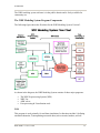


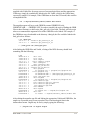
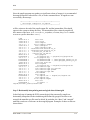


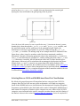


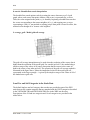
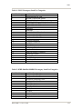


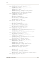
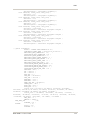


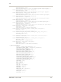
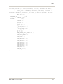


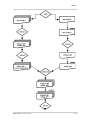


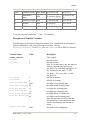

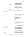
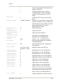
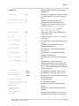


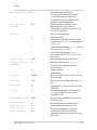


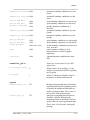

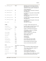
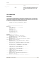


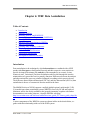


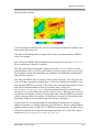
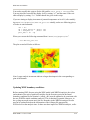
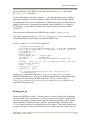

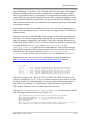
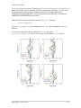


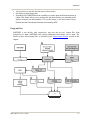


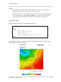


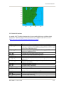
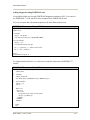
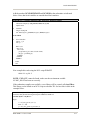
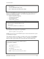


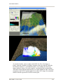


![[DRAFT] User Manual for the LMD Martian Mesoscale Model](http://vs1.manualzilla.com/store/data/005789657_1-11bdf725af45641ff39ff695d9ffff09-150x150.png)