1
User Manual
Parameter Estimation for a Compartmental Tracer Kinetic
Model Applied to PET data
Guadalupe Ayala1
Christina Negoita2
Rosemary A. Renaut3
November 19, 2004
1
This work was supported in part by the Arizona Alzheimer’s Disease Research Center which is funded
by the Arizona Department of Health Services, NIH grant EB 2553301, NSF grant CMG-02223 and the
Underrepresented Graduate Enrichment Match (UGEM) Fellowship award to Guadalupe Ayala
2
Department of Mathematics, Oregon Institute of Technology, Klamath Falls, OR ([email protected]),
Ph. 541 885 1474, http://snoopy.oit.edu/~negoitac.
3
Department of Mathematics and Statistics, Arizona State University, Tempe, AZ 85287-1804
([email protected]), Ph. 480 965 3795, Fax 480 965 8119, http://math.asu.edu/~rosie
Abstract
r
This user manual will aid in the use of a tool that uses a MATLAB
following:
1
graphical interface for the
• FDG parameter estimation, such as k1 − k6 where
– k1 is the transport rate from the blood to the extra-vascular space
– k2 is the transport rate back from the extra-vascular space to the blood
– k3 is the phosphorylation rate of the intra-cellular FDG by hexokinase enzymes to FDG6-phosphate
– k4 is the dephosphorylation rate of the intra-cellular FDG-6-phosphate back to FDG.
– k5 is the spill-over from blood into tissue coefficient
– k6 is (k1 ∗k3 )/(k2 +k3 ) which is proportional to the local cerebral metabolic rate of glucose
and computed explicitly by pixel by pixel analysis
– K is an analog to k6 computed using Patlak analysis, which assumes k4 = 0. It is the
slope of the regression line in the Patlak analysis that is valid only when k4 = 0.
• Investigating different FDG parameter estimation methods.
• Investigating the effect of different filters, parameter constraints, and clustering techniques on
the resulting FDG parameters.
Brief discussion on the use of Positron Emission Tomography as a diagnostic tool for Alzheimer’s
Disease studies is provided. Appropriate references to the standard literature give background on
the topic and methods. Requirements for the tool and a complete description for its use are included.
1 MATLAB
r
is a registered trade mark of The Mathworks, Inc.
Contents
1 Introduction
4
2 Kinetic Parameter Estimation
2.1 Purpose of Kinetic Parameter Estimation
2.2 Compartmental Model for FDG Dynamics
2.3 Spill Over and Partial Volume . . . . . . .
2.4 Extensions . . . . . . . . . . . . . . . . . .
.
.
.
.
.
.
.
.
.
.
.
.
.
.
.
.
.
.
.
.
.
.
.
.
.
.
.
.
.
.
.
.
.
.
.
.
.
.
.
.
.
.
.
.
.
.
.
.
.
.
.
.
.
.
.
.
.
.
.
.
.
.
.
.
.
.
.
.
.
.
.
.
.
.
.
.
.
.
.
.
.
.
.
.
.
.
.
.
.
.
.
.
.
.
.
.
5
5
5
6
6
3 Requirements
3.1 Hardware Requirements . . . .
3.2 Software Requirements . . . . .
3.2.1 Operating System . . .
3.2.2 Necessary Components .
.
.
.
.
.
.
.
.
.
.
.
.
.
.
.
.
.
.
.
.
.
.
.
.
.
.
.
.
.
.
.
.
.
.
.
.
.
.
.
.
.
.
.
.
.
.
.
.
.
.
.
.
.
.
.
.
.
.
.
.
.
.
.
.
.
.
.
.
.
.
.
.
.
.
.
.
.
.
.
.
.
.
.
.
.
.
.
.
.
.
.
.
.
.
.
.
7
7
7
7
7
4 Input Description, Format, File Type and Naming Convention Requirements
4.1 The Plasma Time Activity Curve (PTAC) . . . . . . . . . . . . . . . . . . . . . . .
4.1.1 PTAC File Types . . . . . . . . . . . . . . . . . . . . . . . . . . . . . . . . .
4.2 The Tissue Time Activity Curve (TTAC) For Volume Data . . . . . . . . . . . . .
4.2.1 TTAC Volume File Type . . . . . . . . . . . . . . . . . . . . . . . . . . . .
4.2.2 TTAC Volume File Format . . . . . . . . . . . . . . . . . . . . . . . . . . .
4.3 The Tissue Time Activity Curve (TTAC) for Cluster Data . . . . . . . . . . . . . .
4.3.1 TTAC Cluster File Type . . . . . . . . . . . . . . . . . . . . . . . . . . . . .
4.3.2 TTAC Cluster File Format . . . . . . . . . . . . . . . . . . . . . . . . . . .
4.4 Purpose of Constraints (Only for Slice/Volume Data Runs) . . . . . . . . . . . . .
4.4.1 Constraint Sources . . . . . . . . . . . . . . . . . . . . . . . . . . . . . . . .
4.4.2 Constraint Types . . . . . . . . . . . . . . . . . . . . . . . . . . . . . . . . .
4.4.3 Necessary Files to Set Constraints . . . . . . . . . . . . . . . . . . . . . . .
4.5 The Cluster Map . . . . . . . . . . . . . . . . . . . . . . . . . . . . . . . . . . . . .
4.5.1 Cluster Map File Type . . . . . . . . . . . . . . . . . . . . . . . . . . . . . .
.
.
.
.
.
.
.
.
.
.
.
.
.
.
8
8
8
9
9
9
9
9
10
11
11
12
12
13
13
5 Output Files and their Contents for Each Type of Run
5.1 File Types and File Naming Conventions . . . . . . . . .
5.1.1 Header Files . . . . . . . . . . . . . . . . . . . . .
5.1.2 Results Files . . . . . . . . . . . . . . . . . . . . .
5.1.3 *.tiff Files . . . . . . . . . . . . . . . . . . . . . . .
5.2 Types of Runs and The Format of their Output Files . . .
5.2.1 Single Cluster . . . . . . . . . . . . . . . . . . . . .
5.2.2 Multiple Clusters . . . . . . . . . . . . . . . . . . .
.
.
.
.
.
.
.
14
14
14
14
14
15
15
15
.
.
.
.
.
.
.
.
.
.
.
.
.
.
.
.
.
.
.
.
1
.
.
.
.
.
.
.
.
.
.
.
.
.
.
.
.
.
.
.
.
.
.
.
.
.
.
.
.
.
.
.
.
.
.
.
.
.
.
.
.
.
.
.
.
.
.
.
.
.
.
.
.
.
.
.
.
.
.
.
.
.
.
.
.
.
.
.
.
.
.
.
.
.
.
.
.
.
.
.
.
.
.
.
.
.
.
.
.
.
.
.
.
.
.
.
.
.
.
.
.
.
.
5.2.3
5.2.4
5.2.5
Single Slice . . . . . . . . . . . . . . . . . . . . . . . . . . . . . . . . . . . . .
Multiple Slices . . . . . . . . . . . . . . . . . . . . . . . . . . . . . . . . . . .
Entire Volume . . . . . . . . . . . . . . . . . . . . . . . . . . . . . . . . . . .
16
16
17
6 Estimation Methods and Options
6.1 Kinetic Parameter Estimation Methods . . . . . . . . . . . . . .
6.1.1 The Generalized Linear Least Squares Algorithm - GLLS
6.2 Options . . . . . . . . . . . . . . . . . . . . . . . . . . . . . . . .
6.2.1 Process CSF Option . . . . . . . . . . . . . . . . . . . . .
6.2.2 Spatial Segmentation Option . . . . . . . . . . . . . . . .
6.2.3 Filtering Option . . . . . . . . . . . . . . . . . . . . . . .
.
.
.
.
.
.
.
.
.
.
.
.
.
.
.
.
.
.
.
.
.
.
.
.
.
.
.
.
.
.
.
.
.
.
.
.
.
.
.
.
.
.
.
.
.
.
.
.
.
.
.
.
.
.
.
.
.
.
.
.
.
.
.
.
.
.
18
18
18
18
18
18
19
7 General Procedures
7.1 Reading Input . . . . . . . . . . . . . . . . . . . . . . . . . . .
7.2 Selecting a Data Processing Method . . . . . . . . . . . . . . .
7.3 Selecting a Constraints Option (Only for Volume Data Runs) .
7.4 Selecting a Constraints Source (Only for Volume Data Runs) .
7.5 Starting a Run . . . . . . . . . . . . . . . . . . . . . . . . . . .
7.6 Viewing Current Run Header . . . . . . . . . . . . . . . . . . .
7.7 View Data Fit Plot (Only For Cluster data Runs) . . . . . . .
7.8 Viewing Current Results for Kinetic Parameters . . . . . . . .
7.8.1 Viewing Results as a *.txt file . . . . . . . . . . . . . . .
7.8.2 Viewing Results as.tiff files (Only for Volume data runs)
7.9 Saving Results . . . . . . . . . . . . . . . . . . . . . . . . . . .
7.10 Opening Past Run Headers . . . . . . . . . . . . . . . . . . . .
7.11 Opening Past Run Results and *.tiff Files . . . . . . . . . . . .
7.12 Resetting Application . . . . . . . . . . . . . . . . . . . . . . .
.
.
.
.
.
.
.
.
.
.
.
.
.
.
.
.
.
.
.
.
.
.
.
.
.
.
.
.
.
.
.
.
.
.
.
.
.
.
.
.
.
.
.
.
.
.
.
.
.
.
.
.
.
.
.
.
.
.
.
.
.
.
.
.
.
.
.
.
.
.
.
.
.
.
.
.
.
.
.
.
.
.
.
.
.
.
.
.
.
.
.
.
.
.
.
.
.
.
.
.
.
.
.
.
.
.
.
.
.
.
.
.
.
.
.
.
.
.
.
.
.
.
.
.
.
.
.
.
.
.
.
.
.
.
.
.
.
.
.
.
.
.
.
.
.
.
.
.
.
.
.
.
.
.
20
20
20
20
20
21
21
21
21
21
21
21
22
23
23
. . . .
. . . .
. . . .
Runs)
. . . .
. . . .
. . . .
. . . .
. . . .
.
.
.
.
.
.
.
.
.
.
.
.
.
.
.
.
.
.
.
.
.
.
.
.
.
.
.
.
.
.
.
.
.
.
.
.
.
.
.
.
.
.
.
.
.
24
24
27
29
30
32
34
35
37
38
.
.
.
.
.
.
.
.
.
.
.
.
.
.
8 Sample of a Slice Run
8.1 Step 1: Read PTAC Data from File . . . . . . . . . . . . . . . . . .
8.2 Step 2: Read TTAC From File . . . . . . . . . . . . . . . . . . . . .
8.3 Step 3: Select Constraint Option . . . . . . . . . . . . . . . . . . . .
8.4 Step 4: Select Constraint Source (if necessary, Only for Volume Data
8.5 Step 5: Verify Run Header Information Before Start of Run . . . . .
8.6 Step 6: Indicate the CSF processing Option and Start Run . . . . .
8.7 Step 7: Save Results . . . . . . . . . . . . . . . . . . . . . . . . . . .
8.8 Step 8: View Result Files and Header File . . . . . . . . . . . . . . .
8.9 Step 9: Reset Application . . . . . . . . . . . . . . . . . . . . . . . .
9 Future Implementation
45
10 Notation and Acronyms
46
2
List of Figures
2.1
Compartment model structure for FDG metabolism. . . . . . . . . . . . . . . . . . .
4.1
4.2
4.3
4.4
Real Study PTAC . . . . . . . . . . . . . . . . . . . . . . . . .
TTAC data: Brain Slice 16 over 22 Time Intervals . . . . . . .
TTAC data: An Entire Brain Volume at the Last Time Frame
TTAC Cluster Curves . . . . . . . . . . . . . . . . . . . . . . .
.
.
.
.
8
10
11
12
7.1
Data Fit For Cluster Runs . . . . . . . . . . . . . . . . . . . . . . . . . . . . . . . . .
22
8.1
8.2
8.3
8.4
8.5
8.6
8.7
8.8
8.9
8.10
8.11
8.12
8.13
8.14
8.15
8.16
8.17
8.18
8.19
8.20
8.21
8.22
8.23
8.24
8.25
8.26
8.27
Step 1: Open File Menu . . . . . . . . . . . . . . . . . . . . . . . . .
Step 1: Browse for PTAC data File . . . . . . . . . . . . . . . . . . .
Step 1: Interface Displays PTAC Data . . . . . . . . . . . . . . . . .
Step 2: Open File Menu and Browse Menu to Read Slice . . . . . . .
Step 2: Dialog to Set Options for Reading TTAC File . . . . . . . .
Step 2: Dialog to Enter Slice Number . . . . . . . . . . . . . . . . .
Step 2: Browse for TTAC File that Contains Slice . . . . . . . . . .
Step 3: The Constraint Options Popup Menu . . . . . . . . . . . . .
Step 4: Constraint Source Popup Menu . . . . . . . . . . . . . . . .
Step 4: Browser Dialog to Select Constraint Input File . . . . . . .
Step 5: Open View Menu and View Run Header Data . . . . . . . .
Step 5: Display Dialog for Run Header Information . . . . . . . . . .
Step 6: Run Menu . . . . . . . . . . . . . . . . . . . . . . . . . . . .
Step 6: Prompt for CSF Option . . . . . . . . . . . . . . . . . . . . .
Step 7: Open File Menu to Save Results . . . . . . . . . . . . . . . .
Step 7: Dialog to Enter Filename Prefix to Save Results . . . . . . .
Step 8: Open File Menu to View Past Runs Header and Result Files
Step 8: Select Result File to View . . . . . . . . . . . . . . . . . . .
Step 8: slice run example results.txt . . . . . . . . . . . . . . . . . .
Step 8: Change the File Type to *.tiff . . . . . . . . . . . . . . . . .
Step 8: Select Results File to View . . . . . . . . . . . . . . . . . . .
Step 8: Display window for k2 *.tiff File . . . . . . . . . . . . . . . .
Step 8: Select Header File to View . . . . . . . . . . . . . . . . . . .
Step 8: Header File Displayed After Run . . . . . . . . . . . . . . . .
Step 9: Reset To Start New Run . . . . . . . . . . . . . . . . . . . .
The Volume Run Flow Chart . . . . . . . . . . . . . . . . . . . . . .
The Cluster Run Flow Chart . . . . . . . . . . . . . . . . . . . . . .
25
25
26
27
27
28
28
29
30
31
32
33
34
34
35
36
37
38
39
39
40
40
41
41
42
43
44
3
.
.
.
.
.
.
.
.
.
.
.
.
.
.
.
.
.
.
.
.
.
.
.
.
.
.
.
.
.
.
.
.
.
.
.
.
.
.
.
.
.
.
.
.
.
.
.
.
.
.
.
.
.
.
.
.
.
.
.
.
.
.
.
.
.
.
.
.
.
.
.
.
.
.
.
.
.
.
.
.
.
.
.
.
.
.
.
.
.
.
.
.
.
.
.
.
.
.
.
.
.
.
.
.
.
.
.
.
.
.
.
.
.
.
.
.
.
.
.
.
.
.
.
.
.
.
.
.
.
.
.
.
.
.
.
.
.
.
.
.
.
.
.
.
.
.
.
.
.
.
.
.
.
.
.
.
.
.
.
.
.
.
.
.
.
.
.
.
.
.
.
.
.
.
.
.
.
.
.
.
.
.
.
.
.
.
.
.
.
.
.
.
.
.
.
.
.
.
.
.
.
.
.
.
.
.
.
.
.
.
.
.
.
.
.
.
.
.
.
.
.
.
.
.
.
.
.
.
.
.
.
.
.
.
.
.
.
.
.
.
.
.
.
.
.
.
.
.
.
.
.
.
.
.
.
.
.
.
.
.
.
.
.
.
.
.
.
.
.
.
.
.
.
.
.
.
.
.
.
.
.
.
.
.
.
.
.
5
Chapter 1
Introduction
This user manual is a guide on how to use an application tool designed to estimate kinetic parameters which describe Fluoro-Deoxy-Glucose (FDG) dynamics in the brain of Alzheimer’s disease
patients. The tool uses dynamic PET data obtained from one-dimensional, two-dimensional or
three-dimensional measurements. Chapter 2 provides the background information, the theory and
purpose of kinetic parameter estimation, and a brief description of the compartmental kinetic model
on which the estimation is based. It furthers describes other alternative applications for the tool
in a computational research environment. Chapter 3 lists the hardware and software requirements.
Chapter 4 contains the information on the inputs for the application. This section explains in detail
the format, file type and naming convention for all of the inputs including Plasma Time Activity
Curve (PTAC) , Tissue Time Activity Curve (TTAC) , Constraints, and Cluster Map. It explains
in detail which of these inputs are necessary and which are optional. Chapter 5 describes all the
different classes of possible output files, their file types and the naming conventions. Also, it outlines
which output files are created for each type of run. It also lists all of the variables that are displayed
in the header file for each type of run. Chapter 6 gives information on Generalized Linear Least
Squares (GLLS), which is the estimation method used to estimate the kinetic parameters and explains the different user options. Chapter 7 provides the step by step commands to read inputs, start
runs, view results, and save results. Chapter 8 is intended to familiarize the user with the application
screens and the run process by a walk through of a sample slice run, with detailed directions and
shows the application screens along the way. Finally, Chapter 9 explains the future capabilities that
are planned to be added to the application, and how this could help to evaluate estimation methods
and filtering techniques. Notation used is provided in the final Section.
4
Chapter 2
Kinetic Parameter Estimation
2.1
Purpose of Kinetic Parameter Estimation
We are interested in using PET to image brain activity in patients with Alzheimer’s disease (AD).
In AD studies, one way to measure disease progression is by measuring FDG, which is an analog
of glucose uptake in the brain. Studies [14, 18, 19] which determine a local cerebral metabolic
rate (LCMR) of FDG uptake in a region of interest have proved successful in understanding AD
progression.
More specific information may be obtained by estimating the individual kinetic parameters which
describe FDG dynamics. In particular, it is believed that the individual kinetic parameters may be
used for early detection of AD. This application is used to estimate the kinetic parameters in order
to be able to focus towards understanding the spatial distribution of kinetic parameters in AD, as
well as towards developing a precise measure for utilization in the early detection of AD [15].
2.2
Compartmental Model for FDG Dynamics
The estimation of FDG dynamics kinetic parameters is based on the following compartmental tracer
kinetic model for FDG:
FDG (plasma)
u(t)
k1 FDG (tissue)
−→
k2
y1 (t)
←−
k3 FDG6P (tissue)
−→
k4
y2 (t)
←−
Figure 2.1: Compartment model structure for FDG metabolism.
The PET scanner provides a measure of the combined FDG y1 (t) and phosphorylated FDG
concentration in tissue y2 (t), ie a measure of y(t) = y1 (t) + y2 (t) [15], where
dy1
= k1 u(t) − (k2 + k3 )y1 (t) + k4 y2 (t)
dt
dy2
= k3 y1 (t) − k4 y2 (t)
dt
y1 (0) = 0, y2 (0) = 0.
5
(2.1)
The system rate constants are interpreted as following:
• k1 is the transport rate from the blood to the extra-vascular space
• k2 is the transport rate back from the extra-vascular space to the blood
• k3 is the phosphorylation rate of the intra-cellular FDG by hexokinase enzymes to FDG-6phosphate
• k4 is the dephosphorylation rate of the intra-cellular FDG-6-phosphate back to FDG.
and u(t) is the input data, namely the FDG tracer concentration in plasma.
Although clinical studies [14] have shown that the de-phosphorylation rate k4 is nonzero, many
models such as the the Patlak analysis [3] assume k4 = 0.
2.3
Spill Over and Partial Volume
Real data suffers from noise introduced by spill-over and partial volume effects. Spill-over is usually
bidirectional and accounts for a percentage of the tracer in plasma being counted as total tissuetracer, as well as for some of the tracer in tissue being counted as plasma-tracer (due to limited spatial
resolution). This leads to a blurring effect in the image. Spill-over coefficients can be introduced
in the tracer model, and estimated as additional parameters. However, they can complicate the
numerical identifiability of model parameters [7]. Consequently, one or more venous samples are
made late in the study to improve their identification. Other methods for removing spill-over effects
have been considered [11], but they suffer from being dependent on estimates of the imaged-object
geometry as well as on other factors, like cardiac motion. Principal component analysis is also
introduced to derive tissue-time activity curves free from spill-over effects [2], but we opt to consider
the model dependent method which can be easily incorporated into the compartmental kinetic model.
For brain studies which use an image-derived input function u(t), the tissue into blood spill-over
coefficient is estimated [4] such that one obtains a spill-over corrected input function. In this case,
clearly one needs to only account for the spill-over from blood into tissue coefficient, called here
parameter k5 . We also introduce the parameters k6 = (k1 k3 )/(k2 + K3 ), which is proportional to
the local cerebral metabolic rate of glucose and the analogue to k6 , the parameter K, which is the
slope of the regression line in the patlak analysis that is valid only when k4 = 0.
Partial volume effects (PVE) occur due to the intrinsic spatial resolution of the PET camera;
in objects smaller than the resolution of the tomograph, true tracer concentration will be underestimated. The pixel target tissue mixes with surrounding tissue, and this can lead to an inaccurate
parameter estimation overall [22, 13, 21]. This is a significant concern for region of interest studies
of the heart. Several methods for correcting for partial volume effects have been considered [1, 11].
However, this is currently an active area of research, and we focus here only on model dependent
methods which can account for PVE.
2.4
Extensions
This application also allows the user to compare results with respect to the computational and
estimation methods, filters, constraints, and input sources chosen by the user. Comparing the results
could help find out what are the best estimation methods, what are the constraints or what is the
best filtering technique that provides optimal results. Results could be compared with expected
results according to theoretical information, and an educated decision can be made on what are the
best computational methods to use for every situation.
6
Chapter 3
Requirements
3.1
Hardware Requirements
This a a highly computationally intensive application. The following is the system on which the
application was tested and suggested to run:
• 2.6 GHz Intel Pentium 4 Processor or equivalent.
• Minimum 512 MB of RAM.
3.2
3.2.1
Software Requirements
Operating System
This application will run on any linux based operating system.
3.2.2
Necessary Components
r
This application requires MATLAB
Version 6.0 or higher to be installed on your system. The
following toolbox needs to be installed:
• Nonlinear Optimization Toolbox
7
Chapter 4
Input Description, Format, File
Type and Naming Convention
Requirements
This section describes the input requirements for the application. It outlines file types, format, and
file naming conventions for the input data.
4.1
The Plasma Time Activity Curve (PTAC)
The PTAC, u(t), displays information on the FDG concentration in the blood over time, see Figure
2.1. The FDG plasma time activity curve (PTAC) can be derived either invasively, by blood sampling
or non-invasively, from a region of interest in the reconstructed PET images. [23]. Figure 4.1 shows
a real time study PTAC.
Figure 4.1: Real Study PTAC
4.1.1
PTAC File Types
The source of the PTAC can be either blood sample data or a PTAC reconstruction from *.cpt files.
• If collected through blood sampling, the data should be read from a file of type *.txt. The
*.txt file format is required to be as follows:
The text file should contain 2 columns. The length of the columns will be equal to the number
8
of blood samples. The first column should display the time vector for each of the time points
at which a blood sample was taken. The second column should display the FDG concentation
in blood for each of the time points.
• If collected through PTAC reconstruction, the data should be read from several files of type
*.cpt. The *.cpt files are created using the CTI molecular imaging software. Note that this
form means that any approximate input data, whether from simultaneous estimation or a
population based model can also be used, see papers [12, 20, 8, 10].
4.2
The Tissue Time Activity Curve (TTAC) For Volume
Data
The TTAC data can be read over an entire volume, as single or multiple slices of the entire brain
volume. Each slice is a cross-sectional 2D image of the brain. TTAC volume data are PET images
of the brain over time. PET images are collected by scanning the brains of patients over time.
Furthermore, the brains are divided into a fixed number of slices. Each slice has its own time series.
TTAC slice data is stored in 3D structure of size J ∗ L ∗ N where J ∗ L is the image size of the
slice in pixels, and N is the number of time points in the time series.
The entire volume data is stored in a 4D structure of size J ∗ L ∗ S ∗ N where J ∗ L is the image size of the slice in pixels, S is the number of slices in the entire volume, and N is the number of
time frames in the time series. Figure 4.2 shows TTAC data of brain slice 16 over 22 time intervals.
The next figure shows TTAC data as the entire brain volume comprised of 32 slices at the last
time frame 4.3.
4.2.1
TTAC Volume File Type
TTAC volume data should be read from a file of type *.img. By convention, the TTAC filename
should have numeric string embedded somewhere in the filename. This numeric string will be
identified and interpreted as the $PATIENT ID which will be used to create the directory where
the output files are going to be saved. If more than one numeric string is embedded on the TTAC
filename, then the first numeric string from left to right will be interpreted as the $PATIENT ID.
4.2.2
TTAC Volume File Format
*.img file - a bitmap graphic file.
4.3
The Tissue Time Activity Curve (TTAC) for Cluster
Data
TTAC cluster curves are a representation of grouped data points on brain slices over time as one
point over time. TTAC cluster curves are derived from entire brain volume. Cluster data is created
by grouping together similar pixels according to their value within slice images. An example of 5
TTAC Cluster Curves is shown in Figure 4.4.
4.3.1
TTAC Cluster File Type
r
TTAC Cluster Curves should be read from a MATLAB
file of type *.mat. By convention, the
TTAC filename should have a numeric string embedded somewhere in the filename. This numeric
9
Figure 4.2: TTAC data: Brain Slice 16 over 22 Time Intervals
string will be identified and interpreted as the $PATIENT ID which will be used to create the
directory where the output files are going to be saved. If more than one numeric string is embedded
on the TTAC filename, then the first numeric string from left to right will be interpreted as the
$PATIENT ID.
4.3.2
TTAC Cluster File Format
The *.mat file should contain the following variables names:
grpcurves: This variable holds the TTAC Cluster Curve Values. grpcurves variable should be
a matrix of size C ∗ N where C is the number of clusters and N is the number of time points.
tm: This variable holds the time vector information. Time vector should be of size 1 ∗ N
.
10
Figure 4.3: TTAC data: An Entire Brain Volume at the Last Time Frame
4.4
Purpose of Constraints (Only for Slice/Volume Data Runs)
Constraints are only used for volume runs and are not an available feature for cluster runs. Constraints are used as bounds during the calculation of kinetic parameters of the model. Constraints
are optional and not necessary for a run, hence you can run without any constraints. They are
intended to help improve estimates of the kinetic parameters.
4.4.1
Constraint Sources
Constraints are set from either the user input, a text file or an automatic calculation from cluster
curves.
11
Figure 4.4: TTAC Cluster Curves
4.4.2
Constraint Types
There are three types of constraints, positivity, global and by cluster.
1. When the user selects Positivity Constraints, the lower bounds are set to 0 and upper bounds
are set to 1. These type of constraints do not allow the kinetic parameter estimates to become
negative.
2. When the user selects global constraints, the same set of constraints are used during the
calculations of kinetic parameters on all of the volume data.
3. When the user selects constraints by cluster, different set of constraints are used during the
calculations of the kinetic parameters on each cluster of the volume data. A cluster map is
required when applying constraints by cluster, because we need to identify the label cluster of
each pixel.
4.4.3
Necessary Files to Set Constraints
Constraint files are necessary only when the user chooses to set the constraints from a text file or
to automatically calculate the constraints from a cluster file.
1. If constraints are set from user input, no file is necessary.
2. If constraints are set by positivity constraints, no file is necessary. Consequently, the lower
bounds will be set to 0 and upper bounds for all will be set 1 for all kinetic parameters.
3. If constraints are set from a text file with filename with extension *.txt. This file should contain a matrix with the lower and upper bounds for all k1 − k5 parameters. The following are
examples of what the file might look like:
For the global constraints case:
0
0
0
0
1
1
1
1
12
01
The first column are the lower bounds and the second column are the upper bounds for
k1 , k2 , k3 , k4 , k5 in that order.
For the by cluster constraints case:
0
0
0
0
0
0
0
0
0
0
0
0
0
0
0
0
0
0
0
0
0
0
0
0
0
1
1
1
1
1
1
1
1
1
1
1
1
1
1
1
1
1
1
1
1
1
1
1
1
1
The first matrix’s rows are the lower bounds for k1 , k2 , k3 , k4 , k5 in that order. In this example
each column lists the lower bounds for each of five clusters. The second matrix’s rows are the
upper bounds for the k1 , k2 , k3 , k4 , k5 in that order. Also, each column lists the upper bounds
for each of the five clusters.
4. If automatically calculated from cluster curves, the file type should be *.mat containing TTAC
cluster data. From this data the application will calculate the lower and upper bounds for the
k1 − k5 kinetic parameters.
4.5
The Cluster Map
A Cluster Map maps every pixel on a slice to a cluster hence associating with each pixel a label
pointing to its cluster membership. This information is used to applied different set of constraints
when processing different pixels on a slice according to which cluster they belong. The Cluster Map
file is only necessary when the user chooses to apply constraints by cluster and we are running TTAC
volume data.
4.5.1
Cluster Map File Type
The cluster map should be read from a *.mat file.
Cluster File Map Format
The mat file should contain the following variable:
B: This is a variable of size J ∗ L ∗ 1 where J is the slice width and L is the slice length.
13
Chapter 5
Output Files and their Contents
for Each Type of Run
5.1
File Types and File Naming Conventions
Every Run will save its output into two or more of the following files:
5.1.1
Header Files
The header file lists all the information required to replicate the run. Which variables are displayed
on this file depends on the type of run. The naming convention for this file is F header.txt where
F is filename entered by the user in the Save As dialog while saving the results. Refer to Chapter
5.2 for a detailed description of this file for all the different types of runs. Chapter 5.2 classifies all
runs into single cluster, multiple cluster, single slice, multiple slice, and entire volume, and describes
their header file in detail.
5.1.2
Results Files
The results file lists the resulting kinetic parameters for a cluster run or the filenames where the
results were saved in case of volume data runs. The naming convention for this file is F results.txt
where F is a user defined filename while saving results. Refer to Chapter 5.2 for a detailed description
of this file for all the different types of run. Chapter 5.2 classifies all runs into single cluster, multiple
cluster, single slice, multiple slice, and entire volume, and describes their results file in detail.
5.1.3
*.tiff Files
A single *.tiff file is used to store the information of a single kinetic parameter for a single slice of the
brain. Each pixel on a slice image corresponds to a set of kinetic parameters. Consequently, for each
slice run, 7 *.tiff image files are created representing all the kinetic parameters k 1 , k2 , k3 , k4 , k5 , k6
and K at different regions, where
• k1 is the transport rate from the blood to the extra-vascular space
• k2 is the transport rate back from the extra-vascular space to the blood
• k3 is the phosphorylation rate of the intra-cellular FDG by hexokinase enzymes to FDG-6phosphate
14
• k4 is the dephosphorylation rate of the intra-cellular FDG-6-phosphate back to FDG.
• k5 is the spill-over from blood into tissue coefficient
• k6 is (k1 ∗ k3 )/(k2 + k3) computed explicitly by pixel by pixel analysis
• K is an analog to k6 computed using Patlak analysis, which assumes k4 = 0.
The naming convention for this file is F SliceS kH.tiff . The F is the user defined filename
while saving the results, S NUMBER is the slice number, and H is the kinetic parameter number
in the range of 1-6 and BigK.
5.2
Types of Runs and The Format of their Output Files
The types of runs can be classified by their type of Input. When the user chooses to save the results
after a run, the data is written into header, results, and if applicable to *.tiff files. Which files are
written and the information written depends on the type of run.
5.2.1
Single Cluster
The output for this type of run includes two files, a header file and results file.
Header File Format
The header file displays the following variables:
Data Type: Single Cluster
TTAC Filename: The TTAC Cluster Filename
PTAC Filenames: All the PTAC Filenames
Time Vector Size: The number of time frames
Time Vector: The vector with all the time point intervals
Processing Method: The type of method used to calculate for k1 − k6
Cluster Curve Number: The cluster curve number ran.
Results File Format
The results file contains the kinetic parameter results k1 − k6 .
5.2.2
Multiple Clusters
The output for this type of run includes two files, a header file and results file.
Header File Format
The header file displays the following variables:
Data Type: Multiple Cluster Curves
TTAC Filename: TTAC Cluster Filename
TTAC Filename: The TTAC Cluster Filename
PTAC Filenames: All the PTAC Filenames
Time Vector Size: The number of time frames
Time Vector: The vector with all the time point intervals
15
Processing Method: The type of method used to calculate for k1 − k6
Number of Cluster Curves: Number of cluster curves read from file
Results File Format
The results file contains the kinetic parameter results k1 − k6 for all clusters in the TTAC cluster
file.
5.2.3
Single Slice
The output is a header file, results file, and 7 *.tiff files corresponding to each of the kinetic parameters k1 , k2 , k3 , k4 , k5 , k6 , K.
Header File Format
The header file displays the following variables:
Data Type: Single Slice
TTAC Filename: TTAC Volume Filename
TTAC Filename: The TTAC Volume Filename
PTAC Filenames: All the PTAC Filenames
Time Vector Size: The number of time frames
Time Vector: The vector with all the time point intervals
Processing Method: The type of method used to calculate for k1 − k6 and K
Number of PTAC Files
Number of Slices:1
Slice Number
Filter ON/OFF: Binary Option for Filtering Volume Data while Reading
Spatial Segmentation Option: Binary Option for Spatially Segmenting Slices
Process CSF: Binary Option to process CSF
Results File Format
The Results file displays *.tiff filenames to which the kinetic parameter results were written.
5.2.4
Multiple Slices
The output is several header files, results files, and *.tiff files corresponding to each of the kinetic
parameters for each slice.
Header File Format
The header file displays the following variables:
Data Type: Multiple Slices
TTAC Filename: TTAC Volume Filename
TTAC Filename: The TTAC Volume Filename
PTAC Filenames: All the PTAC Filenames
Time Vector Size: The number of time frames
Time Vector: The vector with all the time point intervals
Processing Method: The type of method used to calculate for k1 − k6 and K
16
Number of PTAC Files
Number of Total Slices
Slice Numbers
Filter ON/OFF: Binary Option for Filtering Volume Data while Reading
Spatial Segmentation Option: Binary Option for Spatially Segmenting Slices
Process CSF: Binary Option to process CSF
Results File Format
The Results file displays *.tiff filenames to which the kinetic parameter results were written.
5.2.5
Entire Volume
The output is several header files, results files, and 7 *.tiff files corresponding to each of the 7 kinetic
parameters for each and all the slices in the entire volume. The kinetic parameters correspond to
k1 − k6 and K.
Header File Format
The header file displays the following variables:
Data Type: Multiple Slices
TTAC Filename: TTAC Volume Filename
TTAC Filename: The TTAC Volume Filename
PTAC Filenames: All the PTAC Filenames
Time Vector Size: The number of time frames
Time Vector: The vector with all the time point intervals
Processing Method: The type of method used to calculate for k1 − k6 and K
Number of PTAC Files
Number of Total Slices in Volume: 31
Slice Numbers: All Slices Were Read
Filter ON/OFF: Binary Option for Filtering Volume Data while Reading
Spatial Segmentation Option: Binary Option for Spatially Segmenting Slices
Process CSF: Binary Option to process CSF
Results File Format
The Results file displays *.tiff filenames to which the kinetic parameter results were written.
17
Chapter 6
Estimation Methods and Options
6.1
Kinetic Parameter Estimation Methods
The user has the ability to choose which method to use during the estimation of the kinetic parameters. The GLLS algorithm with one iteration will be the default method [16, 15].
6.1.1
The Generalized Linear Least Squares Algorithm - GLLS
The GLLS algorithm is introduced in [6]. GLLS is an extension of the generalized least squares
(GLS) algorithm to non-uniformly sampled data. Although GLLS has been used successfully in
studies [6, 9, 5], there is no analytic proof of convergence of this algorithm. In addition, despite its
derivation as an iterative algorithm, GLLS has mostly been used as a one step iteration - see for
example [6, 9, 16, 15].
6.2
Options
Options allow the user to choose whether to process the Cerebral Spinal Fluid (CSF) region of the
brain, spatially segment or filter the brain image slices before processing.
6.2.1
Process CSF Option
The Cerebral Spinal Fluid (CSF) option enables the user to choose whether the CSF region should
be processed or not. This is useful, because a user might want to assumme there is not activity
in the CSF Region. Pixels on the slices are not processed if their intensity values are lower than a
given threshold value. The intensity values of the CSF region are higher than 0.5. Furthermore, the
background region intensity values are lower than 0.5. It is necessary to set the threshold value to
0.5 in order to segment out the background, but not the CSF region. Also, since CSF region pixel
intensity values are lower than 1.0, we have to set the threshold value to 1.0 in order to segment the
CSF region. Any pixel under 1.0 will not be processed, which includes most of the CSF region and
background pixels
6.2.2
Spatial Segmentation Option
The Spatial Segmentation Option allows the user to crop the slice image to segment the background
of the slice out. This option is very useful if you want to process a smaller number of pixels, or
provide a region of interest for analysis.
18
6.2.3
Filtering Option
The filter option allows the user apply an anisotropic diffusion filter to the slice images. Anisotropic
diffusion [17] was developed to smooth an image, thus removing high frequency noise, while preserving the boundaries of structures of interest.
19
Chapter 7
General Procedures
7.1
Reading Input
1. Open File menu
2. Choose type of input to read either TTAC Cluster, TTACVolume data, or PTAC data
a) Read Single Cluster Curve → Browse for cluster data file → Enter Cluster Curve Number
→ Done
b) Read Multiple Cluster Curves → Browse for cluster data file → Done
c) Read Single Slice → Select filter and spatial segmentation options → Enter Slice Number
→ Browse for volume data file → Done
d) Read Multiple Slices → Select filter and spatial segmentation options → Enter slices numbers
comma separated [ex: 1,2,3] → Browse for volume data file → Done
e) Read Entire Volume → Select filter and spatial segmentation options → Browse for volume data
file → Done
f) Read PTAC data → Browse of PTAC data files → Done
7.2
Selecting a Data Processing Method
Click on the Data Processing Method pop-up menu. Default is GLLS.
7.3
Selecting a Constraints Option (Only for Volume Data
Runs)
Click on Select Constraint Option pop-up Menu. This pop-up Menu is disabled for cluster data
runs.
7.4
Selecting a Constraints Source (Only for Volume Data
Runs)
Click on the Select Source for Constraints pop-up menu. This pop-up menu is disabled when
running with no constraints or positivity constraints.
20
7.5
Starting a Run
Open Run menu → Click on Start Run.
7.6
Viewing Current Run Header
After entering all the necessary input to start a run, it is possible to view the header file. This
option aids the user in the verification of all the input parameters. By reviewing the header run
data, the user can verify inputs like constraints, input filenames, and option settings are correct.
After verification, the user can now proceed to start the run. To view run header you need to:
Open View menu → View Run Header Data
7.7
View Data Fit Plot (Only For Cluster data Runs)
This function is only available for cluster runs. The data fit plot allows the user to compare the
original cluster TTAC in a run with the estimated cluster TTAC from the resulting k1 − k5 kinetic
parameters. You will be only to view the data fit plot after you run at least one of the cluster curves.
To view the data fit plot:
Open View menu → View Data Fit Plot
The Figure 7.1 shows a example of data fit plot for a single cluster curve. In this case, the user
ran cluster curve number 3 and then plotted the data fit. Note how closely this two curves lie,
therefore by looking at these curves you should be able check how effective is the estimation method
for calculating the kinetic parameters k1 − k5 .
7.8
Viewing Current Results for Kinetic Parameters
It is possible to view current results at the end of each run. If the last previous run was volume data,
the resulting kinetic paramenter will be printed to different *.tiff files. Also, if the last previous run
was cluster data, the resulting kinetic parameters will be printed to a *.txt file.
7.8.1
Viewing Results as a *.txt file
Open View menu → View Kinetic Parameters
7.8.2
Viewing Results as.tiff files (Only for Volume data runs)
Open View menu → View Kinetic Parameters → Change the file type in the Browse dialog
to *.tiff → Browse for *.tiff file to view and select it → Click Open button.
7.9
Saving Results
Succesful end of run is required to save results.
21
Figure 7.1: Data Fit For Cluster Runs
Open File menu → Save Results As → Type a user defined label in the dialog to use in the
naming convention of all the results files. → Click OK
The resulting output is saved on the following type of files: header.txt files, results.txt files, or
*.tiff files. Please refer to Chapter 5 for more information on the contents and formats of these files.
Unless the user browses to another directory; by default, the output files will be save under
$HOME/Results/$PATIENT ID, where $HOME is the current user home directory and $PATIENT ID is a numeric substring within the PTAC filename. THE $PATIENT ID is automatically derived from the TTAC filename by identifying the first numerical substring within the TTAC
filename as the $PATIENT ID.
7.10
Opening Past Run Headers
If the user wants to analyze past run results, they should be able to review the description of the
run. Header files display all of the information required to replicate a run. Please refer to Chapter
5 for more information on this type of files.
Open File menu → Open Header File → Browse to directory where header file is located →
Pick Header File to View → Click Open
22
7.11
Opening Past Run Results and *.tiff Files
If the user wants to analyze past runs results, they should be able to go back and look at all past
run results data. The results file will be either *.tiff files for volume data runs or Results *.txt files
for cluster data runs.
Open File menu → Open Results File → Choose results file type in the File Type pop-up
menu → Browse to directory where result file is located → Pick Results File to View → Click
Open
Please refer to Chapter 5 regarding output for *.tiff and Results file description.
7.12
Resetting Application
It is essentially important to reset the application every time after the results are saved and a new
run is to be started. This will reinitialize the user interface variables, so you can start additional
runs. Resetting application ensures the run starts with new data and its not running with old data.
In order to reinitialize, follow the following directions:
Open Run menu → Click Reset
23
Chapter 8
Sample of a Slice Run
This section will show in a step by step how to start a slice run, view and save the results. It is
intended to serve as an example on how to run the application. The process requires completing the
following steps:
1. Read PTAC data from file
2. Read TTAC data from file
3. Select constraint option (Only for Volume Data Runs)
4. Select constraint source (if necessary, Only for Volume Data Runs)
5. Verify run header information before start of run
6. Indicate the CSF processing option and start run
7. Save results for future reference
8. Open run result files for analysis
8.1
Step 1: Read PTAC Data from File
Open File menu and Click on Read PTAC Data File as shown in Figure 8.1
A dialog like the one on Figure 8.2 will appear and you will need to browse for the PTAC files.
Select only one of the *.cpt files and then click the Open button. The application will read all of
the *.cpt files in the directory that share the same prefix in their filenames.
Futhermore, the interface will display a plot of the PTAC data on the left axis. In addition, it
will display the number of *.cpt files read and the filename for the first *.cpt file read as shown in
Figure 8.3
24
Figure 8.1: Step 1: Open File Menu
Figure 8.2: Step 1: Browse for PTAC data File
25
Figure 8.3: Step 1: Interface Displays PTAC Data
26
8.2
Step 2: Read TTAC From File
Open File menu, then browse the menu Read TTAC Volume Data to Read Slice as shown on
Figure 8.4.
Figure 8.4: Step 2: Open File Menu and Browse Menu to Read Slice
When you click on Read Slice, a Read Options dialog as in Figure 8.5 will appear. Here you
can select whether you want to spatially segment the slice by cropping the slice or if you want to
apply the default anisotropic filter to the slice while reading. Check the options you desire and click
OK button.
Figure 8.5: Step 2: Dialog to Set Options for Reading TTAC File
A dialog 8.6 will appear to prompt for the slice number to read. For example, if we want to read
slice 16, enter number 16 and click the OK button.
27
Figure 8.6: Step 2: Dialog to Enter Slice Number
Another dialog will prompt you to browse and select the TTAC file. By default, the dialog filters
for a *.img file as in Figure 8.7. Browse to the directory where the TTAC data file is located, select
the file and click the Open button.
Figure 8.7: Step 2: Browse for TTAC File that Contains Slice
28
8.3
Step 3: Select Constraint Option
This step is done only for volume data runs. Since this is a sample slice run, you will have to select a
constraint option for your run, before you can start the run. Select a constraint option through the
popup-menu shown in Figure 8.8. For demonstration purposes select Run Method with Global
Constraints. Refer to Section 4.4 on constraint option types for a description of all the possible
options on the pop-up menu.
Figure 8.8: Step 3: The Constraint Options Popup Menu
29
8.4
Step 4: Select Constraint Source (if necessary, Only for
Volume Data Runs)
Since you chose to run with global constraints, you will have to select a source for the constraints.
Select a constraint source by clicking on the popupmenu as shown in Figure 8.9. Choose Calculate
Constraints From *.mat file.
Figure 8.9: Step 4: Constraint Source Popup Menu
Once you choose the constraint, a browser dialog will appear as shown in Figure 8.10, browse to
the location where the *.mat file is. This *.mat file should contain the cluster data from which the
constraints are going to be calculated. Then, select the *.mat file and click on the Open button.
Refer to Section 4.4 on constraints for more information on the other type of sources for constraints.
30
Figure 8.10: Step 4: Browser Dialog to Select Constraint Input File
31
8.5
Step 5: Verify Run Header Information Before Start of
Run
At this point the Status of the application changes from Waiting for User Inputs to Ready to
Run. Since most users of this application might want to verify they are running the correct data
with the correct parameters, it is recomended to view the run header data before running. For more
information on what variables will be displayed in the runheader data, please refer to Section 5.2.
This Chapter gives a detailed description of all the header files for the different types of runs.
To display and view the run header information, open the View menu and select View Run
Header Data, as shown in Figure 8.11
Figure 8.11: Step 5: Open View Menu and View Run Header Data
The display dialog shown on Figure 8.12 will appear. Here you can verify all the run information
before starting the run.
32
Figure 8.12: Step 5: Display Dialog for Run Header Information
33
8.6
Step 6: Indicate the CSF processing Option and Start
Run
After verifying the run header infomation, start the run by opening the Run menu and clicking on
Start Run, as shown in Figure 8.13.
Figure 8.13: Step 6: Run Menu
When you click on Start Run, a question dialog as shown in Figure 8.14 will prompt you to
whether you want to process CSF or not. For demostration purposes press the No button, and the
run will start.
Figure 8.14: Step 6: Prompt for CSF Option
r
Since MATLAB
does not support multi-tasking, you will not be able to interact with the user
interface until the run is finished.
34
8.7
Step 7: Save Results
When the run is finished, the interface will prompt you to save your results and reset the application.
Before you reset the application you have to view and save your results. Open File menu and click
on Save Results as shown on Figure 8.15
Figure 8.15: Step 7: Open File Menu to Save Results
Subsequently, a dialog will appear prompting for a filename prefix for the results file as shown in
Figure 8.16. Refer to the Chapter 5 for more information on the naming convention for the result
files that are going to be written. Type slice run example and click on Save. The result files had
been saved. Now the next step is to open and view the result files created for by run.
35
Figure 8.16: Step 7: Dialog to Enter Filename Prefix to Save Results
36
8.8
Step 8: View Result Files and Header File
Open the File menu and Click on Open Results File as shown in Figure 8.17
Figure 8.17: Step 8: Open File Menu to View Past Runs Header and Result Files
8.18. The PTAC filename used in this example is p04277dy1 roi1 roi.cpt, therefore the directory where the result files are saved by default is $HOME/Results/04277. We browse to this
directory and select file slice run example results.txt and push Open button.
The file is opened and displayed on a window see Figure 8.19. For slice runs, this file contains
the filenames of the files to which the kinetic parameter results were written. Kinetic parameter
results were written to several *.tiff files. Note the filenames displayed and push the Done button
to close this window.
Now, we would like to view these *.tiff files. Open the File menu and Click on Open Results
File as shown in Figure 8.17. Browse to the directory where the result files are. Use the pop-up
menu on the browser dialog to change the file type to view only desired result files as in Figure 8.20.
For demonstration purposes pick *k2.tiff, so you will only see the kinetic parameter k 2 *.tiff files
saved from the past runs as shown in Figure 8.21. Select file slice run example Slice16 k2.tiff
and push Open button.
A window opens up and displays the k2 kinetic parameter as an image see Figure 8.22. You can
select and view any of the other kinetic parameters in the same manner.
In addition, you can also open the header file of this run. Opening header files will allow you
to go back and review what PTAC, TTAC data and other run time parameters produced the result
files. In order to open the past run header file, open the File menu and click on menu item Open
Header File. A directory browser will appear and you need to browse to the directory where the
37
Figure 8.18: Step 8: Select Result File to View
results were saved see Figure 8.23. In this case the results were saved at $HOME/Results/04277.
Select header file slice run example header.txt and push Open button.
Then, a window displaying the header file will appear as shown in Figure 8.24.
8.9
Step 9: Reset Application
Now, Reset the application to setup and start a new run. Open the Run menu and click the Reset
menu item, see Figure 8.25. The application will reinitialize and all variables will be cleared.
All of these steps for a volume run are illustrated in the flow chart next page, see Figure 8.26.
38
Figure 8.19: Step 8: slice run example results.txt
Figure 8.20: Step 8: Change the File Type to *.tiff
39
Figure 8.21: Step 8: Select Results File to View
Figure 8.22: Step 8: Display window for k2 *.tiff File
40
Figure 8.23: Step 8: Select Header File to View
Figure 8.24: Step 8: Header File Displayed After Run
41
Figure 8.25: Step 9: Reset To Start New Run
42
Start
Read TTAC Data
Read PTAC Data
Filter TTAC?
Yes
Segment TTAC
Image?
Yes
No
Use Constraints?
Yes
No
Select Constraint
Option
Select Constraint
Source
No
Verify Run Header
Information
Start Run
Process CSF?
Yes
No
Save Results
View Header File
View Results File
Start New Run?
Yes
No
Reset Application
End
Figure 8.26: The Volume Run Flow Chart
43
Also, the steps for cluster run are illustrated in Figure 8.27.
Start
Read PTAC Data
Save Results
Verify Run Header
Information
Read TTAC Data
View Header File
Start Run
View Results File
Yes
Start New Run?
Reset Application
No
End
Figure 8.27: The Cluster Run Flow Chart
44
Chapter 9
Future Implementation
Currently, this application enables the user to apply several constraint options while estimating the
kinetic parameters. On the other hand, this application is constrained to GLLS as its only estimation
method for the kinetic parameters. Also, the application implements and applies only the anisotropic
diffusion filter. It is intended that these tool could also be used as an evaluation tool for the different
estimation methods and filters. Therefore, there is going to be future implementation of optional
methods for kinetic parameter estimation.
45
Chapter 10
Notation and Acronyms
k1
k2
k3
k4
k5
k6
K
PTAC
TTAC
GLLS
PET
AD
FDG
LCMR
y1 (t)
y2 (t)
y(t)
u(t)
PVE
J
L
N
S
$PATIENT ID
C
F
S
H
CSF
$HOME
Transport rate from blood to extra-vascular space (1)
Transport rate back from extra-vascular space to blood (1)
Phosphorylation rate intra-cellular FDG to FDG-6-phosphate (1)
Dephosphorylation rate intra-cellular FDG-6-phosphate to FDG (1)
Spill-over from blood to tissue coefficient (1)
(k1 ∗ k3 )/(k2 + k3 ) proportional to local cerebral metabolic rate of glucose (1)
Analog to k6 computed using Patlak analysis (1)
Plasma Time Activity Curve, the FDG concentration in the blood over time (4)
Tissue Time Activity Curve, the FDG concentration in the tissue over time. (4)
Generalized Linear Least Squares, computational method for parameter estimation (4)
Positron Emission Tomography (5)
Alzheimer’s disease (5)
Flouro-Deoxy-Glucose (5)
Local Cerebral Metabolic Rate (5)
The FDG concentration in tissue over time (5)
The phosphorylated FDG concentration in tissue over time (5)
The sum of phosphorylated and non-phosphorylated FDG concentration over time (5)
Input data, namely the FDG tracer concentration in plasma over time (6)
Partial Volume Effects (6)
Length of slice in unit pixels (9)
Width of slice in unit pixels (9)
Number of time points (9)
Number of slices in the entire volume (9)
Numerical string parsed from PTAC filename (9)
The number of cluters (10)
Filename for saving results entered in Save As dialog (14)
Slice number (15)
Kinetic Parameter Number in the range 1-6 (15)
Cerebral Spinal Fluid (18)
The current user home directory (22)
46
Bibliography
[1] J.A.D. Aston, V.J. Cunningham, M-C. Asselin, A. Hammers, A.C. Evans, and R.N. Gunn,
Positron emission tomography partial volume correction: Estimation and algorithms, J. Cerebral
Flow Metab. (2002), 1019–1034.
[2] D. Barber, The use of principal components in the quantitative analysis of gamma camera
dynamic studies, Phys. Med. Biol. (1980), 283–292.
[3] R. Blasberg C. Patlak and J. Fenstermacher, Graphical evaluation of blood to brain transfer
constants from multiple uptake data, J. Cereb. Blood Flow and Metab. (1983), 1–7.
[4] K. Chen, D. Bandy, E. Reiman, S.C. Huang, D. Feng M. Lawson, L. Yun, and A. Palant,
Non-invasive quantification of the cerebral metabolic rate for glucose using positron emission
tomography, F-Fluoro-2-Deoxyglucose the patlak method and an image-derived input function,
J. Cerebral Flow Metab. (1998), 716–723.
[5] K. Chen, M. Lawson, E. Reiman, A. Cooper, S.C. Huang D. Feng, D. Bandy, D. Ho, L. Yen,
and A. Palant, Generalized linear least squares method for fast generation of myocardial blood
flow parametric images with N-13 ammonia PET, IEEE Tran. Med. Imag. 17 (1998), no. 2,
236–243.
[6] S.C. Huang D. Feng, Z. Wang, and D. Ho, An unbiased parametric imaging algorithm for
nonuniformly sampled biomedical system parameter estimation, IEEE Trans. Medical Imaging
15 (1996), no. 4, 512–518.
[7] X. Li D. Feng and S.C.Huang, A new double modeling approach for dynamic cardiac PET
studies using noise and spillover contaminated lv measurements, IEEE Trans. Biomed. Eng.
(1996), 319–327.
[8] S. Eberl, A. R. Anayat, R. R. Fulton, P. K. Hooper, and M. J. Fulham, Evaluation of two
population based input functions for quantitative neurological FDG PET studies, Eur. J. Nucl.
Med. 24 (1997), 299–304.
[9] D. Feng and D. Ho, Parametric imaging algorithms for multicompartmental models dynamic
studies with positron emission tomography, Quantification of Brain Function (1993), 1–10.
[10] D. G. Feng, K.-P. Wong, C.-M. Wu, and W.-C. Siu, A technique for extracting physiological
parameters and the required input function simultaneously from PET image measurements:
Theory and simulation study, IEEE Trans. Inform. Technol. Biomed. 1 (1997), no. 4, 243–254.
[11] S. Gambhir, Quantification of the physical factors affecting the tracer kinetic modeling of cardiac
positron emission tomography data, Ph.D. thesis, UCLA, 1990.
47
[12] Hongbin Guo, Rosemary Renaut, and Kewei Chen, Improved imaged-derived input function for
study of human brain FDG-PET, submitted, 2004.
[13] K. Herholz and C.S. Patlak, The influence of tissue heterogeniety on results of fitting nonlinear
model equations to regional tracer uptake curves with an application to compartmental models
used in positron emission tomography, IEEE Trans. Med. Imag. (2000), 1128–1131.
[14] S.C. Huang, M. Phelps, E. Hoffman, K. Sideris, C. Selin, and D. Kuhl, Non-invasive determination of local cerebral metabolic rate of glucose in man, Am. J. Physiology (1980), E69–E83.
[15] C. Negoita, Global kinetic imaging using dynamic positron tomography data, Ph.D. thesis, Arizona State University, 2003.
[16] Cristina Negoita and Rosemary A Renaut, On the convergence of the generalized linear least
squares algorithm, BIT (2004), accepted.
[17] P. Perona and J. Malik, Scale-space and edge detection using anisotropic diffusion, IEEE Transactions on Pattern Analysis and Machine Intelligence 12 (1990), 629–639.
[18] M. Phelps, S.C. Huang, E. Hoffman, C. Selin, L. Sokoloff, and D. Kuhl, Tomographic measurement of local cerebral glucose metabolic rate in humans with (F-18)2-Fluoro-2-Deoxy-D-Glucose:
Validation of method, Ann. Neurol 6 (1979), 371–388.
[19] S.C. Huang R. Carson and M. Green, Weighted integration method for local cerebral blood flow
measurements with positron emission tomography, Journal Cerebral Flow Metab. (1986), 245–
258.
[20] S. M. Sanabria-Bohorquez, A. Maes, P. Dupont, G. Bormans, T. de Groot, A. Coimbra, W. Eng,
T. Laethem, I. De Lepeleire, J. Gambale, J. M. Vega, and H. D. Burns, Image-derived input
function for [11 C] flumazenil kinetic analysis in human brain, Mol. Imag. Biol. 5 (2003), no. 2,
72–78.
[21] K. Schmidt, G. Mies, and L. Sokoloff, Model of kinetic behavior of deoxyglucose in hetereogenous
tissue in brain: a reinterpretation of the significance of parameters fitted to homogeneous tissue
models, J. Cereb. Blood Flow Metab. (1991), 10–24.
[22] K. Uemura, H. Toyama, Y. Ikoma, K. Oda, M. Senda, and A. Uchiyama, Correction of partial
volume effect on rate constant estimation in compartment model analysis of dynamic PET study,
J. Cereb. Blood Flow Metab. (1991), 10–24.
[23] I. Weinberg, S.C Huang, E. Hoffman, L. Arauho, C. Nienaber, M. GroverMcKay, M. Dahlbom,
and H. Schelbert, Validation of PET-acquired input functions for cardiac studies, Journal Nuclear Med. 29 (1988), 241–247.
48