Download Programming Reference - Time Series Modelling (TSM)

Time Series Modelling Version 4.47
Programming Reference
James Davidson
22th November 2015
Contents
Introduction .................................................................................. 3 Running a Program .................................................................................... 3 Variable Types........................................................................................... 4 TSM Functions .......................................................................................... 5 Options Reference ........................................................................ 9 2.2 Data Input and Output ......................................................................... 9 3.1 Setup .................................................................................................. 10 3.5 Automatic Model Selection ............................................................... 10 3.5 Recursive/Rolling Estimation ........................................................... 11 3.6 Compute Summary Statistics ............................................................ 12 3.8 Semiparametric Long Memory ......................................................... 13 3.9 Cointegration Analysis ...................................................................... 14 3.10 Monte Carlo Experiment ................................................................. 15 4.1 Equation ............................................................................................. 16 4.2 Conditional Variance ......................................................................... 18 4.4 User-coded Functions ........................................................................ 20 4.5 Regime Switching ............................................................................. 21 4.6 Parameter Constraints........................................................................ 23 4.7 Equilibrium Relations........................................................................ 23 4.8 Select Instruments ............................................................................. 24 4.9 Panel Data .......................................................................................... 25 5. Values .................................................................................................. 26 Systems of Equations ............................................................................................. 26 The Parameter Groups ........................................................................................... 27 Inequality Constraints ............................................................................................ 28 Constraint Values .................................................................................................. 29 6. Actions ................................................................................................. 29 8.1 Output and Retrieval Options ............................................................ 31 8.3 Test and Diagnostics Options ............................................................ 32 8.4 Forecasting Options ........................................................................... 36 8.5 Simulation and Resampling Options ................................................. 37 8.7 ML and Dynamics Options ............................................................... 40 8.8 Optimization and Run Options .......................................................... 42 8.9 Special Settings ................................................................................. 43 1
James Davidson 2015
Accessing Results ....................................................................... 43 Summary Statistics .................................................................................. 43 Estimation Outputs .................................................................................. 44 Semiparametric Long Memory ............................................................... 50 Cointegration Analysis ............................................................................ 50 TSM Graphics Reference ........................................................... 52 Graphics Functions .................................................................................. 52 Graphics Options ..................................................................................... 55 GUI Commands ......................................................................... 58 Index of Functions and Variable Names..................................... 60 2
James Davidson 2015
Introduction
As well as running in GUI mode as a free-standing Windows or Linux application,
TSM can be included as a module in a regular Ox program. This can be just an
alternative way to run the program, using text commands. All the options available in
the GUI version (with the exception of the graphics options, currently) can be
implemented, by assigning values to TSM command variables. These are written in
upper case, and are globally defined, and so can appear anywhere in the user’s program.
It is also possible to run Ox code using the GUI version of TSM as a platform. See
Appendix C for details of the functions that can be compiled and run as components of
TSM. Communication between the program and the user’s code is controlled through
the dialog Model / Coded Function. In principle, any variable or function described in
this document can be invoked from within a user’s function.
Running a Program
Since TSM is a big program, a command line switch is needed to reserve more memory
than the default. To run your program from OxEdit, first do the following.
1. Open OxEdit and choose View / Preferences / Add/Remove Modules…
2. Select the entry &Ox.
3. Edit the ‘Arguments’ field to read
-s6000,6000 "$(FilePath)"
(In other words, add the “-s6000,6000” switch at the beginning of the
entry.)
4. Close the dialog. This setting will be remembered by the OxEdit installation.
The program needs to contain as its first line,
#import <packages/tsmod4/tsmknl4>
Otherwise it has the usual Ox structure, with a main() function where execution
starts. A typical program would have the form
#import <packages/tsmod4/tsmknl4>
Text_Input()
{
. . .
}
main()
{
Set_Defaults();
Text_Input();
Run_Estimation();
}
where the ellipsis represents the options to be set. Each option must appear in a line
having the form
OPTION = [value];
where OPTION is one of a set of identifiers, and the user supplies [value]. The
terminating semi-colon is important. Note that Ox is case-sensitive, and the identifiers
must be in upper case. The main() function must always appear last in the file, the
3
James Davidson 2015
general rule being that called functions always precede calling functions. (To deviate
from this rule, see the Ox documentation for more details.)
Comments in Ox (ignored by the compiler) are either placed between /*…*/ pairs, or
are in lines beginning with //. These can be used for annotating the input file in any
convenient manner.
Notes:
1. TSM is not an Ox class, just a precompiled module. This means that there are some
globally defined variables whose use must be avoided in your program. All the
user-selectable options are written wholly in upper case. This usage conflicts with
the Ox convention of writing constants in upper case, but to avoid problems just
don’t use any word from the reserved list to define a constant! A complete
alphabetized list of reserved words can be found in the file tsmknl4.h. Some other
global definitions have the prefix g_ . A number of these are user-accessible and
defined in this document. There are others, but they all relate to interaction with the
GUI module. To avoid trouble, don’t use the ‘g_’ prefix. Declare your global
variables as STATIC, and use the prefix ‘s_’.
2.
Since time is always short, the documentation of programming features tends to lag
behind the development of the program itself. This manual is not always up to date.
However, virtually all TSM features can be implemented in a user’s Ox program.
To see the commands needed to implement particular program features available in
the GUI, give the command File / Settings / Display/Save Text… Please don’t
hesitate to advise the author of commands missing from this manual.
Variable Types
1.
2.
3.
4.
5.
6.
Boolean: either TRUE (equivalently, 1) or FALSE (equivalently, 0).
Integer: whole numbers without decimal points.
Real:
floating point numbers, can include decimal points.
String:
alphanumeric characters enclosed in “”.
Vector:
values of types 1, 2 or 3, separated by commas, and enclosed by <>.
Matrix: values of types 1, 2 or 3 separated by commas and then semi-colons, and
enclosed by <>. (For example, the 22 identity matrix is represented by <1,0;0,1>.)
7. Array:
values of types 1-6, separated by commas and enclosed by {}.
Notes:
1. In Ox, row vectors are written with elements separated by commas, and column
vectors with elements separated by semi-colons. All vector options in TSM are row
vectors. Entering in column form will produce an error.
2. Vectors and matrices are used to input starting values for parameters. Except in the
case of regime switching models, the entry takes the form of a single row.
3. If the vector or matrix you enter has fewer rows/columns than have been specified
for estimation, it will be automatically extended with the default values. If it
contains too many rows or columns it is truncated, and the additional ones are
ignored.
4. In regime switching models with M = NUM_REGIMES regimes, matrices of
switching parameters may have up to M rows, each row representing the starting
values for a regime. If only a row vector is entered and REGIME_DIFFERENCES =
0, this row is automatically replicated M times to form the starting values. If
REGIME_DIFFERENCES = 1, then the additional rows are automatically set to
zero.
4
James Davidson 2015
5. Vectors and matrices are also used to input instructions about parameters, e.g. to fix
them, or include them in a test of significance. In these cases the vector/matrix
should contain ones and zeros, using the starting values as a template to identify the
location of the parameter. The vector/matrix is extended with zeros/truncated, if the
dimension is different from that specified.
6. The <> and {} symbols are optional if vectors/arrays have only one element.
TSM Functions
The following TSM functions can be called.
Set_Defaults()
Initializes program settings at default values. No return value.
Note: This function must always be called first, before any other TSM
functions.
Run_Estimation()
Estimates currently specified model. No return value.
Run_Simulation(const mShocks)
Simulates currently specified model. No return value. The simulated series is
optionally appended to the data matrix.
By default, set mShocks to the empty matrix <> . The random shocks are
obtained from model residuals or through the random number generator,
according to the options selected. Optionally, pass the shocks to the function as
a matrix of dimension (END_SAMPLESTART_SAMPLE+1) 
columns(SERIES).
Note: A call to Run_Estimation must be normally made before a call to
this function, to read in data and set up parameter values. Set
EVALUATE_INIT = 1 to use supplied values instead of estimates.
Load_TextValues()
Loads parameter values and attributes that have been set manually using the
formats described in Section 5. No return value.
Note: This function is called automatically when running programs in console
mode. It must be called explicitly when running Ox code using the GUI version
of TSM as a platform.
SaveModel(const sTitle)
Stores the current model specifications, including parameter values. sTitle is
a text string containing a name used to identify the model in the output.This
function returns an array containing the model, so the correct syntax is of the
form “aMod = SaveModel(sTitle)”.
LoadModel(const aStoreModel, const iMode)
Loads the model stored in the array aStoreModel in a previous call to
SaveModel. This is equivalent to a call to a function Text_Input()
containing the same specifications as TSM commands. Setting iMode = 1 loads
all the values. Set iMode = 0 to avoid loading components that will not be used
for simulations, including fixed values, upper and lower bounds, test values and
testing options. These stay at their existing settings.
WriteListings(const Filename, const bSavedat)
5
James Davidson 2015
Writes the current model settings and outputs (including parameter values,
forecasts, tables, series and graphics) to a .tsd file. Call ReadListings to
access its contents.)
Filename (string)
The file name should include the complete file path, if different from the
home folder, and should be given the extension .tsd. This is a text file
but is not easily human-readable, it is intended to be read only with the
ReadListings function.
bSavedat (Boolean)
TRUE to additionally store the current data set in the file.
FALSE otherwise.
ReadListings(const File, const bModel, const bData)
Retrieve the contents of a previously stored .tsd file. These outputs can now
be accessed, as if generated by an estimation run, for graphing or retrieval for
further analysis.
bModel(Boolean)
TRUE to re-instate stored model settings, otherwise set to
FALSE to keep the current model settings.
bData (Boolean)
TRUE to retrieve the stored data set, if any (this will replace the data
currently loaded).
FALSE otherwise.
If no data set is stored, this setting is ignored.
ReadData(const sFile, const bSetSample, const bMerge,
const iFirstnum)
Reads a data set from a file.
sFile (string):
The path and name of the data file. The extension determines the type of file.
(Remember that the Windows “\” symbol must be represented as “\\” in an Ox
string variable.)
bSetSample (Boolean):
TRUE if all sample settings should be reset to the defaults (the
complete sample),
FALSE otherwise.
bMerge (Boolean):
TRUE if the data are to be merged with the data set currently in
memory
FALSE if the data are to replace the current data, if any.
iFirstnum (Integer):
When data sets are to be merged and the sample periods are different, set to
the offset – the row number of the new data set that matches the first row of
the existing data (can be of either sign). Otherwise set to 0.
Note:
This function needs to be called only if the data are to be manipulated in the
user’s program. Loading a model causes the associated data set to be loaded
6
James Davidson 2015
automatically. The data matrix and array of names are accessed through the
static variables DATA_SET and DATA_NAMES, respectively. To have these data
used in program functions, set ACCESS_DATA = 1.
Summary_Statistics(const aSeries)
If the argument is a single variable name (or a column number of the data
matrix) this function computes summary statistics, quantiles, autocorrelations or
partial autocorrelations, and tests of I(0) and I(1) for the specified series.
If the argument is an array of variable names (or a vector of column numbers)
the function computes either the contemporaneous correlation matrix of the
series, or the cross-autocorrelations of the first two series in the set.
Optional settings for this function are listed in Section 3.6.
LogPeriodogram_Regression(const bMode)
Performs log-periodogram regression on elements of the array
LOGPER_SERIES. Always set bMode = 1.
Cointegration_Analysis(const bMode)
Performs a cointegration-related analysis, as follows.
bMode = 0: Perform tests of I(0) and I(1) on selected data.
bMode = 1: Prints selection criteria for lag length choice.
bMode = 2: Performs Johansen tests of cointegrating rank.
bMode = 3: MINIMAL analysis at 90% level.
bMode = 4: MINIMAL analysis at 95% level.
bMode = 5: MINIMAL analysis at 97.5% level.
bMode = 6: MINIMAL analysis at 99% level.
bMode = 7: Perform specified Wald test of cointegration.
bMode = 8: Perform all Walds test of cointegration.
Run_MonteCarlo(const aSimMod, const aEstMod, const
bExtendRun)
Runs a Monte Carlo experiment. The first two arguments are the models to be
used for generating the data and to be estimated, respectively. The third
argument is Boolean, indicating that the previous experiment is to be extended,
instead of started afresh; set to 0 for most applications. No return value.
Notes: .
1. The models are named arrays, as previously created with SaveModel.
2. The simulation and estimation models can be the same or different, provided
both reference the same data set. The observations for estimation are as
specified in the simulation model.
3. The simulation model must explicitly assign the variables START_SAMPLE
and END_SAMPLE. There are no valid default values.
PrintCall(const bLine, …)
If enabled, sends console output to a text file, (also the results window in GUI
mode). bLine is a Boolean variable, = 1 to terminate the line with a carriage
return, 0 otherwise. The other arguments are items for printing.
No return value.
In addition, the following functions can be used for accessing results inside the user’s
program after calls to Run_Estimation() or Run_Simulation(). See the
section Accessing Results for details.
7
James Davidson 2015
LocP(const iEq, const iPar)
This helps locate parameters and standard errors in multi-equation models.
LocTP(const iReg, const iPar)
This returns the storage locations of parameters and standard errors in Markovswitching models. See the section Accessing Results for details.
LocVar(const Name)
Name (string) is the name of a variable in DATA_NAMES.
Return value: column number of the variable in the matrix DATA_SET.
(This function has a different action from VarNum, which is only for use
in user-supplied functions. )
In addition, the program can include UserFunction() and UserSolve()
functions, as described in Appendix B. Don’t forget to include the compiler directives
#define USER_FUNCTION and #define USER_SOLVE in this case.
Note: Only certain listed TSM functions, as detailed in Appendix C, can be called from
within user-supplied functions. Do not use the functions listed above in this context.
8
James Davidson 2015
Options Reference
The numbering of these sections matches that in the User’s Manual. The same program
options are dealt with in the corresponding sections, as far as possible, and hence
numbering is not consecutive. See the manual for some additional details.
Tip: The quickest way to learn the programming commands is to set up the desired
model and options interactively in the TSM GUI, and then give the command File /
Settings / Save Text. This command writes the contents of the Text_Input()
function needed to generate the same run to a text file, ready for inclusion in your
program.
2.2 Data Input and Output
ACCESS_DATA (Boolean): Default = FALSE.
TRUE
to access the data from a matrix created in the user’s program
FALSE to read the data from a disk file.
DATA_SET (Matrix of Real)
The data matrix, with the observations in rows and variables in columns. Needs to be
defined if ACCESS_DATA = 1.
DATA_NAMES (Array of Strings): Default = {}.
Names for variables, if these are either read from DATA_SET or from disk as an ASCII
matrix file. Number of elements must match the number of columns of either
DATA_SET or the ASCII file, respectively.
INPUT_PATH (String): Default = "".
Full path to the directory containing data files. The default (empty string) points to the
working directory.
INPUT_FILE (String): Default = “input”.
Name of the data file. Data can be read and saved in one of five formats. The format is
specified by the file extension.
".xls", “.xlsx”
Excel Worksheet. The first row of the sheet must contain
variable names. The “.xlsx” format requires Ox 6.20.
".wk1", ".wks"
Lotus 123 worksheet. The first row of the sheet must contain
variable names.
".in7"
GiveWin file, see Ox and Givewin documentation for details.
".dat"
Ox/Givewin "data with load information" file. See the
documentation for details.
".mat", or any other. ASCII file containing a matrix, with variables in columns and
observations in rows. The first line of the file must contain two
integers, number of rows, followed by number of columns.
EDF_FILE (String): Default = “".
Name of spreadsheet file containing empirical distribution function (see EDF_CRITS).
9
James Davidson 2015
Note: See the GUI User’s Manual, Section 3.10 (Setup / Monte Carlo Experiments) for
details of the EDF file format.
ACCESS_RESULTS (Boolean) Default = FALSE.
TRUE
Write estimation results to console (normal output).
FALSE Write estimation results to global variables, no console output.
This option is set when the estimation results are to be used in further processing by the
program, as in Monte Carlo simulation. See the last section of this document.
RESULTS_FOLDER (String): Default = “”.
Full path to the directory where results should be written, including text files and
spreadsheet listings. The default (empty string) points to the working directory.
RUN_ID (Integer) Default = 0.
Initializes the numbering sequence used to identify outputs created by the program,
including console output, listings files and retrieved series. It is incremented each time
Run_Estimation() is called, and so lets the outputs of successive runs be easily
distinguished.
3.1 Setup
DETERMINISTIC (Integer): Default = 0.
1 , To remove mean and linear trend from the dependent variable by preliminary
regression. This option is active only if the series are not differenced.
0, to remove the mean from the series prior to estimation. This option is active
whether or not the series is differenced (see next setting).
1, no transformations applied to the series.
Note: This command is retained for legacy reasons, but estimating intercept and trend
within the model is the recommended option.
START_SAMPLE (Integer): Default = 0.
First observation to be used for estimation. 0 is read as 1.
END_SAMPLE (Integer) Default = 0.
Last observation to be used for estimation. 0 is read as the last observation
available.
Note: if START_SAMPLE > 1 then by default, the pre-sample observations are
used to form lags. See PRESAMPLE_LAGS.
INDIC_SAMPLE (Boolean): Default = FALSE.
TRUE
Select sample according values (1/0) of an indicator series in the data set.
The series must have the name “!selectobs!”.
FALSE Otherwise.
OMIT_NANS (Boolean): Default = FALSE.
TRUE
Omit missing observations from the selected sample without truncating.
(Cross-section data only!)
FALSE otherwise.
3.5 Automatic Model Selection
MULTI_SPEC (Integer): Default = NOMS.
NOMS
Normal Estimation.
10
James Davidson 2015
ARMS
RGMS
To estimate all the ARIMA(p,d,q) or ARFIMA(p,d,q) specifications in
sequence, up to maximum values of p and q and p+q set by the user.
Starting values for each optimisation are generated automatically from
the preceding run. If a conditional variance model is specified with
METHOD = 2, the same specification and starting values, set by the
user, are used for each specification of the mean process. Additional
output options are not available in this case. Regime switching is
disabled.
To compute models with all combinations of included regressors of the
specified type(s), and report the case that optimizes the currently selected
model selection criterion. (INFO_CRIT).
The following settings are ignored unless MULTI_SPEC = 1.
MAX_AR_ORDER (Integer): Default = 2.
Maximum value of p (order of (L)) to be fitted.
MAX_MA_ORDER (Integer): Default = 2.
Maximum value of q (order of (L)) to be fitted .
MAX_TOTAL_ORDER (Integer): Default = 2.
Maximum value of p + q.
Thus, with the default settings the program will estimate the following cases of (p,q),
in the order shown: (0,0), (1,0), (2,0), (0,1), (1,1), (0,2). The starting values for the
estimations are set to either the estimates from the preceding specification, or zero,
as appropriate.
AUTOREG_TYPES (Integer): Default = MSR1.
Specified which regressor Types to include in the regressor selection run specified
by MULTI_SPEC = RGMS.
MR1
Type 1.
MR2
Type 2
MR3
Type 3
MR12
Types 1 and 2
MR13
Types 1 and 3
MR23
Types 2 and 3
MRALL
All Types.
3.5 Recursive/Rolling Estimation
RECURSIVE_ESTIMATION (Boolean): Default = FALSE.
TRUE
To estimate the model repeatedly, for a sequence of samples with
advancing end-dates.
FALSE Regular model estimation.
The following commands are ignored unless RECURSIVE_ESTIMATION = 1. To use
this feature, set START_SAMPLE and END_SAMPLE to represent the first sample in
the desired sequence.
ROLLING_ESTIMATION (Boolean): Default = FALSE.
TRUE
To estimate with fixed sample size, so that the start date and end date
advance together,
FALSE To estimate with fixed start date, and increasing sample size.
RECURSION_ENDDATE (Integer): Default = 0.
11
James Davidson 2015
The terminal end date in the sequence.
RECURSION_STEP (Integer): Default = 1.
The number of observations to advance by at each step.
RECURSION_STATISTICS (Boolean): Default = TRUE.
TRUE
To save all the output, including test statistics, for each estimation
FALSE To save only parameter and estimates and standard errors.
FORECAST_TERMDATE (Boolean): Default = FALSE.
TRUE
To compute ex-ante forecasts up to the fixed date, set as END_SAMPLE
+ FORECAST_STEPS, so that the actual number of forecasts steps
contracts as the end-date of the samples advances.
FALSE To compute ex-ante forecasts a fixed number of steps ahead for each
sample, so that the final forecast date advances with the sample.
Note: this option is ignored unless FORECAST_STEPS > 0 and
EXPOST_FORECASTS = 0
SAVE_RECFORCS (Boolean): Default = FALSE.
TRUE
to save all ex-ante forecasts in a file .
FALSE to save only the terminal forecast. This is recorded with the other model
statistics.
RECURS_RPSTATUS (Boolean): Default = FALSE.
TRUE:
report convergence status of recursions .
FALSE: otherwise.
DO_GRID (Boolean): Default = FALSE.
TRUE
Compute a 1- or 2-dimensional grid of criterion values.
FALSE Otherwise.
Note: the parameters to plot are set up in Fixed Values and Bounds: see User’s Manual
3.6 Compute Summary Statistics
SUMMSTAT_DETREND (Boolean): Default = FALSE.
TRUE
Compute statistics for detrended variables (LS residuals from trend).
FALSE Otherwise.
SUMMSTAT_DIFF (Boolean): Default = FALSE.
TRUE
Compute statistics for differenced variables.
FALSE Otherwise.
SUMMSTAT_CORRELS (Integer): Default = 0.
Order of correlograms/partial correlograms to be calculated.
SUMMSTAT_DATCORR (Boolean): Default = FALSE.
TRUE
Either compute contemporaneous data correlations for any number of
series, or (if SUMMSTAT_CORRELS >0) compute crossautocorrelations for a pair of series.
FALSE Compute summary statistics for individual series..
START_SSTSAMPLE (Integer): Default = 0.
First observation to be used for summary statistics. 0 is read as 1.
END_SSTSAMPLE (Integer) Default = 0.
12
James Davidson 2015
Last observation to be used for summary statistics. 0 is read as the last observation
available.
SUMMSTAT_INTORD (Integer): Default = 0.
Integration order tests to be performed.
NOIT
No tests.
I0T
Tests of I(0).
I1T
Tests of I(1).
I0I1T
Tests of I(0) and I(1).
SUMMSTAT_QUANTILES (Boolean): Default = FALSE.
TRUE
Compute quantiles of the series distribution.
FALSE Otherwise.
SUMMSTAT_PARCORREL (Boolean): Default = FALSE.
TRUE
Compute partial correlograms.
FALSE Compute simple correlograms.
3.8 Semiparametric Long Memory
LOGPER_REGRESSION (Boolean): Default = FALSE.
TRUE
Do log-periodogram regression.
FALSE Otherwise.
This is an indicator used by the Monte Carlo module.
LOGPER_SERIES (Array of Strings): Default = {}.
Variables for long memory estimation.
Note: The models are univariate. The named variables are estimated in sequence.
LOGPERIODGM_TRANS (Integer): Default = 0.
LPRW
Use raw series
LPDF
Use differenced series
LPDT
Use detrended series
LOGPERIODGM_TYPE (Integer): Default = 0.
GPH
Geweke/Porter-Hudak method.
MS
Moulines-Soulier method.
LWH
Local Whittle ML
START_LPRSAMPLE (Integer): Default = 0.
First observation to be used for summary statistics. 0 is read as 1.
END_LPRSAMPLE (Integer) Default = 0.
Last observation to be used for summary statistics. 0 is read as the last observation
available.
GPH_BANDWIDTH (Integer): Default = [(END_SAMPLE – START_SAMPLE)/2].
Bandwidth for Geweke/Porter-Hudak and local Whittle ML estimation.
GPH_SMOOTH (Integer): Default = 1.
Smoothing factor for Geweke/Porter-Hudak estimation.
GPH_TRIM (Integer): Default = 1.
Trimming factor for Geweke/Porter-Hudak estimation.
GPH_BIASTEST (Boolean): Default = FALSE.
13
James Davidson 2015
TRUE
FALSE
Report bias test in Geweke-Porter Hudak estimation.
Otherwise.
GPH_BIASBW (Integer): Default = [(END_SAMPLE – START_SAMPLE)/2]..
Bandwidth for Geweke/Porter-Hudak bias test.
GPH_SSMPLTEST (Boolean): Default = FALSE.
TRUE
Report skip-sampling test of long memory in Geweke-Porter Hudak
estimation.
FALSE Otherwise.
GPH_SSMPLPERD (Integer): Default = 0..
N, the length of the skip-sample intervals for the skip-sampling test. The skip
samples are constructed as every Nth observation. If set to 20, the test is
constructed by maximizing the test statistic over the range N = 2 to N = 12
(experimental setting).
GPH_COMBINEPVALS (Integer): Default = 0..
Set to a positive value (, try 0.3) to compute a composite p-value, based on those
of the skip-sampling test and Wald significance test on d.
GPH_BWPOWERS (0, or 1  5 vector of Reals): Default = 0.
If defined, contains values from the interval [0,1] representing bandwidths as
powers of the sample size. Bandwidth choices are then preserved (approximately)
across different samples. The five elements are: (0) the GPH bandwidth; (1) the
GPH trim factor, (2) the Moulines-Soulier power series, (3) the GPH bias test
bandwidth and (4) the GPH skip-sampling test bandwidth. If this vector is defined,
other bandwidth settings are ignored.
MS_FOURTERMS (Integer): Default = 1.
Number of included Fourier terms for Moulines-Soulier estimation.
3.9 Cointegration Analysis
START_COISAMPLE (Integer): Default = 0.
First observation to be used for summary statistics. 0 is read as 1.
END_COISAMPLE (Integer) Default = 0.
Last observation to be used for summary statistics. 0 is read as the last observation
available.
COINTEGRATION_VARS (Array of Strings): Default = {}.
Variables to include in the cointegrating VAR
COINTEGRATION_LAGS (Integer): Default = 1.
Lag length for cointegrating VAR.
COINTEGRATION_DRIFT (Boolean): Default = FALSE.
TRUE
Include trend term in cointegrating VAR.
FALSE Otherwise.
COINTEGRATION_RANK (Integer): Default = 0.
Assumed cointegrating rank of system for MINIMAL analysis.
COINT_TEST_VARS (Array of Strings): Default = {}.
Subset of COINTEGRATION_VARS to include in Wald test of cointegration
14
James Davidson 2015
MINIMAL_ROTHUMB (Boolean): Default = FALSE.
TRUE
Use rule of thumb to adjust nominal rejection criteria in MINIMAL
analysis.
FALSE otherwise.
3.10 Monte Carlo Experiment
MC_REPS (Integer): Default = 1000.
Number of Monte Carlo replications.
MC_BINS (Integer): Default = 100.
Number of bins for Monte Carlo empirical distributions.
MC_HISTOG (Boolean): Default = FALSE.
TRUE
Report Monte Carlo distributions as a histogram.
FALSE Otherwise.
Note: ignored unless MC_REPS > 1000.
MC_MOMENTS (Boolean): Default = FALSE.
TRUE
Report first 4 empirical moments of parameters.
FALSE Otherwise.
MC_MOMSES (Boolean): Default = 0 FALSE
.
TRUE
Report first 4 empirical moments of parameter standard errors.
FALSE: Otherwise.
MC_CENTRET (Boolean): Default = FALSE.
TRUE
Tabulate distribution of centred t statistics
FALSE Otherwise.
Note: ignored unless parameters match in generated and estimated models.
MC_COMPARE (Boolean): Default = FALSE.
TRUE
Compute bias and RMSE
FALSE Otherwise.
Note: ignored unless parameters match in generated and estimated models.
MC_SIGNT (Boolean): Default = FALSE.
TRUE
Tabulate signed t statistics.
FALSE Otherwise.
MC_QUANTILES (Boolean): Default = FALSE.
TRUE
Tabulate test quantiles.
FALSE: Otherwise.
MC_PEEVALS (Boolean): Default = FALSE.
TRUE
Tabulate EDFs for p-values .
FALSE Otherwise.
MC_2SIDED (Boolean): Default = FALSE.
TRUE
p-value EDFs tabulated for two-sided tests, with equal probabilities in
each tail. (Set with MC_SIGNT = TRUE is equivalent to tabulating
absolute values only when distribution is symmetric.)
FALSE p-value EDFs for rejections in the upper tail.
MC_ITGMM (Boolean): Default = FALSE.
TRUE
Do iterated GMM in estimation.
15
James Davidson 2015
FALSE Do 1-step GMM in estimation.
Note: ignored unless GMM is specified in estimation model.
MC_WARPSPEED (Boolean): Default = FALSE.
TRUE
Use warp-speed method for Monte Carlo analysis of boostrap tests.
FALSE Otherwise.
4.1 Equation
METHOD (Integer): Default = LSQ .
LSQ
Least Squares.
WHITTLE
Whittle (frequency domain) ML.
GMM
Instrumental Variables / Generalized Method of Moments
GAUSS_ML
Conditional Gaussian time domain ML.
STUDENT_T
Conditional Student’s t time domain ML
SKEW_STUDT
Conditional skewed-Student’s t time domain ML
GED_ML
Conditional General error distribution time domain ML
PROBIT
Probit ML (binary data).
LOGIT
Logit ML (binary data)
POISSON
Poisson ML (count data)
NEGBIN1
Negative Binomial I (count data)
NEGBIN2
Negative Binomial II (count data)
Notes:
1. Either the variable name or the integer value can be given.
2. For the procedure for efficient (multi-stage) GMM, see 7.4 Optimization
Options.
SYSTEM (Boolean): Default = FALSE
TRUE
System of equations.
FALSE Single equation.
SERIES (String or Array of Strings): Default = "X".
The name(s) of the dependent variable(s) of the model.
Notes:
1. If this option is given as an integer or row vector of integers, it is read as the
relevant column number(s) of the data matrix.
2. With two or more variables, a system of equations is fitted.
3. A data series must be specified for a simulation run. This supplies start-up
conditions (pre-sample lags), and acts as a ‘placeholder’ in the data matrix. As
an alternative to a true data series, this command can supply the name of a
dummy series composed (e.g.) of zeros.
The following options are ignored if METHOD = WHITTLE). In this case, the series is
always de-meaned prior to computing the periodogram.
INTERCEPT_1 (Boolean): Default = FALSE
TRUE
To fit an intercept of Type 1 .
FALSE To suppress intercept of Type 1.
INTERCEPT_2 (Boolean): Default = FALSE
TRUE
To fit an intercept of Type 2.
FALSE To suppress intercept of Type 2.
16
James Davidson 2015
Note: if both intercepts are selected, the Type 2 selection will be ignored.
TREND (Boolean): Default = FALSE.
TRUE
To fit a linear trend.
FALSE No trend
LINEAR_REGRESSION (Boolean): Default = FALSE.
TRUE
To estimate an equation by ordinary (non-iterative) least squares or
instrumental variables. In this case only the specifications in
REGRESSORS_1, REGRESSORS_2, TREND and INTERCEPT_1 are
used.
FALSE
Estimation by numerical optimzation
Note: Be careful to have IS_ARFIMA, IS_GARCH, IS_FUNCTION, and
IS_REGIMES set to 0.
ADF_TEST (Boolean): Default = FALSE.
TRUE
To compute the augmented Dickey Fuller cointegration test
FALSE Otherwise
PP_TEST (Boolean): Default = FALSE.
TRUE
To compute the Phillips-Perron cointegration test
FALSE Otherwise
FULLYMODIFIED_LS (Boolean): Default = FALSE.
TRUE
To compute Phillips-Hansen fully modified least squares estimates
FALSE Otherwise
SWSAIK_LS (Boolean): Default = FALSE.
TRUE
To compute Stock-Watson/Saikkonen augmented least squares
estimates.
FALSE Otherwise.
IS_ARFIMA (Boolean): Default = FALSE.
TRUE
To enable ARMA/ARFIMA estimation
FALSE To disable ARMA/ARFIMA estimation; ignore all relevant settings in
4.45.5. Only conditional time domain ML estimation is available.
Provides a quick way to ‘switch off’ the time series options without changing all the
lag settings.
DIFFERENCING (Boolean): Default = FALSE.
TRUE
A unit root is imposed in estimation, equivalent to differencing the
dependent variable(s) and regressors of Type 1.
FALSE otherwise.
Note: DIFFERENCING is ignored in linear regression, and when a user-coded
function is specified.
AR_ORDER (Integer): Default = 0.
p, the order of (L) in equation (1).
MA_ORDER (Integer): Default = 0.
q, the order of (L) in equation (1).
17
James Davidson 2015
Note: start/fixed/test/bound matrices have prefix ARMA_
NONLINEAR_MA (Boolean): Default = FALSE.
TRUE
To implement the SPS nonlinear moving average model.
FALSE Otherwise.
IS_DEE (Boolean): Default = FALSE.
TRUE
To fit an ARFIMA(p,d,q) model.
FALSE To fit an ARIMA(p,1,q) or ARMA(p,q) depending on the setting of
DIFFERENCING (see below).
Note: start/fixed/test/bound matrices have prefix DEE_
BILINEAR_ORDER (Integer): Default = 0.
r, the order of (L) in equation (15).
REGRESSORS_1 (Array of Strings): Default = {}.
REGRESSORS_2 (Array of Strings): Default = {}.
REGRESSORS_3 (Array of Strings): Default = {}.
Note: start/fixed/test/bound matrices have prefixes REGR1_, REGR2_, REGR3_
These three options specify the vectors specified in equation2 (1) and (2). Each
should supply an array containing the names of the variables in the data set to be
included.
Notes:
1. if (L) = 1 in equation (1) then there is no distinction between x2t and x3t, and
the contents of these vectors get the same treatment. Similarly for x1t and x2t
if d1 = 0 and (L) = 1.
2. If the dependent variable is differenced, according to the DIFFERENCING
option, then the regressors of Type 1 are also differenced automatically.
Those of Types 2 and 3 are not.
3. If these options are vectors of integer, the entries are read as the relevant
column numbers of the data matrix.
REGR1_LAGS (Integer): Default = 0.
REGR2_LAGS (Integer): Default = 0.
REGR3_LAGS (Integer): Default = 0.
The number of lags of the variables of Types 1, 2 and 3 to be included in the
model. If set to 0, only the current values are included.
Note: While all variables of the same Type must have the same order of lags,
individual lag coefficients can be ‘fixed’ at zero; see Values.
4.2 Conditional Variance
IS_GARCH (Boolean): Default = FALSE.
TRUE
To enable GARCHestimation.
FALSE To disable GARCH estimation; ignore all relevant settings in 4.64.8.
GARCH_AR_ORDER (Integer): Default = 0.
The order of (L) in equation (41) or equation (42) (“AR terms”).
18
James Davidson 2015
GARCH_MA_ORDER (Integer): Default = 0.
The order of (L) in equation (41) or equation (42) (“MA terms”)
Note:
1. Start/fixed/test/bound matrices have prefix GARCH_
2. the ‘AR’ and ‘MA’ terminology strictly applies only in equation (41). See the
notes to GARCH_FORM for further information on the interpretion of the
coefficients.
IS_FGDEE (Boolean): Default = FALSE.
TRUE
To estimate the FIGARCH or FIEGARCH models
FALSE For regular GARCH or EGARCH.
IS_HYGARCH (Boolean) : Default = FALSE. Ignored unless IS_FGDEE = 1.
TRUE
To estimate the HYGARCH model..
FALSE Tor ordinary FIGARCH (or FIEGARCH).
Note: start/fixed/test/bound matrices have prefix FGDEE_
APARCH (Boolean): Default = FALSE.
TRUE
To estimate the APARCH model represented by equation (41)
unrestricted.
FALSE To estimate the GARCH model in equation (2) with  = 2.
EGARCH (Boolean): Default = FALSE.
TRUE
To estimate the EGARCH model
FALSE To estimate the GARCH model.
Note:
1. If APARCH is selected, this option is ignored.
2. there is a choice of algorithm for estimating EGARCH. See the
ITERATE_EGARCH option.
3. The asymmetry parameter  cannot be suppressed. Its value should be fixed at
0 to fit/test a symmetric version of EGARCH.
4. start/fixed/test/bound matrices for asymmetry parameter have prefix ASSYM_
ASYMM_GARCH (Boolean): Default = FALSE.
TRUE
To estimate the leverage parameter .
FALSE Otherwise.
Note:
1. this option is ignored unless EGARCH = 0.
2. start/fixed/test/bound matrices have prefix ASSYM_
DCC_GARCH (Boolean): Default = FALSE.
TRUE
To estimate the DCC multivariate GARCH model.
FALSE Otherwise.
BEKK_GARCH (Boolean): Default = FALSE
TRUE
To estimate the BEKK multivariate GARCH model.
FALSE Otherwise.
GARCH_REGRESSORS_1 (Array of Strings): Default = {}
GARCH_REGRESSORS_2 (Array of Strings): Default = {}.
GARCH_REGRESSORS_3 (Array of Strings): Default = {}.
These options specify the vectors of variables x4t, x5t and x6t.
19
James Davidson 2015
Notes:
1. If these options are vectors of integer, the entries are read as the relevant
column numbers of the data matrix.
2. start/fixed/test/bound matrices have prefixes GREG1_, GREG2_, GREG3_
GREG1_LAGS (Integer): Default = 0.
GREG2_LAGS (Integer): Default = 0.
GREG3_LAGS (Integer): Default = 0.
The number of lags of the variables of Types 1, 2 and 3 to be included in the
condtional variance model. If set to 0, only the current values are included.
Note: While all variables of the same Type must have the same order of lags,
individual lag coefficients can be ‘fixed’ at zero; see Values.
GARCH_M (Boolean): Default = FALSE.
TRUE
To include the conditional variance ht as a regressor, in vectors x1t, x2t or
x3t, respectively.
FALSE Otherwise.
GARCH_M_SD (Boolean): Default = FALSE.
TRUE
To include the conditional standard deviation ht1/2 as a regressor, in
vectors x1t, x2t or x3t, respectively
FALSE Otherwise.
Note: Only one GARCH_M regressor can be included. If both these options are set,
GARCH_M_SD is active and GARCH_M is ignored.
GARCH_M_TYPE (Integer): Default = 1.
Type of GARCH-M regressor (1, 2 or 3)
4.4 User-coded Functions
(These options are ignored if METHOD = WHITTLE. See Appendix C for information
on computing formulae as external Ox functions.)
IS_FUNCTION (Boolean): Default = FALSE
TRUE
To include a user-coded function Yt(), in equation (1).
FALSE To include a measured series Yt.
SUPPLIED_TEST (Boolean): Default = FALSE
TRUE
Compute a user-coded test statistic (see Appendix C) .
FALSE Otherwise.
CODING_TYPE (Integer) Default = NOCD;
NOCD
No coded equations.
EQLHS Equation(s) are coded as strings in the array CODED_EQUATIONS. The
formulae must have the form “[LHS variable] = [formula]”.
EQRES Residual(s) or model components are coded as strings in the array
CODED_EQUATIONS.
NLCMP Coded nonlinear equation component.
NLECM
Coded nonlinear error correction mechanism.
NLMA
Coded nonlinear moving average function.
OXEQ
Equation(s) coded in an external Ox function (returns residuals in same
format as 2).
OXLIK
Log-likelihood terms coded as external Ox function.
20
James Davidson 2015
OXST
DATG
Test statistic(s) for direct evaluation coded as external Ox function.
Data generated as external Ox function.
CODED_EQUATIONS (Array of Strings): Default = {};
These strings containing equation formulae must be defined if CODING_TYPE = 1
or 2. For details of the format see the GUI User’s Manual, Sections 1.5 and 4.6.
The number of array elements must be equal to the number of equations in the
model (or number of equilibrium relations, see ).
Notes:
1. These commands is ignored unless IS_FUNCTION = 1. With this option,
model specifications and estimation method are ignored. See Appendix C for
details of implementing this option.
2. If IS_FUNCTION = 1, the value specified in SERIES is not used in computing
the estimates. The dependent (normalised) variable is specified in the supplied
code, if appropriate. However, the setting of SERIES will be used for headings
in the output, and to select the data for actual and fitted values under
PRINT_SERIES below. Be careful to set this option appropriately.
FUNCTION_HEADING (String): Default = "".
An optional heading to appear in the output, identifying the model being fitted. Can
also be used to identify the desired case in a library of user functions.
FUNCTION_NAMES (Array of Strings): Default = {};
Names for the parameters appearing in the user-supplied function, their order in the
array corresponding to their positions in the vector.
Note:
1. The number of elements in FUNCTION_NAMES is used by the program to
indicate the number of parameters in the supplied function. It is the user's
responsibility to ensure these correspond, otherwise a program crash will
occur.
2. start/fixed/test/bound matrices have prefix FUNCTION_
TEST_HEADING (String): Default = "".
An optional heading to appear in the output, identifying the test statistic being
computed. Can also be used to identify the desired case in a library of user test
statistics.
4.5 Regime Switching
(These options are ignored unless a maximum likelihood estimator is specified.)
IS_REGIMES (Boolean): Default = FALSE
TRUE
Fit a switching regimes model.
FALSE Otherwise. In this case, all subsequent settings in this section ignored.
NUM_REGIMES (Integer): Default = 1.
The number of regimes. Switching options are activated only if set to 2 or greater. The
maximum allowed number of regimes is 4.
SWITCH_ITEMS (Vector of MEAN, VARIANCE, DEE, ARMA, INTPT, REGR, VAR,
STUDT, GARCH, FGDEE, GARCHREG, ASYMM, FUNCTION, EQUIL): Default = <>.
21
James Davidson 2015
This setting selects the parameter types that are to switch, using the usual identifiers.
Any parameter types not listed will be held constant across regimes, and starting values
entered as row vectors in the usual manner.
<MEAN> is equivalent to <DEE,ARMA,REGR,INTPT, FUNCTION>
<VARIANCE> is equivalent to
<VAR,STUDT,GARCH,FGDEE,GARCHREG,ASYMM>
Example: SWITCH_ITEMS = <MEAN,VARIANCE> ; (i.e., all parameters switch.)
Notes:
1. Only the entries MEAN and VARIANCE are active if the Hamilton model is
selected.
2. To prevent a subset of parameters of a listed type from switching, select
REGIME_DIFFERENCES and fix the differences at zero.
3. Integers can be entered in place of variable names. These must correspond to
the variables’ positions in the enumeration list, counting from 0, e.g. 0 for
MEAN, 1 for VARIANCE, etc.
HAMILTON_MODEL (Boolean): Default = FALSE.
TRUE
To estimate the Hamilton/Hamilton-Susmel model of switch means and
variances.
FALSE For simple Markor or explained switching.
HAMILTON_SWITCH (Vector of MEAN, VARIANCE): Default = <>.
Selects the parameter types to switch in Hamilton model, as in SWITCH_ITEMS.
Should contain either or both of the entries MEAN and VARIANCE.
Note: Starting values for the mean and variance parameters must be entered in the
first column positions of INT_START_VALUES and VAR_START_VALUES,
respectively.
EXPLAINED_SWITCHING (Boolean): Default = FALSE.
TRUE
To estimate a model with explained switching probabilities.
FALSE Otherwise
Note: If EXPLAINED SWITCHING is selected, HAMILTON_MODEL is ignored.
EXPLSWITCH_REGIMES (Boolean): Default = FALSE.
TRUE
To estimate a model with regime-dependent explained switching
coefficients.
FALSE Otherwise
SMOOTH_TRANSITION (Boolean): Default = FALSE.
TRUE
To estimate a smooth transition model.
FALSE Otherwise.
Note: if either EXPLAINED SWITCHING or HAMILTON_MODEL is selected, this
setting is ignored.
SWITCHMOD_DUMS (matrix of Boolean): Default = < 0, 0, 0; 0, 0, 0; 0, 0, 0; 0, 0, 0 >
In the Explained Switching model, this matrix should be of maximum dimension 4  3.
If final rows/columns are all zero, they can be omitted. Set the (1, j) element to 1 to
include an intercept in the equation for Pr(St = j | St1 = i). For j = 2,…,M, set the (i, j)
element to 1 to insert a shift dummy I(St1 = i ) in the equation for Pr(St = j | St1 = i).
In the Smooth Transition model, this matrix is of maximum dimension 1  2.
Additional rows/columns are ignored. Set the (1,1) element to 1 to include an intercept
22
James Davidson 2015
in the single-transition model. Set the (1,2) element to 1 to include an intercept in the
double-transition case.
SWITCH_REGRESSORS_1 (Array of Strings): Default = {}
SWITCH_REGRESSORS_2 (Array of Strings): Default = {}.
SWITCH_REGRESSORS_3 (Array of Strings): Default = {}.
These options specify the vectors of explanatory variables to appear in the function
Pr(St = j | St1 = i) for j = 1,…, M  1.
Note:
1. Each specification defines a column of the transition matrix. The rows
optionally differ by shift dummies.
2. start/fixed/test/bound matrices have prefix SWREGR__
REGIME_DIFFERENCES (Boolean): Default = FALSE.
TRUE
To estimate parameters for Regimes 2,…,M as differences from Regime
1
FALSE to estimate the actual parameters for each regime.
SWITCH_LAG (Integer): Default = 0;
Lag of switch regressors.
4.6 Parameter Constraints
IS_CONSTRAINTS (Boolean): Default = FALSE.
TRUE
Set up parameter constraints.
FALSE Otherwise
WALD_TEST (Boolean): Default = FALSE.
TRUE
Use parameter constraints to compute a Wald test.
FALSE Impose parameter constraints in estimation
RESTRIC_TYPE (Integer): Default = 0.
ZOR
Set up multiple zero (exclusion) restrictions.
LNR
Set up r linear restrictions of the form R = c, where  (n  1) is the full
vector of parameters, R (r  n) is a matrix of fixed coefficients and c (r
 1) is a vector of constants.
CDR
Coded restrictions.
TEST_CONSTANTS (Vector/Matrix of Reals): Default = <0>. Ignored unless
RESTRIC_TYPE = 1.
A vector containing the elements of c (transposed).
ALLREGRS_TEST (Boolean): Default = FALSE
TRUE
Compute a Wald test of all included regressors, excluding lagged
dependent variables, intercept and trend.
FALSE otherwise.
RESTRIC_TEXT (Array of strings) : default = {};
Text of the coded restriction(s), must be set if RESTRIC_TYPE = . For details of
the format see the GUI User’s Manual, Sections 1.5 and 4.6.
4.7 Equilibrium Relations
IS_ECM (Boolean): Default = FALSE.
TRUE
The equation(s) of the system contain one or more error correction
terms.
23
James Davidson 2015
FALSE
Otherwise.
ECM_TERMS (Integer): Default = 0.
The number of equilibrium relations to be included.
ECM_LAG (Integer): Default = 1.
The lag to be assigned to the equilibrium relations.
EQUIL_VARIABLES (Array of Strings): Default = {}.
Variables to include in the equilibrium relations.
Note: restrictions are imposed using EQUIL_FIXED_VALUES.
VECM_TYPE (Integer): Default = 0.
ELSL
Variables selected in EQUIL_VARIABLES
ELAR
Equililibrium relations automatically contain dependent variables less
fitted intercepts and Type 1 regressors.
ELCD
Coded equilibrium relations. The formula(e) must be entered in
CODED_EQUATIONS.
Note: This command is ignored unless IS_DEE = 1 and IS_ECM = 1.
NLECM_TYPE (Integer): Default = 0.
ELIN
Linear ECM
ELEX
Nonlinear ECM exponential smooth transition
ELAS
Asymmetric ECM
ELCB
Cubic ECM
FRAC_ECM (Boolean): Default = FALSE.
TRUE
Fractional cointegration is implemented – error correction terms are
fractionally differenced.
FALSE Otherwise.
Note: This command is ignored unless IS_DEE = 1 and IS_ECM = 1.
COMMON_FRAC (Boolean): Default = FALSE.
TRUE
In a system of equations, the fractional integration parameters for
Equations 2,… are estimated as differences from the same parameters in
Equation 1.
FALSE Otherwise.
Note: This command allows equality of the parameters across equation to be easily
imposed and tested. It is ignored in single equation models. However, it applies to all
fractional parameters, whther or not fractional cointegration is specified.
GENERALIZED_COINT (Boolean): Default = FALSE.
TRUE
Generalized fractional cointegration is implemented – components of
cointegrating vectors are fractionally differenced.
FALSE Regular cointegration.
Note: This command is ignored unless IS_DEE = 1 and IS_ECM = 1.
4.8 Select Instruments
INSTRUMENTS (Array of Strings): Default = {}. Instruments for GMM estimation.
INSTR_INTERCEPT (Boolean): Default = TRUE.
TRUE
Include intercept in the instrument set.
FALSE Otherwise
24
James Davidson 2015
INSTR_TREND (Boolean): Default = FALSE.
TRUE
Include trend in the instrument set.
FALSE Otherwise
INSTR_LAGS (Integer): Default = 0.
Number of lags of additional instruments to be included.
INSTR_ENDLAGS (Integer): Default = 0.
Number of lags of endogenous variables to be used as instruments.
INSTR_MINLAG (Integer): Default = 0.
Minimum lag of instruments to be included.
4.9 Panel Data
Panel data estimation requires the data file to be formatted in a specified manner; see
the User’s Manual Section 2.2 for details. When the data are read in this format, the
following commands can be set. Please note that many other estimation and testing
options are unavailable for panels. These options in general will do nothing, if set, but
could conceivably cause a program crash. If in doubt, make sure that doubtful options
are deleted from the input file.
PANEL_TRANSFORM (Integer): Default = 0.
NPT
No transformation
IMD
Individual mean-deviations
IMN
Individual means
DFF
Time first-differences
ORD
Orthogonal deviations
PANEL_TDUMS (Boolean): Default = FALSE.
TRUE
Include time dummies
FALSE Otherwise
PANEL_INDVDUMS (Boolean): Default = FALSE.
TRUE
Include individual dummies
FALSE Otherwise
PANEL_GPDUMS (Boolean): Default = FALSE.
TRUE
Include group dummies
FALSE Otherwise.
PANEL_MTHD (Integer): Default = 0.
POLS
OLS (fixed effects)
PGLS
Feasible GLS (random effects)
PMLE
Maximum likelihood (random effects)
The following two settings are used to generate Gaussian shocks for simulations. They
are not estimation inputs. However, note that the estimated values of these parameters
are written to these locations after an estimation run.
PANEL_SIGV (Real): Default = 0. Variance of within-individual disturbances.
PANEL_TAU (Real): Default = 0.
25
James Davidson 2015
Ratio of between-individual to within-individual variances.
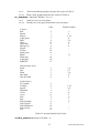
5. Values
Values are entered in matrices having identifiers with the general format
[parameter group]_START_VALUES (real)
[parameter group]_FIXED_VALUES (Boolean)
[parameter group]_UPPER_BOUND (real)
[parameter group]_LOWER_BOUND (real)
[parameter group]_TEST_VALUES (array: first element Boolean, others (optional)
real),
where [parameter group] is one of DEE, AR, MA, BAR, BMA, NMA, INT, REGR1,
REGR2, REGR3, VAR, GAR, GMA, FGDEE, GREG1, GREG2, GREG3, ASYMM,
FUNCTION, STUDT, MARKOV, SWREGR1, SWREGR2, SWREGR3, EQUIL, CORREL,
FRACTPI.
If an element of the [parameter group]_FIXED_VALUES matrices is set to 1 (or
TRUE), the corresponding parameter is fixed at its starting value or, in the case of a grid
evaluation, at grid values.
If an element of the first array element of [parameter group]_TEST_VALUES is set to
1 (or TRUE), the corresponding parameter is included in the Wald test restriction. The
second and subsequent elements, which should be present when RESTRIC_TYPE =
1 and otherwise are ignored, define linear restrictions on the parameters in conjunction
with the vector TEST_CONSTANTS.
The columns of these matrices correspond to parameters, and the rows to different
regimes, where the parameters in question are switching. In non-switching models, or
where no switching is specified for the group, they are simply row vectors. The
[parameter group]_START_VALUES matrix can be regarded as a template for the
others, their elements acting on the parameters in corresponding positions.
Systems of Equations
To specify a system, an array of matrices is required (one matrix for each equation) for
the following groups: DEE, AR, MA, BAR, BMA, NMA, INT, REGR1, REGR2, REGR3,
VAR, GAR, GMA, FGDEE, GREG1, GREG2, GREG3, ASYMM, FUNCTION. The usual
matrices only are required for STUDT, MARKOV, SWREGR1, SWREGR2, SWREGR3,
CORREL, FRACTPI. An array is also required for EQUIL, in this case, one for each
equilibrium relation.
Remember that each equation in a system has the same nominal specification, so each
matrix of a group has the same number of columns. Restrictions are imposed by the
settings of [parameter group]_FIXED_VALUES to specify differences between the
equations.
The items [parameter group]_TEST_VALUES must now be constructed an array of
arrays. The elements of the outer array correspond to the equations, each of them
having tests specified by the inner arrays, as for the single equation case.
26
James Davidson 2015
The Parameter Groups
If the matrices entered do not match the dimensions indicated, they are padded with
default values, or trimmed, as appropriate. Therefore, a matrix only has to be entered if
its contents differs from the defaults.
DEE : rows = 1 or M, columns = 1. ARFIMA d.
Note: When MULTI_SPEC = 1 and, the Robinson (1994) nonparametric
estimate of d is used as a starting value for the initial model fitted, the
ARFIMA(0,d,0). Thereafter, the currently estimated value is used.
AR: rows = 1 or M, columns = AR_ORDER. AR coefficients.
MA: rows = 1 or M, MA_ORDER, default = <>. MA coefficients.
BAR: rows = 1 or M, columns = AR_ORDER. Bilinear AR coefficients.
BMA: rows = 1 or M, columns = BILINEAR_ORDER  1. Bilinear MA coefficients.
NMA: rows = 1 or M, columns = 5. Nonlinear MA parameters, in the order , , , c1,
c2 .
INT: rows = 1 or M, columns = 1. The intercept.
Note: This is the value of the intercept whether of Type 1 or Type 2.
REGR1, REGR2, REGR3 : rows = 1 or M, columns = number of regressors specified of
Types 1, 2 and 3, including trend (must be of type 1) and GARCH-M term. The
trend should be listed after any observed variables, The GARCH-M term should
be last in its assigned type.
Notes:
1. When deleting or adding regressors, don't overlook that the starting
values must be edited to match, or else the wrong values will get used,
without prompting.
2. When lags are specified using REGR1_LAGS, etc., in general the
number of columns equals the number of variables times 1+ the number
of lags. The exception to this rule is in REGR2 , where if a dependent
variable (listed in SERIES) is also listed in REGRESSORS_2 , the
current value is omitted (count lags from 1, not from 0).
3. If, in system estimation, dependent variable(s) are listed in REGR1, the
system is treated as simultaneous, and the FIML estimator is
implemented. The “own” dependent variable will have its coefficient
fixed at zero automatically, if this is not done manually.
4. If equilibrium relations are specified, the ECM coefficients are located
in REGR2, after the other variables.
GAR: rows = 1 or M, columns = GARCH_AR_ORDER GAR coefficients
GMA: rows = 1 or M, columns = GARCH_MA_ORDER, GMA coefficients
Note: Make sure starting values match the GARCH_FORM and MA_FORM
settings. If, in equation (41) , the signs of the starting values do not observe
GARCH positivity constraints, they are reversed. If starting values are either
not set, or not defining fixed values, they are set to 0.1.
FGDEE: rows = 1 or M, columns = 2, FIGARCH d followed by HYGARCH amplitude
parameter .
Note: unless starting values satisfy 0 < d  1 and  > 0 (and are not fixed values) each
is reset to 1.
GREG1, GREG2, GREG3: rows = 1 or M, columns = number of GARCH regressors of
each Type specified, similar to REGR1. etc.
27
James Davidson 2015
ASYMM: rows = 1 or M, columns = 1, TARCH asymmetry or EGARCH asymmetry
parameter.
VAR: rows = 1 or M, columns = 1. Error variance,.
FUNCTION: rows = 1 or M, columns = number of names specified in supplied function.
STUDT : rows = 1 or M, columns = 2.
Parameter(s) depend on the likelihood function selected:
 For Student’s t distribution, degrees of freedom parameter and skewness
parameter if specified.
 For the GED distribution,  parameter (second column empty).
 For Negative Binomial I and II,  parameter (second column empty).
MARKOV: rows = M, columns = M 1. These are the fixed Markov transition
probabilities, Pr(St = j|St1 = i), with i = 1,…,M corresponding to rows and j =
1,…,M1 to columns – the Mth column is not entered, and is defined by the
identity that the rows sum to unity
Notes:
1. If the starting values sum to more than 1, they are ignored and the default
values 1/M are used.
2. For estimation, the probabilities are mapped to the real line by a logistic
transformation.
SWREGR1, SWREGR2, SWREGR3: rows = 1, columns = number of explained switching
variables specified in regimes 1, 2 and 3. These must appear with the intercepts
first in the list, followed by regime dummies, followed by variables.
A maximum of 4 regimes is allowed, and hence at most three independent
models determine the probabilities of switching to a regime.
EQUIL : rows = 1 or M, columns = number variables specified in
EQUIL_VARIABLES.
Note: At least one coefficient in each equilibrium relation must be fixed. The
program will fix the first element of each relation to 1, automatically, if none is
fixed manually.
CORREL : rows = 1 or M, columns = N(N  1)/2 where N = number of equations.
Note: These coefficients represent the correlations of the equation errors. Since the
latter are constrained to lie in (-1,1), they are defined as C/(1+ |C|) where C is
the value set here.
FRACTPI: rows = 1 or M, columns = number of included pre-sample proxy terms
(recommended values, 1 or 2).
Inequality Constraints
IS_BOUNDS (Boolean): Default = FALSE.
TRUE
To enable inequality constraints
FALSE To disable inequality constraints
[parameter type]_LOWER_BOUND (Vector/Matrix of Real) Default = <>,
[parameter type]_UPPER_BOUND (Vector of Real) Default = <>..
These vectors are formatted just like the corresponding [parameter
type]_START_VALUES vectors.
Note:
1. The bounds are ignored unless IS_BOUNDS is set to 1, and the upper one strictly
exceeds the lower. Cancel the setting by putting both bounds to 0.
28
James Davidson 2015
2. It is not recommended to use this technique routinely to impose, e.g., positivity and
stability constraints on lag polynomials. The search algorithm should usually work
OK without this. The method is implemented more as a last resort for difficult
cases.
Constraint Values
There are two cases of [parameter group]_TEST_VALUES, selected with
RESTRIC_TYPE.
1. Zero Restrictions. The arrays have one element, a Boolean matrix, with
elements set to 1 (or TRUE) for each parameter to be constrained to zero, and 0
(or FALSE) otherwise.
2. Linear Restrictions. The arrays have r + 1 elements where r = the number of
linear restrictions. The first elements are Boolean matrices, to indicate
inclusion of the parameter in the restrictions. The remaining elements contains
the relevant segment of the row of R.
Important note:
When running Ox code using the GUI version of TSM as a platform, call the function
Load_TextValues() immediately after setting parameter attributes.
6. Actions
PRINT_INFO ( (Boolean): Default = FALSE.
TRUE
To call the Ox Database function Info, giving descriptive statistics on the
data set.
FALSE To suppress this output.
PRINT_SUMMSTATS (Boolean): Default = FALSE.
TRUE
To print summary statistics and tests of the order of integration for the
dependent variable.
FALSE To suppress this output.
SUMMSTAT_CORRELS (Boolean): Default = FALSE.
TRUE
To print autocorrelations and Q statistics for levels and squares of the
dependent variable.
FALSE To suppress this output.
Ignored unless PRINT_SUMMSTATS = 1.
EVALUATE_INIT (Boolean): Default = FALSE.
TRUE
To print the specified output at the input parameter starting values.
FALSE For normal optimisation procedure.
Use this option to print listings and test results without repeating a lengthy
optimisation.
DO_GRID (Boolean): Default = FALSE.
TRUE
To compute a grid of criterion values at fixed, equally spaced values of
one or two parameters, while optimising over the remaining parameters.
FALSE For normal optimisation procedure.
Use this option to create a contour plot of the concentrated criterion function. The
operation is carried out on the first one or two parameters satisfying the following
29
James Davidson 2015
conditions: 1) the “fixed” flag is set; 2) the upper bound exceeds the lower bound.
Also see Inequality Constraints and GRID_POINTS.
MULTISTAGE_GMM (Boolean): Default = FALSE.
TRUE
To use the efficient GMM minimand, after evaluating the residuals at the
starting values of the parameters.
FALSE To use the standard instrumental variables minimand.
Notes:
1. To do multi-stage GMM, call Run_Estimation() two or more times in
succession, with MULTISTAGE_GMM = 0 for the first run and
MULTISTAGE_GMM = 1 for the subsequent runs. The starting values for these
runs will be the convergence point of the previous run.
2. This setting is ignored if GRID_PLOT = 1 or MULTI_SPEC = 1 or
LINEAR_REGRESSION = 1 .
SPEC_FORCSTS (Boolean): Default = FALSE.
TRUE
Compute currently specified forecasts at current parameter values.
FALSE Otherwise
SPEC_DIAGS (Boolean): Default = FALSE.
TRUE
Compute currently specified diagnostic tests at current parameter values.
FALSE Otherwise
SPEC_MTEST (Boolean): Default = FALSE.
TRUE
Compute currently specified M-test at current parameter values.
FALSE Otherwise
SPEC_SCRTEST (Boolean): Default = FALSE.
TRUE
Compute currently specified score test at current parameter values.
FALSE Otherwise
SPEC_WALD (Boolean): Default = FALSE.
TRUE
Compute currently specified Wald test at current parameter values.
FALSE Otherwise
LMTEST_TYPE (Integer): Default = CM1.
Determines the location of the test variables in a specified score test.
CM1
Conditional Mean model , Type 1 regressor(s)
CM2
Conditional Mean model, Type 2 regressor(s)
CM3
Conditional Mean model, Type 3 regressor(s)
CV1
Conditional Variance model, Type 1 regressor(s)
CV2
Conditional Variance model, Type 2 regressor(s)
CV3
Conditional Variance model, Type 3 regressor(s)
Note: If the selected regressors Type is specified to include lags, the test variables
are lagged similarly. The degrees of freedom of the test are then “number of
variables  1 + number of lags”.
SCRTEST_VARIABLES (Array of strings): Default = {}
Names of variables from the data set to use as indicator variables in the specified
score (LM) test . Specification similar to REGRESSORS_1 etc.
30
James Davidson 2015
CONDITIONAL_MTEST (Boolean): Default = TRUE.
TRUE
To compute a conditional moment test. (Variance matrix computed by
outer-product formula.)
FALSE
To compute a simple moment test (variance matrix computed by HAC
formula.)
SQUARES_MTEST (Boolean): Default = FALSE.
TRUE
To use the squared normalized residuals as the M-test or CM-test
covariate.
FALSE To use the normalized residuals as the M-test or CM-test covariate.
MTEST_VARIABLES (Array of strings): Default = {}
Names of variables from the data set to use as indicator variables in the specified
M-test . Specification similar to REGRESSORS_1 etc.
RECYCLE_RESULTS (Boolean): Default = FALSE.
TRUE
To print the parameter estimates in "input-ready" form.
FALSE, No recycling.
This option creates formatted lines ready to be cut and pasted into the run file,
providing a simple way to repeat the previous run using some or all of the estimates as
starting values. Used in combination with EVALUATE_INIT, it allows tests and
listings to be obtained for a previous run without repeating the optimisation procedure.
Note: If ACCESS_RESULTS = 1, then with RECYCLE_RESULTS = 1 the estimates
are written internally as starting values for the next run. This is appropriate if the
user’s program specifies a succession of estimation runs, where the next run should be
started as near as possible to the estimates obtained on the previous run.
8.1 Output and Retrieval Options
RETRIEVE_RESIDUALS (Boolean): Default = FALSE.
RETRIEVE_FITTED (Boolean): Default = FALSE.
RETRIEVE_VARADJRES (Boolean): Default = FALSE.
RETRIEVE_CONDVARS (Boolean): Default = FALSE
RETRIEVE_PROBS (Boolean): Default = FALSE.
RETRIEVE_SIM (Boolean): Default = FALSE.
RETRIEVE_EQUILS (Boolean): Default = FALSE.
TRUE
to retrieve the created series specified, and append it to the data set.
FALSE otherwise.
The effect of these commands depends on the model specified.
RETRIEVE_VARADJRES (variance-adjusted residuals) and RETRIEVE_CONDVAR
(conditional variances) are active only when GARCH-type and/or regime switching
models with switching variance components are specified.
RETRIEVE_PROBS (Markov filter probabilities, explained switching probabilities,
and regime weights in smooth transition models) is active only in regime-switching
models.
RETRIEVE_SIM retrieves the results of a call to Run_Simulation(0), otherwise it has
no effect.
31
James Davidson 2015
RETRIEVE_EQUILS retrieves equilibrium relations when an ECM model is specified,
otherwise it has no effect.
SHOW_CRITERIA (Boolean): Default = FALSE.
TRUE
To print the log-likelihood and model selection criteria
FALSE Otherwise.
PRINT_COVMATRIX (Boolean): Default = FALSE.
TRUE
To print the covariance matrix of the parameters
FALSE Otherwise.
PRINT_CORRELS (Boolean): Default = FALSE.
TRUE
To print the correlograms of the residuals
FALSE Otherwise.
PRINT_SERIES (Boolean): Default = FALSE.
TRUE
To send series (residuals etc.) to the console.
FALSE Otherwise.
PRINT_LISTINGS (Boolean): Default = FALSE.
TRUE
To send forecasts and impulse-response coefficients to the console.
FALSE Otherwise.
PRINT_RESULTS (Boolean): Default = TRUE.
TRUE
To send results to the console.
FALSE Otherwise.
OUTPUT_RESULTS (Boolean): Default = FALSE.
TRUE
To append results to a text file.
FALSE Otherwise.
AUTOSAVE_LISTS (Boolean): Default = FALSE.
TRUE
To save listings (residuals, forecasts etc.) to a file, of type specified by
the setting of OUTPUT_SERIES.
FALSE Listings not saved to file
OUTPUT_SERIES (Integer): Default = XLS.
XLS
Save listings to Excel spreadsheet (.XLS)
XLSX
Save listings to Excel 2007 spreadsheet (.XLSX)
IN7
Save listings to GiveWin file (.IN7)
DAT
Save listings to data file with format information (.DAT)
MAT
Save listings to matrix file (.MAT)
CSV
Save listings to comma delimited text file (.CSV)
8.2 Test and Diagnostics Options
Q_TEST (Integer): Default = 0.
NOQ
No Q autocorrelation test,
BPQ
To use the Box-Pierce (1970) formula for the Q autocorrelation test,
32
James Davidson 2015
LBQ
To use the Ljung-Box (1978) formula for the Q autocorrelation test.
Q_TEST_ORDER (Integer): Default = 12.
The numbers of lags to be used in computing the Box-Pierce (1979) and McLeod-Li
(1980) diagnostic statistics. (Also see LJUNG_BOX).
CORRELOGRAM_ORDER (Integer): Default = 0.
The number of residual correlogram points of residuals and squared residuals to be
reported, if any. Set to 0 for no correlogram. This choice is independent of the BoxPierce order, note.
LM_TEST (Boolean): Default = FALSE.
TRUE
To print the LM statistic for restrictions imposed with the “fix
parameter” flags (see VALUES).
FALSE Otherwise
SCORE_TEST (Boolean): Default = FALSE.
TRUE
To compute diagnostic score (LM) statistics, as specified by
DIAGNOSTIC_TESTS.
FALSE Otherwise
MOMENT_TEST (Boolean): Default = FALSE.
TRUE
To compute diagnostic conditional moment (CM) statistics, as specified
by DIAGNOSTIC_TESTS.
FALSE Otherwise
DIAGNOSTIC_TESTS (row vector of integers): Default = <>.
The cases are
AUCT
ARCT
FFRT
HT1T
HTWT
ACFT
IFMT
DWTT
KPST
VSST
LRST
HMLT
CSQT
NHST
NHIT
ASST
ASIT
BTIT
RBST
SBJT
SBIT
Autocorrelation;
Neglected ARCH;
Nonlinear Functional Form (RESET);
Heteroscedasticity (Breusch-Pagan);
White’s heteroscedasticity test.
AR Common Factor (COMFAC) test
Information Matrix test.
Durbin-Watson test
KPSS test
V/S test
Lo’s R/S test
HML long memory test (also see HML_SETTINGS)
Cusum of squares test
Nyblom-Hansen specification test
Individual Nyblom-Hansen tests on score elements.
Andrews structural change test
Individual Andrews tests on score elements.
Bootstrap test of I(0) hypothesis.
Bierens’ consistent specification test on residuals
Consistent specification test on score contributions
Individual specification tests on score elements.
33
James Davidson 2015
Construct the vector by concatenating the variables, for example AUCT~ARCT~HT1T .
The type of tests computed in cases 0-3 depend on the settings of SCORE_TEST and
MOMENT_TEST. Either test, or both tests, can be specified. The information matrix test
is computed regardless of these settings.
HMLTEST_C (Real): Default = 1.
Truncation parameter (c) for Harris-McCabe-Leybourne long memory test
HMLTEST_L (Real): Default = 0.66.
Bandwidth parameter (L) for Harris-McCabe-Leybourne long memory test
ANDREWS_LOWER (Real): Default = 0.15.
Lower bound ( 1 ) for Andrews structural break test.
ANDREWS_UPPER (Real): Default = 0.85.
Upper bound (  2 ) for Andrews structural break test.
DGTEST_LAGS (Integer): Default = 1.
Number of lags for diagnostic tests of autocorrelation.
DGTEST_SQLAGS (Integer): Default = 1.
Number of lags for diagnostic tests of neglected ARCH.
DGTEST_FFORDER (Integer): Default = 2.
Maximum power of fitted values to include in test of functional form.
NOPRINT_OUTPUT (Boolean): Default = FALSE.
TRUE
To suppress printed output except for test results. Use this setting in
conjunction with EVALUATE_INIT to compute tests from the current
estimates, without re-estimating.
FALSE
otherwise.
COVMAT_TYPE (Integer): Default = RBT;
IFM
Standard covariance matrix formula (information matrix)
RBT
Robust heteroscedasticity consistent formula (valid for quasi-likelihood
applications).
HAC
Heteroscedasticity and autocorrelation consistent formula.
KVB
Kiefer-Vogelsang-Bunzel inconsistent estimator.
Note: if specified, robust and HAC formulae are used to compute the standard
errors/covariance matrix/Wald and LM tests and also preliminary tests of I(0) (KPSS,
Phillips-Perron, Lo R/S).
KERNEL_TYPE (Integer): Default = PZN;
HET
No kernel (heteroscedasticity correction only, equivalent to
COVMAT_TYPE = RBT);
PZN
Parzen kernel
BLT
Bartlett kernel
QS
Quadratic Spectral kernel
TKH
Tukey-Hanning kernel.
HAC_BANDWIDTH (Integer): Default = 0;
If this setting is positive, its value is used for the bandwidth. If it is zero, the program
defaults are used; [n1/3] for the Bartlett kernel, and [n1/5] for the other cases.
34
James Davidson 2015
INFO_CRIT (Integer): Default = AKKE;
Criterion for lag choice in for ADF tests and S-W/Saikkonen estimates
MANL
None (set manually with ADF_LAGS)
AKKE
Akaike criterion
SCHW
Schwarz criterion
HQ
Hannan-Quinn criterion.
ADF_LAGS (Integer): Default = 0
Lag length for ADF tests and S-W/Saikkonen estimates (used if INFO_CRIT = 0)
EDF_CRITS (Boolean): Default = FALSE;
TRUE
Use supplied empirical distribution to provide test critical values
FALSE Otherwise.
Note: The EDF is read from disk as a spreadsheet file; see EDF_FILE.
HAC_TESTSTATS (Boolean): Default = TRUE.
TRUE
Always use HAC variance estimates in formulation of test statistics,
over-riding COVMAT_TYPE setting.
FALSE
Let COVMAT_TYPE determine variance formulae in tests.
CSTEST_TESTYPE (Integer): Default = SUPT;
SUPT
Sup-conditional moment test
ICMA
Integrated conditional moment test, type A.
ICMB
Integrated conditional moment test, type B
Conditional moment test settings:
CSTEST_VARS (Array of strings): Default = {};
Test variables to be used in conditional moment tests.
CSTEST_LAGS (Integer): Default = 0;
Number of unrestricted lags of test variables to include.
CSTEST_DYNORDER (Integer): Default = 0;
Lag polynomial order of test variables.
CSTEST_ MAXLAG (Integer): Default = 100;
Maximum lag to use in polynomial lag specification of test variables. (Lags are set
to minimum of this setting and available sample.)
CSTEST_SCALE (Real): Default = 3;
Scale factor to determine range of variation of test function under the exponential
transformation.
CSTEST_GAMMA, CSTEST_RHO1, CSTEST_RHO2, CSTEST_RHO3
(Reals): Defaults = 2.5, 0.2, 0.4, 0.1.
Exponents defining the bound for Bierens’ “two-statistic” approximation. See
Models and Methods Section 12.4 for details.
CSTEST_UWGHT (Real): Default = 1;
CSTEST_LWGHT (Real): Default = -1;
Upper and lower bounds of hypercube Ξ.
CSTEST_EVAL (Integer) : Default = 5000;
35
James Davidson 2015
Maximum number of function evaluations to compute integrals by Monte Carlo.
CSTEST_PRECSN (Real) : Default = 0.002.
Precision for evaluation of integrals by Monte Carlo.
8.3 Forecasting Options
FORECAST_STEPS (Integer): Default = 0.
The number of multi-step forecasts of Yt to be computed. This option generates
three series: the point forecasts, and 2 standard error bounds. If a GARCH model
is fitted, the bounds are computed using the m-step ahead conditional variance
forecasts.
MOVING_AVERAGE_COEFFS (Integer): Default = FALSE.
The number of solved moving average lag coefficients from the mean process and
(where fitted) the variance process, to be listed.
EXPOST_FORECASTS (Boolean): Default = FALSE
TRUE
To compute one-step ex-post forecasts (using actual values of lags)
FALSE
To compute dynamic ex-ante multi-step forecasts.
MONTECARLO_FORECASTS (Boolean): Default = FALSE
TRUE
To compute ex-ante forecasts by Monte Carlo stochastic simulation.
FALSE
To compute ex ante forecasts by analytic formulae for mean and
variance.
MCFORECAST_TYPE (Boolean): Default = TRUE
TRUE
To report medians of Monte Carlo distributions with 95% confidence
bands.
FALSE To report means of Monte Carlo distributions with 2SE bands.
MCFORECAST_REPLICATIONS (Integer): Default = 1000.
Number of replications in Monte Carlo forecasts .
FCST_SES (Boolean): Default = TRUE
TRUE
To compute forecast standard errors. This option is forced to TRUE if
FCST_SEBANDS is set to TRUE.
FALSE
Otherwise.
FCST_SEBANDS (Boolean): Default = FALSE
TRUE
To compute forecast confidence bands.
FALSE
Otherwise.
FORC_ERVARDEC (Boolean): Default = FALSE
TRUE
To compute the forecast error variance decomposition (systems only).
FALSE
Otherwise.
EXPORT_MMEDFORCS (Boolean): Default = FALSE
TRUE
Export only the mean or median forecasts (spreadsheet output).
FALSE Export full forecast outputs to a spreadsheet, including forecast
distribution quantiles.
ANNDIFF_FORCS (Boolean): Default = FALSE.
TRUE
Compute forecasts in annual-difference form.
36
James Davidson 2015
FALSE
Otherwise.
Notes:
1. The analytic forecast standard errors are asymptotic, and do not take account
of parameter uncertainty.
2. For ex-post forecasting, or if the model contains regressors from the data set,
the number of forecasts is limited to the available post-sample observations.
However, the trend dummy and the GARCH_M regressor are extended as
necessary.
3. Analytic standard error bands cannot take account of dynamics introduced
through a bilinear or user-supplied function. Use Monte Carlo forecasting in
these cases.
4. Unless estimation is by maximum likelihood, only Gaussian or bootstrap
random numbers are available.
8.4 Simulation and Resampling Options
SIM_DISTRIBUTION (Integer): Default = SGS.
The method of generating shocks for stochastic simulation of the current model, for use
in one-off simulations, Monte Carlo forecasts and bootstrap tests.
SMD
Generate random numbers from the distribution specified by the
likelihood function – Gaussian, Student’s t or skewed Student, using
current parameter values).
SGS
Generate Gaussian random numbers, with zero mean and variance either
set by the user, or that of the current residuals.
SST
Generate stable random numbers, with zero location and parameters set
set by the user.
SFM
Generate random numbers by a coded transformation of the standard
Gaussian and/or Uniform[0,1].
SBT
Use the simple bootstrap, or moving blocks bootstrap (MBB),
resampling the current residuals. They are centered and bias-adjusted by
n/(n  k). Not available unless a model has been estimated.
SSB
Use the stationary bootstrap. This randomizes the length of blocks using
an independent geometric distribution, as well as the startpoints as for
the MBB. Not available unless a model has been estimated.
SWB
Generate random numbers using the wild bootstrap. Not available unless
a model has been estimated.
SFR
Fourier bootstrap (= wild bootstrap applied to the DFT of the data.)
Suitable for stationary autocorrelated data.
SDT
Data resampling. Resamples all observations (data not residuals)
randomly with replacement. Suitable only for i.i.d. data.
Notes:
1. If least squares or instrumental variables is the selected estimator, option SMD is
automatically changed to SGS.
2. The wild bootstrap is not available for Monte Carlo forecasting. If selected, the
regular bootstrap will be used instead.
SIMFORM_TEXT (text string) : Default = {}.
37
James Davidson 2015
Coded formula for random number generation when SIM_DISTRIBUTION =
SFM:
SHOCK_PARS (1×4 row vector of reals): Default = <1,2,0,1> .
First element: Variance of Gaussian shocks. Set to 0 to use residual variance
Second element: “alpha” for stable distribution; <= 2, 2 = Gaussian.
Third element: “beta” for stable distribution; 0 = symmetric.
Fourth element: Skewness factor for wild bootstrap. 1 = symmetric distribution.
BOOTSTRAP_SIEVEAR (Boolean): Default = FALSE.
TRUE
Use sieve autoregression to model autocorrelation in bootstrap sample
FALSE
otherwise.
This option can be combined with any of the bootstrap procedures, including the
wild bootstrap. The AR filter is fitted to the sample data and applied to the
resampled series, however generated.
BOOTSTRAP_SIEVELAGS (Integer) Default = 1.
Maximum lag length to use with sieve-AR bootstrap. The default is to set this
automatically as function of sample size – see the main documentation.
RANDNM_SEED (Integer): Default = 0.
Seed for the random number generator. The default setting, 0, causes the actual seed
to be generated from the system clock, so that the numbers cannot be replicated.
RANDOM_PRESAMPLE (Boolean): Default = FALSE.
TRUE
Pre-sample Data Random in Simulations
FALSE
Pre-sample Data Fixed in Simulations.
TYPEI_FRAC (Boolean): Default = FALSE.
TRUE
Simulate “type I” ARFIMA model. (Must set RANDOM_PRESAMPLE =
1.)
FALSE Simulate regular ARFIMA model.
RESAMPLING (Boolean): Default = FALSE.
TRUE
To compute test p-values and standard errors by the parametric bootstrap
or subsampling methods.
FALSE
For conventional tests.
BOOTSTRAP_STATIC (Boolean) Default = FALSE.
TRUE
Take fitted values from the estimated model to generate the bootstrap
data (lagged endogenous variables from the original sample.)
FALSE
Generate bootstrap data by dynamic simulation.
Note: in a static mode,l the results are identical in each case but run much faster
with the option enabled.
BOOTSTRAP_REPLICATIONS (Integer): Default = 100.
Number of replications to generate the bootstrap distribution.
BOOTSTRAP_BIASCORR (Boolean) Default = FALSE.
TRUE
To apply bootstrap bias correction to parameter estimates.
FALSE
Otherwise.
BOOTSTRAP_BLENGTH (Integer) Default = 1.
38
James Davidson 2015
The length of blocks to resample in the block bootstrap. With
SIM_DISTRIBUTION = 3, setting to 1 (default) yields the regular bootstrap. If
SIM_DISTRIBUTION = 9 (stationary bootstrap) is selected, sets the mean block
length under the geometric distribution.
BOOTSTRAP_CONFINT (Integer) Default = BEQT.
BTSE
To report bootstrap standard errors.
BEQT
To report equal tail bootstrap confidence intervals.
BTPC
To report percentile-t confidence intervals.
BSPT
To report symmetric percentile-t confidence intervals.
BOOTSTRAP_CONFPCENT (Integer) Default = 95.
The coverage probability assigned to the reported bootstrap confidence interval,
expressed as a percentage.
SUBSAMPLING (Boolean) Default = FALSE.
TRUE to compute confidence intervals and p-values by the subsampling method.
FALSE otherwise.
BOOTSTRAP_MOUTOFN (Boolean) Default = FALSE.
TRUE to compute confidence intervals and p-values by the “m out of n” bootstrap
method, where the bootstrap samples are a fraction of the original sample
size. (The size of the bootstrap sample is set as SUBSAMPLE_LENGTH).
FALSE otherwise.
BOOTSTRAP_BLENGTH (Integer) Default = 1.
The length of blocks to resample in the block bootstrap. Setting to 1 yields the
regular bootstrap.
SUBSAMPLE_LENGTH (Integer) Default = 0.
Length, bT , of the contiguous samples to be used in subsampling and “m out of n”
bootstrap analysis. In subsampling, there are then T  bT  1 samples used to
generate the distributions, where T is sample size.
NEWTON_CONV (Double): Default = 0.0001.
Convergence criterion for Newton-Raphson algorithm used for nonlinear bootstrap.
NEWTON_ITERATIONS (Integer): Default = 20.
Maximum number of iterations of Newton-Raphson algorithm used for nonlinear
bootstrap.
NEWTON_ALGRTHM (Boolean) Default = FALSE.
TRUE
To use Newton-Raphson algorithm for Monte Carlo replications.
FALSE
To use BFGS.
FD_BOOTSTRAP (Boolean): Default = FALSE.
TRUE
To compute the fast-double bootstrap.
FALSE
For conventional bootstrap.
The fast double bootstrap is a device aimed at reducing the error in rejection
probability due to estimation error. It is not guaranteed to improve performance in
all cases, but showing that a test outcome is robust to this setting increases
confidence in the result.
39
James Davidson 2015
8.6 ML and Dynamics Options
STUDDF_ROOT (Integer): Default = 2.
The Student t “degrees of freedom” parameter is raised to this power, to represent the
actual d.f. of the likelihood. Set > 1 for better numerical stability. By setting a negative
value, 0 can represent the Gaussian case (d.f. = ).
Note: start/fixed/test/bound matrices for the Student t parameters have prefix STUDT_
LOG_SKEWNESS (Boolean): default = FALSE;
TRUE
Estimate the logarithm of the Student skewness parameter ()
FALSE Otherwise.
ORDERED_PROBIT (Integer) Default = 0.
Additional cases in the ordered probit and ordered logit models.
DISCRETE_ZLAGS (Boolean) Default = FALSE
TRUE
Enables autoregressive dynamic process in discrete data latent process
(lag parameters entered as additional regressors of Type 2.
FALSE Otherwise.
CHISQR_PROBIT (Boolean) Default = FALSE
TRUE
Uses centerd chi-squared as the distribution in probit and ordered probit
models. The degrees of freedom appear as an additional parameter in
group STUDT.
FALSE
Gaussian probit model.
POISSON_EXPARG (Boolean) Default = FALSE
TRUE
The Poisson mean is the exponential of the regression function.
FALSE The Poisson mean is linear in the explanatory variables (must be nonnegative.
DISCRETE_ZINFL (Boolean) Default = FALSE
TRUE
The Poisson and ordered probit models are “zero-inflated”, with
variables explaining the zero regime appearing as regressors of Type 3.
(The intercept is in group STUDT.)
FALSE Otherwise.
MA_FORM (Boolean): Default = FALSE.
TRUE To report the moving average coefficients as j in (L) = 1 + 1L +  +
qLq, and GARCH coefficients as j in (L) = 1 + 1L +  + rLr.
FALSE To report the moving average coefficients as j in (L) = 1  1L   
qLq, and GARCH coefficients as j in (L) = 1  1L    rLr .
Setting this option to 1 writes the MA coefficients of an ARMA or GARCH with
opposite sign to the AR coefficients, relative to the zero-order terms. The default is
consistent with the convention in equation (8), and also more natural. For example,
in the ARMA(1,1) model equal roots cancel each other out, and in this case the
estimates will be equal. Similarly, in the ARMA-in-squares representation of the
GARCH(1,1) model, 1 = 1 corresponds to 1 = 0, (see GARCH_FORM) and the
estimates are again equal in this case.
Note: the starting values must match the convention selected.
RESTRICT_LAGS (Boolean): Default = FALSE
TRUE
To allow truncation of presample lags.
40
James Davidson 2015
FALSE
To use the available pre-sample data to form lags, when
START_SAMPLE > 1.
LAG_TRUNCATION (Integer):Default = 0.
The maximum number of pre-sample observations to be used to form lags. If set
to zero, the estimates are comparable to the case when START_SAMPLE = 1.
This option is ignored unless RESTRICT_LAGS = 1
COMPUTE_ROOTS (Boolean): Default = TRUE.
TRUE
Compute the roots of ARMA and VARMA lag polynomials.
FALSE
Omit root calculations (in some cases these can be time-consuming).
TPI_DEE (Boolean): Default = FALSE.
TRUE
Estimate “type I” ARFIMA model.
FALSE
Estimate regular ARFIMA model.
GARCH_FORM (Boolean): Default = FALSE.
TRUE
To report the GARCH model in the conventional (Bollerslev, 1986)
style, so that the coefficients of lagged squared errors are the coefficients
of (L)  (L) in equations (41) and (42).
FALSE To report the coefficients of the “ARMA-in-squares” representation of
the GARCH model, in which (L) and (L) are the AR and MA
components respectively.
GARCH_INTFORM (Boolean): Default = FALSE.
TRUE
To report the GARCH intercept in Type 2 form.
FALSE To report the GARCH intercept in Type 1 form.
GARCH_INT_POWER (Integer): Default = 1.
The GARCH intercept can be close to 0, the boundary of the parameter space,
which can give difficulty to the search algorithm. Estimating the square root or
fourth root of the parameter (set to 2 or 4) may resolve a convergence problem.
However, be careful to set the starting value, and interpret the estimate,
appropriately.
GM_ITS (Integer): Default = 20.
The GARCH-M likelihood is computed by Gauss-Seidel iteration of equations (1)
and (41), (or (1) and (42)). This option sets the maximum number of iterations.
GM_H_BOUND (Real): Default = 10.
To stabilise the GARCH-M calculations, ht (or ht1/2) is trimmed before inclusion in
(1). The upper bound is set to GM_H_BOUND times the sample variance (or
standard deviation) of the data. Try reducing this setting in case of failure of the
algorithm.
ITERATE_EGARCH (Boolean): Default = TRUE.
TRUE
To evaluate the EGARCH likelihood by Gauss-Seidel interation.
FALSE
To evaluate the EGARCH likelihood by direct nonlinear recursion.
There may be small differences between the two estimates due to treatment of
initial conditions. The main consideration in this choice is one of speed. The
nonlinear equation cannot be solved using Ox’s vector manipulation capability, and
has to be programmed as a loop. This could result in extremely long solution times
in large samples, and the iterative method may be quicker.
41
James Davidson 2015
EGARCH_ITS (Integer): Default = 20.
The maximum number of iterations in the Gauss-Seidel solution of equation (42).
8.7 Optimization and Run Options
MINIMAND (Boolean): Default = FALSE.
TRUE
To report criterion function as minimand
FALSE
To report criterion function as maximand
GRID_POINTS (Integer): Default = 0.
Number of grid points to plot in each direction
Note: # function evaluations = GRID_POINTS in 1-dimensional plot and
(GRID_POINTS)2 in 2-dimensional plot.
MAX_ITERATIONS (Integer): Default = 1000.
Maximum number of BFGS iterations.
PRINT_ITERATIONS (Integer): Default = 0.
Frequency to print current position in search. Set to 0 for no printing.
STRONG_CRITERION (Real): Default = 1.
Criterion for strong convergence (see Ox documentation). Default keeps the Ox
default.
WEAK_CRITERION (Real): Default = 1.
Criterion for weak convergence (see Ox documentation). Default keeps the Ox
default.
ANAL_DERIV (Boolean): Default = TRUE.
TRUE
Use analytic derivatives where available for BFGS iterations.
FALSE
Force use ofs numerical derivatives.
SIM_ANNEALING (Boolean): Default = FALSE.
TRUE
Enable simulated annealing as a preliminary search algorithm, to provide
initial values for BFGS
FALSE
To disable simulated annealing
SA_SETTINGS (1  4 vector of Integer/Real): Default = <500, 5, 0.85, 10>
These are the adjustable settings for the SA algorithm. They are:
1. Maximum number of SA iterations before switching to BFGS
2. Initial temperature
3. Temperature reduction factor
4. Number of iterations befpre temperature reduction.
For more details on choosing these settings see
Goffe, William L., Gary D. Ferrier, and John Rogers (1994). Global Optimization
of Statistical Functions with Simulated Annealing. Journal of Econometrics,
60(1/2): 65-99.
SCALE_FACTOR (Real): Default = 0.
Parameter rescaling factor, to set similar orders of magnitude based on starting
values. The default switches this feature off.
CONSTRAIN_OPT (Real): Default = 3.
42
James Davidson 2015
A penalty is added to the criterion function when dynamic parameters (ARMA and
GARCH coefficients and ds) exceed the absolute value specified. Constraining the
parameter space makes the search routine more robust, and avoids problems with
(e.g.) inverted moving average roots. To remove the constraint, set to a large value.
Note that intercepts and regression coefficients are not constrained.
RESTART_FAILURE (Boolean): Default = TRUE.
TRUE
On failure of the search algorithm, restart the search automatically at the
default parameter values.
FALSE
Otherwise.
8.8 Special Settings
AUTOTRANS_MODEL (Boolean): Default = FALSE.
TRUE
Enable the automatic data transformation modelling feature.
FALSE
Otherwise.
MC_CENSOREP (Boolean): Default = FALSE.
TRUE
Enable replication censoring in Monte Carlo experiments.
FALSE
Otherwise.
EDF_PVALS (Boolean): Default = FALSE.
TRUE
Tabulate bootstrap p-values in EDF tables.
FALSE
Tabulate test statisics in EDF tables..
PLOT_REVADF (Boolean): Default = FALSE.
TRUE
Plot reversed ADF and PP distributions in Monte Carlo experiments
(rejections in upper tail).
FALSE
Otherwise.
CONSTRAIN_OPT (Real): Default = 0.
Upper absolute bound to be imposed on dynamic model parameters in optimization
runs. Set to 0 for unrestricted optimization.
Accessing Results
If ACCESS_RESULTS = TRUE, results are written to program variables instead of to
console output.
Summary Statistics
The following global variables contain the results of the last call to
Summary_Statistics().
SUMM_STATS
(Column vector of Real)
ORDER_TESTS
(Matrix of Real)
DATA_CORRELS
(Matrix of Real)
The elements of SUMM_STATS are as follows. In the case where detrending is
specified, items 0-7 are reported for the original series, other items for the detrended
series (residuals from regression on trend).
0. Minimum of series
43
James Davidson 2015
1. Maximum of series
2. Index of minimum
3. Index of maximum
4. Mean
5. Median
6. Intercept in regression on trend (if detrending specified)
7. Slope in regression on trend (if detrending specified)
8. Standard deviation
9. Skewness
10. Kurtosis
11. Jarque-Bera statistic
12. Robinson’s (1994) estimator of fractional d.
If quantiles are specified, elements 13-21 contain the following 9 quantiles of the series
frequency distribution: 0.01, 0.05, 0.1, 0.3, 0.5, 0.7, 0.9, 0.95, and 0.99. For samples
smaller than 100, the 0.01 and 0.99 points are omitted (vector elements are zero). For
samples smaller than 20, the 0.05 and 0.95 points are also omitted.
ORDER_TESTS is a matrix of dimension 102 , the rows holding respectively the
statistics and p-value upper bounds for the tests (in other words, the available
tabulations show the p-values to be no greater than the quoted values.) The row
elements are identified as follows. If the tests are not specified, the corresponding
elements are zero. The last row contains long-run variance estimates, with the
autoregressive estimator in column 1 and the HAC kernel-based estimator in column 2.
0. Robinson-Lobato (1998) test of I(0).
1. KPSS test of I(0)
2. V/S test of I(0)
3. Lo’s R/S test of I(0)
4. Harris-McCabe-Leybourne (2008) test of I(0)
5. Augmented Dickey-Fuller test of I(1)
6. Phillips-Perron test of I(1)
7. Elliott-Rothenberg-Stock (1996) GLS-Dickey-Fuller test of I(1)
8. Elliott-Rothenberg-Stock (1996) P-test of I(1).
9. Long-run variance estimates (see above).
The content of DATA_CORRELS depends on the options specified: It may be:
 a square matrix of the contemporaneous correlations of the speficied variables;
 a M4 matrix whose columns contain the autocorrelations and Box-Pierce (of
Ljung-Box) statistics of each order up to M of the series specified and the
squared series;
 a M2 matrix containing the partial autocorrelations of the series and squared
series;
 a M4 matrix containing the autocorrelations and cross-autocorrelations of the
pair of series X and Y, in the order: X vs. lagged X , Y vs. lagged Y, X vs.
lagged Y, and Y vs. lagged X.
Estimation Outputs
The following global variables contain the results of the last call to
Run_Estimation().
CONVERGENCE_STATUS
(Integer)
44
James Davidson 2015
CRITERION
(Real)
SELECTION_CRITERIA
(Vector of Real)
PARAMETER_NAMES
(Array of Strings)
PARAMETERS
(Vector of Real)
STANDARD_ERRORS
(Vector of Real)
COVARIANCES
(Matrix of Real)
GRADIENT
(Vector of Real)
GRADIENT_COVARIANCES
(Matrix of Real)
HESSIAN
(Matrix of Real)
ESTIMATED_PARAMS
(Vector of Integers)
RESIDUAL_VARIANCE
(Real)
DIAGNOSTICS
(Array of Real Matrices)
TESTS
(Matrix of real)
WALD_ STATISTIC
(Real)
LM_STATISTIC
(Real)
RESIDUAL_CORRELOGRAMS
(Matrix of Real)
FORECASTS
(Array of Arrays of Real Matrices)
DATA_NAMES
(Array of Strings)
DATA_SET
(Matrix of Real)
BOOTSTRAP_PVALS
(Vector of Real)
ERRMESSAGES
(Array of strings}
Note:
 CONVERGENCE_STATUS is the value returned by the Ox optimization
routine, (MaxBFGS or MaxNewton). See the Ox manual for interpretation.

CRITERION is the final value of the estimation criterion. Note that the sign
(maximand or minimand) can be optionally changed, see the MINIMAND option
in Optimization Options.

SELECTION_CRITERIA has four elements, respectively the Schwarz,
Hannan-Quinn and Akaike selection criteria, and the estimation criterion.

GRADIENT_COVARIANCES is only computed if COVMAT_TYPE > 0.

ESTIMATED_PARAMS is a vector containing the locations in PARAMETERS of
parameters that have been estimated, as opposed to fixed or solved. Only these
parameters have corresponding entries in the gradient and the covariance matrix.
For example, the value and name of the parameter whose gradient entry are
numbered cJ are located at PARAMETERS[ESTIMATED_PARAMS[cJ]]
and PARAMETER_NAMES[ESTIMATED_PARAMS[cJ]] respectively.

BOOTSTRAP_PVALS contains the bootstrap p-values in the order, t-tests on
estimated parameters, diagnostic tests equation by equation, then other tests. See
Tables 1 and 2 below to determine the locations of these tests. Only tests that
are enabled appear in the list, so the tables show the ordering of the vector
elements, but not their absolute positions.
If resampling methods are not used, this variable contains 0.

ERRMESSAGES contains any error messages generated by the estimation
routine to report issues such as matrix singularity, convergence failure,
45
James Davidson 2015
incompatible commands, etc. etc. These are the same lines of text that appear in
the results window when the program runs in GUI mode.
To locate elements of the vectors PARAMETERS and STANDARD_ERRORS, and also
of the array PARAMETER_NAMES, use the globally defined vector g_cP and defined
constants, as follows:
g_cP[UF]
User function parameters
g_cP[IN]
intercept
g_cP[RG1]
regressors of Type 1
g_cP[RG2]
regressors of Type 2
g_cP[RG3]
regressors of Type 3
g_cP[D]
ARFIMA d
g_cP[AR]
AR coefficients
g_cP[MA]
MA coefficients
g_cP[BAR]
Bilinear AR coefficients
g_cP[BMA]
Bilinear MA coefficients
g_cP[GI]
GARCH intercept, or Error Variance
g_cP[GAR]
GARCH AR coefficients
g_cP[GMA]
GARCH MA coefficients
g_cP[FGD]
FIGARCH d or HYGARCH memory and amplitude
parameters
g_cP[TG]
ASYMM coefficient
g_cP[GR1]
GARCH regressors of Type 1
g_cP[GR2]
GARCH regressors of Type 2
g_cP[GR3]
GARCH regressors of Type 3
g_cP[NT]
Student's t-degrees of freedom parameter
g_cP[MKS]
Markov switching parameters
g_cP[ES1]
Explaining regime 1
g_cP[ES2]
Explaining regime 2
g_cP[ES3]
Explaining regime 3
g_cP[EQL]
Equilibrium relations
g_cP[COV]
Error correlations (equation systems only)
Example 1: if an AR(3) is fitted, the AR coefficients are found at locations
PARAMETERS[g_cP[AR]], PARAMETERS[g_cP[AR]+1] and
PARAMETERS[g_cP[AR]+2].
Example 2: If there are two regressors of Type 1 included, the coefficients are at
locations
PARAMETERS[g_cP[RG1]] and PARAMETERS[g_cP[RG1]+1]
The names of these parameters can be found in the corresponding elements of the array
PARAMETER_NAMES.
If a Markov-switching model is fitted, use the function LocTP.
LocTP(const iReg, const iPar)
iReg:
the regime
46
James Davidson 2015
iPar:
return value:
the parameter pointer, as defined above
location in the vector.
If no Markov switching is specified, this function returns its second argument.
Example 3: If an AR(2) with two regimes is fitted, the parameters for each regime are
respectively at locations
PARAMETERS[LocTP(0, g_cP[AR])] , PARAMETERS[LocTP(0,
g_cP[AR]+1)], and PARAMETERS[LocTP(1, g_cP[AR])],
PARAMETERS[LocTP(1, g_cP[AR]+1)]
Example 4: In a 3-regime model, the Markov transition probability parameter t12 (see
(8.5 of Models and Methods) is located at
PARAMETERS[LocTP(0, g_cP[MKS]+1)]
In multi-equation models, the parameters for each equation are located using the
function LocP .
LocP(const iEq, const iPar)
iEq:
the equation
iPar:
parameter block pointer
return value:
location of parameter block in the vector.
Remember that all equations in the system nominally have the same structure, although
some parameters may be suppressed by fixing them at 0. VAR and MA parameters are
arranged in the order, variables, then lags. In a VAR(2), the coefficients in equation j
are ordered as AR1(j,1), AR1(j,2), AR2(j,1), AR2(j,2), for j = 1,2
Example 5: To locate the parameter AR2(2,2) the reference is
PARAMETERS[LocP(1, AR)+3] (counting equations from zero, note!).
The LocP and LocTP functions are straightforwardly combined in a Markovswitching system.
Example 6: To locate the parameter in Example 5 for Regime 2 in a Markov-switching
VAR, the reference is PARAMETERS[LocTP(1, LocP (1, AR)+ 3))].
Note that parameter groups from UF to GR3 inclusive are defined for each equation,
whereas parameter groups from NT to COV inclusive are defined for the system as a
whole. These are accessed just as for a single equation model.
For elements of the covariance matrix, use the same system to locate the required row
and column of COVARIANCES.
DIAGNOSTICS is an array, whose elements correspond to equations of the model.
Each element consists of a 216+ matrix, whose columns correspond to the items in
Table 1. The first rows contain the statistics, while the second rows contain the numbers
of degrees of freedom (restrictions under test) associated with each test, in the case of
test statistics. For the first six elements (descriptive statistics) the second row elements
are zeros. The right-hand column of Table 1 shows the identifiers for the columns. For
example, DIAGNOSTICS[0][SSQ] constains the residual sum of squares.
0.
1.
Residual Sum of Squares
Coefficient of Determination (R2)
47
SSQ
RSQ
James Davidson 2015
2.
3.
4.
5.
6.
7.
8.
9.
10.
11.
12.
13.
14.
15.
Residual Standard Deviation
Residual Skewness
Residual Kurtosis
Residual Jarque-Bera statistic
Residual Q statistic
Squared-Residual Q statistic
First ex-post forecast test
Second ex-post forecast test
Durbin Watson statistic
KPSS Statistic
V/S Statistic
Lo’s R/S Statistic
HML Statistic
Cusum of squares statistic
JB1
JB2
JB3
JB4
BP1
BP2
FC1
FC2
DWT
KPS
VSS
LRS
HML
CSQ
Table 1. Locations of Equation Diagnostics
Note: Items 1-6 are computed from the variance-adjusted residuals in models where the
conditional variance is non-constant (GARCH or regime switching).
TESTS is a 224+ matrix whose first row contains test statistics, or zeros if the test is
not specified. The second row contains a test parameter which in most cases, where the
statistics are asymptotically chi-squared, is the degrees of freedom of the test (the
numerator degrees of freedom if the F versions are specified). If there is no optional
parameter the second element contains 0.
Table 2 identifies the main columns of this matrix. The right-hand column of the table
shows the identifiers for the column numbers.1 In the case of the ADF test,
TESTS[0][ADF] contains the ADF test statistic, if this option has been specified, but
TESTS[1][ADF] contains the number of lags used to compute the statistic, not the
degrees of freedom of the test. For a single equation model,
RESIDUAL_CORRELOGRAMS is a matrix with four columns, and number of rows
equal to CORRELOGRAM_ORDER. The columns are: [0] the residual autocorrelation
coefficients for each lag, [1] Box-Pierce or Ljung-Box statistics, [2] and [3], same for
the squared residuals. For a model with N equations, RESIDUAL_CORRELOGRAMS
has 4N columns, where the first N columns contain the correlograms for each equation,
columns N + 1 to 2N contain the B-P or L-B statistics, and similarly for the squared
residuals. For example, the correlogram for the second equation would be the column
vector RESIDUAL_CORRELOGRAMS[][4], where columns are counted from zero,
note.
FORECASTS is an array with two elements, where the first element contains the level
forecasts, and the second the variance forecasts, if any. Each of these elements is itself
an array of N elements in a model with N equations, containing the relevant
components for each equation. The form of the matrices contained in these array
elements depends on the type of forecast specified. For analytic forecasts, the level
forecasts are contained in a matrix with FORECAST_STEPS rows and two columns,
containing the point forecasts and standard errors respectively. Except in GARCH and
Markov-switching variance models, the second element of FORECASTS is an empty
1
Note that the column identifiers are not consecutive. Some columns of this matrix are reserved for
special uses.
48
James Davidson 2015
array. In those cases its elements contain a single column, the conditional variance
forecasts (no standard errors available for these). For Monte Carlo forecasts the level
forecasts consist of three columns, containing respectively the medians, the 2.5%
percentiles and the 97.5% percentiles. The second set of elements are either empty or,
for GARCH and Markov-switching variance models, have three columns, similarly.
0.
1.
2.
3.
4.
5.
6.
7.
8.
9.
10.
11.
12.
13.
14.
15.
16.
17.
18.
19.
20.
21.
22.
23.
24.
26.
27,…
Sargan test (IV estimates only)
Durbin-Wu-Hausman test (IV estimates only)
Phillips-Perron cointegration test
Phillips-Perron cointegration test with trend
Augmented Dickey-Fuller cointegration test
Augmented Dickey-Fuller cointegration test with trend
Score test for autocorrelation
Score test for neglected ARCH
Score test for nonlinear functional form
Score test for heteroscedasticity (Breusch-Pagan)
Score test for heteroscedasticity (White)
Score test for autoregressive common factors
Conditional moment test for autocorrelation
Conditional moment test for neglected ARCH
Conditional moment test for nonlinear functional form
Conditional moment test for heteroscedasticity (Breusch-Pagan)
Conditional moment test for heteroscedasticity (White)
Conditional moment test for autoregressive common factors
Information matrix test
Nyblom-Hansen specification test
Andrews’ structural change test
Wald test of specified restrictions
LM test of “Fixed parameter” restrictions (not linear regression)
LM test of specified added regressors
M/CM test of specified added regressors
Bootstrap test of I(0)
User-programmed tests (j = 0,1,2…)
SRT
DWH
PPC
PPT
ADF
ADT
SC1
SC2
SC3
SC4
SC5
SC6
MT1
MT2
MT3
MT4
MT5
MT6
IMT
HLC
AST
WDT
LMT
SLT
SMT
IZT
SUT + j
Table 2. Locations of Test Statistics
For example: in a single-equation model, the point analytic forecasts, or median
forecasts, are located in the column vector ((FORECASTS[0])[0])[][0]. The
variance forecasts (if any) are located in ((FORECASTS[1])[0])[][0]. Note that a
nested array is defined even in the single equation case. Be careful also not to confuse
the different ways that correlograms and forecasts are arranged by equation! This just
reflects the way the calculations are organized in each case.
DATA_SET and DATA_NAMES contain the data matrix and column headings,
augmented by any new series retrieved from the run, such as residuals, conditional
variances, and simulations.
To access retrieved series, use the LocVar() function in conjunction with the
following name patterns. In each case, [j] represents a counter, by default 1,2,3,…,
which is incremented at each call of Run_Estimation(). This number can be
49
James Davidson 2015
initialized by setting RUN_ID at the start of your program. [i] must be replaced by a
number between 1 and M  1, denoting the regime. Successive simulations retrieved
following Run [j] are labelled by [k] = 1,2,3,… (Do not include the [] in any of
these identifiers.)
Residuals[j]
.
VarAdjResids[j]
ConditionalVars[j]
Rg[i]_FilProbs[j]
Rg[i]_SwProbs[j]
SmTrWeights[j] .
Simulation[j]_[k]
.
.
.
.
.
.
.
Residuals.
Residuals divided by Conditional SDs.
Conditional Variances.
Filter probabilities for Regime i.
Explained switch probabilities for Regime i.
Smooth Transition Weights (Gt).
Simulation.
For example, the Ox statement
decl res = DATA_SET [][LocVar(”Residuals1”)];
places the retrieved residuals from the first run into the variable res.
In multiple equation models, the identifiers receive a suffix of the general form
“Eq[m]_[j]” for the series from the mth equation in the system. For example, the
residuals from Equation 1 on Run 1 are retrieved by a statement such as
decl res1 = DATA_SET [][LocVar(”ResidualsEq1_1”)];
Semiparametric Long Memory
The following global variables contain the results of a call to
LogPeriodogram_Regression.
PARAMETERS
STANDARD_ERRORS
TESTS
(Vector of Real)
(Vector of Real)
(Matrix of real)
The number of columns of each of these matrices corresponds to the number of
elements of the array LOGPER_SERIES. In other words, each colum contains the
results for a particular variable PARAMETERS constains the estimated values of the
parameter d for each variable specified, and STANDARD_ERRORS the corresponding
asymptotic standard errors, TESTS has two rows, each element containing a test
statistic, if this has been specified, and otherwise zero. The first row contains the
Davidson and Sibbertsen (2009) bias test statistic. The second row contains the skipsampling test statistic (currently an undocumented feature under development).
Cointegration Analysis
The following global variables contain the results of the last call to the function
Cointegration_Analysis, depending on the value assigned to the argument
bMode. (Note: the “bounding p-value” is the smallest tabulated probability such that
the true p-value is known not to exceed it.)
bMode = 0:
INTEGRATION_TESTS (N×4 matrix of real)
For each of the N variables selected for analysis, where N is the
dimension of COINTEGRATION_VARS:
Column 0: KPSS statistic
50
James Davidson 2015
Column 1: KPSS bounding p-value
Column 2: Phillips-Perron statistic
Column 3: Phillips-Perron bounding p-value
bMode = 1:
COINTLAG_INFOCRITS (L×3 matrix of real)
Akaike (col. 0), Schwarz (col. 1) and Hannan_Quinn (col. 2) criteria
for each lag length in the cointegrating VAR.
(Check the row dimension L of this matrix before accessing. The
maximum is 12 lags. The actual value depends on model dimensions
and sample size.)
bMode = 2:
COINTRANK_TESTS (N×4 or N×6 matrix of real)
For each possible cointegrating rank from 0 to N1:
Column 0: Maximum eigenvalue test statistic
Column 1: maximum eigenvalue test bounding p-value
Column 2: trace test statistic
Column 3: trace test bounding p-value.
In the case that a drift is specified, (COINTEGRATION_DRIFT = 1)
Column 4: chi-squared statistic for tests for significant drift.
Column 5: p-value for test for significant drift.
bMode > 2:
COINTEGRATION_BETA (N×R or (N+1)×R matrix of real)
The matrix of cointegrating vectors computed by the Johansen
estimator, where R is the value assigned to COINTEGRATION_RANK.
If COINTEGRATION_DRIFT = 0, the N+1th row contains the
estimated intercepts for the cointegrating relations.
In this release, the results of Wald tests and MINIMAL analysis cannot be retrieved.
These tests are not performed unless ACCESS_RESULTS = 0.
51
James Davidson 2015
TSM Graphics Reference
Graphics Functions
The following TSM functions creates a graphic or graphics, These are either displayed
on the monitor using Gnuplot, or saved as a file in one of a range of bitmap and vector
graphic formats.
Make_Graphic(const iType, const vPlotCode, const vVarlist,
const vFlags, const bExport, const sTitle)
Creates a graphic, or graphics. No return value.
iType (integer): The category of plot.
0:
Equation-related series.
1:
Data series.
2:
Recursive estimation parameters and statistics.
3:
Bootstrap frequency distributions.
4:
Monte Carlo frequency distributions.
5:
Selected distribution plots from MC experiments.
6:
Tabulated density plots.
7:
EDF plots.
vPlotCode (vector of integers): The type(s) of plot to be produced for data
or equation outputs. If iType > 1 this argument is ignored; set it to 0.
Case iType = 0: Elements drawn from the values shown in Table 3. .
Case iType = 1: Elements can be drawn from the following
values.
0:
Series plot.
1:
Correlogram
1:
Partial correlogram.
2:
Spectrum
3:
Normal QQ plot
4:
Histogram/Kernel density
5:
Scatter plot (2 series)
6:
Bivariate histogram/kernel density (2 series, 3D plot)
Case iType > 1: Not used, set to 0.
vVarlist The format of this argument depends on the category of plot.
Case iType = 0: set to 0 (not used).
Case iType = 1: either a row k-vector of integers or a 3  k matrix of
integers.
The (top) row contains numbers of columns of the data matrix.
The second and third rows, where present, may contain the line
style information for plotting: repectively, the colour/
monochrome pattern index, and the width index. If these rows
are not present, the default sequence of line colours is used, with
the default line width.
Case iType > 1: a row k-vector of integers.
These contains the locations of distributions relating to
52
James Davidson 2015
parameter estimates and statistics. Export the outputs as a
spreadsheet to determine their location.
vFlags
The definition of of this argument depends on the type of plot.
Case iType = 0: a 1  2 row vector of integers.
This argument controls the plotting of output for multiple
equation models.
vFlags[0]:
i, to plot ith equation output only.
1, all if equation outputs to be plotted, as multiple
graphs in the same frame.
2, if all equation outputs to be plotted in a single graph.
vFlags[1]:
0 unless the model is an ECM or VECM.
i, to plot ith equilibrium relation.
1, if equilibrium relations to be plotted as multiple
graphs in the same frame.
2, if equilibrium relations to be plotted in a single graph.
Case iType = 1: a 1  6 row vector of Boolean.
vFlags[0]: 1 = detrend the data series by regression
vFlags[1]: 1 = difference the data series
vFlags[2]: 1 = centre the data series
vFlags[3]: 1 = standardize the data series
vFlags[4]: 1 = multiple series plot
vFlags[5]: 1 = use right-hand scale for last series.
Case iType = 5: Boolean, Default = 0.
TRUE
Display the selected kernel density plots (if more than
one) in a single graph.
FALSE Display the selected kernel density plots as separate
graphs in in a single frame.
Cases iType = 2,3,4,6,7: Not used, set to 0.
bExport (Integer) Default = 0.
TRUE
Display plot on the monitor, with Gnuplot.
FALSE Create graphics file with specified format
sTitle (String) Default = "";
A title for the graphic, replaces the default title if GRAPH_EDITITLE
is set to TRUE. For no title, set to the default empty string.
Nonparametric_Regression (const Series, const Regressor,
const iBand, const bScatter)
Plots the Nadaraya –Watson bivariate regression curve. No return value.
Series (String): Name of the dependent variable, or (Integer) Column
number of the series.
Regressor (String): Name of the regressor variable, or (Integer) Column
number of the regressor.
53
James Davidson 2015
iBand (Integer): Default = 8.
Bandwidth for Gaussian smoothing kernel – minimum value 1,
maximum value 26. (Choose desired setting by inspection).
bScatter (Boolean): Default = 0.
1, Show scatter plot,
0, Otherwise.
0
1
2
3
4
5
6.
7.
8.
9.
10.
11.
12.
13.
14.
15
16
20
21.
22.
23.
24
25
30
31.
32
33
34
40
41
42
43.
50.
51.
52.
Actual and fitted values, time plot.
Actual and fitted values, scatter plot.
Residuals and ex post forecasts, time plot.
Variance-adjusted/generalized residuals, time plot.
Conditional variances, time plot.
Residual correlogram.
Variance-adjusted/generalized residuals, correlogram.
Residuals, spectrum.
Variance-adjusted/generalized residuals, spectrum.
Absolute residuals, correlogram.
Absolute variance-adjusted/generalized residuals, correlogram.
Absolute residuals, spectrum.
Absolute variance-adjusted/generalized residuals, spectrum.
Residuals, histogram and/or kernel density.
Absolute variance-adjusted/generalized residuals, histogram.
Residuals, normal QQ plot.
Absolute variance-adjusted/generalized residuals, normal QQ plot.
Forecasts and confidence bands, time plot.
Conditional variance forecasts, time plot.
Monte Carlo forecast, frequency plot for selected period.
Monte Carlo conditional variance forecast, frequency plot for
selected period.
Impulse responses (MA coefficients).
Conditional variance impulse responses (GARCH models).
Equilibrium relation, time plot.
Equilibrium relation, correlogram.
Equilibrium relation, spectrum.
Equilibrium relation, histogram.
Equilibrium relation, normal QQ plot.
Markov-switching filter probabilities, time plot.
Markov-switching smoothed probabilities, time plot.
Explained switching probabilities, time plot.
Smooth transition regime weights, time plot.
Composite equation plot: actual/fitted time plot and scatter, residual
time plot and residual histogram.
Criterion plot (2D or 3D).
Stochastic simulation, time plot.
Table 3. Codes for Equation Plots
54
James Davidson 2015
Graphics Options
EXTD_ACTFIT (Boolean): default = 0.
TRUE
Include actual/fitted scatter and residual histogram in composite
equation plot.
FALSE Show only actual/fitted and residual time plots in composite equation
plot.
DENSITY_BANDWIDTH (Integer > 0): default = 13;
Controls the smoothing of kernel density estimates. 1 gives the minimum
smoothing, 50 the maximum. Experiment with this setting to get the plot desired.
FILL_PVPLOTS (Boolean): default = FALSE.
TRUE
Use the “fill” style to display probability and conditional variance plots
FALSE Otherwise.
START_PLTSAMPLE (Integer): default = 0, read as 1.
First observation for series plots. 0 is read as 1.
END_PLTSAMPLE (Integer) default = 0, read as the last observation available.
Last observation to be used for series plots.
CONFBAND_STYLE (Integer) default = FAN.
Confidence interval style for forecasts and recursions.
NOCB
No confidence interval shown.
CBN
Confidence bands.
CBR
Confidence bars
FAN
Fan chart.
DATES_IN_PLOTS (Integer) default = 0.
Style for time axis labelling in series plots
DLB
Date labels, if supplied in the data file, otherwise the natural numbers..
DY
YY.
DYY
YYYY
DMY
MM/YY
DMYY
MM/YYYY
DDMY
DD/MM/YY
DYMD
YY-MM-DD
GRAPH_CDF (Boolean): default = FALSE;
TRUE
Graph the CDF when displaying histogram/kernel density.
FALSE Otherwise.
GRAPH_DENS (Boolean): default = FALSE;
TRUE
Graph the kernel density when displaying histogram/kernel density.
FALSE Otherwise.
GRAPH_EDITITLE (Boolean): default = FALSE;
TRUE
Use the string appearing as argument sTitle in the Make_Graphic
function as the graph title. If this string is empty, no title appears.
FALSE Let the program set the default graph title.
55
James Davidson 2015
GRAPH_HIST (Boolean): default = TRUE;
TRUE
Graph the histogram when displaying histogram/kernel density.
FALSE Otherwise.
GRAPH_FONT (Integer) default = 0.
Font for titles, legends and axis labelling of graphics (exported grphics files only).
GFA
Arial.
GFT
Times.
GFC
Courier
GFH
Helvetia.
GRAPH_FONTSIZE (Integer) default = 12.
Font size in points for titles, legends and axis labelling of graphics.
GRAPH_NORM (Boolean): default = TRUE;
TRUE
Graph the normal curve with matching moments when displaying
histogram/kernel density.
FALSE Otherwise.
GRAY_BKGRND (Boolean): default = FALSE;
TRUE
Graphs have a gray background.
FALSE Graphs have a white background..
LEGEND_BOX (Boolean): default = FALSE;
TRUE
Enclose the legend in a box.
FALSE Otherwise.
LEGEND_POS (Integer) default = 0.
Legend position in the graph.
LTL
Top left.
LTR
Top right.
LBL
Bottom left
LBR
Bottom right.
NOL
No legend
LINE_STYLES (11  5 matrix of integer).
The columns define the plotting styles for eight lines (used in sequence to plot
series on the same graph), two scatter plots (sample and forecast period data points
respectively), and the fan chart for forecasts.
Row 1 indexes colours
Row 2 indexes line styles for monochrome plots
Row 3 indexes symbol types
Row 4 indexes symbol sizes (1 = smallest)
Row 5 indexes line widths (1 = narrowest)
The codes for rows 1-3 are listed in Table 4
MCFORECAST_DENSITY (Integer) Default = 1.
In a Monte Carlo forecast, the forecast period for which the kernel density
/histogram of the distribution of simulations is to be plotted. (See options 22 and
23 in Table 3.)
MONO_GRAPHS (Boolean): Default = FALSE.
56
James Davidson 2015
TRUE
FALSE
Draw monochrome graphs using the line styles in Table 4.
Draw colour graphs using the line colours in Table 4.
NO_ZEROAXES (Boolean): Default = FALSE.
TRUE
Omit zero axes in series plots.
FALSE Include zero axes (grey broken lines) in series plots.
Code
Default column
Colours:
Red
Brown
Mauve,
Light green
Blue
Olive
Dark Blue
Blue-green
Purple
Yellow
Dark green
Black
Dark gray
Light gray
Band Fill
2
7
5
3
4
12
6
8
13
16
11
1
10
14
17
1
2
3, 10
4
5, 9
6
7
8
11
-
Monochrome Styles
Solid
Dot
Dash
Dot-dash
Dot-dot-dash
1
5
3
4
6
1, 6
2, 7
3, 8
4
5
Symbol Styles
No symbol
Triangle
Square
Diamond
Circle
Cross
Plus
Star
Filled triangle
Filled square
Filled diamond
Filled circle
Fill
5
8
1
9
4
11
2
3
8
0
10
6
12
1, 10
2, 9
3
4
5
6
7
8
-
Table 4: Line and Symbol Style Codes.
OUTPUT_GRAPHICS (Integer): Default = 0
57
James Davidson 2015
Format of exported graphics files – see the user’s manual Section 8.1 for details.
PNG
PNG (bitmap) file.
GIF
GIF (bitmap) file.
EPS
EPS (vector graphics) file.
FIG
FIG (vector graphics) file.
TEX
TEX (vector graphics) file.
PLOT_FEATURES (Integer): Default = 0
Style for plotting time series
PLL
Lines connecting points.
PLS
Symbols marking points.
PLLS
Lines and symbols.
PNGCOLS (Integer): Default = 640.
Number of horizontal pixels (columns) in bitmap files.
PNGROWS (Integer): Default = 480.
Number of vertical pixels (rows) in bitmap files.
PREFORCST_RUN (Integer): Default = 50.
Number of observed pre-forecast data points to be included in a forecast plot.
SCATTER_REGS (Boolean): Default = TRUE.
TRUE
Include the Y-on-X and X-on-Y regression lines (displayed as grey
broken lines) in a scatter plot
FALSE Otherwise.
SCATTER_RGB (Boolean): Default = TRUE.
TRUE
Use the RGB-syle for a scatter plot, so that the plotted points are colour
coded for their position in the sample; red = earliest, blue = latest.
FALSE Otherwise.
SET_GRACORRDER (Boolean): Default = FALSE.
TRUE
Use the setting of SUMMSTAT_CORRELS to control the order of plotted
correlograms and partial correlograms.
FALSE Use the default (sample size/2) for correlogram orders.
GUI Commands
The following commands control aspects of the GUI, and graphics functions. They can
be set in a text input function in the GUI run file, used as described in Appendix E
ASSIGNED_BUTTON1
ASSIGNED_BUTTON2
ASSIGNED_BUTTON3
ASSIGNED_BUTTON4
ASSIGNED_BUTTON5
ASSIGNED_BUTTON6
BOOTSTRAP_ONCE
BUFFER_SIZE
DEGFREE_1
DEGFREE_2
DELETE_TEMPFILES
DRAG_SELECT
ENABLE_NONLIN
END_EDTSAMPLE
ERROR_RECOVERY
EXTD_ACTFIT
LKUP_DISTRIB
MODEL_AUTCOMMENT
MODEL_PRCOMMENT
MODEL_GENERIC
58
MULTIPLE_DATASETS
NPR_BANDWIDTH
NPR_SCATTER
OMIT_DATADESCR
OUTPUT_FILE
RESTORE_DIALOGS
RETRIEVE_ONCE
SAVE_CURRDATA
SAVE_DIALPOS
James Davidson 2015
SAVE_SETTINGS
SAVE_WINDOW
SAVING_PROMPTS
SELECTION_FILE
SHARE_OPTPOS
SHOW_CRITERIA
SHOW_FORECASTS
SHOW_TOOLTIPS
START_EDTSAMPLE
59
STORED_MCPLOTS
TEXT_SIZE
TRANSFORMS_CASE
WINBG_COLOR
James Davidson 2015
Index of Functions and Variable Names
(TSM Programming Options in Boldface)
COINT_TEST_VARS, 15
Cointegration_Analysis, 7, 54
COINTEGRATION_BETA, 54
COINTEGRATION_DRIFT, 55
COINTEGRATION_DRIFT, 15, 54
COINTEGRATION_LAGS, 15
COINTEGRATION_RANK, 15, 55
COINTEGRATION_VARS, 15, 54
COINTLAG_INFOCRITS, 54
COINTRANK_TESTS, 54
COMMON_FRAC, 25
COMPUTE_ROOTS, 43
CONDITIONAL_MTEST, 33
ConditionalVars, 53
CONFBAND_STYLE, 59
CONSTRAIN_OPT, 46
CONSTRAIN_OPT, 45
CONVERGENCE_STATUS, 47, 48
CORREL, 27
CORREL, 28
CORREL, 30
CORRELOGRAM_ORDER, 35, 51
COVARIANCES, 47, 50
COVMAT_TYPE, 36, 37, 48
CRITERION, 47, 48
CSTEST_DYNORDER, 38
CSTEST_EVAL, 38
CSTEST_GAMMA, 38
CSTEST_LAGS, 38
CSTEST_LWGHT, 38
CSTEST_MAXLAG, 38
CSTEST_PRECSN, 38
CSTEST_RHO1, 38
CSTEST_RHO2, 38
CSTEST_RHO3, 38
CSTEST_SCALE, 38
CSTEST_TESTYPE, 37
CSTEST_UWGHT, 38
CSTEST_VARS, 37
DATA_CORRELS, 46, 47
DATA_NAMES, 7, 8, 9, 48, 53
DATA_SET, 7, 8, 9, 48, 53
DATES_IN_PLOTS, 59
ACCESS_DATA, 7, 9
ACCESS_RESULTS, 55
ACCESS_RESULTS, 10, 33, 46
ADF_LAGS, 37
ADF_TEST, 17
ALLREGRS_TEST, 25
ANAL_DERIV, 45
ANDREWS_LOWER, 36
ANDREWS_UPPER, 36
ANNDIFF_FORCS, 39
APARCH, 19, 20
AR, 27, 28
AR_ORDER, 18, 28, 29
ARMA, 18, 22, 23
ASSIGNED_BUTTON1, 63
ASSIGNED_BUTTON2, 63
ASSIGNED_BUTTON3, 63
ASSIGNED_BUTTON4, 63
ASSIGNED_BUTTON5, 63
ASSIGNED_BUTTON6, 63
ASYMM, 22, 23, 27, 28, 29, 49
ASYMM_GARCH, 20
AUTOREG_TYPES, 11
AUTOSAVE_LISTS, 34
AUTOTRANS_MODEL, 46
BAR, 27, 28
BEKK_GARCH, 20
BILINEAR_ORDER, 18
BMA, 27, 28, 29
BOOTSTRAP_BIASCORR, 41
BOOTSTRAP_BLENGTH, 41, 42
BOOTSTRAP_CONFINT, 41
BOOTSTRAP_CONFPCENT, 41
BOOTSTRAP_MOUTOFN, 42
BOOTSTRAP_ONCE, 63
BOOTSTRAP_PVALS, 48
BOOTSTRAP_REPLICATIONS, 41
BOOTSTRAP_SIEVELAGS, 40
BOOTSTRAP_STATIC, 41
BUFFER_SIZE, 63
CHISQR_PROBIT, 43
CODED_EQUATIONS, 21, 25
CODING_TYPE, 21
60
James Davidson 2015
FIXED_VALUES, 25, 27, 28
FORECAST_STEPS, 12, 38, 52
FORECAST_TERMDATE, 12
FORECASTS, 48, 52
FRAC_ECM, 25
FRACTPI, 27, 28, 30
FULLYMODIFIED_LS, 18
FUNCTION, 22, 23, 27, 28, 30
FUNCTION_HEADING, 22
FUNCTION_NAMES, 22
GAR, 27, 28, 29, 49
GARCH, 19, 20, 22, 23, 29, 34, 38, 39,
44, 49, 51, 52
GARCH_AR_ORDER, 19
GARCH_FORM, 43, 44
GARCH_INT_POWER, 44
GARCH_INTFORM, 44
GARCH_M, 21, 39
GARCH_M_SD, 21
GARCH_M_TYPE, 21
GARCH_MA_ORDER, 19
GARCH_REGRESSORS_1, 20
GARCH_REGRESSORS_2, 20
GARCH_REGRESSORS_3, 20
GARCHREG, 22, 23
GAUSS_ML, 16
GED_ML, 16
GENERALIZED_COINT, 26
GM_H_BOUND, 44
GM_ITS, 44
GMA, 27, 28, 29, 49
GMM, 16, 26, 32
GPH_BANDWIDTH, 14
GPH_BIASBW, 14
GPH_BIASTEST, 14
GPH_BWPOWERS, 14
GPH_COMBINEPVALS, 14
GPH_SMOOTH, 14
GPH_SSMPLPERD, 14
GPH_SSMPLTEST, 14
GPH_TRIM, 14
GRADIENT, 47
GRADIENT_COVARIANCES, 48
GRAPH_ EDITITLE, 59
GRAPH_CDF, 59
GRAPH_DENS, 59
GRAPH_FONT, 60
DCC_GARCH, 20
DEE, 18, 22, 23, 27, 28
DEGFREE_1, 63
DEGFREE_2, 63
DELETE_TEMPFILES, 63
DENSITY_BANDWIDTH, 59
DETERMINISTIC, 10
DGTEST_FFORDER, 36
DGTEST_LAGS, 36
DGTEST_SQLAGS, 36
DIAGNOSTIC_TESTS, 35
DIAGNOSTICS, 35, 48, 50
DIFFERENCING, 18, 19
DISCRETE_ZINFL, 43
DISCRETE_ZLAGS, 43
DO_GRID, 31
DRAG_SELECT, 63
ECM_LAG, 25
ECM_TERMS, 25
EDF_CRITS, 37
EDF_FILE, 9
EDF_PVALS, 46
EGARCH, 19, 20, 29
EGARCH_ITS, 44
ENABLE_NONLIN, 63
END_COISAMPLE, 14
END_EDTSAMPLE, 63
END_LPRSAMPLE, 14
END_PLTSAMPLE, 59
END_SAMPLE, 10, 11, 12
END_SSTSAMPLE, 13
EQUIL, 22, 25, 27, 28, 30
EQUIL_VARIABLES, 25, 30
ERRMESSAGES, 48, 49
ERROR_RECOVERY, 63
ESTIMATED_PARAMS, 48
EVALUATE_INIT, 5, 31, 33, 36
EXPLAINED_SWITCHING, 23
EXPLSWITCH_REGIMES, 23
EXPOST_FORECASTS, 12, 38
EXTD_ACTFIT, 59
EXTD_ACTFIT, 63
FCST_SEBANDS, 39
FD_BOOTSTRAP, 42
FGDEE, 19, 22, 23, 27, 28, 29
FILL_PVPLOTS, 59
FilProbs, 53
61
James Davidson 2015
LINE_STYLES, 60
LINEAR_REGRESSION, 17, 32
LJUNG_BOX, 35
LKUP_DISTRIB, 63
LM_STATISTIC, 48
LM_TEST, 35
LMTEST_TYPE, 32
LoadModel, 5
LocP, 8, 50
LocTP, 8, 50
LocVar, 8, 53
LOG_SKEWNESS, 42
LOGIT, 16
LOGPER_REGRESSION, 13
LOGPER_SERIES, 13, 54
LOGPERIODGM_TRANS, 13
LOGPERIODGM_TYPE, 13
LogPeriodogram_Regression, 7
LOWER_BOUND, 27, 30
LSQ, 16
MA, 27, 28
MA_FORM, 29, 43
MA_ORDER, 18, 28, 29
Make_Graphic, 56
MARKOV, 27, 28, 30
MAX_AR_ORDER, 11
MAX_ITERATIONS, 45
MAX_MA_ORDER, 11
MAX_TOTAL_ORDER, 11
MC_2SIDED, 16
MC_BINS, 15
MC_CENSOREP, 46
MC_CENTRET, 15
MC_COMPARE, 15
MC_HISTOG, 15
MC_ITGMM, 16
MC_MOMENTS, 15
MC_MOMSES, 15
MC_PEEVALS, 16
MC_QUANTILES, 16
MC_REPS, 15
MC_SIGNT, 16
MC_WARPSPEED, 16
MCFORECAST_DENSITY, 60
MCFORECAST_REPLICATIONS, 39
MCFORECAST_TYPE, 38
MEAN, 22, 23
GRAPH_FONTSIZE, 60
GRAPH_HIST, 60
GRAPH_NORM, 60
GRAY_BKGRND, 60
GREG1, 20, 27, 28, 29
GREG1_LAGS, 20
GREG2, 20, 27, 28, 29
GREG2_LAGS, 20
GREG3, 20, 27, 28, 29
GREG3_LAGS, 20
GRID_PLOT, 32
GRID_POINTS, 32, 44
HAC_BANDWIDTH, 37
HAC_TESTSTATS, 37
HAMILTON_MODEL, 23
HAMILTON_SWITCH, 23
HESSIAN, 48
HMLTEST_C, 36
HMLTEST_L, 36
INDIC_SAMPLE, 10
INFO_CRIT, 37
INPUT_FILE, 9
INPUT_PATH, 9
INSTR_INTERCEPT, 26
INSTR_LAGS, 26
INSTR_MINLAG, 26
INSTR_TREND, 26
INSTRUMENTS, 26
INT, 23, 27, 28, 29
INTEGRATION_TESTS, 54
INTERCEPT_1, 17
INTERCEPT_2, 17
IS_ARFIMA, 17, 18
IS_BOUNDS, 30
IS_CONSTRAINTS, 24
IS_DEE, 18, 25, 26
IS_ECM, 25, 26
IS_FGDEE, 19
IS_FUNCTION, 17, 21, 22
IS_GARCH, 17, 19
IS_HYGARCH, 19
IS_REGIMES, 17, 22
ITERATE_EGARCH, 20, 44
KERNEL_TYPE, 37
LAG_TRUNCATION, 43
LEGEND_BOX, 60
LEGEND_POS, 60
62
James Davidson 2015
PLOT_REVADF, 46
PNGCOLS, 63
PNGROWS, 63
POISSON, 16
POISSON_EXPARG, 43
PP_TEST, 17
PREFORCST_RUN, 63
PRINT_CORRELS, 34
PRINT_COVMATRIX, 34
PRINT_INFO, 31
PRINT_ITERATIONS, 45
PRINT_LISTINGS, 34
PRINT_RESULTS, 34
PRINT_SERIES, 22, 34
PRINT_SUMMSTATS, 31
PrintCall, 8
PROBIT, 16
Q_TEST, 35
Q_TEST_ORDER, 35
RANDNM_PRESAMPLE, 41
RANDNM_SEED, 40
ReadData, 6
ReadListings, 6
RECURS_RPSTATUS, 12
RECURSION_ENDDATE, 12
RECURSION_STATISTICS, 12
RECURSION_STEP, 12
RECURSIVE_ESTIMATION, 11
RECYCLE_RESULTS, 33
REGIME_DIFFERENCES, 4, 23, 24
REGR, 22, 23
REGR1, 18, 27, 28, 29
REGR1_LAGS, 19, 29
REGR2, 18, 27, 28, 29
REGR2_LAGS, 19
REGR3, 18, 27, 28, 29
REGR3_LAGS, 19
REGRESSORS_1, 17, 18, 33
REGRESSORS_2, 17, 18, 29
REGRESSORS_3, 18
RESAMPLING, 41
RESIDUAL_CORRELOGRAMS, 48, 51
RESIDUAL_VARIANCE, 48
Residuals, 53
RESTART_FAILURE, 45
RESTORE_DIALOGS, 64
RESTRIC_TEXT, 25
METHOD, 11, 16, 17, 21
MINIMAL_ROTHUMB, 15
MINIMAND, 44, 48
MODEL_AUTCOMMENT, 63
MODEL_GENERIC, 64
MODEL_PRCOMMENT, 64
MOMENT_TEST, 35, 36
MONO_GRAPHS, 61
MONTECARLO_FORECASTS, 38
MOVING_AVERAGE_COEFFS, 38
MS_FOURTERMS, 14
MTEST_VARIABLES, 33
MULTI_SPEC, 10, 11, 28, 32
MULTIPLE_DATASETS, 64
MULTISTAGE_GMM, 32
NEGBIN1, 16
NEGBIN2, 16
NEWTON_ALGRTHM, 42
NEWTON_CONV, 42
NEWTON_ITERATIONS, 42
NLECM_TYPE, 25
NMA, 27, 28, 29
NO_ZEROAXES, 61
NONLINEAR_MA, 18
Nonparametric_Regression, 57
NOPRINT_OUTPUT, 36
NPR_BANDWIDTH, 64
NPR_SCATTER, 64
NUM_REGIMES, 4, 22
OMIT_DATADESCR, 64
OMIT_NANS, 10
ORDER_TESTS, 46, 47
ORDERED_PROBIT, 42
OUTPUT_FILE, 64
OUTPUT_GRAPHICS, 62
OUTPUT_RESULTS, 34
OUTPUT_SERIES, 35
PANEL_GPDUMS, 27
PANEL_INDVDUMS, 27
PANEL_MTHD, 27
PANEL_SIGV, 27
PANEL_TAU, 27
PANEL_TDUMS, 27
PANEL_TRANSFORM, 26
PARAMETER_NAMES, 47, 48, 49
PARAMETERS, 47, 48, 49, 50, 53
PLOT_FEATURES, 63
63
James Davidson 2015
RESTRIC_TYPE, 24, 25, 31
RESTRICT_LAGS, 43
RESULTS_FOLDER, 10
RETRIEVE_CONDVARS, 33
RETRIEVE_EQUILS, 34
RETRIEVE_FITTED, 33
RETRIEVE_ONCE, 64
RETRIEVE_PROBS, 34
RETRIEVE_RESIDUALS, 33
RETRIEVE_SIM, 34
RETRIEVE_VARADJRES, 33, 34
ROLLING_ESTIMATION, 11
Run_Estimation, 3, 5, 8, 10, 32,
47, 53
RUN_ID, 10, 53
Run_MonteCarlo, 7
Run_Simulation, 5, 8, 34
SA_SETTINGS, 45
SAVE_ DIALPOS, 64
SAVE_CURRDATA, 64
SAVE_RECFORCS, 12
SAVE_SETTINGS, 64
SAVE_WINDOW, 64
SaveModel, 5
SAVING_PROMPTS, 64
SCALE_FACTOR, 45
SCATTER_REGS, 63
SCATTER_RGB, 63
SCORE_TEST, 35, 36
SCRTEST_VARIABLES, 33
SELECTION_CRITERIA, 47
SELECTION_FILE, 64
SERIES, 17, 22, 29, 34
Set_Defaults, 3, 5
SET_GRACORRDER, 63
SHARE_OPTPOS, 64
SHOCK_PARS, 40
SHOW_ FORECASTS, 64
SHOW_CRITERIA, 34
SHOW_CRITERIA, 64
SHOW_TOOLTIPS, 64
SIM_ANNEALING, 45
SIM_DISTRIBUTION, 39, 40, 41
SIMFORM_TEXT, 40
Simulation, 39
SKEW_STUDT, 16
SMOOTH_TRANSITION, 23
SmTrWeights, 53
SPEC_DIAGS, 32
SPEC_FORCSTS, 32
SPEC_MTEST, 32
SPEC_SCRTEST, 32
SPEC_WALD, 32
SQUARES_MTEST, 33
STANDARD_ERRORS, 47, 49, 53
START_COISAMPLE, 14
START_EDTSAMPLE, 64
START_LPRSAMPLE, 13
START_PLTSAMPLE, 59
START_SAMPLE, 10, 11, 43
START_SSTSAMPLE, 13
START_VALUES, 23, 27, 28, 30
STORED_MCPLOTS, 64
STRONG_CRITERION, 45
STUDDF_ROOT, 42
STUDENT_T, 16
STUDT, 22, 23, 27, 28, 30, 42
SUBSAMPLE_LENGTH, 42
SUBSAMPLING, 41
SUMM_STATS, 46
Summary_Statistics, 7
Summary_Statistics(), 46
SUMMSTAT_CORRELS, 12, 31
SUMMSTAT_DATCORR, 13
SUMMSTAT_DETREND, 12
SUMMSTAT_DIFF, 12
SUMMSTAT_INTORD, 13
SUMMSTAT_PARCORREL, 13
SUMMSTAT_QUANTILES, 13
SUPPLIED_TEST, 21
SWITCH_ITEMS, 22, 23
SWITCH_LAG, 24
SWITCH_REGRESSORS_1, 24
SWITCH_REGRESSORS_2, 24
SWITCH_REGRESSORS_3, 24
SWITCHMOD_DUMS, 24
SwProbs, 53
SWREGR1, 27, 28, 30
SWREGR2, 27, 28, 30
SWREGR3, 27, 28, 30
SWSAIK_LS, 18
SYSTEM, 16
TEST_CONSTANTS, 24
TEST_HEADING, 22
64
James Davidson 2015
TEST_VALUES, 27, 31
TESTS, 48, 51, 53
Text_Input, 3
TEXT_SIZE, 64
TPI_DEE, 43
TRANSFORMS_CASE, 64
TREND, 17
TYPEI_FRAC, 41
UPPER_BOUND, 27, 30
USER_FUNCTION, 8
USER_SOLVE, 8
UserFunction, 8
UserSolve, 8
VAR, 22, 23, 27, 28, 29, 50
VarAdjResids, 53
VARIANCE, 22, 23
VECM_TYPE, 25
WALD_ STATISTIC, 48
WALD_TEST, 24
WEAK_CRITERION, 45
WHITTLE, 16, 17
WINBG_COLOR, 64
WriteListings, 6
65
James Davidson 2015